Polyspectral Signal Analysis Techniques for Condition BasedMaintenance of Helicopter Drive-Train System

by

Mohammed Ahmed Hassan Mohammed

Bachelor of ScinceCairo University, Egypt, 2001

Master of ScienceCairo University, Egypt, 2004

Submitted in Partial Fulfillment of the Requirements

for the Degree of Doctor of Philosophy in

Electrical Engineering

College of Engineering and Computing

University of South Carolina

2013

Accepted by:

Yong-June Shin, Major Professor

Charles Brice, Committee Member

Herbert Ginn, Committee Member

Abdel E. Bayoumi, Committee Member

Lacy Ford, Vice Provost and Dean of Graduate Studies

c© Copyright by Mohammed Ahmed Hassan Mohammed, 2013All Rights Reserved.

ii

Dedication

To my beloved mother.

&

To my lovely wife Hanaa, and my kids Ahmed and Malack.

iii

Acknowledgments

I would like to express my sincere gratitude to my dissertation advisor, Dr. Yong-

June Shin, for his invaluable support and guidance throughout my doctoral study

in the University of South Carolina. His continual, enthusiastic efforts to expand

my academic knowledge, critical thinking, and effective communication skill were

priceless and will help me through out the course of my future carrier.

I would also like to thank the distinguished members of my dissertation commit-

tee: Dr. Charles Brice, Dr. Herbert Ginn, Dr. Abdel E. Bayoumi. They gave me

much valuable advice and guidance during my research which lead to the success-

ful completion of this dissertation. In particular, I would like to acknowledge Dr.

Bayoumi for his effort making all possible resources of the CBM center available to

complete this research. Without his guidance and support, my success in completing

this doctoral work would not have been possible.

I would also like to express my thanks to my fellow graduate students and my

friends and the members of the Power IT research group in the Department of Elec-

trical Engineering, and the CBM research center in the Department of Mechanical

Engineering. A special thanks to my friend David Coats for his invaluable discus-

sions and continuous help. He was always there extending a helping hand whenever

I needed him.

I would also like to extend thanks to the Egyptian Government for my scholarship

through the Government Mission program.

Most greatly I am indebted to my God, from whom all of my blessings flow, and to

my loving and loyal family, particularly my mother who supported me through many

iv

difficult times early in my life and provided an emotional, financial, and spiritual

foundation which shaped my character and my work ethic into what they are today.

Finally, I dedicate this work to my lovely wife, Hanaa Abu Baker. Her optimistic

outlook, spiritual guidance, and unwavering commitment and support have motivated

and inspired me to the finish during both the good and the inevitable difficult times.

Mohammed A. Hassan Mohammed

The University of South Carolina

July 2013

v

Abstract

For an efficient maintenance of a diverse fleet of air- and rotorcraft, effective condi-

tion based maintenance (CBM) must be established based on rotating components

monitored vibration signals. In this dissertation, we present theory and applications

of polyspectral signal processing techniques for condition based maintenance of crit-

ical components in the AH-64D helicopter tail rotor drive train system. Currently

available vibration-monitoring tools are mostly built based on auto- and cross-power

spectral analysis which have limited performance in detecting frequency correlations

higher than second order. Studying higher order correlations provides more informa-

tion about the mechanical system which helps in building more accurate diagnostic

models using the same collected vibration data. Based on bispectrum as higher or-

der spectral analysis tools, new signal processing techniques are developed to assess

health conditions of different critical rotating-components. Real-world vibration data

are collected from a dedicated AH-64D helicopter drive-train research test bed at the

CBM center, University of South Carolina, where experimental tests are conducted

to simulate accelerated conditioning in the tail rotor drive-train components.

First, cross-bispectral analysis is utilized to investigate quadratic nonlinear re-

lationship between two vibration signals simultaneously collected from the forward

and afterward hanger bearing positions in the AH-64D helicopter tail rotor drive

train. Based on cross-bispectrum, quadratic nonlinear transfer function is presented

to model second order nonlinearity in the drive shaft running between the two hanger

bearings. Then, quadratic-nonlinearity coupling coefficient between frequency har-

monics of the rotating shafts is used as condition metric to study different seeded

vi

shaft faults compared to baseline case, namely: 1)- shaft misalignment, 2)- shaft

imbalance, and 3)- combination of shaft misalignment and imbalance. Magnitude re-

sponse of the proposed quadratic-nonlinearity coupling, AQC(1R, 1R), shows ability

to detect the fault in all the studied shaft cases. Moreover, using the phase of the

proposed quadratic-nonlinearity coupling shows better capabilities in distinguishing

the four studied shaft settings than the conventional linear coupling based on cross-

power spectrum. Phase of the AQC(1R, 1R) metric shows more consistent results

comparing vibrations from the same shaft-conditions. It also shows bigger phase

difference between the different studied cases without overlap among them. Bigger

phase difference relaxes the requirements when setting threshold values to diagnose

different faulted cases.

We also develop a new concept of Quadratic-Nonlinearity Power-Index spectrum,

QNLPI(f), that can be used in signal detection and classification, based on bico-

herence spectrum. The proposed QNLPI(f) is derived as a projection of the three-

dimensional bicoherence spectrum into two-dimensional spectrum that quantitatively

describes how much of the mean square power at certain frequency f is generated

due to nonlinear quadratic interaction between different frequency components. The

proposed index, QNLPI(f), can be used to simplify the study of bispectrum and

bicoherence signal spectra. It also inherits useful characteristics from the bicoherence

such as high immunity to additive gaussian noise, high capability of nonlinear-systems

identifications, and amplification invariance. The quadratic-nonlinear power spectral

density PQNL(f) and percentage of quadratic nonlinear power PQNLP are also in-

troduced based on the QNLPI(f). The QNLPI(f) spectrum enables us to gain

more details about nonlinear harmonic generation patterns that can be used to dis-

tinguish between different cases of mechanical faults, which in turn helps to gaining

more diagnostic/prognostic capabilities.

Finally, the behavior of the helicopter’s tail-rotor drive-train under more than

vii

one simultaneous fault is investigated using the proposed signal analysis techniques.

In the presence of drive-shaft faults, shaft harmonics dominate the power spectra of

the vibration signals collected form faulted hanger-bearing making it hard to detect

bearing’s faults. Also, spectral interaction among different fault frequencies leads

to unexpected frequencies to appear in the vibration spectrum which can not be ex-

plained using conventional power spectral analysis. However, bispectral analysis tools

not only detect the bearing’s faults in this extreme case of multi-faulted components,

but also are able relate all the frequencies to their root causes and successfully links

the signal processing to the physics of the underlying faults in the drive-train system.

viii

Table of Contents

Dedication . . . . . . . . . . . . . . . . . . . . . . . . . . . . . . . . . . iii

Acknowledgments . . . . . . . . . . . . . . . . . . . . . . . . . . . . . iv

Abstract . . . . . . . . . . . . . . . . . . . . . . . . . . . . . . . . . . . vi

List of Tables . . . . . . . . . . . . . . . . . . . . . . . . . . . . . . . . xii

List of Figures . . . . . . . . . . . . . . . . . . . . . . . . . . . . . . . xiii

Chapter 1 Introduction . . . . . . . . . . . . . . . . . . . . . . . . . 1

1.1 Condition Based Maintenance (CBM) . . . . . . . . . . . . . . . . . . 1

1.2 CBM Practice in US Army Rotorcrafts . . . . . . . . . . . . . . . . . 4

1.3 CBM Practice at the University of South Carolina . . . . . . . . . . . 6

1.4 Motivations . . . . . . . . . . . . . . . . . . . . . . . . . . . . . . . . 8

1.5 Organization of the Dissertation . . . . . . . . . . . . . . . . . . . . . 11

Chapter 2 Higher Order Statistical (HOS) Analysis . . . . . . . 14

2.1 Higher-Order Auto-Moments and Stationary Fluctuations . . . . . . . 14

2.2 Auto-Correlation and Auto-Power Spectrum . . . . . . . . . . . . . . 16

2.3 Auto-Bicorrelation and Auto-Bispectrum . . . . . . . . . . . . . . . . 17

2.4 Higher-Order Cross-Moments . . . . . . . . . . . . . . . . . . . . . . 19

2.5 Cross-Correlation and Cross-Power Spectrum . . . . . . . . . . . . . 20

2.6 Cross-Bicorrelation and Cross-Bispectrum . . . . . . . . . . . . . . . 21

2.7 Symmetry Properties and Region of Computation for Auto- andCross- Bispectra . . . . . . . . . . . . . . . . . . . . . . . . . . . . . . 21

ix

2.8 Digital Estimation of Auto- and Cross- Bispectra . . . . . . . . . . . 26

Chapter 3 Quadratic-Nonlinearity Coupling and its Applica-tion in Health Assessment of Rotating Drive Shafts 28

3.1 Introduction . . . . . . . . . . . . . . . . . . . . . . . . . . . . . . . . 28

3.2 Cross-Power Spectrum and Linear Coupling Between Spectral Com-ponents of Vibration Signals . . . . . . . . . . . . . . . . . . . . . . . 30

3.3 Cross-Bispectrum and Quadratic-Nonlinear Coupling Among Spec-tral Components of Vibration Signals . . . . . . . . . . . . . . . . . . 31

3.4 Experiment Setup and Vibration Data Description . . . . . . . . . . . 34

3.5 Results and Discussion . . . . . . . . . . . . . . . . . . . . . . . . . . 36

3.6 Fault Detection in Presence of Noise . . . . . . . . . . . . . . . . . . 46

3.7 Conclusion . . . . . . . . . . . . . . . . . . . . . . . . . . . . . . . . . 55

Chapter 4 Quadratic-Nonlinearity Power-Index Spectrum . . . 57

4.1 Introduction . . . . . . . . . . . . . . . . . . . . . . . . . . . . . . . . 57

4.2 Bicoherence Spectrum . . . . . . . . . . . . . . . . . . . . . . . . . . 58

4.3 QNLPI(f) Spectrum . . . . . . . . . . . . . . . . . . . . . . . . . . . 59

4.4 Boundary Limits of QNLPI(f) . . . . . . . . . . . . . . . . . . . . . 61

4.5 Digital Computation of QNLPI(f) . . . . . . . . . . . . . . . . . . . 63

4.6 Quadratic-Nonlinear Power Spectral Density, PQNL(f) . . . . . . . . 63

4.7 Numerical Example of QNLPI(f) . . . . . . . . . . . . . . . . . . . 64

4.8 Application of QNLPI(f) in Health Assessment of Helicopter’sTail-Rotor Drive-Shafts . . . . . . . . . . . . . . . . . . . . . . . . . . 67

4.9 Application of QNLPI(f) to Study Progress of Gearbox Fault . . . . 72

4.10 Conclusion . . . . . . . . . . . . . . . . . . . . . . . . . . . . . . . . . 78

Chapter 5 Condition Assessment of Faulted Hanger Bearingin Multi-Faulted Drivetrain System . . . . . . . . . . . 80

5.1 Introduction . . . . . . . . . . . . . . . . . . . . . . . . . . . . . . . . 80

x

5.2 Experimental set up and data description . . . . . . . . . . . . . . . . 81

5.3 Spalled Inner Race Hanger Bearing . . . . . . . . . . . . . . . . . . . 84

5.4 Coarse Grit Contaminated Grease Hanger Bearing . . . . . . . . . . . 88

5.5 Conclusion . . . . . . . . . . . . . . . . . . . . . . . . . . . . . . . . . 92

Chapter 6 Conclusion . . . . . . . . . . . . . . . . . . . . . . . . . . 93

Bibliography . . . . . . . . . . . . . . . . . . . . . . . . . . . . . . . . 96

xi

List of Tables

Table 3.1 Vibration data set and test numbers . . . . . . . . . . . . . . . . . 34

Table 3.2 Cross-power spectral peak comparison with baseline case at shaftharmonics in dB . . . . . . . . . . . . . . . . . . . . . . . . . . . . 37

Table 3.3 Linear coupling, H(2R), for all shaft settings . . . . . . . . . . . . 42

Table 3.4 Nonlinear coupling, AQC(1R, 1R), for all shaft settings . . . . . . . 42

Table 3.5 Statistical summary of phase information for linear coupling,H(2R), and nonlinear coupling, AQN(1R, 1R) . . . . . . . . . . . . 44

Table 4.1 Comparison with baseline case in terms of SP1, SP2, and SP3 (dB) 69

Table 5.1 Spalled inner race information in the FHB position . . . . . . . . . 82

Table 5.2 Coarse grit contaminated grease mixture in the AHB position . . . 83

Table 5.3 TRDT components rotating frequencies provided by AED . . . . . 85

xii

List of Figures

Figure 1.1 Different methodologies of maintenance practice . . . . . . . . . . 2

Figure 1.2 Functional layers of CBM . . . . . . . . . . . . . . . . . . . . . . 3

Figure 1.3 Schematic of a component lifetime curve [2]. . . . . . . . . . . . . 3

Figure 1.4 (a) AH-64A helicopter, (b) Sensor locations in an AH-64A mon-itored by the MSPU, and (c) Exposed-top MSPU unit [13] . . . . 5

Figure 1.5 (a) Actual TRDT location on AH-64D, and (b) TRDT teststand at USC . . . . . . . . . . . . . . . . . . . . . . . . . . . . . 7

Figure 1.6 Frequency mix effect due to nonlinearities in the system . . . . . 10

Figure 2.1 Symmetric regions and region of computation for (a) continuousauto-bispectrum (b) digitally implemented auto-bispectrum . . . 24

Figure 2.2 Symmetric regions and region of computation for (a) continuouscross-bispectrum (b) digitally implemented cross-bispectrum . . . 25

Figure 3.1 Flow diagram for digital estimation of the quadratic couplingcoefficient, AQC(l, k) . . . . . . . . . . . . . . . . . . . . . . . . . 33

Figure 3.2 Misalignment and imbalance forces and vibrations . . . . . . . . . 36

Figure 3.3 Magnitude of the cross-power spectrum between FHB and AHBvibrations: (a) 00321, (b) 10321, (c) 20321, and (d) 30321 . . . . 38

Figure 3.4 Magnitude of the cross-bispectrum between FHB and AHB vi-brations: (a) 00321, and (b) 10321 . . . . . . . . . . . . . . . . . 40

Figure 3.5 Magnitude of the cross-bispectrum between FHB and AHB vi-brations: (a) 20321, and (b) 30321 . . . . . . . . . . . . . . . . . 41

Figure 3.6 Variations in the phase values for the linear coupling metric, H(2R) 43

Figure 3.7 Variations in the phase values for the quadratic-nonlinear cou-pling metric, AQC(1R, 1R) . . . . . . . . . . . . . . . . . . . . . . 44

Figure 3.8 Normal distribution using µ and σ form variable linear phase . . . 45

xiii

Figure 3.9 Normal distribution using µ and σ form variable nonlinear phase . 45

Figure 3.10 Effect of noise on CI based on magnitude of conventional powerspectrum . . . . . . . . . . . . . . . . . . . . . . . . . . . . . . . 49

Figure 3.11 Effect of STR (Cx/γ) on the variation of the probability of falsealarm, Pfa, with respect to NTR (σn/γ) . . . . . . . . . . . . . . 50

Figure 3.12 Effect of noise on CI based on magnitude of cross-bispectrum . . 54

Figure 3.13 Comparison of the effect of noise on CI based on magnitude ofeither power spectrum or bispectrum . . . . . . . . . . . . . . . . 55

Figure 4.1 Region of computation (ROC) for the proposed QNLPI(f) as-suming aliasing is absent . . . . . . . . . . . . . . . . . . . . . . . 61

Figure 4.2 (a) Power spectral density, (b) Modified bicoherence, (c) QNLPI,and (d) Quadratic-nonlinear power spectral density . . . . . . . . 66

Figure 4.3 Schematic of the TRDT test stand at USC . . . . . . . . . . . . . 67

Figure 4.4 Power spectral density of the AHB: baseline (00321) in (a), andmisaligned (20321) in (b) . . . . . . . . . . . . . . . . . . . . . . . 68

Figure 4.5 Power spectral density of the AHB: unbalanced (10321) in (a),and misaligned-unbalanced (30321) in (b) . . . . . . . . . . . . . 69

Figure 4.6 QNLPI of the AHB: baseline (00321) in (a), and misaligned(20321) in (b) . . . . . . . . . . . . . . . . . . . . . . . . . . . . . 70

Figure 4.7 QNLPI of the AHB: unbalanced (10321) in (a), and misaligned-unbalanced (30321) in (b) . . . . . . . . . . . . . . . . . . . . . . 71

Figure 4.8 TRGB experiment setup: (a) actual TRGB, (b) seeded faultshowing removal of the output seal material . . . . . . . . . . . . 73

Figure 4.9 Borescope picture showing input gear teeth: (a) earlier stage oftesting, and (b) after failure [62] . . . . . . . . . . . . . . . . . . . 74

Figure 4.10 Progress of power spectral density (PSD) change during gearteeth failure . . . . . . . . . . . . . . . . . . . . . . . . . . . . . . 75

Figure 4.11 Progress of nonlinear harmonic generation due to gear teeth failure 77

Figure 4.12 Trend of vibration PQNLP compared to different conditionindicators for the faulted TRGB . . . . . . . . . . . . . . . . . . . 78

Figure 5.1 Schematic showing seeded hanger bearing faults experimental setup 81

xiv

Figure 5.2 Faulted FHB: (a) assembled bearing in the drive train, (b)schematic of assembly components, (c) disassembled inner race . . 82

Figure 5.3 Faulted AHB: (a) assembled bearing, (b) zoom-in view of thecoarse grit contamination . . . . . . . . . . . . . . . . . . . . . . 83

Figure 5.4 Power spectrum of the spalled inner-race FHB with misaligned-unbalanced shafts . . . . . . . . . . . . . . . . . . . . . . . . . . . 84

Figure 5.5 QNLPI(f) of the spalled inner-race FHB with misaligned-unbalanced shafts . . . . . . . . . . . . . . . . . . . . . . . . . . . 86

Figure 5.6 Bicoherence of the spalled inner-race FHB with misaligned-unbalanced shafts . . . . . . . . . . . . . . . . . . . . . . . . . . . 87

Figure 5.7 Power spectrum of the coarse grit contaminated grease AHB . . . 88

Figure 5.8 QNLPI(f) of the coarse grit contaminated grease AHB . . . . . 89

Figure 5.9 Bicoherence the coarse grit contaminated grease AHB . . . . . . . 90

Figure 5.10 Projection of the bicoherence spectrum of the AHB vibrationshowing interaction with (a) f1, and (b) f2 . . . . . . . . . . . . . 91

xv

Chapter 1

Introduction

1.1 Condition Based Maintenance (CBM)

Condition Based Maintenance (CBM) is an approach where troubleshooting and re-

pairing machines, or systems, are performed based on continuous monitoring of their

parts’ condition. Maintenance actions are taken based on observation and analysis

rather than on event of failure (Corrective Maintenance) or by following a strict main-

tenance time schedule (Preventive Maintenance) [1]. Figure 1.1 summarizes different

methodologies of maintenance practice. CBM, if properly established and imple-

mented, could significantly reduce the number or extent of maintenance operations,

eliminate scheduled inspections, reduce false alarms, detect incipient faults, enable

autonomic diagnostics, predict useful remaining life, enhance reliability, enable infor-

mation management, enable autonomic logistics, and consequently reduced life cycle

costs [2].

A full CBM system consists of several functional layers as shown in Figure 1.2. Ac-

cording to Open Systems Architecture for Condition-based Maintenance (OSA-CBM)

standard [3] and Condition Monitoring and Diagnostics of Machines ISO-13374 stan-

dard [4], followings are elements of CBM system:

Data Acquisition: converts an output from a sensor measurement to a digital pa-

rameter, representing a physical quantity and related information such as the time,

velocity, acceleration, sensor configuration.

1

Figure 1.1 Different methodologies of maintenance practice

Data Manipulation: performs signal analysis, computes meaningful descriptors,

and derives virtual sensor readings from the raw measurements.

State Detection: searches for abnormalities whenever new data is acquired, and

determines in which abnormality zone, if any, the data belongs (e.g. alert or alarm).

Health Assessment (Diagnosis): diagnoses any faults and rates the current health

of the equipment or process, considering all state information.

Prognostics Assessment (Prognosis): determines future health states and fail-

ure modes based on the current health assessment and projected usage loads on the

equipment and/or process, as well as remaining useful life (RUL).

Advisory Generation: provides actionable information regarding maintenance or

operational changes required to optimize the life of the process and/or equipment

based on diagnostics/prognostics information and available resources.

2

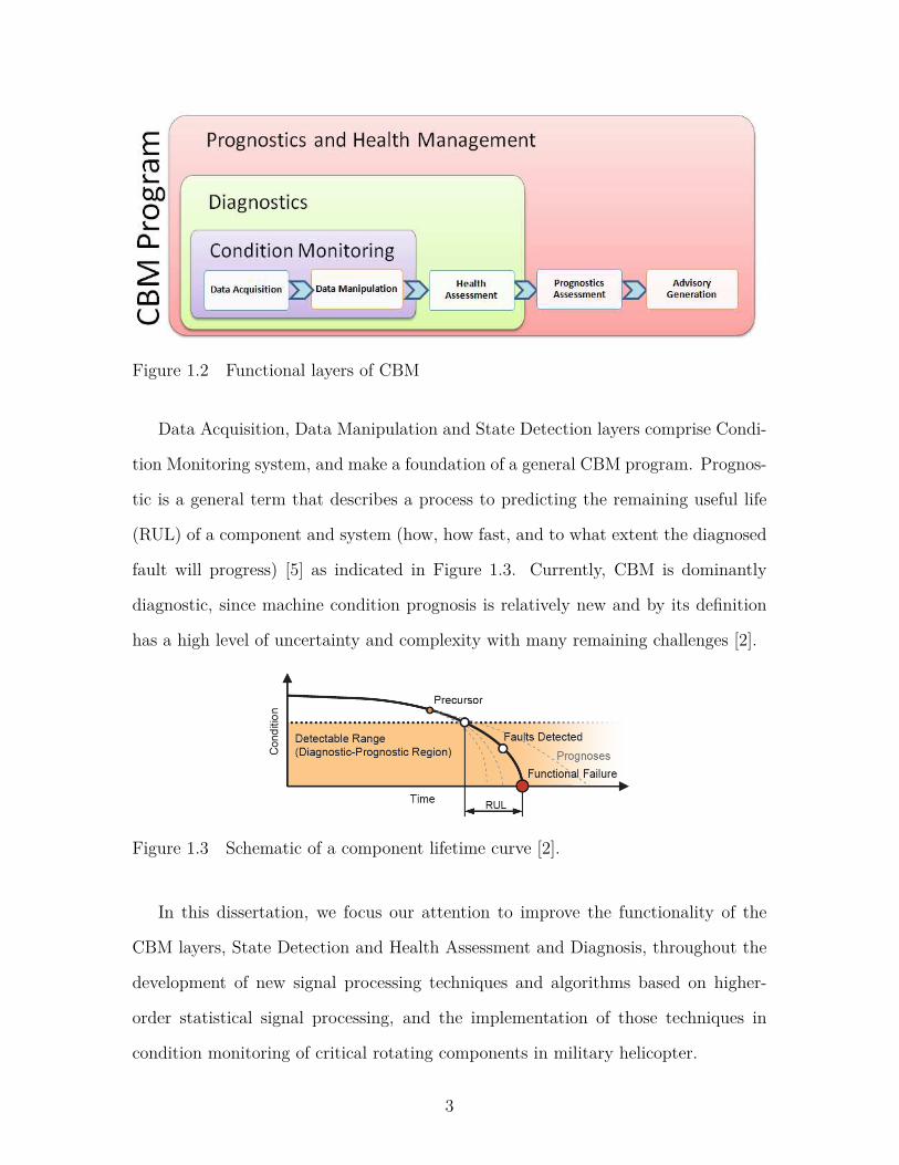
Figure 1.2 Functional layers of CBM

Data Acquisition, Data Manipulation and State Detection layers comprise Condi-

tion Monitoring system, and make a foundation of a general CBM program. Prognos-

tic is a general term that describes a process to predicting the remaining useful life

(RUL) of a component and system (how, how fast, and to what extent the diagnosed

fault will progress) [5] as indicated in Figure 1.3. Currently, CBM is dominantly

diagnostic, since machine condition prognosis is relatively new and by its definition

has a high level of uncertainty and complexity with many remaining challenges [2].

Figure 1.3 Schematic of a component lifetime curve [2].

In this dissertation, we focus our attention to improve the functionality of the

CBM layers, State Detection and Health Assessment and Diagnosis, throughout the

development of new signal processing techniques and algorithms based on higher-

order statistical signal processing, and the implementation of those techniques in

condition monitoring of critical rotating components in military helicopter.

3

1.2 CBM Practice in US Army Rotorcrafts

Over the past decade, great advancements have been made in field of fault detection

and health diagnostic of aircraft systems [6]-[11]. The successes to date in implement-

ing this technology in military helicopters have resulted in the large-scale deployment

of health monitoring systems such as Health and Usage Monitoring Systems (HUMS)

and Vibration Management Enhancement Program (VMEP), which have generated

a wide range of benefits from increased safety to reduced maintenance costs [12]-[15].

The US Army and South Carolina Army National Guard (SCARNG) are cur-

rently employing the HUMS and VMEP systems to shift the standard time-based

maintenance in military aviation toward the innovative CBM practice. VMEP sys-

tem includes an on-board Modern Signal Processing Unit (MSPU) which continuously

monitors the health conditions of crucial aircraft components such as rotor, engines,

gearboxes, and drive train using tachometers and accelerometers sensors distributed

throughout the helicopter’s drive train as shown in Figure 1.4 [13]. The MSPU is

currently deployed on AH-64 Apache, UH-60 Blackhawk and CH-47 Chinook fleets

[16].

Processed data from the MSPU provides rotorcraft maintainers at the ground-

based station with a collection of diagnostic and progressively prognostic vibration-

based indicators summarized by Condition Indicators (CIs) or Health Indicators

(HIs), which collect several CI metrics. Pre-established and baseline measurements

of these typically one-dimensional CI and HI values from existing historical data

and testbed verifications under extreme conditions provide rankings for the status of

individual aerospace and rotorcraft components with ratings such as “Good,” “Cau-

tion,” and “Exceeded,” which in turn provide maintainers of these fleets proactive

time-independent condition based maintenance decision making [17].

4

(a)

(a)(b)

(a)(c)

Figure 1.4 (a) AH-64A helicopter, (b) Sensor locations in an AH-64A monitoredby the MSPU, and (c) Exposed-top MSPU unit [13]

5

1.3 CBM Practice at the University of South Carolina

Since 1998 the University of South Carolina (USC) has been working closely with the

South Carolina Army National Guard (SCARNG) in number of important projects

that were directed at reducing the Army aviation costs and increasing operational

readiness through the implementation of CBM program [18], [19]. Research emphasis

has been to collect and analyze data and to formulate requirements assisting in the

transition toward CBM. The research program at USC seeks to deliver tangible results

which directly contribute to CBM efforts and objectives such as: link and integrate

maintenance management data with on- board sensor data and test metrics, quantify

and evaluate the importance of each data field relative to CBM, understand the

physics and the root causes of faults of components, subsystems and systems, explore

the development of models for early detection of incipient faults, develop models to

predict remaining life of components, subsystems and systems.

These efforts expanded into a fully matured CBM research center within the USC

department of mechanical engineering, which hosts several aircraft component test

stands in support of current US Army CBM objectives. The CBM center at the

University of South Carolina has a complete AH-64D (Apache helicopter) tail rotor

drive train (TRDT) test stand for on-site data collection and analysis, as shown in

Figure 1.5-(b). The TRDT test stand emulates the complete tail rotor drive train

from the main transmission tail rotor takeoff to the tail rotor swash plate assembly,

as shown in Figure 1.5-(a).

All drive train parts on the test stand are actual aircraft hardware. The prime

mover for the drive train is an 800hp AC induction motor controlled by variable fre-

quency drive. An absorption motor of matching rating is used to simulate the torque

loads that would be applied by the tail rotor blade and it is controlled by another

variable frequency drive. The input and the output motors work in dynamometric

configuration to save energy.

6

(a)

(b)

Figure 1.5 (a) Actual TRDT location on AH-64D, and (b) TRDT test stand atUSC

7

The structure, instrumentation, data acquisition systems, and supporting hard-

ware are in accordance with military standards. The signals being collected during the

operational run of the apparatus include vibration data measured by the accelerome-

ters, temperature measured via thermocouples, and speed and torque measurements.

The measurement devices are placed at the forward (FHB) and afterward (AHB)

hanger bearings and two gearboxes as shown in Figure 1.5-(b).

In this dissertation, we use vibration data collected from different locations in

the TRDT test stand in order to assess health conditions of rotating mechanical

components such as drive shafts, gearboxes, and hanger bearings under accelerated

conditioning experiments.

1.4 Motivations

As discussed in the previous section, condition monitoring of critical components in

the aircraft is achieved through processing variety of time-varying signals (waveforms)

collected using sensors attached to those critical components such as vibration, acous-

tic, and temperatures. These signals are the appearance of the operation and wear of

the components. By analyzing these characteristics signatures, we can diagnose the

current status of the components.

The vibration signals are the most common and popular waveform data used in

condition monitoring of rotating and reciprocating components [20]-[25]. Collected

vibration data is analyzed using different signal processing techniques to extract fea-

tures that are used to diagnose current conditions, or used in prognostic models to

estimate the remaining useful life of a component. For example, time-domain anal-

ysis is directly based on the time waveform itself (e.g., [26], [27], [28]). Traditional

time-domain analysis calculates characteristic features from time waveform signals as

descriptive statistics such as mean, peak, peak- to-peak interval, standard deviation,

crest factor, root mean square, skewness, kurtosis, etc. These features are usually

8

called time-domain features. Time-domain analysis provides cheap option for moni-

toring simple machines. However, in the case of complex system composed of many

rotating components with different frequencies, time-domain analysis has very limited

diagnostic capabilities.

Frequency-domain analysis is based on the transformed signal in frequency domain

by mean of Fourier transform. Spectral analysis is the most widely used conventional

analysis technique for feature extraction from vibration data [1]. The advantage of

frequency-domain analysis over time-domain analysis is its ability to easily identify

and isolate certain frequency components of interest and link it to a particular ma-

chine component. Vibration-monitoring using spectrum analysis is done by either

looking at the whole spectrum or looking closely at certain frequency components of

interest and thus extract features from the signal (e.g., [29], [30], [31]).

The most commonly used tool in spectrum analysis is auto-power spectrum which

has the dimension of mean square values/Hz and indicates how the mean square

value is distributed over frequency. Auto-power spectrum is the Fourier transform of

the well known auto-correlation function which is second order statistics, as will be

discussed in Chapter 2.

Unfortunately, conventional auto- and cross-power spectra have limited perfor-

mance in detecting higher order relationship between frequencies inside the signal

spectrum. For example, when the system under study exhibit some nonlinearities,

various spectral components interact (or, “mix”) with one another to form new combi-

nations of “sum” and “difference” frequencies, as indicated by trigonometric identity

in equation (1.1).

cos(2πf1t+ θ1)× cos(2πf2t+ θ2) = 12 [cos(2π(f1 + f2)t+ (θ1 + θ2))

+ cos(2π(f1 − f2)t+ (θ1 − θ2)] (1.1)

9

This frequency mix effect due to nonlinearities in the system is depicted in Figure

1.6. In such a case, higher order correlation, and their Fourier transforms, Higher Or-

der Spectra (HOS), are used to characterize nonlinearities in the system and signals,

as will be introduced in Chapter 2. Higher-order correlation and higher-order spec-

tra will be progressively higher-order dimensional functions of time and frequency,

respectively. This is why polyspectra is sometimes used as synonym of higher-order

spectra.

Figure 1.6 Frequency mix effect due to nonlinearities in the system

Advantages of using higher-order statistics also include:

• Preservation of phase information in the form of a phase difference. Note

that the auto-power spectrum does not preserve phase information.

• Detection and quantification of phase-coupling or phase-coherence be-

tween various frequency components satisfying specific frequency selection rule.

10

Such phase-coupling may be introduced by nonlinear processes.

• Insensitivity to additive and independent Gaussian noise. For exam-

ple, the third-order spectrum, bispectrum, is ideally zero for Gaussian random

process.

Motivated by several advantages of the higher-order statistics mentioned above,

this dissertation presents theory and applications of signal processing techniques

based on higher-order statistics for condition based maintenance of critical compo-

nents in the AH-64D military-helicopter tail rotor drive train system. Our objectives

can be summarized as follows:

• Extracting more information from the same collected vibration data using

higher-order statistics, without the need of adding more hardware.

• Developing more accurate diagnostic models by taking into consideration infor-

mation from higher-order spectra.

• Understanding root causes of certain frequencies appearing in the vibration

spectrum due to nonlinear system behavior and relate those frequencies to the

correct fault in the mechanical system.

• Developing an easy-to-use higher-order statistics’ tools for CBM applications.

1.5 Organization of the Dissertation

The remainder of this dissertation is organized as follows: In Chapter 2, we introduce

the subject of higher order statistical signal processing in order to provide a bridge

to following chapters and lay out mathematical foundations for signal processing

algorithms that will be developed later in this dissertation.

In Chapter 3, the cross-bispectrum is used to investigate and model vibrations’

spectral interaction due to quadratic nonlinearities in faulted drive shafts in an AH-

11

64D helicopter tail-rotor drive-train. Based on cross-bispectrum, quadratic nonlinear

transfer function is presented to model second order nonlinearity in the drive shaft

running between the two hanger bearings. Then, nonlinearity coupling coefficient

between frequency harmonics of the rotating shafts is used as condition metric to

diagnose different seeded shaft faults compared to baseline case, namely: 1)- shaft

misalignment, 2)- shaft imbalance, and 3)- combination of shaft misalignment and

imbalance.

In Chapter 4, we develop a new concept of Quadratic-Nonlinearity Power-Index

spectrum, QNLPI(f), that can be used in signal detection and classification, based

on bicoherence spectrum. The proposed QNLPI(f) is derived as a projection of the

three-dimensional bicoherence spectrum into two-dimensional spectrum that quan-

titatively describes how much of the mean square power at certain frequency f is

generated due to nonlinear quadratic interaction between different frequency com-

ponents. The quadratic-nonlinear power spectral density PQNL(f) and percentage

of quadratic nonlinear power PQNLP are also introduced based on the QNLPI(f).

Concept of the proposed indices and their computational considerations are discussed

first using computer generated data, and then applied to real-world vibration data to

assess health conditions of different rotating components in the drive train including

different combinations of drive-shaft and gearbox faults. The QNLPI(f) spectrum

enables us to gain more details about nonlinear harmonic generation patterns that

can be used to distinguish between different cases of mechanical faults, which in turn

helps to gaining more diagnostic/prognostic capabilities.

In Chapter 5, the behavior of the helicopter’s tail-rotor drive-train under more

than one simultaneous fault is studied using the proposed signal analysis techniques.

In the presence of drive-shaft faults, shaft harmonics dominate the power spectra of

the vibration signals collected form faulted hanger-bearing making it hard to detect

bearing’s faults. Also, spectral interaction between different fault frequencies leads

12

to unexpected frequencies to appear in the vibration spectrum which can not be ex-

plained using conventional power spectral analysis. However, bispectral analysis tools

not only detect the bearing’s faults in this extreme case of multi-faulted components,

but also are able relate all frequencies to their root causes and successfully links the

signal processing to the physics of the underlying faults.

Finally, conclusion of this dissertation is presented in Chapter 6.

13

Chapter 2

Higher Order Statistical (HOS) Analysis

In this chapter, we introduce the subject of higher order statistical signal processing in

order to provide a bridge to following chapters and lay out mathematical foundations

for signal processing algorithms that will be developed later in this dissertation. We

initiate our discussion by considering vibration data as realization of random process

that can be used to characterize unknown conditions of rotating systems. Just as

random variables are characterized by certain expected values (moments) or averages

such as mean and variance, random processes are also characterized by their mean

value, correlation function, and various higher order correlation functions, or mo-

ment functions. Alternatively, random processes may be characterized by the Fourier

transform of the various order correlation functions which are known as higher order

spectra, as will be discussed in the following sections.

2.1 Higher-Order Auto-Moments and Stationary Fluctuations

In probability theory and statistics, n-order central moment of a random variable X

is calculated as the expected value of integer power, n, of the the random variable X

around its mean, as follows:

m(n)x = E{(X − E{X})n} =

∞∫−∞

(x− E{X})n fX(x)dx (2.1)

where E{.} denotes the expected value operator, superscript (n) describes the order

of the central moment, and fX(x) is the probability density function (pdf) of the

14

random variable X. Thus, m(1)x = 0 = the mean value, m(2)

x = mean square value,

m(3)x = mean cube value; and so on. Central moments are used in preference to

ordinary moments, computed in terms of deviations from zero instead of from the

mean, because the higher-order central moments relate only to the spread and shape

of the distribution, rather than also to its location.

Higher order statistical signal processing involve generalization of various order

moments in the case of random variable to moment functions (i.e., correlation func-

tions) in the case of random process. Therefore, it is mathematically desired to

assume that the random process has zero mean for computation convenience, which

what we adopt through out the rest of this dissertation. In the practical cases when

we will be dealing with real vibration data from monitored mechanical components,

the mean of the signal is first computed and subtracted from the signal.

Based on the mathematical foundations of higher order statistical signal processing

in [32], various order correlation functions can be calculated for the random process

as follows:

µx = E{x(t)} = 0 (or, a constant) (2.2)

Rxx(τ) = E{x∗(t)x(t+ τ)} (2.3)

Rxxx(τ1, τ2) = E{x∗(t)x(t+ τ1)x(t+ τ2)} (2.4)

Rxx...x(τ1, τ2, ..., τn) = E{x∗(t)x(t+ τ1)x(t+ τ2)...x(t+ τn)} (2.5)

where E{.} denotes the expected value operator and the superscript asterisk (∗)

denotes complex conjugate. It is worthwhile to note here that the second-order cor-

15

relation function, Rxx(τ), in equation (2.3) is the familiar auto-correlation function.

The third-order correlation function, Rxxx(τ1, τ2), is often called bicorrelation func-

tion, presumably because it is a function of two time variables. The fourth-order

correlation function, Rxxxx(τ1, τ2, τ3), is often called tricorrelation, and so on.

Generally, in the non-stationary case, the correlation function will be a function

of time t, as well as the time differences, τ1, τ2, ..., τn as follows:

Rxx...x(t, τ1, τ2, ..., τn) = E{x∗(t)x(t+ τ1)x(t+ τ2)...x(t+ τn)} (2.6)

Zero-mean fluctuation data is considered strongly stationary (strict sense stationary)

to order n if the mean and the various order correlation functions are functions of time

differences only, i.e. τ1, τ2, ..., τn. In other words, neither the mean nor the correlation

functions depend on absolute time t as indicated in equations (2.2)-(2.5). In the case

of analyzing linear signals and systems, it is enough to have only (2.2)-(2.3) satisfied.

This case is called weakly-stationary (wide-sense stationary) signal. For three-wave

interaction in quadratically nonlinear system as will be discussed later, random signal

is assumed to be stationary to third order (equations (2.2)-(2.4)).

2.2 Auto-Correlation and Auto-Power Spectrum

In signal processing, the auto-correlation function Rxx(τ) for a wide-sense stationary

signal x(t) is defined as

Rxx(τ) = x(t) ? x(t) =∫ ∞−∞

x∗(t)x(t+ τ)dt (2.7)

where the operation of correlation is indicated by a five-pointed star (?). Auto-

correlation Rxx(τ) is a measure of similarity (statistical dependence) between a sig-

nal x(t) and time-shifted version x(t + τ). For the vibration signals collected from

CBM test bed, it is not possible (from experimental point of view) to access all pos-

16

sible realizations of x(t). Therefore, the auto-correlation in this case is statistically

estimated based on a finite number of realizations as indicated in (2.3).

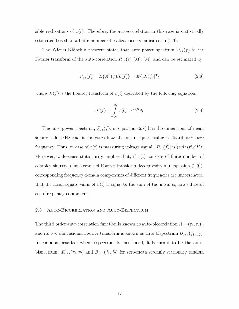
The Wiener-Khinchin theorem states that auto-power spectrum Pxx(f) is the

Fourier transform of the auto-correlation Rxx(τ) [33], [34], and can be estimated by

Pxx(f) = E{X∗(f)X(f)} = E{|X(f)|2} (2.8)

where X(f) is the Fourier transform of x(t) described by the following equation:

X(f) =∞∫−∞

x(t)e−j2πftdt (2.9)

The auto-power spectrum, Pxx(f), in equation (2.8) has the dimensions of mean

square values/Hz and it indicates how the mean square value is distributed over

frequency. Thus, in case of x(t) is measuring voltage signal, [Pxx(f)] is (volts)2�Hz.

Moreover, wide-sense stationarity implies that, if x(t) consists of finite number of

complex sinusoids (as a result of Fourier transform decomposition in equation (2.9)),

corresponding frequency domain components of different frequencies are uncorrelated,

that the mean square value of x(t) is equal to the sum of the mean square values of

each frequency component.

2.3 Auto-Bicorrelation and Auto-Bispectrum

The third order auto-correlation function is known as auto-bicorrelation Rxxx(τ1, τ2) ,

and its two-dimensional Fourier transform is known as auto-bispectrum Bxxx(f1, f2).

In common practice, when bispectrum is mentioned, it is meant to be the auto-

bispectrum. Rxxx(τ1, τ2) and Bxxx(f1, f2) for zero-mean strongly stationary random

17

signal x(t) are defined in (2.10) and (2.11) respectively [35].

Rxxx(τ1, τ2) = E{x∗(t)x(t+ τ1)x(t+ τ2)} (2.10)

Bxxx(f1, f2) = E{X(f1)X(f2)X∗(f3 = f1 + f2)} (2.11)

Bispectral analysis is a powerful signal processing technique in detecting second-

order nonlinearity in signals and systems. When various frequency components of

the vibration signal interact with one another due to quadratic nonlinearity, new

combinations of frequencies are generated at both the sum and the difference of the

interacting frequencies, as indicated in equation (2.12). Those frequency components

are phase coupled to the primary interacted frequencies. Bispectrum uses this phase

coupling signature between frequency components to detect second-order nonlineari-

ties [36].

cos(2πf1t+ θ1)× cos(2πf2t+ θ2) = 12 [cos(2π(f1 + f2)t+ (θ1 + θ2))

+ cos(2π(f1 − f2)t+ (θ1 − θ2)] (2.12)

The definition of the bispectrum in (2.11) shows how the bispectrum measures the

statistical dependence between three waves. That is, Bxxx(f1, f2) will be zero unless

the following two conditions are met:

1. Waves must be present at the frequencies f1, f2, and f1 + f2. That is, X(f1),

X(f2), and X(f1 + f2) must be non-zero.

2. A phase coherence must be present between the three frequencies f1, f2, and

f1 + f2.

18

If waves present at f1, f2, and f1+f2 are spontaneously excited independent waves,

each wave will be characterized by statistical independent random phase. Thus, the

sum phase of the three spectral components will be randomly distributed over (−π, π).

When a statistical averaging denoted by the expectation operator is carried out, the

bispectrum will vanish due to the random phase mixing effect. On the other hand, if

the three spectral components are nonlinearly coupled to each other, the total phase

of three waves will not be random at all, although phases of each wave are randomly

changing for each realization. Consequently, the statistical averaging will not lead to

a zero value of the bispectrum.

The auto-bispectrum Bxxx(f1, f2) is a true spectral density function indicates how

the mean cube value of x(t) is distributed over a two-dimensional frequency plane.

Thus, in case of x(t) is measuring voltage signal, [Bxxx(f1, f2)] is (volts)3�Hz2.

2.4 Higher-Order Cross-Moments

Higher-order moment functions can also be defined for two real random processes x(t)

and y(t). The quantities x(t) and y(t) may, for example, represent the random exci-

tation and response of a nonlinear system. In this case, the cross-moment functions

are given as follows [32]:

Ryx(τ) = E{y∗(t)x(t+ τ)} (2.13)

Ryxx(τ1, τ2) = E{y∗(t)x(t+ τ1)x(t+ τ2)} (2.14)

Ryx...x(τ1, τ2, ..., τn) = E{y∗(t)x(t+ τ1)x(t+ τ2)...x(t+ τn)} (2.15)

19

Once again, the above equations (2.13)-(2.15) assume stationarity and zero-mean.

The second-order cross-moment function, Ryx(τ), in equation (2.13) is the famil-

iar cross-correlation function, while Ryxx(τ1, τ2) and Ryxxx(τ1, τ2, τ3) are referred to

as cross-bicorrelation function and cross-tricorrelation function, respectively. The

cross-bicorrelation and cross-tricorrelation are obviously higher-order moment func-

tions, and their Fourier transforms, the cross-bispectrum and cross-trispectrum are

extremely powerful concepts that can be used to analyze and interpret data associ-

ated with nonlinear phenomena such as nonlinear wave interactions, as we will see in

the following chapters of this dissertation.

2.5 Cross-Correlation and Cross-Power Spectrum

Cross-power spectrum Cyx(f) given in equation (2.16) is the Fourier transform of

the cross-correlation function Ryx(f) in equation (2.13). Cross-correlation function

Ryx(f) and cross-power spectrum Cyx(f) have been fruitfully utilized in many fields

of science and engineering to identify and quantify statistical linear relationships

between two fluctuating quantities x(t) and y(t).

Cyx(f) = E{Y ∗(f)X(f)} (2.16)

Cross-power spectrum can be represented in terms of amplitude spectrum |Cyx(f)|

and phase spectrum θyx(f). That is,

Cyx(f) = |Cyx(f)| eθyx(f) (2.17)

The phase of the cross-power spectrum preserves phase information in the form

of a phase difference. This is perhaps the single most important property of the

cross-power spectrum, and it is employed in too many applications.

20

2.6 Cross-Bicorrelation and Cross-Bispectrum

Cross-bispectrum Sxxy(f1, f2) is the two-dimensional Fourier transform of the third

order cross-correlation function Ryxx(τ1, τ2), and it is estimated by the following equa-

tion,

Sxxy(f1, f2) = E{X(f1)X(f2)Y ∗(f3 = f1 + f2)} (2.18)

The cross-bispectrum is quite similar to the auto-bispectrum except it may be

used to detect and quantify the nonlinear interaction of two spectral components in

one fluctuation record x(t). The two spectral components (which represent complex

amplitude of waves or oscillations) result in the appearance of a sum or difference

frequency wave in second fluctuation record y(t), as illustrated before in equation

(2.12). Therefore, the cross-bispectrum is a key concept in modelling nonlinear sys-

tems and quantitatively evaluating complex coupling coefficient, as will be done in

Chapter 3 of this dissertation.

2.7 Symmetry Properties and Region of Computation for Auto- and

Cross- Bispectra

It is well known that if x(t) is real, magnitude of the Fourier transform is even

symmetric and its phase is odd symmetric arround the zero, that is,

X(−f) = X∗(f) (2.19)

Applying the symmetry property in (2.19) to the case of x(t) and y(t) are real,

the auto-power spectrum Pxx(f) and the cross-power spectrum Cyx(f) also satisfy

21

certain symmetry properties indicated as follows:

Pxx(−f) = Pxx(f) (2.20)

Cyx(−f) = C∗yx(f) (2.21)

Consequently, one needs to calculate auto- and cross-power spectra for positive

frequency only.

In a similar fashion, auto- and cross- bispectra possess certain symmetry properties

in the two-dimensional bi-frequency planes. As a result of the symmetries, it is not

necessary to calculate these spectra over the entire bi-frequency plane. Therefore,

substituting the symmetry property from (2.19) into the auto-bispectrum equation

(2.11), one can easily prove that the bispectrum possesses the following symmetry

properties:

Bxxx(−f1,−f2) = B∗xxx(f1, f2) (symmetry property I) (2.22)

Bxxx(f2, f1) = Bxxx(f1, f2) (symmetry property II) (2.23)

Bxxx(−f2,−f1) = B∗xxx(f1, f2) (symmetry property III) (2.24)

Bxxx(f1,−f2) = B∗xxx(f1 − f2, f2) (symmetry property IV) (2.25)

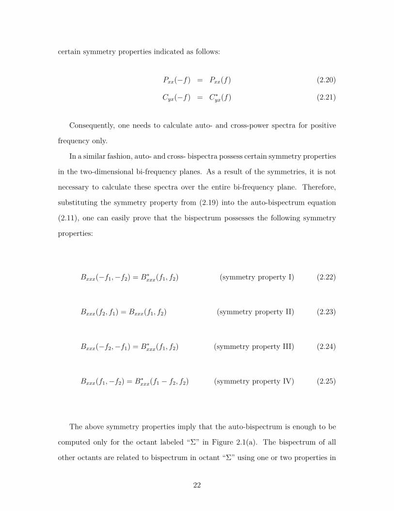
The above symmetry properties imply that the auto-bispectrum is enough to be

computed only for the octant labeled “Σ” in Figure 2.1(a). The bispectrum of all

other octants are related to bispectrum in octant “Σ” using one or two properties in

22

equations (2.22)-(2.25), as illustrated in Figure 2.1(a). In fact, auto-bispectrum will

be estimated digitally. The sampling theory implies that all f1, f2 and f3 = f1 + f2

must be less than or equal to fs

2 , where fs is the sampling frequency. Therefore, when

auto-bispectrum is digitally computed, it will be plotted within the triangular region

defined by the lines f2 = 0, f2 = f1, and f2 = fs

2 − f1, as depicted in Figure 2.1(b).

The cross-bispectrum possesses the same first three symmetry properties possessed

by the auto-bispectrum described above. That is, for x(t) and y(t) real,

Sxxy(−f1,−f2) = S∗xxy(f1, f2) (symmetry property I) (2.26)

Sxxy(f2, f1) = Sxxy(f1, f2) (symmetry property II) (2.27)

Sxxy(−f2,−f1) = S∗xxy(f1, f2) (symmetry property III) (2.28)

It is important to note that symmetry property IV for the auto-bispectrum does

not hold true for the cross-bispectrum. Therefore, it is necessary to compute the

cross-bispectrum for both the sum region represented by octant “Σ” and the difference

region represented by octant “∆”, as illustrated in Figure 2.2(a). Again, since the

cross-bispectrum is to be implemented digitally, sampling theory implies that f1+f2 ≤fs

2 and f2 ≤ fs

2 . These boundaries are indicated in Figure 2.2(b).

23

(a)

(a)(a)(b)

Figure 2.1 Symmetric regions and region of computation for (a) continuousauto-bispectrum (b) digitally implemented auto-bispectrum

24

(a)

(a)(b)

Figure 2.2 Symmetric regions and region of computation for (a) continuouscross-bispectrum (b) digitally implemented cross-bispectrum

25

2.8 Digital Estimation of Auto- and Cross- Bispectra

Throughout the course of this dissertation, we will be analyzing vibration data using

different order of spectral analysis discussed above in order to assess health conditions

of rotating mechanical components. Since vibration data is collected, stored, and

processed in digital form using computer, it is important to make that link to the

discrete signal processing.

Our goal in this section is to outline the procedure of how auto- and cross-bispectra

are estimated directly from the Discrete Fourier Transform (DFT) of sampled versions

of x(t) and y(t). The expected value operator, E{.}, is statistically estimated using

average over ensemble of M realization of the signals under study. Assuming that M

realizations of the vibration signals x(t) and y(t) are available and the duration of

each realization is T seconds. If the sampling frequency is to be fs = 1/ts, number

of samples in each realization will be N = T/ts. To compute the auto- or cross-

bispectrum, the following steps should be carried out.

1. Compute the mean value of each realization,

x(k)[n] = 1N

N−1∑n=0

x(k)[n]

y(k)[n] = 1N

N−1∑n=0

y(k)[n] (2.29)

and subtract the mean value. It is assumed in the following steps that x(k)[n]

and y(k)[n] are zero-mean where the superscript (k) represent the kth realization

of the signal.

26

2. Compute the DFT for each realization,

X(k)[l] = 1N

N−1∑n=0

x(k)[n] e−j2πln�N

Y (k)[l] = 1N

N−1∑n=0

y(k)[n] e−j2πln�N (2.30)

3. Compute the sample auto- or cross-bispectrum for each realization,

B(k)xxx[l1, l2] = X(k)∗[l1 + l2] X(k)[l1] X(k)[l2]

S(k)xxy[l1, l2] = Y (k)∗[l1 + l2] X(k)[l1] X(k)[l2] (2.31)

4. Estimate average the samples auto- or cross-bispectrum over the M realization

to yield the final estimator,

Bxxx[l1, l2] = 1M

M∑k=1

B(k)xxx[l1, l2]

Sxxy[l1, l2] = 1M

M∑k=1

S(k)xxy[l1, l2] (2.32)

Note that Bxxx[l1, l2] needs to be computed only in the sum “Σ” region indi-

cated in Figure 2.1(b), while Sxxy[l1, l2] is computed for both the sum “Σ” and

difference “∆” regions as indicated in Figure 2.2(b).

27

Chapter 3

Quadratic-Nonlinearity Coupling and its

Application in Health Assessment of Rotating

Drive Shafts

In this chapter, the cross-bispectrum is used to investigate and model vibrations’ spec-

tral interaction due to quadratic nonlinearities in faulted drive shafts in an AH-64D

helicopter tail-rotor drive-train. Based on cross-bispectrum, quadratic-nonlinear cou-

pling metric, AQC(l, k), is proposed to model second-order nonlinear behaviour of the

drive shafts, as will be discussed in section 3.3. The proposed quadratic-nonlinearity

metric shows better capabilities in distinguishing different shaft settings than the

conventional linear coupling based on cross-power spectrum, as will be discussed in

section 3.5.

3.1 Introduction

Tail rotor drive train is a critical section of the aircraft in that it consists of trans-

mission system with a single load path to transfer the power from the main rotor to

the tail rotor via a system of drive shafts and gearboxes [37]. Failure of any one of

these series connected components decreases the chances of landing the aircraft safely.

Without the input from the tail rotor system, the ability to control and counter the

torque produced by the main rotor blades does not exist. Thus, condition monitor-

ing systems, such as HUMS and VMEP discussed in section 1.2, keep maintenance

mechanics aware of the health conditions of their aircraft by continuously calculating

28

condition indicators using vibration data collected from those critical components

during the flight [19]-[22].

Current practice in health monitoring of the tail-rotor drive-shafts involves mon-

itoring spectral peaks from two vibration signals simultaneously collected at the two

ends of each shaft [16]. Spectral peaks at the first-three shaft harmonics (1R, 2R,

and 3R) are typically used as condition indicators of the shaft faults such as misalign-

ment and imbalance [38], [39]. In order to calculate those condition indicators, either

auto-power spectrum is averaged between the two vibration signals at one particu-

lar frequency (for example, 2R), or cross-power spectrum between the two vibration

signals is calculated at this particular frequency. Auto- and cross-power spectra are

Fourier transforms of auto- and cross-correlation functions, respectively. Hence, one

can think about cross-power spectrum as a tool to investigate linear correlation be-

tween two vibration signals in terms of spectral frequencies.

However, higher order correlations among vibration spectral components can pro-

vide valuable information about the health of rotating component. Moreover, this

information comes with no additional cost in terms of adding more hardware (sen-

sors, wiring, ect.) since all what we need is further processing of the same collected

vibration data [40].

In this chapter, we utilize the cross-bispectrum as HOS tool to investigate and

model quadratic nonlinear relationship between two vibration signals simultaneously

collected at the forward and afterward hanger bearing positions in an AH-64D heli-

copter tail rotor drive train. Vibration data are gathered from dedicated condition

based maintenance experimental helicopter drive-train simulating different shaft con-

ditions, namely; baseline case, shaft misalignment, shaft imbalance, and combination

of misalignment and imbalance. For each of these settings, the experiment is re-

peated three times using different hanger bearing articles, making a grand total of

twelve experiment runs, as will be discussed in section 3.4.

29

Based on cross-bispectrum, quadratic-nonlinearity coupling coefficient, AQC , is

proposed to quantitatively describe second order nonlinearities in the drive shaft.

Then, AQC(1R, 1R), is used as a condition metric to distinguish between the different

shaft faults compared to baseline case. Magnitude response of the proposed quadratic-

nonlinearity metric, AQC(1R, 1R), shows ability to detect the shaft fault in all the

studied cases, and its phase shows better capabilities in distinguishing different shaft

settings than the conventional linear coupling based on cross-power spectrum, as will

be discussed in section 3.5.

3.2 Cross-Power Spectrum and Linear Coupling Between Spectral

Components of Vibration Signals

When two vibration signals, x(t) and y(t), are collected simultaneously, cross-correlation

Rxy(τ) is a useful function to investigate the linear relation between the two signals

as given in equation (3.1).

Rxy(τ) = E{x(t+ τ)y∗(t)} (3.1)

As discussed in section 2.5, the Fourier transform of the cross-correlation function

is the cross-power spectrum, CXY (f), as given in equation (3.2) where X(f) and Y (f)

are the Fourier transforms of x(t) and y(t), respectively. The cross-power spectrum

is a useful tool to describe linear correlation between the two signals as a function

of frequency which is easy to relate to specific rotating component. The magnitude

of the cross-power spectrum, |Cxy(f)|, describes how strong the linear coupling is

between the two signals at frequency f , while its phase difference, θXY (f), can be

used to differentiate between different physical faults that produce the same vibrating

frequencies.

30

CXY (f) = E{X(f)Y ∗(f)} = |Cxy(f)| ejθXY (f) (3.2)

When X(f) is an input signal to a linear system, the output signal Y (f) is linearly

coupled to X(f) in frequency domain by the following relation:

Y (f) = H(f)X(f) (3.3)

where, H(f), is the linear transfer function of the system.

Therefore, assuming that X(f) and Y (f) are two vibration signals collected at

the hanger bearings supporting a drive-shaft with unknown condition, linear transfer

characteristics of that shaft at any particular frequency can be theoretically estimated

by substituting from (3.3) in (3.2) as follows:

H(f) = C∗XY (f)E{|X(f)|2} = E{X∗(f)Y (f)}

E{|X(f)|2} (3.4)

3.3 Cross-Bispectrum and Quadratic-Nonlinear Coupling Among Spec-

tral Components of Vibration Signals

The cross-bispectrum is the Fourier transform of the cross-bicorrelation function

(third-order moment) as given in (3.5) and (3.6) as follows [32], [41]:

Rxxy(τ1, τ2) = E{x(t+ τ1)x(t+ τ2)y∗(t)} (3.5)

SXXY (f1, f2) = E{X(f1)X(f2)Y ∗(f1 + f2)} (3.6)

The advantage of bispectrum over linear power spectral analysis is its ability to

characterize quadratic nonlinearities in monitored systems. One of the characteristics

of nonlinearities is that various frequencies “mix” to form new combinations of “sum”

31

and “difference” frequencies. An important signature to detect nonlinearity is based

on the fact that there exists a phase coherence, or phase coupling, between the primary

interacting frequencies and the resultant new sum and difference frequencies [35].

In other words, cross-bispectrum given in (3.6) investigates the quadratic nonlinear

coupling between any two frequency components, f1 and f2, in signal X(f) that

interact to produce a third frequency, f1 + f2, at another signal Y (f). This nonlinear

relation is plotted in two-dimensional frequency space (f1 − f2), as shown in Figure

2.2.

By analogy to linear transfer function in equation (3.4), the second-order nonlin-

earity in a the drive-shaft can be estimated based on the cross-bispectrum between two

signals collected at the hanger bearings supporting that shaft. Thus, assuming that

part of the power at frequency component Y (f1 + f2) is generated due to quadratic

nonlinear coupling between X(f1) and X(f2), Y (f1 + f2) = AQC(f1, f2)X(f1)X(f2),

the quadratic coupling coefficient between the two frequencies f1 and f2 can be cal-

culated as follows;

AQC(f1, f2) = S∗XXY (f1, f2)E{|X(f1)X(f2)|2} (3.7)

Using average over ensemble of M realizations to estimate the expected value

operators in equation (3.7), AQC(f1, f2) can be estimated directly from the discrete

Fourier transform of sampled versions of x(t) and y(t) as follows:

AQC(l, k) =1M

M∑i=1

X∗i [l]X∗i [k]Yi [l + k]

1M

M∑i=1|Xi [l]Xi [k]|2

(3.8)

The quadratic-nonlinearity coupling coefficient, AQC(l, k), is two-dimensional com-

plex matrix that characterizes the system under study and it is calculated for the

whole same bi-frequency space as cross-bispectrum shown in Figure 2.2(b). However,

32

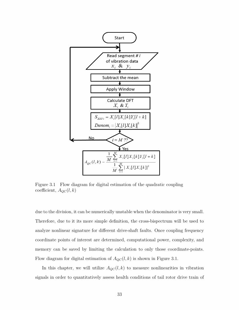
Figure 3.1 Flow diagram for digital estimation of the quadratic couplingcoefficient, AQC(l, k)

due to the division, it can be numerically unstable when the denominator is very small.

Therefore, due to it its more simple definition, the cross-bispectrum will be used to

analyze nonlinear signature for different drive-shaft faults. Once coupling frequency

coordinate points of interest are determined, computational power, complexity, and

memory can be saved by limiting the calculation to only those coordinate-points.

Flow diagram for digital estimation of AQC(l, k) is shown in Figure 3.1.

In this chapter, we will utilize AQC(l, k) to measure nonlinearities in vibration

signals in order to quantitatively assess health conditions of tail rotor drive train of

33

military rotorcraft, whose description is provided in the next section.

3.4 Experiment Setup and Vibration Data Description

The data used in this study consist of 12 experiment runs arranged in 4 sets of shaft

settings taken with different shafts alignment and balance. For each shaft setting,

the experiment is repeated 3 times using different hanger bearing articles in the aft

position of the TRDT test stand described in section 1.3, Figure 1.5. In order to

keep data organized, a naming convention is followed as summarized in Table 3.1.

The first digit in the test number represents the shaft setting and varies from 0 to 3;

where 0 is used to represent baseline case, 1 for unbalanced case, 2 for misalignment,

and 3 for a combined case of both shaft imbalance and misalignment, respectively.

The remaining of the test number consists of the serial number of the hanger bearing

used at the aft position as follows: S/N: 0316, S/N: 0321, and S/N: 0373.

Table 3.1 Vibration data set and test numbers

Test number Hanger bearing S/N0316 0321 0373

Shaf

tse

ttin

g Baseline “0" 00316 00321 00373Imbalance “1" 10316 10321 10373Misaligned “2" 20316 20321 20373

Imbal./Misal. “3" 30316 30321 30373

The original configuration of the test stand uses balanced drive-shafts straightly

aligned as a baseline for normal operations (case “0” in Table 3.1). Aligned-unbalanced

shafts (case “1” in Table 3.1) are tested under the condition of drive shaft #4 is un-

balanced by 0.135 oz-in, and drive shaft #5 is unbalanced by 0.190 oz-in. Angular

misalignment between shafts (case “2” in Table 3.1) is tested under 1.3◦ misalignment

between the #3 and the #4 drive shafts, and 1.3◦ between the #4 and the #5 drive

shafts.A combination of the last two cases, imbalance -misalignment, is also tested

(case “3” in Table 3.1).

34

During each experiment run, accelerometers’ data are collected simultaneously

from the forward and afterward hanger bearing positions (denoted as FHB and AHB

in Figure 1.5) once every two minutes during the course of the thirty minute run,

making total of 15 data segments. Each data segment has 65536 data points collected

at sampling rate of 48kHz (fS) which results in data collection time of approximately

1.31 sec per acquisition. Vibration signals are collected during operation of the test

stand at a constant rotational speed of 4863 rpm (81.05 Hz) from the prime mover,

with a simulation of the output torque at 111 ft.lb. from the output motor. Rotational

speed is the speed of the input shafts and hanger bearings. Output torque is given

by the torque at the output of the tail rotor gearbox simulating rotor operation while

the torque applied to the input shafts and hanger bearings is equal to 32.35 ft.lb.

Nominally, the acceleration at a hanger bearing should be uniform if measured

anywhere along the radial direction with only a difference in phase. However, in the

presence of an imbalanced shaft, there will be a normal force Fu towards the center of

the bearing acting along the radial line to the imbalanced mass centroid. When there

is misalignment between shafts, the shaft no longer rotates about its center of mass

causing a normal force that counters the off-axis inertia, Fm. Both fault conditions

lead to different accelerations at different points around the bearing and elliptical

acceleration profile, Du and Dm, as shown in Figure 3.2. This acceleration is picked

up by the dedicated accelerometer in x axis and recorded as vibrations of the form:

Dx = Ax · cos (ωt+ ψx) (3.9)

where Dx and Ax are displacements and amplitude of displacements in x axis direc-

tions, ω is angular velocity, and ψx is phase angles.

35

(a) (b)

Figure 3.2 Misalignment and imbalance forces and vibrations: (a) cross-section ofthe bearing and the shaft at the accelerometer location, (b) displacement orvibration components in the x-axis directions (Du orbit when ϕy − ϕx = 90◦, Dm

when ϕy − ϕx = 120◦)

3.5 Results and Discussion

In this section, drive-shaft conditions are characterized using the vibration signals

collected at the bearings supporting the shaft. Using system identification approach,

both linear and quadratic transfer characteristics of the drive-shaft can be estimated

based on cross-power spectrum and cross-bispectrum, respectively, as discussed in

section 3.3. Vibration signals at the FHB and AHB in Figure 1.5 are used as x(t)

and y(t). As mentioned in the previous section, each experiment run has 15 vibra-

tion data segments. In order to get bigger set of signal realizations to estimate the

expected value operator by average over ensemble of M realizations, each data seg-

ment is split into two, so we have total number of M=30 data segments for each

experiment run, with each segment has 32768 data points. This results in frequency

resolution equal to ∆f = 1.46Hz when discrete Fourier transform is calculated using

fast Fourier transform (FFT) approach. In the following discussion, for easier nota-

tion of frequency values, we will use “1R, 2R, 3R, . . . ” to denote “first, second, third,

. . . ” harmonics of the shaft rotating frequency (1R = 81.05Hz).

36

Figure 3.3 shows the magnitude plot of the cross-power spectrum for all shaft

settings using vibration data set from hanger bearing with S/N 0321. Ideally, we

expect to see very low vibrations in the baseline case. However, Figure 3.3(a) indicates

that spectral peaks at 1R and 3R dominate the vibration spectrum in this case.

Taking into considering the loading torque transferred to the shafts through the

IGB as shown in Figure 1.5, results in Figure 3.3(a) can be interpreted as possible

oscillations due to the unsymmetrical loading profile on the drive shafts which causes

time varying forces at 1R and 3R frequencies.

Current practice in monitoring rotating shaft conditions involves using the vibra-

tion magnitude at the spectral peaks corresponding to the first three rotating shaft

harmonics (1R, 2R, and 3R) as shaft’s condition indicators [16], [39]. Comparison

with the baseline is usually done on a logarithmic amplitude scale with increases of

6-8 dB considered to be significant and changes greater than 20 dB from the baseline

considered serious [42]. Referring to Figure 3.3, One interesting observation is that

magnitude of 2R frequency (161.1 Hz) is distinguishing all the faulted cases (Figure

3.3(b:d)) from the baseline case (Figure 3.3(a)) with magnitude difference exceeds 6

dB. Vibration magnitude at other shaft harmonics, 1R and 3R, do not show consid-

erable increase compared to the baseline case, as summarized in Table 3.2. Therefore,

we will focus our attention to 2R condition indicator and we will use it to evaluate

the linear coupling between the FHB and AHB vibrations in all the experimental

data set.

Table 3.2 Cross-power spectral peak comparison with baseline case at shaftharmonics in dB

Spectral peak 1R=80.57 2R=161.1 3R=243.2UB(10321) 3.0126 13.0387 -4.7475MA(20321) -0.1402 11.8538 -3.4963

UB/MA(30321) 3.0966 12.7088 -10.6793

37

(a)

0 100 200 300 400 500 600 700 800 900 10000

0.5

1

1.5

2

2.5

3

X: 323.7Y: 0.3929

f (Hz)

|CX

Y(f)|

X: 243.2Y: 2.553

X: 80.57Y: 0.6182

X: 161.1Y: 0.1136

(b)

0 100 200 300 400 500 600 700 800 900 10000

0.5

1

1.5

X: 161.1Y: 0.5097

f (Hz)

|CX

Y(f)|

X: 243.2Y: 1.478

X: 323.7Y: 0.4459

X: 80.57Y: 0.8745

(c)

0 100 200 300 400 500 600 700 800 900 10000

0.5

1

1.5

2

X: 323.7Y: 0.3668

f (Hz)

|CX

Y(f)|

X: 243.2Y: 1.707

X: 80.57Y: 0.6083X: 161.1

Y: 0.4447

(d)

0 100 200 300 400 500 600 700 800 900 10000

0.2

0.4

0.6

0.8

1

X: 323.7Y: 0.5168

f (Hz)

|CX

Y(f)|

X: 243.2Y: 0.7466X: 80.57

Y: 0.883

X: 161.1Y: 0.4907

Figure 3.3 Magnitude of the cross-power spectrum between FHB and AHBvibrations: (a) 00321, (b) 10321, (c) 20321, and (d) 30321

38

More information can be extracted from the same vibration data by extending

the analysis to include third order statistics (bispectrum) to analyze the quadratic-

nonlinear behavior of the drive shaft. Magnitude of the cross-bispectrum is plotted

for the same data set studied before, as shown in Figures 3.4 and 3.5. The base-

line case (aligned-balanced) shown in Figure 3.4(a) has the least quadratic nonlinear

frequency interaction among other cases. Highest bispectral peaks exist at the follow-

ing coordinate points: (2R, 1R), (3R, 3R), (3R, 1R), and (4R,−1R). In the case of

shaft imbalance shown in Figure 3.4(b), increased frequency-interaction along 2R fre-

quency can be observed; namely at the coordinate points of (2R, 2R), (2R, 1R), and

(2R,−1R). Another interesting observation is the high bispectral peak at (1R, 1R)

compared to the baseline case.

It is worthwhile to note that this high peak at (1R, 1R) coordinate point clearly

distinguishes all the faulted cases (Figure 3.4(b) and 3.5(a,b)) from the baseline case

(Figure 3.4(a)). Also, the physical interpretation of this frequency coupling point

explains that part of the vibration power at the 2R frequency, which is used in

conventional power spectral analysis to detect shaft abnormalities (Figure 3.3), is

generated due to quadratic nonlinearity of the drive shaft causing interaction between

two time varying forces at 1R frequency. One of those two forces exists in the baseline

case due to unsymmetrical application of the torque, as discussed before in the results

of Figure 3.3(a). The other interacting force is introduced when shaft misalignment

and/or imbalance take place. Both of the two faults cause cyclical forces at the

bearings at the speed of the shaft, but the forces due to each fault do not oscillate

identically. This allows the errors to be detected uniquely by studying the quadratic

coupling of vibration at the bispectral point (1R, 1R).

39

(a)

(a)(a)(b)

Figure 3.4 Magnitude of the cross-bispectrum between FHB and AHB vibrations:(a) 00321, and (b) 10321

40

(a)

(a)(a)(b)

Figure 3.5 Magnitude of the cross-bispectrum between FHB and AHB vibrations:(a) 20321, and (b) 30321

41

Therefore, for the reasons mentioned above, although careful study of the whole

cross-bispectrum may lead to more nonlinear vibration signatures, we will focus our

attention to (1R, 1R) coordinate point and we will use it to evaluate the nonlinear

coupling between the FHB and AHB vibrations in all the experimental data set.

Thus, for all the studied cases, linear transfer function in equation (3.4) is estimated

at 2R frequency and compared to the quadratic coupling in equation (3.7) at the

bi-frequency point (1R, 1R), as summarized in Table 3.3 and Table 3.4.

Table 3.3 Linear coupling, H(2R), for all shaft settings

Setting SN 0316 SN 0321 SN 0373|H| ph(◦) |H| ph(◦) |H| ph(◦)

BL(0) 0.047 65.46 0.043 84.49 0.094 68.87UB(1) 0.251 94.81 0.293 67.49 0.268 82.88MA(2) 0.276 80.51 0.416 66.68 0.225 46.82

UB/MA(3) 0.259 22.57 0.166 200.45 0.337 66.13

Table 3.4 Nonlinear coupling, AQC(1R, 1R), for all shaft settings

Setting SN 0316 SN 0321 SN 0373|A| ph(◦) |A| ph(◦) |A| ph(◦)

BL(0) 11.55 -66.7 10.92 -70.7 18.68 -61.4UB(1) 59.51 2.5 60.17 -26.9 50.32 -13.7MA(2) 53.46 174.5 78.37 160.2 74.01 234.5

UB/MA(3) 32.10 55.4 37.37 16.7 109.05 7.87

As shown in Tables 3.3 and 3.4, magnitude of both H(2R) and AQC(1R, 1R)

is higher in all the studied faulted cases than the baseline case. Thus, magnitude

response of both coupling coefficients can be used as a good indication of the fault.

In order to differentiate between different faulted cases, the phase of the coupling

can be used. Therefore, phase of both linear and nonlinear coupling will be used

to compare between them in terms of the ability of each to assess different health

conditions of the drive shafts.

42

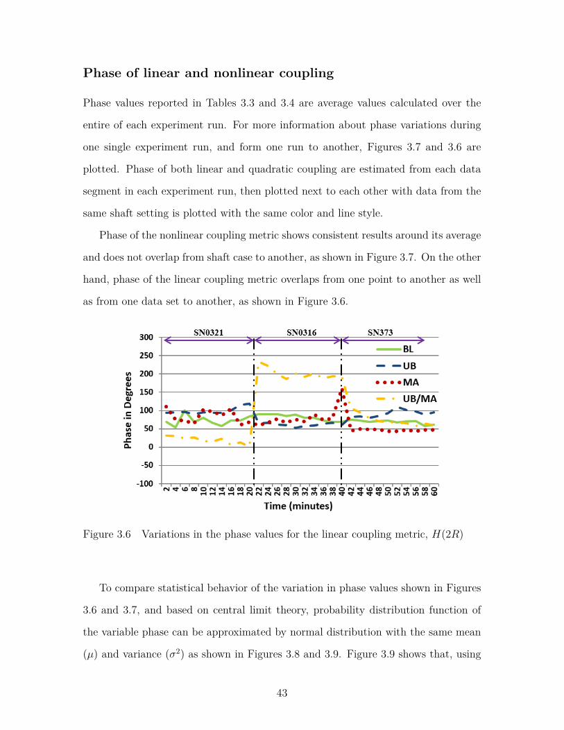
Phase of linear and nonlinear coupling

Phase values reported in Tables 3.3 and 3.4 are average values calculated over the

entire of each experiment run. For more information about phase variations during

one single experiment run, and form one run to another, Figures 3.7 and 3.6 are

plotted. Phase of both linear and quadratic coupling are estimated from each data

segment in each experiment run, then plotted next to each other with data from the

same shaft setting is plotted with the same color and line style.

Phase of the nonlinear coupling metric shows consistent results around its average

and does not overlap from shaft case to another, as shown in Figure 3.7. On the other

hand, phase of the linear coupling metric overlaps from one point to another as well

as from one data set to another, as shown in Figure 3.6.

Figure 3.6 Variations in the phase values for the linear coupling metric, H(2R)

To compare statistical behavior of the variation in phase values shown in Figures

3.6 and 3.7, and based on central limit theory, probability distribution function of

the variable phase can be approximated by normal distribution with the same mean

(µ) and variance (σ2) as shown in Figures 3.8 and 3.9. Figure 3.9 shows that, using

43

Figure 3.7 Variations in the phase values for the quadratic-nonlinear couplingmetric, AQC(1R, 1R)

the phase of the proposed quadratic coupling metric, AQC(1R, 1R), shaft misalign-

ment and imbalance can be separated from the baseline case and from each others.

Wider phase difference among faulted cases relax the requirements on setting the

threshold values to distinguish each case, which in turn decrease the probability of

false alarm. On the other hand, Figure 3.8 shows that it is hard to set the threshold

values to distinguish between the studied cases using the phase of the linear coupling

metric, H(2R). Statistical parameters of phase variations in Figures 3.6 and 3.7 are

summarized in Table 3.5.

Table 3.5 Statistical summary of phase information for linear coupling, H(2R),and nonlinear coupling, AQN(1R, 1R)

Statistical Parameter BL UB MA UB/MA

Ph(H) Mean µ 74.24 84.15 70.62 97.72STD σ 10.84 18.43 25.95 78.95

Ph(AQC) Mean µ -60.29 -5.38 190.52 25.60STD σ 12.12 19.68 38.23 23.80

44

Figure 3.8 Normal distribution using µ and σ form variable phase values (inFigure in )in Figure 3.6

Figure 3.9 Normal distribution using µ and σ form variable phase values (inFigure in )in Figure 3.7

45

3.6 Fault Detection in Presence of Noise

When power spectral peak at 2R frequency is used as condition indicator (CI) to

detect shaft faults, magnitude of the power spectrum at this frequency is estimated

and fault is detected when this magnitude exceeds predefined threshold (γ), which

may be 6dB compared to baseline case, as discussed before. In the presence of white

Gaussian noise, extra power added by the noise may cause a spectral peak magnitude

in a small margin to the detection threshold to exceed it leading to false alarm.

In this section, we theoretically study the effect of noise on condition indicators

(CIs) based on the magnitude of conventional power spectrum compared to CIs based

on magnitude of bispectrum. The idea we are trying to investigate is: if a CI has a

value that is close to the threshold γ, how much noise is going to move the CI level

to hit the threshold level causing false alarm.

Therefore, we consider it to be fault ‘detection’ problem in the form of hypothesis

testing [43] with null hypothesis, H0, and alternative hypothesis, H1, as follows:

H0: No significant fault at the frequency of interest (CI < γ)

H1: Significant fault at the frequency of interest (CI ≥ γ)

For any hypothesis test, two types of possible errors should be considered: false-

negative, and false-positive errors [44]. In the context of our fault detection problem,

the false-negative error is the case when the CI is smaller than the detection threshold,

CI < γ, so that no fault is indicated but in fact there is actually a fault. However,

in our noise analysis study, the false-negative cases do not needed to be considered

because the noise power is merely added to the CI power.

Meanwhile, the false-positive error (or false alarm error) is the case when the

estimated CI is greater than the detection threshold so that it indicates the presence

of fault when in fact fault does not exist. Then, the false alarm probability regarding

46

fault detection becomes as follows;

Pfa = P (H1|H0)

Pfa = P (CI ≥ γ | No significant fault exist) (3.10)

In order to theoretically compare the effect of noise on CIs based on conventional

power spectrum in one side versus CIs based on bispectrum on the other side, we

consider a simple signal model, x(t), to simulate our case as shown in equation (3.11).

x(t) = A1 cos(2πf1t+ θ1) + A2 cos(2πf2t+ θ2)

+A12 cos(2πf1t+ θ1)× cos(2πf2t+ θ2) (3.11)

In the following analysis, we will refer to the noisy signal as xn(t) which represent

the signal under study x(t) with added white Gaussian noise n(t) as follow;

xn(t) = x(t) + n(t) (3.12)

Noise Effect on CIs Based on Magnitude of Conventional Power Spectrum

Consider a condition indicator CI that is based on magnitude of the power spec-

trum of signal xn(t) at certain frequency f (2R in our shaft-fault case). This CI can

be estimated from the power spectrum, as discussed in Chapter 2, as follow;

CI2 = E{Xn(f)X∗n(f)} = E{(X(f) +N(f))(X(f) +N(f))∗} (3.13)

where N(f) is the Fourier transform of the noise signal n(t). Since X(f) and N(f)

are independent, equation (3.13) can be rewritten as follows;

CI2 = E{|X(f)|2}+ E{|N(f)|2} (3.14)

47

The value E{|X(f)|2} in equation (3.14) represents the actual value of the con-

dition indicator based on the pure signal x(t), and we will refer to this part as C2x.

E{|N(f)|2} represents the power added by the noise. Assuming that the noise n(t)

is zero-mean Gaussian random variable (n(t) ∼ N (0, σ2n)), its discrete Fourier trans-

form is also zero-mean Gaussian random variable (N(f) ∼ N (0, σ2n

L)), where L is the

number of discrete Fourier transform points. Recall that the expected value operator

E{.} is practically estimated using average over ensemble of M realization of the sig-

nal, as discussed in Chapter 2. Summation of magnitude squared normal distribution

becomes a central chi-square random variable with M degrees of freedom, as shown

in equation (3.15).

CI2 = C2x + E{|N (0, σ

2n

L)|2}

= C2x + 2

M

M∑i=1|Ni(0,

σ2n

L)|2

= C2x + 2σ2

n

LMχ2M (3.15)

Substituting form equation (3.15) in equation (3.10), probability of false alarm

can now be estimated as follows;

Pfa = P (C2x + 2σ2

n

LMχ2M ≥ γ | No significant fault exist)

Pfa = P

χ2M ≥

LM

2(σn/γ)2

1−(Cxγ

)2 (3.16)

where γ indicates the fault detection threshold, (Cx/γ) is signal-to-threshold ratio

(STR) which indicates how close the pure-signal is to the threshold, and (σn/γ) is

noise-to-threshold ratio (NTR). From (3.16), we can theoretically project the proba-

bility of false alarm with respect to the noise, and clearly conclude that the probability

of false alarm increases as σn increases. It worthwhile to mention here that equation

(3.16) makes sense only when (Cx < γ).

48

Figure 3.10 illustrates the theoretical and experimental results regarding the

change of the probability of false alarm as the noise-to-threshold power ratio (NTR)

increases, and where NTR is defined as follows;

Noise-to-Threshold power Ratio (NTR) = 20 log10

(σnγ

)(3.17)

For this analysis, signal model in (3.11) is considered. The sampling frequency

is set to 4800 Hz, f1=80 Hz, f2=120 Hz, number of signal segments or realizations

M=15, and number of discrete Fourier transform points L=1024. The signal-to-

threshold power ratio (STR) is set to 0.8 (-1.94 dB). Theoretical result is derived

from (3.16), and Monte-carlo type numerical experiments are carried out using the

synthesized signal in (3.11).

Figure 3.10 Effect of noise on CI based on magnitude of conventional powerspectrum: variation of the probability of false alarm, Pfa, with respect tonoise-to-threshold power ratio, NTR (σn/γ)

49

Moreover, using equation (3.16), we can theoretically study the variation of the

probability of false alarm with respect to the number of signal realizations M , the

number of discrete Fourier transform points L, and the signal-to-threshold power

ratio (STR). For example, Figure 3.11 shows variations in the probability of false

alarm with respect to the noise-to-threshold power ratio (NTR) at different values of

signal-to-threshold power ratio (STR).

Figure 3.11 Effect of STR (Cx/γ) on the variation of the probability of falsealarm, Pfa, with respect to NTR (σn/γ)

Noise Effect on Cross-Bispectrum

In this subsection, we study the effect of noise on the cross-bispectrum so we can

use it to analyze the effect of noise on CI based on magnitude of cross-bispectrum.

In order to determine the statistical behaviour of the cross-bispectrum under the

effect of white Gaussian noise, we start with recalling that white Gaussian noise

affects all the frequency components with the same amount of noise power which

50

is normally distributed (N(f) ∼ N (0, σ2n

L)) where L is the number discrete Fourier

transform points. Thus, Xn(f1) = X(f1) +N(f1), Xn(f2) = X(f2) +N(f2), and the

cross-bispectrum becomes as follows;

SXXY (f1, f2) = E{(X(f1)+N(f1))(X(f2)+N(f2))(X(f3 = f1+f2)+N(f3))∗} (3.18)

Since we are dealing with shaft harmonics, our signal of interest mainly consists

of sinusoidal components rather than broadband spectral components. Thus, sig-

nal spectral component at certain frequency can be represented as magnitude and

phase; for example, X(f1) = A12 e

jθ. Thus, cross-bispectrum in equation (3.18) can be

rewritten as follows;

SXXY (f1, f2) = E

{(A1

2 ejθ1 +N(f1))(

A2

2 ejθ2 +N(f2))(

A3

2 ej(θ1+θ2) +N(f3))∗}(3.19)

Please note that magnitude A and phase θ of each sinusoidal frequency compo-

nents are deterministic. Thus, E{.} works only on the noise components which we

will refer to as N1, N2, and N3 for simplicity. Hence, equation (3.19) can be simplified

as follows;

SXXY (f1, f2) =(A1A2A3

8

)+ E{N1N2N

∗3}

+A1

2 ejθ1A2

2 ejθ2E{N∗3}+ A1A3

4 ejθ2E{N2}+ A2A3

4 ejθ1E{N1}

+ A1

2 ejθ1E{N2N∗3}︸ ︷︷ ︸+ A2

2 ejθ2E{N1N∗3}︸ ︷︷ ︸+ A3

2 e−j(θ1+θ2)E{N1N2}︸ ︷︷ ︸E1 E2 E3

=(A1A2A3

8

)+ 0 + 0 + 0 + 0 + E1 + E2 + E3 (3.20)

The noise is assumed to be zero-mean white Gaussian noise. Thus, in equation

(3.20), first-order moments and third order moments are equal to zero, E{N1} =

51

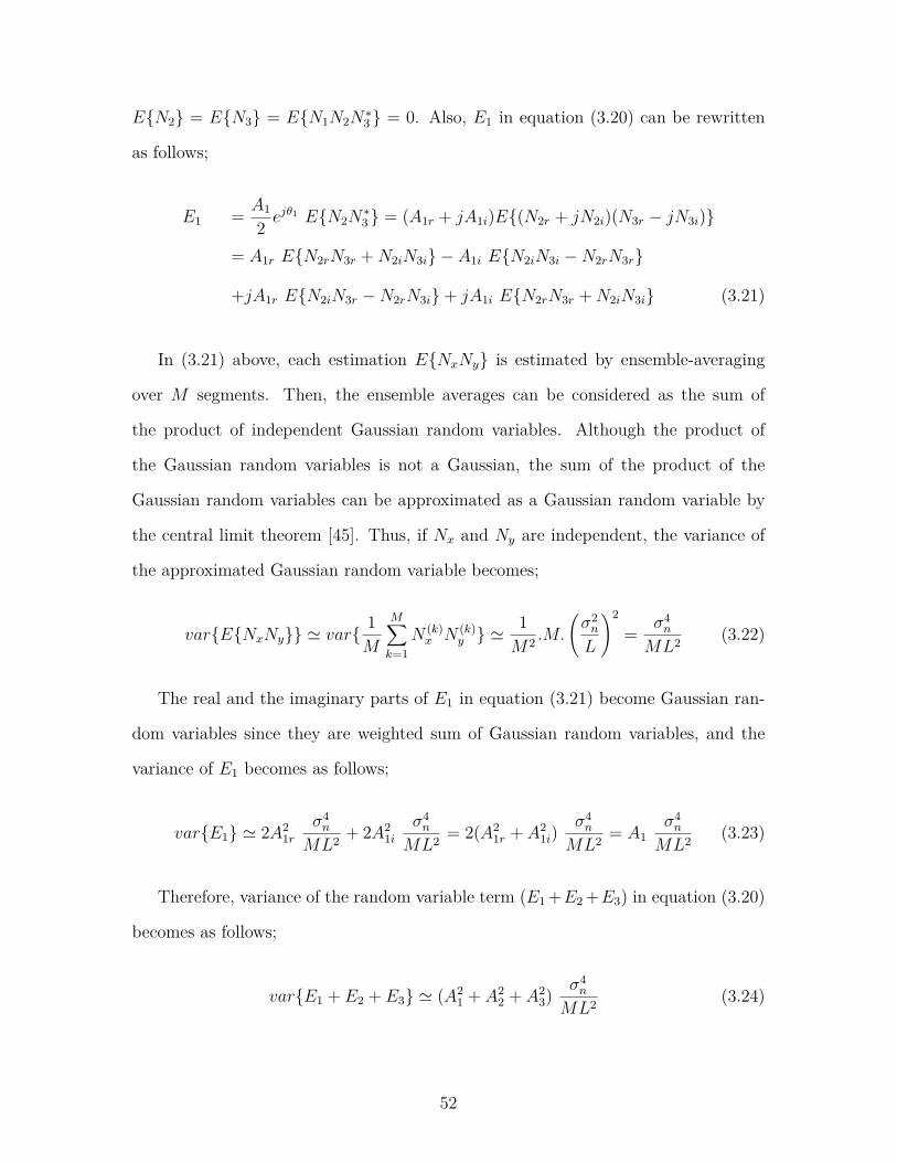
E{N2} = E{N3} = E{N1N2N∗3} = 0. Also, E1 in equation (3.20) can be rewritten

as follows;

E1 = A1

2 ejθ1 E{N2N∗3} = (A1r + jA1i)E{(N2r + jN2i)(N3r − jN3i)}

= A1r E{N2rN3r +N2iN3i} − A1i E{N2iN3i −N2rN3r}

+jA1r E{N2iN3r −N2rN3i}+ jA1i E{N2rN3r +N2iN3i} (3.21)

In (3.21) above, each estimation E{NxNy} is estimated by ensemble-averaging

over M segments. Then, the ensemble averages can be considered as the sum of

the product of independent Gaussian random variables. Although the product of

the Gaussian random variables is not a Gaussian, the sum of the product of the

Gaussian random variables can be approximated as a Gaussian random variable by

the central limit theorem [45]. Thus, if Nx and Ny are independent, the variance of

the approximated Gaussian random variable becomes;

var{E{NxNy}} ' var{ 1M

M∑k=1

N (k)x N (k)

y } '1M2 .M.

(σ2n

L

)2

= σ4n

ML2 (3.22)

The real and the imaginary parts of E1 in equation (3.21) become Gaussian ran-

dom variables since they are weighted sum of Gaussian random variables, and the

variance of E1 becomes as follows;

var{E1} ' 2A21r

σ4n

ML2 + 2A21i

σ4n

ML2 = 2(A21r + A2

1i)σ4n

ML2 = A1σ4n

ML2 (3.23)

Therefore, variance of the random variable term (E1 +E2 +E3) in equation (3.20)

becomes as follows;

var{E1 + E2 + E3} ' (A21 + A2

2 + A23) σ4

n

ML2 (3.24)

52

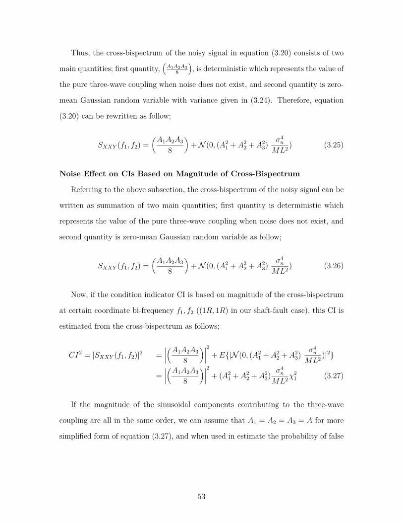
Thus, the cross-bispectrum of the noisy signal in equation (3.20) consists of two

main quantities; first quantity,(A1A2A3

8

), is deterministic which represents the value of

the pure three-wave coupling when noise does not exist, and second quantity is zero-

mean Gaussian random variable with variance given in (3.24). Therefore, equation

(3.20) can be rewritten as follow;

SXXY (f1, f2) =(A1A2A3

8

)+N (0, (A2

1 + A22 + A2

3) σ4n

ML2 ) (3.25)

Noise Effect on CIs Based on Magnitude of Cross-Bispectrum

Referring to the above subsection, the cross-bispectrum of the noisy signal can be

written as summation of two main quantities; first quantity is deterministic which

represents the value of the pure three-wave coupling when noise does not exist, and

second quantity is zero-mean Gaussian random variable as follow;

SXXY (f1, f2) =(A1A2A3

8

)+N (0, (A2

1 + A22 + A2

3) σ4n

ML2 ) (3.26)

Now, if the condition indicator CI is based on magnitude of the cross-bispectrum

at certain coordinate bi-frequency f1, f2 ((1R, 1R) in our shaft-fault case), this CI is

estimated from the cross-bispectrum as follows;

CI2 = |SXXY (f1, f2)|2 =∣∣∣∣(A1A2A3

8

)∣∣∣∣2 + E{|N (0, (A21 + A2

2 + A23) σ4

n

ML2 )|2}

=∣∣∣∣(A1A2A3

8

)∣∣∣∣2 + (A21 + A2

2 + A23) σ4

n

ML2χ21 (3.27)

If the magnitude of the sinusoidal components contributing to the three-wave

coupling are all in the same order, we can assume that A1 = A2 = A3 = A for more

simplified form of equation (3.27), and when used in estimate the probability of false

53

alarm in equations (3.10) gives

Pfa = P ((A6

64

)+ 3A2 σ4

n

ML2χ21 ≥ γ6 | No significant fault exist)

Pfa = P

χ21 ≥

ML2

3(A/γ)2(σn/γ)4

1− 164

(A

γ

)6 (3.28)

where (A/γ) is signal-to-threshold ratio (STR), and (σn/γ) is noise-to-threshold ratio

(NTR).

Figure 3.12 Effect of noise on CI based on magnitude of cross-bispectrum:variation of the probability of false alarm, Pfa, with respect to noise-to-thresholdpower ratio, NTR (σn/γ)

Figure 3.12 illustrates the theoretical and experimental results regarding the

change of the probability of false alarm as the noise-to-threshold power ratio (NTR)

increases. Theoretical result is derived from (3.28), and Monte-carlo type numerical

experiments are carried out using the synthesized signal in (3.11).

Finally, combining graphs from Figures 3.10 and 3.12 clearly indicates that CI

54

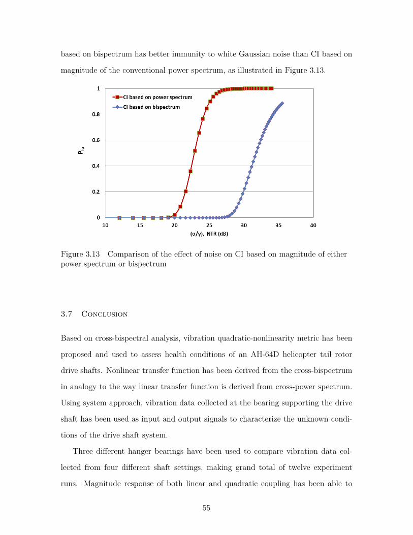
based on bispectrum has better immunity to white Gaussian noise than CI based on

magnitude of the conventional power spectrum, as illustrated in Figure 3.13.

Figure 3.13 Comparison of the effect of noise on CI based on magnitude of eitherpower spectrum or bispectrum

3.7 Conclusion

Based on cross-bispectral analysis, vibration quadratic-nonlinearity metric has been

proposed and used to assess health conditions of an AH-64D helicopter tail rotor

drive shafts. Nonlinear transfer function has been derived from the cross-bispectrum

in analogy to the way linear transfer function is derived from cross-power spectrum.

Using system approach, vibration data collected at the bearing supporting the drive

shaft has been used as input and output signals to characterize the unknown condi-

tions of the drive shaft system.

Three different hanger bearings have been used to compare vibration data col-

lected from four different shaft settings, making grand total of twelve experiment

runs. Magnitude response of both linear and quadratic coupling has been able to

55

detect the faulted cases compared to the baseline case. However, theoretical and

Monte-carlo type experimental analysis have proven that using condition indicators

based on magnitude of the bispectrum has better immunity to white Gaussian noise

than condition indicators based on magnitude of the conventional power spectrum.

Moreover, using the phase of the proposed nonlinear coupling has shown better capa-

bilities in distinguishing the four studied shaft settings than the conventional linear

coupling. Phase of the AQC(1R, 1R) metric has shown more consistent result among

the three studied bearing cases for each shaft setting than what the phase of H(2R)

has done. It also has shown wider phase difference between the studied cases without

overlap among them. Wider phase difference relaxes the requirements when setting

threshold values to diagnose different faulted cases.

56

Chapter 4

Quadratic-Nonlinearity Power-Index Spectrum

In this chapter, a new concept of Quadratic-Nonlinearity Power-Index spectrum,

QNLPI(f), that can be used in signal detection and classification, is proposed based

on bicoherence spectrum. The proposed QNLPI(f) is derived as a projection of the

three-dimensional bicoherence spectrum into two-dimensional spectrum that quan-

titatively describes how much of the mean square power at certain frequency f is

generated by nonlinear quadratic interaction between different frequencies.

4.1 Introduction

Bispectrum and its normalized version bicoherence have shown to be useful tools

in machine condition monitoring fields (e.g., [46]-[51]). However, investigation of

quadratic nonlinearities using bispectrum/bicoherence becomes a challenging task

when the studied signal contains wide range of frequency interactions. The three

dimensional nature of these spectra requires careful design of the view and expert

personnel to interpret the results in the frequency domain. Therefore, it is easier to

use features extracted from those spectra to summarize and describe nonlinearities in

the monitored signals. For example; bispectrum mean-magnitude and phase-entropy

have been used in blind detection of photo-montage [52], normalized bispectrum

entropy and normalized bispectrum squared entropy have been used in health assess-

ment of human cardiac [53], and invariant phases of integrated bispectrum has been

used to detect mines in acoustic images [54], [55]. Since machine fault diagnostic

is better archived by linking certain frequency to a particular rotating component,

57

quadratic-nonlinearity power-index (QNLPI(f)) spectrum has been proposed as a

way to summarize information in the 3D bicoherence into 2D frequency spectrum

[56], [57].

In this Chapter, the proposed concept of the QNLPI(f) is discussed includ-

ing mathematical derivation, considerations in its digital computation and boundary

limits. The quadratic-nonlinear power spectral density PQNL(f) and percentage of

quadratic nonlinear power PQNLP are also introduced based on the QNLPI(f),

as will be discussed in section 4.3. Based on higher order statistical (HOS) analysis,

this chapter presents applications of the proposed nonlinearity measures to real-world

vibration data obtained from a dedicated condition based maintenance experimental

helicopter drive-train, as will be shown in sections 4.8 and 4.9. Health condition of

different rotating components in the drive train is assessed including different com-

binations of drive-shaft and gearbox faults. The QNLPI(f) spectrum enables us

to gain more details about nonlinear harmonic generation patterns that can be used

to distinguish between different cases of mechanical faults, which in turn helps to

gaining more diagnostic/prognostic capabilities.

4.2 Bicoherence Spectrum

As discussed previously in section 2.3, the magnitude of the bispectrum Bxxx(f1, f2)

at coordinate point (f1, f2) measures the degree of phase coherence between the three

frequency components f1, f2, and f3, as repeated in equation (4.1) for convenience.

Bxxx(f1, f2) = E{X(f1)X(f2)X∗(f3 = f1 + f2)} (4.1)

However, this magnitude is also dependent on the magnitude of the relevant

Fourier coefficients. Therefore, a common function used to normalize the bispec-

trum is called bicoherence. The bicoherence function is defined as shown in equation

58

(4.2) [35], [58], [59].

b2xxx(f1, f2) = |Bxxx(f1, f2)|2

E{|X(f1)X(f2)|2}E{|X(f1 + f2)|2} (4.2)

The bicoherence bxxx(f1, f2) in (4.2) is independent of the magnitude of the Fourier

transform and bounded by 0 ≤ bx(f1, f2) ≤ 1, where unity means full three-waves

coupling (i.e., interaction has taken place between the waves), and zero implies an

absence of coherence or interaction. Moreover, it has been proven in [35] that the

squared bicoherence, b2x(f1, f2), quantifies the fraction of mean square power at f3 =

f1 + f2 due to the quadratic coupling between the waves at f1 and f2. This previous

property inspired us to propose a metric that shows the quadratic interaction relation

(3 waves coupling) in terms of the “result” instead of the “source” of the interaction.

Hence, the bi-frequency space required to plot the bicoherence (showing the source

of interaction) can be reduced to a single-frequency space (showing the accumulative

results).

4.3 QNLPI(f) Spectrum

The Quadratic-Nonlinearity Power-Index, QNLPI(f), spectrum is proposed as an

implementation of the idea discussed above, and hence it should quantify the fraction

of the mean square power at a certain frequency f produced by all the possible

combinations of quadratic interactions that may cause the creation of this frequency,

f . This idea can be achieved by integrating the bicoherence spectrum along a straight

line f1 + f2 = f represents the locus of all quadratic interactions in f1− f2 space that

result in f , as represented by equation (4.3).

QNLPI(f) =∫

f1+f2=f

b2xxx(f1, f2) df1 (4.3)

59

This integration along f1 + f2 = f is depicted by the dashed line in Figure 4.1.

However, we should be very careful when we apply this integration in (4.3) to the

conventional region of computation indicated by the triangle “A” shown in Figure

4.1. Due to the symmetry properties, the bicoherence of interacted frequencies in

the fourth quadrant (positive f1 and negative f2) has a redundant copy in this “A”

region. Therefore, the region of computation in f1−f2 plane is modified to fully map

the quadratic interaction between different frequencies as shown in Figure 4.1. The

area covered by triangle “B” maps the difference part of the interaction between two

frequencies (f1,−f2), while area covered by the upper triangle “A” maps only the

sum part (f1, f2). Based on this new region of computation, QNLPI(f) in (4.3) can

be rewritten as follows:

QNLPI(f) =

f2 + fs

4∫f2

b2xxx(f1, f − f1) df1

=

fs4∫

0

b2xxx(

f

2 + f1,f

2 − f1) df1 (4.4)

Equation (4.4) indicates that all the information contained in the bicoherence is

represented in the QNLPI(f) which is function in one variable, f . Moreover, the

QNLPI(f) inherits useful characteristics from the third order statistics, bicoherence,

such as high capability of nonlinear-systems identifications, high immunity to additive

gaussian noise, and amplification invariance. Furthermore, it can be proven that

QNLPI(f) is theoretically bounded between zero and one (0 ≤ QNLPI(f) ≤ 1) as

shown in the following section. Zero value of QNLPI(f) means that no quadratic-

nonlinearity produces any power at this frequency, while one means all the power at

frequency f result from quadratic-nonlinearity.

60

Figure 4.1 Region of computation (ROC) for the proposed QNLPI(f) assumingaliasing is absent: triangle “A” is the conventional ROC for thebispectrum/bicoherence, region “A−B” is used to calculate the proposedQNLPI(f), and dashed line indicates the direction of integration

4.4 Boundary Limits of QNLPI(f)

Assume that the signal at frequency m, X(m), is constructed from finite number of

quadratic coupling pairs plus non-quadratic coupling part as shown in equation (4.5).

X(m) =∑

∀ l+k=mAl,kX(l)X(k) +X

′(m) (4.5)

where Al,k is the coupling coefficient between two frequencies l and k to produce

sum frequency m. X ′(m) represents any non-quadratic coupling power in the signal,

either independent excitation or from other higher order interactions. Assuming that

x(t) is a zero-mean wide-sense stationary random signal, the mean square power at

frequency m, Px(m), can be proven to be as follows [35];

61

Px(m) =∑

(∀ l+k=m)|Al,k|2 E{|X(l)X(k)|2}+ E{|X ′(m)|2} (4.6)

First part of equation (4.6) represents the total power at frequency m due to all

quadratic coupling pairs, while the second part is due to any non-quadratic-coupling

power at this frequency. Substituting from equation (4.2) in equation (4.4),

QNLPI(m) =fs/4∫0

|E{X(m2 + f1)X(m2 − f1)X∗(m)}Px(m) · E{|X(m2 + f1)X(m2 − f1)|2} df1 (4.7)

Then, from equation (4.5) in equation (4.7) recalling properties of expected value

operator, we get the following equation:

QNLPI(m) = 1Px(m)

fs/4∫0

(|A+B|2

C

)df1 (4.8)

where,

A =∑

∀ l+k=mAl,k E

{X(m2 + f1)X(m2 − f1)X∗(l)X∗(k)

}

B = E{X(m2 + f1)X(m2 − f1)X ′∗(m)

}C = E

{|X(m2 + f1)X(m2 − f1)|2

}

The value of the expected value operators in the numerator of equation (4.8) will

be zero except when variable f1 equals to f1 = m2 − l = m

2 + k. Therefore, integration

in equation (4.8) is reduced to summation as follows:

QNLPI(m) =

∑∀l+k=m

|Al,k|2E{|X(l)X(k)|2}

P (m) (4.9)

Note that numerator of equation (4.9) represents the total power at frequency m

due to all quadratic coupling pairs and it is fraction of Px(m) as shown before in

equation (4.6). Hence, the proposed index, QNLPI(m), measures the fraction of the

62

mean square power at frequencym due to quadratic coupling between all combination

of frequencies that possibly result in m. Also, from (4.9), 0 ≤ QNLPI(m) ≤ 1, and

will equal one if, and only if, X ′(m) = 0.

4.5 Digital Computation of QNLPI(f)

The same procedure described in [35] can be followed in order to calculate digital

bicoherence talking into consideration the modified region of computations described

before in Figure 4.1 to separate and account for both positive and negative parts of

frequency interactions. Next, digital computation of the QNLPI(f) can be carried

out by replacing integration in (4.4) by summation as shown in (4.10).

QNLPI(f) =n= N

2 −1∑n=0

b2xxx((

f

2 + n∆f), (f2 − n∆f)) (4.10)

where ∆f is the elementary band width determined from the resolution of DFT

calculation. ∆f = fN/N , fN = fS/2, and N is the number of points used in DFT cal-

culation. The frequency resolution ∆f should be smaller than the difference between

the smallest two frequencies expected to interact in any particular case.

4.6 Quadratic-Nonlinear Power Spectral Density, PQNL(f)

As discussed in section 2.2, power spectral density Pxx(f) is the Fourier transform of

the auto-correlation function Rxx(τ) for a stationary random process x(t) according to

Wiener-Khintchine theorem [33], [34]. Thus, it can be estimated using the following

equation:

Pxx(f) = E{X(f)X∗(f)} = E{|X(f)|2} (4.11)

Pxx(f) has the dimensions of mean square values/Hz and it indicates how the mean

square value is distributed over frequency.

63

Based on the proposed QNLPI(f) index discussed in the preceding subsection,

one can estimate how much of the mean square power at certain frequency is generated

due to the second order nonlinearity by multiplying the QNLPI(f) index at this

frequency by the power spectral density Pxx(f), as follows:

PQNL(f) = QNLPI(f) · Pxx(f) (4.12)

where PQNL(f) is the nonlinear power spectral density showing the distribution of

quadratic-nonlinearly-generated mean square power over frequency, and it also has

the dimensions of mean square values/Hz. Thus, integration of PQNL(f) over the

whole range of frequencies estimates the total quadratic nonlinear power contained in

the signal. It would be also useful to quantify the percentage of quadratic nonlinear

power (PQNLP ) to the total mean square power as follow:

PQNLP =

N−1∑n=0

QNLPI(n∆f) · Pxx(n∆f)N−1∑n=0

Pxx(n∆f)(4.13)

where denominator in equation (4.13) estimates the total power in the signal while

the numerator estimates the overall quadratic nonlinear power. PQNLP is a single-

value metric that is useful in monitoring the severity of nonlinear behavior of the

signal under study which can be used to monitor fault-progress, as will be shown in

section 4.9.

4.7 Numerical Example of QNLPI(f)

Before we apply the proposed indices to study nonlinear coupling in real world vi-

bration data, we will use simple signal to illustrate the usefulness of these metrics

and help understand the physical interpretation of their values. Thus, a computer-

generated test signal has been used as shown in equation (4.14).

64

x(t) = Ab cos(2πfbt+ θb) + Ac cos(2πfct+ θc) + Ae cos(2πfet+ θe)

x(t) = +Ag cos(2πfgt+ θg) + Abc cos(2πfbt+ θb)× cos(2πfct+ θc)

x(t) = +Aeg cos(2πfet+ θe)× cos(2πfgt+ θg) + Ad cos(2πfdt+ θd) (4.14)

where Ab = Ac = Ad = Ae = Ag = 2, Abc = Aeg = 4, sampling frequency fs =

2fN = 4.8 kHz, fb/fN = 0.22, fc/fN = 0.375, fe/fN = 0.292, fg/fN = 0.303 and

fd = fb+fc = fe+fg. All the phases are independently taken from a set of uniformly

distributed random numbers.

In this testing signal x(t), the total power at fd is a share of three equal source;

the independent excitation, the quadratic nonlinear interaction between fb and fc,

and the quadratic nonlinear interaction between fe and fg. The power spectrum

of the test signal, the modified bicoherence b2xxx(f1, f2), the quadratic-nonlinearity

power-index QNLPI(f), and the quadratic-nonlinear power spectrum PQNL(f) are

shown in Figure 4.2.

From Figure 4.2-(b), b2xxx(fc, fb) = 0.324, and b2

xxx(fg, fe) = 0.329 are lined up

on the same f1 + f2 = fd axis. This means that each group contributes to the

quadratic-nonlinearity power-index in Figure 4.2-(c) by approximately one third.

b2xxx(fg,−fe) = 1 and b2

xxx(fc,−fb) = 1 lie in the “B” zone of the modified bicoherence

and represent the negative part of the interaction for both fc − fb and fg − fe. The

detailed bicoherence spectrum in Figure 4.2-(b) is represented by the QNLPI(f) in

Figure 4.2-(c). QNLPI(fd) = 0.653 which means that two-thirds of the total power

at frequency fd is coming from quadratic-nonlinear interaction between different fre-

quencies. The power spectral contents that generated only by quadratic nonlinearity

are separated in the PQNL(f) as shown in Figure 4.2-(d). Percentage of quadratic

nonlinear power, PQNLP , is estimated and found to be = 42.93%.

65

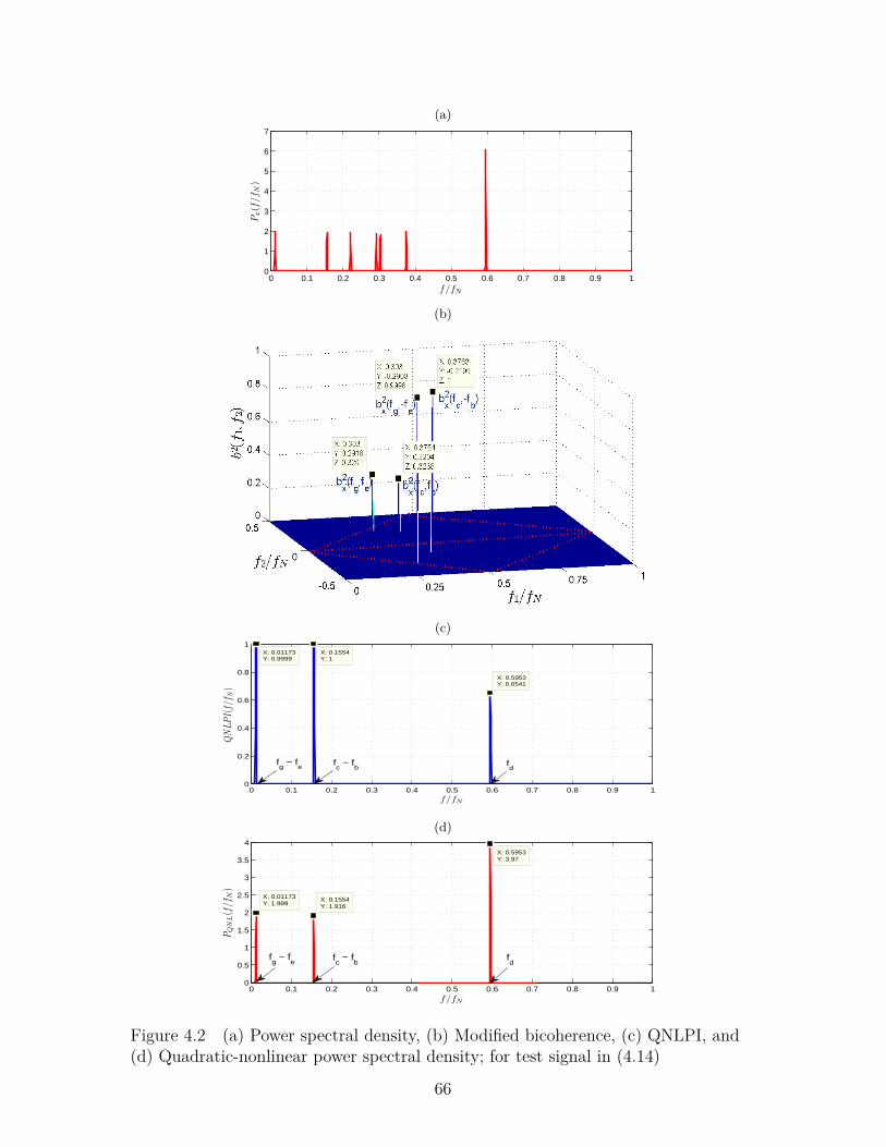
(a)

0 0.1 0.2 0.3 0.4 0.5 0.6 0.7 0.8 0.9 10

1

2

3

4

5

6

7

f/fN

Px(f/f

N)

(b)

(c)

0 0.1 0.2 0.3 0.4 0.5 0.6 0.7 0.8 0.9 10

0.2

0.4

0.6

0.8

1

X: 0.5953Y: 0.6541

f/fN

QNLPI(f/

f N)

X: 0.01173Y: 0.9999

X: 0.1554Y: 1

fc − f

bfg − f

e fd

(d)

0 0.1 0.2 0.3 0.4 0.5 0.6 0.7 0.8 0.9 10

0.5

1

1.5

2

2.5

3

3.5

4

X: 0.01173Y: 1.999

f/fN

PQNL(f/f

N)

X: 0.1554Y: 1.916

X: 0.5953Y: 3.97

fg − f

efc − f

bfd

Figure 4.2 (a) Power spectral density, (b) Modified bicoherence, (c) QNLPI, and(d) Quadratic-nonlinear power spectral density; for test signal in (4.14)

66

4.8 Application of QNLPI(f) in Health Assessment of Helicopter’s

Tail-Rotor Drive-Shafts

Focus of this study is centered on studying different combinations of drive-shafts faults

using both conventional power spectral density (PSD) and the proposed QNLPI(f).

Shafts numbered 3-5 in Figure 1.5-(a) operate at a rotation speed of 4863 RPM

(81.05Hz) corresponding to full-speed of shaft rotation on the fielded rotorcraft, as

shown in the schematic in Figure 4.3. The vibration signals denoted as FHB and

AHB, measured at forward and afterward hanger bearings respectively, are gath-

ered at two minutes intervals at a sampling rate of 48 kHz over the course of thirty

minute test runs. The measurements are taken for different drive-shafts setting un-

der test which include baseline shaft and bearing configuration, unbalance in different

shafts configuration, and shaft misalignment, all common issues on AH-64 drivetrains.

Misalignment of the shafts is studied at 1.3◦ between drive-shafts #3 and #4, 1.3◦

between drive-shafts #4 and #5. Unbalance is studied at drive-shafts #3, #4 and

#5 by 0.140 oz-in, 0.135 oz-in 0.190 oz-in respectively. Different combination of

misalignment and unbalance are tested as summarized previously in Table 3.1.

Figure 4.3 Schematic of the TRDT test stand at USC

Due to the loading scheme of the TRDT test stand with the intermediate gear

box (IGB) and the output motor torque, the 3rd harmonic of the tail rotor drive shaft

(243 Hz) is dominating the power spectrum of the AHB vibrations in the studied

67

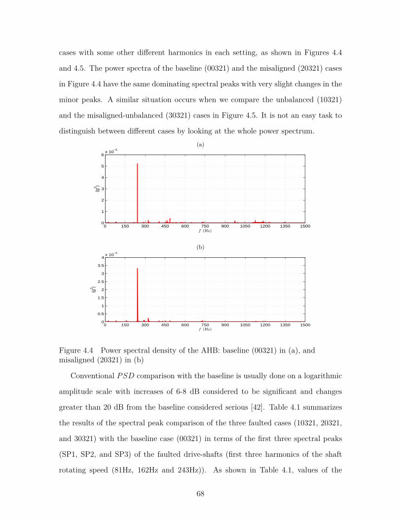
cases with some other different harmonics in each setting, as shown in Figures 4.4

and 4.5. The power spectra of the baseline (00321) and the misaligned (20321) cases

in Figure 4.4 have the same dominating spectral peaks with very slight changes in the

minor peaks. A similar situation occurs when we compare the unbalanced (10321)

and the misaligned-unbalanced (30321) cases in Figure 4.5. It is not an easy task to

distinguish between different cases by looking at the whole power spectrum.(a)

0 150 300 450 600 750 900 1050 1200 1350 15000

1

2

3

4

5

6x 10

−5

f (Hz)

(g2 )

(a)(b)

0 150 300 450 600 750 900 1050 1200 1350 15000

0.5

1

1.5

2

2.5

3

3.5

4x 10

−5

f (Hz)

(g2 )

Figure 4.4 Power spectral density of the AHB: baseline (00321) in (a), andmisaligned (20321) in (b)

Conventional PSD comparison with the baseline is usually done on a logarithmic

amplitude scale with increases of 6-8 dB considered to be significant and changes

greater than 20 dB from the baseline considered serious [42]. Table 4.1 summarizes

the results of the spectral peak comparison of the three faulted cases (10321, 20321,

and 30321) with the baseline case (00321) in terms of the first three spectral peaks

(SP1, SP2, and SP3) of the faulted drive-shafts (first three harmonics of the shaft

rotating speed (81Hz, 162Hz and 243Hz)). As shown in Table 4.1, values of the

68

(a)

0 150 300 450 600 750 900 1050 1200 1350 15000

0.5

1

1.5

2x 10

−5

f (Hz)

(g2 )

(a)(b)

0 150 300 450 600 750 900 1050 1200 1350 15000

0.5

1

1.5x 10

−5

f (Hz)

(g2 )

Figure 4.5 Power spectral density of the AHB: unbalanced (10321) in (a), andmisaligned-unbalanced (30321) in (b)

SP2 for all faulted cases exceed the 6 dB threshold compared to the baseline and

therefore it provides a good indicator for all of the three faulted cases. In fact, SP2

is currently employed in the HUMS system to detect unbalanced and/or misaligned

shafts in a tail rotor drive-train of a rotorcraft [38]. However, this Condition Indicator

(CI) has limited diagnostic capabilities in specifying whether the fault is unbalance,

misalignment or a combination of both faults. The maintainers are told to check for

more than one source that might cause that CI to exceed its limit.

Table 4.1 Comparison with baseline case in terms of SP1, SP2, and SP3 (dB)

A/UB(10321) MA/B (20321) UB/MA(30321)SP1 5.311 -0.081 4.799SP2 9.997 10.255 8.661SP3 -2.001 -2.0667 -8.141

69

The vibration data is then investigated using the proposed QNLPI(f) discussed

in section 4.3. Figure 4.6-(a) shows QNLPI(f) spectrum for the baseline case for

which nonlinearly-generated frequencies located at 1st and 7th harmonics of the drive-

shaft with values 0.68 and 0.77, respectively. These values can be result of interaction

between the dominating 3rd harmonic with the 4th to produce 68% and 77% of the

power at 1st and 7th harmonics, respectively. The remaining fraction of the power

may be independently excited or coming from other forms of nonlinearities.

(a)

0 150 300 450 600 750 900 1050 1200 1350 15000

0.2

0.4

0.6

0.8

1

f (Hz)

QNLPI(f)

(a)(b)

0 150 300 450 600 750 900 1050 1200 1350 15000

0.2

0.4

0.6

0.8

1

f (Hz)

QNLPI(f)

Figure 4.6 QNLPI of the AHB: baseline (00321) in (a), and misaligned (20321) in(b)

Due to different experimental settings, different interaction pattern exists in the

case of misalignment as shown in Figure 4.6-(b). In this case, quadratic nonlinear

interaction between the 3rd and the 1st harmonics is dominating. As a result of this

interaction, 2nd and 4th harmonics are generated with power fraction of 0.72 and 0.64,

respectively. The results in Figure 4.6 give us more details about the content of the

70

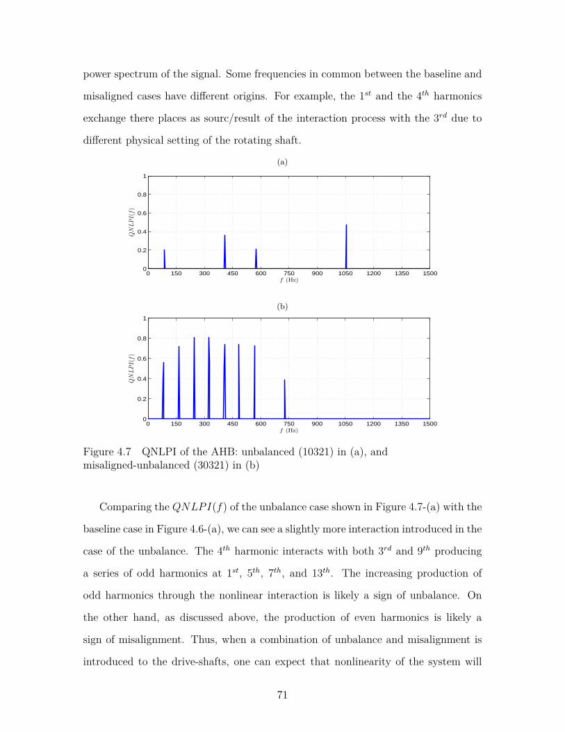
power spectrum of the signal. Some frequencies in common between the baseline and

misaligned cases have different origins. For example, the 1st and the 4th harmonics

exchange there places as sourc/result of the interaction process with the 3rd due to

different physical setting of the rotating shaft.

(a)

0 150 300 450 600 750 900 1050 1200 1350 15000

0.2

0.4

0.6

0.8

1

f (Hz)

QNLPI(f)

(a)(b)

0 150 300 450 600 750 900 1050 1200 1350 15000

0.2

0.4

0.6

0.8

1

f (Hz)

QNLPI(f)

Figure 4.7 QNLPI of the AHB: unbalanced (10321) in (a), andmisaligned-unbalanced (30321) in (b)

Comparing the QNLPI(f) of the unbalance case shown in Figure 4.7-(a) with the

baseline case in Figure 4.6-(a), we can see a slightly more interaction introduced in the

case of the unbalance. The 4th harmonic interacts with both 3rd and 9th producing

a series of odd harmonics at 1st, 5th, 7th, and 13th. The increasing production of

odd harmonics through the nonlinear interaction is likely a sign of unbalance. On

the other hand, as discussed above, the production of even harmonics is likely a

sign of misalignment. Thus, when a combination of unbalance and misalignment is

introduced to the drive-shafts, one can expect that nonlinearity of the system will

71

increase so that a variety of odd/even harmonics of the drive shaft rotating frequency

is produced as shown in Figure 4.7-(b).

From the discussion above, we can see that beside conventional power spectral

density analysis, using QNLPI(f) spectrum helps to gain more details about non-

linear harmonic interaction/generation patterns, which can be used to distinguish

between different fault settings of the tail rotor drive-shafts.

4.9 Application of QNLPI(f) to Study Progress of Gearbox Fault

In this section, we use vibration data collected in the experimental TRDT test stand

to study tail-rotor gearbox failure (denoted TRGB in Figure 1.5) due to lubrication

starvation [62]. This experiment was originally designed to demonstrate whether or

not a gearbox with a leaking output seal could be used in the filed until the aircraft

reached a phase inspection, which currently occurs every 250 hours. The output seals

were seeded to represent a worst-case scenario leak for gearboxes, as shown in Figure

4.8.

For all the tested articles, it was observed that a persistent grease leak through

the output seal resulted in a loss of lubricant in the main gear compartment. Conse-

quently, this condition ultimately resulted in lubricant starvation on the gear meshing

region and catastrophic gear teeth failures, as shown in Figure 4.9. One interesting

finding of this experiment was that gearbox can survive more than 480 hours after

fault seeding for all tested articles.

The secondary objective of the experiment was to identify vibration signatures

which might indicate the impending failure. Here, we use vibration data collected

from this experiment to illustrate the usefulness of the proposed index in keeping

track of the progress of fault in the gearbox.

72

(a) (b)

(c)

Figure 4.8 TRGB experiment setup: (a) actual TRGB, (b) seeded fault showingremoval of the output seal material, and (c) schematic of the TRGB showing thelocation of the seeded fault

73

(a) (b)

Figure 4.9 Borescope picture showing input gear teeth: (a) earlier stage of testing,and (b) after failure [62]

Figure 4.10 shows how the average power spectral density (PSD) of the gearbox

vibration changes during the last four days before failure. Inspection of the PSD

plots indicates that it was not until the day of failure that vibration power at the

third and fourth harmonics of the gear mesh frequency (1334Hz) increased suddenly

to warning values, as shown in Figure 4.10-(d). During the last three days preceding

the failure, shown in Figure 4.10-(a) ∼ (c), PSD stayed almost the same with slightly

monotonic increase of vibration power at the both first and second harmonics of the

gear mesh frequency.

74

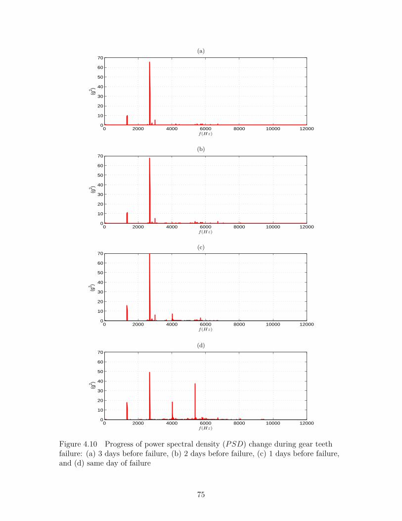
(a)

0 2000 4000 6000 8000 10000 120000

10

20

30

40

50

60

70

f(Hz)

(g2 )

(a)(b)

0 2000 4000 6000 8000 10000 120000

10

20

30

40

50

60

70

f(Hz)

(g2 )

(b)(c)

0 2000 4000 6000 8000 10000 120000

10

20

30

40

50

60

70

f(Hz)

(g2 )

(c)(d)

0 2000 4000 6000 8000 10000 120000

10

20

30

40

50

60

70

f(Hz)

(g2 )

Figure 4.10 Progress of power spectral density (PSD) change during gear teethfailure: (a) 3 days before failure, (b) 2 days before failure, (c) 1 days before failure,and (d) same day of failure

75

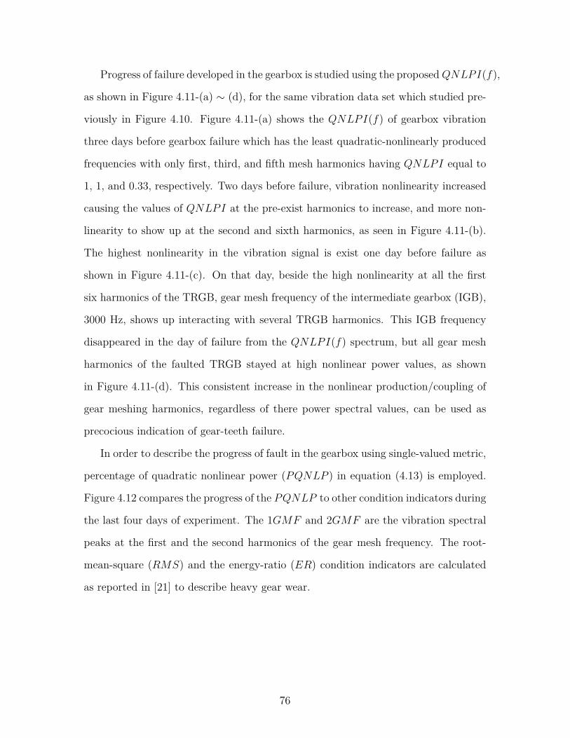
Progress of failure developed in the gearbox is studied using the proposedQNLPI(f),

as shown in Figure 4.11-(a) ∼ (d), for the same vibration data set which studied pre-

viously in Figure 4.10. Figure 4.11-(a) shows the QNLPI(f) of gearbox vibration

three days before gearbox failure which has the least quadratic-nonlinearly produced

frequencies with only first, third, and fifth mesh harmonics having QNLPI equal to

1, 1, and 0.33, respectively. Two days before failure, vibration nonlinearity increased

causing the values of QNLPI at the pre-exist harmonics to increase, and more non-

linearity to show up at the second and sixth harmonics, as seen in Figure 4.11-(b).

The highest nonlinearity in the vibration signal is exist one day before failure as

shown in Figure 4.11-(c). On that day, beside the high nonlinearity at all the first

six harmonics of the TRGB, gear mesh frequency of the intermediate gearbox (IGB),

3000 Hz, shows up interacting with several TRGB harmonics. This IGB frequency

disappeared in the day of failure from the QNLPI(f) spectrum, but all gear mesh

harmonics of the faulted TRGB stayed at high nonlinear power values, as shown

in Figure 4.11-(d). This consistent increase in the nonlinear production/coupling of

gear meshing harmonics, regardless of there power spectral values, can be used as

precocious indication of gear-teeth failure.

In order to describe the progress of fault in the gearbox using single-valued metric,

percentage of quadratic nonlinear power (PQNLP ) in equation (4.13) is employed.

Figure 4.12 compares the progress of the PQNLP to other condition indicators during

the last four days of experiment. The 1GMF and 2GMF are the vibration spectral

peaks at the first and the second harmonics of the gear mesh frequency. The root-

mean-square (RMS) and the energy-ratio (ER) condition indicators are calculated

as reported in [21] to describe heavy gear wear.

76

(a)

0 2000 4000 6000 8000 10000 120000

0.2

0.4

0.6

0.8

1

f (Hz)

QNLPI(f)

(a)(b)

0 2000 4000 6000 8000 10000 120000

0.2

0.4

0.6

0.8

1

f (Hz)

QNLPI(f)

(b)(c)

0 2000 4000 6000 8000 10000 120000

0.2

0.4

0.6

0.8

1

f (Hz)

QNLPI(f)

(c)(d)

0 2000 4000 6000 8000 10000 120000

0.2

0.4

0.6

0.8

1

f (Hz)

QNLPI(f)

Figure 4.11 Progress of nonlinear harmonic generation due to gear teeth failure:(a) 3 days before failure, (b) 2 days before failure, (c) 1 days before failure, and (d)same day of failure

77

(a)

Figure 4.12 Trend of vibration PQNLP compared to different condition indicatorsfor the faulted TRGB during the last four days before failure

As shown in Figure 4.12, the value of PQNLP starts showing considerable in-

crease one day before other condition indicators. It is consistently climbing up until

the gearbox failure due to wear in the input gear teeth which physically can be inter-

preted as increased vibration power due to highly-nonlinear rotating medium. Thus,

this trend can be used as precocious indication of failure. The advantage of using

PQNLP as condition indicator over conventional power spectrum indicators is the

inherent characteristics of HOS-based metrics as amplification invariance and high

immunity to additive Gaussian noise, which reduce the dependency on the character-

istics of the sensor used to collect the vibration data.

4.10 Conclusion

In this chapter, the quadratic-nonlinearity power-index (QNLPI(f)) has been pro-

posed which provides a summary of the nonlinearity information contained in the the

78

3D bicoherence into 2D spectrum presenting an easier way to studying third-order

statistic of signals.

The proposed index has been used to study real-world vibration data collected

from tail-rotor drive train of an AH-64D helicopter. Two case studies have been

conducted. In the first case, QNLPI(f) has shown better diagnostic capabilities in

differentiating between different drive-shaft faults by showing how different physical

settings affect the nonlinear generation of harmonics. In the second case, QNLPI(f)

has shown better capability in detecting gearbox failure. For easier monitoring of

the fault-progress in the gearbox, percentage of total quadratic nonlinear power

(PQNLP ) has been calculated based on the proposed QNLPI(f) and has shown

consistent increase during the gear fault aging. This single-valued metric can be used

in prognostic models to estimate the remanding useful life of mechanical components.

79

Chapter 5

Condition Assessment of Faulted Hanger

Bearing in Multi-Faulted Drivetrain System

In this chapter, hanger bearing faults are studied in the presence of more than one

simultaneous drive-shaft faults using the proposed QNLPI(f) and bicoherence anal-

ysis.

5.1 Introduction

Most of the conventional fault analysis techniques assume that a defect occurs in

a rotating element separately, that we can identify this fault by the characterizing

frequency of that component. For example, ball pass frequency inner-race rotating

frequency (BPFI) is used to detect faults in the inner race of bearings [63]. However,

it is not easy to detect bearing faults when it is combined with shaft faults, as will be

discussed later in this chapter. In the presence of drive-shaft faults, shaft harmonics

dominate the power spectra of the vibration signals collected form the faulted hanger-

bearing making it hard to detect bearing’s faults. Also, spectral interaction between

different fault frequencies leads to unexpected frequencies to appear in the vibration

spectrum which can not be explained using conventional power spectral analysis.

However, bispectral analysis tools not only detect the bearing’s faults in this extreme

case of multi-faulted components, but also are able relate all frequencies to their root

causes and successfully links the signal processing to the physics of the underlying

faults.

80

HOS analysis has been previously used in analyzing harmonic vibration interac-

tion patterns for different combination of shaft misalignment and unbalance with good

(healthy) hanger bearing. In this chapter, two different hanger bearing faults are an-

alyzed under typically misaligned-unbalanced shafts. Experiment setup is described

in section 5.2 and results are then discussed in sections 5.3 and 5.4.

5.2 Experimental set up and data description

Seeded hanger bearing faults experiment was designed to include multi-faulted drive

train components with two faulted hanger bearings running at the same time, one

with a spalled inner race in the FHB position and one with contaminated grease with

coarse grit sand run in the AHB position [64], as illustrated in Figure 5.1. This is done

with 1.3◦ misalignment between drive shafts #3 and #4, 1.3◦ misalignment between

drive shafts #4 and #5, and unbalanced drive shafts #3, #4 and #5 by 0.140 oz-

in, 0.135 oz-in 0.190 oz-in respectively. The forward hanger bearing is machined to

replicate a bearing with a spalled inner race as shown in Figure 5.3. All machining

was done at the army research laboratory (ARL). The holes were milled into the inner

race with a ball mill and were machined to the specs summarized in Table 5.1.

Figure 5.1 Schematic showing seeded hanger bearing faults experimental setup

81

Figure 5.2 Faulted FHB: (a) assembled bearing in the drive train, (b) schematic ofassembly components, (c) disassembled inner race, and (d) zoom in view of thespalled inner race fault

Table 5.1 Spalled inner race information in the FHB position

Spall Spall diameter Spall depth Distance from Distance from(inch) (inch) left shoulder right shoulder

(inch) (inch)#1 0.030 0.017 0.1400 0.2538#2 0.031 0.016 0.1956 0.1985#3 0.031 0.017 0.2567 0.1376

82

The AHB has coarse grit contaminated grease mixed in a ratio of 5% by volume

of the grease. This seeded fault is also done at the ARL with a representative sand

contaminant consist of crushed quartz with the total particle size distribution as

shown in Table 5.2.

Figure 5.3 Faulted AHB: (a) assembled bearing, (b) zoom-in view of the coarsegrit contamination

Table 5.2 Coarse grit contaminated grease mixture in the AHB position

Size (µ) Volume fraction (%)1 0.6 to 1.02 2.2 to 3.73 4.2 to 6.04 6.2 to 8.25 5.0 to 10.57 12.0 to 14.010 17.0 to 22.020 32.0 to 36.040 57.0 to 61.080 87.5 to 89.5120 97.0 to 98.0180 99.5 to 100200 100

83

5.3 Spalled Inner Race Hanger Bearing

The power spectrum of the spalled inner race FHB is shown in Figure 5.4. It is

estimated using average over ensemble of vibration data collected every two minutes

over a 60 minutes run under output torque at the tail rotor equal to 111 lb-ft, and

plotted with 1.465Hz frequency resolution. Due to the misaligned-unbalanced drive

shafts, high magnitudes of the vibration exist at the 80.57Hz, 162.5Hz, and 243.2Hz

as shown in Figure 5.4. These frequencies match 1SO , 2SO, and 3SO reported in

Table 5.3 by the Aviation Engineering Directorate (AED). These shaft harmonics

are typically used to describe shaft misalignment and unbalance by many vibration-

analysis text-books [63], [65]. According to text books, one should also expect to

see the ball pass inner-race frequency (BPFI) that characterizes the faulted hanger

bearing under test, 441Hz as reported in Table 5.3. However, it is not easy to detect

the BPFI frequency in Figure 5.4. The highest non-shaft frequencies in this spectrum

is at 684.1Hz and 279.8Hz which do not match any frequency in Table 5.3. Therefore,

it is obvious that linear spectral analysis fails to detect hanger bearing fault when it

is combined with shaft faults, and also fails to relate all frequencies in the spectrum

to known fault source.

0 500 1000 15000

0.2

0.4

0.6

0.8

1

1.2

1.4

1.6

X: 80.57Y: 0.5299

f (Hz)

g2

X: 162.6Y: 1.509

X: 243.2Y: 1.215

X: 279.8Y: 0.2837

X: 684.1Y: 0.4288

Figure 5.4 Power spectrum of the spalled inner-race FHB withmisaligned-unbalanced shafts

84

Table 5.3 TRDT components rotating frequencies provided by AED

Source(s) or Harmonic Frequency Frequency FrequencyMeshing Components Number Type (Hz) (RPM)

Hanger Bearings 1 CFF 31.95 1917Hanger Bearings 2 CFF 63.90 3834

Driveshaft 1 SO 81.06 4863Hanger Bearings 3 CFF 95.85 5751Hanger Bearings 4 CFF 127.80 7668

Driveshaft 2 SO 162.11 9727Hanger Bearings 1 BSF 182.89 10974

Driveshaft 3 SO 243.17 14590Hanger Bearings 1 BPFO 287.55 17253

Driveshaft 4 SO 324.23 19454Hanger Bearings 2 BSF 365.79 21947Hanger Bearings 1 BPFI 441.96 26518Hanger Bearings 3 BSF 548.68 32921Hanger Bearings 2 BPFO 575.10 34506Hanger Bearings 4 BSF 731.57 43894Hanger Bearings 3 BPFO 862.65 51759Hanger Bearings 2 BPFI 883.92 53035Hanger Bearings 4 BPFO 1150.19 69012Hanger Bearings 3 BPFI 1325.89 79553Hanger Bearings 4 BPFI 1767.85 106071

The FHB vibration is then analyzed using the proposed QNLPI(f) index dis-

cussed in Chapter 4. As discussed previously in section 4.8, due to unbalanced-

misaligned drive shafts, nonlinearity of the system increases so that a variety of

odd/even harmonics of the shaft frequency is produced, as shown in Figure 5.5. Be-

side shaft harmonics, QNLPI(f) has high values corresponding to frequencies of

279.8Hz and 684.1Hz which do not match any fault frequencies, as stated above.

This means that those two frequencies are generated due to quadratic nonlinear in-

teraction between frequency components in the vibration spectrum. This part of the

analysis answers the question of “why 279.8Hz and 684.1Hz exist in the FHB vibra-

tion spectrum?”. However, summarized information in the QNLPI(f) do not answer

the question of “what is the original interacted frequencies that produce 279.8Hz and

684.1Hz?”.

85

Figure 5.5 QNLPI(f) of the spalled inner-race FHB with misaligned-unbalancedshafts

Therefor, In order to get more information to answer the above question, we utilize

the original information in the bicoherence spectrum as shown in Figure 5.6. It can

be seen that a number of shaft order harmonics exist along f1= 161.1Hz, 243.2Hz,

and 323.7Hz which nonlinearly interact with other frequencies in f2 direction. Shaft

harmonic interaction patterns is used in previous chapters to assess drive shaft health

conditions. In our case here, we are concerned more about any interaction with

non-shaft frequencies that might be related to hanger bearing faults. Two non-shaft

frequencies are of interest here at bi-frequency points (440.9,243.2) and (440.9,-161.1),

as shown in Figure 5.6. High bispectral peak at (440.9,243.2) explains that frequency

440.9Hz nonlinearly interacts with third harmonic of the shaft, 243.2Hz, to produce

the sum value 684.1Hz. Also, high bispectral peak at (440.9,-161.1) explains that

frequency 440.9Hz nonlinearly interacts with second harmonic of the shaft, 161.1Hz,

to produce the difference value 279.8Hz. Since 440.9Hz is equal to BPFI in Table 5.3,

this implies that a fault exists in the inner race of the hanger bearing.

From the above discussion, it is clear that QNLPI(f) and bicoherence spectrum

are more useful in both detecting the hanger bearing fault and giving better expla-

nation about source of frequencies in the vibration spectrum.

86

Figure 5.6 Bicoherence of the spalled inner-race FHB with misaligned-unbalancedshafts

87

5.4 Coarse Grit Contaminated Grease Hanger Bearing

The power spectrum of the coarse grit contaminated grease AHB is shown in Figure

5.7. This fault does not have particular frequency to characterize it in the power

spectrum. Although it is clear from the high vibration magnitudes that there is a

fault in this bearing, the power spectrum still can not explain the source of generating

high vibration magnitudes at 279.8Hz, 360.4Hz, 440.9Hz, 522.9Hz, 603.6Hz, 684.1Hz,

927.2Hz, and some other higher frequencies, which are spaced by the shaft rotating

frequency 80.57Hz. The only frequency that can be related to TRDT frequencies in

Table 5.3 is 440.9Hz, the BPFI of the faulted inner-race FHB. This can be misleading

because this hanger bearing has no fault in the inner race. Thus, more analysis may

be needed to confirm whether or not the inner race of this bearing is faulted, and if

not what is the source of the hight vibration power.

0 500 1000 15000

1

2

3

4

5

6

7

8

9

X: 279.8Y: 1.243

f (Hz)

g2

X: 360.4Y: 2.19

X: 522.9Y: 7.911

X: 440.9Y: 2.82

X: 603.5Y: 5.806

X: 684.1Y: 8.847

X: 766.1Y: 6.549

X: 927.2Y: 2.633

X: 846.7Y: 0.6546

Figure 5.7 Power spectrum of the coarse grit contaminated grease AHB

For quick overview of the nonlinearity in the AHB, vibration collected from this

bearing is analyzed using the proposed QNLPI(f) index as shown in Figure 5.8. We

can clearly observe the hight nonlinear-generation of frequencies all over the vibration

spectrum including the BPFI and the shaft harmonics. However, it is still useful to

study the bicoherence spectrum of the vibration for more information about original

source interaction between vibration’s spectral components

88

0 500 1000 15000

0.1

0.2

0.3

0.4

0.5

0.6

0.7

0.8

0.9

1X: 243.2Y: 1

f(Hz)

QNLPI(f)

X: 279.8Y: 1

Figure 5.8 QNLPI(f) of the coarse grit contaminated grease AHB

The bicoherence spectrum of the AHB vibration is shown in Figure 5.9 with

vibration wave-wave interaction among a wide spread of shaft harmonics and non-

harmonics frequencies. This indicates a very high nonlinear rotating medium that

results in this large amount of interaction. Although it is hard to follow each coordi-

nate point in the 3D bicoherence plot, we observe that there are particular frequencies

over f2 direction that interact with other frequencies, namely Shaft Orders 1SO, 2SO,

3SO, ...,8SO, and 279.8Hz, 360.4Hz, 440.9Hz, 522.9Hz, 603.6Hz, 684.1Hz. For a bet-

ter view, bicoherence spectrum is projected along f1 and f2 axes, as shown in Figure

5.10. The trend of vibration interaction is clear that shaft harmonics tend to interact

with the BPFI group that transferred from the FHB through drive shaft #4, with no

other obvious source of interaction. The higher magnitude of the BPFI group of fre-

quencies in the AHB spectrum in Figure 5.7 can be explained by multiple coordinate

points of interaction in the bicoherence spectrum between shaft harmonics and fre-

quencies generated at FHB that causes resonance at those frequencies. For example,

522.9Hz can be generated by frequency mix between the following coordinate pairs

(279.8+3SO), (440.9+1SO), and (684.1-1SO).

89

Figure 5.9 Bicoherence the coarse grit contaminated grease AHB

90

(a)

(b)

Figure 5.10 Projection of the bicoherence spectrum of the AHB vibration showinginteraction with (a) f1, and (b) f2

91

5.5 Conclusion

In this chapter, QNLPI(f) and bicoherence analysis have been used as bispectral

tools to investigate nonlinear wave-wave interaction in vibration signals from an AH-

64D helicopter drive-train simulating accelerated drive-train conditions under multi-

ple faulted components. TRDT has been tested typically with faulted inner race in

one hanger bearing, contaminated grease in another hanger bearing, misaligned and

unbalanced drive shafts. The bispectral analysis have provided more details about

the spectral content of the vibration signal and how different fault frequencies non-

linearly interact with one another. Compared to linear power spectrum, bicoherence

enables us to both detect the hanger bearing faults and also explain the source of new

generated frequencies appear in the power spectrum of the vibration signal. Studying

these cases bispectral analysis was useful to closing the loop between physical source

of non-linearities and resultant frequencies showing up in the power spectrum of the

vibration signal.

92

Chapter 6

Conclusion

In this dissertation, different signal processing techniques have been developed based

on auto- and cross-bispectra as higher-order statistical analysis to assess health con-

ditions of different critical rotating-components in an AH-64D helicopter tail rotor

drive train.

Based on cross-bispectral analysis, vibration quadratic-nonlinearity metric has

been proposed and used to assess health conditions of an AH-64D helicopter tail rotor

drive shafts. Nonlinear transfer function has been derived from the cross-bispectrum

in analogy to the way linear transfer function is derived from cross-power spectrum.

Using system approach, vibration data collected at the bearing supporting the drive

shaft has been used as input and output signals to characterize the unknown con-

ditions of the drive shaft system. Vibration power at the shaft second-harmonic

frequency (2R) has shown considerable increase in the studied faulted cases com-

pared to the baseline case. Thus, this frequency has been used to compare between

two condition indicators that characterize the shaft condition using two different ap-

proaches. Classical approach based on cross-power spectrum, on one hand, measures

the second-order correlation (linear coupling) between the two vibration signals at

the 2R frequency, H(2R), and uses the phase of the coupling to diagnose different

fault conditions. On the other hand, proposed approach in this paper measures the

quadric coupling between the two signals that result in 2R frequency, AQC(1R, 1R),

and also uses the phase of the quadratic coupling to diagnose different shaft faults.

Three different hanger bearings have been used to compare vibration data col-

93

lected from four different shaft settings, making grand total of twelve experiment

runs. Magnitude response of both linear and quadratic coupling has been able to

detect the faulted cases compared to the baseline case. However, theoretical and

Monte-carlo type experimental analysis have proven that using condition indicators

based on magnitude of the bispectrum has better immunity to white Gaussian noise

than condition indicators based on magnitude of the conventional power spectrum.

Moreover, using the phase of the proposed nonlinear coupling has shown better capa-

bilities in distinguishing the four studied shaft settings than the conventional linear

coupling. Phase of the AQC(1R, 1R) metric has shown more consistent result among

the three studied bearing cases for each shaft setting than what the phase of H(2R)

has done. It also has shown wider phase difference between the studied cases without

overlap among them. Wider phase difference relaxes the requirements when setting

threshold values to diagnose different faulted cases.

The quadratic-nonlinearity power-index (QNLPI(f)) has been proposed which

provides a summary of the nonlinearity information contained in the the 3D bicoher-

ence into 2D spectrum presenting an easier way to studying third-order statistic of

signals. The proposed index inherits useful characteristics of the bicoherence such as

high immunity to additive gaussian noise, and amplification invariance; two properties

of interest in practical applications to relax the pardon on sensors used in collecting

time-varying waveforms.

The proposed index has been used to study real-world vibration data collected

from tail-rotor drive train of an AH-64 helicopter. Two case studies have been con-

ducted. In the first case, QNLPI(f) has shown better diagnostic capabilities in

differentiating between different drive-shaft faults by showing how different physical

settings affect the nonlinear generation of harmonics. In the second case, QNLPI(f)

has shown better capability in detecting gearbox failure. For easier monitoring of

the fault-progress in the gearbox, percentage of total quadratic nonlinear power

94

(PQNLP ) has been calculated based on the proposed QNLPI(f) and has shown

consistent increase during the gear fault aging. This single-valued metric can be used

in prognostic models to estimate the remanding useful life of mechanical components.

It is worthwhile to mention here that although the proposed metrics provide more

accurate tools to diagnose mechanical faults compared to the conventional power

spectral analysis, this comes at the cost of computational resources and time. The

computational complexity is O(N2) where N is the number of points in one signal

realization. For example, forN= 4096, it takes 34.517 sec to compute theQNLPI(f),

while it takes 0.251 sec to compute the power spectral density using the same platform.

The behavior of the helicopter’s tail-rotor drive-train under more than one si-

multaneous fault has been studied using the proposed signal analysis techniques. In

the presence of drive-shaft faults, shaft harmonics have dominated the power spec-

tra of the vibration signals collected form faulted hanger-bearing making it hard to

detect bearing’s faults. Also, unexpected frequencies have appeared in the vibration

spectrum which can not be explained using conventional power spectral analysis.

However, bispectral analysis tools have not only detected the bearing’s faults in this

extreme case of multi-faulted components, but also have shown better ability to relate

all frequencies to their root causes and successfully link the signal processing to the

physics of the underlying faults.

Future research in this area includes studying the effect of loading by the trail-rotor

blades on the proposed metrics, and extending the application of the proposed metrics

to study more faults and failure modes in aircrafts and similar rotating systems such as

wind turbines. The unique nonlinearity signature of each fault can be used to design

more accurate and reliable diagnostic algorithms for the condition based maintenance

(CBM) practice.

95

Bibliography[1] A. K.S. Jardine, D. Lin, and D. Banjevic, “A review on machinery diagnostics

and prognostics implementing condition-based maintenance,” Mechanical Systemsand Signal Processing, vol. 20, no. 7, pp. 1483-1510, Oct. 2006.

[2] V. Blechertas, A. Bayoumi, N. Goodman, R. Shah, and Yong-June Shin, “CBMfundamental research at the university of south carolina: a systematic approachto U.S. army rotorcraft CBM and the resulting tangible benefits,” Presented atthe American Helicopter Society Technical SpecialistsâĂŹ Meeting on ConditionBased Maintenance, Huntsville, AL, USA, pp. 1-20, Feb. 2009.

[3] K. Swearingen, W. Majkowski, B. Bruggeman, et al, “An Open System Architec-ture for Condition Based Maintenance Overview,” IEEE Aerospace Conference,pp. 1-8, March 2007.

[4] ISO 13374 Standards, “Condition monitoring and diagnostics of machines,” In-ternational Organization for Standardization, 2003.

[5] Link C. Jaw, “Recent Advancements in Aircraft Engine Health Management(EHM) Technologies and Recommendations for the Next Step,” Proc. of TurboExpo, 50th ASME Int. Gas Turbine & Aeroengine Technical Congress, Reno-Tahoe, Nevada, June, 2005.

[6] S. Kim, J. Choi, Y. Kim, “Fault detection and diagnosis of aircraft actuatorsusing fuzzy-tuning IMM filter,” IEEE Transactions on Aerospace and ElectronicSystems, vol. 44, no. 3, pp. 940-952, Jul. 2008.

[7] Q. Cheng, P. K. Varshney, C. M. Belcastro, “Fault detection in dynamic systemsvia decision fusion,” IEEE Transactions on Aerospace and Electronic Systems,vol. 44, no. 1, pp. 227-242, Jan. 2008.

[8] T. D. Batzel, D. C. Swanson, “Prognostic health management of aircraft powergenerators,” IEEE Transactions on Aerospace and Electronic Systems, vol. 45, no.2, pp. 473-482, Apr. 2009.

96

[9] H. M. Hashemian, W. C. Bean, “State-of-the-art predictive maintenance tech-niques,” IEEE Transactions on Instrumentation and Measurement, vol. 60, no.10, pp. 3480-3492, Oct. 2011.

[10] J. Yu, “Health condition monitoring of machines based on hidden markov modeland contribution analysis,” IEEE Transactions on Instrumentation and Measure-ment, vol. 61, no. 8, pp. 2200-2211, Aug. 2012.

[11] A. Tantawy, X. Koutsoukos, G. Biswas, “Aircraft power generators: hybrid mod-eling and simulation for fault detection,” IEEE Transactions on Aerospace andElectronic Systems, vol. 48, no. 1, pp. 552-571, Jan. 2012

[12] P. Grabill, T. Brotherton, J. Berry, and L. Grant, “The US Army and NationalGuard Vibration Management Enhancement Program (VMEP): Data Analysisand Statistical Results,” Proceeding of the American Helicopter Society 58th An-nual Forum, Montreal, Cananda, pp. 1-15, June 2002.

[13] Intelligent Automation Corporation, AH-64 VMEP Crewmember InformationGuide. Huntsville, AL, 2004.

[14] A. Bayoumi, W. Ranson, L. Eisner, and L.E. Grant, “Cost and effectivenessanalysis of the AH-64 and UH-60 on-board vibrations monitoring system,” IEEEAerospace Conference, Big Sky, MT, pp. 3921-3940, Mar. 2005.

[15] A. Bayoumi, and L. Eisner, “Transforming the US Army through the Implemen-tation of Condition-Based Maintenance,” Journal of Army Aviation, May 2007.

[16] Damian Carr, “AH-64A/D Conditioned Based Maintenance (CBM) ComponentInspection and Maintenance Manual Using the Modernized Signal Processor Unit(MSPU) or VMU (Vibration Management Unit),” Aviation Engineering Direc-torate Apache Systems, Alabama, Tech. Rep., Oct. 2010.

[17] N. Goodman, “ Application of Data Mining Algorithms for the Improvementand Synthesis of Diagnostic Metrics for Rotating Machinery,” Ph.D. dissertation,Dept. of Mech. Eng., USC, Columbia, SC, 2011.

[18] A. Bayoumi, N. Goodman, R. Shah, L. Eisner, L. Grant, and J. Keller,“Conditioned-Based Maintenance at USC - Part I: Integration of MaintenanceManagement Systems and Health Monitoring Systems through Historical DataInvestigation,” Proceedings of AHS International Specialists’ Meeting on Condi-tion Based Maintenance, Huntsville, AL, Feb. 2008.

97

[19] D. Coats, Cho Kwangik, Yong-June Shin, N. Goodman, V. Blechertas, andA. Bayoumi, “Advanced Time-Frequency Mutual Information Measures forCondition-Based Maintenance of Helicopter Drivetrains,” IEEE Transactions onInstrumentation and Measurement, vol. 60, no. 8, pp. 2984-2994, Aug. 2011.

[20] G. Betta, C. Liguori, A. Paolillo, and A. Pietrosanto, “A DSP-based FFT-analyzer for the fault diagnosis of rotating machine based on vibration analy-sis,” IEEE Transactions on Instrumentation and Measurement, vol. 51, no. 6, pp.1316-1322, Dec. 2002.

[21] P. D. Samuel, and D. J. Pines, “A review of vibration-based techniques forhelicopter transmission diagnostics,” Journal of Sound and Vibration, vol. 282,no. 1-2, pp. 475-508, Apr. 2005.

[22] A. S. Sait, and Y. I. Sharaf-Eldeen, “A review of gearbox condition monitoringbased on vibration analysis techniques diagnostics and prognostics,” in RotatingMachinery, Structural Health Monitoring, Shock and Vibration, Vol. 8, T. Proulx,Ed. New York: Springer, 2011, pp. 307-324.

[23] W. Bartelmus, R. Zimroz, “Vibration condition monitoring of planetary gearboxunder varying external load," Mechanical Systems and Signal Processing, vol. 23,no. 1, pp. 246-257, Jan. 2009.

[24] R. B. Randall, J. Antoni, “Rolling element bearing diagnostics-A tutorial," Me-chanical Systems and Signal Processing, vol. 25, no. 2, pp. 485-520, Feb. 2011.

[25] J. Dybala, “Vibrodiagnostics of gearboxes using NBV-based classifier: A patternrecognition approach," Mechanical Systems and Signal Processing, vol. 38, no. 1,pp. 5âĂŞ22, July 2013.

[26] Y. Zhan, V. Makis, A. K. S. Jardine, “Adaptive model for vibration monitoringof rotating machinery subject to random deterioration,” Journal of Quality inMaintenance Engineering, vol. 9, no. 4, pp. 351-375, 2003.

[27] W.J. Wang, R.M. Lin, “The application of pseudo-phase portrait in machinecondition monitoring,” Journal of Sound and Vibration, vol. 259, no. 1-2, pp.1-16, January 2003.

[28] T. Koizumi, N. Tsujiuchi, Y. Matsumura, “Diagnosis with the correlation integralin time domain,” Mechanical Systems and Signal Processing, vol. 14, no. 6, pp.1003-1010, November 2000.

98

[29] R. R. Schoen, and T.G. Habetler, “Effects of time-varying loads on rotor faultdetection in induction machines,” IEEE Transactions on Industry Applications,vol.31, no. 4, pp.900-906, Jul/Aug 1995.

[30] R. G. T. De Almeida, S.A. Da Silva Vicente, and L.R. Padovese, “New techniquefor evaluation of global vibration levels in rolling bearings,” Shock and Vibration,vol. 9, no. 4-5, pp. 225-234, 2002.

[31] Z. Liu, X. Yin, Z. Zhang, D. Chen, and W. Chen, “Online rotor mixed faultdiagnosis way based on spectrum analysis of instantaneous power in squirrel cageinduction motors,”IEEE Transactions on Energy Conversion, vol.19, no.3, pp.485-490, Sept. 2004.

[32] B. Boashash, E. J. Powers, A. M. Zoubir, “Higher-Order Statistical Signal Pro-cessing,” Wiley, 1996.

[33] Leon W. Couch II, “Digital and Analog Communications Systems (sixth ed.),”New Jersey, Prentice Hall, 2001, pp. 406-409.

[34] John G. Proakis, and Dimitris G. Manolakis, “Power spectrum estimation," inDigital Signal Proccessing: Principles, Algorithms, and Applications, 4th ed. NewJersey: Prentice Hall, 2007, pp. 960-1040.

[35] Y. C. Kim, and E. J. Powers, “Digital bispectral analysis and its application tononlinear wave interactions,” IEEE Transactions on Plasma Science, vol. 7, no.2, pp. 120-131, July 1979.

[36] B. Jang, C. Shin, E. J. Powers, and W. M. Grady, “Machine fault detection usingbicoherence spectra,” Proceeding of the IEEE Instrumentation and MeasurementTechnology Conference, vol. 3, no. 1, pp. 1661-1666, May 2004.

[37] James J. Zakrajsek, et al. “Rotorcraft health managment issues and challenges,”first international forum on integrated system health engineering and managementin aerospace, Nampa, California, pp. 1-20, Feb. 2006.

[38] P. Grabill, J. Seale, D. Wroblewski, and T. Brotherton, “iTEDS: the intelligentturbine engine diagnostic system,” Proceedings of 48 International InstrumentaionSymposium, pp. 345-353, May 2002.

[39] C. Scheffer, P. Girdhar, “Practical Machinery Vibration Analysis and PredictiveMaintenance,” Oxford: Newnes, 2004.

99

[40] M. A. Hassan, A. Bayoumi, and Yong-June Shin, “Condition monitoringof helicopter drive-shafts using quadratic-nonlinearity metric based on cross-bispectrum,” to appear in the IEEE Transactions on Aerospace and ElectronicSystems.

[41] T. Kim, W. Cho, E. J. Powers, W. M. Grady, and A. Arapostathis, “ASD systemcondition monitoring using cross bicoherence,” proceeding of the IEEE electricshiptechnologies symposium, pp. 378-383, May 2007.

[42] R. B. Randall, “Fault Detection,” in Vibration-based Condition Monitoring: In-dustrial, Aerospace and Automotive Applications, Wiley, 2011.

[43] S. M. Kay, “Fundamentals of Statistical Signal Processing,” Volume 2: DetectionTheory, Prentice Hall, January 1998.

[44] H. L. VanTrees, “Detection, Estimation, and Modulation Theory,” John Wiley&Sons, December 1968.

[45] R. Ware and F. Lad, “Approximating the distribution for sums of products ofnormal variables,” University of Canterbury Research Report, 2003.

[46] T. W. S. Chow, and Gou Fei, “Three phase induction machines asymmetricalfaults identification using bispectrum," IEEE Transactions on Energy Conver-sioin, vol. 10, no. 4, pp. 688-693, Dec. 1995.

[47] N. Arthur, and J. Penman, “Induction machine condition monitoring with higherorder spectra," IEEE Transactions on Industrial Electronics, vol. 47, no. 5, pp.1031-1041, Oct. 2000.

[48] T. Chow, and H.-Z. Tan, “HOS-based nonparametric and parametric method-ologies for machine fault detection,” IEEE Transactions on Industrial Electronics,vol.47, no. 5, pp. 1051-1059, Oct. 2000.

[49] M. A. Hassan, D. Coats, K. Gouda, Yong-June Shin, and A. Bayoumi, “Anal-ysis of Nonlinear Vibration-Interaction Using Higher Order Spectra to DiagnoseAerospace System Faults,” proceeding of the IEEE Aerospace Conference, March2012.

[50] D. Coats, M. A. Hassan, N. Goodman, V. Blechertas, Yong-June Shin, and A.Bayoumi, “Design of advanced time-frequency mutual information measures foraerospace diagnostics and prognostics,” proceeding of the IEEE Aerospace Con-ference, pp.1-8, March 2011.

100

[51] J. K. Sinha, K. Elbhbah, “A future possibility of vibration based condition mon-itoring of rotating machines,” Mechanical Systems and Signal Processing, vol. 36,no. 1-2, pp. 231âĂŞ240, Jan. 2013.

[52] T-T. Ng, S-F. Chang, and Q. Sun, “Blind detection of photomontage using higherorder statistics,” Proceeding of the IEEE International Symposium on Circuits andSystems (ISCAS), vol. 5, pp. 688-691, May 2004.

[53] K. C. Chua, V. Chandran, U. R. Acharya, and C. M. Lim, “Cardiac state di-agnosis using higher order spectra of heart rate variability,” Journal of MedicalEngineering & Technology, vol. 32, no. 2, pp. 145âĂŞ155, March/April 2008.

[54] V. Chandran, and S. Elgar, “Pattern recognition using invariants defined fromhigher order spectra- One dimensional inputs,” IEEE Transactions on Signal Pro-cessing, vol. 41, no. 1, pp. 205-212, Jan. 1993.

[55] V. Chandran, S. Elgar, and A. Nguyen, “Detection of mines in acoustic imagesusing higher order spectral features,” IEEE Journal of Oceanic Engineering, vol.27, pp. 610- 618, Jul 2002.

[56] M. A. Hassan, D. Coats, Yong-June Shin, and A. Bayoumi, “Quadratic-nonlinearity power-index spectrum and its application in condition based main-tenance (CBM) of helicopter drive trains,” Proceeding of the IEEE InternationalInstrumentation and Measurement Technology Conference (I2MTC), pp. 1456-1460, May 2012.

[57] M. A. Hassan, A. Bayoumi, and Yong-June Shin, “Quadratic-Nonlinearity IndexBased on Bicoherence and Its Application in Condition Monitoring of Drive-TrainComponents,” accepted to appear in the IEEE Transactions on Instrumentationand Measurement.

[58] S. Elgar, and R.T. Guza, “Statistics of bicoherence,”IEEE transaction on Acous-tics Speech and Signal Processing, vol. 36, no. 10, pp. 1667-1668, Oct. 1988.

[59] J. W. A. Fackrell, S. McLaughlin, and P. R. White, “Practical issures in theapplication of the bicoherence for the detection of quadratic phase coupling,” inIEEE signal processing ATHOS workshop on Higher-order statistics, pp.310-314,1995.

[60] J. M. Nichols, C. C. Olson, J. V. Michalowicz, and F. Bucholtz, “The Bispectrumand Bicoherence for Quadratically Nonlinear Systems Subject to Non-Gaussian

101

Inputs,” IEEE Transactions on Signal Processing, vol. 57, no. 10, pp.3879-3890,Oct. 2009.

[61] H. He, and D. J. Thomson, “The Canonical Bicoherence- Part II: QPC Test andIts Application in Geomagnetic Data,” IEEE Transactions on Signal Processing,vol. 57, no. 4, pp. 1285-1292, Apr. 2009.

[62] N. Goodman, A. Bayoumi, V. Blechertas, R. Shah, and Yong-June Shin, “CBMcomponent testing at the university of south carolina: AH-64 tail rotor gearboxstudies," Presented at the American Helicopter Society Technical SpecialistsâĂŹMeeting on Condition Based Maintenance, Huntsville, AL, pp. 1-8, Feb. 2009.

[63] R. K. Mobley, “Failure-Mode Analysis,” in An Introduction to predictive Maine-nance, Elsevier, 2002.

[64] “Amendment 1 to the Test Plan for AH-64 seeded fault Tail Rotor Hanger Bear-ings, Aft and Forward hanger Bearing Assemblies,” U.S. Aviation and MissileR&D, and Engineering Center Memorandum for Record AMSRD-AMR-AE-K,July 27, 2007.

[65] C. Scheffer, P. Girdhar, “Practical Machinery Vibration Analysis and PredictiveMaintenance,” 2004.

102