Population Principles – Malthus

and natural populations

(TSC 220)

Definitions

Population – individuals of the same

species in a defined area

Examples:

● a wildlife ecologist might study the

moose and wolves on Isle Royale

● a human demographer might study

the individuals in a village in Africa

● or attempt to census the population

of the USA on April 1st!

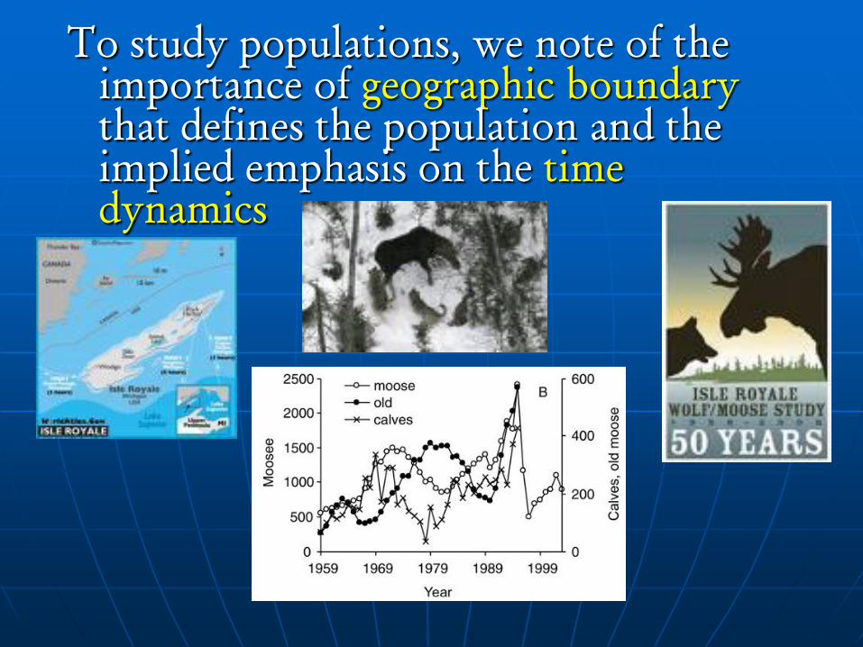
To study populations, we note of the

importance of geographic boundary

that defines the population and the

implied emphasis on the time

dynamics

Historical perspective

Demography – study of vital characteristics

of population life cycle traits, i.e. the

birth, death and dispersal rates

Human motivation to understand

population dynamics and to be aware of

numbers in relation to resources extends

to ancient times

Egyptians and Babylonians may have

conducted a census

King David counted the Israelites in

approximately 1000 BC

Early recognition of potential for

explosive population growth

● Giovanni Botero (1588) enunciated that

populations ultimately did not grow because

resources of the environment were

insufficient

● John Graunt (1662) pioneered analytical side

of demography with studies of the age-

specific mortality of people of London

● Thomas Malthus (1798) drew attention to

population growth at a time when England

was worried about overpopulation

Malthus

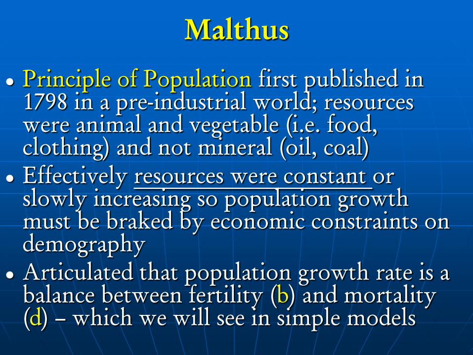
● Principle of Population first published in

1798 in a pre-industrial world; resources

were animal and vegetable (i.e. food,

clothing) and not mineral (oil, coal)

● Effectively resources were constant or

slowly increasing so population growth

must be braked by economic constraints on

demography

● Articulated that population growth rate is a

balance between fertility (b) and mortality

(d) – which we will see in simple models

Malthus

● If b is high then d must reach equally high level –

living standards severely depressed, Malthus called

this the “high pressure or Chinese case”

● In contrast, if b and d are balanced because b

responds to deteriorating standard of living and

falls to meet d before mortality is too high and

living conditions have declined then real incomes

need only fall modestly

● This latter condition could be described as an

early recognition of the goal of sustainability

● Malthus predicted that the world would run out

of food supply by the mid 1800’s, which has not

happened for a host of reasons

Population Processes: the simplest

biological model

The rate of change in a population:

( )dN

rN b d Ndt

In words this equation is:

change in N/time = (birth rate – death rate) N

/dN

N rdt

Divide through by N to visualize the per capita rate of change

which is constant (Density Independent i.e. resources do not limit

b or d; r is often called the Malthusian parameter)

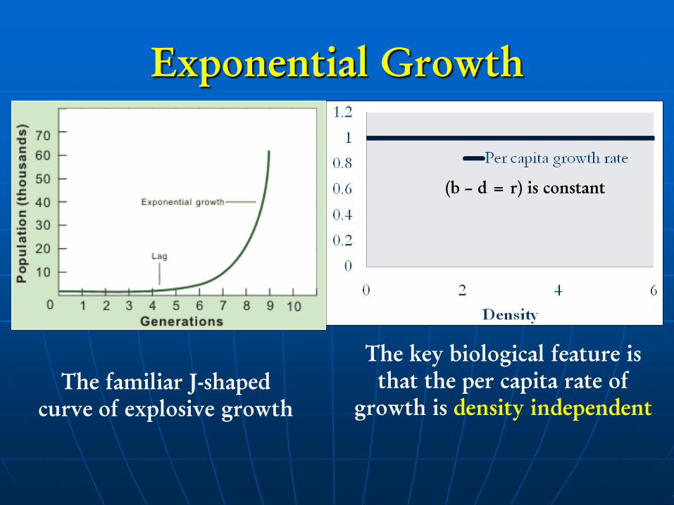
Exponential Growth

The familiar J-shaped

curve of explosive growth

The key biological feature is

that the per capita rate of

growth is density independent

(b – d = r) is constant

Estimates of r and doubling time

Organism r (indiv./indiv./time) Doubling time

Bacterium 58.7/day 17 minutes

Protozoan 1.59/day 10.5 hours

Beetle 0.101/day 6.9 days

Brown rat 0.0148/day 46.8 days

Deer 0.26/year (~0.0007/day) ~2.7 years

Blue whale 0.007/year

(~0.000019/day)

~99 years

Human (Africa)* 0.024/year

(~0.000065/day)

~29 years

Human (North

America)*

0.005/year

(~0.000014/year)

~139 years

* Data from Population Reference Bureau

Population Processes: the logistic model

(Pierre-Francois Verhulst 1838)

The rate of change in a population:

(1 )dN N

rNdt K

In words this equation is: change in N/time =

(exponential rate modified by term that quantifies the

relative ratio of N to K)

/dN r

N r Ndt K

The per capita rate of change declines linearly from a high

level when the population is not limited by resources and

reaches zero net rate of growth when N = K ( the population

reaches “carrying capacity”); this is Density Dependent i.e.

resources limit growth

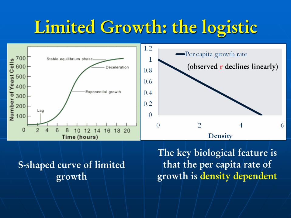
Limited Growth: the logistic

S-shaped curve of limited

growth

The key biological feature is

that the per capita rate of

growth is density dependent

(observed r declines linearly)

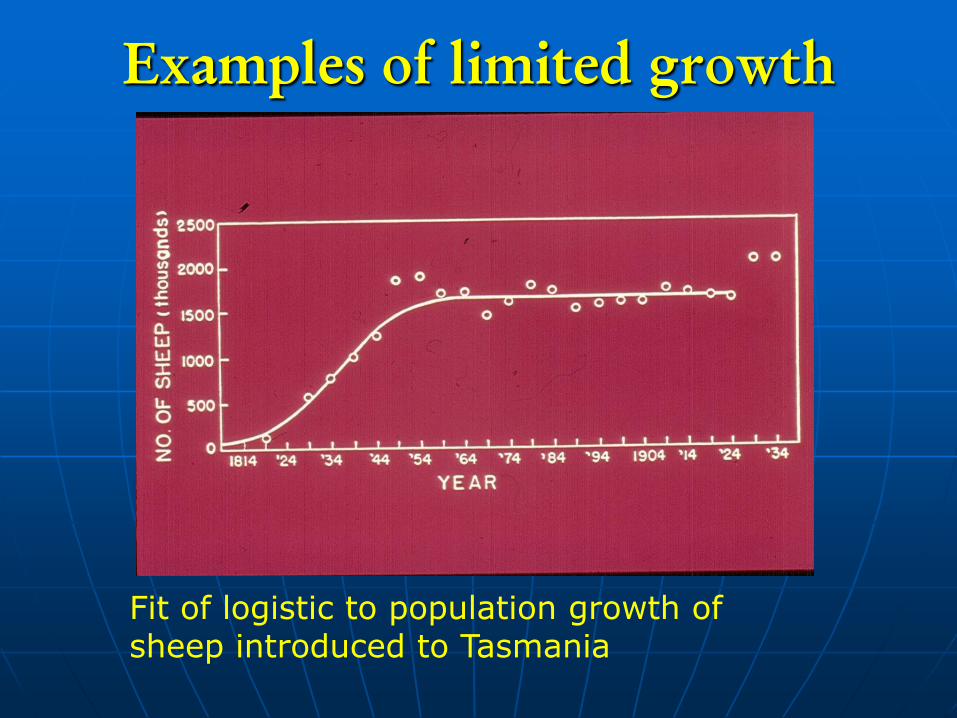
Examples of limited growth

Fit of logistic to population growth of sheep introduced to Tasmania

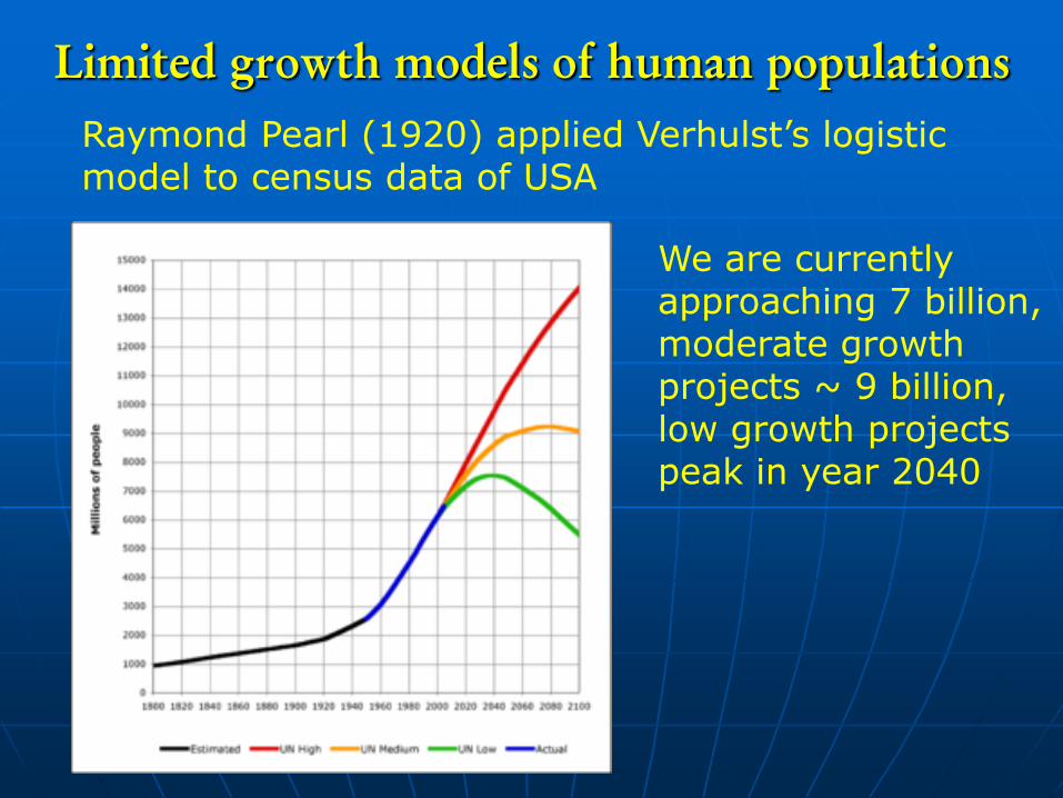
Limited growth models of human populations

Raymond Pearl (1920) applied Verhulst’s logistic model to census data of USA

We are currently approaching 7 billion, moderate growth projects ~ 9 billion, low growth projects peak in year 2040

Time

Stage 1 Stage 2 Stage 3 Stage 4

Natural

increase

Birth rate

Death rate

Note: Natural increase is produced from the excess of births over deaths.

The Classic Stages of Demographic

Transition

Logistic models: fundamental to ecological theory about

food web dynamics

Predator prey models of Paramecium and Didinium,

Georgy Gause (1934) “The Struggle for Existence,”

with contemporary mathematician Vito Volterra

And…ecological theory about competition and

community diversity

Two species of

Paramecium,

competitive exclusion

principle, Gause-

Volterra models of

competition

Competition and predation in the rocky

intertidal, biological interactions that

structure community diversity

Furthermore…practical aspects of sustainable harvest

Logistic model with maximum dN/dt

at N = K/2; application to fisheries

biology assumes the population can

sustain repeated removal of the

increment (MSY); but because of

difficulty in monitoring, time lags,

economic realities…

…collapse of cod fishery,

“fishing down” the size

(age structure)

Survivorship, longevity, and age structure of

populations

Note the log scale on both figures above

Type II survivorship is constant mortality rates at all ages

(exponential decrease)

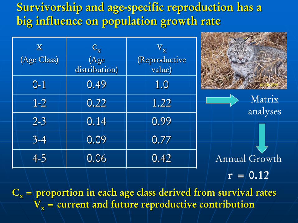
Survivorship and age-specific reproduction has a

big influence on population growth rate

x

(Age Class)

cx

(Age

distribution)

vx

(Reproductive

value)

0-1 0.49 1.0

1-2 0.22 1.22

2-3 0.14 0.99

3-4 0.09 0.77

4-5 0.06 0.42

Matrix

analyses

Annual Growth

r = 0.12

Cx= proportion in each age class derived from survival rates

Vx= current and future reproductive contribution

Population Structures by Age and Sex, 2005 Millions

300 100 100 300300 200 100 0 100 200 300

Less Developed Regions

More Developed Regions

Male Female Male Female

80+ 75-79 70-74 65-69 60-64 55-59 50-54 45-49 40-44 35-39 30-34 25-29 20-24 15-19 10-14

5-90-4

Age

Source: United Nations, World Population Prospects: The 2004 Revision, 2005.

Age Distribution of the World’s Population

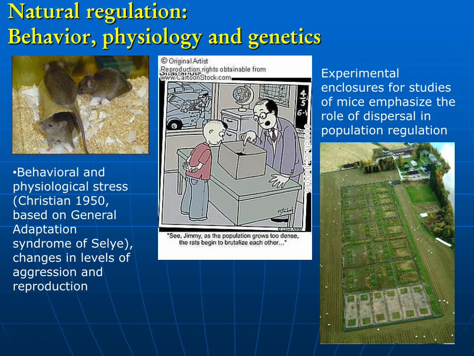
Natural regulation:

Behavior, physiology and genetics

•Behavioral and physiological stress (Christian 1950, based on General Adaptation syndrome of Selye), changes in levels of aggression and reproduction

Experimental enclosures for studies of mice emphasize the role of dispersal in population regulation

The rate of change in a population:

( )dN

rN b d i e Ndt

(birth rate – death rate + immigration rate – emigration rate)

Recall the initial statements about defining the boundaries of the

population under study, populations “open” to movements result

in spatial mosaics which are vastly more realistic and vastly more

complicated

Population Processes: the full model

with dispersal

Estimating immigration and emigration is

very difficult in natural populations

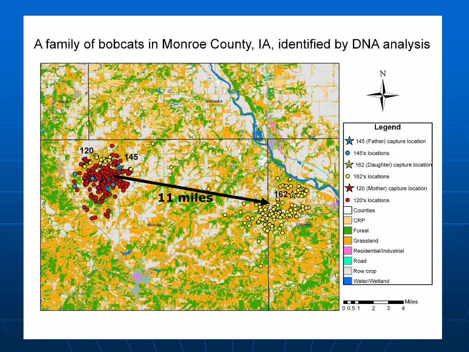
11 miles

Northern forest

Eastern Temperate Forest

Eastern Temperate Forest

Eastern Temperate Forest

Temperate Prairie

South-Central Great Plains

North-Central Great Plains

Level II Ecoregions

The landscape is not a “black box”: heterogeneity

adds to complexity

Cryptic barriers: habitat

biased dispersal

Genetic differentiation

among bobcats in the

Midwest

Source: Population Reference Bureau, 2005 World Population Data Sheet.

Now visualize the importance of migration in human

demographics and the distribution of resources

Percent Population Change, 2005-2050