PORTFOLIO OPTIMIZATIONBRING INTELLIGENCE AND INSIGHT TO THE DECISION

MAKING PROCESS

2 0 1 5 N A S A C O S T S Y M P O S I U M

F R E D K U O

N A S A J O H N S O N S P A C E C E N T E R

1

CONTENTS

• Motivation for this paper

• Management Science Models

• A Mathematical Framework for Optimization

• Some Industry Application Examples

• Application in Schedule/Crashing

• An Example

• Application in Resource Allocation

• An Example

• Concluding remarks

2

MOTIVATION

• The analytical capabilities of cost and schedule risk tools are advancing

steadily.

• Most of these tools can serve as a powerful analytical platform to bring

intelligence and insight to the decision making process.

• There are other Management Science Models that have been widely used

by various industries that can be brought to our community.

• Mathematical programming is a technique that has been widely applied to

many management science problems such as logistics, queuing and

resource planning.

• An important pillar of project management is resource allocation and

optimization.

• Like to introduce the concept and framework of optimization to the

cost/schedule community to stimulate thoughts and efforts in further

advancing the capability of the current tools.

3

MANAGEMENT SCIENCE MODELS

• There are generally two types of models:• Descriptive Model – A model that represents relationship but does not indicate

any course of actions.

• Useful in predicting the behavior of a system but have no capability to identify the “best” course of action. For example:

• Most statistical models

• Regression Models – Cost estimate models

• Schedule Models, JCL

• Model Structure – Dependent and Independent Variables

• Prescriptive Models – A model prescribes the course of action that the decision maker should take to achieve a defined objective.

• It implies that the objective is embedded in the model and it is possible to identify the effect of different courses of action on the objective. It may include a descriptive sub model.

• Model Structure• Objective function(s)

• Decision variables

• Constraints – Equality or Inequality

• Decision Variable Bounds

4

WHAT IS MATHEMATICAL PROGRAMMING

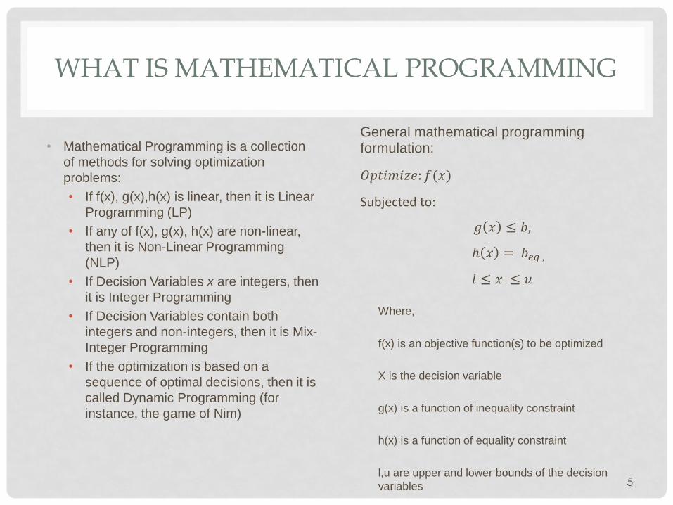
• Mathematical Programming is a collection

of methods for solving optimization

problems:

• If f(x), g(x),h(x) is linear, then it is Linear

Programming (LP)

• If any of f(x), g(x), h(x) are non-linear,

then it is Non-Linear Programming

(NLP)

• If Decision Variables x are integers, then

it is Integer Programming

• If Decision Variables contain both

integers and non-integers, then it is Mix-

Integer Programming

• If the optimization is based on a

sequence of optimal decisions, then it is

called Dynamic Programming (for

instance, the game of Nim)

5

General mathematical programming formulation:

𝑂𝑝𝑡𝑖𝑚𝑖𝑧𝑒: 𝑓(𝑥)

Subjected to:

𝑔 𝑥 ≤ 𝑏,

ℎ 𝑥 = 𝑏𝑒𝑞 ,

𝑙 ≤ 𝑥 ≤ 𝑢

Where,

f(x) is an objective function(s) to be optimized

X is the decision variable

g(x) is a function of inequality constraint

h(x) is a function of equality constraint

l,u are upper and lower bounds of the decision

variables

APPLICATION OF MATHEMATICAL PROGRAMMING

• Mathematical Programming has been applied in virtually any industry that

seeks optimization solutions:

• Revenue optimization and crew rotation for the Airline industry (NLP)

• The famous travelling salesman problem can be formulated in mathematical

programming (Integer Linear Programming)

• Valuation of financial derivatives (Dynamic Programming)

• Portfolio replication of Exchange Traded Funds (ETFs)(Quadratic Programming)

• Critical Path Method/schedule crashing (LP)

• Minimum variance portfolio (NLP)

• Resource allocation (LP or NLP)

5

EXAMPLES AND FORMULATIONS(MAXIMIZE THE PROFIT OF A CHLORINE PLANT)

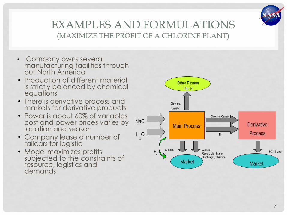
• Company owns several manufacturing facilities through out North America

• Production of different material is strictly balanced by chemical equations

• There is derivative process and markets for derivative products

• Power is about 60% of variables cost and power prices varies by location and season

• Company lease a number of railcars for logistic

• Model maximizes profits subjected to the constraints of resource, logistics and demands

7

Main ProcessNaCl

H2O

Derivative

Process

Market

Other Pioneer

Plants

Chlorine

H2

Chlorine,

Caustic

Chlorine, Caustic

Market

HCl, BleachH2

Caustic

Rayon, Membrane,

Diaphragm, Chemical

PLANT OPERATION AND LOGISTICS MANAGEMENT

•They have two questions:

• What is the optimal production level at each plant based on regional demand

pattern?

• What is the optimal sales volume based on price and location, and what is the

optimal means of delivery ?

Plant (P)

Direct Customer (C)

Terminals (T)

Rail

Truck

Pipeline

Plant (P)

Direct Customer (C)

Terminals (T)

Rail

Truck

Pipeline

sconstraint of vector is b

ariablesdecision v of collection a isx

tscoefficien constraint ofmatrix theisA

cost fixed theis C

costfreight theis f

cost production theis c

demand theis d

product theof price theis p

where

0 x

:

:max

fix

bAxtosubject

Cdfdcdpprofitimize fix

k

kk

j

jj

i

ii

EXAMPLES AND FORMULATIONS(CONSTRUCTING A MINIMUM VARIANCE PORTFOLIO)

8

Minimize : WWp '2

Subjected to:

Solution:

For a 3 asset Portfolio:

APPLICATION OF LP IN SCHEDULE ANALYSIS

A simple example for calculating the

critical path for a schedule.

9

Subjected To:

𝑇𝐹𝑖𝑛𝑖𝑠 ℎ ≥ 𝑇𝐸 + 21

𝑇𝐹𝑖𝑛𝑖𝑠 ℎ ≥ 𝑇𝐻 + 28

𝑇𝐹𝑖𝑛𝑖𝑠 ℎ ≥ 𝑇𝐽 + 45

𝑇𝐸 ≥ 𝑇𝐷 + 20

𝑇𝐻 ≥ 𝑇𝐷 + 20

𝑇𝐽 ≥ 𝑇𝐷 + 20

𝑇𝐽 ≥ 𝑇𝐼 + 30

𝑇𝐺 ≥ 𝑇𝐶 + 5

𝑇𝐺 ≥ 𝑇𝐹 + 25

𝑇𝐼 ≥ 𝑇𝐴 + 30

𝑇𝐹 ≥ 𝑇𝐴 + 30

𝑇𝐶 ≥ 𝑇𝐵 + 15

𝑇𝐷 ≥ 𝑇𝐺 + 14

𝑇𝐵 ≥ 𝑇𝐴 + 30

𝐴𝑙𝑙 𝑇𝑠 ≥ 0

Minimize: Tfinish

APPLICATION OF LP IN SCHEDULE ANALYSIS

10

Activity Duration T

A 90 0

B 15 95

C 5 110

D 20 129

E 21 149

F 25 90

G 14 115

H 28 149

I 30 119

J 45 149

Finish 194

Minimize this

(Objective Function)

Change these

(Decision Variables)

Subjected to these constraints

(Constraint equations)

We want to minimize finished time T_finishBy setting predecessor constraints as inequality constraints

APPLICATION OF LP IN SCHEDULE ANALYSIS

11

Minimize this

(Objective Function)

Change these

(Decision Variables)

Subjected to these constraints

(Constraint equations)

Activity Duration T Slack

A 90 0 0

B 15 90 5

C 5 105 5

D 20 130 0

E 21 150 24

F 25 91 0

G 14 116 0

H 28 150 17

I 30 120 29

J 45 150 0

Finish 195

Using equality constraint to calculate slack

LP AND SCHEDULE CRASHING

• For the same problem, now we

want to crash the schedule by 20

days.

• Due to different type of tasks, there

is a different set of crash costs.

• There is also a limit to how many

days of duration you can shrink

since you can not reduce a task to

zero even at infinite cost.

• Now we want to crash the

schedule by 20 days with a

minimum of cost.

• The new objective function to be

minimized is the sum of the cost of

crashed days

13

Activity Duration

Crashed

Duration

Crash

Cost/Day

A 90 10 200

B 15 5 100

C 5 0 150

D 20 5 150

E 21 6 150

F 25 5 200

G 14 4 200

H 28 5 150

I 30 7 170

J 45 10 200

Crashed Duration = Max. # of days that can be crashed

LP AND SCHEDULE CRASHING

14

Adding a new set of constraints:

Crashed days <= Crashed DurationTfinish = 174 Days

Activity Duration

Crashed

Duration

Crash

Cost/Day Slack Crash days

A 90 10 200 0 10

B 15 5 100 5 0

C 5 0 150 5 0

D 20 5 150 0 5

E 21 6 150 24 0

F 25 5 200 0 0

G 14 4 200 0 0

H 28 5 150 17 0

I 30 7 170 29 0

J 45 10 200 0 5

Finish 194 3750 174

Minimize this

(Sum of Cost * Crashed Days)

What if I want to reduce total duration to 174 days?

To achieve this

Activity Duration

Crashed

Duration

Crash

Cost/Day Slack Crash days

A 90 10 200 0 10

B 15 5 100 5 0

C 5 0 150 5 0

D 20 5 150 0 5

E 21 6 150 24 0

F 25 5 200 0 5

G 14 4 200 0 4

H 28 5 150 17 0

I 30 7 170 29 0

J 45 10 200 0 2

Finish 194 4950 168

LP AND SCHEDULE CRASHING

15

Adding a new set of constraints:

Crashed days <= Crashed Duration

Total Cost <= $5000Minimize this

What is the new total duration given $5000?

Final Cost

RISK MITIGATION/RESOURCE ALLOCATION(EXAMPLE)

• A portfolio of 10 risks. They could be either

cost or schedule risks.

• Each risk has a mitigation strategy to reduce

the amount of risks, in terms of amount

reduction in Mean and Standard Deviation.

• There is also a cost associated with each

risk reduction strategy

• Risks are either mitigated or not, there is no

partial risk mitigation.

• If there is a certain amount of resource ($)

available, what is the optimal way to allocate

which risk to mitigated?

• So the Objective Function can be:

• Overall Mean?

• Portfolio Standard Deviation?

• A combination of the two?

16

Risk No. Mean SD Mean SD Cost

1 10 10 8 7 5

2 30 10 24 7 24

3 20 10 16 7 12

4 15 5 12 3.5 12

5 60 20 48 14 48

6 50 20 40 14 40

7 35 15 28 11 22

8 45 15 36 10 30

9 75 20 60 14 60

10 90 25 72 18 50

Before Mitigation Mitigation Reduction

Risk No. Mean SD Mean SD Cost DV

1 10 10 8 7 5 0

2 30 10 24 7 24 1

3 20 10 16 7 12 1

4 15 5 12 3.5 12 1

5 60 20 48 14 48 0

6 50 20 40 14 40 0

7 35 15 28 11 22 1

8 45 15 36 10 30 1

9 75 20 60 14 60 0

10 90 25 72 18 50 1

Before Mitigation Mitigation Reduction

RISK MITIGATION/RESOURCE ALLOCATION(EXAMPLE)

17

Mean Reduction 188

Cost 150

Total Fund 150

Maximize this, by changing these

With this available fund

𝑀𝑎𝑥: 𝜇𝑖𝐷𝑖

10

𝑖=1

𝐶𝑖𝐷𝑖 ≤ 𝐹

10

𝑖=1

Formulation:

Subjected To:

𝐷𝑖 = [0,1]

SOME THOUGHTS ON POTENTIAL APPLICATION

• Resource load schedule• Optimize resource allocation, or

• Optimize schedule duration, or

• A combination of both

• Operational constraints such as skill set mix can be modelled as constraint equations

• Budget constraint scenario• Ideally suited for mathematical programming model

• Operational constraints such as how to move work or content, budget etc. can be modelled by

constraint equations

• Objective functions to be optimized can be schedule delays, resource allocations, or any other

project objectives or goals

• Risk Mitigation• One can define a risk metrics as a objective function to be optimized

• Constrained by resource or information availability

• You may think of many others

18

SUMMARY AND CONCLUSION

• The cost and schedule community has been mainly been perfecting different

descriptive models:• Better regression model for cost estimates

• Increasing capability and efficiency in simulations

• Better visualization of results

• The next natural step in the evolution of analytics should include Prescriptive Models

to bring more intelligence out of the model for decision makers.

• This paper has briefly introduced the concept of optimization, objective functions, and

decision variables. The tool for optimization is mathematical programming methods.

• Through some simple examples, this paper demonstrated that mathematical

programming can:• Calculate critical path

• Optimally crashing schedule

• Optimally allocating resource for risk mitigation

• The utility of Prescriptive models are only limited by our own creativity.

19