Mechatronics 27 (2015) 47–56

Contents lists available at ScienceDirect

Mechatronics

journal homepage: www.elsevier .com/ locate/mechatronics

Position tracking control of electro-hydraulic single-rod actuator basedon an extended disturbance observer

http://dx.doi.org/10.1016/j.mechatronics.2015.02.0030957-4158/� 2015 Elsevier Ltd. All rights reserved.

⇑ Corresponding author. Tel./fax: +86 (0571) 86791650.E-mail address: jhfang@zju.edu.cn (J. Fang).

Kai Guo, Jianhua Wei, Jinhui Fang ⇑, Ruilin Feng, Xiaochen WangThe State Key Laboratory of Fluid Power Transmission and Control, Zhejiang University, Hangzhou 310027, China

a r t i c l e i n f o a b s t r a c t

Article history:Received 30 March 2014Accepted 15 February 2015Available online 4 March 2015

Keywords:Disturbance observerElectro-hydraulic actuatorParameter uncertaintiesPosition trackingRobust control

This paper presents a nonlinear cascade controller based on an extended disturbance observer to trackdesired position trajectory for electro-hydraulic single-rod actuators in the presence of both external dis-turbances and parameter uncertainties. The proposed extended disturbance observer accounts for exter-nal perturbations and parameter uncertainties separately. In addition, the outer position tracking loopuses sliding mode control to compensate for disturbance estimation error with desired cylinder loadpressure as control output; the inner pressure control loop is designed using the backstepping technique.The stability of the overall closed-loop system is proved based on Lyapunov theory. The controller per-formance is verified through simulations and experiments. The results show that the proposed nonlinearcascade controller, together with the extended disturbance observer, provide excellent tracking perfor-mance in the presence of parameter uncertainties and external disturbances such as hysteresis andfriction.

� 2015 Elsevier Ltd. All rights reserved.

1. Introduction

Electro-hydraulic systems are widely used in many industrialand mobile applications, e.g., robot manipulators [1], hydraulicexcavators [2], and tunnel boring machines [3] because of theirhigh power-to-weight ratio compared with electric drives [4,5].However, the dynamic behaviors of electro-hydraulic servo sys-tems suffer from strong nonlinearities, such as square-root rela-tionship between pressure and flow, temperature and pressuredependent oil properties and friction. Furthermore, industrialapplications are likely to be affected by external disturbancesand system parameter variations, such as the damping coefficient,the time-varying internal leakage coefficient, or supply pressuredrops. These are great challenges for controller design of electro-hydraulic servo systems.

To obtain better dynamic performance, various control methodshave been used. Local linearization of the nonlinear dynamicsabout a nominal operating condition allows the use of techniquessuch as pole placement [6] and adaptive control [7]. However, the-se controllers cannot guarantee satisfactory performance in allworking points and are likely to fail if plant properties change dras-tically. The feedback linearization method was used in [8–10].However, this method is based on cancelling nonlinear terms and

does not account for system uncertainties. So, another controlapproach, sliding mode control (SMC) was applied to electro-hy-draulic control systems in [11–14]. In SMC, trajectories are forcedto reach a desired sliding manifold in finite time and then stayon this manifold for all future time, and dynamics on the slidingsurface are independent of matched uncertainties and distur-bances. However, chattering in the control signal, which is inherentin SMC, can easily excite high frequency modes and degrade sys-tem performance. Adaptive control has been proven to be a validmethod to system uncertainties, therefore several nonlinear adap-tive controllers were proposed for electro-hydraulic control sys-tems in the literature. In [15,16], a nonlinear adaptive controlscheme based on the backstepping method was proposed to theforce control of electro-hydraulic systems. Yao et al. [17–20] pro-posed the nonlinear adaptive robust controller (ARC) for trajectorytracking of hydraulic actuators in the presence of uncertain nonlin-earities and parameter uncertainties. A sliding mode adaptive con-troller was proposed in [21,22] to compensate for nonlinearuncertain parameters due to variations of the original control vol-umes. A novel adaptive controller based on the backstepping tech-nique was proposed in [23].

Load disturbance or unmodeled load force would significantlydegrade position tracking performance because force available tothe system is diminished [24]. To obtain better tracking perfor-mance, disturbance compensation is needed. However, direct mea-surement of disturbances is not always possible in practice,

48 K. Guo et al. / Mechatronics 27 (2015) 47–56

therefore disturbance observers for disturbance rejection is criticaland several disturbance observers have been adopted to solve thisproblem so far. In [25,26], disturbance was estimated and compen-sated according to the observer proposed in [27] for position track-ing. A high-pass disturbance observer was designed for positiontracking of electro-hydraulic actuators in [28] and the disturbanceswithin the observer bandwidth can be cancelled. In [29,30], a dis-turbance observer was used to reject low-frequency disturbancesand high-frequency noises in an electro-hydraulic servo system.An integral sliding mode disturbance compensator was proposedin [31] for load pressure control of hydraulic drives.

Motivated by [20,30], an extended disturbance observer is pro-posed to estimate uncertain parameters and external disturbancessimultaneously. Unlike the disturbance observer used in [30], theproposed extended disturbance observer deals with parameteruncertainties and external disturbances separately. Compared with[20], parameter and disturbance updates proposed in this paperare driven by the state estimation error while that proposed in[20] are driven by the tracking error, in addition, alternative distur-bance observers proposed in [28,32] could be used in this controlscheme. Based on the proposed extended disturbance observer, anonlinear cascade controller is developed for position tracking ofan electro-hydraulic single-rod actuator. It comprises a positiontracking outer loop and a load pressure control inner loop whichprovides the hydraulic actuator the characteristic of a force gen-erator. SMC is also used to compensate for disturbance estimationerrors. Stability of the closed-loop system consisting of the extend-ed disturbance observer, the nonlinear controller and the plantmodel is proved by means of Lyapunov theory.

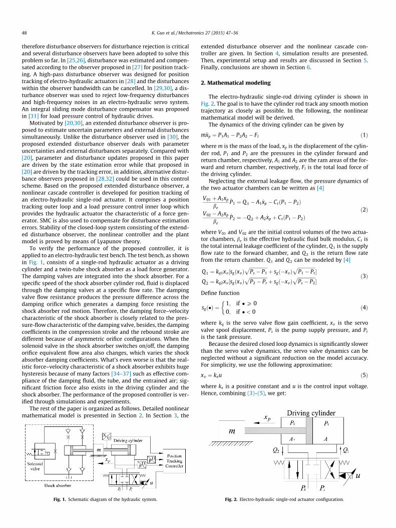
To verify the performance of the proposed controller, it isapplied to an electro-hydraulic test bench. The test bench, as shownin Fig. 1, consists of a single-rod hydraulic actuator as a drivingcylinder and a twin-tube shock absorber as a load force generator.The damping valves are integrated into the shock absorber. For aspecific speed of the shock absorber cylinder rod, fluid is displacedthrough the damping valves at a specific flow rate. The dampingvalve flow resistance produces the pressure difference across thedamping orifice which generates a damping force resisting theshock absorber rod motion. Therefore, the damping force–velocitycharacteristic of the shock absorber is closely related to the pres-sure-flow characteristic of the damping valve, besides, the dampingcoefficients in the compression stroke and the rebound stroke aredifferent because of asymmetric orifice configurations. When thesolenoid valve in the shock absorber switches on/off, the dampingorifice equivalent flow area also changes, which varies the shockabsorber damping coefficients. What’s even worse is that the real-istic force–velocity characteristic of a shock absorber exhibits hugehysteresis because of many factors [34–37] such as effective com-pliance of the damping fluid, the tube, and the entrained air; sig-nificant friction force also exists in the driving cylinder and theshock absorber. The performance of the proposed controller is ver-ified through simulations and experiments.

The rest of the paper is organized as follows. Detailed nonlinearmathematical model is presented in Section 2. In Section 3, the

Fig. 1. Schematic diagram of the hydraulic system.

extended disturbance observer and the nonlinear cascade con-troller are given. In Section 4, simulation results are presented.Then, experimental setup and results are discussed in Section 5.Finally, conclusions are shown in Section 6.

2. Mathematical modeling

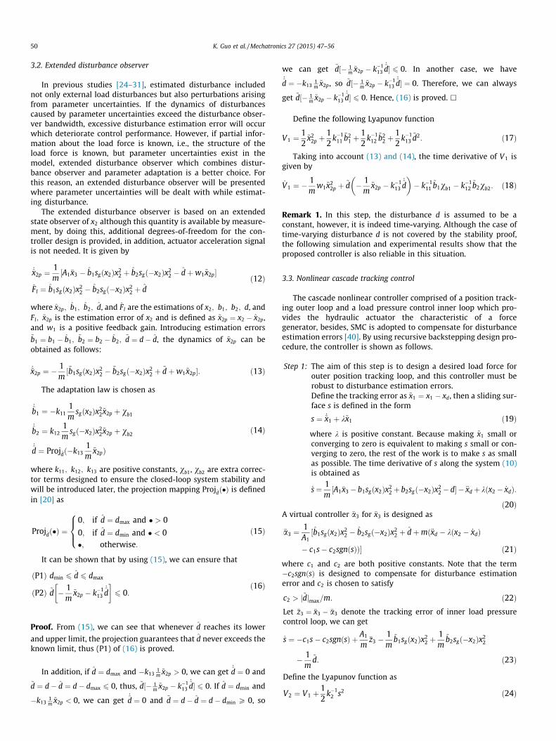
The electro-hydraulic single-rod driving cylinder is shown inFig. 2. The goal is to have the cylinder rod track any smooth motiontrajectory as closely as possible. In the following, the nonlinearmathematical model will be derived.

The dynamics of the driving cylinder can be given by

m€xp ¼ P1A1 � P2A2 � Fl ð1Þ

where m is the mass of the load, xp is the displacement of the cylin-der rod, P1 and P2 are the pressures in the cylinder forward andreturn chamber, respectively, A1 and A2 are the ram areas of the for-ward and return chamber, respectively, Fl is the total load force ofthe driving cylinder.

Neglecting the external leakage flow, the pressure dynamics ofthe two actuator chambers can be written as [4]

V01 þ A1xp

be

_P1 ¼ Q 1 � A1 _xp � CtðP1 � P2Þ

V02 � A2xp

be

_P2 ¼ �Q 2 þ A2 _xp þ CtðP1 � P2Þð2Þ

where V01 and V02 are the initial control volumes of the two actua-tor chambers, be is the effective hydraulic fluid bulk modulus, Ct isthe total internal leakage coefficient of the cylinder, Q1 is the supplyflow rate to the forward chamber, and Q2 is the return flow ratefrom the return chamber. Q1 and Q2 can be modeled by [4]

Q 1 ¼ kq1xv ½sgðxvÞffiffiffiffiffiffiffiffiffiffiffiffiffiffiffiPs � P1

pþ sgð�xvÞ

ffiffiffiffiffiffiffiffiffiffiffiffiffiffiffiP1 � Pt

p�

Q 2 ¼ kq2xv ½sgðxvÞffiffiffiffiffiffiffiffiffiffiffiffiffiffiffiP2 � Pt

pþ sgð�xvÞ

ffiffiffiffiffiffiffiffiffiffiffiffiffiffiffiPs � P2

p�

ð3Þ

Define function

sgð�Þ ¼1; if �P 00; if � < 0

�ð4Þ

where kq is the servo valve flow gain coefficient, xv is the servovalve spool displacement, Ps is the pump supply pressure, and Pt

is the tank pressure.Because the desired closed loop dynamics is significantly slower

than the servo valve dynamics, the servo valve dynamics can beneglected without a significant reduction on the model accuracy.For simplicity, we use the following approximation:

xv ¼ kxu ð5Þ

where kx is a positive constant and u is the control input voltage.Hence, combining (3)–(5), we get:

Fig. 2. Electro-hydraulic single-rod actuator configuration.

K. Guo et al. / Mechatronics 27 (2015) 47–56 49

Q1 ¼ kq1kxu½sgðuÞffiffiffiffiffiffiffiffiffiffiffiffiffiffiffiPs � P1

pþ sgð�uÞ

ffiffiffiffiffiffiffiffiffiffiffiffiffiffiffiP1 � Pt

p�

Q2 ¼ kq2kxu½sgðuÞffiffiffiffiffiffiffiffiffiffiffiffiffiffiffiP2 � Pt

pþ sgð�uÞ

ffiffiffiffiffiffiffiffiffiffiffiffiffiffiffiPs � P2

p�:

ð6Þ

Load force modeling accuracy is a key issue for accurate posi-tion tracking. There are two ways to model shock absorbers:first-principle dynamic modeling based on internal structuresand nonparametric modeling based on experimental data. Thephysical model can capture shock absorber behaviors in a widerange of operating conditions very accurately; however, it is usual-ly computationally complex and is not suitable for control-orient-ed applications. In contrast to physical models, nonparametricmodel is computationally efficient and is able to capture shockabsorber dynamic behaviors for the tested operating conditions[38]. Therefore, nonparametric model is used in this paper to mod-el the shock absorber damping force. Unlike the shock absorberscommonly used in vehicle suspensions [33], the damping orificeflow area of the shock absorber shown in Fig. 1 is independent ofpressure difference across the damping valve, therefore the idealdamping force is proportional to the square of relative velocitybetween the shock absorber piston rod and the cylinder tube. Asecond order polynomial model is used, as shown in (7)

Fl ¼ b1sgð _xpÞ _x2p � b2sgð� _xpÞ _x2

p þ d ð7Þ

where b1 and b2 are the damping coefficients during the forwardand return strokes, respectively, d is a lumped disturbance due tohysteretic force–velocity characteristics of the shock absorber, fric-tional forces, and other unmodeled external disturbances. Usingexperimental data, the damping coefficients are developed usingleast squares regression. The force–velocity plot of the consideredshock absorber when solenoid valve switches on/off is shown inFig. 3. The close match between the mathematical model and theexperimental data demonstrates the effectiveness of the model.

Define the state variables as x ¼ ½x1; x2; x3; x4�T ¼ ½xp; _xp; P1; P2�T .The entire system can be expressed in a state space form as

_x1 ¼ x2

_x2 ¼1m½A1x3 � A2x4 � b1sgðx2Þx2

2 þ b2sgð�x2Þx22 � d�

_x3 ¼ h1ðx1Þ½�A1x2 � Ctðx3 � x4Þ þ kq1kxug1ðx3; uÞ�_x4 ¼ h2ðx1Þ½A2x2 þ Ctðx3 � x4Þ � kq2kxug2ðx4;uÞ�

ð8Þ

Fig. 3. Real and modeled force–velocity characteristic of the shock absorber. (a)Solenoid valve switches off. (b) Solenoid valve switches on.

where

h1ðx1Þ ¼be

V01 þ A1x1

h2ðx1Þ ¼be

V02 � A2x1

g1ðx3;uÞ ¼ sgðuÞffiffiffiffiffiffiffiffiffiffiffiffiffiffiffiPs � x3

pþ sgð�uÞ

ffiffiffiffiffiffiffiffiffiffiffiffiffiffiffix3 � Pt

pg2ðx4;uÞ ¼ sgðuÞ

ffiffiffiffiffiffiffiffiffiffiffiffiffiffiffix4 � Pt

pþ sgð�uÞ

ffiffiffiffiffiffiffiffiffiffiffiffiffiffiffiPs � x4

p:

ð9Þ

The control task can now be summarized as follows: Given thedesired motion trajectory xdðtÞ, the objective is to synthesize abounded control input u such that the output x1 tracks xdðtÞ asclosely as possible in spite of various model uncertainties and dis-turbances. For a practical electro-hydraulic servo system, the fol-lowing assumption is made.

Assumption 1. The desired trajectory xdðtÞ, its velocity _xdðtÞ andacceleration €xdðtÞ and vxdðtÞ are all bounded; under normal workingconditions, P1 and P2 are bounded by Ps and Pt , i.e.,0 < Pt < P1 < Ps, 0 < Pt < P2 < Ps.

3. Controller design

3.1. Design model and issues to be addressed

To make system dynamics (8) fall into the well-known strictfeedback form to use the backstepping method, a new state vari-able is defined as �x3 ¼ x3 � ax4, where a ¼ A2=A1 denotes the pis-ton area ratio, this variable corresponds to the driving force ofthe cylinder. In addition, following the coordinates change pro-posed in [39], a new variable representing the sum pressure,�x4 ¼ x3 þ x4, is used. This new variable reflects the internal dynam-ics of the system, which arises from the physical phenomenon thatthere are more than one pair of (P1; P2Þ which can produce thedesired driving force [20,39]. Therefore, the stability of the internaldynamics is needed and it is shown in the simulation andexperimental results.

Thus system dynamics (8) can be rewritten as

_x1 ¼ x2

_x2 ¼1m½A1�x3 � b1sgðx2Þx2

2 þ b2sgð�x2Þx22 � d�

_�x3 ¼ �f 1x2 � f 2Ctðx3 � x4Þ þ f 3u_�x4 ¼ �f 4x2 � f 5Ctðx3 � x4Þ þ f 6u:

ð10Þ

where

f 1ðx1Þ ¼ h1ðx1ÞA1 þ ah2ðx1ÞA2

f 2ðx1Þ ¼ h1ðx1Þ þ ah2ðx1Þf 3ðx1; x3; x4;uÞ ¼ kx½kq1h1ðx1Þg1ðu; x3Þ þ akq2h2ðx1Þg2ðu; x4Þ�f 4ðx1Þ ¼ h1ðx1ÞA1 � h2ðx1ÞA2

f 5ðx1Þ ¼ h1ðx1Þ � h2ðx1Þf 6ðx1; x3; x4;uÞ ¼ kx½kq1h1ðx1Þg1ðu; x3Þ � kq2h2ðx1Þg2ðu; x4Þ�:

ð11Þ

For the system considered here, load damping coefficients b1

and b2 vary with oil temperature and pressure, they also changewhen solenoid valve switches on/off, and therefore the two para-meters are uncertain. Besides, d is a lumped disturbance due tohysteretic force–velocity characteristic of the shock absorber, fric-tional forces, and other unmodeled external disturbances.

Assumption 2. The unknown disturbance d is bounded within aknown limit, i.e., dmin 6 d 6 dmax, where dmin and dmax are theknown lower and upper bounds of d.

where

Let �z3

contro

Define

50 K. Guo et al. / Mechatronics 27 (2015) 47–56

3.2. Extended disturbance observer

In previous studies [24–31], estimated disturbance includednot only external load disturbances but also perturbations arisingfrom parameter uncertainties. If the dynamics of disturbancescaused by parameter uncertainties exceed the disturbance obser-ver bandwidth, excessive disturbance estimation error will occurwhich deteriorate control performance. However, if partial infor-mation about the load force is known, i.e., the structure of theload force is known, but parameter uncertainties exist in themodel, extended disturbance observer which combines distur-bance observer and parameter adaptation is a better choice. Forthis reason, an extended disturbance observer will be presentedwhere parameter uncertainties will be dealt with while estimat-ing disturbance.

The extended disturbance observer is based on an extendedstate observer of x2 although this quantity is available by measure-ment, by doing this, additional degrees-of-freedom for the con-troller design is provided, in addition, actuator acceleration signalis not needed. It is given by

_̂x2p ¼1m½A1�x3 � b̂1sgðx2Þx2

2 þ b̂2sgð�x2Þx22 � d̂þw1~x2p�

F̂ l ¼ b̂1sgðx2Þx22 � b̂2sgð�x2Þx2

2 þ d̂ð12Þ

where x̂2p; b̂1; b̂2; d̂, and F̂l are the estimations of x2; b1; b2; d, andFl; ~x2p is the estimation error of x2 and is defined as ~x2p ¼ x2 � x̂2p,and w1 is a positive feedback gain. Introducing estimation errors~b1 ¼ b1 � b̂1;

~b2 ¼ b2 � b̂2;~d ¼ d� d̂, the dynamics of ~x2p can be

obtained as follows:

_~x2p ¼ �1m½~b1sgðx2Þx2

2 � ~b2sgð�x2Þx22 þ ~dþw1~x2p�: ð13Þ

The adaptation law is chosen as

_̂b1 ¼ �k11

1m

sgðx2Þx22~x2p þ vb1

_̂b2 ¼ k12

1m

sgð�x2Þx22~x2p þ vb2

_̂d ¼ Projd̂ð�k13

1m

~x2pÞ

ð14Þ

where k11; k12; k13 are positive constants, vb1, vb2 are extra correc-tor terms designed to ensure the closed-loop system stability andwill be introduced later, the projection mapping Projd̂ð�Þ is definedin [20] as

Projd̂ð�Þ ¼0; if d̂ ¼ dmax and � > 0

0; if d̂ ¼ dmin and � < 0�; otherwise:

8><>: ð15Þ

It can be shown that by using (15), we can ensure that

ðP1Þ dmin 6 d̂ 6 dmax

ðP2Þ ~d � 1m

~x2p � k�113

_̂d

� �6 0:

ð16Þ

Proof. From (15), we can see that whenever d̂ reaches its lower

and upper limit, the projection guarantees that d̂ never exceeds theknown limit, thus (P1) of (16) is proved.

In addition, if d̂ ¼ dmax and �k131m

~x2p > 0, we can get _̂d ¼ 0 and

~d ¼ d� d̂ ¼ d� dmax 6 0, thus, ~d½� 1m

~x2p � k�113

_̂d� 6 0. If d̂ ¼ dmin and

�k131m

~x2p < 0, we can get _̂d ¼ 0 and ~d ¼ d� d̂ ¼ d� dmin P 0, so

we can get ~d½� 1m

~x2p � k�113

_̂d� 6 0. In another case, we have_̂d ¼ �k13

1m

~x2p, so ~d½� 1m

~x2p � k�113

_̂d� ¼ 0. Therefore, we can always

get ~d½� 1m

~x2p � k�113

_̂d� 6 0. Hence, (16) is proved. h

Define the following Lyapunov function

V1 ¼12

~x22p þ

12

k�111

~b21 þ

12

k�112

~b22 þ

12

k�113

~d2: ð17Þ

Taking into account (13) and (14), the time derivative of V1 isgiven by

_V1 ¼ �1m

w1~x22p þ ~d � 1

m~x2p � k�1

13_̂d

� �� k�1

11~b1vb1 � k�1

12~b2vb2: ð18Þ

Remark 1. In this step, the disturbance d is assumed to be aconstant, however, it is indeed time-varying. Although the case oftime-varying disturbance d is not covered by the stability proof,the following simulation and experimental results show that theproposed controller is also reliable in this situation.

3.3. Nonlinear cascade tracking control

The cascade nonlinear controller comprised of a position track-ing outer loop and a load pressure control inner loop which pro-vides the hydraulic actuator the characteristic of a forcegenerator, besides, SMC is adopted to compensate for disturbanceestimation errors [40]. By using recursive backstepping design pro-cedure, the controller is shown as follows.

Step 1: The aim of this step is to design a desired load force forouter position tracking loop, and this controller must berobust to disturbance estimation errors.Define the tracking error as ~x1 ¼ x1 � xd, then a sliding sur-face s is defined in the form

s ¼ _~x1 þ k~x1 ð19Þ

where k is positive constant. Because making ~x1 small orconverging to zero is equivalent to making s small or con-verging to zero, the rest of the work is to make s as smallas possible. The time derivative of s along the system (10)is obtained as

_s¼ 1m½A1�x3 � b1sgðx2Þx2

2 þ b2sgð�x2Þx22 � d� � €xd þ kðx2 � _xdÞ:

ð20Þ

A virtual controller �a3 for �x3 is designed as

�a3 ¼1A1½b̂1sgðx2Þx2

2 � b̂2sgð�x2Þx22 þ d̂þmð€xd � kðx2 � _xdÞ

� c1s� c2sgnðsÞÞ� ð21Þ

c1 and c2 are both positive constants. Note that the term

�c2sgnðsÞ is designed to compensate for disturbance estimationerror and c2 is chosen to satisfy

c2 > j~djmax=m: ð22Þ

¼ �x3 � �a3 denote the tracking error of inner load pressurel loop, we can get

_s ¼ �c1s� c2sgnðsÞ þ A1

m�z3 �

1m

~b1sgðx2Þx22 þ

1m

~b2sgð�x2Þx22

� 1m

~d: ð23Þ

the Lyapunov function as

V2 ¼ V1 þ12

k�12 s2 ð24Þ

K. Guo et al. / Mechatronics 27 (2015) 47–56 51

k2 is a positive constant. Combining (18) and (23), the time

wherederivative of V2 is given by � � _V2 ¼ �

1m

w1~x22p þ ~d � 1

m~x2p � k�1

13_̂d � k�1

11~b1vb1 � k�1

12~b2vb2

þ k�12 �c1s2 � c2jsj �

1m

~dsþ A1

m�z3s� 1

msgðx2Þx2

2~b1s

�

þ 1m

sgð�x2Þx22~b2s�: ð25Þ

Then the extra corrector terms vb1, vb2 are chosen as

Fig. 4. Block diagram of the controller structure.

vb1 ¼ �k11k�12

1m

sgðx2Þx22s

vb2 ¼ k12k�12

1m

sgð�x2Þx22s:

ð26Þ

Substituting (26) into (25) yields

� � _V2 ¼ �

1m

w1~x22p � c1k�1

2 s2 þ ~d � 1m

~x2p � k�113

_̂d þ k�1

2 ð�c2jsj

� 1m

~dsÞ þ k�12

A1

m�z3s: ð27Þ

Step 2: In step 1, we have designed a virtual control law �a3 whichis the command input of inner load pressure control loop.In this step, an actual control law for u is determined. Thetime derivative of �z3 is given by

_�z3 ¼ �f 1x2 � f 2Ctðx3 � x4Þ þ f 3u� _�a3: ð28Þ

Fig. 5. Force–velocity dynamics of shock absorber.

Table 1Parameters of the test rig.

Parameter Description Value

m Load mass 200 kgA1 Driving cylinder piston side chamber

area5.027 � 10�3 m2

A2 Driving cylinder rod side chamber area 2.564 � 10�3 m2

Ps Pump supply pressure 2.5 � 107 PaCt Driving cylinder leakage coefficient 0 m3/(s Pa)be Oil bulk modulus 1 � 109 Pakq1 � kx Servo valve flow gain coefficient 8.91 � 10�8 m3/

(s VffiffiffiffiffiffiPap

)kq2 � kx Servo valve flow gain coefficient 8.91 � 10�8 m3/

(s VffiffiffiffiffiffiPap

)

The actual control u is designed as

u ¼ 1f 3

f 1x2 þ f 2Ctðx3 � x4Þ þ _�a3 � c3�z3 � k�12 k31

A1

ms

� �ð29Þ

where c3 and k31 are positive constants. Substituting (29) into (28)yields the dynamics of �z3

_�z3 ¼ �c3�z3 � k�12 k31

A1

ms: ð30Þ

Define the Lyapunov function as

V ¼ V2 þ12

k�131 �z2

3 ð31Þ

where k32 is a positive constant, combining (27) and (30), the timederivative of V is given by

_V ¼ � 1m

w1~x22p � c1k�1

2 s2 � c3k�131 �z2

3 þ ~d � 1m

~x2p � k�113

_̂d

� �

þ k�12 �c2jsj �

1m

~ds� �

: ð32Þ

From (16), we can get ~d½� 1m

~x2p � k�113

_̂d� 6 0. In addition, from

(22), we can also obtain k�12 ð�c2jsj � 1

m~dsÞ 6 0, therefore we get

_V 6 � 1m

w1~x22p � c1k�1

2 s2 � c3k�131 �z2

3 < 0: ð33Þ

Hence, the stability of the closed-loop system consisting of thenonlinear controller and the extended disturbance observer isguaranteed and all system signals are bounded under closed-loopoperation.

Remark 2. In (29), we need the derivate of �a3, however, thederivative of sgn(sÞ at point s = 0 cannot be calculated. Therefore,instead of using the discontinuous switching function sgn(sÞ, thecontinuous tangent function tanh(s/e) is employed, where e is asufficiently small positive constant [26–28]. This comes at theprice of a non-ideal sliding mode within a resulting boundary layerdetermined by the introduced parameter e.

Remark 3. Note that (29) includes the control input u on bothsides of the equation, so (29) cannot be calculated directly [28].However, the control input u on the right side is only used forsgð�Þ function in f 3, since f 3 is always greater than zero, the sign

of u is determined by f 1x2 þ f 2Ctðx3 � x4Þ þ _�a3 � c3�z3 � k�12 k31

A1m s.

Therefore, we use the modified control law

u ¼ ub

f 3ðx1; x3; x4;ubÞ

ub ¼ f 1x2 þ f 2Ctðx3 � x4Þ þ _�a3 � c3�z3 � k�12 k31

A1

ms:

ð34Þ

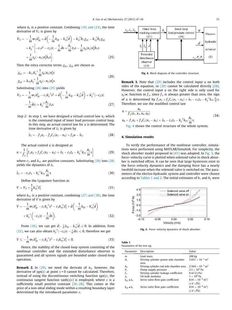
Fig. 4 shows the control structure of the whole system.

4. Simulation results

To verify the performance of the nonlinear controller, simula-tions were performed using MATLAB/Simulink. For simplicity, theshock absorber model proposed in [41] was adopted. In Fig. 5, theforce–velocity curve is plotted when solenoid valve in shock absor-ber is switched off/on. It can be seen that large hysteresis exist inthe force–velocity dynamics and the damping force has a nearlytwofold increase when the solenoid valve is switched on. The para-meters of the electro-hydraulic system and controller were chosenaccording to Tables 1 and 2. The initial estimates of b1 and b2 were

Table 2Parameters of the controller.

Parameter Value Parameter Value

w1 5000 c2 10k11 4 � 1010 c3 160k12 1.25 � 1011 e 0.05k13 6 � 106 k 320k2 10 b̂1ð0Þ 3.54 � 106

k31 1 b̂2ð0Þ 2.45 � 106

c1 380

Fig. 6. Desired profile.

Fig. 7. Tracking errors with solenoid valve in shock absorber switched off. (a) NCcontrol. (b) DOBNC and proposed control (EDOBNC).

Fig. 8. Parameter estimations of EDOBNC with solenoid valve in shock absorberswitched off. (a) b̂1. (b) b̂2. (c) d̂.

52 K. Guo et al. / Mechatronics 27 (2015) 47–56

chosen as least-squares approximations of the shock absorberforce–velocity characteristics when solenoid valve was switchedoff. The friction force, 2500sgn(x2Þ and the desired profile shownin Fig. 6, xd = 0.175 + 0.125 sin (0.2pt + 1.5p), were used.

Three controllers were used and compared; among which thefirst was the proposed extended disturbance observer based non-linear cascade controller (EDOBNC), and the second was a distur-bance observer based controller (DOBNC) without usingparameter adaptation which treated external disturbances andparameter uncertainties as lumped perturbations, i.e., k11 ¼ 0,k12 ¼ 0. The third controller (NC) performed position trackingwithout considering parameter variations and external distur-bances, i.e., k11 ¼ 0, k12 ¼ 0, k13 ¼ 0.

The three controllers were first tested when solenoid valve inshock absorber was switched off. Fig. 7 shows the tracking errors,and the parameter estimations of EDOBNC are shown in Fig. 8. Itshows that the proposed EDOBNC controller and the DOBNC con-troller performed better than the NC controller; it is because theEDOBNC and the DOBNC employ disturbance observation laws tocompensate for unmodeled uncertainties such as hysteresis andfriction in hydraulic systems, while the NC controller just has somerobustness with respect to uncertainties. Furthermore, because theinitial parameter estimates of b1 and b2 were the least-squares fitsof the shock absorber force–velocity dynamics, tracking perfor-mance of the EDOBNC and the DOBNC are similar which showsthe effectiveness of disturbance estimation when parameter uncer-tainties are comparatively small.

To test the influence of variations of parameters b1 and b2 on thecontrol performance, the solenoid valve in the shock absorber wasswitched on which decreased the equivalent orifice diameter andincreased the damping coefficients b1 and b2 almost twofold,besides, the hysteresis coming from shock absorber force–velocitycharacteristics was bigger as shown in Fig. 5. The tracking perfor-mance is shown in Fig. 9 and the parameter estimations of theEDOB are shown in Fig. 10. As seen, the tracking error improveswith the adaptation of the parameters during the first two cycles;even in the face of dramatic variations in damping coefficients b1

and b2, the EDOBNC could still attenuate the unexpected effectsand achieve better performance than the DOBNC and the NC whichillustrates the effectiveness of the proposed EDOBNC controller.The relatively large tracking error during the transition from

positive to negative speed was mainly due to friction effects whichcan be tackled by incorporating detailed mathematical load forcemodels. It can also be seen that the estimated parameters do notconverge to constant values, however, they are bounded andapproach stable limit cycles; such effects may be due to frictionforce, hysteresis and other model uncertainties. The control inputu is shown in Fig. 11.

5. Experimental results

The experimental installation is presented in Fig. 12; a shockabsorber was used as a load force generator. In the test bench,the driving cylinder of which the dimensions were 80 mm/56 mm/700 mm was controlled by a servo valve (Rexroth4WRPH10C3B100L), its bandwidth was above 80 Hz with a 10%control signal. The system states used in the controller, includingcylinder displacement, the pressures in the two cylinder chambers

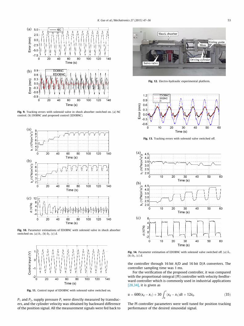
Fig. 9. Tracking errors with solenoid valve in shock absorber switched on. (a) NCcontrol. (b) DOBNC and proposed control (EDOBNC).

Fig. 10. Parameter estimations of EDOBNC with solenoid valve in shock absorberswitched on. (a) b̂1. (b) b̂2. (c) d̂.

Fig. 11. Control input of EDOBNC with solenoid valve switched on.

Fig. 12. Electro-hydraulic experimental platform.

Fig. 13. Tracking errors with solenoid valve switched off.

Fig. 14. Parameter estimation of EDOBNC with solenoid valve switched off. (a) b̂1.(b) b̂2. (c) d̂.

K. Guo et al. / Mechatronics 27 (2015) 47–56 53

P1 and P2, supply pressure Ps were directly measured by transduc-ers, and the cylinder velocity was obtained by backward differenceof the position signal. All the measurement signals were fed back to

the controller through 16 bit A/D and 16 bit D/A converters. Thecontroller sampling time was 1 ms.

For the verification of the proposed controller, it was comparedwith the proportional-integral (PI) controller with velocity feedfor-ward controller which is commonly used in industrial applications[28,34], it is given as

u ¼ 600ðxd � x1Þ þ 30Z t

0ðxd � x1Þdt þ 12 _xd: ð35Þ

The PI controller parameters were well tuned for position trackingperformance of the desired sinusoidal signal.

Fig. 15. Pressure in two cylinder chambers of EDOBNC with solenoid valveswitched off.

Fig. 16. Control input of EDOBNC with solenoid valve switched off.

Fig. 17. Load force estimation performance of EDOBNC with solenoid valveswitched off. (a) Cylinder driving force. (b) Estimated load force.

Fig. 18. Tracking performance with solenoid valve switched on.

Fig. 19. Parameter estimation of EDOBNC with solenoid valve switched on. (a) b̂1.(b) b̂2. (c) d̂.

54 K. Guo et al. / Mechatronics 27 (2015) 47–56

Fig. 13 shows tracking errors of the three controllers when thesolenoid valve in the shock absorber was switched off. As seen, theEDOBNC performed better than the PI controller in terms of track-ing error. This indicates that the extended disturbance observercan effectively attenuate parameter variations and external distur-bances. Due to accurate estimate of damping coefficients, thetracking performances of the EDOBNC and the DOBNC were similarto each other. Parameter estimations of the EDOBNC are shown inFig. 14. In addition, big deviations exist between the simulationand the experimental results; this is mainly due to inaccurate loadforce in the simulation environment.

The pressure P1 and P2 of the EDOBNC are shown in Fig. 15, andthe control input u is shown in Fig. 16. It can be seen that they areall bounded as assumed. The cylinder driving force and the esti-mated load force are shown in Fig. 17. The driving force means

ðP1 � aP2Þ A1, and the estimated load force includes the shockabsorber damping force, friction force, and other external distur-bances. It can be seen that a large jump exists at velocity reversalwhich was mainly caused by friction. Because the estimated loadforce was similar to cylinder driving force, it can be obtained thatthe load force was well estimated.

Fig. 18 shows the tracking performance of the three controllerswhen solenoid valve in shock absorber was switched on. The track-ing errors of the PI controller and the DOBNC were greater than thatof the case when solenoid valve was switched off, whereas thetracking performance of EDOBNC remained almost unchanged. Theparameter estimations of the EDOBNC are shown in Fig. 19.The cylinder driving force and estimated load force are shown inFig. 20. It can be seen that the estimated parameters do not con-verge to constant values, which is the same as the simulationresults. The tracking error improvement is reached within the firstcycle and the remaining parameter updates have little effect on thetracking error because of the almost unchanged estimated loadforce during each cycle. In addition, despite twofold increase inthe shock absorber damping force compared with the case whensolenoid valve was switched off, the load force was also wellestimated.

The three controllers were then run for a fast motion trajectorygiven by xd ¼ 0:175þ 0:125 sin ð0:31pt þ 1:5pÞ. The tracking per-formance is shown in Fig. 21. The PI controller and the DOBNC con-troller exhibited large tracking errors under such an aggressive

Fig. 20. Load force estimation performance of EDOBNC with solenoid valveswitched on. (a) Cylinder driving force. (b) Estimated load force.

Fig. 21. Tracking performance comparison under a fast trajectory with solenoidvalve switched on.

Fig. 22. Tracking performance of ARC and OBCC with solenoid valve switched on.

K. Guo et al. / Mechatronics 27 (2015) 47–56 55

movement. In contrast, the tracking error of the EDOBNC wassmaller, which shows the effectiveness of the proposed EDOBNCcontrol strategy.

In the end, the proposed control scheme was compared with twoalternative control solutions: ARC control as described in [20] andobserver-based cascade control (OBCC) as described in [30]. Thetrajectory shown in Fig. 6 was used and the solenoid valve in theshock absorber was switched on. Fig. 22 shows the tracking perfor-mance. The largest tracking errors occur with the OBCC as a result ofparameter uncertainties, whereas the ARC leads to similar trackingperformance compared with the proposed control scheme.

6. Conclusion

In this paper, a nonlinear cascade trajectory tracking controllerbased on an extended disturbance observer was proposed for an

electro-hydraulic system driven by a single-rod actuator. The innercontrol loop involved a load pressure control, and the outer loopachieved position tracking using sliding mode method. In addition,external disturbances and parameter uncertainties were taken intoaccount through the extended disturbance observer. This novelcontrol scheme paralleled the backstepping method and its sta-bility was proved through Lyapunov method. The effectiveness ofthe control scheme was verified by the simulation and experimen-tal results.

Acknowledgements

This work was supported by the Science Fund for CreativeResearch Groups of National Natural Science Foundation of China(51221004) and National High Technology Research and Develop-ment Program (863 Program) of China (2012AA041801).

References

[1] Taylor CJ, Robertson D. State-dependent control of a hydraulically actuatednuclear decommissioning robot. Control Eng Pract 2013;21(12):1716–25.

[2] Heikkilä M, Linjama M. Displacement control of a mobile crane using a digitalhydraulic power management system. Mechatronics 2013;23(4):452–61.

[3] Wang L, Gong G, Yang H, Yang X, Hou D. The development of a high-speedsegment erecting system for shield tunneling machine. IEEE/ASME Trans Mech2013;18(6):1713–23.

[4] Merritt HE. Hydraulic control systems. New York: John Wiley & Sons; 1967.[5] Jelali M, Kroll A. Hydraulic servo-systems: modelling, identification and

control. London: Springer; 2003.[6] Plummer AR, Vaughan AD. Decoupling pole-placement control, with

application to a multi-channel electro-hydraulic servo system. Control EngPract 1997;5(3):313–23.

[7] Bobrow JE, Lum K. Adaptive, high bandwidth control of a hydraulic actuator.ASME J Dyn Syst Meas, Control 1996;118(4):714–20.

[8] Ayalew B, Jablokow KW. Partial feedback linearising force-tracking control:implementation and testing in electrohydraulic actuation. IET Control TheoryAppl 2007;1(3):689–98.

[9] Seo J, Venugopal R, Kenné J. Feedback linearization based control of arotational hydraulic drive. Control Eng Pract 2007;15(12):1495–507.

[10] Plummer AR. Feedback linearization for acceleration control ofelectrohydraulic actuators. Proc Inst Mech Eng, Part I: J Syst Control Eng1997;211(6):395–406.

[11] Yang L, Yang S, Burton R. Modeling and robust discrete-time sliding-modecontrol design for a fluid power electrohydraulic actuator (EHA) system. IEEE/ASME Trans Mech 2013;18(1):1–10.

[12] Tang R, Zhang Q. Dynamic sliding mode control scheme for electro-hydraulicposition servo system. Proc Eng 2011;24:28–32.

[13] Guo H, Liu Y, Liu G, Li H. Cascade control of a hydraulically driven 6-DOFparallel robot manipulator based on a sliding mode. Control Eng Pract2008;16(9):1055–68.

[14] Wu M, Shih M. Simulated and experimental study of hydraulic anti-lockbraking system using sliding-mode PWM control. Mechatronics2003;13(4):331–51.

[15] Alleyne A, Liu R. A simplified approach to force control for electro-hydraulicsystems. Control Eng Pract 2000;12(8):1347–56.

[16] Liu R, Alleyne A. Nonlinear force/pressure tracking of an electro-hydraulicactuator. ASME J Dyn Syst Meas, Control 1998;122(1):232–6.

[17] Mohanty A, Yao B. Indirect adaptive robust control of hydraulic manipulatorswith accurate parameter estimates. IEEE Trans Control Syst Technol2011;19(2):567–75.

[18] Mohanty A, Yao B. Integrated direct/indirect adaptive robust control ofhydraulic manipulators with valve deadband. IEEE/ASME Trans Mech2011;16(4):707–15.

[19] Yao B, Bu F, Chiu GTC. Non-linear adaptive robust control of electro-hydraulicsystems driven by double-rod actuators. Int J Control 2011;74(8):761–75.

[20] Yao B, Bu F, Reedy J, Chiu GTC. Adaptive robust motion control of single-rodhydraulic actuators: theory and experiments. IEEE/ASME Trans Mech2000;5(1):79–91.

[21] Guan C, Pan S. Adaptive sliding mode control of electro-hydraulic system withnonlinear unknown parameters. Control Eng Pract 2008;16(11):1275–84.

[22] Guan C, Pan S. Nonlinear adaptive robust control of single-rod electro-hydraulic actuator with unknown nonlinear parameters. IEEE Trans ControlSyst Technol 2008;16(3):434–45.

[23] Yao J, Jiao Z, Ma D, Yan L. High-accuracy tracking control of hydraulic rotaryactuators with modeling uncertainties. IEEE/ASME Trans Mech2013;19(2):633–41.

[24] Bonchis A, Corke PI, Rye DC, Ha QP. Variable structure methods in hydraulicservo systems control. Automatica 2001;37(4):589–95.

56 K. Guo et al. / Mechatronics 27 (2015) 47–56

[25] Tafazoli S, de Silva SW, Lawrence PD. Tracking control of an electrohydraulicmanipulator in the presence of friction. IEEE Trans Control Syst Technol1998;6(3):401–11.

[26] Aschemann H, Schindele D. Sliding-mode control of a high-speed linear axisdriven by pneumatic muscle actuators. IEEE Trans Ind Electron2008;55(11):3855–64.

[27] Friedland B, Park YJ. On adaptive friction compensation. IEEE Trans AutomControl 1992;37(10):1609–12.

[28] Wonhee K, Donghoon S, Daehee W, Chung CC. Disturbance-observer-basedposition tracking controller in the presence of biased sinusoidal disturbancefor electrohydraulic actuators. IEEE Trans Control Syst Technol2013;21(6):2290–8.

[29] Luo W, Fu Y, Wang M. Rejecting multi-stage and low-frequency resonancewith disturbance observer and feedforward control for engine servo.Mechatronics 2012;22(6):819–26.

[30] Pi Y, Wang X. Observer-based cascade control of a 6-DOF parallel hydraulicmanipulator in joint space coordinate. Mechatronics 2010;20(6):648–55.

[31] Komsta J, van Oijen N, Antoszkiewicz P. Integral sliding mode compensator forload pressure control of die-cushion cylinder drive. Control Eng Pract2013;21(5):708–18.

[32] Lu Y-S. Sliding-mode disturbance observer with switching-gain adaptationand its application to optical disk drives. IEEE Trans Ind Electron2009;56(9):3743–50.

[33] Dixon JC. The shock absorber handbook. 2nd ed. Chichester: John Wiley &Sons; 2007.

[34] Czop P, SŁawik D. A high-frequency first-principle model of a shock absorberand servo-hydraulic tester. Mech Syst Signal Process 2011;25(6):1937–55.

[35] Boggs C, Ahmadian M, Southward S. Efficient empirical modelling of a high-performance shock absorber for vehicle dynamics studies. Veh Syst Dyn2009;48(4):481–505.

[36] Beghi A, Liberati M, Mezzalira S, Peron S. Grey-box modeling of a motorcycleshock absorber for virtual prototyping applications. Simul Model Pract2007;15(8):894–907.

[37] Mollica R, Youcef-Toumi K. A nonlinear dynamic model of a monotube shockabsorber. In: Proc Am control conf; 1997. p. 704–8.

[38] Cui Y, Kurfess TR, Messman M. Testing and modeling of nonlinear properties ofshock absorber for vehicle dynamics studies. In: Proceedings of the Worldcongress on engineering and computer science; 2010. p. 949–54.

[39] Kemmetmüller W, Kugi A. Immersion and invariance-based impedancecontrol for electrohydraulic systems. Int J Robust Nonlinear Control2010;20:725–44.

[40] Slotine JE, Li W. Applied nonlinear control. Englewood Cliffs (NJ): Prentice-Hall; 1991.

[41] Duym SWR. Simulation tools, modelling and identification, for an automotiveshock absorber in the context of vehicle dynamics. Veh Syst Dyn2000;33(4):261–85.

本文献由“学霸图书馆-文献云下载”收集自网络，仅供学习交流使用。

学霸图书馆（www.xuebalib.com）是一个“整合众多图书馆数据库资源，

提供一站式文献检索和下载服务”的24 小时在线不限IP

图书馆。

图书馆致力于便利、促进学习与科研，提供最强文献下载服务。

图书馆导航：

图书馆首页 文献云下载 图书馆入口 外文数据库大全 疑难文献辅助工具