POSITIVE MAPS, ABSOLUTELY MONOTONIC FUNCTIONS AND

THE REGULARIZATION OF POSITIVE DEFINITE MATRICES

By

Dominique Guillot Bala Rajaratnam

Technical Report No. 2012-11 October 2012

Department of Statistics STANFORD UNIVERSITY

Stanford, California 94305-4065

POSITIVE MAPS, ABSOLUTELY MONOTONIC FUNCTIONS AND

THE REGULARIZATION OF POSITIVE DEFINITE MATRICES

By

Dominique Guillot Bala Rajaratnam

Stanford University

Technical Report No. 2012-11 October 2012

This research was supported in part by National Science Foundation grants

DMS 1106642, CMG 1025465, and AGS 1003823.

Department of Statistics STANFORD UNIVERSITY

Stanford, California 94305-4065

http://statistics.stanford.edu

Positive maps, absolutely monotonic functions and theregularization of positive definite matrices

Dominique GuillotStanford University

Bala RajaratnamStanford University

Abstract

We consider the problem of characterizing entrywise functions that preserve thecone of positive definite matrices when applied to every off-diagonal element. Ourresults extend theorems of Schoenberg [Duke Math. J. 9], Rudin [Duke Math. J,26], Christensen and Ressel [Trans. Amer. Math. Soc., 243], and others, wheresimilar problems were studied when the function is applied to all elements, includingthe diagonal ones. It is shown that functions that are guaranteed to preserve positivedefiniteness cannot at the same time induce sparsity, i.e., set elements to zero. Theseresults have important implications for the regularization of positive definite matrices,where functions are often applied to only the off-diagonal elements to obtain sparsematrices with better properties (e.g., Markov random field structure, better conditionnumber). As a particular case, it is shown that soft-thresholding, a commonly usedoperation in modern high-dimensional probability and statistics, is not guaranteedto maintain positive definiteness, even if the original matrix is sparse. This resulthas a deep connection to graphs, and in particular, to the class of trees. We thenproceed to fully characterize functions which do preserve positive definiteness. Thischaracterization is in terms of absolutely monotonic functions and turns out to bequite different from the case when the function is also applied to diagonal elements.We conclude by giving bounds on the condition number of a matrix which guaranteethat the regularized matrix is positive definite.

1 Introduction

In one of his celebrated papers, Positive definite functions on spheres [Duke Math. J. 9,96-108], I.J. Schoenberg proved that every continuous function f : (−1, 1) → R havingthe property that the matrix (f(aij)) is positive definite for every positive definite matrix(aij) with entries in (−1, 1) has a power series representation with nonnegative coefficients.Functions satisfying this latter property are often known as absolutely monotonic functions.The aformentioned result has been generalized by Rudin [Duke Math. J, 26, (1959) 617-622]who showed that the class of absolutely monotonic functions fully characterizes the class of(not necessarily continuous) functions mapping every positive definite sequence to a positivedefinite sequence. Equivalently, the class of absolutely monotonic functions are exactly thefunctions mapping sequences of Fourier–Stieltjes coefficients to sequences of Fourier–Stieltjescoefficients.

1

In this paper, we revisit and extend Schoenberg’s results with important modern applica-tions in mind. Positive definite matrices arise naturally as covariance or correlation matrices.Consider an n× n covariance (or correlation) matrix Σ. In modern high-dimensional proba-bility and statistics, two of the most common techniques employed to improve the propertiesof Σ are the so-called hard-thresholding and soft-thresholding procedures. Hard-thresholdinga positive definite matrix entails setting small off-diagonal elements of Σ to zero. This tech-nique has the advantage of eliminating spurious or insignificant correlations, and leads tosparse estimates of the matrix Σ. These thresholded matrices generally have better proper-ties (such as better conditioning) and lead to models that are easier to store, interpret, andwork with. At the same time, in contrast with most “regularization” techniques, this proce-dure incurs very little computational cost. Hence it can be applied to ultra high-dimensionalmatrices, as required by many modern-day applications (see [2]).

An important property of thresholded covariance matrices that is generally required forapplications is positive definiteness. Nonetheless, regularization procedures such as hard-thresholding are often used indiscriminately, and with very little attention paid to thealgebraic properties of the resulting thresholded matrices. It is therefore critical to un-derstand whether or not the cone of positive definite matrices is invariant with respect tohard-thresholding (and other similar operations), especially in order for these regularizationmethods to be widely applicable.

We now formalize some notation. Given ε > 0, the hard-thresholding operation is equiv-alent to applying the function fHε : R→ R defined by

fHε (x) =

{x if |x| > ε0 otherwise

(1.1)

to every off-diagonal element of the matrix Σ. As mentioned above, modern probability andstatistics require that the thresholding function is applied only to off-diagonal elements. Asa consequence, previous results from the mathematics literature cannot be directly used todetermine whether hard-thresholding and other similar techniques preserve positive definite-ness. The aim of this paper is to investigate this important question, especially given itssignificance in contemporary mathematical sciences.

Algebraic properties of hard-thresholded matrices have been studied in detail in [2], whereit is shown that, even if the original matrix is sparse, hard-thresholding is not guaranteedto preserve positive definiteness. Thus the function fHε does not map the cone of positivedefinite matrices into itself.

A type of function that is equally frequently used in the literature is the so-called soft-thresholding function fSε : R→ R, given by

fSε (x) = sgn(x)(|x| − ε)+, (1.2)

where sgn(x) denotes the sign of x and (a)+ = max(a, 0). Compared to hard-thresholding,soft-thresholding continuously shrinks all elements of a matrix to zero, thus giving morehope of preserving positive definiteness than hard-thresholding. To the authors’ knowledge,a detailed analysis of whether or not this is true has not been undertaken in the literature.It is also natural to ask whether the hard or soft -thresholding function can be replaced byother functions in order to induce sparsity (i.e., zeros) in positive definite matrices and, atthe same time, maintain positive definiteness.

2

The first theorem of this paper extends results from [2] and shows the rather surprisingresult that, for a given positive definite matrix, even if it is already sparse, there is generallyno guarantee that its soft-thresholded version will remain positive definite. We state thisresult below:

Theorem. Let G = (V,E) be a connected undirected graph and denote by P+G the cone of

positive definite matrices with zeros according to G

P+G := {A = (aij) ∈ P+ : aij = 0 if (i, j) 6∈ E, i 6= j}, (1.3)

where P+ denotes the cone of all positive definite matrices. For ε > 0, denote by ηε(A) thesoft-thresholded matrix

(ηε(A))ij =

{sgn(aij)(|aij| − ε)+ if i 6= j

aij otherwise. (1.4)

Then the following are equivalent:

1. There exists ε > 0 such that for every A ∈ P+G, we have ηε(A) > 0;

2. For every ε > 0 and every A ∈ P+G, we have ηε(A) > 0;

3. G is a tree.

Following this result, we extend Schoenberg’s results by fully characterizing the functionsthat preserve positive definiteness when applied to every off-diagonal element. The statementof the main theorem of the paper is given below.

Theorem. Let 0 < α ≤ ∞ and let f : (−α, α)→ R. For every matrix A = (aij), denote byf ∗[A] the matrix

(f ∗[A])ij =

{f(aij) if i 6= jaij if i = j

. (1.5)

Then f ∗[A] is positive semidefinite for every positive semidefinite matrix A with entries in(−α, α) if and only if f(x) = xg(x) where:

1. g is analytic on the disc D(0, α);

2. ‖g‖∞ ≤ 1;

3. g is absolutely monotonic on (0, α).

When α = ∞, the only functions satisfying the above conditions are the affine functionsf(x) = ax for 0 ≤ a ≤ 1.

The above result does come as a surprise. It formally demonstrates that, except in trivialcases, no guarantee can be given that applying a function to the off-diagonal elements ofa matrix will preserve positive definiteness. There are thus no theoretical safeguards thatthresholding procedures used in innumerable applications will maintain positive definiteness.

3

The remainder of the paper is structured as follows. Section 2 reviews results that havebeen recently established for hard-thresholding. In Section 3, a characterization of matricespreserving positive definiteness upon soft-thresholding is given. The characterization turnsout to have a non-trivial relationship to graphs and the structure of zeros in the original ma-trix. Section 4 then studies the behavior of positive semidefinite matrices when an arbitraryfunction f is applied to every element of the matrix. A review of previous results from theliterature is first given. The results are then extended to include the case where the functionis applied only to the off-diagonal elements of the matrix. A complete characterization offunctions preserving positive definiteness in this modern setting is given. Finally, Section 5gives sufficient conditions for a matrix A and a function f so that the matrix f ∗[A] remainspositive definite. In particular, it is shown that the matrix f ∗[A] is guaranteed to be positivedefinite as long as the condition number of A is smaller than an explicit bound.

Notation: Throughout the paper, we shall make use of the following graph theoretic nota-tion. Let G = (V,E) be an undirected graph with n ≥ 1 vertices V = {1, . . . , n} and edgeset E. Two vertices a, b ∈ V , a 6= b, are said to be adjacent in G if (a, b) ∈ E. A graph issimple if it is undirected, and does not have multiple edges or self-loops. We will only workwith finite simple graphs in this paper.

We say that the graph G′ = (V ′, E ′) is a subgraph of G = (V,E), denoted by G′ ⊂ G,if V ′ ⊆ V and E ′ ⊂ E. In addition, if G′ ⊂ G and E ′ = (V ′ × V ′) ∩ E, we say thatG′ is an induced subgraph of G. A graph G is called complete if every pair of vertices areadjacent. A path of length k ≥ 1 from vertex i to j is a finite sequence of distinct verticesv0 = i, . . . , vk = j in V and edges (v0, v1), . . . , (vk−1, vk) ∈ E. A k-cycle in G is a path oflength k − 1 with an additional edge connecting the two end points. A graph G is calledconnected if for any pair of distinct vertices i, j ∈ V there exists a path between them.

A special class of graphs are trees. These are connected graphs on n vertices with exactlyn− 1 edges. A tree can also be defined as a connected graph with no cycle of length n ≥ 3,or as a connected graph with a unique path between any two vertices.

Graphs provide a useful way to encode patterns of zeros in symmetric matrices by letting(i, j) ∈ E if and only if aij 6= 0. Denote by P+

n the cone of n× n symmetric positive definitematrices, and by P+ the cone of positive definite matrices (of any dimension). We shall writeA > 0 whenever A ∈ P+ and A > B if A − B ∈ P+. Similarly, we write A ≥ 0 wheneverA is positive semidefinite, and A ≥ B if A− B ≥ 0. We define the cone of positive definitematrices with zeros according to a given graph G with n vertices by

P+G := {A ∈ P+

n : aij = 0 if (i, j) 6∈ E, i 6= j}. (1.6)

Denoting the space of n× n matrices by Mn, recall that a (n1 + n2)× (n1 + n2) symmetricblock matrix

M =

(A BBt D

)where A ∈ Mn1×n1 , B ∈ Mn1×n2 , and D ∈ Mn2×n2 , is positive definite if and only if Dis positive definite and S1 = A − BD−1Bt is positive definite. The matrix S1 is calledthe Schur complement of D in M . Alternatively, M is positive definite if and only if A ispositive definite and S2 = D−BtA−1B is positive definite. The matrix S2 is called the Schur

4

complement of A in M . Finally, for a symmetric matrix A, we shall denote by λmin(A) andλmax(A) its smallest and largest eigenvalues respectively.

2 Review of relevant results on hard-thresholding

Algebraic properties of hard-thresholding have been studied in [2]. In particular, two typesof hard-thresholding operations have been considered. Let G be a graph with n vertices.The graph G induces a hard-thresholding operation, mapping every symmetric n×n matrixA = (aij) to a matrix AG defined by

(AG)ij =

{aij if (i, j) ∈ E or i = j0 otherwise.

(2.1)

We say that the matrix AG is obtained from A by thresholding A with respect to the graphG.

The following result from [2] fully characterizes the graphs preserving positive definitenessupon thresholding.

Theorem 2.1 ([2, Theorem 3.1]). Let A be an arbitrary symmetric n× n matrix such thatA > 0, i.e., A ∈ P+

n . Threshold A with respect to a graph G = (V,E) with the resultingthresholded matrix denoted by AG. Then

AG > 0 for any A ∈ P+ ⇔ G =τ⋃i=1

Gi for some τ ∈ N, (2.2)

where Gi, i = 1, . . . , τ , denote disconnected, complete components of G.

The above theorem asserts that a positive definite matrix A is guaranteed to retainpositive definiteness upon thresholding with respect to a graph G only in the trivial casewhen the thresholded matrix can be reorganized as a block diagonal matrix where, withineach block, there is no thresholding. This result can be further generalized to matrices in P+

G

which are thresholded with respect to a subgraph H of G. The following theorem shows thatthresholding matrices from this class yields essentially the same results as in the completegraph case.

Theorem 2.2 ([2, Theorem 3.3]). Let G = (V,E) be an undirected graph and let H =(V,E ′) be a subgraph of G i.e., E ′ ⊂ E. Then AH > 0 for every A ∈ P+

G if and only ifH = G1 ∪ · · · ∪Gk where G1, . . . , Gk are disconnected induced subgraphs of G.

Theorems 2.1 and 2.2 treat the case of thresholding elements regardless of their mag-nitude. In practical applications however, in order to induce sparsity, hard-thresholding isoften performed on the smaller elements of the positive definite matrix. The following resultshows that only matrices with zeros according to a tree are guaranteed to retain positivedefiniteness when hard-thresholded at a given level ε > 0.

Definition 2.3. The matrix B is said to be the hard-thresholded version of A at level ε ifbij = aij when |aij| > ε or i = j, and bij = 0 otherwise.

5

(a) Hard-thresholding (b) Soft-thresholding

Figure 1: Illustration of the hard and soft-thresholding functions with ε = 3

Theorem 2.4 ([2, Theorem 3.6]). Let G be a connected undirected graph. The following areequivalent:

1. There exists ε > 0 such that for every A ∈ P+G, the hard-thresholded version of A at

level ε is positive definite;

2. For every ε > 0 and every A ∈ P+G, the hard-thresholded version of A at level ε is

positive definite ;

3. G is a tree.

The result above demonstrates that hard-thresholding positive definite matrices at agiven level ε can also quickly lead to a loss of positive definiteness, though it is not as severeas when thresholding with respect to a graph. Recall that hard-thresholding a matrix Aat level ε is equivalent to applying the hard-thresholding function given in (1.1) to everyoff-diagonal element of A. It is thus natural to replace the hard-thresholding function byother functions to see if positive definiteness can be retained. A popular alternative is thesoft-thresholding function (see (1.2), (1.4), and Figure 1). The next section is devoted tostudying the algebraic properties of soft-thresholded positive definite matrices. We concludethis section by noting that Theorem 2.4 also yields a characterization of trees via thresholdingmatrices.

3 Soft-thresholding

We now proceed to the more intricate task of characterizing the graphs G for which everymatrix A ∈ P+

G retains positive definiteness when soft-thresholded at a given level ε > 0. Assoft-thresholding is a continuous function as opposed to the hard-thresholding function, itwould seem that soft-thresholding may have better properties in terms of retaining positivedefiniteness.

6

Definition 3.1. For a matrix A = (aij) and ε > 0, the soft-thresholded version of A at levelε is given by:

(ηε(A))ij =

{sgn(aij)(|aij| − ε)+ if i 6= j

aij otherwise. (3.1)

Theorem 3.2. Let G = (V,E) be a connected undirected graph. Then the following areequivalent:

1. There exists ε > 0 such that for every A ∈ P+G, we have ηε(A) > 0;

2. For every ε > 0 and every A ∈ P+G, we have ηε(A) > 0;

3. G is a tree.

Remark 3.3. Regardless of the continuity of the soft-thresholding function fSε , Theorem3.2 demonstrates that soft-thresholding has the same effect as hard-thresholding when itcomes to retaining positive definiteness (see Theorem 2.4). The proof of Theorem 3.2 givenbelow, however, is more challenging as compared to Theorem 2.4. Theorem 3.2 also givesyet another characterization of trees.

Proof of Theorem 3.2. (1 ⇒ 3) We shall prove the contrapositive form. Let Cn denote thecycle graph with n vertices. Recall that a tree is a graph without cycle of length n ≥ 3.Thus, if G is not a tree, then it contains a cycle of length greater or equal than 3. Therefore,to prove this part of the result, it is sufficient to construct, for every n ≥ 3, a positive definitematrix An ∈ P+

Cnwhich does not retain positive definiteness when soft-thresholded at the

given level ε > 0. We will begin by providing such examples of matrices for a fixed value ofε = ε0 := 0.1. We will then show how matrices with the same properties can be built forarbitrary values of ε > 0.

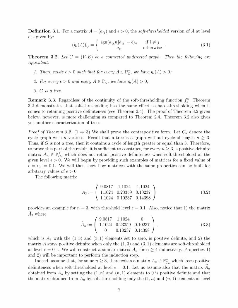
The following matrix

A3 :=

9.0817 1.1024 1.10241.1024 0.23359 0.102371.1024 0.10237 0.14398

(3.2)

provides an example for n = 3, with threshold level ε = 0.1. Also, notice that 1) the matrix

A3 where

A3 :=

9.0817 1.1024 01.1024 0.23359 0.10237

0 0.10237 0.14398

, (3.3)

which is A3 with the (1, 3) and (3, 1) elements set to zero, is positive definite, and 2) thematrix A stays positive definite when only the (1, 3) and (3, 1) elements are soft-thresholdedat level ε = 0.1. We will construct a similar matrix An for n ≥ 4 inductively. Properties 1)and 2) will be important to perform the induction step.

Indeed, assume that, for some n ≥ 3, there exists a matrix An ∈ P+Cn

which loses positive

definiteness when soft-thresholded at level ε = 0.1. Let us assume also that the matrix Anobtained from An by setting the (1, n) and (n, 1) elements to 0 is positive definite and thatthe matrix obtained from An by soft-thresholding only the (1, n) and (n, 1) elements at level

7

ε is positive definite. These properties are satisfied for n = 3 by the matrix A3 given above.We will build a matrix An+1 ∈ P+

Cn+1satisfying the same properties. Let an denote the (1, n)

element of An. For every real number r, let rε := sgn(r)(|r| − ε)+ denote the value of rsoft-thresholded at level ε. To simplify the notation, let us denote by an,ε the value of (an)ε.Now consider the matrix

An+1 :=

an+1

0

An +Dn...0b

an+1 0 . . . 0 b α

(3.4)

where Dn is a diagonal matrix with positive diagonal ((an+1,ε)2/α, 0, . . . , 0, (bε)

2/α). Noticethat An+1 has zeros according to Cn+1. We will prove that an+1, b, α can be chosen so thatAn+1 satisfies the required properties.

Let us first choose the value of an+1 as a function of α and b in such a way that

−an+1,ε bεα

= an,ε. (3.5)

This is always possible if |b| > ε. Indeed, if |b| > ε, then an+1 satisfies equation (3.5) for

an+1 := −αan,εbε

+ sε (3.6)

where s = sgn(−αan,ε/bε).We claim that we can choose α > 0 and b > ε such that:

1. An+1 is positive definite;

2. An+1 is positive definite;

3. An+1 is not positive definite when soft-thresholded at level ε, i.e., ηε(An+1) 6> 0;

4. An+1 is positive definite when only its (1, n + 1) and (n + 1, 1) elements are soft-thresholded at level ε.

Conditions (1) and (3) are the two conditions needed to prove that the matrix An+1 satisfiesthe theorem. Conditions (2) and (4) are required in the induction step.

First, note that the matrix An+1 has been constructed in such a way that the Schurcomplement of α in ηε(An+1) is equal to ηε(An). Therefore, by the induction hypothesis,ηε(An+1) is not positive definite for any value of |b| > ε and α > 0. This proves (3).

Since α > 0, to prove properties (1), (2) and (4), we only need to study the Schur

complement of α in the three matrices: An+1, An+1 and in the matrix obtained from An+1

by soft-thresholding the (1, n + 1) and (n + 1, 1) elements. We will prove that properties(1), (2) and (4) hold true asymptotically as α, b → ∞. Therefore, the result will follow bychoosing appropriately large values of α and b.

8

The Schur complement of α in An+1 is given by

An +Dn −

a2n+1

α. . . an+1b

α...

. . ....

an+1bα

. . . b2

α

= An +

(an+1,ε)2−a2n+1

α. . . −an+1b

α...

. . ....

−an+1bα

. . . b2ε−b2α

(3.7)

Let us take α = b3. Since an+1 and α depend on the value of b and since ε = ε0 is fixed, bbecomes the only “free” parameter. We will prove that properties (1), (2) and (4) hold forlarge values of b. We begin by studying the limiting behavior of different quantities relatedto the Schur complement (3.7). We will show that

an+1,ε

α→ 0 as b→∞ (3.8)

a2n+1

α− (an+1,ε)

2

α→ 0 as b→∞ (3.9)

an+1b

α→ −an,ε as b→∞. (3.10)

Equation (3.8), follows easily by equation (3.5), since

an+1,ε/α = −an,ε/bε → 0 as b→∞. (3.11)

Now to prove 3.9, recall that, by construction, an+1 = an+1,ε ± ε where the sign depends onthe sign of an+1. Therefore

(an+1)2

α− (an+1,ε)

2

α=

(an+1,ε ± ε)2

α− (an+1,ε)

2

α=±2εan+1,ε

α+ε2

α. (3.12)

The first term tends to 0 as b→∞ as shown above. Also, since α = b3, α →∞ as b→∞and so ε2/α→ 0 as b→∞. This proves equation (3.9).

Finally, for (3.10), if b > ε then bε = b− ε and∣∣∣∣an+1b

α− an+1,εbε

α

∣∣∣∣ =

∣∣∣∣(an+1,ε ± ε)(bε + ε)

α− an+1,εbε

α

∣∣∣∣=

∣∣∣∣εan+1,ε

α± εbε

α± ε2

α

∣∣∣∣ .As we have seen above, an+1,ε/α→ 0 as b→∞. Also, bε/α→ 0 as b→∞ since α = b3.

Therefore,an+1b

α− an+1,εbε

α→ 0 (3.13)

as b→∞. But by (3.5), we have an+1,εbε/α = −an,ε. Therefore

an+1b

α→ −an,ε (3.14)

as b→∞.

9

Using the results in equations (3.8)-(3.10), we now proceed to show that properties (1),(2) and (4) hold true for appropriately large values of b. To prove (1), we only need to showthat the Schur complement given by (3.7) is positive definite for large values of b. Indeed,notice that from (3.9) and (3.10), we have

(an+1,ε)2−a2n+1

α. . . −an+1b

α...

. . ....

−an+1bα

. . . b2ε−b2α

→ 0 . . . an,ε

.... . .

...an,ε . . . 0

(3.15)

elementwise. Therefore the Schur complement of α in An+1 given in (3.7) tends to

An +

0 . . . an,ε...

. . ....

an,ε . . . 0

. (3.16)

as b → ∞. This matrix is exactly the matrix An with the (1, n) and (n, 1) elements soft-thresholded at level ε. Therefore, by the induction hypothesis, this matrix is positive definiteand so is An+1 for large values of b. This proves property (1).

To prove property (2) note that the Schur complement of α in An+1 is given by

An +

(an+1,ε)2

α. . . 0

.... . .

...

0 . . . b2ε−b2α

. (3.17)

Notice that the (1, 1) entry of the righthand term is always positive whereas the (n, 1) element

tends to 0 as b → ∞. Since the matrix An is positive definite by the induction hypothesis,the Schur complement of α in An+1 is therefore also positive definite when b is sufficientlylarge. This proves (2).

Similarly, to prove (4), let us consider the Schur complement of α in the matrix An+1

with the (1, n+ 1) and (n+ 1, 1) entries soft-thresholded at level ε

An +

a2n+1−(an+1,ε)2

α. . . −an+1,εb

α...

. . ....

−an+1,εb

α. . . b2ε−b2

α

. (3.18)

We havean+1,εb

α=an+1,ε(bε + ε)

α=an+1,εbεα

+ εan+1,ε

α. (3.19)

From (3.5) and (3.8), we therefore have

an+1,εb

α→ −an,ε (3.20)

as b→∞ and so the preceding Schur complement is asymptotic to the matrix An with the(1, n) and (n, 1) elements soft-thresholded at level ε. By the induction hypothesis, this matrix

10

is positive definite and therefore the same is true for the matrix An+1 with the (1, n+ 1) and(n+ 1, 1) entries soft-thresholded at level ε when b is large enough. This proves (4).

Consequently, a matrix An+1 satisfying properties (1) to (4) can be obtained by choosinga value of b large enough. This completes the induction. Therefore, for every n ≥ 3, thereexists a matrix An ∈ P+

Cnsuch that ηε(An) is not positive definite for ε = ε0 = 0.1.

Now let ε > 0 be arbitrary. Notice that for α > 0 and any matrix A, it holds that

ηαε(αA) = αηε(A). (3.21)

As a consequence, for a given value of n, consider the matrix

A :=ε

ε0An. (3.22)

Then A ∈ P+Cn

since An ∈ P+Cn

. Moreover,

ηε(A) = η εε0ε0(A) =

ε

ε0ηε0(An). (3.23)

Since ηε0(An) is not positive definite by construction, it follows that ηε(A) is not positivedefinite either. This provides the desired example of a matrix A ∈ P+

Cnsuch that ηε(A) is

not positive definite. Therefore, if every matrix A ∈ P+G retains positive definiteness when

soft-thresholded at a given level ε > 0, the graph G must not contain any cycle and so is atree.

(3⇒ 2) The implication in this direction holds for more general functions than the soft-thresholding function. The proof is therefore postponed to Section 4 (see Theorem 4.18).

Finally, since 2 ⇒ 1 trivially, the three statements of the theorem are equivalent. Thiscompletes the proof of the theorem.

Corollary 3.4 (Complete graph case). For every n ≥ 3, and every ε > 0 there exists amatrix A ∈ P+

n such that ηε(A) 6∈ P+n .

4 General thresholding and entrywise maps

The result of the previous section shows that the commonly used soft-thresholding proceduredoes not map the cone of positive definite matrices into itself. A natural question to asktherefore is whether other mappings are better adept at preserving positive definiteness.

In this section, we completely characterize the functions that do so when applied to everyoff-diagonal element of a positive definite matrix. We begin by introducing some notationand reviewing previous results from the literature for the case where the function is alsoapplied to the diagonal.

Definition 4.1. For a function f : R→ R, denote by:

• f [A] the matrix obtained by applying f to every element of the matrix A, i.e.,

(f [A])ij = f(aij); (4.1)

11

• f ∗[A] the matrix obtained by applying f to every element of the matrix A, except thediagonal, i.e.,

(f ∗[A])ij =

{f(aij) if i 6= jaii if i = j.

(4.2)

We now compare f [A] and f ∗[A] for A > 0. Clearly, f ∗[A] = f [A] +DA, where DA is thediagonal matrix

DA = diag(a11 − f(a11), . . . , ann − f(ann)). (4.3)

As a consequence, if f [A] > 0 and the elements of DA are nonnegative, then f ∗[A] > 0. Suchis the case when |f(x)| ≤ |x|.

Remark 4.2. The condition that |f(x)| ≤ |x| is a mild restriction which allows us toconclude that f [A] > 0 ⇒ f ∗[A] > 0. As we shall see below, the converse is generally falsefor matrices of a given dimension. Hence the previous results in the literature characterizingfunctions which preserve positive definiteness, when the function is also applied to diagonalelements, are unnecessarily too restrictive. In this sense, previous results in the field arenot directly applicable to problems that arise in modern-day applications. This reasoningjustifies in a major way our treatment of the problem of applying elementwise maps only tooff-diagonal entries.

4.1 Background material: Results for f [A]

It is well-known that functions preserving positive definiteness when applied to every elementof the matrix must have a certain degree of smoothness and non-negative derivatives. As wewill see later, this is not true anymore when the diagonal is left untouched.

Theorem 4.3 (Horn & Johnson [5], Theorem 6.3.7). Let f be a continuous real-valuedfunction on (0,∞) and suppose that f [A] is positive semidefinite for every n × n positivesemidefinite matrix A = (aij) with positive entries. Then f is (n − 3)-times continuouslydifferentiable and f (k)(t) ≥ 0 for every t ∈ (0,∞) and every k = 0, . . . , n− 3.

Corollary 4.4. The soft-thresholding operation is not guaranteed to preserve positive semidef-initeness when the diagonal is also thresholded.

Proof. This follows easily from the non-differentiability of the soft-thresholding function.

Corollary 4.5. Let f be a continuous function and assume f [A] is positive semidefinitefor every positive semidefinite matrix A with positive entries. Then f ∈ C∞(0,∞) andf (k)(t) ≥ 0 for every t ∈ (0,∞) and every k ≥ 0.

Corollary 4.5 provides a necessary condition for a function f to preserve positive definite-ness when applied elementwise to a positive definite matrix. We shall show below that thiscondition is also sufficient. We first recall some facts about absolutely monotonic functionsand the Hadamard product.

Definition 4.6. Let 0 < α ≤ ∞. A function f ∈ C∞(0, α) is said to be absolutely monotonicon (0, α) if f (k)(x) ≥ 0 for every x ∈ (0, α) and every k ≥ 0.

12

The following theorem characterizes the class of absolutely monotonic functions on (0, α).

Theorem 4.7 (see [6, Chapter IV]). Let 0 < α ≤ ∞. Then the following are equivalent:

1. f is absolutely monotonic on (0, α);

2. f is the restriction to (0, α) of an analytic function on D(0, α) := {z ∈ C : |z| < α}with positive Taylor coefficients, i.e.,

f(x) =∞∑n=0

anxn (x ∈ (0, α)) (4.4)

for some an ≥ 0.

Remark 4.8. Let 0 < α ≤ ∞. A function f : (−α, α)→ R can be represented as:

f(x) =∞∑n=0

anxn (−α < x < α) (4.5)

for some an ≥ 0 if and only if f extends analytically to D(0, α) and is absolutely monotonicon (0, α).

Recall that the Hadamard product (or Schur product) of two n × n matrices A and B,denoted by A ◦ B, is the matrix obtained by multiplying the two matrices entrywise, i.e.,(A ◦ B)ij = (aijbij). Since A ◦ B is a principal submatrix of the Kronecker product A⊗ B,the matrix A ◦ B is positive definite if both A and B are positive definite. This last resultis commonly known as the Schur product theorem. We now state the converse of Corollary4.5. The proof follows immediately from Theorem 4.7 and the Schur product theorem.

Lemma 4.9. Let 0 < α ≤ ∞ and let f : (0, α)→ R be absolutely monotonic on (0, α). Thenf [A] is positive semidefinite for every positive semidefinite matrix A with entries in (0, α).

Combining Corollary 4.5 and Lemma 4.9, we obtain the following characterization offunctions preserving positive definiteness for every positive definite matrix with positiveentries:

Theorem 4.10. Let f : (0,∞) → R. Then f [A] is positive semidefinite for every positivesemidefinite matrix A with positive entries if and only if f is absolutely monotonic on (0,∞).

The following theorem shows that the result remains the same if the entries of the positivesemidefinite matrix A are constrained to be in a given interval. Special cases of this resulthave been proved by different authors; we state only the most general version here.

Theorem 4.11 (see Schoenberg [8], Rudin [7], Vasudeva [10], Hiai [4], Herz [3], Christensenand Ressel [1]). Let 0 < α ≤ ∞ and let f : (−α, α)→ R. Then f [A] is positive semidefinitefor every positive semidefinite matrix A with entries in (−α, α) if and only if f is analyticon the disc {z ∈ C : |z| < α} and absolutely monotonic on (0, α).

13

Recall that one of the primary goals of regularizing positive definite matrices is to “inducesparsity”, i.e., set small elements to zero. The following result shows that no thresholdingfunction that induces sparsity is guaranteed to preserve positive definiteness.

Corollary 4.12. Let 0 < α ≤ ∞ and let f : (−α, α)→ R satisfy f(0) = 0 and f(γ) = 0 forsome γ ∈ (0, α). Assume f 6≡ 0 on (−α, α). Then there exists a positive semidefinite matrixA with entries in (−α, α) such that f [A] is not positive semidefinite.

Proof. Assume f [A] is positive semidefinite for every positive semidefinite matrix A withentries in (−α, α). Then, by Theorem 4.11,

f(z) =∞∑k=1

akzk (z ∈ D(0, α)) (4.6)

where ak = f (k)(0)/k! ≥ 0. Since f(γ) = 0, we must have ak = 0 for every k ≥ 1, i.e., f ≡ 0.Thus, if f 6≡ 0, there exists a positive semidefinite matrix A such that f [A] is not positivesemidefinite.

4.2 Preliminary results for f ∗[A]

Let A be a positive definite matrix. We now proceed to analyze mappings f that are appliedonly to off-diagonal elements of A. The next result provides a basic first constraint that fmust satisfy in order for f ∗[A] to retain positive definiteness.

Lemma 4.13. Let f : R → R and assume |f(ξ)| > |ξ| for some ξ ∈ R. Then, for everygraph G = (V,E) containing at least one edge, there exists a matrix A ∈ P+

G such that f ∗[A]is not positive semidefinite.

Proof. Assume first that |V | = 2, and without loss of generality assume (1, 2) ∈ E. Since|f(ξ)| > |ξ|, there exists ε > 0 such that |f(ξ)| = |ξ|+ ε. Now consider the matrix

B :=

(|ξ|+ ε

2ξ

ξ |ξ|+ ε2

)(4.7)

The matrix B is positive definite, but f ∗[B] is not positive semidefinite. The general case ofa graph with n vertices follows by constructing the matrix A = B ⊕ In−2, where Ik denotesthe k × k identity matrix.

Recall from Theorem 4.2 that functions preserving positive definiteness when applied toevery element of a matrix (including the diagonal) of a given dimension have to be sufficientlysmooth, and have non-negative derivatives on the positive real axis. However, when thediagonal is left untouched, the situation changes quite drastically. More precisely, a farlarger class of functions preserves positivity, as the following result shows.

Proposition 4.14. Let G = (V,E) be a connected undirected graph and denote by ∆ = ∆(G)the maximum degree of the vertices of G. Assume f : R→ R satisfies

|f(x)| ≤ c|x| ∀x ∈ R, (4.8)

for some 0 ≤ c < 1∆

. Then f ∗[A] ∈ P+G for every A ∈ P+

G.

14

Proof. For every A ∈ P+G, denote by MA the matrix with entries

(MA)ij =

f(aij)

aijif aij 6= 0 and i 6= j

1 if i = j0 if aij = 0 and i 6= j

. (4.9)

The matrix f ∗[A] can be written as

f ∗[A] = A ◦MA. (4.10)

Since 0 ≤ c < 1∆

, an application of Gershgorin’s circle theorem demonstrates that MA > 0.As a consequence, by the Schur product theorem, A ◦MA > 0 and so f ∗[A] > 0 for everyA ∈ P+

G.

Corollary 4.15 (Complete graph case). Let n ≥ 2 and assume f : R→ R satisfies

|f(x)| ≤ c|x| ∀x ∈ R, (4.11)

for some 0 ≤ c < 1n−1

. Then f ∗[A] > 0 for every n× n positive definite matrix A.

Corollary 4.16. For every graph G, there exists a function f : R→ R such that f ∗[A] > 0for every A ∈ P+

G.

Remark 4.17. Despite the simplicity of the above proofs (especially in constrast to Theo-rems 3.2, 4.18, and 4.21 of this paper), Proposition 4.14, Corollary 4.15 and Corollary 4.16have important consequences, namely:

1. Contrary to the case where the function is also applied to the diagonal elements ofthe matrix (see Theorem 4.3), Corollary 4.15 shows that, when the diagonal is leftuntouched, preserving every n × n positive semidefinite matrix does not imply anydifferentiability condition on f . Even continuity is not required. We therefore note thestark differences compared with previous results in the area.

2. Proposition 4.14 shows that preserving positive definiteness is relatively easier for ma-trices that are already very sparse in term of connectivity, i.e., matrices with boundedvertex degree.

3. Corollary 4.15 suggests that preserving positive definiteness for non-sparse matricesbecomes increasingly difficult as the dimension n gets larger.

4.3 Characterization of functions preserving positive definitenessfor trees

Recall that a class of sparse positive definite matrices that is always guaranteed to retainpositive definiteness upon either hard or soft-thresholding is the class of matrices with zerosaccording to a tree (see Theorems 2.4 and 3.2). A natural question to ask therefore is whetherfunctions other than hard and soft-thresholding can also retain positive definiteness. Recall

15

from Lemma 4.13 that for every non-empty graph G, the functions f such that f ∗[A] ∈ P+G

for every A ∈ P+G are necessarily contained in the family

C := {f : R→ R : |f(x)| ≤ |x| ∀x ∈ R}. (4.12)

Note that C is the class of functions contracting at the origin. This “shrinkage” property isoften required in practice.

It is natural to ask if we can characterize the set of graphs G for which the functionsmapping P+

G into itself constitute all of C . The following theorem answers this question.

Theorem 4.18. Let G = (V,E) be a graph. Then

{f : R→ R : f ∗[A] ∈ P+G for every A ∈ P+

G} = C (4.13)

if and only if G is a tree.

Thus, the result provides a complete characterization of trees in terms of the maximal familyC .

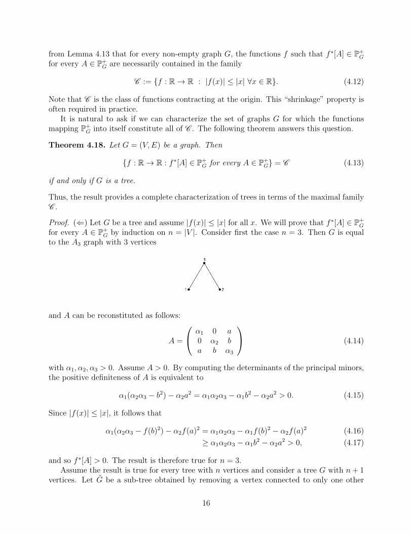
Proof. (⇐) Let G be a tree and assume |f(x)| ≤ |x| for all x. We will prove that f ∗[A] ∈ P+G

for every A ∈ P+G by induction on n = |V |. Consider first the case n = 3. Then G is equal

to the A3 graph with 3 vertices

and A can be reconstituted as follows:

A =

α1 0 a0 α2 ba b α3

(4.14)

with α1, α2, α3 > 0. Assume A > 0. By computing the determinants of the principal minors,the positive definiteness of A is equivalent to

α1(α2α3 − b2)− α2a2 = α1α2α3 − α1b

2 − α2a2 > 0. (4.15)

Since |f(x)| ≤ |x|, it follows that

α1(α2α3 − f(b)2)− α2f(a)2 = α1α2α3 − α1f(b)2 − α2f(a)2 (4.16)

≥ α1α2α3 − α1b2 − α2a

2 > 0, (4.17)

and so f ∗[A] > 0. The result is therefore true for n = 3.Assume the result is true for every tree with n vertices and consider a tree G with n+ 1

vertices. Let G be a sub-tree obtained by removing a vertex connected to only one other

16

node. Without loss of generality, assume this vertex is labeled n + 1 and its neighbor islabeled n. Let A ∈ P+

G. The matrix A has the form

A =

00

A...0a

0 0 . . . 0 a α

. (4.18)

By the induction hypothesis, the n×n principal submatrix A of A stays positive definitewhen f is applied to its off-diagonal elements, i.e., f ∗[A] > 0. It remains to be shown thatthe Schur complement of α in f ∗[A] is positive definite. Note first that the Schur complementof α in A is given as:

S = A−

0 . . . 0...

. . ....

0 . . . a2

α

. (4.19)

Since by assumption A > 0, we have S > 0. We also have S ∈ P+

G. Therefore, by the

induction hypothesis, f ∗[S] > 0. Note that f ∗[S] is different from the Schur complement ofα in f ∗[A]. More specifically,

f ∗[S] = f ∗[A]−

0 . . . 0...

. . ....

0 . . . a2

α

, (4.20)

but the Schur complement of α in f ∗[A] is given by

f ∗[A]−

0 . . . 0...

. . ....

0 . . . f(a)2

α

. (4.21)

Since |f(x)| ≤ |x| by assumption, it follows that the Schur complement of α in f ∗[A] is equalto f ∗[S] + D where D is a diagonal matrix with non-negative entries. Since f ∗[S] > 0, theSchur complement of α in f ∗[A] is positive definite, and therefore, so is f ∗[A]. This completesthe induction.

(⇒) Conversely, assume now that G is not a tree and let ε > 0. Then, by Theorem 3.2,there exists a matrix A ∈ P+

G such that (fSε )∗[A] 6∈ P+G, where fSε denotes the soft-thresholding

function (see (1.2)). This concludes the proof.

Remark 4.19. A similar result also holds for hard-thresholding with respect to a graph.Indeed, note that every subgraph of a graph G is a union of disconnected induced subgraphsif and only if G is a tree. As a consequence, matrices in P+

G are guaranteed to retainpositive definiteness when thresholded with respect to any subgraph of G if and only if Gis a tree (see Theorem 2.2 and [2, Corollary 3.5]). Hence, trees can be characterized by allfour types of thresholding operations that have been considered: 1) graph thresholding, 2)hard-thresholding, 3) soft-thresholding, and 4) general thresholding.

17

Remark 4.20. Corollary 4.16 shows that the converse of Theorem 4.18 is false in general,in the sense that retaining positive definite matrices for every matrix in P+

G does not implythat G is a tree.

4.4 Proof of the main result

We now proceed to completely characterize the functions f preserving positive definitenessfor matrices of arbitrary dimension, when the diagonal is not thresholded.

Theorem 4.21. Let 0 < α ≤ ∞ and let f : (−α, α)→ R. Then f ∗[A] is positive semidefinitefor every positive semidefinite matrix A with entries in (−α, α) if and only if f(x) = xg(x)where:

1. g is analytic on the disc D(0, α);

2. ‖g‖∞ ≤ 1;

3. g is absolutely monotonic on (0, α).

When α = ∞, the only functions satisfying the above conditions are the affine functionsf(x) = ax for 0 ≤ a ≤ 1.

Proof. (⇒) Let n ≥ 2 and let A,B be two n× n positive semidefinite matrices with entriesin (−α, α) such that A ≥ B. We first claim that f ∗[A] ≥ 2f [B]− f ∗[B]. Consider the blockmatrix

M =

(A BB B

)=

(A−B 0

0 0

)+

(B BB B

)≥ 0. (4.22)

Since M is positive semidefinite, f ∗[M ] is also positive semidefinite by hypothesis. Thus

f ∗[M ] =

(f ∗[A] f [B]f [B] f ∗[B]

)≥ 0. (4.23)

In particular,(I −I0 0

)(f ∗[A] f [B]f [B] f ∗[B]

)(I 0−I 0

)=

(f ∗[A]− f [B]− f [B] + f ∗[B] 0

0 0

)≥ 0.

(4.24)Thus, we must have f ∗[A]− 2f [B] + f ∗[B] ≥ 0, i.e., f ∗[A] ≥ 2f [B]− f ∗[B]. This proves theclaim.

Now, denote by 1m the m×m matrix with every entry equal to 1. Since A ≥ B, we alsohave, for every m ≥ 3, that 1m ⊗ A ≥ 1m ⊗B, i.e.,

A A . . . AA A . . . A...

.... . .

...A A . . . A

≥

B B . . . BB B . . . B...

.... . .

...B B . . . B

. (4.25)

18

Applying the claim to the above matrices, it follows that

f ∗[1m ⊗ A] ≥ 2f [1m ⊗B]− f ∗[1m ⊗B]. (4.26)

Let DB denote the diagonal matrix

DB = diag (b11 − f(b11), . . . , bnn − f(bnn)) . (4.27)

Then f ∗[B] = f [B] +DB and so, denoting by Im the m×m identity matrix,

2f [1m ⊗B]− f ∗[1m ⊗B] = 1m ⊗ f [B]− Im ⊗DB. (4.28)

Similarly, ifDA = diag (a11 − f(a11), . . . , ann − f(ann)) , (4.29)

then f ∗[A] = f [A] +DA and

f ∗[1m ⊗ A] = 1m ⊗ f [A] + Im ⊗DA. (4.30)

Combining equations (4.26), (4.28) and (4.30), we obtain

1m ⊗ f [A] + Im ⊗DA ≥ 1m ⊗ f [B]− Im ⊗DB, (4.31)

or equivalently,1m ⊗ (f [A]− f [B]) ≥ −Im ⊗ (DA +DB). (4.32)

In matrix notation, equation (4.32) is equivalent tof [A]−f [B] f [A]−f [B] ... f [A]−f [B]

f [A]−f [B] f [A]−f [B] ... f [A]−f [B]

......

......

f [A]−f [B] f [A]−f [B] ... f [A]−f [B]

≥ −

DA+DB 0 ... 0

0 DA+DB ... 0

......

......

0 0 ... DA+DB

(4.33)

Note that for every n× n symmetric matrix M with eigenvalues λ1, . . . , λn, the eigenvaluesof 1m ⊗M are {0,mλ1, . . . ,mλn}. Now apply Weyl’s inequality to (4.32) to obtain

mλmin(f [A]− f [B]) ≥ −maxi

(aii + bii − f(aii)− f(bii)). (4.34)

Dividing by m and letting m→∞ shows that

f [A]− f [B] ≥ 0. (4.35)

We have thus shown that f [A] ≥ f [B] for every A ≥ B ≥ 0 with entries in (−α, α). Since,by hypothesis, f ∗[A] ≥ 0 for every A ≥ 0, we know from Lemma 4.13 that f has to satisfy|f(x)| ≤ |x| for every x. In particular, f(0) = 0. Applying (4.35) with B = 0 now showsthat f [A] ≥ 0 for every A ≥ 0. Hence, by Theorem 4.11, f is analytic on D(0, α) and isabsolutely monotonic on (0, α), i.e., f (k)(0) ≥ 0 for every k ≥ 0. In other words,

f(z) =∞∑k=1

akzk (4.36)

19

where ak := f (k)(0)/k! ≥ 0. Finally, since f satisfies |f(x)| ≤ |x| (see Lemma 4.13), thefunction g defined by g(0) = 0 and

g(x) :=f(x)

x=∞∑k=1

akxk−1 (x 6= 0), (4.37)

satisfies |g(x)| ≤ 1 for every x, i.e., ‖g‖∞ ≤ 1. Therefore, f(x) = xg(x) for a function g thatis analytic on D(0, α), absolutely monotonic on (0, α), and satisfies the condition ‖g‖∞ ≤ 1.

(⇐) Conversely, assume f(x) = xg(x) for some function g analytic function on D(0, α),absolutely monotonic on (0, α), and satisfying ‖g‖∞ ≤ 1. Then from Theorem 4.11, f [A] ≥ 0for every A ≥ 0 with entries in (−α, α). Note that f ∗[A] = f [A]+D where D is the diagonalmatrix

D = diag(a11 − f(a11), . . . , ann − f(ann)). (4.38)

Since ‖g‖∞ ≤ 1, then |f(x)| ≤ |x| and thus the elements of D are non-negative. Hence,f ∗[A] ≥ 0 for every A ≥ 0 with entries in (−α, α).

In the case when α =∞, the only bounded absolutely monotonic functions g on (0,∞)are the constant functions g(x) ≡ a for some a ≥ 0. Since |f(x)| ≤ |x| we must have0 ≤ a ≤ 1. This completes the proof of the theorem.

Remark 4.22. We now compare and constrast Theorem 4.21 to the analoguous resultsproved in the literature, namely Theorem 4.11.

1. Recall that, for matrices A ≥ 0 of a given dimension, if |f(x)| ≤ |x| and f [A] ≥ 0, thenf ∗[A] ≥ 0. The converse is generally false (see Remarks 4.2 and 4.17).

2. In constrast, for A ≥ 0 of arbitrary dimension, the above proof shows that f [A] ≥ 0and |f(x)| ≤ |x| if and only if f ∗[A] ≥ 0.

Theorem 4.21 shows that only a very narrow class of functions are guaranteed to preservepositive definiteness for an arbitrary positive definite matrix of any dimension. In practicalapplications, thresholding is often performed on normalized matrices (such as correlationmatrices) which have bounded entries. In that case, more functions preserve positive defi-niteness. However, as in the case where the function is applied to the diagonal, the followingresult shows that no thresholding function can induce sparsity (i.e., set non-zero elements tozero) and, at the same time, be guaranteed to maintain positive definiteness for matrices ofevery dimension.

Corollary 4.23. Let 0 < α ≤ ∞ and let f : (−α, α)→ R satisfy f(0) = 0 and f(γ) = 0 forsome γ ∈ (0, α). Assume f 6≡ 0 on (−α, α). Then there exists a positive semidefinite matrixA with entries in (−α, α) such that f ∗[A] is not positive semidefinite.

Proof. The proof is the same as the proof of Corollary 4.12.

20

5 Eigenvalue inequalities

The results of Section 4 show that only a restricted class of functions are guaranteed topreserve positive definiteness when applied elementwise to matrices of arbitrary dimension.Moreover, no function can at the same time induce sparsity (have zeros other than at theorigin) and simultaneously preserve positive definiteness for every matrix. Hence, a naturalquestion to ask is whether certain properties of matrices (such as a lower bound on theminimum eigenvalue or an upper bound on the condition number) are sufficient to maintainpositive definiteness when a given function f is applied to the off-diagonal elements of thematrix. We provide such sufficient conditions in this section. The results are first derivedin Section 5.1 for the case when f is a polynomial. They are then extended to more generalfunctions in the subsequent subsection.

5.1 Bounds for polynomials

We first establish some notation. For a polynomial p(x) =∑d

i=0 aixi, define its “positive”

and “negative” parts by:

p+(x) =∑ai>0

aixi, p−(x) = −

∑ai<0

aixi. (5.1)

Many of the results in this section are motivated by the following idea. Note that

p∗[A] = p+[A]− p−[A] +DA (5.2)

where D is the diagonal matrix DA = diag(a11 − p(a11), . . . , ann − p(ann)). Repeated appli-cations of the Schur product theorem can be used to show that both p+[A] and p−[A] arepositive definite when A is positive definite. Intuitively, a polynomial with a positive partthat is “larger” than its negative part should be able to preserve positive definiteness for awider class of matrices as compared to a polynomial with a “large” negative part. This ideais formalized in Proposition 5.3 below. Before stating the result, recall the following classicalresult that can be used to bound the eigenvalues of Schur products.

Theorem 5.1 (Schur [9]). Let A,B be positive definite matrices. Then for i = 1, . . . , n,

λmin(A) minibii ≤ λi(A ◦B) ≤ λmax(A) max

ibii. (5.3)

Corollary 5.2. Let A be an n×n matrix. Denote by dmin and dmax the minimal and maximaldiagonal element of A respectively. Then for i = 1, . . . , n,

dk−1minλmin(A) ≤ λi(A

◦k) ≤ dk−1maxλmax(A), (5.4)

where A◦k denotes the Hadamard product of k copies of A.

We now proceed to state the main result of this subsection.

Proposition 5.3. Let p be a polynomial and assume p(0) = 0. Let A be an n × n matrix,and denote by dmin and dmax the smallest and largest diagonal elements of A respectively.Then:

21

1. λmin(p∗[A]) ≥ p+(λmin(A))− p−(λmax(A)) + mini=1,...,n

(aii − p(aii));

2. λmin(p∗[A]) ≥ λmin(A)p+(dmin)

dmin

− λmax(A)p−(dmax)

dmax

+ mini=1,...,n

(aii − p(aii)).

Proof. By Weyl’s inequality,

λmin(p[A]) ≥∑ai>0

aiλmin(A◦i) +∑ai<0

aiλmax(A◦i). (5.5)

The first result follows by using Cauchy’s interlacing theorem to observe that λmin(A◦i) ≥λmin(A)i, λmax(A◦i) ≤ λmax(A)i, in addition to the fact that p∗[A] = p[A] +DA, where DA isthe diagonal matrix DA = diag(a11− p(a11), . . . , ann− p(ann)). The second assertion followsby the same argument, but then uses Corollary 5.2 to bound the eigenvalues of the Schurproduct.

Corollary 5.4. Let n ≥ 1 and let p be a polynomial such that p(0) = 0. Let A be an n× nmatrix with spectral radius denoted by ρ(A). Then p∗[A] > 0 if

mini=1,...,n

(aii − p(aii)) ≥ p−(ρ(A)). (5.6)

The following surprising result shows that some polynomials having negative coefficientscan preserve large classes of positive definite matrices (like the class of correlation matrices).

Corollary 5.5. Let n ≥ 1 and let p be a polynomial such that p(0) = 0 and p−(x) ≤ 1−p(1)for every 0 < x < n. Then p∗[A] > 0 for every n× n correlation matrix A.

Proof. This follows from Corollary 5.4 by noticing that λmax(A) < n for every n × n corre-lation matrix A.

Corollary 5.6 below shows that p∗[A] is guaranteed to be positive definite if the conditionnumber of A is sufficiently small. Note that the bound becomes more restrictive as the“negative part” of p becomes larger compared to its “positive part”.

Corollary 5.6. Let p be a polynomial and assume |p(x)| ≤ |x| for every x ∈ [−a, a], forsome a > 0. Then p∗[A] > 0 for every positive definite matrix A with entries in [−a, a] suchthat

cond(A) :=λmax(A)

λmin(A)≤ p+(dmin)

p−(dmax)

dmax

dmin

. (5.7)

Corollary 5.7. Let p be a polynomial and assume |p(x)| ≤ |x| for every x ∈ [−1, 1]. Thenp∗[A] > 0 for every correlation matrix A such that

cond(A) :=λmax(A)

λmin(A)≤ p+(1)

p−(1). (5.8)

22

5.2 Extension to more general functions

We now proceed to extend the results of Section 5.1 to more general thresholding functions.We first recall the following well-known result.

Lemma 5.8. Let P+ be the set of polynomials with positive coefficients and let r > 0.Then the uniform closure of P+ over [−r, r] is the restriction to [−r, r] of the set of analyticfunctions f(z) =

∑n≥0 anz

n on the disc D(0, r) = {z ∈ C : |z| < r} with an ≥ 0 for everyn ≥ 0 and

∑n≥0 anr

n <∞.

Definition 5.9. For r > 0 we define

W+(r) =

{f(z) =

∑n≥0

anzn ∈ Hol(D(0, r)) :

∑n≥0

|an|rn <∞

}. (5.9)

The space W+ := W+(1) is often known as the analytic Wiener algebra of analytic functions.The space W+(r) can be seen as a weighted version of the analytic Wiener algebra.

As mentioned above, every function in W+(r) has a continuous extension to the closeddisc D(0, r). Notice that W+(r) ⊂ H∞(D(0, r)), the space of bounded analytic functions onthe disc D(0, r).

We first begin by extending Proposition 5.3.

Proposition 5.10. Let f ∈ W+(a) for some a > 0 and assume f(0) = 0. Write f = f+−f−where f+, f− ∈ W+(a) have nonnegative Taylor coefficients. Then for every n × n matrixA = (aij) with aij ∈ [−a, a], we have:

1. λmin(f ∗[A]) ≥ f+(λmin(A))− f−(λmax(A)) + mini=1,...,n

(aii − f(aii));

2. λmin(f ∗[A]) ≥ λmin(A)f+(dmin)

dmin

− λmax(A)f−(dmax)

fmax

+ mini=1,...,n

(aii − f(aii)).

Proof. By Lemma 5.8, there exist sequences of polynomials with positive coefficients p(k)+ ,

p(k)− such that

p(k)+ → f+ and p

(k)− → f− (5.10)

uniformly on [−a, a] as k → ∞. Let p(k) := p(k)+ − p

(k)− . An application of the triangle

inequality shows that p(k) → f uniformly on [−a, a]. Now, by Proposition 5.3,

λmin(p(k)[A]) ≥ p(k)+ (λmin(A))− p(k)

− (λmax(A)) + mini=1,...,n

(aii − p(k)(aii)). (5.11)

The first result follows by the continuity of the eigenvalues and uniform convergence. Thesecond part follows similarly.

Corollary 5.6 can also be easily extended using a similar argument.

23

Theorem 5.11. Let f ∈ W+(a) for some a > 0 and assume |f(x)| ≤ |x| for every x ∈[−a, a]. Then f ∗[A] > 0 for every n× n matrix A = (aij) with aij ∈ [−a, a] such that

cond(A) ≤ f+(dmin)

f−(dmax)

dmax

dmin

, (5.12)

where dmin and dmax denote the minimal and maximal diagonal element of A respectively.

The previous results can easily be extended to more general functions that can be ap-proximated pointwise by polynomials. The following result illustrates this idea for Corollary5.6.

Theorem 5.12. Let f : [−a, a] → R for some a > 0 and assume |f(x)| ≤ |x| for everyx ∈ [−a, a]. Moreover, assume f is the pointwise limit of a sequence of polynomials p(n) on[−a, a]. Then f ∗[A] > 0 for every A > 0 with entries in [−a, a] such that

condA ≤ lim supn→∞

p(n)+ (dmin)

p(n)− (dmax)

dmax

dmin

, (5.13)

where dmin and dmax denote the minimal and maximal diagonal element of A respectively.

Proof. Since p(n)[A] converges to f [A] entrywise as n → ∞, the eigenvalues of p(n)[A] con-verge to the eigenvalues of f [A]. The result follows from Corollary 5.6 using a limitingargument similar to the one in the proof of Proposition 5.10.

Acknowledgement and notes : We wish to thank Apoorva Khare for useful comments anddiscussions. This paper has been submitted to the Arxiv under the title Functions operatingon sparse positive definite matrices encoded by graphs.

References

[1] Jens Peter Reus Christensen and Paul Ressel. Functions operating on positive definitematrices and a theorem of Schoenberg. Trans. Amer. Math. Soc., 243:89–95, 1978.

[2] Dominique Guillot and Bala Rajaratnam. Retaining positive definiteness in thresholdedmatrices. Linear Algebra and its Applications, 436(11):4143 – 4160, 2012.

[3] Carl S. Herz. Fonctions operant sur les fonctions definies-positives. Ann. Inst. Fourier(Grenoble), 13:161–180, 1963.

[4] Fumio Hiai. Monotonicity for entrywise functions of matrices. Linear Algebra Appl.,431(8):1125–1146, 2009.

[5] Roger A. Horn and Charles R. Johnson. Topics in matrix analysis. Cambridge UniversityPress, Cambridge, 1991.

[6] G. G. Lorentz. Bernstein polynomials. Chelsea Publishing Co., New York, secondedition, 1986.

24

[7] Walter Rudin. Positive definite sequences and absolutely monotonic functions. DukeMath. J, 26:617–622, 1959.

[8] I. J. Schoenberg. Positive definite functions on spheres. Duke Math. J., 9:96–108, 1942.

[9] J. Schur. Bemerkungen zur theorie der beschrankten bilinearformen mit unendlich vielenveranderlichen. Journal fur die reine und angewandte Mathematik, 140:1–28, 1911.

[10] Harkrishan Vasudeva. Positive definite matrices and absolutely monotonic functions.Indian J. Pure Appl. Math., 10(7):854–858, 1979.

25