potential of driving style adaptation for a maneuver...
TRANSCRIPT

Potential of Driving Style Adaptation for a Maneuver
Prediction System at Urban Intersections
Am Fachbereich Maschinenbau an der
Technischen Universität Darmstadt
zur Erlangung des Grades eines
Doktor-Ingenieurs (Dr.-Ing.)
genehmigte
Dissertation
vorgelegt von
Claas Rodemerk, M.Sc.
aus Rosbach v. d. Höhe
Berichterstatter: Prof. Dr. rer. nat. Hermann Winner
Mitberichterstatter: Prof. Dr.-Ing. Klaus Dietmayer
Tag der Einreichung: 24.10.2016
Tag der mündlichen Prüfung: 10.01.2017
Darmstadt 2017
D 17

II
Please refer to:
URN: urn:nbn:de:tuda-tuprints-67823
URI: http://tuprints.ulb.tu-darmstadt.de/id/eprint/6782
This Document is provided by tuprints,
e-publishing-service of Technische Universität Darmstadt
http://tuprints.ulb.tu-darmstadt.de

III
Vorwort
Die vorliegende Arbeit entstand während meiner Tätigkeit als wissenschaftlicher Mitar-
beiter am Fachgebiet Fahrzeugtechnik (FZD) der Technischen Universität Darmstadt.
Mein besonderer Dank gilt Herrn Prof. Dr. rer. nat. Hermann Winner für die Unterstüt-
zung in der Promotionsphase, sein Vertrauen sowie die zahlreichen fachlichen Diskussio-
nen und Anregungen, die maßgeblich zum Gelingen der vorliegenden Arbeit beigetragen
haben.
Herrn Prof. Dr.-Ing. Klaus Dietmayer danke ich für die freundliche Übernahme des Kor-
referats und den fachlichen Austausch im Entstehungsprozess der Dissertation.
Die vorgestellten Forschungsfragen basieren auf den Ergebnissen eines Kooperationspro-
jekts mit Honda R&D Europe (Deutschland) GmbH. Mein Dank gilt insbesondere Herrn
Dr. Robert Kastner für den regen fachlichen Austausch in den vergangenen Jahren.
Weiterhin bedanke ich mich bei allen ehemaligen und aktuellen Mitarbeitern von FZD
einschließlich der Werkstätten und des Sekretariats für die hervorragende Zusammenar-
beit, die stets für ein sehr angenehmes und produktives Arbeitsklima gesorgt hat. Insbe-
sondere meinen Bürokollegen, die mich während der letzten 4 Jahren als Doktorand
begleitet haben, danke ich für die vielen fachlichen und privaten Diskussionen und die
angenehme Zeit.
Darüber hinaus bedanke ich mich bei allen Studenten, die mich in meiner Zeit als wissen-
schaftlicher Mitarbeiter in Form von zahlreichen Projektarbeiten, Abschlussarbeiten oder
als wissenschaftliche Hilfskräfte begleitet und unterstützt haben und durch ihren Einsatz
einen wertvollen Teil zu der vorliegenden Arbeit beigetragen haben.
Meiner Familie bin ich für ihre stete Unterstützung und Förderung während meiner ge-
samten Ausbildung und insbesondere während der Promotionszeit sehr dankbar. Mein
ganz besonderer Dank gilt meiner Frau Annemarie für ihre fortwährende Unterstützung
in allen Lebenslagen.
Claas Rodemerk Darmstadt, Oktober 2016

IV
Table of Contents
Vorwort ....................................................................................................................... III
Table of Contents ........................................................................................................ IV
Abbreviations ............................................................................................................ VII
Symbols and Indices ................................................................................................ VIII
Summary ..................................................................................................................... XI
1 Introduction and Motivation ................................................................................... 1
1.1 Motivation .......................................................................................................... 1
1.2 Challenges of Intersection Assistance .................................................................. 2
1.3 Using Detected Intentions ................................................................................... 5
1.4 Definitions and Scope of Work............................................................................ 6
1.5 Structure of the Thesis ........................................................................................ 7
2 Driver Intention Detection ....................................................................................... 9
2.1 Driver ................................................................................................................. 9
2.2 Vehicle .............................................................................................................. 11
2.3 Environment ..................................................................................................... 12
2.4 Related Work .................................................................................................... 12
2.5 Conclusion of Related Work.............................................................................. 16
3 Methodology ........................................................................................................... 17
3.1 Research Questions ........................................................................................... 17
3.2 Methodology..................................................................................................... 18
4 Data Generation ..................................................................................................... 21
4.1 Radar Sensors and Head tracking ...................................................................... 23
4.2 Positioning and Digital Map.............................................................................. 24
4.2.1 Working Principle ................................................................................... 24
4.2.2 Information Extracted from Digital Map ................................................. 25
4.3 Image Processing .............................................................................................. 26
4.4 Test Drives ........................................................................................................ 28
4.4.1 Classification of Intersection Types ......................................................... 28
4.4.2 Execution of Test Drives ......................................................................... 29
4.4.3 Test Route ............................................................................................... 31
4.4.4 Test Subjects ........................................................................................... 33

Table of Contents
V
5 Maneuver Prediction .............................................................................................. 35
5.1 Indicator-based Maneuver Prediction ................................................................. 36
5.1.1 Description of Indicators ......................................................................... 37
5.1.2 Transfer Functions ................................................................................... 37
5.1.3 Training Data........................................................................................... 39
5.2 Influence of Distance to Intersection .................................................................. 43
5.3 Free Driving Conditions .................................................................................... 45
5.4 Indicators of the Prediction System .................................................................... 48
5.4.1 Driving Dynamics and Driver's Control Inputs ........................................ 49
5.4.2 Driver's Behavior in Vehicle .................................................................... 50
5.4.3 Environment Perception .......................................................................... 51
5.4.4 Intersection Approach Behavior ............................................................... 53
5.4.5 General Information ................................................................................ 59
5.5 Indicator Quality Assessment............................................................................. 60
5.5.1 Indicator Quality Measure ....................................................................... 60
5.5.2 Sparsely Occupied Intervals .................................................................... 62
5.6 Optimization of Indicators ................................................................................. 64
5.7 Accuracy of Input Signals .................................................................................. 66
6 Evaluation ............................................................................................................... 67
6.1 Inference Methods ............................................................................................. 67
6.2 Training and Test ............................................................................................... 69
6.3 Reference Points ................................................................................................ 70
6.3.1 Location Based Reference Points ............................................................. 70
6.3.2 Ego-motion-based Reference Points ........................................................ 72
6.4 Evaluation Principle .......................................................................................... 74
6.5 Selection of Indicators ....................................................................................... 75
6.6 Exclusion of Alternative Maneuvers .................................................................. 78
6.6.1 Concept of Maneuver Exclusion .............................................................. 78
6.6.2 Predictions on Multiple Exclusion Horizons ............................................ 79
6.6.3 Calculation .............................................................................................. 80
6.6.4 Implementation ....................................................................................... 80
7 Results ..................................................................................................................... 82
7.1 Prediction Performance ..................................................................................... 82
7.1.1 Priority Roads.......................................................................................... 82
7.1.2 Traffic Lights ........................................................................................... 83
7.1.3 Priority to Right Regulated Intersections ................................................. 84
7.1.4 Give Way and Stop Sign Regulated Intersections ..................................... 85
7.1.5 Robustness of Predictions ........................................................................ 86
7.2 Bayesian Network ............................................................................................. 87
7.3 Neglecting Intersection Classes ......................................................................... 89
7.4 Exclusion Results .............................................................................................. 90

Table of Contents
VI
8 Driver-specific Adaptation ..................................................................................... 92
8.1 Driver Classification ......................................................................................... 93
8.2 Results of the Adaptation Process...................................................................... 96
8.3 Adaptation Methods in Real Driving ................................................................. 98
8.4 Biasing ............................................................................................................. 99
8.4.1 Routing Bias ........................................................................................... 99
8.4.2 Local Overfitting .................................................................................. 100
9 Conclusion and Outlook....................................................................................... 102
A Driver Inputs for Maneuver Detection ................................................................ 105
B Radar Based Lane Detection................................................................................ 108
C Localization ...........................................................................................................110
D Image Processing ................................................................................................... 111
E Intersection Classification .....................................................................................114
F Test Drives .............................................................................................................118
G Accuracy of Input Signals .................................................................................... 122
H Reference Points ................................................................................................... 130
I Neglecting Intersection Classes ............................................................................ 133
J Elements of the Adaptation System ..................................................................... 136
List of References ...................................................................................................... 141
Own Publications ...................................................................................................... 153
Supervised Thesis...................................................................................................... 154

VII
Abbreviations
Abbreviation Description
ACC adaptive cruise control
ADAS advanced driver assistance system
CAN controller area network
CAM camera
DOP dilution of precision
FOT field operation test
(E)CDF (empirical) cumulative distribution function
EEG electroencephalogram
GNSS global navigation satellite system
GPS global positioning system
IAS intersection assistance system
IDM intelligent driver model
INS Inertial Navigation System
IMU Inertial Measurement Unit
LIDAR Light detection and ranging
OC oncoming
OSM openstreetmap
POS position
RFID radio-frequency identification
RMSE root mean square error
RADAR radio detection and ranging
STVO Straßenverkehrsordnung
SQDIFF normalized squared Euclidean distance
TTI time to intersection
TTC time to collision
V2X vehicle-to-X-communication

Symbols and Indices
VIII
Symbols and Indices
Symbol Unit Description
a m/s² acceleration
acp % accelerator pedal
age years age of test subjects
d m distance, width
dd - sum of object likelihoods
di - distance interval
c N/° cornering stiffness
E - ego
f - transfer function
fr Hz frequency
g m/s² gravity
h m prediction horizon
I pixel content of search window
L - left
LH -
maneuver probability
m - maneuver
ma kg mass
M - number of potential maneuvers
MG - group of maneuver sequences
O - object
p % probability / likelihood
PV - preceding vehicle
pres bar pressure
q m width of road
Q m² quality of variation
QM, QMT % quality measure
r miscellaneous
range
ra - transmission ratio
R - right
Res miscellaneous
resolution of signal
S - straight
SM % sensitivity measure
t s time
/ % trust / mistrust in quality measure
ttc s time to collision
ttmi s time to maneuver initialization
v km/h, m/s vehicle's speed
u - number of indicators

Symbols and Indices
IX
Symbol Unit Description
x - x-axis
y - y-axis
w - factor/weight
WB m wheelbase
° angle between edges of digital map
°/s, rad/s side slip angle change rate
miscellaneous limit
°, rad steering wheel angle
miscellaneous difference
miscellaneous error, limit
°, rad angle of object detected by radar
1/m curvature
°, rad head / gaze rotation angle
s time gap
°, rad angle between center of circle and intersection center
°, rad heading deviation of leading vehicle
°, rad heading angle
°/s, rad/s yaw rate
Index Description
act active, actual
ai aerial image
b discretized bin
brake braking
char characteristic
city urban areas
comb combined
comf comfortable
cp compound
del delay
di distance intervals
DR dead reckoning
ego ego-vehicle
ex exist
exc exclusion
fr front
HG head- and gaze tracking
in interval size
ind indicator
int intersection
im image processing
L, l, left left / left turn
lim limit

Symbols and Indices
X
loc localization
lon longitudinal
me mean
map digital map
mat matched
mea measured
mod modified
NaN not a number
non-act non-active
obs observation
obj object
org original
pp predicted path
pre predicted
Q5 5 % quantile
Q95 95 % quantile
rad radial
re relevant
real real
ref reference point
rel relative
R, r, right right / right turn
S, s, straight straight driving
sm small
sc shoulder check
stop stopping line
su start up
st stop
stat static
str steering rack
tr training
tra travelled
trans transition
QMT trusted quality measure
v speed
var variation
veh vehicle
y lateral
steering wheel angle
yaw rate
curvature

XI
Summary
Navigating through urban intersections is a challenging task for human drivers in gen-
eral. More than 50 % of accidents with personal injuries caused by passenger car drivers
in urban conditions happen at intersections. Currently, no driver assistance system in
production is able to issue early warnings for pending collisions at urban intersections.
One of the reasons is the warning dilemma at intersections arising from the variety of
potential maneuvers a driver can perform.
To overcome this dilemma, an approach is presented in this work to detect drivers'
intentions on guidance level at urban intersections. The term guidance level is used here
according to three-level hierarchy of the vehicle driving task described by Donges. The
driver's core task on guidance level is to select a target track and target speed for safe
driving. An intention here is understood as a driver's plan to execute a maneuver and is
formulated before a maneuver is initialized. The goal of the intention detection system
introduced here is to detect a maneuver intention based on data measured during inter-
section approach and to predict a pending maneuver before commencement. The predic-
tion quality achieved by the intention detection system solely based on automotive
series sensors is analyzed. The turn indicator state is not used in the intention detection
process at all. The approach introduced in this work is applicable for maneuver intention
detection at arbitrary urban intersections. The intention detection is based on so-called
“indicators”. Indicators have at least one input signal and one output signal for each
potential intention. Indicators use transfer functions to calculate the maneuver likeli-
hoods from any kind of input signal for all potential maneuvers. The indicators' transfer
functions are calculated following the basics of Maximum-Likelihood principle. A
quality measure to assess the quality of indicators and select indicators being beneficial
for intention detection is introduced. The following data are used for intention detection:
driver's control inputs during intersection approach, driver's head and gaze motion and
mirror positions, environment perception information and intersection-specific infor-
mation extracted from a digital map. Using independent indicators allows for the easy
combination of different types of input signals in the prediction process. Different infer-
ence methods for the combination of indicators are discussed. Aside from inference
methods with low computational complexity, a Bayesian network is applied as well.
To analyze the feasibility of the approach introduced here, an experimental vehicle is
equipped with a prototypic implementation of the intention detection system introduced
in this work, using a close-to-production GNSS receiver and navigation map data for
localization only. Test drives with 30 test subjects are carried out in the city of Darm-
stadt. Data recorded in the test drives is used to train indicators' transfer functions and to

Summary
XII
evaluate the system's detection performance. A classification scheme for urban intersec-
tions is introduced and the performance evaluation is presented separately for different
types of intersections. Due to inaccuracies arising from the localization, ego-motion
based reference points are defined in this work for the system' s evaluation. These local-
ization-inaccuracy-free reference points are calculated a posteriori to turn maneuvers
based on the vehicle's motion. Using these reference points, average true-prediction
rates of the implemented system on priority roads are 87.5 % for straight driving ma-
neuvers, 81.5 % for right turns and 84.1 % for left turns, at 1 s second before maneuvers
are initialized.
All intention detection systems identified in related works focus on the detection of at
least one intention connected with an action that the driver is about to perform. Here, a
complimentary approach is introduced: The intention detection system is modified in
order to exclude an intention related to a maneuver that the driver is not going to per-
form. A number of exclusions are calculated for multiple horizons in front of the ego-
vehicle. The advantage of this approach is that it overcomes the limitations of a classic
"positive detection" approach: If a "positive detection" system cannot discriminate
amongst at least two potential and concurring intentions, no decision is made. In this
case the exclusion approach is able to exclude a third potential intention.
Several studies can be found in literature addressing varying driving styles among dif-
ferent drivers. Thus, this work analyses the potential of increasing true prediction rates
by adapting the indicators' transfer functions to individual driving styles. All test sub-
jects are classified into sporty, medium or relaxed drivers based on longitudinal acceler-
ations tolerated by drivers in the study. The driving-style adaption process is able to
increase prediction performance by more than 30 % for single maneuvers of drivers of
the medium group at stop-sign- or give way-sign-regulated intersections. No
appreciable effect to the detection performance could be found for other priority
regulations.

1
1 Introduction and Motivation
1.1 Motivation
A review of German accident statistics shows that among 2.4 millions accidents on
German roads reported to the police in 2014, more than 392,000 people were harmed in
traffic accidents in that year, including 3,377 fatalities. While the majority of fatalities
occur in situations outside of towns, most accidents with injuries happen within city
limits: 53 % of all people seriously injured in traffic accidents and 68 % of all people
with minor injuries are harmed in accidents in urban conditions.1
Enormous progress has been made within the last years in terms of automated driving
and it is assumed that automated driving will come into series production for highway
driving within the next decade.2 As a result of using automated vehicles, traffic acci-
dents with injured or killed are supposed to decrease.3 It is expected that expanding the
field of operation of automated vehicles to situations outside of towns and driving on
rural roads is likely to follow subsequently. However, serial application of automated
vehicles driving in urban conditions is supposed to be a long way off due to the more
challenging surroundings in urban areas.4 Especially difficult urban driving situations
include large intersections without traffic lights, the presence of cyclists near the vehi-
cle, or missing lane markings.5 Thus, medium-term, human drivers will still be neces-
sary for driving in urban conditions.
Focusing on the reasons for traffic accidents with personal injuries shows that the ma-
jority of accidents (> 91 %) happen due to improper human behavior.6,7
Out of more
than 300,000 accidents with personal injuries reported to the German police in 2014,
human error was noted as accident reason approximately 362,000 times. This means,
1 Statistisches Bundesamt: Zeitreihen 2014 (2015), p.44.
2 Pudenz, K.: Schrittweise Automatisierung bis 2025 (2012).
3 Unselt, T.; Schöneburg, R. Bakker J.: Einführung autonomer Fahrzeugsysteme (2013), p.239.
4 Grundhoff, S.: Autos ohne Fahrer (2013).
5 Knecht, J.: Probleme des Autonomen Fahrens (2016).
6 Only 8.6 % of all accidents reported in Germany in 2014 are caused by general causes (road conditions,
influence of weather or obstacles on the road and technical failures).
7 Statistisches Bundesamt: Zeitreihen 2014 (2015), pp. 49–50.

1 Introduction and Motivation
2
that on average, 1.2 human errors are recorded as reasons for each accident. Drivers of
passenger cars cause 68 % of accidents with personal injuries.7 Focusing on accidents
with passenger cars shows that 17.6 % are caused by human error concerning priority or
precedence regulations and 18.6 % are caused due to errors in turning.8 Urban intersec-
tions are especially dangerous in regards to accidents with fatalities and personal inju-
ries. In 2014, 54 % of all personal injuries caused by passenger car drivers in urban
conditions happened at intersections.9 Furthermore, existing advanced driver assistance
systems (ADAS) in mass production are expected to affect the total spread of accidents
in such a way that the proportion of accidents at intersections will increase in the fu-
ture.10
Thus, in order to reduce the number of people harmed in traffic accidents, there is
a need for intersection assistance systems (IAS) to assist the driver at intersections. An
IAS warns the driver of impending collisions with other road users at intersections.
Road users are defined as other vehicles, cyclists, motorcyclists, or pedestrians.
1.2 Challenges of Intersection Assistance
The basic goal of IAS is to help the driver avoid accidents at intersections by providing
information or warnings of potential collisions as early and reliably as possible. The
goal is to issue warnings of potential collisions several seconds before a collision hap-
pens in order to expand the reaction time available to the driver for collision avoidance.
Enke11
gives an estimate of the benefit of an extended driver reaction time. According to
this estimation, 90 % of all accidents at intersections might have been avoided if the
drivers' reactions had been one second earlier. Thus, this work puts a special emphasis
on predicting maneuvers at least one second before they are initiated by the driver.
While predicting impending collisions on straight roads is handled by extrapolating the
actual motion of the ego-vehicle and objects detected in the surroundings, predicting
collisions at intersections presents a much greater challenge. This is due to the potential
maneuvers each traffic participant can perform at intersections. Therefore, an IAS has to
face two main challenges: object detection and the warning dilemma. Object detection
at intersections is very challenging. Objects that belong to crossing traffic demand a
field of view that needs to be covered by environment perception sensors.12
Further-
8 Statistisches Bundesamt: Zeitreihen 2014 (2015), p.151.
9 Statistisches Bundesamt: Zeitreihen 2014 (2015), p.303.
10 Kessler, C.: Aktive Sicherheit (2006). as cited in: Mages, M.: Diss., Einbiege- und Kreuzenassistenten
(2009), p.2.
11 Enke, M.: Collision probability (1979), pp. 789–802.
12 Darms, M. et al.: Classification and tracking of dynamic objects (2008), pp. 1197–1198.

1.2 Introduction and Motivation
3
more, visual field obstructions, like other traffic participants or static objects like trees,
hedges, or buildings, prevent object detections during an intersection approach phase.13
Nevertheless, the challenge of reliable object detection can be solved using vehicular
communication systems based on vehicle-to-X-communication (V2X) including coop-
erative environment perception systems.14
However, the warning dilemma still remains even if information from other traffic
objects is available. The warning dilemma in general describes the tradeoff between
early warnings with a potentially higher false warning rate and later but less actionable
warnings.15
In the case of intersection assistance, the warning dilemma becomes even
worse when considering all drivers’ maneuver options. Depending on the maneuver
planned by the drivers, different objects are relevant for means of collision avoidance.
Figure 1-1 shows an abstracted urban intersection, connecting two roads with a total of
three potential maneuvers considered for each vehicle: turning right (R), driving straight
(S) and turning left (L).
Figure 1-1: Urban four-way intersection
Depending on the ego-vehicle's maneuver (E) and the maneuver of other traffic objects
( and pedestrians ( ,16
the objects relevant for an IAS in the ego-
vehicle are marked with an x in Table 1-1. All object maneuvers are labeled from the
view of each object.
13 Mages, M.: Diss., Einbiege- und Kreuzenassistenten (2009), p.57.
14 Fuchs, H. et al.: Vehicle-2-X (2016), p.664.
15 Fecher, N.; Hoffmann, J.: Driver Warning Elements (2016), pp. 867–869.
16 Note that the consideration done here for pedestrians is also valid for cyclist crossing roads.

1 Introduction and Motivation
4
Table 1-1: Relevance of objects for the ego-vehicle
object (O/P)
object (O)
maneuver R S L R S L R S L S S S S
ego (E) maneuver
R - x - - - - - - x x - - (x)
S - x x x x x - - x - (x) - (x)
L - x x - x x x x - - - x (x)
Potential collisions of the ego-vehicle with pedestrians and are addressed by
forward collision avoidance systems17
and pedestrian emergency braking systems.18
These systems have come onto market in the last years.19
Here, no ADAS especially
designed for intersections is required and the corresponding situations marked with (x)
in Table 1-1 are grayed out.
Without knowing what the driver of the ego-vehicle and drivers of the object vehicles
are about to do, IAS have to warn of all potential collision objects in the situation. This
leads to warnings being issued for all 11 cases not grayed out in Table 1-1 (three poten-
tial maneuvers of each and two pedestrians crossing the roads). Aside
from considering collisions with pedestrians and , an ego-vehicle turning right
has three potential collisions, while driving straight offers up to six collision possibili-
ties and turning left results in up to seven potential collisions. False positive alarms of
an assistance system are annoying to the driver and lower the acceptance of a system.20
Furthermore, studies show that frequent false positive alarms lead to ignoring all alarms
completely.21
Apart from the true positive detection rate (sensitivity) of a system, reach-
ing a low false positive rate is highly prioritized in ADAS development.22
In addition to
the risk of annoying the driver with frequent false positive warnings, studies show that a
cognitive overload of the driver caused by too much information leads to distraction.23
For all such classifying systems, the resulting performance is a tradeoff between false
17 Hulshof, W. et al.: Autonomous Emergency Braking Test Results (2013).
18 Coelingh, E. et al.: Collision Warning with Full Auto Brake and Pedestrian Detection (2010).
19 Rieken, J. et al.: Development Process of Forward Collision Prevention Systems (2016), p.1178.
20 Berndt, H. et al.: Driver Braking Behavior (2007), pp. 387–398.
21 Dingus, T. A. et al.: Automotive Headway Maintenance (1997).
22 Mücke, S.; Breuer, J.: Bewertung von Sicherheitssystemen in Fahrversuchen (2007), p.124.
23 Endsley, M. R.: Toward a theory of situation awareness in dynamic systems (1995), pp. 32–64.

1.3 Introduction and Motivation
5
negatives and false positives.24
Therefore, inferring the driver's intention is a crucial
factor for intersection assistance systems. By inferring the maneuver intended by the
driver, the warning dilemma at intersections is moderated. However, the "classic" warn-
ing dilemma (concerning the warning time) remains. The benefit of knowing the driver's
maneuver intention is that the set of potential collision objects is reduced to relevant
objects for the predicted maneuver.
1.3 Using Detected Intentions
The intention detection system introduced here offers the information of a pending
maneuver to ADAS for collision avoidance at intersections: In general, turning left with
crossing lanes of oncoming traffic is a challenging task for the driver due to the com-
plexity of the maneuver.25
A survey of various studies analyzing left turn accidents and
the effect of priority regulations is presented by Scholz and Ortlepp.26
If a left turn
intention of the ego-vehicle's driver is detected by a maneuver intention detection sys-
tem, this information can be used to initiate collision warnings, even if the turn indicator
has not been activated by the driver. Detecting turn intentions is especially beneficial for
purposes of collision avoidance with vulnerable road users, such as pedestrians and
cyclists travelling parallel to the ego-vehicle. If vulnerable road users are detected and a
turn intention leading to conflicting trajectories, a warning to the driver can be issued.
Thus, a turn intention detection system extends the functionality of state-of-the-art blind
spot monitoring systems:27
Here, the vehicle's turn indicator has to be activated to trig-
ger alerts. In addition, most of the systems available on the market are deactivated at
low speeds.28
Furthermore, oncoming vulnerable road users can be considered for colli-
sion avoidance as well, if they are detected by the ego-vehicle's sensor systems. Turn
assistance systems are especially in the focus of research for heavy commercial vehi-
cles. An analysis of German accident statistics shows that turning and intelligent backup
assistance systems can address a total of 5 % of accidents with commercial vehicles.
Note that these 5 % cover about 70 % of all accidents with commercial vehicles and
vulnerable road users.29
24 Shashua, A. et al.: Pedestrian detection for driving assistance systems (2004), p.4.
25 Mages, M. et al.: Intersection Assistance (2016), p.1269.
26 Scholz, T.; Ortlepp, J.: Auswirkungen der Sonderphase für Linksabbieger (2010), pp. 19–35.
27 Bartels, A. et al.: Lane Change Assistance (2016), pp. 1235–1257.
28 Bartels, A. et al.: Lane Change Assistance (2016), p.1241.
29 Kühn, M. et al.: Fahrerassistenzsysteme für schwere Lkw (2012).

1 Introduction and Motivation
6
1.4 Definitions and Scope of Work
First of all, the use of the terms prediction and intention within this work is defined as:
Prediction: In accordance with a common definition, a prediction is a statement
that is made about an event in the future that has not yet happened.30
Here, the
term prediction is used because this work deals with predicting driver's inten-
tions to perform a maneuver before the execution of a maneuver is started.
Intention: An intention is defined as "an act or instance of determining mentally
upon some action or result".31
Here, intention is used in the context of a short-
term goal that a human plans to achieve. This definition coincides with the Ru-
bicon model of action phases given by Gollwitzer and Heckhausen to describe
the mental development of human actions32
as shown in Figure 1-2. Rubicon de-
scribes a limit of irreversible mental commitment.
Figure 1-2: Rubicon model of action phases
Maneuver initialization: The initialization of a maneuver describes the beginning
of the execution of a maneuver. In this work, maneuvers are initialized after the
reference point of a maneuver has been reached.33
This work focuses on the detection of driver intentions on guidance level at urban inter-
sections according to the three-level hierarchy of the vehicle driving task formulated by
Donges.34
The driver’s intention to execute a maneuver is always formulated before a
maneuver is initialized. The prediction quality achieved by a system solely based on
30 Merriam-Webster, I.: Dictionary (2015). Access: 29.07.2016.
31 N.N.: Dictionary (2016). Access: 29.07.2016.
32 Heckhausen, J.: Motivation und Handeln (2010), p.8.
33 See section 6.3 for definition of reference points.
34 Donges, E.: Driver Behavior Models (2016), pp. 21–22.
gauge expectations(pre-decisional
phase)
plan (pre-actional
phase )
act (actionalphase)
evaluate(post-actional
phase)
intention building
intention initialization
Ru
bic
on
intention de-activation

1.5 Introduction and Motivation
7
automotive series sensors is analyzed. By detecting intentions on guidance level (right
turns, left turns or straight driving) at arbitrary urban intersections, the system predicts
these driving maneuvers. In cases where the ego-vehicle and the object vehicles are
equipped with systems able to detect maneuver intentions, only relevant objects are
selected for collision warnings.
Many prototypic intersection assistance systems have been developed in research pro-
jects within the last years, but hardly any ADAS for early collision warning at intersec-
tions have gone into series application until now. This is due to the limitations of envi-
ronment perception in real driving situations. Furthermore, most prototype systems use
high precision localization systems or require communication systems to provide their
functionality, which are not available in series production even now. A survey of proto-
type systems and approaches is given by Stoff35
and Mages et al.36
1.5 Structure of the Thesis
The work presented here consists of 9 sections in total.
Section 2 introduces methods of intention detection and maneuver prediction at urban
intersections in general followed by a survey of related works and state-of-the-art sys-
tems. This survey is used to identify open points in state-of-the-art intention detection at
urban intersections. Based on the open points, research questions are derived in section
3 and a methodology to analyze the research questions is presented. According to the
methodology, a test vehicle for training data generation is needed. The methods applied
to gather data with the test vehicle, including a description of the measurement data, are
given in section 4.
The basic working principle of the indicator-based maneuver prediction developed in
this work is introduced in section 5. The indicators used for maneuver prediction are
introduced in this section, which includes a method to assess and optimize indicator
quality. An inference method is needed to condense the indicators' outputs into maneu-
ver predictions. Several inference methods are discussed in section 6. For an evaluation
of the maneuver prediction performance, reference points are defined here, as well. An
alternative approach focusing on the exclusion of maneuvers that will not be executed
by the driver is proposed. Subsequently, section 7 presents the prediction quality
reached by the prototypic maneuver prediction system implemented in this work.
35 Stoff, A.: Diss., Automatisierter Kreuzungsassistent, pp. 3–8.
36 Mages, M. et al.: Intersection Assistance (2016), pp. 1259–1285.

1 Introduction and Motivation
8
An open point identified in state-of-the-art systems is that the individual driver’s behav-
ior is hardly addressed as a means of maneuver prediction, so far. Thus, section 8 focus-
es on differences in individual driving styles and presents methods for adapting the
prediction system to different driving styles. Effects to the prediction performance are
also addressed here. Furthermore, additional functionalities needed for an adaptation
and challenges arising because of biasing in the adaptation process are discussed.
Section 9 summarizes the scientific goals with respect to the results obtained in sections
7 and 8. The outcome of this work is discussed critically in Section 9 and further re-
search perspectives are presented.

9
2 Driver Intention Detection
Direct detection of human intentions is not possible because intentions are mental goals
the driver aims to achieve. Inferring human intentions is only indirectly possible by
evaluating actions carried out by the human or analyzing parameters of the driving
situation and the environment of the ego-vehicle. Figure 2-1 summarizes information
potentially useful for driver intention detection using the classification scheme of driver,
vehicle and environment.37
Information not suitable for intention detection at intersec-
tions for series or close-to-production sensor systems are identified based on data from
the test subject study done within this work.38
Figure 2-1: Principal methods for maneuver detection
2.1 Driver
The most obvious way to infer drivers' maneuver intentions while approaching an inter-
section is using the vehicle’s turn indicator state. When drivers use the turn indicator
habitually and in a timely manner before executing turns, no further detection system is
necessary. Indeed, driving studies show an average turn indicator usage rate of approx.
75 % for turn maneuvers.39
Thus, maneuver intention detection relying solely on the
turn indicator state is supposed to fail in at least 25 % of all turn maneuvers. Even
worse, in instances where drivers approach an intersection that has multiple lanes head-
ing towards the intersection and activate their turn indicator for a lane change maneuver,
37 Bubb, H.: Haptik im Kraftfahrzeug (2001), p.155.
38 Details of the test subject study are given in section 4.4.
39 Ponziani, R.: Turn Signal Usage Rate Results (2012), p.6.
data source
driver
turn indicator
control inputs
behavior
vehicle
motion state
naviga-tion
locali-zation
environment
infor-mation
objects

2 Driver Intention Detection
10
a false positive turn maneuver is predicted. Thus, this work focuses on maneuver pre-
diction without using the turn indicator state at all.
Another way to detect drivers' maneuver intentions is evaluating the driver control
inputs to the vehicle. An analysis of minimum and maximum steering wheel angles in
1300 intersection approaches with straight driving maneuvers in the test subject study
done in this project shows that is needed to detect turn maneuvers.40
In order
to check the temporal link between and maneuver initialization,41
intersection
approach sequences of either right and left turn maneuvers gathered in the same test
subject study are used. Here, 78 % of all left turns and 54 % of all right turns show a
time delay of after maneuver initialization before is reached.40
Thus,
detecting turn maneuvers by the steering wheel angle is not a prediction of a pending
maneuver, but a detection of a maneuver already physically carried out. Hence, the
steering wheel angle is not beneficial for a maneuver intention detection system. Further
driver control inputs are the operation of the accelerator and brake pedal as well as the
gear selection in manual gearbox automobiles. These inputs influence the speed profile
during intersection approach. Exploiting the speed profile and driver control inputs
during the intersection approach phase provides information on how (un)likely the
execution of a maneuver is.
In addition, the driver himself and his behavior during intersection approach can be
used to derive maneuver intentions. Inferring a driver’s intended steering actions before
they are started is possible by using an electroencephalography (EEG) as brain-
computer interface.42
Due to feasibility concerns, wiring the driver to an EEG is not a
realistic possibility in series application, so this approach is discarded here. However,
analyzing drivers' viewing behavior by evaluating head and gaze motions during inter-
section approach can be done with series or close-to-production sensor systems.43
If
maneuver-specific patterns can be detected in the viewing behavior that takes place
before maneuver initialization, this information could be used for maneuver prediction.
40 See Annex A.
41 Initialization of a turn maneuver is determined using the calculated reference point as described in
section 6.3.2.
42 Ikenishi, T. et al.: Steering Intention Based on Brain-Computer Interface (2007).
43 Müller, C.: Fahrerbeobachtung als wichtiger Baustein für autonomes Fahren (2016).

2.2 Vehicle
11
2.2 Vehicle
Aside from driver input, data from the vehicle's motion state can be used for maneuver
detection at intersections. Using lateral acceleration instead of steering wheel angle
is a potential method for detecting turn maneuvers. However, this would result in even
higher time delays between maneuver initialization and maneuver detection as opposed
to using the steering wheel angle due to the time lag between and .44
This assump-
tion is confirmed by results of the test subject study. The amount of turn maneuvers
detected with a time delay of between maneuver initialization and exceeding the
turn detection limit is higher than using for maneuver detection. The same applies to
using the vehicle's yaw rate instead of .45
These results are in line with expectations
because and are results of a change in the vehicle's heading initiated by the driver
via the steering wheel. In conclusion, both values are not useful for maneuver prediction
because of their late availability. In situations where the driver is using the vehicle's
navigation system for guidance, it is assumed that the driver will follow the driving
instructions given by the system in most cases. Whereas access to either a built-in navi-
gation device, a mobile device or smartphone-based device is available in most vehicles
currently, the usage of those systems is not guaranteed. A study completed in 2011
shows that 46 % of 359 people questioned use their navigation system less than once a
month. Only 6 % stated a daily usage of their navigation device.46
Specifically, drives in
well-known areas or on frequently driven routes were not entered into navigation sys-
tems.47
Some approaches can be found in the literature for trying to automatically detect
the drivers destination from prior drives to overcome this issue.48,49
However, a naviga-
tion-based approach fails when the driver alters the route due to traffic conditions or
visits an interim destination. Lindkvist et al. state that two thirds of drivers with local
knowledge tend to change their normal route during a trip on a familiar journey due to
congestion reasons.50
Thus, although routing guidance information is available with
high lead times before maneuver initialization, it is discarded in this work.
44 Mitschke, M.: Dynamik von Kraftfahrzeugen (2003), pp. 497–598.
45 See Annex A.
46 Plötz, M.; Vockenroth, N.: Navigationssysteme (2011), p.5.
47 Svahn, F.: In-Car Navigation Usage: An End-User Survey on Existing Systems (2004), pp. 14–15.
48 Hofmann, M. et al.: Prädiktion potentieller Zielorte (2001).
49 Mitrovic, D.: Driving Events Recognition (2005), pp. 198–205.
50 Lindkvist, A. e.: DRIVE II project V2054 (1995). as cited in Svahn, F.: In-Car Navigation Usage: An
End-User Survey on Existing Systems (2004), p.7.

2 Driver Intention Detection
12
In the case of an intersection that has dedicated lanes that allow just one maneuver,
drivers' maneuver intentions can be derived from the localization in a dedicated lane.
Therefore, a high precision digital map of the intersection is needed in combination with
a high precision localization. Based on a lane width of ,51
the maximum
localization error (containing errors of the digital map and positioning) has to be
smaller than
. The availability of localization systems offering an accuracy of
even in urban conditions is uncertain. As a matter of principle, the approach
cannot be applied to intersections without dedicated lanes. Thus, it is not applicable for
maneuver prediction in general.
2.3 Environment
Information from objects detected in the environment of the ego-vehicle and intersec-
tion-specific information is useful to predict maneuvers at intersections, as well. Inter-
section information is any kind of information describing the intersection itself (geome-
try, number and direction of lanes, priority regulation) as well as information of
potential driving maneuvers. In intersections where maneuvers are not possible or per-
mitted due to restrictions or lack of roads, these maneuver intentions are excluded.
Furthermore, information from the ego-vehicle's environment is used as well: Positions
and motions of other traffic participants relative to the ego-vehicle can be used in some
situations to derive the ego-vehicle's maneuver. The existence of adjacent lanes to the
ego-vehicle and their driving directions can be used to derive limitations of potential
maneuvers. Static elements of the intersection like road markings and direction arrows
detected on the road surface are useful for maneuver prediction as well. In general,
evaluating the environment around the ego-vehicle is possible before a maneuver is
initialized by the driver. Thus, using environmental information supports the intention
detection process at intersections.
2.4 Related Work
Many works have been published in recent years concerning the detection of driver
intentions in several situations and for various purposes. A short survey of the most
common fields of research dealing with driver intention detection is given here.
51 Baier, R.: Richtlinien für die Anlage von Stadtstraßen (2007).

2.4 Related Work
13
Numerous research papers have been published on the detection of lane changes and
overtaking intentions. Exemplary work for this field of intention detection can be found
by Morris et al.,52
Henning 53
, Tsogas,54
and Berndt.55
Closely linked to the research
topic lane change intention is the topic of Adaptive Cruise Control (ACC)-related inten-
tions. Schroven et al.56
present an approach to enhance the usability of ACC systems by
adding information from drivers' lane change intentions. Dagli et al.57
introduce an
approach based on driver's motivations inferred from the situation and apply it to ACC-
controlled driving on highways. As well as research to detect drivers' intentions to per-
form evasion maneuvers presented by Welke,58
and intention-based optimization of shift
strategy of automatic gearboxes given by Takahashi and Kuroda59
or Bai,60
several
works have been published dealing with the detection of drivers' intentions related to
navigation and route guidance.49
Many approaches can be found in literature focusing on intention detection and maneu-
ver prediction at intersections. Nevertheless, even now, hardly any systems for assisting
the driver at intersections is available in mass production. Aside from a system offered
by Volvo preventing drivers from pulling out after stopping at an intersection in the case
of a detected collision risk with oncoming traffic,61
Mercedes-Benz offers "BAS PLUS
with Cross-Traffic Assist’’. In the latter, emergency braking is applied in case a collision
risk with cross traffic to the ego lane is detected.62
For crash prediction, these systems
rely on the relative positions and speeds of detected vehicles. No prediction of the ego-
vehicle's maneuver during intersection approach is considered here, so far.
Lots of research to detect drivers stopping/braking intentions at intersections can be
found in the literature. Exemplary systems are presented by Koter63
and Hayashi et al.64
52 Morris, B. et al.: Lane change intent prediction (2011), pp. 895–901.
53 Henning, M.: Diss., Preparation for lane change (2010).
54 Tsogas, M. et al.: Detection of maneuvers using evidence theory (2008), pp. 126–131.
55 Berndt, H.: Diss., Fahrerabsichtserkennung und Gefährlichkeitsabschätzung (2016), pp. 76–81.
56 Schroven, F.; Giebel, T.: Fahrerintentionserkennung für Fahrerassistenzsysteme (2008), pp. 61–71.
57 Dagli, I.; Reichardt, D.: Motivation-based approach to behavior prediction (2002), pp. 227–233.
58 el e iss en man ver r di tion.
59 Takahashi, H.; Kuroda, K.: Mental model for inferring driver's intention (1996), pp. 1789–1794.
60 Bai, J.; Zhang, L.: Identification of Driver's Intentions (2010), pp. 1–4.
61 ADAC e.V.: Autotest Volvo XC90, p.9.
62 N.N.: BAS Plus (2016).
63 Koter, R.: Advanced Indication of Braking (1998).
64 Hayashi, K. et al.: Prediction of stopping maneuver considering driver's state (2006), pp. 1191–1196.

2 Driver Intention Detection
14
Detecting braking and stopping intentions at intersections helps recognize if a driver is
aware of the priority regulation. In the situation where no stopping intention is detected
and the entering of a priority road with cross traffic is predicted, either a warning and/or
automatic brake is applied.65,66
A similar approach is presented by Kosch et al. for de-
tecting stopping intentions at red traffic lights.67
For means of maneuver detection on guidance level at intersections (turning or straight
driving), several approaches based on high precision digital maps and high precision
localization have been identified in the literature review. Systems introduced by Lefèvre
et al.68
or Schendzielorz et al.69
rely on the determination in which lane each vehicle is
located and derive the probability of potential driving directions from the lane assign-
ment. Furthermore, there are several types of intersection assistance systems in exist-
ence based on an activated turn indicator for determination of left turn intention as
introduced by Meitinger.70
Numerous works can be found in the literature for maneuver
detection of either the ego-vehicle’s or other vehicle’s turn maneuvers by trajectory
analysis. Examples for these kinds of approaches are given by Berndt and Dietmayer71
or Kurt et al.72
Approaches evaluating the vehicle's speed for maneuver detection as
introduced by Liebner et al.73
perform well for discriminating between straight driving
and turn maneuvers on priority roads, even in the presence of a preceding vehicle.74
By
design, these approaches are not applicable for maneuver prediction in situations with
priority regulations demanding the driver to slow down or stop for every potential ma-
neuver.
Just within the last few years, the driver and his behavior have started being considered
an additional source of information for maneuver prediction. In general, approaches
based on driver’s brain activity measured by electro-encephalography are expected to
result in the earliest maneuver prediction.75
However, utilizing a brain-computer inter-
65 Mages, M.: Diss., Einbiege- und Kreuzenassistenten (2009), p.27.
66 Meitinger, K.-H.: Diss., Aktive Sicherheitssysteme für Kreuzungen (2009), p.37.
67 Kosch, T.; Ehmanns, D.: Entwicklung von Kreuzungsassistenzsystemen (2006), pp. 1–7.
68 Lefevre, S. et al.: Context-based estimation of driver intent at road intersections (2011), pp. 67–72.
69 Schendzielorz, T. et al.: Vehicle maneuver estimation at urban intersections (2013), pp. 1442–1447.
70 Meitinger, K.-H.: Diss., Aktive Sicherheitssysteme für Kreuzungen (2009), p.70.
71 Berndt, H.; Dietmayer, K.: Driver intention inference (2009), pp. 102–107.
72 Kurt, A. et al.: Hybrid-state driver/vehicle modelling (2010), pp. 806–811.
73 Liebner, M. et al.: Driver intent inference at urban intersections (2012), pp. 1162–1167.
74 Liebner, M. et al.: Velocity-Based Driver Intent Inference (2013), pp. 10–21.
75 Ikenishi, T. et al.: Steering Intentions Using EEG (2008), pp. 1274–1283.

2.4 Related Work
15
face by wiring the driver to the vehicle is not acceptable for series application. In order
to use the driver and his behavior for the prediction process, newer approaches by
Liebner et al.76
and Doshi et al.77
consider the driver’s head ose and gaze direction as
an alternative. An approach taking even the driver's body motions into account is pre-
sented by Cheng and Trivedi.78
Doshi and Trivedi79
present an overview of approaches
for several fields of driver intention detection. Existing works are classified according to
the intention or maneuver to be detected and the information used for the detection
process.
A different approach is presented by Liebner and Klanner.80
The authors give a recent
survey of research published in the field of driver intention detection, as well. The
authors use a classification tree to systematically present existing works by classifying
the driver intention detection system by discriminative or generative methods. Discrim-
inative methods use observed features to select a class that best fits out of a pre-defined
set of classes. In contrast, generative methods output the most likely class identified and
the probabilities for all classes.81
Additionally, they are able to handle partially missing
data, which is the reason why generative methods are preferred to discriminative most
of the time when there are more than two classes to be distinguished.79
In the classifica-
tion tree of Liebner and Klanner80
, a sub-level is defined by describing the level of
interaction for each method. The lowest level in the tree lists the methods applied for
intention inference itself. The following discriminative methods are introduced in short
by the authors: Artificial neural networks, support / relevance vector machines, decision
trees/random forests, conditional random fields, prototype-based methods and utility-
based methods. Concerning generative methods, the authors address Bayesian networks,
parametric models, (layered) hidden Markov models, Gaussian processes, and dynamic
Bayesian networks. In addition to outlining the basic idea of these methods, examples of
existing research is given, as well. A recent survey of works focusing especially on the
driver's behavior is presented by Berndt.82
76 Liebner, M. et al.: Der Fahrer im Mittelpunkt (2012), pp. 87–96.
77 Doshi, A.; Trivedi, M.: exploration of eye gaze and head motion (2008), pp. 49–54.
78 Cheng, S. Y.; Trivedi, M. M.: Turn-Intent Analysis Using Body Pose (2006), pp. 28–37.
79 Doshi, A.; Trivedi, M. M.: Tactical driver behavior prediction and intent inference: A review (2011),
pp. 1892–1897.
80 Liebner, M.; Klanner, F.: Driver Intent Inference and Risk Assessment (2016), pp. 900–906.
81 Liebner, M.; Klanner, F.: Driver Intent Inference and Risk Assessment (2016), p.896.
82 Berndt, H.: Diss., Fahrerabsichtserkennung und Gefährlichkeitsabschätzung (2016), pp. 17–25.

2 Driver Intention Detection
16
2.5 Conclusion of Related Work
Although lots of approaches for the detection of driver's intentions at intersections have
been identified in related work, no approach was found to be designed to detect maneu-
ver intentions on guidance level with respect to all of these conditions:
Driver's maneuver intentions on guidance level are detected at arbitrary urban
intersections.
Maneuver intentions are detected before maneuvers are initialized by the driver.
Intention detection is done without using high-precision localization and a-priori
information of the intersection not included in normal navigation maps.
The prediction system only relies on series or close-to-production sensor sys-
tems.
This is identified as the first open point to be addressed in this work.
While, for example, in the area of gearbox control, automatic adaptation of the gear-
box's behavior to individual driving styles83
has come into series application several
years ago,84
hardly any approach could be identified in the literature addressing the
adaptation of an intention detection system to different driving styles. Thus, the question
of whether or not driving-style-adapted intention prediction at urban intersections is
beneficial is identified as the second open point in this work. Furthermore, all approach-
es identified focus on the prediction of maneuvers planned by the driver. No approach
could be found excluding maneuvers at intersections that are not planned by the driver.
Consequently, the third open point is identified, in which the potential of excluding
alternative maneuver intentions will be analyzed.
83 N.N.: Adaptive Transmission Management (2011).
84 Auto.de: Als die Automatik schalten lernte (2015).

17
3 Methodology
3.1 Research Questions
The research questions (RQ) derived from open points in state-of-the-art systems are
introduced in this section.
This work focuses on the prediction of driver intentions at arbitrary X-or T-shaped
urban intersections with varying geometry and for arbitrary drivers. The RQs analyzed
within this work are listed below:
1. What is the highest prediction performance that can be reached by an intention
detection system for urban intersections?
a. How can intention detection be accomplished at arbitrary urban intersec-
tions?
b. What type of information acquired during intersection approach is bene-
ficial for intention detection?
c. What detection performance can be reached by a prototypic implementa-
tion based on series or close-to-production sensor systems?
Addressing the second open point, a literature review confirms experiences from daily
driving: Driving styles vary among different drivers. Klanner85
shows that drivers clas-
sified as ’’sporty drivers’’ drive at higher speeds longer and use higher decelerations at
intersections. Various approaches for the classification of driving styles can be found in
the literature.86,87
This raises the second research question:
2. Is it possible to increase the prediction performance identified in research ques-
tion one by adapting the detection system to different driving styles?
a. In what way do intersection approach behaviors differ among different
driver types?
b. How can the adaptation be accomplished?
c. What challenges arise with the implementation of an automatic driving-
style adaptation method?
85 Klanner, F.: Diss., Entwicklung eines Querverkehrsassistenten.
86 Johnson, D. A.; Trivedi, M. M.: Driving style recognition (2011).
87 Hebenstreit, B.: Fahrstiltypen (1999).

3 Methodology
18
Concerning the third open point identified above, all approaches found in literature try
to detect the maneuver the driver intends to do. In the case where more than one concur-
rent maneuver option has nearly the same probability of execution, a maneuver predic-
tion can only be carried out with a high degree of difficulty, to the point of non-
feasibility. No approach could be found that tries to detect alternative intentions not
planned by the driver (exclusions). This leads to research question three:
3. Is an alternative approach that excludes intentions not planned by the driver ben-
eficial instead of detecting the actual intention?
a. How can alternative intentions be excluded?
b. Which benefits and disadvantages exist for an exclusion-based system?
c. Using the same information as in research question one, what perfor-
mance can be reached by a prototypic intention exclusion system?
3.2 Methodology
To analyze the first bundle of research questions, a system is developed for detecting
drivers' intentions based on series or close-to-production sensor systems. In order to
assess if the system is suitable for use at arbitrary urban X- or T-shaped intersections, a
classification scheme for discriminating urban intersections is designed.88
Based on this
scheme, different settings are identified for the driver intention detection system. Fur-
thermore, the intention detection performance reached at different intersection types is
analyzed. Different types of information acquired with series or close-to-production
sensor systems during intersection approach are analyzed depending on the maneuver
executed at the intersection. Considering the limitations and inaccuracies arising from
state-of-the-art automotive series sensor systems, the detection performance of the
prototypic intention detection system is analyzed.
Effects of measurement inaccuracies and especially inaccuracies arising from the vehi-
cle's localization are discussed. To predict drivers’ maneuver intentions before maneu-
vers are initialized, information is used that is available prior to the start of maneuvers.
Based on section 2.1-2.3, this information is:
drivers' control inputs during intersection approach (approach behavior / driver-
vehicle interaction)
drivers' head and gaze motion and mirror fixations (driver behavior) acquired via
a vision-based head tracking device
88 See section 4.4.1.

3.2 Methodology
19
intersection-specific information extracted from a digital map and a localization
system (environment)
environment perception information (surrounding objects of any type)
The system developed here focuses on the most common urban intersections connecting
two roads by T-shaped or X-shaped intersections. Depending on the shape of the inter-
section, the ego-vehicle's driver has either 2 or 3 potential maneuver options.89
The
methodology used to assess all research questions mentioned above is summarized in
Figure 3-1.
Addressing research question one, a range of information potentially useful for maneu-
ver prediction is identified along with its availability during intersection approach. From
this, information is identified that can be measured with automotive series sensors. With
respect to future developments in sensor technologies, information potentially useful for
maneuver prediction acquired from close-to-production sensors is considered as well.
All input signals of the prediction system are analyzed for feasibility of maneuver pre-
diction in pre-tests. Training data is generated in test drives with test subjects in urban
conditions for all information suitable for maneuver prediction. The training data is used
to set up the indicators' transfer functions. An inference method is applied to generate
maneuver predictions from the indicators' outputs. To assess the system's prediction
quality, maneuver-specific reference points are defined and an evaluation measure is
applied to the system's prediction.
Research question number two is addressed based on the assumption that drivers show
an individual and "typical" driving style with limited variation in their behavior. 90
Here,
an analysis seeks to prove whether there is an improvement or not in detection perfor-
mance by adapting parameters of the intention detection system to the typical behavior
of the driver. Therefore, the intersection approach behavior of different drivers is ana-
lyzed to find typical behavior. For the prototypic system implemented here, only inter-
section approach data from within one driving style is used in the training process to
adapt the system to a specific driving style. The system's prediction performance is
compared to the performance reached with training data gathered from all test subjects
The challenges that arise in series application from an adaptive system for automatic
driver adaptation are analyzed and a prototypic implementation is outlined.
89 Note that this is the maximum number of potential maneuvers and does not include information of
whether the maneuvers are legal to execute.
90 Limited variation here means that the driver sticks to his "typical" behavior most of the times.

3 Methodology
20
Figure 3-1: Basic methodology
Research question number three is assessed by using the process described above. The
basic principle of the intention detection system designed for research question one is
modified to be applicable for analyzing research question three. Though, here, no detec-
tion of a maneuver intention is carried out, instead alternative intentions (and maneu-
vers) that the driver will not perform within a specific horizon are excluded. Thus, the
underlying calculations are altered as well as the evaluation measure. While for research
question one training data corresponding to the maneuver executed is used, for research
question three training data from everything but the maneuver executed by the driver is
used to determine the excluded intention.91
The remainder of the method is the same as
in research question one.
91 See section 6.6.3.
data
info
rmat
ion
so
urc
es
driver
vehicle
environment
automotive sensor systems
prediction system
training data
test drives
inference method
maneuver prediction
evaluation
prediction quality
evaluation measure
reference
indicator principle
input quality analysis
indicators

21
4 Data Generation
In general, generating training data can either be done virtually or in real driving tests.
With virtual data generation, intersection approaches are simulated using pre-defined
approach models in vehicle dynamics software such as IPG CarMaker.92
While this
method has the benefit that the data generated is free of noise and inaccuracies, the
results are of limited use and vary with the parameters used in the simulation. Transfer-
ability of test results to real driving is not guaranteed.
Another method of generating virtual data is using driving simulators. Here, it is possi-
ble to use test subjects and to record their driving behavior. However, the degree of
conformity of behavior in simulators to real driving is subject to ongoing research.93
Whether test subjects show similar behavior in a driving simulator to behaviour in real
driving conditions varies with the task that is simulated and the degree of immersion
created by the simulator.94
Test drives for data generation can either be carried out on closed test tracks or in real
traffic. Using closed test tracks improves the reproducibility of tests in comparison to
public roads because test conditions (e.g. other traffic objects) are controlled. However,
it is not guaranteed that conducting a study with test subjects on closed test tracks re-
sults in the same results as driving on public roads: Depending on the tests, test subjects
are aware that situations on a test track are artificial and might adapt their normal be-
havior. Furthermore, test tracks offer limited road. Using a real urban road network
therefore offers a greater variety of intersection situations and enhances the validity of
results. In all tests with test subjects, safe test conditions have the highest priority.95
In
cases assessing functionalities with active intervention in vehicle guidance, tests have to
be done on closed test tracks where critical situations are only simulated.96
Test drives within this work are only used for collecting training data and no interven-
tion in vehicle guidance is done. Thus, using a closed test track is not necessary and data
is generated by test subjects driving a vehicle in real urban traffic.
92 IPG Automotive GmbH: CarMaker (2016).
93 Zöller, I. et al.: Wissenssammlung für valide Fahrsimulation (2015), pp. 70–73.
94 Jentsch, M.: Diss., Eignung von Daten im Fahrsimulator (2014), pp. 181–182.
95 Jentsch, M.: Diss., Eignung von Daten im Fahrsimulator (2014), p.11.
96 Hoffmann, J.: Diss., Das Darmstädter Verfahren (EVITA), p.21.

4 Data Generation
22
To evaluate the prediction performance of the approach implemented here, a prototype
system is realized and integrated into a test vehicle. The vehicle is used for road tests in
urban conditions in the city of Darmstadt, Germany. The data acquired in test drives is
used for generating the indicator's transfer functions. The prototype system is imple-
mented using series or close-to-production prototype sensor systems only and normal
precision navigation maps extracted from openstreetmap (OSM).97
All measurement
equipment is integrated inside of the test vehicle to keep it looking inconspicuous in
order to avoid influencing the behavior of other traffic participants. The test vehicle
used by the test subjects is shown in Figure 4-1.
Figure 4-1: Test vehicle
All information acquired from the sensor systems is stored using a real-time prototype
control unit. Data is captured with a frequency of . Calculations for inten-
tion maneuver detection are carried out at this frequency as well. Apart from data of the
vehicle's physical motion state directly acquired from CAN bus, the vehicle is equipped
with additional sensor systems described in sections 4.1 - 4.3. A schematic description
of the vehicle's setup is given in Figure 4-2.
97 N.N.: OpenStreetMap (2016).

4.1 Radar Sensors and Head tracking
23
Figure 4-2: Schematic description of hardware setup
4.1 Radar Sensors and Head tracking
Four 77 GHz prototype radar sensors with extended lateral field of view (as compared
to series sensors) are mounted at the front and rear edges of the bumpers and orientated
in the vehicle's longitudinal direction. The sensor setup enables the detection of objects
in front of and behind the ego-vehicle and in adjacent lanes. Furthermore, an infrared
stereo camera-based head tracking device for contactless head and gaze tracking is
mounted on the test vehicle’s dashboard. The driver does not need to wear any kind of
markers, helmet or glasses and the system is able to operate under varying lighting
conditions in real driving situations. The prototype integration on the vehicle's dash-
board is shown in Figure 4-3. In between the two infrared cameras an infrared light
source is mounted to illuminate the driver's face. Without the active illumination, the
system's tracking capability is reduced to a limited functionality.
Figure 4-3: Head tracker on the vehicle's dashboard
image processing PC
front cam
video
radar
radar front radar rear
vehicle
vehicle motion data
map server
GPS antenna
GPS receiver
map
data storage output
control PC
cam I
cam II headtracking control PC
headtracking
HMI PC
prototype control
unit
result output
in vehicle displayinferred intention

4 Data Generation
24
The infrared cameras are connected to a dedicated PC running the head tracker soft-
ware. Besides the internal image processing to calculate the driver's head pose, a "world
model" is defined here. This model of the vehicle's cockpit contains the positions of
selected objects in relation to the cameras. Here, the elements windscreen, speedometer,
navigation system, radio and three rear-view mirrors (right, left and center) are mod-
eled. If the driver's gaze direction is intersecting with one of these predefined elements,
a fixation on the object is detected.
4.2 Positioning and Digital Map
4.2.1 Working Principle
The operating principle of the positioning system used in the test vehicle is shown in
Figure 4-4. A conventional single frequency global positioning system (GPS) receiver
with dead-reckoning functionality98
in combination with a MATLAB-based map server
is used for localization in the test vehicle.
Figure 4-4: Operating principle
The map server acquires the measured GPS position of the receiver and determines the
most probable position within the digital road network by means of map matching. The
vehicle's matched position is used to extract further information from the digital map
data. The map matching is done using a state-of-the-art map matching procedure de-
scribed by Lou et al.99
and Haunert.100
98 Kleine-Besten, T. et al.: Navigation and Transport Telematics (2016), pp. 1356–1358.
99 Lou, Y. et al.: Map-matching for low-sampling-rate GPS trajectories (2009), pp. 352–361.
100 Haunert, J.-H.; Budig, B.: Map Matching Given Incomplete Road Data (2012), pp. 510–513.
gyroscope
GNSS receiver
map matching algorithm
ego-vehicle’s speed
measuredposition
digital map
information extraction
matchedposition in road network
intersection data
control unit
Map Server
distance to next intersection

4.2 Positioning and Digital Map
25
4.2.2 Information Extracted from Digital Map
First of all, the information is needed to determine if an intersection is within a relevant
area in front of the ego-vehicle. The ego-vehicle's driving direction on a digital road is
determined by comparing the last matched positions as shown in Figure 4-5. With the
known driving direction, the upcoming nodes of the road network in front of the vehicle
are analyzed to find an intersection and to determine the distance remaining and infor-
mation of potential maneuver options.101
Based on an analysis of the road network used
for test drives in this work,102
the allocation of angles and maneuvers shown in Table
4-1 is applied. The allocation goes in line with studies done by Schnabel et al.103
and
Mangel104
who found 77 % of all 4-way intersections analyzed in the city of Munich to
be within .
Table 4-1: Allocation of directions
angle
driving direction left straight right
Figure 4-5: Intersection detection
Consecutively, the priority regulation of the intersection is extracted from the digital
map. Because the priority regulation may depend on the road used for approaching the
intersection as shown in Figure 4-6, the priority regulation has to be annotated to the
map for each edge connected to the node.
101 Further details of the localization system are provided in Annex C.
102 See section 4.4.3.
103 Schnabel, W. et al.: Straßenverkehrstechnik (2011), p.380. as cited in: Stoff, A.: Diss., Automatisierter
Kreuzungsassistent, p.20.
104 Mangel, T.: Diss., Inter-Vehicle Communication at Intersections (2012).
edgenode
Posn,meaPosn+1,mea
Posn,mat
Posn+1,mat
intersectionvehicle’s motion

4 Data Generation
26
Figure 4-6: Priority regulations
4.3 Image Processing
This section summarizes the procedure of extracting environmental information by
means of image processing.105
A front camera mounted on the test vehicle is used for
detection of direction arrows on the road surface and types of lane markings. The image
processing system is provided with the ego-vehicle's speed , the steering wheel
angle and, when applicable, the distance to a leading vehicle for limiting the detection
area. The following section gives a short survey of the detection process.
Road marking detection is carried out by matching search windows containing parts of
the captured image with pre-defined templates. The amount of data captured by the
camera is reduced by cutting areas without relevant information (ego-vehicle's bonnet
and everything above the horizon). The remaining part of the image is converted to
grayscale and transformed to bird's eye view. An area of interest is defined by a path
estimation based on a linear single-track model.106
According to the curvature of the
estimated path, the search windows for template matching are orientated and distorted
as shown in Figure 4-7. The right part of the figure shows the search windows when
driving straight. The left part shows the search windows adapted to the predicted driv-
ing corridor. There are separate search windows used for either the ego lane, the adja-
cent left and the adjacent right lane. To improve the system's robustness and to reduce
influences of pitching motion, three different templates with different pitch angles are
matched in parallel.
105 A detailed survey of the working principle is provided in Annex D.
106 Schramm, D. et al.: Vehicle dynamics (2014), pp. 223–226.

4.3 Image Processing
27
Figure 4-7: Path prediction and search windows
The templates used for the matching process are created following the official rules for
road markings in Germany and are shown in Table 4-2.107
Due to partly shadowed or
worn-out road markings in real driving conditions, neither an edge-based nor a region-
based matching method results in sufficient detection performance if applied inde-
pendently. Thus, a hybrid approach is selected here based on a region-based template
matching and an edge-based corner detector.
Table 4-2: Register of road markings
description straight left right ahead-
right
ahead-
left
lane
reduction
from right
lane
reduction
from left
left-
right
region-based
matching
template
edge-based
matching
template
Up to two different direction arrows are detected for either the ego-vehicle's lane, the
adjacent lane to the left and to the right of the ego-vehicle as shown in Figure 4-8. The
left icture shows the driver’s view of the scene with two direction arrows visible on the
road in the ego-lane The detected arrows are su erim osed with the driver’s view in the
107 BASt: Richtlinien für die Markierung von Straßen (1980).
search windows search windows

4 Data Generation
28
upper part of the right picture. If a direction arrow is detected, the information is saved
until either another arrow is detected or the vehicle's travelled distance exceeds a de-
fined limit .
Figure 4-8: Direction arrows
4.4 Test Drives
4.4.1 Classification of Intersection Types
In order to design a route for test drives, a preselection of intersections to be contained
in the test route has to be done. Because the driver's approach behavior is expected to
vary with the right-of-way regulations, intersections are classified according to their
priority regulations. The classification scheme used here is based on German road traffic
regulations (StVO) and is limited to intersections without overpasses. The basic regula-
tion of priority to right is given in § 8 StVO. Exceptions from this regulation apply to
intersections equipped with traffic sign no. 205 (give way), 206 (stop), 301 (priority at
next intersection), 306 (priority road) and roundabouts.108
A list of the traffic signs
referred to is given in StVO annex 2 (Vorschriftzeichen)109
and StVO annex 3
(Richtzeichen).110
Furthermore, § 37 StVO describes superior regulations that overrule
the regulations mentioned above: Traffic lights, permanent lights and green right turn
arrows permitting vehicles to turn right into right-hand traffic even when red traffic
lights are lit.111
Roundabouts are not addressed for maneuver prediction due there being
only one potential maneuver on guidance level (entering the roundabout). A short sur-
108 Bundesministeriums der Justiz und für Verbraucherschutz: StVO (2015), p.5.
109 Bundesministeriums der Justiz und für Verbraucherschutz: StVO (2015), Annex 2, pp. 35-53.
110 Bundesministeriums der Justiz und für Verbraucherschutz: StVO (2015), Annex 3, pp. 53-67.
111 Bundesministeriums der Justiz und für Verbraucherschutz: StVO (2015), pp. 19–20.

4.4 Test Drives
29
vey of the classification system is given subsequently.112
Intersections operated by
traffic lights are divided into two classes: intersections with separate direction-specific
traffic lights (class 1) and intersections with combined traffic lights regulating all lanes
and their driving directions (class 2) including intersections with green right turn ar-
rows. In class 1, no priority traffic has to be considered for any maneuver of the ego-
vehicle. While class 2 is the same as class 1 for straight driving and right turns,113
on-
coming traffic has to be considered by the driver for left turns. Intersections operated by
stop or give way signs form class 3 and class 4. Here, crossing traffic has priority to the
ego-vehicle in any case. Oncoming vehicles only have priority to the ego-vehicle when
the ego-vehicle is turning left and oncoming vehicles are continuing straight ahead or
turning right. The difference between these two classes is that stopping for all maneu-
vers is mandatory in class 3, while it is not required by definition in class 4. Class 5
includes intersections with priority signs "priority road" and " priority at next intersec-
tion ". Priority regulations are the same as in class 2. Classes 6 and 7 contain turning
priority roads in both directions. On right turning priority roads (class 6), the ego-
vehicle has to consider oncoming traffic from the right on the priority road for straight
driving and left turns. For left turning priority roads (class 7), the ego-vehicle has priori-
ty for each maneuver.114
Intersections operated by priority to right regulation are repre-
sented in class 8. Here, oncoming traffic has priority to ego-vehicle left turns and cross-
ing traffic from the right is relevant for all maneuvers. Intersections with bypass lanes
on the right (allowing right turns without having to line up at traffic lights) are repre-
sented by class 9. For a straight driving or left turning ego-vehicle, the situation is the
same as class 2. In case of right turns, only crossing priority traffic from the left is rele-
vant for the ego-vehicle's driver.
4.4.2 Execution of Test Drives
Different methods for conducting test drives with test subjects are introduced and dis-
cussed in the following.
1. Free driving in urban conditions
The simplest way of executing test drives is leaving the choice of routes to the
test subjects. While this method results in natural driving behavior of test sub-
jects, it will also result in driving on main streets most of the time and will lead
to completely different routes amongst the drivers.
112 See Annex E for more details of the classification system.
113 Note this does not include vulnerable road users travelling in parallel to the ego-vehicle.
114 Based on the assumption of three potential maneuvers at the intersection.

4 Data Generation
30
2. Navigation to prominent spots
Test subjects are instructed to navigate to prominent spots in the city and choose
their own route. While this method is supposed to have minimal influence on the
test subject's driving behavior, local knowledge is mandatory. Drivers without
local knowledge cannot participate or have to use provided maps. Additionally,
the effects of test subjects looking for the correct routing is expected to influence
their driving style. Also, the other disadvantages of the first method apply in the
same way.
3. Memorize parts of a predefined route
The third method relies on using a predefined route provided in parts to the test
subjects. Test subjects are asked to remember a section of the route and upon
reaching a predefined spot, they stop to memorize the next part. The benefit of
this method is that a preplanned route is driven. However, aside from the in-
creased time requirement, this approach is more demanding of test subjects and
error prone.
4. Navigation using road signs
Applying the fourth method, test subjects are asked to follow road signs, e.g. in-
dicating directions to other cities or city districts. While this method will keep
the test subjects only on main roads, test subjects won't show natural driving be-
havior if they focus on looking for road signs.
5. Navigation device
The fifth method uses a navigation device providing a predefined route. The ad-
vantage of this method is that routing instructions are directly given to the driv-
er. The disadvantage is that usage of a navigation device has been shown to in-
fluence driving style. Pre-tests have shown that drivers tend to directly react to
routing instructions given by the navigation device: As soon as the navigation
device announced an upcoming turn, drivers adapted their speed and some driv-
ers even activated the turn indicator at an unusually long distance from the inter-
section.
6. Test conductor giving routing instructions
This method relies on a test conductor being present in the vehicle and guiding
test subjects through the route. To avoid immediate reactions to the conductor's
instructions (as in method five) the conductor always provides the next but one
driving instructions.115
Thus, instructions are always given at least one intersec-
115 As a matter of principle, the procedure is only applied starting with the 2nd intersection.

4.4 Test Drives
31
tion before a maneuver has to be executed by the driver. This method enables
using a pre-defined route containing the desired share of intersection classes and
maneuvers for the tests drives without influencing the driver's behavior. Fur-
thermore, drivers can be directly compared to each other when driving on the
same route. Moreover, an operator is needed in the vehicle anyway to operate
the measurement and data recording systems.
Comparing the methods discussed above shows that method 6 relying on routing in-
structions given by the operator is the most promising method for test drives with test
subjects in real traffic conditions. Consequently, this method is selected here.
4.4.3 Test Route
Based on the intersection classification, an urban test route is generated. The route is
used for test drives and contains intersections from all 9 classes. The design goals con-
sidered for the test route are:
Share of intersection classes
The potential for accident avoidance by maneuver prediction varies among the
intersection classes. On minor roads with priority to right regulations, average
speeds during intersection approach are lower than on priority roads. Here,
emergency braking has the potential to avoid accidents even at low time to colli-
sion values (ttc).116
Thus, the focus on this work is laid on priority roads (class 1,
2 and 5) which form the majority of intersections in the test route. Nevertheless,
intersections of all other classes are included in the test route as well.
Equal share of maneuvers at intersections
The route is designed to have the same number of intersection approaches for
every maneuver (right turns, left turns and straight driving) within one class.
This ensures the availability of sufficient training data for each maneuver. With-
out specific attention to this design goal, test data on priority roads would main-
ly consist of straight driving maneuvers.117
116 Exemplarily assuming a max. deceleration of
and a ego-vehicle speed of
results in
a full braking time of for collision avoidance.
117 Analyzing urban road networks shows that priority roads usually run straight through urban areas.
Thus, following a priority road mainly generates straight driving sequences.

4 Data Generation
32
Covering different districts within the city
Influences on driving behavior arising from local knowledge cannot be excluded
a priori. Thus, a design goal is to use a variety of different districts of the city to
minimize the influence of local knowledge.
Varying size and geometry of intersections
To enable the prediction system to handle different intersections without prior
knowledge of the intersection's geometry, different intersection designs have to
be included in the test route. An analysis of existing roads shows that intersec-
tion designs mostly vary on priority roads due to different road widths, while in-
tersections in residential roads are more similar to each other. This means that
the test route has to include intersections with different numbers of lanes as well
as intersections with and without dedicated turning lanes.
Safety of tests
Safe execution of test drives is an essential demand on the route design. Espe-
cially when tests are done with test subjects on public roads, keeping the risk for
the test subjects as low as possible has the highest priority. The definition of the
test route contributes to this goal by avoiding risky situations on the route. Here,
risky situations are identified as intersections with obstructed and blocked driv-
er's view at the stop line. The test route only consists of driving in urban condi-
tions with a much higher frequency of turn maneuvers than in normal driving
conditions. Thus, driving on the test route is more challenging and fatiguing than
normal driving118
To maintain safe driving conditions, the maximum duration of
the test drives is limited and the efficiency of the tests is kept high. Efficiency
here means that there are as few transit sections as possible. Transit sections are
parts of the route outside of the intersection approach areas that have to be trav-
elled to get to the next intersection.
Taking all points listed above into account, a test route consisting of 149 different inter-
section approaches at an overall length of 22 kilometers of urban driving is defined in
an iterative process. The test route developed for the city of Darmstadt, Germany is
shown in Figure 4-9. Details of the route used for the test drives are given annex F. The
route starts on the upper right side of the figure in the direction indicated by the arrow
and ends in the lower part of the figure marked with a circle.
118 Köhlker, L. et al.: Beanspruchung des Fahrers bei einer Kreuzungsüberquerung (2013), pp. 237–250.

4.4 Test Drives
33
Figure 4-9: Test Route119
4.4.4 Test Subjects
The main task in selecting test subjects is to achieve a representative group in relation to
the population. According to Bubb120
distinguishing criteria need to be formulated that
the test group has to fulfill. In this work, no focus is put on a special group of drivers.
Following the test subject selection used by Hohm,121
test subjects are selected to fulfill
equal ranges of gender, age and driving experience. The definition of age groups used
here is based on age groups defined by the German accident statistics:122
Driver age is
divided in three classes: , and . Male and female
drivers are considered in equal parts. Driver age varies between 20 and 71 years. Figure
4-10 shows the cumulated distribution of the test subjects age.
119 Image created using Google Earth 7.1.5.1557, access: 28.08.2016.
120 Bubb, H.: Wie viele Probanden braucht man (2003), pp. 26–39.
121 Hohm, A.: Diss., Überholassistenzsystem (2010), pp. 46–47.
122 Statistisches Bundesamt: Unfallentwicklung auf deutschen Straßen 2012 (2013), pp. 29–36.

4 Data Generation
34
Figure 4-10: Test Subjects
A survey of annual mileage of more than 23,000 German passenger car found that 47 %
have an annual mileage of .123
Thus, two groups are considered here:
drivers with low driving experience and with high driving experience
.
According to Bubb,120
the number of test subjects needed for equal distribution is
given for a total of k criteria and classes by:
(4-1)
Here, with , and , a total of test subjects is needed.
As recommended by Bubb, has to be multiplied by a factor of . Because
this work does not focus on evaluating differences between the classes of each criterion,
is selected here. Thus, a representative set of 30 test subjects (15 male and 15
female) is selected for the driving tests to reflect a cross-section of the population. The
average age of the test subjects is 41.8 years, that is close to the average age of 46.2
years in Germany.124
With the predefined test route being approximately 22 km long, a database of 660 km of
urban driving containing approximately 4,400 intersection approaches is recorded and
used for the prototypical implementation of the intention detection system.
123 N.N.: Jährliche Fahrleistung in Deutschland (2016).
124 N.N.: Durchschnittsalter (2016).
20 25 30 35 40 45 50 55 60 65 70 750
0.2
0.4
0.6
0.8
1
age of test subjects
cu
mu
lati
ve d
istr
ibu
tio
n
eCDF of Drivers Age

35
5 Maneuver Prediction
Based on methods for maneuver detection introduced in section 2 and the basic meth-
odology to assess the research questions presented in section 3.2, principal requirements
for the maneuver prediction system are derived:
The prediction systems have to be able to deal with different types of input data, handle
uncertain and noisy data, and create predictions based on varying number of input sig-
nals, even with partially missing values. Input data for the prediction system is used
from different signal sources: driver's control inputs acquired via CAN bus, driver's
behavior within the vehicle's cockpit, intersection-specific information and environmen-
tal perception information. Thus, data types of input signals vary from binary to contin-
uous signals. The quality of input data varies and input signals are noisy due to meas-
urement errors. For each intersection class, there is a subset of signals that is used for
maneuver prediction while the remainder is ignored. The size of the subset varies
among different intersection classes and even within an intersection class. For example,
there are signals that are useful for maneuver prediction only if the ego-vehicle is close
to the center of the intersection. Furthermore, due to limitations of sensor systems,
pieces of the input data may be missing partly or completely. Measurement data from
the video-based head tracking system is only available if the driver is within the sensor's
field of view. When the driver leaves the field of view due to large head rotation angles
or leans outside the field of view, tracking stops as long as the driver is not visible to the
system. A prediction has to be carried out in this case as well.
In the following, the concept of indicator-based maneuver prediction is introduced that
fulfills the requirements listed above. The basic principle of indicators is inspired by a
work by Bonnin et al.125
Indicators use transfer functions to transfer any kind of input signal (measurement data)
to maneuver likelihoods. Note that here a likelihood is calculated because contrary to
probabilities, likelihoods refer to past events with known outcomes.126
The prediction
system consists of a total of indicators. The maneuver likelihood outputs of each
indicator are combined into probabilities for each maneuver by an inference system as
described in section 6.1. The maneuver corresponding to the highest probability is
selected as maneuver prediction when the probability exceeds a defined limit .The
structure of the system described is shown in Figure 5-1.
125 Bonnin, S. et al.: General Behavior Prediction (2014), pp. 1478–1488.
126 Weisstein; W, E.: Likelihood (2016).

5 Maneuver Prediction
36
Figure 5-1: System structure
5.1 Indicator-based Maneuver Prediction
The indicator concept allows for the easy combination of all types of information men-
tioned above. By using transfer functions, arbitrary information can be used for maneu-
ver prediction. Detected patterns in driver behavior can be integrated in the same way as
direct measurement data from sensor systems. It is possible to add, remove, activate or
deactivate indicators at any time without changing the overall system structure. Infor-
mation from the ego-vehicle's environment is integrated in the maneuver prediction
process in a simple and flexible way. Gathering contextual information from the envi-
ronment has the major advantage that this information is available at an early phase of
the intersection approach with several seconds remaining to maneuver initiation.
…
indicator 1
pright
pleft
pstraight
indicator N
pright
pleft
pstraight
right turnprobability
left turnprobability
straightprobability
inference method
max.
limits γ
maneuver prediction
SR L
onboard vehicle sensors
environment perception
sensors
driver surveillance
localization and
digital map
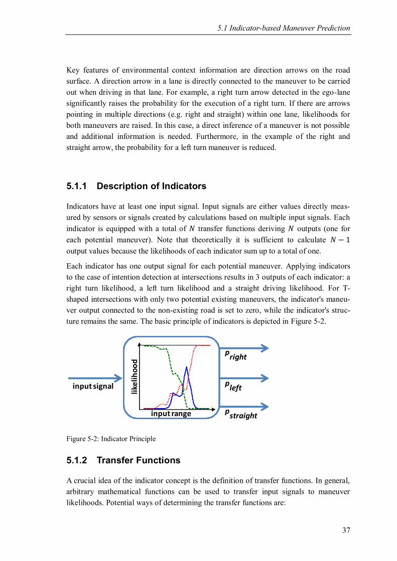
5.1 Indicator-based Maneuver Prediction
37
Key features of environmental context information are direction arrows on the road
surface. A direction arrow in a lane is directly connected to the maneuver to be carried
out when driving in that lane. For example, a right turn arrow detected in the ego-lane
significantly raises the probability for the execution of a right turn. If there are arrows
pointing in multiple directions (e.g. right and straight) within one lane, likelihoods for
both maneuvers are raised. In this case, a direct inference of a maneuver is not possible
and additional information is needed. Furthermore, in the example of the right and
straight arrow, the probability for a left turn maneuver is reduced.
5.1.1 Description of Indicators
Indicators have at least one input signal. Input signals are either values directly meas-
ured by sensors or signals created by calculations based on multiple input signals. Each
indicator is equipped with a total of transfer functions deriving outputs (one for
each potential maneuver). Note that theoretically it is sufficient to calculate
output values because the likelihoods of each indicator sum up to a total of one.
Each indicator has one output signal for each potential maneuver. Applying indicators
to the case of intention detection at intersections results in 3 outputs of each indicator: a
right turn likelihood, a left turn likelihood and a straight driving likelihood. For T-
shaped intersections with only two potential existing maneuvers, the indicator's maneu-
ver output connected to the non-existing road is set to zero, while the indicator's struc-
ture remains the same. The basic principle of indicators is depicted in Figure 5-2.
Figure 5-2: Indicator Principle
5.1.2 Transfer Functions
A crucial idea of the indicator concept is the definition of transfer functions. In general,
arbitrary mathematical functions can be used to transfer input signals to maneuver
likelihoods. Potential ways of determining the transfer functions are:
input signal
pright
pleft
pstraight
like
lih
oo
d
input range

5 Maneuver Prediction
38
Defining transfer functions based on expert knowledge
Using a priori information
Determining transfer functions by training data
When expert knowledge is used to create the transfer functions, this knowledge has to
be modeled mathematically. An example is given in the following: A general rule used
as expert knowledge here is that drivers perform a shoulder check before executing a
turn maneuver. When a shoulder check is detected by sensor systems, a turn maneuver
is assumed to start shortly. Thus, a transfer function is defined with denoting
a shoulder check to the right and to the left. The maneuver likelihoods
correspond to the maneuver options right turn, left turn and straight driving.
Values for the parameter are defined by expert knowledge as well. The likelihood
vector is given by:
(5-1)
Note that this example only demonstrates the process of modeling transfer functions
based on expert knowledge in general. The choice of the parameter is arbitrary and
the prediction results achieved with this transfer function depend on the parameter.
Using a priori information for generating transfer functions follows the same approach.
A priori information is any kind of information that is available prior to an intersection
approach. For example, a priori information is provided by the vehicle's navigation
system. Under the assumption the driver follows to the routing instructions of the navi-
gation system, a likelihood vector depending on driving instructions is used as a
transfer function analogous to (5-1):
(5-2)
Again, the selection of the parameter is arbitrary and directly effects the likelihoods
generated by the indicator. To avoid having to select parameters arbitrarily, another
method of generating transfer functions is applied in this work: Transfer functions are
created by using training data acquired in test drives. Using training data, discretized
transfer functions are generated automatically and no arbitrary parameter selection is
needed. The process of generating transfer functions by training data is described in
detail in the following.

5.1 Indicator-based Maneuver Prediction
39
5.1.3 Training Data
The generation of transfer functions by training data depends on the type of input signal.
A survey of using different types of signals is given below.
Discrete transfer functions
In the first step, the range of the input is determined and discretized in a number of
bins, referred to as intervals in the following. Afterwards, a training dataset contain-
ing intersection approaches for each potential maneuver is analyzed. The absolute fre-
quency of each interval in training data is checked for each maneuver. The result of this
step is histograms for every potential maneuver with bins. Following the basics of
the Maximum-Likelihood calculation,127
relative frequencies (in percentage) are gener-
ated for each interval. An exemplary calculation of the transfer function for longitudinal
acceleration is given in the following:
The sensor's measurement range is . Thus, the intervals are defined
within a range of
. The signal’s range is discretized in
equally spaced intervals. Table 5-1 shows an extraction of the number of occurrences of
intervals separated by maneuver created using training data.
Table 5-1: Frequency in training data
acceleration
in
m/s²
maneuver ... ...
right
13 1436 1091
left
11 1197 1636
straight
0 25 1548
In the example of Table 5-1, accelerations
occurred 1436 times
in training data for right turns, while values within this interval occurred 1197 times for
left turns and 25 times for straight driving. Table 5-2 shows the relative frequencies for
each interval that represents the transfer function. E.g., for interval -3
< a ≤ -1
, the
total amount of training entries is:
. (5-3)
127 Blobel, V.; Lohrmann, E.: Datenanalyse (1998), pp. 183–200.

5 Maneuver Prediction
40
The corresponding relative frequencies are:
(5-4)
Table 5-2: Relative Frequencies
acceleration
in
m/s²
maneuver ... ...
right
0.54 0.54 0.26
left
0.46 0.45 0.38
straight
0.00 0.01 0.36
Continuous transfer functions
Instead of using discretized transfer functions relying on bins, continuous transfer func-
tions can be used. Continuous transfer functions are derived from the empirical cumula-
tive density function (eCDF) of training data that is fitted with a predefined function.
Typically, fitting functions are either based on polynomials or splines. Because the
quality of using a polynomial fit varies with the shape of the eCDF curve, polynomial
fits can lead to non-negligible fitting errors. For example, using a cubic spline interpola-
tion results in an interpolation of the eCDF curve based on splines using all
values provided in the training data as breakpoints.128
Because all data elements of the
eCDF are used as knots of the cubic splines, the eCDF is represented without fitting
errors. However, due to using cubic splines, the derivation of the spline is very
noisy. To avoid this issue, a spline interpolation based on least-squares approximation
can be used. This approximation computes an approximating spline consisting of a pre-
defined number of splines and is not error-free. In the example below, 4 splines are used
to interpolate the eCDF. The advantage of the least-squares approximation is that the
first derivation of the spline is a smooth curve. The slope of the eCDF represents the
density of values in the input signal. Using density functions according to poten-
tial maneuvers describes the relation between potential maneuvers. This relation be-
tween the density measures is used to create the indicator's output by calculating relative
percentages of the density values. An example is given in the following to clarify the
calculation principle.
128 Note that cubic spline interpolation is only selected here as an example and other methods are applica-
ble as well.

5.1 Indicator-based Maneuver Prediction
41
Figure 5-3 shows the eCDF of the ego-vehicle's speed values for a selected maneuver
and the cubic spline interpolation using cubic splines. As discussed above, the
first derivation shows a lot of noise.
Figure 5-3: Cubic spline interpolation using splines
In contrast, Figure 5-4 shows the least-squares approximation of the same data using
four cubic splines and the corresponding derivations. The breakpoints determined in the
approximation are marked by vertical grey lines.
Figure 5-4: Cubic spline approximation using 4 cubic splines
0
0.5
1
cu
mu
lati
ve d
istr
ibu
tio
n
Cubic Spline Interpolation
0 5 10 15 20 25 30 35 40 45 500
0.1
0.2
ego-vehicle's speed in km/h
1st
deri
vate
0
0.5
1
cu
mu
lati
ve d
istr
ibu
tio
n
Least Square Approximation
0 5 10 15 20 25 30 35 40 45 50
0
0.02
0.04
0.06
ego-vehicle's speed in km/h
1st
deri
vate

5 Maneuver Prediction
42
Following this approach, Figure 5-5 shows the resulting continuous density functions
based on four cubic splines for all three potential maneuvers. The density values are
used to calculate the maneuver likelihoods analogue to the discretized transfer func-
tions.
Figure 5-5: Density functions
Comparison of discrete and continuous transfer functions
At first glance, it seems beneficial to use continuous transfer functions generated by
fitting training data with predefined functions. The advantage of continuous functions is
that the functions are derived analytically and therefore are free of quantization errors.
However, the disadvantage of this method is that this procedure creates fitting errors
between the training data and the fitting function. Fitting errors are likely to influence
the transfer function, especially at peripheral areas of the input signal with sparse occu-
pancy. The result acquired with this method is dependent on the number of breakpoints
and order of the splines used. Furthermore, using discrete values enables the identifica-
tion of sparsely occupied areas. When sparse areas are identified, special considerations
are needed with respect to the reduced reliability of these areas. Identifying sparse areas
is not possible when using continuous functions.
Discrete states on ordinal or nominal scale
Calculating transfer functions for binary inputs using training data is similar to the
process of creating discrete transfer functions for continuous and discrete inputs. The
only difference is that for binary signals no discretization of the input is needed. When
zero values correspond to the state "no detection", the amount of non-zero entries in
training data can be counted directly for each maneuver.
0 10 20 30 40 50 600
0.01
0.02
0.03
0.04
0.05
0.06
ego-vehicle's speed in km/h
den
sit
y
Density Approximation
right turns
left turns
straights

5.2 Influence of Distance to Intersection
43
Conditions and pattern matching
Adopting the principle idea of integrating expert knowledge as described above, condi-
tions are formulated that the input signal has to fulfill. Here, the number of matched
conditions in the training data is determined for each maneuver. The calculation of
transfer functions is done analogously by determining relative percentages for each
maneuver with fulfilled conditions. This allows for the integration of any kind of condi-
tion that is described mathematically. So, the main challenge here is to model expected
driver behavior and behavior patterns. For example, an indicator relying on this princi-
ple is the predicted stop distance indicator described in section 5.4.4. Here, the expected
behavior is that drivers will slow down from normal cruising speed to a comfortable
turning speed. This behavior pattern is modeled by extrapolating the ego-vehicle's mo-
tion state. The condition is formulated that a stop of the ego-vehicle is predicted at a
distance of from the intersection center. This condition is applied to the training
data and the frequency of the occurrence of predicted stops is determined for turn ma-
neuvers and for straight drives.
5.2 Influence of Distance to Intersection
A typical intersection approach for a turn maneuver is shown in Figure 5-6. The figure
shows that the driver slows down from regular cruising speed when approaching the
intersection. Thus, to evaluate the vehicle's speed, the relative position of the ego-
vehicle to the intersection needs to be considered for maneuver prediction.
Figure 5-6: Exemplary intersection approach
010203040506010
20
30
40
distance to intersection in m
sp
eed
in
km
/h
Intersection Approach
-400
-200
0
200
ste
eri
ng
wh
eel an
gle
in
°
speed
steering wheel angle

5 Maneuver Prediction
44
The same applies to the driver's behavior and driving inputs as well as all further data
based on driving physics. All information that is not distance-invariant has to be evalu-
ated in relation to the vehicle's position.129
In general, this can either be done by evaluat-
ing the distance remaining between the vehicle and the next intersection or the estimat-
ed time to intersection . Predicting an estimated time until the ego-vehicle reaches the
intersection is done by extrapolating the vehicle's motion state. Here, the vehicle's speed
and longitudinal acceleration as well as the actual distance between the vehicle and the
intersection is needed for the calculation. Furthermore, an assumption has to be made
for the vehicle's future motion state. For example, assuming constant acceleration is a
common method of motion prediction.130
The disadvantage of using is that the pre-
diction becomes less accurate with increasing distance. Aside from inaccuracies in the
estimation of distance to the intersection, the driver's approach behavior for the maneu-
ver planned by the driver influences the prediction quality. These disadvantages are
avoided by using the distance remaining between the ego-vehicle and the next intersec-
tion to classify driver's behavior during the phases of intersection approach. The dis-
tance is determined using a digital map as described in section 4.2.2.
For training purposes, sections of the test drives have to be defined as intersection ap-
proach training data. These sections are referred to as intersection specific "relevant
areas" in the following. The relevant areas for intersection approach start at a distance
to the intersection on the road the ego-vehicle is approaching the intersection and
end at the intersection center defined by the digital map. The distance is determined
following basic motion equations. The distance needed to stop is given by:
(5-5)
Assuming a constant comfortable acceleration of
and a starting velocity
of
leads to a stopping distance of . Considering that braking
to standstill is not necessary, this lowers to . Assuming drivers don't apply
constant deceleration while braking and that turn maneuvers may be started before
reaching the intersection center raises the value of to . With respect to
these effects, the length of the relevant area is set to . With defined limits of
the relevant area, the concept of distance intervals is introduced:
The relevant area is divided into equally spaced intervals, referred to as "distance
intervals" ( ) afterwards. The number of distance intervals used can be varied. Higher
129 Distance-invariant signals are information that do not change within an intersection approach at all.
For example, the number of potential driving directions at an intersection is distance-invariant.
130 Hermes, C. et al.: Long-term vehicle motion prediction (2009), pp. 656–657.

5.3 Free Driving Conditions
45
number of intervals results in lower amount of training data within each distance inter-
val. A total of distance intervals is the minimum value offering benefits as
opposed to completely disregarding the ego-vehicle's distance to the intersection. For
the prototypic implementation done in this work, the length of each distance interval is
set to 10 m. The resulting distance intervals are shown in Figure 5-7. Using distance
intervals, indicators are set up with respect to the remaining distance to the next inter-
section. Indicator’s transfer functions are calculated times, each time only using
training data from the corresponding distance interval. The concept of distance intervals
is applied to all indicators that are distance dependent.
Figure 5-7: Distance intervals
5.3 Free Driving Conditions
Among the indicators used for maneuver prediction described in section 5.4, there are
indicators that are only relevant in free driving conditions. These indicators are called
free-driving-dependent hereafter. ’’Free driving’’ signifies that the driver's choice of
speed is only dependent on the maneuver planned by the driver and the speed limit.
Using information from the ego-vehicle's speed and acceleration as well as all driver
inputs that effect the ego-vehicle's speed is only beneficial for maneuver prediction if
the driver's behavior is not influenced by external conditions. External conditions here
are priority regulations that require the driver to stop or slow down. This includes time-
invariant traffic regulations like stop and give-way regulations as well as traffic lights
demanding the driver to stop at red lights. Information about the actual state of traffic
lights are either acquired in video format by a front camera131
or by V2X communica-
tion devices if a traffic light sends out its state information.132
Furthermore, other traffic
131 Chiang, C.-C. et al.: Detecting and recognizing traffic lights (2011), pp. 6919–6934.
132 Fuchs, H. et al.: Vehicle-2-X (2016), p.674.
5 Maneuver Prediction
46
participants may represent external conditions forcing the driver to adapt his speed
when following a leading vehicle or approaching a stopped vehicle. While following
another vehicle, the driver has to follow the speed profile of the leading vehicle in order
to avoid collisions and to maintain a safe distance. In general, positions and motions of
other traffic objects in the driving corridor of the ego-vehicle are acquired by environ-
ment perception sensors like radar, lidar, camera, or received via V2X, as well. In this
work, radar sensors are used for the detection of other vehicles in the driving corridor
because of their ability to directly measure an object's distance and relative velocity.
There are many car-following models known in literature, with most of them originating
from the area of traffic flow simulation with varying complexity and calculation de-
mands. Famous models are the Newell's car-following model,133
Gipps' model134
and
the Intelligent Driver Model (IDM).135
For example, the IDM calculates an acceleration
demand due to following conditions and compares this acceleration demand to the
actual acceleration. The main challenge in using a model is finding parameters for
fitting the models to measurement data. Here, a simplified model is selected based on
driving physics. To decide whether speed dependent indicators should be activated or
not, the only relevant information needed is if the driver is following another vehicle or
not. Thus, only binary information is needed without a calculation of speed or accelera-
tion demand.
The model applied here is based on distances of objects detected by the front radar
sensors , their relative velocities , and the ego-vehicle's speed . The
following values are calculated for each relevant object detected by the sensors:
time gap for steady following without relative speed between the vehicles:
time to collision for approaching a slower leading vehicle:
time an object is tracked by the radar sensors:
Objects detected by the radar sensors are considered relevant if they are detected within
a range in the longitudinal direction of the ego-vehicle's path and a lateral
range to the ego-vehicle's path as shown in Figure 5-8. The path is estimated using
133 Newell, G. F.: A simplified car-following theory (2002).
134 Gipps, P. G.: Car-following model (1981), pp. 105–111.
135 Treiber, M.; Kesting, A.: Elementary Car-Following Models (2013), pp. 187–191.

5.3 Free Driving Conditions
47
a linear single-track model.136
All objects detected at distances or
are ignored in follow behavior calculations, as well as objects that are
only detected for a time span . This is done due to the increasing inaccuracy
of path prediction by the single track model for increasing distances.
Figure 5-8: Relevant objects of environment perception sensors
In the intention detection system, vehicle follow behavior is activated if at least one of
the following conditions is fulfilled within a discrete calculation step:
ego-vehicle has stopped ( behind a standing object (stationary or lead-
ing vehicle detected braking to standstill)
start up after standstill with
Values for the limits used above are found applying a two-step procedure:
In the first step, values of are determined by analyzing measurement
data from real test drives. Ground truth for existence of relevant objects in the predicted
path is determined by analyzing video data recorded with measurement data. Iteratively
varying and leads to a selection of values that offers the best compromise
between true positives and false negatives. For determination of and , a test
group of five people was asked to classify and label vehicle following behavior by
watching recorded video scenes from pre-tests. Time gaps and time to collision for
relevant objects are calculated for the scenes using the objects detected by the vehicle's
radar sensors. Based on scenes classified as vehicle following behavior by the test
group, values for and are determined. To ignore outliers, the smallest and
largest 5% of the values in the distribution of follow behavior are ignored. The value of
is determined by analyzing the ego-vehicle's speed at the time the driver initializes
136 Schramm, D. et al.: Vehicle dynamics (2014), pp. 223–226.

5 Maneuver Prediction
48
a turn after having stopped during the intersection approach. Figure 5-9 shows the share
of speeds in the test drives when a maneuver is initialized after starting from standstill.
Here, a value of
, corresponding to 95 % of all events, is selected for the
range where follow dependent indicators are ignored after stopping within an intersec-
tion approach. Note that turn initialization is determined according to section 6.3.2 and
can therefore be at
as well.
Figure 5-9: CDF of vehicle's speed initializing a turn maneuver
When vehicle following behavior, red traffic lights, or starting after stopping is detected,
the free driving dependent indicators are not used in the inference system and the ma-
neuver prediction is done solely with the remaining free driving independent indicators.
5.4 Indicators of the Prediction System
Based on the classification of information presented in section 2, the following section
presents indicators that rely on the information and have been analyzed for their predic-
tion capability. Indicators introduced in the following are grouped depending on their
type of input data. Indicators of the first group described in section 5.4.1 are set up
directly using measurement data acquired from driving dynamics and control inputs as
described in section 5.1.3. The second group contains indicators that describe the driv-
er's behavior within the vehicle. Indicators introduced here are based on the driver's
head pose and gaze tracking. Indicators of the third group, using information from
environment perception systems during intersection approach, are described in sec-
tion 5.4.3. The fourth group introduced in section 5.4.4 contains indicators that evaluate
the driver's approach behavior at an intersection and consist of information calculated
0 5 10 15 20 25 30 35 400
0.2
0.4
0.6
0.8
1
ego-vehicle's speed at turn maneuver initialization after stopping in km/h
cu
mu
lati
ve d
istr
ibu
tio
n
eCDF of Speed at Maneuver Initialization

5.4 Indicators of the Prediction System
49
from the vehicle's motion in relation to the intersection. The difference to the first group
is that data used here does not need to have physical counterparts and is not provided
directly by the vehicle's sensor systems. Finally, the last group described in section 5.4.5
contains indicators based on general intersection information.
5.4.1 Driving Dynamics and Driver's Control Inputs
Indicators of this group are set up by analyzing the number of occurrences of the corre-
sponding values for each maneuver. All indicators related to the vehicle's speed are only
considered while the vehicle is in free driving conditions.
Ego-vehicle's Speed Indicator
The ego-vehicle's speed curve is directly connected to the maneuver to be exe-
cuted under the following conditions: The ego-vehicle is in free driving and the
intersection's priority regulations do not demand the vehicle slow down for any
maneuver. Under these conditions, if the vehicle approaches an intersection with
regular urban cruising speed (40 - 50 km/h) and slows down, this behavior is di-
rectly connected to a turn maneuver as shown by measurement data in Figure
5-10. Thus, the ego-vehicle's speed is analyzed directly in an indicator.
Figure 5-10: Speed profiles in free driving conditions
Longitudinal Acceleration Indicator
Analogous to the ego-vehicle's speed, the vehicle's longitudinal acceleration is
analyzed in a separate indicator. Although both values are related to each other,
the acceleration indicator is set up for means of performance comparison with
the speed indicator.
012340
10
20
30
40
50
time to reference point in s
eg
o-v
eh
icle
's s
peed
in
km
/h
turn maneuvers
012340
5
10
15
20
25
30
35
40
45
50
time to reference point in s
eg
o-v
eh
icle
's s
peed
in
km
/h
straight driving

5 Maneuver Prediction
50
Accelerator and Brake Pedal Operation
The control inputs to modify the vehicle's speed are mainly given by the acceler-
ator and brake pedal. Thus, both operations are analyzed in separate indicators.
Current Gear
For vehicles equipped with a manual transmission, the current gear selected by
the driver is analyzed in an indicator under free driving conditions.
5.4.2 Driver's Behavior in Vehicle
This group consists of indicators describing the driver's behavior and motions within the
vehicle's cockpit. Here, data acquired via the head and gaze tracking system mounted
inside the test vehicle is used to set up indicators. The frequency of occurrences is ana-
lyzed for each maneuver in the same way used to set up all other indicators.
Head and Gaze Rotation Angle
Several approaches to using the driver's viewing behavior during intersection
approach can be found in the literature.137
The same applies to the driver's head
rotations in preparation for maneuver initialization.138
Thus, the driver's gaze ro-
tations and head rotations are analyzed in separate indicators. This is done with
respect to the vehicle's motion state. While the gaze direction and head rotation
are supposed to be related to the driver's intentions while the vehicle is moving,
this assumption cannot be maintained during standstill. Here, driver's attention
might be occupied by arbitrary objects outside or inside the vehicle unrelated to
the driving task.
Fixed Objects in the Vehicle's Cockpit
A virtual model of the vehicle's cockpit is set up containing positions of selected
elements of the real vehicle's cockpit. Among others, the vehicle's side and cen-
ter rear-view mirrors are of interest for maneuver prediction. The frequency of
driver's mirror fixations is analyzed in the underlying indicator.
Patterns in Head and Gaze Motion
Aside from direct analysis of the input signal in each discrete calculation step,
the indicator concept also allows for the recognition of patterns in input signals
(e.g. repeated changes from left to right).
137 A recent survey is given in: Liebner, M.; Klanner, F.: Driver Intent Inference and Risk Assessment
(2016), pp. 891–915.
138 Land, M. F.: Predictable eye-head coordination (1992), pp. 318–320.

5.4 Indicators of the Prediction System
51
5.4.3 Environment Perception
Indicators of this group use data from sensor systems for perceiving the surroundings
outside the ego-vehicle. In principal, this can be any kind of sensor such as radar, cam-
era, lidar, etc. The prototypic implementation done here is based on environment per-
ception by radar and camera sensors.
Direction Arrows on Road Surface
All direction arrow indicators are set up in the same way. The indicators only
differ in the type of direction arrow detected and the position of the arrows in re-
lation to the ego-vehicle. Direction arrows on the road surface dictate the ma-
neuver that is allowed while driving in the current lane. Theoretically, the likeli-
hood of the maneuver related to the detected direction arrow can be assumed to
be one, while all likelihoods of alternative maneuvers are set to zero. This ap-
proach is not applicable in real driving due to several reasons:
Information from detected direction arrows is saved until another arrow is de-
tected or the intersection is traversed. Using the save functionality, lane changes
of the ego-vehicle may lead to false maneuver likelihoods if the lane changes are
not detected.139
Furthermore, deriving the predicted maneuver directly from the
direction arrow implies an ideal perception. Considering real driving conditions,
direction arrows that are partly damaged or worn-out exist, which lead to false
detections. Further reasons for imperfect detections are road works with changed
traffic routing or arrows not visible due to other traffic participants as shown in
Figure 5-11. Here, the straight arrow on the right lane is hardly noticeable due to
other traffic participants obstructing the view.
Figure 5-11: Example of imperfect environment perception
139 See Annex D for more details.

5 Maneuver Prediction
52
The calculation of likelihoods is done by calculating relative frequencies for
each arrow in each lane according to section 5.1.3. For lanes adjacent to the ego-
lane, some boundaries arise: Arrows indicating the driving direction of an adja-
cent lane limit potential maneuvers for vehicles in the ego-lane: Multiple lanes
have to be collision free. This means, that no maneuver from any lane may lead
to crossing an adjacent lane heading in the same direction. An exception from
this rule is only applied in the case of hook turns.140
Existence and Traffic Directions of Adjacent Lanes
Information from the existence of additional lanes next to the ego-lane are used
to limit the ego-vehicle's potential maneuvers. Following the principle of colli-
sion free lanes, a detected adjacent lane to the ego-vehicle precludes a turn ma-
neuver on the side the lane is detected.141
Thus, the information needed here is
the existence of adjacent lanes to the left and right and their traffic directions.
While in right hand traffic adjacent lanes to the right are required to have the
same traffic direction as the ego-lane, an adjacent lane to the left can either be
heading the same direction or oncoming. This information can either be acquired
via V2X communication or environment perception sensors. Here, an implemen-
tation based on radar sensors is applied. To determine the traffic direction of
other traffic participants (same direction or oncoming), their relative velocities
and the ego-vehicle's speed are needed. In general, radar sensors perform well in
measuring relative speeds of detected objects using the Doppler effect.142
In ad-
dition, the implementation based on radar sensors is independent of influences
of weather and illumination. The radar based approach also detects static objects
and uses them to calculate the likelihood that an adjacent lane is nonexistent.
The functional principle of the radar based lane detection model is given in an-
nex B. If a lane with oncoming traffic to the left of the vehicle is detected, the
lane is not accessible for the ego-vehicle and no information for maneuver pre-
diction is acquired. The calculation of transfer functions is done accordingly
with the other indicators described above by statistical evaluation of the training
data.
Maneuver Detection of Leading Vehicle
The indicator is based on detecting the maneuver a preceding object is per-
forming. This can be either done by V2V communication or by environment
140 Currie, G.; Reynolds, J.: Hook Turns (2011), pp. 10–19.
141 Note that this is only valid for roads with no more than one turning lane for each direction. However,
intersections with multiple lanes turning the same direction can be identified via digital map data. If
the ego-vehicle approaches such an intersection, the indicator introduced here is not applied.
142 Winner, H.: Automotive RADAR (2016), pp. 332–333.

5.4 Indicators of the Prediction System
53
perception systems. The assumption used in this indicator is that the ego-vehicle
will perform the same maneuver as the leading vehicle. Figure 5-12 shows the
basic principle of the indicator.
Figure 5-12: Angle of leading vehicle
This assumption is only valid in cases where intersections are equipped with
separate lanes for each maneuver. For example, this information could be pro-
vided by localization on a digital map. The implementation selected here is
based on tracking other traffic participants detected by the ego-vehicle's radar
sensors. The leading vehicle in the ego-vehicle's lane is distinguished from all
detected objects. The path the leading vehicle takes is analyzed during intersec-
tion approach. The relative angle between the ego-vehicle's heading and the
leading vehicle's heading is evaluated. If a deviation between both
headings is determined for a minimum time span , the lead vehicle is consid-
ered to be turning. By definition, this indicator is only applicable if a leading ve-
hicle is present. Although separate direction lanes are marked with direction ar-
rows in most cases, this indicator raises the prediction performance if direction
arrows on the road surface have not been detected.
5.4.4 Intersection Approach Behavior
The vehicle's speed curve in correlation with the distance remaining to the intersection
is used to calculate further values of the driver's intersection approach behavior. Indica-
tors of this type are only applied to intersection classes without demands to slow down
for any maneuver. Some of the indicators introduced here rely on a predicted lateral
acceleration when turning. Thus, a maximum radius for a potential turn maneuver at
the intersection is estimated. The radius is determined using a a circle with radius and
tangential transitions between straight parts and the circle as shown in Figure 5-13. The
distance between the ego-vehicle and the intersection's center as well as the angle
between the roads are extracted from the digital map and the localization of the ego-

5 Maneuver Prediction
54
vehicle. The line between the circle's center and the intersection center is the bisector of
the angle between the two roads. Basic geometry results in:
(5-6)
(5-7)
Figure 5-13: Radius estimation
Thus, the max. radius of a turn the ego-vehicle can perform from its current position
is given by:
(5-8)
In cases of intersections allowing turn maneuvers to either the left or the right, radii for
both options are calculated and evaluated independently.
Using , the predicted lateral acceleration for potential turn maneuver is given by:
(5-9)
The acceleration is compared to maximum lateral accelerations tolerated by
drivers in urban turn maneuvers. Data from the test study of this work shows that
for right turns and
is not exceed in 95 % of all turns
in test drives. The share of predicted accelerations on priority roads is given in
Figure 5-14. Here, each curve shows for all intersection approaches of the same
maneuver (right/left/straight) one second prior to initialization. The figure also shows
as dash-dotted vertical lines.

5.4 Indicators of the Prediction System
55
Figure 5-14: Share of predicted lateral acceleration
Figure 5-14 shows that exceeds in 26.7 % of all right turns as well as in
23.7 % of all left turns. This is caused by two effects: is dependent on the localization
and map accuracy. Furthermore, is calculated using a circle for ego-vehicle's turning
trajectory. Analyzing real trajectories shows that driver's turn trajectories aren't circles
with constant radius. For example, turning can be modeled as a phase of constant curva-
ture and a transition phase at the beginning and the end.143
In addition, analyzing data
from test drives shows that in 96.6 % of all recorded right turns, drivers enter the transi-
tion phase at higher speeds compared to the speed at the turns' apex.
Estimated Lateral Acceleration for Turn Maneuvers
Figure 5-14 shows that the majority of straight drives (> 94 %) result in estimat-
ed lateral accelerations one second before a maneuver is ini-
tialized. Thus, the predicted acceleration is beneficial for discriminating
straight driving from turn maneuvers. The indicator's transfer function is calcu-
lated by statistical evaluation of discretized values of using intervals as
described above.
143 Alhayaseen, W. et al.: Variation of Left-turning Vehicle (2011), p.1550.
0 2 4 6 8 10 120
0.2
0.4
0.6
0.8
1
predicted lateral acceleration in m/s2
cu
mu
lati
ve d
istr
ibu
tio
n
eCDF of Predicted Accelerations
right turns
left turns
straights
ay,max

5 Maneuver Prediction
56
Braking to Maintain Maximum Lateral Acceleration
Based on , the necessary speed reduction for comfortable turning speeds is
calculated. If , the potential speed reduction needed for
turning with is calculated by:
(5-10)
(5-11)
The amount is evaluated statistically by discretizing to a number
of predefined intervals covering the range of for all potential maneu-
vers.
Predicted Stop Distance
An alternative method that does not use an estimated radius of potential turn
maneuvers is based on predicting a (theoretical) stop near the intersection center.
Extrapolating the ego-vehicle's actual speed and acceleration under the
assumption of constant acceleration in longitudinal direction, the distance need-
ed for braking to stop is given by:
(5-12)
Due to the relevant area at the intersection (see section 5.2), is limited to
. Using the remaining current distance to the intersection
center, the predicted stopping distance in relation to the intersection center
is calculated:
(5-13)
Figure 5-15 shows an exemplary calculation of based on measurement data
of an approach sequence with a consecutive right turn maneuver.
A stop of the ego-vehicle near the intersection center is predicted if
is detected for a minimum time during the intersection approach. The deriva-
tion resulting from Figure 5-15 is shown in Figure 5-16.

5.4 Indicators of the Prediction System
57
Figure 5-15: Exemplary predicted stopping distance
Figure 5-16: of exemplary approach
Note that this does not mean that the vehicle will come to a stop in reality. Fig-
ure 5-17 summarizes the predicted stops calculated for priority roads. The figure
shows that numerous stops are predicted during the intersection approach for
right and left turn maneuvers. Note that in accordance with the definition of
, values correspond to predicted stops of the ego-vehicle before
the intersection center and vice versa. While this indicator is not capable of dis-
criminating right and left turn maneuvers, it performs well in separating turn
0 5 10 15 20 25 30 35-25
-20
-15
-10
-5
0
5
10
15
20
25Distance Prediction
discrete calculation steps
pre
dic
ted
sto
p d
ista
nce in
m
0 5 10 15 20 25 30 35-15
-10
-5
0
5
10
15
201st Derivate of Distance Prediction
discrete calculation steps
devia
tio
n o
f p
red
icte
d s
top
dis
tan
ce

5 Maneuver Prediction
58
maneuvers from straight drives. Aside from few outliers, no stops are predicted
for straight driving maneuvers within the range of ±30 m. Reviewing the straight
driving maneuvers resulting in the outliers shows that two of the outliers are
generated due to failed detection of vehicle follow conditions. The third outlier
was generated by the driver's behavior in free driving conditions. The test sub-
ject did not correctly interpret the priority regulation and slowed down to give
way to a vehicle from the right, even though the ego-vehicle was driving on a
priority road.
Figure 5-17: Predicted stopping distance
Using test drive data, the occurrence of predicted stops near the intersection cen-
ter is summed up for each turn maneuver and straight driving.
These sums are used to calculate the indicator's transfer functions.
The benefit of this indicator is its availability in an early phase of the intersec-
tion approach. Figure 5-18 shows the share of distances where a stop is predicted
during intersection approach sequences. The plotted line shows that less than
10 % of all predicted stops are detected at distances to the intersection
center.
0102030405060-30
-20
-10
0
10
20
30
40
distance to intersection at 1st prediction of stop in m
pre
dic
ted
sto
p d
ista
nce in
m
Share of Predicted Distances
right turn
left turn
straight

5.4 Indicators of the Prediction System
59
Figure 5-18: eCDF of predicted stopping distance
Lane Change Maneuver (Ego-Vehicle)
At intersections with multiple lanes heading towards the intersection, lane
change maneuvers performed during intersection approach might be related to
the maneuver intended by the driver, but don't have to be. On the one hand, lane
change maneuvers are done to get into dedicated lanes for a maneuver intended
by driver. In this case, the information is beneficial for maneuver prediction. On
the other hand, lane change maneuvers are executed in preparation for maneu-
vers pending at the intersection after the current one, or just due to traffic condi-
tions. Thus, aside from the challenge of detecting lane change maneuvers in ur-
ban conditions, a lane change maneuver cannot be used for reliable maneuver
prediction at the intersection.
5.4.5 General Information
Road Existence
The road existence indicator is based on the number of potential traffic direc-
tions at the intersection the ego-vehicle is heading to. During intersection ap-
proach, the upcoming intersection is checked for the existence of roads for each
potential maneuver (right or left turn or straight driving) and turning restrictions.
If a road corresponding to a potential maneuver is found at the intersection, the
legality of the maneuver is checked. If the related maneuver is allowed for vehi-
cles on the road the ego-vehicle is using (no entering a one-way road from the
wrong direction, no turn restrictions), the potential maneuver is considered as
valid. Taking a number of valid potential maneuvers into account, the road
0 10 20 30 40 50 600
0.2
0.4
0.6
0.8
1
distance to intersection at first detection in m
cu
mu
lati
ve d
istr
ibu
tio
n
Distance to Intersection at Stop Detection

5 Maneuver Prediction
60
existence indicator is set to
for each valid maneuver. For the intersec-
tions considered in this work, is within the range of one and three. Although it
is not possible to predict the maneuver to be executed if more than one maneu-
ver is valid, the overall likelihood of non-valid maneuvers can be reduced by set-
ting to zero for these maneuvers or excluding the maneuver options com-
pletely. In cases of valid potential maneuvers, the road existence indicator
does not affect the overall prediction performance.
Priority Regulation
Indicators' transfer functions are swapped depending on the priority regulation
of the intersection the vehicle is heading to, as described in section 4.4.2. Thus,
the priority regulation is not an indicator itself, but is used to select the transfer
functions corresponding to the actual priority regulation. Furthermore, depend-
ing on the priority regulation, indicators are enabled or disabled if they do not
hold information for the prediction of the pending maneuver. For example, for
priority regulations demanding the driver to slow down or stop for any maneu-
ver, all speed-related indicators are ignored.
5.5 Indicator Quality Assessment
In order to decide which indicator is beneficial for each intersection class, a method for
assessing the indicators' quality is needed. General requirements for an indicator quality
measure are:
true positive detection rate
quality of discrimination among alternatives (sensitivity)
availability of indicator
All factors have to be considered for assessing an indicator and selecting indicators to
be used for maneuver prediction. The indicator assessment is done independently for
each intersection class allowing for the selection of indicators according to their quality.
5.5.1 Indicator Quality Measure
Following the basics of likelihood calculations as introduced above, the indicators'
quality of discrimination among several alternatives is considered. If an indicator out-
puts likelihoods being nearly the same for all maneuvers, the sensitivity is near zero
(like in the left part of Figure 5-19). Otherwise, if an indicator outputs likelihoods that
are clearly different for alternative maneuver options, the sensitivity is high (close to
one) as shown in the right part of Figure 5-19. The sensitivity describes the "sharpness"

5.5 Indicator Quality Assessment
61
of the calculated maneuver likelihoods. Given that by the system's design and the meth-
od applied to calculate transfer functions, assessing the indicators' discrimination quality
automatically contains the indicators' true positive detection rates.
Figure 5-19: Sensitivity measure
The sensitivity measure evaluates the maneuver likelihoods in relation to a uniform
distribution of likelihoods. Uniform distribution is given for :
for maneuver options with
representing maneuver likelihoods based on
relative frequencies. Because maneuver likelihoods
lead to negative terms
squared differences are used instead, also known as geometric distances. Thus, the
sensitivity measure is defined as:
(5-14)
In case of potential maneuvers, the sensitivity measure is given by:
(5-15)
Transforming equation (5-15) using leads to a simplified form:
(5-16)
While in the given form returns in case of uniform distribution
, the
maximum value returned in cases of optimal separation for is
. Therefore, a linear transformation by the factor
is applied to , resulting in the quality measure :
p1
p2
p3
time t time t
likeli
ho
od
p
likeli
ho
od
p
legend

5 Maneuver Prediction
62
(5-17)
In the case maneuver options, is given by:
(5-18)
Note that returns a sensitivity value in the range that can be inter-
preted as percentage.
5.5.2 Sparsely Occupied Intervals
Using transfer functions to calculate maneuver likelihoods follows the basic assump-
tions that relative frequencies observed within one interval correspond to the real (but
unknown) share of data:
(5-19)
The assumption is not valid when an interval is sparsely occupied and has only few
entries for each potential maneuver. In extreme cases, an interval occupied with
returns a quality measure , but the information is useless
due to . Thus, sparsely occupied intervals need to be detected and treated in
a special way. The simplest way to detect barren intervals is to apply a limit that
the interval has to exceed: . Arbitrary values for can be used with-
out reasoning for the selection of .
A more sophisticated way introduced here is based on a trust in the sensitivity deter-
mined for each interval. The trust in the observed distribution is based on the sensitivity
of the quality measure to changes in the input values. The trust is calculated based on
a total of quality measures. In addition to based on the input
values , a total of modified values is calculated with either the -th
likelihood being replaced by:
(5-20)
Aside from the frequencies of the occurrence of , is used to modify to ana-
lyze the sensitivity of .

5.5 Indicator Quality Assessment
63
(5-21)
Based on the quality measures ( a mistrust value is
calculated by the differences of and , representing the gradient of the
sensitivity measure :
(5-22)
For the example of , returns a value of , representing the
highest possible distrust in the quality measure. Otherwise, intervals with ob-
servations result in Thus, the trust in the calculated sensitivity measure is
given by:
(5-23)
Finally, the trust is combined with the interval's quality measure by multiplication:
(5-24)
Only intervals with a high quality measure and sufficient number of observa-
tions result in a highly trusted quality measure . Thus, can be used to
assess the suitability of an indicators' interval for maneuver prediction.
The process of selecting indicators according to their quality is described in section 6.5.
Furthermore, the value is used for optimization of indicators as described in the
following section. Taking sparsely occupied intervals into account as demonstrated
above automatically contains an assessment of the indicators availability. Indicators
based on conditions only available at seldom occurring events result in sparsely occu-
pied intervals. Applying the quality measure of identifies these indicators as well.

5 Maneuver Prediction
64
5.6 Optimization of Indicators
The prediction performance of indicators with transfer functions created by the range of
input signals being discretized into bins depends on the selected value of . By the
system’s design with discrete bins, has to be a natural number. The range of potential
values of is given by:
(5-25)
Here, represents the range of the input signal and the resolution of the input
signal. Using
bins results in empty bins. Selecting is
obviously not suitable for maneuver prediction: With a total of one bin used for the
range of the input signal, transfer functions result in
for each of the potential
maneuvers. Thus, has to be selected. Using a high number of bins e g
results in sparse occupation of bins. The less samples are contained in each bin,
the higher the dependency on the training data is and the risk of overfitting increases.
The optimization is carried out as follows: is varied within the range
with the training data separated accordingly into intervals. The quality meas-
ure is calculated separately for each interval. To determine the quality of the varia-
tion of , a measure to assess the share of all is needed. Thus, an empirically
cumulated distribution function of all trusted quality measures of all training
entries is calculated. The quality of the variation is described by the arithmetic
mean of all :
(5-26)
An example is given in the following for demonstration purposes: For the speed indica-
tor introduced in section 5.4.1, input values are within
with
in urban conditions. The speed signal is recorded with a resolution of
. Potential values of to be analyzed in the optimization process are
within the range . The sensitivity calculation is carried out as described
above. Figure 5-20 shows the resulting for all variations of .

5.6 Optimization of Indicators
65
Figure 5-20: Quality Measures
The figure shows that in this example is the highest for and is identified as
best selection of in the optimization process. The effect of the optimization process
is demonstrated in Figure 5-21, comparing the eCDF of trusted quality measures for
bins and . The solid curve created with bins clearly shows
better performance than the dashed curve for bins.
Figure 5-21: Effect of interval optimization
The optimization procedure to find the best number of intervals as introduced above
has to be carried out independently for each of the distance intervals resulting in a
total of optimal values of for each indicator.
100
101
102
103
0.35
0.4
0.45
0.5
0.55
0.6
0.65
0.7
0.75
0.8Bin Optimization
number of bins used
avera
ge t
ruste
d q
uality
measu
re
0 0.2 0.4 0.6 0.8 10
0.2
0.4
0.6
0.8
1
quality measure
cu
mu
lati
ve d
istr
ibu
tio
n
Optimization Results
8 bins
500 bins

5 Maneuver Prediction
66
5.7 Accuracy of Input Signals
This work analyzes the maneuver prediction capability by using automotive series
sensor systems. Thus, the input signal inaccuracies and their effects on the maneuver
predictions are analyzed. A detailed survey including which inaccuracy affects the
calculation of which indicator is given in annex G. According to the calculations pro-
vided in the annex, neither inaccuracies in the steering wheel angle measurement, nor
inaccuracies in the determination of the vehicle's speed affect the indicator calculation.
Therefore, they are neglected here. The same applies to inaccuracies in the measurement
of the vehicle's lateral acceleration, yaw rate and driver's pedal operations. Analyzing
the accuracy of the head- and gaze tracking system shows that a maximum error of one
interval can occur due to measurement inaccuracies and the detection of fixated objects
on the vehicle's dashboard is not affected. None of the indicators based on radar sensors
detecting environmental objects is affected by the measurement inaccuracies of state of
the art radar sensors in any way. The precision the sensors offer in determining distance,
relative velocity, and azimuth measurement is sufficient for all calculations done here.
In contrast to data from sensors mentioned above, inaccuracies arising from the wrong
or missing detections of road markings (especially direction arrows) clearly have an
influence on the calculation of indicators and maneuver likelihoods. That is why imper-
fections in the perception of road markings are taken in account by using training data
created statistically instead of directly deriving the maneuver from the direction arrow
detected.144
The accuracy of the ego-vehicle's position determined by the GNSS receiver
does affect the calculation of indicators either directly (predicted stop distance, predict-
ed lateral accelerations, e.g.) or indirectly by the distance intervals. All indicators rely-
ing on the distance remaining to the intersection center and using multiple transfer
functions depending on the distance are affected by positioning errors. In the prototypic
implementation used here, a total accuracy of root mean square error
(RMSE) is determined.145
In reality, the road layout of urban intersections varies even
within one intersection class depending on the features of each location, available space
for the intersection, type of roads connected by the intersection, and amounts of traffic
using the road.146
Thus, a variety of intersection geometries exist even within one inter-
section class, resulting in different trajectories. Using the intersection center is an inac-
curacy in itself because the layout of the intersection is not considered. However, the
approach applied in this project deals with this inaccuracy by using training data ac-
quired from a large set of intersections with varying geometry.
144 See Section 5.4.3.
145 See Annex G.
146 Baier, R.: Richtlinien für die Anlage von Stadtstraßen (2007), p.109.

67
6 Evaluation
6.1 Inference Methods
The intention prediction system used here is set up by a total of independent indi-
cators. For means of maneuver prediction on guidance level with a maximum of three
potential maneuvers, each indicator generates three maneuver likelihoods. In case there
is more than one indicator used in the prediction system, an inference method is needed
to combine the results of the indicators. The inference method uses the
indicator output values as inputs and calculates three probabilities for maneuver predic-
tion: a probability for right turns, a probability for left turns, and a probability for
straight driving. For means of maneuver prediction, the maneuver with the highest
probability is selected as the most probable maneuver planned by the driver. Depending
on the inference method, limits are integrated in the prediction process. Only in
cases where the predicted maneuver has a probability that exceeds , is it considered
a valid maneuver prediction. In general, integrating the limits lowers false-positive
detection rates, but true-positive rates are likely to be lowered as well. In cases where
the maneuver with the highest probability does not exceed , no maneuver is pre-
dicted by the system. Several inference methods are analyzed for combining indicator
likelihoods into maneuver probabilities:
Average Calculation
Using the average function as an inference method is the simplest way of com-
bining the indicator likelihoods into probabilities. Here, the average function is
either applied to all right turn likelihoods , to all left turn likelihoods
, or all straight driving likelihoods . The average probability
for each maneuver is given by:
(6-1)
Likelihoods of non-applicable indicators due to the current intersection class or
non-available indicators due to missing input data are ignored by the average
function. The amount of non-available indicators is subtracted from
to avoid effects on the calculation of . Due to the computationally low com-
plexity, the average function is a fast and flexible inference method. Further-

6 Evaluation
68
more, the average probabilities are output within the range [0,1]. Thus, limits
can be directly integrated in the prediction process.
Product Calculation
The product approach is similar to the average calculation introduced above, but
relies on using the product function instead of the average function. Thus, the
compound probability for each maneuver is given by the product of all in-
dicator likelihoods for one maneuver:
(6-2)
Likelihoods of non-applicable indicators due to intersection classes or non-
available indicators are ignored here as well by correcting with .
Comparing the product function to the average function shows the following dif-
ferences: Using the product function as an inference method "penalizes" proba-
bilities containing small likelihood values (e.g. ). The computational
needs and flexibility in the number of indicators is similar to the average func-
tion. However, integrating limits in the overall maneuver prediction is not
directly possible. Although still is within the range [0,1], it varies widely
with the number of indicators used for the calculation. The more indicators
with likelihoods are used, the smaller gets. For example, apply-
ing the average function to indicators with always re-
sults in the overall likelihood of . In contrast, applying the product
function returns for , for and so
on. Thus, limits have to be defined and selected based on the number of ac-
tive indicators .
Instead of using an inference method and selecting the maximum probability provided
by the inference method’s output, a classifier can be used alternatively. Although a
classifier uses the same inputs as an inference method, it directly returns a classification
result based on the inputs. In the literature review, numerous systems based on machine
learning approaches such as Bayesian networks, hidden Markov models, neuronal net-
works, and decision trees are identified. According to the guideline of classifier selec-
tion given by Pedregosa,147,148
a Bayesian network is implemented and used as classifi-
er. Bayesian networks have proven to be well performing classifiers in cases of noisy
147 Pedregosa, F. et al.: Scikit-learn: Machine Learning in Python (2011).
148 scikit-learn developers: Choosing the right estimator (2014).

6.2 Training and Test
69
data and inaccuracies in input data.149
In general, Bayesian networks are represented by
directed acyclic graphs and consist of nodes and edges. Each node represents a variable
with probabilities according to the conditional probability table of each node. A detailed
introduction to Bayesian networks is given by Jensen.150
6.2 Training and Test
To determine the prediction performance of a classifier in general, the classification
performance of data not already known to the classifier is of interest.151
If large amounts
of data are available to train a classifier, the data provided is split into training data (to
train a classifier and to set up the structure), validation data (to optimize classifiers
parameters), and test data (to calculate the error rate). If only a limited amount of data is
available, best practice is to split data into training and test datasets.152
This procedure is
selected in this work. While training data is used for the calculation of transfer func-
tions, test data is used only for evaluation. Aside from achieving realistic performance
results, separating training and test data ensures that the prediction system is able to deal
with data not known to the system a priori. Here, a dilemma arises: To have as much
training data as possible, the amount of unused data in the training process should be as
small as possible. In contrast, the smaller the amount of test data becomes, the lower the
confidence in the test results is and the higher the risk that the holdout (data not used in
training and left for testing) is not representative for the entire collection of data.151
In
addition, test data should be stratified: The relation of test samples within the holdout
should be equivalent to the relation of samples in the overall amount of data. There are
several methods known in the literature to overcome this dilemma. A survey of existing
methods is given by Nordman.153
Here, the k-fold cross-validation is applied by splitting all data available in k disjoint
and stratified subsets. The classifier error rate is calculated k times. In each calculation,
the k-th subset is used for testing and all remaining data is used for training. After per-
forming k calculations, the average error rate of the classifier is known. According to
Steinlein153
and Witten154
, the most common method for evaluation in machine learning
149 denauer, J.: Diplomarbeit, Probabilistische Verfahren zur Entscheidungsfindung (2003), p.29.
150 Jensen, F. V.: An introduction to Bayesian networks (1996).
151 Witten, I. H.; Frank, E.: Data Mining (2001), pp. 128–130.
152 Steinlein, U.: Data Mining (2004), pp. 53–54.
153 Nordman, A.: Data Mining - Evaluation (2011), pp. 3–6.
154 Witten, I. H.; Frank, E.: Data Mining (2001), p.135.

6 Evaluation
70
applications has become a stratified ten-fold cross-validation. Indeed, ongoing research
points out that a ten-fold cross-validation is the best selection method for evaluation
classifiers.155
Thus for the work presented here, a stratified ten-fold cross-validation is
selected. The classifier used here predicts maneuvers (right/left/straight) and classifica-
tion errors correspond to false predictions.
6.3 Reference Points
In order to evaluate the prediction performance of the approach introduced above, refer-
ence points need to be defined. These points represent the initialization of a maneuver
and correspond to prediction time. All results shown in section 7 and 8 refer to
the reference points defined here. In terms of maneuver prediction at intersections,
various reference points are used in the literature. For instance, exemplary reference
points are intersections centers or positions of artificial or real stopping lines.156
Results
referring to different reference points impede the comparison among other related pre-
diction performance work and the approach used here. Furthermore, depending on the
type of reference point that is used, inaccuracies arise.
6.3.1 Location Based Reference Points
For defining location based reference points at intersections, reference points are select-
ed based on the area of potential collisions with other traffic participants. This area is
given by the overlap of crossing roads at an intersection as shown in the left part of
Figure 6-1. The point where the ego-vehicle enters the potential collision area generally
corresponds to a stopping line in cases of stop sign or give-way regulated intersections.
Figure 6-1: Potential collision area
155 Markatou, M. et al.: Variance of Cross-Validation Estimators (2005), pp. 1127–1168.
156 Mages, M.: Diss., Einbiege- und Kreuzenassistenten (2009), p.33.

6.3 Reference Points
71
If no stopping lines exist (e.g. priority to right regulations) or the stopping line marked
on the road is set back due to pedestrian crossings, a "virtual stopping line" can be used
as introduced by Mages.156
This virtual line is acquired by an interpolation of the cross-
ing road's lane marking next to the ego-vehicle, as depicted in the right part of Figure
6-1. The position of a (virtual) stopping line that serves as reference point for straight
driving can be determined as follows: The position of the stopping line can either be
determined directly by using GNSS localization and storing the position of stopping
lines in the digital map. An approach following this principle and using many recorded
trajectories from the same intersection to deal with inaccuracies arising from GNSS
localization is presented by Ruhhammer et al.157
However, using location based refer-
ence points at intersections has to face two main causes of errors: The inaccuracy of the
vehicle's localization and the inaccuracy of the digital map used for determining the
reference point. Especially with normal precision GNSS receivers, localization accuracy
in urban areas varies within the range of several meters.158
As shown in appendix G, the
average positioning error of the localization used in this work is in the range of
. Taking a typical approach speed of
into account, the evaluation
time inaccuracy created by inaccuracies in the reference point is within a range of
. Hence, is similar to the maneuver prediction time desired to achieve a
prediction with the chance of collision avoidance. Within the example of an approach
speed of
, in order to reach a reference point induced time inaccuracy of
, a total localization error (positioning and digital map) has
to be maintained. Due to the selected system setup with normal precision navigation
maps, neither the map nor the localization system offer sufficient precision to define
location based reference points. In addition, selecting location based reference points
does not take into account the beginnings of different maneuvers. In cases of right hand
traffic and intersecting two-way roads, right turns are generally initialized at larger
distances between the vehicle and the intersection center as compared to left turns. This
is due to the fact that the target lane for right turns is closer to an intersection approach-
ing vehicle than the target lane for left turns is, as illustrated in Figure 6-2. Using the
same reference point for both maneuvers artificially adds extra time before a left turn is
initialized.
157 Ruhhammer, C. et al.: Crowdsourcing zum Erlernen von Kreuzungsparametern (2014), pp. 95–104.
158 Modsching, M. et al.: GPS Accuracy in a medium size city (2006), p.214.

6 Evaluation
72
Figure 6-2: Maneuver initialization
6.3.2 Ego-motion-based Reference Points
In the following, an approach for the calculation of maneuver dependent reference
points for turn maneuvers is introduced. The calculation is based solely on retrospective
motion data measured by the ego-vehicle and is therefore free of inaccuracies arising
from localization or a digital map. Reference points are calculated a posteriori for each
intersection, depending on the maneuver executed and the trajectory the driver drove.
This means that a unique reference point is calculated for every intersection approach
sequence. The basic idea used here is to identify the apex of a turning motion and to
relate the reference point to the apex of the turning trajectory.159
The apex describes the
center of the turning motion. The apex is reached at the point where half of the distance
of the turn is travelled. The path driven while steering into the curve equals the path
travelled while steering back to neutral. Figure 6-3 shows apex points for right and left
turn maneuvers.
Figure 6-3: Reference points
159 odemer C et al Predicting river’s Turn Intentions (2015) 964–969.

6.3 Reference Points
73
Several approaches are known in the literature for curvature calculation. Following a
survey given by Winner,160
a hybrid curvature calculation based on the vehicle's yaw
rate sensor and the curvature calculation using the steering wheel angle is
applied. Details of the calculation are provided in annex H. The calculated curvatures
and are mixed in cases with being the transition speed. A
speed dependent factor is defined using the transition speed of :
(6-3)
The total curvature is given by:
(6-4)
Based on , the apex of the turn is determined using the area under the curvature
versus travelled distance curve as shown in Figure 6-4. The area under the curve is
calculated between and representing a curvature of
. The min-
imum value of
is used to exclude noise in the curvature measured while
straight driving resulting from steering activity for maintaining the lane.
Figure 6-4: Apex
The reference point for turn maneuver initialization is defined according to 2 % of the
apex's curvature.161
The approach has proven its robustness and reliability even in chal-
lenging situations with the vehicle stopping during a turn or initializing the maneuver by
steering in the opposite direction to enlarge the curve radius.
160 Winner, H.; Schopper, M.: Adaptive Cruise Control (2016), pp. 1116–1117.
161 Note that any other value can be selected as well without altering the general calculation principle.
0 20 40 60 80 100 120-0.2
-0.15
-0.1
-0.05
0
0.05
distance in m
cu
rva
ture
in
1/m
apex
κstart κend
referencepoint
Reference Point Calculation

6 Evaluation
74
However, the apex based method described above is not applicable to straight driving
maneuvers. Thus, a location based reference point has to be used despite the inaccura-
cies arising from this method. Thus, for straight driving maneuvers, the (virtual) stop-
ping line is identified at each intersection of the test route and used as reference point.
6.4 Evaluation Principle
The prediction system's structure is shown in Figure 6-5. First of all, the localization
unit determines the next intersection in front of the ego-vehicle. Based on the intersec-
tion identified, the priority regulation (intersection class) is extracted from the digital
map. The class selector selects the set of transfer functions corresponding to the inter-
section type and the list of indicators to be used. The transfer functions are handed over
to the indicators along with all measurement data and the distance remaining between
the ego-vehicle and the intersection center.
Figure 6-5: Evaluation structure
All measurement data acquired during an intersection approach sequence (starting with
the ego-vehicle entering the relevant area before reaching an intersection and ending
with the vehicle reaching the reference point) is sampled to discrete calculation steps.
The actual values of the indicators' input signals are compared to the indicators' inter-
classselector
indicators
inference system
priority regulation
distance to intersection
transfer functions
maneuver probabilities
list of active
indicators
measurementdata
localizationunit
maneuverprobabilities
maneuver prediction
d<dmaxyes
no
free driving?
list of inactive indicators
all indicators active
yes
no
no prediction
APmin
> γmin
yes
no

6.5 Selection of Indicators
75
vals. Depending on the input value, the corresponding intervals are selected in each
indicator. Furthermore, the actual distance interval inferred from the remaining distance
of the ego-vehicle to the intersection center is determined. Thus, the input values and
the distance interval are applied to a two-dimensional look-up-table containing the
transfer functions to generate the indicators' output. In the implementation of the ma-
neuver prediction system used here, each indicator contains three transfer functions, one
for each potential maneuver. The indicators' outputs are connected to the inference
system. The inference system receives the list of indicators to activate and deactivate
due to the intersection class and the free driving conditions calculation. Note that the
first list always has priority over the latter by system design. If the ego-vehicle is inside
the relevant area before an intersection , the prediction done by the infer-
ence system is forwarded to the system's output if the limit is exceeded. Otherwise,
no calculation is completed at all and no maneuver is predicted.
6.5 Selection of Indicators
Depending on the intersection class, different sets of indicators are used by the inference
system. To decide whether an indicator is used or not, all indicators introduced above
are analyzed using the trusted quality measure as described in section 5.5.2. Start-
ing with the optimization of the number of bins, as described in section 5.6, a value of
resulting in the best performance is determined for each distance interval. In addi-
tion, an analysis of all intersection approach data originating from one intersection class
and distance interval 162 is done: is calculated for each discrete calculation step
of each intersection approach sequence. Here, is the number of calculation steps
within one intersection approach and distance interval and is the number of inter-
section approach sequences available in training data. The result of this step is
quality values :
(6-5)
To determine whether an indicator performs well in an intersection class, the average
value is calculated. Repeating this process for all distance intervals
results in values . Exemplary results of for an indicator based
on the ego-vehicle's speed in free flow are given in Figure 6-6. The figure shows
for an exemplary selection of distance intervals for intersection
162 Distance intervals are defined according to section 5.2.

6 Evaluation
76
class 2 (priority regulated by traffic lights). Note that distance intervals are labeled
ascending from the beginning of the relevant area at distance to the intersection
center. Note that is used only for discrete steps with inactive follow behavior.
Figure 6-6: Average of speed indicator at intersections with traffic lights
Figure 6-7 shows for the same indicator as in the previous figure. Here, the
figure shows the same parameter for intersections regulated by stop signs (class 3).
Figure 6-7: Average of speed indicator at intersection with stop signs
The results are in line with expectations: in class 3 is clearly lower than
in class 2. Because of the need to stop for any potential maneuver, the ego-
vehicle's speed is hardly of any use for maneuver prediction at stop signs.
5 4 3 2 10
0.2
0.4
0.6
0.8
1Average Quality Measure of Speed Indicator at Traffic Lights
distance interval
mean
tru
ste
d q
uality
measu
re
1 2 3 4 50
0.2
0.4
0.6
0.8
1Average Quality Measure of Speed Indicator at Stop Signs
distance interval
mean
tru
ste
d q
uality
measu
re

6.5 Selection of Indicators
77
is calculated for all indicators analyzed in this work. The result of this
step is a x matrix containing values. This matrix enables the selec-
tion of the best performing indicators of each distance interval . In principle, the
selection of indicators to activate can be done in two different ways.
The first way is based on defining an arbitrary limit . All indicators with
are set as active, while the remainder are deactivated. The
disadvantage of this method is that a fixed limit has to be defined arbitrari-
ly for all indicators with the risk of excluding too many well performing indica-
tors and including too many low performing indicators.
Selecting active indicators using the second method avoids this problem. Here,
the selection is done as follows: In each distance interval , the lowest per-
forming indicators are selected out of and deactivated. Using the remaining
active indicators for maneuver prediction ensures that the best per-
forming indicators are used in every distance interval .
In addition to using the quality measures for indicator selection, correlations along the
indicators' input signals are checked. If correlations are found, only the better perform-
ing indicator is used for maneuver prediction: Pearson correlation coefficients163
are
calculated among all indicators' input signals. If at least a significant correlation is
found among two indicators, (corresponding to ),164
only the better performing
indicator is used. A striking example is given in the following to demonstrate the pro-
cess: Checking for correlations among the two obviously correlating indicators "Brak-
ing to maintain maximum lateral acceleration" and "Estimated lateral acceleration for
potential turn maneuvers"165
shows a strong correlation of that is
highly significant .166 Figure 6-8 shows a scatter plot of both indicators'
input signals. This is in line with expectations because the calculations of both signals
refer to the same physical value: a lateral acceleration in cases of a turn maneuver.
163 Benesty, J.: Noise reduction in speech processing (2009), pp. 37–38.
164 Fenton, N. E.; Neil, M.: Risk assessment and decision analysis (2012), pp. 12–13.
165 A description of both indicators is given in section 5.4.4.
166 N.N.: Correlation coefficients (2016).

6 Evaluation
78
Figure 6-8: Scatter plot of correlations
Comparing the true-prediction rates of both indicators shows that predictions solely
based on lateral accelerations result in higher true prediction rates as opposed to using
the other indicator. Thus, the predicted lateral acceleration indicator is selected and the
"Braking to maintain maximum lateral acceleration" indicator is discarded.
6.6 Exclusion of Alternative Maneuvers
6.6.1 Concept of Maneuver Exclusion
The evaluation introduced in section 6.4 is referred to as ’’positive calculation method’’
in the following. The positive calculation method predicts a maneuver that the driver is
about to perform by selecting the option with the highest maneuver probability. For
example, this maneuver information can be used to predict a driving corridor and focus
perception systems on this corridor. However, selecting potentially dangerous objects in
the driving corridor is only possible if one maneuver is identified with a maneuver
probability . To overcome this limitation, the concept of excluding alterna-
tive maneuver options is introduced here. The basic idea of the exclusion method is not
to predict which maneuver is likely to be executed by the driver, but to predict what the
driver is not going to do and to exclude this maneuver option.167
The exclusion concept
overcomes some general limitations of the "classic" positive calculation method: The
167 Rodemerk, C. et al.: Exklusion alternativer Manöveroptionen (2015), pp. 119–128.
2 3 4 5 6 7 80
2
4
6
8
10
12
14
16
18
lateral acceleration in case of turn in m/s2
req
uir
ed
sp
eed
red
ucti
on
fo
r tu
rn in
km
/h
Correlation of Inputs
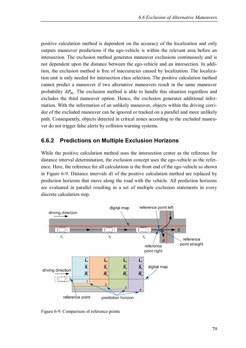
6.6 Exclusion of Alternative Maneuvers
79
positive calculation method is dependent on the accuracy of the localization and only
outputs maneuver predictions if the ego-vehicle is within the relevant area before an
intersection. The exclusion method generates maneuver exclusions continuously and is
not dependent upon the distance between the ego-vehicle and an intersection. In addi-
tion, the exclusion method is free of inaccuracies caused by localization. The localiza-
tion unit is only needed for intersection class selection. The positive calculation method
cannot predict a maneuver if two alternative maneuvers result in the same maneuver
probability . The exclusion method is able to handle this situation regardless and
excludes the third maneuver option. Hence, the exclusion generates additional infor-
mation. With the information of an unlikely maneuver, objects within the driving corri-
dor of the excluded maneuver can be ignored or tracked on a parallel and more unlikely
path. Consequently, objects detected in critical zones according to the excluded maneu-
ver do not trigger false alerts by collision warning systems.
6.6.2 Predictions on Multiple Exclusion Horizons
While the positive calculation method uses the intersection center as the reference for
distance interval determination, the exclusion concept uses the ego-vehicle as the refer-
ence. Here, the reference for all calculations is the front end of the ego-vehicle as shown
in Figure 6-9. Distance intervals of the positive calculation method are replaced by
prediction horizons that move along the road with the vehicle. All prediction horizons
are evaluated in parallel resulting in a set of multiple exclusion statements in every
discrete calculation step.
Figure 6-9: Comparison of reference points

6 Evaluation
80
6.6.3 Calculation
For the exclusion concept, the basic calculation of transfer functions introduced in
section 5.1 has to be altered. In the positive calculation method, transfer functions are
calculated based on the training data available for the corresponding maneuver. For
instance, right turn training data is used to train right turns only. In the exclusion con-
cept, all training data available from every maneuver is allocated into two groups: a
maneuver group and a not-maneuver group . The maneuver group contains
data from the maneuver that is trained (approach sequences of right turns in the case of
the example above). The not-maneuver group contains all remaining data (all left
turn approach sequences plus all straight driving sequences). Data from groups and
are used to generate transfer functions in the same way as the positive calculation
method. Indicators used in the exclusion approach are the same as in the positive calcu-
lation method. However, some indicators cannot be calculated without using the dis-
tance between the ego-vehicle and the intersection. Because this information is not used
in the exclusion approach, these indicators are left out.
Because of the different amount of training data in the groups created by the exclusion
method (group contains approx. twice the data of group ), a weighting has to be
done. The weighting factor is calculated for each interval by comparing the
amount of data in the groups:
(6-6)
Taking the prediction horizon into account, the occurrence of training data in
interval in group in relation to the overall occurrence of training data in the inter-
val defines the exclusion likelihood for maneuver :
(6-7)
Note that is the weighted occurrence of training data in and unlike the posi-
tive calculation method, the exclusion likelihoods of all maneuvers don't add up to a
total of one.
6.6.4 Implementation
The implementation of the exclusion approach is done similarly to the positive ap-
proach. The basic structure of the concept is given in Figure 6-10. The difference to the
structure of the positive calculation method is that the distance is not used and that
indicators generate exclusion likelihoods from input signals.

6.6 Exclusion of Alternative Maneuvers
81
Figure 6-10: Exclusion structure
Based on the input data, all indicator exclusion likelihoods for either right turns, left
turns or straight driving are summed up for each prediction horizon in the inference
system. This results in overall exclusion probabilities for either right turns
, left turns or for straight driving maneuvers . For
the selection of a maneuver to be excluded in a distance horizon , the maximum value
of , and is selected and the corresponding maneuver is
excluded.
classselector
indicators
inference system
priority regulation
transfer functions
maneuver probabilities list of
active indicators
measurementdata
localizationunit
overall exclusion rates
maneuver exclusion
free driving?
list of inactive indicators
all indicators active
yes
no
no exclusion
Exmax
> γmin
yes
no

82
7 Results
This section gives a survey of the prediction performance achieved by applying the
prediction system introduced in this work to measurement data from the test subject
study carried out in this work. Note that all results presented in the following are gener-
ated without using the vehicle's turn indicator state at all. According to section 6.3,
reference points for turn maneuvers are defined as using 2 % of the curvature's apex.
The results presented in section 7.1 are generated using a selection of the indicators
introduced and discussed above. The average function is applied here as an inference
method for the calculation of maneuver probabilities. This is done to show that even this
simple mathematical and computational method is able to detect intentions. In compari-
son, prediction results achieved by using a Bayesian network instead of the average
function are presented in section 7.2.
7.1 Prediction Performance
In the evaluation, the maneuver with the highest probability is compared to the maneu-
ver executed in reality in each discrete calculation step. True predictions are counted if
the predicted maneuver is the same as the real maneuver executed by the driver. True
prediction rates are shown for a time span of prior to reference points. The
figures present the results of a stratified 10-fold cross validation. True prediction rates
of all classes considered here are summarized in Table 7-2 in section 7.3. Note that for
all results shown here, standstill times during the intersection approach are removed so
that the results present only predictions done while the ego-vehicle is moving.
7.1.1 Priority Roads
Figure 7-1 shows the true positive prediction rates for intersection class 5 containing all
intersections the ego-vehicle approaches via a priority road not regulated by traffic
lights, independent of the intersection's size and geometry. Best classification results are
achieved for straight driving maneuvers with true positive predictions at
1 second prior to the reference point. Right turn maneuvers are classified correctly with
at 1 second prior to the initialization of turn maneuvers. Left turn maneu-
vers are predicted correctly with at 1 second prior to the initialization of a
left turn maneuver.

7.1 Prediction Performance
83
Figure 7-1: Results of class 5, priority roads
7.1.2 Traffic Lights
Figure 7-2 presents the true positive classification rate of intersection class 2 containing
intersections operated by general traffic lights (traffic lights that show the same light at
once for all legal maneuver options). The prediction performance is similar to tpr of
class 5: Best classification performance is achieved for right turns at 1 s
prior to maneuver initialization, followed by left turns and straight driving
maneuvers . While the prediction performance at 1 s is similar, true predic-
tion rates for higher times to maneuver initialization are higher than in class 5.
Figure 7-2: Results of class 2, traffic lights for all directions
0123456789100
0.1
0.2
0.3
0.4
0.5
0.6
0.7
0.8
0.9
1
time to reference point in s
tru
e p
osit
ive p
red
icti
on
rate
sPrediction Performance for Priority Roads (Class 5)
right turns
left turns
straights
0123456789100
0.1
0.2
0.3
0.4
0.5
0.6
0.7
0.8
0.9
1
time to reference point in s
tru
e p
osit
ive p
red
icti
on
rate
s
Prediction Performance for Traffic Lights (Class 2)
right turns
left turns
straights
data: priority roads
drivers: all
inference: average
data: traffic lights
drivers: all
inference: average
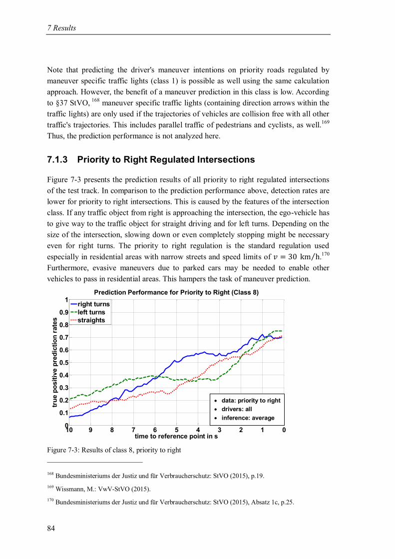
7 Results
84
Note that predicting the driver's maneuver intentions on priority roads regulated by
maneuver specific traffic lights (class 1) is possible as well using the same calculation
approach. However, the benefit of a maneuver prediction in this class is low. According
to §37 StVO, 168
maneuver specific traffic lights (containing direction arrows within the
traffic lights) are only used if the trajectories of vehicles are collision free with all other
traffic's trajectories. This includes parallel traffic of pedestrians and cyclists, as well.169
Thus, the prediction performance is not analyzed here.
7.1.3 Priority to Right Regulated Intersections
Figure 7-3 presents the prediction results of all priority to right regulated intersections
of the test track. In comparison to the prediction performance above, detection rates are
lower for priority to right intersections. This is caused by the features of the intersection
class. If any traffic object from right is approaching the intersection, the ego-vehicle has
to give way to the traffic object for straight driving and for left turns. Depending on the
size of the intersection, slowing down or even completely stopping might be necessary
even for right turns. The priority to right regulation is the standard regulation used
especially in residential areas with narrow streets and speed limits of .170
Furthermore, evasive maneuvers due to parked cars may be needed to enable other
vehicles to pass in residential areas. This hampers the task of maneuver prediction.
Figure 7-3: Results of class 8, priority to right
168 Bundesministeriums der Justiz und für Verbraucherschutz: StVO (2015), p.19.
169 Wissmann, M.: VwV-StVO (2015).
170 Bundesministeriums der Justiz und für Verbraucherschutz: StVO (2015), Absatz 1c, p.25.
0123456789100
0.1
0.2
0.3
0.4
0.5
0.6
0.7
0.8
0.9
1
time to reference point in s
tru
e p
osit
ive p
red
icti
on
rate
s
Prediction Performance for Priority to Right (Class 8)
right turns
left turns
straights
data: priority to right
drivers: all
inference: average

7.1 Prediction Performance
85
7.1.4 Give Way and Stop Sign Regulated Intersections
Prediction results achieved by the system for intersections operated by give way signs
(class 4) are shown in Figure 7-4. The overall prediction performance is lower than for
priority to right regulations. Predicting maneuvers in intersection classes 3 & 4 is the
hardest task due to the demand to stop the vehicle or drive at low speeds in all cases and
independent of maneuver. Thus, no speed-related indicators and no indicators based on
driver's control inputs to affect the vehicle's speed are used at all. Driver's head- and
gaze behavior is mainly dependent on the geometry of the intersections and view ob-
structions. In addition, typical driver behavior was observed in test drives that further
exacerbated the difficulty of the prediction task: Having stopped the vehicle at line of
sight, drivers turn their heads at large angles ( ) to the direction priority traffic
is coming from. These angles are outside the field of view of the head tracking device
used in this work. In order to track head and gaze rotations in these situations as well,
more cameras and measuring devices with greater range would have to be used.
Figure 7-4: Results of class 4, give way sign
The same applies to the prediction results achieved at stop sign regulated intersections
(class 3) shown in Figure 7-5, that are even lower than in class 4.
0123456789100
0.1
0.2
0.3
0.4
0.5
0.6
0.7
0.8
0.9
11
time to reference point in s
tru
e p
osit
ive p
red
icti
on
rate
s
Prediction Performance at Give Way Signs (Class 4)
right turns
left turns
straights
data: give way signs
drivers: all
inference: average

7 Results
86
Figure 7-5: Results of class 3: stop sign
The low prediction quality achieved by the prediction system for straight driving ma-
neuvers in both classes results from the trajectories used by drivers at stop sign and give
way regulated intersections. A review of data recorded in the test drives for these two
intersection classes shows a general pattern of trajectories: Trajectories for right turns
clearly differ from the trajectories of the other two maneuvers at the same intersection.
Intersection approach trajectories for straight driving and left turns lead straight to the
stop line until the vehicle comes to a stop. Thus, approaching sequences for left turn
maneuvers and straight drives are likely to be mistaken by the prediction system. None-
theless, the intention prediction method is applicable to these two classes as well, even
though the prediction performance is clearly lower than the performance achieved in
other classes.
7.1.5 Robustness of Predictions
This section analyzes the frequency of dropped true predictions that are initially correct.
Here, the entirety of true predictions at a time to maneuver initialization ( is
analyzed for consistency of consequent predictions. Figure 7-6 shows the variation of
dropout rates for predictions at intersections regulated by traffic lights. The analysis is
based on a total of 383 true predictions at .
0123456789100
0.1
0.2
0.3
0.4
0.5
0.6
0.7
0.8
0.9
11
time to reference point in s
tru
e p
osit
ive p
red
icti
on
rate
s
Prediction Performance at Stop Signs (Class 3)
right turns
left turns
straights
data: give way signs
drivers: all
inference: average

7.2 Bayesian Network
87
Figure 7-6: Robustness analysis
Dropout rates for all intersection classes analyzed here are given in Table 7-1 based on
the total of true predictions at .
Table 7-1: Comparison of prediction
intersection class 2 3 4 5 8
dropout rates at
5.1 5.9 5.4 4.2 7.7
dropout rates at
6.0 7.6 8.3 5.4 9.8
dropout rate at
7.1 8.2 7.9 5.7 10.5
7.2 Bayesian Network
In addition to using the average or product function, a Bayesian network is set up in this
work. The conditional probability table of each node in the network are learned using
the same data that is used for generating the results in the previous section. The remain-
der of the evaluation is the same as in the previous section. The structure of the Bayesi-
an network is shown in Figure 7-7.
0 0.5 1.0 1.5 2.00
0.01
0.02
0.03
0.04
0.05
0.06
0.07
0.08
time to reference point in s
rate
of
dro
pp
ed
tru
e p
red
icti
on
sRobustness of True Predictions 2 s a Priori to Reference Point

7 Results
88
Figure 7-7: Bayesian network
Prediction results generated using the Bayesian network for class 2 and class 5 are
shown in Figure 7-8 and Figure 7-9.
Figure 7-8: Results of class 5, priority roads, Bayesian network
As expected, true positive detection rates generated by the Bayesian network outper-
form the results generated by using the average function for left turns by 5.7 %
( ). For straight driving maneuvers, the performance is
nearly the same (+0.3 % ). The true prediction rate of right turn maneuvers
is even slightly lower ( . In intersection class 2 (traffic
lights), using the Bayesian network results in 1 s before maneuver
initialization of left turns, for right turns and
for straight driving. This corresponds to raised true prediction rates of +0.3 %
for left turns, +7.7 % for right turns and +15 % for straight driving. In this class, using
the Bayesian network clearly raises the prediction performance.
1
2 3 4 5 6
7 8 9 10
0123456789100
0.1
0.2
0.3
0.4
0.5
0.6
0.7
0.8
0.9
1
time to reference point in s
tru
e p
osit
ive p
red
icti
on
rate
s
Prediction Performance for Priority Roads - Bayesian Network
right turns
left turns
straights
data: priority roads
drivers: all
inference: Bayesian

7.3 Neglecting Intersection Classes
89
Figure 7-9: Results of class 2, traffic lights for all directions, Bayesian network
7.3 Neglecting Intersection Classes
In order to assess research question one introduced in section 3.1, the effect of the inter-
section classes on the prediction performance is analyzed. This is done by comparing
two types of performance calculations: One type with respect to intersection classes (as
introduced above) and one type neglecting intersection classes and using training data
from all intersection approaches recorded in the test study. The figures given in annex I
present the prediction performance for the latter calculation type. They are created
based on the same conditions as in the previous section (average function as an infer-
ence system and 10-fold cross validation). Table 7-2 compares the prediction perfor-
mance (tp=true positive rate) one second prior to maneuver initialization ( = 1 s).
Table 7-2: Prediction performance at ttmi = 1 s
int. class 2 3 4 5 8
ma-
neuver
int. class
used
tp rate in
%
tp rate in
%
tp rate in
%
tp rate in
%
tp rate in
%
R yes 83.6 58.6 71.4 82.7 72.3
no 76.2 52.1 72.0 77.9 57.7
S yes 76.5 35.0 37.8 87.2 62.4
no 79.6 20.2 35.2 81.3 65.0
L yes 80.7 72.5 66.7 78.4 68.1
no 81.7 65.2 66.7 67.5 67.9
all y 80.0 55.3 57.7 83.3 67.3
n 79.6 45.8 57.0 76.5 63.6
0123456789100
0.1
0.2
0.3
0.4
0.5
0.6
0.7
0.8
0.9
1
time to reference point in s
tru
e p
osit
ive p
red
icti
on
rate
sPrediction Performance for Traffic Lights - Bayesian Network
right turns
left turns
straights
data: traffic lights
drivers: all
inference: Bayesian

7 Results
90
Comparing the results shows that the four prediction rates in bold in the table have
slightly better prediction performance for a single maneuver while neglecting intersec-
tion classes rather than predictions considering intersection classes. The overall predic-
tion performance of all maneuvers at prior to the reference point is higher
for all intersection classes after separating intersection classes in the training process.
The increase in prediction performance depends on the type of intersection class. While
the overall gain for intersection class 2 and 4 is below 1 %, true prediction rates of
intersection classes 3, 5 and 8 are raised by 9.5 %, 6.8 % and 3.7 % using intersection
classes. The average prediction rates for all three maneuver types within each intersec-
tion class are raised using the intersection classification scheme.
7.4 Exclusion Results
In the evaluation of the exclusion method utilized here, an exclusion is considered true
if a maneuver that differs from the driver’s executed maneuver is excluded . Exclusions
are calculated for multiple prediction horizons. For means of comparing the results
achieved by the exclusion approach to the results of the positive approach, the same
representation is selected here. Exclusions from all predictions horizons are transferred
to the same reference points used in positive approach. The exclusion of the prediction
horizon that corresponds to the distance remaining to the reference point is selected and
used for evaluation. Figure 7-10 shows the true exclusion rates achieved by the proto-
typic implementation for driving on priority roads separated by maneuvers the driver
performs.
Figure 7-10: Exclusion performance
0123456789100
0.1
0.2
0.3
0.4
0.5
0.6
0.7
0.8
0.9
1
time to reference point in s
tru
e p
osit
ive e
xclu
sio
n r
ate
s
Exclusion Performance for Priority Roads
right turns
left turns
straights
data: priority roads
drivers: all
inference: exclusion

7.4 Exclusion Results
91
The figure shows that a true exclusion rate of 92.2 % is reached for right turns on priori-
ty roads 1 second prior to maneuver initialization (ttmi = 1 s). This means that in 92.2 %
of all intersection approaches with right turns performed by the driver, a maneuver
different from a right turn is excluded by the system. Analogously, the exclusion rates
for left turns are 87.9 % and 95.6 % for straight driving maneuvers. Table 7-3 compares
the true positive rates of the positive calculation method and the exclusion method,
showing that the exclusion calculation clearly outperforms the positive calculations in
terms of true positive rates.
Table 7-3: Prediction and exclusion rates
maneuver R L S
ttmi tp rates
in %
exclusion
rates in %
tp rates
in %
exclusion
rates in %
tp rates
in %
exclusion
rates in %
1 82.7 92.2 78.4 87.9 87.2 95.6
2 71.6 89.5 67.5 80.4 75.0 92.6
3 61.6 87.4 56.7 78.7 72.2 86.5

92
8 Driver-specific Adaptation
Prediction results described in the previous section were generated using data from all
test subjects considered in this work. Differences in the individual driving behavior
among the test subjects has not been taken into account so far. This section analyzes the
potential of improving the intention detection system's prediction quality by adapting
the indicators' transfer functions to different driving styles. A review of the literature
shows that at least two different driving styles have to be considered: careful and re-
laxed drivers on the one hand and sporty drivers on the other hand.171
In general, relaxed
driving is characterized by lower longitudinal and lateral accelerations when compared
to sporty driving. A careful driver initiates a braking maneuver during intersection
approach earlier and applies less deceleration than a sporty driver.172
In general, two
different methods can be applied to adapt a driving style and are therefore considered
here. The goal of both methods is to conform to the driver's individual behavior:
The first method classifies the driving style and combines all drivers of the test
study with the same driving style into one group. Transfer functions are created
using training data only from drivers within the groups.
The second method calculates individual transfer functions for each driver. Here,
the transfer functions are adapted to the driver's individual behavior.
Adapting the transfer functions to the driving style of only one driver requires copious
amounts of data during the training process for each intersection class. Considering only
data from one driver instead of data generated by all drivers results in a decrease to the
size of the training set to 1/30 of the initial amount of data. Note that the amount of data
available is reduced even further by splitting recorded data into a training and a test set.
Applying this procedure to the training data generated in this project shows that the
amount of data available for an individual driver is too low for reliable maneuver pre-
diction. Thus, the second method is discarded here and the first method is applied. The
procedure to analyze the adaptation potential of the intention detection system is out-
lined in the following:
Drivers are categorized into a predefined number of groups using a classification
measure.
171 Donges, E.: Driver Behavior Models (2016), pp. 29–30.
172 Meitinger, K.-H.: Diss., Aktive Sicherheitssysteme für Kreuzungen (2009), p.41.

8.1 Driver Classification
93
Group-specific (adapted) transfer functions are calculated based only on training
data from drivers within one group.
The prediction system's performance using the adapted transfer functions for
drivers within one group is evaluated for all groups.
The system's prediction performance using the adapted transfer functions is
compared to the prediction performance using non-adapted transfer functions.
8.1 Driver Classification
There are several methods known in the literature for classifying driving behavior. A
commonly used approach is to provide a questionnaire to test subjects and let drivers to
a self-assess of their driving style. Based on Keller173
and Porst174
, a questionnaire with
labeled endpoints is developed and presented to test subjects before starting test drives.
Among other things, the questionnaire asks the test subjects to assess their own driving
style on a scale of 1 to10 with 10 labeled as "sporty" and 1 labeled as "relaxed/careful".
Out of the 30 participants of the test study, 6 drivers classified themselves as sporty
drivers (with a score from 8 to 10). 10 test subjects classified their own driving style as
relaxed and careful (with a score from 1 to 3). The remaining 14 test subjects stated that
their own driving style was neither sporty nor relaxed based on scores from 4 to 7 on the
questionnaire. The results of the questionnaire are summarized in Table 8-1. Aside from
the driver's self-assessment, a classification of whether the test subject behaved more or
less sporty as compared to the average of all drivers is given in the table. Note that a
variety of methods for assessing drivers' driving styles can be applied. Graichen et al.175
found significant differences between different drivers in the ego-vehicle's speed when
releasing the accelerator pedal, as well as for maximum longitudinal acceleration after
turning. Cheng et al.
176 analyzes the use of the acceleration pedal, the steering wheel
angle and the lateral accelerations tolerated by the driver to identify driving behavior. A
survey of different methods for driving style recognition is given by Bolovinou et al.177
For means of maneuver prediction, the driving behavior during intersection approach is
of interest to this work. Here, the ego-vehicle's speed and the longitudinal acceleration
applied by the driver during intersection approach is analyzed. For the analysis, inter-
173 Keller, D.: Skala in Fragebögen (2013).
174 Porst, R.: Fragebogen (2014).
175 Graichen, M.; Nitsch, V.: Effects of Driver Characteristics (2017), pp. 15–29.
176 Chen, Y.; Li, L.: Advances in Intelligent Vehicles (2014), p.151.
177 Bolovinou, A. et al.: Driving style recognition (2014), pp. 73–78.

8 Driver-specific Adaptation
94
section approach data is used from give way sign regulated intersections, stop sign
regulated intersections, and intersections with priority to right regulations. These inter-
section classes are selected for driving style analysis because external conditions influ-
encing the driver's behavior are minimized: The driver has to slow down during all
intersection approaches due to priority regulations and is aware of the need to slow
down at an early phase of the approach.178
Thus, the approaching behavior is not influ-
enced by external conditions such as traffic lights. In this work, it has proven that using
the longitudinal acceleration during intersection approach enables a better driver classi-
fication at different intersections with varying geometry as opposed to using the vehi-
cle's speed for driver classification.
Thus, longitudinal accelerations applied by the driver during intersection approach are
compared to the accelerations applied by all drivers in the same situations. Figure 8-1
exemplarily shows a cumulated distribution of lateral accelerations applied by test
subject No. 16 while approaching give way sign regulated intersections. For means of
comparison, the eCDF of longitudinal accelerations recorded for all drivers under the
same conditions is given, as well.
Figure 8-1: Driving style comparison
Depending on the relative position of both eCDF curves, the driver is classified as either
sporty (+), medium (o) or relaxed (-) in relation to the other test subjects of the study.
178 In contrast to situations when approaching traffic light intersections, where a light change could
potentially force the driver to slow down more quickly than anticipated, the intersection classes used
here have unchanging regulations, so it is clear to the driver that he has to slow down at the beginning
of the intersection approach sequence.
-4 -3 -2 -1 0 1 2 30
0.2
0.4
0.6
0.8
1
acceleration in m/s2
cu
mu
lati
ve d
istr
ibu
tio
n
Longitudinal Acceleration of Drivers
average of all drivers
test subject no. 16

8.1 Driver Classification
95
Table 8-1 shows the results of this relative assessment, as well as whether the relative
assessment correlates to the driver's self-assessment.
Table 8-1: Sporty driving assessment
driver no. sporty
driving (self-
assessment)
sporty
driving
(test)
self as-
sessment
correct?
1 9 + y
2 6 o y
3 8 o n
4 3 - y
5 6 o y
6 2 o n
7 5 + n
8 5 o y
9 8 o n
10 6 + n
11 10 - n
12 3 o n
13 2 o n
14 6 o y
15 7 o y
16 6 + n
17 5 - n
18 3 o n
19 6 - n
20 3 o n
21 3 o n
22 6 - n
23 1 + n
24 10 + y
25 6 o y
26 4 o y
27 1 - y
28 3 o n
29 8 - n
30 6 - n
As shown in the table, only 11 out of 30 drivers have matching self-assessments and
relative assessments. Thus, drivers are not grouped based on their self-assessment, but
based on the classification done by the longitudinal accelerations measured during
intersection approach.

8 Driver-specific Adaptation
96
8.2 Results of the Adaptation Process
This section shows the results of the driving style adaptation as introduced above. Three
groups of drivers are considered: The first group contains drivers that drive more re-
laxed and carefully, with lower longitudinal accelerations during intersection approach
as compared to the average of all drivers in the study. The second group consists of
drivers that show only small differences to the average acceleration profile. Finally, the
third group contains drivers that use higher longitudinal accelerations than the average
driver. The classification of drivers into either the average or one of the other groups is
done according to the amount of RMSE between the eCDFs.
At stop sign regulated intersections (class 3), no positive effect of the driving style
adaptation could be found for the first group (relaxed) and the third group (sporty). In
contrast, raised true prediction rates for right turns and straight driving have been found
for the second group containing only the drivers that match the average acceleration
profiles, as shown in Figure 8-2. The adapted prediction rates are compared to the non-
adapted rates in Table 8-2.
Figure 8-2: Driving style adapted prediction performance class 3
Table 8-2: Adapted prediction performance at ttmi = 1 s
maneuver tp rate in % (non-adapted) tp rate in % adapted increase
in %
R 58.6 72.3 +13.7
L 72.5 66.0 -6.5
S 35.0 70.9 +35.9
all maneuvers 55.3 69.7 +14.4
0123456789100
0.2
0.4
0.6
0.8
1
time to reference point in s
tru
e p
osit
ive p
red
icti
on
rate
s
Prediction Performance for Stop Signs (Adapted)
right turns
left turns
straights
data: stop signs
drivers: 2nd group
inference: average

8.2 Results of the Adaptation Process
97
The adaptation results for give way sign regulated intersections (class 4) are similar to
those of class 3 shown above. While the results for the first group and the third group
are nearly the same as the non-adapted true positive rates for all maneuvers
(58.9 % with an increase of +1.2 % for the first group and 60.7 % (+3 %) for 3rd
group), the prediction performance of the second group is clearly increased, as shown in
Figure 8-3 and Table 8-3.
Figure 8-3: Driving style adapted prediction performance class 4
Table 8-3: Adapted prediction performance at ttmi = 1 s
maneuver tp rate in % (non-adapted) tp rate in % adapted increase
in %
R 71.4 68.2 -3.2
L 66.7 70.2 +3.5
S 37.8 75.0 +37.2
all maneuvers 57.7 71.1 +13.4
For priority to right regulated intersections (class 8), the effect of using an adapted
transfer function on prediction results is minor: The first group (relaxed) results in
71.4 % overall true positive rates, the second group (average) in 66.8 % overall true
positive rates, and the third group (sporty) in 69.2 % overall true positive rates. All
results only show small improvements over the 67.3 % overall true positive rate for
non-adapted calculations. The effect of the adaptation is further reduced in intersection
class 2 (general traffic lights) and 5 (priority roads). For both intersection classes, the
results of all three groups' true positive rates vary within 2 % of the non-adapted true
positive rates.
0123456789100
0.2
0.4
0.6
0.8
1
time to reference point in s
tru
e p
osit
ive p
red
icti
on
rate
s
Prediction Performance for Give Way Signs (Adapted)
right turns
left turns
straights
data: give way signs
drivers: 2nd group
inference: average

8 Driver-specific Adaptation
98
In conclusion, a positive effect of the adaptation process, including increased true
prediction rates, is found especially for the second group of drivers (containing drivers
close to average behavior) for intersections regulated by stop signs and give way signs.
For driving on priority roads and priority to right regulated intersections, no appreciable
effect on the results can be found.
8.3 Adaptation Methods in Real Driving
This chapter describes the procedure of driver-individualized adaptation of transfer
functions and the challenges arising in series implementation. The basic principle of the
process is summarized in Figure 8-4. In the initialization phase shown in the upper half
of the figure, the driver is identified. If the driver is classified as already known to the
system, the driver specific data pool is selected corresponding to the driver. Otherwise,
the default data pool provided by the system is used. Based on the active data pool, the
indicators' transfer functions are calculated as described in section 5.1.
Figure 8-4: Adaptation Process
After completing the initialization phase, the adaptation process is started, as shown in
the lower part of Figure 8-4. Here, new intersection approach sequences are added to the
data pool. Based on the modified data pool, driver specific adapted transfer functions
are generated. Modified transfer functions are stored along with the driver's identifica-
maneuver detection
entering relevant
area
measurementdata
adapted transfer
functions
maneuver initialization
temporary data buffer
data pool
L S R
training sequence
maneuver
calculation unit
transferfunctions
driver recognition
driver known?
yes
no
driver-specific data pool
L S R
standard data pool
L S R
calculation unit
calculation unit
standard transfer
functions
driver-specific transfer
functions
driver id
transferfunctions
transferfunctions
Phase 1: Initialization
Phase 2: Adaption

8.4 Biasing
99
tion. Necessary elements shown in the figure for transforming measurement data into
driver-individualized adapted transfer functions are:179
1. Temporary Data Buffer
needed to buffer data of intersection approach until maneuver initialization (ter-
mination of approach sequence)
2. Maneuver Detector
mandatory for classifying approach sequence; maneuver performed by driver is
determined a posteriori
3. Data Pool
containing frequency of occurrences of indicators
4. Calculation Unit
generates transfer functions from the data pool
5. Driver Identification Unit
needed to switch or reset adapted transfer functions for different drivers
6. Monitoring Function
for limiting the of amount of new intersection approach data added to the data
pool from reaching saturation for a single driver
8.4 Biasing
Adapting the transfer functions in real road application, as proposed in the prior section,
leads to the challenge of biasing. Challenges arise from choice of typical routes (routing
bias) and local overfitting, as described in the following.
8.4.1 Routing Bias
Analyzing drivers’ normal routing in urban areas shows a pattern that is applied for
most urban drives. When starting in residential areas, drivers usually select a direct path
to a nearby main street or priority road and stay on this road as long as possible until
reaching their destination. This strategy results in shorter travel times than driving sole-
ly on residential roads, due to higher average speed on main and priority streets. This is
the same basic principle that is applied in navigation devices for routing calculations.180
As a matter of fact, most urban main streets and priority roads run more or less straight
through urban areas. Hence, a challenge arises for the adaptation process: Driving on
main streets and adding each intersection sequence to the data pool mainly results in
179 The functionality of these elements is described in greater detail in Annex J.
180 Kleine-Besten, T. et al.: Navigation and Transport Telematics (2016), p.1365.

8 Driver-specific Adaptation
100
straight driving sequences being added. The longer the adaptation process is active, the
more the initial data pool becomes distorted by adding many more straight driving
sequences versus turning sequences. Using such a distorted data pool (containing sever-
al times more straight driving sequences than turn maneuvers), the most common ma-
neuver (straight driving) will be predicted most of the time. Thus, a compensation
method is needed. Two potential methods of compensation can be applied:
In the first method, new sequences are only added in a set of three to the data pool with
every set containing a sequence for right turns, one for left turns, and one for straight
driving. Applying this method ensures that the data pool is not distorted by a different
amount of sequences for each maneuver. The disadvantage of this method is that the
adaptation process is slower. In extreme cases, the adaptation process can even be disa-
bled if there are not enough training sequences containing a set of three sequences for
each type of intersection within one trip. The second method uses each intersection
approach sequence and integrates it into the data pool. The different numbers of inter-
section approaches are accepted here and taken into account by weighting factors. The
weighting factors are calculated by the number of sequences available for each maneu-
ver. The calculation is done analogously to the weighting factors introduced for the
exclusion method in Section 6.6.3.
8.4.2 Local Overfitting
Regularly driving the same route may lead to local overfitted transfer functions that are
adapted to exactly this route (e.g. if a vehicle is used mainly for commuting to and from
work). Each sequence that is added to the data pool originates from the same limited set
of intersections. As long as the driver sticks exactly to this route, the prediction will
perform well, but in case a different route is used than the regularly driven one, the
prediction results might be worse than using non-adapted transfer functions. The prob-
lem is demonstrated by the following situation: Assuming the regularly driven route
contains exactly one maneuver of the intersection class priority to right and there is a
parking spot hindering the driver from driving straight towards the intersection as de-
picted in Figure 8-5.
Figure 8-5: Local overfitting example

8.4 Biasing
101
If this approach sequence is added to the data pool regularly, each time the driver passes
this intersection, the initial share of data for this intersection class is influenced signifi-
cantly and the pool becomes overfitted. In this case, the system is falsely adapted to the
information that this driver always performs an evasive maneuver before turning at
priority to right intersections. This example shows that aside from the approach se-
quence itself and the maneuver executed, the intersection at which the approach se-
quence is generated has to be considered. To avoid local overfitting, the maximum
number of additional sequences generated at the same intersection and approach direc-
tion has to be limited. The limit on how many approach sequences of the same intersec-
tion are tolerated in the data pool has to be determined in real road tests and is depend-
ent upon the routes and if they are regularly driven by the driver. Therefore, it is
possible that this issue is only of theoretical nature and may not be relevant in real use
of an adaptation system.

102
9 Conclusion and Outlook
In this work, it has been analyzed to which extent the detection of intentions (corre-
sponding to a prediction of maneuvers) is possible before maneuvers are initialized by
the driver without using the vehicle's turn indicator state at all.
The option to enable or disable indicators depending on the situation, without altering
the overall design, is the key feature for the flexibility of the indicator principle. To
enable the intention detection system to perform at arbitrary urban intersections, a clas-
sification system for urban intersections has been introduced based on official priority
regulations.181
Applying the prototypic implementation of the intention detection system
to data recorded in the test subject study done in this work shows that more than 80 %
of all maneuvers are predicted correctly one second before the maneuver is initialized
on priority roads with and without existence of traffic lights.
The results show that a maneuver prediction system on guidance level at urban intersec-
tions based on the indicator concept and series or close-to-production sensor systems is
able to operate at varying intersection types. Despite using only a close to series locali-
zation unit and no information from the upcoming intersection aside from the right-of-
way regulation, the prediction system implemented here is able to predict maneuvers at
a great variety of urban intersections. Indicators can be replaced or additional indicators
can be added without altering the approach at all. Thus, the system can be easily modi-
fied in case additional sensor systems are added to the vehicle or additional driver's
behavior is modeled. Within the development of the approach, different inference meth-
ods and algorithms for combining the indicators outputs were analyzed. As a result, it is
concluded that either simple inference methods, such as the average or product function,
can be used or more sophisticated approaches based on machine learning methods can
be applied to the indicators outputs (e.g. Bayesian networks or support vector ma-
chines). Each system has individual advantages and disadvantages. A recent survey
comparing the most common methods for automated decision making is given by
Firl.182
Comparing results achieved with different inference methods shows that the quality of
the inputs to the inference method is more important than the inference method itself.
For that reason, a quality measure based on the indicators ability of maneuver separation
is defined and applied in this work. Aside from intersection and distance dependent
181 Bundesministeriums der Justiz und für Verbraucherschutz: StVO (2015).
182 Firl, J.: Diss., Probabilistic Maneuver Recognition (2014), pp. 11–31.

9 Conclusion and Outlook
103
selection of highly discerning indicators, the quality measure is used for optimizing the
indicators itself.
Besides the "classic" method of inferring which maneuver the driver is about to per-
form, a complimentary approach is developed in this work in parallel. The novelty of
the so-called "exclusion approach" is that it relies on excluding alternative maneuvers
that the driver is not going to perform. The advantage of this approach is that false
positive alerts of IAS are avoided effectively by excluding potential maneuver options.
The exclusion approach is based on the same indicators as the positive calculation
method. Comparing the results of both approaches shows that the exclusion method
reaches higher true positive rates than the positive calculation, even at several seconds
before maneuver initialization by the driver. Thus it offers high potential for use in
series application without annoying drivers by frequent false alerts.
Note that the selection of reference points has enormous impact on the system's detec-
tion performance. The closer to the intersection center a reference point is defined, the
better the prediction performance gets. In addition, the accuracy of the reference point
effects the system's performance. Another key feature of this work is the definition of
localization-independent reference points: As discussed in this work, the initialization of
maneuvers is heavily dependent on the intersections' geometry and size. Consequently,
for performance evaluation in this work, reference points have been defined based
solely on the ego-vehicle's driven trajectory. Note that this procedure is only applicable
for means of a posteriori performance evaluation. An a priori determination of the refer-
ence point during intersection approach before a turn maneuver is initiated is not possi-
ble as a matter of principle. Due to varying reference points used in related works, a
comparison of the prediction performance reached by the prototype implementation
done here to related works is not feasible.
In addition to the system's general feasibility to detect intentions at different types of
intersections, the potential of adapting the indicators' transfer functions to different
driving styles has been analyzed in this work. Using the longitudinal acceleration during
intersection approach, drivers are categorized as either sporty, average, or relaxed.
Using transfer functions adapted to one driving style, a potential enhancement of the
intention detection system is given for drivers of the average group for intersection
classes 3 (stop signs) and 4 (give way signs). For this group of drivers, a raised
prediction performance of 14.4 % and 13.4 % respectively, has been demonstrated. The
results are in line with the expectations: The highest potential for increasing the predic-
tion performance was found for intersection classes with the predictions depending only
on the driving behavior. All kinds of information that is beneficial for maneuver predic-
tion on priority roads, such as environmental information and especially road markings,
are usually not available for maneuver prediction at stop sign or give way sign regulated
intersections. For drivers of the other two groups (sporty and relaxed drivers) no raised

9 Conclusion and Outlook
104
prediction performance could be identified in the adaptation analysis. Further research
has to address the question if this is caused by the size of the groups. In the test study
done here, the average driver group consisted of about twice the number of drivers than
the other two groups. The effect of the amount of drivers in the two smaller groups has
to be addressed in further extended studies. However, a critical review of the data rec-
orded in test drives leads to the assumption that the test subjects adapted their driving
behavior to the test situation: Test subjects showed a turn indicator usage rate of ap-
proximately 95 % for turn maneuvers. This rate is 20 % higher than the rate observed in
natural driving.183
In addition, with the test conductor being present in the vehicle and
test subjects being aware of data recording, most drivers showed a careful driving style.
Even drivers who claimed to have a very sporty driving style in self-assessment rarely
exceed lateral accelerations of
in test drives (< 5 % of all turn maneuvers).
Further research potential lies in analyzing the effect of drivers being aware of test
conditions and data recording to their driving style. To answer the question if drivers
alter their intersection approach behavior in this case, data from a long-term field opera-
tion test (FOT) 184
has to be used for analyzing the driver's natural intersection approach
behavior. Aside from gathering a much larger amount of data in a FOT, the potential of
the adaptation procedures has to be re-evaluated.
183 Ponziani, R.: Turn Signal Usage Rate Results (2012), p.6.
184 FOT-Net: Field operational tests (2010).

105
A Driver Inputs for Maneuver Detection
The distribution of minimum and maximum steering wheel angles recorded at all inter-
section approaches of the test subject study185
with straight driving maneuvers is given
in Figure A-1 as a cumulated distribution function. Regarding the range between
and results in a range for steering
wheel angles linked to straight driving maneuvers.
Figure A-1: Minimum and maximum steering wheel angles while driving straight
If a limit of is used for turn maneuver detection, the resulting time delay
between initialization of a turn maneuver186
and reaching a steering wheel angle
is given in Figure A-2.
The figure shows eCDFs of for each of the turn maneuvers recorded
in the test subject study. It is found that 78 % of all left turns and 54 % of all right turns
are detected with a time delay of after maneuver initialization.
185 See Section 4.4 for details of the test subject study.
186 Initialization of a turn maneuver is determined using the calculated reference point as described in
section 6.3.2.
-80 -60 -40 -20 0 20 40 60 800
0.2
0.4
0.6
0.8
1
steering wheel angle in °
cu
mu
lati
ve d
istr
ibu
tio
n
eCDF of Steering Wheel Angle
max angles
min angles

A Driver Inputs for Maneuver Detection
106
Figure A-2: Time delay between reference point and maneuver detection by steering
Applying the same procedure described above to the vehicle's lateral acceleration results
in 89 % of all left turns and 71 % of all right turns being detected with a time delay of
between maneuver initialization and exceeding the turn detection limit as shown
in Figure A-3.
Figure A-3: Time delay reference point and maneuver detection by lateral acceleration
The same applies to using the vehicle's yaw rate instead of lateral acceleration follow-
ing the same procedure. As shown in Figure A-4, 81 % of all left turns and 56 % of all
right turns show a delay of
0 1 2 3 4 5 6 7 8 9 100
0.2
0.4
0.6
0.8
1
time delay in s
cu
mu
lati
ve d
istr
ibu
tio
n
eCDF of Time Delay by Steering Wheel Maneuver Detection
right turns
left turns
0 1 2 3 4 5 6 7 8 9 100
0.2
0.4
0.6
0.8
1
time delay in s
cu
mu
lati
ve d
istr
ibu
tio
n
eCDF of Time Delay by Lateral Acceleration Maneuver Detection
right turns
left turns

A Driver Inputs for Maneuver Detection
107
Figure A-4: Time delay between reference point and maneuver detection by yaw rate
0 1 2 3 4 5 6 7 8 9 100
0.2
0.4
0.6
0.8
1
time delay in s
cu
mu
lati
ve d
istr
ibu
tio
n
eCDF of Time Delay by Yaw Rate Maneuver Detection
right turns
left turns

108
B Radar Based Lane Detection
A brief summary of the basic working principle of the radar-based lane detection is
given here.
All objects detected by radar sensors are categorized according to their positions in
relation to the ego-vehicle and their motion state. Based on the ego-vehicle's speed and
the measured relative speed of the radar objects, each object is classified as moving in
the same direction, stationary, or oncoming, and according to its position on the left or
right of the ego-vehicle. Based on the ego-vehicle's motion state, an ego-path prediction
is done using a linear single track model. Objects are only taken into account if they are
detected in a range of in front of or behind the ego-vehicle and within a lateral
range of to the ego-vehicle's center along the predicted path. Each object
classified as moving is assigned an existence value for an adjacent lane on the side of
the vehicle the object is detected (right/left). Depending on the lateral position of the
object, a weighting function is applied to the object's existence value, modifying it
within the range between zero and one. Furthermore, a weighting function is ap-
plied to reduce the influence of detected objects at higher distances with respect to
increasing inaccuracies of path prediction at higher distances. For lane existence calcu-
lation, all objects of each category (stationary/oncoming/moving in same direction) are
summed up along with their existence values. The more moving objects are detected by
the radar sensors, the higher the lane existence likelihood is. The total number of n
moving objects on either the left or the right side of the ego-vehicle is used for calculat-
ing the lanes existence likelihoods:
(B-1)
Static objects are considered in the same way as the dynamic objects. Combining all
relevant static objects leads to existence values for solid elements and therefore no
accessible adjacent lanes next to the ego-vehicle.
Depending on the relation between static and moving objects, the existence likelihood
of a lane is calculated as follows:
(B-2)
Formula (B-2) automatically returns an existence likelihood that is normalized to the
range between 0 and 1 with 0.5 representing a state without detections.

B Radar Based Lane Detection
109
In addition, the driving direction for the left lane is estimated, taking the relation be-
tween static and moving objects in account. This is done by subtracting the two sums of
weighted likelihoods of all relevant objects: The sum of all oncoming object likelihoods
is subtracted from the sum of all object likelihoods moving in the same direction as the
ego-vehicle:
(B-3)
n = number of relevant objects in same driving direction
m = number of relevant objects in opposite driving direction
Depending on the value of , the model outputs the following values:
(B-4)
A lower limit is applied for a minimum number of sufficient objects that need to be
detected for calculation of a lane existence. If less than moving objects are detect-
ed on the left of the ego-vehicle, the first row of (B-4) is activated and the model out-
puts corresponding to no information. If sufficient moving objects
) moving in the same direction are detected on the left of the ego-vehicle, the third
row is activated and the model outputs indicating that there is an adjacent lane
to the left in the same direction. If both objects driving in the same direction and on-
coming objects are detected, the model outputs a linear interpolation between the two
states. The more objects there are driving in the same direction in relation to detected
oncoming objects, the higher is. For means of indicator calculation, the existence
likelihood of the left lane is evaluated in combination with the lane's driving direction.

C Localization
110
C Localization
To distinguish whether an intersection is within a relevant area in front of the ego-
vehicle, the ego-vehicle's driving direction on a digital road needs to be determined.
This is done by comparing the last matched positions on the same edge. Thus, a mini-
mum of two consecutive GPS positions are needed. The resulting information from this
step is whether the vehicle is moving in the same or the opposite direction of the road
modeled on the digital map. Knowing the driving direction, the next node in the vehi-
cle's driving direction in the road network is analyzed. For detection of an intersection,
the number of edges from this node to further nodes needs to be larger than one. If no
intersection is detected at the next node in front of the ego-vehicle, the node after the
next one is analyzed. This procedure is extended to all following nodes until an intersec-
tion is found. With the known position of the next intersection and the ego-vehicle's
position, the remaining distance to the next intersection along the path of the digital map
is calculated by summing up the length of road segments between the vehicle's position
and the intersection. Having identified the next intersection, the edge's angles in
relation to the edge leading to the intersection are calculated as shown in Figure C-5.
Knowing the relative angles enables an allocation of the edges to driving directions.
Figure C-5: Road direction allocation
In this step, information of the paths and the potential driving directions at the intersec-
tion are extracted from the map. Subsequently, information about the legality of the
corresponding maneuvers is needed. If there are any restrictions stored in the map deny-
ing the execution of a maneuver by traffic regulations, a maneuver dependent legality
flag is set to zero. In addition, the calculation checks if the edges are labeled as one-way
roads. In that case, the legal driving direction of the road is extracted from the map, as
well. If a potential maneuver at an intersection leads to entering a one-way road from
the wrong direction, the legality flag is set to zero, as well.

111
D Image Processing
Working Principle
The front camera is operated in logarithmic mode using a pinhole model. The camera is
used for detection of direction arrows and the type of lane markings (dashed or solid) on
the road surface. The distance to the leading vehicle (ACC target) provided by the pro-
totype control unit is used for limiting the detection area. Without a limit, false positive
detections can occur because parts of leading cars may look similarly to parts of tem-
plates. Thus, if a leading vehicle is detected, its distance is transferred into a maximum
height limiting the detection area in the video image. The following section gives a
survey of the detection process. Detections are carried out by matching parts of the
image with predefined templates. Before the matching is done, the amount of data that
has to be evaluated is reduced due to performance reasons.
The template matching process is done using a bird's eye view of the scene. This allows
for the use of the same template for matching at any point in the video image without
having to adapt the templates to the relative position to the ego-vehicle. For the match-
ing process, template arrows are reduced to the upper parts of the arrows, with the
arrowhead defining the type of arrow. These templates are compared to contents of the
search windows and similarity measures calculated. Numerous similarity measures can
be found in the literature.187
Here, the normalized squared Euclidean distance (SQDIFF)
is selected as similarity measure:188
(D-1)
In (D-1), represents the template image, the content of the search window and
describes the matching metrics of and for each location of the template
in the source image.189
The global maximum of represents the best matches of the
template with the search window and is labeled as a matching score.
If at least one matching score exceeds a limit , the detection is considered valid.
The value of is determined in tests, evaluating the false and true positive detec-
187 Mitchell, H. B.: Image Fusion (2010), pp. 167–185.
188 Möller, B.; Williams, D.: Tracking (2003), pp. 5–9.
189 Opencv Dev Team: Template Matching (2016).

D Image Processing
112
tion rates of the system. The best two template matches are selected and sent to the
control unit for each lane. If both best matches result from the same template, the tem-
plate with the third best matching score is transferred, as well. Thus, up to two different
direction arrows are detected in the ego-vehicle's lane, the adjacent lane to the left, or
the adjacent lane to the right.
Direction Arrow Indicator
When the ego-vehicle changes lanes, it is necessary to extract information from lane
markings in order to detect such lane changes in urban conditions. Thus, detecting lane
markings on the road surface using video sensors is a crucial factor in using direction
arrows for maneuver prediction.190
If the ego-vehicle is driving on a road with multiple lanes leading towards an intersec-
tion and the lanes head in different directions after the intersection, they are marked
with differing direction arrows. If a direction arrow is detected in one lane and the ego-
vehicle changes to another lane heading in a different direction, the change has to be
recognized to incorporate the new direction arrow information. Without the recognition
of the lane change, the detected arrows are wrong, as given in the example in Figure
D-6. Here, both direction arrows are detected during the intersection approach and
assigned to the lanes correctly at position 1. Assuming the ego-vehicle changes to the
turning lane at position 2 and neither the lane change is noticed nor the arrows are re-
detected, the information derived from the direction arrows is wrong. Without noticing
the lane change to the right, the detected arrows remain as "straight-left" in the ego-lane
and "right" for the (at position 3 nonexistent) right lane leading to wrong predictions at
position 3.
Figure D-6: Direction arrows without lane change detection
190 Bar Hillel, A. et al.: Recent progress in road and lane detection (2014), pp. 727–745.

D Image Processing
113
The calculation of likelihoods is done as follows: All intersection approaches from the
training data are checked for the appearance of each direction arrow in each lane. This is
done separately for each maneuver (right turns, left turns, and straight driving). Having
processed all training data, a total amount for the number of appearances for each direc-
tion arrow is available.
The indicator calculation for direction arrows in adjacent lanes is done analogously to
the calculation of ego-lane arrows likelihoods. Here, some boundaries arise: Arrows
indicating the driving direction of an adjacent lane limit potential maneuvers for vehi-
cles in the ego-lane: Multiple lanes heading in the same direction towards an intersec-
tion have to be collision free. This means, that no maneuver from any lane may lead to
crossing an adjacent lane heading in the same direction. Thus, if a direction arrow is
detected in an adjacent lane indicating a maneuver where a vehicle in that lane has to
cross the path of the ego-vehicle, the ego-vehicle has to perform the same maneuver, as
well. The only exception from this rule is applied in the case of hook turns.191
However,
with respect to perception errors, the statistical evaluation of detected arrows has to be
applied in the same way as used for direction arrows in the ego-lane.
191 Currie, G.; Reynolds, J.: Hook Turns (2011), pp. 10–19.

114
E Intersection Classification
Intersections Regulated by Traffic Lights
Intersections operated by traffic lights are divided into two classes: Intersections with
separate direction specific traffic lights (class 1) and intersections with combined traffic
lights regulating all lanes and their driving directions (class 2). As shown in Figure E-1
in class 1, priority traffic does not have to be considered for any maneuver. In the fol-
lowing figures, priority traffic is depicted as blue vehicle with the index indicating the
direction the priority traffic is coming from (O=oncoming, R=right, L=left) and the ego-
vehicle is shown in yellow. While class 2 is the same as class 1 for straight driving and
right turns, oncoming traffic has to be considered by the driver for left turns, as shown
in Figure E-2.
Figure E-1: Class 1: direction specific traffic lights
Figure E-2: Class 2: traffic lights for all directions
Intersections with green right turn arrows, as shown in Figure E-3 allowing a right turn
even at red traffic lights, are a special case of class 2. For the ego-vehicle driving
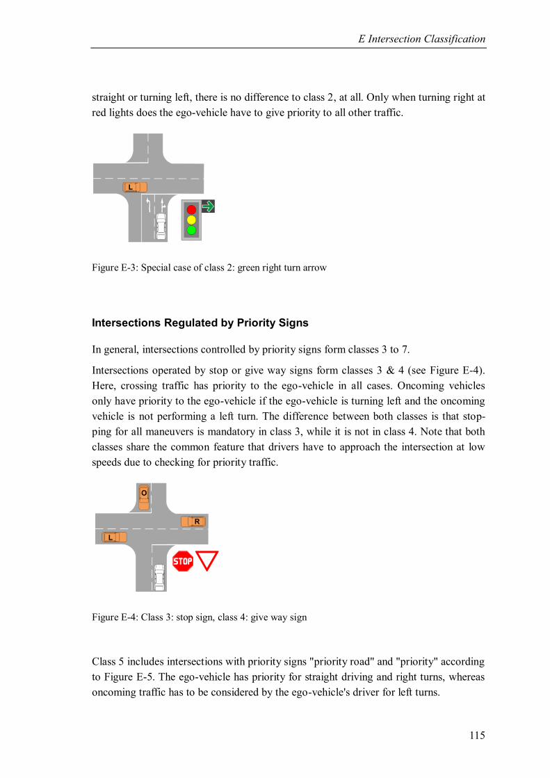
E Intersection Classification
115
straight or turning left, there is no difference to class 2, at all. Only when turning right at
red lights does the ego-vehicle have to give priority to all other traffic.
Figure E-3: Special case of class 2: green right turn arrow
Intersections Regulated by Priority Signs
In general, intersections controlled by priority signs form classes 3 to 7.
Intersections operated by stop or give way signs form classes 3 & 4 (see Figure E-4).
Here, crossing traffic has priority to the ego-vehicle in all cases. Oncoming vehicles
only have priority to the ego-vehicle if the ego-vehicle is turning left and the oncoming
vehicle is not performing a left turn. The difference between both classes is that stop-
ping for all maneuvers is mandatory in class 3, while it is not in class 4. Note that both
classes share the common feature that drivers have to approach the intersection at low
speeds due to checking for priority traffic.
Figure E-4: Class 3: stop sign, class 4: give way sign
Class 5 includes intersections with priority signs "priority road" and "priority" according
to Figure E-5. The ego-vehicle has priority for straight driving and right turns, whereas
oncoming traffic has to be considered by the ego-vehicle's driver for left turns.

E Intersection Classification
116
Figure E-5: Class 5: priority road and priority sign
Classes 6 and 7 contain turning priority roads that turn both directions. This class is only
relevant for the ego-vehicle driving on the priority road. If the ego-vehicle is approach-
ing a turning priority road via a minor road, class 3 or 4 is applied because of the give-
way regulations for minor roads intersecting with priority roads. On right turning priori-
ty roads (class 6), the ego-vehicle has to consider oncoming traffic (from the right) on
the priority road for straight driving and left turns, as shown in Figure E-6. For left
turning priority roads (class 7), the ego-vehicle has priority for every maneuver.
Figure E-6: Class 6 and class 7: turning priority roads

E Intersection Classification
117
Intersections Regulated by General Regulations
Intersections operated by priority to right regulation are represented by class 8. Here,
oncoming traffic has priority for ego-vehicle left turns and crossing traffic from the
right is relevant for all maneuvers as shown in Figure E-7.
Figure E-7: Class 8: priority to right
Intersection with Bypass Roads
Intersections with bypass roads to the right (allowing right turns without having to line
up at traffic lights) are represented by class 9, as shown in Figure E-8. For a straight
driving or left turning ego-vehicle, the situation is the same as class 2. In cases of right
turns, only crossing priority traffic from the left is relevant for the ego-vehicle's driver.
Figure E-8: Class 9: Bypass roads

118
F Test Drives
The following table summarizes the driving instructions provided to test subjects during
driving.
Start in Heinrich-Fuhr-Straße in public parking lot
drive straight, crossing Heinrich-Fuhr-Straße
turn left on to Wilhelm-Jäger-Straße
turn right on to Gundolfstraße
turn left on to Heidenreichstraße
turn right on to Roßdörfer Straße
turn right on to Inselstraße
turn right on to Soderstraße
turn right on to Heidenreichstraße
drive straight, crossing Roßdörfer Straße
turn right on to Heinrichstraße
turn right on to Inselstraße
turn right on to Roßdörfer Straße
drive straight, crossing Heidenreichstraße
turn right on to Frankenäckerweg
turn left on to Heinrichstraße
turn left on to Erlenweg
turn left on to Roßdörfer Straße
drive straight, crossing Hicklerstraße
turn right on to Wilhelm-Jäger-Straße
turn left on to Gundolfstraße, then turn left on to Heidenreichstraße
drive straight, crossing Roßdörfer Straße
turn left on to Heinrichstraße
turn right on to Rehkopfweg
turn left on to Kohlbergweg
turn left on to Dachsbergweg
turn left on to Heinrichstraße, turn right in Frankenäckerweg
turn left on to Roßdörfer Straße
drive straight, crossing Heidenreichstraße
turn left on to Inselstraße
drive straight, crossing Kiesstraße
drive straight, crossing Heinrichstraße
drive straight, crossing Glasbergweg
turn left on to Kohlbergweg
turn left on to Heidenreichstraße

F Test Drives
119
drive straight, crossing Glasbergweg
drive straight, crossing Heinrichstraße
turn left on to Roßdörfer Straße, then turn left on to Inselstraße
turn right on to Heinrichstraße
drive straight, crossing Beckstraße
turn right on to Gervinusstraße
drive straight, crossing Kiesstraße
drive straight, crossing Roßdörfer Straße
turn right on to Soderstraße
turn right on to Beckstraße
drive straight, crossing Roßdörfer Straße
turn right on to Kiesstraße
turn left on to Gervinusstraße
turn right on to Heinrichstraße
turn right on to Wienerstraße
drive straight, crossing Kiesstraße
drive straight, crossing Roßdörfer Straße
turn left on to Soderstraße
drive straight, crossing Martin-Buber-Straße
turn left on to Teichhausstraße
drive straight, crossing Nieder-Ramstädter Straße
turn left on to Heinrichstraße
turn left on to Gervinusstraße
turn left on to Kiesstraße
drive straight, crossing Wienerstraße
turn right on to Nieder-Ramstädter Straße
turn right on to Roßdörfer Straße
drive straight, crossing Martin-Buber-Straße
turn right on to Wienerstraße
turn right on to Kiesstraße, then turn right on to Nieder-Ramstädter Straße
turn left on to Nieder-Ramstädter Straße
drive straight, crossing Riedlingerstraße
turn left on to Hochstraße
turn left on to Kiesstraße
turn right in Hoffmannstraße
drive straight, crossing Heinrichstraße, then turn right on to Hochstraße
drive straight, crossing Heinrichstraße
turn left on to Kiesstraße
turn left on to Karlstraße
turn left on to Heinrichstraße
turn right on to Martinstraße
drive straight, crossing Rückertstraße

F Test Drives
120
turn right on to Steinackerstraße
turn right on to Karlstraße, then turn left on to Annastraße
drive straight, crossing Wilhelminenstraße
drive straight, crossing Eichbergstraße
drive straight, crossing Stauffenbergstraße
turn right on to Heidelberger Straße
turn right on to Hügelstraße
turn left on to Saalbaustraße
turn left on to Elisabethenstraße
drive straight, crossing Neckarstraße
turn left on to Landgraf-Philipps-Anlage
turn left on to Hügelstraße
turn left on to Neckarstraße
turn right on to Elisabethenstraße
turn right on to Saalbaustraße, then turn right on to Hügelstraße
turn right on to Neckarstraße
drive straight, crossing Elisabethenstraße
drive straight, crossing Adelungstraße
drive straight, crossing Rheinstraße, then turn left on to Bleichstraße
turn left on to Steubenplatz
turn right on to Rheinstraße
turn right on to Feldbergstraße, then turn right on to Mornewegstraße and Steubenplatz
turn left on to Rheinstraße
turn right on to Neckarstraße
turn left on to Adelungstraße
turn right on to Saalbaustraße
drive straight, crossing Elisabethenstraße
turn right on to Hügelstraße
turn left on to Neckarstraße
drive straight, crossing Riedeselstraße
drive straight, crossing Heinrichstraße
drive straight, crossing Annastraße
drive straight, crossing Hermannstraße
turn right on to Ehretstraße
turn left on to Donnersbergring
turn left on to Bessunger Straße
turn right on to Heidelberger Straße
drive straight, crossing Sandbergstraße
turn left on to Weinbergstraße
drive straight, crossing Brüder-Knauß-Straße
drive straight, crossing Sturzstraße
turn left on to Ludwigshöhstraße

F Test Drives
121
drive straight, crossing Sandbergstraße
turn right on to Jahnstraße, then turn into roundabout back on to Jahnstraße
turn left on to Bessunger Straße
turn right on to Sandbergstraße
turn left on to Kiesbergstraße
turn left on to Weinbergstraße, then turn left on to Ludwigshöhstraße
turn left on to Bessunger Straße
turn right on to Heidelberger Straße
drive straight, crossing Niederstraße
turn right on to Hermannstraße
drive straight, crossing Eichbergstraße
drive straight, crossing Bessunger Straße
turn right on to Klappacher Straße, then turn left in roundabout in Jahnstraße
turn right on to Clemensstraße
turn right on to Seekatzstraße
turn left on to Klappacher Straße
turn right on to Herrngartenstraße
turn left on to Prälat-Diehl-Straße
drive straight, crossing Moosbergstraße
turn left on to Landskronstraße
turn left on to Klappacher Straße
turn left on to Moosbergstraße
drive straight, crossing Mendelssohnstraße
turn right on to Prälat-Diehl-Straße
turn right on to Herrngartenstraße
turn right on to Moosbergstraße, then drive straight, crossing Mendelssohnstraße
turn left on to Prälat-Diehl-Straße, then turn left on to Landskronstraße
turn right to stay on Landskronstraße
turn left on to Nieder-Ramstädter Straße
turn left on to Heinrichwingertsweg
(destination reached)

122
G Accuracy of Input Signals
Data Acquired via CAN Bus
All input data used for maneuver prediction acquired from the vehicle's sensors via
CAN bus are listed below. Typical values for the accuracy of state-of-the-art automotive
sensor systems are given and used for the analysis of effects in the following.
Typical steering wheel angle sensors have an accuracy of .192 Inaccuracies in
the steering wheel angle affect the path prediction of the linear one track model. The
path prediction influences all information gathered by image processing, the detection
of adjacent lanes, and detection of vehicle follow behavior. Data from test drives done
in this work shows that steering wheel angles of are used by test subjects for
corrective lane keeping actions even when driving straight. Furthermore, drivers do not
drive curves with constant steering wheel angles, as shown in Figure G-1. They adapt
their steering wheel angle according to the yaw motion of the vehicle in relation to the
desired path. Depending on the steering behavior, the inaccuracy in the path prediction
is of one or two orders of magnitude higher than .
Figure G-1: Exemplary steering motion during turning
192 Mörbe, M.: Vehicle Dynamics Sensors for DAS (2016), p.293.
0 1 2 3 4 5 6-300
-250
-200
-150
-100
-50
0
50
time in s
ste
eri
ng
wh
eel an
gle
in
°
Curve Steering

G Accuracy of Input Signals
123
Automotive ego-speed measurement is done by wheel rotation sensors. Actual speed
sensors reach an accuracy of
.193
The vehicle's speed is used for the
speed indicator itself, calculation of predicted stop distances, estimated lateral accelera-
tions in cases of turns, detection of adjacent lanes, and detection of vehicle follow be-
havior. Even when using a total of 50 speed intervals
, the maximum
error caused by inaccuracies in the speed signal is 10 times smaller than the interval
width and is therefore neglected for the speed indicator. The predicted stop distance is
calculated according to (5-12) and (5-13). Here, the error caused by a speed
inaccuracy of
, assuming a typical acceleration of
and an
approach speed of
, is . Thus, the effect of is neg-
ligible in comparison to the distance inaccuracy caused by the localization system.
Lateral accelerations based on the distance to the next intersection and road geometry,
as estimated in (5-9), are affected by , as well. Assuming a minimum turn radius
of and an approach speed of
results in an error of
that is ignored, as well. Finally, the ego-vehicle's speed is used to
classify radar objects detected around the ego-vehicle in oncoming traffic and driving in
same direction. Here, the relative speeds of objects detected by the radar sensors are at
least two orders of magnitude higher than , so that is without effect on the classi-
fication. The same applies to the effect of on the detection of vehicle follow behav-
ior: While driving, the ego-vehicle's speed is two orders of magnitudes higher than
.
Sensors for measuring longitudinal accelerations for vehicle dynamics control show a
measurement accuracy of
.194
The ego-vehicle's lateral acceleration is
used for the acceleration indicator and the calculation of the predicted stop distance. The
interval width of the acceleration indicator is one order of magnitude higher than ,
so the influence of is neglected. Using the same assumptions as above, an inaccu-
racy of results from . Due to the fact that varying intersection
geometries influence the driver's behavior and therefore result in varying predicted stop
distances, is without effect on the detection of a predicted stop near the intersec-
tion center.
193 Niehues, D.: Diss., Positionsbestimmung von Fahrzeugen, p.66.
194 Mörbe, M.: Vehicle Dynamics Sensors for DAS (2016), pp. 296–297.

G Accuracy of Input Signals
124
Automotive yaw rate sensors reach an accuracy of approx.
.195
The vehicle's
yaw rate is used to calculate the curvature of the path driven during a turn maneuver.
The curvature is used to define the reference point a posteriori, as described in section
6.3.2. Assuming typical yaw rates of
during turning and a turning speed of
,196
a measurement error of
leads to an error of
that is two orders of magnitude smaller than and therefore not considered in the
following.
The driver's pedal operation inputs are measured by the brake pressure sensor and the
acceleration pedal sensor. Typical brake pressure sensors are within a range of
.197
Typical values for the accuracy of pedal states are
.198
Inaccuracies in both signals affect only the corresponding indicator
directly. The maximum error caused by the acceleration pedal inaccuracy is 10 times
smaller than the interval width of the indicator. Thus, the effect of the inaccuracy of the
acceleration pedal signal is neglected. Due to the higher number of intervals and the
higher maximum error in the brake pressure measurement as compared to the accelera-
tion pedal, the maximum resulting error is higher. Here, the inaccuracy of
can lead to activating up to one interval higher or lower than the
real value corresponds to. However, a maximum error of one interval is tolerated here.
The gear position is transferred as an absolute gear number. Thus, no measurement
inaccuracy discussion is needed.
Head and Gaze Tracking Data
The inaccuracy in the measurement of the head and gaze rotation is given by
, according to the specifications of the headtracking system used.199
The
minimum width of intervals in the head and gaze indicator is five times larger than
. Thus, a maximum error of one interval can occur due to measurement inaccura-
cies. For the detection of a fixation on the rear view mirrors, bounding boxes that repre-
sent the mirrors are used within the head tracking software. If a fixation on a bounding
box is detected by the head tracking system, the box is activated and set as the active
element. To cope with inaccuracies in the gaze direction, bounding boxes are slightly
195 Reif, K.: Automobilelektronik (2014), p.119.
196 The typical turning speed was determined in pre-tests before starting the test subject study.
197 N.N.: Brake pressure sensor.
198 Mörbe, M.: Vehicle Dynamics Sensors for DAS (2016), pp. 300–301.
199 N.N.: faceLAB5 (2009).

G Accuracy of Input Signals
125
larger than the real mirror is. Thus, the inaccuracy in the measurement is without effect.
Furthermore, the head and gaze rotation angles vary with the driver's seat adjust-
ments, as schematically shown for a smaller and a larger driver in Figure G-2.
Figure G-2: Effect of seat adjustment
Assuming a longitudinal distance of and a lateral distance of
as typical values for the distance between the driver's head and the rear mirror, a lateral
seat adjustment range of results in a change of . Thus, the
effect of is, however, ignored.
Radar Detections
Using the concept of radar separation capability as cell volume for the dimensions
distance, relative velocity, and azimuth angle,200
typical values for state-of-the-art auto-
motive radar sensor are:201
(G-1)
The measurement inaccuracy in longitudinal distance affects the detection of
vehicle follow behavior, the detection of adjacent lanes to the ego-vehicle, and the
maneuver detection of a leading vehicle for multiple lanes. Due to the fact that the -
based and the -based criterion introduced in section 5.3 detect vehicle follow behavior
by underruning a limit that is at least one order of magnitude higher than , the
effect of is neglected. The same applies to the radar based detection of adjacent
lanes and the tracking of preceding vehicles. An object detected by radar sensors is used
for the calculation of adjacent lane state as soon as it is within a range defined as rele-
vant around the ego-vehicle and being two orders of magnitude higher than .
200 Winner, H.: Automotive RADAR (2016), p.370.
201 Winner, H.: Automotive RADAR (2016), p.382.

G Accuracy of Input Signals
126
Apart from the detection of follow behavior, the accuracy of objects’ relative speed
is used to classify objects detected by the radar sensors into oncoming
traffic and traffic driving in the same direction. Here, the same applies as above: Rela-
tive speeds of objects are two orders of magnitude higher than so that is
without effect to the classification. The same applies to the detection of follow vehicle
behavior: Typical relative speeds are one order of magnitude higher than .
The measurement accuracy of objects’ azimuth angle affects the target selection of
preceding vehicles, the assignment of objects to adjacent or ego-lanes, and the maneu-
ver detection of a leading vehicle. Based on the regulations for designing urban roads,202
a road with two lanes shall have a width of . Considering one lane,
the unknown position of the ego-vehicle in the lane, and the unknown point of reflection
of a target vehicle,
is used to calculate the maximum longitudinal distance
without affecting the lane allocations caused by :
(G-2)
For all objects detected at distances , is without affect on the lane
assignment. Furthermore, as mentioned above, the path prediction based on the steering
wheel input by the driver creates higher inaccuracies than the inaccuracy caused by .
Therefore, the distance of objects used for detecting adjacent lanes and selecting and
tracking preceding vehicles is limited to .
Road Markings
Detected road markings are transferred into binary into the control unit. Inaccuracies in
the detection process arise due to false positive and negative detections in the image
processing, nondetected lane changes of the ego-vehicle, and missed changes in the
arrows during the intersection approach, as shown in Figure G-3. In this example, both
direction arrows are detected at position 1. If the arrows’ changed layout is not detected
at position 2, both arrows are kept active for the ego-lane, even at position 3.
202 Baier, R.: Richtlinien für die Anlage von Stadtstraßen (2007), p.69.

G Accuracy of Input Signals
127
Figure G-3: Missed change detection of road markings
As discussed in section 5.4.3, imperfections in the perception of road markings are
taken into account by using training data created statistically, instead of directly deriv-
ing the maneuver from the direction arrow detected.
Localization
The positioning accuracy of a conventional GNSS receiver varies with the conditions it
is used in and is influenced by several sources of errors, as for example the dilution of
precision (DOP), multipath scattering, atmospheric effects, and clock errors. These
errors can sum up to a total inaccuracy of .203
To reduce the localization error, Inertial Navigation System (INS) that measure rotation
and acceleration of the vehicle via an Inertial Measurement Unit (IMU) are combined
with GNSS receivers.204
A similar principle is applied by the dead reckoning process in
the GNSS receiver used in this work. Instead of accelerations, an odometer signal pro-
vided by the vehicle is combined with a gyroscope to calculate a relative position to the
starting point. This position is combined with the received GNSS position by internal
models of the receiver. Thus, the localization accuracy using a GNSS receiver with dead
reckoning functionality is enhanced in relation to a localization based solely on
GNSS.205
To determine the remaining positioning error, three types of errors have to be
considered in this work, as shown in Figure G-4: The positioning error of the
measured GPS position, the error of the digital map, and the positioning error
of the aerial image used as ground truth.
203 N.N.: GNSS Error Sources (2016).
204 N.N.: GNSS and INS (2016).
205 N.N.: Dead Reckoning (2016).

G Accuracy of Input Signals
128
Figure G-4: Positioning errors
A recent study comparing the results of previous studies focusing on the accuracy of
aerial images provided by Google Earth206
states a root mean square error (RMSE) of
2.18 m in horizontal accuracy.207
Pre-tests done in this project have shown an RMSE GNSS localization error of
in relation to aerial images provided by Google Earth and an average map
precision of of the road network of openstreetmap208
in relation to the
aerial image. Note that these values are only average values and that the accuracy varies
depending on the location. The remaining distance to the intersection center is
extracted from the map matched position of the vehicle. According to Figure G-4, an
average error of in relation to the aerial image occurs. Consider-
ing and , the maximum resulting positioning inaccuracy is
. Following the approach introduced in this work
relying on distance intervals, the inaccuracy affects the calculation of all indica-
tors’ transfer functions due to the potentially wrong determination of the actual distance
interval. In reality, the road layout of urban intersections varies heavily even within one
intersection class depending upon the features of each location, available space for the
intersection, type of roads connected by the intersection, and the amount of traffic using
206 Google Earth 7.1.5.1557, access: 20.06.2015.
207 Farah, A.; Algarni, D.: Accuracy of Googleearth (2014), p.104.
208 N.N.: OpenStreetMap (2016).

G Accuracy of Input Signals
129
the road.209
Thus, a variety of geometric forms exist even within one intersection class,
resulting in different trajectories. Using the intersection center is an inaccuracy itself
because the layout of the intersection is not considered. However, the approach applied
in this project deals with this inaccuracy by using training data acquired from a large set
of intersections with varying geometry.
Furthermore, affects the calculation of the predicted stop distance and the esti-
mated lateral accelerations, as introduced in section 5.4.4. Due to varying intersection
size and layout, all predicted stops near the intersection center are
used. Thus, a limitation for is derived:
(G-3)
209 Baier, R.: Richtlinien für die Anlage von Stadtstraßen (2007), pp. 109–110.

130
H Reference Points
Especially with the ego-vehicle driving at low speeds, curvature calculation based on
the vehicle's yaw rate sensor is error-prone due to signal noise. During standstill, the
calculation fails completely due to the absence of a yaw rate aside from noise. A
survey of different methods to derive the curvature given by Winner210
shows that a
well performing calculation of the curvature can be achieved by combining the curva-
ture calculation based on the vehicle's yaw rate sensor and the curvature calcula-
tion using the steering wheel angle . The curvature based on the output of the
vehicle's yaw rate sensor and the ego-vehicle's speed is given by:
(H-1)
The approximation of the curvature is based on a linear single track model, using the
vehicle's steering wheel angle , the steering transmission ratio , the vehicle's
speed , its characteristic speed
, and the wheelbase WB:210
(H-2)
The vehicle's characteristic speed describes the vehicle's understeering behavior based
on the relation of the axles' cornering stiffness and is given by:211
(H-3)
Here, and represent the cornering stiffness of the front and rear axles, the
ego-vehicle's mass, and and are the lever arms between the axles and the
vehicle's center of gravity. While the curvature calculation is based solely on the yaw
rate sensor when the vehicle is driving above a transition speed , a mixture of
and is applied below the transition speed. When the vehicle is stopped, is used
solely. A speed dependent factor is defined using the transition speed of
:
210 Winner, H.; Schopper, M.: Adaptive Cruise Control (2016), pp. 1116–1117.
211 Mitschke, M.: Dynamik von Kraftfahrzeugen (2003), p.562.

H Reference Points
131
(H-4)
The total curvature is given by
(H-5)
The calculation of is simplified by neglecting the vehicle's characteristic speed
. The simplification is done based on the following assumption: Typical values of
the characteristic speed for understeering vehicles are
.
212 Assuming
, the factor
is limited to a maximum of
,
with the vehicle driving at
. Using the speed dependent factor , the
total error is reduced depending on the vehicle's speed. Thus, neglecting the characteris-
tic speed results in a maximum error in of 1.6 % at an ego-vehicle speed of
. Thus, the simplified calculation of is given by:
(H-6)
Figure H-1 shows the curvatures of an exemplary turn maneuver. The turn maneuver is
executed at a low speed resulting in a noisy signal of the ego-vehicle's yaw rate sensor
and a noisy curvature , displayed as dashed line. The calculated curvature is
displayed as dash-dotted line and the combined curvature is displayed as solid
line.
Figure H-1: Curvatures
212 Halfmann, C.; Holzmann, H.: Kraftfahrzeugdynamik (2003), p.214.
0 5 10 15 20
-0.15
-0.1
-0.05
0
0.05
time in s
cu
rva
ture
in
1/m
Curvature Calculation
kappa_psi_p
kappa_delta
kappa_total

H Reference Points
132
Based on the combined curvature, the apex of the turn maneuver is determined using the
area under the curvature-vs.-travelled-distance curve. The distance travelled during the
turn is acquired by integrating the ego-vehicle's velocity over time:
(H-7)
With a known apex of the maneuver, the reference point for turn maneuver initialization
is defined as a percentage of the apex's curvature.
Using a percentage of the apex results in an individualized maneuver reference point
free of localization inaccuracies.

133
I Neglecting Intersection Classes
The figures shown in this annex present the prediction performance reached with the
prediction system when intersection classes are ignored during training.
Figure I-1: Results of class 5 without separated training data (priority road and priority sign)
Figure I-2: Results of class 2 without separated training data (traffic lights for all directions)
0123456789100
0.1
0.2
0.3
0.4
0.5
0.6
0.7
0.8
0.9
1
time to reference point in s
tru
e p
osit
ive p
red
icti
on
rate
s
Prediction Performance for Priority Roads (Class 5)
right turns
left turns
straights
0123456789100
0.1
0.2
0.3
0.4
0.5
0.6
0.7
0.8
0.9
1
time to reference point in s
tru
e p
osit
ive p
red
icti
on
rate
s
Prediction Performance for Traffic Lights (Class 2)
right turns
left turns
straights
data: all
drivers: all
inference: average
data: all
drivers: all
inference: average

I Neglecting Intersection Classes
134
Figure I-3: Results of class 4 without separated training data (give way sign)
Figure I-4: Results of class 3 without separated training data (stop sign)
0123456789100
0.1
0.2
0.3
0.4
0.5
0.6
0.7
0.8
0.9
1
time to reference point in s
tru
e p
osit
ive p
red
icti
on
rate
s
Prediction Performance at Give Way Signs (Class 4)
right turns
left turns
straights
0123456789100
0.1
0.2
0.3
0.4
0.5
0.6
0.7
0.8
0.9
1
time to reference point in s
tru
e p
osit
ive p
red
icti
on
rate
s
Prediction Performance at Stop Signs (Class 3)
right turns
left turns
straights
data: all
drivers: all
inference: average
data: all
drivers: all
inference: average

I Neglecting Intersection Classes
135
Figure I-5: Results of class 8 without separated training data (priority to right)
0123456789100
0.1
0.2
0.3
0.4
0.5
0.6
0.7
0.8
0.9
11
time to reference point in s
tru
e p
osit
ive p
red
icti
on
rate
sPrediction Performance for Priority to Right (Class 8)
right turns
left turns
straights
data: all
drivers: all
inference: average

136
J Elements of the Adaptation System
Temporary Data Buffer
The adaptation process is carried out while the vehicle is in use and is driving on urban
roads. Thus, a stream of measurement data and calculations are produced by the vehi-
cle's sensors and based on sensor data. For the adaptation process, sequences of inter-
section approaches have to be extracted from the data stream. The beginning of these
approach sequences is located at the time the ego-vehicle enters the relevant area before
the intersection. The sequences terminate at the reference point of the maneuver (initial-
ization of the maneuver). Because the termination of sequences is not known a priori, all
relevant data used for maneuver prediction has to be stored in a temporary data buffer.
This data is no longer needed when the ego-vehicle has left the intersection, so the
sequence is transferred to the data pool and the temporary buffer is cleared.
Maneuver Detection
To classify the approach sequence, a maneuver detector is needed. The maneuver detec-
tor detects which maneuver is performed by the ego-vehicle and outputs the information
to the data pool. The maneuver will be known at the very latest after the ego-vehicle has
left the intersection, so the maneuver specific reference point can then be calculated.213
Several methods can be applied for a posteriori maneuver detection. Turn maneuvers
can be detected by evaluating the vehicle's steering wheel angle , lateral acceleration
or yaw rate . These methods all require the definition of limits that the input signal
has to exceed for at least a minimum distance travelled (e.g. a turn is detected if
for a minimum travel distance ). Aside from that, varying intersection
size and geometry lead to false detections when applying these methods and straight
driving maneuvers at intersections cannot be identified at all. To be able to detect
straight driving maneuvers, information of the existence of an intersection is needed.
This information is taken from a localization system and a digital map as described in
section 4.2. Using a localization system and a digital map offers an alternative maneu-
ver detection manner: With the ego-vehicle's position matched to the streets of a digital
map, the maneuver is detected as follows: The way id214
and vehicle's driving direction
213 Note that the reference point marks the initialization of the maneuver itself and the end of the approach
sequence.
214 A way id is an unique identifier in OSM used to identify a way.
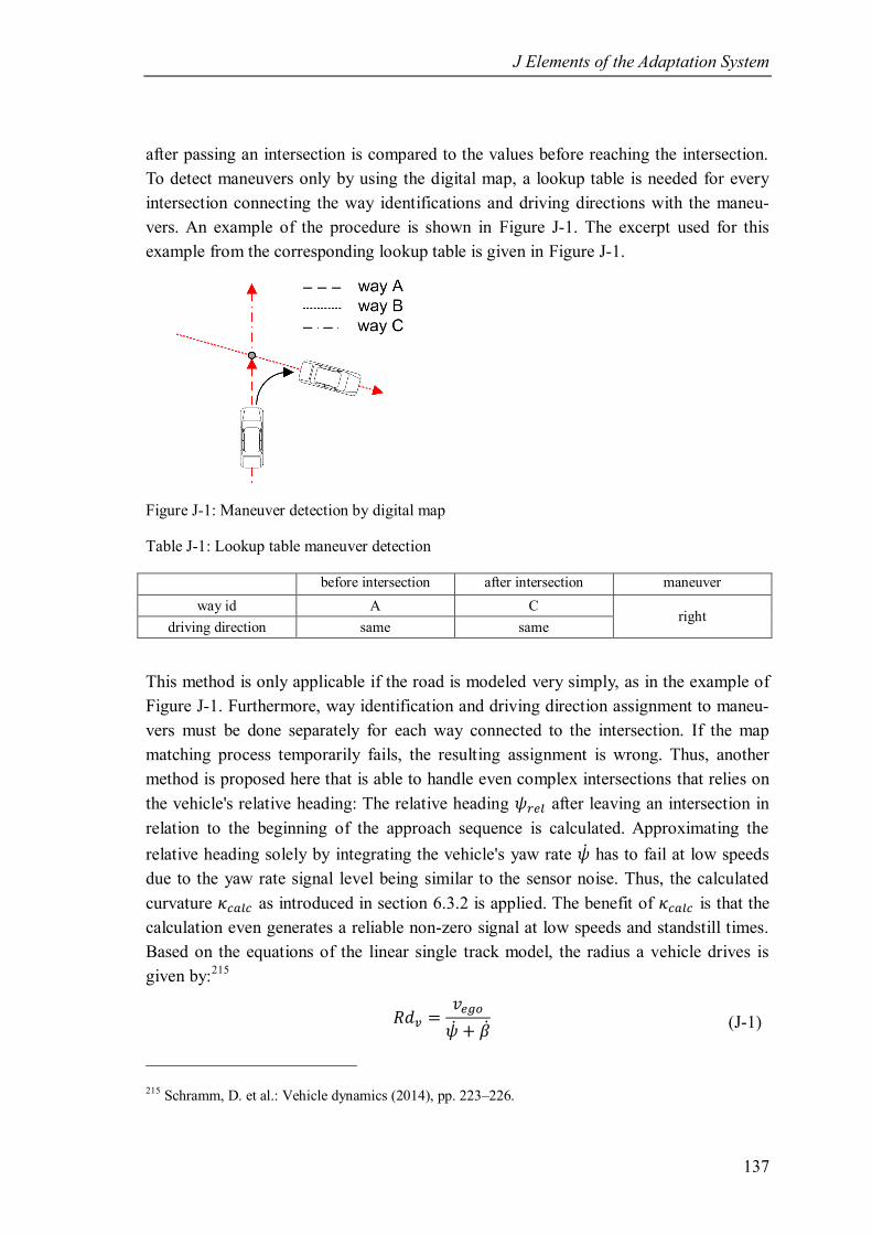
J Elements of the Adaptation System
137
after passing an intersection is compared to the values before reaching the intersection.
To detect maneuvers only by using the digital map, a lookup table is needed for every
intersection connecting the way identifications and driving directions with the maneu-
vers. An example of the procedure is shown in Figure J-1. The excerpt used for this
example from the corresponding lookup table is given in Figure J-1.
Figure J-1: Maneuver detection by digital map
Table J-1: Lookup table maneuver detection
before intersection after intersection maneuver
way id A C right
driving direction same same
This method is only applicable if the road is modeled very simply, as in the example of
Figure J-1. Furthermore, way identification and driving direction assignment to maneu-
vers must be done separately for each way connected to the intersection. If the map
matching process temporarily fails, the resulting assignment is wrong. Thus, another
method is proposed here that is able to handle even complex intersections that relies on
the vehicle's relative heading: The relative heading after leaving an intersection in
relation to the beginning of the approach sequence is calculated. Approximating the
relative heading solely by integrating the vehicle's yaw rate has to fail at low speeds
due to the yaw rate signal level being similar to the sensor noise. Thus, the calculated
curvature as introduced in section 6.3.2 is applied. The benefit of is that the
calculation even generates a reliable non-zero signal at low speeds and standstill times.
Based on the equations of the linear single track model, the radius a vehicle drives is
given by:215
(J-1)
215 Schramm, D. et al.: Vehicle dynamics (2014), pp. 223–226.

J Elements of the Adaptation System
138
Neglecting the side slip angle change rate and using
leads to:
(J-2)
Integrating the product of the calculated curvature and the ego-vehicle's speed
results in the vehicle's relative heading . Here, is the start of the intersection
approach sequence and the end of the maneuver after having left the intersection.
(J-3)
However, information of the existence of an intersection is necessary for this calculation
method, as well. The advantage of this method is that the detection is independent of the
intersection's size and geometry. The only information that is needed is the intersec-
tion’s existence. Figure J-2 shows the cumulative distribution functions of the ego-
vehicle's relative heading after leaving the intersection. The figure is based on data from
the test drives, as described above. Thus, using the calculated relative heading, right
turn maneuvers are detected at relative headings , left turns at ,
and straight drives are detected for .
Figure J-2: Vehicle's relative heading after leaving intersection
Data Pool and Calculation Unit
With a known start and end of the approach sequence and the information from the
performed maneuver (right turn, left turn, or straight driving), the approach sequence is
extracted from the temporary buffer and sent to the vehicle's data pool. The data pool
contains all approach sequences known to the prediction system ( for each poten-
-150 -100 -50 0 50 100 1500
0.2
0.4
0.6
0.8
1
relative heading in °
cu
mu
lati
ve d
istr
ibu
tio
n
Heading after Intersection
right turns
left turns
straights

J Elements of the Adaptation System
139
tial maneuver). Thus, before the adaptation process is started, the data pool contains the
initial set of training sequences from all drivers. Within the adaptation process, sequenc-
es extracted from the data stream are added to the data pool according to the maneuver
detected by the maneuver detection unit.
The calculation unit performs the calculations for generating the updated transfer func-
tions, using all sequences of the updated data pool. The result of this calcula-
tion is adapted transfer functions.
Driver Identification
A driver identification unit is essential for the system to cope with various drivers. If a
vehicle is used by more than one driver (or the ownership is transferred to another
person), each driver needs for the transfer functions to be adapted to his personal driv-
ing style, or at least to be a reset to the initial version. Nevertheless, an individual data
pool needs to be stored for each driver. Furthermore, the driver must be identified by the
system to select the personal data pool and to calculate the corresponding transfer func-
tions. In addition, a copy of the initial data pool must always be accessible in the vehicle
that is used if the system fails to identify the driver or a driver is using the vehicle for
the first time. Driver identification here means that the system has to be able to distin-
guish between different people and to recognize individuals already known to the sys-
tem. Potential methods of identifying the driver are introduced in the following.
The easiest but most inaccurate way of driver identification is identifying different
drivers by their memory seat adjustments. This method needs no additional sensors, but
is error-prone for several reasons. If there are more drivers than memory positions
available for seat adjustment, the driver's seat adjustment will automatically vary each
time the setting is done manually. This leads to false detections. If similar settings are
used among different drivers, the system cannot distinguish the drivers as well. Thus,
this method is not feasible.
A more reliable method is using personalized ignition keys or personal tags for each
driver. The latter is available on the market for commercial vehicles that are regularly
driven by various drivers. Here, a couple of systems based on RFID tags that the driver
needs to start the vehicle are available on the market.216
This method has the advantage
that drivers are identified reliably as long as they use their own tag. The disadvantage of
this method is that an additional RFID reader must be placed in the dash and it is less
comfortable for the driver. Especially as keyless starter systems become more and more
popular, having to provide the RFID tag each time the vehicle is used is expected to
have little approval from drivers.
216 N.N.: Automatic driver identification (20161).

J Elements of the Adaptation System
140
A third method for identifying the driver is using video. Here, a camera is used that is
placed on the vehicle's dashboard facing towards the driver. The driver's face is recog-
nized by biometric features. Assuming that the camera is mounted in the vehicle for
monitoring the driver's state and fatigue anyway, no additional hardware is needed. This
method offers the most reliable driver identification without loss of comfort for the
driver. A prototype of such an identification system for automotive use was presented
several years ago.217
Monitoring of Adaptation Process
With the adaptation functionality working as described above, the number of intersec-
tion approach sequences stored in the data pool increases with each intersection the
vehicle crosses. Due to limitations of physical storage and computing power, a monitor-
ing function that limits the process of adding new sequences to the data pool is needed.
The increase in prediction performance of the individualized driver adaptation has to
reach a saturation level if the adapted transfer functions absolutely conform to the indi-
vidual driving style. Adding additional training sequences beyond the saturation only
increases the data pool without altering the transfer functions. Thus, a monitoring func-
tion is applied that regularly compares the adapted transfer functions to a copy of an
older state. If the correlation between the "old" state of the functions and the current one
is above a predefined limit, the adaptation process is aborted.
Note that intervals between the current and the "old" set of transfer functions that are
compared have to be big enough for reliable comparison results. Comparing two sets of
transfer functions with insufficient training sequences to distinguish both data pools
used for creating the functions will lead to the false decision that the training process is
finished. Based on that wrong decision, no additional sequences are accepted for further
increasing the data pool. The interval that is needed for reliable assessment of whether
the training process is finished or not has to be identified by real road tests.
217 N.N.: BMW Fahrererkennung (2008).

141
List of References
ADAC e.V.: Autotest Volvo XC90
ADAC e.V.: Autotest Volvo XC90 D5 Momentum AWD Geartronic
Alhayaseen, W. et al.: Variation of Left-turning Vehicle (2011)
Alhayaseen, Wael; Asano Miho; Suzuki Kazufumi; Nakamura Hideki: Analysis on the Variation of Left-
turning Vehicle Spatial Trajectories Inside Intersections, in: Journal of the Eastern Asia Society for
Transportation Studies , Issues 9, pp. 1543–1557, 2011
Auto.de: Als die Automatik schalten lernte (2015)
Auto.de: Als die Automatik schalten lernte; http://www.auto.de/magazin/als-die-automatik-schalten-
lernte/, 2015, Access 07.09.2016
Bai, J.; Zhang, L.: Identification of Driver's Intentions (2010)
Bai, Jingwen; Zhang, Licai: Study on Identification of Driver's Intentions Based on Cloud Model, in:
Institute of Electrical and Electronics Engineers (IEEE) (Ed.): 2010 International Conference on E-
Product E-Service and E-Entertainment (ICEEE 2010), 2010
Baier, R.: Richtlinien für die Anlage von Stadtstraßen (2007)
Baier, Reinhold: Richtlinien für die Anlage von Stadtstraßen (RASt), FGSV , Issues 200, 2006. Edition,
FGSV-Verl., Köln, 2007
Bar Hillel, A. et al.: Recent progress in road and lane detection (2014)
Bar Hillel, Aharon; Lerner, Ronen; Levi, Dan; Raz, Guy: Recent progress in road and lane detection: a
survey, in: Machine Vision and Applications (3) , Issues 25, pp. 727–745, 2014
Bartels, A. et al.: Lane Change Assistance (2016)
Bartels, Arne; Meinecke, Marc-Michael; Steinmeyer, Simon: Lane Change Assistance, in: Winner,
Hermann et al. (Eds.): Handbook of Driver Assistance Systems, Springer Verlag, 2016
BASt: Richtlinien für die Markierung von Straßen (1980)
Bundesanstalt für Straßenwesen: Richtlinien für die Markierung von Straßen, Bonn, 1980
Benesty, J.: Noise reduction in speech processing (2009)
Benesty, Jacob (Ed.) Noise reduction in speech processing, Springer Topics in Signal Processing , Issues
2, Springer, Berlin, London, 2009
Berndt, H. et al.: Driver Braking Behavior (2007)
Berndt, Holger; Wender, Stefan; Dietmayer, Klaus: Driver Braking Behavior during Intersection Ap-
proaches and Implications for Warning Strategies for Driver Assistant Systems, in: Institute of Electrical
and Electronics Engineers (IEEE) (Ed.): 2007 IEEE Intelligent Vehicles Symposium (IV), 2007
Berndt, H.: Diss., Fahrerabsichtserkennung und Gefährlichkeitsabschätzung (2016)
Berndt, Holger: Fahrerabsichtserkennung und Gefährlichkeitsabschätzung für vorausschauende Fahreras-
sistenzsysteme, Dissertation Universität Ulm, Schriftenreihe des Instituts für Mess-, Regel- und Mikro-
technik Band 16, Universität Ulm, Institut für Mess-, Regel- und Mikrotechnik, Ulm, 2016

List of References
142
Berndt, H.; Dietmayer, K.: Driver intention inference (2009)
Berndt, Holger; Dietmayer, Klaus: Driver intention inference with vehicle onboard sensors, in: Institute
of Electrical and Electronics Engineers (IEEE) (Ed.): 2009 IEEE International Conference on Vehicular
Electronics and Safety (ICVES), 2009
Blobel, V.; Lohrmann, E.: Datenanalyse (1998)
Blobel, Volker; Lohrmann, Erich: Statistische und numerische Methoden der Datenanalyse, Teubner-
Studienbücher : Physik, Teubner, Stuttgart, Leipzig, 1998
Bolovinou, A. et al.: Driving style recognition (2014)
Bolovinou, Anastasia; Amditis, Angelos; Bellotti, Francesco; Tarkiainen, Mikko: Driving style recogni-
tion for co-operative driving: A survey, in: IARIA (Ed.): Proceedings of 6th International Conference on
Adaptive and Self-Adaptive Systems and Applications, 2014
Bonnin, S. et al.: General Behavior Prediction (2014)
Bonnin, Sarah; Weisswange, Thomas H.; Kummert, Franz; Schmuedderich, Jens: General Behavior
Prediction by a Combination of Scenario-Specific Models, in: IEEE Transactions on Intelligent Transpor-
tation Systems (4) , Issues 15, pp. 1478–1488, 2014
Bubb, H.: Haptik im Kraftfahrzeug (2001)
Bubb, Heiner: Haptik im Kraftfahrzeug, in: Jürgensohn, Thomas; Timpe, Klaus-Peter (Eds.): Kraftfahr-
zeugführung, Springer Berlin Heidelberg, Berlin, Heidelberg, 2001
Bubb, H.: Wie viele Probanden braucht man (2003)
Bubb, Heiner: Wie viele Probanden braucht man für allgemeine Erkenntnisse aus Fahrversuchen?, in:
Landau, Kurt; Winner, Hermann; Abendroth, Bettina (Eds.): Fahrversuche mit Probanden? Nutzwert und
Risiko, Fortschrittberichte VDI, Verkehrstechnik / Fahrzeugtechnik Nr. 12, Düsseldorf, 2003
Bundesministeriums der Justiz und für Verbraucherschutz: StVO (2015)
Bundesministeriums der Justiz und für Verbraucherschutz Straßenverkehrs-Ordnung; Straßenverkehrs-
Ordnung vom 6. März 2013 (BGBl. I S. 367), die zuletzt durch Artikel 2 der Verordnung vom 15., 2015
Chen, Y.; Li, L.: Advances in Intelligent Vehicles (2014)
Chen, Y.; Li, L.: Advances in Intelligent Vehicles, Elsevier Science, 2014
Cheng, S. Y.; Trivedi, M. M.: Turn-Intent Analysis Using Body Pose (2006)
Cheng, Shinko Y.; Trivedi, M. M.: Turn-Intent Analysis Using Body Pose for Intelligent Driver Assis-
tance, in: IEEE Pervasive Computing (4) , Issues 5, pp. 28–37, 2006
Chiang, C.-C. et al.: Detecting and recognizing traffic lights (2011)
Chiang, Cheng-Chin; Ho, Ming-Che; Liao, Hong-Sheng; Pratama, Andi; Syu, Wei-Cheng: Detecting and
recognizing traffic lights by genetic approximate ellipse detection and spatial texture layouts, in: Interna-
tional Journal of Innovative Computing, Information and Control (12) , Issues 7, pp. 6919–6934, 2011
Coelingh, E. et al.: Collision Warning with Full Auto Brake and Pedestrian Detection (2010)
Coelingh, Erik; Eidehall, Andreas; Bengtsson, Mattias: Collision Warning with Full Auto Brake and
Pedestrian Detection, in: Institute of Electrical and Electronics Engineers (IEEE) (Ed.): 2010
IEEE Annual Conference on Intelligent Transportation Systems (ITSC), IEEE, [Piscataway, N.J.], 2010
Currie, G.; Reynolds, J.: Hook Turns (2011)
Currie, Graham; Reynolds, James: Managing Trams and Traffic at Intersections with Hook Turns, in:
Transportation Research Record: Journal of the Transportation Research Board , Issues 2219, pp. 10–19,
2011

List of References
143
Dagli, I.; Reichardt, D.: Motivation-based approach to behavior prediction (2002)
Dagli, I.; Reichardt, D.: Motivation-based approach to behavior prediction, in: Institute of Electrical and
Electronics Engineers (IEEE) (Ed.): 2002 IEEE Intelligent Vehicle Symposium, 2002
Darms, M. et al.: Classification and tracking of dynamic objects (2008)
Darms, Michael; Rybski, Paul; Urmson, Chris: Classification and tracking of dynamic objects with
multiple sensors for autonomous driving in urban environments, in: Institute of Electrical and Electronics
Engineers (IEEE) (Ed.): 2008 IEEE Intelligent Vehicles Symposium (IV), 2008
Dingus, T. A. et al.: Automotive Headway Maintenance (1997)
Dingus, Thomas A.; McGehee, Daniel V.; Manakkal, Natarajan; Jahns, Steven K.; Carney, Cher; Hankey,
Jonathan M.: Human Factors Field Evaluation of Automotive Headway Maintenance/Collision Warning
Devices, in: Human Factors: The Journal of the Human Factors and Ergonomics Society (2) , Issues 39,
pp. 216–229, 1997
Donges, E.: Driver Behavior Models (2016)
Donges, Edmund: Driver Behavior Models, in: Winner, Hermann et al. (Eds.): Handbook of Driver
Assistance Systems, Springer Verlag, 2016
Doshi, A.; Trivedi, M.: exploration of eye gaze and head motion (2008)
Doshi, Anup; Trivedi, Mohan: A comparative exploration of eye gaze and head motion cues for lane
change intent prediction, in: Institute of Electrical and Electronics Engineers (IEEE) (Ed.): 2008 IEEE
Intelligent Vehicles Symposium (IV), 2008
Doshi, A.; Trivedi, M. M.: Tactical driver behavior prediction and intent inference: A review
(2011)
Doshi, Anup; Trivedi, Mohan M.: Tactical driver behavior prediction and intent inference: A review, in:
Institute of Electrical and Electronics Engineers (IEEE) (Ed.): 2011 14th International IEEE Conference
on Intelligent Transportation Systems - (ITSC 2011), 2011
Endsley, M. R.: Toward a theory of situation awareness in dynamic systems (1995)
Endsley, Mica R.: Toward a theory of situation awareness in dynamic systems, in: Human Factors: The
Journal of the Human Factors and Ergonomics Society (1) , Issues 37, pp. 32–64, 1995
Enke, M.: Collision probability (1979)
Enke, M.: Collision probability related to the shift forward of driver reaction, in: National Highway
Traffic Safety Administration (Ed.): Proceedings of 7th International Technical Conference on Experi-
mental Safety Vehicles, 1979
Farah, A.; Algarni, D.: Accuracy of Googleearth (2014)
Farah, Ashraf; Algarni, Dafer: Positional Accuracy Assessment of Googleearth in Riyadh, in: Artificial
Satellites (2) , Issues 49, 2014
Fecher, N.; Hoffmann, J.: Driver Warning Elements (2016)
Fecher, Norbert; Hoffmann, Jens: Driver Warning Elements, in: Winner, Hermann et al. (Eds.): Hand-
book of Driver Assistance Systems, Springer Verlag, 2016
Fenton, N. E.; Neil, M.: Risk assessment and decision analysis (2012)
Fenton, Norman E.; Neil, Martin: Risk assessment and decision analysis with Bayesian networks, Taylor
& Francis, Boca Raton, 2012
Firl, J.: Diss., Probabilistic Maneuver Recognition (2014)
Firl, Jonas: Probabilistic Maneuver Recognition in Traffic Scenarios, Dissertation Karlsruher Institut für
Technologie, Schriftenreihe / Institut für Mess- und Regelungstechnik, Karlsruher Institut für Technolo-
gie , Issues 031, KIT Scientific Publishing, Karlsruhe, 2014

List of References
144
FOT-Net: Field operational tests (2010)
FOT-Net: Field operational tests, 2010
Fuchs, H. et al.: Vehicle-2-X (2016)
Fuchs, Hendrik; Hofmann, Frank; Löhr, Hans; Schaaf, Gunther: Vehicle-2-X, in: Winner, Hermann et al.
(Eds.): Handbook of Driver Assistance Systems, Springer Verlag, 2016
Gipps, P. G.: Car-following model (1981)
Gipps, Peter G.: A behavioural car-following model for computer simulation, in: Transportation Research
Part B: Methodological (2) , Issues 15, pp. 105–111, 1981
Graichen, M.; Nitsch, V.: Effects of Driver Characteristics (2017)
Graichen, Matthias; Nitsch, Verena: Effects of Driver Characteristics and Driver State on Predicting
Turning Maneuvers in Urban Areas: Is There a Need for Individualized Parametrization?, in: Stanton,
Neville A. et al. (Eds.): Advances in Human Aspects of Transportation, Advances in intelligent systems
and computing Nr. 484, Springer International Publishing, Cham, 2017
Grundhoff, S.: Autos ohne Fahrer (2013)
Grundhoff, Stefan: In fünf Jahren fahren unsere Autos ohne Fahrer;
http://www.focus.de/auto/ratgeber/autonomesfahren/tid-29647/autonomes-fahren-in-fuenf-jahren-fahren-
unsere-autos-ohne-fahrer_aid_924084.html, 2013, Access 2016-04-01
Halfmann, C.; Holzmann, H.: Kraftfahrzeugdynamik (2003)
Halfmann, Christoph; Holzmann, Henning: Adaptive Modelle für die Kraftfahrzeugdynamik, VDI-Buch,
Springer Berlin Heidelberg, Berlin, Heidelberg, 2003
Haunert, J.-H.; Budig, B.: Map Matching Given Incomplete Road Data (2012)
Haunert, Jan-Henrik; Budig, Benedikt: An Algorithm for Map Matching Given Incomplete Road Data, in:
Cruz, Isabel (Ed.): 20th International Conference on Advances in Geographic Information Systems, ACM
Digital Library, ACM, New York, NY, 2012
Hayashi, K. et al.: Prediction of stopping maneuver considering driver's state (2006)
Hayashi, K.; Kojima, Y.; Abe, K.; Oguri, K.: Prediction of stopping maneuver considering driver's state,
in: Institute of Electrical and Electronics Engineers (IEEE) (Ed.): 2006 IEEE Intelligent Transportation
Systems Conference, 2006
Hebenstreit, B.: Fahrstiltypen (1999)
Hebenstreit, Benedikt: Fahrstiltypen beim Autofahren, in: Flade, Antje; Limbourg, Maria (Eds.): Frauen
und Männer in der mobilen Gesellschaft, VS Verlag für Sozialwissenschaften, Wiesbaden, 1999
Heckhausen, J.: Motivation und Handeln (2010)
Heckhausen, Jutta: Motivation und Handeln, Springer-Lehrbuch, 4. Edition, Springer, Berlin [u.a.], 2010
Henning, M.: Diss., Preparation for lane change (2010)
Henning, Matthias: Preparation for lane change manoeuvres: Behavioural indicators and underlying
cognitive processes, Dissertation TU Chemnitz, 2010
Hermes, C. et al.: Long-term vehicle motion prediction (2009)
Hermes, Christoph; Wohler, Christian; Schenk, Konrad; Kummert, Franz: Long-term vehicle motion
prediction, in: Institute of Electrical and Electronics Engineers (IEEE) (Ed.): 2009 IEEE Intelligent
Vehicles Symposium (IV), 2009
Hoffmann, J.: Diss., Das Darmstädter Verfahren (EVITA)
Hoffmann, Jens: Das Darmstädter Verfahren (EVITA) zum Testen und Bewerten von Frontalkollisions-
gegenmaßnahmen, Dissertation TU Darmstadt, Darmstadt

List of References
145
Hofmann, M. et al.: Prädiktion potentieller Zielorte (2001)
Hofmann, M.; Bengler, K.; Lang, M.: Ein Assistenzsystem zur fahrer- und situationsadaptiven Prädiktion
potentieller Zielorte für eine robuste Interaktion mit sprachgesteuerten Navigationssystemen, in: VDI
Verlag (Ed.): Tagungsband "Elektronik im Fahrzeug", Baden-Baden, VDI-Verlag, 2001
Hohm, A.: Diss., Überholassistenzsystem (2010)
Hohm, Andree: Umfeldklassifikation und Identifikation von Überholzielen für ein Überholassistenzsys-
tem, Dissertation TU Darmstadt, Fortschritt-Berichte VDI : Reihe 12, Verkehrstechnik, Fahrzeugtechnik ,
Issues 727, VDI-Verl., Darmstadt, 2010
Hulshof, W. et al.: Autonomous Emergency Braking Test Results (2013)
Hulshof, Wesley; Knight, Ian; Edwards, Alix; Avery, Matthew; Grover, Colin: Autonomous Emergency
Braking Test Results, 2013
IEEE: 2008 IEEE Intelligent Vehicles Symposium (IV) (2008)
Institute of Electrical and Electronics Engineers (Ed.) 2008 IEEE Intelligent Vehicles Symposium (IV),
2008
IEEE: ITSC 2010 (2010)
Institute of Electrical and Electronics Engineers (Ed.) 2010 IEEE Annual Conference on Intelligent
Transportation Systems (ITSC), IEEE, [Piscataway, N.J.], 2010
IEEE: ITSC 2011 (2011)
Institute of Electrical and Electronics Engineers (Ed.) 2011 14th International IEEE Conference on
Intelligent Transportation Systems - (ITSC 2011), 2011
Ikenishi, T. et al.: Steering Intention Based on Brain-Computer Interface (2007)
Ikenishi, Toshihito; Kamada, Takayoshi; Nagai, Masao: Classification of Driver Steering Intention Based
on Brain-Computer Interface Using Electroencephalogram, in: SAE International (Ed.): Asia Pacific
Automotive Engineering Conference, SAE Technical Paper Series, SAE International, Warrendale,
Pennsylvania, USA, 2007
Ikenishi, T. et al.: Steering Intentions Using EEG (2008)
Ikenishi, Toshihito; Kamada, Takayoshi; Nagai, Masao: Classification of Driver Steering Intentions
Using an Electroencephalogram, in: Journal of System Design and Dynamics (6) , Issues 2, pp. 1274–
1283, 2008
IPG Automotive GmbH: CarMaker (2016)
IPG Automotive GmbH: CarMaker; http://ipg.de/de/simulation-software/carmaker/, 2016, Access
27.09.2016
Jensen, F. V.: An introduction to Bayesian networks (1996)
Jensen, Finn V.: An introduction to Bayesian networks, Springer, New York, 1996
Jentsch, M.: Diss., Eignung von Daten im Fahrsimulator (2014)
Jentsch, Martin: Eignung von objektiven und subjektiven Daten im Fahrsimulator am Beispiel der Akti-
ven Gefahrenbremsung - eine vergleichende Untersuchung, Dissertation TU Chemnitz, 1. Edition,
Universitätsverlag der TU Chemnitz, Chemnitz, 2014
Johnson, D. A.; Trivedi, M. M.: Driving style recognition (2011)
Johnson, Derick A.; Trivedi, Mohan M.: Driving style recognition using a smartphone as a sensor plat-
form, in: Institute of Electrical and Electronics Engineers (IEEE) (Ed.): 2011 14th International IEEE
Conference on Intelligent Transportation Systems - (ITSC 2011), 2011

List of References
146
Keller, D.: Skala in Fragebögen (2013)
Keller, Daniela: Wahl der Skala in Fragebögen; http://www.statistik-und-beratung.de/2013/02/wahl-der-
skala-in-fragebogen/, 2013, Access 10.09.2016
Kessler, C.: Aktive Sicherheit (2006)
Kessler, Christoph: Aktive Sicherheit durch erweiterte Bremsassistenz und die erforderliche Aktuatorik,
in: TÜV Akademie (Ed.): brake.tech 2006, 2006
Klanner, F.: Diss., Entwicklung eines Querverkehrsassistenten
Klanner, Felix: Entwicklung eines kommunikationsbasierten Querverkehrsassistenten im Fahrzeug,
Dissertation TU Darmstadt, Darmstadt
Kleine-Besten, T. et al.: Navigation and Transport Telematics (2016)
Kleine-Besten, Thomas; Kersken, Ulrich; Pöchmüller, Werner; Schepers, Heiner; Mlasko, Thorsten;
Behrens, Ralph; Engelsberg, Andreas: Navigation and Transport Telematics, in: Winner, Hermann et al.
(Eds.): Handbook of Driver Assistance Systems, Springer Verlag, 2016
Knecht, J.: Probleme des Autonomen Fahrens (2016)
Knecht, Jochen: Autonomes Fahren: Die größten Probleme; http://www.auto-motor-und-
sport.de/news/autonomes-fahren-probleme-2016-11523070.html, 2016, Access 27.08.2016
Köhlker, L. et al.: Beanspruchung des Fahrers bei einer Kreuzungsüberquerung (2013)
Köhlker, L.; Mergl, C.; Blaese, D.; Bengler, K.: Fahrerbeanspruchung im urbanen Raum, in: VDI Verlag
(Ed.): 7. VDI-Tagung Der Fahrer im 21. Jahrhundert Nr. 2205, VDI-Verlag, Düsseldorf, 2013
Kosch, T.; Ehmanns, D.: Entwicklung von Kreuzungsassistenzsystemen (2006)
Kosch, T.; Ehmanns, D.: Entwicklung von Kreuzungsassistenzsystemen und Funktionalitätserweiterun-
gen durch den Einsatz von Kommunikationstechnologien, in: TÜV Akademie (Ed.): 2. Tagung Aktive
Sicherheit durch Fahrerassistenz, 2006
Koter, R.: Advanced Indication of Braking (1998)
Koter, Reuven: Advanced Indication of Braking: A Practical Safety Measure for Improvement of Deci-
sion-Reaction Time for Avoidance of Rear-End Collisions, 1998
Kühn, M. et al.: Fahrerassistenzsysteme für schwere Lkw (2012)
Kühn, Matthias; Hummel, Thomas; Bende, Jenö: Ermittlung des Nutzenpotentials von Fahrerassistenz-
systemen für schwere Lkw auf Basis des Schadengeschehens der Deutschen Versicherer, in: DEKRA
Automobil GmbH (Ed.): DEKRA Symposium 2012 Sicherheit von Nutzfahrzeugen, 2012
Kurt, A. et al.: Hybrid-state driver/vehicle modelling (2010)
Kurt, Arda; Yester, John L.; Mochizuki, Yutaka; Ozguner, Umit: Hybrid-state driver/vehicle modelling,
estimation and prediction, in: Institute of Electrical and Electronics Engineers (IEEE) (Ed.): 2010
IEEE Annual Conference on Intelligent Transportation Systems (ITSC), IEEE, [Piscataway, N.J.], 2010
Land, M. F.: Predictable eye-head coordination (1992)
Land, Michael F.: Predictable eye-head coordination during driving, in: Nature (6393) , Issues 359, pp.
318–320, 1992
Lefevre, S. et al.: Context-based estimation of driver intent at road intersections (2011)
Lefevre, Stephanie; Ibanez-Guzman, Javier; Laugier, Christian: Context-based estimation of driver intent
at road intersections, in: Institute of Electrical and Electronics Engineers (IEEE) (Ed.): 2011 IEEE Sym-
posium On Computational Intelligence In Vehicles And Transportation Systems, 2011

List of References
147
Liebner, M. et al.: Der Fahrer im Mittelpunkt (2012)
Liebner, Martin; Klanner, Felix; Stiller, Christoph: Der Fahrer im Mittelpunkt–Eye-Tracking als Schlüs-
sel zum mitdenkenden Fahrzeug?, in: Uni-DAS e.V. (Ed.): 8. Workshop Fahrerassistenzsysteme, 2012
Liebner, M. et al.: Driver intent inference at urban intersections (2012)
Liebner, Martin; Baumann, Michael; Klanner, Felix; Stiller, Christoph: Driver intent inference at urban
intersections using the intelligent driver model, in: Institute of Electrical and Electronics Engineers
(IEEE) (Ed.): 2012 IEEE Intelligent Vehicles Symposium (IV), 2012
Liebner, M. et al.: Velocity-Based Driver Intent Inference (2013)
Liebner, M.; Klanner, F.; Baumann, M.; Ruhhammer, C.; Stiller, C.: Velocity-Based Driver Intent Infer-
ence at Urban Intersections in the Presence of Preceding Vehicles, in: IEEE Intelligent Transportation
Systems Magazine (2) , Issues 5, pp. 10–21, 2013
Liebner, M.; Klanner, F.: Driver Intent Inference and Risk Assessment (2016)
Liebner, Martin; Klanner, Felix: Driver Intent Inference and Risk Assessment, in: Winner, Hermann et al.
(Eds.): Handbook of Driver Assistance Systems, Springer Verlag, 2016
Lindkvist, A. e.: DRIVE II project V2054 (1995)
Lindkvist, A. e. a.: DRIVE II project V2054, 1995
Lou, Y. et al.: Map-matching for low-sampling-rate GPS trajectories (2009)
Lou, Yin; Zhang, Chengyang; Zheng, Yu; Xie, Xing; Wang, Wei; Huang, Yan: Map-matching for low-
sampling-rate GPS trajectories, in: Wolfson, Ouri; Agrawal, Divyakant; Lu, Chang-Tien (Eds.): 17th
ACM SIGSPATIAL International Conference, 2009
Mages, M.: Diss., Einbiege- und Kreuzenassistenten (2009)
Mages, Mark: Top-Down-Funktionsentwicklung eines Einbiege- und Kreuzenassistenten, Dissertation
TU Darmstadt, Fortschrittberichte VDI / 12 Nr. 694, VDI-Verl., Düsseldorf, 2009
Mages, M. et al.: Intersection Assistance (2016)
Mages, Mark; Klanner, Felix; Stoff, Alexander: Intersection Assistance, in: Winner, Hermann et al.
(Eds.): Handbook of Driver Assistance Systems, Springer Verlag, 2016
Mangel, T.: Diss., Inter-Vehicle Communication at Intersections (2012)
Mangel, Thomas: Inter-Vehicle Communication at Intersections, Dissertation Karlsruher Institut für
Technologie, KIT Scientific Publishing, Karlsruhe, 2012
Markatou, M. et al.: Variance of Cross-Validation Estimators (2005)
Markatou, Marianthi; Tian, Hong; Biswas, Shameek; Hripcsak, George: Analysis of Variance of Cross-
Validation Estimators of the Generalization Error, in: Journal of Machine Learning Research (6), pp.
1127–1168, 2005
Meitinger, K.-H.: Diss., Aktive Sicherheitssysteme für Kreuzungen (2009)
Meitinger, Karl-Heinz: Top-Down-Entwicklung von aktiven Sicherheitssystemen für Kreuzungen,
Dissertation TU München, Fortschritt-Berichte VDI : Reihe 12, Verkehrstechnik, Fahrzeugtechnik ,
Issues 701, VDI-Verl., München, 2009
Merriam-Webster, I.: Dictionary (2015)
Merriam-Webster, Incorporated: Dictionary; http://www.merriam-webster.com/dictionary/prediction,
2015, Access 29.07.2016
Mitchell, H. B.: Image Fusion (2010)
Mitchell, H. B.: Image Fusion, Springer Berlin Heidelberg, 2010

List of References
148
Mitrovic, D.: Driving Events Recognition (2005)
Mitrovic, D.: Reliable Method for Driving Events Recognition, in: IEEE Trans. Intell. Transport. Syst.
(IEEE Transactions on Intelligent Transportatitron Systems) (2) , Issues 6, pp. 198–205, 2005
Mitschke, M.: Dynamik von Kraftfahrzeugen (2003)
Mitschke, M.: Dynamik von Kraftfahrzeugen, 4. Edition, Springer, Berlin, 2003
Modsching, M. et al.: GPS Accuracy in a medium size city (2006)
Modsching, Marko; Kramer, Ronny; Hagen, Klaus ten: Field trial on GPS Accuracy in a medium size
city: The influence of built-up, in: Niccimon, Niedersächsisches Kompetenzzentrum Informationssysteme
für die Mobile Nutzung Oldenburg (Ed.): 3rd Workshop on Positioning, Navigation and Communication
2006 ( PNC’ 06) Hannoversche Beitr ge zur Nachrichtentechni ha er 2006
Möller, B.; Williams, D.: Tracking (2003)
Möller, Birgit; Williams, Denis: Tracking
Martin-Luther-Universität Halle-Wittenberg, Halle (Saale), Germany, 2003
Mörbe, M.: Vehicle Dynamics Sensors for DAS (2016)
Mörbe, Matthias: Vehicle Dynamics Sensors for DAS, in: Winner, Hermann et al. (Eds.): Handbook of
Driver Assistance Systems, Springer Verlag, 2016
Morris, B. et al.: Lane change intent prediction (2011)
Morris, Brendan; Doshi, Anup; Trivedi, Mohan: Lane change intent prediction for driver assistance: On-
road design and evaluation, in: Institute of Electrical and Electronics Engineers (IEEE) (Ed.): 2011 IEEE
Intelligent Vehicles Symposium (IV), 2011
Mücke, S.; Breuer, J.: Bewertung von Sicherheitssystemen in Fahrversuchen (2007)
Mücke, S.; Breuer, J.: Bewertung von Sicherheitssystemen in Fahrversuchen, in: Bruder, Ralph (Ed.):
Wie objektiv sind Fahrversuche?, Ergonomia-Verl., Stuttgart, 2007
Müller, C.: Fahrerbeobachtung als wichtiger Baustein für autonomes Fahren (2016)
Müller, Christian: Die Fahrerbeobachtung als wichtiger Baustein für autonomes Fah-
ren‐Fahrerzustandsanalyse zur Steigerung der Sicherheit und Erweiterung des HMI, in: GMM-
Fachbericht-AmE 2016‐Automotive meets Electronics, 2016
N.N.: Brake pressure sensor
N.N.: Brake pressure sensor
N.N.: BMW Fahrererkennung (2008)
N.N.: BMW-Innovationstag: Von der Fahrererkennung bis zur Teleprogrammierung;
http://www.heise.de/autos/artikel/Vernetzte-Autowelten-BMW-zeigt-IT-Innovationen-im-Automobil-
444886.html, 2008, Access 10.09.2016
N.N.: faceLAB5 (2009)
N.N.: faceLAB5, 2009
N.N.: Adaptive Transmission Management (2011)
N.N.: BMW Technology Guide : Adaptive Transmission Management (ATM);
http://www.bmw.com/com/en/insights/technology/technology_guide/articles/adaptive_trans_management
.html?, 2011, Access 07.09.2016
N.N.: GNSS Error Sources (2016)
N.N.: An Introduction to GNSS; http://www.novatel.com/an-introduction-to-gnss/chapter-4-gnss-error-
sources/, 2016, Access 19.05.2016

List of References
149
N.N.: GNSS and INS (2016)
N.N.: An Introduction to GNSS; http://www.novatel.com/an-introduction-to-gnss/chapter-6-gnss-
ins/gnss-ins-systems/, 2016, Access 19.05.2016
N.N.: BAS Plus (2016)
N.N.: BAS Plus; https://www.mbusa.com/mercedes/technology/videos/detail/title-safety/videoId-
20f758b451127410VgnVCM100000ccec1e35RCRD, 2016, Access 03.09.2016
N.N.: Dictionary (2016)
N.N.: Dictionary - Intention; http://www.dictionary.com/browse/intention, 2016, Access 31.07.2016
N.N.: Durchschnittsalter (2016)
N.N.: Durchschnittsalter der Bevölkerung in Industrie- und Schwellenländern 2015 | Statistik;
http://de.statista.com/statistik/daten/studie/37220/umfrage/altersmedian-der-bevoelkerung-in-
ausgewaehlten-laendern/, 2016, Access 10.09.2016
N.N.: Jährliche Fahrleistung in Deutschland (2016)
N.N.: Jährliche Fahrleistung des PKW in Deutschland 2015;
http://de.statista.com/statistik/daten/studie/183003/umfrage/pkw---gefahrene-kilometer-pro-jahr/, 2016,
Access 09.09.2016
N.N.: Correlation coefficients (2016)
N.N.: MATLAB Documentation: correlation coefficients;
http://de.mathworks.com/help/matlab/ref/corrcoef.html#bunkanr, 2016, Access 19.09.2016
N.N.: OpenStreetMap (2016)
N.N.: OpenStreetMap; http://www.openstreetmap.org, 2016, Access 09.09.2016
N.N.: Dead Reckoning (2016)
N.N.: u-blox 3D Automotive Dead Reckoning technology; https://www.u-blox.com/en/u-blox-3d-
automotive-dead-reckoning-technology, 2016, Access 19.05.2016
N.N.: Automatic driver identification (20161)
N.N.: Frotcom - Automatic driver identification; http://www.frotcom.com/features/automatic-driver-
identification, 20161, Access 10.09.2016
Newell, G. F.: A simplified car-following theory (2002)
Newell, G. F.: A simplified car-following theory: a lower order model, in: Transportation Research Part
B: Methodological (3) , Issues 36, pp. 195–205, 2002
Niehues, D.: Diss., Positionsbestimmung von Fahrzeugen
Niehues, Daniel: Hochgenaue Positionsbestimmung von Fahrzeugen als Grundlage autonomer Fahrre-
gime im Hochgeschwindigkeitsbereich, Dissertation TU Dresden, Dresden
Nordman, A.: Data Mining - Evaluation (2011)
Nordman, Aida: Data Mining, Linköping, 2011
Opencv Dev Team: Template Matching (2016)
Opencv Dev Team: Template Matching;
http://docs.opencv.org/2.4/doc/tutorials/imgproc/histograms/template_matching/template_matching.html#
which-are-the-matching-methods-available-in-opencv.%20access:%202016-03-29, 2016, Access
10.09.2016

List of References
150
Pedregosa, F. et al.: Scikit-learn: Machine Learning in Python (2011)
Pedregosa, F.; Varoquaux, G.; Gramfort, A.; Michel, V.; Thirion, B.; Grisel, O.; Blondel, M.;
Prettenhofer, P.; Weiss, R.; Dubourg, V.; Vanderplas, J.; Passos, A.; Cournapeau, D.; Brucher, M.;
Perrot, M.; Duchesnay, E.: Scikit-learn: Machine Learning in Python, in: Journal of Machine Learning
Research , Issues 12, pp. 2825–2830, 2011
Plötz, M.; Vockenroth, N.: Navigationssysteme (2011)
Plötz, Martin; Vockenroth, Niklas: Thema des Monats: Navigationssysteme, 2011
Ponziani, R.: Turn Signal Usage Rate Results (2012)
Ponziani, Richard: Turn Signal Usage Rate Results: A Comprehensive Field Study of 12,000 Observed
Turning Vehicles, SAE International, Warrendale, PA, 2012
Porst, R.: Fragebogen (2014)
Porst, Rolf: Fragebogen, Studienskripten zur Soziologie, 4. Edition, Imprint: Springer VS, Wiesbaden,
2014
Pudenz, K.: Schrittweise Automatisierung bis 2025 (2012)
Pudenz, Katrin: Schrittweise Automatisierung bis 2025: Teilautomatisierung bereits in 2016 möglich;
https://www.springerprofessional.de/fahrzeugtechnik/schrittweise-automatisierung-bis-2025-
teilautomatisierung-bereit/6561454, 2012, Access 04.06.2016
Reif, K.: Automobilelektronik (2014)
Reif, Konrad: Automobilelektronik, Morgan Kaufmann, [Place of publication not identified], 2014
Rieken, J. et al.: Development Process of Forward Collision Prevention Systems (2016)
Rieken, Jens; Reschka, Andreas; Maurer, Markus: Development Process of Forward Collision Prevention
Systems, in: Winner, Hermann et al. (Eds.): Handbook of Driver Assistance Systems, Springer Verlag,
2016
Rodemerk, C. et al.: Exklusion alternativer Manöveroptionen (2015)
Rodemerk, C.; Kastner, R.; Winner, H.: Manöverprädiktion an innerstädtischen Knotenpunkten durch
Exklusion alternativer Manöveroptionen, in: Stiller, C. (Ed.): 10. Workshop Fahrerassistenzsysteme, Uni-
DAS e.V, Germany, 2015
Rodemerk, C. et al.: Predicting Driver’s Turn Intentions (2015)
Rodemerk, Claas; inner Hermann; Kastner obert Predicting the river’s Turn Intentions at Urban
Intersections Using Context-based Indicators, in: Institute of Electrical and Electronics Engineers (IEEE)
(Ed.): 2015 IEEE Intelligent Vehicles Symposium (IV), 2015
R den uer, J.: Diplomarbeit, Probabilistische Verfahren zur Entscheidungsfindung (2003)
denauer rg: Einsatz probabilistischer Verfahren zur Entscheidungsfindung im RoboCup, Diplomar-
beit
Universität Stuttgart, Stuttgart, 2003
Ruhhammer, C. et al.: Crowdsourcing zum Erlernen von Kreuzungsparametern (2014)
Ruhhammer, Christian; Atanasov, Atanasko; Klanner, Felix; Stiller, Christoph: Crowdsourcing als
Enabler für verbesserte Assistenzsysteme: Ein generischer Ansatz zum Erlernen von Kreuzungsparame-
tern, in: Färber, Berthold (Ed.): 9. Workshop Fahrerassistenzsysteme FAS 2014, Uni-DAS, Darmstadt,
2014
Schendzielorz, T. et al.: Vehicle maneuver estimation at urban intersections (2013)
Schendzielorz, T.; Mathias, P.; Busch, F.: Infrastructure-based vehicle maneuver estimation at urban
intersections, in: Institute of Electrical and Electronics Engineers (IEEE) (Ed.): 2013 16th International
IEEE Conference on Intelligent Transportation Systems - (ITSC 2013), 2013

List of References
151
Schnabel, W. et al.: Straßenverkehrstechnik (2011)
Schnabel, Werner; Lohse, Dieter; Knote, Thoralf: Straßenverkehrstechnik, Studium / Schnabel; Lohse ;
Bd. 1, 3. Edition, Beuth; Kirschbaum, Berlin [u.a.], Bonn, 2011
Scholz, T.; Ortlepp, J.: Auswirkungen der Sonderphase für Linksabbieger (2010)
Scholz, Thomas; Ortlepp, Jörg: Verkehrstechnische Auswirkungen der Sonderphase für Linksabbieger an
Knotenpunkten mit Lichtsignalanlage, Forschungsbericht / Gesamtverband der Deutschen Versiche-
rungswirtschaft e.V , Issues1, GDV; Unfallforschung der Versicherer, Berlin, Berlin, 2010
Schramm, D. et al.: Vehicle dynamics (2014)
Schramm, Dieter; Hiller, Manfred; Bardini, Roberto: Vehicle dynamics, 2014
Schroven, F.; Giebel, T.: Fahrerintentionserkennung für Fahrerassistenzsysteme (2008)
Schroven, F.; Giebel, T.: Fahrerintentionserkennung für Fahrerassistenzsysteme, in: VDI Verlag (Ed.):
24. VDI-VW-Gemeinschaftstagung Integrierte Sicherheit und Fahrerassistenzsysteme, VDI-Berichte Nr.
2048, VDI-Verlag, Düsseldorf, 2008
scikit-learn developers: Choosing the right estimator (2014)
scikit-learn developers: Choosing the right estimator; http://scikit-
learn.org/stable/tutorial/machine_learning_map/, 2014
Shashua, A. et al.: Pedestrian detection for driving assistance systems (2004)
Shashua, A.; Gdalyahu, Y.; Hayun, G.: Pedestrian detection for driving assistance systems: single-frame
classification and system level performance, in: Institute of Electrical and Electronics Engineers (IEEE)
(Ed.): 2004 IEEE Intelligent Vehicles Symposium, 2004
Statistisches Bundesamt: Unfallentwicklung auf deutschen Straßen 2012 (2013)
Statistisches Bundesamt: Unfallentwicklung auf deutschen Straßen 2012, Wiesbaden, 2013
Statistisches Bundesamt: Zeitreihen 2014 (2015)
Statistisches Bundesamt: Verkehrsunfälle, Wiesbaden, 2015
Steinlein, U.: Data Mining (2004)
Steinlein, Uwe: Data Mining als Instrument der Responseoptimierung im Direktmarketing, 1. Edition,
Cuvillier, Göttingen, 2004
Stoff, A.: Diss., Automatisierter Kreuzungsassistent
Stoff, Alexander: Potential und Machbarkeit eines automatisierten Kreuzungsassistenten für den vorfahrt-
berechtigten Verkehrsteilnehmer, Dissertation TU Darmstadt, Fortschritt-Berichte VDI : Reihe 12,
Verkehrstechnik, Fahrzeugtechnik , Issues 789, VDI-Verl., Darmstadt
Svahn, F.: In-Car Navigation Usage: An End-User Survey on Existing Systems (2004)
Svahn, Frederik: In-Car Navigation Usage: An End-User Survey on Existing Systems, in: IRIS (Ed.):
Proceedings of Information Systems Research Conference in Scandinavia, 2004
Takahashi, H.; Kuroda, K.: Mental model for inferring driver's intention (1996)
Takahashi, H.; Kuroda, K.: A study on mental model for inferring driver's intention, in: Institute of
Electrical and Electronics Engineers (IEEE) (Ed.): 35th IEEE Conference on Decision and Control, 1996
Treiber, M.; Kesting, A.: Elementary Car-Following Models (2013)
Treiber, Martin; Kesting, Arne: Elementary Car-Following Models, in: Treiber, Martin; Kesting, Arne
(Eds.): Traffic Flow Dynamics, Springer Berlin Heidelberg, Berlin, Heidelberg, 2013

List of References
152
Tsogas, M. et al.: Detection of maneuvers using evidence theory (2008)
Tsogas, Manolis; Dai, Xun; Thomaidis, George; Lytrivis, Panagiotis; Amditis, Angelos: Detection of
maneuvers using evidence theory, in: Institute of Electrical and Electronics Engineers (IEEE) (Ed.): 2008
IEEE Intelligent Vehicles Symposium (IV), 2008
Unselt, T.; Schöneburg, R. Bakker J.: Einführung autonomer Fahrzeugsysteme (2013)
Unselt, T.; Schöneburg, R. Bakker J.: Insassen- und Partnerschutz unter den Rahmenbedingungen der
Einfuehrung autonomer Fahrzeugsysteme, in: VDI Verlag (Ed.): 9. VDI-Tagung Fahrzeugsicherheit,
Sicherheit 2.0, VDI-Berichte Nr. 2204, VDI-Verl., Düsseldorf, 2013
Weisstein; W, E.: Likelihood (2016)
Weisstein; W, Eric: Likelihood; http://mathworld.wolfram.com/Likelihood.html, 2016, Access
24.08.2016
Welke, S.: Diss en n ver r di tion
el e ebastian en man ver r di tion basierend auf einer nalyse der hirnele trischen tivit t des
Fahrers, Dissertation TU Berlin, Berlin
Winner, H.: Automotive RADAR (2016)
Winner, Hermann: Automotive RADAR, in: Winner, Hermann et al. (Eds.): Handbook of Driver Assis-
tance Systems, Springer Verlag, 2016
Winner, H. et al.: Handbook of Driver Assistance Systems (2016)
Winner, Hermann; Hakuli, Stephan; Lotz, Felix; Singer, Christina (Eds.) Handbook of Driver Assistance
Systems, Springer Verlag, 2016
Winner, H.; Schopper, M.: Adaptive Cruise Control (2016)
Winner, Hermann; Schopper, Michael: Adaptive Cruise Control, in: Winner, Hermann et al. (Eds.):
Handbook of Driver Assistance Systems, Springer Verlag, 2016
Wissmann, M.: VwV-StVO (2015)
Wissmann, M.: Allgemeine Verwaltungsvorschrift zur Straßenverkehrs-Ordnung (VwV-StVO);
http://www.verwaltungsvorschriften-im-internet.de/bsvwvbund_26012001_S3236420014.htm, 2015,
Access 10.09.2016
Witten, I. H.; Frank, E.: Data Mining (2001)
Witten, Ian H.; Frank, Eibe: Data mining, Hanser, München, Wien, 2001
Zöller, I. et al.: Wissenssammlung für valide Fahrsimulation (2015)
Zöller, Ilka; Mautes, Nicole; Ren, Wen; Abendroth, Bettina: Wissenssammlung für valide Fahrsimulati-
on, in: ATZ - Automobiltechnische Zeitschrift Dezember, 2015

Own Publications
153
Own Publications
Rodemerk, C.; Winner, H.; Kastner, R.: Fahrmanövervorhersage an innerstädtischen
Kreuzungen basierend auf Kontextinformationen, in: 7. Tagung Fahrerassistenz,
Munich, Germany, 2015.
Rodemerk, C.; Kastner, R.; Winner, H.: Manöverprädiktion an innerstädtischen
Knotenpunkten durch Exklusion alternativer Manöveroptionen, in: 10. Workshop
Fahrerassistenzsysteme, Walting im Altmühltal, Walting, Germany, 2015.
Rodemerk, C.; Kastner, R.; Winner, H.: Fahrmanövervorhersage an innerstädtischen
Kreuzungen basierend auf Kontextinformationen, in: WKM Symposium 2015,
Munich, Germany, 2015..
Rodemerk, C.; Winner, H.; Kastner, R.: Predicting the river’s Turn Intentions at
Urban Intersections Using Context-based Indicators, in: Proc. IEEE Intelligent
Vehicles Symposium (IV), Seoul, South Korea, 2015.
Rodemerk, C., Habenicht; S., Weitzel, A., Winner, H., Schmitt, T.: Development of
a general criticality criterion for the risk estimation of driving situations and its
application to a maneuver-based lane change assistance system, in: Proc. IEEE
Intelligent Vehicles Symposium (IV), Alcalá de Henares, Spain, 2012.
Rodemerk, C.; Kastner, R.; Winner, H.: Driver's intention prediction apparatus and
method and vehicle including such an apparatus, Patent Application, Application
Number: DE 10 2015 200 059.1, Filing Date: 2015-07-01
Rodemerk, C.; Kastner, R.; Winner, H.: Driving Style Evaluating Device, Patent
Application, Application Number: DE 10 2015 222 963.7; Filing Date: 2015-11-20.
Rodemerk, C.; Kastner, R.; Winner, H.: Driver's intention prediction apparatus and
method and vehicle including such an apparatus, Patent Application, Application
Number: DE 10 2015 222 964.5; Filing Date: 2015-11-20.
Rodemerk, C.; Kastner, R.; Winner, H.: Method for maneuver prediction on priority
roads during intersection approach, Patent Application.

Lebenslauf
154
Supervised Thesis
Ackermann, Stefan: Entwicklung eines Systems zur Eigenlokalisierung und Nutzung
von Informationen aus digitalen Karten. Bachelorthesis Nr. 1153/13, 2013
Alles, Jonas; Brötz, Nicolas; Mrosek, Markus; Rösner, Arnfinn; Schneider, Jan;
Seyfried, Stefan: Weiterentwicklung eines automatisierten und Smartphone-basierten
Aufzeichnungssystem von Fahrdaten. Advanced Design Project Nr. 66/15, 2015
Behrendt, Maria: Entwicklung eines Algorithmus zur Fahrerabsichtsdetektion unter
Verwendung Bayesscher Netze. Bachelorthesis Nr. 1164/13, 2013
Bensch, Valerie: Potentialanalyse zur Fahrerabsichtsdetektion in innerstädtischen Fahr-
situationen. Masterthesis Nr. 498/12, 2012
Bobev, Galin; Louiset, Pierre; Picard, Simon; Tretter, Michael: Entwicklung einer
portablen Radarmesseinrichtung zur universellen Verwendung an verschiedenen Fahr-
zeugen. Advanced Design Project Nr. 45/12, 2012
Fiebig, Christian: Planung, Durchführung und Auswertung von Fahrversuchen für ein
Stauassistenzsystem. Studienarbeit Nr. 1122/12, 2012
Gebauer, Oliver: Entwicklung eines Systems zur videobasierten Detektion von Fahr-
bahnmarkierungen. Bachelorthesis Nr. 1157/13, 2013
Jow, Yun-Chen: Analyse der Kopfbewegungen und des Blickverhaltens von Fahrern
bei der Annäherung an innerstädtischen Kreuzungen. Masterthesis Nr. 529/13, 2013
Knabe, Jonas: Literaturrecherche zu Konzepten und Umsetzungen von Stauassistenz-
systemen. Bachelorthesis Nr. 1103/12, 2012
Röhrs, Michael: Entwicklung und Validierung einer Methodik zur Durchführung einer
Probandenstudie zur Fahrerabsichtsdetektion im realen Straßenverkehr. Bachelorthesis
Nr. 1198/14, 2014
Schad, Julian: Entwicklung eines Algorithmus zur Fahrerabsichtsdetektion unter Ver-
wendung von Hidden-Markov-Modellen. Bachelorthesis Nr. 1165/13, 2013
Schäfer, Uwe: Entwicklung und Analyse eines Frameworks zur Einbindung aufge-
zeichneter Messfahrten in IPG CarMaker. Bachelorthesis Nr. 1189/14, 2014
Spalthoff, Stephan: Ermittlung des Stands der Forschung und Technik auf dem Gebiet
der Nutzenbetrachtungen und Kosten-Nutzen-Analysen aktiver Sicherheitssysteme.
Bachelorthesis Nr. 1126/12, 2012

Supervised Thesis
155
Spalthoff, Stephan: Konzepte von Kreuzungsassistenzfunktionen. Forschungsseminar
Nr. 90/13, 2013
Spohr, Thorben: Analyse der Qualität einer Umfeldwahrnehmung durch Radarsenso-
ren. Bachelorthesis Nr. 1156/13, 2013
Weber, Moritz: Entwicklung eines Kreuzungsassistenzsystems in IPG CarMaker unter
Berücksichtigung bekannter Fahrerabsichten. Masterthesis Nr. 547/14, 2014
Weible, Michael: Erstellung eines radarbasierten Modells zur Detektion benachbarter
Fahrstreifen. Bachelorthesis Nr. 1181/14, 2014
Weißenseel, Stefan: Entwicklung eines Fuzzy-Logic-basierten Algorithmus zur Fahrer-
absichtsdetektion. Bachelorthesis Nr. 1158/13, 2013