potential flow of viscous fluids: historical notes
TRANSCRIPT
International Journal of Multiphase Flow 32 (2006) 285–310
www.elsevier.com/locate/ijmulflow
Review
Potential flow of viscous fluids: Historical notes
Daniel D. Joseph *
Department of Aerospace Engineering and Mechanics, University of Minnesota, 110 Union Street SE, Minneapolis, MN 55455, USA
Received 15 May 2005; received in revised form 29 September 2005
Abstract
In this essay I will attempt to identify the main events in the history of thought about irrotational flow of viscous fluids.I am of the opinion that when considering irrotational solutions of the Navier–Stokes equations it is never necessary andtypically not useful to put the viscosity to zero. This observation runs counter to the idea frequently expressed that poten-tial flow is a topic which is useful only for inviscid fluids; many people think that the notion of a viscous potential flow is anoxymoron. Incorrect statements like ‘‘. . . irrotational flow implies inviscid flow but not the other way around’’ can befound in popular textbooks.
Though convenient, phrases like ‘‘inviscid potential flow’’ or ‘‘viscous potential flow’’ confuse properties of the flow(potential or irrotational) with properties of the material (inviscid or viscous); it is better and more accurate to speakof the irrotational flow of an inviscid or viscous fluid.
0301-9
doi:10.
* TelE-m
Every theorem about potential flow of perfect fluids with conservative body forces applies equally to viscous fluids inregions of irrotational flow.
� 2006 Elsevier Ltd. All rights reserved.
Keywords: Perfect fluid; Inviscid fluid; Viscous fluid; Potential flow; Irrotational flow; Vorticity; Viscous decay; Dissipation method;Boundary layer; Drag; Lift
Contents
1. Navier–Stokes equations. . . . . . . . . . . . . . . . . . . . . . . . . . . . . . . . . . . . . . . . . . . . . . . . . . . . . . . . . . . . 2862. Stokes theory of potential flow of viscous fluid. . . . . . . . . . . . . . . . . . . . . . . . . . . . . . . . . . . . . . . . . . . . 287
3
1
.:
2.1. The dissipation method. . . . . . . . . . . . . . . . . . . . . . . . . . . . . . . . . . . . . . . . . . . . . . . . . . . . . . . 2882.2. The distance a wave will travel before it decays by a certain amount . . . . . . . . . . . . . . . . . . . . . . . 2892.3. The stress of a viscous fluid in potential flow . . . . . . . . . . . . . . . . . . . . . . . . . . . . . . . . . . . . . . . 2892.4. Viscous stresses needed to maintain an irrotational wave. Viscous decay of the free wave . . . . . . . . . 290
3. Irrotational solutions of the Navier–Stokes equations; irrotational viscous stresses. . . . . . . . . . . . . . . . . . . 2914. Irrotational solutions of the compressible Navier–Stokes equations and the equations of motion for certain
viscoelastic fluids . . . . . . . . . . . . . . . . . . . . . . . . . . . . . . . . . . . . . . . . . . . . . . . . . . . . . . . . . . . . . . . . . 2925. Irrotational solutions of the Navier–Stokes equations: viscous contributions to the pressure . . . . . . . . . . . . 293
22/$ - see front matter � 2006 Elsevier Ltd. All rights reserved.
016/j.ijmultiphaseflow.2005.09.004
+1 612 625 0309; fax: +1 612 626 1558.ail address: [email protected]
286 D.D. Joseph / International Journal of Multiphase Flow 32 (2006) 285–310
6. Irrotational solutions of the Navier–Stokes equations: classical theorems . . . . . . . . . . . . . . . . . . . . . . . . . 2957. Critical remarks about the ‘‘The impossibility of irrotational motions in general’’ . . . . . . . . . . . . . . . . . . . 2958. The drag on a spherical gas bubble . . . . . . . . . . . . . . . . . . . . . . . . . . . . . . . . . . . . . . . . . . . . . . . . . . . . 296
8.1. Dissipation calculation. . . . . . . . . . . . . . . . . . . . . . . . . . . . . . . . . . . . . . . . . . . . . . . . . . . . . . . . . 2968.2. Direct calculation of the drag using viscous potential flow (VPF) . . . . . . . . . . . . . . . . . . . . . . . . . . 2978.3. Pressure correction (VCVPF) . . . . . . . . . . . . . . . . . . . . . . . . . . . . . . . . . . . . . . . . . . . . . . . . . . . . 2978.4. Acceleration of a spherical gas bubble to steady flow . . . . . . . . . . . . . . . . . . . . . . . . . . . . . . . . . . . 2988.5. The rise velocity and deformation of a gas bubble computed using VPF . . . . . . . . . . . . . . . . . . . . . 2998.6. The rise velocity of a spherical cap bubble computed using VPF . . . . . . . . . . . . . . . . . . . . . . . . . . . 299
9. Dissipation and drag in irrotational motions over solid bodies . . . . . . . . . . . . . . . . . . . . . . . . . . . . . . . . . 300
9.1. Energy equation . . . . . . . . . . . . . . . . . . . . . . . . . . . . . . . . . . . . . . . . . . . . . . . . . . . . . . . . . . . . . 3009.2. d’Alembert paradox. . . . . . . . . . . . . . . . . . . . . . . . . . . . . . . . . . . . . . . . . . . . . . . . . . . . . . . . . . . 3019.3. Different interpretations of the boundary conditions for irrotational flows over solids. . . . . . . . . . . . 3019.4. Viscous dissipation in the irrotational flow outside the boundary layer and wake . . . . . . . . . . . . . . . 30210. Major effects of viscosity in irrotational motions can be large; they are not perturbations of potential flows ofinviscid fluids. . . . . . . . . . . . . . . . . . . . . . . . . . . . . . . . . . . . . . . . . . . . . . . . . . . . . . . . . . . . . . . . . . . . 303
10.1. Exact solutions . . . . . . . . . . . . . . . . . . . . . . . . . . . . . . . . . . . . . . . . . . . . . . . . . . . . . . . . . . . . . 30310.2. Gas–liquid flows: bubbles, drops and waves. . . . . . . . . . . . . . . . . . . . . . . . . . . . . . . . . . . . . . . . . 30410.3. Rayleigh–Taylor instability. . . . . . . . . . . . . . . . . . . . . . . . . . . . . . . . . . . . . . . . . . . . . . . . . . . . . 30410.4. Capillary instability . . . . . . . . . . . . . . . . . . . . . . . . . . . . . . . . . . . . . . . . . . . . . . . . . . . . . . . . . . 30510.5. Kelvin–Helmholtz instability. . . . . . . . . . . . . . . . . . . . . . . . . . . . . . . . . . . . . . . . . . . . . . . . . . . . 30510.6. Free waves on highly viscous liquids . . . . . . . . . . . . . . . . . . . . . . . . . . . . . . . . . . . . . . . . . . . . . . 30610.7. The effect of viscosity on the small oscillations of a mass of liquid about the spherical form . . . . . . 30610.8. Viscosity and vorticity . . . . . . . . . . . . . . . . . . . . . . . . . . . . . . . . . . . . . . . . . . . . . . . . . . . . . . . . 30711. Boundary layers when the Reynolds number is not so large . . . . . . . . . . . . . . . . . . . . . . . . . . . . . . . . . . . 307Acknowledgments . . . . . . . . . . . . . . . . . . . . . . . . . . . . . . . . . . . . . . . . . . . . . . . . . . . . . . . . . . . . . . . . 309References . . . . . . . . . . . . . . . . . . . . . . . . . . . . . . . . . . . . . . . . . . . . . . . . . . . . . . . . . . . . . . . . . . . . . . 309
1. Navier–Stokes equations
The history of Navier–Stokes equations begins with the 1822 memoir of Navier who derived equations forhomogeneous incompressible fluids from a molecular argument. Using similar arguments, Poisson (1829)derived the equations for a compressible fluid. The continuum derivation of the Navier–Stokes equation isdue to Saint-Venant (1843) and Stokes (1845). In his 1851 paper (Section 49), Stokes wrote that
Let P1, P2, P3 be the three normal, and T1, T2, T3 be the three tangential pressures in the direction ofthree rectangular planes parallel to the co-ordinate planes, and let D be the symbol of differentiation withrespect to t when the particle and not the point of space remains the same. Then the general equationsapplicable to a heterogeneous fluid (Eqs. (10) of my former (1845) paper) are
qDuDt
� X� �
þ dP 1
dxþ dT 3
dyþ dT 2
dz¼ 0; ð132Þ
with the two other equations which may be written down from symmetry. The pressures P1, etc. aregiven by the equations
P 1 ¼ p � 2ldudx
� d
� �; T 1 ¼ �l
dvdz
þ dwdy
� �; ð133Þ
and four other similar equations. In these equations
3d ¼ dudx
þ dvdy
þ dwdz
. ð134Þ
The equations written by Stokes in his 1845 paper are the same ones we use today:
D.D. Joseph / International Journal of Multiphase Flow 32 (2006) 285–310 287
qdu
dt� X
� �¼ divT; ð1:1Þ
T ¼ �p � 2
3ldivu
� �1þ 2lD½u�; ð1:2Þ
du
dt¼ ou
otþ u � rð Þu; ð1:3Þ
D½u� ¼ 1
2ruþruT� �
; ð1:4Þ
dqdt
þ qdivu ¼ 0. ð1:5Þ
Inviscid fluids are fluids with zero viscosity. Viscous effects on the motion of fluids were not understoodbefore the notion of viscosity was introduced by Navier in 1822. Perfect fluids, following the usage of Stokesand other 19th century English mathematicians, are inviscid fluids which are also incompressible. Statementslike Truesdell’s (1954),
In 1781 Lagrange presented his celebrated velocity-potential theorem: if a velocity potential exists at onetime in a motion of an inviscid incompressible fluid, subject to conservative extraneous force, it exists atall past and future times.
though perfectly correct, could not have been asserted by Lagrange, since the concept of an inviscid fluid wasnot available in 1781.
2. Stokes theory of potential flow of viscous fluid
The theory of potential flow of a viscous fluid was introduced by Stokes (1851). All of his work on this topicis framed in terms of the effects of viscosity on the attenuation of small amplitude waves on a liquid–gas surface.Everything he said about this problem is cited below. The problem treated by Stokes was solved exactly usingthe linearized Navier–Stokes equations, without assuming potential flow, was solved exactly by Lamb (1932).
Stokes discussion is divided into three parts discussed in Sections 51–53:
(1) The dissipation method in which the decay of the energy of the wave is computed from the viscousdissipation integral where the dissipation is evaluated on potential flow (Section 51).
(2) The observation that potential flows satisfy the Navier–Stokes equation together with the notion thatcertain viscous stresses must be applied at the gas–liquid surface to maintain the wave in permanent form(Section 52).
(3) The observation that if the viscous stresses required to maintain the irrotational motion are relaxed, thework of those stresses is supplied at the expense of the energy of the irrotational flow (Section 53).
Lighthill (1978) discussed Stokes’ ideas but he did not contribute more to the theory of irrotational motionsof a viscous fluid. On page 234 he notes that
Stokes ingenious idea was to recognize that the average value of the rate of working given by sinusoidalwaves of wave number
2lb o/=oxð Þo2/=oxozþ o/=ozð Þo2/=oz2cz¼0
which is required to maintain the unattenuated irrotational motions of sinusoidal waves must exactlybalance the rate at which the same waves when propagating freely would lose energy by internaldissipation.
Lamb (1932) gave an exact solution of the problem considered by Stokes in which vorticity and boundarylayers are not neglected. He showed that the value given for the decay constant computed by Stokes is twicethe correct value. Joseph and Wang (2004a) computed the decay constant for gravity waves directly as an
288 D.D. Joseph / International Journal of Multiphase Flow 32 (2006) 285–310
ordinary stability problem in which the velocity is irrotational, the pressure is given by Bernoulli’s equationand the viscous component of the normal stress is evaluated on the irrotational flow. This kind of analysiswe call viscous potential flow or VPF. The decay constant computed by VPF is one half the correct valuescomputed by the dissipation method when the waves are longer than critical value for which progressive wavesgive way to monotonic waves. For waves shorter than the critical value the decay constant is given by g/2tk;the decay constant from Lambs exact solution agrees with the dissipation value for long waves and with theVPF value for short waves.
2.1. The dissipation method
Section 51. By means of the expression given in Art. 49, for the loss of vis viva due to internal friction, wemay readily obtain a very approximate solution of the problem: To determine the rate at which themotion subsides, in consequence of internal friction, in the case of a series of oscillatory waves propa-gated along the surface of a liquid. Let the vertical plane of xy be parallel to the plane of motion,and let y be measured vertically downwards from the mean surface; and for simplicity’s sake supposethe depth of the fluid very great compared with the length of a wave, and the motion so small thatthe square of the velocity may be neglected. In the case of motion which we are considering, udx + vdyis an exact differential d/ when friction is neglected, and
/ ¼ ce�my sin mx� ntð Þ; ð140Þ
where c, m, n are three constants, of which the last two are connected by a relation which it is not nec-essary to write down. We may continue to employ this equation as a near approximation when friction istaken into account, provided we suppose c, instead of being constant, to be parameter which variesslowly with the time. Let V be the vis viva of a given portion of the fluid at the end of the time t. ThenV ¼ qc2m2
Z Z Ze�2my dxdy dz. ð141Þ
But by means of the expression given in Art. 49, we get for the loss of vis viva during the time dt,observing that in the present case l is constant, w = 0, d = 0, and udx + vdy = d/, where / is indepen-dent of z,
4ldtZ Z Z
d2/dx2
� �2
þ d2/dy2
� �2
þ 2d2/dxdy
� �2( )
dxdy dz;
which becomes, on substituting for / its value,
8lc2m4 dtZ Z Z
e�2mydxdy dz.
But we get from (141) for the decrement of vis viva of the same mass arising from the variation of theparameter c,
�2qm2cdcdt
dtZ Z Z
e�2mydxdy dz.
�1
Equating the two expressions for the decrement of vis viva, putting for m its value 2pk , where k is thelength of a wave, replacing l by l 0q, integrating, and supposing c0 to be the initial value of c, wegetc ¼ c0e�16p2l0 t
k2 .
In a footnote on page 624, Lamb notes that ‘‘Through an oversight in the original calculation the value
D.D. Joseph / International Journal of Multiphase Flow 32 (2006) 285–310 289
k2/16p2m was too small by one half.’’ The value 16 should be 8.
1 Truvorticiirrotatequatioequatio
It will presently appear that the value offfiffiffiffil0p
for water is about 0.0564, an inch and a second being theunits of space and time. Suppose first that k is 2 in., and t is 10 s. Then 16p2l 0tk�2 = 1.256, andc:c0::1:0.2848, so that the height of the waves, which varies as c, is only about a quarter of what itwas. Accordingly, the ripples excited on a small pool by a puff of wind rapidly subside when the excitingcause ceases to act.Now suppose that k is to fathoms or 2880 in., and that t is 86,400 s or a whole day. In this case16p2l 0tk�2 is equal to only 0.005232, so that by the end of an entire day, in which time waves of thislength would travel 574 English miles, the height would be diminished by little more than the onetwo hundredth part in consequence of friction. Accordingly, the long swells of the ocean are but littleallayed by friction, and at last break on some shore situated at the distance of perhaps hundreds of milesfrom the region where they were first excited.
2.2. The distance a wave will travel before it decays by a certain amount
The observations made by Stokes about the distance a wave will travel before its amplitude decays by agiven amount, point the way to a useful frame for the analysis of the effects of viscosity on wave propagation.Many studies of nonlinear irrotational waves can be found in the literature but the only study of the effects ofviscosity on the decay of these waves known to me is due to Longuet-Higgins (1997) who used the dissipationmethod to determine the decay due to viscosity of irrotational steep capillary-gravity waves in deep water. Hefinds that the limiting rate of decay for small amplitude solitary waves are twice those for linear periodic wavescomputed by the dissipation method. The dissipation of very steep waves can be more than ten times morethan linear waves due to the sharply increased curvature in wave troughs. He assumes that the nonlinear wavemaintains its steady form while decaying under the action of viscosity. The wave shape could change radicallyfrom its steady shape in very steep waves. These changes could be calculated for irrotational flow using VPF asin the work of Miksis et al. (1982) (see Section 11).
Stokes (1880) studied the motion of nonlinear irrotational gravity waves in two dimensions which are prop-agated with a constant velocity, and without change of form. This analysis led to the celebrated maximumwave whose asymptotic form gives rise to a pointed crest of angle 120�. The effects of viscosity on such extremewaves has not been studied but they may be studied by the dissipation method or same potential flow theoryused by Stokes (1851) for inviscid fluids with the caveat that the normal stress condition that p vanish on thefree surface be replaced by the condition that
p þ 2loun=on ¼ 0
on the free surface with normal n where the velocity component un = o//on is given by the potential.
2.3. The stress of a viscous fluid in potential flow
Section 52. It is worthy of remark, that in the case of a homogeneous incompressible fluid, wheneverudx + vdy + wdz is an exact differential, not only are the ordinary equations of fluid motion satisfied,1
but the equations obtained when friction is taken into account are satisfied likewise. It is only the equa-tions of condition which belong to the boundaries of the fluid that are violated. Hence any kind ofmotion which is possible according to the ordinary equations, and which is such that udx + vdy + wdzis an exact differential, is possible likewise when friction is taken into account, provided we suppose a
esdell (1950) discussed Bernoulli’s theorem for viscous compressible fluids under some exotic hypothesis for which in general thety is not zero. He notes ‘‘. . . Long ago Craig 1890 noticed that in the degenerate and physically improbable case of steadyional flow of a viscous incompressible fluid. . . the classical Bernoulli theorem of type (A) still holds. . .’’ Type (A) is a Bernoullin for a compressible fluid which holds throughout the fluid. Craig does not consider the linearized case for which the Bernoullin for compressible fluids has an explicit dependence on viscosity which is neither degenerate or improbable.
290 D.D. Joseph / International Journal of Multiphase Flow 32 (2006) 285–310
certain system of normal and tangential pressures to act at the boundaries of the fluid, so as to satisfyEqs. (133). Since l disappears from the general equations (1), it follows that p is the same function asbefore. But in the first case the system of pressures at the surface was P1 = P2 = P3 = p,T1 = T2 = T3 = 0. Hence if DP1, etc. be the additional pressures arising from friction, we get from(133), observing that d = 0, and that udx + vdy + wdz is an exact differential d/,
DP 1 ¼ �2ld2/dx2
; DP 2 ¼ �2ld2/dy2
; DP 3 ¼ �2ld2/dz2
; ð142Þ
DT 1 ¼ �2ld2/dy dz
; DT 2 ¼ �2ld2/dzdx
; DT 3 ¼ �2ld2/dxdy
. ð143Þ
0 0 0
Let dS be an element of the bounding surface, l , m , n the direction-cosines of the normal drawnoutwards, DP, DQ, DR the components in the direction of x, y, z of the additional pressure on a planein the direction of dS. Then by the formula (9) of my former paper applied to Eqs. (142), (143) wegetDP ¼ �2l l0d2/dx2
þ m0 d2/
dxdyþ n0
d2/dxdz
� �; ð144Þ
with similar expressions for DQ and DR, and DP, DQ, DR are the components of the pressure which mustbe applied at the surface, in order to preserve the original motion unaltered by friction.
2.4. Viscous stresses needed to maintain an irrotational wave. Viscous decay of the free wave
Section 53. Let us apply this method to the case of oscillatory waves, considered in Art. 51. In this casethe bounding surface is nearly horizontal, and its vertical ordinates are very small, and since the squaresof small quantities are neglected, we may suppose the surface to coincide with the plane of xz in calcu-lating the system of pressures which must be supplied, in order to keep up the motion. Moreover, sincethe motion is symmetrical with respect to the plane of xy, there will be no tangential pressure in thedirection of z, so that the only pressures we have to calculate are DP2 and DT3. We get from (140),(142) and (143), putting y = 0 after differentiation,
DP 2 ¼ �2lm2c sin mx� ntð Þ; DT 3 ¼ 2lm2c cos mx� ntð Þ. ð145Þ
If u1, v1 be the velocities at the surface, we get from (140), putting y = 0 after differentiation,
u1 ¼ mc cos mn� ntð Þ; v1 ¼ �mc sin mx� ntð Þ. ð146Þ
It appears from (145) and (146) that the oblique pressure which must be supplied at the surface in orderto keep up the motion is constant in magnitude, and always acts in the direction in which the particlesare moving.The work of this pressure during the time dt corresponding to the element of surface dxdz, is equal todxdz(DT3 Æ u1dt + DP1 Æ v1dt). Hence the work exerted over a given portion of the surface is equal to
2lm3c2 dtZ Z
dxdz.
In the absence of pressures DP2, DT3 at the surface, this work must be supplied at the expense of vis viva.Hence 4lm3c2 dt
R Rdxdz is the vis viva lost by friction, which agrees with the expression obtained in
Art. 51, as will be seen on performing in the latter the integration with respect to y, the limits beingy = 0 to y = 1.
D.D. Joseph / International Journal of Multiphase Flow 32 (2006) 285–310 291
3. Irrotational solutions of the Navier–Stokes equations; irrotational viscous stresses
Consider first the case of incompressible fluids divu = 0. If X has a potential w and the fluid is homo-geneous (q and l are constants independent of position at all times) then it is readily shown that
qou
otþ 1
2r uj j2 � u ^ x
� ¼ �r p þ wð Þ þ lr2u; ð3:1Þ
where x = curlu. It is evident that x = 0 is a solution of the curl (3.1). In this case
u ¼ r/; r2/ ¼ 0. ð3:2Þ
Since l$2u = l$$2/ = 0 independent of l, for large viscosities as well as small viscosities, (3.1) showsthatr qo/ot
þ q2r/j j2 þ p þ w
� �¼ 0; ð3:3Þ
and p = pI is determined by Bernoulli’s equation
qo/ot
þ q2r/j j2 þ pI þ w ¼ F ðtÞ. ð3:4Þ
Potential flow u = $/, $2/ is a solution of the homogeneous, incompressible Navier–Stokes with a pressurep = pI determined by Bernoulli’s equation, independent of viscosity. All of this known, maybe even wellknown, but largely ignored by the fluid mechanics community from the days of Stokes up till now.
Much less well known, and totally ignored, is the formula (1.2) for the viscous stress evaluated on potentialflow u = $/,
T ¼ �p1þ 2lr�r/. ð3:5Þ
The formula shows directly and with no ambiguity that viscous stresses are associated with irrotational flow.This formula is one of the most important that could be written about potential flows. It is astonishing, thataside from Stokes (1851), this formula which should be in every book on fluid mechanics, cannot be found inany.The resultants of the irrotational viscous stresses (3.5) do not enter into the Navier–Stokes equations (3.1).Irrotational motions are determined by the condition that the solenoidal velocity is curl free and the evolutionof the potential is associated with the irrotational pressure in the Bernoulli equation. However, the dissipationof the energy of potential flows and the power of viscous irrotational stresses do not vanish. Regions of curlfree motions of the Navier–Stokes equations are guaranteed by various theorems concerning the persistence ofirrotationality in the motions of parcels of fluid emanating from regions of irrotational flow (see Section 9). Allflows on unbounded domains which tend asymptotically to rest or uniform motion and all the irrotationalflows outside of vorticity boundary layers give rise to an additional irrotational viscous dissipation whichdeserves consideration.
The effects of viscous irrotational stresses which are balanced internally enter into the dynamics of motionat places where they become unbalanced such as at free surfaces and at the boundary of regions in which vor-ticity is important such as boundary layers and even at internal points in the liquid at which stress inducedtensions exceed the breaking strength of the liquid. Irrotational viscous stresses enter as an important elementin a theory of stress induced cavitation. In this theory, the field of principal stresses which determine the placesand times at which the tensile stress is greater than the cavitation threshold must be computed (Funada et al.,2006b; Padrino et al., 2005).
Irrotational flows cannot satisfy no-slip conditions at boundaries when l = 0. No real fluid has l = 0.Perfect fluids cannot be used to study viscous effects of real fluids in irrotational flow.
Irrotational flows of a viscous fluid scale with the Reynolds number as do rotational solutions of theNavier–Stokes equations generally. The solutions of the Navier–Stokes equations, rotational and irrotational,are thought to become independent of the Reynolds number at large Reynolds numbers. They can be said toconverge to a common set of solutions corresponding to irrotational motion of an inviscid fluid. This limit
292 D.D. Joseph / International Journal of Multiphase Flow 32 (2006) 285–310
should be thought to correspond a condition of flow, large Reynolds numbers, and not to a weird materialwithout viscosity; the viscosity should not be put to zero.
Stokes thought that the motion of perfect fluids is an ideal abstraction from the motion of real fluids withsmall viscosity, like water. He did not mention irrotational flows of very viscous fluids which are associatedwith normal stresses
sn ¼ 2ln � ðr � r/Þ � n
in situations in which the dynamical effects of shear stresses in the direction t,
ss ¼ 2lt � ðr � r/Þ � n
are negligible. The irrotational purely radial motion of a gas bubble in a liquid (the Rayleigh–Poritsky bubble(Poritsky, 1951), usually incorrectly attributed to Rayleigh–Plesset (Plesset, 1949)) is a potential flow. Theshear stresses are zero everywhere but the irrotational normal stresses scale with the viscosity for any viscosity,large or small.
Another exact irrotational solution of the Navier–Stokes equations is the flow between rotating cylinders inwhich the angular velocities of the cylinders are adjusted to fit the potential solution in circles with
u ¼ ehu;
u ¼ a2xa=r ¼ b2xb=r.
The torques necessary to drive the cylinders are proportional to the viscosity of the liquid for any viscosity,large or small. This motion may be realized approximately in a cylinder of large height with a free surfaceon top anchored in a bath of mercury below.
A less special example is embedded in almost every complex flow of a viscous fluid at each and every stag-nation point. The flow at a point of stagnation is a purely extensional flow, a potential flow with extensionalstresses proportional to the product of viscosity times the rate extension there. The irrotational viscous exten-sional stresses at points of extension can be huge even when the viscosity is small.
A somewhat more complex set of flows of viscous fluids which are very nearly irrotational are generated bywaves on free surfaces. The shear stresses on the free surfaces vanish but the normal stresses generated by theup and down motion of the waves do not vanish; gravity waves on highly viscous fluids are greatly retarded byviscosity. It is not immediately obvious that the effects of vorticity on such waves are so well approximated bypurely irrotational motions (see Lamb, 1932; Wang and Joseph, 2006c). Many theories of irrotational flows ofa viscous fluid which update and greatly improve conventional studies of perfect fluids are assembled and canbe downloaded from PDF files at http://www.aem.umn.edu/people/faculty/joseph/ViscousPotentialFlow/.
4. Irrotational solutions of the compressible Navier–Stokes equations and the equations of motion for certain
viscoelastic fluids
The velocity may be obtained from a potential provided that the vorticity x = curlu = 0 at all points in asimply connected region. This is a kinematic condition which may or may not be compatible with the equa-tions of motion. For example, if the viscosity varies with position or the body forces are not potential, thenextra terms, not containing the vorticity will appear in the vorticity equation and x = 0 will not be a solutionin general. Joseph and Liao (1994) formulated a compatibility condition for irrotational solutions u = $/ of(1.1) in the form
du
dtþ gradv ¼ 1
qdivT½u�. ð4:1Þ
If
1
qdivT r/½ � ¼ �rw; ð4:2Þ
then x = 0 is a solution of (4.1) and
D.D. Joseph / International Journal of Multiphase Flow 32 (2006) 285–310 293
qo/ot
þ 1
2r/j j2 þ v
� �þ w ¼ f tð Þ ð4:3Þ
is the Bernoulli equation.Consider first (Joseph, 2003a) the case of viscous compressible flow for which the stress is given by (1.2).
The gradient of density and viscosity which may generate vorticity do not enter the equations which perturbuniform states of pressure p0, density q0 and velocity U0.
To study acoustic propagation, the equations are linearized; putting v = 0 and
½u; p; p� ¼ ½u0; p0 þ p0; q0 þ q0�; ð4:4Þ
where u 0, p 0 and q 0 are small quantities, we obtainT ij ¼ � p0 þ p0 þ 2
3l0 divu
0� �
dij þ l0
ou0ioxj
þou0joxi
� �; ð4:5Þ
q0
ou0
ot¼ �rp0 þ l0 r2u0 þ 1
3rdivu0
� �; ð4:6Þ
oq0
otþ q0 divu
0 ¼ 0; ð4:7Þ
where p0, q0 and l0 are constants. For acoustic problems, we assume that a small change in q induces smallchanges in p by fast adiabatic processes; hence
p0 ¼ C20q
0; ð4:8Þ
where C0 is the speed of sound.Forming now the curl of (4.6) we find that curlu 0 = 0 is a solution and u 0 = $/. This gives rise to a viscositydependent Bernoulli equation
o/ot
þ p0
q0
� 4
3m0r2/ ¼ 0. ð4:9Þ
After eliminating p 0 in (4.5), using (4.9), we get
T ij ¼ � p0 � q0
o/ot
þ 2l0r2/
� �dij þ 2l0
o2/oxi oxj
.
To obtain the equation satisfied by the potential /, we eliminate q 0 in (4.7) with p 0 using (4.8), theneliminate u 0 = $/ and p 0 in terms of / using q0
o/ot þ p0 � 4
3l0r2/ ¼ 0 to find
o2/ot2
¼ C20 þ
4
3v0
o
ot
� �r2/; ð4:10Þ
where the potential / depends on the speed of sound and the kinematic viscosity v0 = l0/q0.The theory of irrotational motion of a viscous compressible fluid was applied by Funada et al. (2006a) to
the study of the stability of a liquid jet in a high Mach number air stream.Joseph and Liao (1994) showed that most models of a viscoelastic fluid do not satisfy the compatibility con-
dition (4.2) in general but it may be satisfied for particular irrotational flows like stagnation point flow of anyfluid. The equations of motion satisfy the compatibility equation (4.2) in the case of inviscid, viscous and linearviscoelastic fluids for which w = 0 is the usual Bernoulli pressure and the second order fluid model (Joseph,1992, extending results of Pipkin, 1970) for which
w ¼ p � b r�r/ð Þ2;
where b = n2 � n1/2 and n1 and n2 are the coefficients of the first and second normal stress difference.5. Irrotational solutions of the Navier–Stokes equations: viscous contributions to the pressure
A viscous contribution to the pressure in irrotational flow is a new idea which is required to resolve thediscrepancy between the direct VPF calculation of the decay of an irrotational wave and the calculation based
294 D.D. Joseph / International Journal of Multiphase Flow 32 (2006) 285–310
on the dissipation method. The calculation by VPF differs from the calculation based on potential flow of aninviscid fluid because the viscous component of the normal stress at the free surface is included in the normalstress balance. The viscous component of the normal stress is evaluated on potential flow. The dissipation cal-culation starts from the evolution of energy equation in which the dissipation integral is evaluated on the irro-tational flow; the pressure does not enter into this evaluation. Why does the decay rate computed by these twomethods give rise to different values? The answer to this question is associated with a viscous correction ofthe irrotational pressure which is induced by the uncompensated irrotational shear stress at the free surface;the shear stress should be zero there but the irrotational shear stress, proportional to viscosity, is not zero. Theirrotational shear stress cannot be made to vanish in potential flow but the explicit appearance of this shearstress in the traction integral in the energy balance can be eliminated in the mean by the selection of anirrotational pressure which depends on viscosity.
The idea of a viscous contribution to the pressure seems to have been first suggested to Moore (1963) byBatchelor as a method of reconciling the discrepancy in the values of the drag on a spherical gas bubble cal-culated on irrotational flow by the dissipation method and directly by VPF (Section 11). The first successfulcalculation of this extra pressure was carried out for the spherical bubble by Kang and Leal (1988a,b). Theirwork suggested that this extra viscous pressure could be calculated from irrotational flow without reference toboundary layers or vorticity.
Lamb (1932, Sections 348 and 349) performed an analysis of the effect of viscosity on free gravity waves. Hecomputed the decay rate by a dissipation method using the irrotational flow only. He also constructed an exactsolution for this problem, which satisfies both the normal and shear stress conditions at the interface.
Joseph and Wang (2004a) studied Lamb’s problem using the theory of viscous potential flow (VPF) andobtained a dispersion relation which gives rise to both the decay rate and wave-velocity. They also computeda viscous correction for the irrotational pressure and used this pressure correction in the normal stress balanceto obtain another dispersion relation. This method is called a viscous correction of the viscous potential flow(VCVPF). Since VCVPF is an irrotational theory the shear stress cannot be made to vanish. However, thecorrected pressure eliminates this uncompensated shear stress from the power of traction integral arising inan energy analysis of the irrotational flow.
Wang and Joseph (2006c) find that the viscous pressure correction of the irrotational motion gives rise to ahigher order irrotational correction to the irrotational velocity which is proportional to the viscosity and doesnot have a boundary layer structure.
The effect of viscosity on the decay of a free gravity wave can be approximated by a purely irrotationaltheory in which the explicit dependence of the power of traction of the irrotational shear stress is eliminatedby a viscous contribution pv to irrotational pressure. The kinetic energy, potential energy and dissipation ofthe flow can be computed using the potential flow solution u = $/ where / = Aent+ky+ikx. The potential flowsolution is inserted into the mechanical energy equation
d
dt
ZVq juj2=2dV þ
Z k
0
qgg2=2dx� �
¼Z k
0
½vð�p þ syyÞ þ usxy �dxþZV2lD : DdV ; ð5:1Þ
where g is the elevation of the surface, p = pI + pv and pv is the pressure correction, satisfying $2pv = 0 and thecorrection formula
Z k0
vð�pvÞdx ¼Z k
0
usxy dx. ð5:2Þ
The pressure correction
pv ¼ �2lk2Aentþkyþikx
can be balanced by a purely irrotational velocity.The corrected velocity depends strongly on viscosity and is not related to vorticity; the whole package is
purely irrotational. The corrected irrotational flow gives rise to a dispersion relation which is in splendidagreement with Lamb’s exact solution, which has no explicit viscous pressure. The agreement with the exactsolution holds for fluids even 107 times more viscous than water and for small and large wave numbers wherethe cutoff wave number kc marks the place where progressive waves give rise to monotonic decay. They find
D.D. Joseph / International Journal of Multiphase Flow 32 (2006) 285–310 295
that VCVPF gives rise to the same decay rate as in Lamb’s exact solution and in his dissipation calculationwhen k < kc. The exact solution agrees with VPF when k > kc. The effects of vorticity are sensible only in asmall interval centered on the cutoff wave number.
6. Irrotational solutions of the Navier–Stokes equations: classical theorems
An authorative and readable exposition of irrotational flow theory and its applications can be found inChapter 6 of the book on fluid dynamics by Batchelor (1967). He speaks of the role of the theory of flowof an inviscid fluid. He says
In this and the following chapter, various aspects of the flow of a fluid regarded as entirely inviscid (andincompressible) will be considered. The results presented are significant only inasmuch as they representan approximation to the flow of a real fluid at large Reynolds number, and the limitations of each resultmust be regarded as information as the result itself.
Most of the classical theorems reviewed in Chapter 6 do not require that the fluid be inviscid. These the-orems are as true for viscous potential flow as they are for inviscid potential flow. Kelvin’s minimum energytheorem holds for the irrotational flow of a viscous fluid. The theory of the acceleration reaction leads to theconcept of added mass; it follows from the analysis of unsteady irrotational flow. The theory applies to viscousand inviscid fluids alike.
Jeffreys (1928) derived an equation (his (20)) which replaces the circulation theorem of classical (inviscid)hydrodynamics. When the fluid is homogeneous, Jeffrey’s equation may be written as
dCdt
¼ � lq
Icurlx � dl; ð6:1Þ
where
CðtÞ ¼I
u � dl
is the circulation round a closed material curve drawn in the fluid. This equation shows that
. . . the initial value of dC/dt around a contour in a fluid originally moving irrotationally is zero, whetheror not there is a moving solid within the contour. This at once provides an explanation of the equality ofthe circulation about an aeroplane and that about the vortex left behind when it starts; for the circula-tion about a large contour that has never been cut by the moving solid or its wake remains zero, andtherefore the circulations about contours obtained by subdividing it must also add up to zero. It alsoindicates why the motion is in general nearly irrotational except close to a solid or to fluid that haspassed near one.
Saint-Venant (1869) interpreted the result of Lagrange about the invariance of circulation dC/dt = 0 tomean that
vorticity cannot be generated in the interior of a viscous incompressible fluid, subject to conservativeextraneous force, but is necessarily diffused inward from the boundaries.
The circulation formula (6.1) is an important result in the theory of irrotational flows of a viscous fluid. Aparticle which is initially irrotational will remain irrotational in motions which do not enter into the vorticallayers at the boundary.
7. Critical remarks about the ‘‘The impossibility of irrotational motions in general’’
This topic is treated in Section 37 of the monograph by Truesdell (1954). The basic idea is that, in general,irrotational motions of incompressible fluids satisfy Laplace’s equation and the normal and tangential veloc-ities at the bounding surfaces cannot be simultaneously prescribed. The words ‘‘in general’’ allow for ratherspecial cases in which the motion of the bounding surfaces just happens to coincide with the velocities given by
296 D.D. Joseph / International Journal of Multiphase Flow 32 (2006) 285–310
the derivatives of the potential. Such special motions were studied for viscous incompressible fluids by Hamel(1941). A bounding surface must always contact the fluid so the normal component of the velocity of the fluidmust be exactly the same as the normal component of the velocity of the boundary. The no-slip condition can-not then ‘‘in general’’ be prescribed. Truesdell uses ‘‘adherence condition’’ meaning ‘‘sticks fast’’ rather thanthe usual no-slip condition of Stokes. The no slip condition is even now a topic of discussion and the mech-anisms by which fluids stick fast are not clear. Truesdell does not consider liquid–gas surfaces or, more exactly,liquid–vacuum surfaces on which slip is allowed.
Truesdell’s conclusion
. . . that the boundary condition customarily employed in the theory of viscous fluids makes irrotationalmotion is a virtual impossibility.
is hard to reconcile with the idea that flows outside boundary layers, are asymptotically irrotational. Manyexamples of irrotational motions of viscous fluids which approximate exact solutions of the Navier–Stokesequations and even agree with experiments at low Reynolds numbers are listed on Joseph’s web based archive.
8. The drag on a spherical gas bubble
As in the case of irrotational waves, the problem of the drag on gas bubbles in a viscous liquid may bestudied using viscous potential flow directly and by the dissipation method and the two calculations do notagree.
The idea that viscous forces in regions of potential flow may actually dominate the dissipation of energywas first expressed by Stokes (1851), and then, with more details, by Lamb (1932) who studied the viscousdecay of free oscillatory waves on deep water (Section 348) and small oscillations of a mass of liquid aboutthe spherical form (Section 355) using the dissipation method. Lamb showed that in these cases the rate ofdissipation can be calculated with sufficient accuracy by regarding the motion as irrotational.
8.1. Dissipation calculation
The computation of the drag D on a sphere in potential flow using the dissipation method seems to havebeen given first by Bateman (1932) (see Dryden et al., 1956) and repeated by Ackeret (1952). They found thatD = 12palU where l is the viscosity, a is the radius of the sphere and U its velocity. This drag is twice theStokes drag and is in better agreement with the measured drag for Reynolds numbers in excess of about 8.
The same calculation for a rising spherical gas bubble was given by Levich (1949). Measured values of thedrag on spherical gas bubbles are close to 12palU for Reynolds numbers larger than about 20. The reasons forthe success of the dissipation method in predicting the drag on gas bubbles have to do with the fact that vor-ticity is confined to thin layers and the contribution of this vorticity to the drag is smaller in the case of gasbubbles, where the shear traction rather than the relative velocity must vanish on the surface of the sphere. Agood explanation was given by Levich (1949) and by Moore (1959, 1963); a convenient reference is Batchelor(1967). Brabston and Keller (1975) did a direct numerical simulation of the drag on a gas spherical bubble insteady ascent at terminal velocity U in a Newtonian fluid and found the same kind of agreement with exper-iments. In fact, the agreement between experiments and potential flow calculations using the dissipationmethod are fairly good for Reynolds numbers as small as 5 and improves (rather than deteriorates) as theReynolds number increases.
The idea that viscosity may act strongly in the regions in which vorticity is effectively zero appears to con-tradict explanations of boundary layers which have appeared repeatedly since Prandtl. For example, Glauert(1943) says (p. 142) that
. . .Prandtl’s conception of the problem is that the effect of the viscosity is important only in a narrowboundary layer surrounding the surface of the body and that the viscosity may be ignored in the freefluid outside this layer.
According to Harper (1972), this view of boundary layers is correct for solid spheres but not for sphericalbubbles. He says that
D.D. Joseph / International Journal of Multiphase Flow 32 (2006) 285–310 297
. . .for R � 1, the theories of motion past solid spheres and tangentially stress-free bubbles are quite dif-ferent. It is easy to see why this must be so. In either case vorticity must be generated at the surfacebecause irrotational flow does not satisfy all the boundary conditions. The vorticity remains within aboundary layer of thickness d = O(aR�1/2), for it is convected around the surface in a time t of ordera/U, during which viscosity can diffuse it away to a distance d if d2 = O(mt) = O(a2/R). But for a solidsphere the fluid velocity must change by O(U) across the layer, because it vanishes on the sphere, whereasfor a gas bubble the normal derivative of velocity must change by O(U/a) in order that the shear stress bezero. That implies that the velocity itself changes by O(Ud/a) = O(UR�1/2) = o(U). . .In the boundary layer on the bubble, therefore, the fluid velocity is only slightly perturbed from that ofthe irrotational flow, and velocity derivatives are of the same order as in the irrotational flow. Then theviscous dissipation integral has the same value as in the irrotational flow, to the first order, because thetotal volume of the boundary layer, of order a2d, is much less than the volume, of order a3, of the regionin which the velocity derivatives are of order U/a. The volume of the wake is not small, but the velocityderivatives in it are, and it contributes to the dissipation only in higher order terms. . .
The drag on a spherical gas bubble in steady flow at modestly high Reynolds numbers (say, Re > 50) can becalculated using the dissipation method assuming irrotational flow without any reference to boundary layersor vorticity. The dissipation calculation gives D = 12palU or CD = 48/R where R = 2aUq/l.
8.2. Direct calculation of the drag using viscous potential flow (VPF)
Moore (1959) calculated the drag directly by integrating the pressure and viscous normal stress of thepotential flow. The irrotational shear stress is not zero but is not used in the drag calculation. The shear stresswhich is zero in the real flow was put to zero in the direct calculation. The pressure is computed fromBernoulli’s equation and it has no drag resultant. Moore’s direct calculation gave D = 8palU or CD = 32/Rinstead of CD = 48/R.
8.3. Pressure correction (VCVPF)
The discrepancy between the dissipation calculation leading to CD = 48/R and the direct VPF calculationleading to CD = 32/R led Batchelor, as reported in Moore (1963), to suggest the idea of a pressure correctionto the irrotational pressure. In that paper, Moore performed a boundary layer analysis and his pressurecorrection is readily obtained by setting y = 0 in his Eq. (2.37):
pm ¼4
R sin2 hð1� cos hÞ2ð2þ cos hÞ; ð8:1Þ
which is singular at the separation point where h = p. The presence of separation is a problem for the appli-cation of boundary layers to the calculation of drag on solid bodies. To find the drag coefficient Moorecalculated the momentum defect, and obtained the Levich value 48/R plus contributions of order R�3/2 orlower.
The first successful calculation of a viscous pressure correction was carried out by Kang and Leal (1988a).They calculated a viscous correction of the irrotational pressure by solving the Navier–Stokes equations underthe condition that the shear stress on the bubble surface is zero. Their calculation could not be carried out tovery high Reynolds numbers, and it was not verified that the dissipation in the liquid is close to the value givenby potential flow. They find indications of a boundary layer structure but they do not establish the existence ofproperties of a layer in which the vorticity is important. They obtain the drag coefficient 48/R by direct inte-gration of the normal stress and viscous pressure over the boundary. This shows that the force resultant of thepressure correction does indeed contribute exactly the 16/R which is needed to reconcile the difference betweenthe dissipation calculation and the direct calculation of drag.
Kang and Leal (1988a) obtain their drag result by expanding the pressure correction as a spherical har-monic series and noting that only one term of this series contributes to the drag, no appeal to the boundarylayer approximation being necessary. Kang and Leal (1988b) remark that
298 D.D. Joseph / International Journal of Multiphase Flow 32 (2006) 285–310
In the present analysis, we therefore use an alternative method which is equivalent to Lamb’s dissipationmethod, in which we ignore the boundary layer and use the potential flow solution right up to theboundary, with the effect of viscosity included by adding a viscous pressure correction and theviscous stress term to the normal stress balance, using the inviscid flow solution to estimate theirvalues.
The VCVPF approach to problems of gas–liquid flows taken by Joseph and Wang (2004a,b) and Wang andJoseph (2006c), in which the viscous contribution to the pressure is selected to remove the uncompensatedirrotational shear stress ss from the traction integral as was done in (5.2), is different than that used by Kangand Leal (1988a,b).
For the case of a gas bubble rising with the velocity U in a viscous fluid, it is possible to prove that the dragD1 computed indirectly by the dissipation method is equal to the drag D2 computed directly by our formula-tion of VCVPF. Suppose that the drag on the bubble is given as D1 ¼ D=U , where D is the dissipation. Then
D1 ¼ D=U ¼ZV2lD : DdV =U ¼
ZAn � 2lD � udA=U ¼
ZAðsnun þ ssusÞdA=U ¼
ZAð�pv þ snÞun dA=U
¼ZAex � enð�pv � pi þ snÞdA ¼
ZAex � T � en dA ¼ D2;
where we have used the normal velocity continuity un = Uex Æ en, the zero-shear-stress condition at the gas–liquid interface and the fact that the Bernoulli pressure does not contribute to the drag.
Dissipation calculations for the drag on a rising oblate ellipsoidal bubble was given by Moore (1965) andfor the rise of a spherical liquid drop, approximated by Hill’s spherical vortex in another liquid in irrotationalmotion, by Harper and Moore (1968). The drag results from these dissipation calculations were obtained byJoseph and Wang (2004a), using the irrotational viscous pressure.
8.4. Acceleration of a spherical gas bubble to steady flow
A spherical gas bubble accelerates to steady motion in an irrotational flow of a viscous liquid induced by abalance of the acceleration of the added mass of the liquid with the Levich drag. The equation of rectilinearmotion is linear and may be integrated giving rise to exponential decay with decay constant 18mt/a2 where m isthe kinematic viscosity of the liquid and a is the bubble radius. The problem of decay to rest of a bubble mov-ing initially when the forces maintaining motion are inactivated and the acceleration of a bubble initially atrest to terminal velocity are considered (Joseph and Wang, 2004b). The equation of motion follows fromthe assumption that the motion of the viscous liquid is irrotational. It is an elementary example of how poten-tial flows can be used to study the unsteady motions of a viscous liquid suitable for the instruction of under-graduate students.
Consider a body moving with the velocity U in an unbounded viscous potential flow. Let M be the mass ofthe body and M 0 be the added mass. Then the total kinetic energy of the fluid and body is
T ¼ 1
2ðM þM 0ÞU 2. ð8:2Þ
Let D be the drag and F be the external force in the direction of motion. Then the power of D and F should beequal to the rate of the total kinetic energy,
ðF þ DÞU ¼ dTdt
¼ ðM þM 0ÞU dUdt
. ð8:3Þ
We next consider a spherical gas bubble, for which M = 0 and M 0 ¼ 23pa3qf . The drag can be obtained by di-
rect integration using the irrotational viscous normal stress and a viscous pressure correction: D = �12plaU.Suppose the external force just balances the drag, then the bubble moves with a constant velocity U = U0.Imagine that the external force suddenly disappears, then (8.3) gives rise to
�12plaU ¼ 2
3pa3qf
dUdt
. ð8:4Þ
D.D. Joseph / International Journal of Multiphase Flow 32 (2006) 285–310 299
The solution is
U ¼ U 0e�18m
a2t; ð8:5Þ
which shows that the velocity of the bubble approaches zero exponentially.If gravity is considered, then F ¼ 4
3pa3qf g. Suppose the bubble is at rest at t = 0 and starts to move due to
the buoyant force. Eq. (8.3) can be written as
4
3pa3qf g � 12plaU ¼ 2
3pa3qf
dUdt
. ð8:6Þ
The solution is
U ¼ a2g9m
1� e�18ma2t
�; ð8:7Þ
which indicates the bubble velocity approaches the steady state velocity
U ¼ a2g9m
. ð8:8Þ
8.5. The rise velocity and deformation of a gas bubble computed using VPF
The shape of a rising bubble, or of a falling drop, in an incompressible viscous liquid was computed numer-ically by Miksis et al. (1982), omitting the condition on the tangential traction at the bubble or drop surface.The shape is found, together with the flow of the surrounding fluid, by assuming that both are steady and axi-ally symmetric, with the Reynolds number being large. The flow is taken to be a potential flow and the viscousnormal stress, evaluated on the irrotational flow, is included in the normal stress balance. This study is exactlywhat we have called VPF; it follows the earlier study of Moore (1959), but it differs markedly from Moore’sstudy because the bubble shape is computed.
When the bubble is sufficiently distorted, its top is found to be spherical and its bottom is found to be ratherflat. Then the radius of its upper surface is in fair agreement with the formula of Davies and Taylor (1950).This distortion occurs when the effect of gravity is large while that of surface tension is small. When the effectof surface tension is large, the bubble is nearly a sphere. The difference in these two cases is associated withlarge and small Morton numbers.
8.6. The rise velocity of a spherical cap bubble computed using VPF
Davies and Taylor (1950) studied the rise velocity of a lenticular or spherical cap bubble assuming thatmotion was irrotational and the liquid inviscid. The spherical cap is round at the top and rather flat at thebottom. These are the shapes of large volume bubbles of gas rising in the liquid. They measured the bubbleshape and showed that it indeed had a spherical cap when rising in water. Brown (1965) did experiments whichshows the cap is very nearly spherical even when the liquid in which the gas bubble rises is very viscous.
Joseph (2003b) and Funada et al. (2004a) applied the theory of viscous potential flow VPF to the problemof finding the rise velocity U of a spherical cap bubble. The rise velocity is given by
UffiffiffiffiffiffigD
p ¼ � 8
3
vffiffiffiffiffiffiffiffigD3
p þffiffiffi2
p
31þ 32v2
gD3
� 1=2; ð8:9Þ
where R = D/2 is the radius of the cap and v is the kinematic viscosity of the liquid. Davies and Taylor’s (1950)result follows from (8.9) when the viscosity is zero. Eq. (8.9) may be expressed as a drag law
CD ¼ 6þ 32=Re. ð8:10Þ
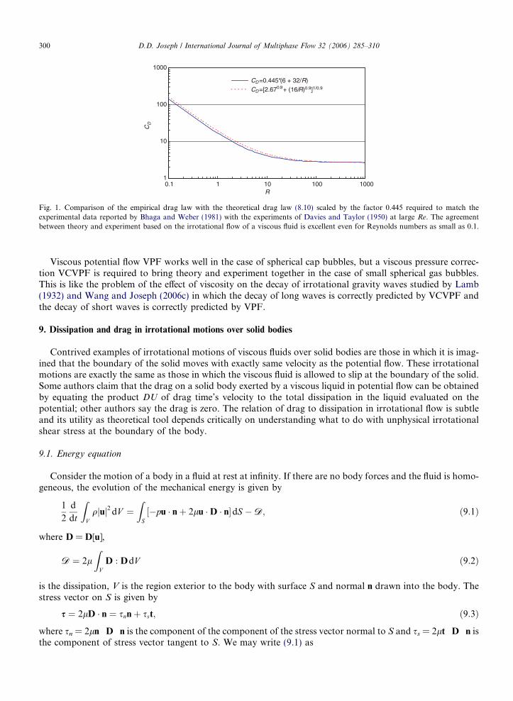
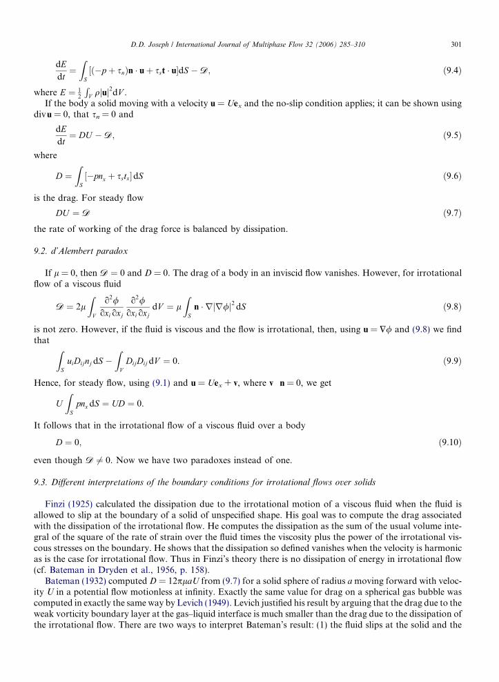
This drag law is in excellent agreement with experiments at large Morton numbers reported by Bhaga andWeber (1981) after the drag law is scaled so that the effective diameter used in the experiments and the spher-ical cap radius of Davies and Taylor (1950) are the same (see Fig. 1).
1
10
100
1000
0.1 1 10 100 1000R
CD
CD =0.445*(6 + 32/R)CD =[2.670.9+ (16/R)0.9]1/0.9
Fig. 1. Comparison of the empirical drag law with the theoretical drag law (8.10) scaled by the factor 0.445 required to match theexperimental data reported by Bhaga and Weber (1981) with the experiments of Davies and Taylor (1950) at large Re. The agreementbetween theory and experiment based on the irrotational flow of a viscous fluid is excellent even for Reynolds numbers as small as 0.1.
300 D.D. Joseph / International Journal of Multiphase Flow 32 (2006) 285–310
Viscous potential flow VPF works well in the case of spherical cap bubbles, but a viscous pressure correc-tion VCVPF is required to bring theory and experiment together in the case of small spherical gas bubbles.This is like the problem of the effect of viscosity on the decay of irrotational gravity waves studied by Lamb(1932) and Wang and Joseph (2006c) in which the decay of long waves is correctly predicted by VCVPF andthe decay of short waves is correctly predicted by VPF.
9. Dissipation and drag in irrotational motions over solid bodies
Contrived examples of irrotational motions of viscous fluids over solid bodies are those in which it is imag-ined that the boundary of the solid moves with exactly same velocity as the potential flow. These irrotationalmotions are exactly the same as those in which the viscous fluid is allowed to slip at the boundary of the solid.Some authors claim that the drag on a solid body exerted by a viscous liquid in potential flow can be obtainedby equating the product DU of drag time’s velocity to the total dissipation in the liquid evaluated on thepotential; other authors say the drag is zero. The relation of drag to dissipation in irrotational flow is subtleand its utility as theoretical tool depends critically on understanding what to do with unphysical irrotationalshear stress at the boundary of the body.
9.1. Energy equation
Consider the motion of a body in a fluid at rest at infinity. If there are no body forces and the fluid is homo-geneous, the evolution of the mechanical energy is given by
1
2
d
dt
ZVqjuj2 dV ¼
ZS½�pu � nþ 2lu �D � n�dS �D; ð9:1Þ
where D = D[u],
D ¼ 2lZVD : DdV ð9:2Þ
is the dissipation, V is the region exterior to the body with surface S and normal n drawn into the body. Thestress vector on S is given by
s ¼ 2lD � n ¼ snnþ sst; ð9:3Þ
where sn = 2ln Æ D Æ n is the component of the component of the stress vector normal to S and ss = 2lt Æ D Æ n isthe component of stress vector tangent to S. We may write (9.1) as
D.D. Joseph / International Journal of Multiphase Flow 32 (2006) 285–310 301
dEdt
¼ZS½ð�p þ snÞn � uþ sst � u�dS �D; ð9:4Þ
where E ¼ 12
RV qjuj
2dV .If the body a solid moving with a velocity u = Uex and the no-slip condition applies; it can be shown using
divu = 0, that sn = 0 and
dEdt
¼ DU �D; ð9:5Þ
where
D ¼ZS½�pnx þ sstx�dS ð9:6Þ
is the drag. For steady flow
DU ¼ D ð9:7Þ
the rate of working of the drag force is balanced by dissipation.9.2. d’Alembert paradox
If l = 0, then D ¼ 0 and D = 0. The drag of a body in an inviscid flow vanishes. However, for irrotationalflow of a viscous fluid
D ¼ 2lZV
o2/oxi oxj
o2/oxi oxj
dV ¼ lZSn � rjr/j2 dS ð9:8Þ
is not zero. However, if the fluid is viscous and the flow is irrotational, then, using u = $/ and (9.8) we findthat
ZSuiDijnj dS �
ZVDijDij dV ¼ 0. ð9:9Þ
Hence, for steady flow, using (9.1) and u = Uex + v, where v Æ n = 0, we get
UZSpnx dS ¼ UD ¼ 0.
It follows that in the irrotational flow of a viscous fluid over a body
D ¼ 0; ð9:10Þ
even though D 6¼ 0. Now we have two paradoxes instead of one.
9.3. Different interpretations of the boundary conditions for irrotational flows over solids
Finzi (1925) calculated the dissipation due to the irrotational motion of a viscous fluid when the fluid isallowed to slip at the boundary of a solid of unspecified shape. His goal was to compute the drag associatedwith the dissipation of the irrotational flow. He computes the dissipation as the sum of the usual volume inte-gral of the square of the rate of strain over the fluid times the viscosity plus the power of the irrotational vis-cous stresses on the boundary. He shows that the dissipation so defined vanishes when the velocity is harmonicas is the case for irrotational flow. Thus in Finzi’s theory there is no dissipation of energy in irrotational flow(cf. Bateman in Dryden et al., 1956, p. 158).
Bateman (1932) computed D = 12plaU from (9.7) for a solid sphere of radius amoving forward with veloc-ity U in a potential flow motionless at infinity. Exactly the same value for drag on a spherical gas bubble wascomputed in exactly the same way by Levich (1949). Levich justified his result by arguing that the drag due to theweak vorticity boundary layer at the gas–liquid interface is much smaller than the drag due to the dissipation ofthe irrotational flow. There are two ways to interpret Bateman’s result: (1) the fluid slips at the solid and the
302 D.D. Joseph / International Journal of Multiphase Flow 32 (2006) 285–310
dissipation is balanced by the power of the traction leading to zero drag (9.10) or (2) the fluid does not slip, thereis a region at the boundary which may be small or large in which vorticity is important and 12plaU approxi-mates the additional drag due to the viscous dissipation in the irrotational flow outside the boundary layer.
Some German researchers (Hamel, 1941; Ackeret, 1952; Romberg, 1967; Zierep, 1984) considered the prob-lem of dissipation and drag on solid bodies in contrived irrotational motions of a viscous fluid. Hamel (1941)noted that though the resultants of the viscous irrotational stresses vanish, the work done by these stresses donot vanish. This observation motivated his discussion of dissipation and drag. The papers of Hamel and Ack-eret are very similar; they both use the formula (9.7) relating dissipation and drag for solid bodies under theassumption that the boundary of the solid moves with the velocity of the irrotational flow. Ackeret gives dragresults for circular cylinders in a uniform stream with circulation, for elliptic cylinders, for spheres and otherbodies. Zierep (1984) in a paper on viscous potential flow discusses the dissipation and drag associated withthe moving wall calculations of Hamel and Ackeret; he calls this a pseudo drag which ‘‘originates from fric-tion.’’ He says that ‘‘. . . A real drag does not appear in potential flows including those with friction.’’ Zierep’sclaim that the drag on a solid body in irrotational flow vanishes is a consequence of d’Alembert’s principle forflows with a non-zero dissipation embodied in (9.10). The assumption that the boundary of the solid moveswith the velocity of the irrotational flow could be interpreted to mean that the edge of the boundary layer onthe body moves with the velocity of the irrotational flow because the velocity is continuous there. The differ-ence between the dissipation in the irrotational flow outside the boundary layer on a rigid body and the dis-sipation outside the same body whose velocity is contrived to move at the velocity of the irrotational flowcould be close if the boundary layer is not too thick and the dissipation in regions of strong vorticity arisingfrom boundary layer separation is ignored. The dissipation in the irrotational flow outside a moving body isexactly the same when the fluid slips and when the motion of the boundary of the body is imagined to movewith the slip velocity.
Zierep’s discussion of viscous potential flow is confused: he says that viscous potential flow is independentof the Reynolds number; he did not discuss the irrotational viscous stresses which scale with the Reynoldsnumber. He notes that the drag on a sphere with a moving wall computed from (9.7) is the same as the dragon a spherical gas bubble computed by Levich (1949). He notes that drag on the bubble is in good agreementwith experiment and he attributes this difference to the fact that the shear stress on the bubble surface vanishesand the gas liquid is like moving wall. He does not confront the discrepancy posed by the non-zero viscous andirrotational shear stress in the theory and the zero shear stress condition required in practice.
9.4. Viscous dissipation in the irrotational flow outside the boundary layer and wake
The paper on dissipation and drag by Romberg (1967) is important and deserves to be better known. In thispaper
The connection between drag and dissipation in incompressible flows is derived. Two cases are consid-ered: Firstly the surface of the body is at rest and secondly the surface elements can move.In the furthercase the flow outside the boundary layer and the wake contributes a term to the drag coefficient which isproportional to Reynolds number to the minus one (high Reynolds number assumed). The coefficient ofthis term is completely fixed by the frictionless flow.
The dissipation in the irrotational flow of a viscous fluid outside the boundary layer had not been consid-ered before Romberg. I learned about this paper from Zierep (1984) that discussed the first two topics butignored the flow outside the boundary layer. Much later and independently, Wang and Joseph (2006a) pre-pared a work on pressure corrections for the effects of viscosity on the irrotational flow outside Prandtl’sboundary layer; in one chapter they calculated the additional drag on a Joukowski airfoil at an angle of attackby the dissipation method.
The existence of an added drag due to viscosity in the irrotational flow outside the very small vorticity layerat the bubble surface is widely accepted by fluid mechanics researchers. The situation there and in other gas–liquid free surface problems is complicated by the uncompensated irrotational shear stress at the interfacewhich is intimately connected to the viscous action in the irrotational flow. This complication does not appearin the equivalent formulation in which the irrotational effects of viscosity are computed using the dissipation
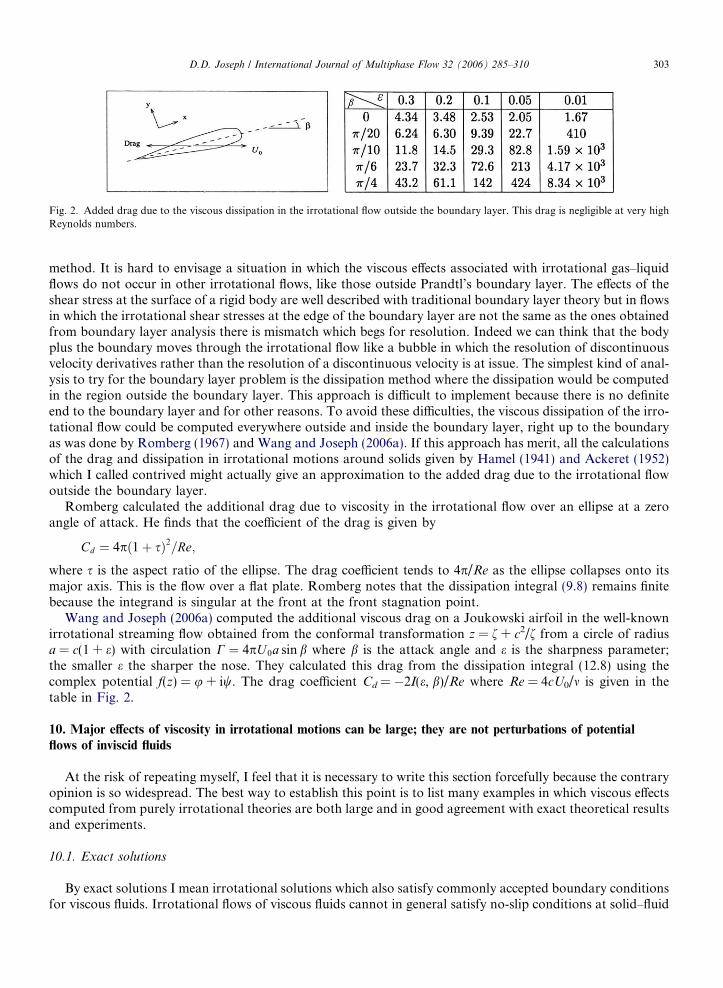
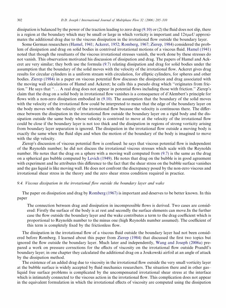
Fig. 2. Added drag due to the viscous dissipation in the irrotational flow outside the boundary layer. This drag is negligible at very highReynolds numbers.
D.D. Joseph / International Journal of Multiphase Flow 32 (2006) 285–310 303
method. It is hard to envisage a situation in which the viscous effects associated with irrotational gas–liquidflows do not occur in other irrotational flows, like those outside Prandtl’s boundary layer. The effects of theshear stress at the surface of a rigid body are well described with traditional boundary layer theory but in flowsin which the irrotational shear stresses at the edge of the boundary layer are not the same as the ones obtainedfrom boundary layer analysis there is mismatch which begs for resolution. Indeed we can think that the bodyplus the boundary moves through the irrotational flow like a bubble in which the resolution of discontinuousvelocity derivatives rather than the resolution of a discontinuous velocity is at issue. The simplest kind of anal-ysis to try for the boundary layer problem is the dissipation method where the dissipation would be computedin the region outside the boundary layer. This approach is difficult to implement because there is no definiteend to the boundary layer and for other reasons. To avoid these difficulties, the viscous dissipation of the irro-tational flow could be computed everywhere outside and inside the boundary layer, right up to the boundaryas was done by Romberg (1967) and Wang and Joseph (2006a). If this approach has merit, all the calculationsof the drag and dissipation in irrotational motions around solids given by Hamel (1941) and Ackeret (1952)which I called contrived might actually give an approximation to the added drag due to the irrotational flowoutside the boundary layer.
Romberg calculated the additional drag due to viscosity in the irrotational flow over an ellipse at a zeroangle of attack. He finds that the coefficient of the drag is given by
Cd ¼ 4pð1þ sÞ2=Re;
where s is the aspect ratio of the ellipse. The drag coefficient tends to 4p/Re as the ellipse collapses onto itsmajor axis. This is the flow over a flat plate. Romberg notes that the dissipation integral (9.8) remains finitebecause the integrand is singular at the front at the front stagnation point.Wang and Joseph (2006a) computed the additional viscous drag on a Joukowski airfoil in the well-knownirrotational streaming flow obtained from the conformal transformation z = f + c2/f from a circle of radiusa = c(1 + e) with circulation C ¼ 4pU 0a sin b where b is the attack angle and e is the sharpness parameter;the smaller e the sharper the nose. They calculated this drag from the dissipation integral (12.8) using thecomplex potential f(z) = u + iw. The drag coefficient Cd = �2I(e, b)/Re where Re = 4cU0/m is given in thetable in Fig. 2.
10. Major effects of viscosity in irrotational motions can be large; they are not perturbations of potential
flows of inviscid fluids
At the risk of repeating myself, I feel that it is necessary to write this section forcefully because the contraryopinion is so widespread. The best way to establish this point is to list many examples in which viscous effectscomputed from purely irrotational theories are both large and in good agreement with exact theoretical resultsand experiments.
10.1. Exact solutions
By exact solutions I mean irrotational solutions which also satisfy commonly accepted boundary conditionsfor viscous fluids. Irrotational flows of viscous fluids cannot in general satisfy no-slip conditions at solid–fluid
304 D.D. Joseph / International Journal of Multiphase Flow 32 (2006) 285–310
surfaces or continuity conditions on the tangential components of velocity and stress at the interface betweenliquids. At a gas–liquid surface the tangential component velocity in the liquid is essentially unrestricted as itwould be at a vacuum–liquid surface but the continuity of the shear stress leads to the condition that the shearstress must be essentially zero in the liquid as it is in the vacuum or nearly in the gas. I know only of twonon-contrived examples of potential flows which satisfy these strict conditions. The first is the purely rotaryflow between rotating cylinders adjusted so that the velocity of the fluid in circles is proportional to c/r.The second solution arises in purely radial gas–liquid flows of spherical bubbles or drops (Poritsky, 1951).In these purely radial flows, shear stresses cannot develop but irrotational viscous normal stresses propor-tional to the viscosity are not zero. The irrotational solutions of these problems work for water and pitch,independent of viscosity.
10.2. Gas–liquid flows: bubbles, drops and waves
Irrotational studies of gas–liquid flows cannot be made to satisfy the zero shear stress condition on the freesurface. This mismatch leads to the generation of vorticity. Very often the contribution of vorticity is confinedto a boundary layer and the viscous effects in these layers are much smaller than the viscous effects in thepurely irrotational flow. The purely irrotational analysis of the rise velocity of a spherical cap bubble describedin Fig. 1 is in good agreement with experiment at high Morton numbers even at Reynolds numbers of 0.1.Classical studies of interfacial stability for potential flow of inviscid fluids are as easily done for the potentialflow of viscous and even viscoelastic fluids.
10.3. Rayleigh–Taylor instability
Joseph et al. (1999) studied the breakup of drops in a high speed air stream behind a shock wave. At firstthe drop flattens due to high pressure at the front and back of drop. The accelerations can be 105 times gravity;this huge acceleration is main dynamical feature for generating the RT instability which give rise to the cor-rugations seen on the front face of the drop before it is set into motion by acceleration (see Fig. 3). The anal-ysis of RT instability can be done exactly from the linearized Navier–Stokes equations and from viscouspotential flow VPF. The growth rates and the wave length for maximum growth depend strongly on viscosity;the difference between VPF and the exact solution is about 2% at most for small and large viscosities. Similaragreement between the irrotational theory, exact solutions and experiments for RT instability were given byJoseph et al. (2002).
Silicone Oil 100
0
20000
40000
60000
80000
100000
120000
140000
160000
0 500 1000 1500 2000
k
n
Water
0
20000
40000
60000
80000
100000
120000
140000
160000
0 200 400 600 800 1000
k
n
Fig. 3. Growth rate curves for Rayleigh–Taylor instability for water (1 cp) silicon oil (100 cp). The critical cut off wave number is given bykc = (qa/c)1/2, where a is acceleration c is surface tension, is independent of viscosity. The maximum value of the growth rate decreasesstrongly with viscosity and the maximum value of the growth rate shifts strongly to longer waves. The growth rate curves here computedfrom viscous potential flow are less than 2% different than the curves from the exact theory. The irrotational theory agrees with exacttheory and with experiments even when the viscosity is very large.
D.D. Joseph / International Journal of Multiphase Flow 32 (2006) 285–310 305
10.4. Capillary instability
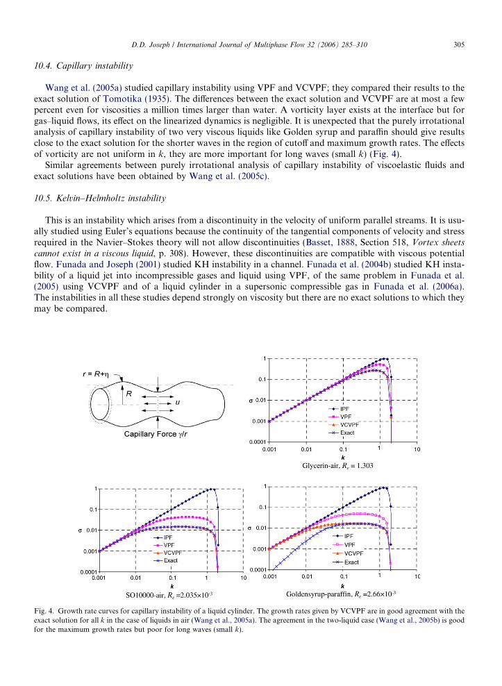
Wang et al. (2005a) studied capillary instability using VPF and VCVPF; they compared their results to theexact solution of Tomotika (1935). The differences between the exact solution and VCVPF are at most a fewpercent even for viscosities a million times larger than water. A vorticity layer exists at the interface but forgas–liquid flows, its effect on the linearized dynamics is negligible. It is unexpected that the purely irrotationalanalysis of capillary instability of two very viscous liquids like Golden syrup and paraffin should give resultsclose to the exact solution for the shorter waves in the region of cutoff and maximum growth rates. The effectsof vorticity are not uniform in k, they are more important for long waves (small k) (Fig. 4).
Similar agreements between purely irrotational analysis of capillary instability of viscoelastic fluids andexact solutions have been obtained by Wang et al. (2005c).
10.5. Kelvin–Helmholtz instability
This is an instability which arises from a discontinuity in the velocity of uniform parallel streams. It is usu-ally studied using Euler’s equations because the continuity of the tangential components of velocity and stressrequired in the Navier–Stokes theory will not allow discontinuities (Basset, 1888, Section 518, Vortex sheets
cannot exist in a viscous liquid, p. 308). However, these discontinuities are compatible with viscous potentialflow. Funada and Joseph (2001) studied KH instability in a channel. Funada et al. (2004b) studied KH insta-bility of a liquid jet into incompressible gases and liquid using VPF, of the same problem in Funada et al.(2005) using VCVPF and of a liquid cylinder in a supersonic compressible gas in Funada et al. (2006a).The instabilities in all these studies depend strongly on viscosity but there are no exact solutions to which theymay be compared.
Fig. 4. Growth rate curves for capillary instability of a liquid cylinder. The growth rates given by VCVPF are in good agreement with theexact solution for all k in the case of liquids in air (Wang et al., 2005a). The agreement in the two-liquid case (Wang et al., 2005b) is goodfor the maximum growth rates but poor for long waves (small k).
306 D.D. Joseph / International Journal of Multiphase Flow 32 (2006) 285–310
10.6. Free waves on highly viscous liquids
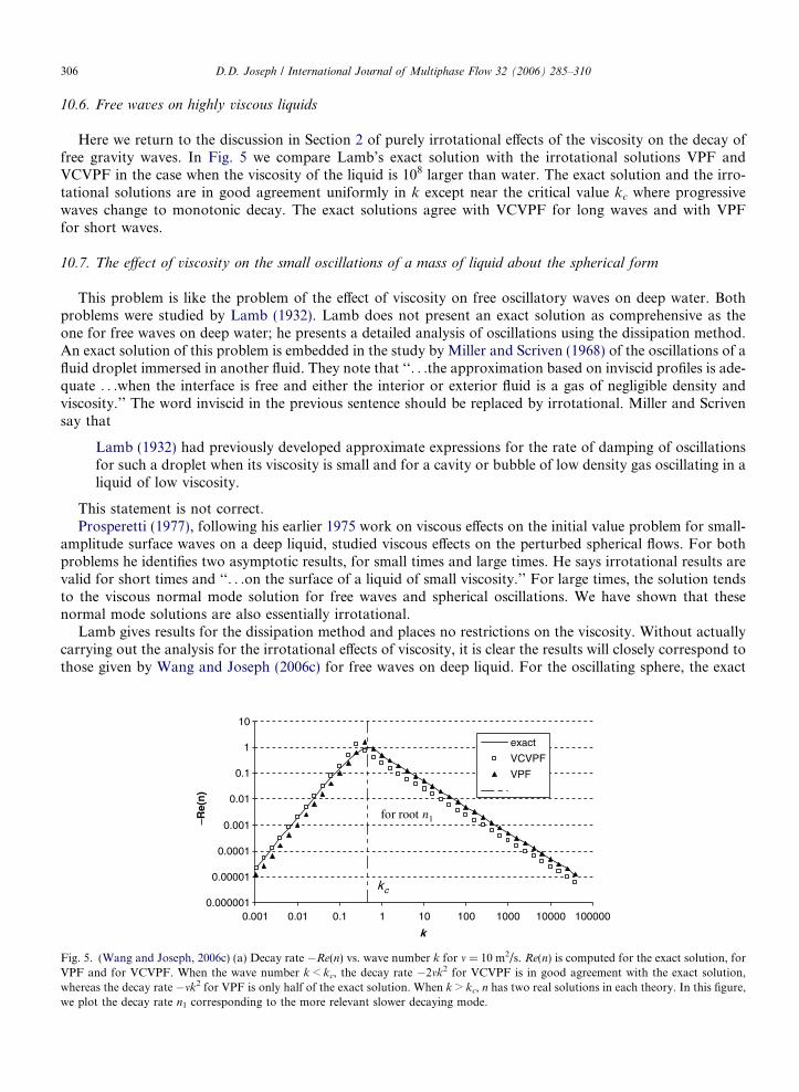
Here we return to the discussion in Section 2 of purely irrotational effects of the viscosity on the decay offree gravity waves. In Fig. 5 we compare Lamb’s exact solution with the irrotational solutions VPF andVCVPF in the case when the viscosity of the liquid is 108 larger than water. The exact solution and the irro-tational solutions are in good agreement uniformly in k except near the critical value kc where progressivewaves change to monotonic decay. The exact solutions agree with VCVPF for long waves and with VPFfor short waves.
10.7. The effect of viscosity on the small oscillations of a mass of liquid about the spherical form
This problem is like the problem of the effect of viscosity on free oscillatory waves on deep water. Bothproblems were studied by Lamb (1932). Lamb does not present an exact solution as comprehensive as theone for free waves on deep water; he presents a detailed analysis of oscillations using the dissipation method.An exact solution of this problem is embedded in the study by Miller and Scriven (1968) of the oscillations of afluid droplet immersed in another fluid. They note that ‘‘. . .the approximation based on inviscid profiles is ade-quate . . .when the interface is free and either the interior or exterior fluid is a gas of negligible density andviscosity.’’ The word inviscid in the previous sentence should be replaced by irrotational. Miller and Scrivensay that
Fig. 5.VPF awhereawe plo
Lamb (1932) had previously developed approximate expressions for the rate of damping of oscillationsfor such a droplet when its viscosity is small and for a cavity or bubble of low density gas oscillating in aliquid of low viscosity.
This statement is not correct.Prosperetti (1977), following his earlier 1975 work on viscous effects on the initial value problem for small-
amplitude surface waves on a deep liquid, studied viscous effects on the perturbed spherical flows. For bothproblems he identifies two asymptotic results, for small times and large times. He says irrotational results arevalid for short times and ‘‘. . .on the surface of a liquid of small viscosity.’’ For large times, the solution tendsto the viscous normal mode solution for free waves and spherical oscillations. We have shown that thesenormal mode solutions are also essentially irrotational.
Lamb gives results for the dissipation method and places no restrictions on the viscosity. Without actuallycarrying out the analysis for the irrotational effects of viscosity, it is clear the results will closely correspond tothose given by Wang and Joseph (2006c) for free waves on deep liquid. For the oscillating sphere, the exact
0.000001
0.00001
0.0001
0.001
0.01
0.1
1
10
0.001 0.01 0.1 1 10 100 1000 10000 100000
k
–Re(
n)
exact
VCVPF
VPF
kc
for root n1
(Wang and Joseph, 2006c) (a) Decay rate �Re(n) vs. wave number k for m = 10 m2/s. Re(n) is computed for the exact solution, fornd for VCVPF. When the wave number k < kc, the decay rate �2mk2 for VCVPF is in good agreement with the exact solution,s the decay rate �mk2 for VPF is only half of the exact solution. When k > kc, n has two real solutions in each theory. In this figure,t the decay rate n1 corresponding to the more relevant slower decaying mode.
D.D. Joseph / International Journal of Multiphase Flow 32 (2006) 285–310 307
solution is well approximated by the dissipation method which probably can also be computed from VCVPF.When the viscosity is very great the oscillations stop and the surface perturbations will decay monotonically;the monotonic decay is probably well approximated by VPF.
The following citation from Lamb makes the point about viscosity and irrotationality in oscillations of aliquid globe. He gives the formula for decay constant s for exp(�t/s) from the dissipation analysiss = a2/(n � 1)(2n + 1)v and says that
the most remarkable feature of this result is the excessively minute extent to which the oscillations ofa globe of moderate dimensions are affected by such a degree of viscosity as is ordinarily met innature. For a globe of the size of the earth, and of the same kinematic viscosity as water, we have,on the cgs system, a = 6.37 · 108, m = .0178 and the value of s for the gravitational oscillation of longestperiod (n = 2) is therefore
s ¼ 1:44� 1011 years.
Even with the value found by Darwin (1878) for the viscosity of pitch near the freezing temperature, viz.l = 1.3 · 108 · g, we find, taking g = 980, the value
s ¼ 180 h
for the modulus of decay of the slowest oscillation of a globe the size of the earth, having the density ofwater and the viscosity of pitch. Since this is still large compared with the period of 1 h 34 min found inArt. 262, it appears that such a globe would oscillate almost like a perfect fluid.
10.8. Viscosity and vorticity
Vorticity is generated by the no-slip condition at the boundary of solids; it is generated by continuity con-ditions for the tangential components of velocity and stress at liquid–liquid surfaces and by the zero shear con-dition at a liquid–gas surface. The effects of viscosity on the formation of regions of vorticity are a topic at thefoundation of boundary layer theory. In solid–liquid flows the major effects of viscosity emanate from regionsof non-zero vorticity. At high Reynolds numbers, the major part of the drag is due to the shear stress at theboundary; a small contribution to the drag may arise from the viscous contribution to dissipation in the irro-tational flow outside the boundary layer. Typically, the effects of viscosity arising from the boundary layer atliquid–gas flows are small because the rates of strain in these layers are no larger than in the irrotational flowand the layer thickness is small. It is possible to study the effect of viscosity emanating from such layers byperturbing the irrotational flow of an inviscid fluid with terms emanating from the viscous terms in the normalstress balance at the free surface for small viscosity as was done by Lundgren and Mansour (1988). Thisapproach captures the viscous effects from the boundary layer when the viscosity is small. These effects of vis-cosity due to the formation of boundary layers of vorticity to remove the unphysical irrotational shear stress atthe bubble interface may be added to the direct effects of viscosity on the irrotational flow. In the direct irro-tational theories which we called VPF and VCVPF the effects of viscosity on vorticity generation are ignoredbut there is there is no restriction on the size of the viscosity. The limits of applicability of irrotational theoriesare determined by an analysis of the effects of vorticity. This is well known. The new idea is that significanteffects of viscosity arise in regions irrotational flow even in problems in which vorticity is important.
Saffman (1992) in his monograph on vortex dynamics collects results on the classical theory of inviscidincompressible fluids containing finite regions of vorticity. This approach is consistent with the fact that vortexsheets cannot exist in a viscous fluid which is perhaps an intuitively obvious result proved in Section 518 ofBasset (1888). In view of the results collected in this essay, a theory of irrotational flow of viscous fluidscontaining finite regions of vorticity might be considered.
11. Boundary layers when the Reynolds number is not so large
Prandtl’s boundary layer theory arises when the Reynolds number is very large. The flow in the boundarylayer satisfies the no-slip boundary conditions the solid wall. Vorticity is generated at the wall. At large
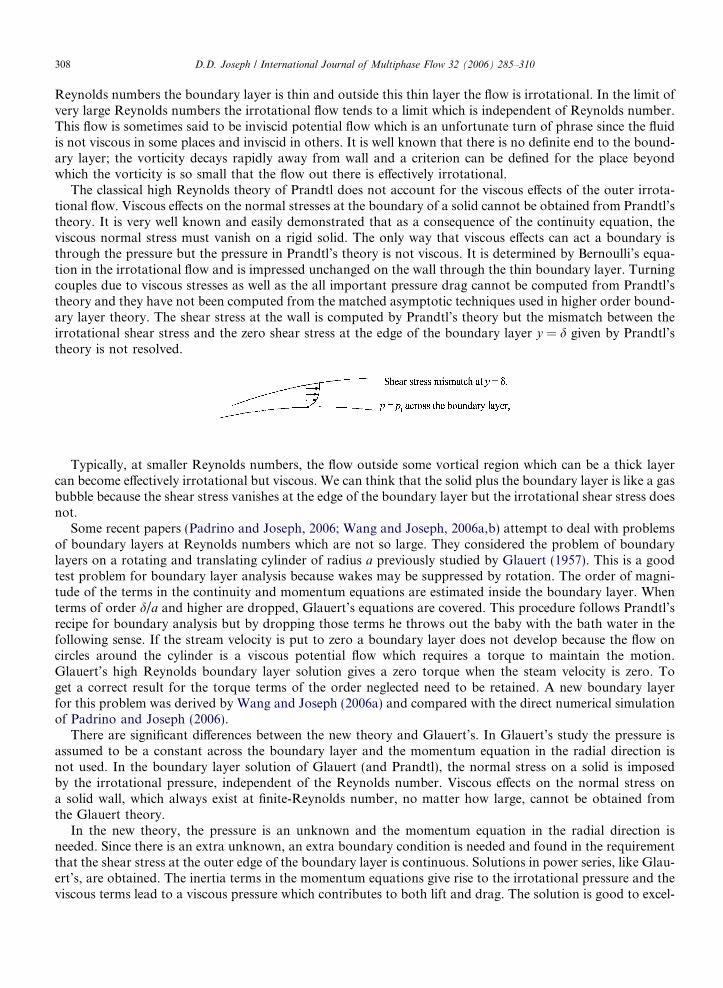
308 D.D. Joseph / International Journal of Multiphase Flow 32 (2006) 285–310
Reynolds numbers the boundary layer is thin and outside this thin layer the flow is irrotational. In the limit ofvery large Reynolds numbers the irrotational flow tends to a limit which is independent of Reynolds number.This flow is sometimes said to be inviscid potential flow which is an unfortunate turn of phrase since the fluidis not viscous in some places and inviscid in others. It is well known that there is no definite end to the bound-ary layer; the vorticity decays rapidly away from wall and a criterion can be defined for the place beyondwhich the vorticity is so small that the flow out there is effectively irrotational.
The classical high Reynolds theory of Prandtl does not account for the viscous effects of the outer irrota-tional flow. Viscous effects on the normal stresses at the boundary of a solid cannot be obtained from Prandtl’stheory. It is very well known and easily demonstrated that as a consequence of the continuity equation, theviscous normal stress must vanish on a rigid solid. The only way that viscous effects can act a boundary isthrough the pressure but the pressure in Prandtl’s theory is not viscous. It is determined by Bernoulli’s equa-tion in the irrotational flow and is impressed unchanged on the wall through the thin boundary layer. Turningcouples due to viscous stresses as well as the all important pressure drag cannot be computed from Prandtl’stheory and they have not been computed from the matched asymptotic techniques used in higher order bound-ary layer theory. The shear stress at the wall is computed by Prandtl’s theory but the mismatch between theirrotational shear stress and the zero shear stress at the edge of the boundary layer y = d given by Prandtl’stheory is not resolved.
Typically, at smaller Reynolds numbers, the flow outside some vortical region which can be a thick layercan become effectively irrotational but viscous. We can think that the solid plus the boundary layer is like a gasbubble because the shear stress vanishes at the edge of the boundary layer but the irrotational shear stress doesnot.
Some recent papers (Padrino and Joseph, 2006; Wang and Joseph, 2006a,b) attempt to deal with problemsof boundary layers at Reynolds numbers which are not so large. They considered the problem of boundarylayers on a rotating and translating cylinder of radius a previously studied by Glauert (1957). This is a goodtest problem for boundary layer analysis because wakes may be suppressed by rotation. The order of magni-tude of the terms in the continuity and momentum equations are estimated inside the boundary layer. Whenterms of order d/a and higher are dropped, Glauert’s equations are covered. This procedure follows Prandtl’srecipe for boundary analysis but by dropping those terms he throws out the baby with the bath water in thefollowing sense. If the stream velocity is put to zero a boundary layer does not develop because the flow oncircles around the cylinder is a viscous potential flow which requires a torque to maintain the motion.Glauert’s high Reynolds boundary layer solution gives a zero torque when the steam velocity is zero. Toget a correct result for the torque terms of the order neglected need to be retained. A new boundary layerfor this problem was derived by Wang and Joseph (2006a) and compared with the direct numerical simulationof Padrino and Joseph (2006).
There are significant differences between the new theory and Glauert’s. In Glauert’s study the pressure isassumed to be a constant across the boundary layer and the momentum equation in the radial direction isnot used. In the boundary layer solution of Glauert (and Prandtl), the normal stress on a solid is imposedby the irrotational pressure, independent of the Reynolds number. Viscous effects on the normal stress ona solid wall, which always exist at finite-Reynolds number, no matter how large, cannot be obtained fromthe Glauert theory.
In the new theory, the pressure is an unknown and the momentum equation in the radial direction isneeded. Since there is an extra unknown, an extra boundary condition is needed and found in the requirementthat the shear stress at the outer edge of the boundary layer is continuous. Solutions in power series, like Glau-ert’s, are obtained. The inertia terms in the momentum equations give rise to the irrotational pressure and theviscous terms lead to a viscous pressure which contributes to both lift and drag. The solution is good to excel-
D.D. Joseph / International Journal of Multiphase Flow 32 (2006) 285–310 309
lent agreement with the numerical solution when the boundary layer thickness d is properly chosen. Theboundary layer is relatively thick and the Reynolds numbers are not so large. The new solution is not selfcontained because d is not selected internally but is selected to fit data.
Acknowledgments
This work was supported in part by the National Science Foundation. My collaborations with T. Funadaand J. Wang on various topics mentioned in this essay is most gratefully acknowledged. I wish to thankAndrea Prosperetti for engaging discussions of matters related to this essay over the course of years andfor calling my attention to the interesting paper by Poritsky (1951). I profited from conversations with FritzBusse about the contributions of the German researchers Ackeret (1952), Hamel (1941), Romberg (1967) andZierep (1984).
References
Ackeret, J., 1952. Uber exakte Losungen der Stokes–Navier–Gleichungen inkompressibler Flussigkeiten bei veranderten Grenzbeding-ungen. Z. Angew. Math. Phys. 3, 259–270.
Basset, A.B., 1888. A Treatise on Hydrodynamics, vol. 2. Deighton, Bell and Company (reprinted by Dover, 1961).Batchelor, G.K., 1967. An Introduction to Fluid Dynamics. Cambridge University Press.Bateman, H., 1932. See Dryden et al. (1956).Bhaga, T., Weber, M., 1981. Bubbles in viscous liquids: shapes, wakes and velocities. J. Fluid Mech. 105, 61–85.Brabston, D.C., Keller, H.B., 1975. Viscous flows past spherical gas bubbles. J. Fluid Mech. 69, 179–189.Brown, R.A.S., 1965. The mechanics of large gas bubbles in tubes. Can. J. Chem. Engng. Q2, 217–223.Darwin, G.H., 1878. On the bodily tides of viscous and semi-elastic spheroids. Philos. Trans. cixx 1.Davies, R.M., Taylor, G.I., 1950. The mechanics of large bubbles rising through liquids in tubes. Proc. R. Soc. Lond. A 200, 375–390.Dryden, H., Murnaghan, F., Bateman, H. Hyrdrodynamics, 1932. Dover (a complete unabridged reprinting of National Research Council
Bulletin 84, 1956).Finzi, B., 1925. Sulla funzione di dissipazione di Lord Rayleigh. Atti Accad. Lincei 6, 215–220.Funada, T., Joseph, D.D., 2001. Viscous potential flow analysis of Kelvin–Helmholtz instability in a channel. J. Fluid Mech. 445, 263–283.Funada, T., Joseph, D.D., Maehara, T., Yamashita, S., 2004a. Ellipsoidal model of the rise of a Taylor bubble in a round tube. Int. J.
Multiphase Flow 31, 473–491.Funada, T., Joseph, D.D., Yamashita, S., 2004b. Stability of a liquid jet into incompressible gases and liquids. Int. J. Multiphase Flow 30,
1177–1208.Funada, T., Saitoh, M., Wang, J., Joseph, D.D., 2005. Stability of a liquid jet into incompressible gases and liquids: Part 2. Effects of the
irrotational viscous pressure. Int. J. Multiphase Flow 31, 1134–1154.Funada, T., Joseph, D.D., Yamashita, S., Saitoh, M., 2006a. Liquid jet into a high Mach number air stream. Int. J. Multiphase Flow 32,
20–50.Funada, T., Wang, J., Joseph, D.D., 2006b. Viscous potential flow analysis of stress induced cavitation in an aperture flow. Atomizat.
Sprays (7), in press.Glauert, H., 1943. The Elements of Aerofoil and Airscrew Theory. Cambridge University Press.Glauert, M.B., 1957. The flow past a rapidly rotating cylinder. Proc. R. Soc. Lond A 242, 108–115.Hamel, G., 1941. Uber die Potentialstromungen zaher Flussigkeiten. Z. Angew. Math. Mech. 21, 129–139.Harper, J.F., 1972. The motion of bubbles and drops through liquids. Adv. Appl. Mech. 12, 59–129.Harper, J.F., Moore, D.W., 1968. The motion of a spherical drop at high Reynolds number. J. Fluid Mech. 32, 367–391.Jeffreys, H., 1928. Equations of viscous fluid motion and the circulation theorem. Proc. Cambridge Philos. Soc. 24, 477–479.Joseph, D.D., 1992. Bernoulli equation and the competition of elastic and inertial pressures in the potential flow of a second-order fluid.
J. Non-Newtonian Fluid Mech. 42, 385–389.Joseph, D.D., 2003a. Viscous potential flow. J. Fluid Mech. 479, 191–197.Joseph, D.D., 2003b. Rise velocity of a spherical cap bubble. J. Fluid Mech. 453, 109–132.Joseph, D.D., Belanger, J., Beavers, G.S., 1999. Breakup of a liquid drop suddenly exposed to a high-speed airstream. Int. J. Multiphase
Flow 25, 1263–1303.Joseph, D.D., Beavers, G.S., Funada, T., 2002. Rayleigh–Taylor instability of viscoelastic drops at high Weber numbers. J. Fluid Mech.
453, 109–132.Joseph, D.D., Liao, T.Y., 1994. Potential flow of viscous and viscoelastic fluids. J. Fluid Mech. 265, 1–23.Joseph, D.D., Wang, J., 2004a. The dissipation approximation and viscous potential flow. J. Fluid Mech. 505, 365–377.Joseph, D.D., Wang, J., 2004b. The motion of a spherical gas bubble in viscous potential flow. Available from: <http://www.aem.
umn.edu/people/faculty/joseph/ViscousPotentialFlow/>.Kang, I.S., Leal, L.G., 1988a. The drag coefficient for a spherical bubble in a uniform streaming flow. Phys. Fluids 31, 233–237.
310 D.D. Joseph / International Journal of Multiphase Flow 32 (2006) 285–310
Kang, I.S., Leal, L.G., 1988b. Small-amplitude perturbations of shape for a nearly spherical bubble in an inviscid straining flow (steadyshapes and oscillatory motion). J. Fluid Mech. 187, 231–266.
Lagrange, J., 1781. Memoire sur la theorie du mouvement des fluides, Nouv. Mem. Acad. Berlin, 151–198 = Oeuvres 4, 695–748.Lamb, H., 1932. Hydrodynamics, sixth ed. Cambridge University Press (reprinted by Dover, 1945).Levich, V.G., 1949. The motion of bubbles at high Reynolds numbers. Zh. Eksp. Teor. Fiz. 19, 18. Also in Physiochemical
Hydrodynamics (English transl. By Scripta Technica), p. 436f. Prentice-Hall, 1962.Lighthill, J., 1978. Waves in Fluids. Cambridge University Press.Longuet-Higgins, M.S., 1997. Viscous dissipation in steep capillary–gravity waves. J. Fluid Mech. 344, 271–289.Lundgren, T.S., Mansour, N.N., 1988. Oscillations of drops in zero gravity with weak viscous effects. J. Fluid Mech. 194, 479.Miksis, M., Vanden-Broeck, J.-M., Keller, J.B., 1982. Rising bubbles. J. Fluid Mech. 123, 31–41.Miller, C.A., Scriven, L.E., 1968. The oscillations of a fluid droplet immersed in another fluid. J. Fluid Mech. 32, 417–435.Moore, D.W., 1959. The rise of gas bubble in a viscous liquid. J. Fluid Mech. 6, 113–130.Moore, D.W., 1963. The boundary layer on a spherical gas bubble. J. Fluid Mech. 16, 161–176.Moore, D.W., 1965. The velocity of rise of distorted gas bubbles in a liquid of small viscosity. J. Fluid Mech. 23, 749–766.Navier, C.L.M.H., 1822. On the laws of motion of fluids taking into consideration the adhesion of the molecules. Ann. Chim. Phys. 19,
234–245.Padrino, J.C., Joseph, D.D., 2006. Numerical study of the steady state uniform flow past a rotating cylinder. J. Fluid Mech., in press.Padrino, J.C., Joseph, D.D., Funada, T., Wang, J., 2005. Stress induced cavitation for the streaming motion of a viscous liquid past a
sphere. Available from: <http://www.aem.umn.edu/people/faculty/joseph/ViscousPotentialFlow>.Pipkin, A.C., 1970. Nonlinear phenomena in continua in nonlinear continuum theories in mechanics and physics and their applications
‘‘Edizione Cremonese,’’ Roma, pp. 51–150. See also: Pipkin, A.C., Tanner, R. In: Nemat-Nasser, S. (Ed.), A survey of theory andexperiment in viscometric flows of viscoelastic liquid in mechanics today, vol. 1, Pergamon, 1972.
Plesset, M., 1949. The dynamics of cavitation bubbles. ASME J. Appl. Mech. 16, 228–231.Poisson, S.D., 1829. Memoire sur les equations generales de l’equilibre et du mouvement des corps solides elastiques et des fluides. J. Ecole
Poly. 13, 1–174.Poritsky, M., 1951. The collapse on growth of a spherical bubble on cavity in a viscous fluid. In: Proceedings of the first US National
Congress of Applied Mechanics held at the Illinois Institute of Technology. ASME, pp. 813–821.Prosperetti, A., 1975. Viscous effects on small-amplitude surface waves. Phys. Fluids 19, 195–203.Prosperetti, A., 1977. Viscous effects on perturbed spherical flows. Quart. J. Appl. Math. 35, 339–352.Romberg, G., 1967. Uber die Dissipation in dichtebestandiger Stromung. Z. Angew. Math. Mech. 47, 155–162.Saffman, P.G., 1992. Vortex Dynamics. Cambridge University Press.Saint-Venant, A.-J.-C.-B. De., 1843. Note to be added to the memoir on the dynamics of fluids. Compt. Rend. 17, 1240–1243.Saint-Venant, A.-J.-C.-B., De., 1869. Probleme des mouvements que peuvent prendre les divers points d’une masse liquide, ou solide
ductile, continue dans un vase a parois verticales, pendant son ecoulement par un orifice horizontal interieur. C.R. Acad. Sci. Paris68, 221–237.
Stokes, G.G., 1851(read on December 9, 1850). On the effect of the internal friction of fluids on the motion of pendulums. Trans.Cambridge Phil. Soc. IX, 8–106, Mathematical and Physical Papers 3, 1–141.
Stokes, G.G., 1880. Considerations relative to the greatest height of oscillatory irrotational waves which can be propagated withoutchange of form. Mathematical and Physical Papers I, 225–228.
Stokes, G.G., 1845. On the theories of the internal friction of fluids in motion. Trans. Cambridge Philos. Soc. 8, 287–319, Mathematicaland Physical Papers 1, 75–129.
Tomotika, S., 1935. On the instability of a cylindrical thread of a viscous liquid surrounded by another viscous fluid. Proc. Roy. Soc.Lond. A 150, 322–337.
Truesdell, C.A., 1950. Bernoulli’s theorem for viscous compressible fluids. Phys. Rev. 17, 535–536.Truesdell, C.A., 1954. The Kinematics of Vorticity. Indiana University Science Series, No. 19. Indiana University Press.Wang, J., Joseph, D.D., 2006a. Pressure corrections for the effects of viscosity on the irrotational flow outside Prandtl’s boundary layer.
J. Fluid. Mech., in press.Wang, J., Joseph, D.D., 2006b. Boundary layer analysis for effects of viscosity of the irrotational flow on the flow induced by a rapidly
rotating cylinder in a uniform stream. J. Fluid Mech., in press.Wang, J., Joseph, D.D., 2006c. Purely irrotational theories of the effect of the viscosity on the decay of free gravity waves. Available from:
<http://www.aem.umn.edu/people/faculty/joseph/ViscousPotentialFlow>. J. Fluid Mech., in press.Wang, J., Joseph, D.D., Funada, T., 2005a. Pressure corrections for potential flow analysis of capillary instability of viscous fluids. J. Fluid
Mech. 522, 383–394.Wang, J., Joseph, D.D., Funada, T., 2005b. Viscous contributions to the pressure for potential flow analysis of capillary of two viscous
fluids. Phys. Fluids 17, 052105a.Wang, J., Joseph, D.D., Funada, T., 2005c. Purely irrotational theories of the effects and viscoelasticity on capillary instability of a liquid
cylinder. J. Non-Newtonian Fluid Mech. 129, 106–116.Zierep, J., 1984. Viscous potential flow. Arch. Mech. 36, 127–133, Warszawa.