power balancing in autonomous renewable energy systems
TRANSCRIPT

Power balancing in autonomous
renewable energy systems
The design and construction of the renewable energy laboratory
DENlab ®


Power balancing in autonomous
renewable energy systems
The design and construction of a renewable energy laboratory
DENlab ®
PROEFSCHRIFT
Ter verkrijging van de graad van doctor aan de Technische Universiteit Delft,
op gezag van de Rector Magnificus Prof. dr. ir. J.T. Fokkema, voorzitter van het College voor Promoties,
in het openbaar te verdedigen op maandag 24 november 2008 om 12:30 uur door
Arjan Marco van VOORDEN
elektrotechnisch ingenieur
geboren te Rotterdam

Dit proefschrift is goedgekeurd door de promotor:
Prof. ir. L. van der Sluis
Copromotor:
Dr. ir. G.C. Paap
Samenstelling promotiecommissie:
Rector Magnificus, voorzitter Prof. ir. L. van der Sluis, Technische Universiteit Delft, promotor Dr. ir. G.C. Paap, Technische Universiteit Delft, copromotor Prof. dr. ir. J. Hellendoorn, Technische Universiteit Delft Prof. ir. W.L. Kling, Technische Universiteit Delft Prof. dr. J. Schoonman, Technische Universiteit Delft Prof. dr. ir. J. Driessen, Katholieke Universiteit Leuven, België Dr. ir. F. van Overbeeke, EMforce B.V.
Dit onderzoek is financieel ondersteund door het Samenwerkingsverband Duurzame
Energie (SDE) en het onderzoeksprogramma Sustainable ENergy: Extraction,
Conversion and Use (SENECU), TU Delft.
Printed by: Drukkerij Verloop, Alblasserdam.
ISBN:
Copyright © 2008 by Arjan van Voorden
All rights reserved. No part of the material protected by this copyright notice may be
reproduced or utilized in any form or by any means, electronic or mechanical, including
photocopying, recording or by any information storage and retrieval system, without
permission form the publisher or author.

PREFACE
A thesis like this one is the result of the efforts of not only one person. Some efforts contribute directly to the thesis by giving guidance during the research, comments on the manuscript or assist during the laboratory set-up and its measurements. Other people contribute more indirectly to the thesis, but provide in other ways support during the research and dissemination.
Firstly, I want to thank my colleague ing. Johan Vijftigschild for his many contributions during the research, especially for practical assistance, but not limited to that only. We had many discussions about how to program the PLC software and how to adept the standard Siemens components to be useful for our purpose. Together with the project leader, Dr. ir. Bob Paap, we worked as the DENlab team.
Dr. Paap is the one I will thank secondly for his initial ideas and support at the difficult moments during the installation and the monitoring phase. Beside of these activities, also thank for revising the papers and taking part in the committee.
I also want to thank my promotor, Prof. ir. Lou van der Sluis, for giving me the opportunity to perform a quite practical Ph.D-project. Ph.D. theses with a high practical component in it are not very common in our research group. One of your initial ideas was to attract and interest more students in renewable energies. We can state that this goal is realised. From primary school to Master of Science students from all over the world.
I do not forget the assistance of ing. Rob Schoevaars. The Renewable Energy Laboratory is constructed with a lot of power electronic components. Rob was always willing to help by all kind of technical problems, sharing his wide knowledge on electronic components and circuits from kilowatts to microwatts. I will thank Rob for all his time for teaching me and Johan.
The partners in the SDE (Samenwerkingsverband Duurzame Energie) project, under supervision of ir. Sigrid Bestebroer and Dr. ir. Frank van Overbeeke, ir. Rob van Gerwen, drs. ing. Koen Kok, drs. Jan Uitzinger and drs. Harm Jeeninga.
The partners in the SENECU (Sustainable ENergy: Extraction, Conversion and Use) interfacultary research project, under leadership of Prof. dr. Joop Schoonman. It was great to have discussions with colleagues which are used to milliwatts instead of our kilowatts-scale. We all try to contribute to the transition to a new clean and environmental-friendly society.
Special thanks also to my students, which I guided during my Ph.D-study. First of all my Portuguese Erasmus students, with their beautiful names: Diogo Nuno Pita da Silva e Vasconcelos (2000), Luis Miguel de Crasto Natario (2004) and Pedro Miguel Paulino (2006), but also Gael Marchand from Toulouse, France (2004) and Wilco Boonstra (2001). With their Master theses, they have made a contribution to this thesis. It was very stimulating to guide you with the different assignments.
However there was no direct contribution from my current employer, I want to thank STEDIN for the support in completing this thesis and financial support publishing in color.
From a different order is my gratitude to my family. My wife, Ina, our children, Joanne, Joost and Mark, my parents who stimulate me all to continue my study after finishing the B.Sc.-study in 1995. We all did not expect that it all would lead to a Ph.D.-degree in Electrical Engineering. We all believe that this was not possibly without the gifts all people

get from their Creator. He gives me this opportunity to contribute to the society with this thesis work and with other, completely different, contributions especially under the next generation. For of Him, and through Him, and to Him, are all things: to Whom be glory for ever. Amen. [Romans 11:36]
Arjan van Voorden Capelle aan den IJssel, oktober 2008

SUMMARY
Future needs and possibilities in power supply require solutions to accommodate the changes in the world of power systems, market operation and the need to reduce greenhouse gasses. To develop scenarios for the future, is therefore essential. The desirability of reducing greenhouse gasses evokes research on the most effective application of renewable energy. This research aims at finding new ways to generate electricity from renewable sources. Besides the search for new sources and innovative conversion methods, the electrical infrastructure of the next generation also requires special attention. In both contexts, this research attempts study the autonomous electricity systems with a high penetration of renewable energy sources.
Problems with applying many renewable sources, such as wind and solar conversion systems, are the fluctuation and the difficulty in forecasting the power generation of these sources. An additional problem is the fluctuation not only in supply, but also in demand.
As in every power system, the total of generated and demanded power requires balance at every moment. Using a grid connected system, inequity between demanded and generated power leads to a change in actual kinetic energy. This change in turn causes a frequency change in the network. By applying a primary and secondary control, the synchronous generators in the network react on this frequency deviation by increasing their active power. Contrary to the grid connected system, an autonomous system, with no directly coupled synchronous machines, cannot apply such a balance control. The voltage and frequency in these autonomous networks are dictated by a power electronic component, with a Voltage Source Converter (VSC) control. This type of control prevents the frequency from changing, provided the component operates within its boundaries (maximum current and operating between the DC voltage limits).
Consequently, the discrepancy between supply and demand leads to a change in actual VSC-current, in order to compensate this. A storage system makes the power that is generated, or delivered by this VSC available.
As a consequence of the fluctuations in the renewable sources, the peaks in the load demand (by considering a limited number of households) and the absence of coherence between the fluctuations, the power exchange between the storage system and the rest of the system will fluctuated in a high extent.
This means an unpredictability of the power exchange in direction but also in magnitude. (Furthermore, this power is independent of the actual state of charge of the battery storage.)
In 2000, the department Power Systems Laboratory of the Delft University of Technology decided to build a renewable energy laboratory to study the system integration of renewable energy sources in an autonomous system so as to create vision on the fluctuations in an autonomous renewable system and to design control strategies for mastering the expected fluctuation. From the onset, the size of the laboratory had to be large enough to ensure reliable predictions of larger systems (extendable results). The decision fell on a scale of ten households.
During the study on the fluctuation and the power exchange in the system, two aspects play a major role: the short term (fluctuation, short term stability) and the long term (availability of energy, long term stability).

To get insight into the power exchange and the availability of energy from the sources, the KNMI provided data on wind and Satellight on sun-irradiance data. Based on these databases with mean hour values, a first estimation was made on the potential energy and powers.
Based on the energy calculation with these data and the available space on the roofs of ten houses, it is shown at 120 m2 of solar panels, a wind turbine of 30 kW and a Combined Heat and Power set of 5.5 kWe (12 kWth) are necessary to supply the energy demand of ten houses. The size of the energy buffer is calculated to be 100 kWh, assuming conventional lead-acid batteries.
In the fist design, the laboratory was equipped with state of the art components. Together with Siemens NL, we decided to compose the laboratory with components from the driving industry. These components were then programmed with the right parameters, to obtain desired functionality. However, due to limitations inherent to laboratory set-ups, additional components were required to make ends meet. Although these additions are not necessary in the real situation, they do not influence the research activities. With all these components, the laboratory has now obtained the flexibility which is essential for a study object.
While installing all components, the system is gaining in functionality; the overall control strategies are programmed in the Programmable Logic Controller (PLC); the dedicated software, Step7, is installed; and a Profibus-based user interface is made to control, log and monitor the system behaviour. Also, all relevant units (powers, voltages, currents, SoC‟s) are stored for analyses purposes.
By the design of the optimal control strategy, two aspects are especially important: the availability of energy and the minimal use of the CHP-unit. The first concept provides a control strategy, which gives the system a high flexibility, by only limiting the maximal and minimal SoC value. The second concept studies the application of two parallel battery stacks. Here the control strategy can decide to use one or both batteries. The third strategy is to use load forecasting. Once you can forecast periods with a high risk on energy shortage, the CHP is then started up earlier to prevent low SoC periods. The fourth strategy that is examined applies equalisation processes. The final strategy forecasts the renewable energy supply, in order to minimize the use of the CHP (gas consumption). This last strategy gives the best results: a higher mean value of SoC, a lower number of CHP-starts and the lowest use of the CHP-unit, which ensures a longer battery life.
Besides these strategies, the added value of forecasting of renewable energy is investigated. This value is measured by the reduction of fossil fuel (use of CHP-unit) and the optimal use of the battery (extending lifetime). It is shown in this research that a “simple” persistence method is relative good, but the expected efficiency improvement is not realised in this system configuration.
The first results lead to believe that the system is able to reliably supply energy to the consumers. However, a closer analysis of the measurement and simulation results prove that the power fluctuations are so high and fast that an unacceptable reduction of the battery‟s life time can be expected and that its performance is influencing the energy calculations.
As a solution to this problem, the battery must be relieved by another fast and efficient storage system, such as a super capacitor. They have as an additional advantage the capability to catch the fast fluctuations of the power. In this way, the battery provides the mean value of the storage system on in a certain time frame/on any given time/in a

predetermined time frame. The remaining fluctuation in the battery power depends directly on the size of the super capacitors. The end of this thesis shows simulations with super capacitors and batteries. Two different combinations are compared: the DC and the AC coupled variant. The AC option is preferred over the DC version, because of the measure of controllability.
In conclusion, a renewable energy laboratory is realised to analyse the autonomous application of renewable energy sources to a system of ten households (50 kVA). With some small adaptations, a weak-grid, grid-connected or a parallel operating situation can be created. This flexibility, which was one of the starting-points by the set-up, gives the opportunity to also integrate other renewable sources with ease, both in hardware and in software models.
Based on the research on autonomous renewable energy systems, the autonomous operation is possible, however difficult because of the limited number of households.
Arjan van Voorden

SAMENVATTING
Onder invloed van veranderingen in de elektriciteitswereld, aangedreven door enerzijds marktwerking en anderzijds de noodzakelijkheid om de uitstoot van broeikasgassen te beperken, wordt er gezocht naar scenario‟s waarin in de toekomst energie duurzaam geleverd kan worden aan de gebruikers. Beperking van de broeikasgassen leidt tot het onderzoek naar de meest effectieve toepassing van duurzame energie. Continu wordt er door verschillende instellingen onderzoek gedaan naar nieuwe vormen van duurzame energie afkomstig uit bronnen die bij conversie naar elektriciteit geen of een minimale bijdrage leveren aan de uitstoot van milieu belastende gassen. Naast het onderzoek naar bronnen en conversiemethoden focust het onderzoek zich ook op de elektrische infrastructuur die voldoet aan de eisen van de toekomst. In dat kader valt deze studie: het onderzoek naar autonome elektriciteitssystemen met een hoge penetratie van duurzame energiebronnen.
Problemen bij de toepassing van veel duurzame bronnen, zoals wind energie en zonne-energie is de fluctuerende en moeilijk voorspelbare opbrengst van elektriciteit. Bijkomend probleem bij een autonome toepassing met een beperkte omvang (geografisch én schaalgrootte) is de fluctuaties aan de gebruikerszijde, de elektrische belastingen.
Zoals in elk elektriciteitssysteem zal ook in een autonoom systeem de totale hoeveelheid geleverd vermogen en gevraagd vermogen op elk moment met elkaar in evenwicht moeten zijn. Bij een netgekoppeld systeem leidt een onbalans tussen vraag en aanbod tot een verhoging van de frequentie, veroorzaakt door een verandering van de kinetische energie van de synchrone machines. De verandering van de frequentie leidt via de geïnstalleerde primaire regeling op de generatoren tot een verandering van het opgewekte vermogen.
Bij een autonoom systeem waarbij mogelijk geen direct gekoppelde synchrone machine is verbonden met het netwerk, kan de balansregeling zoals bij de netgekoppelde situatie niet toegepast worden. De spanning en frequentie wordt in een dergelijk systeem bepaald door een vermogenselektronische component die in Spanningsbron regeling („Voltage Source Converter [VSC]‟) is ingesteld. Bij de toepassing van deze regeling kán de frequentie van het netwerk niet wijzigen, zolang de component functioneert binnen de grenzen (maximale stromen en voldoende gelijkspanning).
Het gevolg van de toepassing van deze regeling is, dat de onbalans tussen vraag en aanbod van vermogens leidt tot een verandering van de actuele stroom van deze VSC, waardoor de totale vermogensbalans altijd in evenwicht is. Het vermogen dat door deze stroom veroorzaakt wordt, wordt opgeslagen of komt vrij uit een opslagsysteem.
Gezien de fluctuaties in de duurzame opwekeenheden door de aard van hun primaire energiebron (zon en wind) én de niet-constantheid van de belastingsvraag én het afwezig zijn van coherentie tussen de fluctuaties, zal de vermogensuitwisseling tussen het opslagsysteem en de rest van het systeem eveneens sterk fluctueren. Dit betekent een onvoorspelbaar gedrag in snelheid van de verandering, maar ook een onvoorspelbaarheid van de grootte van dit vermogen. Daarbij is dit vermogen ook onafhankelijk van de momentane ladingstoestand van het opslagsysteem.
Om de systeemintegratie te onderzoeken ten einde inzicht te krijgen op de invloed van fluctuaties op het autonome systeemgedrag en regelingen te ontwerpen om deze verwachte fluctuaties beheersbaar te maken, is in 2000 besloten tot de bouw van een

duurzaam energie laboratorium. Uitgangspunt bij het ontwerp van dit laboratorium is geweest dat er een systeem moest komen met een schaalgrootte waarbij, op grond van de resultaten uit dit project, uitspraken gedaan konden worden over grotere systemen, met andere woorden de resultaten moesten extrapoleerbaar zijn. Besloten is om een schaalgrootte te kiezen van 10 huishoudens.
Bij het onderzoek naar de fluctuaties en het verloop van de energiestromen in het systeem spelen twee aspecten: de korte termijn (fluctuerende vermogens) en de langere termijn (beschikbare energie).
Om beide inzichten te verwerven is gebruik gemaakt van beschikbare meetdata van o.a. het KNMI (windgegevens) en de Europese database Satellight (instralinggegevens). Op basis van deze gegevens is een eerste inschatting gemaakt van de fluctuaties die voor kunnen komen in een systeem met deze energiebronnen.
Uit de energieberekeningen op basis van deze gegevens en de beschikbare ruimte op standaard huizen, is gebleken dat als bronnen 120 m
2 zonnepanelen nodig waren (12 m
2
per huis), een wind turbine van 30 kW en een micro warmte krachteenheid van 5.5 kWe. De grootte van de energiebuffer moest 100 kWh bedragen, uitgaande van conventionele lood-zuuraccu‟s.
Bij de bouw van het laboratorium is geprobeerd uitsluitend met „state-of-the-art‟ componenten te werken. In samenspraak met Siemens Nederland is gekozen voor een opstelling met componenten die ontworpen zijn voor de aandrijfwereld. Door de componenten met de juiste instellingen te programmeren is de gewenste functionaliteit gerealiseerd. In de huidige opstelling zijn er een beperkt aantal operationele beperkingen en een aantal componenten, dat in een echte realisatie van het systeem niet geïnstalleerd zullen worden (b.v. transformatoren voor galvanische scheiding). Niettemin is een systeem opgezet waarmee het gewenste onderzoek kan plaatsvinden en dat voldoende flexibiliteit bezit om het huidige, maar ook het toekomstige onderzoek uit te voeren.
Bij de installatie en inregeling van alle componenten is de gewenste functionaliteit aan het systeem gegeven. Hierbij behoort ook de externe hardware (zonnepanelen en omvormers) en de signaalgevers (belastingspatroon en anemometer). Deze regelingen zijn geprogrammeerd in de dedicated controller van het systeem een PLC (programmable logic controller). Hiervoor is gebruik gemaakt van de dedicated software (Step 7) voor het programmeren van een PLC. Hiermee kan het systeem volledig zelfstandig zijn beslissingen nemen. Daarnaast is met behulp van een eigen geschreven software programma een interface gemaakt op basis van het Profibus systeem, waarbij de controle van het systeem ook handmatig uitgevoerd kan worden. Bij dit software programma hoort ook een dataopslag systeem van alle relevante grootheden van het systeem (vermogens, spanningen, stromen en ladingstoestanden). Op basis van deze meetgegevens wordt de werking van het systeem ook verder geanalyseerd.
Bij het ontwerpen van een optimale regeling wordt er enerzijds gekeken naar de beschikbaarheid van energie en anderzijds naar het minimale gebruik van de warmtekrachteenheid. Als eerste regelconcept is gekozen voor een regeling waarin een grote mate van vrijheid aan het systeem gegeven wordt. Hierbij wordt alleen grenzen gesteld aan de maximale en minimale ladingstoestand van de batterij (95% resp. 20%). Als tweede concept is de toepassing van twee parallelle batterij stacks onderzocht, waarbij de regeling kan beslissen om bij grote stromen deze te verdelen over twee batterijen en om in andere periode de hoogst opgeladen batterij te ontladen en de minst geladen batterij op te laden.

Als derde strategie is de toepassing van belastingsvoorspelling onderzocht. Indien er periode voorzien worden waarin er een tekort dreigt te ontstaan, kan in een eerdere fase de warmtekrachteenheid ingeschakeld worden om diepe ontladingen te voorkomen. De vierde strategie die onderzocht is, is de toepassing van processen om de verschillen in de ladingstoestand van in seriegeschakelde batterijen te vereffenen (“equalization proces”). Als laatste is naast de voorspelling van de belasting, ook het energie aanbod voorspeld om de regeling te optimaliseren. Optimaal gedrag is dan het minimale gebruik van de warmtekrachteenheid (gasverbruik) met een goede omgang met de batterijen eenheid.
Daarnaast is onderzocht in hoeverre aanbod voorspellers (zonne- en windenergie) een bijdrage kan leveren aan een betere prestatie van het energiesysteem. Deze prestatie wordt gemeten in een beperking van het gebruik van de warmtekrachteenheid (gebruik van gas) en een optimaal gebruik van de batterij (levensduur verlenging). Uit het onderzoek is gebleken dat een eenvoudige “persistentie” voorspeller redelijk voldoet, al blijkt de meerwaarde ten opzichte van de systemen zonder aanbodvoorspeller relatief te zijn, voor deze systeemconfiguratie.
Uit de eerste resultaten is gebleken dat het systeem inderdaad in staat is om een betrouwbare levering van elektriciteit te waarborgen. Echter, uit nadere analyse van de meetresultaten is gebleken dat de vermogensfluctuaties in het opslagsysteem zo groot zijn, dat een onaanvaardbare korte levensduur van de conventionele batterij te verwachten is. Hiervoor is een oplossing uitgewerkt om de batterij systemen te verlichten met behulp van super capaciteiten, die ontworpen zijn voor snelle vermogensuitwisselingen. Door deze componenten samen te laten werken, kan de levensduur van het batterij systeem aanzienlijk worden vergroot. Deze laatste analyse is met behulp van computersimulaties (Matlab) geanalyseerd en nog niet in hardware uitgevoerd,
Geconcludeerd kan worden dat een laboratorium voor duurzame energie is gerealiseerd, waarmee de autonome toepassing geanalyseerd kan worden met een schaalgrootte tot 10 huishoudens (50 kVA). Daarnaast is met enige aanpassingen ook de „zwak-netgekoppelde‟, de direct netgekoppelde en de parallel opererende situatie te creëren. De flexibiliteit waarmee het systeem is opgezet biedt tevens de mogelijkheid om ook met gedrag van andere opwekkers mee te nemen in de analyse, zowel hardwarematig als softwarematig.
Over het onderzoek naar autonome duurzame energie systemen kan gezegd worden dat de autonome bedrijfsvoering mogelijk is, maar dat het niet eenvoudig is voor een systeem op beperkte schaal. Daarnaast dat er een grote mate van over-dimensionering noodzakelijk is, vanwege de vele verliezen in het opslagsysteem én het voorkomen van energie tekorten gedurende bepaalde perioden van het jaar. Hoe een autonoom systeem zich manifesteert ten opzichte van andere alternatieven, kan niet op voorhand gezegd worden. De technische en economische ontwikkelingen zullen afgewacht moeten worden om te zien of in de (nabije) toekomst een autonoom systeem ook in Nederland rendabel zal blijken. Technisch gezien zijn er geen onoverkomelijke beperkingen waardoor het niet mogelijk zou zijn om de elektriciteitsvoorziening duurzaam én autonoom te organiseren.
Arjan van Voorden
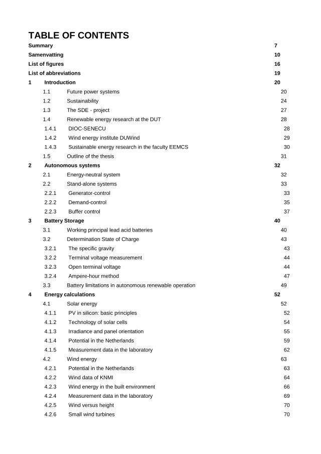
TABLE OF CONTENTS Summary 7 Samenvatting 10 List of figures 16 List of abbreviations 19
1 Introduction 20
1.1 Future power systems 20 1.2 Sustainability 24 1.3 The SDE - project 27
1.4 Renewable energy research at the DUT 28
1.4.1 DIOC-SENECU 28
1.4.2 Wind energy institute DUWind 29 1.4.3 Sustainable energy research in the faculty EEMCS 30
1.5 Outline of the thesis 31 2 Autonomous systems 32
2.1 Energy-neutral system 32
2.2 Stand-alone systems 33 2.2.1 Generator-control 33
2.2.2 Demand-control 35 2.2.3 Buffer control 37
3 Battery Storage 40
3.1 Working principal lead acid batteries 40 3.2 Determination State of Charge 43
3.2.1 The specific gravity 43 3.2.2 Terminal voltage measurement 44
3.2.3 Open terminal voltage 44 3.2.4 Ampere-hour method 47
3.3 Battery limitations in autonomous renewable operation 49 4 Energy calculations 52
4.1 Solar energy 52 4.1.1 PV in silicon: basic principles 52
4.1.2 Technology of solar cells 54
4.1.3 Irradiance and panel orientation 55 4.1.4 Potential in the Netherlands 59 4.1.5 Measurement data in the laboratory 62
4.2 Wind energy 63
4.2.1 Potential in the Netherlands 63
4.2.2 Wind data of KNMI 64 4.2.3 Wind energy in the built environment 66 4.2.4 Measurement data in the laboratory 69 4.2.5 Wind versus height 70 4.2.6 Small wind turbines 70
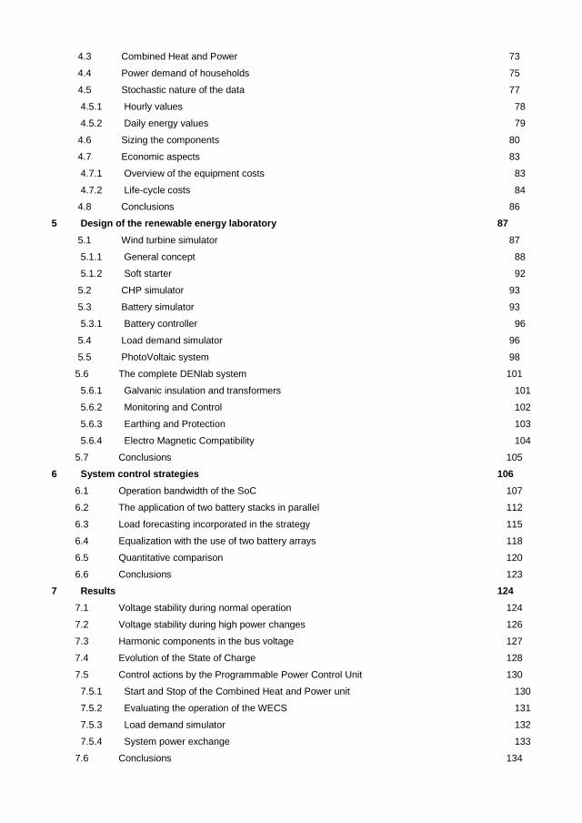
4.3 Combined Heat and Power 73
4.4 Power demand of households 75 4.5 Stochastic nature of the data 77 4.5.1 Hourly values 78 4.5.2 Daily energy values 79
4.6 Sizing the components 80
4.7 Economic aspects 83 4.7.1 Overview of the equipment costs 83 4.7.2 Life-cycle costs 84
4.8 Conclusions 86 5 Design of the renewable energy laboratory 87
5.1 Wind turbine simulator 87 5.1.1 General concept 88
5.1.2 Soft starter 92 5.2 CHP simulator 93
5.3 Battery simulator 93 5.3.1 Battery controller 96
5.4 Load demand simulator 96
5.5 PhotoVoltaic system 98
5.6 The complete DENlab system 101 5.6.1 Galvanic insulation and transformers 101 5.6.2 Monitoring and Control 102
5.6.3 Earthing and Protection 103 5.6.4 Electro Magnetic Compatibility 104
5.7 Conclusions 105 6 System control strategies 106
6.1 Operation bandwidth of the SoC 107
6.2 The application of two battery stacks in parallel 112
6.3 Load forecasting incorporated in the strategy 115
6.4 Equalization with the use of two battery arrays 118 6.5 Quantitative comparison 120 6.6 Conclusions 123
7 Results 124
7.1 Voltage stability during normal operation 124
7.2 Voltage stability during high power changes 126 7.3 Harmonic components in the bus voltage 127 7.4 Evolution of the State of Charge 128
7.5 Control actions by the Programmable Power Control Unit 130 7.5.1 Start and Stop of the Combined Heat and Power unit 130 7.5.2 Evaluating the operation of the WECS 131
7.5.3 Load demand simulator 132 7.5.4 System power exchange 133
7.6 Conclusions 134

8 Renewable Energy Forecasting 135
8.1 Wind Forecasts 135 8.1.1 Persistence 136
8.2 Sun Forecasts 141 8.3 Results with forecasting method 144 8.4 Conclusions applying forecasting 148
9 Super Capacitors 149
9.1 Theory 150 9.2 Different battery-supercapacitor combinations 152
9.2.1 Model simplifications 155
9.2.2 A comparison between the DC and AC-configuration 158 9.3 Sizing of SC systems 159 9.4 Control strategy 161
9.5 Simulation results 161 10 Conclusions 166 References 169
Appendix Benchmarking project for hybrid power systems 172 Curriculum Vitae 176

LIST OF FIGURES
Figure 1-1 Historical and predicted electricity demand in the Netherlands......................................................... 20
Figure 1-2 Driver forces to new Power Systems, source: SmartGrids [6] .......................................................... 23
Figure 1-3 the relationships between the different SDE-projects ....................................................................... 28
Figure 2-1 AGC control action .......................................................................................................................... 35
Figure 2-2 Example of dump-load application in AES ....................................................................................... 36
Figure 2-3 Electrical appliances with different properties .................................................................................. 36
Figure 2-4 A Three phase inverter ................................................................................................................... 37
Figure 2-5 Sinusoidal PWM ............................................................................................................................. 38
Figure 2-6 Harmonic spectrum ........................................................................................................................ 39
Figure 3-1 State of Charge indices during charge and discharge operation ...................................................... 43
Figure 3-2 Charging voltage as a function of SOC and the C-rate ..................................................................... 45
Figure 3-3 Discharge voltage vs. SOC and C-rate ............................................................................................ 45
Figure 3-4 Trend line (polynomial) .................................................................................................................... 46
Figure 3-5 The P-factor as a function of the discharge currents ........................................................................ 48
Figure 3-6 Charge efficiency near top-of-charge ............................................................................................... 49
Figure 3-7 A number of battery problems .......................................................................................................... 50
Figure 4-1 PN-process by incoming photons .................................................................................................... 53
Figure 4-2 Solar radiation components ............................................................................................................. 55
Figure 4-3 Irradiance diagram for the Netherlands ............................................................................................ 56
Figure 4-4 Orientation angles for the solar modules .......................................................................................... 57
Figure 4-5 Solar panels output power from direct and diffuse radiation ............................................................. 58
Figure 4-6 Total hourly solar power (Psolar) pattern for 1996 & 1997 .................................................................. 59
Figure 4-7 Monthly global irradiance pattern 1996 ............................................................................................ 59
Figure 4-8 Monthly global irradiance pattern 1997 ............................................................................................ 59
Figure 4-9 Global sun irradiations in the Netherlands in kWh/year .................................................................... 60
Figure 4-10 PV power on July 6. and July 7. in 2004, measured in DENLAB (120m2) ....................................... 61
Figure 4-11 PV output power, based on measurements in DENlab 2005 .......................................................... 62
Figure 4-12 Average wind speed in the Netherlands ......................................................................................... 64
Figure 4-13 Distribution and Cumulative frequency distribution of wind speed at Zestienhoven ........................ 65
Figure 4-14 Wind rose calculated from station Zestienhoven ............................................................................ 66
Figure 4-15 CFD calculations of wind turbulence around a building .................................................................. 67
Figure 4-16 Zone of wind turbulence caused by an obstacle ............................................................................. 68
Figure 4-17 Satellite view of the DENlab anemometer site ............................................................................... 68
Figure 4-18 One minute average of the wind speed on 1-5-2004, measured in DENlab ................................... 69
Figure 4-19 Power Curve of the Turby (left) and Furlander FL30 (right) ............................................................ 71
Figure 4-20 Fuhrlander FL30 (left) and Turby (right) ......................................................................................... 71
Figure 4-21 Calculated values of wind turbine output in DENlab ....................................................................... 72
Figure 4-22 Schematic of micro CHP ................................................................................................................ 74
Figure 4-23 The coincidence factor as function of the number of consumers in the group................................. 75
Figure 4-24 Typical load pattern for different number of houses........................................................................ 76
Figure 4-25 Random four weeks load pattern of 10 households ....................................................................... 77
Figure 4-26 Scatter plot with hourly values of PV and Wind .............................................................................. 78
Figure 4-27 Scatter plot with daily values of PV and Wind ................................................................................ 79
Figure 4-28 Daily energy of solar and Load ...................................................................................................... 80
Figure 4-29 Effect of battery storage on auxiliary power contribution ................................................................ 81
Figure 4-30 Effect of battery storage of hours of operating aux. source ............................................................ 82
Figure 5-1 Set-up of the wind turbine simulator ................................................................................................. 88
Figure 5-2 Example of the power curve for a stall-regulated wind turbine ......................................................... 89
Figure 5-3 Motor-generator set 37 kW as it is installed in DENlab ..................................................................... 89
Figure 5-4 Full torque-speed characteristic for three different stator frequencies .............................................. 90
Figure 5-5 Soft starter circuit ............................................................................................................................. 92
Figure 5-6 Example of soft starter characteristic ............................................................................................... 92
Figure 5-7 Motor-generator set representing the CHP (left Motor, right Generator) ........................................... 93
Figure 5-8 Circuit diagram of the battery simulator ............................................................................................ 94
Figure 5-9 An AC/DC/AC system representing the battery simulator................................................................. 95
Figure 5-10 A feedback system to control the battery current ........................................................................... 96
Figure 5-11 Load demand simulator ................................................................................................................. 97
Figure 5-12 Inverter part of the load demand simulator ..................................................................................... 97
Figure 5-13 Roof for PV-panels (1st part), at the right-side the high-rise building .............................................. 98
Figure 5-14 Detail of PV installation .................................................................................................................. 99
Figure 5-15 Set-up of PV-panels at DUT .......................................................................................................... 99
Figure 5-16 View of the first part of the PV system ......................................................................................... 100
Figure 5-17 Actual set-up of the DENlab laboratory ........................................................................................ 101
Figure 5-18 User interface of the laboratory system ........................................................................................ 103
Figure 5-19 TN-S system ................................................................................................................................ 103
Figure 5-20 Snapshot of the laboratory system ............................................................................................... 104
Figure 6-1 State diagram first strategy ............................................................................................................ 107
Figure 6-2 Flowchart first strategy ................................................................................................................... 108
Figure 6-3 Plot of results for entire year (first strategy) .................................................................................... 109
Figure 6-4 Plot of results for first month (first strategy) .................................................................................... 109
Figure 6-5 Simulation result with excessive power variant .............................................................................. 112
Figure 6-6 State diagram second strategy ...................................................................................................... 113
Figure 6-7 Plot of results for the entire year (second control strategy) ............................................................. 113
Figure 6-8 Plot of results for first month (second control strategy) ................................................................... 114
Figure 6-9 Control diagram (third control strategy) .......................................................................................... 115
Figure 6-10 Plot of results for entire year (third control method) ...................................................................... 116
Figure 6-11 Plot of results for first month (third control method) ...................................................................... 116
Figure 6-12 Control diagram (fourth control strategy) ...................................................................................... 118
Figure 6-13 Plots of the results for entire year (fourth control strategy) ........................................................... 119
Figure 6-14 Plot of the result of the first month (fourth control strategy) .......................................................... 119
Figure 7-1 Basic circuit Active Frond End Converter ....................................................................................... 125
Figure 7-2 RMS voltage during normal operation ............................................................................................ 126

Figure 7-3 Measurement of the voltage of the autonomous grid...................................................................... 126
Figure 7-4 Voltage waveform at the autonomous rail ...................................................................................... 127
Figure 7-5 Harmonic Spectrum of the voltage waveform ................................................................................. 127
Figure 7-6 Battery current and SoC evolution ................................................................................................. 128
Figure 7-7 CHP start at low SoC level............................................................................................................. 130
Figure 7-8 Wind speed and power of the WECS ............................................................................................. 131
Figure 7-9 Load demand pattern..................................................................................................................... 132
Figure 7-10 Measurement result of DENlab system ........................................................................................ 133
Figure 8-1 RMS errors for different forecasting models .................................................................................. 135
Figure 8-2 Autocorrelation values for wind speed and power time series, for DENlab and S344 ..................... 137
Figure 8-3 Wind forecasting errors for different ............................................................................................... 138
Figure 8-4 Wind power forecasts compared with the real wind power produced ............................................. 140
Figure 8-5 a) models for sun power forecasting b) Autocorrelation function for sun power output in 2005 ....... 141
Figure 8-6 Simple persistence (p) and new persistence (np) results for sun forecasting ................................. 142
Figure 8-7 MAE and RMSE for six models predicting sun power for 2005 ...................................................... 143
Figure 8-8 Real solar output vs. one and three hours forecast ........................................................................ 143
Figure 8-9 General structure of simulation programs ...................................................................................... 145
Figure 8-10 Cost function values for 2005 models, with the three different types of forecasts ......................... 147
Figure 9-1 Overview storage systems source: electricitystorage.org ............................................................... 149
Figure 9-2 Construction of a Double Layer Capacitor...................................................................................... 150
Figure 9-3 S.C. price evolution from 1996 to 2010 (expected), source: Maxwell (2006) .................................. 151
Figure 9-4 Super capacitor and Battery combination on one DC-system ........................................................ 152
Figure 9-5 Matlab Simulink model of option B ................................................................................................. 153
Figure 9-6 Currents [Amps] in DC- Super capacitor and Battery combination ................................................. 154
Figure 9-7 Voltages [V] of Super capacitor and Battery combination in DC-system ......................................... 154
Figure 9-8 Supercapacitor-battery system with decoupled DC-circuits ............................................................ 155
Figure 9-9 Simplified models for VSC and CSC converters ............................................................................. 156
Figure 9-10 Powers vs. time for decoupled DC-buses .................................................................................... 157
Figure 9-11 Super-capacitor battery system with decoupled DC-buses .......................................................... 158
Figure 9-12 Power exchange between SC and battery ................................................................................... 160
Figure 9-13 Battery current control system ..................................................................................................... 161
Figure 9-14 Final autonomous energy system, with an integrated SC storage system .................................... 162
Figure 9-15 Power exchange between system components during 1 hour ...................................................... 163
Figure 9-16 Power exchange between system components during 2 minutes ................................................ 164
Figure 9-17 Currents [A] and voltages [V] of the battery and the Super Capacitor ........................................... 165

LIST OF ABBREVIATIONS
AGM Absorbent Glass Mat
ARES Autonomous Renewable Energy System
CHP Combined Heat and Power
DG Distributed Generation
DoD Depth of Discharge
DSM Demand Side Management
FET Field Effect transistor
KNMI Royal Dutch Meteorological Institute
LCC Life-cycling costing
PCC Point of Common Coupling
PLC Programmable Logic Controller
PV Photo-Voltaic
PWM Puls-Width Modulation
RES Renewable Energy Source
SC Super Capacitor
SDE Samenwerkingsverband Duurzame Energy
SoC State of Charge
UPS Uninterruptible Power Supply
VRLA Valve-Regulated Lead Acid (battery)
WECS Wind Energy Conversion System

1 INTRODUCTION
The history of the electrical engineering started with the early experiments of Benjamin Franklin (1706-1790), Michael Faraday (1791-1867), Luigi Galvani (1737-1798), Alessandro Volta (1745-1827), André-Marie Ampère (1775-1836) and Georg Simon Ohm (1789-1854). Because of their inventions, there became a fundament for an electrical society. The influence of the electricity in the modern society is nowadays essential: a world without electricity is now inconceivable. In particular during power failures, i.e. black-outs, the society‟s dependency on electrical energy becomes perceptible. A high quality design of the electrical infrastructure, with redundancy, the continuous monitoring of the system and maintenance of the system components has resulted in a very reliable power system in particular in the economically strong countries. The Dutch power system is currently one of the most reliable systems in the world.
In the last decade, the electrical energy consumption has grown in the Netherlands from 80 TWh in 1990 to 108 TWh in 2000, being an increase of 35%. Estimations show that the electricity consumption in 2010 will be 125 TWh [1].
Figure 1-1 Historical and predicted electricity demand in the Netherlands
1.1 Future power systems
Traditional Power Systems are nowadays changing under the influence of two mechanisms: the market operation of the power system and the introduction of renewable energy conversion systems. [2-6].

1. Introduction 21 21
The electrical infrastructure in most OECD Countries (Organisation for Economic Co-operation and Development) is typically composed of rather large power systems with ageing generation and grid assets. In 2010, close to approximately 65% of this central power generation will be based on fossil fuels. In order to break this trend and increase generation efficiency a substantial replacement and refurbishment program will have to be initiated within the next years. The historical development of transmission and distribution assets is closely associated with the development of generation but the technical lifetime is often longer.
Another important driver is the increasingly strong focus being placed on environmental issues. This encompasses generation as well as transmission and distribution. In the field of generation, environmental concerns drive the search for cleaner technologies (less or no greenhouse emission) as well as higher energy conversion efficiencies. In transmission and distribution area, a reduction of visual, electromagnetic and acoustic impact is foreseen as well as a reduction in transmission losses.
Yet another driver is the liberalisation of energy markets currently taking place, which influences the properties of the markets. I.e. the investments have been kept relatively low for the past decade due to the competitive pressure. Regulators and investors therefore actively seek new mechanisms for new technical solutions in order to cope adequately with the electricity market dynamics.
The electricity sector faces new challenges and opportunities which must be responded to in a vision of the future [6]:
User-centric approach: increased interest in electricity markets opportunities, value added services, flexible demand for energy, lower prices, micro-generation opportunities;
Electricity networks renewal and innovation: pursuing efficient asset management, increasing the degree of automation for better quality of service; using system wide remote control; applying efficient investments to solve infrastructure ageing;
Security of supply: limited primary resources of traditional energy sources, flexible storage; need for higher reliability and quality; increasing network and generation capacity;
Liberalised markets: responding to the requirements and opportunities of liberalisation by developing and enabling both new products and new services; high demand flexibility and controlled price volatility, flexible and predictable tariffs; liquid markets for trading of energy and grid services;
Interoperability of European electricity networks: supporting the implementation of the internal market; efficient management of cross border and transit network congestion; improving the long-distance transport and integration of renewable energy sources; strengthening European security of supply through enhanced transfer capabilities;
Distributed generation (DG) and renewable energy sources (RES): local energy management, losses and emissions reduction, integration within power networks;
Central generation: renewal of the existing power-plants, development of efficiency improvements, increased flexibility towards the system services, integration with RES and DG;
Environmental issues: reaching Kyoto Protocol targets; evaluate their impact on the electricity transits in Europe; reduce losses; increasing social responsibility

1. Introduction 22 22
and sustainability; optimising visual impact and land-use; reduce permission times for new infrastructure;
Demand response and demand side management (DSM): developing strategies for local demand modulation and load control by electronic metering and automatic meter management systems;
Politics and regulatory aspects: continuing development and harmonisation of policies and regulatory frameworks in the European Union (EU) context;
Social and demographic aspects: considering changed demand of an ageing society with increased comfort and quality of life.
Today‟s electricity networks provide an essential service for society, built to ensure access for every single electricity customer. The power flow was controlled by a vertically operated system with dominant power plants, a distributed consumption and no direct interconnection between the control areas.
In response to new challenges and opportunities, electricity networks have started to evolve. The aim is that they accommodate more decentralised generation services, with many actors involved in the generation, transmission, distribution and operation of the system.
Future visions on Power Systems differ in details. The CIGRE Workgroup JAG 02 TC [2] supposes that a centralised generation structure, based on the present power system, prevails. Two scenarios are proposed: the distribution scenario and the „mixtribution‟ scenario. The last scenario is closely related to the SMARTGRIDS vision [6], which predicts that Europe‟s electricity networks in 2020 and beyond will be “FARE”:
Flexible Fulfilling customers‟ needs whilst responding to the changes and challenges ahead;
Accessible Granting connection access to all network users, particularly for renewable energy systems (RES) and high efficiency local generation with zero or low carbon emissions;
Reliable Assuring and improving security and quality of supply, consistent with the demands of the digital age;
Economic Providing best value through innovation, efficient energy management and „level playing field‟ competition and regulation.
Driving factors in the move towards SmartGrids are the European Internal Markets, the security and quality of supply and the environment.

1. Introduction 23 23
Liberalisation
Low prices and
efficiency
Innovation and
competitiveness
Primary energy
availability
Capacity
Reliability and quality
Nature and wildlife
preservation
Climate change Pollution
INTE
RN
AL M
AR
KE
TENVIRONMENT
SE
CU
RIT
Y O
F S
UP
PLY
Figure 1-2 Driver forces to new Power Systems, source: SmartGrids [6]
Hydro- and nuclear power plants are well established methods of generation with nearly zero greenhouse gasses. Accommodating change may be possible by incorporating new generation technologies. Successful examples are wind turbines and solar panels, but there are other distributed generation technologies that are either already commercial or
close to being on the market, such as micro combined heat and power systems (CHP).
These forms of power generation have different characteristics from traditional power plants. Most of them have much smaller electricity outputs; some of the newer technologies also exhibit greater intermittency.
It is difficult to predict the impact of distributed generation on the future energy mix. Research in this area is essential.
There is uncertainty in many aspects of future grids:
In the primary energy mix; In the electricity flows created by the liberalised market; Of the instantaneous power output of many renewable energy sources; In regulatory frameworks and investment remuneration in innovation.
The best strategy for managing these uncertainties is to build flexibility and robustness into the future network.
Distribution grids will become active and will have to accommodate bi-directional power flows. The European electricity systems have moved to operate under the framework of a market model.

1. Introduction 24 24
The future grids will have six properties:
User specified quality, security and reliability of supply for the digital age; Flexible, optimal and strategic grid expansion, maintenance and operation; Flexible DSM and customer-driven value added services; Harmonised legal frameworks facilitating cross-border trading of power and grid
services; Massive small, distributed generation connected close to end customers; Coordinated, local energy management and full integration of DG and RES.
This study will focus on the last two topics.
1.2 Sustainability
Sustainable development is an important issue for the coming century [4]. The new built areas in 2020 will already be influenced by the drive for sustainability. An often-quoted definition of sustainability, proposed by the commission Brundlandt, is [7]:"Meeting the needs of the present generation without compromising the needs of future generations to meet their own needs."
It includes two key concepts:
The concept of „needs‟, in particular the essential needs of the world‟s poor part that overriding priority should be given; and
The idea of limitations imposed by the state of technology and social organization on the environment‟s ability to meet present and future needs.
Interpretations will vary, but share certain general features. It must develop from a consensus on the basic concept of sustainable development to a broad strategic framework for achieving it. The development involves a progressive transformation of economy and society. A development path that is sustainable in a physical sense could theoretically be pursued.
Sustainable development authors view the challenge of sustainable consumption as a spectrum. At the near end of this spectrum are measures that require less in terms of intervention and active change. Examples of simple technological interventions are the installation of solar cells and a big cut in standby power requirements for audio and video equipment. They could have a very positive environmental impact. In the centre of the spectrum are more radical changes in habits and routines, such as restoring a sense of seasonality to what we eat, turning off lights and opting to walk or cycle in the neighbourhood rather then taking the car. At the far end of the spectrum are innovations and measures that allow people to change behaviour in a more fundamental way, such as limiting the air traffic. [8]
Meeting essential needs partly depend on achieving full growth potential and sustainable development clearly requires economic growth in places where such needs are not being met.
A society may in many ways compromise its ability to meet the essential needs of future generations by overexploiting resources, for example. The direction of technological developments may solve some immediate problems but may lead to even greater ones in the future.
As for non-renewable resources, like fossil fuels and minerals, their use reduces the stock available for future generations. But this does not mean that such resources should

1. Introduction 25 25
not be used. In general the rate of depletion should take into account the criticality of that resource, the availability of technologies for minimizing depletion, and the likelihood of substitutes being available. Sustainable development requires that the rate of depletion of non renewable resources should excluded future options as few as possible.
In essence, sustainable development is a process of change in which the exploitation of resources, the direction of investments, the orientation of technological development and institutional change are all in harmony and enhance both current and future potential to meet human. As the commission Brundlandt says: The world must quickly design strategies that will allow nations to move from present, often destructive, processes of growth and development onto sustainable development paths.
Energy is an essential human need, one that cannot be universally met unless energy consumption patterns change. The ultimate limits to global development are perhaps determined by the availability of energy resources and by the biosphere‟s capacity to absorb the by-products of energy use. First, there are the supply problems: the depletion of oil reserves, the high cost and environmental impact of coal mining and gas winning, and the hazards of nuclear technology. Second, there are emission problems, most notably acid pollution and carbon dioxide build-up leading to global warming.
Some of these problems can be met by increasing use of renewable energy sources. But the exploitation of some renewable sources such as biomass and hydropower also entails ecological problems. Hence sustainability requires a clear focus on conserving and efficiently using energy.
In its broadest sense, the strategy for sustainable development aims to promote harmony among human beings and between humanity and nature. In the specific context of the development and environmental crises of the 1980s, which current national and international political and economic institutions have not and perhaps cannot overcome, the pursuit of sustainable development requires:
A political system that secures effective citizen participation in decision making; An economic system that is able to generate surpluses and technical knowledge
on a self-reliant and sustained basis; A social systems that provides solutions for the tensions arising from
disharmonious development; A production system that respects the obligation to preserve the ecological base
for development; A technological system that can search continuously for new solutions; An international system that fosters sustainable patterns of trade and finance; An administrative system that is flexible and has the capacity for self-correction.
These requirements are more in the nature of goals that should underlie national and international action on development.
Focusing on energy issues, it‟s clear that today‟s primary sources of energy are mainly non-renewable: natural gas, oil, coal and conventional nuclear power. There are also renewable sources, hydro power, geothermal sources, solar, wind, and wave energy, as well as biomass. In theory, all the various energy sources can contribute to the future energy mix, but each had its own economic, health and environmental costs, limitations, benefits and risks. Choices must be made, but in the certain knowledge that choosing an energy strategy inevitably means choosing an environmental strategy.

1. Introduction 26 26
Patterns and changes in energy usage today are already dictating patterns well into the next century. According to the Brundlandt commission, the key elements of sustainability that have to be reconciled are:
Sufficient growth of energy supplies to meet human needs; Energy efficiency and conservation measures, such that waste of primary
resources is minimized; Public health, recognizing the problems of risks to safety inherent in energy
sources; Protection of the biosphere and prevention of more localized forms of pollution.
The crucial point about lower energy-efficient is not whether they are perfectly realizable in their proposed time frames. Political and institutional mind shifts are required to restructure investment potential in order to move along these lower consumption or more energy-efficient paths.
Many forecasts of exploitable oil reserves and resources suggest that oil production will level off by the early decades of the next century and then gradually fall during a period of reduced supplies and higher prices. Gas supplies should last over 200 years and coal about 3000 years at present rates of use. The estimates persuade many analysts that the world should immediately embark on a vigorous oil conservation policy. In terms of pollution risks, gas is by far the cleanest fuel, with oil next and coal a poor third. But they all pose three interrelated atmospheric pollution problems: global warming, urban industrial air pollution and acidification of the environment.
Focussing on the built-up environment, a broad range of technical measures for improving energy efficiency in homes are already well understood to be cost-effective and readily available on the market. These are: insulation, draught proofing, secondary and double glazing, improved heating systems, wider use of heating controls and efficient lighting and appliances. Installing micro-generation also reduces demand for centrally supplied energy, such as with solar hot water systems, ground source heat pumps and photovoltaics. Micro CHP boilers allow households to generate electricity whilst consuming gas for heating, and community wide CHP schemes provide probably the most cost effective option for reducing demand for energy in certain housing densities.
To encourage more sustained and widespread adoption of energy efficiency measures, the steps in the following directions can be taken: [9]
Improved consumer information through measures such as installing smart meters into houses, liked on the fuel bills or compared to typical households;
Improved incentives and requirements for building contractors and energy suppliers in homes or the introduction of personal carbon credit system.
Renewable energy sources could in theory provide the global energy consumption [10]. Solar energy use is small globally, but it is beginning to assume an important place in the energy consumption patterns of some countries, especially in the „hot countries‟ like Australia, Greece and the Middle East.
Wind power has been used for centuries – mainly for pumping water. Recently its use has been growing rapidly in regions such as California and Scandinavia. In these cases, the wind turbines are used to generate electricity for the local grid. Many countries have already successful programs, but the untapped potential is still high.
Most renewable energy systems operate best at small to medium scales, ideally suited for rural and suburban applications. The need for a steady transition to a broader and

1. Introduction 27 27
more sustainable mix of energy sources is beginning to become accepted. Renewable energy sources could contribute substantially to this.
1.3 The SDE - project
In 1997 a third-partner project was initiated to design an autonomous energy system for supplying energy to households. The project focuses on the development of a Power Control Unit that supervises and controls an energy system, powered by renewable energy sources that supplies approximately 10 households. In the design, a small wind
turbine, solar panels and a micro Combined Heat and Power system (-CHP) were selected to supply the necessary electrical energy for ten households. To balance the generated and consumed power a battery storage system was foreseen. The design of the laboratory environment to carry out this project is the main subject of this initial project.
Preliminary calculations were made, mainly based on simplified models of the generation system as such in combination with mean values of wind speeds, solar irradiations and load side power demands. This research resulted in a general impression about the feasibility of an autonomous renewable energy system in relation to the local conditions.
This rough impression was, however, not sufficient to develop the Power Control Unit and the available computer models did not suit for the power range of this particular case. Apart from that, experience with other projects has learned that building a system in practice is in fact the best way to study and understand the system.
In 1999, we decided to the build the DENlab ® laboratory model for the study of
autonomous system with three aims:
To develop a Programmable Power Control Unit; To model system components with practical verification; To acquire practical knowledge about how to set up autonomous renewable
energy systems;
Based on a project application, SDE (Samenwerkingsverband Duurzame Energie), a cooperative body initiated by the Ministry of Economic Affairs chooses this project to participate in its research program: System Integration of Renewable Energy in the built-environment.
The participating partners in this research program are KEMA-Arnhem, IVAM-Amsterdam, ECN-Amsterdam, ECN-Petten, TNO-MEP Apeldoorn and the Delft University of Technology (DUT).
The following topics were addressed in this research:
The prediction of contribution of wind and solar energy to the energy balance for the coming 24 to 48 hours; (ECN-Petten)
The generation of a realistic load demand pattern generator based on the input of questionnaires as well as on actual measurements; (KEMA-IVAM)
To find out how load demand can influence the user behaviour by setting goals and giving feedback (ECN-Amsterdam)
To develop of a functional description of an overall power controller (KEMA) To develop and to test a prototype of an optimised power control unit for
autonomous renewable energy systems applied to households (DUT).

1. Introduction 28 28
User
Behaviour and Acception
Energy demand
Pattern and Prediction
Household demand
System
Control Optimization
Sources
Pattern and Predictions
Solar and Wind
Functional design Controls and Protection
Test facility and PPCU
Monitoring and Evaluation
Tested Prototype
Figure 1-3 the relationships between the different SDE-projects
1.4 Renewable energy research at the DUT
The technological demands arising from the challenges facing society are becoming increasingly complex. Protecting the land from the water, for example, is not simply a question of building dikes. Other factors have to be taken into consideration, including the minimum acceptable human and capital risks, climate change and changing societal needs. These complex problems need to be studied from a multidisciplinary perspective when we want to find robust and sustainable solutions. The thirteen Delft Research Centres (DRCs) provide integrated solutions for these multidisciplinary problems by bundling excellent research. In this way, the knowledge and expertise built up over the years on thirteen important research themes is made available to society, industry and policy. This thesis is partly a result from research in the framework of one of these thirteen DRCs: Sustainable Energy.
1.4.1 DIOC-SENECU
The Delft University of Technology decided in 1997 to direct a substantial part of the University's fundamental and applied research to a strong contribution to the research and development of cleaner energy systems, which obviously do include sustainable energy sources. They are the targeted fields of research and development for securing our future energy supply and, in particular, protecting the environment. Hence, the scientific research program of the Technology Theme Sustainable Energy: Extraction, Conversion and Use has the ambition to deliver important contributions to the utilization

1. Introduction 29 29
of sustainable energy via in depth fundamental and applied research and development projects. In line with the recent interest on a National Level in Sustainable Hydrogen, research on sustainable energy conversion and storage of hydrogen constitutes an important part of the present Technology Theme.
The scientific program of the Technology Theme "Sustainable Energy: Extraction, Conversion and Use" is based on the sub - themes: Solar Energy Conversion, Wind Energy in the Built Environment, Biomass Gasification and Gas Purification, Storage of Electrical Energy in Rechargeable Batteries, Production and Storage of Sustainable Hydrogen, Conversion of Chemical to Electrical Energy using Fuel Cells, and Power Electronics. Attention will also be focused on the societal acceptance of sustainable energy sources, in particular, of hydrogen.
The Technology Theme has its roots in the program "Decentralized Production and Storage of Electricity for Large-Scale Application of Renewable Energy" of the Delft Interfaculty Research Centre (DIOC) "Extraction, Conversion and Use of Energy", which was executed very successfully in the period 1997-2001, and the more recent program "Sustainable Hydrogen: Energy Carrier of the Future", which received financial support from TU Delft in December 2001. The continuation of the first program and the "Sustainable Hydrogen" program constitute the program of the present Technology Theme. It is emphasized that as a prelude to a Hydrogen Economy, the present Technology Theme comprises a substantial number of projects directed to the production of hydrogen, using sustainable energy sources, the safe and cheap storage of hydrogen, supported by fundamental characterization studies, and utilization.
The search for cleaner, cheaper, and more efficient alternative energy technologies has been driven by recent developments in materials science and engineering. Indeed, advanced solar cells with nanostructures, rechargeable batteries based on materials with nanostructures, hydrogen storage composite materials, based on light-weight metal hydrides and transition-metal oxide catalysts, IT-SOFC components, and wind turbine blades are and will be to a large extend, the result of materials science and engineering successes.
Biomass gasification and gas purification is another route to sustainable hydrogen and is supported by advanced reactor technology. The use of high-temperature waste heat for the thermo chemical production of hydrogen is an important feasibility study.
At the Delft University of Technology unique experimental characterization and theoretical modelling techniques are available. These will guide the materials scientists in designing, in particular, storage devices for electrons and hydrogen.
1.4.2 Wind energy institute DUWind
The wind institute, DUWind, has founded in August 1999 to stimulate the synergy between the different disciplines which are related to implementation of wind energy. The wind institute covers the wide scope of topics as erecting and founding wind turbines, its aero-dynamic aspects, its off-shore aspects and electro dynamical behaviour of wind turbines. Each discipline of the participating research groups has its own specific expertise, but an increasing number of research problems require a multi-disciplinary approach.
On all these issues the Section Wind Energy has contributed significantly to the increase of knowledge and the development of numerical tools. The SWING
® series of numerical

1. Introduction 30 30
wind field simulators, the DU-W
® airfoil family, the airfoil design code XFOIL, the rotor
aerodynamic codes PREDICHAT and PREDICDYN, and the DUWECS® dynamic wind
turbine simulator have been results of these modelling efforts.
Since the beginning of the nineties offshore application of wind turbines is also a field of research interest at Delft University. The dynamic loads code DUWECS
® was extended
to incorporate wave loads, and a more extensive soil model was added to incorporate the effects of variation of soil properties. The latter is of special importance for the modelling of monopod foundations. Over the decade an integrated design approach was developed for large scale offshore wind farms. Apart from integrated numerical structural models with simultaneous wind and wave loads, such an approach required the development of cost models and operational research models. The integrated design philosophy was first demonstrated in the design solution presented within the Opti-OWECS project, an international EU funded research project, which was coordinated by the TU Delft.
The use of wind energy in the built environment has gained new interest. Apart from the application of standard "propeller-type" wind turbines near buildings the research focuses on the potential of specially adapted wind turbines, often with a vertical axis and slow running, and of "passive" use of wind power. In the latter case it is tried to use pressure differences originating from ambient wind conditions to perform work, e.g. by powering natural ventilation or by augmenting the performance of more or less standard wind turbines on top of a building.
1.4.3 Sustainable energy research in the faculty EEMCS
Within the faculty Electrical Engineering, Mathematics and Computer Science (EEMCS), the sustainability projects are mainly concentrated in the Electrical Power Engineering (EPE) department. Only one research group outside the EPE department has activities on the renewable energy field; the microelectronic department (DIMES) investigates the development of new solar cells techniques.
This EPE department consists of the High Voltage Technology and Management laboratory (HTM), the Electrical Power Processing laboratory (EPP) and the Electrical Power Systems laboratory (EPS).
The sustainable research issues of HTM group are concentrated on the research on materials. Some of the High-Voltage switchgear uses the toxic and environmental unfriendly insulation gas SF6 and polluting oil. Research is essential to investigate the applicability and the properties of other materials. On the other hand, life time extension of the Power System assets is investigated in order to minimize or at least extend the need of replacement of the components.
The EPP-group is a research group focusing on energy conversion issues: power electronics and electrical machines and drives. They made a substantial contribution in renewable energy solutions such as the Archimedes Wave Swing (applying wave energy as a renewable power source) and new types of generators for wind turbines. For the application and conversion of renewable energy sources, the power electronics is more and more important. Within the framework of the EMVT-IOP (A Dutch acronym for Electrical Magnetic Power Technology Innovative Research Program), research is carried out to develop power electronic solutions in order to make the future power system intelligent.

1. Introduction 31 31
The Electrical Power Systems laboratory focuses on the analysis of electrical power systems. The liberalization and the deregulation of the energy market combined with the fast increase of distributed generation makes the need for new simulation tools and the analysis of the foreseen new system behaviour necessary. Traditionally, the power system is divided into its voltage level and its functionality: transmission network (U > 110 kV), the distribution network (10 – 110 kV) and the low voltage network (0.4 – 10 kV). On all these levels, the influence of distributed generation is analysed in order to acquire a reliable operation of the future power system. The analyses of the future power systems can only be carried out with the help of software tools, because other means are not very practical: to large and to expensive. A physical laboratory is a realistic option for research on the lowest voltage level, where the behaviour of individual households is investigated.
1.5 Outline of the thesis
In this introduction general information concerning renewable energy systems and the background of this research are given.
Chapter two focuses on different autonomous systems. Several definitions are used in literature. This chapter clarifies the differences between the systems and defines the chosen concept for this research.
Chapter three presents a literature study on the battery application in autonomous energy systems. This chapter focuses on the determination of the State of Charge and describes the limitations of using batteries for this application.
In chapter four, energy calculations are carried out in order to size the system components. Furthermore this chapter gives some more details about the different parts of the system (PV, wind, CHP and Load demand).
Chapter five describes the representation of the individual components in the laboratory and the construction of the laboratory, including the monitoring system. Some specific laboratory aspects as EMC and Earthing and Protection, are discussed here.
Chapter six presents four different overall control strategies and the effects of these strategies on the overall performance of the system.
Chapter seven describes the results of the measurements in the laboratory. The obtained results are compared with the standard EN50160.
Chapter eight investigates the added value of renewable energy forecasting for the overall system performance.
Chapter nine proves the possibility of applying super capacitors in parallel to the batteries in order to prevent the battery from fast power changes. Batteries have a limited response time which is not suitable on the nature of the used sources and sinks in the described system.
In chapter ten, conclusions are drawn concerning the work and results presented in this thesis.

2 AUTONOMOUS SYSTEMS
Within the context of the project, a literature study has been carried out to find out what‟s already described in the literature and what issues are still „white spots‟ in the field.
The white spots are defined to be: the system integration of renewable energy sources within a small autonomous systems and the application of standard batteries in order to maintain the power balance in an autonomous energy system.
This chapter reviews the different forms of autonomous systems. Chapter 3 will discuss the battery behaviour in autonomous systems.
Looking into history, the first built power systems were in fact autonomous energy systems. Large cities established their own power stations and distribution system to supply their inhabitants. In a latter phase, these local distribution systems were coupled to regional energy companies to increase the overall reliability of the system. These regional power systems were coupled in the Netherlands in the period of 1935 to 1950. Large power plants were built as a result of the economy of scale: the higher the power range, the higher the efficiency. This economic principal is however not valid for some of the new renewable energy sources, like solar cells and micro CHP. Together with the advantage of no transmission losses, new interest has raised for autonomous energy systems. When we speak about autonomous systems, three different systems can be distinguished.
2.1 Energy-neutral system
The first type of autonomous system is called the energy-neutral system. This system has a connection with the public grid. Energy neutral means that during a certain time span (i.e. a day or a week) the total delivered energy from the grid to the system balances the total delivered energy from the system to the grid. The instantaneous power exchange between the public grid and the autonomous system depends on the actual situation (available wind power and solar power, the energy level of the energy buffer and the actual load demand). The public grid dictates the system frequency and the voltage at the Point of Common Coupling (PCC). This system is called an autonomous system, because it generates its own energy.
Storage is not directly necessary in these systems. If batteries are used in these systems, they are mostly applied for:
Peak-shaving at the interface with the grid; To serve as an uninterrupted Power Supply source; To control the power demand; the real power as well as the reactive power.
Examples of these systems are described in literature [11-15] and some of them are built in practice.

2.Autonomous systems 33 33
2.2 Stand-alone systems
The second type of autonomous systems is a so-called the stand-alone systems. These systems operate totally isolated from the public grid. One of the main issues in this type of autonomous systems is the problem: how to maintain the power and energy balance. Power balancing means that the generated power has to be consumed and/or stored at each moment in time. Energy balancing means that the balance between generated and consumed energy is fulfilled over a certain time frame, days, weeks, or a complete seasons.
There are several ways to control the power balance. All of them are already described in literature many times. The power balance can be expressed as:
generated consumed storedP P P
Equation 2-1 Power Balance equation
To maintain the power balance, the generated power must equal the demanded power. This can be fulfilled in three ways or using a combination of these three methods:
adapting the generated power (generator control) adapting the demanded power (demand-side management or dump-resistor) using a storage system (i.e. controlled batteries)
2.2.1 Generator-control
The first way to fulfil the power balance is called the generator-control method. This method operates similar to the primary and secondary control in large scale power systems, which keeps the system frequency close to the reference value (50 Hz).
A change in the balance between the generation of active power and the consumption of active power changes the kinetic energy of the rotating mass of the generators, and alters the system frequency. Without control actions the deceleration (acceleration) continues. By increasing or decreasing the mechanical power of the generator, the active power balance can be restored and so the frequency. The control system which restores the active power balance in this way is called the speed governor. The speed governor can be set with a characteristic (frequency-power relation): the rotational speed (and thus the frequency) is in steady state independent from the generator loading. The speed governor has a one-to-one relation between frequency and power. The characteristic has a negative slope and a higher (lower) active power output is established when the frequency drops (rises). The slope of the frequency-power characteristic is called the droop (or regulation) and can be expressed as:
/
/
r
r
f fR
P P
Equation 2-2 droop function
R the droop or regulation [pu] Δf the change in frequency [Hz], fr the rated frequency of the unit [Hz] ΔP the change in active power output [W], Pr the rated power of the unit [W]
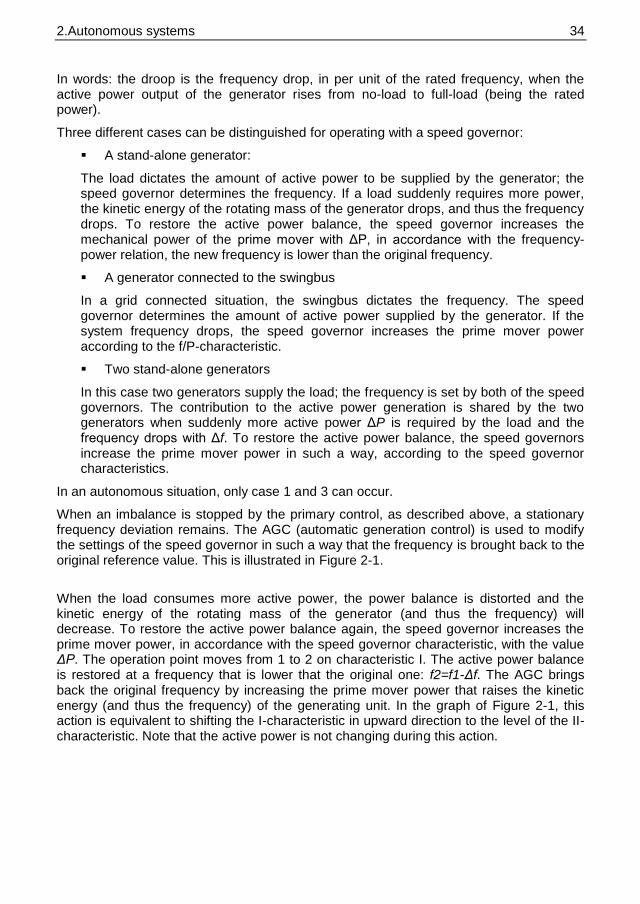
2.Autonomous systems 34 34
In words: the droop is the frequency drop, in per unit of the rated frequency, when the active power output of the generator rises from no-load to full-load (being the rated power).
Three different cases can be distinguished for operating with a speed governor:
A stand-alone generator:
The load dictates the amount of active power to be supplied by the generator; the speed governor determines the frequency. If a load suddenly requires more power, the kinetic energy of the rotating mass of the generator drops, and thus the frequency drops. To restore the active power balance, the speed governor increases the mechanical power of the prime mover with ΔP, in accordance with the frequency-power relation, the new frequency is lower than the original frequency.
A generator connected to the swingbus
In a grid connected situation, the swingbus dictates the frequency. The speed governor determines the amount of active power supplied by the generator. If the system frequency drops, the speed governor increases the prime mover power according to the f/P-characteristic.
Two stand-alone generators
In this case two generators supply the load; the frequency is set by both of the speed governors. The contribution to the active power generation is shared by the two generators when suddenly more active power ΔP is required by the load and the frequency drops with Δf. To restore the active power balance, the speed governors increase the prime mover power in such a way, according to the speed governor characteristics.
In an autonomous situation, only case 1 and 3 can occur.
When an imbalance is stopped by the primary control, as described above, a stationary frequency deviation remains. The AGC (automatic generation control) is used to modify the settings of the speed governor in such a way that the frequency is brought back to the original reference value. This is illustrated in Figure 2-1.
When the load consumes more active power, the power balance is distorted and the kinetic energy of the rotating mass of the generator (and thus the frequency) will decrease. To restore the active power balance again, the speed governor increases the prime mover power, in accordance with the speed governor characteristic, with the value ΔP. The operation point moves from 1 to 2 on characteristic I. The active power balance is restored at a frequency that is lower that the original one: f2=f1-Δf. The AGC brings back the original frequency by increasing the prime mover power that raises the kinetic energy (and thus the frequency) of the generating unit. In the graph of Figure 2-1, this action is equivalent to shifting the I-characteristic in upward direction to the level of the II-characteristic. Note that the active power is not changing during this action.

2.Autonomous systems 35 35
DP
Df
P
f
II
I
12
Figure 2-1 AGC control action
On the lower power scale of autonomous renewable energy systems, several authors has described their systems in papers and articles [16-23].
2.2.2 Demand-control
Another way to fulfil the power balance is by adapting the demanded power of the power system. This way of control is applied in systems with dump resistors. Intelligent systems of controlling the demand are called: demand-side management (DSM). Dump loads are controllable resistors, which are controlled by a voltage or frequency deviation [15, 18, 24, 25].
Demand Side Management in general refers to actions taken on the load side to change the amount or timing of energy consumption. Utility DSM programs offer a variety of measures that can reduce energy consumption and consumer energy expenses. Electricity DSM strategies have the goal of maximizing end-use efficiency to avoid or postpone the construction of new generating plants.
DSM will be implemented in the „house of the future‟, where sensors measure the presence of people to reduce the light and/or heating and/or air-conditioning system.

2.Autonomous systems 36 36
Wind
Turbine
Synchr.
GenDiesel drive
ExciterGoverner
Dump load
Controller
Village load
Wind power
Figure 2-2 Example of dump-load application in AES
In Figure 2-2, an example of an application of Dump-loads is depicted. When the unbalance between wind power (generated) and village power (demand) is positive (more power is generated than consumed), the dump load will balance the system. If the unbalance is negative (more power is consumed then generated), the diesel drive will compensate the power shortage. The controllers can respond to either the bus voltage or the system frequency. This method is not very intelligent and efficient, but is easy to implement for example in rural areas.
Low High
Low
High
Need for Continuity of Service
Qu
an
tity
of
Po
we
r R
eq
uir
ed
Water
heating
Space
heating
Refrigerator
Audio/Video
applications
Computer
Figure 2-3 Electrical appliances with different properties

2.Autonomous systems 37 37
Demand Side Management can be used as an addition to the other types of autonomous systems. In a household application (village or cities), there are a lot of loads that can be controlled easily, such as refrigerators and heat pumps. The application of DSM is rapidly increasing in the United States of America. The applicability of these technologies presupposes the availability of communication systems in the components.
Figure 2-3 shows a number of applications plotted on a two-dimensional basis according to the relative importance of quantity and continuity of service in determining their successful operation. [26] Traditionally, demand has been viewed only as a requirement for quantity of power, but as can be seen, the true value of electric service depends on both dimensions of delivery. A realistic consideration of both dimensions leads to the discovery of possibilities of demand-side management.
2.2.3 Buffer control
Another method is to implement a buffer system, such as batteries or a flywheel. This buffer system can be applied automatically, by using a voltage source converter (VSC). A VSC is defined as a DC/AC converter with voltage source behaviour. By its workings principal, it keeps the voltage and frequency constant.
A three phase Voltage Source Converter (VSC) consists of minimal six power electronic switches (IGBT‟s), six freewheel diodes and two input capacitors. Applying these switches in a specific pattern, the component is able to produce a three phase AC voltage (A, B, C) from a DC input voltage Vd.
TA + DA +
TA -DA -
Vd
2
Vd 0
A
TB + DB +
TB -DB -
B
TC + DC +
TC -DC -
C
Vd
2
+
-
+
+
-
-
id
Figure 2-4 A Three phase inverter

2.Autonomous systems 38 38
The three phase VSC‟s can be divided into the following two general categories [27]:
Pulse-width-modulated inverters: In these inverters, the input dc voltage is essentially constant in magnitude. Therefore, the inverter must control the magnitude and the frequency of the ac output voltages. This is achieved by PWM of the inverter switches and hence such inverters are called PWM inverters. There are various schemes to pulse-width modulate the inverter switches in order to shape the output ac voltages to be as close to a sine wave as possible.
Square-wave inverters: In these inverters, the input dc voltage is controlled in order to control the magnitude of the output ac voltage, and therefore the inverter has to control only the frequency of the output voltage. The output ac voltage has a waveform similar to a square wave, and hence these inverters are called square-wave inverters.
PWM control
Because of their almost sinusoidal waveform, the PWM technology is dominant. Since these converters are used in our laboratory, the PWM inverters are discussed more in detail here.
Using a PWM controller means that the control signals of the switches are based on the PWM-strategy. Here, a control signal vcontrol (constant or slowly varying in time) is compared with a repetitive switching-frequency triangular waveform in order to generate the switching signals. In inverter circuits, the inverter output has to be sinusoidal, with controllable magnitude and frequency. In order to produce a sinusoidal output voltage waveform at a fixed frequency, a sinusoidal control signal at that frequency is compared with a triangular, as shown in Figure 2-5.
0 0.002 0.004 0.006 0.008 0.01 0.012 0.014 0.016 0.018 0.02-1.5
-1
-0.5
0
0.5
1
1.5
time [s]
0 0.002 0.004 0.006 0.008 0.01 0.012 0.014 0.016 0.018 0.02-1.5
-1
-0.5
0
0.5
1
1.5
time [s]
Vcontrol
VAVAo
Vtriangle
Figure 2-5 Sinusoidal PWM

2.Autonomous systems 39 39
The frequency of the triangular waveform establishes the inverter switching frequency and is generally kept constant along with its amplitude vtri and has a frequency (fs), also called the sampling frequency. The control signal vcontrol is used to modulate the switch duty ratio and has a frequency f1, which is the desired fundamental frequency of the inverter voltage output, recognizing that the inverter output voltage will not be a perfect sine wave and will contain voltage components at harmonic frequencies of f1.
Since the two switches in one branch are never off simultaneously, the output voltage vAo fluctuates between two values (½Vd and -½Vd).
An example of a harmonic spectrum of vAo is depicted in Figure 2-6.
mf mf +2 2mf mf +2 3mf 3mf +21
Harmonics h of f 1
1.2
1
0.8
0.6
0.4
0.2
VAo
Vdma =0.8, mf =15
Figure 2-6 Harmonic spectrum
The harmonics in the inverter output voltage waveform appear as sidebands, are centered around the switching frequency and its multiplies, that is, around harmonic components of the sample frequency. These higher harmonic components can be removed from the inverter output waveform by the application of a so-called sinus filter (a L-C circuits).
The PWM-VSC acts as an adjustable alternating voltage source which controls the voltage and the frequency on its terminal. As a result, the current is not dictated for this component. The currents, that will flow into or out of the buffer system is the result of the actual currents of the other components in the system. At the point of common coupling (PCC), the VSC fulfils the Kirchhoff‟s Current Law (KCL). As a result, fluctuations in power generation (solar and wind energy) and fluctuations in power load demand are translated to very fluctuating currents in the VSC. If a battery storage is connected to the DC side of the VSC, the battery current is charged or discharged with these resulting currents.
This conclusion is important for the battery behaviour under fluctuating charge and discharge regimes. The effects on the batteries are discussed in chapter 3. The magnitude and the frequency of these fluctuations are discussed in chapter 6 (simulations) and 7 (measurements).
3 BATTERY STORAGE
Batteries are widely used in a variety of applications from watches and mobile telephones to automotive and uninterruptible power supplies (UPS). Batteries make use of a chemical process to supply and store electricity. They are based on different technologies depending on their field of application. Lead-acid batteries are commonly used, the biggest market being the car industry. Since the invention of this technology in 1859 by the French physicist, Gaston Planté, a lot of knowledge has gained to extend the life-time and improve the performance, but the exact behaviour of the chemical processes is difficult. For this reason, a very accurate indication of for instance the state of charge can not be given.
Within the context of this study, only stationary batteries (designed for service in permanent location) are considered. There are two main applications for stationary batteries: as serving as Standby (UPS) and serving as primary power source batteries, i.e. in off-grid hybrid power sources. In the stand-by application, the battery is only used in emergency situations. In its normal operating condition, the battery is fully charged. In the second application, the State of Charge changes continuously in time by the fluctuation in charge and discharge mode and rate. The construction of the battery, the operation and the maintenance are rather different for both applications. Using a standby battery that has to undergo (withstand) great number of charging and discharge cycles will result in shorter life time and poor performance.
In this chapter, we focus on the stationary cycle application, in which the battery is charged or discharged depending on the mismatch in generated and demanded power. Because of the fact that this balance will change continuously, the battery power as such is unpredictable. Batteries may therefore subject to cycles of varying duration and depth, with frequent incomplete recharge periods between discharges. This poses a challenge to both battery design and sizing of the battery stack, because this type of operation can lead to an apparent fading of overall capacity.
Prolonged cycling operation with improper recharging is known as partial state-of-charge (PSOC) cycling and this way of operation can be damaging for some battery types. There is a need for periodic equalizing and/or maintenance cycles to reduce imbalance between the different plates. Frequent refreshment of the cells is necessary to extend the battery stacks‟ life time. This important issue should be taken into account when developing a control strategy for the energy management system of an autonomous energy application using batteries as a primary power source.
3.1 Working principal lead acid batteries
A typical lead acid battery is built up from individual cells, each consisting of two plates. One plate is made from Lead (Pb), while the other is manufactured from lead oxide (PbO2). The Lead Plate contains a negative electrical charge, the Lead Oxide a positive charge. Between the plates of each cell a special liquid (an acid) maintains a chemical process.
The cells themselves are separated from each other by insulating material. When a fully charged battery is put under load, a reaction occurs between the negative lead plate and

3. Battery Storage 41 41
the positive lead oxide plate, through their interaction with the electrolyte produces electrons.
The electrolyte is a solution of sulphuric acid and water and that molecules of H2SO4 will ionise in the water of the solution to supply the ionic current carriers of 2H
+ and SO4
=. As
the acid ionises and reacts with the plates it is consumed, thus lowering the electrolyte specific gravity.
The reaction at the lead (Pb) negative plate, which generates the electron current source, is:
ePbSOSOPb 244
Equation 3-1 Negative plate reaction (discharge)
The reaction at the lead dioxide (PbO2) positive plate, which accepts the electrons from the negative plate, is:
OHPbSOeHSOPbO 2442 224
Equation 3-2 Positive plate reaction (discharge)
The net discharge reaction is:
OHPbSOPbSOHPbO 24422 222
Equation 3-3 Description of the net chemical process (discharge)
Notice that the reaction results in the sulfation of both plates and the consumption of the acid from the electrolyte.
The discharge reaction of Equation 3-3 is fully reversible.
This means that following reactions will occur:
eHSOPbOOHPbSO 242 4224
Equation 3-4 reaction at positive plate (recharge)
44 2 SOPbePbSO
Equation 3-5 reaction at negative plate (recharge)
4244 24 SOHSOHSO
Equation 3-6 reaction in the electrolyte (recharge)
PbSOHPbOOHPbSO 42224 222
Equation 3-7 Net recharge reaction
In theory, the lead acid battery will produce one ampere-hour (Ah) of energy through the electrochemical reaction of 4.5 grams of lead dioxide (PbO2) and 3.9 grams of lead (Pb) with 3.7 grams of sulphuric acid (H2SO4). Obviously, the more grams of the active materials that is available for reaction the greater will be the Ah capacity of the battery.

3. Battery Storage 42 42
Charging with too high rates and overcharging for a long period, leads to destruction of the battery. At the poles, a hydrogen gas is formed, and the distilled water is consumed. This overcharging is a common cause of premature battery failure.
In the valve regulated lead acid (VRLA) cell the electrolyte is immobilized by either being in a gelled form or being completely absorbed in an absorbent glass mat (AGM) separator between the plates. This prevents the oxygen generated at the positive plate form percolating up and out of the cell and facilitates the oxygen gas (O2) diffusion to the negative plate where the following reactions will occur.
eHOOH 442 22
Equation 3-8 Positive plate reaction (VRLA)
The oxygen gas generated at the positive plate is channeled through the gel or absorbent glass mat (AGM) to the negative lead (Pb) plate where the following series of reactions will occur.
PbOOPb 22 2
Equation 3-9 The oxygen gas oxidizes on negative plate
OHPbSOSOHPbO 2442 2222
Equation 3-10 The oxidized areas react at the positive plate
424 22442 SOHPbeHPbSO
Equation 3-11 The discharged areas of the negative plate are recharged
Under perfect conditions there is no net reaction, which means that there is no water loss or hydrogen gas evolved as a result of the electrolysis of the water at the positive plate.
The depth of discharging which can be tolerated depends on the type of battery. Lead-acid batteries are manufactured in three basic types: start, light and deep-cycle batteries. These batteries differ in the way of how the plates are constructed.
For application in renewable energy systems, deep-cycle batteries are most suited because of their capability to withstand deep discharge cycles, because of the larger available bandwidth between the maximum and the minimum State of Charge. Deep-cycle batteries allow a maximum depth of discharge (DoD) of 80% (that means a minimum state of charge of 20%), without any damage caused. Starting-batteries have for instance thicker plates and are able to withstand high currents.
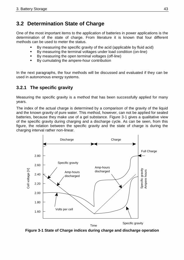
3. Battery Storage 43 43
3.2 Determination State of Charge
One of the most important items to the application of batteries in power applications is the determination of the state of charge. From literature it is known that four different methods can be used to meter the status.
By measuring the specific gravity of the acid (applicable by fluid acid) By measuring the terminal voltages under load condition (on-line) By measuring the open terminal voltages (off-line) By cumulating the ampere-hour contribution
In the next paragraphs, the four methods will be discussed and evaluated if they can be used in autonomous energy systems.
3.2.1 The specific gravity
Measuring the specific gravity is a method that has been successfully applied for many years.
The index of the actual charge is determined by a comparison of the gravity of the liquid and the known gravity of pure water. This method, however, can not be applied for sealed batteries, because they make use of a gel substance. Figure 3-1 gives a qualitative view of the specific gravity during charging and a discharge cycle. As can be seen, from this figure, the relation between the specific gravity and the state of charge is during the charging interval rather non-linear.
1.60
1.80
2.00
2.20
2.40
2.60
2.80
Time
Discharge Charge
Specific gravity
Amp-hours
discharged
Amp-hours
discharged
Specific gravity
Volts per cell
Cell
voltage [V
]
Specific
gra
vity
Am
pere
hours
Full Charge
Figure 3-1 State of Charge indices during charge and discharge operation
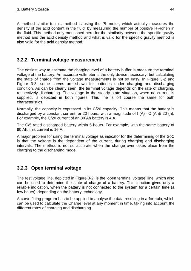
3. Battery Storage 44 44
A method similar to this method is using the Ph-meter, which actually measures the density of the acid content in the fluid, by measuring the number of positive H2-ionen in the fluid. This method only mentioned here for the similarity between the specific gravity method and the acid density method and what is valid for the specific gravity method is also valid for the acid density method.
3.2.2 Terminal voltage measurement
The easiest way to estimate the charging level of a battery buffer is measure the terminal voltage of the battery. An accurate voltmeter is the only device necessary, but calculating the state of charge from the voltage measurements is not so easy. In Figure 3-2 and Figure 3-3, some curves are shown for batteries under charging and discharging condition. As can be clearly seen, the terminal voltage depends on the rate of charging, respectively discharging. The voltage in the steady state situation, when no current is supplied, is depicted in both figures. This line is off course the same for both characteristics.
Normally, the capacity is expressed in its C/20 capacity. This means that the battery is discharged by a constant current for 20 hours, with a magnitude of I (A) =C (Ah)/ 20 (h). For example, the C/20 current of an 80 Ah battery is 4 A.
The C/5 rated discharged battery within 5 hours. For example, with the same battery of 80 Ah, this current is 16 A.
A major problem for using the terminal voltage as indicator for the determining of the SoC is that the voltage is the dependent of the current, during charging and discharging intervals. The method is not so accurate when the change over takes place from the charging to the discharging mode.
3.2.3 Open terminal voltage
The rest voltage line, depicted in Figure 3-2, is the „open terminal voltage‟ line, which also can be used to determine the state of charge of a battery. This function gives only a reliable indication, when the battery is not connected to the system for a certain time (a few hours), depending on the battery technology.
A curve fitting program has to be applied to analyse the data resulting in a formula, which can be used to calculate the Charge level at any moment in time, taking into account the different rates of charging and discharging.
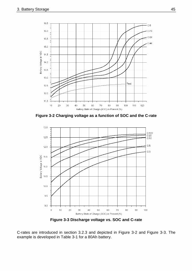
3. Battery Storage 45 45
Figure 3-2 Charging voltage as a function of SOC and the C-rate
Figure 3-3 Discharge voltage vs. SOC and C-rate
C-rates are introduced in section 3.2.3 and depicted in Figure 3-2 and Figure 3-3. The example is developed in Table 3-1 for a 80Ah battery.

3. Battery Storage 46 46
Type Charge/Discharge current [A] Discharge/Charge time [h]
C/5 16 5
C/10 8 10
C/20 4 20
C/40 2 40
C/100 0.8 100
Table 3-1 C-values of 80 Ah battery
Note that the energy contents is heavily depending of the discharge respectively charge current. More about this issue will be described in section 3.2.4. In the definition of the C-rate, this effect is, however, not taken into account.
y = -9E-05x2 + 0,0203x + 11,536R² = 0,9911
11,5
11,7
11,9
12,1
12,3
12,5
12,7
12,9
13,1
13,3
13,5
0 20 40 60 80 100 120State of Charge [%]
Rest battery voltage [V]
Figure 3-4 Trend line (polynomial)
Figure 3-4 shows an example of curve fitting. The rest voltage line of this figure is fitted into a polynomial form from the second order. Curve fitting software calculates the best fitting curve. In this example, the battery terminal voltage line (BTV) is approximated with the following polynomial:
5 29 10 0.0203 11.536BTV SoC SoC
Equation 3-12 Polynomial approximation of BTV

3. Battery Storage 47 47
3.2.4 Ampere-hour method
A frequently advised method to determine the SoC is integrating the battery current. From all the available methods, this method is the one related closest to the physical process itself. However, the chemical process is non-linear and for this reason not so easy to catch it in a simple formula. Applying the developed charging and discharging efficiencies, a rather reliable estimation can be acquired. These efficiency-values are depending on their turn on the charging and discharging rate, but this influence is relatively small. A major problem with the Ampere-hour method is the numerical error-accumulation as a result from the integrating the currents. A repeated calibration with another method, (for instance the terminal voltage of a fully charged and/or fully discharged) makes the method even more accurate.
Correction factors
As mentioned earlier, the battery capacity is usually given by its C20-value. When a battery is discharged by a higher current, the capacity of the battery decreases and the other way around the capacity is increased because at a lower current rate the battery can deliver more Ah‟s. This phenomenon is known in literature [28-30] as the Peukert effect and described by the Peukert equation. The Peukert effect is valid for discharging and can not be applied for charging.
In its original form, the equation is written as:
CtI n
Equation 3-13 Peukert equation
Where:
I : discharging current [A], n : The Peukert number (typical between 1.3 and 1.4), t : time [h], C : A constant coefficient (not C-rate).
This equation can be written in a different form expressing the virtual capacity Q in [Ah], in terms of current I.
Both sides of the equal sign are multiplied by I1-n
, to reach the form: Q (I x t) = C x I1-n
, with Q being the capacity in [Ah], C the coefficient which is empirically derived and n, the Peukert number. This Peukert effect has to be taken into account, when we want to determine the battery state of charge.
The factor P(I), represents the Peukert effect in the equation below.
11
20)( nn
c IIIP
For example, when the C20 current of a 100 Ah battery is 5 A and the Peukert number is 1.33. The proposed p-factor at a discharging current of 10A respectively 50A is:
P(10) = 5-0.33
x 10-(-0.33)
= 1.25
P(50) = 5-0.33
x 50-(-0.33)
= 2.14

3. Battery Storage 48 48
0 10 20 30 40 50 60 70 80 90 1000
0.5
1
1.5
2
2.5
3
discharge current [Amps]
corr
ection facto
r
P-factor as function of discharge current
Figure 3-5 The P-factor as a function of the discharge currents
Near top-of-charge
The battery‟s behaviour when it is close to its maximum charging level is described in [31]. Researchers of the National Renewable Energy Laboratory (NREL) in Colorado, USA, have experimentally determined that the charge efficiency drops rather quickly when the battery reaches its maximum charging level. Curve fitting gives the following expression:
( ) (1 )SoCSoC e
With:
η : The charge efficiency as function of the actual SoC [ ]
α : The charge efficiency at lower charge levels [ ]
β, δ: parameters derived from experiments [ ]
SOC: The State of Charge in [%]
The values of α, β and δ should be experimental determined by doing actual laboratory tests. Figure 3-6 shows a curve fit to actual measurements from which parameters α, β and δ are extracted. In this example: α = 0.95, β = 1.34x10
-3, δ = 0.0608
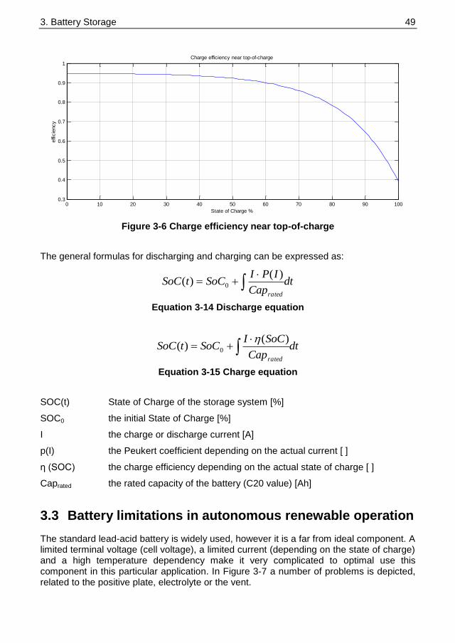
3. Battery Storage 49 49
0 10 20 30 40 50 60 70 80 90 1000.3
0.4
0.5
0.6
0.7
0.8
0.9
1
effi
cie
ncy
State of Charge %
Charge efficiency near top-of-charge
Figure 3-6 Charge efficiency near top-of-charge
The general formulas for discharging and charging can be expressed as:
dtCap
IPISoCtSoC
rated
)(
)( 0
Equation 3-14 Discharge equation
dtCap
SoCISoCtSoC
rated
)(
)( 0
Equation 3-15 Charge equation
SOC(t) State of Charge of the storage system [%]
SOC0 the initial State of Charge [%]
I the charge or discharge current [A]
p(I) the Peukert coefficient depending on the actual current [ ]
η (SOC) the charge efficiency depending on the actual state of charge [ ]
Caprated the rated capacity of the battery (C20 value) [Ah]
3.3 Battery limitations in autonomous renewable operation
The standard lead-acid battery is widely used, however it is a far from ideal component. A limited terminal voltage (cell voltage), a limited current (depending on the state of charge) and a high temperature dependency make it very complicated to optimal use this component in this particular application. In Figure 3-7 a number of problems is depicted, related to the positive plate, electrolyte or the vent.

3. Battery Storage 50 50
positive plate Electrolyte Safety vent, sealed part
Grid corrosion Increase in
charging current
Deterioration of
seal
Amount of
electrolyte is
reduced
Increase in
relative density
Grid growth Grid becomes
thin or broken
Poor adhesion
between active
material and
grid
Amount of effective
material is reduced
Amount of
effective
electrolyte is
reduced
Absorption of
oxygen from
outside
Capacity is
decreased
Deterioration of
negative plate
Service lifeDamage to container
and coverDeterioration of
post
Container, cover Post, bus-bar
Figure 3-7 A number of battery problems
One of the fundamental differences between standby operation and many cycling applications is the availability of energy for charging, particularly where this is from renewable sources [32]. An implicit assumption in standby applications is that charging energy is essentially unlimited. With renewable sources such as PV and wind, however, energy output can be highly variable on a diurnal and/or seasonal basis. Batteries may therefore be subjected to cycles of varying depth, frequently with incomplete recharge between discharges.
This type of operation can lead to an apparent fading of capacity. This is more correctly described as a state-of-charge (SOC) imbalance between the positive and negative plates, which occurs because the negatives of both lead-acid and nickel-cadmium cells tend to recharge more efficiently than the positives. Prolonged cycling operation with incomplete recharging is known as partial state-of-charge (PSOC) cycling. PSOC can be damaging for some battery types, and there is a general need for periodic equalizing and/or maintenance cycles to remove the imbalance.

3. Battery Storage 51 51
On the other hand, batteries may be required to supply longer-duration energy-type loads or shorter-duration power-type loads, depending on the actual situation (applications). Any battery type can be sized to supply short duration power loads, but high-power battery designs supply them more effectively than others.
The main design principle for high-power battery designs is that the battery can discharge a higher percentage of its stored energy over short durations than can lower-power „energy‟ designs. High-power batteries are more efficient for short discharges; the energy that is removed during a power discharge represents a small percentage of the total. Hence, power-type cycling tends to be in the form of shallow discharges to a low depth of discharge (DOD). Energy-type cycling, on the other hand, frequently results in deep discharges to a high DOD, which is more stressful for the battery.
The critically of system loads and the typical failure modes exhibited by a battery in cycling operation can influence the management of the overall system over its life.
The characteristic aging of lead acid batteries in stand-by applications is for the capacity to increase gradually to around 105-110% of rated and to remain there until about two-thirds of the life has elapsed. The capacity then starts decreases to 80% of rated.
Aging mechanisms in cycling applications may be different from the standby model. For example, prolonged undercharging may cause capacity loss due to sulfation. However, the 80% end-of-life capacity is generally used in battery sizing for these applications also.
In cycling applications, batteries rarely if ever reach a float charge condition during normal operation, although float charges, or more often equalization charges, can be implemented as part of the system setup and performed infrequently according to a customer command. [33]
In fact, the issue for many cycling systems, as opposed to standby ones, is that there is a significant danger that the batteries will not receive an adequate charge or a sufficiently long finish charge. If analysis of the particular cycling application indicates that there will be periods of several weeks or more when the battery is incompletely charged, then the system design should look into possibility of making special charging arrangements, e.g. by incorporating another charge power source and making sure this is used appropriately. The gel type of the Valve Regulated Lead-acid battery (VRLA) is better resisting these circumstances than the „water-types‟.
Alternatively, two battery systems can be used in parallel to enlarge the flexibility to equalize one battery stack during normal operation.
4 ENERGY CALCULATIONS
After selecting the components of the autonomous renewable energy system, the next step is to determine size the components. Starting point these energy calculations is the customers load before calculating the energy supply capacity of the various renewable sources per installed unit. In our scope, wind energy and solar energy are the main sources, because of their more or less mature stage of development. The emphasis lays on system integration of the renewable energy sources, on the storage and on the behaviour of the load. The behaviour of these renewable sources (wind and sun) are already well-known and described in literature. As described in the introduction of this thesis, the research has to be focussed on the system integration because the behaviour of these components in grid-connected operation is known. Besides of this argument, the studied sources should be realistic for the Netherlands in the coming years.
4.1 Solar energy
Solar energy is a general name for energy which is directly abstracted from the sun. Nowadays, there are two groups of solar energy conversion systems that are widely used: solar boilers and photovoltaics. A solar boiler is applied to generate hot water from the irradiance of the sun. The discussion of this component is, however, out of the scope of this thesis.
Photovoltaic is the technology of the direct conversion of solar radiation into electricity. This conversion is performed with a solid-state device. Photovoltaic has often been characterized as the showpiece of the renewable energy technologies. [34] One reason for that is the simplicity in use and long lifetime of a photovoltaic system due to a lack of moving parts. A second reason is the universal applicability under all climates at an arbitrary scale of size. The main reason is the technical potential of photovoltaics to satisfy the growing world energy demand in both industrialized and developing countries.
4.1.1 PV in silicon: basic principles
PV cells consist, in essence, of a junction between two thin layers of dissimilar semi-conducting materials, known respectively as „p‟ (positive)-type and „n‟ (negative)-type semiconductors. These semiconductors are usually made from silicon, however new technologies with other materials are under development.
N-type semiconductors are made from crystalline silicon that has been „doped‟ with tiny quantities of an impurity (usually phosphorus) in such a way that the doped material possesses a surplus of free electrons.
P-type semiconductors are also made from crystalline silicon, but are „doped‟ with very small amounts of a different impurity (usually boron) which causes the material to have a deficit of free electrons. These missing electrons are called holes.

4. Energy Calculations 53 53
We can create what is known as a p-n junction by joining these two types of semiconductors. This creates an electric field in the region of the junction. It will cause negatively charged particles to move in one direction, and positively charged particles to move in the opposite direction. This movement creates a P-N junction band where no charge carriers are available (depletion region).
Light consists of a stream of tiny particles of energy, called photons. When photons from light of a suitable wavelength fall within the material, the can transfer their energy to some of the electrons in the material and move them to a higher energy level. Normally, these electrons can not move freely, but in their excited state, the electrons become free to conduct electric current by moving through the material. In addition, when electrons move they leave behind holes in the material, which can also move.
When an electron in the junction region is stimulated by an incoming photon to „jump‟ into the conduction band, it leaves behind a hole in the valence band.
energy
gap valence band
conduction band
energy
level
distance
N P
photon
photon
Figure 4-1 PN-process by incoming photons
The process is envisaged in terms of the energy levels in the material, see Figure 4-1. The electrons that have been stimulated by incoming photons to enter the conduction band can be thought as „rolling downwards‟, under the influence of the electric field at the junction, into the n-region; similarly, the holes can be thought of as „floating upwards‟, under the influence of the junction field, into the p-region.
The flow of electrons to the n-region is, by definition, an electric current. If there is an external circuit for the current to flow through, the moving electrons will eventually flow out of the semiconductor via one of the metallic contacts on the top of the cell. The holes will flow in the opposite direction.
In order to produce power, the PV cell must generate voltage as well as the current provided by the flow of electrons. This voltage is, in effect, provided by the internal electric field set up at the pn-junction.
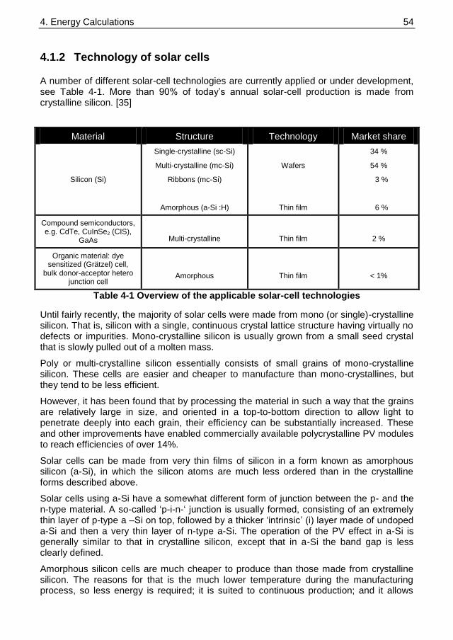
4. Energy Calculations 54 54
4.1.2 Technology of solar cells
A number of different solar-cell technologies are currently applied or under development, see Table 4-1. More than 90% of today‟s annual solar-cell production is made from crystalline silicon. [35]
Material Structure Technology Market share
Silicon (Si)
Single-crystalline (sc-Si)
Multi-crystalline (mc-Si)
Ribbons (mc-Si)
Amorphous (a-Si :H)
Wafers
Thin film
34 %
54 %
3 %
6 %
Compound semiconductors, e.g. CdTe, CuInSe2 (CIS),
GaAs
Multi-crystalline
Thin film
2 %
Organic material: dye sensitized (Grätzel) cell,
bulk donor-acceptor hetero junction cell
Amorphous
Thin film
< 1%
Table 4-1 Overview of the applicable solar-cell technologies
Until fairly recently, the majority of solar cells were made from mono (or single)-crystalline silicon. That is, silicon with a single, continuous crystal lattice structure having virtually no defects or impurities. Mono-crystalline silicon is usually grown from a small seed crystal that is slowly pulled out of a molten mass.
Poly or multi-crystalline silicon essentially consists of small grains of mono-crystalline silicon. These cells are easier and cheaper to manufacture than mono-crystallines, but they tend to be less efficient.
However, it has been found that by processing the material in such a way that the grains are relatively large in size, and oriented in a top-to-bottom direction to allow light to penetrate deeply into each grain, their efficiency can be substantially increased. These and other improvements have enabled commercially available polycrystalline PV modules to reach efficiencies of over 14%.
Solar cells can be made from very thin films of silicon in a form known as amorphous silicon (a-Si), in which the silicon atoms are much less ordered than in the crystalline forms described above.
Solar cells using a-Si have a somewhat different form of junction between the p- and the n-type material. A so-called „p-i-n-„ junction is usually formed, consisting of an extremely thin layer of p-type a –Si on top, followed by a thicker „intrinsic‟ (i) layer made of undoped a-Si and then a very thin layer of n-type a-Si. The operation of the PV effect in a-Si is generally similar to that in crystalline silicon, except that in a-Si the band gap is less clearly defined.
Amorphous silicon cells are much cheaper to produce than those made from crystalline silicon. The reasons for that is the much lower temperature during the manufacturing process, so less energy is required; it is suited to continuous production; and it allows
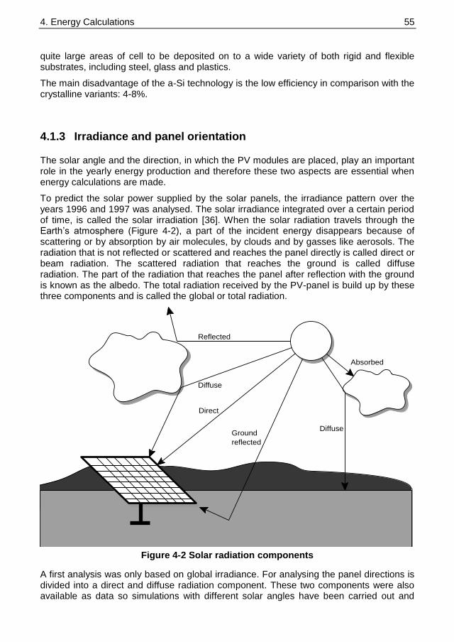
4. Energy Calculations 55 55
quite large areas of cell to be deposited on to a wide variety of both rigid and flexible substrates, including steel, glass and plastics.
The main disadvantage of the a-Si technology is the low efficiency in comparison with the crystalline variants: 4-8%.
4.1.3 Irradiance and panel orientation
The solar angle and the direction, in which the PV modules are placed, play an important role in the yearly energy production and therefore these two aspects are essential when energy calculations are made.
To predict the solar power supplied by the solar panels, the irradiance pattern over the years 1996 and 1997 was analysed. The solar irradiance integrated over a certain period of time, is called the solar irradiation [36]. When the solar radiation travels through the Earth‟s atmosphere (Figure 4-2), a part of the incident energy disappears because of scattering or by absorption by air molecules, by clouds and by gasses like aerosols. The radiation that is not reflected or scattered and reaches the panel directly is called direct or beam radiation. The scattered radiation that reaches the ground is called diffuse radiation. The part of the radiation that reaches the panel after reflection with the ground is known as the albedo. The total radiation received by the PV-panel is build up by these three components and is called the global or total radiation.
Text
Direct
Ground
reflected
Diffuse
Reflected
Absorbed
Diffuse
Figure 4-2 Solar radiation components
A first analysis was only based on global irradiance. For analysing the panel directions is divided into a direct and diffuse radiation component. These two components were also available as data so simulations with different solar angles have been carried out and
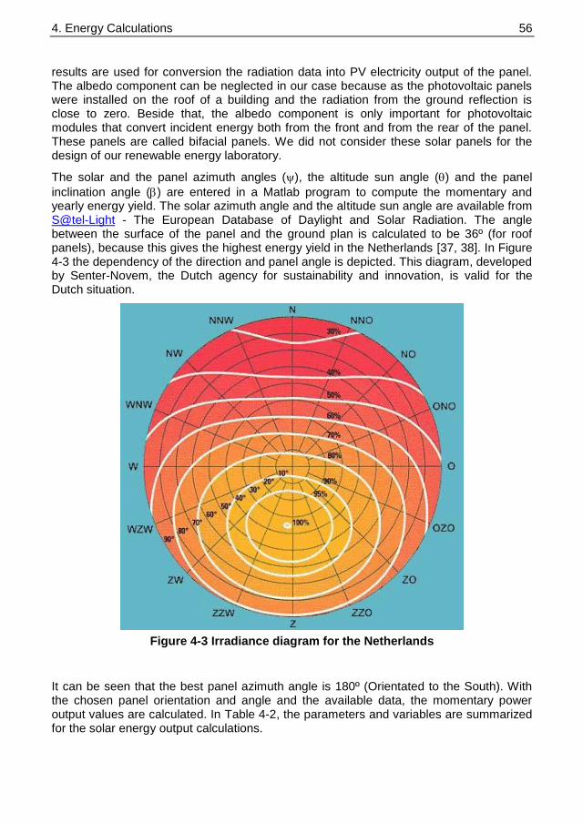
4. Energy Calculations 56 56
results are used for conversion the radiation data into PV electricity output of the panel. The albedo component can be neglected in our case because as the photovoltaic panels were installed on the roof of a building and the radiation from the ground reflection is close to zero. Beside that, the albedo component is only important for photovoltaic modules that convert incident energy both from the front and from the rear of the panel. These panels are called bifacial panels. We did not consider these solar panels for the design of our renewable energy laboratory.
The solar and the panel azimuth angles (), the altitude sun angle () and the panel
inclination angle () are entered in a Matlab program to compute the momentary and yearly energy yield. The solar azimuth angle and the altitude sun angle are available from S@tel-Light - The European Database of Daylight and Solar Radiation. The angle between the surface of the panel and the ground plan is calculated to be 36º (for roof panels), because this gives the highest energy yield in the Netherlands [37, 38]. In Figure 4-3 the dependency of the direction and panel angle is depicted. This diagram, developed by Senter-Novem, the Dutch agency for sustainability and innovation, is valid for the Dutch situation.
Figure 4-3 Irradiance diagram for the Netherlands
It can be seen that the best panel azimuth angle is 180º (Orientated to the South). With the chosen panel orientation and angle and the available data, the momentary power output values are calculated. In Table 4-2, the parameters and variables are summarized for the solar energy output calculations.

4. Energy Calculations 57 57
South
North
Zenith
SunNormal to
horzontal
surface
Solar
panel
Panel
Tilt
b
Panel
Azimuth
Solar
Altitude
q
Normal to
tilted
surface
Sun
Azimuth
Y
Figure 4-4 Orientation angles for the solar modules
Panel Orientation Solar Orientation
= 36º (setting)
Panel Azimuth (PA) = 180º (setting);
= data downloadable;
= data downloadable;
x
y
z
P = cos ( ) · cos ( )
P = cos ( ) · sin ( )
P = sin ( )
PA
PA
x
y
z
S = cos ( ) · cos ( )
S = cos ( ) · sin ( )
S = sin ( )
P
= [Px Py Pz] and P
= 1; S
= [Sx Sy Sz] and S
= 1;
Table 4-2 Used parameters and variables for the solar energy calculations
With these data, the area in the panels [m2] where the sun falls upon per hour can be
calculated by using Equation 4-1. The total surface of the PV modules considered for the renewable energy laboratory is 120 m
2 (12 m
2 x 10 houses).

4. Energy Calculations 58 58
PV Modules Area with sun = ( S
x P
) x Total PV Area
Equation 4-1 Calculation of the effective area of the panel
When these values are related to the direct and diffusion irradiation [W/m2], one can
obtain the output power from the solar panels, see Figure 4-5. Occasionally, negative values are a result of the calculation for several hours of the day (at early night and during the night), the angles have a negative sine. All negative values from direct and diffuse output power were not taken into account because a solar panel can only generate electrical energy and never use it.
0 2000 4000 6000 8000 10000 12000 14000 16000 180000
1
2
3
4
5x 10
4 Power from Direct Solar Radiation 1996 & 1997
Hours [h]
Pow
er [W
]
0 2000 4000 6000 8000 10000 12000 14000 16000 180000
2
4
6
8
10x 10
4
Pow
er [W
]
Hours [h]
Power from Diffuse Solar Radiation 1996 & 1997
Figure 4-5 Solar panels output power from direct and diffuse radiation
In a first analyse, these values seem too high but they are not. Indeed, if all the sun irradiation was absorbed by 100% efficient solar cells this would be a reality. As remarks it can be said that the average hourly power for both years (1996 & 1997), in this case, would be almost 5.4 kW for the power from the direct solar radiation and around 4.7 kW for the power from the diffuse solar radiation.
Applying the chosen efficiency for the panels (12%) and adding the above results to get the solar power from the total or global irradiation, we can simulate the output solar power (Psolar), see Figure 4-6
Jan ‟96 July ‟96 Dec‟96/Jan ‟97 July ‟97 Dec „97
Jan ‟96 July ‟96 Dec‟96/Jan ‟97 July ‟97 Dec „97

4. Energy Calculations 59 59
0 2000 4000 6000 8000 10000 12000 14000 16000 180000
5000
10000
15000
Hours [h]
Pow
er [
W]
Psolar
for 1996 & 1997
Figure 4-6 Total hourly solar power (Psolar) pattern for 1996 & 1997
The calculations are based on diffuse and on direct irradiance. Side-effects, such as a drop of efficiency by the influence of panel temperature, are omitted.
Jan Feb Mar Apr May Jun Jul Aug Sep Oct Nov Dec0
50
100
150
200
250
Irra
dia
nce L
eve
l [W
/m2]
Monthly Global Irradiance Average Pattern 1996
Figure 4-7 Monthly global irradiance
pattern 1996
Jan Feb Mar Apr May Jun Jul Aug Sep Oct Nov Dec0
50
100
150
200
250
Irra
dia
nce L
eve
l [W
/m2]
Monthy Global Irradiance Average Pattern 1997
Figure 4-8 Monthly global irradiance
pattern 1997
4.1.4 Potential in the Netherlands
A report of the Centre of Energy reduction (CE) in Delft [39] revealed that in 2010 a year yield of ca. 95 TWh can be reached when all roofs of domestic houses in the Netherlands are covered with PV-panels. A distinction was made between two different roofs as can be seen in Table 4-3.
Potential in 2010 Flat roofs Other roofs Total area
Area (km2) 118.3 543.77 662.07
Peak power (MWp) 20.904 96.084 116.988
Production (TWh/year) 94.73
Table 4-3 Potential roof area and PV-energy in the Netherlands in 2010
Jan ‟96 July ‟96 Dec‟96/Jan ‟97 July ‟97 Dec „97

4. Energy Calculations 60 60
The solar energy production is linear dependent with the solar irradiance, which is dependent on the presence of clouds. The KNMI, the Royal Dutch Meteorological Institute, has published a map, wherein areas of equal solar energy are drawn, see Figure 4-9.
Figure 4-9 Global sun irradiations in the Netherlands in kWh/year
One of the problems by using solar energy is the great fluctuations in short time frames. These fluctuations are caused by fast moving clouds. It is concluded that the energy production is mainly dependent on the direct irradiation and for a small part on the diffuse component.
The problem which is mentioned here is that fluctuations in the power production should be compensated by other sources and/or storage systems.

4. Energy Calculations 61 61
Figure 4-10 PV power on July 6. and July 7. in 2004, measured in DENLAB (120m2)
Figure 4-10 shows that the variation in the power output can be very high. The power can vary from 8 kW till 1 kW (at 15.00 PM) within a few minutes. The measurements were done with 10 minutes intervals. The depicted values of power are the 10-min. averages.
In one of the research projects, [37], we have found out the yearly energy yield of a 1 m2
solar panel in the different directions. The calculations were carried out with the irradiance data of 1996 and 1997. In this study, we keep the panel tilt on 36º, but vary the solar panel azimuth. We calculate the energy yield of a solar panel of 1 m
2, facing to the
South, West and East direction. Table 4-4 presents the results of this calculation.
Year Energy yield per direction of the solar panel
South West East
1996 86 kWh 70 kWh 68 kWh
1997 87 kWh 70 kWh 70 kWh
Table 4-4 Energy yield by different panel orientation
Assuming that 50% of the houses are build in the North-South-direction, and 50% of the houses are build in the West-East direction, we can calculate the average yield of solar panel per squared meter, to be 78 kWh.
At a standard house, 12 m2 is available for solar panels, so the PV-energy potential for
ten households, which a complete PV covered roof contributes 9360 kWh/year.[40]

4. Energy Calculations 62 62
4.1.5 Measurement data in the laboratory
Within the DENLAB-project we record the power readings since the start in October 2001. We handle a time interval of 10 minutes. From this measurements from 2003, we derived that 1 m
2 active area produces 90 kWh (324 MJ) of energy in Delft.
0 5 10 15 20 250
1000
2000
3000
4000
5000
6000
time [hours]
avera
ge P
V p
ow
er
outp
ut
[W]
December
June
average
Figure 4-11 PV output power, based on measurements in DENlab 2005
In Figure 4-11, three average curves are depicted. The graphs are based on measurements in the Renewable Energy laboratory. The lowest curve shows the average power per hour in December 2005, the highest curve shows the power production in June 2005 and the middle curve shows the year average per hour.
It can be seen that the electricity production in the winter period starts later than in the summer. On the other hand, the top of the summer curve is off course much higher than in the winter period.
The average curve is smoother than the other curves. It is caused by the averaging of all 365 day-graphs of one year. The monthly average curves are based on 30 day-graphs.
Another noticeable point is the dip in the summer power at noon. This reduction in power is probably caused by the influence of the highest temperature of the panel, which decreases the efficiency of the solar cell.

4. Energy Calculations 63 63
4.2 Wind energy
Generating mechanical power from wind has a very long history [41]. Very old documentation (1219) described the application of a windmill in China. In the Netherlands the first windmills are introduced in the early 17
th century. These wind mills were applied
to grind meal, to saw wood or to pump water.
The first concepts to generate electricity from wind power date from the end of the 19th
century. Firstly, the small turbines (less then 1 horse power) were tested and later on the bigger turbines. The first application of a large windmill to generate electricity was built in 1888 by Charles F. Brush in Cleveland, Ohio. It had a rotor diameter of 17 meters. It was the first windmill with a step-up gearbox. The rotor diameter has taken an enormous flight to 120m in 2003. This Wind Energy Conversion System (WECS) produces 4.5 MW [42].
Beside of the trend to bigger wind turbines for near shore and off-shore applications, there is also a trend in producing small wind turbines to be used in the built environment. The power of these turbines is mostly limited to 5 kW whereby special attention is given to aesthetics and the reduction of noise and vibration.
4.2.1 Potential in the Netherlands
The wind speed in the Netherlands is more location dependent then the solar irradiance. This can be concluded by a comparison between Figure 4-9 and Figure 4-12. The average wind speed in coastal areas is more then twice the wind speed in the eastern parts of the Netherlands. Because of the fact that the wind power is in the cubic dependent from the actual wind speed, there is no one to one relation between this picture and the produced wind energy. But at least it gives an indication where to most suitable places are located.

4. Energy Calculations 64 64
Figure 4-12 Average wind speed in the Netherlands
4.2.2 Wind data of KNMI
Royal Netherlands Meteorological Institute (KNMI) has released a lot of historical, climatological data which is available for research purposes. In this database, there is also historic data of wind speeds in the vicinity of the Delft University: station Zestienhoven (the airport at Rotterdam).
From this data, the frequency table is derived that shows the mean wind speed of this station. The values are cumulative calculated.

4. Energy Calculations 65 65
0 2 4 6 8 10 12 14 16 18 200
2
4
6
8
10
12
14
16
18
wind speed
perc
enta
ge
wind distribution at station Zestienhoven
0 5 10 15 20 25 300
10
20
30
40
50
60
70
80
90
100station Zestienhoven
windspeed [m/s]
cum
ula
tive r
ela
tive
Figure 4-13 Distribution and Cumulative frequency distribution of wind speed at
Zestienhoven
Cumulative means the cumulative relative frequency of occurrence of a certain wind speed class. For example with respect to the relative manner of presenting: a value of 33.32 corresponding with 4.0-4.9 means that in 33.32% of the total number of hours the hourly mean wind speed does not exceed 5.0 m/s. The calculation whereon is based, covers a period from 1971-2000. From Figure 4-13, it can be concluded that a wind turbine, with a cut-in speed of 4.0 m/s do not generate any power in 40% of its installed time.
The wind direction depicted in Figure 4-14 is mostly south-west.

4. Energy Calculations 66 66
Figure 4-14 Wind rose calculated from station Zestienhoven
4.2.3 Wind energy in the built environment
One of the potential areas of wind energy is the built environment. The reason of installing wind turbines in this area, is that it is relatively easy to install (in comparison to on-shore and offshore wind turbines) and power is generated close to the demand, and so reducing the transport losses.
The drawback of installing WECS in the built environment is the higher requirements of the turbine on background noise, vibrations on the buildings and horizon pollution, which makes the design more complex and increases the prices. On the other hand, the wind speed is very variable from direction and the mean value is reduced by the large number of obstacles. These obstacles makes the speed reduction also directional dependent. These obstacles are normally expressed by the roughness indicator [43, 44].
The surface winds do suffer influence from the topography of the terrain, but with good knowledge of those topography characteristics, one can physically model the wind flows with reasonable accuracy through downscaling processes as referred in [45].
When the topography of the terrain becomes highly modified by human made constructions, this kind of approach is most of the time not accurate enough [46], because buildings have very particular local air flows around and over them, that can only be modelled through a combination of specifically designed computational fluid dynamics and on-site measurements. WAsP developers [47], for example, admit that their downscaling tool is not appropriate for the kind of topography that urban areas have.

4. Energy Calculations 67 67
Although the basic wind patterns on a site may be obtained from meteorological data, each site must be studied in detail to understand the specific individual features such as nearby obstacles that affect the wind flow.
In Figure 4-15 from [48] we can see the computational fluid dynamics (CFD) calculation of the streamlines around the roof of a building with flow at 45º to the windward side of the building. The roof wind turbine (in this case a vertical axis one) should be sited well above the high turbulence zone on the roof unless it has been specifically designed for it.
Figure 4-15 CFD calculations of wind turbulence around a building
Looking at this figure, the recommendations commonly stated in bibliography for small conventional wind turbine sitting are easy to understand [49]:
Higher towers minimize turbulence and avoid the ground drag that slows down the wind;
If there are obstacles located upstream of the direction of the prevailing winds, the top of the obstacles should be considered the effective ground line for the wind system;
Any wind turbine should be placed at least 10 meters above any obstacle within a 200 meter distance;
Any obstacle located within 1 km upstream of the direction of the prevailing winds will modify the wind characteristics, increase turbulence and produce gustier winds, making simple calculations more uncertain;
All these recommendations can be easily understood looking at another figure showing the size of the wind turbulence zone caused by obstacles.

4. Energy Calculations 68 68
Figure 4-16 Zone of wind turbulence caused by an obstacle
It is clear that in a built environment, there is never a turbulence free environment. The turbulences on a specific place depend on the specificities of the site, obstacles within 1 km, the direction of the prevailing winds, among other things. Wind speed and direction databases for the sites are very useful because the distance between buildings and wind turbines can be shortened depending on the direction of the prevailing winds in relation to the building and the wind turbine positions.
It is interesting to compare the previous figures with a satellite photo of the site where the DENlab‟s anemometer is placed.
Figure 4-17 Satellite view of the DENlab anemometer site
Figure 4-17 contains a lot of information. On the upper left corner we have a wind rose that shows the prevailing wind direction in KNMI station of airport Zestienhoven in the last 30 years. It can be seen that the wind comes mostly from southwest, as indicated by the yellow arrow. The red squares are very tall buildings, more than 10 storeys high (more

4. Energy Calculations 69 69
than 35 meters), the yellow squares are buildings 10 to 20 meters higher than the anemometer height (25 m), and the light blue squares are buildings lower than 20 meters. The green square is the Electrical Engineering building, where the anemometer is mounted, and the location of the anemometer is marked by the cross on the green square.
Comparing the three previous figures, it can be seen that physically modelling DENlab‟s site would not be an easy task, because there are at least two very tall buildings whose influence could not be ignored due to their distance to the anemometer.
4.2.4 Measurement data in the laboratory
At the DENlab facility a wind speed measurement system is installed that records the actual wind speed on a 2 sec. time base. The measurement system consists of a simple anemometer, which measures the magnitude of the wind speed at one specific point in the air. The meter is placed on metal pole of 5 meter, which is mounted on one side of a lift shaft of 2.5 meter high. This lift shaft is located on the top of the third stage so totally, the anemometer is 18 meters above ground level.
Figure 4-18 One minute average of the wind speed on 1-5-2004, measured in
DENlab
In a previous research [37] the capacity factor for wind energy in Delft (NL) is calculated to be 0.13. This factor shows the ratio between the generated power and the theoretical maximum possible energy, which can be generated (rated power times maximum time). For a wind turbine of 30 kW does this mean that 34164 kWh/year can be expected as the yearly energy production.

4. Energy Calculations 70 70
4.2.5 Wind versus height
Apart from the topographic description of the terrain already mentioned, the hub height has a major influence on wind speeds. The variation of wind speed with height depends on the roughness class of the terrain, but in general it can be said that wind speed increases with height. The equations that determine this variation are defined in several books about wind energy, and depend on the simplifications that one makes, but a simple and fairly accurate equation is:
ref
0
ref
0
zv ln
z v =
zln
z
Equation 4-2 correction equation for different heights
where v is the wind speed at height z above ground level, vref is the wind speed we already know at height zref, and z0 is the roughness length. This equation will help to understand how wind speed varies with height. It says that the wind speeds are mainly influenced by the roughness of the terrain, the obstacles on its surface and the height considered. It is very important to refer that few investigation about wind forecasting has been done for the built-up environment. The chapter 8 of this thesis discusses this topic more into detail.
4.2.6 Small wind turbines
The problem of wind turbines within the built environment is the low cut-in speed. The cut-in wind speed is the wind speed where a wind turbine starts to deliver electricity. The wind speed in the built environment, sometimes a very rough terrain, is in general low. Figure 4-13 has already shown the distribution and cumulative frequency of the wind speed at the airport Zestienhoven. The cumulative frequency shows that during 40% of the time, the wind is below 4 m/s. Many turbines do not produce power at these low wind speeds. In our measurements we found out that the average wind speed on top of the University building is lower than the measurements at the airport. This is explained by the higher roughness of the terrain.
Lots of small wind turbines are already being developed for this application. The most known in Delft is the Turby concept, developed at the Delft University of Technology [48, 50].

4. Energy Calculations 71 71
0 5 10 15 20 250
5
10
15
20
25
30
35Fuhrlander FL 30
wind speed [m/s]
Pow
er
[kW
]
Figure 4-19 Power Curve of the Turby (left) and Furlander FL30 (right)
This wind turbine has a vertical axis, is based on the Darrieus principle, and is suitable for the built environment because of its direction independency. Wind turbines in the built environment are mostly mounted on roofs, where wind speeds at roof-borders are often gained by aerodynamic effects. This enlarges the output power of these wind turbines, whereas it makes demand on the mechanical construction.
Figure 4-20 Fuhrlander FL30 (left) and Turby (right)

4. Energy Calculations 72 72
Besides the Turby design, there are other wind turbines, like the Fuhrlander (FL30), which have a cut-in wind speed of 2.5 m/s. The Fuhrlander (see Figure 4-20) is a horizontal axis wind turbine, which do not have the direction independency. The makes this design less suitable for roof installation. This type is more suitable for the off-grid application, like meadows in the vicinity of farmers
Using measured wind speed data, the steady state output power of the wind turbine can be derived from the stationary power curve. The output power is depicted in Figure 4-21. In the x-direction, the days are displayed (1
st July is day 211). The y-direction gives the
time on one particular day. Due to the fact that the data is divided in 10 minute-intervals, the number of values on one single day amounts 144 (6 intervals per hour for 24 hours in one day). The z-direction gives the output power in kW. The maximum power of the WECS is 30 kW.
It can be seen that the maximum output power is seldom delivered. The most power and energy is produced in the period February-March and the least energy is harvested in June-July.
There might be future opportunities for using buildings as a means of extracting wind energy by designing the building shape to accelerate wind to higher speeds. In this way it might be possible to reduce the actual size of wind turbines for a certain power output and to overcome the topographical roughness effects that slow down local winds in urban environments. [34, 51]
Figure 4-21 Calculated values of wind turbine output in DENlab

4. Energy Calculations 73 73
4.3 Combined Heat and Power
Cogeneration (also called combined heat and power (CHP) or some times referred as micro-turbines) generates both heat and electricity. Conventional power plants emit the heat, which is created as a by-product of the electricity generation, into the environment through cooling towers, or cooling by river water. CHP uses the produced heat for domestic or the generation of steam, when distributed through steam pipes to heat local housing. This is called district heating. [52]
Micro-turbines have a number of potential advantages compared with other technologies used for small-scale power generation. They have, for example, a compact size and a low-weight per unit of power which leads to a reduction of the civil engineering and maintenance costs, a lower number of moving parts, a lower noise level, multi-fuel capabilities as well as a lower emission rate.
In addition, gas turbines have some advantages over diesel engines in relation to mini- and micro-power generation. They produce high-grade waste heat, have low maintenance costs, a low vibration level and can be produced in a short time span.
The main technical barrier for the implementation of micro-turbine technology is that the gas turbine still has a lower efficiency for its basic configuration compared with other power producing engines. In addition, the efficiency of the gas turbine decreases when it is not fully loaded. Apart from that, electricity distribution systems are not always suited to connect a large number of small generating units and therefore, they need modification and these costs have to be considered as well. Also, a micro-turbine plant requires power-frequency control to generate electricity at grid frequency and this gives additional costs.
Main non-technical barriers to the introduction of gas turbine technology on a large scale are that equipment maintenance requires more skilled personnel and that makes small gas turbines extra expensive compared with central generation. The grid connection code of the utilities is another barrier. A main non-technical barriers to the implementation of CHP systems can also be that the investment payback period is considerable (sometimes up to six years), the costs of grid connection can be high, the access to the public grid to sell electricity is not always possible (i.e. export power, back-up power and top-up power), access to the gas network is not always readily available and there can be still administrative and legal barriers for the application of CHP in a country. CHP technology and its benefits are not widely known, but it can increase local pollution and it is necessary that electric and heat load closely match.
Micro-turbines are mostly single-stage, single-shaft, low pressure ratio gas turbines.
Systems are in its simplest form single cycle and no heat is recovered from the exhaust and used for preheating of the combustion gases. Recuperation of this heat typically doubles the electrical efficiency of the unit but reduces the amount of recoverable heat from the boiler. If this is desirable depends on the application: is the unit mainly used for electricity generation or for heat production.
A principle lay out of a simple micro CHP system is shown in Figure 4-22. This example uses a Stirling engine for the power production, other options are possible. A Stirling engines needs opposite to the conventional machines heat from outside and applies the temperature and pressure difference of „cooled-water‟ and the „burned air‟. The internal

4. Energy Calculations 74 74
air is normally a special gas, like Helium, which expands by heating. The heat exchanger at the stirling engine is used to further improve the efficiency.
Figure 4-22 Schematic of micro CHP
The rating of micro-turbines could vary in a wide range. Micro-turbine systems range available on the market in output varies from 25 to 80 kW; Also smaller units, smaller than 25 kW, become commercially available. [8, 53, 54] Table 4-5 shows four different CHP systems in the lower power range.
CHP PE (kW) ηE (%) PT (kW) ηT (%)
Senertec 5.5 27 12.5 61
Ecopower 4.7 25 12.5 65
Solo 2-9.5 24 8-26 72
Whispertech 1 12 4.9-8 80
Table 4-5 Power and efficiency of CHP technologies
In our application, where is focussed on system integration of renewable energy components, the CHP unit is applied in the system as a back-up facility. A next step in this study is to implement the heat demand in the control strategies of the energy management system. Another important point is that the CHP-Unit in this application a constant power output. Recent developments show that a CHP with a variable power output can also be considered. [55]

4. Energy Calculations 75 75
4.4 Power demand of households
The final project definition of this research specifies a scale of ten households. The maximum power demand is off course the sum of all individual power demands of the different loads. The power demand of a specific apparatus can vary in time, think of a washing machine, or could be more or less constant in time (like refrigerators and lights bulbs).
Some loads depend on the season: air conditioners are mainly in use during the summer period. Some loads are dependent on the presence of inhabitants (light, audio-sets, etc.) and some of them are intermittent (hot water boilers, refrigerators). Forecasting the load demand of a single household is rather impossible.
When the number of loads (and the number of households) increases an averaging of individual peak power occurs. To quantify the effect of the coincidence of individual peaks, a coincidence factor, C, is introduced [26], which is defined as the ratio between the observed peak for a group and the sum of the individual peaks.
(observed peak for the group)
(individual peaks)
C
Equation 4-3 Definition of coincidence factor
Figure 4-23 shows the coincidence factor by increasing number of households. The steady state value for a high number of households amounts 40%.
Figure 4-23 The coincidence factor as function of the number of consumers in the
group
0
0.25
0.5
0.75
1
1 10 100 1000
Number of households
Coincidence factor

4. Energy Calculations 76 76
Figure 4-24 Typical load pattern for different number of houses
Figure 4-24 shows the time series for a different number of households. In these four figures, the effect of coincidence is shown. The DENlab laboratory operates with a time series of data, which result from the SDE-project, called a load pattern generator [56]. This load pattern generator is the result of many questionnaires and the pattern itself was afterwards validated by practical measurements. The pattern generator is built from specific equipment profiles and load-application data. Based on the questionnaires, specific determinants have been defined, like house type, the age of the breadwinner, the number of inhabitants per house and uses specific parameters such as the presence of a washing machine, a dishwasher and/or a boiler.
When for a selected household it is clear which loads are present, the individual power demand of each piece of equipment is calculated. Next, the application data are taken into account, whether the specific equipment is used in the day time or not and this data is randomized ad as a last step, the total power pattern of the household is calculated. The standby-power losses of the electronic equipment are also taken into account.
The individual peaks of the loads are smoothed when the number of considered households increases. The contribution of the individual loads remains inherent stochastic.
Considering also season effects, two simulators have been made on to generate a summer week and a winter week. Both simulators generate a data range with values for each minute of the day. In Figure 4-25 a random four week period is illustrated.

4. Energy Calculations 77 77
0 5 10 15 20 25 300
5
10
15
20load in Winterperiod
time [days]
pow
er
[kW
]
0 5 10 15 20 25 300
5
10
15load in Summerperiod
time [days]
pow
er
[kW
]
Figure 4-25 Random four weeks load pattern of 10 households
Because of the fact that the software generates a summer week and a winter week pattern, an estimate of the overall energy consumption can be made by taking into account 26 summer weeks and 26 winter weeks in a year. The total consumed energy for ten households is 35020 kWh. This value corresponds with the average values published in the annual reports of the CBS (Statistics Netherlands), TenneT (Transmission System Operator in the Netherlands) and EnergieNed (Federation of Utilities in the Netherlands).
4.5 Stochastic nature of the data
In this section, we describe the stochastic nature of the data. Since we have datasets on different time resolutions (however consistence within the set), it is easy to analyse the stochastic dependence nature between the wind, solar and load data.
In probability theory and statistics, correlation, also called correlation coefficient, is a measure of dependency and indicates the strength and direction of a linear relationship between two random variables. In general statistical use, correlation or co-relation refers to the departure of two variables from independence, although correlation does not imply causation. In this broad sense there are several coefficients, measuring the degree of correlation, adapted to the nature of data.
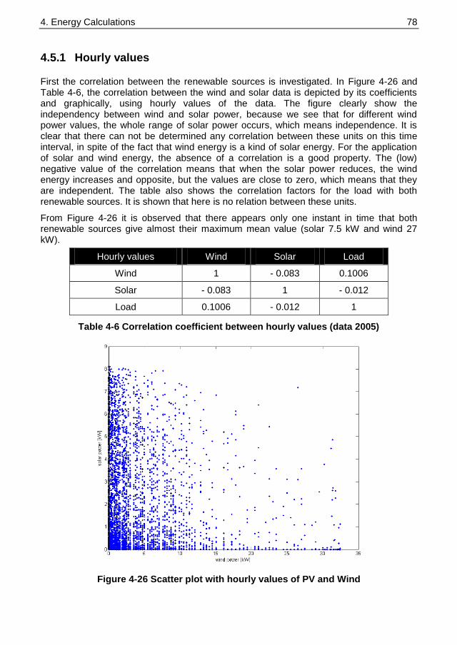
4. Energy Calculations 78 78
4.5.1 Hourly values
First the correlation between the renewable sources is investigated. In Figure 4-26 and Table 4-6, the correlation between the wind and solar data is depicted by its coefficients and graphically, using hourly values of the data. The figure clearly show the independency between wind and solar power, because we see that for different wind power values, the whole range of solar power occurs, which means independence. It is clear that there can not be determined any correlation between these units on this time interval, in spite of the fact that wind energy is a kind of solar energy. For the application of solar and wind energy, the absence of a correlation is a good property. The (low) negative value of the correlation means that when the solar power reduces, the wind energy increases and opposite, but the values are close to zero, which means that they are independent. The table also shows the correlation factors for the load with both renewable sources. It is shown that here is no relation between these units.
From Figure 4-26 it is observed that there appears only one instant in time that both renewable sources give almost their maximum mean value (solar 7.5 kW and wind 27 kW).
Hourly values Wind Solar Load
Wind 1 - 0.083 0.1006
Solar - 0.083 1 - 0.012
Load 0.1006 - 0.012 1
Table 4-6 Correlation coefficient between hourly values (data 2005)
Figure 4-26 Scatter plot with hourly values of PV and Wind
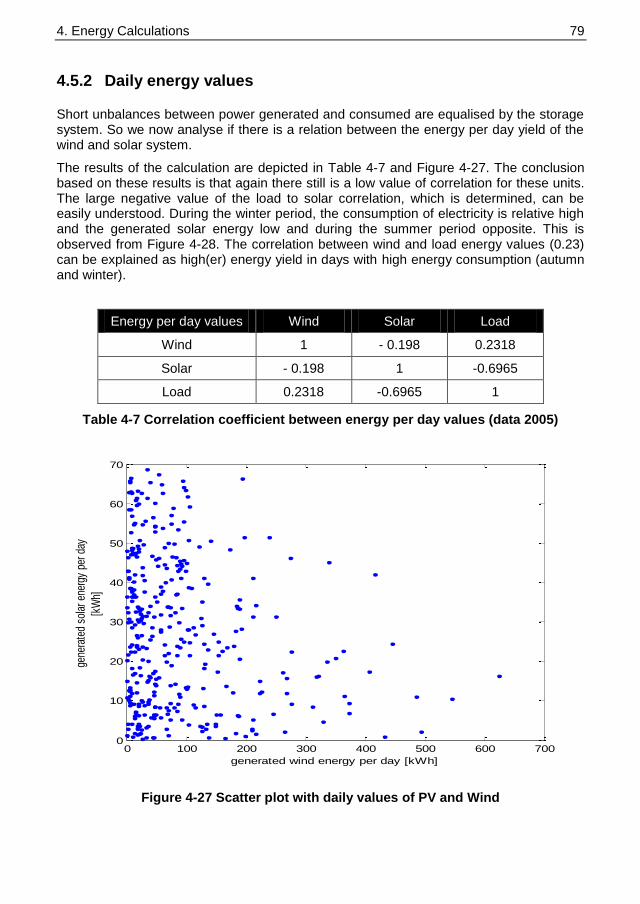
4. Energy Calculations 79 79
4.5.2 Daily energy values
Short unbalances between power generated and consumed are equalised by the storage system. So we now analyse if there is a relation between the energy per day yield of the wind and solar system.
The results of the calculation are depicted in Table 4-7 and Figure 4-27. The conclusion based on these results is that again there still is a low value of correlation for these units. The large negative value of the load to solar correlation, which is determined, can be easily understood. During the winter period, the consumption of electricity is relative high and the generated solar energy low and during the summer period opposite. This is observed from Figure 4-28. The correlation between wind and load energy values (0.23) can be explained as high(er) energy yield in days with high energy consumption (autumn and winter).
Energy per day values Wind Solar Load
Wind 1 - 0.198 0.2318
Solar - 0.198 1 -0.6965
Load 0.2318 -0.6965 1
Table 4-7 Correlation coefficient between energy per day values (data 2005)
0 100 200 300 400 500 600 7000
10
20
30
40
50
60
70
gene
rate
d so
lar e
nerg
y pe
r day
[kW
h]
generated wind energy per day [kWh]
Figure 4-27 Scatter plot with daily values of PV and Wind

4. Energy Calculations 80 80
0 50 100 150 200 250 300 350 4000
50
100
150
200
kW
h p
er
day
daynumber
Figure 4-28 Daily energy of solar and Load
4.6 Sizing the components
For the calculation of the size of the system components, the following procedure is used:
1. Meet all the system load, at any time in the year; 2. Use as much as possible energy from the solar and wind energy input; 3. Use batteries as energy buffer; 4. Use the Combined Heat and Power set as a back-up facility during
energy shortages.
In the previous sections, the “specific” energy yield (kWh/m2.year) and energy need
(kWh/household) is explained for the considered ten households. It should be taken into account, that fulfilling the energy balance on a year-base gives no guarantees for the various months and weeks. This problem is caused by the absence of a correlation between generation and consumption. Both have a stochastic behaviour. Stochastic analyses and time calculations through out the year give information about the coincidence of generated and consumed power and serves as a starting point for sizing the energy buffer system.
A first indication of the component sizes is nevertheless given by the yearly energy values.
Yearly energy overview for a system including ten households:
Consumed energy (10 households) 35.02 MWh
Generated wind energy (30 kW turbine) 34.16 MWh
Generated PV energy (10 x 12m2) 9.33 MWh
Table 4-8 Annual energy values based on recorded data

4. Energy Calculations 81 81
The total generated renewable energy (PV and Wind) is more than the consumed energy, but over dimension is necessary to:
Cover the power and conversion losses; Supply extra energy for reconditioning the batteries; Limit the actual size of the storage facility.
To determine the size of the energy buffer, we have to keep in mind that the size is defined by the number of days of autonomy (without any generated power) and the useable battery bandwidth [57].
100
1( )
EB C A
U Bb
Equation 4-4 Battery size equation
With: B(C100) = Battery capacity (C100-value) (Ah) E = Average Energy demand of one day (Wh/day) U = Voltage of the battery stack (V) A = Days of autonomy (day) Bb = Useable battery bandwidth (%)
Looking at the total electricity demand of ten households, an average energy of 4 kWh per hour is consumed. Based on literature [57], the number of autonomous days for the Northern of Europe region is 20 days. The bandwidth in which the battery stage of charge can vary is 75% (95% top and 20% lower limit). The battery size for ten households should therefore be 2560 kWh.
Nevertheless, this calculation assumes that the only power is delivered by the renewable sources (wind and sun) which could be absence for some days. In the chosen concept of this study, the system is applied with a combined heat and power set which is independent of the weather conditions. During power (energy) shortages the CHP set could be switch on, independent from the actual heat demand. This opportunity makes it valid to decrease significant the size of the battery. In [58] the optimal sizing of the battery is described for a stand-alone pv+diesel+battery system. For battery sizing purposes, this set-up is comparable to our system. It is shown in this study that a storage capacity equivalent to 12-18 hours of maximum monthly average hourly demand needs to be used.
Figure 4-29 Effect of battery storage on auxiliary power contribution

4. Energy Calculations 82 82
Figure 4-29 shows graphically the effect of the battery on the annual ratio of an auxiliary source to the annual load. It shows a pivot at 12 hours of battery storage capacity. Increasing this battery capacity will not contribute to a further reduction of the auxiliary power source contribution. The effect on the hours of operation is shown in Figure 4-30. It is now expected to have the same pivot at 12 hours of battery storage capacity. This minimum number of hours is needed to supply the load in dark and calm weather periods.
Figure 4-30 Effect of battery storage of hours of operating aux. source
These figures show that a 12 to 18 hours of battery storage capacity is a good value.
Converting these hour-values to energy-values, the average load demand for ten households is shown to be 35000 kWh/year and 4 kWh/hour. This leads to a battery capacity of 48 to 72 kWh. In the light of optimum use of battery-storage/aux. power unit and as a conservative estimation a battery capacity of 100 kWh is considered.
Within the energy context of households, the heat power balance has to be considered too. To generate heat for room-heating and washing purposes a Combined Heat and Power set is installed to generate heat and power in an efficient way. New trends on today‟s energy market are small and efficient CHP that are developed for houses and apartment houses, the so-called mini and micro CHP. The power range for these sets is a few kilowatts. The heat balance is kept out of the scope for the design of the renewable energy laboratory, but the energy generated by the installed micro CHP-set is has an impact in the electrical power balance. Based on an available market study, a 12.5 kW (heat) / 5.5 kW (electricity) CHP set has been selected [55] to fulfil the heat demand.

4. Energy Calculations 83 83
4.7 Economic aspects
The final decision to start with a project is mostly lead by the economic aspects on the system design. In this section, the concept of life-cycle costing is introduced, and its importance for hybrid renewable energy systems and limitations is discussed.
4.7.1 Overview of the equipment costs
A global overview of the typical costs of the individual components is made here. It should be noted that equipment prices, in what is still a small and immature market, can be highly variable, depending on country and location, the source and quality of equipment and the taxes or subsidies applied.
Table 4-9 shows a cost estimation of a renewable energy system with the mentioned dimensions. These figures are drawn from several internet sites of manufacturers and recently published books [26, 40]. It is the expectation of experts in the field that the prices of all these components will further reduce in the coming decade(s).
The replacement costs of the battery system takes into account a full replacement within 5 years. This is expected by the unusual application of lead-acid batteries. The application of Super Capacitors in parallel with the battery system will extend the life time of the battery and as a result, reduces the high replacement costs. Chapter 9 will discuss this application in detail.
The lifetime of the wind turbine and the Photovoltaic System is assumed to be 30 years. The lifespan of the CHP is much shorter and assumed to be 7-8 years. Small CHP units are rather new on the market. The life time is not known from figures and is probably a little bit underestimated.
Fuses and other protection equipment, as well as control equipment are part of the post „Other material‟.
Technology Size Typical investment
costs Maintenance and Operation costs
Replacement costs
Investment cost
Wind turbine 30 kW € 3.33 / W € 500 /year € 3.000 /year € 100.000
PV system 12 kW € 4.25 / Wp € 100 /year € 2.000 /year € 50.000
CHP 5.5 kW € 2.700 /kW € 300 /year € 500 /year € 15.000
Battery storage
100 kWh
€ 100 /kWh € 500 /year € 2.000 /year € 10.000
Other material € 100 /year € 1.000 /year € 25.000
Total € 1.500/year € 8.500/year € 200.000
Table 4-9 Cost indication of system components [2007]
4. Energy Calculations 84 84
4.7.2 Life-cycle costs
The initial cost is only one element in the overall economics of a system. Some type of economic assessment is required to determine if the system gives a good value for money in the longer run, either for the customer or for the economy as a whole.
The economics of PV and other renewable-energy technologies are rather different to those of conventional small power systems, in that:
The capital cost of the equipment is relatively high; The running costs are low and there are no fuel costs; The output of the system depends on its locations; The output of the system depends on the load pattern.
When comparing for instance PV with a diesel generator set, the high initial investment costs make PV look unattractive at first sight. However, the picture changes with an appreciation of the longer-term economic facts. This is normally achieved through the method of life-cycle costing.
A life cycle cost analysis calculates the cost of a system or product over its entire life span. This also involves the process of Product Life Cycle Management so that the life cycle profits are maximised.
The analysis of a typical system could include costs for:
planning, research and development, production, operation, maintenance, cost of replacement, disposal or salvage.
This cost analysis depends on values calculated from other reliability analyses like failure rate, cost of spares, repair times, and component costs.
A life cycle cost analysis is important for cost accounting purposes. In deciding to produce or purchase a product or service, a timetable of life cycle costs helps show what costs need to be allocated to a product so that an organization can recover its costs. If all costs can not be recovered, it would not be wise to produce the product or service.
A typical quantitative analysis would involve the use of a statement where an easy comparison of costs can be seen by having the different products a company produces next to each other.
The life-cycle cost of a project can be calculated using the formula:
pw pw pw pwLCC C M E R S
Equation 4-5 Life-cycle cost calculation
where the pw subscript indicates the present worth of each factor.

4. Energy Calculations 85 85
The capital cost (C) of a project includes the initial capital expense for equipment, the system design, engineering, and installation. This cost is always considered as a single payment occurring in the initial year of the project, regardless of how the project is financed. Recent trends indicate a steady decline in for instance PV technology costs, especially module costs and selected components linked to PV systems on the international market. In addition there will be further improvements in component efficiencies.
Maintenance (M) is the sum of all yearly scheduled operation and maintenance (O&M) costs. Fuel or equipment replacement costs are not included. O&M costs include such items as an operator's salary, inspections, insurance, property tax, and all scheduled maintenance. It have to be taken into account that autonomous systems are typically used in sparsely populated, isolated areas, serviced most effectively by a local representative who can attend problems in a matter of hours or days.
The energy cost (E) of a system is the sum of the yearly fuel cost. Energy cost is calculated separately from operation and maintenance costs, so that differential fuel inflation rates may be used. For renewable energy sources, these costs are zero. In our system, only the fuel costs of the CHP have to be taken into account.
Replacement cost (R) is the sum of all repair and equipment replacement cost anticipated over the life of the system. The replacement of a battery is a good example of such a cost that may occur once or twice during the life of a hybrid system. Normally, these costs occur in specific years and the entire cost is included in those years.
The salvage value (S) of a system is its net worth in the final year of the life-cycle period. It is common practice to assign a salvage value of 20 percent of original cost for mechanical equipment that can be moved. This rate can be modified depending on other factors such as obsolescence and condition of equipment.
A fully LCC calculation is not performing here; it‟s a bit out of the scope of this thesis. However, a rough estimation can be made.
The fuel costs (CHP-commitment) follow from the simulations which are performed in the next chapter, but it is here assumed to be € 8000 per year.
The replacement costs are assumed to be € 8500 per year.
The maintenance costs are assumed to be € 1500 per year.
The salvage value of the system is neglected.
The total LCC amounts € 840.000, when we assume a 30 years life time of the total system. Interest costs are estimated on an extra € 10.000 per year.
For this price, the electricity demand of 10 houses is covered for 30 years and a lot of heat (2000 h x 30 years x 12.5 kW th) is produced.
When only the covered electricity demand is taken into account, a total energy consumption of 35000 x 30 year = 1.050.000 kWh is used in the life time of the system.
In this rough estimation, the energy price per kWh is € 0.80. This value is almost four times higher than the actual electricity price from a utility, which price amounts €

4. Energy Calculations 86 86
0.226/kWh. (5 cents network contribution, 9 cents fuel and 9 cents taxes). However, it has to be taken into account that today‟s customers paid a fix amount for “being connected to the grid” and the cost for metering. The Dutch households have to pay € 190 per year for both costs. For the ten households this money has to be decupled to € 1900 per year.
4.8 Conclusions
Energy calculations are performed in this chapter. Starting point of the sizing operation is always the consumption of energy in the households (demand) which should be supplied by the sources. Secondly, the available space on the house roofs determines the contribution from solar panels. The solar energy is calculated using meteorological data, panel facing and technology efficiency. Thirdly, a suitable wind turbine is chosen for the built-environment. Its power curve and the local available wind data determine the energy yield. From reliability point of view, the battery system size amounts ten days of autonomy. Point of attention is the coherency of the available energy or power from the different sources and the demand pattern. The correlation analysis shows negative values, which means that we could not expect that the power generation and power demand will be on the same time and the same magnitude. Together with the fact that the energy storage capacity is limited, an over dimension of the power sources is essential.
The system sizing considerations in this chapter are based on the Delfts‟ (Dutch) situation and takes into account a number of reference points concerning the available roof area and local wind and solar data. This chapter describes, nevertheless the sizing procedure, which can be in general used for all renewable energy projects.

5 DESIGN OF THE RENEWABLE ENERGY LABORATORY
The focus of this research is concentrated on the system behaviour of an autonomous renewable energy system. The best way to analyse this behaviour is to build and measure this system in real situation, because software models show up their modelled behaviour. Only if you fully understand all the phenomena and their interactions, software models can be used. In the power range and the autonomous operation, the behaviour is not clearly understood already. For this reason, a full scale laboratory is created for the analyses.. For this reason, this laboratory is constructed with as much as state of the art components which are selected for its market availability and their reliable and well-defined operation. Their model description and system parameters can be found in literature. Most models however are developed for grid connected application and differ in power range. In the context of this project, the focus of the research is on the system integration of today‟s renewable sources. It is clear that this research is a first step in the autonomous renewable energy research by creating a laboratory facility. In a second phase, new components could be integrated and investigated in the laboratory environment.
Most components are however represented by an analogue model to be flexible in the laboratory environment and to avoid unwanted situations. Real components are applied at the coupling point with the autonomous grid to be sure that the system behaviour is as similar as possible to a real system. These simulators are described in sections 5.1-5.4. In section 5.5 a detailed description of the Photo-Voltaic system is presented. The total DENlab laboratory system is described in section 5.6.
5.1 Wind turbine simulator
In section 4.6 wind energy calculations are performed and it was concluded that a 30 kW wind energy conversion system (WECS) can supply that amount of energy which is needed from an energy point of view. The reason to use a wind turbine simulator was two fold. Firstly, when a real wind turbine is used, only the local situation can be analysed. From experience and literature is known, that the local situation has a great influence of on the total energy yield and dynamics by turbulences (see section 4.2.3) Secondly, it was not easy to get permission to install a wind turbine close to the laboratory. In order to create the necessary flexibility, a wind turbine simulator was developed, based on a motor-generator set, driven by a frequency converter. The set-up is depicted in Figure 5-1.

5. The design of the renewable energy laboratory 88 88
Figure 5-1 Set-up of the wind turbine simulator
5.1.1 General concept
In today‟s wind turbine research, three different wind turbine technologies are considered: constant speed, variable speed and a concept based on the double fed induction principal [59]. In lowest power ranges, most WECS use the simplest concept: constant speed. However, new wind turbines use the variable speed concept. They were however not available on the market or did not have shown a stable operation at the design phase of this project.
In general, two different techniques are applied to control the power of a wind turbine: The pitch angle control and the stall regulation control. Pitch angle control means that the blades are turned to limit the power on the axis to its nominal value. With the stall regulation method, the power on the axis is limited as a result of the aerodynamics around the blades. The shape of the blades is adjusted in order to limit the pressure on the blades caused by the turbulences at the back-side of the blades. These turbulences results in a negative torque on the axis, which reduces the net output torque, see Figure 5-2. The result is that the axis power is limited for higher wind speeds.
Because of costs considerations, wind turbines for the lower power ranges are mainly equipped with a stall-regulated control. For this reason, both stall-regulation and constant speed concept are used as control mechanisms in our wind turbine simulator.
H(s)
G AC
AC
Wind Speed
M soft starter
Autonomous
grid
TU grid

5. The design of the renewable energy laboratory 89 89
Figure 5-2 Example of the power curve for a stall-regulated wind turbine
An electric motor supplies the „wind torque‟ to the generator. The motor is fed by a back-to-back voltage source converter, with adjustable frequency. A feedback loop controls the output frequency of the converter, and the power which corresponds to the actual wind s speed is supplied by the generator.
rated
rated
rated
Δ/Y
Δ/Y
P =37 kW
n =2850 rev/min
cos = 0.89
I = 65/38 A
V =400/690 V
Figure 5-3 Motor-generator set 37 kW as it is installed in DENlab

5. The design of the renewable energy laboratory 90 90
A voltage source converter, with a variable output frequency, drives a conventional squirrel cage induction machine. Another induction machine is mounted on the same shaft which serves as the generator of a wind turbine. The idea is to drive the motor with higher than rated frequency (> 50 Hz) to force the second machine to be in generator mode. In Figure 5-4, torque characteristics are displayed for three different frequencies. In this example the chosen frequencies are respectively 49, 50 and 51 Hz.
0.7 0.8 0.9 1 1.1 1.2 1.3-4
-3
-2
-1
0
1
2
3
4
Mechanical speed (p.u.)
Ele
ctr
ical to
rque (
p.u
.)
49
50
51
Figure 5-4 Full torque-speed characteristic for three different stator frequencies
The solid curve represents the torque-speed curve by a frequency of 50 Hz. This is curve is valid for the generator. Since the two machines are mechanically coupled, the mechanical speed for both machines is equal. When the stator frequency of the motor increases, the motor-generator set finds a new equilibrium point. In this steady state situation the mechanical speed and axis torque are equal for both machines.
For the generator, the allowed electrical torque lies between 0 and –1 pu. This means that the maximum speed deviation (slip) is only a few percent. It can be concluded, that the maximum allowable stator frequency of the motor is 51 Hz. This value depends on the machine parameters. We assume in this calculation that the stator frequency of the autonomous grid is fixed to 50 Hz. Like can be seen in the figure, the relation between torque and speed, as well as between speed and stator frequency, is almost linear in the operating area (Mechanical torque: 0 to 1 pu).

5. The design of the renewable energy laboratory 91 91
The maximum allowable stator frequency of the driving motor can be calculated as follows:
The actual mechanical frequency,
,
,50
,
(1 )nom gen
m act s Hz
nom gen
sP
P
The synchronous radial frequency, s, which corresponds with the actual set
point of mechanical torque and frequency, Tmech and m.
,
,
(1 )
m
s
nom motor
act
nom motor
sP
P
Wind speed data can be obtained from two sources: from a stored data set or from the on-line anemometer. The wind speed data is transformed to wind power data by a static power curve, programmed in the Programmable Logic Controller. In this controller, either a mathematical expression or a look-up table can be used to relate wind speed with wind power.
The reactive power of induction machines can be compensated by a capacitor bank to reduce the current from the battery converters. The size of the capacitor bank is determined by the nominal value of the reactive power demand of the generators.
phaseper
c
ll
FX
C
kQ
VXc
PSQ
S
P
77.34.8502
11
4.819
400
kVAr 19
kVA 6.4189.0
37
89.0cos
kW 37
22
22

5. The design of the renewable energy laboratory 92 92
5.1.2 Soft starter
During the start of the motor-generator-set and the coupling with the autonomous grid, the induction generator must be synchronized with the voltage on the connected bus, but has to avoid large transient inrush currents. Soft-starters, which are normally used for induction motors can be used for induction generators as well. Soft-starters built up the voltage on the load side by adjusting the firing angle on the gate-input of the thyristors, see Figure 5-5.
Figure 5-5 Soft starter circuit
On most modern soft-starters, three parameters can be tuned: starting voltage U0, rise time tr, ramp-down time tf, see Figure 5-6.
U
Ustart
Unom
trise ttdown
Figure 5-6 Example of soft starter characteristic
At the end of the start-up procedure, a contactor bypasses the soft starter, in order to have a direct, lossless connection between the generator and the voltage bus. Some soft starters have a feature that they keep on monitoring the voltage and disconnected from the system when an voltage imbalance is detected. This functionality has been disabled for the DENlab system.

5. The design of the renewable energy laboratory 93 93
5.2 CHP simulator
Like the wind turbine simulator, a CHP simulator is built with a motor-generator combination. It‟s supplied by a power electronic frequency converter. Unlike the wind simulator, the CHP simulator has in this study only one fixed set point. This represents a CHP-set which is state of the art on today‟s market. Other CHP-sets with variable outputs are under consideration nowadays. Expanding functionality of the CHP-set can be easily programmed. However the induction machine is much smaller than for the wind simulator and as a consequence the magnetizing currents are much smaller too, a soft-starter is also applied in order to relieve the battery units from these (reactive) currents. Like in the case of the wind turbine a capacitor bank, for size of its nominal reactive power is connected.
Figure 5-7 Motor-generator set representing the CHP (left Motor, right Generator)
5.3 Battery simulator
Within the context of our laboratory set up, the installation of a real battery stack of 100 kWh was not feasible. Extreme situations are created and analysed in search for the limits of the autonomous system. In such situations there could be an increased risk of an explosion and generation of toxic gasses.

5. The design of the renewable energy laboratory 94 94
Another reason to choose for simulating battery‟s behaviour is the extra degree of freedom to analyse different battery types, such as lead-acid, lithium-ion and NiCd batteries.
A three phase inverter converts the DC-power of the battery that has to be converted into AC-power and vice versa. This inverter has to be able to dictate the voltage and the frequency when the power system operates autonomously. In grid-connected operation, the inverter must behave as a current controlled voltage source (CCVS). The mode of operation is controlled by the software, which drives the IGBT‟s.
A rectifier with regenerative capabilities, represents the battery. The DC voltage level, which is actually a DC link voltage between two converters, is programmed to be depending on the actual State of Charge level of the storage unit. In Figure 5-8 the battery simulator is schematically depicted. A reference battery is fed by a part of the main circuit. The terminal voltage of the reference battery is measured and send back to an AC/DC converter.
Figure 5-8 Circuit diagram of the battery simulator
In this simulator the actual current (Iref) in the main-circuit is measured. The value of the current is a parameter for the battery controller. This battery control system controls the actual current in the reference battery to be as close as the reference current value. When the battery current is positive (charge mode), the battery is powered by an external voltage source. The right part of the circuit is blocked by the NFET transistor, which has in this case a negative gate-source voltage. The PFET is used as a controllable resistance. Its resistance value depends on the gate-source voltage (output of the control system).
AC
DC
AC
DC
K 1
Battery control
A
A
V
K 2 +
-
Charge circuit
Discharge circuit
1
I ref I batt
V gs
V set
TU grid Autonomous
grid

5. The design of the renewable energy laboratory 95 95
At negative currents (discharge mode) the battery power is consumed by a resistor of 1 Ω and by the power NFET. The actual current is in this situation depending on the resistance of the NFET (controlled by the battery controller), the 1 Ω resistance and the actual battery voltage. The resistance of the FET is adjusted by the controller in order to give a good reference current.
The actual voltage of the battery is measured by transducer V. This measured value is multiplied by the number of batteries (K2) that are stacked in series in the real situation. (e.g. 60). This value is transferred to the rectifier as a set point to control the DC link voltage.
The battery voltage range from uncharged (10.5 V) to fully charge (14 V) amounts 3.5 V/battery. This means that the DC link voltage varies from 630 to 840 V.
Figure 5-9 An AC/DC/AC system representing the battery simulator
Figure 5-9 shows a picture of the Battery simulator as built in the laboratory. On both sides, the L-C filter is mounted for the harmonic voltage suppression. The two boxes in the middle are the DC/AC converters.
Figure 5-9 An AC/DC/AC system representing the battery simulator
Figure 6-9 shows a picture of the Battery simulator as built in the laboratory. On both sides, the LC filter is mounted for the harmonic voltage suppression. The two boxes in the middle are the DC/AC converters.
L/C filter
Rectifier
Inverter
L/C filter
Reactors

5. The design of the renewable energy laboratory 96 96
5.3.1 Battery controller
To control the battery current, a rather simple feedback controller is used as shown in Figure 5-10.
VgsxIref
Iact
+
-
Figure 5-10 A feedback system to control the battery current
Iref is the desired current, derived from the main circuit [A]
Iact is the measured current in the reference battery [A]
Vgs is the Gate-Source voltage of the NFET and PFET. [V]
1/s is the integrator, with a unit time constant
This feedback control circuit adjusts the battery current by varying the gate-source voltage (Vgs) from two power FET‟s. A P-channel FET is adjusting the charging current, in the left part of the system. A N-channel FET controls the discharge current in the right part of the circuit. This value of Vgs varies between –15 and +15 V. At positive values, the discharging circuit is active, whereby a lot of energy is dissipated in the 1 ohm resistance.
For positive Gate-Source voltages, the resistance of the P-channel FET in the charging circuit is very high (charge current is zero). For negative values, the charging circuit is in operation and the discharge current is zero. The necessary power is delivered by the external voltage source, whereby the current is controlled by the P-channel FET. The discharge circuit is blocked by a negative Gate-Source voltage on the N-channel FET.
Both FET‟s have a threshold voltage of approximately 4 V. This limits the „switching speed‟ from positive to negative currents and from negative to positive currents. In this situation, the output of the integrator should rise or fall 8 volts in total. The response time from the charge to the discharge mode, however, is sufficient for the aim of this project.
5.4 Load demand simulator
The load of the system is represented by a load demand simulator, which extracts power from the autonomous grid and feeds it back to the public grid. The actual quantity of the power demand is defined by the load pattern, which is already described in section 4.4.
The simulator is constructed with two back-to-back DC/AC converters. One converter acts as a rectifier and the other as a regenerative unit. This is depicted in Figure 5-11.
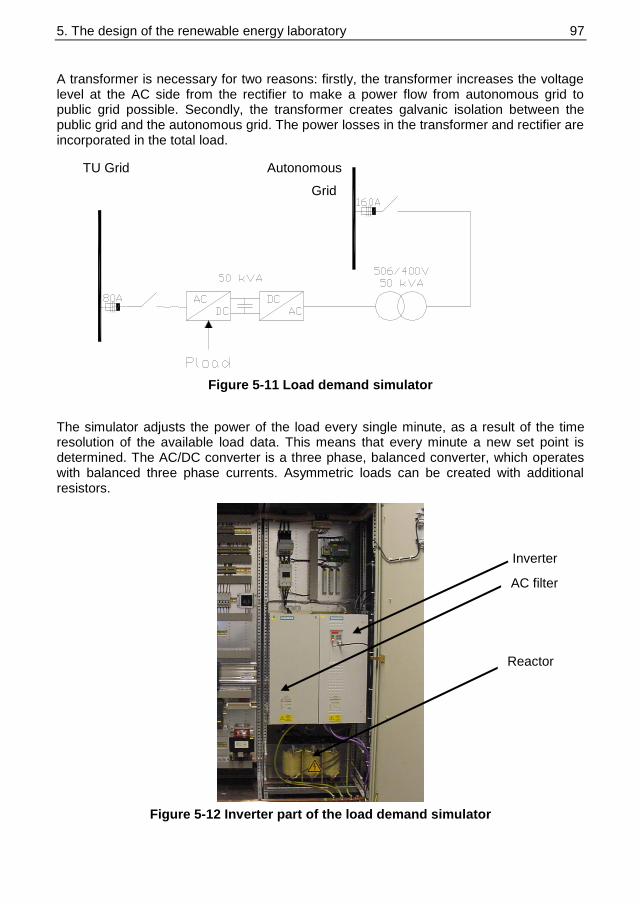
5. The design of the renewable energy laboratory 97 97
A transformer is necessary for two reasons: firstly, the transformer increases the voltage level at the AC side from the rectifier to make a power flow from autonomous grid to public grid possible. Secondly, the transformer creates galvanic isolation between the public grid and the autonomous grid. The power losses in the transformer and rectifier are incorporated in the total load.
Figure 5-11 Load demand simulator
The simulator adjusts the power of the load every single minute, as a result of the time resolution of the available load data. This means that every minute a new set point is determined. The AC/DC converter is a three phase, balanced converter, which operates with balanced three phase currents. Asymmetric loads can be created with additional resistors.
Figure 5-12 Inverter part of the load demand simulator
TU Grid Autonomous
Grid
Inverter
AC filter
Reactor
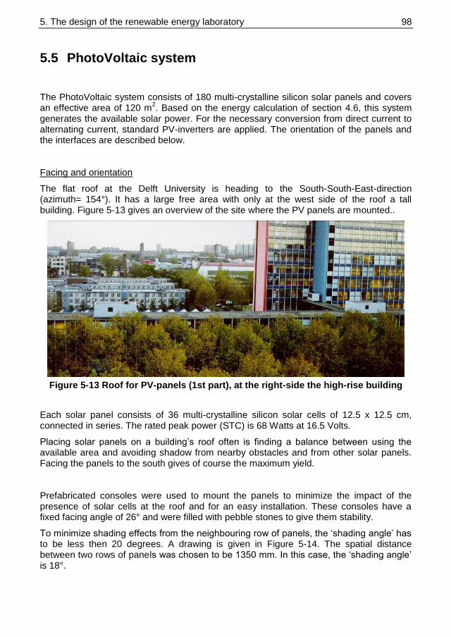
5. The design of the renewable energy laboratory 98 98
5.5 PhotoVoltaic system
The PhotoVoltaic system consists of 180 multi-crystalline silicon solar panels and covers an effective area of 120 m
2. Based on the energy calculation of section 4.6, this system
generates the available solar power. For the necessary conversion from direct current to alternating current, standard PV-inverters are applied. The orientation of the panels and the interfaces are described below.
Facing and orientation
The flat roof at the Delft University is heading to the South-South-East-direction (azimuth= 154°). It has a large free area with only at the west side of the roof a tall building. Figure 5-13 gives an overview of the site where the PV panels are mounted..
Figure 5-13 Roof for PV-panels (1st part), at the right-side the high-rise building
Each solar panel consists of 36 multi-crystalline silicon solar cells of 12.5 x 12.5 cm, connected in series. The rated peak power (STC) is 68 Watts at 16.5 Volts.
Placing solar panels on a building‟s roof often is finding a balance between using the available area and avoiding shadow from nearby obstacles and from other solar panels. Facing the panels to the south gives of course the maximum yield.
Prefabricated consoles were used to mount the panels to minimize the impact of the presence of solar cells at the roof and for an easy installation. These consoles have a fixed facing angle of 26° and were filled with pebble stones to give them stability.
To minimize shading effects from the neighbouring row of panels, the „shading angle‟ has to be less then 20 degrees. A drawing is given in Figure 5-14. The spatial distance between two rows of panels was chosen to be 1350 mm. In this case, the „shading angle‟ is 18°.

5. The design of the renewable energy laboratory 99 99
Figure 5-14 Detail of PV installation
The width of the roof is approx. 9 metres. For safety reason, two metres is reserved on both sides of the roof and a path of one meter in the middle. This means that a net width of approx. 6 metres remains for the installation of the solar panels. The applied solar cells (Shell Solar: RSM 70) has a width of 120 mm, so this means that a row of 5 panels can be made, divided into two parts, 3 and 2 panels respectively. This results in the set-up like depicted in Figure 5-15.
Figure 5-15 Set-up of PV-panels at DUT
DC/AC inverters
To convert the DC power into AC power, a standard PV converter is applied. Because of the fact that one of the manufacturers of PV converters was a sponsor of the DENlab project, an intensive comparison study for different converters has not been carried out. From this manufacturer, only one type is used in the project: the OK4-E100. This 100W converter has an input voltage of 24 V and has a input power limit of 100 W. The input voltage and the power range determine the configuration of the attached PV panels. Like discussed above, the applied solar panel has a nominal output power of 70 Wp at an output voltage of 12 V. This leads for the 100 W converters to two PV panels in series per converter. Under dimensioning of the inverters is quite common, because of the large periods of low sun-irradiance. In these periods the PV panels generate less then the nominal rated power and the efficiency of the conversion depends on the actual power.

5. The design of the renewable energy laboratory 100 100
Figure 5-16 View of the first part of the PV system

5. The design of the renewable energy laboratory 101 101
5.6 The complete DENlab system
Figure 5-17 shows the total DENlab laboratory. It consists of the building blocks, described in the previous sections. A comparison was made between the laboratory set-up and the real-system. Practical aspects which are related to the laboratory system are discussed in this section.
50A
200A
40A
80A
160A
40A
Grid
connection
25 kVA 25 kVA
AC
AC
Vwind
AC
AC
80A
25A
TU grid
400 V
30 kW
M
25 kVA
M
5.5 kW
GSoft
starter
25 kVA
GSoft
starter
40A
50 kVA
Pload
AC
DC
DC
AC
40A
160A
160A
AC
DC
AC
DC
80A
32A
autonomous
grid 400 V
asymmetric
grid 400V
PV
PV AC
DC
DC
AC
AC
DC
DC
AC
cos phi
compensation
50A
Batt. 1
CHP-set
Batt. 2
Wind-set
Dy 5
50 kVA
460V /400V
50 kVA
400V /400V
50 kVA
160A
160A
Figure 5-17 Actual set-up of the DENlab laboratory
5.6.1 Galvanic insulation and transformers
As can be seen in Figure 5-17, the system contains three transformers. The Dy5-transformer is a 1:1 transformer, placed for the required galvanic insulation in the loop from TU grid via Battery 2 to the autonomous grid and via the Battery 1 back to the TU grid. Because of the fact that these DC/AC- converters have no galvanic insulation, an uncontrolled common mode current can flow via these components. This transformer is situated here. In this place, it does not contribute to the losses in the laboratory system, because these are covered by the grid.
The second transformer is an Yz11 transformer, which is placed between both battery systems and the rest of the system. A Z-transformer is used to prevent the battery converters from an unbalanced three phase voltage and current system. In the real applications, where the household load normally is distributed over the three phases, an asymmetric current and voltage system can easily be present. However, in this research only a balanced system is considered. The second reason for this Yz11 transformer is the galvanic insulation in the loop: TU grid, battery 2, autonomous bus bar, grid connection, TU grid.

5. The design of the renewable energy laboratory 102 102
The third transformer in this system is placed in the load simulator. The rectifying unit of this simulator is a thyristor bridge converter, which has a maximum DC voltage of 1.35 times the line-to-line voltage of the AC system. (1.35 x 400V = 540V). This maximum voltage is under the operation limit of the AC/DC converter (600-740V). For this reason the transformer must have a step-up function to bring the DC voltage to the required level. The other reason is, again, the galvanic insulation in the loop grid connection – load simulator or battery 2 – load simulator.
In a real application, the only transformer of importance is the Yz11 transformer for the asymmetrical system voltage.
5.6.2 Monitoring and Control
The control and monitoring of signals is carried out by the Profibus control system. This system is the standard bus-protocol in the drive industry. It has a communication speed of 1.5 Mbit/s, which is fast enough for this application. Each individual converter has on board measurements which values are released by the protocol. The available units which are internally measured depends on the type of converters. At least the actual AC-current, AC-voltage and power is released and transferred to the Programmable Logic Controller (PLC). This central processor is used to monitor the signals of the converters, the external signals via the analog and digital inputs (wind speed, load demand pattern, etc.) and runs the user-defined program to control the system components and drives the digital and analog outputs.
Besides the internal monitoring in the converters, nine additional Simeas P meters are installed to measure the actual voltages and power. These measurements are stored by a self developed computer program, communicating via the Profibus system. The sample rate of the measurements is one second and is stored in a text-file.
The user interface (own-written software) is depicted in Figure 5-18.

5. The design of the renewable energy laboratory 103 103
Figure 5-18 User interface of the laboratory system
5.6.3 Earthing and Protection
The autonomous bus system is earthed, with the earth line from the utility. We called it the TN-earthing system. This earth conductor is connected to the star point of the secondary (z) side of the Yz11 transformer. The autonomous grid is earthed in this way. The DC/AC converters require a floating voltage system. This means that the neutral of the TU grid is not connected to the bus bar “TU grid”. The cabinets themselves are also connected to the earth connection of the TU grid.
Figure 5-19 TN-S system
A protective earth neutral (PEN) connection is a combined PE and N connector and ensures that all exposed conductive surfaces are at the same electrical potential as the

5. The design of the renewable energy laboratory 104 104
surface of the earth, to avoid the risk of electrical shock if a person touches a device in which an insulation fault has occurred. It also ensures that in the case of an insulation fault, a high fault current flows, which will trigger an overcurrent protection device (fuse, MCB) that disconnects the power supply.
The protection of the system is distributed. Each component has externally its own fuses (fast and slow) and internally a very fast monitoring of currents and voltages, also di/dt and dv/dt, to protect the system. The power electronic devices have a rather small heat capacity. For this reason the off-switch command must be very fast to prevent the component from unrecoverable damage. At this moment, a fault in a component leads to a blackout of the whole system. It is recommended to take measures in order to isolate only the fault location, by creating selectivity.
5.6.4 Electro Magnetic Compatibility
The system has taken measures to prevent the laboratory system from EMC problems. The galvanic insulation is created by the transformers as described in the previous sections. L/C filters are placed to cancel the high-switching frequency components in the voltage system. These filters, nevertheless, create a voltage drop for the 50 Hz system, which must be taken into consideration. Their influence together with the influence of the commutation coil gives a voltage drop at high currents. The voltage may vary, according to the most standards, between +10% and -10%, but can easily a source of voltage flicker.
The mutual coupling (crosstalk) is limited by a good engineering of the cabinets itself. The components are shielded and critical communication wires (Profibus) is performed by shielded cables.
Figure 5-20 Snapshot of the laboratory system
Frequency
Converter
Wind & CHP
Soft starter
Wind & CHP
Motor/Generator
connections

5. The design of the renewable energy laboratory 105 105
5.7 Conclusions
The design and realisation of the laboratory is described in this chapter. The considerations which lead to this way of „simulation/representation‟ of the real component are described and argued. This laboratory is designed to be a flexible research environment, which is suitable for experiments with current and new components (sources, storage systems and loads). The designed measurement system, which is based on the common Profibus protocol, is adequate to monitor essential data and can be extended easily.
As described in section 5.6 a number of components is necessary in this laboratory, and will not appear in a real environment. For example, two of the three transformers are added for galvanic isolation and motors are installed to simulate the driving power which normally comes from gas flow (CHP) or air flow (WECS). This leads to additional losses in the laboratory, which are not present in a real situation.
Nevertheless, taking into account the right system definition, the laboratory measurements will correspond to the real world situation.
As central controller, a PLC is chosen because of its stable operation, which is shown in its long operation in complex situations in the industry. It has easily internal and external communication properties (input and output cards). The programming language is closely related to the digital techniques, which is a part of the skills of an electrical engineer.
Communication between components and central controller is done by on the Profibus protocol, which meets the actual standards in communication.

6 SYSTEM CONTROL STRATEGIES
The design of the renewable energy system is discussed in chapter 5. The proposed laboratory model is shown to be a realistic representation of the real autonomous renewable energy system. The contribution of the system components to the energy balance depends on the local conditions of the system and the component size. This chapter discusses the control strategies in order to guarantee a stable an reliable power supply to the ten houses, in terms of available energy. The basis of the control system is the state of charge of the battery and the actual battery current, because when the battery is operating well and is kept at a good energy level, the system is able to perform its primary task. Besides the reliable supply of power, a renewable energy system wants to maximize the use of the energy from the renewable sources. On the other hand, the care for the battery buffer is important for the life time of that buffer. Life time extension leads to a reduction of the replacement costs.
In this chapter, different control strategies are proposed, with its advantages and disadvantages. A strategy is defined here as a way of controlling the system. The strategic goals are the same in all simulations but the available data (measured or estimated) differs in the discussed strategies. The level of available data is incremental, with other words: strategy 2 has at least the same data as strategy 1, but other information is added and used.
Four strategies are simulated in MATLAB based on real measurements obtained from the laboratory set up. The power data for solar, wind and loads are recorded in the laboratory on a ten minutes time basis. This is adequate enough for the analysis of the impact of strategies concerning the system‟s operation, control and management. The battery has a strong non-linear behaviour which makes the application of mean-values of the data less accurate. Nevertheless, the application of super capacitors in parallel with the batteries can be seen as a way to smooth the variations in the battery (charge or discharge) current. Chapter 9 describes in detail how this parallel buffer system works. This validates the application of mean values in this chapter.
Four different control strategies are investigated and compared [60]. The first strategy is a very straightforward method taking into account only the upper and lower SoC-bound. The second is improved by splitting the complete battery stack into two separate controllable battery systems. In cases of high battery current, both systems work in parallel. In cases of low battery currents only one of them is in use. These both control methods do not use any forecast information: they only respond on actual values. Control strategy 3 uses a preview of the expected load demand. It is assumed that the weeks have a strong repetitive pattern. If a high energy demand is expected, the CHP unit is started earlier, in order to keep the battery in a high SoC level and to prevent the batteries from deep discharges.
The last control strategy in this chapter decides to recondition the batteries on a regular basis. During a period of low battery power demand, one of the two batteries is fully charged and remains on 100% during 12 hours.
The main objectives for comparing the control strategies are the improvement of the Battery Lifetime (Qualitative) and the optimal use of renewable energy (Quantitative). The last objective is measured by a minimal usage of fossil fuel (CHP-unit) and the effective use of the available renewable energy. The control system can decide about the necessity of load reduction. This means that the load is reduced to stop the discharge

6. Control strategies 107 107
mode when the battery reaches its absolute minimum SoC-level. The final comparison between the control strategies is only qualitatively. Besides this qualitative value of the lifetime, prices of the components and fuel costs are always changing and limit the validity of the considerations.
As an overview of all the quality and quantity aspects, the following issues are important:
Use of the CHP unit (periods per year); Number of starts and stops of the CHP unit; The balance between used and unused renewable energy; Amount of necessary load reduction; Average state of charge of the batteries; Periods of low State of Charge (less than 50%); Periods of very low State of Charge (less than 30%). Number of equalisation cycles.
6.1 Operation bandwidth of the SoC
The first control strategy is rather straightforward. The battery buffer compensates, without any restriction, the mismatch between generated and demanded power. At the minimum SoC level the CHP is connected to the system regardless the heat demand. At the maximum SoC level the CHP is disconnected. When the maximum allowable SoC level is reached, PV and Wind energy input is also switched off. The load is then only fed by the battery system. The amount of energy that is not used is a measure of the correlation between the power demand and generation and is mainly caused by the limited storage capacity. At the end of this section, other variants on this control method are investigated and presented.
Figure 6-1 State diagram first strategy
Charge Discharge
CHP ON/OFF (CHP = 5.5kW)
if ;CHP OFF if (SOC<0.7)
;CHP ON
No charge or discharge AmpHour = 0
(SOC>0.7)

6. Control strategies 108 108
Figure 6-1 shows a state diagram of the first control method. In this method, the generated and demanded power is subtracted from each other and this results in a „delta power‟ value. This power has to be exchanged with the battery storage system. When the delta power is divided by the actual battery voltage, the battery current is calculated. The integral of the battery current results in an „Amp-Hour‟ value. Every ten minutes, a new State of Charge value is calculated as shown in the flowchart of Figure 6-2. In the calculation of the SoC, the efficiency effects, such as charge acceptance and the Peukert effect are taken into account. The control system only controls the commitment of the CHP unit. The size of the time step of the calculation influences in this simulation the moment of CHP turning on or off. This is one reason why the SoC can exceed the predefined limits sometimes. Another reason for exceeding the limits is the inability of the CHP to cover the load demand in a specific period. The load demand of the ten households can be that high that is exceeds the 5.5 kW electrical power of the CHP in windless and dark periods leading to low energy charging levels. This calculation issues does not happen in a real situation with a non-discrete control system.
BEGINNING OF MAIN CYCLE (t = 1:n-1)
START BATTERY SOC CONTROL
DeltaPower = wind(t) + solar(t) - loads(t)
RETURN TO MAIN CYCLE (t=t+1)
Call Function CALC_SOC
a new SOC(t+1) is calculated
using obtained AmpHour(t)
PROGRAM END
SOC(t) < 0.7Turn on CHP
(5.5 KWh)
SOC > 0.9 Turn off CHPYES
YES
Batteries Empty?SOC(t+1)=
SOC(t)-0.0002
Batteries FULL?SOC(t+1)=
SOC(t)-0.0001
YES
YES
Calculate AmpHour((DeltaPower+CHP)/720)
Figure 6-2 Flowchart first strategy
Figure 6-3 shows the time results of the Matlab simulation with this control method. The x-axis covers the complete year, displayed with the month number. It shows a surplus of renewable energy in the summer periods. The CHP unit is seldom used in this period. In the first and last period of the year (winter periods) the contribution of the CHP is

6. Control strategies 109 109
necessary for the electricity balance. This meets the heat demand of the houses. It means that, if the control is extended with heat demand pattern, it leads naturally to almost the same commitment of this unit.
0 2 4 6 8 10 12-40
-20
0
20
40
Am
phour-
valu
e [
Ah]
0 2 4 6 8 10 120
2
4
6
CH
P p
ow
er
[kW
]
0 2 4 6 8 10 12
0.2
0.4
0.6
0.8
1
SoC
time (months)
Figure 6-3 Plot of results for entire year (first strategy)
0 5 10 15 20 25 30-50
0
50
Am
phour-
valu
e [
Ah]
0 5 10 15 20 25 300
2
4
6
CH
P p
ow
er
[kW
]
0 5 10 15 20 25 30
0.2
0.4
0.6
0.8
1
SoC
time [days]
Figure 6-4 Plot of results for first month (first strategy)

6. Control strategies 110 110
Figure 6-4 shows a detailed view of the first month of the simulated year. It shows high dips in the AmpHour value, which is in fact the battery power demand. During those periods, the SoC decreases very quickly by the non-linear behaviour of the battery during high currents interval, which is described by Peukert number (see section 3.2.4).
Number of times the CHP was started 234 x
CHP connected to the grid 1933 h (22%)
Renewable Energy balance Used (kWh/year) Unused (kWh /year)
Wind energy 20072 13069
Solar energy 8547 3330
Total Renewable Energy 28619 16399
Battery State of Charge Battery 1
Average SoC 84.1 %
SoC <50% 19 x
SoC <30% 6 x
Total conversion losses 6050 kWh
Load reduction 1.86 kWh
Table 6-1 Simulation results for the first strategy
Analysing the result of this first strategy, summarized in Table 6-1, the following conclusions can be drawn:
the average State of Charge is rather high: 84%. This has a positive effect on the battery life time;
The load reduction is rather low, less than 2 kWh. This situation occurs in December;
The number of times that the State of Charge is low: 19 times below 50% and 6 times below 30% has a drawback on the life time, because a frequent discharge to low levels is necessary to prevent the batteries from their memory effect. This memory effect is the reduction in storage capacity due to low discharge periods. (This memory effect plays typically a role for lead-acid batteries. When using other battery technologies, this is not an issue)
The total conversion losses caused by the inefficiency of charge and discharge modes, adds up to more than 6000 kWh per year.
The unused renewable energy is nearly 36.4% of the total available renewable energy.
Two variant control methods on the first strategy
In the presented control strategy, the renewable sources are both switched off at upper limit of the State of Charge. As a result, the present load is then supplied by the energy of the battery. This leads to a decreasing of the State of Charge (SoC) of that battery, although the energy is in potential present from the renewable sources. In the first variant on the first control strategy, the excessive power is consumed by a „dump load‟, which can be equipment like a heat pump, electrical boiler or air conditioner or a controllable storage system, like the production of hydrogen by electrolyse. In this way, the battery current is kept zero in order to prevent the battery from overcharging, but it keeps the battery on top of the SoC.
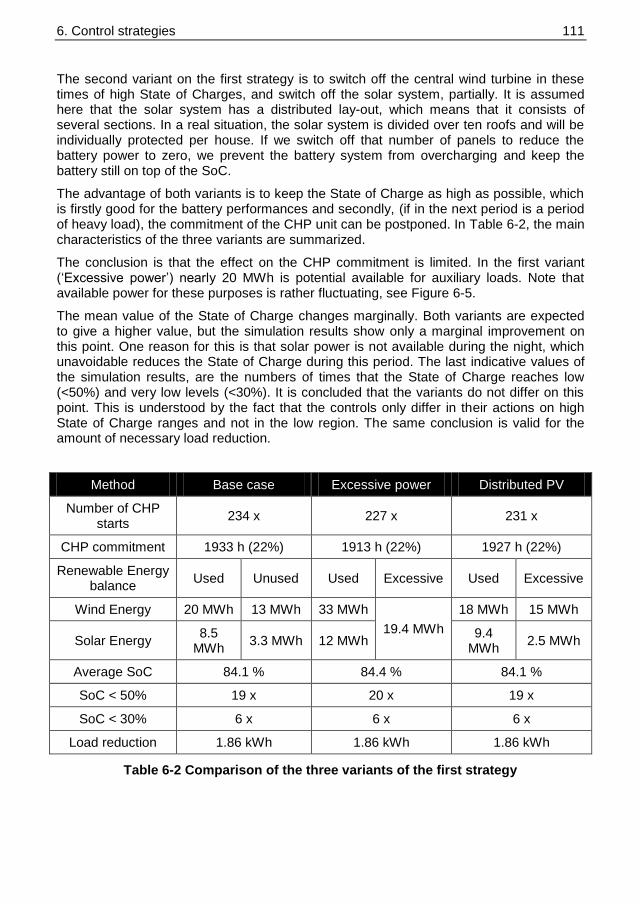
6. Control strategies 111 111
The second variant on the first strategy is to switch off the central wind turbine in these times of high State of Charges, and switch off the solar system, partially. It is assumed here that the solar system has a distributed lay-out, which means that it consists of several sections. In a real situation, the solar system is divided over ten roofs and will be individually protected per house. If we switch off that number of panels to reduce the battery power to zero, we prevent the battery system from overcharging and keep the battery still on top of the SoC.
The advantage of both variants is to keep the State of Charge as high as possible, which is firstly good for the battery performances and secondly, (if in the next period is a period of heavy load), the commitment of the CHP unit can be postponed. In Table 6-2, the main characteristics of the three variants are summarized.
The conclusion is that the effect on the CHP commitment is limited. In the first variant („Excessive power‟) nearly 20 MWh is potential available for auxiliary loads. Note that available power for these purposes is rather fluctuating, see Figure 6-5.
The mean value of the State of Charge changes marginally. Both variants are expected to give a higher value, but the simulation results show only a marginal improvement on this point. One reason for this is that solar power is not available during the night, which unavoidable reduces the State of Charge during this period. The last indicative values of the simulation results, are the numbers of times that the State of Charge reaches low (<50%) and very low levels (<30%). It is concluded that the variants do not differ on this point. This is understood by the fact that the controls only differ in their actions on high State of Charge ranges and not in the low region. The same conclusion is valid for the amount of necessary load reduction.
Method Base case Excessive power Distributed PV
Number of CHP starts
234 x 227 x 231 x
CHP commitment 1933 h (22%) 1913 h (22%) 1927 h (22%)
Renewable Energy balance
Used Unused Used Excessive Used Excessive
Wind Energy 20 MWh 13 MWh 33 MWh
19.4 MWh
18 MWh 15 MWh
Solar Energy 8.5
MWh 3.3 MWh 12 MWh
9.4 MWh
2.5 MWh
Average SoC 84.1 % 84.4 % 84.1 %
SoC < 50% 19 x 20 x 19 x
SoC < 30% 6 x 6 x 6 x
Load reduction 1.86 kWh 1.86 kWh 1.86 kWh
Table 6-2 Comparison of the three variants of the first strategy

6. Control strategies 112 112
0 5 10 15 20 25 30-50
0
50A
mphour-
valu
e [
Ah]
0 5 10 15 20 25 300
2
4
6
CH
P p
ow
er
[kW
]
0 5 10 15 20 25 30
0.2
0.4
0.6
0.8
1
SoC
0 5 10 15 20 25 30
0
20
40
excessiv
e p
ow
er
[kW
]
time [days]
Figure 6-5 Simulation result with excessive power variant
6.2 The application of two battery stacks in parallel
The second optimization strategy is the application of two battery stacks in parallel instead of one single battery stack, where the lowest charged battery stack is charged and the higher charged battery stack is discharged. In periods of high battery currents, either for charging or for discharging, both batteries are used in the same state. The choice of definition of high currents is arbitrary. We choose a value of C/10 (that current which discharges the battery completely within 10 hours) as being a maximum for one battery stack. At higher current rates, two batteries are used in the same mode. Furthermore, the control system monitors that the battery with the lowest state of charge is being charged and in case of discharging, the highest charged battery is connected. When this control is applied, the difference in State-of-Charge of the batteries is never very high.

6. Control strategies 113 113
Use
Battery 1Use
Battery 2
if SOC_B1 < 0.46
if SOC_B2 < 0.46
CHP on/off(CHP=5.5kW)
if (SOC_B1(t)>0.9) | (SOC_B2(t)>0.9), CHP OFF
if (SOC_B1(t)<0.45) | (SOC_B1(t)<0.45), CHP ON
No charge or
discharge
AmpHour = 0
Use Both
Batteries
if Full
if Empty
If |AmpHour|>9
If |AmpHour|>9
Figure 6-6 State diagram second strategy
Figure 6-6 shows the results of the simulation, through the year, whereas Figure 6-7 shows again a detail of the first month.
0 2 4 6 8 10 12-40
-20
0
20
40
Am
phour-
valu
e [
Ah]
0 2 4 6 8 10 120
1
2
3
4
5
6
CH
P p
ow
er
[kW
]
0 2 4 6 8 10 12
0.2
0.4
0.6
0.8
1
SoC
months
Figure 6-7 Plot of results for the entire year (second control strategy)

6. Control strategies 114 114
0 5 10 15 20 25 30-50
0
50
Am
phour-
valu
e [
Ah]
0 5 10 15 20 25 300
1
2
3
4
5
6
CH
P p
ow
er
[kW
]
0 5 10 15 20 25 30
0.2
0.4
0.6
0.8
1
SoC
days
Figure 6-8 Plot of results for first month (second control strategy)
With this strategy, we create abilities for maintenance on the battery system. Table 6-3 shows the facts of this simulation.
Number of times the CHP was
started 81 x
CHP connected to the grid 2451 h. (28 %)
Renewable Energy balance Used (kWh/year) Unused (kWh /year)
Wind energy 25424 7716
Solar energy 9868 2010
Total Renewable Energy 35292 9726
Battery State of Charge Battery 1 Battery 2
Average SoC 82.5 % 86.7 %
Period SoC <50% 134 x 78 x
Period SoC <30% 11 x 14 x
Conversion losses 15571 kWh
Load reduction 1.01 kWh
Table 6-3 Simulation results of second strategy

6. Control strategies 115 115
Analysing all the results, two main drawbacks become apparent. The first one is the high values of unused renewable energy; the second is the high value of conversion losses, which are caused by inefficient charging and discharging of the battery. If we separate the battery system into two systems with half energy contents, the rate of the battery current is double, when we have only one battery stack in operation. This leads to a less efficient charge and discharge process (see section 3.2.4).
6.3 Load forecasting incorporated in the strategy
In strategy 1 and 2, the control system only responds to actual values, without anticipating on any future possible scenario. In strategy 3 and 4, a kind of load estimator is applied. It is investigated to forecast any of the values that are used to calculate power mismatch. The solar and wind power prediction is rather difficult (see chapter 8), so the first approach is to use only the load estimation in order to predict periods of high load demands and to try anticipate on it.
Although in this simulation the power loads are very predictable as they are based on a weekly data repeated each week, in the real situation it is very likely that people repeat their activities in the house every week at the same time, and therefore storing the weekly power loads and using them to “preview” the loads for next week is likely to give us some realistic results.
BEGINNING OF MAIN CYCLE (t = 1:n-1)
START BATTERY CONTROL
Read present power values
and find DeltaPower
(wind + solar - loads)
AmpHour is
Very High?
CHARGE both Batteries
AmpHour is divided into:
½ to AmpHour_B1
½ to AmpHour_B2
AmpHour is
Very Low?
YES
Case
state =
if
AmpHour>0
‘Use_Battery_2’
YES
(charging)
RETURN TO MAIN CYCLE (next time period)
Call Function
CHP_CONTROL
YES
Call Function CALC_SOC
a new SOC(t+1) is calculated
using obtained AmpHour(t)
DISCHARGE both Batteries
AmpHour is divided into:
½ to AmpHour_B1
½ to AmpHour_B2
batteries
Empty?
NO
(discharging)
Batteries
Full?
B2 Full?B2 Empty?
AmpHour_B1=0
AmpHour_B2=0
yesSystem_fails!
AmpHour_B1=0
AmpHour_B2=0
yes
state =
Use_Battery1
yesstate =
Use_Battery1
yes
‘Use_Battery_1’
if
AmpHour>0 YES
(charging)
batteries
Empty?
NO
(discharging)
Batteries
Full?
B2 Full?B2 Empty?
AmpHour_B1=0
AmpHour_B2=0
yesSystem
fails!
yes
State=
Use_B2
yesstate=
Use_B2
yes
PROGRAM END
Drain_Preview
(relation between batteries
SOC and loads from table)
Store present load in
the weekly table
Position
Me
mo
ry ma
trix with
wee
kly loads
(100
8 - p
erio
ds o
f 10 m
inu
tes)
Write
(t)
Read
(t+40),
(t+80)
SOC_preview<0.5
or low P
Turn on CHP
(5.5 KWh)
Batteries charged
or high DeltPower
Turn off
CHP
YES
End CHP_CONTROL
YES
Function CHP_CONTROL
Find Position(current week “position”)
Figure 6-9 Control diagram (third control strategy)
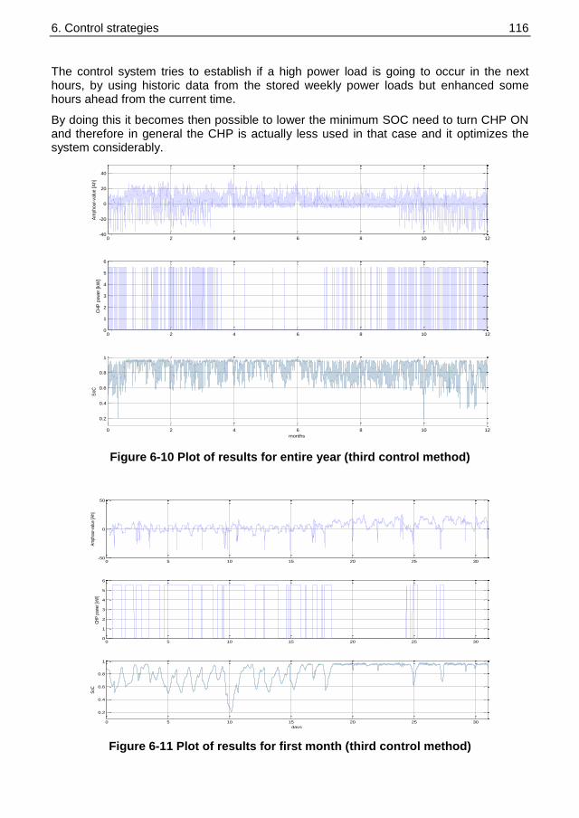
6. Control strategies 116 116
The control system tries to establish if a high power load is going to occur in the next hours, by using historic data from the stored weekly power loads but enhanced some hours ahead from the current time.
By doing this it becomes then possible to lower the minimum SOC need to turn CHP ON and therefore in general the CHP is actually less used in that case and it optimizes the system considerably.
0 2 4 6 8 10 12-40
-20
0
20
40
Am
phour-
valu
e [
Ah]
0 2 4 6 8 10 120
1
2
3
4
5
6
CH
P p
ow
er
[kW
]
0 2 4 6 8 10 12
0.2
0.4
0.6
0.8
1
SoC
months
Figure 6-10 Plot of results for entire year (third control method)
0 5 10 15 20 25 30-50
0
50
Am
phou
r-va
lue
[Ah]
0 5 10 15 20 25 300
1
2
3
4
5
6
CH
P p
ower
[kW
]
0 5 10 15 20 25 30
0.2
0.4
0.6
0.8
1
SoC
days
Figure 6-11 Plot of results for first month (third control method)
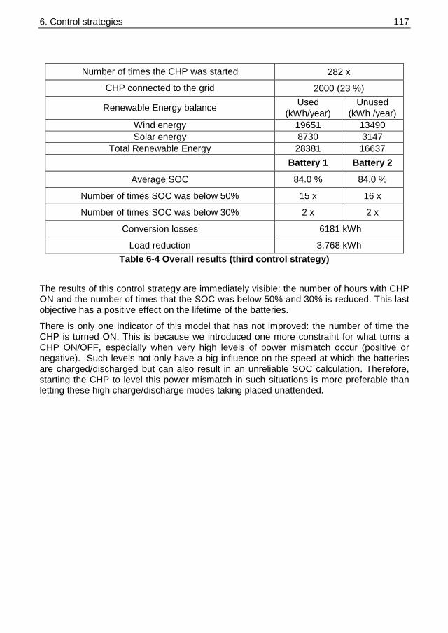
6. Control strategies 117 117
Number of times the CHP was started 282 x
CHP connected to the grid 2000 (23 %)
Renewable Energy balance Used
(kWh/year)
Unused
(kWh /year)
Wind energy 19651 13490
Solar energy 8730 3147
Total Renewable Energy 28381 16637
Battery 1 Battery 2
Average SOC 84.0 % 84.0 %
Number of times SOC was below 50% 15 x 16 x
Number of times SOC was below 30% 2 x 2 x
Conversion losses 6181 kWh
Load reduction 3.768 kWh
Table 6-4 Overall results (third control strategy)
The results of this control strategy are immediately visible: the number of hours with CHP ON and the number of times that the SOC was below 50% and 30% is reduced. This last objective has a positive effect on the lifetime of the batteries.
There is only one indicator of this model that has not improved: the number of time the CHP is turned ON. This is because we introduced one more constraint for what turns a CHP ON/OFF, especially when very high levels of power mismatch occur (positive or negative). Such levels not only have a big influence on the speed at which the batteries are charged/discharged but can also result in an unreliable SOC calculation. Therefore, starting the CHP to level this power mismatch in such situations is more preferable than letting these high charge/discharge modes taking placed unattended.

6. Control strategies 118 118
6.4 Equalization with the use of two battery arrays
Equalization is especially very important when we have an array with several batteries, since each battery does not necessarily have the same characteristics, because some batteries will charge/discharge faster than others. The difference among individual batteries in stored energy increases during every cycle. The solution to cope with this problem is to perform an equalization process on regular time base.
BEGINNING OF MAIN CYCLE (t = 1:n-1)
START BATTERY CONTROL
Read present power values
and find DeltaPower
(wind + solar - loads)
AmpHour is
Very High?
CHARGE both Batteries
AmpHour is divided into:
½ to AmpHour_B1
½ to AmpHour_B2
AmpHour is
Very Low?
YES
Case
state =
if
AmpHour>0
‘Use_Battery_2’
RETURN TO MAIN CYCLE (next time period)
Call Function
CHP_CONTROL
YES
Call Function CALC_SOC
a new SOC(t+1) is calculated
using obtained AmpHour(t)
DISCHARGE both Batteries
AmpHour is divided into:
½ to AmpHour_B1
½ to AmpHour_B2
Ah<0 &
batteries Empty?
Ah>1 &
batteries Full
B2 Full?B2 Empty?
Equalization:
yes
System_fails!
AmpHour_B1=0
AmpHour_B2=0
yes
state=Use_B1
Eq_B1=1
yesstate=Use_B1
Eq_B2=1
yes
‘Use_Battery_1’
if
AmpHour>0YES
(charging)
NO
(discharging)
B1 Full?B1 Empty?state=Use_B1
Eq_B2=1
yesstate=Use_B1
Eq_B1=1
yes
Drain_Preview
(relation between batteries
SOC and loads from table)
Store present load in
the weekly table
Position
Me
mo
ry m
atrix
with
we
ekly
loads
(10
08
- perio
ds o
f 10
min
ute
s)
Write
(t)
Read
(t+40),
(t+80)
SOC_preview<0.5
or low P
Turn on CHP
(5.5 KWh)
Batteries charged
or high DeltPower
Turn off
CHP
YES
End CHP_CONTROL
YES
Function CHP_CONTROL
Find Position(current week “position”)
YES
(charging)
NO
(discharging)
t
Odd / Even YESNO
1<Eq_B2<721<Eq_B1<72Pulse to
Battery2
yesPulse to
Battery1
yes
Figure 6-12 Control diagram (fourth control strategy)
The equalization in this simulation was done using values from Sonnenschein and it is done for a period of 12 hours (72 time steps) with a low current (1A), the voltage used to do the overcharge should also be higher depending on the chosen battery model and they will vary from 2.4V up to 2.8V in certain types of solar batteries.
Final plots of the last optimization are presented, along with the table with the overall results.

6. Control strategies 119 119
0 2 4 6 8 10 12-40
-20
0
20
40
Am
phour-
valu
e [
Ah]
0 2 4 6 8 10 120
2
4
6
CH
P p
ow
er
[kW
]
0 2 4 6 8 10 12
0.2
0.4
0.6
0.8
1
SoC
months
Figure 6-13 Plots of the results for entire year (fourth control strategy)
0 5 10 15 20 25 30-50
0
50
Am
phour-
valu
e [
Ah]
0 5 10 15 20 25 300
2
4
6
CH
P p
ow
er
[kW
]
0 5 10 15 20 25 30
0.2
0.4
0.6
0.8
1
SoC
days
Figure 6-14 Plot of the result of the first month (fourth control strategy)

6. Control strategies 120 120
Number of times CHP was started 291 x
CHP connected to the grid 1887 h (21.5%)
Renewable Energy balance Used (kWh/year) Unused
(kWh /year)
Wind energy 32509 632
Solar energy 11811 67
Total Renewable Energy 44320 699
Battery 1 Battery 2
Average SOC 85.1% 85.2%
Number of times SOC was below 50% 39 x 45 x
Number of times SOC was below 30% 15 x 17 x
Number of equalisations 12 x 12 x
Conversion losses 21492 kWh
Load reduction 6,4 kWh
Table 6-5 Overall results (fourth Optimization)
Some conclusions could be easily drawn. When overcharging, we allow the batteries to obtain a SOC of almost 100% (here we consider the theoretical maximum of 99%), raising the overall SOC, and improving other values such as the number of periods that the CHP was on during the whole year leaving us with the best results of all simulations.
It becomes clear from Table 6-5 that the conversion losses are high. The reason for that is the bad charge efficiency at nearly full charge states plays an important role. The mean value of the State of Charge is high (>85%) and the number of times of low State of Charges are limited to nearly ones a month per battery. Every month both batteries are equalised. It is shown that this control strategy will lead to a longer battery life time.
6.5 Quantitative comparison
All these developed strategies have different parameters, as was seen in their descriptions. The several results are analyzed and checked if the changes are moving to a more efficient strategy. This efficiency can be measured by a lot of factors, some of which were already presented in the previous tables, but it is difficult to compare many control methods without clarifying which are the most important results, so they are listed below, from the most to the least important:
1. Number of times that SoC is below 30%, SoC30%, should be minimized, as this rapidly decreases the lifetime of the batteries;
2. Total number of hours that the CHP is on, CHPON, should also be minimized, because CHP use means using fossil fuels, which is expensive and pollutant;
3. Average SoC value along the year, SoCavg, should be raised to values from 80 to 85%, but the higher, the better, because it increases batteries lifetime.

6. Control strategies 121 121
These are the most important factors, and, therefore, the ones that should help to decide which combination of parameters is the best for each model, and also which model is the best. Other results from the simulations are not so important but, between two models with equivalent results in 1, 2 and 3, parameters 4 and 5 should make the difference:
4. Number of times that SoC is below 50%, SoC50%, should be minimized;
5. Number of times the CHP is turned on, CHPON/OFF, should be minimized.
Some other results like the number of equalizations or the amount of conversion losses could be taken into account, but this would make the decision process too complex. Conversion losses or wasted renewable energy are important but evaluating this or the CHP use has the same effect for the goals of this project.
The differences between scenario‟s are often compared by defining a cost-function, where the five most relevant numbers (described above) are weighted. Four indicators has a negative contribution on the cost function (i.e. the lower, the better), while the average SoC has a positive contribution (the higher, the better).
It was already seen that some of these desired results are contradictory in the sense that improving one necessarily worsens some other. In order to choose the best combination of these parameters a cost function was defined. Through this function a certain weight can be given to each of the above mentioned parameters and with the cost function value of each simulation, the best model can be chosen.
The cost function equation to be maximized is:
)()()()()()( 543%502%301 STARTSONavgf CHPcCHPcSoCcSoCcSoCcstrategyc
where:
cf (strategy): cost function calculated for each different control method;
c1 .. c5 : weight factor given to each model result, from 1 to 5 respectively.
It is important to make a weighted comparison between the individual factors. A possibility is to convert the parameters to real cost. With other words: low SoC periods reduce the life time of the battery and make an earlier replacement necessary. This gives an indication to the choice of the weight of c1. The problem is, however, that these factors are still not quantitative described. In the appendix of this thesis, the results of benchmarking project about hybrid renewable energy systems are briefly described, but the described strategies in this section will be all in the same category. The only possibility that remains is an estimation of the corresponding to real cost of the units.
The height of the weight-factor (C1) for the low SoC periods is estimated to be 1.4. The assumption was made here that if every day (365 times) the battery is discharged to 30%, the life time is reduced from 5 to 4 years. The increment of the costs is in that case € 500 per year extra, see section 4.7.1. By capitalizing this value, the costs of low SoC period is 500/365 = € 1.4/time.
The effect of a 50% level pass is assumed to be a factor of 10 lower: C2 = 0.14.
A good reference in any article, where the positive effect on the lifetime with a higher average SoC was described with quantitative numbers, was not found. Many papers

6. Control strategies 122 122
describe this impact only qualitative. For that reason, it is assumed that 30 is a good value for C3.
C4 indicates the weight of the fuel costs. Based on the calculations in section 4.7.1, € 8000 is assumed there to be the total fuel costs for a standard year. The simulations in chapter 6 give an average value of 2000 hours as the number of operating hours per year. This means that the fuel cost of every hour amounts € 4. However, it seems to be not valid to qualify the whole € 4 as costs because it also has the “heat value”. For this reason, the contribution is reduced to € 1. This value indicates the heat losses or overproduction of the heat.
C5 indicates the maintenance cost of the CHP unit. The reason for an increment of the maintenance cost is the number of starts and stops of the CHP unit. The assumption here was that per 1000 starts and stops a maintenance action of € 100 should be made. This leads to the value of 0.1 for C5.
Summarized:
C1=1.4 C2=0.14 C3=30 C4=1 C5=0.1.
It should be cleared out that the results chosen to be in the cost function and the weights given to each of these results are not irreversible decisions, and should be adapted to each particular case, especially having in mind the type of energy storage.
indicator Weight Scenario 1 Scenario 2 Scenario 3 Scenario 4
SoC < 30%
(number) -1.4 6 11 2 15
SoC < 50%
(number) -0.14 19 134 15 39
CHP ON
(hours) -1 1933 2451 2000 1887
CHP Starts
(number) -0.1 234 81 282 291
Average SoC
(percentage) 30 84.1 84.6 84 85.1
Result 555,5 44,7 486,9 610,4
Table 6-6 Quantitative comparison different Scenario’s

6. Control strategies 123 123
6.6 Conclusions
In this chapter, four different control strategies are compared and the simulation results are presented. With the application of a cost-function to compare the four strategies, it is shown that the last strategy has the best performance. In this section, the obtained results are also qualitative reviewed.
A noticeable point independent from the chosen strategy, is the high amount of unused wind and solar energy. This is a problem that is inherent to the autonomous operation and caused by the low correlation between power generation and power demand. There are periods of high yield of wind and solar energy, which cannot be used and only limited stored. When the battery is fully charged, the power sources have to be switched off to protect the batteries. Decreasing the size of the wind turbine of the PV system is not a good option, because of the periods in the year where less renewable energy is produced. Increasing the storing capacity is an option to optimize the use of renewable energy and to reduce the commitment of the CHP unit, but leads to higher initial investment costs. Sensitivity analysis has shown that the improvement of doubling the storing capacity is limited.
The conditioning of the battery to extend its lifetime is important. On the other hand, the maximum use of renewable energy and the minimal use of the CHP-power are also attractive of course.
Comparing the simulation results, there is less difference in the utilization of renewable energy and the CHP for the first 3 scenarios. In scenario 4 a larger amount of the available renewable energy is applied for the equalization process, while the utilization of the CHP unit remains the same. Therefore, also from a qualitative view, scenario 4 is the best option for this system.
The overall conclusion about the autonomous energy system as presented here is that the renewable energy sources are rather oversized when we consider the energy balance. It is shown that over sizing is necessary for guaranteeing a continuous power supply throughout the year. The surplus of generated power should not be a waste of energy but can be applied to other applications, such as storage of heat and cold or the production of hydrogen in the future.

7 RESULTS
In chapter 5, the construction of the renewable energy laboratory is outlined, whereas chapter 6 discusses the different control strategies which can be applied to a renewable energy system. The laboratory system is constructed and the control functionality is programmed in the Programmable Logic Controller (PLC). Section 5.6.2 describes the monitoring and control aspects of the laboratory, which is used to validate the desired functionality of the laboratory. A standard PC with a Profibus card is connected to the communication system and is able to read all the measured data from the individual components. The conclusions of the experiments are summarized in the last chapter of this thesis.
In order to show the stable behaviour of the system, the following objectives are analysed:
The voltage stability during normal operation;
The voltage stability during high power changes;
The harmonic components in bus voltage;
The evolution of the State of Charge
The control actions of the PPCU.
7.1 Voltage stability during normal operation
The three phase voltage on the system bus is controlled by the battery converter. The basic circuit of this converter is depicted in Figure 7-1. This converter is called an Active Frond End (AFE) – converter, representing the ability of active control of the magnitude and phase angle of the generated voltage. For the proper operation, an AFE-reactor is connected in series. The value of this reactor is 1.59 mH. (XL = 0.5 Ω at 50 Hz).
The values of the L-C filter are Lf = 515 μH and Cf = 3μF respectively. The cut-off frequency (-3 dB) of this filter is 4 kHz. The switching frequency of the converter is set to be 6 kHz. The impedance value of the filter reactor is 0.16 Ω at 50 Hz, so the total impedance in the forward direction amounts 0.66 Ω at 50 Hz.
The inverter has an internal feedback system to control the output voltage on the reference value. This means that the voltage between the external terminal and the internal terminals of the IGBT is current depended. The total voltage drop is caused by the filter- and reactor impedance.
The maximum current of the AFE amounts 32.5 A, so the maximum voltage drop (or rise) becomes in theory 21 Volts (Imax x Ztot). This maximum value does not exceed the limits of slow voltage changes, as defined by the standard EN50160, see Table 7-1.
Figure 7-2 depicts the RMS voltage under normal operation. The average value is set to be 390 V. The graph shows small variations around this value. (20 V, 5%)

7. Results 125 125
LRLf
Cf
CUSA
U2
V2
W2
L1, L2, L3
Clean Power Filter AFE reactor AFE inverter with
control unit
L+
L-
Figure 7-1 Basic circuit Active Frond End Converter
Supply voltage phenomenon
Acceptable limits Measurement
Interval Monitoring
Period Acceptance Percentage
Grid frequency 49.5Hz to 50.5Hz
47Hz to 52Hz 10 s 1 Week
95%
100%
Slow voltage changes 230V ± 10% 10 min 1 Week 95%
Voltage Sags or Dips (≤ 1min)
10 to 1000 times per year (under 85% of nominal)
10 ms 1 Year 100%
Short Interruptions
(≤ 3min)
10 to 100 times per year (under 1% of
nominal) 10 ms 1 Year 100%
Accidental long interruptions (>3 min)
10 to 50 times per year (under 1% of
nominal) 10 ms 1 Year 100%
Voltage unbalance Mostly 2% but
occasionally 3% 10 min 1 Week 95%
Harmonic Voltages 8% Total Harmonic
Distortion (THD) 10 min 1 Week 95%
Table 7-1 Summary of EN50160

7. Results 126 126
0 1000 2000 3000 4000 5000 6000 7000 8000 9000 10000360
370
380
390
400
410
420
430
440
time [sec]
volta
ge [V
]Voltage on autonomous grid
Figure 7-2 RMS voltage during normal operation
7.2 Voltage stability during high power changes
In Figure 7-3, the voltage of the autonomous grid during a high current period is depicted. The time interval is from 15000 to 20000 seconds, more than 8 hours. During this time interval there are periods were the battery unit is heavily loaded with 15 kVA (21 A). The battery converter controls the voltage between the filter and the AFE-reactor. It creates a voltage drop of about 14 Volts across the impedances (Z=0.65 Ω), but the system keeps stable. The small variations are caused by the variations in the current (causing a variable voltage drop), internal control actions of the Active Frond End converter and noise in the measurement system.
1.5 1.55 1.6 1.65 1.7 1.75 1.8 1.85 1.9 1.95 2
x 104
375
380
385
390
395
400
405
410
415
time [sec]
volta
ge [V
]
Figure 7-3 Measurement of the voltage of the autonomous grid
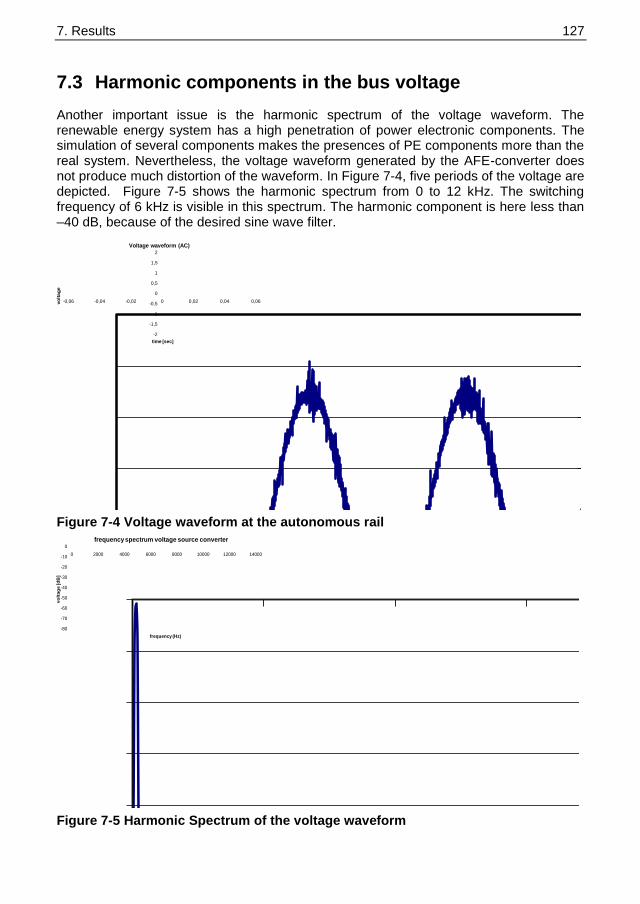
7. Results 127 127
7.3 Harmonic components in the bus voltage
Another important issue is the harmonic spectrum of the voltage waveform. The renewable energy system has a high penetration of power electronic components. The simulation of several components makes the presences of PE components more than the real system. Nevertheless, the voltage waveform generated by the AFE-converter does not produce much distortion of the waveform. In Figure 7-4, five periods of the voltage are depicted. Figure 7-5 shows the harmonic spectrum from 0 to 12 kHz. The switching frequency of 6 kHz is visible in this spectrum. The harmonic component is here less than –40 dB, because of the desired sine wave filter.
-2
-1,5
-1
-0,5
0
0,5
1
1,5
2
-0,06 -0,04 -0,02 0 0,02 0,04 0,06vo
lta
ge
time [sec]
Voltage waveform (AC)
Figure 7-4 Voltage waveform at the autonomous rail
-80
-70
-60
-50
-40
-30
-20
-10
0
0 2000 4000 6000 8000 10000 12000 14000
vo
ltag
e [d
B]
frequency (Hz)
frequency spectrum voltage source converter
Figure 7-5 Harmonic Spectrum of the voltage waveform

7. Results 128 128
7.4 Evolution of the State of Charge
In section 3.2, the determination of the State of Charge is described. The chosen method is the „weighted current integration‟, which means that the State of Charge is determined by the integration of the battery current, but the efficiency in charge and discharge mode depends on the actual State of Charge and the actual current rate.
This method is programmed in the Programmable Logic Controller (PLC) and the results are discussed here.
0 2 4 6 8 10 1210
20
30
40
50
60
70
80
SoC
[%
]
Battery 1, current & SoC
0 2 4 6 8 10 120
5
10
15
20
25
30
time [hours]
AC
curr
ent
[A]
Figure 7-6 Battery current and SoC evolution
In the period between 2 and 4 hours, the battery current (AC) has a mean value of 5 Amps. The Active Frond End converter is adjusted to a power factor of 1, so the power delivered by the converter amounts 3290 W. Assuming an efficiency of 95%, the DC
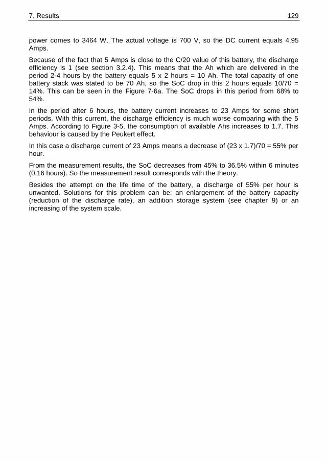
7. Results 129 129
power comes to 3464 W. The actual voltage is 700 V, so the DC current equals 4.95 Amps.
Because of the fact that 5 Amps is close to the C/20 value of this battery, the discharge efficiency is 1 (see section 3.2.4). This means that the Ah which are delivered in the period 2-4 hours by the battery equals 5 x 2 hours = 10 Ah. The total capacity of one battery stack was stated to be 70 Ah, so the SoC drop in this 2 hours equals 10/70 = 14%. This can be seen in the Figure 7-6a. The SoC drops in this period from 68% to 54%.
In the period after 6 hours, the battery current increases to 23 Amps for some short periods. With this current, the discharge efficiency is much worse comparing with the 5 Amps. According to Figure 3-5, the consumption of available Ahs increases to 1.7. This behaviour is caused by the Peukert effect.
In this case a discharge current of 23 Amps means a decrease of (23 x 1.7)/70 = 55% per hour.
From the measurement results, the SoC decreases from 45% to 36.5% within 6 minutes (0.16 hours). So the measurement result corresponds with the theory.
Besides the attempt on the life time of the battery, a discharge of 55% per hour is unwanted. Solutions for this problem can be: an enlargement of the battery capacity (reduction of the discharge rate), an addition storage system (see chapter 9) or an increasing of the system scale.

7. Results 130 130
7.5 Control actions by the Programmable Power Control
Unit
In this section, we validate the control actions which are taken by the PLC. Based on the actual information (state of charges, wind speed, solar power and load demand), the software PPCU controls a number of components in the system. The following tasks are to be fulfilled and are evaluated here:
Starting and Stopping the CHP unit; Starting and Stopping the WECS; Use of one or two battery stacks; Following the load demand pattern by the load demand simulator.
7.5.1 Start and Stop of the Combined Heat and Power unit
During the developing of the control strategies (presented in chapter 6), the CHP should start depending on the State of Charge of the battery. In this way, the CHP is used as an extra production unit of electricity. Figure 7-7 shows two graphs with the State of Charge of Battery 1 and the actual Power of the CHP unit. The time-scale (x-axis) is too large to see the start effect on the CHP-power. The small variations on the power are caused by a change in the terminal voltage. Since the control system of the CHP-unit has no feedback of the power circuit (in constant speed mode), variations on the terminal voltage are not corrected. In this situation, however, the CHP unit is not able to charge the battery, because of the high demand of power in this period (not displayed in Figure 7-7).
3 4 5 6 7 8 9 100
20
40
60
80
time [hour]
SoC
batt
ery
1 [
%]
3 4 5 6 7 8 9 10-2
0
2
4
6
time [hour]
CH
P P
ow
er
[kW
]
Figure 7-7 CHP start at low SoC level
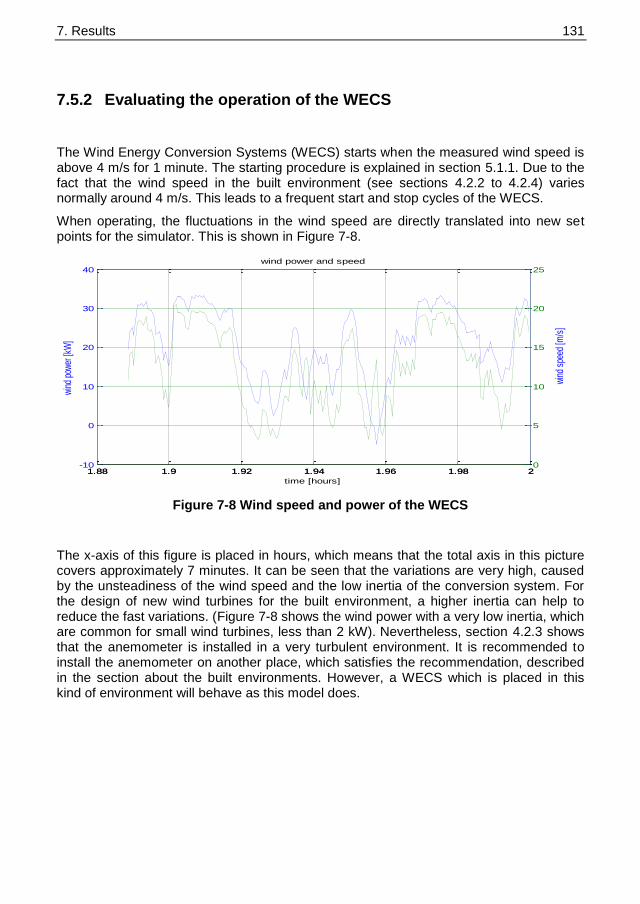
7. Results 131 131
7.5.2 Evaluating the operation of the WECS
The Wind Energy Conversion Systems (WECS) starts when the measured wind speed is above 4 m/s for 1 minute. The starting procedure is explained in section 5.1.1. Due to the fact that the wind speed in the built environment (see sections 4.2.2 to 4.2.4) varies normally around 4 m/s. This leads to a frequent start and stop cycles of the WECS.
When operating, the fluctuations in the wind speed are directly translated into new set points for the simulator. This is shown in Figure 7-8.
1.88 1.9 1.92 1.94 1.96 1.98 2-10
0
10
20
30
40
time [hours]
win
d po
wer
[kW
]
win
d sp
eed
[m/s
]
1.88 1.9 1.92 1.94 1.96 1.98 20
5
10
15
20
25wind power and speed
Figure 7-8 Wind speed and power of the WECS
The x-axis of this figure is placed in hours, which means that the total axis in this picture covers approximately 7 minutes. It can be seen that the variations are very high, caused by the unsteadiness of the wind speed and the low inertia of the conversion system. For the design of new wind turbines for the built environment, a higher inertia can help to reduce the fast variations. (Figure 7-8 shows the wind power with a very low inertia, which are common for small wind turbines, less than 2 kW). Nevertheless, section 4.2.3 shows that the anemometer is installed in a very turbulent environment. It is recommended to install the anemometer on another place, which satisfies the recommendation, described in the section about the built environments. However, a WECS which is placed in this kind of environment will behave as this model does.

7. Results 132 132
7.5.3 Load demand simulator
The set-points of the load demand simulator are based on the pattern, which is a result of the work of IVAM (see section 4.4). In this section it is shown that the set points indeed leads to a demand power of the laboratory. The programmed feedback system controls the demanded power, like can be seen in a comparison between the two graphs in Figure 7-9. From this figure and experiences in the laboratory, it is assessed that the load demand simulator is working properly.
0 2 4 6 8 10 12 14 160
10
20
30
40
time [hour]
measure
d p
ow
er
[kW
]
load demand simulator
0 2 4 6 8 10 12 14 160
1
2
3
4x 10
4
setp
oin
t pow
er
[W]
time [hour]
Figure 7-9 Load demand pattern

7. Results 133 133
7.5.4 System power exchange
As described in section 5.6.2, the actual value of all components power is measured and communicated by the Profibus. A connected computer with an own written Delphi program has the ability to store the data on a minute time-basis. All power figures are taken positive when generation units deliver power and load units are consuming power. A random shot is depicted in Figure 7-10. Variations in the power exchange are shown. The only negative value in this graph indicates that the batteries are charged in this time interval. With these components, the actual power of the battery amounts the total delivered power (wind and sun) minus the load demand and the losses.
Fluctuations in wind power are almost „mirrored‟ in the battery power by the voltage source behaviour of the battery converter. In this way, the battery system maintains the power balance. This limits the use of the batteries for this autonomous renewable energy system application.
The stable operation is guaranteed by a stable AC output voltage of the battery converter (being the master). This AC voltage will be kept at the adjusted value, if the DC voltage is inside its operation window and the actual power is not exceeding the power rating of the converter.
-20
-15
-10
-5
0
5
10
15
20
1 101 201 301 401 501 601 701 801 901
po
wer
[kW
]
time [sec]
P_stored
P_wind
P_PV
P_load
Figure 7-10 Measurement result of DENlab system

7. Results 134 134
7.6 Conclusions
In this chapter it is shown that the laboratory system works properly. The most important factor for the reliable operation of the system is however the availability of a stable voltage for the connected equipment. The voltage on the central bus meets the norms, which are drawn up for grid operation (EN50160). In this way, it is shown that every standard component can be used.
During simulations and measurement in the laboratory it was observed that the fluctuation in generated and demand power could be very fast, more than expected from the performed analyses so far. The sum of the (varying) current is delivered by or stored in the battery system. Very fast fluctuations can not be captured by the relatively slow acting batteries and fast discharge and charge rates reduce the life time of the battery. To enlarge the overall performance of the battery, this storage system has to be smoothly charged and discharged. Chapter 9 discusses a feasible solution to cancel the high current peaks from the battery. The size of the super capacitor and the life time of the battery system are proportional: the larger the super capacitor, the longer the life time. The applied control strategy is kept simple and efficient.
The battery‟s State of Charge is calculated by the method of „weighted current integration‟. This means that the energy contents of the battery is based on the integral of the current, whereby the battery current is weighted according to the Peukert effect. The implementation of the control strategy is tested and shows that the desired functionality is realized.

8 RENEWABLE ENERGY FORECASTING
In chapter 6, control strategies are developed to run an autonomous energy system in an optimal way. The measure for this optimal operation was the maximum reduction of the fossil fuel usage and the care about the batteries expressed in a high average SoC, limited number of periods with low SoC-values and the number of equalizations. During this study, the idea came up to what extend forecasting of renewable energy could help optimization in the performance of this system. This concept is analyzed and presented in this chapter [43, 45].
8.1 Wind Forecasts
Wind forecasting is certainly the most active research theme in the renewable energy power forecasting. This is due to the fact that wind energy is the renewable energy source with the highest growing rate during the past years, and the increasing penetration of wind energy in the grid makes a reliable forecasting of the wind power production essential for a reliable grid operation. Wind forecasting can be divided into two main groups: forecasting with weather prediction models and with persistence models. The first needs data from a meteorological institute like the Dutch KNMI, the second uses only historical data. In Figure 8-1, the root mean square error is depicted as function from the forecast length in hours for a study on a wind farm in Norway [61].
Figure 8-1 RMS errors for different forecasting models
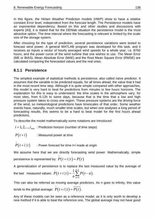
8. Renewable Energy Forecasting 136 136
In this figure, the Hirlam Weather Prediction models (HWP) show to have a relative constant Error level, independent from the forecast length. The Persistence models have an exponential dependency. Based on this and other studies and discussions with experts [43], it is stated that for the DENlab situation the persistence model is the most attractive option. The time interval where the forecasting is relevant is limited by the scale size of the storage system.
After choosing for the type of prediction, several persistence variations were tested to forecast wind power. A general MATLAB program was developed for this task, and it receives as inputs a vector of hourly averaged wind speeds for a whole year, i.e. 8760 hours, and the power curve of the wind turbine that one wishes to use. The Mean Error (ME or BIAS), Mean Absolute Error (MAE) and the Root Mean Square Error (RMSE) are calculated comparing the forecasted values and the real ones.
8.1.1 Persistence
The simplest example of statistical methods is persistence, also called naïve predictor. It assumes that the variable to be predicted equals, for all times ahead, the value that it had in the most recent time step. Although it is quite simple compared with other approaches, this model is very hard to beat for predictions from minutes to few hours horizons. The explanation for this is easy to understand: the time scales in the atmosphere vary, for most sites, from 6-12h to some days, because that is the time that a low and high pressure system takes to cross one region. These pressure systems are the driving force of the wind, so meteorological predictions have timescales of that order. Some weather events have, naturally, much smaller time scales, but when one analyses a long period of forecasting results, this seems to be a hard to beat model for the first hours ahead predictions.
To describe the model mathematically some notations are introduced:
max1,2,...,i i : Prediction horizon (number of time steps)
P t i : Measured power at time
~
|P t i t : Power forecast for time t+i made at origin
We assume here that we are directly forecasting wind power. Mathematically, simple
persistence is represented by: ~
|P t i t P t
A generalization of persistence is to replace the last measured value by the average of
the last measured values: 1~
0
1|
n
a
P t i t P t an
.
This can also be referred as moving average predictors. As n goes to infinity, this value
tends to the global average: ~
|P t i t P t .
Any of these models can be seen as a reference model, as it is only worth to develop a new method if it is able to beat the reference one. The global average may not have good

8. Renewable Energy Forecasting 137 137
results when few short-term predictions are considered, since it is not very dynamic, but for further look ahead times, its skill can be better than the one of simple persistence [62].
A new model can be derived from these two, in order to get the best of their performance over the whole range of prediction horizons: simple persistence to the shortest horizons, and moving average predictor to the further ahead ones [61]. This results in:
~
| 1 k kP t i t P t a P t a , where ak is defined as the correlation
coefficient between P t and P t i .
This prediction is the simple persistence when ak, meaning that the forecasted values are totally dependent from previous ones, and the global average predictor when ak-1 meaning that forecasted values are equal to the global average.
An interesting note about this last model (referred as new persistence) is that by including this average term in the forecast, it can improve the error made in relation to simple persistence as much as some more or less advanced statistical forecasting techniques do [62]. The reason is that any statistical model tries to relate the coming power outputs to the past ones. The way to relate them and the complexity of this relation is the factor changing between the several models, but this simple relation can already achieve a good improvement for some cases.
First of all, the simple and the new persistence, and the average value model were tested. The simple persistence uses only the last hour value, i.e. it says that in the next time step the wind speed will be as it was in the last one. The new persistence tries to relate the wind speed for the next time step with the past ones through the autocorrelation function. However, it is interesting to look at the autocorrelation function for the years 2004 and 2005, plotted in Figure 8-2, for the wind speed and power time series, in DENlab and S344 (station airport Zestienhoven).
Figure 8-2 Autocorrelation values for wind speed and power time series, for DENlab and S344
The autocorrelation function tells us how similar one value is to a previous one n hours before, called the time lag, and its behavior is similar in both DENlab and S344. High autocorrelation (maximum is 1) means that the values are very similar to the previous

8. Renewable Energy Forecasting 138 138
ones. It can be seen that the present wind speed is more similar to the previous hour than to the one 2 hours ago, and that it is more similar to the one two hours ago than to the one 3 hours ago, and so on. This behavior continues until one entire day has passed, and then it can be seen that the autocorrelation tends to stabilize around 24 hours, after which it goes down again. Around 48 hours the autocorrelation value tends to stabilize again (or even go up a little), which means that the wind speed now is as similar to the one in 40 hours as to the one in 48 hours, for example. Though not very significant for this project, this shows that in some days there is a repeated daily pattern that causes this behavior in the autocorrelation function.
It can also be seen that wind power is much less related to previous values. This can be understood looking at the power curve of the wind turbine: though wind speed values are closely related with previous ones, these small variations in wind speed leads to large wind power changes.
When using the persistence method with the average value in the method, referred as new persistence (np) now, the results are different when forecasting wind speed (and then converting to wind power) or wind power directly, because the autocorrelation function changes. Both cases were tried and the results are very similar for the first 12 hours but about 2% better RMS error and 1% better MAE when forecasting wind power, so this was the chosen method.
The results for both persistence methods, forecasting wind power for 2005, are presented in Figure 8-3. The autocorrelation and mean wind power values are from the year 2004 (in order to simulate a real operation environment, because if we would be forecasting in the year 2005, that year‟s autocorrelation function would not be available), and the errors presented are normalized to the wind turbine nominal power, 30 kW.
Figure 8-3 Wind forecasting errors for different
This graph shows, for example, that with simple forecasting for DENlab, for one hour ahead, the MAE is about 4% and the RMSE is about 6%, and when forecasting for the 10
th hour ahead the errors are about 10% and 16%, and so on. The errors plotted for
each look-ahead time are independent from each other: for example, the error for the 12th
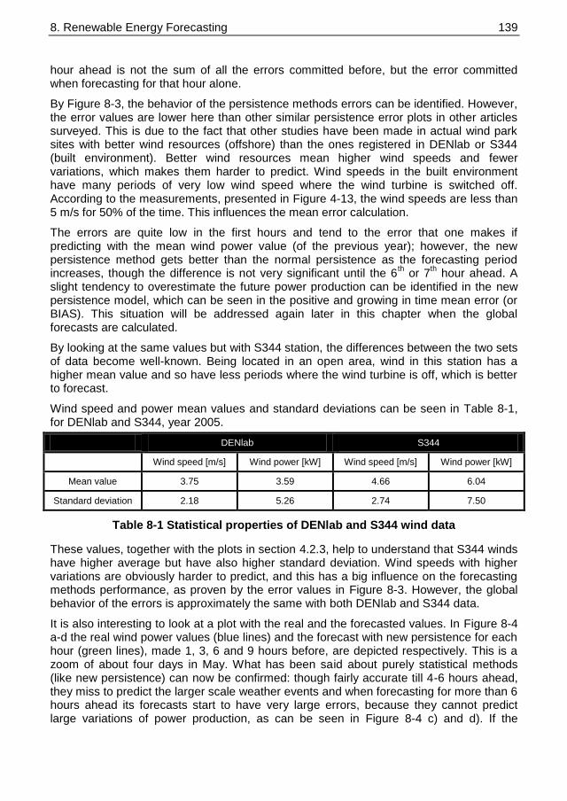
8. Renewable Energy Forecasting 139 139
hour ahead is not the sum of all the errors committed before, but the error committed when forecasting for that hour alone.
By Figure 8-3, the behavior of the persistence methods errors can be identified. However, the error values are lower here than other similar persistence error plots in other articles surveyed. This is due to the fact that other studies have been made in actual wind park sites with better wind resources (offshore) than the ones registered in DENlab or S344 (built environment). Better wind resources mean higher wind speeds and fewer variations, which makes them harder to predict. Wind speeds in the built environment have many periods of very low wind speed where the wind turbine is switched off. According to the measurements, presented in Figure 4-13, the wind speeds are less than 5 m/s for 50% of the time. This influences the mean error calculation.
The errors are quite low in the first hours and tend to the error that one makes if predicting with the mean wind power value (of the previous year); however, the new persistence method gets better than the normal persistence as the forecasting period increases, though the difference is not very significant until the 6
th or 7
th hour ahead. A
slight tendency to overestimate the future power production can be identified in the new persistence model, which can be seen in the positive and growing in time mean error (or BIAS). This situation will be addressed again later in this chapter when the global forecasts are calculated.
By looking at the same values but with S344 station, the differences between the two sets of data become well-known. Being located in an open area, wind in this station has a higher mean value and so have less periods where the wind turbine is off, which is better to forecast.
Wind speed and power mean values and standard deviations can be seen in Table 8-1, for DENlab and S344, year 2005.
DENlab S344
Wind speed [m/s] Wind power [kW] Wind speed [m/s] Wind power [kW]
Mean value 3.75 3.59 4.66 6.04
Standard deviation 2.18 5.26 2.74 7.50
Table 8-1 Statistical properties of DENlab and S344 wind data
These values, together with the plots in section 4.2.3, help to understand that S344 winds have higher average but have also higher standard deviation. Wind speeds with higher variations are obviously harder to predict, and this has a big influence on the forecasting methods performance, as proven by the error values in Figure 8-3. However, the global behavior of the errors is approximately the same with both DENlab and S344 data.
It is also interesting to look at a plot with the real and the forecasted values. In Figure 8-4 a-d the real wind power values (blue lines) and the forecast with new persistence for each hour (green lines), made 1, 3, 6 and 9 hours before, are depicted respectively. This is a zoom of about four days in May. What has been said about purely statistical methods (like new persistence) can now be confirmed: though fairly accurate till 4-6 hours ahead, they miss to predict the larger scale weather events and when forecasting for more than 6 hours ahead its forecasts start to have very large errors, because they cannot predict large variations of power production, as can be seen in Figure 8-4 c) and d). If the

8. Renewable Energy Forecasting 140 140
accuracy was to be maintained at acceptable levels for longer look-ahead forecasts, weather prediction data would have to be included in the forecasting model.
Figure 8-4 Wind power forecasts compared with the real wind power produced
Other kinds of persistence based methods were tested. Stating that the next time step power value is going to be the average of the last n time-steps (with n varying between 1 and 10) only improves results in about 0.5% of the MAE for look-ahead periods above 12 hours.
Instead of using the autocorrelation function for the whole year, it was tested if it would not be better to use this function for a shorter period, for example, the previous week. This has the advantage of „missing‟ changing along the year and taking into account the seasonal patterns of wind. If the last week was very windy with many wind gusts, or, by the contrary, it had very low wind speeds, it should be better to relate the future values with this closer period than with the whole year‟s average. These intuitive results were confirmed by the simulations, but the improvements were, again, not significant for the first 6 hours, and even after that the ME was only about 1% lower than the new persistence. These results did not justify the overhead work of computing a new autocorrelation function for every time step, so the decision was to use the new persistence model as our forecasting method.

8. Renewable Energy Forecasting 141 141
8.2 Sun Forecasts
Sun forecasts are slightly different from wind forecasts. While wind persistence means stating that future wind power values are equal to wind power in the time step immediately before, sun persistence can mean that future sun power values are equal to the same hour of the previous day. This means that if forecasts are being made for the period from 12h to 13h, the persistence forecast is that the sun power for the present day, for that one hour period, will be the same as the sun power for the same one hour period of the previous day, i.e. 24 hours before.
Saying that the sun in some hours will be the same as now is reasonable for the next hour but it is easy to understand that for more than two hours the forecasting errors will rise substantially, due to the daily pattern of the sun power. This can be confirmed in Figure 8-5a, where the errors for simple persistence for 2005 (forecast is the last hour value) are plotted, and in Figure 8-5b, where the autocorrelation function for the sun power can be observed. The errors are normalized to the peak power production of all the solar panels, 9 kW.
Figure 8-5 a) models for sun power forecasting b) Autocorrelation function for sun power output in 2005
This figure depicts also the result of forecasting with the mean sun power value of the previous year. Looking at the autocorrelation it is clear that the day and night cycles are the dominant event that determines the sun power value, and after about 4 hours it is even better to forecast with the mean value than with the previous hour.
Results for forecasting with 24 hours before value are plotted in Figure 8-6, together with the new persistence results, which relates the 24 hours before value with the future ones through the autocorrelation function.
These are typical results when it is stated that the forecast for n hours ahead is the value x hours before, and for hour n+1 is the value x+1 hours before, i.e. the distance between the forecasted time step and the past time step used for the estimation is constant. This error also remains constant when forecasting for any look-ahead time. In simple

8. Renewable Energy Forecasting 142 142
persistence for wind this distance grows as we forecast for larger look-ahead times, and this is why the error increases too.
Figure 8-6 Simple persistence (p) and new persistence (np) results for sun forecasting
The results in Figure 8-6 are not so easy to analyze. The MAE of the new persistence is more than 1% worse than the MAE of the simple persistence with the 24 hours before value, but RMSE has the opposite behavior.
Statistically the MAE and BIAS values are associated with the first moment of the prediction error, so they are directly related to the output power. RMSE values are associated with the second order moment, which means they are related to the variance of the prediction error. For the latter measures large prediction errors have the largest effect [61]. This means that though the average error is higher with new persistence, the error variance is smaller, i.e. there are fewer forecasts with large errors. As none of these two models presents clear advantages, if no other model would be available, the choice would be the simplest one, i.e. using the value 24 hours before.
As with wind, several other models derived from the persistence basic principle were studied. In Figure 8-7 the errors of six models can be seen, forecasting for the year 2005:
F1 refers to forecasting with the mean value of 2004; F2 is the normal persistence, using the last hour; F3 is the normal persistence, using the 24 hours ago value; F4 is the normal persistence, using the average of the 24 and 48 hours ago
values; F5 is the normal persistence, but using the average between the last hour and
the 24 hours ago values; F6 refers to the new persistence, with autocorrelation computed for the whole
year.

8. Renewable Energy Forecasting 143 143
Forecasting with the new persistence model using the autocorrelation of the past days or weeks data did not improve the results in comparison with using the autocorrelation for the whole year, so its results are no presented.
Figure 8-7 MAE and RMSE for six models predicting sun power for 2005
F1, F2 and F3 errors had already been plotted before in Figure 8-6, but here they can be seen in comparison with the other models tested. The best results come from F3, F4 and F6, except for the first two hours, in which the F2 and F5 are better by 2% in MAE and 3% in RMSE. The model used in the project was chosen from the analysis of these plots: for the first two hours, forecasts were made using F5, and from then on F4 was used.
An example of the results obtained using these methods can be seen in Figure 8-8 for about 4 days in May (the same period as in Figure 8-4 for wind forecasts). This is a plot of the real solar power (blue line) and the forecasted value 1 and 3 hours before, in a) and b) respectively (green line). When forecasting with F5 the results are the same for 3, 9 or 18 hours ahead. F4 is more accurate in the first hour forecasts (and for the second too, though not shown in the picture) because it averages the last day and the last hour values, and this is more accurate when the previous day was different from the present one.
Figure 8-8 Real solar output vs. one and three hours forecast

8. Renewable Energy Forecasting 144 144
8.3 Results with forecasting method
Matlab programs are written to analyze the improvements of the system by the application of forecasted values. With the data of 2004, the models are developed in order to find appropriate values for the forecast model. When the models are derived, the models are unchanged applied to the data of 2005. The look-ahead time is changed for the different models and the level of uncertainty in SoC estimation. The second simulated forecast is the perfect forecast. Its simulation is trivial: data for the next time steps are always available, since we are using stored time-series for our simulations. Thought it is not a very realistic situation, because it is virtually impossible to have a perfect forecast, this can give a clear idea of the full potential of inserting forecasts information in an autonomous system like DENlab.
The third simulated forecast has exactly half of the error of the forecasts presented before in this chapter. Its simulation is also simple: the normal real forecast is calculated as described in the previous sections, and then compared to the real future value. To have a forecast with half of the error for n hours ahead is equivalent to applying the following
equation: 50%
( ) ( )( ) ( )
2
perfect normal
error normal
P t n P t nP t n P t n
The main goal of having this forecast is to understand whether it is useful to pursue a better forecast, with different models from the ones used in this project, like physical methods. If the results present using this forecast are much better than the ones presented with the normal forecast, it can be concluded that further investigation on forecast accuracy is advantageous, because having forecasts with 50% of the error is a more realistic objective than having perfect ones.
The advantage of simulating forecasts from real ones is that the only variable changed is the amplitude of the error. This is very important because the situations where the model is less accurate will remain untouched, or, by other words, the behavior of the error along the simulated period will remain the same, except for its amplitude.
The cost function to evaluate the different performances of the control models is already defined in section 6.5. In this way, the results obtained here can be directly compared with the results obtained without applying the extended forecast method. The freedom in the control method here, is the look ahead time of the method and the allowed uncertainty in predicting the SoC for the coming hours.
It is also important that the best combination of these parameters is chosen in a realistic way, i.e. the parameters chosen for one year should be based on the best combination for the year before. The procedure in this project was to choose the best set of parameters for each model, for the year 2004, and then run it with 2005 data, comparing the results between the several 2005 models to check the improvements between them. In this way, the developed control strategy was a kind of adaptive process.
In the simulation program, the following settings are applied:
CHPON: the level of the SoC, where the CHP is started; CHPOFF: the level of the SoC, where the CHP is switch off; x1 & x2: values, where the SoC-level is increased, used for decision purposes as
a consequence of uncertainty in the prediction; Forecasting hours ahead: Prediction horizon that is actually used in the decision strategy.
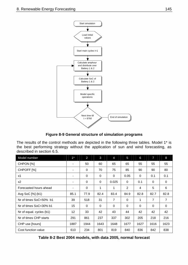
8. Renewable Energy Forecasting 145 145
Start simulation
Load initial
values
Start main cycles t=1
Calculate amphour
and distribute over
Battery 1 & 2
Model specific
operations
Calculate SoC of
Battery 1 & 2
Next time till
t = 8760End of simulation
Figure 8-9 General structure of simulation programs
The results of the control methods are depicted in the following three tables. Model 1* is the best performing strategy without the application of sun and wind forecasting, as described in section 6.5.
Model number 1* 2 3 4 5 6 7 8
CHPON [%] - 50 60 65 65 55 55 55
CHPOFF [%] - 0 70 75 85 90 90 80
x1 - 0 0 0 0.05 0 0.1 0.1
x2 - 0 0 0.025 0 0.1 0 0
Forecasted hours ahead - 0 1 1 2 4 5 6
Avg SoC [%] (b1) 85.1 77.9 82.4 83.4 84.9 82.8 82.7 82.8
Nr of times SoC<50% b1 39 518 31 7 0 1 7 7
Nr of times SoC<30% b1 15 0 0 0 0 0 0 0
Nr of equal. cycles (b1) 12 33 42 43 44 42 42 42
Nr of times CHP starts 291 861 237 337 302 205 218 216
CHP use [hours] 1887 1944 1643 1648 1677 1627 1616 1623
Cost function value 610 234 801 819 840 836 842 838
Table 8-2 Best 2004 models, with data 2005, normal forecast

8. Renewable Energy Forecasting 146 146
It can be seen in this table the forecasts improve the cost function value significantly for a look-ahead time from 2 to 3 hours. Including more that 4 hours ahead does not improve the results, or it can even make them worse. The reason for that could be the increasing error for these look-ahead times and the big changes which can occur in a time period of hours. It is noticeable that the SoC level below 30% is never reached. This is one advantage of forecasting the SoC level.
As a continuation of this research, it is analyzed if further improvements in forecasting the energy supply by wind and sun is worthwhile. The maximum improvement is examined by using the exact values as the perfect forecasting. The same control models are used, with now the perfect forecasting. Table 8-3 shows the results. It shows that the maximum value for the defined cost function with the data of 2005, is 821 points (model 7 and 8). It has a minimum number of CHP use and a still good average SoC-level.
Model number 1* 2 3 4 5 6 7 8
CHPON [%] - 50 60 65 65 55 55 55
CHPOFF [%] - 0 70 75 85 90 90 80
x1 - 0 0 0 0.05 0 0.1 0.1
x2 - 0 0 0.025 0 0.1 0 0
Forecasted hours ahead - 0 1 1 2 4 5 6
Avg SoC [%] (b1) 85.1 77.9 82.1 83.4 84.8 82.7 82.2 82.2
Nr of times SoC<50% b1 39 518 28 2 0 3 3 6
Nr of times SoC<30% b1 15 0 0 0 0 0 0 0
Nr of equal. cycles (b1) 12 33 42 42 43 42 42 42
Nr of times CHP starts 291 861 227 331 269 175 185 190
CHP use [hours] 1887 1944 1612 1603 1622 1568 1543 1543
Cost function value 610 234 824 866 895 895 904 903
Table 8-3 Best 2004 models, with data 2005 and perfect forecast
The last exercise which is carryout with this data is to assume a 50% enhancement of the forecasting in comparison with that of Table 8-2. In this way, a sensitivity analysis is performed on the possible improvements and the influences on the final results. It is clear that this three forecast method has similar behavior in relation to the improvements they bring to the system performance. It is further shown that a look-ahead time of 3 hours is enough. Higher look – ahead times are not contributing to a proportional achievement.
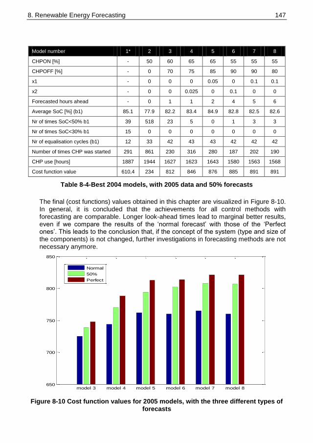
8. Renewable Energy Forecasting 147 147
Model number 1* 2 3 4 5 6 7 8
CHPON [%] - 50 60 65 65 55 55 55
CHPOFF [%] - 0 70 75 85 90 90 80
x1 - 0 0 0 0.05 0 0.1 0.1
x2 - 0 0 0.025 0 0.1 0 0
Forecasted hours ahead - 0 1 1 2 4 5 6
Average SoC [%] (b1) 85.1 77.9 82.2 83.4 84.9 82.8 82.5 82.6
Nr of times SoC<50% b1 39 518 23 5 0 1 3 3
Nr of times SoC<30% b1 15 0 0 0 0 0 0 0
Nr of equalisation cycles (b1) 12 33 42 43 43 42 42 42
Number of times CHP was started 291 861 230 316 280 187 202 190
CHP use [hours] 1887 1944 1627 1623 1643 1580 1563 1568
Cost function value 610,4 234 812 846 876 885 891 891
Table 8-4-Best 2004 models, with 2005 data and 50% forecasts
The final (cost functions) values obtained in this chapter are visualized in Figure 8-10. In general, it is concluded that the achievements for all control methods with forecasting are comparable. Longer look-ahead times lead to marginal better results, even if we compare the results of the „normal forecast‟ with those of the „Perfect ones‟. This leads to the conclusion that, if the concept of the system (type and size of the components) is not changed, further investigations in forecasting methods are not necessary anymore.
model 3 model 4 model 5 model 6 model 7 model 8650
700
750
800
850
Normal
50%
Perfect
Figure 8-10 Cost function values for 2005 models, with the three different types of forecasts

8. Renewable Energy Forecasting 148 148
8.4 Conclusions applying forecasting
In an autonomous system like DENlab, forecasting does not improve the overall system operation as it was expected before. The main reason for that is the limit battery capacity. Without forecasts the system operation may not fail; in other words the uncertainty in the forecast may never lead to a system blackout, so a certain safety margin has always to be taken into account. Nevertheless, a reasonable improvement is shown by the simulation results in this chapter. It is now clear that the application of forecasts leads to a reduction of the CHP use, a prevention of SoC levels lower than 30% and a limitation of the CHP starts. The average SoC level was slightly reduced in comparison with the strategies without forecasting models, but are still high (>82%).
Good forecasts can already be obtained by simple forecasting methods, like persistence for a look ahead periods of three hours. The best improvement that forecasts can bring, which is to predict low SoC‟s and to turn on CHP sooner, raises the SoC average (good) but also raises the CHP use in some cases (which is in fact bad). A general cost function where all values are weighted brings the overall best result.
CHP usage can not be reduced below ~1000 hours, no matter how good the system is or how accurate are the forecasts; This is not a really big problem, because there is often also a heat demand.
However, CHP was reduced with a 60 hours, as the difference between model 8 and the reference model (1*). To decide if this is worth the forecasting burden, the heat demand pattern should also be taken into account. This was, however, not in the scope of this research.

9 SUPER CAPACITORS
Analyzing the simulated battery currents in chapter 6 and the measured values in section 7.5.4, it is clear that the battery current shows high peaks. Values of 30 - 40 A (DC) and high dI / dt values are simulated and measured as well on the real system. The definition of (dis)charge-rate is described in section 3.2.2 as the ratio between the actual current and the battery capacity. The maximum rate which is measured is almost 40%. Currents of this size reduce the State of Charge as well as the lifetime of the battery quickly. But not only is the magnitude of the current a problem, the fast power changes is to heavy for standard lead-acid batteries. The cause of these fast changes is the fluctuations in demanded and generated power. These are described in Chapter 5.
It is not very easy to quantify this problem and to tell which fluctuations are allowable for the batteries and in what extent the degradation of the battery takes place. The battery configuration (plate thickness and area) plays an important role, however the battery technology is not suitable for the delivering of pulsed power applications. A secondary storage system is needed to relieve the battery.
In Figure 9-1 the most common storage systems are depicted, with their discharge rate and available power. This picture shows that Super Capacitors (SC) is the most promising candidate as a fast component in the power range till 50 kVA. Besides SC, the flywheel is shown as a second best option. SMES (Superconducting Magnetic Energy Storage) has high performance but is too expensive at this moment.
Figure 9-1 Overview storage systems source: electricitystorage.org

9. Super capacitors 150 150
9.1 Theory
In literature, the super capacitors appear under different names: ultra capacitor (UC), electrochemical double layer capacitor (EDLC) or super capacitor (SC). A super capacitor is an electrochemical capacitor that has an unusually large amount of energy storage capability relative to its size when comparing to common capacitors. These are of particular interest in automotive applications for hybrid vehicles and as supplemental storage for battery electric vehicles. The first super capacitor based on a double layer mechanism was developed in 1957 by General Electronics in a patent using a porous carbon electrode. It was believed that the energy was stored in the carbon pores and it exhibited "exceptionally high capacitance", although the mechanism was unknown at that time.
Electrochemical capacitors (EC) store electrical energy in the two series capacitors of the electric double layer (EDL), which is formed between each of the electrodes and the electrolyte ions, see Figure 9-2). The distance over which the charge separation occurs is just a few angstroms (10
-10 meter). The capacitance and energy density of these devices
is thousands of times larger than electrolytic capacitors.
+
+
Po
rou
s C
arb
on
Ele
ctr
od
e
Po
rou
s C
arb
on
Ele
ctr
od
e
+
+
+
+
+
+
+
+
+
+
+
+
+
+
+
+
+
+
+
+
+
+
+
+
+
+
-
-
-
-
-
-
-
-
-
-
-
-
-
-
-
-
-
-
-
- + + + + + + + + + + + + + +
- - - - - - - - - - - - - -
+- ELECTROLYTE IONS
DOUBLE LAYER CAPACITORS
ELECTROLYTE
Figure 9-2 Construction of a Double Layer Capacitor
The electrodes are often made with porous carbon material. The electrolyte is made from either aqueous or organic material. The aqueous capacitors have a lower energy density due to a lower cell voltage but are less expensive and work in a wider temperature range. The asymmetrical capacitor that uses metal for one of the electrodes has a significantly larger energy density than the symmetric ones and has lower leakage current.
Such energy storage has several advantages relative to batteries:

9. Super capacitors 151 151
Very high rates of charge and discharge; Little degradation over hundreds of thousands of cycles; Good reversibility; Light weight; Low toxicity of materials used; High cycle efficiency (95% or more).
Disadvantages:
The amount of energy stored per unit weight is considerably lower than that of an electrochemical battery (3-5 Wh/kg for a UC compared to 30-40 Wh/kg for a battery);
The voltage varies with the energy stored. To effectively store and recover energy requires sophisticated electronic control and switching equipment.
Figure 9-3 shows the evaluation of the price of Super Capacitors from 1996 to the expected price in 2010. The prices of the Super Capacitors have fallen quickly, with cost/kJ dropping faster than cost cost/Farad as voltage are increased. The existing electrodes can be made to support higher voltages in the capacitors. By 2010, experts of Maxwell expects device to be specified for 3 V, an increase of 10% from the value of 2006.
1996 1998 2000 2002 2004 2006 2008 20100.001
0.01
0.1
1
10
year
price
$/F
$/kJ
Figure 9-3 S.C. price evolution from 1996 to 2010 (expected), source: Maxwell (2006)
A fully charged SC system (740V, 10F) has an energy potential of 2738 kJ (0.76 kWh). The expected price in 2010 for this system amounts almost € 2600. When comparing with the maintenance and replacements cost of a battery system (see section 4.7.1), the return on investment period will be less than two years
.

9. Super capacitors 152 152
9.2 Different battery-supercapacitor combinations
In the application of renewable energy system, the super capacitor can relieve the battery from its high charge and discharge peaks. In this combination, the better of two components is reached: the battery delivers the energy (average power) and the super capacitor delivers the (fast) power fluctuations.
Research demonstrates that the combination of super-capacitors and batteries achieves a longer run-time and a higher power capability compared to a battery-alone. [63-69]
In Figure 9-4, the three most attractive battery-super capacitor combinations are depicted.
DC
AC
Battery SC+
_
DC
AC
Battery SC+
_
DC
DC
A
B
Vac-bus
DC
AC
BatterySC+
_
DC
DC
C
Figure 9-4 Super capacitor and Battery combination on one DC-system
In option A, the small RC value of the Super capacitor (compared to the Battery) reacts faster than the battery system. In this case, the battery delivers the average energy which is the integral the power on a certain time interval. Depending on difference in characteristic times, the super capacitor relieves the battery in more or less extent.

9. Super capacitors 153 153
Because of the fact that both components are directly coupled, the freedom in control is not available.
In option B and C, a DC-DC converter is placed between the Battery and Super Capacitor. This component gives the opportunity to control the bidirectional power exchange between both components. Due to the working principle of this DC-DC component (e.g. a buck-boost converter) the DC-voltage at one side should be doubled at the other side. This brings limitations on its control area. The difference between option B en C is the actual place of the DC/DC circuit. In system C, the battery voltage is connected to the input of the DC/AC converter. In system B, the input voltage is the super capacitor. The voltage of a super capacitor is directly related to its energy content, by the
equation: 21
2E CV . Using a battery, the voltage decreases only 25% between fully
charged and empty. From a stored energy point of view, option C is more suitable than option B. On the other hand, the current control in case C should be very fast to smooth the battery current.
The control of this system is based on the voltage on the Super Capacitor. The double battery voltage (24 Volts) is chosen as a reference value for the SC-voltage. For a good operation of the DC-DC converter, the SC-value may vary between 16 and 32 Volts. The control system increases the battery current when the SC-voltage becomes lower than the reference and opposite.
Figure 9-5 shows a Matlab/Simulink model for a DC-DC system with a battery and Super Capacitor. It shows the
Figure 9-5 Matlab Simulink model of option B

9. Super capacitors 154 154
0 50 100-50
0
50current supercap
0 50 100-50
0
50current inductor
0 50 100-50
0
50reference current battery
0 50 100-50
0
50current source
Figure 9-6 Currents [Amps] in DC- Super capacitor and Battery combination
The x-axis shows the time in seconds and the y-axis the current in Amps.
0 50 1000
5
10
15
20
25
30Battery voltage
0 50 1000
5
10
15
20
25
30Supercap voltage
Figure 9-7 Voltages [V] of Super capacitor and Battery combination in DC-system
Model data: Capacity = 10 F, Rsc=0.1 Ω, Usc=24 V
Battery: 12 V, Rbatt=0.05 Ω (equivalent resistance, more batteries in parallel)

9. Super capacitors 155 155
A different option is to use a hybrid storage system (battery and super capacity) with a decoupled DC-circuit, as depicted in Figure 9-8. In this case, the DC/AC converter connected to the SC should act as a Voltage Voltage Source Converter (VSC) to catch the fast fluctuating powers. The battery DC/AC converter acts as a Current Controlled Voltage Source Converter (CCVSC) which is controlled by the average power of the Super Capacitor in combination with the voltage of the Super Capacitor.
SC
DC
AC
DC
AC
Battery+
_
D
Vac-bus
Figure 9-8 Supercapacitor-battery system with decoupled DC-circuits
9.2.1 Model simplifications
To analyse the behaviour of the system of Figure 9-8, rather simplified models are used for the DC/AC converters. These models only describe the fundamental frequency (50 Hz) behaviour of the AC-side of the converters. The DC-side of these converters is modelled as a separate system, where the power balance makes the connection between the AC and DC system. The model of the Voltage Controlled Voltage Source Converter (VCVSC), which controls the AC voltage, differs from the Current Controlled Voltage Source Converter (CCVSC) which follows the applied AC voltage and controls the AC current. Due to its nature, the VSC acts as a kind of slack node and maintains in this way the power balance of the total system on the AC bus.
From the given (controlled) AC voltage (output of the VCVSC) and the measured current, an AC power can be derived, taking into account the power factor. The connection between the DC and the AC system means that the DC power is equal to the AC power (a loss less conversion is assumed). With the measured DC voltage of the connected device (Super Capacitor or Battery), the current control signal is calculated by dividing the DC power by the DC voltage.
For the CCVSC, the current contribution is manually or automatically set. In this case, the output voltage is externally fixed. This model is further simplified to be a CSC, as shown in Figure 9-10. The difference between a CCVSC and a CSC is the behaviour on a short

9. Super capacitors 156 156
time scale. There is however no difference in behaviour in our case, because we are looking at longer time intervals.
The way of simulating the DC side of the CSC is exactly the same as the VSC converter, as described above. The models are depicted in Figure 9-9 and can be implemented in various simulation software tools, like Matlab/Simulink, RTDS, etc.
+
-
Vdc
Vabc
DC side AC side
Idc Vabc
Simplified voltage source converter
+
-
Vdc
Vabc
DC side AC side
Idc Iabc
Simplified current source converter
Figure 9-9 Simplified models for VSC and CSC converters
The model of the Super Capacitor is kept simple: a series connection of capacitor and a resistor. Self discharging is neglected here, which is allowed for this application. The model of the battery is also kept simple: a DC voltage source, with a capacitor and a resistor in series. The resistor represents here the losses and gives a voltage drop at higher current rates. The capacitor represents the effect of charging and discharging of the battery.
The values for the simulation which are used here are shown in Table 9-1.

9. Super capacitors 157 157
Component Capacitance (F) Resistance (Ω/Ω) (reference) voltage
(V)
Super Capacitor 10 0.01 670
Battery 2760 0.1 720
Table 9-1 Model data of storage systems
Figure 9-10 Powers vs. time for decoupled DC-buses

9. Super capacitors 158 158
Figure 9-11 Super-capacitor battery system with decoupled DC-buses
9.2.2 A comparison between the DC and AC-configuration
When both battery-super capacity systems are compared, the following remarks can be made:
In the DC system, the nominal voltage of the super capacity is twice the battery voltage. The DC voltage should be in between 600 and 740 V, which is necessary for the DC/AC converter to generate a current (or voltage) with minimal harmonic injections. This means that the voltage of the battery stacks should be between 300 and 370 V. This reduced voltage leads to higher currents and a higher I
2 R – losses in the battery.
In the AC-system, the voltage of the Super cap should be also high (600-740V), this gives limitations to the energy uses, because a Super cap charged to 600 V contains still a lot of energy, which cannot be used. However, as a result of the quadratic relation between energy and voltage, the higher voltage range contains much more energy.
Another difference between both systems is further that different components are used. In the DC-system, a buck-boost DC/DC converter is additionally used, while in the AC configuration, an additional DC/AC converter is

9. Super capacitors 159 159
necessary. The buck-boost DC/DC converter has less components, both needs an expensive coil. The DC/AC converter needs a full converter with 6 IGBT including driving circuits, but belongs to „state of the art‟ technology.
The AC system has a better controllability and its control is more straightforward.
The set-up of the AC system is closely related to the DENlab set-up and makes it easy to implement.
For this application, the AC configuration is the best choice, but the DC system is nevertheless possible.
9.3 Sizing of SC systems
By applying different storage systems, with different time responses, it‟s always a consideration between several aspects. In this case, a higher capacity (more Farads) leads to higher investment costs but enhances the performance of the battery system. The control system can acts slower and reduces the fluctuations in the battery current. The minimal size of the super capacity depends on the maximum allowable fluctuation of the battery current. This maximum is never a fixed limit, but reduces the battery life time.
To quantify this problem at least, the following calculation procedure is proposed.
Take the measurements of one arbitrary day
Calculated the mean of the stored power in this day.
Determine the deviation of the storage power from the mean value.
The difference between the mean and the actual value should be stored in the super capacitor. Calculate the maximum energy from a charge or discharge period in that day.
Calculate the capacity, taken into account the allowable voltage bandwidth of the inverter.

9. Super capacitors 160 160
0 500 1000 1500 2000 2500 3000 3500 4000 4500 5000-40
-30
-20
-10
0
10
20
30
time [sec]
pow
er
[kW
]
Figure 9-12 Power exchange between SC and battery
In Figure 9-12, the power into the storage system is depicted. It is shown to be very fluctuating in time (Lowest fluctuating curve). With the help of a moving average filter (smoothing period 1 minute) a slow fluctuating curve is made, which is the average of the fluctuating power of the storage system. This average power will be delivered by the battery system, whereas the difference between mean and actual value (upper fluctuating curve) will be delivered by the super capacitor. Note that the average power of the super capacitor is almost zero.
As can be seen in the curve of Figure 9-12, there is a intensive period of 300 seconds for the super capacitor, in which the wherein its energy request amounts 740.000 Ws. In the calculation, we assume that the super capacitor voltage decreases from 740 to 600 V (maximum to minimum operating voltage of the inverter).
2 2
max min
1( )
2
EC
V V
Equation 9-1 Calculation of minimum capacitance
From this calculation, it follows that a minimum capacity is 7.88 F. To be on the safe side, a higher value is chosen:10 Farad.

9. Super capacitors 161 161
9.4 Control strategy
The final goal of a super capacitor- battery combination is to protect the battery buffer from fast changes in the power demand. A super capacitor is very suitable to perform this task, but has limited energy content. The control strategy is developed to maximize the use of the super capacitor. Like discussed before, the operating voltage window of the super capacitor is from 600 to 740 V, with a mean value of 670 V. The strategy controls the super capacitor voltage by changing the battery current. If the autonomous network faces a change in the power balance, the super capacitor will maintain this balance as a result of the Voltage Source Converter characteristic. As a result of the contribution of the Super Capacitor, its voltage is changed (positive or negative). This voltage change is detected by the control system of the battery current and immediately equalizes the voltage of the super capacitor to its reference value. The change in the battery current is proportional to the deviation of the super capacitor voltage. The battery current changes smoothly by applying a first order integrator controller as depicted in Figure 9-13. The response of the battery current can be influenced by changing the transfer function. In this example, the transfer function is experimentally derived.
Figure 9-13 Battery current control system
9.5 Simulation results
The complete autonomous renewable energy system is simulated in the Real-Time Digital Simulator (RTDS). The real-time values of the wind speed and the solar power are generated by the DENlab system and transferred to the RTDS. All the components of the DENlab system are modelled for this simulator. This software/hardware combination makes it in particular easy to integrate new components in the system or to develop new control strategies.
One battery stack is replaced by a super capacitor unit of 10 F at a voltage level op 670 V. At system start-up, the super capacitor is externally charged to the reference voltage.
The final lay-out (primary circuit) is depicted in Figure 9-14. This system was programmed in the RTDS, where the wind input power was online calculated with the actual wind speed as input and the solar contribution follows the online measurements in the DENlab laboratory. The load follows the programmed curve, with a time change interval of 1

9. Super capacitors 162 162
minute, the resolution of the available data. The following figures Figure 9-15 and Figure 9-16 show the power exchange during two different time intervals: 1 hour and 2 minutes.
Figure 9-17 shows the voltages and currents of the battery and SC during the same 100 seconds. From this simulation it is shown that the fast fluctuations in demand and generation are firstly covered by the Super Capacitor system. The battery system follows with a time delay. This indicates that the aim of the system extension with SC is reached: the battery system is protected from fast fluctuations and its life time is extended considerable in this way.
GSoft
starter
GSoft
starter
AC
DC
AC
DC
AC 400V
PV
PV DC
AC
DC
AC
Battery
Super
Caps
load
CHP
WIND
Figure 9-14 Final autonomous energy system, with an integrated SC storage system

9. Super capacitors 163 163
0 0.1 0.2 0.3 0.4 0.5 0.6 0.7 0.8 0.9 1-30
-20
-10
0
10
20
30
time [hour]
Pow
er
[kW
]
Pbatt
Psc
Pstored
Ppv
Pwind
Pload
Figure 9-15 Power exchange between system components during 1 hour
Figure 9-15 shows the intensity of the power exchange in an autonomous system for one hour. On this day, the solar irradiation on the panels and wind speed was variable, caused by a windy day with fast moving clouds. This shows that the power exchange between the different components can be very high. Not only the magnitude is varying, but also the rate of changes is also rather high. It shows again the necessity of a fast storage element, which is applied in this system. It shows further that the application of a SC of 10F (in this case) does not reduce the magnitude of the battery current. If that is required, the capacity of the SC should be increased. The SC power is oscillating around zero, which means that there is no net energy storage in the SC-system. To what extend the SC releases the battery from high (de)charging rates can be seen from a detailed time window of this measurement.
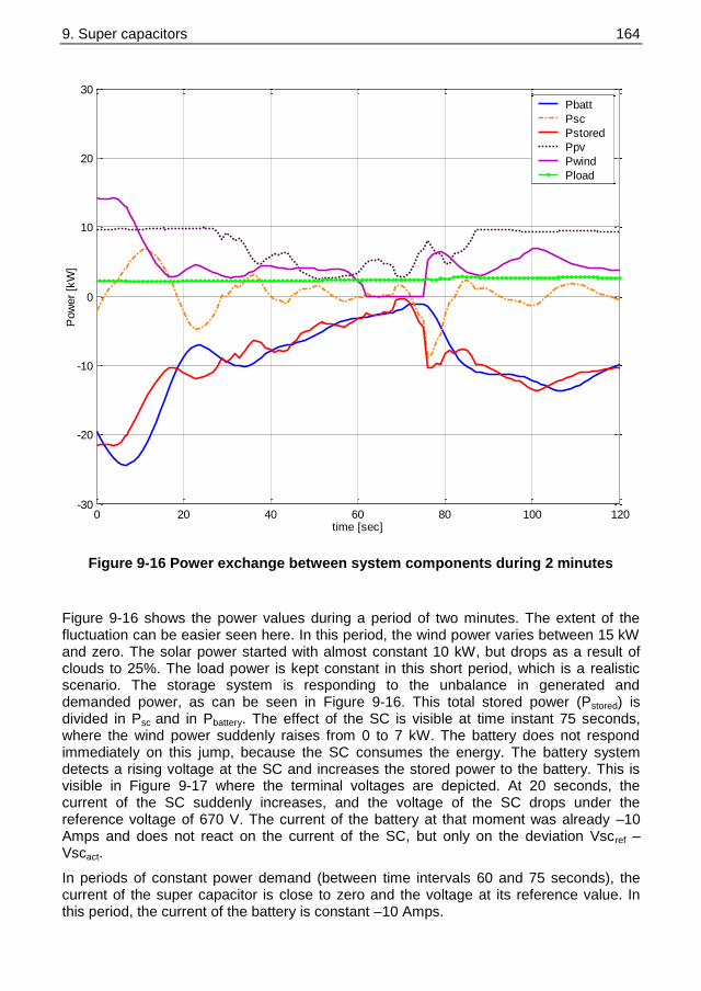
9. Super capacitors 164 164
0 20 40 60 80 100 120-30
-20
-10
0
10
20
30
time [sec]
Pow
er
[kW
]
Pbatt
Psc
Pstored
Ppv
Pwind
Pload
Figure 9-16 Power exchange between system components during 2 minutes
Figure 9-16 shows the power values during a period of two minutes. The extent of the fluctuation can be easier seen here. In this period, the wind power varies between 15 kW and zero. The solar power started with almost constant 10 kW, but drops as a result of clouds to 25%. The load power is kept constant in this short period, which is a realistic scenario. The storage system is responding to the unbalance in generated and demanded power, as can be seen in Figure 9-16. This total stored power (Pstored) is divided in Psc and in Pbattery. The effect of the SC is visible at time instant 75 seconds, where the wind power suddenly raises from 0 to 7 kW. The battery does not respond immediately on this jump, because the SC consumes the energy. The battery system detects a rising voltage at the SC and increases the stored power to the battery. This is visible in Figure 9-17 where the terminal voltages are depicted. At 20 seconds, the current of the SC suddenly increases, and the voltage of the SC drops under the reference voltage of 670 V. The current of the battery at that moment was already –10 Amps and does not react on the current of the SC, but only on the deviation Vscref – Vscact.
In periods of constant power demand (between time intervals 60 and 75 seconds), the current of the super capacitor is close to zero and the voltage at its reference value. In this period, the current of the battery is constant –10 Amps.
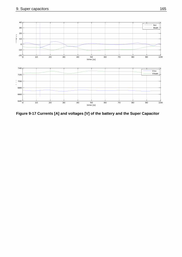
9. Super capacitors 165 165
0 10 20 30 40 50 60 70 80 90 100-20
-10
0
10
20
30
40
time [s]
volta
ge [V
]
0 10 20 30 40 50 60 70 80 90 100640
660
680
700
720
740
time [s]
volta
ge [V
]
Isc
Ibatt
Vsc
Vbatt
Figure 9-17 Currents [A] and voltages [V] of the battery and the Super Capacitor

10 CONCLUSIONS
The objective of this thesis is to prove the feasibility of an autonomous renewable energy system. This aim is realised by the construction and investigation of a real-scale physical laboratory model. The research can be divided into three parts:
Energy balancing calculations;
Construction of the laboratory
General autonomous renewable energy system related issues.
After a general introduction and problem definition for this research, energy calculations are performed for the local situation of the laboratory. Starting point of sizing the system components is always the consumption of energy in the households (demand) which the sources need to supply. Secondly, the available space on the house roofs determines the maximum contribution from solar panels. The solar energy yield is calculated using meteorological data, panel facing and technology efficiency. Thirdly, a suitable wind turbine is chosen for the built-environment. Its power curve and the local available wind data determine the energy yield.
To ensure a measure of reliability, the battery system size is chosen to match a period of autonomy. The estimations are based on the Delfts (Dutch) situation, which include considerations on a number of reference points concerning the available roof area and local wind and solar data. Chapter 4 describes a scaling procedure, which can be implemented in any renewable energy project.
Control strategies, as described in Chapter 6, are not only necessary to prevent the storage system from overloading, but they also minimize the use of the CHP. A weak point in autonomous systems is always the storage system, in this case the battery system. The task of the control system is to take care of this component as much as possible. This includes a frequent equalisation of the battery.
The application of renewable energy forecasting is investigated with the purpose of proving the possibilities to increase the efficiency of the system operation, measured by a reduction of the usage of fossil fuel and battery life time extension. It is concluded that a small profit could be reached with a forecast system extension. It is also concluded that the application persistence models (only based on historical and actual data) give better results that those which are based on weather forecasting. The added value of a long „look ahead‟ time is limited by the maximum allowable uncertainty in available power. This thesis demonstrates that for this study, with battery storage of 100 kWh, the optimal „look-ahead‟ time is 3 hours.
Simulations show that over-dimensioning of the renewable sources is essential due to the incoherency of both the renewable power sources and the conversion and self-discharge losses in the battery system. However, since storage systems are by definition limited, there is no solution to the first problem. It can be expected that innovations in storage technology increase the applicability by using new storage concepts with low self-discharging and with reduced conversion losses. Although lead-acid batteries proved to be unsuitable for this particular application, they are wide spread available and have a

10. Conclusions 167 167
good price-performance ratio. With the application of Super Capacitors, the conversion losses of the battery are further reduced. For this moment, Super Capacitors are still expensive, but it is expected that their price will drop in the near future.
The design and realisation of the laboratory is described in chapter 5. At the start of the project, it was chosen to build a renewable energy laboratory with free available components to keep the focus on system behaviour. The considerations which lead to this particular representation of the real component are described. For instance, this laboratory is designed to be a flexible research environment, which is suitable for experiments with current and new components (sources, storage systems and loads). The developed measurement system, which is based on the common Profibus protocol, is adequate to monitor the essential information and can be easily extended.
As described in section 5.6 a number of components are necessary in this laboratory, although they do not appear in a real situation when supplying energy to the households. These extensions comprehend two of the three transformers (for galvanic separation) and two induction motors, who simulate the driving power which normally comes from gas flow (CHP) or air flow (WECS). This leads to additional losses in the laboratory, which are not present in a real situation. Nevertheless, taking the right system definition into account, the laboratory measurements will correspond with the practical situation.
As a central controller, a PLC is chosen because of its stability, which has already been demonstrated in its long operation in complicated processes in the industry. In addition, it is easy to operate.
Components and central controller communicate by means of the Profibus protocol, which meets the actual standards in communication.
All components, used in the laboratory model, originate from the Electrical Drives Industry. However, the settings are programmed in such a way, that they are now applicable for this purpose.
This thesis demonstrates that a reliable power supply is feasible for duration of at least two days. Longer tests have not yet been carried out. The reason for that is the unavailability of a full-size CHP unit and the absence of the Super Capacitor system in the laboratory. However, there is no indication that a long-run test will show a system‟s failure, because the components themselves have been applied in industry already for a long time. Although the application has been built in a different setting, the limits of the specifications are never violated.
During simulations and measurement in the laboratory, it was observed that the fluctuation in generated and demanded power can be very high (more than expected from the simulations). The sum of the (varying) current is delivered by or stored into the battery system. Fast fluctuations can not be captured by the relatively slow acting batteries. Also, fast discharge and charge rates reduce the life time of the battery. Therefore, to enlarge the overall performance of the battery, this storage system has to be smoothly charged and discharged. Chapter 9 presents a feasible solution to catch the high current peaks from the battery. The size of the super capacitor and the life time of the battery system show a proportional relationship: the bigger the super capacitor, the larger the life time. The applied control strategy is kept simple and efficient. However, this is not the most important factor for a reliable operation of the system. That would be the availability of a stable voltage for the connected equipment. The voltage on the central bus meets the standard, which are drawn up for grid operation (EN50160). As such, any standard component can be used.

10. Conclusions 168 168
The battery‟s State of Charge is calculated by the method of „weighted current integration‟. This means that the energy content of the battery is based on the integral of the current, in which the battery current is weighted according to the Peukert effect. The implementation of the control strategy reached its desired functionality.
This thesis states that the technical feasibility of an autonomous renewable energy system is shown for the Delft situation. Moreover, this thesis gives guidelines for the design and construction of an autonomous renewable energy system.
The system integration is shown with real components in this specific configuration and the weak points in the system operation are discussed and solutions are proposed. By taking into account the necessary dimensions of the sources and the storage unit on local conditions, a reliable electricity supply can be guaranteed. To extend the lifetime of the battery, special measures are undertaken to relieve the battery of high-current peaks.
The described laboratory facility provides possible research extensions due to its flexible lay-out. The connection to the other research facility of the Power Systems group, the Real-Time Digital Simulator (RTDS) gives a very good opportunity to investigate systems, which is partly physical and partly simulated in software.

REFERENCES
1. Bakker, S.J.A., Boonekamp, P.G.M., Het ProgNet-model, robuuste prognoses van Nederlandse Elektriciteitsvraag Trends. 2004, ECN: Petten.
2. CIGRE, Electric Power Systems 2020. 2003, Joint Advisory Group SC15/E1 -JAG 02 TC. 3. Duurzame energie in opmars, actieprogramma 1997-2000. 1997, ministerie van
Economische Zaken. 4. Technologies for Tommorow. IEEE Power Engineering Review, 1998. 18(9). 5. Meij, J.M., Stroomversnelling, de volgende innovatiegolf [in Dutch]. 1999, The Hague:
Stichting toekomstbeeld der techniek. 6. SmartGrids, vision and strategy for Europe's Electricity Networks of the Future. 2006,
European Commission. 7. Committee-Brundlandt, Our common future. 1987, UN Report. 8. Stevenson, G., Keehn, B., I will if you will; Towards sustainable consumption. May 2006,
Sustainable consumption round table. 9. Power, A., (editor), Stock Take: Delivering improvements in existing housing. May 2006,
Sustainable Development Commission. 10. Flavin, C., Deudney, D., Renewable Energy: The Power to Choose. 1983. 11. Hadjsaid, N., Dispersed Generation Impact on Distribution Networks. IEEE Computer
Application in Power, 1999. 12(2). 12. Hirachi, K. Feasible Developments of Utility-Interactive Multi-Functional Bi-directional
Converter for Solar Photovoltaic Generating System Incorporating Storage Batteries. in 26th Annual IEEE Power Electronics Specialists 1995.
13. Chiang, S.J., Three-phase multifunctional battery energy storage system. IEEE Proceedings Electrical Power Applications, 1995. 42(4).
14. Borle, L.J., Development and Testing of a 20-kW Grid Interactive Photovoltaic Power Conditioning System in Western Australia, . IEEE Transactions in Industry Applications,
1997. 33(2). 15. Tsai, M.-T., Design and Implementation of a Demand-Side Multifunction Battery Energy
Storage System. IEEE Transactions on Industrial Electronics, 1995. 42(6). 16. Dokopoulus, P.S., Prediction and Evaluation of the Performance of Wind-Diesel Energy
Systems. IEEE Transactions on Energy Conversion, 1996. 11(2). 17. Contaxis, G.C., Short Term Scheduling in a wind/diesel autonomous energy system,. IEEE
Transactions on Power Systems, 1991. 6(3). 18. Ashari, M., A single phase Parallely Connected Uninterruptible Power supply/Demand
Side Management System. IEEE Transactions on Energy Conversion, 2000. 15. 19. Rajendiram, K. PSCAD/EMTDC Based Simulation of a Wind-Diesel conversion schema. in
IEEE Power Engineering Society Winter Meeting. 2000. 20. Elhadidy, M.A., Parametric Study of hybrid (wind+solar+diesel) power generating systems.
Renewable Energy, 2000. 21. 21. Bonanno, F., Transient Analysis of Integrated Diesel-Wind Photovoltaic Generation
Systems. IEEE Transactions on Energy Conversion, 1999. 14(2). 22. J.T. Bialasiewicz. Modular Simulation of a Hybrid Power Systems with Diesel and Wind
Turbine Generation, . in Windpower’98. 1998. Bakersfield, CA. 23. Karlis, A. Small Power Systems Fed by Hydro, Photovoltaic, Wind Turbines and Diesel
Generators. in ICECS. 1996. 24. Tomilson, A., et all. Modelling an autonomous wind-diesel system using Simulink. in
Canadian Conference on Electrical and Computer Engineering. 1997. 25. Wilson, T.L., Bell, D.G. Energy conservation and demand control using distribution
automation technologies. in Rural Electric Power Conference. 2004. 26. Willis, H.L., Scott, W.G., Distributed Power Generation. 2000, New York: Marcel Dekker
Inc. 27. Mohan, N., Power Electronics, converters, applications and design. 2003: Wiley. 28. Perez, R.A., The Complete Battery Book. 1995, Blue Ridge Summit: TAB Books Inc. 29. Handbook for Gel_VRLA-Batteries. Vol. I: Sonnenschein.

References 170 170
30. Linden, D., Handbook of Batteries. 1995: Mc Graw Hill. 31. Stevens, J.W., G.P. Corey. A study of Lead-Acid battery efficiency near top of charge and
the impact on PV system design. in 25th IEEE Photovoltaic Specialists Conference 1996. 32. McDowall, J.A. Batteries for Stationary Standby and for Cycling Applications, Part 3:
Operating Issues. in Power Engineering Society General Meeting. 2003. Toronto, Canada. 33. Symons, P.C. Batteries for Stationary Standby and for Stationary Cycling Applications,
Part 4: Charge Management. in Power Engineering Society General Meeting. 2003.
Toronto, Canada. 34. Boyle, G., Renewable Energy, power for a sustainable future. 2 ed. 2004, Oxford: The
Open University. 35. Woyte, A., Design issues of photovoltaic systems and their grid integration. 2003,
Katholieke Universiteit Leuven: Leuven. p. 201. 36. Markvart, T., Solar Electricity 2nd edition. 1997: John Wiley & Sons. 37. van Voorden, A.M., Slootweg J.G. , Paap, G.C., Van der Sluis, L. Potential for Renewable
Energy in Urban Distribution Networks. in CIRED 2001. 2001. Amsterdam. 38. Novem, Instralingsschijf zonne-energie, Novem bestelnummer 2 DEN-01.08. 39. F.G.P. Corten, The potential on roofs and walls in the Netherlands. 1996, Centrum voor
energiebesparing en schone technologie: Delft. 40. Stand-Alone Photovoltaic Power Systems, lessons learned. 1999, IEA-PVPS International
Energy Agency Photovoltaic Power Systems Programme. 41. Dodge, D.M., Illustrated History of Wind Power Development, Littleton: Colarado. 42. van Kuik, G.A.M., Are wind turbines growing too fast? in European Wind Energy
Conference and Exhibition. 2001. Copenhagen, Denmark. 43. J.K. Kok, A.J.B., Voorspellen van duurzame energie in de bebouwde omgeving, SDE,
Editor. 2003, ECN: Petten. 44. Wit, M.H. de, Wind in de gebouwde omgeving. 2001, Technische Universiteit Eindhoven. 45. Paulino, P., Renewable Energy Forecasting applied to Autonomous Renewable Energy
Systems, in Power Systems. 2006, Delft University of Technology: Delft. p. 100. 46. Dutton, A.G., Halliday, J.A., Blanch, M.J., The Feasibility of Building Mounted/Integrated
Wind Turbines (BUWTs): Achieving their potential for carbon emission reduction. 2005, CLRC Rutherford Appleton Laboratory: Chilton.
47. http://www.wasp.dk/, The Wind Atlas Analysis and Application Program. 48. Mertens, S., The energy yield of roof mounted wind turbines. Wind Engineering, 2003.
27(6): p. 507-518. 49. Sagrillo, M., Tower Economics. Home Power, 1993. 37. 50. Mertens, S., Performance of an H-Darrieus in the skewed flow on a roof. Journal of Solar
Energy Engineering, Transactions of the ASME, 2003. 125(4): p. 433-440. 51. www.spaceforwind.nl, TU Delft. 52. Pilavachi, P.A., Mini- and micro-gas turbines for combined heat and power. Applied
Thermal Engineering, 2002. 22. 53. Pearce, J.M., Electricity generation in the home: evaluation of single-house domestic
combined heat and power. IEE Proceedings-Sci. Meas. Technology, 1996. 143(6). 54. De Paepe, M., D'Herdt, P., Mertens, D., Micro-CHP systems for residential applications.
Energy Conversion and Management, 2006. 47. 55. www.senertec.de, DACHS-WRA. 56. Uitzinger, J., Sepath, simulatie van energievraagpatronen van huishoudens, SDE, Editor.
2003, IVAM: Amsterdam. 57. J. Nijs, W.D.H., Zonne-energie, lecture notes, ed. K. Leuven. 58. Shaahid, S.M., Elhadidy, M.A., Optimal sizing of battery storage for stand-alone hybrid
(photovoltaic+diesel) power systems. International journal of sustainable energy, 2005. 24. 59. Slootweg, J.G., Wind Power, Modelling and Impact on Power System Dynamics, in Power
Systems Laboratory. 2003, Delft University of Technology: Delft. 60. van Voorden, A.M., Paap, G.C., van der Sluis, L. The Use of Batteries in Autonomous
Renewable Energy Systems. in PowerTech 2005. 2005. St. Petersburg. 61. H. Madsen, e.a., A Protocol for Standardizing the Performance Evaluation of Short-term
Wind Power Prediction Models. 2004, Anemos, EU R&D Project.

References 171 171
62. Giebel, G., The State of the art in Short-Term Prediction of Wind Power, A literature
Overview. 2003, Project ANEMOS, http://anemos.cma.fr. 63. Schupbach, R.M., Balda, J.C. 35 kW Ultra Capacitor Unit for Power Management of
Hybrid Electric Vehicles: Bi-directional Dc-Dc Converter Design. in 35th Annual IEEE Power Electronics Specialists Conference. 2004. Aachen, Germany.
64. Gao, L., Dougal, R.A., Liu, S. Active power sharing in hybrid battery/capacitor power sources. in Applied Power Electronics Conference and Exposition 2003. Madrid, Spain.
65. Gao, L., Dougal, R.A., Liu, S., Power Enhancement of an Actively Controlled Battery/Ultracapacitor Hybrid. IEEE Transactions on Power Electronics, 2005. 20(1): p. 236-243.
66. Smith, T.A., Mars, J.P., Turner, G.A. Using Supercapacitors to Improve Battery Performance. in 33th Power Electronics Specialists Conference. 2002. Cairns, Australia.
67. Pay, S., Baghzouz, Y. Effectiveness of Battery-Supercapacitor Combination in Electric Vehicles. in IEEE PowerTech Conference. 2003. Bologna, Italy.
68. Lohner, A., Evers, W. Intelligent Power Management of a Supercapacitor based Hybrid Power Train for Light-rail Vehicles and City buses. in 35th Annual IEEE Power Electronics Specialists Conference. 2004. Aachen, Germany.
69. Rufer, A., Barrada, Ph., A Supercapacitor-Based Energy-Storage System for Elevators With Soft Commutated Interface. IEEE Transactions in Industry Applications, 2002. 38(5).

APPENDIX: BENCHMARKING PROJECT FOR HYBRID POWER SYSTEMS
This appendix contains background information about a public database on RES components and operation (http://www.benchmarking.eu.org). Within the context of this research EU-research program, it is analyzed how a specific Renewable Energy System (RES) operates and what factors the conditions of use of its components influence. RES‟s are very site specific. Without knowledge of the renewable energy resources and it‟s site, it is impossible to optimally plan the system, size its components, plan the operating regime, and select the most suitable components. In addition, no applications are identical, and even small variations may lead to differences in the energy throughput of the system and some critical operating conditions or their components. While making general recommendations for RES‟s and batteries is straightforward, making specific recommendations is impossible without a detailed analysis of the location and the application, including a sensitivity analysis concerning the various assumptions and their likely variations over time.
The creation of categories of similar use for making detailed recommendations and for benchmarking components concerning their suitability for specific RES‟s is at the heart of project work. Without the creation of such categories, no distinction would be possible between batteries with high annual energy throughput and a daily full charge and batteries for systems with many days of autonomy, a very low annual energy throughput, and periods of months without a full charge.
Schematic diagram showing end-of-lifetime definition
Recent papers offered an analysis of what lifetime and performance prediction mean. End of lifetime is reached if the state vector of performance no longer lies within the acceptable range of values. A vector rather than a scalar value of performance needs to be used because it is too simplistic to tie end of lifetime to one performance value (in most cases, capacity). Other performance requirements whose values can also lead to the battery no longer being able to fulfill the performance requirements are self-discharge,

Appendix: Benchmarking project for Hybrid power systems 173 173
charge acceptance, high rate power capability at medium SOC and low temperature, energy requirement during charging, and cost of energy delivered in systems with auxiliary energy generation. The radar plot above shows a schematic diagram of such a state vector. In RES‟s it is important not to use the usual value of 80% or 60% of capacity as the only performance indicator for end of life because often the optimum replacement time should be at a much lower residual capacity.
The 'stress factors' defined during the benchmarking project are defined in detail. More information could be found on the mentioned website. A summary of this is depicted in the table below.
Stress factor Intensity benchmark Note
TIME BETWEEN FULL CHARGE
Average time between recharge over 90% SOC. [day] 5: very high intensity >8 4: high intensity (2.5 ; 8] 3: medium (1.2 ; 2.5] 2: low (0.7 ; 1.2] 1: very low <=0.7
CHARGE FACTOR
Average charge factor per a year: [%] 5: very high intensity >130 4: high intensity (115 ; 130] 3: medium (108 ; 115] 2: low (102 ; 108] 1: very low <=102
Average charge factor per year: the ratio between the Ah charging and the Ah discharging.
DISCHARGE RATE
Highest average current at which 1% of the Ah throughput was discharged * [I10] 5: very high intensity > 1.7 4: high intensity (1.4 ; 1.7] 3: medium (0.5 ; 1.4] 2: low (0.1 ; 0.5] 1: very low <=0.1
Higher intensity means higher discharge rate.
Ah THROUGHPUT
Cumulative Ah throughput per a year: [Cn] 5: very high intensity >100 4: high intensity (70 ; 100] 3: medium (40 ; 70] 2: low (10 ; 40] 1: very low <= 10
LOW SOC
Cumulative operation time of a year at SOC <35%: [%] 5: very high intensity >25 4: high intensity (15.5 ; 25] 3: medium (4.5 ; 15.5] 2: low (1 ; 4.5] 1: very low <= 1

Appendix: Benchmarking project for Hybrid power systems 174 174
PARTIAL CYCLING
Weighted Ah throughput in given SOC ranges, expressed in a single Partial Cycle value PC 5: very high intensity >70 4: high intensity (50 ; 70] 3: medium (40 ; 50] 2: low (30 ; 40] 1: very low <= 30
Higher intensity means higher partial cycling = higher cumulative discharged Ah in lower SOC range.
TEMPERATURE ACCELERATION FACTOR
Temperature acceleration factor
T = battery temperature; T0=20°C
dt
dteaT
TTk
ac
)( 0*
10°C increase double the factor
10
2ln,1 ka
5: very high intensity >1.6 4: high intensity <1.15 ; 1.6] 3: medium <0.85 ; 1.15] 2: low <0.4 ; 0.85] 1: very low <=0.4
Higher intensity means higher operating temperature.
A low intensity means a low operating temperature.
Nominal operating temperature is 20°C.
LOW BATTERY ENVIRONMENTAL TEMPERATURE
The lowest operating battery temp. maintained at least for 12 hours (average in the 12 hours period).
[°C] 5: very high intensity <-9 4: high intensity [-9 ; -5) 3: medium [-5 ; 0) 2: low [0 ; 5) 1: very low >= 5
Higher intensity = lower operating temperature = higher risk of electrolyte freeze.
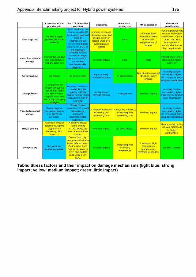
Appendix: Benchmarking project for Hybrid power systems 175 175
Corrosion of the
positive grid
hard / irreversible
sulfationshedding
water loss /
drying outAM degradation
electrolyte
stratification
discharge rate
Indirect through
positive electrode
potential
higher discharge rate
creates smaller AM
sulphate crystals and
leads to
inhomogeneous
current distribution
causes inh. SOC on
the electrode
probably increased
shedding; outer AM
fraction cycles at
higher DOD level
cycling [pasted
plates]
none
increases inner
resistance due to
AOS-model
(agglomerate of
sphere)
Higher discharge rate
reduces electrolyte
stratification. On the
other hand less
homogeneous
current distribution
plays negative role.
time at low states of
charge
Indirect through low
acid concentration
and low potentials
A strong positive
correlation: longer
time at a low SOC
accelerates
hard/irreversible
sulphation.
no direct impact none None
Indirect effect longer
time lead to higher
sulphation
Ah throughput no impact no direct impactimpact through
mechanical stressno direct impact
loss of active material
structure, larger
crystals
A strong positive
correlation: Higher
Ah throughput leads
to higher stratification
charge factor
a strong indirect
impact because a
high charge factor
and an extensive
charge is associated
with a high charging
voltages
negative correlation,
impact through
regimes with high
charge factors which
reduces the risk of
sulphation
strong impact
through gassingstrong impact no direct impact
A strong positive
correlation: Higher
charge factor leads to
lower stratification
Time between full
charge
Strong negative
correlation: shorter
time increases
corrosion.
Strong positive
correlation: Frequent
full recharge
decreases
hard/irreversible
sulphation.
A negative influence,
increasing with
decreasing time.
A negative influence,
increasing with
decreasing time
no direct impact
A strong positive
correlation: Higher
Ah throughput leads
to higher stratification
Partial cycling
An impact through
potential variations
(depends on
frequency, SOC
level, ..)
A positive impact.
Partial cycling
(f>1Hz) increases
size of lead-sulfate
crystals.
No direct impact. No direct impact. no direct impact
Higher partial cycling
at lower SOC leads
to higher
stratification.
TemperatureStrong impact,
positive correlation
On one hand high
temperature helps to
better fully recharge.
On the other hand
high temp. leads to
more hard sulfate
build up at a low
SOC.
no direct impact
increasing with
increasing
temperature
low impact high
temperature
degrades neg.
electrode expanders
no direct impact.
Table: Stress factors and their impact on damage mechanisms (light blue: strong impact; yellow: medium impact; green: little impact)

CURRICULUM VITAE
Arjan Marco van Voorden was born on April 11th, 1972 in Rotterdam. He attended
secondary school at the Jacobus Reviuscollege in Rotterdam from 1984 to 1988. After obtaining his MAVO-degree in May 1988, he started his long Electrical Engineering study at the “Christelijke MTS” in Rotterdam-Schiebroek. His specialisation here was already Electrical Power Engineering. He finished the theoretical part of this education within three years.
He continues his education at the University of Professional Education at the “Haagse Hogeschool”. After two years of general education on Electrical Engineering, he has chosen again the Power Engineering specialisation. His final thesis project was carried out at KEMA, section Transmission and Distribution. The title of this thesis was: The loading capability of an asymmetric cable circuit.
After the successful completing of this B.Sc. study, he switched to the Delft University of Technology for his Master Study. This was carried out in the Power Systems Laboratory. His master thesis was successfully defended in April 1998, under supervision of Dr. ir. G.C. Paap. The title of this works was: “The power supply on autonomous households”.
After graduating on the DUT, he first continues his master thesis work with an extended research, performing detailed simulation of autonomous households. In 2000 a Ph.D. opportunity was available after the allocation of a research project, which comprehends the built of a renewable energy laboratory for research purposes.
Under the supervision of project leader Dr. ir. Bob Paap and with the excellent technical assistance of ing. Johan Vijftigschild, he completes the design and construction of the renewable energy laboratory.
In 2007, Arjan continues his carrier in the Electrical Power Engineering at Eneco Netbeheer (Stedin), one of the Dutch regional distribution system operator. His current job focuses on the Risk and Portfolio analyses at the Asset Management department.
Since 1998, Arjan is married to Ina van Voorden - Taale and together they have one daughter Joanne (2000) and two sons, Joost (2001) and Mark (2004).