power control for mobile radio systems using …...appendix a itu speech files 157 appendix b...
TRANSCRIPT

The University of Western AustraliaSchool of Electrical, Electronic, and Computer Engineering
Crawley, WA 6009
Power Control for Mobile Radio Systems UsingPerceptual Speech Quality Metrics
BEHROOZ ROHANI MEHDIABADI
This thesis is presented for the degree ofDoctor of Philosophy
ofThe University of Western Australia
February 2007

ii

Dedication
To my uncle and aunt Jamshid and Banou ROHANI.
iii

iv

Abstract
As the characteristics of mobile radio channels vary over time, transmit power must becontrolled accordingly to ensure that the received signal level is within the receiver’s sen-sitivity. As a consequence, modern mobile radio systems employ power control to regu-late the received signal level such that it is neither less nor excessively larger than receiversensitivity in order to maintain adequate service quality. In this context, speech qualitymeasurement is an important aspect in the delivery of speech services as it will impactsatisfaction of customers as well as the usage of precious system resources. A varietyof techniques for speech quality measurement has been produced over the last few yearsas result of tireless research in the area of perceptual speech quality estimation. Theseare mainly based on psychoacoustic models of the human auditory systems. However,these techniques cannot be directly applied for real-time communication purposes as theytypically require a copy of the transmitted and received speech signals for their operation.
This thesis presents a novel technique of incorporating perceptual speech quality met-rics with power control for mobile radio systems. The technique allows for standardizedperceptual speech quality measurement algorithms to be used for in-service measurementof speech quality. The accuracy of the proposed Real-Time Perceptual Speech QualityMeasurement (RTPSQM) technique with respect to measuring speech quality is first val-idated by extensive simulations. On this basis, RTPSQM is applied to power control inthe Global System for Mobile (GSM) communication and the Universal Mobile Telecom-munication System (UMTS). It is shown by simulations that the use of perceptual-basedpower control in GSM and UMTS outperforms conventional power control in terms of re-ducing the transmitter signal power required for providing adequate speech quality. Thisin turn facilitates the observed increase in system capacity and thus offers better utiliza-tion of available system resources. To enable an analytical performance assessment ofperceptual speech quality metrics in power control, the mathematical frameworks for con-ventional and perceptual-based power control are derived. The derivations are performedfor Code Division Multiple Access (CDMA) systems and kept as generic as possible. Nu-merical results are presented which could be used in a system design to readily find theErlang capacity per cell for either of the considered power control algorithms.
v

vi

Acknowledgements
I am thankful to many people who have helped me at various stages of work on this thesis,but special gratitude goes to the following people:
Professor Hans-Jurgen Zepernick, my supervisor. Although extremely busy, Hansalways would somehow find the time to answer my questions and give guidance. Thiscontinued even after he departed from Western Australian Telecommunication ResearchInstitute (WATRI) and started work at Blekinge Institute of Technology (BTH) in Sweden.I owe Hans a debt of gratitude for being my supervisor, and honor him for his manyvirtues, including punctuality, organization, discipline, trustworthiness and unwaveringquest for excellence.
Dr. Bijan Rohani, my co-supervisor. Bijan has always been a source of inspiration forme as an older brother and has always been available for my support in every sense of theword.
Professor Sven Nordholm, my associate supervisor for his never-ending support, par-ticularly with matters dealing with administrative side of my Ph.D. candidature.
Dr. Manora Caldera for her support, encouragements, thorough proof-reading of mythesis, and suggestions to improve its presentation.
I would like to acknowledge the financial support from the Western Australian Telecom-munications Research Institute (WATRI), Australian Telecommunications CooperativeResearch Centre (ATcrc), the Australian Postgraduate Award (APA) scheme and BTH.
I am grateful to Messrs. Kambiz and Kassra Homayounfar of PHYBIT Inc. com-pany in Singapore for permitting me to use their simulation models for GSM and UMTSphysical layers.
I would like to also thank and acknowledge OPTICOM GmbH of Germany, the copy-right holders of Perceptual Evaluation of Speech Quality (PESQ) algorithm/software, forpermitting me to modify and use PESQ for my academic research purposes.
Finally, I would like to express deepest appreciation to my family, especially, myparents and wife for their understanding and support during the times while I was workingon this thesis.
vii

viii

Table of Contents
List of Abbreviations xiii
List of Common Symbols xvii
1 Introduction 11.1 Thesis Structure . . . . . . . . . . . . . . . . . . . . . . . . . . . . . . . 21.2 Summary of Major Contributions . . . . . . . . . . . . . . . . . . . . . . 4
1.2.1 Real-time perceptual speech quality metric . . . . . . . . . . . . 41.2.2 Application of RTPSQM in power control of mobile radio systems 51.2.3 Mathematical analysis of UMTS power control . . . . . . . . . . 6
1.3 List of Publications . . . . . . . . . . . . . . . . . . . . . . . . . . . . . 6
2 Power Control Schemes and Speech Quality Metrics for Mobile Radio Sys-tems 92.1 Introduction . . . . . . . . . . . . . . . . . . . . . . . . . . . . . . . . . 92.2 Power Control Schemes . . . . . . . . . . . . . . . . . . . . . . . . . . . 9
2.2.1 Centralized power control . . . . . . . . . . . . . . . . . . . . . 102.2.2 Distributed power control . . . . . . . . . . . . . . . . . . . . . 132.2.3 Open-loop and closed-loop power control . . . . . . . . . . . . . 16
2.3 Power Control in Mobile Radio Systems . . . . . . . . . . . . . . . . . . 172.3.1 GSM power control . . . . . . . . . . . . . . . . . . . . . . . . . 172.3.2 IS-95 power control . . . . . . . . . . . . . . . . . . . . . . . . 182.3.3 UMTS power control . . . . . . . . . . . . . . . . . . . . . . . . 192.3.4 cdma2000 power control . . . . . . . . . . . . . . . . . . . . . . 21
2.4 Speech Quality Metrics and Measurement Methods . . . . . . . . . . . . 212.4.1 Conventional speech quality metrics . . . . . . . . . . . . . . . 222.4.2 Perceptual speech quality measurement . . . . . . . . . . . . . . 24
2.5 Objective Perceptual Speech Quality Metrics . . . . . . . . . . . . . . . 282.5.1 Perceptual evaluation of speech quality . . . . . . . . . . . . . . 282.5.2 The E-model . . . . . . . . . . . . . . . . . . . . . . . . . . . . 312.5.3 The single sided speech quality measure . . . . . . . . . . . . . . 32
2.6 Summary . . . . . . . . . . . . . . . . . . . . . . . . . . . . . . . . . . 33
3 Novel Technique for Real-Time Perceptual Speech Quality Measurement 353.1 Introduction . . . . . . . . . . . . . . . . . . . . . . . . . . . . . . . . . 353.2 Frame-based Speech Communication Systems . . . . . . . . . . . . . . . 37
ix

TABLE OF CONTENTS
3.3 Proposed Real-Time Perceptual Speech Quality Measurement Technique . 393.3.1 Motivation . . . . . . . . . . . . . . . . . . . . . . . . . . . . . 393.3.2 Solution . . . . . . . . . . . . . . . . . . . . . . . . . . . . . . . 40
3.4 Performance Evaluation of the Proposed Technique . . . . . . . . . . . . 423.5 Summary of Results and Discussion . . . . . . . . . . . . . . . . . . . . 44
3.5.1 Training part: determination of mapping functions . . . . . . . . 453.5.2 Verification part: analyzing accuracy of mapping functions . . . . 50
3.6 Summary . . . . . . . . . . . . . . . . . . . . . . . . . . . . . . . . . . 57
4 Perceptual-based Power Control for GSM 594.1 Introduction . . . . . . . . . . . . . . . . . . . . . . . . . . . . . . . . . 594.2 GSM Power Control . . . . . . . . . . . . . . . . . . . . . . . . . . . . 604.3 Simulation Model . . . . . . . . . . . . . . . . . . . . . . . . . . . . . . 61
4.3.1 Input speech file . . . . . . . . . . . . . . . . . . . . . . . . . . 624.3.2 Speech codec . . . . . . . . . . . . . . . . . . . . . . . . . . . . 644.3.3 Channel coding and interleaving . . . . . . . . . . . . . . . . . . 654.3.4 Channel model . . . . . . . . . . . . . . . . . . . . . . . . . . . 654.3.5 Power control . . . . . . . . . . . . . . . . . . . . . . . . . . . . 664.3.6 Simulation parameters . . . . . . . . . . . . . . . . . . . . . . . 73
4.4 Methodology . . . . . . . . . . . . . . . . . . . . . . . . . . . . . . . . 744.5 Results . . . . . . . . . . . . . . . . . . . . . . . . . . . . . . . . . . . . 744.6 Capacity Gain Calculation . . . . . . . . . . . . . . . . . . . . . . . . . 794.7 Summary . . . . . . . . . . . . . . . . . . . . . . . . . . . . . . . . . . 83
5 Perceptual-based Power Control for UMTS 855.1 Introduction . . . . . . . . . . . . . . . . . . . . . . . . . . . . . . . . . 855.2 Power Control in UMTS . . . . . . . . . . . . . . . . . . . . . . . . . . 85
5.2.1 Closed-loop power control in FDD mode . . . . . . . . . . . . . 865.2.2 Conventional UMTS outer-loop power control algorithm . . . . . 885.2.3 Conventional UMTS inner-loop power control algorithms . . . . 88
5.3 Simulation Model . . . . . . . . . . . . . . . . . . . . . . . . . . . . . . 915.3.1 Input speech file . . . . . . . . . . . . . . . . . . . . . . . . . . 915.3.2 Speech codec . . . . . . . . . . . . . . . . . . . . . . . . . . . . 935.3.3 Multiplexing and channel coding . . . . . . . . . . . . . . . . . . 935.3.4 Power control . . . . . . . . . . . . . . . . . . . . . . . . . . . . 945.3.5 Channel . . . . . . . . . . . . . . . . . . . . . . . . . . . . . . . 975.3.6 Summary of simulation parameters . . . . . . . . . . . . . . . . 99
5.4 Methodology . . . . . . . . . . . . . . . . . . . . . . . . . . . . . . . . 995.5 Simulation Results . . . . . . . . . . . . . . . . . . . . . . . . . . . . . 995.6 Summary . . . . . . . . . . . . . . . . . . . . . . . . . . . . . . . . . . 103
6 Mapping Between FER, Residual BER and MOS 1076.1 Introduction . . . . . . . . . . . . . . . . . . . . . . . . . . . . . . . . . 1076.2 Factors Influencing Perceptual Speech Quality . . . . . . . . . . . . . . . 1086.3 Simulation Model . . . . . . . . . . . . . . . . . . . . . . . . . . . . . . 109
6.3.1 Input speech . . . . . . . . . . . . . . . . . . . . . . . . . . . . 109
x

TABLE OF CONTENTS
6.3.2 AMR codec . . . . . . . . . . . . . . . . . . . . . . . . . . . . . 1096.3.3 Channel model . . . . . . . . . . . . . . . . . . . . . . . . . . . 1106.3.4 PESQ . . . . . . . . . . . . . . . . . . . . . . . . . . . . . . . . 1106.3.5 Other physical layer parameters . . . . . . . . . . . . . . . . . . 110
6.4 Methodology . . . . . . . . . . . . . . . . . . . . . . . . . . . . . . . . 1116.5 Results . . . . . . . . . . . . . . . . . . . . . . . . . . . . . . . . . . . . 1126.6 Summary . . . . . . . . . . . . . . . . . . . . . . . . . . . . . . . . . . 112
7 Comparative Erlang Capacity of UMTS 1157.1 Introduction . . . . . . . . . . . . . . . . . . . . . . . . . . . . . . . . . 1157.2 Erlang Capacity of Multiuser Systems . . . . . . . . . . . . . . . . . . . 1167.3 Conventional Power Control . . . . . . . . . . . . . . . . . . . . . . . . 118
7.3.1 Conventional outer-loop power control algorithm . . . . . . . . . 1187.3.2 Erlang capacity in the steady state of the Markov chain . . . . . . 1237.3.3 Numerical Results . . . . . . . . . . . . . . . . . . . . . . . . . 130
7.4 Perceptual-based Power Control . . . . . . . . . . . . . . . . . . . . . . 1337.4.1 Perceptual-based outer-loop power control algorithm . . . . . . . 1337.4.2 Perceptual-based transition probabilities of the Markov chain . . . 1347.4.3 Erlang capacity for perceptual-based power control . . . . . . . . 141
7.5 Numerical Results . . . . . . . . . . . . . . . . . . . . . . . . . . . . . . 1427.5.1 Capacity gain of perceptual-based power control . . . . . . . . . 144
7.6 Summary . . . . . . . . . . . . . . . . . . . . . . . . . . . . . . . . . . 147
8 Conclusions 1498.1 Summary of Major Findings and Contributions . . . . . . . . . . . . . . 1508.2 Suggestions for Future Work . . . . . . . . . . . . . . . . . . . . . . . . 153
Appendices 155
Appendix A ITU Speech Files 157
Appendix B Simulation Results for UMTS Outer-loop Power Control 159
Appendix C ITU Speech Files Used for AMR Performance Characterization 163
Appendix D 165D.1 Matlab Script for Solving Equilibrium Equations of Markov Chains . . . 165D.2 Capacity Results of UMTS Power Control . . . . . . . . . . . . . . . . . 169
Bibliography 175
xi

xii

List of Abbreviations
ACELP Algebraic Code Excited Linear PredictionACR Absolute Category RatingAMR Adaptive Multi-RateASD Auditory Spectrum DistanceAWGN Additive White Gaussian NoiseBER Bit Error RateBSC Base Station ControllerBSD Bark Spectral DistanceBSS Base Station SubsystemBTS Base Transceiver StationsCC Convolutional CodingCCTrCH Coded Composite Transport ChannelCDMA Code Division Multiple AccessCePC Centralized Power ControlCIR Carrier-to-Interference RatioCLPC Closed Loop Power ControlCPC Conventional Power ControlCRC Cyclic Redundancy CheckDB Distributed BalancingDCPC Distributed Constrained Power ControlDCR Degradation Category RatingDDPC Distributed Discrete Power ControlDMOS Degradation Mean Opinion ScoreDPC Distributed Power ControlDTX Discontinuous TransmissionE-model The ETSI Computation ModelETSI European Telecommunications Standards InstituteFDD Frequency Division DuplexFDMA Frequency Division Multiple Access
xiii

FE Frame ErasureFEC Forward Error CorrectionFEP Frame Erasure PatternFER Frame Error RateFFT Fast Fourier TransformFH Frequency HoppingFQI Frame Quality IndicatorGSM Global System for Mobile communicationMAI Multiple Access InterferenceMNB Measuring Normalizing BlocksMOS Mean Opinion ScoreOPCS Optimum Power Control SchemePAMS Perceptual Analysis Measurement SystemPAQM Perceptual Audio Quality MeasureP-CCPCH Primary Common Control Physical ChannelPCM Pulse Code ModulationPDF Probability Density FunctionPESQ Perceptual Evaluation of Speech QualityPPC Perceptual Power ControlPSD Power Spectral DensityPSNR Peak Signal-to-Noise RatioPSQM Perceptual Speech Quality MeasurementQoS Quality of ServiceRBER Residual Bit Error RateRTPSQM Real-Time Perceptual Speech Quality MeasurementRxLev Received LevelRxQual Received QualitySIR Signal-to-Interference RatioSNR Signal-to-Noise RatioTDD Time Division DuplexTDMA Time Division Multiple AccessTPC Transmit Power ControlTrCH Transport ChannelsTTI Transmission Time IntervalTU Typical UrbanTVPC Time Variant distributed constrained Power ControlUE User Equipment
xiv

UMTS Universal Mobile Telecommunication SystemVoIP Voice over Internet Protocol
xv

xvi

List of Common Symbols
a Gradient of a lineb y-intercept of a lineAE−model Advantage factor in E-ModelB Event of MOS being badBSi Base station in cell i
Bt Total allocated spectrum for the systemBc Bandwidth of the radio channelsCu Capacity in terms of the number of users per cellCIRmin Minimum carrier-to-interference ratioCIRmin,c Minimum CIR for conventional power controlCIRmin,p Minimum CIR for perceptual-based power controle(n) Difference between RTPSQM MOS(n) and Tmos at interval n
eA Event of error(s) in Class A bitseB Event of error(s) in Class B bitseC Event of error(s) in Class C bitserf(x) Error functionEb Bit energyfrm(n) nth frameF Event of occurrence of a frame errorg Process gainGij Link gain between BSj and MSi
I0 Interference power spectral densityI(P) Interference functionIBS Interference signal power at base stationId Impairments caused by delay in E-modelIs Impairments occurring simultaneously with speech signal in E-modelIe Impairments caused by codecs in E-modelK Constant used to set the FER target for UMTS outer-loop power control
xvii

L0 Long-term average downlink path lossLdl Downlink path lossmc Capacity metric of the conventional power control schememe,MOS Mean of estimation error in MOSmp Capacity metric of the perceptual power control schemeM Highest state in a Markov chainMSi Mobile station in cell i
nB Number of bad framesnF Number of framesnFB Number of bad frames receivedN0 Noise power spectral densityNpilot Number of pilot bitsNTFCI Number of Transport Format Combination Indicator (TFCI) bitsNTPC Number of TPC bitsPi Transmit power of mobile i
Pr[Blocking] Blocking probabilityPr(X) Probability of event X
Q Number of co-channel interferersr Pearson correlation coefficientrxTPCcmd Received TPC commandR Transmission rating of the E-modelR0 SNR in E-modelS Event of receiving a silent frameSIRtarget SIR target used in UMTS outer-loop power controlSIRth SIR thresholdtxTPCcmd Transmitted TPC commandTmos Target MOSV ar(x) Variance of random variable x
W Spread signal bandwidthY Received SIR in dBZ Blocking conditionα FEC coding gainαms Weighting factor calculated by the mobile stationβ A constant equal to 0.1ln(10) = 0.23
βc Normalization constant used in some power control algorithmsδ Step size of UMTS inner-loop power control∆down Power control step down value in dB
xviii

∆up Power control step up value in dBη Threshold of N0/I0
γ0 CIR thresholdΓi CIR at mobile i
λ Arrival rateλi ith eigenvalue of a matrixλ∗ Largest eigenvalue of a matrixλ/µ Erlang capacityµ Service rateπi Probability of Markov chain state being i
ρ Voice activity factorσe,MOS Standard deviation of estimation error in MOSZ Link gain matrixZij Downlink gain ratio
xix

xx

List of Figures
2.1 Link geometry and gain of a simple mobile radio system [9]. . . . . . . . 112.2 Components of a GSM base station subsystem (BSS). . . . . . . . . . . . 182.3 Categorization of various speech quality metrics and measurement methods. 222.4 Quality metrics and where they are measured in a simplified digital com-
munication system. . . . . . . . . . . . . . . . . . . . . . . . . . . . . . 232.5 Basic operations performed by a perceptual speech quality metric. . . . . 262.6 Structure of the PESQ model [50]. . . . . . . . . . . . . . . . . . . . . . 29
3.1 Block diagram of a speech communication system. . . . . . . . . . . . . 383.2 Typical AMR encoder output for UMTS . . . . . . . . . . . . . . . . . . 393.3 Generic AMR frame structure. . . . . . . . . . . . . . . . . . . . . . . . 403.4 Functional block diagram for perceptual quality estimation based on frame
erasure pattern. . . . . . . . . . . . . . . . . . . . . . . . . . . . . . . . 413.5 Actual speech quality MOSact versus estimated speech quality MOSest
for AMR codec rate 4.75 kbps and FER target (a) 1%, (b) 3% and (c) 5%. 473.6 Actual speech quality MOSact versus estimated speech quality MOSest
for AMR codec rate 7.40 kbps and FER target (a) 1%, (b) 3% and (c) 5%. 483.7 Actual speech quality MOSact versus estimated speech quality MOSest
for AMR codec rate 12.2 kbps and FER target (a) 1%, (b) 3% and (c) 5%. 493.8 Actual speech quality MOSact,v versus calculated speech quality MOSfep
for AMR codec rate 4.75 kbps and FER target of (a) 1%, (b) 3% and (c)5%. . . . . . . . . . . . . . . . . . . . . . . . . . . . . . . . . . . . . . 51
3.9 Actual speech quality MOSact,v versus calculated speech quality MOSfep
for AMR codec rate 7.4 kbps and FER target of (a) 1%, (b) 3% and (c) 5%. 523.10 Actual speech quality MOSact,v versus calculated speech quality MOSfep
for AMR codec rate 12.2 kbps and FER target of (a) 1%, (b) 3% and (c)5%. . . . . . . . . . . . . . . . . . . . . . . . . . . . . . . . . . . . . . 53
3.11 Histogram of estimation errors for AMR codec rate of (a) 4.75 kbps, (b)7.40 kbps and (c) 12.2 kbps. . . . . . . . . . . . . . . . . . . . . . . . . 56
4.1 RXQUAL- and RXLEV-based decision regions of conventional GSM powercontrol scheme. . . . . . . . . . . . . . . . . . . . . . . . . . . . . . . . 62
4.2 Block diagram of GSM simulation model. . . . . . . . . . . . . . . . . . 634.3 RXQUAL-based GSM power control. . . . . . . . . . . . . . . . . . . . 684.4 Application of RTPSQM in GSM power control. . . . . . . . . . . . . . 704.5 Case I of RTPSQM-based GSM power control. . . . . . . . . . . . . . . 71
xxi

LIST OF FIGURES
4.6 Case II of RTPSQM-based GSM power control. . . . . . . . . . . . . . . 724.7 Power control comparison between RTPSQM- and RXQUAL-based sys-
tems for Case I when power control resolution of both systems is 480 ms;vehicular speeds of (a) 3 km h−1, (b) 50 km h−1, and (c) 120 km h−1. . . . 78
4.8 Power control comparison between RTPSQM- and RXQUAL-based sys-tems for Case II when power control resolution of the systems are 160 msand 480 ms, respectively; vehicular speeds of (a) 3 km h−1, (b) 50 km h−1,and (c) 120 km h−1. . . . . . . . . . . . . . . . . . . . . . . . . . . . . . 78
5.1 Block diagram of UMTS closed-loop power control procedure. . . . . . . 875.2 Flow chart of conventional UMTS outer-loop power control algorithm. . . 895.3 Block diagram of the simulation model of UMTS physical layer (FDD
mode). . . . . . . . . . . . . . . . . . . . . . . . . . . . . . . . . . . . . 925.4 Application of RTPSQM in UMTS outer-loop power control. . . . . . . . 965.5 Flow chart of RTPSQM-based UMTS outer-loop power control algorithm. 985.6 Performance comparison of RTPSQM-based and conventional power con-
trol (shadowing profile 5 and4 = 0.005 dB): (a) 3 km h−1, (b) 50 km h−1
and (c) 120 km h−1. . . . . . . . . . . . . . . . . . . . . . . . . . . . . . 1055.7 Performance comparison of RTPSQM-based and conventional power con-
trol (shadowing profile 3 and 4 = 0.02 dB): (a) 3 km h−1, (b) 50 km h−1
and (c) 120 km h−1. . . . . . . . . . . . . . . . . . . . . . . . . . . . . . 106
6.1 Simulation block diagram used for AMR performance characterization. . 1096.2 Speech quality degradation for all eight AMR codec rates as a function of
(a) FER and (b) RBER. . . . . . . . . . . . . . . . . . . . . . . . . . . . 1136.3 Speech quality expressed in PESQ MOS for all eight AMR codec rates as
a function of (a) FER and (b) RBER. . . . . . . . . . . . . . . . . . . . . 114
7.1 State transition diagram of the examined conventional outer-loop powercontrol algorithm. . . . . . . . . . . . . . . . . . . . . . . . . . . . . . . 121
7.2 Squared inverse Q-function versus blocking probability. . . . . . . . . . . 1317.3 Erlang capacity per cell of UMTS with CPC for different coding gain,
standard deviation of inner-loop CLPC, and step size of outer-loop CLPC. 1327.4 Frame structure of an AMR encoder using three classes of bits. . . . . . . 1367.5 Erlang capacity of PPC, for different step sizes and Yth = 5 dB. . . . . . . 1437.6 Erlang capacity of PPC, for different step sizes and Yth = 5 dB. . . . . . . 1447.7 Gain of PPC over CPC, for different step sizes and Yth = 5 dB. . . . . . . 1467.8 Gain of PPC over CPC, for different SIRth and step size of 0.005 dB. . . 147
D.1 Erlang capacity per cell of UMTS with PPC for different coding gain,standard deviation of inner-loop CLPC, and step size of outer-loop CLPCfor Yth =4.5 dB. . . . . . . . . . . . . . . . . . . . . . . . . . . . . . . . 169
D.2 Average Erlang traffic of PPC, for different step sizes and Yth = 5.5 dB. . 170D.3 Average Erlang traffic of PPC, for different step sizes and Yth = 6 dB. . . 171D.4 Gain of PPC over CPC, for different step sizes and Yth = 4.5 dB. . . . . . 172D.5 Gain of PPC over CPC, for different step sizes and Yth = 5.5 dB. . . . . . 173D.6 Gain of PPC over CPC, for different step sizes and Yth = 6 dB. . . . . . . 174
xxii

List of Tables
2.1 Possible scores in an ACR test. . . . . . . . . . . . . . . . . . . . . . . . 242.2 Possible scores in a DCR test. . . . . . . . . . . . . . . . . . . . . . . . 25
3.1 Main simulation parameters. . . . . . . . . . . . . . . . . . . . . . . . . 433.2 Gradient a and y-intercept b of regression lines for three AMR codec rates
and FER targets. . . . . . . . . . . . . . . . . . . . . . . . . . . . . . . . 463.3 Pearson correlation coefficient r between MOSfep and MOSact,v for dif-
ferent AMR codec rates and FER targets. . . . . . . . . . . . . . . . . . 543.4 Mean me,MOS and standard deviation σe,MOS of estimation errors. . . . . 55
4.1 Mapping of the received signal strength into RXLEV. . . . . . . . . . . . 604.2 Mapping of the received BER into RXQUAL. . . . . . . . . . . . . . . . 614.3 Bit allocation for AMR codec mode 7 (12.2 kbps). . . . . . . . . . . . . 654.4 Tapped-delay-line parameters for a typical urban environment. . . . . . . 664.5 Main simulation parameters. . . . . . . . . . . . . . . . . . . . . . . . . 734.6 Average transmitter power and PESQ MOS values for different GSM
power control schemes and vehicular speed of (a) 3 km h−1, (b) 50 km h−1,and (c) 120 km h−1. . . . . . . . . . . . . . . . . . . . . . . . . . . . . . 75
4.7 Transmitter power gain and perceptual quality comparison of the threepower control schemes. . . . . . . . . . . . . . . . . . . . . . . . . . . . 76
4.8 Percent capacity gains of RTPSQM-based schemes over RXQUAL-basedscheme. . . . . . . . . . . . . . . . . . . . . . . . . . . . . . . . . . . . 80
4.9 Capacities in terms of the number of users per cell for the two examinedRTPSQM-based schemes. . . . . . . . . . . . . . . . . . . . . . . . . . . 83
5.1 Summary of AMR codec mode 7 frame structure. . . . . . . . . . . . . . 935.2 Conventional UMTS power control parameters. . . . . . . . . . . . . . . 955.3 Tapped-delay-line parameters for Vehicular A environment [77]. . . . . . 975.4 Main simulation parameters. . . . . . . . . . . . . . . . . . . . . . . . . 1005.5 Results for conventional and RTPSQM-based power control algorithms
with outer-loop step down4down = 0.005 dB and vehicular speed of (a) 3km h−1, (b) 50 km h−1, and (c) 120 km h−1. . . . . . . . . . . . . . . . . 101
5.6 Results for conventional and RTPSQM-based power control algorithmsfor all simulated outer-loop step sizes and and vehicular speed of (a) 3km h−1, (b) 50 km h−1, and (c) 120 km h−1. . . . . . . . . . . . . . . . . 102
6.1 Summary of AMR codec modes [58]. . . . . . . . . . . . . . . . . . . . 110
xxiii

LIST OF TABLES
6.2 Main simulation parameters. . . . . . . . . . . . . . . . . . . . . . . . . 111
7.1 Parameters used for the calculation of Erlang capacity per cell of UMTS. 1307.2 Number of states in the Markov model for different step sizes. . . . . . . 131
A.1 ITU speech files used in the training part of evaluation of the FEP-basedreal-time perceptual speech quality measurement technique. . . . . . . . 157
A.2 ITU speech files used for verification part of evaluation of the FEP-basedreal-time perceptual speech quality measurement technique. . . . . . . . 157
B.1 Results for conventional and RTPSQM-based power control algorithmswith4down = 0.01 dB and vehicular speed of (a) 3 km h−1, (b) 50 km h−1,and (c) 120 km h−1. . . . . . . . . . . . . . . . . . . . . . . . . . . . . . 160
B.2 Results for conventional and RTPSQM-based power control algorithmswith 4down = 0.015 dB and vehicular speed of (a) 3 km h−1, (b) 50km h−1, and (c) 120 km h−1. . . . . . . . . . . . . . . . . . . . . . . . . 161
B.3 Results for conventional and RTPSQM-based power control algorithmswith4down = 0.02 dB and vehicular speed of (a) 3 km h−1, (b) 50 km h−1,and (c) 120 km h−1. . . . . . . . . . . . . . . . . . . . . . . . . . . . . . 162
C.1 ITU speech files used in AMR performance characterization simulationsof Chapter 6. . . . . . . . . . . . . . . . . . . . . . . . . . . . . . . . . 163
xxiv

Chapter 1
Introduction
Since the 1970’s, the demand for mobile communications has been increasing at a rapidpace. Although modern mobile radio systems have become versatile and provide variousmultimedia services such as image, video, data, and speech communication, still the maindemand for these systems is for speech communication. From a speech service providersperspective, revenue is proportional to the demand for the service provided. Demand forthe service, on the other hand, strongly depends on the customers’ satisfaction from theQuality of Service (QoS) they receive. It is, therefore, important for the speech serviceproviders to monitor the QoS they deliver to their customers. This will allow them tocontrol speech quality by making necessary adjustments on their side so as to rectify anypotential loss of quality on the customer side.
Currently, speech quality is estimated based on some channel quality measure thatis available in the receiver [1]. The average Bit Error Rate (BER), average Frame ErrorRate (FER), average packet loss ratio, and Carrier-to-Interference Ratio (CIR) are a fewexamples of channel quality measures. Although these measures are related to the speechquality, it has been shown that they do not provide accurate and reliable estimates ofquality [2]. For example, in the Universal Mobile Telecommunication System (UMTS),FER is used as the main quality metric for speech communication whereby typicallyFER = 1% is considered desirable for good quality. However, FER is a statistical qualityindicator that does not provide any information about either the distribution or perceptualimportance of the erroneous frames. The distribution of errors is important [3] because,for a given FER, randomly distributed frame errors are less damaging to overall speechquality than a bursty distribution. Moreover, there are some speech frames which are ofless importance than others in influencing the speech quality and as such their erroneousreception could be safely neglected. This implies that depending on the distribution andcontent of erroneous frames, the FER could at times be allowed to increase beyond 1%with no perceptible quality degradation. However, in the absence of required information
1

1.1. THESIS STRUCTURE
about distribution or significance of erroneous frames, adaptive adjustment of FER isnot possible. Therefore, a conservative approach is taken and FER is set to a fixed andsufficiently low value which ensures adequate quality at all times, albeit at the expense ofprecious network resources.
Monitoring the QoS is not only important for ensuring delivery of adequate qualityto customers and their satisfaction, but also for saving system resources. In mobile radiosystems, speech quality is widely maintained through power control in conjunction withchannel coding. That is, the transmitter signal power is frequently adjusted in responseto variations in the quality as indicated by the employed quality metric. If the qualitymetric indicates that the quality is “bad”, the signal power is increased in an effort toimprove the delivered quality. A more-than-adequate quality indication by the qualitymetric prompts the transmitter to decrease its signal power to avoid wastage of signalpower. Any reduction in the average signal power of the transmitters will have benefits,such as increased system capacity in terms of the number of users that could use thesystem, and longer talk time for the mobiles. Therefore, an effective power control iscrucial in saving system resources.
It is noted that the accuracy of the quality metric used for measuring speech qualitylies at the core of reliable QoS monitoring as well as efficient radio resource management.It is the lack of such an accurate speech quality metric in mobile radio systems that mo-tivated the present study. A novel technique for speech quality measurement is presentedin this thesis. The technique allows for industry-standardized perceptual speech qualitymeasurement algorithms, which are based on models of human auditory system, to beused for in-service measurement of speech quality in mobile radio systems. The tech-nique relies on feedback of error pattern of speech frames from the receiver side to thetransmitter side of a digital communication system. The feedback information about theframe error pattern is used to synthesize a speech signal at the transmitter side which ishighly correlated with the speech signal at the receiver side. Segments of the synthesizedspeech signal together with their corresponding segments of the original speech signal,also available at the transmitter side, are input to a perceptual speech quality measure-ment software to measure the speech quality level. The calculated speech quality levelis subsequently used in decision making of power control algorithm of the mobile radiosystem of interest.
1.1 Thesis Structure
Chapter 2 consists of two main parts. In the first part, a survey of power control schemesfor mobile radio systems is presented. This includes practical power control schemes
2

1.1. THESIS STRUCTURE
which are implementable as well as schemes which, though too complex to implement,are useful in providing a benchmark for performance comparison of various power controlalgorithms. The second part of this chapter is dedicated to a survey of the available speechquality metrics and their applications.
In Chapter 3, a novel Real-Time Perceptual Speech Quality Measurement (RTPSQM)technique which is both accurate in measuring perceptual speech quality and appropriatefor incorporation in power control of mobile radio systems is described. The performanceof the proposed technique is evaluated in terms of measuring perceptual speech qualityfor UMTS in a simulation environment. The quality scores obtained by the RTPSQMtechnique are compared against relevant benchmarks and are statistically analyzed. Bypresenting the RTPSQM technique in this chapter, the foundation is laid upon which therest of the thesis is built. This is because in RTPSQM the desired solution is found whichaddresses the lack of an accurate speech quality metric in mobile radio systems.
Chapter 4 focuses on application of the RTPSQM technique in power control ofGlobal System for Mobile (GSM) communication. Here the performance of conventionalGSM power control is compared against two RTSPQM-based power control algorithmsthrough computer simulations. In the first RTSPQM-based algorithm, also referred to asCase I, except for the quality metric, all the other aspects of the algorithm are kept identi-cal to that of its conventional counterpart. This will allow a fair comparison between thetwo algorithms. It is shown that the capacity gain, in terms of number of radio channelsper cell for this algorithm over that of the conventional GSM power control algorithm isbetween 29% to 55%. Replacing the conventional GSM power control algorithm withRTPSQM-based power control algorithm Case I requires no modifications to existingGSM signalling standards. This is a desirable feature as it will allow for easy upgrade ofpower control algorithms of the previously-deployed GSM networks. However, if modifi-cations to GSM signalling standards are accommodated, then the use of RTPSQM-basedpower control algorithm Case II, which uses variable power control step sizes as well asfaster power control update rate, is recommended. It is shown that the RTPSQM-basedpower control algorithm Case II gives even higher capacity gains (between 47% to 86%)for moderate to high vehicular speeds compared to those of Case I, albeit at the expenseof higher implementation complexity.
In Chapter 5, application of the RTPSQM technique in power control of mobile radiosystems is extended to that of UMTS. Here an RTPSQM-based power control algorithmfor UMTS is presented and its performance is compared with that of the UMTS conven-tional power control algorithm. It is shown that RTPSQM-based power control achievesadequate speech quality while using less system resources. In particular, it is shown thatup to 18% reduction in the average Signal-to-Interference Ratio (SIR) target could be
3

1.2. SUMMARY OF MAJOR CONTRIBUTIONS
achieved when using the proposed RTPSQM-based power control algorithm as comparedto its conventional counterpart.
In Chapter 6, the conventional quality metrics, FER and Residual BER (RBER) (aremapped to the perceptual quality measure: Mean Opinion Score (MOS). This mapping isnecessary as it facilitates analytical calculation of Erlang capacity of UMTS based on theresults obtained in Chapter 5.
In Chapter 7, it is shown that the use of perceptual speech quality metrics in powercontrol of Code Division Multiple Access (CDMA) systems, in general, and UMTS, inparticular, results in increased Erlang capacity per cell. First, an analytical method forcalculation of capacity of UMTS with its power control based on conventional speechquality metrics is presented. This is followed by modification of the conventional analyti-cal method to incorporate the effect of perceptual speech quality metrics. It is shown thatthe use of perceptual speech quality metrics results in a capacity improvement of at least10% over UMTS using conventional power control. Furthermore, numerical results whichcould be used to readily find the Erlang capacity per cell, as well as, percentage capacitygain of UMTS when using perceptual-based power control as opposed to conventionalpower control are presented.
Chapter 8 concludes the thesis with a summary of major findings and suggestions forfuture works.
1.2 Summary of Major Contributions
In this section, the major contributions of this thesis are summarized. These contributions,to the best of the author’s knowledge, are maiden and have not been published by otherauthors previously.
1.2.1 Real-time perceptual speech quality metric
There are two types of perceptual speech quality metrics, namely, referenced and non-referenced. Referenced metrics, as the name implies, require a copy of the referencespeech signal to be able to predict the perceptual quality of the processed or degradedsignal. Although there are a number of referenced perceptual quality metrics that havealready been proven reliable for predicting speech quality such as Perceptual Evaluationof Speech Quality (PESQ) [4], they are not suitable for real-time quality measurement.The main reason being the absence of either reference or degraded signal at the point ofmeasurement in real-time communication applications.
On the other hand, there are non-referenced metrics such as the Single Sided Speech
4

1.2. SUMMARY OF MAJOR CONTRIBUTIONS
Quality Measure (3SQM) [5] that can predict the quality of speech without needing a copyof the reference speech signal. These metrics, though have the potential to be used forreal-time measurement of speech quality, are generally more computationally expensiveand are less reliable in predicting speech quality compared with their referenced coun-terparts. The proposed RTPSQM technique presented in Chapter 3 is not only suitablefor real-time applications, but also computationally efficient and provides a novel wayof measuring the perceptual speech quality with an accuracy comparable with those ofreferenced metrics. These characteristics make RTPSQM a good candidate for real-timeapplications such as power control of mobile radio systems.
The more specific contributions related to the RTPSQM technique are as follows:
• Provision of a novel technique for speech quality measurement which is both suit-able for real-time applications and is based on models of human auditory system.
• Extensive evaluation of the performance of the RTPSQM technique for measuringperceptual speech quality.
• Statistical analysis of the quality scores obtained by the RTPSQM technique againstPESQ scores.
1.2.2 Application of RTPSQM in power control of mobile radio sys-tems
The proposed RTPSQM technique was applied to power control of GSM and UMTS.The specific contributions made through application of RTPSQM to power control of theabove two systems are as follows:
• Presentation and evaluation of two RTPSQM-based power control algorithms forGSM. For the first algorithm, only the conventional quality indicator for GSMpower control is replaced by RTPSQM, leaving the remaining power control pa-rameters, such as update rate and step size unchanged. It is shown through simula-tions that this power control algorithm results in a capacity gain of between 29% to55% as compared with the conventional power control algorithm. For the secondRTPSQM-based power control algorithm, an update rate three times faster thanthat of the conventional GSM power control is used and the power step sizes areallowed to be variable as opposed to the conventional GSM power control whichuses constant step sizes. The capacity gain of this power control scheme over thatof conventional GSM is shown to be between 47% to 86% for moderate to highvehicular speeds.
5

1.3. LIST OF PUBLICATIONS
• Presentation and evaluation of an RTPSQM-based power control algorithm forUMTS. It is shown through simulations that the RTPSQM-based power control,while delivering adequate QoS, reduces the average required SIR by up to 18%relative to the conventional UMTS power control algorithm. This reduction in therequired SIR is desirable as it will lead to higher system capacity in terms of theErlang traffic supported as shown in Chapter 7.
Furthermore, it should be mentioned that application of RTPSQM technique to powercontrol of GSM and UMTS has minimal impact on GSM and UMTS standards. As ex-plained in Section 3.3, implementation of RTPSQM requires feedback, from the receiverto the transmitter side, of one information bit for each received 20 ms speech frame. How-ever, the feedback of this low bit rate information bit stream to the receiver side can easilybe accommodated in the existing feedback channels of both GSM and UMTS standards.
1.2.3 Mathematical analysis of UMTS power control
Any study of a new power control algorithm is incomplete without theoretical analysis ofthe algorithm. Therefore, a proposed power control which is based on a perceptual speechquality metric is analyzed. Specifically the following contributions have been made:
• A mathematical framework for calculation of Erlang capacity per cell of UMTSwith conventional power control is derived. Analytical derivations are based on atruncated Markov chain model of the power control algorithm.
• A mathematical framework for calculation of Erlang capacity per cell of UMTSwith perceptual-based power control is derived.
• The capacity of the system using the proposed power control algorithm, which isbased on perceptual speech quality metrics, is calculated and compared to its con-ventional counterpart.
• Numerical results of capacity are presented which could be used in a system designto readily find the Erlang capacity per cell as well as the capacity gain of UMTSwhen using perceptual-based power control.
1.3 List of Publications
The following publications corroborate the material presented in this thesis:
6

1.3. LIST OF PUBLICATIONS
(P.1) Behrooz Rohani, Bijan Rohani, and Hans-Jurgen Zepernick, “Frame Erasure Pat-tern Feedback for Real-Time Perceptual Quality Estimation,” in Proc. International
Conference on Information, Communications and Signal Processing- IEEE Pacific-
Rim Conference On Multimedia, Singapore, Dec. 2003, pp. 110-113.
(P.2) Behrooz Rohani, Hans-Jurgen Zepernick, and Bijan Rohani, “Application of a Per-ceptual Speech Quality Metric for Link Adaptation in Wireless Systems,” in Proc.
International Symposium on Wireless Communication Systems, Mauritius,Sep. 2004, pp. 260 - 264, (Winner of outstanding paper award).
(P.3) Behrooz Rohani, Hans-Jurgen Zepernick, and Bijan Rohani, “Feedback Method forReal-Time Perceptual Quality Estimation,” IEE Electronics Letters, vol. 40, no. 14,Jul. 2004, pp. 913-914.
(P.4) Behrooz Rohani, Hans-Jurgen Zepernick, and Bijan Rohani, “An Efficient Methodfor Perceptual Evaluation of Speech Quality in UMTS,” in Proc. International Con-
ference on Multimedia Communications Systems, Montreal, Canada, Aug. 2005,pp. 185-190.
(P.5) Behrooz Rohani, Bijan Rohani, and Hans-Jurgen Zepernick, “Combined AMRMode Adaptation and Fast Power Control for GSM Phase 2+,” in Proc. Asia-Pacific
Conference on Communications, Perth, Australia, Oct. 2005, pp. 411-415.
(P.6) Behrooz Rohani and Hans-Jurgen Zepernick, “Application of a Perceptual SpeechQuality Metric in Power Control of UMTS,” in Proc. ACM International Workshop
on QoS and Security for Wireless Networks, Torremolinos, (Malaga), Spain, Oct.2006, pp. 87-94.
(P.7) Behrooz Rohani, Bijan Rohani, Manora Caldera, and Hans-Jurgen Zepernick, “Ben-efits of Perceptual Speech Quality Metrics in Modern Cellular Systems,” IEE Elec-
tronics Letters, vol. 42, no. 21, Oct. 2006, pp. 1250 - 1251.
(P.8) Bijan Rohani, Behrooz Rohani, Manora Caldera, and Hans-Jurgen Zepernick, “Adap-tive Control of Perceptual Speech Quality in Modern Wireless Networks,” Interna-
tional Conference of Measurement of Speech, Audio and Video Quality in Networks,Prague, Czech Republic, June 2007, on CD-ROM.
(P.9) Behrooz Rohani, Hans-Jurgen Zepernick, and Bijan Rohani, “Capacity Evaluationof Perceptual-Based Power Control in Mobile Radio Systems,” in Proc. IEEE Ve-
hicular Technology Conference, Baltimore, USA, Sep. 2007, to appear.
7

8

Chapter 2
Power Control Schemes and SpeechQuality Metrics for Mobile RadioSystems
2.1 Introduction
Power control schemes have been proposed to regulate the effects of channel fading andinterference to provide higher service quality and greater capacity in mobile radio sys-tems [6, 7]. Power control could be viewed as an optimization problem whose aim is toadjust the transmitter power in each base station to mobile station link such that the powerconsumption is minimized while at the same time adequate service quality, in the pres-ence of interference and channel fading, is maintained. It is obvious that measurement ofthe service quality plays an important role in performance of power control schemes. Inthis chapter, first a survey of power control schemes for mobile radio systems is presentedfollowed by a review of the available metrics for power control.
2.2 Power Control Schemes
Power control has been identified as a crucial aspect of mobile radio systems [6] and hasbeen extensively studied for Frequency Division Multiple Access (FDMA), Time DivisionMultiple Access (TDMA) [8–13] and CDMA systems [6, 7, 14–19]. In FDMA/TDMA-based mobile radio systems, due to limited availability of frequency spectrum, frequencyreuse is employed. The more the radio frequencies are reused the higher is the systemcapacity. The number of times radio frequencies could be reused in a given area, however,is limited by co-channel interference. Power control reduces the effects of co-channel
9

2.2. POWER CONTROL SCHEMES
interference and thus allows higher reuse of frequencies.
In CDMA-based mobile radio systems, power control insures equal distribution ofresources among users. In absence of power control, all mobiles transmit their signalswith the same power, without considering the fading and their distance from the basestation. This results in mobiles that are closer to the base station causing significantinterference on the signals from mobiles that are farther away from the base station, aphenomenon commonly referred to as near-far effect. It is due to the presence of thisnear-far effect that an accurate power control is particularly crucial for proper functioningof CDMA-based systems. In the absence of power control, the capacity of CDMA-basedsystems is reduced to levels even lower than that of mobile radio systems based on FDMA.
A secondary benefit of power control in mobile radio systems is the prolonged batterylife of the mobiles. This is achieved by minimizing the average transmitter power requiredto achieve a given QoS.
In the sequel, the two approaches adopted in power control, namely, centralized anddistributed, are briefly reviewed.
2.2.1 Centralized power control
Centralized Power Control (CePC) is an approach where a central station controls all thelinks in the entire system. This approach is also referred to as optimum or global powercontrol. Due to relatively high complexity of CePC algorithms, they are not usually imple-mented in mobile radio systems, but are useful in providing a benchmark for comparisonof the various power control algorithms which are implemented in practice.
The fundamental work on CePC was carried out by Zander in 1992 [9]. In this work,the theoretical optimum power control in the downlink, that is Base Station (BS) to Mo-bile Station (MS), of a generic mobile radio system was studied. Later works showedsimilar results for the uplink (MS to BS) power control [20]. Zander’s CePC algorithm ispresented next.
Consider Fig. 2.1 which shows a simplified link geometry of a mobile radio system.The mobile station MSi in cell i uses the base station BSi in a cell which is the closestto it for communication purposes. The base station BSi transmits at a power level Pi
and the link gain between BSi and MSi is Gii. Thus the power that reaches MSi isGiiPi. However, mobile station MSi will also receive interference from base stations inthe neighboring cells who might be transmitting on the same frequency channel, i.e. co-channel interferers. Therefore, assuming the number of co-channel interferers is Q, CIRat mobile station MSi, denoted by Γi, could be written as
10

2.2. POWER CONTROL SCHEMES
Cell j Cell iMSj
MSi G iiG jj G ji G ij BSi = Base station in cell iMSi = Mobile station in cell iGij = Link gain between MSi and BSjBS j BS iFigure 2.1: Link geometry and gain of a simple mobile radio system [9].
Γi =GiiPi
Q∑j=1
GijPj −GiiPi
(2.1)
Dividing the numerator and denominator of the right hand side of (2.1) by Gii, we have
Γi =Pi
Q∑j=1
ZijPj − Pi
(2.2)
where the gain ratio Zij is defined as
Zij =Gij
Gii
(2.3)
The aim of CePC is to find transmit powers Pi ≥ 0 such that all CIR values Γi areabove a desired target threshold γ0 below which the signal quality is considered to beunacceptable.
Assuming transmit power Pi = 1, it can be shown based on diagonalization of the socalled downlink gain matrix Z = [Zij]Q×Q that the CIR at mobile station MSi formulatedin (2.2) can be re-written as
Γi =1
λi − 1, 1 ≤ i ≤ Q (2.4)
where λi is the ith eigenvalue of Z and it represents the sum of signal and interference
11

2.2. POWER CONTROL SCHEMES
powers on mobile station MSi. In this case, we have
Γi ≥ 1
λ∗ − 1, 1 ≤ i ≤ Q (2.5)
where λ∗ is the largest eigenvalue of Z.By definition, the maximum achievable CIR γ∗ is given according to [9] by
γ∗ = max{γ|∃ P ≥ 0 : Γi ≥ γ, ∀i} (2.6)
That is, γ∗ is the largest γ for which, given there exists a positive power vector P, thereceived CIR of all mobile stations MSi is greater than or equal to γ.
From (2.5) and (2.6), the maximum achievable CIR for all mobile stations is given by
γ∗ =1
λ∗ − 1(2.7)
Accordingly, the eigenvector P∗ corresponding to the eigenvalue λ∗ is the power vec-tor for which the mobiles achieve the maximum CIR of γ∗. If γ∗ ≥ γ0 then P∗ is thedesired power vector, else a Step Removal Algorithm (SRA), as described below, is pro-posed in [9] for finding the desired power vector. In essence, the SRA sequentially re-moves cells which cause the largest interference on other cells and also are themselvessubject to the largest interference in the system.
Algorithm 2.1 Step removal algorithm
Step 1: Define downlink gain matrix Z = [Zij]Q×Q.
Step 2: Find the largest real eigenvalue λ∗ of Z.
Step 3: Using (2.7) calculate maximum achievable CIR γ∗ from largest eigenvalue λ∗ ofdownlink gain matrix Z.
Step 4: If γ∗ ≥ γ0, then find the eigenvector P∗ corresponding to λ∗ and goto Step 7.
Step 5: Remove the cell k for which the row and column sums
rk =
Q∑j=1
Zkj and ck =
Q∑i=1
Zik are maximized and
form the (Q− 1)× (Q− 1) matrix Z′.
Step 6: Set Z = Z′ and Q = Q− 1 and goto Step 2.
Step 7: Adjust base station transmit powers based on P∗. ¤
12

2.2. POWER CONTROL SCHEMES
The above approach to CePC reduces the power control problem to a general eigen-value problem and provides an elegant solution for it, but this approach has a major limita-tion. That is, to compute the power for a given mobile MSi, the data for all other mobileshave to be available to the central controller. As the number of mobiles increases, the sig-nalling load increases significantly and, thus, this approach becomes impractical. Evenif the link gain matrix is available, there are no guarantees that the maximum achievableCIR for all mobiles would meet the minimum required CIR, therefore, the SRA wouldhave to be employed, which adds significantly to the complexity of the system.
Wu authored two papers on centralized power control [14, 15]. In [14], the OptimumPower Control Scheme (OPCS) for CDMA systems is analyzed and the upper bounds forall transmitter power control schemes are presented. It is also shown that, using OPCS,system capacity is increased by 55% over an Interim Standard 95 (IS-95) system with aperfect power control. In [15], the work on OPCS is expanded and an optimum powercontrol algorithm for mobile radio systems based on heterogenous SIR is presented. Here,heterogenous SIR means that different SIR values are used for different links. This is par-ticularly useful for systems, such as CDMA, which facilitate multimedia (speech, image,video, etc) communication at varying bit rates. As SIR is a function of the bit rate, chan-nel fading and the required QoS, systems with heterogeneous SIR values enable the basestations to dynamically allocate to each link a different SIR value as necessitated by thestate of the link at the time. This will, ideally, minimize the average SIR value requiredfor each link without compromising the QoS.
2.2.2 Distributed power control
Distributed Power Control (DPC) is based on the idea that each base station takes chargeof controlling the transmit powers of the mobile stations in its own cell. Therefore, theresponsibility of power control is distributed to all base stations and no longer a central-ized controller is needed. It is noted that DPC schemes are more appropriate for practicalimplementation as they are computationally less complex and require significantly lesssignalling as compared to their CePC counterparts. In DPC the only information requiredby each base station are the CIRs and link gains of the local mobiles.
The preliminary studies on DPC were carried out by Axen [21, 22]. Axen imple-mented a DPC using a simple proportional control algorithm, which decreased the trans-mitter power in a link if the CIR was above a target threshold value and increased thetransmitter power value when CIR was too low. Although Axen’s algorithm worked wellin most cases, it would become unstable in cases when the target CIR threshold was settoo high. In such cases, the transmitters increased their output powers to achieve the
13

2.2. POWER CONTROL SCHEMES
given target. This, however, increased the interference on all other transmitters, trigger-ing a “race” among the transmitters to increase their output power to attain the target CIRin the presence of an ever-increasing interference. This would result in transmitters con-tinually increasing their power until they reached their peak output power. They wouldthen saturate and stay in a “locked” state. This so called problem was subsequently ad-dressed by Zander in [13] by presenting a DPC algorithm that incorporated distributedCIR balancing, which is described briefly below.
Zander’s distributed discrete-time power control algorithm, which is also called Dis-tributed Balancing (DB), is based on the model and assumptions in [9]. The DB algorithmfor adjusting the transmit power P
(n)i of the base station to a given mobile station in cell
i at discrete time n is as follows (see Fig. 2.1).
Algorithm 2.2 Distributed balancing algorithm
Step 1: Start (i.e. n = 0) with an arbitrary positive value P0 and set P(0)i = P0.
Step 2: Measure Γ(n)i , CIR received by MSi at time n, and report to BSi.
Step 3: Adjust BSi’s transmit power to MSi using
P(n+1)i = βcP
(n)i
(1 +
1
Γ(n)i
)(2.8)
where βc is a positive constant used for normalization.
Step 4: Set n = n + 1 and goto Step 2. ¤
This algorithm calculates the next power control adjustment P(n+1)i based on the cur-
rent transmitter power level P(n)i and an inverse proportion of the current CIR. Neglect-
ing the effects of thermal noise, it is proven in [13] that in the limit, the DB algorithmconverges to the desired power vector P∗ for CePC that corresponds to the maximumachievable CIR γ∗ as defined in (2.7). That is
limn→∞
P(n) = P∗ (2.9)
limn→∞
Γ(n)i = γ∗ (2.10)
where P(n) = [P(n)1 , P
(n)2 , · · · , P
(n)Q ].
One of the main assumptions in [13] is that the link gain matrix Z is constant. It isnoted that in a real mobile radio system, matrix Z would vary due to movement of mobiles.
14

2.2. POWER CONTROL SCHEMES
However, with the provision that the update iteration of the DB algorithm, compared withthe rate of variation of Z, is fast enough, the assumption of constancy of Z is valid.
Although the DB algorithm appears at first to be distributed, in practice, the globalknowledge of transmission powers is necessary for calculation of values of the normal-ization constant βc such that the potential problem of “racing” is avoided [13].
Another DPC algorithm, slightly different from the DB algorithm, was proposed byGrandhi et al. [11]. This algorithm is the same as the DB algorithm above with the differ-ence that (2.8) is replaced by
P(n+1)i = βc
P(n)i
γ(n)i
. (2.11)
Granghi’s algorithm also calculates the next power level adjustments based on the cur-rent transmitter power level and an inverse proportion of the current CIR. In [11], theauthors show that, neglecting the thermal noise, their algorithm has a faster convergencerate to the power vector P∗ and also results in less outage probability compared to DBalgorithm. However, the problem of normalizing the transmitter powers by selection ofan appropriate βc still remained unaddressed.
Foschini and Miljanic addressed this in [12]. They proved convergence of Granghi’salgorithm in the presence of noise and observed that, when taking noise into considera-tion, adaptation of βc is no longer necessary as βc could be considered as part of the targetCIR which the algorithm attempts to achieve.
All the above papers assumed no constraint on the maximum transmitter power. Inpractice, however, there is a limit on the maximum transmitter power. Using Grandhi’salgorithm as the basis, Grandhi, Zander and Yates proposed the Distributed ConstrainedPower Control (DCPC) [23] and proved its convergence. The results presented in thispaper indicated that introduction of constraints on maximum power levels did not causeany stability problems.
Another common assumption in most of the above papers is that the transmitter powerlevel is controlled with infinite resolution. In [24], Andersin, Rosberg and Zander ex-tended the study of transmitter power control by considering the effects of transmitterpower level quantization. They characterized the optimal discrete power vector and pre-sented a Distributed Discrete Power Control (DDPC) algorithm which converged to theoptimal power vector. The authors also investigated the impact of the power control stepsize on the outage probability.
All the above algorithms, which expanded on the DB algorithm in [13], assume thelink gain matrix Z to be constant. In [25], Andersin and Rosberg studied the powercontrol problem in a mobile radio system where link gains vary according to a slow fading
15

2.2. POWER CONTROL SCHEMES
process. Here they proposed the Time Variant distributed constrained Power Control(TVPC) algorithm which coped well with users’ mobility. They recommended that whenZ is not constant, the target CIR should be scaled up by a constant and provided guidelinesfor choosing an appropriate value for this constant.
In [26], Yates presented another approach to DPC by introducing the concept of inter-ference functions and their associated properties. Yates proposed that optimal CIR for alllinks can be achieved by the following relationship:
P = I(P) (2.12)
where P = [P1, ..., PQ] is the transmitter power vector and Pi denotes the transmitterpower of mobile station MSi. In (2.12), I(P) = [I1(P), ..., IQ(P)] is the interferencefunction, with Ii(P) denoting the effective interference of other mobiles that MSi mustovercome. The notation P = I(P) is used to indicate that each element of P is equalto the corresponding element of I(P). The solution to (2.12) can be found iterativelyaccording to
P(n+1) = τP(n) + (1− τ)I(P(n)), 0 ≤ τ < 1 (2.13)
The lowpass filtering effect of (2.13) has the desirable property of reducing fluctuations intransmit power arising from inaccurate estimation of P(n). In steady state, the transmitterpower vector P(n) converges to the desired power vector P∗, in which case (2.13) can bewritten as
P∗ = τP∗ + (1− τ)I(P∗), 0 ≤ τ < 1 (2.14)
and then simplified to give the solution to (2.12).
2.2.3 Open-loop and closed-loop power control
Systems based on DPC employ one or both forms of two adaptive power control schemes,namely, open-loop and closed-loop power control [27]. In systems using closed-looppower control, information regarding the state of the channel on the uplink is relayedfrom the BS back to the MS. The MS then makes use of this information by adjusting itstransmitted signal power to compensate for the channel on the uplink. Closed-loop powercontrol on the downlink also operates in a similar way. If the round trip delay betweenthe MS and BS is smaller than the correlation time of the channel, then such a schemecan compensate for the fast multipath fading [27]. Availability of some form of reverse
16

2.3. POWER CONTROL IN MOBILE RADIO SYSTEMS
or feedback channel between the MS and the BS is essential for operation of this scheme.Another form of adaptive power control is the open-loop scheme. This scheme relies
on channel state information obtained on the opposite link. For example, the MS wouldestimate the state of the channel on the downlink and use this as an estimate of the up-link channel state to adjust its transmitter power level on the uplink. Such a scheme isonly suitable for compensating channel variations which are similar on both uplink anddownlink, e.g., path loss due to distance between the MS and the BS [27, 28].
2.3 Power Control in Mobile Radio Systems
In this section we briefly describe the power control schemes used in some of the morewidespread second generation (2G) and third generation (3G) cellular mobile radio sys-tems. In particular, the power control schemes of the following systems are described:
• GSM
• IS-95 also known as cdmaOne
• UMTS
• IS-2000 also known as cdma2000
It should be noted that all the above systems employ a distributed rather than a centralizedpower control scheme. It is also noted that GSM and IS-95 are examples of 2G mobileradio systems, whereas UMTS and cdma2000 are examples of 3G mobile radio systems.
2.3.1 GSM power control
Power control of GSM is one of the most important features of the system as its perfor-mance directly affects the service quality and the network capacity [13, 29]. In Fig. 2.2,a number of mobile stations which are in communication with a Base Station Subsys-tem (BSS) are shown. The components of a GSM BSS include a Base Station Controller(BSC) and a number of Base Transceiver Stations (BTS). A BTS performs all the trans-mission and reception functions relating to the GSM radio interface. The BTS acts as acomplex radio modem that takes the radio signal from a MS and converts it into data fortransmission to other modules within the GSM network, and vice versa. The managementof the radio interface is performed by a BSC. One of the BSC management functions ispower control for individual MSs. The MS must be instructed to use the minimum powerlevel necessary to achieve effective communication with the BTS. Better power controlfor uplink means more MS battery lifetime and better quality through lower interference.
17

2.3. POWER CONTROL IN MOBILE RADIO SYSTEMS
BSCBTSBTSBTSMSMS
BSSFigure 2.2: Components of a GSM base station subsystem (BSS).
In GSM, power control is mandatory in the uplink direction, and optional in the down-link direction. The power control is based on two metrics, namely, Received Quality(RxQual) and Received Level (RxLev). These are the raw BER and the received signallevel, respectively, that are measured and quantized. For downlink power control, the MSreports these metrics to the BTS every 480 ms, which may be acted upon by the BSS.For uplink power control, on the other hand, these metrics are measured at the BTS andappropriate power control commands are sent to the MS every 480 ms. The power controlof GSM is discussed in more detail in Section 4.2.
2.3.2 IS-95 power control
The IS-95 system, which is the first operational commercial CDMA system, employsthree different power control mechanisms [30]. In the uplink, both open-loop and fastclosed-loop power control are employed (see Section 2.2.3). In the downlink, a relativelyslow power control algorithm is employed. The uplink open-loop power control is pri-marily a function of the MS and the BS does not have an active role. However, this is notthe case for uplink closed-loop and downlink power control, where the BS is involved.
Power control for the uplink is based on a fixed step size distributed algorithm. Theaim of uplink open-loop power control is to maintain the BS received power near a targetlevel. To do this, the MS measures the strength of the downlink pilot signal for estimatingthe path loss and shadowing on the downlink. The MS then adjusts its transmitter powerlevel to account for these losses. Open-loop power control is only used for coarse powercontrol as the frequency separation of the uplink and downlink greatly exceeds the coher-
18

2.3. POWER CONTROL IN MOBILE RADIO SYSTEMS
ence bandwidth of the channel. As such, fading on uplink and downlink are not stronglycorrelated and open-loop power control cannot fully account for the uplink power fluctu-ations. For more accurate power control, closed-loop control is also employed.
The closed-loop power control consists of inner-loop and outer-loop. As part of theinner-loop, the BS measures, every 1.25 ms, the average received power or the SIR inthe uplink. This is then compared against a target SIR and an appropriate one-bit powercontrol command is sent to the MS. On reception of the control command (one bit every1.25 ms, i.e. 800 bits per second), the MS will adjust its transmit power by a fixed stepsize up or down. The step size is a system parameter and its value can be 0.25, 0.5, or1.0 dB.
The SIR target for the inner-loop is set by the outer-loop. The SIR target requiredto produce a certain QoS varies according to radio environment and multipath fadingconditions. The BS uses the uplink FER as the measure of QoS for adjusting inner-loopSIR target. Necessary adjustments to SIR target ensures that the FER is maintained neara required value, typically around 1% for speech communication. The outer-loop actsconsiderably slower than the inner-loop with a nominal update rate of once every 20 ms.
The downlink, or more specifically, downlink slow power control is operated by theBS periodically reducing its transmit power. This periodical power reduction is continueduntil the MS requests additional power due to increased FER. The BS receives the poweradjustment requests from each mobile station and responds by increasing its transmitterpower by a fixed amount, which is small and is approximately 0.5 dB. The rate of changeof power is slower than that used for the uplink and is nominally once per 15-20 ms[6, 16, 31].
2.3.3 UMTS power control
UMTS contains both the Frequency Division Duplex (FDD) and Time Division Duplex(TDD) modes of operation. Although power control is used by both FDD and TDDmodes, generally FDD mode employs faster uplink and downlink power control ratesthan the TDD mode. It is noted that UMTS also uses open-loop and closed-loop powercontrols. Open-loop power control is only used in TDD mode and for initial power settingof the FDD mode, whereas closed-loop power control is used in FDD mode and in thedownlink of TDD mode [7, 19].
Uplink power control in FDD mode
For uplink power control, after initial open-loop power setting, a closed-loop power con-trol is activated. This closed-loop power control itself is comprised of two processes
19

2.3. POWER CONTROL IN MOBILE RADIO SYSTEMS
operating simultaneously: outer- and inner-loop, which are described below.Outer-loop power control in UMTS is responsible for adjusting the SIR target values
for the inner-loop in an effort to maintain MS’s measured FER at the BS close to a givenvalue. The inner-loop power control, on the other hand, adjusts the transmitted powerof the MS in order to combat the fading of the uplink radio channel and meet the SIRtarget set by the outer-loop. More specifically, at the BS, for each MS, the received powerand total uplink interference in the current frequency band are estimated and used tocalculate a SIR estimate. The estimated SIR is then compared with the SIR target forthat particular MS to generate appropriate Transmit Power Control (TPC) command bitswhich are communicated to the MS to be acted upon. For more detailed discussion onUMTS uplink power control in FDD mode, the reader is referred to Section 5.2.
Downlink power control in FDD mode
Inner-loop and outer-loop power control algorithms are also used in downlink. The MSuses the pilot symbols on the control channel to estimate the downlink received SIR andto generate appropriate TPC signalling. Upon receiving the TPC bits, the BS may adjustits downlink power. However, there is no obligation on the BS to respond to the TPCsignalling from the MS. In fact, the BS may choose not to change its transmit power.Should the BS decide to change its transmit power, then it must use one of the four stepsizes of 0.5, 1, 1.5, or 2 dB. Support for 1 dB step size is mandatory and it is optional forthe remaining step sizes [6, 17].
Uplink power control in TDD mode
The transmit power on an uplink channel is determined based on the following parameters.
Measured downlink path loss: Assuming that uplink and downlink path losses are equalin TDD mode, the BS broadcasts the value of its transmit power to all the MSs in itscoverage area for their reference. Each MS then measures the actual received powerfrom the BS and subtracts it from the reference power from the BS to calculate thedownlink path loss Ldl.
Long-term average downlink path loss: Denoted by L0, this value is calculated by theMS and represents the average path loss on downlink.
Interference signal power at base station: Denoted by IBS this value is measured at theBS and is broadcast on a downlink control channel to all the MSs in that BS’s area.
SIR target: Denoted by SIRtarget, this is a value set by the higher protocol layers in theBS to achieve the target FER and is signalled to each MS.
20

2.4. SPEECH QUALITY METRICS AND MEASUREMENT METHODS
Using the above parameters the MS then calculates the uplink transmit power accordingto the following equation:
Pmobile = αmsLdl + (1− αms)L0 + IBS + SIRtarget + C (2.15)
where C is a constant signalled to the MSs by the network. This allows the networkoperator to have some control on adjusting the power of the MSs. The weighting factorαms, calculated by the MS, is a measure of quality of downlink path loss which is esti-mated from uplink path loss. Although the standards do not specify how this parameteris calculated, it is usually a function of the time delay between the uplink and downlinktime-slots [17].
Downlink power control in TDD mode
For downlink power control in TDD mode, the power of downlink Primary CommonControl Physical Channel (P-CCPCH) is set by the network. However, the other down-link dedicated channels use a closed-loop power control in a similar way to FDD mode,explained in Section 2.3.3. The feedback rate of uplink TPC commands is a parameterwhich is negotiated between the MS and the network, but must be faster than 100 s−1 [17].
2.3.4 cdma2000 power control
The cdma2000 system is the next stage in the evolution of IS-95 system. The cdma2000system supports both FDD and TDD modes of operation. In FDD mode, fast powercontrol is used for both the uplink and downlink. Although the uplink power control ofcdma2000 is the same as in IS-95 described in Section 2.3.2, the downlink power controlof the two systems are different. For the cdma2000 downlink, a fast power control usinga closed-loop algorithm with an update rate of 800 s−1 is employed. The nominal powerstep size used in the closed-loop power control is 1 dB with step sizes 0.5 dB and 0.25 dBavailable optionally [6].
2.4 Speech Quality Metrics and Measurement Methods
There is a wide range of metrics that are either currently used or could be used in mo-bile radio systems for speech quality measurement. As shown in Fig. 2.3, these metricsrange from more easily measured, conventional metrics such as BER or CIR, to percep-tual speech quality metrics, which try to quantify how a listener perceives the quality.When discussing multimedia communication, other quality metrics, such as Peak Signal-
21

2.4. SPEECH QUALITY METRICS AND MEASUREMENT METHODS
to-Noise Ratio (PSNR) used for image quality measurement, should also be considered.However, here we will focus only on speech quality metrics.
In the following subsections we will briefly describe both conventional and perceptualspeech quality metrics as depicted in Fig. 2.3.Speech QualityMetricsConventional PerceptualSubjective ObjectiveReferenced Non-referencedFigure 2.3: Categorization of various speech quality metrics and measurement methods.
2.4.1 Conventional speech quality metrics
Three of the more widely used quality metrics which are applied in power control ofmobile radio systems are CIR, BER and FER. These are described below with referenceto Fig. 2.4:
Carrier-to-Interference Ratio: The first quality measure available at the receiver side isCIR, which is defined in terms of the properties of the radio wave, before demod-ulation. By definition, CIR is the ratio of the desired carrier signal power to theinterfering signal power. Because CIR is directly related to the transmitted signalpower, it can be easily controlled. The choice of CIR also conveniently facilitatesanalytical study and comparison of various power control algorithms.
Bit Error Rate: The next quality metric is the BER, which can be measured after de-modulation. The BER is calculated as the number of bits that are in error over thetotal number of bits received over a given period of time. The BER is usually es-timated through comparison of received version of a known bit sequence, such assynchronization word, with its error free copy.
22

2.4. SPEECH QUALITY METRICS AND MEASUREMENT METHODSSourceEncoder ModulatorChannelEncoder ChannelSourceDecoder DemodulatorChannelDecoderSpeech in TransmitterReceiver CIRBERFER ReconstructedSpeech outPerceptual SpeechQuality MetricFigure 2.4: Quality metrics and where they are measured in a simplified digital commu-
nication system.
Frame Error Rate: The next quality measurement may be performed after the channeldecoder resulting in FER. In digital communication systems, speech is transmittedin blocks or frames of controlled sizes. The bits used to form these frames aregrouped into different classes, based on their perceptual importance for reconstruc-tion of the speech signal. Any error in the perceptually most important bits of aspeech frame could result in severe artifacts and as such the corresponding frame iserased to avoid these artifacts. By definition, FER is the average ratio of the erro-neous frames to the total number of frames received over a given period of time.
In reference to Fig. 2.4, it is logical that since perceptual speech quality metrics measurethe speech quality as perceived by human beings, who are the ultimate judge of quality,they are the most adequate choice for speech quality measurement. Conventional met-rics, such as CIR, BER and FER, provide an average measure of the speech quality. Forexample, FER can be related to the average speech quality through codec performancecharacterization curves, e.g., see Fig. 6.3 in Chapter 6. However, the actual speech qualitynot only depends on the FER but also the distribution of the erroneous frames, the per-formance of the error concealment procedure and the contents of the erroneous frames.Similarly, the speech quality is loosely related to BER and CIR. In the context of Fig 2.4,CIR is first mapped to BER, and FER is derived from BER, before mapping to MOS.The mapping from BER to FER is not a function of the average rate of occurrence of biterrors alone, because the error correcting capability of the channel decoder is influencedby the distribution of the errors as well. In a like manner, the mapping from CIR to BER
23

2.4. SPEECH QUALITY METRICS AND MEASUREMENT METHODS
is also affected by factors such as the number of multipath, the Doppler frequency andthe performance of the demodulator [32]. As the speech quality is estimated based onmetrics further away from the output of the speech decoder, it is observed that many morefactors affect the speech quality estimation whose exclusion from quality estimation leadsto increased unreliability of speech quality estimates [33, 34].
2.4.2 Perceptual speech quality measurement
As shown in Fig. 2.3, perceptual speech quality metrics are further divided into twosub-categories of subjective and objective perceptual speech quality metrics, which arediscussed separately below.
Subjective speech quality measurement
Speech quality metrics based on ratings by human listeners are called subjective speechquality measures. The ITU P.800 Recommendation [35] describes several methods andprocedures for subjective evaluations of transmission quality. The most commonly usedmethod is the Absolute Category Rating (ACR) test. Degradation Category Rating (DCR)test is also used in some occasions. Subjective tests are normally carried out under con-trolled conditions in a laboratory. Great care is required in defining the test conditions andinterpretation of the results. This makes subjective measures time consuming, expensiveand inappropriate for real-time applications such as link adaptation. Nonetheless, subjec-tive measures are important because they are the ultimate measure of quality and providea benchmark for evaluation and comparison of other speech quality measures.
Absolute Category Rating: For ACR listening test, subjects, who are untrained listen-ers, are asked to rate the overall quality of a speech clip (possibly distorted) undertest without access to the original speech clip. The rating of quality is based on anopinion scale as shown in Table 2.1. The average of opinion scores of the subjectsgives the MOS.
Table 2.1: Possible scores in an ACR test.
Score Speech quality5 Excellent4 Good3 Fair2 Poor1 Bad
24

2.4. SPEECH QUALITY METRICS AND MEASUREMENT METHODS
Degradation Category Rating: In the DCR test, listeners are asked to rate annoyance ordegradation level by comparing the speech clip under test to the original clip. Therating scales are shown in Table 2.2. The average of the opinion scores of subjectsin DCR is called Degradation Mean Opinion Score (DMOS).
The DCR test provides greater sensitivity in evaluating speech quality than the ACRtest because the reference speech is provided. This is specially so when speech clipsof good quality are evaluated. In such cases, ACR test tends to be insensitive to theextent that small differences in quality are not detected.
Table 2.2: Possible scores in a DCR test.
Score Degradation level5 Inaudible4 Audible but not annoying3 Slightly annoying2 Annoying1 Very annoying
Objective perceptual speech quality measurement
Objective perceptual speech quality metrics are based on models which take the charac-teristics of human perceptions into account in an attempt to come up with quality esti-mates close to subjective MOS. These metrics are divided into two categories, namelyreferenced (a.k.a. intrusive or double-ended) and non-referenced (a.k.a. non-intrusive orsingle-ended). Each of these categories is described below.
Referenced Objective Speech Quality Metrics: In referenced objective speech qualitymeasurement methods, a known or reference signal is passed through the systemunder test, then the processed signal, which is potentially degraded, is captured andcompared with the reference signal to derive a quality score that should correlatewell with subjective scores, e.g., MOS.
The basic operations performed by referenced or intrusive perceptual speech qual-ity measurement methods are shown in Fig. 2.5. The model in Fig. 2.5 consistsof two modules: perceptual transformation and cognition. The perceptual trans-formation module transforms the signal into a psychoacoustic representation thatapproximates human perception. The cognition module, on the other hand, mapsthe difference between the original and degraded signals into estimated perceptual
25

2.4. SPEECH QUALITY METRICS AND MEASUREMENT METHODS
distortion or even further to MOS scale. The operation of these modules is furtherexplained by way of an example in Section 2.5.1.PerceptualTransformationPerceptualTransformation Cognition EstimateddistortionOriginalspeechDegradedspeech
Figure 2.5: Basic operations performed by a perceptual speech quality metric.
In 1985, Karjalainen [36] introduced a method for measuring the audibility of er-rors introduced in speech signals. This method was based on Auditory SpectrumDistance (ASD), which relies on comparison of audible time-frequency-loudnessrepresentations of the signals. Karjalainen’s work, however, was not noticed bymany later authors.
In 1988, Quackenbush in his book [37], also described various models which useddistortion parameters extracted from the signal to estimate subjective quality scores.Although Quackenbush’s models used objective measures such as the cepstral dis-tance, they did not strongly follow the perceptual approach. Similarly, other re-searchers came up with models that used objective measures, e.g., in 1998, Voranintroduced the Measuring Normalizing Blocks (MNB) model which was based ona multi-scale method to compute a quality score from the difference between loga-rithmic spectrograms of the signals [2, 38]. However, for intrusive applications theperceptual approach prevailed.
In the early 1990s, a number of new perceptual quality measurement models forspeech and audio codecs were introduced. Wang et al. [39] computed loudness on aSone scale [40] in Bark bands [41], and evaluated the mean squared Bark SpectralDistance (BSD). Subsequently, Hollier [42] generalized the approach used by Wanget al., to model both the amount and the distribution of errors.
Exploration of perceptual methods for quality assessment of audio codecs and sys-tems in 1990s [43–45] introduced some new concepts that were subsequently usedin the speech quality models. It should be noted that when audio is mentioned, itis meant wideband 20 kHz signals as opposed to speech by which is implied 3 kHznarrowband signals. In 1992, for example, the asymmetry factor was introduced byBeerends and Stemerdink’s Perceptual Audio Quality Measure (PAQM) [43]. This
26

2.4. SPEECH QUALITY METRICS AND MEASUREMENT METHODS
asymmetry factor, which involved weighting the difference between degraded andreference signals in each time-frequency cell by the power ratio of the two signals,was adapted into a method for speech codec evaluation known as the PerceptualSpeech Quality Measure (PSQM) [46]. Subsequently, PSQM was adopted as theobjective quality measurement method for speech codecs by ITU in 1998.
Although most of the models described above were good for testing speech or audiocodecs, they were not suitable for measuring speech quality delivered by commu-nications networks. Such networks introduce problems like filtering, level changesand unknown delay which could vary dynamically. If these problems are not con-sidered, they would render intrusive models very inaccurate and useless. Therefore,from the mid-1990s, research on intrusive models was focused on solving theseproblems with the aim of designing models that operated accurately for communi-cation networks.
Linear filtering can occur in several places in communications systems. Rix [47] in-troduced innovations in a model based on that of Hollier [42] to address the problemof linear filtering. This new model was called the Perceptual Analysis MeasurementSystem (PAMS). Around the same time, Beerends and Hekstra also improved onPSQM, using a similar method as that of Rix to account for the problem of linearfiltering. The improved version of PSQM was named PSQM99 [48].
Accounting for time-delay and in particular variable time-delay encountered inVoice over Internet Protocol (VoIP) networks proved challenging in the design ofperceptual speech quality measurement models [47]. Although, for proper opera-tion, perceptual models required the degraded and reference signals to be alignedin time, none of the early models were equipped to do this alignment if and whennecessary. Rix and Reynolds addressed this problem by adding a set of methods toPAMS that allowed identification and adjustments for delay changes in speech sig-nals [47]. Subsequently, in 2001, PSQM was replaced by Perceptual Evaluation ofSpeech Quality (PESQ) [4] which was based on both PSQM99 and PAMS. The av-erage Pearson correlation coefficient between PESQ MOS and subjective MOS ofITU verification database has been reported to be 0.935 [4]. To date, PESQ remainsas the ITU-standardized intrusive objective method for end-to-end speech qualityassessment of narrow-band telephone networks and speech codecs.
Non-referenced Objective Speech Quality Metrics: Intrusive speech quality measure-ment methods by their nature require a reference signal to be injected into the net-work and live traffic has to be interrupted during the test. On the other hand, non-intrusive methods do not need the injection of a reference signal and are appropriate
27

2.5. OBJECTIVE PERCEPTUAL SPEECH QUALITY METRICS
for monitoring live traffic. There are two approaches to non-intrusive speech qualityprediction, namely, parametric and signal-based. The parametric approach predictsspeech quality directly from varying network impairment parameters, e.g., packetloss, jitter and delay. Therefore, this approach can only be used with certain typesof network, such as VoIP. Signal-based models, on the other hand, process the audioor speech stream directly to extract distortion indicators which could be used to esti-mate MOS. As signal-based models are not dependant on the type of network, theyare more applicable than their parametric counterparts. Examples of non-referencedspeech quality metrics based on parametric and signal-based approaches are the E-model [49] and Single Sided Speech Quality Measure (3SQM) [5], respectively.These are described briefly in Sections 2.5.2 and 2.5.3, respectively.
2.5 Objective Perceptual Speech Quality Metrics
In this section some of the objective perceptual speech quality metrics are briefly de-scribed. Specifically, the following metrics are described:
• Perceptual Evaluation of Speech Quality (PESQ).
• The E-model.
• The Single Sided Speech Quality Measure (3SQM).
PESQ is a referenced quality metrics, whereas the E-model and 3SQM are non-referencedspeech quality metrics.
2.5.1 Perceptual evaluation of speech quality
The structure of the PESQ model is shown in Fig. 2.6. Each of the building blocks of thismodel are briefly described below. For a more comprehensive description of these blocks,the reader is referred to [4, 50].
Level alignment
Both the reference and degraded signals are level-aligned to the same constant powerlevel to account for overall system gain/attenuation and slow gain/attenuation changes.First the signals are filtered, then their average power values computed, and finally gainsare applied to level-align both signals.
28
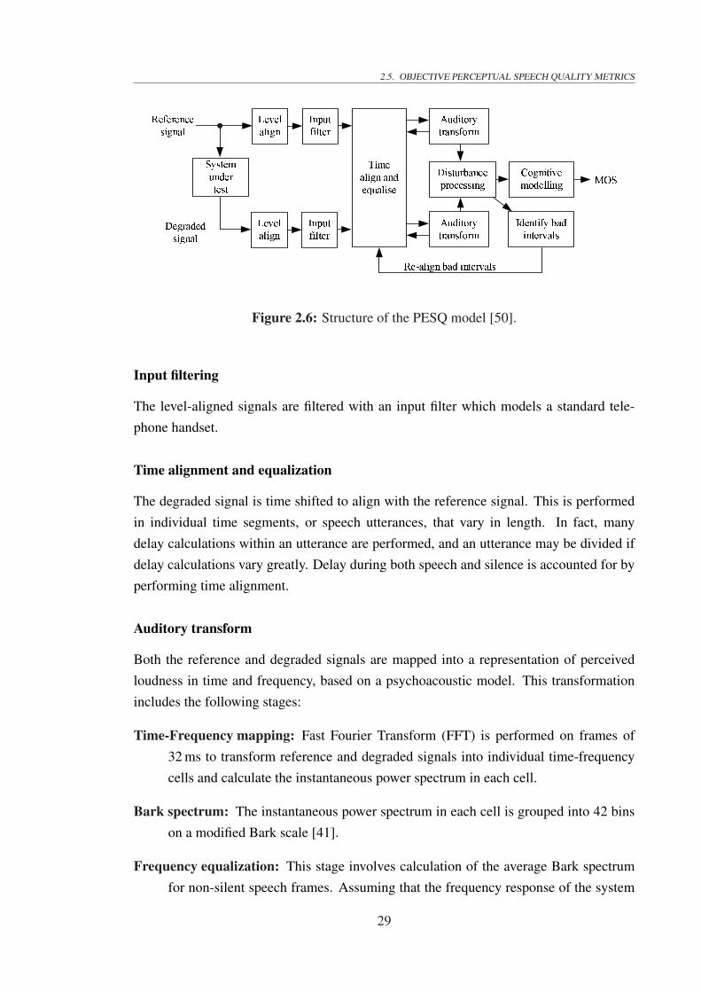
2.5. OBJECTIVE PERCEPTUAL SPEECH QUALITY METRICSInputfilterLevelalign Timealign andequalise AuditorytransformAuditorytransformDisturbanceprocessing CognitivemodellingIdentify badintervalsInputfilterLevelalign Re-align bad intervals MOSReferencesignalDegradedsignal SystemundertestFigure 2.6: Structure of the PESQ model [50].
Input filtering
The level-aligned signals are filtered with an input filter which models a standard tele-phone handset.
Time alignment and equalization
The degraded signal is time shifted to align with the reference signal. This is performedin individual time segments, or speech utterances, that vary in length. In fact, manydelay calculations within an utterance are performed, and an utterance may be divided ifdelay calculations vary greatly. Delay during both speech and silence is accounted for byperforming time alignment.
Auditory transform
Both the reference and degraded signals are mapped into a representation of perceivedloudness in time and frequency, based on a psychoacoustic model. This transformationincludes the following stages:
Time-Frequency mapping: Fast Fourier Transform (FFT) is performed on frames of32 ms to transform reference and degraded signals into individual time-frequencycells and calculate the instantaneous power spectrum in each cell.
Bark spectrum: The instantaneous power spectrum in each cell is grouped into 42 binson a modified Bark scale [41].
Frequency equalization: This stage involves calculation of the average Bark spectrumfor non-silent speech frames. Assuming that the frequency response of the system
29

2.5. OBJECTIVE PERCEPTUAL SPEECH QUALITY METRICS
under test is constant, the ratio between the spectra of reference and degraded sig-nals gives an estimate of the transfer function of the system. This estimate is usedto equalize the degraded to the reference signal.
Equalization of gain variation: In each frame, the ratio between the audible power ofthe reference and degraded signals is first calculated. This ratio is then used toequalize the gain of the degraded and reference signals in that frame.
Loudness mapping: The Bark spectrum is mapped to Sone [40] loudness scale to givean indication of the perceived loudness in each time-frequency cell.
Disturbance processing and cognitive modeling
After mapping of both the reference and degraded signals to Sone loudness scale, theabsolute value of the loudness difference between the two signals in each frame is cal-culated. This difference, which gives a measure of audible error, is processed in severalstages, as explained below, before it is mapped to MOS scale.
Masking of small distortions: A simple threshold is defined below which loudness dif-ferences are considered inaudible. To model the effect of masking, this threshold issubtracted from the absolute loudness difference in each frame. The masked valueof the absolute loudness difference in each frame is called frame disturbance.
Asymmetry processing: Here, first the ratio of the Bark spectral density of the degradedto the reference signal in each time-frequency cell is calculated. This ratio is thenraised to the power 1.2 to give an asymmetry factor. This asymmetry factor is mul-tiplied with each frame disturbance to obtain an asymmetric weighted disturbance.The asymmetric weighted disturbance is used for measuring additive distortions,i.e., distortions due to new time-frequency components added to the signal by thecodec or other sources of errors. Additive distortions are more audible to listenersthan distortions caused by a codec leaving or removing a time-frequency compo-nent.
Disturbance values aggregation and MOS prediction: Two disturbance averages arecalculated, one from asymmetric weighted disturbance values and the other fromframe disturbance values before they are weighted by the asymmetry factor. Thesetwo average values are combined linearly to calculate a MOS.
30

2.5. OBJECTIVE PERCEPTUAL SPEECH QUALITY METRICS
Identification of bad intervals
Another assessment of time alignment is performed for consecutive frame disturbanceswhose values are above a given threshold. If time alignment is determined to be inaccurateresulting in large frame disturbances, time alignment is repeated and frame disturbancesare recomputed.
2.5.2 The E-model
The E-model, which is an abbreviation for the European Telecommunications StandardsInstitute (ETSI) Computation Model, was developed in 1996. Although initially it wasdeveloped as a computational tool for network planning [49], it is now being used to pre-dict speech quality non-intrusively for VoIP applications [51]. The E-model assumes anadditive relationship between a number of transmission parameters that affect the speechquality. These parameters are: R0 which represents the signal-to-noise ratio; Is represent-ing the impairments occurring simultaneously with the speech signal, e.g., quantizationnoise, sidetone level and received speech level; Id representing the impairments caused bydelay, e.g., talker/listener echo and absolute delay; Ie representing the impairments due toinformation loss caused by speech codecs in the process of speech compression and de-compression. As for AE−model, it is the advantage factor, e.g., mobile phone users may tol-erate lower speech quality, compared with the quality offered by land line phones, becauseof the convenience offered by the mobile phones. Therefore, for land lines, AE−model is 0while for GSM it is 10.
The E-model produces a transmission rating R which can be used to estimate conver-sation quality. The value of R, which lies between 0 and 100, is calculated as follows [49]:
R = R0 − Is − Id − Ie + AE−model (2.16)
An R value below 50 indicates unacceptable or very poor quality while a value between90 to 100 indicates excellent quality.
Although since its introduction, the E-model has evolved and has been enhanced tobecome a useful tool for non-intrusive voice quality measurement in VoIP networks, it hassome limitations which hinders its widespread application in other communication net-works. For example, because expensive and time-consuming subjective tests are requiredto derive model parameters, the E-model is only applicable to a limited number of codecsand network conditions. Furthermore, the E-model is based on the assumption that theindividual transmission parameters, used in calculation of R in (2.16), are independent ofeach other and are additive, which may not always be true [52].
31

2.5. OBJECTIVE PERCEPTUAL SPEECH QUALITY METRICS
2.5.3 The single sided speech quality measure
In 2003, the companies Psytechnics, OPTICOM, and SwissQual combined their expe-rience, expertise and individual models to create the best possible algorithm to date fornon-intrusive speech quality measurement. After considerable testing and verification thecollaborative effort from the above three companies was selected and standardized by theITU-T as Recommendation P.563, also known as 3SQM, released in May 2004.
Briefly, 3SQM model starts by pre-processing the input speech signal. This pre-processing involves modeling the receiving handset, identification of portions of the signalthat contain speech, calculation of speech signal level and subsequent adjustment of thesignal level to a given constant level.
After pre-processing, the speech signal is further analyzed and a set of characteriz-ing signal parameters are extracted. Based on a restricted set of key parameters such asaverage pitch of the signal and SNR, an assignment to a main distortion class is made.The assigned distortion class together with the key parameters are used to adjust a speechquality model which would give objective quality estimates of subjective MOS. The av-erage Pearson correlation coefficient between 3SQM MOS and subjective MOS has beenreported to be 0.89. For a more comprehensive description of 3SQM, the reader is referredto [5].
Although, initially one would think that 3SQM would be ideal for application withlink adaption in mobile radio systems, there are some observations that make 3SQM anunattractive candidate. They are as follows:
• The quality scores of 3SQM are based on ACR. This means that if the originalsignal, before it is transmitted, is of bad quality (for example because of somebackground noise at the source) then 3SQM cannot differentiate if the degradationin quality is from the source or due to transmission errors. Therefore, a link adap-tion technique based on 3SQM may assume that the degradation of the quality isdue to deterioration in the link and it will be pointless to try to compensate forit. This, however, is not the case with the referenced speech quality measurementmethods, such as PESQ. A referenced speech quality metric would give a qualityscore relative to the quality of the original signal. As such, if deteriorations in theoriginal signal due to transmission errors are negligible, a referenced metric wouldgive a high quality score even if the absolute quality rating of the original signal isunacceptably low.
• Intrusive metrics are generally more accurate than their non-intrusive counterpartsand give a higher correlation with the subjective MOS. The correlation coefficient
32
2.6. SUMMARY
of 3SQM scores with subjective MOS values is on average 0.89 as compared to thatof PESQ which is 0.935.
• The minimum length of active speech required for quality assessment by 3SQM is3 s. This means that for conversational speech, assuming the activity rate is 50%,the update rate of 3SQM would at best be 1/6 s−1. This is an unacceptably slowupdate rate for link adaptation in radio systems such as power control of UMTS.
• It is reported that the MOS scores produced by 3SQM are more widely spread thanthose produced by PESQ, and it is necessary to average the results of multiple testsin order to achieve a stable quality metric. This implies that the update rate of3SQM may be even slower than 1/6 s−1.
2.6 Summary
In this chapter, the necessary background information required for study of the rest ofthe thesis was presented. As this thesis is concerned with power control of mobile radiosystems using perceptual speech quality metrics, first the favorable power control schemeswere presented in general. This was followed by examples of power control schemesemployed in some widespread 2G and 3G systems. Additionally, the role of power controlas one of the more important features in saving precious resources and increasing thecapacity of mobile radio systems was emphasized.
The second part of this chapter was dedicated to review of the quality metrics that areused for speech quality assessment. Here we described some of the conventional metricscommonly used in power control algorithms and compared them with each other. Wealso presented a survey of perceptual speech quality measurement methods. A referencedobjective perceptual speech quality metric, PESQ, was particularly described in moredetail, as it will form the core of our novel technique for real-time perceptual speechquality measurement in the next chapter. Furthermore, as none of the quality metrics usedin conventional power control algorithms of mobile radio systems is based on models ofhuman auditory system, it will be shown that the application of our novel technique inthese power control algorithms will improve their efficiency.
33

34

Chapter 3
Novel Technique for Real-TimePerceptual Speech QualityMeasurement
3.1 Introduction
In many mobile radio systems, accurate speech quality measurements are required for avariety of reasons. These range from daily system maintenance to resource managementsuch as power control. While objective perceptual speech quality measurement techniqueshave been improved significantly over the last decade, their usage has been restricted tomainly non real-time applications such as speech codec tests [4]. The main reason for thishas been the dependence of these speech quality measurement techniques on the originalspeech signal so it can be used as reference for accurate quality estimation. However,the reference signal cannot be provided in the receiver in real-time applications such aspower control of a mobile radio system. Consequently, metrics such as CIR, BER, FERand a variety of other channel quality metrics have commonly been used for estimation ofspeech quality [1, 53, 54].
It should be noted that speech quality estimation techniques, which are based on chan-nel metrics, are not truly perceptual as they are not based on human auditory system andthus do not exploit the psychoacoustic properties of the speech signal. Some of the impor-tant psychoacoustic properties that need to be modeled and taken into account by a speechquality metric are masking, loudness of partially masked time-frequency components andloudness of time-frequency components that are not masked. Masking itself is describedas the effect by which a weaker, but audible signal (the maskee) becomes imperceptiblein the presence of a relatively louder signal (the masker) [55].
35

3.1. INTRODUCTION
In this chapter, the novel Real-Time Perceptual Speech Quality Measurement (RTP-SQM) technique for mobile radio systems is described. This technique is based on thewell-known ITU Recommendation P.862 - PESQ. As PESQ requires both the originaland the degraded speech samples for measuring the speech quality, a feedback methodis proposed that will be used to synthesize the degraded speech sample at the transmitterwhere the original speech sample is available.
Although the proposed technique can be employed in any communication system thatuses the Adaptive Multi-Rate (AMR) speech codec (see Section 3.2), such as GSM andUMTS, here the performance of the technique is investigated for UMTS. Before describ-ing the proposed technique, some background on the operation of relevant building blocksof a typical frame-based speech communication system, in general, and UMTS in partic-ular is given.
The contributions and findings of this chapter are:
• Presentation of a novel technique for real-time perceptual speech quality measure-ment of frame-based mobile radio systems.
• Performance evaluation of the proposed RTPSQM technique in terms of measuringperceptual speech quality for UMTS in a simulation environment. The simulationswere carried out for a representative set of test conditions, including three vehicularspeeds of 3, 50 and 120 km/h, three AMR codec rates of 4.75, 7.40 and 12.2 kbps,and three FER targets of 1, 3 and 5%.
• Statistical analysis of the relationship between perceptual speech quality scores ob-tained by the proposed RTPSQM technique and PESQ. Here a set of linear regres-sion equations that could be used to map the quality scores obtained by the proposedtechnique to those of PESQ are presented. Using these regression equations, it isfound that the standard deviation of estimation error between the quality scores ofthe proposed technique and PESQ is less than 0.2 MOS. A MOS difference of 0.2is hardly perceivable by human ear. The mean of the estimation error is found to beapproximately zero, which is ideal.
• Since the proposed RTPSQM technique can accurately measure the perceptual speechquality and in real-time, it finds application in link adaptation algorithms of frame-based mobile radio systems. In such systems, the speech quality metric providedby the proposed technique, can replace the conventional metrics, e.g., BER andFER of the link adaptation algorithms to improve their performance. Applicationof the proposed technique in power control of GSM and UMTS is investigated inChapters 4 and 5, respectively.
36

3.2. FRAME-BASED SPEECH COMMUNICATION SYSTEMS
3.2 Frame-based Speech Communication Systems
In a typical frame-based speech communication system as shown in Fig. 3.1, the analogspeech is digitized and divided into blocks of fixed duration by, usually, a Pulse CodeModulation (PCM) encoder. Each PCM-encoded speech block is then compressed (orencoded) by a speech encoder and is output as a frame of pre-determined size. The speechencoder removes redundant information in the speech frames in such a way that theycould be reproduced by a corresponding speech decoder at the receiver. The variousbits at the output of the speech encoder have unequal perceptual importance. That is,bit errors affect the quality of the reconstructed speech differently depending on whichbits are corrupted. In this case, the bits at the output of the speech encoder may berearranged according to their perceptual importance and protected by unequal ForwardError Correction (FEC) codes. Thus, those bits that are perceptually more important forreconstruction of speech are protected by more powerful FEC codes, whereas the lessimportant bits are either protected by less powerful FEC codes or not protected at all.After FEC-encoding, the frames are further processed (filtering, modulation, etc.) andtransmitted through a medium, which in our case is the mobile radio channel, to thereceiver. At the receiver, the reverse of all the above operations are performed in anattempt to synthesize a speech signal which is as close as possible to the original speechsignal. That is, after some processing on the received signal, such as equalization anddemodulation, it is decoded using an appropriate FEC decoder and then converted toPCM format using a corresponding speech decoder.
An example of a frame-based speech communication system described above isUMTS. Some of the functional blocks of a UMTS transmitter are shown in Fig. 3.2.UMTS employs an AMR speech codec [56]. The AMR speech encoder accepts digitizedspeech blocks of 20 ms duration, compresses the speech blocks using an Algebraic CodeExcited Linear Prediction (ACELP) algorithm [57, 58] and rearranges its output bits intothree classes of A, B, and C in decreasing order of their perceptual importance [58]. In atypical implementation, Class A bits are protected by rate 1/3 Convolutional Coding (CC),Class B bits with rate 1/2 CC, and Class C bits are left unprotected or protected by rate1/2 CC [59]. Class A bit errors can cause undesirable artifacts in the reproduced speech,while Class B and Class C bit errors cause less severe degradation of speech quality. Forthis reason, in addition to applying extra error protection to Class A bits, a Cyclic Redun-dancy Check (CRC) word is added to Class A bits to detect possible errors in decodedClass A bits at the receiver.
Additionally, the AMR speech decoder at the receiver end of the communication sys-tem employs an error-concealment procedure to conceal the undesirable effects of erro-
37

3.2. FRAME-BASED SPEECH COMMUNICATION SYSTEMS
Speech inTransmitter Receiver
Reconstructed Speech outChannel
Channel DecoderSpeech Encoder
Filtering and ModulationPCM Encoder
Speech DecoderEqualization, Demodulation
PCM DecoderChannel Encoder
Figu
re3.
1:B
lock
diag
ram
ofa
spee
chco
mm
unic
atio
nsy
stem
.
38

3.3. PROPOSED REAL-TIME PERCEPTUAL SPEECH QUALITY MEASUREMENT TECHNIQUEConvolutionalCodingCRCClass A bitsClass B bitsClass C bits Rate 1/2Rate 1/2Rate 1/3AMRSpeechCodecDigitizedSpeechFigure 3.2: Grouping of compressed bits at the output of an AMR encoder and a typical
forward error correction scheme for UMTS.
neous Class A bits [60]. Class A bit errors result in erasure of the corresponding frame inwhich case, the Class A bits are substituted with either a repetition or an extrapolation ofClass A bits from previous “good” speech frame(s). Frame Erasure (FE) itself is decidedbased on the so-called Frame Quality Indicator (FQI). This is a binary flag associatedwith every received speech frame. After a CRC on decoded Class A bits at the receiver,the value of FQI is determined and set in the header of the AMR frame. For a genericstructure of an AMR frame and how FQI fits in that structure, see Fig. 3.3. An expla-nation of the other constituents of an AMR frame, i.e., Frame Type, Mode Indication,Mode Request and Codec CRC (this is a different CRC from the one shown in Fig. 3.2)is not relevant to our topic and as such the interested reader is referred to [58] for moreinformation.
It should be pointed out here that in view of the fact that generally in systems em-ploying an AMR codec a frame error would result in erasure of that frame, therefore, forsuch systems frame error rate is equal to frame erasure rate. As in this thesis, we focus onmobile radio systems that use an AMR codec, FER is used to represent both frame errorrate and frame erasure rate interchangeably.
3.3 Proposed Real-Time Perceptual Speech Quality Mea-surement Technique
3.3.1 Motivation
Due to high accuracy of PESQ in measuring perceptual quality of speech for a wide rangeof network conditions and error types including errors due to mobile radio channels [50],
39

3.3. PROPOSED REAL-TIME PERCEPTUAL SPEECH QUALITY MEASUREMENT TECHNIQUE
AMR Core Frame(Speech or comfortnoise data)Frame Type (4 bits)Codec CRC (8 bits)Mode Request (3 bits)Mode Indication (3 bits)Frame Quality Indicator (1 bit)Class C bitsClass B bitsClass A bits AMR HeaderAMR AuxiliaryInformationFigure 3.3: Generic AMR frame structure.
it is sensible to use PESQ for speech quality measurement in a mobile radio system.However, to use PESQ at the receiver side of a communication system, where the conven-tional metrics such as CIR, BER or FER are measured, is impractical. The reason beingthat PESQ is a referenced quality measurement algorithm requiring a copy of the originalspeech signal at the point of measurement.
Unable to use PESQ at the receiver side of a communication system, the question isthen asked: How about using PESQ at the transmitter side where the original signal isreadily available? The initial answer to this question is, that although at the transmitterwe have access to the original speech signal, we do not have access to the received or de-coded speech signal which is also required by PESQ for quality measurement. Therefore,regardless of where PESQ is used, transmitter or receiver, one of the required speech sig-nals for PESQ is missing. However, knowing how frame-based communication systemswork, it is possible to find a way around this problem, which is presented in the sequel.
3.3.2 Solution
For real-time measurement of perceptual speech quality, it is proposed that the FrameErasure Pattern (FEP) of the received frames is sent back to the transmitter via a returnchannel as shown in Fig. 3.4. At the receiver side, the CRC words on Class A bits ofthe speech frames are tested by the frame quality check block. This block generates anFQI flag for every received frame. Specifically, a binary “1” or “0” is generated to signalthat a received frame was “bad” or “good”, respectively. This pattern of “1”s and “0”scorresponds to the pattern of frame erasure associated with the AMR error-concealment
40

3.3. PROPOSED REAL-TIME PERCEPTUAL SPEECH QUALITY MEASUREMENT TECHNIQUE
ReceiverSpeech SignalTransmitter AMR Encoder
Frame Quality CheckAMR DecoderReceived SpeechDelay D
elay + AMR DecoderFEPPESQ
Physical LayerReference SignalSynthesized Signal
Objective Quality Save to fileSave to file
PESQ
=Pe
rcep
tual
Eva
luat
ion
ofSp
eech
Qua
lity
AM
R=
Ada
ptiv
eM
ulti-
Rat
eFE
P=
Fram
eE
rasu
rePa
ttern
Figu
re3.
4:Fu
nctio
nalb
lock
diag
ram
forp
erce
ptua
lqua
lity
estim
atio
nba
sed
onfr
ame
eras
ure
patte
rn.
41

3.4. PERFORMANCE EVALUATION OF THE PROPOSED TECHNIQUE
procedure. In Fig. 3.4, a corresponding binary signal, denoted by FEP, is sent back tothe transmitter. The fed back FEP is used for synthesizing the receiver speech signal.This is achieved by applying the same error-concealment procedure at the transmitter asused in the receiver. The transmitted frames are buffered to account for the round-tripdelay, which for our simulation model is 40 ms, the time duration of two speech frames.This delay is introduced by the interleaver/deinterleaver arrays which need to be filledin before interleaving/deinterleaving operations could start. The buffered frames whosequality is now available through the FEP feedback channel are decoded by the AMRdecoder. The FQI flag in the header of each speech frame output by the AMR encoder ismodified based on the corresponding bit from FEP before that frame is sent to the AMRdecoder at the transmitter. The speech signal synthesized in this way contains the samequality degradation resulting from frame erasures as the decoded signal at the receiver.This synthesized speech signal is suggested to be fed to PESQ, as an approximation ofthe decoded speech signal at the receiver, to calculate the objective quality.
Although the synthesized speech signal includes the quality degradation from Class Abits, degradations due to Class B and C errors are not accounted for. However, knowingthat Class A bits are perceptually the most important bits, it is shown in the sequel thatexclusion of the effect of erroneous Class B and C bits in calculation of objective qualitydoes not make a significant impact on the results.
Furthermore, the following points should be noted about the RTPSQM technique:
• Frame errors that comprise the FEP are sent to the transmitter individually and arenot accumulated for a number of frames.
• Although for transmission of a frame error which can have a value of “1” or “0”,one data bit is sufficient, for practical implementation one might use a byte perframe error.
• The proposed implementation of RTPSQM assumes that FEP bits are not corruptedby channel errors despite the fact that they are not protected by any FEC codes.However, if frame errors were to be transmitted in bytes, then a simple repetitioncode could be used to provide error protection for the FEP bits.
3.4 Performance Evaluation of the Proposed Technique
The performance of the proposed FEP feedback based RTPSQM technique, in terms ofits ability to estimate perceptual speech quality, was investigated through computer simu-lations. The simulations were based on the system model depicted in Fig. 3.4 which was
42

3.4. PERFORMANCE EVALUATION OF THE PROPOSED TECHNIQUE
implemented on Matlab Simulink platform. The AMR codec was based on the third gen-eration Partnership Project (3GPP) reference implementation [57]. The physical layer ofUMTS was implemented in detail, at chip-level1, according to 3GPP specifications [61].The PESQ software was the one provided by ITU [4]. A summary of the model parame-ters are given in Table 3.1.
It should be noted that in Fig. 3.4, the received and synthesized speech signals atthe receiver and transmitter sides, respectively, were saved in a file. This was necessaryduring evaluation phase of the proposed technique only. In application of the proposedtechnique in mobile radio systems, there is no need to save the received and synthesizedspeech signals.
Table 3.1: Main simulation parameters.
Chip rate 3.84 Mc/sSpreading factor 128Channel bit rate 60 kbpsTransmission Time Interval (TTI) 20 msTime slot format #8
(Npilot, NTPC , NTFCI ) (4, 2, 0)Rate matching Discontinuous transmission used in downlinkPower control Outer & inner loopChannel type
Additive White Gaussian Noise (AWGN) ONLog-normal fading ON (standard deviation 8 dB)Fast fading 6-tap Vehicular A model
Vehicular speed 3, 50 and 120 km/hChannel coding
Class A Rate 1/3 CC + 12 bits CRCClass B Rate 1/2 CCClass C Rate 1/2 CC
AMR codec rates 4.75, 7.40 and 12.20 kbpsFER target 1, 3 and 5%
The simulations were carried out for two sets of speech files, where each set contained32 files, obtained from the ITU database for voice quality measurement tests [62]. Thefiles in the first set were used as training data to obtain a set of mapping functions betweenthe estimated quality by the proposed technique and the actual quality. The purpose ofthe second set of speech files was to verify the accuracy of the mapping functions derivedfrom the training data. Each speech file was of 8 s duration and contained short utterancesseparated by silence intervals with equal proportions of speech and silence. Speech from
1We would like to thank and acknowledge PHYBIT Inc. Singapore for permitting us to use their UMTSphysical layer simulation software.
43

3.5. SUMMARY OF RESULTS AND DISCUSSION
both male and female speakers were used. For the name of the ITU speech files used intraining and verification parts, see Tables A.1 and A.2, respectively, in Appendix A.
For performance evaluation of the proposed technique, different AMR codec rates,vehicular speeds and FER targets were considered, the reasons for which are as follows:
The need for different AMR codec rates: The quality degradation due to Class B andC errors depends on the perceptual importance of the affected bits as well as theBER of the decoded bits. The perceptual importance of bits is a function of thespeech codec rate. It is evident that these bits become more important in the qualityof the reconstructed speech as the codec rate is decreased. As such, at any givenBER, the quality of speech is expected to decrease with lower codec rates, hencethe need to consider different AMR codec rates. In our simulations we used threeAMR codec rates of 4.75 kbps (the lowest of the eight possible AMR codec ratesspecified in [57]), 7.4 kbps and 12.2 kbps (the highest codec rate specified in [57]).
The need for different vehicular speeds: Another important factor in evaluating the per-formance of the proposed technique is the BER of the decoded bits. Obviously, thespeech quality for a given AMR codec rate is expected to degrade with increasedBER. The BER is affected by the channel conditions, which is affected by vehicularspeed, and the received SIR. For this reason, the simulations were carried out fordifferent vehicular speeds. The three vehicular speeds considered were 3, 50 and120 km/h.
The need for different FER targets: It was mentioned that one of the factors affectingthe BER of decoded bits is the received SIR. However, the received SIR itself iscontrolled within a practical range by applying different FER target values for theouter-loop power control. A FER target of 1% is a practical choice for good re-ceived speech quality [16, 18]. A choice of 5% for FER target is considered tolead to poor speech quality, in which case, a handover is usually initiated. In oursimulations, three FER target values of 1, 3 and 5% were used.
3.5 Summary of Results and Discussion
The results are presented in two parts. First the results for the training part are presentedand discussed, followed by those of the verification part. As explained in Section 3.4, thetraining part was used to obtain a set of mapping functions between the quality scoresas estimated by the proposed technique and the actual quality measured by PESQ. Thepurpose of the verification part, on the other hand, was to analyze the accuracy of themapping functions derived from the training data.
44

3.5. SUMMARY OF RESULTS AND DISCUSSION
3.5.1 Training part: determination of mapping functions
Using the simulation model shown in Fig. 3.4, for any one input ITU speech file fromTable A.1 (see Appendix A), two output files were obtained. These output files were usedto calculate two scores: one for actual quality MOSact, and the other for estimated qualityMOSest. The PESQ MOS obtained when the two inputs to PESQ software were the ITUspeech file and the saved speech file at the receiver side, was called MOSact. Whereasthe PESQ MOS obtained when the two inputs to PESQ software were the ITU speechfile and the synthesized speech file saved at the transmitter side, was called MOSest. Theprocedure for calculating the actual and estimated qualities is as follows:
Procedure 3.1 Determination of actual and estimated quality scores for a givenITU speech file
Step 1: Initialize the simulation model (see Fig. 3.4). This involves the following:
• Setting the rates for the AMR encoder and the two AMR decoders identically.
• Setting the parameters of the UMTS physical layer to simulate the requiredvehicular speed and FER target value of the outer-loop power control.
• Initialize the frame index n = 1.
Step 2: Read in nth frame frm(n) from the ITU input speech file.
Step 3: Encode frm(n) using the AMR encoder.
Step 4: Transmit the AMR encoded frm(n) through the UMTS physical layer.
Step 5: Decode the received frm(n) by the AMR decoder in the receiver and at the sametime send the FQI of frm(n) to the transmitter.
Step 6: Save the output frame of the receiver’s AMR decoder in a file.
Step 7: At the transmitter side, use the FQI of frm(n), received from the FEP feedbackchannel, to modify the FQI of frm(n) output by the AMR encoder before decodingthe frame by the transmitter’s AMR decoder. It should be noted that due to a fixeddelay in arrival of the FQI of frm(n) at the transmitter, the output of AMR encoderneeds to be delayed appropriately (see Fig. 3.4).
Step 8: Save the output of the transmitter’s AMR decoder for frm(n) in a file.
Step 9: Check if there is any more frames in the ITU input speech file. If yes, then setn = n + 1 and goto Step 2. Else goto Step 10.
45

3.5. SUMMARY OF RESULTS AND DISCUSSION
Step 10: Calculate the PESQ MOS when the two inputs to PESQ software are the ITUspeech file and the saved file at the output of the receiver’s AMR decoder. Namethe PESQ MOS thus calculated as MOSact.
Step 11: Calculate the PESQ MOS when the two inputs to PESQ software are the ITUspeech file and the saved file at the output of the transmitter’s AMR decoder. Namethe PESQ MOS thus calculated as MOSest.
Step 12: Exit the procedure. ¤
The plots of actual versus estimated quality scores for the three AMR codec rates of4.75, 7.40 and 12.20 kbps with different permutations of FER target values and vehicularspeeds are shown in Figs. 3.5, 3.6, and 3.7, respectively. Each figure has three sub-figureslabeled (a), (b), and (c), corresponding to FER targets of 1, 3 and 5%, respectively.
Furthermore, on all figures, a linear regression mapping function is shown which couldbe used to map the MOSest to MOSact. If the linear equation for the mapping functionsis given by
y = ax + b (3.1)
where, y, a, x, and b represent MOSact, the line gradient, MOSest, and the line y-intercept, respectively, then a and b values for the regression lines of Figs. 3.5, 3.6, and 3.7are as shown in Table 3.2. The ideal case for performance of the FEP feedback technique
Table 3.2: Gradient a and y-intercept b of regression lines for three AMR codec rates andFER targets.
AMR rate 4.75 kbps 7.40 kbps 12.2 kbpsFER target 1% 3% 5% 1% 3% 5% 1% 3% 5%
a 0.91 0.83 0.85 0.96 0.79 0.83 0.93 0.84 0.78b 0.06 0.21 0.08 -0.06 0.43 0.26 -0.11 0.09 0.21
would be when MOSest = MOSact, i.e., the quality estimates of FEP feedback techniqueare equal to actual PESQ MOS values. This is shown by the linear function y = x on Figs.3.5, 3.6, and 3.7 (dashed line). However, plots of MOSact versus MOSest show that inall simulated cases the regression lines are below the line y = x, which implies that FEPfeedback technique, generally, overestimates the actual quality. This overestimation, asexplained in Section 3.3.2, is due to absence of the effect of Class B and C bit errors inthe synthesized signal (see Fig. 3.4), which was used to approximate the received signal.
With the regression line equations determined as shown in Table 3.2, their suitabilityin estimating the perceptual quality is verified next.
46

3.5. SUMMARY OF RESULTS AND DISCUSSION
y = x y = 0.91x + 0.06
2
2.5
3
3.5
4
2 2.5 3 3.5 4
MOS est
MO
S act
Veh. speed of 3 km/hVeh. speed of 50 km/hVeh. speed of 120 km/hIdealRegression
(a)
y = x y = 0.83x + 0.21
2
2.5
3
3.5
4
2 2.5 3 3.5 4
MOS est
MO
S act
Veh. speed of 3 km/hVeh. speed of 50 km/hVeh. speed of 120 km/hIdealRegression
(b)
y = xy = 0.85x + 0.08
2
2.5
3
3.5
4
2 2.5 3 3.5 4
MOS est
MO
S act
Veh. speed of 3 km/hVeh. speed of 50 km/hVeh. speed of 120 km/hIdealRegression
(c)
Figure 3.5: Actual speech quality MOSact versus estimated speech quality MOSest forAMR codec rate 4.75 kbps and FER target (a) 1%, (b) 3% and (c) 5%.
47

3.5. SUMMARY OF RESULTS AND DISCUSSION
y = x y = 0.96x - 0.06
2
2.5
3
3.5
4
2 2.5 3 3.5 4
MOS est
MO
S act
Veh. speed of 3 km/hVeh. speed of 50 km/hVeh. speed of 120 km/hIdealRegression
(a)
y = x y = 0.79x + 0.43
2
2.5
3
3.5
4
2 2.5 3 3.5 4
MOS est
MO
S act
Veh. speed of 3 km/hVeh. speed of 50 km/hVeh. speed of 120 km/hIdealRegression
(b)
y = x y = 0.83x + 0.26
2
2.5
3
3.5
4
2 2.5 3 3.5 4
MOS est
MO
S act
Veh. speed of 3 km/hVeh. speed of 50 km/hVeh. speed of 120 km/hIdealRegression
(c)
Figure 3.6: Actual speech quality MOSact versus estimated speech quality MOSest forAMR codec rate 7.40 kbps and FER target (a) 1%, (b) 3% and (c) 5%.
48

3.5. SUMMARY OF RESULTS AND DISCUSSION
y = x y = 0.93x - 0.11
2
2.5
3
3.5
4
2 2.5 3 3.5 4
MOS est
MO
S act
Veh. speed of 3 km/hVeh. speed of 50 km/hVeh. speed of 120 km/hIdealRegression
(a)
y = x y = 0.84x + 0.09
2
2.5
3
3.5
4
2 2.5 3 3.5 4
MOS est
MO
S act
Veh. speed of 3 km/hVeh. speed of 50 km/hVeh. speed of 120 km/hIdealRegression
(b)
y = x y = 0.78x + 0.21
2
2.5
3
3.5
4
2 2.5 3 3.5 4
MOS est
MO
S act
Veh. speed of 3 km/hVeh. speed of 50 km/hVeh. speed of 120 km/hIdealRegression
(c)
Figure 3.7: Actual speech quality MOSact versus estimated speech quality MOSest forAMR codec rate 12.2 kbps and FER target (a) 1%, (b) 3% and (c) 5%.
49

3.5. SUMMARY OF RESULTS AND DISCUSSION
3.5.2 Verification part: analyzing accuracy of mapping functions
To verify the accuracy of the regression lines of Table 3.2, the simulations of Section 3.4were repeated, but this time using a different set of ITU input speech files (see Table A.2in Appendix A) to obtain two new sets of MOSest,v and MOSact,v quality scores. Theindex v is used to indicate that these scores are for the verification part and are differentfrom their counterparts, obtained during the training part. For each value of MOSest,v anappropriate regression line equation from Table 3.2, was used to calculate the correspond-ing PESQ MOS. The PESQ MOS values thus calculated were represented by MOSfep,where the subscript “fep” was used to emphasize that MOSfep is a calculated MOS basedon the proposed FEP-based technique and is different from MOSact,v which is measuredby the PESQ software. The steps involved are summarized in the procedure below.
Procedure 3.2 Determination of MOSfep for a given ITU speech file
Step 1: Run Procedure 3.1 to obtain MOSest,v and MOSact,v for the given ITU speechfile.
Step 2: For the given AMR codec rate and FER target value, use an appropriate regres-sion line equation from Table 3.2 to map MOSest,v to MOSfep
Step 3: Exit the procedure. ¤
Using Procedure 3.2, MOSfep values for all combinations of the three AMR codecrates, vehicular speeds, FER targets (see Table 3.1) and the 32 ITU speech files of TableA.2 (see Appendix A) were calculated. The values of MOSact,v were plotted againsttheir corresponding MOSfep values and are shown in Figs. 3.8, 3.9, and 3.10 for AMRcodec rates of 4.75, 7.4, and 12.2 kbps, respectively. From these scatter diagrams, itcan be observed that for all considered AMR codec rates and FER targets, the pointsare scattered around the ideal line of y = x. To further evaluate the performance ofthe proposed technique, however, some statistical analysis of the MOSfep and MOSact,v
values is performed in the sequel.
Correlation coefficients
To measure the correlation between MOSfep and MOSact,v values, the Pearson linearcorrelation coefficient is used. The Pearson correlation coefficient r is a real number inthe interval [-1, +1]. A value of +1 means that there is a perfect positive (or direct) linearrelationship between the two data sets. A value of -1 means that there is a perfect negative
50

3.5. SUMMARY OF RESULTS AND DISCUSSION
y = x
2
2.5
3
3.5
4
2.0 2.5 3.0 3.5 4.0
MO
S act
,v
MOS fep
Veh. speed of 3 km/hVeh. speed of 50 km/hVeh. speed of 120 km/hIdeal
(a)
y = x
1.5
2
2.5
3
3.5
1.5 2 2.5 3 3.5
MOS fep
MO
S act
,v
Veh. speed of 3 km/hVeh. speed of 50 km/hVeh. speed of 120 km/hIdeal
(b)
y = x
1.5
2
2.5
3
3.5
1.5 2 2.5 3 3.5
MOS fep
MO
S act
,v
Veh. speed of 3 km/hVeh. speed of 50 km/hVeh. speed of 120 km/hIdeal
(c)
Figure 3.8: Actual speech quality MOSact,v versus calculated speech quality MOSfep
for AMR codec rate 4.75 kbps and FER target of (a) 1%, (b) 3% and (c) 5%.
51

3.5. SUMMARY OF RESULTS AND DISCUSSION
y = x
2
2.5
3
3.5
4
2 2.5 3 3.5 4
MOS fep
MO
S act
,v
Veh. speed of 3 km/hVeh. speed of 50 km/hVeh. speed of 120 km/hIdeal
(a)
y = x
2
2.5
3
3.5
4
2 2.5 3 3.5 4
MOS fep
MO
S act
,v
Veh. speed of 3 km/hVeh. speed of 50 km/hVeh. speed of 120 km/hIdeal
(b)
y = x
2
2.5
3
3.5
4
2 2.5 3 3.5 4
MOS fep
MO
S act
,v
Veh. speed of 3 km/hVeh. speed of 50 km/hVeh. speed of 120 km/hIdeal
(c)
Figure 3.9: Actual speech quality MOSact,v versus calculated speech quality MOSfep
for AMR codec rate 7.4 kbps and FER target of (a) 1%, (b) 3% and (c) 5%.
52

3.5. SUMMARY OF RESULTS AND DISCUSSION
y = x
2
2.5
3
3.5
4
2 2.5 3 3.5 4
MOS fep
MO
S act
,v
Veh. speed of 3 km/hVeh. speed of 50 km/hVeh. speed of 120 km/hIdeal
(a)
y = x
2
2.5
3
3.5
4
2 2.5 3 3.5 4
MOS fep
MO
S act
,v
Veh. speed of 3 km/hVeh. speed of 50 km/hVeh. speed of 120 km/hIdeal
(b)
y = x
1.5
2
2.5
3
3.5
1.5 2 2.5 3 3.5
MOS fep
MO
S act
,v
Veh. speed of 3 km/hVeh. speed of 50 km/hVeh. speed of 120 km/hIdeal
(c)
Figure 3.10: Actual speech quality MOSact,v versus calculated speech quality MOSfep
for AMR codec rate 12.2 kbps and FER target of (a) 1%, (b) 3% and (c) 5%.
53

3.5. SUMMARY OF RESULTS AND DISCUSSION
(or inverse) linear relationship, and a value of 0 means there is no linear relationship at allbetween the data sets. Given a set of N data pairs (xi, yi), i = 1, 2, . . . , N , the Pearsonlinear correlation coefficient is defined as
r =
N∑i=1
(xi − x)(yi − y)
√√√√N∑
i=1
(xi − x)2N∑
i=1
(yi − y)2
(3.2)
where, in our case, xi and yi represent MOSfep,i and MOSact,v,i, respectively, and x andy are the means of the respective data sets calculated as follows:
x =1
N
N∑i=1
xi and y =1
N
N∑i=1
yi (3.3)
The Pearson correlation coefficients between MOSfep,i and MOSact,v,i values ofFigs. 3.8, 3.9, and 3.10 were calculated using (3.2) and are tabulated in Table 3.3.
Table 3.3: Pearson correlation coefficient r between MOSfep and MOSact,v for differentAMR codec rates and FER targets.
AMR codec rate 4.75 kbps 7.40 kbps 12.2 kbpsFER target 1% 3% 5% 1% 3% 5% 1% 3% 5%
r 0.87 0.86 0.84 0.89 0.91 0.93 0.82 0.85 0.89
Two observations can be made from the Pearson correlation coefficients r shown inTable 3.3:
• For all three FER targets, the correlation coefficient r is greater or equal to 0.82,indicating a high correlation between the MOSfep,i and MOSact,v,i values.
• All correlation coefficients are positive, indicating a direct correlation betweenMOSfep,i and MOSact,v,i values. That is, with increasing calculated speech qualityMOSfep,i, the actual speech quality values MOSact,v,i also increase.
Estimation errors
Apart from Pearson’s correlation coefficient, there are other measures that may be used togive an alternative view of the closeness of MOSfep,i to MOSact,v,i values. For example,if the estimation error between MOSfep,i and MOSact,v,i, i = 1, 2, . . . , N , is defined by
ei = MOSfep,i −MOSact,v,i (3.4)
54

3.5. SUMMARY OF RESULTS AND DISCUSSION
then the histogram of estimation errors provides a quick view of how frequently errorsof different magnitudes occur. The histograms of estimation errors for AMR codec ratesof 4.75, 7.4 and 12.2 kbps are shown in Figs. 3.11(a), 3.11(b), and 3.11(c), respectively.From these histograms it can be observed that the distributions of the estimation errorsare approximately normal.
Furthermore, the mean me,MOS and standard deviation σe,MOS of estimation errorsfor the three AMR codec rates and the three simulated FER targets were calculated andare tabulated in Table 3.4. The mean of each histogram represents the average bias inestimation of the quality. It is observed from the results of Table 3.4 that means of thehistograms are practically equal to zero, confirming that the mapping functions on averagehelped in removing the quality overestimation arising from overlooking Class B and Cerrors. As for the standard deviations σe,MOS of the histograms, they range between 0.08and 0.15 MOS points. In each histogram, the deviations of the estimation error from themean are largely due to the mapping function’s inability to take into account the effect ofClass B and C bit errors exactly as well as the effect of the vehicular speed, which hadnot been accounted for in the proposed scheme. It is noted that in all cases the standarddeviations of estimation errors are sufficiently small to be perceived by human ears.
Table 3.4: Mean me,MOS and standard deviation σe,MOS of estimation errors.
AMR codec rate 4.75 kbps 7.40 kbps 12.2 kbpsFER 1% 3% 5% 1% 3% 5% 1% 3% 5%
me,MOS -0.01 -0.01 0.01 0.01 0.00 -0.01 -0.01 -0.01 0.00σe,MOS 0.11 0.12 0.12 0.10 0.10 0.08 0.15 0.13 0.11
55
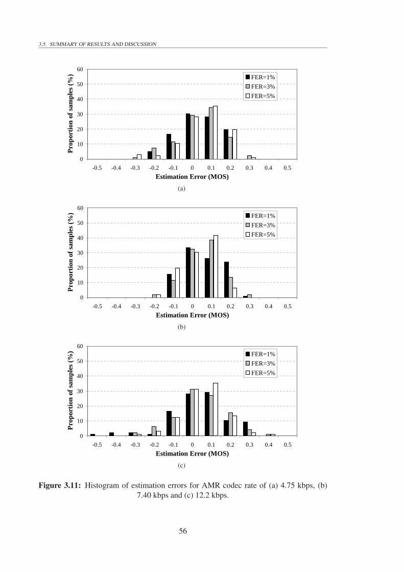
3.5. SUMMARY OF RESULTS AND DISCUSSION
0
10
20
30
40
50
60
-0.5 -0.4 -0.3 -0.2 -0.1 0 0.1 0.2 0.3 0.4 0.5
Estimation Error (MOS)
Pro
port
ion
of s
ampl
es (
%) FER=1%
FER=3%
FER=5%
(a)
0
10
20
30
40
50
60
-0.5 -0.4 -0.3 -0.2 -0.1 0 0.1 0.2 0.3 0.4 0.5
Estimation Error (MOS)
Pro
port
ion
of s
ampl
es (
%) FER=1%
FER=3%
FER=5%
(b)
0
10
20
30
40
50
60
-0.5 -0.4 -0.3 -0.2 -0.1 0 0.1 0.2 0.3 0.4 0.5
Estimation Error (MOS)
Pro
port
ion
of s
ampl
es (
%) FER=1%
FER=3%
FER=5%
(c)
Figure 3.11: Histogram of estimation errors for AMR codec rate of (a) 4.75 kbps, (b)7.40 kbps and (c) 12.2 kbps.
56

3.6. SUMMARY
3.6 Summary
The RTPSQM technique for estimation of perceptual speech quality was described in thischapter. This technique relies on the feedback of the FEP from the receiver to constructan approximation of the received speech signal at the transmitter. This approximationcan be used in conjunction with the PESQ software and an appropriate mapping functionto provide a reasonably accurate measurement of the speech quality as perceived by theend user. Because the original speech signal is available at the point of measurement, thetechnique is appropriate for real-time applications.
Computer simulations based on the UMTS were carried out to investigate the perfor-mance of the proposed technique. The results confirmed that high estimation accuracywould be achieved even though only the information about the pattern of frame erasuresat the receiver is utilized. It was found that the perceptual speech quality could be esti-mated with a standard deviation of less than 0.2 MOS point for the simulated cases. Thisis more accurate than human ears can discern.
It should be pointed out that there is no provision for FEP feedback in either UMTSor GSM standards. However, both these systems use some form of feedback to facilitateresource management functions. Therefore, FEP could be easily included in the feedbackchannels already available. The other important aspect of FEP feedback is its low capacityrequirement in the feedback channel. For UMTS, the information rate that needs to besent back to the transmitter is only 50 bps, i.e. one bit per 20 ms speech frame.
57

58

Chapter 4
Perceptual-based Power Control forGSM
4.1 Introduction
Power control is one of the most important features of GSM as its performance directlyaffects the service quality and the network capacity. The aim of power control is to en-sure acceptable QoS at minimum transmission power. In GSM, radio link measurements(see Section 4.2) are used to determine QoS. However, as discussed in Chapter 2, radiolink-based quality metrics are poorly correlated with the perceived speech quality. Assuch, these conventional radio link-based metrics lead to reduced effectiveness of powercontrol.
In this chapter, the conventional quality metric of GSM power control is replaced withthe RTPSQM technique presented in Chapter 3. Aside from the quality metric, the othersystem parameters, such as power-update rate and step size, are kept the same to allow fora fair comparison between the two schemes. It is shown that, due to improved accuracyof quality measurement of RTPSQM, efficiency of the GSM power control is improvedsignificantly compared to when conventional metrics are used. The improvement in termsof reduced average transmitter power is shown through simulations to be on average about2.88 dB.
Furthermore, a new power control scheme, again featuring RTPSQM, but with vari-able power control step size and an update rate three times faster than the conventionalGSM power control is presented. This scheme is shown to improve the performance ofGSM power control even more, compared to when RTPSQM is used alone with the samepower update rate as that of conventional GSM power control.
The contributions and findings of this chapter are:
59

4.2. GSM POWER CONTROL
• Presentation and evaluation of an RTPSQM-based power control scheme for GSMwhose update rate and step size are the same as that of conventional GSM powercontrol. It is shown that the capacity gain in terms of number of radio channels percell of RTPSQM-based over conventional GSM power control is between 29% to55%.
• Presentation and evaluation of an alternative RTPSQM-based power control schemefor GSM whose update rate is three times faster than that of conventional GSMpower control and uses variable step sizes. The capacity gain of the proposedperceptual-based power control scheme over that of conventional GSM power con-trol is shown to be between 47% to 86% for moderate to high vehicular speeds.
4.2 GSM Power Control
While downlink power control in GSM is optional, its implementation in uplink is manda-tory [63]. In GSM, the MS must be instructed to use the minimum power level necessaryto achieve effective communication with the BTS. Better power control in uplink meanslower transmitted power of MSs and, therefore, lower co-channel interference amongthem. Lower co-channel interference, in turn, allows denser frequency reuse and, con-sequently, higher capacity in terms of the number of users supported by the network.Reduction in power consumption of the MS also prolongs the battery talk time [29].
In GSM networks, the MS measures the received power level of the serving BTS,the quality of received signal in terms of BER, and the received power level of up to sixneighboring BTSs. The BS measures the received power level and signal quality of eachMS, the distance to the MS, and the transmit power of the MS. Signal power level isdetermined by averaging the incoming signal level over a specified period of time.
Table 4.1: Mapping of the received signal strength into RXLEV.
RXLEV Signal Strength (dBm)0 < -1101 -110 to -1092 -109 to -1083 -108 to -107. .. .
62 -49 to -4863 > -48
The received power level in dBm is quantized and mapped to a value between 0 to 63,
60

4.3. SIMULATION MODEL
represented by the so-called RXLEV. For the mapping between the received power levelin dBm and its RXLEV value see Table 4.1 [29].
The quality is determined by computing the average BER before channel decodingover regular intervals of 480 ms. The BER is mapped to 8 levels where 0 is the best quality(BER < 0.002) and 7 represents the worst quality (BER < 0.128). The eight quantizedlevels are represented by RXQUAL. The mapping between the BER and RXQUAL isshown in Table 4.2. Both MS and BTS power levels can be stepped up or down in stepsof 2 dB between the peak power for the class of MS down to a minimum of 13 dBm (20mW) [29].
Table 4.2: Mapping of the received BER into RXQUAL.
RXQUAL BER (%)0 < 0.21 0.2 to 0.42 0.4 to 0.83 0.8 to 1.64 1.6 to 3.25 3.2 to 6.46 6.4 to 12.87 > 12.8
The decision regions of GSM power control based on the reported values of RXLEVand RXQUAL are shown in Fig. 4.1. There are two regions in this figure (shaded Regions1 and 9) where RXQUAL- and RXLEV-based transmit power control commands conflictwith each other. In such cases, the priority is always given to the metric indicating a needfor increase in the transmit power. For example in Region 9, RXQUAL value is high indi-cating that BER is high, therefore, an increase for transmit power is requested. But in thissame region, RXLEV is also high which means that the received signal strength is high.Consequently, based on RXLEV value, the transmitter power should be decreased. Asthe two metrics, RXQUAL and RXLEV, demand conflicting modification to the transmitpower, priority is given to RXQUAL which has requested an increase in transmit power.
4.3 Simulation Model
In Chapter 3, it was explained how FEP of speech frames at the receiver side of a commu-nication system could be fed back to the transmitter to synthesize a speech signal highlycorrelated with the actual received speech signal (see Fig. 3.4). The synthesized speechsignal, together with a delayed version of the original speech signal, readily available at
61

4.3. SIMULATION MODEL
the transmitter were then used in conjunction with PESQ to provide a real-time perceptualspeech quality metric, RTPSQM. In this section, RTPSQM is applied to power control ofGSM in a simulation environment and its performance is compared with conventionalGSM power control. The simulation model is described next.
Region 1Increase TX power toincrease RXLEV,Decrease TX power toincrease RXQUAL Region 2Increase TX power toincrease RXLEV Region 3Increase TX power toincrease RXLEV,Increase TX power todecrease RXQUALRegion 4Decrease TX power toincrease RXQUAL Region 5Do not change TXpower Region 6Increase TX power toDecrease RXQUALRegion 7Decrease TX power todecrease RXLEV,Decrease TX power toincrease RXQUAL Region 8Decrease TX power toDecrease RXLEV Region 9Decrease TX power toDecrease RXLEV,Increase TX power toIncrease RXQUAL
RXQUALRXLEV
Upper Threshold(RXQUAL corresponds to ‘good’quality, e.g. RXQUAL= 0) Lower Threshold(RXQUAL corresponds to ‘bad’quality, e.g. RXQUAL =5)Upper Threshold(RXLEV corresponds tostrong signal level, e.g.RXLEV= 31)Lower Threshold(RXLEV corresponds toweak signal level, e.g.RXLEV= 25)Figure 4.1: RXQUAL- and RXLEV-based decision regions of conventional GSM power
control scheme.
The physical layer of GSM was implemented on Matlab Simulink platform in detail1.The block diagram of the simulation model showing the relevant functional blocks isdepicted in Fig. 4.2. It should be noted that blocks such as modulator, equalizer, demod-ulator, etc., though implemented are not relevant to our study and as such are not shownin Fig. 4.2. The simulation model is briefly described in the sequel.
4.3.1 Input speech file
The input speech file was only one 40 s long file, which was formed by concatenation ofmultiple copies of two different speech files, o-m01l01.pcm and o-m02l2d.pcm, from the
1We would like to thank and acknowledge PHYBIT Inc. Singapore for permitting us to use their GSMphysical layer simulation software.
62

4.3. SIMULATION MODEL
Transmitter ReceiverSpeech Encoder Speech DecoderInput Speech File
ChannelPower Control
Received Speech FileChannel Encoding Block encodingConvolutional encodingInterl- eaving Channel Decoding Block decodingConvolutional decodingDe- Interleaving
Figu
re4.
2:B
lock
diag
ram
ofG
SMsi
mul
atio
nm
odel
.
63

4.3. SIMULATION MODEL
ITU database for voice quality measurement tests [62]. Although both ITU speech filesinitially contained prerecorded sentences of 8 s duration with approximately 50% speechand 50% silence intervals and were recorded in 16-bit, 16 kHz linear PCM format, theyhad to be modified for the simulation model. The modifications and the reasons for themare explained below:
• Down-sampling by a factor of 2, i.e., converting from 16 kHz to 8 kHz format.This was necessary as the AMR speech codec would only support speech framesdigitized at 8 kHz sampling rate.
• Removing the silent intervals. It was decided to do this to eliminate the impactof Discontinuous Transmission (DTX) in comparison of various power controlschemes considered in this chapter. During silent intervals, if DTX mode is en-abled, signal transmission is suspended to save power. This would, however, intro-duce inaccuracies in calculation of RXQUAL, which in the simulations is alwaysthe average BER over a period of 480 ms. Removing the silent intervals in theinput speech file ensures that conventional GSM power control, which is based onRXQUAL, would not be disadvantaged in DTX mode.
4.3.2 Speech codec
For all simulations in this chapter the AMR codec, which is the default speech codec forGSM 2+ [64] has been used. The AMR codec is based on ACELP. The AMR encoderaccepts speech frames of 20 ms duration, digitized at 8 kHz sampling rate, and outputsencoded frames of 20 ms duration but varying bit-sizes. The bit-size of the output framedepends on the AMR codec mode used. There are a maximum of eight codec modespossible, 0 to 7, which correspond to bit rates of 4.75, 5.15, 5.90, 6.70, 7.40, 7.95, 10.2,and 12.2 kbps, respectively. The output bits are rearranged into three classes of Ia, Ib andII in decreasing order of their perceptual importance in reconstruction of speech. In thesimulations, only the AMR codec mode 7 has been considered. The reason for this wasthat the AMR codec in GSM is operated either in fixed mode at 12.2 kbps or in adaptivemode in which case the rate is controlled based on channel quality. The adaptive modecomplements the power control in GSM so at times when the power control is too slow totrack channel changes, AMR codec rate can be traded off with higher channel coding rate.Therefore, the speech quality is most vulnerable in fixed mode operation. As such, theability of the proposed power control scheme for providing adequate quality in fixed modeof operation is demonstrated. The frame structure of AMR codec mode 7 is summarizedin Table 4.3.
64

4.3. SIMULATION MODEL
Table 4.3: Bit allocation for AMR codec mode 7 (12.2 kbps).
Class Ia Ib IINum. of bits 81 103 60
4.3.3 Channel coding and interleaving
As shown in Fig. 4.2, the channel codec block consists of three sub-blocks, namely, block(de)coder, convolutional (de)coder and (de-)interleaver.
Any error in Class Ia bits of the output frames of AMR speech codec will result inundesirable artifacts and severe quality degradation. Therefore, it is important for thereceiver to detect when there are still errors in Class Ia bits after channel decoding. Thisis achieved by using an error detecting block code which adds parity bits only to Class Iabits.
The block-encoded Class Ia bits are then concatenated with Class Ib and II bits andprotected by a rate 1/2 convolutional code before they are interleaved. Interleaving is usedto randomize the bit errors occurring during transmission. In the mobile radio environ-ment, the errors in the transmitted bits tend to occur in bursts as the mobile station movesinto and out of deep fades. The convolutional encoder is most effective when the errorsare randomly distributed throughout the bit stream. For this reason the coded data areinterleaved before they are transmitted over the radio interface. At the receiver, the de-interleaving process tends to distribute the error bursts randomly throughout the receiveddata thus increasing the effectiveness of the subsequent convolutional decoding.
4.3.4 Channel model
To simulate the wireless channel, a six-path Rayleigh fading together with AWGN and alog-normal shadowing model were used. The tapped-delay-line parameters for the six-path Rayleigh fading channel were based on ETSI specifications for a Typical Urban (TU)environment [65] and are shown in Table 4.4. As for the log-normal shadowing model, itsstandard deviation and the de-correlation length were set to 5 dB and 20 m, respectively.Interference from other mobile stations was modeled as AWGN. This assumes that thesystem comes with Frequency Hopping (FH) which will distribute the adjacent and co-channel interference evenly on all channels or, in other words, randomize the interferencefrom other users. Furthermore, it is assumed that the number of interferers is sufficientlylarge. According to the central limit theorem, this leads to a Gaussian distribution. Itshould be mentioned that although implementation of FH in GSM is optional [32] andis left to the network operator, it is widely in use because of its benefits which include
65

4.3. SIMULATION MODEL
mitigation of interference and multipath fading [30, 66, 67].
Table 4.4: Tapped-delay-line parameters for a typical urban environment.
Tap Relative Relative Avg. Doppler
Number Time (µs) Power (dB) Spectrum
1 0.0 -3.0 Jakes
2 0.2 0.0 Jakes
3 0.6 -2.0 Jakes
4 1.6 -6.0 Jakes
5 2.4 -8.0 Jakes
6 5.0 -1.0 Jakes
4.3.5 Power control
The performance of GSM power control when using RXQUAL as the control variablewas compared with its RTPSQM-based counterparts. Details of each scheme are given inthe sequel.
Conventional power control
As mentioned in Section 4.2, conventional GSM power control is based on the two metricsof RXQUAL and RXLEV. In the simulations, assuming that the RXLEV is always greaterthan the lower threshold (see Fig. 4.1), the decision regions were narrowed down to 4, 5,6, 7, 8, and 9, i.e., the upper and middle rows in Fig. 4.1. Furthermore, in these regions theregulation of transmit power was based on the control variable RXQUAL alone. Theseare both fair assumptions, the justifications for which are as follows. When RXLEVfalls below its lower threshold, normally, the handoff procedure is invoked and the MSis handed over to a BS which can provide a stronger received signal level, RXLEV. Asfor the second assumption of using RXQUAL as the only power control variable whenRXLEV is above its lower threshold, this is already the case in the six decision Regions of4 to 9, except for Region 8. In Region 8, RXQUAL is in the acceptable range but RXLEVis high. Although, according to the standards the high RXLEV in this region, warrants adecrease in transmit power, in practice the transmitter power is not decreased and is keptunchanged. The reason being that RXLEV and RXQUAL are not independent of eachother. A decrease in RXLEV, results in an increase in average BER or RXQUAL. AsBER is the actual quality metric in GSM, usually, the conservative approach is taken and
66

4.3. SIMULATION MODEL
the transmit power level is unchanged to ensure the quality is not unduly compromised.This implies that in Region 8, RXQUAL is used as the control variable for power controlas well.
The flow chart of the employed power control algorithm is shown in Fig. 4.3. Thealgorithm starts by initialization of four variables which are as follows:
Current speech block index: The index n indicates which block of speech is currentlybeing processed. As each speech block consists of 24 speech frames and eachspeech frame is of 20 ms duration, this implies that n is updated every 480 ms.
Transmit power level in dB: The transmitter power level P (n) in dB is updated every480 ms and is initially set to P (0) = 0 dB as pathloss is not considered in thesimulations. In practice P (0) is set to the value calculated based on open-loop powercontrol.
Step up size: Power step up size ∆up is a value in dB which is added to transmitterpower levels when necessary. In the simulation model, this is set to +2 dB [68] atinitialization.
Step down size: Power step down size ∆down specifies the amount of reduction in trans-mitter power level in dB. It is set to -1 dB [68] for the simulations.
For each speech block of 480 ms duration, the RXQUAL value is measured. The higherthe RXQUAL value, the worse is the channel quality. When RXQUAL is greater than orequal to 3, the channel is considered to be “bad”. Therefore, the power control step size∆ is set to ∆up. If RXQUAL is equal to 2, the channel is considered to be neither “good”nor “bad” and no changes are made to the transmitter power, i.e., ∆ is set to 0 dB. AnRXQUAL value of less than or equal to 1 is deemed to indicate a “good” channel qualityand results in reduction of the transmitter power by setting ∆ to ∆down. Once the powerstep size ∆ is determined, it is added to the current transmitter power level P (n) whileensuring the new transmit power level P (n+1) is within the allowed dynamic range.
RTPSQM-based power control
For this part of simulations, the FEP-based real-time perceptual speech quality metric,RTPSQM, was used to replace RXQUAL as the power control variable. Specifically, RTP-SQM was used in an arrangement as shown in the functional block diagram of Fig. 4.4.Although the operation of this scheme for all eight different AMR codec rates was studiedin Chapter 3, in this chapter only AMR codec rate 12.2 kbps was considered. The round
67

4.3. SIMULATION MODEL StartMeasure RXQUAL(n)RXQUAL(n) 3 ?
Adjust transmitter power to P(n+1)
YesNoInitializationn = 1P(0) = 0 dBup = +2 dBdown = -1 dB upRXQUAL(n) = 2 ? 0 dB
No
YesdownP(n+1) = P(n) + P(n+1) >Maximum allowedpower?P(n+1) <Minimum allowedpower?NoNo
n = n + 1P(n+1) = Maximumallowed powerP(n+1) = Minimumallowed power
≥
YesYesFigure 4.3: RXQUAL-based GSM power control.
68

4.3. SIMULATION MODEL
trip delay, mainly due to channel interleaver/deinterleaver, was 120 ms corresponding to6 AMR speech frames. The channel block
was simulated as explained in Section 4.3.4 and the RTPSQM block was a modified ver-sion of PESQ software supplied by ITU.
The modifications to PESQ included 1) disabling the level alignment function and 2)adding some interfacing code (wrappers) to the original C code, provided by the ITU, sothat the software could run on Matlab Simulink platform.2
Moreover, to compare the performance of RTPSQM- and RXQUAL-based power con-trol schemes, based on the power control resolution, two cases of RTPSQM-based powercontrol schemes were considered:
Case I: 480 ms power control resolution: In this case, all aspects of the RTPSQM- andRXQUAL-based models were kept the same, except for quality metric used forpower control. That is, the power control resolution of the RTPSQM model wasset to 480 ms; and its power control step up and down values in dB were set to 2and -1, respectively. As for power change decision thresholds, if the MOS outputof the RTPSQM module, represented by RTPSQM MOS(n) was greater than orequal to 4.13 and less than or equal to 4.50 the speech quality was considered to be“good” and the transmitter power was reduced by 1 dB. For an RTPSQM MOS lessthan 4.13 and greater than or equal to 4.00, no changes were made to the transmitterpower. RTPSQM MOS outputs less than 4.00 were, however, considered to indicatea “bad” speech quality and resulted in a transmitter power increase of 2 dB. Thethreshold RTPSQM MOS values of 4.00 and 4.13, used in power control decisionmaking, were obtained empirically to correspond with RXQUAL values of 3 and2, respectively, used in the RXQUAL-based power control. The flow chart of thisRTPSQM-based power control algorithm is shown in Fig. 4.5. With reference toRTPSQM MOS values in Fig. 4.5, it should be pointed out that since in calculationof RTPSQM MOS, the synthesized speech signal, instead of the received speechsignal, is used ( see Fig. 4.4 ) the deterioration in speech quality due to Class B andC bit errors is not considered. As such, RTPSQM MOS would always be greaterthan the actual MOS that would be measured if the received speech signal is used.
Case II: 160 ms power control resolution: For this case, the power control resolutionof the RTPSQM scheme was reduced to 160 ms (minimum duration of speech seg-ments required for reliable operation of PESQ), and a variable transmitter powerstep size was used. A simple scheme was used to determine the power step up/down
2We would like to thank and acknowledge OPTICOM GmbH of Germany, the copyright holders ofPESQ, for permitting us to modify PESQ algorithm/software and use it for our academic research purposes.
69

4.3. SIMULATION MODEL
Outer-loop Power controlReceiver
Speech SignalTransmitter AMR encoder
CRC CheckAMR DecoderReceived Speech
DelayDelay AMR decoder
FEP
RTPSQM
Channel
Reference SignalSynthesized Signal+
AMR = Adaptive Multi-Rate
RTPSQM = Real-Time Perceptual Speech Quality Measurement
FEP = Frame Erasure Pattern Fi
gure
4.4:
App
licat
ion
ofR
TPS
QM
inG
SMpo
wer
cont
rol.
70

4.3. SIMULATION MODELStartMeasureRTPSQM_MOS(n)4.13 RTPSQM_MOS(n) 4.50
Adjust transmitter power to P(n+1)
YesNoInitializationn = 1P(0) = 0 dBup = +2 dBdown = -1 dB down
No
YesupP(n+1) = P(n) + P(n+1) >Maximum allowedpower?P(n+1) <Minimum allowedpower?NoNo
n = n + 1P(n+1) = Maximumallowed powerP(n+1) = Minimumallowed power
≤ ≤4.00 RTPSQM_MOS(n) 4.13≤ ≤ 0 dBYesYes
Figure 4.5: Case I of RTPSQM-based GSM power control.
71

4.3. SIMULATION MODEL
values. Briefly, the process control scheme worked as follows. Given the processoutput at interval n is RTPSQM MOS(n) and the process manipulatable variable isthe transmitter power level P (n), then the required adjustment to the manipulatablevariable to keep RTPSQM MOS(n) as close as possible to a target MOS of Tmos isgiven by
P (n+1) − P (n) = −1
ge(n) (4.1)
where e(n) is the difference between RTPSQM MOS(n) and Tmos at interval n, i.e.,
e(n) = RTPSQM MOS(n)− Tmos (4.2)
The parameter g is a constant called the process gain, which relates the magnitudeof a change in transmitter power level P (n) to a change in measured speech qualityRTPSQM MOS(n). For the simulation purposes g and Tmos were set to 1.4 and3.87, respectively. Both these values were obtained empirically. Setting g to 1.4enabled the power control scheme to respond to variations of e(n) effectively, whileTmos of 3.87 was found to provide an adequate and comparable perceptual qualityto that delivered by the RXQUAL-based and RTPSQM-based Case I power controlalgorithms. The flow chart of this power control is shown in Fig. 4.6. It should benoted that for this power control the frame index n is updated every 160 ms.StartMeasure RTPSQM_MOS(n)
Adjust transmitter power to P(n+1)Initializationn = 1P(n) = 0 dBe(n) = RTPSQM_MOS(n) - Tmos
NoP(n+1) = P(n) - e(n)P(n+1) >Maximum allowedpower ?P(n+1) <Minimum allowedpower ?Non = n + 1
P(n+1) = Maximumallowed powerP(n+1) = Minimumallowed powerYesYesg1Figure 4.6: Case II of RTPSQM-based GSM power control.
72

4.3. SIMULATION MODEL
4.3.6 Simulation parameters
Main simulation parameters are summarized in Table 4.5.
Table 4.5: Main simulation parameters.
Channel bit rate 22.8 kbpsSpeech coding AMR (rate 12.2 kbps)Channel coding
Class Ia Rate 1/2 CC + 6 bits CRCClass Ib Rate 1/2 CCClass II Rate 1/2 CC with puncturingInterleaving Both block-diagonal and inter-burst
Power controlRXQUAL
Control variable RXQUAL onlyAveraging window 480 msStep up size 2dBStep down size 1dBUpdate rate ≈ 2 s−1 (once every 480 ms)Dynamic range 30 dB
RTPSQM, Case IControl variable RTPSQM onlyAveraging window 480 msStep up size 2dBStep down size 1dBUpdate rate ≈ 2 s−1 (once every 480 ms)Dynamic range 30 dB
RTPSQM, Case IIControl variable RTPSQM onlyAveraging window 160 msStep up/down size VariableUpdate rate 6.25 s−1 (once every 160 ms)Dynamic range 30 dB
Channel typeAWGN ONLog-normal fading ON (std. deviation 5dB, decorrelation distance 20m)Fast fading 6-tap Typical Urban
Vehicular speed 3, 50 and 120 km/hEqualization On (Viterbi)Initial C/I 12 dB
73

4.4. METHODOLOGY
4.4 Methodology
For performance comparison between RXQUAL-based GSM power control and bothcases (I and II) of RTPSQM-based power control, 3 different vehicular speeds of 3, 50,and 120 km h−1 were considered. Furthermore, for each vehicular speed, 10 differentchannel shadowing profiles were simulated to ensure the channel error patterns were in-dependent among the simulations. For each simulation, the following actions were per-formed:
• The 40 s speech file (see Section 4.3.1) was transmitted through the GSM physicallayer shown in Fig. 4.2 with only one of the power control schemes enabled at atime.
• The transmitter power step up and down values in dB were recorded.
• The channel profile was recorded.
• At the end of transmission of the 40 s speech file, the received speech file and theoriginal transmitted file were used as the two required inputs of PESQ algorithm tocalculate the corresponding PESQ MOS for the files.
4.5 Results
For each of the three vehicular speeds of 3, 50, and 120 km h−1, the average transmitterpower (over 40 s duration of the speech files) for the 10 simulated shadowing profiles andthe three different power control schemes are summarized in Table 4.6. This table alsoshows PESQ MOS values as well as the transmitter power gains for the two RTPSQM-based power control schemes. The gains are calculated by subtracting the transmitterpower level in dB of either RTPSQM-based power control algorithms, Case I or Case IIfrom the transmitter power level of the corresponding RXQUAL-based PC scheme.
The results in Table 4.6 show that both RTPSQM-based power control schemes, gen-erally, outperform their RXQUAL-based conventional counterparts by significantly sav-ing the transmitter power, while providing adequate (greater than 3.00 MOS) perceptualquality. Table 4.6(a) shows that at vehicular speed of 3 km h−1, for all shadowing pro-files, a positive gain was recorded for RTPSQM-based Case I. The power gains for Case Iranged from 0.76 dB to 3.58 dB with an average of 2.21 dB. For RTPSQM-based Case II,although for a couple of the shadowing profiles (8 and 10) negative gains were obtained,an overall average gain of 1.84 dB was achieved.
74

4.5. RESULTS
Table 4.6: Average transmitter power and PESQ MOS values for different GSM powercontrol schemes and vehicular speed of (a) 3 km h−1, (b) 50 km h−1, and (c) 120 km h−1.
(a)Shadowing Tx power (dB) Tx power gain (dB) PESQ MOS
profile Conv. Case I Case II Case I Case II Conv. Case I Case II1 0.03 -1.99 -0.06 2.02 0.09 3.87 3.51 3.582 0.44 -1.26 -0.37 1.70 0.81 3.89 3.70 3.863 2.11 -0.4 -0.41 2.51 2.52 3.86 3.60 3.524 3.55 0.77 -0.04 2.78 3.59 3.84 3.47 3.195 4.53 2.39 1.02 2.14 3.51 3.85 3.50 3.486 5.83 2.25 2.51 3.58 3.32 3.87 3.53 3.657 9.64 6.52 6.66 3.12 2.98 3.86 3.33 3.438 -0.06 -2.15 0.73 2.09 -0.79 3.88 3.61 3.669 6.27 4.88 3.68 1.39 2.59 3.89 3.51 3.40
10 -1.08 -1.84 -0.88 0.76 -0.2 3.91 3.51 3.88Average 3.13 0.92 1.28 2.21 1.84 3.87 3.53 3.56
(b)Shadowing Tx power (dB) Tx power gain (dB) PESQ MOS
profile Conv. Case I Case II Case I Case II Conv. Case I Case II1 6.72 3.73 3.38 2.99 3.34 3.49 3.15 3.242 2.29 1.29 2.19 1.00 0.10 3.33 3.19 3.323 3.95 4.10 2.56 -0.15 1.39 3.49 3.36 3.514 6.28 3.88 1.96 2.40 4.32 3.60 3.36 3.215 8.15 4.35 3.86 3.80 4.29 3.43 3.26 3.466 13.1 4.72 4.23 8.38 8.87 3.49 3.27 3.297 8.08 7.34 9.34 0.74 -1.26 3.61 3.33 3.478 7.10 5.42 2.55 1.68 4.55 3.47 3.18 3.319 8.50 5.01 6.06 3.49 2.44 3.64 3.17 3.29
10 8.02 6.32 2.72 1.70 5.30 3.50 3.29 3.35Average 7.22 4.62 3.89 2.60 3.33 3.50 3.26 3.35
(c)Shadowing Tx power (dB) Tx power gain (dB) PESQ MOS
profile Conv. Case I Case II Case I Case II Conv. Case I Case II1 7.81 3.81 2.68 4.00 5.13 3.50 3.16 3.272 9.91 3.05 3.69 6.86 6.22 3.43 3.17 3.213 9.09 5.08 3.58 4.01 5.51 3.52 3.29 3.394 8.44 3.68 2.51 4.76 5.93 3.47 3.10 3.215 10.9 8.93 5.50 1.97 5.40 3.36 3.36 3.306 12.62 4.96 3.74 7.66 8.88 3.50 3.43 3.287 7.33 5.89 6.19 1.44 1.14 3.63 3.26 3.408 8.45 7.25 3.05 1.20 5.40 3.27 3.48 3.349 11.52 6.93 6.60 4.59 4.92 3.35 3.29 3.16
10 8.5 6.79 3.17 1.71 5.33 3.35 3.25 3.06Average 9.46 5.64 4.07 3.82 5.39 3.44 3.28 3.26
75

4.5. RESULTS
At vehicular speed of 50 km h−1 (see Table 4.6(b)), for 9 out of 10 simulated shadow-ing profiles both RTPSQM-based power control schemes outperformed their RXQUAL-based counterpart by recording a positive transmit power gain. Transmitter power gains ofRTPSQM-based Case I ranged from -0.15 dB to 8.38 dB with an average gain of 2.60 dB.The gains of RTPSQM Case II ranged from -1.26 dB to 8.87 dB with an average gain of3.33 dB.
As for vehicular speed of 120 km h−1, Table 4.6(c) shows that for all 10 simulatedshadowing profiles, the transmitter power gains of the RTPSQM-based schemes werepositive. The gains for RTPSQM-based Case I ranged between 1.20 dB and 7.66 dB withan average of 3.82 dB. The gains for RTPSQM-based Case II, ranged from 1.14 dB to8.88 dB with an average of 5.39 dB.
To compare the perceptual quality of the received speech files PESQ software wasused. The method described in Section 4.4 was used to calculate PESQ MOS values foroutput speech files of each of the simulated combinations of channel profile and powercontrol. These PESQ MOS values are also shown in Table 4.6. The PESQ MOS valuesfor all three power control schemes were between 3.00 and 4.00 corresponding to “Fair”and “Good” on the MOS scale, respectively. Therefore, in general, all three power controlschemes delivered adequate perceptual quality.
The ensemble averages of the transmitter power gains and PESQ MOS values for thethree power control schemes have also been calculated and are summarized in Table 4.7.Three trends in average transmitter power gains of the RTPSQM-based power control
Table 4.7: Transmitter power gain and perceptual quality comparison of the three powercontrol schemes.
Average power gain (dB) Average PESQ MOSMetric 3 50 120 All 3 3 50 120 All 3
km h−1 km h−1 km h−1 speeds km h−1 km h−1 km h−1 speedsRXQUAL - - - - 3.87 3.50 3.44 3.60
RTPSQM, I 2.21 2.60 3.82 2.88 3.53 3.26 3.28 3.36RTPSQM, II 1.84 3.33 5.39 3.52 3.56 3.35 3.26 3.39
schemes can be observed from Table 4.7. These trends are as follows:
• On average both RTPSQM schemes outperformed their RXQUAL-based counter-part by saving the transmitter power, with RTPSQM Case I having a minimum gainof 2.21 dB and RTPSQM Case II a minimum gain of 1.84 dB. The average gain ofRTPSQM Case II over all 3 speeds, which was 3.52 dB, however, was greater thanCase I gain of 2.88 dB.
76

4.5. RESULTS
• The average gain of both RTPSQM-based schemes dropped with decreasing vehic-ular speed. This was due to the slower time variations of the mobile radio channelat low vehicular speeds. At lower speeds, the power control update rate of theRXQUAL-based scheme was fast enough to track channel variations effectivelyand, therefore, the power saving gain between RTPSQM- and RXQUAL-basedschemes decreased.
• For high to moderate vehicular speeds RTPSQM Case II outperformed RTPSQMCase I. However, this was achieved at the cost of increased system complexity.RTPSQM Case II used a variable power control step size which would increase thecomplexity of hardware design and implementation cost.
Although all three power control schemes delivered adequate quality to the user, gen-erally, the quality delivered by the conventional power control scheme was slightly higherthan its perceptual counterparts. The reason for this observation was the ability of theperceptual schemes to trade-off average transmit power with perceptual quality in a morecontrolled manner. On the other hand, inefficiencies in conventional power control doesnot allow precise control of the speech quality. That is, at times more than necessary qual-ity is provided, while at other times quality is degraded though the power control is tech-nically performing its task of maintaining RXQUAL (and RXLEV) within a prescribedrange. The proposed power control schemes, being based on a perceptual speech qual-ity metric, always maintain adequate perceptual quality at reduced transmission powerwhenever possible.
Representative curves showing the power control steps for Cases I and II are shown inFig. 4.7 and 4.8, respectively. Figures 4.7(a)-(c) show the transmitter power levels and theshadowing profiles for Case I for vehicular speeds of 3, 50, and 120 km h−1, respectively.The corresponding transmitter power gains, when using RTPSQM-based system, for thesespeeds were 2.13, 3.81, and 1.98 dB. Figures 4.8(a)-(c) show the transmitter power levelsand the shadowing profiles for Case II for the same shadowing profiles and vehicularspeeds as those of Fig. 4.7. The transmitter power of the RTPSQM-based system inthis case are 3.50, 4.29, and 5.40 dB for vehicular speeds of 3, 50, and 120 km h−1,respectively.
77

4.5. RESULTS
0 5 10 15 20 25 30 35-25-20-15-10-505101520
25
Time (sec)Power Magnitude (dB)
Transmit powers (dB): RXQUAL-based = 4.53, RTPSQM-based = 2.39,RTPSQM-based gain = 2.13Shadowing profileRTPSQM-based Power Control StepsRXQUAL-based Power Control Steps
(a)
0 5 10 15 20 25 30 35-25-20-15-10-50510152025
Time (sec)Power Magnitude (dB)
Transmit powers (dB): RXQUAL-based = 8.15, RTPSQM-based = 4.35,RTPSQM-based gain = 3.81Shadowing profileRTPSQM-based Power Control StepsRXQUAL-based Power Control Steps
(b)
Time (sec)Power Magnitude (dB)
Transmit powers (dB): RXQUAL-based = 10.90, RTPSQM-based = 8.93,RTPSQM-based gain = 1.98Shadowing profileRTPSQM-based Power Control StepsRXQUAL-based Power Control Steps0 5 10 15 20 25 30 35-25-20-15-10-50510152025
(c)
Figure 4.7: Power control comparison between RTPSQM-and RXQUAL-based systems for Case I when power controlresolution of both systems is 480 ms; vehicular speeds of (a) 3km h−1, (b) 50 km h−1, and (c) 120 km h−1.
Time (sec)Power Magnitude (dB)
Transmit powers (dB): RXQUAL-based = 4.53, RTPSQM-based = 1.02,RTPSQM-based gain = 3.50Shadowing profileRTPSQM-based Power Control StepsRXQUAL-based Power Control Steps0 5 10 15 20 25 30 35-25-20-15-10-50510152025
(a)
Time (sec)Power Magnitude (dB)
Transmit powers (dB): RXQUAL-based = 8.15, RTPSQM-based = 3.86,RTPSQM-based gain = 4.29Shadowing profileRTPSQM-based Power Control StepsRXQUAL-based Power Control Steps0 5 10 15 20 25 30 35-25-20-15-10-50510152025
(b)
0 5 10 15 20 25 30 35-25-20-15-10-50510152025
Time (sec)Power Magnitude (dB)
Transmit powers (dB): RXQUAL-based = 10.90, RTPSQM-based = 5.50,RTPSQM-based gain = 5.40Shadowing profileRTPSQM-based Power Control StepsRXQUAL-based Power Control Steps
(c)
Figure 4.8: Power control comparison between RTPSQM-and RXQUAL-based systems for Case II when power controlresolution of the systems are 160 ms and 480 ms, respectively;vehicular speeds of (a) 3 km h−1, (b) 50 km h−1, and (c) 120km h−1.
78

4.6. CAPACITY GAIN CALCULATION
4.6 Capacity Gain Calculation
The capacity of GSM networks is limited by the co-channel interference from neighboringcells. Specifically, network capacity is related to the minimum carrier-to-interferenceratio CIRmin that is required for adequate communication between the BTS and MS.The following assumptions are made:
• A hexagonal footprint for the cells is used.
• Omnidirectional BTS antennas.
• Maximum interference occurs when the mobile is at the edge of its serving cell.
• Path loss exponents of the serving cell and its six closest co-channel cells are iden-tical and equal to 4.
In this case, the radio capacity metric mcap of GSM, in terms of channels per cell has beenshown in Chapter 8 of [69] to be given by
mcap =Bt
Bc
√23CIRmin
(radio channels per cell), (4.3)
where Bt is the total allocated spectrum for the system and Bc is the bandwidth of theradio channels.
Denoting the required CIR for perceptual and conventional power control by CIRmin,p
and CIRmin,c, respectively, the capacity gain of the perceptual scheme defined by the ra-tio of radio capacity metrics mp and mc of the perceptual and conventional schemes isgiven as
Cp =mp
mc
=
√CIRmin,c
CIRmin,p
. (4.4)
If CIRmin,c and CIRmin,p are expressed in dB, then (4.4) can be written as
Cp = 10CIRmin,c − CIRmin,p
20 , (4.5)
where CIRmin,c and CIRmin,p denote dB values of CIRmin,c and CIRmin,p, respectively.
Noting that CIRmin,c for GSM is typically 12 dB [69], the capacity gain given in (4.5)can be written as
Cp = 1012 − CIRmin,p
20 (4.6)
79

4.6. CAPACITY GAIN CALCULATION
Therefore, if CIRmin,p is known, (4.6) can be used to calculate the capacity gain of theRTPSQM-based schemes in terms of channels per cell.
Table 4.7 summarizes the average transmitter power gains of the RTPSQM-basedscheme for different vehicular speeds. These transmitter power gains can be used tofind CIRmin,p values and then the capacity gains. For example the transmitter powergain of RTPSQM-based, Case I scheme at vehicular speed of 120 km h−1 is recorded at3.82 dB. This implies that, in this instance, the RTPSQM-based scheme can deliver thesame speech quality as that of the conventional, RXQUAL-based GSM with a CIRmin,p
of 3.82 dB less than that of RXQUAL-based scheme. Therefore, CIRmin,p would be12− 3.82 = 8.18 dB. Substituting this value in (4.6), we have:
Cp = 1012−8.18
20 = 1.55 (4.7)
That is, at a vehicular speed of 120 km h−1, RTPSQM-based scheme of Case I schemecan achieve 55% more capacity in terms of channels per cell than its RXQUAL-basedcounterpart. The percent capacity gains for other vehicular speeds have been calculatedsimilarly and summarized in Table 4.8.
Table 4.8: Percent capacity gains of RTPSQM-based schemes over RXQUAL-basedscheme.
Metric Capacity gain (%)3 km h−1 50 km h−1 120 km h−1 All 3 speeds
RTPSQM, Case I 29 35 55 39RTPSQM, Case II 24 47 86 50
Moreover, the capacity in terms of radio channels per cell can be mapped to capacityin terms of the number of users per cell as follows:
Procedure 4.1 Calculation of capacity in terms of the number of users per cell
Step 1: Using (4.3) calculate the capacity in terms of radio channels per cell, mc, forGSM with conventional power control.
Step 2: Use mc and the percent capacity gain of the RTPSQM schemes from Table 4.8to calculate Cp and subsequently mp values for the RTPSQM-based power controlschemes using the following equations:
Cp = 1 +Percent capacity gain
100(4.8)
mp = mc × Cp. (4.9)
80

4.6. CAPACITY GAIN CALCULATION
Step 3: Find the number of trunks or voice channels per cell for RXQUAL- and bothRTPSQM-based schemes. Because in GSM, each radio channel is divided into 8time-slots or voice channels, mc and mp values are multiplied by 8 to calculate thenumber of voice channels per cell. That is:
Nch,c = b8×mcc (4.10)
Nch,p = b8×mpc, (4.11)
where Nch,c and Nch,p denote the number of speech channels for RXQUAL- andRTPSQM-based schemes, respectively, and b.c is the “floor” operator returning thegreatest integer smaller than its operand.
Step 4: Use the number of speech channels calculated in Step 3 to calculate the Erlang Bcapacity for each power control scheme. The Erlang B formula is given in [69] as
Pr[Blocking] =
( λµ
)S
S!
S∑k=0
( λµ
)k
k!
, (4.12)
where Pr[Blocking] is the blocking probability, S = Nch is the number of speechchannels, and the ratio λ
µof arrival rate λ to service rate µ is called the total offered
traffic or Erlang capacity presuming a given blocking probability.
For a given blocking probability, the Erlang capacity per cell could either be calcu-lated using (4.12) or looked up from Erlang B tables [70].
Step 5: Calculate the capacity Cu in terms of the number of users per cell as follows:
Cu =
⌊λ
µ× (1− Pr[Blocking])
⌋. (4.13)
Step 6: End of procedure. ¤
The use of Procedure 4.1 in calculation of capacity in terms of the number of usersper cell is illustrated by an example.
Example 4.1 In GSM the total allocated spectrum Bt and the bandwidth per channel Bc
are 25 MHz and 200 kHz, respectively. Employing RTPSQM-based Case I power controland requiring a blocking probability of 1%, calculate the capacity in terms of the numberof users per cell when the vehicular speed is 120 km h−1.
81

4.6. CAPACITY GAIN CALCULATION
Following Step 1 of Procedure 4.1, and knowing that Bt = 25 MHz, Bc = 200 kHz andtypically CIRmin = 12 dB, then
mcap =Bt
Bc
√23CIRmin
=25000
200√
23× 10
1210
= 38.46 (radio channels per cell).
Next the percent capacity gain for RTPSQM-based Case I system at vehicular speedof 120 km h−1 is looked up from Table 4.8 to be 55%. Using this value and (4.8) fromStep 2 of Procedure 4.1:
Cp = 1 +55
100= 1.55, (4.14)
and from (4.9):
mp = mc × Cp = 38.46× 1.55 = 59.61 (radio channels per cell). (4.15)
Using (4.10) and (4.11) from Step 3, gives
Nch,c = b8×mcc = b8× 38.46c = 307, (4.16)
Nch,p = b8×mpc = b8× 59.61c = 476. (4.17)
Next, for the number of channels equal to 307 and 476, the corresponding Erlang B ca-pacities are calculated using (4.12) to be 284.0 and 450.3, respectively.
Having obtained Erlang capacities, the capacity in terms of the number of usersper cell for RXQUAL- and RTPSQM-based schemes are calculated using (4.13). ForRXQUAL-based scheme, we obtain
Cu = bλµ× (1− Pr[Blocking])c
= b284× (1− 0.01)c = 281 users per cell. (4.18)
whereas for RTPSQM-based Case I scheme, we have
Cu = b450.3× (1− 0.01)c = 445 users per cell. (4.19)
Procedure 4.1 was used similarly as shown in Example 4.1 to calculate capacity interms of number of users per cell for each of the three power control schemes and vehic-ular speeds. The results are summarized in Table 4.9.
82
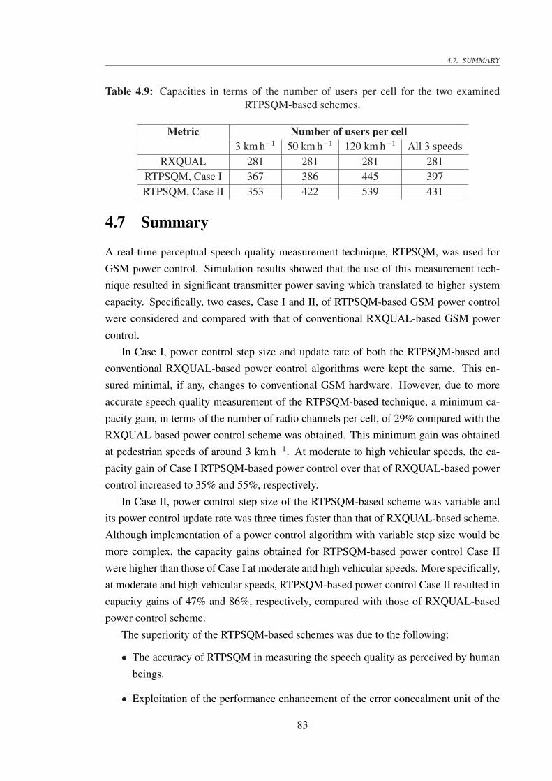
4.7. SUMMARY
Table 4.9: Capacities in terms of the number of users per cell for the two examinedRTPSQM-based schemes.
Metric Number of users per cell3 km h−1 50 km h−1 120 km h−1 All 3 speeds
RXQUAL 281 281 281 281RTPSQM, Case I 367 386 445 397RTPSQM, Case II 353 422 539 431
4.7 Summary
A real-time perceptual speech quality measurement technique, RTPSQM, was used forGSM power control. Simulation results showed that the use of this measurement tech-nique resulted in significant transmitter power saving which translated to higher systemcapacity. Specifically, two cases, Case I and II, of RTPSQM-based GSM power controlwere considered and compared with that of conventional RXQUAL-based GSM powercontrol.
In Case I, power control step size and update rate of both the RTPSQM-based andconventional RXQUAL-based power control algorithms were kept the same. This en-sured minimal, if any, changes to conventional GSM hardware. However, due to moreaccurate speech quality measurement of the RTPSQM-based technique, a minimum ca-pacity gain, in terms of the number of radio channels per cell, of 29% compared with theRXQUAL-based power control scheme was obtained. This minimum gain was obtainedat pedestrian speeds of around 3 km h−1. At moderate to high vehicular speeds, the ca-pacity gain of Case I RTPSQM-based power control over that of RXQUAL-based powercontrol increased to 35% and 55%, respectively.
In Case II, power control step size of the RTPSQM-based scheme was variable andits power control update rate was three times faster than that of RXQUAL-based scheme.Although implementation of a power control algorithm with variable step size would bemore complex, the capacity gains obtained for RTPSQM-based power control Case IIwere higher than those of Case I at moderate and high vehicular speeds. More specifically,at moderate and high vehicular speeds, RTPSQM-based power control Case II resulted incapacity gains of 47% and 86%, respectively, compared with those of RXQUAL-basedpower control scheme.
The superiority of the RTPSQM-based schemes was due to the following:
• The accuracy of RTPSQM in measuring the speech quality as perceived by humanbeings.
• Exploitation of the performance enhancement of the error concealment unit of the
83

4.7. SUMMARY
AMR codecs.
• Faster power control update rate.
• Use of variable step sizes for power control.
• Ability to trade-off transmit power with perceptual quality in a more controlledmanner while still providing adequate quality to the users.
84

Chapter 5
Perceptual-based Power Control forUMTS
5.1 Introduction
As UMTS is a CDMA based technology, it requires accurate power control to minimizeinterference among all users while providing adequate QoS. Better management of userinterference and QoS through improved power control can lead to increased system ca-pacity. In addition, this will prolong the battery life of the MS which is referred to as UserEquipment (UE) in the context of UMTS.
In this chapter, the power control techniques used in UMTS are first reviewed. Meth-ods for improving the performance of these techniques in the case of speech commu-nication are then proposed. This is achieved by incorporating the RTPSQM techniquediscussed in Chapter 3 in the outer-loop power control.
The contributions of this chapter are as follows:
• Presentation of an algorithm involving RTPSQM in the outer-loop power control ofUMTS.
• Comparison of the performance of RTPSQM- and FER-based outer-loop powercontrol algorithms through simulations. It is shown that the RTPSQM-based powercontrol achieves adequate speech quality while reducing the average SIR target byup to 18% relative to the conventional algorithm.
5.2 Power Control in UMTS
In UMTS, the received signal level is affected through channel variations due to the rela-tive movement of the UE and the BS. Therefore, the transmit power must be changed in
85

5.2. POWER CONTROL IN UMTS
response to channel variations to ensure reliable signal demodulation. Otherwise, if thereceived signal level is too weak, the QoS is degraded. Conversely, if the signal level istoo high, it creates excessive interference that would decrease system capacity. Moreover,excessive transmission power in the uplink will shorten the battery life of UE. Therefore,CDMA-based systems, such as UMTS, employ power control in an attempt to regulatethe received signal level such that it is within a desired range [7].
The power control in UMTS is divided into open-loop and closed-loop. In open-loop power control, the transmitter does not depend on feedback information from thereceiver end of the communication link. Instead, the transmitter calculates the path lossvariations and adjusts its power level based on the measurements of the average receivedsignal power. This type of power control is most effective if the uplink and downlinkchannels are symmetrical. Since path loss and shadowing are frequency dependent, theuplink and the downlink channels are symmetrical when they operate on the same fre-quency. This symmetry is utilized by the open-loop power control to continuously adjustthe transmit power by an amount inversely proportional to changes in the received signalpower [71,72]. However, in systems where the transmitter and receiver operate on differ-ent frequency bands, the assumption of symmetry of the uplink and downlink channelsdoes not hold [71]. Therefore, in UMTS, open-loop power control is predominantly usedin Time Division Duplex (TDD) mode. However, its use in Frequency Division Duplex(FDD) mode is limited only to initial power setting.
Unlike open-loop power control, its closed-loop counterpart depends on feedbackinformation from the receiver end of the communication link. In UMTS FDD mode,closed-loop power control is used in both uplink and downlink, but in TDD mode it isonly used in downlink [17]. In the next section closed-loop power control for FDD mode,which is the more widely used mode [73], will be discussed.
5.2.1 Closed-loop power control in FDD mode
The closed-loop power control procedure in UMTS is divided into two processes, outer-loop and inner-loop. The block diagram of UMTS closed-loop power control with anindication of the location where each function is performed, e.g. in UE or BS, is shownin Fig. 5.1.
With reference to Fig. 5.1, outer-loop power control operates within the BS. It dy-namically sets the SIR target for the inner-loop based on a FER target (usually 1% forspeech services) for achieving a satisfactory QoS. The inner-loop power control, on theother hand, will regulate the transmit power of the UE in an attempt to compensate sig-nal amplitude fading and meet the SIR target. When the inner-loop is unable to combat
86

5.2. POWER CONTROL IN UMTSSet SIR Target CompareSIREstimationCalculate CRC UplinkDownlink Step SelectionAdjust PowerInner-loopOuter-loopFunction performed in BSFunction performed in UE
TPCTPC = Transmit Power Control commandSIR = Signal-to-Interference RatioCRC = Cyclic Redundancy Check
FER TargetFER = Frame Error RateChannel
Figure 5.1: Block diagram of UMTS closed-loop power control procedure.
channel fading, the FER increases. Consequently, the outer-loop increases the SIR targetin trying to maintain the FER target.
The inner-loop operates at a much higher rate than the outer-loop which updates SIRtarget every 10-100 ms. During this time, the CRC for each frame is calculated and isused to adjust SIR target. The algorithm used for conventional UMTS outer-loop powercontrol is described in Section 5.2.2. As for the inner-loop, the BS estimates the receivedSIR and compares it against the SIR target once every 0.666 ms time-slot. If the estimatedreceived SIR is less than the SIR target, the BS sends a Transmit Power Control (TPC)command “1” to the UE, otherwise a “0” is transmitted. The received TPC commandbits are used by the UE to adjust its transmit power based on one of the two algorithmsdescribed in Section 5.2.3.
It should be noted that the need for outer-loop power control arises from the factthat fixed mapping between FER and SIR is not applicable in time-varying propagationconditions. In UMTS, this mapping is influenced by the vehicular speed and the numberof multipaths in the channel. For example, an average received SIR of 4 dB may besufficient for maintaining an FER of 1% at a UE speed of 3 km/h. However, if the SIR iskept at 4 dB while the UE speed increases to 50 km/h, the FER deteriorates to more than1% [74]. As such, in the absence of the outer-loop, an inner-loop power control would
87

5.2. POWER CONTROL IN UMTS
have to use a fixed SIR target that achieves FER of 1% under the “worst-case” channelcondition. This would result in some UEs transmitting at unnecessarily high power levels,leading to increased interference and reducing system capacity.
5.2.2 Conventional UMTS outer-loop power control algorithm
The flow chart of conventional UMTS outer-loop power control algorithm is shown in Fig.5.2. For each received speech frame at the BS, the integrity of the frame is checked byperforming a CRC operation. If CRC indicates that the frame is in error, then the SIR tar-get is increased by K multiples of a given step size4 in dB, where K is a positive integer.The value of K determines the average FER in the steady state, i.e., FER = 1/(K + 1)
(see Section 7.3.1). In the steady state, the SIR target varies around the minimum SIRrequired for achieving the FER target. As a result, the SIR target is on average in excessof the minimum required SIR by a value proportional to 4. Using a small 4 to reducethe excess SIR may result in a longer convergence time and poor tracking of channel vari-ations. On the other hand, a large 4 can converge to channel changes rapidly, however,it increases the excess SIR in the steady state. This will lead to larger interference andreduces system capacity [18]. Given the step size 4 and integer K, then the outer-loopstep down size 4down and step up size 4up can be formulated as
4down = 4 and 4up = K ×4. (5.1)
As the dynamic range of SIR target is limited, the new SIR target is checked againstthe allowed minimum and maximum limits of SIR target. If SIR target goes beyondany one of these two limits, it is clamped to that limit. The same steps are repeated forsubsequent frames.
5.2.3 Conventional UMTS inner-loop power control algorithms
It was mentioned in Section 5.2.1 that once every time-slot, the BS compares the receivedSIR against the SIR target and generates an appropriate TPC bit for transmission to theUE. On receiving the TPC bit rxTPCcmd, the UE derives a single transmit TPC com-mand txTPCcmd for each time-slot based on one of the two following algorithms. It isnoted that multiple TPC bits are received when UE is in soft handover, in which case, thebehaviour of the algorithms slightly varies. However, in this study, only the case whenthe UE is not in soft handover is considered. These algorithms are performed in the blocklabeled “Step Selection” in Fig. 5.1. The step sizes for inner-loop and outer-loop powerpower controls are distinct. Therefore, for the sake of clarity the step size of inner-loop
88

5.2. POWER CONTROL IN UMTSStartCheck CRC ofcurrent frameCRC inerror ?SIR_target =SIR_target + SIR_target =SIR_target - SIR_target >maximum SIR_target? SIR_target <minimum SIR_target?SIR_target =maximum SIR_target SIR_target =minimum SIR_targetProcess nextframe
Yes NoNo NoYes Yesup down
Initialization
Figure 5.2: Flow chart of conventional UMTS outer-loop power control algorithm.
89

5.2. POWER CONTROL IN UMTS
power control is represented as δ.
Algorithm 1 UE receives one rxTPCcmd in each time slot and adjusts its transmitpower in the same time slot
Step 1: Initialise time slot index l to 1.
Step 2: Wait for arrival of rxTPCcmd for time slot l.
Step 3: Decide on the value of txTPCcmd for time slot l.If rxTPCcmd = 0, then
txTPCcmd = −1.else if rxTPCcmd = 1, then
txTPCcmd = +1.
Step 4: Calculate step size δ for adjusting the transmitter power as
δ = δTPC × txTPCcmd (5.2)
where δTPC can take on values of either 1 dB or 2 dB [7].
Step 5: Adjust transmitter power by step size δ.
Step 6: Set l = l + 1 and goto Step 2. ¤
Algorithm 2 UE receives one rxTPCcmd in each time slot and its transmit poweris adjusted based on a 5-slot cycle
Step 1: Initialise time slot index l to 1.
Step 2: Wait for arrival of rxTPCcmd for time slot l.
Step 3: Decide on the value of txTPCcmd for time slot l.If l is not divisible by 5, i.e. this is not the fifth time slot in a 5-slot cycle
txTPCcmd = 0.else
If last five rxTPCcmd = 0, thentxTPCcmd = −1.
else if last five rxTPCcmd = 1, thentxTPCcmd = +1.
elsetxTPCcmd = 0.
90

5.3. SIMULATION MODEL
Step 4: Calculate step size δ for adjusting the transmitter power as
δ = δTPC × txTPCcmd (5.3)
where δTPC can only be 1 dB [7].
Step 5: Adjust transmitter power by step size δ.
Step 6: Set l = l + 1 and goto Step 2. ¤
5.3 Simulation Model
In this section, the RTPSQM technique described in Chapter 3 is incorporated in theouter-loop of the UMTS power control. The performance of this RTPSQM-based outer-loop is compared against its conventional UMTS counterpart using computer simulations.RTPSQM was not included in the inner-loop because its update rate of 1500 s−1 is toofast for the PESQ algorithm used with RTPQSM to function reliably in terms of providinggood estimates of speech quality.
A Matlab Simulink implementation of the UMTS physical layer was used for simula-tions. The physical layer was implemented at chip level according to the 3GPP technicalspecifications1. The block diagram of the simulation model showing the relevant func-tional blocks is depicted in Fig. 5.3. The building blocks and some of the importantsimulation parameters are described briefly in the following sub-sections.
5.3.1 Input speech file
Only one input speech file of 40 second duration was used for all simulations in this chap-ter. This speech file was constructed by concatenation of five speech files (o-f01l7d.pcm,o-m01l0b.pcm, o-f01l63.pcm, o-m01l26.pcm, and o-f01lb7.pcm) from the ITU databasefor voice quality measurement tests [62]. Each of the constituent speech files containedprerecorded sentences of 8 seconds duration with approximately 50% speech and 50%silence intervals. Furthermore, the constituent files were recorded in 16-bit, 8 kHz linearPCM format.
1We would like to thank and acknowledge PHYBIT Inc. Singapore for permitting us to use their UMTSphysical layer simulation software.
91
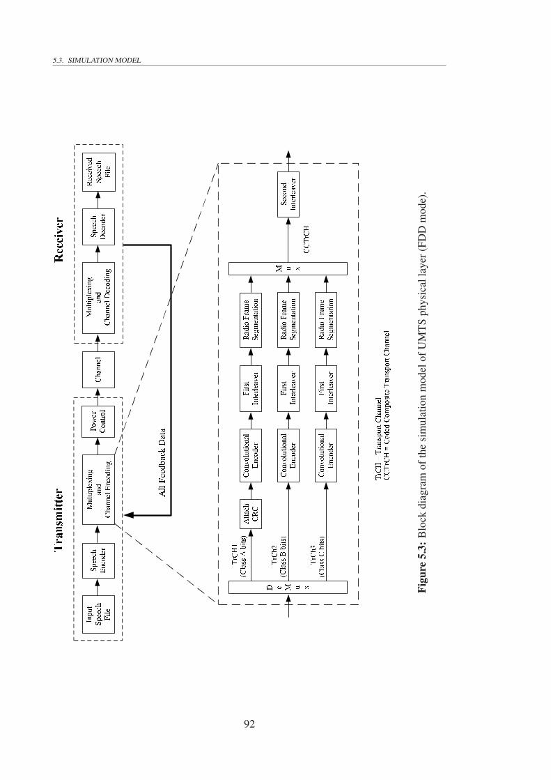
5.3. SIMULATION MODEL
Transmitter
Receiver
Speech Encoder
Speech Decoder
Input Speech File
ChannelPower ControlReceived Speech FileMultiplexing and Channel Decoding
Multiplexing and Channel Encoding D e M u xConvolutional EncoderAttach CRCFirst InterleaverRadio Frame Segmentation
Second InterleaverM u xConvolutional EncoderFirst InterleaverRadio Frame Segmentation
Convolutional EncoderFirst InterleaverRadio Frame Segmentation
(Class A bits) (Class B bits) (Class C bits)
CCTrCH
TrCH1 TrCh2 TrCh3 TrCH = Transport Channel CCTrCH = Coded Composite Transport Channel
All Feedback DataFi
gure
5.3:
Blo
ckdi
agra
mof
the
sim
ulat
ion
mod
elof
UM
TS
phys
ical
laye
r(FD
Dm
ode)
.
92

5.3. SIMULATION MODEL
5.3.2 Speech codec
The AMR speech codec has been employed for all the simulations in this chapter. Thiscodec, which is mandatory for UMTS [56] was described in Section 4.3.2 in conjunctionwith GSM. In UMTS the alternative designations of Class A, B, and C, are adopted insteadof GSM Class Ia, Ib, and II bits, respectively.
Generally, the AMR codec mode 7 is the preferred mode because of its superior speechquality. Therefore, this mode has been considered in the simulations in this chapter. Theframe structure of AMR codec mode 7 is summarized in Table 5.1.
Table 5.1: Summary of AMR codec mode 7 frame structure.
Codec Num. of Num. of Num. of Num. ofRate (kbps) bits per frame Class A bits Class B bits Class C bits
12.2 244 81 103 60
5.3.3 Multiplexing and channel coding
In the simulation model of Fig. 5.3, the 20 ms encoded speech frames are processed by“Multiplexing and Channel Encoding”. Hereafter, this block is referred to as the MCblock. In UMTS, data arriving from Layer 2 is processed in so called Transmission TimeIntervals (TTI). In this case, each AMR speech frame corresponds to 20 ms TTI. Theoperations of the MC block in each TTI are summarized below.
Transport Channel (TrCH) allocation
In UMTS, the transmitted data can be divided into distinct logical channels referred to asTransport Channels (TrCH). A separate TrCH is assigned to the AMR output bits ClassA, B, and C denoted as TrCH1, TrCH2, and TrCh3, respectively.
CRC attachment
A 12-bit CRC is attached to the TrCH1 in every TTI. The CRC bits are used in the receiverto detect any potential Class A errors. There are no CRC bits for TrCH2 and TrCH3.
Channel coding
Convolutional coding (CC) has been recommended for speech [75]. A rate 1/3 code isused for TrCH1 while TrCh2 and TrCh3 are protected with rate 1/2 code [75].
93

5.3. SIMULATION MODEL
First interleaving
There are two stages of interleaving in UMTS to achieve the best performance by spread-ing the channel errors as widely as possible. The first interleaver is an inter-frame inter-leaver operating individually on each TrCH every TTI. For speech, TrCH bits are enteredinto the interleaver row-by-row where each row contains two columns. Subsequently, thebits are read out in columns [19].
Radio frame segmentation
In UMTS, data transmitted in 10 ms radio frames. This corresponds to two radio framesper TTI for speech. Radio frame segmentation involves dividing data from each TrCHinto two consecutive radio frames.
Multiplexing
The transport channels are multiplexed into a single Coded Composite Transport Channel(CCTrCH). This is a simple serial multiplexing on a frame-by-frame basis. Each transportchannel provides data in 10 ms frames for this multiplexing.
Second interleaving
The second interleaver is an intra-frame interleaver which operates on 10 ms radio frames.In this case, the bits from a radio frame are read into the interleaver row-by-row whereeach row contains 30 columns. Subsequently, the bits are read out in columns after intercolumn permutation has been applied.
5.3.4 Power control
In this section, the simulation details of the conventional UMTS power control algorithmand its RTPSQM-based counterpart are given.
Conventional UMTS power control
The closed-loop power control explained in Section 5.2.1 was simulated for the conven-tional UMTS power control incorporating both inner- and outer-loops. The TPC com-mands for the inner-loop were applied based on Algorithm 1 given in Section 5.2.3. Thetransmission power was updated using a step size δ of 1 dB, which is the mandatory stepsize specified in [59], and an update rate of 1500 s−1 corresponding to once every timeslot. The outer-loop was based on the algorithm proposed by Sampath et al. [18]. The
94

5.3. SIMULATION MODEL
flow chart of the algorithm is shown in Fig. 5.2. The FER target for the algorithm was setto 1%. The SIR target was updated using a step size 4 of 0.005 dB [7] at a rate of 50 s−1
corresponding to once every speech frame. A summary of the simulation parameters forthe conventional UMTS power control is given in Table 5.2.
Table 5.2: Conventional UMTS power control parameters.
Type Algorithm Update Step up Step down FER
rate (s−1) size (dB) size (dB) Target (%)
Outer-loop Sampath et. al. 50 4up = 0.495 4down = 0.005 1
Inner-loop 1 1500 δup = 1 δdown = 1 -
RTPSQM-based UMTS power control
The simulation model for UMTS power control based on RTPSQM described in Chapter 3is shown in Fig. 5.4. In this case, the perceptual speech quality is measured by RTPSQMand is applied in the outer-loop power control.
In Fig. 5.4, the delay was introduced to account for the round-trip delay between theAMR encoder and the decoder at the transmitter. The RTPSQM technique employed thePESQ reference implementation software supplied by ITU [4]. The following minor mod-ifications were made to the reference implementation to integrate PESQ in the simulationmodel:
Disabling the level alignment function: In these simulations, it is noted that the inputspeech files from ITU database would already be level-aligned and the signal trans-mission path as shown in Fig. 5.4 does not affect signal levels. In this case, levelalignment in the reference implementation was disabled in order to speed up simu-lations. Moreover, the performance of PESQ with and without level alignment wereconfirmed to be identical.
Interfacing with Simulink: The reference implementation of PESQ was written in C. Itwas therefore necessary to add additional lines of code in order to integrate PESQinto Matlab Simulink.
The flow chart for the RTPSQM-based outer-loop power control is depicted in Fig. 5.5.Note that this flow chart differs from the flow chart for the conventional UMTS powercontrol shown in Fig. 5.2 only in the highlighted block. In contrast to the conventionalpower control, when the CRC indicates errors in Class A bits of the received frame the SIR
95

5.3. SIMULATION MODEL
Outer-loop Power ControlReceiver
Speech SignalTransmitter AMR Encoder
CRC CheckAMR DecoderReceived Speech
DelayDelay AMR Decoder
FEP
RTPSQM
Channel
Reference SignalSynthesized Signal+
Figu
re5.
4:A
pplic
atio
nof
RT
PSQ
Min
UM
TS
oute
r-lo
oppo
wer
cont
rol.
96

5.3. SIMULATION MODEL
target is not automatically increased. In this case, the perceptual quality correspondingto 8 speech frames immediately before the current frame is checked. The SIR target isonly increased if RTPSQM MOS indicates “bad” quality relative to the predeterminedthreshold MOSthreshold. Otherwise, the SIR target is decreased. The justification for thisapproach is that when the perceptual quality of the previous frames is “good”, the errorconcealment procedure will be more effective in masking the impact of the current frameerror. It should be remembered that RTPSQM incorporates the AMR decoder includingassociated error concealment procedure for calculation of the quality.
5.3.5 Channel
Mobile radio channels are characterized by fast fading, shadowing and Multiple AccessInterference (MAI). The presence of AWGN is often included in MAI. For the purpose ofour simulations the 6-ray Vehicular A channel model specified by 3GPP [76,77] has beenconsidered for modeling the fast fading multipath channel. The relative time delays andaverage powers of individual paths of the channel models are summarized in Table 5.3.The Power Spectral Densities (PSD) for individual paths follow the classical PSD [78].The shadowing, in logarithmic scale, was modeled according to correlated normal distri-bution. In practice, the mean value of the distribution is equal to the path loss. However,in this study the path loss was assumed to be compensated by the power control subsys-tem so that the mean of the distribution was equal to 0 dB. The standard deviation ofthe distribution is a function of the propagation environment. For urban environments,standard deviation of 8 dB has been used [79]. In addition, signal shadowing decorre-lates with traveled distance where the so called decorrelation distance is dependent on thepropagation environment. For urban environment a decorrelation distance of 20 m hasbeen used [80].
Table 5.3: Tapped-delay-line parameters for Vehicular A environment [77].
Tap Relative Relative Avg. Doppler
Number delay (ns) Power (dB) Spectrum
1 0.0 0.0 Classical
2 310 -1.0 Classical
3 710 -9.0 Classical
4 1090 -10.0 Classical
5 1730 -15.0 Classical
6 2510 -20.0 Classical
97

5.3. SIMULATION MODEL StartCheck CRC ofcurrent frameCRC inerror ?SIR_target =SIR_target + SIR_target =SIR_target - SIR_target >maximum SIR_target? SIR_target <minimum SIR_target?SIR_target =maximum SIR_target SIR_target =minimum SIR_targetProcess nextframe
Yes NoNo NoYes Yes
RTPSQM MOS< Threshold? Yes Noup downInitialization
Figure 5.5: Flow chart of RTPSQM-based UMTS outer-loop power control algorithm.
98

5.4. METHODOLOGY
5.3.6 Summary of simulation parameters
A summary of main simulation parameters is given in Table 5.4. From the table it is notedthat MOSthreshold was set to 4.20. The significance of this choice is explained as follows:As it will be shown in Fig. 6.3(a) of Chapter 6, for AMR codec mode 7 (12.2 kbps),the actual PESQ MOS starts deteriorating rapidly once it reaches the value 3.6. Thiscorresponds to a RTPSQM MOS value of 4.0 according to the mapping function betweenthe actual PESQ MOS and the estimated RTPSQM MOS shown in Fig. 3.7(a). A marginof 0.2 MOS points is added to this value to obtain a MOSthreshold = 4.0+0.2 = 4.2. Themargin is to ensure that the RTPSQM-based power control activates SIR target reductiononly when the quality is good.
5.4 Methodology
In accordance with 3GPP recommendations [76], three representative speeds of 3, 50,and 120 km h−1 were considered for performance comparison between conventional andRTPSQM-based UMTS power control algorithms. Furthermore, ten different channelshadowing profiles were simulated for each vehicular speed to ensure the channel errorpatterns were independent for the simulations. Each power control algorithm was simu-lated for outer-loop step-sizes 4 of 0.005, 0.01, 0.015 and 0.02 dB. For each simulation,a 40 s speech file was transmitted on the UMTS physical layer shown in Fig. 5.3 enablingonly one power control algorithm at a time. In each case, the variations of the SIR targetand the channel shadowing profile were recorded.
For each simulation, the PESQ algorithm was applied to the received speech file to-gether with the original transmitted file and the corresponding actual PESQ MOS wascalculated.
5.5 Simulation Results
The simulation results for the outer-loop step size of 0.005 dB and vehicular speeds of 3,50, and 120 km h−1 are given in Table 5.5(a)-(c), respectively. These results include theaverage of SIR target and the PESQ MOS corresponding to the two different power con-trol algorithms obtained for each shadowing profile. In addition, the gain of the RTPSQM-based power control with respect to the conventional power control calculated as the dif-ference between the SIR targets in the two cases, is shown. The ensemble averages overall shadowing profiles are also included.
For brevity, only the ensemble averages for the outer-loop step sizes of 0.01, 0.015,
99

5.5. SIMULATION RESULTS
Table 5.4: Main simulation parameters.
Chip rate 3.84 Mc/sSpreading factor 128Channel bit rate 60 kbpsSpeech coding AMR (rate 12.2 kbps)Channel coding
Class A Rate 1/3 CC + 12-bit CRCClass B Rate 1/2 CCClass C Rate 1/2 CCInterleaving both inter- and intra-frame
Modulation QPSKPower control
Inner-loopUpdate rate 1500 s−1
Up or down step size (δup or δdown) 1 dBOuter-loop (conventional)
FER target 1%Control variable CRC flagsStep down 4down 0.005, 0.01, 0.015 and 0.02 dBStep up 4up 0.495, 0.99, 1.485 and 1.98 dBUpdate rate 50 s−1
Outer-loop (RTPSQM-based)FER target 1%Control variable RTPSQM MOS and CRC flagsRTPSQM MOS update rate 6.25 s−1 (every 160 ms)MOSthreshold 4.20 MOSStep up/down as conventional aboveUpdate rate 50 s−1
Channel typeAWGN ActiveLog-normal shadowing Active(standard deviation, decorrelation distance) (8 dB, 20 m)Fast Fading 6-tap Vehicular A
Vehicular speed 3, 50 and 120 km/hReceiver Rake (6 fingers)Initial SIR 4 dB
100

5.5. SIMULATION RESULTS
Table 5.5: Results for conventional and RTPSQM-based power control algorithms withouter-loop step down 4down = 0.005 dB and vehicular speed of (a) 3 km h−1, (b) 50
km h−1, and (c) 120 km h−1.
(a)Shadowing SIR target (dB) PESQ MOS
profile Conv. RTPSQM Gain Conv. RTPSQM Difference1 4.22 3.88 0.34 3.19 3.02 0.172 4.20 3.81 0.39 3.23 3.10 0.133 4.17 3.80 0.37 3.23 2.97 0.264 4.23 3.89 0.34 3.29 3.14 0.155 4.23 3.90 0.33 3.25 3.03 0.226 4.19 3.88 0.31 3.21 3.06 0.157 4.19 3.94 0.25 3.23 3.12 0.108 4.00 3.75 0.25 3.18 3.00 0.189 4.21 4.05 0.16 3.26 3.14 0.1210 4.32 3.84 0.48 3.33 3.05 0.28
Ensemble avg. 4.20 3.87 0.32 3.24 3.06 0.18
(b)Shadowing SIR target (dB) PESQ MOS
profile Conv. RTPSQM Gain Conv. RTPSQM Difference1 4.17 4.07 0.10 3.27 3.18 0.092 4.27 4.16 0.11 3.19 3.15 0.043 4.19 4.16 0.03 3.25 3.20 0.054 4.26 4.09 0.17 3.21 3.17 0.045 4.13 3.98 0.15 3.14 3.07 0.076 4.22 4.07 0.15 3.22 3.15 0.077 4.47 4.27 0.20 3.28 3.26 0.028 4.23 4.06 0.17 3.23 3.16 0.079 4.26 4.06 0.10 3.27 3.16 0.1110 4.28 4.24 0.04 3.21 3.18 0.03
Ensemble avg. 4.25 4.12 0.13 3.23 3.17 0.06
(c)Shadowing SIR target (dB) PESQ MOS
profile Conv. RTPSQM Gain Conv. RTPSQM Difference1 3.06 2.94 0.12 3.28 3.16 0.122 3.23 2.89 0.34 3.39 3.25 0.143 3.64 3.06 0.58 3.53 3.21 0.324 3.19 3.08 0.11 3.36 3.21 0.155 3.18 2.66 0.52 3.28 3.00 0.286 3.23 2.98 0.25 3.44 3.28 0.167 3.18 3.09 0.09 3.29 3.18 0.118 3.32 3.07 0.25 3.40 3.28 0.129 3.24 3.09 0.15 3.33 3.25 0.0810 3.25 3.12 0.13 3.32 3.18 0.14
Ensemble avg. 3.25 3.00 0.25 3.36 3.20 0.16
101

5.5. SIMULATION RESULTS
and 0.02 dB are given in Table 5.6(a)-(c), respectively. For detailed results, refer to Ap-pendix B.
From Table 5.5(a)-(c) and Table 5.6(a)-(c), it is observed that the RTPSQM-basedpower control achieved between 3% to 18% gain in the SIR target. The resulting per-ceptual speech qualities were noted to have slightly degraded. However, the degradationswere generally too small to make noticeable difference to human ears. It should be notedthat the same gains could not be achieved by allowing a larger FER target for the con-ventional power control without affecting the perceptual quality more severely. In thiscase, the FER is increased regardless of the effect on the perceptual quality, whereas withRTPSQM-based power control, the FER is only increased when the quality is not affectednoticeably.
The SIR target gain is due to the number of times RTPSQM-based algorithm avoidsincreasing the SIR target while the conventional algorithm does not. In this case, the gainincreases with the power control step size as noted in Table 5.5(a)-(c) and Table 5.6(a)-(c).
Table 5.6: Results for conventional and RTPSQM-based power control algorithms for allsimulated outer-loop step sizes and and vehicular speed of (a) 3 km h−1, (b) 50 km h−1,
and (c) 120 km h−1.
(a)Step SIR target (dB) PESQ MOS
size (dB) Conv. RTPSQM Gain Conv. RTPSQM Difference0.005 4.20 3.87 0.33 3.24 3.06 0.180.010 4.30 3.98 0.32 3.28 3.08 0.200.015 4.47 4.06 0.41 3.34 3.08 0.260.020 4.56 4.15 0.41 3.34 3.09 0.25
(b)Step SIR target (dB) PESQ MOS
size (dB) Conv. RTPSQM Gain Conv. RTPSQM Difference0.005 4.25 4.12 0.13 3.23 3.17 0.060.010 4.35 4.14 0.21 3.22 3.15 0.070.015 4.50 4.29 0.21 3.28 3.17 0.110.020 4.66 4.38 0.28 3.30 3.21 0.09
(c)Step SIR target (dB) PESQ MOS
size (dB) Conv. RTPSQM Gain Conv. RTPSQM Difference0.005 3.25 3.00 0.25 3.36 3.20 0.160.010 3.34 3.03 0.31 3.37 3.15 0.220.015 3.38 2.96 0.42 3.41 3.18 0.230.020 3.72 3.06 0.66 3.45 3.14 0.31
102

5.6. SUMMARY
A set of representative curves comparing the performance of RTPSQM-based and con-ventional outer-loop power control algorithms are shown in Fig. 5.6(a)-(c) for vehicularspeeds of 3 km h−1, 50 km h−1, and 120 km h−1, respectively. In each case, the shadowingprofile and the SIR targets for the two algorithms are shown. The CRC flags with frameerasures depicted as spikes are also shown. In addition, the results of RTPSQM MOScomparison against MOSthreshold have been represented by “RTPSQM-MOS-BAD” inthe figures. A level high signal indicates a RTPSQM MOS value below MOSthreshold,i.e., bad quality. It can be observed from Fig. 5.6(a)-(c) that the SIR target for the con-ventional outer-loop power control was increased whenever the corresponding CRC flagindicated a frame erasure. The same happened for the RTPSQM-based power controlwhen frame erasures occurred and “RTPSQM-MOS-BAD” was high. However, therewere situations when the frame erasures coincided with low “RTPSQM-MOS-BAD” sig-nal level. In such situations, the SIR target was not increased giving rise to the observedgaps between the SIR targets in the two algorithms in Fig. 5.6(a)-(c). The average areaof the gap corresponded to the gain achieved through RTPSQM-based algorithm over itsconventional counterpart. The set of curves corresponding to the best case scenario, whichresulted in highest average SIR target gain, are shown in Fig. 5.7(a)-(c). In this case, theSIR target gains of 0.37, 0.29, and 1.28 dB for vehicular speeds of 3, 50, and 120 km h−1,respectively were achieved given a step size of 0.02 dB.
It is observed that the benefits, in terms of saving system resources, of applying RTP-SQM technique to power control of UMTS are relatively smaller compared to those ofGSM. However, for certain scenarios, as shown in Fig. 5.7(a)-(c), application of RTP-SQM in UMTS outer-loop power control resulted in significant average SIR target gainscompared with UMTS with a conventional outer-loop power control.
5.6 Summary
A real-time perceptual speech quality metric, RTPSQM, was incorporated in UMTSouter-loop power control. The RTPSQM-based power control was designed in such away to avoid unnecessary increases in transmitter power levels when the perceived speechquality was adequate. The RTPSQM-based algorithm would enable the network oper-ators to have a direct control on the perceptual speech quality by setting the value ofMOSthreshold. However, this could not be achieved with the conventional UMTS powercontrol, as the network operator could only control the delivered service quality by ad-justing the FER target.
The performance of both RTPSQM-based and conventional UMTS power controlswas compared by computer simulations using a comprehensive set of parameters. These
103

5.6. SUMMARY
parameters were the step size of the outer-loop power control, vehicular speed and channelshadowing profile. The simulation results showed that the RTPSQM-based power controlachieved adequate speech quality while reducing the average SIR target by up to 18%relative to the conventional algorithm.
The reduced average SIR target of the RTPSQM-based system will be shown in Chap-ter 7 to lead to improved Erlang capacity by the system.
104

5.6. SUMMARY
0 5 10 15 20 25 30 35 40-25-20-15-10-50510152025
Time (sec)Amplitude (dB) Average SIR Targets (dB): Conventional = 4.23, RTPSQM = 3.90, gain = 0.33
FlagShadowing profile (dB) CRC flag (RTPSQM system)CRC flag (Conventional system)RTPSQM SIR Targets (dB)Conventional SIR Targets (dB) RTPSQM-MOS-BAD flag (True = High)
(a)
0 5 10 15 20 25 30 35 40-25-20-15-10-50510152025
Time (sec)Amplitude (dB) Average SIR Targets (dB): Conventional = 4.13, RTPSQM = 3.98, gain = 0.15
FlagShadowing profile (dB) CRC flag (RTPSQM system)CRC flag (Conventional system)RTPSQM SIR Targets (dB)Conventional SIR Targets (dB) RTPSQM-MOS-BAD flag (True = High)
(b)
0 5 10 15 20 25 30 35 40-25-20-15-10-50510152025
Time (sec)Amplitude (dB) Average SIR Targets (dB): Conventional = 3.18, RTPSQM = 2.66, gain = 0.52
FlagShadowing profile (dB) CRC flag (RTPSQM system)CRC flag (Conventional system)RTPSQM SIR Targets (dB)Conventional SIR Targets (dB) RTPSQM-MOS-BAD flag (True = High)
(c)
Figure 5.6: Performance comparison of RTPSQM-based and conventional power control(shadowing profile 5 and4 = 0.005 dB): (a) 3 km h−1, (b) 50 km h−1 and (c) 120 km h−1.
105

5.6. SUMMARY
0 5 10 15 20 25 30 35 40-25-20-15-10-50510152025
Time (sec)Amplitude (dB) Average SIR Targets (dB): Conventional = 4.53, RTPSQM = 4.16, gain = 0.37
FlagShadowing profile (dB) CRC flag (RTPSQM system)CRC flag (Conventional system)RTPSQM SIR Targets (dB)Conventional SIR Targets (dB) RTPSQM-MOS-BAD flag (True = High)
(a)
0 5 10 15 20 25 30 35 40-25-20-15-10-50510152025
Time (sec)Amplitude (dB) Average SIR Targets (dB): Conventional = 4.66, RTPSQM = 4.37, gain = 0.29
FlagShadowing profile (dB) CRC flag (RTPSQM system)CRC flag (Conventional system)RTPSQM SIR Targets (dB)Conventional SIR Targets (dB) RTPSQM-MOS-BAD flag (True = High)
(b)
0 5 10 15 20 25 30 35 40-25-20-15-10-50510152025
Time (sec)Amplitude (dB) Average SIR Targets (dB): Conventional = 4.37, RTPSQM = 3.09, gain = 1.28
FlagShadowing profile (dB) CRC flag (RTPSQM system)CRC flag (Conventional system)RTPSQM SIR Targets (dB)Conventional SIR Targets (dB) RTPSQM-MOS-BAD flag (True = High)
(c)
Figure 5.7: Performance comparison of RTPSQM-based and conventional power control(shadowing profile 3 and 4 = 0.02 dB): (a) 3 km h−1, (b) 50 km h−1 and (c) 120 km h−1.
106

Chapter 6
Mapping Between FER, Residual BERand MOS
6.1 Introduction
Mapping of FER and Residual BER (RBER) to perceptual speech quality measured onMOS scale has usually been performed for characterization of the AMR speech codec[81–84]. In this chapter, however, mapping of FER and RBER to MOS are carried out aspart of calculation of Erlang capacity of UMTS when a perceptual quality metric is usedfor power control. As calculation of Erlang capacity of UMTS is carried out in Chapter 7,this chapter could be viewed as a pre-requisite for Chapter 7.
The performance of the AMR codec has been characterized using subjective listeningtests [81,82]. This characterization has been carried out under a variety of test conditionsincluding different codec modes, channel path profiles, and FER targets, in both uplinkand downlink. However, due to the time-consuming and costly nature of subjective tests,the number of test conditions were restricted in order to keep the characterization processto a manageable size. As such, the characterization in [81, 82] has been limited to onlythree FER target values of 0.5%, 1%, and 3% with the outer-loop power control disabled.In this chapter, the characterization of AMR codec is achieved by means of objectivequality measurement methods. The characterization was extended beyond FER target of3% with the outer-loop power control also enabled.
In Section 6.2, some of the important factors influencing the perceptual quality ofspeech in digital communication systems are first described. This is followed by presen-tation of the simulation model used for mapping of FER and RBER to perceptual qualityin Section 6.3. In Section 6.4, the methodology for obtaining the results is described fol-lowed by presentation and discussion of the results in Section 6.5. Finally, concluding
107

6.2. FACTORS INFLUENCING PERCEPTUAL SPEECH QUALITY
remarks are made in Section 6.6.
The contributions and findings of this chapter are:
• Presentation of numerical results showing mapping of FER and RBER to perceptualquality for AMR codec, under test conditions which are more comprehensive thanthose published in [83].
• For each codec rate, it is found that there exists a critical FER below which theimpact of changes in FER on perceptual quality is negligible, while for FER valuesabove this critical FER, the perceptual quality is rapidly deteriorated.
• The critical FER for all AMR codec rates is found to be approximately 1%. Thisfinding is commensurate with the FER target value stated in the literature for achiev-ing adequate speech quality [16, 18].
6.2 Factors Influencing Perceptual Speech Quality
Perceptual quality of speech in conjunction with AMR codec is affected by many factors.Some of the important factors are:
Codec mode: The type of speech codec has obviously a direct impact on the perceptualquality. The AMR codec can operate in 8 different bit rates ranging from 4.75 to12.2 kbps. The lower the codec rate, the more the speech compression and the morethe information content in each of the output bits of the AMR codec. Therefore, itis expected that, for the same FER target, frame erasures in speech clips encodedwith lower codec rates, e.g. 4.75 kbps, would result in greater loss of perceptualquality than higher codec rates, e.g. 12.2 kbps.
FER and RBER: Speech quality is also dependent on the FER, which is a measure ofthe rate of occurrence of the so called “bad” frames, and the residual BER, whichis the bit error rate for the “good” frames. These are actually the two variables thatare mapped to MOS on AMR performance characterization curves.
The distribution of frame errors in the speech clip: The other important factor influ-encing the perceptual speech quality is the distribution of the frame errors in thereceived speech clips. For a given FER, a speech clip whose frame errors are dis-tributed randomly can result in better speech quality than a clip whose frame errorsoccur in bursts. This is mainly due to the way the error-concealment procedurewhich is integrated into the AMR codec operates.
108

6.3. SIMULATION MODEL
Gender and age of the talkers: Finally, the gender and the age of the talkers have animpact on the perceptual quality of the speech signal degraded by errors introducedduring transmission of the signal through mobile radio channels. Based on thegender and the age of the talkers, the pitch content of a speech signal can varysignificantly. As the efficiency of the error-concealment procedure employed by theAMR decoder is dependent on the pitch of the speech signal [34], the perceptualquality degradation after error-concealment also varies with the gender and the ageof the talker.
6.3 Simulation Model
The block diagram of the simulation model for AMR performance characterization isshown in Fig. 6.1. Matlab Simulink platform was used to carry out all simulations.InputSpeech AMREncoder ChannelModel AMRDecoderPESQDistorted Speech MOS
Figure 6.1: Simulation block diagram used for AMR performance characterization.
6.3.1 Input speech
The input speech signals were stored in files. The files were obtained from ITU databasefor voice quality measurement tests [62]. The files contained prerecorded sentences of 8seconds long and were recorded in 16-bit linear PCM (binary) format sampled at 8 kHz.The sentences contained approximately 50% speech and 50% silence intervals. Voicesfrom ten male and ten female speakers were used in the simulations. The ITU speech filesused have been listed in Table C.1 (see Appendix C).
6.3.2 AMR codec
For all simulations in this chapter, the AMR speech codec was employed [56]. This codechas already been described in Sections 4.3.2 and 5.3.2. The AMR codec can operate in
109
6.3. SIMULATION MODEL
eight different modes which have been summarized in Table 6.1.
Table 6.1: Summary of AMR codec modes [58].
Codec Codec Num. of Num. of Num. of Num. ofMode Rate bits per Class Class Class
(kbps) frame A bits B bits C bits0 4.75 95 42 53 01 5.15 103 49 54 02 5.90 118 55 63 03 6.70 134 58 76 04 7.40 148 61 87 05 7.95 159 75 84 06 10.2 204 65 99 407 12.2 244 81 103 60
6.3.3 Channel model
The 6-ray Vehicular A channel model specified by 3GPP [77] has been considered formodeling the fast fading multipath channel. The tapped delay line parameters for thismodel have already been presented in Table 5.3. Shadowing was modeled by allowingthe large scale average of the signal power (in dB) vary randomly according to a zero-mean normal distribution with standard deviation of 8 dB and the decorrelation distanceof 20 m. For more information on the channel model, the reader is referred to Section5.3.5.
6.3.4 PESQ
PESQ is the referenced objective speech quality measurement software standardized byITU in 2001 [4]. For more information on PESQ, see Section 2.5.1.
6.3.5 Other physical layer parameters
The major parameters of the simulation model are presented in Table 6.2. These param-eters are very similar to what has been used in the simulation of UMTS physical layer inChapter 5 (see Table 5.4). For description of some of the parameters in Table 6.2, e.g.,inter-frame interleaving, the reader is referred to Section 5.3.
110

6.4. METHODOLOGY
6.4 Methodology
For a given average FER, the calculated objective MOS would be affected by factorssuch as distribution of bad frames in the speech clip, speakers’ gender and age, and thesentences uttered. To reduce the dependency of calculated voice quality on the abovefactors, ensemble averaging of the results was used. This was done by considering twentyspeech clips for each FER value. The speech clips were for ten female and ten malespeakers uttering sentences in English. The distribution of bad frames was different foreach file. For each received speech clip, the objective MOS value was calculated byPESQ. The results were then expressed in both PESQ MOS and differential MOS, whichwas the quality degradation with respect to the quality achieved when the same clip istransmitted with 12.2 kbps codec rate under error-free condition. The objective qualityfor each FER was then calculated by taking the average of PESQ MOS and differentialMOS results for the corresponding twenty speech clips.
Table 6.2: Main simulation parameters.
Chip rate 3.84 Mc/sSpreading factor 128Channel bit rate 60 kbpsTransmission Time Interval (TTI) 20 msTime slot format #8
(Npilot, NTPC , NTFCI ) (4, 2, 0)Channel coding
Class A Rate 1/3 CC + 12-bit CRCClass B Rate 1/2 CCClass C Rate 1/2 CCInterleaving both inter- and intra-frame
Modulation QPSKPower control
Inner-loopUpdate rate 1500 s−1
Up or down step size 1 dBOuter-loop
Step down 0.005 dBStep up 0.495 dBUpdate rate 50 s−1
Channel typeAWGN ONLog-normal fading ONFast fading 6-tap Vehicular A
Vehicular speed 50 km/hReceiver Rake (6 fingers)
111

6.5. RESULTS
6.5 Results
The AMR characterization test results for the simulated cases are presented as a functionof FER and RBER in Figs. 6.2 and 6.3. In Fig. 6.2, the quality degradation has beenexpressed in differential MOS, whereas in Fig. 6.3 the perceptual quality is expressed inPESQ MOS. The following trends can be observed from Fig. 6.2:
• The quality under error-free condition degraded with decreasing codec rate.
• For every codec rate, the quality degraded gradually as the FER was increased.After a critical FER, the quality degraded rapidly with FER.
• The critical FER value for each codec rate gave rise to the knee on the speech qualitycurve of that codec rate. The knee FER values were between 0.6% and 1.0%, withthe knees for higher codec rates occurring at higher values in this range. This couldbe attributed to the increased robustness of the AMR codec to errors at higher codecrates.
6.6 Summary
Using simulations a full set of AMR performance characteristic curves for UMTS, map-ping FER and RBER to perceptual quality, were obtained in this chapter. This AMRperformance characterization was more comprehensive than what has been presented in3G Technical Requirement [81, 82]. In [81, 82], the FER target has been limited to threevalues of 0.5%, 1% and 3%, whereas in this chapter, the FER target was allowed to in-crease beyond 3% to a maximum of 10%.
The simulation results showed a common trend in the AMR codec speech quality forvarious codec rates. For each codec rate, the speech quality remained practically the samewith increasing FER until the critical FER value for that codec rate was reached. Thecritical FER and RBER values for all AMR codec rates ranged between 0.6% and 1%.These results have been used in Sections 5.3.6 and 7.4. In Section 5.3.6, the plot of MOSversus FER has been used to determine the value of MOSthreshold, whereas in Section 7.4the knowledge of critical FER and RBER values has been used in calculation of Erlangcapacity of UMTS.
112
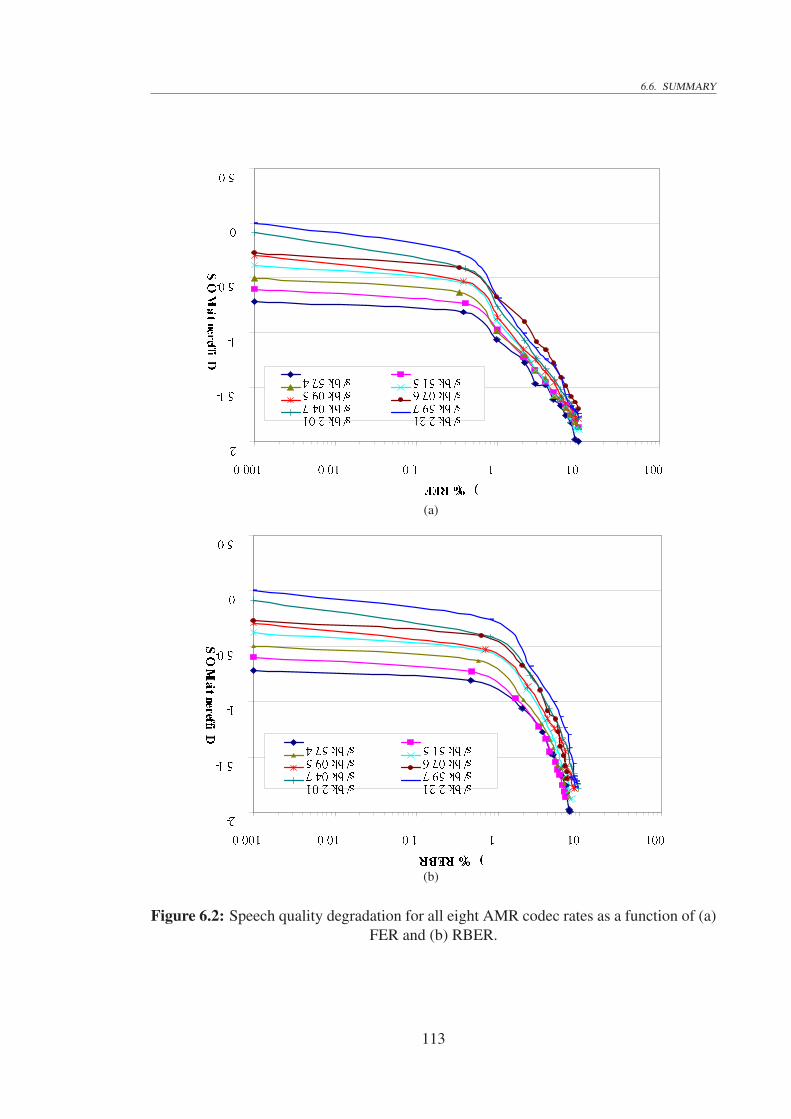
6.6. SUMMARY
- 2- 1 . 5- 1- 0 . 5 0
0 . 50 . 0 0 1 0 . 0 1 0 . 1 1 1 0 1 0 0F E R ( % )
Differential MOS 4 . 7 5 k b / s 5 . 1 5 k b / s5 . 9 0 k b / s 6 . 7 0 k b / s7 . 4 0 k b / s 7 . 9 5 k b / s1 0 . 2 k b / s 1 2 . 2 k b / s(a)
- 2- 1 . 5- 1- 0 . 5 0
0 . 50 . 0 0 1 0 . 0 1 0 . 1 1 1 0 1 0 0R B E R ( % )
Differential MOS 4 . 7 5 k b / s 5 . 1 5 k b / s5 . 9 0 k b / s 6 . 7 0 k b / s7 . 4 0 k b / s 7 . 9 5 k b / s1 0 . 2 k b / s 1 2 . 2 k b / s
(b)
Figure 6.2: Speech quality degradation for all eight AMR codec rates as a function of (a)FER and (b) RBER.
113

6.6. SUMMARY
PESQ MOS 4 . 7 5 k b / s 5 . 1 5 k b / s5 . 9 0 k b / s 6 . 7 0 k b / s7 . 4 0 k b / s 7 . 9 5 k b / s1 0 . 2 k b / s 1 2 . 2 k b / s22 . 5 33 . 5 4
4 . 50 . 0 0 1 0 . 0 1 0 . 1 1 1 0 1 0 0F E R ( % )
(a)
R B E R ( % )
PESQ MOS 4 . 7 5 k b / s 5 . 1 5 k b / s5 . 9 0 k b / s 6 . 7 0 k b / s7 . 4 0 k b / s 7 . 9 5 k b / s1 0 . 2 k b / s 1 2 . 2 k b / s22 . 5 33 . 5 4
4 . 50 . 0 0 1 0 . 0 1 0 . 1 1 1 0 1 0 0
(b)
Figure 6.3: Speech quality expressed in PESQ MOS for all eight AMR codec rates as afunction of (a) FER and (b) RBER.
114

Chapter 7
Comparative Erlang Capacity of UMTS
7.1 Introduction
The benefits of perceptual-based power control have been demonstrated in the previouschapters of this thesis for the cases of GSM and UMTS using simulations. In order tosupport an analytical approach for performance assessment of perceptual speech qualitymetrics in power control, the mathematical frameworks for conventional and perceptual-based power control are derived in the sequel. The evaluation is aimed at the Erlangcapacity per cell as this is a frequently used measure to characterise the performance ofmultiuser systems. The derivations are performed for power controlled CDMA systemsand kept as generic as possible. Thus, the impact of changes of system parameters such ascoding gain and others can be investigated analytically. At some points of the derivationspractical considerations such as particulars of UMTS are included. The developed mathe-matical framework is therefore well suited to analyse perceptual speech quality metrics inpower control of UMTS and compare their performance in terms of Erlang capacity percell with conventional power control. However, the different components of the analyticalapproach could be adapted to other CDMA systems as well using their particular systemspecifications. As Erlang capacity in CDMA systems such as UMTS is interference lim-ited, the prominent Erlang-B formula known from queuing theory cannot be used and adifferent analysis based on interference considerations is required.
This chapter is organized as follows. First, some foundations on Erlang capacity areprovided in order to introduce the required notation from traffic theory. Second, an ana-lytical approach for calculation the Erlang capacity of UMTS with its power control basedon conventional speech quality metrics is laid out. Third, by modifying the framework forconventional power control to incorporate the effect of perceptual speech quality metrics,an analytical approach for perceptual-based power control in UMTS is presented. Finally,numerical results are given that show the benefits of perceptual-based power control over
115

7.2. ERLANG CAPACITY OF MULTIUSER SYSTEMS
conventional power control in UMTS.The contributions and findings of this chapter are:
• A mathematical framework for calculation of Erlang capacity per cell of UMTSwith conventional power control is derived. The approach follows known resultsfor the second generation CDMA system IS-95 and modifies it towards UMTS. Atruncated Markov chain model of the power control algorithm is used as basis ofthe analytical derivation.
• A mathematical framework for calculation of Erlang capacity per cell of UTMSwith perceptual-based power control is derived. In particular, the transition prob-abilities for the truncated Markov chain model of the power control algorithm aredeveloped.
• A comparison of the capacity of the system using the proposed power control al-gorithm, which is based on perceptual speech quality metrics, with respect to theconventional counterpart is performed. This is supported by numerical results onErlang capacity over a variety of system parameters for both considered power con-trol approaches.
• Numerical results are presented which could be used in a system design to readilyfind the Erlang capacity per cell for either of the considered power control algo-rithms as well as the capacity gain of UMTS when using perceptual-based powercontrol.
• It is shown that the use of perceptual speech quality metrics results in a capacitygain of at least 10% over the conventional UMTS.
• It is shown that the capacity gain may increase significantly with the increase of thestandard deviation of the inner-loop power control in conjunction with a decreaseof the coding gain. For example, gains in Erlang capacity per cell may reach valuesover 80% for certain settings of the system parameters.
7.2 Erlang Capacity of Multiuser Systems
Performance of multiuser systems can be characterized by the peak load that the systemsupports for a particular service with given availability and quality. The research fieldof traffic theory provides the related analytical toolset for evaluating the performance ofmultiuser systems. In this context, the availability of a service can be quantified by theso-called blocking probability. In case of the speech services considered in this thesis, a
116

7.2. ERLANG CAPACITY OF MULTIUSER SYSTEMS
blocking probability of 1% is commonly accepted as being satisfactory and will be usedbelow in the calculation of numerical results. The traffic in a multiuser communicationsystem may be characterized by the arrival rate λ and service rate µ, respectively, that is
λ =Number of calls
Time unitand µ =
1
E[Service time]. (7.1)
The ratio of arrival rate λ to service rate µ is called average traffic whereas for a givenblocking probability Pr[Blocking] the ratio is referred to as Erlang capacity:
Erlang capacity , λ
µ
∣∣∣∣Pr[Blocking]
(7.2)
In the conventional multiuser mobile radio systems that use time division or frequencydivision multiple access, the blocking probability of the system for a given load is usuallycalculated assuming a queuing system. The related queuing system is modeled to havea Markovian arrival process with arrival rate λ calls per second and Markovian serviceprocess with service rate µ calls per second or its inverse µ−1 seconds per call. Giventhe queuing system provides S servers for processing the average traffic λ/µ measuredin the pseudo-unit Erlang, the blocking probability can be calculated using the Erlang-Bformula [29]:
Pr[Blocking] =(λ
µ)S/S!
S∑k=0
(λµ)k/k!
(7.3)
In other words, for a given probability Pr[Blocking], (7.3) may be inverted to calculatethe related Erlang capacity λ/µ. Alternatively, the average number Nactive of active usersin the system for a given average traffic and blocking probability can be expressed as
Nactive =
(λ
µ
)(1− Pr[Blocking]) (7.4)
However, the calculation of Erlang capacity in multiuser systems that use CDMAtechniques is not as straightforward. This is due to the fact that CDMA systems areinterference limited and therefore depend on the interference induced by other users inthe system and the background or thermal noise. The mathematical framework and ex-pressions for Erlang capacity of CDMA systems using conventional power control andperceptual-based power control will be derived in the following Sections 7.3 and 7.4.
117

7.3. CONVENTIONAL POWER CONTROL
7.3 Conventional Power Control
Sampath et al. [18] proposed a popular outer-loop power control in 1997. Although thisalgorithm was originally proposed for use in outer-loop power control of IS-95, it hasalso been adopted for UMTS. This algorithm shall be presented in the sequel to serveas a starting point in developing an analytical framework for outer-loop power controlin cellular mobile radio systems. In view of an analytical approach, we will replacemnemonics used in the simulation frameworks by mathematical symbols. For example,the following alternative notations are used where applicable:
SIR target: SIRtarget ↔ X (dB) or X (non-dB)
SIR threshold: SIRth ↔ Yth (dB) or Yth (non-dB)(7.5)
7.3.1 Conventional outer-loop power control algorithm
The algorithm for adjusting the SIR target X in dB of the outer-loop closed-loop powercontrol (CLPC) to achieve an adequate performance in terms of FER is as follows:
Procedure 7.1 Algorithm for adjusting SIR target of the outer-loop CLPC
Step 1: Set frame index to j = 1 and SIR target to X = X1 = Xinit.
Step 2: Perform CRC to determine if frame j is in error.
Step 3: If jth frame is in error, thenXj+1 = Xj + K4,Goto Step 4.
elseXj+1 = Xj −4.
Step 4: Increment frame index j = j + 1.
Step 5: Goto Step 2. ¤
In the above algorithm, the integer j ≥ 1 represents the frame index, 4 denotes the stepsize of the outer-loop CLPC in dB, and integer K ≥ 1 specifies the increment in SIRtarget X as a multiple of step size 4 when a frame is in error.
Steady state FER
It is noted that the choice of upward jump in terms of K is related to the desired FER thatthe particular mobile radio systems should maintain. The performance of Procedure 7.1
118

7.3. CONVENTIONAL POWER CONTROL
may therefore be quantified by the steady state FER that can be achieved for a givenupward jump of K. In order to derive a closed-form expression for the steady state FER,let fj denote a binary random variable with fj = 1 when the jth frame is in error andfj = −1 otherwise. The examined outer-loop CLPC algorithm as described by Procedure7.1 may then be formulated as
Xj+1 = Xj +1
2{(fj + 1)K4+ (fj − 1)4}. (7.6)
Clearly, the average SIR target for frame index j + 1 can be calculated from (7.6) as
E[Xj+1] = E[Xj] +1
2E[(fj + 1)K4+ (fj − 1)4] (7.7)
where E[·] denotes the expectation operator. Given that by definition, the steady statevalue of the SIR target is characterised by the condition
E[Xj+1] = E[Xj] (7.8)
we can set the difference between the expectation of the SIR target of the jth and (j +1)th
frame to zero and hence write
E[Xj+1]− E[Xj] =1
2K4E[fj + 1] +
1
24E[fj − 1] = 0 (7.9)
Solving (7.9) for K, reveals the following simple relationship:
K =1− E[fj]
1 + E[fj](7.10)
where the expectation of the binary random variable fj is calculated as
E[fj] = (+1) · Pr(fj = 1) + (−1) · Pr(fj = −1). (7.11)
As Pr(fj =1)=FER and similarly Pr(fj =−1)=1−FER, we can rewrite (7.11) as
E[fj] = (+1) · FER + (−1) · (1− FER) = 2FER− 1. (7.12)
Substituting (7.12) into (7.10) and then solving the result for FER, we finally obtain therelationship between the steady state FER and the upward jump K as follows:
FER =1
K + 1. (7.13)
119

7.3. CONVENTIONAL POWER CONTROL
Discrete-time Markov chain model of conventional outer-loop power control
The algorithm described by Procedure 7.1 can be modeled as a discrete-time Markovchain. An illustration of the model shall be given with reference to state transition dia-gram that is depicted in Fig. 7.1. The states of such a Markov chain model are labeledwith an integer i. Because Procedure 7.1 describes an infinite Markov chain and due topractical limitations on power consumption, it is further assumed that the SIR target canvary only between the minimum SIR target Xmin and the maximum SIR target Xmax. Theminimum and maximum SIR targets are associated with State 0 and State M , respectively,which means that the Markov chain is truncated to comprise a total of M + 1 states. Thetransitions between these states are determined by the changes in SIR target Xi in State i
to SIR target Xi+k in state i + k, which differs by a multiple of the step size 4. In otherwords, the SIR target in State i + k is given by
Xi+k = Xi + k4 (7.14)
where indices i and k are integers. In the context of the considered conventional outer-loop power control algorithm, we have
k =
{−1 downward jump in power given an error free frame+K upward jump in power given an erroneous frame
(7.15)
The states in Fig. 7.1 may be grouped into four different categories based on how therandom process could reach those states:
State 0: This is the initial state and could be reached in two ways, namely, when theprocess had previously been in either state 1 or 0 and there was no frame error.
States 1 to K-1: The only way the process could end up in these states is when it hadbeen previously in the next higher state and no frame error had occurred.
States K to M-1: These states could be reached in two ways. One way is when the pro-cess had been previously in the next higher state and there was no frame error. Theother way is when the process had been previously in a state K levels below thecurrent state and a frame error had occurred.
State M: This is a special case that was not included in the original paper of Sampathet. al. [18]. Although its exclusion does not impact the final results significantly, itis included here for the sake of completeness and practical relevance. The integerM corresponds to the highest state that the process could reach and represents the
120

7.3. CONVENTIONAL POWER CONTROL
0 1-Pr01-Pr1Pr0Pr1PrK-11-PrK1-PrK+1 to2K-1K-1K
1
PrM-K PrM-K+1 1-PrM-K+1PrM-1 1-PrM PrM
M-KK+1M-K+1M-1M
1-Pr2 2
1-PrM-K M-K-1PrK to2KPrK+1 to2K+1
PrM-2Kfrom M-2KPrM-2K+1
from M-2K+1PrM-2K-1 from M-2K-1 PrM-K-1
Pr2 toK+2 Pri1-Pri Figu
re7.
1:St
ate
tran
sitio
ndi
agra
mof
the
exam
ined
conv
entio
nalo
uter
-loo
ppo
wer
cont
rola
lgor
ithm
.
121

7.3. CONVENTIONAL POWER CONTROL
maximum SIR target Xmax permissible by the outer-loop CLPC. This state can bereached in K + 1 different ways. For the process to reach state M it must havepreviously been in any of the states M −K to M and a frame error had occurred.
The conditional probabilities Pr(j|i) of jumping to State j given the Markov chainis in State i are referred to as transition probabilities and can be related to the event of aframe being detected in error or error free. In particular, we define the following transitionprobabilities Pr(j|i) in State i for notational convenience:
i=0 : Pr(j|0) =
Pr(K|0) , Pr0 if frame in error
Pr(0|0) , 1−Pr0 if frame error free(7.16)
0 < i < M−K : Pr(j|i) =
Pr(i+K|i) , Pri if frame in error
Pr(i−1|i) , 1−Pri if frame error free(7.17)
M−K ≤ i < M : Pr(j|i) =
Pr(M |i) , Pri if frame in error
Pr(i− 1|i) , 1−Pri if frame error free(7.18)
i=M : Pr(j|M) =
Pr(M |M) , PrM if frame in error
Pr(M−1|M) , 1−PrM if frame error free(7.19)
In order to complete the discrete-time Markov model, let πi; i = 0, 1, · · · ,M , denotethe steady state probability of the Markov chain being in State i. In view of calculat-ing performance of power control algorithms in the steady state, we can formulate theequilibrium equations for the Markov chain as illustrated in Fig. 7.1 as follows:
πi =
π0(1− Pr0) + π1(1− Pr1) for i = 0
πi+1(1− Pri+1) for 1 ≤ i ≤ K − 1
πi+1(1− Pri+1) + πi−KPri−K for K ≤ i < M
M∑s=M−K
πsPrs for i = M
(7.20)
where the following condition applies:
M∑i=0
πi = 1. (7.21)
122
7.3. CONVENTIONAL POWER CONTROL
7.3.2 Erlang capacity in the steady state of the Markov chain
In order to calculate the Erlang capacity per cell that can be supported by a mobile radiosystem with a given blocking probability, the following procedure may be recommended:
Procedure 7.2 Erlang capacity calculation
Step 1: Calculate transition probabilities Pri; 0 ≤ i ≤ M .
Step 2: Calculate mean SIR target mX in steady state of the Markov chain based on (7.20)and (7.21) as a function of the step size 4.
Step 3: Calculate Erlang capacity based on the mean SIR target mX of Step 2 and a givenblocking probability (typically 1% for speech services). ¤
Given the components of the Markov chain such as transition and steady state probabil-ities, it is possible to calculate Erlang capacity for conventional outer-loop CLPC usingProcedure 7.2. In the sequel, the required components used in each of the steps of Proce-dure 7.2 shall be elaborated. The derivations follow the ideas presented in [18] but for adiscrete-time Markov chain that is truncated with respect to the number of states.
Transition probabilities
As each particular state of the Markov chain defines a certain SIR target of the powercontrol algorithm, it consequently determines also the probability of a frame error Pri inthat state. The probability of frame error Pri in State i can be derived from the probabilityof bit error Prb|i,Yi
given the received SIR Yi. It is noted that the received SIR Yi shall beconverted into non-dB representation Yi in order to facilitate the subsequent derivations,that is
Yi = 10Yi/10 ↔ Yi = 10 log(Yi) (7.22)
Assuming BPSK or QPSK modulation, which would achieve the same BER [85], theconditional probability of bit error Prb,i|Yi
in State i for received SIR Yi is given by [18]
Prb,i|Yi= Prb,i|Yi
= Q(
√2αYi), (7.23)
where α denotes the coding gain and the Q-function Q(x) is defined as
Q(x) =1√2π
∫ ∞
x
e−u2/2du. (7.24)
123

7.3. CONVENTIONAL POWER CONTROL
It has to be taken into account that the received SIR will vary around the SIR targetdue to imperfections in the inner-loop CLCP such as round-trip delay and power controltransmission errors. In this context it has to be remembered that the inner-loop CLPCoperates much faster than the outer-loop CLPC. Therefore, the inner-loop CLPC measuresand provides several values of the received SIR within each SIR target update interval.Accordingly, we can calculate an average probability of bit error in State i by taking theexpectation of (7.23) with respect to the received SIR Yi and obtain
Prb,i = E{Prb,i|Yi} = E{Prb,i|Yi
} = E
{Q
(√2αYi
)}. (7.25)
In [73], it is reported that the random variable Yi is approximately log-normally distributedwith mean mYi
equal to the SIR target Xi and standard deviation σYiin the range between
1 dB to 2 dB. Due to the log-normal distribution of the random variable Yi and the relatedprobability density function
f(Yi) =
1σYi
Yi
√2π
e− (lnYi−mYi
)2
2σYi for Yi ≥ 0
0 for Yi < 0
(7.26)
a closed form calculation of this expectation would be difficult to obtain. It is thereforerecommended to adopt the numerical approximation of [18, 86] instead, that is
Prb,i≈ 2
3Q
[√2αE(Yi)
]+
1
6Q
[√2αE(Yi)+
√3σYi
]+
1
6Q
[√2αE(Yi)−
√3σYi
](7.27)
For convenience and for connecting units for mathematical calculations with practicalmeasurements (dB versus non-dB), we may resort to the following relationship betweenthe mean and variance of Yi and their logarithmic versions using [73]:
E(Yi) = exp
[βE(Yi) +
1
2β2V ar(Yi)
](7.28)
V ar(Yi) = E2(Yi)[exp{β2V ar(Yi)} − 1
](7.29)
where the constant β = 0.1 ln(10) = 0.23 accounts for the transformation between thenatural logarithm ln(·) and common base-10 logarithm log(·). In State i, we can thenwrite the desired mean E(Yi) of the received SIR Yi as being equal to the SIR target Xi,that is E(Yi) = Xi. Furthermore, the variance V ar(Yi) of the received SIR Yi is a knownfixed value between 1.0 and 4.0 dB, which depends on the effectiveness of the inner-loopCLPC and is independent of State i. Then, the relationships in (7.28) and (7.29) can be
124

7.3. CONVENTIONAL POWER CONTROL
used to calculate the mean E(Yi) and the variance V ar(Yi) of the received SIR Yi in Statei as a non-dB value, respectively.
Finally, the probability Pri of a frame being in error in State i of the consideredMarkov chain for conventional outer-loop CLPC can be calculated from the probabilityof bit error Prb,i in State i as
Pri = 1− (1− Prb,i)N (7.30)
where N denotes the length of a frame. In view of applying the above expression for theexample of UMTS, we recall that any error in Class A bits of an AMR-encoded speechframe would cause that frame to be flagged as erroneous. In the calculation of systemcapacity for UMTS with nA Class A bits in a frame, we would use (7.30) with the length
N = nA. (7.31)
Mean SIR target
Because the probabilities Pri of a frame being in error in State i represent also the tran-sition probabilities between states in the Markov chain represented by the state diagramin Fig. 7.1, we are now in the position to solve the system of equilibrium equations (7.20)for the steady state probabilities πi; i = 0, 1, . . . , M . In order to solve this system ofequations, (7.20) may be first re-arranged as
π0Pr0 − π1(1− Pr1) = 0 for i = 0
πi − πi+1(1− Pri+1) = 0 for 1 ≤ i ≤ K − 1
πi − πi+1(1− Pri+1)− πi−KPri−K = 0 for K ≤ i < M
πM(1− PrM)−M−1∑
s=M−K
πsPrs = 0 for i = M
M∑i=0
πi = 1
(7.32)
and then expressed in matrix form as shown in (7.33). A simple Matlab M-script (seeAppendix D.1) was written to solve large systems of equations up to an order of 4400 ×4400. The largest required order of 4400 for the system of equations in the context of theexample of UMTS was calculated using the largest range of variation of SIR target, here22 dB, divided by the smallest step size ∆ = 0.005 dB. The solution in terms of a vectorcontaining the steady state probabilities πi was then found by Gaussian elimination forK = 99 corresponding to an FER target of 1% and different values of M .
125

7.3. CONVENTIONAL POWER CONTROL
Pr 0
Pr 1−
10
00···
00
00
0···
00
00
···
00
0
01
Pr 2−
10
0···
00
00
0···
00
00
···
00
0
00
1P
r 3−
10···
00
00
0···
00
00
···
00
0
. . .. . .
. . .. . .
. . .. . .
. . .. . .
. . .. . .
. . .. . .
. . .. . .
. . .. . .
. . .. . .
. . .. . .
00
00
0···
1P
r K−
10
00···
00
00
···
00
0
−Pr 0
00
00···
01
Pr K
+1−
10
0···
00
00
···
00
0
0−P
r 10
00···
00
1P
r K+
2−
10···
00
00
···
00
0
. . .. . .
. . .. . .
. . .. . .
. . .. . .
. . .. . .
. . .. . .
. . .. . .
. . .. . .
. . .. . .
. . .. . .
00
00
0···
00
00
0···
0−P
r M−
K−
10
0···
01
Pr M
−1
00
00
0···
00
00
0···
00
−Pr M
−K
−Pr M
−K
+1···
−Pr M
−1
1−
Pr M
11
11
1···
11
11
1···
11
11
···
11
1
π0
π1
π2 . . .
πK−
1
πK
πK
+1
. . .
πM−
2
πM−
1
πM
=
0 0 0 . . . 0 0 0 . . . 0 0 1
(7.3
3)
126

7.3. CONVENTIONAL POWER CONTROL
The set of state probabilities πi represents the probability distribution f(Xi) of theSIR targets Xi and are needed for calculation of mean mX of X . In particular, we have
mX = E(X) =M∑i=0
Xi · f(Xi) =M∑i=0
Xi · πi (7.34)
Erlang capacity
The Erlang capacity of a system is defined as the average traffic load measured as theaverage number of users requesting service that results in a given blocking probability.To calculate the Erlang capacity of a power controlled CDMA system the approach usedby Audrey and Andrew Viterbi in [73] is adopted in the sequel.
As Erlang capacity in CDMA systems is interference limited, a nonblocking conditionZ is defined to occur when the ratio of the total interference power spectral density I0 fromall users to the background (or thermal) noise power spectral density N0 is less than 1/η,that is
Z , I0
N0
<1
η(7.35)
where η is nominally set to a value of 0.1. The derivation of an analytical expression forthe nonblocking condition Z shall be based on the following assumptions:
• The number of active users is a random variable with Poisson distribution withmean λ/µ.
• The voice activity factor of each user is ρ while the users are gated off accordinglywith a probability of 1− ρ.
• Power control is used to adjust the required bit energy-to-interference ratio Eb/I0
of each user to maintain a given quality in terms of FER.
• All cells have the same number of users which are uniformly distributed over thecells.
In this case, the nonblocking condition holds when the sum of the home cell interference,other cell interference, and thermal noise is less than or equal to the total allowable in-terference. Mathematically, this version of the nonblocking condition can be expressedas
k∑n=1
νnEb,nR +other cells∑
p
k∑n=1
ν(p)n E
(p)b,nR + N0W ≤ I0W (7.36)
127

7.3. CONVENTIONAL POWER CONTROL
where the following notations are used
k , Number of users or active calls per cell,
νn , Binary random variable denoting voice activity of user n; Pr(νn = 1) = ρ,
W , Spread-spectrum bandwidth,
R , Bit rate,
Eb,n , Bit energy for user n,
N0 , Background or thermal noise power spectral density,
I0 , Maximum total acceptable interference power spectral density.
After dividing both sides of (7.36) by I0R and defining εn = Eb,n/I0, the nonblockingcondition becomes
Z =k∑
n=1
νnεn +other cells∑
p
k∑n=1
ν(p)n ε(p)
n ≤ (W/R)(1− η) (7.37)
Given the nonblocking condition in (7.37), the blocking probability Pr[Blocking] can bedefined
Pr[Blocking] = Pr[Z > (W/R)(1− η)] (7.38)
Assuming each user is power controlled with the received SIR being log-normally dis-tributed around the target SIR and the blocking condition Z being normally distributeddue to the central limit theorem, then [73]:
Pr[Blocking] ≈ Q
[A− E(Z ′)√
V ar(Z ′)
](7.39)
where the following expressions have been used:
A =W/R(1− η)
exp(βmY ), (7.40)
Z ′ = Z/ exp(βmY ), (7.41)
E(Z ′) = (λ/µ)ρ exp[(βσY )2/2], (7.42)
V ar(Z ′) = (λ/µ)ρ exp[2(βσY )2], (7.43)
with constant β = 0.23 and σY denotes the standard deviation of the received SIR Y .Given the expression for the blocking probability in (7.39) along with the relationships
128

7.3. CONVENTIONAL POWER CONTROL
in (7.40)-(7.43), it is straightforward to deduce the average Erlang capacity λ/µ. For thispurpose, we may commence the derivation with inverting (7.39), that is
Q−1(Pr[Blocking]) =A− E(Z ′)√
V ar(Z ′), (7.44)
and replacing for E(Z ′) and V ar(Z ′) from (7.42) and (7.43) such that
λ
µρ exp[2(βσY )2][Q−1(Pr[Blocking])]2 =
{A− λ
µρ exp[(βσY )2/2]
}2
. (7.45)
Continuing the derivation with performing some elementary analysis towards solving forthe ratio λ/µ, we can finally obtain Erlang capacity per cell as
λ
µ=
(W/R)(1− η)
ρ exp(βmY )· F (B, σY ) (7.46)
where
F (B, σY ) = exp
(−β2σ2
Y
2
)
1+B
2exp
(3β2σ2
Y
2
)1−
√√√√1+4
B exp(
3β2σ2Y
2
)
(7.47)
B = [Q−1(Pr[Blocking])]2/A (7.48)
The function F (B, σY ) does not have any apparent physical interpretation and is usedmerely for notational convenience.
In order to derive a more general bound on the Erlang capacity, the so called meanouter-cell interference fraction f may be included. This factor accounts for the averageeffect of other users that are power-controlled by other base stations. An improved upperbound on the factor f has been shown to assume values between 0.44 and 0.91 [73]. Then,(7.46) may be simply modified as
λ
µ=
(W/R)(1− η)
ρ (1 + f) exp(βmY )· F (B, σY ) (7.49)
where F (B, σY ) is given by (7.48). For the numerical results provided in the sequel,however, we will calculate Erlang capacity using (7.46) as the mean outer-cell interfer-ence fraction f would only operate as a scaler but not impair the general trends of theresults. In other words, the ratio between Erlang capacity of conventional power controland perceptual-based power control would remain unchanged. This will also confine theotherwise unlimited options for permutations of values for the mean outer-cell interfer-
129

7.3. CONVENTIONAL POWER CONTROL
ence fraction f and voice activity factor ρ.
7.3.3 Numerical Results
The developed analytical framework can be used to determine the Erlang capacity percell of UMTS when conventional outer-loop CLPC is deployed. The system parametersused in the calculations for a typical scenario are summarized in Table 7.1. The standarddeviation of inner-loop CLPC, coding gain and the step size of outer-loop CLPC arevaried as shown in the table whereas the remaining parameters are kept constant. It isnoted that Class B and C bits are of no concern here as Class A bits only affect the FERand transition probabilities Pri in the scenario of conventional outer-loop CLPC.
Table 7.1: Parameters used for the calculation of Erlang capacity per cell of UMTS.
Parameter Value
Minimum SIR target Xmin −7 dB
Maximum SIR target Xmax 15 dB
Dynamic range of SIR target 22 dB
SIR target increment K 99 (FER = 1%)
Processing gain W/R 128
Coding gain α 4, 5, 6, 7, 8, 9, 10, 11, 12
Number of Class A bits per frame nA 81 (AMR codec rate 12.2 kbps)
Standard deviation of inner-loop CLPC σY 1.0, 1.25, 1.50, 1.75, 2.0 dB
Outer-loop CLPC step size 4 0.005, 0.01, 0.015, 0.02, 0.025, 0.03 dB
Background noise to interference ratio η 0.1
Voice activity factor ρ 0.5
Blocking probability Pr[Blocking] 1%
Depending on the particular outer-loop CLPC step size ∆, the corresponding numberM of states to be considered in the Markov chain model of the power control algorithmis given as follows (see also Table 7.2):
M =Dynamic range of SIR targetOuter-loop CLPC step size
(7.50)
It should be mentioned that the inverse of the Q-function [Q−1(Pr[Blocking])]2 neededin (7.40) was calculated using numerical methods. A plot of this function for differentvalues of blocking probability Pr[Blocking] is provided in Fig. 7.2. In the consideredcase of the blocking probability being 1%, we obtain [Q−1(Pr[Blocking])]2 = 5.41.
130

7.3. CONVENTIONAL POWER CONTROL
Table 7.2: Number of states in the Markov model for different step sizes.
Step size 4 Number of states M
0.005 4400
0.01 2200
0.015 1467
0.02 1100
0.025 880
0.03 733
1.522.533.544.555.5
10-2 10-1[Q-1(Pr[Blocking])]2
Pr[Blocking]Figure 7.2: Squared inverse Q-function versus blocking probability.
Having all components specified to feed Procedure 7.2 and the associated analyticalexpressions, the Erlang capacity per cell for conventional outer-loop power control (CPC)in UMTS can be calculated and the obtained numerical results are presented in Fig 7.3.The following findings can be deduced from these plots:
• For a given standard deviation of the inner-loop CLPC and step size of the outer-loop CLPC, the Erlang capacity per cell increases monotonically with the increasein coding gain.
• For a given step size of the outer-loop CLPC and coding gain, the Erlang capacityper cell decreased with increasing the standard deviation of the inner-loop CLPC.
• For a given standard deviation of the inner-loop CLPC and coding gain, the Erlangcapacity per cell decreased slightly with the step size of the outer-loop CLPC.
131

7.3. CONVENTIONAL POWER CONTROL
6 6.5 7 7.5 8 8.5 9 9.5 10 10.50
50
100
150
200
250
300
Coding gain of FEC used on Class A bits (dB)
Erl
ang
capa
city
of
CP
C
σY
=1 dB σ
Y =1.25 dB
σY
=1.5 dB σ
Y =1.75 dB
σY
=2 dB
(a) Step size: ∆ = 0.005 dB
6 6.5 7 7.5 8 8.5 9 9.5 10 10.50
50
100
150
200
250
300
Coding gain of FEC used on Class A bits (dB)
Erl
ang
capa
city
of
CP
C
σY
=1 dB σ
Y =1.25 dB
σY
=1.5 dB σ
Y =1.75 dB
σY
=2 dB
(b) Step size: ∆ = 0.01 dB
6 6.5 7 7.5 8 8.5 9 9.5 10 10.50
50
100
150
200
250
300
Coding gain of FEC used on Class A bits (dB)
Erl
ang
capa
city
of
CP
C
σY
=1 dB σ
Y =1.25 dB
σY
=1.5 dB σ
Y =1.75 dB
σY
=2 dB
(c) Step size ∆ = 0.015 dB
6 6.5 7 7.5 8 8.5 9 9.5 10 10.50
50
100
150
200
250
300
Coding gain of FEC used on Class A bits (dB)
Erl
ang
capa
city
of
CP
C
σY
=1 dB σ
Y =1.25 dB
σY
=1.5 dB σ
Y =1.75 dB
σY
=2 dB
(d) Step size: ∆ = 0.02 dB
6 6.5 7 7.5 8 8.5 9 9.5 10 10.50
50
100
150
200
250
300
Coding gain of FEC used on Class A bits (dB)
Erl
ang
capa
city
of
CP
C
σY
=1 dB σ
Y =1.25 dB
σY
=1.5 dB σ
Y =1.75 dB
σY
=2 dB
(e) Step size: ∆ = 0.025 dB
6 6.5 7 7.5 8 8.5 9 9.5 10 10.50
50
100
150
200
250
300
Coding gain of FEC used on Class A bits (dB)
Erl
ang
capa
city
of
CP
C
σY
=1 dB σ
Y =1.25 dB
σY
=1.5 dB σ
Y =1.75 dB
σY
=2 dB
(f) Step size: ∆ = 0.03 dB
Figure 7.3: Erlang capacity per cell of UMTS with CPC for different coding gain, stan-dard deviation of inner-loop CLPC, and step size of outer-loop CLPC.
132

7.4. PERCEPTUAL-BASED POWER CONTROL
7.4 Perceptual-based Power Control
Given the potential for performance improvements of power control using perceptual-based algorithms as revealed by simulation in Chapter 4 and Chapter 5 for GSM andUMTS, respectively, a more generic analytical framework for perceptual-based powercontrol shall be derived in this section. This approach is motivated in addition by the factthat UMTS uses an AMR speech codec whose decoder incorporates an error concealmentprocedure. Although all erroneous frames are erased at the receiver by the error conceal-ment procedure, the erasure of some frames are concealed more effectively than others.Erasure of a frame which is highly correlated with its previous frames will not impact theperceptual quality as much as the erasure of a frame which is weakly correlated with itspredecessors. Therefore, to blindly increase the SIR target of the outer-loop CLPC forevery frame error, as is currently done in UMTS, is inefficient.
In view of the above argument, an algorithm is introduced and analysed in the sequelthat incorporates perceptual importance of speech frames. The related analytical frame-work is developed and then applied to UMTS. This will support the performance com-parison in terms of Erlang capacity per cell between conventional and perceptual-basedpower control in mobile radio systems that use CMDA techniques.
7.4.1 Perceptual-based outer-loop power control algorithm
The proposed perceptual-based outer-loop power control algorithm is similar to the algo-rithm of the conventional outer-loop power control presented in Section 7.3.1. However,in contrast to the conventional algorithm, an upward jump in SIR target is only allowedif an erroneous frame is perceptually important whereas the SIR target is kept as it standsotherwise. This modification can be formalized by the following procedure.
Procedure 7.3 Perceptual-based adjustment of SIR target of the outer-loop CLPC
Step 1: Set frame index to j = 1 and X1 to initial value (typically 4− 4.5 dB).
Step 2: Perform CRC to determine if frame j is in error.If jth frame is in error, then
Check if the frame is perceptually important, that is whether a framewhich is in error causes “Bad” MOS.
If yes,Xj+1 = Xj + K4;
elseXj+1 = Xj −4,
133

7.4. PERCEPTUAL-BASED POWER CONTROL
goto Step 3.else
Xj+1 = Xj −4.
Step 3: Increment frame index j = j + 1.
Step 4: Goto Step 2. ¤
As with conventional power control, the perceptual-based outer-loop CLPC algorithmdefined by Procedure 7.3 can be represented by a discrete-time Markov chain model. Therelated state diagram truncated such that power is constrained to fall between Xmin andXmax is the same as with conventional power control whereas the transition probabilitiesPri, i = 1, 2, . . . ,M for upward jumps need to be calculated differently.
7.4.2 Perceptual-based transition probabilities of the Markov chain
In order to derive an expression for the probability of an upward jump in SIR target whenperceptual-based power control is used, let us define the following events:
J = {Upward jump in SIR target},B = {Received frame results in “Bad” MOS},F = {Frame error}.
In view of the condition for an upward jump in SIR target as formulated in Step 2 ofProcedure 7.3, the related event can be expressed as
J = F ∩B (7.51)
and the associated probability of an upward jump is given using Bayes rule as
Pr(J) = Pr(F ∩B) = Pr(F |B) · Pr(B) (7.52)
In the sequel, we derive expressions for the probability Pr(B) that a received frameresults in a “Bad” MOS and the probability P (F |B) of a frame error given the receivedframe resulted in a “Bad” MOS. The relationship to a particular State i of the underlyingMarkov chain will not be stressed at this point for notational convenience but shall beincluded into the derivation once the connection to the SIR target is revealed.
134

7.4. PERCEPTUAL-BASED POWER CONTROL
Probability that a received frame results in a “Bad” MOS
The derivation of an expression for the probability P (B) can be related to the complemen-tary event B of B that the received frame results in “Good” MOS using the relationship
Pr(B) = 1− Pr(B). (7.53)
It shall be recalled from Chapter 6 that perceptual quality in terms of MOS is referred toas “Good” if either the frame represents non-silent speech and the residual bit error rateRBER is less than a threshold value RBERth, or the frame represents a silent period inthe speech data. Accordingly, the following events may be defined:
R = {RBER < RBERth}, (7.54)
S = {Silent frame}. (7.55)
The event B of a frame resulting in “Good” MOS can then be written as
B = (R ∩ S) ∪ S (7.56)
and the related probability is given by
Pr(B) = Pr[(R ∩ S) ∪ S]
= Pr(R ∩ S) + Pr(S)− Pr[(R ∩ (S ∩ S)]
= Pr(R ∩ S) + Pr(S)− Pr[(R ∩ ∅]= Pr(R ∩ S) + Pr(S)− Pr(∅)= Pr(R ∩ S) + Pr(S).
(7.57)
It is also known that R and S are two statistically independent events as the probability ofreceiving a non-silent speech frame is a constant that is typically in the range of 0.4− 0.6
regardless of what the residual bit error rate is. In other words, the behavior of a speakertalking a sentence is independent of the error mechanism imposed by the transmissionmedium and vice versa. Then, we can write the first term in (7.57) as
Pr(R ∩ S) = Pr(R) · Pr(S). (7.58)
Substituting (7.58) into (7.57) and subsequently using the obtained result in (7.53) gives,after some elementary algebra, the following relationship:
Pr(B) = Pr(S) · Pr(R) (7.59)
135

7.4. PERCEPTUAL-BASED POWER CONTROL
It should be mentioned that the probability Pr(S) in (7.59) is related to the voice activityfactor ρ. For instance, for a voice activity factor of ρ = 0.5, we have Pr(S) = Pr(S) =
0.5 as is the case with the examined speech files used in our simulations.
Probability of residual bit error rate being less than a given threshold
Let us recall the speech frame structure of an AMR encoder as shown in Fig. 7.4. The bitsare grouped into three Classes of A, B and C according to their perceptual importance. Itis noted that out of eight AMR modes of 0 to 7, only the modes 6 and 7 have Class C bitspresent in the output frame.Class A bits Class C bitsClass B bits
Figure 7.4: Frame structure of an AMR encoder using three classes of bits.
As the residual bit error rate RBER is defined as the probability of having Class B orC bit errors given that the Class A bits are error free, the related events
eA = {Error(s) in Class A bits} (7.60)
eB = {Error(s) occur in Class B bits} (7.61)
eC = {Error(s) occur in Class C bits} (7.62)
can be used to formulate the residual bit error rate as
RBER = Pr(eB ∪ eC |eA) (7.63)
As channel interleaving is commonly deployed in mobile radio systems to randomizetransmission errors on bit level, the events eA, eB and eC can be assumed as being statis-tically independent and (7.63) can therefore be simplified to read
RBER = Pr(eB) + Pr(eC)− Pr(eB) · Pr(eC)
= [1− Pr(eB)] + [1− Pr(eC)]− [1− Pr(eB)] · [1− Pr(eC)]
= 1− Pr(eB)Pr(eC)
(7.64)
Alternatively, the probabilities Pr(eB) and Pr(eC) of a block of nB and nC being errorfree may be formulated as
Pr(eB) = [1− Pr(b)]nB and Pr(eC) = [1− Pr(c)]nC (7.65)
136

7.4. PERCEPTUAL-BASED POWER CONTROL
respectively, where Pr(b) and Pr(c) denote the probability of Class B and C bit error.
In the context of UMTS, it has to be noted that the probabilities Pr(b) and Pr(c) ofbit error for bits in the Classes B and C, respectively, relate to QPSK modulation whereaseach class of bits may deploy a different channel coding scheme giving different codinggain. Therefore, the following three cases have to be distinguished for calculation of theresidual bit error rate RBER. In addition, it is noted that the standards for UMTS givenin [87, 88] specify the following values:
Pr(b) ≤ 1× 10⁻³ (7.66)
Pr(c) ≤ 5× 10⁻³ (7.67)
nB ≤ 103 (7.68)
nC ≤ 60 (7.69)
Case 1 - Class B and C bits present with no channel coding applied to Class C bits:This case applies to AMR modes 6 and 7 where both Class B and C bits are presentin the speech frame. Class C bits do not have any error protection, in which casePr(c) À Pr(b) and as a result RBER will be dominated by Class C errors. Thus,we may use the approximation
RBER ≈ 1− [1− Pr(c)]nC . (7.70)
Expanding the polynomial on right-hand side of (7.70), we can write
RBER ≈ 1−[1− nCPr(c) +
(nC
2
)Pr2(c)−
(nC
3
)Pr3(c) + . . .
]. (7.71)
and in view of (7.67) and (7.69) may terminate the expansion (7.70) as
RBER ≈ nCPr(c). (7.72)
Case 2 - Class B and C bits are present using identical channel coding: This case alsoapplies to AMR modes 6 and 7 only, where both Class B and C bits are present inthe speech frame. As Class C bits have the same error protection as Class B bits,RBER is no longer dominated by probability of Class C errors alone. Instead bothClass B and C errors should be considered in calculation of the RBER in (7.64):
RBER = 1− {[1− Pr(b)]nB}{[1− Pr(c)]nC}= 1− [
1− nBPr(b) +(
nB
2
)Pr2(b)− (
nB
3
)Pr3(b) + . . .
]
· [1− nCPr(c) +(
nC
2
)Pr2(c)− (
nC
3
)Pr3(c) + . . .
].
(7.73)
137

7.4. PERCEPTUAL-BASED POWER CONTROL
Terminating the expansion in (7.73) with respect to exponents of the probabilitiesPr(b) and Pr(c) greater than one, leads to the approximation
RBER ≈ nBPr(b)− nBnCPr(b)Pr(c) + nCPr(c). (7.74)
In view of (7.67) to (7.68), the product term nBnCPr(b)Pr(c) in (7.74) can beneglected. Thus, we may write
RBER ≈ nBPr(b) + nCPr(c). (7.75)
As in the case under study both Class B and C bits have identical error protection,Pr(b) = Pr(c) applies and (7.75) can be further simplified to
RBER ≈ (nB + nC)Pr(c). (7.76)
Case 3 - No Class C bits are present: This case applies to AMR modes 0 to 5, whereClass C bits are not used. As such RBER is dominated by the probability of ClassB errors and may be derived following similar reasoning as above as
RBER = [1− Pr(b)]nB ≈ nBPr(b). (7.77)
Depending on the AMR mode used and the channel coding scheme applied to thedifferent classes of bits in the AMR encoder output frame, one of (7.72), (7.76) or (7.77)which define RBER as a linear function of post-decoding bit error probabilities Pr(b) orPr(c) could be used. However, the probabilities Pr(b) and Pr(c) depend on the receivedSIR Yi in State i and as such are functions of the first and second order statistics E(Yi)
and V ar(Yi). In particular, we have
Pr(b), P r(c) ⇔ Prb,i (7.78)
where the post-decoding bit error probability Prb,i and involved statistics have been de-rived in Section 7.3.2 and are recalled here for convenience as
Prb,i ≈ 2
3Q
(√2αE(Yi)
)+
1
6Q
(√2αE(Yi)+
√3σYi
)+
1
6Q
(√2αE(Yi)−
√3σYi
)
where
E(Yi) = exp[βE(Yi) +1
2β2V ar(Yi)]
V ar(Yi) = E2(Yi)[exp{β2V ar(Yi)} − 1].
138

7.4. PERCEPTUAL-BASED POWER CONTROL
In view of (7.78), it is possible to express the residual bit error rate RBER, its relatedthreshold RBERth, and the probability Pr(R) that RBER < RBERth. As these ratesand probabilities are determined by post-decoding bit error probabilities and these in turndepend on the received SIR Yi in State i of the considered Markov chain, the rates RBER
and RBERth need to be related to received SIR and SIR target. This will be derived inthe following paragraphs.
Residual bit error rate and related probabilities
In order to relate the residual bit error rate RBER and its threshold RBERth to receivedSIR and SIR target, let us solve the expressions (7.72), (7.76), and (7.77) for the differentAMR modes for the involved bit error rates as follows:
Case 1: Pr(c) =RBER
nC
(7.79)
Case 2: Pr(b) = Pr(c) =RBER
nB + nC
(7.80)
Case 3: Pr(b) =RBER
nB
(7.81)
In each case, the particular post-decoding bit error rate can be calculated for a givenresidual bit error rate RBER and the related received SIR can be obtained by inverting theexpression for the probability of bit error Prb,i. Since inverting the Q-function is a rathercumbersome operation, numerical methods are usually deployed to perform this task.Clearly, the same reasoning can be applied to obtain an SIR threshold Yth correspondingto a given threshold RBERth for the residual bit error rate.
Finally, we can express the probability Pr(R) that RBER is greater than or equalto the threshold RBER in terms of received SIR Y being less than or equal to the SIRthreshold Yth. For this purposes the associated probability is calculated using a Gaussianprobability density function (PDF) whose mean mY is the SIR target in the particular stateand has a given standard deviation σY . Then, we can write
Pr(R) = Pr(Y ≤ Yth) =1
σY
√2π
∫ Yth
−∞exp
[−(Y −mY )2
2σ2Y
]d Y (7.82)
Conditional probability of frame error given perceptual quality is unsatisfactory
The derivation of an analytical expression for the conditional probability Pr(F |B) of aframe being in error given the perceptual quality is “Bad” can be classified as difficultto deduce without imposing typical characteristics of practical mobile radio systems and
139

7.4. PERCEPTUAL-BASED POWER CONTROL
speech services. In view of the considered speech files in our simulations and the nu-merical results presented for the conventional power control algorithm in Section 7.3.3,we will base our derivation on the assumption of a voice activity factor of ρ = 0.5. Inaddition, we will resort to approximating probabilities by relative occurrences of the re-spective events.
Let nF , nB, and nFB denote the number of occurrences of the events F , B, and F ∩B,respectively, and provided that the total number n of considered frames is sufficientlylarge, the conditional probability of interest can be approximated as
Pr(F |B) =Pr(F ∩B)
Pr(B)≈ nFB/n
nB/n=
nFB
nB
. (7.83)
As half of the frames are assumed to be “silent” and the perceptual quality of silent framesis considered as “Good”, the following relationship holds:
nB ≤ 0.5n. (7.84)
It is also reasonable to assume that it is more likely that a frame is of inferior perceptualquality when a frame is in error compared to the case when a frame is error free, providedthe original speech signal at the transmitter is of sufficiently high perceptual quality. Then,we may write
nFB ≥ nFB. (7.85)
Adding the term nFB to both sides of (7.85) and noting that nF =nFB+nFB applies, thefollowing inequality is obtained:
nFB ≥ 0.5nF . (7.86)
Substituting (7.86) as numerator and (7.84) as denominator of (7.83), a lower bound forthe conditional probability of interest is revealed as
Pr(F |B) ≈ nFB
nB
≥ nF
n≈ Pr(F ) or Pr(F |B) ≥ Pr(F ) (7.87)
In order to derive an upper bound for the conditional probability Pr(F |B), we analysedour extensive data base of speech files and obtained the relationship
Pr(F |B) ≤ 1.2Pr(F ). (7.88)
The inequalities given in (7.87) and (7.88) allow bounding the conditional probability
140

7.4. PERCEPTUAL-BASED POWER CONTROL
Pr(F |B) with respect to the probability Pr(F ) of a frame error, which equals the prob-ability of an upward jump in SIR target for conventional power control. In particular, thefollowing bound may be used hereinafter to support the calculation of Erlang capacity ofperceptual-based power control:
Pr(F ) ≤ Pr(F |B) ≤ 1.2Pr(F ). (7.89)
7.4.3 Erlang capacity for perceptual-based power control
As mentioned above, the Erlang capacity for the perceptual-based power control algo-rithm formalized in Procedure 7.3 can be calculated using the same truncated Markovchain model as for conventional power control. The calcualtion differs by the state tran-sition probabilities Pri, i = 0, 1, . . . , M , which have been derived in the sections aboveand the obtained results shall be summarized hereinafter.
The transition probabilities Pri for a given State i of the Markov chain can be definedas probability P (J) of an upward jump in SIR target. The latter can be expressed in termsof the probability Pr(F |B) of a frame being in error given the received frame results in“Bad” MOS and the probability Pr(B) of a frame being in error as
Pri , Pr(J) = Pr(F |B) · Pr(B)
where the following bound applies:
Pr(F ) ≤ Pr(F |B) ≤ 1.2Pr(F )
The probability Pr(B) of a frame resulting in “Bad” MOS can be related to the voiceactivity factor Pr(S) = ρ and the probability Pr(R) of R = {RBER ≥ RBERth} as
Pr(B) = Pr(S) · Pr(R)
The derivation has assumed a voice activity factor of ρ = 0.5. For a given residual biterror rate RBER and the different groupings of Class B and C bits according to Case 1,2, and 3, a relationship to the SIR target has been revealed to complete the calculation ofthe probability of an upward jump. Especially, we have
Pr(R) = Pr(Y ≤ Yth) =1
σY
√2π
∫ Yth
−∞exp
[−(Y −mY )2
2σ2Y
]d Y
141

7.5. NUMERICAL RESULTS
7.5 Numerical Results
The Erlang capacity supported per cell of UMTS using perceptual-based power controlhas been examined for the system parameters as given in Table 7.1. In addition, theperceptual component of Procedure 7.3 is accounted for by the SIR threshold Yth, whichcorresponds to the residual bit error rate threshold RBERth at which perceptual quality isconsidered acceptable. For a given RBERth, the value of Yth depends on the coding gainachieved by the channel coding schemes used on Class B and C. A number of differentYth values is considered to cover different coding gains, that is
Yth ∈ {4.5 dB, 5.0 dB, 5.5 dB, 6.0 dB}. (7.90)
Furthermore, we consider the aforementioned Case 2, where Class B and Class C bitsare present using identical channel coding. As far as the transition probabilities Pri areconcerned, the worst-case scenario with the probability Pr(F |B) of occurrence of a frameerror given the received frame results in “Bad” MOS being equal to the upper bound of(7.89) is used. Thus, we account for the perceptual part of the power control algorithm byusing the transition probabilities
Pri = 1.2Pr(F )Pr(B), i = 1, 2, . . . , M. (7.91)
where Pr(F ) denotes the probability of frame error (erasure) and Pr(B) is the probabilityof the received speech frame resulting in “Bad” MOS.
In order to illustrate the general characteristics of perceptual-based outer-loop CLPC,the numerical results for Yth = 5.0 dB are presented in the sequel. Results for the remain-ing values of considered SIR targets can be found in Appendix D.2.
Figure 7.5 shows the Erlang capacity per cell of UMTS using perceptual-based powercontrol (PPC). As with conventional power control, the following main trends also applyto perceptual-based power control as can be observed from the figures:
• For a given standard deviation of the inner-loop CLPC and step size of the outer-loop CLPC, the Erlang capacity per cell increases monotonically with the increasein coding gain.
• For a given step size of the outer-loop CLPC and coding gain, the Erlang capacityper cell decreased with increasing the standard deviation of the inner-loop CLPC.
• For a given standard deviation of the inner-loop CLPC and coding gain, the Erlangcapacity per cell decreased slightly with the step size of the outer-loop CLPC.
142

7.5. NUMERICAL RESULTS
6 6.5 7 7.5 8 8.5 9 9.5 10 10.50
50
100
150
200
250
300
Coding gain of FEC used on Class A bits (dB)
Erl
ang
capa
city
of
PP
C
σY
=1 dB σ
Y =1.25 dB
σY
=1.5 dB σ
Y =1.75 dB
σY
=2 dB
(a) Step size: ∆ = 0.005 dB
6 6.5 7 7.5 8 8.5 9 9.5 10 10.50
50
100
150
200
250
300
Coding gain of FEC used on Class A bits (dB)
Erl
ang
capa
city
of
PP
C
σY
=1 dB σ
Y =1.25 dB
σY
=1.5 dB σ
Y =1.75 dB
σY
=2 dB
(b) Step size: ∆ = 0.01 dB
6 6.5 7 7.5 8 8.5 9 9.5 10 10.50
50
100
150
200
250
300
Coding gain of FEC used on Class A bits (dB)
Erl
ang
capa
city
of
PP
C
σY
=1 dB σ
Y =1.25 dB
σY
=1.5 dB σ
Y =1.75 dB
σY
=2 dB
(c) Step size: ∆ = 0.015 dB
6 6.5 7 7.5 8 8.5 9 9.5 10 10.50
50
100
150
200
250
300
Coding gain of FEC used on Class A bits (dB)
Erl
ang
capa
city
of
PP
C
σY
=1 dB σ
Y =1.25 dB
σY
=1.5 dB σ
Y =1.75 dB
σY
=2 dB
(d) Step size: ∆ = 0.02 dB
6 6.5 7 7.5 8 8.5 9 9.5 10 10.50
50
100
150
200
250
300
Coding gain of FEC used on Class A bits (dB)
Erl
ang
capa
city
of
PP
C
σY
=1 dB σ
Y =1.25 dB
σY
=1.5 dB σ
Y =1.75 dB
σY
=2 dB
(e) Step size: ∆ = 0.025 dB
6 6.5 7 7.5 8 8.5 9 9.5 10 10.50
50
100
150
200
250
300
Coding gain of FEC used on Class A bits (dB)
Erl
ang
capa
city
of
PP
C
σY
=1 dB σ
Y =1.25 dB
σY
=1.5 dB σ
Y =1.75 dB
σY
=2 dB
(f) Step size: ∆ = 0.03 dB
Figure 7.5: Erlang capacity per cell of UMTS with PPC for different coding gain, stan-dard deviation of inner-loop CLPC, and step size of outer-loop CLPC for Yth = 5 dB.
143

7.5. NUMERICAL RESULTS
Figure 7.6 shows the Erlang capacity versus coding gain on Class A bits for differentSIR targets and step size of outer-loop CLPC given as ∆ = 0.005 dB. It can be seen fromFig. 7.6(a)-(d) that in the considered range, the SIR threshold has negligible impact onthe Erlang capacity of the perceptual-based power control.
6 6.5 7 7.5 8 8.5 9 9.5 10 10.50
50
100
150
200
250
300
Coding gain of FEC used on Class A bits (dB)
Erl
ang
capa
city
of
PP
C
σY
=1 dB σ
Y =1.25 dB
σY
=1.5 dB σ
Y =1.75 dB
σY
=2 dB
(a) SIR threshold: Yth = 4.5 dB
6 6.5 7 7.5 8 8.5 9 9.5 10 10.50
50
100
150
200
250
300
Coding gain of FEC used on Class A bits (dB)
Erl
ang
capa
city
of
PP
C
σY
=1 dB σ
Y =1.25 dB
σY
=1.5 dB σ
Y =1.75 dB
σY
=2 dB
(b) SIR threshold: Yth = 5.0 dB
6 6.5 7 7.5 8 8.5 9 9.5 10 10.50
50
100
150
200
250
300
Coding gain of FEC used on Class A bits (dB)
Erl
ang
capa
city
of
PP
C
σY
=1 dB σ
Y =1.25 dB
σY
=1.5 dB σ
Y =1.75 dB
σY
=2 dB
(c) SIR threshold: Yth = 5.5 dB
6 6.5 7 7.5 8 8.5 9 9.5 10 10.50
50
100
150
200
250
300
Coding gain of FEC used on Class A bits (dB)
Erl
ang
capa
city
of
PP
C
σY
=1 dB σ
Y =1.25 dB
σY
=1.5 dB σ
Y =1.75 dB
σY
=2 dB
(d) SIR threshold: Yth = 6.0 dB
Figure 7.6: Erlang capacity per cell of UMTS with PPC for different coding gain, stan-dard deviation of inner-loop CLPC, and SIR threshold for step size of outer-loop CLPC
∆ = 0.005 dB.
7.5.1 Capacity gain of perceptual-based power control
Given Erlang capacity per cell for UMTS using conventional and perceptual-based powercontrol, the numerical results presented in Section 7.3.3 and Section 7.5 can be used tocalculate the capacity gain of PPC versus CPC for the considered system parameters.
Figure 7.7 presents the capacity gain in percent as the ratio of Erlang capacity of PPCto that of CPC. The numerical results are given for six different step sizes and five different
144

7.5. NUMERICAL RESULTS
standard deviations of inner-loop CLPC whereas the SIR threshold of Yth = 5.0 dB isexamined. The capacity gain for the other considered Yth values can be found in AppendixD.2. The following characteristics can be deduced from Fig. 7.7:
• The considered step sizes of the outer-loop CLPC have negligible impact on thecapacity gain of PPC over CPC.
• For a given step size of the outer-loop CLPC, the higher the standard deviation ofthe inner-loop CLPC, the higher the capacity gain of PPC over CPC.
• For a given step size of the outer-loop CLPC, the higher the coding gain achievedby the deployed channel coding, the lower the capacity gain of PPC over CPC. Thisdrop in capacity gain becomes more pronounced as the standard deviation of theinner-loop CLPC increases from 1.0 dB to 2.0 dB.
• At high coding gains, for instance above 10 dB, for standard deviations of the inner-loop CLPC of 1.0, 1.25, 1.5, and 1.75 dB, the capacity gain of PPC over CPC con-verges to a minimum of approximately 10%. However, for the standard deviationof the inner-loop CLPC of 2.0 dB, the minimum capacity gain is around 15%.
Figure 7.8 shows the capacity gain of the PPC system against coding gain for dif-ferent standard deviations of inner-loop CLPC and Yth values. It can be seen from theplots that the capacity gain of the PPC system decreases with increasing values of Yth.This decrease in capacity gain is particulary noticeable at lower coding gains and higherstandard deviations of inner-loop CLPC. Moreover, it is noticed that the impact of Yth onthe minimum achievable capacity gain of the PPC system is negligible when the standarddeviation of inner-loop CLPC is less or equal 1.75 dB. However, the same statement doesnot hold when the standard deviation of inner-loop CLPC is 2.0 dB. In this case, the min-imum achievable capacity gain of the PPC system decreases noticeably with increasingYth. Especially, the minimum capacity gain is approximately 20% at an Yth of 4.5 dB anddecreases to 15% at an Yth of 6.0 dB.
145

7.5. NUMERICAL RESULTS
6 6.5 7 7.5 8 8.5 9 9.5 10 10.50
10
20
30
40
50
60
70
80
90
100
Coding gain of FEC used on Class A bits (dB)
Erl
ang
capa
city
gai
n of
PP
C o
ver
CP
C (
%)
σY
=1 dB σ
Y =1.25 dB
σY
=1.5 dB σ
Y =1.75 dB
σY
=2 dB
(a) Step size: ∆ = 0.005 dB
6 6.5 7 7.5 8 8.5 9 9.5 10 10.50
10
20
30
40
50
60
70
80
90
100
Coding gain of FEC used on Class A bits (dB)
Erl
ang
capa
city
gai
n of
PP
C o
ver
CP
C (
%)
σY
=1 dB σ
Y =1.25 dB
σY
=1.5 dB σ
Y =1.75 dB
σY
=2 dB
(b) Step size: ∆ = 0.01 dB
6 6.5 7 7.5 8 8.5 9 9.5 10 10.50
10
20
30
40
50
60
70
80
90
100
Coding gain of FEC used on Class A bits (dB)
Erl
ang
capa
city
gai
n of
PP
C o
ver
CP
C (
%)
σY
=1 dB σ
Y =1.25 dB
σY
=1.5 dB σ
Y =1.75 dB
σY
=2 dB
(c) Step size: ∆ = 0.015 dB
6 6.5 7 7.5 8 8.5 9 9.5 10 10.50
10
20
30
40
50
60
70
80
90
100
Coding gain of FEC used on Class A bits (dB)
Erl
ang
capa
city
gai
n of
PP
C o
ver
CP
C (
%)
σY
=1 dB σ
Y =1.25 dB
σY
=1.5 dB σ
Y =1.75 dB
σY
=2 dB
(d) Step size: ∆ = 0.02 dB
6 6.5 7 7.5 8 8.5 9 9.5 10 10.50
10
20
30
40
50
60
70
80
90
100
Coding gain of FEC used on Class A bits (dB)
Erl
ang
capa
city
gai
n of
PP
C o
ver
CP
C (
%)
σY
=1 dB σ
Y =1.25 dB
σY
=1.5 dB σ
Y =1.75 dB
σY
=2 dB
(e) Step size: ∆ = 0.025 dB
6 6.5 7 7.5 8 8.5 9 9.5 10 10.50
10
20
30
40
50
60
70
80
90
100
Coding gain of FEC used on Class A bits (dB)
Erl
ang
capa
city
gai
n of
PP
C o
ver
CP
C (
%)
σY
=1 dB σ
Y =1.25 dB
σY
=1.5 dB σ
Y =1.75 dB
σY
=2 dB
(f) Step size: ∆ = 0.03 dB
Figure 7.7: Capacity gain of PPC over CPC for different coding gain, standard deviationof inner-loop CLPC, and step size of outer-loop CLPC for Yth = 5 dB.
146

7.6. SUMMARY
6 6.5 7 7.5 8 8.5 9 9.5 10 10.50
10
20
30
40
50
60
70
80
90
100
Coding gain of FEC used on Class A bits (dB)
Erl
ang
capa
city
gai
n of
PP
C o
ver
CP
C (
%)
σY =1 dB
σY =1.25 dB
σY =1.5 dB
σY =1.75 dB
σY =2 dB
(a) SIR threshold: Yth = 4.5 dB
6 6.5 7 7.5 8 8.5 9 9.5 10 10.50
10
20
30
40
50
60
70
80
90
100
Coding gain of FEC used on Class A bits (dB)
Erl
ang
capa
city
gai
n of
PP
C o
ver
CP
C (
%)
σY
=1 dB σ
Y =1.25 dB
σY
=1.5 dB σ
Y =1.75 dB
σY
=2 dB
(b) SIR threshold: Yth = 5.0 dB
6 6.5 7 7.5 8 8.5 9 9.5 10 10.50
10
20
30
40
50
60
70
80
90
100
Coding gain of FEC used on Class A bits (dB)
Erl
ang
capa
city
gai
n of
PP
C o
ver
CP
C (
%)
σY
=1 dB σ
Y =1.25 dB
σY
=1.5 dB σ
Y =1.75 dB
σY
=2 dB
(c) SIR threshold: Yth = 5.5 dB
6 6.5 7 7.5 8 8.5 9 9.5 10 10.50
10
20
30
40
50
60
70
80
90
100
Coding gain of FEC used on Class A bits (dB)
Erl
ang
capa
city
gai
n of
PP
C o
ver
CP
C (
%)
σY
=1 dB σ
Y =1.25 dB
σY
=1.5 dB σ
Y =1.75 dB
σY
=2 dB
(d) SIR threshold: Yth = 6.0 dB
Figure 7.8: Capacity gain of PPC over CPC for different coding gain, standard deviationof inner-loop CLPC, and SIR threshold for step size of outer-loop CLPC of ∆ = 0.005 dB.
7.6 Summary
In this chapter, an analytical framework for the calculation of Erlang capacity per cell ofperceptual-based power controlled CDMA systems in general and application to UMTS inparticular was developed. The related procedures for conventional and perceptual-basedpower control were formulated and modelled by a truncated discrete-time Markov chain.As CDMA systems are interference limited, the Markov chain model was used to deriveexpressions for the mean SIR target to support the derivation of the Erlang capacity percell in UMTS. The algorithms presented and the mathematical approach taken aim at theouter-loop component of the closed loop power control of UMTS as the update rate of
147

7.6. SUMMARY
the outer-loop CLPC is sufficiently slow such that perceptual metrics for speech can beincorporated. This was done by including a condition for unsatisfactory MOS (“Bad”MOS) into the power controlled system leading to a perceptual-based outer-loop CLPCalgorithm. The developed mathematical framework could be used to readily examine andcompare the Erlang capacity per cell of UMTS for conventional and perceptual-basedpower control. As mathematical expressions are given, an overview of the impact of sys-tem parameters and their modifications on the performance of the considered multiusersystem can be easily obtained without depending on time consuming and complex simu-lations.
Numerical results for typical parameters of practical UMTS scenarios and assumingthat identical channel coding schemes are applied to Class B and C bits of AMR frameswere presented. The results show that employing the perceptual-based power control willincrease the Erlang capacity per cell of the system by at least 10% when the standarddeviation of the inner-loop CLPC is less or equal 1.75 dB. This minimum capacity gain isincreased to 15% when the standard deviation of inner-loop CLPC is 2.0 dB. It is notedthat for certain settings of the system parameters such as coding gain and standard devia-tion of the inner-loop CLPC, gains in Erlang capacity per cell of perceptual-based powercontrol over conventional power control may reach values of more than 80%.
148

Chapter 8
Conclusions
Since the introduction of commercial mobile radio systems in the 1970’s, the market formobile radio systems has expanded rapidly with major proportion of the traffic compris-ing of speech. The high demand for speech communication over mobile radio systemshas spurred researchers on to search for ways of increasing the capacity of mobile radiosystems while providing adequate QoS to customers. An important means of achievingthis has been through subdividing the coverage area into a cellular layout and using powercontrol to minimise interference among cells.
Over the years, power control has received considerable attention and many goodpower control algorithms have been proposed. However, all these algorithms measurespeech quality indirectly based on some channel quality metric such as BER, FER andCIR. Since these indirect metrics do not take into consideration the actual speech signaland its characteristics they are not reliable for accurate assessment of speech quality asperceived by the user. Inaccuracies in speech quality measurements introduce inefficien-cies in power control algorithms. In this case, at times, more than adequate quality isprovided at the expense of network capacity, while at other times a connection is consid-ered technically successful but quality may be poor.
One way to avoid inefficiencies in power control is to use more reliable speech qualitymeasures. In view of the fact that the final judge of speech quality is a human listener, itwould be logical to design power control algorithms based on perceptual speech qualitymetrics, which are based on models of human auditory system. Despite availability of anumber of reliable perceptual speech quality metrics, such as PESQ, their use in real-timeapplications, such as power control, had not been previously considered. Even if theseperceptual speech quality metrics were to be used in real-time applications, they havesome limitations that need to be addressed first. The referenced perceptual speech qualitymetrics, such as PESQ, require a copy of the reference and degraded signals at the pointof measurement. Whereas, their non-referenced counterparts need to process to at least
149

8.1. SUMMARY OF MAJOR FINDINGS AND CONTRIBUTIONS
three seconds of speech signal to make reliable speech quality measurements.
In this thesis, a novel technique for real-time perceptual speech quality measurementin mobile radio systems has been presented. The proposed technique has been applied topower control of GSM and UMTS and its effectiveness in better addressing the aforemen-tioned trade-off between radio resources and speech quality has been shown by computersimulations as well as analysis. The major findings and contributions of this thesis to-gether with possible extensions of it are summarized as follows.
8.1 Summary of Major Findings and Contributions
In this thesis, RTPSQM has been proposed as a novel technique for real-time measure-ment of perceptual speech quality in mobile radio systems. RTPSQM is based on PESQand thus benefits from its relatively low complexity and high reliability in measuringspeech quality. The proposed technique uses FEP feedback from the receiver side to syn-thesize a speech signal at the transmitter, which represents the degraded speech signal aswould have been received at the receiver. The synthesized signal as well as the referencesignal are then fed to PESQ. In this way, RTPSQM satisfies the requirement of PESQwhich needs both the reference and degraded speech signals at the point of measurement.
In Chapter 3, the performance of the RTPSQM technique in terms of measuring per-ceptual speech quality for UMTS has been evaluated in a simulation environment. Thequality scores obtained by the RTPSQM technique have been compared against relevantbenchmarks and statistically analyzed. Because RTPSQM did not consider the errorsin Class B and C bits of the AMR codec, it was observed that the estimated quality byRTPSQM was offset from the actual quality. This offset was accounted for by a set ofregression line equations that mapped the estimated quality of RTPSQM to the actualquality. After regression mapping, RTPSQM was found to estimate the perceptual speechquality with a root mean square error of less than 0.2 MOS point. This is too small anerror to be perceptible by human ear. Furthermore, the Pearson correlation coefficientbetween the RTPSQM estimated quality and the actual measured perceptual quality wasfound to be higher than 0.82, indicating high reliability of RTPSQM.
Having evaluated the performance of RTPSQM, its application in power control ofmobile radio systems was then investigated to reveal its benefits towards increasing sys-tem capacity. To this end, the widely used mobile radio systems of GSM and UMTS wereconsidered. In Chapter 4, two RTPSQM-based power control algorithms were comparedagainst the conventional RXQUAL-based GSM power control algorithm. The first algo-rithm replaced RXQUAL with RTPSQM as the quality measurement technique for powercontrol decision making, while keeping the power control update rate and step size of the
150

8.1. SUMMARY OF MAJOR FINDINGS AND CONTRIBUTIONS
two (RXQUAL and RTPSQM-based) algorithms the same. This allowed fair comparisonof the performance of the two algorithms. In this case, the use of RTPSQM resulted ina capacity gain, in terms of the number of radio channels per cell, of between 29% to55% compared to RXQUAL-based system depending on the conditions, such as vehicu-lar speed. As for the second RTPSQM-based algorithm, it used a higher update rate anda variable step size. Although this algorithm resulted in higher capacity gains of between47% to 86% as compared with the RXQUAL-based algorithm, its implementation did notstrictly follow GSM signalling standards. Therefore, the network operators have a choice.Either use the first RTPSQM-based power control which requires no changes to standardsand still gives a capacity gain in excess of 29%, or use the second RTPSQM-based algo-rithm which provides higher capacity gains but at the cost of increased system complexity.The latter RTPSQM-based algorithm may be accommodated with future upgrades of theGSM signalling standards.
The high capacity gain obtained for GSM when using RTPSQM in its power controlmotivated the use of RTPSQM in power control of UMTS as well. This was done inChapter 5 where the UMTS outer-loop power control was modified to employ RTPSQMin it. Instead of increasing the SIR target every time a frame error occurred, first theperceptual importance of the erroneous frame was determined by RTPSQM technique.If the erroneous frame was of sufficient perceptual importance, only then the SIR targetincrease was allowed, otherwise the SIR target was decreased. The performance of bothperceptual-based and conventional UMTS outer-loop power control were compared bysimulations using a comprehensive set of parameters. The simulation results showed thatthe perceptual-based power control reduced the average SIR target by up to 18% relativeto conventional power control.
The following observations were made from application of RTPSQM in power controlof GSM and UMTS:
• The perceptual-based power control algorithms enabled the trade-off of averageperceptual quality with transmit power (for GSM) or average SIR target (for UMTS)in a more controlled manner. This could not be achieved with the conventionalpower control algorithms of GSM or UMTS. The reason being inefficiencies inconventional power control which would not allow accurate control of the speechquality. These inefficiencies were mainly due to inaccuracy of the conventional,channel-based metrics in representing the perceptual speech quality. In the absenceof a perceptual quality measure, the conventional power control algorithms triedto keep the channel-based metrics, such as RXQUAL and FER within a specifiedrange that would guarantee good quality in all situations. This, however, at timesmeant that more than necessary perceptual quality was provided.
151

8.1. SUMMARY OF MAJOR FINDINGS AND CONTRIBUTIONS
• The application of RTPSQM in power control of UMTS, though resulted in savingthe average transmit power and increasing the system capacity, did not produceas good results as those obtained for its GSM counterpart. This observation wasattributed to the fact that FER, which is the quality metric used in UMTS powercontrol, was more closely related to speech quality than RXQUAL (see Section2.4.1). In addition, the power control in UMTS is much faster then in GSM.
• In case of perceptual-based UMTS outer-loop power control, although generally theaverage SIR target gains achieved were small, for some channel shadowing profilesthe SIR target gains were relatively high. This was observed when the step sizeof the outer-loop power control was large. In such cases, because SIR target wasnot increased during the intervals that the perceptual quality was good, the largestep size meant the gap between the average SIR target curves of the conventionaland perceptual power control algorithms increased, resulting in recoding a higheraverage SIR target gain for the power control algorithm.
• Employment of the RTPSQM technique in power control of both GSM and UMTSrequired feedback of FEP, every 20 ms, from the receiver end of the communicationlink to the transmitter, implying the need for a feedback channel for this purpose.Although there is no provision for FEP feedback in either GSM or UMTS standards,both these systems come with some form of feedback channel to facilitate resourcemanagement functions. Therefore, FEP could be included in the feedback channelsalready available.
In Chapter 6, FER and RBER were mapped to MOS for different AMR codec rates.This was necessary for theoretical analysis of UMTS which used a perceptual speechquality metric in its outer-loop power control. It was observed that, on average, whenFER and RBER were below 1%, the perceptual quality measured in MOS was above 3.0which was adequate.
Finally, in Chapter 7, a framework for analytical calculation of Erlang capacity ofperceptual-based power control of CDMA systems in general and application to UMTSin particular was developed. The outer-loop of UMTS power control was modeled by atruncated discrete-time Markov chain for both the conventional and the perceptual powercontrol algorithms. The Markov chain-based models were used to calculate and com-pare Erlang capacity per cell of UMTS for both the conventional and perceptual-basedpower control algorithms. Thus the mathematical models provided a convenient way tooverview the impact of system parameters and their modifications on the performance ofUMTS without having to depend on time-consuming and complex simulations. The nu-merical results showed that employment of the perceptual-based power control increased
152

8.2. SUGGESTIONS FOR FUTURE WORK
the Erlang capacity of the system by at least 10% compared to its conventional counter-part. This was achieved when the standard deviation of the inner-loop CLPC was lessthan or equal to 1.75 dB. The minimum capacity gain was increased to 15% when thestandard deviation of inner-loop CLPC was increased to 2 dB. It was also observed thatfor some permutations of system parameters, e.g., coding gain and standard deviation ofinner-loop CLPC, the system with a perceptual-based power control could produce gainsin Erlang capacity per cell of more than 80% compared to UMTS with the conventionalouter-loop power control.
8.2 Suggestions for Future Work
The benefits of using the RTPSQM technique in power control of mobile radio systemswere shown in this thesis by increasing the system capacity and saving precious systemresources such as transmitter signal power. Nevertheless, there are a number of extensionsto this work that could be considered for future research to potentially improve the per-formance of the RTPSQM technique even more. The suggested extensions are as follows:
Increasing the update rate of RTPSQM
The minimum duration of speech segments required for reliable operation of PESQ, whichis at the core of RTPSQM, was found to be 160 ms. This meant that the update rate of theproposed RTPSQM-based power control algorithms could maximally be every 160 ms or6.25 s−1. If the minimum required speech duration for reliable operation of PESQ couldbe further reduced, the update rate of the power control algorithms could be increased.This increase in update rate of the power control algorithms will in turn result in highersystem capacity gains.
Preemptive perceptual power control
The proposed perceptual power control algorithms are reactive as opposed to proactive.That is, these algorithms wait for a frame error to occur and then based on the percep-tual importance of the erroneous frame react in an attempt to keep the overall perceptualquality within a prescribed range. However, one may ask, what if the received frames,on which quality measurement were made, were corrupted to an extent that the overallperceived quality would be degraded significantly? In such cases since the frames havealready been transmitted, there is little that could be done to improve the quality. How-ever, preemptive measures would avoid such situations by predicting perceptual signifi-cance of frames before they are transmitted and protect them accordingly. This protection
153

8.2. SUGGESTIONS FOR FUTURE WORK
of frames can be done in a number ways, such as unequal error protection, unequal signalpower allocation for the frames, etc.
Simplification of PESQ
The PESQ algorithm has been designed to work for a wide range of applications, as suchit could be considered a general-purpose algorithm for perceptual speech quality mea-surement. For a specific application, however, such as in mobile radio systems, the PESQalgorithm could probably be simplified and “tailored” for that application without loosingmuch accuracy. For example, in this thesis, the level-alignment function of PESQ wasdisabled with negligible impact on the performance of PESQ. There are other functionalblocks in PESQ, such as input filtering, whose inclusion in PESQ algorithm in the contextof power control of mobile radio systems should be studied and justified. Obviously, thefewer the number of functional blocks employed by the PESQ algorithm, the smaller isthe memory space required for implementation of PESQ on mobile and base stations andthe faster will be the execution time of the algorithm.
154

Appendices
155


Appendix A
ITU Speech FilesTable A.1: ITU speech files used in the training part of evaluation of the FEP-based
real-time perceptual speech quality measurement technique.
Speaker gender ITU file name Speaker gender ITU file namefemale O-F01L59.pcm male O-M01L01.pcmfemale O-F01L5A.pcm male O-M01L07.pcmfemale O-F01L6A.pcm male O-M01L0A.pcmfemale O-F01L70.pcm male O-M01L10.pcmfemale O-F01L7A.pcm male O-M01L1A.pcmfemale O-F01L80.pcm male O-M01L20.pcmfemale O-F01LB5.pcm male O-M01L25.pcmfemale O-F02L85.pcm male O-M01L2A.pcmfemale O-F02L8A.pcm male O-M01LB3.pcmfemale O-F02L8B.pcm male O-M02L2D.pcmfemale O-F02L90.pcm male O-M02L30.pcmfemale O-F02L9A.pcm male O-M02L3A.pcmfemale O-F02L9D.pcm male O-M02L40.pcmfemale O-F02LA0.pcm male O-M02L4A.pcmfemale O-F02LAA.pcm male O-M02L50.pcmfemale O-F02LB0.pcm male O-M02LB2.pcm
Table A.2: ITU speech files used for verification part of evaluation of the FEP-basedreal-time perceptual speech quality measurement technique.
Speaker gender ITU file name Speaker gender ITU file namefemale O-F01L5D.pcm male O-M01L03.pcmfemale O-F01L62.pcm male O-M01L08.pcmfemale O-F01L6C.pcm male O-M01L0B.pcmfemale O-F01L72.pcm male O-M01L12.pcmfemale O-F01L7D.pcm male O-M01L1B.pcmfemale O-F01L82.pcm male O-M01L21.pcmfemale O-F01LB7.pcm male O-M01L28.pcmfemale O-F02L87.pcm male O-M01L2B.pcmfemale O-F02L8B.pcm male O-M01LB6.pcmfemale O-F02L8F.pcm male O-M02L2E.pcmfemale O-F02L93.pcm male O-M02L31.pcmfemale O-F02L9F.pcm male O-M02L3C.pcmfemale O-F02LA1.pcm male O-M02L42.pcmfemale O-F02LA5.pcm male O-M02L4B.pcmfemale O-F02LAC.pcm male O-M02L52.pcmfemale O-F02LB1.pcm male O-M02LB8.pcm
157

158

Appendix B
Simulation Results for UMTSOuter-loop Power Control
The following tables list the simulation results for conventional and RTPSQM-basedpower control algorithms of Chapter 5 when the outer-loop step size, 4down, is set to0.01, 0.015 and 0.02 dB.
159

Table B.1: Results for conventional and RTPSQM-based power control algorithms with4down = 0.01 dB and vehicular speed of (a) 3 km h−1, (b) 50 km h−1, and (c) 120 km h−1.
(a)Shadowing SIR target (dB) PESQ MOS
profile Conv. RTPSQM Gain Conv. RTPSQM Difference1 4.34 4.08 0.26 3.33 3.11 0.222 4.34 3.97 0.37 3.28 3.09 0.193 4.39 4.03 0.36 3.32 3.02 0.304 4.21 3.86 0.35 3.17 3.01 0.165 4.32 4.05 0.27 3.26 3.06 0.206 4.11 3.92 0.19 3.22 3.17 0.057 4.45 3.92 0.53 3.37 3.07 0.308 4.12 3.88 0.24 3.24 3.08 0.169 4.30 4.02 0.28 3.25 3.04 0.21
10 4.40 4.02 0.38 3.41 3.10 0.31Ensamble avg. 4.30 3.98 0.32 3.28 3.08 0.21
(b)Shadowing SIR target (dB) PESQ MOS
profile Conv. RTPSQM Gain Conv. RTPSQM Difference1 4.33 4.24 0.09 3.23 3.16 0.072 4.41 4.32 0.09 3.22 3.11 0.113 4.26 3.93 0.33 3.25 3.13 0.124 4.38 4.13 0.25 3.25 3.18 0.075 4.30 4.04 0.26 3.18 3.10 0.086 4.49 4.30 0.19 3.23 3.11 0.127 4.43 4.13 0.30 3.23 3.17 0.068 4.23 4.03 0.20 3.22 3.17 0.059 4.33 4.14 0.19 3.24 3.14 0.10
10 4.34 4.11 0.23 3.18 3.20 -0.02Ensamble avg. 4.35 4.14 0.21 3.22 3.15 0.08
(c)Shadowing SIR target (dB) PESQ MOS
profile Conv. RTPSQM Gain Conv. RTPSQM Difference1 3.22 3.13 0.09 3.40 3.13 0.272 3.22 2.98 0.24 3.38 3.13 0.253 3.77 3.20 0.57 3.41 3.26 0.154 3.40 2.96 0.44 3.37 3.18 0.195 3.18 2.87 0.31 3.38 3.09 0.296 3.47 3.09 0.38 3.36 3.21 0.157 3.16 2.89 0.27 3.31 3.12 0.198 3.26 3.14 0.12 3.35 3.19 0.169 3.35 2.87 0.48 3.40 3.06 0.34
10 3.32 3.19 0.13 3.29 3.15 0.14Ensamble avg. 3.34 3.03 0.30 3.37 3.15 0.21
160

Table B.2: Results for conventional and RTPSQM-based power control algorithms with4down = 0.015 dB and vehicular speed of (a) 3 km h−1, (b) 50 km h−1, and (c) 120 km h−1.
(a)Shadowing SIR target (dB) PESQ MOS
profile Conv. RTPSQM Gain Conv. RTPSQM Difference1 4.51 3.90 0.61 3.33 3.09 0.242 4.36 3.85 0.51 3.36 3.02 0.343 4.48 4.00 0.48 3.40 3.00 0.404 4.18 4.02 0.16 3.30 3.01 0.295 4.70 4.28 0.42 3.40 3.15 0.256 4.36 4.12 0.24 3.16 3.09 0.077 4.56 3.95 0.61 3.45 3.09 0.368 4.41 3.99 0.42 3.16 3.13 0.039 4.50 4.09 0.41 3.43 3.11 0.32
10 4.60 4.40 0.20 3.43 3.10 0.33Ensamble avg. 4.47 4.06 0.41 3.34 3.08 0.26
(b)Shadowing SIR target (dB) PESQ MOS
profile Conv. RTPSQM Gain Conv. RTPSQM Difference1 4.50 4.50 0.00 3.24 3.21 0.032 4.58 4.47 0.11 3.26 3.19 0.073 4.57 4.28 0.29 3.36 3.20 0.164 4.45 4.26 0.19 3.29 3.16 0.135 4.53 4.26 0.27 3.23 3.12 0.116 4.51 4.33 0.18 3.24 3.17 0.077 4.58 4.35 0.23 3.28 3.25 0.038 4.37 4.18 0.20 3.27 3.14 0.139 4.44 4.05 0.39 3.31 3.12 0.19
10 4.48 4.21 0.27 3.27 3.17 0.10Ensamble avg. 4.50 4.29 0.21 3.28 3.17 0.10
(c)Shadowing SIR target (dB) PESQ MOS
profile Conv. RTPSQM Gain Conv. RTPSQM Difference1 3.15 3.02 0.13 3.29 3.15 0.142 3.23 2.87 0.36 3.36 3.17 0.193 4.07 2.84 1.23 3.55 3.18 0.374 3.47 3.04 0.43 3.42 3.14 0.285 3.34 2.95 0.39 3.37 3.12 0.256 3.10 2.82 0.28 3.33 3.19 0.147 3.29 2.92 0.37 3.49 3.17 0.328 3.39 2.85 0.54 3.45 3.20 0.259 3.42 3.07 0.35 3.49 3.30 0.19
10 3.32 3.19 0.13 3.34 3.19 0.15Ensamble avg. 3.38 2.96 0.42 3.41 3.18 0.23
161

Table B.3: Results for conventional and RTPSQM-based power control algorithms with4down = 0.02 dB and vehicular speed of (a) 3 km h−1, (b) 50 km h−1, and (c) 120 km h−1.
(a)Shadowing SIR target (dB) PESQ MOS
profile Conv. RTPSQM Gain Conv. RTPSQM Difference1 4.57 4.26 0.31 3.32 3.13 0.192 4.66 3.92 0.74 3.36 3.01 0.353 4.53 4.16 0.37 3.33 3.13 0.204 4.38 4.25 0.13 3.28 3.07 0.215 4.50 4.18 0.32 3.23 3.10 0.136 4.59 3.80 0.79 3.32 3.00 0.327 4.68 4.23 0.45 3.38 3.12 0.268 4.45 4.10 0.35 3.20 3.09 0.119 4.65 4.41 0.24 3.42 3.13 0.29
10 4.63 4.19 0.44 3.52 3.10 0.42Ensamble avg. 4.56 4.15 0.41 3.34 3.09 0.25
(b)Shadowing SIR target (dB) PESQ MOS
profile Conv. RTPSQM Gain Conv. RTPSQM Difference1 4.68 4.59 0.09 3.33 3.24 0.092 4.68 4.55 0.13 3.31 3.24 0.073 4.66 4.37 0.29 3.33 3.20 0.134 4.60 4.36 0.24 3.25 3.13 0.125 4.76 4.51 0.25 3.27 3.18 0.096 4.65 4.16 0.49 3.25 3.12 0.137 4.60 4.31 0.29 3.28 3.23 0.058 4.53 4.48 0.05 3.27 3.27 0.009 4.76 4.01 0.75 3.38 3.19 0.19
10 4.69 4.46 0.23 3.33 3.29 0.04Ensamble avg. 4.66 4.38 0.28 3.30 3.21 0.09
(c)Shadowing SIR target (dB) PESQ MOS
profile Conv. RTPSQM Gain Conv. RTPSQM Difference1 3.79 3.03 0.76 3.40 3.25 0.152 3.66 2.85 0.81 3.50 3.14 0.363 4.37 3.09 1.28 3.53 3.10 0.434 3.66 2.84 0.82 3.52 3.02 0.505 3.62 3.16 0.46 3.32 3.17 0.156 3.75 3.19 0.56 3.43 3.22 0.217 3.52 3.12 0.40 3.38 3.10 0.288 3.70 3.02 0.68 3.57 3.13 0.449 3.63 3.04 0.59 3.43 3.06 0.37
10 3.54 3.22 0.32 3.37 3.22 0.15Ensamble avg. 3.72 3.06 0.65 3.45 3.14 0.3
162

Appendix C
ITU Speech Files Used for AMRPerformance Characterization
Table C.1: ITU speech files used in AMR performance characterization simulations ofChapter 6.
Speaker gender ITU file name Speaker gender ITU file namefemale O-F01L59.pcm male O-M01L18.pcmfemale O-F01L5A.pcm male O-M01L25.pcmfemale O-F01L65.pcm male O-M02L2D.pcmfemale O-F01L6A.pcm male O-M02L35.pcmfemale O-F01L71.pcm male O-M02L3D.pcmfemale O-F01L77.pcm male O-M02L42.pcmfemale O-F01L7A.pcm male O-M02L49.pcmfemale O-F01L83.pcm male O-M02L4E.pcmfemale O-F02L8B.pcm male O-M02L55.pcmfemale O-F02L9B.pcm male O-M02LBB.pcm
163

164

Appendix D
D.1 Matlab Script for Solving Equilibrium Equations ofMarkov Chains
%***************************************************************************% Program to solve the equilibrium equations of the Markov chain
% of outer loop power control of UMTS. The equilibrium eqautions
% are:
%
% pi_0 = (1-P_0)pi_0 + (1-P1)pi_1
% pi_i = [(1-P_(i+1)]pi_(i+1) for i = 1,...,K-1
% pi_i = [(1-P_(i+1)]pi_(i+1) + pi_(i-K)Pi_(i-K) for i >=K1
% pi_M = Sum(pi_s x P_s) for s = M-K,..M
% Sum(pi_i) = i for i=0,..M
%***************************************************************************clear all;%
pc_StepSizes=[0.005, 0.01, 0.015, 0.02];%
num_iteration=length(pc_StepSizes);
% These arrays will hold the outputs. Each row will have the results for one of
three SIR Target values:
% row1 for SIR target value 1.0dB
% row2 for SIR target value 1.5dB
% row3 for SIR target value 2.0dB
avg_SIR_Ary_dB=zeros(3,num_iteration);
std_SIR_Ary_dB=zeros(3,num_iteration);
alpha = 4; %coding gain
beta = log(10)/10; beta_sqr = betaˆ2;
% Class A bits are only checked for detection of frame errors.
num_class_A_bits = 81;
tgt_FER = 0.01; % Target step size.
for std_SIR_dB=1.0:0.5:2.0,
%Choose appropriate SIR range based on the std deviation of log-normal SIR.
switch std_SIR_dB
case 1.0,
min_SIR_dB = -3;
165

D.1. MATLAB SCRIPT FOR SOLVING EQUILIBRIUM EQUATIONS OF MARKOV CHAINS
max_SIR_dB = 9;
case 1.5,
min_SIR_dB = -1;
max_SIR_dB = 11;
case 2.0,
min_SIR_dB = 3
max_SIR_dB = 15
otherwise,
min_SIR_dB = -7;
max_SIR_dB = 25;
end
for j=1:num_iteration,
%****************************% INITIALISATION
%****************************K = 1/tgt_FER - 1;
var_SIR_dB = std_SIR_dBˆ2; % Variance of received SIR in dB.
% Calculate how many equilibrium states would there be.
num_states = floor((max_SIR_dB - min_SIR_dB)/pc_StepSizes(j)) ;
% This column vector will have the stationary probabilities, Pi’s.
stationary_probs = [zeros(1,num_states)]’;
% Will hold the transition probabilities for each Markov state.
tran_prob = zeros(1,num_states);
% Will hold target SIR’s (in dB) for each Markov state.
tgt_SIR_dB = zeros(1,num_states);
% This is a [num_states+1 x num_states] matrix that will hold the coefficients of
stationary states.
coeff_matrix = zeros(num_states+1,num_states);
% This is the Right Hand Side matrix in systems of linear equations:
% [coeff_matrix].[Pi’s]=[rhs_matrix]
% Knowing [coeff_matrix] and [rhs_matrix] we need to find [Pi’s]. This can be
% solved using Matlab’s ’\’ operator. That is [Pi’s] = [coeff_matrix] \ [rhs_matrix].
rhs_matrix = [zeros(1,num_states),1]’; % Note use of transpose operator " ’ ".
% Calculate Transition probabilities for each Markov state.
for i=1:num_states,
tgt_SIR_dB(i) = min_SIR_dB + pc_StepSizes(j) * (i-1);
% These two are needed to calculate ensemble average of BER when Rxed SIR is
%log-normally distributed around a sir target (in dB).
mean_SIR = exp(beta*tgt_SIR_dB(i) + 0.5*beta_sqr*var_SIR_dB);
var_SIR = mean_SIR*mean_SIR*(exp(beta_sqr*var_SIR_dB)-1);
% These terms are used in the numerical approximation formula for ensemble average
A= 2*alpha*mean_SIR; % done this way to save time.
B= 2*alpha*sqrt(3*var_SIR);
term1= sqrt(A);
term2= sqrt(A + B);
166

D.1. MATLAB SCRIPT FOR SOLVING EQUILIBRIUM EQUATIONS OF MARKOV CHAINS
term3= sqrt(A - B);
% note in the following :
% sqrt(2)/6 is used instead of (2/3)* cor_factor and
% sqrt(2)/24) is used instead of (1/6)* cor_factor to make the program more efficient.
% for the actual formula for the probability of error see Sapmath, 1997 equation (3).
% Also note that Q(x) = 0.5*erfc(x/sqrt(2)), where erfc(x) is the one used by Matlab.
%P_ber = (sqrt(2)/6)*erfc(term1) + (sqrt(2)/24)*erfc(term2) + (sqrt(2)/24)*erfc(term3);
P_ber = (1/3)*erfc(term1/sqrt(2)) +
(1/12)*erfc(term2/sqrt(2)) +
(1/12)*erfc(term3/sqrt(2));
% Calculate probability of no error
P_no_ber = 1 - P_ber;
% Calculate probability of frame error and...
P_fer = 1 - P_no_berˆnum_class_A_bits;
%...store it in the dedicated array for later use.
tran_prob(i) = P_fer;
end
%Next create the matrix of coefficients of the system of linear equations.
%First initialise all its elements to.
coeff_matrix = zeros(num_states+1,num_states);
% row 1 has only two non-zero values which are at columns 1 and 2.
coeff_matrix(1,1) = tran_prob(1); % fill in with P1.
coeff_matrix(1,2) = -(1 - tran_prob(2)); % fill in with -(1-P2).
% Fill in rows 2 to K next
for i=2:K,
coeff_matrix(i,i)=1;
coeff_matrix(i,i+1)=-(1-tran_prob(i+1));
end
% Fill in rows K+1 to (num_states - 1)
for i=K+1:(num_states-1),
coeff_matrix(i,i-K) = -tran_prob(i-K);
coeff_matrix(i,i) = 1;
coeff_matrix(i,i+1) = -(1-tran_prob(i+1));
end
% Fill in the last row which is also a special case
for i=(num_states-K):(num_states-1),
coeff_matrix(num_states,i) = -tran_prob(i);
end
coeff_matrix(num_states,num_states) = 1 - tran_prob(num_states);
%NEED TO ALSO ADD AN ALL ONES ROW SO THAT SUM OF ALL Pi’s IS 1
for i=1:num_states,
coeff_matrix(num_states+1,i) = 1;
end
% Now solve the system of equations to obtain the stationary probabilities, Pi’s
167

D.1. MATLAB SCRIPT FOR SOLVING EQUILIBRIUM EQUATIONS OF MARKOV CHAINS
stationary_probs = coeff_matrix \ rhs_matrix;
%Next knowing Pi’s and target SIR values for each state we can calculate the
% average and standard deviation of received SIR value. Using the following Formulae:
%
%Average SIR = E(tgt_SIR) = SUM[tgt_SIR_dB(i)*Pi_i] ; for i=1,2,3..., num_states
%
%Standard deviation of target SIR = SQR(tgt_SIR)) - SQR(Average target SIR)
%where variance = E(SQR(tgt_SIR)) - SQR(Average target SIR)
% = SUM[SQR(tgt_SIR_dB(i))*Pi_i] - SQR(Average target SIR)
avg_SIR = 0;
avg_of_squares = 0;
for i=1:num_states,
temp = tgt_SIR_dB(i)*stationary_probs(i);
avg_SIR = avg_SIR + temp;
avg_of_squares = avg_of_squares + temp*tgt_SIR_dB(i);
end
var_SIR = avg_of_squares - avg_SIRˆ2;
std_SIR = sqrt(var_SIR);
% Convert to dB and store in appropriate arrays to be plotted later.
avg_SIR_Ary_dB((floor(std_SIR_dB/0.5)-1),j) = avg_SIR;
std_SIR_Ary_dB((floor(std_SIR_dB/0.5)-1),j) = std_SIR;
end
end
%plot 3 curves for average SIR’s.
f_avg=figure(1);
set(f_avg,’Position’,[1 29 1024 672]) % enlarge the figure
p0=plot(pc_StepSizes, avg_SIR_Ary_dB(1,:),’k-ˆ’, pc_StepSizes,
avg_SIR_Ary_dB(2,:),’b-*’, pc_StepSizes, avg_SIR_Ary_dB(3,:),’r-o’);
lo=legend(’Standard deviation = 1.0dB’,’Standard deviation =
1.5dB’,’Standard deviation = 2.0dB’, 2);
x0=xlabel(’Step Size (dB)’); y0=ylabel(’mean SIR target(dB)’);
set(x0,’fontsize’,12, ’FontWeight’,’bold’); set(y0,’fontsize’,12,
’FontWeight’,’bold’);
%plot 3 curves for SIR standard deviations.
f_std=figure(2);
set(f_std,’Position’,[1 29 1024 672]) % enlarge the figure
p1=plot(pc_StepSizes, std_SIR_Ary_dB(1,:),’k-ˆ’, pc_StepSizes,
std_SIR_Ary_dB(2,:),’b-*’, pc_StepSizes, std_SIR_Ary_dB(3,:),’r-o’);
l1=legend(’Standard deviation = 1.0dB’,’Standard deviation =
1.5dB’,’Standard deviation = 2.0dB’, 2);
x1=xlabel(’Step Size (dB)’); y1=ylabel(’Standard deviation of SIR
target(dB)’); set(x1,’fontsize’,12, ’FontWeight’,’bold’);
set(y1,’fontsize’,12, ’FontWeight’,’bold’);
% save the plots
print -f1 -dmeta fe2_avg_81Abits.emf; print -f2 -dmeta
fe2_std_81Abits.emf;
168

D.2. CAPACITY RESULTS OF UMTS POWER CONTROL
D.2 Capacity Results of UMTS Power Control
6 6.5 7 7.5 8 8.5 9 9.5 10 10.50
50
100
150
200
250
300
Coding gain of FEC used on Class A bits (dB)
Erl
ang
capa
city
of
PP
C
σY
=1 dB σ
Y =1.25 dB
σY
=1.5 dB σ
Y =1.75 dB
σY
=2 dB
(a) Step size: ∆ = 0.005 dB
6 6.5 7 7.5 8 8.5 9 9.5 10 10.50
50
100
150
200
250
300
Coding gain of FEC used on Class A bits (dB)
Erl
ang
capa
city
of
PP
C
σY
=1 dB σ
Y =1.25 dB
σY
=1.5 dB σ
Y =1.75 dB
σY
=2 dB
(b) Step size: ∆ = 0.01 dB
6 6.5 7 7.5 8 8.5 9 9.5 10 10.50
50
100
150
200
250
300
Coding gain of FEC used on Class A bits (dB)
Erl
ang
capa
city
of
PP
C
σY
=1 dB σ
Y =1.25 dB
σY
=1.5 dB σ
Y =1.75 dB
σY
=2 dB
(c) Step size: ∆ = 0.015 dB
6 6.5 7 7.5 8 8.5 9 9.5 10 10.50
50
100
150
200
250
300
Coding gain of FEC used on Class A bits (dB)
Erl
ang
capa
city
of
PP
Cσ
Y =1 dB
σY
=1.25 dBσ
Y =1.5 dB
σY
=1.75 dBσ
Y =2 dB
(d) Step size: ∆ = 0.02 dB
6 6.5 7 7.5 8 8.5 9 9.5 10 10.50
50
100
150
200
250
300
Coding gain of FEC used on Class A bits (dB)
Erl
ang
capa
city
of
PP
C
σY
=1 dB σ
Y =1.25 dB
σY
=1.5 dB σ
Y =1.75 dB
σY
=2 dB
(e) Step size: ∆ = 0.025 dB
6 6.5 7 7.5 8 8.5 9 9.5 10 10.50
50
100
150
200
250
300
Coding gain of FEC used on Class A bits (dB)
Erl
ang
capa
city
of
PP
C
σY
=1 dB σ
Y =1.25 dB
σY
=1.5 dB σ
Y =1.75 dB
σY
=2 dB
(f) Step size: ∆ = 0.03 dB
Figure D.1: Erlang capacity per cell of UMTS with PPC for different coding gain, stan-dard deviation of inner-loop CLPC, and step size of outer-loop CLPC for Yth =4.5 dB.
169

D.2. CAPACITY RESULTS OF UMTS POWER CONTROL
6 6.5 7 7.5 8 8.5 9 9.5 10 10.50
50
100
150
200
250
300
Coding gain of FEC used on Class A bits (dB)
Erl
ang
capa
city
of
PP
C
σY
=1 dB σ
Y =1.25 dB
σY
=1.5 dB σ
Y =1.75 dB
σY
=2 dB
(a) Step size: ∆ = 0.005 dB
6 6.5 7 7.5 8 8.5 9 9.5 10 10.50
50
100
150
200
250
300
Coding gain of FEC used on Class A bits (dB)
Erl
ang
capa
city
of
PP
C
σY
=1 dB σ
Y =1.25 dB
σY
=1.5 dB σ
Y =1.75 dB
σY
=2 dB
(b) Step size: ∆ = 0.01 dB
6 6.5 7 7.5 8 8.5 9 9.5 10 10.50
50
100
150
200
250
300
Coding gain of FEC used on Class A bits (dB)
Erl
ang
capa
city
of
PP
C
σY
=1 dB σ
Y =1.25 dB
σY
=1.5 dB σ
Y =1.75 dB
σY
=2 dB
(c) Step size: ∆ = 0.015 dB
6 6.5 7 7.5 8 8.5 9 9.5 10 10.50
50
100
150
200
250
300
Coding gain of FEC used on Class A bits (dB)
Erl
ang
capa
city
of
PP
C
σY
=1 dB σ
Y =1.25 dB
σY
=1.5 dB σ
Y =1.75 dB
σY
=2 dB
(d) Step size: ∆ = 0.02 dB
6 6.5 7 7.5 8 8.5 9 9.5 10 10.50
50
100
150
200
250
300
Coding gain of FEC used on Class A bits (dB)
Erl
ang
capa
city
of
PP
C
σY
=1 dB σ
Y =1.25 dB
σY
=1.5 dB σ
Y =1.75 dB
σY
=2 dB
(e) Step size: ∆ = 0.025 dB
6 6.5 7 7.5 8 8.5 9 9.5 10 10.50
50
100
150
200
250
300
Coding gain of FEC used on Class A bits (dB)
Erl
ang
capa
city
of
PP
C
σY
=1 dB σ
Y =1.25 dB
σY
=1.5 dB σ
Y =1.75 dB
σY
=2 dB
(f) Step size: ∆ = 0.03 dB
Figure D.2: Erlang capacity per cell of UMTS with PPC for different coding gain, stan-dard deviation of inner-loop CLPC, and step size of outer-loop CLPC for Yth =5.5 dB.
170

D.2. CAPACITY RESULTS OF UMTS POWER CONTROL
6 6.5 7 7.5 8 8.5 9 9.5 10 10.50
50
100
150
200
250
300
Coding gain of FEC used on Class A bits (dB)
Erl
ang
capa
city
of
PP
C
σY
=1 dB σ
Y =1.25 dB
σY
=1.5 dB σ
Y =1.75 dB
σY
=2 dB
(a) Step size: ∆ = 0.005 dB
6 6.5 7 7.5 8 8.5 9 9.5 10 10.50
50
100
150
200
250
300
Coding gain of FEC used on Class A bits (dB)
Erl
ang
capa
city
of
PP
C
σY
=1 dB σ
Y =1.25 dB
σY
=1.5 dB σ
Y =1.75 dB
σY
=2 dB
(b) Step size: ∆ = 0.01 dB
6 6.5 7 7.5 8 8.5 9 9.5 10 10.50
50
100
150
200
250
300
Coding gain of FEC used on Class A bits (dB)
Erl
ang
capa
city
of
PP
C
σY
=1 dB σ
Y =1.25 dB
σY
=1.5 dB σ
Y =1.75 dB
σY
=2 dB
(c) Step size: ∆ = 0.015 dB
6 6.5 7 7.5 8 8.5 9 9.5 10 10.50
50
100
150
200
250
300
Coding gain of FEC used on Class A bits (dB)
Erl
ang
capa
city
of
PP
C
σY
=1 dB σ
Y =1.25 dB
σY
=1.5 dB σ
Y =1.75 dB
σY
=2 dB
(d) Step size: ∆ = 0.02 dB
6 6.5 7 7.5 8 8.5 9 9.5 10 10.50
50
100
150
200
250
300
Coding gain of FEC used on Class A bits (dB)
Erl
ang
capa
city
of
PP
C
σY
=1 dB σ
Y =1.25 dB
σY
=1.5 dB σ
Y =1.75 dB
σY
=2 dB
(e) Step size: ∆ = 0.025 dB
6 6.5 7 7.5 8 8.5 9 9.5 10 10.50
50
100
150
200
250
300
Coding gain of FEC used on Class A bits (dB)
Erl
ang
capa
city
of
PP
C
σY
=1 dB σ
Y =1.25 dB
σY
=1.5 dB σ
Y =1.75 dB
σY
=2 dB
(f) Step size: ∆ = 0.03 dB
Figure D.3: Erlang capacity per cell of UMTS with PPC for different coding gain, stan-dard deviation of inner-loop CLPC, and step size of outer-loop CLPC for Yth =6 dB.
171

D.2. CAPACITY RESULTS OF UMTS POWER CONTROL
6 6.5 7 7.5 8 8.5 9 9.5 10 10.50
10
20
30
40
50
60
70
80
90
100
Coding gain of FEC used on Class A bits (dB)
Erl
ang
capa
city
gai
n of
PP
C o
ver
CP
C (
%)
σY =1 dB
σY =1.25 dB
σY =1.5 dB
σY =1.75 dB
σY =2 dB
(a) Step size: ∆ = 0.005 dB
6 6.5 7 7.5 8 8.5 9 9.5 10 10.50
10
20
30
40
50
60
70
80
90
100
Coding gain of FEC used on Class A bits (dB)
Erl
ang
capa
city
gai
n of
PP
C o
ver
CP
C (
%)
σY
=1 dB σ
Y =1.25 dB
σY
=1.5 dB σ
Y =1.75 dB
σY
=2 dB
(b) Step size: ∆ = 0.01 dB
6 6.5 7 7.5 8 8.5 9 9.5 10 10.50
10
20
30
40
50
60
70
80
90
100
Coding gain of FEC used on Class A bits (dB)
Erl
ang
Cap
acit
y ga
in o
f P
PC
ove
r C
PC
(%
)
σY
=1 dB σ
Y =1.25 dB
σY
=1.5 dB σ
Y =1.75 dB
σY
=2 dB
(c) Step size: ∆ = 0.015 dB
6 6.5 7 7.5 8 8.5 9 9.5 10 10.50
10
20
30
40
50
60
70
80
90
100
Coding gain of FEC used on Class A bits (dB)
Erl
ang
capa
city
gai
n of
PP
C o
ver
CP
C (
%)
σY
=1 dB σ
Y =1.25 dB
σY
=1.5 dB σ
Y =1.75 dB
σY
=2 dB
(d) Step size: ∆ = 0.02 dB
6 6.5 7 7.5 8 8.5 9 9.5 10 10.50
10
20
30
40
50
60
70
80
90
100
Coding gain of FEC used on Class A bits (dB)
Erl
ang
capa
city
gai
n of
PP
C o
ver
CP
C (
%)
σY
=1 dB σ
Y =1.25 dB
σY
=1.5 dB σ
Y =1.75 dB
σY
=2 dB
(e) Step size: ∆ = 0.025 dB
6 6.5 7 7.5 8 8.5 9 9.5 10 10.50
10
20
30
40
50
60
70
80
90
100
Coding gain of FEC used on Class A bits (dB)
Erl
ang
capa
city
gai
n of
PP
C o
ver
CP
C (
%)
σY
=1 dB σ
Y =1.25 dB
σY
=1.5 dB σ
Y =1.75 dB
σY
=2 dB
(f) Step size: ∆ = 0.03 dB
Figure D.4: Capacity gain of PPC over CPC for different coding gain, standard deviationof inner-loop CLPC, and step sizes of outer-loop CLPC for Yth =4.5 dB.
172

D.2. CAPACITY RESULTS OF UMTS POWER CONTROL
6 6.5 7 7.5 8 8.5 9 9.5 10 10.50
10
20
30
40
50
60
70
80
90
100
Coding gain of FEC used on Class A bits (dB)
Erl
ang
capa
city
gai
n of
PP
C o
ver
CP
C (
%)
σY
=1 dB σ
Y =1.25 dB
σY
=1.5 dB σ
Y =1.75 dB
σY
=2 dB
(a) Step size: ∆ = 0.005 dB
6 6.5 7 7.5 8 8.5 9 9.5 10 10.50
10
20
30
40
50
60
70
80
90
100
Coding gain of FEC used on Class A bits (dB)
Erl
ang
capa
city
gai
n of
PP
C o
ver
CP
C (
%)
σY
=1 dB σ
Y =1.25 dB
σY
=1.5 dB σ
Y =1.75 dB
σY
=2 dB
(b) Step size: ∆ = 0.01 dB
6 6.5 7 7.5 8 8.5 9 9.5 10 10.50
10
20
30
40
50
60
70
80
90
100
Coding gain of FEC used on Class A bits (dB)
Erl
ang
capa
city
gai
n of
PP
C o
ver
CP
C (
%)
σY
=1 dB σ
Y =1.25 dB
σY
=1.5 dB σ
Y =1.75 dB
σY
=2 dB
(c) Step size: ∆ = 0.015 dB
6 6.5 7 7.5 8 8.5 9 9.5 10 10.50
10
20
30
40
50
60
70
80
90
100
Coding gain of FEC used on Class A bits (dB)
Erl
ang
capa
city
gai
n of
PP
C o
ver
CP
C (
%)
σY
=1 dB σ
Y =1.25 dB
σY
=1.5 dB σ
Y =1.75 dB
σY
=2 dB
(d) Step size: ∆ = 0.02 dB
6 6.5 7 7.5 8 8.5 9 9.5 10 10.50
10
20
30
40
50
60
70
80
90
100
Coding gain of FEC used on Class A bits (dB)
Erl
ang
capa
city
gai
n of
PP
C o
ver
CP
C (
%)
σY
=1 dB σ
Y =1.25 dB
σY
=1.5 dB σ
Y =1.75 dB
σY
=2 dB
(e) Step size: ∆ = 0.025 dB
6 6.5 7 7.5 8 8.5 9 9.5 10 10.50
10
20
30
40
50
60
70
80
90
100
Coding gain of FEC used on Class A bits (dB)
Erl
ang
capa
city
gai
n of
PP
C o
ver
CP
C (
%)
σY
=1 dB σ
Y =1.25 dB
σY
=1.5 dB σ
Y =1.75 dB
σY
=2 dB
(f) Step size: ∆ = 0.03 dB
Figure D.5: Capacity gain of PPC over CPC for different coding gain, standard deviationof inner-loop CLPC, and step size of outer-loop CLPC for Yth =5.5 dB.
173

D.2. CAPACITY RESULTS OF UMTS POWER CONTROL
6 6.5 7 7.5 8 8.5 9 9.5 10 10.50
10
20
30
40
50
60
70
80
90
100
Coding gain of FEC used on Class A bits (dB)
Erl
ang
capa
city
gai
n of
PP
C o
ver
CP
C (
%)
σY
=1 dB σ
Y =1.25 dB
σY
=1.5 dB σ
Y =1.75 dB
σY
=2 dB
(a) Step size: ∆ = 0.005 dB
6 6.5 7 7.5 8 8.5 9 9.5 10 10.50
10
20
30
40
50
60
70
80
90
100
Coding gain of FEC used on Class A bits (dB)
Erl
ang
capa
city
gai
n of
PP
C o
ver
CP
C (
%)
σY
=1 dB σ
Y =1.25 dB
σY
=1.5 dB σ
Y =1.75 dB
σY
=2 dB
(b) Step size: ∆ = 0.01 dB
6 6.5 7 7.5 8 8.5 9 9.5 10 10.50
10
20
30
40
50
60
70
80
90
100
Coding gain of FEC used on Class A bits (dB)
Erl
ang
capa
city
gai
n of
PP
C o
ver
CP
C (
%)
σY
=1 dB σ
Y =1.25 dB
σY
=1.5 dB σ
Y =1.75 dB
σY
=2 dB
(c) Step size: ∆ = 0.015 dB
6 6.5 7 7.5 8 8.5 9 9.5 10 10.50
10
20
30
40
50
60
70
80
90
100
Coding gain of FEC used on Class A bits (dB)
Erl
ang
capa
city
gai
n of
PP
C o
ver
CP
C (
%)
σY
=1 dB σ
Y =1.25 dB
σY
=1.5 dB σ
Y =1.75 dB
σY
=2 dB
(d) Step size: ∆ = 0.02 dB
6 6.5 7 7.5 8 8.5 9 9.5 10 10.50
10
20
30
40
50
60
70
80
90
100
Coding gain of FEC used on Class A bits (dB)
Erl
ang
capa
city
gai
n of
PP
C o
ver
CP
C (
%)
σY
=1 dB σ
Y =1.25 dB
σY
=1.5 dB σ
Y =1.75 dB
σY
=2 dB
(e) Step size: ∆ = 0.025 dB
6 6.5 7 7.5 8 8.5 9 9.5 10 10.50
10
20
30
40
50
60
70
80
90
100
Coding gain of FEC used on Class A bits (dB)
Erl
ang
capa
city
gai
n of
PP
C o
ver
CP
C (
%)
σY
=1 dB σ
Y =1.25 dB
σY
=1.5 dB σ
Y =1.75 dB
σY
=2 dB
(f) Step size: ∆ = 0.03 dB
Figure D.6: Capacity gain of PPC over CPC for different coding gains, standard devia-tions of inner-loop CLPC, and step sizes of outer-loop CLPC for Yth =6 dB.
174

Bibliography
[1] S. Nanda, K. Balachandran, and S. Kumar, “Adaptation Techniques in WirelessPacket Data Services,” IEEE Commun. Mag., vol. 38, no. 1, pp. 54–64, Jan. 2000.
[2] Objective Quality Measurement of Telephone-band (300 to 3400 Hz) Speech Codecs,ITU-T Recommendation P.861, Feb. 1998.
[3] C. Hoene, B. Rathke, and A. Wolisz, “On the Importance of a VoIPPacket,” in Proc. ISCA Tutorial and Research Workshop on Auditory Quality
of Systems, Mont-Cenis, Germany, Apr. 2003, pp. 55–62. [Online]. Available:http://www.tkn.tu-berlin.de/publications/papers/paper10.pdf
[4] Perceptual Evaluation of Speech Quality (PESQ), An Objective Method for End-to-
End Speech Quality Assessment of Narrow Band Telephone Networks and Speech
Codecs, ITU-T Recommendation P.862, Feb. 2001.
[5] Single-ended Method for Objective Speech Quality Assessment in Narrow-band
Telephony Applications, ITU-T Recommendation P.563, May 2004.
[6] D. M. Novakovic and M. L. Dukic, “Evolution of the Power Control Techniques forDS-CDMA Toward 3G Wireless Communication Systems,” IEEE Commun. Surveys
and Tutorials, vol. 3, no. 4, pp. 2–15, Oct. 2000.
[7] H. Holma and A. Toskala, Eds., WCDMA for UMTS. Chichester: John Wiley andSons, 2004.
[8] S. C. Chen, N. Bambos, and G. J. Potie, “On Distributed Power Control for RadioNetworks,” in Proc. IEEE International Conference on Communications, vol. 3, LosAngeles, USA, May 1994, pp. 1281–1285.
[9] J. Zander, “Performance of Optimum Transmitter Power Control in Cellular RadioSystems,” IEEE Trans. Veh. Technol., vol. 41, no. 1, pp. 57–62, Feb. 1992.
175

BIBLIOGRAPHY
[10] H. Panzer and R. Beck, “Adaptive Resource Allocation in Metropolitan Area Cellu-lar Mobile Radio Systems,” in Proc. 40th IEEE Vehicular Technology Conference,Florida, USA, May 1990, pp. 638–645.
[11] S. A. Grandhi, R. Vijayan, and D. J. Goodman, “Distributed Power Control in Cellu-lar Radio Systems,” IEEE Trans. Commun., vol. 42, no. 2, pp. 226–228, Feb. 1994.
[12] G. J. Foschini and Z. Miljanic, “A Simple Distributed Autonomus Power ControlAlgorithm and its Convergence,” IEEE Trans. Veh. Technol., vol. 42, no. 3, pp. 641–646, Nov. 1993.
[13] J. Zander, “Distributed Cochannel Interference Control in Cellular Radio Systems,”IEEE Trans. Veh. Technol., vol. 41, no. 3, pp. 305–311, Aug. 1992.
[14] Q. Wu, “Performance of Optimum Transmitter Power Control in CDMA CellularMobile Systems,” IEEE Trans. Veh. Technol., vol. 48, no. 2, pp. 571–575, Mar.1999.
[15] ——, “Optimum Transmitter Power Control in Cellular Systems with Heteroge-neous SIR Thresholds,” IEEE Trans. Veh. Technol., vol. 49, no. 4, pp. 1424–1429,July 2000.
[16] R. Prasad and T. Ojanpera, “An Overview of CDMA Evolution Toward WidebandCDMA,” IEEE Commun. Surveys, vol. 1, no. 1, pp. 2–28, Oct. 1998.
[17] M. Baker and T. Moulsley, “Power Control in UMTS Release ’99,” in First Inter-
national conference on 3G Mobile Communication Technologies, no. 471, London,UK, Mar. 2000, pp. 36–40.
[18] A. Sampath, P. S. Kumar, and J. Holtzman, “On Setting Reverse Link Target SIRin a CDMA System,” in IEEE Vehicular Technology Conference, vol. 2, Phoenix,USA, May 1997, pp. 929–933.
[19] R. Tanner and J. Woodard, Eds., WCDMA Requirements and Practical Design,3rd ed. Chichester: John Wiley and Sons, 2004.
[20] J. Zander and M. Frodigh, “Comment on Performance of Optimum TransmitterPower Control in Cellular Radio Systems,” IEEE Trans. Veh. Technol., vol. 43, no. 3,p. 636, Feb. 1994.
[21] H. Axen, “Power Control in Cellular Mobile Telephone Systems (in Swedish),” Er-icsson Radio Systems, Internal Report BT/SU 90:1708, 1990.
176

BIBLIOGRAPHY
[22] ——, “Uplink C/I as Control Parameter for Mobile Station Power Control (inSwedish),” Ericsson Radio Systems, Internal Report BT/SU 90:2377, 1990.
[23] S. A. Grandhi, J. Zander, and R. Yates, “Constrained Power Control,” Wireless Per-
sonal Communications, vol. 1, no. 4, pp. 257–270, Apr. 1995.
[24] M. Andersin, Z. Rosberg, and J. Zander, “Distributed Discrete Power Control inCellular PCS,” Wireless Personal Communications, vol. 6, no. 3, pp. 211–231, Mar.1998.
[25] M. Andersin and Z. Rosberg, “Time Variant Power Control in Cellular Networks,”in Proc. IEEE Personal, Indoor and Mobile Radio Communications, vol. 1, Taipeei,Taiwan, Oct. 1996, pp. 193–197.
[26] R. D. Yates, “A Framework for Uplink Power Control in Cellular Radio Systems,”IEEE J. Select. Areas Commun., vol. 13, no. 7, pp. 1341–1347, Sept. 1995.
[27] A. Monk and L. Milstein, “Open-loop Power Control Error in a Land Mobile Satel-lite System,” IEEE J. Select. Areas Commun., vol. 13, no. 2, pp. 205–212, Feb. 1995.
[28] A. J. Viterbi, CDMA: Principle of Spread Spectrum Communication. Reading,MA: Addison-Wesley, 1995.
[29] R. Steele, Mobile Radio Communications. London: Pentech Press, 2000.
[30] R. Steele, C. C. Lee, and P. Gould, GSM, cdmaOne and 3G Systems. Chichester:John Wiley and Sons, 2001.
[31] S. G. Glisic, Adaptive WCDMA: Theory and Practice. New York: John Wiley andSons, 2003.
[32] R. Steele and L. Hanzo, Eds., Mobile Radio Communications, Second and Third
Generation Cellular and WATM Systems, 2nd ed. Chichester: John Wiley andSons, 2000.
[33] F. Gunnarsson, “Power Control in Cellular Radio System: Analysis, Design andEstimation,” Ph.D. dissertation, Linkoping University, Linkoping, Sweden, 2000.[Online]. Available: http://www.control.isy.liu.se/publications
[34] M. Abaii and R. Esmailzadeh, “Transmission Power Control Using Perceptual Qual-ity Metrics,” in Proc. IEEE Personal, Indoor and Mobile Radio Communications,vol. 3, Beijing, China, Sept. 2003, pp. 2317–2321.
177

BIBLIOGRAPHY
[35] Methods for Subjective Determination of Transmission Quality, ITU-R Recommen-dation P.800, Aug. 1996.
[36] M. Karjalainen, “A New Auditory Model for the Evaluation of Sound Quality ofAudio System,” in Proc. IEEE International Conference on Acoustics, Speech, and
Signal Processing, vol. 10, Florida, USA, Apr. 1985, pp. 608–611.
[37] S. R. Quackenbush, T. P. B. III, and M. A. Clements, Objective Measures of Speech
Quality. New York: Prentice Hall, 1988.
[38] S. Voran, “Objective Estimation of Perceived Speech Quality - Part I: Developmentof the Measuring Normalizing Block Technique,” IEEE Trans. Speech Audio Pro-
cessing, vol. 7, pp. 371–382, July 1999.
[39] S. Wang, A. Sekey, and A. Gersho, “An Objective Measure for Predicting SubjectiveQuality of Speech Coders,” IEEE J. Select. Areas Commun., vol. 10, no. 5, pp. 819–829, June 1992.
[40] R. Mannell, “The Perceptual and Auditory Implications of Parametric Scalingin Synthetic Speech,” Ph.D. dissertation, Macquarie University, Sydney,Australia, 1994. [Online]. Available: http://www.ling.mq.edu.au/speech/perception/psychoacoustics/chapter2.html#intensity
[41] J. I. Smith and J. Abel, “Bark and ERB Bilinear Transforms,” IEEE Trans. Speech
Audio Processing, vol. 7, no. 6, pp. 697–708, Nov. 1999.
[42] M. P. Hollier, M. O. Hawksford, and D. R. Guard, “Error Activity and Error Entropyas a Measure of Psychoacoustic Significance in the Perceptual Domain,” in Proc.
IEE Vision, Image and Signal Processing, vol. 141, no. 3, June 1994, pp. 203–208.
[43] J. G. Beerends and J. A. Stemerdink, “A Perceptual Audio Quality Measure Basedon a Psychoacoustic Sound Representation,” Journal of the Audio Engineering So-
ciety, vol. 40, no. 12, pp. 963–974, Dec. 1992.
[44] B. Paillard, P. Mabilleau, S. Morisette, and J. Soumagne, “PERCEVAL: Percep-tual Evaluation of the Quality of Audio Signals,” Journal of the Audio Engineering
Society, vol. 40, no. 1/2, pp. 21–31, Jan. 1992.
[45] C. Colomes, M. Lever, J. B. Rault, and Y. F. Dehery, “A Perceptual Model Appliedto Audio Bit-rate Reduction,” Journal of the Audio Engineering Society, vol. 43,no. 4, pp. 233–240, Apr. 1995.
178

BIBLIOGRAPHY
[46] J. G. Beerends and J. A. Stemerdink, “A Perceptual Speech Quality Measure Basedon a Psychoacoustic Sound Representation,” Journal of the Audio Engineering So-
ciety, vol. 42, no. 3, pp. 115–123, Nov. 1994.
[47] A. Rix, J. Beerends, M. Hollier, and A. Hekstra, “The Perceptual Analysis Measure-ment System for Robust End-to-end Speech Quality Assessment,” in Proc. IEEE
International Conference on Acoustics, Speech, and Signal Processing, vol. 3, Is-tanbul, Turkey, June 2000, pp. 1515–1518.
[48] A. Rix, “Perceptual Speech Quality Assessment - A Review,” in Proc. IEEE Inter-
national Conference on Acoustics, Speech, and Signal Processing, vol. 3, Montreal,Canada, May 2004, pp. 1056–1059.
[49] The E-model, a Computational Model for Use in Transmission Planning, ITU-TRecommendation G.107, July 2002.
[50] A. Rix, J. Beerends, M. Hollier, and A. Hekstra, “Perceptual Evaluation of SpeechQuality (PESQ)-A New Method for Speech Quality Assessment of Telephone Net-works and Codecs,” in Proc. IEEE International Conference on Acoustics, Speech,
and Signal Processing, vol. 2, Salt Lake City, USA, May 2001, pp. 749–752.
[51] A. P. Markopoulou, F. A. Tobagi, and M. Karam, “Assessment of VoIP QualityOver Internet Backbones,” in Proc. IEEE Conference on Computer Communica-
tions, vol. 1, New York, USA, June 2002, pp. 150–159.
[52] S. Moller and J. Berger, “Describing Telephone Speech Codec Quality Degradationsby Means of Impairment Factors,” Journal of the Audio Engineering Society, vol. 50,no. 9, pp. 667–680, Sept. 2002.
[53] A. Karlsson, G. Heikkila, T. Minde, M. Nordlund, B. Timus, and N. Wiren, “Ra-dio Link Parameter Based Speech Quality Index-SQI,” in Proc. IEEE International
Conference on Electronics, Circuits and Systems, vol. 3, Pafos, Cyprus, Sept. 1999,pp. 1569–1579.
[54] I. Gaspard, “Efficient Methods for Evaluation and Prediction of Subjective SpeechQuality in GSM Mobile Networks,” in Proc. IEEE Vehicular Technology Confer-
ence, vol. 1, Stockholm, Sweden, June 1994, pp. 334–337.
[55] M. Kahrs and K. Brandenburg, Eds., Applications of Digital Signal Processing to
Audio and Acoustics. Hingham, USA: Kluwer Academic Publishers, 1998.
179

BIBLIOGRAPHY
[56] Mandatory Speech Codec Speech Processing Functions; Performance Characteri-
zation of the Adaptive Multi-Rate (AMR) Speech Codec (Release 6), 3GPP TechnicalSpecification 26.975, Dec. 2004.
[57] AMR Speech Codec; ANSI-C code (Release 6), 3GPP Technical Specification26.073, Dec. 2004.
[58] Mandatory Speech Codec Speech Processing Functions; Adaptive Multi-Rate
(AMR) Speech Codec Frame Structure (Release 6), 3GPP Technical Specification26.101, Sept. 2004.
[59] Technical Specification Group Radio Access Network; Physical Layer Procedures
(FDD) (Release 6), 3GPP Technical Specification 25.214 V6.2.0, June 2004.
[60] Mandatory Speech Codec Speech Processing Functions; Adaptive Multi-Rate
(AMR) Speech Codec; Error Concealment of Lost Frames (Release 6), 3GPP Tech-nical Specification 26.091, Dec. 2004.
[61] Physical Layer; General Description (Release 6), 3GPP Technical Specification25.201, Dec. 2004.
[62] ITU-T Coded-Speech Database, ITU-T Recommendation Series, Supplement 23,Feb. 1998. [Online]. Available: http://www.itu.int/rec/T-REC-P.Sup23/en
[63] Digital Cellular Telecommunications System (Phase 2+);Radio Subsystem Link
Control (GSM 05.08), ETSI GSM Technical Specification ETSI GTS 05.08 V5.1.0,July 1996.
[64] Digital Cellular Telecommunications System (Phase 2+) (GSM); Adaptive Multi-
Rate (AMR); Speech Processing Functions; General Descriptions, ETSI TechnicalSpecification GSM 06.71, version 7.0.2, Dec. 1998.
[65] Digital Cellular Telecommunications System (GSM Phase 2+); Radio Transmission
and Reception, ETSI Technical Specification ETSI TS100 910 V8.16.0, Aug. 2003.
[66] P. Chambreuil and A. Caminada, “Spectrum Management in GSM Frequency Hop-ping Systems,” in Proc. IEEE Vehicular Technology Conference, vol. 2, Dallas,USA, Sept. 2005, pp. 1179–1182.
[67] M. Ahmed and S. Mahmoud, “Capacity Analysis of GSM Systems Using Slow Fre-quency Hopping and Smart Antennas,” in Proc. IEEE Vehicular Technology Confer-
ence, vol. 1, Tokyo, Japan, May 2000, pp. 355–359.
180

BIBLIOGRAPHY
[68] BS Output Power Dynamics (TDD), 3GPP TSG-RAN Working Group 4 MeetingNo. 6, July 1999. [Online]. Available: http://www.3gpp.org/ftp/tsg ran/WG4 Radio/TSGR4 06/Docs/Pdfs/r4-99399.pdf
[69] T. S. Rappaport, Wireless Communications, Principles and Practice. New Jersey:Prentice-Hall, 1996.
[70] Extract from the Table of the Erlang Loss Formula, ITU course document number18-E, Oct. 1996. [Online]. Available: http://www.itu.int/itudoc/itu-d/dept/psp/ssb/planitu/plandoc/erlangt.html
[71] V. Vanghi, A. Damnjanovic, and B. Vojcic, The cdma2000 System for Mobile Com-
munications, T. S. Rappaport, Ed. New Jersey: Prtentice Hall PTR, 2004.
[72] J. P. Castro, The UMTS Network and Radio Access Technology: Air Interface Tech-
niques for Future Mobile Systems. Chichester: John Wiley and Sons, 2001.
[73] A. M. Viterbi and A. J. Viterbi, “Erlang Capacity of a Power Controlled CDMASystem,” IEEE J. Select. Areas Commun., vol. 11, no. 6, pp. 892–900, Aug. 1993.
[74] S. H. Won, W. W. Kim, Y. I. Oh, and I. M. Jeong, “Effect of controlling target SIR oncapacity enhancement in a CDMA system,” in Proc. IEEE International Conference
on Personal Wireless Communications, Mumbai, India, Dec. 1997, pp. 223 – 226.
[75] Channel Coding and Multiplexing Examples Release 4), 3GPP Technical Report25.101 V4.1.0, June 2001.
[76] User Equipment (UE) Radio Transmission and Reception (FDD) (Release 6), 3GPPTechnical Specification 25.101 V6.10.0, Dec. 2005.
[77] Guidelines for Evaluation of Radio Transmission Technologies for IMT-2000, ITU-R Recommendation M.1225, Feb. 1997.
[78] W. Jakes, Microwave Mobile Communications. New York: John Wiley and Sons,1978.
[79] K. S. Gilhousen, I. Jacobs, R. Padovani, A. Viterbi, L. Weaver, and C. E. W. III,“On the Capacity of a Cellular CDMA System,” IEEE Trans. Veh. Technol., vol. 40,no. 2, pp. 303–312, May 1991.
[80] M. C. Jeruchim, P. Balaban, and K. S. Shanmugan, Simulation of Communication
Systems. Modeling, Methodology and Techniques, 2nd ed. New York: KluwerAcademic, 2000.
181

BIBLIOGRAPHY
[81] Proposal of Error Pattern Conditions for 3G AMR Characterization, 3GPP TdocSA WG4, Sept. 2000. [Online]. Available: http://www.3gpp.org/ftp/tsg sa/WG4CODEC/AMR-NB 3G-Characterization/EID Error Patterns/3G patterns AO.zip
[82] AMR-NB 3G Characterization Experiment 1B Results, 3GPP Tdoc SA WG4000 561, Nov. 2000. [Online]. Available: http://www.3gpp.org/ftp/tsg sa/WG4CODEC/AMR-NB 3G-Characterization/S4-000561-amrnb3g-exp1b-lmgt.zip
[83] Performance Chracterization of the Adaptive Multi-Rate (AMR) Speech Codec (Re-
lease 6), 3GPP Technical Requirement 26.975, Dec. 2004.
[84] Mandatory Speech Codec Speech Processing Functions; Adaptive Multi-Rate
(AMR) Speech Codec, General Descrition (Release 6), 3GPP Technical Specifica-tion 26.071, Dec. 2004.
[85] S. Haykin, Communication Systems, 3rd ed. New York: John Wiley and Sons,1994.
[86] J. M. Holtzman, “A Simple Accurate Method to Calculate Spread-Spectrum Multi-ple Access Error Probabilities,” IEEE Trans. Commun., vol. 40, no. 3, pp. 461–464,Mar. 1992.
[87] Services Provided by the Physical Layer (Release 6), 3GPP Technical Specification25.302, Dec. 2004.
[88] Mandatory Speech Codec; Adaptive Multi-Rate (AMR) Speech Codec; Interface to
Iu, Uu and Nb (Release 6), 3GPP Technical Specification 26.102 V6.0.0, Sept. 2004.
182