power flow analysis - srm · pdf filefig. 2.2 power network ± example 2.1 2 4 3 1 . j...
TRANSCRIPT

EE 0308 POWER SYSTEM ANALYSIS
Chapter 2
POWER FLOW ANALYSIS

Primitive network
A power network is essentially an interconnection of several two-terminal
components such as generators, transformers, transmission lines, motors and
loads. Each element has an impedance. The voltage across the element is called
element voltage and the current flowing through the element is called the element
current. A set of components when they are connected form a Primitive network.
A representation of a power system and the corresponding oriented graph are
shown in Fig. 2.1.
2 4
3
1
Fig. 2.1 A power system and corresponding oriented graph
7
6
5 4
3
2 1
1 2 3
4
0

1 2 3 4 5 6 7
Connectivity various elements to form the network can be shown by the bus
incidence matrix A. For above system, this matrix is obtained as
A =
-1 1
-1 1 -1 1
-1 -1
-1 1 -1
Fig. 2.1 A power system and corresponding oriented graph
4
3
2
1
(2.1)
7
6
5 4
3
2 1
1 2 3
4
0

Element voltages are referred as v1, v2, v3, v4, v5, v6 and v7. Element currents are
referred as i1, i2, i3, i4, i5, i6 and i7. In power system network, bus voltages and bus
currents are of more useful. For the above network, the bus voltages are V1, V2, V3
and V4. The bus voltages are always measured with respect to the ground bus.
The bus currents are designated as I1, I2, I3, and I4. The element voltages are
related to bus voltages as:
7
6
5 4
3
2 1
1 2 3
4
0
v1 = - V1
v2 = - V2
v3 = - V4
v4 = V4 – V3
v5 = V2 - V3
v6 = V1 – V2
v7 = V2 – V4

I2 I3
I1
I4
Expressing the relation in matrix form
7v
v
v
v
v
v
v
6
5
4
3
2
1
=
Thus v = AT Vbus (2.3)
The element currents are related to bus currents as:
-1
-1
-1
-1 1
1 -1
1 -1
1 -1
V1
V2
V3
V4
(2.2)
I1 = - i1 + i6
I2 = - i2 + i5 – i6 + i7
I3 = - i4 – i5
I4 = - i3 + i4 – i7
7
6
5 4
3
2 1
1 2 3 4
0

Expressing the relation in matrix form
4
3
2
1
I
I
I
I
=
Thus Ibus = A i (2.4)
-1 1
-1 1 -1 1
-1 -1
-1 1 -1
I1 = - i1 + i6
I2 = - i2 + i5 – i6 + i7
I3 = - i4 – i5
I4 = - i3 + i4 – i7
i1
i2
i3
i4
i5
i6
i7

The element voltages and element impedances are related as:
7v
v
v
v
v
v
v
6
5
4
3
2
1
=
77767574737271
67666564636261
57565554535251
47464544434241
37363534333231
27262524232221
17161514131211
zzzzzzz
zzzzzzz
zzzzzzz
zzzzzzz
zzzzzzz
zzzzzzz
zzzzzzz
7i
i
i
i
i
i
i
6
5
4
3
2
1
(2.5)
Here zii is the self impedance of element i and zij is the mutual impedance
between elements i and j. In matrix notation the above can be written as
v = z i (2.6)
Here z is known as primitive impedance matrix. The inverse form of above is
i = y v (2.7)
In the above y is called as primitive admittance matrix. Matrices z and y are
inverses of each other.

v = z i (2.6)
i = y v (2.7)
Similar to the above two relations, in terms of bus frame
Vbus = Zbus Ibus (2.8)
Here Vbus is the bus voltage vector, Ibus is the bus current vector and Zbus is the
bus impedance matrix. The inverse form of above is
Ibus = Ybus Vbus (2.9)
Here Ybus is known as bus impedance matrix. Matrices Zbus and Ybus are inverses
of each other.

Derivation of bus admittance matrix
It was shown that
v = AT Vbus (2.3)
Ibus = A i (2.4)
i = y v (2.7)
Ibus = Ybus Vbus (2.9)
Substituting eq. (2.7) in eq. (2.4)
Ibus = A y v (2.10)
Substituting eq. (2.3) in the above
Ibus = A y AT Vbus (2.11)
Comparing eqs. (2.9) and (2.11)
Ybus = A y AT (2.12)
This is a very general formula for bus admittance matrix and admits mutual
coupling between elements.

In power system problems mutual couplings will have negligible effect and often
omitted. In that case the primitive impedance matrix z and the primitive
admittance matrix y are diagonal and Ybus can be obtained by inspection. This is
illustrated through the seven-elements network considered earlier. When mutual
couplings are neglected
77
66
55
44
33
22
11
y
y
y
y
y
y
y
y (2.13)
Ybus = A y AT
= A
77
66
55
44
33
22
11
y
y
y
y
y
y
y
-1
-1
-1
-1 1
1 -1
1 -1
1 -1

=
-1 1
-1 1 -1 1
-1 -1
-1 1 -1
-y11
-y22
-y33
-y44 y44
y55 -y55
y66 -y66
y77 -y77
y11 + y66 - y66 0 0
- y66 y22 + y55 + y66+y77 - y55 - y77
0 - y55 y44 + y55 - y44
0 - y77 - y44 y33 + y44 + y77
Ybus =
1
1
2
2
3
3
4
4

The rules to form the elements of Ybus are:
The diagonal element Yii equals the sum of the admittances directly
connected to bus i.
The off-diagonal element Yij equals the negative of the admittance
connected between buses i and j. If there is no element between buses i
and j, then Yij equals to zero.
y11 + y66 - y66 0 0
- y66 y22 + y55 + y66+y77 - y55 - y77
0 - y55 y44 + y55 - y44
0 - y77 - y44 y33 + y44 + y77
Ybus =
1
1
2
2
3
3
4
4
7
6
5 4
3
2 1
1 2 3
4
0

Bus admittance matrix can be constructed by adding the elements one by one.
Separating the entries corresponding to the element 5 that is connected between
buses 2 and 3 the above Ybus can be written as
It can be inferred that the effect of adding element 5 between buses 2 and 3 is to
add admittance y55 to elements Ybus(2,2) and Ybus(3,3) and add – y55 to elements
Ybus(2,3) and Ybus(3,2). To construct the bus admittance matrix Ybus, initially all the
elements are set to zero; then network elements are added one by one, each time
four elements of Ybus are modified.
y11 + y66 - y66 0 0
- y66 y22 + y66+y77 0 -y77
0 0 y44 - y44
0 -y77 - y44 y33 + y44 + y77
0 0 0 0
0 y55 - y55 0
0 - y55 y55 0
0 0 0 0
Ybus =
1
1
2
2
3
3
4
4
+
1
1
2
2
3
3
4
4
6
4
3
2 1
1 2 3 4
0

Example 2.1
Consider the power network shown in Fig. 2.2. The ground bus is marked as 0.
Grounding impedances at buses 1, 2, and 4 are j0.6 Ω, j0.4 Ω and j0.5 Ω
respectively. Impedances of the elements 3-4, 2-3, 1-2 and 2-4 are j0.25 Ω, j0.2 Ω,
j0.2 Ω and j0.5 Ω. The mutual impedance between elements 2-3 and 2-4 is j0.1 Ω.
Obtain the bus admittance matrix of the power network.
Fig. 2.2 Power network – Example 2.1
2 4
3
1

j 0.5
j 0.2
j 0.2 j 0.25
j 0.5 j 0.4
j 0.1
1 2
7
5
3
z = j
1 2 3 4 5 6 7
1
2
3
4
5
6
7
Solution
The oriented graph of the network, with impedances marked is shown in Fig. 2.3.
Primitive impedance matrix is:
0.6
0.4
0.5
0.25
0.2 0.1
0.2
0.1 0.5
Fig. 2.3 Data for Example 2.1
j 0.6
1 2 3
4
0
6
4

y = - j
A =
1 2 3 4 5 6 7
1
2
3
4
5
6
7
Inverting this
Bus incidence matrix A is:
1.6667
2.5
2.0
4.0
5.5556 -1.1111
5.0
-1.1111 2.2222
-1 1
-1 1 -1 1
-1 -1
-1 1 -1

Ybus = - j A
Ybus = - j
Bus admittance matrix Ybus = A y AT
1.6667
2.5
2.0
4.0
5.5556 -1.1111
5.0
-1.1111 2.2222
-1
-1
-1
-1 1
1 -1
1 -1
1 -1
-1.6667
- 2.5
- 2.0
- 4.0 4.0
4.4444 - 5.5556 1.1111
5.0 - 5.0
1.1111 1.1111 - 2.2222
-1 1
-1 1 -1 1
-1 -1
-1 1 -1
- j6.6667 j5.0 0 0
j5.0 - j13.0556 j4.4444 j1.1111
0 j4.4444 - j9.5556 j5.1111
0 j1.1111 j5.1111 - j8.2222
Ybus =
1
1
2
2
3
3
4
4

- j2.0
- j 5.0
- j5.0
50.2
- j 4.0
- j 2.0 - j 2.5 1 2
7
5
3
Example 2.2
Neglect the mutual impedance and obtain Ybus for the power network described in
example 2.1.
Solution
Admittances of elements 1 to 7 are
- j1.6667, - j2.5, - j2.0, - j4.0, - j5.0, - j5.0 and – j2.0. They are marked blow.
- j6.6667 j5.0 0 0
j5.0 - j14.5 j5.0 j2.0
0 j5.0 - j9.0 j4.0
0 j2.0 j4.0 - j8.0
Ybus =
1
1
2
3
4
2 3 4
- j 1.6667
1 2 3
4
0
6
4

Example 2.3
Repeat previous example by adding elements one by one.
Solution
Initially all the elements of Ybus are set to zeros.
Add element 1: It is between 0-1 with admittance – j1.6667
Add element 2: It is between 0-2 with admittance – j2.5
- j1.6667 0 0 0
0 0 0 0
0 0 0 0
0 0 0 0
- j1.6667 0 0 0
0 - j2.5 0 0
0 0 0 0
0 0 0 0
Ybus =
1
1
2
3
4
2 3 4
Ybus =
1
1
2
3
4
2 3 4

Add element 3: It is between 0-4 with admittance – j2
Add element 4: It is between 3-4 with admittance – j4
- j1.6667 0 0 0
0 - j2.5 0 0
0 0 0 0
0 0 0 - j2.0
- j1.6667 0 0 0
0 - j2.5 0 0
0 0 - j4.0 j4.0
0 0 j4.0 - j6.0
Ybus =
1
1
2
3
4
2 3 4
Ybus =
1
1
2
3
4
2 3 4

Add element 5: It is between 2-3 with admittance – j5
Add element 6: It is between 1-2 with admittance – j5
Add element 7: It is between 2-4 with admittance – j2.Final bus admittance matrix
- j1.6667 0 0 0
0 - j7.5 j5.0 0
0 j5.0 - j9.0 j4.0
0 0 j4.0 - j6.0
- j6.6667 j5.0 0 0
j5.0 - j12.5 j5.0 0
0 j5.0 - j9.0 j4.0
0 0 j4.0 - j6.0
- j6.6667 j5.0 0 0
j5.0 - j14.5 j5.0 j2.0
0 j5.0 - j9.0 j4.0
0 j2.0 j4.0 - j8.0
Ybus =
1
1
2
3
2 3 4
4
Ybus =
1
1
2
3
2 3 4
4
Ybus =
1
1
2
3
2 3 4
4

NETWORK REDUCTION
For a four node network, the performance equations in bus frame using the
admittance parameter can be written as:
4
3
2
1
I
I
I
I
=
44434241
34333231
24232221
14131211
YYYY
YYYY
YYYY
YYYY
4
3
2
1
V
V
V
V
Suppose current I4 = 0, the node 4 can be eliminated and the network equations
can be written as:
3
2
1
I
I
I
=
'
33
'
32
'
31
'
23
'
22
'
21
'
13
'
12
'
11
YYY
YYY
YYY
3
2
1
V
V
V
Consider the first set of equations. The equation corresponding to node 4 is
Y41 V1 + Y42 V2 + Y43 V3 + Y44 V4 = 0
Thus, V4 = - 44
41
Y
Y V1 -
44
42
Y
Y V2 -
44
43
Y
Y V3

Thus, V4 = - 44
41
Y
Y V1 -
44
42
Y
Y V2 -
44
43
Y
Y V3
Substituting the above in the equation of node 1
I1 = Y11 V1 + Y12 V2 + Y13 V3 + Y14 (- 44
41
Y
Y V1 -
44
42
Y
Y V2 -
44
43
Y
Y V3)
( Y11 - 44
4114
Y
YY) V1 + ( Y12 -
44
4214
Y
YY) V2 + ( Y13 -
44
4314
Y
YY V3)
Comparing the above with I1 = Y11’ V1 + Y12
’ V2 + Y13’ V3
Y11’ = Y11 -
44
4114
Y
YY
Y12’ = Y12 -
44
4214
Y
YY
Y13’ = Y13 -
44
4314
Y
YY

Y11’ = Y11 -
44
4114
Y
YY
Y12’ = Y12 -
44
4214
Y
YY
Y13’ = Y13 -
44
4314
Y
YY
Thus in general, when node k is eliminated, the modified elements can be
calculated as
Yij’ = Yij -
kk
kjik
Y
YY
where i = 1, 2, …, N i ≠ k and j = 1, 2, …, N j ≠ k

Example
Solve the equations
0.83330.50.33330
0.50.750.250
0.33330.251.08330.5
000.50.625
4
3
2
1
V
V
V
V
=
4
0
2
0
for the node voltages using network reduction.
Solution
Eliminating node 1, we get
0.83330.50.3333
0.50.750.25
0.33330.250.6833
4
3
2
V
V
V
=
4
0
2

Eliminating node 1, we get
0.83330.50.3333
0.50.750.25
0.33330.250.6833
4
3
2
V
V
V
=
4
0
2
Eliminating node number 3, we get
0.50.5
0.50.6
4
2
V
V =
4
2
On solving the above, V2 = 60 and V4 = 68

0.83330.50.33330
0.50.750.250
0.33330.251.08330.5
000.50.625
4
3
2
1
V
V
V
V
=
4
0
2
0
The node 1 equation of first set gives
0.625 V1 – 0.5 V2 = 0 Thus V1 = 480.625
60x0.5
The node 3 equation of first set gives
- 0.25 V2 + 0.75 V3 - 0.5 V4 = 0 Thus V3 = 65.33330.75
68x0.560x0.25
Thus
4
3
2
1
V
V
V
V
=
68
65.3333
60
48

Formulation of Power Flow problem
Power flow analysis is the most fundamental study to be performed in a
power system both during the Planning and Operational phases. It
constitutes the major portion of electric utility. The study is concerned with
the normal steady state operation of power system and involves the
determination of bus voltages and power flows for a given network
configuration and loading condition.
The results of power flow analysis help to know
1 the present status of the power system, required for continuous
monitoring.
2 alternative plans for system expansion to meet the ever increasing
demand.
The mathematical formulation of the power flow problem results in a
system of non-linear algebraic equations and hence calls for an iterative
technique for obtaining the solution. Gauss-Seidel method and Newton
Raphson ( N.R.) method are commonly used to get the power flow solution.

With reasonable assumptions and approximations, a power system may be
modeled as shown in Fig. 2.4 for purpose of steady state analysis.
Fig. 2.4 Typical power system network
Static Capacitor
4
44 jQDPD
2
3
22 jQDPD
G
33 V
33 jQGPG
G
1
5
11 jQGPG
11 jQDPD
G 55 jQGPG
a:1

The model consists of a network in which a number of buses are
interconnected by means of lines which may either transmission lines or
power transformers. The generators and loads are simply characterized by
the complex powers flowing into and out of buses respectively. Each
transmission line is characterized by a lumped impedance and a line
charging capacitance. Static capacitors or reactors may be located at
certain buses either to boost or buck the load-bus voltages at times of
need.
Thus the Power Flow problem may be stated as follows:
Given the network configuration and the loads at various buses, determine
a schedule of generation so that the bus voltages and hence line flows
remain within security limits.

A more specific statement of the problem will be made subsequently after
taking into consideration the following three observations.
1 For a given load, we can arbitrarily select the schedules of all the
generating buses, except one, to lie within the allowable limits of the
generation. The generation at one of the buses, called as the slack
bus, cannot be specified beforehand since the total generation should be
equal to the total demand plus the transmission losses, which is not
known unless all the bus voltages are determined.
2 Once the complex voltages at all the buses are known, all other
quantities of interest such as line flows, transmission losses and
generation at the buses can easily be determined. Hence the foremost
aim of the power flow problem is to solve for the bus voltages.

3 It will be convenient to use the Bus Power Specification which is
defined as the difference between the specified generation and load at a
bus. Thus for the thk bus, the bus power specification kS is given by
)
kQD
kQG(j)
kPD
kPG(
)k
QDjk
PD()k
QGjk
PG(
kQIj
kPI
kS
In view of the above three observations Power Flow Problem may be
defined as that of determining the complex voltages at all the buses, given
the network configuration and the bus power specifications at all the buses
except the slack bus.
(2.14)

Classification of buses
There are four quantities associated with each bus. They are PI, QI, ΙVΙ, and δ.
Here PI is the real power injected into the bus
QI is the reactive power injected into the bus
ΙVΙ is the magnitude of the bus voltage
δ is the phase angle of the bus voltage
Any two of these four may be treated as independent variables ( i.e.
specified ) while the other two may be computed by solving the power flow
equations. Depending on which of the two variables are specified, buses
are classified into three types. Three types of bus classification based on
practical requirements are shown below.
ss QI,PI ss δ,V kk QI,PI kV , kδ mm QI,PI mV , mδ
? ? ? ? ? ?
Fig. 2.5 Three types of buses

Slack bus
In a power system with N buses, power flow problem is primarily concerned
with determining the 2N bus voltage variables, namely the voltage
magnitude and phase angles. These can be obtained by solving the 2N
power flow equations provided there are 2N power specifications. However
as discussed earlier the real and reactive power injection at the SLACK
BUS cannot be specified beforehand.
This leaves us with no other alternative but to specify two variables sV
and sδ arbitrarily for the slack bus so that 2( N-1 ) variables can be solved
from 2( N-1 ) known power specifications.
Incidentally, the specification of sV helps us to fix the voltage level of the
system and the specification of sδ serves as the phase angle reference for
the system.
Thus for the slack bus, both V and δ are specified and PI and QI are
to be determined. PI and QI can be computed at the end, when all the V s
and δ s are solved for.

Generator bus
In a generator bus, it is customary to maintain the bus voltage magnitude
at a desired level which can be achieved in practice by proper reactive
power injection. Such buses are termed as the Voltage Controlled Buses
or P – V buses. In these buses, PI and V are specified and QI and δ are
to be solved for.
Load bus
The buses where there is no controllable generation are called as Load
Buses or P – Q buses. At the load buses, both PI and QI are specified
and V and δ are to be solved for.

Iterative solution for solving power flow model
The power flow model will comprise of a set of simultaneous non-linear
algebraic equations. The following two methods are used to solve the
power flow model.
1. Gauss-Seidel method
2. Newton Raphson method
Gauss-Seidel method
Gauss-Seidel method is used to solve a set of algebraic equations.
Consider
NNNN2N21N1
2N2N222121
1N1N212111
yxaxaxa
yxaxaxa
yxaxaxa

Specifically
N,1,2,k
xaya
1xgivesThis
xayxaThus
yxaxaxaxa
m
N
km1m
kmk
kk
k
N
km1m
mkmkkkk
kNkNkkk2k21k1
In Gauss-Seidel method, initially, values of N21 x,,x,x are assumed. Updated
values are calculated using the above equation. In any iteration 1h , up to
,1km values of mx calculated in 1h iteration are used and for
1km to N , values of mx calculated in h iteration are used. Thus
1k
1m
N
1km
h
mkm
1h
mkmk
kk
1h
k xaxaya
1x (2.15)

Gauss-Seidel method for power flow solution
In this method, first an initial estimate of bus voltages is assumed. By
substituting this estimate in the given set of equations, a second estimate,
better than the first one, is obtained. This process is repeated and better
and better estimates of the solution are obtained until the difference
between two successive estimates becomes lesser than a prescribed
tolerance.
First let us consider a power system without any P-V bus. Later, the modification
required to include the P-V busses will be discussed. This means that given the
net power injection at all the load bus, it is required to find the bus voltages at all
the load busses.
The expression for net power injection being Vk Ik*, the equations to be solved are
Vk Ik* = PIk + j QIk for
sk
N,1,2,k
(2.16)

Vk Ik* = PIk + j QIk for
sk
N,1,2,k
In the above equations bus currents Ik are the intermediate variables that are to
be eliminated. Taking conjugate of the above equations yields
Vk* Ik = PIk - j QIk (2.17)
Therefore Ik = *
k
kk
V
QIjPI
From the network equations
N
2
1
I
I
I
=
NNN2N1
2N2221
1N1211
YYY
YYY
YYY
N
2
1
V
V
V
(2.19)
(2.16)
(2.18)

we can write
Ik = Yk1 V1 + Yk2 V2 + ….. + Ykk Vk + …..+ YkN VN
= Ykk Vk +
N
km1m
mkm VY (2.20)
Combining equations (2.20) and (2.18), we have
sk
N,1,2,k
VY
Y
V
1
Y
QIjPI
sk
N,1,2,k
VYV
jQIPI
Y
1VThus
m
N
km1m kk
km
*
kkk
kk
N
km1m
mkm*
k
kk
kk
k
*
k
kkm
N
km1m
kmkkkV
QIPIVYVY
(2.21)

m
N
km1m kk
km
*
kkk
kkk V
Y
Y
V
1
Y
QIjPIV
A significant reduction in computing time for a solution can be achieved
by performing as many arithmetic operations as possible before initiating
the iterative calculation. Let us define
k
kk
kk AY
QIjPI
(2.22)
km
kk
km BY
Yand (2.23)
Having defined kmk BandA equation (2.21) becomes
skN,1,2,kVBV
AV
N
km1m
mkm*
k
kk
(2.24)
When Gauss-Seidel iterative procedure is used, the voltage at the thk bus
during th1h iteration, can be computed as
skN;........2.1,kforVBVBV
AV
N
1km
h
mkm
1k
1m
1h
mkm*h
k
k1h
k
(2.25)
(2.21)

m k
ykm’ ykm
’
Ikm
Line flow equations
Knowing the bus voltages, the power in the lines can be computed as
shown below.
'
kmkkmmkkm yVy)VV(ICurrent (2.26)
Power flow from bus k to bus m is
*
kmkkmkm IVQjP (2.27)
Substituting equation (2.26) in equation (2.27)
]yVy)VV([VQjP *'
km
*
k
*
km
*
m
*
kkkmkm (2.28)
kmy
Fig. 2.6 Circuit or line flow calculation
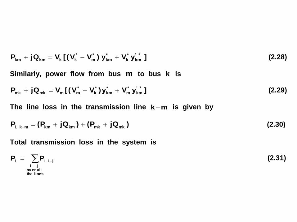
]yVy)VV([VQjP *'
km
*
k
*
km
*
m
*
kkkmkm (2.28)
Similarly, power flow from bus m to bus k is
]yVy)VV([VQjP *'
km
*
m
*
km
*
k
*
mmmkmk (2.29)
The line loss in the transmission line mk is given by
)QjP()QjP(P mkmkkmkmmkL (2.30)
Total transmission loss in the system is
linestheallov erji
jiLL PP (2.31)

Example 2.4
For a power system, the transmission line impedances and the line
charging admittances in p.u. on a 100 MVA base are given in Table 1. The
scheduled generations and loads on different buses are given in Table 2.
Taking the slack bus voltage as 1.06 + j 0.0 and using a flat start perform
the power flow analysis and obtain the bus voltages, transmission loss and
slack bus power.
Table 1 Transmission line data:
Sl. No. Bus code
k - m
Line Impedance
kmz HLCA
1 1 – 2 0.02 + j 0.06 j 0.030
2 1 – 3 0.08 + j 0.24 j 0.025
3 2 – 3 0.06 + j 0.18 j 0.020
4 2 – 4 0.06 + j 0.18 j 0.020
5 2 – 5 0.04 + j 0.12 j 0.015
6 3 – 4 0.01 + j 0.03 j 0.010
7 4 – 5 0.08 + j 0.24 j 0.025

Table 2 Bus data:
Solution
Flat start means all the unknown voltage magnitude are taken as 1.0 p.u.
and all unknown voltage phase angles are taken as 0.
Thus initial solution is
0j1.0VVVV
0j1.06V
(0)
5
(0)
4
(0)
3
(0)
2
1
Bus code
k
Generation Load Remark
MWinPGk MVARinQGk MWinPDk MVARinQDk
1 --- --- 0 0 Slack bus
2 40 30 20 10 P – Q bus
3 0 0 45 15 P – Q bus
4 0 0 40 5 P – Q bus
5 0 0 60 10 P – Q bus

STEP 1
For the transmission system, the bus admittance matrix is to be calculated.
Sl. No.
Bus code k - m
Line Impedance
kmz
Line admittance ykm
HLCA
1 1 – 2 0.02 + j 0.06 5 - j 15 j 0.030
2 1 – 3 0.08 + j 0.24 1.25 – j 3.75 j 0.025
3 2 – 3 0.06 + j 0.18 1.6667 – j 5 j 0.020
4 2 – 4 0.06 + j 0.18 1.6667 – j 5 j 0.020
5 2 – 5 0.04 + j 0.12 2.5 – j 7.5 j 0.015
6 3 – 4 0.01 + j 0.03 10 – j 30 j 0.010
7 4 – 5 0.08 + j 0.24 1.25 – j 3.75 j 0.025
Y22 = (5 – j15) + (1.6667 – j5) + (1.6667 – j5) + (2.5 – j7.5) + j 0.03 + j 0.02 + j 0.02 + j 0.015
= 10.8334 – j 32.415
Similarly Y33 = 12.9167– j 38.695 ; Y44 = 12.9167 – j 38.695 ; Y55 = 3.75 – j 11.21
1 2 3 4 5
1 --- --- --- --- ---
2 -5 +j15 10.8334–j32.415 -1.6667 + j5 -1.6667+j5 -2.5 + j7.5
Y = 3 -1.25 + j3.75 -1.6667 + j5 12.9167–j38.695 -10 + j30 0
4 0 -1.6667 + j5 -10 + j30 12.9167-j38.695 -1.25 + j3.75
5 0 -2.5+j7.5 0 -1.25+j3.75 3.75-j11.21

STEP 2
Calculation of elements of A vector and B matrix.
manner.similaraincalculatedbecanBmatrixofelementsOther
0.00036j0.4626332.415j10.8334
5j5
Y
YB
.calculatedareAandA,ASimilarly
0.0037j0.007432.415j10.8334
0.2j0.2
Y
QIjPIA
0.2j0.2QIjPI
0.2j0.2)20j20(100
1QIjPI
Y
YBand
Y
QIjPIA
22
2121
543
22
222
22
22
kk
kmkm
kk
kkk
1

Thus
1 -----
2 0.00740 + j 0.00370
A = 3 -0.00698 - j 0.00930
4 -0.00427 - j 0.00891
5 -0.02413 - j 0.04545
B =
--- --- --- --- ---
- 0.46263 + j 0.00036
---
- 0.15421 + j 0.00012
- 0.15421 + j 0.00012
- 0.23131 + j 0.00018
- 0.09690 + j 0.00004
- 0.12920 + j 0.00006
---
- 0.77518 + j 0.00033
0
0 - 0.12920
+ j 0.00006 - 0.77518
+ j 0.00033
--- - 0.09690
+ j 0.00004
0 - 0.66881
+ j 0.00072
0 - 0.33440
+ j 0.00036
---

STEP 3
Iterative computation of bus voltage can be carried out as shown.
New estimate of voltage at bus 2 is calculated as:
0.00290j1.03752
)0.0j1.0()0.00018j0.23131(
)0.0j1.0()0.00012j0.15421()0.0j1.0()0.00012j0.15421(
)00.0j1.06()0.00036j0.46263(0j1.0
0.00370j0.00740
VBVBVBVBV
AV )0(
525
)0(
424
)0(
323121*)0(
2
2)1(
2
This value of voltage )1(
2V will replace the previous value of voltage )0(
2V
before doing subsequent calculations of voltages.

The rate of convergence of the iterative process can be increased by
applying an ACCELERATION FACTOR α to the approximate solution
obtained. For example on hand, from the estimate )1(
2V we get the change
in voltage
0.00290j0.03752
)0j1.0()0.00290j1.03752(VVVΔ )0(
2
)1(
22
The accelerated value of the bus voltage is obtained as
0.00406j1.05253
)0.00290j0.03752(1.4)0j1.0(V
1.4assumingBy
ΔVVV
)1(
2
2
)0(
2
)1(
2
This new value of voltage )1(
2V will replace the previous value of the bus
voltage )0(
2V and is used in the calculation of voltages for the remaining
buses. In general
)VV(VV h
k
1h
k
h
k
1h
accldk (2.32)

The process is continued for the remaining buses to complete one
iteration. For the next bus 3
0.00921j1.00690
)0j1.0()0.00033j0.77518(
)0.00406j1.05253()0.00006j0.12920(
)0j1.06()0.00004j0.09690(0j1.0
0.00930j0.00698
VBVBVBV
AV )0(
434
)1(
232131*)0(
3
3)1(
3
The accelerated value can be calculated as
0.01289j1.00966
)0.00921j0.00690(1.4)0j1.0(
)VV(VV )0(
3
)1(
3
)0(
3
)1(
accld3

Continuing this process of calculation, at the end of first iteration, the bus
voltages are obtained as
0.07374j1.02727V
0.02635j1.01599V
0.01289j1.00966V
0.00406j1.05253V
0.0j1.06V
)1(
5
)1(
4
)1(
3
)1(
2
1
If and are the acceleration factors for the real and imaginary
components of voltages respectively, the accelerated values can be
computed as
)ff(βff
)ee(ee
h
k
1h
k
h
k
1h
accldk
h
k
1h
k
h
k
1h
accldk
(2.33)

CONVERGENCE
The iterative process must be continued until the magnitude of change of
bus voltage between two consecutive iterations is less than a certain level
for all bus voltages. We express this in mathematical form as
ΔVmax = max. of h
k
1h
k VV for k = 1,2, …… , N k ≠ s
and ΔVmax < ε
If 1ε and 2ε are the tolerance level for the real and imaginary parts of
bus voltages respectively, then the convergence criteria will be
ΔVmax 1 = max. of ;h
k
1h
k ee ΔVmax 2 = max. of
h
k
1h
k ff
for k = 1,2, …… , N k ≠ s
ΔVmax 1 < ε1 and ΔVmax 2 < ε2
(2.34)
ε
(2.35) (2.35)

For the problem under study 0.0001εε 21
The final bus voltages obtained after 10 iterations are given below.
0.10904j1.01211V
0.09504j1.01920V
0.08917j1.02036V
0.05126j1.04623V
0.0j1.06V
5
4
3
2
1
COMPUTATION OF LINE FLOWS AND TRANSMISSION LOSS
Line flows can be computed from
)0.086j0.888(
])0.03j0.0(0)j1.06(
)15j5()0.05126j1.04623()0j1.06([)0j(1.06
]yVy)VV([VQjP
]yVy)VV([VQjP
*'
12
*
1
*
12
*
2
*
111212
*'
km
*
k
*
km
*
m
*
kkkmkm

)0.062j0.874(
])0.03j(0.0)0.05126j1.04623(
15)j5()0j1.06(0.05126)j1.04623([)0.05126j1.04623(
yVy)VV([VQjP
Similarly
*'
12
*
2
*
12
*
1
*
222121
Power loss in line 1 – 2 is
)0.024j0.014(
0.062)j0.874(0.086)j(0.888)QjP()QjP(P 2121121221L
Power loss in other lines can be computed as
0.051j0.0P
0.019j0.0P
0.002j0.011P
0.029j0.004P
0.033j0.004P
0.019j0.012P
54L
43L
52L
42L
32L
31L
Total transmission loss = ( 0.045 - j 0.173 ) i.e.
Real power transmission loss = 4.5 MW
Reactive power transmission loss = 17.3 MVAR ( Capacitive )

COMPUTATION OF SLACK BUS POWER
Slack bus power can be determined by summing up the powers flowing
out in the lines connected at the slack bus.
Thus in this case slack bus power is
)0.075j1.295()0.086j0.888()0.011j0.407(
)QjP()QjP(QjP 12121313ss
Thus the power supplied by the slack bus:
Real power = 129.5 MW
Reactive power = 7.5 MVAR (Capacitive )
P13 + j Q13
Ps + j Qs G
3 1
2
P12 + j Q12

VOLTAGE CONTROLLED BUS
In voltage controlled bus k net real power injection kPI and voltage
magnitude kV are specified. Normally minmax QIandQI will also be
specified for voltage controlled bus. Since kQI is not known, kA given by
kk
kk
Y
QIjPI cannot be calculated. An expression for kQI can be developed
as shown below.
We know *
kkkkm
N
1m
mkk IVQIjPIandVYI
Denoting haveweδVVandθYY iiijijiji
N
1m
mkmkmkmkk
mkmkmk
N
1m
mk
mmkm
N
1m
mkkkkk
)θδδ(sinYVVQIThus
θδδYVV
δθVYδVQIjPI
(2.36)

N
1m
mkmkmkmkk )θδδ(sinYVVQIThus
The value of kV to be used in equation (2.36) must satisfy the relation
specifiedkk VV
Because of voltage updating in the previous iteration, the voltage
magnitude of the voltage controlled bus might have been deviated from the
specified value. It has to be pulled back to the specified value, using the
relation
Adjusted voltage h
k
h
k
h
kh
k
h
k1h
k
h
kspecifiedk
h
k fjeVtaking)e
f(tanδwhereδVV
Using the adjusted voltage h
kV as given in eqn. (2.37), net injected reactive
power h
kQI can be computed using eqn. (2.36). As long as h
kQI falls within
the range specified, h
kV can be replaced by the Adjusted h
kV and kA can
be computed.
(2.37)
(2.36)

In case if h
kQI violates any one the limits specified, then h
kV should not be
replaced by Adjusted h
kV ; h
kQI is set to the limit and kA can be
calculated. In this case bus k is changed from P – V to P – Q type.
Once the value of kA is known, further calculation to find 1h
kV will be
the same as that for P – Q bus.
Complete flow chart for power flow solution using Gauss-Seidel method is
shown in Fig. 2.7. The extra calculation needed for voltage controlled bus
is shown between X – X and Y – Y.

START
READ LINE DATA & BUS DATA
FORM Y MATRIX
ASSUME skNkVk ,,2,1)0(
COMPUTE kA FOR P – Q BUSES
COMPUTE kmB SET h = 0
SET k = 1 AND 0.0 MAXV
k : s YES
X -------------------------------------------- NO-----------------------------------------
NO k : V.C. Bus X YES
COMPUTE h
k ADJUSTED VOLTAGE, h
kQI
MAXk
h
k QIQI : MINk
h
k QIQI :
> <
REPLACE h
kQI BY MAXkQI REPLACE h
kQI BY MINkQI REPLACE h
kV BY ADJ h
kV
Y COMPUTE kA Y
-----------------------------------------------------------------------------------------------------------------
COMPUTE ;1h
kV COMPUTE h
k
h
k VVV 1
YES
MAXVV SET VVMAX NO
REPLACE h
kV BY 1h
kV
SET k = k + 1
k : N IS MAXV < YES
NO
SET h = h + 1
COMPUTE LINE FLOWS, SLACK BUS POWER
PRINT THE RESULTS
STOP
>

Representation of off nominal tap setting transformer
A transformer with no tap setting arrangement can be represented similar to a
short transmission line. However off nominal tap setting transformer which has tap
setting facility at the HT side calls for different representation.
Consider a transformer 110 / 11 kV having tap setting facility. Its nominal ratio is
10 : 1 i.e. its nominal turns OR voltage ratio = 10. Suppose the tap is adjusted so
that the turns ratio becomes 11 : 1. This can be thought of connecting two
transformers in cascade, the first one with ratio 11 : 10 and the second one with the
ratio 10 : 1 (Nominal ratio). In this case the off nominal turns ratio is 11 / 10 = 1.1.
Suppose the tap is adjusted so that the turns ratio becomes 9 : 1. This is same as
two transformers in cascade, the first with a turn ratio 9 : 10 and the second with
the ratio 10 : 1 ( Nominal ratio ). In this case off nominal turn ratio is 9 / 10 = 0.9.

A transformer with off nominal turn ratio can be represented by its impedance or
admittance, connected in series with an ideal autotransformer as shown in Fig. 2.10.
An equivalent ∏ circuit as shown in Fig. 2.11, will be useful for power flow studies.
The elements of the equivalent ∏ circuit can be treated in the same manner as the
line elements.
Let ''a be the turn ratio of the autotransformer. ''a is also called as off nominal
turns ratio. Usually ''a varies from 0.85 to 1.15.
Fig. 2.10 Representation of off nominal transformer
a:1
pqy
pI tqi
p q t
qI

The parameters of the equivalent ∏ circuit shown in Fig. 2.11 can be derived by
equating the terminal current of the transformer with the corresponding current of
the equivalent ∏ circuit.
It is to be noted that aI
ianda
E
E
p
qt
t
p (2.86)
We are going to write Ip and Iq in terms of Ep nd Eq.
q
qp
p2
qp
qpq
p
qpqt
qt
p
Ea
yE
a
y
y)Ea
E(
a
1y)EE(
a
1
a
iI
qqpp
qp
qp
p
qqptqq
EyEa
y
y)a
EE(y)EE(I Also
pqy
pItqi
p q t
qI
(2.87)
(2.88)

qqpp
qp
q EyEa
yI
Referring to the ∏ equivalent circuit
qppqpp EAE)BA(BEA)E(EI and
qpqpqq E)CA(EACEA)EE(I
Comparing the coefficients of pE and
qE in eqns. (2.87) to (2.90), we get
qp
qp
2
qp
yCA
a
yA
a
yBA
qp
qp
qp
qp
qp
2
qp
qp
y)a
11(
a
yyC
y)1a
1(
a
1
a
y
a
yB
a
yAThus
(2.90)
(2.89)
q
qp
p2
qp
p Ea
yE
a
yI
Q P
C B
A
Iq IP
Fig. 2.11
Parameters A,B and C
are ADMITTANCES

a
y qp
qpy)1a
1(
a
1 qpy)
a
11(
p
The equivalent ∏ circuit will then be as shown in Fig. 2.12
When the off nominal turns ratio is represented at bus p for transformer
connected between p and q is included, the following modifications are
necessary in the bus admittance matrix.
a
yYY
a
yYY
yYy)a
11(
a
yYY
a
yYy)1
a
1(
a
1
a
yYY
qp
oldpqnewpq
qp
oldqpnewqp
qpoldqqqp
qp
oldqqnewqq
2
qp
oldppqp
qp
oldppnewpp
I q I p
q
(2.91)
Fig. 2.12 Equivalent circuit of off nominal transformer

Obtain the bus admittance matrix of the transmission system with the following
data.
Line data
Line
No.
Between
buses Line Impedance HLCA
Off
nominal
turns ratio
1 1 – 4 0.08 + j 0.37 j 0.007 ---
2 1 – 6 0.123 + j 0.518 j 0.010 ---
3 2 – 3 0.723 + j 1.05 0 ---
4 2 – 5 0.282 + j 0.64 0 ---
5 4 – 3 j 0.133 0 0.909
6 4 – 6 0.097 + j 0.407 j 0.0076 ---
7 6 – 5 j 0.3 0 0.976
Shunt capacitor data
Bus No. 4 Admittance j 0.005

Line No.
Between buses
Line admittance HLCA ypq / a ypq / a2
1 1 4 0.5583 – j2.582 j 0.007 --- ---
2 1 6 0.4339 – j1.8275 j 0.01 ---- ---
3 2 3 0.4449 – j 0.6461 0 ---- ----
4 2 5 0.5765 – j 1.3085 0 ---- ----
5 4 3 - j 7.5188 0 - j8.2715 - j 9.0996
6 4 6 0.5541 – j 2.3249 j 0.0076 ---- ----
7 6 5 - j 3.3333 0 - j 3.4153 - j 3.4993
Y11 = 0.5583 – j 2.582 + j 0.007 + 0.4339 – j 1.8275 + j 0.01 = 0.9922 – j 4.3925
Y22 = 0.4449 – j0.6461 + 0.5765 – j1.3085 = 1.0214 – j 1.9546
Y33 = 0.4449 – j0.6461 – j7.5188 = 0.4449 – j 8.1649
Y44 = 0.5583 – j 2.582 + j 0.007 – j 9.0996 + 0.5541 – j 2.3249 + j 0.0076 + j0.005
= 1.1124 – j 13.9869
Y55 = 0.5765 – j1.3085 – j 3.3333 = 0.5765 – j 4.6418
Y66 = 0.4339 – j 1.8275 + j 0.01+ 0.5541– j 2.3249 + j0.0076 - j 3.4993 = 0.988 – j 7.6341

Answer
j7.6341
0.988
j3.4153j2.3209
0.554100
j1.8275
0.4339
j3.4153j4.6418
0.576500
j1.3085
0.57650
j2.3249
0.5541
0j13.9869
1.1124j8.27150
j2.5820
0.5583
00j8.2715j8.1649
0.4449
j0.6461
0.44490
0j1.3085
0.57650
j0.6461
0.4449
j1.9546
1.02140
j1.8275
0.4339
0j2.5820
0.558300
j4.3925
.99220

%
% Bus admittance matrix including off nominal transformer
% Shunt parameter must be in ADMITTANCE
% Reading the line data
%
Nbus = 6; Nele = 7; Nsh = 1;
%
% Reading element data
%
Edata=[1 1 4 0.08+0.37i 0.007i 1;2 1 6 0.123+0.518i 0.01i 1;…
3 2 3 0.723+1.05i 0 1; 4 2 5 0.282+0.64i 0 1; ...
5 4 3 0.133i 0 0.909;6 4 6 0.097+0.407i 0.0076i 1; ...
7 6 5 0.3i 0 0.976];
%
% Reading shunt data
%
Shdata = [1 4 0.005i];

%
% Displaying data
%
disp([' Sl.No From bus To bus Line
Impedance HLCA ONTR'])
Edata
if Nsh~=0
disp([' Sl.No. At bus Shunt Admittamce'])
Shdata
end
%
% Formation of Ybus matrix
%
Ybus = zeros(Nbus,Nbus);

for k = 1:Nele
p = Edata(k,2);
q = Edata(k,3);
yele = 1/Edata(k,4);
Hlca = Edata(k,5);
offa = Edata(k,6);
offaa = offa*offa;
Ybus(p,p) = Ybus(p,p) + yele/offaa + Hlca;
Ybus(q,q) = Ybus(q,q) + yele + Hlca;
Ybus(p,q) = Ybus(p,q) - yele/offa;
Ybus(q,p) = Ybus(q,p) - yele/offa;
end
if Nsh~=0
for i = 1:Nsh
q = Shdata(i,2);
yele = Shdata(i,3);
Ybus(q,q) = Ybus(q,q) + yele;
end
end
disp([' *** BUS ADMITTANCE MATRIX ***'])
Ybus

Introduction to Power Flow Analysis by Newton Raphson method
Gauss-Seidel method of solving the power flow has simple problem formulation and hence
easy to explain However, it has poor convergence characteristics. It takes large number of
iterations to converge. Even for the five bus system discussed in Example 2.4, it takes 10
iterations to converge.
Newton Raphson (N.R.) method of solving power flow is based on the Newton Raphson
method of solving a set of non-linear algebraic equations.
N. R. method of solving power flow problem has very good convergence characteristics.
Even for large systems it takes only two to four iterations to converge.

Power flow model of Newton Raphson method
The equations describing the performance of the network in the bus admittance
form is given by
I = Y V (2.38)
In expanded form these equations are
N
2
1
I
I
I
=
NNN2N1
2N2221
1N1211
YYY
YYY
YYY
N
2
1
V
V
V
(2.39)
Typical element of the bus admittance matrix is
jiY = jiY jiθ = jiY cos jiθ + j jiY sin jiθ = jiG + j jiB (2.40)
Voltage at a typical bus i is
iV = iV iδ = iV ( cos iδ + j sin iδ ) (2.41)
The current injected into the network at bus i is given by
n
N
1n
ni
nNi22i11ii
VY
VYVYVYI
(2.42)

In addition to the linear network equations given by eqn. (2.39), bus power
equations should also be satisfied in the power flow problem. These bus power
equations introduce non- linearity into the power flow model. The complex power
entering the network at bus i is given by
*
iiii IVQjP (2.43)
Bus power equations can be obtained from the above two equations (2.42) and (2.43) by
eliminating the intermediate variable iI . From eqn. (2.43)
iIVQjP*
iii = *
iV n
N
1n
ni VY
= iV iδ
N
1n
niY niθ nV nδ
=
N
1n
iV nV niY niθ + nδ - iδ
Separating the real and imaginary parts, we obtain
iP =
N
1n
iV nV niY cos ( niθ + nδ - iδ ) (2.44)
iQ = -
N
1n
iV nV niY sin ( niθ + nδ - iδ ) (2.45)

iP =
N
1n
iV nV niY cos (niθ + nδ -
iδ ) (2.44)
iQ = -
N
1n
iV nV niY sin ( niθ + nδ - iδ ) (2.45)
The real and reactive powers obtained from the above two equations are referred as
calculated powers. During the power flow calculations, their values depend on the latest
bus voltages. Finally,these calculated powers should be equal to the specified powers. Thus
the non-linear equations to be solved in power flow analysis are
N
1n
iV nV niY cos ( niθ + nδ - iδ ) = iPI (2.46)
-
N
1n
iV nV niY sin ( niθ + nδ - iδ ) = iQI (2.47)
It is to be noted that equation (2.46) can be written for bus i only if real power injection at
bus i is specified.
Similarly, equation (2.47) can be written for bus i only if reactive power injection at bus
i is specified.

N
1n
iV nVniY cos (
niθ + nδ - iδ ) = iPI (2.46)
-
N
1n
iV nVniY sin ( niθ + nδ - iδ ) = iQI (2.47)
Of the N total number of buses in the power system, let the number of P-Q buses be
1N , P-V buses be 2N . Then 1NNN 21 . Basic problem is to find the
i) Unknown phase angles δ at the 21 NN number of P-Q & P-V buses and
ii) Unknown voltage magnitudes V at the 1N number of P-Q buses.
Thus total number of unknown variables = 21 NN2
We can write 21 NN real power specification equations (eqn.2.46) and 1N reactive
power specification equations (eqn.2.47).
Thus total number of equations = 21 NN2 .
Therefore Number of equations = Number of variables = 21 NN2

Thus in power flow study, we need to solve the equations
N
1n
iV nVniY cos ( niθ + nδ - iδ ) = iPI (2.48)
for i = 1, 2, …….., N
i ≠ s
and
-
N
1n
iV nVniY sin ( niθ + nδ - iδ ) = iQI (2.49)
for i = 1, 2, …….., N
i ≠ s
i ≠ P – V buses
for the unknown variables δi i = 1,2,…….., N, i ≠ s and
|Vi| i = 1,2,…....., N, i ≠ s , i ≠ P – V buses
The unknown variables are also called as state variables.

Example 2.5
In a 9 bus system, bus 1 is the slack bus, buses 2,5 and 7 are the P-V buses. List the state
variables. Also indicate the specified power injections.
Solution
Buses 3,4,6,8 and 9 are P-Q buses.
9864398765432 VandV,V,V,V,δ,δ,δ,δ,δ,δ,δ,δ are the state variables.
9864398765432 QIandQI,QI,QI,QI,PI,PI,PI,PI,PI,PI,PI,PI are the specified power
injections.

=
Newton Raphson method of solving a set of non-linear equations
Let the non-linear equations to be solved be
1k)x,,x,(xf n211
2n212 k)x,,x,(xf
(2.50)
nn21n k)x,,x,(xf
Let the initial solution be (0)
n
(0)
2
(0)
1 x,,x,x
If 0)x,,x,(xfk(0)
n
(0)
2
(0)
111
0)x,,x,(xfk(0)
n
(0)
2
(0)
122
0)x,,x,(xfk(0)
n
(0)
2
(0)
1nn
then the solution is reached. Let us say that the solution is not reached.

Let us say that the solution is not reached. Assume n21 Δx,,Δx,Δx are the
corrections required on (0)
n
(0)
2
(0)
1 x,,x,x respectively. Then
1k)]Δx(x ,), Δx(x),Δx[(x f n
(0)
n2
(0)
21
(0)
11
2n
(0)
n2
(0)
21
(0)
12 k)]Δx(x,),Δx(x),Δx[(xf (2.51)
nn
(0)
n2
(0)
21
(0)
1n k)]Δx(x ,),Δx(x),Δx[(xf
Each equation in the above set can be expanded by Taylor’s theorem around(0)
n
(0)
2
(0)
1 x,,x,x . For example, the following is obtained for the first equation.
(0)
n
(0)
2
(0)
11 x,,x,(xf 1
1
x
f)
2
1
1x
fΔx
n
1
2x
fΔx
11n kφΔx

0
0
0 0
0
(0)
n
(0)
2
(0)
11 x,,x,(xf 1
1
x
f)
2
1
1x
fΔx
n
1
2x
fΔx
11n kφΔx
where 1φ is a function of higher derivatives of 1f and higher powers of
n21 Δx,,Δx,Δx . Neglecting 1φ and also following the same for other equations,
we get
(0)
n
(0)
2
(0)
11 x,,x,(xf 1
1
x
f)
2
1
1x
fΔx
n
1
2x
fΔx
1n kΔx
(0)
n
(0)
2
(0)
12 x,,x,(xf 1
2
x
f)
2
2
1x
fΔx
n
2
2x
fΔx
2n kΔx
(0)
n
(0)
2
(0)
1n x,,x,(xf 1
n
x
f)
2
n
1x
fΔx
n
n
2x
fΔx
nn kΔx
(2.52)
0 0
0
0

0 0 0
0 0 0
0 0 0
(2.53)
The matrix form of equations (2.52) is
)x,,x,x(fkΔxx
f
x
f
x
f (0)
n
(0)
2
(0)
1111
n
1
2
1
1
1
)x,,x,x(fkΔxx
f
x
f
x
f (0)
n
(0)
2
(0)
1222
n
2
2
2
1
2
)x,,x,x(fkΔxx
f
x
f
x
f (0)
n
(0)
2
(0)
1nnn
n
n
2
n
1
n
The above equation can be written in a compact form as
)X(FKΔX)X(F(0)(0)' (2.54)
This set of linear equations need to be solved for the correction vector
n
2
1
Δx
Δx
Δx
ΔX
=

)X(FKΔX)X(F(0)(0)' (2.54)
In eqn.(2.54) )X(F(0)' is called the JACOBIAN MATRIX and the vector )X(FK
(0)
is called the ERROR VECTOR. The Jacobian matrix is also denoted as J.
Solving eqn. (2.54) for ΔX
ΔX = 1)0(')X(F
)X(FK)(0 (2.55)
Then the improved estimate is
ΔXXX)0(1)(
Generalizing this, for th)1h( iteration
ΔXXX)h()1h( where (2.56)
)X(FK)X(FΔX)h(1)h(' (2.57)
i.e. ΔX is the solution of )X(FKΔX)X(F)h()h(' (2.58)

Thus the solution procedure to solve K)X(F is as follows :
(i) Calculate the error vector )X(FK(h)
If the error vector zero, convergence is reached; otherwise formulate
)X(FKΔX)X(F(h)(h)'
(ii) Solve for the correction vector ΔX
(iii) Update the solution as
ΔXXX(h)1)(h
Values of the correction vector can also be used to test for convergence.
It is to be noted that Error vector = specified vector – vector of calculated values

Example 2.6
Using Newton-Raphson method, solve for 1x and 2x of the non-linear equations
4 2x sin 1x = - 0.6
4 2
2x - 4 2x cos 1x = - 0.3
Choose the initial solution as (0)
1x = 0 rad. and (0)
2x = 1. Take the precision index on error
vector as 310
.
Solution
Errors are calculated as
- 0.6 – (4 2x sin )1x ) = - 0.6
- 0.3 – (4 2
2x - 4 2x cos 1x ) = - 0.3
The error vector
0.3
0.6is not small.
1x
0x
2
1
1x
0x
2
1

It is noted that 1f = 4 2x sin 1x
2f = 4 2
2x - 4 2x cos 1x
Jacobian matrix is: J =
2
2
1
2
2
1
1
1
x
f
x
f
x
f
x
f
=
1212
112
xcos4x8xsinx4
xsin4xcosx4
Substituting the latest values of state variables 1x = 0 and 2x = 1
J =
40
04 ; Its inverse is 1
J =
0.250
00.25
Correction vector is calculated as
2
1
xΔ
xΔ =
0.250
00.25
0.3
0.6 =
0.075
0.150
The state vector is updated as
2
1
x
x =
1
0 +
0.075
0.150 =
0.925
0.150
This completes the first iteration.

Errors are calculated as
- 0.6 – (4 2x sin 1x ) = = - 0.047079
- 0.3 – (4 2
2x - 4 2x cos 1x ) = - 0.064047
The error vector
0.064047
0.04709is not small.
Jacobian matrix is: J =
1212
112
xcos4x8xsinx4
xsin4xcosx4
=
3.4449160.552921
0.5977533.658453
0.925x
rad.0.15x
2
1
0.925x
rad.0.15x
2
1
0.925x
rad.0.15x
2
1

Correction vector is calculated as
2
1
xΔ
xΔ =
3.4449160.552921
0.5977533.658453
0.064047
0.047079 =
0.021214
0.016335
The state vector is updated as
2
1
x
x =
0.925
0.150 +
0.021214
0.016335 =
0.903786
0.166335
This completes the second iteration.
Errors are calculated as
- 0.6 – (4 2x sin 1x ) = = - 0.001444
- 0.3 – (4 2
2x - 4 2x cos 1x ) = - 0.002068
Still error vector exceeds the precision index.
0.903786x
rad.0.166335x
2
1
- 1
0.903786x
rad.0.166335x
2
1

Jacobian matrix is: J =
1212
112
xcos4x8xsinx4
xsin4xcosx4
=
3.2854950.598556
0.6622763.565249
Correction vector is calculated as
2
1
xΔ
xΔ =
3.2854950.598556
0.6622763.565249
0.002068
0.001444 =
0.000728
0.000540
The state vector is updated as
2
1
x
x =
0.903786
0.166335 +
0.000728
0.000540 =
0.903058
0.166875
0.903786x
rad.0.166335x
2
1
- 1

Errors are calculated as
- 0.6 – (4 2x sin 1x ) = = - 0.000002
- 0.3 – (4 2
2x - 4 2x cos 1x ) = - 0.000002
Errors are less than 10-3
.
The final values of 1x and 2x are - 0.166875 rad. and 0.903058 respectively.
The results can be checked by substituting the solution in the original equations:
4 2x sin 1x = - 0.6
4 2
2x - 4 2x cos 1x = - 0.3
0.903058x
rad.0.166875x
2
1
0.903058x
rad.0.166875x
2
1

In this example, we have actually solved our first power flow problem by N.R. method.
This is because the two non-linear equations of this example are the power flow model of
the simple system shown in Fig. 2.8.
1V 1δ 2V 2δ
Here bus 1 is the slack bus with its voltage 1V 1δ = 1.0 00 p.u. Further 1x represents
the angle 2δ and 2x represents the voltage magnitude 2V at bus 2.
We now concentrate on the application of Newton-Raphson procedure in the power flow
studies.
Fig. 2.8 Two bus power flow model
p.u.)0.3j0.6(QP 2d2d
j 6.0 p.u.
j 0.25 p.u.
G
1 2

Power flow solution by Newton Raphson method
As discussed earlier, taking the bus voltages and line admittances in polar form, in power
flow study we need to solve the non-linear equations
N
1n
iV nV niY cos ( niθ + nδ - iδ ) = iPI (2.59)
-
N
1n
iV nV niY sin ( niθ + nδ - iδ ) = iQI (2.60)
Separating the term with in we get
ii
2
i GV +
N
in1n
iV nV niY cos ( niθ + nδ - iδ ) = iPI (2.61)
ii
2
i BV
N
in1n
iV nV niY sin ( niθ + nδ - iδ ) = iQI (2.62)

In a compact form, the above non-linear equations can be written as
PI)Vδ,(P (2.63)
QI)Vδ,(Q (2.64)
On linearization, we get
ΔQ
ΔP
VΔ
Δδ
V
Q
δ
Q
V
P
δ
P
(2.65)
where
PIΔP calculated value of )Vδ,(P corresponding to the present solution.
QIΔQ calculated value of )Vδ,(Q corresponding to the present solution.

To bring symmetry in the elements of the coefficient matrix, V
VΔ is taken as
problem variable in place of VΔ . Then eqn. (2.65) changes to
ΔQ
ΔP
V
VΔ
Δδ
VV
Q
δ
Q
VV
P
δ
P
(2.66)
In symbolic form, the above equation can be written as
ΔQ
ΔP
V
VΔ
Δδ
LM
NH
(2.67)

The matrix H N is known as JACOBIAN matrix.
M L
The dimensions of the sub-matrices will be as follows:
H )N(N 21 x )N(N 21
N )N(N 21 x 1N
M 1N x )N(N 21 and
L 1N x 1N
where 1N is the number of P-Q buses and 2N is the number of P-V buses.
Consider a 4 bus system having bus 1 as slack bus, buses 2 and 3 as P-Q buses
and bus 4 as P-V bus for which real power injections 432 PI&PI,PI and reactive
power injections 32 QI&QI are specified. Noting that 32432 VandV,δ,δ,δ are
the problem variables, linear equations that are to be solved in each iteration will
be

32432 VVδδδ
2P
3
3
2
2
2
2
4
2
3
2
2
2 VV
PV
V
P
δ
P
δ
P
δ
P
2Δδ 2ΔP
3P 3
3
3
2
2
3
4
3
3
3
2
3 VV
PV
V
P
δ
P
δ
P
δ
P
3Δδ 3ΔP
4P 3
3
4
2
2
4
4
4
3
4
2
4 VV
PV
V
P
δ
P
δ
P
δ
P
4Δδ = 4ΔP (2.68)
2Q 2
2
δ
δQ
3
2
δ
Q
4
2
δ
Q
2
2
2 VV
Q
3
3
2 VV
Q
2
2
V
VΔ 2ΔQ
3Q 2
3
δ
δQ
3
3
δ
Q
4
3
δ
Q
2
2
3 VV
Q
3
3
3 VV
Q
3
3
V
VΔ 3QΔ

The following is the solution procedure for N.R. method of power flow analysis.
1 Read the line data and bus data; construct the bus admittance matrix.
2 Set k = 0. Assume a starting solution. Usually a FLAT START is assumed in
which all the unknown phase angles are taken as zero and unknown voltage
magnitudes are taken as 1.0 p.u.

k
3 Compute the mismatch powers i.e. the error vector. If the elements of error
vector are less than the specified tolerance, the problem is solved and hence go to
Step 7; otherwise proceed to Step 4.
4 Compute the elements of sub-matrices H, N, M and L. Solve
ΔQ
ΔP
V
VΔ
Δδ
LM
NH
for
V
VΔ
Δδ
5 Update the solution as
V
δ =
V
δ +
VΔ
Δδ
6 Set k = k + 1 and go to Step 3.
7 Calculate line flows, transmission loss and slack bus power. Print the
results and STOP.
k
k+1 k

Calculation of elements of Jacobian matrix
We know that the equations that are to be solved are
ii
2
i GV +
N
in1n
iV nV niY cos ( niθ + nδ - iδ ) = iPI (2.69)
ii
2
i BV
N
in1n
iV nV niY sin ( niθ + nδ - iδ ) = iQI (2.70)
i.e. ii PI)V,(δP (2.71)
ii QI)Vδ,(Q (2.72)
The suffix i should take necessary values.
Jacobian matrix is
LM
NH where
VV
QLand
δ
QM;V
V
PN;
δ
PH

Here
iP = ii
2
i GV +
N
in1n
iV nV niY cos (niθ + nδ -
iδ ) (2.73)
iQ = ii
2
i BV
N
in1n
iV nV niY sin (niθ + nδ -
iδ ) (2.74)
Diagonal elements:
i
i
iiδ
PH
=
N
in1n
iV nV niY sin (niθ + nδ -
iδ ) = ii
2
ii BVQ (2.75)
ii
2
ii
i
i
ii GV2VV
PN
+
N
in1n
iV nV niY cos ( niθ + nδ - iδ )
= iP + ii
2
i GV (2.76)
i
i
iiδ
QM
=
N
in1n
iV nV niY cos ( niθ + nδ - iδ ) = iP - ii
2
i GV (2.77)
i
i
i
ii VV
QL
= ii
2
i BV2 -
N
in1n
iV nV niY sin ( niθ + nδ - iδ )
= iQ ii
2
i BV (2.78)

Off-diagonal elements:
We know that
iP = ii
2
i GV +
N
in1n
iV nV niY cos ( niθ + nδ - iδ ) (2.79)
iQ = ii
2
i BV
N
in1n
iV nV niY sin ( niθ + nδ - iδ ) (2.80)
jiji
j
i
ji YVVδ
PH
sin ( jiθ + jδ - iδ ) (2.81)
j
j
i
ji VV
PN
= jiji YVV cos ( jiθ + jδ - iδ ) (2.82)
j
i
jiδ
QM
= jiji YVV cos ( jiθ + jδ - iδ ) (2.83)
j
j
i
ji VV
QL
= jiji YVV sin ( jiθ + jδ - iδ ) (2.84)

Summary of formulae
iiH ii
2
ii BVQ
iiN iP + ii
2
i GV
iiM iP ii
2
i GV
iiL iQ ii
2
i BV
jiH jiji YVV sin ( jiθ + jδ - iδ )
jiN jiji YVV cos ( jiθ + jδ - iδ )
jiM jiji YVV cos ( jiθ + jδ - iδ )
jiL jiji YVV sin ( jiθ + jδ - iδ )
Flow chart for N.R. method of power flow solution is shown below.
(2.85)

k
START
READ LINE and BUS DATA
COMPUTE Y MATRIX
ASSUME FLAT START
SET k = 0
FOR ALL P-V BUSES COMPUTE iQ
IF iQ VIOLATES THE LIMITS SET
iQ = LimitiQ AND TREAT BUS i AS A P-Q BUS
COMPUTE MISMATCH POWERS ΔQ&ΔP
COMPUTE MATRICES H,N,M & L
FORM
ΔQ
ΔP
V
VΔΔδ
LM
NH ; SOLVE FOR
V
VΔΔδ
AND UPDATE
V
δ =
V
δ +
VΔ
Δδ
YES
SET k = k + 1
COMPUTE LINE FLOWS, TRANSMISSION LOSS & SLACK BUS POWER
PRINT THE RESULTS
STOP
NO
k+1 k
ELEMENTS OF
ΔQ&ΔP < ε ?

Example 2.7
Perform power flow analysis for the power system with the data given below, using
Newton Raphson method, and obtain the bus voltages.
Line data ( p.u. quantities )
Bus data ( p.u. quantities )
Bus
No Type
Generator Load V δ minQ maxQ
P Q P Q
1 Slack --- --- 0 0 1.0 0 --- ---
2 P - V 1.8184 --- 0 --- 1.1 --- 0 3.5
3 P - Q 0 0 1.2517 1.2574 --- --- --- ---
0.2j0313
0.2j0322
0.1j0211
impedancesLinebusesBetweenNo.Line

Solution
The bus admittance matrix can be obtained as
1 2 3
Y =
j10j5j5
j5j15j10
j5j10j15
; G = [0]; B =
1055
51510
51015
Y
1055
51510
51015
and θ =
000
000
000
909090
909090
909090
In this problem
1.2574QI
1.2517PI
1.8184PI
3
3
2
and unknown quantities =
3
3
2
V
δ
δ
1
2
3
1
2
3
1 2 3
1
2
3
1 2 3

With flat start 0
1 01.0V
0
2 01.1V
0
3 01.0V
We know that
iP = ii
2
i GV +
N
in1n
iV nV niY cos ( niθ + nδ - iδ )
iQ = ii
2
i BV
N
in1n
iV nV niY sin ( niθ + nδ - iδ )
Substituting the values of bus admittance parameters, expressions for 2P , 3P and 3Q
are obtained as follows
2P = )δδθ(cosYVV)δδθ(cosYVVGV 233232322112121222
2
2
= 0 + )δδ90(cosVV5)δδ90(cosVV10 23322112
= )δδ(sinVV5)δδ(sinVV10 23322112

Similarly
3P = 5 3V 1V )δδ(sin 31 5 3V 2V )δδ(sin 32
Likewise
33
2
33 BVQ 3V 1V )δδ90(sinY 3113 3V 2V )δδ(90sinY 3223
= 5V102
3 3V 1V 5)δδ(cos 31 3V 2V )δδ(cos 32
Iteration starts:
To check whether bus 2 will remain as P-V bus, 2Q need to be calculated.
10V15Q2
22 2V 1V 5)δδ(cos 21 2V 3V )δδ(cos 23
= ( 15 x 1.1 x 1.1 ) – ( 10 x 1.1 x 1 x 1 ) – ( 5 x 1.1 x 1 x 1 ) = 1.65
This lies within the Q limits. Thus bus 2 remains as P – V bus.

Since 0,δδδ 321
we get 0PP 32
3Q = ( 10 x 1 x 1 ) – ( 5 x 1 x 1 ) – ( 5 x 1 x 1.1 ) = - 0.5
Mismatch powers are: 1.818401.8184PPIΔP 222
1.251701.2517PPIΔP 333
0.75740.51.2574QQIΔQ 333
333332
333332
232322
332
LMM
NHH
NHH
Vδδ
3
3
3
2
V
VΔ
Δδ
Δδ
=
3
3
2
ΔQ
ΔP
ΔP
2P
3P
3Q
Linear equations
to be solved are

Summary of formulae
iiH ii
2
ii BVQ
iiN iP + ii
2
i GV
iiM iP ii
2
i GV
iiL iQ ii
2
i BV
jiH jiji YVV sin ( jiθ + jδ - iδ )
jiN jiji YVV cos ( jiθ + jδ - iδ )
jiM jiji YVV cos ( jiθ + jδ - iδ )
jiL jiji YVV sin ( jiθ + jδ - iδ )
(2.85)

ii
2
iiii
iiiiii
ii
2
iiii
BVQL
PM;PN
BVQH
)δδ(sinYVVM
)δδ(sinYVVN
)δδ(cosYVVH
ijjijiji
ijjijiji
ijjijiji
For this problem, since iiG are zero and
jiθ are 090
22
2
2222 BVQH - 1.65 + ( 1.1 x 1.1 x 15 ) = 16.5
10.5100.5BVQH 33
2
3333
0PM;0PN 333333
9.5100.5BVQL 33
2
3333
32H 2V 3V )δδ(cosY 2332 = 5.51x5x1x1.1 and 23H = 5.5
32N 2V 3V 0)δδ(sinY 2332
32M 3V 2V 0)δδ(sinY 3223

Thus
9.500
010.55.5
05.516.5
3
3
3
2
V
VΔ
Δδ
Δδ
=
0.7574
1.2517
1.8184
Solving the above
3
3
3
2
V
VΔ
Δδ
Δδ
=
0.0797
0.07449
0.08538
Therefore
0)1(
2 4.89rad.0.085380.085380δ
0)1(
3 4.27rad.0.074490.074490δ
0.92030.07971.0V)1(
3
Thus 0
1 01.0V
0
2 4.891.1V
0
3 4.270.9203V
This completes the first iteration.

Second iteration:
2Q (15 x 1.1 x 1.1) - (10 x 1.1 x 1.0 cos 04.89 ) - (5 x 1.1 x 0.9203 cos 0
9.16 )
= 2.1929
This is within the limits. Bus 2 remains as P-V bus.
2P (10 x 1.1 x 1.0 sin 04.89 ) + ( 5 x 1.1 x 0.9203 sin 0
9.16 ) = 1.7435
3P - ( 5 x 0.9203 x 1.0 sin 4.270 ) – ( 5 x 0.9203 x 1.1 sin 9.16
0 ) = -1.1484
3Q = 10 x 0.9203 x 0.9203 - ( 5 x 0.9203 x 1.0 cos 4.270) - ( 5 x 0.9203 x 1.1 cos 9.16
0)
= - 1.1163
2ΔP 1.8184 – 1.7435 = 0.0749
3ΔP - 1.2517 + 1.1484 = - 0.1033
3ΔQ - 1.2574 + 1.1163 = -0.1444

22H - 2.1929 + ( 1.1 x 1.1 x 15 ) = 15.9571
33H 1.1163 + (0.9203 x 0.9203 x 10) = 9.5858
33N = - 1.1484; 33M = - 1.1484
33L - 1.1163 + ( 0.92032 x 10 ) = 7.3532
23H - 1.1 x 0.9203 x 5 cos 9.160 = - 4.9971
32H = - 4.9971
23N 1.1 x 0.9203 x 5 sin 9.160 = 0.8058
32M = 0.8058
The linear equations are
7.35321.14840.8058
1.14849.58584.9971
0.80584.997115.9571
3
3
3
2
V
VΔ
Δδ
Δδ
=
0.1444
0.1033
0.0749

Its solution is
3
3
3
2
V
VΔ
Δδ
Δδ
=
0.021782
0.012388
0.001914
3VΔ - 0.9203 x 0.02178 = - 0.02
0)2(
2 5.00rad.0.087290.0019140.08538δ
0)2(
3 4.98rad.0.086880.0123880.07449δ
0.90320.020.9232V)2(
3

Thus at the end of second iteration
0
1 01.0V
0
2 5.001.1V
0
3 4.980.9032V
Continuing in this manner the final solution can be obtained as
0
1 01.0V
0
2 51.1V
0
3 50.9V
Once we know the final bus voltages, if necessary, line flows, transmission loss and
the slack bus power can be calculated following similar procedure adopted in the
case of Gauss – Seidel method.

j 0.25
j 0.25
j 0.15
j 0.2
j 0.4
j 0.125
EE 0308 Power System Analysis - Problem Set 2
PROBLEM 1
Consider the transmission network shown. Generators of reactances j1.25 are
connected at busses 3 and 4. The network graph is also shown below.
i) Obtain the bus admittance matrix of the power system.
ii) Neglect the mutual coupling and find the bus admittance matrix.
4
7
6
5
4 3
2
1
3
1
0
4
2
1
2
3

Answer
- j16.75 j11.75 j2.5 j2.5
j11.75 - j19.25 j2.5 j5
j2.5 j2.5 - j5.8 0
j2.5 j5 0 - j8.3
- j14.5 j8 j4 j2.5
j8 - j17 j4 j5
j4 j4 - j8.8 0
j2.5 j5 0 - j8.3
Ybus =
1
1
2
3
4
2 3 4
Ybus =
1
1
2
2 3 4

PROBLEM 2 For the transmission network with the following data,
determine the bus admittance matrix.
Sl.
No.
Bus Code
k - m
Line Impedance
kmz HLCA
1 1 - 2 0.02 + j 0.06 j 0.03
2 1 -3 0.08 + j 0.24 ---
3 2 – 3 0.06 + j 0.18 j 0.02
4 2 – 4 0.06 + j 0.18 j 0.02
5 2 – 5 0.04 + j 0.12 ---
6 3 – 4 0.01 + j 0.025 j 0.015
7 4 – 5 0.08 + j 0.2 ---
j11.8104.224j4.3101.7240j7.52.50
4.310j1.724j43.75817.184j34.48313.793j51.6670
0j34.48313.793j43.19816.71j51.667j3.751.25
j7.52.5j51.667j51.667j32.4310.834j155
00j3.751.25j155j18.726.25

PROBLEM 3 Obtain the bus admittance matrix of the transmission system with
the following data.
Line data
Line
No.
Between
buses Line Impedance HLCA
Off
nominal
turns ratio
1 1 – 4 0.08 + j 0.37 j 0.007 ---
2 1 – 6 0.123 + j 0.518 j 0.010 ---
3 2 – 3 0.723 + j 1.05 0 ---
4 2 – 5 0.282 + j 0.64 0 ---
5 4 – 3 j 0.133 0 0.909
6 4 – 6 0.097 + j 0.407 j 0.0076 ---
7 6 – 5 j 0.3 0 0.976
Shunt capacitor data
Bus No. 4 Admittance j 0.005

Answer
j7.6341
0.988
j3.4153j2.3209
0.554100
j1.8275
0.4339
j3.4153j4.6418
0.576500
j1.3085
0.57650
j2.3249
0.5541
0j13.9869
1.1124j8.27150
j2.5820
0.5583
00j8.2715j8.1649
0.4449
j0.6461
0.44490
0j1.3085
0.57650
j0.6461
0.4449
j1.9546
1.02140
j1.8275
0.4339
0j2.5820
0.558300
j4.3925
.99920

Bus data
0.10.34
0.51.03
0.20.52
1
QIPINo.Bus
PROBLEM 4
Consider the power system with the following data:
Line data
0.15j0.0543
0.30j0.1042
0.45j0.1532
0.30j0.1031
0.15j0.0521
impedanceLinecodeBus
All the buses other than the slack bus are P – Q type. Assuming a flat voltage
start and slack bus voltage as 001.04 , find all the bus voltages at the
end of first Gauss – Seidel iteration.
Answer
0.00923j1.02505V
0.08703j1.02802V
0.04636j1.01909V
0.0j1.04V
(1)
4
(1)
3
(1)
2
1

PROBLEM 5
In the previous problem, let bus 2 be a P – V bus with 2V = 1.04 p.u.
Compute
4322 VandV,V,QI at the end of first Gauss – Seidel iteration. Assume flat
start and 1.0QI0.2 2 p.u.
Answer
0.0149j1.03968V
0.08929j1.03387V
0.03388j1.05129V
0.20799QI
4
3
2
2
PROBLEM 6
Repeat the previous problem taking the limits on reactive powers as
p.u.1.0QI0.25 2
Answer
0.01540j1.04118V
0.08949j1.034473V
0.03278j1.05460V
0.25QI
4
3
2
2