ppa 723: managerial economics lecture 10: production

PPA 723: Managerial Economics

Lecture 10:

Production

Managerial Economics, Lecture 10: Production

Outline

Production Technology in the Short Run

Production Technology in the Long Run


ProductionA production process transform inputs

or factors of production into outputs.

Common types of inputs:capital (K): buildings and equipmentlabor services (L)materials (M): raw goods and processed

products.


Production FunctionsA production function specifies:

the relationship between quantities of inputs used and the maximum quantity of output that can be produced

given current knowledge about technology and organization.

For example, q = f(L, K)


Short Run versus Long Run Short run: A period of time so brief that at

least one factor of production is fixed.

Fixed input: A factor that cannot be varied practically in the short run (capital).

Variable input: a factor whose quantity can be changed readily during the relevant time period (labor).

Long run: A time period long enough so that all inputs can be varied.


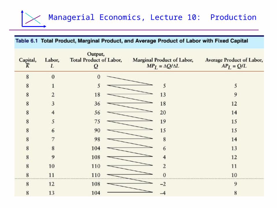
Total, Average, and Marginal Product of Labor

Total product: q

Marginal product of labor: MPL = q/L

Average product of labor: APL = q/L

The graphs for these concepts appear smooth because a firm can hire a "fraction of a worker" (part time).

ManagerialEconomicsLecture 10:Production

Output, q,

Units per day

B

A

C

11640

L , Workers per day

Marginal product, MPL

Average product, APL

AP L, MPL

110

90

56

(a)

b

a

c

11640

L , Workers per day

20

15

(b)

Figure 6.1 ProductionRelationships with Variable Labor

APL = Slope of

straight line

to the originMPL = Slope of

total product

curve

APL = MPL at

maximum APL


Effects of Added LaborAPL

Rises and then falls with labor.Equals the slope of line from the origin to

the point on the total product curve.

MPL First rises and then falls. Cuts the APL curve at its peak.Is the slope of the total product curve.


Law of Diminishing Marginal Returns

As a firm increases an input, holding all other inputs and technology constant,

the marginal product of that input will eventually diminish,

which shows up as an MPL curve that slopes downward above some level of output.


Long-Run Production: Two Variable Inputs

Both capital and labor are variable.

A firm can substitute freely between L and K.

Many different combinations of L and K produce a given level of output.


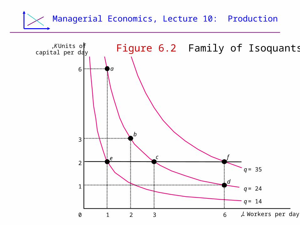
Isoquant An isoquant is a curve that shows efficient

combinations of labor and capital that can produce a single (iso) level of output (quantity):

Examples:A 10-unit isoquant for a Norwegian printing firm

10 = 1.52 L0.6 K0.4

Table 6.2 shows four (L, K) pairs that produce q = 24

( , )q f L K


Figure 6.2 Family of IsoquantsK, Units ofcapital per day

e

b

a

d

fc

63210 L , Workers per day

6

3

2

1

q = 14

q = 24

q = 35


Isoquants and Indifference Curves

Isoquants and indifference curves have most of the same properties.

The biggest difference:An isoquant holds something measurable

(quantity) constantAn indifference curve holds something that

is unmeasurable (utility) constant


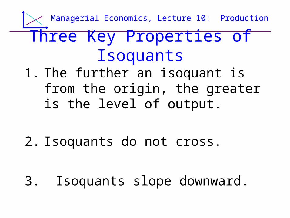
Three Key Properties of Isoquants

1. The further an isoquant is from the origin, the greater is the level of output.

2. Isoquants do not cross.

3. Isoquants slope downward.


The Shape of Isoquants

The slope of isoquant shows how readily a firm can substitute one input for another

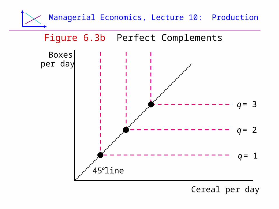
Extreme cases:perfect substitutes: q = x + yfixed-proportions (no substitution):

q = min(x, y)

Usual case: bowed away from the origin


Figure 6.3a Perfect Substitutes: Fixed Proportions

y, Idaho potatoesper day

x, Maine potatoes per day

q = 3q = 2q = 1


Figure 6.3b Perfect Complements

Boxesper day

Cereal per day

q = 3

q = 2

q = 1

45° line


Figure 6.3c Substitutability of Inputs

q = 1

K, Capital perunit of time

L, Labor per unit of time


Marginal Rate of Technical Substitution

The slope of an isoquant tells how much a firm can increase one input and lower the other without changing quantity.

The slope is called the marginal rate of technical substitution (MRTS).

The MRTS varies along a curved isoquant, and is analogous to the MRS.


Figure 6.4 How the Marginal Rate of Technical Substitution Varies Along an Isoquant

K, Units ofcapital per year

e

b

K = –18

–7

–4–2

L = 1

d

c

63

11

1

4 520 L, Workers per day

39

21

14

108 q = 10

a


The Slope of an IsoquantIf firm hires L more workers, its output

increases by MPL = q/L

A decrease in capital by K causes output to fall by MPK = q/K

To keep output constant, q = 0:

or

( ) ( ) 0L KMP L MP K

L

K

MP KMRTS

MP L


Returns to ScaleReturns to scale (how output changes

if all inputs are increased by equal proportions) can be:

Constant: when all inputs are doubled, output doubles,

Increasing: when all inputs are doubled, output more than doubles, or

Decreasing: when all inputs are doubled, output increase < 100%.


Kcapital per year

q = 100q = 200

q = 251

500400300200100 450350250150500L, Units of labor per year

600

500

400

300

200

100

(c) Concrete Blocks and Bricks: Increasing Returns to Scale

, Units of

ppa 723: managerial economics lecture 10: production

Documents

production slide

production total

production output

production isoquant

factor of production

managerial economics

production relationships

production process