pqmf filter bank, mpeg-1 / mpeg-2 bc audio · prof. dr.-ing. k. brandenburg,...
TRANSCRIPT
© Fraunhofer IDMT
PQMF Filter Bank,MPEG-1 / MPEG-2 BC
Audio
© Fraunhofer IDMT
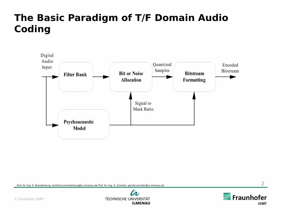
The Basic Paradigm of T/F Domain Audio Coding
Digital Audio Input
Filter Bank
Psychoacoustic Model
Bitstream Formatting
Signal to Mask Ratio
Quantized Samples
Encoded BitstreamBit or Noise
Allocation
Prof. Dr.-Ing. K. Brandenburg, [email protected] Prof. Dr.-Ing. G. Schuller, [email protected] 2
© Fraunhofer IDMT
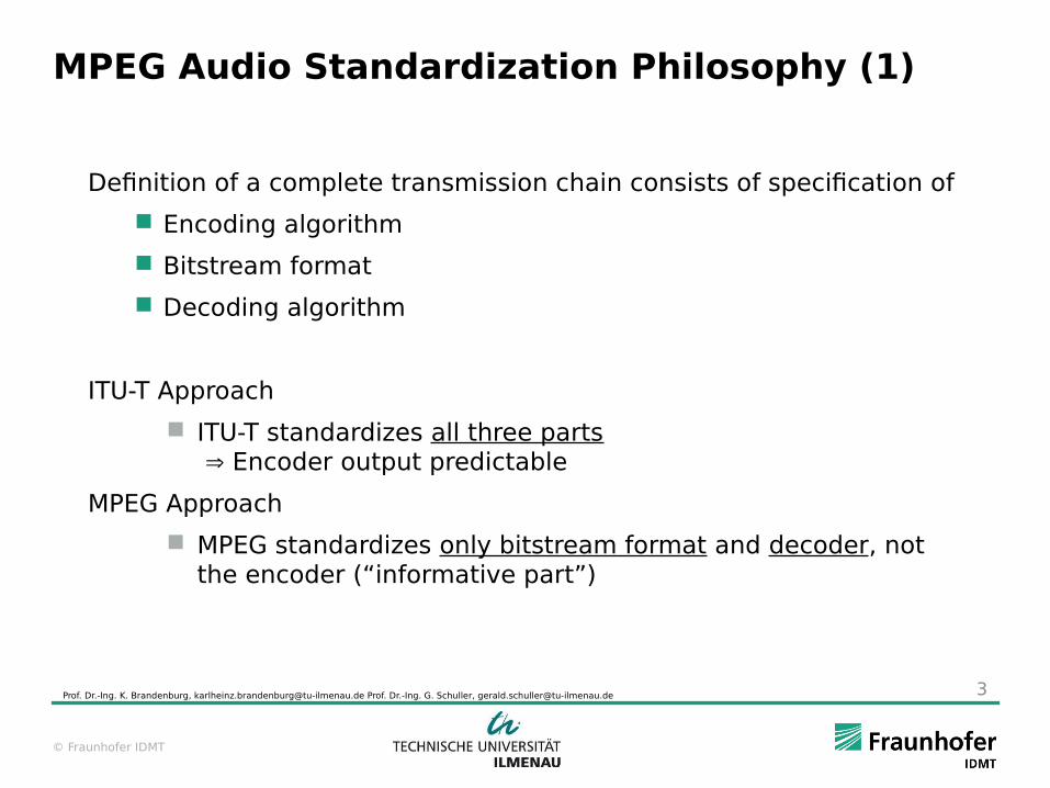
MPEG Audio Standardization Philosophy (1)
Definition of a complete transmission chain consists of specification of
Encoding algorithm
Bitstream format
Decoding algorithm
ITU-T Approach
ITU-T standardizes all three parts Encoder output predictable
MPEG Approach
MPEG standardizes only bitstream format and decoder, not the encoder (“informative part”)
Prof. Dr.-Ing. K. Brandenburg, [email protected] Prof. Dr.-Ing. G. Schuller, [email protected] 3
© Fraunhofer IDMT
MPEG Audio Standardization Philosophy (2)
Motivation: open for further improvements, room for specific corporate know-how
But: No sound quality guaranteed !
Prof. Dr.-Ing. K. Brandenburg, [email protected] Prof. Dr.-Ing. G. Schuller, [email protected] 4
© Fraunhofer IDMT
MPEG-1/2 Audio
MPEG-1 Audio
Audio coding 32 - 48 kHz, mono/stereo
Layer 1, 2, 3
Layer-3 (aka .mp3) optimized for lower bit-rates
Copy protection via SCMS included
MPEG-2 Audio
Low sampling frequencies audio add 16 - 24 kHz to Layer 1, 2, 3
Multichannel audio, BC (Backward Compatible)
Prof. Dr.-Ing. K. Brandenburg, [email protected] Prof. Dr.-Ing. G. Schuller, [email protected] 5
© Fraunhofer IDMT
MPEG-1 Audio
Developed Dec. 88 to Nov. 92
Coding of mono and stereo signals
Bitrates from 32 kbit/s to 448 kbit/s
Three "Layers":
Layer 1: lowest complexity
Layer 2: increased complexity and quality
Layer 3: highest complexity and quality at low bit-rates
Sampling frequencies supported:
48 kHz, 44.1 kHz, 32 kHz
Prof. Dr.-Ing. K. Brandenburg, [email protected] Prof. Dr.-Ing. G. Schuller, [email protected] 6

© Fraunhofer IDMT
The main building blocks
Perceptual model using psychoacoustics, mostly proprietary
Filter bank subdividing the input signal into spectral components more lines → more coding gain longer impulse response → pre-echo artifacts
Quantization and coding this is the step introducing quantization noise spectral shape of quantization noise determines the audibility can be designed to leave encoding methods optional
Prof. Dr.-Ing. K. Brandenburg, [email protected] Prof. Dr.-Ing. G. Schuller, [email protected] 7
© Fraunhofer IDMT
MPEG Audio - Short Description of the Layers (1)
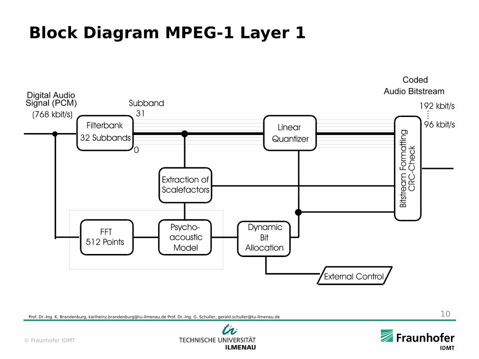
Layer I
Frame length: 384 samples (8 ms@ 48 kHz)
Frequency resolution: 32 subbands from a PQMF filter bank
Quantization: Block-companding (12 samples), amplitude of subband samples indicated by “scalefactors” (SCF)
Layer II
Frame length: 1152 samples (24 ms@ 48 kHz)
Frequency resolution: 32 subbands from a PQMF filter bank
Quantization: Block-companding (12 samples)
Use of Scalefactor select information
Prof. Dr.-Ing. K. Brandenburg, [email protected] Prof. Dr.-Ing. G. Schuller, [email protected] 8
© Fraunhofer IDMT
MPEG Audio - Short Description of the Layers (2)
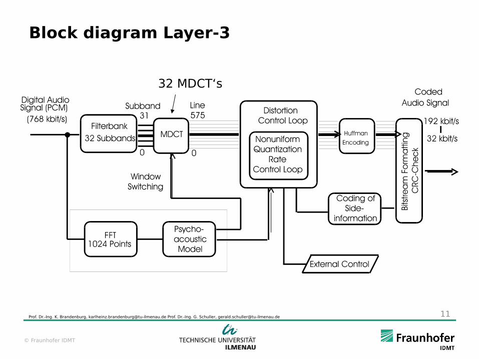
Layer III
Standard frame length: 1152 samples (24 ms @ 48 kHz)
Frequency resolution: 576 or 192 subbands, from a 2-stage filter bank:
a 32-band PQMF filter bank in the first stage, followed by
a 6 or 18 band MDCT in each of the 32 PQMF subbands (hence 32*6=192, or 32*18=576) in the second stage.
Quantization: non-uniform with Huffman coding
Use of Scalefactor Select Information
Prof. Dr.-Ing. K. Brandenburg, [email protected] Prof. Dr.-Ing. G. Schuller, [email protected] 9
© Fraunhofer IDMT
Block Diagram MPEG-1 Layer 1
Prof. Dr.-Ing. K. Brandenburg, [email protected] Prof. Dr.-Ing. G. Schuller, [email protected] 10
© Fraunhofer IDMT
Block diagram Layer-3
32 MDCT‘s
Prof. Dr.-Ing. K. Brandenburg, [email protected] Prof. Dr.-Ing. G. Schuller, [email protected] 11
© Fraunhofer IDMT
Example for the Time/Frequency Resolution for the 2-Stage Layer III Coder
Prof. Dr.-Ing. K. Brandenburg, [email protected] Prof. Dr.-Ing. G. Schuller, [email protected] 12
The first stage has a 32 subband QMF filter bank. For simplicity we only take aan MDCT. We can visualize a 32 subband filter bank with our Python program “pyrecplayMDCT.py”, by editing the line for the number of subbands N to:N=32;And run it withpython pyrecplayMDCT.pyObserve: We get a very narrow spectrogram, because we only have 32 subbands, but it runs very fast, because we donwsample only by 32. We can also listen to a subband (by setting the other subbands to zero), and we will here more than just a tone, because the subbands are wider than for AAC.
© Fraunhofer IDMT
Example for the Time/Frequency Resolution for the 2-Stage Layer III Coder
Prof. Dr.-Ing. K. Brandenburg, [email protected] Prof. Dr.-Ing. G. Schuller, [email protected] 13
Now set it to the number of subbands after the second stage:N=576And run it withpython pyrecplayMDCT.pyHere now it becomes more similar to the AAC filter bank. We see a broader spectrogram, but it runs slower, because we have an increased downsampling rate of 576. The second layer does it by replacing every 12 or 18 time samples in each of the 32 subbands by 12 or 18 finer subbands.When we now listen to a subband, it sound more like a tone, because the subbands are more narrow.
© Fraunhofer IDMT
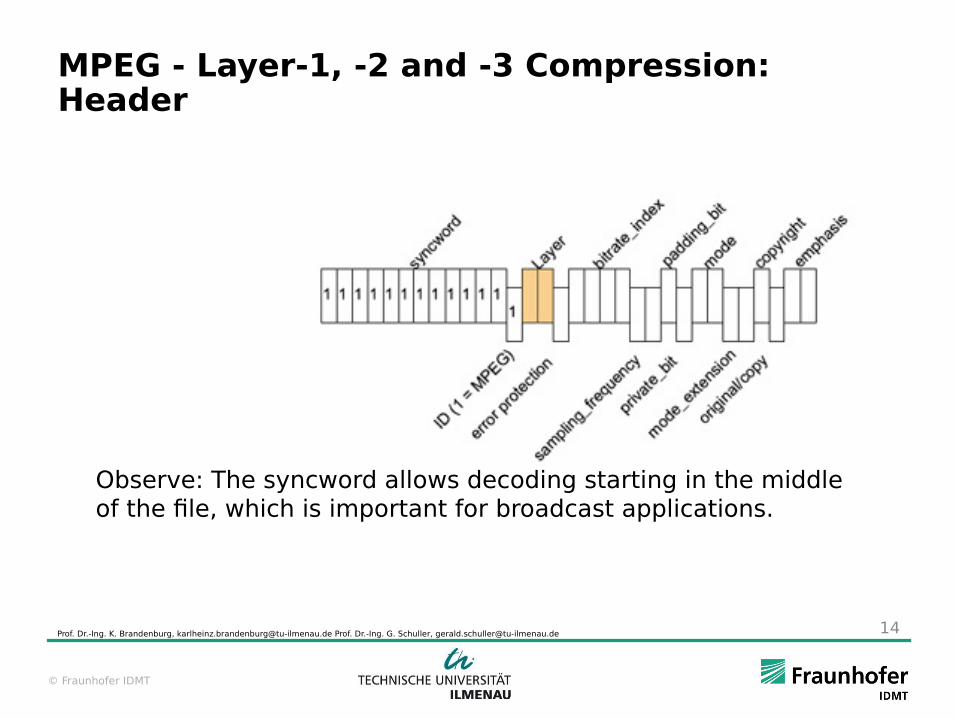
MPEG - Layer-1, -2 and -3 Compression: Header
Prof. Dr.-Ing. K. Brandenburg, [email protected] Prof. Dr.-Ing. G. Schuller, [email protected] 14
Observe: The syncword allows decoding starting in the middle of the file, which is important for broadcast applications.
© Fraunhofer IDMT
The Pseudo-Quadrature-Mirror Filter Bank (PQMF)
Prof. Dr.-Ing. K. Brandenburg, [email protected] Prof. Dr.-Ing. G. Schuller, [email protected] 15
The PQMF is also used for ● parametric surround coding● Parametric high frequency generation
For that reason we now take a closer look at the PQMF filter bank(See also lecture slides Filter Banks 2)

© Fraunhofer IDMT
The Pseudo-Quadrature-Mirror Filter Bank (PQMF)
Prof. Dr.-Ing. K. Brandenburg, [email protected] Prof. Dr.-Ing. G. Schuller, [email protected] 16
● The PQMF is a filter bank which has only “near” perfect reconstruction, unlike the MDCT, which has really perfect reconstruction.
● In the same sense it is near para-unitary or orthogonal, which means the synthesis filter are the time reversed analysis filters.
● But it has the advantage that we have design methods to design filter banks with “good” longer filters, with more overlap than we use with the MDCT. This results in improved nearby stopband attenuation.
● An often used configuration is 32 subbands with filters with length of 512 or 640 coefficients, hence 16 or 20-times overlap (compare that with 2-times overlap in the MDCT)

© Fraunhofer IDMT
PQMF Definition
Prof. Dr.-Ing. K. Brandenburg, [email protected] Prof. Dr.-Ing. G. Schuller, [email protected] 17
The analysis filters of an N-band PQMF filter bank with filters of length L are defined as:
With the phase defined as: With some integer r. For convenience we omit scaling factors.The synthesis filters are the time reverse analysis filters:
(See also: https://ccrma.stanford.edu/~jos/sasp/Pseudo_QMF_Cosine_Modulation_Filter.html
Book: Spanias, Painter: “Audio Signal Processing and Coding”, Wiley Press)
hk (n)=h(n)⋅cos( πN⋅(k+0.5)⋅(n− L2+12)+Φk)
gk (n)=hk (L−1−n)
Φk+1−Φk=(2r+1)⋅π
2
© Fraunhofer IDMT
PQMF Reformulation
Prof. Dr.-Ing. K. Brandenburg, [email protected] Prof. Dr.-Ing. G. Schuller, [email protected] 18
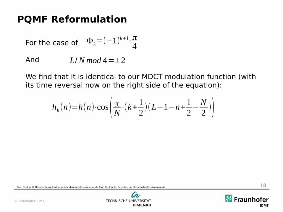
For the case of
And
We find that it is identical to our MDCT modulation function (with its time reversal now on the right side of the equation):
Φk=(−1)k+1⋅π4
L/N mod 4=±2
hk (n)=h(n)⋅cos( πN⋅(k+ 12)(L−1−n+1
2−
N2))
© Fraunhofer IDMT
PQMF Design
Prof. Dr.-Ing. K. Brandenburg, [email protected] Prof. Dr.-Ing. G. Schuller, [email protected] 19
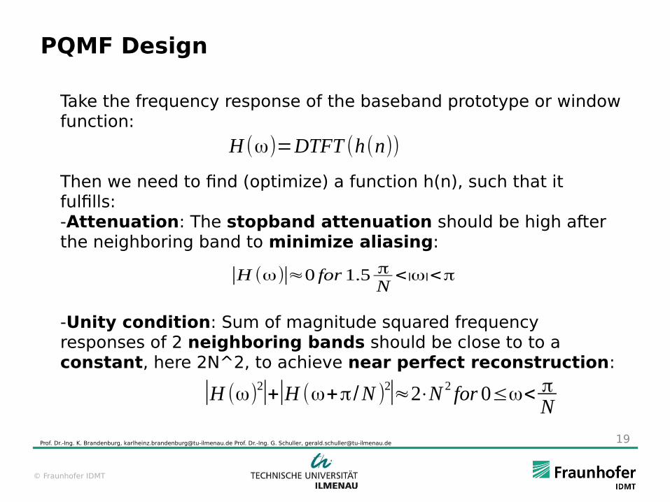
Take the frequency response of the baseband prototype or window function:
Then we need to find (optimize) a function h(n), such that it fulfills:-Attenuation: The stopband attenuation should be high after the neighboring band to minimize aliasing:
-Unity condition: Sum of magnitude squared frequency responses of 2 neighboring bands should be close to to a constant, here 2N^2, to achieve near perfect reconstruction:
H (ω)=DTFT (h(n))
|H (ω)|≈0 for 1.5 πN<|ω|<π
|H (ω)2|+|H (ω+π/N )
2|≈2⋅N 2 for 0≤ω< πN
© Fraunhofer IDMT
Python Example Optimization
Prof. Dr.-Ing. K. Brandenburg, [email protected] Prof. Dr.-Ing. G. Schuller, [email protected] 20
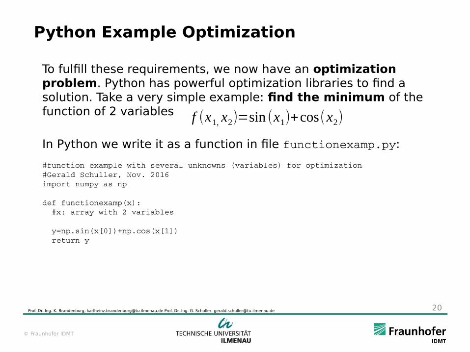
To fulfill these requirements, we now have an optimization problem. Python has powerful optimization libraries to find a solution. Take a very simple example: find the minimum of the function of 2 variables
In Python we write it as a function in file functionexamp.py:
#function example with several unknowns (variables) for optimization#Gerald Schuller, Nov. 2016import numpy as np
def functionexamp(x): #x: array with 2 variables
y=np.sin(x[0])+np.cos(x[1]) return y
f (x1, x2)=sin (x1)+cos(x2)
© Fraunhofer IDMT
Python Example Optimization
Prof. Dr.-Ing. K. Brandenburg, [email protected] Prof. Dr.-Ing. G. Schuller, [email protected] 21
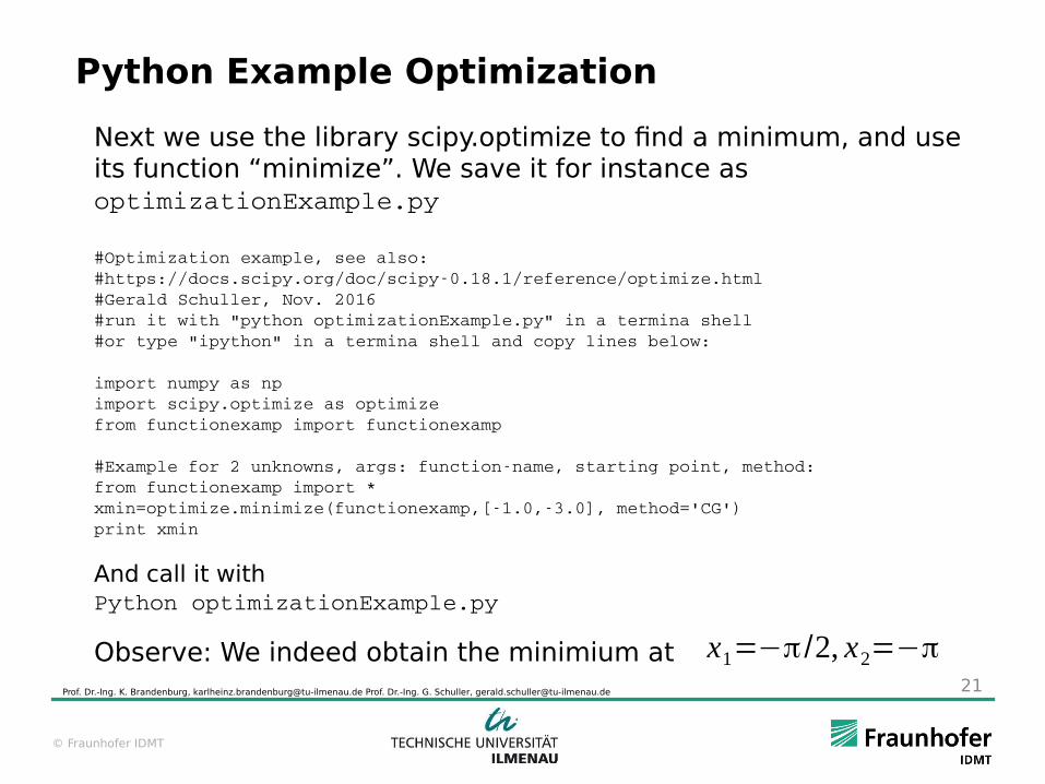
Next we use the library scipy.optimize to find a minimum, and use its function “minimize”. We save it for instance as optimizationExample.py
#Optimization example, see also:#https://docs.scipy.org/doc/scipy0.18.1/reference/optimize.html#Gerald Schuller, Nov. 2016#run it with "python optimizationExample.py" in a termina shell#or type "ipython" in a termina shell and copy lines below:
import numpy as npimport scipy.optimize as optimizefrom functionexamp import functionexamp
#Example for 2 unknowns, args: functionname, starting point, method:from functionexamp import *xmin=optimize.minimize(functionexamp,[1.0,3.0], method='CG')print xmin
And call it withPython optimizationExample.py
Observe: We indeed obtain the minimium at x1=−π/2, x2=−π
© Fraunhofer IDMT
PQMF Optimization, Python Example, Optimization Function
Prof. Dr.-Ing. K. Brandenburg, [email protected] Prof. Dr.-Ing. G. Schuller, [email protected] 22
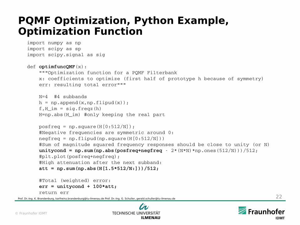
import numpy as npimport scipy as spimport scipy.signal as sig
def optimfuncQMF(x): """Optimization function for a PQMF Filterbank x: coefficients to optimize (first half of prototype h because of symmetry) err: resulting total error""" N=4 #4 subbands h = np.append(x,np.flipud(x)); f,H_im = sig.freqz(h) H=np.abs(H_im) #only keeping the real part posfreq = np.square(H[0:512/N]); #Negative frequencies are symmetric around 0: negfreq = np.flipud(np.square(H[0:512/N])) #Sum of magnitude squared frequency responses should be close to unity (or N) unitycond = np.sum(np.abs(posfreq+negfreq 2*(N*N)*np.ones(512/N)))/512; #plt.plot(posfreq+negfreq); #High attenuation after the next subband: att = np.sum(np.abs(H[1.5*512/N:]))/512;
#Total (weighted) error: err = unitycond + 100*att; return err

© Fraunhofer IDMT
PQMF Optimization, Python Example, Optimizer
Prof. Dr.-Ing. K. Brandenburg, [email protected] Prof. Dr.-Ing. G. Schuller, [email protected] 23
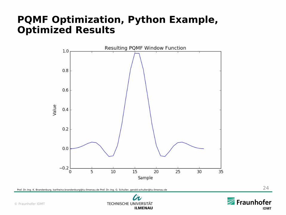
Now we have a function to minimize, and we can use Pythons powerful optimization library to minimize this function:import numpy as npimport matplotlib.pyplot as pltimport scipy.optimize as optimport scipy.signal as sigfrom optimfuncQMF import optimfuncQMF#optimize for 16 filter coefficients:xmin = opt.minimize(optimfuncQMF,16*np.ones(16),method='SLSQP')xmin = xmin["x"]
#Restore symmetric upper half of window:h = np.concatenate((xmin,np.flipud(xmin)))
plt.plot(h)plt.show()f,H = sig.freqz(h)plt.plot(f,20*np.log10(np.abs(H)))plt.show()
© Fraunhofer IDMT
PQMF Optimization, Python Example, Optimized Results
Prof. Dr.-Ing. K. Brandenburg, [email protected] Prof. Dr.-Ing. G. Schuller, [email protected] 24
© Fraunhofer IDMT
PQMF Optimization, Python Example, Attenuation Condition
Prof. Dr.-Ing. K. Brandenburg, [email protected] Prof. Dr.-Ing. G. Schuller, [email protected] 25
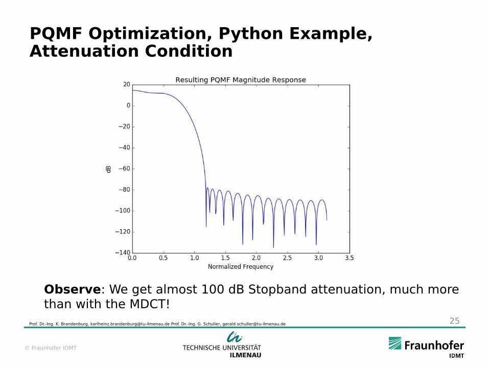
Observe: We get almost 100 dB Stopband attenuation, much morethan with the MDCT!
© Fraunhofer IDMT
PQMF Optimization, Python Example, Unity Condition
Prof. Dr.-Ing. K. Brandenburg, [email protected] Prof. Dr.-Ing. G. Schuller, [email protected] 26
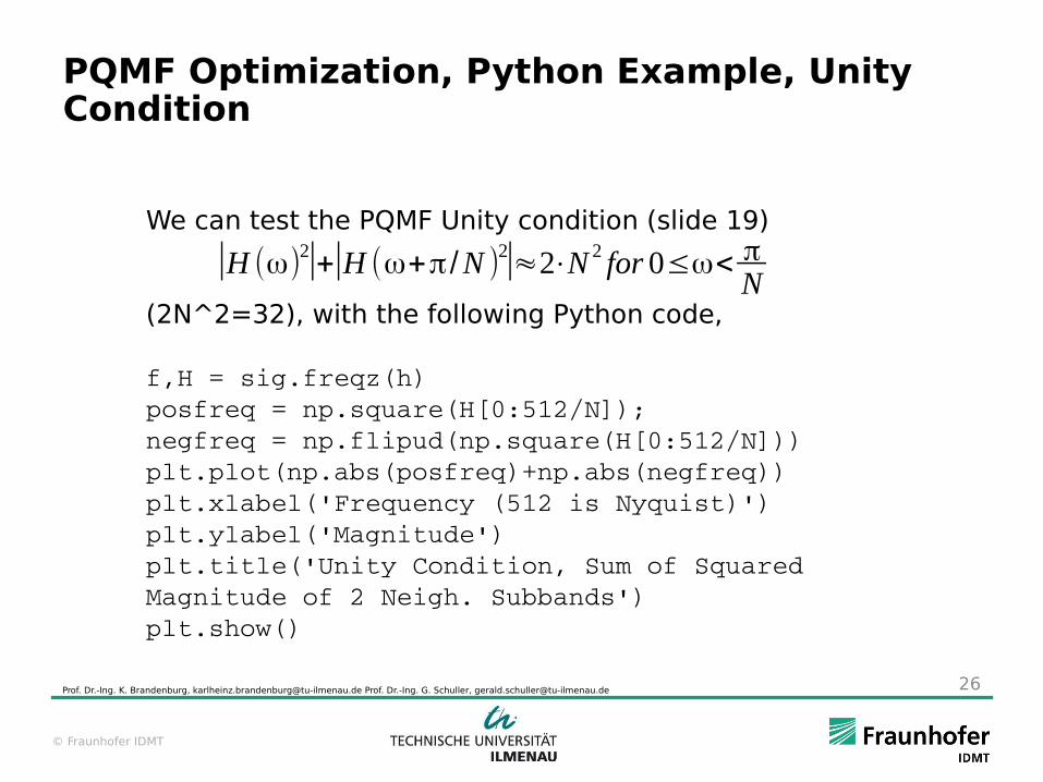
We can test the PQMF Unity condition (slide 19)
(2N^2=32), with the following Python code,
f,H = sig.freqz(h)posfreq = np.square(H[0:512/N]);negfreq = np.flipud(np.square(H[0:512/N]))plt.plot(np.abs(posfreq)+np.abs(negfreq))plt.xlabel('Frequency (512 is Nyquist)')plt.ylabel('Magnitude')plt.title('Unity Condition, Sum of Squared Magnitude of 2 Neigh. Subbands')plt.show()
|H (ω)2|+|H (ω+π/N )
2|≈2⋅N 2 for 0≤ω< πN

© Fraunhofer IDMT
PQMF Optimization, Python Example, Unity Condition
Prof. Dr.-Ing. K. Brandenburg, [email protected] Prof. Dr.-Ing. G. Schuller, [email protected] 27
Observe: We get indeed a curve close to 2N^2=32, but with someDeviation, which shows that we get indeed only “near” Perfect Reconstruction!
© Fraunhofer IDMT
PQMF Optimization, Python Example, Optimized Results
Prof. Dr.-Ing. K. Brandenburg, [email protected] Prof. Dr.-Ing. G. Schuller, [email protected] 28
● Observe: We obtain a 4-band filter bank with filter length of 32 taps, hence 8 times overlap.
● The stopband attenuation reaches almost 100 dB, almost right after the passband, much more than with the MDCT!
© Fraunhofer IDMT
PQMF Optimization, Polyphase Implementation, Analysis
Prof. Dr.-Ing. K. Brandenburg, [email protected] Prof. Dr.-Ing. G. Schuller, [email protected] 29
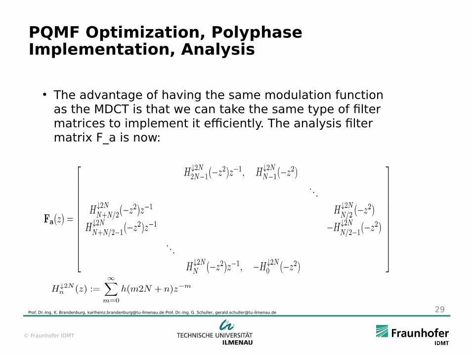
● The advantage of having the same modulation function as the MDCT is that we can take the same type of filter matrices to implement it efficiently. The analysis filter matrix F_a is now:
© Fraunhofer IDMT
PQMF Optimization, Polyphase Implementation, Synthesis
Prof. Dr.-Ing. K. Brandenburg, [email protected] Prof. Dr.-Ing. G. Schuller, [email protected] 30
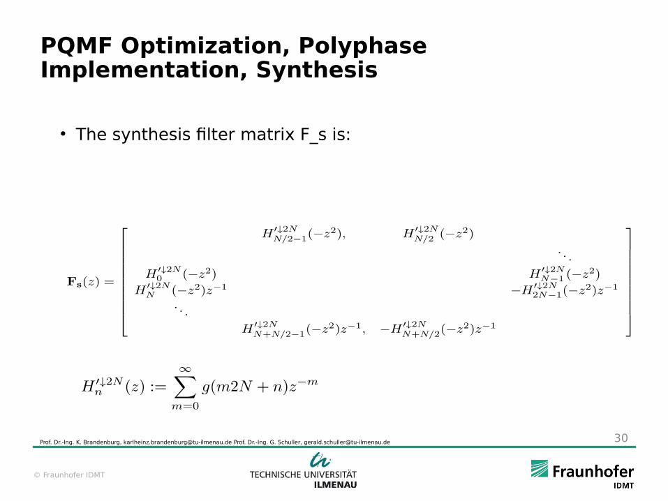
● The synthesis filter matrix F_s is:
© Fraunhofer IDMT
PQMF Optimization, Polyphase Implementation, Analysis and Synthesis
Prof. Dr.-Ing. K. Brandenburg, [email protected] Prof. Dr.-Ing. G. Schuller, [email protected] 31
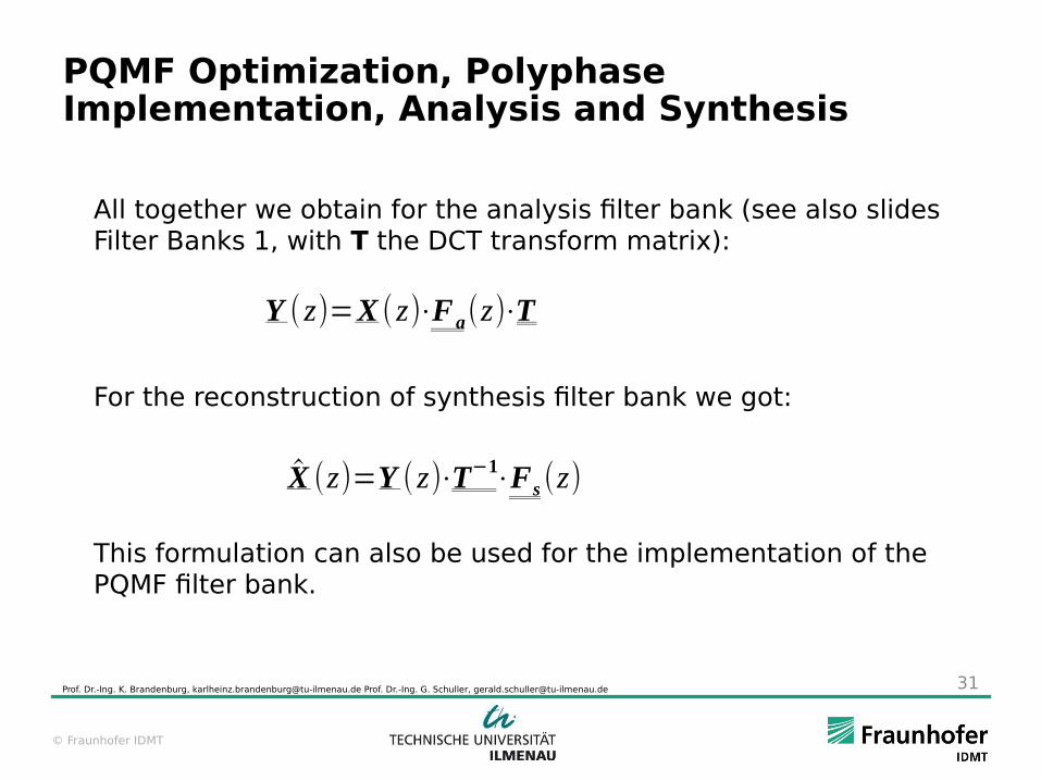
All together we obtain for the analysis filter bank (see also slides Filter Banks 1, with T the DCT transform matrix):
For the reconstruction of synthesis filter bank we got:
This formulation can also be used for the implementation of the PQMF filter bank.
Y (z)=X (z)⋅Fa(z)⋅T
X̂ (z)=Y (z)⋅T−1⋅Fs (z)

© Fraunhofer IDMT
Hybrid Filter Bank & Aliasing (1)
e.g. 32kHz e.g. 32Hz
32 bands
6-18 bands
32*18=576 bands
Filter bank is critically sampled
Problem of aliasing in the analysis filter bank
Aliasing in the subbands
32 bands6 or 18
switching for pre-echo avoidance
better compression
Prof. Dr.-Ing. K. Brandenburg, [email protected] Prof. Dr.-Ing. G. Schuller, [email protected] 32
© Fraunhofer IDMT
Hybrid Filter Bank & Aliasing (2)
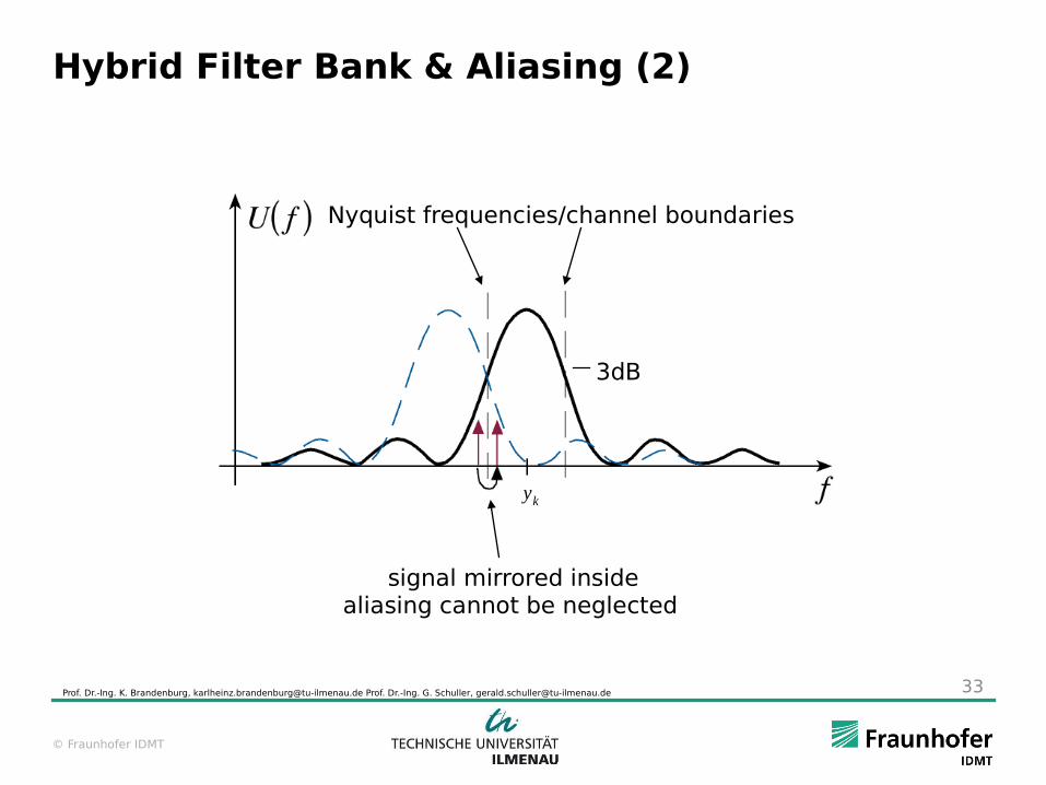
Nyquist frequencies/channel boundaries
yk
signal mirrored inside
3dB
aliasing cannot be neglected
Prof. Dr.-Ing. K. Brandenburg, [email protected] Prof. Dr.-Ing. G. Schuller, [email protected] 33
© Fraunhofer IDMT
Hybrid Filter Bank & Aliasing (3)
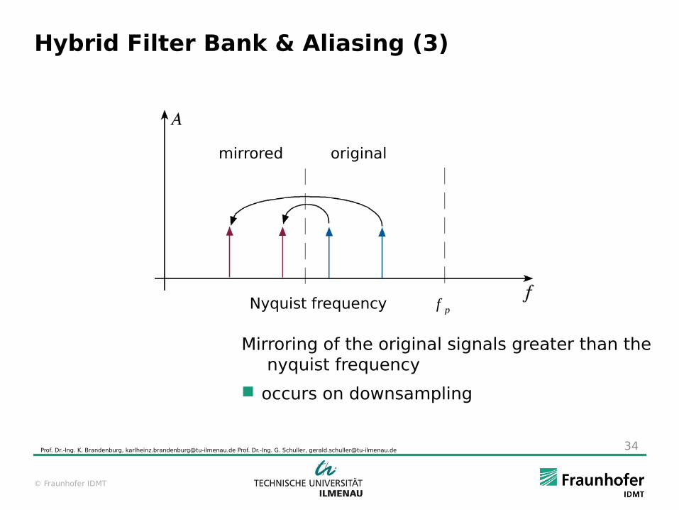
Mirroring of the original signals greater than the nyquist frequency
occurs on downsampling
Nyquist frequency f p
mirrored original
Prof. Dr.-Ing. K. Brandenburg, [email protected] Prof. Dr.-Ing. G. Schuller, [email protected] 34
© Fraunhofer IDMT
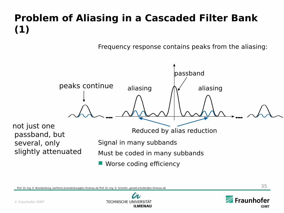
Problem of Aliasing in a Cascaded Filter Bank (1)
Frequency response contains peaks from the aliasing:
Signal in many subbands
Must be coded in many subbands
Worse coding efficiency
Reduced by alias reduction
passband
aliasing aliasing
not just one passband, but several, only slightly attenuated
peaks continue
Prof. Dr.-Ing. K. Brandenburg, [email protected] Prof. Dr.-Ing. G. Schuller, [email protected] 35

© Fraunhofer IDMT
Problem of Aliasing in a Cascaded Filter Bank (2)
Result of cascading:
Far off frequencies are aliased into the SB of the
2nd filter bank
Nyquist frequency
attenuation ofthe filter
subband of 1st FB
subbands of 2nd FB
signal aliased signal
first stagefilter bank
Observe:Aliasing spreads over several subbands of second stage! Not the case for only single stage FB (practically)
Prof. Dr.-Ing. K. Brandenburg, [email protected] Prof. Dr.-Ing. G. Schuller, [email protected] 36
© Fraunhofer IDMT
32bands
6/18bands
6/18bands
-
-
n
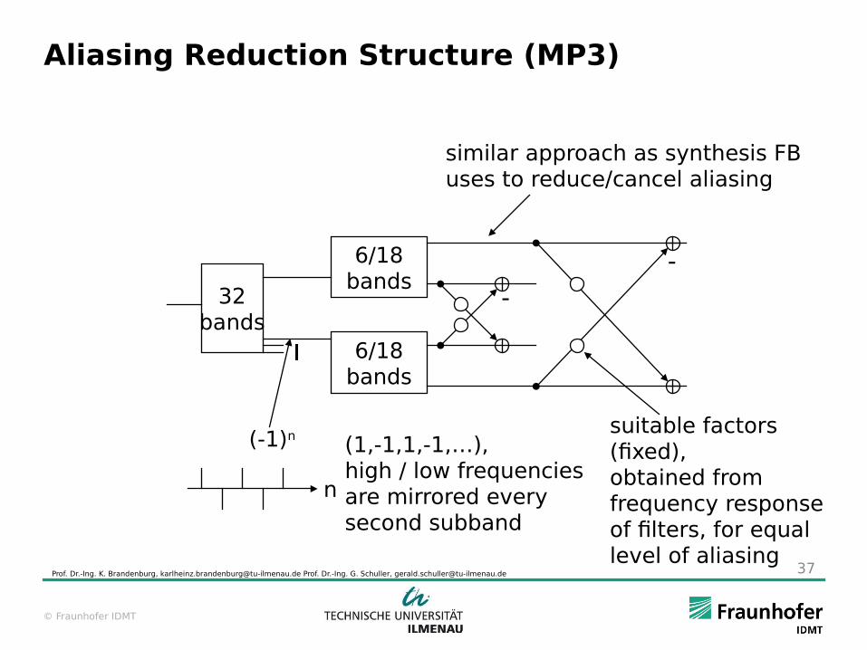
Aliasing Reduction Structure (MP3)
similar approach as synthesis FBuses to reduce/cancel aliasing
(-1)n (1,-1,1,-1,…),high / low frequenciesare mirrored everysecond subband
suitable factors (fixed),obtained from frequency response of filters, for equal level of aliasing
Prof. Dr.-Ing. K. Brandenburg, [email protected] Prof. Dr.-Ing. G. Schuller, [email protected] 37

© Fraunhofer IDMT
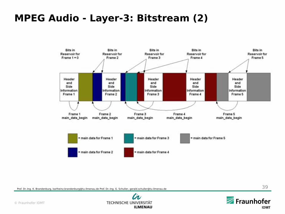
MPEG Audio - Layer-3: Bitstream
Organization of the bit streams
Fixed length of bytes: 17 at mono, 32 at stereo, independent of the bitrate
Constant Section Header (ISO Standard, like with Layer-1 and -2) Additional information for a frame (e.g. Pointer to the variable section) Additional information for each granule (e.g. Number of the Huffman-Code table)
Variable Section Scalefactors Huffman-coded frequency lines Additional Data
Prof. Dr.-Ing. K. Brandenburg, [email protected] Prof. Dr.-Ing. G. Schuller, [email protected] 38
© Fraunhofer IDMT
MPEG Audio - Layer-3: Bitstream (2)
Prof. Dr.-Ing. K. Brandenburg, [email protected] Prof. Dr.-Ing. G. Schuller, [email protected] 39
© Fraunhofer IDMT
MPEG-1 Audio Decoder
Prof. Dr.-Ing. K. Brandenburg, [email protected] Prof. Dr.-Ing. G. Schuller, [email protected] 40
© Fraunhofer IDMT
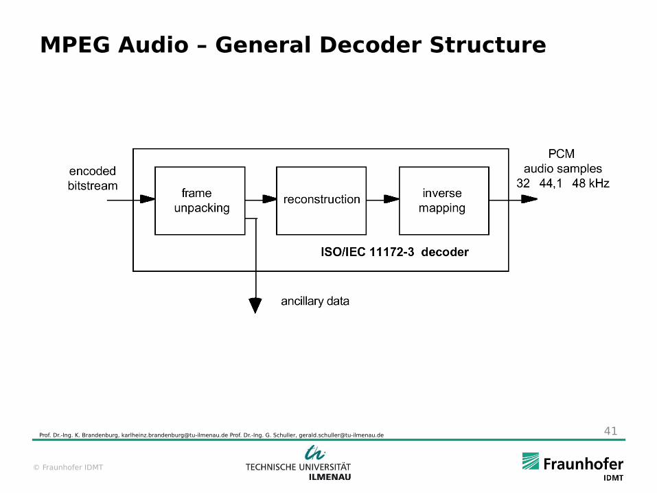
MPEG Audio – General Decoder Structure
Prof. Dr.-Ing. K. Brandenburg, [email protected] Prof. Dr.-Ing. G. Schuller, [email protected] 41

© Fraunhofer IDMT
MPEG - Audio Decoder Process (1) Layer-3 Decoder flow chart
Prof. Dr.-Ing. K. Brandenburg, [email protected] Prof. Dr.-Ing. G. Schuller, [email protected] 42

© Fraunhofer IDMT
MPEG - Audio Decoder Process (2) Layer-3 Decoder Diagramm
Prof. Dr.-Ing. K. Brandenburg, [email protected] Prof. Dr.-Ing. G. Schuller, [email protected] 43
© Fraunhofer IDMT
Annex: Abbreviations and Companies
Prof. Dr.-Ing. K. Brandenburg, [email protected] Prof. Dr.-Ing. G. Schuller, [email protected] 44
© Fraunhofer IDMT
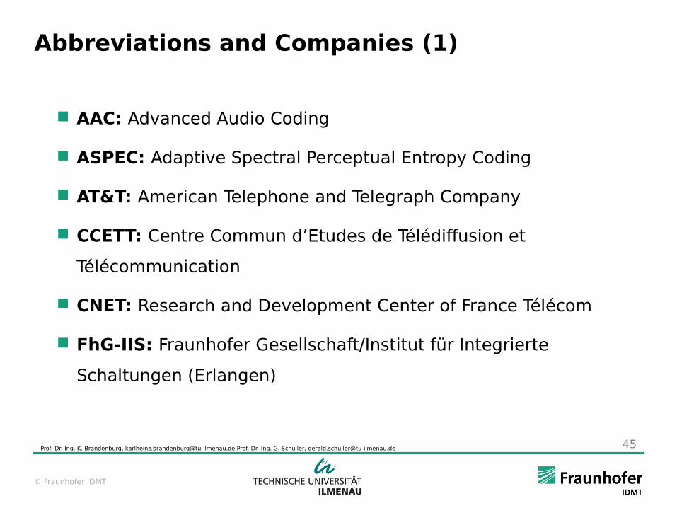
Abbreviations and Companies (1)
AAC: Advanced Audio Coding
ASPEC: Adaptive Spectral Perceptual Entropy Coding
AT&T: American Telephone and Telegraph Company
CCETT: Centre Commun d’Etudes de Télédiffusion et
Télécommunication
CNET: Research and Development Center of France Télécom
FhG-IIS: Fraunhofer Gesellschaft/Institut für Integrierte
Schaltungen (Erlangen)
Prof. Dr.-Ing. K. Brandenburg, [email protected] Prof. Dr.-Ing. G. Schuller, [email protected] 45

© Fraunhofer IDMT
Abbreviations and Companies (2)
IRT: Institut für Rundfunktechnik GmbH, München, Research
and Development Institute of ARD, ZDF, DLR, ORF and SRG
ITU-R: International Telecommunication Union – Radio
Communication Sector
MASCAM: Masking-pattern Adapted Subband Coding and
Multiplexing AT&T:American Telephone and Telegraph
Company
MUSICAM: Masking-pattern Universal Subband Integrated
Coding and Multiplexing
Prof. Dr.-Ing. K. Brandenburg, [email protected] Prof. Dr.-Ing. G. Schuller, [email protected] 46
© Fraunhofer IDMT
Abbreviations and Companies (3)
NTT: Nippon Telegraph and Telephone Corp./Human Interface
Laboratories
Thomson: Thomson, Telefunken, Saba, RCA, GE, ProScan
TwinVQ: Transform-domain Weighted Interleave Vector
Quantization
Prof. Dr.-Ing. K. Brandenburg, [email protected] Prof. Dr.-Ing. G. Schuller, [email protected] 47