practical guidelines for solving difficult linear...
TRANSCRIPT
Practical Guidelines for Solving Difficult Linear Programs1
Ed Klotz† • Alexandra M. Newman‡†IBM, 926 Incline Way, Suite 100, Incline Village, NV 89451
‡Division of Economics and Business, Colorado School of Mines, Golden, CO 80401
[email protected] • [email protected]
2
Abstract3
The advances in state-of-the-art hardware and software have enabled the inexpensive, effi-4
cient solution of many large-scale linear programs previously considered intractable. However, a5
significant number of large linear programs can require hours, or even days, of run time and are6
not guaranteed to yield an optimal (or near-optimal) solution. In this paper, we present sugges-7
tions for diagnosing and removing performance problems in state-of-the-art linear programming8
solvers, and guidelines for careful model formulation, both of which can vastly improve perfor-9
mance.10
Keywords: linear programming, algorithm selection, algorithmic tuning, numerical stability,11
memory use, run time, tutorials12
1 Introduction13
Operations research practitioners have been formulating and solving linear programs since the 1940s14
(Dantzig, 1963). State-of-the-art optimizers such as CPLEX (IBM, 2012), Gurobi (Gurobi, 2012),15
MOPS (MOPS, 2012), Mosek (MOSEK, 2012), and Xpress-MP (FICO, 2012) can solve most prac-16
tical large-scale linear programs effectively. However, some “real-world” problem instances require17
days or weeks of solution time. Furthermore, improvements in computing power and linear pro-18
gramming solvers have often prompted practitioners to create larger, more difficult linear programs19
that provide a more accurate representation of the systems they model. Although not a guarantee20
of tractability, careful model formulation and standard linear programming algorithmic tuning of-21
ten result in significantly faster solution times, in some cases admitting a feasible or near-optimal22
solution which could otherwise elude the practitioner.23
In this paper, we briefly introduce linear programs and their corresponding commonly used24
algorithms, show how to assess optimizer performance on such problems through the respective25
algorithmic output, and demonstrate methods for improving that performance through careful26
formulation and algorithmic parameter tuning. We assume basic familiarity with fundamental27
1
mathematics, such as matrix algebra, and with optimization. We expect that the reader has for-28
mulated linear programs and has a conceptual understanding of how the corresponding problems29
can be solved. The interested reader can refer to basic texts such as Chvatal (1983), Dantzig and30
Thapa (1997), Rardin (1998), Winston (2004), and Bazaraa et al. (2005) for more detailed intro-31
ductions to mathematical programming, including geometric interpretations. For a more general32
discussion of good optimization modeling practices, we refer the reader to Brown and Rosenthal33
(2008). However, we contend that this paper is self-contained such that relatively inexperienced34
practitioners can use its advice effectively without referring to other sources.35
The remainder of the paper is organized as follows. In Section 2, we introduce linear programs36
and the simplex and interior point algorithms. We also contrast the performance of these algo-37
rithms. In Section 3, we address potential difficulties when solving a linear program, including38
identifying performance issues from the corresponding algorithmic output, and provide suggestions39
to avoid these difficulties. Section 4 concludes the paper with a summary. Sections 2.1 and 2.2,40
with the exception of the tables, may be omitted without loss of continuity for the practitioner41
interested only in formulation and algorithmic parameter tuning without detailed descriptions of42
the algorithms themselves. To illustrate the concepts we present in this paper, we show output43
logs resulting from having run a state-of-the-art optimizer on a standard desktop machine. Unless44
otherwise noted, this optimizer is CPLEX 12.2.0.2, and the machine possesses four 3.0 gigahertz45
Xeon chips and eight gigabytes of memory.46
2 Linear Programming Fundamentals47
We consider the following system where x is an n× 1 column vector of continuous-valued, nonneg-48
ative decision variables, A is an m× n matrix of left-hand-side constraint coefficients, c is an n× 149
column vector of objective function coefficients, and b is an m× 1 column vector of right-hand-side50
data values for each constraint.51
(PLP ) : min cT x
subject to Ax = b
x ≥ 0
Though other formats exist, without loss of generality, any linear program can be written in52
the primal standard form we adopt above. Specifically, a maximization function can be changed53
to a minimization function by negating the objective function (and then negating the resulting54
2
optimal objective). A less-than-or-equal-to or greater-than-or-equal-to constraint can be converted55
to an equality by adding a nonnegative slack variable or subtracting a nonnegative excess variable,56
respectively. Variables that are unrestricted in sign can be converted to nonnegative variables by57
replacing each with the difference of two nonnegative variables.58
We also consider the related dual problem corresponding to our primal problem in standard59
form, (PLP ). Let y be an m × 1 column vector of continuous-valued, unrestricted-in-sign decision60
variables; A, b and c are data values with the dimensionality given above in (PLP ).61
(DLP ) : max yT b
subject to yT A ≤ cT
The size of a linear program is given by the number of constraints, m, the number of variables, n,62
and the number of non-zero elements in the A matrix. While a large number of variables affects the63
speed with which a linear program is solved, the commonly used LP algorithms solve linear systems64
of equations dimensioned by the number of constraints. Because these linear solves often dominate65
the time per iteration, the number of constraints is a more significant measure of solution time than66
the number of variables. Models corresponding to practical applications typically contain sparse A67
matrices in which more than 99% of the entries are zero. In the context of linear programming, a68
dense matrix need not have a majority of its entries assume non-zero values. Instead, a dense LP69
matrix merely has a sufficient number or pattern of non-zeros so that the algorithmic computations70
using sparse matrix technology can be sufficiently time consuming to create performance problems.71
Thus, a matrix can still have fewer than 1% of its values be non-zero, yet be considered dense.72
Practical examples of such matrices include those that average more than 10 non-zeros per column73
and those with a small subset of columns with hundreds of non-zeros. State-of-the-art optimizers74
capitalize on matrix sparsity by storing only the non-zero matrix coefficients. However, even for75
such matrices, the positions of the non-zero entries and, therefore, the ease with which certain76
algorithmic computations (discussed below) are executed, can dramatically affect solution time.77
A basis for the primal system consists of m variables whose associated matrix columns are78
linearly independent. The basic variable values are obtained by solving the system Ax = b given79
the resulting n −m non-basic variables are set to values of zero. The set of the actual values of80
the variables in the basis, as well as those set equal to zero, is referred to as a basic solution. Each81
primal basis uniquely defines a basis for the dual (see Dantzig (1963), pp. 241-242). For each basis,82
there is a range of right-hand-side values such that the basis retains the same variables. Within83
this range, each constraint has a corresponding dual variable value which indicates the change in84
3
the objective function value per unit change in the corresponding right hand side. (This variable85
value can be obtained indirectly via the algorithm and is readily available through any standard86
optimizer.) Solving the primal system, (PLP ), provides not only the primal variable values but also87
the dual values at optimality; these values correspond to the optimal variable values to the problem88
(DLP ). Correspondingly, solving the dual problem to optimality provides both the optimal dual89
and primal variable values. In other words, we can obtain the same information by solving either90
(PLP ) or (DLP ).91
Each vertex (or extreme point) of the polyhedron formed by the constraint set Ax = b corre-92
sponds to a basic solution. If the solution also satisfies the nonnegativity requirements on all the93
variables, it is said to be a basic feasible solution. Each such basic feasible solution, of which there is94
a finite number, is a candidate for an optimal solution. In the case of multiple optima, any convex95
combination of extreme-point optimal solutions is also optimal. Because basic solutions contain96
significantly more zero-valued variables than solutions that are not basic, practitioners may be more97
easily able to implement basic solutions. On the other hand, basic solutions lack the “diversity” in98
non-zero values that solutions that are not basic provide. In linear programs with multiple optima,99
solutions that are not basic may be more appealing in applications in which it is desirable to spread100
out the non-zero values among many variables. Linear programming algorithms can operate with a101
view to seeking basic feasible solutions for either the primal or for the dual system, or by examining102
solutions that are not basic.103
2.1 Simplex Methods104
The practitioner familiar with linear programming algorithms may wish to omit this and the fol-105
lowing subsection. The primal simplex method (Dantzig, 1963), whose mathematical details we106
provide later in this section, exploits the linearity of the objective and convexity of the feasible107
region in (PLP ) to efficiently move along a sequence of extreme points until an optimal extreme-108
point solution is found. The method is generally implemented in two phases. In the first phase,109
an augmented system is initialized with an easily identifiable extreme-point solution using artificial110
variables to measure infeasibilities, and then optimized using the simplex algorithm with a view to111
obtaining an extreme-point solution to the augmented system that is feasible for the original system.112
If a solution without artificial variables cannot be found, the original linear program is infeasible.113
Otherwise, the second phase of the method uses the original problem formulation (without artificial114
variables) and the feasible extreme-point solution from the first phase and moves from that solution115
to a neighboring, or adjacent, solution. With each successive move to another extreme point, the116
objective function value improves (assuming non-degeneracy, discussed in §3.2) until either: (i) the117
4
algorithm discovers a ray along which it can move infinitely far (to improve the objective) while118
still remaining feasible, in which case the problem is unbounded, or (ii) the algorithm discovers an119
extreme-point solution with an objective function value at least as good as that of any adjacent120
extreme-point solution, in which case that extreme point can be declared an optimal solution.121
An optimal basis is both primal and dual feasible. In other words, the primal variable values122
calculated from the basis satisfy the constraints and nonnegativity requirements of (PLP ), while the123
dual variable values derived from the basis satisfy the constraints of (DLP ). The primal simplex124
method works by constructing a primal basic feasible solution, then working to remove the dual125
infeasibilities. The dual simplex method (Lemke, 1954) works implicitly on the dual problem126
(DLP ) while operating on the constraints associated with the primal problem (PLP ). It does so by127
constructing a dual basic feasible solution, and then working to remove the primal infeasibilities.128
In that sense, the two algorithms are symmetric. By contrast, one can also explicitly solve the129
dual problem (DLP ) by operating on the dual constraint set with either the primal or dual simplex130
method. In all cases, the algorithm moves from one adjacent extreme point to another to improve131
the objective function value (assuming non-degeneracy) at each iteration.132
Primal simplex algorithm:133
We give the steps of the revised simplex algorithm, which assumes that we have obtained a134
basis, B, and a corresponding initial basic feasible solution, xB, to our system as given in (PLP ).135
Note that the primal simplex method consists of an application of the algorithm to obtain such136
a feasible basis (phase I), and a subsequent application of the simplex algorithm with the feasible137
basis (phase II).138
We define cB and AB as, respectively, the vector of objective coefficients and matrix coefficients139
associated with the basic variables, ordered as the variables appear in the basis. The nonbasic140
variables belong to the set N , and are given by {1, 2, ...n} − {B}.141
The revised simplex algorithm mitigates the computational expense and storage requirements142
associated with maintaining an entire simplex tableau, i.e., a matrix of A, b, and c components of a143
linear program, equivalent to the original but relative to a given basis, by computing only essential144
tableau elements. By examining the steps of the algorithm in the following list, the practitioner can145
often identify the aspects of the model that dominate the revised simplex method computations,146
and thus take suitable remedial action to reduce the run time.147
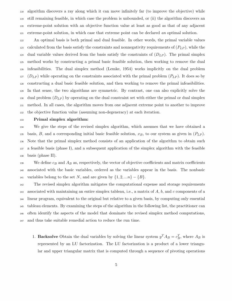
1. Backsolve Obtain the dual variables by solving the linear system yT AB = cTB, where AB is
represented by an LU factorization. The LU factorization is a product of a lower triangu-
lar and upper triangular matrix that is computed through a sequence of pivoting operations
5
analogous to the operations used to compute the inverse of a matrix. Most simplex algorithm
implementations compute and maintain an LU factorization rather than a basis inverse be-
cause the former is sparser and can be computed in a more numerically stable manner. See
Duff et al. (1986) for details. Given a factorization AB = LU , it follows that A−1B = U−1L−1,
so the backsolve is equivalent to solving
yT = cTBAB
−1 = cTBU−1L−1 (1)
This can be calculated efficiently by solving the following sparse triangular linear systems148
(first, by computing the solution of a linear system involving U , and then using the result to149
solve a linear system involving L); this computation can be performed faster than computing150
yT as a matrix product of cT and AB−1.151
pT U = cTB
yT L = pT .
2. Pricing Calculate the reduced costs cTN = cT
N − yT AN , which indicate for each nonbasic152
variable the rate of change in the objective with a unit increase in the corresponding variable153
value from zero.154
3. Entering variable selection Pick the entering variable xt and associated incoming column155
At from the set of nonbasic variable indices N with cTN < 0. If cT
N ≥ 0, stop with an optimal156
solution x = (xB, 0).157
4. Forward solve Calculate the corresponding incoming column w relative to the current basis158
matrix by solving ABw = At.159
5. Ratio test Determine the amount by which the value of the entering variable can increase160
from zero without compromising feasibility of the solution, i.e., without forcing the other basic161
variables to assume negative values. This, in turn, determines the position r of the outgoing162
variable in the basis and the associated index on the chosen variable xj , j ∈ {1, 2, ...n}. Call163
the outgoing variable in the rth position xjr . Then, such a variable is chosen as follows: r =164
argmini:wi>0
xji
wi.165
Let θ = mini:wi>0
xji
wi.166
6
If there exists no i such that wi > 0, then θ is infinite; this implies that regardless of the167
size of the objective function value given by a feasible solution, another feasible solution168
with a better objective function value always exists. The extreme-point solution given by169
(xB, 0), and the direction of unboundedness given by the sum of (−w, 0) and the unit vector170
et combine to form the direction of unboundedness. Hence, stop because the linear program171
is unbounded. Otherwise, proceed to Step 6.172
6. Basis update Update the basis matrix AB and the associated LU factorization, replacing173
the outgoing variable xjr with the incoming variable xt. Periodically refactorize the basis174
matrix AB using the factorization given above in Step 1 in order to limit the round-off error175
(see Section 3.1) that accumulates in the representation of the basis as well as to reduce the176
memory and run time required to process the accumulated updates.177
7. Recalculate basic variable values Either update or refactorize. Most optimizers perform178
between 100 and 1000 updates between each refactorization.179
(a) Update: Let xt = θ; xi ← xi − θ · wi for i ∈ {B} − {t}180
(b) Refactorize: Using the refactorization mentioned in Step 1 above, solve ABxB = b.181
8. Return to Step 1.182
A variety of methods can be used to determine the incoming variable for a basis (see Step 3)183
while executing the simplex algorithm. One can inexpensively select the incoming variable using184
partial pricing by considering a subset of nonbasic variables and selecting one of those with negative185
reduced cost. Full pricing considers the selection from all eligible variables. More elaborate variable186
selection schemes entail additional computation such as normalizing each negative reduced cost such187
that the selection of the incoming variable is based on a scale-invariant metric (Nazareth, 1987).188
These more elaborate schemes can diminish the number of iterations needed to reach optimality189
but can also require more time per iteration, especially if a problem instance contains a large190
number of variables or if the A matrix is dense, i.e., it is computationally intensive to perform the191
refactorizations given in the simplex algorithm. Hence, if the decrease in the number of iterations192
required to solve the instance does not offset the increase in time required per iteration, it is193
preferable to use a simple pricing scheme. In general, it is worth considering non-default variable194
selection schemes for problems in which the number of iterations required to solve the instance195
exceeds three times the number of constraints.196
Degeneracy in the simplex algorithm occurs when a basic variable assumes a value of zero as it197
enters the basis. In other words, the value θ in the minimum ratio test in Step 5 of the simplex198
7
algorithm is zero. This results in iterations in which the objective retains the same value, rather199
than improving. Theoretically, the simplex algorithm can cycle, revisiting bases multiple times with200
no improvement in the objective. While cycling is primarily a theoretical, rather than a practical,201
issue, highly degenerate LPs can generate long, acyclic sequences of bases that correspond to the202
same objective, making the problem more difficult to solve using the simplex algorithm.203
While space considerations preclude us from giving an analogous treatment of the dual simplex204
method (Fourer, 1994), it is worth noting that the method is very similar to that of the primal205
simplex method, only preserving dual feasibility while iterating towards primal feasibility, rather206
than vice versa. The dual simplex algorithm begins with a set of nonnegative reduced costs; such a207
set can be obtained easily in the presence of an initial basic, dual-feasible solution or by a method208
analogous to the Phase I primal simplex method. The primal variable values, x, are checked for209
feasibility, i.e., nonnegativity. If they are nonnegative, the algorithm terminates with an optimal210
solution; otherwise, a negative variable is chosen to exit the basis. Correspondingly, a minimum211
ratio test is performed on the quotient of the reduced costs and row associated with the exiting212
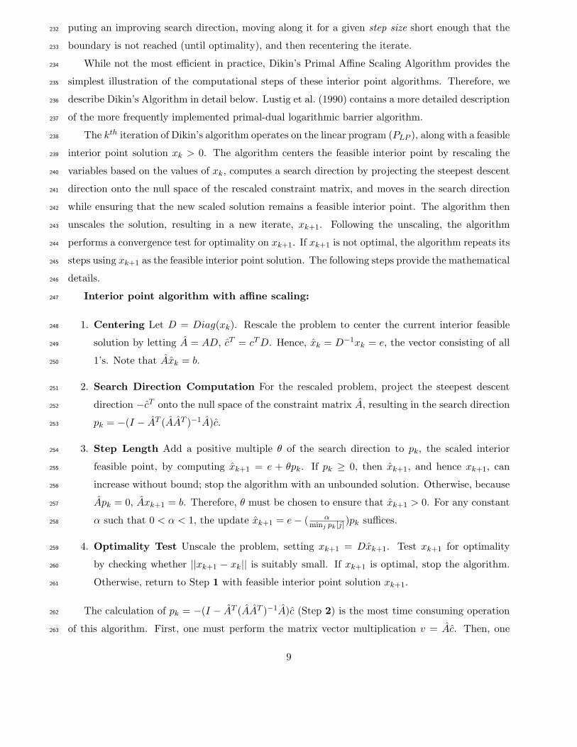
basic variable relative to the current basis (i.e., the simplex tableau row associated with the exiting213
basic variable). The ratio test either detects infeasibility or identifies the incoming basic variable.214
Finally, a basis update is performed on the factorization (Bertsimas and Tsitsiklis, 1997).215
2.2 Interior Point Algorithms216
The earliest interior point algorithms were the affine scaling algorithm proposed by Dikin (1967)217
and the logarithmic barrier algorithm proposed by Fiacco and McCormick (1968). However, at218
that time, the potential of these algorithms for efficiently solving large-scale linear programs was219
largely ignored. The ellipsoid algorithm, proposed by Khachian (1979), established the first poly-220
nomial time algorithm for linear programming. But, this great theoretical discovery did not trans-221
late to good performance on practical problems. It wasn’t until Karmarkar’s projective method222
(Karmarkar, 1984) had shown great practical promise and was subsequently demonstrated to be223
equivalent to the logarithmic barrier algorithm (Gill et al., 1986), that interest in these earlier in-224
terior point algorithms increased. Subsequent implementations of various interior point algorithms225
revealed primal-dual logarithmic barrier algorithms as the preferred variant for solving practical226
problems (Lustig et al., 1994).227
None of these interior point algorithms or any of their variants uses a basis. Rather, the algo-228
rithm searches through the interior of the feasible region, avoiding the boundary of the constraint229
set until it finds an optimal solution. Each variant possesses a different means for determining a230
search direction. However, all variants fundamentally rely on centering the current iterate, com-231
8
puting an improving search direction, moving along it for a given step size short enough that the232
boundary is not reached (until optimality), and then recentering the iterate.233
While not the most efficient in practice, Dikin’s Primal Affine Scaling Algorithm provides the234
simplest illustration of the computational steps of these interior point algorithms. Therefore, we235
describe Dikin’s Algorithm in detail below. Lustig et al. (1990) contains a more detailed description236
of the more frequently implemented primal-dual logarithmic barrier algorithm.237
The kth iteration of Dikin’s algorithm operates on the linear program (PLP ), along with a feasible238
interior point solution xk > 0. The algorithm centers the feasible interior point by rescaling the239
variables based on the values of xk, computes a search direction by projecting the steepest descent240
direction onto the null space of the rescaled constraint matrix, and moves in the search direction241
while ensuring that the new scaled solution remains a feasible interior point. The algorithm then242
unscales the solution, resulting in a new iterate, xk+1. Following the unscaling, the algorithm243
performs a convergence test for optimality on xk+1. If xk+1 is not optimal, the algorithm repeats its244
steps using xk+1 as the feasible interior point solution. The following steps provide the mathematical245
details.246
Interior point algorithm with affine scaling:247
1. Centering Let D = Diag(xk). Rescale the problem to center the current interior feasible248
solution by letting A = AD, cT = cT D. Hence, xk = D−1xk = e, the vector consisting of all249
1’s. Note that Axk = b.250
2. Search Direction Computation For the rescaled problem, project the steepest descent251
direction −cT onto the null space of the constraint matrix A, resulting in the search direction252
pk = −(I − AT (AAT )−1A)c.253
3. Step Length Add a positive multiple θ of the search direction to pk, the scaled interior254
feasible point, by computing xk+1 = e + θpk. If pk ≥ 0, then xk+1, and hence xk+1, can255
increase without bound; stop the algorithm with an unbounded solution. Otherwise, because256
Apk = 0, Axk+1 = b. Therefore, θ must be chosen to ensure that xk+1 > 0. For any constant257
α such that 0 < α < 1, the update xk+1 = e− ( αminj pk[j])pk suffices.258
4. Optimality Test Unscale the problem, setting xk+1 = Dxk+1. Test xk+1 for optimality259
by checking whether ||xk+1 − xk|| is suitably small. If xk+1 is optimal, stop the algorithm.260
Otherwise, return to Step 1 with feasible interior point solution xk+1.261
The calculation of pk = −(I − AT (AAT )−1A)c (Step 2) is the most time consuming operation262
of this algorithm. First, one must perform the matrix vector multiplication v = Ac. Then, one263
9
must compute the solution w to the linear system of equations (AAT )w = v. This step typically264
dominates the computation time of an iteration. Subsequently, one must perform a second matrix265
vector multiplication, AT w, then subtract c from the result.266
The simplex algorithm creates an m×m basis matrix of left-hand-side coefficients, AB, which267
is invertible. By contrast, interior point algorithms do not maintain a basis matrix. The matrix268
AAT is not guaranteed to be invertible unless A has full rank. Fortunately, in the case of solving269
an LP, full rank comes naturally, either through removal of dependent constraints during presolve,270
or because of the presence of slack and artificial variables in the constraint matrix.271
Other interior point algorithms maintain feasibility by different means. Examples include ap-272
plying a logarithmic barrier function to the objective rather than explicitly projecting the search273
direction onto the null space of the rescaled problem, and using a projective transformation instead274
of the affine transformation of Dikin’s algorithm to center the iterate. Some also use the primal and275
dual constraints simultaneously, and use more elaborate methods to calculate the search direction276
in order to reduce the total number of iterations. However, in all such practical variants to date,277
the dominant calculation remains the solution of a system of linear equations similar to the form278
(AAT )w = v, as in Dikin’s algorithm. As of the writing of this paper, the primal dual barrier279
algorithm, combined with Mehrotra’s predictor-corrector method (Mehrotra, 1992), has emerged280
as the method of choice in most state-of-the-art optimizers.281
Because the optimal solutions to linear programs reside on the boundary of the feasible re-282
gion, interior point algorithms cannot move to the exact optimal solution. They instead rely on283
convergence criteria. Methods to identify an optimal basic solution from the convergent solution284
that interior point algorithms provide have been developed (Megiddo, 1991). A procedure termed285
crossover can be invoked in most optimizers to transform a (typically near optimal) interior solution286
to an optimal extreme-point solution. (In the case of a unique solution, the interior point method287
would converge towards the optimal extreme-point solution, i.e., a basic solution.) Crossover pro-288
vides solutions that are easier to implement in practice. While crossover typically comprises a289
small percentage of the run time on most models, it can be time consuming, particularly when290
initiated on a suboptimal interior point solution with significant distance from an optimal solution.291
For primal-dual interior algorithms (Wright, 1997), the optimality criterion is usually based on a292
normalized duality gap, e.g., the quotient of the duality gap and primal objective (or dual objective293
since they are equal at optimality): (cT x−yT b)cT x
.294
In order to solve the linear system (AAT )w = v efficiently, most practical implementations295
maintain a Cholesky factorization (AAT ) = LLT . The non-zero structure, i.e., the positions in the296
matrix in which non-zero elements of AAT lie, profoundly influences interior point algorithm run297
10
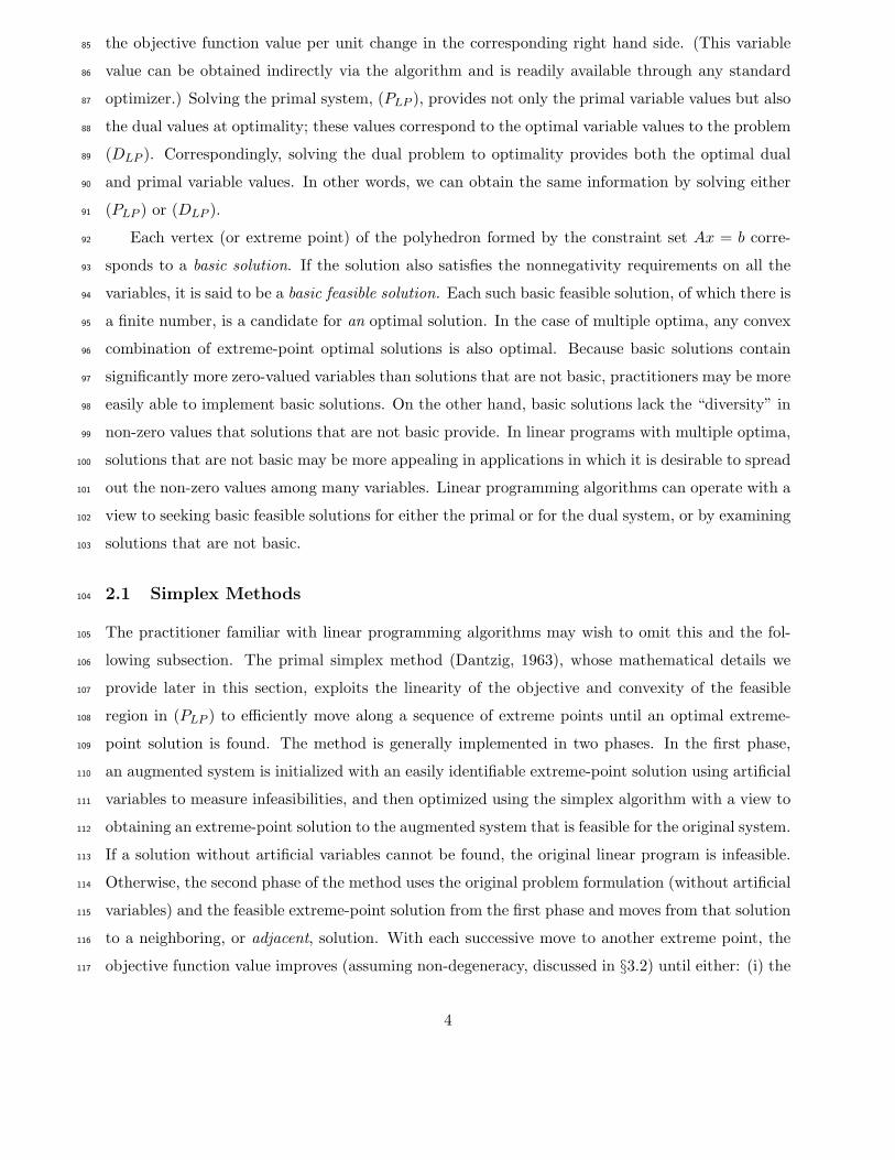
x 0 0 0 0x x 0 0 0x 0 x 0 0x 0 0 x 0x 0 0 0 x
∗
x x x x x
0 x 0 0 00 0 x 0 00 0 0 x 00 0 0 0 x
=
x x x x x
x x x x x
x x x x x
x x x x x
x x x x x
x x x x x
0 x 0 0 00 0 x 0 00 0 0 x 00 0 0 0 x
∗
x 0 0 0 0x x 0 0 0x 0 x 0 0x 0 0 x 0x 0 0 0 x
=
x x x x x
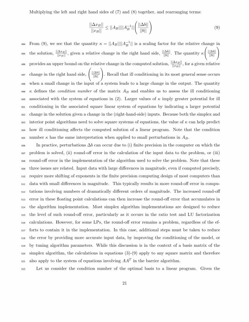
x x 0 0 0x 0 x 0 0x 0 0 x 0x 0 0 0 x
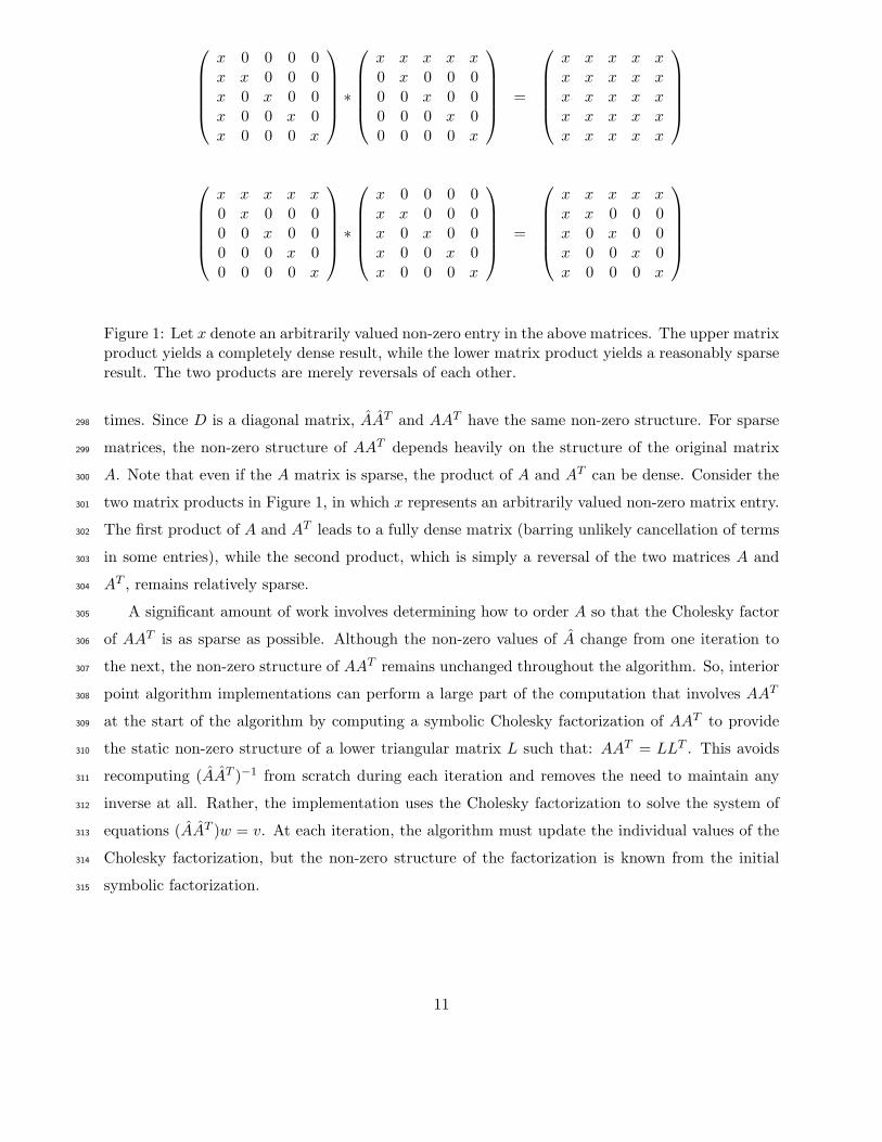
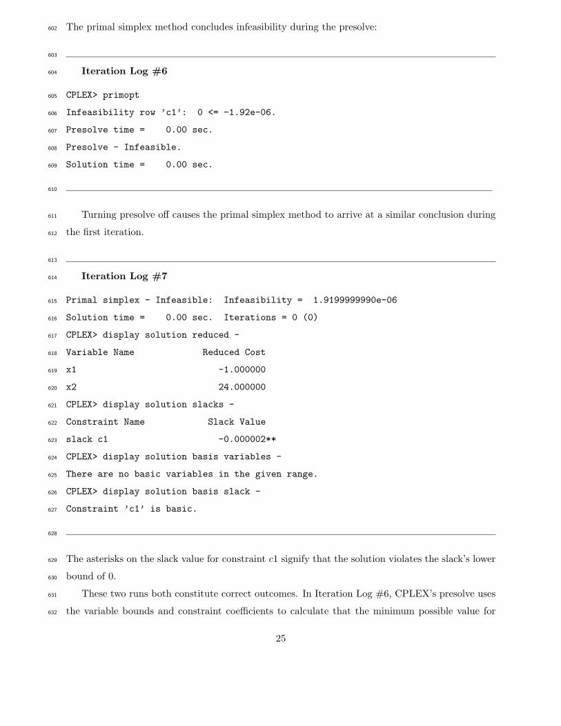
Figure 1: Let x denote an arbitrarily valued non-zero entry in the above matrices. The upper matrixproduct yields a completely dense result, while the lower matrix product yields a reasonably sparseresult. The two products are merely reversals of each other.
times. Since D is a diagonal matrix, AAT and AAT have the same non-zero structure. For sparse298
matrices, the non-zero structure of AAT depends heavily on the structure of the original matrix299
A. Note that even if the A matrix is sparse, the product of A and AT can be dense. Consider the300
two matrix products in Figure 1, in which x represents an arbitrarily valued non-zero matrix entry.301
The first product of A and AT leads to a fully dense matrix (barring unlikely cancellation of terms302
in some entries), while the second product, which is simply a reversal of the two matrices A and303
AT , remains relatively sparse.304
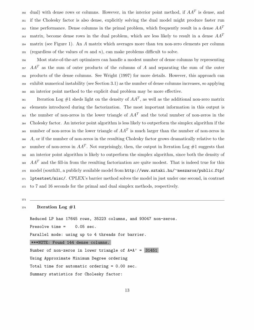
A significant amount of work involves determining how to order A so that the Cholesky factor305
of AAT is as sparse as possible. Although the non-zero values of A change from one iteration to306
the next, the non-zero structure of AAT remains unchanged throughout the algorithm. So, interior307
point algorithm implementations can perform a large part of the computation that involves AAT308
at the start of the algorithm by computing a symbolic Cholesky factorization of AAT to provide309
the static non-zero structure of a lower triangular matrix L such that: AAT = LLT . This avoids310
recomputing (AAT )−1 from scratch during each iteration and removes the need to maintain any311
inverse at all. Rather, the implementation uses the Cholesky factorization to solve the system of312
equations (AAT )w = v. At each iteration, the algorithm must update the individual values of the313
Cholesky factorization, but the non-zero structure of the factorization is known from the initial314
symbolic factorization.315
11
2.3 Algorithm Performance Contrast316
The linear programming algorithms we have discussed perform differently depending on the char-317
acteristics of the linear programs on which they are invoked. Although we introduce (PLP ) in318
standard form with equality constraints, yielding an m×n system with m equality constraints and319
n variables, we assume for the following discussion that our linear program is given as naturally320
formulated, i.e., with a mixture of equalities and inequalities, and, as such, contains m equality321
and inequality constraints and n variables.322
The solution time for simplex algorithm iterations is more heavily influenced by the number323
of constraints than by the number of variables. This is because the row-based calculations in the324
simplex algorithm involving the m × m basis matrix usually comprise a much larger percentage325
of the iteration run time than the column-based operations. One can equivalently solve either326
the primal or the dual problem, so the practitioner should select the one that most likely solves327
fastest. Some optimizers have the ability to create the dual model before or after presolving a328
linear program, and to use internal logic for determining when to solve the explicit dual. The329
aspect ratio, nm
, generally indicates whether solving the primal or the dual problem, and/or solving330
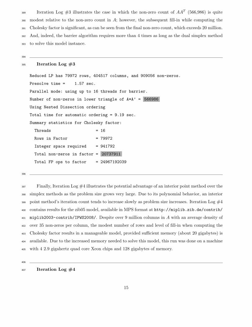
the problem with the primal or the dual simplex method is likely to be more efficient. If m << n,331
it is more expedient to preserve the large aspect ratio. In this case, the primal simplex algorithm332
with partial pricing is likely to be effective because reduced costs on a potentially small subset333
of the nonbasic variables need to be computed at each iteration. By contrast, the dual simplex334
algorithm must compute a row of the simplex tableau during the ratio test that preserves dual335
feasibility. This calculation in the dual simplex algorithm involves essentially the same effort as336
full pricing in the primal simplex algorithm. This can consume a large portion of the computation337
time of each iteration. For models with m >> n, an aspect ratio of 0.5 or smaller indicates that338
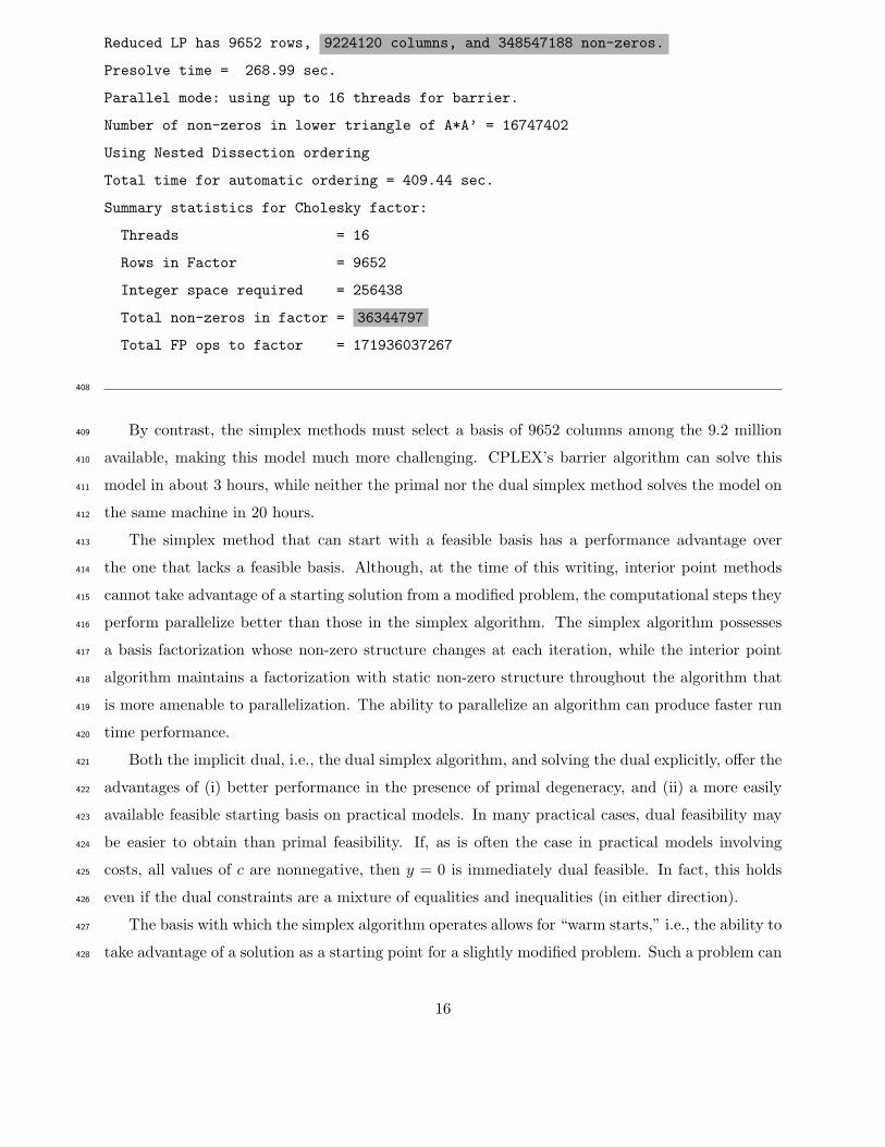
solving the dual explicitly yields faster performance than the dual simplex method, though solving339
the dual explicitly can also be faster even if the aspect ratio is greater than 0.5. Also, under primal340
degeneracy, implicitly solving the dual problem via the dual simplex method or solving the explicit341
dual can dramatically reduce the iteration count.342
Regarding interior point algorithms, they may be effective when m << n. And, when m is343
relatively small, AAT has only m rows and m columns, which gives the interior point algorithm344
a potential advantage over simplex algorithms, even when AAT is relatively dense. For m >> n,345
the interior point algorithm applied to the dual problem has potential to do very well. If A has346
either dense rows or dense columns, choosing between solving the primal and the dual affects only347
the interior point algorithm performance. Neither the primal nor the dual simplex algorithm and348
the associated factorized basis matrices has an obvious advantage over the other on an LP (or its349
12
dual) with dense rows or columns. However, in the interior point method, if AAT is dense, and350
if the Cholesky factor is also dense, explicitly solving the dual model might produce faster run351
time performance. Dense columns in the primal problem, which frequently result in a dense AAT352
matrix, become dense rows in the dual problem, which are less likely to result in a dense AAT353
matrix (see Figure 1). An A matrix which averages more than ten non-zero elements per column354
(regardless of the values of m and n), can make problems difficult to solve.355
Most state-of-the-art optimizers can handle a modest number of dense columns by representing356
AAT as the sum of outer products of the columns of A and separating the sum of the outer357
products of the dense columns. See Wright (1997) for more details. However, this approach can358
exhibit numerical instability (see Section 3.1) as the number of dense columns increases, so applying359
an interior point method to the explicit dual problem may be more effective.360
Iteration Log #1 sheds light on the density of AAT , as well as the additional non-zero matrix361
elements introduced during the factorization. The most important information in this output is362
the number of non-zeros in the lower triangle of AAT and the total number of non-zeros in the363
Cholesky factor. An interior point algorithm is less likely to outperform the simplex algorithm if the364
number of non-zeros in the lower triangle of AAT is much larger than the number of non-zeros in365
A, or if the number of non-zeros in the resulting Cholesky factor grows dramatically relative to the366
number of non-zeros in AAT . Not surprisingly, then, the output in Iteration Log #1 suggests that367
an interior point algorithm is likely to outperform the simplex algorithm, since both the density of368
AAT and the fill-in from the resulting factorization are quite modest. That is indeed true for this369
model (south31, a publicly available model from http://www.sztaki.hu/∼meszaros/public ftp/370
lptestset/misc/. CPLEX’s barrier method solves the model in just under one second, in contrast371
to 7 and 16 seconds for the primal and dual simplex methods, respectively.372
373
Iteration Log #1374
Reduced LP has 17645 rows, 35223 columns, and 93047 non-zeros.
Presolve time = 0.05 sec.
Parallel mode: using up to 4 threads for barrier.
***NOTE: Found 144 dense columns.
Number of non-zeros in lower triangle of A*A’ = 31451
Using Approximate Minimum Degree ordering
Total time for automatic ordering = 0.00 sec.
Summary statistics for Cholesky factor:
13
Threads = 4
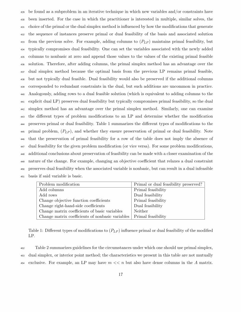
Rows in Factor = 17789
Integer space required = 70668
Total non-zeros in factor = 116782
Total FP ops to factor = 2587810
375
Now consider Iteration Log #2 which represents, in fact, output for the same model instance376
as considered in Iteration Log #1, but with dense column handling disabled. The A matrix has377
93, 047 non-zeros, while the lower triangle of AAT from which the Cholesky factor is computed378
has over 153 million non-zeros, which represents a huge increase. The additional fill-in associated379
with the factorization is relatively negligible, with 153, 859, 571−153, 530, 245 = 329, 326 additional380
non-zeros created.381
382
Iteration Log #2383
Reduced LP has 17645 rows, 35223 columns, and 93047 non-zeros.
Presolve time = 0.05 sec.
Parallel mode: using up to 4 threads for barrier.
Number of non-zeros in lower triangle of A*A’ = 153530245
Using Approximate Minimum Degree ordering
Total time for automatic ordering = 11.88 sec.
Summary statistics for Cholesky factor:
Threads = 4
Rows in Factor = 17645
Integer space required = 45206
Total non-zeros in factor = 153859571
Total FP ops to factor = 1795684140275
384
The barrier algorithm must now perform calculations with a Cholesky factor containing over385
153 million non-zeros instead of fewer than 120, 000 non-zeros with the dense column handling.386
This increases the barrier run time on the model instance from less than one second to over 19387
minutes.388
14
Iteration Log #3 illustrates the case in which the non-zero count of AAT (566,986) is quite389
modest relative to the non-zero count in A; however, the subsequent fill-in while computing the390
Cholesky factor is significant, as can be seen from the final non-zero count, which exceeds 20 million.391
And, indeed, the barrier algorithm requires more than 4 times as long as the dual simplex method392
to solve this model instance.393
394
Iteration Log #3395
Reduced LP has 79972 rows, 404517 columns, and 909056 non-zeros.
Presolve time = 1.57 sec.
Parallel mode: using up to 16 threads for barrier.
Number of non-zeros in lower triangle of A*A’ = 566986
Using Nested Dissection ordering
Total time for automatic ordering = 9.19 sec.
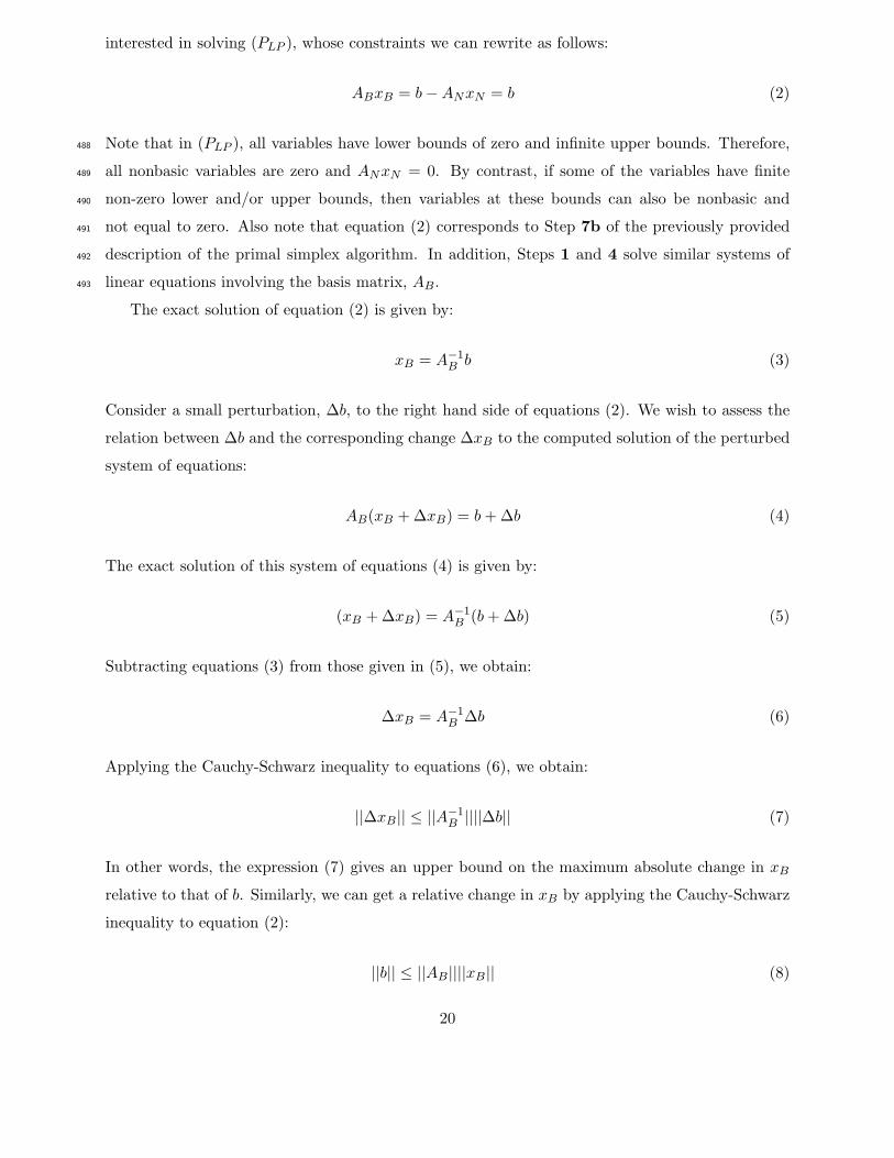
Summary statistics for Cholesky factor:
Threads = 16
Rows in Factor = 79972
Integer space required = 941792
Total non-zeros in factor = 20737911
Total FP ops to factor = 24967192039
396
Finally, Iteration Log #4 illustrates the potential advantage of an interior point method over the397
simplex methods as the problem size grows very large. Due to its polynomial behavior, an interior398
point method’s iteration count tends to increase slowly as problem size increases. Iteration Log #4399
contains results for the zib05 model, available in MPS format at http://miplib.zib.de/contrib/400
miplib2003-contrib/IPWS2008/. Despite over 9 million columns in A with an average density of401
over 35 non-zeros per column, the modest number of rows and level of fill-in when computing the402
Cholesky factor results in a manageable model, provided sufficient memory (about 20 gigabytes) is403
available. Due to the increased memory needed to solve this model, this run was done on a machine404
with 4 2.9 gigahertz quad core Xeon chips and 128 gigabytes of memory.405
406
Iteration Log #4407
15
Reduced LP has 9652 rows, 9224120 columns, and 348547188 non-zeros.
Presolve time = 268.99 sec.
Parallel mode: using up to 16 threads for barrier.
Number of non-zeros in lower triangle of A*A’ = 16747402
Using Nested Dissection ordering
Total time for automatic ordering = 409.44 sec.
Summary statistics for Cholesky factor:
Threads = 16
Rows in Factor = 9652
Integer space required = 256438
Total non-zeros in factor = 36344797
Total FP ops to factor = 171936037267
408
By contrast, the simplex methods must select a basis of 9652 columns among the 9.2 million409
available, making this model much more challenging. CPLEX’s barrier algorithm can solve this410
model in about 3 hours, while neither the primal nor the dual simplex method solves the model on411
the same machine in 20 hours.412
The simplex method that can start with a feasible basis has a performance advantage over413
the one that lacks a feasible basis. Although, at the time of this writing, interior point methods414
cannot take advantage of a starting solution from a modified problem, the computational steps they415
perform parallelize better than those in the simplex algorithm. The simplex algorithm possesses416
a basis factorization whose non-zero structure changes at each iteration, while the interior point417
algorithm maintains a factorization with static non-zero structure throughout the algorithm that418
is more amenable to parallelization. The ability to parallelize an algorithm can produce faster run419
time performance.420
Both the implicit dual, i.e., the dual simplex algorithm, and solving the dual explicitly, offer the421
advantages of (i) better performance in the presence of primal degeneracy, and (ii) a more easily422
available feasible starting basis on practical models. In many practical cases, dual feasibility may423
be easier to obtain than primal feasibility. If, as is often the case in practical models involving424
costs, all values of c are nonnegative, then y = 0 is immediately dual feasible. In fact, this holds425
even if the dual constraints are a mixture of equalities and inequalities (in either direction).426
The basis with which the simplex algorithm operates allows for “warm starts,” i.e., the ability to427
take advantage of a solution as a starting point for a slightly modified problem. Such a problem can428
16
be found as a subproblem in an iterative technique in which new variables and/or constraints have429
been inserted. For the case in which the practitioner is interested in multiple, similar solves, the430
choice of the primal or the dual simplex method is influenced by how the modifications that generate431
the sequence of instances preserve primal or dual feasibility of the basis and associated solution432
from the previous solve. For example, adding columns to (PLP ) maintains primal feasibility, but433
typically compromises dual feasibility. One can set the variables associated with the newly added434
columns to nonbasic at zero and append those values to the values of the existing primal feasible435
solution. Therefore, after adding columns, the primal simplex method has an advantage over the436
dual simplex method because the optimal basis from the previous LP remains primal feasible,437
but not typically dual feasible. Dual feasibility would also be preserved if the additional columns438
corresponded to redundant constraints in the dual, but such additions are uncommon in practice.439
Analogously, adding rows to a dual feasible solution (which is equivalent to adding columns to the440
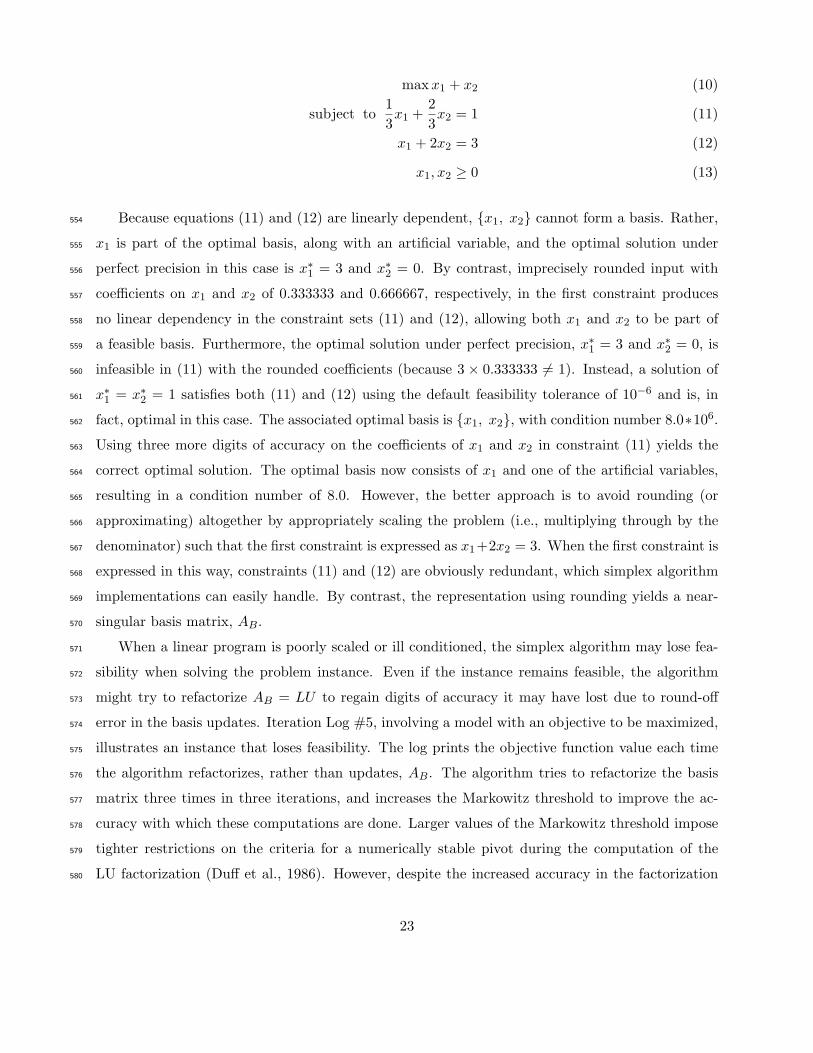
explicit dual LP) preserves dual feasibility but typically compromises primal feasibility, so the dual441
simplex method has an advantage over the primal simplex method. Similarly, one can examine442
the different types of problem modifications to an LP and determine whether the modification443
preserves primal or dual feasibility. Table 1 summarizes the different types of modifications to the444
primal problem, (PLP ), and whether they ensure preservation of primal or dual feasibility. Note445
that the preservation of primal feasibility for a row of the table does not imply the absence of446
dual feasibility for the given problem modification (or vice versa). For some problem modifications,447
additional conclusions about preservation of feasibility can be made with a closer examination of the448
nature of the change. For example, changing an objective coefficient that relaxes a dual constraint449
preserves dual feasibility when the associated variable is nonbasic, but can result in a dual infeasible450
basis if said variable is basic.451
Problem modification Primal or dual feasibility preserved?
Add columns Primal feasibilityAdd rows Dual feasibilityChange objective function coefficients Primal feasibilityChange right-hand-side coefficients Dual feasibilityChange matrix coefficients of basic variables NeitherChange matrix coefficients of nonbasic variables Primal feasibility
Table 1: Different types of modifications to (PLP ) influence primal or dual feasibility of the modifiedLP.
Table 2 summarizes guidelines for the circumstances under which one should use primal simplex,452
dual simplex, or interior point method; the characteristics we present in this table are not mutually453
exclusive. For example, an LP may have m << n but also have dense columns in the A matrix.454
17
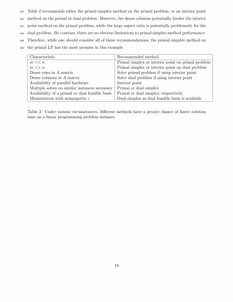
Table 2 recommends either the primal simplex method on the primal problem, or an interior point455
method on the primal or dual problem. However, the dense columns potentially hinder the interior456
point method on the primal problem, while the large aspect ratio is potentially problematic for the457
dual problem. By contrast, there are no obvious limitations to primal simplex method performance.458
Therefore, while one should consider all of these recommendations, the primal simplex method on459
the primal LP has the most promise in this example.460
Characteristic Recommended method
m << n Primal simplex or interior point on primal problemm >> n Primal simplex or interior point on dual problemDense rows in A matrix Solve primal problem if using interior pointDense columns in A matrix Solve dual problem if using interior pointAvailability of parallel hardware Interior pointMultiple solves on similar instances necessary Primal or dual simplexAvailability of a primal or dual feasible basis Primal or dual simplex, respectivelyMinimization with nonnegative c Dual simplex as dual feasible basis is available
Table 2: Under various circumstances, different methods have a greater chance of faster solutiontime on a linear programming problem instance.
18
3 Guidelines for Successful Algorithm Performance461
3.1 Numerical Stability and Ill Conditioning462
Because most commonly used computers implement floating point computations in finite precision,463
arithmetic calculations such as those involved in solving linear programming problems can be prone464
to inaccuracies due to round-off error. Round-off error can arise from numerical instability or ill465
conditioning. In general terms, ill conditioning pertains to the situation in which a small change466
to the input can result in a much larger change to the output in models or systems of equations467
(linear or otherwise). Ill conditioning can occur under perfect arithmetic as well as under finite468
precision computing. Numerical stability (or lack thereof) is a characteristic of procedures and469
algorithms implemented under finite precision. A procedure is numerically stable if its backward470
error analysis results in small, bounded errors on all data instances, i.e., if a small, bounded471
perturbation to the model would make the computed solution to the unperturbed model an exact472
solution. Thus, numerical instability does not imply ill conditioning, nor does ill conditioning imply473
numerical instability. But, a numerically unstable algorithm introduces larger perturbations into474
its calculations than its numerically stable counterpart; this can lead to larger errors in the final475
computed solution if the model is ill conditioned. See Higham (1996) for more information on the476
different types of error analysis and their relationships to ill conditioning.477
The practitioner cannot always control the floating point implementations of the computers on478
which he works and, hence, how arithmetic computations are done. As of this writing, exact floating479
point calculations can be done, but these are typically done in software packages such as Maple480
(Cybernet Systems Co., 2012) and Mathematica (Wolfram, 2012), which are not large-scale linear481
programming solvers. The QSopt optimizer (Applegate et al., 2005) reflects significant progress in482
exact linear programming, but even this solver still typically performs some calculations in finite483
precision. Regardless, the practitioner can and should be aware of input data and the implications of484
using an optimization algorithm and a floating point implementation on a model instance with such485
data. To this end, let us consider the derivation of the condition number of a square matrix, and486
how ill conditioning can affect the optimization of linear programs on finite-precision computers.487
Consider a system of linear equations in standard form, ABxB + ANxN = b, where B consti-
tutes the set of basic variables, N constitutes the set of non-basic variables, and AB and AN are
the corresponding left-hand-side basic and non-basic matrix columns, respectively. Equivalently,
xB and xN represent the vectors of basic and non-basic decision variables, respectively. We are
19
interested in solving (PLP ), whose constraints we can rewrite as follows:
ABxB = b−ANxN = b (2)
Note that in (PLP ), all variables have lower bounds of zero and infinite upper bounds. Therefore,488
all nonbasic variables are zero and ANxN = 0. By contrast, if some of the variables have finite489
non-zero lower and/or upper bounds, then variables at these bounds can also be nonbasic and490
not equal to zero. Also note that equation (2) corresponds to Step 7b of the previously provided491
description of the primal simplex algorithm. In addition, Steps 1 and 4 solve similar systems of492
linear equations involving the basis matrix, AB.493
The exact solution of equation (2) is given by:
xB = A−1B b (3)
Consider a small perturbation, ∆b, to the right hand side of equations (2). We wish to assess the
relation between ∆b and the corresponding change ∆xB to the computed solution of the perturbed
system of equations:
AB(xB + ∆xB) = b + ∆b (4)
The exact solution of this system of equations (4) is given by:
(xB + ∆xB) = A−1B (b + ∆b) (5)
Subtracting equations (3) from those given in (5), we obtain:
∆xB = A−1B ∆b (6)
Applying the Cauchy-Schwarz inequality to equations (6), we obtain:
||∆xB|| ≤ ||A−1B ||||∆b|| (7)
In other words, the expression (7) gives an upper bound on the maximum absolute change in xB
relative to that of b. Similarly, we can get a relative change in xB by applying the Cauchy-Schwarz
inequality to equation (2):
||b|| ≤ ||AB||||xB|| (8)
20
Multiplying the left and right hand sides of (7) and (8) together, and rearranging terms:
||∆xB||
||xB||≤ ||AB||||A
−1B ||
(
||∆b||
||b||
)
(9)
From (9), we see that the quantity κ = ||AB||||A−1B || is a scaling factor for the relative change in494
the solution, ||∆xB ||||xB || , given a relative change in the right hand side, ||∆b||
||b|| . The quantity κ
(
||∆b||||b||
)
495
provides an upper bound on the relative change in the computed solution, ||∆xB ||||xB || , for a given relative496
change in the right hand side,
(
||∆b||||b||
)
. Recall that ill conditioning in its most general sense occurs497
when a small change in the input of a system leads to a large change in the output. The quantity498
κ defines the condition number of the matrix AB and enables us to assess the ill conditioning499
associated with the system of equations in (2). Larger values of κ imply greater potential for ill500
conditioning in the associated square linear system of equations by indicating a larger potential501
change in the solution given a change in the (right-hand-side) inputs. Because both the simplex and502
interior point algorithms need to solve square systems of equations, the value of κ can help predict503
how ill conditioning affects the computed solution of a linear program. Note that the condition504
number κ has the same interpretation when applied to small perturbations in AB.505
In practice, perturbations ∆b can occur due to (i) finite precision in the computer on which the506
problem is solved, (ii) round-off error in the calculation of the input data to the problem, or (iii)507
round-off error in the implementation of the algorithm used to solve the problem. Note that these508
three issues are related. Input data with large differences in magnitude, even if computed precisely,509
require more shifting of exponents in the finite precision computing design of most computers than510
data with small differences in magnitude. This typically results in more round-off error in compu-511
tations involving numbers of dramatically different orders of magnitude. The increased round-off512
error in these floating point calculations can then increase the round-off error that accumulates in513
the algorithm implementation. Most simplex algorithm implementations are designed to reduce514
the level of such round-off error, particularly as it occurs in the ratio test and LU factorization515
calculations. However, for some LPs, the round-off error remains a problem, regardless of the ef-516
forts to contain it in the implementation. In this case, additional steps must be taken to reduce517
the error by providing more accurate input data, by improving the conditioning of the model, or518
by tuning algorithm parameters. While this discussion is in the context of a basis matrix of the519
simplex algorithm, the calculations in equations (3)-(9) apply to any square matrix and therefore520
also apply to the system of equations involving AAT in the barrier algorithm.521
Let us consider the condition number of the optimal basis to a linear program. Given the522
21
typical machine precision of 10−16 for double precision calculations and equation (9) that defines523
the condition number, a condition number value of 1010 provides an important threshold value.524
Most state-of-the-art optimizers use default feasibility and optimality tolerances of 10−6. In other525
words, a solution is declared feasible when solution values that violate the lower bounds of 0 in526
(PLP ) do so by less than the feasibility tolerance. Similarly, a solution is declared optimal when527
any negative reduced costs in (PLP ) are less (in absolute terms) than the optimality tolerance.528
Because of the values of these tolerances, condition numbers of 1010 or greater imply a level of529
ill conditioning that could cause the implementation of the algorithm to make decisions based on530
round-off error. Because (9) is an inequality, a condition number of 1010 does not guarantee ill531
conditioning, but it provides guidance as to when ill conditioning is likely to occur.532
Round-off error associated with finite precision implementations depends on the order of magni-533
tude of the numbers involved in the calculations. Double precision calculations involving numbers534
with orders of magnitude larger than 100 can introduce round-off error that is larger than the ma-535
chine precision. However, because machine precision defines the smallest value that distinguishes536
two numbers, calculations involving numbers with smaller orders of magnitude than 100 still pos-537
sess round-off errors at the machine precision level. For example, for floating point calculations538
involving at least one number on the order of 105, round-off error due to machine precision can539
be on the order of 105 ∗ 10−16 = 10−11. Thus, round-off error for double precision calculations540
is relative, while most optimizers use absolute tolerances for assessing feasibility and optimality.541
State-of-the-art optimizers typically scale the linear programs they receive to try to keep the round-542
off error associated with double precision calculations close to the machine precision. Nonetheless,543
the practitioner can benefit from formulating LPs that are well scaled, avoiding mixtures of large544
and small coefficients that can introduce round-off errors significantly larger than machine preci-545
sion. If this is not possible, the practitioner may need to consider solving the model with larger546
feasibility or optimality tolerances than the aforementioned defaults of 10−6.547
Equations (3) − (9) above are all done under perfect arithmetic. Finite-precision arithmetic548
frequently introduces perturbations to data. If a perturbation to the data is on the order of549
10−16 and the condition number is on the order of 1012, then round-off error as large as 10−16 ∗550
1012 = 10−4 can creep into the calculations, and linear programming algorithms may have difficulty551
distinguishing numbers accurately within its 10−6 default optimality tolerance. The following linear552
program provides an example of ill conditioning and round-off error in the input data:553
22
max x1 + x2 (10)
subject to1
3x1 +
2
3x2 = 1 (11)
x1 + 2x2 = 3 (12)
x1, x2 ≥ 0 (13)
Because equations (11) and (12) are linearly dependent, {x1, x2} cannot form a basis. Rather,554
x1 is part of the optimal basis, along with an artificial variable, and the optimal solution under555
perfect precision in this case is x∗1 = 3 and x∗
2 = 0. By contrast, imprecisely rounded input with556
coefficients on x1 and x2 of 0.333333 and 0.666667, respectively, in the first constraint produces557
no linear dependency in the constraint sets (11) and (12), allowing both x1 and x2 to be part of558
a feasible basis. Furthermore, the optimal solution under perfect precision, x∗1 = 3 and x∗
2 = 0, is559
infeasible in (11) with the rounded coefficients (because 3 × 0.333333 6= 1). Instead, a solution of560
x∗1 = x∗
2 = 1 satisfies both (11) and (12) using the default feasibility tolerance of 10−6 and is, in561
fact, optimal in this case. The associated optimal basis is {x1, x2}, with condition number 8.0∗106.562
Using three more digits of accuracy on the coefficients of x1 and x2 in constraint (11) yields the563
correct optimal solution. The optimal basis now consists of x1 and one of the artificial variables,564
resulting in a condition number of 8.0. However, the better approach is to avoid rounding (or565
approximating) altogether by appropriately scaling the problem (i.e., multiplying through by the566
denominator) such that the first constraint is expressed as x1+2x2 = 3. When the first constraint is567
expressed in this way, constraints (11) and (12) are obviously redundant, which simplex algorithm568
implementations can easily handle. By contrast, the representation using rounding yields a near-569
singular basis matrix, AB.570
When a linear program is poorly scaled or ill conditioned, the simplex algorithm may lose fea-571
sibility when solving the problem instance. Even if the instance remains feasible, the algorithm572
might try to refactorize AB = LU to regain digits of accuracy it may have lost due to round-off573
error in the basis updates. Iteration Log #5, involving a model with an objective to be maximized,574
illustrates an instance that loses feasibility. The log prints the objective function value each time575
the algorithm refactorizes, rather than updates, AB. The algorithm tries to refactorize the basis576
matrix three times in three iterations, and increases the Markowitz threshold to improve the ac-577
curacy with which these computations are done. Larger values of the Markowitz threshold impose578
tighter restrictions on the criteria for a numerically stable pivot during the computation of the579
LU factorization (Duff et al., 1986). However, despite the increased accuracy in the factorization580
23
starting at iteration 6391, enough round-off error accumulates in the subsequent iterations so that581
the next refactorization, at iteration 6456, results in a loss of feasibility.582
583
Iteration Log #5584
Iter: 6389 Objective = 13137.039899585
Iter: 6390 Objective = 13137.039899586
Iter: 6391 Objective = 13726.011591587
Markowitz threshold set to 0.3.588
Iter: 6456 Scaled infeas = 300615.030682589
...590
Iter: 6752 Scaled infeas = 0.000002591
Iter: 6754 Objective = -23870.812630592
593
Although the algorithm regains feasibility at iteration 6754, it spends an extra 298 (6754 -594
6456) iterations doing so, and the objective function is much worse than the one at iteration 6389.595
Additional iterations are then required just regain the previously attained objective value. So, even596
when numerical instability or ill conditioning does not prevent the optimizer from solving the model597
to optimality, it may slow down performance significantly. Improvements to the model formulation598
by reducing the source of perturbations and, if needed, changes to parameter settings can reduce599
round-off error in the optimizer calculations, resulting in smaller basis condition numbers and faster600
computation of optimal solutions.601
As another caveat, the practitioner should avoid including data with meaningful values smaller
than the optimizer’s tolerances. Similarly, the practitioner should ensure that the optimizer’s
tolerances exceed the largest round-off error in any of the data calculations. The computer can
only handle a fixed number of digits. Very small numerical values force the algorithm to make
decisions about whether those smaller values are real or due to round-off error, and the optimizer’s
decisions can depend on the coordinate system (i.e., basis) with which it views the model. Consider
the following feasibility problem:
c1 : −x1 + 24x2 ≤ 21 (14)
−∞ < x1 ≤ 3 (15)
x2 ≥ 1.00000008 (16)
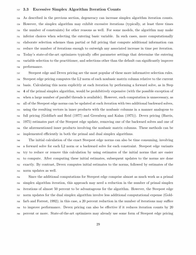
(17)
24
The primal simplex method concludes infeasibility during the presolve:602
603
Iteration Log #6604
CPLEX> primopt605
Infeasibility row ’c1’: 0 <= -1.92e-06.606
Presolve time = 0.00 sec.607
Presolve - Infeasible.608
Solution time = 0.00 sec.609
610
Turning presolve off causes the primal simplex method to arrive at a similar conclusion during611
the first iteration.612
613
Iteration Log #7614
Primal simplex - Infeasible: Infeasibility = 1.9199999990e-06615
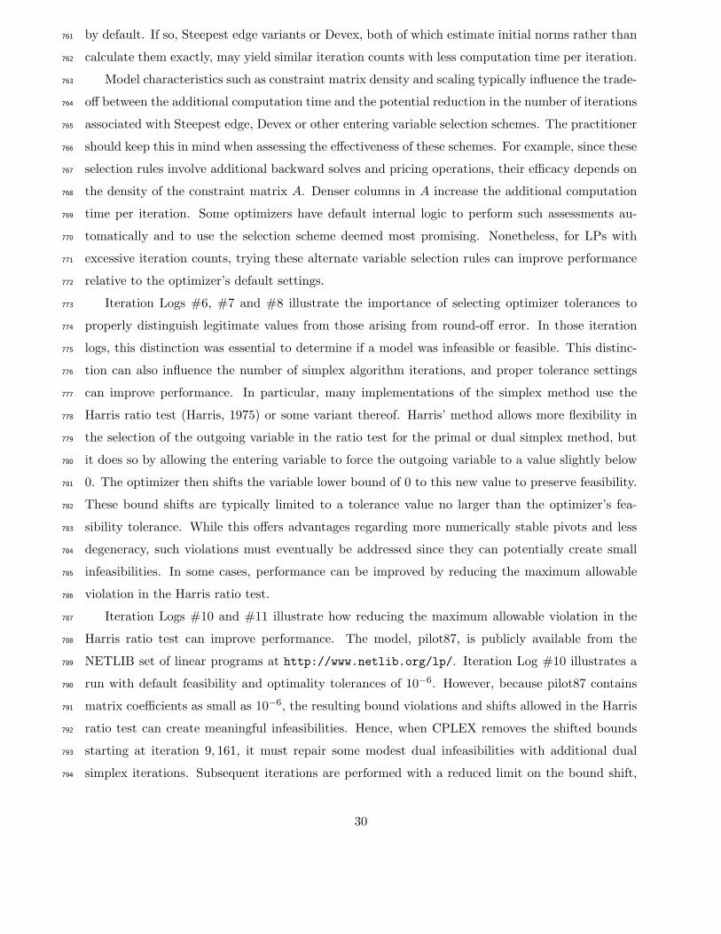
Solution time = 0.00 sec. Iterations = 0 (0)616
CPLEX> display solution reduced -617
Variable Name Reduced Cost618
x1 -1.000000619
x2 24.000000620
CPLEX> display solution slacks -621
Constraint Name Slack Value622
slack c1 -0.000002**623
CPLEX> display solution basis variables -624
There are no basic variables in the given range.625
CPLEX> display solution basis slack -626
Constraint ’c1’ is basic.627
628
The asterisks on the slack value for constraint c1 signify that the solution violates the slack’s lower629
bound of 0.630
These two runs both constitute correct outcomes. In Iteration Log #6, CPLEX’s presolve uses631
the variable bounds and constraint coefficients to calculate that the minimum possible value for632
25
the left hand side of constraint c1 is −3 + 24 ∗ 1.00000008 = 21 + 1.92 ∗ 10−6. This means that633
the left hand side must exceed the right hand side, and by a value of more than that of CPLEX’s634
default feasibility tolerance of 10−6. Iteration Log #7 shows that with presolve off, CPLEX begins635
the primal simplex method with the slack on constraint c1 in the basis, and the variables x1 and636
x2 at their respective bounds of 3 and 1.00000008. Given this basis, the reduced costs, i.e., the637
optimality criterion from Phase I, indicate that there is no way to remove the infeasibility, so the638
primal simplex method declares the model infeasible. Note that most optimizers treat variable639
bound constraints separately from general linear constraints, and that a negative reduced cost on a640
variable at its upper bound such as x1 indicates that decreasing that variable from its upper bound641
cannot decrease the objective. Now, suppose we run the primal simplex method with a starting642
basis of x2, the slack variable nonbasic at its lower bound, and x1 nonbasic at its upper bound.643
The resulting basic solution of x1 = 3, x2 = 1, slack on c1 = 0 satisfies constraint c1 exactly. The644
variable x2 does not satisfy its lower bound of 1.00000008 exactly, but the violation is less than645
many optimizers’ default feasibility tolerance of 10−6. So, with this starting basis, an optimizer646
could declare the model feasible (and hence optimal, because the model has no objective function):647
648
Iteration Log #8649
Primal simplex - Optimal: Objective = 0.0000000000e+00650
Solution time = 0.00 sec. Iterations = 0 (0)651
652
In this example, were we to set the feasibility tolerance to 10−9, we would have obtained653
consistent results with respect to both bases because the data do not possess values smaller than654
the relevant algorithm tolerance. Although the value of .00000008 is input data, this small numerical655
value could have just as easily been created during the course of the execution of the algorithm. This656
example illustrates the importance of verifying that the optimizer tolerances properly distinguish657
legitimate values from those arising from round-off error. When a model is on the edge of feasibility,658
different bases may prove feasibility or infeasibility relative to the optimizer’s tolerances. Rather659
than relying on the optimizer to make such important decisions, the practitioner should ensure660
that the optimizer’s tolerances are suitably set to reflect the valid precision of the data values661
in the model. In the example we just examined, one should first determine whether the lower662
bound on x2 is really 1.00000008, or if, in fact, the fractional part is round-off error in the data663
calculation and the correct lower bound is 1.0. If the former holds, the practitioner should set664
26
the optimizer’s feasibility and optimality tolerances to values smaller than .00000008. If the latter665
holds, the practitioner should change the lower bound to its correct value of 1.0 in the model.666
In this particular example, the practitioner may be inclined to deduce that the correct value for667
the lower bound on x2 is 1.0, because all other data in the instance are integers. More generally,668
examination of the possible round-off error associated with the procedures used to calculate the669
input data may help to distinguish round-off error from meaningful values.670
One particularly problematic source of round-off error in the data involves the conversion of671
single precision values to their double precision counterparts used by most optimizers. Precision672
for an IEEE single precision value is 6 ∗ 10−8, which is almost as large as many of the important673
default optimizer tolerances. For example, CPLEX uses default feasibility and optimality tolerances674
of 10−6. So, simply representing a data value in single precision can introduce round-off error of675
at least 6 ∗ 10−8, and additional single precision data calculations can increase the round-off error676
above the afore-mentioned optimizer tolerances. Hence, the optimizer may subsequently make677
decisions based on round-off error. Computing the data in double precision from the start will678
avoid this problem. If that is not possible, setting the optimizer tolerances to values that exceed679
the largest round-off error associated with the conversion from single to double precision provides680
an alternative.681
All linear programming algorithms can suffer from numerical instability. In particular, the682
choice of primal or dual simplex algorithm does not affect the numerical stability of a problem683
instance because the LU factorizations are the same with either algorithm. However, the interior684
point algorithm is more susceptible to numerical stability problems because it tries to maintain an685
interior solution, yet as the algorithm nears convergence, it requires a solution on lower dimensional686
faces of the polyhedron, i.e., the boundary of the feasible region.687
3.2 Degeneracy688
Degeneracy in the simplex algorithm occurs when the value θ in the minimum ratio test in Step 5689
of the simplex algorithm (see §2.1) is zero. This results in iterations in which the objective retains690
the same value, rather than improving. Highly degenerate LPs tend to be more difficult to solve691
using the simplex algorithm. Iteration Log #9 illustrates degeneracy: the nonoptimal objective692
does not change between iterations 5083 and 5968; therefore, the algorithm temporarily perturbs693
the right hand side or variable bounds to move away from the degenerate solution.694
695
Iteration Log #9696
27
Iter: 4751 Infeasibility = 8.000000697
Iter: 4870 Infeasibility = 8.000000698
Iter: 4976 Infeasibility = 6.999999699
Iter: 5083 Infeasibility = 6.000000700
Iter: 5191 Infeasibility = 6.000000701
...702
Iter: 5862 Infeasibility = 6.000000703
Iter: 5968 Infeasibility = 6.000000704
Perturbation started.705
706
After the degeneracy has been mitigated, the algorithm removes the perturbation to restore the707
original problem instance. If the current solution is not feasible, the algorithm performs additional708
iterations to regain feasibility before continuing the optimization run. Although a pricing scheme709
such as Bland’s rule can be used to mitigate cycling through bases under degeneracy, this rule holds710
more theoretical, than practical, importance and, as such, is rarely implemented in state-of-the-art711
optimizers. While such rules prevent cycles of degenerate pivots, they do not necessarily prevent712
long sequences of degenerate pivots that do not form a cycle, but do inhibit primal or dual simplex713
method performance.714
When an iteration log indicates degeneracy, first consider trying all other LP algorithms. De-715
generacy in the primal LP does not necessarily imply degeneracy in the dual LP. Therefore, the716
dual simplex algorithm might effectively solve a highly primal degenerate problem, and vice versa.717
Interior point algorithms are not prone to degeneracy because they do not pivot from one extreme718
point to the next. Interior point solutions are, by definition, nondegenerate. If alternate algorithms719
do not help performance (perhaps due to other problem characteristics that make them disadvan-720
tageous), a small, random perturbation of the problem data may help. Primal degenerate problems721
can benefit from perturbations of the right hand side values, while perturbations of the objective722
coefficients can help on dual degenerate problems. While such perturbations do not guarantee that723
the simplex algorithm does not cycle, they frequently yield improvements in practical performance.724
Some optimizers allow the practitioner to request perturbations by setting a parameter; otherwise,725
one can perturb the problem data explicitly.726
28
3.3 Excessive Simplex Algorithm Iteration Counts727
As described in the previous section, degeneracy can increase simplex algorithm iteration counts.728
However, the simplex algorithm may exhibit excessive iterations (typically, at least three times729
the number of constraints) for other reasons as well. For some models, the algorithm may make730
inferior choices when selecting the entering basic variable. In such cases, more computationally731
elaborate selection schemes than partial or full pricing that compute additional information can732
reduce the number of iterations enough to outweigh any associated increase in time per iteration.733
Today’s state-of-the-art optimizers typically offer parameter settings that determine the entering734
variable selection to the practitioner, and selections other than the default can significantly improve735
performance.736
Steepest edge and Devex pricing are the most popular of these more informative selection rules.737
Steepest edge pricing computes the L2 norm of each nonbasic matrix column relative to the current738
basis. Calculating this norm explicitly at each iteration by performing a forward solve, as in Step739
4 of the primal simplex algorithm, would be prohibitively expensive (with the possible exception of740
when a large number of parallel threads is available). However, such computation is unnecessary, as741
all of the Steepest edge norms can be updated at each iteration with two additional backward solves,742
using the resulting vectors in inner products with the nonbasic columns in a manner analogous to743
full pricing (Goldfarb and Reid (1977) and Greenberg and Kalan (1975)). Devex pricing (Harris,744
1975) estimates part of the Steepest edge update, removing one of the backward solves and one of745
the aforementioned inner products involving the nonbasic matrix columns. These methods can be746
implemented efficiently in both the primal and dual simplex algorithms.747
The initial calculation of the exact Steepest edge norms can also be time consuming, involving748
a forward solve for each L2 norm or a backward solve for each constraint. Steepest edge variants749
try to reduce or remove this calculation by using estimates of the initial norms that are easier750
to compute. After computing these initial estimates, subsequent updates to the norms are done751
exactly. By contrast, Devex computes initial estimates to the norms, followed by estimates of the752
norm updates as well.753
Since the additional computations for Steepest edge comprise almost as much work as a primal754
simplex algorithm iteration, this approach may need a reduction in the number of primal simplex755
iterations of almost 50 percent to be advantageous for the algorithm. However, the Steepest edge756
norm updates for the dual simplex algorithm involve less additional computational expense (Gold-757
farb and Forrest, 1992); in this case, a 20 percent reduction in the number of iterations may suffice758
to improve performance. Devex pricing can also be effective if it reduces iteration counts by 20759
percent or more. State-of-the-art optimizers may already use some form of Steepest edge pricing760
29
by default. If so, Steepest edge variants or Devex, both of which estimate initial norms rather than761
calculate them exactly, may yield similar iteration counts with less computation time per iteration.762
Model characteristics such as constraint matrix density and scaling typically influence the trade-763
off between the additional computation time and the potential reduction in the number of iterations764
associated with Steepest edge, Devex or other entering variable selection schemes. The practitioner765
should keep this in mind when assessing the effectiveness of these schemes. For example, since these766
selection rules involve additional backward solves and pricing operations, their efficacy depends on767
the density of the constraint matrix A. Denser columns in A increase the additional computation768
time per iteration. Some optimizers have default internal logic to perform such assessments au-769
tomatically and to use the selection scheme deemed most promising. Nonetheless, for LPs with770
excessive iteration counts, trying these alternate variable selection rules can improve performance771
relative to the optimizer’s default settings.772
Iteration Logs #6, #7 and #8 illustrate the importance of selecting optimizer tolerances to773
properly distinguish legitimate values from those arising from round-off error. In those iteration774
logs, this distinction was essential to determine if a model was infeasible or feasible. This distinc-775
tion can also influence the number of simplex algorithm iterations, and proper tolerance settings776
can improve performance. In particular, many implementations of the simplex method use the777
Harris ratio test (Harris, 1975) or some variant thereof. Harris’ method allows more flexibility in778
the selection of the outgoing variable in the ratio test for the primal or dual simplex method, but779
it does so by allowing the entering variable to force the outgoing variable to a value slightly below780
0. The optimizer then shifts the variable lower bound of 0 to this new value to preserve feasibility.781
These bound shifts are typically limited to a tolerance value no larger than the optimizer’s fea-782
sibility tolerance. While this offers advantages regarding more numerically stable pivots and less783
degeneracy, such violations must eventually be addressed since they can potentially create small784
infeasibilities. In some cases, performance can be improved by reducing the maximum allowable785
violation in the Harris ratio test.786
Iteration Logs #10 and #11 illustrate how reducing the maximum allowable violation in the787
Harris ratio test can improve performance. The model, pilot87, is publicly available from the788
NETLIB set of linear programs at http://www.netlib.org/lp/. Iteration Log #10 illustrates a789
run with default feasibility and optimality tolerances of 10−6. However, because pilot87 contains790
matrix coefficients as small as 10−6, the resulting bound violations and shifts allowed in the Harris791
ratio test can create meaningful infeasibilities. Hence, when CPLEX removes the shifted bounds792
starting at iteration 9, 161, it must repair some modest dual infeasibilities with additional dual793
simplex iterations. Subsequent iterations are performed with a reduced limit on the bound shift,794
30
but the removal of the additional bound shifts at iteration 10, 008 results in some slight dual in-795
feasibilities requiring additional iterations. Overall, CPLEX spends 993 additional dual simplex796
iterations after the initial removal of bound shifts at iteration 9, 161. Since this model has (appar-797
ently legitimate) matrix coefficients of 10−6, the default feasibility and optimality tolerances are798
too large to enable the optimizer to properly distinguish legitimate values from round-off error.799
The bound shifts thus are large enough to create dual infeasibilities that require additional dual800
simplex iterations to repair.801
Iteration Log #10802
Problem ’/ilog/models/lp/all/pilot87.sav.gz’ read.
...
Iteration log . . .
Iteration: 1 Scaled dual infeas = 0.676305
Iteration: 108 Scaled dual infeas = 0.189480
Iteration: 236 Scaled dual infeas = 0.170966
...
Iteration: 8958 Dual objective = 302.913722
Iteration: 9056 Dual objective = 303.021157
Iteration: 9137 Dual objective = 303.073444
Removing shift (4150).
Iteration: 9161 Scaled dual infeas = 0.152475
Iteration: 9350 Scaled dual infeas = 0.001941
Iteration: 9446 Scaled dual infeas = 0.000480
Iteration: 9537 Dual objective = 299.891447
Iteration: 9630 Dual objective = 301.051704
Iteration: 9721 Dual objective = 301.277884
Iteration: 9818 Dual objective = 301.658507
Iteration: 9916 Dual objective = 301.702665
Removing shift (41).
Iteration: 10008 Scaled dual infeas = 0.000136
Iteration: 10039 Dual objective = 301.678880
Iteration: 10140 Dual objective = 301.710360
31
Removing shift (8).
Iteration: 10151 Objective = 301.710354
Dual simplex - Optimal: Objective = 3.0171035068e+02
Solution time = 6.38 sec. Iterations = 10154 (1658)
By contrast, Iteration Log #11 illustrates the corresponding run with feasibility and optimality803
tolerances reduced to 10−9. This enables CPLEX to distinguish the matrix coefficient of 10−6 as804
legitimate in the model. Thus, it uses smaller bound violations and shifts in the Harris ratio test.805
Therefore, it needs to remove the bound shifts once, and only requires 32 additional dual simplex806
iterations to prove optimality. While the overall reduction in run time with this change is a modest807
four percent, larger improvements are possible on larger or more numerically challenging models.808
Iteration Log #11809
New value for feasibility tolerance: 1e-09
New value for reduced cost optimality tolerance: 1e-09
...
Iteration log . . .
Iteration: 1 Scaled dual infeas = 0.676355
Iteration: 123 Scaled dual infeas = 0.098169
...
Removing shift (190).
Iteration: 9332 Scaled dual infeas = 0.000004
Iteration: 9338 Dual objective = 301.710248
Dual simplex - Optimal: Objective = 3.0171034733e+02
Solution time = 6.15 sec. Iterations = 9364 (1353)
3.4 Excessive Barrier Algorithm Iteration Counts810
Section 2.3 included a discussion of how the non-zero structure of the constraint matrix influences811
barrier and other interior point algorithms’ time per iteration. On most LPs, the weakly poly-812
nomial complexity of the barrier algorithm results in a very modest number of iterations, even813
32
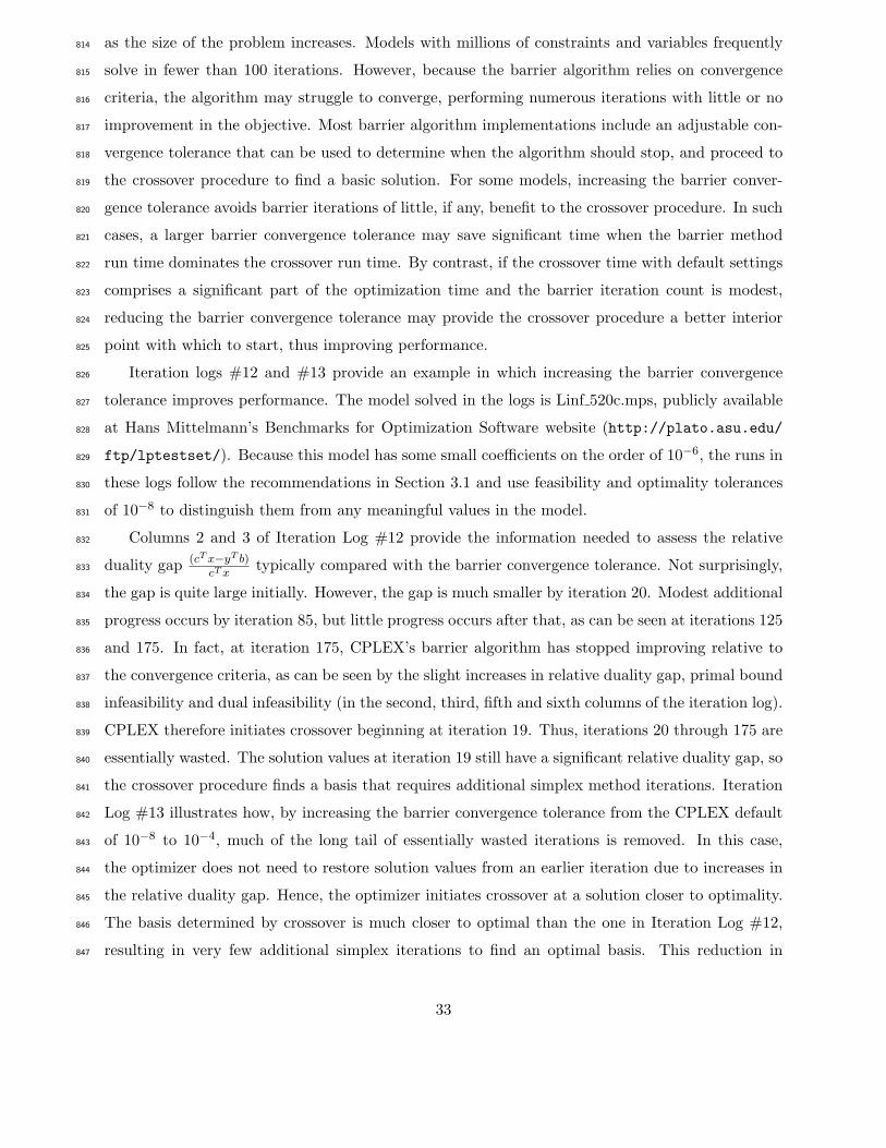
as the size of the problem increases. Models with millions of constraints and variables frequently814
solve in fewer than 100 iterations. However, because the barrier algorithm relies on convergence815
criteria, the algorithm may struggle to converge, performing numerous iterations with little or no816
improvement in the objective. Most barrier algorithm implementations include an adjustable con-817
vergence tolerance that can be used to determine when the algorithm should stop, and proceed to818
the crossover procedure to find a basic solution. For some models, increasing the barrier conver-819
gence tolerance avoids barrier iterations of little, if any, benefit to the crossover procedure. In such820
cases, a larger barrier convergence tolerance may save significant time when the barrier method821
run time dominates the crossover run time. By contrast, if the crossover time with default settings822
comprises a significant part of the optimization time and the barrier iteration count is modest,823
reducing the barrier convergence tolerance may provide the crossover procedure a better interior824
point with which to start, thus improving performance.825
Iteration logs #12 and #13 provide an example in which increasing the barrier convergence826
tolerance improves performance. The model solved in the logs is Linf 520c.mps, publicly available827
at Hans Mittelmann’s Benchmarks for Optimization Software website (http://plato.asu.edu/828
ftp/lptestset/). Because this model has some small coefficients on the order of 10−6, the runs in829
these logs follow the recommendations in Section 3.1 and use feasibility and optimality tolerances830
of 10−8 to distinguish them from any meaningful values in the model.831
Columns 2 and 3 of Iteration Log #12 provide the information needed to assess the relative832
duality gap (cT x−yT b)cT x
typically compared with the barrier convergence tolerance. Not surprisingly,833
the gap is quite large initially. However, the gap is much smaller by iteration 20. Modest additional834
progress occurs by iteration 85, but little progress occurs after that, as can be seen at iterations 125835
and 175. In fact, at iteration 175, CPLEX’s barrier algorithm has stopped improving relative to836
the convergence criteria, as can be seen by the slight increases in relative duality gap, primal bound837
infeasibility and dual infeasibility (in the second, third, fifth and sixth columns of the iteration log).838
CPLEX therefore initiates crossover beginning at iteration 19. Thus, iterations 20 through 175 are839
essentially wasted. The solution values at iteration 19 still have a significant relative duality gap, so840
the crossover procedure finds a basis that requires additional simplex method iterations. Iteration841
Log #13 illustrates how, by increasing the barrier convergence tolerance from the CPLEX default842
of 10−8 to 10−4, much of the long tail of essentially wasted iterations is removed. In this case,843
the optimizer does not need to restore solution values from an earlier iteration due to increases in844
the relative duality gap. Hence, the optimizer initiates crossover at a solution closer to optimality.845
The basis determined by crossover is much closer to optimal than the one in Iteration Log #12,846
resulting in very few additional simplex iterations to find an optimal basis. This reduction in847
33
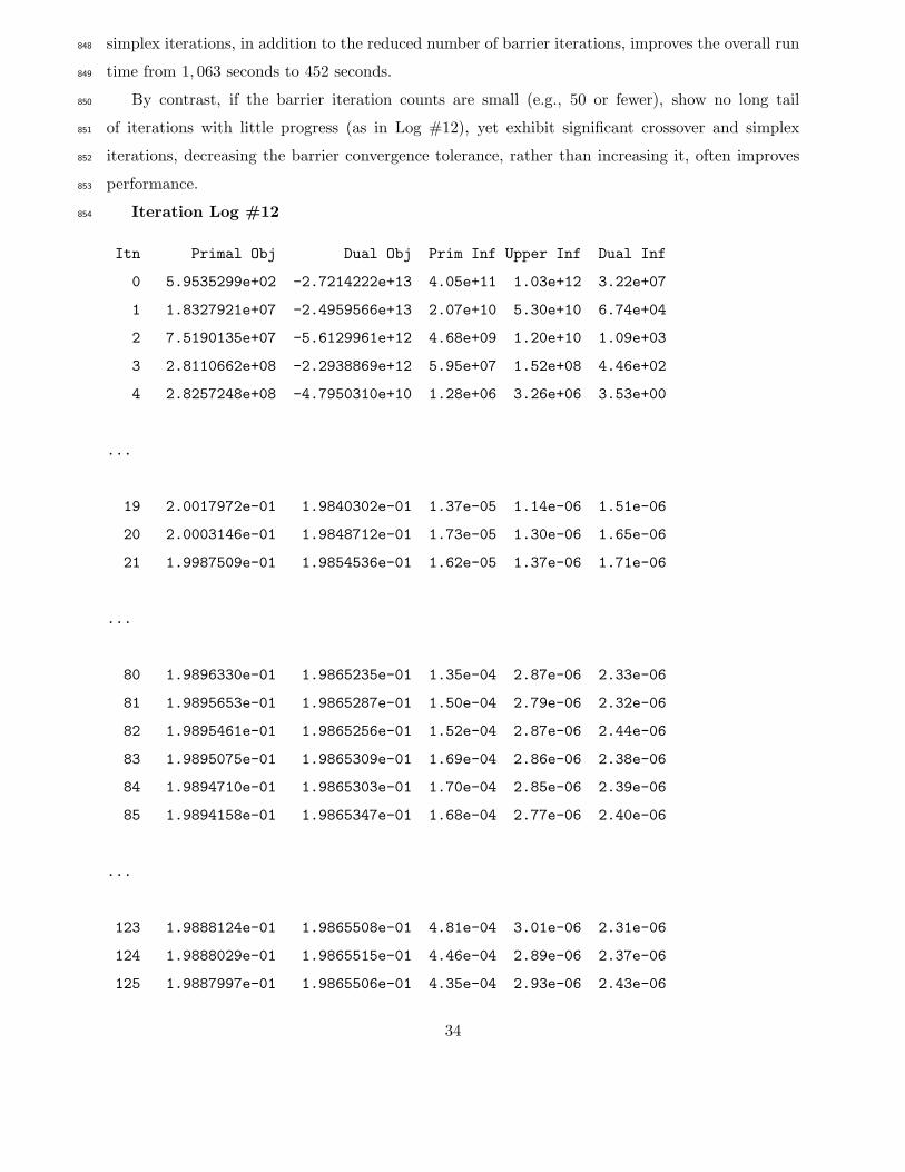
simplex iterations, in addition to the reduced number of barrier iterations, improves the overall run848
time from 1, 063 seconds to 452 seconds.849
By contrast, if the barrier iteration counts are small (e.g., 50 or fewer), show no long tail850
of iterations with little progress (as in Log #12), yet exhibit significant crossover and simplex851
iterations, decreasing the barrier convergence tolerance, rather than increasing it, often improves852
performance.853
Iteration Log #12854
Itn Primal Obj Dual Obj Prim Inf Upper Inf Dual Inf
0 5.9535299e+02 -2.7214222e+13 4.05e+11 1.03e+12 3.22e+07
1 1.8327921e+07 -2.4959566e+13 2.07e+10 5.30e+10 6.74e+04
2 7.5190135e+07 -5.6129961e+12 4.68e+09 1.20e+10 1.09e+03
3 2.8110662e+08 -2.2938869e+12 5.95e+07 1.52e+08 4.46e+02
4 2.8257248e+08 -4.7950310e+10 1.28e+06 3.26e+06 3.53e+00
...
19 2.0017972e-01 1.9840302e-01 1.37e-05 1.14e-06 1.51e-06
20 2.0003146e-01 1.9848712e-01 1.73e-05 1.30e-06 1.65e-06
21 1.9987509e-01 1.9854536e-01 1.62e-05 1.37e-06 1.71e-06
...
80 1.9896330e-01 1.9865235e-01 1.35e-04 2.87e-06 2.33e-06
81 1.9895653e-01 1.9865287e-01 1.50e-04 2.79e-06 2.32e-06
82 1.9895461e-01 1.9865256e-01 1.52e-04 2.87e-06 2.44e-06
83 1.9895075e-01 1.9865309e-01 1.69e-04 2.86e-06 2.38e-06
84 1.9894710e-01 1.9865303e-01 1.70e-04 2.85e-06 2.39e-06
85 1.9894158e-01 1.9865347e-01 1.68e-04 2.77e-06 2.40e-06
...
123 1.9888124e-01 1.9865508e-01 4.81e-04 3.01e-06 2.31e-06
124 1.9888029e-01 1.9865515e-01 4.46e-04 2.89e-06 2.37e-06
125 1.9887997e-01 1.9865506e-01 4.35e-04 2.93e-06 2.43e-06
34
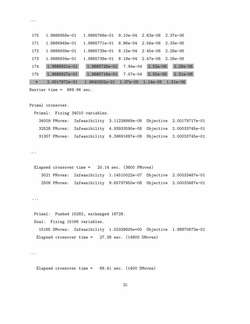
...
170 1.9886958e-01 1.9865768e-01 9.10e-04 2.63e-06 2.37e-06
171 1.9886949e-01 1.9865771e-01 8.96e-04 2.56e-06 2.33e-06
172 1.9886939e-01 1.9865739e-01 8.15e-04 2.45e-06 2.28e-06
173 1.9886934e-01 1.9865738e-01 8.19e-04 2.47e-06 2.26e-06
174 1.9886931e-01 1.9865728e-01 7.94e-04 2.52e-06 2.29e-06
175 1.9886927e-01 1.9865716e-01 7.57e-04 2.55e-06 2.31e-06
* 2.0017972e-01 1.9840302e-01 1.37e-05 1.14e-06 1.51e-06
Barrier time = 869.96 sec.
Primal crossover.
Primal: Fixing 34010 variables.
34009 PMoves: Infeasibility 3.11238869e-08 Objective 2.00179717e-01
32528 PMoves: Infeasibility 4.93933590e-08 Objective 2.00033745e-01
31357 PMoves: Infeasibility 6.39691687e-08 Objective 2.00033745e-01
...
Elapsed crossover time = 20.14 sec. (3600 PMoves)
3021 PMoves: Infeasibility 1.14510022e-07 Objective 2.00033487e-01
2508 PMoves: Infeasibility 9.65797950e-08 Objective 2.00033487e-01
...
Primal: Pushed 15282, exchanged 18728.
Dual: Fixing 15166 variables.
15165 DMoves: Infeasibility 1.03339605e+00 Objective 1.98870673e-01
Elapsed crossover time = 27.38 sec. (14800 DMoves)
...
Elapsed crossover time = 68.41 sec. (1400 DMoves)
35
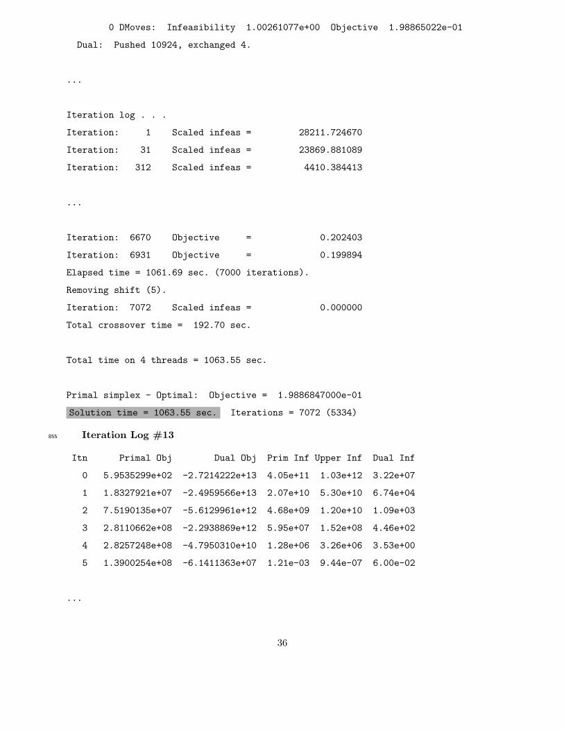
0 DMoves: Infeasibility 1.00261077e+00 Objective 1.98865022e-01
Dual: Pushed 10924, exchanged 4.
...
Iteration log . . .
Iteration: 1 Scaled infeas = 28211.724670
Iteration: 31 Scaled infeas = 23869.881089
Iteration: 312 Scaled infeas = 4410.384413
...
Iteration: 6670 Objective = 0.202403
Iteration: 6931 Objective = 0.199894
Elapsed time = 1061.69 sec. (7000 iterations).
Removing shift (5).
Iteration: 7072 Scaled infeas = 0.000000
Total crossover time = 192.70 sec.
Total time on 4 threads = 1063.55 sec.
Primal simplex - Optimal: Objective = 1.9886847000e-01
Solution time = 1063.55 sec. Iterations = 7072 (5334)
Iteration Log #13855
Itn Primal Obj Dual Obj Prim Inf Upper Inf Dual Inf
0 5.9535299e+02 -2.7214222e+13 4.05e+11 1.03e+12 3.22e+07
1 1.8327921e+07 -2.4959566e+13 2.07e+10 5.30e+10 6.74e+04
2 7.5190135e+07 -5.6129961e+12 4.68e+09 1.20e+10 1.09e+03
3 2.8110662e+08 -2.2938869e+12 5.95e+07 1.52e+08 4.46e+02
4 2.8257248e+08 -4.7950310e+10 1.28e+06 3.26e+06 3.53e+00
5 1.3900254e+08 -6.1411363e+07 1.21e-03 9.44e-07 6.00e-02
...
36
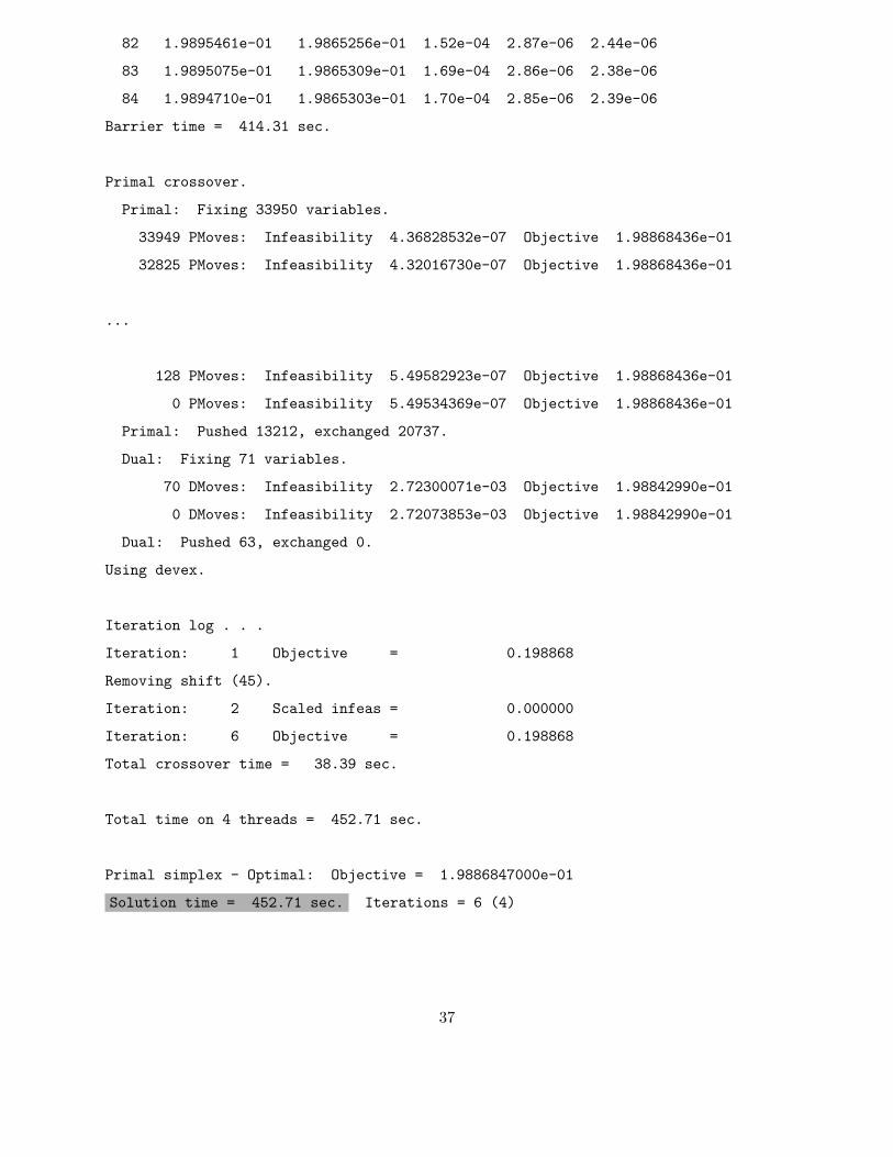
82 1.9895461e-01 1.9865256e-01 1.52e-04 2.87e-06 2.44e-06
83 1.9895075e-01 1.9865309e-01 1.69e-04 2.86e-06 2.38e-06
84 1.9894710e-01 1.9865303e-01 1.70e-04 2.85e-06 2.39e-06
Barrier time = 414.31 sec.
Primal crossover.
Primal: Fixing 33950 variables.
33949 PMoves: Infeasibility 4.36828532e-07 Objective 1.98868436e-01
32825 PMoves: Infeasibility 4.32016730e-07 Objective 1.98868436e-01
...
128 PMoves: Infeasibility 5.49582923e-07 Objective 1.98868436e-01
0 PMoves: Infeasibility 5.49534369e-07 Objective 1.98868436e-01
Primal: Pushed 13212, exchanged 20737.
Dual: Fixing 71 variables.
70 DMoves: Infeasibility 2.72300071e-03 Objective 1.98842990e-01
0 DMoves: Infeasibility 2.72073853e-03 Objective 1.98842990e-01
Dual: Pushed 63, exchanged 0.
Using devex.
Iteration log . . .
Iteration: 1 Objective = 0.198868
Removing shift (45).
Iteration: 2 Scaled infeas = 0.000000
Iteration: 6 Objective = 0.198868
Total crossover time = 38.39 sec.
Total time on 4 threads = 452.71 sec.
Primal simplex - Optimal: Objective = 1.9886847000e-01
Solution time = 452.71 sec. Iterations = 6 (4)
37
3.5 Excessive Time per Iteration856
Algorithms may require an unreasonable amount of time per iteration. For example, consider857
Iteration Log #14 in which 37,000 iterations are executed within the first 139 seconds of the858
run; at the bottom of the log, 1000 (140,000 - 139,000) iterations require about 408 (25,145.43 -859
24,736.98) seconds of computation time.860
861
Iteration Log #14862
Elapsed time = 138.23 sec. (37000 iterations)
Iter: 37969 Infeasibility = 387849.999786
Iter: 39121 Infeasibility = 379979.999768
Iter: 40295 Infeasibility = 375639.999998
Elapsed time = 150.41 sec. (41000 iterations)
...
Elapsed time = 24318.58 sec. (138000 iterations)
Iter: 138958 Infeasibility = 23.754244
Elapsed time = 24736.98 sec. (139000 iterations)
Elapsed time = 25145.43 sec. (140000 iterations)
863
This slowdown in iteration execution can be due to denser bases and the associated denser864
factorization and solve times in the simplex algorithm, specifically in Steps 1, 4 and 7. In this865
case, the practitioner should try each LP algorithm and consider an alternate pricing scheme866
if using the simplex algorithm. The more computationally expensive gradient pricing schemes867
available in today’s state-of-the-art optimizers calculate (exactly or approximately) the norm of868
each nonbasic matrix column relative to the current basis. The most expensive calculations involve869
computing these norms exactly, while less expensive calculations involve progressively cheaper (but870
progressively less accurate) ways of estimating these exact norms (Nazareth, 1987). All of these871
norm calculations involve extra memory, extra computation, and extra pricing operations.872
Another reason for excessive time per iteration is the computer’s use of virtual memory. A873
general rule requires one gigabyte of memory per million constraints of a linear program and even874
more if the A matrix is very dense or if there is a significantly larger number of columns (variables)875
than rows (constraints). Short of purchasing more memory, some optimizers support non-default876
settings that compress data and/or store data efficiently to disk. For example, CPLEX has a877
38
memory emphasis parameter whose overhead is mitigated by removing the optimizer’s reliance on878
the operating system’s virtual memory manager. This can help preserve memory and ultimately879
lead to finding a good solution reasonably quickly.880
While the change in density of the basis matrices used by the simplex method can alter the881
time per iteration, each iteration of the barrier algorithm and related interior point methods solves882
a linear system involving AAT with constant non-zero structure. Hence, barrier algorithm mem-883
ory usage and time per iteration typically exhibit little change throughout the run. Section 2.3884
describes how the density of AAT and the associated Cholesky factorization influence the time per885
barrier algorithm iteration. However, that section assumed that the density of the Cholesky factor886
was given, and identified guidelines for assessing when the density was favorable for the barrier887
algorithm. While state-of-the-art optimizers do offer some parameter settings that can potentially888
reduce the density of the Cholesky factor, the default settings are very effective regarding the889
sparsity of the Cholesky factor for a given non-zero structure of AAT . Instead of trying to find a890
sparser Cholesky factor for a given AAT , the practitioner can adjust the model formulation so that891
AAT is sparser, resulting in a sparser Cholesky factor and faster barrier algorithm iterations. One892
example of reformulation involves splitting dense columns into sparser ones (Lustig et al. (1991)893
and Vanderbei (1991)). While this increases the number of constraints and variables in the model,894
those dimensions are not the source of the performance bottleneck. A larger model with a Cholesky895
factor that has more constraints but fewer non-zeros can result in faster performance. For example,896
if Aj is a dense matrix column associated with variable xj , it can be split into two (or more) sparser897
columns A1j and A2
j that, when combined, intersect the same rows as Aj . By defining A1j and A2
j898
so that Aj = A1j + A2
j , and their non-zero indices do not intersect, a single dense column can be899
replaced by two sparser ones. In the model formulation, Ajxj is replaced by A1jx
1j + A2
jx2j . The900
model also requires an additional constraint x1j − x2
j = 0. The value of xj in the final solution is x1j901
(or x2j ).902
Column splitting increases the problem size to improve performance. However, this somewhat903
counterintuitive approach can be effective because the reduction in run time associated with the904
dense columns exceeds the increase in run time associated with additional variables and constraints.905
More generally, if an increase in problem size removes a performance problem in an algorithm906
without creating a new bottleneck, it may improve overall algorithm performance.907
Table 3 summarizes problems and suggestions for resolving them as addressed in Section 3.908
These suggestions assume that the practitioner has formulated the model in question with the909
correct fidelity, i.e., that the model cannot be reduced without compromising the value of its910
solution. When the model size becomes potentially problematic, as illustrated in Iteration Logs #2911
39
and #14, the practitioner should also consider whether solving a less refined, smaller model would912
answer his needs.913
LP performance issue Suggested resolution
Numerical instability Calculate and input model data in double precisionEliminate nearly-redundant rows and/or columns of A a priori
Avoid mixtures of large and small numbers:(i) Be suspicious of κ between 1010 and 1014;(ii) Avoid data leading to κ greater than 1014
Use alternate scaling (in the model formulation or optimizer settings)Increase the Markowitz thresholdEmploy the numerical emphasis parameter (if available)
Lack of objective function Try all other algorithms (and variants)improvement under degeneracy Perturb data either a priori or using algorithmic settings
Primal degeneracy Use either dual simplex or interior point on primal problem
Dual degeneracy Employ either primal simplex or interior point on primal problem
Both primal and dual degeneracy Execute interior point on primal or dual problem
Excessive time per iteration Try all other algorithms (and variants)Use algorithmic settings to conserve memory or purchase more externallyTry less expensive pricing settings if using simplex algorithms
Excessive simplex algorithm Try Steepest edge or Devex variable selectioniterations
Multiple bound shift removals or Reduce feasibility and optimality tolerancessignificant infeasibilities afterremoving shifts
Barrier algorithm iterations Increase barrier convergence tolerance inwith little or no progress order to initiate crossover earlier
Too much time in crossover Reduce barrier convergence tolerance inorder to provide better starting point for crossover
Table 3: LP Performance issues and their suggested resolution
When neither the tactics in Table 3 nor any other tuning of the simplex method or barrier914
algorithms yields satisfactory performance, the practitioner may also consider more advanced vari-915
ants of the simplex method. Such variants frequently solve a sequence of easier, more tractable916
LPs, resulting in an optimal solution to the more difficult LP of interest. Some variants, such as917
sifting (also called the SPRINT technique by its originator, John Forrest (Forrest, 1989)), work918
on parts of the LP of interest, solving a sequence of LPs in which the solution of the previous919
one defines problem modifications for the next one. In particular, sifting works well on LPs in920
which the number of variables dramatically exceeds the number of constraints. It starts with an921
LP consisting of all constraints but a manageable subset of the variables. After solving this LP922
subproblem, it uses the optimal dual variables to compute reduced costs that identify potential923
40
variables to add. The basis from the previous LP is typically primal feasible, speeding up the next924
optimization. Through careful management of added and removed variables from the sequence of925
LPs it solves, sifting can frequently solve the LP of interest to optimality without ever having to926
represent it in memory in its entirety. Sifting can also work well on models for which the number of927
constraints dramatically exceeds the number of variables by applying sifting to the dual LP. Other928
variants are more complex, maintaining two or more distinct subproblems, and using the solution929
of one to modify the other. The most frequently used methods are Dantzig-Wolfe Decomposition930
and Benders’ Decomposition. These methods both maintain a master problem and solve a separate931
subproblem to generate modifications to the master problem. Both the master and subproblem are932
typically much easier to solve than the original LP of interest. Repeatedly optimizing the master933
and subproblem ultimately yields an optimal solution to the original problem. Dantzig-Wolfe De-934
composition is column-based, using the subproblem to generate additional columns for the master935
problem, while Benders’ Decomposition is row-based, solving the subproblem to generate additional936
rows for the master problem. It can be shown that Benders’ Decomposition applied to the primal937
representation of an LP is equivalent to applying Dantzig-Wolfe Decomposition to the dual LP.938
The details and application of these and other decomposition methods are beyond the scope of this939
paper. Dantzig and Thapa (2003) provide more information about these approaches.940
4 Conclusions941
We summarize in this paper commonly employed linear programming algorithms and use this942
summary as a basis from which we present likely algorithmic trouble and associated avenues for their943
resolution. While optimizers and hardware will continue to advance in their capabilities of handling944
hard linear programs, practitioners will take advantage of corresponding improved performance to945
further refine their models. The guidelines we present are useful, regardless of the anticipated946
advances in hardware and software. Practitioners can implement many of these guidelines without947
expert knowledge of the underlying theory of linear programming, thereby enabling them to solve948
larger and more detailed models with existing technology.949
Acknowledgements950
Dr. Klotz wishes to acknowledge all of the CPLEX practitioners over the years, many of whom951
have provided the wide variety of models that revealed the guidelines described in this paper. He952
also wishes to thank the past and present CPLEX development, support, and sales and marketing953
teams who have contributed to the evolution of the product. Professor Newman wishes to thank954
41

the students in her first advanced linear programming class at the Colorado School of Mines for955
their helpful comments; she also wishes to thank her colleagues Professor Josef Kallrath (BASF-956
AG, Ludwigshafen, Germany) and Jennifer Rausch (Jeppeson, Englewood, Colorado) for helpful957
comments on an earlier draft. Both authors thank an anonymous referee for his helpful comments958
that lead to the improvement of the paper.959
Both authors also wish to remember Lloyd Clarke (February 14, 1964-September 20, 2007). His960
departure from the CPLEX team had consequences that extended beyond the loss of an important961
employee and colleague.962
42
References963
Applegate, D., Cook, W. and Dash, S., 2005. “QSopt.” http://www.isye.gatech.edu/∼wcook/964
qsopt/.965
Bazaraa, M., Jarvis, J. and Sherali, H., 2005. Linear Programming and Network Flows, John Wiley966
& Sons, Inc.967
Bertsimas, D. and Tsitsiklis, J., 1997. Introduction to Linear Optimization, Prentice Hall, chap. 4.968
Brown, G. and Rosenthal, R., 2008. “Optimization tradecraft: Hard-won insights from real-world969
decision support.” Interfaces, 38(5): 356–366.970
Chvatal, V., 1983. Linear Programming, W. H. Freeman.971
Cybernet Systems Co., 2012. “Maple.” http://www.maplesoft.com/.972
Dantzig, G., 1963. Linear Programming and Extensions, Princeton University Press.973
Dantzig, G. and Thapa, M., 1997. Linear Programming 1: Introduction, Springer.974
Dantzig, G. and Thapa, M., 2003. Linear Programming 2: Theory and Extensions, Springer.975
Dikin, I., 1967. “Iterative solution of problems of linear and quadratic programming.” Soviet Math-976
ematics Doklady, 8: 674–675.977
Duff, I., Erisman, A. and Reid, J., 1986. Direct Methods for Sparse Matrices, Clarendon Press978
Oxford.979
Fiacco, A. and McCormick, G., 1968. Nonlinear Programming: Sequential Unconstrained Mini-980
mization Techniques, Wiley.981
FICO, 2012. Xpress-MP Optimization Suite, Minneapolis, MN.982
Forrest, J., 1989. “Mathematical programming with a library of optimization routines.” Presenta-983
tion at 1989 ORSA/TIMS Joint National Meeting.984
Fourer, B., 1994. “Notes on the dual simplex method.” http://users.iems.northwestern.edu/985
∼4er/WRITINGS/dual.pdf.986
Gill, P., Murray, W., Saunders, M., Tomlin, J. and Wright, M., 1986. “On projected Newton987
barrier methods for linear programming and an equivalence to Karmarkar’s projective method.”988
Mathematical Programming, 36(2): 183–209.989
Goldfarb, D. and Forrest, J., 1992. “Steepest-edge simplex algorithms for linear programming.”990
Mathematical Programming, 57(1): 341–374.991
Goldfarb, D. and Reid, J., 1977. “A practical steepest-edge simplex algorithm.” Mathematical992
Programming, 12(1): 361–371.993
Greenberg, H. and Kalan, J., 1975. “An exact update for Harris’ TREAD.” Mathematical Program-994
ming Study, 4(1): 26–29.995
Gurobi, 2012. Gurobi Optimizer, Houston, TX.996
43
Harris, P., 1975. “Pivot selection methods in the Devex LP code.” Mathematical Programming997
Study, 4(1): 30–57.998
Higham, N., 1996. Accuracy and Stability of Numerical Algorithms, SIAM.999
IBM, 2012. ILOG CPLEX, Incline Village, NV.1000
Karmarkar, N., 1984. “A new polynomial-time algorithm for linear programming.” Combinatorica,1001
4(4): 373–395.1002
Khachian, L., 1979. “A polynomial algorithm for linear programming.” Soviet Mathematics Dok-1003
lady, 20: 191–194.1004
Lemke, C., 1954. “The dual method of solving the linear programming problem.” Naval Research1005
Logistics Quarterly, 1(1): 36–47.1006
Lustig, I., Marsten, R., Saltzman, M., Subramanian, R. and Shanno, D., 1990. “Interior-point1007
methods for linear programming: Just call Newton, Lagrange, and Fiacco and McCormick!”1008
Interfaces, 20(4): 105–116.1009
Lustig, I., Marsten, R. and Shanno, D., 1994. “Interior-point methods for linear programming:1010
Computational state of the art.” ORSA Journal on Computing, 6(1): 1–14.1011
Lustig, I., Mulvey, J. and Carpenter, T., 1991. “Formulating two-stage stochastic programs for1012
interior point methods.” Operations Research, 39(5): 757–770.1013
Megiddo, N., 1991. “On finding primal- and dual- optimal bases.” ORSA Journal on Computing,1014
3(1): 63–65.1015
Mehrotra, S., 1992. “On the implementation of a primal-dual interior point method.” SIAM Journal1016
on Optimization, 2(4): 575–601.1017
MOPS, 2012. MOPS, Paderborn, Germany.1018
MOSEK, 2012. MOSEK Optimization Software, Copenhagen, Denmark.1019
Nazareth, J., 1987. Computer Solution of Linear Programs, Oxford University Press.1020
Rardin, R., 1998. Optimization in Operations Research, Prentice Hall, chap. 6.1021
Vanderbei, R., 1991. “Splitting dense columns in sparse linear systems.” Linear Algebra and its1022
Applications, 152(1): 107–117.1023
Winston, W., 2004. Operations Research: Applications and Algorithms, Brooks/Cole, Thompson1024
Learning.1025
Wolfram, 2012. “Mathematica.” http://www.wolfram.com/mathematica/.1026
Wright, S., 1997. Primal-Dual Interior-Point Methods, SIAM.1027
44