precipitable water from gps zenith delays using north...

Precipitable Water from GPS Zenith Delays Using North American RegionalReanalysis Meteorology

JAMES D. MEANS AND DANIEL CAYAN

Scripps Institution of Oceanography, University of California, San Diego, La Jolla, California

(Manuscript received 14 March 2012, in final form 19 October 2012)

ABSTRACT

Precipitable water or integrated water vapor can be obtained from zenith travel-time delays from global

positioning system (GPS) signals if the atmospheric pressure and temperature at theGPS site is known. There

have been more than 10 000 GPS receivers deployed as part of geophysics research programs around the

world; but, unfortunately, most of these receivers do not have collocated barometers. This paper describes

a new technique to use North American Regional Reanalysis pressure, temperature, and geopotential height

data to calculate station pressures and surface temperature at theGPS sites. This enables precipitable water to

be calculated at those sites using archived zenith delays. The technique has been evaluated by calculating

altimeter readings at aviation routine weather report (METAR) sites and comparing them with reported

altimeter readings. Additionally, the precipitable water values calculated using this method have been found

to agree with SuomiNetGPS precipitable water, with RMS differences of 2 mm or less, and are also generally

in agreement with radiosonde measurements of precipitable water. Applications of this technique are shown

and are explored for different synoptic situations, including atmospheric-river-type baroclinic storms and the

North American monsoon.

1. Introduction

Precipitable water (PW), or integrated water vapor,

is a useful meteorological quantity in many different

contexts. It is defined as the ‘‘total atmospheric water

vapor contained in a vertical columnof unit cross-sectional

area extending between any two specified levels’’

(Glickman 2000, p. 591). Typically, the levels chosen

are the surface and the top of the atmosphere, or some

height sufficiently high that there is very little water

vapor above that level. Its value can be given as either an

areal mass density or as the depth of water that would

exist on a unit surface if all the water vapor in the col-

umn above were condensed. In this paper, we give its

value in millimeters.

In forecasting, it can be used to estimate the rain-

fall potential for a weather system, or to estimate rain

rate, given a knowledge of the upward vertical velocity

(Carlson 1998). Accurate knowledge of precipitable

water not only improves precipitation forecasts, but it

may also improve weather forecasting in general be-

cause water vapor is a key element of the energetics of

weather systems, through the latent heat of condensa-

tion (Emanuel 1988). The positive impacts of assimila-

tion of precipitable water values into numerical models

have been demonstrated by Smith et al. (2007). Their

study noted improvements in forecasts of water vapor

content in the 20-kmRapidUpdateCyclemodel (RUC20)

for 3–12-h forecasts. The importance of such an im-

provement was shown in a case study of forecasting of a

tornado outbreak in the Midwest, for which the opera-

tional model was compared against one that assimilated

global positioning system (GPS) precipitable water. The

operational model underestimated the convective avail-

able potential energy (CAPE) of the situation, while

the model that assimilated GPS precipitable water had

higher CAPE, which more accurately portrayed the se-

vere storm threat.

With the advent of GPS, people realized that atmo-

spheric water vapor could affect measurements, and in

the early 1990s the idea of using the GPS signal delay in

order to determine atmospheric column water vapor

was suggested (Bevis et al. 1992). Most of the applica-

tions to date have used collocated or nearby meteoro-

logical observations to provide the surface pressure and

Corresponding author address: James D. Means, Scripps In-

stitution of Oceanography, Mail Code 0224, University of Cal-

ifornia, San Diego, 9500 Gilman Dr., La Jolla, CA 92093.

E-mail: [email protected]

MARCH 2013 MEANS AND CAYAN 485

DOI: 10.1175/JTECH-D-12-00064.1

� 2013 American Meteorological Society

temperature necessary to calculate GPS precipitable

water. A notable exception is the global study by Wang

et al. (2007), which uses National Centers for Environ-

mental Prediction–National Center for Atmospheric

Research (NCEP–NCAR) reanalysis to derive the sur-

face temperature while still incorporating surface ob-

servations to derive the station pressure.

The goal of this paper is to demonstrate how reanalysis

can be used to derive both the station pressure and sur-

face temperature, and hence provide the meteorological

information necessary to compute GPS precipitable

water, when combined with the zenith delay. This tech-

nique can be applied to the archived delays of the more

than 10 000 GPS receivers that have been deployed

worldwide for geophysical applications. We have chosen

to focus on California and Nevada because of the very

high density of GPS sites, but similar concentrations of

GPS receivers can be found in the Pacific Northwest,

Hawaii, Japan, and other areas of active geophysical in-

vestigation. The high density of GPS receivers and fre-

quency of observations enable precipitable water to be

resolved on spatial and temporal scales that were not

previously possible, albeit at the expense of the easily

quantifiable accuracy available at GPS sites with collo-

cated meteorological stations.

Travel-time delays between satellites and fixed ground-

basedGPS sites vary due to a number of factors, but most

importantly because of the amount of air and water

vapor between the GPS receiver and the satellite. This is

a consequence of the nonunit index of refraction of air

(Hopfield 1971; Smith and Weintraub 1953). From the

index of refraction, the delay due to the dry air can be

calculated if the atmospheric pressure is known at the

site (station pressure) and then the delay due to the in-

tegrated atmospheric water vapor (precipitable water)

can be simply related to the total delay, as given in Duan

et al. (1996):

zt 5 zh1 zw .

Here, zt is the total delay, zh is the ‘‘hydrostatic’’ de-

lay, entirely due to the amount of dry air above a site and

easily related to the atmospheric pressure, and zw is the

‘‘wet’’ delay, due to the amount of water vapor above

a site.An accurate approximate expression (Saastamoinen

1973) for the hydrostatic delay is

zh 5 77:63 1026RPs/g0 ,

where R is the gas law constant for dry air; g0 is the ac-

celeration of gravity; and Ps is the station pressure

measured in millibars (hectopascals), that is, the pres-

sure measured at the GPS site and not reduced to mean

sea level. If one knows the wet delay, station pressure,

and temperature, then the precipitable water at the GPS

site can easily be calculated. To effect this calculation,

we use the following formula relating precipitable water

and wet delay (Bevis et al. 1994):

PW5P3 zw .

The derivation of this relation relies on an assumption

of azimuthal symmetry, since different slant paths to

different GPS satellites are combined. Azimuthal sym-

metry implies that there are not strong lateral gradients

in the pressure, temperature, and moisture field, so the

relationship will hold best in quiescent weather situa-

tions and may have significant errors in the vicinity of

fronts.

The following expression for the semiempirical func-

tion P is given by Bevis et al. (1992):

P(Tm)5105

4613

��3:7763 105

Tm

�1 17

� .

Here Tm is the integrated mean temperature, defined

in terms of the partial pressure of water vapor, Py , as

Tm 5

ð(Py/T) dzð(Py/T

2) dz

,

where the integrals are taken over the total height of the

atmosphere. A good approximation for Tm has been

given by Bevis et al. (1992) and is

Tm 5 70:21 0:72Ts ,

where Ts is the surface temperature. We use this ap-

proximation in our calculation of P(Tm).

The virtue of being able to infer temperature and

pressure from reanalysis is that it opens up many more

GPS sites for precipitable water measurements than

would be available otherwise. Geophysicists and geod-

esists have deployed large numbers of fixed GPS re-

ceivers in order to track motions of lithospheric plates,

as well as decipher local crustal deformation resulting

from earthquakes. In some areas of the world, particu-

larly California, these stations are spatially dense. In

California and Nevada there are over 500 GPS sites (see

Fig. 1), many of which have been operating since 2003.

The delay information from these sites is archived at the

Scripps Orbit and Permanent Array Center (SOPAC,

http://sopac.ucsd.edu/). These delays are recorded on an

486 JOURNAL OF ATMOSPHER IC AND OCEAN IC TECHNOLOGY VOLUME 30

hourly basis and are generally available in the archive

within a few days of observation. If the station pressures

and temperatures were available for these sites, then the

precipitable water could be calculated and the archived

delay data would provide a unique resource of climate

information. By comparison, there are only six radio-

sonde sites in California and Nevada from which pre-

cipitable water data can be obtained, and only at 12-h

intervals. It is also possible through microwave imagers

tomake all-weather retrievals of precipitable water over

the oceans (Schluessel and Emery 1990); however, such

techniques are limited by the time of and swath of the

satellite overpass.

In the rest of this paper, we will demonstrate how

reanalysis can be used to estimate temperature and

pressure at GPS sites that do not have observations

available (section 2), examine the accuracy of the esti-

mated pressure by comparison with observations and

determine the resultant error in precipitable water es-

timation (section 3), compare our observations with

other methods of determining precipitable water (sec-

tions 4 and 5), and highlight some particular applications

that may benefit from having a database of precipitable

water (section 6).

2. Methodology

Wehave used theNorthAmericanRegionalReanalysis

(NARR) to estimate historical pressure and temperature

at theGPS sites. TheNARRprovides geopotential height

and sea level pressure at 32-km resolution over its do-

main (Mesinger et al. 2006), which includes North

America and surrounding regions. The NARR data are

available for every 3 h from 1979 to the present. Since at

a given level surface pressure is usually a fairly slowly

varying function of horizontal position, the NARR ge-

opotential height grids can be interpolated horizontally

to the GPS site and then the hypsometric equation is

used to calculate the station pressure at the elevation of

the GPS receiver, shown as

Z22Z15H ln(p1/p2) .

The geopotential heights Z1 and Z2 are known for

standard pressure levels p1 and p2, respectively, from the

NARR output. The scale height H can then be calcu-

lated for that particular layer, and the station pressure

can be determined by extrapolating upward (or down-

ward) from the elevation of that pressure level. For ex-

ample, if a station lies at an elevation Zstation, where

Zstation5Z11DZ ,

then the pressure at Zstation can be found from

p(Zstation)5 p1 exp(2DZ/H) .

A one-sided extrapolation is used for those stations

with elevations below sea level. For the surface temper-

ature at the GPS sites, we use a simple two-dimensional

interpolation of the reanalysis gridpoint surface temper-

atures. It would also be possible to modify this horizon-

tally interpolated surface temperature to the elevation of

the GPS site by using an assumed local lapse rate, but we

have chosen not to do that here because of the number of

assumptions that must be invoked in determining the

lapse rate. The next section will show that the calculation

is relatively insensitive to errors in temperature, so that

little is gained in precipitable water accuracy by a small

increase in the accuracy of surface temperature.

3. Implementation and error analysis

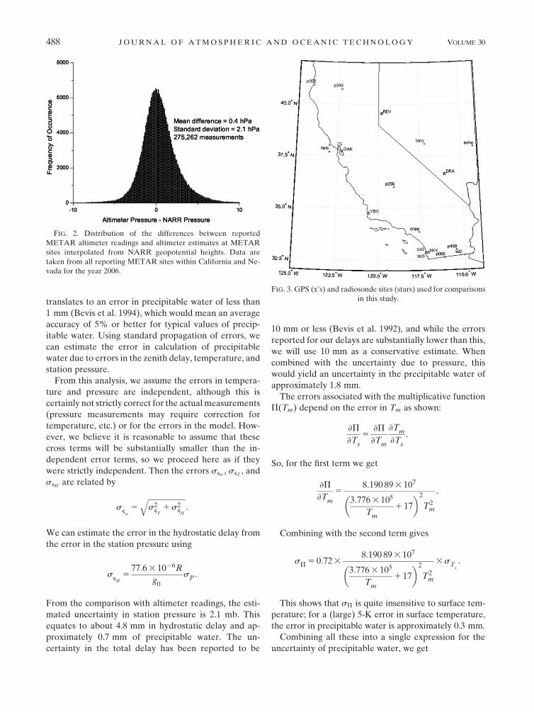
The accuracy of the above technique for estimating

pressure has been checked by comparing more than

a quarter of a million NARR-estimated altimeter

readings with those reported hourly at all reporting

aviation routine weather report (METAR) sites within

California and Nevada, for the year 2006. A plot of the

difference between these values is shown in Fig. 2. It was

found that the NARR-estimated altimeter readings had

a negative bias of 0.4 hPa compared to the METAR

altimeter readings, with a standard error of 2.1 hPa. This

value of bias in estimated versus observed pressures

FIG. 1. GPS sites in California and Nevada used in this PW study.


translates to an error in precipitable water of less than

1 mm (Bevis et al. 1994), which would mean an average

accuracy of 5% or better for typical values of precip-

itable water. Using standard propagation of errors, we

can estimate the error in calculation of precipitable

water due to errors in the zenith delay, temperature, and

station pressure.

From this analysis, we assume the errors in tempera-

ture and pressure are independent, although this is

certainly not strictly correct for the actualmeasurements

(pressure measurements may require correction for

temperature, etc.) or for the errors in the model. How-

ever, we believe it is reasonable to assume that these

cross terms will be substantially smaller than the in-

dependent error terms, so we proceed here as if they

were strictly independent. Then the errors s§w , s§T , and

s§H are related by

s§w5

ffiffiffiffiffiffiffiffiffiffiffiffiffiffiffiffiffiffiffiffis2§T1s2

§H

q.

We can estimate the error in the hydrostatic delay from

the error in the station pressure using

s§H

577:63 1026R

g0sP .

From the comparison with altimeter readings, the esti-

mated uncertainty in station pressure is 2.1 mb. This

equates to about 4.8 mm in hydrostatic delay and ap-

proximately 0.7 mm of precipitable water. The un-

certainty in the total delay has been reported to be

10 mm or less (Bevis et al. 1992), and while the errors

reported for our delays are substantially lower than this,

we will use 10 mm as a conservative estimate. When

combined with the uncertainty due to pressure, this

would yield an uncertainty in the precipitable water of

approximately 1.8 mm.

The errors associated with the multiplicative function

P(Tm) depend on the error in Tm as shown:

›P

›Ts

5›P

›Tm

›Tm

›Ts

.

So, for the first term we get

›P

›Tm

58:190 893 107�

3:7763 105

Tm

1 17

�2

T2m

.

Combining with the second term gives

sP 5 0:7238:190 893 107�

3:7763 105

Tm

1 17

�2

T2m

3sTs.

This shows that sP is quite insensitive to surface tem-

perature; for a (large) 5-K error in surface temperature,

the error in precipitable water is approximately 0.3 mm.

Combining all these into a single expression for the

uncertainty of precipitable water, we get

FIG. 2. Distribution of the differences between reported

METAR altimeter readings and altimeter estimates at METAR

sites interpolated from NARR geopotential heights. Data are

taken from all reporting METAR sites within California and Ne-

vada for the year 2006.

FIG. 3. GPS (x’s) and radiosonde sites (stars) used for comparisons

in this study.


sPW 5PW3

ffiffiffiffiffiffiffiffiffiffiffiffiffiffiffiffiffiffiffiffiffiffiffiffiffiffiffiffiffiffiffiffiffiffiffiffi�sP

P

�21

�s§w

§w

�2s

.

This yields errors of less than 2.5 mm for all rea-

sonable values of precipitable water and measurement

uncertainties. Since sP and szw have finite lower bounds

as the precipitable water goes to zero, the fractional

uncertainty must go up as the precipitable water mag-

nitude goes down. So, for very dry conditions, with

precipitable water of 5 mm, the uncertainty will be

about 20% of the measurement; but, during wet con-

ditions with precipitable water of 40 mm, it will be

about 6%.

The relatively large spread in the estimation of station

pressure is a bit troublesome, but perhaps not too

surprising considering that the wide variation in ele-

vations at METAR sites, ranging from below sea level

to more than 2 km above sea level. An inspection of

the errors indicates that errors are larger for higher-

elevation stations. This is actually somewhat conve-

nient, since water vapor is concentrated in the lower

parts of the atmosphere, the errors will be proportionally

smaller where the values are of most interest.

After estimating the station pressure and temperature

at the GPS sites, the precipitable water can be calculated

in a straightforwardway, given theGPS delays at the sites.

This technique was used to develop a database of pre-

cipitable water at 3-h intervals for 2003–09. In the fol-

lowing sections, we compare precipitable water obtained

through our technique with conventional GPS estima-

tions of precipitable water and with radiosonde estimates.

FIG. 4. GPS PW, at 3-h intervals, January–December 2009, for the SuomiNet site p499. The

blue curve shows the PW data from the National Oceanic and Atmospheric Administration’s

(NOAA) GPS meteorology program, while the black curve shows the PW estimated using

NARR-derived meteorological data.

FIG. 5. Scatterplots of reanalysis-derived GPS PW plotted against SuomiNet PW for the sites cnpp, sio3, and p066 for the calendar

year 2009.


4. Comparison with SuomiNet GPS PW data

A test of the NARRGPS technique is to compare the

value of precipitable water calculated for a site where

barometric pressure and temperature are measured (or

inferred from nearby sites) and precipitable water is

already calculated. Such a comparison was made for

nine sites (see Fig. 3) where precipitable water is cal-

culated as part of the SuomiNet (Ware et al. 2000)

(http://www.suominet.ucar.edu/). The values calculated

by SuomiNet were compared with our own calculated

values for the year 2009. Their method of calculation is

essentially the same as the one used here (Wolfe and

Gutman 2000), but SuomiNet uses pressure and tem-

peratures either measured at the GPS sites or at a nearby

Automated Surface Observation System (ASOS) site,

while we infer the temperature and pressure from re-

analysis. Also, SuomiNet uses GPS zenith delays ob-

tained from a high-speed evaluation of orbits, while we

use zenith delays that are not available in real time but

instead are available a few days later and are typically

more accurate. The sampling intervals were also some-

what different: values of precipitable water from the

SuomiNet observations are taken at 15 and 45 min after

the hour, while the reanalysis values were calculated at

the times of the reanalysis data, which is every 3 h starting

at 0000 UTC.

Figure 4 shows the time series of the NARR and

SuomiNet precipitable water overlaid for site p499. The

agreement is very close, especially considering that the

sampling intervals are different. As a further compari-

son of SuomiNet PW and NARR PW values, we have

plotted calculated linear fits and show scattergrams for

three of the six sites in Fig. 5. To compensate for the

difference in sample times, the SuomiNet times at

15 min before and after the hour were averaged to

produce a value appropriate for sampling on the hour,

and then plotted against theNARR values at 0300, 0600,

0900, 1200, 1500, 1800, and 2100UTC for the entire year.

Scattergram plots are shown in Figs. 5a–c. The linear

relation is obvious, with only a few outliers.

The fitting parameters, Table 1, represent a nearly

one-to-one relationship between the SuomiNet and

NARR values of precipitable water, with high (r$ 0:97)

correlations between the two estimates. Precipitable

water, like many meteorological variables, shows per-

sistence and is also strongly correlated with itself. For

time series that have strong autocorrelations, it is nec-

essary to use a reduced number of degrees of freedom,

since consecutive observations are not independent. We

follow the procedure given in Quenouille (1952) refer-

encing Bartlett (1935) and use the following:

Nind 5Nffiffiffiffiffiffiffiffiffiffiffiffiffiffiffiffiffiffiffiffiffiffiffiffiffiffiffiffiffiffiffiffiffiffiffiffiffiffiffiffiffiffiffiffiffiffi

11 2r1r011 2r2r

021 � � �

q .

Here, Nind is the effective number of independent

observations in testing between two series, with each

having N observations with autocorrelation coefficients

r1, r01 for lag 1, r2, r

02 for lag 2, and so on. In practice this

sum is taken until the autocorrelations become small.

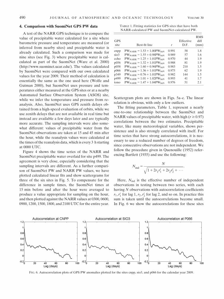
In Fig. 6 we show the autocorrelations for these sites

TABLE 1. Fitting statistics for GPS sites that have both

NARR-calculated PW and SuomiNet-calculated PW.

GPS

site Best-fit line r

Effective

D.F.

RMS

diff

(mm)

cnpp PWNARR 5 1:531 1:00PWSuN 0.991 58 1.8

sio3 PWNARR 5 1:551 0:98PWSuN 0.989 57 1.6

echo PWNARR 5 1:251 1:01PWSuN 0.970 44 1.9

p056 PWNARR 5 1:321 1:01PWSuN 0.988 81 1.9

p058 PWNARR 5 1:601 0:96PWSuN 0.983 210 1.5

p066 PWNARR 5 1:361 1:01PWSuN 0.975 62 1.9

p349 PWNARR 5 0:761 1:01PWSuN 0.982 144 1.5

p499 PWNARR 5 1:011 1:02PWSuN 0.993 41 1.7

tono PWNARR 5 1:471 1:04PWSuN 0.976 51 2.1

FIG. 6. Autocorrelation plots of GPS PW anomalies plotted for the sites cnpp, sio3, and p066 for the calendar year 2009.


calculated from the NARR precipitable water values

(autocorrelations calculated from the SuomiNet pre-

cipitable water values are very similar). While there

is little variation of the autocorrelation between the

SuomiNet and NARR values for precipitable water,

there are distinct variations from site to site that may be

connected to the climatic setting of the site. They all

show a persistence that drops off rapidly over a time

scale of about one week (;50 observations) and then

more slowly after that, until approaching zero at a time

lag of about 60–80 days. In Table 1 we have taken the

sum out to lag 500 (;62 days) to calculate the effective

observations and from that the effective degrees of

freedom (D.F.), which range from 41 to 210.

5. Comparison with radiosonde data

As a further test of this technique, NARR GPS pre-

cipitable water values are compared with the twice-daily

values of precipitable water obtained from balloon

soundings for five radiosonde sites in California and

Nevada (see Fig. 3). For the year 2006, the NARR

GPS precipitable water values have been interpolated

to the radiosonde sites, using the times when the GPS

observations and balloon soundings were coincident.

Since each GPS site is at a different elevation than the

launch site for the balloon, there is an elevation de-

pendence that we have partially compensated for by

adjusting according to the scale height of precipitable

water obtained by Means (2011). Each sounding is ac-

tually representative not of a vertical sounding centered

at the radiosonde site but instead of the complex three-

dimensional path the balloon followed until its burst

point, so there is some uncertainty in the interpolation.

Also, the accuracy of the interpolation will depend on

how close the GPS sites are to the radiosonde site. This

TABLE 2. Fitting statistics for comparisons of raob PW with PW

from NARR-calculated PW and interpolated to radiosonde loca-

tion. DRA 5 Mercury, Nevada. REV 5 Reno, Nevada.

Raob

site Best-fit line r

Effective

D.F.

F

statistic

NKX PWRAOB 5 0:651 0:99PWGPS 0.806 22 120.

DRA PWRAOB 5 0:641 0:84PWGPS 0.949 34 308.

REV PWRAOB 5 0:561 0:95PWGPS 0.946 56 479.

OAK PWRAOB 5 4:681 0:84PWGPS 0.807 180 333.

VBG PWRAOB 5 1:091 0:94PWGPS 0.852 117 312.

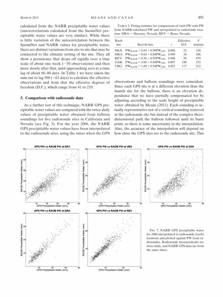
FIG. 7. NARR GPS precipitable water

for 2006 interpolated to radiosonde (raob)

locations and plotted against PW from ra-

diosondes. Radiosonde measurements are

twice daily, and NARRGPS data are from

the same times.


will cause some variance between the two values, but the

overall shape of the time series should be similar. An

important aspect for comparison of the two time series is

the similarity of the amplitude and temporal structure of

specific events, such as winter storms, summer moist

pulses, and very dry Santa Ana episodes.

Fitting parameters for NARR GPS versus radio-

sonde precipitable water are given in Table 2, and

scatterplots are shown in Fig. 7. As with the comparison

of the SuomiNet values, it is clear that the NARR

and radiosonde values are highly correlated, and the

F statistic yields a significance level for the correlation

greater than 99.9% at all the sites, as would be expected

for measurement of the same quantity using different

techniques.

Even so, the agreement is not nearly as good as might

be expected, especially for the coastal sites of Okland

(OAK), Vandenberg (VBG), and San Diego (NKX),

California. The scatterplots show that many of the

values for the radiosonde precipitable water are less

than those seen for GPS. There have been suggestions of

hygristor problems on the current generation of radio-

sondes (Maddox 2012), resulting in precipitable water

values that are too low in certain situations, and it is

possible that the differences seen are evidence of that.

A systematic study with a GPS collocated at the radio-

sonde launch site would be the best way to understand

what is causing these differences.

6. Applications of the technique

In this section three applications of the GPS NARR

database of precipitable are examined: 1) the spatial and

time variation of precipitable water across the region, 2)

the precipitable water associated with landfalling at-

mospheric rivers, and 3) the variation of precipitable

water with the North American monsoon. These ex-

amples, while not exhaustive, demonstrate the possi-

bilities for exploiting the precipitable water database.

Considering how much the climate varies across

California and Nevada, it is not surprising that the pre-

cipitable water varies greatly from site to site. Here, we

give a few examples of the temporal variation of pre-

cipitable water across the time span of this study. The

plots in Fig. 8 show time series of precipitable water

for the 2004–10 period at a variety of stations across

the region. Most show a strong annual cycle with pre-

cipitable water peaking in late summer and reaching

minimum values in midwinter. There is also a clear de-

pendence on latitude and elevation, with southern low-

land stations showing the greatest precipitable water

and the northern and mountain stations showing the

least.

In Fig. 8 the Southern California coastal site sio5

shows a strong summer increase, with precipitable water

values over 50 mm during intrusions of monsoonal air.

Peaks during the winter season correspond to baroclinic

storm passages. The southern desert site iid2 has a sim-

ilar annual cycle to sio5 but with much larger summer

amplitude because the North American monsoon exerts

a stronger influence in the southeastern deserts. The

strong annual cycles seen at the southern sites contrast

to the much weaker annual signal seen at the north coast

site farb on Farallon Island. The weak annual signal is

most likely due to strong and frequent baroclinic storm

passages, little monsoon influence, and the small annual

temperature range. Nearby onshore sites have similar

annual cycles but with more seasonal variation than is

seen at farb.

Also shown are maps of California and Nevada that

display the data as dots color coded by the magnitude of

FIG. 8. NARR GPS PW for 2004–10 for three sites: iid2, sio5,

and farb.


the precipitable water (Fig. 9b) and as color-shaded

contour maps (Figs. 10a and 10b). The NARR GPS

technique opens the door to making high-resolution

analyses of precipitable water on land, which can yield

insights into both precipitating and nonprecipitating

systems. It offers an advantage over Geostationary

Operational Environmental Satellite (GOES) sounder

images, in that it can be made in all weather conditions

and that it complements Special Sensor Microwave

Imager (SSM/I) water vapor images because it allows

plots to be made over land surfaces, while the SSM/I

only works over bodies of water. As an example of how

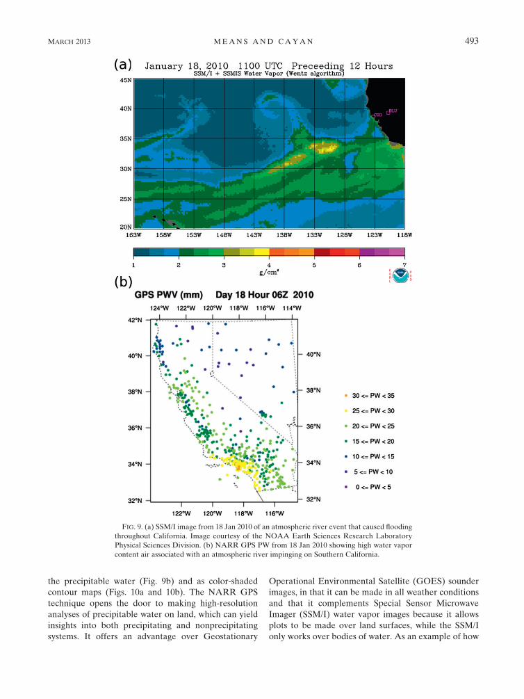
FIG. 9. (a) SSM/I image from 18 Jan 2010 of an atmospheric river event that caused flooding

throughout California. Image courtesy of the NOAA Earth Sciences Research Laboratory

Physical Sciences Division. (b) NARR GPS PW from 18 Jan 2010 showing high water vapor

content air associated with an atmospheric river impinging on Southern California.


this might be applied, Figs. 9a and 9b show precipitable

water snapshots of a baroclinic system that caused ex-

tensive damage throughout California. The system was

of the type that is characterized as an ‘‘atmospheric

river’’ (Ralph et al. 2004; Zhu and Newell 1994) because

of the relatively narrow band of high moisture content

air that arises from a connection between the deep

tropics and the midlatitudes. The SSM/I image of Fig. 9a

shows the structure of the atmospheric river impinging

on the coastline, but previously there was no good way

of seeing what happened over land; Fig. 9b shows the

NARRGPS precipitable water image for the day of the

storm, clearly showing the same high water vapor con-

tent air. The large number of GPS sites available to this

technique and the 3-hourly availability of data enable

high temporal and spatial resolution of precipitable

water in these storms, which could be key in un-

derstanding the occurrence of flooding associated with

these systems.

While such midlatitude baroclinic systems as atmo-

spheric rivers are usually quite obvious in satellite im-

ages, it is sometimes difficult to recognize incursions of

moisture associated with the North American monsoon,

and the dearth of observational data in the U.S. South-

west and Mexico can make analysis and forecasting of

summer-monsoon-related phenomena difficult. GPS

water vapor measurements offer the ability to directly

image the water vapor of the monsoonal flow and detect

the moisture necessary for deep convection and de-

termine its horizontal structure. Figure 10 shows water

vapor images before and after the onset of the monsoon

in the California and Nevada region: Fig. 10a shows dry

conditions over all of California and Nevada for 21 June

2006, while Fig. 10b shows the situation approximately

five weeks later, with approximately the southern one-

third of California and Nevada covered with a deep

moist layer, with precipitable water values exceeding

40 mm.

7. Conclusions and future directions

Using the NARR dataset has been shown to be an

effective method for generating GPS PW data at sites

that do not have meteorological instrumentation, and it

provides spatial density and temporal coverage that are

not available with conventionalmeasures of precipitable

water at an accuracy that is comparable to radiosonde or

traditional GPS precipitable water. The database of

GPS water vapor maps for California and Nevada is

being extended backward through the GPS archive and

forward as more data becomes available. However, we

do not believe the present level of accuracy is sufficient

to ascertain long-term trends in water vapor. Never-

theless, within the limitations of its accuracy, it can

FIG. 10. (a) Contoured NARRGPS PW vapor on 21 Jun 2006, prior to the onset of the monsoon. Interpolation is

performed using NCAR Command Language (NCL) and is based on a triangular mesh algorithm. (b) Contoured

NARRGPS PW vapor on 27 Jul 2006, showing fully developedmonsoon with sharp moisture gradient from south to

north. Interpolation is performed using NCL and is based on a triangular mesh algorithm.


provide insight into the statistics of precipitable water at

a site and help in the understanding of particular syn-

optic events.

Additionally, a real-time version of the algorithm has

been implemented in order to take advantage of the

large number of low latency, high bandwidth (1 Hz)

GPS sites that have been installed in connection with

automated earthquake warning networks. By using the

Rapid Update Cycle (RUC) model for the pressure and

height data instead of the NARR, precipitable water

maps can be generated every hour, or more often if

desired. Assimilation of GPW precipitable water into

numerical weather prediction models has already shown

to improve forecasting skill (Gutman et al. 2004; Kuo

et al. 1993; Marcus et al. 2007; Smith et al. 2000, 2007),

and the availability to forecasters of real-time high-

resolution water vapor images should improve forecasts.

It is expected that this might improve operational fore-

casting and possibly result in more accurate forecasts of

incipient flooding situations.

Acknowledgments. We thank Mary Tyree and Peng

Fang for their computing assistance in the preparation of

these results, and Yehuda Bock and the Scripps Orbit

and Permanent Array Center for providing the zenith

delays. We would also like to thank the anonymous re-

viewers for taking the time and effort to make this

a better paper.

This work was supported by a grant from the California

Energy Commission and a Blasker grant from the San

Diego Foundation.

REFERENCES

Bartlett, M. S., 1935: Some aspects of the time-correlation problem

in regard to tests of significance. J. Roy. Stat. Soc., 98, 536–543.

Bevis, M., S. Businger, T. A. Herring, C. Rocken, R. A. Anthes,

and R. H. Ware, 1992: GPS meteorology: Remote sensing of

atmospheric water vapor using the global positioning system.

J. Geophys. Res., 97 (D14), 15 787–15 801.

——, ——, S. Chiswell, T. A. Herring, R. A. Anthes, C. Rocken,

and R. H. Ware, 1994: GPS meteorology: Mapping zenith wet

delays onto precipitable water. J. Appl. Meteor., 33, 379–386.Carlson, T. N., 1998: Mid-Latitude Weather Systems. Amer. Me-

teor. Soc., 507 pp.

Duan, J., and Coauthors, 1996: GPS meteorology: Direct estima-

tion of the absolute value of precipitable water. J. Appl. Me-

teor., 35, 830–838.

Emanuel, K. A., 1988: The maximum intensity of hurricanes.

J. Atmos. Sci., 45, 1143–1155.Glickman, T. S., 2000: Glossary of Meteorology. 2nd ed. Amer.

Meteor. Soc., 855 pp.

Gutman, S. I., S. R. Sahm, S. G. Benjamin, B. E. Schwartz, K. L.

Holub, J. Q. Stewart, and T. L. Smith, 2004: Rapid retrieval

and assimilation of ground based GPS precipitable water ob-

servations at theNOAAForecast SystemsLaboratory: Impact

on weather forecasts. J. Meteor. Soc. Japan, 351–360.

Hopfield, H. S., 1971: Tropospheric effect on electromagnetically

measured range: Prediction from surface weather data. Radio

Sci., 6, 357–367.Kuo, Y.-H., Y.-R. Guo, and E. R.Westwater, 1993: Assimilation of

precipitable water measurements into a mesoscale numerical

model. Mon. Wea. Rev., 121, 1215–1238.

Maddox, R.A., cited 2012:Overviewof problemswith data from the

RSS Sippican sondes. [Available online at http://madweather.

blogspot.com/2007/08/overview-of-problems-with-data-from-rss.

html.]

Marcus, S., J. Kim, T. Chin, D. Danielson, and J. Laber, 2007: In-

fluence of GPS precipitable water vapor retrievals on quan-

titative precipitation forecasting in Southern California.

J. Appl. Meteor. Climatol., 46, 1828–1839.Means, J. D., 2011: GPS precipitable water measurements used in

the analysis of California and Nevada climate. Ph.D. disser-

tation, Scripps Institution of Oceanography, University of

California at San Diego, 333 pp.

Mesinger, F., and Coauthors, 2006: North American Regional

Reanalysis. Bull. Amer. Meteor. Soc., 87, 343.

Quenouille, M. H., 1952: Associated Measurements. Butterworths

Scientific Publications, 242 pp.

Ralph, F. M., P. J. Neiman, and G. A. Wick, 2004: Satellite and

CALJET aircraft observations of atmospheric rivers over the

eastern North Pacific Ocean during the winter of 1997/98.

Mon. Wea. Rev., 132, 1721–1745.

Saastamoinen, J., 1973: Contributions to the theory of atmospheric

refraction. Part II. Refraction corrections in satellite geodesy.

Bull. Geod., 107, 13–34.Schluessel, P., and W. J. Emery, 1990: Atmospheric water-vapor

over oceans from SSM/I measurements. Int. J. Remote Sens.,

11, 753–766.Smith, E. K. J., and S. Weintraub, 1953: The constants in the

equation for atmospheric refractive index at radio frequencies.

Proc. Inst. Radio Eng., 41, 1035–1037.

Smith, T. L., S. G. Benjamin, B. E. Schwartz, and S. I. Gutman,

2000: UsingGPS-IPW in a 4-D data assimilation system.Earth

Planets Space, 52, 921–926.

——, ——, S. I. Gutman, and S. Sahm, 2007: Short-range forecast

impact from assimilation of GPS-IPW observations into the

Rapid Update Cycle. Mon. Wea. Rev., 135, 2914–2930.

Wang, J., L. Zhang, A. G. Dai, T. Van Hove, and J. Van Baelen,

2007: A near-global, 2-hourly data set of atmospheric precip-

itable water from ground-based GPSmeasurements. J. Geophys.

Res., 112, D11107, doi:10.1029/2006JD007529.

Ware, R. H., and Coauthors, 2000: SuomiNet: A real-time national

GPS network for atmospheric research and education. Bull.

Amer. Meteor. Soc., 81, 677–694.

Wolfe, D. E., and S. I. Gutman, 2000: Developing an operational,

surface-based, GPS, water vapor observing system forNOAA:

Network design and results. J. Atmos. Oceanic Technol., 17,426–440.

Zhu, Y., and R. E. Newell, 1994: Atmospheric rivers and bombs.

Geophys. Res. Lett., 21, 1999–2002.


precipitable water from gps zenith delays using north...

Documents