PREDICTING LAKE ACIDIFICATION and REGIONALIZATION OF PREDICTIONS: TWO CONFERENCE PAPERS

Juha Kamari and Maximilian Posch International Institute for Applied Systems Analysis, La.xenburg, Austria

RR- 87- 18 September 1987

1. Prediction Models for Acidification. Invited keynote paper reprinted from the proceedings of the International Symposium on Acidification and Water Pathways (with modifications to Figure 1, Table 1, and the References), sponsored by the Norwegian National Committee for Hydrology; UNESCO; NMO ; and the IHP Com­mittees of Denmark , Finland , and Sweden.

2. Regional Application of a Simple Lake Acidification Model to Northern Europe. Reprinted from M.B. Beck (ed .) , Systems Analysis in Water Quality Management , 1987 .

INTERNATIONAL INSTITUTE FOR APPLIED SYSTEMS ANALYSIS Laxenburg, Austria

Research Reports, which record research conducted at IIASA, are independently reviewed before publication. However, the views and opinions they express are not necessarily those of the Institute or the National Member Organizations that support it.

1. Reprinted with permission from the proceedings of the International Symposium on Acidification and Water Pathways (with modifications to Figure 1, Table 1, and the References), sponsored by the Norwegian National Committee for Hydrology; UNESCO; NMO; and the IHP Committees of Denmark, Finland, and Sweden.

2. Reprinted with permission from M.B. Beck (ed.), Systems Analysis in Water Quality Management, pp. 73-84. Copyright© 1987 Pergamon Press (Oxford).

All rights reserved. No part of this publication may be reproduced or transmitted in any form or by any means, electronic or mechanical, including photocopy, recording, or any information storage or retrieval system, without permission in writing from the copyright holder.

Printed by Novographic, Vienna, Austria

iii

FOREWORD

Effects of air pollutants transported over long distances and across national boun­daries were first found in Scandinavian lakes in the early 1970s. Since then research on acidification, its causes and effects, has grown rapidly. Today we know much more about acid rain, especially about processes governing small-scale phenomena. For policy purposes, however, one needs to investigate acid rain on a much higher level of aggregation. Ques­tions of regionalization of local data and small-scale models need to be addressed.

This Research Report contains reprints of two papers dealing with just this problem for lake acidification. The first paper, an invited keynote address by Juha Kamari, com­pares different lake acidification models, the processes involved, and the models' range of application. The second paper, by Juha Kamari and Maximilian Posch, describes a regional lake acidification model that is a submode! of IIASA's Regional Acidification INforma­tion and Simulation (RAINS) model. The paper shows an application of the model to lakes in Northern Europe.

Both papers show the possibilities of generalizing from small-scale data and discuss to some extent the problems connected with regionalization.

LEEN HORDIJK Leader

Acid Rain Project

PREDICTION MODELS FOR ACIDIFICATION

Juha Kamari

International Institute for Applied Systems Analysis A-2961 Laxenburg, Austria

ABSTRACT

Only in recent years with the fast development of modern computers has the analysis of ecological systems become a practical possibility. Systems analysis implies a description of the system and its processes, i.e. a development af a model representing the real system, the behavior of which closely resembles that of the real system. Two broad categories of models can be distinguished capable of predicting acidification: Research models and Management models. In acidification research, models of the first type have proven useful in their hypothesis-generating role as well as in improving our understanding of the important mechanisms of acidification. Management models, in turn, can significantly assist in the evaluation of emission control strategies. There are two basic ways of using a prediction model in a decision-making context; scenario analysis and optimization analysis. The different ways to use prediction models are discussed.

INTRODUCTION

The difficulty of prediction has been well demonstrated in several attempts to

estimate for example future oil prices, currencies or weather. The performance

of predictive methods depend on how well the laws governing the deterministic

system or the initial conditions of the system are known. Prediction becomes

quite reliable when the laws of the system have been clarified, and e.g. sun

eclipses can be calculated centuries ahead of time with great accuracy. For any

such well established system the limiting factor for the predictive power is the

knowledge on initial conditions. The observation techniques allow the initial

conditions to be determined only approximately, thus also the predictions based

on the deterministic laws are approximations.

Natural systems are extremely complex. Nevertheless, in order to avoid the des­

truction of sensitive ecosystems, we have to learn to understand both these sys­

tems themselves and the consequences of human actions on them. Only in recent

years with the availability of efficient computers has the analysis of ecological

systems become a practical possibility. The purpose of this analysis, termed sys­

tems analysis, is the better understanding of a given system, usually to permit

predictions and better management decisions based on them. This implies a

description of the system and its processes, i.e. a development af a model

representing the real system, the behavior of which resembles that of the real

system as close as possible.

A model can obviously never be as complex as the real system itself. Models

work with aggregated representations of reality . The unlimited number of

interactions between system components are reduced in the model description to

a few mathematical equations. Model development is a selective and hence par­

tially a subjective procedure, which involves several sequential steps (see e.g.

Beck 1983). In model conceptualization there is a choice regarding the level of

spatial and temporal aggregation, the separation between chemical, physical and

ecological elements as well as the processes to be incorporated into the model

structure. After decisions have been taken on how the system will be

represented, the model builder has to choose from several possible model types.

There is a choice for example between dynamic and steady-state models, distri­

buted and lumped models as well as between internally descriptive (mechanistic)

and black-box (input-output) models. All the above selections are based on the

goals and objectives of the final model application and on data availability . A

study investigating the future long-term effects of land-use changes on water

quality necessitates a different kind of model than a study attempting to predict

the effects of a particular sewage discharge.

Prediction models can in a very broad sense be classified into two categories on

basis of their application objectives. First, models can be applied as research

tools which can provide indicators for further directions of investigation. Espe­

cially in early stages of research on a badly defined system, time series data are

likely to be scarce, and the only way to progress in this situation is to use some

form of simulation model in the hypothesis-generating role (see Young 1983) .

Necessarily there is no immediate practical application for the model results,

whereas in the case of the second type of models, management models, the

applications have to be known and carefully specified. The term management

can in this context includes objectives like long-term planning, designing

environmental policies, estimating environmental consequences of human

actions and designing treatment facilities for pollutants.

PREDICTING ACIDIFICATION

Scientific knowledge on the whole acidification phenomenon has increased

tremendously since Oden (1968) outlined the changing acidity of precipitation as

a regional phenomenon in Europe and postulated this acidity as a probable

cause of decline in fish populations. Since that time acidification research has

developed from a few single studies to a new field of science.

This development of acidification science resembles the Kuhnian route to normal

science. Kuhn (1970) describes normal science as research firmly based upon

past scientific achievements, paradigms, which some particular scientific com­

munity acknowledges as supplying the foundation for its further practice. Before

any paradigms, laws or theories, were established in acidification, there

remained competing hypotheses and alternative explanations for the widely

observed regional surface water acidification. Now there seems to be a near con­

sensus that acidic deposition plays an important role in aquatic acidification and

that there are certain soil chemical processes regulating the acidification. The

scientific community takes these paradigms for granted, and there is no longer

need to start every time from first principles and justify each concept used.

Conceptualization of the acidification phenomenon has naturally been based on

the recent findings on soil and water chemistry. Yet, since we are dealing with a

new problem area and thus with a fairly poorly defined system, the modelers

have not always chosen the same processes for the key mechanisms that are

thought to determine the system behavior. Additionally, the approaches chosen

to represent these various processes and observed water quality patterns compu­

tationally have varied. The modeling approaches used to date include represen­

tatives from practically all existing model types. They range from simple to

complex, from dynamic to steady-state and from black-box models to highly

deterministic models.

In Table 1, ten models are listed that all can be used to predict surface water

acidification. An attempt was made to point out which processes the models

consider in their structures. This turned out, however, to be a difficult task,

since the models might incorporate several processes in one kinetic formulation

(cf. Schnoor et al. 1984). Table 1 illustrates the level of detail and determinism

of the different models. It does not tell how well the models perform in predic­

tions. In the another extreme, there is the IL WAS model which is very

comprehensive and describes numerous processes in canopy, snowpack, litter, in

different soil layers, stream as well as in the lake. Only a part of the processes

considered in the IL WAS model are listed in Table 1. The empirical model

represents the other extreme with no process description explicitly incorporated

in its structure. The empirical model uses a static black-box approach, where

future steady-state acidity is predicted on the basis of some present-day water

quality variables.

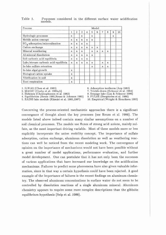
Table 1. Processes considered m the different surface water acidification models.

Process Model

1 2 3 4 5 6 1 8 9 10

Hydrologic processes x x x x

Mobile anion concept x x x x x

SO A-adsorption/mineralization x x x x

Cation exchange x x x x x x

Mineral weathering x x x x x x x

Al-mineral dissolution x x x x x

Soil carbonic acid equilibria x x x x

Lake/ stream carbonic acid equilibria x x x x x x x

In-lake sulfate retention x x x

In-lake algal growth x

Biological cation uptake x

Nitrification in soil x

Root respiration x

1. ILW AS (Chen et al. 1983) 6. Adsorption isotherm (Arp 1983) 2. MAGIC (Cosby et al. 1985a,b) 3. Birkenes (Christophersen et al. 1982)

1. Trickle-down (Schnoor et al. 1984) 8. Seepage lake (Lin & Schnoor 1986)

4. Equilibrium (Reuss 1980,Reuss & Johnson 1985) 9. PULSE (Bergstrom et al. 1986) 5. RAINS lake module (Kamari et al. 1985,1987) 10. Empirical (Wright & Henriksen 1983)

Concerning the process-oriented mechanistic approaches there is a significant

convergence of thought about the key processes (see Reuss et al. 1986). The

models listed above indeed contain many similar assumptions on a number of

soil chemical processes. The models use fluxes of strong acid anions, mainly sul­

fate, as the most important driving variable. Most of these models more or less

explicitly incorporate the anion mobility concept. The importance of sulfate

adsorption, cation exchange, aluminum dissolution as well as weathering reac­

tions can well be noticed from the recent modeling work. The convergence of

opinion on the importance of mechanisms would not have been possible without

a great number of model applications, performance evaluation, and further

model development. One can postulate that it has not only been the successes

of various applications that have increased our knowledge on the acidification

mechanisms. Failures to predict some phenomena have also given valuable infor­

mation, since in that way a certain hypothesis could have been rejected. A good

example of the importance of failures is the recent findings on aluminum chemis­

try. The observed aluminum concentrations in surface water do not seem to be

controlled by dissolution reactions of a single aluminum mineral. Aluminum

chemistry appears to require some more complex descriptions than the gibbsite

equilibrium hypothesis (Seip et al. 1986).

To date, the model applications have been mainly performed for providing infor­

mation on the importance of different processes in determining the dynamics of

studied catchments. These models have been research tools that have offered

one way of quantifying the effect of the poorly known processes. For the early

'pre-paradigm' phase of acidification science these applications have been more

than valuable. Simulation models, by predicting satisfactorily some observed

patterns of surface water acidity, have been able to give support to the

hypothesis, that acidic deposition is the most important cause to widely

observed regional acidification. Models have confirmed that under some cir­

cumstances acidic deposition may have a dominant effect on freshwater chemis­

try. Moreover, model application have brought new ideas and working

hypotheses for experimental scientist to test. For example, recent model applica­

tion have been able to provide examples of how both acidic deposition and con­

ifer afforestation can increase streamwater acidity (Neal et al. 1986).

The divergence in modeling philosophy is, an unavoidable, and in fact, a desired

fact. The main reason for the existence of a wide range of different model types

can be explained by the differences in the goals and objectives of the model

applications. The decision on what is going to be predicted deserves a critical

evaluation, because that more than anything else affects the model to be con­

structed. The research models tend to give more detailed descriptions on the

processes so that different phenomena and hypotheses can be evaluated and the

short-term dynamics can be reproduced. The prediction models designed for

management purposes use a more simple "lumped parameter" approach, which

is thought to be suitable for producing the long-term system behavior that is

required from a tool attempting to assist in a decision-making process. In the

following chapter an example prediction model is taken to demonstrate the

methods available to use such a acidification model for comparing and designing

alternative action strategies.

PREDICTION MODEL AS MANAGEMENT TOOL

Descriptions on quantitative consequences of alternative scenarios can assist in

formulating policies for emission control. Unfortunately to date, there has been

only a tenuous link between political decisions and scientific evidence concerning

acidification. For example, the most common policy discussed in Europe for

controlling acidification impacts is a 30% reduction of sulfur emissions by 1993

relative to their 1980 level. Although this policy will be costly to virtually every

European country, the actual benefits of this policy in protecting the natural

environment are rarely investigated. But even augmenting scientific information

about the problem will not necessarily lead to identification of suitable policies

for controlling acidification of the environment. This information must also be

structured in a form usable to decision makers. Integrated simulation models

attempt to provide such a structure. To combine the dimensions of the

acidification problem with the goal of providing useful information for decision

makers, the following guidelines for model formulation are proposed.

{1) The model should be simple. A model designed for the use of policy makers, should be both comprehensible and easy to use. In addition it should incor­porate past and current research in the field of acidification, yet deal with the most important processes first. The major advantage of the simplicity is the fast computer response, which permits interactive model use and the application of the model on a large regional scale. It also allows a theoreti­cal basis for assessing confidence in the scenarios.

{2) The model should analyze the long-term behavior of the environment. A model incorporating processes accounting only for the short-term dynamics of catchment behavior is surely not the best possible model for making future projections of catchment responses . Therefore, since acidification is a slow process, the model should incorporate those processes regulating the long-term behavior.

{3) The model should be dynamic in nature. It is important for the model users to see how a problem evolves and how it can be corrected over time. The dynamic upstream models describing the pollutant generation as well as the pollutant transport require dynamic models also for describing the environ­mental impact to be able to give estimates on the time scales of the responses. It is crucial to consider the slow dynamic processes, like soil acidification, in order to gain a complete picture of the problem in time, from past to future.

{4) The model should be applicable on a regional scale. To date, mechanistic models have been applied mostly on single catchments. From a decision makers point of view, however, the behavior of a single catchment is rather uninteresting. The assessment should investigate broad scale aspects of alternative policy formulations. To give an overall picture of the conse­quences of different control strategie::: , the models applications should be

geographically extensive. (5) The model output should be easy to interpret. Communication of the

model's operation and results should be an essential part of the model development. The model applications should produce well defined illustra­tive information which can easily be related to the effectiveness of the scenario being selected.

Integrated models for analyzing the consequences of future emission patterns are

being developed both in Europe and North America. The RAINS (Regional

Acidification /Mormation and Simulation) model of the International Institute

for Applied Systems Analysis attempts to provide a link between scientists and

policy makers (Alcamo et al. 1985, 1987). The purpose of the set of models is to

assist decision makers in the evaluation of control strategies for acidification in

Europe. The overall framework of RAINS consists of three linked compart­

ments: Pollutant Generation, Atmospheric Processes and Environmental

Impact. Each of these compartments can be filled by different substitutable sub­

models. The model currently includes submodels analyzing sulfur emissions,

long-range transport, forest soil acidification and lake acidification as well as

costs and optimization. Submodels which deal with NOx emissions and deposi­

tion and other environmental impacts are presently being added to the model.

The first submode! computes sulfur emissions for each country and these are

then input into the second submode!, which calculates sulfur deposition by

adding the contributions from each country together to compute the total sulfur

deposition at any location in Europe. The sulfur deposition is then in turn input

to the submodels estimating environmental impacts, forest soil acidification and

lake acidification. There are two basic ways of using such an integrated model:

(1) scenario analysis and (2) optimization analysis.

Scenario analysis

When creating scenarios the model user essentially moves from top to bottom

through the model as depicted in Figure 1, and first specifies an energy pattern

and an emission control strategy. This information is input to the models which

calculate and display the sulfur emissions of each country, the sulfur deposition

throughout Europe resulting from these emissions, and the resultant environ­

mental impact . After the model has been run, implications of the policy assump­

tions are carefully examined both for the performance of the scenario and for the

adequacy of the model. The first refers to the degree to which the scenario pro­

duce appealing results. The user has the option of evaluating output from any

of the submodels, e.g. sulfur emissions in a particular country or group of coun­

tries, costs of control on a country basis, sulfur deposition or 802 concentration

at different locations in Europe or mapped for all Europe, pictures of levels of

soil acidification, lake acidification, forest dieback due to 802 concentration at

different locations or mapped for all Europe. The second criterion, the adequacy

of the model, refers to the model validity and the uncertainties associated with

the produced scenarios.

A consistent set of energy pattern, sulfur emissions, sulfur deposition and

environmental impacts is called a scenario and the type of analysis is termed

scenario analysis. Scenario analysis permits great flexibility to the model user;

he or she may examine the consequences of many different pollution control pro­

grams that are optimal or desirable to the user because of the user's unexpressed

cost or institutional considerations . The whole procedure of constructing

scenarios is done in an iterative interactive fashion. In effect, Figure 2 shows an

example model output in which consequences of two emission patterns are com­

pared. Based on subjective evaluation of the output an alternative emission

control strategy for comparison can be selected. In this way the model user can

quickly analyze the impact of many different policies.

Optimization analysis

In the other operational mode, optimization analysis, the user in a sense inverts

the scenario analysis procedure by starting with goals of environmental protec­

tion and having the model work "backwards" to determine a cost effective

scenario for reducing sulfur emissions in Europe to accomplish these goals. For

example, the user can run the model by setting an environmental or deposition

objective and then compute a desirable emissions reduction plan according to

specified cost and institutional constraints. These computations are accom­

plished by mathematical "searching techniques" which draw on linear program­

ming or other similar mathematical algorithms.

The optimization submode! of RAINS permits the generation and analysis of

targetted emission control strategies based on chosen indicators. Indicators

represent environmental impacts, economic factors, and/or other policy objec­

tives. In targetted strategies, the emission reductions are determined in a

manner which meets the goals or constraints implied by the indicators in an

economical or efficient fashion. The procedure for generating targetted control

strategies within the RAINS framework is explained in Batterman et al. (1986).

Optimization Scenarto Analysis

S02 Control Stretegtes

················r----,.-----. :········ .. ·········., ; Groundweter l

1 .••• -.~-~~-~ ...... J Forest Soil Direct Forest

Actdtly Impacts

Figure 1: Procedures of using the RAINS model (from Alcamo et al. 1987)

70

ALL REGIONS

100

65

2 3 I PH<S.0 2 S.0<PH<6.0 3 6.0<PH

31

Figure 2: The mean annual lake acidity situation in Northern Europe for 2010 is pro­duced with two example scenarios. The higher scenario (shaded bars) as­sumes by the year 1995 a 30% flat rate reduction in emissions of all countries from 1980 levels. The lower scenario (white bars) makes the following as­sumptions for each country in Europe in the year 2000: (1) 90% of the con­sumed energy of the conversion (oil and coal) and power plant (oil and coal) sectors will have Flue Gas Desulfurization (FGD) with 90% sulfur removal efficiency; (2) 50% of the capacity of the industrial (oil and coal) sector will have FGD with 90% efficiency; and 100% of the capacity of domestic (oil) and transport (oil) sectors will receive desulfurization with 50% removal efficiency . This scenario assumes further that all controls will be phased in from the year 1985 onwards.

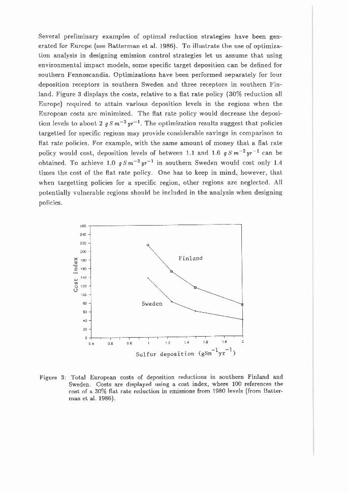
Several preliminary examples of optimal reduction strategies have been gen­

erated for Europe (see Batterman et al. 1986). To illustrate the use of optimiza­

tion analysis in designing emission control strategies let us assume that using

environmental impact models, some specific target deposition can be defined for

southern Fennoscandia. Optimizations have been performed separately for four

deposition receptors in southern Sweden and three receptors in southern Fin­

land. Figure 3 displays the costs, relative to a flat rate policy (30% reduction all

Europe) required to attain various deposition levels in the regions when the

European costs are minimized. The flat rate policy would decrease the deposi­

tion levels to about 2 g S m - 2 yr- 1• The optimization results suggest that policies

targetted for specific regions may provide considerable savings in comparison to

flat rate policies. For example, with the same amount of money that a flat rate

policy would cost, deposition levels of between 1.1 and 1.6 g S m - 2 yr - 1 can be

obtained. To achieve 1.0 g S m-2 yr- 1 in southern Sweden would cost only 1.4

times the cost of the flat rate policy. One has to keep in mind, however, that

when targetting policies for a specific region, other regions are neglected. All

potentially vulnerable regions should be included in the analysis when designing

policies.

260

240

220

200

:-< 180 ~

"Cl ~ 160 .,., .... 140

Cl)

0 120 u

100

BO

60

40

20

D.• 0 .6 0 .8

Finland

Sweden

1.2 1.• 1.6 1.8

-1 -1 Sulfur deposition (gSm yr )

Figure 3: Total European costs of deposition reductions in southern Finland and Sweden. Costs are displayed using a cost index, where 100 references the cost of a 30% flat rate reduction in emissions from 1980 levels (from Batter­man et al. 1986).

CONCLUDING REMARKS

Model analyzing acidification have proven very useful. They have quantified

some aspects of the problem that have earlier been described in qualitative

terms. Moreover, acidification models have provided a method for assessing the

potential environmental consequences of future emission patterns . The two

above objectives for model applications, research and management, are by no

means competing ways to use models. Research models and their applications

are required in order to increase our knowledge on various processes and in

order to develop better and more reliable models for practical applications .

REFERENCES

Alcamo, J .. , L. Hordijk, J . Kamari, P . Kauppi, M. Posch and E . Runca 1985. Integrated analysis of acidification in Europe. J. Environ. Manage. 21: 47-61.

Alcamo, J., Amann, M., Hettelingh , J .-P., Holmberg, M., Hordijk , L., Kamari , J ., Kauppi, L., Kauppi , P ., Kamai, G . and Makela, A. 1987. Acidification in Europe: A simulation model for evaluating control strategies. Forthcoming in Ambio.

Arp, P .A. 1983. Modeling the effects of acid precipitation on soil leachates: a simple approach. Ecol. Modelling 19, pp. 105-117.

Batterman, S., Amann, M., Hettelingh, J .-P., Hordijk , L. and Kornai , G . 1986. Optimal S02 abatement policies in Europe: Some examples. IIASA Working Paper WP-86-42, International Institute for Applied System Analysis, Laxenburg, Austria.

Beck, M.B. 1983. A procedure for modeling. In: Orlob, G .T . (ed.), Mathematical model­ing of water quality : Streams, lakes and reservoirs . John Wiley & Sons, Chichester, pp. 11-41.

Bergstrom, S., Carlsson, B., Sandberg , G. and Maxe, L. 1985. Integrated modeling of runoff, alkalinity and pH on a daily basis. Nord . Hydro!. 16, pp. 89-104 .

Chen, C .W., Gherini , S.A., Hudson, R.J .M. and Dean, J.D. 1983. The Integrated Lake­Watershed Acidification Study. Vol. 1: Model principles and application procedure. Final Report, Tetra Tech. Inc ., Lafayette, USA.

Christophersen, N., Seip, H.M. and Wright , R.F . 1982. A model for streamwater chem­istry at Birkenes, Norway . Water Resour. Res. 18, pp. 977-996.

Cosby, B.J ., Wright, R.F., Hornberger, G.M. and Galloway , J .N. 1985a. Modelling the effects of acid deposition : Assessment of a lumped parameter model of soil water and streamwater chemistry. Water Resour . Res . 21, pp. 51-63.

Cosby , B.J ., Wright, R.F ., Hornberger , G.M. and Galloway, J .N. 1985b. Modelling the effects of acid deposition: Estimation of long-term water quality responses in a small forested catchment. Water Resour. Res. 21, pp. 1591-1601.

Kamari, J., Posch, M. and Kauppi , L. 1985. A model for analyzing lake water acidification on a large regional scale. Part 1: Model structure. IIASA Collaborative Paper CP-85-48, International Institute for Applied Systems Analysis, Laxenburg, Aus­tria.

Kamari , J. and Posch, M. 1987. Regional application of a simple lake acidification model to Northern Europe. In: Beck, M.B. (ed .), Systems analysis in water quality management . Pergamon Press, London, pp. 73-84.

Kuhn, T .S. 1970. The structure of scientific revolutions. The University of Chicago Press, Chicago (2nd ed .) .

Lin, J .C. and Schnoor, J .L. 1986. An acid precipitation model for seepage lakes. J. Environ. Eng. 112, pp. 677-694.

Oden, S. 1968. The acidification of air and precipitation and its consequences in the natural environment. Ecology Committee Bulletin no. 1. Swedish National Science Research Council, Stockholm.

Neal, C., Whitehead, P ., Neale, R. and Cosby, J. 1986. Modelling the effects of acidic deposition and conifer afforestation on stream acidity in the British uplands. J . Hydro!. 86, pp. 15-26.

Reuss, J .0 . 1980. Simulation of soil nutrient losses resulting from rainfall acidity . Ecol. Modelling 11 , pp. 15-38.

Reuss, J .O . and Johnson, D.W. 1985. Effect of soil processes on the acidification of water by acid deposition. J . Environ. Qua!. 14, pp. 26-31.

Reuss, J.O., Christophersen, N. and Seip, H.M. 1986. A critique of models for freshwa­ter and soil acidification. Water Air Soil Pollut . 30, pp. 909-930.

Schnoor, J .L., Palmer, W.D. and Glass, G.E. 1984. Modeling impacts of acid precipita­tion for northeastern Minnesota. In : Schnoor, J .L. (ed .) , Modeling of total acid precipi­tation impacts. Butterworth Publishers, Boston, pp. 155-174.

Seip, H.M., Christophersen, N. and Rustad, S. 1986. Changes in streamwater chemistry and fishery status following reduced sulphur deposition: tentative predictions based on the "Birkenes model". Workshop on reversibility of acidification, Grimstad, Norway 8-11 June 1986. Commission of European Communities.

Wright, R.F . and Henriksen, A. 1983. Restoration of Norwegian lakes by reduction in sulphur deposition. Nature 305, pp. 422-424.

Young, P. 1983. The validity and credibility of models for badly defined systems. In : Beck, M.D. and van Straten, G . (eds .), Uncertainty and forecasting of water quality. Springer-Verlag, Berlin, pp. 69-98.

REGIONAL APPLICATION OF A SIMPLE LAKE ACIDIFICATION MODEL TO NORTHERN EUROPE

J. Kamari and M. Posch

International Institute for Applied Systems Analysis (IIASA) , A-2362 Laxenburg, Austria

ABSTRACT

The principal objective of the RAINS model , being developed at IIASA, is to assist in the evaluation of policies for controlling the acidification of Europe's environment. As part of this task, a dynamic model has been developed for describing the key processes assumed to be important in determining the long-term dynamics of surface water acidification. The input data available on a large regional scale are few. The model is regionalized by selecting input combinations from feasible ranges or fre­quency distributions . Monte Carlo techniques are used to determine those combinations of parameters that produce the observed present-day lake acidity distribution for each individual region, when the model is driven by a specified historical deposition . The ensembles obtained in this filtering pro­cedure for each lake region are then used for the scenario analysis . The model runs, assuming dif­ferent future energy-emission scenarios,suggest that all reductions in emissions are likely to reduce also the number of lakes being threatened by acidic deposition. In conclusion, the Monte Carlo method seems to provide a working tool for the application of catchment models on a large regional scale .

KEYWORDS

Lake acidification , simulation model, Monte Carlo procedure, scenario analysis, regional assessment, Fennoscandia.

INTRODUCTION

Governments of Europe and North America have shown their willingness to take remedial action against acidification of the environment. A wide range of scientific research devoted to this subject is continuously expanding our knowledge on the causes and effects of acidification. Unfortunately, augmenting scientific information will not necessarily lead to identification of suitable policies for its control. This information must also be structured in a form usable to decision-makers . The RAINS (Regional Acidification INformation and Simulation) model of the International Institute for Applied Systems Analysis (IIASA) attempts to provide such a structure .

Descriptions on quantitative consequences of alternative scenarios can assist in formulat ing policies for emission control. In fact , numerous mathematical models have been developed that all have the potential to estimate the quality of surface water in response to varying atmospheric deposition . All

73

74 J . KAMARI and M. POSCH

models can be calibrated so that a satisfactory fit with observed data will be obtained. Different models are constructed, however, for different purposes. Models should be applied only within the limits of their applicability. Therefore, combining the dimensions of the acidification problem with the goals of the model development, has led us to adopt the following guidelines for the models of RAINS describing environmental impacts.

(1) The model should be simple. As the model is designed for the use of policy makers, we believe it should be both comprehensible and easy to use . In addition it should incorporate past and current research in the field of acidification, yet deal with the most important processes first. The major advantage of simplicity is the fast computer response, which permits interactive model use and the application of the model on a large regional scale . It also allows a theoretical basis for assessing confidence in the scenarios.

(2) The model should analyze the long-term behavior of the environment. A model incorporating processes accounting only for the short-term dynamics of catchment behavior is surely not suit­able for making future projections of catchment responses. Therefore, since acidification is a slow process, the model should incorporate those processes regulating the long-term behavior.

(3) The model should be dynamic in nature. It is important for the model users to see how a prob­lem evolves and how it can be corrected over time. The dynamic upstream models describing the pollutant generation as well as the pollutant transport require dynamic models also for describ­ing the envirnnmental impact to be able to give estimates of the time scales of the responses. It is crucial to consider the slow dynamic processes, like soil acidification, in order to gain a com­plete picture of the problem in time, from past to future.

(4) The model should be applicable on a regional scale. To date, mechanistic models have been applied only on single catchments. From a decision-maker's point of view, however, the behavior of a single catchment is rather uninteresting. The assessment should investigate broad scale aspects of alternative policy formulations. To give an overall picture of the consequences of dif­ferent control strategies, the models analyzing environmental impacts should be geographically extensive.

(5) The model output should be easy to interpret . Communication of the model's operation and results should be an essential part of the model development. The model applications should pro­duce well defined illustrative information which can easily be related to the effectiveness of the scenario being selected.

Following the above guidelines, a simple process-oriented dynamic lake acidification model has been developed (see Kii.mii.ri et al., 1.986) and, in this paper, a method is introduced for applying the model on a large regional scale.

MODEL STRUCTURE

The RAINS model currently consists of three linked compartments: (a) Pollutant Generation, (b) Atmospheric Processes, and (c) Environmental Impacts. Although many different submodels can be -­and actually have been -- inserted into these compartments, only the submodels used in this study as upstream models for producing deposition scenarios are briefly described in the following.

The first submode!, the Sulfur Emissions submode!, computes sulfur emissions for each of the 27 European countries based on a user-selected energy pathway for each country. The model user has a choice of a number of possible pathways for each country, which are based on published estimates from the Economic Commission of Europe (EGE, 1983) or from the International Energy Agency (!EA, 1985) . Each energy pathway specifies how much energy will be used by four fuel types in a country· oil, coal, gas and other. The sulfur-producing fuels, oil and coal, are broken down further into 11 sec­tors (Alcamo et al., 1985). The model can compute sulfur emissions for each country with or without pollution control. To reduce sulfur emissions the user may specify any combination of the following four pollution control alternatives: (1.) fuel cleaning; (2) flue gas control devices; (3) low sulfur power plants , e.g. fluidized bed plants with limestone injection; (4) low sulfur fuel.

The sulfur emissions comptited for each country are then input into the second submode!, the EMEP Sulfur Transport submode!. This submode! computes sulfur deposition in Europe due to the sulfur

Regional application of a simple lake acidification model 75

emissions in each country and lhen adds the contributions from each country together to compute the total sulfur deposition at any location in Europe. The submode! consists of a source-receptor matrix, which gives the amount of sulfur· deposited in a grid square (150 by 150 kilometers) due to sul­fur emissions originating from grid squares in each country of Europe. The source-receptor matrix is based on a more complicated model of long range transport of air pollutants in Europe developed by the Organization for Economic Cooperation and Development (OECD) and the Co-operative Pro­gram for The Monitoring and Evaluation of Long Range Transmission of Air Pollutants in Europe (F.MEP) (see Eliassen and Saltbones, 1983). The source-receptor matrix was made available to IIASA by the Institute of Meteorology in Oslo, Norway.

The sulfur· deposition computed by the second submode! is then input to the submodels estimating envirnnmental impacts. Multiple simulations of different policy alternatives will give information on the effectiveness of chosen policy options. Each simulation represents a set of assumptions on the energy development and on the measures taken to control emissions. A consistent set of assumptions (a policy set) is here called an energy-emission scenario and the type of analysis is termed scenari0 analysis .

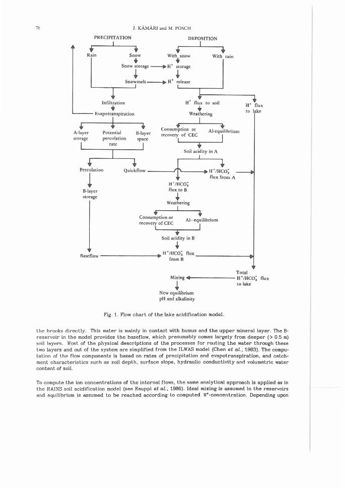
The Catchment Model

For the lake acidification study our modeling philosophy has been to use a simplified approach which is watTanted fm- a broad geographical scope. The objective has been to retain the simplicity of the model but still have few physically realistic processes incorporated in its structure. The model con­sists of four major parts. In the heart of the model there is a module describing the long-term chemi­cal soil processes. The processes considered in the model are summarized in Table 1. The overall model stnicture is presented in Figure 1.

TABLE 1 Processes considered in the lake acidification model.

Process Reference

Partitioning between snow and rain Snow melt Release of deposition from snowpack Evapotranspiration Percolation from upper to lower reservoir Lateral flow Silicate weathering Cation exchange Aluminum equilibrium with gibbsite Inorganic carbon equilibrium

Shih et al., 1972 Chow, 1964 Johannessen and Henriksen, 1978 Christophersen et al., 1984 Chen et al .. 1983 Chen et al., 1983 Ulrich, 1983 Ulrich, 1983 Christophersen et al., 1982 Stumm and Morgan, 1981

In the model, the monthly sulfur deposition, computed by the air pollutant transport model, is transformed into acid load in various sectors of the catchment. The monthly mean precipitation is brnken down into rain and snow according to local mean monthly temperature . Snowpack accumulates and melts at a temperature-dependent rate. Deposition is assumed to accumulate when snow accumu­lates, the same fraction of deposition as of total precipitation is retained in the snowpack. During the snowmelt, the rate for the release of deposition from the snowpack is assumed to he higher than the melting rate. This fractionation effect observed during the snowmelt (Johannessen and Henrik­sen, 1978) implies that most of the impurities in the snowpack are found in the first meltwater.

To provide a method for simulating the routing of internal flows a simple two-layer structure is applied (see Christophersen et al., 1984). The terrestrial catchment is vertically segmented into snowpack and two soil layers (A- and B-reservoirs). Precipitation is routed into quickflow, baseflow, and flow between soil layers, percolation . Physically, the flow from the upper reservoir can be thought of as quickflow, which drains down the hillsides as piped flow or fast throughflow and enters

76 J . KAMARI and M. POSCH

PRECIPITATION I

DEPOSITION

+ With rain

I + + + Rain Snow With snow L '""+~-H· i"·~ ~melt--+ H• r•e-le_a_se---. _],_-_-:_-_-_-_-:_-:_~------

Infiltration

+ Evapotranspiration

+ i A-layer Potential storage percolation

I rate

Percolation

i B-layer storage

tt• flux to soil

+ Weathering

+. I + +

B-layer Consumpt10n or recovery of CEC

I

Al-equilibrium

space • I Soil acidity in A

+

tt•mco; flux to B

+ Weathering I

I

Consumption or recovery of CEC

I

Al-equilibrium

+ I

Soil acidity in B

+

I

H• flux to lake

Baseflow ----------... tt• tHco; flux -----------;.i from B

Total Mixing•-------- tt• /HCo; flux

~ to lake

New equilibrium pH and alkalinity

Fig. 1. Flow chart of the lake acidification model.

the brooks directly . This water is mainly in contact with humus and the upper mineral layer. The 8-reservoir in the model provides the baseflow, which presumably comes largely from deeper (> 0 .5 m) soil layers. Most of the physical descriptions of the processes for routing the water through these two layers and out of the system are simplified from the ILWAS model (Chen et al., 1983). The compu­tation of the flow components is based on rates of precipitation and evapotranspiration, and catch­ment characteristics such as soil depth, surface slope, hydraulic conductivity and volumetric water content of soil.

To compute the ion concentrations of the internal flows, the same analytical approach ls applied as in the RAINS soil acidification model (see Kauppi et al. , 1986). Ideal mixing is assumed in the reservoirs and equilibrium is assumed to be reached according to computed . .ff+-concentration. Depending upon

Regional applicatio n of a simple lake acidification model 77

the acid load to the soil there is either a net production of base cations or there is an exhaustion of cation exchange capacity. In case the deposition rate of strong acids is lower than the silicate buffer rate, the weathering first fills up the cation exchange complex and after that an excess supply of base cations to the surface waters occurs. The contribution of the soil reservoir to the alkalinity of the surface water is assumed to equal the amount of the excess base cations . The leaching of acidity to surface waters is simulated on the basis of simulated hydrogen ion concentrations in the soil solu­tion and the discharges from both reservoirs .

The c hange in lake water chemistry is predicted by means of titration of the base content of the lake, total alkalinity, with strong acid originating from the atmosphere. The carbonate alkalinity can be assumed to be the only significant buffering agent. The ion loads to the lake are assumed to be mixed within a layer which depends on location and season . During the snowmelt the mixing layer is assumed to be the topmost water layer. The change in lake acidity is calculated according to equili­brium reactions of inorganic carbon species. The risk of aquatic impacts are estimated on the basis of s imple threshold pH and alkalinity values. These characteristics are most likely to indicate damage to fish populations and other aquatic organisms.

MODEL APPI..ICATION

Method for application

In an ideal case, if there were correct a. priori information on the shape of distributions of all pat·ameters, initial conditions as well as catchment characteristics, and if the model would be a perfec t desc ription of all interactions in the catchment, no calibration would be necessary . The model would produce reliable output distributions in the future projections . In simulation models of environmental systems, however , the model stnicture, the model inputs, the initial conditions as well as the parameter values all necessarily include uncertainties . The data available on a large regional scale like Europe is characterized by a high degree of heterogeneity and generalization . It has been emphasized in several studies that the analysis of models should concentrate on identifying ranges of inputs, rather than on traditional parameter estimation (e.g . Fedra, 1.983; Hornberger and Cosby, 1985) . The same rule applies to the output information.

Our approach for assessing regional surface water impacts has two distinct levels. At the first level the catchment model is able to analyze changes over time in the chemistry of a specific lake . The model can be run for any known system for which the relevant lake, catchment and soil information is available. When the catchment model is regionalized the model is incorporated into a larger structure which scales the scenarios from individual catchment up to a regional level. In the regional lake aci­dification assessment a Monte Carlo parame ter estimation procedure is applied in order to model regional lake water quality distributions.

The Monte Carlo method is a trial-and-error procedure for the solution of the inverse problem , i.e . for estimating poorly known input and parameter values from comparing model outputs with available measurements (Fedra, 1983). To this end performance criteria (constraints on the output) are formu­lated describing the expected satisfactory behavior of the model. Next, probability distributions are defined for all unknown input and parameter values. The Monte Carlo program then randomly samples the parameter vectors from these distributions, runs the simulation model through a selected period of time and finally tests for violations of constraint conditions . This process is repeated for a large number of trials.

In the regional application, the Monte Carlo method is used to determine the combinations of inputs and parameters that produce an acceptable distribution of output values observed in the study region. For all inputs and parameters, ranges are chosen broad enough so that any reasonable value for an input can be selected. Monte Carlo simulations are then carried out by randomly selecting a set of input values from these designated ranges and integrating the equations from 1960 on,using this particular set of values . In this way a subset of accepted input values corresponding to the actual observed present-day frequency distribution in 1980 in each lake region , is obtained .

78 J. KAMARI and M. POSCH

Mathematically this procedure can be described as follows: The adopted model structure can be represented by a vector function f = (f 1 , . .. .Jm) . The arguments of this function are the input and parameter values driving the model , say :z:: = (:z: 1 , ... ,xn) (e .g. z 1 = lake size, x 2 = catchment size, .. . , etc .) and time t. With 11 = (11 1 •. .. ,ym) we denote the output of a model run, e.g. lake-water alkalinity, lake-water pH, ... , etc.

11 f(:z:: ,t) (la)

or, writing Equation la for each component,

(lb)

Instead of taking fixed input values :z:: and running the model once to obtain the output (prediction) at time t , one allows the input values to vary within an interval , "'tmtn,,; "'t ,,; "'tm•x. k = 1, ... ,n, where the lower and upper bounds are estimated from the catchment characteristics of the region studied. To put it precisely , each input parameter is randomized with a distribution Pt • k = 1 , . .. ,n, obeying

(2a)

b

and J Pt (x )dz is the probability that Zt lies in the interval [a ,b]. Obviously a

1. for k = 1, ... ,n (2b)

The frequency distributions Pt represent the distribution of the parameters x., in the region as close as possible; and in case of a poorly known input parameter a uniform distribution over [:z::.,mt• ,xt•x] is chosen, where the boundaries are wide enough to encompass any feasible value in the region under consideration . To be able to apply the Monte-Carlo procedure the distributions of the output values 11 at a certain point in time t 1, say q1, l = 1, ... ,m, have to be known from measurements . For the description of the procedure used to solve the inverse problem, i.e . to determine the input parameter distributions for future projections of the model, we consider only one output value 11 (i.e . m =1; say lake-water pH) and furthermore we assume that the measured distribution at t 1 is a discrete one (/ ... number of classes, 771 . . . class boundaries)

q (11)

with

and

'70

1

for '7!-l < y:.: 77 1 i=1 , ... ,/ else

E q1 <111 - 111 -1> 1 j =1

11mln and '71

(3a)

(3b)

(3c)

Actually, the assumption of a discrete distribution is not very stringent, since (a) measurements are always given as histograms , and (b) any continuous distribution c·an be approximated by a discrete one . In order to derive "acceptable" input parameter distributions the model is run many times , each time with a new randomly selected input vector z, where the random selection is performed according to the distributions Pt · Let P = fz<ll, ... ,.z<N>! be the set of these random vectors .z and

Regional application of a simple lake acidification model 79

Q = fy(l>, .. ,y<N>j the set of output values of these runs at time t 1 . These N output values are classi­fied according to the classes defined in Equation 3a. Let Nt be the number of realizations with 7lt _1 < y s 7lt with y e: Q (obviously °Et Nt = N). Monte-Carlo runs are performed until N1 O!: N 0q 1 for all i = 1, ... ,/, where N0 is a preselected number of runs to be accepted (e.g. N0 = 100). In this way a sub­set Q 0 = fy 1 ... . ,yN

0l of Q is selected, so that there are N 0qt output values with ry 1 _1 <y :s:ry1

(i = 1, ... ,/) with y e:Q 0 . (Note that y 1 is the i-th value of the set Q, not the i-th component of a vec­tor y .) To this subset Q0 corresponds a subset P 0 = f:r: 1, ... ,:r:N

0l of P of accepted input vectors :r:.

From this set of accepted input vectors "new" input parameter distributions p~. A: = 1, ... ,n. can be derived; and these distributions are used for future projections, i.e. for computing y-values for t >ti-

Assuming that the set of input values obtained in the calibration is representative of real catchments in the study region, this ensemble can be used for the scenario analysis of the response of lake sys­tems to different patterns of acid load.

Data for application

The above initialization of the model for scenario analysis, in other words the scaling up of the catch­ment model to a regional level, had several preparatory steps. First of all, ranges or distributions for unknown parameters were estimated. In the estimation procedure, best available information and best guesses for the input distributions were used as a starting point. Then for the model output, a target distribution was specified on the basis of a large number of water quality observations. Finally, the filtering procedure was applied .

As an input for the filtering procedure frequency distributions wer0 estimated independently for the following fourteen input and output parameters : 1) Lake surface area, 2) Lake catchment area to lake surface area ratio, 3) Lake mean depth, 4) Mean catchment soil thickness, 5) Mean surface slope, 6) Silicate weathering rate, 7) Total cation exchange capacity, 8) Base saturation in A-layer, 9) Base saturation in B-layer, 10) Soil moisture content at field capacity, 11) Soil moisture content at satura­tion, 12) Climatic mean of monthly air temperature. 13) Climatic mean of monthly precipitation, 14) Lake pH and alkalinity.

All the relevant lake and catchment information was interpreted for 14 lake regions considered in this application. Some of the required input data has been obtained from common sources for all three countries; Finland, Norway and Sweden . This information included the silicate buffer rate, sur­face slope, precipitation, air temperature as well as soil moisture contents at field capacity and

saturation . The International Geological Map of Europe and the Mediterranean Region (UNESCO, 1972) was used for assigning distributions for the weathering rate of the silicate parent material. The same classification of different rock types into weathering rate classes was applied as in Kauppi et al.

(1986).

The Soil Map of the World (FAO-UNESCO, 1974) provided information on the distributions of typi­

cal surface slopes.

Ranges for the mean monthly temperature and precipitation of each district were derived from climatic data of about 200 observation stations in Europe (Muller, 1982). The minimum and max­imum mean monthly values for each region were obtained by interpolating the observed mean monthly values over the whole of Europe . The ranges used, therefore , reflect the climatic varia­bility within the region.

A frequency distribution for the soil moisture content at field capacity was formulated on the basis of the texture classes obtained also from the soil map.

Values for the range of the soil moisture content at saturation was obtained from literature (e.g. Chen et al. 1983).

80 J. KAMARI and M. POSCH

For some input parameters, there was not enough a priori information available for all countries to allow detailed distributions to be formulated . In those cases the input variables, like the mean catchment soil thickness and the ratio of lake area to catchment area, were assigned ranges broad enough so that any reasonable value for an input could be selected from these rectangular distributions.

Much of the required input information has been made available by research institutes in each of the individual countries. For example , a large number of water quality observations has become available in national survey programs investigating the present extent of lake acidification . At present, lake survey information has been implemented for the use of regional modeling from three Nordic coun­tries , Finland , Norway and Sweden . In the following, the data sources of each country are listed. All other parameters besides those listed in this section were assigned constant values since , based on the model analysis above, they do not significantly affect the output.

Finland Data of 8900 lakes from the years 1975 - 1984 was made available by the Finnish National Board of Waters and Environment, Water Quality Data Bank . The lake pH information was divided into five parts to form lake ac idity distributions for five distinct lake regions . Information on the lake size distribution was provided by the Hydrological Office of the Finnish National Board of Waters . An inventory, determining the number and the size distribution of lakes for the whole of Finland, was completed in 1985. The total number of lakes in Finland (larger than 500 m 2 ) was counted to be 187,888 . The lake depth distribution was obtained from the Water Quality Data Bank of the National Board of Waters by approximating from the observed maximum lake depths.

All the soil information for the Finnish lake regions was obtained from a soil survey of 100 catchments conducted in 1984 and 1985 by the Geological Survey of Finland. Whenever a catchment contained different soil types in their terrestr ial catchment areas , samples were taken from all major soil types. Altogether, about 200 samples were analyzed and the to~al CEC and the base saturation for both A- and B-layers were calculated for all samples . Frequency distributions for these inputs were formulated by summing up the coverage fractions of each CEC and base saturation class within all the catchments .

Sweden. An extensive lake survey was conducted in Sweden in 1980 and reported by Johansson and Nyberg (1981) . The lake pH and alkalinity distributions were given separately for each of the 24 pro­vinces in Sweden. These data were aggregated at IIASA to form six lake regions each of them receiv­ing more or less homogeneous deposition. The frequency distributions of lake surface area and lake mean depth for Sweden were obtained from the Swedish Lake Register of the Swedish Meteorological and Hydrological Institute (SMHI) . The initial cation exchange capacities as well as the soil base saturation were assigned distributions for all lake districts both in Sweden and Norway based on the FAQ-UNESCO soil map of the world (FAQ-UNESCO, 1974).

Norway-'- Regional lake surveys were conducted in Norway in October 1974, March 1975, March 1976 and March 1977 (Wright et al., 1977). The survey in 1974 included also information about the catch­ments , e .g . vegetation , catchment size and geology. All survey information was made available to IIASA by the Norwegian Institute for Water Research (NIVA) . Distributions for lake pH, lake size and catchment size to lake size ratio were interpreted at IIASA for three separate regions. When evaluat­ing simulations for Norway, it should be kept in mind, however, that the survey 1974-1977 concen­trated on sensitive catchments and therefore might not be representative for the whole of Norway.

MODEL RESULTS

Having performed the filtering procedure and obtained a representative set of parameter comliina­tions, the model is applicable for providing estimates of the time -patterns of regional lake acidifica­tion for any energy-emission scenario and year between 1980 and 2040 . The model is run through the period of 60 years separately for each predefined lake region, for the preselected number of times there is accepted parameter sets stored. An estimate of the lake pH or lake alkalinity frequency dis­tdbution for either spring or summer is produced as the output.

Regional application of a simple lake acidification model 81

In the following, two example energy-emission scenarios, produced by the upstream submodels of RAINS, are compared. The two examples are only intended to demonstrate the model behavior as well as the model display. No conclusion L~ to be drawn on the effectiveness of the selected control stra­tegies. From 1960 until 1980 the two constructed energy-emission scenarios were identical. The his­torical deposition pattern obtained on basis of energy-emission trends was used as a driving force for the filtering procedure. For the whole time span covered by the model, the scenarios assumed the same rates of energy development as defined by the latest estimates of the International Energy Agency (IEA, 1985). From 1980 on the scenarios departed so that the 'base' scenario did not assume any pollution controls, whereas the 'low' scenario assumed effective measures taken for the control of sulfur emissions. These controls were defined as 1) pollution control devices on all power plants and 2) fuel cleaning in the domestic energy sector (cf . Alcamo et al., 1985). The development of total sulfur emissions with time in the two example scenarios is displayed in Figure 2.

a: >-

' a: :::i "-_J :::i (/)

.... :i::

35.0

3'2!. r2!

25.0

2'2!. 0

15.0

1'2!. 0

5.0

0.-+-~~--1~~~--+-~~~~~~-+-~~-+~~~+-~~-;

19 0 l9 ti.' 19 0 l9 0 20 0 2010

Fig. 2. Total sulfur emissions in Europe for the 'base' and 'low' energy-emission scenarios.

20 0

By the year 1980, lake acidification was reported to be an observed phenomenon over practically all Fennoscandia. In the worst acidified areas, on the West coast of Sweden, over 30 % of the total number of lakes are acidified, having measured summer pH values lower than 5.0 . In southern Finland, less than 10 % of the lakes are acidic. In spring, when the annual minimum pH in the surface waters occurs, the acidity of the lakes is even greater.

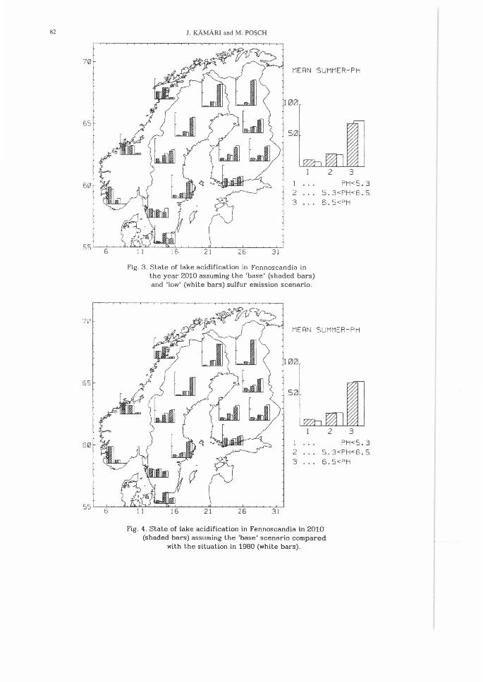
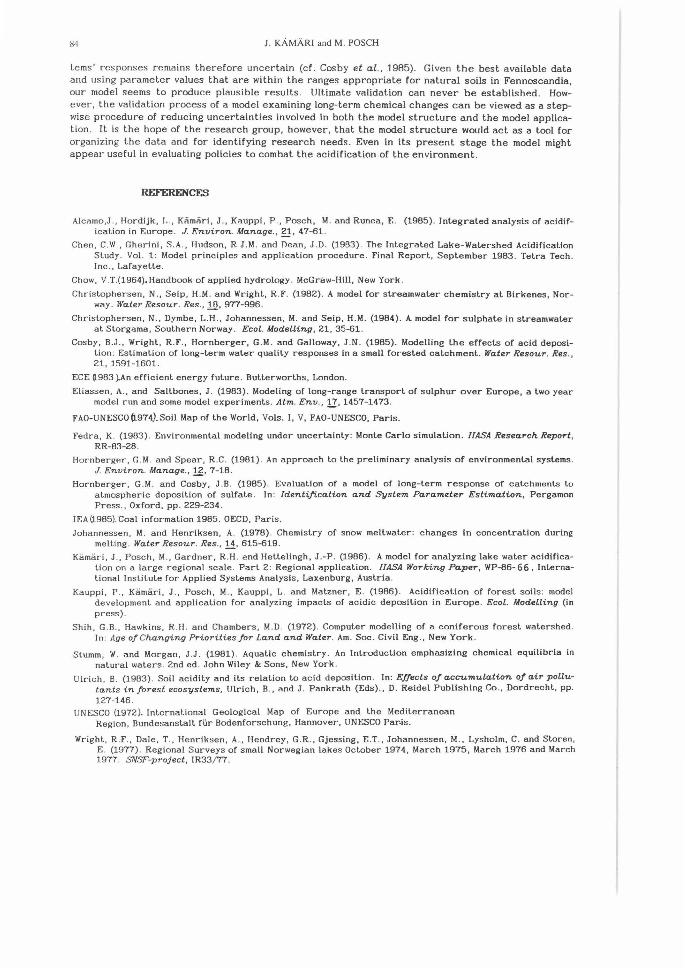
The results of the model runs under the two scenarios show a clear difference in the resulting summer pH values, for example for the year 2010 (Figure 3). When the 'base' scenario was used as the input, acidification tended to continue, and comparing with the 1980 situation, the frequency distri­butions for the summer pH showed a shift towards the lower end of the distribution (Figure 4). How­ever, continuing from 1980 on with the 'low' scenario, the model resulted in an improvement of. the situation. This shift in the frequency distributions towards higher pH values implied that the deposi­tion had lowered so much that for some lakes the alkalinity produ'ction exceeded the deposition, and consequently, the model estimated a recovery. For Lappland, deposition was calculated to remain at such low levels even with the 'base' scenario that no drastic effects on the lake water chemistry was predicted.

82

70

65

60

70

65

60

J. KAMARI and M. POSCH

MERN SUMMER-PH

1 2

2 3 PH<S .3

5.3<PH<6.5 3 6.5<PH

Fig. 3 . State of lake acidification in Fcnnosca ndia in the year 2010 assuming the 'base' (shaded bars ) and 'low' (white bars) sulfur emission scenario.

~~~

twU MERN SUMMER-PH

100

~l~~~0 c ~ ~-~5 ·~

2 3 PH<S.3 \1 . 2 5 . 3<PH<6 .5

9 3 6.5<PH

(v

Fig. 4 . State of lake acidification in Fennoscandia in 2010 {shaded bars) assuming the 'base' scenario compared

with the situation in 1980- (white bars).

Regional application of a simple lake acidification model 83

DISCUSSION

Uncertainty inherent in environmental modeling is inevitable. It seems unlikely that any complex environmental system can be well described in the traditional physicochemical sense (Hornberger and Spear. 1901). The credibility of the models results is, however, a key issue in using mathematical models for decision-making. An essential aspect of the credibility of the model is how well the user is aware of the uncertainties. Jn regional applications, there remains uncertainty in the accuracy of the data at two levels. First, measurements from the study area, forming the input data used, always include measurement. errors. The second level has to do with the interpretation of the regional pro­perties . Measurements can only be viewed as samples of the regional system under consideration. It is definitely impossible to sample every one of the catchments in Europe. The aggregation and interpretation of large scale information limit the utility of regional data as such. In some cases measurements are completely missing and the inputs have to be chosen From expert opinion or even guesses. A fi.ltering procedure is therefore chosen in order to restrict unrealistic input ranges from producing an unrealistic output.

The regional application itself forms an additional source of uncertainty, which in fact may result in systematic errnrs . When determining the input ensembles that produced acceptable distributions for output variables, a fixed historical deposition pattern from 1960 to 1.900 was assumed. IF this deposi­tion pattern was altered, a new different set of inputs would be obtained from the allowable ranges. Besides the historical deposition pattern, also, the shortness of the calibration period (20 years) forms a possible source of error. An effort is underway at IIASA to construct a longer historical emission data base for European countries. A longer historical deposition pattern obtained from this emission data will then be used to test the importance of the length of the calibration period to the long-term predictions.

The results of the evaluation of parameters of the regional lake acidification model show that, despite the large uncertainties in some key parameters, the model seems to prnvide a fair representation of measured pH levels in Finland (see Kamari et al., 1986). The analyses show that in order to improve the results and reduce the uncertainties associated with scenarios, effort should be made to define more accurate input distributions for the most critical parameters: the mean catchment soil thick­ness and the weathering rate of silicate in the region. Relatively little emphasis has been given so far to these two parameters that together largely determine the long-term behavior of the catchments. Current research is, however, continuously expanding our knowledge on them and we expect to be able to incorporate more realistic a priori distributions in the future.

The information provided by the sensitivity and uncertainty analysis can be used, moreover, as a basis for further development of the model. Processes associated with parameters which have shown to be relatively unimportant, can be aggregated and in this way the model can be simplified. Experi­ments are underway with model versions using a semi-annual or an annual lime step instead of the current monthly one, because monthly temperature and precipitation account for the hydrology and thus for the seasonal variation in acidity, but they have no effect on the long-term development of the catchment.

The filtering procedure for finding an acceptable subset of parameter combinations is by no means a final solution to the problem how to deal with uncertain and unknown regional input data. The tech­nique using a priori criteria to select a satisfactory subset of model simulation resulted in some improvements in the predicted results (Kamari et al., 1986). Investigations are continuing at IIASA in order to obtain more reliable sets of parameters for the lake regions considered. These parameters will then provide the basis for estimating the expected environmental effects and associated uncer­tainties of different energy-emission scenarios.

Acidification models assessing long-term responses are extremely difficult to verify. Strict validation of these types of models would require long time series to determine, whether the model estimates match the observed catchment responses. Unfortunately very few, if any, such records exist. The question whether the long term responses estimated by the model are true projections of real sys-

84 J. KAMARI and M. POSCH

terns ' responses remains therefore uncertain (cf. Cosby et al., 1985). Given the best available data and using parameter values that are within the ranges appropriate for natural soils in Fennoscandia, our model seems to produce plausible results . Ultimate validation can never be established. How­ever, the validation process of a model examining long-term chemical changes can be viewed as a step­wise procedure of reducing uncertainties involved in both the model structure and the model applica­tion . It is the hope of the research group, however, that the model structure would act as a tool for organizing the data and for identifying research needs. Even in its present stage the model might appear useful in evaluating policies to combat the acidification of the environment.

REFERENCES

Alcamo,J ., Hordijk, I •.• Kiimiiri, J., Kauppi , P . , Posch, M. and Runca, E . (1985). lnlegraled analysis of acidif­ication in Europe . J. F.nviron. Manage. , ~. 47-61.

Chen, C.W., Gherini, S.A ., Hudson, RJ.M . and Dean, J .D. (1963) . The Inlegraled Lake-Watershed Acidification Study. Vol. 1 : Model principles and application procedure. Final Report, September 1983. Tetra Tech. Inc ., Lafayette.

Chow, V.T.(1964),Handbook of applied hydrology. McGraw-Hill, New York.

Chrislophersen, N ., Seip, H.M. and Wright, R.F. {l.982) . A model for slreamwaler chemistry al Birkenes, Nor­way. Water Resour. Res., l!)., 977-996 .

Christophersen, N., Dymbe, I..H., Johannessen, M. and Seip, H.M. (1984). A model for sulphate in slreamwaler al Slorgama, Southern Norway. Ecol. Modelling, 21, 35-61.

Cosby, B.J., Wright, R .F., Hornberger, G.M. and Galloway, J .N. (1985). Modelling lhe effects of acid deposi­tion: Eslimalion of long-lerm waler quality responses in a small forested calchmenl. Water Resour. Res., 21, 1591-1601.

ECE ~963 ~An efficient energy future. Bullerworths, London.

Eliassen, A., and Sallbones, J. (1983). Modeling of long-range lransporl of sulphur over Europe, a lwo year model run and some model experiments. Atm. Env .• 11. 1457-1473.

FAO-UNESCO(l.974).Soil Map of lhe World, Vols. I, V, FAD-UNESCO, Paris.

Fedra, K. (1903). Environmental modeling under uncertainly: Monte Carlo simulation . IIASA Research Report, RR-83-28 .

Hornberger, G.M. and Spear, R .C. (1.981) . An approach lo the preliminary analysis of environmental systems. J. Environ. Manage., g, 7-18 .

Hornberger, G.M. and Cosby, J.B . (1985). Evaluation of a model of long-term response of calchmenls lo atmospheric deposition of sulfate . In: Identification and System Parameter Estimation, Pergamon Press., Oxford, pp . 229-234.

IEA(l.985).Coal information 1985. OECD, Paris.

Johannessen, M. and Henriksen, A. (1978) . Chemistry of snow mellwaler: changes in concenlralion during melting . Water Resour. Res., !_i, 615-619.

Kamari, J., Posch, M., Gardner, R .H. and Hellelingh, J.-P. (1986) . A model for analyzing lake waler acidifica­tion on a large regional scale. Part 2: Regional application. IIASA Working Pa.per, WP-86-66, Inlerna­lional Institute for Applied Systems Analysis, Laxenburg, Austria .

Kauppi, P ., Kamari, J . , Posch, M., Kauppi , L. and Malzner , E. (1986) . Acidification of forest soils : model development and application for analyzing impacts of acidic deposition in Europe. Ecol. Modelling (in press).

Shih, G.B., Hawkins, R .H. and Chambers, M.D . (1972) . Computer modelling of a coniferous forest watershed. In : Age of Changing Priorities for Land and Water . Am. Soc. Civil Eng., New York.

Stumm, W. and Morgan, J.J. (1981) . Aquatic chemistry . An Introduction emphasizing chemical equilibria in natural waters. 2nd ed. John Wiley & Sons, New York .

Ulrich, B. (1983) . Soil acidity and ils relation to acid deposition . In: Effects of accumulation of air pollu­tants in forest ecosystems, Ulrich, B. , and J. Pankralh (Eds)., D. Reidel Publishing Co., Dordrechl, pp. 127-146.

UNESCO (1972). International Geological Map of Europe and lhe Mediterranean Region. Bundesanslall filr Bodenforschung, Hannover , lJN~;sco Par-is.

Wright, R .F., Dale, T., Henriksen, A., Iiendrey , G.R. , Gjessing, E .T., Johannessen, M., Lysholm, C. and Sloren, E . (1977) . Regional Surveys of small Norwegian lakes October 1974, March 1975, March 1976 and March 1977. SNSF-project, IR33/ 77.