predicting mobile network behavior by simulation -...

Predicting mobile network behavior by simulation

S i m o n B . J ø r g e n s e n - s 1 0 3 1 8 2

Course 34330

Introduction to Mobile

Communication

DTU – November 2012

Predicting mobile network behavior by simulation s103182

Side 1 af 14

Indhold Introduction ............................................................................................................................................................................ 1

GPRS / EDGE ........................................................................................................................................................................... 2

Simulation setup ................................................................................................................................................................. 2

Results and discussions ....................................................................................................................................................... 2

Conclution ........................................................................................................................................................................... 4

UMTS....................................................................................................................................................................................... 5

Simulation setup ................................................................................................................................................................. 5

Results and discussions ....................................................................................................................................................... 5

Conclusion ........................................................................................................................................................................... 9

HSDPA ................................................................................................................................................................................... 10

Simulation setup ............................................................................................................................................................... 10

Results and discussions ..................................................................................................................................................... 10

Conclusion ......................................................................................................................................................................... 12

Iub capacity ........................................................................................................................................................................... 13

Simulation setup ............................................................................................................................................................... 13

Results and discussions ..................................................................................................................................................... 13

Conclution ......................................................................................................................................................................... 14

Overall Conclusion ................................................................................................................................................................ 14

Introduction This report is based on the lab simulation where GPRS, EDGE, UMTS, HSDPA and the Iub interfase is simulated. In mobile

networks it is very beneficial to simulate realistic scenarios. Because of the controllability to tweak parameters such as

capacity, modulation schemes, traffic load, user behavior, radio conditions or RAB algorithms. Another benefit is the

possibility to upscale or downscale a problem and because it is processed by a computer the time for testing can be

have a positive effect on time spend and the cost for the carriers. But with that said – the simulation does not always

mirror the real life scenario because so many factors have to be taken into account.


Side 2 af 14

GPRS / EDGE

Simulation setup In the first case the simulation consist of 40% GPRS MSC 10 and 60% EDGE MSC 10. The goal is to see the difference in

the two technologies. There are 3 cells, where one of the cells has a poor radio condition. Each cell contains 3 TRXs and

8 time slots are able to run on EDGE. The download load is divided into 40% HTTP (web browsing), 30 % FTP (file

download) and 30% Email. The simulation duration is 6000 seconds and with 1000 samples.

Results and discussions The goal with the first simulation is to show the difference between EDGE and GPRS. The following graph shows the

HTTP page respond time for GPRS MSC (Orange graph) and EDGE (Blue graph).

The two following graph is showing the same situation except for the difference in used aplication. The following graph

is for the Email retrieval time where the GPRS MSC is the Orange graph and EDGE MSC is the blue graph.


Side 3 af 14

The next graph shows the FTP Download response time where the GPRS MSC is the Orange graph and EDGE MSC is the

blue graph.

Looking at the 3 graphs, it’s noticed that in 73% of the time the user with expect that EDGE is faster than GPRS. The user

will also noticed that if the download process takes long time (over 50 sec. for FTP) the two technologies follow each

other as well. In this situation the poor cell is the reason.

Some of the biggest differences between EDGE and GPRS are that EDGE uses the new modulation and coding scheme 8-

PSK which can triple the bitrate. EDGE also uses incremental redundancy, which means that if the signal gets poor or

noise occur then the coding scheme can be retransmitted more robustly such as GMSK. This is what happens on the

graphs where they begin to have the same values in response time.

Now the goal is to compare the difference in the radio signal. Therefore cell 1 (good signal) and cell 3 (poor signal) are

graphed. It is seen that cell 3 is approximately twice as slow as cell 1. The reason for that is again because of the chosen

modulation scheme.

To decide the QoS the timeslot (TS) allocation in each cell are now inspected. On the two following graphs it’s clear that

the mean of the cell with good signal is better than the one with poor radio conditions. Cell 1 has uses about in average

4.6 allocated timeslots for data capacity where cell 3 uses 5.4 timeslots – it is about 15% better for cell 1. The reason is

that cell 3 needs to do more retransmission and therefore take up some timeslots for doing that.

It is also seen that even if the timeslots are dynamically assigned the two cells almost the whole time never use less than

3 timeslots.


Side 4 af 14

Cell 1:

Cell 3:

After testing with the poor radio condition, cell 3 is now changed to have a good radio condition. So the following graph

shows that changing the radio conditions will improve the QoS and that EDGE is dependent on the modulation scheme.

Conclution From simulation with GPRS and EDGE, it’s clear that improvements in EDGE such as incremental redundancy and better

modulation scheme increases the bitrates. The simulation also showed that in EDGE a poor radio condition will affect

the QoS.


Side 5 af 14

UMTS

Simulation setup Now we are looking at UMTS with two Node Bs. The cellphones uses dynamic rate adaptation. The average traffic load is

100 kbps - 50% HTTP and 50% FTP. The FTP traffic pattern is based on a file size of 200 kBytes and with a constant

repetition of 300 seconds. The HTTP traffic pattern is based on a webpage with size of 1000 bytes containing 10 objects

(5 kByte each) and with a repetition of 120 seconds. The RAB (Radio Access Bearer) setup algorithm is very important as

seen later. The two scenarios are as followed:

Vendor X Vendor Y

Initial bit rate (UL) 32 kbps 64 kbps

Initial bit rate (DL) 32 kbps 64 kbps

Supported bit rates (UL) 32,64,128 kbps 8, 32,64,128 kbps

Supported bit rates (DL) 32,64,128,384 kbps 8, 32,64,128,384 kbps

RAB setup algorithm USE initial Negotiate

Results and discussions After the simulation of the UMTS for both vendor X and vendor Y the results are analyzed and compared:

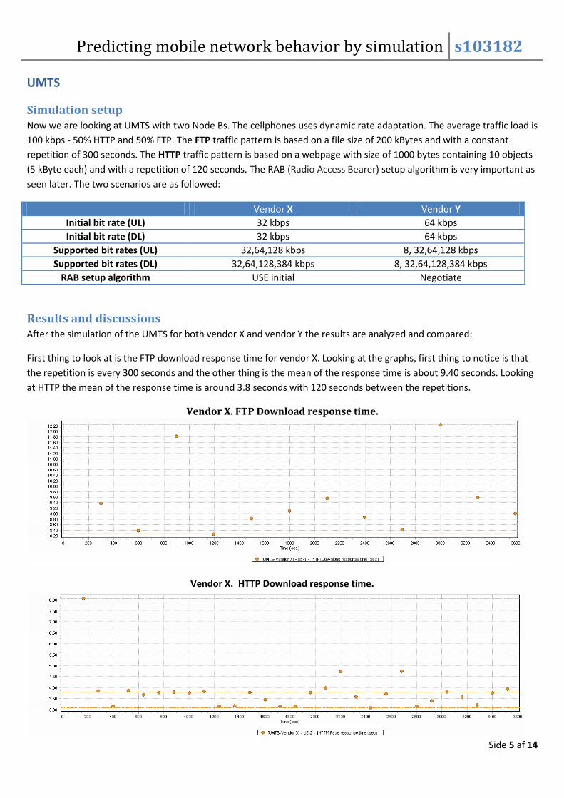
First thing to look at is the FTP download response time for vendor X. Looking at the graphs, first thing to notice is that

the repetition is every 300 seconds and the other thing is the mean of the response time is about 9.40 seconds. Looking

at HTTP the mean of the response time is around 3.8 seconds with 120 seconds between the repetitions.

Vendor X. FTP Download response time.

Vendor X. HTTP Download response time.


Side 6 af 14

Now the vendor Y is under the scope. It is noticed that the mean for FTP is around 12.6 seconds which is about 25%

worse than vendor X. Looking at the HTTP also for vendor Y the mean here is about 3,6 which is almost the same as

vendor X. This is because HTTP only is loading a webpage of 1 Kbyte per 120 sec.

Vendor Y. FTP Download response time.

Vendor Y. HTTP Download response time.

Now the focus is the Rate adaption behavior in Vendor X. The two services we are working with are the DCH allocation

(Bit rate allocation Download) and the Throughput Download from the RLC (Radio Link Control). On the graph (FTP) first

thing to notice is the theoretically blue graph of the DCH allocation. The initial “step” is set to 32 kbps and after 2

seconds(each sample) the maximum DL rate is 384 kbps. Looking at the Orange graph the practical radio link DL is

showing that the initial bit rate is flollowing the theoretically. The bursts seen on the RLC throughput is happening

because of the acknowledgements. The RLC could be in the third mode of acknowledgement mode (AM).


Side 7 af 14

Now the same two services (DCH and RLC) are looked at but now just for HTTP where it is seen that the same principles

of the initial bitrate is used.

So now that we have looked at vendor X the time has come to vendor Y which has a higher initial bit rate and a different

RAB algorithm. This is also seen on the simulated graph for FTP and HTTP where it just starts right away. The maximum

bit rate is still 386 kbps.

Vendor Y: FTP

Vendor Y: HTTP


Side 8 af 14

Dynamic rate adaption

To simulate a typical airport hotspot the traffic volume is set to 200 kbps and the application to 50% FTP and 50% HTTP.

This is applied for both vendor X and vendor Y. To determent the percentage of the users that get a HTTP download

response time below 15 seconds the CDF graph is created. From the graph we get that 93% of the users in vendor X gets

a response time less than 15 seconds and for the vendor Y the percentage is 80%. Also seen on the graph is that both

vendors have the accepted 98% have a response time of 55 seconds or less.

Now the same simulation but instead of HTTP the FTP is under the scope. It is seen that about 88% of the users in

vendor X will have a download response time less than 30 sec. For the vendor Y users this is 78%.

Both cases show that vendor X is giving more users a faster response time. But this is not always the case. Looking at the

FTP- graph - vendor Y is actually giving 68% of the users a faster response, but after that the vendor X is fastest.


Side 9 af 14

Now we look at the numbers of HTTP session initializations. On the graph it’s seen that the total number of sessions is

900 and that the after about 475 seconds the vendor Y takes over and uses the full bandwidth.

The graph right under here shows the numbers of successful sessions. It is seen that for vendor X (red) that almost 820

out of 900 initialized sessions succeeds but for vendor Y (blue) only about 740 succeeds. That is 91% for X and 82% for Y.

The reason why vendor X has a worse success rate is that it sometimes uses the whole bandwidth for only one user

where vendor Y is deciding for each user. This is because of the RAB setup.

Conclusion The simulations with vendor X and vendor Y in the UMTS network showed that the allocated RAB algorithm and the

dynamic rate adaptation are very important to obtain a better QoS.


Side 10 af 14

HSDPA

Simulation setup In the simulation the scenarios consist of one cell from Node B serving 1 to 6 UE all running FTP.

The goal is to compare UMTS with HSDPA. The file size is 1 MB and the inter request time has a mean of 600 sec.

Results and discussions The first test is to compare the DL throughput between UMTS and HSDPA:

Looking at the graph it is clear that HSDPA is about 32/8 = 4 time as fast as UMTS. The reason is some new

improvements compared to UMTS. There’s a new modulation scheme (16 QAM and later 64 QAM) but HSDPA also uses

AMC (adaptive modulation and coding) which can change on the fly. Other improvements like HARQ (Hybrid Automated

Repeat Request) for retransmission, the use of shared downlink channel (HS-DSCH) and a spreading factor of 16

altogether makes the bitrate faster.

After comparing the FTP response time it could be interesting to look at the IP Throughput in the two networks. It is

again clear that HSDPA is faster than UMTS. The main difference from UMTS is that HSDPA uses the shared channel in

downlink. It is also seen that the HSDPA is jumping in bitrates which is because of the adaptive modulation schemes.


Side 11 af 14

In the previous simulations for HSDPA there where only one UE. The next simulations there are 6 UEs. Now that there

are multiple UEs then there are some different scheduling algorithms. The HSDPA RR is using the Round Robin allocation

where the users are assigned in order such that all users are handled without priority. This is also seen on the graph

below where HSDPA has a FTP download response time of around 8 sec. where HSDPA RR is around 18 sec. and the

UMTS 32 sec.

The Throughput in DL for the NodeB is also graphed to see the difference for the three configurations:

It is seen that the HSDPA RR has the highest bitrates because one user will use the whole allocated capacity where the

HSDPA only sometimes reach the high bitrates. The UMTS has a lower bitrate as expected.


Side 12 af 14

For answering the question on page 32 about how many users in the HSDPA RR scenario that will experience an FTP

download response time of 10 sec. or less, a CDF graph is made:

From the graph we get that about 40% will experience an FTP download response time of 10 sec or less. The other

question about what 70% of the users will experience. The answer to that is about 20 sec. or less.

Conclusion After simulation and comparing UMTS and HSDPA the conclusion is that HSDPA has around 4 times as fast bitrates

(using FTP) than UMTS. The reason is the main improvements in HSDPA such as the adaptive modulation and coding and

the shared downlink channel.


Side 13 af 14

Iub capacity

Simulation setup The Iub interface (the interface from the base station to the RNC) is now tested. We simulate two simple scenarios with

one Node B in each case. This makes the result simpler and easier to see the difference in the Iub. In the simulation zero

or low voice call load is used. Also no cell reselection and uniformly user distribution per radius are chosen. The second

Iub has doubled as much capacity (4096000 bps) than the first one.

Results and discussions So after the simulation the FTP download response time is looked at for the two Iub interfaces.

So it is seen that when the capacity is doubled about 90% of the users will experience a faster response time. Roughly

speaking for the 90% of the users then they will experience that the response time is 0.1 to 0.4 second better.

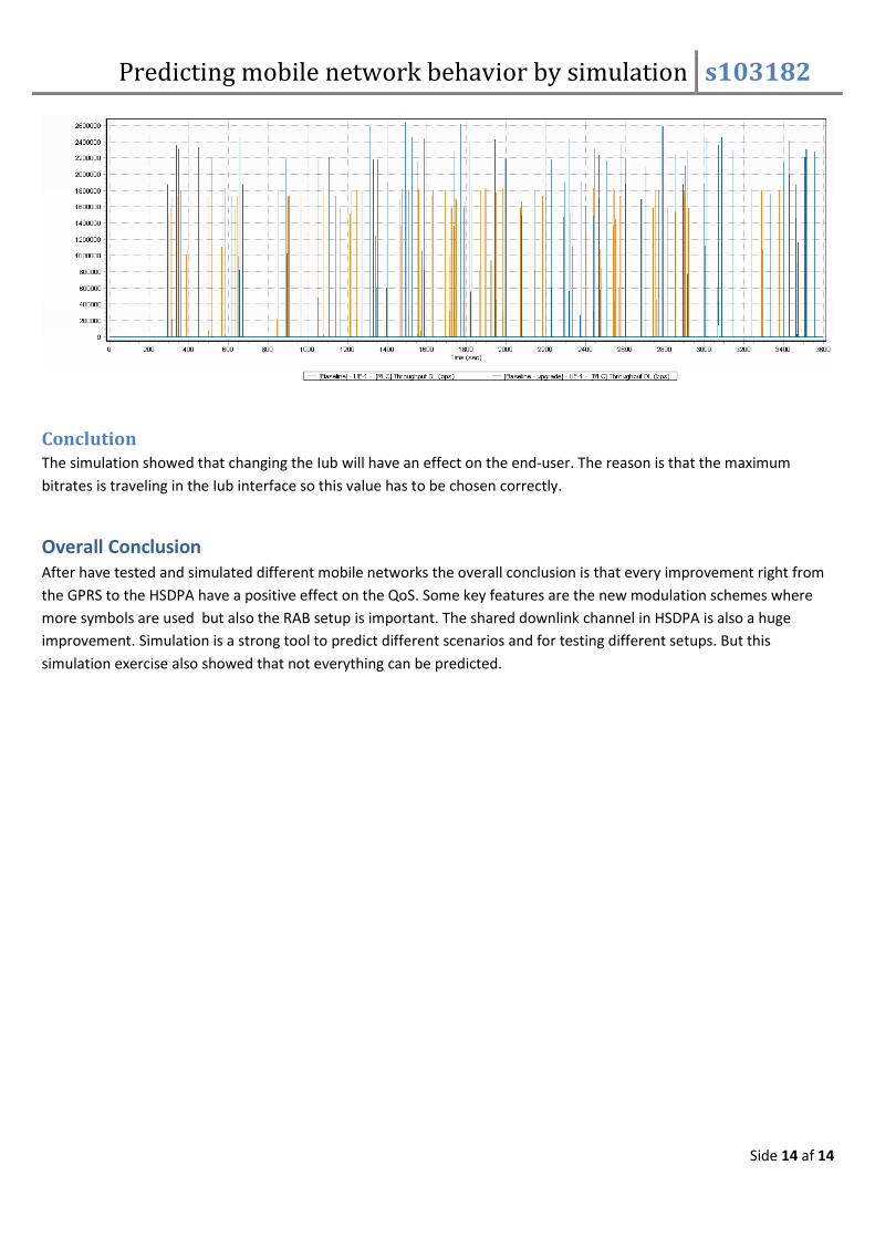
Now we look at the actual bitrates in the two scenarios. On the graph below the “normal” Iub has some maximum peaks

of about 1.8 Mbps and the improved Iub has 2.6 Mbps. For the “normal” Iub this could be critical since the maximum

capacity is around 2 Mbps. For the improved case there is a higher span to the 4 Mbps.


Side 14 af 14

Conclution The simulation showed that changing the Iub will have an effect on the end-user. The reason is that the maximum

bitrates is traveling in the Iub interface so this value has to be chosen correctly.

Overall Conclusion After have tested and simulated different mobile networks the overall conclusion is that every improvement right from

the GPRS to the HSDPA have a positive effect on the QoS. Some key features are the new modulation schemes where

more symbols are used but also the RAB setup is important. The shared downlink channel in HSDPA is also a huge

improvement. Simulation is a strong tool to predict different scenarios and for testing different setups. But this

simulation exercise also showed that not everything can be predicted.

predicting mobile network behavior by simulation -...

Documents