predicting the performance of - trussell

1

"Simulating The Performance of Fixed-Bed Granular Activated Carbon Adsorbers: Removal of Synthetic Organic Chemicals in the

Presence of Background Organic Matter"

Michelle Edith Jarvie David W Hand

John C Crittenden Dave R Hokanson

2

ABSTRACT

Granular Activated Carbon (GAC) adsorption is an effective treatment technology for the

removal of Synthetic Organic Chemicals (SOCs) from drinking water supplies. This

treatment process can be expensive if not properly designed. Application of

mathematical models is an attractive method to evaluate the impact of process variables

on process design and performance. Practical guidelines were developed to select an

appropriate model framework and to estimate site-specific model parameters to predict

GAC adsorber performance. Pilot plant and field scale data from 11 different studies

were utilized to investigate the effectiveness of this approach in predicting adsorber

performance in the presence of background organic batter (BOM). These data represent

surface and ground water sources from four different countries. The modeling approach

was able to adequately describe fixed-bed adsorber performance for the purpose of

determining the carbon usage rate and process design variables. This approach is more

accurate at predicting bed life in the presence of BOM than the current methods

commonly used by practicing engineers.

3

INTRODUCTION

Granular activated carbon (GAC) adsorption is an effective treatment technique for

removing synthetic organic chemicals (SOCs) from surface and groundwaters, but GAC

may be an expensive process if not properly designed. The design of GAC adsorbers

requires the proper selection of the following variables: type of adsorbent, empty bed

contact time (EBCT), and bed configuration (e.g., beds in series or parallel operation).

Present design information is obtained from rapid small scale columns (RSSCTs), vendor

experience and pilot plant studies. RSSCTs and pilot investigations can be time

consuming and expensive, especially if they are not properly planned. An additional or

complementary approach involves the use of mathematical models to predict process

performance and select the optimum process design. Mathematical models can be used

to: (1) assess the preliminary design and economic feasibility of using adsorption

processes by estimating GAC usage rates, (2) plan the scope of RSSCT and pilot plant

studies, and (3) interpret RSSCT and pilot plant results.

The main obstacle in using mathematical models is that they require site-specific

parameters that can only be obtained through a number of bench-scale experiments.

Furthermore, sufficient knowledge of various adsorption model options is required for a

designer to select appropriate adsorption models and the sequence of the model

application to predict the adsorber performance in removing SOCs under field conditions.

Hence, this paper presents an approach that will: 1) estimate site-specific adsorption

4

model parameters; and 2) select appropriate models to predict the adsorber performance

in removing SOCs under specific field conditions.

Background Organic Matter (BOM) Effects on SOC Adsorption

Factors that influence the effect of BOM on SOC adsorption include BOM preloading

time, adsorbent type, background water constituents and physical properties, and

solute type, each of which will be discussed in this section.

BOM Preloading Time

The solid-phase solute concentration (amount of solute adsorbed onto the adsorbent) is

assumed to be in equilibrium with the liquid-phase solute concentration at the adsorbent

surface. The Freundlich single solute isotherm is used to estimate this equilibrium:

1/ ne eq = KC (1)

Where:

Ce = the equilibrium concentration of the solute in the liquid at the particle interface

(Nmole/L)

qe = the equilibrium solid-phase mass of solute per mass of adsorbent (Nmole/g)

K = Freundlich coefficient (Nmole/g[L/Nmole]1/n)

5

1/n = Freundlich exponent accounting for adsorption site energy distribution

(dimensionless)

It is important to note that the values for the experimentally determined Freundlich

parameters K and 1/n are solute and adsorbent specific.

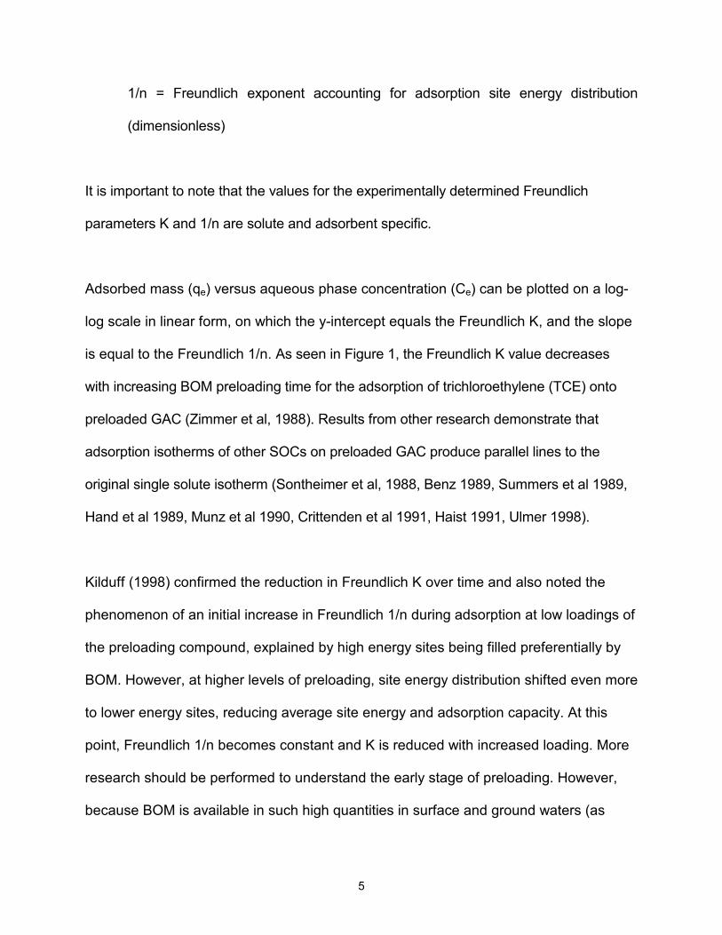
Adsorbed mass (qe) versus aqueous phase concentration (Ce) can be plotted on a log-

log scale in linear form, on which the y-intercept equals the Freundlich K, and the slope

is equal to the Freundlich 1/n. As seen in Figure 1, the Freundlich K value decreases

with increasing BOM preloading time for the adsorption of trichloroethylene (TCE) onto

preloaded GAC (Zimmer et al, 1988). Results from other research demonstrate that

adsorption isotherms of other SOCs on preloaded GAC produce parallel lines to the

original single solute isotherm (Sontheimer et al, 1988, Benz 1989, Summers et al 1989,

Hand et al 1989, Munz et al 1990, Crittenden et al 1991, Haist 1991, Ulmer 1998).

Kilduff (1998) confirmed the reduction in Freundlich K over time and also noted the

phenomenon of an initial increase in Freundlich 1/n during adsorption at low loadings of

the preloading compound, explained by high energy sites being filled preferentially by

BOM. However, at higher levels of preloading, site energy distribution shifted even more

to lower energy sites, reducing average site energy and adsorption capacity. At this

point, Freundlich 1/n becomes constant and K is reduced with increased loading. More

research should be performed to understand the early stage of preloading. However,

because BOM is available in such high quantities in surface and ground waters (as

6

compared to the concentrations of micropollutants for GAC removal), BOM preloading

results in an isotherm that is parallel to the original single solute isotherm, but lower on

the y-axis, or with a decreased Freundlich K value. Thus, this model accounts for BOM

preloading by reducing the Freundlich K of the adsorbate.

Influence of Adsorbent Type

Zimmer et al (1988) compared the effect of BOM preloading time on three different

carbon types and found that, for a specific BOM and SOC the effect of preloading time

varied between adsorbents.

Carter et al (1992) examined the adsorption of TCE preloaded GAC of different mesh

sizes, which are a function of the particle diameter. Initially, mesh size mattered over a

period of less than 4 weeks. However, carbon adsorbers used in drinking water

treatment typically operate for much longer periods of time, on a scale of months to

years, where different mesh carbons begin to approach the same behavior. Due to the

relative magnitude of internal surface area as compared to external surface area on

GAC particles, it is expected that mesh size will not affect adsorption unless it does so

by greatly reducing the intraparticle diffusion path in cases where diffusion is the

dominant adsorption mechanism.

Li et al (2003) examined influence of PAC pore size distribution and BOM molecular

weight on the pore blockage effects of BOM on atrazine adsorption. Comparing the

adsorption behavior of atrazine onto BOM preloaded PACs, the authors found that PAC

7

with larger fractions of mesopores (20-500 Å) and secondary micropores (8-20 Å)

displayed less pore blocking effects from BOM than compared with PAC that had a

smaller fraction of such pores.

Influence of Water Type and Solution Chemistry

To understand how BOM effects SOC adsorption, it is important to first understand the

adsorption behavior of BOM. Kilduff, Karanfil, and Weber (1996) observed that

increases in ionic strength (IS) cause a reduction in the molecular size of humic

molecules in solution by causing the macromolecules to coil, allowing them to enter

smaller pores than they would have access to at their greater sizes. Further research

by Kilduff and Karanfil (2002) examined the question of how solution chemistry effects

SOC uptake. GAC uptake of TCE was found to decrease with increasing ionic strength

(IS) due to an increased adsorption of dissolved organic matter (DOM) during the

preloading at higher IS, resulting in less sites available for the subsequent TCE

adsorption. An important conclusion here is that the chemistry of a solution can

influence the physical characteristics of the adsorbates.

Molecular weight of BOM also influences its adsorption behavior. Fettig (1985) showed

that when the adsorption behavior of BOM fractions of molecular weight less than 600,

from 600 to 3000, and greater than 3000 were compared; the lowest molecular weight

BOM fraction adsorbed the strongest, displaying the steepest isotherm, and the largest

molecular weight fraction displayed the most shallow isotherm slope.

8

Kilduff, Karanfil, and Weber (1998) showed that GAC loaded with humic substances of

molecular weight greater than 3,000 adsorbed similar TCE amounts as virgin GAC;

while GAC preloaded with humic substances of molecular weight less than 3,000

adsorbed less TCE than the virgin GAC. As an explanation for the different effects of

the two molecular weight classes of BOM, the authors suggested that lower molecular

weight BOM could occupy the portion of the GAC that contained smaller pores, of

diameter less than 10 Å, which the larger molecular weight BOM could not reach.

Additionally, when mixed fractions of low and high molecular weight BOM were exposed

to the GAC, those mixtures with a greater fraction of BOM of molecular weight less than

3,000 influenced TCE adsorption the greatest.

Research by Li et al, (2003) examined the molecular weight distribution of BOM

adsorbed onto PAC, and found that (on a scale of molecular weights from zero to 2000)

BOM within the molecular weight range of 200-700 Daltons was responsible for most of

the pore blocking that caused the subsequent reduction in adsorbent capacity for

SOCs.

Solution chemistry, including the effects of ionic strength, dissolved oxygen

concentration, and BOM molecular weight fractionation, influences how BOM

preloading impacts subsequent SOC adsorption. Thus, on similar adsorbents, the same

SOC may show different adsorption behavior in the presence of different background

waters. Figure 2 shows how the Freundlich K of TCE varies with preloading time in the

9

presence of the five different background waters (three surface and two ground water)

included in the model.

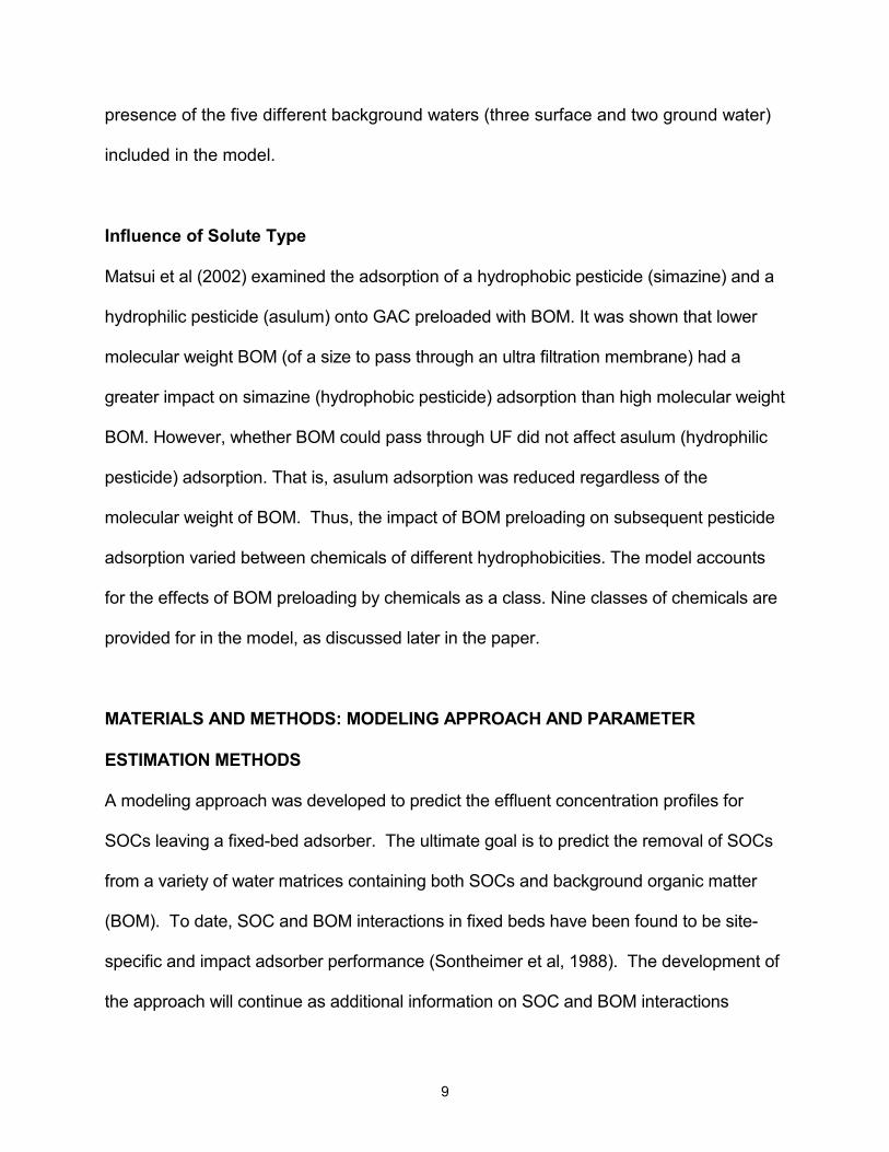
Influence of Solute Type

Matsui et al (2002) examined the adsorption of a hydrophobic pesticide (simazine) and a

hydrophilic pesticide (asulum) onto GAC preloaded with BOM. It was shown that lower

molecular weight BOM (of a size to pass through an ultra filtration membrane) had a

greater impact on simazine (hydrophobic pesticide) adsorption than high molecular weight

BOM. However, whether BOM could pass through UF did not affect asulum (hydrophilic

pesticide) adsorption. That is, asulum adsorption was reduced regardless of the

molecular weight of BOM. Thus, the impact of BOM preloading on subsequent pesticide

adsorption varied between chemicals of different hydrophobicities. The model accounts

for the effects of BOM preloading by chemicals as a class. Nine classes of chemicals are

provided for in the model, as discussed later in the paper.

MATERIALS AND METHODS: MODELING APPROACH AND PARAMETER

ESTIMATION METHODS

A modeling approach was developed to predict the effluent concentration profiles for

SOCs leaving a fixed-bed adsorber. The ultimate goal is to predict the removal of SOCs

from a variety of water matrices containing both SOCs and background organic matter

(BOM). To date, SOC and BOM interactions in fixed beds have been found to be site-

specific and impact adsorber performance (Sontheimer et al, 1988). The development of

the approach will continue as additional information on SOC and BOM interactions

10

provides better insight into model parameter selection. Accordingly, the practical

guidelines described herein may be considered a work in progress, which can easily be

updated as new information on SOC and BOM interactions becomes available. The

approach described herein brings together a collection of models that describe adsorption

equilibrium (thermodynamic models) and the transport of SOCs in a fixed-bed (column

models) in a logical fashion.

Fixed Bed Models

The pore and surface diffusion model (PSDM) is a comprehensive mass transfer model

that includes the mass transfer mechanisms shown in Figure 3. The pore diffusion model

(PDM) includes only the contribution of pore diffusion to the intraparticle mass flux, and is

the actual model utilized when BOM is present. Mass balances for the mobile fluid and

stationary adsorbent phases for the models results in two partial differential (PDEs), one

for the liquid-phase mass balance and the other for the intraparticle phase. The

development and solution of the equations for the PSDM, PDM, and surface diffusion

model (SDM), are given by Friedman (1985), Crittenden et al (1986), Sontheimer et al

(1988), and Hand et al (1984).

Fixed-Bed Model Parameter Estimation

The following recommendations are in no way the last word on fixed bed model

parameter estimation. One inherent problem with the mass transfer models is that

diffusion interactions are described without cross diffusion coefficients. Obtaining a

complete set of diffusion coefficients including diffusion interaction is a formidable task.

11

Moreover, when BOM interactions are considered, it may be impossible to predict

diffusion and equilibrium interactions. Accordingly, diffusion and equilibrium interactions

are considered in an empirical fashion as described below. They are based on several

hundred model-data comparisons; and, as more experience is obtained in determining

model parameters, improvements may be expected.

Equilibrium parameters for mass transfer models.

The solid-phase solute concentration (amount of solute adsorbed onto the adsorbent) is

assumed to be in equilibrium with the liquid-phase solute concentration at the adsorbent

surface. The Freundlich single solute isotherm is used to estimate this equilibrium, given

previously (as Equation 1).

Unidentified background organic matter (BOM) present in surface and ground waters

reduces the GAC capacity for SOCs (Sontheimer et al, 1988, Zimmer et al 1988, Haist

1991, Benz 1989, Summers et al 1989, Hand et al 1989, Munz et al 1990, Crittenden et

al 1991). These results and others demonstrate that parallel lines to the original isotherm

description are obtained for surface and ground waters, as discussed previously.

Accordingly, the reduction in column capacity for individual SOCs can be represented as

a reduction of the Freundlich capacity parameter, K (Zimmer et al, 1988) in fixed bed

calculations, with no change modeled in the Freundlich 1/n value for a given solute. The

following empirical equation is used to obtain the Freundlich capacity parameter that

describes the column capacity for SOCs in the presence of BOM (Sontheimer et al,

1988):

12

t)]*(-A4*A3 + t*A2 - [A1*0.01 = K

K(t) exp (2)

Where:

K(t) = the Freundlich coefficient (Nmole/g[L/Nmole]1/n) of a solute within a specific

water matrix containing BOM, at time (t) of exposure to the BOM

t = the adsorber operation time (days)

A1, A2, A3, A4 = empirical kinetic constants specific to a given SOC, water matrix,

and GAC type.

Table 1 summarizes the empirical constants (Equation 2) for trichloroethene (TCE), for

the five different water matrices and two GAC types available within the current model.

The five water choices consist of two surface waters, Portage Lake (Houghton, MI,

DOC=1.6mg/L) and Rhine River (where the Rhine water represents a surface water with

significant anthropogenic inputs, DOC=2.25mg/L), and three ground waters (Houghton,

MI, DOC=1.5mg/L; Wausau, WI, DOC=8.1mg/L; and Karlsruhe, Germany,

DOC=0.7mg/L). Figure 2 shows a graph of the reduction in Freundlich K for TCE with

time in each of the five background water matrices.

A general relationship between column capacity reduction and the K and 1/n values of

single solute isotherms for a variety of SOCs has yet to be developed (Zimmer et al 1988,

Sontheimer et al, 1988, Benz et al 1989). However, once a background water matrix is

chosen from the five available, the reduction in Freundlich K for TCE in that water can be

estimated. The model includes Freundlich K reduction factors for nine chemical groups,

13

including halogenated alkanes, halogenated alkenes, trihalomethanes, aromatics, nitro

compounds, chlorinated hydrocarbons, phenols, polynuclear-aromatics and pesticides, as

shown in Table 2, and applied in the equation below (Bhuvendralingam, 1992).

1 2TCE

K(t) K(t)=K K

B Bª ºu �« »¬ ¼ (3)

The parameters in Table 2 were determined from isotherms conducted on Calgon F-100

GAC pre-exposed to Karlsruhe (Germany) groundwater, and strictly speaking they are

only valid for that water. Thus, it is assumed that relative reductions observed between

the various classes of SOCs and TCE are similar for other waters. Accordingly, the

impact of BOM on column capacity can be determined from Tables 1 and 2 for a variety

of compounds and waters by applying first equation 2 and then equation 3. This

approach for determining the impact of BOM on column capacity has resulted in

reasonable predictions of breakthrough curves (Zimmer et al, 1988; Bhuvendralingam

1992, Alben et al, 1992).

Concentration of the micropollutant is known to have very little impact on the reduction

in carbon capacity for the SOC due to the presence of BOM. It can be calculated from

the data shown in Figure 3 that for TCE adsorbed onto F-400 carbon in the presence of

groundwater, at 10 µg/L there is a 99% reduction in carbon capacity and at 1000 µg/L

there is a 97.6% reduction on carbon capacity (Baldauf and Zimmer, 1986). In this

case, over the range of SOC concentrations of concern in drinking water treatment,

there was a less than 2% difference in the reduction of carbon capacity due to the

presence of background NOM. Thus, the concentration of the micropollutant in the

presence of BOM is not treated as a factor which influences the Freundlich K values.

14

External mass transfer coefficients for mass transfer models.

External mass transfer coefficients are estimated from this correlation (Gnielinski 1978):

> @Sc Re 0.644 + 2 2R

D))-1.5(1 + (1 = k 1/31/2f

AIH (4)

in which,

AA

D = 13.26 * 10

V

-5

1.14b0.589� (5)

Re =

2 R V A

A

re m (6)

Sc =

DA

A A

mr (7)

in which, kf is the liquid phase mass transfer coefficient (cm/sec); H is the fixed-bed void

fraction, R is the adsorbent particle radius (cm); I is the adsorbent particle shape

correction factor (Sontheimer et al, 1988); Dl is the liquid diffusivity of the SOC (cm2/sec);

mw is the viscosity of water (centipoise); Uw is the density of water (g/cm3); V is the

superficial loading velocity (cm/sec); and Vb is the molar volume of the SOC at the boiling

point temperature (cm3/mol). The value of I depends on how R is determined. If the

average value of R is determined by spatial analysis the value of I is between 1.1 and 1.4

for GACs (Sontheimer et al, 1988). If R is obtained from a sieve analysis, no shape factor

(sphericity) is required because most GAC particles tend to be cylindrical and small

values of R will be obtained. In most cases, intraparticle diffusion controls the adsorption

15

rate and I will be set at a value of 1. The model allows differing values of I to be used.

However, for all model runs presented herein, a value of 1 was used.

Intraparticle mass transfer coefficients for mass transfer models.

Figure 4 shows that intraparticle mass transfer can occur by either surface or pore

diffusion. Surface diffusion coefficients are calculated from the following equation, which

is obtained by relating the surface diffusion flux to the pore diffusion flux (Crittenden et al

1987).

sp o

p1/ n

o a

D = SPDFR * D C K C A �

� �

LNM

OQP (8)

in which, SPDFR is the surface to pore diffusion flux ratio, Co is the average influent liquid

phase concentration (Nmole/L), Ua is the apparent adsorbent particle density including

pore volume (g/cm3), Wp is the tortuosity of the diffusion path length within the adsorbent

particle, and Hp is the adsorbent particle void fraction.

Pore diffusion coefficients are calculated from the following equation which relates the

liquid phase diffusivity and intraparticle physical properties (Zimmer et al, 1988).

W p

pD

= D A (9)

16

Intraparticle pore and surface diffusion mechanisms are influenced by diffusion

interactions, and it is only possible to provide the following general guidelines to estimate

diffusion coefficients.

A method for calculating the impact of BOM fouling on the intraparticle diffusion rate was

proposed by Sontheimer et al (1988), and presents the data and methodology for a

correlation to account for the impact of BOM fouling on the intraparticle diffusion rate.

When the adsorption process is controlled by the competitive interactions between SOCs

and BOM, pore diffusion is the dominate intraparticle mass transfer mechanism and

Equation 9 is used. (The SPDFR in Equation 8 is set equal to zero in this case, and the

PSDM becomes a PDM.) Experience has shown that when the adsorber operation time

is less than about 70 days, Wp is equal to 1.0 (Sontheimer et al, 1988). After 70 days of

adsorber operation, Wp is assumed to increase linearly with time and the following

equation is used (Sontheimer, et al, 1988).

p = + X * t� 0 334 6 61 10 6. . - (10 )

in which, time is expressed in minutes. Approximating GAC Use Rate with Hand Calculations

Engineers often require quick, back of the envelope calculations to approximate GAC use

rates. The current method used by engineers, and taught in most engineering curriculum

is based on a steady state mass balance around the carbon reactor (Metcalf & Eddy

2002, Qasim et al 2000, Faust & Aly 1998).

17

e

eGAC

qCC

= Qt

m �0 (11)

Where mGAC is the mass of carbon in grams, Q is the volumetric water flow rate in

liters/time, t is time, C0 is the influent liquid concentration of the pollutant in

micrograms/liter, Ce is the effluent liquid concentration of the pollutant in micrograms/liter,

and qe is the concentration of pollutant on the adsorbent in migrograms/gram of GAC,

which is calculated using the Freundlich isotherm (equation 1) in the appropriate units.

Equation 11 calculates the carbon use rate in grams/liter. To compare these use rates

with those provided in the model results for GAC, which are presented in units of liters of

water treated per gram of GAC used, the reciprocal of the results if Equation 11 was

taken. This provided results of comparable units.

RESULTS AND DISCUSSION

Figure 1 displays the reduction in capacity of the GAC as a function of exposure time of

the GAC to BOM for TCE. As shown in Figure 2 and Tables 1 & 2, the reduction in K

depends on the water source and the type of compound. For fixed bed calculations,

Equation 2 and Table 1 are used to account for the influence of BOM on TCE adsorption

due to varying background water matricies; then Equation 3 and Table 2 are used to

relate the effect of BOM on TCE to the effect of BOM on various chemical groups. Table

3 describes the studies that were used to determine the heuristics for model parameter

estimation. In all, fixed bed data from 15 studies on 11 different water sources, 10

different compounds and 50 different EBCTs were compared to the PSDM. As shown in

Table 3, it appears at this point that two K reduction correlations with time describe most

18

of the data: (1) Rhine river water, and (2) Karlsruhe ground water. The Rhine correlation

tends to give the greatest impact as a function of time initially and the Karlsruhe

correlation gives the lowest initial impact as a function of time. The Karlsruhe correlation

is remarkably similar to the reductions which were observed with the Wausau water

matrix. Consequently, these correlations tend to span the expected impact of BOM

based on the data that is available to date.

Figure 5 shows the model predictions for the removal of chloroform ( C0 = 930.4 Ng/L,

EBCT = 9.8 min, v = 5.19 m/hr, data source Alben et al, 1992) from Hudson River water

using the two surface water choices provided in the model (Rhine River and Keweenaw

Waterway) and organic free water (OFW). The Environmental Protection Agency

(EPA) maximum contaminant level (MCL) for total trihalomethanes (TTHMs) is 0.1 mg/L

or 100 Ng/L. Thus, the carbon use rates for each of the models was compared at the

MCL. Table 4 shows the volume of water treated per mass of GAC (VTM) as predicted

by the hand calculations (Equation 11) and for each of the Freundlich K reduction

correlations in addition to the standard deviation between a regression of the effluent

data and the model effluent predictions up to the effluent concentration specified on the

table.

As shown in Table 4, the Equation 11 estimates the largest VTM (13.03 L/g), which is

approximately three and a half times the actual VTM (3.73 L/g), and results in the

largest standard deviation between this model and the regressed data. The PDM using

19

the Rhine River Water predicts the VTM (4.13 L/g) closest to the actual data, as

evidenced by the smallest standard deviation between this model and the regressed

effluent data.

Figure 6 shows the model predictions for the removal of 1,2-dichloropropane ( C0 = 0.5

Ng/L, EBCT = 14.3 min, v = 7.23 m/hr, Data source Kruithoff et al 1989) from Dutch

ground water using the three ground water choices provided in the model (Karlsruhe,

Wausau, and Houghton). The EPA MCL for 1,2-dichloropropane is 0.005 mg/L or 5

Ng/L. However, the data for this model included an average influent concentration of 0.5

Ng/L. Thus, the carbon use rates for each of the models could not be compared at the

MCL, and were instead compared at C/C0 of fifty percent, or an effluent concentration

of 0.25 Ng/L .

Table Table 5 shows the volume of water treated per mass of GAC (VTM) for each of

these models in addition to the PSDM using organic free water, including the standard

deviation between a regression of the effluent data and each of the model effluent

predictions at the effluent concentration specified within the table. Once again, the

equation 12 VTM (427 L/g) is much higher than the PDM using Karlsruhe (65.8 L/g) or

Wausau (72.4 L/g) ground water, or the PSDM in OFW (215 L/g). Thus, the model,

using the Karlsruhe groundwater matrix, provides a much smaller standard deviation

from the data VTM (52.3 L/g) than the PSDM in organic free water or Equation 11 (see

Table 5).

20

Figure 7 shows the model predictions for the removal of TCE (C0 = 90 Ng/L EBCT = 4.8

min, v = 10 m/hr, Data source Bhuvendralingam 1992) from Manheim ground water

using the three ground water choices provided in the model. The EPA MCL for TCE is

5 Ng/L. Table 6 shows the accompanying VTMs for these models and the PSDM using

OFW; including the standard deviation between a regression of the effluent data and

each of the model effluent predictions. Once again, Equation 11 provides the highest

VTM predictions, while the PSDM using OFW VTM predictions provide predictions

much higher than the PDM using surrogate surface waters.

Figure 8 shows the model predictions for the removal of PCE (C0 = 26 Ng/L EBCT = 4.8

min, v = 10 m/hr, Data source Bhuvendralingam 1992) from Manheim ground water

using the three ground water choices provided in the model. The EPA MCL for PCE is

5 Ng/L. Table 7 shows the accompanying VTMs for these models and the PSDM using

OFW; including the standard deviation between a regression of the effluent data and

each of the model effluent predictions. Once again, Equation 11 provides the highest

VTM predictions (2243 L/g), while the PSDM using OFW VTM predictions (994 L/g) are

much higher than the PDM using surrogate surface waters (ranging from 119.5 L/g to

145 L/g). Thus, the model provides a much smaller standard deviation from the data

than the PSDM in organic free water (see Table 7 and Figure 8) or Equation 11.

21

Although there is some variation in model results based on surrogate water matrix choice,

regardless of matrix used, the standard deviation between the model and data was

significantly less for this model than for a PSDM not accounting for organic matter, and

exceptionally smaller than that of Equation 11.

CONCLUSIONS

Equilibrium and kinetic studies have shown that background organic matter (expressed

in terms of DOC) which are present in ground and surface waters can significantly

reduce both adsorption capacity and kinetics for SOCs on GAC. Currently, there are no

mass transfer models which have been developed to predict diffusion and equilibrium

interactions that occur in fixed-beds. However, some trends in the manner in which the

effective surface and pore diffusivities change with time and bed-length can be

observed from comparisons of the models with field data. Models that account for the

dependence of adsorption capacity and kinetics upon time and bed-length can be used

to estimate effective diffusivities with enough precision to make crude design

calculations. Equation 3 is used to predict the reduction in Freundlich K by chemical

class. As more data becomes available for the adsorption of different compounds in

the presence of NOM, the correlations can be refined for each chemical class.

Accordingly, the practical guidelines described herein may be considered a work in

progress, and more model data comparisons are needed to develop some confidence in

the model’s ability to describe GAC performance in the field.

ACKNOWLEDGMENTS

22

This research is based upon work supported by the National Center for Clean and

Industrial and Treatment Technologies (CenCITT) sponsored by the U.S.

Environmental Protection Agency, National Science Foundation (NO. ECE 8603615),

and the Environmental Engineering Center for Water and Waste Management at

Michigan Technological University. Any opinions, findings, conclusions or

recommendations expressed in this publication are those of the authors and do not

necessarily reflect the view of the supporting organizations. Most of the isotherm data

for Figure 1 are from Tom Speth and Richard Miltner at EPA, Cincinnati. Laboratory

and field data from the studies on the removal of SOCs in Germany were analyzed and

provided by G. Baldauf, Gerhard Zimmer and the late Professor Heinrich Sontheimer at

Engler-Bunte-Institut, University of Karlsruhe.

REFERENCES

Alben, K. Shpirt, E. Mathevet, L. Kaczmarczyk, J. Nothakun, S. Bhuvendralingam, S.

Hand, D. and Crittenden, J. (1992) Consistent SOC Removal by GAC Adsorption under

Dynamic Conditions. AWWA Research Foundation Report, Denver CO.

Baldauf, Gimmer G. (1986) Adsorptive Entfernung leichtfluchtiger

Halogenkohlenwasserstoffe bei der Wasseraufbereitung. Vom Wasser. 66, 21-31.

Benz, M. Haist, B. and Zimmer, G. (1989) Micro Pollutant Behavior in Activated Carbon

Filters. DVGW-Forschungsstelle, Engler-Bunte-Institut, Federal Republic of Germany.

23

Bhuvendralingam, S. (1992) A Decision Algorithm for Optimizing Granular Actuvated

Carbon Adsorption Process Design. Doctoral Dissertation, Michigan Technological

University, Houghton, MI, 236

Carter, M. Weber Jr., W. and Olmstead, K. (1992) Effects of Background Dissolved

Organic Matter on TCE Adsorption by GAC. Journal AWWA Research and Technology,

August, 81-91.

Crittenden, J. Hutzler, N. Geyer, D. Oravitz, J. and Friedman, G. (1986) Transport of

Organic Compounds with Saturated Groundwater Flow: Model Development and

Parameter Sensitivity. Water Resource Research. 22(3), 271-284.

Crittenden, J. Luft, P. and Hand, D. (1985) Prediction of Multicomponent Adsorption

Equilibria in Background Mixtures of Unknown Composition. Water Research. 19(12),

1537-1548.

Crittenden, J. Luft, P. and Hand, D. (1987) Prediction of Fixed-bed Adsorber Removal

of Organics in Unknown Mixtures. J. Envir. Engrg. Div., ASCE. 113(EE3), 486-498.

Crittenden, J. Reddy, P. Arora, H. Trynoski, J. Hand, D. Perram, D. and Summers, R.

(1991) Predicting GAC Performance with Rapid Small-Scale Column Tests. Journal

AWWA. 83(1), 77.

24

Crittenden, J. Speth, T. Hand, D. Luft, P. and Lykins, B. (1987) Multicomponent

Competition in Fixed-Beds. J. Envir. Engrg. Div., ASCE. 113(6), 1364-1375.

Crittenden, J. Wong, B. Thacker, W. Snoeyink, V. and Hinrichs, R. (1980) Mathematical

Model of Sequential Loading in Fixed-Bed Adsorbers. J. Water Poll. Control Fed. 52,

2780.

El-Behlil, M. (1990) An Investigation of the Impact of Background Organic Matter on the

Design of Fixed-Bed Adsorbers that Remove Synthetic Organic Chemicals from

Drinking Water Supplies: Experimental Studies and Model Simulation. Doctoral

Dissertation, Michigan Technological University, Houghton, MI.

Faust, S. and Aly, O. (1998) Chemistry of Water Treatment, 2nd Ed. Ann Arbor Press,

Ann Arbor, MI.

Fettig, J. (1985) Zur Kinetik der Adsorption Organischer Substanzgemische aus

Wäßrigen Lösungen an Aktivkohle. Doctoral Dissertation, University of Karlsruhe, West

Germany.

Fettig, J. and Sontheimer, H. (1987) Kinetics of Adsorption on Activated Carbon: I.

Single Solute Systems. J. Envir. Engrg. Div., ASCE. 113(EE4), 764-794.

25

Fettig, J. and Sontheimer, H. (1987) Kinetics of Adsorption on Activated Carbon: II.

Multisolute Systems. J. Envir. Engrg. Div., ASCE. 113(EE4), 780-794.

Fettig, J. and Sontheimer, H. (1987) Kinetics of Adsorption on Activated Carbon: III:

Natural Organic Matter. J. Envir. Engrg. Div., ASCE. 113(EE4), 795-810.

Gnielinski, V. (1975) Berechnung mittlerer Waerme-und Stoffuebergangs-Koeffizienten

von laminar and Turbulent veberstroemten Einzelkoerpernmit Hilke einer einheitlichen

gleichung. Forsch. Ing.-Wesen. 41(5), 145-153.

Gnielinski, V. (1978) Gleichungen zur Berechnung des Warme- und Stoffaustausches

in durchstromten ruhenden Kugelschuttungen bei mitteren und grossen Pecletzahlen,

Verf. Tech. 12(6), 363-366.

Haist-Gulde, B. (1991) Zur Adsorption von Spurenverunreinigungen aus

Oberflächenwässern. Doctoral Dissertation, University of Karlsruhe, Germany. 138.

Hand, D. Crittenden, J. Arora, H. Miller, J. and Lykins Jr., B. (1989) Designing Fixed-

Bed Adsorbers to Remove Mixtures of Organics. Jour. AWWA. 81(1), 67-77.

Hand, D. Crittenden, J. and Thacker, W. (1983) User Oriented Batch Reactor Solutions

to the Homogeneous Surface Diffusion Model. J. Envir. Engrg. Div., ASCE. 109(1), 82.

26

Hand, D. Crittenden, J. and Thacker, W. (1984) Simplified Models for Design of Fixed-

Bed Adsorption Systems. Journal of Environmental Engineering, ASCE. 110(2), 440.

Kilduff, J. Karanfil, T. and Weber Jr., W. (1996) Competitive Interactions Among

Components of Humic Acids in Granular Activated Carbon Adsorption Systems: Effects

of Solution Chemistry. Environmental Science and Technology. 3(4), 1344-1351.

Kilduff, J. Karanfil, T. and Weber, W., (1998) Competative Effects of Nondisplaceable

Organic Compounds on TCE Uptake by Activated Carbon. I. Thermodynamic

Predictions and Sensitivity Analysis. Journal of Colloid and Interface Science. 205, 271-

279.

Li, Q. Snoeyink, V. Campos, C. and Mariñas, B. (2002) Displacement Effect of NOM on

Atrazine Adsoprtion by PACs with Different Pore Size Distributions. Environmental

Science and Technology. 36, 1510-1515.

Li, Q. Snoeyink, V. Mariãas, B. Campos, C. (2003) Elucidating Competitive Adsorption

Mechanisms of Atrazine and NOM Using Model Compounds. Water Research. 37, 773-

784.

27

Matsui, Y. Iwaki, K. Uematsu, M. and Yuasa, A. (2002), Pesticide Removal by GAC

Preloaded with Natural Organic Matter. Water Science and Technology Water Supply.

2(1), 147-154.

Metropolitan Water District of Southern California. Optimization and Economic

Evaluation of Granular Activated Carbon for Organic Removal. Report to American

Water Work Association Research Foundation, Denver, Colorado, 1989.

Munz, C. Walther, J. Gunther, B. Boller, M. and Bland, R. (1990) Evaluating Layered

Upflow Carbon Adsorption for the Removal of trace Organic Contaminants. Journal

AWWA Research and Technology. March, 63-76.

Qasim, S. Momtley, E. and Zhu, G. (2000) Water Works Engineering: Planning, Design,

& Operation, Prentice Hall, PTR.

Sontheimer, H. Crittenden, J. and Summers, R. (1988) Activated Carbon for Water

Treatment, Second Edition, DVGW-Forschungsstelle am Engler-Bunte Institut der

Universitat Karlsruhe, West Germany.

Sontheimer, H. and Hubele, C. (1986) The Use of Ozone and Activated Carbon in

Drinking Water Treatment. Proceedings of the Second National Conference on Drinking

Water, Edmonton, Canada. 45-66.

28

Speth, T. (1986) Prediction Equilibria for Single Solute and Multicomponent Aqueous

Phase Adsorption onto Activated Carbon, Masters Thesis, Michigan Tech. Univ.,

Michigan.

Speth, T. and Miltner, R. (1990) Technical Note: Adsorption Capacity of GAC for

Synthetic Organics. J. Am. Water Works Assoc. 82, 2.

Stensel, D. Tchobanoglous, G. Burton, F. Burton, F. (2002) Wastewater Engineering:

Treatment and Reuse, 4TH ed. Metcalf & Eddy, Inc. McGraw-Hill Companies, 1848.

Summers, R. Haist, B. Koehler, J. Ritz, J. Zimmer, G. and Sontheimer, H. (1989) The

Influence of Background Organic Matter on GAC Adsorption. Journal of AWWA. 81(5),

66.

Summers, R. and Robert, P. (1984) Simulation of DOC Removal in Activated Carbon

Beds. J. Envir. Engrg. Div., ASCE. 110(1), 73

Thacker, W. Crittenden, J. and Snoeyink, V. (1984) Modeling of Adsorber Performance:

Variable Influent Concentration and Comparison of Adsorbents. J. Water Poll. Control

Fed. 56(3), 243-250.

29

Ulmer, M. (1998) Zur Adsorption Aromatischer Sulfonate an Aktivkohle. Doctoral

Dissertaion, University of Karlsruhe, Germany, 238.

Weber Jr., W. and Liu, K. (1980) Determination of Mass Transfer Parameters for Fixed-

Bed Adsorbers. Chem. Eng. Comm. 6, 49-60.

Zimmer, G. Crittenden, J. Sontheimer, H. and Hand, D. (1988) Design Considerations

for Fixed-Bed Adsorbers that Remove Synthetic Organic Chemicals in the Presence of

Natural Organic Matter. Proceedings of the AWWA Annual Conference, Orlando,

Florida. 211-219.

30

Table 1: Empirical Kinetic Constants Describing the Reduction in the Freundlich Isotherm Capacity Parameter for TCE in the Presence of Various Background Water Matrices, for use with Equation 2 (Sontheimer et al, 1988)

Background Water Matrix

DOC3

(mg/L)

Empirical Kinetic Constants A1 A2 A3 A4 (-) (day-1) (-) (day-1)

Surface water with significant anthropogenic input. (Rhine River, Germany)1

2.25

35.0

8.86x10-4

65.0

1.29x10-1

Surface water with a small amount of anthropogenic input. (Portage Lake, Michigan)2

1.6

51.0

1.33x10-1

49.0

4.03x10-2

Ground water in Germany that caused reduction in capacity similar to six other German ground waters. (Karlsruhe, Germany)1

0.7

65.0

9.66x10-2

35.0

1.44x10-1

Rural Midwestern ground water (Wausau, Wisconsin)2

8.1 83.0 1.31x10-1 17.0 3.82x10-1

Rural Northern ground water (Houghton, Michigan)2

1.5 66.0 2.23x10-2 34.0 1.05x10-1

1Calgon F100 GAC 2Calgon F400 GAC 3Dissolved Organic Carbon (DOC), (El-Behlil, 1990)

31

Table 2: Correction Factors for the Reduction in the Freundlich Isotherm Capacity Parameter for Different Classes of Compounds, for use with Equation 3 (Bhuvendralingam, 1992).

Group Surrogate

Compound Equation Relative to the Reference Compound - TCE

Halogenated Alkanes

1,1,1-Trichloroethane K(t)K

=1.2K(t)K

-0.2TCE

ª¬«

º¼»

Halogenated Alkenes

Trichloroethene K(t)K

=K(t)K TCE

ª¬«

º¼»

Trihalo- methanes

Chloroform K(t)K

=K(t)K TCE

ª¬«

º¼»

Aromatics Toluene K(t)K

=0K(t)K

+0.1TCE

.9ª¬«

º¼»

Nitro Compounds

3,4-Dinitrotoluene K(t)K

=0K(t)K

+0.25TCE

.75ª¬«

º¼»

Chlorinated Hydrocarbons

1,4-Dichlorobenzene K(t)K

=0K(t)K

+0.41TCE

.59ª¬«

º¼»

Phenols 2,4-Dichlorophenol K(t)K

=0K(t)K

+0.35TCE

.65ª¬«

º¼»

Polynuclear- Aromatics (PNAs)

Methylene Blue

K(t)K

=0K(t)K

+0.68TCE

.32ª¬«

º¼»

Pesticides Atrazine K(t)K

=0.05

32

Table 3: Summary of pilot plant and full-scale studies used to evaluate the empirical model correlations.

Water Source Organic Compounds Present in (Pg/L),

and DOC Concentration (mg/L) GAC Type/ No. of

Studies/ Scale EBCT (minutes) Surrogate Water Source

Used in PSDM Groundwater,

Wausau, WI USA cis-1,2-Dichloroethene, 70.9

Trichloroethene, 47.9 Tetrachloroethene, 37.6

1,1,1-Trichloroethane, 0.90 Xylenes, 19.0; Toluene, 19.3

Ethylbenzene, 4.50 DOC, 8.35

F-400 (12x40 mesh)

2 studies, Pilot and

Full Scale

Pilot 1.01, 3.09, 5.08, 10.4, 21.2, 32.3

Full Scale 12.7

Groundwater Karlsruhe, Germany

Portage Lake Water Houghton, MI USA

Chloroform, 930.4 Bromoform, 1,838.4

Dibromochloromethane, 1,618.5 1,2-Dibromomethane, 1,418.6

Trichloroethene, 878.2 Tetrachloroethene, 1,023.6

DOC, 1.5 - 6.5

F-400 (12x40 mesh)

Pilot Study

Pilot 2.37, 4.73

9.77

Portage Lake Water Houghton, MI USE

Groundwater, Lahnstein, Germany


DOC, 1.3

H71 (12x30 mesh)

Pilot Study

Pilot 2.41, 6.29

9.67, 13.06


Groundwater, Pforziem, Germany

1,1,1-Trichloroethane, 1.0 Trichloroethene, 32.0

Tetrachloroethene, 12.0 DOC, 1.4

H71 (12x30 mesh)

Pilot Study

Pilot 2.1,4.7,7.3, 11.5,

14.1


Groundwater, Isolohn, Germany

1,1,1-Trichloroethane, 37.0 Trichloroethene, 250.0

Tetrachloroethene, 48.0 DOC, 0.8

F100 (12x40 mesh)

H71 (12x30 mesh)

Pilot 1.0, 3.5, 6.0, 8.5,

10.0

Pilot 1.0, 3.5,6.0, 8.5,

10.0


Groundwater, Mannheim, Germany


DOC, 0.6

F100 (12x40 mesh)

Full Scale 4.8, 7.8, 15.6


Hudson River Water Waterford, NY USA

Chloroform, 2.4 Trichloroethene, 97.0

Atrazine, 7.8 (2,4-Dichlorophenoxy)acetic acid, 18.0

DOC, 2.2

F300 (12x30 mesh)

Pilot 16.0

Rhine River Water Speyer, Germany

Dutch Groundwater, Netherlands

1,2-Dichloropropane Bentazone

F400 (12x30 mesh)

Pilot 10.2, 14.3



Trichloroethene F100 (12x40 mesh)


Greater Miami Aquifer Ohio, USA

cis-1,2-Dichloroethene F400 (12x40 mesh)

Pilot 1.8, 4.54, 7.95


Spring Water Porrentruy, Switzerland

Trichloroethene

F100 (12x40 mesh)

Pilot 6.6, 9.0, 12.0


33

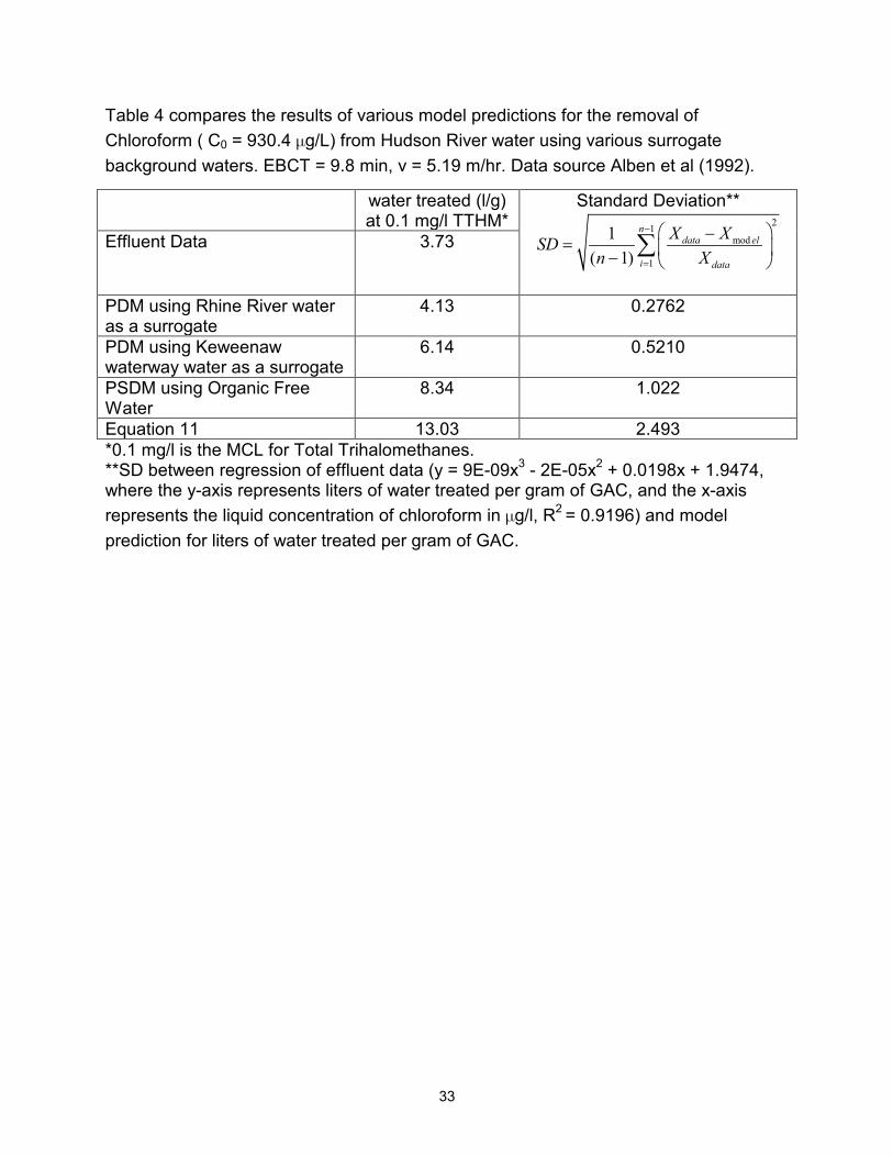
Table 4 compares the results of various model predictions for the removal of Chloroform ( C0 = 930.4 Ng/L) from Hudson River water using various surrogate background waters. EBCT = 9.8 min, v = 5.19 m/hr. Data source Alben et al (1992).

water treated (l/g) at 0.1 mg/l TTHM*

Standard Deviation** 21

mod

1

1( 1)

ndata el

i data

X XSDn X

�

§ ·� ¨ ¸� © ¹

¦

Effluent Data 3.73

PDM using Rhine River water as a surrogate

4.13 0.2762

PDM using Keweenaw waterway water as a surrogate

6.14 0.5210

PSDM using Organic Free Water

8.34 1.022

Equation 11 13.03 2.493 *0.1 mg/l is the MCL for Total Trihalomethanes. **SD between regression of effluent data (y = 9E-09x3 - 2E-05x2 + 0.0198x + 1.9474, where the y-axis represents liters of water treated per gram of GAC, and the x-axis represents the liquid concentration of chloroform in Ng/l, R2 = 0.9196) and model prediction for liters of water treated per gram of GAC.

34

Table 5. compares the results of the model prediction for the removal of 1,2-dichloropropane (C0 = 0.5 Ng/L, EBCT = 14.3 min, v = 7.23 m/hr, adsorbed on Calgon F-400 GAC. Data Source Kruithoff et al, 1989) from Dutch ground water using varying background water matricies, with that of actual adsorber effluent data, and the ECM model for the removal of 1,2-dichloropropane from Dutch ground water. water treated (l/g)

at 0.25 Ng/l of DCP*

Standard Deviation** 21

mod

1

1( 1)

ndata el

i data

X XSDn X

�

§ ·� ¨ ¸� © ¹

¦

Effluent Data 52.3

PDM using Karlsruhe ground water as a surrogate

65.8 0.4532

PDM Wausau ground water as a surrogate

72.4 0.6020

PDM using Houghton ground water

92.6

0.9551

PSDM using OFW 215 3.112 Equation 11 427 7.164 *5 Ng/l is the MCL for 1,2-dichloropropane, but the data from this adsorber has a C0 of

0.5 Ng/l. Thus, 0.25 Ng/l is C/C0 = 0.5. **SD between regression of effluent data (y = -511.49x3 + 436.44x2 + 33.783x + 24.59, where the y-axis represents liters of water treated per gram of GAC, and the x-axis represents the liquid concentration of DCP in Ng/l, R2 = 0.9185) and model prediction for liters of water treated per gram of GAC.

35

Table 6 compares the results of the model for the adsorption of Trichloroethene (Co = 90 Ng/L, adsorbed on Calgon F-100, EBCT=4.8min, v=10m/h, T= 12oC, Data Source: Bhuvendralingam 1992) using varying background water matricies with that of adsorption data from Manheim ground water, Germany, and the PSDM using OFW and ECM models. water treated (l/g)

at 5 Ng/l of TCE* Standard Deviation**

21mod

1

1( 1)

ndata el

i data

X XSDn X

�

§ ·� ¨ ¸� © ¹

¦

Effluent Data 28.8


11.8 0.4136


14.4 0.3658


12 0.4495

PSDM using OFW 95 2.010 Equation 11 200 5.944 *5 Ng/l is MCL for TCE. **SD between regression of effluent data (y = 0.0006x3 - 0.0798x2 + 3.7463x + 11.992, where the y-axis represents liters of water treated per gram of GAC, and the x-axis represents the liquid concentration of TCE in Ng/l, R2 = 0.9703) and model prediction for liters of water treated per gram of GAC.

36

Table 7 compares the results of the model for the adsorption of Tetrachloroethene (Co = 26 Ng/L, adsorbed on Calgon F-100, EBCT=4.8 min v=10m/h T=12C, Data Source Bhuvendralingam 1992) using varying background water matricies, with that of actual adsorber effluent data, and the ECM model for the removal of tetrachloroethene from Manheim (Germany) groundwater. water treated (l/g)

at 5 Ng/l of PCE* Standard Deviation**

21mod

1

1( 1)

ndata el

i data

X XSDn X

�

§ ·� ¨ ¸� © ¹

¦

Effluent Data 96


119.5 0.2030


130.5 0.3164


145 0.4936

PSDM using OFW 994 9.354 Equation 11 2243 22.36 *5 Ng/l is MCL for PCE. **SD between regression of effluent data (y = -0.0078x3 + 0.2305x2 + 5.6178x + 62.666, where the y-axis represents liters of water treated per gram of GAC, and the x-axis represents the liquid concentration of PCE in Ng/l, R2 = 0.996) and model prediction for liters of water treated per gram of GAC.

37

1

10

100

1 10 100 1000Liquid-Phase Concentration (mg/m3)

Solid

-pha

se C

once

ntra

tion

(mg/

g)

TRICHLOROETHENE ISOTHERMSPRELOADING TIME IN WEEKSCALGON F-100 GAC (12x40 mesh)PRELOADING RATE = 10 m/hrSource: Zimmer et al. (1988)

Single Solute (q=3.27 C0.458)

27

25

34

50

70 100

Figure 1. Adsorption Equilibrium Isotherm for TCE as a Function of Exposure Time to Karlsruhe Tap Water (After Zimmer et al. 1988)

38

0

20

40

60

80

100

120

0 10 20 30 40 50 60 70 80Preloading Time (weeks)

Rel

ativ

e Fr

eund

lich

Para

met

er K

%

TRICHLOROETHENESource: Zimmer et al. (1988) Hand et al. (1989) El- Behlil (1990)

Wausau GW(F-400 GAC)

Houghton GW(F-400 GAC)

Karlsruhe GW(F-100 GAC)

Portage Lake(F-400 GAC)

Rhine River(F-100 GAC)

Figure 2. Freundlich K reductions for TCE as a function of time for various background waters.

39

Figure 3. The solid-phase concentration, at complete breakthrough, as a function of aqueous concentration for several groundwater sources and nine activated carbons (Baldauf and Zimmer, 1986).

40

Local EquilibriumBetween Fluid Phaseand Adsorbent Phase

PoreDiffusion

SurfaceDiffusion

R

r+'r

r

BulkSolution

LinearDrivingForce

BoundaryLayer

r

Cb

Cs

qr

Cp,r

qr=KCp,r1/n

Fluid Phase Adsorbent Phase

MassFlux � �= k f Cb Cs�

MassFlux

'r

= -Dqr

D C

rs al p

p

p,rUww

H

W

w

w�

Figure 4. Mechanisms which are included in partial differential equations that describe the pore surface diffusion model (PSDM).

41

0

500

1000

1500

2000

0 4 8 12 16

Liter of Water per Gram of GAC

Chl

orof

orm

( Ng/

l)

Influent DataEffluent DataKeweenaw WaterwayRhine RiverNo NOM Fouling

Figure 5. PDM prediction for the removal of Chloroform ( C0 = 930.4 Ng/L) from Hudson River water using various surrogate background waters. EBCT = 9.8 min, v = 5.19 m/hr. Data source Alben et al (1992). Table 5 shows a comparison of the volume of water treated per mass of GAC for each of the model predictions, and compares the standard deviation between the effluent data and model predictions.

42

0

0.25

0.5

0.75

1

0 25 50 75 100Liters of Water Treated per Gram of GAC

1,2-

dich

loro

prop

ane

( Ng/

l)

Influent DataEffluent DataKarlsruhe GWWausau GWHoughton GW

Figure 6. PDM prediction for the removal of 1,2-dichloropropane (C0 = 0.5 Ng/L) from Dutch ground water using Karlsruhe ground water as a surrogate. EBCT = 14.3 min, v = 7.23 m/hr, adsorbed on Calgon F-400 GAC. Data Source Kruithoff et. al. (1989).

43

0

50

100

150

0 50 100 150Liters of Water Treated Per Gram of GAC

TC

E ( N

g/l)

Influent DataEffluent DataKarlsruhe GWWausau GWHoughton GWNo NOM Fouling

Figure 7 Trichloroethene (Co = 90 Ng/L) adsorption data from Manheim ground water, Germany, adsorbed on Calgon F-100, EBCT=4.8min, v=10m/h, T= 12oC, Data Source: Bhuvendralingam 1992.

44

0

20

40

60

0 50 100 150 200 250

Liters of Water Treated per Gram of GAC

PCE

( Ng/

l)

Influent DataEffluent DataKarlsruhe GWWasau GWHoughton GW

Figure 8 Tetrachloroethene (Co = 26 Ng/L) adsorption data from Manheim Ground Water, Germany, adsorbed on Calgon F-100, EBCT=4.8 min v=10m/h T=12C, Data Source Bhuvendralingam 1992.

predicting the performance of - trussell

Documents