prediction of winter rainfall using adaptive fuzzy neural ... · prediction of winter rainfall...

Prediction of winter rainfall using Adaptive Fuzzy Neural Networks, Case study: Khorasan Razavi Province, Iran

Gholamabbas Fallah Ghalhari1, Fahimeh Shakeri2

1- Assistant professor, Faculty of Geography and Environmental Sciences, Hakim Sabzevari University, I.R of Iran

[email protected]

2- PH.D student of climatology, Faculty of Geography and Environmental Sciences, Hakim Sabzevari University, I.R of Iran

[email protected] Abstract: -This study purpose is to predict winter rainfall of Khorasan Razavi Province using Adaptive fuzzy neural networks. To do this, first average regional rainfall was calculated by Kriging method. In the next stage, rainfall correlation was analyzed by climatic predictors in different intervals. After identifying the effective predictors on regional rainfall, adaptive fuzzy neural network model was trained in 1970-1997 period and finally the rainfall was predicted for 1998-2007 period. The results show that adaptive fuzzy neural networks are able to predict the rainfall amount in an acceptable accuracy. Root mean square error was obtained 7.4 mm for the model. Key-words:- Root mean square error, adaptive fuzzy neural network, climate prediction, Kriging method

1. Introduction Prediction of weather is a complicated process which includes many fields of skills and knowledge. To forecast weather, different methods are used, but only two methods are available and the others are derived from them. The methods include empirical and dynamic ones. Empirical method is based on comparative events (similar climatic conditions) and the dynamic is based on atmospheric equations. Empirical method is to forecast weather in a regional or local scale while dynamic one is suitable to model climatic phenomena in larger scales. During the recent years, many investigations have been conducted on long and mid-term predictions (seasonal and monthly) in different points throughout the world; most of them have been done based on large-scale climatological parameters. Zhang and Scofield (1994) applied Artificial Neural Network (ANN) in prediction of rainfall through satellite data [1]. Allen and Marshall (1994) compared the performance of Artificial Neural Network approach and discrimination analysis method for operational forecasting of rainfall and established the 4 superiority of neural network approach over conventional statistical approach in forecasting rainfall over Australia [2]. Bardossy et al (1995) implemented fuzzy logic in classifying atmospheric circulation patterns [3]. Pesti et al (1996) implemented fuzzy logic in draught assessment [4]. Baum et al (1997) developed cloud

classification model using fuzzy logic [5]. Fujibe (1998) classified the pattern of precipitation at Honshu with fuzzy C-means method [6]. Choi (1999) used neural networks and GIS (Geographic Information System) to forecast the rainfall which revealed efficiency of GIS and neural networks to forecast the rainfall [7]. Vivekanandan et al (1999) developed and implemented a fuzzy logic algorithm for hydrometeor particle identification that is simple and efficient enough to run in real time for operational use [8]. Silverman and Dracup (2000) used from Artificial Neural Networks (ANNs) model to forecast rainfall in California. Results showed that the pattern of rainfall predicted by the ANN model matched closely the observed rainfall with a 1-year time lag for most California climate zones and for most years. This research showed the possibility of making long-range predictions using ANNs and large-scale climatological parameters [9]. Maria et. al (2005) used regression models and neural networks to predict rainfall in Sao-Paulo, Brazil. The used variables included: vertical component of the wind, specific humidity, air temperature, precipitable water, vorticity and humidity flux divergence. The results showed the efficiency in both methods to predict rainfall [10]. Hall et al (2009) used from artificial neural network to forecast rainfall for the Dallas–Fort Worth, Texas area. Results showed that the linear correlation

Advances in Environmental and Geological Science and Engineering

ISBN: 978-1-61804-314-6 412

mailto:[email protected]

between the forecast and observed precipitation amount was 0.95. In addition, the system indicates a potential for more accurate precipitation forecasting [11]. Gonzalez et.al (2010) used from circulation patterns associated with May-to-July rainfall (MJJ) variability over the Limay and Neuquén river basin. The results showed that MJJ rainfall in both basins is related to sea surface temperature and geopotential heights at different levels in some specific areas of Indian and Pacific Ocean, probably due to wave trains which begin in those areas and then displace towards the Argentine Patagonia coast, thus generating precipitation systems [12]. Fallah-Ghalhari et.al (2010) used adaptive fuzzy neural networks to forecast spring rainfall in Khorasan Razavi province. Their results suggest the method efficiency in prediction of seasonal rainfall [13]. Sarah et.al (2011) used from integrated artificial neural network-fuzzy logic-wavelet model for Long term rainfall forecasting in Karoon basin, in Iran. Results showed that the root mean squared error for the two-year and annual periods is 6.22 and 7.11 mm, respectively. Results also showed that the root mean squared error for six months prediction is 13.15 mm [14]. Somia et.al (2011) modeled rainfall events using rule-based fuzzy inference system. The results were in high agreements with the recorded data for the stations with increasing in output values towards the real time rain events [15]. Folorunsho et.al (2012) used from Adaptive Neuro Fuzzy Inference System (ANFIS) in River Kaduna discharge forecasting. The analysis shows high level of accuracy with regards to the ANFIS-based model developed in forecasting the river discharge

especially with a correlation (r) value of 86% [16]. Fallah Ghalhari (2012) used from Artificial Neural Networks for rainfall prediction in Khorasan-Razavi province, Iran. The results showed that ANN model were successful in the Prediction of spring rainfall with a root mean square error of 2.5 milliliters [17]. Regarding to the importance of rainfall amount in many decision making processes, it's been tried in this study to provide a model to forecast regional rainfall using Adaptive Neuro-Fuzzy Inference System and climatic parameters.

2. Materials and Methods 2.1 The area under study

The study area is Khorasan Razavi Province in Northern east of Iran. The time series of the study is the average winter rainfall (January-March) in 38 synoptic, climatologic and rain gauge stations in 1970-2007 which was taken from Iranian Meteorological Organization and ministry of power. 24 stations belong to rain gauge stations of ministry of power and the others were related to Iranian Meteorological Organization. Also, one station was climatologic (Bar Neyshabour), three stations were synoptic (Mashhad, Sabzevar and Torbat -Heydarieh) and 34 ones were rain gauge. Figure.1 shows the area under study and Table.1 shows name and geographical properties of the used stations. In this study, differentials and ratios method were used to complete some of rainfall information and Run Test was used for testing of data homogenization. The statistical properties of selected stations have been also shown in Table 2.

Fig. 1. The area under study


ISBN: 978-1-61804-314-6 413

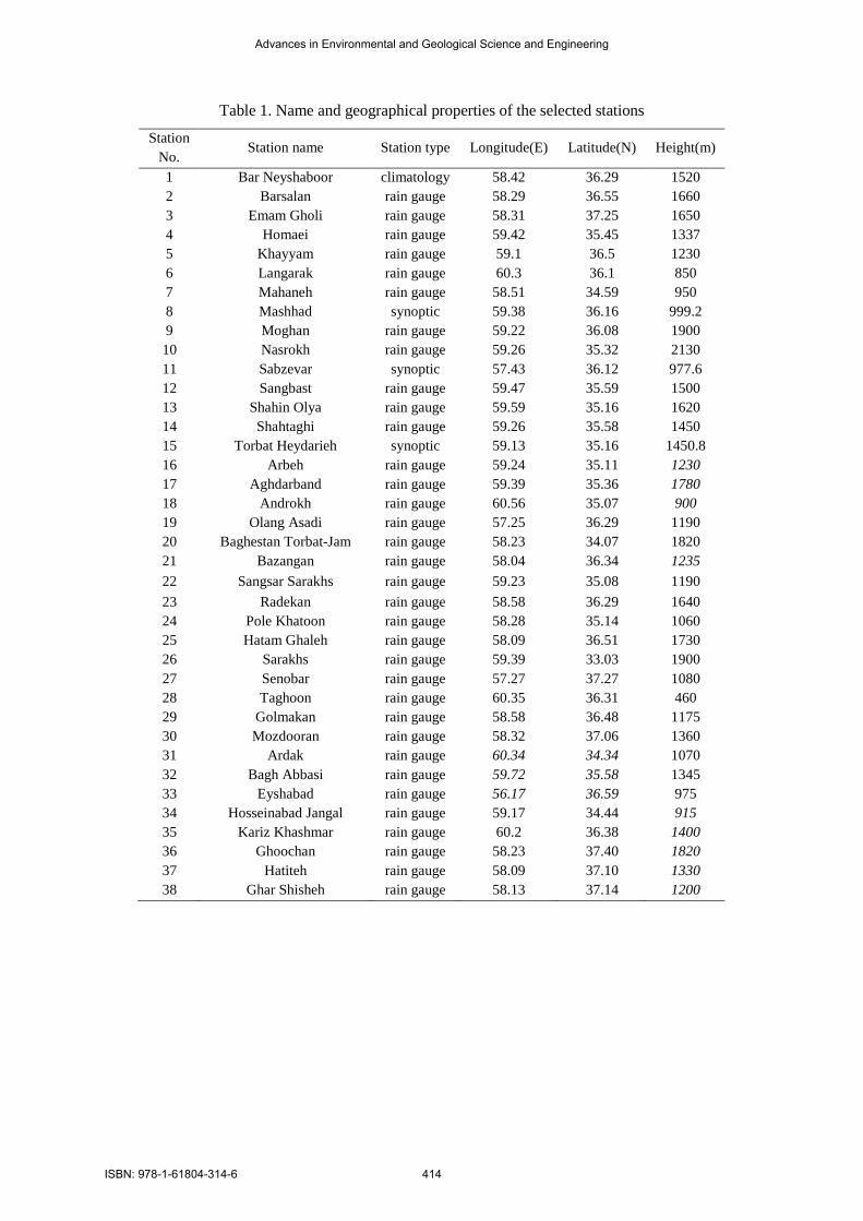
Table 1. Name and geographical properties of the selected stations

Station No.

Station name Station type Longitude(E) Latitude(N) Height(m)

1 Bar Neyshaboor climatology 58.42 36.29 1520 2 Barsalan rain gauge 58.29 36.55 1660 3 Emam Gholi rain gauge 58.31 37.25 1650 4 Homaei rain gauge 59.42 35.45 1337 5 Khayyam rain gauge 59.1 36.5 1230 6 Langarak rain gauge 60.3 36.1 850 7 Mahaneh rain gauge 58.51 34.59 950 8 Mashhad synoptic 59.38 36.16 999.2 9 Moghan rain gauge 59.22 36.08 1900 10 Nasrokh rain gauge 59.26 35.32 2130 11 Sabzevar synoptic 57.43 36.12 977.6 12 Sangbast rain gauge 59.47 35.59 1500 13 Shahin Olya rain gauge 59.59 35.16 1620 14 Shahtaghi rain gauge 59.26 35.58 1450 15 Torbat Heydarieh synoptic 59.13 35.16 1450.8 16 Arbeh rain gauge 59.24 35.11 1230 17 Aghdarband rain gauge 59.39 35.36 1780 18 Androkh rain gauge 60.56 35.07 900 19 Olang Asadi rain gauge 57.25 36.29 1190 20 Baghestan Torbat-Jam rain gauge 58.23 34.07 1820 21 Bazangan rain gauge 58.04 36.34 1235 22 Sangsar Sarakhs rain gauge 59.23 35.08 1190 23 Radekan rain gauge 58.58 36.29 1640 24 Pole Khatoon rain gauge 58.28 35.14 1060 25 Hatam Ghaleh rain gauge 58.09 36.51 1730 26 Sarakhs rain gauge 59.39 33.03 1900 27 Senobar rain gauge 57.27 37.27 1080 28 Taghoon rain gauge 60.35 36.31 460 29 Golmakan rain gauge 58.58 36.48 1175 30 Mozdooran rain gauge 58.32 37.06 1360 31 Ardak rain gauge 60.34 34.34 1070 32 Bagh Abbasi rain gauge 59.72 35.58 1345 33 Eyshabad rain gauge 56.17 36.59 975 34 Hosseinabad Jangal rain gauge 59.17 34.44 915 35 Kariz Khashmar rain gauge 60.2 36.38 1400 36 Ghoochan rain gauge 58.23 37.40 1820 37 Hatiteh rain gauge 58.09 37.10 1330 38 Ghar Shisheh rain gauge 58.13 37.14 1200


ISBN: 978-1-61804-314-6 414

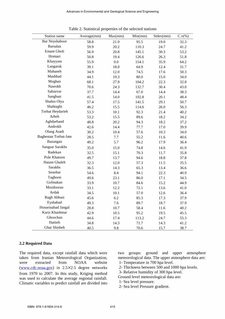
Table 2. Statistical properties of the selected stations

Station name Average(mm) Max(mm) Min(mm) Stdev(mm) C.v(%) Bar Neyshaboor 58.8 21.9 95.5 19.0 32.3

Barsalan 59.9 20.2 110.3 24.7 41.2 Emam Gholi 56.9 20.8 145.1 30.3 53.2

Homaei 50.8 19.4 126.6 26.3 51.8 Khayyam 55.9 0.0 154.1 35.9 64.2 Langarak 39.1 18.0 64.9 12.4 31.7 Mahaneh 34.9 12.0 74.5 17.6 50.3 Mashhad 44.1 19.3 80.0 15.0 34.0 Moghan 68.1 27.9 104.2 22.3 32.8 Nasrokh 70.6 24.3 132.7 30.4 43.0 Sabzevar 37.7 14.4 67.0 14.4 38.3 Sangbast 41.5 14.0 102.8 20.1 48.4

Shahin Olya 57.4 17.5 141.5 29.1 50.7 Shahtaghi 46.2 15.5 114.6 26.0 56.3

Torbat Heydarieh 53.3 10.1 92.3 21.4 40.2 Arbeh 53.2 15.5 89.6 18.2 34.2

Aghdarband 48.8 20.2 94.3 18.2 37.2 Androkh 42.6 14.4 77.7 17.0 39.9

Olang Asadi 30.2 10.4 57.6 10.3 34.0 Baghestan Torbat-Jam 28.5 7.7 55.2 11.6 40.6

Bazangan 49.2 5.7 96.2 17.9 36.4 Sangsar Sarakhs 35.0 15.0 74.8 14.6 41.9

Radekan 32.5 15.1 70.3 11.7 35.8 Pole Khatoon 49.7 13.7 94.6 18.8 37.8 Hatam Ghaleh 32.3 12.0 57.3 11.5 35.5

Sarakhs 36.5 14.3 65.3 13.4 36.6 Senobar 54.6 8.4 94.1 22.3 40.9 Taghoon 49.6 23.1 86.0 17.1 34.5

Golmakan 33.9 10.7 84.6 15.2 44.9 Mozdooran 33.1 12.2 72.1 13.6 41.0

Ardak 34.5 10.1 57.0 12.6 36.4 Bagh Abbasi 45.6 6.2 85.3 17.3 37.9

Eyshabad 49.3 7.6 89.7 18.7 37.9 Hosseinabad Jangal 28.8 10.7 58.4 11.6 40.2

Kariz Khashmar 42.9 10.5 95.2 19.5 45.5 Ghoochan 44.6 17.4 113.2 24.7 55.3

Hatiteh 34.8 14.3 71.7 14.3 41.2 Ghar Shisheh 40.5 9.8 70.6 15.7 38.7

2.2 Required Data

The required data, except rainfall data which were taken from Iranian Meteorological Organization, were extracted from NOAA website (www.cdc.noaa.gov) in 2.5 2.5 degree networks from 1970 to 2007. In this study, Kriging method was used to calculate the average regional rainfall. Climatic variables to predict rainfall are divided into

two groups: ground and upper atmosphere meteorological data. The upper atmosphere data are: 1- Temperature in 700 hpa level. 2- Thickness between 500 and 1000 hpa levels. 3- Relative humidity of 300 hpa level. Ground level meteorological data are: 1- Sea level pressure. 2- Sea level Pressure gradient.


ISBN: 978-1-61804-314-6 415

http://www.cdc.noaa.gov/

3- Sea level temperature. 4- Temperature difference between sea level and 1000 hpa level. 5- Zonal component of the wind 6- Meridional component of the wind 7- Precipitable water 8- The long wave outgoing long wave radiation from ground level

2.3 Methodology

To predict rainfall in the studied region, first the average rainfall was measured in a statistic period for each year by using Kriging method and the average regional rainfall time series was prepared. Following that, some points in different areas of seas, the effects of which had been revealed on the region weather, were selected according to the previous studies ( [18], [19]) and the predictor

correlation of these points were analyzed by average regional rainfall variations. These points are shown in Figure.2.To analyze the above atmospheric data and also three parameters in ground level including wind Meridional component, wind zonal component and Precipitable water, factor analysis method in two networks 5 5 and 10 10 degrees was used. The area in which meteorological data were analyzed in ground and upper atmospheric levels, was 0-80 °E and 10-50 °N for 5 5 network and 0-100 °E and 0-70 °N in 10 10 networks. In this study, the predictors were used in which Pearson's correlation coefficient was more than 60% to the considered factor and the described variance by them was more than 5%.

Fig. 2. Name and coordinates that have used for relation between regional rainfall and predictors

2.4 Adaptive Neuro-Fuzzy Inference System (ANFIS)

ANFIS is a combination between artificial neural networks and fuzzy inference system. It has a hybrid algorithm to estimate the parameters, least square to estimate the linear parameter and error back

propagation to estimate nonlinear parameter. There are four layers in ANFIS. The linear parameter will be estimated in first layer and the nonlinear parameter in fourth layer. There are some technical terms in ANFIS modeling, such as fuzzy set and fuzzy inference systems. Both terms are the basis of

SIBERIA GRID

ISLAND GRID

ADRIATIC SEA NORTH ASPIAN SEA

WESTof MEDITERRANEAM SEA

NORTH OF PERSIAN

NORTH OF RED SEA NORTH OF PERSIAN SOUTH OF PERSIAN GULF

SOUTH OF RED SEA

OMAN SEA

ARABIC SEA

ADEN GULF

ARAL SEA


ISBN: 978-1-61804-314-6 416

ANFIS modeling. Fuzzy set is the set where the membership of each element does not have clear boundaries. Fuzzy inference system is a method that interprets the values in the input vector and, based on user-defined rules, assigns values to the output vector. Fuzzy set has a concept that difference with the classical set. The input space is mapped into a given weight or degree of membership through a function called membership function. It defines how each point in the input space is mapped into weights or degrees of membership between 0 and 1 [20]. Figure.3 shows the fuzzy neural network structure. The system has four layers. The input dimensions are divided into two categories. The first type of dimension is for the fuzzy grid partition and is denoted as "g-dimensions. The other type of dimension is for the fuzzy ellipsoid partition and is denoted as "w-dimension". The inputs belonging to each dimension are called "g-input" and "e-input" respectively. In the following description system with a single input of g-dimension and single output are considered, but the result are easily expanded for system with more than one g-dimension and outputs. The functions of the nodes in each layer are described as follows: Layer 1. The nodes of this layer transmit values directly to the next layer. The "g1-node" takes the input from the g-dimension. "e-nodes" take the inputs from the e-dimensions. The number of nodes is equal to the number of input

dimensions: For the g-dimension (1)

For the ith e-dimension (2) Layer 2. This layer performs a

fuzzification. There are two kinds of nodes in this layer. One type of node, denoted "g-nodes", takes the output of the corresponding g-node as the input. The other type of node, denoted "e-nodes" takes the output of all e-nodes as inputs. Each node in this layer represents the condition part of rules, and the node output is equal to the degree of match for each condition. The node function of the jth g-node is:

−−=

2

2)(exp g

j

ggjg

jU

Uσ

µ (3)

Where g

jµ and gjσ are respectively, the center and

the width (or variance) of the bell-shaped function of the jth node. Correspondingly, the node function of the k th 2e -node is:

−−=Π

=2

2

1

)(exp eki

ei

eki

n

i

ek

UUσ

µ (4)

Where n is the number of 1e -nodes; eiU is the input

from the ith e-dimension: ekiµ and e

kiσ are, respectively, the center and the width (or variance) of the bell-shaped function of the ith input. Layer 3. This layer performs a fuzzy inference, which is carried out by multiplication. Each node in this layer corresponds to a rule, and the node output is equal to the firing strength of each rule. The number of nodes in this layer is equal to the number of rules. The node function corresponding to jth g2-node and kth e2- node is:

gj

ekkj UUU ×= (5)

Layer 4. The nodes in this layer transmit the decision signal out of the network. These nodes act as the defuzzifier. The number of nodes in this layer is equal to the output dimension. The following function is used to simulate the center of gravity defuzzication method.

∑ ∑∑ ∑

= =

= == n

k

m

j kj

n

k

m

j kjkj

U

UY

1 1

1 1µ

(6)

Where n and m are the numbers of 2e -nodes and

2g -nodes. Respectively, and skjµ are the centers of the membership functions [21], [13].

ei

e XU i =

gg XU =


ISBN: 978-1-61804-314-6 417

Fig. 3. Fuzzy neural network structures [21], [13].

In this paper, subtractive clustering method was used to classify and analyze the data automatically and to produce fuzzy inductive system, eventually. Also, in order to evaluate the model accuracy, Root Mean Square Error (RMSE) index was used. the formula of which is as follow:

(7)

n

eoRMSE

n

iii∑

=

−= 1

2)(

Where, RMSE is root mean square error, and are observed and forecasted values of the

variable in point i, respectively, and n is the number of observations.

3. Results and dissection As it was mentioned in the last section, in order to obtain climatic predictors influencing the

regional rainfall, Pearson's correlation coefficient was used so that all predictors which showed significant relation or correlation with the region rainfall in a confidence level of 5% were used. Various studies showed that the most correlation between climatic predictors and average regional rainfall was obtained from July to November. On this basis, the following predictors were selected as the model input from July to November: -X1: air temperature in 700 hpa level in region 1 in 10 degree networks (Figure 4). -X2: air temperature in 700 hpa level in region 3 in 10 degree networks (Figure 4). -X3: air temperature in 700 hpa level in region 6 in 10 degree networks (Figure 4). -X4: air temperature in 1000 hpa level in Oman Sea. - X5: Outgoing long wave radiation from ground level in North Sea.


ISBN: 978-1-61804-314-6 418

-X6: Relative humidity of 300 hpa level in region 1 in 10 degree-networks (Figure 5). -X7: Relative humidity of 300 hpa level in region 2 in 10 degree-networks (Figure 5). - X8: Standardized pressure of sea level in north of Caspian Sea - X9: Standardized pressure of sea level in south of Caspian Sea - X10: Standardized temperature of sea level in Adriatic Sea - X11: Standardized temperature of sea level in North of Persian Gulf. -X12: Thickness between 500 and 1000 hpa levels in region 1 in 5×5 degree networks (Figure.6) -X13: Thickness between 500 and 1000 hpa levels in region 2 in 5×5 degree networks (Figure.6) -X14: Thickness between 500 and 1000 hpa levels in region 1 in 10×10 degree networks (Figure.7) -X15: Thickness between 500 and 1000 hpa levels in region 1 in 10×10 degree networks (Figure.7) -X16: Wind zonal component in region 6 in 5×5 degree networks (Figure.8) -X17: Wind zonal component in region 1 in 10×10 degree networks (Figure.9) -X18: Standardized Pressure difference of sea level between Golf of Aden and south of Caspian Sea -X19: Standardized Pressure difference of sea level between Adriatic Sea and north of Caspian Sea.

-X20: Standardized Pressure difference of sea level between Adriatic Sea and south of Caspian Sea -X21: Standardized Pressure difference of sea level between Arab Sea and Oman Sea -X22: Standardized Pressure difference of sea level between Indian Ocean and north of Caspian Sea -X23: Standardized Pressure difference of sea level between Indian Ocean and south of Caspian Sea -X24: Standardized Pressure difference of sea level between north of Caspian Sea and north of Persian Gulf -X25: Standardized Pressure difference of sea level between north of Caspian Sea and north of Red Sea -X26: Standardized Pressure difference of sea level between north of Caspian Sea and Northern Sea. -X27: Standardized Pressure difference of sea level between north of Persian Gulf and south of Caspian Sea -X28: Standardized Pressure difference of sea level between north of Red Sea and south of Caspian Sea -X29: Standardized Pressure difference of sea level between south of Caspian Sea and Sudanese network -X30: Standardized Pressure difference of sea level between south of Caspian Sea and West of Mediterranean Sea. Table 3 shows time series of regional rainfall and selected predictors in period between 1970-2007.


ISBN: 978-1-61804-314-6 419

Fig. 4. The identified areas of temperature at 700 hPa level from July to November in 5×5 networks by using

factor analysis method

Fig. 5. Identified areas of relative humidity at 300 hPa level from July to November in 10×10 degree networks


ISBN: 978-1-61804-314-6 420

Fig. 6. Identified areas of thickness between 500 and 1000 hPa levels in 5×5 degree networks

Fig. 7. Identified areas of thickness between 500 and 1000 hPa levels from July to Nov in 10×10 degree

networks


ISBN: 978-1-61804-314-6 421

Fig. 8. Identified areas of zonal wind component from Jul to Nov in 5×5 degree networks

Fig. 9. Identified areas of Meridional wind component from Jul to Nov in 10×10 degree networks


ISBN: 978-1-61804-314-6 422

Table 3. Time series of regional rainfall and selected predictors in the period 1970-2007.

Rainfall x1 x2 x3 x4 x5 x6 x7 x8 x9 x10 x11 x12 x13 x14 43.8 8.8 -5.9 5.6 0.6 -7.3 23.9 26.2 -0.7 -1.8 -0.4 -0.7 5765.8 5674.6 5753.4 25.8 8.2 -4.7 4.5 -0.8 -1.2 23.2 24.5 0.0 -1.1 -0.7 -1.1 5756.7 5663.8 5742.3 41.0 8.7 -5.7 5.0 0.0 -0.7 23.2 25.3 0.2 -1.4 -1.5 -0.9 5769.0 5669.6 5752.1 43.1 8.8 -7.2 5.5 -0.2 -3.5 22.2 24.5 -0.1 0.2 0.5 -0.3 5765.7 5674.4 5752.7 47.5 8.6 -5.2 5.3 -0.3 -7.6 23.5 25.4 0.5 0.1 -1.0 -0.4 5760.6 5675.0 5748.3 44.2 9.0 -6.1 5.8 0.0 -4.8 23.3 25.0 -1.0 -0.7 -1.2 -0.5 5769.8 5690.9 5757.3 42.8 8.5 -6.9 4.9 -0.8 5.3 22.8 24.6 0.3 0.7 -0.6 -1.1 5762.2 5676.9 5749.5 40.2 8.5 -6.5 4.7 -0.6 -2.1 22.0 23.8 -0.3 0.5 -0.8 -0.6 5765.7 5678.3 5748.7 33.6 8.6 -6.6 4.7 -1.2 -2.3 22.4 24.1 -0.9 -0.2 -1.6 -1.5 5761.5 5673.7 5751.4 49.8 9.2 -5.0 5.5 -0.1 -4.4 23.5 24.9 0.0 0.0 -0.5 0.1 5773.8 5688.7 5759.5 46.5 9.2 -5.6 5.8 -0.4 -5.9 23.2 24.9 -1.3 -1.2 -0.4 -0.5 5775.5 5700.7 5761.0 51.3 9.1 -3.3 5.2 0.2 -3.3 24.7 25.5 -0.9 -0.6 0.2 -0.6 5769.2 5687.6 5757.5 45.6 8.9 -5.4 5.7 1.2 -1.0 23.3 24.6 -0.1 0.8 1.6 -1.1 5769.4 5682.9 5755.2 44.9 9.3 -5.7 5.7 1.1 4.7 23.8 25.0 -1.6 -1.2 0.1 -1.2 5776.9 5683.8 5762.8 33.6 8.8 -6.2 5.6 -1.6 -4.6 23.1 24.8 -1.0 -0.7 -0.7 -1.3 5764.3 5682.4 5752.0 31.6 8.8 -5.8 5.4 -1.5 -3.0 23.6 25.2 -0.5 0.2 -0.8 -1.0 5765.6 5687.3 5753.5 36.3 8.8 -6.0 5.5 -1.7 -2.5 22.5 23.9 0.2 0.7 -0.5 0.8 5764.6 5683.6 5753.3 44.7 9.5 -5.7 6.1 -0.2 -4.9 23.4 25.1 0.6 1.7 1.7 0.5 5780.1 5696.2 5766.7 44.3 9.1 -4.8 5.6 1.6 -0.4 24.7 25.8 -1.2 -0.7 0.0 0.8 5771.1 5687.5 5760.8 50.3 9.0 -4.6 5.2 0.7 5.8 23.5 24.8 -1.2 -1.0 -1.4 0.5 5767.4 5684.3 5756.1 35.5 9.1 -6.2 5.5 0.4 0.5 23.3 25.2 -1.0 -0.6 -0.9 0.2 5772.5 5697.5 5761.1 46.6 9.1 -4.5 5.2 -1.1 4.6 23.5 24.8 -0.1 0.3 -0.9 -1.1 5771.1 5691.9 5757.6 56.8 8.6 -5.9 5.7 1.1 -2.8 22.7 24.3 -0.4 0.5 0.4 -1.3 5761.1 5683.1 5749.5 49.5 8.9 -7.0 5.8 0.9 1.8 22.4 24.4 1.2 2.0 -0.7 -0.2 5771.5 5696.5 5756.1 50.1 8.8 -5.3 5.9 0.9 4.7 23.7 24.8 -0.2 0.1 1.3 -0.1 5766.0 5690.5 5753.8 38.5 9.1 -4.8 4.9 1.0 7.3 24.5 25.5 -1.8 -1.8 0.3 -0.4 5774.0 5681.2 5759.9 47.0 9.1 -5.4 5.0 -2.6 2.2 23.0 24.4 0.2 -0.2 -1.5 0.7 5769.6 5686.8 5757.1 45.2 9.3 -5.6 5.6 1.5 5.8 23.1 25.6 0.6 -0.5 0.3 0.1 5779.3 5681.4 5761.5 45.2 9.8 -5.5 6.1 0.7 -2.1 24.3 25.9 0.4 -0.1 0.9 2.3 5783.4 5714.0 5770.9 61.6 9.2 -5.2 5.8 0.2 5.3 23.9 25.8 0.3 -0.4 1.1 2.2 5772.5 5703.0 5760.4 44.2 9.2 -5.3 5.7 0.0 -2.7 23.4 25.1 2.0 1.3 1.1 0.9 5771.7 5694.5 5759.1 25.1 9.5 -6.0 5.9 0.2 -1.5 23.2 25.4 0.3 -0.1 0.9 1.0 5778.3 5700.3 5764.8 27.7 9.3 -5.7 5.7 -1.4 1.6 23.1 25.3 -0.1 -0.5 0.9 1.0 5778.5 5701.1 5761.8 51.0 9.5 -4.3 6.0 0.6 5.4 24.7 26.3 0.1 0.2 1.8 0.9 5778.8 5705.1 5766.2 57.7 9.2 -5.0 5.7 -0.7 0.2 24.1 25.9 1.8 1.8 1.5 0.9 5775.6 5694.9 5759.6 63.2 9.6 -3.1 5.6 0.1 5.6 25.2 26.2 2.2 1.5 0.5 0.4 5783.2 5696.0 5766.7 54.9 9.6 -5.0 5.8 0.4 4.7 24.7 26.1 1.3 0.7 1.2 1.1 5783.5 5694.3 5768.1 49.3 9.5 -3.5 5.9 1.6 3.1 25.5 26.9 2.0 1.9 0.1 1.6 5782.9 5703.6 5767.0


ISBN: 978-1-61804-314-6 423

Table 3. Continue

x15 x16 x17 x18 x19 x20 x21 x22 x23 x24 x25 x26 x27 x28 x29 x30 5440.9 0.4 0.3 0.1 0.1 0.2 0.0 0.1 0.5 -0.5 0.6 0.4 -0.2 0.5 -0.1 -2.7 5454.6 0.6 0.1 0.7 0.5 -0.6 0.3 -0.1 -2.7 2.0 -0.7 -1.7 0.8 1.8 -0.9 -2.0 5450.9 0.6 0.3 2.6 0.3 -2.3 2.3 -4.2 -7.6 11.5 -0.2 -1.4 2.5 1.8 -1.2 -1.6 5409.6 1.6 0.1 -0.9 1.6 1.0 -2.5 6.5 -0.2 -9.3 1.0 -0.9 -1.0 -1.2 1.5 -0.7 5465.1 0.0 0.2 0.9 -0.2 -0.7 1.1 -2.4 -1.8 4.8 0.9 2.8 -0.2 -0.4 0.6 -0.1 5441.1 1.1 0.3 0.4 0.9 -0.1 -0.5 1.8 -2.0 -1.3 -2.0 -0.6 1.0 1.7 -1.9 -0.7 5437.5 1.5 0.3 -2.6 1.2 2.9 -3.7 8.6 6.5 -17.1 0.9 -0.9 -2.2 -1.2 2.2 0.2 5425.3 1.8 0.3 -0.2 1.4 0.5 -1.6 4.6 -1.4 -5.8 -1.2 -0.6 -0.5 0.5 0.8 1.9 5424.4 2.0 0.1 1.1 1.9 -1.0 -0.8 3.5 -6.8 -0.4 -2.3 -2.0 0.7 1.6 -1.6 -3.1 5456.7 1.1 0.1 1.6 1.0 -1.6 0.6 -0.2 -6.7 4.9 -0.6 -0.1 1.3 0.6 -0.4 0.2 5442.2 0.8 0.3 2.3 0.5 -2.0 1.8 -3.1 -7.0 9.4 -2.1 -0.6 1.8 2.0 -2.0 -1.4 5488.9 -0.4 0.2 0.8 -0.6 -0.6 1.4 -3.5 -0.4 5.4 -1.2 -0.6 0.8 0.9 -1.8 -2.8 5460.4 0.8 0.3 -0.7 0.4 1.1 -1.2 2.8 2.3 -5.7 -1.7 0.6 1.3 0.8 -0.7 0.9 5449.7 1.2 0.4 0.6 0.8 -0.2 -0.2 1.3 -2.3 -0.3 -2.8 -2.7 2.0 2.4 -2.6 -1.9 5441.5 1.5 0.1 1.6 1.4 -1.4 0.2 0.9 -7.1 3.5 -1.7 0.0 2.1 1.5 -1.5 -0.4 5447.4 1.3 0.3 0.1 1.1 0.2 -1.0 3.0 -1.6 -3.3 -1.1 -1.3 0.5 0.3 -0.3 -0.6 5440.9 1.4 0.1 1.3 1.3 -1.2 -0.1 1.5 -6.3 2.1 -1.7 -0.3 0.7 1.2 -0.9 -1.0 5442.9 1.3 0.4 -1.5 0.9 1.8 -2.3 5.6 3.7 -10.7 -0.2 1.0 -0.4 -0.8 1.1 2.3 5462.7 0.4 0.4 -0.3 0.0 0.7 -0.3 0.7 2.0 -2.3 -0.6 -1.1 0.0 0.1 0.1 -1.4 5461.6 0.4 0.3 0.8 0.1 -0.5 0.7 -1.3 -1.7 3.2 -1.5 -2.2 1.4 1.4 -1.2 -1.2 5435.4 2.0 0.4 0.9 1.6 -0.5 -0.7 2.9 -4.6 -1.0 -1.6 -0.7 0.5 1.2 -0.7 -0.3 5468.2 1.4 0.5 0.2 0.9 0.3 -0.7 2.3 -0.8 -2.8 -1.2 -0.3 0.2 0.8 -0.5 0.2 5436.7 1.0 0.4 0.9 0.6 -0.5 0.3 0.0 -2.8 1.9 -1.7 1.1 0.8 0.8 -1.4 -0.1 5414.7 1.7 0.4 -1.3 1.3 1.7 -2.7 6.7 2.3 -11.3 1.2 0.4 -1.4 -1.9 1.9 3.1 5449.9 2.4 0.5 1.0 1.9 -0.5 -0.9 3.8 -5.4 -1.8 0.1 -0.4 -0.4 -0.4 -0.1 0.4 5461.8 1.0 0.4 1.3 0.6 -0.9 0.8 -1.0 -3.9 4.2 -0.9 -2.6 1.1 1.0 -1.1 -1.4 5456.4 0.8 0.2 0.2 0.5 0.1 -0.4 1.2 -0.8 -1.2 1.3 0.6 -0.2 -0.9 0.0 0.8 5438.7 0.5 0.5 1.4 0.0 -0.9 1.4 -2.9 -2.8 6.2 0.1 -0.2 0.8 0.9 -0.7 1.2 5448.3 0.6 0.4 -1.4 0.2 1.8 -1.6 3.4 5.1 -8.4 1.8 1.8 -1.6 -1.3 1.7 0.4 5458.1 1.1 0.5 -1.0 0.6 1.5 -1.5 3.6 3.4 -7.6 1.5 0.3 -1.7 -0.8 1.0 0.9 5462.4 0.9 0.3 -3.3 0.6 3.6 -3.9 8.5 9.7 -19.1 4.0 4.6 -2.5 -3.4 2.9 2.6 5447.8 1.7 0.4 -0.7 1.3 1.1 -1.9 5.1 0.7 -7.9 1.1 0.7 -0.3 -0.7 -0.3 -0.2 5446.8 1.0 0.5 1.6 0.5 -1.1 1.1 -1.7 -4.4 5.6 0.7 0.2 0.8 -0.3 -0.6 1.4 5476.5 -0.5 0.6 -0.6 -1.0 1.1 0.5 -2.0 5.4 -0.9 1.6 -0.6 -0.6 -1.6 0.7 1.0 5461.9 0.9 0.3 -2.1 0.6 2.5 -2.7 5.9 6.3 -13.0 2.4 2.3 -1.4 -2.4 2.2 2.0 5499.3 -0.1 0.5 -1.7 -0.6 2.2 -1.1 1.7 7.9 -7.9 2.5 1.7 -1.8 -1.8 1.7 1.3 5465.4 0.6 0.4 -1.2 0.2 1.6 -1.4 3.0 4.2 -7.2 2.3 2.2 -1.4 -1.7 1.1 0.7 5486.8 0.0 0.5 -2.9 -0.5 3.4 -2.4 4.2 11.3 -14.0 3.0 1.1 -3.3 -2.8 3.2 2.2

3.1 Prediction of Winter Rainfall Using Adaptive Fuzzy-Neural Networks

In order to forecast the rainfall by using adaptive fuzzy neural networks, data are divided into three different sections including training, validation and testing data. In the other words, from 38 years data, 19 years data were used as training data (1970-1988), 19 years data as validation data (1989-1997), and the left 10 years as testing data (1998-2007). In the other words, from the historic data, two third (1970-1997) were considered as calibration data and

one third (1998-2007) as testing data. After different tests to study the network, hidden layer neuron number and different activity functions in hidden and output layers, finally the final model had the least error to an input layer (signals mentioned in the previous part), a hidden layer and an output layer (winter mean rainfall) and selected as the final model. The obtained results are shown in Table.4 and Figure.11. It should be noted that the root mean square error was obtained 10.7 mm for the model.


ISBN: 978-1-61804-314-6 424

Table.4 . Rainfall prediction of the studied periods

by ANFIS model

Observed rainfall (mm)

Predicted rainfall (mm) Year

45.2 43.4 1998 61.6 49.7 1999 44.2 46.2 2000 25.1 46.4 2001 27.7 48.4 2002 51 54.8 2003

57.7 50.3 2004 63.2 64.3 2005

54.9 54.01 2006 49.3 56.4 2007

As it can be seen in the figure, the model can't forecast very arid or moist years. The reason is that

these extreme years have not been repeated in training period of the network and calibration period of the model parameters and the model has not been able to forecast rainfall in these years, but in the rest years the prediction procedure is suitable. Properties of training period and also ANFIS model structure are shown in Table.5 and Table.6. To solve this problem, the model should be trained with these extreme data. for this reason and to develop ANFIS model to predict seasonal rainfall (so that it can be used for all cases including dry, wet and normal years), 1998-2000 period which is extreme year in the test period and one is representative of semi dry and the other for semi wet year, were removed from the test data and transferred to the training and calibration period data and other data were substituted instead of them. Table.7 and Figure.11 show the model results in the two conditions.

0

10

20

30

40

50

60

70

1996 1998 2000 2002 2004 2006 2008

Year

Rai

nfal

l (m

m)

Observed rainfallPredicted rainfall

Fig. 10. Comparison of the observed and predicted rainfall by ANFIS

Table 5. ANFIS training period properties parameter value

Rang of influence 2 Epoch 20

Optimization method combination Squash factor 1.25 Accept ratio 0.5 reject ratio 0.15

Table 6. Structural properties of ANFIS model name value

Number of nodes 343 Number of linear parameters 155

Number of non linear parameters 300 Total parameters 455

Number of training pair data 18 Number of validation pair data 10

Number of fuzzy rules 5 As it can be seen, the model accuracy has increased for identifying arid, rainy and normal years and it can be noted that the model accuracy is better than the previous one. Figure 11 shows this subject.

Therefore, it can be concluded that a change in training data has been effective to predict the model and the rainfall can be predicted more accurately.


ISBN: 978-1-61804-314-6 425

Table 7. Prediction of the studied area rainfall by

ANFIS model

Observed rainfall (mm)

Predicted rainfall (mm)

year

45.2 45.7 1 44.2 43.9 2 44.2 50.4 3 46.5 49.4 4 27.7 36.8 5 51 63.2 6

57.7 51.5 7 63.2 62.5 8 54.9 53.3 9 49.3 64.4 10

It should be noted that the root mean square error was obtained 7.4 mm for this model. The properties of training period and also ANFIS model structure after modifying the training period with the new data are shown in Tables 8, 9 and 10.

Table 8. Training properties of ANFIS after modifying

the training data

value name 1.5 Number of nodes 20 Number of linear parameters

combination Number of nonlinear parameters 1.25 Total number of parameters 0.5 Number of training data pairs

0.15 Number of checking data pairs

Table.9 General properties of ANFIS model after

modifying the training data

name value Number of nodes 1087

Number of linear parameters 527 Number of nonlinear parameters 1020

Total number of parameters 1547 Number of training data pairs 18 Number of checking data pair 10

Number of fuzzy rules 17

Table.10 Structural properties of ANFIS model after modifying the training data

Value Field Sugeno Type

Prod And method

Probor Or Method

wtaver Defuzz Method

Prod Imp method

Sum Agg Method

<1×30 Struct> input

<1×1 Struct> output

<1×17 Struct> rulr

0

10

20

30

40

50

60

70

0 2 4 6 8 10 12

Year

Rai

nfal

l (m

m)

Predicted RainfallObserved Rainfall

Fig. 11. Observed and Predicted Rainfall by ANFIS model after modifying the training course by historic data.


ISBN: 978-1-61804-314-6 426

4. Conclusion In general, the model results show that the difference between observed and predicted rainfall is acceptable and the model has been able to forecast the rainfall during all the years with an acceptable error. Root mean square error was obtained 7.4mm for the model and this shows the model accuracy to predict the regional rainfall. Of the whole subjects mentioned above, it can be inducted that between the two models which were used for rainfall forecast, the second had a better efficiency with a root mean square error of 7.4mm and also it can be concluded that the variables given to the model, have been able to explain dispersion and distribution of rainfall during the studied years easily and accurately and have been used successfully to forecast winter rainfall. Reference [1] Zhang, M., Scofield, A. R., Artificial Neural

Network techniques for estimating rainfall and recognizing cloud merger from satellite data, Int. J. Remote Sens, 1994, 16: 3241-3262.

[2] Allen, G., Marshall, J. F., An evaluation of neural networks and discrimination analysis methods for application in operational rain forecasting, Aust. Meteor. Mag. 1994, 43: 17-28.

[3] Bardossy, A., Duckstein, L. and Bogardi, I., Fuzzy rule-based classification of atmospheric circulation patterns, Int J Climatol, 1995, 15: 1087-1097

[4] Pesti, G., Shrestha, B.P., Duckstein, L., Bogardi, I., A fuzzy rule-based approach to drought assessment, Water Resour Res, 1996, 32: 1741-1747.

[5] Baum, B.A., Tovinkere, V., Titlow, J., Welch, R.M., 1997: Automated cloud classification of global AVHRR data using a fuzzy logic approach, J. Appl. Meteorol, 1997, 36: 1519-1540.

[6] Fujibe, F., Short-term precipitation patterns in central Honshu, Japan---classification with the fuzzy c-means method, J. Meteor. Soc. Japan, 1989, 67: 967-982.

[7] Choi, L. 1999: An application hydroinformatic tools for rainfall forecasting, Thesis (PhD). University of New South Wales (Australia),1999, pp 752.

[8] Vivekanandan, J., Ellis, S.M., Oye, R., Zrnic, D.S., Ryzhkov, A.V., and Straka, J., Cloud Microphysics Retrieval Using S-band Dual-Polarization Radar Measurements, Bull. Amer. Meteor. Soc., 1999, 80: 381–388.

[10] Maria, C. Haroldo, F and Ferreira, N., Artificial neural network technique for rainfall forecasting applied to the Sao Paulo region, J. Hydrol , 2005, 301(1-4),146-162.

[11] Hall, T., Brooks, H.E., Doswell, C.A., Precipitation Forecasting Using a Neural Network, Wea. Forecasting, 1999, 14: 338-345.

[12] Gonzalez, M.H., Skansi, M.M., Lozano, F., A statistical study of seasonal winter rainfall prediction in the Comahue region, Argentina, Atmosphera, 2010, 23(3), 277-294.

[13] Fallah Ghalhary G.A, Habibi-Nokhandan M., Mousavi-Baygi M., Khoshhal J., Shaemi Barzoki A., Spring rainfall prediction based on remote linkage controlling using adaptive neuro-fuzzy inference system (ANFIS), Theor Appl Climatol, 2010, 101: 217–233.

[15] Somia A. A., Khaled, E., Youssef, I.K., Abd El-wahab, M., Rainfall events prediction using rule-based fuzzy inference system, Atmos Res, 2011, 101, 228-236.

[16] Folorunsho, J.O., Iguisi, E.O., Mu’azu, M.B., Garba, S., Application of Adaptive Neuro Fuzzy Inference System (ANFIS) in River Kaduna Discharge Forecasting, Res. J. Appl. Sci. Eng. Technol., 2012, 4(21): 4275-4283.

[17] Fallah Ghalhari, Gholam Abbas., Rainfall Prediction Using Teleconnection Patterns through the Application of Artificial Neural Networks, Modern Climatology, Shih-Yu (Simon) Wang and Robert R. Gillies, InTech, 2012: pp 364-391.

[18] Mousavi Baygi, M., Fallah Ghalhari, G.A., and Habibi Nokhandan, M., Assessment of the relation between the large scale climatic signals with rainfall in the Khorasan, J. Agric. Sci. Natur. Resour, 2008, 15(2): 1-9.

[19] Nazemosadat, M.J. 2001: Will it rain? Drought and rainfall in Iran and their relation with ENSO, 102, Shiraz University Press, 2001, pp. 45-46.

[20] Faulina, F., Suhartono, M., Hybrid ARIMA-ANFIS for Rainfall Prediction in Indonesia, International Journal of Science and Research (IJSR),2013, 2(2): 159-162.

[21] Leondes, TC., Fuzzy theory system, techniques and applications, 954, Academic, New York, 1999, 2(1).


ISBN: 978-1-61804-314-6 427

http://www.sciencedirect.com/science/journal/00221694

http://www.sciencedirect.com/science?_ob=PublicationURL&_tockey=%23TOC%235811%232005%23996989998%23541281%23FLA%23&_cdi=5811&_pubType=J&_auth=y&_acct=C000050221&_version=1&_urlVersion=0&_userid=10&md5=068fc05e5eb26d7890b145005666e542

http://www.intechopen.com/books/editor/modern-climatology

http://www.intechopen.com/books/editor/modern-climatology

prediction of winter rainfall using adaptive fuzzy neural ... · prediction of winter rainfall...

Documents