Predictions and Measurements of Film-Cooling on the Endwall of a First Stage Vane

Daniel G. Knost

Thesis submitted to the Faculty of the Virginia Polytechnic Institute and State University

in partial fulfillment of the requirements for the degree of

Master of Science in

Mechanical Engineering

Dr. K. A. Thole, Chair Dr. W. F. Ng Dr. B. Vick

September 12, 2003 Blacksburg, VA

Keywords: endwall, gas turbine, gas turbine heat transfer

© 2003, Daniel G. Knost

PREDICTIONS AND MEASUREMENTS OF FILM-COOLING ON THE ENDWALL OF A FIRST STAGE VANE

Daniel G. Knost

Abstract

In gas turbine development, the direction has been toward higher turbine inlet

temperatures to increase the work output and thermal efficiency. This extreme

environment can significantly impact component life. One means of preventing

component burnout in the turbine is to effectively use film-cooling whereby coolant is

extracted from the compressor and injected through component surfaces. One such

surface is the endwall of the first stage nozzle guide vane.

This thesis details the design, prediction, and testing of two endwall film-cooling

hole patterns provided by leading gas turbine engine companies. In addition a flush, two-

dimensional slot was included to simulate leakage flow from the combustor-turbine

interface.

The slot coolant was found to exit in a non-uniform manner leaving a large,

uncooled ring around the vane. Film-cooling holes were effective at distributing coolant

throughout much of the passage, but at low blowing rates were unable to provide any

benefit to the critical vane-endwall junction both at the leading edge and along the

pressure side. At high blowing ratios, the increased momentum of the jets induced

separation at the leading edge and in the upstream portion of the passage along the

pressure side, while the jets near the passage exit remained attached and penetrated

completely to the vane surface.

Computational fluid dynamics (CFD) was successful at predicting coolant

trajectory, but tended to under-predict thermal spreading and jet separation.

Superposition was shown to be inaccurate, over-predicting effectiveness levels and thus

component life, because the flow field was altered by the coolant injection.

iii

Acknowledgments

I would like to briefly acknowledge those who have provided guidance and assistance in this study as well as those who have been deeply involved in my personal and professional development. First I would like to thank the United States Department of Energy for providing the funding for this project as well as those at General Electric, Pratt & Whitney, and Rolls Royce who provided input during the developmental phase of the project.

I must also extend my sincerest gratitude to my advisor Dr. Karen Thole for bringing me into her lab and providing support and guidance to me as I wandered through this process. I would also like to thank Dr. Brian Vick and Dr. Wing Ng for sitting on my committee and reviewing this thesis. I must acknowledge my fellow students at VTExCCL (the Virginia Tech Experimental and Computational Convection Lab): Andy, Andrew, Chris, Eric, Erik, Erin, Evan, Jeff, Jesse, Joe, Mike, Severin, Sachin, Will, and William, who have provided both ideas and friendship during our two years together. Special recognition is also due to Andy Lethander, Lyle Sewall and John Hatchet who assisted in building the test section, and both a shout out and big ups are owed to Jeff Prausa who was instrumental in helping me collect and analyze my data. I would like to thank all of my professors both at North Carolina State University and at Virginia Tech and give mention to Dr. Manoel Gonzalez, my advisor at N.C. State, who encouraged me to take a risk and do something that I wasn’t sure that I was capable of. I would also like to extend special recognition to all of my teachers at Providence Day School in Charlotte who gave me 13 years of guidance and encouragement and challenged me to realize my potential. I never realized what a special environment existed there until I was out of it. I also had the pleasure of working two summers at Duke Energy and would like to thank all of those who took me under their wing and worked to maximize my learning experience and enjoyment there.

On a personal level I would like to thank my mom, dad, and sister, Melissa, for their love and support. I know I don’t say it frequently, but I love you all. I would also like to thank Nicole for her love, support, encouragement, and the occasional kick in the pants when appropriate. I know without doubt that I would not have achieved many of my successes without you. Finally, I would like to thank Chuck Amato, head football coach of the N.C. State Wolfpack, for taking our team to a level of national prominence, instilling a sense of confidence in the program, and making it fun to be passionate about N.C. State. You are an inspiring man, and it is wonderful to have a leader who has a great sense of Pack Pride. Once again, thank you to you all and GO PACK !!!

iv

Table of Contents

Abstract .......................................................................................................................... ii

Acknowledgements ....................................................................................................... iii

Table of Contents.......................................................................................................... iv

Nomenclature ................................................................................................................ vi

List of Tables ...............................................................................................................viii

List of Figures ............................................................................................................... ix

1. Introduction................................................................................................................1

2. Summary of Past Literature .....................................................................................13

3. Design of Cooling Configurations and Test Matrix ................................................17

3.1 Vane Description........................................................................................17

3.2 Endwall Cooling Configuration Design.....................................................18

3.3 Test Matrix Development ..........................................................................21

4. Computational Methods ...........................................................................................31

4.1 Construction and Meshing of Model .........................................................31

4.2 Boundary Conditions .................................................................................33

4.3 Governing Equations and Solution Methods .............................................34

4.4 Turbulence and Near-wall Modeling .........................................................36

4.5 Convergence, Grid Adaption, and Independence ......................................37

4.6 Data Post-Processing .................................................................................39

5. Experimental Facility and Methods .........................................................................54

5.1 Wind Tunnel Overview..............................................................................54

5.2 Thermal Conditioning System ...................................................................56

5.3 Construction of Endwall Test Plate ...........................................................57

5.4 Coolant Plenums ........................................................................................58

5.5 Instrumentation ..........................................................................................59

5.6 Setting Flow Conditions ............................................................................63

5.7 Endwall Image, Collection, Calibration, and Assembly............................66

v

5.8 Repeatability ..............................................................................................70

5.9 Uncertainty Analysis..................................................................................70

6. Computational Results .............................................................................................99

6.1 Predictions of Adiabatic Effectiveness ....................................................100

6.2 Superposition of Results ..........................................................................105

6.3 Secondary Flow Field Analysis ...............................................................106

6.4 Summary..................................................................................................108

7. Experimental Results .............................................................................................119

7.1 Measurements of Adiabatic Effectiveness for an Isothermal

Inlet Profile ..............................................................................................120

7.2 Momentum Ratio at the Leading Edge and Along the Pressure Side ......129

7.3 Area-Averaged Effectiveness Levels.......................................................131

7.4 Effects of a Steep Temperature Gradient on Film-Cooling .....................133

7.5 Streamline Analysis of Film-Coolant Trajectory.....................................134

7.6 Spatial Superposition Analysis ................................................................138

7.7 Thermal Field Analysis ............................................................................140

7.8 Summary..................................................................................................141

8. Comparison of Predictions and Measurements......................................................167

8.1 Adiabatic Effectiveness Contours ............................................................167

8.2 Area-Averaged Adiabatic Effectiveness ..................................................179

8.3 Summary..................................................................................................180

9. Conclusions and Recommendations for Future Study...........................................193

9.1 Analysis of Predictions ............................................................................193

9.2 Analysis of Measurements.......................................................................194

9.3 Comparison of Predictions and Measurements........................................195

9.4 Recommendations for Future Study ........................................................196

References ..................................................................................................................198

Appendix A: Sample Experimental Data Sheet .........................................................201

Appendix B: Code for Program Used to Align Images in Global Coordinates .........204

Appendix C: Visual Basic Code for Secondary Flow Calculations ..........................219

Vita.............................................................................................................................239

vi

Nomenclature C = true chord of stator vane Ca = axial chord of stator vane CD = discharge coefficient CL = lift coefficient Cp = pressure coefficient d = hole diameter

I = momentum flux ratio, I = ρjuj2/ρ¶u¶

2

h = convection heat transfer coefficient l = hole length

⋅m = mass flowrate M = mass flux ratio, m = ρjuj/ρ¶u¶

Ma = Mach Number q’’ = heat flux P,p = vane pitch; hole pitch Po, p = total and static pressures Re = Reynolds number defined as Re = C U∞ / ν s = distance along vane from flow stagnation S = span of stator vane T = temperature x, y, z = local coordinates X,Y,Z = global coordinates u,v,w = local velocity U,V,W = velocity in global frame

= lateral average = area average

Greek α = flow angle leaving vane ε = turbulence kinetic energy η = adiabatic effectiveness, η?= (T∞ -Taw)/( T∞ -Tc) θ = dimensionless temperature, θ?= (T∞ -T)/( T∞-Tc) κ = turbulence dissipation rate ν = kinematic viscosity ρ = density φ = deviation from axial direction ψ = streamline Subscripts 1 = combustor/contraction exit ave = average aw = adiabatic wall

vii

c = coolant conditions dyn = dynamic G = global h = hot in = inlet conditions ∞ = freestream conditions j = jet loc = local ms = midspan n = normal plen = plenum s = streamline sup = superposition w = wall z = spanwise

viii

List of Tables Table 3.1 Parameters for Stator Vane Operating at Altitude and Wind Tunnel Conditions . 22 Table 3.2 Summary of Geometric Cooling Parameters for Both Cooling Configurations ... 23 Table 3.3 Comparison of Features at Engine and Study Scales ............................................ 23 Table 3.4 Hole Center Locations and Angle from Axial Direction for Hole Pattern #1 ...... 24 Table 3.5 Hole Center Locations and Angle from Axial Direction for Hole Pattern #2 ...... 25 Table 3.6 Experimental and Computational Test Matrix ...................................................... 26 Table 4.1 Cell Edge Length in Regions of Constant Cell Size ............................................. 42 Table 4.2 Beginning and Ending Cell Edge Length in Regions of Graduated Mesh Size .... 42 Table 4.3 Various Settings for Under Relaxation Factors .................................................... 42 Table 5.1 Typical Experimental Operating Conditions ........................................................ 71 Table 5.2 Experimental Pressure Ratios and Film-cooling Discharge Coefficients ............. 71 Table 5.3 Global Locations of Markers Used to Align Images ............................................ 72 Table 5.4 Global Locations of Endwall Thermocouples Used for Image Calibration.......... 73 Table 6.1 Computational Test Matrix and Hole Discharge Coefficients ............................ 110 Table 6.2a Film-Cooling Blowing Ratios for Selected Holes in Pattern #1 ....................... 110 Table 6.2b Film-Cooling Blowing Ratios for Selected Holes in Pattern #2 ....................... 110 Table 7.1 Experimental Test Matrix ................................................................................... 143 Table 7.2 Local Blowing and Momentum Ratio of Selected Holes for Various Cases ...... 144 Table 8.1 Test Matrix of Cases with Both Predictions and Measurements ........................ 182 Table A.1 Steady State Check ............................................................................................. 202

ix

List of Figures Figure 1.1 Schematic of an aeolipile, invented by Hero in 150 A.D (http://www.aviation-history.com/engines/theory.htm) .........................................................................................7 Figure 1.2 The Wright brothers achieved the first powered flight on December 17, 1903 at Kill Devel Hills, North Carolina. This photo was taken just after the Wright flyer took off (Library of Congress). ....................................................................................................7 Figure 1.3 The W-1 flight demonstration engine designed by Sir Frank Whittle in 1939 .8 Figure 1.4 Pratt & Whitney’s F-119 turbo fan engine used to power the F-22 fighter.......8 Figure 1.5 GE MS7001EA power turbine producing 85 MW. This engine is used in both simple and combined cycle applications. (http://www.gepower.com/corporate/en_us/assets/gasturbines_heavy/prod/pdf/gasturbine_2002.pdf) ............................................................................................................................9 Figure 1.6a-c The Brayton cycle defining the combustion turbine in its simplest form is illustrated. (a) The system, (b) p-v diagram, and (c) T-s diagram are illustrated. ............10 Figure 1.7 Endwall secondary flow model for a turbulent boundary layer presented by Langston (1980). The horseshoe vortex develops as the leading edge and the passage vortex results from strong cross-passage flows along the endwall. ...................................11 Figure 1.8 A heat damaged first stage stator vane is shown. At the time of removal this part was still considered a serviceable part. .......................................................................11 Figure 1.9 Film-cooling holes are shown both on the vane surface and along the vane endwall. Film-cooling holes use cool fluid bled from the compressor to create a cool film blanket over the metal sur faces of the hardware (Friedrichs, 1997). .................................12 Figure 2.1a-c Friedrichs et al. originally studied a conventional circumferential film-cooling pattern shown in (a). Based on flow visualization they then identified (b) four regions with varying cooling requirements and designed a new pattern (c) to meet the individual needs of the regions. .........................................................................................16 Figure 2.2 Harasgama and Burton studied film-cooling holes along an iso-velocity contour. Their row of holes lay on contour F corresponding to Ma = 0.25. .....................16 Figure 3.1 Characteristic lengths used to define airfoil geometry....................................27 Figure 3.2a The two film-cooling patterns that were designed for this study (Pattern #1 and #2) and labels for several specific film cooling holes. In addition, a secondary flow plane is identified that was used to evaluate the flow field. .............................................28

x

Figure 3.2b Shown are the directions of the coolant hole injection along with iso–velocity contours (U/U1) and the gutter location for mating two turbine vane platforms. 28

Figure 3.3 Critical dimensions of the slot and film-cooling holes at model scale (9X) . Note that the figure is not drawn to scale...........................................................................29

Figure 3.4 A turbine disc is shown with the gutter(s) marked. The stators shown are singlets, but stators are often grouped as doublets.............................................................30

Figure 3.5 Nozzle guide vane doublet shown with vane and endwall film-cooling holes. Gutters would be formed by adjoining another doublet to each side. Slot leakage would come from the upstream edge (Friedrichs, 1997). .............................................................30

Figure 4.1a-b (a) Top and (b) side views of the computational domain are shown along with the boundary conditions. Symmetry and periodic boundary conditions were used to reduce the size of the model. ..............................................................................................43 Figure 4.2a-b Models for the slot combined with (a) film pattern #1 and (b) film pattern #2 are shown with one periodic repeat. Models were also developed for each film-pattern without the slot and for the slot without film-cooling. ......................................................44 Figure 4.3a-c The face mesh on the endwall for (a) pattern #1 and (b) pattern #2 is shown. (c) The film-cooling holes and the film-cooling plenum were individually meshed. The reduction of cell size near the holes to maintain a conformal mesh is clearly visible. ................................................................................................................................45 Figure 4.4 The volume mesh for the entire domain is shown. The mesh is graduated so that larger cells exist near inlet and outlet where the flow field is less complex with smaller cells in the passage. The mesh is also graduated from the wall, where viscous effects are present, to the midspan where the flow is inviscid...........................................46 Figure 4.5a-b (a) While a uniform temperature and velocity profile are specified at the inlet to the vane, (b) at the combustor exit the approaching velocity field is distorted by the vane downstream. .........................................................................................................47 Figure 4.6 The two methods for modeling the viscous boundary layer are illustrated. In the wall function approach, semi-emperical relations are used to predict the boundary layer while thin elements are used to compute the boundary layer in the near-wall modeling approach (Fluent 2002). .....................................................................................48 Figure 4.7a-b (a) Convergence of residuals in initial computations are shown to go unstable beginning with the energy equation. (b) By reducing the under relaxation factors to the values shown in the “Partially Modified” column of Table 4.3 the solution

xi

converged smoothly. The large jumps correspond to resumption of calculation after adapting the grid.................................................................................................................49 Figure 4.8a-c A hanging node adaption is shown in (a) where all nodes are not shared with a neighboring cell. Adaption of simple two-dimensional cells is shown in (b) while a more complex tetrahedral cell is divided into eight tetrahedrons in (c)..........................50 Figure 4.9 The endwall grid is shown before and after adaption. Cells were added near the throat and along the vane surfaces to capture the accelerating flow. ...........................51 Figure 4.10 The lift coefficient and area-averaged endwall temperature were used to evaluate grid independence of the results. The lift coefficient and average endwall temperature were not significantly altered despite adapting the grid after 1000 and 2000 iterations.............................................................................................................................52 Figure 4.11 Multiple coordinate systems are used to define the secondary flow vectors.53 Figure 5.1 Illustration of wind tunnel facility. The flow is split into the primary channel and secondary channels before passing through the combustor simulator section and the vane cascade.......................................................................................................................74 Figure 5.2 The flow is driven by a Joy Technologies 50 hp 0-60 Hz fan.........................74 Figure 5.3 A perforated plate with 24.6% open area is used to achieve the proper pressure drop through the core flow channel. ....................................................................75 Figure 5.4 Plenums in the combustor bypass feed film-cooling and dilution holes in the combustor simulator. The plenums were closed off and liner holes covered over because no combustor flows were simulated. .................................................................................75 Figure 5.5 Cooling air from the bypass channel passes into the supply plenums through holes at the end of the combustor bypass. The cooling air is then injected into the passage through the slot or the holes where it interacts with the hot mainstream gases. ..76 Figure 5.6 A three zone heater bank is used to generate various combustor exit temperature profiles. ..........................................................................................................76 Figure 5.7 Watlow Series 988 controller used to specify percentage of full power to the heater banks........................................................................................................................77 Figure 5.8 Each of the three heater sub-banks is wired in a three phase delta with each leg consiting of two elements in parallel (Vakil 2002). .....................................................77 Figure 5.9 Film-cooling holes were cut with a water jet. (a) Passage 1 and (b) the leading edge region are shown. .......................................................................................................78

xii

Figure 5.10 The upstream slot was constructed from balsa wood to provide improved stiffness. .............................................................................................................................78 Figure 5.11a-b Schematics of balsa wood slot. Extent of the slot is shown in (a) while locations of the endwall static pressure taps are shown in (b). ..........................................79 Figure 5.12 The rear plenum provides coolant flow through the film-cooling holes. ......80 Figure 5.13 A division was added to separate the front plenum which fed the slot flow. 80 Figure 5.14a-b Coolant flow passes from the combustor bypass into the plenums through two feed slots. ....................................................................................................................81 Figure 5.15 A typical shutter control is shown. Panes connected to a pushrod slide past stationary panes to open and close the flow area. ..............................................................81 Figure 5.16 The plenun control devices are shown along with a splash plate to aid in mixing the slot flow. ..........................................................................................................82 Figure 5.17 The gate was raised and lowered to control flow into the hole plenum. .......82 Figure 5.18 Three Scani-Valve wafers were used to scan pressure measurements (Vakil 2002). .................................................................................................................................83 Figure 5.19 Eight pressure transducers converted pressure readings into voltages for the data acquisition system (Vakil 2002).................................................................................84 Figure 5.20a-b A pitot tube measures the difference between the total pressure and static pressure yielding the dynamic pressure and thus the velocity. ..........................................85 Figure 5.21 Seven pitchwise velocity measurements were averaged to determine the cascade inlet velocity. The inlet profile exhibits periodicity. ............................................85 Figure 5.22a-c A thermocouple rake was used to document the thermal field at a plane within the passage. .............................................................................................................86 Figure 5.23a-c (a) The thermocouple rake was suspended from a boom and (b) moved by a computer controlled traverse. (c) The rake is shown in the passage...............................87 Figure 5.24a-d The data acquisition (DAQ) system is depicted. (a) Voltage outputs from the thermocouples and tranducers are connected to a SCXI-1303 terminal block. The terminal block plugs into one of (b) three SCXI-1100 modules which are housed in the (c) SCXI-1000chassis. The signal is output to (d) the DAQ card where it is digitized for processing on the computer (Vakil 2002). .........................................................................88

xiii

Figure 5.25 A Flir P20 infra-red camera was used to thermally image the endwall surface and record endwall temperature data. ................................................................................89 Figure 5.26 A flexible wall allows the passage flows to be adjusted in order to achieve the proper pressure distribution. The wall is adjusted with various knobs. ......................90 Figure 5.27 The pressure coefficient was verified at multiple locations along the vane. The pressure coefficient was verified at multiple locations along the vane. .....................90 Figure 5.28 A linear fit was used to calculate the global discharge scaling parameter for each passage based upon computational predictions. ........................................................91 Figure 5.29a-d The bisection method used to calculate the experimental pressure difference is illustrated. (a) The mid-point of the possible pressure range is calculated and slightly higher and lower pressure are selected (points a and b). The discharge coefficient and corresponding mass flow of each search point are calculated. (b) The error of each search point is calculated. The search point with the greater error along with the range between that pressure and the limit are discarded. (c) The new mid-point is calculated and errors are again compared. (d) Bisection continues until the error between the points is less than the specified tolerance.........................................................................................92 Figure 5.30 When setting experimental cooling flows, four pressure measurements were recorded for both the slot flow and the film-cooling for the pattern of interest as shown by the wiring diagram. The pressure measurements were averaged to determine the coolant flow rates............................................................................................................................93 Figure 5.31 Images were collected at 13 different locations to entirely map the endwall thermal contours.................................................................................................................94 Figure 5.32 Small markers were embedded in the endwall to provide global reference points and thermocouples were used to post calibrate the infra-red images......................95 Figure 5.33 The multiple images were combined using know global locations to form a mosaic of the endwall thermal contours. ...........................................................................96 Figure 5.34a-e The image transformation process is illustrated. (a) an image in space has two markers at know global locations. (b) The transition matrix from a pixel aligned coordinate system to the marker aligned system is developed by projecting the pixel basis onto the marker basis. (c) The vector from the left to right marker in the global frame is found by a vector subtraction of the vectors to the markers. (d) The transition matrix from the marker frame to the global frame is found by projecting the marker basis onto the global basis. (e) The offset vector to one of the markers positions the image globally.....97 Figure 5.35a-d Both endwall contour data (a and b) and thermal field data (c and d) showed excellent repeatability. ..........................................................................................98

xiv

Figure 6.1a-b Predicted contours of adiabatic effectiveness for (a) 0.5% slot flow alone, case 1S0F0 and (b) 1.0% slot flow alone, case 3S0F0. ...................................................111 Figure 6.2 Pitchwise-averaged adiabatic effectiveness levels through the vane passage for slot flow alone. ...........................................................................................................111 Figure 6.3a-b The film-cooling patterns are shown with (a) several featured holes used for comparisons between passages. A secondary flow plane is also indicated where the flow field was examined. (b) Iso-velocity contours as well as the gutter location and arrows indicating the direction of hole injection are shown. ...........................................112 Figure 6.4a-b Predicted contours of adiabatic effectiveness for the baseline film cooling cases without slot flow (a) pattern #1, 0.5% film alone, case 0S1F1 and (b) pattern #2 0.5% film alone, case 0S1F2............................................................................................113 Figure 6.5a-b Predicted adiabatic effectiveness levels for pattern #1 at 0.5% slot flow combined with (a) the low 0.5% film flow rate, case 1S1F1 and (b) the high 0.75% film flow rate, case 1S2F1. ......................................................................................................114 Figure 6.6a-b Predicted adiabatic effectiveness levels for pattern #2 at 0.5% slot flow combined with (a) the low 0.5% film flow rate, case 1S1F2 and (b) the high 0.75% film flow rate, case 1S2F2. ......................................................................................................114 Figure 6.7 Pitchwise-averaged adiabatic effectiveness levels through the vane passage for the combined slot and film-cooling cases. .................................................................115 Figure 6.8 Summary of area-averaged effectiveness values for all of the computational cases studied. It can be seen that including film-cooling leads to higher averaged effectiveness levels than slot flow alone..........................................................................116 Figure 6.9 Comparison of predicted pitchwise-averaged effectiveness levels as compared with those calculated using the superposition for the 0.5% slot and 0.5% film-cooling flow cases with hole pattern #2........................................................................................117 Figure 6.10a-d Secondary flow and thermal fields for the (a) slot cooling alone, case 1S0F0 (b) film-cooling alone, case 0S1F2 (c) combined slot flow-and low film flow rate, case 1S1F2 (d) combined film-cooling and slot flow at the higher film blowing ratio, case 1S2F2. Cooling hole pattern #2 was used for these results. ...........................................118 Figure 7.1 Measured inlet temperature profiles for the cases investigated. These temperature profiles were measured just upstream of the contraction of the wind tunnel.145 Figure 7.2a-c Contours of adiabatic effectiveness for the cases of slot flow without film-cooling (a) 0.5%, case 1S0F0, (b) 0.75%, case 2S0F0, and (c) 1.0% case 3S0F0. .........146

xv

Figure 7.3 Laterally averaged effectiveness levels for the three cases of slot flow injection without film-cooling. ........................................................................................147 Figure 7.4a-d Contours of adiabatic effectiveness for the baseline film-cooling only cases: (a) pattern #1, 0.5% film, case 0S1F1, (b) pattern #1, 0.75% film, case 0S2F1, (c) pattern #2, 0.5% film, case 0S1F1, and (d) pattern #2, 0.75% film, case 0S2F2. ...........148 Figure 7.5 Laterally averaged effectiveness levels for the four cases of film-cooling injection without slot injection. ........................................................................................149 Figure 7.6a-d Contours of adiabatic effectiveness for pattern #1 at the various combined slot and film-cooling cases (a) 0.5% slot 0.5% film, case 1S1F1, (b) 0.5% slot 0.75% film, case 1S2F1, (c) 0.75% slot 0.5% film, case 2S1F1, and (d) 0.75% slot 0.75% film, case 2S2F1. ......................................................................................................................150 Figure 7.7 Laterally averaged adiabatic effectiveness levels for pattern #1 at four cooling combinations of slot and film-coolant injection. .............................................................151 Figure 7.8a-d Contours of adiabatic effectiveness for pattern #2 at the various combined slot and film-cooling cases (a) 0.5% slot 0.5% film, case 1S1F2, (b) 0.5% slot 0.75% film, case 1S2F2, (c) 0.75% slot 0.5% film, case 2S1F2, and (d) 0.75% slot 0.75% film, case 2S2F2. ......................................................................................................................152 Figure 7.9 Laterally averaged adiabatic effectiveness levels for pattern #2 at four cooling combinations of slot and film-coolant injection. .............................................................153 Figure 7.10a-b Momentum flux ratios for holes indicated by the dashed lines are shown in (a) the leading edge region and (b) the upstream and downstream pressure side regions. Adiabatic effectiveness levels of neighboring holes are also pictured for reference.......154 Figure 7.11 Area-averaged effectiveness levels are shown for the 15 experimental cases with a uniform inlet profile. The cases are grouped by cumulative coolant flow rate providing a quantifiable method of assessing the effects of distributing coolant between the slot and film-cooling holes.........................................................................................155 Figure 7.12a-d Adiabatic effectiveness contours are shown for case 1S1F2 with both an (a) endwall-peaked and (b) center-peaked inlet profile. Contours were normalized by the maximum temperature in the profile. The same cases are shown in (c) and (d) with the adiabatic wall temperature normalized by the spatially averaged temperature from the profile. ..............................................................................................................................156 Figure 7.12e Adiabatic effectiveness contours are shown for case 1S1F2 with a near-wall peaked profile. The contours are normalized by the average near-wall temperature (0%-5% span) to illustrate that when properly scaled, the results from all three temperature profiles for case 1S1F2 appear the same..........................................................................157

xvi

Figure 7.13a-d Contours of flow angle, φ? measured in degrees as deviation from the downstream axial direction are shown along with streamlines for (a) the midspan corresponding to inviscid predictions (b) 2% span with a low 0.5% slot coolant flow rate and (c) 2% span with a high 0.75% slot coolant flow rate. The streamlines for all three cases are superimposed in (d) to illustrate the strengthened cross flow because of the slot.158 Figure 7.14a-b Predicted streamlines at 2% span for both the low and mid-level slot flow rates are presented with the hole locations of pattern #1 (a) and pattern #2 (b) shown for reference...........................................................................................................................159 Figure 7.15a-d Predicted streamlines at 2% span for 0.5% slot flow without film-cooling are superimposed on (a) pattern #1 with 0.5% slot flow and 0.5% film-cooling and (b) pattern #2 with 0.5% slot flow and 0.5% film-cooling. The two cases are shown with predicted streamlines at the midspan superimposed in (c) and (d). .................................160 Figure 7.16a-d Predicted streamlines at 2% span for 1% slot flow without film-cooling are superimposed on (a) pattern #1 with 1% slot flow and 0.5% film-cooling and (b) pattern #2 with 1% slot flow and 0.5% film-cooling. The same two cases are shown with predicted streamlines at the midspan superimposed in (c) and (d). .................................161 Figure 7.17a-d Contours of the difference between the predicted flow angles at 2% span and midspan are shown for the low 0.5% slot flow case (a) and (b) and the mid-level 0.75% slot flow case (c) and (d). The hole locations of pattern #1 and pattern #2 are shown for reference..........................................................................................................162 Figure 7.18a-d Contours of adiabatic effectiveness are shown for (a) case 1S0F0, 0.5% slot flow and (b) case 0S1F2, 0.75% film. Contours of adiabiatic effectiveness for case 1S1F2, 0.5% slot 0.5% film, are shown from both (c) superposition and (d) measurements...................................................................................................................163 Figure 7.19a-b (a) Superposition predicted and (b) measured contours of adiabatic effectiveness are shown for case 1S2F2, 0.5% slot 0.75% film. .....................................164 Figure 7.20a-b (a) Superposition predicted and (b) measured contours of adiabatic effectiveness are shown for case 2S1F2, 0.75% slot 0.5% film. .....................................164 Figure 7.21a-b (a) Superposition predicted and (b) measured contours of adiabatic effectiveness are shown for case 2S2F2, 0.75% slot 0.75% film. ...................................165 Figure 7.22a-d Thermal field data was acquired in (a) a plane normal to the pressure surface at x/Ca = -0.77. Contours of non-dimensional temperature are shown for (b) 0.5% slot flow without film-cooling, case 1S0F0, (c) 0.5% slot flow with 0.5% film-cooling, case 1S1F2, and (d) 0.5% slot flow with 0.75% film-cooling, case 1S2F2.......166 Figure 8.1a-b (a) Predictions and (b) measurements of adiabatic effectiveness are shown for the low 0.5% slot flow rate, case 1S0F0. ...................................................................183

xvii

Figure 8.2a-b (a) Predictions and (b) measurements of the non-dimensional thermal field for case 1S0F0..................................................................................................................183 Figure 8.3a-b (a) Predictions and (b) measurements of adiabatic effectiveness are shown for the high 1.0% slot flow rate, case 3S0F0. ..................................................................184 Figure 8.4 Comparison of laterally-averaged adiabatic effectiveness for predicted and measured cases of slot flow alone....................................................................................184 Figure 8.5a-b (a) Predictions and (b) measurements of adiabatic effectiveness for pattern #1 at 0.5% film-cooling without slot flow, case 0S1F1...................................................185 Figure 8.6a-b (a) Predictions and (b) measurements of adiabatic effectiveness for pattern #2 at 0.5% film-cooling without slot flow, case 0S1F2...................................................185 Figure 8.7 Comparison of laterally-averaged adiabatic effectiveness for predicted and measured cases of film-cooling flow alone......................................................................186 Figure 8.8a-b (a) Predictions and (b) measurements of adiabatic effectiveness for pattern #1 at 0.5% slot with the low 0.5% film-cooling flow rate, case 1S1F1...........................187 Figure 8.9a-b (a) Predictions and (b) measurements of adiabatic effectiveness for pattern #1 at 0.5% slot with the high 0.75% film-cooling flow rate, case 1S2F1. ......................187 Figure 8.10 Comparison of laterally-averaged adiabatic effectiveness from predictions and measurements for 0.5% slot flow with film cooling from pattern #1 at 0.5% and 0.75%. ..............................................................................................................................188 Figure 8.11a-b (a) Predictions and (b) measurements of adiabatic effectiveness for pattern #2 at 0.5% slot flow with the low 0.5% film-cooling flow rate, case 1S1F2. .....189 Figure 8.12a-b (a) Predictions and (b) measurements of the non-dimensional thermal field for case 1S1F2. ........................................................................................................189 Figure 8.13a-b (a) Predictions and (b) measurements of adiabatic effectiveness for pattern #2 at 0.5% slot flow with the high 0.75% film-cooling flow rate, case 1S2F2. ..190 Figure 8.14a-b (a) Predictions and (b) measurements of the non-dimensional thermal field for case 1S2F2. ........................................................................................................190 Figure 8.15 Comparison of laterally-averaged adiabatic effectiveness from predictions and measurements for 0.5% slot flow with film cooling from pattern #2 at 0.5% and 0.75%. ..............................................................................................................................191

xviii

Figure 8.16 Area-averaged adiabatic effectiveness levels from predictions and measurements grouped by cumulative coolant flow rate.................................................192 Figure B.1 Graphical User Interface to Program for Image Alignment .........................204 Figure C.1 The “Enter Parameters” button opens a GUI to input plane data to the spreadsheet. ......................................................................................................................219 Figure C.2 The “Import Data” button runs the Text File Import Wizard. ......................219 Figure C.3 After importing the data all rows with text are deleted. ...............................220 Figure C.4 The “Manipulate Data” button sorts the data, performs the flow plane calculatons, and formats the output..................................................................................220

Chapter 1: Introduction 1

Chapter 1

Introduction

As we move into the new millennium, combustion turbine engines have become

an integral part of our daily lives. Gas turbines are used to propel aircraft, tanks, and

large naval ships. They also provide pumping power to large pipelines and are used for

peaking power on the electrical grid. In some parts of the world where cooling water for

steam cycle plants is in short supply, combustion turbines have also been implemented

for base load power supply. As research is pursued, the technology of the combustion

turbine will continue to grow providing more power at a higher efficiency in today’s

more environmentally conscious, yet energy thirsty, world.

The principles of propulsion were first demonstrated by Hero in 150 A.D. (Hill

and Peterson, 1992). Hero’s engine, consisting of a heated sphere with two vent ports is

shown in Figure 1.1. An understanding of the physics driving Hero’s engine was not

developed until the period of Newton, though. Around the turn of the 20th century the

steam turbine entered service and today has become the primary source of electrical

generation around the world.

At the same time Wilbur and Orville Wright achieved the first powered flight on

December 17, 1903 on the dunes of Kill Devil Hills, North Carolina. The first flight

covered 120 feet and lasted 12 seconds with Wilbur piloting the flyer. The historic

moment captured just after take-off is shown in Figure 1.2. By the end of the day, the

brothers were learning to control their flyer and on the final flight of the day Wilbur was

able to cover 852 feet in 59 seconds. The Wright flyer was powered by a home-made

four-cylinder internal combustion engine making 12 hp.

As flight technology developed the demand quickly arose for more powerful

engines. The steam turbine was a proven power plant with good efficiency, but was not

practical for flight applications because of the bulky equipment necessary for steam

generation. As metallurgical technology improved, the possibilities of a new working

fluid, air, began to be realized. In 1939 Sir Frank Whittle introduced the first gas turbine

demonstration engine, shown in Figure 1.3. The gas turbine had advantages over the

Chapter 1: Introduction 2

reciprocating engines because there were no reciprocating parts, leading to less wear, and

a much larger percentage of the machine could contain the working fluid leading to a

significantly better power to weight ratio. While initial efforts were geared toward

generating shaft power, the developmental focus quickly shifted toward the turbojet

engine which propels the aircraft by thrust. By the 1950s the gas turbine had become the

engine of choice for aviation and was beginning to make an impact in other applications

as well.

Today two primary applications of combustion turbines are aero propulsion and

power generation. A modern turbofan engine, the Pratt & Whitney F-119, is illustrated in

Figure 1.4. Turbofan engines typically use a dual spool configuration consisting of a

high-pressure turbine coupled with a high-pressure compressor and a low-pressure

turbine coupled with a fan. The bypass ratio, or the ratio of fluid bypassing the core to

fluid passing through the core, is varied to accommodate efficiency and performance

needs. Thrust is developed by the momentum of the fluid exiting the engine.

Commercial airliners typically use high bypass ratios, generating thrust by moving large

quantities of air, because this is more efficient. Military engines put a premium on

performance and often use low bypass ratios and high jet velocities sacrificing some

efficiency.

The second wide spread application of combustion turbine technology is power

generation. Power turbines are much larger than aero turbines because weight and space

are not an issue. They are frequently as large as a school bus and place a premium on

efficiency. Units range in size from output measured in kW to 500 MW. A GE

MS7001EA power turbine is shown in Figure 1.5. Combustion turbines are ideal for

peaking power (meeting maximum power needs) because they can be started and provide

power to the grid in minutes. In contrast, a nuclear power plant, which is used for base

load power, must go through multiple modes and testing at startup and may take up to

three days to reach full power. Combustion turbines have also found wide spread use in

the power industry as merchant plants. Merchant plants are stationed in areas of high

power demand, such as California, and when the local utility has a shortage of power or a

plant off-line, the owner of the merchant plant can fire the plant and sell to the utility to

meet their needs. Merchant plants have boomed because they are relatively inexpensive

Chapter 1: Introduction 3

(in the millions) and can be erected in a few months. Once again, the nuclear power plant

would take more than ten years to be operational and the cost would be well in excess of

$10 billion dollars. In arid environments such has the Middle East, combustion turbines

have become part of the base load power supply as well. This is because fossil and

nuclear plants that use steam cycles require a large water supply for condensing purposes.

In areas where water is limited, large steam plants are not practical.

One of the newest, and perhaps most promising, applications of power turbines is

the combined cycle unit. Combined cycle plants employ a gas turbine combined with a

power turbine to turn a generator just as a conventional cycle unit would. The waste heat

from the turbine is then used to generate steam which drives a steam turbine. Thermal

efficiency of combined cycle plants has approached 60%.

The thermodynamics of a combustion turbine are described in simplest form by

the Brayton cycle illustrated in Figures 1.6a-c. The basic components of the combustion

turbine are labeled in Figure 1.4. Air enters the machine from the atmosphere through

the intake and absorbs work from the compressor which raises both the pressure and

temperature of the fluid. The air then passes through the combustor where heat energy is

added in the form of fuel. The combustion gases are then expanded through the turbine,

extracting useful work, and finally exhausted to the atmosphere out of the nozzle.

The turbine is coupled with the compressor and this unit together with the

combustor is known as the gas generator. The turbine extracts only enough work to

continue driving the compressor. In turbojet and turbofan applications, the relatively

high enthalpy fluid leaving the turbine is then accelerated through the exit nozzle creating

a high momentum jet which delivers thrust. In other applications where thrust is not

desirable, such as power plants or helicopter engines, the fluid is then further expanded

through a second turbine known as the power turbine. The power turbine is coupled to a

generator, propeller, or some other shaft driven device.

Two parameters are used to measure the performance of non-aero engines. They

are thermal efficiency, ηth, and specific work. These parameters are defined as:

3

4

in

Tth T

T1QW

−==η (1.1)

Chapter 1: Introduction 4

−−

−= 1

TT

TT

1TT

TCW

4

3

3

4

1

3

1p

T (1.2)

Thermal efficiency quantifies how effectively the input energy is converted to useful

output energy in the form of work, and specific work is the amount of work that a plant

of a given size is capable of producing.

As seen in equations 1.1 and 1.2 both performance parameters are dependent upon the T3,

the temperature of the fluid entering the turbine. The direction of turbine development

has been to increase the temperature exiting the combustor to improve performance. As

turbine inlet temperatures continue to rise the metallurgical limits of the machine have

been pushed and frequently exceeded. Modern turbines have inlet temperatures of

approximately 1650° C (3000°F ) while the melting point of the turbine materials is

approximately 1205° C (2200° F) (Mattingly, 1996).

As the fluid approaches the first stage stator, used to accelerate and direct the flow

into the first stage rotor, secondary flows develop. A classic secondary flow model for a

turbulent boundary layer, presented by Langston (1980), is shown in Figure 1.7. A

vortex develops at the vane leading edge with legs extending into the passage around

both the pressure and suction sides. This vortex is called the horseshoe vortex. Another

vortex, known as the passage vortex, also develops because of strong cross-passage

currents generated by the sharp pressure gradient across the passage. These secondary

flows can entrain the hot mainstream gases convecting them down onto the metal

surfaces and leading to component burnout. An example of this is shown in the heat

damaged first stage stator vane of Figure 1.8. If the surface temperature can be lowered

even by only 28° C (50° F) this can have a dramatic impacting on component life

increasing by as much as a factor of two (Cohen, 2001).

One method of combating this overheating problem is through the use of film-

cooling holes whereby cooler air 675° C (1250° F) is extracted from the compressor,

bypasses the combustor, and is injected through discrete holes in the vane and endwall

surfaces. A vane with film-cooling holes is shown in Figure 1.9. Film-cooling hole

placement has traditionally been based upon designer experience. If an area of the vane

has been troublesome a film-cooling hole is placed there.

Chapter 1: Introduction 5

In addition to film-cooling, most turbines have a slot at the combustor-turbine

interface where bypass gases leak through. Depending on the design the slot may have a

forward or backward facing step or flush configuration. If designed properly, the leakage

flow from the slot may be relied upon as source of coolant for the endwall.

The goal of this research was to develop an understanding of the trajectory of slot

and film-coolant as well as effectiveness levels achieved by each of these cooling

methods. A test matrix was developed to evaluate the effectiveness and distribution of

both slot flow and film-coolant from two original endwall film-cooling designs at various

blowing and momentum flux ratios. The patterns were based on different design

philosophies allowing a comparison of the design methods. Areas requiring special

consideration were identified. The slot and film-cooling patterns were also combined to

evaluate the influence that each cooling mechanism had on the other. The coolant

distribution and effectiveness levels were both predicted using computational fluid

dynamics (CFD) and measured in a large scale, low speed wind tunnel. The effects of

coolant injection on the flow field and thermal field were also examined. The accuracy

of the predictions was evaluated to determine if CFD was a viable tool to aid a designer

in the development of a cooling scheme.

Chapter 2 provides a summary of the past studies on endwall film-cooling. The

relevance and uniqueness of this study is explained. Chapter 3 lends insight into the

development of the cooling schemes as well as the test matrix. Chapter 4 provides a

detailed account of the computational modeling process. The options available to the

computationalist are discussed as well as reasoning for the modeling techniques that were

used. Chapter 5 details the test facility as well as experimental setup, instrumentation,

and data acquisition and analysis techniques. Chapter 6 provides analysis of the

predictions. Both adiabatic effectiveness levels and flow and thermal field phenomena

are examined. A laterally-averaged superposition of results is also evaluated. Chapter 7

provides analysis of the measurements. Endwall adiabatic effectiveness levels are

examined as well as the effect of blowing ratio on jet separation in critical areas. Spatial

superposition of measurements is evaluated and a method for identifying hard to cool

areas based on streamline predictions is developed. Chapter 8 provides a comparison of

Chapter 1: Introduction 6

the predictions and measurements, and finally, chapter 9 discusses conclusions drawn

from this research and suggests areas for further investigation.

Chapter 1: Introduction 7

Figure 1.1 Schematic of an aeolipile, invented by Hero in 150 A.D (http://www.aviation-history.com/engines/theory.htm)

Figure 1.2 The Wright brothers achieved the first powered flight on December 17, 1903 at Kill Devel Hills, North Carolina. This photo was taken just after the Wright flyer took off (Library of Congress).

Chapter 1: Introduction 8

Figure 1.3 The W-1 flight demonstration engine designed by Sir Frank Whittle in 1939

Figure 1.4 Pratt & Whitney’s F-119 turbo fan engine used to power the F-22 fighter (Courtesy of Pratt & Whitney).

Compressor Combustor 1st Stage

Vane Turbine

Flow

Chapter 1: Introduction 9

Figure 1.5 GE MS7001EA power turbine producing 85 MW. This engine is used in both simple and combined cycle applications. (http://www.gepower.com/corporate/en_us/assets/gasturbines_heavy/prod/pdf/gasturbine_2002.pdf)

Chapter 1: Introduction 10

Figure 1.6a-c The Brayton cycle defining the combustion turbine in its simplest form is illustrated. (a) The system, (b) p-v diagram, and (c) T-s diagram are illustrated.

Combustor

Fuel

Shaft Power

TurbineCompressor

Intake Air Exhaust Gas

Combustor

Fuel

Shaft Power

TurbineCompressor

Intake Air Exhaust Gas

v

p T

s

1 1

1

2

2

2

3

3

3

4

4

4

Qin

Qin

Qout Qout

Win Win

Wout Wout

a)

b) c)

Chapter 1: Introduction 11

Figure 1.7 Endwall secondary flow model for a turbulent boundary layer presented by Langston (1980). The horseshoe vortex develops as the leading edge and the passage vortex results from strong cross-passage flows along the endwall.

Figure 1.8 A heat damaged first stage stator vane is shown. At the time of removal this part was still considered a serviceable part.

Chapter 1: Introduction 12

Figure 1.9 Film-cooling holes are shown both on the vane surface and along the vane endwall. Film-cooling holes use cool fluid bled from the compressor to create a cool film blanket over the metal surfaces of the hardware (Friedrichs, 1997).

Chapter 2: Summary of Past Literature 13

Chapter 2

Summary of Past Literature

There have been a number of studies documenting endwall film-cooling and a

number of studies documenting cooling from the turbine-combustor junction. As will also

be discussed in this summary, there has been only one study presented in the literature

that has combined endwall film-cooling with coolant leakage from an upstream slot.

The most recent studies of detailed endwall film cooling have been those

conducted by Friedrichs et al. (1996, 1997, and 1999). The endwall patterns studied by

Friedrichs et al. are shown in Figures 2.1a-c. The results of their first study (1996) which

were all surface measurements or visualization, indicated a strong influence of the

secondary flows on the film cooling and an influence of the film-cooling on the

secondary flows. Quite counter-intuitive to most, their data showed that the angle at

which the coolant leaves the hole did not dictate the coolant trajectory except near the

hole exit. Furthermore the endwall cross-flow was altered so that the cross-flow was

turned toward the inviscid streamlines, which was due to the film-cooling injection.

Harrasgama and Burton (1992) suggested that locating film-cooling holes along

iso-Mach lines would provide more uniform blowing ratios and help to prevent jet lift

off. The iso-Mach lines of their passage are shown in Figure 2.2. There have been a few

studies that have measured endwall heat transfer as a result of injection from a two-

dimensional, flush slot just upstream of the vane. Blair (1974) measured adiabatic

effectiveness levels and heat transfer coefficients for a range of blowing ratios through a

flush slot placed just upstream of the leading edges of his single passage channel. One of

the key findings was that the endwall adiabatic effectiveness distributions showed

extreme variations across the vane gap. Much of the coolant was swept across

the endwall toward the suction side corner resulting in reduced coolant near the pressure

side. As the blowing ratio was increased, he found that the extent of the coolant coverage

also increased. Measured heat transfer coefficients were similar between no slot and slot

injection cases. In a later study by Granser and Schulenberg (1990), similar adiabatic

Chapter 2: Summary of Past Literature 14

effectiveness results were reported with higher values occurring near the suction side of

the vane.

A series of experiments have been reported for various injection schemes

upstream of a nozzle guide vane with a contoured endwall by Burd and Simon (2000);

Burd et al. (2000); Oke, et al. (2000); and Oke et al. (2001). In the studies presented by

Burd and Simon (2000), Burd et al. (2000) and Oke, et al. (2000) coolant was injected

from an interrupted, flush slot that was inclined at 45° just upstream of their vane. Similar

to others, they found that most of the slot coolant was directed toward the suction side

at low slot flow conditions. As they increased the percentage of slot flow to 3.2% of the

exit flow, however, their measurements indicated better coverage occurred between the

airfoils. In contrast, the study by Oke et al. (2001) used a double row of filmcooling holes

that were aligned with the flow direction and inclined at 45°with respect to the surface

while maintaining nearly the same optimum 3% bleed flow of their previously described

studies. They found that the jets lifted off the surface producing more mixing thereby

resulting in a poorer thermal performance than the single slot.

Roy et al. (2000) compared their experimental measurements and computational

predictions for a flush cooling slot that extended over only a portion of the pitch directly

in front of the vane stagnation. Contrary to the previously discussed studies, their

adiabatic effectiveness measurements indicated that the coolant migrated toward the

pressure side of the vane. Their measurements indicated reduced values of local heat

transfer coefficients at the leading edge when slot cooling was present relative to no slot

cooling.

Colban et al. (2002, 2002) reported flow field and endwall effectiveness contours

for a backward-facing slot with several different coolant exit conditions. Their results

indicated the presence of a tertiary vortex that developed in the vane passage due to a

peaked total pressure profile in the near-wall region. For all of the conditions simulated,

the effectiveness contours indicated the coolant from the slot was swept towards

the suction surface. While this study was completed for the same vane geometry as that

reported in our paper, the slot geometry has been altered to be flush with the endwall

surface.

Chapter 2: Summary of Past Literature 15

The only studies to have combined an upstream slot with film-cooling holes in the

downstream endwall vane passage were those of Kost and Nicklas (2001) and Nicklas

(2001). One of the most interesting results from this study was that they found for the

slot flow alone, which was 1.3% of the passage mass flow, the horseshoe vortex became

more intense. This increase in intensity resulted in the slot coolant being moved off of

the endwall surface and heat transfer coefficients that were over three times that

measured for no slot flow injection. They attributed the strengthening of the horseshoe

vortex to the fact that for the no slot injection the boundary layer was already separated

with fluid being turned away from the endwall at the injection location. Given that the

slot had a normal component of velocity, injection at this location promoted the

separation and enhanced the vortex. Their adiabatic effectiveness measurements indicated

higher values near the suction side of the vane due to the slot coolant migration.

Zhang and Moon (2003) tested a two row film-cooling configuration upstream of

a contoured endwall. Both a flush transition and a backward facing step were examined.

For the flush transition, the film effectiveness levels on the endwall increased in a non-

linear fashion indicating interference by the secondary flows. At low mass flows the

secondary flows dominated the film-cooling jets resulting in low effectiveness levels. At

the high mass flow rates the jet momentum was sufficient to overcome the secondary

flows and provide improved cooling. The effectiveness levels were considerably lower

for the backward-facing step configuration indicating that the secondary flows were

exacerbated by the step.

Clearly there is a need for further study on the cooling problems associated with

the endwall of a turbine platform. This study focuses on the interaction between the

coolant leaving a two-dimensional slot at the combustor-turbine interface and the endwall

film-cooling injection. It is unique in combining slot coolant with two full endwall

cooling patterns. This study also uses a non-unity density ratio, different from the other

full cooling pattern studies by Friedrichs, and was performed at a large scale to provide

improved measurement resolution.

Chapter 2: Summary of Past Literature 16

Figure 2.1a-c Friedrichs et al. (1995, 1998) originally studied a conventional circumferential film-cooling pattern shown in (a). Based on flow visualization they then identified (b) four regions with varying cooling requirements and designed a new pattern (c) to meet the individual needs of the regions.

Figure 2.2 Harasgama and Burton (1991) studied film-cooling holes along an iso-velocity contour. Their row of holes lay on contour F corresponding to Ma = 0.25.

a) b) c)

Chapter 3: Design of Cooling Configurations and Test Matrix 17

Chapter 3

Design of Cooling Configurations and Test Matrix Two original vane endwall cooling configurations were developed for this study

based upon industrial input. The endwall requires cooling because of the extreme

environment that it is exposed to as hot combustion gases move through the passage and

are transported to the endwall by secondary flows. It is the goal of this chapter to

describe the airfoil geometry and to describe the different cooling mechanisms that were

studied as well as to explain the sizing and location of the various cooling mechanisms.

Section 3.1 will detail the geometry of the turbine vane in the wind tunnel

cascade. Section 3.2 will discuss the design philosophy behind each cooling

configuration that was studied. The specific cooling mechanisms, or features of the

design, will be detailed as well as the methodology used in determining the physical

characteristics and location of the features. Section 3.3 will present the test matrix and

discuss the reasoning and goals behind the various test cases.

3.1 Vane Description

The vane used in the study was a first stage stator guide vane from the Pratt &

Whitney 6000 series engine. The vane was originally described in a number of

publications such as Radomsky and Thole (2000). The vane was two-dimensional with

the midspan geometry modeled along the entire span. The vane was geometrically scaled

up by a factor of nine in order to achieve good measurement resolution. Several

characteristic lengths, which may be seen in Figure 3.1, are used to describe the vane

cascade. The chord is the maximum extent of the vane, while the axial chord is the

distance from the vane leading edge to the trailing edge in the axial direction. The span is

the radial extent of the vane, and the pitch is the circumferential distance between

adjacent vanes. The characteristic lengths for both the engine and the scaled up cascade

are presented in Table 3.1. The absolute flow angle, α2, leaving the pressure side of the

blade was 72°. Radomsky (2000) showed surface heat transfer to be a strong function of

the Reynolds number but only a weak function of Mach number which could not be

Chapter 3: Design of Cooling Configurations and Test Matrix 18

matched at large scale. Therefore the inlet Reynolds number based on inlet velocity and

vane chord was matched. In addition, the dimensionless pressure coefficient distribution

in,dyn

in,sloc,sp p

ppC

−= (3.1)

was matched to the 2-D, low speed, inviscid prediction presented by Kang et al.(1999)

along the vane midspan.

3.2 Endwall Cooling Configuration Design

As was stated in the literature review, there is very little public documentation of

leakage slot flow combined with endwall film-cooling. As such, two unique cooling

configurations, designated pattern #1 and pattern #2, were designed based upon industry

input for the purpose of examining the relationship between these two cooling

mechanisms. The two cooling schemes may be seen in Figures 3.2a-b. Several

individual holes are numbered for the purpose of analyses to follow. Iso-velocity

contours and the direction of hole injection are shown in Figure 3.2b. Iso-velocity lines

are normalized by the mass averaged inlet velocity. An upstream slot as well as the

location of where a “gutter” would be are also illustrated. A gutter is a gap between two

mating vane platforms on a turbine disc. A gutter is a potential source of leakage flow

but was not simulated in the current study. Tables 3.2 and 3.3 provide a summary of data

relevant to the cooling schemes.

The first cooling mechanism, which was common to both pattern #1 and pattern

#2, was a flush, two-dimensional slot. The upstream edge of the slot was located 0.31Ca

upstream of the dynamic stagnation point on the vane. Due to geometric constraints of

the test facility, the slot had to be moved 1.27 cm upstream to -0.35Ca for the

experiments. The slot location is indicated in Figure 3.2a. The slot was designed to

simulate the junction between the combustor and turbine sections. One would expect to

have bypass leakage flow through this junction resulting in some thermal benefit to the

endwall. The slot injected in the inlet direction at an angle of 45° with respect to the

endwall with a length (flow path length) to width (cross-sectional width) ratio of 1.8 as is

shown in Figure 3.3.

Chapter 3: Design of Cooling Configurations and Test Matrix 19

Downstream of the slot, two different film-cooling patterns were employed based

upon different design philosophies. All film-cooling holes injected at an angle of 30°

with respect to the endwall and had a length (flow path length) to diameter (cross-

sectional) ratio of 8.3.

Each of the two film-cooling patterns could be divided into two distinct zones: the

leading edge zone and the zone within the passage between the vanes as shown in Figure

3.2a. The leading edge region could be further sub-divided into the group of holes

directly upstream of the vane and the holes between the vanes. The holes directly

upstream of the leading edge were termed “leading edge blockers”. The leading edge

blockers injected in the inlet direction and had a pitch (center-to-center spacing) to

diameter ratio of three. These holes were intended to blanket the vane-endwall junction

of the leading edge where temperatures rise due to stagnating flow. The leading row

holes between the vanes were rotated to inject perpendicular to the inlet flow in the

direction of the vane turning. The holes in this region were spaced with p/d = 4. The

leading row of holes was identical for each of the two film-cooling patterns with the

exception of a discontinuity in the perpendicular holes in pattern #2 as compared to a

continuous row for pattern #1. This gap for hole pattern #2 is present to allow for the

gutter design which was previously discussed.

Harasgama and Burton (1992) suggested that locating film-cooling holes along

iso-Mach lines would help to insure a uniform blowing ratio and momentum flux helping

to prevent jet lift-off. Hole pattern #1 was designed such that the film-cooling holes were

located along straight lines approximating iso-velocity lines predicted by Radomsky

(2000). Iso-velocity contours were used because experimentation was performed in a

large-scale, low-speed facility with little variation in Mach number. The hole closest to

the pressure side was positioned allowing space for a 0.127 cm (0.050 inch) extent

manufacturing fillet at engine scale, which was not simulated. The rows of holes were

then extended with p/d = 3 along the approximate iso-velocity contours allowing for a

manufacturing fillet on the suction side as well. Two rows of holes were extended across

the entire width of the passage, while the remaining rows were limited to three holes

nearer to the pressure side. It was thought that the cross passage rows would provide

some cooling to the endwall near the suction side, while the cross passage secondary

Chapter 3: Design of Cooling Configurations and Test Matrix 20

flows would be relied upon to transport the coolant from the truncated rows. Three holes

were placed across the passage at the trailing edge in order to provide cooling

downstream of the vanes. This row was oriented at an angle of 135° from the inlet

direction. The locations of the 65 holes in pattern #1 are presented in Table 3.4. All

holes within the passage injected downstream in the axial direction.

The second cooling configuration, also shown in Figures 3.2a-b, was designed

around a feature known as the gutter. Examples of gutters may be seen in Figures 3.4

and 3.5. The design gutter was 0.127 cm (0.050 inches) wide at engine scale and

extended through the passage at an angle of forty-five degrees with respect to the axial

direction. Ordinarily, one may expect to achieve some cooling benefit from leakage flow

through the gutter. However, because of the preliminary nature of the current film-

cooling study, the gutter was not simulated in this study. Nonetheless, the gutter

dramatically impacted the location of film-cooling holes in passage #2. The hole nearest

to the pressure surface in each row was placed in the same manner as in passage #1.

Each hole was located along the same iso-velocity contours as were used in passage #1

while allowing for a 0.127 cm extent manufacturing fillet. Each row was then extended

upstream through the passage along axial lines with p/d =3. Three short rows of three

holes each were located along the pressure surface in the upstream portion of the passage.

Two extended rows were used to provide cooling near the shoulder of the suction side. If

a hole intersected the gutter the hole was omitted. Upstream of the gutter the row was

continued with the first hole located along the axial row with the hole center three hole

diameters upstream of the gutter. The row was then extended upstream until the hole

inlets would interfere with the leading row of holes. Two holes were located near trailing

edge. These holes were rotated by forty-five degrees with the turning in order to avoid

interference from the gutter and still provide cooling to the region just downstream of the

trailing edge. All other holes within the passage of pattern #2 injected downstream in the

axial direction. Pattern #2 had 51 cooling holes equating to only 78% of the cooling area

of pattern #1. The locations of the holes in pattern #2 are presented in Table 3.5.

Chapter 3: Design of Cooling Configurations and Test Matrix 21

3.3 Test Matrix Development

The test matrix, consisting of 17 different coolant combinations, was developed

with the goal of examining the relationship between the slot flow and film-cooling flow

from an adiabatic endwall effectiveness perspective. The test matrix may be seen in

Table 3.6. Based upon industry input, two coolant flow rates were established to test low

and high flow rates. The lower limit was set at 0.5% of the core flow and the upper limit

was set at 0.75% of the core flow. This limited the cumulative coolant flow rate for any

single platform to 1.5% of the core flow. As was stated previously, it is desirable to limit

coolant flow because the coolant must be bled off of the compressor bypassing the

combustor. This leads to a lower enthalpy thereby decreasing the work potential of the

fluid.

It was desirable to test all flow rates in both cooling configurations as a means of

comparing the effectiveness of the two different design philosophies. Each cooling

mechanism was also tested independently in order to assess the validity of a

superposition solution of the individual results. Coolant was distributed between the two

cooling mechanisms at varying rates while maintaining cumulative coolant flow rates of

0.5, 1.0, 1.25, and 1.5% of the core flow, in order to assess the effects of varying the

coolant distribution. Nine of the cases were also computed in an attempt to predict the

coolant distribution and effectiveness levels. Thermal fields were documented for three

cases for the purpose of comparison with computed solutions. Finally, three different

temperature profiles were studied in order to analyze the effects of temperature gradients

at the combustor exit/turbine inlet. A flat temperature profile was used as a baseline case,

with center peaked and near wall peaked profiles as the perturbation cases.

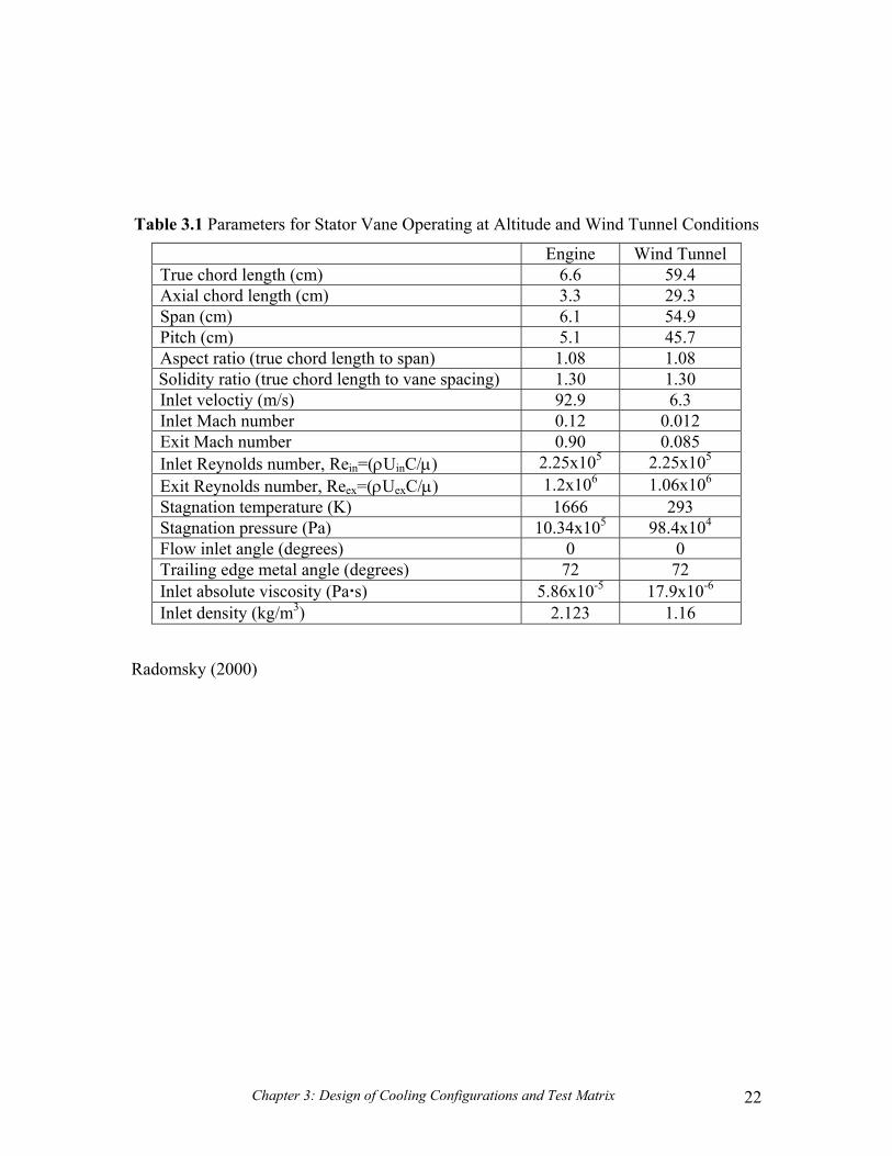
Chapter 3: Design of Cooling Configurations and Test Matrix 22

Table 3.1 Parameters for Stator Vane Operating at Altitude and Wind Tunnel Conditions

Engine Wind Tunnel True chord length (cm) 6.6 59.4 Axial chord length (cm) 3.3 29.3 Span (cm) 6.1 54.9 Pitch (cm) 5.1 45.7 Aspect ratio (true chord length to span) 1.08 1.08 Solidity ratio (true chord length to vane spacing) 1.30 1.30 Inlet veloctiy (m/s) 92.9 6.3 Inlet Mach number 0.12 0.012 Exit Mach number 0.90 0.085 Inlet Reynolds number, Rein=(ρUinC/µ) 2.25x105 2.25x105 Exit Reynolds number, Reex=(ρUexC/µ) 1.2x106 1.06x106 Stagnation temperature (K) 1666 293 Stagnation pressure (Pa) 10.34x105 98.4x104 Flow inlet angle (degrees) 0 0 Trailing edge metal angle (degrees) 72 72 Inlet absolute viscosity (Pa s) 5.86x10-5 17.9x10-6 Inlet density (kg/m3) 2.123 1.16

Radomsky (2000)

Chapter 3: Design of Cooling Configurations and Test Matrix 23

Table 3.2 Summary of Geometric Cooling Parameters for Both Cooling Configurations

Parameter Value Cooling hole l/d 8.3 Hole injection angle 30˚ p/d for leading edge holes 4 / 3 p/d for passage holes 3 Slot length to width 1.8 Upstream slot location of vane -0.31CaSlot injection angle 45˚

Table 3.3 Comparison of Features at Engine and Study Scales

Feature Engine Study Scale 1 9 Slot width, cm (in) 0.165 (0.065) 1.485 (0.585) Slot length, cm (in) 0.299 (0.118) 2.694 (1.061) Cooling hole diameter, cm (in) 0.051 (0.020) 0.457 (0.180) Cooling hole length, cm (in) 0.508 (0.200) 3.810 (1.500) Gutter width, cm (in) 0.127 (0.050) 1.143 (0.450) Cooling hole l/d 10 8.3

Chapter 3: Design of Cooling Configurations and Test Matrix 24

Table 3.4 Hole Center Locations and Angle from Axial Direction for Hole Pattern #1 Hole # X [m] Y [m] φ Hole # X [m] Y [m] φ

1 0.0248 -0.3555 0 34 0.1540 -0.1050 0 2 0.0134 -0.3479 0 35 0.1404 -0.1058 0 3 0.0020 -0.3404 0 36 0.1268 -0.1069 0 4 0.0705 -0.2926 0 37 0.2476 -0.0211 0 5 0.0600 -0.2838 0 38 0.2351 -0.0154 0 6 0.0495 -0.2750 0 39 0.2226 -0.0098 0 7 0.1112 -0.2426 0 40 -0.0253 -0.4570 0 8 0.1004 -0.2341 0 41 -0.0253 -0.4433 0 9 0.0896 -0.2257 0 42 -0.0418 -0.4069 90 10 0.0788 -0.2173 0 43 -0.0418 -0.3886 90 11 0.0679 -0.2089 0 44 -0.0418 -0.3703 90 12 0.0573 -0.2002 0 45 -0.0418 -0.3520 90 13 0.0482 -0.1899 0 46 -0.0418 -0.3338 90 14 0.0391 -0.1797 0 47 -0.0418 -0.3155 90 15 0.0300 -0.1694 0 48 -0.0418 -0.2972 90 16 0.0209 -0.1591 0 49 -0.0418 -0.2789 90 17 0.0144 -0.1471 0 50 -0.0418 -0.2606 90 18 0.0111 -0.1338 0 51 -0.0418 -0.2423 90 19 0.0078 -0.1204 0 52 -0.0418 -0.2240 90 20 0.0045 -0.1071 0 53 -0.0418 -0.2057 90 21 0.1422 -0.2033 0 54 -0.0418 -0.1875 90 22 0.1301 -0.1968 0 55 -0.0418 -0.1692 90 23 0.1180 -0.1903 0 56 -0.0418 -0.1509 90 24 0.1669 -0.1693 0 57 -0.0418 -0.1326 90 25 0.1537 -0.1656 0 58 -0.0418 -0.1143 90 26 0.1405 -0.1619 0 59 -0.0253 -0.0960 0 27 0.1902 -0.1340 0 60 -0.0253 -0.0823 0 28 0.1765 -0.1332 0 61 -0.0253 -0.0686 0 29 0.1628 -0.1324 0 62 -0.0253 -0.0549 0 30 0.2086 -0.1026 0 63 -0.0253 -0.0411 0 31 0.1949 -0.1032 0 64 -0.0253 -0.0274 0 32 0.1812 -0.1038 0 65 -0.0253 -0.0137 0 33 0.1676 -0.1044 0

Note – (0,0) is at dynamic stagnation point of center vane in three vane cascade

φ

y

x

Chapter 3: Design of Cooling Configurations and Test Matrix 25

Table 3.5 Hole Center Locations and Angle from Axial Direction for Hole Pattern #2 Hole # X [m] Y [m] φ Hole # X [m] Y [m] φ

1 0.0701 0.1606 0 27 0.2375 0.4121 45 2 0.0564 0.1606 0 28 0.2238 0.4121 45 3 0.0427 0.1606 0 29 -0.0253 0.0000 0 4 0.1108 0.2107 0 30 -0.0253 0.0137 0 5 0.0971 0.2107 0 31 -0.0418 0.0564 90 6 0.0834 0.2107 0 32 -0.0418 0.0746 90 7 0.1419 0.2505 0 33 -0.0418 0.0929 90 8 0.1282 0.2505 0 34 -0.0418 0.1112 90 9 0.1144 0.2505 0 35 -0.0418 0.1295 90 10 0.1673 0.2863 0 36 -0.0418 0.1478 90 11 0.1536 0.2863 0 37 -0.0418 0.2147 90 12 0.1398 0.2863 0 38 -0.0418 0.2330 90 13 0.0623 0.2863 0 39 -0.0418 0.2513 90 14 0.0485 0.2863 0 40 -0.0418 0.2695 90 15 0.0348 0.2863 0 41 -0.0418 0.2878 90 16 0.0211 0.2863 0 42 -0.0418 0.3061 90 17 0.1902 0.3227 0 43 -0.0418 0.3244 90 18 0.1765 0.3227 0 44 -0.0418 0.3427 90 19 0.0986 0.3227 0 45 -0.0253 0.3610 0 20 0.0849 0.3227 0 46 -0.0253 0.3747 0 21 0.0712 0.3227 0 47 -0.0253 0.3884 0 22 0.0574 0.3227 0 48 -0.0253 0.4021 0 23 0.0437 0.3227 0 49 -0.0253 0.4159 0 24 0.0300 0.3227 0 50 -0.0253 0.4296 0 25 0.0163 0.3227 0 51 -0.0253 0.4433 0 26 0.2086 0.3548 0

Note – (0,0) is at dynamic stagnation point of center vane in three vane cascade

φ

y

x

Chapter 3: Design of Cooling Configurations and Test Matrix 26

Table 3.6 Experimental and Computational Test Matrix

Case Slot Flow %min

Film Flow %min

Inlet Temp Profile

CFD Thermal Field

1S0F0 0.50 - - - Flat Y Y 2S0F0 0.75 - - - Flat N N 3S0F0 1.00 - - - Flat Y N 0S1F1 - - - 0.50 Flat Y N 0S1F2 - - - 0.50 Flat Y N 0S2F1 - - - 0.75 Flat N N 0S2F2 - - - 0.75 Flat N N 1S1F1 0.50 0.50 Flat Y N 1S1F2 0.50 0.50 Flat Y Y

1S1F2Bot 0.50 0.50 Bot N N 1S1F2Mid 0.50 0.50 Mid N N

2S1F1 0.75 0.50 Flat N N 2S1F2 0.75 0.50 Flat N N 1S2F1 0.50 0.75 Flat Y N 1S2F2 0.50 0.75 Flat Y Y 2S2F1 0.75 0.75 Flat N N 2S2F2 0.75 0.75 Flat N N

Key:

#S#F#Prof

Number Passage Number Flow Rate %min 0 No Film-Cooling No Cooling 1 1 0.50 2 2 0.75 3 - - - 1.00

Slot flow rate

Film flow rate

Passage Number

Chapter 3: Design of Cooling Configurations and Test Matrix 27

Figure 3.1 Characteristic lengths used to define airfoil geometry

Chord, C

Pitch, P

Axial Chord, Ca

α2

Chapter 3: Design of Cooling Configurations and Test Matrix 28

1

2

3

4

5

Gutter

1.1

1.2

1.4

1.6

2.1

2.2

2.4

2.6

1.5

2.5

SecondaryFlow Plane

1.3

2.3

Slot

Pattern #2

Pattern #1

Figure 3.2a The two film-cooling patterns that were designed for this study (Pattern #1 and #2) and labels for several specific film cooling holes. In addition, a secondary flow plane is identified that was used to evaluate the flow field.

Figure 3.2b Shown are the directions of the coolant hole injection along with iso–velocity contours (U/U1) and the gutter location for mating two turbine vane platforms.

U/U1 =

x

y

Leading Edge

Passage Holes

Chapter 3: Design of Cooling Configurations and Test Matrix 29

Figure 3.3 Critical dimensions of the slot and film-cooling holes at model scale (9X) . Note that the figure is not drawn to scale.

0.46cm 1.49cm

1.91cm Slot

45° 30°

Endwall Surface

Film-Cooling Hole

Vane

Chapter 3: Design of Cooling Configurations and Test Matrix 30

Figure 3.4 A turbine disc is shown with the gutter(s) marked. The stators shown are singlets, but stators are often grouped as doublets (Cohen, 2001).

Figure 3.5 Nozzle guide vane doublet shown with vane and endwall film-cooling holes. Gutters would be formed by adjoining another doublet to each side. Slot leakage would come from the upstream edge (Friedrichs, 1997).

Gutter

Gutter

Slot Gutter

Chapter 4: Computational Methods 31

Chapter 4

Computational Methods

Computational fluid dynamics (CFD) is a powerful tool which has become

invaluable in the modern design process of fluid machinery. CFD easily facilitates

parametric studies and allows a designer to test multiple design configurations at low

expense and in a brief time frame. Many choices must be made during the modeling

process, however, that automatically constrain the solution set before computation has

begun. Some decisions may not have an adverse effect on the results. The domain is

generally modeled in a geometrically correct fashion, but if a feature is unimportant to

the solution it may be altered without consequence. For example, a hexagonal bolt head

may be modeled as a cylinder if it is not in a region of interest. Other decisions may have

far more significant impacts, though. Are the boundary conditions appropriate? Is the

flow incompressible or should a variable density model be considered? Is transient

behavior important?

The focus of this chapter is to explain the modeling procedures and choices that

were made in this study. Section 4.1 describes the construction and meshing of the

model. Section 4.2 presents the applied boundary conditions. Section 4.3 discusses the

governing equations and the methods used to solve them. The turbulence model is

discussed in section 4.4. Much of the discussion in sections 4.3 and 4.4 was excerpted

from the thesis of Erik Hohlfeld. The convergence requirements as well as grid adaption

and the characterization of grid independence of results are presented in section 4.5.

Finally, section 4.6 describes the methods used to process the data from the

computational results.

4.1 Construction and Meshing of Model

The first step in the computational process is constructing the model. The model

was developed in Gambit, which is the modeling and meshing companion to the solver

Fluent. Five permutations of the model were constructed: (1) slot only; (2) film-cooling

pattern #1 without the slot; (3) film-cooling pattern #2 without the slot; (4) film-cooling

pattern #1 with the slot; and (5) film-cooling pattern #2 with the slot. Included in the

Chapter 4: Computational Methods 32

models were: the vane (modeled to midspan) with the pressure and suction surfaces

forming one passage, endwall , film-cooling holes, slot, and a 15.6° contraction which

was part of the combustor simulator section of the wind tunnel where experimental data

was acquired. Two views of the computational domain are shown in Figures 4.1a-b. The

combined slot and film-cooling models for each of the two patterns are shown in Figures

4.2a-b. The only differences are the location and number of film-cooling holes. The

coolant for the slot and film-cooling holes was supplied through two plenums allowing

individual control of the flow through both of the cooling features.

The model was built by starting with vertices defining all features. The vertices

were then connected forming lines and the lines were connected to form faces. Finally

the faces were stitched together to form the volumes. The main passage, as well as the

film-cooling holes and the film plenum were modeled as individual volumes to allow

greater control when meshing. The volumes were merged together to form a single

volume and the holes and plenum were then re-divided using split planes at the endwall

level and at the plenum level to regain the individual volumes. This step was necessary

to establish connections between the volumes so that the mesh would be conformal at the

volume interfaces.

Meshing proceeded in the same fashion. First the periodic faces, which will be

discussed in section 4.2, were linked so that the mesh on each matching face would be

identical. Next the edges were meshed to control the cell size. Features within the

passage were given uniform node spacing. The node spacing for each of these features is

given in Table 4.1. Edges upstream and downstream of the passage were graduated so

that the cell size would expand further away from the passage to avoid wasting cells in

areas where the flow was inviscid with few gradients. Table 4.2 lists the cell edge length

near the passage and the larger cell edge length away from the passage for these edges.

Next the faces were meshed with a tri-pave routine using the maximum node

spacing for the given feature. For example, the nodes within the passage were spaced 8

mm apart while the nodes in the holes were spaced only 2 mm apart. When meshing the

endwall, which is part of the passage but has the holes in it, the face mesh cell size was

specified as 8 mm. Therefore the maximum cell size was 8 mm, but near the holes the

cell size was reduced to 2 mm because of the conformal meshing routine. The mesh on

Chapter 4: Computational Methods 33

the endwall of each pattern is shown in Figures 4.3a-b. Finally the volumes were meshed

once again using the maximum desired cell edge length within the particular volume. An

unstructured mesh consisting of tetrahedral elements was generated. The holes were

meshed first with a cell edge length of 2 mm resulting in approximately 500 cells per

film-cooling hole. Then the hole plenum was meshed. The mesh in the holes and hole

plenum of pattern #2 is shown in Figure 4.3c. The reduced size of the cells near the holes

are clearly visible in this figure. Finally the main passage was meshed as shown in

Figure 4.4 resulting in approximately 7x105 cells in the model. It is seen that the mesh is

graduated so that larger cells exist near the inlet and outlet where the flow field is less

complex with smaller cells in the passage. The mesh is also graduated from the wall,

where viscous effects, are present to the midspan where the flow is inviscid.

4.2 Boundary Conditions

After meshing, the entire domain was specified as a continuum and boundary

conditions were applied as shown in Figures 4.1a-b. The vane was divided at the

dynamic stagnation point and trailing edge, and a single passage was modeled with

periodic boundaries specified in both the leading and trailing planes to reduce the size of

the model. The model size was further reduced by imposing a symmetry condition at

midspan. No-slip was imposed at the combustor wall, endwall, and vane surfaces. The

inlet to the domain was specified as a velocity inlet and located one chord upstream of the

contraction. Hermanson and Thole (2000) showed that a velocity inlet located at least

one chord upstream of the vane would exhibit no effects from the vane. The velocity

inlet gives the option to model various profiles as inlet conditions. For the cases

presented, however, only a uniform velocity of approximately Uin = 3.6 m/s and a

uniform temperature of Tin = 333.15 K were specified. Figures 4.5a-b show that at the

exit of the combustor, though, the inlet velocity is no longer uniform as a result of

pressure distortion by the vane immediately downstream. Also, a reference pressure of

101,325 Pa was specified at midspan in the center of the velocity inlet. An outflow

boundary was located 1.5C downstream of the trailing edge. In addition, a 0.5C

extension was added to the exit of the domain to avoid highly skewed cells at the domain

exit. As stated previously, the coolant was supplied through two plenums. Mass flow

Chapter 4: Computational Methods 34

inlets were imposed at the entrances of the plenums and the appropriate flow rate (kg/s)

at Tc = 291.15 K was specified for each computation.

4.3 Governing equations and solution methods

Computations were performed for incompressible, viscous, low-speed conditions

with an exit Reynolds number of Reex = 1.2x106 based on the vane chord. The

simulations were performed using the FLUENT commercial software package (Fluent

2002). FLUENT/UNS is a pressure-based, incompressible flow solver for unstructured

meshes. FLUENT/UNS allows for unstructured meshing capability and also allows

solution-adaptive mesh refinement in order to resolve regions of high gradients.

Solutions were computed on one of two UNIX computer systems: the SGI Origin 2100,

located in the VTExCCL computer laboratory and the ICAM SGI Origin 2000, located at

the Interdisciplinary Center for Applied Mathematics on the Virginia Tech campus. The

Origin 2100 is a four processor machine while the Origin 2000 has 32 processors.

Solution times varied substantially based on the mesh size and the number of processors

over which the model was distributed. Generally, a solution could be obtained within 48

hours when divided over 3-4 processors.

The Reynolds Averaged Navier Stokes (RANS) equations as well as the energy

and turbulence equations were solved using a control volume technique. Fluent offers

two solver options: a segregated solution algorithm (FLUENT/UNS) using a control

volume based technique or a coupled solver (RAMPANT) also employing a control

volume technique. The basic premise behind the segregated solver, which was used

exclusively in this study, involves the integration of the mass, momentum, energy and

turbulence equations for each unknown variable. The discretized equations are then

linearized with a solution of the resulting system of linear equations providing updated

results to the unknown variables.

The governing equations were solved sequentially employing an implicit form of

linearization where, for each variable, the value of interest in each cell was computed

through the use of equations that used both known and unknown values from various

neighboring cells. Ultimately each unknown appeared in a series of equations that must

Chapter 4: Computational Methods 35

be solved simultaneously. A converged solution requires multiple iterations and included

the following general process:

(1) fluid properties are updated with the current solution,

(2) the u, v, w momentum equations are each solved with current values for

pressure and mass fluxes to update the velocity field,

(3) the velocities from step one may not locally satisfy the continuity equation so

adjustments are made by correction equations so that continuity is satisfied,

(4) scalar equations are solved for such things as turbulence and energy with the

previously updated values from other variables, and

(5) a convergence check is made of the equations.

Fluent offers several discretization techniques for the convective terms of each

governing equation. Using the segregated solver, the operator may choose to have either

first or second order discretization of terms. The first order method computes the

solution at the center of each cell while the second order method computes the solution at

the center of each face (Fluent 2002). The first order discretization is generally

acceptable for simple flows when the grid is aligned with the flow and a quadrilateral or

hexahedral grid is in place. A second order discretization method reduces errors over the

first order methods, while generally increasing the difficulty of obtaining a converged

solution. For triangular and tetrahedral grids when the flow is not aligned with the grid, a

second order method is recommended for superior results. The second order

discretization was used for all simulations in this study.

Pressure and velocity were coupled with the Semi-Implicit Method for Pressure

Linked Equations (SIMPLE) algorithm. SIMPLE uses a relationship between velocity

and pressure corrections to obtain mass conservation and a pressure field. The pressure

discretization scheme was the default value, Standard.

Before beginning computation, the flow within the model must be initialized

based on some condition within the model. This initialization process acts as an initial

guess at the solution of the flow field. The flow field was initialized by the inlet

conditions to the model for all simulations.

Chapter 4: Computational Methods 36

4.4 Turbulence and near-wall modeling

Because of the numerous cooling jets injecting through the endwall, the boundary

layer was assumed turbulent. All simulations employed the RNG k-ε turbulence model

with non-equilibrium wall functions. Past studies by Hermanson (1999) and Radomsky

(2000) have shown this method to adequately model secondary flows within a turbine

passage. The RNG k-ε model was derived from the instantaneous Navier-Stokes

equations. The analytical derivation results in a model with constants that are different

from those used with the standard k-ε models. Additional terms and functions are also

present in the transport equations for k and ε.

An RNG k-ε turbulence model is generally very similar in form to the k-ε model,

with the following refinements:

(1) the RNG model has an additional term in its ε equation that significantly

improves the accuracy for rapidly strained flows (such as that seen in a blade

passage),

(2) the effect of swirl on turbulence is included in the RNG model, enhancing

accuracy for swirling flows,

(3) the RNG theory provides an analytical formula for turbulent Prandtl numbers,

while the standard k-ε model uses user-specified, constant values, and

(4) while the standard k-ε model is a high-Reynolds-number model, the RNG

theory provides an analytically-derived differential formula for effective

viscosity that accounts for low-Reynolds-number effects. Note that effective

use of this feature does depend on an appropriate treatment of the near-wall

region.

Two approaches to predicting the near-wall region are illustrated in Figure 4.6.

The near-wall flow can be predicted through near-wall modeling or the use of wall

functions. The near-wall modeling approach involves a very fine mesh near the wall that

must transition to a larger mesh in the free stream. The near-wall model permits the

viscosity-affected region to be fully resolved all the way to the wall. Wall functions do

Chapter 4: Computational Methods 37

not fully resolve the viscous sub-layer and buffer layer, leaving semi-empirical formulas

to bridge the viscosity-affected region between the wall and the mainstream turbulent

flow. Within the figure notice that the wall functions method maintains a relatively large

mesh from the free stream down to the wall where the wall models take over.

The wall-function approach offers a significant savings in computational

resources over near wall modeling by using a collection of formulas and empirical data to

approximate laws-of-the-wall for mean velocity and temperature and formulas for near-

wall turbulent quantities. There are some instances when wall functions may not always

be accurate because of a departure from ideal conditions that include strong body forces,

severe pressure gradients which may lead to boundary layer separation, highly three-

dimensional effects near the wall, and large blowing and suction around the wall.

Fluent offers two types of wall functions: standard wall functions and non-

equilibrium wall functions, both of which require the non-dimensionalized y+ values of

turbulence to be resolved to levels between 30 and 60. The standard wall functions are

based on proposals by Launder and Spalding (1974) while the non-equilibrium wall

functions offer several modifications to the standard function. Included in these

modifications is a log-law that is sensitized to pressure-gradient effects and the two-layer-

based concept that computes turbulent kinetic energy in neighboring cells. Generally,

non-equilibrium wall functions are considered more robust and accurate than the standard

wall function. Because of limited computing power, non-equilibrium wall functions were

used in all computations in this study to approximate the viscous near-wall layer.

The free stream turbulence intensity was set at 1% with a dissipation length scale

of 0.1m. This low turbulence was set because an industrial application was being

simulated where large dilution jets are not used in the combustor to mix the flow.

4.5 Convergence, Grid Adaption and Independence

The basic method employed in this study to judge the convergence of a solution

involved monitoring the normalized residuals of the continuity, x-, y- and z- momentum,

energy, k and ε after each iteration. The normalized residuals are calculated by first

finding the unscaled residuals. The unscaled residuals are the result of computations that

have some numerical errors and as these solutions run through many iterations the

Chapter 4: Computational Methods 38

numerical errors become smaller and smaller, normally dropping several orders of

magnitude. In order to judge convergence it is most convenient to monitor the scaled

(normalized) residuals. Taking the largest residual values from the initial iterations and

dividing each subsequent residual value by this number will provide a scaled residual.

Most models experience significant noise in the residual values during the initial

iterations followed by a smooth decaying slope of these quantities.

There is no exact rule for determining when a solution is complete. Fluent has

default residual values of convergence set to 10-3 for all quantities except energy, which

is set to 10-6. For this study the residual levels for convergence were lowered to values of

10-4 with the exception of energy which was required to reach 10-7.

During initial computations the residuals would decline for approximately 200

iterations before going unstable as shown in Figure 4.7a. To prevent this problem, the

under relaxation factors were reduced to the values listed in Table 4.3. When computing

a solution the value of interest, φ, is computed at each step by:

φ∆α+φ=φ oldnew (4.1)

where 0 ≤ α ≤ 1 is called the under relaxation factor. Reducing the under relaxation

factors acts as a numerical brake to slow and control the computation. Originally all

under relaxation factors were reduced to the values suggested in the Fluent manual to

prevent instability. This was effective, but the convergence of the solution was quite

slow. Then, because the instability originated in the energy equation and a constant ideal

gas density model was used, only the energy and density under relaxation factors were

reduced. As seen in Figure 4.7b, this was effective in controlling the convergence of the

solution while still converging at a reasonable rate.

For this study a solution was computed for 1000 iterations after which the

residuals had not reduced to the convergence limits of 10-7 for energy and 10-4 for

everything else, but the solution was unchanging. The grid was then adapted based upon

y+ values and temperature and velocity gradients. All cells where 30 ≤ y+ ≤ 60 was not

true were marked for adaption. Then the maximum temperature and velocity gradients

were calculated and any cells with gradients higher than half of the maximum were

marked for adaption. The gradient marking technique generally only resulted in a few

thousand marked cells most of which had already been marked because of y+ values. The

Chapter 4: Computational Methods 39

grid was then adapted using the hanging node method illustrated in Figures 4.8a-c. Each

cell is subdivided along each leg resulting in eight tetrahedrons from a single tetrahedron

shown in Figure 4.8c. The method is called hanging node because, as shown in Figure

4.8a, adapted cells will have nodes that are not shared with a neighboring cell. This

results in a non-conformal grid at these locations. The adapted grid on the endwall is

shown in Figures 4.9a-b. It is important for the user to note that cells may only be

expanded (combined) in a 2-D grid and then the combination of cells is limited to the

original grid (original cells may not be combined to generate super cells). Therefore, it is

preferable to start with larger cells and adapt in the necessary areas rather than starting

with a grid that is too fine. After adaption the computation was continued for another

1000 iterations. The adaption results in a large increase in the residuals during the first

few iterations as seen in Figure 4.7b. Another adaption was performed resulting in a

mesh with approximately 1.3x106 cells, and finally 1000 more iterations were computed.

To evaluate whether results were grid independent, the lift coefficient and area-

averaged endwall temperature were also monitored after each iteration. As seen in

Figures 4.10a-b, these values are relatively constant even after the two grid adaptions.

After adapting from a mesh size of 8.5x105 to 1.3x106 cells the area-averaged

effectiveness predictions on the endwall were found to vary by only ∆η = ±0.005 at a

level of η = 0.11 indicating that the solution was converged and grid independent despite

failing to reach the specified residual levels. In order to use these additional monitors, a

solution was first computed for five iterations to get the solution started and then the

monitors were activated.

4.6 Data Post-Processing

To visualize the secondary flow patterns throughout the passage a method was

developed by Hermanson and Thole (2000) where secondary flow vectors are presented

as in plane deviations from the midspan streamlines. The calculation procedure is given

in equations 4.2 through 4.12 and illustrated in Figure 4.11. Fluid flow at the mid-span is

assumed as the reference condition because no viscous effects are present. Variations

from this reference flow path are plotted as secondary flows within the turbine passage.

The general methodology employed for this visualization technique involves a

Chapter 4: Computational Methods 40

transformation from the global -X, -Y, -Z, -U, -V, -W system to a local –x, -y, -z, -u,-v, -

w system. The entire transformation is based on the rotation, φ, of a plane normal to the

vane surface from the axial direction. The in plane calculations are as follows:

x = X cos φ + Y sin φ (4.2)

y = -X sin φ + Y cos φ (4.3)

z = Z (4.4)

u = U cos φ + V sin φ (4.4)

v = -U sin φ + V cos φ (4.6)

w = W (4.7)

Phi was calculated from known points along the vane surface on either side of the plane

∆X∆Ytan 1−=φ (4.8)

The flow angle of the inviscid flow at the midspan was calculated from:

ms

ms1ms u

vtanΨ −= (4.9)

After obtaining an angle for Ψms, a translation from the local coordinate system

consisting of -x, -y, -z and -u, -v, -w to a coordinate system in the form of a tangential

and normal component to the inviscid streamline was necessary. The equations used for

this transformation consisted of the following:

Vs = u cos Ψms + v sin Ψms (4.10)

Vn = -u sin Ψms + v cos Ψms (4.11)

Vz = w (4.12)

This concluded the transformation. Plots were then constructed with the components Vn

and Vz illustrating the off-axis flow phenomena (secondary flows).

Two dimensionless thermal values were also computed. The adiabatic

effectiveness level, η, and the dimensionless temperature, θ, represent surface and fluid

temperatures respectively. They are calculated in the same fashion:

∞

∞

−−

=ηTTTT

c

aw (4.13)

∞

∞−−

=θTTTT

c (4.14)

Chapter 4: Computational Methods 41

Once adiabatic effectiveness is known the temperature at the wall is simply a function of

the coolant and mainstream flow. This is obtained experimentally by using a wall

material of low thermal conductivity while computationally a wall boundary condition is

set as adiabatic. For a value of η = 1, the wall would have the same temperature as the

coolant and we would say the coolant effectiveness is at a maximum. For a value of η =

0, the coolant would have no effect on the wall temperature since it would be the same

temperature as the mainstream flow. Simply put, surface adiabatic effectiveness

measures the local fluid temperature. When measuring heat transfer within an engine

often times the adiabatic wall temperature, Taw, is used as shown in equation 4.15.

)TT(hq aww"w −= (4.15)

So, if the adiabatic wall temperature and heat transfer coefficient, h, are known then the

metal temperature, Tw, can be predicted for any maximum and coolant temperatures and a

given heat flux, or the heat flux can be determined from surface temperature

measurements.

Non-dimensional fluid temperature is presented as θ and similar to adiabatic

effectiveness varies from zero to one. A value of zero corresponds to a fluid temperature

of the mainstream gas, T∞, while a value of one corresponds to the temperature of the

coolant, Tc. Normalizing the thermal field in this fashion allows for a direct comparison

between the thermal field temperatures and the surface temperatures.

With all of the computational methods laid out and presented within this chapter,

along with a general understanding of the data analysis techniques, the results from the

computations are presented in chapter 6.

Chapter 4: Computational Methods 42

Table 4.1 Cell Edge Length in Regions of Constant Cell Size Feature Cell Size (mm)

Holes 2 Hole Plenum 8 Slot 8 Slot Plenum 8 Endwall 8 Outflow 20

Table 4.2 Beginning and Ending Cell Edge Length in Regions of Graduated Mesh Size Edge Start Cell Size (mm) End Cell Size (mm)

Contraction Entrance to Contraction Exit 14 8

Velocity Inlet to Contraction Entrance 24 14

Inlet at Endwall to Inlet Midspan 24 30

Inlet at Midspan to Contraction Exit 30 8

Trailing Edge to OutFlow 8 20

Table 4.3 Various Settings for Under Relaxation Factors Variable Default Fluent Modified Partially Modified

Pressure 0.3 0.2 0.3 Density, ρ 1 0.8 0.7 Body Force 1 0.8 1 Momentum 0.7 0.5 0.7 Turbulence Kinetic Energy, ε 0.8 0.5 0.8 Turbulence Dissipation Rate, κ 0.8 0.5 0.8 Turbulent Viscocity 1 0.8 1 Energy 1 0.8 0.7

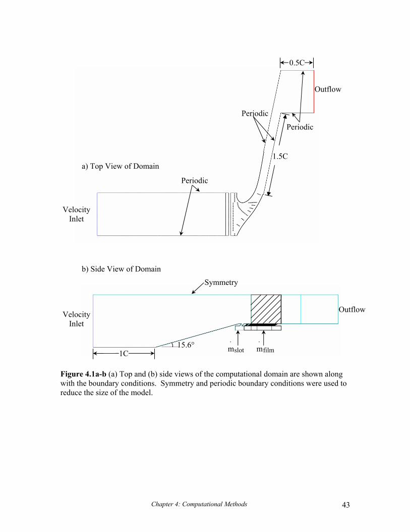
Chapter 4: Computational Methods 43

Figure 4.1a-b (a) Top and (b) side views of the computational domain are shown along with the boundary conditions. Symmetry and periodic boundary conditions were used to reduce the size of the model.

a) Top View of Domain

b) Side View of Domain

Velocity Inlet

Velocity Inlet

Outflow

Outflow

Symmetry

Periodic

Periodic

Periodic

slotm⋅

filmm⋅

0.5C

1.5C

1C 15.6°

Chapter 4: Computational Methods 44

Figure 4.2a-b Models for the slot combined with (a) film pattern #1 and (b) film pattern #2 are shown with one periodic repeat. Models were also developed for each film-pattern without the slot and for the slot without film-cooling.

a) b)

Chapter 4: Computational Methods 45

Figure 4.3a-c The face mesh on the endwall for (a) pattern #1 and (b) pattern #2 is shown. (c) The film-cooling holes and the film-cooling plenum were individually meshed. The reduction of cell size near the holes to maintain a conformal mesh is clearly visible.

a) b)

c)

Chapter 4: Computational Methods 46

Figure 4.4 The volume mesh for the entire domain is shown. The mesh is graduated so that larger cells exist near inlet and outlet where the flow field is less complex with smaller cells in the passage. The mesh is also graduated from the wall, where viscous effects are present, to the midspan where the flow is inviscid.

Chapter 4: Computational Methods 47

Figure 4.5a-b (a) While a uniform temperature and velocity profile are specified at the inlet to the vane, (b) at the combustor exit the approaching velocity field is distorted by the vane downstream.

1C

15.6°

1.4C

0.13C

Coolant

U1

Plane 1

Inlet Flow

Vane

0

0.2

0.4

0.6

0.8

1

1.2

-0.5 0 0.50

0.25

0.5

0.75

1

y/P

z/S

U/U1

a)

b)

Chapter 4: Computational Methods 48

Figure 4.6 The two methods for modeling the viscous boundary layer are illustrated. In the wall function approach, semi-emperical relations are used to predict the boundary layer while thin elements are used to compute the boundary layer in the near-wall modeling approach (Fluent 2002).

Viscous sublayer

Wall Function Approach Near-Wall Model Approach

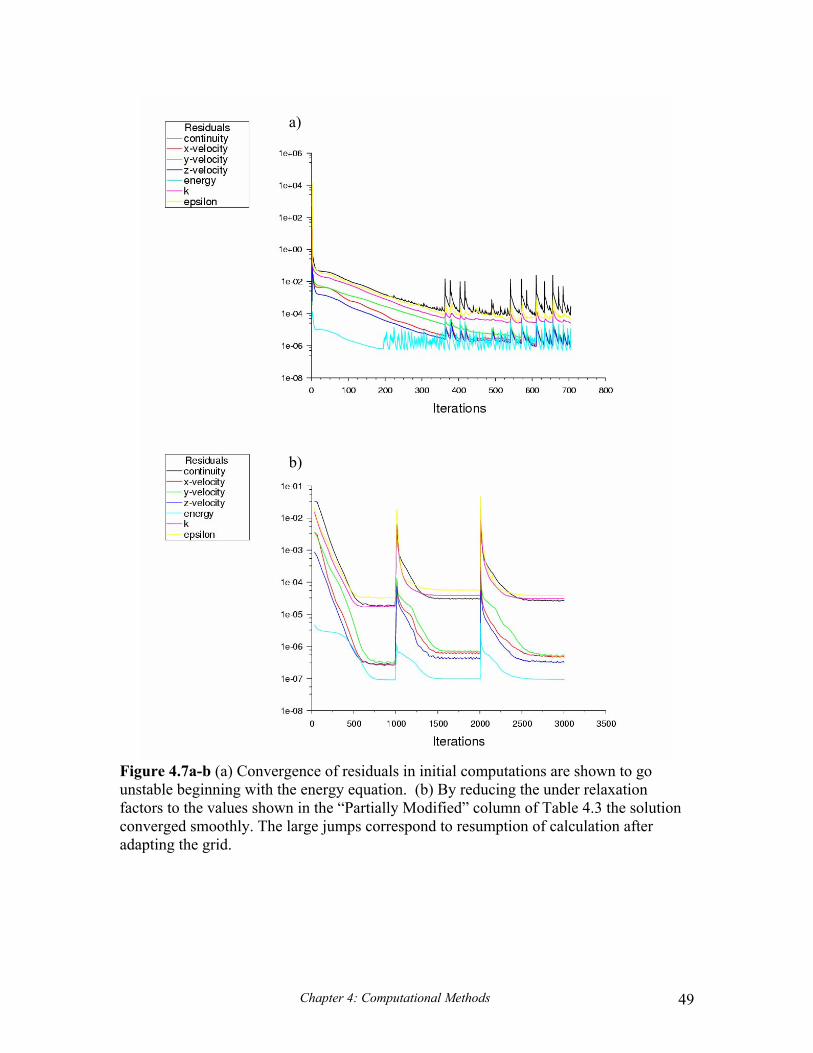
Chapter 4: Computational Methods 49

Figure 4.7a-b (a) Convergence of residuals in initial computations are shown to go unstable beginning with the energy equation. (b) By reducing the under relaxation factors to the values shown in the “Partially Modified” column of Table 4.3 the solution converged smoothly. The large jumps correspond to resumption of calculation after adapting the grid.

a)

b)

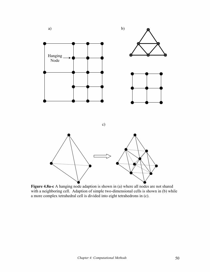
Chapter 4: Computational Methods 50

Figure 4.8a-c A hanging node adaption is shown in (a) where all nodes are not shared with a neighboring cell. Adaption of simple two-dimensional cells is shown in (b) while a more complex tetrahedral cell is divided into eight tetrahedrons in (c).

a) b)

c)

Hanging Node

Chapter 4: Computational Methods 51

Figure 4.9 The endwall grid is shown before and after adaption. Cells were added near the throat and along the vane surfaces to capture the accelerating flow.

Original Adapted

Chapter 4: Computational Methods 52

Figure 4.10 The lift coefficient and area-averaged endwall temperature were used to evaluate grid independence of the results. The lift coefficient and average endwall temperature were not significantly altered despite adapting the grid after 1000 and 2000 iterations.

CL

(K)

Chapter 4: Computational Methods 53

Figure 4.11 Multiple coordinate systems are used to define the secondary flow vectors.

φ

X,U

Y,V

x,u y,v

ψms s,Vs

n,Vn

Z,W

z,w

z,Vz

Chapter 5: Experimental Facility and Methods 54

Chapter 5

Experimental Facility and Methods

Before presenting experimental results it is necessary to discuss the facility in

which data was acquired. It is also important to detail data collection methods,

measurement tools, and to explain the development of any data processing techniques.

This chapter is dedicated to providing an overview of the facility and its capabilities. The

chapter is also intended to elaborate on all instrumentation used in data collection and to

explain the methods of setting up experiments and collecting and post processing data.

Section 5.1 provides an overview of the entire wind tunnel facility. The

capabilities of the facility and the main components encountered by the flow are briefly

discussed. Section 5.2 provides a more thorough discussion of the flow conditioning

elements in the facility. Specific settings for this study are also presented. Section 5.3

details the construction of the slot and film-cooling test plate. Section 5.4 presents a

general discussion of plenums and their usage as well as discussing the plenums and flow

controllers used in this study. Section 5.5 details the instrumentation used for data

collection in this study. The pressure taps and transducers, pitot tube, thermocouples,

data acquisition system, and infra-red camera are discussed. Section 5.6 details the

methods of setting experimental flows. The development of a global discharge

coefficient to quantify mass flow through the film-cooling holes is discussed. Section 5.7

explains the collection, calibration, and mapping of endwall thermal images. The

transition matrix method used to locate images in the global frame is explained. Section

5.8 briefly discusses the repeatability of experimental results. Finally, Section 5.9

quantifies the uncertainty of experimental results.

5.1 Wind Tunnel Overview

All experimental data presented in this study was collected in a large scale, low

speed, closed loop, non-rotating wind tunnel facility owned and operated by the Virginia

Tech Experimental and Computational Convection Lab (VTExCCL). The laboratory is

located in Randolph Hall on the main campus of Virginia Tech in Blacksburg, Virginia.

A diagram of the facility is shown in Figure 5.1. The flow in the wind tunnel is driven by

Chapter 5: Experimental Facility and Methods 55

a 50 hp, 0-60 Hz Joy Technologies axial vane fan, seen in Figure 5.2, which is controlled

by a Toshiba variable frequency inverter. Downstream of the fan, the flow is turned by a

90° elbow and passes through the primary flow, finned-tube heat exchanger used to cool

the bulk flow. After being turned by another 90° elbow, the flow encounters a three-way

flow split. Flow passing through the upper or lower passage, which are shown in blue in

Figure 5.1, is used as coolant while flow passing through the center passage simulates

heated primary or core flow.

Downstream of the flow split, the primary flow passes through a perforated plate

with 24.6% open area (0.269 m2), shown in Figure 5.3, to obtain the proper pressure drop

in the main gas path and force some of the air into the bypass legs. The core flow then

passes through a heater bank, a series of screens used for flow straightening, and into the

combustor simulator. The combustor simulator has a fixed span segment and then a 2-D,

15.6° contraction in the vertical direction leading to the vane cascade. In the cascade two

full passages are modeled with three vanes. A bleed is positioned on either side of the

two-passage cascade to remove edge effects from the side walls of the combustor

simulator and to balance the flow through each passage insuring periodicity of the inlet

flow. Periodicity of the facility has been documented by Kang et al. (1999).

The flow passing through the upper and lower bypass channels is used to simulate

coolant flow. Only the lower bypass channel was used for this study. The bypass flow in

each channel passes through a secondary finned-tube heat exchanger, where it is cooled

below the bulk flow temperature, and into the combustor simulator bypass. At this point,

the flow encounters a series of plenums below the combustor liner panels as seen in

Figure 5.4. No combustor cooling was simulated in this study because an industrial

application was being simulated where methods other than film-cooling are used for

combustor liner cooling. Therefore, the plenums were closed off and the combustor liner

panels were covered over with thin Lexan sheets. The coolant flow instead passes

through the end wall of the combustor simulator into two separate plenums as shown in

Figure 5.5. One plenum is used for slot coolant and the second plenum is used for

endwall film-cooling.

The coolant is injected into the cascade through either the slot or the film-cooling

holes and travels through the passage along with the core flow. The flow from the bleed

Chapter 5: Experimental Facility and Methods 56

channels is reintroduced beyond the passage, and the bulk flow exits the modular test

section. The flow is then turned by another 90° elbow and returned to the fan.

5.2 Thermal Conditioning System

Actual engine operating conditions could not be simulated due to many factors

including: size of the facility, equipment limitations, required power, and thermal

limitations of wind tunnel materials. It was, however, desirable to obtain as large of a

temperature difference as possible within these constraints. As was briefly discussed in

the previous section, the flow passes through a series of flow conditioning elements in

order to simulate hot core flow gases and cooler bypass gases. A temperature difference

of 35 °C - 42 °C was achieved between the mainstream and coolant flows as a result of

this thermal conditioning. Typical operating conditions for the thermal conditioning

elements are shown in Table 5.1.

The primary flow, finned-tube heat exchanger is located downstream of the fan,

and two smaller finned-tube heat exchangers are located in the bypass legs of the

combustor simulator section. These heat exchangers can be run with either chiller or tap

water. The primary heat exchanger is used to cool the bulk flow after the fan, while the

secondary heat exchanger is used to further cool the bypass air in the combustor

simulator.

A 40 kW Freeze Co. Systems chiller is available to supply cooling water to the

heat exchangers. The compressor is programmed to shut off once the outgoing cooling

water reaches 7.2 ° C in order to prevent pipe freeze. Unfortunately, because the airflow

rate was so low in the secondary channel, the heat load was not large enough to prevent

the chiller from cycling on and off. Because of this cycling problem, tap water was used

as a coolant supply rather than chilled water. Both the primary and secondary heat

exchanger were typically run at 26.5 lpm. The bypass air was cooled to 12-18 ° C using

tap water in the heat exchangers.

Downstream of the perforated plate, the core flow passes through a section of

finned, electric heating elements, shown in Figure 5.6, which are used to simulate hot

combustion gases in a turbine engine. The heater section contains three parallel heater

banks with each having six Watlow heating elements. The heating elements have a

Chapter 5: Experimental Facility and Methods 57

resistance of 75 ohms each and are stacked vertically and perpendicular to the flow

stream. Each bank of heaters is independently controlled by a Watlow Series 988

controller, shown in Figure 5.7, allowing different inlet temperature profiles to be

generated. The user must specify the percentage of total available power supplied to each

of the three banks. The heaters are powered by an industrial 3-phase, 480 volt line.

The banks are wired in a 3-Phase Delta configuration, shown in Figure 5.8, where

each leg consists of two elements wired in parallel with an effective leg resistance of 37.5

ohms. The total available heating power for each bank can be calculated from:

( )bank

W432,185.37V4803

RV3P

22L

Delta =Ω

=⋅

= (5.1)

The delta configuration provides an available power of 18,432 W to the lower, middle,

and upper heater banks resulting in a total of 55,296 W of available heating power. In

order to counter buoyancy effects and maintain a uniform temperature profile, the lower,

middle, and upper heater banks were typically run at 80, 82, and 50 percent of full power

respectively resulting in an 11 °C temperature increase across the heater section.

Representative temperature profiles that were generated will be presented in chapter 7.

5.3 Construction of Endwall Test Plate

When designing the endwall test surface, two goals were to achieve the proper

flow length for the cooling holes and to limit conduction through the surface as much as

possible. The engine scale design called for l/d = 10 for the film-cooling holes. A test

plate thickness of 1.9 cm (0.75 in) was selected because it most closely approximated the

design length scale yielding l/d = 8.3. Last-A-Foam FR6708 was selected as the endwall

material because of its extremely low 0.033 W/m·K thermal conductivity. Last-A-Foam

is a closed cell foam manufactured by General Plastics Manufacturing Co. of Tacoma,

Washington. To insure the precision and integrity of the cooling hole pattern, the holes

were cut with a five-axis water jet cutting machine by Springfield Manufacturing in

York, South Carolina. Portions of the hole patterns are shown in Figures 5.9a-b. A 1.27

cm thick sheet of Lexan was attached to the underside of the foam to provide stiffness to

the structure during the water jetting process. The Lexan backing was retained for

Chapter 5: Experimental Facility and Methods 58

stiffness purposes when the endwall test plate was constructed. Large holes were cut in

the Lexan beneath the film-cooling holes, to insure that the Lexan did not alter airflow

into the holes and to maintain the proper p/d for the holes. Five hole diameters were left

between the holes and the Lexan backing. Finally, the endwall surface was painted black

to enhance the radiative emissivity of the surface. This was because an infra-red camera,

which measures radiation, was used to image the test surface.

The slot, shown in Figure 5.10, was constructed from balsa wood which had the

same thermal conductivity as the FR6708 foam but was stiffer. Stiffness was important

because the slot had a 1.18 m unsupported span. The balsa wood extended 0.32 cm

downstream of the slot and 11.4 cm upstream of the slot to the contraction exit as shown

in Figures 5.11a-b. The downstream edge of the slot was 0.35Ca upstream of the

dynamic stagnation point.

5.4 Coolant Plenums

Coolant air for the slot and the film-cooling holes was provided from two separate

plenums. A plenum is a supply chamber where the fluid is stagnant. In general fluid

energy can be stored in three basic forms: static pressure, dynamic pressure, and

elevation head, as shown by the Bernoulli equation.

elevation

dynamic

2

statics

totalo gzV

21 p P ρ+ρ+=

321 (5.2)

In the plenum, there is no velocity and elevation head is negligible if the datum is at

plenum level, so all the energy is stored in the pressure head. Therefore, the total

pressure is equal to the static pressure. Energy is a conserved quantity, so if one head is

increased, the others will decrease accordingly. Because air has relatively low density,

the elevation head may be neglected except for drastic changes in altitude. Therefore, if

the coolant is fed from a plenum one can deduce the coolant flow rate by measuring the

difference between the pressure in the plenum, and the pressure at the location where the

coolant exits.

Two supply plenums, seen in Figures 5.12 and 5.13, were constructed to provide

independent control of the slot and film-cooling flow rates. The front plenum supplied

Chapter 5: Experimental Facility and Methods 59

the slot flow, and the rear plenum supplied the film-cooling. Flow into the plenums was

fed through two slots from the combustor bypass flow shown in Figures 5.14a-b. The

slot flow was controlled by a window shutter mechanism, where a rod is connected to

several short covers in a track. When the rod is pushed or pulled the window covers slide

back and forth in the track to expose or cover an open section behind them. A typical

shutter mechanism is shown in Figure 5.15. A splash plate was positioned just above the

shutter, as shown in Figure 5.16, to aid in mixing the slot coolant.

Flow into the film-cooling plenum was controlled by a lift gate. The gate was

connected to a threaded rod by two arms attached to nuts. When the crank on the

threaded rod was turned the nuts would move down the rod and pull the arms thereby

lifting the gate. The threaded rod, rocker arms and gate, as well as the pushrod used to

open and close the window shutters and the gate crank, may be seen in Figures 5.16 and

5.17.

5.5 Instrumentation

Several different types of instrumentation were used to document the flow

conditions and record data. Pressure taps were used to deduce coolant flow rates and

document the flow conditions around the vane, and a pitot tube was used to measure the

inlet flow velocity. Thermocouples measured the freestream temperature, coolant

temperatures, and temperature at several locations on the endwall. Thermal fields were

documented for three cases with a thermocouple rake. All pressure and temperature data

was collected using LabVIEW virtual instruments and a National Instruments SCXI data

acquisition (DAQ) system. The endwall thermal distribution was recorded with an infra-

red camera.

Static pressure measurements were taken using 0.156 cm diameter copper tubes

connected to nylon hose made by Scani-Valve. The pressure taps were grouped by

expected pressure reading and connected to one of three 24 channel Scani-Valve wafers,

shown in Figure 5.18, allowing three simultaneous pressure measurements. Each of the

three wafers had a single output channel which was connected to one of eight pressure

transducers manufactured by Setra and Omega and housed in a box shown in Figure 5.19.

The pressure transducers measure voltage and convert that to a corresponding pressure.

Chapter 5: Experimental Facility and Methods 60

The transducers, which were wired in parallel, required between 9 and 30 volts each and

were powered by two 12 volt lantern batteries wired in series. The voltage readings were

output to the DAQ via BNC cables.

Thirty-one pressure taps were positioned along the vane to record the pressure

distribution, and three pressure taps were located in each of the two plenums as well as

three pressure taps 2.54 cm upstream of the slot on the endwall to document the coolant

flows. The endwall pressure taps were spaced 22.86 cm (0.5P) apart to capture variations

in static pressure from upstream of the leading edge to upstream of the passage centers.

A variation of 5 Pa (2.7% to 23.8% of the driving pressure difference depending on the

pattern and flow rate) was typically seen from the leading edge pressure tap to the taps

located upstream of the passages and the static pressure upstream of pattern #2 was

generally 0.5 Pa (0.27% to 2.27% of driving pressure difference) higher than upstream of

pattern #1.

The inlet velocity was measured with a pitot tube, shown in Figures 5.20a and b.

The pitot tube contains two concentric tubes. One tube has a small opening at the tip of

the probe. Flow enters the hole and stagnates yielding the stagnation pressure of the flow

stream. The second tube has four small holes around the perimeter of the pitot probe

used to measure the static pressure of the flow stream. When the total pressure is

measured against the static pressure, the dynamic pressure is recorded yielding the

velocity and allowing the mass flow rate to be calculated. The inlet velocity was

measured at seven different locations, as shown in Figure 5.21, and averaged to obtain

the inlet flow velocity. Higher velocities were seen upstream of the passages and lower

velocities upstream of the vanes with a typical range of approximately 1.27 m/s.

Type E thermocouples, consisting of chromel (+) and constantan (-), were used

for all thermal measurements. An arc welder was used to fuse the positive and negative

wires together forming a small, round bead. When exposed to a given temperature, each

material heats up generating a current in the wire. The difference between the positive

and negative wires creates a voltage drop, which is used to determine the temperature that

the thermocouple is experiencing. Five thermocouple strips were also used consisting of

chromel and constantan ribbons that were soldered together. The strip thermocouples,

which lie flush on the surface, were to verify the temperatures that were being recorded

Chapter 5: Experimental Facility and Methods 61

by the thermocouple beads and insure that surface temperatures, rather than air

temperatures, were being reported. Agreement within 0.1°C or better was found between

the strip and beaded thermocouples located within one inch of each other upstream of the

cascade.

Two thermocouples were located on each of the three vanes at 5% span and 30%

span. These thermocouples helped monitor variations along the vane in the span-wise

direction as well as variations from passage to passage of the incoming flow. At high

film-cooling rates the thermocouples near the endwall measured cooler temperatures than

the free stream thermocouples as a result of coolant from the leading edge holes

separating and impacting the vane. Variations in free stream temperature from passage to

passage were generally less than 1.5 °C or ∆θ ≤ 0.0375. When normalizing surface

temperatures to adiabatic effectiveness, the average temperature from the thermocouple

at 30% span on the center vane was always used as the maximum temperature. Three

thermocouples were also located in both the slot and film-cooling plenums with one

thermocouple beneath each of the passages and one beneath the center vane. These

thermocouples allowed gradients in the coolant supply to be documented. Variation

within the plenums was generally less than 0.3 °C or ∆θ ≤ 0.0075. When normalizing

surface temperatures to adiabatic effectiveness, the average temperatures from the

thermocouple beneath the passage of interest and the thermocouple below the center vane

were averaged to determine the coolant temperature.

The endwall, vane, and plenum thermocouples were also used to document when

steady state was achieved. Six endwall thermocouples from various locations in the

passages as well as the center vane, free stream thermocouple and a thermocouple from

each of the two coolant plenums were documented at ten minute intervals. The range

between the free stream thermocouple and the coolest plenum thermocouple was also

calculated. Once the temperatures and temperature difference were stable for 30 minutes,

a steady state was assumed. This was satisfactory because data collection could be

completed in approximately 15 minutes. Typical time to steady state from a cold startup

of the wind tunnel was 3 hours. If flows were adjusted for a second data set collection,

steady state was generally re-achieved in 1 ½ hours.

Chapter 5: Experimental Facility and Methods 62

A thermocouple rake, illustrated in Figures 5.22a-c was used to document the

thermal field for several cases. The rake had 16 probes spaced 0.635 cm apart. The

thermocouple wire diameter was 0.3 mm, and the bead diameter was approximately 0.8

mm. The beads were positioned 0.6 cm below the fingers to eliminate any conduction

heating from the fingers that might alter the bead temperature. The rake was lowered into

the passage from a boom, shown in Figure 5.23a-c, and moved by a computer controlled

traverse. A single thermocouple moved by a computer controlled traverse was used to

document the inlet temperature profile in the combustor simulator section.

Voltage outputs from the thermocouples and pressure transducers were handled

by the National Instruments DAQ system shown in Figures 5.24a-d. Voltage outputs

were connected to a 32 channel SCXI-1303 terminal block which was plugged into one

of three SCXI-1100 modules. The modules serve as multiplexers and amplifiers. The

modules switch between all 32 input channels and output all signals on a single line. The

three modules were housed in a four slot SCXI-1000 chassis which powers the modules

and orchestrates all timing, triggering, and signal routing between the modules and the

DAQ card. The data was sent from the chassis via shielded cable to a National

Instruments NI AT-MIO-16E-2 DAQ card. The DAQ card was capable of receiving up

to 16 single-ended analog inputs from multiple SCXI chasses. The card performed 12-bit

digitization sampling analog signals at up to 500 kHz. The user controlled the DAQ

system using Virtual Instruments developed in LabView. When setting flows and

recording temperature data for camera calibration, pressure and temperature

measurements were collected from data blocks of 4096 samples collected at 1024 Hz.

For thermal field measurements, block size was increased to 10,240 samples while still

sampling at a frequency of 1024 Hz.

An Inframetrics P20 infrared camera, shown in Figures 5.25, was acquired

specifically to achieve the spatial resolution needed to resolve the film cooling holes on

the endwall. This camera was used to measure adiabatic wall temperatures on the endwall

surface. The camera detects radiation with a Focal Plane Array (FPA), uncooled,

microbolemeter (FLIR 2002). The wall temperature is then back calculated from the

measured radiation which is a function of temperature. Measurements were taken at

thirteen different viewing locations to insure that the entire endwall surface was mapped.

Chapter 5: Experimental Facility and Methods 63

From a camera distance of 55.23 cm, each picture covered an area that was 24 cm by 18

cm with the area being divided into 320 by 240 pixel locations. The spatial integration for

the camera was 0.715 mm (0.16 hole diameters).

5.6 Setting Flow Conditions

The dimensionless pressure coefficient distribution was set to insure that the

flows through the passages were properly balanced. The pressure coefficient is defined

as:

in,dyn

in,sloc,sp p

ppC

−= (5.3)

Pressure taps were located along the surface of the vane at midspan to document the

static pressure distribution. Measurements were compared to the two-dimensional,

inviscid prediction for periodic flow at low speed conditions presented by Kang et al.

(1999). The pressure side wall of the outer passage, shown in Figure 5.26, was

constructed of 0.32 cm thick Lexan. The flow through the passages could be altered by

turning several adjustment knobs which were used to move the wall in and out and

achieve the proper pressure distribution, shown in Figure 5.27. A bulb seal was used on

the top and bottom of the flexible wall to prevent leakage flow from the atmosphere

entering the passage.

Determining the film coolant flow rates proved challenging because the film-

cooling holes were fed from a common plenum, but the local static pressure field varied

greatly from hole to hole. Friedrichs (1996) suggested that the blowing ratio could be

characterized by the blowing ratio of a single loss-free hole injecting into inlet conditions

and calculated from:

in,sin,o

in,sc,opPpP

M−

−= (5.4)

for the case of a unity coolant to freestream density ratio. The blowing ratio for a non-

uniform density ratio can, therefore, be calculated from:

in,sin,o

in,sc,o

in

cideal pP

pPM

−

−⋅

ρρ

= (5.5)

Chapter 5: Experimental Facility and Methods 64

A modification of this approach was taken for this study. A global discharge

coefficient, CD, was desired so that the cumulative flow rate through either cooling

pattern could be characterized based on the pressure difference between the plenum and

the inlet static pressure. A CD model was developed from the computational cases. The

inlet mass flow rate, average inlet static pressure, coolant density, and plenum pressure

were determined for each of the six film-cooling predictions. The total coolant flow rate

as a fraction of inlet core flow was calculated from:

holes#A

ACMm

m

in

holeDideal

core

c ⋅⋅⋅=⋅

⋅

(5.6)

where CD was iterated using the Microsoft Excel Solver until the proper coolant fraction,

which was known from the CFD, was achieved for each predicted case. The discharge

coefficient for each prediction was then plotted against the square root of the pressure

difference between the plenum and inlet static pressure.

( )in,splen,oD pPfC −= (5.7)

Even though there were three computational cases for both passage #1 and passage #2,

two of the cases were very close together because the film flow rate was the same for the

film-only cases and the low slot flow, low film flow cases. Therefore, a linear fit was

developed in order to determine the discharge coefficient at a given pressure difference as

shown in Figure 5.28. Regardless of the true shape of the ∆P1/2 vs. CD curve, the linear fit

is sufficient because experimental operating points were very close to the calculated

points. This is because the density ratio was similar between the predictions and

experiments. Therefore, any error as a result of the linear approximation should be

minimal. A different curve fit was used for each of the two cooling patterns, because the

patterns had a different number of holes in different locations. Therefore, they were

different orifice plates, which one would not expect to have the same flow coefficients.

When examining the computational data from passage #1 in Figure 5.28, one will

notice that CD > 1 is necessary to properly match the flow rate to the computed pressure

difference at the low coolant flow rates. One should consider CD to be more of a scaling

factor relative to the difference between plenum and inlet conditions rather than a viscous

loss coefficient. If CD > 1 this simply means that the average film-cooling hole in the

Chapter 5: Experimental Facility and Methods 65

pattern requires a greater pressure difference than what is measured between the plenum

and the inlet to provide the proper amount of coolant. This is achieved by the

accelerating flow through the passage which lowers the static pressure and creates a

greater local pressure difference in the downstream portion of the passage as compared

with the upstream region.

Once the CD models were developed, the pressure difference between the plenum

and the cascade inlet for a given experiment was determined using the bisection method

illustrated in Figures 5.29a-d. First, the inlet flow rate was documented by averaging

seven measurement locations at the cascade inlet, and the plenum and free stream

temperatures were documented to determine the density ratio. Then the desired mass

flow rate was specified as fraction of the core flow. A range of possible driving pressures

was specified based upon knowledge of the system. For this study the initial range was 0

≤ ∆p ≤ 250 Pa. The midpoint of the pressure range was calculated, and a slightly lower

(a) and slightly higher pressure (b) were selected as shown in Figure 5.29a. The

discharge coefficient for each search pressure, a and b, was calculated from the curve fit

corresponding to the passage of interest, and the mass fraction was calculated from

equation 5.6. The specified mass fraction was subtracted from the calculated value at

each search point to determine the error of the two search pressures. The errors were

then compared, and the pressure with the larger error, along with all other pressures

between that value and the range limit, were discarded as shown in Figure 5.29b. A new

midpoint and search points were determined for the new interval, and the process was

repeated as shown in Figures 5.29c-d. The process was repeated until the difference

between the errors at each search point was less than a specified tolerance. Once the

difference in the errors was less than the tolerance, the solution was converged and the

midpoint pressure was selected as the operating point for the experiment.

The slot flow rate was calculated using the traditional Bernoulli equation method

modified by a discharge coefficient. Once again equations 5.5 and 5.6 were used to

calculate the pressure difference necessary to drive the slot flow. A constant discharge

coefficient of CD = 0.6 was used because the local static pressure was measured from

pressure taps just upstream of the slot, and there were no huge variations in pressure

Chapter 5: Experimental Facility and Methods 66

dictating the need of a global discharge calculation in the manner of the film-cooling

holes.

The plenum controls, which were discussed in section 5.4, were used to adjust the

plenum pressures until the desired pressure was obtained. At the low slot flow rate, the

shutter had to be completely closed to lower the coolant flow to the desired level. Three

pressure taps were located with one in the outer passage region, one in the stagnation

region, and one in the inner passage region in each of the slot plenum, the hole plenum,

and 2.54 cm upstream of the slot on the endwall. The coolant flow rates were calculated

using the average of four pressure difference measurements for both the slot and the film-

cooling pattern of interest to verify the mass flows. The pressure combinations are

shown in Figure 5.30. The discharge coefficient was recalculated based on the recorded

pressure differences when computing the experimental mass flow rates. The pressure

ratios and mass flow rates of the slot and film-cooling holes as well as the discharge

coefficient for the film-cooling holes for each case are presented in Table 5.2. A sample

experimental data sheet is available in Appendix A.

The multiple pressure measurements were also used to observe any pressure

variations across the plenums and the cascade inlet. The static pressure was always

observed to be approximately 5 Pa (2.7% to 23.8% of the driving pressure difference

depending on the pattern and flow rate) higher in the center of the cascade inlet due to the

presence of the downstream vane. Pressures were constant across the width of the supply

plenums.

5.7 Endwall Image Collection, Calibration, and Assembly

Endwall temperature data was collected using an infra-red camera. Because the

image size was only 18 cm by 24 cm multiple pictures were needed in order to fully

image the endwall surface. Images were acquired through 13 view ports positioned

above the endwall. The locations are illustrated in Figure 5.31.

Copper tube segments of diameter 15.88 mm were embedded in the endwall

surface to serve as global marker locations, and thermocouples were embedded in the

endwall for image calibration purposes. The locations of the markers and thermocouples

may be seen in Figure 5.32 and are listed in Tables 5.3 and 5.4. The origin is at the

Chapter 5: Experimental Facility and Methods 67

dynamic stagnation point of the center vane. The film-cooling holes were also used as

markers in the global coordinate system. Care was taken to insure that at least two

markers were visible at each image location. Thermocouples were positioned based upon

predictions of adiabatic effectiveness with an attempt to locate thermocouples in both and

high and low temperature, low gradient areas. Five images were acquired at each

viewing port for averaging purposes.

The images were post calibrated using ThermaCam Researcher 2002, the

companion software for the camera. Thermocouple data was continuously acquired

during image collection. A typical thermocouple data set would consist of 350

measurements from each of the 30 thermocouples. Each measurement was sampled at

1024 Hz for four seconds. Measurements had a range of approximately 0.8 °C with a

standard deviation of 0.17 °C during the image collection time. The thermocouple data

was then averaged to determine the mean operating and endwall temperatures during data

collection. The emissivity and background temperature were adjusted until the

thermocouple data was within 1 °C of the corresponding image data location. The same

emissivity was used to calibrate each image in a set, and the necessary background

temperatures from the images were averaged to obtain a single background temperature

for the set. Typical values were an emissivity of ε = 0.89 and a background temperature

of 45 °C. Once the images were calibrated, the data was exported to a GUI-based Matlab

program for image assembly. A sample image set for pattern #1 is shown in Figure 5.33.

The transition matrix method was used to position the images in the global

coordinate system. The transition method is illustrated in Figure 5.34. The method

involves projecting vectors from one coordinate system onto the basis vectors of another

coordinate system. If given any coordinate vector xa with respect to the basis [ aa yx ˆ,ˆ ], to

find the corresponding coordinate vector xb with respect to basis [ bb yx ˆ,ˆ ], one simply left

multiplies the transition matrix, T, times xa (Leon 1998). The transition matrix from one

system to another is simply the basis unit vectors of the original system expressed in

terms of the basis unit vectors of the new system. T

a

aT

b

byx

Tyx

=

(5.8)

Chapter 5: Experimental Facility and Methods 68

where

[ ]Tba

Tba yxT →→= ˆˆ (5.9)

For the image alignment problem there are three coordinate systems: (1) aligned

with the pixels of the image, (2) aligned along the markers in the image, and (G) the

global coordinate system. First the image must be scaled into the proper dimensions.

Each point in the image matrix, which can be uniquely identified by its index pair

(xpix,ypix), corresponds to a pixel in the image. Using the pixel indices and the known

global location of the markers, one can determine the scaling factor:

( ) ( )

( ) ( )

−+−

−+−= pixel

inchesyyxx

yyxxScale

LMPixRMPixLMPixRMPix

LMGRMGLMGRMG22

22 (5.10)

where RMG is the global location of the right marker, LMG is the global location of the

left marker, RMPix is the pixel number of the right marker, and LMPix is the pixel

number of the left marker. The pixel index matrix was then shifted so that the origin

(0,0) was at the pixel corresponding to the left marker. It is critical that the origin in each

system be based at the left marker. This insures that all coordinate systems are right

handed. The pixel coordinate matrix was then multiplied by the scaling factor to get the

pixel aligned coordinate system into the same units as the marker aligned and global

coordinate systems. This was done to make the transition matrix a projection of basis

unit vectors which is more easily visualized because all basis vectors then have the same

magnitude. Vectors may be projected, however, without normalizing to unit length first.

Once the pixel frame of reference had been scaled and offset, a unit vector was

constructed from the left marker to the right marker forming the x-dimension for the

marker aligned coordinate system. The y-dimension unit vector for this system is not

readily apparent, but because all images lie in the same plane, the z-dimension unit vector

is known to be (0,0,1). The y-dimension unit vector can then be found from the cross

product of the known vectors.

222 ˆˆˆ xzy ×= (5.11)

The marker aligned system (2) can then be expressed in terms of the pixel aligned system

(1), but in order to convert from the pixel aligned system to the marker aligned system,

the basis for system 1 must be expressed in terms of system 2. The transition matrix from

Chapter 5: Experimental Facility and Methods 69

system 1 to system 2 is obtained by simply inverting the transition matrix from system 2

to system 1.

11221

−→→ = TT (5.12)

Once T1→2 is known the image can be mapped into the marker aligned coordinate system

as shown in Figure 5.34b. Although this computation is not performed, the step is

necessary because the markers are the known locations corresponding to the global

coordinate system.

Next the image must be transformed from the marker aligned system to the global

system. First, the vector from the left marker to the right marker is determined in the

global system by taking the vector difference of vectors from the global origin to each of

the two markers, or the marker coordinates, as shown in Figure 5.34c.

( ) LMGRMGGRMLM MMMvvv

−=→ (5.13)

This vector must be normalized by its length to obtain the unit vector, 2x , and once again

the corresponding 2y vector can be found from equation 5.11. The transition matrix

from the marker aligned system to the global system is then:

[ ]TG

TGG yxT →→→ = 222 ˆˆ (5.14)

as illustrated in Figure 5.34d. For simplification, the transition matrix from the original

pixel aligned system to the global system can then be found by left multiplying the

transition matrix from 2 to G by the transition matrix from 1 to 2.

11222121

−→→→→→ ⋅=⋅= TTTTT GGG (5.15)

Finally the image is offset in the global coordinate system by the vector from the origin

one of the markers as shown in Figure 5.34e. The final image transition equation is of

the form:

[ ] [ ] [ ]LMGLMGGGG yxyxTyx +⋅= → 111 (5.16)

After transforming each image, pixels corresponding to the marker location as

well as any other user specified blemish points were discarded from the sample. The user

could also apply a “data window” to sample only a subset of the image if extraneous data

such as the vane was included in the image.

Chapter 5: Experimental Facility and Methods 70

5.8 Repeatabilty

When collecting experimental data, it is important to show that results are

independent of any local conditions, such as atmospheric pressure and temperature,

absolute values of measured temperature, etc. To that end, a few test cases were repeated

at different times and the results were compared. Figures 5.35a-d exhibit excellent

repeatability of both adiabatic effectiveness and thermal field data. The adiabatic

effectiveness data sets were taken on February 19, 2003 and March 14, 2003 respectively.

The thermal field was taken on April 12, 2003 and repeated on April 15,2003.

5.9 Uncertainty Analysis

An uncertainty analysis was performed on the measurements of adiabatic

effectiveness using the partial derivative method described at length by Moffat (1988).

The precision uncertainty was determined by taking the standard deviation of six

measurement sets of IR camera images, with each set consisting of five measurements.

The standard deviation was then multiplied by the factor corresponding to a 95%

confidence interval. The precision uncertainty of the measurements was ±0.0143 °C.

The bias uncertainty was ±1.02 °C based on the calibration of the image. The bias

uncertainty of the thermocouples was ±0.5 °C. The total uncertainty was then calculated

as ±1.02 °C for the images and ±0.51 °C for the thermocouples where total uncertainty is

defined as:

22u BiPr

T+=δ (5.17)

The uncertainty in adiabatic effectiveness, η, was then found based on the partial

derivative of η with respect to each temperature in the definition and the total uncertainty

in the measurements. Uncertainty is calculated from the square root of the sum of the

squares of each partial-uncertainty product.

2

u

2

uc

2

uaw

TcTawT TTT

δ

∂η∂

+

δ

∂η∂

+

δ

∂η∂

=η∂∞∞

(5.18)

An uncertainty of ∂η = ±0.0825 at η = 0.2 and ∂η = ±0.0292 at η = 0.9 were calculated.

Chapter 5: Experimental Facility and Methods 71

Table 5.1 Typical Experimental Operating Conditions Fan speed, Hz 38.5 Atmospheric pressure, kPa 94.5 Atmospheric temperature, C 24.0 Primary HX, lpm 26.5 Lower HX, lpm 26.5 Lower heater bank, % power 80 Middle heater bank, % power 82 Upper heater bank % power 50 T∞ - Tc, C 40 ρc/ρ∞ 1.14 Turbulence intensity Tu, % 1.35 Turbulent length scale Λx , m 0.04

Table 5.2 Experimental Pressure Ratios and Film-cooling Discharge Coefficients

Slot Film-cooling

Case ∆po,c-∞,in/∆pin mdot ∆po,c-∞,in/∆pin CD mdot 1S0F0 0.198 0.5 - - - - - - - - - 2S0F0 0.449 0.75 - - - - - - - - - 3S0F0 0.794 1 - - - - - - - - - 0S1F1 - - - - - - 1.156 1.093 0.5 0S2F1 - - - - - - 4.428 0.835 0.751 0S1F2 - - - - - - 3.27 0.809 0.494 0S2F2 - - - - - - 9.705 0.71 0.755 1S1F1 0.229 0.528 1.095 1.1 0.493

1S1F1Bot 0.21 0.492 1.282 1.066 0.514 1S1F1Mid 0.229 0.53 1.119 1.099 0.497

1S2F1 0.223 0.518 4.424 0.839 0.744 2S1F1 0.478 0.762 1.184 1.095 0.494 2S2F1 0.465 0.75 4.822 0.837 0.75 1S1F2 0.197 0.492 3.382 0.805 0.504 1S2F2 0.218 0.512 9.698 0.708 0.742 2S1F2 0.461 0.75 3.871 0.804 0.507 2S2F2 0.458 0.746 10.945 0.707 0.749

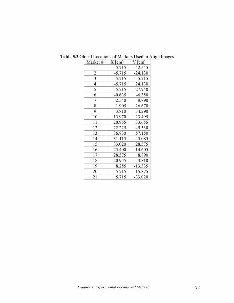
Chapter 5: Experimental Facility and Methods 72

Table 5.3 Global Locations of Markers Used to Align Images Marker # X [cm] Y [cm]

1 -5.715 -42.5452 -5.715 -24.1303 -5.715 5.7154 -5.715 24.1305 -5.715 27.9406 -0.635 -6.3507 2.540 8.8908 1.905 26.6709 3.810 34.29010 13.970 23.49511 20.955 33.65512 22.225 49.53013 36.830 57.15014 31.115 45.08515 33.020 28.57516 25.400 14.60517 28.575 8.89018 20.955 -3.81019 8.255 -13.33520 5.715 -15.87521 5.715 -33.020

Chapter 5: Experimental Facility and Methods 73

Table 5.4 Global Locations of Endwall Thermocouples Used for Image Calibration Thermocouple # X [cm] Y [cm]

1 -5.715 -15.2402 -5.715 3.8103 -5.715 30.4804 19.050 41.9105 24.130 39.3706 25.400 52.0707 38.100 52.0708 34.290 38.1009 33.020 25.40010 28.575 10.160

Chapter 5: Experimental Facility and Methods 74

Figure 5.1 Illustration of wind tunnel facility. The flow is split into the primary channel and secondary channels before passing through the combustor simulator section and the vane cascade.

Figure 5.2 The flow is driven by a Joy Technologies 50 hp 0-60 Hz fan.

Chapter 5: Experimental Facility and Methods 75

Figure 5.3 A perforated plate with 24.6% open area is used to achieve the proper pressure drop through the core flow channel.

Figure 5.4 Plenums in the combustor bypass feed film-cooling and dilution holes in the combustor simulator. The plenums were closed off and liner holes covered over because no combustor flows were simulated.

Chapter 5: Experimental Facility and Methods 76

Figure 5.5 Cooling air from the bypass channel passes into the supply plenums through holes at the end of the combustor bypass. The cooling air is then injected into the passage through the slot or the holes where it interacts with the hot mainstream gases.

Figure 5.6 A three zone heater bank is used to generate various combustor exit temperature profiles.

15.6°

99 cm 54.9 cm Vane

Chapter 5: Experimental Facility and Methods 77

Figure 5.7 Watlow Series 988 controller used to specify percentage of full power to the heater banks.

Figure 5.8 Each of the three heater sub-banks is wired in a three phase delta with each leg consiting of two elements in parallel (Vakil 2002).

IL

R1 R2

R3

VL

Chapter 5: Experimental Facility and Methods 78

Figure 5.9 Film-cooling holes were cut with a water jet. (a) Passage 1 and (b) the leading edge region are shown.

Figure 5.10 The upstream slot was constructed from balsa wood to provide improved stiffness.

a) b)

Slot

Chapter 5: Experimental Facility and Methods 79

Figure 5.11a-b Schematics of balsa wood slot. Extent of the slot is shown in (a) while locations of the endwall static pressure taps are shown in (b).

11.43 cm 0.318 cm

Pressure Tap

22.86 cm 2.54 cm

a) Side View

b) Top View

Chapter 5: Experimental Facility and Methods 80

Figure 5.12 The rear plenum provides coolant flow through the film-cooling holes.

Figure 5.13 A division was added to separate the front plenum which fed the slot flow.

PlenumDividerWall

Chapter 5: Experimental Facility and Methods 81

Figure 5.14a-b Coolant flow passes from the combustor bypass into the plenums through two feed slots.

Figure 5.15 A typical shutter control is shown. Panes connected to a pushrod slide past stationary panes to open and close the flow area.

ControlRod

Sliding Window Stationary Pane

Plenum Feed Slots

a) b)

Chapter 5: Experimental Facility and Methods 82

Figure 5.16 The plenun control devices are shown along with a splash plate to aid in mixing the slot flow.

Figure 5.17 The gate was raised and lowered to control flow into the hole plenum.

Gate Crank

Window Shutter Pushrod

Splash Plate

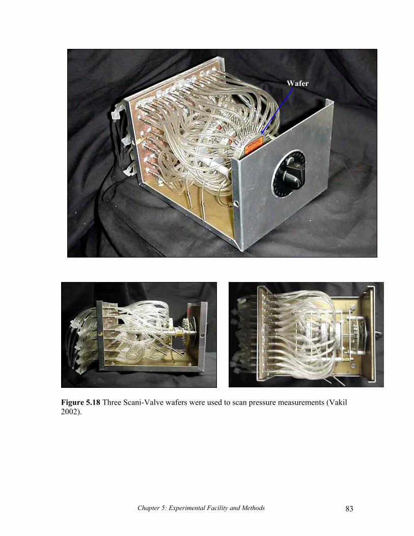
Chapter 5: Experimental Facility and Methods 83

Figure 5.18 Three Scani-Valve wafers were used to scan pressure measurements (Vakil 2002).

Wafer

Chapter 5: Experimental Facility and Methods 84

Figure 5.19 Eight pressure transducers converted pressure readings into voltages for the data acquisition system (Vakil 2002).

Omega and Setra Pressure Transducers

On/Off Switches

Battery Power Supply Input

BNC Voltage Signal Outputs

High/Low Pressure Transducer Inputs

Chapter 5: Experimental Facility and Methods 85

Figure 5.20a-b A pitot tube measures the difference between the total pressure and static pressure yielding the dynamic pressure and thus the velocity.

5.0

5.5

6.0

6.5

7.0

7.5

8.0

-1.5 -1.0 -0.5 0.0 0.5 1.0 1.5

V (m/s)

y/P Figure 5.21 Seven pitchwise velocity measurements were averaged to determine the cascade inlet velocity. The inlet profile exhibits periodicity.

Flow

po

ps

a) b)

Chapter 5: Experimental Facility and Methods 86

Figure 5.22a-c A thermocouple rake was used to document the thermal field at a plane within the passage.

0.6 cm

0.635 cm

9.525 cm

0.159 cm

~0.08 to ~0.1 cm

6.2 cm

a) b)

c)

Chapter 5: Experimental Facility and Methods 87

Figure 5.23a-c (a) The thermocouple rake was suspended from a boom and (b) moved by a computer controlled traverse. (c) The rake is shown in the passage.

a)

b) c)

Chapter 5: Experimental Facility and Methods 88

Figure 5.24a-d The data acquisition (DAQ) system is depicted. (a) Voltage outputs from the thermocouples and tranducers are connected to a SCXI-1303 terminal block. The terminal block plugs into one of (b) three SCXI-1100 modules which are housed in the (c) SCXI-1000chassis. The signal is output to (d) the DAQ card where it is digitized for processing on the computer (Vakil 2002).

Voltage Inputs

(a) (b)

(d) (c)

via shielded cable

Housed within the

Chapter 5: Experimental Facility and Methods 89

Figure 5.25 A Flir P20 infra-red camera was used to thermally image the endwall surface and record endwall temperature data.

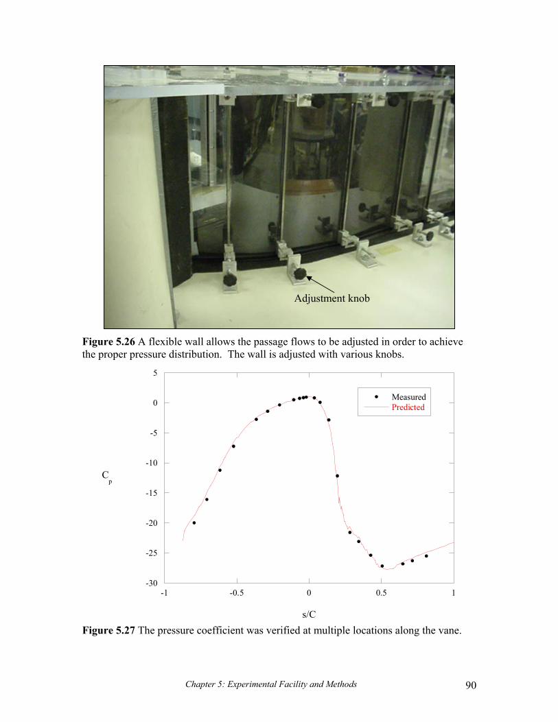
Chapter 5: Experimental Facility and Methods 90

Figure 5.26 A flexible wall allows the passage flows to be adjusted in order to achieve the proper pressure distribution. The wall is adjusted with various knobs.

-30

-25

-20

-15

-10

-5

0

5

-1 -0.5 0 0.5 1

MeasuredPredicted

Cp

s/C Figure 5.27 The pressure coefficient was verified at multiple locations along the vane.

Adjustment knob

Chapter 5: Experimental Facility and Methods 91

0

0.2

0.4

0.6

0.8

1

1.2

0 2 4 6 8 10 12 14 16

Pass 1 CFDPass 2 CFD

CD1

= 1.363 - 0.058x

CD2

= 0.945 - 0.017x

CD

∆p1/2

Figure 5.28 A linear fit was used to calculate the global discharge scaling parameter for each passage based upon computational predictions.

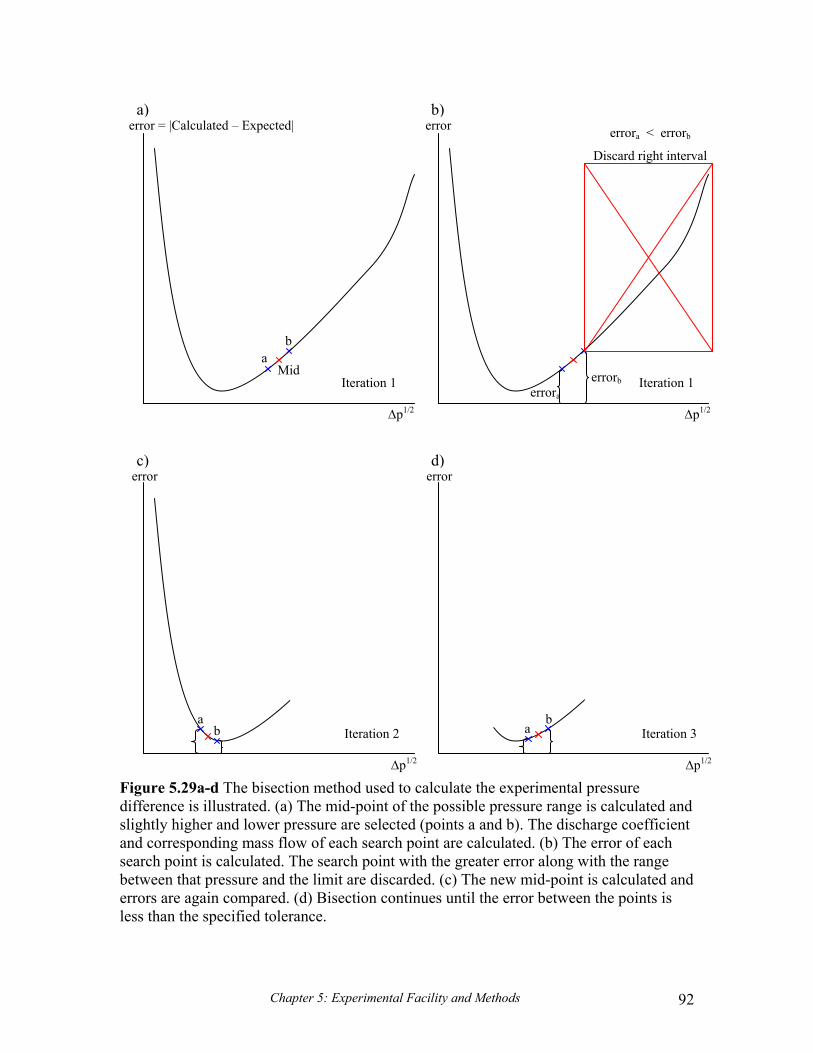
Chapter 5: Experimental Facility and Methods 92

Figure 5.29a-d The bisection method used to calculate the experimental pressure difference is illustrated. (a) The mid-point of the possible pressure range is calculated and slightly higher and lower pressure are selected (points a and b). The discharge coefficient and corresponding mass flow of each search point are calculated. (b) The error of each search point is calculated. The search point with the greater error along with the range between that pressure and the limit are discarded. (c) The new mid-point is calculated and errors are again compared. (d) Bisection continues until the error between the points is less than the specified tolerance.

error = |Calculated – Expected|

∆p1/2

Mid

b

a

errora

errorb

errora < errorb

Discard right interval

error

∆p1/2

Iteration 1

error

∆p1/2

error

∆p1/2

Iteration 1

Iteration 2 Iteration 3

a) b)

c) d)

aba

b

Chapter 5: Experimental Facility and Methods 93

Figure 5.30 When setting experimental cooling flows, four pressure measurements were recorded for both the slot flow and the film-cooling for the pattern of interest as shown by the wiring diagram. The pressure measurements were averaged to determine the coolant flow rates.

Pattern 1 Pattern 2

Outside Middle Inside

Slot Plenum Total

Endwall Static

Hole Plenum Total

Chapter 5: Experimental Facility and Methods 94

Figure 5.31 Images were collected at 13 different locations to entirely map the endwall thermal contours.

-1.00

-0.75

-0.50

-0.25

0.00

0.25

0.50

0.75

1.00

1.25

-0.50 -0.25 0.00 0.25 0.50 0.75

Y/P

X/C

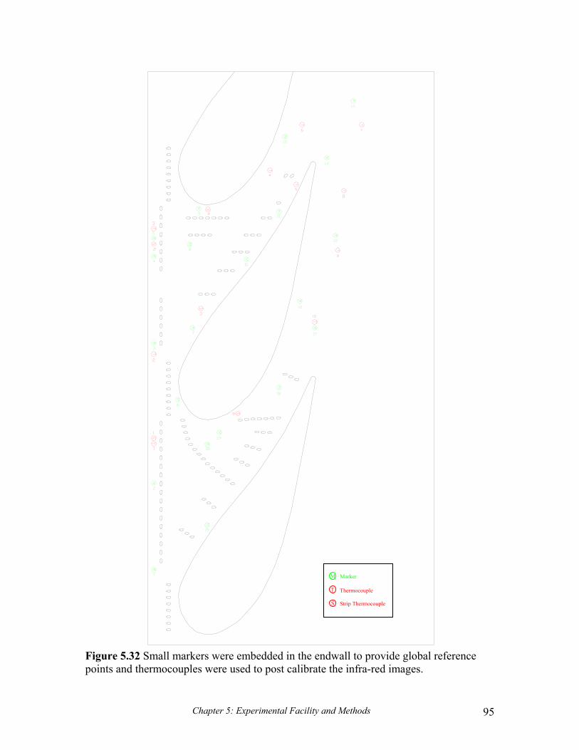
Chapter 5: Experimental Facility and Methods 95

Figure 5.32 Small markers were embedded in the endwall to provide global reference points and thermocouples were used to post calibrate the infra-red images.

T

S

M Marker

Thermocouple

Strip Thermocouple

Chapter 5: Experimental Facility and Methods 96

Figure 5.33 The multiple images were combined using know global locations to form a mosaic of the endwall thermal contours.

Chapter 5: Experimental Facility and Methods 97

Figure 5.34a-e The image transformation process is illustrated. (a) an image in space has two markers at know global locations. (b) The transition matrix from a pixel aligned coordinate system to the marker aligned system is developed by projecting the pixel basis onto the marker basis. (c) The vector from the left to right marker in the global frame is found by a vector subtraction of the vectors to the markers. (d) The transition matrix from the marker frame to the global frame is found by projecting the marker basis onto the global basis. (e) The offset vector to one of the markers positions the image globally.

YG

XG

Offset Vector

XG

YG

Y1

YG

XG

Y2

X2

Y2

X1

X2

YG

XG

( )GRMLMM →v

RMGMv

LMGMv

a)

c)

e)

b)

d)

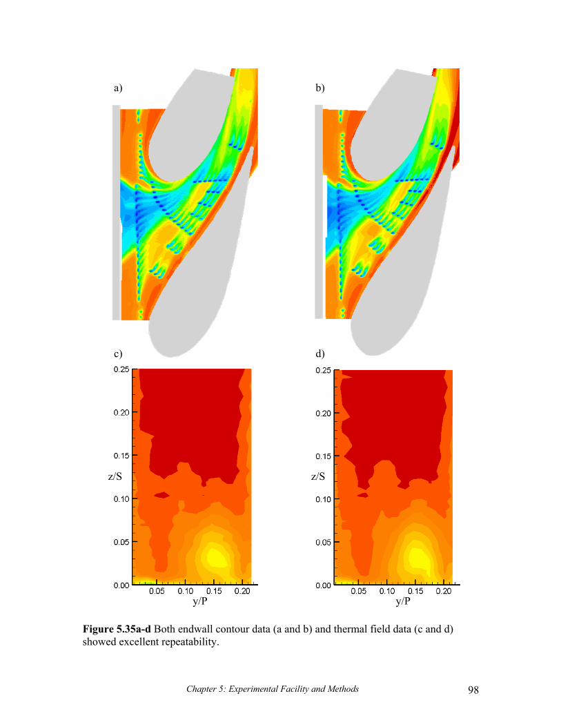
Chapter 5: Experimental Facility and Methods 98

Figure 5.35a-d Both endwall contour data (a and b) and thermal field data (c and d) showed excellent repeatability.

a)

c) d)

b)

y/P y/P

z/S z/S

Chapter 6: Computational Results 99

Chapter 6

Computational Results

Computational modeling has revolutionized modern engineering. Designs can be

quickly developed and evaluated without the expensive and time consuming process of

prototyping and testing multiple design ideas. Computational Fluid Dynamics (CFD) has

been integrated into the gas turbine design process to evaluate both the aerodynamic and

thermal impacts of various airfoil geometries and cooling methods.

This study was focused on reducing heat transfer to the endwall surface of a first-

stage vane through the implementation of slot leakage flow at the combustor-turbine

interface and two unique endwall film-cooling patterns. A computational test matrix,

shown in Table 6.1, was developed in order evaluate the performance of each cooling

mechanism alone as well as the slot and film-cooling holes in concert at low and high

flow rates to determine the effectiveness and interactions of the cooling mechanisms.

Performance was evaluated based upon adiabatic film-cooling effectiveness levels which

are the temperatures that the surface would see if no heat were conducted through the

endwall surface. Experimental results will be presented in chapter 7 and the predictions

from this chapter will be benchmarked against the experimental data in chapter 8. Note

that for all of the calculations, the density ratio (jet-to-mainstream) was held fixed at 1.14

to allow for comparisons with experiments.

Much of the discussion in this chapter was taken from the conference paper by

Knost and Thole (2003). The results from the predictions made for the test cases shown

in Table 6.1 will be discussed in a logical progression of complexity in Section 6.1. First,

the cooling provided from the leakage slot flow alone will be examined. Second,

adiabatic effectiveness levels for the case with film-cooling alone for both endwall

patterns will be discussed. Finally, the predictions for the combined slot and film-cooling

configurations will be compared to the predictions for the slot alone and endwall film-

cooling alone. In Section 6.2, the superposition method will be evaluated using the slot

alone and endwall film-cooling alone as compared with the predictions for the combined

slot and film-cooling configurations. Section 6.3 will present thermal and flow field

Chapter 6: Computational Results 100

predictions from a plane intended to lend insight into the superposition evaluation.

Finally, a summary of findings from the predictions will be given in Section 6.4.

6.1 Predictions of Adiabatic Effectiveness

Slot Injection at the Combustor-Turbine Interface

As previously discussed several cases were computed for a two-dimensional flush

slot upstream of the turbine vane (cases 1S0F0 and 3S0F0 in Table 6.1). Figure 6.1a

shows the predicted contours for the 0.5% coolant flow (case 1S0F0). There is

essentially no coolant exiting the slot directly upstream of the vane stagnation for case

1S0F0. In fact, a small amount of ingestion was predicted upstream of the leading edge.

The slot coolant is swept across the passage toward the suction side-endwall junction

leaving a large uncooled ring around the vane which is especially pronounced at the

leading edge and along the pressure side. Cooling levels within the slot flow rapidly

decrease to approximately η = 0.5.

The predicted adiabatic effectiveness levels for the slot cooling, with the coolant

flow being 1% of the exit mass flow, are shown in Figure 6.1b. There is a definite

increase in the predicted effectiveness levels for the 1% coolant flow as compared to the

0.5% coolant flow (case 1S0F0). The coolant exits across the entire width of the slot, but

still in a non-uniform manner, and is again swept towards the suction side-endwall

junction. Higher effectiveness levels are maintained throughout the slot affected region

when compared to the low flow case. There is a warm ring around the airfoil that extends

from the stagnation location and along the entire pressure side. A large portion of the

suction side also has a warm ring along the endwall in the vane-endwall juncture. The

computational results indicate that at s/C = 0.65, the coolant from the slot impacts the

suction side of the vane which is upstream of the predicted impact location at the low slot

flow rate. The warm ring is a result of the horseshoe vortex that is wrapping around the

vane as well as the large passage vortex that is convected toward the suction side of the

vane. The coolant is lifted from the endwall surface by the upward velocity vectors of

the secondary flow thereby reducing the cooling effectiveness on the endwall.

Pitchwise averaged effectiveness levels predicted for the 0.5% and 1% cases are

shown in Figure 6.2. These averages indicate improved cooling for the higher coolant

Chapter 6: Computational Results 101

flow condition in the upstream endwall region. There is a large improvement in the

leading edge region for the higher coolant flow condition. Progressing downstream,

however, the two coolant flow conditions give approximately the same pitchwise-

averaged effectiveness levels which is expected because coolant is no longer present

across much of the passage.

Cooling Hole Injection Along the Vane Endwall

Two cases were computed for the endwall cooling investigation, which included

the two different endwall cooling hole patterns with each having 0.5% coolant injection.

Note that there are 14 more cooling holes for the cooling hole configuration #1 as

compared with #2, which was dictated by the designs given by industry (pattern #2 has

78% of the hole area of pattern #1). As a result of this disparity in the number of cooling

holes, the coolant flow distribution is different for each of the hole patterns. The blowing

ratios based on the inlet flow conditions (Min) for patterns #1and #2 were 1.2 and 1.5,

respectively as listed in Table 6.1.

As would be expected based on the iso-velocity contours, there is a large variation

in the local flow rate through each of the holes given that all of the holes are fed from a

common plenum supply. The blowing ratio (Min) based on the inlet mass flux of a

number of representative holes is listed in Tables 6.2a and 6.2b for the two hole patterns.

Of interest for this section of the discussion are cases 0S1F1 and 0S1F2 listed in Tables

6.2a and 6.2b. The locations of these holes, which are nearly paired between the two

passages, are shown in Figure 6.3a. Tables 6.2a and 6.2b show that near the leading edge

(holes 1.6 and 2.6) the blowing ratio is the lowest with a large discrepancy between the

two cooling hole patterns. The large difference between the two hole patterns is

attributed to the fact that there are fewer holes in pattern #2 as compared with pattern #1.

One could predict the blowing ratio, and thus the mass flow rate, through any of the

cooling holes using a known discharge coefficient and the total plenum to exit static

pressure difference. Since the total flow through each of the holes is known from the

CFD results, it was possible to deduce a representative discharge coefficient. These

discharge coefficients are listed in Table 6.1 for the various cases. As the pressure ratio

increases, so does the discharge coefficient.

Chapter 6: Computational Results 102

Figures 6.4a and 6.4b present the predicted endwall effectiveness levels for the

two cooling hole patterns at 0.5% coolant. The computational results indicate that the

injection from the cooling holes in the first streamwise row of holes remain relatively

discrete for pattern #1 (Figure 6.4a), particularly nearer to the suction side of the vane

passage. Recall all of the holes in this first row are injecting towards the top of the

picture, as was indicated in Figure 6.3b. Closer to the pressure side of the vane but still

in the first row of holes, the jets are slightly more merged as a result of the sweeping

motion of the passage vortex at this location. The endwall cooling along the pressure

side of the airfoil is non-existent for pattern #1 as illustrated by the η = 0 contours in this

region. The coolant injected from holes in the vane passage located near the pressure

side of the airfoil is primarily blowing in the same direction as the streamlines even

though these holes are directed towards the pressure surface. Relatively good cooling

along most of the endwall, with the exception of the band near the pressure surface, is

predicted for pattern #1 at a film-cooling flow rate of 0.5%.

There are a number of noticeable differences in the effectiveness levels for hole

pattern #2 relative to pattern #1. For the cooling holes located just upstream of the vane

stagnation, it is clear that the cooling is much more effective for hole pattern #2 as

compared with hole pattern #1 even though the hole configuration at this location is the

same for the two patterns. The reason for this better cooling is because there is

proportionally a higher flow rate through the set of holes at the leading edge for the

pattern #2 as compared with pattern #1 (see holes 2.6 and 1.6 in Tables 6.2a and 6.2b).

The effectiveness contours are much cooler in the stagnation area extending along the

suction side of the vane for pattern #2 as compared to pattern #1.

In the passage itself, the most noticeable difference between the two cooling hole

patterns is that while relatively uniform coverage in the passage existed for hole pattern

#1 (with the exception of near the pressure surface), the effectiveness contours for hole

pattern #2 indicate the presence of a hot streak that travels down the mid-passage of the

vane. This hot streak is a result of the break in the cooling hole placement due to the

gutter that would be present in the region where adjacent vane platforms meet (discussed

previously). Coolant exiting from the gutter could potentially alleviate these high

Chapter 6: Computational Results 103

temperatures, but if no coolant leaked out of the gutter region there would be damage to

the endwall in this high temperature region.

Similar to pattern #1, the cooling from the first row of holes remains relatively

discrete for the pitchwise row of holes injecting nearer to the suction side of the vane

passage for pattern #2. For the first row holes in the mid-passage region of pattern #2,

the coolant does not remain in discrete streaks, but rather merges into one large, cooler

area. Also similar to pattern #1, there is no coolant present along the endwall close to the

pressure side of the airfoil for pattern #2. In the case of hole pattern #2, the endwall

cooling holes along the pressure side of the vane are injecting directly towards the vane.

Although the coolant was not able to overcome the crossflows present resulting in a hot

region along the pressure side, the overall cooling effectiveness levels downstream of the

jet injection were higher than in the case for hole pattern #1 in this region.

Combined Slot and Film-Cooling Injection

Four cases were computed for the combined slot and film-cooling injection

studies, which included the slot combined with the two hole patterns at two different

film-cooling flow conditions. The slot flowrate remained fixed at 0.5% of the core flow

while the film-cooling flowrates considered were 0.5% (cases 1S1F1 and 1S1F2) and

0.75% (cases 1S2F1 and 1S2F2). Note that the slot and the film-cooling flow rates were

set independently through the use of two different supply plenums. Tables 6.2a and 6.2b

give the local blowing ratios for the hole locations indicated in Figure 6.3a. Note that all

of the blowing ratios slightly increased for the combined film-cooling/slot cases for both

hole patterns. The reason for this slight increase is because the exit mass flow through

the vane was held fixed and, as such, relatively more coolant was sent through the holes

since the slot flow was taken out of the mainstream flow. Other than the slightly higher

blowing ratios, the relative difference between the cooling holes was nominally the same.

Figures 6.5a-b show the contour plots for the two flowrate conditions for the combined

slot and cooling hole pattern #1. Figure 6.5a illustrates that the slot coolant contributes to

the cooling effectiveness near the suction side of the airfoil and rather than discrete jets as

was shown in Figure 5a, this region is relatively cooled uniformly. The trajectory of the

cooling jets looks to be very similar for the endwall cooling alone as compared with the

Chapter 6: Computational Results 104

combined slot/endwall cooling configuration. The exit slot flow is also not effected by

the downstream cooling hole injection.

There is a definite increase in the adiabatic effectiveness levels for the increased

film-cooling flow as shown by Figure 6.5b. The leading edge holes indicate a much

better performance with continued increases in effectiveness along the pressure side of

the airfoil. The pressure side region showed the most dramatic increases in effectiveness

with the increased coolant flow from the film-cooling holes. The trajectory of the

cooling jets has changed significantly for the higher cooling flow case, particularly along

the pressure side. Rather than being swept in the streamwise direction, these jets have

enough momentum to penetrate closer towards the pressure side of the vane. There is

also a slight improvement in effectiveness along the suction side of the vane.

For cooling hole pattern #2, shown in Figures 6.6a-b at the two coolant flow

conditions, the slot interaction with the cooling holes showed one noticeable effect. In

the case with only endwall cooling, the jets exiting from the holes in the leading edge row

near the mid-passage region were more directed toward the pressure side of the vane

(Figure 6.4b) as compared to the predictions shown in Figure 6.6a. For the combined

slot/hole configuration, Figure 6.6a shows that the leading edge jets in the mid-passage

region are being entrained by the slot flow. This effect is even more dramatic at the

higher cooling flow case shown in Figure 6.6b with the coolant from these jets being

strongly turned toward the suction side of the adjacent vane.

For both coolant flow conditions in hole pattern #2, the hot streaks through mid-

passage still remain for the combined slot/hole configuration. For the higher film-cooling

flowrate shown in Figure 6.6b, there is a predicted increase in effectiveness levels as

compared with the lower film-cooling flowrate shown in Figure 6.6a. The detriment at

the higher blowing ratio for hole pattern #2 is that the hot streak becomes wider as shown

in Figure 6.6b. The reason for this widening is because the jets are more directed towards

the pressure surface. These results indicate that even with the presence of the gutter, it

may not be possible to cool the entire hot streak region.

Figure 6.7 compares the pitchwise averaged effectiveness levels for the combined

slot/hole configuration for hole patterns #1 and #2 at the two different film-cooling

flowrates. For all of the cases, the averaged effectiveness levels agree just after the slot

Chapter 6: Computational Results 105

to x/Ca = -0.15. The peak in effectiveness level occurs just downstream of the slot for all

of the cases with a second peak occurring for hole pattern #1 at x/Ca = 0.6. Downstream

of the slot, the averages indicate the highest predicted effectiveness averages occur for

hole pattern #1 at the higher coolant flow condition. There is a distinct increase in the

pitchwise-averaged effectiveness levels for hole pattern #1 at the higher coolant flow

condition. This is not the case for hole pattern #2, which indicates nearly the same

pitchwise averaged effectiveness levels for the two coolant flow conditions. The reason

for the lack of improved performance is because of the large hot streak in the mid-

passage for hole pattern #2, which occurs at both the low and high coolant flow

conditions.

Figure 6.8 provides an overall summary of the area-averaged effectiveness levels

for all of the cases evaluated. These area-averaged effectiveness levels can be used as a

guide for designers in choosing whether coolant is more effectively used through the slot

interface or through the cooling holes. Note that the areas for these cases were all

computed based on the axial position located at the downstream edge of the slot. As a

result of this fixed area, there is a large uncooled portion of the endwall upstream of the

holes that brings down the area-averaged effectiveness levels for the two cases without

slot flow. In all of the flow rates considered, pattern #1 was superior to pattern #2. It is

also evident that increasing the flow rate from pattern #2 did not result in much benefit

from an average endwall temperature perspective. Figure 6.8 also indicates that for the

0.5% coolant flow, it is beneficial from an average perspective to inject the coolant flow

from the cooling holes alone rather than from the slot alone. One word of caution,

however, is that the local variations without the slot cooling (such as upstream of the first

row of holes) may be too great and, as such, the area averaged effectiveness values alone

do not tell the entire story.

6.2 Superposition of Results

An analysis was made based on the predicted effectiveness levels as to whether

superposition may be appropriate in which effectiveness predictions for the slot alone and

for the film-cooling holes alone could be combined to give an indication of the

effectiveness levels for a case with a combined slot and film-cooling holes. Figure 6.9

Chapter 6: Computational Results 106

shows the predictions made for each cooling mechanism alone (slot or cooling holes), the

two combined using superposition, and the directly predicted pattern #2 which was used

for this exercise, the results are representative of what occurs for hole pattern #1 as well.

The pitchwise-averaged effectiveness values in Figure 6.9 indicate that there is a slight

effect of the downstream film-cooling on the exit slot flow as indicated by the slightly

lower averaged effectiveness predicted by the superposition just downstream of the slot.

Progressing downstream of the slot, the predicted averaged effectiveness values are

slightly higher than the superimposed values until x/Ca = 0.15. Downstream of this

location, the superposition solution indicates higher values. In general, these results

indicate that a superposition analysis can not be simply applied for the combined film-

cooling and slot flows. Recall that superposition theory presumes that the flow field

remains constant for the two solutions used in the analysis. As such, one potential reason

for the inability to accurately use superposition theory for the combined slot and film-

cooling flows is that the flow field has significantly changed for the combined slot and

film-cooling case as compared with the slot alone and the film-cooling alone.

6.3 Secondary Flow Field Analysis

Secondary flow fields were analyzed at a number of locations throughout the vane

passage. Presented here is only one flow field plane, which is near the exit of the vane

passage and is normal to the pressure side of the vane (indicated by the line shown in

Figure 6.3b at the trailing edge of the pressure surface). The secondary flow fields are

plotted using vectors of Vn and Vz, as defined in the nomenclature, thereby representing

the deviation of the flow relative to that for the mid-span inviscid flow. The view taken

for the plots is looking upstream. Figures 6.10a-d show the secondary flow vectors with

superimposed thermal fields for the following cases: 0.5% slot flow alone (case 1S0F0),

0.5% film-cooling alone (case 0S1F2), 0.5% film-cooling (case 1S1F2) combined with

0.5% slot cooling, and 0.75% film-cooling combined with 0.5% slot cooling(case

1S2F2). Since the secondary flow field results are similar between hole patterns #1 and

#2, representative results will only be presented for hole pattern #2. These plots are for

15% of the span (z/S = 0.15) where y/P = 0 is located on the pressure side of the vane.

Chapter 6: Computational Results 107

Figure 6.10a shows the typical passage vortex that is expected to occur in most

turbine vane flows with a low slot flow condition. The vortex center is located near 5%

of the span near mid-passage (y/P = 0.1). In contrast, Figure 6.10b indicates that with the

film-cooling alone there is a strong cross-flow along the endwall, but the roll-up of the

vortex is not as well-defined. The stronger cross-flow near the endwall is a result of the

lower momentum fluid near the endwall that is present from the film-cooling injection as

compared with the slot alone. The thermal fields in Figure 6.10b clearly show the

existence of the gap in cooling along the endwall.

Figure 6.10c shows the secondary flow and thermal fields for the case with the

low combined slot and film-cooling flows. The secondary flow pattern for the combined

cooling flows is the strongest relative to the slot or film-cooling alone. The vortex

pattern has shifted toward the suction side of the vane and is closer to the endwall than

that shown in Figures 6.10a and 6.10b. The thermal fields in Figure 6.10c indicate the

slot coolant has helped fill the gap along the endwall compared to Figure 6.10b.

The case with the higher film-cooling injection is shown in Figure 6.10d

indicating a stronger secondary flow pattern than that shown in Figure 6.10c. As the

film-cooling flow is further increased, more of the coolant is convected up the suction

side of the vane. The other noticeable difference is the spreading apart of the two cool

regions along the endwall. For the lower blowing case shown in Figure 6.10c, the peak

effectiveness levels were located at y/P = 0.05 and y/P = 0.18 while for the higher

blowing case shown in Figure 6.10d, the peak effectiveness levels were located at y/P =

0.03 and y/P = 0.2. This difference in the location of the effectiveness peaks between the

two blowing ratios occurs as a result of the higher momentum jets for the higher blowing

ratio case. In addition to the difference in peak locations, there is a greater thermal

spreading for the higher blowing ratio near the pressure side of the vane as indicated by

comparing Figures 6.10c and 6.10d and coolant affects the pressure side up to 3% span.

Based on these secondary flow patterns and the thermal field contours, it is not

surprising that the superposition method is not viable for predicting the coolant

effectiveness along the endwall for the slot flow alone and film-cooling flow alone to

give the cooling effectiveness for the combined cooling methods. As was shown in

Chapter 6: Computational Results 108

Figure 6.9, an over-prediction of effectiveness results through the use of the superposition

method as compared with the predicted effectiveness levels.

6.4 Summary

The predictions presented in this chapter showed the effect of coolant injected

from a two-dimensional slot at the combustor-turbine interface alone; endwall film-

cooling alone; and combined slot and endwall film-cooling. The resulting endwall

effectiveness from slot cooling alone showed a pattern that is quite non-uniform along the

endwall with most of the coolant being swept toward the suction side of the vane. One

could expect a burn-out near the vane-endwall juncture if only depending on the slot

cooling from the combustor-turbine interface as a result of a warm ring extending most of

the vane.

Placing film-cooling holes in the endwall is critical for increasing component life.

The placement of these holes is difficult because the trajectory of the jets is not intuitive

given the strong cross-flows that develop in the endwall region. The results of these

predictions showed that the jet trajectory is highly dependent on the local blowing ratio

for the cooling holes. One of the most significant findings was a lack of endwall film-

cooling along the region where two turbine vanes are mated. While this region typically

has a gutter with some leakage flow, it is particularly important that there is cooler

leakage flow present since it provides cooling to the regions where the endwall film-

cooling does not.

Combining the slot and film-cooling flows provided the best overall coverage for

the endwall, but the warm ring around the vane was still present until a higher flow rate

through the film-cooling flows was introduced. The higher flow rate provided a higher

momentum for the pressure side film-cooling jets thereby allowing for a jet trajectory that

approached the vane. One important finding was that there was a change in the

secondary flows that developed for the combined film-cooling and slot flow studies as

compared to the film-cooling alone and slot alone. This is important because this change

in flow fields explained why the superposition method can not be used to predict the

combined endwall film-cooling and slot cooling effectiveness levels. Moreover, using

Chapter 6: Computational Results 109

the superposition method resulted in an over-prediction of cooling results thereby over-

predicting component life.

Chapter 6: Computational Results 110

Table 6.1 Computational Test Matrix and Hole Discharge Coefficients Slot flow

%mexit/Min

Film flow %mexit/Min

Discharge Coefficient

Case 1S0F0 0.5 / 0.18 - - - - - - Case 3S0F0 1.0 / 0.37 - - - - - - Case 0S1F1 - - - 0.5 /1.2 0.49 Case 0S1F2 - - - 0.5 / 1.5 0.50 Case 1S1F1 0.5 / 0.17 0.5 / 1.2 0.57 Case 1S1F2 0.5 / 0.18 0.5 / 1.5 0.58 Case 1S2F1 0.5 / 0.17 0.75 / 1.8 0.59 Case 1S2F2 0.5 / 0.18 0.75 / 2.2 0.60

Key:

#S#F#Prof

Number Passage Number Flow Rate %min 0 No Film-Cooling No Cooling 1 1 0.50 2 2 0.75 3 - - - 1.00

Table 6.2a Film-Cooling Blowing Ratios for Selected Holes in Pattern #1

Hole Case 0S1F1 Case 1S1F1 Case 1S2F1 1.1 0.82 0.92 1.59 1.2 1.22 1.42 1.95 1.3 2.37 2.77 3.07 1.4 0.70 0.89 1.58 1.5 0.86 0.90 1.55 1.6 0.33 0.33 1.27

Table 6.2b Film-Cooling Blowing Ratios for Selected Holes in Pattern #2

Hole Case 0S1F2 Case 1S1F2 Case 1S2F2 2.1 1.18 1.32 2.14 2.2 2.09 2.34 2.92 2.3 2.51 2.92 3.39 2.4 1.10 1.31 2.18 2.5 1.28 1.31 2.16 2.6 0.94 0.96 1.93

Slot flow rate

Film flow rate

Passage Number

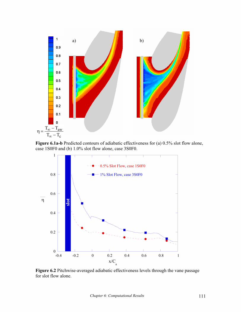
Chapter 6: Computational Results 111

Figure 6.1a-b Predicted contours of adiabatic effectiveness for (a) 0.5% slot flow alone, case 1S0F0 and (b) 1.0% slot flow alone, case 3S0F0.

Figure 6.2 Pitchwise-averaged adiabatic effectiveness levels through the vane passage for slot flow alone.

0

0.2

0.4

0.6

0.8

1

-0.4 -0.2 0 0.2 0.4 0.6 0.8 1

0.5% Slot Flow, case 1S0F0

1% Slot Flow, case 3S0F0

x/Ca

η

slot

c

awTT

TT−−

=η∞

∞

a) b)

Chapter 6: Computational Results 112

Figure 6.3a-b The film-cooling patterns are shown with (a) several featured holes used for comparisons between passages. A secondary flow plane is also indicated where the flow field was examined. (b) Iso-velocity contours as well as the gutter location and arrows indicating the direction of hole injection are shown.

1.1

1.2

1.4

1.6

2.1

2.2

2.4

2.6

1.5

2.5

SecondaryFlow Plane

1.3

2.3

Slot

1

2

3

4

5

Gutter

Pattern #2

Pattern #1

a) b)

inUU

Chapter 6: Computational Results 113

Figure 6.4a-b Predicted contours of adiabatic effectiveness for the baseline film cooling cases without slot flow (a) pattern #1, 0.5% film alone, case 0S1F1 and (b) pattern #2 0.5% film alone, case 0S1F2.

c

awTT

TT−−

=η∞

∞

a) b)

Chapter 6: Computational Results 114

Figure 6.5a-b Predicted adiabatic effectiveness levels for pattern #1 at 0.5% slot flow combined with (a) the low 0.5% film flow rate, case 1S1F1 and (b) the high 0.75% film flow rate, case 1S2F1.

Figure 6.6a-b Predicted adiabatic effectiveness levels for pattern #2 at 0.5% slot flow combined with (a) the low 0.5% film flow rate, case 1S1F2 and (b) the high 0.75% film flow rate, case 1S2F2.

c

awTT

TT−−

=η∞

∞

a) b)

c

awTT

TT−−

=η∞

∞

a) b)

Chapter 6: Computational Results 115

Figure 6.7 Pitchwise-averaged adiabatic effectiveness levels through the vane passage for the combined slot and film-cooling cases.

0

0.2

0.4

0.6

0.8

1

-0.4 -0.2 0 0.2 0.4 0.6 0.8 1

0.5% Slot / 0.5% Film

0.5% Slot / 0.75% Film

0.5% Slot / 0.5% Film

0.5% Slot / 0.75% Film

x/Ca

η

slot

Pattern #1 Pattern #2

Chapter 6: Computational Results 116

Figure 6.8 Summary of area-averaged effectiveness values for all of the computational cases studied. It can be seen that including film-cooling leads to higher averaged effectiveness levels than slot flow alone.

0

0.1

0.2

0.3

0.4

0.5Slot FlowFilm, Pattern #1Film, Pattern #2

Slot + Film, Pattern #1Slot + Film, Pattern #2

Cumulative Coolant Flow

η

0.5% 1% 1.25%

~ slot

~ film

Chapter 6: Computational Results 117

Figure 6.9 Comparison of predicted pitchwise-averaged effectiveness levels as compared with those calculated using the superposition for the 0.5% slot and 0.5% film-cooling flow cases with hole pattern #2.

0

0.2

0.4

0.6

0.8

1

-0.4 -0.2 0 0.2 0.4 0.6 0.8 1

0.5% slot, case 1S0F0

0.5% film, pattern #2, case 0S1F2

Predicted solution, case 1S1F2

Superposition solution, case (1S0F0 + 0S1F2)

x/Ca

η slot

Chapter 6: Computational Results 118

Figure 6.10a-d Secondary flow and thermal fields for the (a) slot cooling alone, case 1S0F0 (b) film-cooling alone, case 0S1F2 (c) combined slot flow-and low film flow rate, case 1S1F2 (d) combined film-cooling and slot flow at the higher film blowing ratio, case 1S2F2. Cooling hole pattern #2 was used for these results.

PS a) SS PS b) SS

PS d) SS PS c) SSc

awTT

TT−−

=θ∞

∞

Chapter 7: Experimental Results 119

Chapter 7

Experimental Results

Experimental data provides the backbone for most research work. Before being

implemented into production any product or design must be tested to validate the

expected performance. An extensive test matrix of 17 experimental cases was developed

to assess the impact of both slot cooling and film-cooling for the two different hole

patterns. The test matrix, shown in Table 7.1, was designed to study the interaction of the

slot and film-cooling holes as well as evaluate the impact of adjusting the coolant flow

rates. Three different temperature profiles were studied. The inlet profiles are shown in

Figure 7.1. An isothermal inlet temperature profile served as the baseline case and was

tested at all coolant flow conditions. In addition, a near-wall peaked and center peaked

profile were studied to evaluate the effects of a steep temperature gradient on endwall

effectiveness levels and coolant trajectory. The adiabatic effectiveness contours were

shown to be similar provided that the proper temperature, specifically the approaching

near-wall temperature, was used in the normalization. A method was developed to

identify areas of varying cooling needs and the spatial superposition method was

evaluated to assess whether combined cooling cases could be accurately predicted from

measurements of the individual cooling mechanisms. Finally, thermal field

measurements were acquired for subsequent comparison with predictions.

Section 7.1 presents measurements of adiabatic effectiveness for all the various

coolant flow rates and combinations with an isothermal inlet temperature profile. The

effects of varying the momentum ratio of holes in the leading edge, upstream pressure

side, and downstream pressure side regions are further discussed in Section 7.2. Jet

separation as well as penetration to the vane is examined. Section 7.3 shows the effects

of varying coolant between the slot and film-cooling holes by examining the area-

averaged effectiveness levels. Section 7.4 evaluates the effects of a steep temperature

gradient on endwall effectiveness levels and coolant trajectory. A method of identifying

regions of varying cooling needs based upon deviation from the midspan streamlines is

discussed in Section 7.5. The superposition method is evaluated in Section 7.6. The

Chapter 7: Experimental Results 120

intent is to determine if superposition can be used to accurately predict effectiveness

levels and coolant trajectories for the combined slot and film-cooling cases. Section 7.7

briefly presents thermal field measurements for three cases, and finally, Section 7.8

provides a brief summary of the results.

7.1 Measurements of Adiabatic Effectiveness for an Isothermal Inlet Profile

Three different inlet temperature profiles, shown in Figure 7.1, were tested. The

isothermal profile served as the baseline. The temperature profiles were generated by

three independently controlled heater banks upstream of the contraction in the wind

tunnel. The temperature profiles have been normalized such that θ = 0 corresponds to the

maximum temperature and θ = 1 corresponds to the coolant temperature in the plenum.

The profiles were normalized in this manner to allow direct comparison to the measured

adiabatic wall temperatures. The results of the different cooling mechanisms and flow

rates with an isothermal inlet profile are discussed in the following sections.

Slot Injection at the Combustor-Turbine Interface

It is seen from Figures 7.2a-c that increasing the amount of slot flow has a

dramatic effect on the endwall adiabatic effectiveness levels. At the low 0.5% slot flow

rate shown in Figure 7.2a, the slot flow only exits in the middle of the passage with no

coolant coming out upstream of the vane leading edge. When the slot flow is increased

by 50% to 0.75% of the core flow, shown in Figure 7.2b, coolant exits across the entire

width of the slot albeit still in a non-uniform manner. In both cases, though, a large

uncooled region is left around the vane. This warm ring is especially evident in the

stagnation region and along the pressure side. At the low slot flow rate the minimum

effectiveness level is approximately 0.1 which corresponds to the near-wall

dimensionless temperature shown in the uniform profile of Figure 7.1. This slight

cooling effect of the near-wall fluid was due to the long 4m, (6.8C) unheated boundary

between the heater bank used to condition the core flow and the test section. At the

increased blowing rate, the coolant exiting across the entire width of the slot is thought to

funnel the cooler near-wall fluid with the slot flow allowing the hotter mainstream gases

Chapter 7: Experimental Results 121

to convect down onto the surface leading to a measured adiabatic effectiveness level of

zero.

When the slot flow is doubled from the baseline case to 1.0% of the core flow, as

shown in Figure 7.2c, the coolant pattern is seen to be quite similar to the 0.75% case.

The coolant, however, does slightly decrease the uncooled zone in the stagnation region,

pushing the saddle point of the horseshoe vortex closer to the vane and slightly narrowing

the hot ring along the pressure side. The coolant at the highest flow rate also appears to

impact the vane suction side slightly further upstream than in the 0.75% case. In all cases

the slot flow exits in a non-uniform manner and appears to be funneled between the legs

of the horseshoe vortex towards the suction side.

Laterally-averaged adiabatic effectiveness levels for the three cases of slot flow

without film-cooling are presented in Figure 7.3. Values are truncated at x/Ca = 0.8 due

to limited optical access beyond this point. Increasing the slot coolant by both 50% and

100% is seen to effectively double the cooling effectiveness levels at the slot exit with the

highest slot flow rate performing only marginally better than the 0.75% flow rate

throughout the passage. All three cases are seen to decay rapidly upstream of the vane

and then decay more gradually through the passage with all three cases providing

approximately the same cooling effectiveness levels hear the trailing edge. This is the

region where the coolant has narrowed to only a thin band in the contours.

Film-Cooling without Slot Injection

The baseline film-cooling cases without slot flow for each of the two patterns are

shown in Figures 7.4a-d. The location of the slot, which was not simulated, is shown in

black for reference. Each pattern was tested with a low and high film-cooling flow rate

of 0.5% and 0.75% of the core flow respectively. The minimum effectiveness levels are

shown to be η = 0.1 for all cases corresponding to temperature of the slightly cooler

boundary layer of the approaching fluid.

For pattern #1 at the low film flow rate, shown in Figure 7.4a, a fairly uniform

coverage is seen across much of the passage. The leading row holes near the suction side

inject as discrete jets in the direction of the streamlines despite being directed normal to

the inlet direction (towards the top of the page). The leading row holes near the pressure

Chapter 7: Experimental Results 122

side inject in a more merged and directed pattern. The leading row holes just upstream of

the leading edge, or the “leading edge blockers”, are quite ineffective at the low film

blowing rate. The pressure side leading edge blockers appear to have virtually no coolant

while the suction side leading edge blockers are quickly swept around the shoulder of the

suction side leaving an uncooled region at the vane-endwall junction of the leading edge.

The jets along the pressure side appear to inject in the streamwise direction and follow

the contour of the vane, despite being directed axially downstream at the vane, leaving an

uncooled region along the pressure side.

For the increased film-cooling case of pattern #1, shown in Figure 7.4b, several

effects are seen from the heightened blowing. First the suction side jets of the leading

row still inject as discrete jets, but lower adiabatic effectiveness values downstream of the

holes indicate that the jets are lifting off of the surface. The pressure side leading row

holes appear to be slightly more directed with coolant traces not appearing until

downstream of the fourth hole from the pressure side as opposed to the third hole in the

low blowing case. The upstream most row of three holes also exhibits lower η values

and smaller affected areas in the high blowing case, once again exhibiting the

characteristics of jet detachment. The leading edge blockers of pattern #1 at the 0.75%

coolant flow rate are far more effective than at the 0.5% case. The suction side leading

edge blockers appear highly effective at cooling the vane-endwall junction. The pressure

side leading edge blockers appear to lift off at the injection location, impact the vane, and

convect down the vane onto the endwall. This lift-off is evidenced by the coolant

accumulating along the vane-endwall junction near the dynamic stagnation point on the

pressure side. The pressure side holes within the passage penetrate approximately one

hole diameter closer to the vane as compared with the 0.5% case thereby reducing, but

not eliminating, the warm zone along the pressure side. This improved penetration is

attributed to the increased momentum of the jets at the higher blowing ratio allowing the

coolant to more closely approach the vane. Effects of increasing the momentum ratio are

further discussed in section 7.2.

For pattern #2 at the low blowing rate, shown in Figure 7.4c, the most noticeable

feature is the large hot streak through the center of the passage. This hot streak exists in

the location where the gutter would be so including the gutter flow may tend to slightly

Chapter 7: Experimental Results 123

alleviate the problem. The effect of the gutter flow is expected to be minimal on most of

the hot streak along the endwall, though. This is because, as shown in Figure 3.1b, the

gutter runs along the downstream edge of the upstream rows of passage holes meaning

that in a streamwise sense to any cross passage flows, which would distribute the coolant,

the gutter would be downstream of the hot streak thereby providing little, if any, relief to

the uncooled zone.

Once again the suction side leading row holes inject with the streamlines despite

being directed towards the top of the page, although the local effectiveness levels are

lower than in the corresponding case for pattern #1 indicating partial jet separation. The

pressure side leading row holes inject in merged unison and are swept into the center of

the passage providing a small measure of relief to the hot streak. The leading edge

blockers of pattern #2 are far more effective than the leading edge blockers of pattern #1

at the same low 0.5% cumulative coolant flow rate. This is attributed to hole pattern #2

having only 78% of the cooling area of pattern #1 resulting in more available coolant per

hole in pattern #2. The pressure side holes in the passage of pattern #2 also appear to

reduce the uncooled zone along the vane-endwall junction when compared to pattern #1

once again because of the higher coolant per hole leading to a higher momentum flux at

the pressure side holes.

The results of increasing the film-cooling flow rate, in pattern #2, to the high

blowing rate are shown in Figure 7.4d. The jet detachment of the suction side, leading

row holes appears to be exacerbated resulting in low effectiveness levels on the endwall.

The coolant from the leading row holes just to the suction side of the gutter gap is

initially more directed resulting in an impact of the upstream passage rows two holes

upstream of the impact location at the low blowing rate. The coolant from the suction

side, leading row holes also appears to be less effective at the high coolant flow rate and

may suffer from blocking by the holes directionally downstream (bottom to top on the

image) in the row causing the coolant to liftoff as it impacts coolant from the adjacent jet.

The leading edge blockers appear to be largely unaffected although the coolant emerges

as discrete jets just downstream of the holes and the local effectiveness levels are slightly

lower. Within the passage, the pressure side jets appear well merged and penetrate to the

vane-endwall junction eliminating the hot zone along the second half of the pressure side.

Chapter 7: Experimental Results 124

Local effectiveness levels are actually lower for these holes at the high blowing rate when

compared to the results in Figure 7.4c, but effectiveness levels still appear to be more

than adequate.

Laterally-averaged effectiveness data for the four cases without slot flow is

presented in Figure 7.5. A spike is seen at x/Ca = -0.1 where the leading row holes and

leading edge blockers are encountered. Both patterns are seen to perform better in this

region at the low blowing rate because separation of the leading row jets is induced at the

high blowing rates. The average effectiveness levels for pattern #1 exceed those of

pattern #2 for both flow rates. Pattern #2 has the large hot streak in the center of the

passage which adversely affects the averaged levels. Pattern #2 shows slightly elevated

cooling effectiveness levels at the higher blowing rate, while pattern #1 provides nearly

identical results at either blowing rate.

Slot Flow Combined with Film-Cooling for Pattern #1

Moving along to the combined cooling mechanism cases, the adiabatic

effectiveness levels for pattern #1 at each of the four low and high, slot and film-cooling

combinations are shown in Figures 7.6a-d. For the low slot, low film case, shown in

Figure 7.6a, the combined contours appear, at least physically, to be somewhat of a

superposition of the cases of the film-cooling mechanisms alone. The minimum

effectiveness level is η = 0.1. Once again, the slot flow does not emerge in the stagnation

region and is funneled towards the suction side. The leading edge blockers are also quite

ineffective leaving an uncooled area in the stagnation region. The pressure side jets in

the passage inject in the stream-wise direction despite being aimed towards the vane

leaving an uncooled zone along the pressure side.

When the film flow rate is increased to 0.75%, as shown in Figure 7.6b, the flow

exiting the slot appears to be largely unaffected. The pressure side jets of the leading row

are more directed and leave only low effectiveness coolant traces along the endwall

surface indicating that a high momentum flux is inducing jet lift off. The same can be

said for the upstream most row of three holes along the pressure side. The pressure side

jets at the high film rate once again penetrate approximately one hole diameter closer to

the vane slightly reducing the warm ring along the pressure side. The hot spot just

Chapter 7: Experimental Results 125

upstream of the second cross-passage row also appears to be enlarged at the increased

blowing ratio as a result of the pressure side leading row jets pushing the slot flow closer

to the suction side. This can be verified by counting that six film cooling holes in the

upstream, cross-passage row are immersed in slot coolant at the low film flow rate as

opposed to only five holes at the increased blowing rate. The minimum effectiveness

level for this case is η = 0.5.

When the slot flow is increased to 0.75% of the core flow while the film-cooling

is maintained at 0.5%, it is seen from Figure 7.6c that the slot coverage area is

dramatically increased. Coolant exits across the entire width of the slot, but is still

funneled towards the suction side. Adiabatic effectiveness levels across much of the

upstream portion of the endwall are nearly unity indicating overcooling by the slot. The

leading row holes in this area appear not to be necessary for endwall cooling. Therefore,

the coolant emerging from these holes could be redistributed to more advantageous

locations. As has consistently been the case, the leading edge blockers of pattern #1 at

the low film-cooling rate appear to be quite ineffective leaving an uncooled zone at the

leading edge as the coolant is immediately swept around the suction side. Also, the

pressure side jets in the passage inject with the streamlines once again leaving an

uncooled band along the pressure side. The minimum effectiveness level is h = 0

corresponding to the temperature of the fluid just above the boundary layer which

convects down as the boundary layer is swept with the slot coolant.

Finally, for pattern #1 at high slot and high film flow rates shown in Figure 7.6d,

we see that the slot flow cools much of the endwall upstream of the vanes. Again, the

pressure side leading row jets appear to constrict the slot flow pushing it further towards

the suction side. These holes also separate and mix with the hot gases just above the

endwall leading to minimum effectiveness levels of η = 0.1. The suction side leading

edge blockers remain attached to the endwall providing coolant around the shoulder of

the vane, while a small amount of coolant is also carried along the vane-endwall junction

to the pressure side. The upstream rows of three holes along the pressure side exhibit the

characteristics of jet lift-off with only low effectiveness levels downstream of the holes.

Also the hole closest to the pressure side of each row in the passage appears to be more

Chapter 7: Experimental Results 126

directed at the hole exit opening a gap between the discrete jet and the other jets in the

row before being swept downstream following the contour of the vane.

The laterally-averaged adiabatic effectiveness levels for the four combined slot

and film-cooling cases for pattern #1 are shown in Figure 7.7. The average effectiveness

levels immediately downstream of the slot are seen to be nearly 1 at the high slot flow

rates when coolant exits across the entire slot. A spike at x/Ca = -0.1 corresponds to the

leading row and leading edge blockers. For both slot flow rates, the effectiveness levels

are seen to be slightly higher at the low film-cooling rates in the region upstream of the

vane. This is due to separation of the leading row jets and leading edge blockers as well

as a constriction of the slot flow by the impinging pressure side, leading row jets. The

effectiveness levels in the upstream half of the passage are also higher at the low blowing

rates because of jet separation effects. The effectiveness levels of the two high slot flow

cases are greater than those of the two low slot flow cases within the passage, because of

the widened footprint of the slot coolant at the high flow rates. Beyond approximately

x/Ca = 0.6 all flow conditions yield approximately the save laterally averaged

effectiveness levels.

Slot Flow Combined with Film-Cooling for Pattern #2

The contours of adiabatic effectiveness for pattern #2 at each of the four low and

high, slot and film-cooling combinations are shown in Figures 7.8a-d. For the low slot

and film-cooling case, shown in Figure 7.8a, the slot flow exits across only a portion of

the slot. When compared to pattern #1 at the same flow rates, shown in Figure 7.6a, the

exit location of the slot flow is seen to have migrated slightly toward the suction side of

the vane relative to pattern #2 injecting from upstream of the leading edge blockers. This

was not the case for pattern #1. The minimum effectiveness levels are approximately η =

0.1 corresponding the temperature of the approaching boundary layer. Also immediately

noticeable is the large hot streak through the center of the passage that was also present

without slot flow. The coolant from the pressure side leading row holes, which provided

a small measure of relief to the hot streak without the presence of slot flow, appears

drawn across the gap and merges with the slot coolant at the upstream rows of passage

holes. The leading edge blockers are more effective at the same low film rate than they

Chapter 7: Experimental Results 127

were in pattern #1. Again, this is attributed to more available coolant per hole due to

fewer holes in pattern #2. The coolant from the leading edge blockers fails to penetrate

entirely to the vane, however, leaving a thin uncooled region at the vane endwall junction

of the leading edge. The pressure side jets in the passage of pattern #2 at the low blowing

ratio are seen to be more directed than their counterparts in pattern #1 because of the

higher momentum due to fewer jets, but the coolant still fails to fully penetrate to the

vane leaving a thin uncooled zone along the pressure side.

When the film-cooling is increased to 0.75% while maintaining the low 0.5% slot

flow rate, the pressure side, leading row holes appear to constrict the slot coolant pressing

it towards the suction side of the passage as shown in Figure 7.8b. This is seen in the slot

coolant impacting the upstream row of holes further upstream than in the low blowing

case resulting in a widening of the hot streak in the area between the upstream passage

rows and the upstream most pressure side row of three holes. The passage pressure side

jets also approach the vane providing coolant to most of the vane endwall junction along

the pressure side. As with the low blowing rate the minimum adiabatic effectiveness

levels are measured to be approximately η = 0.1.

For the high slot flow, low film flow case of pattern #2, shown in Figure 7.8c, the

slot coolant exits across the entire span of the slot just as in the slot alone and pattern #1

high slot flow cases. A small area where η = 0 is seen just upstream of the first row of

three holes along the pressure side. This is thought to occur because of hot gases just

above the boundary layer convecting down onto the endwall as the slot coolant sweeps

the cooler boundary layer fluid towards the suction side. The slot flow appears to entrain

the pressure side, leading row jets rather than the jets injecting downstream with the

stream lines as was seen at the low slot flow conditions. The slot flow also appears to

draw the upstream most jet of each of the pressure side rows across the passage while the

jets closer to the pressure side follow the contour of the vane. This seems to illustrate the

division between regions 2 and 3, as identified by Friedrichs (1998) and shown in Figure

2.1b, where the coolant in region 2 approximately follows the direction of the inviscid

streamlines, and the coolant in region 3 is drawn across the passage by the strong endwall

crossflows. The local effectiveness levels of the pressure side jets are slightly lower than

Chapter 7: Experimental Results 128

for the low film case with low slot flow shown in Figure 7.8a. The leading edge blockers

perform similarly to the low slot and film-cooling case.

Finally, for pattern #2, the adiabatic effectiveness levels for the high 0.75% slot

and 0.75% film-cooling cases are shown in Figure 7.8d. It is thought that the minimum

effectiveness levels are slightly greater than zero because the pressure side, leading row

jets separate and mix with the hot mainstream gases as they convect down onto the

endwall surface. The increased momentum of the pressure side leading row jets

constricts the slot flow pressing it towards the suction side as evidenced by the larger η =

0.5 streak in the gap between the upstream and pressure side holes of the two cross-

passage rows. The foot print of the coolant appears to be the same in this area but the

distribution of the effectiveness levels has been altered from the high slot, low film flow

case. In addition the upstream most jets in the pressure side rows appear more directed at

the hole exits preventing the coolant from being immediately pulled out across the

passage as was seen in Figure 7.8c. Once again the pressure side jets approach the vane

eliminating much of the uncooled area at the vane-endwall junction along the pressure

side. Also, the local effectiveness levels of the upstream most row of three holes appear

lower than the corresponding holes at the low film flow rate indicating possible jet lift-off

due to high momentum and jet blockage effects. The leading edge blockers of pattern #2

at the high film-cooling and high slot flow rates provide adequate cooling around the

shoulder of the suction side while the pressure side leading edge blockers appear to

separate and impact the vane before being washed down onto the endwall near the

dynamic stagnation point. Separation is induced on the pressure side because of the

stagnating flow in this area increasing the momentum ratio of the jets.

Laterally-averaged adiabatic effectiveness levels for the four combined slot and

film-cooling cases for pattern #2 are presented in Figure 7.9. As was seen with pattern

#1, increasing the slot coolant to 0.75% of the core flow dramatically increases the

laterally averaged effectiveness levels at the slot exit. The effectiveness levels are also

seen to be higher at the leading row holes and leading edge blockers because the width of

the slot coverage area is greater. The performance is seen to be slightly worse at the low

slot flow rate with increased blowing and slightly better at the high slot flow rate with

increased blowing when compared to the low blowing cases. For the low slot flow rate,

Chapter 7: Experimental Results 129

local effectiveness levels along the pressure side were generally lower at the high film-

cooling rate. At the high slot flow rate, however, local effectiveness levels for the holes

along the pressure side were not significantly impacted by increasing the blowing.

Because of the higher momentum jets, coolant from these holes was not drawn across the

passage leading to a more coherent cooling zone along the pressure side. These effects

along with the penetration to the vane-endwall junction led to improved average adiabatic

effectiveness levels at the high blowing with high slot flow case. At approximately x/Ca

= 0.45, the low slot, low film case is seen to be superior to the high slot low film case.

This is because the higher slot flow draws the upstream most jets of the pressure side

rows across the passage reducing their effectiveness. The low slot flow is not strong

enough to adversely affect these jets.

7.2 Momentum Ratio at the Leading Edge and Along the Pressure Side

Jet separation and penetration to the vane as a result of increased jet momentum

was discussed frequently in the preceding section. Three key areas: the leading edge,

upstream pressure side, and downstream pressure side, were selected to examine the

effects of varying the momentum ratio in more detail. Holes 1.1, 2.1, 1.3, 2.3, 1.6, and

2.6 as indicated in Figure 3.2a, were selected as representative holes because they lie in

identical locations in each passage. Momentum ratios for each of these holes for the six

cases involving low slot flow (three for each passage) are listed in increasing order in

Table 7.2. The momentum ratios were calculated from predictions using:

( )loc,sin,o

2

jj

jj

2

2jj

pp2

Am

v

vI

−

ρρ

=ρ

ρ=

⋅

∞∞ 7.1

The momentum ratios for these holes are also plotted in Figures 7.10a-b along with

subsets of the effectiveness contours for the representative hole and surrounding holes

which should be subject to similar momentum flux ratios. The frames are depicted in the

accompanying cartoon for reference. The corresponding case number and a dotted line

indicating the particular hole are shown for each data point.

Chapter 7: Experimental Results 130

Holes 1.6 and 2.6 lie at the leading edge almost immediately upstream of the

dynamic stagnation point. The blowing ratios for the leading edge holes are seen to be

significantly higher than for the holes along the pressure side despite the velocity of these

jets being lower. This occurs because of the stagnating core flow greatly reducing the

kinetic energy of the mainstream. The lowest momentum flux ratios occur for pattern #1

with low slot and film-cooling flow and with only film-cooling. The jets are seen to

barely emerge from the hole, if at all, for case 1S1F1. When I is increased slightly for

case 0S1F1 the coolant is seen to emerge in the upstream direction. In both cases coolant

from the leading edge blockers was swept around the suction side with no benefit to the

pressure side. For pattern #2, the lowest momentum ratio was achieved for the case

without slot injection where I = 1.843. Hole 2.6 was not captured in the image, but

coolant from the leading edge blockers is noted accumulating at the vane-endwall

junction while no coolant traces are seen from the hole immediately adjacent to hole 2.6.

This indicates that complete jet separation has occurred at this momentum flux ratio.

Adding slot leakage results in a slightly higher momentum flux ratio from hole 2.6. No

coolant traces are seen downstream of the hole with coolant accumulation against the

vane, once again indicative of complete jet separation. Holes immediately to the suction

side of hole 2.6 are seen to be attached or only partially detached. The static pressure

around the suction side is considerably lower leading to lower momentum flux ratios at

the leading edge holes closer to the suction side. As the momentum flux ratio is

increased at the leading edge by transitioning to the higher blowing rate for pattern #1,

hole 1.6 appears fully detached. The holes to the suction side of hole 1.6 also exhibit

lower effectiveness levels because of partial detachment. Coolant from these holes is

thought to impact higher up on the vane and effectiveness levels at the vane-endwall

junction are reduced as not enough coolant is available to wash down onto the endwall.

At the highest case of I = 6.291, all holes at the leading edge are fully detached, but

effectiveness levels along the vane-endwall junction are improved. This is because

enough coolant exits the holes that when it impacts vane and is washed down a cooling

benefit is still achieved.

The momentum flux data for the pressure side holes is presented in the zoomed

frame of Figure 7.10b. At the upstream pressure side holes, represented by holes 1.1 and

Chapter 7: Experimental Results 131

2.1, the jets appear fully attached up to I = 0.462. At I = 0.553 the effectiveness levels

are not maintained as far downstream of the holes indicating partial or impending jet lift-

off. Also, the upstream most hole for the cases 0S1F2 and 1S1F2, the two low blowing

cases for pattern #2, are drawn away from the vane and towards the center of the passage.

At the highest blowing ratio for hole 1.1 where I = 0.730, shown in case 1S2F1, The jet

appears nearly fully detached. The same is true of hole 2.1 at the highest blowing rate.

Also the upstream most hole for pattern #2, shown in case 1S2F2 remains coherent with

its neighboring jets rather than being drawn into the passage. The upstream pressure side

jets were not able to penetrate to vane before separation was induced.

The downstream pressure side jets, represented by holes 1.3 and 2.3, appear fully

attached in all cases. A maximum momentum flux ratio of only I = 0.459 was achieved

because of the high mainstream velocities as the flow approaches the passage exit. As

the momentum flux ratio was increased the downstream pressure side jets did penetrate

closer to the vane finally impacting at the highest blowing ratio.

When comparing all holes, separation was induced in the range 0.553 ≤ I ≤ 0.730.

The upstream pressure side holes separated before impacting the vane while the

downstream pressure side holes were able to penetrate completely to the vane. Complete

detachment was noted to occur in the range 1.255 ≤ I ≤ 1.843. Thole, Sinha, Bogard, and

Crawford (1992) showed full detachment for I > 0.8 for a hole with no compound angle

on a flat plate. Holes on the endwall, however, are more analogous to compound angle

holes.

7.3 Area-Averaged Effectiveness Levels

The area-averaged adiabatic effectiveness level for each of the 15 experimental

cases with an isothermal temperature profile is presented in Figure 7.11. The averages

were computed from the axial location x/Ca = -0.24, corresponding to the location

furthest upstream where the images covered the entire pitch for all cases, to x/Ca = 0.74

where limited optical access prevented the entire width of the passage from being

imaged. The various cases have been grouped by cumulative coolant flow rate to provide

a quantification of the effects of distributing coolant between the slot and film-cooling

holes.

Chapter 7: Experimental Results 132

It is seen that at the lowest coolant flow rate of 0.5%, the film-cooling holes

provide a greater average cooling effectiveness than the slot flow alone. When the

coolant and slot flow rates are increased to 0.75% of the core flow, the slot flow provides

the highest average effectiveness level. This is somewhat misleading, though, because

the slot average effectiveness levels have been artificially inflated by overcooling the

large area in the upstream, center portion of the passage while providing no relief to the

vane-endwall junction along both the leading edge and pressure side. Therefore, the most

critical portion of the endwall experiences no cooling benefit. Also, one should notice

that the average effectiveness level of pattern #1 is roughly the same as at the low flow

case while pattern #2 actually performs worse at the increased blowing rate. This is due

to jet separation which was noticed at many of the upstream holes and, in the case of

pattern #2, the widening of the hot streak in the center of the passage.

For a cumulative flow rate of 1.0% of the core flow, both the slot only case and

combined slot and film-cooling cases were tested. By including film-cooling with the

slot flow, the average effectiveness levels were nearly matched while eliminating much

of the uncooled ring along the pressure side. If the film-cooling holes were strategically

placed so as to avoid holes in the area cooled by the slot, the average effectiveness levels

of the combined cases would surely exceed that of the slot flow alone.

The 1.25% grouping consisted of four cases where the coolant was varied

between slot and film-cooling holes. For pattern #1, a higher average effectiveness level

was seen for the higher slot flow combined with low film-cooling. This combination

produced the highest area-averaged effectiveness level of all conditions tested. The slot

flow over cooled the upstream portion of the passage inflating the area-averaged

effectiveness levels. No cooling was provided to the leading edge or along the pressure

side. In addition the broad slot flow region blocked the slightly cooler near-wall fluid

allowing the hotter mainstream gases just above to migrate down to the surface of the

uncooled areas. The low slot, high film case also provided coolant to much of the

endwall without wasting as much slot flow overcooling the upstream portion of the

endwall. The iso-velocity design helped to prevent jet-liftoff in much of the passage,

while the higher blowing rate provided enough momentum to the jets to cover the leading

edge and penetrate near the airfoil, leaving very little of the endwall without any cooling.

Chapter 7: Experimental Results 133

Pattern #2 showed the same trend with the high slot, low film condition

outperforming the low slot, high film cases, at least in the average sense. The higher film

blowing rate narrowed the footprint of the slot flow and provided more direction to the

pressure side jets widening the hot streak in the process. The upstream holes also

exhibited characteristics of jet detachment, likely from interference by adjacent jets. The

higher slot flow rate provided significantly more coolant to the broad uncooled area in the

upstream portion of the passage. This combined with the less directed, stream-wise

injection of the pressure side holes minimized the hot streak.

Finally, the high 0.75% slot flow rate combined with the high film-cooling rate

for each pattern provided adequate effectiveness levels for both patterns. Pattern #1

showed a slight decline from the high slot, low film case because of lower local

effectiveness levels due to jet lift-off. Pattern #2 exhibited a slightly higher average

effectiveness level as the hot zone along the pressure surface was eliminated. The

highest combined cooling cases indicate that the extra coolant is not justified as equal or

higher effectiveness levels can be achieved with slightly less coolant. In all cases, hot

spots, which are washed out in the averaging process, are still a concern and must be

addressed.

7.4 Effects of a Steep Temperature Gradient on Film-Cooling

It was desired to determine if a strong temperature gradient would alter the

coolant trajectories and effectiveness levels of the cooling mechanisms. Two inlet

conditions, near-wall and center-peaked profiles, were considered to evaluate gradient

effects. The profiles are shown in Figure 7.1.

Figures 7.12a and 7.12b provide the measured effectiveness levels for pattern #1

for the 0.5% slot and 0.5% film-cooling flow conditions. Figure 7.12a gives the

effectiveness measurements for the near-wall (bottom peaked) temperature profile while

Figure 7.12b gives the effectiveness measurements for the midspan peaked temperature

profile. In both cases (Figures 7.12a and 7.12b), the normalizing temperature was that of

the peak temperature whether it occurred near the wall or near the mid-span. While the

coolant trajectories look quite similar the effectiveness levels are very different. For the

midspan peaked temperature profile (Figure 7.12b) the range of effectiveness levels is

Chapter 7: Experimental Results 134

quite small given that the midspan to coolant temperature potential is large relative to

what is being experienced in the near-wall region. The effectiveness levels for the near-

wall peaked temperature case are nearly identical to that shown in Figure 7.6a. This

illustrates that provided the representative temperature scaling is used, the effectiveness

contours would be identical.

Figure 7.12c and 7.12d illustrate the effectiveness contours using the spatially

averaged temperature for the bottom and midspan peaked temperature profiles shown in

Figure 7.1. Because the near-wall peaked temperature is relatively small with regards to

the entire cascade area, the effectiveness contours appear to be very much the same. To

further illustrate the same phenomena is happening for all three temperature profiles, the

adiabatic wall temperatures were further analyzed for the midspan peaked temperature

profile in which the near-wall temperature (average temperature in the first 5% of the

span) was used in the definition of effectiveness. Figure 7.12e illustrates that the

contours are nearly identical to Figures 7.6a, 7.12a, and 7.12c. Based on these results it is

clear that the endwall temperatures are dependent upon the temperatures leaving the

combustor in the near-wall region and the local cooling.

7.5 Streamline Analysis of Film-Coolant Trajectory

When placing film-cooling holes, a designer would like to predict film-coolant

trajectory, which can be highly non-intuitive, in order to insure that the cooling needs of

critical areas are met. A first approximation might be made using a 2-D inviscid

prediction of the streamlines, which is often available, to predict the path of the coolant.

In both the predictions and measurements presented in this study, the film-coolant has

appeared to inject with the streamlines rather than in the direction of hole orientation

lending credence to the streamline approach. Figures 7.13a-c illustrate contours of the

predicted flow angle and streamlines at midspan, corresponding to the inviscid case, as

well as at the 2% span location for both the low and high slot flow rates without film-

cooling. Figure 7.13d shows the streamlines for all three cases superimposed. It can be

seen from these figures that the midspan predictions are adequate at some locations, but

the near-wall flow deviates considerably from the freestream in several key areas. These

Chapter 7: Experimental Results 135

differences indicate that the slot flow must be modeled to properly determine the coolant

trajectory.

Around the leading edge strong flow turning is seen at the midspan which is

expected. In the near-wall region, however, the flow turning is even more pronounced at

the leading edge as well as along the upstream portion of the pressure side. The flow

angle contours for the high slot flow rate, shown in Figure, 7.13c, indicate that the

stagnation point has shifted slightly towards the suction side. In Figure 7.13d, the

streamlines corresponding to near-wall locations with slot flow are seen to be drawn

away from the vane and towards the middle of the passage. This is especially evident at

the high slot flow case along the upstream portion of the pressure side. Upstream of the

center of the passage, there appears to be little difference between the near-wall and the

freestream and no difference between low and high slot flow. This occurs in the area

where the slot coolant ejects at both the low and high slot flow rates. This low pressure

area acts as a sink drawing all flow towards it. Both within and at the exit of the passage,

the near-wall streamlines are seen to cross the inviscid streamlines indicating stronger

cross flows along the wall which would be expected.

The 2% span streamlines for both the low and high slot flow cases are

superimposed on the hole patterns in Figures 7.14a-b indicating the expected path

traversed by jets emerging from the holes. It is seen that especially along the upstream

portion of the pressure side, and the upstream portion along the suction side to a lesser

extent, the coolant trajectory can be dramatically altered depending upon the slot flow

rate. At a high slot flow rate, the coolant jets are drawn across the passage towards the

slot flow, but at the low flow rate the slot coolant does not appear strong enough to

entrain the jets along the pressure side. The cross flows at the exit of the passage are also

shown to be slightly stronger at the high slot flow rate.

The streamlines presented in Figure 7.13d have been superimposed on

measurements to determine if they are an accurate predictor of coolant trajectory in

Figures 7.15a-d and 7.16a-d for low and high slot flows, respectively.

Predicted streamlines at 2% span for 0.5% slot flow without film-cooling are

shown superimposed on measurements of the two patterns with 0.5% slot flow and 0.5%

film flow in Figures 7.15a-b. For both patterns the film-coolant trajectories follow the

Chapter 7: Experimental Results 136

predicted streamlines quite well. The coolant from the leading edge holes is swept

around the suction side and the jets along the pressure side follow the predictions. The

slot coolant deviates from the predictions on the pressure side boundary due to

impingement by the pressure side, leading row holes which were not included in the

prediction. Also slightly stronger turning is seen in the measurements for pattern #1 near

the trailing edge.

Predicted streamlines at the midspan are superimposed on the same two data sets

in Figures 7.15c-d. The inviscid streamlines predict the coolant trajectories fairly well

along the pressure surface in the downstream portion of the passage where only slightly

stronger turning is shown in the measurements compared with the streamlines. At the

leading edge and the upstream pressure side holes, however, the midspan computations

under-predict the turning as the coolant traces are more directed towards the center of the

passage. As with the near-wall predictions impingement by the pressure side, leading

row holes on the slot coolant is not accounted for resulting in a misprediction of the shape

of the slot coolant footprint along the pressure side boundary.

Predictions of the streamlines at 2% span for the highest 1% slot flow rate are

superimposed on measurements of each pattern with 0.75% slot coolant and 0.5% film-

cooling in Figures 7.16a-b. The case of 0.75% slot coolant without film-cooling was not

computed, but because the 0.75% and 1% slot coolant cases were shown to be extremely

similar in the measurements, the predicted streamlines for the higher slot flow case will

still be used to illustrate the differences between predicting coolant trajectories based

upon the inviscid streamlines versus near-wall predictions including slot flow. The near-

wall streamlines again predict the coolant trajectories quite well. The leading edge holes

follow the streamlines as do the pressure side holes both in the upstream and downstream

regions. The small hot spot upstream of the first pressure side row for pattern #2 assumes

the shape of the predicted streamlines. The slot coolant also conforms quite well to the

predictions and is not influenced as strongly by the impinging pressure side, leading row

jets.

In contrast, the midspan streamlines shown in Figures 7.16c-d do a relatively poor

job of predicting the coolant trajectories. Turning is under predicted both at the leading

edge and along the pressure side. This misprediction is most pronounced in the upstream,

Chapter 7: Experimental Results 137

pressure side rows which are drawn much more strongly towards the center of the

passage. Stronger cross-passage flows are also seen in the hot spot of pattern #2 which

does not conform well to the predicted streamlines. In addition the pressure side

boundary of the slot coolant footprint is more strongly turned towards the center of the

passage than the inviscid streamlines would predict. Turning near the trailing edge is

also underpredicted.

Contour plots of the difference between the near-wall flow angles and the

midspan flow angles, shown in Figures 7.17a-d, provide another method of viewing the

flow angle information. At the low 0.5% slot flow rate, the near-wall flow angles deviate

from the midspan by only about 10° except at the leading edge. This indicates that for

low slot flow rates, the slot coolant exits only in the very low pressure region at the center

of the passage where it is not strong enough to greatly influence the film-cooling jets

along the pressure side. Conversely, at the higher 0.75% slot flow rate, where the coolant

was shown to exit across the entire width of the slot, the cross flows induced by the larger

slot flow are much stronger with a deviation of upwards of 40° from the midspan. This

was noted particularly at the high slot, low film case of pattern #2, where the upstream

most jets of the pressure side rows were drawn across the passage while the jets closer to

the vane appeared to follow the inviscid streamlines. When examining the locations of

the pressure side holes of pattern #2 in Figure 7.17d, the upstream most holes of the rows

are seen to lie in an area with high deviations in flow angle from the midspan while the

holes next to the vane are in areas of very little deviation from midspan. Consequently

the coolant diverged appearing as discrete jets. When the film-cooling rate was

increased, the jets had enough momentum to overcome the strong turning local to the

hole and reach to the lower deviation zone before being swept downstream. This resulted

in a coherent cool zone downstream of the jets. The misprediction of the coolant

trajectories in the areas shown to have high deviations from the midspan was noted when

examining the streamlines superimposed on the measurements.

The low pressure area in the middle of the passage acts as a sink drawing the slot

flow in with little variation in streamlines from the midspan. Film-cooling holes in this

area would be best used elsewhere as this area is naturally cooled by the flow field.

Chapter 7: Experimental Results 138

By examining contours of the difference between the near-wall and midspan

streamlines, one is able to identify areas where the flow field is diverging by the strong

gradients in the contours. This can aid a designer in identifying areas which will be

harder to cool and help the designer assess the effects, from a coolant trajectory

perspective, of slightly increasing or decreasing the film-cooling rate.

7.6 Spatial Superposition Analysis

A spatial superposition of results was performed to assess whether measurements

of each cooling mechanism alone could be combined to accurately predict the results

from the combined case. The method is illustrated in Figures 7.18a-c. The adiabatic

effectiveness levels from the 0.5% slot flow alone and 0.5% film flow alone for patten

#2, shown in Figures 7.18a-b, are combined using the superposition equation developed

by Sellers (1963):

( )121sup 1 η−η+η=η (7.1)

to produce the combined case shown in Figure 7.18c. The superposition results are then

compared to measurements of the combined case shown in Figure 7.18d.

For the low slot, low pattern #2 film-cooling case, shown in Figures 7.18c-d, the

combined superposition-predicted effectiveness levels over predict the measured

effectiveness levels by about 10% in many areas. The effectiveness levels of the

uncooled areas are dictated by the near-wall fluid, as was shown in Section 7.4. If the

temperature profile had been held perfectly isothermal (θ = 0) in the near-wall region

then the uncooled areas would be accurately predicted, but because the effectiveness

levels were slightly above zero in the individual measurements, the superposition

magnified the cooling effects over predicting the effectiveness levels in the uncooled

areas.

The effectiveness levels of the pressure side leading row holes are also over

predicted as the cooling performance of these holes appears diminished when comparing

the combined case measurements to those of the film only measurements and the

superposition prediction. The slot flow appears to induce partial detachment of the

pressure side leading row jets. When examining the flow angle deviation contours in

Figure 7.17b, it is seen that coolant in this area is subject to slightly stronger cross flows

Chapter 7: Experimental Results 139

which would cause the jets to stack up lifting the coolant closest to the pressure side off

of the surface.

When comparing the coolant trajectories between the superposition solution and

the combined measurements, one will notice that the width of the slot exit area is

mispredicted. For the combined case, slot flow exits upstream of the leading edge

blockers allowing the slot flow to cover both rows of upstream passage holes. The

superposition fails to accurately predict the coverage of both upstream passage rows. In

addition, the pressure side leading row jets are shown to push the slot coolant slightly

towards the suction side causing the coolant to cling to the downstream edge of the

upstream rows of film-cooling holes. In contrast, the superposition solution shows

coolant up to three hole diameters axially downstream of the holes thereby under

predicting the width of the hot streak in the passage.

One will also notice that for the combined measurements, the leading edge

blockers fail to fully penetrate to the vane-endwall junction. Once again when examining

the flow angle deviation contours in 7.17b, the turning is seen to be stronger in this area

when the slot flow is included, so the coolant is drawn towards the slot flow before it can

reach the vane-endwall junction. When examining the pressure side jets, the

superposition predicts the trajectories fairly accurately. This is because the low slot flow

rate does not have the strength to impact cooling holes in this area.

The superposition predicted adiabatic effectiveness levels as well as the

measurements of case 1S2F2 are shown in Figures 7.19a-b. Once again the uncooled

areas are overpredicted as well as the local effectiveness levels of the pressure side

leading row jets and the pressure side passage jets. The width of the slot flow exit area

and the coverage of the upstream passage rows are under predicted. The impact of the

pressure side leading row jets impacting the slot coolant and forcing it against the

upstream passage rows is also not represented by the superposition solution.

Figures 7.20a-b present the superposition predicted and measured adiabatic

effectiveness levels for the higher 0.75% slot flow rate combined with the low film-

cooling flow rate for pattern #2. As was seen at the low slot flow rates, the superposition

over predicts the effectiveness levels, but the misprediction seems to be more

pronounced. We also see that the footprint of the slot flow is once again overpredicted

Chapter 7: Experimental Results 140

along with the penetration of the leading edge blockers. In addition, the superposition

fails to predict the upstream most hole of each pressure side row being drawn across the

passage. These results are not all too surprising, because as seen in Figure 7.17d, the

higher slot flow rate tends to more dramatically alter the endwall cross flows.

Finally, Figures 7.21a-b present the predicted and measured adiabatic

effectiveness levels for case 2S2F2, 0.75% slot flow and 0.75% film-cooling in pattern

#2. As before, the effectiveness levels are somewhat over predicted, and the slot

coverage area fails to include effects of the impinging film-cooling jets from the pressure

side leading row. The trajectories and coverage area of the pressure side jets within the

passage however, are predicted quite well. This is because at the high blowing rate, these

holes are able to penetrate to the area of low deviation from the midspan where the slot

coolant has little influence over the film-cooling.

7.7 Thermal Field Analysis

Thermal field measurements were taken for three cases to allow comparisons with

predictions in the following chapter. The plane location and measurements are shown in

Figures 7.22a-d and will be discussed briefly here. The plane is normal to the pressure

side at s/C = -0.77 and extends across the passage to the adjacent vane. The plane is

viewed from downstream as indicated by the arrow so that the pressure side is on the left

at y/P = 0 and the suction side of the adjacent vane is on the right.

For the low slot flow case without film-cooling, shown in Figure 7.22b, the

coolant is entrained in the passage vortex and transported across the passage to the

suction side. The core of the coolant is located above the endwall at 2% span with a

coolant foot extending down to the endwall. The peak endwall effectiveness is shown at

y/P = 0.17.

The combined low slot and film case is shown in Figure 7.22c. Once again the

core slot flow is entrained in the passage vortex and transported across the passage. A

slightly cooler center is seen most likely from the cooling jets. The slot core is also lifted

slightly and shifted further towards the suction side by the stronger secondary flows

resulting from coolant injection. The pressure side jets are seen at approximately y/P =

Chapter 7: Experimental Results 141

0.04. They adhere relatively well to the endwall surface. The hot streak in the center of

the passage, which was shown in the adiabatic effectiveness contours, is clearly visible.

Finally, the increased blowing rate with the low slot flow for pattern #2 is shown

in Figure 7.22d. The slot flow, as seen before, is entrained in the passage vortex and

transported towards the suction side. The vortex is again strengthened, resulting in a

more skewed shape, as a result of the increased blowing. A cool center from the endwall

cooling jets clings to the endwall at y/P = 0.19. The slot and film-cooling along the

suction surface is seen to climb the vane providing coolant below approximately z/S =

0.04. The pressure side jets also impact the vane climbing to z/S = 0.02. A cool center

from the pressure side jets is maintained. The hot streak is visibly widened and the

coolant concentrations spread apart as a result of the increased directionality of the

cooling jets.

7.8 Summary

Measurements of endwall adiabatic effectiveness have been presented for an

extensive test matrix combining both coolant from a flush slot and film-cooling from two

distinct hole patterns. Slot flow without film-cooling was shown to adequately cool

portions of the endwall while providing no benefit to the crucial vane-endwall junction

both at the leading edge and along the pressure side. Film-cooling holes were shown to

distribute coolant more evenly throughout the passage. Pattern #2, however, left a large

uncooled streak down the center of the passage due to a provision for the gutter.

Film-cooling blowing ratio was shown to have a significant impact on cooling

performance. The higher momentum flux associated with higher blowing allowed the

coolant to penetrate to hard to cool areas at the leading edge and along the pressure side.

Cooling jets in high pressure areas at the leading edge and along the upstream portion of

the pressure side showed a tendency to separate before impacting the vane, while jets in

the downstream region penetrated to the vane without separating. The higher momentum

jets were also able to overcome the sink effect of the slot flow avoiding being drawn into

the center of the passage.

Predicted streamlines at 2% span with included slot flow and at the midspan were

compared and superimposed on measurements of film-cooling effectiveness. A

Chapter 7: Experimental Results 142

considerable deviation between the near-wall and midspan streamlines was observed and

it was shown that slot flow rate and near-wall effects must be considered when predicting

film-coolant trajectory based on streamlines. As the slot flow rate was increased the

influence of the slot became greater making inclusion of the slot flow even more critical.

A method of identifying cooling regions was developed by examining the differences in

flow angles between the near-wall fluid and the midspan. Areas of large deviation

proved challenging to cool while areas of small deviation acted as sinks drawing coolant

in.

The spatial superposition method has been shown to over predict adiabatic

effectiveness levels as well as mispredicting coolant trajectories in areas affected by the

inclusion of slot flow as identified by the flow angle deviation method presented in

Section 7.4. The superposition method may be a useful tool for designers wanting to gain

an idea of the combined effects of two cooling mechanisms, however, as long as the

designer identifies areas where the flow field is altered by interaction of the cooling

mechanisms and applies a factor of safety to cooling effectiveness predictions.

Finally, thermal field measurements from three cases were presented. Coolant

was shown to become entrained in the passage vortex and transported towards the suction

side. Including film-cooling intensified the passage vortex and distorted the coolant

structure. Increased jet momentum led to a widening of the jets between the pressure and

suction side. The thermal fields will be compared to computational predictions in the

following chapter.

Chapter 7: Experimental Results 143

Table 7.1 Experimental Test Matrix

Case Slot Flow %min

Film Flow %min

Inlet Temp Profile

Thermal Field

1S0F0 0.50 - - - Flat Y 2S0F0 0.75 - - - Flat N 3S0F0 1.00 - - - Flat N 0S1F1 - - - 0.50 Flat N 0S1F2 - - - 0.50 Flat N 0S2F1 - - - 0.75 Flat N 0S2F2 - - - 0.75 Flat N 1S1F1 0.50 0.50 Flat N 1S1F2 0.50 0.50 Flat Y

1S1F1Bot 0.50 0.50 Bot N 1S1F1Mid 0.50 0.50 Mid N

2S1F1 0.75 0.50 Flat N 2S1F2 0.75 0.50 Flat N 1S2F1 0.50 0.75 Flat N 1S2F2 0.50 0.75 Flat Y 2S2F1 0.75 0.75 Flat N 2S2F2 0.75 0.75 Flat N

Key:

#S#F#Prof

Number Passage Number Flow Rate %min 0 No Film-Cooling No Cooling 1 1 0.50 2 2 0.75 3 - - - 1.00

Slot flow rate

Film flow rate

Passage Number

Chapter 7: Experimental Results 144

Table 7.2 Local Blowing and Momentum Ratio of Selected Holes for Various Cases

Hole Region M I Separated Case 1.6 L.E. 0.469 0.241 N 1S1F1 1.6 L.E. 0.528 0.313 N 0S1F1 2.6 L.E. 1.295 1.843 Y 0S1F2 2.6 L.E. 1.377 2.112 Y 1S1F2 1.6 L.E. 1.722 3.265 Y 1S2F1 2.6 L.E. 2.409 6.291 Y 1S2F2 1.1 U.P.S. 0.465 0.219 N 0S1F1 1.1 U.P.S. 0.510 0.264 N 1S1F1 2.1 U.P.S. 0.675 0.462 N 0S1F2 2.1 U.P.S. 0.738 0.553 N 1S1F2 1.1 U.P.S. 0.848 0.730 Y 1S2F1 2.1 U.P.S. 1.113 1.255 Y 1S2F2 1.3 D.P.S. 0.487 0.238 N 0S1F1 2.3 D.P.S. 0.493 0.243 N 0S1F2 1.3 D.P.S. 0.560 0.314 N 1S1F1 2.3 D.P.S. 0.602 0.363 N 1S1F2 1.3 D.P.S. 0.611 0.374 N 1S2F1 2.3 D.P.S. 0.677 0.459 N 1S2F2

Region Key

L.E. Leading Edge U.P.S. Upstream Pressure Side D.P.S. Downstream Pressure Side

Chapter 7: Experimental Results 145

0

0.2

0.4

0.6

0.8

1

-0.2 -0.1 0 0.1 0.2 0.3 0.4 0.5 0.6

Flat Profile Midspan Peaked Profile Nearwall Peaked Profile

z/S

(Tmax

- T) / (Tmax

- Tcool

)

Figure 7.1 Measured inlet temperature profiles for the cases investigated. These temperature profiles were measured just upstream of the contraction of the wind tunnel.

Chapter 7: Experimental Results 146

Figure 7.2a-c Contours of adiabatic effectiveness for the cases of slot flow without film-cooling (a) 0.5%, case 1S0F0, (b) 0.75%, case 2S0F0, and (c) 1.0% case 3S0F0.

c

awTT

TT−−

=η∞

∞

b) c) a)

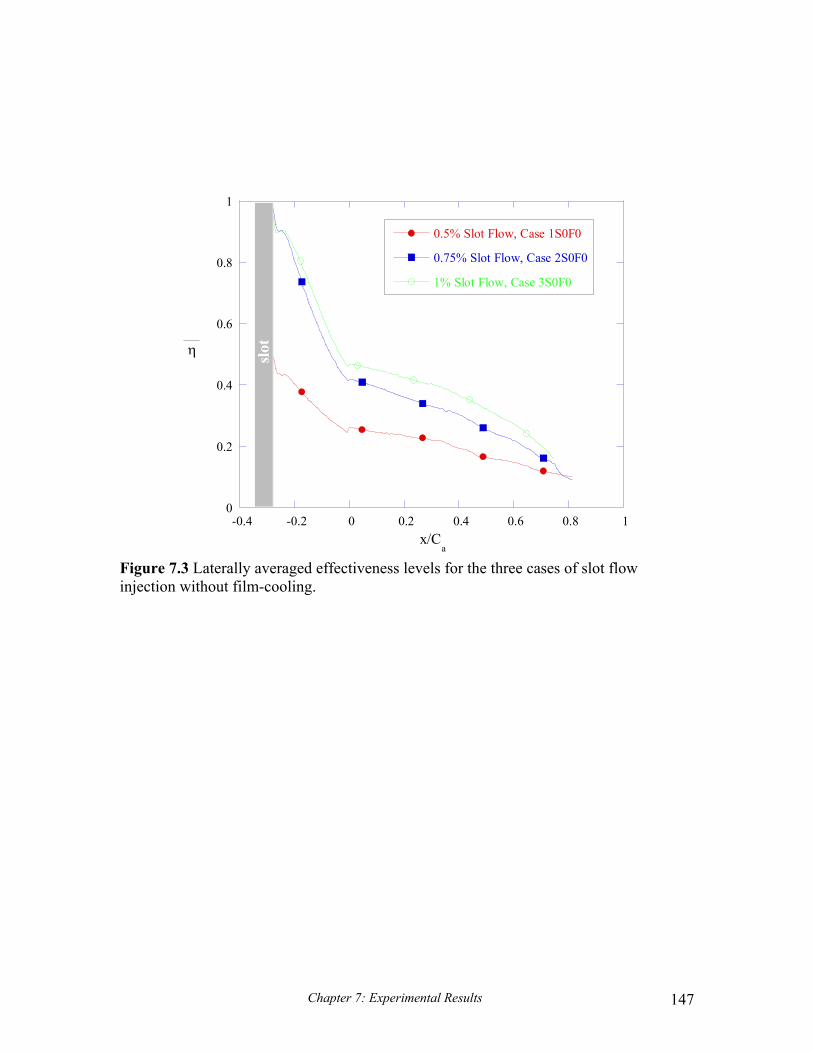
Chapter 7: Experimental Results 147

0

0.2

0.4

0.6

0.8

1

-0.4 -0.2 0 0.2 0.4 0.6 0.8 1

0.5% Slot Flow, Case 1S0F0

0.75% Slot Flow, Case 2S0F0

1% Slot Flow, Case 3S0F0

x/Ca

η slot

Figure 7.3 Laterally averaged effectiveness levels for the three cases of slot flow injection without film-cooling.

Chapter 7: Experimental Results 148

Figure 7.4a-d Contours of adiabatic effectiveness for the baseline film-cooling only cases: (a) pattern #1, 0.5% film, case 0S1F1, (b) pattern #1, 0.75% film, case 0S2F1, (c) pattern #2, 0.5% film, case 0S1F1, and (d) pattern #2, 0.75% film, case 0S2F2.

c

awTT

TT−−

=η∞

∞

a)

d) c)

b)

Chapter 7: Experimental Results 149

0

0.2

0.4

0.6

0.8

1

-0.4 -0.2 0 0.2 0.4 0.6 0.8 1

0.5% Film Pattern #1, Case 0S1F10.5% Film Pattern #2, Case 0S1F2

0.75% Film Pattern #1, Case 0S2F10.75% Film Pattern #2, Case 0S2F2

x/Ca

η slot

Figure 7.5 Laterally averaged effectiveness levels for the four cases of film-cooling injection without slot injection.

Chapter 7: Experimental Results 150

Figure 7.6a-d Contours of adiabatic effectiveness for pattern #1 at the various combined slot and film-cooling cases (a) 0.5% slot 0.5% film, case 1S1F1, (b) 0.5% slot 0.75% film, case 1S2F1, (c) 0.75% slot 0.5% film, case 2S1F1, and (d) 0.75% slot 0.75% film, case 2S2F1.

c

awTT

TT−−

=η∞

∞

a)

c) d)

b)

Chapter 7: Experimental Results 151

0

0.2

0.4

0.6

0.8

1

-0.4 -0.2 0 0.2 0.4 0.6 0.8 1

0.5% Slot / 0.5% Film, Case 1S1F10.75% Slot / 0.5% Film, Case 2S1F1

0.5% Slot / 0.75% Film, Case 1S2F10.75% Slot / 0.75% Film, Case 2S2F1

x/Ca

η slot

Pattern #1

Figure 7.7 Laterally averaged adiabatic effectiveness levels for pattern #1 at four cooling combinations of slot and film-coolant injection.

Chapter 7: Experimental Results 152

Figure 7.8a-d Contours of adiabatic effectiveness for pattern #2 at the various combined slot and film-cooling cases (a) 0.5% slot 0.5% film, case 1S1F2, (b) 0.5% slot 0.75% film, case 1S2F2, (c) 0.75% slot 0.5% film, case 2S1F2, and (d) 0.75% slot 0.75% film, case 2S2F2.

c

awTT

TT−−

=η∞

∞

a) b)

d) c)

Chapter 7: Experimental Results 153

0

0.2

0.4

0.6

0.8

1

-0.4 -0.2 0 0.2 0.4 0.6 0.8 1

0.5% Slot / 0.5% Film, Case 1S1F20.75% Slot / 0.5% Film, Case 2S1F2

0.5% Slot / 0.75% Film, Case 1S2F20.75% Slot / 0.75% Film, Case 2S2F2

x/Ca

η slot

Pattern #2

Figure 7.9 Laterally averaged adiabatic effectiveness levels for pattern #2 at four cooling combinations of slot and film-coolant injection.

Chapter 7: Experimental Results 154

Figure 7.10a-b Momentum flux ratios for holes indicated by the dashed lines are shown in (a) the leading edge region and (b) the upstream and downstream pressure side regions. Adiabatic effectiveness levels of neighboring holes are also pictured for reference.

0.0

0.2

0.4

0.6

0.8

1.0

1.2

1.4

0

1

2

3

4

5

6

7

Leading Edge Blockers

Upstream Pressure Side

Downstream Pressure Side

Upstream Pressure Side

Downstream Pressure Side

I

I

1S2F2

1S2F1

1S1F2 0S1F2

0S1F1 1S1F1

1S2F2

1S2F1

1S1F2

0S1F2

1S1F1 0S1F1

1S2F2 1S2F1 1S1F2 1S1F1 0S1F2 0S1F1

Leading Edge Blockers Upstream Pressure Side Downstream Pressure Side

c

awTT

TT−−

=η∞

∞

Chapter 7: Experimental Results 155

0

0.1

0.2

0.3

0.4

0.5

0.6

0.5 0.75 1 1.25 1.5

Slot Only

Film Only, Pattern #1

Film Only, Pattern #2

Slot + Film, Pattern #1

Slot + Film, Pattern #2

0.75% Slot + 0.5% Film, Pattern #1

0.75% Slot + 0.5% Film, Pattern #2

η

Cumulative Coolant Rate (%mexit

)

Figure 7.11 Area-averaged effectiveness levels are shown for the 15 experimental cases with a uniform inlet profile. The cases are grouped by cumulative coolant flow rate providing a quantifiable method of assessing the effects of distributing coolant between the slot and film-cooling holes.

Chapter 7: Experimental Results 156

Figure 7.12a-d Adiabatic effectiveness contours are shown for case 1S1F2 with both an (a) endwall-peaked and (b) center-peaked inlet profile. Contours were normalized by the maximum temperature in the profile. The same cases are shown in (c) and (d) with the adiabatic wall temperature normalized by the spatially averaged temperature from the profile.

ch

awhTT

TT−−

=η

a)

c)

b)

d)

cave

awaveTT

TT−−

=η

Chapter 7: Experimental Results 157

Figure 7.12e Adiabatic effectiveness contours are shown for case 1S1F2 with a near-wall peaked profile. The contours are normalized by the average near-wall temperature (0%-5% span) to illustrate that when properly scaled, the results from all three temperature profiles for case 1S1F2 appear the same.

e)

cnw

awnwTT

TT−−

=η

Chapter 7: Experimental Results 158

Figure 7.13a-d Contours of flow angle, φ, measured in degrees as deviation from the downstream axial direction are shown along with streamlines for (a) the midspan corresponding to inviscid predictions (b) 2% span with a low 0.5% slot coolant flow rate and (c) 2% span with a high 0.75% slot coolant flow rate. The streamlines for all three cases are superimposed in (d) to illustrate the strengthened cross flow because of the slot.

-80

-60

-40

-20

0

20

40

60

80 φ

a)

d) c)

b)

Chapter 7: Experimental Results 159

Figure 7.14a-b Predicted streamlines at 2% span for both the low and mid-level slot flow rates are presented with the hole locations of pattern #1 (a) and pattern #2 (b) shown for reference.

a) b)

Chapter 7: Experimental Results 160

Figure 7.15a-d Predicted streamlines at 2% span for 0.5% slot flow without film-cooling are superimposed on (a) pattern #1 with 0.5% slot flow and 0.5% film-cooling and (b) pattern #2 with 0.5% slot flow and 0.5% film-cooling. The two cases are shown with predicted streamlines at the midspan superimposed in (c) and (d).

c

awTT

TT−−

=η∞

∞

Chapter 7: Experimental Results 161

Figure 7.16a-d Predicted streamlines at 2% span for 1% slot flow without film-cooling are superimposed on (a) pattern #1 with 1% slot flow and 0.5% film-cooling and (b) pattern #2 with 1% slot flow and 0.5% film-cooling. The same two cases are shown with predicted streamlines at the midspan superimposed in (c) and (d).

c

awTT

TT−−

=η∞

∞

Chapter 7: Experimental Results 162

Figure 7.17a-d Contours of the difference between the predicted flow angles at 2% span and midspan are shown for the low 0.5% slot flow case (a) and (b) and the mid-level 0.75% slot flow case (c) and (d). The hole locations of pattern #1 and pattern #2 are shown for reference.

msspan%2 φ−φ

a)

d)

b)

c)

Chapter 7: Experimental Results 163

Figure 7.18a-d Contours of adiabatic effectiveness are shown for (a) case 1S0F0, 0.5% slot flow and (b) case 0S1F2, 0.75% film. Contours of adiabiatic effectiveness for case 1S1F2, 0.5% slot 0.5% film, are shown from both (c) superposition and (d) measurements.

( )121sup 1 η−η+η=η

c

awTT

TT−−

=η∞

∞

a)

d)

(1) (2)

c)

b)

Chapter 7: Experimental Results 164

Figure 7.19a-b (a) Superposition predicted and (b) measured contours of adiabatic effectiveness are shown for case 1S2F2, 0.5% slot 0.75% film.

Figure 7.20a-b (a) Superposition predicted and (b) measured contours of adiabatic effectiveness are shown for case 2S1F2, 0.75% slot 0.5% film.

c

awTT

TT−−

=η∞

∞

a) b)

c

awTT

TT−−

=η∞

∞

a) b)

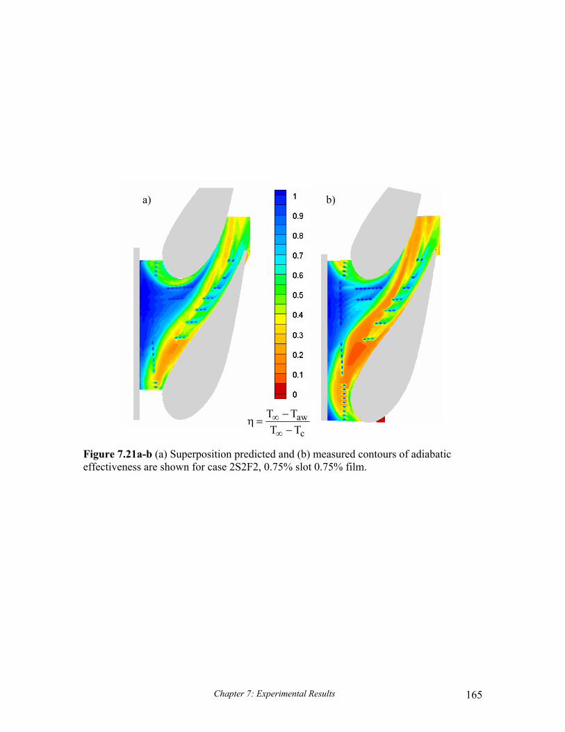
Chapter 7: Experimental Results 165

Figure 7.21a-b (a) Superposition predicted and (b) measured contours of adiabatic effectiveness are shown for case 2S2F2, 0.75% slot 0.75% film.

c

awTT

TT−−

=η∞

∞

a) b)

Chapter 7: Experimental Results 166

Figure 7.22a-d Thermal field data was acquired in (a) a plane normal to the pressure surface at x/Ca = -0.77. Contours of non-dimensional temperature are shown for (b) 0.5% slot flow without film-cooling, case 1S0F0, (c) 0.5% slot flow with 0.5% film-cooling, case 1S1F2, and (d) 0.5% slot flow with 0.75% film-cooling, case 1S2F2.

a)

d) c)

b)

Chapter 8: Comparison of Predictions and Measurements 167

Chapter 8

Comparison of Predictions and Measurements

Computer simulation has become an integral part of the modern day engineering

design process. Many different designs can be quickly generated and evaluated at

relatively low expense. Computational simulation also lends itself to optimization studies

so that the most critical design parameters can be identified and the impact of altering

these parameters can be quantified. Before, a computational package can be relied upon

in the design process, however, it must be compared to benchmark data to evaluate the

validity and accuracy of solutions. This chapter provides a comparison of the

computational results presented in chapter 6, with experimental results presented in

chapter 7. The matrix of cases that were performed both computationally and

experimentally is presented in Table 8.1.

Section 8.1 compares predicted and measured contours of adiabatic effectiveness

for the eight cases. The contours are used to evaluate accuracy of coolant trajectory

predictions as well as cooling effectiveness levels. The laterally-averaged adiabatic

effectiveness levels are examined to evaluate trends in the cooling patterns between the

predictions and measurements as well as between cases. Thermal field measurements are

also presented for three cases to examine the migration of coolant once detached from the

endwall. Section 8.2 compares the area-averaged adiabatic effectiveness levels between

predictions and measurements and between cases. Trends produced by altering the

coolant distribution between the cooling mechanisms are examined. Finally, Section 8.3

provides a brief summary of the comparisons.

8.1 Adiabatic Effectiveness Contours

Slot Flow Comparisons

The most simplistic cooling case of a low, 0.5% slot flow without film-cooling

was first computed. The prediction of endwall adiabatic effectiveness is shown in Figure

8.1a. The slot coolant is seen to exit in a non-uniform manner with no slot flow exiting

upstream of the leading edge. The adiabatic effectiveness level rapidly decays at the slot

Chapter 8: Comparison of Predictions and Measurements 168

exit to approximately η = 0.5. The coolant is swept across the passage and exits along

the suction side leaving an uncooled ring around the vane. The ring is particularly

pronounced at the leading edge and along the pressure side. The adiabatic effectiveness

levels in this area are η = 0 corresponding to the temperature of the isothermal inlet flow.

Measurements of case 1S0F0 are shown in Figure 8.1b. Immediately noticeable,

is that the lowest recorded adiabatic effectiveness levels are approximately η = 0.1. As

was discussed in Section 7.1, this is a result of cooling of the near-wall fluid due to a long

unheated section of the wind tunnel between the heater bank where the uniform

temperature was generated and the test section. The adiabatic effectiveness levels in

these areas correspond to the temperature of the approaching near-wall fluid and are not

the result of any cooling benefit from the slot flow.

As was predicted, the slot coolant exits in a non-uniform manner with no coolant

upstream of the leading edge and is swept towards the suction side. The width and exit

location of the slot flow seems well predicted. The slightly cooled periphery of the slot

flow prediction is not exhibited in the measurements, though, and the adiabatic

effectiveness levels within the slot streak do not decay nearly as rapidly as was predicted.

Also a slightly stronger turning of the pressure side edge of the coolant boundary towards

the suction side is seen in the measurements just beyond the slot exit. Approximately

half way through the passage in the measurements, the slot coolant is seen to taper to

only a narrow area and is turned into the suction side. In contrast, the prediction shows a

broader coolant band which extends through the passage and is not turned as sharply into

the vane.

The thermal field was documented for case 1S0F0 in the plane indicated by the

black line on Figures 8.1a-b. The plane is normal to pressure side at the surface location

s/C = -0.77 and extends across the passage to the suction side of the adjacent vane. The

predictions and measurements are shown in Figures 8.2a and 8.2b respectively. The

plane is viewed from downstream so that the pressure side is on the left and the suction

side is on the right. The slot flow is predicted to be a coherent, well-defined structure,

which is transported towards the suction side. A cool core is present at the endwall at the

plane-width location 0.15 ≤ y/P ≤ 0.18. Rings around the cool core lead to the slightly

cooled gradients seen on the edges of the endwall slot flow pattern.

Chapter 8: Comparison of Predictions and Measurements 169

Measurements also show the slot coolant as a coherent structure that is

transported towards the suction side. The dimensionless temperature at the endwall for

much of the plane is the same as the inlet near-wall temperature indicating the presence

of the upstream thermal boundary layer. The effects of the coolant are seen up to 7%

span which is consistent with the prediction. The cool core of the slot flow is seen at y/P

= 0.13 and z/S = 0.02. The computation failed to predict the coolant core being lifted off

of the endwall surface. In addition, the migration of the core towards the suction side

was over-predicted. The measurements do, however, show a coolant foot at the plane

width location 0.15 ≤ y/P ≤ 0.18 corresponding to the location of the coolant core in the

prediction.

Predictions and measurements of endwall adiabatic effectiveness for case 3S0F0,

1.0% slot flow without film-cooling, are shown in Figures 8.3a-b. In both the prediction

and measurements, the slot flow exits across the entire span of the slot. The coolant is

convected towards the suction side leaving an uncooled perimeter around the vane. The

footprint of the slot flow seems well predicted, but thermal spreading is under-predicted

with a broader more gradual gradient around the periphery of the slot flow region than

the measurements would suggest. In addition, the maximum cooling effectiveness levels

are not sustained in as large an area as is shown at the slot exit of the measurements.

Contrary to the low slot flow rate, the minimum effectiveness level was measured to be η

= 0, matching the minimum predicted level. As was discussed in chapter 7, it is believed

that the coolant exiting across the entire width of the slot tended to block the approaching

near-wall fluid, which was slightly cooler, and funnel it along with the slot coolant into

the center of the passage and towards the suction side. This drew the hotter gasses just

above the boundary layer down onto the surface leading to a measured adiabatic

effectiveness level of η = 0.

A comparison of the laterally-averaged adiabatic effectiveness levels from the

predictions and measurements of both of the slot coolant rates is shown in Figure 8.4.

Laterally-averaged effectiveness levels are often used to evaluate the performance of

coolant as it progresses downstream. The average effectiveness levels are higher than

predicted for both flow rates. At the low 0.5% flow rate the laterally-averaged

effectiveness levels are higher than predicted both because the maximum effectiveness

Chapter 8: Comparison of Predictions and Measurements 170

levels are maintained over a larger area within the slot flow region and because the

minimum effectiveness levels are higher than predicted because of the slightly cooler

boundary layer. At the high, 1% slot flow rate, the measured values are higher than

predicted because the maximum effectiveness levels are again maintained over a larger

area than predicted and because the higher effectiveness levels extend closer to the

coolant boundary rather than having a large, low gradient area around the periphery of

the slot flow region. The trend of high effectiveness at the slot exit followed by a

decaying adiabatic effectiveness was properly predicted through the passage. The

measurements also tend to parallel the predicted values indicating that only the

magnitudes of cooling effectiveness were significantly mispredicted.

Endwall Film-Cooling Comparisons

The film-cooling patterns were tested at the low 0.5% coolant flow rate without

slot flow in order to gain a comparative baseline for the combined cooling mechanism

cases. The predictions and measured contours of adiabatic effectiveness for pattern #1,

the pattern based upon the iso-velocity line design, are shown in Figures 8.5a-b. Once

again, the minimum measured effectiveness level corresponds to the temperature of the

near-wall fluid rather than the slightly hotter midspan. The suction side leading row jets

are predicted to inject as discrete jets along the incoming streamlines despite being

directed normal to the inlet and in the direction of turning. The pressure side, leading

row jets are also predicted to inject with the streamlines, but in a slightly less discrete

fashion. The suction side, leading row jets were shown to inject with the streamlines as

discrete jets in the measurements as well. The pressure side, leading row jets, however,

were considerably more well directed than the predictions would suggest. This leads to a

more contiguous cool zone just upstream of the first cross-passage row, but also supplies

little, if any, coolant to the area just to the side of the two upstream, short rows. In

addition, the cooling effectiveness of the leading row jets is predicted to decay more

rapidly than the measurements indicate.

The performance of the leading edge blockers appears well predicted. The

pressure side leading edge blockers provide no cooling relief, while the suction side

leading edge blockers fail to penetrate to the vane-endwall junction and are swept around

Chapter 8: Comparison of Predictions and Measurements 171

the suction side. As with the leading row holes, the local effectiveness levels are

somewhat under-predicted.

An uncooled streak along the pressure side was predicted and verified by the

measurements. Coolant emerges from the downstream edge of the film-cooling holes in

the measurements rather than from the side of the holes, as predicted, resulting in slightly

narrower uncooled region. Cooling effectiveness levels along the pressure side, as well

as throughout the passage, do not decay as rapidly as predicted.

A warm spot just upstream of the second cross-passage row is indicated in both

the predictions and measurements, but the predicted adiabatic effectiveness level in this

area is only η = 0.15 where it was measured to be η = 0.3. In the exit region of the

passage, as well as beyond the trailing edge, the coolant is turned more strongly towards

the suction side than was predicted. In addition, thermal spreading within the passage

seems under-predicted resulting in less uniform effectiveness levels than are shown by

the measurements.

Predictions and measurements of adiabatic effectiveness for case 0S1F2, 0.5%

film-cooling without slot flow for pattern #2, are shown in Figures 8.6a-b. As with the

low slot flow alone and the film-cooling alone for pattern #1, the minimum effectiveness

levels correspond to the temperature of the approaching near-wall fluid and effectiveness

levels are generally under-predicted throughout the passage. A hot streak is both

predicted and measured, although the width of the hot streak is under-predicted.

The leading row, suction side holes are predicted to inject in the streamwise

direction with low effectiveness levels of approximately η = 0.35. These holes are shown

to inject with the streamlines in the measurements as well, but the jets spread leaving less

distinct traces. The local effectiveness levels were also measured to be higher than

predicted at η = 0.5. The leading row, pressure side holes are predicted to inject

downstream with the streamlines as well but in a less discrete fashion. The local

effectiveness levels are again predicted to be η = 0.35, but they do not decay as rapidly as

suction side leading row holes. Coolant from the suction side, leading row holes is

carried downstream along the upstream edge of the pressure side rows. In contrast,

coolant from these holes is seen to be more directed in the measurements. The coolant

exits in a narrower more merged area and progresses downstream into the middle of the

Chapter 8: Comparison of Predictions and Measurements 172

hot streak. Coolant from the pressure side, leading row holes forces coolant from the

suction side, leading row holes, as well as from the downstream holes of the two

upstream passage rows, to adhere to the downstream edge of the two upstream passage

rows. Coolant from these holes appears axially downstream of the upstream rows in the

predictions. Local adiabatic effectiveness levels for the pressure side, leading row holes

were measured to be approximately η = 0.5, consistent with local levels for the suction

side, leading row holes, but as with predictions, the effectiveness levels do not decay as

quickly downstream of the pressure side, leading row holes.

The leading edge blockers are well predicted on the suction side, except that the

effectiveness levels are under-predicted. In both the predictions and measurements, the

suction side leading edge blockers penetrate to the vane-endwall junction and provide

coolant around the shoulder of the suction side. The pressure side leading edge blockers,

however, are not as well predicted. This area is quite hard to predict because the

stagnating flow requires very large cells in order to obtain the proper y+ values. If the

cell size is increased, though, resolution is sacrificed. For the computations, smaller cells

(lower y+) were used to avoid having a small section of cells which were much larger

than other cells on the endwall. Coolant from the pressure side leading edge blockers is

predicted to adhere to the endwall and be pulled away from the vane. The measurements

indicate no cooling local to the hole. The jets appear to separate upon injection and

impact the vane before being washed down into the vane-endwall junction along the

pressure side near the stagnation point.

An uncooled area along the pressure side is both predicted and measured.

Coolant from the pressure side jets penetrates slightly closer to the vane than predicted,

just as was the case with pattern #1. Finally, the upstream most jet of each pressure side

row appears to be drawn slightly more towards the center of the passage indicating

stronger turning than predicted. This was also seen in the cases with slot flow alone.

A comparison of the laterally averaged effectiveness values for the two film-

cooling patterns without slot flow for the predictions and measurements is shown in

Figure 8.7. As with the cases with only slot flow, the average effectiveness levels are

higher than predicted in large part due to cooling of the near-wall fluid before the test

Chapter 8: Comparison of Predictions and Measurements 173

section. This effect is easily seen from the predicted levels just downstream of the slot

location, which are still upstream of the leading row of holes.

When examining the leading edge region where -0.2 ≤ x/Ca ≤ 0, two peaks are

predicted corresponding to the spacing between the leading edge row holes oriented

normal to the inlet flow and the leading edge blockers. This double peak is not seen in

the measurements because the local effectiveness levels just downstream of the leading

row holes are higher than predicted reducing the discrepancy in the average effectiveness

levels at the axial locations just upstream and downstream of the leading edge blockers.

The trends through the passage are once again paralleled by the predictions with

the average effectiveness levels rising until approximately x/Ca = 0.6 where the levels

slightly decay. When comparing the pattern #1 to pattern #2, pattern #1 is seen to be

slightly more effective than predicted. From the computations, pattern #1 is slightly less

effective in the leading edge region and does not outperform pattern #2 until

approximately x/Ca = 0.5. Pattern #1 is then superior to pattern #2, in the laterally-

averaged sensed, throughout the exit of the passage. In contrast, the measurements show

pattern #1 to be equal or superior to pattern # 2 throughout the entire passage. Comparison of Slot Flow Combined with Film-Cooling for Pattern #1

Moving along to the combined slot and film-cooling cases, the predictions and

measurements of the low 0.5% slot flow combined with the low 0.5% film-cooling rate

for pattern #1 are shown in Figures 8.8a-b.The width of the slot flow exit area is slightly

over-predicted. The coolant is constricted between the leading row and the first cross-

passage row, by the impinging pressure side, leading row jets in both the computations

and measurements. Slightly stronger turning is also exhibited in the measurements

resulting in the coolant impacting the suction side of the upper vane upstream of the

impact location predicted by the computations.

The pressure side, leading row holes are shown to be more directed and merged in

the measurements with a larger, contiguous affected zone and a higher adiabatiac

effectiveness level of η = 0.5, as compared to the predicted level of η = 0.35. The

trajectory of the leading edge blockers is well predicted. Coolant exits and is swept

around the suction side leaving an uncooled region at the leading edge. The coolant is

Chapter 8: Comparison of Predictions and Measurements 174

shown to impact the shoulder in the measurements, but is not predicted to impact the

upper vane until near the trailing edge.

An uncooled region along the pressure side is also properly predicted. The

upstream rows of three holes, however, are more directed in the measurements and decay

less rapidly. Thermal spreading of the downstream jets along the pressure side and

beyond the second cross-passage row also appears under-predicted resulting in more

uniform adiabatic effectiveness levels in the measurements.

The results of increasing the film flow rate to 0.75% while maintaining the slot

flow rate at 0.5% for pattern #1 are shown in Figures 8.9a-b. Again, the width of the slot

exit region is slightly under-predicted, and a cool core is maintained just downstream of

the leading row. The concentration of the highest effectiveness levels, forming the cool

core, is not seen in the prediction. A constriction of the slot flow is exhibited in both the

predictions and measurements as a result of impingement from the pressure side, leading

row holes.

Increasing the coolant flow rate is predicted to improve the cooling performance

of the pressure side, leading row holes, but it is seen from the measurements that

increasing the cooling rate actually reduces the effectiveness of the these holes. Also, the

predicted adiabatic effectiveness levels of the pressure side, leading row holes are higher

than the measured values. Both the over-prediction of the effectiveness levels and the

misprediction of the trend are most likely due to jet separation which was either not

captured or not as pronounced in the computations. The upstream rows of three holes

along the pressure side also exhibit jet separation which was not fully captured by the

computations. In addition, the hole closest to the pressure side in these two rows appears

to follow the contour of the vane while the other two holes in the rows are drawn more

towards the center of the passage. The computations predict that all three holes in these

two rows will inject in the same direction leading to more uniform coverage of the areas

just downstream of the rows. The uncooled area along the pressure side is well predicted

and shows a reduction when compared to the low film-cooling rate for both the

predictions and measurements.

The computations accurately predict the leading edge blockers on the suction side

penetrating fully to the vane and providing coolant around the shoulder of the suction

Chapter 8: Comparison of Predictions and Measurements 175

side. As with the upstream pressure side holes, though, the effectiveness levels are over-

predicted indicating that partial jet detachment is not properly captured. This problem

seems exacerbated at the pressure side leading edge blockers. The predictions show

coolant at the endwall between the holes and the stagnation point. The measurements

indicate that the jets detach at the injection location and impact the vane before being

washed down onto the vane endwall junction as evidenced by the coolant accumulation

only along the junction at the pressure side.

Thermal spreading within the passage seems more accurately predicted with the

varying effectiveness levels corresponding well although the warm spot upstream of the

second cross-passage row is shown to be broader than predicted.

The predicted and measured laterally-averaged adiabatic effectiveness levels are

compared for the two cases of combined slot and film-cooling for pattern #1 in Figure

8.10. At the low film-cooling flow rate, the trends throughout the passage are captured in

the predictions, but, once again, the magnitudes are over-predicted by approximately ∆η

= 0.1. At the increased blowing rate, both the trends and magnitudes are quite well

predicted. The average effectiveness levels are only slightly over-predicted in the

upstream half of the passage where jet separation did not appear to be well captured.

Comparison of Slot Flow Combined with Film-Cooling for Pattern #2

The adiabatic effectiveness contours for pattern #2 with combined 0.5% slot and

0.5% film-cooling flow rates are shown in Figures 8.11a-b. The exit location of the slot

flow is seen to be mispredicted with coolant exiting closer to the upper vane in the

measurements. The large area where η = 0.5 to the pressure side of the upstream passage

rows is also not seen in the measurements and the maximum effectiveness level is

maintained over a much larger area. Slot coolant is predicted to cover the gutter gap in

the leading row of holes and be present axially downstream of the upstream passage

rows, but the measurements show that the entire gutter gap is not covered and that the

slot coolant adheres to the downstream edge of the upstream passage rows. Also, slightly

stronger turning is seen near the flow plane indicated by the black line resulting in an

impact location of the slot flow upstream of the predicted impact location.

Chapter 8: Comparison of Predictions and Measurements 176

The directionality of the pressure side, leading row holes is also under-predicted

while the effectiveness of these holes is over-predicted. The measurements show low η =

0.35 effectiveness levels indicating a potential jet separation. The coolant is also more

merged and a thin, uncooled region between the slot flow and the coolant from the

pressure side, leading row holes is evident. The predictions show higher η = 0.5

effectiveness levels and cooling effects from the pressure side, leading row holes as far

axially downstream as the upstream edge of the pressure side holes. Coolant from these

holes is directed into the middle of the passage in the measurements. As a result of the

higher directionality of the jets, the hot streak is shown to be broader in the

measurements.

The local effectiveness levels of the leading edge blockers appear well predicted

except the effectiveness levels do not decay as rapidly around the shoulder of the suction

side. In addition, the coolant was predicted to travel to the vane-endwall junction, but the

measurements show that the jets do not fully penetrate to the vane. The performance of

the pressure side leading edge blockers, however, is especially mispredicted. Coolant is

predicted to adhere to the endwall and be carried along the pressure side, but the jets are

shown to be detached with coolant impacting the vane before washing down onto the

junction in the measurements.

An uncooled region along the pressure side is shown in both the predictions and

measurements. Both trajectories and local effectiveness levels of the pressure side jets

are well predicted with the exception of the upstream most hole in each of the two

upstream most rows of three holes. These two jets appear slightly more drawn towards

the center of the passage resulting in a more discrete cooling pattern on the endwall.

Predictions and measurements of the thermal field taken in the plane indicated by

the black line are presented in Figures 8.12a-b. In both the predictions and

measurements, the hot streak in the center of the passage is clearly visible. The

predictions indicate two areas of coolant concentration: one near the pressure side and

one near the suction side. Both areas have a cool core of θ = 0.65 at the endwall. The

minimum of the larger coolant zone, consisting of both slot and film-coolant, is shown at

0.18 ≤ y/P ≤ 0.2. This coolest area is closer to the suction side than the center of the

coolant mass which is seen above the endwall at z/S = 0.02 and y/P = 0.17.

Chapter 8: Comparison of Predictions and Measurements 177

The measurements also show two areas of coolant concentration. The cool core

of the slot and film coolant is shown off of the wall in the center of the coolant mass at

z/S = 0.035 and y/P = 0.16. This is quite different from the predictions of the coolant

core on the endwall. The computations failed to predict that the coolant would be lifted

off of the endwall and be entrained in the center of the passage vortex. A small coolant

foot is maintained, however, at the endwall in the same location as the predicted coolant

core. Both the predictions and measurements indicate a small measure of cooling

effectiveness on the suction side of the vane below approximately z/S = 0.04. The film-

cooling mass along the pressure side is seen to be much flatter and broader than

predicted. A thin zone of maximum effectiveness θ = 0.6 is maintained at 0.04 ≤ y/P ≤

0.05 which corresponds to the predicted maximum location.

Predictions and measurements of increasing the film-cooling to 0.75% of the core

flow while maintaining the slot at 0.5% are shown in Figures 8.13a-b. As with the low

film-cooling flow rate for pattern #2, the exit location of the slot flow is mispredicted

with coolant exiting closer to the upper vane in the measurements. As a result, the entire

width of the gutter gap in the leading row of holes is not cooled.

The directionality of the leading row, pressure side holes appears well predicted

with the exception the slightly cooled region axially downstream of the leading row,

pressure side holes. This is most likely cooling as a result of the mainstream mixing with

the injecting jets, rather than the coolant jets convecting down through the center the

passage in the hot streak region. The cooling effectiveness levels are over-predicted at η

= 0.5 while they were measured at only η = 0.35. The extremely low measured cooling

effectiveness levels would seem to indicate jet separation which is not well captured by

the predictions. In both the predictions and measurements, the slot flow is constricted by

the pressure side, leading row holes impacting the upstream most hole of the upstream

passage rows.

The leading edge blockers are predicted to inject in a discrete fashion indicating

partial jet separation with maximum adiabatic effectiveness levels of η = 0.5. The

measurements show the leading edge blockers being completely detached and impacting

the vane before being washed down onto the vane-endwall junction. The maximum

adiabatic effectiveness level in this region was also measured to be η = 0.5. Coolant

Chapter 8: Comparison of Predictions and Measurements 178

adheres to the pressure side in the vane-endwall junction just beyond the dynamic

stagnation point in both the predictions and measurements.

Both predictions and measurements indicated only a thin uncooled region along

the pressure side at the upstream rows of pressure side holes, while the cooling holes

nearer to the exit penetrated to the vane endwall junction. The cooling effectiveness

levels and direction of the pressure side jets are well predicted except that coolant from

the upstream most hole of both the fourth pressure side row and the trailing edge row is

drawn slightly more across the passage indicating stronger cross flow in the exit region

than predicted.

The thermal fields in the indicated plane for case 1S2F2 are shown in Figures

8.14a-b. Both the predictions and the measurements show a widening of the hot steak

between the two coolant zones when compared to the results of the low film flow case in

Figures 8.11a-b. The larger coolant zone, consisting of slot and film coolant, is shifted

closer to the suction side and appears more skewed indicating a stronger passage vortex

for the higher film-cooling flow. A cool core is predicted and measured at the endwall

and extends up to z/S = 0.02. The maximum dimensionless temperature, corresponding

the minimum fluid temperature, is over-predicted at θ = 0.7 as compared to a measured

value of θ = 0.4. The plane width location is also slightly over-predicted at y/P = 0.2.

Coolant is seen to accumulate against the suction side of the vane reaching a predicted

height of z/S = 0.07 and a measured height of z/S = 0.06.

The film-cooling zone along the pressure side has also moved closer to the vane

with the predicted plane location from 0.01 ≤ y/P ≤ 0.06 and the measured range from 0

≤ y/P ≤ 0.06. The coolant is predicted in a semi-circular pattern with a cool core of θ =

0.6 at 0.03 ≤ y/P ≤ 0.045. The measurements however show the coolant accumulating

more against the vane rising up to z/S = 0.02. The maximum measured dimensionless

temperature is θ = 0.5.

A comparison of the predicted and measured laterally-averaged adiabatic

effectiveness levels for slot flow combined with film-cooling pattern #2 is shown in

Figure 8.15. For both cases the coolant was slightly more effective at the slot exit than

predicted. As with pattern #1, at the low film-cooling rate, the measured effectiveness

values exceed the predicted values throughout the entire passage. The deviation however

Chapter 8: Comparison of Predictions and Measurements 179

is only approximately ∆η = 0.05. At the increased film-cooling flow rate, the predicted

values exceed the measured average effectiveness level in the range 0.4 ≤ x/Ca ≤ 0.6

which is approximately where the gutter gap exists between the upstream passage rows

and the pressure side holes. It is seen that the cool region from the slot flow and

upstream passage rows is not as broad and less effective than predicted in this area and,

the local effectiveness levels at the pressure side holes are slightly lower than predicted

leading to the discrepancy.

8.2 Area-Averaged Adiabatic Effectiveness

Area-averaged effectiveness values provide a metric for comparing the effects of

varying coolant distribution between the slot and film-cooling mechanisms. The area-

averaged adiabatic effectiveness levels for to eight cases which were both computed and

measured are shown in Figure 8.16. The cases are grouped by cumulative coolant flow

rate. Area-averaged values were calculated from the axial location x/Ca = -0.235

corresponding to the upstream most point where the measurements covered the full pitch

of the cascade to x/Ca = 0.8 where optical access to the passage was limited. The

average effectiveness levels were consistently under-predicted because the endwall was

artificially cooled by a slightly cooler approaching boundary layer than the predictions

accounted for. As a result the measured adiabatic effectiveness levels in uncooled

regions were often η = 0.1 rather than η = 0. Also, thermal spreading was consistently

under-predicted contributing to increased predicted endwall temperatures. At high

blowing ratios, separation was induced in many of the upstream holes which was also not

well captured. This led to closer agreement between the measurements and predictions,

because local cooling was over-predicted offsetting the effects of the uncooled areas

which were over-predicted because of the cooler near-wall fluid. This close agreement is

seen in the 1.25% grouping.

The trends induced by changing the coolant distribution within the groups were

well predicted. At 0.5% cumulative coolant flow, both the predictions and measurements

indicate that the film-cooling holes alone provide superior cooling, in the area averaged

sense, to the slot flow alone with pattern # 1 outperforming pattern #2. Within the 1%

grouping, the slot flow was inaccurately predicted to provide the lowest area-averaged

Chapter 8: Comparison of Predictions and Measurements 180

effectiveness of the group when in fact it provided the highest area-averaged

effectiveness. This case does not provide superior performance to the combined cases,

though, because the area-averaged effectiveness levels have been inflated by large,

overcooled slot area, while a warm uncooled ring was left around the vane. The film-

cooling patterns offered similar average effectiveness levels without the large uncooled

zones. Pattern #1 was accurately predicted to provide slightly better performance than

pattern #2 at the 0.5% coolant flow rate when combined with 0.5% slot flow. In addition,

all three cases with 1% cumulative coolant were shown both computationally and

experimentally to provide improved are-averaged effectiveness levels over their

corresponding 0.5% cumulative coolant flow cases. At 1.25% the best agreement was

found between computations and experiments. The predicted trends from increasing the

film blowing from 0.5% to 0.75% while maintaining the slot at 0.5% were not accurate.

Film pattern #2 was predicted to yield equal performance, while film pattern #1 was

predicted to provide improved performance, but measurements showed a decline in area-

averaged effectiveness for both patterns. This was because the computations failed to

accurately capture the separation of many of the upstream holes at the increased blowing

rate.

8.3 Summary

Contours of adiabatic effectiveness were compared for eight cases consisting of

slot cooling alone, film-cooling alone for the two film-cooling hole patterns, and slot

cooling combined with the film-cooling patterns. Computations were shown to be a

valuable tool in aiding to locate film-cooling holes and predict coolant coverage. The

coolant trajectories and footprint were generally well predicted while cooling

effectiveness levels and thermal spreading were frequently under-predicted relative to the

experiments. Minimum effectiveness levels were often lower than measured because the

inlet profile was slightly cooler in the near-wall rather than having a perfectly uniform

inlet profile as mandated by the computations. Large, uncooled rings around the vanes

for the cases with only slot flow were properly predicted as well as uncooled areas along

the pressure side, at the leading edge, and in the center of pattern #2 when film-cooling

was included. The pressure side, leading row holes were frequently more directed than

Chapter 8: Comparison of Predictions and Measurements 181

predicted and stronger turning was seen along the upstream edge of the pressure side

rows and in the exit region of the passage. Jet separation in the leading edge region and

the upstream pressure side holes was also not well predicted.

Chapter 8: Comparison of Predictions and Measurements 182

Table 8.1 Test Matrix of Cases with Both Predictions and Measurements

Case Slot Flow %min

Film Flow %min

Inlet Temp Profile

Thermal Field

1S0F0 0.50 - - - Isothermal Y 3S0F0 1.00 - - - Isothermal N 0S1F1 - - - 0.50 Isothermal N 0S1F2 - - - 0.50 Isothermal N 1S1F1 0.50 0.50 Isothermal N 1S1F2 0.50 0.50 Isothermal Y 1S2F1 0.50 0.75 Isothermal N 1S2F2 0.50 0.75 Isothermal Y

Chapter 8: Comparison of Predictions and Measurements 183

Figure 8.1a-b (a) Predictions and (b) measurements of adiabatic effectiveness are shown for the low 0.5% slot flow rate, case 1S0F0.

Figure 8.2a-b (a) Predictions and (b) measurements of the non-dimensional thermal field for case 1S0F0.

c

awTT

TT−−

=θ∞

∞

a) b)PS PS SS SS

c

awTT

TT−−

=η∞

∞

a) b)

Chapter 8: Comparison of Predictions and Measurements 184

Figure 8.3a-b (a) Predictions and (b) measurements of adiabatic effectiveness are shown for the high 1.0% slot flow rate, case 3S0F0.

0

0.2

0.4

0.6

0.8

1

-0.4 -0.2 0 0.2 0.4 0.6 0.8 1

0.5% Slot Flow, Case 1S0F01% Slot Flow, Case 3S0F0

1S0F03S0F0

x/Ca

η

slot

Predictions Measurements

Figure 8.4 Comparison of laterally-averaged adiabatic effectiveness for predicted and measured cases of slot flow alone.

c

awTT

TT−−

=η∞

∞

a) b)

Chapter 8: Comparison of Predictions and Measurements 185

Figure 8.5a-b (a) Predictions and (b) measurements of adiabatic effectiveness for pattern #1 at 0.5% film-cooling without slot flow, case 0S1F1.

Figure 8.6a-b (a) Predictions and (b) measurements of adiabatic effectiveness for pattern #2 at 0.5% film-cooling without slot flow, case 0S1F2.

c

awTT

TT−−

=η∞

∞

a) b)

c

awTT

TT−−

=η∞

∞

a) b)

Chapter 8: Comparison of Predictions and Measurements 186

0

0.2

0.4

0.6

0.8

1

-0.4 -0.2 0 0.2 0.4 0.6 0.8 1

0.5% Film Only Pattern #1, Case 0S1F10.5% Film Only Pattern #2, Case 0S1F2

0S1F10S1F2

x/Ca

η

slot

Predictions Measurements

Figure 8.7 Comparison of laterally-averaged adiabatic effectiveness for predicted and measured cases of film-cooling flow alone.

Chapter 8: Comparison of Predictions and Measurements 187

Figure 8.8a-b (a) Predictions and (b) measurements of adiabatic effectiveness for pattern #1 at 0.5% slot with the low 0.5% film-cooling flow rate, case 1S1F1.

Figure 8.9a-b (a) Predictions and (b) measurements of adiabatic effectiveness for pattern #1 at 0.5% slot with the high 0.75% film-cooling flow rate, case 1S2F1.

c

awTT

TT−−

=η∞

∞

a) b)

c

awTT

TT−−

=η∞

∞

a) b)

Chapter 8: Comparison of Predictions and Measurements 188

0

0.2

0.4

0.6

0.8

1

-0.4 -0.2 0 0.2 0.4 0.6 0.8 1

0.5% Slot / 0.5% Film Pattern #1, Case 1S1F10.5% Slot / 0.75% Film Pattern #1, Case 1S2F1

1S1F11S2F1

x/Ca

η

slot

Predictions Measurements

Figure 8.10 Comparison of laterally-averaged adiabatic effectiveness from predictions and measurements for 0.5% slot flow with film cooling from pattern #1 at 0.5% and 0.75%.

Chapter 8: Comparison of Predictions and Measurements 189

Figure 8.11a-b (a) Predictions and (b) measurements of adiabatic effectiveness for pattern #2 at 0.5% slot flow with the low 0.5% film-cooling flow rate, case 1S1F2.

Figure 8.12a-b (a) Predictions and (b) measurements of the non-dimensional thermal field for case 1S1F2.

c

awTT

TT−−

=θ∞

∞

a) b)PS SS PS SS

c

awTT

TT−−

=η∞

∞

a) b)

Chapter 8: Comparison of Predictions and Measurements 190

Figure 8.13a-b (a) Predictions and (b) measurements of adiabatic effectiveness for pattern #2 at 0.5% slot flow with the high 0.75% film-cooling flow rate, case 1S2F2.

Figure 8.14a-b (a) Predictions and (b) measurements of the non-dimensional thermal field for case 1S2F2.

c

awTT

TT−−

=η∞

∞

a) b)

c

awTT

TT−−

=θ∞

∞

a) b)PS SS PS SS

Chapter 8: Comparison of Predictions and Measurements 191

0

0.2

0.4

0.6

0.8

1

-0.4 -0.2 0 0.2 0.4 0.6 0.8 1

0.5% Slot/ 0.5% Film Pattern #2, Case 1S1F20.5% Slot / 0.75% Film Pattern #2, Case 1S2F2

1S1F21S2F2

x/Ca

η

slot

Predictions Measurements

Figure 8.15 Comparison of laterally-averaged adiabatic effectiveness from predictions and measurements for 0.5% slot flow with film cooling from pattern #2 at 0.5% and 0.75%.

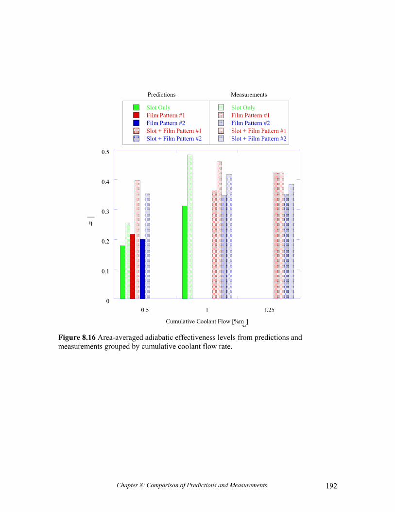
Chapter 8: Comparison of Predictions and Measurements 192

0

0.1

0.2

0.3

0.4

0.5

0.5 1 1.25

Slot Only Slot OnlyFilm Pattern #1 Film Pattern #1Film Pattern #2 Film Pattern #2Slot + Film Pattern #1 Slot + Film Pattern #1Slot + Film Pattern #2 Slot + Film Pattern #2

η

Cumulative Coolant Flow [%mex

]

Predictions Measurements

Figure 8.16 Area-averaged adiabatic effectiveness levels from predictions and measurements grouped by cumulative coolant flow rate.

Chapter 9: Conclusions and Recommendations for Future Study 193

Chapter 9

Conclusions and Recommendations for Future Study

The goal of this research was to develop an understanding of the trajectory of slot

and film-coolant as well as effectiveness levels achieved by each of these cooling

methods. A test matrix was developed to evaluate the effectiveness and distribution of

both slot flow and film-coolant from two original endwall film-cooling designs at various

blowing and momentum flux ratios. The patterns were based on different design

philosophies allowing a comparison of the design methods. Areas requiring special

consideration were identified. The slot and film-cooling patterns were also combined to

evaluate the influence that each cooling mechanism had on the other. The coolant

distribution and effectiveness levels were both predicted using computational fluid

dynamics (CFD) and measured in a large scale, low speed wind tunnel. The effects of

coolant injection on the flow field and thermal field were also examined. The accuracy

of the predictions was evaluated to determine if CFD was a viable tool to aid a designer

in the development of a cooling scheme.

Section 9.1 provides a summary of the results obtained from the predictions.

Section 9.2 recounts the findings from the measurements. The comparison of the

predictions and measurements are outlined in section 9.3. Finally, section 9.4 offers

suggestions for further investigation of this topic.

9.1 Analysis of Predictions

Predictions were made of the effects of coolant injected from a two-dimensional

slot at the combustor-turbine interface alone; endwall film-cooling alone; and combined

slot and endwall film-cooling. The resulting endwall effectiveness from slot cooling

alone showed a pattern that was quite non-uniform along the endwall with most of the

coolant being swept toward the suction side of the vane. One could expect a burn-out

near the vane-endwall juncture if only depending on the slot cooling from the combustor-

turbine interface as a result of a warm ring extending most of the vane.

Chapter 9: Conclusions and Recommendations for Future Study 194

Placing film-cooling holes in the endwall is critical for increasing component life.

The placement of these holes is difficult because the trajectory of the jets is not intuitive

given the strong cross-flows that develop in the endwall region. The predictions showed

that the jet trajectory is highly dependent on the local blowing ratio for the cooling holes.

One of the most significant findings was a lack of endwall film-cooling along the region

where two turbine vanes are mated. While this region typically has a gutter with some

leakage flow, it is particularly important that there is cooler leakage flow present since it

provides cooling to the regions where the endwall film-cooling does not.

Combining the slot and film-cooling flows provided the best overall coverage for

the endwall, but the warm ring around the vane was still present until a higher flow rate

through the film-cooling flows was introduced. The higher flow rate provided a higher

momentum for the pressure side, film-cooling jets thereby allowing for a jet trajectory

that approached the vane. One important finding was that there was a change in the

secondary flows that developed for the combined film-cooling and slot flow studies as

compared to the film-cooling alone and slot alone. This is important because this change

in flow fields explained why the superposition method can not be used to predict the

combined endwall film-cooling and slot cooling effectiveness levels. Moreover, using

the superposition method resulted in an over-prediction of cooling results thereby over-

predicting component life.

9.2 Analysis of Measurements

Measurements of endwall adiabatic effectiveness were presented for an extensive

test matrix combining both coolant from a flush slot and film-cooling from two distinct

hole patterns. Slot flow without film-cooling was shown to adequately cool portions of

the endwall while providing no benefit to the crucial vane-endwall junction both at the

leading edge and along the pressure side. Film-cooling holes were shown to distribute

coolant more evenly throughout the passage. Pattern #2, however, left a large uncooled

streak down the center of the passage due to a provision for the gutter.

Film-cooling blowing ratio was shown to have a significant impact on cooling

performance. The higher momentum flux associated with higher blowing allowed the

coolant to penetrate to hard to cool areas at the leading edge and along the pressure side.

Chapter 9: Conclusions and Recommendations for Future Study 195

Cooling jets in high pressure areas at the leading edge and along the upstream portion of

the pressure side showed a tendency to separate before impacting the vane, while jets in

the downstream region penetrated to the vane without separation. The higher momentum

jets were also able to overcome the sink effect of the slot flow avoiding being drawn into

the center of the passage.

Predicted streamlines at 2% span with included slot flow and at the midspan were

compared and superimposed on measurements of film-cooling effectiveness. A

considerable deviation between the near-wall and midspan streamlines was observed and

it was shown that the slot flow rate and near-wall effects must be considered when

predicting film-coolant trajectory based on streamlines. As the slot flow rate was

increased the influence of the slot became greater making inclusion of the slot flow even

more critical. A method of identifying cooling regions was developed by examining the

differences in flow angles between the near-wall fluid and the midspan. Areas of large

deviation proved challenging to cool while areas of small deviation acted as sinks

drawing coolant in.

The spatial superposition method was shown to over predict adiabatic

effectiveness levels as well as mispredicting coolant trajectories in areas affected by the

inclusion of slot flow as identified by the flow angle deviation method. The

superposition method may be a useful tool for designers wanting to gain an idea of the

combined effects of two cooling mechanisms, however, as long as the designer identifies

areas where the flow field is altered by interaction of the cooling mechanisms and applies

a factor of safety to cooling effectiveness predictions.

Finally, thermal field measurements from three cases were presented. Coolant

was shown to become entrained in the passage vortex and transported towards the suction

side. Including film-cooling intensified the passage vortex and distorted the coolant

structure. Increased jet momentum led to a widening of the jets between the pressure and

suction side.

9.3 Comparison of Predictions and Measurements

Contours of adiabatic effectiveness were compared for eight cases consisting of

slot cooling alone, film-cooling alone for the two film-cooling hole patterns, and slot

Chapter 9: Conclusions and Recommendations for Future Study 196

cooling combined with the film-cooling patterns. Computations were shown to be a

valuable tool in aiding to locate film-cooling holes and predict coolant coverage. The

coolant trajectories and footprint were generally well predicted while cooling

effectiveness levels and thermal spreading were frequently under-predicted relative to the

experiments. Minimum effectiveness levels were often lower than measured because the

inlet profile was slightly cooler in the near-wall region rather than having a perfectly

isothermal profile as mandated by the computations. Large, uncooled rings around the

vanes for the cases with only slot flow were properly predicted as well as uncooled areas

along the pressure side, at the leading edge, and in the center of pattern #2 when film-

cooling was included. The pressure side, leading row holes were frequently more

directed than predicted and stronger turning was seen along the upstream edge of the

pressure side rows and in the exit region of the passage. Jet separation in the leading

edge region and the upstream pressure side holes was also not well predicted.

9.4 Recommendations for Future Study

This study was performed to gain a greater understanding of slot and film-cooling

trajectories and effectiveness and the interaction between the two cooling methods.

Many possibilities exist for further study of these complex flows.

For this work traditional, round holes were used at a specific spacing with axial

orientations. Fanned holes could be examined to lower the momentum of the jets and

further diffuse the coolant. An optimization study could also be performed to determine

optimal hole shape, number, spacing, injection angle, and compound angle.

In addition, two design philosophies were tested, one based on iso-velocity

contours and the other on traditional axial rows. A new pattern could be designed based

on streamline evaluation or other methods. Film-cooling holes could also be relocated or

eliminated from the areas cooled by the slot flow.

Alternative slot configurations might also be evaluated. One potential

configuration would be a partial slot only upstream of the vane leading edge. This may

allow large, but imprecise, slot flow to cool the leading edge region while relying on

discrete film holes to cool the specific trouble spots within the vane. Also, the film-

coolant in this study was supplied from a common plenum, but a multiple plenum design

Chapter 9: Conclusions and Recommendations for Future Study 197

might be evaluated. This would allow more control over the quantity of coolant injected

in specific areas which could lead to the prevention of jet separation in critical regions

and the prevention of over-cooling in non-critical regions. In addition, this study was

performed with a density near unity. During operation, a density ratio of 2:1 is not

uncommon. The film-cooling effectiveness levels could be examined with the same mass

flow rates, but the more realistic density ratio. This would alter the momentum flux

ratios of the film-cooling jets.

Finally, the gutter flow effects should be considered. The gutter flow was not

included in this study because the focus was on film-cooling, but the gutter flow is

present in the engine and its cooling potential should be evaluated.

198

References Barringer, M. D., Richard, O. T., Walter, J. P., Stitzel, S. M., and Thole, K. A., 2002, “Flow Field Simulations of a Gas Turbine Combustor,” Journal of Turbomachinery, 124, pp. 508-516. Blair, M. F., 1974, “An Experimental Study of Heat Transfer and Film Cooling on Large-Scale Turbine Endwalls,” Journal of Heat Transfer, pp. 524-529. Burd, S. W. and Simon, T. W., “Effects of Slot Bleed Injection over a Contoured Endwall on Nozzle Guide Vane Cooling Performance: Part I: Flow Field Measurements,” 2000-GT-199. Burd, S. W., Satterness, C. J., and Simon, T. W., “Effects of Slot Bleed Injection over a Contoured Endwall on Nozzle Guide Vane Cooling Performance: Part II Thermal Measurements,” 2000-GT-200. Cohen, H., Rogers, G.F.C., Saravanamuttoo, H.I.H, 2001, Gas Turbine Theory, Fifth Edition, Prentice Hall. Colban, W. F., Lethander, A. T., Thole, K. A., and Zess, G., 2002, “Combustor-Turbine Interface Studies: Part 2: Flow and Thermal Field Measurements,” GT-2002-30527. Colban, W. F., Thole, K. A., and Zess, G., 2002, “Combustor-Turbine Interface Studies: Part 1: Endwall Measurements,” GT-2002-30526. Fluent Inc., Version 6.0, 2002 (Fluent Inc: New Hampshire). Friedrichs, S., Hodson, H. P. and Dawes, W. N., 1996, “Distribution of Film-Cooling Effectiveness on a Turbine Endwall Measured Using the Ammonia and Diazo Technique,” Journal of Turbomachinery, 118, pp. 613-621. Friedrichs, S., Hodson, H. P. and Dawes, W. N., 1997, “Aerodynamic Aspects of Endwall Film-Cooling,” Journal of Turbomachinery, 119, pp. 786-793. Friedrichs, S., Hodson, H. P. and Dawes, W. N., 1999, “The Design of an Improved Endwall Film-Cooling Configuration,” Journal of Turbomachinery, 121, pp. 772-780. Friedrichs, S.,1997, “Endwall Film-Cooling in Axial Flow Turbines,” PhD Dissertation, Girton College. Granser, D. and Schulenberg, T., 1990, “Prediction and Measurement of Film Cooling Effectiveness for a First-Stage Turbine Vane Shroud,” 90-GT-95.

199

Harasgama, S. P., and Burton, C. D., 1992, “Film Cooling Research on the Endwall of a Turbine Nozzle Guide Vane in a Short Duration Annular Cascade: Part 1—Experimental Technique and Results,” Journal of Turbomachinery, 114, pp. 734-540. Hermanson, K., and Thole, K.A., 2000, “Effect of Inlet Profiles on Endwall Secondary Flows,” Journal of Propulsion and Power, 16, pp 286-296. Hill, P., Peterson, C., 1992, Mechanics and Thermodynamics of Propulsion, Second Edition, Addison Wesley. Hohlfeld, E.M., 2003, “Film Cooling Predictions Along the Tip and Platform of a Turbine Blade,” Masters Thesis, Department of Mechanical Engineering, Virginia Polytechnic Institute and State University. http://www.aviation-history.com/engines/theory.htm http://www.gepower.com/corporate/en_us/assets/gasturbines_heavy/prod/pdf/gasturbine_2002.pdf Kang, M., Kohli, A., and Thole, K. A., 1999, “Heat Transfer And Flowfield Measurements In The Leading Edge Region of A Stator Vane Endwall,” Journal of Turbomachinery, vol. 121, no. 3, pp. 558-568 (ASME Paper 98-GT-173). Knost, D.K., Thole, K.A., “Computational Predictions of Endwall Film-Cooling for a First Stage Vane,” GT-2003-38252. Kost, F. and Nicklas, M., 2001, “Film-Cooled Turbine Endwall in a Transonic Flow Field: Part I – Aerodynamic Measurements,” 2001-GT-0145. Langston, L.S., 1980, “Crossflows in a Turbine Cascade Passage,” Journal of Engineering for Power, vol. 102, pp. 866-874. Mattingly, J.D., 1996, Elements of Gas Turbine Propulsion, McGraw Hill. Moffat, R. J., 1988, “Describing the Uncertainties in Experimental Results,” Experimental Thermal and Fluid Science, 1, pp. 3-17. Nicklas, M., 2001, “Film-Cooled Turbine Endwall in a Transonic Flow Field: Part II – Heat Transfer and Film-Cooling Effectiveness Measurements,” 2001-GT-0146. Oke, R., Simon, T., Burd, S. W., Vahlberg, R., “Measurements in a Turbine Cascade Over a Contoured Endwall: Discrete Hole Injection of Bleed Flow,” 2000-GT-214. Oke, R., Simon, T., Shih, T. Zhu, B., Lin, Y. L., Chyu, M. “Measurements Over a Film-Cooled, Contoured Endwall with Various Coolant Injection Rates,” 2001-GT-140.

200

Radomsky, R. W., and Thole, K. A., 2000, “Flowfield Measurements for a Highly Turbulent Flow in a Stator Vane Passage,” Journal of Turbomachinery, 122, pp. 255-262. Radomsky, R., and Thole, K. A., 2000, “High Freestream Turbulence Effects in the Endwall Leading Edge Region,” Journal of Turbomachinery, vol. 122, pp. 699-708 (ASME Paper 2000-GT-201). Radomsky, R.W., 2000, “High Freestream Turbulence Studies on a Scaled-Up Stator Vane,” PhD Dissertation, Department of Mechanical Engineering, University of Wisconsin - Madison. Roy, R. P., Squires, K. D., Gerendas, M., Song, S., Howe, W. J., and Ansari, A., “ Flow and Heat Transfer at the Hub Endwall of Inlet Vane Passages-Experiments and Simulations,” 2000-GT-198. Sellers, J.P., 1963, “Gaseous Film Cooling with Multiple Injection Stations,” AIAA Journal, vol. 1, pp. 2154-2156. Thole, K.A., Sinha, A.K., Bogard, D.G., and Crawford, M.E., 1992, “Mean Temperature Measurements of Jets with a Crossflow for Gas Turbine Film Cooling Application,” Rotating Machinery Transport Phenomena, J.H. Kim and W.J. Yang, ed., Hemishphere Pub. Corp., New York. Vakil, S.S., 2002, “ Flow and Thermal Field Measurements in a Combustor Simulator Relevant to a Gas Turbine Aero-Engine,” Masters Thesis, Department of Mechanical Engineering, Virginia Polytechnic Institute and State University. Zhang, L., Moon, H.K., “Turbine Nozzle Endwall Inlet Film Cooling – The Effect of a Back-Facing Step,” GT-20030-38319.

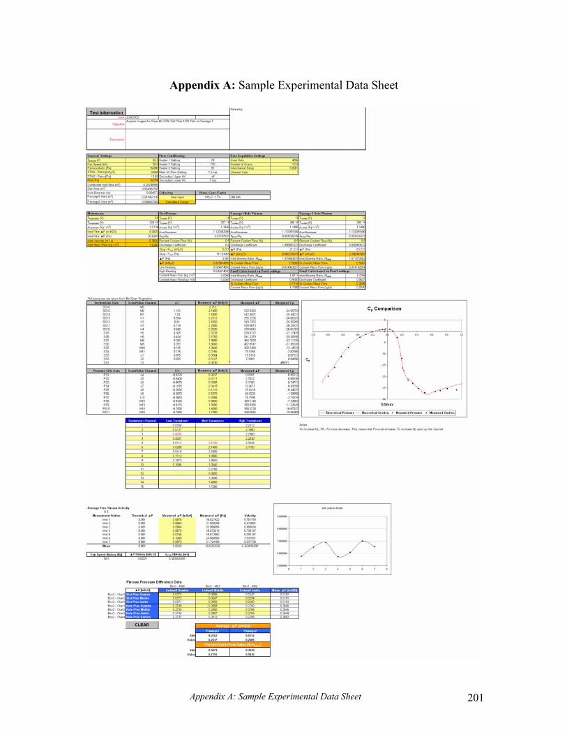
Appendix A: Sample Experimental Data Sheet 201

Appendix A: Sample Experimental Data Sheet

Appendix A: Sample Experimental Data Sheet 202

Table A.1 Steady State Check

Time 3:39 3:48 4:05 4:23 Tinf 52.95 52.8 52.88 52.95 T1 45.92 45.87 45.98 45.97 T2 39.65 39.65 39.75 39.74 T4 42.03 42 42.16 42.08 T5 28.69 28.74 28.93 28.93 T9 36.72 36.82 37.01 36.82 TS5 37.23 37.19 37.3 37.2 THPM 14.15 14.13 14.12 14.09 TSPM 14.87 14.86 14.86 14.86 TempDiff 38.8 38.67 38.76 38.86

Visual Basic Codes to Calculate Driving Pressure Option Explicit

Function fcnDeltaPCalc(PassNum As Double, Target As Double, PDynIn, DensRatio As Double, AreaRatio As Double) Dim Pdin As Double, Count As Double Dim P1 As Double, P2 As Double, PSearch As Double Dim Pa As Double, DeltaPa As Double, MIna As Double, Mdota As Double, Cda As Double, Errora As Double Dim Pb As Double, DeltaPb As Double, MInb As Double, Mdotb As Double, Cdb As Double, Errorb As Double Dim tol As Double, Delta As Double, Error As Double Target = Target / 100 'Initialize Search Range P1 = 0 'Lower Bound (Pa) P2 = 250 'Upper Bound (Pa) Delta = 0.001 tol = 0.000001 Count = 1 Do If Count > 1000 Then MsgBox ("Computation has exceeded maximum number of iterations") Exit Do End If PSearch = (P2 - P1) / 2 + P1 ' Calculate for Value just below search Pt Pa = PSearch - Delta Cda = fcnCd(PassNum, Pa) ' DeltaPa = (Target / Cda) * (Target / Cda) * Pdin * DensRatio * AreaRatio * AreaRatio MIna = Sqr(DensRatio * (Pa / PDynIn)) Mdota = MIna * AreaRatio * Cda

Appendix A: Sample Experimental Data Sheet 203

Errora = Mdota - Target ' Calculate for Value just above search Pt Pb = PSearch + Delta Cdb = fcnCd(PassNum, Pb) MInb = Sqr(DensRatio * (Pb / PDynIn)) Mdotb = MInb * AreaRatio * Cdb Errorb = Mdotb - Target ' Determine Interval to Eliminate If Abs(Errora) > Abs(Errorb) Then 'Throw out the left half of the search range P1 = Pa Error = Errora Else 'Throw out the right half of the search range P2 = Pb Error = Errorb End If Count = Count + 1 Loop While Abs(Error) > tol fcnDeltaPCalc = (Pb - Pa) / 2 + Pa End Function

Function fcnCd(PassNum, DeltaP As Double) If PassNum = 1 Then fcnCd = -0.058 * Sqr(DeltaP) + 1.363 Else fcnCd = -0.0174 * Sqr(DeltaP) + 0.9448 End If End Function

Sub ClearPlenumData() ' ' ClearPlenumData Macro ' Macro recorded 1/30/2003 by dknost ' ' Range("D114:F120").Select Selection.ClearContents Range("D114").Select End Sub

Appendix B: Code for Program Used to Align Images in Global Coordinates 204

Appendix B: Code for Program Used to Align Images in Global Coordinates

Figure B.1 Graphical User Interface to Program for Image Alignment

% function IRLoad % Calling Script for Image Processing Program clear all tic close all clc % Input Dialog Box to gather image information title = 'Image Data Input'; prompt = 'Number of Image Locations:','Number of Rows in Image:','Number of Columns in Image:', ...

'Number of Points to Skip when Sampling:','Masking Radius in Pixels:','Smoothing Radius in Pixels'; lines = 1;

default = '13','240','320','1','3','0.8'; answers = inputdlg(prompt,title,lines,default); if size(answers,1) == 0 clear all return end % Global variables to store X-loc, Y-loc, and Image Data

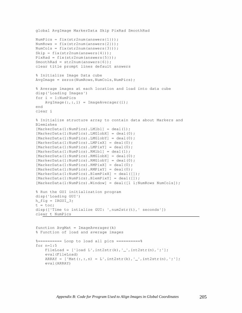
Appendix B: Code for Program Used to Align Images in Global Coordinates 205

global AvgImage MarkerData Skip PixRad SmoothRad NumPics = fix(str2num(answers1)); NumRows = fix(str2num(answers2)); NumCols = fix(str2num(answers3)); Skip = fix(str2num(answers4)); PixRad = fix(str2num(answers5)); SmoothRad = str2num(answers6); clear title prompt lines default answers % Initialize Image Data cube AvgImage = zeros(NumRows,NumCols,NumPics); % Average images at each location and load into data cube disp('Loading Images') for i = 1:NumPics AvgImage(:,:,i) = ImageAverager(i); end clear i % Initialize structure array to contain data about Markers and Blemishes [MarkerData(1:NumPics).LMlbl] = deal(1); [MarkerData(1:NumPics).LMGlobX] = deal(0); [MarkerData(1:NumPics).LMGlobY] = deal(0); [MarkerData(1:NumPics).LMPixX] = deal(0); [MarkerData(1:NumPics).LMPixY] = deal(0); [MarkerData(1:NumPics).RMlbl] = deal(1); [MarkerData(1:NumPics).RMGlobX] = deal(0); [MarkerData(1:NumPics).RMGlobY] = deal(0); [MarkerData(1:NumPics).RMPixX] = deal(0); [MarkerData(1:NumPics).RMPixY] = deal(0); [MarkerData(1:NumPics).BlemPixX] = deal([]); [MarkerData(1:NumPics).BlemPixY] = deal([]); [MarkerData(1:NumPics).Window] = deal([1 1;NumRows NumCols]); % Run the GUI initialization program disp('Loading GUI') h_fig = IRGUI_3; t = toc; disp(['Time to intialize GUI: ',num2str(t),' seconds']) clear t NumPics

function AvgMat = ImageAverager(k) % Function of load and average images %========== Loop to load all pics ==========% for n=1:5 FileLoad = ['load L',int2str(k),'_',int2str(n),';']; eval(FileLoad) ARRAY = ['Mat(:,:,n) = L',int2str(k),'_',int2str(n),';']; eval(ARRAY)

Appendix B: Code for Program Used to Align Images in Global Coordinates 206

Clear = ['clear L',int2str(k),'_',int2str(n),' L',int2str(k),'_',int2str(n),'_DateTime L',int2str(k),'_',int2str(n),'_FrameInfo L',int2str(k),'_',int2str(n),'_ObjectParam L',int2str(k),'_',int2str(n),'_Scaling']; eval(Clear) end AvgMat = mean(Mat,3);

function varargout = IRGUI_3(varargin) % IRGUI_3 Application M-file for IRGUI_3.fig % FIG = IRGUI_3 launch IRGUI_3 GUI. % IRGUI_3('callback_name', ...) invoke the named callback. % Last Modified by GUIDE v2.0 06-Mar-2003 16:15:11 global AvgImage GlobMarkData if nargin == 0 % LAUNCH GUI fig = openfig(mfilename,'reuse'); % Generate a structure of handles to pass to callbacks, and store it. handles = guihandles(fig); guidata(fig, handles); if nargout > 0 varargout1 = fig; end % MarkLbls = 'Other';'Marker 1';'Marker 2';'Marker 3';'Marker 4';'Marker 5';'Marker 6';'Marker 7';'Marker 8';'Marker 9';'Marker 10'; ... % 'Marker 11';'Marker 12';'Marker 13';'Marker 14';'Marker 15';'Marker 16';'Marker 17';'Marker 18';'Marker 19';'Marker 20'; % MarkXY = [[0:length(MarkLbls)-1]' [0:length(MarkLbls)-1]']; load DMarkerData MarkLbls = DMarkerData1,1; MarkXY = DMarkerData1,2; set([handles.cboLeftMark;handles.cboRightMark],'String',MarkLbls) set([handles.edLMGlobX;handles.edRMGlobX],'UserData',MarkXY(:,1)) set([handles.edLMGlobY;handles.edRMGlobY],'UserData',MarkXY(:,2)) set(handles.txtImageCount,'String',['of ',int2str(size(AvgImage,3))]) % Contour plot the first Image m = jet(128); [C,h_con,Cf] = contourf(AvgImage(:,:,1),128);

Appendix B: Code for Program Used to Align Images in Global Coordinates 207

set(h_con,'LineStyle','none') set(gca,'YDir','reverse','DrawMode','fast') colormap(m) colorbar drawnow set(handles.txtStatus,'String','Done') % Initialize Pixel clicking settings set(gcf,'WindowButtonDownFcn','IRGUI_3(''Image_Click'',gcbo,[],guidata(gcbo))') set(gca,'UserData','Left') % Initialize Marker to left for image clicking purposes set(handles.chkLeftMark,'value',1) elseif ischar(varargin1) % INVOKE NAMED SUBFUNCTION OR CALLBACK try [varargout1:nargout] = feval(varargin:); % FEVAL switchyard catch disp(lasterr); end end %| ABOUT CALLBACKS: %| GUIDE automatically appends subfunction prototypes to this file, and %| sets objects' callback properties to call them through the FEVAL %| switchyard above. This comment describes that mechanism. %| %| Each callback subfunction declaration has the following form: %| <SUBFUNCTION_NAME>(H, EVENTDATA, HANDLES, VARARGIN) %| %| The subfunction name is composed using the object's Tag and the %| callback type separated by '_', e.g. 'slider2_Callback', %| 'figure1_CloseRequestFcn', 'axis1_ButtondownFcn'. %| %| H is the callback object's handle (obtained using GCBO). %| %| EVENTDATA is empty, but reserved for future use. %| %| HANDLES is a structure containing handles of components in GUI using %| tags as fieldnames, e.g. handles.figure1, handles.slider2. This %| structure is created at GUI startup using GUIHANDLES and stored in %| the figure's application data using GUIDATA. A copy of the structure %| is passed to each callback. You can store additional information in %| this structure at GUI startup, and you can change the structure %| during callbacks. Call guidata(h, handles) after changing your %| copy to replace the stored original so that subsequent callbacks see %| the updates. Type "help guihandles" and "help guidata" for more %| information.

Appendix B: Code for Program Used to Align Images in Global Coordinates 208

%| %| VARARGIN contains any extra arguments you have passed to the %| callback. Specify the extra arguments by editing the callback %| property in the inspector. By default, GUIDE sets the property to: %| <MFILENAME>('<SUBFUNCTION_NAME>', gcbo, [], guidata(gcbo)) %| Add any extra arguments after the last argument, before the final %| closing parenthesis. % -------------------------------------------------------------------- function varargout = Image_Click(h, eventdata, handles, varargin) global AvgImage MarkerData p = round(get(gca,'CurrentPoint')); % Test to see if figure was clicked within axes if p(1,1) >= 1 & p(1,1) <= size(AvgImage,2) if p(1,2) >= 1 & p(1,2) <= size(AvgImage,1) MarkerLoc = get(gca,'UserData'); switch MarkerLoc case 'Left' set(handles.edLMPixX,'String',num2str(p(1,1))) set(handles.edLMPixY,'String',num2str(p(1,2))) % switch to Right Marker Pixel Data set(gca,'UserData','Right') off = [handles.chkLeftMark;handles.chkBlemish]; mutual_exclude(off) set(handles.chkRightMark,'value',1) case 'Right' set(handles.edRMPixX,'String',num2str(p(1,1))) set(handles.edRMPixY,'String',num2str(p(1,2))) % switch to Blemish Pixel Data set(gca,'UserData','Blemish') off = [handles.chkRightMark;handles.chkLeftMark]; mutual_exclude(off) set(handles.chkBlemish,'value',1) case 'Window' pt1 = p; rbbox; pt2 = round(get(gca,'CurrentPoint')); ImageNum = str2num(get(handles.edImageNum,'String')); MarkerData(ImageNum).Window = [pt1(1,2:-1:1);pt2(1,2:-1:1)]; otherwise % Blemish case ImageNum = str2num(get(handles.edImageNum,'String')); MarkerData(ImageNum).BlemPixX = [MarkerData(ImageNum).BlemPixX p(1,1)]; MarkerData(ImageNum).BlemPixY = [MarkerData(ImageNum).BlemPixY p(1,2)]; Count = str2num(get(handles.txtBlemCount,'string')); set(handles.txtBlemCount,'String',int2str(Count+1)) end end end

Appendix B: Code for Program Used to Align Images in Global Coordinates 209

% -------------------------------------------------------------------- function varargout = edImageNum_Callback(h, eventdata, handles, varargin) % Stub for Callback of the uicontrol handles.edImageNum. global AvgImage MarkerData ImageNum = str2num(get(handles.edImageNum,'String')); if ImageNum < 1 ImageNum = 1; set(h,'String',ImageNum) elseif ImageNum > 14 ImageNum = 14; set(h,'String',ImageNum) end set(handles.txtStatus,'String','Working ...') % Contour Plot and turn off lines [C,h_con,Cf] = contourf(AvgImage(:,:,ImageNum),128); set(h_con,'LineStyle','none') set(gca,'YDir','reverse','DrawMode','fast') % Set Left Marker Data set(handles.cboLeftMark,'Value',MarkerData(ImageNum).LMlbl) set(handles.edLMGlobX,'String',num2str(MarkerData(ImageNum).LMGlobX,'%6.3f')) set(handles.edLMGlobY,'String',num2str(MarkerData(ImageNum).LMGlobY,'%6.3f')) set(handles.edLMPixX,'String',num2str(MarkerData(ImageNum).LMPixX)) set(handles.edLMPixY,'String',num2str(MarkerData(ImageNum).LMPixY)) % Set Right Marker Data set(handles.cboRightMark,'Value',MarkerData(ImageNum).RMlbl) set(handles.edRMGlobX,'String',num2str(MarkerData(ImageNum).RMGlobX,'%6.3f')) set(handles.edRMGlobY,'String',num2str(MarkerData(ImageNum).RMGlobY,'%6.3f')) set(handles.edRMPixX,'String',num2str(MarkerData(ImageNum).RMPixX)) set(handles.edRMPixY,'String',num2str(MarkerData(ImageNum).RMPixY)) % Set Blemish Counter Count = size(MarkerData(ImageNum).BlemPixX,2); set(handles.txtBlemCount,'String',int2str(Count)) colorbar drawnow set(handles.txtStatus,'String','Done') set(gca,'UserData','Left') IRGUI_3('chkLeftMark_Callback',gcbo,[],guidata(gcbo)); % -------------------------------------------------------------------- function varargout = cboLeftMark_Callback(h, eventdata, handles, varargin) % Stub for Callback of the uicontrol handles.cboLeftMark. MarkNum = get(h,'Value');

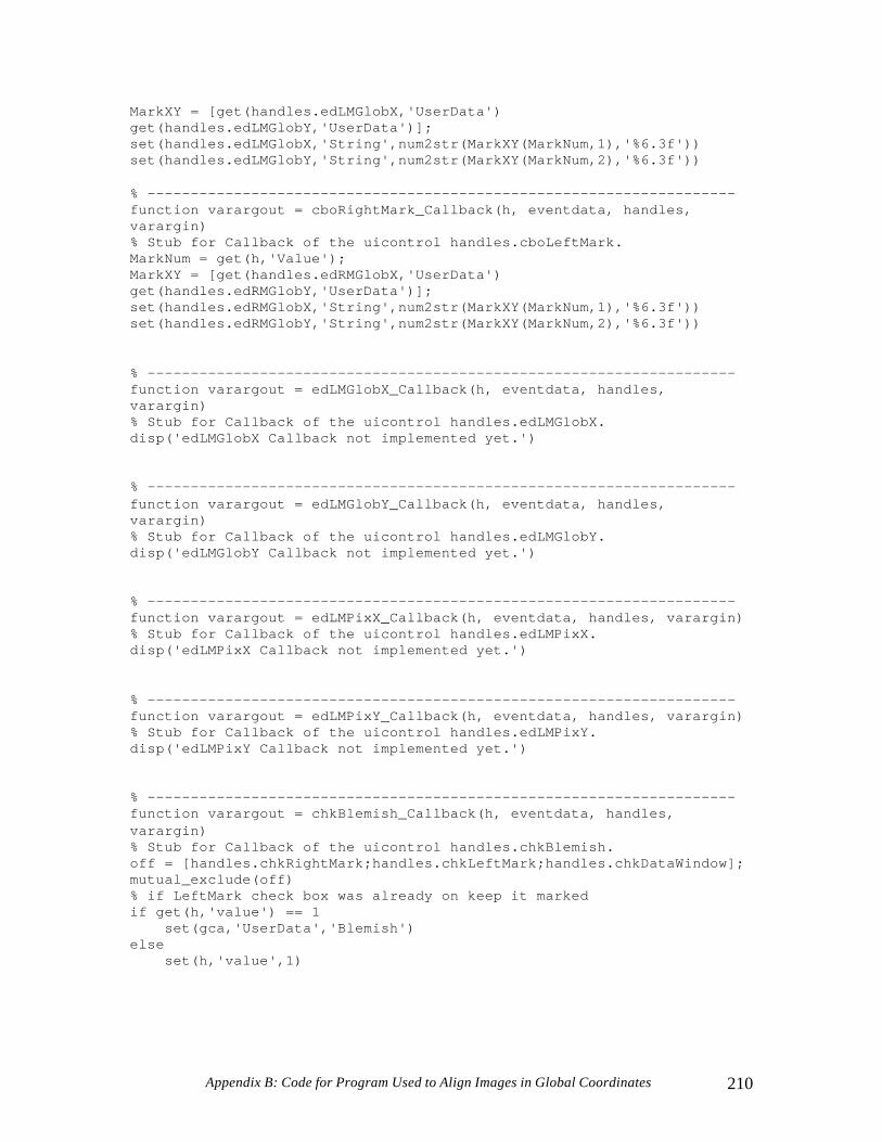
Appendix B: Code for Program Used to Align Images in Global Coordinates 210

MarkXY = [get(handles.edLMGlobX,'UserData') get(handles.edLMGlobY,'UserData')]; set(handles.edLMGlobX,'String',num2str(MarkXY(MarkNum,1),'%6.3f')) set(handles.edLMGlobY,'String',num2str(MarkXY(MarkNum,2),'%6.3f')) % -------------------------------------------------------------------- function varargout = cboRightMark_Callback(h, eventdata, handles, varargin) % Stub for Callback of the uicontrol handles.cboLeftMark. MarkNum = get(h,'Value'); MarkXY = [get(handles.edRMGlobX,'UserData') get(handles.edRMGlobY,'UserData')]; set(handles.edRMGlobX,'String',num2str(MarkXY(MarkNum,1),'%6.3f')) set(handles.edRMGlobY,'String',num2str(MarkXY(MarkNum,2),'%6.3f')) % -------------------------------------------------------------------- function varargout = edLMGlobX_Callback(h, eventdata, handles, varargin) % Stub for Callback of the uicontrol handles.edLMGlobX. disp('edLMGlobX Callback not implemented yet.') % -------------------------------------------------------------------- function varargout = edLMGlobY_Callback(h, eventdata, handles, varargin) % Stub for Callback of the uicontrol handles.edLMGlobY. disp('edLMGlobY Callback not implemented yet.') % -------------------------------------------------------------------- function varargout = edLMPixX_Callback(h, eventdata, handles, varargin) % Stub for Callback of the uicontrol handles.edLMPixX. disp('edLMPixX Callback not implemented yet.') % -------------------------------------------------------------------- function varargout = edLMPixY_Callback(h, eventdata, handles, varargin) % Stub for Callback of the uicontrol handles.edLMPixY. disp('edLMPixY Callback not implemented yet.') % -------------------------------------------------------------------- function varargout = chkBlemish_Callback(h, eventdata, handles, varargin) % Stub for Callback of the uicontrol handles.chkBlemish. off = [handles.chkRightMark;handles.chkLeftMark;handles.chkDataWindow]; mutual_exclude(off) % if LeftMark check box was already on keep it marked if get(h,'value') == 1 set(gca,'UserData','Blemish') else set(h,'value',1)

Appendix B: Code for Program Used to Align Images in Global Coordinates 211

end % -------------------------------------------------------------------- function mutual_exclude(off) set(off,'Value',0) % -------------------------------------------------------------------- function varargout = radiobutton_Color(h, eventdata, handles, varargin) % Stub for Callback of the uicontrol handles.radiobutton1. % h_rad = handles.radiobutton1 off = [handles.radBlackWhite]; mutual_exclude(off) if get(h,'value') == 1 m = jet(32); % Check to see if colormap is inverted if get(handles.togInvert,'Value') == 1 m = flipud(m); end set(handles.txtStatus,'String','Working ...') set(gcf,'ColorMap',m); colorbar drawnow set(handles.txtStatus,'String','Done') else % if Radio button was already on keep it marked set(h,'value',1) end % -------------------------------------------------------------------- function varargout = radiobutton_BW(h, eventdata, handles, varargin) % Stub for Callback of the uicontrol handles.radiobutton1. % h_rad = handles.radiobutton1 off = [handles.radColor]; mutual_exclude(off) if get(h,'value') == 1 m = bone(32); % Check to see if colormap is inverted if get(handles.togInvert,'Value') == 1 m = flipud(m); end set(handles.txtStatus,'String','Working ...') set(gcf,'ColorMap',m); colorbar drawnow set(handles.txtStatus,'String','Done') else % if Radio button was already on keep it marked set(h,'value',1) end % -------------------------------------------------------------------- function varargout = togInvert_Callback(h, eventdata, handles, varargin)

Appendix B: Code for Program Used to Align Images in Global Coordinates 212

% Stub for Callback of the uicontrol handles.togInvert. m = flipud(get(gcf,'ColorMap')); set(handles.txtStatus,'String','Working ...') set(gcf,'ColorMap',m); colorbar drawnow set(handles.txtStatus,'String','Done') % -------------------------------------------------------------------- function varargout = cmdBack_Callback(h, eventdata, handles, varargin) % Stub for Callback of the uicontrol handles.cmbBack. ImageNum = str2num(get(handles.edImageNum,'String')); Write_Marker_Data(ImageNum,guidata(gcbo)) % Proceed to previous image BackNum = ImageNum - 1; if BackNum >= 1 set(handles.edImageNum,'String',BackNum) IRGUI_3('edImageNum_Callback',gcbo,[],guidata(gcbo)); set(gca,'UserData','Left') end % -------------------------------------------------------------------- function varargout = cmdNext_Callback(h, eventdata, handles, varargin) % Stub for Callback of the uicontrol handles.cmdNext. ImageNum = str2num(get(handles.edImageNum,'String')); Write_Marker_Data(ImageNum,guidata(gcbo)) % Proceed to next Image NextNum = ImageNum + 1; if NextNum <= 14 set(handles.edImageNum,'String',NextNum) IRGUI_3('edImageNum_Callback',gcbo,[],guidata(gcbo)); set(gca,'UserData','Left') end % -------------------------------------------------------------------- function varargout = cmdEnter_Callback(h, eventdata, handles, varargin) % Stub for Callback of the uicontrol handles.cmbBack. ImageNum = str2num(get(handles.edImageNum,'String')); Write_Marker_Data(ImageNum,guidata(gcbo)) % -------------------------------------------------------------------- function varargout = cmdCancel_Callback(h, eventdata, handles, varargin) % Stub for Callback of the uicontrol handles.cmdCancel. close 'Infra Red Camera GUI'

Appendix B: Code for Program Used to Align Images in Global Coordinates 213

% -------------------------------------------------------------------- function varargout = cmdFinish_Callback(h, eventdata, handles, varargin) % Stub for Callback of the uicontrol handles.cmdFinish. ImageNum = str2num(get(handles.edImageNum,'String')); Write_Marker_Data(ImageNum,guidata(gcbo)) Pass = get(handles.edPassage,'String'); MarkerLocs = [get(handles.edLMGlobX,'UserData') get(handles.edLMGlobY,'UserData')]; close 'Infra Red Camera GUI' IRCalc(MarkerLocs, Pass) % -------------------------------------------------------------------- function varargout = Write_Marker_Data(ImageNum,handles) global MarkerData % Write Left Marker Data to Matrix MarkerData(ImageNum).LMlbl = get(handles.cboLeftMark,'Value'); MarkerData(ImageNum).LMGlobX = str2num(get(handles.edLMGlobX,'String')); MarkerData(ImageNum).LMGlobY = str2num(get(handles.edLMGlobY,'String')); MarkerData(ImageNum).LMPixX = round(str2num(get(handles.edLMPixX,'String'))); MarkerData(ImageNum).LMPixY = round(str2num(get(handles.edLMPixY,'String'))); % Write Right Marker Data to Matrix MarkerData(ImageNum).RMlbl = get(handles.cboRightMark,'Value'); MarkerData(ImageNum).RMGlobX = str2num(get(handles.edRMGlobX,'String')); MarkerData(ImageNum).RMGlobY = str2num(get(handles.edRMGlobY,'String')); MarkerData(ImageNum).RMPixX = round(str2num(get(handles.edRMPixX,'String'))); MarkerData(ImageNum).RMPixY = round(str2num(get(handles.edRMPixY,'String'))); % -------------------------------------------------------------------- function varargout = chkLeftMark_Callback(h, eventdata, handles, varargin) % Stub for Callback of the uicontrol handles.chkLeftMark. off = [handles.chkRightMark;handles.chkBlemish;handles.chkDataWindow]; h_chk = handles.chkLeftMark; mutual_exclude(off) % if LeftMark check box was already on keep it marked if get(h_chk,'value') == 1 set(gca,'UserData','Left') else set(h_chk,'value',1) end

Appendix B: Code for Program Used to Align Images in Global Coordinates 214

% -------------------------------------------------------------------- function varargout = chkRightMark_Callback(h, eventdata, handles, varargin) % Stub for Callback of the uicontrol handles.chkRightMark. off = [handles.chkLeftMark;handles.chkBlemish;handles.chkDataWindow]; h_chk = handles.chkRightMark; mutual_exclude(off) % if RightMark check box was already on keep it marked if get(h_chk,'value') == 1 set(gca,'UserData','Right') else set(h_chk,'value',1) end % -------------------------------------------------------------------- function varargout = chkDataWindow_Callback(h, eventdata, handles, varargin) off = [handles.chkLeftMark;handles.chkRightMark;handles.chkBlemish]; mutual_exclude(off) % if LeftMark check box was already on keep it marked if get(h,'value') == 1 set(gca,'UserData','Window') else set(h,'value',1) end % -------------------------------------------------------------------- function varargout = edPassage_Callback(h, eventdata, handles, varargin) % Stub for Callback of the uicontrol handles.edit10. disp('edit10 Callback not implemented yet.')

function IRCalc(MarkerLocs, Pass) % Calling Function for Calculation and Plotting Routines global AvgImage MarkerData Skip PixRad [Data,MarkCheck,Scale] = IRImageOrient(MarkerLocs, Pass); SmoothData = IRSmooth(Data,Scale); if nargin == 1 Pass = '0'; end tic disp('Writing Data Files ...') switch Pass case '1','2'

Appendix B: Code for Program Used to Align Images in Global Coordinates 215

save PassIRImageData save('PassSmoothData.dat','SmoothData','-ASCII','-DOUBLE','-TABS') otherwise save IRImageData save('SmoothData.dat','SmoothData','-ASCII','-DOUBLE','-TABS') end t = toc; disp(['Time to write data: ',num2str(t),' seconds']) ContourAndPatch(SmoothData);

function [Data,MarkCheck,Scale] = IRImageOrient(MarkerLocs, Pass) % Function to perform image transformations with transition matrix tic disp('Performing Image Transformations...') global AvgImage MarkerData Skip PixRad s = size(AvgImage); % Generate X and Y matrices. Y is reversed in order to increase with % the global Y axis. All images are intially assumed to be aligned % with the bottom edge along the global X axis and left edge along % the global Y axis [X Y Z] = meshgrid(1:s(2),s(1):-1:1,1:s(3)); Z = 0*Z; % Delete the "other" marker location row MarkerLocs(1,:) = []; % Initialize X, Y,and Z Global Matrices and Blemish Pt Matrix XG = zeros(size(AvgImage)); YG = zeros(size(AvgImage)); ZG = zeros(size(AvgImage)); BlemPts = []; Data = []; % for i = 1:s(3) switch Pass case '1' Images = [1 2 3 10 11 12 13]; case '2' Images = 3:8; otherwise Images = 1:s(3); end for i = Images % Vectors containing x and y data for Left(1) and Right(2) Marker Glob1 = [MarkerData(i).LMGlobX MarkerData(i).LMGlobY]'; Glob2 = [MarkerData(i).RMGlobX MarkerData(i).RMGlobY]'; Pix1 = [MarkerData(i).LMPixX MarkerData(i).LMPixY]'; Pix2 = [MarkerData(i).RMPixX MarkerData(i).RMPixY]'; % Pixel location BlemPix = [MarkerData(i).BlemPixX' MarkerData(i).BlemPixY']; % Calculate local reference distances and scaling

Appendix B: Code for Program Used to Align Images in Global Coordinates 216

RefPix = sqrt((Pix2(1)-Pix1(1))^2 + (Pix2(2)-Pix1(2))^2); DeltaX = Glob2(1) - Glob1(1); DeltaY = Glob2(2) - Glob1(2); RefDist = sqrt((Glob2(1)-Glob1(1))^2 + (Glob2(2)-Glob1(2))^2); Scale(i) = RefDist/RefPix; % inches/pixel % Shift Pixel indices so that 0,0 is at Marker 1 X(:,:,i) = X(:,:,i) - X(1,Pix1(1),i); Y(:,:,i) = Y(:,:,i) - Y(Pix1(2),1,i); % Scale Local coordinates from Pixels to inches X(:,:,i) = X(:,:,i)*Scale(i); Y(:,:,i) = Y(:,:,i)*Scale(i); % Develop transformation Matrix to go from rotated local coordinates to system aligned with picture % 1 - Coordinate System aligned with image % 2 - Coordinate System in image with x aligned along Markers % G - Global Coordinate System % Vector from Left Marker to Right marker Vector_L = [X(Pix2(2),Pix2(1),i) Y(Pix2(2),Pix2(1),i) 0]' - [X(Pix1(2),Pix1(1),i) Y(Pix1(2),Pix1(1),i) 0]'; % Normalize to unit vector x_2 = Vector_L/sqrt(sum(Vector_L.^2)); z_2 = [0 0 1]'; % Unit y vector in image coordinates where x lies along line between markers y_2 = cross(z_2,x_2); % Transformation matrix from 1 to 2 is the inverse of T from 2 to 1 which is % the transpose for a rotation matrix T1_2 = inv([x_2 y_2 z_2]); % Vectors in the Global coordinate system from origin to Marker locations M1_G = [Glob1(1) Glob1(2) 0]'; M2_G = [Glob2(1) Glob2(2) 0]'; % Vector from Left to Right Marker expressed in Global Units Vector_G = M2_G - M1_G; % Normalize to unit vector x_G = Vector_G/sqrt(sum(Vector_G.^2)); z_G = [0 0 1]'; % Unit y vector in global coordinates y_G = cross(z_G,x_G); T2_G = [x_G y_G z_G]; T1_G = T2_G*T1_2; % Rotate the Coordinates Matrices and offset XG(:,:,i) = T1_G(1,1)*X(:,:,i) + T1_G(1,2)*Y(:,:,i) + T1_G(1,3)*Z(:,:,i) + Glob1(1); YG(:,:,i) = T1_G(2,1)*X(:,:,i) + T1_G(2,2)*Y(:,:,i) +

Appendix B: Code for Program Used to Align Images in Global Coordinates 217

T1_G(2,3)*Z(:,:,i) + Glob1(2); ZG(:,:,i) = T1_G(3,1)*X(:,:,i) + T1_G(3,2)*Y(:,:,i) + T1_G(3,3)*Z(:,:,i) + 0; % Vector of marker locations after rotation and translation MarkCheck(:,:,i) = [XG(Pix1(2),Pix1(1),i) YG(Pix1(2),Pix1(1),i) ZG(Pix1(2),Pix1(1),i); ... XG(Pix2(2),Pix2(1),i) YG(Pix2(2),Pix2(1),i) ZG(Pix2(2),Pix2(1),i)]; j = 1; % Sample Image Rows = MarkerData(i).Window(:,1); Cols = MarkerData(i).Window(:,2); Xpts = XG(Rows(1):Skip:Rows(2),Cols(1):Skip:Cols(2),i); Ypts = YG(Rows(1):Skip:Rows(2),Cols(1):Skip:Cols(2),i); Tpts = AvgImage(Rows(1):Skip:Rows(2),Cols(1):Skip:Cols(2),i); ImageData = [Xpts(:) Ypts(:) Tpts(:)]; Data = [Data;ImageData]; while j <= size(BlemPix,1) BlemPts = [BlemPts;XG(BlemPix(j,2),BlemPix(j,1),i)' YG(BlemPix(j,2),BlemPix(j,1),i)']; j = j + 1; end end clear X Y Z i j BlemPix DeltaPixX DeltaPixY DeltaX DeltaY Glob1 Glob2 M1_G M2_G Pix1 Pix2 RefDist RefPix ... ScaleX ScaleY T1_2 T2_G T1_G Vector_G Vector_L s x_2 x_G y_2 y_G z_2 z_G MaskPts = [MarkerLocs;BlemPts]; % Convert blemish radius from pixels to inches and delete all chosen points within the Blemish radius Radius = PixRad*mean(Scale); for i = 1:size(MaskPts,1); Dist = sqrt((Data(:,1)-MaskPts(i,1)).^2 + (Data(:,2)-MaskPts(i,2)).^2); Ind = find(Dist <= Radius); Data(Ind,:) = []; end t = toc; disp(['Time to compute image transformations: ',num2str(t),' seconds']);

function SmoothData = IRSmooth(Data,Scale) % This function is only used to convert to metric units % Loop through pts and average all points that fall with in search radius of each point tic global SmoothRad % Smooth loop turned off because of time. Smoothing performed by griddata

Appendix B: Code for Program Used to Align Images in Global Coordinates 218

% Radius = SmoothRad*mean(Scale); % j = 1; k = 0; SmoothData = []; % disp('Beginning smoothing process') % for i = 1:size(Data,1); % CurrentPt = Data(i,:); % Dist = sqrt((Data(:,1)-CurrentPt(1)).^2 + (Data(:,2)-CurrentPt(2)).^2); % Ind = find(Dist <= Radius); % if length(Ind) > 1 % One pt will be the current point % Avg = mean(Data(Ind,3)); % SmoothData(j,:) = [CurrentPt(1:2) Avg]; % k = k + 1; % else % SmoothData(j,:) = [CurrentPt]; % end % j = j + 1; % end SmoothData = Data; t = toc; % disp([int2str(k),' of ',int2str(size(Data,1)),' points were smoothed in ',num2str(t),' seconds.']) SmoothData(:,1:2) = SmoothData(:,1:2)*0.0254; % Plot Data Pt locations plot(SmoothData(:,1),SmoothData(:,2),'.'); axis equal

function ContourAndPatch(SmoothData) % Function to contour temperature data and see if images are in place tic % sample data for faster plotting SubData = SmoothData(1:7:end,:); xv = linspace(min(SubData(:,1)),max(SubData(:,1)),250); yv = linspace(min(SubData(:,2)),max(SubData(:,2)),1000); disp('Mapping Data...') [XG,YG,TG] = griddata(SubData(:,1),SubData(:,2),SubData(:,3),xv,yv'); disp('Contouring Data...') figure [Cf,h,C] = contourf(XG,YG,TG,20); axis equal tight set(h,'LineStyle','none') m = jet(20); colormap(m) load VaneXY load SlotXY h(1) = patch(VaneXY(:,1),VaneXY(:,2),[0.7 0.7 0.7]); h(2) = patch(VaneXY(:,1),VaneXY(:,2)+0.457,[0.7 0.7 0.7]); h(3) = patch(VaneXY(:,1),VaneXY(:,2)-0.457,[0.7 0.7 0.7]); h(4) = patch(SlotXY(:,1),SlotXY(:,2), [0.7 0.7 0.7]); set(h,'LineStyle','none') t = toc; disp(['Time to grid and contour data: ',num2str(t),' seconds'])

Appendix C: Visual Basic Code for Secondary Flow Calculations 219

Appendix C: Visual Basic Code for Secondary Flow Calculations

Figure C.1 The “Enter Parameters” button opens a GUI to input plane data to the spreadsheet.

Figure C.2 The “Import Data” button runs the Text File Import Wizard.

Appendix C: Visual Basic Code for Secondary Flow Calculations 220

Figure C.3 After importing the data all rows with text are deleted.

Figure C.4 The “Manipulate Data” button sorts the data, performs the flow plane calculatons, and formats the output.

Appendix C: Visual Basic Code for Secondary Flow Calculations 221

Enter Parameters Button Module Option Explicit '=============================================================== ' ' 'This module contains functions for calling custom dialog Boxes ' ' '=============================================================== Sub ShowParametersForm() frmParameters.Show End Sub Sub ShowAnalysisPlanesForm() frmAnalysisPlane.Show End Sub

Parameter Input GUI Option Explicit Const Pi = 3.14159265358979 Private Sub cmbPlanes_Click() Select Case cmbPlanes.ListIndex Case 0 txtXbase.Text = "" txtYBase.Text = "" txtAngle.Text = "" Case 1 txtXbase.Text = "-0.000305" txtYBase.Text = "0.455970" txtAngle.Text = "180" Case 2 txtXbase.Text = "0.124328" txtYBase.Text = "0.381655" txtAngle.Text = "310.9602825" Case 3 txtXbase.Text = "0.249921" txtYBase.Text = "0.379524" txtAngle.Text = "153.576204" End Select End Sub Private Sub cmbVanes_Click() Select Case cmbVanes.ListIndex Case 0 txtPitch.Text = "" txtSpan.Text = "" txtChord.Text = "" Case 1

Appendix C: Visual Basic Code for Secondary Flow Calculations 222

txtPitch.Text = "0.457" txtSpan.Text = "0.54864" txtChord.Text = "0.594" End Select End Sub Private Sub cmdCancel_Click() Unload frmParameters End Sub Private Sub cmdOK_Click() Dim Msg As String 'Prompt Dim Config As Long 'Button Configuration Dim Title As String 'Title Dim Ans As Long 'MsgBox response ' Activate the propersheet If IsNumeric(txtXbase.Text) And IsNumeric(txtYBase.Text) And _ IsNumeric(txtAngle.Text) And IsNumeric(txtPitch.Text) And _ IsNumeric(txtSpan.Text) And IsNumeric(txtChord) Then Workbooks("VelocityVectorGenerate1.xls").Sheets("DataSort").Activate If optIn1.Value = True Then Range("xBase").Value = Val(txtXbase.Text) * 0.0254 Else Range("xBase").Value = Val(txtXbase.Text) End If If optIn2.Value = True Then Range("yBase").Value = Val(txtYBase.Text) * 0.0254 Else Range("yBase").Value = Val(txtYBase.Text) End If Sheets("VectorCalcs").Activate Range("AngleDeg").Value = Val(txtAngle.Text) Range("AngleRad").Value = (Range("AngleDeg").Value-90)* Pi/180 If optIn3.Value = True Then Range("pitch").Value = Val(txtPitch.Text) * 0.0254 Else Range("pitch").Value = Val(txtPitch.Text) End If If optIn4.Value = True Then Range("span").Value = Val(txtSpan.Text) * 0.0254 Else Range("span").Value = Val(txtSpan.Text) End If If optIn5.Value = True Then

Appendix C: Visual Basic Code for Secondary Flow Calculations 223

Range("chord").Value = Val(txtChord.Text) * 0.0254 Else Range("chord").Value = Val(txtChord.Text) End If Unload frmParameters ' Format the data entries Sheets("DataSort").Select Range("xBase:yBase").Select With Selection .NumberFormat = "0.000000" .HorizontalAlignment = xlCenter End With Sheets("VectorCalcs").Select Range("AngleDeg,pitch:span,chord").Select With Selection .NumberFormat = "0.0000" .HorizontalAlignment = xlCenter End With Range("A5").Activate Sheets("DataSort").Select Range("A5").Activate Else Msg = "You must enter a number for each parameter." & vbCrLf Msg = Msg & "Would you like to try again" Config = vbYesNo + vbExclamation Title = "Error!" ' Ask user to try again Ans = MsgBox(Msg, Config, Title) Select Case Ans Case vbYes Exit Sub Case Else Unload frmParameters End Select End If End Sub Private Sub UserForm_Initialize() cmbPlanes.AddItem "" cmbPlanes.AddItem "Stagnation Plane" cmbPlanes.AddItem "SS2" cmbPlanes.AddItem "DPS1" cmbPlanes.ListIndex = 0 cmbVanes.AddItem "" cmbVanes.AddItem "Pratt & Whitney Vane" cmbVanes.ListIndex = 0

Appendix C: Visual Basic Code for Secondary Flow Calculations 224

End Sub

Data Import Button Module Option Explicit Sub DataImport() Dim ErrMsg Dim Msg As String, DataFile As String, Title As String Dim Count As Integer Sheets("DataSort").Activate On Error GoTo ErrorMessage For Count = 1 To 3 Msg = "Select file containing " Select Case Count Case 1 Range("A5").Activate DataFile = "x & y data to import" Msg = Msg & DataFile MsgBox Msg Application.Dialogs(xlDialogImportTextFile).Show Case 2 Range("C5").Activate DataFile = "z & u data to import" Msg = Msg & DataFile MsgBox Msg Application.Dialogs(xlDialogImportTextFile).Show Case 3 Range("E5").Activate DataFile = "v & w data to import" Msg = Msg & DataFile MsgBox Msg Application.Dialogs(xlDialogImportTextFile).Show End Select Next Count NonDataDelete Columns("A:G").Select Selection.Columns.AutoFit Range("A4").Select Exit Sub ErrorMessage: If DataFile <> "" Then MsgBox "You have generated and error while selecting " & DataFile Else

Appendix C: Visual Basic Code for Secondary Flow Calculations 225

ErrMsg = Error(Err) MsgBox "ERROR: " & ErrMsg End If End Sub Sub NonDataDelete() Dim Msg As String, DataType Dim BlankCount As Integer, Row As Integer Dim TextCells, Cell As Object Application.ScreenUpdating = False Range("A5").Activate BlankCount = 0 Do Until BlankCount > 10 Select Case ActiveCell Case Empty Row = ActiveCell.Row Rows(Row).Delete BlankCount = BlankCount + 1 Case Else Select Case IsNumeric(ActiveCell) Case True ActiveCell.Offset(1, 0).Activate BlankCount = 0 Case Else Row = ActiveCell.Row Rows(Row).Delete End Select End Select Loop End Sub

Manipulate Data Button Module Option Explicit Const Pi = 3.14159265358979 '====================================================================== ' ' 'This module contains functions for analyzing ss2 and stag plane ' ' '====================================================================== Sub PlaneDetermine() Application.ScreenUpdating = False Workbooks("VelocityVectorGenerate1.xls").Activate Sheets("VectorCalcs").Select Select Case Range("AngleDeg").Value Case "" MsgBox "You must define the plane first" Sheets("DataSort").Select

Appendix C: Visual Basic Code for Secondary Flow Calculations 226

Exit Sub Case 180 Call StagnationDataArrange Case Else Call DataArrange End Select End Sub Sub StagnationDataArrange() Workbooks("VelocityVectorGenerate.xls").Activate Sheets("DataSort").Activate Range("A5").Activate Dim NumRows As Integer, NumCols As Integer Application.ScreenUpdating = False NumRows = Range(ActiveCell, ActiveCell.End(xlDown)).Count NumCols = Range(ActiveCell, ActiveCell.End(xlToRight)).Count Call CopyZ Call RoundZ(NumRows) Call SecondThirdQuadDataSort Call PlaneLoc(NumRows) Call PlaneLocCheck(NumRows) Call VectorCalcsPaste Call EdgeFormat Call xC(NumRows) Call zS(NumRows) Call StagVnScale(NumRows) Call StagVzScale(NumRows) Call StagVectorCalcsFormat End Sub Sub DataArrange() Workbooks("VelocityVectorGenerate1.xls").Activate Sheets("DataSort").Activate Range("A5").Activate Dim NumRows As Integer, NumCols As Integer Application.ScreenUpdating = False NumRows = Range(ActiveCell, ActiveCell.End(xlDown)).Count NumCols = Range(ActiveCell, ActiveCell.End(xlToRight)).Count ' Call SubRoutines Call CopyZ Call RoundZ(NumRows)

Appendix C: Visual Basic Code for Secondary Flow Calculations 227

Call DataSort Call PlaneLoc(NumRows) Call PlaneLocCheck(NumRows) Call VectorCalcsPaste Call EdgeFormat Call yP(NumRows) Call zS(NumRows) Call uCalc(NumRows) Call vCalc(NumRows) Call zCopy(NumRows) Call PsiRad(NumRows) Call PsiDeg(NumRows) Call VsCalc(NumRows) Call VnCalc(NumRows) Call VzCalc(NumRows) Call VnScale(NumRows) Call VzScale(NumRows) Call VectorCalcsFormat End Sub Sub CopyZ() ' Copy contents of "Z" to another row Range("C5").Activate Range(ActiveCell, ActiveCell.End(xlDown)).Copy Range("H5") Application.CutCopyMode = False End Sub Sub RoundZ(NumRows As Integer) Dim Cell As Object Dim Row As Integer Range(ActiveCell, ActiveCell.End(xlDown)).ClearContents ' Use ROUND to elimate truncation error Row = ActiveCell.Row Range(ActiveCell, ActiveCell.Offset(NumRows - 1, 0)).Select For Each Cell In Selection ActiveCell.Value = Round(ActiveCell.Offset(0, 5).Value, 5) ActiveCell.Offset(0, 5).ClearContents ActiveCell.Offset(1, 0).Activate Next Cell End Sub Sub DataSort() ' Sort the Data Range("A5").CurrentRegion.Select Selection.Sort Key1:=Range("C5"), Order1:=xlDescending, Key2:=Range("A5") _ , Order2:=xlAscending ' Format Data

Appendix C: Visual Basic Code for Secondary Flow Calculations 228

With Selection .NumberFormat = "0.000000" .HorizontalAlignment = xlCenter End With End Sub Sub SecondThirdQuadDataSort() ' Sort the Data Range("A5").CurrentRegion.Select Selection.Sort Key1:=Range("C5"), Order1:=xlDescending, Key2:=Range("A5") _ , Order2:=xlDescending ' Format Data With Selection .NumberFormat = "0.000000" .HorizontalAlignment = xlCenter End With End Sub Sub PlaneLoc(NumRows As Integer) Dim Row As Double, Col As Double Dim xVal, yVal Dim xLength As Single, yLength As Double Dim Count As Integer Range("G4").Activate ActiveCell.Select ActiveCell.FormulaR1C1 = "PlaneLoc [m]" With Selection .HorizontalAlignment = xlCenter .Font.Bold = True With .Borders(xlEdgeLeft) .LineStyle = xlContinuous .Weight = xlMedium End With With .Borders(xlEdgeTop) .LineStyle = xlContinuous .Weight = xlMedium End With With .Borders(xlEdgeBottom) .LineStyle = xlContinuous .Weight = xlMedium End With With .Borders(xlEdgeRight) .LineStyle = xlContinuous .Weight = xlMedium End With End With Row = 0 For Count = 1 To NumRows 'Row = Row + 1

Appendix C: Visual Basic Code for Secondary Flow Calculations 229

ActiveCell.Offset(1, 0).Activate Row = ActiveCell.Row Col = ActiveCell.Column xLength = Cells(Row, 1).Value - Range("xBase").Value yLength = Cells(Row, 2).Value - Range("yBase").Value ActiveCell.Value = Sqr(xLength * xLength + yLength * yLength) Next Count ' Copy contents of "PlaneLoc" to another row Range("G5").Activate Range(ActiveCell, ActiveCell.End(xlDown)).Copy Range("I5") Application.CutCopyMode = False Dim Cell As Object Range(ActiveCell, ActiveCell.End(xlDown)).ClearContents ' Use ROUND to elimate truncation error Row = ActiveCell.Row Range(ActiveCell, ActiveCell.Offset(NumRows - 1, 0)).Select For Each Cell In Selection ActiveCell.Value = Round(ActiveCell.Offset(0, 2).Value, 4) ActiveCell.Offset(0, 2).ClearContents ActiveCell.Offset(1, 0).Activate Next Cell With Selection .NumberFormat = "0.0000" .Font.Bold = False .HorizontalAlignment = xlCenter End With Columns("L:L").EntireColumn.AutoFit End Sub Sub PlaneLocCheck(NumRows As Integer) Dim Row As Integer, Col As Integer Dim RowCount As Integer, ActiveRow As Integer Dim i, Diff Dim Msg As String Range("G6").Activate Row = ActiveCell.Row Col = ActiveCell.Column ' Count Number of cells which have already been read RowCount = 1 ' Find the first repeating row Do Until ActiveCell.Value < Cells(Row - 1, Col).Value ActiveCell.Offset(1, 0).Activate Row = ActiveCell.Row RowCount = RowCount + 1 Loop

Appendix C: Visual Basic Code for Secondary Flow Calculations 230

Msg = "There is a problem in cell(s)" & vbCrLf & vbCrLf ' Test to see if points are properly stagered For i = 1 To NumRows - (RowCount + 1) ActiveRow = ActiveCell.Row Diff = ActiveCell.Value - Cells(ActiveRow - RowCount, Col).Value Diff = Round(Diff, 4) If Diff <> 0 Then Msg = Msg & ActiveCell.Address & vbCrLf ActiveCell.Interior.Color = vbRed End If ActiveCell.Offset(1, 0).Activate Next i If Msg <> "There is a problem in cell(s)" & vbCrLf & vbCrLf Then MsgBox Msg & vbCrLf & "Please examine these cells" Exit Sub End If End Sub Sub VectorCalcsPaste() Range("A4").CurrentRegion.Copy Worksheets("VectorCalcs").Range("A4") End Sub Sub EdgeFormat() Sheets("VectorCalcs").Select Range("G4").Activate Range(ActiveCell, ActiveCell.End(xlDown)).Select With Selection.Borders(xlEdgeRight) .LineStyle = xlDouble .Weight = xlThick .ColorIndex = xlAutomatic End With End Sub Sub yP(NumRows As Integer) Dim Count As Integer, Row As Integer Range("H4").Activate ActiveCell.Value = "y/P" ActiveCell.Offset(1, 0).Activate For Count = 1 To NumRows Row = ActiveCell.Row ActiveCell.Value = Cells(Row, 7).Value / Range("pitch").Value ActiveCell.Offset(1, 0).Activate Next Count End Sub Sub xC(NumRows As Integer) Dim Count As Integer, Row As Integer

Appendix C: Visual Basic Code for Secondary Flow Calculations 231

Range("H4").Activate ActiveCell.Value = "x/C" ActiveCell.Offset(1, 0).Activate For Count = 1 To NumRows Row = ActiveCell.Row ActiveCell.Value = -Cells(Row, 7).Value / Range("chord").Value ActiveCell.Offset(1, 0).Activate Next Count End Sub Sub zS(NumRows As Integer) Dim Count As Integer, Row As Integer Range("I4").Activate ActiveCell.Value = "z/S" ActiveCell.Offset(1, 0).Activate For Count = 1 To NumRows Row = ActiveCell.Row ActiveCell.Value = Cells(Row, 3).Value / Range("span").Value ActiveCell.Offset(1, 0).Activate Next Count End Sub Sub uCalc(NumRows As Integer) Dim Count As Integer, Row As Integer Dim AngleRad As Double Range("J5").Activate AngleRad = Range("AngleRad").Value For Count = 1 To NumRows Row = ActiveCell.Row ActiveCell.Value = Cells(Row, 4).Value * Cos(AngleRad) + Cells(Row, 5).Value * Sin(AngleRad) ActiveCell.Offset(1, 0).Activate Next Count End Sub Sub vCalc(NumRows As Integer) Dim Count As Integer, Row As Integer Dim AngleRad As Double Range("K5").Activate AngleRad = Range("AngleRad").Value For Count = 1 To NumRows Row = ActiveCell.Row ActiveCell.Value = Cells(Row, 5).Value * Cos(AngleRad) - Cells(Row, 4).Value * Sin(AngleRad) ActiveCell.Offset(1, 0).Activate Next Count End Sub

Appendix C: Visual Basic Code for Secondary Flow Calculations 232

Sub zCopy(NumRows As Integer) Dim Count As Integer, Row As Integer Range("L5").Activate For Count = 1 To NumRows Row = ActiveCell.Row ActiveCell.Value = Cells(Row, 6).Value ActiveCell.Offset(1, 0).Activate Next Count End Sub Sub PsiRad(NumRows As Integer) Dim i As Integer, Row As Integer, Col As Integer Dim Count As Integer, RowRepeat As Integer, NewRows As Integer Dim PlaneLocation As Double, RowSearch As Double, ColSearch As Double, PsiRef As Double Range("M5").Activate Row = ActiveCell.Row Col = ActiveCell.Column i = 1 ' Calculate values in first two cells For i = 1 To 2 ActiveCell.Value = Atn(Cells(Row, Col - 2).Value / Cells(Row, Col - 3).Value) ActiveCell.Offset(1, 0).Activate Row = ActiveCell.Row Next i ' Calculate value of Psi at the midspan and search for the point where midspan data ends Do Until Cells(Row, Col - 4) <> Cells(Row - 1, Col - 4).Value ActiveCell.Value = Atn(Cells(Row, Col - 2).Value / Cells(Row, Col - 3).Value) ActiveCell.Offset(1, 0).Activate Row = ActiveCell.Row Loop ' Adjust the number of rows that need to be calculated ' 4 compensates for cells above and including label, 1 includes active cell RowRepeat = Row - (4 + 1) NewRows = NumRows - RowRepeat For Count = 1 To NewRows PlaneLocation = Cells(Row, Col - 6).Value Range("G5").Activate RowSearch = ActiveCell.Row ColSearch = ActiveCell.Column Do Until ActiveCell.Value = PlaneLocation ActiveCell.Offset(1, 0).Activate

Appendix C: Visual Basic Code for Secondary Flow Calculations 233

RowSearch = ActiveCell.Row Loop PsiRef = Cells(RowSearch, Col).Value Cells(Row, Col).Activate ActiveCell.Value = PsiRef ActiveCell.Offset(1, 0).Activate Row = ActiveCell.Row Next Count End Sub Sub PsiDeg(NumRows As Integer) Dim Count As Integer, Row As Integer, Col As Integer Range("N5").Activate Row = ActiveCell.Row Col = ActiveCell.Column For Count = 1 To NumRows ActiveCell.Value = Cells(Row, Col - 1).Value * 180 / Pi ActiveCell.Offset(1, 0).Activate Row = ActiveCell.Row Next Count End Sub Sub VsCalc(NumRows As Integer) Dim Count As Integer, Row As Integer, Col As Integer Range("O5").Activate Col = ActiveCell.Column For Count = 1 To NumRows Row = ActiveCell.Row ActiveCell.Value = Cells(Row, Col - 5).Value * Cos(Cells(Row, Col - 2)) + _ Cells(Row, Col - 4).Value * Sin(Cells(Row, Col - 2)) ActiveCell.Offset(1, 0).Activate Next Count End Sub Sub VnCalc(NumRows As Integer) Dim Count As Integer, Row As Integer, Col As Integer Range("P5").Activate Col = ActiveCell.Column For Count = 1 To NumRows Row = ActiveCell.Row ActiveCell.Value = Cells(Row, Col - 5).Value * Cos(Cells(Row, Col - 3)) - _ Cells(Row, Col - 6).Value * Sin(Cells(Row, Col - 3))

Appendix C: Visual Basic Code for Secondary Flow Calculations 234

ActiveCell.Offset(1, 0).Activate Next Count End Sub Sub VzCalc(NumRows As Integer) Dim Count As Integer, Row As Integer, Col As Integer Range("Q5").Activate Col = ActiveCell.Column For Count = 1 To NumRows Row = ActiveCell.Row ActiveCell.Value = Cells(Row, 6).Value ActiveCell.Offset(1, 0).Activate Next Count End Sub Sub VnScale(NumRows As Integer) Dim Count As Integer, Row As Integer, Col As Integer Range("R5").Activate Row = ActiveCell.Row Col = ActiveCell.Column For Count = 1 To NumRows ActiveCell.Formula = "=" & Cells(Row, Col - 2).Address & "/scale" ActiveCell.Offset(1, 0).Activate Row = ActiveCell.Row Next Count End Sub Sub StagVnScale(NumRows As Integer) Dim Count As Integer, Row As Integer, Col As Integer Range("R5").Activate Row = ActiveCell.Row Col = 4 For Count = 1 To NumRows ActiveCell.Formula = "=" & Cells(Row, Col).Address & "/scale" ActiveCell.Offset(1, 0).Activate Row = ActiveCell.Row Next Count End Sub Sub VzScale(NumRows As Integer) Dim Count As Integer, Row As Integer, Col As Integer Range("S5").Activate Row = ActiveCell.Row Col = ActiveCell.Column

Appendix C: Visual Basic Code for Secondary Flow Calculations 235

For Count = 1 To NumRows ActiveCell.Formula = "=" & Cells(Row, Col - 2).Address & "/scale" ActiveCell.Offset(1, 0).Activate Row = ActiveCell.Row Next Count End Sub Sub StagVzScale(NumRows As Integer) Dim Count As Integer, Row As Integer, Col As Integer Range("S5").Activate Row = ActiveCell.Row Col = 6 For Count = 1 To NumRows ActiveCell.Formula = "=" & Cells(Row, Col).Address & "/scale" ActiveCell.Offset(1, 0).Activate Row = ActiveCell.Row Next Count End Sub Sub VectorCalcsFormat() Dim Row As Integer, Col As Integer Dim Msg As String Range("G6").Activate Row = ActiveCell.Row Col = ActiveCell.Column Do Until ActiveCell.Value < Cells(Row - 1, Col).Value ActiveCell.Offset(1, 0).Activate Row = ActiveCell.Row Loop Cells(Row, 1).Activate Range(ActiveCell, ActiveCell.End(xlToRight)).Select With Selection.Borders(xlEdgeTop) .LineStyle = xlContinuous .Weight = xlMedium .ColorIndex = xlAutomatic End With Range("H5").Select Range(Selection, Selection.End(xlDown)).Select Range(Selection, Selection.End(xlToRight)).Select With Selection .NumberFormat = "0.000000" .Font.Bold = False .Font.Italic = False .HorizontalAlignment = xlCenter End With

Appendix C: Visual Basic Code for Secondary Flow Calculations 236

Range("A4").Select Range(Selection, Selection.End(xlToRight)).Select With Selection .Font.Bold = True .Font.Italic = False .HorizontalAlignment = xlCenter End With Columns("A:S").Select Selection.Columns.AutoFit Application.ScreenUpdating = True Range("scale").Select Msg = "Adjust the scale until an appropriate vector" & vbCrLf Msg = Msg & "length is obtained in DeltaGraph" MsgBox Msg End Sub Sub StagVectorCalcsFormat() Dim Row As Integer, Col As Integer Dim Msg As String Range("G6").Activate Row = ActiveCell.Row Col = ActiveCell.Column Do Until ActiveCell.Value < Cells(Row - 1, Col).Value ActiveCell.Offset(1, 0).Activate Row = ActiveCell.Row Loop Cells(Row, 1).Activate Range(ActiveCell, ActiveCell.End(xlToRight)).Select With Selection.Borders(xlEdgeTop) .LineStyle = xlContinuous .Weight = xlMedium .ColorIndex = xlAutomatic End With Cells(Row, 18).Activate Range(ActiveCell, ActiveCell.End(xlToRight)).Select With Selection.Borders(xlEdgeTop) .LineStyle = xlContinuous .Weight = xlMedium .ColorIndex = xlAutomatic End With Range("H5").Select Range(Selection, Selection.End(xlDown)).Select Range(Selection, Selection.End(xlToRight)).Select With Selection .NumberFormat = "0.000000"

Appendix C: Visual Basic Code for Secondary Flow Calculations 237

.Font.Bold = False .Font.Italic = False .HorizontalAlignment = xlCenter End With Range("R5").Select Range(Selection, Selection.End(xlDown)).Select Range(Selection, Selection.End(xlToRight)).Select With Selection .NumberFormat = "0.000000" .Font.Bold = False .Font.Italic = False .HorizontalAlignment = xlCenter End With Range("A4").Select Range(Selection, Selection.End(xlToRight)).Select With Selection .Font.Bold = True .Font.Italic = False .HorizontalAlignment = xlCenter End With Columns("A:I").Select Selection.Columns.AutoFit Columns("R:S").Select Selection.Columns.AutoFit Application.ScreenUpdating = True Range("scale").Select Msg = "Adjust the scale until an appropriate vector" & vbCrLf Msg = Msg & "length is obtained in DeltaGraph" MsgBox Msg End Sub

Save File Button Module Option Explicit Option Private Module Public NewFileName As Variant Public CallSave As Boolean Public NoSave As Boolean Sub SaveButton() Dim InitialFilename As String, FileFilter As String Dim FilterIndex As String, Title As String InitialFilename = "VelocityVectors1.xls" FileFilter = "Microsoft Excel Workbook (*.xls),*.xls," & _ "Web Page (*.htm;*.html),*.htm;*.html," & _

Appendix C: Visual Basic Code for Secondary Flow Calculations 238

"Web Archive (*.mht;*.mhtml),*.mht;*.mhtml," & _ "XML Spreadsheet (*.xml),*.xml," & _ "Template (*.xlt),*.xlt," & _ "Text (Tab delimited) (*.txt),*.txt" FilterIndex = 1 Title = "Save As" ' Show SaveAs dialogbox NewFileName = Application.GetSaveAsFilename(InitialFilename, FileFilter, FilterIndex, Title) ' Test to see a filename was chosen or the dialog was cancelled If NewFileName = False Then ' Cancel the variable indicating that a call has been made to save the file CallSave = False ' Variable to indicate that the user has declined to save the file NoSave = True Exit Sub Else ' Set flag so that BeforeSaveMethod recognizes that SaveAs dialog was displayed CallSave = True ActiveWorkbook.SaveAs FileName:=NewFileName End If End Sub

239

Vita Daniel G. Knost was born on December 21, 1978 to Jack and Susan Knost in Charlotte,

North Carolina. For 13 years Daniel attended Providence Day School in Charlotte

graduating in 1997. While at Providence Day, Daniel earned four varsity letters in tennis

and three in football. During his senior seasons he was selected as homecoming captain

for the football team and was team captain and #1 singles and doubles player for the

tennis team. In August, 1997 Daniel enrolled at North Carolina State University. At

N.C. State, Daniel participated in the University Scholars Program and played one year

on the club tennis team at #1 singles. Daniel graduated Magna Cum Laude in May of

2001 with a B.S. in mechanical engineering. He came to Virginia Tech in June of 2001

and began work on his M.S. Daniel currently plans to pursue a PhD in mechanical

engineering at Virginia Tech. He would also like to hold an engineering position in

motorsports and obtain his P.E. license upon completion of his schooling. In his free

time Daniel enjoys watching and attending sporting events, especially for the Wolfpack,

playing tennis, visiting his family, and spending time with his girlfriend Nicole and

beagle Katie.

A few of Daniel’s favorite things are:

College Team : N.C. State Wolfpack

Professional Team: Carolina Panthers

Tennis Player: Andre Agassi / Steffi Graf

Tennis Tournament : U.S. Open

Racecar Driver: Dale Earnhardt / Dale Earnhardt Jr.

Trucks: Chevrolet

Movie : Top Gun / Days of Thunder / Crocodile Dundee

City: Chicago

Food: Cheeseburgers / Pork Bar-B-Que

Soda: Cheerwine / Pepsi