predictive modeling of dc arc flash in 125 volt system
TRANSCRIPT

University of Kentucky University of Kentucky
UKnowledge UKnowledge
Theses and Dissertations--Mining Engineering Mining Engineering
2019
PREDICTIVE MODELING OF DC ARC FLASH IN 125 VOLT SYSTEM PREDICTIVE MODELING OF DC ARC FLASH IN 125 VOLT SYSTEM
Austin Cody Gaunce University of Kentucky, [email protected] Digital Object Identifier: https://doi.org/10.13023/etd.2019.112
Right click to open a feedback form in a new tab to let us know how this document benefits you. Right click to open a feedback form in a new tab to let us know how this document benefits you.
Recommended Citation Recommended Citation Gaunce, Austin Cody, "PREDICTIVE MODELING OF DC ARC FLASH IN 125 VOLT SYSTEM" (2019). Theses and Dissertations--Mining Engineering. 46. https://uknowledge.uky.edu/mng_etds/46
This Master's Thesis is brought to you for free and open access by the Mining Engineering at UKnowledge. It has been accepted for inclusion in Theses and Dissertations--Mining Engineering by an authorized administrator of UKnowledge. For more information, please contact [email protected].

STUDENT AGREEMENT: STUDENT AGREEMENT:
I represent that my thesis or dissertation and abstract are my original work. Proper attribution
has been given to all outside sources. I understand that I am solely responsible for obtaining
any needed copyright permissions. I have obtained needed written permission statement(s)
from the owner(s) of each third-party copyrighted matter to be included in my work, allowing
electronic distribution (if such use is not permitted by the fair use doctrine) which will be
submitted to UKnowledge as Additional File.
I hereby grant to The University of Kentucky and its agents the irrevocable, non-exclusive, and
royalty-free license to archive and make accessible my work in whole or in part in all forms of
media, now or hereafter known. I agree that the document mentioned above may be made
available immediately for worldwide access unless an embargo applies.
I retain all other ownership rights to the copyright of my work. I also retain the right to use in
future works (such as articles or books) all or part of my work. I understand that I am free to
register the copyright to my work.
REVIEW, APPROVAL AND ACCEPTANCE REVIEW, APPROVAL AND ACCEPTANCE
The document mentioned above has been reviewed and accepted by the student’s advisor, on
behalf of the advisory committee, and by the Director of Graduate Studies (DGS), on behalf of
the program; we verify that this is the final, approved version of the student’s thesis including all
changes required by the advisory committee. The undersigned agree to abide by the statements
above.
Austin Cody Gaunce, Student
Dr. Joseph Sottile, Major Professor
Dr. Zach Agioutantis, Director of Graduate Studies
PREDICTIVE MODELING OF DC ARC FLASH IN 125 VOLT SYSTEM
________________________________________
THESIS ________________________________________
A thesis submitted in partial fulfillment of the requirements for the degree of Master of Science in Mining Engineering in the
College of Engineering at the University of Kentucky
By
Austin Cody Gaunce
Lexington, Kentucky
Director: Dr. Joseph Sottile, Professor of Mining Engineering
Lexington, Kentucky
2019
Copyright © Austin Cody Gaunce 2019

ABSTRACT OF THESIS
PREDICTIVE MODELING OF DC ARC FLASH
IN 125 VOLT SYSTEM
Arc flash is one of the two primary hazards encountered by workers near electrical equipment. Most applications where arc flash may be encountered are alternating current (AC) electrical systems. However, direct current (DC) electrical systems are becoming increasingly prevalent with industries implementing more renewable energy sources and energy storage devices. Little research has been performed with respect to arc flash hazards posed by DC electrical systems, particularly energy storage devices. Furthermore, current standards for performing arc flash calculations do not provide sufficient guidance when working in DC applications. IEEE 1584-2002 does not provide recommendations for DC electrical systems. NFPA 70E provides recommendations based on conservative theoretical models, which may result in excessive personal protective equipment (PPE). Arc flash calculations seek to quantify incident energy, which quantifies the amount of thermal energy that a worker may be exposed to at some working distance. This thesis assesses arc flash hazards within a substation backup battery system. In addition, empirical data collected via a series of tests utilizing retired station batteries is presented. Lastly, a predictive model for determining incident energy is proposed, based on collected data.
KEYWORDS: Arc Flash, DC Arc Flash, Electrical Safety, Incident Energy, Batteries
Austin Cody Gaunce (Name of Student)
03/12/2019
Date
PREDICTIVE MODELING OF DC ARC FLASH
IN 125 VOLT SYSTEM
By Austin Cody Gaunce
Joseph Sottile Director of Thesis Zach Agioutantis Director of Graduate Studies 03/12/2019
Date

iii
ACKNOWLEDGMENTS
This thesis was made possible through the generosity and support of multiple
individuals and organizations. First, I would like to thank the Central Appalachian Regional
Education and Research Center (CARERC). The funding provided to me through my
fellowship with the CARERC has provided me the opportunity to pursue a graduate degree
free from financial stress. Furthermore, the CARERC has allowed me the ability to engage
and interact with a number of safety professionals through conference attendance and site
visits. My peers and advisors within the CARERC have been a major source of support
throughout my endeavors.
Secondly, I would like to thank American Electric Power (AEP) for sponsoring the
research presented within this thesis. In addition, I would like to pay special tribute to the
employees of AEP’s Dolan Technology Center who dedicated their time and effort to this
effort; from constructing the test setup to performing testing to data collection. The
following are the names of individuals that were significantly involved with testing: Xuan
Wu, Dennis Hoffman, John Mandeville, Anthony “Tony” Clarke, Surya Baktiono, Dave
Klinect, Chase Leibold, Amrit Khalsa, and Ron Wellman. Without the contributions made
by these individuals, this thesis would not have been possible.
Lastly, but certainly not least, I would like to thank my family and friends for
providing me the encouragement, love, and support necessary throughout my studies and
the process of constructing this thesis.

iv
TABLE OF CONTENTS
ACKNOWLEDGMENTS ................................................................................................. iii LIST OF FIGURES ............................................................................................................ v
LIST OF TABLES ............................................................................................................. vi
CHAPTER 1: INTRODUCTION ....................................................................................... 7
1.1: Statement of the Problem ......................................................................................... 7
1.2: Scope of Work ....................................................................................................... 10
CHAPTER 2: LITERATURE REVIEW .......................................................................... 11
2.1: Characteristics of an Arc........................................................................................ 11
2.2 History of Arc Flash Research ................................................................................ 13
2.3: Research on IEEE 1584-2002 Test Methodology ................................................. 24
2.4: DC Arc Flash Research.......................................................................................... 25
2.5: Battery-Specific DC Arc Flash Research .............................................................. 30
CHAPTER 3: METHODOLOGY .................................................................................... 34
3.1: Test Setup .............................................................................................................. 34
3.2: Summary of Test Equipment and Sampling Parameters ....................................... 43
3.3: Initial Testing Procedure ........................................................................................ 44
3.4: Testing ................................................................................................................... 45
CHAPTER 4: RESULTS AND DISCUSSION ................................................................ 49
4.1: Data Manipulation ................................................................................................. 49
4.2: Data Analysis ......................................................................................................... 50
4.2.1: Temperature Rise/Incident Energy vs. Gap Width ......................................... 50
4.2.1.1: Working Distance: 22 Inches ................................................................... 50
4.2.1.2: Working Distance: 15 Inches ................................................................... 53
4.2.2: Incident Energy vs. Working Distance ........................................................... 55
4.2.3: Arc Energy vs. Gap Width .............................................................................. 59
4.2.4: Weather vs. Arc Duration ............................................................................... 64
4.3: Development of a Preliminary Equation ............................................................... 67
CHAPTER 5: CONCLUSION AND FUTURE WORK .................................................. 75
REFERENCES ................................................................................................................. 79
VITA ................................................................................................................................. 83

v
LIST OF FIGURES
Figure 2.1: Electric Arc Regions and Associated Voltage Profile.................................... 12 Figure 2.2: Thevenin Equivalent DC System Model ........................................................ 26 Figure 3.1: Horizontal Electrode Configuration [40] ....................................................... 34 Figure 3.2: Vertical Electrode Configuration with 90 Degree Bend [40] ......................... 34 Figure 3.3: Vertical Electrode Configuration with Insulating Barrier [40] ...................... 35 Figure 3.4: Power Schematic of Test Setup [41] .............................................................. 36 Figure 3.5: 2 x 3 x 2 Calorimeter Arrangement [42] ........................................................ 40 Figure 3.6: Enclosure and Calorimeter Mounting ............................................................ 41 Figure 3.7: Chargers, Disconnect Switches, and DC Circuit Breaker .............................. 42 Figure 3.8: Electrodes after Test ....................................................................................... 42 Figure 4.1: Peak Temperature Rise vs. Gap Width at 22 Inches ...................................... 51 Figure 4.2: Peak Incident Energy vs. Gap Width at 22 Inches ......................................... 51 Figure 4.3: Average Temperature Rise vs. Gap Width at 22 Inches ................................ 52 Figure 4.4: Peak Incident Energy vs. Gap Width at 15 Inches ......................................... 54 Figure 4.5: Average Temperature Rise vs. Gap Width at 15 Inches ................................ 55 Figure 4.6: Peak Incident Energy vs. Working Distance: ................................................. 57 Figure 4.7: Average Temperature Rise vs. Working Distance ......................................... 58 Figure 4.8: Central Calorimeter Temperature Rise vs. Working Distance ....................... 58 Figure 4.9: Example Arc Current and Voltage Plots ........................................................ 60 Figure 4.10: Example Arc Power Plot .............................................................................. 60 Figure 4.11: Arc Energy vs. Gap Width ........................................................................... 63 Figure 4.12: Arc Energy vs. Gap Width with Selected Observations Omitted ................ 63 Figure 4.13: SAS Results for Multivariate Linear Regression of Arc Duration ............... 66 Figure 4.14: Nonlinear Regression of Incident Energy and Working Distance ............... 68 Figure 4.15: Peak Incidnet Energy vs. Working Distance ................................................ 69 Figure 4.16: Polynomial Regression of Arc Energy and Gap Width ............................... 70 Figure 4.17: Nonlinear Regression of Incident Energy, Arc Energy, and Working Distance............................................................................................................................. 73
vi
LIST OF TABLES
Table 3.1: Summary of Test Equipment ........................................................................... 43 Table 3.2: Test Procedure Summary ................................................................................. 48 Table 4.1: Temperature Rise and Incident Energy Data for 22-inch Working Distance .. 50 Table 4.2: Calorimeter Data at 22 Inches ......................................................................... 53 Table 4.3: Temperature Rise and Incident Energy Data for 15-inch Working Distance .. 54 Table 4.4: Calorimeter Data at 15 Inches ......................................................................... 55 Table 4.5: Temperature Rise and Incident Energy Data over all Working Distances ...... 56 Table 4.6: Calorimeter Data over all Working Distances ................................................. 59 Table 4.7: Arc Energy Data .............................................................................................. 61 Table 4.8: Summary of Weather Data during Testing ...................................................... 64
7
CHAPTER 1: INTRODUCTION 1.1: Statement of the Problem
Electricity provides society with its current standard of living; however, it can also
pose serious dangers. The two key hazards associated with electricity are
electrocution/shock and arc flash. Arc flash is a phenomenon that occurs when a system
has sufficient electrical energy to ionize surrounding air during a fault, thereby generating
an arc. These incidents produce significant amounts of heat; however, heat is not the only
form of hazard presented by arc flash. Intense light, sound, and pressure are other means
by which arc flash may harm an individual. Because of these hazards, extensive research
has been conducted on arc flash in the effort to protect personnel who are at risk of
exposure. Research efforts have focused primarily on AC (alternating current) electrical
systems due to commonality; thereby leaving gaps in knowledge with respect to DC (direct
current) electrical systems.
Today, two standards exist to provide guidance on arc flash calculations in the
United States: IEEE Standard 1584 and NFPA 70E. These standards provide equations to
perform arc flash studies. The calculations pertaining to arc flash focus on quantifying the
amount of heat released during an event. The amount of heat to which a worker may be
exposed at a certain distance from the arc is termed incident energy and is expressed in
units of cal/cm2. Using incident energy and guidelines established by the abovementioned
standards, one can define arc flash boundaries. Arc flash boundaries dictate the minimum
amount of personal protective equipment (PPE) required within a specified distance to a
piece of equipment. In addition, for excessively high levels of incident energy, it may be
recommended to install protective devices, such as fuses and circuit breakers, to limit the
amount of energy. Though the procedure of performing an arc flash study may appear to
8
be simple, calculating incident energy is a complicated subject because numerous factors
influence arc behavior: a worker’s position in relation to the arc, fault current, system
voltage, orientation of the arc, and the duration of the arc.
It is important to note that the equations offered by IEEE 1584 and NFPA 70E are
primarily for AC electrical systems since these equations were derived from research
performed on said systems. Since the issuance of IEEE 1584 in 2002, technical literature
has produced various theoretical models to calculate incident energy in DC systems. The
two most commonly used models are associated with Dan Doan and Ravel Ammerman.
Though sufficient in protecting workers, these models tend to utilize assumptions that
produce highly conservative estimates. Therefore, workers may be required to wear
excessive equipment, which exposes them to a different set of hazards.
The need for a more refined DC arc flash model has become increasingly apparent.
Proliferation of solar photovoltaic (PV) systems and energy storage systems (ESSs) will
continue [1]. In addition, solar PV systems and ESSs are likely to increase in power.
Furthermore, there are plans to increase the number of high-voltage direct current (HVDC)
transmission lines as a means of increasing the integration of renewable energy sources
into the grid [2]. Therefore, the footprint of DC electricity within the U.S. grid will continue
to grow. In addition, electric vehicles (EVs) are becoming increasingly popular. According
to Bloomberg New Energy Finance (BNEF), EVs will account for “55% of all new car
sales” by the year 2040 and will comprise “33% of the global [vehicle] fleet,” which
corresponds to approximately 559 million EVs being in service [3]. In addition, battery-
powered mining equipment has become increasingly available, such as haulers, which can

9
contain batteries with voltages up to 240 Vdc. These various trends will lead to an increase
in the frequency of DC arc flash incidents in the near future.
In 2016, there were 154 electrical fatalities and 1,640 lost-time electrical injuries
[4]. Electrical burns (which arc flash injuries can be reported as [5]) accounted for four of
the electrical fatalities in 2016. Nonfatal electrical burn injuries were more common than
shock injuries within the construction industry with 270 occurrences versus 150. In
addition, 50 nonfatal electrical burn injuries were reported within the utility industry.
Nonfatal electric shock injuries within the utility industry were unavailable for 2016.
Though the utility and construction industries are commonly associated with electrical
injuries (fatal and nonfatal), the mining industry had the highest rate of nonfatal electrical
burn injury in 2016 with an incident rate of 1.0 per 10,000. The industries with the second
and third highest incident rates of nonfatal electrical burn injuries were the utility industry
(0.9 per 10,000) and the construction industry (0.4 per 10,000) [4].
To address the need for improved DC arc flash models, IEEE and NFPA are
preparing to perform DC arc flash testing as part of their ongoing arc flash research
collaboration. The initial focus of this research will likely be medium voltage (MV) and
high voltage (HV) systems due to the increased injury severity posed [6]. Thus, that
research will address risks posed by some current DC electrical systems as well as those
systems that will come about in the near future. However, low voltage (LV) DC systems
will continue to lack empirical arc flash data during that research phase despite already
being widely implemented in industry. Though not as likely to be fatal as incidents in HV
systems, arc flash can occur in LV DC systems and result in serious bodily harm, such as
third-degree burns. Examples of common LV DC systems include individual solar panels,

10
electric vehicle batteries, battery powered haulage equipment in mines, and battery systems
utilized in various other applications, such as substations and switchyards. In addition, out
of the examples presented, solar panels (and solar PV systems in general) have received
the greatest portion of attention with independent researchers of DC arc flash.
1.2: Scope of Work The primary objective of the research presented within this thesis is to generate a
predictive model for identifying and quantifying the arc flash hazard presented by DC
systems. Two independent variables are used for modeling: gap width and working
distance. These variables were selected due to controllability. Gap widths tested include
the following increments: 1/16 inch (0.0625), 1/8 inch (0.125), 3/16 inch (0.1875), and ¼
inch (0.250). Working distances tested include 22 inches, 18 inches, 15 inches, 12 inches,
9 inches, and 6 inches.
The applicability of this model is limited by the system utilized during research.
Therefore, the proposed model can only be used for DC systems supplied via batteries
with a system voltage of 125 V and an associated short circuit capability of
approximately 4000 A. Furthermore, the model does not consider charger contributions
since the batteries were disconnected from their respective chargers prior to each test. In
addition, the effect of protection devices, such as fuses, was not considered. Lastly, tests
were conducted utilizing an enclosure with a length, width, and depth of 20 inches.
Therefore, the concentration effect of smaller enclosures may not be adequately captured
by the proposed model.
11
CHAPTER 2: LITERATURE REVIEW 2.1: Characteristics of an Arc
Arcs form whenever there is sufficient electrical energy between two points for air
to undergo a process known as dielectric breakdown. Dielectric breakdown is the
phenomenon where a dielectric material becomes conductive, and therefore, creates a path
for the free movement of electrons. Once air becomes conductive, electrons rapidly flow
from the point of higher electric potential to a point of lower electric potential. This rapid
flow of electrons generates high levels of heat, thereby turning surrounding air into plasma.
Three regions comprise an arc: a cathode region, an anode region, and a plasma column,
with the electrode regions serving as a transition between the “gaseous plasma cloud and
the solid conductors” [7]. Each region is associated with various levels of heat. The
conductor terminals can exhibit temperatures up to, and even exceeding, 20,000 K whereas
the plasma column can exhibit temperatures around 13,000 K. These temperatures exceed
those found on the surface of the sun by factors of four and two-and-a-half, respectively
[8]. In addition to heat, pressure waves accompany arcs. Pressure waves are generated as a
byproduct of heat. Two mechanisms govern the generation of pressure: metal expansion
via boiling and rapid heating of air [9]. Overall, the generation of pressure waves during
arcing is analogous the creation of thunder during an electrical storm.
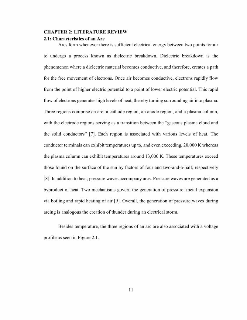
Besides temperature, the three regions of an arc are also associated with a voltage
profile as seen in Figure 2.1.

12
Figure 2.1: Electric Arc Regions and Associated Voltage Profile
This voltage profile depicts voltage drop over a provided arc length. This voltage drop
directly correlates with total arc length; however, the determination of arc length is difficult
as it can deviate from the gap length between electrodes [7]. Various factors influence arc
length such as electrode orientation, gap length, environmental conditions, and available
system voltage [8]. Besides arc length, the composition of air between electrodes can
influence voltage drop since air composition dictates the resistance the arc must pass
through. Larger voltage drops are indicative of higher pathway resistance, which influences
the production of heat since heat is a function of I2R losses. For reference, the voltage drop
in an arc typically ranges between 75 and 100 V/in, which is far greater than any voltage
drop associated with a solid conductor [8].
Two overarching groups classify free-burning arcs in open air: high-pressure and
low-pressure (or vacuum) [10]. High-pressure arcs occur in the presence of air whereas
low-pressure tend to occur in a vacuum. In addition, high-pressure arcs subdivide into
axisymmetric and non-axisymmetric categories [10]. Axisymmetric arcs are uniform along
13
their length and do not deviate from their central axis. Therefore, axisymmetric arcs tend
to be easily controlled. An example of an axisymmetric arc would be that formed by an arc
welder. Conversely, non-axisymmetric are dynamic. Thus, variation along the length of the
arc and deviation from the arc’s central axis is common [7]. A number of different factors
influence this chaotic behavior including “thermal convection, electromagnetic forces,
burn back of electrode material, arc extinction and re-striking, and plasma jets [7].” Arc
flash and arcing from switching operations are examples of non-axisymmetric arcs.
2.2 History of Arc Flash Research Arcing phenomena have been a subject of research since the early 20th century with
early arc research delving into possible lighting applications [7]. In addition, early research
sought to develop equations to characterize arcs. During this period, several different
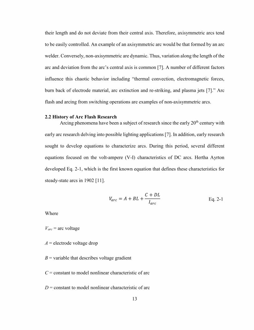
equations focused on the volt-ampere (V-I) characteristics of DC arcs. Hertha Ayrton
developed Eq. 2-1, which is the first known equation that defines these characteristics for
steady-state arcs in 1902 [11].
𝑉𝑉𝑎𝑎𝑎𝑎𝑎𝑎 = 𝐴𝐴 + 𝐵𝐵𝐵𝐵 +
𝐶𝐶 + 𝐷𝐷𝐵𝐵𝐼𝐼𝑎𝑎𝑎𝑎𝑎𝑎
Where
Varc = arc voltage
A = electrode voltage drop
B = variable that describes voltage gradient
C = constant to model nonlinear characteristic of arc
D = constant to model nonlinear characteristic of arc
Eq. 2-1
14
L = arc length in millimeters
Iarc = arc current
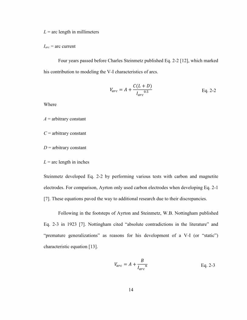
Four years passed before Charles Steinmetz published Eq. 2-2 [12], which marked
his contribution to modeling the V-I characteristics of arcs.
𝑉𝑉𝑎𝑎𝑎𝑎𝑎𝑎 = 𝐴𝐴 +
𝐶𝐶(𝐵𝐵 + 𝐷𝐷)𝐼𝐼𝑎𝑎𝑎𝑎𝑎𝑎0.5
Where
A = arbitrary constant
C = arbitrary constant
D = arbitrary constant
L = arc length in inches
Steinmetz developed Eq. 2-2 by performing various tests with carbon and magnetite
electrodes. For comparison, Ayrton only used carbon electrodes when developing Eq. 2-1
[7]. These equations paved the way to additional research due to their discrepancies.
Following in the footsteps of Ayrton and Steinmetz, W.B. Nottingham published
Eq. 2-3 in 1923 [7]. Nottingham cited “absolute contradictions in the literature” and
“premature generalizations” as reasons for his development of a V-I (or “static”)
characteristic equation [13].
𝑉𝑉𝑎𝑎𝑎𝑎𝑎𝑎 = 𝐴𝐴 +
𝐵𝐵𝐼𝐼𝑎𝑎𝑎𝑎𝑎𝑎𝑛𝑛
Eq. 2-3
Eq. 2-2
15
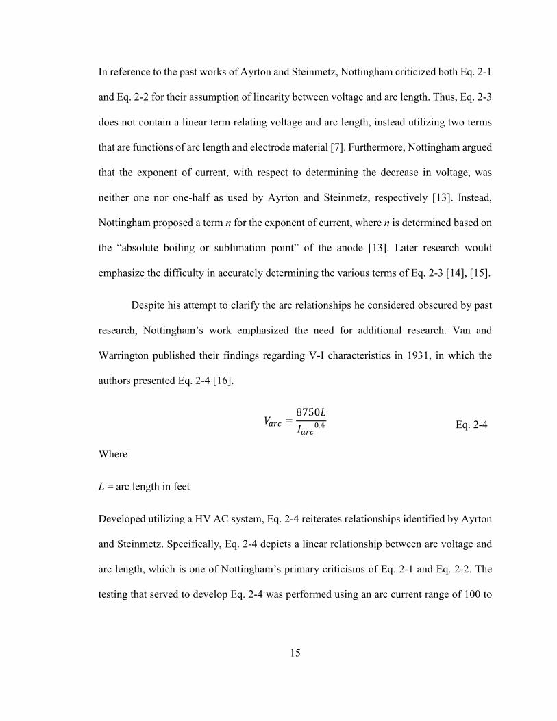
In reference to the past works of Ayrton and Steinmetz, Nottingham criticized both Eq. 2-1
and Eq. 2-2 for their assumption of linearity between voltage and arc length. Thus, Eq. 2-3
does not contain a linear term relating voltage and arc length, instead utilizing two terms
that are functions of arc length and electrode material [7]. Furthermore, Nottingham argued
that the exponent of current, with respect to determining the decrease in voltage, was
neither one nor one-half as used by Ayrton and Steinmetz, respectively [13]. Instead,
Nottingham proposed a term n for the exponent of current, where n is determined based on
the “absolute boiling or sublimation point” of the anode [13]. Later research would
emphasize the difficulty in accurately determining the various terms of Eq. 2-3 [14], [15].
Despite his attempt to clarify the arc relationships he considered obscured by past
research, Nottingham’s work emphasized the need for additional research. Van and
Warrington published their findings regarding V-I characteristics in 1931, in which the
authors presented Eq. 2-4 [16].
𝑉𝑉𝑎𝑎𝑎𝑎𝑎𝑎 =
8750𝐵𝐵𝐼𝐼𝑎𝑎𝑎𝑎𝑎𝑎0.4
Where
L = arc length in feet
Developed utilizing a HV AC system, Eq. 2-4 reiterates relationships identified by Ayrton
and Steinmetz. Specifically, Eq. 2-4 depicts a linear relationship between arc voltage and
arc length, which is one of Nottingham’s primary criticisms of Eq. 2-1 and Eq. 2-2. The
testing that served to develop Eq. 2-4 was performed using an arc current range of 100 to
Eq. 2-4
16
1000 A and gap widths that spanned feet in contrast to past research that utilized spacing
on the scale of inches and millimeters [16].
Though the work of Van and Warrington supported the findings of Ayrton and
Steinmetz, research conducted by Hall, Myers, and Vilcheck supported Nottingham. Hall,
Myers, and Vilcheck sought to assess the potential hazards that could occur in DC trolley
systems during faults [17]. They published their results in 1978 after performing over a
100 tests using numerous system configurations. One of the key contributions of their
research was the generation of a plot relating arc voltage and current. This plot mirrored
other plots produced by Eq. 2-3 [7], thereby supporting the findings of Nottingham.
Despite the amount of research conducted to determine the characteristics of arcs,
little, if any, research focused on arc flash and the associated hazard. However, the creation
of the Occupational Safety and Health Administration (OSHA) in 1970 led to increasing
awareness of arc flash as a potential worker hazard. Following OSHA’s creation, the
National Fire Protection Agency (NFPA) formed a subcommittee to assist OSHA with the
development of electrical standards. This committee is responsible for the creation of
NFPA 70E [18]. In 1982, the first significant work pertaining to arc flash phenomena was
published: “The Other Electrical Hazard: Electrical Arc Blast Burns” by Ralph Lee. In his
paper, Lee sought to quantify the relationship between arcs and heat along with potential
harm posed to the human body. Lee identified the hazard posed by arcs by acknowledging
that arc burns can be fatal to anyone within several feet of the source and that debilitating
burns can occur at distances up to 10 feet. Furthermore, clothing can ignite within close
proximity, which can also result in fatal or debilitating burns [8].

17
Lee’s paper also provides Eq. 2-5 and Eq. 2-6 to determine the distances at which
a worker would receive “just” curable burns or “just” fatal burns based upon equipment
MVA ratings and length of exposure [8].
𝐷𝐷𝑎𝑎 = �2.65 × 𝑀𝑀𝑉𝑉𝐴𝐴𝑏𝑏𝑏𝑏 × 𝑡𝑡 = √53 × 𝑀𝑀𝑉𝑉𝐴𝐴 × 𝑡𝑡
Where
Dc = distance of a “just” curable burn
MVAbf = Bolted fault MVA at location of interest
MVA = transformer rated MVA
t = exposure duration in seconds
𝐷𝐷𝑏𝑏 = �1.96 × 𝑀𝑀𝑉𝑉𝐴𝐴𝑏𝑏𝑏𝑏 × 𝑡𝑡 = √39 × 𝑀𝑀𝑉𝑉𝐴𝐴 × 𝑡𝑡
Where
Df = distance of a “just” fatal burn
Lee used several assumptions in developing the aforementioned equations. The first
assumption was that the shape of the arc does not matter, and thus it modeled the energy
of the arc as a sphere. The second assumption was that various skin absorption coefficients
and reflectivity factors, which would exacerbate or mitigate the amount of heat absorbed
by the skin, were negligible. Lastly, Lee assumed maximum power transfer to ensure that
his equations were conservative [8]. The maximum power transfer theorem states that the
maximum power produced by an arc is when the resistance of the arc is equal to the system
resistance. Despite the inaccuracies, Lee’s method provided a foundation for subsequent
Eq. 2-5
Eq. 2-6
18
arc flash hazard research. Furthermore, IEEE 1584-2002 recommends using Lee’s method
for various scenarios outside the range of test conditions utilized in the standard’s
development [19].
Approximately five years later, in 1987, Ralph Lee published another influential
work on arc flash phenomena titled “Pressures Developed by Arcs.” In this paper, Lee
details the various hazards that stem from the pressure generated by an arc. Some hazards
mentioned include “rearward propulsion” of personnel, which can result in various types
of blunt force trauma, bone fractures, and concussions; propulsion of the plasma cloud,
which can result in serious burns; and expulsion of metal particulates, which can also result
in serious burns [9]. Furthermore, hearing loss may occur as the pressure wave can damage
the internal structures of the ear. Besides harm posed to workers, Lee also mentioned the
risk of damage to nearby structures [9]. Utilizing theoretical calculations developed by Dr.
R. D. Hill [20] and measurements collected by M. G. Drouet and F. Nadeau [21], Lee
developed a family of lines that relate distance from an arc and pressure with each line
associated with a different arc current. In addition, Lee details four different case studies
that emphasize the threat posed by the pressure waves generated during arc flash incidents.
In 1991, Stokes and Oppenlander published their findings on the behavior of arcs
in various electrode configurations [22]. The two major electrode configurations tested
were vertical and horizontal. Furthermore, the electrodes were in series, which means that
the electrode terminals were directed at one another along the same axis. For comparison,
parallel electrodes are arranged side-by-side along the same axis with the electrode
terminals oriented in the same direction. The culmination of the collected data was a series
of curves that detail the relationship between arc voltage and current for each configuration

19
given a specified gap width. Similar to previous studies concerning the V-I characteristics
of arcs, the curves depict an inverse relationship between arc voltage and current until a
transition occurs. The transition point is defined by Eq. 2-7 [22]:
𝐼𝐼𝑡𝑡 = 10 + 0.2𝑧𝑧𝑔𝑔
Where
It = current at transition point
zg = gap width in millimeters
After the transition point, arc voltage and current begin to exhibit a direct relationship.
Stokes and Oppenlander developed Eq. 2-8 to model the relationship beyond the transition
point [22]:
𝑉𝑉𝑎𝑎𝑎𝑎𝑎𝑎 = (20 + 0.534𝑧𝑧𝑔𝑔)𝐼𝐼𝑎𝑎𝑎𝑎𝑎𝑎0.12
Following Stokes and Oppenlander, Paukert developed another set of equations for
V-I characteristics. Whereas Stokes and Oppenlander performed a large number of tests to
generate their formulae, Paukert compiled arc data with various electrode arrangements,
gap widths, current levels, and voltage types to generate his equations [23]. Paukert
published the findings of his research in 1993. Using the data from seven researchers,
Paukert developed V-I characteristic equations for various gap widths. The characteristic
equations reiterate the findings of previous research with arc voltage and current exhibiting
an inverse relationship for currents below 100 A. In addition, for currents above 100 A, the
equations display a direct relationship between arc voltage and current, which reinforces
the work of Stokes and Oppenlander. When comparing the data of Stokes and Oppenlander
Eq. 2-7
Eq. 2-8

20
with that compiled by Paukert, there is agreement between the data sets, with higher arc
current ranges exhibiting closer agreement [1].
C.E. Solver continued the research of arc behavior. Solver utilized copper
electrodes and various gap widths to generate a family of curves [24]. Solver’s results differ
from his predecessors in that the various curves do not begin to display a direct relationship
between arc voltage and current at higher current levels; but flatten instead, indicating an
independent relationship [24]. In addition, Solver found that arc voltage behaved
differently for different arc lengths. The voltage of short arcs is a function of the voltage
drops that occur at the electrodes whereas the voltage of long arcs “tends to be of the order
of 10 V/cm [24],” regardless of electrode voltage drops. This tendency of long arcs requires
current levels to exceed a transition point that is a function of gap width, similar to the
work of Stokes and Oppenlander.
In 1997, Doughty, Neal, Dear and Bingham published “Testing Update on
Protective Clothing & Equipment for Electric Arc Exposure.” The authors conducted two
series of tests: the first series of tests sought to simulate arc flash incidents within
equipment enclosures whereas the second series of tests sought to quantify the
effectiveness of various eye, face, and hand protection. In addition, a number of tables
containing updated information about the arc performance of various clothing materials
were included in the paper. Furthermore, data pertaining to peak sound levels obtained
during the first series of tests is included. Data from the first series of tests showed that arc
power increases as gap width increases until reaching a maximum, after which, arc power
begins to decrease. Furthermore, the maximum arc power is approximately “75% to 80%
of the theoretical maximum” according to maximum power transfer [25]. Additionally, as

21
gap width increases, incident energy also reaches a maximum; however, the gap width
associated with maximal incident energy is larger than the width associated with maximal
arc power. Other findings include direct proportionality between incident energy and arc
duration; incident energy is influenced by the surrounding environment; and the existence
of an inverse relationship between incident energy and distance from the location of the
arc [25]. One noteworthy finding of this paper is the relationship between incident energy
in open air and in an enclosure. The authors found that the presence of an enclosure
increases incident energy approximately threefold [25]. This was the first paper to describe
the interaction between arcing behavior and enclosures [25].
Building upon some of the ideas of the previous paper, Doughty, Neal, and Floyd
published “Predicting Incident Energy to Better Manage the Electric Arc Hazard on 600-
V Power Distribution Systems” in 2000. This publication continued tests to simulate arc
flash incidents, ultimately producing semi-empirical equations that would serve in NFPA
70E for incident energy calculations [26]. The test setup was similar to that of the previous
paper, with the primary difference being the dimensions of the enclosure. Over a one-week
period, approximately 100 tests were performed (25 test arrangements, 4 tests per
arrangement). Bolted fault current and distance from the location of arc flash served as the
independent variables for testing.
Upon conclusion of testing, data was curve-fitted to develop Eq. 2-9 and Eq. 2-10,
which relate incident energy to bolted fault current and distance from the arc [26].
𝐸𝐸𝑀𝑀𝑀𝑀 = 527.1𝐷𝐷𝑀𝑀−1.9593[0.0016𝐹𝐹2 − 0.0076𝐹𝐹 + 0.8938]
Where
Eq. 2-9

22
EMA = Maximum incident energy in open-air
F = bolted fault current in kA
DA = distance from arc in open-air
𝐸𝐸𝑀𝑀𝑀𝑀 = 103.87𝐷𝐷𝑀𝑀−1.4738[0.0093𝐹𝐹2 − 0.3453𝐹𝐹 + 5.9675]
Where
EMB = Maximum incident energy in enclosure
DA = distance from arc in enclosure
The first equation is for arc flash incidents that occur in open-air whereas the second is for
incidents in which an enclosure is present. After deriving these two equations, the authors
introduced a time variable based on the test duration (six cycles) and solved for distance,
resulting in Eq. 2-11 and Eq. 2-12 [26]:
𝐷𝐷𝑀𝑀 = [�𝑡𝑡𝑀𝑀𝐸𝐸𝑀𝑀𝑀𝑀
� (8.434𝐹𝐹2 − 40.06𝐹𝐹 + 4711)]0.5104
Where
tA = duration of the arc in seconds
𝐷𝐷𝑀𝑀 = [�𝑡𝑡𝑀𝑀𝐸𝐸𝑀𝑀𝑀𝑀
� (9.66𝐹𝐹2 − 358.7𝐹𝐹 + 6198)]0.6785
These distance equations allow the determination of arc flash boundaries based on
system characteristics. When compared with Lee’s equations, the open-air arc flash
equation showed agreement. However, Lee’s equations underestimated distances when
Eq. 2-11
Eq. 2-12
Eq. 2-10

23
considering arc flash within an enclosure. Furthermore, the comparison revealed that
deviation between equation results increased with rising bolted fault current [26].
Early arc flash research culminated with the publication of IEEE 1584 in 2002. The
standard provides a series of empirically derived models for calculating incident energies
and arc flash boundaries for a number of different system configurations. The development
of these models required extensive testing and built upon the semi-empirical equations and
findings presented by previous papers such as “Testing Update on Protective Clothing &
Equipment for Electric Arc Exposure” and “Predicting Incident Energy to Better Manage
the Electric Arc Hazard on 600-V Power Distribution Systems.” Despite this extensive
testing, IEEE 1584-2002 possesses limitations. Applicability of the models depends on the
system configurations used throughout testing. Therefore, the IEEE 1584-2002 empirical
models are only applicable to three-phase AC electrical systems with voltage levels ranging
from 208 V to 15 kV with an operating frequency of 60 or 50 Hz and bolted fault current
levels ranging from 700 A to 106 kA. In addition, system enclosures must be of a common
size and conductor gap widths must range between 13 mm and 152 mm [19]. Furthermore,
faults considered for analysis include only three-phase faults. The system may be grounded
or ungrounded. For three-phase systems outside the scope of the empirical models, such as
systems with voltages greater than 15 kV, a theoretical model based on Ralph Lee’s work
in “The Other Electrical Hazard: Electrical Arc Blast Burns” is provided [19]. Since the
publication of IEEE 1584-2002, work has continued to refine and improve the standard via
updating the test methodology and gaining an understanding of arc flash hazards presented
by systems outside the scope of the standard, such as DC systems.
24
2.3: Research on IEEE 1584-2002 Test Methodology Following the publication of IEEE 1584-2002, Stokes and Sweeting published
“Electric Arcing Burn Hazards.” The paper criticized IEEE 1584’s use of vertical
electrodes that terminated in open air. This criticism is due to the direction of the plasma
cloud developed during testing. With the orientation used in IEEE 1584-2002, the plasma
cloud moves to the base of the box and eventually overflows. Since the plasma cloud is
off-axis with the calorimeters, the calorimeters can only measure radiated heat [27].
Radiated heat is only a small portion of the total energy emitted in an arc flash incident as
the majority of energy, approximately 80% to 90%, is contained within the plasma cloud
[28]. Therefore, they argued that IEEE 1584-2002 underestimates the total energy during
an arc flash incident. To remedy this issue, Stokes and Sweeting proposed placing the
electrodes in a horizontal configuration [27]. This orientation allows the calorimeters to
measure the thermal energy of the plasma cloud.
The criticism of IEEE 1584-2002 by Stokes and Sweeting inspired additional
research concerning the standard’s test setup. “Effect of Electrode Orientation In Arc Flash
Testing” by Wilkins, Allison, and Lang sought to verify the statements of Stokes and
Sweeting. It was determined that horizontal electrodes produce incident energies
approximately three times greater than vertical electrodes, confirming statements by Stokes
and Sweeting [29]. However, it was also determined that when current limiting fuses are
considered, there is no appreciable difference between the two electrode configurations
[29]. “Effect of Insulating Barriers in Arc Flash Testing” followed and researched the effect
of terminating electrodes with an insulating barrier. Terminating the electrodes with an
insulating barrier can be viewed as a compromise between the work of Stokes and Sweeting

25
and industry. Though the horizontal configuration proposed by Stokes and Sweeting
produced greater incident energies, industry believed that the configuration was not
representative of equipment utilized in North America [30]. The inclusion of the insulating
barrier had a number of effects. First, the barrier deflected the plasma cloud providing a
trajectory similar to a horizontal configuration. Second, the incident energy increased for
each case with an insulating barrier. Third, the inclusion of the insulating barrier simulated
the presence of a power block or fuse at the base of the electrode, thereby, providing a
closer approximation of equipment utilized in industry. Lastly, the insulating barrier
allowed arcs to be self-sustaining at low voltages, which is an issue noted in IEEE 1584-
2002 [19]. The primary drawback associated with the inclusion of the barrier is accelerated
electrode deterioration during testing [30].
2.4: DC Arc Flash Research Hall, Myers, and Vilcheck performed the earliest work dealing with the hazards
associated with DC arcs in 1978, which predates the work of Ralph Lee. Since then, little
research has focused on the hazards of DC systems, especially arc flash. In their paper, the
authors focus on the fault behavior in trolley systems and V-I characteristics of DC arcs as
the concept of incident energy was not defined until later. The first models for determining
DC arc flash hazard were published in 2010, eight years after the publication of IEEE 1584-
2002. Both models are theoretical and are still commonly used: Doan’s model and
Ammerman’s model.
Doan’s model utilizes the maximum power transfer theorem and a simplified DC
system model as its basis. In addition, Doan utilizes two major assumptions: the current
passing through the arc is under steady state conditions and only resistive components of

26
system impedance are considered. These two assumptions along with the maximum power
transfer theorem allow a very conservative estimate of incident energy. Besides the system
resistance definition, another way of stating the maximum power transfer theorem is that
arcs produce maximum power when the arc voltage is half of the system voltage [31].
Figure Figure 2.2 depicts the simplified DC system model used by Doan:
Figure 2.2: Thevenin Equivalent DC System Model
The model represents the Thevenin equivalent of a DC system. Using the maximum power
transfer theorem, the simplified DC system model, and a conversion factor to translate
joules to calories, Doan produced Eq. 2-13 [31]:
𝐸𝐸𝑀𝑀𝑎𝑎𝑀𝑀 𝑃𝑃𝑃𝑃𝑃𝑃𝑃𝑃𝑎𝑎 = 0.239 ∗�𝑉𝑉𝑠𝑠𝑠𝑠𝑠𝑠
2 �2
𝑅𝑅𝑠𝑠𝑠𝑠𝑠𝑠∗ 𝑇𝑇𝑎𝑎𝑎𝑎𝑎𝑎
Where
EMax Power = maximum energy in calories assuming maximum power transfer
Vsys = system voltage
Rsys = system resistance
Tarc = arc duration in seconds
Eq. 2-13

27
Assuming that the energy produced by an arc propagates as a perfect sphere, dividing
energy by surface area results in the final form of Doan’s model, Eq. 2-14 [31]:
𝐼𝐼𝐸𝐸𝑀𝑀𝑎𝑎𝑀𝑀 𝑃𝑃𝑃𝑃𝑃𝑃𝑃𝑃𝑎𝑎 = 0.005 ∗
𝑉𝑉𝑠𝑠𝑠𝑠𝑠𝑠2
𝑅𝑅𝑠𝑠𝑠𝑠𝑠𝑠∗𝑇𝑇𝑎𝑎𝑎𝑎𝑎𝑎𝐷𝐷2
Where
IEMax Power = incident energy assuming maximum power transfer
D = distance from arc
Therefore, one can solve for the incident energy of a DC system utilizing system voltage
(Vsys), system resistance (Rsys), duration of the arc (Tarc), and distance from the arc (D).
Doan highlights the difficulty of determining arcing time due to the influence of inductance
on current rise, which in turn dictates the operating speed of protective devices [31]. Doan
concludes his paper with a number of examples including a UPS (uninterruptable power
supply) battery system, a substation battery set, and an electrochemical cell DC bus.
Though the model is conservative by definition, Doan recommends the use of a multiplying
factor for situations involving enclosures since previous research [26] indicates an
increased concentration of incident energy [31].
Ammerman’s model is similar to Doan’s; however, Ammerman utilizes arc
parameters instead of system parameters. Ammerman refers to past research into the
characteristics of DC arcs to develop his model. The emphasis on past research is necessary
to develop an understanding of DC arc behavior to determine various arc characteristics,
such as current and resistance [7]. Similar to Doan, Ammerman derives his model from the
Eq. 2-14

28
definition of electric power and converts the equation to energy via multiplication with a
time factor, resulting in Eq. 2-15 [7]:
𝐸𝐸𝑎𝑎𝑎𝑎𝑎𝑎 ≈ 𝐼𝐼𝑎𝑎𝑎𝑎𝑎𝑎2 𝑅𝑅𝑎𝑎𝑎𝑎𝑎𝑎𝑡𝑡𝑎𝑎𝑎𝑎𝑎𝑎
Where
Earc = arc energy
Rarc = arc resistance
Tarc = arc duration
Determination of arc resistance and arc current is handled via an iterative process involving
Eq. 2-16 [7]:
𝑅𝑅𝑎𝑎𝑎𝑎𝑎𝑎 =
20 + 0.534𝑧𝑧𝑔𝑔𝐼𝐼𝑎𝑎𝑎𝑎𝑎𝑎0.88
Eq. 2-16 was derived from the work of Stokes and Oppenlander. Ammerman offers two
equations to account for working distance depending on whether the arc is initiated in open
air or within an enclosure. For open air, Eq. 2-17 is applicable [7].
𝐸𝐸𝑠𝑠 =𝐸𝐸𝑎𝑎𝑎𝑎𝑎𝑎4𝜋𝜋𝑑𝑑2
Where
Es = arc energy at a specific distance
d = distance from arc
For arcs inside an enclosure, Eq. 2-18 is applicable [7].
Eq. 2-15
Eq. 2-16
Eq. 2-17
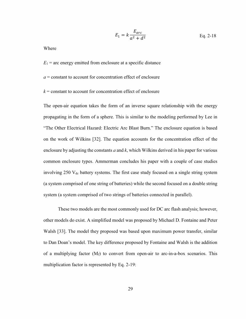
29
𝐸𝐸1 = 𝑘𝑘𝐸𝐸𝑎𝑎𝑎𝑎𝑎𝑎
𝑎𝑎2 + 𝑑𝑑2
Where
E1 = arc energy emitted from enclosure at a specific distance
a = constant to account for concentration effect of enclosure
k = constant to account for concentration effect of enclosure
The open-air equation takes the form of an inverse square relationship with the energy
propagating in the form of a sphere. This is similar to the modeling performed by Lee in
“The Other Electrical Hazard: Electric Arc Blast Burn.” The enclosure equation is based
on the work of Wilkins [32]. The equation accounts for the concentration effect of the
enclosure by adjusting the constants a and k, which Wilkins derived in his paper for various
common enclosure types. Ammerman concludes his paper with a couple of case studies
involving 250 Vdc battery systems. The first case study focused on a single string system
(a system comprised of one string of batteries) while the second focused on a double string
system (a system comprised of two strings of batteries connected in parallel).
These two models are the most commonly used for DC arc flash analysis; however,
other models do exist. A simplified model was proposed by Michael D. Fontaine and Peter
Walsh [33]. The model they proposed was based upon maximum power transfer, similar
to Dan Doan’s model. The key difference proposed by Fontaine and Walsh is the addition
of a multiplying factor (Mf) to convert from open-air to arc-in-a-box scenarios. This
multiplication factor is represented by Eq. 2-19:
Eq. 2-18

30
𝑀𝑀𝑏𝑏 =
𝐼𝐼𝐸𝐸𝑏𝑏𝐼𝐼𝐸𝐸𝑃𝑃𝑎𝑎
Where
Mf = multiplication factor relating open-air and enclosed incident energies
IEb = incident energy with enclosure present
IEoa = incident energy when arc is in open-air
The full definition of this multiplication factor is derived from the work of Wilkins,
specifically Eq. 2-18. Eq. 2-20 provides the full definition of the multiplication factor.
𝑀𝑀𝑏𝑏 =
𝑘𝑘 ∗ 4𝜋𝜋
1 + �𝑎𝑎𝑑𝑑�2
In cases where a variable factor is used, such as Ammerman’s model, the multiplication
factor must be determined iteratively [33]. By modifying maximum power equations,
Fontaine and Welsh proposed Eq. 2-21 for the determination of incident energy:
𝐼𝐼𝐸𝐸 =
0.004755 ∗ 𝑉𝑉𝑠𝑠𝑠𝑠𝑠𝑠 ∗ 𝐼𝐼𝑏𝑏𝑏𝑏 ∗ 𝑀𝑀𝑏𝑏 ∗ 𝑇𝑇𝑎𝑎𝑎𝑎𝑎𝑎𝐷𝐷𝑎𝑎𝑐𝑐2
This equation for incident energy is very similar to the equation utilized with NFPA 70E
[34].
2.5: Battery-Specific DC Arc Flash Research Research regarding DC arc flash hazards posed by battery systems is still relatively
sparse. Some literature has focused upon performing case studies to identify and quantify
potential arc flash hazards with battery systems. Other research involved empirical testing
to assess arc flash hazards. The research presented in [35], [36], and [37] fall into the former
Eq. 2-19
Eq. 2-20
Eq. 2-21
31
classification; whereas, the research conducted by Bonneville Power Authority (BPA) and
Kinetrics fall into the latter. “Arc-Flash in Large Battery Energy Storage Systems – Hazard
Calculation and Mitigation” by F.M. Gatta, A. Geri, M. Maccioni, S. Lauria, and F. Palone
describes arc flash analysis using software known as ATP-EMTP (Alternative Transients
Program – Electromagnetic Transients Program). Using ATP-EMTP, the researchers
modeled the system of interest and applicable protective devices. Studies were conducted
with consideration of lithium-ion and sodium-sulfide type batteries. Conclusions were
drawn regarding the application and effectiveness of the fast acting fuses with respect to
the limitation of incident energy.
In “Arc-Flash Calculation Comparison for Energy Storage Systems” the authors
applied both Ammerman’s and Doan’s equations to the same energy storage system and
compared results. Arc characteristics utilized in Ammerman’s model were determined via
three different methods: the Nottingham method [13], the Stokes method [22], and the
Paukert method [23]. Furthermore, three possible fault locations were considered: “a fault
on the lithium-titanate battery DC ACB (Air Circuit Breaker), a fault occurring on the LV
cable box of the 11kV/350V transformer; and a fault on the HV RMU (Ring Main Unit)
[36].” In addition, the paper presented the various PPE recommendations that would be
associated with the results calculated for each incident energy equation. The primary focus
of the paper was to showcase the similarities and differences between the various arc flash
calculation methods available today and provide a better understanding of potential arc
flash hazards that could occur within the energy storage systems utilized within the paper
[36].

32
Lastly, “Case Study- DC Arc Flash and Safety Considerations in a 400 VDC UPS
Architecture Power System Equipped with VRLA Battery” by M. M. Krzywosz analyzed
the potential arc flash hazard presented by VRLA (Valve-Regulated Lead-Acid) batteries,
which are commonly used in data center UPS power systems. Similar to the previous paper,
assessment of the potential arc flash hazard was conducted using Doan’s and Ammerman’s
models. The models were applied at various potential fault locations within the system of
interest and the results were compared. A third, “Look-up Table Method” [37] was also
considered in the comparison. The “Look-up Table Method” was included in the 2012
version of NFPA 70E. Provided working voltage and arcing current are known, the table
allows one to find PPE recommendations without needing to perform any calculations. The
paper offers reasons why further research must be conducted with respect to arc flash in
DC systems [37].
As previously mentioned, there is little empirical data regarding arc flash in DC
systems. As known of this writing, Bonneville Power Authority (BPA) and Kinectrics (on
behalf of Bruce Power) are the only two organizations that have published empirical
research regarding DC arc flash. Others may have performed DC arc flash testing;
however, results have not been published. Since these two organizations have performed
empirical research, their publications serve as the most comparable ones to the research
performed for this thesis.
“Arc Flash Hazards of 125 Vdc Station Battery Systems” by J. Hildreth and K.
Feeney reports the findings made by BPA. Their testing was performed using lead-acid
batteries with a voltage of 125 V, a capacity of 1,300 Ah, and 11,000 A bolted fault current
[38]. Data were collected for 50 tests of various configurations. Configurations included
33
vertical versus horizontal electrodes, connected versus disconnected charger, and different
gap widths. Arc durations were not controlled during testing in order to observe how long
an arc would naturally be sustained. Ultimately, testing performed by BPA showed that
present standards are very conservative in their assumptions, especially when considering
the allowable time of arcing is two seconds for arc flash calculations. During testing, no
arc exceeded a duration of 0.715 seconds [38]. In addition, the maximum incident energy
measured at a working distance of 18 inches was 0.9 cal/cm2 [38].
Lastly, Kinectrics performed a series of DC arc flash tests for Bruce Power. These
tests were conducted at Kinectrics’ high-current lab. A low-impedance transformer was
utilized with rectifiers to achieve desired DC system voltages. The voltages used for DC
tests were 130 V and 260 V. Tests were conducted over a number of different current levels
and gap widths [39]. The results acquired by Kinectrics have been referenced by other
papers and were the sole source of empirical DC arc flash information for a number of
years. The Kinectrics results were even used to develop/validate Ammerman’s model [7].
With respect to their 130 Vdc tests, Kinectrics was able to sustain arcs at 0.25 inches and
0.5 inches; however, larger gap widths could only sustain arcs in terms of milliseconds
[39]. At 0.25 and 0.50 inches, arcs were sustainable until the arc vaporized sufficient
electrode material to self-extinguish [39]. As for incident energy, Kinectrics measured
sufficient heat flux with sustained 0.50-inch arcs to warrant the use of arc flash PPE [39].
34
CHAPTER 3: METHODOLOGY 3.1: Test Setup
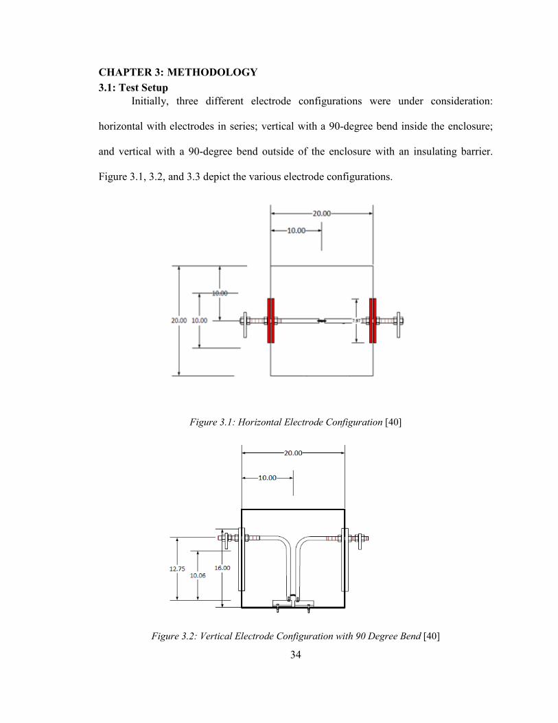
Initially, three different electrode configurations were under consideration:
horizontal with electrodes in series; vertical with a 90-degree bend inside the enclosure;
and vertical with a 90-degree bend outside of the enclosure with an insulating barrier.
Figure 3.1, 3.2, and 3.3 depict the various electrode configurations.
Figure 3.1: Horizontal Electrode Configuration [40]
Figure 3.2: Vertical Electrode Configuration with 90 Degree Bend [40]
35
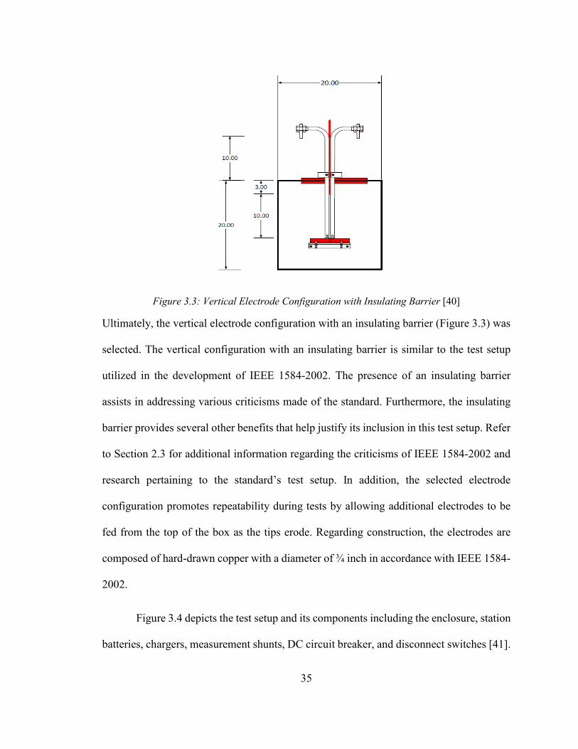
Figure 3.3: Vertical Electrode Configuration with Insulating Barrier [40]
Ultimately, the vertical electrode configuration with an insulating barrier (Figure 3.3) was
selected. The vertical configuration with an insulating barrier is similar to the test setup
utilized in the development of IEEE 1584-2002. The presence of an insulating barrier
assists in addressing various criticisms made of the standard. Furthermore, the insulating
barrier provides several other benefits that help justify its inclusion in this test setup. Refer
to Section 2.3 for additional information regarding the criticisms of IEEE 1584-2002 and
research pertaining to the standard’s test setup. In addition, the selected electrode
configuration promotes repeatability during tests by allowing additional electrodes to be
fed from the top of the box as the tips erode. Regarding construction, the electrodes are
composed of hard-drawn copper with a diameter of ¾ inch in accordance with IEEE 1584-
2002.
Figure 3.4 depicts the test setup and its components including the enclosure, station
batteries, chargers, measurement shunts, DC circuit breaker, and disconnect switches [41].

36
Figure 3.4: Power Schematic of Test Setup [41]

37
The enclosure containing the electrodes is a steel box that has a height, width, and depth
of 20 inches. Dimensions for the enclosure stem from test setups in IEEE 1584-2002 and
previous literature [26], [29], [30]. Additionally, the electrodes terminate at the center of
the enclosure (10 inches) and enter four inches from the back via a pair of holes placed in
the top of the enclosure. The front of the enclosure is open while the remaining five sides
are solid. The batteries utilized for this experiment have a nominal voltage rating of 125
Vdc and possess capacities of 100 Ah and 150 Ah. Batteries are produced by different
manufacturers; thus, the batteries possess variances in construction. For testing, it was
assumed that any differences in characteristics between batteries (such as internal
resistance) were negligible. Three preliminary shots were performed to verify the validity
of this assumption.
For these preliminary tests, the batteries were connected to a large coil to serve as
an impedance. The batteries were then “shorted” in a manner similar to how normal tests
would be performed. While “shorted,” currents were measured to determine available short
circuit current. The first two tests utilized one battery at a time and the third test utilized
the batteries connected in parallel. In addition, battery impedances were checked indirectly
by measuring the battery voltages and currents immediately prior to and after initiating
each test (provided voltage and current were stabilized). The differences between voltages
and currents were determined and the impedance was calculated using Ohm’s Law. This
procedure for indirectly determining battery impedance was performed periodically during
testing to verify that there were no drastic changes in battery impedance due to
deterioration.
38
Preliminary testing showed only minor differences between the batteries;
therefore, the assumption was deemed sound. Similar to the batteries, the battery chargers
are of different manufacturers. Availability dictated the selection of these chargers.
Because the chargers were disconnected before shots, any differences between chargers
are irrelevant. A pair of shunts served to measure current from each of the batteries.
Disconnect switches were used to manage the connections between the batteries and DC
circuit breaker. Lastly, the DC circuit breaker was used to control the arc duration;
however, it also acted as an emergency shutoff switch if testing presented a dangerous
situation.
The primary measurement during testing is thermal energy. However, attempts
were made to collect additional light and sound levels. Pressure sensors were considered
but deemed likely to interfere with the calorimeters, since both measurement devices
should occupy the same space. Thus, the measurement devices for testing include
calorimeters, a sound recorder, and a light sensor. In addition, a series of cameras were
used to capture arc flash behavior. These cameras include two high-speed cameras with
various frame rates, a thermal imaging camera, and a standard high definition camera. To
protect the cameras from possible lighting damage, the cameras are placed off axis from
the arc. In addition, one high-speed camera had a light dampening filter.
Calorimeters were constructed based on IEEE 1584-2002. Therefore, the
calorimeters were composed of copper and have a diameter of 1.6 inches. The thickness of
the calorimeters is 1/16 inch. The side of the calorimeter to face the enclosure was painted
with flat black paint with a high temperature rating. In addition, the paint required an
emissivity rating greater than 0.9 [42]. Specialized paint products exist; however, most

39
black paints have a natural emissivity approximately equal to or greater than 0.9 [43], [44].
Therefore, the paint used was high temperature automotive paint from a local store.
Emissivity is important because it influences heat transfer. High emissivity objects emit
heat more readily than low emissivity objects. Furthermore, objects that possess high
emissivity tend to exhibit higher absorptivity, which dictates an objects ability to capture
heat [45]. Thus, by painting the one side of the calorimeters, the calorimeters should collect
the majority of the heat energy created during each shot. Furthermore, the calorimeters
should emit the captured heat between shots, which prevents thermal energy captured from
one shot from skewing the temperature reading for the following shot.
Calorimeters were connected to the data acquisition system via thermocouples.
Type K thermocouples were used due to availability and cost. Initially, type J
thermocouples were considered due to the setup used in IEEE 1584-2002. Type J
thermocouples possess higher sensitivity compared with Type K; however, they possess a
narrower range of heat limits. The range of heat limits is the primary concern for testing.
Since Type K thermocouples include the range of Type J thermocouples, Type K
thermocouples are a valid alternative. Lastly, the size used for the thermocouples was 30
AWG, which is based on IEEE 1584-2002.
During testing, the calorimeters were held in place via a mounting. The mounting
was constructed with pipes to allow thermocouples to be protected during testing. In
addition, the mounting possesses wheels to facilitate distance adjustments between tests.
To prevent movement during tests, cinderblocks were used to secure the mounting.
Furthermore, the mounting is designed to allow for the following configuration of
calorimeters:
40
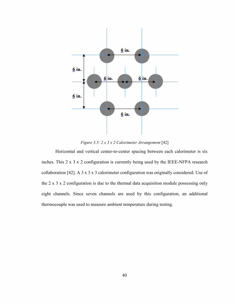
Figure 3.5: 2 x 3 x 2 Calorimeter Arrangement [42]
Horizontal and vertical center-to-center spacing between each calorimeter is six
inches. This 2 x 3 x 2 configuration is currently being used by the IEEE-NFPA research
collaboration [42]. A 3 x 3 x 3 calorimeter configuration was originally considered. Use of
the 2 x 3 x 2 configuration is due to the thermal data acquisition module possessing only
eight channels. Since seven channels are used by this configuration, an additional
thermocouple was used to measure ambient temperature during testing.

41
The thermal data acquisition module was connected to the main data acquisition
module, which possesses 16 channels. Other measurement devices, such as the sound
recorder and light sensor, were connected directly to the main module. The light sensor
was attached to the calorimeter mounting and was capable of measuring various forms of
UV radiation. The sound recorder was capable of capturing peak sound levels. In relation
to the calorimeter mounting, the sound recorder was placed slightly behind the mounting
in a space between calorimeters. Voltage measurements at the electrodes were collected
via a pair of voltage probes. Figures 3.6, 3.7, and 3.8 show the test setup.
Figure 3.6: Enclosure and Calorimeter Mounting

42
Figure 3.7: Chargers, Disconnect Switches, and DC Circuit Breaker
Figure 3.8: Electrodes after Test
43
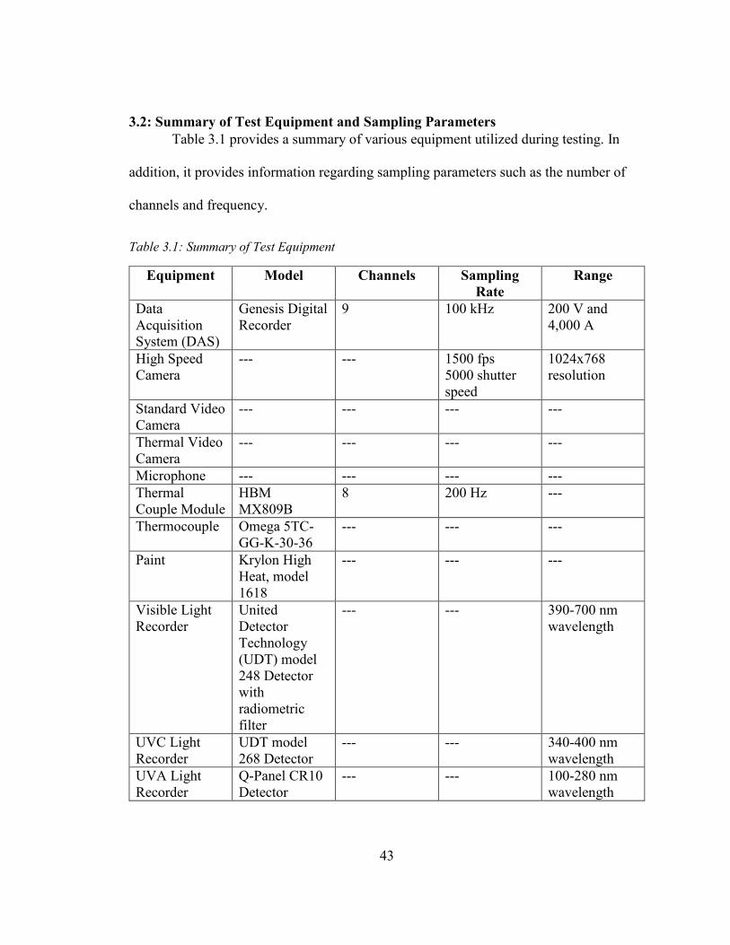
3.2: Summary of Test Equipment and Sampling Parameters Table 3.1 provides a summary of various equipment utilized during testing. In
addition, it provides information regarding sampling parameters such as the number of
channels and frequency.
Table 3.1: Summary of Test Equipment
Equipment Model Channels Sampling Rate
Range
Data Acquisition System (DAS)
Genesis Digital Recorder
9 100 kHz 200 V and 4,000 A
High Speed Camera
--- --- 1500 fps 5000 shutter speed
1024x768 resolution
Standard Video Camera
--- --- --- ---
Thermal Video Camera
--- --- --- ---
Microphone --- --- --- --- Thermal Couple Module
HBM MX809B
8 200 Hz ---
Thermocouple Omega 5TC-GG-K-30-36
--- --- ---
Paint Krylon High Heat, model 1618
--- --- ---
Visible Light Recorder
United Detector Technology (UDT) model 248 Detector with radiometric filter
--- --- 390-700 nm wavelength
UVC Light Recorder
UDT model 268 Detector
--- --- 340-400 nm wavelength
UVA Light Recorder
Q-Panel CR10 Detector
--- --- 100-280 nm wavelength
44
3.3: Initial Testing Procedure Electrodes were refinished after each test to permit multiple tests with a single pair
of electrodes. The overall length of the electrodes exceeded the 10 inches of electrodes
placed in the box. Therefore, after refinishing, the electrodes were moved down to ensure
the length of electrodes within the box was 10 inches. For the initial series of testing,
calorimeters were placed six inches from the opening of the box, which corresponds with
a distance of 22 inches from the electrodes. Furthermore, the central calorimeter was in
line with the center of the electrodes and was at the same height as the terminal of the
electrodes.
Gap width served as one independent variable for testing. For initial tests, gap
widths ranged from 1/8 inch to one inch with 1/8 inch increments. The initial gap width
used was ½ inch. After the first test, the electrodes were moved apart or closer together
based on arc behavior. If an arc occurred, the electrodes were moved 1/8 inch further apart
and tested again. This procedure was repeated until no arc formed between the electrodes.
The distance at which no arc formed was recorded. If no arc formed from the initial test,
the electrodes were moved 1/8 inch closer and tested again. This procedure was repeated
until an arc formed and. that distance was recorded. After determining the maximum
distance at which arcing occurs or the minimum distance at which arcing ceases, the
electrodes were reset to the largest gap width at which arcing still occurred. Additional
shots were performed for each gap width for which arcing occurred.
Distance from the electrodes (i.e., working distance) serves as a second independent
variable for testing. After completing the first series of tests regarding gap width, the
electrodes were set to the gap width associated with arcs having the greatest thermal
45
energy. The working distance was increased to 36 inches and three tests were performed.
Following the last shot, the calorimeters were moved forward to a distance of 18 inches
from the electrodes and another series of shots was performed. This procedure was repeated
for distances of 15 inches, 12 inches, nine inches, and six inches.
The timeframe for testing was limited. Therefore, special consideration was given
to the rate of testing. The downtime between tests was determined via the behavior and
performance of the batteries and the time required to reset the test setup between shots.
Furthermore, batteries were charged between each shot to promote consistency. Based on
these considerations, the expected test rate was two tests per hour. Based on the expected
test rate, the performance of approximately 32 to 48 shots was predicted. These shots were
equally divided among the various test setup arrangements. With respect to sound
measurements, if any test produced noteworthy sound levels, the test was performed again
with only the sound recorders.
3.4: Testing DC Arc Flash testing was performed from August 7 to August 15, 2018. Testing
was performed in three stages. The first stage had the calorimeters positioned at a working
distance of 22 inches from the electrodes. During this stage, the gap width between the
electrodes was adjusted to assess the effect of gap width on calorimeter temperature rise.
To begin, the gap width was set to ½ inch and progressively reduced until arcing was
achieved. Arcing was first sustained at 1/8 inch gap width. Afterwards, a series of tests was
performed at gap widths of 1/16 and 3/16 inches. Three repetitions were performed for
each test setup. An attempt was made to initiate arcs at ¼ inch; however, no arc was
sustained.
46
The second stage of testing had the gap width set to 1/8 inch. This gap width was
selected because it provided the most consistent arcing during stage 1 testing. Three
additional tests were performed at a working distance of 22 inches to initialize the data set
and ensure that arcing was well behaved. Afterwards, the calorimeter stand was moved
closer to the electrodes and a series of three tests was performed. Tests were performed
using working distances of 22, 18, 15, 12, 9, and 6 inches. The goal of the second test stage
was to assess the influence of working distance on measured temperature rise. The final
stage of testing had the calorimeter stand returned to a working distance of 15 inches and
additional tests were performed at gap widths of 1/16 and 1/4 inches. The 15-inch working
distance was selected due to AEP (American Electric Power) using 15 inches for arc flash
calculations. The purpose of this stage was to acquire additional gap width measurements
with greater temperature changes and allow for comparison with tests performed at the 22
inch working distance to assess the possibility of interaction among independent variables.
Adjustments had to be made to the original test setup during testing as issues were
encountered. One issue encountered dealt with the application of the fuse wire. Initially,
the fuse wire was tied around each electrode with a single wire bridging the gap. This
method of attaching the fuse wire became difficult to perform at small gap widths.
Therefore, a figure-8 pattern was selected due to ease of application and the ability of it to
resist movement by electromagnetic forces.
Following the standardization of attaching the fuse wire, a new issue occurred in
which the test setup was unable to melt the fuse wire and initiate an arc. It was identified
that the figure-8 pattern increased the amount of material between the electrodes, thereby,
47
increasing the amount of material that needed to melt to establish an arc. To counteract
this, the fuse wire was changed from 16 to 20 gauge.
The next issue encountered concerned the DC circuit breaker. During some tests,
the DC circuit breaker would trip due to internal overcurrent protection. In order to prevent
unintentional tripping the different poles of the circuit breaker were bridged to divide the
fault current over four poles instead of two. This modification prevented the circuit breaker
from unintentionally tripping during tests.
The last adjustment made occurred after August 8th. On August 8th there was
difficulty sustaining arcs, even at gap widths that had previously been successful. Two
hypotheses were proposed. The first hypothesis was that weather was having an adverse
effect on the arcs. The second hypothesis was that the erosion of the barrier was influencing
the arcs. The barrier was initially a piece of red fiberglass. It was noticed that during a shot,
a large portion of the barrier would be vaporized. Since the red fiberglass was an insulator,
it was hypothesized that filaments were being introduced into the pathway of the arc during
testing and that these filaments were having a form of damping effect. Thus, the barrier
was changed to a piece of mica, which proved more resilient during testing and lacked the
fibers that were a concern with the red fiberglass.
Table 3.2 provides a summary of the testing procedure.

48
Table 3.2: Test Procedure Summary
Test Stage 1: Gap Width Tests at 22-inch Working Distance Step 1: Performed first test at ½ inch gap width. Step 2: Checked test data, refinished electrodes, and reset test setup. Step 3: If arc was not sustained, gap width was decreased by 1/8 inch
increment and the test was repeated. Step 4: Continued decreasing gap width by 1/8 inch increments and
repeating tests until an arc was sustained. Step 5: Once arc sustaining gap width was determined, the test setup
was repeated two additional times for three total repetitions. Step 6: Gap width was decreased by 1/16 inch increment and the test
was repeated. Step 7: If arc was successfully sustained, the test was repeated two
additional times. Step 8: Gap width was increased to 3/16 inch and the test was
repeated. See Step 7 if arc was sustained. Test Stage 2: Working Distance Tests at 1/8-inch Gap Width
Step 1: Test setup was set to 1/8-inch gap width due to consistent arcing behavior. Test setup was not moved from initial working distance of 22 inches.
Step 2: Three tests were performed to initialize new data set. Step 3: After completing the three tests at 22 inches, the calorimeter
stand was moved forward to 18 inches and tests were repeated.
Step 4: After completing three tests at 18 inches, the calorimeter stand was moved three inches closer to the electrodes and the tests were repeated.
Step 5: General procedure outlined by Steps 3 and 4 was repeated for working distances of 15 inches, 12 inches, 9 inches, and 6 inches.
Test Stage 3: Gap Width Tests at 15-inch Working Distance Step 1: Calorimeter stand was moved to 15-inch working distance. Step 2: Electrodes were set to 1/16-inch gap width and three tests
were performed. Step 3: Electrodes were set to ¼-inch gap width and three tests were
performed.
49
CHAPTER 4: RESULTS AND DISCUSSION 4.1: Data Manipulation The data were collected using a Genesis data acquisition system and exported into
a series of MATLAB files. Several MATLAB scripts were written to allow easier access
and manipulation of data. Two scripts oversee the importing of data; one script manages
voltage and current information, while the second script manages temperature data. A third
script was created to import light intensity data collected during testing; however, these
data were not used. A series of other scripts were used to generate multidimensional arrays
corresponding with battery voltages, battery currents, total current, arc voltage, and
temperature. A moving average was applied to the data for smoothing. The number of
samples utilized for the moving average was 101, which corresponds to a time interval of
1.01 milliseconds. The use of 101 samples instead of 100 was to center the averaging
window on a single sample. One script was created for each gap width and for each type
of data (electrical versus thermal). This was done to allow MATLAB to operate faster by
reducing the total size of the scripts. Another script was created for calculating total energy
produced by the arc during the test duration. This calculation does not omit the contribution
from the fuse wire. This was deemed acceptable for two reasons. First, the time spent
burning the fuse wire was brief in proportion to the duration of the arc and complete test.
Second, the burning of the fuse wire did contribute to measured temperature rise.
Power was calculated by performing elementwise multiplication of arc voltage
current. Next, graphs were generated for the resulting power arrays to verify whether the
array appeared appropriate. Energy was then determined using the trapz() function within
MATLAB to apply the trapezoidal rule for numerical integration. The results were checked
by performing a hand calculation using a single trapezoid and bounding the integration

50
interval. The difference between the hand calculation and MATLAB calculation was
approximately 1% and was deemed acceptable. Additionally, the trapz() function returned
the same result whether performed bounded or unbounded; therefore, any contribution
from remaining noise was deemed negligible.
4.2: Data Analysis 4.2.1: Temperature Rise/Incident Energy vs. Gap Width 4.2.1.1: Working Distance: 22 Inches
Data analysis began by assessing the behavior of temperature rise versus gap width
at a working distance of 22 inches. Table 4.1 summarizes the data used for this analysis.
Table 4.1: Temperature Rise and Incident Energy Data for 22-inch Working Distance
Peak incident energy was calculated by using the conversion factor 0.135
cal/(cm2*˚C) [42]. Using the data in Table 4.1, Figures 4.1 and 4.2 were produced. The
trendlines, equations, and R2 values for each figure were determined utilizing the chart
tools in Microsoft Excel. Since temperature rise and incident energy differ by a constant,
the remainder of the report will primarily use incident energy for convenience.
Test Gap Width (inches)
Peak Temperature Rise (˚C)
Peak Incident Energy (cal/cm2)
187_001 0.1875 0.94 0.1269 187_002 0.1875 0.63 0.0851 187_003 0.1875 0.48 0.0648 125_007 0.125 0.52 0.0702 125_008 0.125 0.68 0.0918 125_010 0.125 0.66 0.0891 125_011 0.125 0.44 0.0594 125_012 0.125 0.71 0.0959 125_013 0.125 0.77 0.1040 125_014 0.125 0.77 0.1040 062_001 0.0625 0.08 0.0108 062_002 0.0625 0.36 0.0486 062_003 0.0625 0.59 0.0797

51
Figure 4.1: Peak Temperature Rise vs. Gap Width at 22 Inches
Figure 4.2: Peak Incident Energy vs. Gap Width at 22 Inches
The trend depicted by the Figures 4.1 and 4.2 is unexpected. Based on intuition,
increasing gap widths should exhibit increasing resistance due to greater amounts of air to
y = -34.987x2 + 11.467x - 0.2367R² = 0.411
0
0.1
0.2
0.3
0.4
0.5
0.6
0.7
0.8
0.9
1
0 0.02 0.04 0.06 0.08 0.1 0.12 0.14 0.16 0.18 0.2
Tem
pera
ture
Rise
(Cel
sius)
Gap Width (Inches)
Peak Temperature Rise vs. Gap Width at 22 Inches
y = -4.7232x2 + 1.548x - 0.032R² = 0.411
0
0.02
0.04
0.06
0.08
0.1
0.12
0.14
0 0.02 0.04 0.06 0.08 0.1 0.12 0.14 0.16 0.18 0.2
Inci
dent
Ene
rgy
(cal
/sq.
cm
)
Gap Width (Inches)
Peak Incident Energy vs. Gap Width at 22 Inches

52
ionize. This increased resistance should result in greater temperature rise since heat
emission is proportional to I2R. Given how close the measurements are to each other and
that there is overlap between temperature rises at different working distances; there may
be insufficient variation to distinguish the various measurements. Figure 4.3 was generated
utilizing average temperature rise since shrapnel was e during every test and may have
introduced additional error by impacting the calorimeter near the thermocouple. Since
Figure 4.3 depicts a similar trend as Figures 4.1 and 4.2, shrapnel likely had minimal effect
on these results. This conclusion seems reasonable given the distance between the
electrodes and calorimeter setup. Table 4.2 summarizes the data utilized to generate Figure
4.3.
Figure 4.3: Average Temperature Rise vs. Gap Width at 22 Inches
y = -38.67x2 + 10.776x - 0.2905R² = 0.4098
0
0.1
0.2
0.3
0.4
0.5
0.6
0.7
0 0.02 0.04 0.06 0.08 0.1 0.12 0.14 0.16 0.18 0.2
Tem
pera
ture
Rise
(Cel
sius)
Gap Width (Inches)
Average Temperature Rise vs. Gap Width at 22 Inches

53
Table 4.2: Calorimeter Data at 22 Inches
Temperature Rise per Calorimeter (˚C) Test Gap Width (inches) 1 2 3 4 5 6 7 Avg.
187_001 0.1875 0.37 0.66 0.30 0.36 0.38 0.32 0.94 0.48 187_002 0.1875 0.28 0.63 0.25 0.39 0.26 0.30 0.23 0.33 187_003 0.1875 0.48 0.32 0.25 0.29 0.32 0.20 0.25 0.30 125_007 0.125 0.25 0.46 0.28 0.40 0.52 0.25 0.29 0.35 125_008 0.125 0.43 0.56 0.30 0.56 0.68 0.51 0.32 0.48 125_010 0.125 0.55 0.66 0.27 0.45 0.33 0.27 0.19 0.39 125_011 0.125 0.40 0.36 0.28 0.44 0.36 0.31 0.02 0.31 125_012 0.125 0.44 0.50 0.39 0.64 0.71 0.26 0.29 0.46 125_013 0.125 0.49 0.57 0.47 0.71 0.63 0.52 0.77 0.59 125_014 0.125 0.65 0.77 0.52 0.54 0.62 0.51 0.46 0.58 062_001 0.0625 0.05 0.06 0.01 0.08 0.05 0.04 0.04 0.05 062_002 0.0625 0.31 0.33 0.20 0.36 0.29 0.17 0.20 0.27 062_003 0.0625 0.34 0.59 0.30 0.37 0.48 0.28 0.32 0.38
4.2.1.2: Working Distance: 15 Inches Table 4.3 summarizes data collected for a working distance of 15 inches. Figure
4.4 was generated using the incident energy data contained in Table 4.3. Similar to
Figures 4.1, 4.2, and 4.3, Figure 4.4 displays a polynomial trend. However, the trend
displayed is opposite to that shown by the 22-inch working distance data. A possible
explanation for this is that there is interaction between working distance and gap width,
which is obscuring the true relationship; however, defining interaction with nonlinear
models is difficult to quantify. Since the calorimeters were closer to the electrodes (15
inches compared with 22 inches), the displayed relationship should be more accurate than
that observed at 22 inches since the calorimeters detected greater temperature variance.

54
Table 4.3: Temperature Rise and Incident Energy Data for 15-inch Working Distance
Test Gap Width (inches)
Peak Temperature Rise (˚C)
Peak Incident Energy (cal/cm2)
250_004 0.25 1.87 0.2525 250_005 0.25 2.25 0.3038 250_006 0.25 2.13 0.2876 125_019 0.125 1.09 0.1472 125_020 0.125 1.24 0.1674 125_021 0.125 1.07 0.1445 062_004 0.0625 1.15 0.1553 062_005 0.0625 1.46 0.1971 062_006 0.0625 0.70 0.0945 062_007 0.0625 1.68 0.2268
Figure 4.4: Peak Incident Energy vs. Gap Width at 15 Inches
Figure 4.5 was created using temperature rise data averaged for all calorimeters.
Figure 4.5 and Table 4.4, which contains the associated data, follow. Unlike the 22-inch
working distance, the trends depicted by Figures 4.4 and 4.5 differ based upon whether
peak values or averages are used. Thus, there is a possibility that shrapnel ejected during
y = 6.7872x2 - 1.5192x + 0.2369R² = 0.7243
0
0.05
0.1
0.15
0.2
0.25
0.3
0.35
0 0.05 0.1 0.15 0.2 0.25 0.3
Inci
dent
Ene
rgy
(cal
/sq.
cm
)
Gap Width (Inches)
Peak Incident Energy vs. Gap Width at 15 Inches
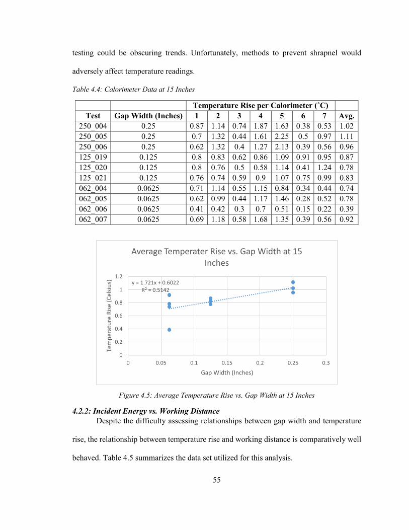
55
testing could be obscuring trends. Unfortunately, methods to prevent shrapnel would
adversely affect temperature readings.
Table 4.4: Calorimeter Data at 15 Inches
Temperature Rise per Calorimeter (˚C) Test Gap Width (Inches) 1 2 3 4 5 6 7 Avg.
250_004 0.25 0.87 1.14 0.74 1.87 1.63 0.38 0.53 1.02 250_005 0.25 0.7 1.32 0.44 1.61 2.25 0.5 0.97 1.11 250_006 0.25 0.62 1.32 0.4 1.27 2.13 0.39 0.56 0.96 125_019 0.125 0.8 0.83 0.62 0.86 1.09 0.91 0.95 0.87 125_020 0.125 0.8 0.76 0.5 0.58 1.14 0.41 1.24 0.78 125_021 0.125 0.76 0.74 0.59 0.9 1.07 0.75 0.99 0.83 062_004 0.0625 0.71 1.14 0.55 1.15 0.84 0.34 0.44 0.74 062_005 0.0625 0.62 0.99 0.44 1.17 1.46 0.28 0.52 0.78 062_006 0.0625 0.41 0.42 0.3 0.7 0.51 0.15 0.22 0.39 062_007 0.0625 0.69 1.18 0.58 1.68 1.35 0.39 0.56 0.92
Figure 4.5: Average Temperature Rise vs. Gap Width at 15 Inches
4.2.2: Incident Energy vs. Working Distance Despite the difficulty assessing relationships between gap width and temperature
rise, the relationship between temperature rise and working distance is comparatively well
behaved. Table 4.5 summarizes the data set utilized for this analysis.
y = 1.721x + 0.6022R² = 0.5142
0
0.2
0.4
0.6
0.8
1
1.2
0 0.05 0.1 0.15 0.2 0.25 0.3
Tem
pera
ture
Rise
(Cel
sius)
Gap Width (Inches)
Average Temperater Rise vs. Gap Width at 15 Inches
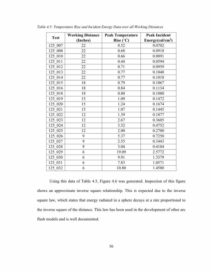
56
Table 4.5: Temperature Rise and Incident Energy Data over all Working Distances
Test Working Distance (Inches)
Peak Temperature Rise (˚C)
Peak Incident Energy(cal/cm2)
125_007 22 0.52 0.0702 125_008 22 0.68 0.0918 125_010 22 0.66 0.0891 125_011 22 0.44 0.0594 125_012 22 0.71 0.0959 125_013 22 0.77 0.1040 125_014 22 0.77 0.1010 125_015 18 0.79 0.1067 125_016 18 0.84 0.1134 125_018 18 0.80 0.1080 125_019 15 1.09 0.1472 125_020 15 1.24 0.1674 125_021 15 1.07 0.1445 125_022 12 1.39 0.1877 125_023 12 2.67 0.3605 125_024 12 3.52 0.4752 125_025 12 2.00 0.2700 125_026 9 5.37 0.7250 125_027 9 2.55 0.3443 125_028 9 3.04 0.4104 125_029 6 19.09 2.5772 125_030 6 9.91 1.3379 125_031 6 7.83 1.0571 125_032 6 10.80 1.4580
Using this data of Table 4.5, Figure 4.6 was generated. Inspection of this figure
shows an approximate inverse square relationship. This is expected due to the inverse
square law, which states that energy radiated in a sphere decays at a rate proportional to
the inverse square of the distance. This law has been used in the development of other arc
flash models and is well documented.

57
Figure 4.6: Peak Incident Energy vs. Working Distance:
Inspection of average temperature rise displays a similar, albeit weaker
relationship. This relationship is displayed in Figure 4.7. This variation between
relationships can be explained by how the position of the calorimeters changed in relation
to the location of the arc as distance decreased. As the calorimeters approached the
electrodes, the proportion of temperature rise focused on the central calorimeter increased
and the amount of temperature rise detected by the surrounding calorimeters decreased.
This hypothesis is given more credibility by Figure 4.8, which depicts the relationship
between the temperature rise of the central calorimeter and working distance. Figures 4.7
and 4.8 were generated from the data contained in Table 4.6.
y = 68.508x-2.193
R² = 0.9311
0
0.5
1
1.5
2
2.5
3
0 5 10 15 20 25
Inci
dent
Ene
rgy
(cal
/sq.
cm
)
Working Distance (Inches)
Peak Incident Energy vs. Working Distance

58
Figure 4.7: Average Temperature Rise vs. Working Distance
Figure 4.8: Central Calorimeter Temperature Rise vs. Working Distance
y = 23.389x-1.273
R² = 0.9061
0
0.5
1
1.5
2
2.5
3
3.5
4
0 5 10 15 20 25
Tem
pera
ture
Rise
(Cel
sius)
Working Distance (Inches)
Average Temperature Rise vs. Working Distance
y = 506.2x-2.291
R² = 0.8954
0
5
10
15
20
25
0 5 10 15 20 25
Tem
pera
ture
Rise
(Cel
sius)
Working Distance (Inches)
Central Calorimeter Temp. Rise vs. Working Distance
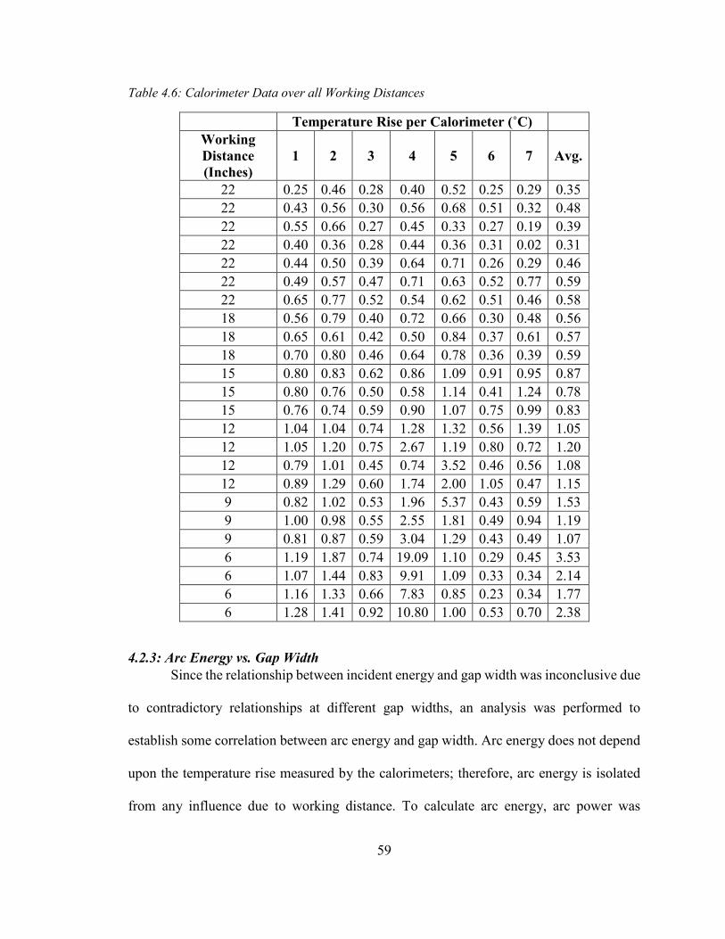
59
Table 4.6: Calorimeter Data over all Working Distances
Temperature Rise per Calorimeter (˚C) Working Distance (Inches)
1 2 3 4 5 6 7 Avg.
22 0.25 0.46 0.28 0.40 0.52 0.25 0.29 0.35 22 0.43 0.56 0.30 0.56 0.68 0.51 0.32 0.48 22 0.55 0.66 0.27 0.45 0.33 0.27 0.19 0.39 22 0.40 0.36 0.28 0.44 0.36 0.31 0.02 0.31 22 0.44 0.50 0.39 0.64 0.71 0.26 0.29 0.46 22 0.49 0.57 0.47 0.71 0.63 0.52 0.77 0.59 22 0.65 0.77 0.52 0.54 0.62 0.51 0.46 0.58 18 0.56 0.79 0.40 0.72 0.66 0.30 0.48 0.56 18 0.65 0.61 0.42 0.50 0.84 0.37 0.61 0.57 18 0.70 0.80 0.46 0.64 0.78 0.36 0.39 0.59 15 0.80 0.83 0.62 0.86 1.09 0.91 0.95 0.87 15 0.80 0.76 0.50 0.58 1.14 0.41 1.24 0.78 15 0.76 0.74 0.59 0.90 1.07 0.75 0.99 0.83 12 1.04 1.04 0.74 1.28 1.32 0.56 1.39 1.05 12 1.05 1.20 0.75 2.67 1.19 0.80 0.72 1.20 12 0.79 1.01 0.45 0.74 3.52 0.46 0.56 1.08 12 0.89 1.29 0.60 1.74 2.00 1.05 0.47 1.15 9 0.82 1.02 0.53 1.96 5.37 0.43 0.59 1.53 9 1.00 0.98 0.55 2.55 1.81 0.49 0.94 1.19 9 0.81 0.87 0.59 3.04 1.29 0.43 0.49 1.07 6 1.19 1.87 0.74 19.09 1.10 0.29 0.45 3.53 6 1.07 1.44 0.83 9.91 1.09 0.33 0.34 2.14 6 1.16 1.33 0.66 7.83 0.85 0.23 0.34 1.77 6 1.28 1.41 0.92 10.80 1.00 0.53 0.70 2.38
4.2.3: Arc Energy vs. Gap Width Since the relationship between incident energy and gap width was inconclusive due
to contradictory relationships at different gap widths, an analysis was performed to
establish some correlation between arc energy and gap width. Arc energy does not depend
upon the temperature rise measured by the calorimeters; therefore, arc energy is isolated
from any influence due to working distance. To calculate arc energy, arc power was
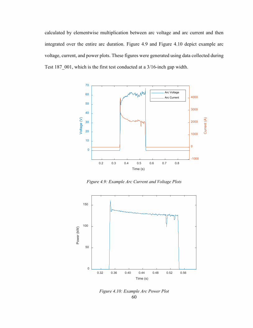
60
calculated by elementwise multiplication between arc voltage and arc current and then
integrated over the entire arc duration. Figure 4.9 and Figure 4.10 depict example arc
voltage, current, and power plots. These figures were generated using data collected during
Test 187_001, which is the first test conducted at a 3/16-inch gap width.
Figure 4.9: Example Arc Current and Voltage Plots
Figure 4.10: Example Arc Power Plot
0.2 0.3 0.4 0.5 0.6 0.7 0.8
Time (s)
0
10
20
30
40
50
60
70Vo
ltage
(V)
-1000
0
1000
2000
3000
4000
Cur
rent
(A)
Arc Voltage
Arc Current
0.32 0.36 0.40 0.44 0.48 0.52 0.56
Time (s)
0
50
100
150
Pow
er (k
W)

61
Table 4.7 summarizes the data used to analyze the relationship between arc energy
and gap width. Energy was calculated in joules and then converted into calories by the
conversion factor 0.239006 cal/J. This conversion factor was determined via Eq. 4-1:
1 𝑐𝑐𝑎𝑎𝑐𝑐 = 4.184 𝐽𝐽 →
1 𝑐𝑐𝑎𝑎𝑐𝑐4.184 𝐽𝐽
≈ 0.239006 𝑐𝑐𝑎𝑎𝑐𝑐/𝐽𝐽
Table 4.7: Arc Energy Data
Test MATLAB Tag Gap Width (inches) Arc Energy (cal) 187_001 VI_187(1) 0.1875 6,199 187_002 VI_187(2) 0.1875 6,201 187_003 VI_187(3) 0.1875 6,148 125_007 VI_125_R8(5) 0.125 5,864 125_008 VI_125_R8(6) 0.125 5,161 125_010 VI_125_R8(8) 0.125 6,008 062_001 VI_062(1) 0.0625 894 062_002 VI_062(2) 0.0625 4,386 062_003 VI_062(3) 0.0625 4,954 250_004 VI_250_R9(3) 0.25 6,046 250_005 VI_250_R9(4) 0.25 6,189 250_006 VI_250_R9(5) 0.25 6,037 062_004 VI_062_R10(1) 0.0625 5,617 062_005 VI_062_R10(2) 0.0625 5,793 062_006 VI_062(4) 0.0625 3,308 062_007 VI_062(5) 0.0625 5,559 125_011 VI_125_R9(1) 0.125 4,716 125_012 VI_125_R9(2) 0.125 6,009 125_013 VI_125_R9(3) 0.125 6,124 125_014 VI_125_R9(4) 0.125 6,239 125_015 VI_125_R9(5) 0.125 6,001 125_016 VI_125_R9(6) 0.125 6,121 125_018 VI_125_R9(8) 0.125 6,142 125_019 VI_125_R9(9) 0.125 6,257 125_020 VI_125_R9(10) 0.125 6,168 125_021 VI_125_R9(11) 0.125 6,244 125_022 VI_125_R9(12) 0.125 6,165 125_023 VI_125_R9(13) 0.125 5,843 125_024 VI_125_R9(14) 0.125 5,929 125_025 VI_125_R9(15) 0.125 5,772
Eq. 4-1

62
125_026 VI_125_R9(16) 0.125 5,834 125_027 VI_125_R9(17) 0.125 5,874 125_028 VI_125_R9(18) 0.125 5,936 125_029 VI_125_R9(19) 0.125 6,083 125_030 VI_125_R9(20) 0.125 5,811 125_031 VI_125_R10(1) 0.125 5,999 125_032 VI_125_R10(2) 0.125 6,064
The data contained in Table 4.7 was used to generate Figure 4.11. Inspection of Figure 4.11
reveals a possible trend; however, there is significant variability in values associated with
1/16 inch measurements. This variability is likely due to differences in arc duration
between tests. Literature regarding arc flash research mentions using a time correction
factor to minimize variation in test duration [19]; however, extrapolation from these
corrected values could have adverse effects upon the developed model. Therefore, any arc
that was not sustained within 5% of the set test duration (200 milliseconds) was omitted.
In other words, any test with a duration less than 190 milliseconds or greater than 210
milliseconds would not be used. In addition, certain tests exhibited uncharacteristically
high temperature rises. These tests were also omitted from the data set because they
indicated the calorimeter being impacted by molten material near the thermocouple. Thus,
the following tests were excluded for the subsequent analyses: 125_008, 062_001,
062_002, 062_003, 062_006, 125_011, 125_029. Removing the selected observations
produce Figure 4.12, which displays an improved fit for energy.
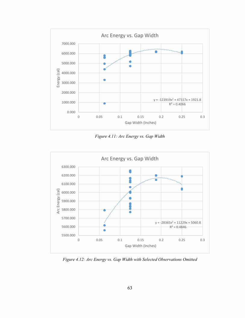
63
Figure 4.11: Arc Energy vs. Gap Width
Figure 4.12: Arc Energy vs. Gap Width with Selected Observations Omitted
y = -123919x2 + 47317x + 1921.8R² = 0.4066
0.000
1000.000
2000.000
3000.000
4000.000
5000.000
6000.000
7000.000
0 0.05 0.1 0.15 0.2 0.25 0.3
Ener
gy (c
al)
Gap Width (Inches)
Arc Energy vs. Gap Width
y = -28365x2 + 11229x + 5060.8R² = 0.4846
5500.000
5600.000
5700.000
5800.000
5900.000
6000.000
6100.000
6200.000
6300.000
0 0.05 0.1 0.15 0.2 0.25 0.3
Arc
Ener
gy (c
al)
Gap Width (Inches)
Arc Energy vs. Gap Width
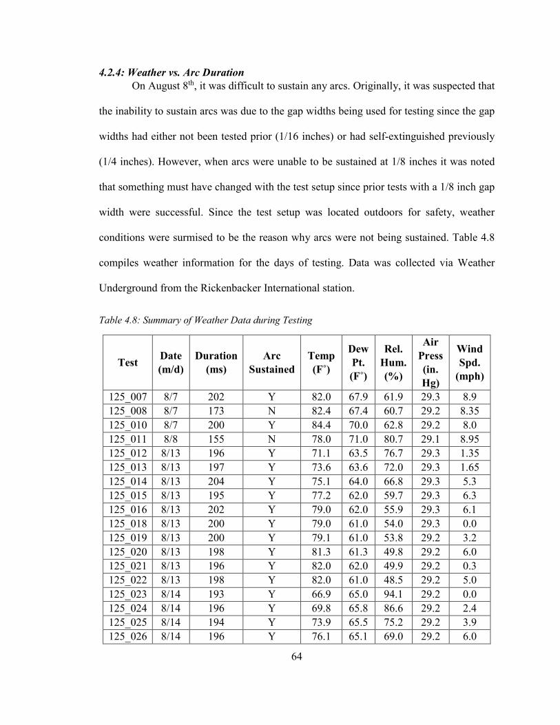
64
4.2.4: Weather vs. Arc Duration On August 8th, it was difficult to sustain any arcs. Originally, it was suspected that
the inability to sustain arcs was due to the gap widths being used for testing since the gap
widths had either not been tested prior (1/16 inches) or had self-extinguished previously
(1/4 inches). However, when arcs were unable to be sustained at 1/8 inches it was noted
that something must have changed with the test setup since prior tests with a 1/8 inch gap
width were successful. Since the test setup was located outdoors for safety, weather
conditions were surmised to be the reason why arcs were not being sustained. Table 4.8
compiles weather information for the days of testing. Data was collected via Weather
Underground from the Rickenbacker International station.
Table 4.8: Summary of Weather Data during Testing
Test Date (m/d)
Duration (ms)
Arc Sustained
Temp (F˚)
Dew Pt. (F˚)
Rel. Hum. (%)
Air Press (in. Hg)
Wind Spd.
(mph)
125_007 8/7 202 Y 82.0 67.9 61.9 29.3 8.9 125_008 8/7 173 N 82.4 67.4 60.7 29.2 8.35 125_010 8/7 200 Y 84.4 70.0 62.8 29.2 8.0 125_011 8/8 155 N 78.0 71.0 80.7 29.1 8.95 125_012 8/13 196 Y 71.1 63.5 76.7 29.3 1.35 125_013 8/13 197 Y 73.6 63.6 72.0 29.3 1.65 125_014 8/13 204 Y 75.1 64.0 66.8 29.3 5.3 125_015 8/13 195 Y 77.2 62.0 59.7 29.3 6.3 125_016 8/13 202 Y 79.0 62.0 55.9 29.3 6.1 125_018 8/13 200 Y 79.0 61.0 54.0 29.3 0.0 125_019 8/13 200 Y 79.1 61.0 53.8 29.2 3.2 125_020 8/13 198 Y 81.3 61.3 49.8 29.2 6.0 125_021 8/13 196 Y 82.0 62.0 49.9 29.2 0.3 125_022 8/13 198 Y 82.0 61.0 48.5 29.2 5.0 125_023 8/14 193 Y 66.9 65.0 94.1 29.2 0.0 125_024 8/14 196 Y 69.8 65.8 86.6 29.2 2.4 125_025 8/14 194 Y 73.9 65.5 75.2 29.2 3.9 125_026 8/14 196 Y 76.1 65.1 69.0 29.2 6.0

65
125_027 8/14 198 Y 77.8 66.0 67.3 29.3 6.5 125_028 8/14 197 Y 81.6 63.4 54.6 29.2 5.0 125_029 8/14 200 Y 82.0 64.0 54.7 29.2 7.7 125_030 8/14 196 Y 83.0 63.0 50.8 29.2 6.8 125_031 8/14 197 Y 83.0 62.0 49.0 29.2 6.0 125_032 8/14 197 Y 84.0 64.0 50.0 29.2 10.9 062_001 8/8 10 N 75.8 72.0 89.4 29.2 7.0 062_002 8/8 148 N 77.0 72.0 84.3 29.2 7.4 062_003 8/8 171 N 76.0 71.3 85.3 29.17 10.8 062_004 8/14 198 Y 83.7 63.0 49.4 29.2 8.3 062_005 8/15 196 Y 68.0 67.0 96.0 29.3 5.0 062_006 8/15 118 N 69.1 67.0 93.9 29.3 5.0 062_007 8/15 193 Y 70.9 67.9 89.3 29.3 5.9 250_002 8/8 126 N 72.0 71.2 99.2 29.2 3.3 250_003 8/8 8 N 72.9 72.0 98.3 29.2 5.9 250_004 8/15 192 Y 72.5 68.0 86.1 29.3 4.7 250_005 8/15 195 Y 74.9 69.0 82.2 29.3 3.0 250_006 8/15 194 Y 76.4 68.8 77.0 29.3 2.4
Since the weather readings collected through Weather Underground did not match
the exact start time of each test, interpolation was used to determine approximate weather
conditions. A multivariate linear regression utilizing all weather variables was performed
using SAS. In addition, all gap widths were utilized within the analysis since each gap
width was known to be capable of sustaining the arc for the full test duration. Figure 4.13
displays the SAS results. Dew point was not included since it is a product of other weather
variables being considered such as humidity and air pressure. Based on the multivariate
linear regression, temperature and humidity are the only statistically significant variables
with p-values of 0.0375 and 0.0007, respectively. Comparatively, temperature is less
statistically significant than humidity since the p-value associated with temperature is
closer to the threshold value of 0.05. Since the number of tests where the arc self-
extinguished is small compared to the total number of tests (8/36) there is likely an

66
insufficient amount of data to make a definitive conclusion. However, there does appear to
be some environmental factor that adversely affected arc sustainability. A more rigorous
analysis on how environmental factors influence arc flash could be pursued as part of future
work.
Figure 4.13: SAS Results for Multivariate Linear Regression of Arc Duration
67
4.3: Development of a Preliminary Equation Two relationships depict sufficient potential to develop an equation for a predictive
incident energy model. These relationships are incident energy versus working distance
and arc energy versus gap width. Selection of these relationships was based upon the
statistical significance and suitability to compose an equation of a desired format based
upon other equations utilized by industry for arc flash studies. Eq. 4-2 represents the
desired predictive model equation.
𝐼𝐼𝐸𝐸 =
𝐶𝐶𝐶𝐶 ∗ 𝐺𝐺𝐺𝐺 ∗ 𝑡𝑡𝐺𝐺𝐷𝐷𝑎𝑎
Where
IE = incident energy in cal/cm2
Cf = correction factor that accounts for factor conversions and safety factors
GW = gap width in inches
t = arc duration in seconds
WD = working distance in inches
a = exponential term
To develop an equation similar to Eq. 4-2, a more rigorous statistical analysis of the
selected relationships was conducted using SAS. Figure 4.14 depicts the results achieved
using nonlinear regression and curve fitting for incident energy versus working distance.
Eq. 4-2
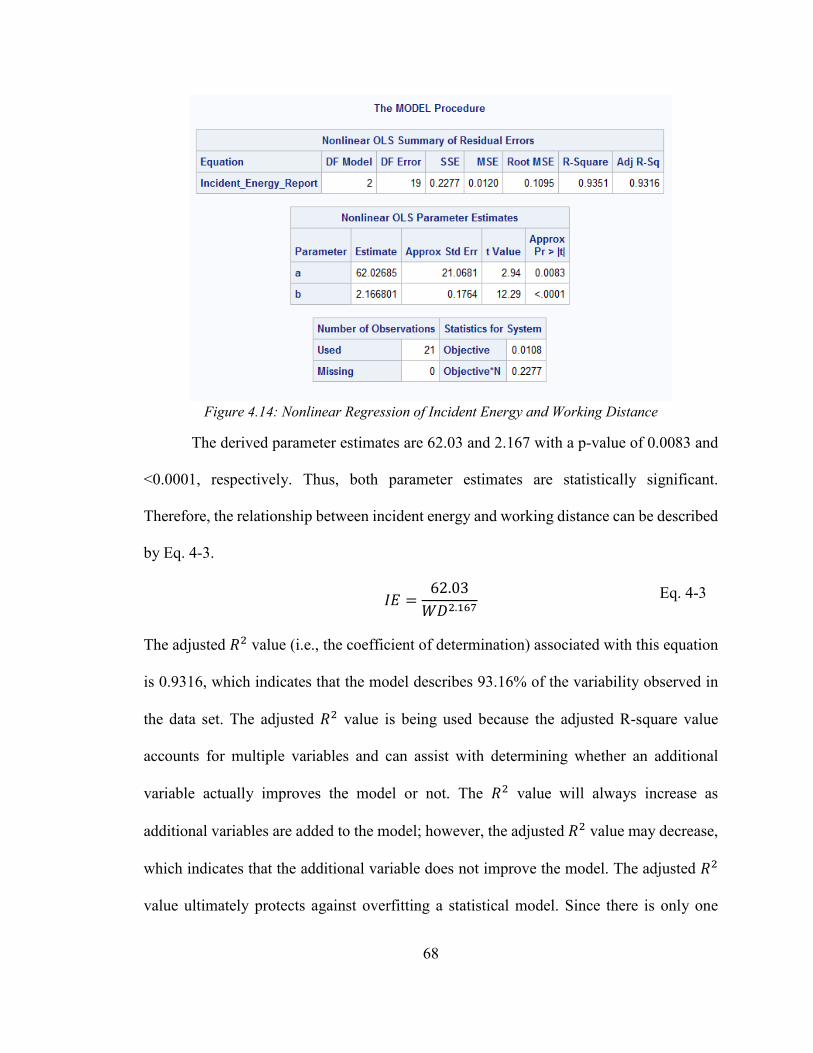
68
Figure 4.14: Nonlinear Regression of Incident Energy and Working Distance
The derived parameter estimates are 62.03 and 2.167 with a p-value of 0.0083 and
<0.0001, respectively. Thus, both parameter estimates are statistically significant.
Therefore, the relationship between incident energy and working distance can be described
by Eq. 4-3.
𝐼𝐼𝐸𝐸 =
62.03𝐺𝐺𝐷𝐷2.167
The adjusted 𝑅𝑅2 value (i.e., the coefficient of determination) associated with this equation
is 0.9316, which indicates that the model describes 93.16% of the variability observed in
the data set. The adjusted 𝑅𝑅2 value is being used because the adjusted R-square value
accounts for multiple variables and can assist with determining whether an additional
variable actually improves the model or not. The 𝑅𝑅2 value will always increase as
additional variables are added to the model; however, the adjusted 𝑅𝑅2 value may decrease,
which indicates that the additional variable does not improve the model. The adjusted 𝑅𝑅2
value ultimately protects against overfitting a statistical model. Since there is only one
Eq. 4-3
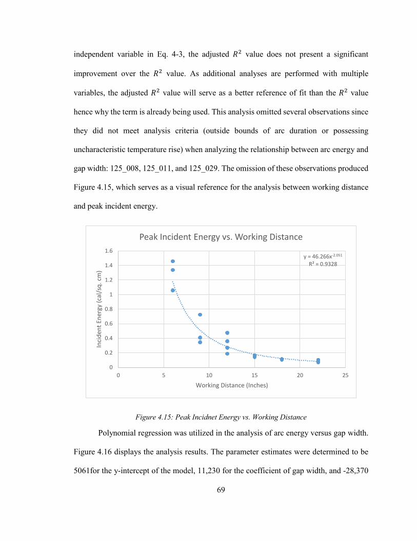
69
independent variable in Eq. 4-3, the adjusted 𝑅𝑅2 value does not present a significant
improvement over the 𝑅𝑅2 value. As additional analyses are performed with multiple
variables, the adjusted 𝑅𝑅2 value will serve as a better reference of fit than the 𝑅𝑅2 value
hence why the term is already being used. This analysis omitted several observations since
they did not meet analysis criteria (outside bounds of arc duration or possessing
uncharacteristic temperature rise) when analyzing the relationship between arc energy and
gap width: 125_008, 125_011, and 125_029. The omission of these observations produced
Figure 4.15, which serves as a visual reference for the analysis between working distance
and peak incident energy.
Figure 4.15: Peak Incidnet Energy vs. Working Distance
Polynomial regression was utilized in the analysis of arc energy versus gap width.
Figure 4.16 displays the analysis results. The parameter estimates were determined to be
5061for the y-intercept of the model, 11,230 for the coefficient of gap width, and -28,370
y = 46.266x-2.051
R² = 0.9328
0
0.2
0.4
0.6
0.8
1
1.2
1.4
1.6
0 5 10 15 20 25
Inci
dent
Ene
rgy
(cal
/sq.
cm
)
Working Distance (Inches)
Peak Incident Energy vs. Working Distance

70
for the coefficient of gap width squared. The associated p-values are <0.0001, 0.0003, and
0.0019, respectively. Therefore, similar to incident energy versus working distance, the
parameter estimates are statistically significant.
Figure 4.16: Polynomial Regression of Arc Energy and Gap Width
Using the determined parameter estimates, Eq. 4-4 was constructed to describe the
relationship between arc energy and gap width.
𝐴𝐴𝐸𝐸 = −28,370(𝐺𝐺𝐺𝐺)2 + 11,230(𝐺𝐺𝐺𝐺) + 5061
Where
AE = arc energy in calories
Eq. 4-4
71
The adjusted 𝑅𝑅2 value associated with this proposed model is 0.4464, which indicates that
the model accounts for 44.64% of the variability associated with arc energy and gap width.
Possible methods to improve the model prediction would be to increase the number of tests
at gap widths other than 1/8 inch. This stems from the fact that a large number of tests were
conducted at 1/8 inch due to the arc consistency observed at that gap width. Thus, the model
is probably being affected by the large number of tests at 1/8-inch gap width. Besides the
possible skewing, observation of the associated scatterplot indicates that there appears to
be a large amount of variability that is simply intrinsic to arc flash. This is made apparent
by the large spread observed in the 1/8 inch data. Thus, there may always be substantial
variance that cannot be explained by gap width alone. However, that does not mean that
additional tests would not improve the model.
The two relationships previously depicted predict different forms of energy based
on an exclusive dependent variable. Working distance can be used to predict the amount
of incident energy that would be measured by the calorimeters. Gap width can be used to
predict the amount of energy produced by an arc. Therefore, working distance and gap
width are associated with different forms of energy. Reconciliation of these differences can
be achieved by the Law of Conservation of Energy, which states that energy can neither be
created nor destroyed. Therefore, energy produced by the arc and the energy measured by
the calorimeters can be equated due to their association with the same event. Thus, there
exists some conversion factor between the two types of energy. Rather than defining a
conversion factor and applying it, nonlinear regression was used to develop a final
relationship between incident energy and arc energy thereby allowing SAS to incorporate
72
the conversion factor within the correction factor (Cf) of the desired equation. The final
relationship analyzed is shown in Eq. 4-5.
𝐼𝐼𝐸𝐸 =
𝐶𝐶𝐶𝐶 ∗ 𝐴𝐴𝐸𝐸𝐺𝐺𝐷𝐷𝑎𝑎
Nonlinear regression was performed to assess the relationship of incident energy
versus arc energy and working distance. The result of this analysis is presented in Figure
4.17. Since the working distance tests were performed at a gap width of 1/8 inch, arc energy
values were constrained to 1/8 inch for comparability. The parameter estimate for the
constant Cf was determined to be 0.01053 with an associated p-value of 0.0089. Therefore,
the parameter estimate is statistically significant. A value of 2.172 was estimated for the
exponential term associated with working distance. The p-value associated with the
exponential term was determined to be <0.0001. Therefore, the parameter estimate is
statistically significant. Substituting the parameter estimates into the previously proposed
model produces Eq. 4-6 for incident energy.
𝐼𝐼𝐸𝐸 =
0.01053 ∗ 𝐴𝐴𝐸𝐸𝐺𝐺𝐷𝐷2.172
The associated adjusted 𝑅𝑅2 value is 0.9297, which indicates that the model explains
92.97% of the variability between incident energy, arc energy, and working distance.
Eq. 4-5
Eq. 4-6
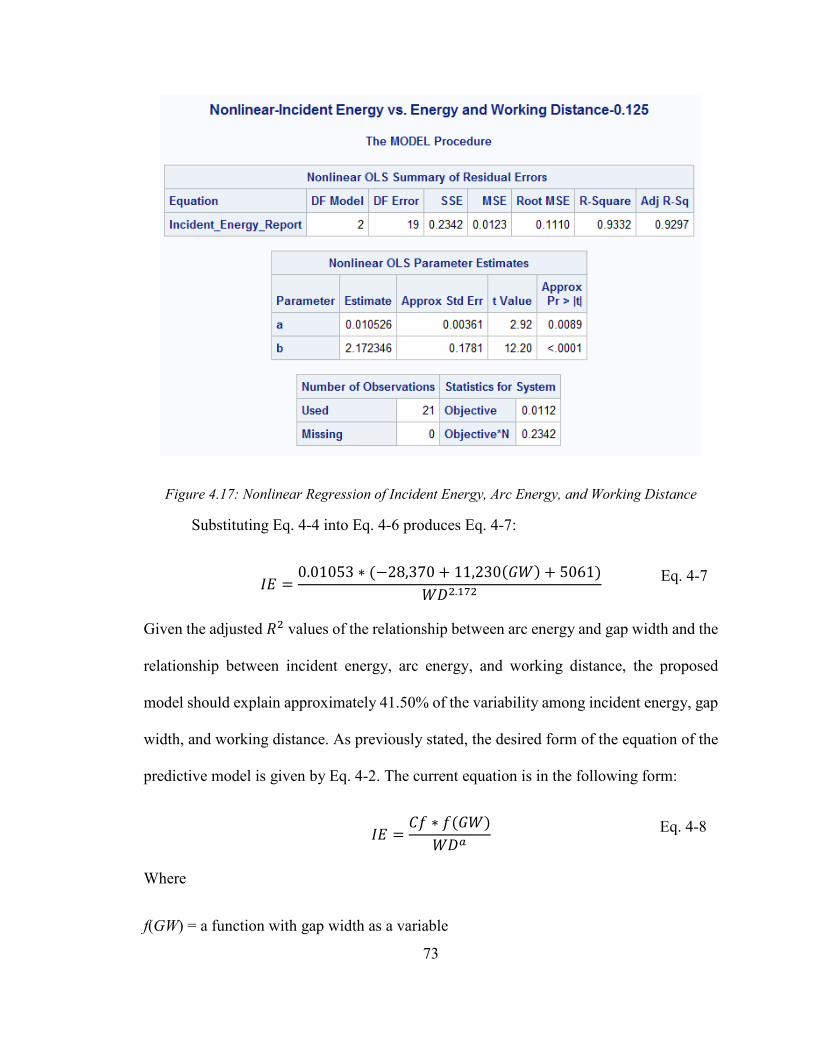
73
Figure 4.17: Nonlinear Regression of Incident Energy, Arc Energy, and Working Distance
Substituting Eq. 4-4 into Eq. 4-6 produces Eq. 4-7:
𝐼𝐼𝐸𝐸 =
0.01053 ∗ (−28,370 + 11,230(𝐺𝐺𝐺𝐺) + 5061)𝐺𝐺𝐷𝐷2.172
Given the adjusted 𝑅𝑅2 values of the relationship between arc energy and gap width and the
relationship between incident energy, arc energy, and working distance, the proposed
model should explain approximately 41.50% of the variability among incident energy, gap
width, and working distance. As previously stated, the desired form of the equation of the
predictive model is given by Eq. 4-2. The current equation is in the following form:
𝐼𝐼𝐸𝐸 =
𝐶𝐶𝐶𝐶 ∗ 𝐶𝐶(𝐺𝐺𝐺𝐺)𝐺𝐺𝐷𝐷𝑎𝑎
Where
f(GW) = a function with gap width as a variable
Eq. 4-7
Eq. 4-8
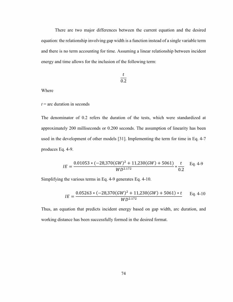
74
There are two major differences between the current equation and the desired
equation: the relationship involving gap width is a function instead of a single variable term
and there is no term accounting for time. Assuming a linear relationship between incident
energy and time allows for the inclusion of the following term:
𝑡𝑡0.2
Where
t = arc duration in seconds
The denominator of 0.2 refers the duration of the tests, which were standardized at
approximately 200 milliseconds or 0.200 seconds. The assumption of linearity has been
used in the development of other models [31]. Implementing the term for time in Eq. 4-7
produces Eq. 4-9.
𝐼𝐼𝐸𝐸 =
0.01053 ∗ (−28,370(𝐺𝐺𝐺𝐺)2 + 11,230(𝐺𝐺𝐺𝐺) + 5061)𝐺𝐺𝐷𝐷2.172 ∗
𝑡𝑡0.2
Simplifying the various terms in Eq. 4-9 generates Eq. 4-10.
𝐼𝐼𝐸𝐸 =
0.05263 ∗ (−28,370(𝐺𝐺𝐺𝐺)2 + 11,230(𝐺𝐺𝐺𝐺) + 5061) ∗ 𝑡𝑡𝐺𝐺𝐷𝐷2.172
Thus, an equation that predicts incident energy based on gap width, arc duration, and
working distance has been successfully formed in the desired format.
Eq. 4-9
Eq. 4-10
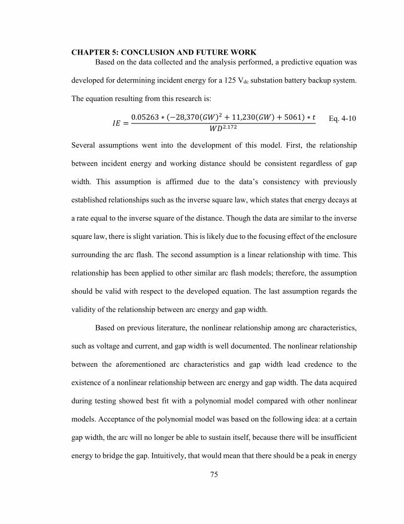
75
CHAPTER 5: CONCLUSION AND FUTURE WORK Based on the data collected and the analysis performed, a predictive equation was
developed for determining incident energy for a 125 Vdc substation battery backup system.
The equation resulting from this research is:
𝐼𝐼𝐸𝐸 =
0.05263 ∗ (−28,370(𝐺𝐺𝐺𝐺)2 + 11,230(𝐺𝐺𝐺𝐺) + 5061) ∗ 𝑡𝑡𝐺𝐺𝐷𝐷2.172
Several assumptions went into the development of this model. First, the relationship
between incident energy and working distance should be consistent regardless of gap
width. This assumption is affirmed due to the data’s consistency with previously
established relationships such as the inverse square law, which states that energy decays at
a rate equal to the inverse square of the distance. Though the data are similar to the inverse
square law, there is slight variation. This is likely due to the focusing effect of the enclosure
surrounding the arc flash. The second assumption is a linear relationship with time. This
relationship has been applied to other similar arc flash models; therefore, the assumption
should be valid with respect to the developed equation. The last assumption regards the
validity of the relationship between arc energy and gap width.
Based on previous literature, the nonlinear relationship among arc characteristics,
such as voltage and current, and gap width is well documented. The nonlinear relationship
between the aforementioned arc characteristics and gap width lead credence to the
existence of a nonlinear relationship between arc energy and gap width. The data acquired
during testing showed best fit with a polynomial model compared with other nonlinear
models. Acceptance of the polynomial model was based on the following idea: at a certain
gap width, the arc will no longer be able to sustain itself, because there will be insufficient
energy to bridge the gap. Intuitively, that would mean that there should be a peak in energy
Eq. 4-10
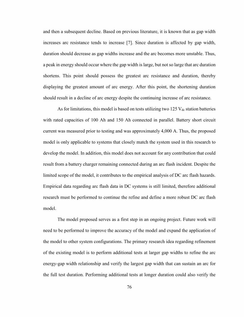
76
and then a subsequent decline. Based on previous literature, it is known that as gap width
increases arc resistance tends to increase [7]. Since duration is affected by gap width,
duration should decrease as gap widths increase and the arc becomes more unstable. Thus,
a peak in energy should occur where the gap width is large, but not so large that arc duration
shortens. This point should possess the greatest arc resistance and duration, thereby
displaying the greatest amount of arc energy. After this point, the shortening duration
should result in a decline of arc energy despite the continuing increase of arc resistance.
As for limitations, this model is based on tests utilizing two 125 Vdc station batteries
with rated capacities of 100 Ah and 150 Ah connected in parallel. Battery short circuit
current was measured prior to testing and was approximately 4,000 A. Thus, the proposed
model is only applicable to systems that closely match the system used in this research to
develop the model. In addition, this model does not account for any contribution that could
result from a battery charger remaining connected during an arc flash incident. Despite the
limited scope of the model, it contributes to the empirical analysis of DC arc flash hazards.
Empirical data regarding arc flash data in DC systems is still limited, therefore additional
research must be performed to continue the refine and define a more robust DC arc flash
model.
The model proposed serves as a first step in an ongoing project. Future work will
need to be performed to improve the accuracy of the model and expand the application of
the model to other system configurations. The primary research idea regarding refinement
of the existing model is to perform additional tests at larger gap widths to refine the arc
energy-gap width relationship and verify the largest gap width that can sustain an arc for
the full test duration. Performing additional tests at longer duration could also verify the
77
applicability of the linear time relationship and the behavior of the arc with respect to how
it travels along the electrodes. During testing, a single test was performed using a one-
second duration. After the test was completed, it was noted that the bottom of the electrode
was almost completely consumed by the arc; however, there was no strong evidence that
the arc began to travel vertically upward along the electrodes. Longer tests could reveal
more information regarding this behavior. The main concern with longer tests is rapid
deterioration of the batteries. With a test duration of only 200 milliseconds, physical
deterioration of the batteries could be visually observed with plates warping as testing
proceeded. The observed deformation did not largely affect the resistance of the batteries.
Therefore, tests requiring longer durations will likely need additional batteries for
replacements.
Regarding expansion of the proposed model, tests can be performed utilizing larger
batteries, different enclosure sizes, and other electrode/barrier configurations. Provided the
tests follow similar structuring, the model should be able to incorporate the influence of
these additional dependent variables, thereby, expanding the proposed model to different
enclosures and different system voltages and currents. Additional testing that includes
charger contributions should also be performed. Some literature indicates that researchers
have sought to analyze this contribution; however, additional testing should provide
additional clarity [46]. Lastly, future work could focus on how arc flash tests should be
conducted. During testing, it was noted that weather might have affected the tests. Thus,
more research should be conducted to assess how the environment influences testing and
provide a relationship accounting for certain weather conditions. In addition, the fuse wire
geometry appeared to have some effect on test results. Therefore, additional research may

78
delve into whether or not arc flash research should follow a more standardized procedure
for initiating the arc, since at low voltages, the sustainability of the arc and direction of the
plasma cloud and shrapnel varied based on the size, geometry, and tightness of the fuse
wire.
The successful generation of a predictive DC arc flash model developed for this
research is the first step to developing a comprehensive dc arc flash model. Empirical
research regarding DC arc flash significantly lags empirical research regarding AC arc
flash. Therefore, further testing is needed to better assess the hazards posed by DC arc flash
and develop improved predictive models. The speed at which this research will be
conducted will be decided by the proliferation of larger DC systems and an increasing
perception of risk, or an increase in dc arc flash incidents. The data collected and research
conducted for the purpose of this thesis will be beneficial for future research regarding the
topic of DC arc flash.
79
REFERENCES
[1] U.S. Energy Information Administration (EIA), Annual Energy Outlook 2018, Washington D.C.: Office of Energy Analysis, Feb. 6, 2018.
[2] C. Marcy, “EIA study examines the role of high-voltage power lines in integrating renewables,” eia.gov, Jun. 28, 2018. [Online]. Available: https://www.eia.gov/todayinenergy/detail.php?id=36393. [Accessed Dec. 21, 2018].
[3] Bloomberg New Energy Finance (BNEF), “Electric Vehicle Outlook 2018,” bnef.com. [Online]. Available: https://about.bnef.com/electric-vehicle-outlook/. [Accessed Jan. 29, 2019].
[4] Electrical Safety Foundation International (ESFI), “Workplace Fatalities and Injuries 2003-2016,” esfi.org, Mar. 5, 2018. [Online]. Available: https://www.esfi.org/resource/workplace-fatalities-and-injuries-2003-2016-644. [Accessed Dec. 21, 2018].
[5] D. Doan, Private Communication.
[6] W. Lee, Private Communication.
[7] R. F. Ammerman, T. Gammon, P. K. Sen, and J. Nelson, “DC Arc Models and Incident Energy Calculations,” In 2009 Record of Conference Papers – IEEE IAS 56th Annual PCIC, 14-16 Sept. 2009, pp. 1-13.
[8] R. Lee, “The Other Electrical Hazard: Electric Arc Blast Burns,” IEEE Transactions on Industry Applications, vol. IA-18, no. 3, May/Jun., pp. 246-251, 1982.
[9] R. Lee, “Pressures Developed by Arcs,” IEEE Transactions on Industry Applications, vol. IA-23, no. 4, Jul./Aug., pp. 760-763, 1987.
[10] S. Rau, Z. Zhang, and W. Lee, “3-D Magnetohydrodynamic Modeling of DC Arc in Power System,” IEEE Transactions on Industry Applications, vol. 52, no. 6, Nov./Dec., pp. 4549-4555, 2016.
[11] H. Ayrton, The Electric Arc, The Electrician, London, U.K., 1902
[12] C.P. Steinmetz, “Electric power into light, Section VI. The Arc,” Transactions of the American Institute of Electrical Engineers, p. 802, 1906.
[13] W. Nottingham, “A New Equation for the Static Characteristic of the Normal Electric Arc,” Journal of the American Institute of Electrical Engineers, vol. 42, no. 1, Jan., pp. 12-19, 1923.
[14] J. D. Cobine, Gaseous Conductors, McGraw-Hill, pp. 371-378, 1941.
80
[15] D. B. Miller and J. L. Hildebrand, “DC arc model including circuit constraints,” IEEE Transactions on Power Apparatus and Systems, vol. PAS-92, no. 6, pp. 1926-1934, Nov. 1973.
[16] A. R. Van and C. Warrington, “Reactance relays negligibly affected by arc impedance,” Electrical World, pp. 502-505, 1931.
[17] P. M. Hall, K. Myers, and W. S. Vilicheck, “Arcing faults on direct current trolley systems,” Proceedings of the Fifty WVU Conference on Coal Mine Electrotechnolgy, Morgantown, WV, 1978, pp. 21-1—21-19.
[18] R. F. Ammerman, P. K. Sen, and J. P. Nelson, “Electrical Arcing Phenomena: A historical perspective and comparative study of the standards IEEE 1584 and NFPA 70E,” IEEE Industry Applications Magazine, vol. 15, no. 3, May/June, pp. 42-52, 2009. Published by IEEE on 21 Apr. 2009.
[19] “IEEE 1584-2002,” IEEE Guide for Performing Arc-Flash Hazard Calculations.
[20] R.D. Hill, “Channel heating in return stroke lightning,” J. Geophys. Res., Jan. 20, 1971.
[21] M. G. Drouet and F. Nadeau, “Pressure Waves due to Arcing Faults in a Substation,” IEEE Transactions on Power Apparatus and Systems, vol. PAS-98, no. 5, pp. 1632-1635, Sept. 1979.
[22] A. D. Stokes and W. T. Oppenlander, “Electric Arcs in Open Air,” Journal of Physics D: Applied Physics, pp. 26-35, 1991.
[23] J. Paukert, “The Arc Voltage and Arc Resistance of LV Fault Arcs,” Proceedings of the 7th International Symposium on Switching Arc Phenomena, 1993, pp. 49-51.
[24] C.E. Solver, “Electric Arcs and Arc Interruption,” Chalmers University of Technology, Gotenburg, Sweden, EEK 195 High Voltage Technology, Lecture 7. Available: http://193.140.122.139/high_voltage/elkraft/www.elkraft.chalmers.se/GU/EEK195/lectures/Lecture7.pdf.
[25] R. Doughty, T. Neal, T. Dear, and A. Bingham, Testing Update on Protective Clothing & Equipment for Electric Arc Exposure, In Record of Conference Papers, IEEE Industry Applications Society (IAS) 44th Annual Petroleum and Chemical Industry Conference (PCIC). 15-17 Sept. 1997, pp. 323-336.
[26] R. Doughty, T. Neal, and H. Floyd, “Predicting Incident Energy to Better Manage the Electric Arc Hazard on 600-V Power Distribution Systems,” IEEE Transactions on Industry Applications, vol. 36, no. 1, Jan./Feb., pp. 257-269, 2000.
81
[27] A. D. Stokes and D. K. Sweeting, “Electric Arcing Burn Hazards,” IEEE Transactions on Industry Applications, vol. 42, no. 1, Jan./Feb., pp 134-141, 2006.
[28] A. D. Stokes and D. K. Sweeting, “Closure to Discussions of ‘Electrical Arcing Burn Hazards,’” IEEE Transactions on Industry Applications, vol. 42, no. 1, Jan./Feb. pp. 146-147, 2006.
[29] R. Wilkins, M. Allison, and M. Lang, “Effect of Electrode Orientation In Arc Flash Testing,” In Conference Record of 2005 Industry Applications Conference, 2005, 2005 IEEE 40th IAS Annual Meeting, 2-6 Oct. 2005, pp. 459-465.
[30] R. Wilkins, M. Lang, and M. Allison, “Effect of Insulating Barriers in Arc Flash Testing,” IEEE Transactions on Industry Applications, vol. 44, no. 5, Sep./Oct., pp. 1354-1359, 2008.
[31] D. Doan, “Arc Flash Calculations for Exposures to DC Systems,” IEEE Transactions on Industry Applications, vol. 46, no. 6, Nov./Dec., pp. 2299-2302, 2010.
[32] R. Wilkins, “Simple Improved Equations for Arc Flash Hazard Analysis,” Jul. 2004, Posted Aug. 30, 2004 on IEEE Electrical Safety Forum. No longer available on forum.
[33] M. Fontaine, and P. Walsh, “DC Arc Flash Calculations – Arc-In-Open-Air & Arc-In-A-Box – Using a Simplified Approach (Multiplication Factor Method),” 2012 IEEE IAS Electrical Safety Workshop (ESW). 31 Jan.- 3 Feb. 2012, pp. 1-8.
[34] “NFPA 70E-2015,” Standard for Electrical Safety in the Workplace.
[35] F. M. Gatta, A. Geri, M. Maccioni, S. Lauria, and F. Palone, “Arc-Flash in Large Battery Energy Storage Systems—Hazard Calculation and Mitigation,” 2016 IEEE 16th International Conference on Environment and Electrical Engineering (EEEIC). 7-10 June 2016, pp. 1-6.
[36] S. J. Royston, D. Strickland, D. A. Stone, D. T. Gladwin, M. P. Foster, and S. Nejad, “Arc-Flash Calculation Comparison for Energy Storage Systems,” 2017 IEEE 52nd International Universities Power Engineering Conference (UPEC). 28-31 Aug. 2017, pp. 1-6.
[37] M. M. Krzywosz, “CASE STUDY - DC Arc Flash and Safety Considerations in a 400VDC UPS Architecture Power System Equipped with VRLA Battery,” 2014 IEEE 36th International Telecommunications Energy Conference (INTELEC). 28 Sept.-2 Oct. 2014, pp. 1-9.
[38] J. G. Hildreth and K. Feeney, “Arc Flash Hazards of 125 Vdc Station Battery Systems,” 2018 IEEE Power & Energy Society General Meeting (PESGM), 5-10 Aug. 2018, pp. 1-5.

82
[39] C. Keyes and C. Maurice, “DC Arc Hazard Assessment Phase II,” Kinectrics, Toronto, ON, Canada, Rep. K-012623-RA-0001-R00, Jul. 7, 2007.
[40] J. Mandeville, Private Communication.
[41] J. Mandeville, “DC Arc Flash Instrumentation Report,” American Electric Power (AEP), Columbus, OH, Rep. PTS 213769.000.
[42] M. Lang, “Info on Calorimeters for AEP,” Personal email (July 6, 2018).
[43] ThermoWorks, Inc., “Emissivity Table” thermoworks.com. [Online]. Available: https://www.thermoworks.com/emissivity_table. [Accessed July 8, 2018].
[44] J. H. Henninger, “Solar Absorptance and Thermal Emittance of Some Common Spacecraft Thermal-Control Coatings (NASA ref. pub. 1121),” U.S. National Aeronautics and Space Administration (NASA), Washington D.C.: NASA Headquarters, Apr. 1984.
[45] Z. S. Spakovszky, “19.2 Kirchhoff’s Law and ‘Real Bodies,’” 16.Unified: Thermodynamics and Propulsion, Massachusetts Institute of Technology (MIT), Cambridge, MA. Available: https://web.mit.edu/16.unified/www/FALL/thermodynamics/notes/notes.html. [Accessed July 8, 2018].
[46] “IEEE 946-2004,” IEEE Recommended Practice for the Design of DC Auxiliary Power Systems for Generating Stations.

83
VITA
Austin Cody Gaunce Education: University of Kentucky Bachelor of Science in Mining Engineering: May 2016 Power and Energy Institute of Kentucky (PEIK) Graduate Certificate Dec. 2017 Work Experience: Student Intern, American Electric Power, New Albany, OH May 29-August 17, 2018 Honors and Awards: Central Appalachian Education Research Center (ERC) Graduate Fellowship