PRESIDENTS AND THE U.S. ECONOMY:AN ECONOMETRIC EXPLORATION

Alan S. BlinderMark W. Watson

WORKING PAPER 20324

NBER WORKING PAPER SERIES

PRESIDENTS AND THE U.S. ECONOMY:AN ECONOMETRIC EXPLORATION

Alan S. BlinderMark W. Watson

Working Paper 20324http://www.nber.org/papers/w20324

NATIONAL BUREAU OF ECONOMIC RESEARCH1050 Massachusetts Avenue

Cambridge, MA 02138July 2014

For advice on and help with obtaining data, and for making replication files available to us, we thankSteve Davis, William Dunkelberg, Wendy Edelberg, Otmar Issing, Jan Hatzius, Karl Mertens, NolanMcCarty, Valerie Ramey, Morten Ravns, Eric Sims, Nora Traum, and Egon Zakrajšek. We also thankRay Fair, James Hamilton, Lutz Kilian, John Londregan, Edward Nelson, Jeremy Piger and participantsat workshops at Princeton and elsewhere for many useful comments. None of them, of course, bearsany responsibility for the views expressed here. Replications files can be downloaded from http://www.princeton.edu/~mwatson. The views expressed herein are those of the authors and do not necessarily reflect the views of theNational Bureau of Economic Research.

NBER working papers are circulated for discussion and comment purposes. They have not been peer-reviewed or been subject to the review by the NBER Board of Directors that accompanies officialNBER publications.

© 2014 by Alan S. Blinder and Mark W. Watson. All rights reserved. Short sections of text, not toexceed two paragraphs, may be quoted without explicit permission provided that full credit, including© notice, is given to the source.

Presidents and the U.S. Economy: An Econometric ExplorationAlan S. Blinder and Mark W. WatsonNBER Working Paper No. 20324July 2014JEL No. E30,E60

ABSTRACT

The U.S. economy has grown faster—and scored higher on many other macroeconomic metrics—whenthe President of the United States is a Democrat rather than a Republican. For many measures, includingreal GDP growth (on which we concentrate), the performance gap is both large and statistically significant,despite the fact that postwar history includes only 16 complete presidential terms. This paper asks why.The answer is not found in technical time series matters (such as differential trends or mean reversion),nor in systematically more expansionary monetary or fiscal policy under Democrats. Rather, it appearsthat the Democratic edge stems mainly from more benign oil shocks, superior TFP performance, amore favorable international environment, and perhaps more optimistic consumer expectations aboutthe near-term future. Many other potential explanations are examined but fail to explain the partisangrowth gap.

Alan S. BlinderDepartment of EconomicsPrinceton UniversityPrinceton, NJ 08544-1021and NBERblinder@princeton.edu

Mark W. WatsonDepartment of EconomicsPrinceton UniversityPrinceton, NJ 08544-1013and NBERmwatson@princeton.edu

1

An extensive and well-known body of scholarly research documents and explores the fact

that macroeconomic performance is a strong predictor of U.S. presidential election outcomes.

Scores of papers find that better performance boosts the vote of the incumbent’s party.1 In stark

contrast, economists have paid scant attention to predictive power running in the opposite

direction: from election outcomes to subsequent macroeconomic performance. The answer,

while hardly a secret, is not nearly as widely known as it should be: The U.S. economy grows

notably faster when a Democrat is president than when a Republican is.2

We begin in Section 1 by documenting this fact, which is not at all “stylized.” The U.S.

economy not only grows faster, according to real GDP and other measures, during Democratic

versus Republican presidencies, it also produces more jobs, lowers the unemployment rate,

generates higher corporate profits and investment, and turns in higher stock market returns.

Indeed, it outperforms under almost all standard macroeconomic metrics. By some measures, the

partisan performance gap is startlingly large--so large, in fact, that it strains credulity, given how

little influence over the economy most economists (or the Constitution, for that matter) assign to

the President of the United States.

Most of the paper is devoted to econometric investigations of possible explanations of the

Democrat-Republican performance gap in annualized real GDP growth—which we find to be 1.8

percentage points in postwar data. In discussing this large gap with economists, we frequently

encounter the objection that the partisan difference must be statistically insignificant owing to

the paucity of presidential administrations. That is not true, as we show in Section 1.

In Section 2, we ask whether the partisan gap is spurious in the sense that it is really either

the makeup of Congress or something else about presidents (other than their party affiliations)

that matter for growth. The answers are no. Section 3 investigates whether trends (Democrats

were in the White House more often when trend growth was high) or inherited initial conditions

(Democrats were elected more often when the economy was poised for relatively rapid growth)

can explain what appears to be a partisan gap. They cannot.

1 The literature is large in economics and voluminous in political science. Ray Fair’s (1978, 2011) work may be the best known to economists. 2 See, for example, Alesina and Sachs (1988), Bartels (2008, Chapter 2), Comiskey and Marsh (2012). An important precursor is Hibbs (1977). Earlier evidence on the unemployment rate and other cyclical indicators motivated some of the economic literature on political business cycles; see, for example, Alesina and Roubini (1997), and Faust and Irons (1999).

2

Sections 4 and 5 comprise the heart of the paper. There we examine possible economic

mechanisms that might explain the partisan growth gap, including factors that might be

construed as “just good luck” and factors that might be interpreted as superior economic policy.

We find that government spending associated with the Korean War (which began under a

Democrat and ended under a Republican) explains part of the 1.8 percentage point partisan gap,

but that the gap remains large (1.4 points) even after excluding the Korean War administrations.

We find that oil shocks, productivity shocks, international growth shocks, and (perhaps) shocks

to consumer expectations about the future jointly explain about half of the partisan gap. The first

three of these look a lot more like good luck than good policy. In sharp contrast to these

explanations, our empirical analysis finds that fiscal or monetary shocks do not explain the

partisan growth gap.

Section 6 looks briefly at four other advanced countries: Canada, France, Germany, and the

UK. Only Canadian data display a similar partisan growth gap. Finally, Section 7 provides a

brief summary of what we (think we’ve) learned.

1. The stark facts

1.1 Gross domestic product growth and recessions

For most of this paper, the dataset begins either when U.S. quarterly NIPA accounts begin,

in 1947:Q1, or at the start of Harry Truman’s elected term and extends through 2013:Q1. In

many of our calculations, we group observations by four-year presidential terms; so the sample

contains seven complete Democratic terms (Truman-2, Kennedy-Johnson, Johnson, Carter,

Clinton-1, Clinton-2, and Obama-1) and nine complete Republican terms (Eisenhower-1,

Eisenhower-2, Nixon, Nixon-Ford, Reagan-1, Reagan-2 , Bush I, Bush II-1, and Bush II-2),

where the suffixes denote terms for two-term presidents.

During the 64 years that make up these 16 terms, real GDP growth averaged 3.33% at an

annual rate. But the average growth rates under Democratic and Republican presidents were

starkly different: 4.35% and 2.54% respectively. This 1.80 percentage point gap (henceforth, the

“D-R gap”) is astoundingly large relative to the sample mean. It implies that over a typical four-

year presidency the U.S. economy grew by 18.6% when the president was a Democrat, but only

by 10.6% when he was a Republican. And the variances of quarterly growth rates are roughly

3

equal (3.8% for Democrats, 3.9% for Republicans, annualized), so Democratic presidents preside

over growth that is faster but not more volatile.3

The estimated D-R growth gap is sensitive to the presumed lag between a presidential

election and any possible effects of the newly-elected president on the economy. In our main

results, the first quarter of each president’s term is attributed to the previous president. While we

focused on this one-quarter lag on a priori grounds, we did repeat the calculation with lags of

zero, two, three, and four quarters. Results were similar, although using lags of zero, two, three,

and four quarters all lead to smaller estimated D-R gaps.4

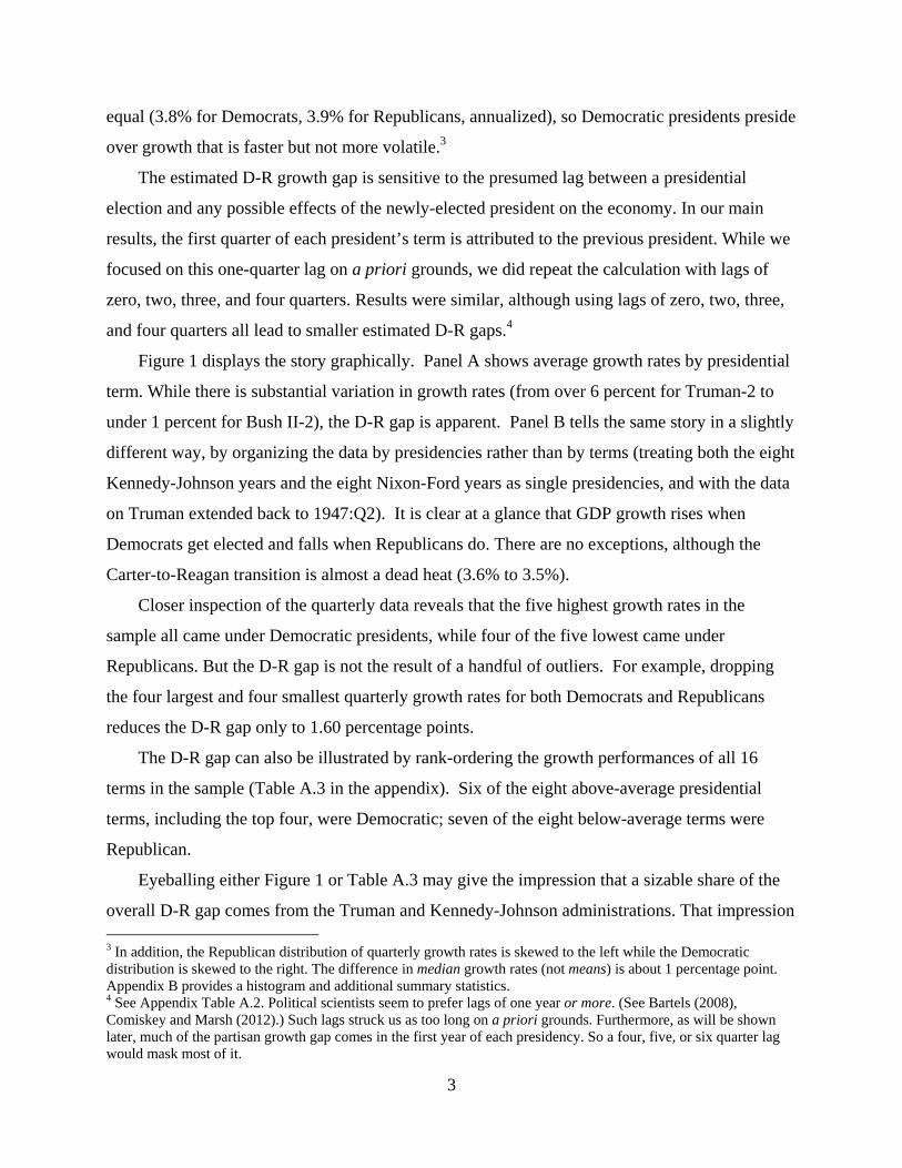
Figure 1 displays the story graphically. Panel A shows average growth rates by presidential

term. While there is substantial variation in growth rates (from over 6 percent for Truman-2 to

under 1 percent for Bush II-2), the D-R gap is apparent. Panel B tells the same story in a slightly

different way, by organizing the data by presidencies rather than by terms (treating both the eight

Kennedy-Johnson years and the eight Nixon-Ford years as single presidencies, and with the data

on Truman extended back to 1947:Q2). It is clear at a glance that GDP growth rises when

Democrats get elected and falls when Republicans do. There are no exceptions, although the

Carter-to-Reagan transition is almost a dead heat (3.6% to 3.5%).

Closer inspection of the quarterly data reveals that the five highest growth rates in the

sample all came under Democratic presidents, while four of the five lowest came under

Republicans. But the D-R gap is not the result of a handful of outliers. For example, dropping

the four largest and four smallest quarterly growth rates for both Democrats and Republicans

reduces the D-R gap only to 1.60 percentage points.

The D-R gap can also be illustrated by rank-ordering the growth performances of all 16

terms in the sample (Table A.3 in the appendix). Six of the eight above-average presidential

terms, including the top four, were Democratic; seven of the eight below-average terms were

Republican.

Eyeballing either Figure 1 or Table A.3 may give the impression that a sizable share of the

overall D-R gap comes from the Truman and Kennedy-Johnson administrations. That impression 3 In addition, the Republican distribution of quarterly growth rates is skewed to the left while the Democratic distribution is skewed to the right. The difference in median growth rates (not means) is about 1 percentage point. Appendix B provides a histogram and additional summary statistics. 4 See Appendix Table A.2. Political scientists seem to prefer lags of one year or more. (See Bartels (2008), Comiskey and Marsh (2012).) Such lags struck us as too long on a priori grounds. Furthermore, as will be shown later, much of the partisan growth gap comes in the first year of each presidency. So a four, five, or six quarter lag would mask most of it.

4

is correct. If we estimate the gap using data ending right after the Eisenhower presidency, it is a

whopping 4.14 percentage points (t-ratio = 2.6 using Newey-West standard errors described

below). If we end the subsample after the Nixon-Ford administrations, the estimated gap is 3.17

percentage points (t = 3.4). Ending after the Bush-I administration yields an estimate of 2.36

percentage points (t = 2.8). Finally, if we consider a subsample extending from Truman through

Bush II, the D-R gap is 2.13 percentage points (t = 3.3). Clearly, the partisan gap has been

mostly shrinking over time. But at 1.80 percentage points (t = 2.8) in the full sample, it remains

large and significant.

NBER recession dating gives an even more lopsided view of the D-R difference. Over the

256 quarters in these 16 terms, Republicans occupied the White House for 144 quarters,

Democrats for 112. But of the 49 quarters classified by the NBER as in recession, only eight

came under Democrats versus 41 under Republicans.5 Thus, the U.S. economy was in recession

for 1.1 quarters on average during each Democratic term, but for 4.6 quarters during each

Republican term.

These results for GDP and quarters-in-recession are summarized in Panel A of Table 1. The

table shows the Democratic and Republicans averages, the D-R gap (labeled “Difference”), and

both standard errors and p-values to gauge statistical significance. Standard errors are computed

in two ways. The first, shown in parentheses (), clusters observations by presidential terms,

which allows arbitrary correlation within a term but no correlation between terms. The second,

shown in square brackets [], uses a standard HAC formula, which allows conditional

heteroskedasticity and (limited) correlation within and between terms. In both cases, statistical

significance for the D-R difference can be assessed by using the usual t-statistic.6 For the D-R

gap in GDP growth, the two standard errors are almost identical; each yields a t-statistic greater

than 2.7. For quarters-in-recession, the two standard errors differ a bit; but both yield t-statistics

with absolute values above 3. Thus, the t-statistics imply a statistically significant D-R gap in

economic performance despite the small number of observations.

5 As before, the first quarter of each presidency is “charged” to the previous president. Thus, for example, the recession quarter 2001:1 is charged to Bill Clinton and 2009:1 is charged to George W. Bush. 6 The effective sample size for the t-statistic constructed with clustered standard errors is the number of administrations (nDem = 7 and nRep = 9). Conservative inference can be carried out using the critical value from the Student’s – t distribution with min[(nDem–1),(nRep−1)] = 6 degrees of freedom. (The 5% two-sided critical value from the t6 distribution is 2.5.) Ibragimov and Müller (2010, 2011) show that this procedure remains conservative under heteroskedacity.

5

We also assessed statistical significance by using a non-parametric test that involves random

assignment of a party label (D or R) to each of the sixteen 16-quarter blocks of data in the

sample. Specifically, we assigned nine Republican and seven Democratic labels randomly to

each four-year period (e.g., 1949:Q2-1953Q1, 1953:Q2-1957:Q1, etc.) and then computed the

difference in average growth rates under these randomly-assigned “Democratic” and

“Republican” terms. Doing so enables us to construct the distribution of differences in average

growth rates under the null hypothesis that political party and economic performance are

independent (because party labels are randomly assigned to each term). This distribution can

then be used to compute the p-value of the difference in the actual growth rates under the null.

As shown in the final column of Table 1, this p-value is 0.01 for GDP, which corresponds to the

probability of observing an absolute difference of 1.80% (the actual value) or larger under

random assignment of party. The p-value for quarters-in-recession is also 0.01; so the lopsided

realization of recessions is similarly unlikely under the assumption that party and economic

performance are independent.

1.2 Other indicators

The finding of a large partisan gap is not peculiar to the time series on real GDP growth and

NBER recession dates. The other panels of Table 1 summarize results for a wide variety of other

indicators of economic performance.

Panel B considers alternative measures of aggregate output. The D-R gap for the growth

rate of GDP per capita, which corrects for any differences in population growth, is essentially

the same as for GDP itself (1.76% versus 1.80%). The D-R gap is somewhat larger in the

nonfarm business sector (2.15%) and much larger for industrial production (3.77%). Each of

these partisan growth gaps is statistically significant.

Panel C considers employment and unemployment. The D-R gap in the annual growth rate

of payroll employment is 1.42 percentage points, the gap in employee hours in nonfarm

businesses is somewhat larger (1.65 points), and both are statistically significant. Somewhat

puzzling, given these results, the partisan gap for employment is much smaller in the household

survey—just 0.56 percentage point—and not statistically significant at conventional levels.7 The

average unemployment rate is lower under Democrats (5.6% vs. 6.0%), but that difference is also

7 Examination of the payroll and household employment series shows two sustained episodes in which employment growth in the establishment survey exceeded employment growth in the household survey substantially and persistently; one was late in the Truman administration, the other was in the Kennedy-Johnson boom.

6

small and not statistically significant. There is, however, a very large and statistically significant

difference in the change in the unemployment rate, computed as the average unemployment rate

in the final year of the term minus the average value in the final year of the previous term.

During Democratic presidential terms, the unemployment rate fell by 0.8 percentage points, on

average, while it rose by 1.1 percentage points, on average, during Republican terms--yielding a

D-R gap of -1.9 percentage points.

Delving into the sectoral details (shown in Appendix Table A.4), the growth rates of every

major component of real GDP except exports were higher under Democratic rather than

Republican presidents, although the margins are small and statistically insignificant in a number

of cases. The table reveals that much of the Democratic growth advantage comes from higher

spending on consumer durables and private investment, especially nonresidential fixed

investment, where the partisan gap is 4.8 percentage points. Another large growth gap (5.1

percentage points) shows up in federal defense spending. But because defense spending is so

volatile, even that large a difference is not statistically significant. We return to defense spending

later.

Partisan differences extend well beyond the standard indicators of real growth and

employment. For example, Panel D of Table 1 shows that annualized stock market returns for

firms in the S&P 500 are 5.4 percentage points higher when a Democrat occupies the White

House than when a Republican does.8 But given the extreme volatility of stock prices, even

differences that large are statistically significant at only the 17% level. The corporate profit share

of gross domestic income was also higher under Democrats: by 5.6% versus 4.7% (p-

value=0.03). Though business votes Republican, it prospers more under Democrats.

Panel E shows that both real wages (compensation per hour in the nonfarm business sector)

and labor productivity increased slightly faster under Democrats than Republicans, although

neither D-R gap is statistically significant. Growth in total factor productivity was much faster

under Democrats (1.9% versus 0.9% for Republicans, with a p-value of 0.08), although the gap

nearly disappears when TFP is adjusted for resource utilization. We discuss productivity as a

potential explanation of the D-R gap in Section 5 below.

8 The partisan gap in stock market returns seems to have attracted a lot more attention—at least from economists—than the partisan gap in GDP growth. See, for example, Santa-Clara and Valkanov (2003) and other references cited there. For much earlier evidence, see Allvine and O’Neill (1980).

7

Moving yet farther afield, and now using Congressional Budget Office data which are

available only from the Kennedy-Johnson term through 2012:Q3, the structural federal budget

deficit has been, on average, smaller under Democratic presidents (1.5% of potential GDP) than

under Republican presidents (2.2% of potential GDP), although the difference is far from

statistically significant. (See Panel F.) And Bartels (2008) (not shown in the table) has

documented that income inequality rises under Republicans but falls under Democrats.

The only notable exception to the rule that Democrats outperform Republicans seems to be

inflation, where the economy fares about equally well under presidents of either party. For

example, Panel of G of Table 1 shows that while the average inflation rate was slightly lower

under Democratic presidents (2.97% versus 3.32% using the PCE deflator; 2.88% versus 3.44%

using the GDP deflator), neither difference comes close to statistical significance. Inflation does

show a tendency to rise under Democrats and fall under Republicans, however. For example,

using the PCE deflator, inflation rises on average by 1.05 percentage points during a Democratic

presidency, falls by 0.83 percentage point during a Republican presidency, and the difference of

1.88 percentage points is statistically significant at the 12% level.

Of course, weaker GDP growth and lower employment growth under Republicans could be

responsible for the differential inflation performance. A simple back-of-the-envelope calculation

suggests that it is. With unemployment averaging 0.4 percentage point less under Democrats,

traditional estimates of the Phillips curve (e.g., Staiger, Stock, and Watson (2001)) suggest that

the change in inflation should be roughly 0.1 percentage points more per quarter, or about 1.6

percentage points over a four-year presidential term—which is close to what we find.

Given the findings on inflation, it is perhaps not surprising to find (in Panel H) that short-

term nominal interest rates are a bit lower under Democratic presidents (though not significantly

so) but that they tend to rise under Democrats and fall under Republicans. This last difference is

very large (3.2 and 4.4 percentage points) and highly significant. We will return to interest rate

differences when we consider monetary policy in Section 5.

From here on, we concentrate attention on real GDP growth.

1.3 The D-R gap over a longer historical period

Official quarterly GDP data begin only in 1947, but both the nation and the economy date

back much further. What happens if we extend the data back in time? We know that the

Democratic-Republican gap would widen notably if we included the long presidency of Franklin

8

D. Roosevelt, for real GDP growth from 1933 to 1946 averaged a heady 7.4% per annum. Going

back to Hoover would also boost the measured D-R gap. But what about earlier U.S. history?

Owang, Ramey, and Zubairy (2013), building on previous work by Balke and Gordon

(1989), construct a quarterly real GDP series that dates all the way back to 1875. For the 72-year

period spanning 1875:Q1 through 1947:Q1, the average GDP growth rates in their data are

5.15% when Democrats sat in the White House (119 quarters) and 3.91% when Republicans did

(169 quarters).9 That D-R growth gap of 1.24 percentage points is smaller than the postwar gap,

but still noteworthy. Similarly, the NBER says the U.S. economy was in recession in 133 of

those 288 historical quarters (46% of the time). But 94 of those recessionary quarters came under

Republican presidents (56% of the time) versus only 39 under Democratic presidents (33% of the

time). Thus our main facts seem to be far from new.

The Democratic growth edge over the 1875-1947 period is, however, entirely due to the

economy’s excellent performance under Franklin D. Roosevelt. Excluding the FDR years,

growth was actually higher under Republicans. So one might say that higher growth under

Democrats began with Hoover.

2. But might it actually be...?

Having established the basic fact that the U.S. economy has grown faster under Democratic

than Republican presidents (see Table 1), we ask in this short section whether the president’s

party affiliation might actually be standing in for something else. For example, might the key

difference really be some presidential trait other than his party affiliation? Or might the partisan

makeup of Congress actually be the key ingredient? The answers, as we will see next, are no.

2.1 Other presidential traits

The four top presidential terms, ranked by GDP growth, are all Democratic: Truman’s

elected term, Kennedy-Johnson, Johnson’s elected term, and Clinton’s second term. Those four

are the foundation of the overall D-R growth gap. But might there be some other characteristic,

shared by these presidents, that explains the differential growth performance better? For

example, maybe younger-than-average presidents--a group that includes Kennedy, Johnson, and

9 Until Eisenhower, presidents were inaugurated on March 4 instead of January 20. So, for the historical data, we attributed the first two quarters of the calendar year to the previous president.

9

Clinton--do better. (They do.) Or maybe presidents who were once members of Congress--a

group that includes Truman, Kennedy, and Johnson--do better. (They also do.)

Table 2 displays average GDP growth rates for presidents grouped by various attributes:

political party (our focus), prior experience as either a member of Congress or as a governor, and

whether the president was younger or taller than average.10 The first row of the table repeats our

central fact. The next row contrasts growth under the seven presidents with congressional

experience (3.84 percentage points) with the nine without (2.94 percentage points). The

difference is sizable (0.91 percentage points), but not statistically significant. The next row

compares the administrations of former governors to non-governors. Growth was marginally

lower under former governors, but the difference falls far short of statistical significance. The

final two rows sort presidents by age and height (top half vs. bottom half). Growth is higher

under younger and taller presidents, but again the differences are not statistically significant.

Overall, the table shows systematic differences in performance associated with the party of the

president, but little evidence of systematic differences associated with other presidential

attributes.

2.2 Congress

We mentioned the Constitution earlier because it assigns the power of the purse—and most

other powers as well—to Congress, not to the president. Could the key partisan difference really

be which party controls Congress rather than which party controls the White House? The answer

is no. The rightmost column of Table 3 displays average GDP growth rates when the Democratic

Party controlled both houses of Congress, when control of the two houses was split (regardless of

which party controlled which house), and when the Republican Party controlled both houses.

Average growth was highest when Democrats controlled Congress (3.47%), but the difference

with Republican control (3.36%) is trivial. The table shows a further breakdown of average

GDP growth rates by president and by partisan control of Congress. Growth was highest when

Democrats controlled both houses of Congress and the White House (4.69%) and next highest

when a Democrat was president and Republicans controlled Congress (3.88%), although the

difference between these two averages is not statistically significant. In contrast, average growth

under Republican presidents was less than 3% regardless of which party controlled Congress.

Table 3 suggests that it’s been the president, not Congress, that mattered.

10 Most of these data come from King and Ragsdale (1988), updated by us.

10

3. Trends and initial conditions

We next ask whether the D-R gap could stem from different trend growth rates under

Democratic and Republican administrations, or whether Democrats were more likely than

Republicans to be elected when the economy was poised for a period of rapid growth (so that

causality runs from growth to party rather than from party to growth).

3.1 Trends

Recall that Figure 1 showed that the three presidential terms with the fastest growth rates

came early in the sample while three of the terms with the slowest growth (G.W. Bush’s two

terms and Obama) came late. Since trend increases in the labor force and productivity were

higher in the early post-WWII years than they have been since 2000, part of the difference in the

average growth rates under Democrats and Republicans might be explained by the timing of

these low-frequency movements.

To investigate this possibility, we computed average growth rate differences after detrending

the quarterly GDP growth rates using increasingly flexible trends computed from long two-sided

weighted moving averages.11 The flexibility of the estimated trend is adjusted by varying a

weighting parameter, . = ∞ means that the trend growth rate does not change over the

sample period. As gets smaller, the weights become more concentrated around the current time

period and start looking more like cycles than trends.

Figure A.2 in the appendix plots GDP growth rates and trends computed for different values

of . The four choices produce trends that range from completely constant at the sample average

( = ∞) to quite variable. When = 67, the trend growth rate is 4% through the early 1960s and

falls to roughly 2% in the 2000s.

Table 4 shows the average detrended growth rates for Democratic and Republican

presidents, using these four different definitions of “trend.” In the benchmark specification

(constant trend, = ∞), the Democratic and Republican averages are the deviations from the full-

sample average. Thus, the average value shown for Democrats is +1.06 percentage points, which

is the average growth rate for Democrats (4.35% from Table 1) minus the full-sample average of

3.29%; the average value shown for Republicans is -0.74 percentage point (= 2.54% -3.29%).12

11 The weights are computed using a bi-weight kernel. See Stock and Watson (2012). 12 The 3.29% figure for the grand mean used here differs slightly from the 3.33% figure cited earlier because, here, we extend the sample all the way back to 1947:2.

11

The D-R gap is thus 1.80 points, which is, of course, the same value shown in Table 1. For the

other trend specifications, the underlying trend is allowed to vary over time, so D-R differences

need not match the 1.80 percentage point value reported in Table 1. However, the table shows

that results using = 100 or = 67 hardly differ from the benchmark. Indeed, even when =33,

a “trend” that is so flexible that it seems to capture cyclical elements, the estimated D-R gap

remains large (1.46 percentage points) and highly significant. In sum, low-frequency factors

appear to explain little, if any, of the D-R gap.

3.2 Initial conditions

A different question of timing is whether the Democratic advantage can be attributed to

relatively favorable initial conditions. That is, are Democrats more likely to take office just as

the economy is poised to take off, and/or are Republicans more likely to take office when the

economy is primed for a recession? If so, the direction of causality runs from economic

performance to party of the president rather than from party to performance.

Figure 2A provides a first piece of evidence on this question by showing when, within four-

year presidential terms, the Democratic advantage is the largest and when it is the smallest. The

figure makes it clear that the advantage comes in the first two years, and especially in the first,

when the D-R growth gap is over 4 percentage points. The figure also shows (on the far left) the

average growth rate in the final year of the previous administration. Notice that Democrats

inherit growth rates of 1.9% from the final year of the previous term, while Republicans inherit a

growth rate of 4.3%--a clear advantage to Republicans.

Figure 2A treats the second term of each two-term presidency (e.g., Eisenhower-2) the same

as when a new president from one party replaces an outgoing president from the other party (e.g.,

Truman-2 to Eisenhower-1). So Figure 2B limits the sample to the eight presidential terms that

were preceded by a president from the opposite party. Among the incoming Democratic

presidents, that means Kennedy-Johnson, Carter, Clinton-1, and Obama-1. Among Republicans,

it means Eisenhower-1, Nixon, Reagan-1, and Bush II’s first term. In this restricted sample, more

than 100% of the four-year advantage occurs in a new president’s first year, when the D-R

growth gap is 4.8 percentage points--an average of 4.2% in the first year of a new Democratic

president versus minus 0.6% in the first year of a new Republican president. The figure also

shows that Democrats inherit growth rates averaging 0.6% from the final year of the previous

Republican president, while Republicans inherit growth rates averaging 3.8% from outgoing

12

Democrats. Thus the election of a Democrat seems to turn things around on a dime, while the

election of a new Republican seems to signal a recession.

Were these turnarounds anticipated? That is, were Democrats elected when future growth

was expected to be strong and/or Republicans elected when recessions were imminent? Simple

time series calculations suggest not. After all, GDP growth is positively serially correlated, so

that high growth in year t is more likely to be followed by high growth in year t+1 than by low

growth. Because Republicans inherit high growth, they should be more likely to experience high

growth early in their administrations than Democrats. But Figure 2 indicates just the opposite.

Thus, the reverse-causality explanation for the D-R gap is inconsistent with the serial correlation

in the data.

But perhaps the serial correlation calculation is too simplistic. Maybe unique factors in the

transition years made high growth for new Democratic administrations and low growth for new

Republican administrations forecastable. This question is investigated in several ways in Table 5,

and the answer appears to be that little, if any, of the D-R gap was forecastable. The first panel

shows median GDP growth forecasts from the Survey of Professional Forecasters (SPF).

Because the SPF data begin only in 1968, the analysis starts with Nixon’s first term. The data

come from surveys conducted in the first quarter of each presidential term and pertain to

forecasted growth over the next four quarters. For example, the Carter results use the survey

conducted in 1977:Q1 and show median growth forecasts for the four quarters from 1977:Q1

through 1978:Q1.13 The table also shows actual realized values for growth in the line just below.

With real GDP subject to substantial revisions over time, one issue with using SPF forecasts

is the vintage of data the forecasters were attempting to forecast. A standard practice is to

compare the forecasts to a vintage that includes only “near term” revisions, and we follow this

practice by comparing these forecasts to “actuals” from real time datasets that were available two

years after the forecast date. (So, for example, the “actual growth” of real output from 1977:Q1-

1978:Q2 is measured using data available in 1979:Q2.)

Real output growth was forecast by the SPF to be essentially the same, on average, over the

first years of presidential terms covered in the available sample period: 3.1% for Democrats

versus 3.2% for Republicans. In fact, however, Democrats beat the SPF forecasts by 0.4

13 Detailed results underlying Table 5 are provided in appendix Table A.5. That table also shows results using the SPF surveys conducted in the second quarter of each administration.

13

percentage points while Republicans fell short by 2.2 percentage points, leading to actual growth

rates of 3.5% for Democrats versus only 1.0% for Republicans.

Perhaps SPF forecasts are not indicative of other forecasts. Panel B of Table 5 shows

analogous results using the Federal Reserve’s Greenbook forecasts of growth, which are

available only for the Nixon/Ford through Bush II-2 terms. SPF and Greenbook forecasts match

up well except for the first year of the Reagan presidency, when the SPF forecast was 3.0% but

the Greenbook forecast was -0.1%. (Actual growth was far lower than both: -2.5%.)14 This single

large difference explains much of why the Greenbook forecasts shown in the table are, on

average, 1 percentage point lower for Republicans, thus accounting for just over a third of the

actual D-R gap of 2.7 percentage points.

The remaining panels of Table 5 show results from forecasts constructed from three pure

time series models (ARs and VARs) estimated over the full sample. These are not real-time

forecasts because they use fully-revised data to estimate models over the full-sample period. But

the forecasts do capture the average persistence in the data over the sample.

The time series model forecasts employ the same timing convention as in Panels A and B:

forecasts are constructed based on data through the first quarter of each presidential term and

pertain to growth over the subsequent four quarters. We consider three models: an AR(4) model

for real GDP growth; a VAR(4) that includes GDP growth and a yield curve spread (long-term

Aaa corporate bonds minus 3-month Treasury bills15); and a nonlinear AR model that allows for

potential rapid growth (“bounceback”) following recessions.16 Panel C shows results for the time

series models over the same sample period (Nixon through Obama-1) as the SPF forecasts. Panel

D shows results for the entire sample period (Truman-2 through Obama-1).

The simple AR models forecast lower average GDP growth for Democrats than

Republicans. This is what you would expect from positive serial correlation in GDP growth and

the lower average GDP growth inherited by Democrats; but it suggests a D-R gap in the opposite

direction from the facts. The forecasts from the VAR model and the non-linear AR model are

mixed; two of the four indicate slightly higher expected growth under Democrats. For example,

over the full-sample period, the nonlinear AR model forecasts first-year growth that averages 3.4

14 Romer and Romer (2000) provide evidence that the Greenbook forecasts of real output growth were more accurate than the SPF over the 1981-1991 sample period. 15 We use the long-term corporate bond rate because it is available over the entire post-war sample period. 16 The nonlinear specification augments the AR model with lags of a binary recession indicator, Rt, and interactions of Rt and lags of GDP growth. See, for example, Kim and Nelson (1999) and Morley and Piger (2012).

14

percentage points for Democrats versus 3.2 percentage points for Republicans. But this

difference is tiny compared to the actual 4.1 percentage point D-R gap in first-year average GDP

growth.

In sum, with the exception of the Greenbook forecasts for the early part of the first Reagan

administration, forecasts suggest little reason to believe that Democrats inherited more favorable

initial conditions (in terms of likely future growth) from Republicans than Republicans did from

Democrats. The D-R gap cannot be explained by reverse causality.

These findings on forecasts raise an interesting question: Could forecasters in the past have

improved the accuracy of their GDP growth forecasts by adding an easily observable variable

with significant predictive power: the party of the president. At least for AR forecasts, the

surprising answer is no (or, more accurately, by only a small and insignificant amount). The

reason is that, while the D-R gap is large and reasonably precisely estimated using all the data, it

would have been less precisely estimated in real time. Thus, surprisingly, sampling errors would

have led to a deterioration in the accuracy of the forecasts.

4. Explaining the partisan growth gap: Methods

Having explored and disposed of a variety of mechanical explanations for why economic

growth was so much faster when Democrats occupied the White House, we now turn our

attention to economic mechanisms. This section offers two standard frameworksone historical

and the other econometricthat will guide our analysis. We begin with a synopsis of the

macroeconomic history of the post-WWII United States. This history provides several candidate

factors that might explain the D-R gap. We then outline an econometric specification that we

will use in Section 5 to quantify the effects of several of these causal factors.

4.1 A short narrative history

Our data sample spans nine presidential transitions, eight of which were from one party to

the other. What do we know about these transitions that might help us explain the large growth

differences under Democratic versus Republican presidents?

After the Truman prosperity, which was fueled in part by high spending on the Korean War,

Dwight Eisenhower won the 1952 election, determined to end the war. He did so, and the sharp

cutbacks in defense spending were the main reason for the 1953-1954 recession. Later, even

more (albeit milder) defense cutbacks contributed to a short-but-sharp recession in1957-1958. So

15

growth plummeted from the Truman years to the Eisenhower years, and defense spending seems

to have been a major cause.

The third Eisenhower recession (1960-1961) paved the way for the election of President

John F. Kennedy, and subsequently for the Kennedy-Johnson tax cuts--the first example of

deliberate countercyclical fiscal policy in U.S. history. Those tax cuts ushered in a long boom,

raising the growth rate under Kennedy-Johnson far above Eisenhower levels. The 1960s boom

went too far, however, when Vietnam War spending helped to bring on the highest U.S. inflation

rates since the 1940s. The war, the inflation, and the anti-inflationary monetary and fiscal

policies promulgated in reaction to it helped Richard Nixon win the White House in 1968. So,

once again, fiscal policy—both tax cuts and defense spending--appears to have played a major

role.

The contractionary policies left over from Lyndon Johnson’s belated efforts to fight inflation

gave Nixon a recession early in his first term. But by 1972, aided by both monetary and fiscal

stimulus, the economy was booming again, and Nixon was reelected in a landslide.17 That all

changed, however, and inflation rose again, after OPEC I struck in late 1973. So when he

resigned in 1974, Nixon left a troubled economy to Gerald Ford. On balance, growth under

Nixon-Ford was markedly slower than under Kennedy-Johnson, and the oil shock of 1973-1974

was one major reason.

The poor economy, plus the adverse popular reaction to Ford’s pardon of Nixon, contributed

to Ford’s defeat by Jimmy Carter in the close election of 1976. While Carter is remembered for

presiding over a weak economy, that memory is faulty. Figure 1 and Table 1 remind us that real

GDP growth under Carter was higher than it had been under Ford and about the same as it would

be under Reagan–despite a disastrous 1980:Q2, caused by the imposition of credit controls that

were quickly removed. Carter’s main problem was high inflation—brought on, in part, by OPEC

II in 1979-1980. Again, we are pushed to think about oil shocks.

Ronald Reagan’s presidency is remembered for large tax cuts, large budget deficits, and the

long boom of the 1980s. But it began with a severe recession. Over Reagan’s full eight years,

GDP growth averaged just 3.5%, falling just shy of the Carter performance. Thanks to the 1990-

1991 recession—which is often attributed to tight money and a spike in oil prices—growth was

substantially slower during George H. W. Bush’s term.

17 The political business cycle literature leans heavily on this episode, which may have been sui generis.

16

Bill Clinton presided over the long boom of the 1990s, which was likely started by falling

interest rates—in part, a product of Clinton’s deficit-reduction efforts—and helped along by both

permissive Federal Reserve policy and the tech boom. The latter led to surges in investment

spending, stock prices, and productivity. The productivity surge, in turn, helped hold down

inflation as the unemployment rate fell as low as 3.9%, a rate not seen since the late 1960s. This

episode highlights the importance of fiscal policy and productivity shocks.

Unfortunately for Clinton’s successor, George W. Bush, a stock market crash began in 2000

and its effects lingered into his first term, probably precipitating the 2001 recession. Although

that recession was extremely mild, recovery from it was slow. Then the financial crisis struck in

late 2008 (although the NBER dates the Great Recession as starting in December 2007). On

balance, the Bush II administration turned in the worst growth performance since Hoover. In his

second term, the economy barely grew at all.

The economic catastrophe continued, of course, into the early months of the Obama

administration. Recovery began, according to the NBER, after June 2009; but it proved to be

sluggish. As Figure 1 shows, growth during the Obama administration through 2013:Q1averaged

only 2.1%.

This brief narrative directs our attention to several specific factors as potential causes of the

D-R gap: fiscal policy, monetary policy, oil shocks, defense spending, productivity performance,

and financial shocks.

4.2 Empirical methods

Several of these explanations suggest that the D-R gap arises in part from variables or

“shocks” (e.g., oil price shocks, productivity shocks, or defense spending shocks) that we can

potentially measure. Let et denote one of these shocks, yt denote the growth rate of real GDP,

and suppose the dynamic effect of et on yt is given by a distributed lag so that yt = (L)et + other

factors. Because the value of et varies through time, realizations of (L)et under Democrats

would likely be different than realizations under Republicans during any specific historical

sample. Such differences might explain part of the D-R gap. Specifically, the portion of the D-R

gap associated with et over any historical sample is the simple difference between the average

levels of (L)et under Democrats versus Republicans during that period.

If the e shocks are exogenous non-policy variables (such as oil price shocks), their

contribution to the Democratic-Republican difference is just a matter of luck in the sense that it

17

is unrelated to policy.18 If, on the other hand, the e shocks are measures of policy (such as fiscal

shocks), then they capture an element of differential economic performance that is associated

with policy differences between Democrats and Republicans.

The D-R gap attributed to any particular shock over any particular time period depends on

both the realizations of the shock over that period, et, and on the estimated distributed lag

coefficients (L). If we estimate these coefficients allowing for k different shocks plus other

omitted factors that cause average differences in yt during Democratic and Republican

administrations, our basic regression is of the form:

yt = Demt + Rept + 1(L)e1t + 2(L)e2t + … + k(L)ekt + ut (1)

where Demt is an indicator variable for a Democratic president, Rept is an indicator for a

Republican president, and ut is a regression error. (Clearly, Demt + Rept = 1 for every t.) We will

use estimates of equation (1) to compute the portion of the D-R gaps associated with each shock

over any time period for which we have data. We can also compute the joint effects of any

subset of shock variables, recognizing that they are not quite orthogonal.19

5. Explaining the partisan growth gap: Results

Our historical narrative highlighted several candidates for et which might usefully be

categorized as luck (oil and productivity shocks, defense spending associated with wars), as

policy (both fiscal and monetary), or as mixtures of the two (financial disruptions and other

factors). We organize our econometric investigation along these lines. We begin by treating each

of the various factors in isolation, that is, with versions of (1) that incorporate only one e variable

at a time. Later, we present estimates of the effects of each of the various factors using versions

of (1) with multiple shocks.

5.1 Luck

We start with the “luck” factors: oil shocks, productivity shocks, defense spending due to

wars, and foreign influences.

18 Economic policy, that is. Arguably, oil shocks have something to do with U.S. foreign policy—the two Gulf Wars being prominent examples. 19 The shock and time-period specific D-R gaps are linear combinations of the coefficients. If, say, 1(L) contains p

lags, then the D-R gap for e1 can be written as 1 1 11( )

p Dem Repi i ii

e e

, where e1iDem (1 / N Dem ) e1,titT1

T2 and similarly

for e1iRep . The estimated gap is 1 1 11

ˆ ( )p Dem Rep

i i iie e

, and the standard error of the estimate is computed from the

covariance matrix of the estimates ̂ holding the weights (e1iDem e1i

Rep ) fixed.

18

5.1.1 Oil shocks

Hamilton’s (1983) classic paper makes the case that disruptions in the oil market and the

associated increases in prices and quantity constraints were important causes of recessions well

before OPEC I. Hamilton (2003) measured these disruptions using a nonlinear transformation of

oil prices, “net oil price increases,” which measures the value of the time t oil price relative to its

largest value over the preceding 12 quarters:

12: 1max 0,100 ln( / )Hamilton M axt t t tP O O .

Here Ot denotes the price of oil, measured as the crude petroleum component of the producer

price index, and 12: 1Maxt tO is the largest value of Ot between t−12 and t−1. Note that Hamilton’s

measure captures only oil price increases, not decreases, so it looks for an asymmetric effect of

oil prices on economic activity. By assumption, increases in oil prices effect economic

activity—presumably negatively—while decreases do not.

Killian (2008) provides a different measure of oil market disruptions by computing

shortfalls in OPEC production associated with wars and other “exogenous” events. This variable

is arguably a purer “shock” since prices depend on market reactions. But Killian’s measure is

available only over a relatively short period: 1971:Q1 – 2004:Q3.

The first two lines of Table 6 show results from using these two oil shocks, in turn, as the

sole e variable in estimating (1). HamiltontP is available over the entire sample period, and it

explains 50 basis points of the 180 basis point full-sample D-R gap.20 QtKillian explains only 21

basis points of the much smaller 82 basis point D-R gap over its shorter sample period (and is not

significant). But notice that the share of the gap explained by oil shocks is similar in the two

cases—a bit over a quarter.

The first two lines of Table 7 look into oil prices more deeply by displaying the estimated

effects of oil shocks for each presidential term. Using PtHamilton , there are large negative growth

effects in the Nixon-Ford and Carter terms (OPEC I and OPEC II). But the largest estimated

negative effect by far comes in G.W. Bush’s second term. Oil prices increased three-fold during

Bush II-2 and undoubtedly played an important role in the onset of the Great Recession (see

Hamilton (2009)). However, most economists believe that financial factors were the major cause

20 We also estimated equation (1) using Hamilton’s measure allowing for a break in the oil price coefficients in 1985. The results are similar to the full-sample results reported in Table 6.

19

of the 2007-2009 recession. We will examine financial factors below. For now, we merely

observe that excluding the post-2007 period (not shown in Table 6) reduces the portion of the D-

R gap explained by HamiltontP from 50 to 34 basis points.

5.1.2 Productivity

Panel E of Table 1 showed that total factor productivity (TFP) grew substantially faster

under Democratic presidents but that the difference almost disappears when the TFP data are

adjusted for utilization. Remember that both TFP and resource utilization are systematically

higher under Democrats, so the adjustment, made by Fernald (2012), is potentially important.

Lines 3-5 of Table 6 shows results that control for productivity shocks in three different

ways. The first uses Fernald’s quarterly utilization-adjusted TFP growth; it explains 42 basis

points of the full-sample 180 basis point D-R gap. Examining the term-by-term detail in Table 7

reveals that much of the explanatory power comes from large positive TFP shocks in the Truman

and Kennedy-Johnson administrations plus sizable negative shocks in Reagan’s first term, Bush

I, and the second term of Bush II. But since adjusting for utilization is always somewhat

problematic,21 we repeated the exercise using annual data from Basu, Fernald, and Kimball

(2006), as updated by Fernald (2013).22 Fortunately, the results, shown in line 4 of Table 6, are

almost the same as the quarterly results.23

These results attribute roughly a quarter of the observed D-R gap to utilization-adjusted TFP

shocks, even though Table 1 showed a negligible difference between the average values under

Democratic and Republican presidents. The apparent inconsistency is explained by the lagged

effects of TFP growth on output. The Table 6 results control for both current and lagged TFP

growth rates, and some of the latter are inherited from the previous term. For example, using

Basu et al.’s annual series, the average value of utilization-adjusted TFP growth during the final

year of the preceding term was 2.7% for Democrats versus only 1.2% for Republicans. Thus,

while Democrats inherited weaker GDP growth from the previous administration, as we saw in

Figure 2, they also inherited more favorable TFP growth--which the regression uses to explain a

portion of the D-R gap.

21 Fernald (2012) discusses potential problems with the quarterly adjustments. 22 The annual specification uses yt measured as the rate of from Q2 of year t to Q2 of year t+1 and Fernald’s annual utilization-adjusted TFP growth series as et. The specification includes the current and one lag of et. 23 These results depend on the number of lags included in (1). Using Fernald’s utilization adjusted TFP, the TFP explains 42 basis points of the D-R gap in the 6-lag benchmark specification shown in Table 6. But this estimate falls to 14 basis points in a 4-lag specification and increases to 59 basis points when 8 lags are used.

20

Finally, line 5 of Table 6 shows results using Gali’s (1999) VAR-based measure of long-run

shocks to labor productivity (not TFP). We computed these shocks using a VAR(6) that

included real GDP, payroll employment, inflation (from the GDP deflator), and the 3-month

Treasury bill rate. Gali’s measure suggests a much smaller, but still highly significant, role for

productivity shocks than the Fernald measures do.

5.1.3 Wars

Wars are important, and arguably exogenous, fiscal shocks. Sharp increases in military

spending tend to cause growth spurts, while sharp cutbacks in military spending can cause

recessions. The U.S. experienced four major wars in the post-WWII period. Could it be that

much of the Democratic growth edge comes from the timing of wars? For example, Truman

presided over the Korean War boom, and Eisenhower ended it; and Johnson presided over the

Vietnam buildup while Nixon, after a long delay, ended it. On the other hand, Reagan initiated a

huge military buildup in peacetime, and both Bushes were wartime presidents.

A look at the historical record shows a huge partisan gap in the growth rates of federal

defense spending. Real military spending grew, on average, by 5.9% under Democrats but only

by 0.8% under Republicans (see Appendix Table A.4). However, on average, federal defense

spending accounts for just 8% of GDP over the postwar period. It would be hard for a tail that

small to wag such a big dog.

One simple but crude way to take out the effect of wars on the Democratic-Republican

difference in economic performance is to eliminate the following presidential terms from the

analysis: Truman (1949-53) and Eisenhower 1 (1953-1957) for the Korean War, Johnson (1965-

1969) and Nixon (1969-1973) for the Vietnam War, Bush I (1987-1991) for the Gulf War, and

the Bush and Obama administrations for the Iraq and Afghanistan Wars. Table 8 shows the

results of doing this in various combinations. The largest difference by far is associated with the

Korean War. In fact, essentially all of the large D-R difference in the average growth of defense

spending is associated with Korea. With the Truman administration eliminated, defense spending

increased on average by 1.2% during Democratic administrations compared to 0.8% under

Republicans. Eliminating the Truman and first Eisenhower terms from the analysis lowers the

Democratic-Republican difference in average GDP growth from 1.80 percentage points to just

1.46 percentage points.

21

Lines 6 and 7 of Table 6 show results from using more refined defense spending shocks.

The first is the defense-related government expenditure shocks identified by Ramey (2011) from

the legislative record. These shocks explain 20 basis points of the full-sample D-R gap. Term-by-

term results in Table 7 show that Ramey defense spending shocks led to an increase in average

GDP growth of 1.1 percent during the Truman administration, but had only small effects in other

administrations. We also carried out the analysis using the defense-related government

expenditures shocks measured by Fisher and Peters (2010). These shocks are constructed as

excess returns for a portfolio of stocks of defense contractors. Because these returns were not

unusually large during the Korean War buildup, the Fisher-Peter shocks explain essentially none

of D-R gap.

5.1.4 International Growth

Could it be that Democratic presidents were just luckier than Republican presidents in a

different sense: that growth in the rest of the world happened to be faster when they were in

office, and that this faster growth abroad helped pull the U.S. along? This channel is difficult to

measure because it involves finding changes in rest-of-the-world growth that are exogenous to

U.S. domestic sources of growth. Line 8 of Table 6 shows the results from one attempt to do so.

We measure international shocks by using real GDP growth among the European OECD

countries, where feedback is eliminated by using the residuals from regressing this growth rate

on four of its own lags and the current and four lagged values of the U.S. GDP growth rate. The

point estimates suggest that these European growth rate residuals explain roughly 20 basis points

of the 133 basis point D-R gap over the period 1962-2012. Eyeballing the term-by-term results in

Table 7 suggest that the European growth variable captures some of the same effects as

Hamilton’s oil price shocks, suggesting the importance of studying these shocks jointly—as we

will do later.

5.2 Fiscal and Monetary Policy

5.2.1 Fiscal policy

We have just seen that defense spending shocks explain none of the D-R growth gap since

the Korean War buildup. But what about other sorts of fiscal policy shocks or deliberate

(systematic) fiscal stabilization policy?

Lines 9 and 10 of Table 6 show results using two different measures of tax shocks

constructed from the narrative record. The first is from Romer and Romer (2010). The second is

22

personal and corporate tax shocks from Mertens and Ravn (2013) which build on the Romer and

Romer series. The table shows that these shocks explain none of the Democratic-Republican

difference. Line 11 shows results for government spending shocks constructed from the fiscal

policy VAR model used in Mertens and Ravn (2013). Their VAR includes seven variables: real

per capita GDP, government purchases, average personal and corporate tax rates and tax bases,

and the level of government debt. Shocks to government spending are identified by putting

government purchases first in a Wold causal ordering (motivated by the identification restriction

used in Blanchard and Perotti (2002)). Line 11 shows that these identified government spending

shocks explain a small portion of the Democratic-Republican difference. We found similar

results when we used the Ramey defense shocks discussed earlier as an instrument to identify

government spending shocks.24

So far, our analysis of fiscal policy has focused on shocks rather than on systematic

differences between Democrats and Republicans in their policy reactions to the state of the

economy. Limited data make it difficult to estimate even relatively simple policy functions, such

as those in Auerbach (2012), reliably.25 However, we offer one simple piece of empirical

analysis that suggests little difference between Democratic and Republican presidents in their

discretionary fiscal reactions to economic activity.

Figure 3 plots the four-quarter change in the structural surplus (as a share of potential GDP),

for each quarter of each presidential term starting with the fourth, measured vertically, against

the four-quarter change in real GDP (lagged one year), measured horizontally.26 Plus signs (+)

in the chart connote observations for Democratic presidents and dots (•) connote observations for

Republicans. There are 13 observations per term, but because the structural surplus data begin in

1959, the data only start with the Kennedy-Johnson term. The figure shows regression lines fit

24 We also carried out the analysis using SVAR-based tax shocks estimated by Mertens and Ravn (2013). These SVAR shocks explain nearly half of the Democratic-Republican difference—an astonishingly high share. But examination of the shocks led us to be skeptical. The high explanatory power arises from a SVAR shock that is identified using corporate tax rate shocks from the legislative record. This identified shock explains a large fraction of real GDP growth rates in (2) (the marginal R2 is 0.40), and it explains much of the decline in real GDP during the recessions of 1957 (Eisenhower-2) and 1974 (Nixon-Ford) despite the absence of any major changes in corporate tax rates preceding these recessions. Thus, we are inclined to discount this estimate as a fluke rather than as a coherent explanation of the Democratic-Republican difference. 25 It is interesting, however, that Auerbach and Gorodnichenko’s (2012) analysis suggests stronger effects of fiscal policy during recessions, so that Republicans (who presided over more recessions) had a more powerful fiscal lever than Democrats. 26 We begin with the third quarter of each term because we are using four-quarter lags. The first three quarters thus would straddle presidential terms.

23

separately to observations corresponding to Democratic and Republican presidents. These lines

are like rump fiscal reaction functions for the two parties, and the scatter-plot suggests no fiscal

stabilization under Democratic presidents (the slope is 0.02 with standard error 0.08) and a

modest amount under Republican presidents (slope = 0.20, s.e. = 0.08). Thus fiscal policy

appears to have been somewhat more stabilizing under Republicans.

5.2.2 Monetary policy

U.S. presidents do not control monetary policy, of course. And since the famous Treasury-

Fed accord occurred in 1951, pre-Accord data cannot be influencing our calculations much. Yet

we know, for example, that Arthur Burns was disposed to assist Richard Nixon’s reelection

campaign in 1972.27 And we know that President Reagan was eager to get rid of Paul Volcker,

who was viewed as insufficiently pliable, in 1987.28 While these are both examples of

Republican influence on monetary policy,29 could it be that Democratic presidents have wielded

their appointment (or persuasion) powers more skillfully to obtain more growth-oriented Federal

Reserve Boards?

The proposition seems implausible, but to test it we label a Fed chairman as a Democrat if

he was first appointed by a Democratic president, and as a Republican if he was first appointed

by a Republican president. Under this classification, Marriner Eccles, Thomas McCabe, William

McChesney Martin, G. William Miller, and Paul Volcker code as Democrats while Arthur

Burns, Alan Greenspan, and Ben Bernanke code as Republicans—even though Volcker was

probably the most hawkish of the lot and Greenspan and Bernanke were probably the most

dovish.

The U.S. economy did grow faster under Democratic Fed chairmen than under Republican

chairs. Table 9 shows that average real GDP growth was 4.00% when Democrats led the Fed, but

only 2.74% when Republicans did—a notable growth gap of 1.26 percentage points (rightmost

column).30 The table also displays average growth rates under all four possible party

configurations of president and Fed chair. We see that the economy grew fastest (5.27%) when

Democrats held both offices (example: Truman and Martin) and slowest (2.41%) when 27 See, for example, Abrams (2006). 28 See Silber (2012), Chapter 15. 29 Greenspan’s tight monetary policies, however, are widely (and probably correctly) blamed for costing George H.W. Bush a second term. 30 Unlike the D-R growth gap for presidents, changes in trend matter for assessing the D-R growth gap for Fed chairmen. Detrending GDP growth rates (using the = 67 trend mentioned earlier) reduces the 1.26 percentage point D-R gap to just 0.43 percentage point.

24

Republicans held both (example: Bush I and Greenspan). Faster growth under Democratic rather

than Republican Fed chairmen is apparent whether the president was a Democrat or a

Republican, but the difference is minimal when a Republican occupied the Oval Office and large

when a Democrat did.

If Federal Reserve policy fostered faster growth under Democratic presidents, the FOMC

was not doing it via lower interest rates, as Panel H of Table 1 showed. The average levels of

both nominal and real interest rates were lower under Democratic presidents, but these

differences do not come close to statistical significance. There is, however, a notable tendency

for both the nominal and real Federal funds rate to trend upward during Democratic presidencies

and downward during Republican presidencies, suggesting that the Fed normally tightens under

Democrats and eases under Republicans.31 Of course, such an empirical finding does not imply

that the Fed is “playing politics” to favor Republicans. Rather, it is just what you would expect if

the economy grows faster (with rising inflation) under Democrats and slower (with falling

inflation) under Republicans—as it does.

Figure 4 presents two scatter plots that summarize the correlation between changes in the

Federal funds rate and lagged real growth, in much the same way as Figure 3 did for fiscal

policy. Specifically, each point plots the four-quarter change in the Federal funds rate vertically

and the four-quarter change in the logarithm of real GDP (lagged one year) horizontally for each

quarter (so there are 13 points for each term). Democratic terms are again plotted as plus signs

and Republican terms are plotted as dots. An upward slope connotes a stabilizing monetary

policy: raising interest rates when the economy grows faster.

Panel A plots the change in nominal interest rates, and Panel B uses real interest rates

(computed as rt = Rt – 100×ln(Pt/Pt−4), where Rt is the nominal rate and Pt is the PCE price

deflator). With real rates, arguably the superior measure, the scatterplot shows a slight positive

slope under Democratic presidencies (0.13, s.e. = 0.10) and essentially no slope under

Republicans (0.04, se = 0.10), so there is little monetary stabilization under either party. That the

Democratic line is a bit higher indicates that monetary policy was, on average, slightly tighter

when the president was a Democrat.

31 For these simple calculations, we use ex post rather than ex ante real rates, with inflation measured over the current and three preceding quarters.

25

By contrast, nominal rates show a distinctly positive (thus, stabilizing) slope under

Republicans (0.40, with s.e.=0.12) but much less under Democrats (0.12, with s.e.=0.08). And,

as noted earlier, there is a strong case to be made that nominal interest rates rose, on average,

under Democrats but fell under Republicans. Thus, if there was any partisan advantage stemming

from monetary policy, it would seem to have favored Republican presidents.

Lines 12-14 of Table 6 consider the effects of controlling for monetary policy shocks in the

same regression framework we have used to control for other shocks. Line 12 uses shocks

identified from the narrative record by Romer and Romer (2004); these are available for only a

small portion of the sample: 1970-1996. The other two monetary policy shocks are computed

from SVAR models. The first are the interest rate shocks identified by Sims and Zha (2006) in

their Markov-switching SVAR (available from 1961-2003), and the second uses a standard

Cholesky identification with the Federal funds ordered last in a VAR that also includes real

GDP, inflation, and commodity prices. (The sample period is truncated at 2008:Q4 to avoid

potential nonlinearities associated with the zero-lower bound for the funds rate.) If anything,

controlling for monetary policy shocks pushes in the “wrong” direction, suggesting a policy-

induced growth advantage for Republican presidents—just as suggested by Figure 4

5.3 Other Factors

5.3.1 Financial sector disruptions

Financial market disruptions are difficult to measure and doubtless contain important

endogenous components, which might even be related to policy. We measure such shocks in

two distinct ways.

The first uses various interest rate spreads. We consider three. The first is the Baa-Aaa bond

yield spread, a risk spread on long-term bonds; it is available over the entire postwar sample

period. The second is the “excess bond premium,” constructed by Gilchrist and Zakrajšek

(2012), which measures the spread of corporate over riskless bonds, after controlling for the

normal effect of the business cycle.32 As discussed in Gilchrist and Zakrajšek (2012) and in

Gilchrist, Yankov, and Zakrajšek (2009), the GZ spread is designed to be an indicator of credit

market conditions such as the price of bearing risk. It is available from 1973. The final spread is

32 The GZ spread also controls for maturity, callability, and default risk.

26

the Eurodollar-Treasury bill spread (the “Ted” spread), which is a common indicator of liquidity

problems, available from 1971.33

The second method of assessing financial stress uses the Federal Reserve’s Senior Loan

Officers Opinion Survey (FRB SLOOS), which provides a direct, albeit subjective, measure of

credit market tightening or loosening. We use a version of the FRB SLOOS that is available

from 1970.

We computed shocks to each of these four financial variables as residuals from a regression

that included four lags of the financial variable and current and four lags of GDP growth rates.

Thus, in SVAR parlance, the financial shock is identified using a Wold causal ordering with the

financial variable ordered after GDP.

Lines 15-18 of Table 6 show the results when these variables are analyzed one at a time. The

estimated effects on the D-R gap differ markedly across the variables, although the standard

errors are relatively large. The two risk spreads (Baa-Aaa and the GZ spread) explain 21 or 33

basis points of the D-R gap, the Ted spread explains essentially none of the gap, and the SLOOS

makes the average growth rate under Democrats 24 basis points lower.

The term-by-term results in Table 7 tell an interesting story. The estimates suggest that the

financial turbulence captured by the Ted spread and the SLOOS had a substantial negative effect

on average growth during the second Bush II administration—the time of the financial crisis.

However, these two variables show even larger negative effects on average growth in the Carter

administration, presumably due to the financial market disruptions associated with credit

controls. They differ greatly during the Reagan presidency, when senior loan officers reported

much easier credit conditions but the Ted spread was essentially neutral. The Baa-Aaa spread

shows its two most negative impacts during the Reagan-1 and Bush II-2 terms. The GZ spread

differs markedly from the other financial indicators. Amazingly, it estimates roughly an average

impact on GDP growth for the Bush II-2 term, much more negative impacts during the Reagan

years, and a higher than average growth effect during Carter’s term. Clearly, this spread is

capturing phenomena different than the financial turmoil in the Carter and Bush II terms.

33 Since 1986, the Ted spread has been conventionally defined as the spread between LIBOR and T-bills. We use the original meaning to create a consistent series dating back to 1971.

27

5.3.2 Confidence, Expectations, and Uncertainty

“Confidence,” be it consumer confidence or business confidence, is a slippery concept—and

would not normally be thought of as an instrument of economic policy. But the observed faster

GDP growth under Democrats could have elements of a self-fulfilling prophecy if the election of

a Democratic president boosts confidence (because people believe Democrats will produce faster

income growth) and that, in turn, boosts spending.

Two facts seem to point in this direction. First, Appendix Table A.4 showed that two of the

major spending components where the Democratic growth edge is most pronounced are

consumer durables and business investment, each of which is presumably sensitive to

confidence. Second, the most extreme partisan gap in growth performance occurs in the first year

of a newly-elected Democratic president (see Figure 2). While each of these facts is suggestive,

can we find more direct evidence that confidence drives partisan differences?

Since February 1979, the Gallup Poll has been asking Americans, “In general, are you

satisfied or dissatisfied with the way things are going in the United States at this time?”34

Looking at how the balance of “satisfied” versus “dissatisfied” Americans changed during

presidential transition periods shows only small impacts of presidential elections, and a

negligible difference between the two parties.35

Business confidence is even harder to measure. The longest consistent time series seems to

be the National Federation of Independent Business’s (NFIB) Small Business Optimism Index,

which dates back to 1975. Those data enable us to consider five presidential transitions from one

party to the other, each running from the fourth quarter of the election year to the first quarter of

the following year. Three of these transitions are Republican-to-Democrat (Ford to Carter, Bush

I to Clinton, and Bush II to Obama), and the average change in the NFIB index during them was

just +0.2 points. (This includes the Bush II to Obama transition, during which the economy was

collapsing.) The other two are Democrat-to-Republican transitions (Carter to Reagan, and

Clinton to Bush II), where the change in the NFIB index averages -2.0 points. Surprisingly, this

very pro-Republican portion of the population (proprietors of small businesses) has been a bit

more optimistic about incoming Democrats. But the differences are small.

34 This question preceded the now-famous “right-track/wrong track” question, which has a much shorter history. 35 Since the precise calendar dates of the survey change over time, we could not always “bracket” the election-to-inauguration period. Furthermore, the available data cover only four transitions: Carter to Reagan, Bush I to Clinton, Clinton to Bush II, and Bush II to Obama.

28

The performance of the stock market between Election Day and Inauguration Day might be

taken, in part, as a statement of investor confidence—or lack thereof—in the incoming

administration. It gives a slight edge to incoming Republicans,36 despite the fact—displayed in

Panel D of Table 1--that stock prices actually rise much faster under Democratic presidents than

under Republican presidents. Specifically, the S&P 500 gained a minuscule 0.15%, on average,

during the four Democrat-to-Republican transitions, but lost an average of 1.38% during the four

Republican-to-Democrat transitions. However, more than 100 percent of the average Democratic

transition loss came because stock prices were crashing during the Obama transition. Since the

economy was collapsing at the time, it is hard to attribute this drop to lack of confidence in

Barack Obama.

The University of Michigan’s Index of Consumer Sentiment (ICS) has been collected on a

consistent basis since 1960. Barsky and Sims (2012) note that the ICS is based in part on answers

to questions focused on evaluating the current (or recent past) economic situation and in part on

answers to questions focused on expectations of future conditions. The ICS can be decomposed

into an index associated with current conditions (the ICC) and another associated with

expectations of future conditions (the ICE). We construct “shocks” to each of these two indices

by using the same procedure as for the financial variables, that is, by ordering it last in a bivariate

SVAR(4) that also includes GDP growth rates.

Results from assessing the impacts of these confidence shocks in equation (1) are shown in

lines 19 and 20 of Table 6. Evidently, controlling for the current-conditions component of the

Index of Consumer Sentiment has no effect on the D-R gap. In contrast, shocks to consumer

expectations, thus measured, explain 33 basis points of the 126 basis point D-R gap over the

shorter 1962-2013 period, a notable and highly significant amount.37 The term-by-term results

shown in Table 7 show a pattern for the effects of consumer expectations that is somewhat

similar to the pattern for oil prices and international shocks, suggesting once again the need for

multi-variable analysis.38

36 We measure the closing price of the S&P 500 from the day before Election Day (always a Monday) until Inauguration Day (January 20). In one case, Inauguration Day fell on a Saturday; in that case, we used January 19. 37 We find similar results using the 5-year-ahead and 12-month-ahead expectations component of the ICE. 38 We have also investigated the effects of future (“news”) productivity shocks using the identification scheme of Barsky and Sims (2011). Using their data and sample period (1960-2007), “news” and “surprise” components of TFP explain none of the D-R gap (indeed, the gap is larger after controlling for these shocks).

29

Uncertainty is sometimes viewed as indicating a lack of confidence. Line 21 of Table 6

shows results using shocks to the historical news-based index of policy uncertainty developed by

Baker, Bloom, and Davis (2013), where the shocks are again computed using a bivariate

SVAR(4). Uncertainty shocks, measured this way, appear have favored Republicans by 18 basis

points. Table 7 shows that Eisenhower’s two terms were the biggest “winners” (low uncertainty)

while Obama’s was the biggest “loser” (high uncertainty).

5.4 The joint effects of multiple shocks

Of course, the shocks we have considered are not mutually exclusive. For example, Table 7

reveals that the high GDP growth during Truman’s elected term (the highest in our sample)

reflected positive productivity shocks, an extraordinary defense buildup, better-than-average oil-

price performance, and low uncertainty. Growth during Bush II’s second term (the lowest in the

sample) was plagued by a huge oil shock, poor TFP performance, slow economic growth in

Europe, severe financial disruption, and—unsurprisingly—low expectations. Furthermore, the

different shocks are not quite orthogonal.39 So the joint effects of various shocks in combination

cannot be determined by adding up the univariate estimates presented so far.

Table 10 summarizes the effects of various shocks from several versions of equation (1). Out

of thousands of possible combinations, we limit ourselves to 28. Each line in the table represents

a different regression of the form (1), and each includes both oil shocks and productivity shocks

because these are our two strongest and most robust explanatory variables. Most of the

regressions also include one or two additional variables—e.g., the Ramey defense-spending

shocks or the international growth shocks—and a few in Panels B and C include as many as four

more.

Table 10 comes in three parts. Panel A shows estimated effects computed over different

sample periods: in each case, the longest sample the available data permit. (Thus the 19 lines are

not comparable.) We begin each line by displaying the sample period and the estimated D-R gap

over that sample; notice that these gaps range from a high of 213 basis points (line 3) to a low of

66 basis points (line 15). Then we show the portion of the gap explained by the regression, which

ranges from 102 basis points (line 1) to minus 21 basis points (line 10). The next two columns

show the estimated impacts of Hamilton’s oil prices and Fernald’s TFP shocks on the D-R gap.

39 If you exclude multiple measures of the same shock (e.g., monetary policy or financial disruptions), the various righthand variables come close to being orthogonal. Very few correlations are as large as 0.3 in absolute value. See Table A.6 in the appendix.

30

And the final two columns show the name and estimated effect of some third variable. There are

18 different choices.

Over the longest sample (line 1), we succeed in explaining 102 basis points out of the total

187 basis point D-R gap, or 55 percent--with oil prices explaining 49 basis points, TFP

explaining 31 basis points, and defense spending explaining the remaining 22 basis points.40

For oil prices and defense spending, these estimated contributions closely match the univariate

estimates in Table 6. But the contribution of TFP shocks drops from 42 basis points in the

univariate case (Table 6, line 3) to 31 basis points when the other variables are included (Table

10A, line 1).

Line 2 uses the same three explanatory variables, but begins the sample in 1953:Q2 so as to

exclude the Truman-2 term and the Korean War. The D-R gap falls to 150 basis, of which 64

basis points (or 43%) is explained by the three shocks. The largest decline in explanatory power

is, naturally, for defense spending, which no longer matters. This finding is, of course,

consistent with the univariate analysis of Table 6: The defense spending effect is concentrated in

the Korean War. Line 3 shows that the explanatory power of defense spending is negligible with

the Fisher-Peters measure; as mentioned above, this measure does not show large excess returns

for defense contractors associated with the Korean War buildup. Hereafter, we will omit defense

spending shocks when working with sample periods that do not include the Korean War years.

Line 4 reports the first such example: a specification that replaces Hamilton’s oil price shock

with Killian’s oil quantity shock. The latter is only available from 1972:Q3 to 2004:Q3, and over

this short sample, it explains 26 basis points of the 82 basis point D-R gap (and TFP shocks

actually favor Republicans). Line 4 illustrates how sensitive the estimates are to the sample

period.

Line 5 replaces Fernald’s TFP shocks by Gali’s labor productivity shocks, which explain a

comparable share of the D-R growth gap.

Beginning with line 6, we are always adding an additional explanatory variable to the oil

price and TFP shocks, starting with the international growth shock. Again, the estimation period

must change line by line. However, consistent with the results in Table 7, these international

40 The raw D-R gap is 187 basis points in this regression, rather than the 180 basis points that we have been emphasizing, because including the Ramey defense shocks forces us to drop the last two quarters.

31

shocks are modestly (and negatively) correlated with oil-price shocks, so the estimates

underlying this line transfer some of the oil effect to international shocks.

Taken together, the results so far suggest that somewhat over half of the full-sample D-R gap

of 1.80 percentage points can be explained by such “luck” variables.41 Roughly 20 basis points

can be explained by the defense buildup associated with the Korean War, some 25-30 basis

points by TFP (which boosted growth during the Truman and Kennedy and Kennedy-Johnson

administrations and retarded growth during Reagan-1), and 40 to 50 basis points from a

combination of oil and other internationally-based shocks.

What about monetary and fiscal policy? Lines 7-12 introduce, respectively, two different

measures of tax shocks, VAR-based government spending shocks, and three different versions of

monetary policy shocks as additional variables. Consistent with the univariate findings in Table

6, none of them contribute much to explaining the D-R gap (the Sims-Zha shocks do best), and

monetary policy goes the “wrong” way in two of the three cases.

Lines 13-16 try our four measures of financial disruption as additional variables, one at a

time. The sample periods vary, but only the Gilchrist- Zakrajšek “excess bond premium” seems

to matter. The regression underlying line 15 is estimated over a much shorter time period

(1975:Q3 to 2012:Q4), but for what it is worth has high explanatory power. Oil price shocks,

TFP shocks, and the excess bond premium jointly explain 48 basis points of the 66 basis point D-

R gap over this short period, or 73%. Note, however, that the 66 basis point gap in line 15 is

atypical; it’s the smallest in Table 10. Our reading of the results in lines 13-16 is that they are

consistent with the popular wisdom that much of the low average growth in the Bush II-2 term

was associated with the 2008 financial collapse. However, Democrats also suffered from periods

of financial turmoil (sometimes self-induced, as with the Carter credit controls), and on net

financial market factors explain little of the full-sample D-R gap.

Lines 17-19 experiment with consumer confidence (ICC), consumer expectations (ICE), and

uncertainty.42 In the case of the ICE over the period 1962:Q3 to 2013:Q1, the large univariate

41 While we refer to these variables as “luck,” each may be affected by policy. For example, while the timing of the oil price shocks of the 1970s and early 1980s were largely a matter of luck, the oil price shocks associated with the Gulf War and Iraq War were caused by policy decisions; defense spending is a policy decision; and, while utilization-adjusted TFP shocks are a bit of black box, government decisions can presumably influence productivity in a variety of ways. 42 Just as in the univariate results, the uncertainty variable points out an area of Republican growth advantage.

32

contribution of 33 basis points found in Table 6 (line 20) is whittled down to 19 basis points

when TFP and oil prices are included (Table 10A, line 18). But it is still significant.

To summarize, as a broad generalization, Table 10A shows that most of the univariate

findings from Table 6 are reasonably robust to the inclusion or exclusion of other explanatory

variables, but that many are not robust to changing the estimation period. Defense spending is

important only if the Korean War is included. TFP shocks clearly matter, accounting for

something around 30 basis points of the D-R gap in the full sample. Oil shocks certainly matter,

but their impact is difficult to determine because oil shocks can be measured by price or quantity

(albeit over a smaller sample), and the estimated effects depend on what else is in the regression

(e.g., whether or not international growth is included). The Michigan Index of Consumer

Expectations may account for up to 20 basis points of the partisan growth gap, but it is a bit hard

to sort out from international growth. Over the full sample, about the best we can do is explain

about 100 basis points of the 180 basis point D-R gap.43

Panel B of Table 10 zeroes in on the longest sample over which multiple shock variables are

available: 1949:Q4 through 2012:Q3. Over this particular sample, the estimated D-R gap is 1.92

percentage points, and the highest explanatory power (99 basis points) is found in line 1 (oil,

TFP, and defense), which nearly matches line 1 of Panel A.

Panel C investigates a few other potentially important variables which are available only over

a much shorter time period beginning in 1962:Q4. Line 1duplicates line 6 of Panel A. Lines 2-5

show that our basic findings for oil prices, TFP, and European growth are robust to the inclusion

or exclusion of the Baa-Aaa interest rate spread, ICE, and the news-based measure of

uncertainty. Among these last three shocks, only ICE helps to explain the D-R gap. Line 3

manages to explain 63 basis points out of the total 133 basis point gap, or 47%.

6. Does a partisan growth gap show up in other countries?

Finally, we ask whether other Western-style democracies display comparable growth

differences when governed by left-leaning versus right-leaning political parties. To provide

useful comparisons to the United States, the country must (a) have a stable two-party system

43 We have also investigated the source of the D-R gap using three estimated DSGE models: the well known Smets-Wouters (2007) model, the model of Leeper, Plante, and Traum (2010) that has a relatively rich fiscal sector, and the model of Schmitt-Grohé and Uribe (2012) which features a prominent role for “news” shocks. Each of these models suggested that productivity shocks provided part of the explanation, but otherwise produced estimates that were not easy to interpret. Details are provided in Appendix D.

33

(that eliminated Italy); (b) change the president’s or prime minister’s party often enough to

permit statistical analysis (that eliminated Japan); and (c) offer a reasonably long time series on

real GDP (that eliminated many countries). We also wanted to stick with large countries (that

eliminated The Netherlands and many others). In the end, we studied partisan differences in four

other countries: the United Kingdom, Canada, France, and Germany. Results are summarized in

Table 11.

6.1 The United Kingdom

We were able to trace quarterly real GDP in the UK back to 1955:Q1. Over that period, the

British parliamentary system has been dominated by either the Labor or the Conservative

(“Tory”) party, although there have been occasional coalition governments. “Labor” and

“Conservative” in the UK map very roughly into “Democratic” and “Republican” in the US,

although the ideological differences between the two British parties are historically greater than

between the two American parties, and the entire political spectrum is shifted notably to the left

in the UK.

Of the 229 available quarters, Labor ruled in 95, over which the average GDP growth rate

was 2.47%.44 Conservative governments ruled in 134 quarters, over which the average growth

rate was 2.67%. Thus the partisan growth gap in the UK goes in the opposite direction from that

in the US, but is tiny (20 basis points) and comes nowhere close to statistical significance.

6.2 Canada

Canada is like the US in many respects, and has long-lived Liberal and Conservative parties

like the UK, though Canada’s are probably less ideological. Canadian quarterly GDP data go

back only to 1961. Thus we have 205 quarters to work with, of which 135 were under Labor

governments and 70 were under Conservative governments. A partisan growth gap similar to that

in the United States emerges in Canada: Growth averaged 3.89% under Labor but only 2.48%

under the Conservatives.

Canadian economic performance tends to be dominated by that of its giant neighbor to the

south. On a quarterly basis, the correlation between Canadian and US GDP growth rates is 0.49,

which is quite high for such noisy data. Indeed, empirical macroeconomic studies of Canada

44 In parliamentary systems such as the UK’s, elections come at various times. We “rounded” the election quarter according to which party ruled for the majority of that quarter. Then we counted the newly-elected party as responsible for the economy beginning in the next quarter. Example: The Blair (Labor) government began on May 2, 1997. We counted 1997:2 as having a Conservative prime minster, and started counting 1997:3 as under Labor.

34

often find US variables to be as important or more important as independent variables than

Canadian variables.45

So we also compared Canadian growth rates when the US president was a Democrat versus

a Republican. The results were striking. Canadian growth averaged 4.30% when the US had a

Democratic president but only 2.67% when the US had a Republican president. That cross-

national partisan gap of 1.63 percentage points is actually a bit larger than the purely Canadian

gap (1.41 percentage points) and almost as large as the US gap (1.80 points).46 This result could

be because US booms and busts cause Canadian booms and busts, or it could be because Canada

generally had Liberal prime ministers when the US had Democratic presidents and had

Conservative prime ministers when the US had Republican presidents. The former seems more

important than the latter. Both countries were led either by the more liberal or by the more

conservative party 57% of the time, and by parties of different ideological stripes 43% of the

time. The 57-43 split, while significantly different from 50-50 with 205 observations, is

substantively close to 50-50. Canada seems more tightly linked to the US economically than

politically.

6.3 France

France is trickier because the names of the left-leaning and right-leaning parties change over

time. But they can readily be identified as either labor/socialist or republican/Gaullist. Quarterly

GDP data allow us to trace French economic history all the way back to 1949. Of those 253

quarters, France had a “labor” government in 96,47 with an average real GDP growth rate of

3.19%. Of the 157 quarters with a “republican” government, the growth rate averaged 3.42%.

Thus, on this dimension, France resembles the UK, not the US or Canada. The right does very

slightly (and insignificantly) better.

6.4 Germany

Germany, meaning West Germany before 1991, has had a stable two-party system at least

since 1949. The Christian Democratic Union (CDU) is the center-right party, and the Social

Democratic Party (SPD in German) is the center-left party. The bigger challenge in Germany is

obtaining a long time series on quarterly GDP that covers all of Germany, including the former

45 For a recent discussion, see Bank of Canada (2013). 46 But note that the time periods do not match. 47 In two instances between 1981 and 1995, there was “cohabitation.” We code these as “labor.” In addition, there were two very brief periods (between DeGaulle and Pompidou, and between Pompidou and Giscard) in which the technocrat Alain Poher served as interim president. We code those two quarters as Gaullist.

35

East Germany. The furthest we can go back is to 1970, so we have only 169 quarters to work

with. Of these, 89 quarters were under a CDU chancellor and 80 were under an SPD chancellor.

Partitioning the growth data long these partisan lines, we find no CDU-SPD difference at all.

Rounded to the first decimal place, Germany’s annualized growth rate was 2.2% regardless of

which party was dominant.

To summarize, in terms of growth differences by political party, Canada closely resembles

the United States—but this may be, in part, because the giant American economy pushes the

much smaller Canadian economy around. The UK, France, and Germany do not exhibit partisan

differences in growth rates. While further study is surely merited, the stark left-right gap in

economic performance may be largely a U.S. phenomenon.

7. Conclusions

While economists, political scientists, and even lay people have known for decades that

macroeconomic variables like GDP growth and inflation influence elections, this paper makes a

landing on a previously-dark intellectual continent: How, if at all, do election outcomes influence

subsequent economic performance. What have we learned from this exploration?

There is a systematic and large gap between the US economy’s macroeconomic

performance when a Democrat is President of the United States versus when a Republican is.

While other macroeconomic indicators largely agree, we have concentrated on real GDP growth

over the full sample, which is 1.8 percentage points higher under Democrats--a stunningly large

partisan gap relative to the sample mean of 3.3 percent. The growth advantage is correlated with

Democratic control of the White House, not with Democratic control of Congress. A similar

partisan growth gap appears in Canada, but not in the UK, France, or Germany.

On the spending side, much of the D-R growth gap in the United States comes from business

fixed investment and spending on consumer durables. And it comes mostly in the first year of a

presidential term. Yet faster growth under Democrats is not forecastable by standard techniques,

which means it cannot be attributed to superior initial conditions. Nor does it stem from different

trend rates of growth at different times, nor to any (measureable) boost to confidence from

electing a Democratic president.

Democrats would no doubt like to attribute the large D-R growth gap to macroeconomic

policy choices, but the data do not support such a claim. If anything, and we would not make too

36

much of small differences, both fiscal and monetary policy actions seem to be a bit more

stabilizing when a Republican is president—even though Federal Reserve chairmen appointed by

Democrats preside over faster growth than Federal Reserve chairmen appointed by Republicans

by a wide margin.

It seems we must look instead to several variables that are mostly “good luck,” with perhaps

a touch of “good policy.” Specifically, Democratic presidents have experienced, on average,

better oil shocks than Republicans (some of which may have been induced by foreign policy), a

better legacy of productivity shocks, more favorable international conditions, and perhaps more

optimistic consumer expectations (as measured by the Michigan ICE).

These factors together explain slightly more than half of the 1.80 percentage point D-R

growth gap. The rest remains, for now, a mystery of the still mostly-unexplored continent. The

word “research,” taken literally, means search again. We invite other researchers to do so.

37

References

Abrams, Burton (2006), “How Richard Nixon Pressured Arthur Burns: Evidence from the Nixon

Tapes,” Journal of Economic Perspectives, Vol. 20 (No. 4), pp. 177-188.

Alesina, Alberto and Nouriel Roubini (1997), Political Business Cycles and the Macroeconomy,

MIT Press, Cambridge.

Alesina, Alberto and Jeffrey Sachs (1988), “Political Parties and the Business Cycle in the

United States, 1948-1984,” Journal of Money, Credit, and Banking, Vol. 20 (No. 1), pp.

63-82.

Allvine, Fred C. and Daniel E. O’Neill (1980), “Stock Market Returns and the Presidential

Election Cycle.” Financial Analysts Journal, Vol. 36 (No. 5), 49-56.

Auerbach, Alan J. (2012), “The Fall and Rise of Keynesian Fiscal Policy,” manuscript, UC

Berkeley.

Auerbach, Alan J. and Yuriy Gorodnichenko (2012), “Measuring the Output Responses to Fiscal

Policy,” American Economic Journal: Economic Policy, 4 (1), 1–27.

Baker, Scott R., Nicholas Bloom, and Steven J. Davis (2013), “Measuring Economic Policy

Uncertainty,” manuscript, University of Chicago.

Balke, Nathan S. and Robert J. Gordon (1989), “The Estimation of Prewar GNP: Methodology

and New Evidence,” Journal of Political Economy, 97 (1), 38-92.

Bank of Canada Review, Summer 2013.

Bartels, Larry M. (2008), Unequal Democracy: The Political Economy of the New Gilded Age.

New York: Russell Sage Foundation, and Princeton, NJ: Princeton University Press.

Barsky, Robert and Eric R. Sims (2011), “New Shocks and Business Cycles,” Journal of

Monetary Economics, 58(3), 273-289.

Barsky, Robert and Eric R. Sims (2012), “Information, Animal Spirits, and the Meaning of

Innovations in Consumer Confidence,” American Economic Review, 102(4), 1343-1377.

Basu, Susanto, John Fernald, and Miles Kimball (2006). “Are Technology Improvements

Contractionary?” American Economic Review 96 (5): 1418-1448.

Blanchard, Olivier J. and Roberto Perotti (2002), “An Empirical Characterization of the

Dynamic Effects of Changes in Government Spending and Taxes on Output,” Quarterly

Journal of Economics, Vol. 117, No. 4, 1329-1368.

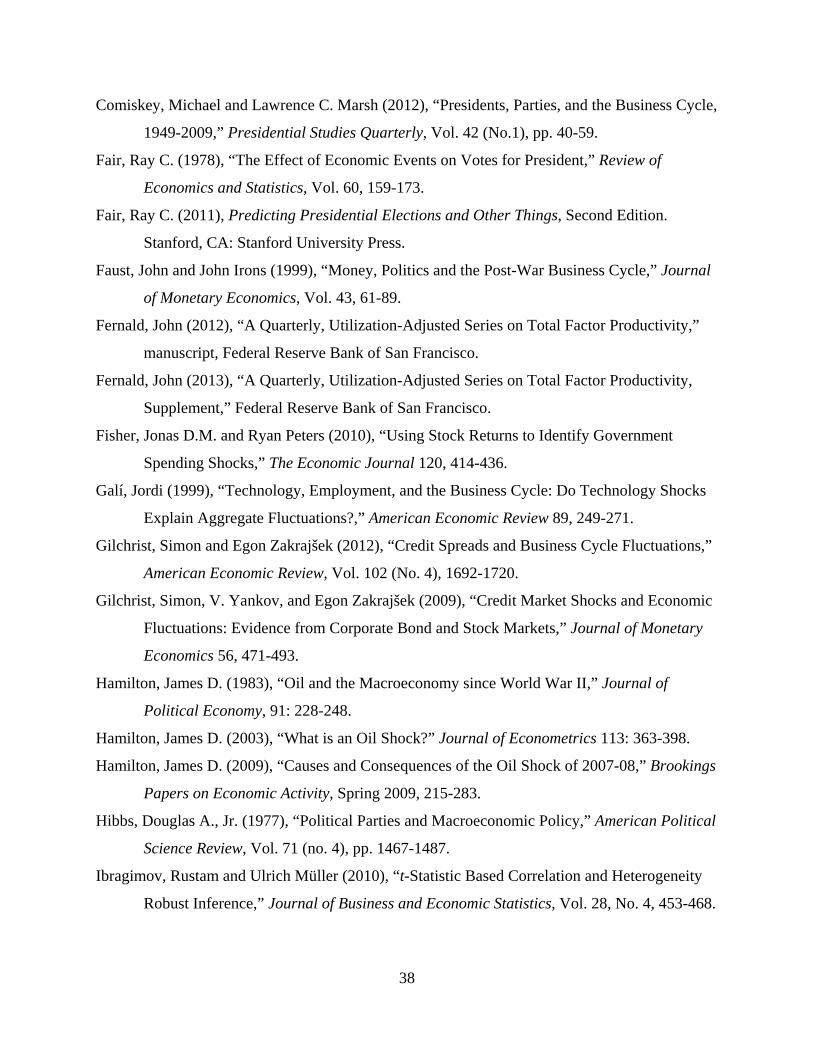
38

Comiskey, Michael and Lawrence C. Marsh (2012), “Presidents, Parties, and the Business Cycle,

1949-2009,” Presidential Studies Quarterly, Vol. 42 (No.1), pp. 40-59.

Fair, Ray C. (1978), “The Effect of Economic Events on Votes for President,” Review of

Economics and Statistics, Vol. 60, 159-173.

Fair, Ray C. (2011), Predicting Presidential Elections and Other Things, Second Edition.

Stanford, CA: Stanford University Press.

Faust, John and John Irons (1999), “Money, Politics and the Post-War Business Cycle,” Journal

of Monetary Economics, Vol. 43, 61-89.

Fernald, John (2012), “A Quarterly, Utilization-Adjusted Series on Total Factor Productivity,”

manuscript, Federal Reserve Bank of San Francisco.

Fernald, John (2013), “A Quarterly, Utilization-Adjusted Series on Total Factor Productivity,

Supplement,” Federal Reserve Bank of San Francisco.

Fisher, Jonas D.M. and Ryan Peters (2010), “Using Stock Returns to Identify Government

Spending Shocks,” The Economic Journal 120, 414-436.

Galí, Jordi (1999), “Technology, Employment, and the Business Cycle: Do Technology Shocks

Explain Aggregate Fluctuations?,” American Economic Review 89, 249-271.

Gilchrist, Simon and Egon Zakrajšek (2012), “Credit Spreads and Business Cycle Fluctuations,”

American Economic Review, Vol. 102 (No. 4), 1692-1720.

Gilchrist, Simon, V. Yankov, and Egon Zakrajšek (2009), “Credit Market Shocks and Economic

Fluctuations: Evidence from Corporate Bond and Stock Markets,” Journal of Monetary

Economics 56, 471-493.

Hamilton, James D. (1983), “Oil and the Macroeconomy since World War II,” Journal of

Political Economy, 91: 228-248.

Hamilton, James D. (2003), “What is an Oil Shock?” Journal of Econometrics 113: 363-398.

Hamilton, James D. (2009), “Causes and Consequences of the Oil Shock of 2007-08,” Brookings

Papers on Economic Activity, Spring 2009, 215-283.

Hibbs, Douglas A., Jr. (1977), “Political Parties and Macroeconomic Policy,” American Political

Science Review, Vol. 71 (no. 4), pp. 1467-1487.

Ibragimov, Rustam and Ulrich Müller (2010), “t-Statistic Based Correlation and Heterogeneity

Robust Inference,” Journal of Business and Economic Statistics, Vol. 28, No. 4, 453-468.

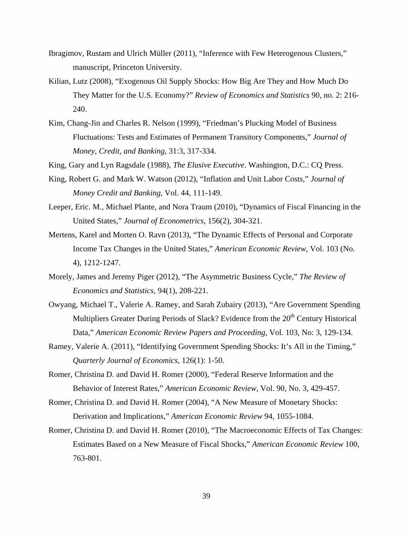
39

Ibragimov, Rustam and Ulrich Müller (2011), “Inference with Few Heterogenous Clusters,”

manuscript, Princeton University.

Kilian, Lutz (2008), “Exogenous Oil Supply Shocks: How Big Are They and How Much Do

They Matter for the U.S. Economy?” Review of Economics and Statistics 90, no. 2: 216-

240.

Kim, Chang-Jin and Charles R. Nelson (1999), “Friedman’s Plucking Model of Business

Fluctuations: Tests and Estimates of Permanent Transitory Components,” Journal of

Money, Credit, and Banking, 31:3, 317-334.

King, Gary and Lyn Ragsdale (1988), The Elusive Executive. Washington, D.C.: CQ Press.

King, Robert G. and Mark W. Watson (2012), “Inflation and Unit Labor Costs,” Journal of

Money Credit and Banking, Vol. 44, 111-149.

Leeper, Eric. M., Michael Plante, and Nora Traum (2010), “Dynamics of Fiscal Financing in the

United States,” Journal of Econometrics, 156(2), 304-321.

Mertens, Karel and Morten O. Ravn (2013), “The Dynamic Effects of Personal and Corporate

Income Tax Changes in the United States,” American Economic Review, Vol. 103 (No.

4), 1212-1247.

Morely, James and Jeremy Piger (2012), “The Asymmetric Business Cycle,” The Review of

Economics and Statistics, 94(1), 208-221.

Owyang, Michael T., Valerie A. Ramey, and Sarah Zubairy (2013), “Are Government Spending

Multipliers Greater During Periods of Slack? Evidence from the 20th Century Historical

Data,” American Economic Review Papers and Proceeding, Vol. 103, No: 3, 129-134.

Ramey, Valerie A. (2011), “Identifying Government Spending Shocks: It’s All in the Timing,”

Quarterly Journal of Economics, 126(1): 1-50.

Romer, Christina D. and David H. Romer (2000), “Federal Reserve Information and the

Behavior of Interest Rates,” American Economic Review, Vol. 90, No. 3, 429-457.

Romer, Christina D. and David H. Romer (2004), “A New Measure of Monetary Shocks:

Derivation and Implications,” American Economic Review 94, 1055-1084.

Romer, Christina D. and David H. Romer (2010), “The Macroeconomic Effects of Tax Changes:

Estimates Based on a New Measure of Fiscal Shocks,” American Economic Review 100,

763-801.

40

Santa-Clara, Pedro and Rossen Valkanov (2003), “The Presidential Puzzle: Political Cycles and

the Stock Market,” Journal of Finance, Vol. 58, No. 5, 1841-1872.

Schmitt-Grohé, Stephanie and Martín Uribe (2012), “What’s News in Business Cycles,”

Econometrica, Vol. 80, No. 6, 2733-2764.

Silber, William L (2012), Volcker: The Triumph of Persistence, Bloomsbury Press.

Sims, Christopher A. and Tao Zha (2006), “Were There Regime Switches in U.S. Monetary

Policy?” American Economic Review, 96:1, 54-81.

Smets, Frank and Raph Wouters (2007), “Shocks and Frictions in U.S. Business Cycles: A

Bayesian DSGE Approach,” American Economic Review, 97:3, 586-606.

Staiger, Douglas, James H. Stock, and Mark W. Watson (2001), “Prices, Wages and the U.S.

NAIRU in the 1990s” in The Roaring 90s: Can Full Employment Be Sustained, edited

by Alan B. Krueger and Robert Solow, New York: Russell Sage and Century Fund.

Stock, James H. and Mark W. Watson (2012), “Disentangling the Channels of the 2007-2009

Recession,” Brookings Papers on Economic Activity, Spring 2012, 81-135.

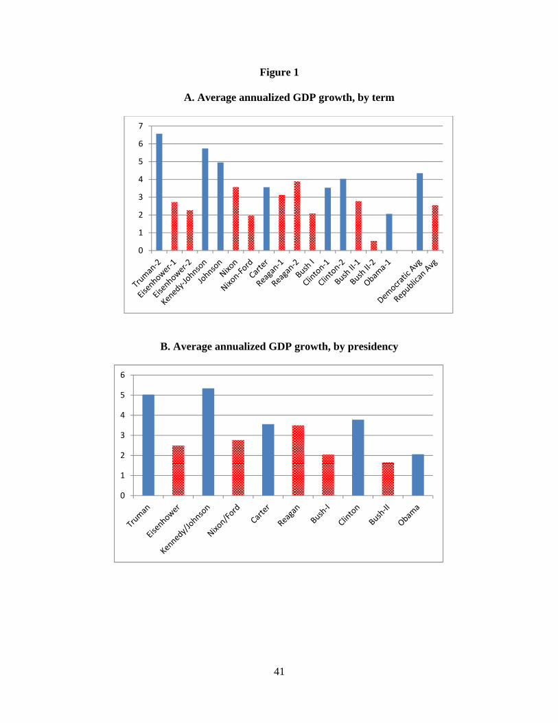
41

Figure 1

A. Average annualized GDP growth, by term

B. Average annualized GDP growth, by presidency

0

1

2

3

4

5

6

7

0

1

2

3

4

5

6

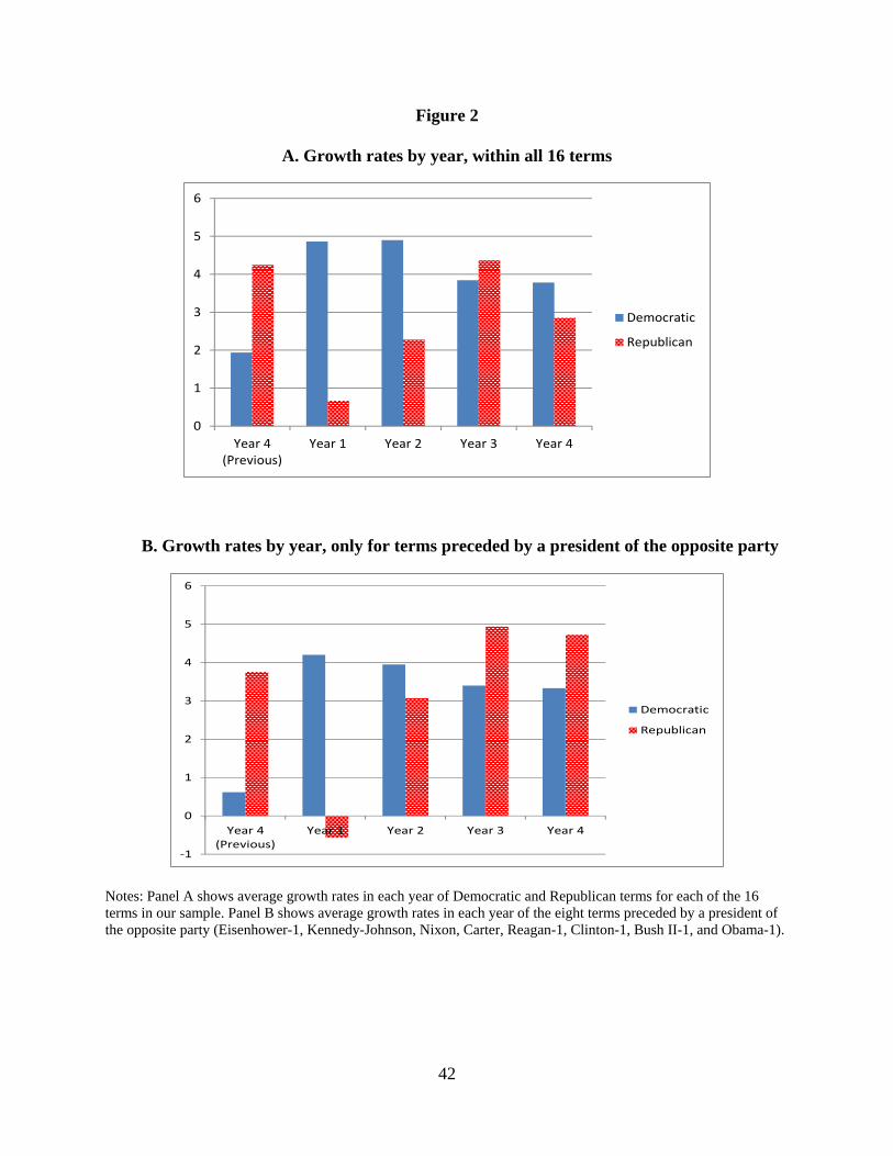
42

Figure 2

A. Growth rates by year, within all 16 terms

B. Growth rates by year, only for terms preceded by a president of the opposite party

Notes: Panel A shows average growth rates in each year of Democratic and Republican terms for each of the 16 terms in our sample. Panel B shows average growth rates in each year of the eight terms preceded by a president of the opposite party (Eisenhower-1, Kennedy-Johnson, Nixon, Carter, Reagan-1, Clinton-1, Bush II-1, and Obama-1).

0

1

2

3

4

5

6

Year 4(Previous)

Year 1 Year 2 Year 3 Year 4

Democratic

Republican

‐1

0

1

2

3

4

5

6

Year 4(Previous)

Year 1 Year 2 Year 3 Year 4

Democratic

Republican

43

Figure 3 Change in full employment surplus and lagged GDP growth

Democrats: + and dashed line Republicans: circles and solid line

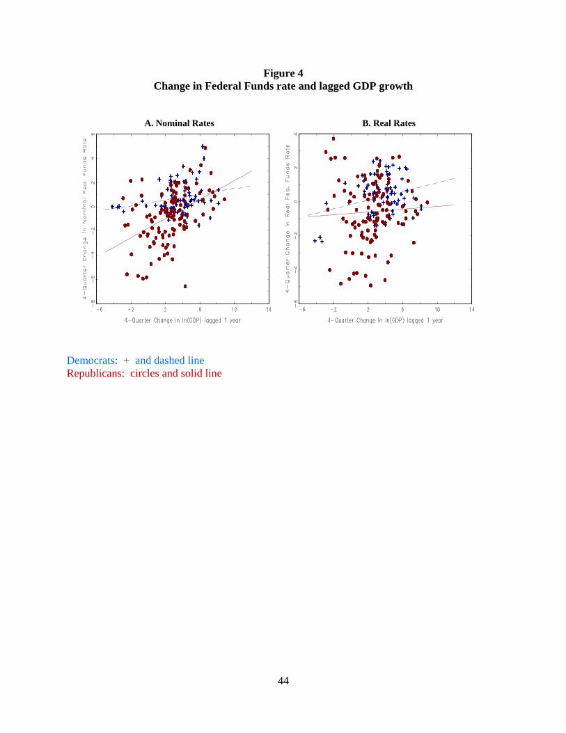
44

Figure 4 Change in Federal Funds rate and lagged GDP growth

A. Nominal Rates B. Real Rates

Democrats: + and dashed line Republicans: circles and solid line

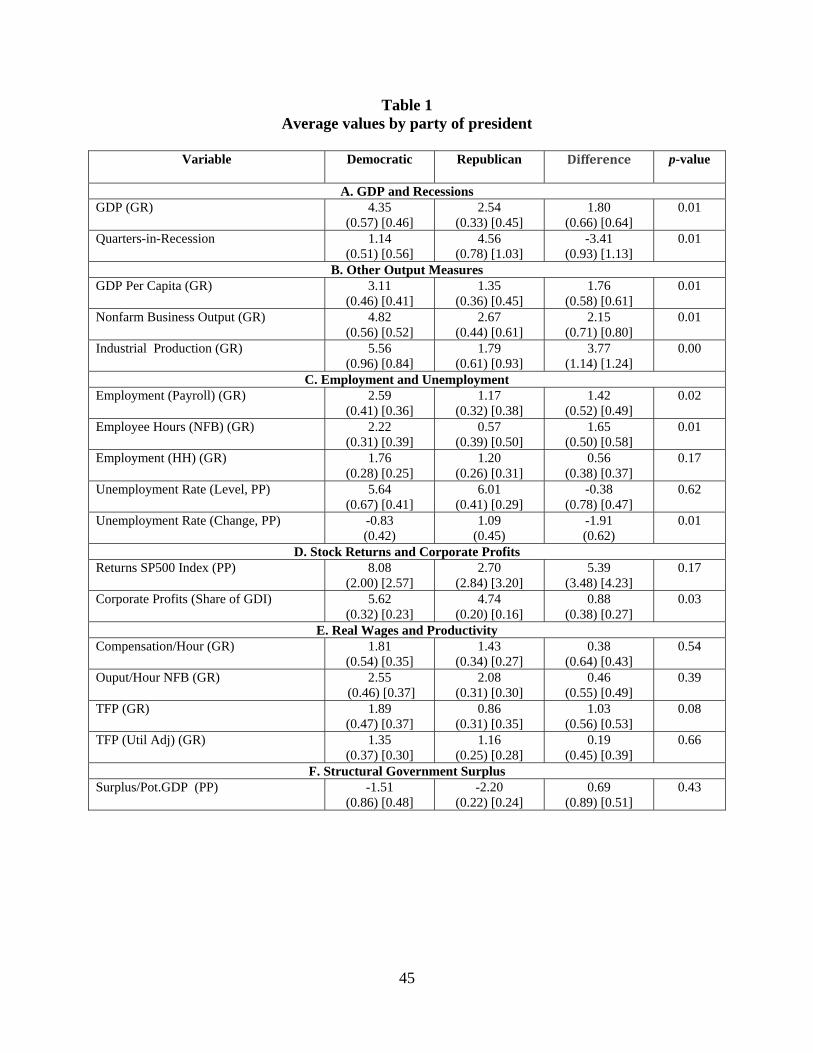
45

Table 1 Average values by party of president

Variable Democratic Republican Difference p-value

A. GDP and Recessions GDP (GR) 4.35

(0.57) [0.46] 2.54

(0.33) [0.45] 1.80

(0.66) [0.64] 0.01

Quarters-in-Recession 1.14 (0.51) [0.56]

4.56 (0.78) [1.03]

-3.41 (0.93) [1.13]

0.01

B. Other Output Measures GDP Per Capita (GR) 3.11

(0.46) [0.41] 1.35

(0.36) [0.45] 1.76

(0.58) [0.61] 0.01

Nonfarm Business Output (GR) 4.82 (0.56) [0.52]

2.67 (0.44) [0.61]

2.15 (0.71) [0.80]

0.01

Industrial Production (GR) 5.56 (0.96) [0.84]

1.79 (0.61) [0.93]

3.77 (1.14) [1.24]

0.00

C. Employment and Unemployment Employment (Payroll) (GR) 2.59

(0.41) [0.36] 1.17

(0.32) [0.38] 1.42

(0.52) [0.49] 0.02

Employee Hours (NFB) (GR) 2.22 (0.31) [0.39]

0.57 (0.39) [0.50]

1.65 (0.50) [0.58]

0.01

Employment (HH) (GR) 1.76 (0.28) [0.25]

1.20 (0.26) [0.31]

0.56 (0.38) [0.37]

0.17

Unemployment Rate (Level, PP) 5.64 (0.67) [0.41]

6.01 (0.41) [0.29]

-0.38 (0.78) [0.47]

0.62

Unemployment Rate (Change, PP) -0.83 (0.42)

1.09 (0.45)

-1.91 (0.62)

0.01

D. Stock Returns and Corporate Profits Returns SP500 Index (PP) 8.08

(2.00) [2.57] 2.70

(2.84) [3.20] 5.39

(3.48) [4.23] 0.17

Corporate Profits (Share of GDI) 5.62 (0.32) [0.23]

4.74 (0.20) [0.16]

0.88 (0.38) [0.27]

0.03

E. Real Wages and Productivity Compensation/Hour (GR) 1.81

(0.54) [0.35] 1.43

(0.34) [0.27] 0.38

(0.64) [0.43] 0.54

Ouput/Hour NFB (GR) 2.55 (0.46) [0.37]

2.08 (0.31) [0.30]

0.46 (0.55) [0.49]

0.39

TFP (GR) 1.89 (0.47) [0.37]

0.86 (0.31) [0.35]

1.03 (0.56) [0.53]

0.08

TFP (Util Adj) (GR) 1.35 (0.37) [0.30]

1.16 (0.25) [0.28]

0.19 (0.45) [0.39]

0.66

F. Structural Government Surplus Surplus/Pot.GDP (PP) -1.51

(0.86) [0.48] -2.20

(0.22) [0.24] 0.69

(0.89) [0.51] 0.43

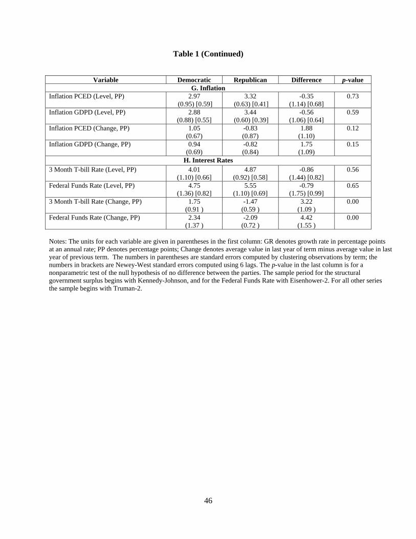
46

Table 1 (Continued)

Variable Democratic Republican Difference p-value

G. Inflation Inflation PCED (Level, PP) 2.97

(0.95) [0.59] 3.32

(0.63) [0.41] -0.35

(1.14) [0.68] 0.73

Inflation GDPD (Level, PP) 2.88 (0.88) [0.55]

3.44 (0.60) [0.39]

-0.56 (1.06) [0.64]

0.59

Inflation PCED (Change, PP) 1.05 (0.67)

-0.83 (0.87)

1.88 (1.10)

0.12

Inflation GDPD (Change, PP) 0.94 (0.69)

-0.82 (0.84)

1.75 (1.09)

0.15

H. Interest Rates 3 Month T-bill Rate (Level, PP) 4.01

(1.10) [0.66] 4.87

(0.92) [0.58] -0.86

(1.44) [0.82] 0.56

Federal Funds Rate (Level, PP) 4.75 (1.36) [0.82]

5.55 (1.10) [0.69]

-0.79 (1.75) [0.99]

0.65

3 Month T-bill Rate (Change, PP) 1.75 (0.91 )

-1.47 (0.59 )

3.22 (1.09 )

0.00

Federal Funds Rate (Change, PP) 2.34 (1.37 )

-2.09 (0.72 )

4.42 (1.55 )

0.00

Notes: The units for each variable are given in parentheses in the first column: GR denotes growth rate in percentage points at an annual rate; PP denotes percentage points; Change denotes average value in last year of term minus average value in last year of previous term. The numbers in parentheses are standard errors computed by clustering observations by term; the numbers in brackets are Newey-West standard errors computed using 6 lags. The p-value in the last column is for a nonparametric test of the null hypothesis of no difference between the parties. The sample period for the structural government surplus begins with Kennedy-Johnson, and for the Federal Funds Rate with Eisenhower-2. For all other series the sample begins with Truman-2.

47

Table 2 Average GDP growth by presidential attribute

Attribute terms With Without Difference p-value

Political Party Democrat 7 4.35

(0.57) [0.46] 2.54

(0.33) [0.45] 1.80

(0.66) [0.64] 0.01

Other Attributes Congressional

experience 7 3.84

(0.73) [0.56] 2.94

(0.36) [0.43] 0.91

(0.81) [0.70] 0.25

Gubernatorial experience

7 3.06 (0.45) [0.47]

3.54 (0.59) [0.47]

-0.48 (0.74) [0.65]

0.55

Youngest half 8 3.78 (0.41) [0.38]

2.89 (0.63) [0.57]

0.89 (0.75) [0.68]

0.26

Tallest half 8 3.67 (0.46) [0.40]

2.99 (0.61) [0.55]

0.67 (0.77) [0.68]

0.39

Notes: The table shows average GDP growth rates for presidents with and without the attribute shown in the first column, where the value of terms denotes the number of administration whose presidents have the attribute. (The total number of administrations is 16.) Standard errors shown in parentheses and brackets and p-value shown in the final column are computed as in Table 1.

Table 3 Average GDP Growth under presidents and by Congressional control

Partisan control of Congress Party of President

All Democrat Republican Democrats control both houses 4.69 (0.58) [80] 2.37 (0.56) [88] 3.47 (0.47) [168] Divided Congress 2.30 (0.44) [8] 2.80 (1.07) [32] 2.70 (0.87) [40] Republicans control both houses 3.88 (0.44) [24] 2.84 (0.84) [24] 3.36 (0.53) [48]

All 4.35 (0.46) [112] 2.54 (0.45) [144] 3.33 (0.34) [256] Notes: Entries are average growth rates in real GDP (in percentage points at an annual rate) by party of the President and partisan control of Congress. The numbers in parentheses are standard errors (Newey-West with 6 lags) and the numbers in brackets are the number of quarters.

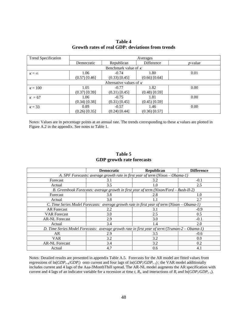
48

Table 4 Growth rates of real GDP: deviations from trends

Trend Specification Averages

Democratic Republican Difference p-value Benchmark value of

= ∞ 1.06 (0.57) [0.46]

-0.74 (0.33) [0.45]

1.80 (0.66) [0.64]

0.01

Alternative values of = 100 1.05

(0.37) [0.39] -0.77

(0.31) [0.45] 1.82

(0.48) [0.59] 0.00

= 67 1.06 (0.34) [0.38]

-0.75 (0.31) [0.45]

1.81 (0.45) [0.59]

0.00

= 33 0.89 (0.26) [0.35]

-0.57 (0.24) [0.44]

1.46 (0.36) [0.57]

0.00

Notes: Values are in percentage points at an annual rate. The trends corresponding to these values are plotted in Figure A.2 in the appendix. See notes to Table 1.

Table 5 GDP growth rate forecasts

Democratic Republican Difference

A. SPF Forecasts: average growth rate in first year of term (Nixon – Obama-1) Forecast 3.1 3.2 -0.1 Actual 3.5 1.0 2.5 B. Greenbook Forecasts: average growth in first year of term (Nixon/Ford – Bush-II-2)

Forecast 3.8 2.8 1.0 Actual 3.8 1.1 2.7

C. Time Series Model Forecasts: average growth rate in first year of term (Nixon – Obama-1) AR Forecast 2.2 3.1 -0.9 VAR Forecast 3.0 2.5 0.5

AR-NL Forecast 2.9 3.0 -0.1 Actual 3.4 1.4 2.0

D. Time Series Model Forecasts: average growth rate in first year of term (Truman-2 – Obama-1) AR 2.9 3.5 -0.6 VAR 3.2 3.2 0.0

AR-NL Forecast 3.4 3.2 0.2 Actual 4.7 0.6 4.1

Notes: Detailed results are presented in appendix Table A.5. Forecasts for the AR model are fitted values from regressions of ln(GDPt+4/GDPt) onto current and four lags of ln(GDPt/GDPt−1) ; the VAR model additionally includes current and 4 lags of the Aaa-3MonthTbill spread. The AR-NL model augments the AR specification with current and 4 lags of an indicator variable for a recession at time t, Rt, and interactions of Rt and ln(GDPt/GDPt−1).

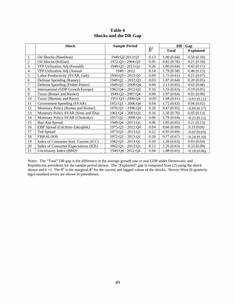
49

Table 6 Shocks and the DR-Gap

Shock Sample Period

R2

DR - Gap Total Explained

1 Oil Shocks (Hamilton) 1949:Q2-2013:Q1 0.13 1.80 (0.64) 0.50 (0.10) 2 Oil Shocks (Killian) 1972:Q3 - 2004:Q3 0.05 0.82 (0.76) 0.21 (0.19) 3 TFP Utilization Adj (Fernald) 1949:Q2 - 2013:Q1 0.26 1.80 (0.64) 0.42 (0.11) 4 TFP Utilization Adj (Annual 1949 – 2012 0.14 1.79 (0.58) 0.46 (0.13) 5 Labor Productivity (SVAR, Gali) 1950:Q3 – 2013:Q1 0.09 1.73 (0.61) 0.21 (0.07) 6 Defense Spending (Ramey) 1949:Q2 - 2012.Q3 0.03 1.87 (0.64) 0.20 (0.05) 7 Defense Spending (Fisher-Peters) 1949:Q2 - 2008:Q4 0.00 2.13 (0.65) 0.02 (0.06) 8 International (GDP Growth Europe) 1962:Q4 – 2012:Q3 0.16 1.33 (0.63) 0.19 (0.05) 9 Taxes (Romer and Romer) 1949:Q2 - 2007:Q4 0.00 1.97 (0.64) 0.01 (0.06) 10 Taxes (Mertens and Ravn) 1951:Q3 - 2006:Q4 -0.05 1.68 (0.61) 0.03 (0.11) 11 Government Spending (SVAR) 1952:Q3 - 2006:Q4 0.04 1.72 (0.63) 0.06 (0.02) 12 Monetary Policy (Romer and Romer) 1970:Q3 - 1996:Q4 0.20 0.47 (0.95) 0.09 (0.17) 13 Monetary Policy SVAR (Sims and Zha) 1961:Q4 - 2003:Q1 0.16 1.50 (0.70) 0.05 (0.13) 14 Monetary Policy SVAR (Cholesky) 1957:Q2 - 2008.Q4 0.06 1.78 (0.64) 0.23 (0.12) 15 Baa-Aaa Spread 1949:Q4 – 2013:Q1 0.06 1.85 (0.65) 0.21 (0.13) 16 EBP Spread (Gilchrist-Zakrajšek) 1975:Q3 – 2012:Q4 0.04 0.66 (0.69) 0.33 (026) 17 Ted Spread 1973:Q3 – 2013:Q1 0.22 0.93 (0.69) 0.02 (0.03) 18 FRB SLOOS 1972:Q3 – 2013:Q1 0.20 0.77 (0.67) 0.24 (0.10) 19 Index of Consumer Sent. Current (ICC) 1962:Q3 – 2013:Q1 0.10 1.26 (0.63) 0.03 (0.04) 20 Index of Consumer Expectations (ICE) 1962:Q3 – 2013:Q1 0.13 1.26 (0.63) 0.33 (0.09) 21 Uncertainty Index (BBD) 1949:Q4 - 2012:Q4 0.04 1.88 (0.65) 0.18 (0.06) Notes: The “Total” DR-gap is the difference in the average growth rate or real GDP under Democratic and Republicans presidents for the sample period shown. The “Explained” gap is computed from (2) using the shock shown and k =1. The R2 is the marginal R2 for the current and lagged values of the shocks. Newey-West (6 quarterly lags) standard errors are shown in parentheses.

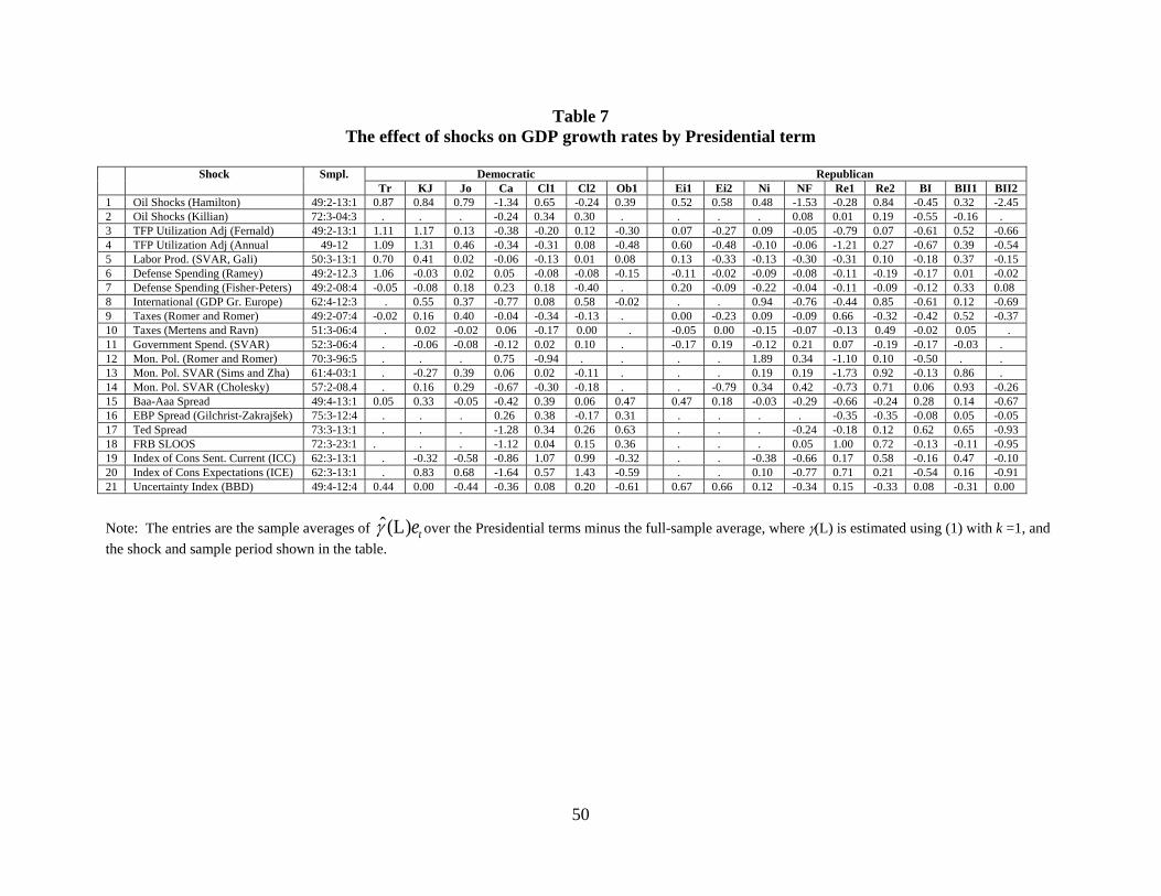
50

Table 7 The effect of shocks on GDP growth rates by Presidential term

Shock Smpl. Democratic Republican

Tr KJ Jo Ca Cl1 Cl2 Ob1 Ei1 Ei2 Ni NF Re1 Re2 BI BII1 BII2 1 Oil Shocks (Hamilton) 49:2-13:1 0.87 0.84 0.79 -1.34 0.65 -0.24 0.39 0.52 0.58 0.48 -1.53 -0.28 0.84 -0.45 0.32 -2.45 2 Oil Shocks (Killian) 72:3-04:3 . . . -0.24 0.34 0.30 . . . . 0.08 0.01 0.19 -0.55 -0.16 . 3 TFP Utilization Adj (Fernald) 49:2-13:1 1.11 1.17 0.13 -0.38 -0.20 0.12 -0.30 0.07 -0.27 0.09 -0.05 -0.79 0.07 -0.61 0.52 -0.66 4 TFP Utilization Adj (Annual 49-12 1.09 1.31 0.46 -0.34 -0.31 0.08 -0.48 0.60 -0.48 -0.10 -0.06 -1.21 0.27 -0.67 0.39 -0.54 5 Labor Prod. (SVAR, Gali) 50:3-13:1 0.70 0.41 0.02 -0.06 -0.13 0.01 0.08 0.13 -0.33 -0.13 -0.30 -0.31 0.10 -0.18 0.37 -0.15 6 Defense Spending (Ramey) 49:2-12.3 1.06 -0.03 0.02 0.05 -0.08 -0.08 -0.15 -0.11 -0.02 -0.09 -0.08 -0.11 -0.19 -0.17 0.01 -0.02 7 Defense Spending (Fisher-Peters) 49:2-08:4 -0.05 -0.08 0.18 0.23 0.18 -0.40 . 0.20 -0.09 -0.22 -0.04 -0.11 -0.09 -0.12 0.33 0.08 8 International (GDP Gr. Europe) 62:4-12:3 . 0.55 0.37 -0.77 0.08 0.58 -0.02 . . 0.94 -0.76 -0.44 0.85 -0.61 0.12 -0.69 9 Taxes (Romer and Romer) 49:2-07:4 -0.02 0.16 0.40 -0.04 -0.34 -0.13 . 0.00 -0.23 0.09 -0.09 0.66 -0.32 -0.42 0.52 -0.37 10 Taxes (Mertens and Ravn) 51:3-06:4 . 0.02 -0.02 0.06 -0.17 0.00 . -0.05 0.00 -0.15 -0.07 -0.13 0.49 -0.02 0.05 .11 Government Spend. (SVAR) 52:3-06:4 . -0.06 -0.08 -0.12 0.02 0.10 . -0.17 0.19 -0.12 0.21 0.07 -0.19 -0.17 -0.03 . 12 Mon. Pol. (Romer and Romer) 70:3-96:5 . . . 0.75 -0.94 . . . . 1.89 0.34 -1.10 0.10 -0.50 . . 13 Mon. Pol. SVAR (Sims and Zha) 61:4-03:1 . -0.27 0.39 0.06 0.02 -0.11 . . . 0.19 0.19 -1.73 0.92 -0.13 0.86 . 14 Mon. Pol. SVAR (Cholesky) 57:2-08.4 . 0.16 0.29 -0.67 -0.30 -0.18 . . -0.79 0.34 0.42 -0.73 0.71 0.06 0.93 -0.26 15 Baa-Aaa Spread 49:4-13:1 0.05 0.33 -0.05 -0.42 0.39 0.06 0.47 0.47 0.18 -0.03 -0.29 -0.66 -0.24 0.28 0.14 -0.67 16 EBP Spread (Gilchrist-Zakrajšek) 75:3-12:4 . . . 0.26 0.38 -0.17 0.31 . . . . -0.35 -0.35 -0.08 0.05 -0.05 17 Ted Spread 73:3-13:1 . . . -1.28 0.34 0.26 0.63 . . . -0.24 -0.18 0.12 0.62 0.65 -0.93 18 FRB SLOOS 72:3-23:1 . . . -1.12 0.04 0.15 0.36 . . . 0.05 1.00 0.72 -0.13 -0.11 -0.95 19 Index of Cons Sent. Current (ICC) 62:3-13:1 . -0.32 -0.58 -0.86 1.07 0.99 -0.32 . . -0.38 -0.66 0.17 0.58 -0.16 0.47 -0.10 20 Index of Cons Expectations (ICE) 62:3-13:1 . 0.83 0.68 -1.64 0.57 1.43 -0.59 . . 0.10 -0.77 0.71 0.21 -0.54 0.16 -0.91 21 Uncertainty Index (BBD) 49:4-12:4 0.44 0.00 -0.44 -0.36 0.08 0.20 -0.61 0.67 0.66 0.12 -0.34 0.15 -0.33 0.08 -0.31 0.00

Note: The entries are the sample averages of ̂ (L)et over the Presidential terms minus the full-sample average, where (L) is estimated using (1) with k =1, and

the shock and sample period shown in the table.

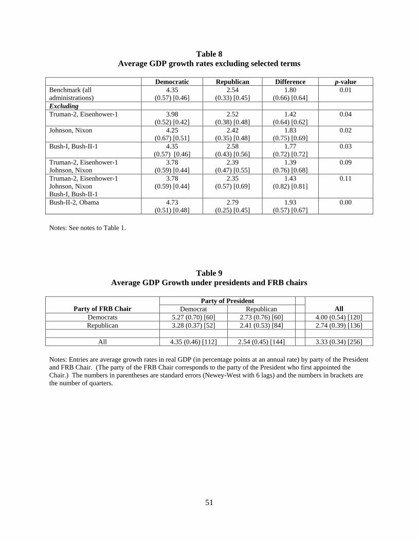
51

Table 8 Average GDP growth rates excluding selected terms

Democratic Republican Difference p-value Benchmark (all administrations)

4.35 (0.57) [0.46]

2.54 (0.33) [0.45]

1.80 (0.66) [0.64]

0.01

Excluding Truman-2, Eisenhower-1 3.98

(0.52) [0.42] 2.52

(0.38) [0.48] 1.42

(0.64) [0.62] 0.04

Johnson, Nixon 4.25 (0.67) [0.51]

2.42 (0.35) [0.48]

1.83 (0.75) [0.69]

0.02

Bush-I, Bush-II-1 4.35 (0.57) [0.46]

2.58 (0.43) [0.56]

1.77 (0.72) [0.72]

0.03

Truman-2, Eisenhower-1 Johnson, Nixon

3.78 (0.59) [0.44]

2.39 (0.47) [0.55]

1.39 (0.76) [0.68]

0.09

Truman-2, Eisenhower-1 Johnson, Nixon Bush-I, Bush-II-1

3.78 (0.59) [0.44]

2.35 (0.57) [0.69]

1.43 (0.82) [0.81]

0.11

Bush-II-2, Obama 4.73 (0.51) [0.48]

2.79 (0.25) [0.45]

1.93 (0.57) [0.67]

0.00

Notes: See notes to Table 1.

Table 9 Average GDP Growth under presidents and FRB chairs

Party of FRB Chair Party of President

All Democrat Republican Democrats 5.27 (0.70) [60] 2.73 (0.76) [60] 4.00 (0.54) [120] Republican 3.28 (0.37) [52] 2.41 (0.53) [84] 2.74 (0.39) [136]

All 4.35 (0.46) [112] 2.54 (0.45) [144] 3.33 (0.34) [256]

Notes: Entries are average growth rates in real GDP (in percentage points at an annual rate) by party of the President and FRB Chair. (The party of the FRB Chair corresponds to the party of the President who first appointed the Chair.) The numbers in parentheses are standard errors (Newey-West with 6 lags) and the numbers in brackets are the number of quarters.

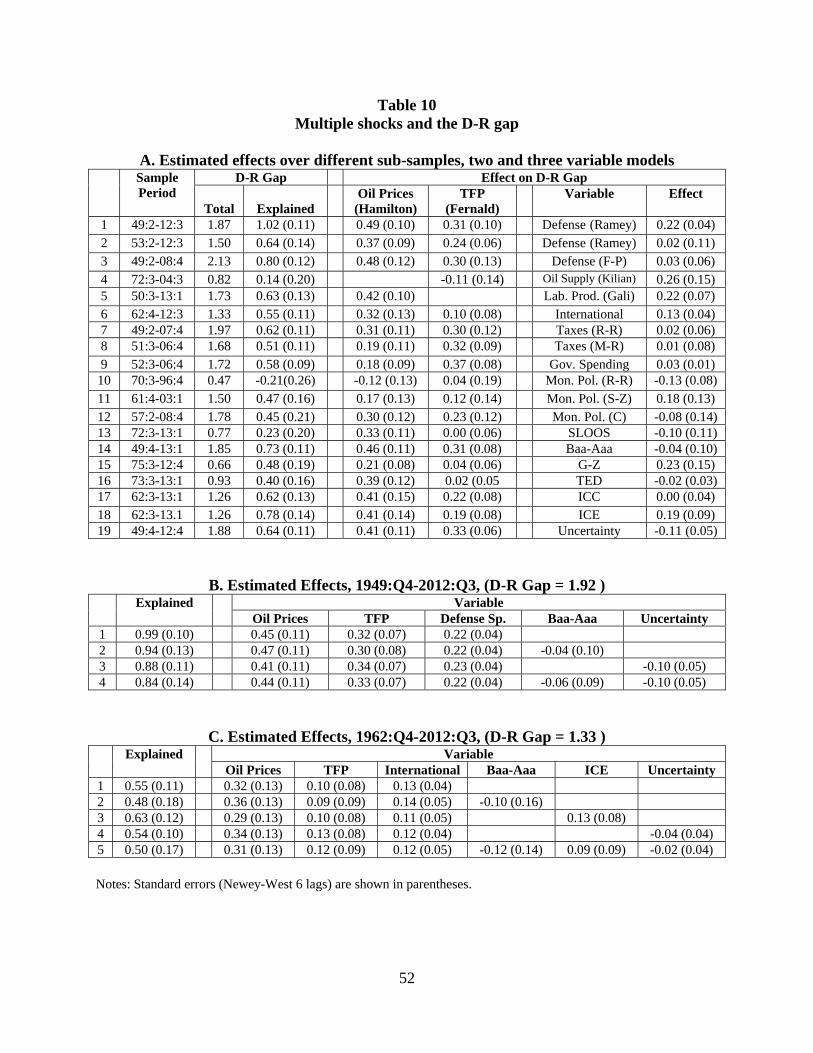
52

Table 10 Multiple shocks and the D-R gap

A. Estimated effects over different sub-samples, two and three variable models

Sample Period

D-R Gap Effect on D-R Gap

Total

Explained Oil Prices

(Hamilton)TFP

(Fernald) Variable Effect

1 49:2-12:3 1.87 1.02 (0.11) 0.49 (0.10) 0.31 (0.10) Defense (Ramey) 0.22 (0.04) 2 53:2-12:3 1.50 0.64 (0.14) 0.37 (0.09) 0.24 (0.06) Defense (Ramey) 0.02 (0.11) 3 49:2-08:4 2.13 0.80 (0.12) 0.48 (0.12) 0.30 (0.13) Defense (F-P) 0.03 (0.06) 4 72:3-04:3 0.82 0.14 (0.20) -0.11 (0.14) Oil Supply (Kilian) 0.26 (0.15) 5 50:3-13:1 1.73 0.63 (0.13) 0.42 (0.10) Lab. Prod. (Gali) 0.22 (0.07) 6 62:4-12:3 1.33 0.55 (0.11) 0.32 (0.13) 0.10 (0.08) International 0.13 (0.04) 7 49:2-07:4 1.97 0.62 (0.11) 0.31 (0.11) 0.30 (0.12) Taxes (R-R) 0.02 (0.06) 8 51:3-06:4 1.68 0.51 (0.11) 0.19 (0.11) 0.32 (0.09) Taxes (M-R) 0.01 (0.08) 9 52:3-06:4 1.72 0.58 (0.09) 0.18 (0.09) 0.37 (0.08) Gov. Spending 0.03 (0.01)

10 70:3-96:4 0.47 -0.21(0.26) -0.12 (0.13) 0.04 (0.19) Mon. Pol. (R-R) -0.13 (0.08) 11 61:4-03:1 1.50 0.47 (0.16) 0.17 (0.13) 0.12 (0.14) Mon. Pol. (S-Z) 0.18 (0.13) 12 57:2-08:4 1.78 0.45 (0.21) 0.30 (0.12) 0.23 (0.12) Mon. Pol. (C) -0.08 (0.14) 13 72:3-13:1 0.77 0.23 (0.20) 0.33 (0.11) 0.00 (0.06) SLOOS -0.10 (0.11) 14 49:4-13:1 1.85 0.73 (0.11) 0.46 (0.11) 0.31 (0.08) Baa-Aaa -0.04 (0.10) 15 75:3-12:4 0.66 0.48 (0.19) 0.21 (0.08) 0.04 (0.06) G-Z 0.23 (0.15) 16 73:3-13:1 0.93 0.40 (0.16) 0.39 (0.12) 0.02 (0.05 TED -0.02 (0.03) 17 62:3-13:1 1.26 0.62 (0.13) 0.41 (0.15) 0.22 (0.08) ICC 0.00 (0.04) 18 62:3-13.1 1.26 0.78 (0.14) 0.41 (0.14) 0.19 (0.08) ICE 0.19 (0.09) 19 49:4-12:4 1.88 0.64 (0.11) 0.41 (0.11) 0.33 (0.06) Uncertainty -0.11 (0.05)

B. Estimated Effects, 1949:Q4-2012:Q3, (D-R Gap = 1.92 ) Explained Variable

Oil Prices TFP Defense Sp. Baa-Aaa Uncertainty 1 0.99 (0.10) 0.45 (0.11) 0.32 (0.07) 0.22 (0.04) 2 0.94 (0.13) 0.47 (0.11) 0.30 (0.08) 0.22 (0.04) -0.04 (0.10) 3 0.88 (0.11) 0.41 (0.11) 0.34 (0.07) 0.23 (0.04) -0.10 (0.05) 4 0.84 (0.14) 0.44 (0.11) 0.33 (0.07) 0.22 (0.04) -0.06 (0.09) -0.10 (0.05)

C. Estimated Effects, 1962:Q4-2012:Q3, (D-R Gap = 1.33 )

Explained Variable Oil Prices TFP International Baa-Aaa ICE Uncertainty

1 0.55 (0.11) 0.32 (0.13) 0.10 (0.08) 0.13 (0.04) 2 0.48 (0.18) 0.36 (0.13) 0.09 (0.09) 0.14 (0.05) -0.10 (0.16) 3 0.63 (0.12) 0.29 (0.13) 0.10 (0.08) 0.11 (0.05) 0.13 (0.08) 4 0.54 (0.10) 0.34 (0.13) 0.13 (0.08) 0.12 (0.04) -0.04 (0.04) 5 0.50 (0.17) 0.31 (0.13) 0.12 (0.09) 0.12 (0.05) -0.12 (0.14) 0.09 (0.09) -0.02 (0.04)

Notes: Standard errors (Newey-West 6 lags) are shown in parentheses.

53

Table 11 Average GDP growth rates for different countries

Country Sample Period Political Party Difference

Left Right United States 1949:Q2 – 2013:Q1 4.35 (0.46) 2.54 (0.45) 1.80 (0.64) Canada 1961:Q2 – 2012:Q2 3.89 (0.38) 2.48 (0.71) 1.41 (0.80) France 1949:Q2 – 2012:Q2 3.19 (0.51) 3.42 (0.50) -0.23 (0.72) Germany 1970:Q2 -2012:Q2 2.18 (0.55) 2.17 (0.51) 0.02 (0.75) United Kingdom 1955:Q2 – 2012:Q2 2.47 (0.47) 2.67 (0.49) -0.20 (0.70) Notes: Standard errors (Newey-West 6 lags) are shown in parentheses.

54

Appendix A: Data sources

The table below lists the data series, sources, and miscellaneous notes about the data used in this paper.

Series Source Notes Data used in Figure 1

Real GDP FRED: GDPC96 Additional Series Used in Table 1

Quarters-in-Recession NBER GDP Per Capita FRED:

A939RC0Q052SBEA The nominal series from FRED is deflated by the GDP deflator

Nonfarm Business Output FRED: OUTNFB Industrial Production FRED: INDPRO Employment (Payroll) FRED: PAYEMS Employee Hours (NFB) FRED: HOANBS Employment (HH) FRED: CE16OV Unemployment Rate FRED: UNRATE Returns SP500 Index WRDS Corporate Profits (Share of GDI) BEA Corporate profits with inventory valuation and

capital consumption adjustments, domestic industries, After Tax, from NIPA Table 1.10 Divided by GDI

Gross Domestic Income FRED: GDI Compensation/Hour FRED: COMPRNFB Ouput/Hour NFB FRED: OPHNFB TFP Supplied by John

Fernald

TFP (Util Adj) Supplied by John Fernald

Surplus/Pot.GDP CBO Net Federal Government Saving Without Automatic Stabilizers as Percent of potential output (CBO XLS File Col. Q)

PCE Deflator FRED: PCECTPI GDP Deflator FRED: GDPDEF

Additional Series Used in Table 5 Aaa bond rate FRED: Aaa Moody's Seasoned Aaa Corporate Bond Yield Three month Treas. bill rate FRED: TB3MS 3-Month Treasury Bill: Secondary Market Rate

Additional Series Used in Table 6Oil Price Shocks (Hamilton) BLS: WPU0561 Constructed using equation (3) in the text, with

Ot WPU0561 Oil Supply Shocks (Killian) Supplied by Lutz Killian Defense Spending (Ramey) Supplied by Valerie

Ramey This is an updated version of the Ramey(2011) series from Owyang, Ramey, and Zubairy (2013).

Defense Spending (Fisher-Peters) Supplied by Valerie Ramey

OECD GDP Growth Europe OECD Growth rates were detrended using a local average with biweight kernel and = 67.

Taxes (Romer and Romer) Supplied by David Romer

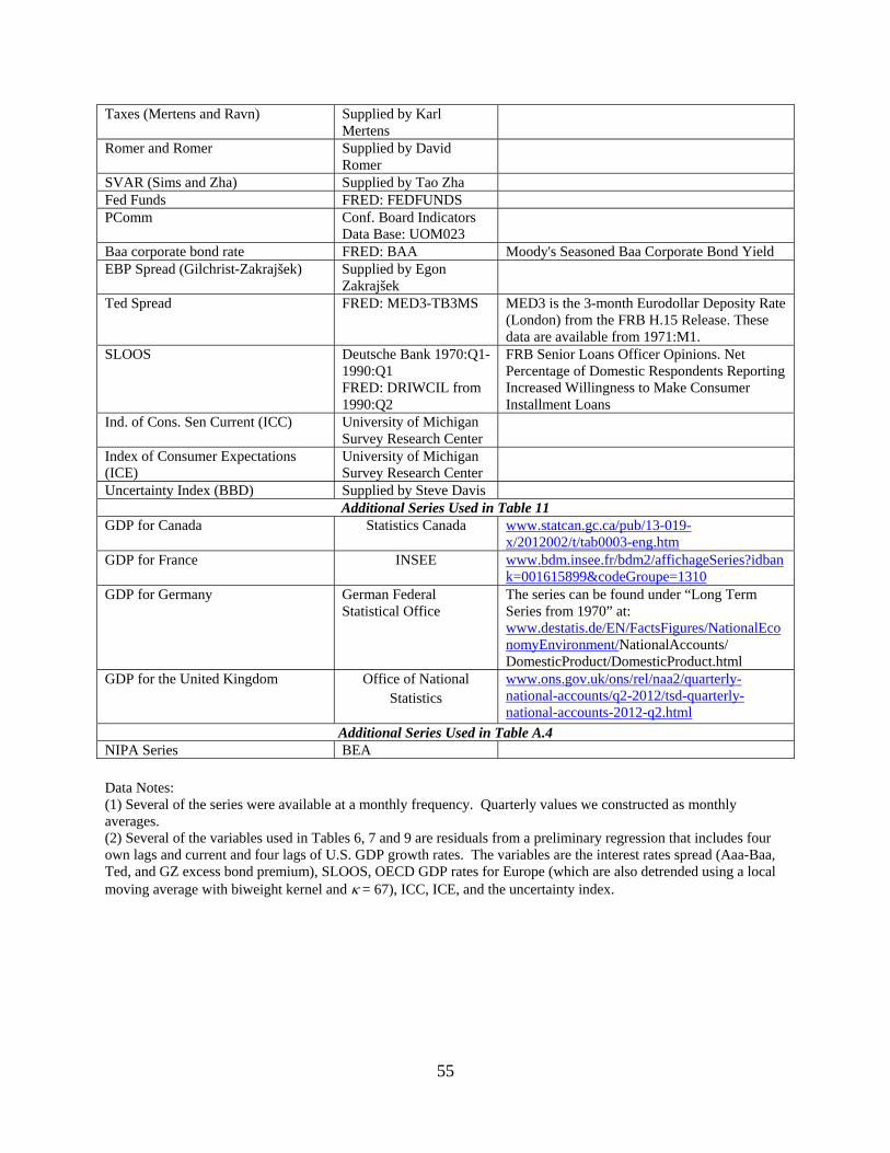
55

Taxes (Mertens and Ravn) Supplied by Karl Mertens

Romer and Romer Supplied by David Romer

SVAR (Sims and Zha) Supplied by Tao Zha Fed Funds FRED: FEDFUNDS PComm Conf. Board Indicators

Data Base: UOM023

Baa corporate bond rate FRED: BAA Moody's Seasoned Baa Corporate Bond Yield EBP Spread (Gilchrist-Zakrajšek) Supplied by Egon

Zakrajšek

Ted Spread FRED: MED3-TB3MS MED3 is the 3-month Eurodollar Deposity Rate (London) from the FRB H.15 Release. These data are available from 1971:M1.

SLOOS Deutsche Bank 1970:Q1-1990:Q1 FRED: DRIWCIL from 1990:Q2

FRB Senior Loans Officer Opinions. Net Percentage of Domestic Respondents Reporting Increased Willingness to Make Consumer Installment Loans

Ind. of Cons. Sen Current (ICC) University of Michigan Survey Research Center

Index of Consumer Expectations (ICE)

University of Michigan Survey Research Center

Uncertainty Index (BBD) Supplied by Steve Davis Additional Series Used in Table 11

GDP for Canada Statistics Canada www.statcan.gc.ca/pub/13-019-x/2012002/t/tab0003-eng.htm

GDP for France INSEE www.bdm.insee.fr/bdm2/affichageSeries?idbank=001615899&codeGroupe=1310

GDP for Germany German Federal Statistical Office

The series can be found under “Long Term Series from 1970” at: www.destatis.de/EN/FactsFigures/NationalEconomyEnvironment/NationalAccounts/ DomesticProduct/DomesticProduct.html

GDP for the United Kingdom Office of National Statistics

www.ons.gov.uk/ons/rel/naa2/quarterly-national-accounts/q2-2012/tsd-quarterly-national-accounts-2012-q2.html

Additional Series Used in Table A.4NIPA Series BEA Data Notes: (1) Several of the series were available at a monthly frequency. Quarterly values we constructed as monthly averages. (2) Several of the variables used in Tables 6, 7 and 9 are residuals from a preliminary regression that includes four own lags and current and four lags of U.S. GDP growth rates. The variables are the interest rates spread (Aaa-Baa, Ted, and GZ excess bond premium), SLOOS, OECD GDP rates for Europe (which are also detrended using a local moving average with biweight kernel and = 67), ICC, ICE, and the uncertainty index.

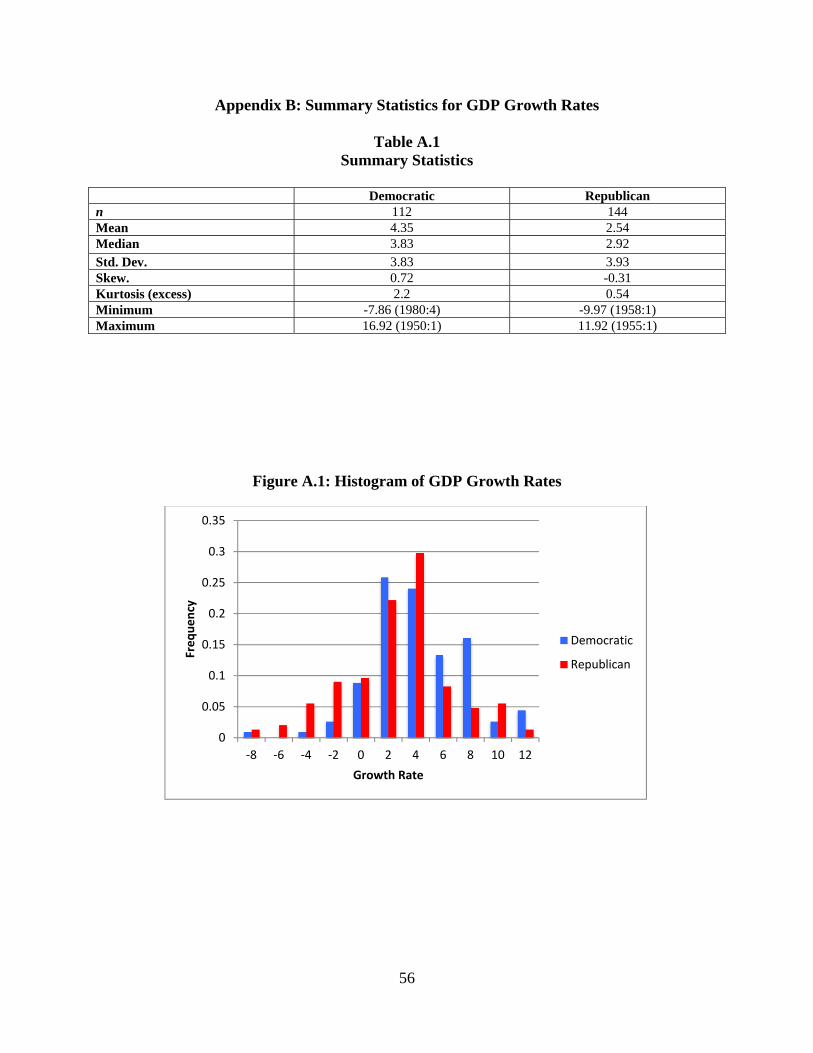
56

Appendix B: Summary Statistics for GDP Growth Rates

Table A.1 Summary Statistics

Democratic Republican n 112 144 Mean 4.35 2.54 Median 3.83 2.92 Std. Dev. 3.83 3.93 Skew. 0.72 -0.31 Kurtosis (excess) 2.2 0.54 Minimum -7.86 (1980:4) -9.97 (1958:1) Maximum 16.92 (1950:1) 11.92 (1955:1)

Figure A.1: Histogram of GDP Growth Rates

0

0.05

0.1

0.15

0.2

0.25

0.3

0.35

‐8 ‐6 ‐4 ‐2 0 2 4 6 8 10 12

Frequency

Growth Rate

Democratic

Republican

57

Appendix C: Additional Tables and Figures

Figure A.2 GDP growth rates and different trends

Trends: −−−−−− = ∞ −−−−−− = 100 −−−−−− = 67 −−−−−− = 33

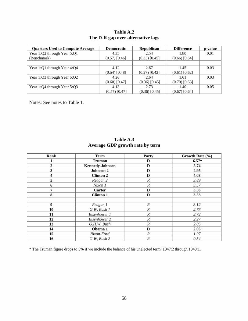
58

Table A.2 The D-R gap over alternative lags

Quarters Used to Compute Average Democratic Republican Difference p-value

Year 1:Q2 through Year 5:Q1 (Benchmark)

4.35 (0.57) [0.46]

2.54 (0.33) [0.45]

1.80 (0.66) [0.64]

0.01

Year 1:Q1 through Year 4:Q4 4.12

(0.54) [0.48] 2.67

(0.27) [0.42] 1.45

(0.61) [0.62] 0.03

Year 1:Q3 through Year 5:Q2 4.26 (0.60) [0.47]

2.64 (0.36) [0.45]

1.61 (0.70) [0.63]

0.03

Year 1:Q4 through Year 5:Q3 4.13 (0.57) [0.47]

2.73 (0.36) [0.45]

1.40 (0.67) [0.64]

0.05

Notes: See notes to Table 1.

Table A.3 Average GDP growth rate by term

Rank Term Party Growth Rate (%)

1 Truman D 6.57* 2 Kennedy-Johnson D 5.74 3 Johnson 2 D 4.95 4 Clinton 2 D 4.03 5 Reagan 2 R 3.89 6 Nixon 1 R 3.57 7 Carter D 3.56 8 Clinton 1 D 3.53 9 Reagan 1 R 3.12

10 G.W. Bush 1 R 2.78 11 Eisenhower 1 R 2.72 12 Eisenhower 2 R 2.27 13 G.H.W. Bush R 2.05 14 Obama 1 D 2.06 15 Nixon-Ford R 1.97 16 G.W, Bush 2 R 0.54

* The Truman figure drops to 5% if we include the balance of his unelected term: 1947:2 through 1949:1.

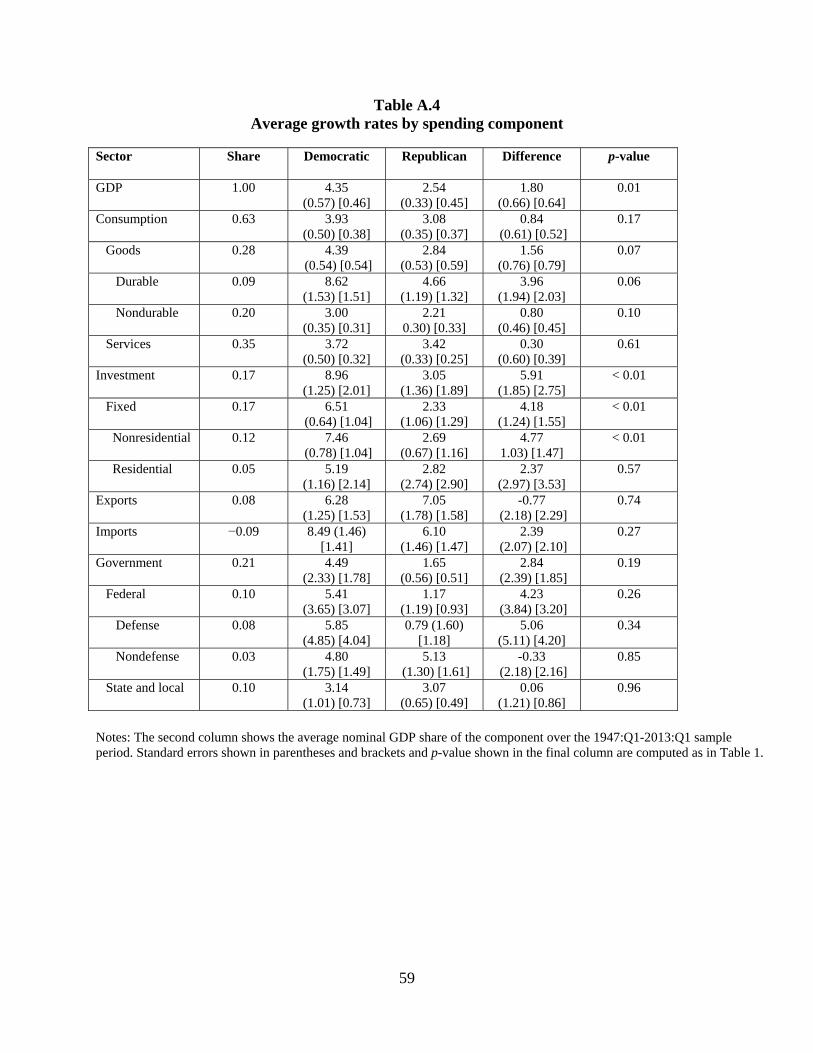
59

Table A.4 Average growth rates by spending component

Sector Share Democratic Republican Difference p-value

GDP 1.00 4.35 (0.57) [0.46]

2.54 (0.33) [0.45]

1.80 (0.66) [0.64]

0.01

Consumption 0.63 3.93 (0.50) [0.38]

3.08 (0.35) [0.37]

0.84 (0.61) [0.52]

0.17

Goods 0.28 4.39 (0.54) [0.54]

2.84 (0.53) [0.59]

1.56 (0.76) [0.79]

0.07

Durable 0.09 8.62 (1.53) [1.51]

4.66 (1.19) [1.32]

3.96 (1.94) [2.03]

0.06

Nondurable 0.20 3.00 (0.35) [0.31]

2.21 0.30) [0.33]

0.80 (0.46) [0.45]

0.10

Services 0.35 3.72 (0.50) [0.32]

3.42 (0.33) [0.25]

0.30 (0.60) [0.39]

0.61

Investment 0.17 8.96 (1.25) [2.01]

3.05 (1.36) [1.89]

5.91 (1.85) [2.75]

< 0.01

Fixed 0.17 6.51 (0.64) [1.04]

2.33 (1.06) [1.29]

4.18 (1.24) [1.55]

< 0.01

Nonresidential 0.12 7.46 (0.78) [1.04]

2.69 (0.67) [1.16]

4.77 1.03) [1.47]

< 0.01

Residential 0.05 5.19 (1.16) [2.14]

2.82 (2.74) [2.90]

2.37 (2.97) [3.53]

0.57

Exports 0.08 6.28 (1.25) [1.53]

7.05 (1.78) [1.58]

-0.77 (2.18) [2.29]

0.74

Imports −0.09 8.49 (1.46) [1.41]

6.10 (1.46) [1.47]

2.39 (2.07) [2.10]

0.27

Government 0.21 4.49 (2.33) [1.78]

1.65 (0.56) [0.51]

2.84 (2.39) [1.85]

0.19

Federal 0.10 5.41 (3.65) [3.07]

1.17 (1.19) [0.93]

4.23 (3.84) [3.20]

0.26

Defense 0.08 5.85 (4.85) [4.04]

0.79 (1.60) [1.18]

5.06 (5.11) [4.20]

0.34

Nondefense 0.03 4.80 (1.75) [1.49]

5.13 (1.30) [1.61]

-0.33 (2.18) [2.16]

0.85

State and local 0.10 3.14 (1.01) [0.73]

3.07 (0.65) [0.49]

0.06 (1.21) [0.86]

0.96

Notes: The second column shows the average nominal GDP share of the component over the 1947:Q1-2013:Q1 sample period. Standard errors shown in parentheses and brackets and p-value shown in the final column are computed as in Table 1.

60

Table A.5 Detailed forecasting results

A. Results for the SPF

Ca Cl1 Cl2 Ob1 Ni NF Re1 Re2 BI BII1 BII2 D R

Actual 3.6 3.7 4.2 2.4 0.2 -0.3 -2.5 3.1 1.3 1.4 3.7 3.5 1.0 Forecast

(SPF Dated Q1) 6.1 3.1 2.2 0.9 3.3* 4.3 3.0 3.7 1.6 3.2 3.5 3.1 3.2

Forecast (SPF Dated Q2)

5.8 3.1 2.4 0.7 2.5 4.0 2.5 3.3 1.6 2.2 3.3 3.0 2.8

B. Results for the Greenbook

Ca Cl1 Cl2 Ni NF Re1 Re2 BI BII1 BII2 D R Actual 3.6 3.7 4.2 0.2 -0.3 -2.5 3.1 1.3 1.4 3.7 3.8 1.0 Forecast 6.3 2.9 2.4 4.9 -0.1 3.3 2.0 2.8 3.9 3.8 2.8 Greenbook Date 2/9/77 1/29/93 1/29/97 2/7/73 1/28/81 2/6/85 2/1/89 1/25/01 1/26/05 Forecast 6.2 2.5 2.2 1.7* 4.9 0.8 2.9 1.8 2.2 3.7 3.6 2.6 Greenbook Date 5/11/77 5/14/77 5/15/97 5/21/69 5/9/73 5/13/81 5/15/85 5/10/89 5/9/01 4/28/05

C. Results for the Time Series Models (Nixon – Obama-1)

Ca Cl1 Cl2 Ob1 Ni NF Re1 Re2 BI BII1 BII2 D R

Actual 4.1 3.4 4.5 1.6 0.3 0.7 -2.5 4.1 2.8 1.4 3.1 3.4 1.4 AR 2.5 2.2 2.8 1.1 2.7 3.7 4.4 2.4 3.1 2.1 3.1 2.2 3.1

VAR 3.0 3.6 2.9 2.6 1.8 3.3 1.5 3.8 2.1 1.7 3.2 3.0 2.5 AR-NL 2.5 2.5 3.1 3.7 2.9 4.0 4.6 2.8 3.2 0.4 3.0 2.9 3.0

D. Results for the Time Series Models (Truman-2 – Obama-1)

Tr KJ Jo Ca Cl1 Cl2 Ob1 Ei1 Ei2 Ni NF Re1 Re2 BI BII1 BII2 D R

Actual 3.8 7.3 8.1 4.1 3.4 4.5 1.6 -1.8 -2.9 0.3 0.7 -2.5 4.1 2.8 1.4 3.1 4.7 0.6 AR 1.7 3.4 4.0 3.4 2.7 3.0 2.3 3.9 3.4 3.5 3.9 4.7 3.0 3.3 2.5 3.4 2.9 3.5

VAR 1.5 3.6 3.8 3.7 3.4 3.2 3.4 3.6 2.7 3.1 3.7 3.5 4.1 2.5 2.3 3.4 3.2 3.2 AR-NL 2.2 3.9 4.0 3.2 2.6 2.9 5.3 3.7 2.4 3.5 4.3 5.4 3.3 3.0 0.5 2.8 3.4 3.2

Notes: Values are averages of GDP growth rates from Q2 of the inaugural year to Q1 of the following year. The SPF forecasts shown in panel A are from surveys dated Q1 and Q2 of the inaugural year. The actual values shown panels A and B are are from the FRB Philadelphia real time data sets dated Q2 in year 3 of the administration. *Forecasts are for average growth rate in 1969:Q2-1969:Q4 because of missing data.

61

Table A.6 Correlation matrix of shocks

1 2 3 4 5 6 7 8 9 10 11 12 13 14 15 16 17 18 19 20 21

1 1.00 . . . . . . . . . . . . . . . . . . . .

2 -0.11 1.00 . . . . . . . . . . . . . . . . . . .

3 -0.07 -0.07 1.00 . . . . . . . . . . . . . . . . . .

4 0.01 0.02 0.23 1.00 . . . . . . . . . . . . . . . . .

5 0.00 -0.08 -0.02 0.08 1.00 . . . . . . . . . . . . . . . .

6 0.07 -0.02 0.13 0.00 0.07 1.00 . . . . . . . . . . . . . . .

7 -0.21 0.10 0.02 -0.08 -0.12 -0.10 1.00 . . . . . . . . . . . . . .

8 0.15 0.02 -0.06 0.06 0.00 -0.06 0.00 1.00 . . . . . . . . . . . . .

9 -0.01 0.17 -0.06 -0.07 -0.01 0.05 0.07 0.57 1.00 . . . . . . . . . . . .

10 -0.01 0.13 -0.12 -0.09 -0.04 -0.01 0.09 0.41 0.38 1.00 . . . . . . . . . . .

11 -0.05 0.02 0.13 0.09 0.07 -0.09 0.07 -0.03 0.02 -0.04 1.00 . . . . . . . . . .

12 0.06 -0.11 0.10 -0.37 0.11 0.13 -0.02 -0.13 0.01 0.04 0.03 1.00 . . . . . . . . .

13 -0.02 -0.20 0.07 -0.41 0.03 0.18 -0.02 -0.17 -0.01 0.08 -0.01 0.79 1.00 . . . . . . . .

14 -0.01 -0.13 0.04 -0.31 0.06 0.02 0.06 -0.01 0.07 0.01 0.03 0.49 0.64 1.00 . . . . . . .

15 -0.11 0.05 -0.11 0.00 -0.06 0.08 0.04 -0.08 -0.07 -0.12 -0.03 0.06 0.02 -0.43 1.00 . . . . . .

16 0.06 -0.15 0.08 0.19 0.03 0.02 0.05 0.09 0.01 0.05 0.07 -0.31 -0.30 0.02 -0.31 1.00 . . . . .

17 -0.01 -0.07 0.07 -0.02 -0.01 0.31 -0.05 -0.11 0.01 0.06 0.02 0.18 0.18 0.10 -0.04 0.34 1.00 . . . .

18 0.07 -0.11 0.05 0.00 0.09 0.03 -0.10 0.07 0.01 -0.04 0.02 0.05 0.10 0.42 -0.60 0.36 0.14 1.00 . . .

19 -0.21 -0.01 -0.05 -0.17 -0.03 0.03 -0.01 -0.09 -0.03 -0.01 -0.05 0.24 0.25 -0.02 0.41 -0.41 -0.09 -0.38 1.00 . .

20 -0.27 -0.04 0.05 -0.12 -0.02 0.09 0.03 -0.03 0.07 0.06 -0.06 0.07 0.22 0.04 0.17 -0.20 -0.01 -0.16 0.61 1.00 .

21 0.09 0.03 0.05 0.07 0.04 0.00 -0.03 0.07 0.13 0.01 0.06 -0.02 -0.06 -0.03 -0.09 0.13 0.05 0.19 -0.22 -0.34 1.00

Note: Time series used Number Series Number Series Number Series

1 Oil Shocks (Hamilton) 8 Taxes (Romer and Romer) 15 Ted Spread 2 Oil Shocks (Killian) 9 Taxes (Mertens and Ravn) 16 Baa-Aaa Spread 3 TFP Utilization Adj (Fernald) 10 Taxes (Mertens and Ravn) 17 EBP Spread (Gilchrist-Zakrajšek) 4 Labor Prod (SVAR, Gali) 11 Government Spending (SVAR) 18 FRB SLOOS 5 Defense Spending (Ramey) 12 Monetary Pol. (Romer and Romer) 19 Index of Cons. Sent. Current (ICC)6 Defense Spending (Fisher-Peters) 13 Monetary Pol. SVAR (Sims-Zha) 20 Index of Consumer Expectations (ICE) 7 International (European growth) 14 Monetary Pol. SVAR (Cholesky) 21 Uncertainty Index (BBD)

Notes: Correlations are computed over the longest common sample period for each pair of series. Sample correlations larger than 0.30 in absolute value are show in bold.

62

Appendix D: Accounting for the D-R gap using DSGE models

In this appendix, we ask how three DSGE models account for the D-R gap. The models were estimated over different sample periods (shown in the first row of Table A.7), and use somewhat different measures of output. The well-known Smets-Wouters (2007) (SW) model uses demeaned per capita values of real GDP; the Leeper, Plante, and Traum (LPT) (2010) (LPT) model uses per capita measures, log-detrended values of consumption, investment, and government spending, with per capita GDP computed from C+I+G using a log-linear approximation; and the Schmitt-Grohé and Uribe (2012) (SGU) model use GDP growth rates. The second row of Table A.7 shows the D-R gap computed using the model-specific sample periods and data. The D-R gap ranges between 1.15 and 1.53 percentage points.

The remaining rows of the table decompose each D-R gap using realizations of the shocks for the relevant models. While the list of shocks differs substantially across models, we have tried to group the shocks into familiar categories (TFP, Investment, and so forth).48

Neutral productivity shocks explain approximately 20 basis points of the D-R gap in each of the models. This is smaller than the approximate 30 basis points for utilization-adjusted TFP shocks shown in panel B of Table 9, although some of the difference is explained by differences in the sample periods. Both the SW and LPT models attribute much of the D-R gap to investment-specific productivity shocks, but these have little effect in the SGU model. The LPT and SGU models attribute much of the D-R gap to labor shocks (labor supply shocks in LPT, and wage markup shocks in SGU). Wage markup shocks are modestly important in the SW model, but labor supply shocks have huge effects in the LPT model. Intertemporal preference shocks have large, but inconsistent, effects across the models.

These models suggest (or impose) little role for policy in explaining the D-R gap. Monetary shocks in the SW model favor Republicans, which is consistent the evidence presented in Tables 6 and 9. Shocks to government purchases have little effect in any of the models--although the earliest sample period begins in 1955 and thus does not the Korean War. This is also consistent with our reduced-form findings. Finally, the tax and transfer shocks in the LPT model do not explain the D-R gap.

48 For the SGU model, the TFP and Investment categories include the contributions from the stationary and non-stationary shocks in the model, and each category includes both realized and anticipated shocks. Detailed results for the SGU model are presented in appendix Table A.8.

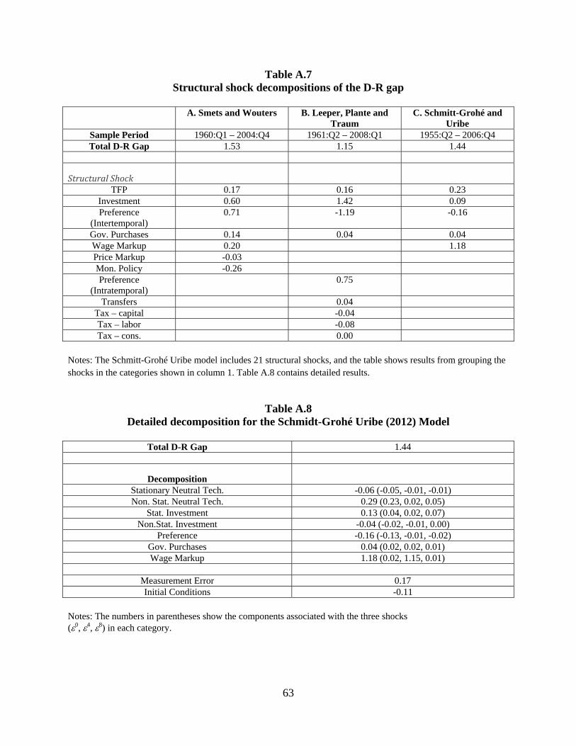
63

Table A.7 Structural shock decompositions of the D-R gap

A. Smets and Wouters

B. Leeper, Plante and

Traum C. Schmitt-Grohé and

Uribe Sample Period 1960:Q1 – 2004:Q4 1961:Q2 – 2008:Q1 1955:Q2 – 2006:Q4 Total D-R Gap 1.53 1.15 1.44

StructuralShock

TFP 0.17 0.16 0.23 Investment 0.60 1.42 0.09 Preference

(Intertemporal) 0.71 -1.19 -0.16

Gov. Purchases 0.14 0.04 0.04 Wage Markup 0.20 1.18 Price Markup -0.03 Mon. Policy -0.26 Preference

(Intratemporal) 0.75

Transfers 0.04 Tax – capital -0.04 Tax – labor -0.08 Tax – cons. 0.00

Notes: The Schmitt-Grohé Uribe model includes 21 structural shocks, and the table shows results from grouping the shocks in the categories shown in column 1. Table A.8 contains detailed results.

Table A.8

Detailed decomposition for the Schmidt-Grohé Uribe (2012) Model

Total D-R Gap 1.44

Decomposition

Stationary Neutral Tech. -0.06 (-0.05, -0.01, -0.01) Non. Stat. Neutral Tech. 0.29 (0.23, 0.02, 0.05)

Stat. Investment 0.13 (0.04, 0.02, 0.07) Non.Stat. Investment -0.04 (-0.02, -0.01, 0.00)

Preference -0.16 (-0.13, -0.01, -0.02) Gov. Purchases 0.04 (0.02, 0.02, 0.01) Wage Markup 1.18 (0.02, 1.15, 0.01)

Measurement Error 0.17 Initial Conditions -0.11

Notes: The numbers in parentheses show the components associated with the three shocks (0, 4, 8) in each category.