pressurised water reactor main steam line · pdf filepressurised water reactor main steam line...
TRANSCRIPT
NEA/NSC/DOC(2000)21
NEA NUCLEAR SCIENCE COMMITTEENEA COMMITTEE ON SAFETY OF NUCLEAR INSTALLATIONS
PRESSURISED WATERREACTOR MAIN STEAM LINEBREAK (MSLB) BENCHMARK
Volume II: Summary Results of Phase I (Point Kinetics)
by
T. Beam, K. Ivanov, B. Taylor and A. BarettaNuclear Engineering Program
The Pennsylvania State UniversityUniversity Park, PA 16802, USA
December 2000
US Nuclear Regulatory CommissionOECD Nuclear Energy Agency

ORGANISATION FOR ECONOMIC CO-OPERATION AND DEVELOPMENT
Pursuant to Article 1 of the Convention signed in Paris on 14th December 1960, and which came into forceon 30th September 1961, the Organisation for Economic Co-operation and Development (OECD) shall promote policiesdesigned:
to achieve the highest sustainable economic growth and employment and a rising standard of living in Member countries,while maintaining financial stability, and thus to contribute to the development of the world economy;
to contribute to sound economic expansion in Member as well as non-member countries in the process of economicdevelopment; and
to contribute to the expansion of world trade on a multilateral, non-discriminatory basis in accordance with internationalobligations.
The original Member countries of the OECD are Austria, Belgium, Canada, Denmark, France, Germany,Greece, Iceland, Ireland, Italy, Luxembourg, the Netherlands, Norway, Portugal, Spain, Sweden, Switzerland, Turkey,the United Kingdom and the United States. The following countries became Members subsequently through accession atthe dates indicated hereafter: Japan (28th April 1964), Finland (28th January 1969), Australia (7th June 1971), NewZealand (29th May 1973), Mexico (18th May 1994), the Czech Republic (21st December 1995), Hungary (7th May1996), Poland (22nd November 1996) and the Republic of Korea (12th December 1996). The Commission of theEuropean Communities takes part in the work of the OECD (Article 13 of the OECD Convention).
NUCLEAR ENERGY AGENCY
The OECD Nuclear Energy Agency (NEA) was established on 1st February 1958 under the name of theOEEC European Nuclear Energy Agency. It received its present designation on 20th April 1972, when Japan became itsfirst non-European full Member. NEA membership today consists of 27 OECD Member countries: Australia, Austria,Belgium, Canada, Czech Republic, Denmark, Finland, France, Germany, Greece, Hungary, Iceland, Ireland, Italy,Japan, Luxembourg, Mexico, the Netherlands, Norway, Portugal, Republic of Korea, Spain, Sweden, Switzerland,Turkey, the United Kingdom and the United States. The Commission of the European Communities also takes part inthe work of the Agency.
The mission of the NEA is:
− to assist its Member countries in maintaining and further developing, through international co-operation,the scientific, technological and legal bases required for a safe, environmentally friendly and economicaluse of nuclear energy for peaceful purposes, as well as
− to provide authoritative assessments and to forge common understandings on key issues, as input togovernment decisions on nuclear energy policy and to broader OECD policy analyses in areas such asenergy and sustainable development.
Specific areas of competence of the NEA include safety and regulation of nuclear activities, radioactivewaste management, radiological protection, nuclear science, economic and technical analyses of the nuclear fuel cycle,nuclear law and liability, and public information. The NEA Data Bank provides nuclear data and computer programservices for participating countries.
In these and related tasks, the NEA works in close collaboration with the International Atomic EnergyAgency in Vienna, with which it has a Co-operation Agreement, as well as with other international organisations in thenuclear field.
© OECD 2000Permission to reproduce a portion of this work for non-commercial purposes or classroom use should be obtained through the Centrefrançais d’exploitation du droit de copie (CCF), 20, rue des Grands-Augustins, 75006 Paris, France, Tel. (33-1) 44 07 47 70, Fax (33-1)46 34 67 19, for every country except the United States. In the United States permission should be obtained through the CopyrightClearance Center, Customer Service, (508)750-8400, 222 Rosewood Drive, Danvers, MA 01923, USA, or CCC Online:http://www.copyright.com/. All other applications for permission to reproduce or translate all or part of this book should be made toOECD Publications, 2, rue André-Pascal, 75775 Paris Cedex 16, France.

3
FOREWORD
Since the beginning of the pressurised water reactor (PWR) main steam line break (MSLB)benchmark activities, four benchmark workshops have taken place. The first was held in WashingtonDC, USA (April 1997), the second in Madrid, Spain (June 1998), the third in Garching near Munich,Germany (March 1999) and the fourth in Paris, France (January 2000). It was agreed that inperforming this series of exercises participants were working at the edge of present developments inthe coupling of neutronics and thermal hydraulics, and that this benchmark would lead to a commonbackground understanding of the key issues. It was also agreed that the PWR MSLB Benchmarkwould be published in four volumes.
Volume 1 of the PWR MSLB Benchmark: Final Specifications, was issued by the OECD/NEAin April 1999 [NEA/NSC/DOC(99)8]. A small team at Pennsylvania State University (PSU) wasresponsible for authoring the final specifications, co-ordinating the benchmark activities, answeringquestions, analysing the solutions submitted by benchmark participants and providing reportssummarising the results for each phase. In performing these tasks the PSU team collaborated withAdi Irani and Nick Trikouros of GPU Nuclear, Inc.
Volume 2 summarises the results of Phase I on point kinetics. The report is supplemented by briefdescriptions of the system codes used, as provided by the participants. In addition, detaileddescriptions (including graphs where useful) of the models used are given. These are presented asanswers to the questionnaire for the first exercise, so that compliance with the specifications can beverified. The list of deviations from the specifications, if any, is provided, and any specific assumptionsare stated. Based on the information provided, the benchmark co-ordinators and report reviewersdecided whether the models used in the solutions provided by the participants complied sufficientlywith the system model’s specifications. Solutions that deviated in the modelling in ways not compatiblewith the specifications were not included in the statistical evaluation procedure.
4
Acknowledgements
This report is dedicated to the students of Penn State University, the next generation of nuclearengineers, who are the reason why we are here.
The authors would like to thank Dr. H. Finnemann of Siemens, Dr. S. Langenbuch from theGesellschaft für Reaktorsicherheit (GRS), and Professor J. Aragones from Universidad PolitécnicaMadrid (UPM), whose support and encouragement in establishing and carrying out this benchmarkwere invaluable.
This report is the sum of many efforts, by the participants, the sponsoring agencies – the USNuclear Regulatory Commission and the OECD Nuclear Energy Agency – and their staff. Specialappreciation goes to the report reviewers: Adi Irani from GPU Nuclear Inc., Dr. S. Langenbuch fromGRS, and Dr. A. Knoll from Siemens. Their comments and suggestions were very valuable andsignificantly improved the quality of this report. We would like to thank them for the effort and timeinvolved.
Particularly noteworthy were the efforts of Farouk Eltawila assisted by David Ebert, both of theUS Nuclear Regulatory Commission. With their help, funding was secured, enabling this project toproceed. We also thank them for their excellent technical advice and assistance.
The authors wish to express their sincere appreciation for the outstanding support offered byDr. Enrico Sartori, who not only provided efficient administration, organisation and valuable technicalrecommendations, but most importantly provided friendly counsel and advice.
Finally, we are grateful to Nadejda Todorova and Amanda Costa for having devoted theircompetence and skills to the final editing of this report.

5
TABLE OF CONTENTS
FOREWORD...................................................................................................................................... 3
Acknowledgements ............................................................................................................................. 4
Chapter 1. INTRODUCTION........................................................................................................ 9
Chapter 2. DESCRIPTION OF FIRST BENCHMARK EXERCISE ....................................... 11
Description of MSLB transient ...................................................................................... 11
Simulated transient scenario .......................................................................................... 12
Initial steady state conditions......................................................................................... 13
Reactor point kinetics parameters .................................................................................. 13
Analysis assumptions..................................................................................................... 16
Chapter 3. STATISTICAL METHODOLOGY........................................................................... 21
Standard techniques for comparison of results .............................................................. 21
Time history data ........................................................................................................... 21
Reference results............................................................................................................ 22
Chapter 4. RESULTS AND DISCUSSION .................................................................................. 25
Break flow rate............................................................................................................... 25
Pressure.......................................................................................................................... 26
Temperatures ................................................................................................................. 27
Reactor power ................................................................................................................ 30
Reactivity ....................................................................................................................... 33
Steam generator mass .................................................................................................... 33
Sequence of events......................................................................................................... 35
Chapter 5. CONCLUSIONS .......................................................................................................... 65
6
REFERENCES................................................................................................................................... 69
APPENDIX A – Description of computer codes used for analysis in the first phaseof the PWR MSLB benchmark................................................................................ 71
APPENDIX B – Sequence of events for the first phase of the PWR MSLB benchmark ................... 77
APPENDIX C – Questionnaire for the first phase of the PWR MSLB benchmark........................... 83
List of figures
Figure 2.1. EOC HFP assembly relative radial power distribution (quarter core symmetry) ............ 16
Figure 2.2. EOC HFP core average power relative power distribution.............................................. 16
Figure 2.3. Steam line nodalisation .................................................................................................... 17
Figure 4.1. Total break flow rate ........................................................................................................ 37
Figure 4.2. Break flow rate – 24 inch................................................................................................. 38
Figure 4.3. Break flow rate – 8 inch................................................................................................... 39
Figure 4.4. Average pressure.............................................................................................................. 40
Figure 4.5. Broken loop pressure ....................................................................................................... 41
Figure 4.6. Intact loop pressure .......................................................................................................... 42
Figure 4.7. Pressuriser pressure.......................................................................................................... 43
Figure 4.8. Broken steam line pressure .............................................................................................. 44
Figure 4.9. Intact steam line pressure................................................................................................. 45
Figure 4.10. Average coolant temperature ......................................................................................... 46
Figure 4.11. Broken hot leg temperature............................................................................................ 47
Figure 4.12. Intact hot leg temperature .............................................................................................. 48
Figure 4.13. Broken cold leg temperature .......................................................................................... 49
Figure 4.14. Intact cold leg temperature............................................................................................. 50
Figure 4.15. Fuel temperature ............................................................................................................ 51
Figure 4.16. Fission power ................................................................................................................. 52
Figure 4.17. Total power .................................................................................................................... 53

7
Figure 4.18. Decay power .................................................................................................................. 54
Figure 4.19. Total reactivity ............................................................................................................... 55
Figure 4.20. Moderator reactivity....................................................................................................... 56
Figure 4.21. Doppler reactivity .......................................................................................................... 57
Figure 4.22. Scram reactivity ............................................................................................................. 58
Figure 4.23. Broken steam generator mass......................................................................................... 59
Figure 4.24. Intact steam generator mass ........................................................................................... 60
Figure 4.25. Heat transfer: broken steam generator ........................................................................... 61
Figure 4.26. Heat transfer: intact steam generator.............................................................................. 62
Figure 4.27. Integrated leakage: vapour mass .................................................................................... 63
Figure 4.27. Integrated leakage: liquid mass...................................................................................... 64
List of tables
Table 1.1. List of participants in the first phase of the PWR MSLB benchmark ............................... 10
Table 2.1. Initial conditions for TMI-1 at 2 772 MWt........................................................................ 13
Table 2.2. Summary of point kinetics analysis input values .............................................................. 15
Table 2.3. Delay constants and fractions of delayed neutrons ........................................................... 15
Table 2.4. Rod worth versus time after trip (Versions 1 and 2) ......................................................... 15
Table 2.5. MSLB analysis assumptions ............................................................................................. 17
Table 2.6. Description of MSSVs per OTSG ..................................................................................... 18
Table 2.7. Main feedwater flow boundary conditions to broken SG.................................................. 18
Table 2.8. Main feedwater flow boundary conditions to intact steam generator................................ 18
Table 2.9. HPI flow versus pressure................................................................................................... 19
Table 4.1. Deviations: total break flow rate, 24 inch break flow rate and 8 inch breakflow rate at end of transient ............................................................................................... 26
Table 4.2. Deviations: average pressure, pressure in the broken loop and pressurein the intact loop ................................................................................................................ 27

8
Table 4.3. Deviations: broken steam line pressure, intact steam line pressure andpressuriser pressure ........................................................................................................... 28
Table 4.4. Deviations: broken loop hot and cold leg temperatures at the end of transient................. 29
Table 4.5. Deviations: intact loop hot and cold leg temperatures at the end of transient ................... 29
Table 4.6. Deviations: average moderator temperature and fuel temperature at theend of the transient ............................................................................................................ 30
Table 4.7. Deviations: time of reactor trip (initial peak) and time of highest powerafter trip (second peak)...................................................................................................... 31
Table 4.8. Deviations: percentage of initial power at time of reactor trip (initial peak), timeof highest power after trip (second peak) and end of transient for total power................. 32
Table 4.9. Deviations: percentage of initial power at time of reactor trip (initial peak), timeof highest power after trip (second peak) and end of transient for fission power ............. 32
Table 4.10. Deviations: total reactivity at time of highest power after reactor trip and atend of transient ................................................................................................................ 34
Table 4.11. Deviations: moderator reactivity, Doppler reactivity and scram reactivity atend of transient ................................................................................................................ 34

9
Chapter 1
INTRODUCTION
Incorporation of a full three-dimensional (3-D) reactor core model into system transient codesallows “best-estimate” simulations of interactions between reactor core behaviour and plant dynamics.Until recently, few system transient codes incorporated full 3-D modelling of the reactor core;however, recent progress in computer technology made the development of such coupled code systemsfeasible. Unfortunately, there is limited experience using this technology. One way to verify theperformance of these computer codes is to develop plant transient benchmarks for which a 3-Dneutronics core model can be used and verified. The Nuclear Energy Agency Nuclear ScienceCommittee (NEA NSC) has developed such a series of benchmarks.
Over the past eight years, the NEA NSC has developed a series of benchmark problems to studythe accuracy of the computer codes used to obtain solutions for coupled space-time kinetics/thermal-hydraulic problems in nuclear reactors. These benchmarks, based on well-defined problemswith a complete set of input data, are used to verify the data exchange and test the neutronics couplingto the fuel-rod-heat conduction solution methodology [1]. This series of benchmarks studies 3-D coretransient calculations for light water reactors (LWR), boiling water reactors (BWR) and pressurisedwater reactors (PWR). A recent addition to this series, sponsored by the Organisation for EconomicCo-operation and Development (OECD), United States Nuclear Regulatory Commission (US NRC),and the Pennsylvania State University (PSU), is the PWR Main Steam Line Break (MSLB) benchmarkproblem [2].
The PWR MSLB benchmark problem uses a three-dimensional neutronics core model to furtherverify the capability of coupled codes to analyse complex transients with coupled core-plantinteractions and to fully test the thermal-hydraulic coupling. It is based on real plant design andoperational data for the Three Mile Island Unit 1 nuclear power plant (TMI-1 NPP). The purpose ofthis benchmark is threefold: to verify the capability of system codes to analyse complex transientswith coupled core-plant interactions; to fully test the 3-D neutronics/thermal-hydraulic coupling; andto evaluate discrepancies between the predictions of coupled codes in best-estimate transient simulations.
The purposes of this benchmark are met via the use of three exercises that are briefly describedbelow [3]:
1. A point kinetics plant simulation, which models the primary and secondary systems.The purpose of this exercise is to test the thermal-hydraulic system response. The participantsare provided with compatible point kinetics model inputs that preserve axial and radial powerdistribution, and scram reactivity obtained using a 3-D core neutronics model and a completesystem description.
2. A coupled 3-D neutronics thermal-hydraulics evaluation of core response. The purposeof this phase is to test the neutronics response to imposed thermal-hydraulic conditions.The participants are provided with transient boundary conditions (radial distribution of mass
10
flow rates and liquid temperatures at the core inlet, and radial averaged pressure versus timeat both the core inlet and outlet), the initial axial liquid velocities, the initial axial distributionof liquid temperatures and a complete core description.
3. A best-estimate coupled core-plant transient model. This exercise simulates the entiretransient and combines the first two exercises, fully testing the thermal-hydraulic/neutroniccoupling.
A small benchmark team at PSU is responsible for authoring the final specification for the PWRMSLB benchmark problem, answering questions, analysing the solutions submitted by benchmarkparticipants and providing reports summarising the results for each phase.
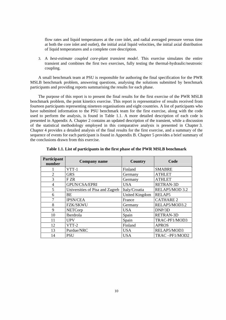
The purpose of this report is to present the final results for the first exercise of the PWR MSLBbenchmark problem, the point kinetics exercise. This report is representative of results received fromfourteen participants representing nineteen organisations and eight countries. A list of participants whohave submitted information to the PSU benchmark team for the first exercise, along with the codeused to perform the analysis, is found in Table 1.1. A more detailed description of each code ispresented in Appendix A. Chapter 2 contains an updated description of the transient, while a discussionof the statistical methodology employed in this comparative analysis is presented in Chapter 3.Chapter 4 provides a detailed analysis of the final results for the first exercise, and a summary of thesequence of events for each participant is found in Appendix B. Chapter 5 provides a brief summary ofthe conclusions drawn from this exercise.
Table 1.1. List of participants in the first phase of the PWR MSLB benchmark
Participantnumber Company name Country Code
1 VTT-1 Finland SMABRE2 GRS Germany ATHLET3 F ZR Germany ATHLET4 GPUN/CSA/EPRI USA RETRAN-3D5 Universities of Pisa and Zagreb Italy/Croatia RELAP5/MOD 3.26 BE United Kingdom RELAP57 IPSN/CEA France CATHARE 28 FZK/SKWU Germany RELAP5/MOD3.29 NETCorp USA DNP/3D
10 Iberdrola Spain RETRAN-3D11 UPV Spain TRAC-PF1/MOD312 VTT-2 Finland APROS13 Purdue/NRC USA RELAP5/MOD314 PSU USA TRAC –PF1/MOD2

11
Chapter 2
DESCRIPTION OF FIRST BENCHMARK EXERCISE
The transient chosen for this benchmark is a simulated main steam line break (MSLB) transient ina pressurised water reactor (PWR). The PWR in this case is modelled after real plant design andoperational data for the Three Mile Island Unit 1 nuclear power plant (TMI-1 NPP). Traditionally, thisproblem has been modelled using the point kinetics approach. Unfortunately, the point kineticsapproach requires the use of extremely conservative assumptions in order to account for the asymmetryin the core region that takes place during the transient. These conservative assumptions unnecessarilylimit the ability of the plant to undergo power upgrades or extended fuel cycles. Using the 3-D kineticsapproach for this transient may provide a margin to re-criticality over the point kinetics, thus allowingfor the improvement of both operational flexibility and nuclear power plant performance. The purposeof this chapter is to provide a detailed description of the simulated main steam line break transientspecified for this benchmark problem.
Description of MSLB transient
Significant space-time effects in the core caused by asymmetric cooling and an assumed stuck-outcontrol rod during reactor trip characterise the MSLB transient. The asymmetry in the reactor core,both neutronically and thermal-hydraulically, is caused by the expected power tilt, and makes thistransient difficult to analyse. Realistic simulation requires evaluation of core response using a coupled3-D neutronics/core thermal-hydraulics code supplemented by a 1-D simulation of the remainder ofthe reactor coolant system (RCS). The limiting MSLB for TMI-1 is at hot full power (HFP) becausethe steam generator liquid inventory increases with increasing power level. The worst case overcoolingoccurs at the maximum power level, which corresponds to the maximum liquid inventory in the steamgenerator (SG).
As mentioned previously, the reference problem for this benchmark is a simulated MSLBresulting from the double-ended rupture of one steam line upstream of the cross-connect. The steamline break results in the loss of secondary coolant, and the broken SG depressurises, while the intactSG is isolated when the turbine stop valves slam shut. As a result of the break in the steam line thesteam flow rate in the broken SG increases, thus improving heat transfer and lowering the averagereactor coolant temperature. As the average reactor coolant temperature decreases, the power begins toincrease. Unfortunately, the loop with the break sees a great deal of cooling, while the intact loop seeslittle, if any, cooling throughout the transient. Because of the difference in temperatures between thetwo loops, one would expect to see a power tilt within the core to the cooler side.
The power tilt within the core region is expected because of the negative moderator temperaturecoefficient. A reactor trip occurs due to either low reactor coolant pressure or high neutron flux.Following the reactor trip, the turbine trips and the turbine stop valves and feedwater control valvesclose. Low steam line pressure initiates automatic feedwater isolation, which causes the steamgenerator associated with the rupture to blow dry. While not modelled for this exercise, continuedRCS cool-down and decay heat removal would be achieved by emergency feedwater (EFW) flow to

12
the intact SG with steam flow through the turbine bypass valve. The high-pressure injection (HPI)system may be activated due to low RCS pressure during the cool-down period following a large areasteam line break.
One of the major concerns for the MSLB transient is the return to power and criticality in thelatter half of the transient. Because of this concern, the MSLB scenario is based on assumptions thatconservatively maximise the consequences for a return to power. These assumptions, along with adetailed description of the reference problem, can be found in the following paragraphs.
Simulated transient scenario
The double-ended rupture of one steam line is assumed to occur upstream of the MSIVs at thecross-connect. The rupture of the 24 inch (60.96 cm) outer diameter main steam line (this is the largestpossible break) results in the highest break flow and maximises the RCS cool-down. The worst singlefailure is the mechanical failure in the open position of the feedwater regulating valve associated withthe affected SG. This failure causes feedwater to cross the common header from the intact to thebroken steam generator, thus maximising feedwater flow to the broken steam generator. Closing thefeedwater block valve 30 seconds after the break occurs terminates the feedwater flow to the brokenSG. This is a conservative assumption and helps to maximise RCS cool-down.
Following break initiation and reactor scram, the steam line turbine stop valves slam shut,effectively isolating the intact steam generator. The 8 inch (20.32 cm) cross-connect between the twosteam lines of the broken SG remains open.
Since maximising the primary to secondary heat transfer results in maximum RCS cool-down, allfour RCS pumps are assumed to operate during the event. No credit is taken for pressuriser heateroperation. This conservative assumption enhances the RCS depressurisation.
The reactor trip is modelled to occur when the neutron power reaches 114% of 2 772 MWt, orwhen the primary system pressure at the hot leg pressure tap reaches 1 945 psia (13.41 MPa). A tripdelay of 0.4 seconds is used for the high neutron flux trip, while the low RCS pressure trip delay is0.5 seconds. These values bound the actual delays for TMI-1 and represent the delay from the time thetrip condition is reached until the time the control rods are free to fall.
The high-pressure injection (HPI) system initiates with a 25 second delay when the primarysystem pressure drops to 1 645 psia (11.34 MPa). HPI is expected to activate because of the largeovercooling which occurs during this simulated MSLB transient. No credit is taken for the negativereactivity insertion from the addition of boron, and no other emergency core coolant system (ECCS)action is expected.
Since the primary-to-secondary heat transfer is the driving force behind the RCS cool-down anddepressurisation, the choice of initial steam generator inventory is important to provide the adequatecool-down capability. An initial steam generator inventory of 57 320 lbm (26 000 kg) is assumed.In addition, the mass of the feedwater between the feedwater isolation valve and the affected steamgenerator, calculated to be 35 500 lbm (16 103 kg), is modelled as part of the feedwater function andcontributes to the overcooling and depressurisation of the RCS.
Vessel mixing is based on test data from Duke Power Company’s Oconee Plant, also a B&Wdesign plant. These tests define the amount of mixing that occurs within the vessel as a ratio of the
13
difference in hot leg temperatures to the difference in cold leg temperatures. There is 20% mixing inthe lower plenum and 80% in the upper plenum, and the ratio (dThot/dTcold) is chosen to be 0.5, aconservative estimate.
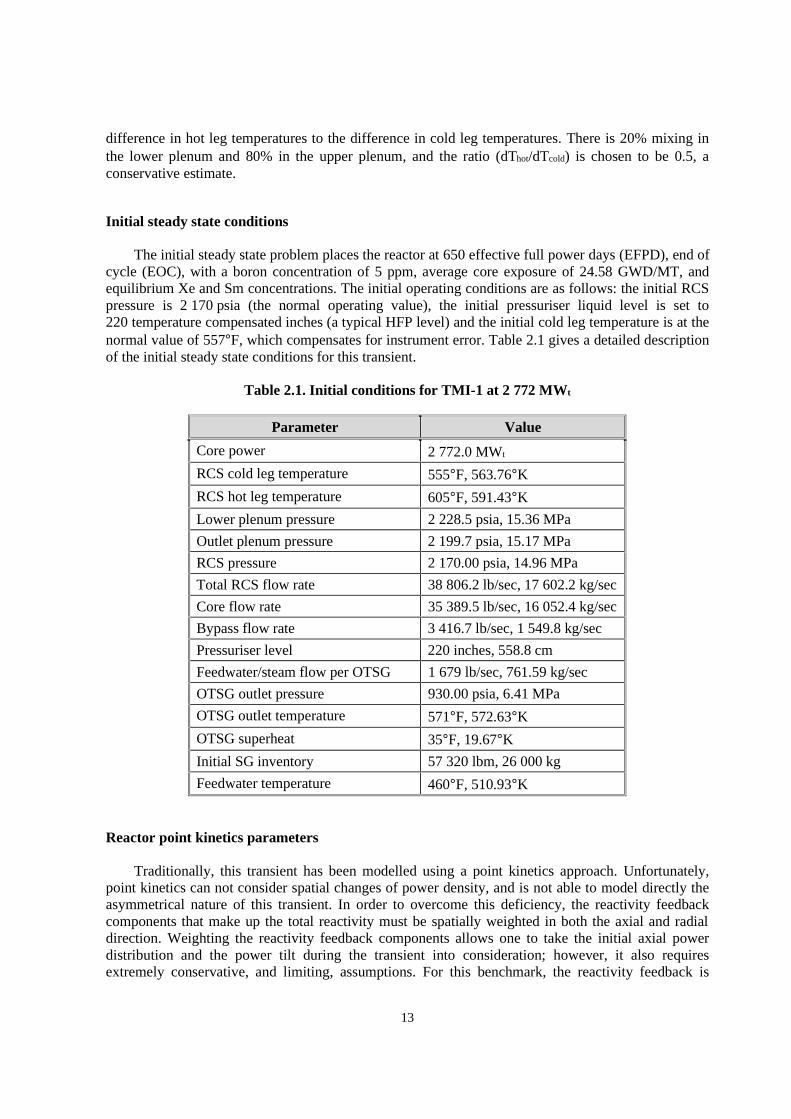
Initial steady state conditions
The initial steady state problem places the reactor at 650 effective full power days (EFPD), end ofcycle (EOC), with a boron concentration of 5 ppm, average core exposure of 24.58 GWD/MT, andequilibrium Xe and Sm concentrations. The initial operating conditions are as follows: the initial RCSpressure is 2 170 psia (the normal operating value), the initial pressuriser liquid level is set to220 temperature compensated inches (a typical HFP level) and the initial cold leg temperature is at thenormal value of 557°F, which compensates for instrument error. Table 2.1 gives a detailed descriptionof the initial steady state conditions for this transient.
Table 2.1. Initial conditions for TMI-1 at 2 772 MWt
Parameter Value
Core power 2 772.0 MWt
RCS cold leg temperature 555°F, 563.76°K
RCS hot leg temperature 605°F, 591.43°K
Lower plenum pressure 2 228.5 psia, 15.36 MPa
Outlet plenum pressure 2 199.7 psia, 15.17 MPa
RCS pressure 2 170.00 psia, 14.96 MPa
Total RCS flow rate 38 806.2 lb/sec, 17 602.2 kg/sec
Core flow rate 35 389.5 lb/sec, 16 052.4 kg/sec
Bypass flow rate 3 416.7 lb/sec, 1 549.8 kg/sec
Pressuriser level 220 inches, 558.8 cm
Feedwater/steam flow per OTSG 1 679 lb/sec, 761.59 kg/sec
OTSG outlet pressure 930.00 psia, 6.41 MPa
OTSG outlet temperature 571°F, 572.63°K
OTSG superheat 35°F, 19.67°K
Initial SG inventory 57 320 lbm, 26 000 kg
Feedwater temperature 460°F, 510.93°K
Reactor point kinetics parameters
Traditionally, this transient has been modelled using a point kinetics approach. Unfortunately,point kinetics can not consider spatial changes of power density, and is not able to model directly theasymmetrical nature of this transient. In order to overcome this deficiency, the reactivity feedbackcomponents that make up the total reactivity must be spatially weighted in both the axial and radialdirection. Weighting the reactivity feedback components allows one to take the initial axial powerdistribution and the power tilt during the transient into consideration; however, it also requiresextremely conservative, and limiting, assumptions. For this benchmark, the reactivity feedback is

14
weighted axially by the core average relative axial power distribution calculated using the 3-D nodalcode. Radially, the reactivity feedback is weighted by the assembly relative radial power distribution(quarter core symmetry) calculated using the 3-D nodal code. In each case, the distributions are takenusing EOC, HFP conditions.
In order to make the point kinetics and 3-D simulations compatible, one must specify pointkinetics model inputs, which preserve axial and radial core power distributions, as well as scramreactivity obtained with the 3-D nodal core model. The following parameters for the point kineticsmodel and the 3-D neutronic transient core model should be consistent:
• Tripped rod worth.
• Radial power distribution.
• Axial power distribution.
• Moderator temperature coefficient.
• Doppler coefficient.
• Kinetics parameters.
In addition to the parameters specified above, all initial and boundary conditions must be identicalbetween the two cases. The scram worth and maximum stuck rod worth at control rod position N12are calculated using the 3-D nodal core model. These values are calculated at EOC, hot zero power(HZP) for the conditions shown below:
• Power level equal to 2 772 MWt, full flow and operating pressure.
• Boron concentration of 5 ppm.
• All control rods in except Group 8 (axial power shape rods – APSR).
• Xe distribution fixed at HFP conditions.
• Moderator temperature of 532°F (551°K).
An estimated value for the tripped rod worth (TRW) was calculated for use as an input parameterin the point kinetics simulation based on the calculated values for the scram and maximum stuck rodworth, and including a 10% rod worth uncertainty at HZP. This scenario is the basic scenario, calledVersion 1 (V1), and it is used in the current licensing practice. The second scenario version wasdefined – Version 2 (V2), for the purposes of the second and third exercises in order to better test theneutronics/thermal-hydraulic coupling. The difference is in the calculated TRW value; the minimumvalue estimated with the 3-D nodal code is used. A summary of the input values for the point kineticsanalysis is shown in Table 2.2. Table 2.3 shows the time constants and fractions of delayed neutronsfor the six delayed neutron groups used for neutron modelling. EOC, HFP radial and axial relativepower distributions (based on 24 equal nodes with an axial height of 14.88 cm) are shown inFigures 2.1 and 2.2, respectively. A scram reactivity table is provided in Table 2.4.

15
Table 2.2. Summary of point kinetics analysis input values
Parameter ValueHFP EOC MTC -34.64 pcm/°F, -62.35 pcm/°KHFP EOC DTC -1.43 pcm/°F, -2.57 pcm/°K
HFP EOC delayed neutron fraction (βeff) 0.5211E-02HFP EOC prompt neutron lifetime 0.18445E-04
EOC TRW – V1 4.526% dk/kEOC TRW – V2 3.040% dk/k
Table 2.3. Decay constants and fractions of delayed neutrons
Group Decayconstant (s-1)
Relative fraction ofdelayed neutrons (%)
1 0.012818 0.01532 0.031430 0.10863 0.125062 0.09654 0.329776 0.20195 1.414748 0.07916 3.822362 0.0197
Total fraction of delayed neutrons: 0.5211%.
Table 2.4. Rod worth versus time after trip (Versions 1 and 2)
Time afterreactor trip
(seconds)
Per cent ofreactivity
insertion (%)
Rod worthinserted*(% dk/k)
Rod worthinserted**(% dk/k)
0.0 0.0 -0.000 -0.0000.2 0.58 -0.026 -0.0180.3 0.99 -0.045 -0.0300.4 1.83 -0.083 -0.0560.6 5.29 -0.239 -0.1610.8 12.33 -0.558 -0.3751.0 21.41 -0.969 -0.6511.2 33.09 -1.498 -0.1011.4 50.75 -2.297 -1.4281.6 72.96 -3.302 -2.2181.8 91.30 -4.132 -2.7762.0 99.26 -4.493 -3.0182.2 99.99 -4.526 -3.0402.3 100.00 -4.526 -3.040106 100.00 -4.526 -3.040
* Based on 4.526% dk/k TRW – Version 1** Based on 3.040% dk/k TRW – Version 2

16
Figure 2.1. EOC HFP assembly relative radial power distribution (quarter core symmetry)
Core centre0.918 1.253 1.057 1.285 1.031 1.248 0.805 0.4391.253 1.023 1.270 1.051 1.278 1.048 1.124 0.4961.057 1.270 1.039 1.278 1.022 1.254 1.051 0.4761.285 1.053 1.278 1.048 1.273 0.952 0.7671.031 1.282 1.022 1.271 1.035 1.093 0.5801.248 1.043 1.254 0.952 1.093 0.7400.805 1.121 1.051 0.767 0.5800.439 0.493 0.475
Core reflector/boundary
Figure 2.2. EOC HFP core average power relative power distribution
Bottom0.8008 0.9718 1.05563 1.06437 1.05347 1.03940 1.0245 1.01800 1.00775 1.00160 0.99907 0.997980.99785 0.99857 1.0041 1.00391 1.00980 1.01896 1.03230 1.05048 1.05834 1.03893 0.94526 0.79778
Top
Analysis assumptions
There are three primary assumptions, which maximise the likelihood of a return to power. Theseassumptions are described below:
1. The transient is assumed to take place at HFP, end of cycle (EOC) to ensure the worstpossible case scenario. TMI-1 is a Babcox and Wilcox (B&W) designed PWR, and has aonce-through steam generator (OTSG). This type of steam generator is unlike a U-tube steamgenerator, in which the inventory decreases with increasing power, in that its inventoryincreases with increasing power. The amount of RCS cool-down following a steam line breakaccident is a function of SG water inventory available for cooling; therefore, the worst caseovercooling occurs at the maximum power level, which corresponds to the maximum liquidinventory in the SG. The moderator temperature coefficient is most negative at EOC; therefore,this also is a limiting assumption because it increases the likelihood for a return to power andcriticality.
2. The second conservative assumption is the use of a minimal shutdown margin. This leads to agreater chance of a return to power, as well as a larger increase in the power if the systemreturns to criticality. For this transient, the lowest allowable margin of 1% dk/k is used.
3. The final conservative assumption is that the control rod with the highest worth is stuck outduring the transient. This is limiting because it reduces the available scram worth even furtherand increases the likelihood of a return to power and criticality.
The key assumptions for performing the MSLB analysis are summarised in Table 2.5. Thoseassumptions that require a more detailed explanation are described below.

17
Table 2.5. MSLB analysis assumptions
Parameter ValueVessel mixing dThot/dTcold = 0.5Boron injection No credit takenSteam line break 1Steam line break 2
24 inch rupture (60.96 cm)8 inch rupture (20.32 cm)
Critical flow model Moody, cont. coeff. = 1.0Decay heat multiplier 1.0High flux trip set point 114%High flux trip delay time 0.4 secMain feedwater flow Flow vs. timeEmergency feedwater flow No credit takenHigh pressure injection flow Flow vs. pressureLow pressure trip set-point 1 945 psia, 13.41 MPaLow pressure trip delay time 0.5 secHigh pressure trip set-point 2 370 psia, 16.34 MPaHigh pressure trip delay time 0.6 secTurbine stop valve closure time 0.5 sec
• Break modelling. For the purposes of this benchmark, a double-ended rupture of one steamline is assumed to occur upstream of the cross-connect. The break is a double-ended break ofa 24 inch (60.96 cm) outer diameter main steam line. However, the limiting break area for oneend of the break is an 8 inch (20.32 cm) diameter cross-connect area. These assumptions resultin the highest break flow assumption and maximise the RCS cool-down. The main steam linepiping length of approximately 146.98 ft (44.8 m) is included in the steam line model.The steam line nodalisation, numbered according to the RETRAN model [4], is shown inFigure 2.3. This break model represents a simplistic way of modelling the break flow bymodelling a 24 inch and an 8 inch break.
Figure 2.3. Steam line nodalisation
164
264
365
265
To turbine
165
To turbine
To turbine/break
Cross-connect steam lines8 inches/break
Steam safety valves(271-274)
165
265
365
266
366
166
18
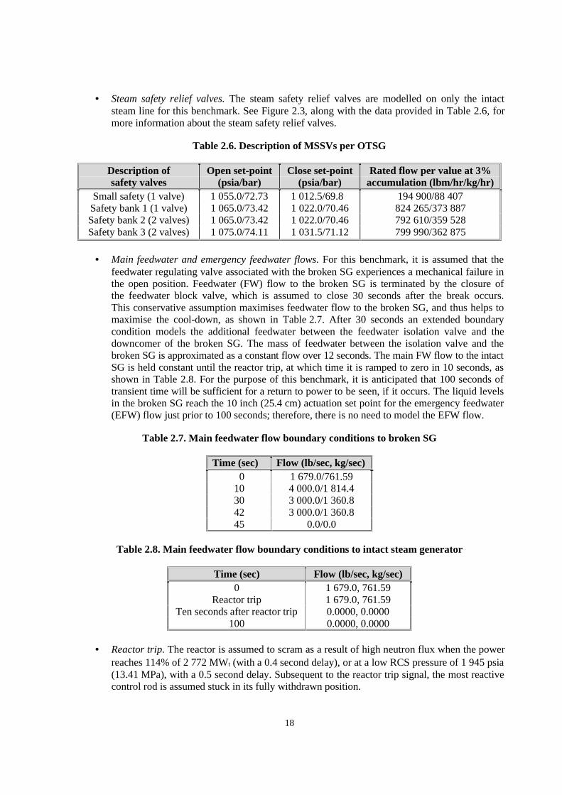
• Steam safety relief valves. The steam safety relief valves are modelled on only the intactsteam line for this benchmark. See Figure 2.3, along with the data provided in Table 2.6, formore information about the steam safety relief valves.
Table 2.6. Description of MSSVs per OTSG
Description ofsafety valves
Open set-point(psia/bar)
Close set-point(psia/bar)
Rated flow per value at 3%accumulation (lbm/hr/kg/hr)
Small safety (1 valve) 1 055.0/72.73 1 012.5/69.80 194 900/88 407Safety bank 1 (1 valve) 1 065.0/73.42 1 022.0/70.46 824 265/373 887Safety bank 2 (2 valves) 1 065.0/73.42 1 022.0/70.46 792 610/359 528Safety bank 3 (2 valves) 1 075.0/74.11 1 031.5/71.12 799 990/362 875
• Main feedwater and emergency feedwater flows. For this benchmark, it is assumed that thefeedwater regulating valve associated with the broken SG experiences a mechanical failure inthe open position. Feedwater (FW) flow to the broken SG is terminated by the closure ofthe feedwater block valve, which is assumed to close 30 seconds after the break occurs.This conservative assumption maximises feedwater flow to the broken SG, and thus helps tomaximise the cool-down, as shown in Table 2.7. After 30 seconds an extended boundarycondition models the additional feedwater between the feedwater isolation valve and thedowncomer of the broken SG. The mass of feedwater between the isolation valve and thebroken SG is approximated as a constant flow over 12 seconds. The main FW flow to the intactSG is held constant until the reactor trip, at which time it is ramped to zero in 10 seconds, asshown in Table 2.8. For the purpose of this benchmark, it is anticipated that 100 seconds oftransient time will be sufficient for a return to power to be seen, if it occurs. The liquid levelsin the broken SG reach the 10 inch (25.4 cm) actuation set point for the emergency feedwater(EFW) flow just prior to 100 seconds; therefore, there is no need to model the EFW flow.
Table 2.7. Main feedwater flow boundary conditions to broken SG
Time (sec) Flow (lb/sec, kg/sec)00 1 679.0/761.5910 4 000.0/1 814.430 3 000.0/1 360.842 3 000.0/1 360.845 0.0/0.0
Table 2.8. Main feedwater flow boundary conditions to intact steam generator
Time (sec) Flow (lb/sec, kg/sec)0 1 679.0, 761.59
Reactor trip 1 679.0, 761.59Ten seconds after reactor trip 0.0000, 0.0000
100 0.0000, 0.0000
• Reactor trip. The reactor is assumed to scram as a result of high neutron flux when the powerreaches 114% of 2 772 MWt (with a 0.4 second delay), or at a low RCS pressure of 1 945 psia(13.41 MPa), with a 0.5 second delay. Subsequent to the reactor trip signal, the most reactivecontrol rod is assumed stuck in its fully withdrawn position.
19
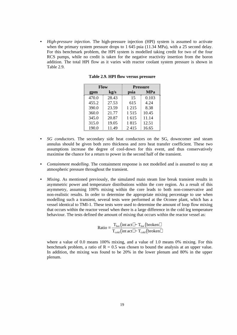
• High-pressure injection. The high-pressure injection (HPI) system is assumed to activatewhen the primary system pressure drops to 1 645 psia (11.34 MPa), with a 25 second delay.For this benchmark problem, the HPI system is modelled taking credit for two of the fourRCS pumps, while no credit is taken for the negative reactivity insertion from the boronaddition. The total HPI flow as it varies with reactor coolant system pressure is shown inTable 2.9.
Table 2.9. HPI flow versus pressure
Flow Pressuregpm kg/s psia MPa470.0 28.43 15 0.103455.2 27.53 615 4.24390.0 23.59 1 215 8.38360.0 21.77 1 515 10.45345.0 20.87 1 615 11.14315.0 19.05 1 815 12.51190.0 11.49 2 415 16.65
• SG conductors. The secondary side heat conductors on the SG, downcomer and steamannulus should be given both zero thickness and zero heat transfer coefficient. These twoassumptions increase the degree of cool-down for this event, and thus conservativelymaximise the chance for a return to power in the second half of the transient.
• Containment modelling. The containment response is not modelled and is assumed to stay atatmospheric pressure throughout the transient.
• Mixing. As mentioned previously, the simulated main steam line break transient results inasymmetric power and temperature distributions within the core region. As a result of thisasymmetry, assuming 100% mixing within the core leads to both non-conservative andnon-realistic results. In order to determine the appropriate mixing percentage to use whenmodelling such a transient, several tests were performed at the Oconee plant, which has avessel identical to TMI-1. These tests were used to determine the amount of loop flow mixingthat occurs within the reactor vessel when there is a large difference in the cold leg temperaturebehaviour. The tests defined the amount of mixing that occurs within the reactor vessel as:
( ) ( )( ) ( )
RatioT act T broken
T act T brokenhot hot
cold cold
=−−
int
int
where a value of 0.0 means 100% mixing, and a value of 1.0 means 0% mixing. For thisbenchmark problem, a ratio of R = 0.5 was chosen to bound the analysis at an upper value.In addition, the mixing was found to be 20% in the lower plenum and 80% in the upperplenum.


21
Chapter 3
STATISTICAL METHODOLOGY
Standard techniques for comparison of results
The end result of the benchmark exercises should be a comprehensive comparison of all sets ofresults to the specified problem, as provided by the various participants and their preferred systemcodes. Such a comparison must necessarily include a figure of merit or similar means to quantify thedegree of agreement, or disagreement, among the participants. This goal is, in the present instance,complicated by two circumstances. First, experimental data is not available for a PWR MSLBtransient scenario, rendering traditional code-to-data comparison methods inapplicable. Second, severalparticipants have submitted results from multiple versions of the same code. Consequently, not all ofthe sets of results are completely independent of each other, and simple averaging techniques may notprovide an accurate statistical representation of the data.
To resolve these issues, the reference solution for all parameters is based upon a statisticalmean value of all submitted values, corrected to account for the interdependence of some results [5].Comparisons are accomplished by a similarly amended standard deviation. The comparisons to followare thus properly called code-to-code comparisons, rather than code-to-data comparisons. While perhapsnot ideal, this method provides the strongest basis from which to complete a statistical analysis andcomparison of the results for this exercise.
Time history data
In this exercise, various parameters such as power, temperature and pressure are plotted as afunction of time; these plots are denoted as time histories. Points of interest are isolated and submittedto a basic statistical analysis as described below.
• Step 1: Isolate points of interest. Such points include time of highest return to power, highestpower before and after trip, and values at the end of transient (EOT) for all parameters. Thesepoints are identified for all time-series data sets, and the values of all participants arecollected. For Exercise One, most of the parameters are evaluated at EOT, with a few alsobeing evaluated at the power peaks before or after reactor scram.
• Step 2: Calculate mean values and standard deviations. This calculation is completed in twostages to account for the multiple versions of some codes. First, the results of all dependentcode versions are averaged to provide a single mean value for that code. As discussedpreviously, the code versions, which are dependent on one another, are those which differonly by perturbations of the calculation or boundary models. In the second stage, theseaveraged values and the results from single version codes are averaged again to provide theoverall mean value, which will serve as the reference solution for that parameter.

22
In both stages, the averaging process obeys the formula for statistical mean value:
N
x
x
N
ii∑
=
(3.1)
The standard deviation is calculated for the final average and obeys the equation:
( )
1
2
−
−±=σ
∑N
xxN
ii
(3.2)
where x represents the final mean value and xi is the averaged result for those codes withmultiple versions or the single value for independent codes. These mean and standarddeviation values are calculated at each of the points defined in Step 1 above, to be used in theremaining steps that follow.
• Step 3: Identify outliers and recalculate mean, if necessary. It has been noted that for certainparameters, some of the results submitted by one or more participants lie far outside the meanrange. To avoid extreme skewing of the mean solution by these outliers, a rudimentary outlieranalysis is performed. If any result lays more than three standard deviations above or belowthe mean solution, it is excluded from the averaging process and the mean and standarddeviations are recalculated. Such results are the NETCorp results, which are not included inTables 4.1-4.11 of Chapter 4. The only other results lying outside of the three-sigma toleranceare the IPSN/CEA predictions of break flow rates and these are denoted with (*) in Table 4.1.This process is repeated until no points lie beyond this three-sigma range.
• Step 4: Determine and report the deviation and figure of merit for each participant’s value.The deviation, e, which is merely the difference between the participant’s value and the meanas determined in Step 2, is calculated according to:
( )xxe ii −= (3.3)
After calculating the deviation, the figure of merit can be determined according to the formula:
σ=Φ e (3.4)
This figure of merit provides a means for comparison that is more easily interpreted thanraw deviations by relating the participant’s deviation to the overall standard deviation.The deviations and figures of merit for all codes will be tabulated in the final report for thisexercise.
Reference results
The reference results for Phase I of the PWR MSLB benchmark – point kinetics exercise – arebased upon a statistical mean value of all submitted results. The reference results are shown at thebeginning of Tables 4.1-4.11 of Chapter 4. Fifteen time histories are compared at the EOT. Of particular

23
interest are total power, fission power and reactivity time histories. For them three points are isolated:highest power before and after trip, and values at the EOT. At each of these isolated points meanvalues and standard deviations are obtained, according to the methods described above.


25
Chapter 4
RESULTS AND DISCUSSION
The plots and tables in this section provide a comparison of the participants’ results for theparameters that have the greatest effect on the MSLB transient. These parameters include power,temperature, pressure, reactivity, break flow rate and steam generator mass. In each case, the tables(Tables 4.1-4.8) show values for the absolute and relative difference between the mean solution andeach participant’s results for the given parameter, while the figures (Figures 4.1-4.28) graphicallyillustrate the agreement or disagreement of participants’ predictions. Statistical evaluation is employedfor the parameters in the tables in an attempt to make a quantitative comparison. The star in Table 4.1signifies that the marked result was not included in the generation of mean value and standarddeviation for the specified parameter. The NETCorp results are presented only in the plots. The tablesand figures for each parameter are discussed in more detail below. Note that the two sets of VTT,Finland results are produced with two different codes – SMABRE (VTT 1) and APROS (VTT 2) whilethe two sets of the University of Valencia results are produced with the same code (TRAC-PF1) usingdifferent vessel models. Valencia 1 results are calculated with the 3-D TRAC vessel model in cylindricalgeometry (similar to the PSU model) and the Valencia 2 results are calculated using a channel model.
A remark must be made regarding the comparison of parameters at EOT. When looking at thetime of second power peak (Table 4.7), one can see a discrepancy of about 18 seconds between thefastest predictions (Iberdrola and PSU) and the slowest one (IPSN/CEA). Other solutions are placedbetween these two extremes in terms of chronology. The differences in the predicted transientchronology have consequences for some parameters at EOT (break flow rate, secondary pressure andfuel temperature). For example, if the return to power occurs later, the fuel temperature at EOT ishigher, the break flow rate is higher and the broken SG may not be dry yet.
Break flow rate
Figures 4.1, 4.2 and 4.3 provide a comparison for the behaviour of the total, 24 inch and 8 inchbreak flow rates, respectively. The MSLB transient is initiated at 0.001 seconds by a double-endedbreak of the Loop A steam line upstream of the MSIVs. As expected, there is an initial peak in theflow out of breaks when the transient is initiated. The second peak occurs 30 seconds into the transientsand coincides with the feedwater in the broken SG being ramped to zero. After this second peak, theflow rate of breaks goes to zero as the SG blows dry. In each case, the participants’ results are inreasonable agreement concerning the behaviour of this parameter, but there are a number of localdeviations throughout the transient. These local deviations are caused by modelling differences in thesteam line, break, break flow rate and various other modelling assumptions and code correlations.For example, the differences in the steam-liquid interface friction in the SG influences the liquidentrainment into the steam line and to the break during the blow-down.
A summary of the deviation from the reference results for the break flow rates at the end of thetransient are presented in Table 4.1. The values are relatively small, with IPSN/CEA having the largest

26
Table 4.1. Deviations: total break flow rate, 24 inch breakflow rate and 8 inch break flow rate at end of transient
BREAK FLOWRATES
TotalMean = 4.858 kg/s
σ = 7.85 kg/s
24 inch breakMean = 4.392 kg/s
σ = 7.11 kg/s
8 inch breakMean = 0.655 kg/s
σ = 0.79 kg/sTotal break flow rate 24 inch break flow rate 8 inch break flow rate
Participante Φ e Φ e Φ
British Energy -4.56 -0.58 -4.09 -0.58 -0.66 -0.83CSA/GPUN/EPRI 3.74 0.48 2.61 0.37 0.95 1.20
GRS -4.86 -0.62 -4.39 -0.62 -0.66 -0.83Iberdrola -4.36 -0.56 -4.09 -0.58 -0.46 -0.58
IPSN/CEA 115.24* 14.68* 97.41* 13.69* 17.65* 22.44*Pisa/Zagreb 7.24 0.92 6.51 0.91 0.95 1.20
PSU 21.74 2.77 20.01 2.81 1.56 1.98Purdue/NRC -4.06 -0.52 -3.79 -0.53 -0.46 -0.58Rossendorf -0.36 -0.05 -0.39 -0.06 -0.16 -0.20
Siemens/FZK -1.96 -0.25 -2.79 -0.39 0.60 0.76Valencia 1 -3.06 -0.39 -2.69 -0.38 -0.56 -0.71Valencia 2 -4.86 -0.62 -2.69 -0.38 -0.46 -0.58
VTT 2 -2.01 -0.26 -1.91 -0.27 -0.29 -0.37VTT 1 -4.66 -0.59 -4.19 -0.59 -0.66 -0.83
deviation for the total, 24 inch and 8 inch break flow rates. The differences in participants’ results forthe flow at the end of the break can be attributed primarily to differences in modelling assumptionsand/or minor differences in the SG and steam-line nodalisation models.
Pressure
Figures 4.4-4.9 show comparisons for the average, broken and intact loop, broken and intactsteam line and pressuriser pressures throughout the transient. In each case, the participants are inreasonable agreement concerning the behaviour of the parameter, and the results form a single cluster.Any local deviations in the pressure behaviour throughout the transient are caused by modellingdifferences in the reactor coolant system and steam lines, modelling assumptions and code correlations.
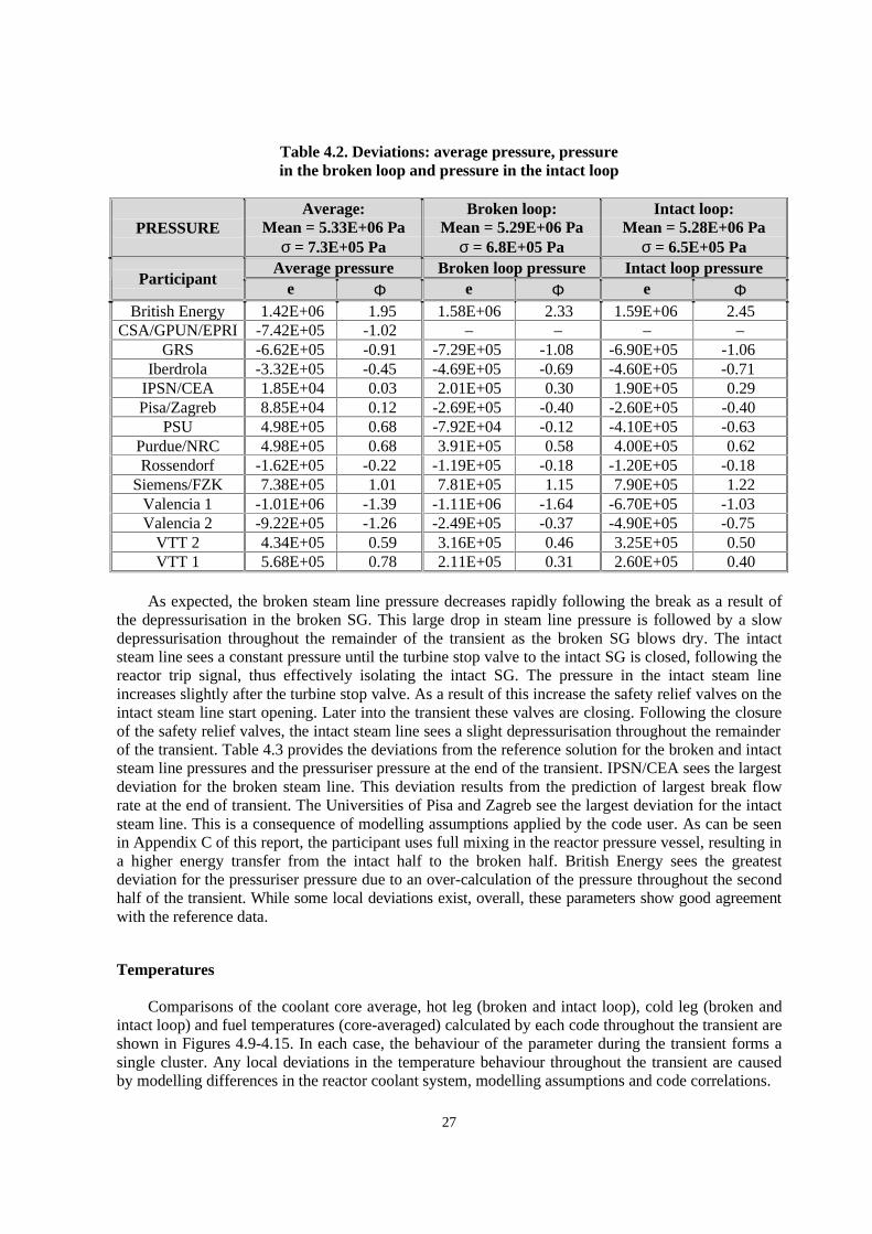
The depressurisation of the broken SG results in overcooling of the reactor coolant system (RCS)fluid, which results in a lower average temperature in the core region. As the RCS fluid cools down, itshrinks, resulting in a rapid decrease in the RCS pressure. The HPI low pressure signal is received andHPI is activated with a 25 second delay. As a result of injecting cold water into the core region, thepower begins to increase and the RCS pressure begins to even out. Table 4.2 provides a summary ofthe deviations from the reference (mean) solution for the average pressure and the broken and intactloop pressures at the end of the transient for each participant. The two results of the University ofValencia and the British Energy result show the largest deviation for the average pressure. The deviationfor University of Valencia is explained by the fact that this participant’s code calculates a largerpressure drop after the initial break as compared, for example, with PSU. Since PSU and theUniversity of Valencia are using the same code to calculate the data submitted for this benchmark, thisdeviation can be attributed to the differences in modelling assumptions and the nodalisation used forthe TMI-1 model. The British Energy large positive deviation is a result of over-calculating thepressure in the broken and intact loops throughout the second half of the transient.
27
Table 4.2. Deviations: average pressure, pressurein the broken loop and pressure in the intact loop
PRESSUREAverage:
Mean = 5.33E+06 Paσ = 7.3E+05 Pa
Broken loop:Mean = 5.29E+06 Pa
σ = 6.8E+05 Pa
Intact loop:Mean = 5.28E+06 Pa
σ = 6.5E+05 PaAverage pressure Broken loop pressure Intact loop pressure
Participante Φ e Φ e Φ
British Energy 1.42E+06 1.95 1.58E+06 2.33 1.59E+06 2.45CSA/GPUN/EPRI -7.42E+05 -1.02 – – – –
GRS -6.62E+05 -0.91 -7.29E+05 -1.08 -6.90E+05 -1.06Iberdrola -3.32E+05 -0.45 -4.69E+05 -0.69 -4.60E+05 -0.71
IPSN/CEA 1.85E+04 0.03 2.01E+05 0.30 1.90E+05 0.29Pisa/Zagreb 8.85E+04 0.12 -2.69E+05 -0.40 -2.60E+05 -0.40
PSU 4.98E+05 0.68 -7.92E+04 -0.12 -4.10E+05 -0.63Purdue/NRC 4.98E+05 0.68 3.91E+05 0.58 4.00E+05 0.62Rossendorf -1.62E+05 -0.22 -1.19E+05 -0.18 -1.20E+05 -0.18
Siemens/FZK 7.38E+05 1.01 7.81E+05 1.15 7.90E+05 1.22Valencia 1 -1.01E+06 -1.39 -1.11E+06 -1.64 -6.70E+05 -1.03Valencia 2 -9.22E+05 -1.26 -2.49E+05 -0.37 -4.90E+05 -0.75
VTT 2 4.34E+05 0.59 3.16E+05 0.46 3.25E+05 0.50VTT 1 5.68E+05 0.78 2.11E+05 0.31 2.60E+05 0.40
As expected, the broken steam line pressure decreases rapidly following the break as a result ofthe depressurisation in the broken SG. This large drop in steam line pressure is followed by a slowdepressurisation throughout the remainder of the transient as the broken SG blows dry. The intactsteam line sees a constant pressure until the turbine stop valve to the intact SG is closed, following thereactor trip signal, thus effectively isolating the intact SG. The pressure in the intact steam lineincreases slightly after the turbine stop valve. As a result of this increase the safety relief valves on theintact steam line start opening. Later into the transient these valves are closing. Following the closureof the safety relief valves, the intact steam line sees a slight depressurisation throughout the remainderof the transient. Table 4.3 provides the deviations from the reference solution for the broken and intactsteam line pressures and the pressuriser pressure at the end of the transient. IPSN/CEA sees the largestdeviation for the broken steam line. This deviation results from the prediction of largest break flowrate at the end of transient. The Universities of Pisa and Zagreb see the largest deviation for the intactsteam line. This is a consequence of modelling assumptions applied by the code user. As can be seenin Appendix C of this report, the participant uses full mixing in the reactor pressure vessel, resulting ina higher energy transfer from the intact half to the broken half. British Energy sees the greatestdeviation for the pressuriser pressure due to an over-calculation of the pressure throughout the secondhalf of the transient. While some local deviations exist, overall, these parameters show good agreementwith the reference data.
Temperatures
Comparisons of the coolant core average, hot leg (broken and intact loop), cold leg (broken andintact loop) and fuel temperatures (core-averaged) calculated by each code throughout the transient areshown in Figures 4.9-4.15. In each case, the behaviour of the parameter during the transient forms asingle cluster. Any local deviations in the temperature behaviour throughout the transient are causedby modelling differences in the reactor coolant system, modelling assumptions and code correlations.

28
Table 4.3. Deviations: broken steam line pressure,intact steam line pressure and pressuriser pressure
PRESSUREBroken steam line:
Mean = 1.41E+05 Paσ = 1.2E+04 Pa
Intact steam line:Mean = 4.82E+06 Pa
σ = 4.8E+05 Pa
Pressuriser:Mean = 5.59E+06 Pa
σ = 7.2E+05 PaBroken steam line
pressureIntact steam line
pressure Pressuriser pressureParticipant
e Φ e Φ e ΦBritish Energy -4.03E+04 -0.35 4.26E+05 0.90 9.75E+05 1.36
CSA/GPUN/EPRI -1.39E+05 -1.20 -3.34E+05 -0.70 – –GRS -3.83E+04 -0.33 -1.04E+05 -0.22 – –
Iberdrola -2.03E+04 -0.18 -4.24E+05 -0.89 – –IPSN/CEA 2.65E+05 2.29 -1.54E+05 -0.32 -5.65E+05 -0.79Pisa/Zagreb -4.19E+04 -0.36 -1.21E+06 -2.55 – –
PSU -2.73E+04 -0.24 5.16E+05 1.08 -5.05E+05 -0.71Purdue/NRC -4.03E+04 -0.35 5.16E+05 1.08 9.50E+04 0.13Rossendorf -3.93E+04 -0.34 -2.34E+05 -0.49 – –
Siemens/FZK 2.40E+05 2.07 6.64E+04 0.14 – –Valencia 1 -3.83E+04 -0.33 1.96E+05 0.41 – –Valencia 2 -3.76E+04 -0.31 1.06E+05 0.22 – –
VTT 2 -4.11E+04 -0.34 -1.22E+05 -0.25 – –VTT 1 -4.03E+04 -0.35 5.36E+05 1.13 – –
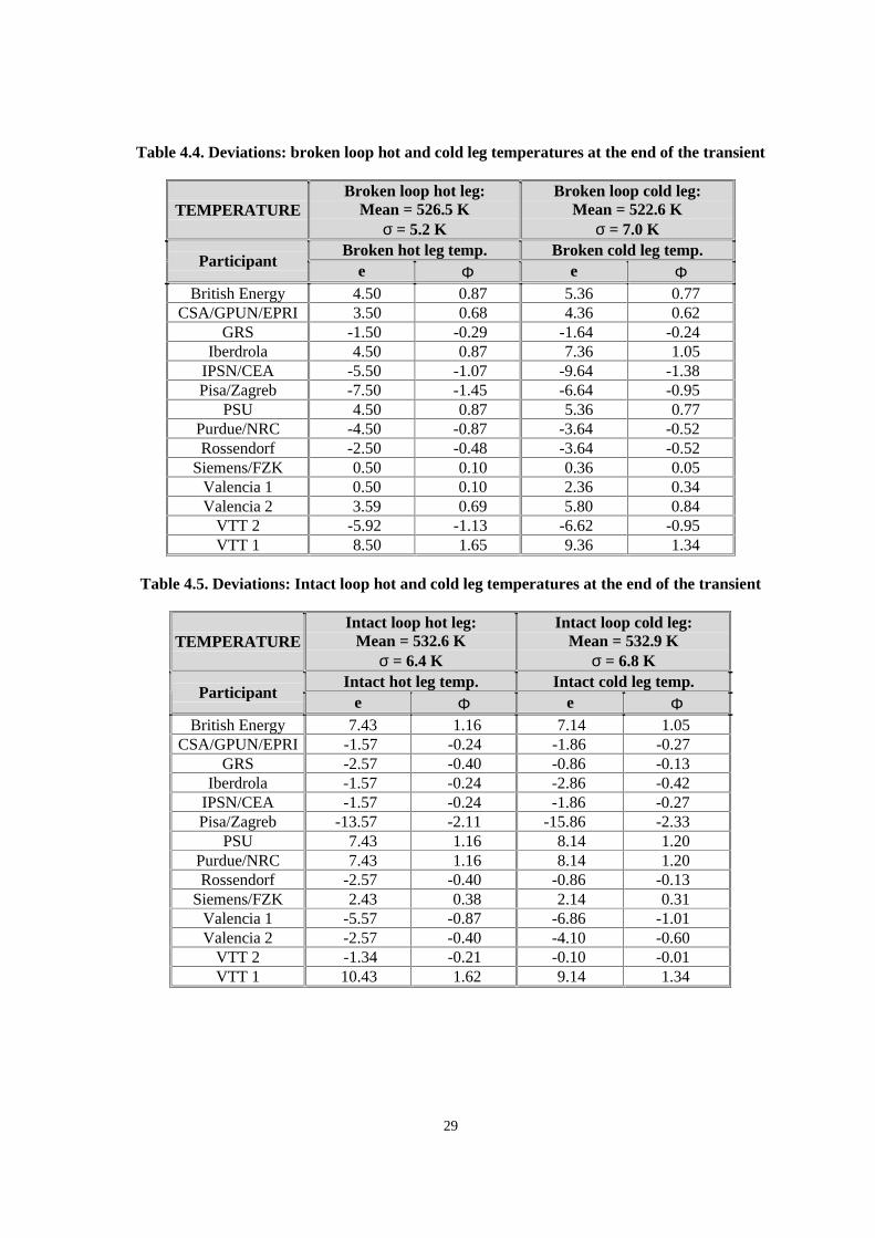
When the steam line break occurs, the pressure in the broken SG decreases rapidly, which causesthe flow rate within the SG to increase. The increased flow rate results in an increase in the heattransfer and overcooling of the RCS fluid. The cold leg temperature plots show an immediatetemperature decrease as a result of the broken SG depressurisation; however, the hot leg temperatureplots show a more graduate decline. The reason is that the decreasing RCS temperature results in anincrease in the core power, which initially offsets the broken SG’s cooling effect. Following the initialdecrease, the intact cold leg temperature sees a slight increase in temperature as a result of the turbinestop valve closure, which isolates the intact SG. In the second half of the transient, there is an increasein the core power, and the overcooling effect from the broken SG becomes secondary. In addition tothe increase in power, the broken SG loses its cooling capacity throughout the transient as it blowsdry. The broken loop sees an increase in RCS temperature as a result of this power increase, whilethe intact loop see the temperature approaching a constant value in the later half of the transient.The deviations for the broken loop are fairly low for both the hot and cold legs, with VTT (Smabre)showing the largest deviation in each case (see Table 4.4). This difference is caused by under-coolingin the broken SG and may be the result of different code correlations. As with the broken looptemperatures, there are small deviations in the intact hot and cold leg temperatures, with theUniversities of Pisa and Zagreb seeing the largest deviation (see Table 4.5). This difference isexplained by overcooling of the intact cold leg, which is a result of mixing assumptions.
Table 4.6 provides a summary of the deviations for the average moderator and fuel temperaturesat the end of the transient. The Universities of Pisa and Zagreb show the largest deviation for theaverage moderator temperature because of a slight under-cooling in the intact loop throughout thesecond half of the transient. As expected the fuel temperature time evolution follows the behaviour ofthe reactor power throughout the transient. IPSN/CEA shows the largest deviation for the fueltemperature as a consequence of the predicted transient behaviour. IPSN/CEA predicts lower breakflow rates in the first half of the transient, which results in higher reactor coolant temperatures and
29
Table 4.4. Deviations: broken loop hot and cold leg temperatures at the end of the transient
TEMPERATUREBroken loop hot leg:
Mean = 526.5 Kσ = 5.2 K
Broken loop cold leg:Mean = 522.6 K
σ = 7.0 KBroken hot leg temp. Broken cold leg temp.
Participante Φ e Φ
British Energy 4.50 0.87 5.36 0.77CSA/GPUN/EPRI 3.50 0.68 4.36 0.62
GRS -1.50 -0.29 -1.64 -0.24Iberdrola 4.50 0.87 7.36 1.05
IPSN/CEA -5.50 -1.07 -9.64 -1.38Pisa/Zagreb -7.50 -1.45 -6.64 -0.95
PSU 4.50 0.87 5.36 0.77Purdue/NRC -4.50 -0.87 -3.64 -0.52Rossendorf -2.50 -0.48 -3.64 -0.52
Siemens/FZK 0.50 0.10 0.36 0.05Valencia 1 0.50 0.10 2.36 0.34Valencia 2 3.59 0.69 5.80 0.84
VTT 2 -5.92 -1.13 -6.62 -0.95VTT 1 8.50 1.65 9.36 1.34
Table 4.5. Deviations: Intact loop hot and cold leg temperatures at the end of the transient
TEMPERATUREIntact loop hot leg:
Mean = 532.6 Kσ = 6.4 K
Intact loop cold leg:Mean = 532.9 K
σ = 6.8 KIntact hot leg temp. Intact cold leg temp.
Participante Φ e Φ
British Energy 7.43 1.16 7.14 1.05CSA/GPUN/EPRI -1.57 -0.24 -1.86 -0.27
GRS -2.57 -0.40 -0.86 -0.13Iberdrola -1.57 -0.24 -2.86 -0.42
IPSN/CEA -1.57 -0.24 -1.86 -0.27Pisa/Zagreb -13.57 -2.11 -15.86 -2.33
PSU 7.43 1.16 8.14 1.20Purdue/NRC 7.43 1.16 8.14 1.20Rossendorf -2.57 -0.40 -0.86 -0.13
Siemens/FZK 2.43 0.38 2.14 0.31Valencia 1 -5.57 -0.87 -6.86 -1.01Valencia 2 -2.57 -0.40 -4.10 -0.60
VTT 2 -1.34 -0.21 -0.10 -0.01VTT 1 10.43 1.62 9.14 1.34

30
Table 4.6. Deviations: average moderator temperatureand fuel temperature at the end of the transient
TEMPERATUREModerator:
Mean = 528.7 Kσ = 5.8 K
Fuel:Mean = 546.8 K
σ = 10.0 KModerator temperature Fuel temperature
Participante Φ e Φ
British Energy 6.33 1.10 0.17 0.02CSA/GPUN/EPRI – – -2.83 -0.28
GRS -0.67 -0.12 0.17 0.02Iberdrola 2.33 0.40 -2.83 -0.28
IPSN/CEA -4.67 -0.81 24.83 2.49Pisa/Zagreb -10.67 -1.85 15.17 1.52
PSU 6.33 1.10 8.17 0.82Purdue/NRC 1.33 0.23 1.17 0.12Rossendorf -2.67 -0.46 – –
Siemens/FZK 1.33 0.23 1.17 0.12Valencia 1 -1.67 -0.29 -0.83 -0.08Valencia 2 0.90 0.16 3.50 0.35
VTT 2 -3.07 -0.53 2.24 0.22VTT 1 9.33 1.62 11.17 1.12
later return to power. At the end of the transient (t = 100 s) the IPSN/CEA calculation shows higherreactor power than other participants’ results. In summary the fuel temperature deviations reflect thepower deviations. Those reflect more or less the deviations in the break flow rates. In addition thedifferences in fuel temperature predictions at the same power predictions and same coolant temperaturepredictions can be attributed to the heat structure modelling assumptions as the number of radial zonesfor the fuel rod.
Reactor power
A comparison of the fission, total and decay power calculated by each code throughout thetransient is shown in Figures 4.16-4.18. The power response and the magnitude of the return to powerduring the transient as predicted by different codes are functions of the total reactivity time evolution.When the break is initiated, the core sees a gradual rise in power in response to the temperaturechanges within the core region. A rapid power rise occurs when the overcooled liquid from the brokenloop reaches the core. The power rise continues until the reactor trips. After the trip, a sharp decreasein power results from the negative reactivity inserted into the core when the reactor scrams. The brokenSG continues to overcool the RCS fluid together with the cold water injected from the HPI system,and the reactor sees an increase in power later into the transient. This rise in power quickly decreasesbecause the broken SG loses its cooling capability as its mass and pressure go to zero.
In general, the results follow the above-described behaviour. NETCorp shows the largest deviationbecause the code has extremely conservative correlations and calculates an increase in power morequickly than the other codes. Twelve of the fifteen participants see a more pronounced return to powerin the second half of the transient. The three participants – the Universities of Pisa and Zagreb, GRSand GPU/CSA/EPRI – see a slight rise in power around the same time the other participants experiencea higher return-to-power. While there is general agreement about the behaviour of the power

31
throughout the transient, there is a great deal of disagreement about the size of the return to power.This disagreement is explained below while discussing the differences in the total reactivity timeevolution prediction.
Table 4.7 shows the deviation from the reference results for the time of reactor trip (initial peak)and the time of highest power after the trip (second peak). The values vary, with the Universities ofPiza and Zagreb showing the largest deviation for the initial peak (at reactor scram) and IPSN/CEAshowing the largest deviation for the second peak.
Table 4.7. Deviations: time of reactor trip (initial peak)and time of highest power after trip (second peak)
TIMEInitial peak:
Mean = 5.64 secσ = 0.79 sec
Second peak:Mean = 70.2 sec
σ = 15.0 secInitial peak Second peak
Participante Φ E Φ
British Energy -0.54 -0.68 -2.90 -0.19CSA/GPUN/EPRI -0.14 -0.18 -6.21 -0.41
GRS 0.86 1.08 6.79 0.45Iberdrola -0.64 -0.81 -9.21 -0.61
IPSN/CEA 0.39 0.50 12.58 0.84Pisa/Zagreb 1.86 2.34 4.79 0.32
PSU 0.36 0.45 -9.21 -0.61Purdue/NRC -1.14 -1.44 4.79 0.32Rossendorf -0.94 -1.19 11.40 0.76
Siemens/FZK -0.14 -0.18 3.79 0.25Valencia 1 0.56 0.71 -4.64 -0.31Valencia 2 0.56 0.71 -4.31 -0.29
VTT 2 0.56 0.71 11.60 0.77VTT 1 0.36 0.45 -4.21 -0.28
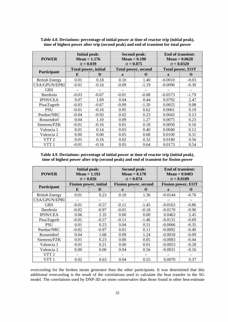
Tables 4.8 and 4.9 provide deviations from the reference solution for the ratio of the total andfission power to the initial power level (as calculated by each participant at t = 0.0 seconds) at the firstand second peaks and at the end of the transient. The deviations at the first peak are relatively small,with IPSN/CEA having the largest deviation for both the fission and total powers. One reason is thatthe IPSN/CEA high flux trip delay time (0.46 seconds) is slightly greater than specified. Anotherobservation is that all participants start at approximately same initial total power level while the initialfission power level varies, depending on the decay heat model used. The effective decay heat energyfraction of the total thermal power (the relative contribution in the steady state) is specified to be equalto 0.07143, which assumes approximately 2 574 MW as initial fission power level. For exampleIPSN/CEA starts at an initial fission power level of 2 616 MW. The greatest deviations at the end ofthe transient are calculated by IPSN/CEA for both fission and total powers. In each case, the difference isexplained by the prediction of a late return to power in the second half of the transient.
The deviations for the total and fission power at the second peak are quite large, with NETCorphaving the greatest value in each case. The results submitted by NETCorp predict a much larger returnto power than the other participants’ results and the reference results for this parameter. It wasdetermined, after consultation with NETCorp, that this difference can be explained by examiningFigures 4.25 and 4.26. From these plots is obvious that NETCorp is calculating a greater amount of
32
Table 4.8. Deviations: percentage of initial power at time of reactor trip (initial peak),time of highest power after trip (second peak) and end of transient for total power
POWERInitial peak:
Mean = 1.176σ = 0.039
Second peak:Mean = 0.190
σ = 0.075
End of transient:Mean = 0.0628
σ = 0.0320Total power, initial Total power, second Total power, EOT
ParticipantE Φ e Φ e Φ
British Energy 0.01 0.18 0.10 1.40 -0.0010 -0.03CSA/GPUN/EPRI -0.01 -0.16 -0.09 -1.19 -0.0096 -0.30
GRS – – – – – –Iberdrola -0.03 -0.67 -0.01 -0.08 -0.0573 -1.79
IPSN/CEA 0.07 1.69 0.04 0.44 0.0792 2.47Pisa/Zagreb -0.03 -0.67 -0.09 -1.20 0.0025 0.08
PSU -0.01 -0.16 0.05 0.62 0.0061 0.19Purdue/NRC -0.04 -0.93 0.02 0.23 0.0043 0.13Rossendorf 0.04 1.10 0.09 1.27 0.0075 0.23
Siemens/FZK -0.01 -0.16 0.01 0.18 0.0050 0.16Valencia 1 0.01 0.14 0.03 0.40 0.0040 0.12Valencia 2 0.00 0.00 0.05 0.68 0.0100 0.31
VTT 2 0.01 0.16 0.02 0.32 0.0180 0.56VTT 1 -0.01 -0.16 0.05 0.64 0.0173 0.54
Table 4.9. Deviations: percentage of initial power at time of reactor trip (initial peak),time of highest power after trip (second peak) and end of transient for fission power
POWERInitial peak:
Mean = 1.193σ = 0.026
Second peak:Mean = 0.170
σ = 0.074
End of transient:Mean = 0.0403
σ = 0.0189Fission power, initial Fission power, second Fission power, EOT
ParticipantE Φ e Φ e Φ
British Energy 0.01 0.23 0.10 1.36 -0.0144 -0.76CSA/GPUN/EPRI – – – – – –
GRS -0.01 -0.57 -0.11 -1.45 -0.0163 -0.86Iberdrola -0.02 -0.97 -0.01 -0.18 -0.0170 -0.90
IPSN/CEA 0.06 2.35 0.00 0.00 0.0463 2.45Pisa/Zagreb -0.01 -0.57 -0.11 -1.46 -0.0131 -0.69
PSU 0.01 0.23 0.04 0.51 -0.0066 -0.35Purdue/NRC -0.02 -0.97 0.01 0.11 -0.0092 -0.49Rossendorf 0.04 1.68 0.09 1.24 -0.0018 -0.09
Siemens/FZK 0.01 0.23 0.00 0.05 -0.0083 -0.44Valencia 1 0.01 0.21 0.00 0.01 -0.0053 -0.28Valencia 2 0.00 0.00 0.04 0.56 -0.0031 -0.16
VTT 2 – – – – – –VTT 1 0.02 0.63 0.04 0.55 0.0070 0.37
overcooling for the broken steam generator than the other participants. It was determined that thisadditional overcooling is the result of the correlations used to calculate the heat transfer in the SGmodel. The correlations used by DNP-3D are more conservative than those found in other best-estimate

33
codes. As a result, there is additional heat transfer in the broken SG, which results in both an earlierand a greater degree of overcooling of the reactor core. These conservative correlations account for theearly reactor trip and the large return-to-power in the second half of the transient.
All of the participants except for PSU and the University of Valencia (Valencia 1) use a channelmodel. PSU and Valencia 1 results are calculated using the 3-D TRAC-PF1 vessel model in cylindricalgeometry. In order to evaluate the differences between channel and 3-D vessel modelling for thesimulated MSLB transient a detailed comparative analysis was performed for both sets of theUniversity of Valencia’s results produced with the same code TRAC-PF1. However, the Valencia 2results are calculated using a channel model. The impact on the transient simulation can be summarisedas follows: the channel model produces a slightly higher return to power at almost the same time withmost of the other predicted parameters in very good agreement.
Reactivity
Figures 4.19-4.22 show comparisons for the behaviour of the total, moderator, Doppler and scramreactivity throughout the transient. The scram reactivity is plotted to show that it follows the tableprovided in the specification. As expected, its value remains at zero until the reactor trips, at whichtime it drops to a value of -4.526% dk/k and remains at this value through the remainder of thetransient. Since the inserted negative tripped rod reactivity is specified, the differences in the totalreactivity time evolution arise from the predictions of moderator feedback and Doppler feedbackreactivity components. The moderator reactivity component follows the cold leg temperature.The discrepancies in the cold leg temperature predictions are due mostly to differences in modellingthe secondary side. It was observed that the major factors affecting the dynamics of the transient arebreak flow modelling (critical flow model), liquid entrainment, modelling of the aspirator flow andnodalisation of the SG down comer. In addition the disagreement can be attributed to differences inthe SG heat transfer correlations used within each participant’s code. The Doppler feedback reactivitypredictions are sensitive to the relation used for Doppler fuel temperature as well as to the radial andaxial nodalisation of the heat structure used (fuel rod).
Table 4.10 provides a summary of deviations from the reference results for the total reactivity atthe second peak and the end of the transient. British Energy shows the largest deviation for the secondpeak, and IPSN/CEA shows the largest deviation at the end of transient. Five participants – NETCorp,British Energy, IPSN/CEA, Rossendorf and Purdue/NRC see return to criticality.
Table 4.11 provides deviations from the reference solution for the moderator, Doppler and scramreactivity values at the end of the transient. The deviations for the moderator reactivity are the result ofdifferent code models since none of the participants over-calculate or under-calculate this parameterthroughout the transient. The deviations are relatively small for the Doppler reactivity due to the reasonsdiscussed above. The exceptions are the NETCorp results, as can be seen in Figures 4.20 and 4.21.The scram reactivity throughout the transient is provided in the specification and, as one would expect,no disagreement exists for this parameter at the end of the transient.
Steam generator mass
Figures 4.23 and 4.24 provide a comparison for the behaviour of the intact and broken steamgenerator masses throughout the transient. As expected, the mass in the broken SG decreases throughoutthe transient, until it eventually blows dry. The intact SG mass initially increases as a result of theclosure of the turbine isolation valve for the intact SG at the turbine trip. This mass eventually decreases

34
Table 4.10. Deviations: total reactivity at time ofhighest power after reactor trip and at end of transient
REACTIVITYTotal (second peak):
Mean = -1.02E-03σ = 1.41E-03
Total (end of transient):Mean = -5.09E-03
σ = 2.03E-03Total reactivity(second peak)
Total reactivity(end of transient)Participant
e Φ e ΦBritish Energy 1.96E-03 1.39 -2.03E-03 -1.00
CSA/GPUN/EPRI -1.95E-03 -1.38 -2.91E-03 -1.43GRS -1.33E-03 -0.94 -7.22E-04 -0.35
Iberdrola 1.00E-03 0.71 -1.52E-03 -0.75IPSN/CEA 1.16E-03 0.82 2.93E-03 1.44Pisa/Zagreb 1.50E-04 0.11 1.45E-03 0.71
PSU -9.70E-04 -0.69 -2.19E-03 -1.08Purdue/NRC 1.12E-03 0.80 6.50E-04 0.33Rossendorf 1.52E-03 1.08 1.91E-03 0.94
Siemens/FZK 9.90E-04 0.70 -4.02E-04 -0.20Valencia 1 6.60E-04 0.47 -3.82E-04 -0.19Valencia 2 9.85E-04 0.70 -2.90E-04 -0.14
VTT 2 1.36E-03 0.96 1.21E-03 0.60VTT 1 9.70E-04 0.69 8.88E-04 0.44
Table 4.11. Deviations: moderator reactivity, Dopplerreactivity and scram reactivity at end of transient
REACTIVITYModerator:
Mean = 3.22E-02σ = 2.0E-03
Doppler:Mean = 7.97E-03
σ = 8.9E-04
Scram:Mean = -4.53E-02
σ = 0.00Moderator reactivity Doppler reactivity Scram reactivity
ParticipantE Φ e Φ e Φ
British Energy -7.27E-04 -0.37 -1.33E-03 -1.48 0.00E+00 –CSA/GPUN/EPRI -6.27E-04 -0.32 -8.96E-04 -1.00 0.00E+00 –
GRS 3.73E-04 0.19 -1.09E-03 -1.21 0.00E+00 –Iberdrola -1.93E-03 -0.99 4.04E-04 0.45 0.00E+00 –
IPSN/CEA 2.17E-03 1.11 6.44E-04 0.72 0.00E+00 –Pisa/Zagreb – – – – – –
PSU -3.43E-03 -1.75 1.21E-03 1.36 0.00E+00 –Purdue/NRC -2.73E-05 -0.01 -6.96E-04 -0.78 0.00E+00 –Rossendorf 8.73E-04 0.45 9.84E-04 1.10 0.00E+00 –
Siemens/FZK – – – – – –Valencia 1 -1.03E-03 -0.53 6.54E-04 0.73 0.00E+00 –Valencia 2 -1.38E-03 -0.69 1.03E-03 1.15 0.00E+00 –
VTT 2 1.73E-03 0.09 -5.26E-04 -0.59 0.00E+00 –VTT 1 4.73E-04 0.24 4.54E-04 0.51 0.00E+00 –
35
due to the MSSV’s action and further evens and remains constant until the end of the transient.While there is general agreement about the behaviour of the masses in each SG, the analysis shows agreat deal of disagreement about the values of the masses throughout the transient. This parametershows the largest deviation out of all those presented in this report; however, this is not surprisingwhen one considers the complexity involved with modelling the OTSG. Originally, it was thought thatthe SG mass discrepancy was the result of the differences in modelling of both the SG and the steamline. Since that time, the break nodalisation has been made uniform amongst all the participants and agreat deal of additional information has been provided about the OTSG, concerning both the way itworks and its geometry. The initial mass of the SG has been modified to remove the artificial increaseof 3 000 kg that a number of the participants were having trouble reproducing. Putting the SG massesback to 26 000 kg has helped to make the results more uniform; however, discrepancies still exist.
Overall, the masses for both SGs are fairly consistent amongst all participants. All the participantswere provided with the same base deck from which to take SG information, as well as the samesubsequent information. As a result, any differences in the value or behaviour of this parameterthroughout the transient can be attributed to three major factors:
1. Differences in the code models, which significantly influence the transient behaviour, likemodels for break flow rate, and steam-liquid interface friction or liquid entrainment duringblow-down.
2. Differences in the heat transfer correlations used within each participant’s code. This isespecially true for the participants who use proprietary correlations that are specific to U-tubeSGs in their codes, as a behaviour of an OTSG is much different than a U-tube SG, and alsoinvolves superheat, something U-tube SG users do not have to worry about modelling.
3. Differences in the noding of the SG, which can produce significant differences in the SGbehaviour.
As a lot of time was spent making sure that the participants’ models for the SG are the same,additional information for the transient SG behaviour was requested and compared in Figures 4.25-4.28.This approach certainly helped to explain the observed differences in the participants’ predictions.
Sequence of events
The modelling sequence of events for the MSLB transient is specified in the final specificationsand has been discussed at the benchmark workshops and meetings. The double-ended break occursat 0.001 seconds. It is followed by an immediate closure of the turbine isolation valve of the brokenSG and all flow from the broken SG goes out to break. Reactor trip is modelled to occur at the highneutron flux trip set point (with delay of 0.4 seconds) or at the low RCS pressure set point (with adelay of 0.5 seconds). The turbine trip begins at the reactor trip. At the turbine trip the turbine isolationvalve for the intact SG closes with a closure time of 0.5 seconds. With increasing pressure in the intactsteam line some of the safety relief valves (MSSVs) will open and subsequently close at the set points,defined in the final specification. High pressure injection (HPI) occurs when the primary systempressure drops to the defined set point with a 25 second delay.
Looking at Table B.1 of Appendix B it can be seen that there are variations among the participantsin interpreting the modelling sequence of events. Some participants initiate the break at 0.01 seconds.Further, there are different interpretations of the time of the turbine trip and the closure of the turbineisolation valve for the intact SG. Some participants interpret the time of reactor trip as the time when

36
the trip condition is reached, while others are consider the time when the reactor scram begins, i.e. takinginto account the delay. While these misinterpretations may not be significant, they contribute to thedifferences of the participants’ predictions at the beginning of the transient. Later into the transient allthe participants see a rise in power, twelve of them see a return to power and five of them (NETCorp,British Energy, Rossendorf, IPSN/CEA and Purdue/NRC) also see a return to criticality.
In summary the explanation of differences in the transient chronology predicted by participants isquite complex. The main parameter seems to be the broken SG break flow rate but the differences resultfrom many other parameters, as was discusses above. These factors include break flow correlation, SGnodalisation, steam line pressure drop, liquid entrainment model, steam-liquid interface friction model,primary to secondary heat transfer calculation, primary flow rate and core mixing assumptions.

Fig
ure
4.1.
Tot
al b
reak
flow
rat
e
0
500
1000
1500
2000
2500
3000
010
2030
4050
6070
8090
100
Tim
e (s
)
Flow Rate (kg/s)
IPS
N
Ros
send
orf
Brit
ish
Ene
rgy
Sie
men
s/F
ZK
Pis
a/Z
agre
b
VT
T_1
NE
TC
OR
P
GR
S
Iber
drol
a
VT
T_2
Val
enci
a_1
Val
enci
a_2
Pur
due
GP
UN
PS
U
37
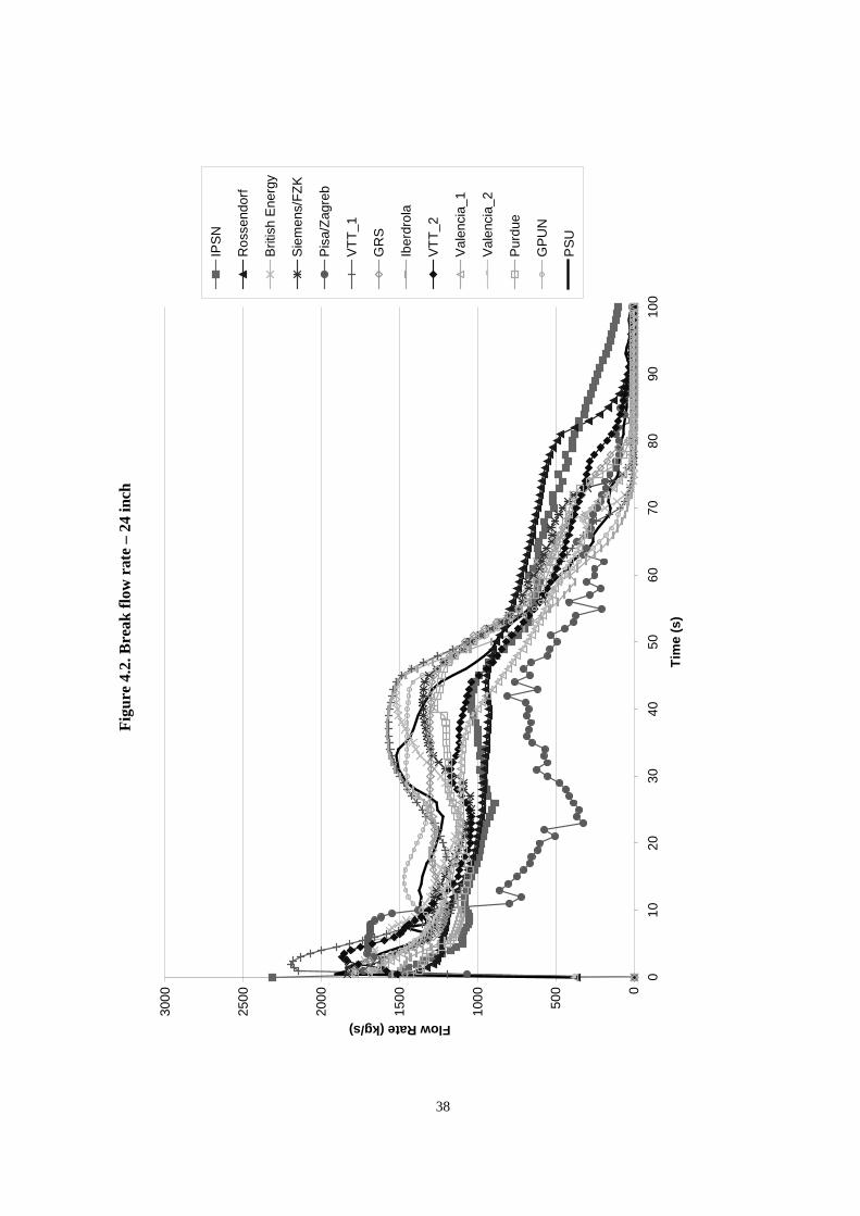
Fig
ure
4.2.
Bre
ak fl
ow r
ate
– 24
inch
0
500
1000
1500
2000
2500
3000
010
2030
4050
6070
8090
100
Tim
e (s
)
Flow Rate (kg/s)
IPS
N
Ros
send
orf
Brit
ish
Ene
rgy
Sie
men
s/F
ZK
Pis
a/Z
agre
b
VT
T_1
GR
S
Iber
drol
a
VT
T_2
Val
enci
a_1
Val
enci
a_2
Pur
due
GP
UN
PS
U
38

Fig
ure
4.3.
Bre
ak fl
ow r
ate
– 8
inch
0
500
1000
1500
2000
2500
3000
010
2030
4050
6070
8090
100
Tim
e (s
)
Flow Rate (kg/s)
IPS
N
Ros
send
orf
Brit
ish
Ene
rgy
Sie
men
s/F
ZK
Pis
a/Z
agre
b
VT
T_1
GR
S
Iber
drol
a
VT
T_2
Val
enci
a_1
Val
enci
a_2
Pur
due
GP
UN
PS
U
39

Fig
ure
4.4.
Ave
rage
pre
ssur
e
024681012141618
010
2030
4050
6070
8090
100
Tim
e (s
)
Pressure (MPa)
IPS
N
Ros
send
orf
Brit
ish
Ene
rgy
Sie
men
s/F
ZK
Pis
a/Z
agre
b
VT
T_1
GR
S
Iber
drol
a
VT
T_2
Val
enci
a_1
Val
enci
a_2
Pur
due
GP
UN
PS
U
40

Fig
ure
4.5.
Bro
ken
loop
pre
ssur
e
024681012141618
010
2030
4050
6070
8090
100
Tim
e (s
)
Pressure (MPa)
IPS
N
Ros
send
orf
Brit
ish
Ene
rgy
Sie
men
s/F
ZK
Pis
a/Z
agre
b
VT
T_1
GR
S
Iber
drol
a
VT
T_2
Val
enci
a_1
Val
enci
a_2
Pur
due
PS
U
41

Fig
ure
4.6.
Int
act
loop
pre
ssur
e
024681012141618
010
2030
4050
6070
8090
100
Tim
e (s
)
Pressure (MPa)
IPS
N
Ros
send
orf
Brit
ish
Ene
rgy
Sie
men
s/F
ZK
Pis
a/Z
agre
b
VT
T_1
GR
S
Iber
drol
a
VT
T_2
Val
enci
a_1
Val
enci
a_2
Pur
due
PS
U
42

Fig
ure
4.7.
Pre
ssur
iser
pre
ssur
e
024681012141618
010
2030
4050
6070
8090
100
Tim
e (s
)
Pressure (MPa)
IPS
N
Brit
ish
Ene
rgy
NE
TC
OR
P
Pur
due
PS
U
43

Fig
ure
4.8.
Bro
ken
stea
m li
ne p
ress
ure
0.0
1.0
2.0
3.0
4.0
5.0
6.0
7.0
8.0
9.0
10.0
010
2030
4050
6070
8090
100
Tim
e (s
)
Pressure (MPa)
IPS
N
Ros
send
orf
Brit
ish
Ene
rgy
Sie
men
s/F
ZK
Pis
a/Z
agre
b
VT
T_1
NE
TC
OR
P
GR
S
Iber
drol
a
VT
T_2
Val
enci
a_1
Val
enci
a_2
Pur
due
GP
UN
PS
U
44

Fig
ure
4.9.
Int
act
stea
m li
ne p
ress
ure
0.0
1.0
2.0
3.0
4.0
5.0
6.0
7.0
8.0
9.0
10.0
010
2030
4050
6070
8090
100
Tim
e (s
)
Pressure (MPa)
IPS
N
Ros
send
orf
Brit
ish
Ene
rgy
Sie
men
s/F
ZK
Pis
a/Z
agre
b
VT
T_1
NE
TC
OR
P
GR
S
Iber
drol
a
VT
T_2
Val
enci
a_1
Val
enci
a_2
Pur
due
GP
UN
PS
U
45

Fig
ure
4.10
. Ave
rage
coo
lant
tem
pera
ture
500
510
520
530
540
550
560
570
580
590
600
010
2030
4050
6070
8090
100
Tim
e (s
)
Temperature (K)
IPS
N
Ros
send
orf
Brit
ish
Ene
rgy
Sie
men
s/F
ZK
Pis
a/Z
agre
b
VT
T_1
NE
TC
OR
P
GR
S
Iber
drol
a
VT
T_2
Val
enci
a_1
Val
enci
a_2
Pur
due
PS
U
46

Fig
ure
4.11
. Bro
ken
hot
leg
tem
pera
ture
500
510
520
530
540
550
560
570
580
590
600
010
2030
4050
6070
8090
100
Tim
e (s
)
Temperature (K)
IPS
N
Ros
send
orf
Brit
ish
Ene
rgy
Sie
men
s/F
ZK
Pis
a/Z
agre
b
VT
T_1
NE
TC
OR
P
GR
S
Iber
drol
a
VT
T_2
Val
enci
a_1
Val
enci
a_2
Pur
due
GP
UN
PS
U
47

Fig
ure
4.12
. Int
act
hot
leg
tem
pera
ture
500
510
520
530
540
550
560
570
580
590
600
010
2030
4050
6070
8090
100
Tim
e (s
)
Temperature (K)
IPS
N
Ros
send
orf
Brit
ish
Ene
rgy
Sie
men
s/F
ZK
Pis
a/Z
agre
b
VT
T_1
NE
TC
OR
P
GR
S
Iber
drol
a
VT
T_2
Val
enci
a_1
Val
enci
a_2
Pur
due
GP
UN
PS
U
48

Fig
ure
4.13
. Bro
ken
cold
leg
tem
pera
ture
480
490
500
510
520
530
540
550
560
570
580
010
2030
4050
6070
8090
100
Tim
e (s
)
Temperature (K)
IPS
N
Ros
send
orf
Brit
ish
Ene
rgy
Sie
men
s/F
ZK
Pis
a/Z
agre
b
VT
T_1
NE
TC
OR
P
GR
S
Iber
drol
a
VT
T_2
Val
enci
a_1
Val
enci
a_2
Pur
due
GP
UN
PS
U
49

Fig
ure
4.14
. Int
act
cold
leg
tem
pera
ture
500
510
520
530
540
550
560
570
580
590
600
010
2030
4050
6070
8090
100
Tim
e (s
)
Temperature (K)
IPS
N
Ros
send
orf
Brit
ish
Ene
rgy
Sie
men
s/F
ZK
Pis
a/Z
agre
b
VT
T_1
NE
TC
OR
P
GR
S
Iber
drol
a
VT
T_2
Val
enci
a_1
Val
enci
a_2
Pur
due
GP
UN
PS
U
50

Fig
ure
4.15
. Fue
l tem
pera
ture
500
550
600
650
700
750
800
850
900
950
1000
010
2030
4050
6070
8090
100
Tim
e (s
)
Temperature (K)
IPS
N
Brit
ish
Ene
rgy
Sie
men
s/F
ZK
VT
T_1
NE
TC
OR
P
GR
S
Iber
drol
a
VT
T_2
Val
enci
a_1
Val
enci
a_2
Pur
due
GP
UN
PS
U
51

Fig
ure
4.16
. Fis
sion
pow
er
0.00
E+0
0
5.00
E+0
8
1.00
E+0
9
1.50
E+0
9
2.00
E+0
9
2.50
E+0
9
3.00
E+0
9
3.50
E+0
9
4.00
E+0
9
010
2030
4050
6070
8090
100
Tim
e (s
)
Power (W)
IPS
N
Ros
send
orf
Brit
ish
Ene
rgy
Sie
men
s/F
ZK
Pis
a/Z
agre
b
VT
T_1
NE
TC
OR
P
GR
S
Iber
drol
a
VT
T_2
Val
enci
a_1
Val
enci
a_2
Pur
due
PS
U
52

Fig
ure
4.17
. Tot
al p
ower
0.00
E+0
0
5.00
E+0
8
1.00
E+0
9
1.50
E+0
9
2.00
E+0
9
2.50
E+0
9
3.00
E+0
9
3.50
E+0
9
4.00
E+0
9
010
2030
4050
6070
8090
100
Tim
e (s
)
Power (W)
IPS
N
Ros
send
orf
Brit
ish
Ene
rgy
Sie
men
s/F
ZK
Pis
a/Z
agre
b
VT
T_1
NE
TC
OR
P
Iber
drol
a
VT
T_2
Val
enci
a_1
Val
enci
a_2
Pur
due
GP
UN
PS
U
53

Fig
ure
4.18
. Dec
ay p
ower
0.00
E+
00
5.00
E+
07
1.00
E+
08
1.50
E+
08
2.00
E+
08
2.50
E+
08
3.00
E+
08
3.50
E+
08
4.00
E+
08
010
2030
4050
6070
8090
100
Tim
e (s
)
Power (W)
NE
TC
OR
P
Iber
drol
a
Val
enci
a_1
Val
enci
a_2
Pur
due
PS
U
54

Fig
ure
4.19
. Tot
al r
eact
ivit
y
-5.0
E-0
2
-4.5
E-0
2
-4.0
E-0
2
-3.5
E-0
2
-3.0
E-0
2
-2.5
E-0
2
-2.0
E-0
2
-1.5
E-0
2
-1.0
E-0
2
-5.0
E-0
3
0.0E
+00
5.0E
-03
010
2030
4050
6070
8090
100
Tim
e (s
)
Reactivity (dk/k)
IPS
N
Ros
send
orf
Brit
ish
Ene
rgy
Sie
men
s/F
ZK
Pis
a/Z
agre
b
VT
T_1
NE
TC
OR
P
GR
S
Iber
drol
a
VT
T_2
Val
enci
a_1
Val
enci
a_2
Pur
due
GP
UN
PS
U
55

Fig
ure
4.20
. Mod
erat
or r
eact
ivit
y
-5.0
E-0
3
0.0E
+00
5.0E
-03
1.0E
-02
1.5E
-02
2.0E
-02
2.5E
-02
3.0E
-02
3.5E
-02
4.0E
-02
4.5E
-02
010
2030
4050
6070
8090
100
Tim
e (s
)
Reactivity (dk/k)
IPS
N
Ros
send
orf
Brit
ish
Ene
rgy
VT
T_1
NE
TC
OR
P
GR
S
Iber
drol
a
VT
T_2
Val
enci
a_1
Val
enci
a_2
Pur
due
GP
UN
PS
U
56
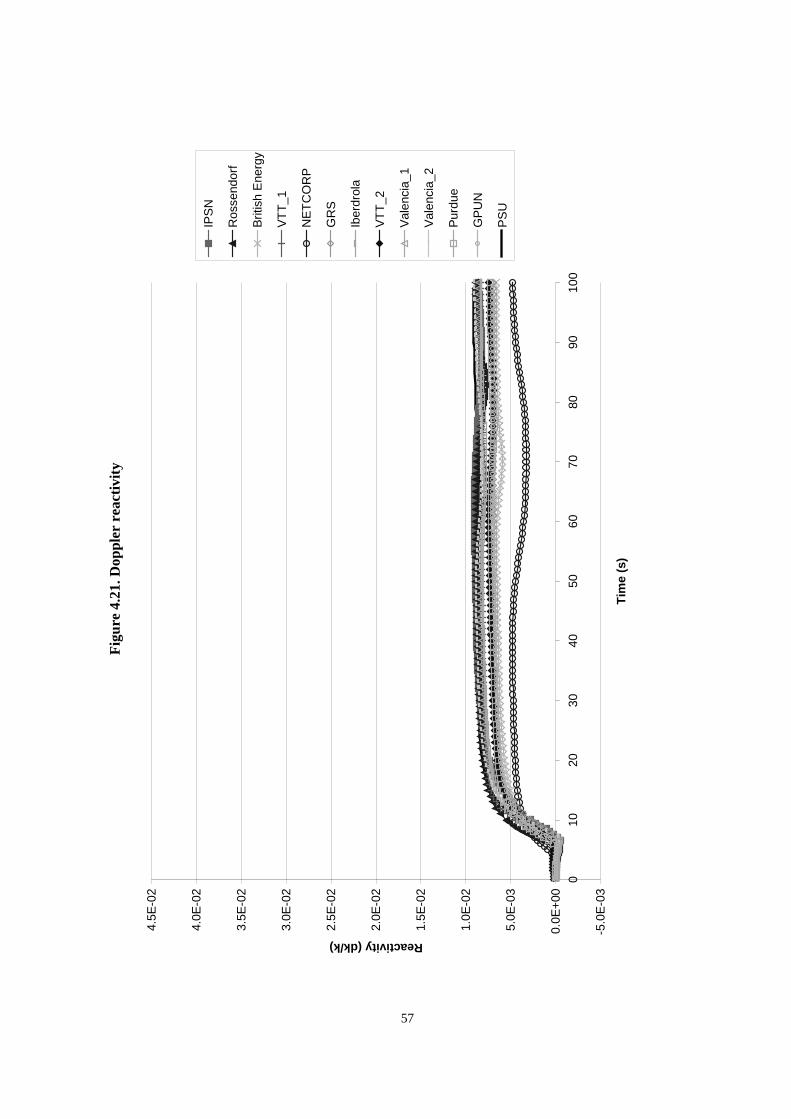
Fig
ure
4.21
. Dop
pler
rea
ctiv
ity
-5.0
E-0
3
0.0E
+00
5.0E
-03
1.0E
-02
1.5E
-02
2.0E
-02
2.5E
-02
3.0E
-02
3.5E
-02
4.0E
-02
4.5E
-02
010
2030
4050
6070
8090
100
Tim
e (s
)
Reactivity (dk/k)
IPS
N
Ros
send
orf
Brit
ish
Ene
rgy
VT
T_1
NE
TC
OR
P
GR
S
Iber
drol
a
VT
T_2
Val
enci
a_1
Val
enci
a_2
Pur
due
GP
UN
PS
U
57

Fig
ure
4.22
. Scr
am r
eact
ivit
y
-5.0
E-0
2
-4.5
E-0
2
-4.0
E-0
2
-3.5
E-0
2
-3.0
E-0
2
-2.5
E-0
2
-2.0
E-0
2
-1.5
E-0
2
-1.0
E-0
2
-5.0
E-0
3
0.0E
+00
5.0E
-03
010
2030
4050
6070
8090
100
Tim
e (s
)
Reactvity (dk/k)
IPS
N
Ros
send
orf
Brit
ish
Ene
rgy
NE
TC
OR
P
GR
S
Iber
drol
a
VT
T_2
Val
enci
a_1
Val
enci
a_2
Pur
due
GP
UN
PS
U
58

Fig
ure
4.23
. Bro
ken
stea
m g
ener
ator
mas
s
0
5000
1000
0
1500
0
2000
0
2500
0
3000
0
3500
0
4000
0
010
2030
4050
6070
8090
100
Tim
e (s
)
Mass (kg)
IPS
N
Ros
send
orf
Brit
ish
Ene
rgy
Sie
men
s/F
ZK
Pis
a/Z
agre
b
VT
T_1
NE
TC
OR
P
GR
S
Iber
drol
a
VT
T_2
Val
enci
a_1
Val
enci
a_2
Pur
due
GP
UN
PS
U
59

Fig
ure
4.24
. Int
act
stea
m g
ener
ator
mas
s
0
5000
1000
0
1500
0
2000
0
2500
0
3000
0
3500
0
4000
0
010
2030
4050
6070
8090
100
Tim
e (s
)
Mass (kg)
Ros
send
orf
Brit
ish
Ene
rgy
Sie
men
s/F
ZK
Pis
a/Z
agre
b
VT
T_1
NE
TC
OR
P
GR
S
Iber
drol
a
VT
T_2
Val
enci
a_1
Val
enci
a_2
Pur
due
GP
UN
PS
U
60

Fig
ure
4.25
. Hea
t tr
ansf
er: b
roke
n st
eam
gen
erat
or
-4.0
0E+
08
0.00
E+
00
4.00
E+
08
8.00
E+
08
1.20
E+
09
1.60
E+
09
2.00
E+
09
2.40
E+
09
2.80
E+
09
3.20
E+
09
3.60
E+
09
4.00
E+
09
010
2030
4050
6070
8090
100
Tim
e (s
)
Heat Transfer (W)
Ros
send
orf
Sie
men
s/F
ZK
VT
T_1
NE
TC
OR
P
GR
S
Iber
drol
a
VT
T_2
Val
enci
a_1
Val
enci
a_2
Pur
due
61

Fig
ure
4.26
. Hea
t tr
ansf
er: i
ntac
t st
eam
gen
erat
or
-4.0
0E+
08
0.00
E+
00
4.00
E+
08
8.00
E+
08
1.20
E+
09
1.60
E+
09
2.00
E+
09
2.40
E+
09
2.80
E+
09
3.20
E+
09
3.60
E+
09
4.00
E+
09
010
2030
4050
6070
8090
100
Tim
e (s
)
Heat Transfer (W)
Ros
send
orf
Sie
men
s/F
ZK
VT
T_1
NE
TC
OR
P
GR
S
Iber
drol
a
VT
T_2
Val
enci
a_1
Val
enci
a_2
Pur
due
62

Fig
ure
4.27
. Int
egra
ted
leak
age:
vap
our
mas
s
0
1000
0
2000
0
3000
0
4000
0
5000
0
6000
0
7000
0
010
2030
4050
6070
8090
100
Tim
e (s
)
Mass (kg)
Ros
send
orf
Sie
men
s/F
ZK
VT
T_1
GR
S
VT
T_2
Pur
due
63
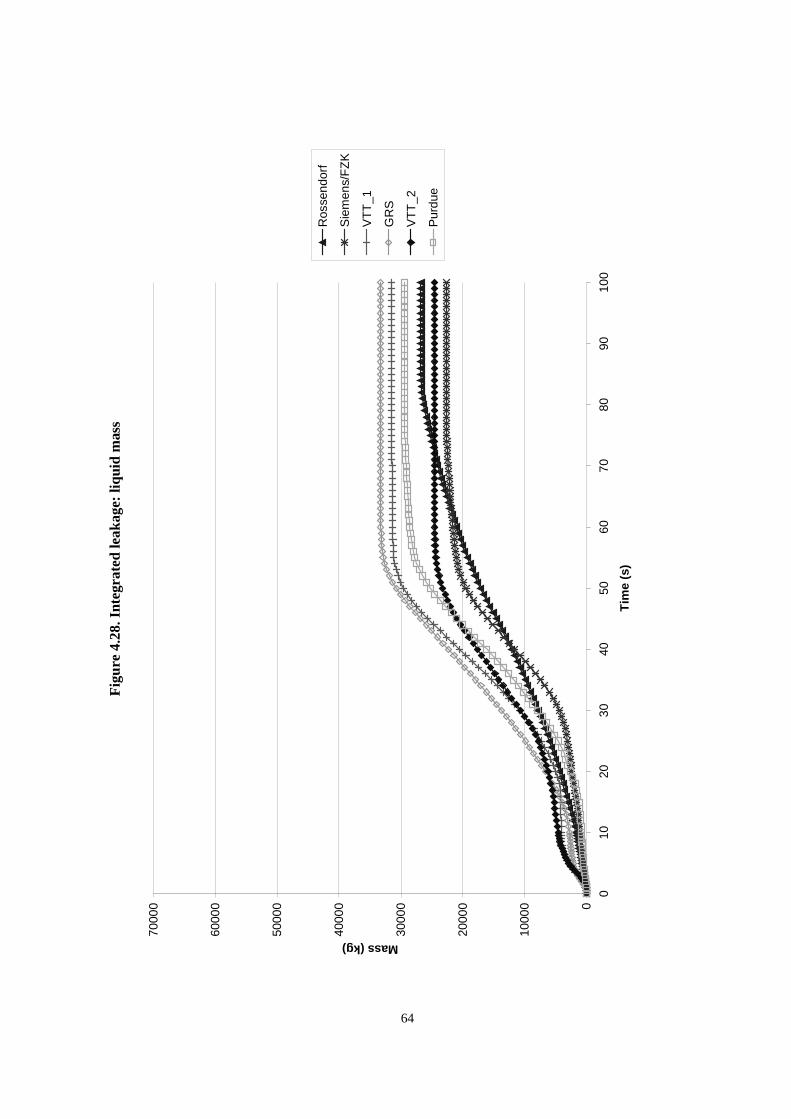
Fig
ure
4.28
. Int
egra
ted
leak
age:
liqu
id m
ass
0
1000
0
2000
0
3000
0
4000
0
5000
0
6000
0
7000
0
010
2030
4050
6070
8090
100
Tim
e (s
)
Mass (kg)
Ros
send
orf
Sie
men
s/F
ZK
VT
T_1
GR
S
VT
T_2
Pur
due
64

65
Chapter 5
CONCLUSIONS
In order to meet the objectives of the validation of best-estimate coupled codes a systematicapproach has been introduced to evaluate the MSLB transient. Such codes use separate temporal andspatial models and numerical methods for core neutronics, core thermal-hydraulics and systemthermal-hydraulics simulations. Therefore, the validation of these codes should include a testing ofthese models for the defined transient (in this case a MSLB) as phases (separate exercises) of theoverall benchmark. The ultimate goal is to enable participants to initiate and verify these modelsbefore focusing on the major objective – testing of coupling methodologies in terms of numerics,temporal and spatial mesh overlays. This approach allows one to evaluate in a more consistent way themodelling of combined effects (determined by neutronics/T-H as well as core/plant interactions) byremoving the uncertainties introduced with separate models. In order to perform such a comprehensivevalidation of coupled codes a multi-level methodology is employed. It includes the application of threeexercises (phases), the evaluation of several steady states, and simulation of two transient scenarios.
The analysis of the MSLB benchmark has been performed in an iterative manner. Subsequent topreliminary calculations and comparisons, the specific list of relevant parameters for comparison ineach exercise has finally been established. The practical experience gained in this benchmark showsthat only after such preliminary stages of analysis can all peculiarities and requirements of modellingbe fixed. In this context the international benchmark workshops and ad-hoc meetings (held inconjunction with international conferences) have played important roles as forums for discussing theobtained results and observed deviations as well as the sources of modelling uncertainties andsubsequent modifications of the benchmark specification [6-8]. Over the course of the benchmarkactivities a professional community has been created, and its members became involved in an in-depthdiscussion of different aspects considered in the validation process.
Exercise 1 is defined as point kinetics (PK) plant simulation. The purpose of this exercise is totest the primary and secondary system model responses. Compatible point kinetics model inputs whichpreserve axial and radial power distributions and tripped rod reactivity are provided from the coupledthree-dimensional (3-D) kinetics/system T-H calculations. During the course of benchmark calculationsabout fourteen participants from eight countries were assisted in modelling the first exercise andsubsequently submitted their PK results. Overall, this benchmark has been well accepted internationallyand a like number will be participating in the remaining two phases.
Based on the preliminary comparisons of participants’ results it was concluded that the overallagreement of the compared parameters could be improved. The analysis performed demonstrated thatthe deviations are primarily due to the modelling differences rather than the different code theoreticalmodels. These modelling differences were identified as follows: the conservative initial steamgenerator (SG) masses, modelling the additional feedwater to the broken SG, steam line break flowmodelling, the flow paths to the upper head of reactor vessel and different reactor vessel mixingmodels. The need to resolve these issues was addressed by carrying out parametric studies whichdemonstrated sensitivity of power response during the MSLB transient to key input parameters.This initiated a detailed discussion concerning the main effects during a MSLB transient and the

66
sensitivity of these effects to the modelling assumptions. As a result a three-step procedure wasapplied: additional information was provided, some modelling assumptions were made explicit (suchas the additional feedwater to the broken SG, which was specified as feedwater mass flow rate versustime) and other assumptions were made consistent (such as the SG initial mass).
Due to the sensitive nature of this transient to small variations in initial parameters, theparticipants were advised to follow the final specifications as closely as possible. To avoid possiblemisinterpretations, the benchmark team provided further clarifications before the final results weresubmitted. The motivation behind such clarifications were to narrow down to the extent possible themodelling differences for the initial steady state conditions as well as for the transient scenario.This strategy helped to obtain a cluster of solutions to be used as a basis for deviations. A statisticalmethodology for evaluation of discrepancies between different code predictions was employed forsingle value parameters.
In this volume, the first phase of the OECD/NRC PWR MSLB benchmark is discussed in detail.The final results submitted by the participants for the first phase are used to make code-to-codecomparisons and a subsequent statistical analysis. This information encompasses approximately26 thermal-hydraulic and neutronic parameters that affect the reactor behaviour during a MSLBaccident, including powers, pressures, temperatures, reactivities, mass flow rates and SG massesthroughout the transient. It is presented in plots graphically illustrating the agreement in different codepredictions and tables containing relative differences for each of the participant’s results for eachparameter. The calculation is performed for single value parameters for chosen time points during thetransient based on statistical mean value solution.
A detailed assessment of the differences between the calculated results submitted by theparticipants for the first exercise were presented in Chapter 4 of this volume. The power response andthe magnitude of the return to power during the transient as predicted by different codes are functionsof the total reactivity time evolution. Since the negative tripped rod reactivity inserted is specified, thedifferences arise from the predictions of moderator feedback and Doppler feedback reactivitycomponents. The moderator reactivity component follows the cold leg temperature. The discrepanciesin the cold leg temperature predictions are mostly due to differences in modelling the secondary side.It was observed that the major factors affecting the dynamics of the transient are break flow modelling(critical flow model), liquid entrainment, modelling of the aspirator flow and nodalisation of theSG down comer. These factors affect the SG mass parameter for both the broken and intact SGs.This parameter shows the greatest deviation amongst participant results, both in the value andbehaviour of the SG masses throughout the transient. In addition the disagreement can be attributed todifferences in the heat transfer correlations used within each participant’s code. This is especially truefor the participants who use proprietary correlations that are specific to U-tube SGs in their codes, asthe behaviour of a OTSG is much different than a U-tube SGs, and also involves superheat, somethingU-tube SGs do not have. The Doppler feedback reactivity predictions are sensitive to the relation forDoppler fuel temperature used as well as to the radial and axial nodalisation of the heat structure used(fuel rod).
Overall, it was determined that for the first phase of this benchmark, the key parameters were theSG masses, the break flow rates, the coolant and fuel temperatures and the powers. The other parameterswere useful to analyse because they helped to determine what was causing the behaviour of the keyparameters. As expected, the break flow rates/modelling was very sensitive to the SG masses/modellingand vice versa. In addition, it was proven that the SG model has a great effect on the power throughoutthe transient. In particular, the way the additional feedwater was introduced into the steam generator,the aspirator junction area, down comer nodalisation and the OTSG model in general proved to be asource for many differences in the preliminary results. Various interpretations of the steam line break

67
also caused a great deal of uncertainty before the model was made uniform amongst all participants.One of the most important lessons learned from the first phase of the benchmark was that it isextremely important, as well as very difficult, to ensure consistency in the modelling for any problem.
This type of analysis requires considerably more output than was required by previous benchmarks,and this is especially true of the remaining phases. In addition to requesting more output, the processof determining which parameters to request from the participants must be completed well in advance.From the benchmark team’s experiences to date, it is evident that for any future large-scale coupledanalyses, closer attention must be paid to the thermal-hydraulic aspect of the benchmark. In addition todoing a better job specifying the transient scenario, it should be designated in such a way that multipleinterpretations are not possible. Overall it was determined that:
• The possible redefinition of the problem to help clarify the participants’ understanding shouldbe allowed for.
• The participants should be provided with a standard file into which they insert data.
• It is not possible to do a “blind” benchmark of this complexity.
Numerous questions arose despite a concerted effort, including a participant review, to generate acomplete and accurate benchmark specification. Problems with the interpretation of the transientscenario, the physics and the models used in various codes led to numerous requests for clarificationand changes to the final specification. While certain problems were anticipated, such as modelling ofthe OTSG, many others came as a surprise. The participants had difficulty with the break and flowdistribution information, the kinetics parameters, reactor vessel mixing and the feedwater flow pipingand mass flow parameters provided in the original specification. Difficulties led to an interactiveprocess stretching the benchmark to a three-year effort, and required several iterations on results toobtain a consistent interpretation of the specification and the transient.
While some of the lessons learned by the benchmark team came as a surprise, the point kineticsresults were as expected. They verify that point kinetics analysis may be overly conservative and thusmay limit the operational flexibility of NPPs in the areas of higher burn-ups, longer fuel cycles andpower upgrades. The results of the first phase will be combined with results from the next two phasesof the PWR MSLB benchmark to help verify coupled 3-D neutronics/thermal-hydraulic system codesresults and to assist the users in gaining a more in-depth knowledge of these best estimate codes.The recent progress in computer technology made the development of such advanced codes for realisticmodelling of plant transient and accident conditions feasible and they will play a critical role in thefuture of nuclear analysis.


69
REFERENCES
[1] C. Jackson and H. Finnemann, “Verification of the Coupled RELAP5/PANBOX System withthe NEACRP LWR Core Transient Benchmark”, Proc. of the International Conference onMathematics and Computations, Reactor Physics, and Environmental Analyses, Portland,Oregon, 30 April-1 May 1995, p. 297.
[2] K. Ivanov, T. Beam, A. Baratta, A. Irani and N. Trikorous, “PWR MSLB Benchmark. Volume 1:Final Specifications”, NEA/NSC/DOC(99)8, April 1999.
[3] T. Beam, K. Ivanov and A. Baratta, “Benchmarking Advanced Coupled Neutronic/Thermal-Hydraulic Computer Code Models for Nuclear Power Plants”, Proc. of the JointInternational Conference on Mathematical Methods and Supercomputing for NuclearApplications, Vol. 1, Saratoga Springs, New York, 5-9 October 1997, p. 263.
[4] K. Ivanov, T. Beam, A. Baratta, A. Irani and N. Trikouros, “MSLB Analysis of TMI Unit-1Using TRAC-PF1/NEM”, Proceedings of the International RETRAN Conference 1998, EPRITR-109622, pp. 28-17 to 28-56, June 1998.
[5] B. Taylor and K. Ivanov, “Statistical Methods Used for Code-to-Code Comparisons in theOECD/NRC PWR MSLB Benchmark”, Annals of Nuclear Energy, 27 (2000), 1589-1605.
[6] “Summary of the 2nd PWR MSLB Benchmark Workshop”, Madrid, Spain, 25-26 June 1998,NEA/NSC/DOC(98)4.
[7] “Summary of the 3rd PWR MSLB Benchmark Workshop”, Garching, Germany, 24-25 Mar. 1999,NEA/NSC/DOC(99)6.
[8] “Summary of the 4th PWR MSLB Benchmark Workshop”, Paris, France, 24-25 January 2000,NEA/NSC/DOC(2000)2.
[9] K. Ivanov, A. Baratta and E. Sartori, “OECD/NRC MSLB Benchmark – A SystematicApproach to Validate Best-Estimate Coupled Codes Using a Multi-Level Methodology”,Proceedings of CSNI/NRC Workshop on Best Estimate Methods and Codes, Barcelona, Spain,15-19 April 2000.


71
APPENDIX A
Description of ComputerCodes Used for Analysisin the First Phase of thePWR MSLB Benchmark


73
SMABRE (VTT-1)
The SMABRE computer code is used by VTT for the point kinetics phase of the benchmarkexercise. This computer code has 1-D kinetics and thermal-hydraulics; however, it is able to model3-D thermal-hydraulic effects using parallel channel nodalisation. SMABRE contains a five-equation,two-phase, thermal-hydraulic model, using the drift flux model. The point kinetics model allows forone energy group and six delayed neutron groups, with cross-sections coming from polynomials usingfeedback reactivity coefficients or from a user defined table. The numerical solution method used inSMABRE is a predictor-corrector type non-iterative solution. The code has been used by VTT foranalysis of VVER reactor transients.
RELAP5/MOD3.2 (FZK/Siemens-KWU, Germany; Universities of Pisa and Zagreb, Italy andCroatia; and BE, United Kingdom)
RELAP5/MOD3.2 is a full six equations, two-phase flow, thermal-hydraulic code developed byINEEL/NRC to simulate both operational transients and loss of coolant accidents in light waterreactors. The code models the primary and secondary reactor coolant system as well as the reactorwith a one-dimensional approach. A point kinetics model is available to predict the core kinetics withrelated feedback mechanisms. By the use of one-dimensional flow channels and cross-flow junctions alimited 3-D modelling of the flow inside the RPV is possible. The RELAP5 system model is solvednumerically using a semi-implicit finite difference technique. Here, a direct sparse matrix solutiontechnique is used. The user that allows violation of the material Courant limit can also select a nearlyimplicit finite difference technique.
RELAP5/MOD3 (Purdue University/NRC, USA)
The RELAP5 code has been developed for best-estimate transient simulation of light water reactorcoolant systems during postulated accidents. RELAP5 is a highly generic code that, in addition tocalculating the behaviour of a reactor coolant system during a transient, can be used for simulation of awide variety of hydraulic and thermal transients in both nuclear and non-nuclear systems involvingmixtures of steam, water, non-condensable and solute.
The RELAP5/MOD3 code is based on a non-homogeneous and non-equilibrium model for thetwo-phase system that is solved by a fast, partially implicit numerical scheme to permit economicalcalculation of system transients. The code includes many generic component models from whichgeneral systems can be simulated. The component models include pumps, valves, pipes, heat releasingor absorbing structures, reactor point kinetics, electric heaters, jet pumps, turbines, separators,accumulators and control system components. In addition, special process models are included foreffects such as form loss, flow at an abrupt area change, branching, choked flow, boron tracking andnon-condensable gas transport.
ATHLET (GRS and FZR, Germany)
The ATHLET code is under development by GRS and the Nuclear Research Centre Rossendorfand is a best estimate code for the analysis of anticipated and abnormal transients, small and intermediatebreaks as well as large breaks in light water reactors. This code will be used by GRS and RCR formodelling the thermal-hydraulic aspect of the benchmark. It employs point and one-dimensionalkinetics. It can be coupled to a three-dimensional kinetics code using a generalised interface.

74
Using a channelised model, the core can be simulated in a multi-dimensional manner. The code isa two-fluid thermal-hydraulic code using either a five- or four-equation model. A full range drift-fluxmodel is available for calculating relative phasic velocities. A full two-fluid six-equation version isunder development.
DYNODE-P 3/D (NETCorp, USA)
Nuclear Engineering Technology Corporation uses the DYNODE-P 3/D code for the benchmark.The code has point and multi-dimensional spatial kinetics models for calculation of core power.The code solves for the change in enthalpy within a volume based on the change in pressure and heatsources in the volume and the flow of mass into the volume. A series of component models are used todescribe the system. Each is hardwired to represent different components.
RETRAN-3D (GPUN/CSA/EPRI, USA; and IBERDROLA, Spain)
While similar to RETRAN 03, the RETRAN 3D code includes a three-dimensional kineticsmodule. The reactor core is modelled as a series of parallel channels coupled to the kinetics module.Iberdrola is working in this benchmark with the version MOD002. This version does not have a decayheat model in the 3-D mode.
CATHARE2 (IPSN/CEA, France)
The CATHARE2 code features a full six-equation, two-fluid, non-equilibrium, non-homogeneous,three-dimensional hydrodynamic model. The numerics are fully implicit in the one-dimensionalcomponents and semi-implicit in the three-dimensional components.
The CATHARE code is a French system code for nuclear thermal-hydraulics developed at CEAGrenoble by EDF, FRAMATOME and IPSN for PWR safety analysis. Two-phase flows are describedusing a full six-equation, two-fluid, non-equilibrium, non-homogeneous two-fluid model. The presenceof an incondensable can be taken in account by one to four additive transport equations.
CATHARE has a modular structure. Various modules (0-D, 1-D and 3-D) can be connected tomodel the primary and secondary circuits of any PWR. Sub-modules can be used to calculate theneutronics, the fuel thermo-mechanics, the pump characteristics, accumulators, sources, sinks, wallsand re-flooding. All kinds of two-phase flow patterns are modelled. Co-current and counter-currentflows are modelled with prediction of counter current flow limitation. Heat transfer with wall structuresand fuel are calculated taking into account all heat transfer processes (natural and forced convectionwith liquid, with gas, sub-cooled and saturated nucleate boiling, critical heat flux, film boiling, filmcondensation). The interfacial heat and mass transfers describe the vaporisation due to superheatedsteam and the direct condensation due to sub-cooled liquid, but also the steam condensation or liquidflashing due to metastable sub-cooled steam or superheated liquid.
The calculations for Exercise 1 of the MSLB benchmark have been performed with the versionV1.3L_1, which contains revision 5.
TRAC-PF1/MOD2 (Polytechnic University of Valencia, Spain; and PSU, USA)
The TRAC series of codes use a two-fluid (six-equation), non-equilibrium, non-homogeneous,three-dimensional hydrodynamic model in the reactor vessel. The balance of the plant is modelled

75
using one-dimensional flow. The solution method used is the semi-implicit SETS method. Based onversion 5.4 from LANL, the Penn State version of TRAC-PF1/MOD2 was modified to include severalnew options, including axial decay heat model, an improved fuel element model and an improvedboron-tracking algorithm.
APROS (VTT-2)
APROS (Advanced PROcess Simulator) is a multi-functional simulation environment for thedynamic simulation of nuclear and conventional power plant processes and for the simulation ofindustrial process dynamics. The Technical Research Centre of Finland (VTT) has developed it withFortum Engineering Ltd. The APROS simulation environment consists of an executive system, modelpackages, equation solvers, a real-time database and interface models. APROS has been programmedusing Fortran 77 and C languages. All the physical models, like neutronics or thermal-hydraulics, arewritten with Fortran 77.
The essential models in the calculations performed within the MSLB have been the core pointkinetics model for Phase I and the six-equation thermal-hydraulic model. In the APROS calculation ofthe MSLB benchmark with point kinetics model the reactor core was divided into six independentflow channels in thermal-hydraulics. Each flow channel was divided into 12 axial nodes. For the pointkinetics calculation a conventional point kinetics model had to be programmed into APROS. Also forthe point kinetics calculation, the average values of fuel and coolant temperatures obtained from thethermal-hydraulic channels were used. In the renewed calculation the coolant temperature coefficientwas used according to the proper benchmark definition. The fuel pellet dimensions and materialproperties according to the updated final specifications were used. The axial and radial profiledefinitions given in the benchmark could not be taken into account in the point kinetics calculation.
The six-equation thermal-hydraulic model describes the behaviour of one-dimensional two-phaseflow. The model is based on the conservation equations of mass, momentum and energy for the gasand liquid phases separately. The equations are coupled with empirical correlations describing varioustwo-phase phenomena. The pressures and velocities, volume fractions and enthalpies of each phase aresolved from the discretised equations using an iterative procedure. Heat transfer modules connect thesix-equation thermal-hydraulic model with heat conduction solution. Boric acid concentration solutionis included in the thermal-hydraulic part. The thermal-hydraulic part also contains calculation of fuelenthalpy and oxide layer thickness on cladding surface and power production by cladding oxidationaccording to the Baker-Just model. For the calculation of fuel rod temperatures the fuel rod isdescribed as a solid heat structure consisting of three materials: fuel, fuel-cladding gap and cladding.The one-dimensional heat conduction solution in the fuel rod is calculated using ten radial nodes.

77
APPENDIX B
Sequence of Events forthe First Phase of the
PWR MSLB Benchmark


79
Table B.1. Sequence of events for the first phase of the PWR MSLB benchmark problem
Event NETCorp IPSN/CEA VTT 1(SMABRE)
Univ. of ValenciaV 1/V 2
Univ. ofPisa andZagreb
Break opens 0.000 0.0010 0.000 0.0001/0.0001 0.000
Turbine isolation valvecloses – broken SG
N/A N/A 0.500 N/A N/A
High neutron flux set point N/A 5.5700 5.700 N/A N/A
Low RCS pressure set point N/A N/A N/A N/A N/A
Reactor trip 3.075 6.0300 6.200 6.2575/6.1919 7.390
Turbine isolation valvecloses – intact SG
2.670 6.0300 6.600 6.7575/6.6919 8.39
Steam line B small safetyvalve opens
N/A 6.9100 7.200 7.51/8.011 N/A
Steam line B safety valveGroup 1 opens
N/A 6.9600 7.400 8.011/8.011 N/A
Steam line B safety valveGroup 2 opens
N/A 6.9600 7.400 N/A N/A
Steam line B safety valveGroup 3 opens
N/A 7.6000 7.600 N/A N/A
HPI initiated N/A N/A 10.900 N/A N/A
Steam line B safety valveGroup 3 closed
N/A 22.1700 28.1000 N/A N/A
Steam line B safety valveGroup 2 closed
N/A 31.9400 34.9000 N/A N/A
Steam line B safety valveGroup 1 closed
N/A 31.9400 34.900 19.51/17.52 N/A
Steam line B small safetyvalve closed
N/A 35.2700 38.000 21.51/21.02 N/A
HPI starts 36.140 35.5500 35.900 37.7944/37.5497 45.530
Return to criticality 48.00 77.00 N/A N/A N/A
Point of maximum powerafter trip
65.00 82.78 66.0 65.66/6589 75.00
Transient ends 100.000 100.00 100.000 100.000 100.000

80
Table B.1. Sequence of events for the first phase of the PWR MSLB benchmark problem (cont.)
Event GRS Rossendorf Purdue/NRC
BE GPUN/CSA/EPRI
VIT 2(APROS)
Break opens 0.0 0.1 0.001 0.0 0.001 0.01
Turbine isolation valvecloses – broken SG
N/A N/A 0.001 N/A N/A N/A
High neutron flux set point N/A 4.21 4.5 N/A N/A N/A
Low RCS pressure set point N/A N/A N/A N/A N/A N/A
Reactor trip 6.56 4.61 4.9 5.4 5.5 6.135
Turbine isolation valvecloses – intact SG
6.56 N/A 5.4 5.9 5.7 6.7
Steam line B small safetyvalve opens
N/A N/A 6.2 N/A 6.55 N/A
Steam line B safety valveGroup 1 opens
N/A N/A 6.6 N/A 7.14 N/A
Steam line B safety valveGroup 2 opens
N/A N/A 6.6 N/A 7.14 N/A
Steam line B safety valveGroup 3 opens
N/A N/A 7.7 N/A 11.8 N/A
HPI initiated N/A N/A 10.0 N/A N/A N/A
Steam line B safety valveGroup 3 closed
N/A N/A 14.7 N/A 15.15 N/A
Steam line B safety valveGroup 2 closed
N/A N/A 31.8 N/A 21.1 N/A
Steam line B safety valveGroup 1 closed
N/A N/A 17.9 N/A 21.2 N/A
Steam line B small safetyvalve closed
N/A N/A 37.2 N/A 23.8 N/A
HPI starts 42.95 35.89 35.0 27.75 38.5 39.1
Return to criticality N/A 70.2 67.2 62.0 N/A 68.0
Point of maximum powerafter trip
77.0 81.60 73.5 67.50 64.00 81.8
Transient ends 100 100 100 100 100 N/A

81
Table B.1. Sequence of events for the first phase of the PWR MSLB benchmark problem (cont.)
Event Siemens/FZK Iberdrola PSU
Break opens 0.15 0.001 0.001
Turbine isolation valvecloses – broken SG
0.15 N/A 0.001
High neutron flux set point 5.2 N/A 5.60
Low RCS pressure set point N/A N/A N/A
Reactor trip 5.6 5.327 6.01
Turbine isolation valvecloses – intact SG
5.6 5.9 6.51
Steam line B small safetyvalve opens
7.44 8.402 8.4467
Steam line B safety valveGroup 1 opens
7.62 8.9713 9.1587
Steam line B safety valveGroup 2 opens
7.62 N/A 10.2061
Steam line B safety valveGroup 3 opens
7.8 N/A N/A
HPI initiated 11.375 N/A 12.8774
Steam line B safety valveGroup 3 closed
32.23 N/A N/A
Steam line B safety valveGroup 2 closed
33.76 N/A 31.7471
Steam line B safety valveGroup 1 closed
33.91 12.5374 40.7525
Steam line B small safetyvalve closed
36.75 21.4102 40.7525
HPI starts 36.375 34.069 37.9483
Return to criticality N/A N/A N/A
Point of maximum powerafter trip
74.0 61.0 61.0
Transient ends 100 100 100


83
APPENDIX C
Questionnaire forthe First Phase of the
PWR MSLB Benchmark


85
QUESTIONNAIRE FOR THE FIRST EXERCISE
I. Primary system
1. Vessel thermal-hydraulic (T-H) model and nodalisation (1-D, 3-D and number T-H channels orcells) – how are channels/T-H cells chosen?
2. Mixing model – how is the required mixing ratio implemented?
3. Upper plenum and upper head (of reactor vessel) paths (junctions) modelling?
4. Radial and axial heat structure (fuel rod) nodalisation?
5. Relation used for Doppler temperature?
II. Secondary system
1. Initial steam generator (SG) mass inventory?
2. SG down-comer nodalisation?
3. Aspirator flow modelling?
4. Steam line modelling?
5. Break flow modelling and critical flow model?
6. Are you using the updated steam safety relief valves data (see Updated Specifications, April 1999,Table 5.4.2, p. 69)?
7. Are you using the updated additional feedwater mass data (between the feedwater isolation valveand the broken SG) (see Updated Specifications, April 1999, Table 5.4.3, p. 69)?
III. General
1. Deviations from the updated final specifications (April 1999, NEA/NSC/DOC(99)8)?
2. User assumptions?
3. Specific features of the codes used?
86
FZR
Germany
I. Primary system
1. Vessel thermal-hydraulic (T-H) model and nodalisation (1-D, 3-D and number T-H channels orcells) – how are channels/T-H cells chosen?
One-dimensional vessel model: two parallel and independent flow paths (see 1.2) simulating theflow from the cold legs outlet through the down-comer and the lower plenum to the core, the coreis modelled with two channels for the fuel assemblies and two channels for the bypass, from thecore outlet the flow paths go through the upper plenum to the inlet of the hot legs, additional flowpathes for the upper head: see 1.3, connections between the flow paths: see 1.2.
2. Mixing model – how is the required mixing ratio implemented?
The primary circuit is fully split into two parts, two connection points are introduced between theseparts for pressure balance (core reflector and upper head) – at each time step the actual mixingratio is determined – by means of a controller energy is exchanged in the lower and the upperplenum to match the required value of 0.5.
3. Upper plenum and upper head (of reactor vessel) paths (junctions) modelling?
Two flow paths (one for each half of the circuit) are modelled from the upper plenum to the upperhead and back to the upper plenum to ensure the cooling of the upper head (the summary flow rateis about 1 000 kg/s).
4. Radial and axial heat structure (fuel rod) nodalisation?
Two fuel rods are modelled each with 24 nodes in axial and five nodes in radial direction.
5. Relation used for Doppler temperature?
Standard ATHLET approach (?).
II. Secondary system
1. Initial steam generator (SG) mass inventory?
26 077 kg.
2. SG down-comer nodalisation?
Eleven nodes.

87
3. Aspirator flow modelling?
Aspirator flow is modelled as a junction between the SG and the SG down-comer, the flow rate inthe initial state is about 80 kg/s.
4. Steam line modelling?
For the broken SG two steam lines are modelled, the cross connection is modelled, and each steamline also has 10 nodes up to the break.
5. Break flow modelling and critical flow model?
The break is modelled as double ended rupture within 0.1 s > for the description of the critical flowthe 1-D finite difference critical discharge model of ATHLET is used. It is a four-equation model,the field equations for this two-phase flow model are based on the 1-D stationary conservationlaws for liquid mass, vapour mass, mixture energy and mixture momentum.
Due to convergence problems, the Moody model could not be used, but investigations at the earlystage of the benchmark work showed that the differences between these two models are negligible.
6. Are you using the updated steam safety relief valves data (see Updated Specifications, April 1999,Table 5.4.2, p. 69)?
Yes.
7. Are you using the updated additional feedwater mass data (between the feedwater isolation valveand the broken SG) (see Updated Specifications, April 1999, Table 5.4.3, p. 69)?
Yes.
III. General
1. Deviations from the updated final specifications (April 1999, NEA/NSC/DOC(99)8)?
Critical flow model and determination of the Doppler temperature (probably).
2. User assumptions?
3. Specific features of the codes used?

88
FZK/SKWU
Germany
I. Primary system
1. Vessel thermal-hydraulic (T-H) model and nodalisation (1-D, 3-D and number T-H channels orcells) – how are channels/T-H cells chosen?
To model the vessel (RPV) thermal-hydraulics for the MSLB transient the RPV was split almostinto two equal halves, one half connected to the coolant stream of the broken Loop A and the otherone to the coolant stream of the intact Loop B. Each RPV half consists of following fluid volumesalong the main flow streams: RPV inlet, down-comer, lower plenum, core bypass, core, core outlet,upper plenum, one annular region between baffle and the core support shield and one dead-endannular region formed by the core support shield and the RPV wall. The uppermost upper plenumvolume connects both RPV halves to each other. In addition there are two volumes in the upperplenum for the mixing modelling. Four volume stacks (two per loop) thermal-hydraulicallyrepresent the core itself with 10 axial nodes. The two volume stacks belonging to a core half arehydraulically connected at each axial node by a cross-connection junction. There is no connectionbetween the core volumes of both Loop A and Loop B. The main in-vessel structures and the RPVwalls are also modelled. In total 64 fluid volumes are used to represent the whole RPV with itsmain flow paths.
2. Mixing model – how is the required mixing ratio implemented?
A precondition to model the coolant mixing according to the specification was the splitting of theRPV. So, at the lower plenum the mixing was reached adding two junctions to connect Loop A withLoop B. To get the recommended mixing ratio of 0.5, appropriate flow areas of the connectingjunctions had to be defined. In this way a mixing ratio close to 0.5 was obtained during almost thewhole transient calculation.
3. Upper plenum and upper head (of reactor vessel) paths (junctions) modelling?
At the upper plenum, the main flow paths are defined by the baffle and the baffle holes as well asby the annular region between the baffle and the core support shield. As earlier mentioned sixvolumes in three elevations were considered per core halves. Two additional volumes were defined(elevation 2 and 3) for mixing of both loops (A and B) occurs. The uppermost volume connects bothloops. In addition, two representative guide tubes per halves were modelled that conjoin the coreoutlet volumes (of Loop A and Loop B) with the uppermost volume.
4. Radial and axial heat structure (fuel rod) nodalisation?
Four heat structures, each one representing a quarter of the total core fuel rods, were modelled.Each heat structure is connected with one volume stack (core channel) by convective boundaryconditions. Axially the same number of nodes as the corresponding flow channels were chosen,

89
i.e. 10 nodes. Each heat structure consists radially of three material zones: UO2, gap and Zrycladding. The pellet and cladding are subdivided in two zones respectively. The axial power profileprovided in the Final Specifications was used. No radial power peaking distribution wasconsidered in the model for the Phase I since a point kinetics approach is used for total corereactivity and total core power prediction.
5. Relation used for Doppler temperature?
In RELAP5 the node wise volume average fuel temperature is used to predict the Dopplerreactivity feedback. A test calculation have shown that the Doppler temperature calculated by therelation given in the Final Specification is close to the average fuel temperature used in RELAP5.Thus the RELAP5 approach, which is comparable to the PSU procedure, was used in Phase I.
II. Secondary system
1. Initial steam generator (SG) mass inventory?
26 450 kg.
2. SG down-comer nodalisation?
An annulus volume with four internal volumes models the steam generator down-comer. Feedwateris injected at the down comer top and flows out of the down-comer to the volume representing thelower tube sheet, which is modelled as a branch. From this branch the flow is directed upwardthrough two volume stacks representing the boiler part of the steam generator.
3. Aspirator flow modelling?
The aspirator is modelled by a cross-flow junction that connects the boiler (at an elevation of9.73 m) with the down-comer top. The aspirator flow area mounts to 0.972 m2 but it was reduced to0.1858 m2 to obtain the initial fluid inventory of about 26 tonnes.
4. Steam line modelling?
The steam lines are modelled in detail considering their whole length as recommended by theSpecifications. It was represented by a RELAP5 pipe with 15 internal volumes. A cross-connectionline per loop was also considered in the model only for the intact loop. For this Loop B four banksof main steam safety valves (SRV) were modelled as prescribed in the Specifications. A turbine stopvalve (MSIV) per steam line, i.e. four in total, was also modelled. Finally the common header, theturbine check valve and the turbine itself (as pressure boundary) were also included in themodelling of the steam lines.
5. Break flow modelling and critical flow model?
Modelling the breaks the default choking model of RELAP5/MOD3.2, i.e. the Trapp & Ramsonmodel, together with the abrupt area option were used. To use the Moody critical flow model,modifications of the RELAP5 code beyond the scope of this benchmark are necessary. Thus, thehomogeneous instead of the non-homogeneous flow model was activated (recommendation of theRELAP5 manuals). An additional run was performed with the optional Henry Fauske model of

90
RELAP5/MOD3.2, which uses the thermal non-equilibrium model as default option. From theperformed calculations it was concluded that the differences in the break outflow rate of bothmodels are marginal.
6. Are you using the updated steam safety relief valves data (see Updated Specifications, April 1999,Table 5.4.2, p. 69)?
Yes.
7. Are you using the updated additional feedwater mass data (between the feedwater isolation valveand the broken SG) (see Updated Specifications, April 1999, Table 5.4.3, p. 69)?
Yes.
III. General
1. Deviations from the updated Final Specifications (April 1999, NEA/NSC/DOC(99)8)?
a) Use of the node-wise volume average fuel temperature instead of the relation given in thespecification (exploring run demonstrated that both approach are comparable).
b) Use of the Trapp & Ramson critical flow model instead of the Moody model.
2. User assumptions?
a) No radial nodalisation of the fuel rods since a point kinetics model is used to predict thereactivity and power.
b) Reduction of the aspirator flow is to get the initial fluid inventory in the steam generatorsecondary side.
3. Specific features of the codes used?
a) Use of the node-wise volume average fuel temperature to predict the Doppler reactivitycoefficient.
b) Trapp & Ramson critical flow model as default (Henry Fauske model as alternative).
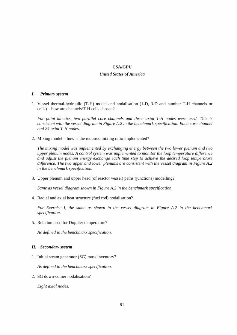
91
CSA/GPU
United States of America
I. Primary system
1. Vessel thermal-hydraulic (T-H) model and nodalisation (1-D, 3-D and number T-H channels orcells) – how are channels/T-H cells chosen?
For point kinetics, two parallel core channels and three axial T-H nodes were used. This isconsistent with the vessel diagram in Figure A.2 in the benchmark specification. Each core channelhad 24 axial T-H nodes.
2. Mixing model – how is the required mixing ratio implemented?
The mixing model was implemented by exchanging energy between the two lower plenum and twoupper plenum nodes. A control system was implemented to monitor the loop temperature differenceand adjust the plenum energy exchange each time step to achieve the desired loop temperaturedifference. The two upper and lower plenums are consistent with the vessel diagram in Figure A.2in the benchmark specification.
3. Upper plenum and upper head (of reactor vessel) paths (junctions) modelling?
Same as vessel diagram shown in Figure A.2 in the benchmark specification.
4. Radial and axial heat structure (fuel rod) nodalisation?
For Exercise I, the same as shown in the vessel diagram in Figure A.2 in the benchmarkspecification.
5. Relation used for Doppler temperature?
As defined in the benchmark specification.
II. Secondary system
1. Initial steam generator (SG) mass inventory?
As defined in the benchmark specification.
2. SG down-comer nodalisation?
Eight axial nodes.

92
3. Aspirator flow modelling?
As defined in the benchmark specification. The aspirator flow paths (junctions 150 and 250) shownin benchmark specification Figure A.1 are consistent with the way it was modelled.
4. Steam line modelling?
As defined in the benchmark specification and as shown in Figures A.3 and A.4.
5. Break flow modelling and critical flow model?
The geometry was as defined in the benchmark specification. An isoenthalpic critical flow modelwas used instead of the specified Moody critical flow model.
6. Are you using the updated steam safety relief valves data (see Updated Specifications, April 1999,Table 5.4.2, p. 69)?
Yes.
7. Are you using the updated additional feedwater mass data (between the feedwater isolation valveand the broken SG) (see Updated Specifications, April 1999, Table 5.4.3, p. 69).
Yes.
III. General
1. Deviations from the updated Final Specifications (April 1999, NEA/NSC/DOC(99)8)?
There were three deviations from the specifications that we are aware of in our analysis. The firstis the choice of critical flow models for Exercises I (see Question 4 above). The second is we usedthe 1979 ANS decay heat model within RETRAN rather than the specified decay heat. We compareddecay heat values and the differences were insignificant.
2. User’s assumptions?
None other than discussed above.
3. Specific features of the codes used?
None.

93
NETCorp
United States of America
I. Primary system
1. Vessel thermal-hydraulic (T-H) model and nodalisation (1-D, 3-D and number T-H channels orcells) – how are channels/T-H cells chosen?
See the figures below.
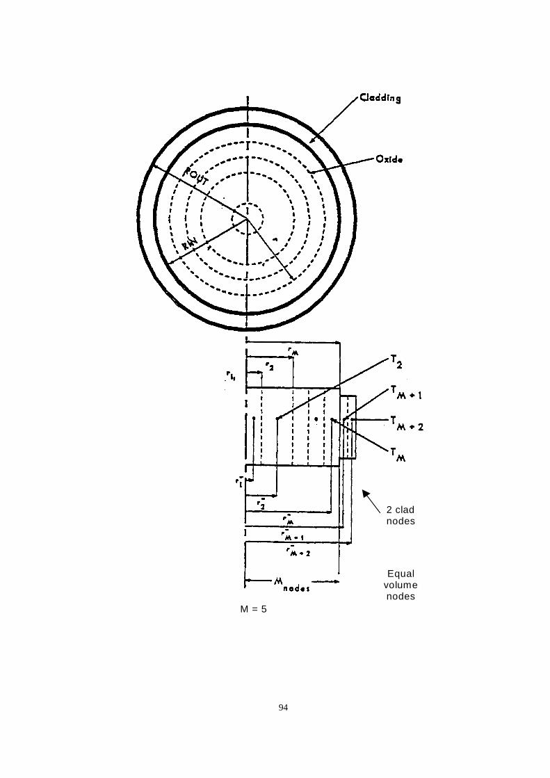
94
M = 5
Equalvolumenodes
2 cladnodes

95
Prim
ary
side
tube
s
SUB-COOLED
FeedwaterAspirator
SATURATED
SUPER-HEATED
Qsub
Qsat
Qsup
BRGAK
MSIV
Main steam

96

97
2. Mixing model – how is the required mixing ratio implemented?
DNP/3D did not use a mixing model for the first exercise.
3. Upper plenum and upper head (of reactor vessel) paths (junctions) modelling?
See Figures above.
4. Radial and axial heat structure (fuel rod) nodalisation?
See Figures above.
5. Relation used for Doppler temperature?
For the first exercise, the average fuel temperature was used for the Doppler reactivity.

98
II. Secondary system
1. Initial steam generator (SG) mass inventory?
Down-comer liquid = 36 023 lbmTube bundle liquid = 16 697 lbmTube bundle steam = 4 597 lbmTotal = 57 317 lbm
2. SG down-comer nodalisation?
See Figures above.
3. Aspirator flow modelling?
Initial aspirator flow based on raising feedwater flow to saturation.
4. Steam line modelling?
See Figures above.
5. Break flow modelling and critical flow model?
See Figures above.Moody critical flow model assuming saturated steam at the exit plane.No pressure drop losses from the steam dome to the exit plane.
6. Are you using the updated steam safety relief valves data (see Updated Specifications, April 1999,Table 5.4.2, p. 69)?
Yes.
7. Are you using the updated additional feedwater mass data (between the feedwater isolation valveand the broken SG) (see Updated Specifications, April 1999, Table 5.4.3, p. 69).
Yes.
III. General
1. Deviations from the updated Final Specifications (April 1999, NEA/NSC/DOC(99)8)?
None known.
2. User assumptions?
Nothing special.
3. Specific features of the codes used?
OTSG model option.

99
UNIVERSITIES OF PISA AND ZAGREB
Italy and Croatia
I. Primary system
1. Vessel thermal-hydraulic (T-H) model and nodalisation (1-D, 3-D and number T-H channels orcells) – how are channels/T-H cells chosen?
The RPV geometry is 1-D (around 150 nodes are included). The core is also 1-D. However, onestack of hydraulic nodes for the active region and one stack for the bypass should be distinguished.In addition, the hydraulic stack for the active region includes four parallel thermal structurestacks. Each hydraulic (two) or structures (four) stacks consists of 24 axial nodes.
2. Mixing model – how is the required mixing ratio implemented?
Full mixing has been considered.
3. Upper plenum and upper head (of reactor vessel) paths (junctions) modelling?
All flow paths modelled: down-comer to upper head, upper head to upper plenum, upper head toupper plenum via control rod drive tubes, down-comer to hot legs.
4. Radial and axial heat structure (fuel rod) nodalisation?
See the answer to the Question 1.
5. Relation used for Doppler temperature?
The relation between fuel temperature and reactivity is the one supplied by the specifications(Table 5.3.1). However, the average fuel temperature has been estimated taking as reference onlyone of the four stacks of structures (see answer to Question 1). The considered stack includes thelargest number of fuel assemblies (124 over 177).
II. Secondary system
1. Initial steam generator (SG) mass inventory?
Data are reported in Table 4 of NT 398. Taking as reference the submission of October 1999(No. 3 in Table 4), the initial mass of SG is 26 230 (see Table 5 of the same report).
2. SG down-comer nodalisation?
The down-comer noding can be seen in Figure 2 of the report mentioned in the question above.Down-comer region modelled by 24 hydraulic nodes and a similar number of structures.

100
3. Aspirator flow modelling?
Modelled according to the latest information received (in other terms, all the received informationhas been considered).
4. Steam line modelling?
The steam line noding can be seen in Figure 2 of the report mentioned in Question 1 above.Sixty-four hydraulic nodes have been considered for the two branches of the steam line. Structureshave been modelled in each branch.
5. Break flow modelling and critical flow model?
The steam line noding can be seen in Figure 2 of the report mentioned in Question 1 above (rightpart of the figure). The critical flow model adopted is embedded into the used version of the code.(See the code manual. Caution: actual critical flow results depend upon the model, thenodalisation, the triggering of user options and the way the model is implemented into the code.)
6. Are you using the updated steam safety relief valves data (see Updated Specifications, April 1999,Table 5.4.2, p. 69)?
Yes (run No. 3 of Table 2 of the mentioned report).
7. Are you using the updated additional feedwater mass data (between the feedwater isolation valveand the broken SG) (see Updated Specifications, April 1999, Table 5.4.3, p. 69).
Yes (run No. 3 of Table 2 of the mentioned report).
III. General
1. Deviations from the updated Final Specifications (April 1999, NEA/NSC/DOC(99)8)?
Consideration of the mixing in the RPV (see the answer to Question I. 2).
2. User assumptions?
A number of user assumptions unavoidably are part of the input deck. However a standardprocedure has been adopted. Therefore all user choices are commonly used at University of Pisa.
3. Specific features of the codes used?
The official versions of the code have been adopted. No modification to the code has beenimplemented.
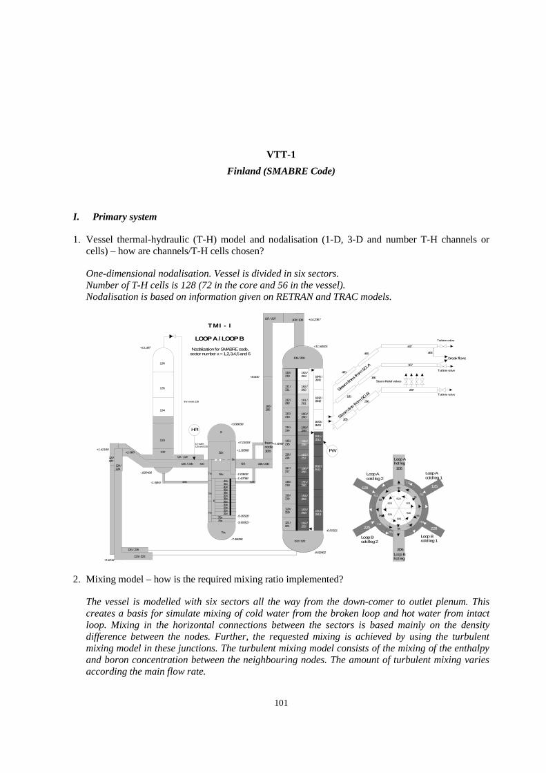
101
VTT-1
Finland (SMABRE Code)
I. Primary system
1. Vessel thermal-hydraulic (T-H) model and nodalisation (1-D, 3-D and number T-H channels orcells) – how are channels/T-H cells chosen?
One-dimensional nodalisation. Vessel is divided in six sectors.Number of T-H cells is 128 (72 in the core and 56 in the vessel).Nodalisation is based on information given on RETRAN and TRAC models.
127/ 227
126 / 226
109 / 209
122 / 222-7.49299
-5.69915
-5.09528
-1.43768-1.03632
- 0.0-0.0
+2.13418
+3.88068
+1.29598
125 / 225
8
6
51x
52x
9x
71x
72x
73x
74x
75x76x
41x42x
33x34x35x36x37x
31x32x
40x
38x39x
108 / 208
124 / 224
123 / 223
105 / 205
1642 / 2642
1643 / 2643
1641 / 2641
116 / 216
115 / 215
114 / 214
113 / 213
112 / 212
111 / 211
110 / 210
157 / 257
158 / 258
159 / 259
160 / 260
161 / 261
162 / 262
163 / 263
-8.62462
+11.50315
+14.2367
+1.066+1.42190
-9.4244
-1.9050
-.920496
132
133
134
135
131 130
136
FW
+8.500
+1.8288
+11.357
-6.50321
HPI
to nodes125 and 225
from node 128
T M I - I
LOOP A / LOOP B
121 / 221
120 / 220
119 / 219
118 / 218
117 / 217
152 / 252
153 / 253
154 / 254
155 / 255
156 / 256
1512 / 2512
1513 / 2513
1511 / 2511
from node106
107 / 207
125
711
521
522
523
524
525
526
128
225
106
206
712
713
714
715
716
228
91
92
93
94
95
96
Loop A hot leg
Loop B hot leg
Loop A cold leg 1
Loop A cold leg 2
Loop B cold leg 2
Loop B cold leg 1
Nodalization for SMABRE code,sector number x = 1,2,3,4,5 and 6
break flows
Turbine valve
Steam Relief valves
267
Turbine valve
Turbine valve
167
467
466
465
166
165
266
265
468
Steam
lines
from SG
A
Stea
m line f
rom SG
B
106 / 206
2. Mixing model – how is the required mixing ratio implemented?
The vessel is modelled with six sectors all the way from the down-comer to outlet plenum. Thiscreates a basis for simulate mixing of cold water from the broken loop and hot water from intactloop. Mixing in the horizontal connections between the sectors is based mainly on the densitydifference between the nodes. Further, the requested mixing is achieved by using the turbulentmixing model in these junctions. The turbulent mixing model consists of the mixing of the enthalpyand boron concentration between the neighbouring nodes. The amount of turbulent mixing variesaccording the main flow rate.

102
3. Upper plenum and upper head (of reactor vessel) paths (junctions) modelling?
In the upper plenum the mixing is mainly based on the six parallel sectors and turbulent mixingmodel described above. Here the uppermost node, the upper head takes also part in mixing, sincepart of the flow in the model goes through the single node in upper head.
4. Radial and axial heat structure (fuel rod) nodalisation?
The core is divided in six sectors. Each sector is divided in 12 axial T-H and heat structure nodes.In radial direction the fuel rod is divided into three heat structure nodes. One layer for fuel pellet,one for gas cap and one for cladding.
5. Relation used for Doppler temperature?
Doppler temperature in SMABRE model is the average of fuel temperatures in 12 levels.
II. Secondary system
1. Initial steam generator (SG) mass inventory?
26 078 for A and 25 731 kg for steam generator B.
2. SG down-comer nodalisation?
Three nodes. See figure of the nodalisation in Question I.1.
3. Aspirator flow modelling?
The aspirator junction, steam out-take from tube bundle to down-comer to preheat the feedwater, ismodelled with the given flow area, 0.96 m2. At the steady state in the SMABRE model 100 kg/ssteam and also 400 kg/s of saturated water is flowing from the tube bundle to the top of down-comer.During the transient at the aspirator junction no reversal flow is allowed.
4. Steam line modelling?
Steam line A1: three nodes until the break.Steam line A2: four nodes until the break.Steam line B: four nodes until the turbine valve.See picture of nodalisation in Question I.1.
5. Break flow modelling and critical flow model?
Main steam line:• Break area: 0.2462 m2.• Hydraulic diameter: 0.5599 m.
Cross-connect line:• Break area: 0.0324 m2.• Hydraulic diameter: 0.2031 m.

103
Critical flow:• The Moody model is used for critical break flow model with the contraction coefficient 1.0 for
saturated flow.
6. Are you using the updated steam safety relief valves data (see Updated Specifications, April 1999,Table 5.4.2, p. 69)?
Yes.
7. Are you using the updated additional feedwater mass data (between the feedwater isolation valveand the broken SG) (see Updated Specifications, April 1999, Table 5.4.3, p. 69).
Yes.
III. General
1. Deviations from the updated Final Specifications (April 1999, NEA/NSC/DOC(99)8)?
The superheating of the main steam flow in SMABRE model is 26°C instead of 19°C given in thespecification.
2. User assumptions?
None.
3. Specific features of the codes used?
Turbulent mixing model (Q I.1).

104
PURDUE UNIVERSITY/NRC
United States of America
I. Primary system
1. Vessel thermal-hydraulic (T-H) model and nodalisation (1-D, 3-D and number T-H channels orcells) – how are channels/T-H cells chosen?
Core: 1-D pipe component, two parallel channels, six axial levels each.Bypass: 1-D pipe component, six axial levels.
2. Mixing model – how is the required mixing ratio implemented?
Two parallel lower plenum channels and two parallel upper plenum channels were connected withjunctions with no momentum transfer across junction (s = 3). The friction losses were adjusted toachieve the desired mixing ratio.
3. Upper plenum and upper head (of reactor vessel) paths (junctions) modelling?
Each of the core channels was connected to an upper plenum. Both upper plenums were connectedto a single upper head and two parallel outlet plenums. The upper head was connected back to theoutlet plenums. The outlet plenum was connected to a hot leg. The frictional losses were adjustedso that about 20% of the core flow goes through the upper head. This modelling was chosen to besimilar to the RETRAN skeleton input deck included in the final specifications.
4. Radial and axial heat structure (fuel rod) nodalisation?
Six axial levels, corresponding to six T-H axial levels.Nine radial intervals – six for the pellet (equally spaced), one for the gap and two for the clad(equally spaced).
5. Relation used for Doppler temperature?
The correlation from p. 29 of the April 99 specifications was used (0.3/0.7 fuel centreline/surfaceweighting).
II. Secondary system
1. Initial steam generator (SG) mass inventory?
~26 005 kg.

105
2. SG down-comer nodalisation?
Five axial levels.
3. Aspirator flow modelling?
A junction connecting SG 2/3 way up with FW inlet was used. Form losses were adjusted toachieve 10% of the outlet SG flow through the aspirator junction.
4. Steam line modelling?
Fifteen axial levels, from SG outlet plenum to the MSIV. One steam line on the intact side, twosteam lines on the broken side. Four relief valves connected to the four last axial levels of the intactsteam line.
5. Break flow modelling and critical flow model?
Henry-Fauske critical flow model for the break. The 24” and 8” breaks were connected to separatesteam lines, both at 44.8 m of the steam line.
6. Are you using the updated steam safety relief valves data (see Updated Specifications, April 1999,Table 5.4.2, p. 69)?
Yes.
7. Are you using the updated additional feedwater mass data (between the feedwater isolation valveand the broken SG) (see Updated Specifications, April 1999, Table 5.4.3, p. 69).
Yes.
III. General
1. Deviations from the updated Final Specifications (April 1999, NEA/NSC/DOC(99)8)?
Mixing ratio of 0.6 was used.
2. User assumptions?
Turbine sink pressure adjusted to achieve SL inlet pressure of 6.41 MPa.
3. Specific features of the codes used?
The RELAP5 code has been developed for best estimate transient simulation of light water reactorcoolant systems during postulated accidents. RELAP5 is a highly generic code that, in addition tocalculating the behaviour of a reactor coolant system during a transient, can be used forsimulation of a wide variety of hydraulic and thermal transients in both nuclear and non-nuclearsystems involving mixtures of steam, water, non-condensable and solute.
The RELAP5/MOD3 code is based on a non-homogeneous and non-equilibrium model for thetwo-phase system that is solved by a fast, partially implicit numerical scheme to permit economicalcalculation of system transients. The code includes many generic component models from whichgeneral systems can be simulated. The component models include pumps, valves, pipes, heat

106
releasing or absorbing structures, reactor point kinetics, electric heaters, jet pumps, turbines,separators, accumulators and control system components. In addition, special process models areincluded for effects such as form loss, flow at an abrupt area change, branching, choked flow,boron tracking and non-condensable gas transport.

107
IPSN/CEA
France
I. Primary system
1. Vessel thermal-hydraulic (T-H) model and nodalisation (1-D, 3-D and number T-H channels orcells) – how are channels/T-H cells chosen?
The core is separated into two 1-D channels. The lower and upper plenums are separated in threevolumes for mixing requirements.
2. Mixing model – how is the required mixing ratio implemented?
The lower plenum has been separated into three volumes:• A volume LOWERPA connected to the intact leg.• A volume LOWERPB connected to the broken leg.• A volume LOWERPC connected to both intact and broken legs.
The mixing ratio of MSLB specifications has been obtained by choosing the size of Volume C forboth lower and upper plenum. The upper plenum has been separated in two volumes UPPERPAand UPPERPB. Three others volumes are used for the junction with core. As for lower plenum, thesize of these three volumes has been calculated in function of mixing ratio specifications.

108
3. Upper plenum and upper head (of reactor vessel) paths (junctions) modelling?
Each volume UPPERPA and UPPERPB has a junction with the upper head and two junctions withhot leg inlet. A 1 409 kg/s flow between upper plenum and upper head exists at initial state.
4. Radial and axial heat structure (fuel rod) nodalisation?
The axial fuel rod nodalisation has 24 cells. The radial fuel rod nodalisation has 10 cells.
5. Relation used for Doppler temperature?
For each cells of axial fuel rod nodalisation, the Doppler temperature is calculated by the relationTcell = αTc + (1-α)Ts.
II. Secondary system
1. Initial steam generator (SG) mass inventory?
26 tonnes.
2. SG down-comer nodalisation?
Auxiliary feedwater
Feedwater
Riser
Steam line
3. Aspirator flow modelling?
A junction between the upper and lower part of down-comer.
4. Steam line modelling?
24’’ break
8’’ break
Blind condition

109
5. Break flow modelling and critical flow model?
The 8” and 24” break flows are calculated by the Gros d’Aillon correlation.
6. Are you using the updated steam safety relief valves data (see Updated Specifications, April 1999,Table 5.4.2, p. 69)?
Yes.
7. Are you using the updated additional feedwater mass data (between the feedwater isolation valveand the broken SG) (see Updated Specifications, April 1999, Table 5.4.3, p. 69).
Yes.
III. General
1. Deviations from the updated Final Specifications (April 1999, NEA/NSC/DOC(99)8)?
2. User assumptions?
3. Specific features of the codes used?

110
GRS
Germany
I. Primary system
1. Vessel thermal-hydraulic (T-H) model and nodalisation (1-D, 3-D and number T-H channels orcells) – how are channels/T-H cells chosen?
The coolant flow through the reactor vessel and reactor core is modelled by two equal parallelflow paths by splitting the down-comer, the lower plenum, the reactor core and the upper plenum.These parallel flow paths consisting of 1-D pipe models behave independently, except ofconnections with the upper head volumes. The nodalisation is as follows:
Object NodesUpper down-comerLower down-comerLower headLower plenumActive coreBypassInner upper plenumOuter upper plenumUpper head
010301012424010101
In addition, mixing is modelled between the two halves of lower and upper plenum as specified.
2. Mixing model – how is the required mixing ratio implemented?
The required mixing ratio is modelled by exchanging energy between the two halves of lower andupper plenum. The mixing ratio of coolant temperatures in the hot and cold legs is calculated.The deviation from the specified value R = 0.5 is determined and corresponding to the differencepower is exchanged within the lower and the upper plenum, as proposed 20% in the lower plenumand 80% in the upper plenum. The General Control System Module (GCSM) of ATHLETautomatically calculates the value of exchange rate.
3. Upper plenum and upper head (of reactor vessel) paths (junctions) modelling?
For simulating the coolant flow between upper plenum and upper head, the upper plenum isdivided in an inner and outer part. A junction pipe models the exchange between these parts.Junction pipes also model the flow between upper head and both volumes of upper plenum.The mass flow rates of these junctions correspond to the specification.

111
4. Radial and axial heat structure (fuel rod) nodalisation?
Four radial layers of equal volume, a specified gap and a cladding layer model the fuel rod.The number of axial nodes is 24.
5. Relation used for Doppler temperature?
The Doppler temperature is calculated as a weighted sum from the mean layer temperatures of theinner and outer fuel layer.
II. Secondary system
1. Initial steam generator (SG) mass inventory?
The initial steam generator mass inventory is 28.103 kg.
2. SG down-comer nodalisation?
The steam generator model for the unaffected and affected loop is different. The model for theunaffected loop only has two nodes on the secondary side and no down-comer. The SG model forthe affected loop is more detailed. The down-comer consists of two parts. The lower down-comerhas 14 nodes; the upper down-comer has 10 nodes. Between the riser and the down-comer heatconduction is considered.
3. Aspirator flow modelling?
The aspirator flow between the riser and the lower down-comer is modelled. The initial value is100 kg/s, the time dependence is calculated by the pressure difference.
4. Steam line modelling?
The steam line for the affected SG is simulated as a single pipe. The distance between the SG outletand the discharge is 38 m, discretised by four nodes. The cross-connect is located at a distance of35 m.
5. Break flow modelling and critical flow model?
The break flow modelling consists of two discharge valves, one for the steam line and one for thecross-connect. The Moody model calculates the critical discharge rate.
6. Are you using the updated steam safety relief valves data (see Updated Specifications, April 1999,Table 5.4.2, p. 69)?
The updated steam safety relief valves as proposed in Table 5.4.2 are used.
7. Are you using the updated additional feedwater mass data (between the feedwater isolation valveand the broken SG) (see updated specifications, April 1999, Table 5.4.3, p. 69)?
The additional feedwater mass data as proposed in Table 5.4.3 are used.

112
III. General
1. Deviations from the updated Final Specifications (April 1999, NEA/NSC/DOC(99)8)?
No relevant deviations from the specifications.
2. User assumptions?
No.
3. Specific features of the codes used?
No.

113
IBERDROLA
Spain
I. Primary system
1. Vessel thermal-hydraulic (T-H) model and nodalisation (1-D, 3-D and number T-H channels orcells) – how are channels/T-H cells chosen?
The vessel model and nodalisation used by RETRAN-3D MOD002 was selected according to thespecifications.
Vessel nodalisation: specifications (Figure 3.1).
RETRAN VESSEL
UH8
OP OP9 UP 9
5
CDC 4 D C7 7
B C6 3
C2
LP1
0.0 m
1.79 m
3.62 m
4.84 m
6.06 m
6.46 m
7.85 m
9.63 m
11.37 m
2.40 m
7.49 m
Number of vessel volumes: 9 Core volume: 3: Heat conductor 25Number of core volumes: 3 Core volume: 4: Heat conductor 26Number of heat conductors: 3 Core volume: 5: Heat conductor 27

114
Characteristics of the vessel volumes: according to specifications (Appendix A).
Reactor vesselVolume Z Volume FlowA DiamV Elev
001 621.64 7.8665 38.95 3.84 -24.5833 Lower plenum002 196.862 4.00 49.2154 0.04277 -16.7168 Core – lower sect003 196.862 4.00 49.2154 0.04277 -12.7168 Core – middle sect004 196.682 4.00 49.2154 0.04277 -8.7169 Core – upper sect005 877.90 11.7187 81.4 0.5783 -4.7168 Upper plenum006 193.23 12.00 17.11 0.0349 -16.7168 Core bypass007 689.37 19.865 35.13 1.67 -18.698 Reactor down-comer008 492.57 5.73 104.58 7.11 7.0019 Upper head009 247.96 10.65 23.29 1.29 -3.40 Outlet plenum
2. Mixing model – how is the required mixing ratio implemented?
The mixing model is not implemented in RETRAN-3D.
3. Upper plenum and upper head (of reactor vessel) paths (junctions) modelling?
Upper plenum and upper head are modelled with volumes as usual in RETRAN-3D:
4
3
2
6
Upper plenum: VOLUME 5
Upper head: VOLUME 8
Outletplenum
9
From upper headVolume 8
Junction 9
From upper plenumVolume 5
Junction 10
Function modelling: specifications (Appendix A):
From To Junction area Junction elev.8 9 08.564 7.0019 From upper head to outer plenum5 9 50.750 4.2519 From upper plenum to outer plenum

115
4. Radial and axial heat structure nodalisation?
The nodalisation corresponds to the heat core T-H sectors of the core.
Radially: Core section is modelled with one volume which represents the active core and anothervolume which represents the bypass.
Axially: The axial heat structure consists of three volumes the total height of the active core, andthe bypass is modelled with only one volume.
4
3
2
6
6
Core volume
Associated heatconductor
Bypass
5. Relation used for Doppler temperature?
Doppler temperature has been modelled using an averaged fuel temperature, and the relationTf = 0.3*Tf,c + 0.7*Tf,s has not been used, because the code does not have this option.
II. Secondary system
1. Initial steam generator (SG) mass inventory?
26 048 kg for both steam generators.
2. SG down-comer nodalisation?
YES [Volume 251 (intact), Volume 151 (broken)].
251 151
Intact SG Broken SG
3. Aspirator flow modelling?
Bypass connects the steam generator with the inlet water, in the secondary side steam generator.
INTACT steam: Junction 250 (from: 259 to: 25).FAULTED steam: Junction 150 (from: 159 to: 151).
251 151
Intact SG Broken SG250 150

116
4. Steam line modelling?
164365
165
264 265
501 TURBINE
503 TURBINE
502 TURBINE
18224 inches brCONTAIN
1838 inches brCONTAIN
Faulted loop
Intact loop
5. Break flow modelling and critical flow model?
The break flow has been modelled for both breaks, by the use of one valve joint to a time dependentvolume (TDV) simulating the break.
No choking flow model is used in this exercise.
6. Are you using the updated steam safety relief valves data (see Updated Specifications, April 1999,Table 5.4.2, p. 69)?
No updated steam safety relief valves have been used.
7. Are you using the updated additional feedwater mass data (between the feedwater isolation valveand the broken SG) (see updated specifications, April 1999, Table 5.4.3, p. 69)?
Yes, the additional feedwater mass is included in a FILL as follows:
Table 5.4.3 (Specifications)
Time (sec) Flow (lb/sec /kg/sec)
0 1 679.0/761.5910 4 000.0/1 814.430 3 000.0/1 360.842 3 000.0/1 360.8
45 0.0/0.0

117
Seconds
Flow(lbm/s)
10 20 30 40 50
4 000
3 000
2 000
1 000
Equivalent toVolume 149
III. General
1. Deviations from the updated Final Specifications (April 1999, NEA/NSC/DOC(99)8)?
No.
2. User assumptions?
No.
3. Specific features of the codes used?
Vessel and SG nodalisation using volumes, as usual in RETRAN3D-MOD002.

118
UNIVERSITY OF VALENCIA
Spain
I. Primary system
1. Vessel thermal-hydraulic (T-H) model and nodalisation (1-D, 3-D and number T-H channels orcells) – how are channels/T-H cells chosen?
We have model the vessel with the vessel component TRAC. The vessel consists of six levels andeighteen thermal-hydraulic sectors. We only have modelled the core reactor.
2. Mixing model – how is the required mixing ratio implemented?
No mixing is implemented.
3. Upper plenum and upper head (of reactor vessel) paths (junctions) modelling?
We have used the PLENUM TRAC component to model the upper plenum and upper head.
4. Radial and axial heat structure (fuel rod) nodalisation?
The radial and axial heat structures correspond to the heat core T-H sectors of the core. Moreaccurately, we only have an axial heat structure per T-H sector in the core. On the other hand,axially, each heat structure consists of seven nodal nodes.
5. Relation used for Doppler temperature?
Averaged fuel temperature has been used in order to calculate Doppler temperature. Furthermore,in graphical representation, the following relation has not been used:
Tf = 0.3*Tf,c + 0.7*Tf,s
We have used this relation for the second and third exercise.
II. Secondary system
1. Initial steam generator (SG) mass inventory?
The secondary side mass inventory is 26 031 kg in steam generators 1 and 2.
2. SG down-comer nodalisation?
We did not model the bypass connecting the steam with the inlet water in the secondary side steamgenerator.

119
3. Aspirator flow modelling?
We did not model the bypass connecting the steam with the inlet water in the secondary side steamgenerator.
4. Steam line modelling?
We have two-steam line modelling. It has been represented in the following diagram.P
LEN
UM
167
JUN 211 212 213 214
205FILL
PIPE
PLENUM 266
J26
6
J267
J268
PIPE 267
J268
J269
PIPE 265 30
Stg
en
100
J164
J152
B) INTACT STEAM LINE
301 TEE 365
VALVE 168
J36
5
J8429
BREAK 88
BREAK 84
J87
J88
1 302
2
PIPE 165
J16
6J3
66
BR
OK
EN
ST
EA
M G
EN
ER
ATO
R
seco
ndar
y si
de
BREAK 86J86
24 inchs rupture
8 inchs rupture
VALVE 87
A) BROKEN STEAM LINE
BREAK 94
VALVE 268
1
Stg
en
200
J264
J252
INT
AC
T S
TE
AM
GE
NE
RA
TO
R
J264 1 2 3
206 207 208
J201 J202 J203 J204
201 202 203 204
5. Break flow modelling and critical flow model?
We have modelled the break flow by means of a valve followed by a BREAK TRAC component.The pressure in component “BREAK 84” is 6.31E6 Pa and in time 0.5 seconds after trip theVALVE 168 is closed. The small break is also modelled with the VALVE 87 followed by aBREAK 88, which maintains a pressure of 1.03419E5 during the transient. The critical flow modelused is the choked flow model developed in TRAC.
6. Are you using the updated steam safety relief valves data (see Updated Specifications, April 1999,Table 5.4.2, p. 69)?
Yes, but with an exception: we have considered the same point of pressure. It is located in Cell 21of PIPE 265.

120
7. Are you using the updated additional feedwater mass data (between the feedwater isolation valveand the broken SG) (see Updated Specifications, April 1999, Table 5.4.3, p. 69)?
Yes, but we have considered 16 103 kg of water inside a pipe and do not in the FILL during theinterval from 30-42 seconds of transient.
III. General
1. Deviations from the updated Final Specifications (April 1999, NEA/NSC/DOC(99)8)?
2. User assumptions?
3. Specific features of the codes used?

121
BE
United Kingdom
I. Primary system
1. Vessel thermal-hydraulic (T-H) model and nodalisation (1-D, 3-D and number T-H channels orcells) – how are channels/T-H cells chosen?
Principally, we obtained the RELAP5 input deck from the US NRC. We modified the core alongsimilar lines as to how we model Sizewell B. The model has two equal, parallel core channels thatcommunicate fluid only at the inlet and outlet plenum. Each half of the core is associated with oneof the steam generator loops. Each core channel contains 12 equal volumes and receives heat fromhalf of the fuel. The axial variation of heat output from the fuel (which is also in twelve equallengths) is taken from the specification.
There is a single guide tube connecting the upper plenum and the upper head. This featureintroduces a mixing flow between the two core halves, which is in addition to any mixing in theupper and lower plenum.
The loops contain all the significant features and were not modified except in the steam generatorswhere the number of primary side (and secondary side) axial nodes was increased (now 34 ofequal length) to achieve the initial secondary side steam conditions.
The total volume of all primary components/volumes (and secondary volumes) is not identical to thespecification, however, we are within a few per cent and the difference was judged to be negligible.
In the 3-D calculations the only difference is that the heat supplied to each of the 24 core nodes iscalculated explicitly with PANTHER.
2. Mixing model – how is the required mixing ratio implemented?
The RELAP5 model was modified such that the cold leg temperatures were made constant, with atemperature difference between one half of the model and the other half. Valves were installed atboth the inlet and the outlet of the core between the two halves of the core and the inlet/outletplenum to enable to mixing to be varied. The mixing ratio was calculated according to thespecification using the ratio of hot and cold leg temperatures. Once the desired mixing ratio hadbeen achieved the area of each valve was frozen.
3. Upper plenum and upper head (of reactor vessel) paths (junctions) modelling?
As above, there is a single guide tube connecting the upper plenum and the upper head. The upperhead splits in two and each half connects to the top of a down-comer (there are two, one associatedwith each loop). The single guide tube introduces a mixing flow between the two core halves, whichis in addition to any mixing in the upper and lower plenum.

122
4. Radial and axial heat structure (fuel rod) nodalisation?
Yes, the radial noding was followed. Axially only twelve nodes were modelled for compatibilitywith the hydraulic nodes.
5. Relation used for Doppler temperature?
Yes, the Doppler temperature was calculated according to the specification. The average was aweighted sum using the power factors to represent a flux weighting. Each half of the core wasweighted equally.
II. Secondary system
1. Initial steam generator (SG) mass inventory?
We achieve the revised specification.
2. SG down-comer nodalisation?
This is modelled as an annulus with eight equal length axial nodes.
3. Aspirator flow modelling?
A connection from the riser to the top of the down-comer inside the steam generator is used tomodel the aspirator flow. We have no experience with the once-through steam generator designand have therefore copied this data from one of the other participants using RELAP5 (Purdue).
4. Steam line modelling?
The arrangement of the steam pipes, including the length of the steam piping, is modelledaccording to the specification.
5. Break flow modelling and critical flow model?
The break flow and critical flow model is RELAP5’s own since we do not have control over this(we believe that this is a feature of development versions). The flow through the break ishomogeneous and goes through an abrupt area change. The flow does not choke.
6. Are you using the updated steam safety relief valves data (see Updated Specifications, April 1999,Table 5.4.2, p. 69)?
The steam safety valves on the unaffected steam generator have been modelled according to thespecification. This is implemented by a flow versus pressure table since the specification did notinclude values to assume for accumulation and blow down of the valves. It was judged that thistreatment for the relief on this steam generator was adequate for this problem.
7. Are you using the updated additional feedwater mass data (between the feedwater isolation valveand the broken SG) (see Updated Specifications, April 1999, Table 5.4.3, p. 69).
Yes, we are using the updated feed flow data specification.

123
III. General
1. Deviations from the updated Final Specifications (April 1999, NEA/NSC/DOC(99)8)?
Specifically, none.
2. User assumptions?
Although it is not mentioned in the specification, it has been assumed that there is no transientcontrol on the mixing ratio. We did not believe a transient control system to be practical orrealistic.
3. Specific features of the codes used?
As above, we do not have control over the break flow model in this release of RELAP5 andtherefore cannot guarantee that we are using the Moody correlation.

124
PSU
United States of America
I. Primary system
1. Vessel thermal-hydraulic (T-H) model and nodalisation (1-D, 3-D and number T-H channels orcells) – how are channels/T-H cells chosen?
The TRAC-PF1 VESSEL component is used to model thermal-hydraulically the TMI-1 vessel in3-D cylindrical geometry. The vessel model is subdivided into 14 axial layers, five radial rings, andsix azimuthal sectors for a total of 420 hydrodynamic cells as shown in Figures 1.1 and 1.3.
2. Mixing model – how is the required mixing ratio implemented?
Since TRAC-PF1 has a 3-D vessel fluid-dynamic capability and by explicitly modelling radialcross-flows between thermal-hydraulic cells, the code accounts for thermal loop flow mixing in abest-estimate manner.
3. Upper plenum and upper head (of reactor vessel) paths (junctions) modelling?
See Figures 1.1 and 1.2.
4. Radial and axial heat structure (fuel rod) nodalisation?
The radial and axial heat structure nodalisation follows the thermal-hydraulic nodalisation of thecore region. The heat structure consist of 18 fuel rods radially and six axial layers.
5. Relation used for Doppler temperature?
Pellet volume averaged fuel temperature value is used for Doppler temperature relation.
II. Secondary system
1. Initial steam generator (SG) mass inventory?
26 000 kg.
2. SG down-comer nodalisation?
See Figure 2.1 – eight nodes.
3. Aspirator flow modelling?
According to the Final Specifications – see Figure 2.1.

125
4. Steam line modelling?
See Figure 2.2.
5. Break flow modelling and critical flow model?
The critical flow model used is the TRAC-PF1 choked flow model.
6. Are you using the updated steam safety relief valves data (see Updated Specifications, April 1999,Table 5.4.2, p. 69)?
Yes.
7. Are you using the updated additional feedwater mass data (between the feedwater isolation valveand the broken SG) (see Updated Specifications, April 1999, Table 5.4.3, p. 69)?
Yes.
III. General
1. Deviations from the updated Final Specifications (April 1999, NEA/NSC/DOC(99)8)?
Doppler temperature relation.
2. User assumptions?
None.
3. Specific features of the codes used?
3-D vessel thermal-hydraulic capability.

126
Figure 1.1. Axial nodalisation of the TMI-1 TRAC-PF1 vessel

127
Figure 1.2. Side view of the TRAC-PF1 TMI-1 vessel component
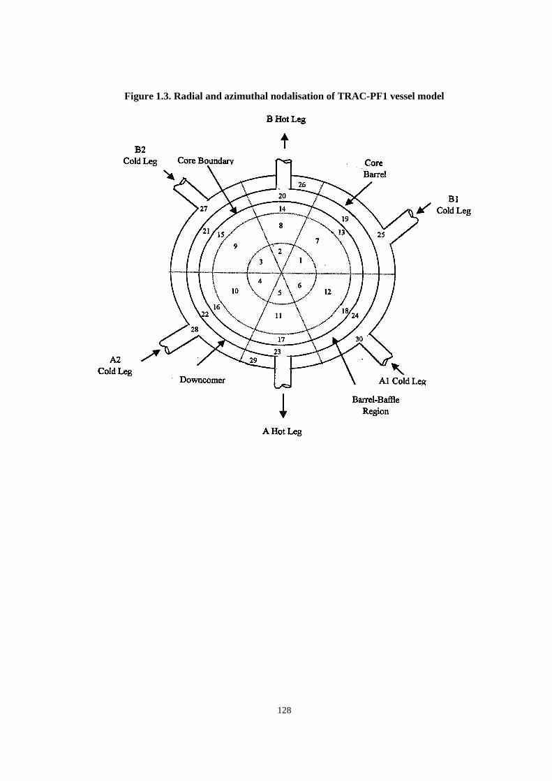
128
Figure 1.3. Radial and azimuthal nodalisation of TRAC-PF1 vessel model

129
Figure 2.1 TMI-1 once-through steam generator model

130
Figure 2.2. TRAC-PF1 TMI-1 steam line nodalisation

131
VTT-2
Finland (APROS code)
I. Primary system
1. Vessel thermal-hydraulic (T-H) model and nodalisation (1-D, 3-D and number T-H channels orcells) – how are channels/T-H cells chosen?
One-dimensional nodalisation. Vessel is divided in six sectors.Number of T-H cells is 139 (72 in the core and 67 in the vessel).Nodalisation is based on information given on RETRAN and TRAC models.
Steam lin
es fro
m SG A
Steam lin
e from
SG B
-7.493
-5.699
-5.095
-1.52
-1.036
-0.0
+2.21
+1.296
pv_8
6
pv_51x
pv_52x
9x
71x
72x
73x
pv_74x
pv_75xpv_76x
no11no12
no3no4no5no6no7
re_chax_no1no2
no10
no8no9
-8.62462
+11.503
+14.237
+3.411
+1.066+1.42190
-9.144
-1.905
-.92
+1.829
+11.357
+9.382
-6.50321
HPI
T M I - I
LOOP A / LOOP B
cl_a1_p3
pv_711
pv_521
pv_522
pv_523
pv_524
pv_525
pv_526
cl_a2_p3
cl_b2_p3
hl_a_p1
hl_b_p1
712
pv_713
pv_714
715
pv_716
cl_b1_p3
pv_91
pv_92
pv_93
pv_94
pv_95
pv_96
Loop A hot leg
Loop B hot leg
Loop A cold leg 1
Loop A cold leg 2
Loop B cold leg 2
Loop B cold leg 1
nodalization for APROS code
- 0.0
break flows
Turbine valve
Steam Relief valves
Turbine valve
150
prz_sv
+4.298
Control valve
Control valve
+7.492
Feed water
The nodalisation used in APROS is basically the same as with the SMABRE code. However, smalldifferences exist, mainly because of the way the model is constructed in the codes.
2. Mixing model – how is the required mixing ratio implemented?
The vessel is modelled with six sectors all the way from the down-comer to outlet plenum (figurebelow). This creates an artificial two-dimensional model to simulate mixing of cold water from thebroken loop and hot water from intact loop. The horizontal connections between the sectors are

132
described in the APROS model with “cross-flow” junctions. Flow areas and form loss factors aredefined so that the temperature difference between broken and intact hot legs is about 50% of thetemperature difference in cold legs. In the down-comer region the flow area of “cross-flow”junctions is 0.1 m2 and form loss factor is 50. In the lower plenum the form loss factor is 35. Mostof the mixing should occur in the upper plenum (80%), which is why the flow areas are large andform loss factors lower there (1.0 m2, 10 and 20). When simulating mixing with this kind of modelthe defined fixed mixing ratio was not followed. On the other hand, mixing depends on flow ratedensity differences, especially in the down-comer region (like in reality).
cl_a1
DOWNCOMER
cl_a2
REACTOR VESSEL
cl_b1
UPPER PLENUM
cl_b2
REACTOR CORE
LOWER PLENUM
hot leg A
t_core_in_a
dt_ratio
dt_core_in
dt_cold_leg
dt_ratio_core_in
t_core_in_b
hot leg B
3. Upper plenum and upper head (of reactor vessel) paths (junctions) modelling?
In the upper plenum the adjacent channels are connected with “cross-flow” junctions like in thedown-comer. In addition to this mixing with channels the hot and cold halves of the reactor areconnected to allow required mixing. The upper head also takes part in mixing, since part of he flowin the model goes through the single node in upper head.

133
4. Radial and axial heat structure (fuel rod) nodalisation?
The core is divided in six sectors. Each sector is divided in 12 axial T-H and head structure nodes.In radial direction the fuel rod is divided in 10 heat structure nodes. Seven layers for fuel pellet,one for gas cap and one for cladding.
5. Relation used for Doppler temperature?
At each heat structure node the Doppler temperature is calculated as 0.3x (temperature at fuelpellet centre) + 0.7x (temperature at fuel pellet outer rim). When the core in APROS was dividedinto six sectors and each of the sectors into 12 axial nodes, this procedure produces 72 Dopplertemperature values. The final Doppler temperature used in the feedback correlation is the (volume)average of the 72 individual values obtained.
II. Secondary system
1. Initial steam generator (SG) mass inventory?
26 015 kg.
2. SG down-comer nodalisation?
Five nodes. See figure of the nodalisation in Question I.1
3. Aspirator flow modelling?
The once-through steam generator is modelled as detailed as possible with given data, because it isan important contributor to the transient. The feedwater nozzles are modelled with the real flow areaand diameter. Momentum flux was transferred in feedwater nozzle to take into account the velocityof feedwater spray in condensing steam in the top of down-comer (br6_mom_flux_used T).The hydraulic diameter of feedwater node (SG_A – inlet) was 4.78 mm to take in accountcharacteristic dimension of the nozzle in condensation.
The aspirator junction, steam out-take from tube bundle to down-comer to preheat the feedwater, ismodelled with the given flow area, 0.96 m2. To heat up 761 kg/s of feedwater to saturation requires102 kg/s steam, which has to condense in the down-comer. The drawback is that during the steamline break, part of the feedwater goes through the aspirator junction directly into the middle of thetube bundle (see figure). The aspirator flow was modelled with a normal junction allowing reversalflow. It was not possible to judge the realism of the modelling, without knowing the actualgeometry of the aspirator connection and the behaviour of the once-through steam generator indetail.
The once-through steam generator (model) was sensitive to aspirator flow and water level. Quite alot of work was needed to adjust the model in the requested state (water inventory and steamsuperheat). Calculated temperature and void fraction profiles in steady state are plotted in thefigures below. In the void fraction profile one can see the effect of steam out-take through theaspirator junction in Node 6 from the top. In the bottom of the steam generator water is close tosaturation point (about 2ºC sub-cooled) and in the top steam is almost 20ºC superheated, as givenin the specifications of the benchmark.
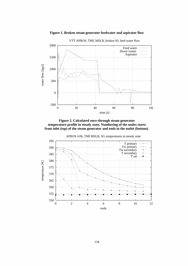
134
Figure 1. Broken steam generator feedwater and aspirator flow
-500
0
500
1000
1500
2000
0 20 40 60 80 100
wat
er f
low
[kg
/s]
time [s]
VTT APROS, TMI, MSLB, broken SG feed water flow
Feed waterDown comer
Aspirator
Figure 2. Calculated once-through steam generatortemperature profile in steady state. Numbering of the nodes starts
from inlet (top) of the steam generator and ends in the outlet (bottom).
550
555
560
565
570
575
580
585
590
595
0 2 4 6 8 10 12
tem
pera
ture
[K
]
node
APROS 4.06, TMI MSLB, SG temperatures in steady state
T primaryTw primary
Tw secondaryT secondary
T sat

135
Figure 3. Calculated once-through steam generator void fraction profile in steady state
0
0.1
0.2
0.3
0.4
0.5
0.6
0.7
0.8
0.9
1
0 2 4 6 8 10 12
void
fra
ctio
n
node
APROS 4.06, TMI, OTSG void fraction in steady state
4. Steam line modelling?
Steam line A1: four nodes until the break (turbine valve).Steam line A2: five nodes until the break.Steam line B: four nodes until the turbine valve.See picture of nodalisation in Question I.1.
5. Break flow modelling and critical flow model?
Main steam line:• Break area: 0.2462 m2.• Hydraulic diameter: 0.5599 m.• Form loss coefficient: 1.0.
Cross-connect line:• Break area: 0.0324 m2.• Hydraulic diameter: 0.2031 m.• Form loss coefficient: 0.0 ! (error in modelling).
Critical flow: “frozen” sound velocity model. Break flow velocity is limited to sound velocity ofsteam and liquid, weighted with void fraction.
6. Are you using the updated steam safety relief valves data (see Updated Specifications, April 1999,Table 5.4.2, p. 69)?
Yes.

136
7. Are you using the updated additional feedwater mass data (between the feedwater isolation valveand the broken SG) (see Updated Specifications, April 1999, Table 5.4.3, p. 69)?
Yes.
III. General
1. Deviations from the updated Final Specifications (April 1999, NEA/NSC/DOC(99)8)?
None as far as we know.
2. User assumptions?
Reverse flow allowed in SG aspirator junction.
3. Specific features of the codes used?
Six-equation thermal-hydraulic model. Normal point kinetics calculation for this exercise.