Working Paper Researchby Cédric Duprez and Glenn Magerman

October 2018 No 352

Price updating in production networks

Price Updating in Production Networks∗

Cedric Duprez† and Glenn Magerman‡

First draft: October, 2018

Abstract

This paper evaluates how firms change their prices in response to cost shocks and other price changes in their

environment. We first document three new facts on the heterogeneity of firm-level producer prices and their relation-

ship to buyers and suppliers in a production network. We then develop a non-parametric framework of how producers

update their prices, taking into account this production network. The framework is very general, and accounts for

the heterogeneity in price changes and the production network from the stylized facts. Moreover, the framework is

consistent with various price setting mechanisms, and does not impose a particular market structure or demand func-

tional form. Exploiting rich data on producer prices and the network structure of production in Belgium, we estimate

the model to evaluate the importance of both channels in the data. We find that, on average, input price pass-through

is incomplete and very much below one, while firms also strongly react to other prices in their environment. This

implies that firms can adjust their markups in response to both cost shocks and prices of other firms. Furthermore,

firms react differently to common shocks than to idiosyncratic shocks, on average completely passing through com-

mon shocks, but much less idiosyncratic shocks.

Keywords: Pricing, production networks, pass-through, variable markups.

JEL codes: D21, L14, L16.

∗This research has been performed in the context of the 2018 Colloquium of the National Bank of Belgium on "Understanding inflation dynamics:the role of costs, mark-ups and expectations". We would like to thank Emmanuel Dhyne and Catherine Fuss from the National Bank of Belgium,Joep Konings, Mathieu Parenti and Thomas De Muynck for various comments, and Danny Delcambre at Eurostat for help with the RAMON productclassification files.†National Bank of Belgium.‡ECARES, Université libre de Bruxelles.

1

1 Introduction

How do firms adjust their prices? What is the impact of cost shocks on prices, and the response of firms to changesin other prices in their environment? How much of cost shocks are ultimately passed on in the aggregate, and howmuch is absorbed by the markups of firms? The nature of price setting has important implications for a wide range ofissues in both macroeconomics, including the welfare consequences of business cycles, the behavior of real exchangerates and optimal monetary policy, and in microeconomics, such as efficiency, reallocation, productivity, competitionand firms’ decisions to trade. The topic has also attracted considerable attention in industrial organization, particularlybecause pass-through can elucidate the welfare implications from various types of imperfect competition or pricediscrimination. Incomplete pass-through can reveal important characteristics about supply, demand, or market power.Moreover, repeated empirical evidence has been presented on incomplete pass-through in various settings.

Changes in output prices have been rationalized along two main lines: (i) changes in the costs of the firm, and(ii) firms’ responses to other prices in their environment. Unfortunately, while both the micro and macro responsesto cost shocks depend on the exact nature of these cost shocks (e.g. brownian motion versus lumpy shocks as inAlvarez et al. (2016)), firm-level information on cost changes is generally missing. At best, one observes changesin output prices, but not changes in particular input prices. Any prediction on changes in output prices then dependson assumptions on the nature of these cost shocks. Furthermore, even if cost information is available at the firmlevel, this information is generally incomplete, and studies focus on one aspect that is identifiable such as exchangerates, or detailed information on costs in particular sectors. Additionally, while many papers only observe retail priceinformation (e.g. Eichenbaum et al. (2011)), there is evidence that a significant fraction of aggregate incomplete pass-through occurs at the firm level along the value chain (Alvarez et al. (2016)). Any update in prices of consumptiongoods is thus confounded with price updating along the value chain, which is not observed with consumption dataonly.

This paper studies how firms change their output prices in the presence of production networks, and makes fourmain contributions. First, we document three new stylized facts about the distribution of changes in producer pricesand the distribution of input expenditures across suppliers. These facts exploit unique information on prices forgoods producers in Belgium and input expenditures of these producers across all their suppliers, both domestic andinternational. Second, we develop a general, non-parametric model of how producers update output prices, takinginto account input prices from suppliers in the production network and price changes in their output environment.Third, the model provides a structural estimation of cost pass-through and other price effects, exploiting the Belgianproduction network data, which is consistent with a large class of pricing models and functional forms. Importantly,there is no need to estimate either marginal costs or markups in our framework. Finally, we propose a new and detailedprocedure to concord product-level production data and international trade data over time, as well as across statisticalclassifications.

We start by documenting three facts on price changes and supplier-buyer connections for goods producers inBelgium. The empirical analysis in this paper exploits very detailed data on output prices at the firm-product level forall firms in the Prodcom survey, combined with information on expenditures for all suppliers of these producers andcorresponding input prices from these suppliers. First, the distribution of producer price changes exhibits both largeincreases and decreases from one year to another. Moreover, the median price change is zero. This is very differentfrom consumer prices, which predominantly go up in nominal terms. Second, there is a striking difference in patternsof co-movement of producer prices. A fraction of prices tend to co-move within narrowly defined product categories,but at the same time, large idiosyncrasies exist: many output price changes are not correlated with the changes ofother producers in the same product category. Third, across all producers, one supplier tends to dominate in terms ofinput expenditures, which is not vanishing in the number of suppliers. However, there is no correlation between the

2

importance of the input share and size of an input price shock.Next, we develop a general model of how producers change output prices in the presence of production networks.

Firms produce output according to a non-parametric cost function, combining inelastic factors with inputs from otherfirms. The framework allows for variable markups at the firm level with minimal restrictions on costs, possible pricesetting mechanisms and product-market competition. In particular, firms are cost minimizing and the cost functionexhibits constant returns to scale with respect to variable inputs. Under these conditions, the resulting pricing equationis consistent with a large class of mechanisms, including but not limited to profit maximization, cost-plus pricing andrevenue maximization. Moreover, markups charged by the firm are not necessarily an equilibrium outcome such as astrategic best response function across oligopolistic competitors, but are also consistent with models in which the firmis a price follower in its sector or in the aggregate.

The model allows to recover underlying elasticities that are consistent with a broad class of price setting modelsand functional forms. These elasticities represent how firms change their output prices in response to a combinationof cost shocks and adjustment of prices by other firms in the same product market, the latter which is captured by ageneral index of other firms’ prices. We then exploit the rich data on pricing and the production network in Belgiumto structurally estimate these elasticities. Importantly, we can estimate a cost pass-through parameter without the needto estimate marginal costs or markups. Instead, we directly obtain a change in the input price index from the data oninput prices and input expenditures.

Estimating the pricing equation however, implies dealing with endogeneity issues: both input price changes andother firms’ price changes can be simultaneously determined with changes in output prices. Hence, we employ aninstrumental variable approach, and use average import prices and productivity shocks to construct three instrumentsfrom the different micro datasets. As the estimation equation requires information on productivity shocks, we followa large literature when estimating productivity (TFP) (e.g. De Loecker & Warzynski (2012); Ackerberg et al. (2015)).However, standard estimates of TFP rely on revenue-based or value-added production function estimations, generatingadditional simultaneity in prices. Therefore, we estimate a quantity based measure of productivity (TFPq), whichpurges the TFP measure from prices. Moreover, we do not have to rely on sector-level price deflators for materials.Instead, we construct the change the input price index from the micro data, generating a firm-level measure of inputprice expenditures and changes therein, rather than firms in the same sector facing the same input price deflators,avoiding another possible source of simultaneity.

The results are telling: on average across all firms, the cost pass-through of input price shocks to output pricesis incomplete and well below one, with an estimated coefficient of 0.44: a 1% increase in input prices leads to a0.44% increase in output prices. The environment’s price elasticity is also highly significant and positive at 0.28.This implies that empirically, models of price setting behavior with constant markups, such as perfect competition ormonopolistic competition with CES preferences are refuted, at least at the average. These average results possiblyconceal heterogeneity in price responses. We re-estimate the pricing equation on common shocks and idiosyncraticshocks separately, and find that firms on average fully pass through common shocks (with an estimated coefficient ofone), while the pass-through rates for idiosyncratic shocks are much lower, around 0.4.

Finally, in order to combine both international trade data and domestic production data, we have developed a de-tailed concordance procedure that takes into account changes in the statistical classifications of the Combined Nomen-clature (CN) and Prodcom (PC). These classifications tend to change regularly over time, and for various reasons,which makes tracing products over time hard. Our procedure takes into account these changes, including not onlyone-to-one correspondences, but also non-singular correspondences (i.e. many-to-one, one-to-many and many-to-many) from one year to another. Our procedure differs from other concordance methods, most importantly in thesense that we do not need to group products into "family trees" (Pierce & Schott (2012)) over time. Instead, we iden-

3

tify price changes for products between any two years, and do not impose a panel structure over time. This procedureis applied to both the CN and PC datasets over time, as well as a contemporaneous correspondence between CN andPC .

This paper connects to different strands of literature. First, the paper is related to the theoretical literature onincomplete pass-through and variable markups (e.g. Atkeson & Burstein (2008); Melitz & Ottaviano (2008); Weyl &Fabinger (2013); Atkin & Donaldson (2015); Edmond et al. (2015); Amiti et al. (2016); Parenti et al. (2017); Arkolakis& Morlacco (2018)). We provide a very general and non-parametric framework of price setting that is consistent with abroad class of models of competition and demand. Importantly, variable markups in our set-up can arise from strategicinteraction between firms, but also from non-strategic responses of firms to their environments, such as aggregate priceindices or even simply following the market price evolution.

Second, this paper relates to the empirical literature on variable markups and the estimation of incomplete pass-through. For instance, many contributions from the international macro literature have focused on how internationalshocks such as exchange rate movements, affect domestic prices through importers (for an overview, see Burstein &Gopinath (2014)). Conversely, many papers have estimated incomplete pass-through and variable markups in specificindustries, such as coffee (Nakamura & Zerom (2010)), beer (Goldberg & Hellerstein (2013)), cars (Goldberg &Verboven (2001)), or electricity (Fabra & Reguant (2014)). Exploiting the rare features of the various datasets, westructurally estimate pass-through rates and adjustment of firms’ prices to their environment’s price index across allmanufacturing sectors.

Third, this paper speaks to a growing literature on production networks, pricing and propagation (e.g. Magermanet al. (2016); Baqaee (ming); Baqaee & Farhi (2018)). However, most models impose perfect pass-through, even underdouble marginalization, and any shock ultimately ends up unattenuated at the final consumer. This has importantaggregation implications, as changes in both producer and consumer surplus are accrued over the whole network ofproduction. Some notable exceptions with incomplete pass-through include Kikkawa et al. (2018); Grassi (2018);Heise (2018).

The remainder of this paper is organized as follows. Section 2 describes the data and stylized facts. Section 3describes the non-parametric model of pricing. Section 4 discusses identification and estimation. Section 5 presentsthe main results, while Section 6 presents additional results. Section 7 concludes.

2 Data and stylized facts

2.1 Data sources and construction

The empirical analysis in this paper exploits several comprehensive data sources on the firm-to-firm production net-work and micro prices in Belgium. The three main datasets are (i) the Belgian Prodcom Survey, (ii) the NBB B2BTransactions Dataset, and (iii) the International Trade data at the National Bank of Belgium (NBB). All data sourcesare panel data, and cover the period 2002-2014. A brief description of the data structure follows below, while Ap-pendix A discusses the data sources and construction in detail.

First, input cost shares are obtained by combining information from the NBB B2B Transactions dataset for do-mestic firm-to-firm relationships (Dhyne et al. (2015)) with information on imports from the International Trade dataat the NBB. In particular, the input share in cost expenditures accounted for by supplier i in input consumption of firmj is defined as ωi jt ≡

mi jt∑i mi jt

, where mi jt is the value of sales by supplier i to producer j in period t. The NBB B2BTransactions dataset contains information on the yearly value of sales mi jt , from any firm i to any firm j across alleconomic sectors (including goods and services) within Belgium. From the International Trade data at the NBB, goods

4

import values mi jt are obtained as the value of product-country i to firm j in Belgium at time t. Imported products aredefined at the 8-digit Combined Nomenclature level (CN8). Both datasets combined provide complete information onfirm j’s expenditures across all sourced inputs i at time t, domestically and imported. We perform two corrections toensure measured inputs are used in production and reflect variable inputs: to account for re-exports that are importedbut not used in production, exports are subtracted from imports at the firm-product level.1 To account for expendituresthat are not used as variable inputs in production, capital goods are excluded from both domestic and imported inputs.

Second, yearly changes in output prices at the firm-product level are obtained from the Belgian Prodcom survey.This survey contains information on values and quantities at the 8-digit product level (PC8), sold for firms in Belgium,active in Mining and Quarrying or Manufacturing (NACE Rev.2 Sections 8-33). Price changes by producer j fromyear t − 1 to t are defined as log-differences in unit values. In the Prodcom database, sales to both domestic andforeign markets are not recorded separately. However, we will use output price changes from Prodcom producers asinput price changes for other firms, and thus we need to correct for exports to obtain domestic price changes. Changesin domestic output prices are obtained by subtracting exported values and quantities using the detailed internationaltrade data.2

Third, changes in input prices i to j, are obtained from combining both the NBB B2B Transactions dataset andthe International Trade data. For imports, changes in input prices are obtained from values and quantities reported atthe firm-country-product level. For domestic inputs, input price changes are obtained as the change in output price ofsupplier i.

Fourth, we have developed a detailed concordance method, taking into account possible changes in the statisticalclassifications of domestic products (PC8) over time, including both one-to-one correspondences and non-singularcorrespondences (i.e. many-to-one, one-to-many and many-to-many) from one year to another, while also ensuringthe unit of measurement of the product is identical when going from t−1 to t. Similarly, this concordance method isalso applied to concord the international trade data (CN8) over time. Moreover, the developed method also generatesa detailed contemporaneous correspondence between PC8 and CN8, used to combine the domestic and internationalflows in this paper.3

2.2 Stylized facts

This section provides three stylized facts about the distribution of changes in producer prices and the distribution ofinput expenditures across suppliers.

Fact 1: The distribution of producer price changes is symmetric, centered around zero and highly dispersed.

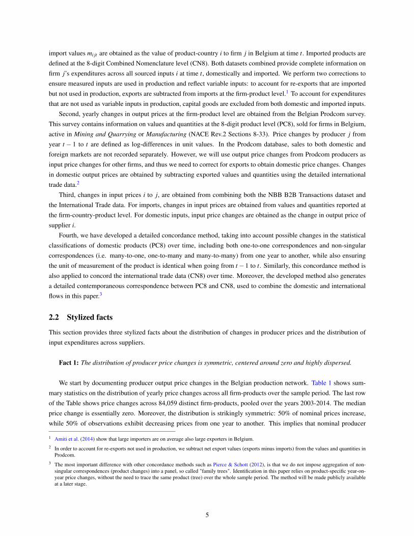
We start by documenting producer output price changes in the Belgian production network. Table 1 shows sum-mary statistics on the distribution of yearly price changes across all firm-products over the sample period. The last rowof the Table shows price changes across 84,059 distinct firm-products, pooled over the years 2003-2014. The medianprice change is essentially zero. Moreover, the distribution is strikingly symmetric: 50% of nominal prices increase,while 50% of observations exhibit decreasing prices from one year to another. This implies that nominal producer

1 Amiti et al. (2014) show that large importers are on average also large exporters in Belgium.2 In order to account for re-exports not used in production, we subtract net export values (exports minus imports) from the values and quantities in

Prodcom.3 The most important difference with other concordance methods such as Pierce & Schott (2012), is that we do not impose aggregation of non-

singular correspondences (product changes) into a panel, so called "family trees". Identification in this paper relies on product-specific year-on-year price changes, without the need to trace the same product (tree) over the whole sample period. The method will be made publicly availableat a later stage.

5

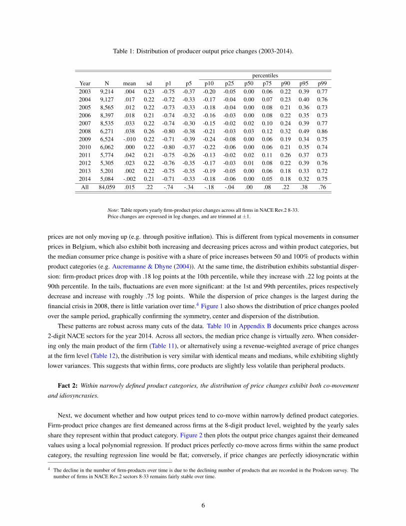
Table 1: Distribution of producer output price changes (2003-2014).

percentilesYear N mean sd p1 p5 p10 p25 p50 p75 p90 p95 p992003 9,214 .004 0.23 -0.75 -0.37 -0.20 -0.05 0.00 0.06 0.22 0.39 0.772004 9,127 .017 0.22 -0.72 -0.33 -0.17 -0.04 0.00 0.07 0.23 0.40 0.762005 8,565 .012 0.22 -0.73 -0.33 -0.18 -0.04 0.00 0.08 0.21 0.36 0.732006 8,397 .018 0.21 -0.74 -0.32 -0.16 -0.03 0.00 0.08 0.22 0.35 0.732007 8,535 .033 0.22 -0.74 -0.30 -0.15 -0.02 0.02 0.10 0.24 0.39 0.772008 6,271 .038 0.26 -0.80 -0.38 -0.21 -0.03 0.03 0.12 0.32 0.49 0.862009 6,524 -.010 0.22 -0.71 -0.39 -0.24 -0.08 0.00 0.06 0.19 0.34 0.752010 6,062 .000 0.22 -0.80 -0.37 -0.22 -0.06 0.00 0.06 0.21 0.35 0.742011 5,774 .042 0.21 -0.75 -0.26 -0.13 -0.02 0.02 0.11 0.26 0.37 0.732012 5,305 .023 0.22 -0.76 -0.35 -0.17 -0.03 0.01 0.08 0.22 0.39 0.762013 5,201 .002 0.22 -0.75 -0.35 -0.19 -0.05 0.00 0.06 0.18 0.33 0.722014 5,084 -.002 0.21 -0.71 -0.33 -0.18 -0.06 0.00 0.05 0.18 0.32 0.75All 84,059 .015 .22 -.74 -.34 -.18 -.04 .00 .08 .22 .38 .76

Note: Table reports yearly firm-product price changes across all firms in NACE Rev.2 8-33.Price changes are expressed in log changes, and are trimmed at ±1.

prices are not only moving up (e.g. through positive inflation). This is different from typical movements in consumerprices in Belgium, which also exhibit both increasing and decreasing prices across and within product categories, butthe median consumer price change is positive with a share of price increases between 50 and 100% of products withinproduct categories (e.g. Aucremanne & Dhyne (2004)). At the same time, the distribution exhibits substantial disper-sion: firm-product prices drop with .18 log points at the 10th percentile, while they increase with .22 log points at the90th percentile. In the tails, fluctuations are even more significant: at the 1st and 99th percentiles, prices respectivelydecrease and increase with roughly .75 log points. While the dispersion of price changes is the largest during thefinancial crisis in 2008, there is little variation over time.4 Figure 1 also shows the distribution of price changes pooledover the sample period, graphically confirming the symmetry, center and dispersion of the distribution.

These patterns are robust across many cuts of the data. Table 10 in Appendix B documents price changes across2-digit NACE sectors for the year 2014. Across all sectors, the median price change is virtually zero. When consider-ing only the main product of the firm (Table 11), or alternatively using a revenue-weighted average of price changesat the firm level (Table 12), the distribution is very similar with identical means and medians, while exhibiting slightlylower variances. This suggests that within firms, core products are slightly less volatile than peripheral products.

Fact 2: Within narrowly defined product categories, the distribution of price changes exhibit both co-movement

and idiosyncrasies.

Next, we document whether and how output prices tend to co-move within narrowly defined product categories.Firm-product price changes are first demeaned across firms at the 8-digit product level, weighted by the yearly salesshare they represent within that product category. Figure 2 then plots the output price changes against their demeanedvalues using a local polynomial regression. If product prices perfectly co-move across firms within the same productcategory, the resulting regression line would be flat; conversely, if price changes are perfectly idiosyncratic within

4 The decline in the number of firm-products over time is due to the declining number of products that are recorded in the Prodcom survey. Thenumber of firms in NACE Rev.2 sectors 8-33 remains fairly stable over time.

6

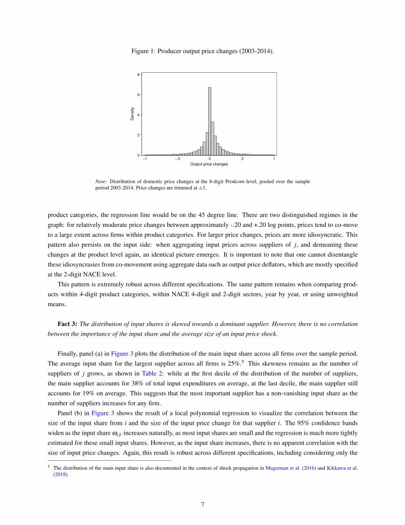
Figure 1: Producer output price changes (2003-2014).

0

2

4

6

8

Density

−1 −.5 0 .5 1

Output price changes

Note: Distribution of domestic price changes at the 8-digit Prodcom level, pooled over the sampleperiod 2003-2014. Price changes are trimmed at ±1.

product categories, the regression line would be on the 45 degree line. There are two distinguished regimes in thegraph: for relatively moderate price changes between approximately -.20 and +.20 log points, prices tend to co-moveto a large extent across firms within product categories. For larger price changes, prices are more idiosyncratic. Thispattern also persists on the input side: when aggregating input prices across suppliers of j, and demeaning thesechanges at the product level again, an identical picture emerges. It is important to note that one cannot disentanglethese idiosyncrasies from co-movement using aggregate data such as output price deflators, which are mostly specifiedat the 2-digit NACE level.

This pattern is extremely robust across different specifications. The same pattern remains when comparing prod-ucts within 4-digit product categories, within NACE 4-digit and 2-digit sectors, year by year, or using unweightedmeans.

Fact 3: The distribution of input shares is skewed towards a dominant supplier. However, there is no correlation

between the importance of the input share and the average size of an input price shock.

Finally, panel (a) in Figure 3 plots the distribution of the main input share across all firms over the sample period.The average input share for the largest supplier across all firms is 25%.5 This skewness remains as the number ofsuppliers of j grows, as shown in Table 2: while at the first decile of the distribution of the number of suppliers,the main supplier accounts for 38% of total input expenditures on average, at the last decile, the main supplier stillaccounts for 19% on average. This suggests that the most important supplier has a non-vanishing input share as thenumber of suppliers increases for any firm.

Panel (b) in Figure 3 shows the result of a local polynomial regression to visualize the correlation between thesize of the input share from i and the size of the input price change for that supplier i. The 95% confidence bandswiden as the input share ωi jt increases naturally, as most input shares are small and the regression is much more tightlyestimated for these small input shares. However, as the input share increases, there is no apparent correlation with thesize of input price changes. Again, this result is robust across different specifications, including considering only the

5 The distribution of the main input share is also documented in the context of shock propagation in Magerman et al. (2016) and Kikkawa et al.(2018).

7

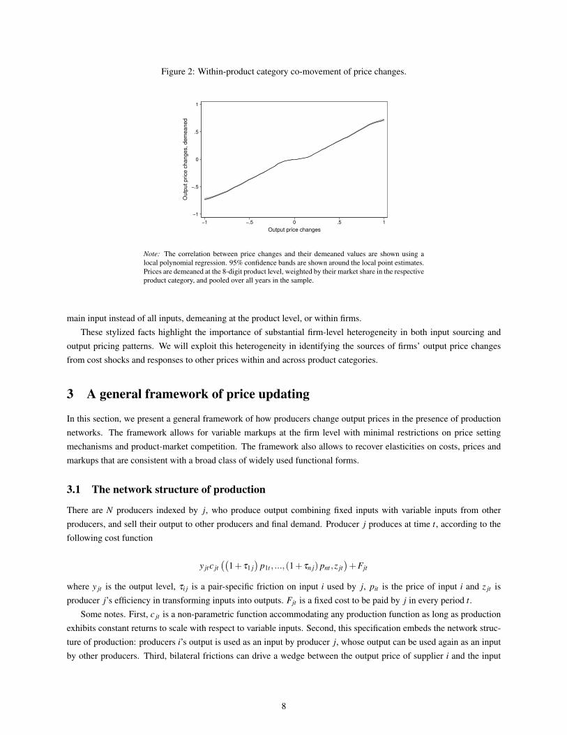
Figure 2: Within-product category co-movement of price changes.

−1

−.5

0

.5

1

Outp

ut price c

hanges, dem

eaned

−1 −.5 0 .5 1

Output price changes

Note: The correlation between price changes and their demeaned values are shown using alocal polynomial regression. 95% confidence bands are shown around the local point estimates.Prices are demeaned at the 8-digit product level, weighted by their market share in the respectiveproduct category, and pooled over all years in the sample.

main input instead of all inputs, demeaning at the product level, or within firms.These stylized facts highlight the importance of substantial firm-level heterogeneity in both input sourcing and

output pricing patterns. We will exploit this heterogeneity in identifying the sources of firms’ output price changesfrom cost shocks and responses to other prices within and across product categories.

3 A general framework of price updating

In this section, we present a general framework of how producers change output prices in the presence of productionnetworks. The framework allows for variable markups at the firm level with minimal restrictions on price settingmechanisms and product-market competition. The framework also allows to recover elasticities on costs, prices andmarkups that are consistent with a broad class of widely used functional forms.

3.1 The network structure of production

There are N producers indexed by j, who produce output combining fixed inputs with variable inputs from otherproducers, and sell their output to other producers and final demand. Producer j produces at time t, according to thefollowing cost function

y jtc jt((

1+ τ1 j)

p1t , ...,(1+ τn j) pnt ,z jt)+Fjt

where y jt is the output level, τi j is a pair-specific friction on input i used by j, pit is the price of input i and z jt isproducer j’s efficiency in transforming inputs into outputs. Fjt is a fixed cost to be paid by j in every period t.

Some notes. First, c jt is a non-parametric function accommodating any production function as long as productionexhibits constant returns to scale with respect to variable inputs. Second, this specification embeds the network struc-ture of production: producers i’s output is used as an input by producer j, whose output can be used again as an inputby other producers. Third, bilateral frictions can drive a wedge between the output price of supplier i and the input

8

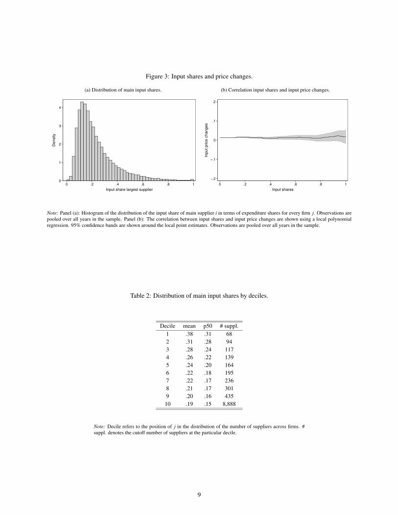
Figure 3: Input shares and price changes.

(a) Distribution of main input shares.

0

1

2

3

4

Density

0 .2 .4 .6 .8 1

Input share largest supplier

(b) Correlation input shares and input price changes.

−.2

−.1

0

.1

.2

Input price c

hanges

0 .2 .4 .6 .8 1

Input shares

Note: Panel (a): Histogram of the distribution of the input share of main supplier i in terms of expenditure shares for every firm j. Observations arepooled over all years in the sample. Panel (b): The correlation between input shares and input price changes are shown using a local polynomialregression. 95% confidence bands are shown around the local point estimates. Observations are pooled over all years in the sample.

Table 2: Distribution of main input shares by deciles.

Decile mean p50 # suppl.1 .38 .31 682 .31 .28 943 .28 .24 1174 .26 .22 1395 .24 .20 1646 .22 .18 1957 .22 .17 2368 .21 .17 3019 .20 .16 43510 .19 .15 8,888

Note: Decile refers to the position of j in the distribution of the number of suppliers across firms. #suppl. denotes the cutoff number of suppliers at the particular decile.

9

price faced by buyer j. These frictions are very general conditional on being fixed at the pair level, and can includebilateral taxes, tariffs, transport costs etc. Fourth, this specification does not impose a particular form of technologicalchange z jt , and is consistent with for instance Hicks- and Harrod-neutral productivity, but also allows for non-neutraltechnological change. Finally, for ease of exposition, in the main text we consider single-product firms. Appendix Cderives a multi-product version of the model and identifies the additional identification assumptions.

3.2 Pricing and markups

Next, consider the following pricing equation of producers j at time t, which holds under cost minimization:

ln p jt = lnc jt((

1+ τ1 j)

p1t , ...,(1+ τn j) pnt ,z jt)+ ln µ jt (p jt ,P− jt) (1)

where p jt is the output price of producer j, and µ jt represents the markup of j, which is a function of j’s own pricep jt and an index of other prices P− jt .

It is important to note that this pricing equation is consistent with a large class of price setting mechanisms. First,eq(1) does not impose profit maximization, but is still consistent with other pricing schemes such as cost-plus pricingor revenue maximization. Second, the pricing equation does not impose any particular market structure, and allowsfor either no markups, constant markups, or variable markups. Moreover, ln µ jt (p jt ,P− jt) does not have to be anequilibrium outcome such as a strategic best response function across oligopolistic competitors. Third, the index ofother prices P− jt is very general, and the exact construction of P− jt depends on the underlying model of price settingbehavior. This can include the price of direct competitors, but also geographically close firms, sector-level or aggregateprice indices etc. Hence, eq(1) can also be seen as a reduced form pricing equation, in which the nature of price settingis not specified.

3.3 Price updating in production networks

Next, totally differentiating eq(1) leads to the following decomposition of the pricing equation:

d ln p jt = ∑i∈S jt

∂ lnc jt

∂ ln pitd ln pit︸ ︷︷ ︸

total input price shock

+∂ lnc jt

∂ lnz jtd lnz jt︸ ︷︷ ︸

productivity shock

+∂ ln µ jt

∂ ln p jtd ln p jt︸ ︷︷ ︸

own price markup effect

+∂ ln µ jt

∂ lnP− jtd lnP− jt︸ ︷︷ ︸

environment price index effect

(2)

where S jt is the set of suppliers to j. A change in j’s output price is a combination of (i) a total change in input pricespit , (ii) a productivity shock to the j’s technology z jt , and (iii) a change in markups µ jt(p jt ,P− jt).

Eq(2) merits some explanation. First, the total input price shock evaluates how changes in input prices affect thecost function. It is a linear combination of shocks to all input prices pit to j, and reflects how j’s cost function respondsto all these input price shocks combined. This implies that shocks to all input prices can be linearly aggregated,independent of the exact functional form of the cost function. Moreover, the cost response to an input price shock canbe written as

∂ lnc jt

∂ ln pit=

(1+ τi j)pitxi jt

∑i∈S jt (1+ τi j)pitxi jt≡ ωi jt (3)

where ∑i∈S jt (1+ τi j)pitxi jt is j’s total variable cost, and ωi jt is the elasticity of the marginal cost with respect to achange in one input price pit . The second equality uses Shephard’s lemma to equate the input elasticity to the share ofexpenditures on input i. Next, it is straightforward to aggregate individual input price shocks to a change in the inputprice index for producer j:

10

d lnPjt ≡ ∑i∈S jt

ωi jtd ln pit (4)

The total change in j’s input price index, d lnPjt , is a weighted average of price shocks to inputs i bought by j, weightedby their share in total variable costs ωi jt . It is important to stress that eq(4) is not restricted to a Cobb-Douglas inputprice index, but is consistent with several functional forms: individual price shocks can be aggregated linearly to atotal input price shock, independent of the underlying functional form of the cost function or the input price index.

Second, eq(2) separates the impact of input price shocks from that of productivity shocks within the cost function.Again from an envelope theorem argument, at the cost minimizing input tuple (x∗1 jt , ...,x

∗n jt), any potential input real-

location effects through d lnxi jt have no effect on marginal costs, and therefore also not on output prices. Hence, thetotal impact of a productivity shock on marginal cost is given by ∂ lnc jt

∂ lnz jtd lnz jt =

∂ lny jt (x1 jt ,...,xn jt ,z jt )

∂ lnz jtd lnz jt .

Third, the markup adjustment is a combination of change in j’s own price p jt , and that of j’s environment priceindex P− jt . The first markup effect isolates the own price effect on j’s markup. This elasticity determines the amountof cost pass-through, as discussed below. The environment’s price index effect evaluates how j adjusts its markup inresponse to its output environment.

3.4 Cost pass-through

Finally, rearranging eq(2) and eq(3) generates an estimation equation that can be taken to the data.

d ln p jt = β jt ∑i∈S jt

ωi jtd ln pit + γ jtd lnz jt +δ jtd lnP− jt (5)

where the coefficients have a clear structural interpretation:

β jt =1

1−∂ ln µ jt∂ ln p jt

γ jt =1

1−∂ ln µ jt∂ ln p jt

∂ lny jt∂ lnz jt

δ jt =1

1−∂ ln µ jt∂ ln p jt

∂ ln µ jt∂ lnP− jt

(6)

First, β jt can be interpreted as a cost pass-through parameter. It captures how much a change in input prices pit relatesto a change in output price p jt , and nests several pricing mechanisms. Under either no or constant markups, ∂ ln µ jt

∂ ln p jt= 0

and β jt = 1. In this case, cost pass-through is complete. Under variable markup regimes however, ∂ ln µ jt∂ ln p jt

6= 0, and thus

β jt 6= 1. Whether ∂ ln µ jt∂ ln p jt

≶ 0 depends on the specification of µ jt (p jt ,P− jt), but most standard price setting models

with variable markups will generate ∂ ln µ jt∂ ln p jt

< 0, such that β jt < 1 and incomplete pass-through occurs.

4 Identification and estimation

In order to estimate eq(5), we exploit the rich structure of the different datasets described above.

4.1 Variables

In addition to price changes d ln p jt and d ln pit , and input shares ωi jt , estimating eq(5) requires information on effi-ciency shocks d lnz jt and changes in other prices d lnP− jt . First, we use lagged input shares, ωi jt−1 when estimating

11

the pricing equation. The use of lagged input expenditure shares avoids measurement issues with weights being influ-enced by contemporaneous changes in prices.6

Second, input price shocks d ln pi jt are obtained from changes in input prices pit sold to j. These include domesticinputs and imported inputs from the different datasets described in Section 2. Capital inputs and labor are consideredto be part of fixed costs.7

Next, lnz jt is estimated as the residual of a production function. Our procedure is similar to the productivityliterature (e.g. De Loecker & Warzynski (2012), Ackerberg et al. (2015)), but with some marked differences exploitingthe rich structure of the different datasets. These datasets allow us to overcome several typical measurement problems,which in turn improve identification of the resulting TFP estimates. First, exploiting the Prodcom data, the productionfunction is estimated in quantities, generating a measure of T FPq, rather than the more commonly estimated revenue-or value added-based measures. This is crucial, as (i) the TFP measure is then purged from prices, avoiding potentialsimultaneity issues when estimating eq(5), and (ii) output quantities are not derived from firm revenues and sector-level output price deflators. Second, estimation does not rely on input price deflators. Instead, d lnPjt is constructeddirectly from information on supplier prices and their input shares as described above. This implies that producersface firm-specific input prices for their input bundles, which take into account heterogeneity in sourcing patterns andprices paid for those bundles, rather than sector-level prices resulting from deflators. Note that, while the pricingschemes in this paper are very general, a few more assumptions are needed on the underlying production functionto estimate productivity using the machinery of the productivity literature. These include some restrictions on theadmissible functional forms and timing assumptions on how firms choose variable and fixed inputs.8 We want tostress that these assumptions are only imposed to estimate lnz jt and the resulting control variable d lnz jt , and do notaffect the generality of the pricing equation.

Finally, for exposition, we follow Amiti et al. (2016), and changes in the price index of other producers d lnP− jt

are calculated as the market share weighted average of price changes of other producers in the same product category.In particular,

d lnP− jt =∑l∈{D jt∪I jt} Slt−1d ln plt

∑l∈{D jt∪I jt} Slt−1(7)

where D jt is the set of domestic producers, producing the same output as j at time t,9 I jt is the set of importedproducts corresponding to output j in Belgium at time t, and Slt−1 is the sales value by producer l in year t − 1.Alternatively, one can construct a price index based on assumptions of the underlying model of competition, includinggeographic competition, or responses of j with respect to aggregate price indices.

4.2 Instruments

Estimating eq(5) using OLS might lead to biased coefficients due to potential endogeneity arising from simultaneityand measurement error.

6 While using lagged input shares implies only price changes for continuing products from t−1 to t are identified, this is a mild constraint in thedata: across all producers, the average input expenditure share of continuing products is over 90%. Taking into account changes on the extensivemargin of the input product mix would imply estimating shadow prices for unobserved products, forcing us to take a stance on price settingbehavior and functional forms. Alternatively, one could use the average share between t− 1 and t, but then weights are again contaminated bychanges in prices.

7 Particularly in Belgium, hiring and firing is not flexible, and many wages are subject to indexation schemes that are linked to inflation. Therefore,as a baseline, we consider labor to be part of fixed costs, to be paid by j at the start of every period t. Note that hired labor through temporaryemployment agencies (NACE 7820) is recorded as intermediary inputs in our data, and is part of variable costs. Hence labor can be split up intoa fixed and variable part.

8 Lagged materials are used as a regressor in this setup, so the estimation sample starts from 2004 instead of 2003.9 Producer j is excluded from the set, as this would otherwise generate a mechanical correlation between j and the resulting weighted average.

12

First, simultaneity arises if changes in output prices d ln p jt also affect changes in input prices d ln pit . For example,this might be due to cyclicality of the network structure of production, in which a producer j is (in-)directly supplyingits supplier i. Alternatively, prices might co-move across the board, inducing simultaneity in both input and outputprices. As prices tend to be positively correlated, OLS estimates of β will be biased downwards.

Second, while we exploit the rare features of the data in constructing ∑i∈S jt ωi jtd ln pit , using unprecedented detailon micro prices and input shares, there is still potential measurement error. In particular, changes in input prices d ln pit

are obtained from unit values, which are arguably a noisy measure of true but unobserved prices.Third, changes in other prices d lnP− jt are also potentially simultaneously determined with d ln p jt . For example,

if they reflect competitors prices, these can be jointly determined in a strategic price setting scheme.To account for these different endogeneity issues and to obtain consistent estimates, an instrumental variable

approach is implemented. In particular, we generate three instruments, which are used to instrument changes in inputprices d ln pit and changes in other producers’ prices d lnP− jt .

As a first instrument, changes in input prices d ln pit are instrumented using a market share-weighted averagechange in import prices of the same product d ln p̄−it . More formally

d ln p̄−it =∑m∈Iit Smt−1d ln pmt

∑m∈Iit Smt−1

where Iit is the set of imported products corresponding to input i in Belgium at time t, and Smt−1 is the value ofimports. For imported inputs, d ln p̄−it is constructed excluding input i. For domestic inputs, we use the concordanceprocedure from CN8 to PC8 to obtain a weighted average price change for these inputs.

The rationale for instrumenting input price changes using average import price shocks is that the average importprice change only affects a change in output prices d ln p jt through the input prices d ln pit , theoretically satisfyingthe exclusion restriction. For domestic inputs, producers j could have sourced the input internationally instead ofdomestically. Then, all instrumented input price shocks are aggregated across inputs of producer j, so that10

d lnPIV 1jt = ∑

i∈S jt

ωi jt−1d ln p̄−it

The average change in prices of other producers, d lnP− jt , also suffers from the same endogeneity issues. As a secondinstrument, average changes in import prices are used again, but now to instrument price changes other firms in thesame product space, instead of those of suppliers. In particular, the instrument is constructed as

d lnP IV 2− jt =

∑l∈I jt Slt−1d ln plt

∑l∈I jt Slt−1

Finally, as a third instrument, changes in components of d lnP− jt are instrumented with productivity shocks d lnzlt

to producers l. In order to satisfy the exclusion restriction, a productivity shock to a firm l has no direct impact onthe change in output price of j, but is only correlated with a change in output price of j through the change in l’sprice d ln plt . Productivity shocks across all producers l for producer j are then aggregated using product market shareweights as

d lnP IV 3− jt =

∑l∈D jt Slt−1d lnzlt

∑l∈D jt Slt−1

10 Whenever a domestic supplier i is a multi-product firm, we calculate the instrument by averaging across its output products, using revenue sharesas weight.

13

4.3 Estimation specifications

The model in Section 3 presents a general framework on how single-product producers update prices in the presenceof production networks. In Appendix C, an extension is presented for multi-product firms, along with additionalassumptions required for identification. When presenting the empirical results below, Section 5 reports regressionresults for the main product of producer j, trivially including single-product firms. Alternative specifications, includingpass-through regressions for an output price index d ln P̃jt at the firm level are discussed in the robustness section.

Additionally, in order to obtain an estimate for cost pass-through, eq(5) is estimated using d lnPjt =∑i∈S jt ωi jt−1d ln pit

as the total impact of all suppliers’ shocks to j. From eq(2), it is possible to evaluate individual shocks to any supplier i

on output prices of j. The robustness section discusses in more detail how to disentangle common versus idiosyncraticshocks on the input bundle.

Finally, estimating the cost pass-through regression does not impose using any type of fixed effects (including aregression constant). Under an alternative specification, markups can be a function of demand shifters to producer j

,ξ jt , so that ln µ jt (p jt ,P− jt ;ξ jt). One might be tempted to use product or sector fixed effects to account for thesepossible demand shocks. However, these fixed effects will not only capture demand shocks but also the common partof supply shocks. Therefore, the baseline specifications do not impose fixed effects, but their addition is discussedin the results section. It is important to stress however, that under these fixed effects specifications, the estimatedparameters are not their theoretical counterparts in eq(2), but instead deviations from their product or industry means.

5 Results on price updating

5.1 Baseline results

Table 3 reports our baseline results from estimating equation eq(5). Columns (i)-(iii) report the coefficients by estima-tion of eq(5) using OLS. Column (i) shows results without fixed effects, while columns (ii) and (iii) add in year andsector fixed effects sequentially. All estimated coefficients are significant at the 1% level, with robust standard errorsclustered at the 4-digit NACE level.

The estimated cost pass-through coefficient is .23, indicating that a 1% shock to input prices by suppliers of j,d lnPjt , correlates with a .23% increase in the output price of j on average, all else equal. The coefficient on theproductivity shock d lnz jt is -.09, implying that an increase in productivity correlates with a downward adjustmentof output prices. Finally, price changes of other firms, d lnP− jt , are important: on average, and conditional on costshocks, a 1% increase in the price of producers in the same the 8-digit product (PC8) level, relates to a .33% increasein j’s own price on average, entirely accruing to an increase in its markup. When accounting for year and sector fixedeffects in columns (ii) and (iii), both the cost pass-through and effect of other firms’ prices slightly decline, with theeffect of the productivity shock on the output price remaining stable.

However, these estimates are likely to suffer from endogeneity bias due to simultaneity and measurement error, asdiscussed above. To deal with these endogeneity issues and to obtain consistent estimates, we implement an instrumen-tal variable approach. In particular, changes in input prices d lnPjt and changes in prices of other producers d lnP− jt

are instrumented using three instruments: changes in input prices are instrumented using average import price shocksto suppliers of j, aggregated to a weighted average using input expenditure shares, d lnPIV 1

jt . Changes in prices of otherproducers are instrumented using both average import prices and productivity shocks to these producers, aggregatedto a weighted average using market shares in the product space k, respectively d lnP IV 2

− jt and d lnP IV 3− jt .

For these instruments to be valid, they have to be correlated with the endogenous variables (relevance) and onlyaffect the dependent variable through these endogenous variables (exclusion). Table 4 reports the results of the first

14

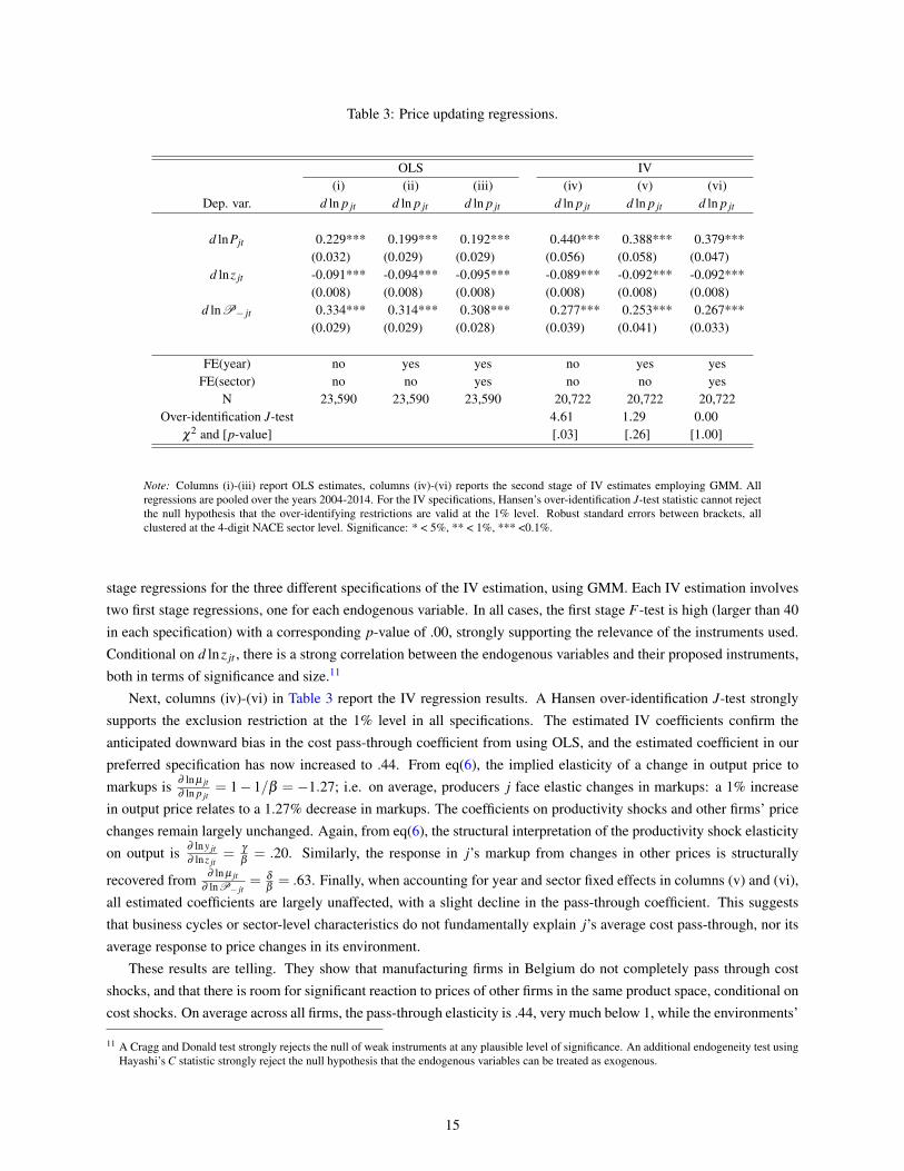
Table 3: Price updating regressions.

OLS IV(i) (ii) (iii) (iv) (v) (vi)

Dep. var. d ln p jt d ln p jt d ln p jt d ln p jt d ln p jt d ln p jt

d lnPjt 0.229*** 0.199*** 0.192*** 0.440*** 0.388*** 0.379***(0.032) (0.029) (0.029) (0.056) (0.058) (0.047)

d lnz jt -0.091*** -0.094*** -0.095*** -0.089*** -0.092*** -0.092***(0.008) (0.008) (0.008) (0.008) (0.008) (0.008)

d lnP− jt 0.334*** 0.314*** 0.308*** 0.277*** 0.253*** 0.267***(0.029) (0.029) (0.028) (0.039) (0.041) (0.033)

FE(year) no yes yes no yes yesFE(sector) no no yes no no yes

N 23,590 23,590 23,590 20,722 20,722 20,722Over-identification J-test 4.61 1.29 0.00

χ2 and [p-value] [.03] [.26] [1.00]

Note: Columns (i)-(iii) report OLS estimates, columns (iv)-(vi) reports the second stage of IV estimates employing GMM. Allregressions are pooled over the years 2004-2014. For the IV specifications, Hansen’s over-identification J-test statistic cannot rejectthe null hypothesis that the over-identifying restrictions are valid at the 1% level. Robust standard errors between brackets, allclustered at the 4-digit NACE sector level. Significance: * < 5%, ** < 1%, *** <0.1%.

stage regressions for the three different specifications of the IV estimation, using GMM. Each IV estimation involvestwo first stage regressions, one for each endogenous variable. In all cases, the first stage F-test is high (larger than 40in each specification) with a corresponding p-value of .00, strongly supporting the relevance of the instruments used.Conditional on d lnz jt , there is a strong correlation between the endogenous variables and their proposed instruments,both in terms of significance and size.11

Next, columns (iv)-(vi) in Table 3 report the IV regression results. A Hansen over-identification J-test stronglysupports the exclusion restriction at the 1% level in all specifications. The estimated IV coefficients confirm theanticipated downward bias in the cost pass-through coefficient from using OLS, and the estimated coefficient in ourpreferred specification has now increased to .44. From eq(6), the implied elasticity of a change in output price tomarkups is ∂ ln µ jt

∂ ln p jt= 1− 1/β = −1.27; i.e. on average, producers j face elastic changes in markups: a 1% increase

in output price relates to a 1.27% decrease in markups. The coefficients on productivity shocks and other firms’ pricechanges remain largely unchanged. Again, from eq(6), the structural interpretation of the productivity shock elasticityon output is ∂ lny jt

∂ lnz jt= γ

β= .20. Similarly, the response in j’s markup from changes in other prices is structurally

recovered from ∂ ln µ jt∂ lnP− jt

= δ

β= .63. Finally, when accounting for year and sector fixed effects in columns (v) and (vi),

all estimated coefficients are largely unaffected, with a slight decline in the pass-through coefficient. This suggeststhat business cycles or sector-level characteristics do not fundamentally explain j’s average cost pass-through, nor itsaverage response to price changes in its environment.

These results are telling. They show that manufacturing firms in Belgium do not completely pass through costshocks, and that there is room for significant reaction to prices of other firms in the same product space, conditional oncost shocks. On average across all firms, the pass-through elasticity is .44, very much below 1, while the environments’

11 A Cragg and Donald test strongly rejects the null of weak instruments at any plausible level of significance. An additional endogeneity test usingHayashi’s C statistic strongly reject the null hypothesis that the endogenous variables can be treated as exogenous.

15

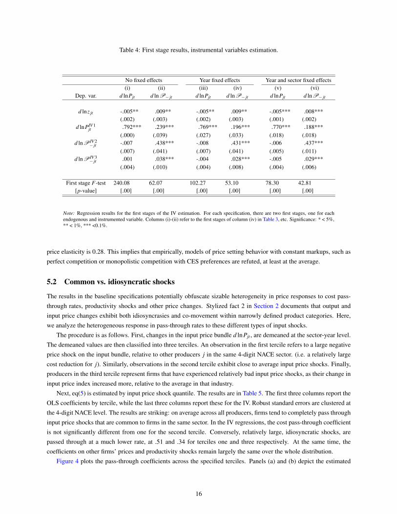
Table 4: First stage results, instrumental variables estimation.

No fixed effects Year fixed effects Year and sector fixed effects(i) (ii) (iii) (iv) (v) (vi)

Dep. var. d lnPjt d lnP− jt d lnPjt d lnP− jt d lnPjt d lnP− jt

d lnz jt -.005** .009** -.005** .009** -.005*** .008***(.002) (.003) (.002) (.003) (.001) (.002)

d lnPIV 1jt .792*** .239*** .769*** .196*** .770*** .188***

(.000) (.039) (.027) (.033) (.018) (.018)d lnP IV 2

− jt -.007 .438*** -.008 .431*** -.006 .437***(.007) (.041) (.007) (.041) (.005) (.011)

d lnP IV 3− jt .001 .038*** -.004 .028*** -.005 .029***

(.004) (.010) (.004) (.008) (.004) (.006)

First stage F-test 240.08 62.07 102.27 53.10 78.30 42.81[p-value] [.00] [.00] [.00] [.00] [.00] [.00]

Note: Regression results for the first stages of the IV estimation. For each specification, there are two first stages, one for eachendogenous and instrumented variable. Columns (i)-(ii) refer to the first stages of column (iv) in Table 3, etc. Significance: * < 5%,** < 1%, *** <0.1%.

price elasticity is 0.28. This implies that empirically, models of price setting behavior with constant markups, such asperfect competition or monopolistic competition with CES preferences are refuted, at least at the average.

5.2 Common vs. idiosyncratic shocks

The results in the baseline specifications potentially obfuscate sizable heterogeneity in price responses to cost pass-through rates, productivity shocks and other price changes. Stylized fact 2 in Section 2 documents that output andinput price changes exhibit both idiosyncrasies and co-movement within narrowly defined product categories. Here,we analyze the heterogeneous response in pass-through rates to these different types of input shocks.

The procedure is as follows. First, changes in the input price bundle d lnPjt , are demeaned at the sector-year level.The demeaned values are then classified into three terciles. An observation in the first tercile refers to a large negativeprice shock on the input bundle, relative to other producers j in the same 4-digit NACE sector. (i.e. a relatively largecost reduction for j). Similarly, observations in the second tercile exhibit close to average input price shocks. Finally,producers in the third tercile represent firms that have experienced relatively bad input price shocks, as their change ininput price index increased more, relative to the average in that industry.

Next, eq(5) is estimated by input price shock quantile. The results are in Table 5. The first three columns report theOLS coefficients by tercile, while the last three columns report these for the IV. Robust standard errors are clustered atthe 4-digit NACE level. The results are striking: on average across all producers, firms tend to completely pass throughinput price shocks that are common to firms in the same sector. In the IV regressions, the cost pass-through coefficientis not significantly different from one for the second tercile. Conversely, relatively large, idiosyncratic shocks, arepassed through at a much lower rate, at .51 and .34 for terciles one and three respectively. At the same time, thecoefficients on other firms’ prices and productivity shocks remain largely the same over the whole distribution.

Figure 4 plots the pass-through coefficients across the specified terciles. Panels (a) and (b) depict the estimated

16

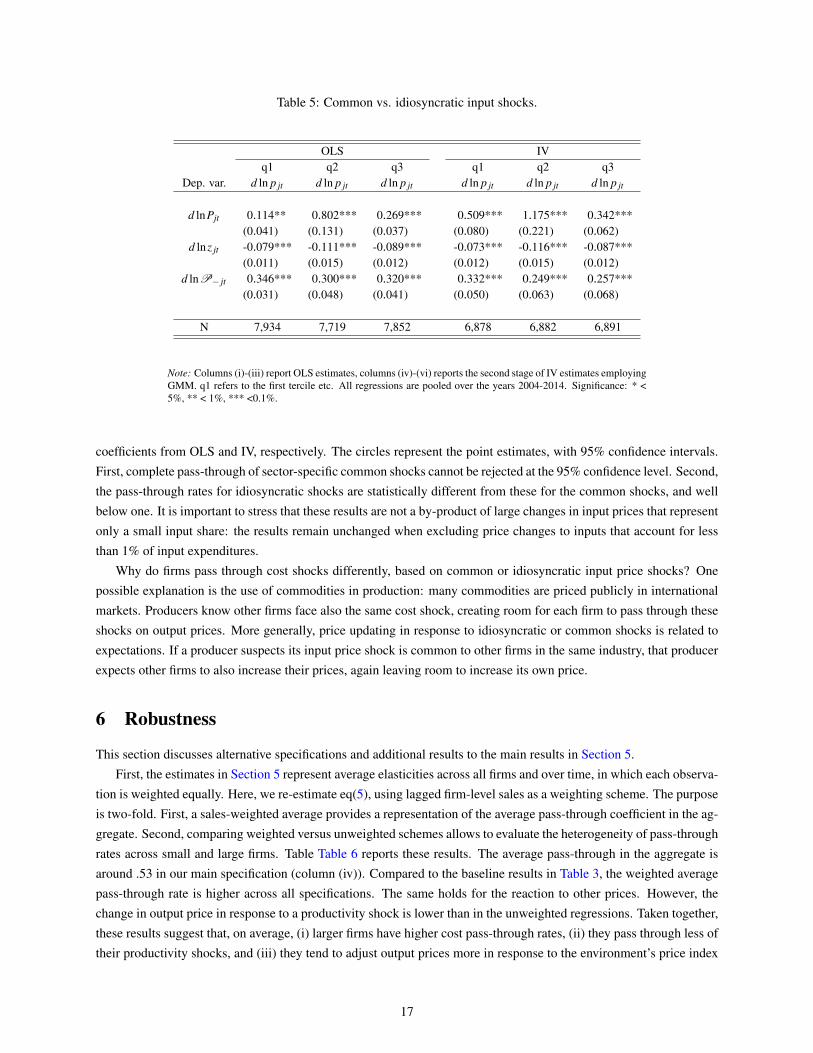
Table 5: Common vs. idiosyncratic input shocks.

OLS IVq1 q2 q3 q1 q2 q3

Dep. var. d ln p jt d ln p jt d ln p jt d ln p jt d ln p jt d ln p jt

d lnPjt 0.114** 0.802*** 0.269*** 0.509*** 1.175*** 0.342***(0.041) (0.131) (0.037) (0.080) (0.221) (0.062)

d lnz jt -0.079*** -0.111*** -0.089*** -0.073*** -0.116*** -0.087***(0.011) (0.015) (0.012) (0.012) (0.015) (0.012)

d lnP− jt 0.346*** 0.300*** 0.320*** 0.332*** 0.249*** 0.257***(0.031) (0.048) (0.041) (0.050) (0.063) (0.068)

N 7,934 7,719 7,852 6,878 6,882 6,891

Note: Columns (i)-(iii) report OLS estimates, columns (iv)-(vi) reports the second stage of IV estimates employingGMM. q1 refers to the first tercile etc. All regressions are pooled over the years 2004-2014. Significance: * <5%, ** < 1%, *** <0.1%.

coefficients from OLS and IV, respectively. The circles represent the point estimates, with 95% confidence intervals.First, complete pass-through of sector-specific common shocks cannot be rejected at the 95% confidence level. Second,the pass-through rates for idiosyncratic shocks are statistically different from these for the common shocks, and wellbelow one. It is important to stress that these results are not a by-product of large changes in input prices that representonly a small input share: the results remain unchanged when excluding price changes to inputs that account for lessthan 1% of input expenditures.

Why do firms pass through cost shocks differently, based on common or idiosyncratic input price shocks? Onepossible explanation is the use of commodities in production: many commodities are priced publicly in internationalmarkets. Producers know other firms face also the same cost shock, creating room for each firm to pass through theseshocks on output prices. More generally, price updating in response to idiosyncratic or common shocks is related toexpectations. If a producer suspects its input price shock is common to other firms in the same industry, that producerexpects other firms to also increase their prices, again leaving room to increase its own price.

6 Robustness

This section discusses alternative specifications and additional results to the main results in Section 5.First, the estimates in Section 5 represent average elasticities across all firms and over time, in which each observa-

tion is weighted equally. Here, we re-estimate eq(5), using lagged firm-level sales as a weighting scheme. The purposeis two-fold. First, a sales-weighted average provides a representation of the average pass-through coefficient in the ag-gregate. Second, comparing weighted versus unweighted schemes allows to evaluate the heterogeneity of pass-throughrates across small and large firms. Table Table 6 reports these results. The average pass-through in the aggregate isaround .53 in our main specification (column (iv)). Compared to the baseline results in Table 3, the weighted averagepass-through rate is higher across all specifications. The same holds for the reaction to other prices. However, thechange in output price in response to a productivity shock is lower than in the unweighted regressions. Taken together,these results suggest that, on average, (i) larger firms have higher cost pass-through rates, (ii) they pass through less oftheir productivity shocks, and (iii) they tend to adjust output prices more in response to the environment’s price index

17

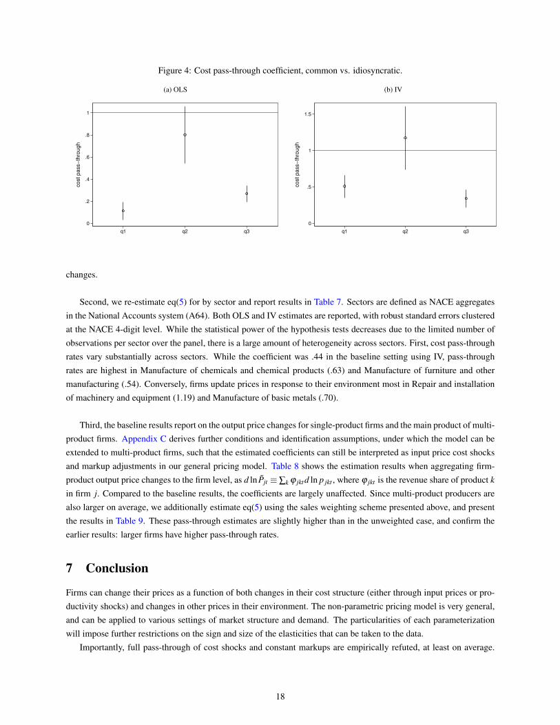
Figure 4: Cost pass-through coefficient, common vs. idiosyncratic.

(a) OLS

0

.2

.4

.6

.8

1

cost pass−

thro

ugh

q1 q2 q3

(b) IV

0

.5

1

1.5

cost pass−

thro

ugh

q1 q2 q3

changes.

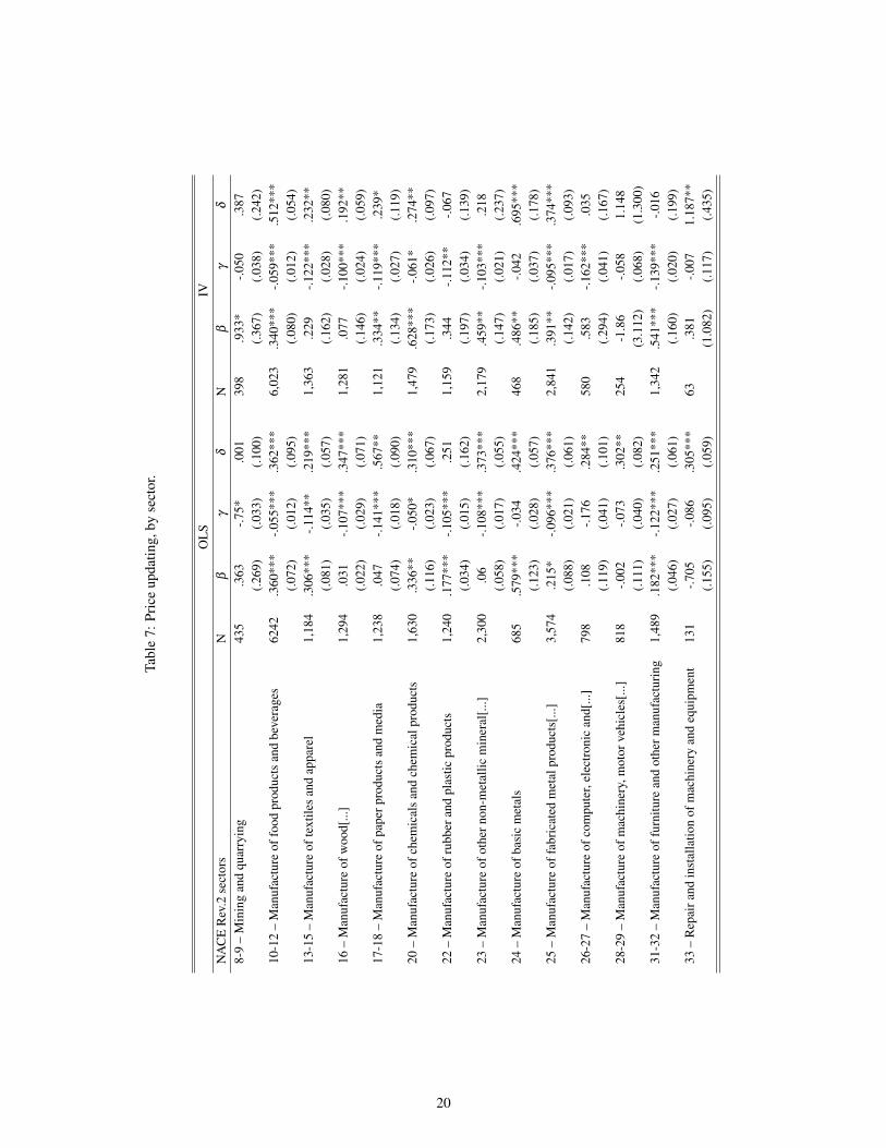
Second, we re-estimate eq(5) for by sector and report results in Table 7. Sectors are defined as NACE aggregatesin the National Accounts system (A64). Both OLS and IV estimates are reported, with robust standard errors clusteredat the NACE 4-digit level. While the statistical power of the hypothesis tests decreases due to the limited number ofobservations per sector over the panel, there is a large amount of heterogeneity across sectors. First, cost pass-throughrates vary substantially across sectors. While the coefficient was .44 in the baseline setting using IV, pass-throughrates are highest in Manufacture of chemicals and chemical products (.63) and Manufacture of furniture and othermanufacturing (.54). Conversely, firms update prices in response to their environment most in Repair and installationof machinery and equipment (1.19) and Manufacture of basic metals (.70).

Third, the baseline results report on the output price changes for single-product firms and the main product of multi-product firms. Appendix C derives further conditions and identification assumptions, under which the model can beextended to multi-product firms, such that the estimated coefficients can still be interpreted as input price cost shocksand markup adjustments in our general pricing model. Table 8 shows the estimation results when aggregating firm-product output price changes to the firm level, as d ln P̃jt ≡∑k ϕ jktd ln p jkt , where ϕ jkt is the revenue share of product k

in firm j. Compared to the baseline results, the coefficients are largely unaffected. Since multi-product producers arealso larger on average, we additionally estimate eq(5) using the sales weighting scheme presented above, and presentthe results in Table 9. These pass-through estimates are slightly higher than in the unweighted case, and confirm theearlier results: larger firms have higher pass-through rates.

7 Conclusion

Firms can change their prices as a function of both changes in their cost structure (either through input prices or pro-ductivity shocks) and changes in other prices in their environment. The non-parametric pricing model is very general,and can be applied to various settings of market structure and demand. The particularities of each parameterizationwill impose further restrictions on the sign and size of the elasticities that can be taken to the data.

Importantly, full pass-through of cost shocks and constant markups are empirically refuted, at least on average.

18

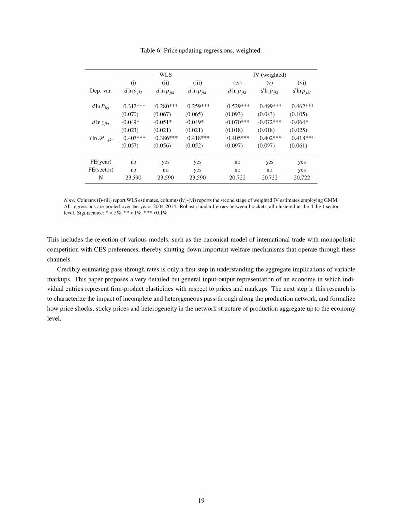
Table 6: Price updating regressions, weighted.

WLS IV (weighted)(i) (ii) (iii) (iv) (v) (vi)

Dep. var. d ln p jkt d ln p jkt d ln p jkt d ln p jkt d ln p jkt d ln p jkt

d lnPjkt 0.312*** 0.280*** 0.259*** 0.529*** 0.499*** 0.462***(0.070) (0.067) (0.065) (0.093) (0.083) (0.105)

d lnz jkt -0.049* -0.051* -0.049* -0.070*** -0.072*** -0.064*(0.023) (0.021) (0.021) (0.018) (0.018) (0.025)

d lnP− jkt 0.407*** 0.386*** 0.418*** 0.405*** 0.402*** 0.418***(0.057) (0.056) (0.052) (0.097) (0.097) (0.061)

FE(year) no yes yes no yes yesFE(sector) no no yes no no yes

N 23,590 23,590 23,590 20,722 20,722 20,722

Note: Columns (i)-(iii) report WLS estimates, columns (iv)-(vi) reports the second stage of weighted IV estimates employing GMM.All regressions are pooled over the years 2004-2014. Robust standard errors between brackets, all clustered at the 4-digit sectorlevel. Significance: * < 5%, ** < 1%, *** <0.1%.

This includes the rejection of various models, such as the canonical model of international trade with monopolisticcompetition with CES preferences, thereby shutting down important welfare mechanisms that operate through thesechannels.

Credibly estimating pass-through rates is only a first step in understanding the aggregate implications of variablemarkups. This paper proposes a very detailed but general input-output representation of an economy in which indi-vidual entries represent firm-product elasticities with respect to prices and markups. The next step in this research isto characterize the impact of incomplete and heterogeneous pass-through along the production network, and formalizehow price shocks, sticky prices and heterogeneity in the network structure of production aggregate up to the economylevel.

19

Tabl

e7:

Pric

eup

datin

g,by

sect

or.

OL

SIV

NA

CE

Rev

.2se

ctor

sN

βγ

δN

βγ

δ

8-9

–M

inin

gan

dqu

arry

ing

435

.363

-.75*

.001

398

.933

*-.0

50.3

87(.2

69)

(.033

)(.1

00)

(.367

)(.0

38)

(.242

)10

-12

–M

anuf

actu

reof

food

prod

ucts

and

beve

rage

s62

42.3

60**

*-.0

55**

*.3

62**

*6,

023

.340

***

-.059

***

.512

***

(.072

)(.0

12)

(.095

)(.0

80)

(.012

)(.0

54)

13-1

5–

Man

ufac

ture

ofte

xtile

san

dap

pare

l1,

184

.306

***

-.114

**.2

19**

*1,

363

.229

-.122

***

.232

**(.0

81)

(.035

)(.0

57)

(.162

)(.0

28)

(.080

)16

–M

anuf

actu

reof

woo

d[...

]1,

294

.031

-.107

***

.347

***

1,28

1.0

77-.1

00**

*.1

92**

(.022

)(.0

29)

(.071

)(.1

46)

(.024

)(.0

59)

17-1

8–

Man

ufac

ture

ofpa

perp

rodu

cts

and

med

ia1,

238

.047

-.141

***

.567

**1,

121

.334

**-.1

19**

*.2

39*

(.074

)(.0

18)

(.090

)(.1

34)

(.027

)(.1

19)

20–

Man

ufac

ture

ofch

emic

als

and

chem

ical

prod

ucts

1,63

0.3

36**

-.050

*.3

10**

*1,

479

.628

***

-.061

*.2

74**

(.116

)(.0

23)

(.067

)(.1

73)

(.026

)(.0

97)

22–

Man

ufac

ture

ofru

bber

and

plas

ticpr

oduc

ts1,

240

.177

***

-.105

***

.251

1,15

9.3

44-.1

12**

-.067

(.034

)(.0

15)

(.162

)(.1

97)

(.034

)(.1

39)

23–

Man

ufac

ture

ofot

hern

on-m

etal

licm

iner

al[..

.]2,

300

.06

-.108

***

.373

***

2,17

9.4

59**

-.103

***

.218

(.058

)(.0

17)

(.055

)(.1

47)

(.021

)(.2

37)

24–

Man

ufac

ture

ofba

sic

met

als

685

.579

***

-.034

.424

***

468

.486

**-.0

42.6

95**

*(.1

23)

(.028

)(.0

57)

(.185

)(.0

37)

(.178

)25

–M

anuf

actu

reof

fabr

icat

edm

etal

prod

ucts

[...]

3,57

4.2

15*

-.096

***

.376

***

2,84

1.3

91**

-.095

***

.374

***

(.088

)(.0

21)

(.061

)(.1

42)

(.017

)(.0

93)

26-2

7–

Man

ufac

ture

ofco

mpu

ter,

elec

tron

ican

d[...

]79

8.1

08-.1

76.2

84**

580

.583

-.162

***

.035

(.119

)(.0

41)

(.101

)(.2

94)

(.041

)(.1

67)

28-2

9–

Man

ufac

ture

ofm

achi

nery

,mot

orve

hicl

es[..

.]81

8-.0

02-.0

73.3

02**

254

-1.8

6-.0

581.

148

(.111

)(.0

40)

(.082

)(3

.112

)(.0

68)

(1.3

00)

31-3

2–

Man

ufac

ture

offu

rnitu

rean

dot

herm

anuf

actu

ring

1,48

9.1

82**

*-.1

22**

*.2

51**

*1,

342

.541

***

-.139

***

-.016

(.046

)(.0

27)

(.061

)(.1

60)

(.020

)(.1

99)

33–

Rep

aira

ndin

stal

latio

nof

mac

hine

ryan

deq

uipm

ent

131

-.705

-.086

.305

***

63.3

81-.0

071.

187*

*(.1

55)

(.095

)(.0

59)

(1.0

82)

(.117

)(.4

35)

20

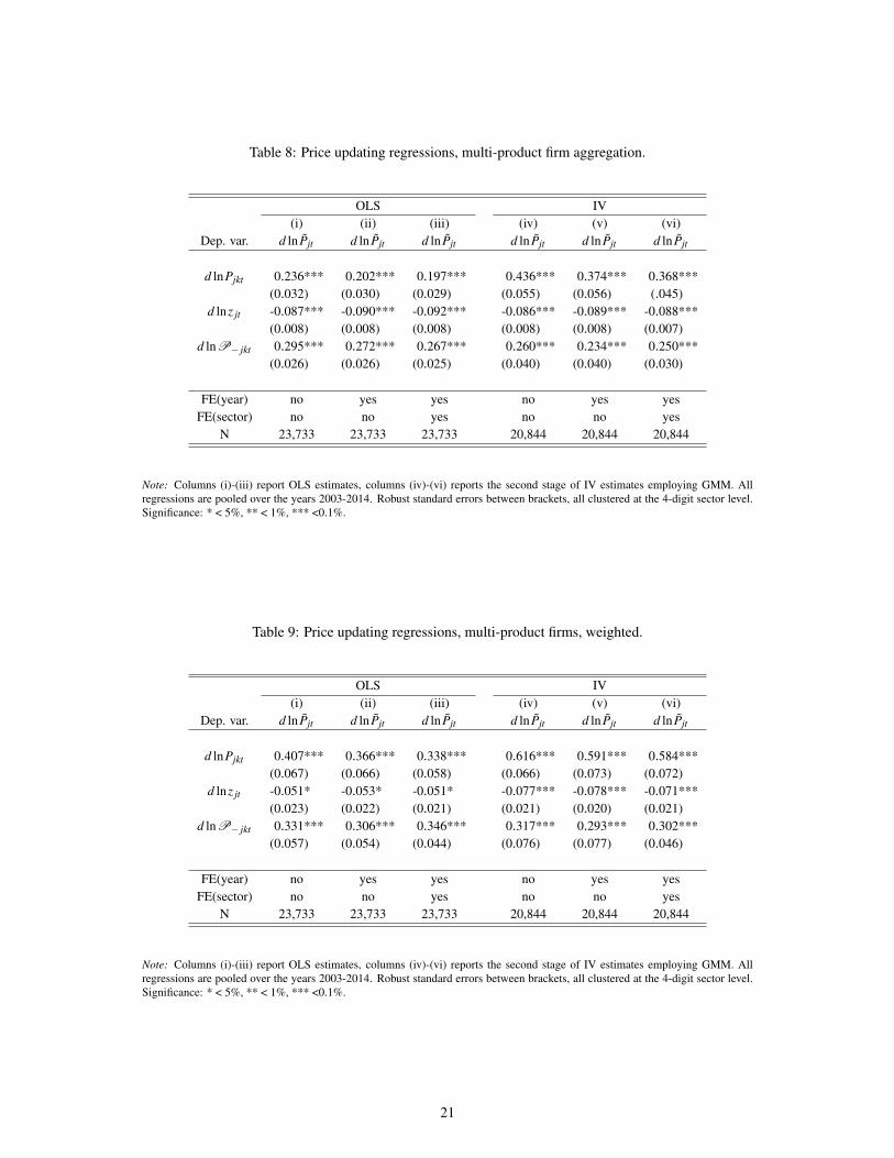
Table 8: Price updating regressions, multi-product firm aggregation.

OLS IV(i) (ii) (iii) (iv) (v) (vi)

Dep. var. d ln P̃jt d ln P̃jt d ln P̃jt d ln P̃jt d ln P̃jt d ln P̃jt

d lnPjkt 0.236*** 0.202*** 0.197*** 0.436*** 0.374*** 0.368***(0.032) (0.030) (0.029) (0.055) (0.056) (.045)

d lnz jt -0.087*** -0.090*** -0.092*** -0.086*** -0.089*** -0.088***(0.008) (0.008) (0.008) (0.008) (0.008) (0.007)

d lnP− jkt 0.295*** 0.272*** 0.267*** 0.260*** 0.234*** 0.250***(0.026) (0.026) (0.025) (0.040) (0.040) (0.030)

FE(year) no yes yes no yes yesFE(sector) no no yes no no yes

N 23,733 23,733 23,733 20,844 20,844 20,844

Note: Columns (i)-(iii) report OLS estimates, columns (iv)-(vi) reports the second stage of IV estimates employing GMM. Allregressions are pooled over the years 2003-2014. Robust standard errors between brackets, all clustered at the 4-digit sector level.Significance: * < 5%, ** < 1%, *** <0.1%.

Table 9: Price updating regressions, multi-product firms, weighted.

OLS IV(i) (ii) (iii) (iv) (v) (vi)

Dep. var. d ln P̃jt d ln P̃jt d ln P̃jt d ln P̃jt d ln P̃jt d ln P̃jt

d lnPjkt 0.407*** 0.366*** 0.338*** 0.616*** 0.591*** 0.584***(0.067) (0.066) (0.058) (0.066) (0.073) (0.072)

d lnz jt -0.051* -0.053* -0.051* -0.077*** -0.078*** -0.071***(0.023) (0.022) (0.021) (0.021) (0.020) (0.021)

d lnP− jkt 0.331*** 0.306*** 0.346*** 0.317*** 0.293*** 0.302***(0.057) (0.054) (0.044) (0.076) (0.077) (0.046)

FE(year) no yes yes no yes yesFE(sector) no no yes no no yes

N 23,733 23,733 23,733 20,844 20,844 20,844

Note: Columns (i)-(iii) report OLS estimates, columns (iv)-(vi) reports the second stage of IV estimates employing GMM. Allregressions are pooled over the years 2003-2014. Robust standard errors between brackets, all clustered at the 4-digit sector level.Significance: * < 5%, ** < 1%, *** <0.1%.

21

Appendices

A Data sources and construction

The empirical analysis in this paper mainly draws from three data sources at the National Bank of Belgium (NBB).These include (i) information on production values and quantities from the Prodcom Survey, (ii) domestic supplier-buyer relationship values from the NBB B2B Transactions Dataset, and (iii) international trade data at the firm-product-country level from Intrastat and Extrastat. Firms are identified by a unique corporate registration number from theCrossroads Bank for Enterprises, which allows for unambiguous merging across all datasets.

Additional data comes from the Crossroads Bank for Enterprises, from which we extract the main NACE sector atthe 4-digit industry of each firm. Finally, product classification tables and correspondence files for international trade(CN) and Prodcom (PC) are obtained from Eurostat to construct our concordance method.

Prodcom SurveyThe Prodcom Classification (PC) provides statistics on the production of manufactured goods and industrial servicesacross Mining and Quarrying (NACE Rev.2 Section B) and Manufacturing (Section C) in the EU. Depending on theyear, the classification describes roughly 4,000 industrial products at the disaggregated 8-digit (PC8) level.12 Forexample, in 2014, within the 6-digit grouping of "Polymers of ethylene, in primary forms", code 20.16.10.35 refers to"Linear polyethylene having a specific gravity < 0,94, in primary forms", code 20.16.10.39 is "Polyethylene having

a specific gravity < 0,94, in primary forms (excluding linear)", code 20.16.10.50 refers to "Polyethylene having a

specific gravity of ≥ 0,94, in primary forms", etc.All firms that produce goods covered by the Prodcom Classification, and that have at least 20 persons employed

or a turnover of at least 3,928,137 euro in the previous reference year, have to submit a monthly report to StatisticsBelgium.13 Reporting thresholds are defined at the consolidated level, such that daughters of surveyed firms alsoreport their production and sales, independent of their size. The database reports, for each product in the prodcom list,values and quantities for total production and sold production in Belgium during the reference period. Some productsonly have to report values, not quantities, such as some industrial manipulations (e.g. bleaching of leather, dying oftextile). Values are reported in current euro. Quantities are reported in one of several possible units (over two thirdsof observation are in kilograms; other units include liters, meters, square meters, kilowatt, kg of active substanceetc.), and we keep track of these units when we compare and harmonize international trade data and Prodcom datalater on.14 The survey is collected in an electronic format, which includes automatic checks when filing the data andadditional checks and cross-references with both micro and macro data by the national statistical office, to ensure apristine quality of reporting.

We extract information from the monthly Prodcom Survey for all firms with their main activity in Mining, Quar-rying and Manufacturing for the period 2002-2014. For some monthly observations at the firm-product level, eithervalues or quantities are missing. We impute these by first calculating the average monthly unit value for that firm-product, and then back out values or quantities for these months. We aggregate values and quantities from monthlyto yearly observations. We obtain firm-product prices as values over quantities. We subtract net exports from total

12 In the Prodcom survey for Belgium, the following sectors are covered: NACE Rev.2 Divisions 08-33, except 09, 19, 1011 and the slaughterhousepart of 1051. These represent roughly 2,500 PC8 codes in a given year, produced in Belgium.

13 See here for more info.14 For example, we correct the Prodcom sales data for net exports to obtain domestic unit values. To do so, we need to concord the trade data

with the Prodcom data, identify products that can be corresponded from CN to PC, and when subtracting quantities, we need to ensure that bothproducts are reported in the same unit of measurement.

22

Prodcom sales by the firm, as we need to obtain a measure of domestic output prices to be used as input prices forother firms (see the procedure below).

Next, we calculate the change in logs of domestic output prices for every continuing firm-product-year observation.We have constructed a custom concordance method that takes into account changes in the PC classification over time,and that makes sure the product is reported in the same units in both years.15 In short, as the classification changesover time, some product codes are merged to one single PC code in from one year to another, or one PC code can besplit up into different codes from one year to the next. We identify these changes and deal with merges and splits yearby year. We do not impose a harmonization over time, as we only need to identify continuing products from t−1 to t.Whenever 1:m matches occur over time, so that one PC8 product in t−1 splits into multiple products in t, we allocateprices proportionally to the new products in t, with firm-level weights given by the revenue shares of these productsin t. Whenever m:1 matches occur, we generate a weighted average of prices in t−1 to calculate price changes. Wealso identify the units of measurement each year, so that we do not erroneously calculate price changes based on unitvalues in kilograms and square meters from one year to another for instance. We trim log-differenced unit values at±1.

Firm-to-firm relationshipsThe confidential NBB B2B Transactions Dataset contains the values of yearly sales relationships among all VAT-liableBelgian enterprises for the years 2002 to 2014, and is based on the VAT listings collected by the tax authorities. Atthe end of every calendar year, all VAT-liable enterprises have to file a complete listing of their Belgian VAT-liablecustomers over that year.16 An observation in this dataset refers to the sales value in euro of enterprise i selling toenterprise j within Belgium, excluding the VAT amount due on these sales. The reported value is the sum of invoicesfrom i to j in a given calendar year. Whenever this aggregated value is 250 euros or greater, the relationship has tobe reported. Fines are imposed for late and/or erroneous reporting. Each observation mi j is directed, as firm i canbe selling to j, but not necessarily the other way around, i.e. mi j 6= m ji. A detailed description of the collection andcleaning of this dataset is given in Dhyne et al. (2015). We keep producers j that are sellers in the Prodcom data, andextract all input suppliers i to these firms. We drop suppliers to j that mainly produce capital goods (NACE Rev.2codes 28 and 41-43), as these goods are not part of the marginal cost bundle of their customers.

International trade dataWe obtain information on imports and exports from the Intrastat (intra-EU) and Extrastat (extra-EU) declarations forBelgium. Observations in this dataset are at the firm-product-country-year level. Products are defined at the 8-digitCombined Nomenclature (CN8) level. We exploit information on values and quantities to generate import and exportprices, and we additionally retain information on the units of measurement for quantities reported. At the CN8 level,most products’ export and import quantities are recorded in weight (kilograms). Depending on the particular product,some products’ quantities are also recorded in a secondary unit (which is the same as the PC8 unit if there exists aconcordance between the CN8 and PC8 products).

Data cleaning proceeds as follows. First, we calculate the average export price at the firm-product-year level astotal export value over total export quantities, summed across all export destinations. We need this to correct for exportprices in the Prodcom data to obtain domestic unit values. Second, we use imports as inputs in production. For that,we (i) subtract goods that are re-exported without manipulation by the firm, and (ii) ignore imported capital goods as

15 The method is slightly different from e.g. Pierce & Schott (2012), as we do not harmonize products over the whole sample period. Harmonizingwould imply creating “family trees”, in which m:1, 1:m and m:m matches over time are collapsed to single products. The longer the time horizonof the data, the more granularity the dataset would lose. With our method, we can track all changes of 1:1, 1:m, m:1 and m:m from t−1 to t andidentify price changes for these products.

16 Sample VAT listings forms can be found at here (French) and here (Dutch).

23

inputs, as both types of goods are not part of the marginal cost of the firm in our setup. We identify capital goods fromthe concordance tables between CN and BEC (Broad Economic Classification), and drop imports that are marked ascapital goods in the BEC classification (codes 410 and 521). Re-exports can be a particular issue in Belgium, whichis considered as a transit country (see e.g. Duprez (2014)). To clean imports from re-exports, we subtract the value ofexported products at the CN8 level that are also imported by the firm in the same year. We proportionally redistributeexports over all import countries for the same firm-product observation. Next, we obtain prices for imports at thefirm-product-country-year level as net imported values over net imported quantities.

The next step is to obtain the change in prices for continuing imports at the product-country level. We use thesame methodology for changes in CN8 from year to year, and for m:1, 1:m and m:m correspondences as the procedureabove for yearly changes in PC8. Finally, log-differenced unit values are trimmed at ±1.

B Additional descriptive statistics

This section provides additional statistics on the stylized facts presented in the main text. Table 10 shows the distribu-tion of output price changes at the firm-product level by 2-digit NACE sector for the year 2014. Sectors with at least10 observations are reported. Table 11 shows the distribution of output price changes by year, using the main outputfor each firm instead of all products in the main text. Similarly, Table 12 shows the distribution using a sales-weightedaverage of product price changes at the firm level.

C Model with multi-product firms

This section develops an extended version of the model, in which firms now produce multiple outputs instead of beingsingle-product firms as in the main text. Two variants of the model are presented, in which the unit of observationis either the firm-product or the firm as a whole. This distinction has implications for the identification assumptionswhen taken to the data.

C.1 Model at the firm-product level

The cost function of output k by firm j is now

y jktc jkt((

1+ τ1 j)

p1t , ...,(1+ τn j) pnt ,z jt)+Fjkt

For our purpose of identifying the sources of output price changes, allowing for multi-product firms requires thefollowing additional assumptions:

Assumption 1. No physical synergies across products within producers.

This implies that the cost function of one product is independent of the production of the other products within thefirm.

24

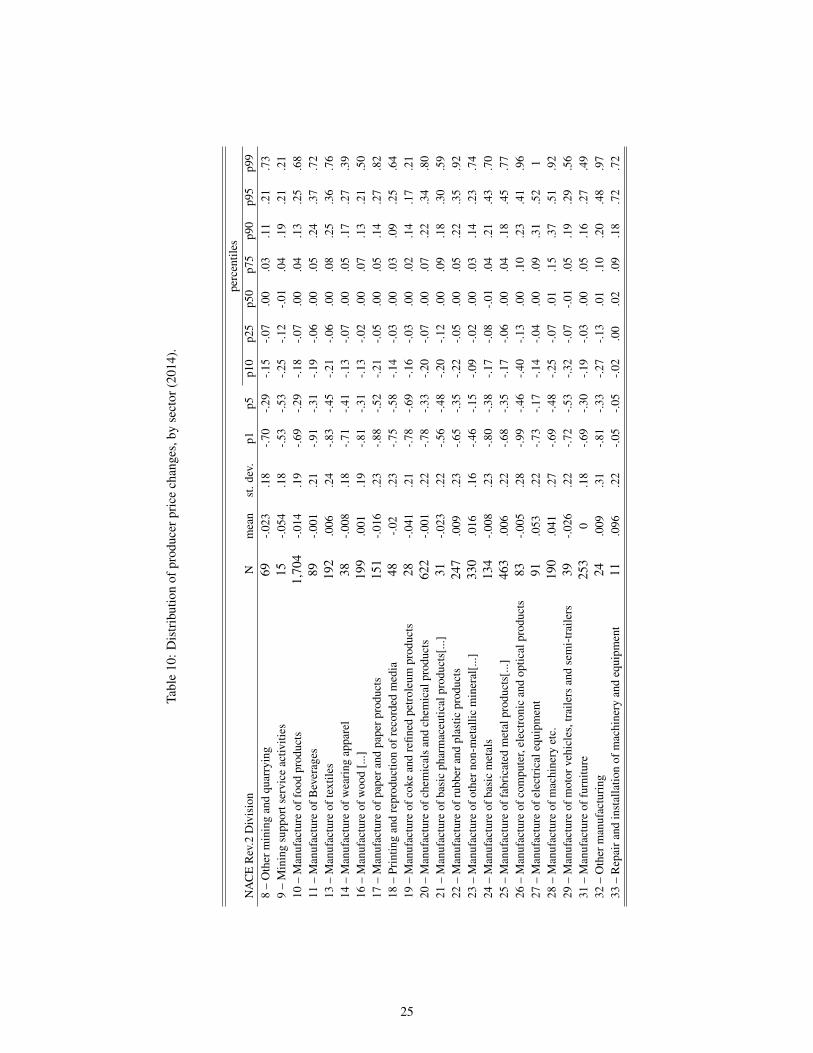
Tabl

e10

:Dis

trib

utio

nof

prod

ucer

pric

ech

ange

s,by

sect

or(2

014)

.

perc

entil

esN

AC

ER

ev.2

Div

isio

nN

mea

nst

.dev

.p1

p5p1

0p2

5p5

0p7

5p9

0p9

5p9

98

–O

ther

min

ing

and

quar

ryin

g69

-.023

.18

-.70

-.29

-.15

-.07

.00

.03

.11

.21

.73

9–

Min

ing

supp

orts

ervi

ceac

tiviti

es15

-.054

.18

-.53

-.53

-.25

-.12

-.01

.04

.19

.21

.21

10–

Man

ufac

ture

offo

odpr

oduc

ts1,

704

-.014

.19

-.69

-.29

-.18

-.07

.00

.04

.13

.25

.68

11–

Man

ufac

ture

ofB

ever

ages

89-.0

01.2

1-.9

1-.3

1-.1

9-.0

6.0

0.0

5.2

4.3

7.7

213

–M

anuf

actu

reof

text

iles

192

.006

.24

-.83

-.45

-.21

-.06

.00

.08

.25

.36

.76

14–

Man

ufac

ture

ofw

eari

ngap

pare

l38

-.008

.18

-.71

-.41

-.13

-.07

.00

.05

.17

.27

.39

16–

Man

ufac

ture

ofw

ood

[...]

199

.001

.19

-.81

-.31

-.13

-.02

.00

.07

.13

.21

.50

17–

Man

ufac

ture

ofpa

pera

ndpa

perp

rodu

cts

151

-.016

.23

-.88

-.52

-.21

-.05

.00

.05

.14

.27

.82

18–

Prin

ting

and

repr

oduc

tion

ofre

cord

edm

edia

48-.0

2.2

3-.7

5-.5

8-.1

4-.0

3.0

0.0

3.0

9.2

5.6

419

–M

anuf

actu

reof

coke

and

refin

edpe

trol

eum

prod

ucts

28-.0

41.2

1-.7

8-.6

9-.1

6-.0

3.0

0.0

2.1

4.1

7.2

120

–M

anuf

actu

reof

chem

ical

san

dch

emic

alpr

oduc

ts62

2-.0

01.2

2-.7

8-.3

3-.2

0-.0

7.0

0.0

7.2

2.3

4.8

021

–M

anuf

actu

reof

basi

cph

arm

aceu

tical

prod

ucts

[...]

31-.0

23.2

2-.5

6-.4

8-.2

0-.1

2.0

0.0

9.1

8.3

0.5

922

–M

anuf

actu

reof

rubb

eran

dpl

astic

prod

ucts

247

.009

.23

-.65

-.35

-.22

-.05

.00

.05

.22

.35

.92

23–

Man

ufac

ture

ofot

hern

on-m

etal

licm

iner

al[..

.]33

0.0

16.1

6-.4

6-.1

5-.0

9-.0

2.0

0.0

3.1

4.2

3.7

424

–M

anuf

actu

reof

basi

cm

etal

s13

4-.0

08.2

3-.8

0-.3

8-.1

7-.0

8-.0

1.0

4.2

1.4

3.7

025

–M

anuf

actu

reof

fabr

icat

edm

etal

prod

ucts

[...]

463

.006

.22

-.68

-.35

-.17

-.06

.00

.04

.18

.45

.77

26–

Man

ufac

ture

ofco

mpu

ter,

elec

tron

ican

dop

tical

prod

ucts

83-.0

05.2

8-.9

9-.4

6-.4

0-.1

3.0

0.1

0.2

3.4

1.9

627

–M

anuf

actu

reof

elec

tric

aleq

uipm

ent

91.0

53.2

2-.7

3-.1

7-.1

4-.0

4.0

0.0

9.3

1.5

21

28–

Man

ufac

ture

ofm

achi

nery

etc.

190

.041

.27

-.69

-.48

-.25

-.07

.01

.15

.37

.51

.92

29–

Man

ufac

ture

ofm

otor

vehi

cles

,tra

ilers

and

sem

i-tr

aile

rs39

-.026

.22

-.72

-.53

-.32

-.07

-.01

.05

.19

.29

.56

31–

Man

ufac

ture

offu

rnitu

re25

30

.18

-.69

-.30

-.19

-.03

.00

.05

.16

.27

.49

32–

Oth

erm

anuf

actu

ring

24.0

09.3

1-.8

1-.3

3-.2

7-.1

3.0

1.1

0.2

0.4

8.9

733

–R

epai

rand

inst

alla

tion

ofm

achi

nery

and

equi

pmen

t11

.096

.22

-.05

-.05

-.02

.00

.02

.09

.18

.72

.72

25

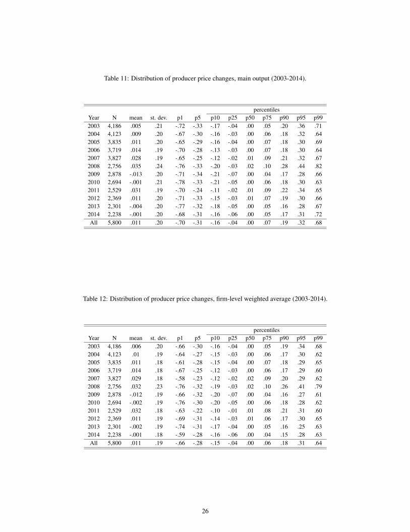
Table 11: Distribution of producer price changes, main output (2003-2014).

percentilesYear N mean st. dev. p1 p5 p10 p25 p50 p75 p90 p95 p992003 4,186 .005 .21 -.72 -.33 -.17 -.04 .00 .05 .20 .36 .712004 4,123 .009 .20 -.67 -.30 -.16 -.03 .00 .06 .18 .32 .642005 3,835 .011 .20 -.65 -.29 -.16 -.04 .00 .07 .18 .30 .692006 3,719 .014 .19 -.70 -.28 -.13 -.03 .00 .07 .18 .30 .642007 3,827 .028 .19 -.65 -.25 -.12 -.02 .01 .09 .21 .32 .672008 2,756 .035 .24 -.76 -.33 -.20 -.03 .02 .10 .28 .44 .822009 2,878 -.013 .20 -.71 -.34 -.21 -.07 .00 .04 .17 .28 .662010 2,694 -.001 .21 -.78 -.33 -.21 -.05 .00 .06 .18 .30 .632011 2,529 .031 .19 -.70 -.24 -.11 -.02 .01 .09 .22 .34 .652012 2,369 .011 .20 -.71 -.33 -.15 -.03 .01 .07 .19 .30 .662013 2,301 -.004 .20 -.77 -.32 -.18 -.05 .00 .05 .16 .28 .672014 2,238 -.001 .20 -.68 -.31 -.16 -.06 .00 .05 .17 .31 .72All 5,800 .011 .20 -.70 -.31 -.16 -.04 .00 .07 .19 .32 .68

Table 12: Distribution of producer price changes, firm-level weighted average (2003-2014).

percentilesYear N mean st. dev. p1 p5 p10 p25 p50 p75 p90 p95 p992003 4,186 .006 .20 -.66 -.30 -.16 -.04 .00 .05 .19 .34 .682004 4,123 .01 .19 -.64 -.27 -.15 -.03 .00 .06 .17 .30 .622005 3,835 .011 .18 -.61 -.28 -.15 -.04 .00 .07 .18 .29 .652006 3,719 .014 .18 -.67 -.25 -.12 -.03 .00 .06 .17 .29 .602007 3,827 .029 .18 -.58 -.23 -.12 -.02 .02 .09 .20 .29 .622008 2,756 .032 .23 -.76 -.32 -.19 -.03 .02 .10 .26 .41 .792009 2,878 -.012 .19 -.66 -.32 -.20 -.07 .00 .04 .16 .27 .612010 2,694 -.002 .19 -.76 -.30 -.20 -.05 .00 .06 .18 .28 .622011 2,529 .032 .18 -.63 -.22 -.10 -.01 .01 .08 .21 .31 .602012 2,369 .011 .19 -.69 -.31 -.14 -.03 .01 .06 .17 .30 .652013 2,301 -.002 .19 -.74 -.31 -.17 -.04 .00 .05 .16 .25 .632014 2,238 -.001 .18 -.59 -.28 -.16 -.06 .00 .04 .15 .28 .63All 5,800 .011 .19 -.66 -.28 -.15 -.04 .00 .06 .18 .31 .64

26

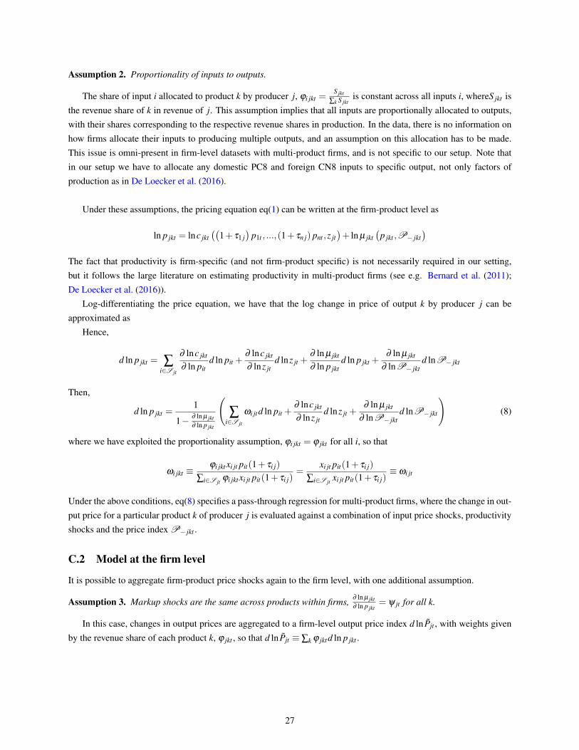
Assumption 2. Proportionality of inputs to outputs.

The share of input i allocated to product k by producer j, ϕi jkt =S jkt

∑k S jktis constant across all inputs i, whereS jkt is

the revenue share of k in revenue of j. This assumption implies that all inputs are proportionally allocated to outputs,with their shares corresponding to the respective revenue shares in production. In the data, there is no information onhow firms allocate their inputs to producing multiple outputs, and an assumption on this allocation has to be made.This issue is omni-present in firm-level datasets with multi-product firms, and is not specific to our setup. Note thatin our setup we have to allocate any domestic PC8 and foreign CN8 inputs to specific output, not only factors ofproduction as in De Loecker et al. (2016).

Under these assumptions, the pricing equation eq(1) can be written at the firm-product level as

ln p jkt = lnc jkt((

1+ τ1 j)

p1t , ...,(1+ τn j) pnt ,z jt)+ ln µ jkt

(p jkt ,P− jkt

)The fact that productivity is firm-specific (and not firm-product specific) is not necessarily required in our setting,but it follows the large literature on estimating productivity in multi-product firms (see e.g. Bernard et al. (2011);De Loecker et al. (2016)).

Log-differentiating the price equation, we have that the log change in price of output k by producer j can beapproximated as

Hence,

d ln p jkt = ∑i∈S jt

∂ lnc jkt

∂ ln pitd ln pit +

∂ lnc jkt

∂ lnz jtd lnz jt +

∂ ln µ jkt

∂ ln p jktd ln p jkt +

∂ ln µ jkt

∂ lnP− jktd lnP− jkt

Then,

d ln p jkt =1

1− ∂ ln µ jkt∂ ln p jkt

(∑

i∈S jt

ωi jtd ln pit +∂ lnc jkt

∂ lnz jtd lnz jt +

∂ ln µ jkt

∂ lnP− jktd lnP− jkt

)(8)

where we have exploited the proportionality assumption, ϕi jkt = ϕ jkt for all i, so that

ωi jkt ≡ϕi jktxi jt pit(1+ τi j)

∑i∈S jt ϕi jktxi jt pit(1+ τi j)=

xi jt pit(1+ τi j)

∑i∈S jt xi jt pit(1+ τi j)≡ ωi jt

Under the above conditions, eq(8) specifies a pass-through regression for multi-product firms, where the change in out-put price for a particular product k of producer j is evaluated against a combination of input price shocks, productivityshocks and the price index P− jkt .

C.2 Model at the firm level

It is possible to aggregate firm-product price shocks again to the firm level, with one additional assumption.

Assumption 3. Markup shocks are the same across products within firms, ∂ ln µ jkt∂ ln p jkt

= ψ jt for all k.

In this case, changes in output prices are aggregated to a firm-level output price index d ln P̃jt , with weights givenby the revenue share of each product k, ϕ jkt , so that d ln P̃jt ≡ ∑k ϕ jktd ln p jkt .

27

Eq(2) then becomes

d ln P̃jt = ∑k

ϕ jkt

(∑

i∈S jt

∂ lnc jkt

∂ ln pitd ln pit +

∂ lnc jkt

∂ lnz jtd lnz jt +

∂ ln µ jkt

∂ ln p jktd ln p jkt +

∂ ln µ jkt

∂ lnP− jktd lnP− jkt

)

Rearranging:

d ln P̃jt (1−ψ jt) = ∑k

ϕ jkt

(∑

i∈S jt

∂ lnc jkt

∂ ln pitd ln pit +

∂ lnc jkt

∂ lnz jtd lnz jt +

∂ ln µ jkt

∂ lnP− jktd lnP− jkt

)

Finally, the pass-through regression becomes

d ln P̃jt = β jt

n

∑i=1

ωi jtd ln pit + γ jt ∑k

ϕ jkt∂ lnc jkt

∂ lnz jtd lnz jt +δ jt ∑

kϕ jkt

∂ ln µ jkt

∂ lnP− jktd lnP− jkt

where β jt =

11−ψ jt

γ jt =1

1−ψ jt

∂ lnc jkt∂ lnz jt

δ jt =1

1−ψ jt

∂ ln µ jkt∂ lnP− jt

28

References

Ackerberg, D., Caves, K., & Frazer, G. (2015). Identification properties of recent production function estimators.Econometrica, 83(6), 2411–2451.

Alvarez, F., Le Bihan, H., & Lippi, F. (2016). The real effects of monetary shocks in sticky price models: a sufficientstatistic approach. American Economic Review, 106(10), 2817–2851.

Amiti, M., Itskhoki, O., & Konings, J. (2014). Importers, exporters, and exchange rate disconnect. American Economic

Review, 104(7), 1942–1978.

Amiti, M., Itskhoki, O., & Konings, J. (2016). International shocks and domestic prices: how large are strategiccomplementarities? NBB working paper 295.

Arkolakis, C. & Morlacco, M. (2018). Variable Demand Elasticity, Markups, and Pass-Through. Technical report.

Atkeson, A. & Burstein, A. (2008). Pricing-to-market, trade costs, and international relative prices. American Eco-

nomic Review, 98(5), 1998–2031.

Atkin, D. & Donaldson, D. (2015). Who’s getting globalized? the size and implications of intra-national trade costs.

Aucremanne, L. & Dhyne, E. (2004). How frequently do prices change? evidence based on the micro data underlyingthe belgian cpi. National Bank of Belgium Working Paper, (44).

Baqaee, D. (forthcoming). Cascading failures in production networks. Econometrica.

Baqaee, D. & Farhi, E. (2018). Productivity and misallocation in general equilibrium.

Bernard, A., Redding, S., & Schott, P. (2011). Multi-product firms and trade liberalization. Quarterly Journal of

Economics, 126(3), 1271–1318.

Burstein, A. & Gopinath, G. (2014). International prices and exchange rates. Handbook of International Economics,(pp. 391–451).

De Loecker, J., Goldberg, P., Khandelwal, A., & Pavcnik, N. (2016). Prices, markups and trade reform. Econometrica,84(2), 445–510.

De Loecker, J. & Warzynski, F. (2012). Markups and firm-level export status. American Economic Review, 102(6),2437–2471.

Dhyne, E., Magerman, G., & Rubinova, S. (2015). The belgian production network 2002-2012. National Bank of

Belgium Working Paper, 288.

Duprez, C. (2014). Value creation in exports: A diagnosis for belgium. NBB Economic Review.

Edmond, C., Midrigan, V., & Yi Xu, D. (2015). Competition, markups, and the gains from international trade.American Economic Review, 105(10), 3183–3221.

Eichenbaum, M., Jaimovich, N., & Rebelo, S. (2011). Reference prices, costs and nominal rigidities. American

Economic Review, 101(1), 234–262.

Fabra, N. & Reguant, M. (2014). Pass-through of emissions costs in electricity markets. American Economic Review,104(9), 2872–99.

29

Goldberg, P. & Hellerstein, R. (2013). A structural approach to identifying the sources of local-currency price stability.Review of Economic Studies, 80(1), 175–210.

Goldberg, P. & Verboven, F. (2001). The evolution of price dispersion in the european car market. Review of Economic

Studies, 68(4), 811–848.

Grassi, B. (2018). Io in i-o: Size, industrial organization, and the input-output network make a firm structurallyimportant.

Heise, S. (2018). Firm-to-firm relationships and the pass-through of shocks. SSRN Working Paper No. 2898148.

Kikkawa, K., Magerman, G., & Dhyne, E. (2018). Imperfect Competition in Firm-to-Firm Trade. Technical report.

Magerman, G., De Bruyne, K., Dhyne, E., & Van Hove, J. (2016). Heterogeneous firms and the micro origins ofaggregate fluctuations. National Bank of Belgium Working Paper 312.

Melitz, M. & Ottaviano, G. (2008). Market size, trade, and productivity. Review of Economic Studies, 75(295-316).

Nakamura, E. & Zerom, D. (2010). Accounting for incomplete pass-through,. Review of Economic Studies, 77,1192–1230.

Parenti, M., Ushchev, P., & Thisse, J.-F. (2017). Towards a theory of monopolistic competition. Journal of Economic

Theory, 167, 86–115.

Pierce, J. & Schott, P. (2012). Concording u.s. harmonized system codes over time. Journal of Official Statistics,28(1), 53–68.

Weyl, G. & Fabinger, M. (2013). Pass-through as an economic tool: Principles of incidence under imperfect competi-tion. Journal of Political Economy, 121(3), 528–583.

30

NBB WORKING PAPER No. 352 – OCTOBER 2018 31

NATIONAL BANK OF BELGIUM - WORKING PAPERS SERIES

The Working Papers are available on the website of the Bank: http://www.nbb.be.

302. “The transmission mechanism of credit support policies in the Euro Area”, by J. Boeckx, M. de Sola Pereaand G. Peersman, Research series, October 2016.

303. “Bank capital (requirements) and credit supply: Evidence from pillar 2 decisions”, by O. De Jonghe,H. Dewachter and S. Ongena, Research series, October 2016.

304. “Monetary and macroprudential policy games in a monetary union”, by R. Dennis and P. Ilbas, Researchseries, October 2016.

305. “Forward guidance, quantitative easing, or both?, by F. De Graeve and K. Theodoridis, Research series,October 2016.

306. “The impact of sectoral macroprudential capital requirements on mortgage loan pricing: Evidence from theBelgian risk weight add-on”, by S. Ferrari, M. Pirovano and P. Rovira Kaltwasser, Research series, October2016.

307. “Assessing the role of interbank network structure in business and financial cycle analysis”, by J-Y Gnaboand N.K. Scholtes, Research series, October 2016.

308. “The trade-off between monetary policy and bank stability”, by M. Lamers, F. Mergaerts, E. Meuleman andR. Vander Vennet, Research series, October 2016.

309. “The response of euro area sovereign spreads to the ECB unconventional monetary policies”, byH. Dewachter, L. Iania and J-C. Wijnandts, Research series, October 2016.

310. “The interdependence of monetary and macroprudential policy under the zero lower bound”, by V. Lewisand S. Villa, Research series, October 2016.

311. “The impact of exporting on SME capital structure and debt maturity choices”, by E. Maes,N. Dewaelheynes, C. Fuss and C. Van Hulle, Research series, October 2016.

312. “Heterogeneous firms and the micro origins of aggregate fluctuations”, by G. Magerman, K. De Bruyne, E.Dhyne and J. Van Hove, Research series, October 2016.

313. “A dynamic factor model for forecasting house prices in Belgium”, by M. Emiris, Research series,November 2016.

314. “La Belgique et l’Europe dans la tourmente monétaire des années 1970 – Entretiens avec Jacques vanYpersele”, by I. Maes and S. Péters, Research series, December 2016.

315. “Creating associations to substitute banks’ direct credit. Evidence from Belgium”, by M. Bedayo, Researchseries, December 2016.

316. “The impact of export promotion on export market entry”, by A. Schminke and J. Van Biesebroeck,Research series, December 2016.

317. “An estimated two-country EA-US model with limited exchange rate pass-through”, by G. de Walque,Ph. Jeanfils, T. Lejeune, Y. Rychalovska and R. Wouters, Research series, March 2017.

318. Using bank loans as collateral in Europe: The role of liquidity and funding purposes”, by F. Koulischer andP. Van Roy, Research series, April 2017.

319. “The impact of service and goods offshoring on employment: Firm-level evidence”, by C. Ornaghi,I. Van Beveren and S. Vanormelingen, Research series, May 2017.

320. “On the estimation of panel fiscal reaction functions: Heterogeneity or fiscal fatigue?”, by G. Everaert andS. Jansen, Research series, June 2017.

321. “Economic importance of the Belgian ports: Flemish maritime ports, Liège port complex and the port ofBrussels - Report 2015”, by C. Mathys, Document series, June 2017.

322. “Foreign banks as shock absorbers in the financial crisis?”, by G. Barboni, Research series, June 2017.323. “The IMF and precautionary lending: An empirical evaluation of the selectivity and effectiveness of the

flexible credit line”, by D. Essers and S. Ide, Research series, June 2017.324. “Economic importance of air transport and airport activities in Belgium – Report 2015”, by S. Vennix,

Document series, July 2017.325. “Economic importance of the logistics sector in Belgium”, by H. De Doncker, Document series, July 2017.326. “Identifying the provisioning policies of Belgian banks”, by E. Arbak, Research series, July 2017.327. “The impact of the mortgage interest and capital deduction scheme on the Belgian mortgage market”, by

A. Hoebeeck and K. Inghelbrecht, Research series, September 2017.

328. “Firm heterogeneity and aggregate business services exports: Micro evidence from Belgium, France,Germany and Spain”, by A. Ariu, E. Biewen, S. Blank, G. Gaulier, M.J. González, Ph. Meinen, D. Mirza,C. Martín and P. Tello, Research series, September 2017.

329. “The interconnections between services and goods trade at the firm-level”, by A. Ariu, H. Breinlichz,G. Corcosx, G. Mion, Research series, October 2017.

32 NBB WORKING PAPER No. 352 – OCTOBER 2018

330. “Why do manufacturing firms produce services? Evidence for the servitization paradox in Belgium”, byP. Blanchard, C. Fuss and C. Mathieu, Research series, November 2017.

331. “Nowcasting real economic activity in the euro area: Assessing the impact of qualitative surveys”, byR. Basselier, D. de Antonio Liedo and G. Langenus, Research series, December 2017.

332. “Pockets of risk in the Belgian mortgage market: Evidence from the Household Finance and ConsumptionSurvey (HFCS)”, by Ph. Du Caju, Research series, December 2017.

333. “The employment consequences of SMEs’ credit constraints in the wake of the great recession” byD. Cornille, F. Rycx and I. Tojerow, Research series, December 2017.

334. “Exchange rate movements, firm-level exports and heterogeneity”, by A. Berthou and E. Dhyne, Researchseries, January 2018.

335 “Nonparametric identification of unobserved technological heterogeneity in production”, by L. Cherchye,T. Demuynck, B. De Rock and M. Verschelde, Research series, February 2018.

336 “Compositional changes in aggregate productivity in an era of globalisation and financial crisis”, by C. Fussand A. Theodorakopoulos, Research series, February 2018.

337. “Decomposing firm-product appeal: How important is consumer taste?”, by B. Y. Aw, Y. Lee andH. Vandenbussche, Research series, March 2018.

338 “Sensitivity of credit risk stress test results: Modelling issues with an application to Belgium”, byP. Van Roy, S. Ferrari and C. Vespro, Research series, March 2018.

339. “Paul van Zeeland and the first decade of the US Federal Reserve System: The analysis from a Europeancentral banker who was a student of Kemmerer”, by I. Maes and R. Gomez Betancourt, Research series,March 2018.

340. “One way to the top: How services boost the demand for goods”, by A. Ariu, F. Mayneris and M. Parenti,Research series, March 2018.

341 “Alexandre Lamfalussy and the monetary policy debates among central bankers during the Great Inflation”,by I. Maes and P. Clement, Research series, April 2018.

342. “The economic importance of the Belgian ports: Flemish maritime ports, Liège port complex and the portof Brussels – Report 2016”, by F. Coppens, C. Mathys, J.-P. Merckx, P. Ringoot and M. Van Kerckhoven,Document series, April 2018.

343. “The unemployment impact of product and labour market regulation: Evidence from European countries”,by C. Piton, Research series, June 2018.

344. “Trade and domestic production networks”, by F. Tintelnot, A. Ken Kikkawa, M. Mogstad, E. Dhyne,Research series, September 2018.

345. “Review essay: Central banking through the centuries”, by I. Maes, Research series, October 2018.346 “IT and productivity: A firm level analysis”, by E. Dhyne, J. Konings, J. Van den Bosch, S. Vanormelingen,

Research series, October 2018.347 “Identifying credit supply shocks with bank-firm data: methods and applications”, by H. Degryse,

O. De Jonghe, S. Jakovljević, Klaas Mulier, Glenn Schepens, Research series, October 2018.348 “Can inflation expectations in business or consumer surveys improve inflation forecasts?”, by R. Basselier,

D. de Antonio Liedo, J. Jonckheere and G. Langenus, Research series, October 2018.349 “Quantile-based inflation risk models”, by E. Ghysels, L. Iania and J. Striaukas, Research series,

October 2018.350 “International food commodity prices and missing (dis)inflation in the euro area”, by G. Peersman,

Research series, October 2018.351 “Pipeline pressures and sectoral inflation dynamics”, by F. Smets, J. Tielens and J. Van Hove, Research

series, October 2018.352 “Price updating in production networks”, by C. Duprez and G. Magerman, Research series, October 2018.

© Illustrations : National Bank of Belgium

Layout : Analysis and Research Group Cover : NBB AG – Prepress & Image

Published in October 2018

Editor

Jan SmetsGovernor of the National Bank of Belgium

National Bank of Belgium Limited liability company RLP Brussels – Company’s number : 0203.201.340 Registered office : boulevard de Berlaimont 14 – BE -1000 Brussels www.nbb.be