pricing parisian-type options

Pricing Parisian-Type Options

A Thesis Submitted to the Graduate Institute ofFinance of Management School of NationalTaiwan University in Partial Fulfillment of the

Requirement for the Degree of Master

By Tung, Ya-ChingGraduate Institute of FinanceNational Taiwan University

June 2003

Contents

1 Introduction 1

1.1 Setting the Ground . . . . . . . . . . . . . . . . . . . . . . . . 1

1.2 Survey of Literature . . . . . . . . . . . . . . . . . . . . . . . 5

1.3 Thesis Structure . . . . . . . . . . . . . . . . . . . . . . . . . . 6

2 Fundamental Concepts 7

2.1 Option Pricing Preliminaries . . . . . . . . . . . . . . . . . . . 7

2.1.1 The Process for Stock Prices . . . . . . . . . . . . . . . 8

2.1.2 Risk-Neutral Valuation . . . . . . . . . . . . . . . . . . 10

2.2 Tree Model . . . . . . . . . . . . . . . . . . . . . . . . . . . . 12

2.3 Tree Model for Option with

Barrier Feature . . . . . . . . . . . . . . . . . . . . . . . . . . 15

2.4 Auxiliary State Vector . . . . . . . . . . . . . . . . . . . . . . 17

3 Pricing Parisian Options 22

3.1 Pricing Cumulative Parisian Options . . . . . . . . . . . . . . 22

3.2 Pricing Consecutive Parisian Options . . . . . . . . . . . . . . 27

4 Numerical Evaluation 30

5 Conclusions 39

1

List of Figures

1.1 Feature of a Barrier Option. . . . . . . . . . . . . . . . . . . . 3

2.1 A Two-Period Trinomial Tree. . . . . . . . . . . . . . . . . . . 14

2.2 Trinomial Tree Not adjusted for the Barrier Feature. . . . . . 16

2.3 The Adjusted Trinomial Tree. . . . . . . . . . . . . . . . . . . 17

3.1 Cumulative Parisian Option Pricing Algorithm. . . . . . . . . 24

3.2 Trinomial Tree When k = N − 1. . . . . . . . . . . . . . . . . 25

3.3 Consecutive Parisian Option Pricing Algorithm. . . . . . . . . 29

4.1 Comparing the Convergence Behavior Before and After Adjustment—

A Cumulative Parisian Option. . . . . . . . . . . . . . . . . . 31

4.2 Comparing the Convergence Behavior Before and After Adjustment—

A Consecutive Parisian Option). . . . . . . . . . . . . . . . . . 32

4.3 Numerical Results for a Cumulative Parisian Option. . . . . . 33

4.4 Numerical Results for a Cumulative Parisian Option. . . . . . 34

4.5 Numerical Results for a Consecutive Parisian Option. . . . . . 35

4.6 Numerical Results for a Consecutive Parisian Option. . . . . . 36

4.7 Option Values of Consecutive Parisian Call Option and Cu-

mulative Parisian Call Option. . . . . . . . . . . . . . . . . . . 38

2

List of Tables

4.1 Option Values under Different Market Risk. . . . . . . . . . . 34

3

Abstract

A derivative is a financial instrument whose payoff depends on the underlying

assets, such as stocks or futures contracts. As the financial market becomes

more prosperous, various new derivatives are designed to fulfill the needs of

investors. Some derivatives are complicated in their terms, and give rise to

problems in valuation.

A path-dependent option is among all the most complicated derivative

in its valuation. The terminal payoff for an option of such type depends

critically on the price path of its underlying financial instrument. In this

thesis we develop pricing techniques for Parisian type options. These options

have path-dependent feature and their terms vary. We focus on the pricing

of cumulative Parisian options and consecutive Parisian options.

Tree models are standard approaches to pricing path-dependent deriva-

tives. Few researches focus on the pricing of Parisian type options, and the

discussions on the applications of tree models for options of such type is rare.

We develop a modified trinomial tree model and adjust the tree lattice to fit

the special excursion figure of such options. The numerical convergence be-

havior is much smoother, and the price obtained from the approach is more

accurate. Monte Carlo simulation is used to obtain price approximations

for the Parisian type options. It is less efficient than the tree methods in

computation time.

Some numerical results are also tested to demonstrate the characteristics

of cumulative Parisian options and consecutive Parisian options.

Chapter 1

Introduction

1.1 Setting the Ground

Options are financial contracts that give buyer the right to buy or sell the

underlying asset at a certain price on a certain date. Investors pay “premium”

for options. There are two basic types of options. A call option gives its buyer

the right to buy the underlying asset, and a put option offers the right to sell

the underlying asset. The price at which the underlying asset is bought or

sold is called exercise price or strike price, and the date specified on the

that the option expires is called expiration date. Their payoff is defined

as:

max(ST −X, 0)

for a call option, and

max(X − ST , 0)

for a put option. ST is the underlying asset’s price at the expiration date T ,

and X is the stride price.

These options described above are sometimes called plain vanilla op-

tions. They are the simplest type of option contracts. They are widely

1

2

traded financial securities, and depending on the purpose of the contract,

their underlying asset could be stock, stock index, futures contract, inter-

est rate, etc. They are derivative securities or derivatives because their

values depend on the underlying asset.

Options that can be exercised only at the expiration date are called “Eu-

ropean,” whereas those that can be exercised at or before the expiration

date (the duration period of an option) are called “American.”

Other than plain vanilla options, there are many kinds of non-standard

options designed to meet a variety of needs in the markets. They are called

exotic options. The barrier option is a very popular type of exotic

option. Its payoff depends on whether the price of the underlying asset

reaches a certain level at a certain period of time during the duration period

of the option. Barrier options can have two forms: knock-out and knock-

in. Holder of a knock-out option would see his right to exercise the option

terminated if the underlying asset price reaches a certain barrier; holder of

a knock-in option receives the right to exercise when underlying asset price

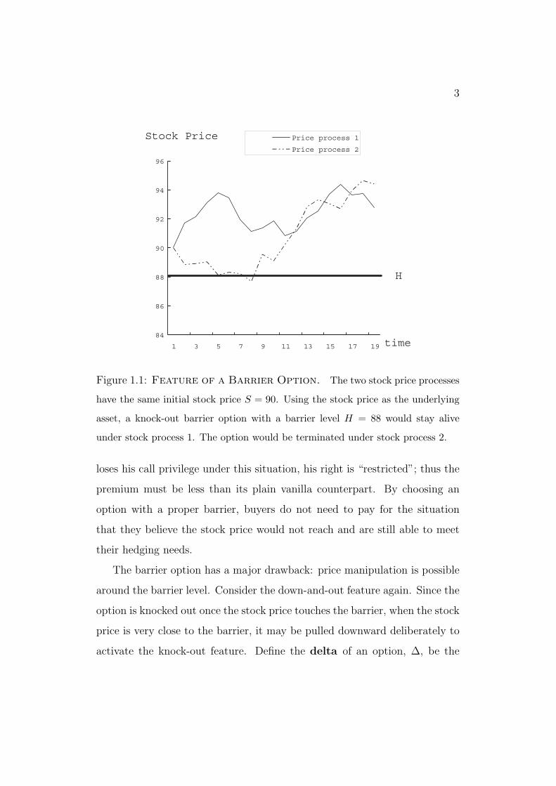
reaches a barrier. Figure 1.1 demonstrates two possible stock price process

with the same initial stock price S0 = 90. In stock process 2, the stock

price goes below 88 dollars during the process, whereas stock process 1 stays

above 88 dollars at the time. A knock-out barrier option with a barrier level

H = 88 would stay alive if its underlying stock price follows process 1 and

would be knocked out if the stock price follows process 2.

Barrier option is less expensive than a plain vanilla option with the same

parameters, and is therefore attractive to buyers. Take a down-and-out call

option as an example. It is one type of barrier option, and would cease to

exist if the underlying asset price reaches a certain barrier level, H. H is

below the initial stock price. Since the option might cease to exist, the buyer

3

H

84

86

88

90

92

94

96

1 3 5 7 9 11 13 15 17 19 time

Stock Price Price process 1

Price process 2

Figure 1.1: Feature of a Barrier Option. The two stock price processes

have the same initial stock price S = 90. Using the stock price as the underlying

asset, a knock-out barrier option with a barrier level H = 88 would stay alive

under stock process 1. The option would be terminated under stock process 2.

loses his call privilege under this situation, his right is “restricted”; thus the

premium must be less than its plain vanilla counterpart. By choosing an

option with a proper barrier, buyers do not need to pay for the situation

that they believe the stock price would not reach and are still able to meet

their hedging needs.

The barrier option has a major drawback: price manipulation is possible

around the barrier level. Consider the down-and-out feature again. Since the

option is knocked out once the stock price touches the barrier, when the stock

price is very close to the barrier, it may be pulled downward deliberately to

activate the knock-out feature. Define the delta of an option, ∆, be the

4

rate of change of the option price with respect to the price of the underlying

asset, and the gamma of an option, Γ be the rate of change of the option’s

delta with respect to the price of the underlying asset. We have:

∆ =∂P

∂S,

and

Γ =∂2P

∂S2.

P and S stand for the option price and underlying stock price. Notice that

the delta of the option would be discontinuous around the barrier, and the

gamma would approach infinity. Hedging therefore would be difficult.

Derivatives with various modifications have been introduced to address

the flaw of barrier options. Parisian type options are one of such kinds

that are widely practiced in the OTC market. This is an option whose

value depends on whether the underlying asset reaches or goes beyond a

certain price level (the excursion level) within a certain time interval for

a pre-determined period of time. Like the barrier option, it can have the

form of a down-and-out, up-and-out, down-and-in, up-and-in call or put. It

contains a great variety of features, and can be adapted to different needs.

For example, a down-and-out Parisian option will have a premium lower

than a plain vanilla option but higher than a barrier option with the same

parameters. Because the stock price would have to stay on or below the

excursion level for a period of time rather than just touch it, the chance of

being knocked out is lower than the barrier one; therefore, a higher premium

is charged. Also, since more than mere touching is required to activate the

knock-out feature, price manipulation is harder.

This thesis will focus on the pricing of two Parisian type options: cumu-

lative Parisian option and consecutive Parisian option. The former’s value

5

depends on the cumulative time the underlying asset’s price spends beyond

the excursion level, and the latter’s depends on the consecutive time its un-

derlying asset’s price spends. These type of options are “path-dependent”

since their values rely critically on the price path of the underlying asset.

The pricing for options with path-dependent feature could be difficult since

their value depend not only on the terminal value of the underlying assets,

but also on the assets’ prices path during the duration period of the options.

We will use the tree model to price the options. This method can capture

the path-dependent feature of such options, and when analytical solutions

are difficult to obtain, the tree model is still able to find approximation for

the prices. To handle the Parisian feature, we use trinomial trees instead of

the commonly practiced binomial trees and introduce a stretch parameter

discussed by Ritchken (1995) in the process. As to the period that is re-

quired to stimulate knock-out or knock-in, or the excursion period, since

the tree model is a discrete approximation of the asset price process, when

the time to expiration is divided into some small interval ∆t, the excursion

period may not contain an integer number of interval ∆t, and will result in

unsmooth convergence of the option value. In this thesis, we introduce a new

technique to adjust the lattice of the tree to solve the problem. Our model is

a generalization of Kwok and Lau (2001) and can be used to price Parisian

type contracts with different excursion periods.

1.2 Survey of Literature

Several researches address the pricing of Parisian options. Analytical, quasi-

analytical, or numerical approaches have been used. Chesney, Jeanblanc-

Picque, and Yor (1997) use the theory of Brownian excursions and define the

Parisian option value in terms of an integral expressed as an inverse Laplace

transform. Fusai, and Tagliani (2001) use different numerical methods, in-

cluding the multidimensional inverse Laplace transform, finite difference par-

tial differential equation (PDE) solution, and Monte Carlo simulation, to

price occupation time derivatives. They examine the effect of continuous

and discrete monitoring of the underlying asset. Hugonnier (1999) obtains

closed-form formulae for the cumulative Parisian option that is monitored

continuously. Haber, Schonbucher, and Wilmott (1999) develop PDE for

continuously monitored consecutive and cumulative options and provide fi-

nite difference approach to evaluate them.

Tree-based algorithms are popular in pricing options with path-dependence

characteristics. Babbs (2000) presents a straightforward binomial approxi-

mation scheme to evaluate lookback options. It also allows for the pricing of

American versions. Hsueh and Liu (2002) propose the step-reset option and

offer a trinomial tree model to account for the discrete nature of reset moni-

toring. Tian (1999) develops a flexible binomial model with a tilt parameter.

The model calibrates nodes on a binomial tree to fit the features of different

contracts and improve the rate of convergence.

1.3 Thesis Structure

The remainder of this thesis will be organized as follows. Chapter 2 reviews

the pricing technologies and option features. Chapter 3 covers the pricing of

cumulative Parisian options and consecutive Parisian options. The numerical

results are presented in chapter 4. Chapter 5 concludes.

Chapter 2

Fundamental Concepts

In this chapter, we review the background concepts and numerical pricing

techniques.

2.1 Option Pricing Preliminaries

Options or other derivatives are financial products whose value depend on the

price of the underlying asset. Therefore, a good description of the underlying

asset’s price process during the life of a option is critical to its valuation. We

describe a widely used model for stock price process. It can be applied to

the process of other assets with similar behavior. Also, when evaluating the

present value of an option that expires at a future date, one needs to find

the appropriate discount factor. We introduce the concept of risk-neutral

valuation. Under a risk-neutral world, one can find the present value of a

financial product by simply using the risk-free interest rate to discount it.

7

8

2.1.1 The Process for Stock Prices

We first state the Markov property and Ito’s Lemma below without proof.

A definition of standard Brownian motion is also given here. They are very

useful in the modelling of stock price process.

Lemma 1 (The Markov Property) For any time t, let f : ZT−t+1 → Rbe arbitrary. Then there exists a fixed function g:Z → R such that for any i

in Z,

Ei[f(Xt, ..., XT )|Ft] = Ei[f(Xt, ..., XT )|Xt] = g(Xt),

where Ei denotes expectation under Pi.

A stochastic process that has the Markov property is called a Markov

process.

Definition 1 (Standard Brownian Motion) In a probability space (Ω,F , P ),

a process is a measurable function on Ω×[0,∞) into R. A standard Brownian

motion B is a process defined by the following properties:

(a) B(0) = 0 almost surely;

(b) for any times t and s > t, B(s) − B(t) is normally distributed with

mean zero and variance s− t;

(c) for any times t0, . . . , tn such that 0 ≤ t0 < t1 < · · · < tn < ∞, the

random variables B(t0), B(t1)−B(t0), . . . , B(tn)−B(tn−1) are independently

distributed; and

(d) for each w in Ω, the sample path t → B(w, t) is continuous.

Lemma 2 (Ito’s Lemma) Suppose x is an Ito process with dx(t) = µ(x(t), t)dt+

σ(x(t), t)dB(t), and let f : R2 → R be twice continuously differentiable.

9

Then the process Y defined by Y (t) = f(x(t), t) is an Ito process with

dY (t) =

(∂Y (t)

∂x(t)µ(x(t), t)+

∂Y (t)

∂t+1

2

∂2Y (t)

∂x2(t)σ2(x(t), t)

)dt+

∂Y (t)

∂xσ(x(t), t)dB(t).

Stock price is usually assumed to follow a Markov process. It implies that

the market is efficient in the weak form. That is to say, all past information

is reflected in the current stock price, and no arbitrage opportunities would

exist.

An appropriate model for the stock price process must capture the fol-

lowing properties. First, the expected rate of return required by an investor

must be independent of the current stock price. Therefore for some constant

parameter µ, a stock that worth S at time t must have an increment of value

by µS∆t after a small interval of time ∆t, where µ is the expected rate of

return to the stock. The model can be illustrated as follows:

∆S = µS∆t.

As ∆t approaches zero, the model can be written as

dS = µSdt.

Therefore

St = S0 exp (µt),

where St and S0 are the stock price at time t and time zero.

Second, the variability of the expected rate of return over a small time

interval ∆t must be the same regardless of the current stock price. Thus the

volatility (or the standard deviation) of the stock price change over a short

period of time ∆t must be proportional to the price itself. Define σ as the

stock price volatility. We have the model

dS = µSdt+ σSdB. (2.1)

10

This model captures the two characteristics of the stock price return rate,

and is most widely used for the modelling of price process. The process is

called a geometric Brownian motion.

In stead of a normal distribution, stock price is usually modelled to follow

a log-normal distribution. It is because a variable that has a log-normal

distribution takes value between zero and infinity. A variable that follows

normal distribution can have value from negative infinity to positive infinity,

which is not consistent with the real world stock price behavior. The log-

normal distribution is more appropriate.

Assume the stock price process follows the geometric Brownian motion

in equation (2.1). Let Y = lnS. We can derive the process of lnS by Ito’s

lemma, thus

lnS =

(µ− σ2

2

)dt+ σdB.

Since the drift rate µ− σ2/2 and variance rate σ2 are both constant, it also

follows a geometric Brownian motion. The change in lnS between time zero

and t is normally distributed, where

lnSt − lnS0 ∼ Φ

[(µ− σ2

2

)t, σ

√t

].

Thus we know that St follows a log-normal distribution. The stock price

process becomes

St = S0 exp

[(µ− σ2

2

)t+ σB

]. (2.2)

2.1.2 Risk-Neutral Valuation

We state the definition of an equivalent martingale measure and a resulting

theorem without proof.

11

Definition 2 (Equivalent Martingale Measure) Define a new proba-

bility measure Q to be equivalent to P if Q and P assign zero probabilities to

the same events. A probability measure Q is equivalent to P is an equivalent

martingale measure for (δ, S) if and only if ST = 0 and the discounted gain

process Gr is a martingale with respect to Q.

Here, δ is the dividend process δ = (δ1, . . . , δN) for N securities, and S =

(S1, . . . , SN) is their adapted price process. G is the gain process for (δ, S),

Gr is the deflated gain process under a deflator r.

Theorem 1 (The Equivalent Martingale Measure Result) There is

no arbitrage if and only if there exists an equivalent martingale measure.

Moreover, π is a state-price deflator if and only if an equivalent martingale

measure Q has the density process ξ defined by ξt = Et(ξT ) = R0,tπt/π0,

where π is a state-price deflator, R0,t the payback at time t of one unit of

account borrowed risklessly at time 0 and rolled over in short-term borrowing

repeatedly until date t.

Define a dollar money market account D that worth $1 at time zero and

earns a instantaneous risk-free rate r at any given time in the future. Its

process can be written as follows:

dD = rDdt

The equivalent martingale measure result shows that, when there is no arbi-

trage opportunity, for a given numeraire security D, θ = f/D is a martingale

for all securities f if the market price of risk is set equal to the volatility of

D. Since the market price of risk for a dollar money market account D is

zero, the world that used D as numeraire has zero market price of risk, and

12

is referred to as the traditional risk-neutral world.

Under the traditional risk-neutral world, f/D is a martingale and there-

fore has the following property:

f0

D0

= EQ

(fT

DT

)

or

f0 = D0EQ

(fT

DT

)(2.3)

The short-term interest rate r can be stochastic, but here we will assume it

to be a constant r. Thus we have

DT = erT .

Use the above result, and the fact that D0 = 1, equation (2.3) is reduced to

f0 = EQ(e−rTfT )

= e−rTEQ(fT ). (2.4)

From equation (2.4), we can conclude that under a traditional risk-neutral

world, the discount factor used to price a security that mature at some future

time t is the market risk-free rate r.

2.2 Tree Model

Tree models are widely practiced numerical approaches to price options. The

main idea of a tree model is to simulate the stock price process in a discrete-

time and discrete-state version, and calculate the value of options underlain

by the stock. In this thesis the trinomial version of tree models will be used

as the valuation tool.

13

We assume the underlying stock price follows a geometric Brownian mo-

tion S = eX so that dS = µSdt + σdB. From equation (2.2) we know

X = lnS is normally distributed with parameters (µ − σ2/2, σ); thus S fol-

lows a log-normal distribution. Under the traditional risk-neutral world, the

expected drift rate µ is equal to the risk-free interest rate r. The trinomial

approximation of the process can be described as follows. Let the current

time be time zero, and τ be the time to maturity of an option. Divide τ into

n period such that ∆t = τ/n. Let St be the stock price at time t, 0 ≤ t ≤ τ ,

then for a small time interval ∆t, we have

lnSt+∆t

St

∼ Φ

[(µ− σ2

2

)∆t, σ∆t

].

At any time t, 0 ≤ t ≤ τ , the stock price is assumed to have three possible

drift directions. It can either move up by u, stay unchanged, or move down

by d after ∆t time period. The point on a tree that demonstrates a possible

stock price at some time t is called a node of the tree. Therefore we have node

(i, j) represent the jth possible stock price at time i∆t, where j = 0, 1, . . . , 2i

for any time i∆t. See Figure 2.1 for a two-period trinomial tree.

Let ud = 1 and pu, pm, pd be the probabilities of an up, middle, down

movements of stock price from time t to time t + ∆t. The three possible

stock price after time ∆t would be

St+∆t =

Stu with probability pu

St with probability pm

Std with probability pd.

From equation (2.2) and properties of the log-normal distribution, we

have

E(St+∆t) = Ster∆t,

14

t∆

Figure 2.1: A Two-Period Trinomial Tree.

and

Var(St+∆t) = S2t e

2r∆t(eσ2∆t − 1).

Now we let the trinomial model match the mean and variance of the stock

price at time t+∆t. Also, sum of the probabilities must be equal to 1. Thus

we have

1 = pu + pm + pd,

E(S) = S(puu+ pm + pdd

),

Var(S) = pu

(Stu− E(S)

)2+ pm

(St − E(S)

)2+ pd

(Std− E(S)

)2.

The probabilities can be derived as follows:

pu =u(V +M2 −M)− (M − 1)

(u− 1)(u2 − 1) ,

pd =u2(V +M2 −M)− u3(M − 1)

(u− 1)(u2 − 1) ,

15

pm = 1− pu − pd,

where M ≡ er∆t and V ≡ M2(eσ2∆t − 1).We need to make sure that the probabilities lie between zero and one.

Use

u = eλσ√

∆t,

where λ ≥ 1 is a parameter to adjust the tree lattice.

As the time interval ∆t becomes smaller, that is, as n becomes larger,

a trinomial tree will become a better approximation to the real stock price

process. When a trinomial tree model is used to price options, satisfactory

numerical results will be obtained as n becomes sufficiently large.

2.3 Tree Model for Option with

Barrier Feature

A tree model can be used to illustrate stock price process and evaluate option

price. When the model is used to price options with the barrier features, like

the Parisian options, some problems will arise. Since we cannot assure the

barrier to lie exactly on a layer of nodes on a tree, convergence will be very

slow when a tree algorithm is used to price option of this type. The results

will be significantly erractic even after a large number of time steps n.

Ritchken (1995) suggests a good way to solve the problem. By adjusting

the value of λ, we allow the barrier to be set exactly on a layer of nodes in

a trinomial tree.

Consider a downward barrier of a knock-out (knock-in) option for in-

stance. The idea is to take

h =ln(S/H)

λσ√∆t

16

H

S0

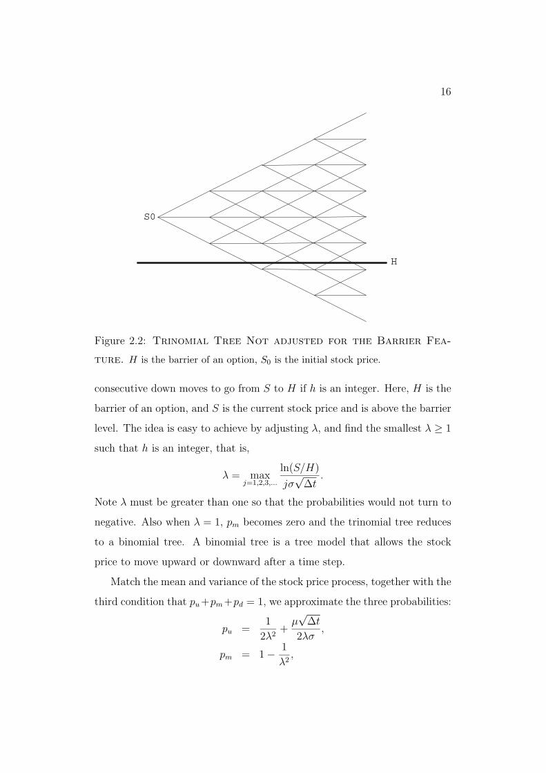
Figure 2.2: Trinomial Tree Not adjusted for the Barrier Fea-

ture. H is the barrier of an option, S0 is the initial stock price.

consecutive down moves to go from S to H if h is an integer. Here, H is the

barrier of an option, and S is the current stock price and is above the barrier

level. The idea is easy to achieve by adjusting λ, and find the smallest λ ≥ 1

such that h is an integer, that is,

λ = maxj=1,2,3,...

ln(S/H)

jσ√∆t

.

Note λ must be greater than one so that the probabilities would not turn to

negative. Also when λ = 1, pm becomes zero and the trinomial tree reduces

to a binomial tree. A binomial tree is a tree model that allows the stock

price to move upward or downward after a time step.

Match the mean and variance of the stock price process, together with the

third condition that pu+pm+pd = 1, we approximate the three probabilities:

pu =1

2λ2+

µ√∆t

2λσ,

pm = 1− 1

λ2,

17

pd =1

2λ2− µ

√∆t

2λσ,

where µ ≡ r − q − σ2/2, q is the continuous dividend rate of S.

The adjusted tree is demonstrated in figure 2.3.

H

S0

Figure 2.3: The Adjusted Trinomial Tree. H is the barrier of an option,

S0 is the initial stock price.

2.4 Auxiliary State Vector

In order to price an exotic path-dependent derivative, we need to capture

the specific path-dependent feature of the option. An auxiliary state vector

is used to record the characteristics of an option at each lattice node in a

tree model. This method is especially appreciable when a derivative’s partial

differential equation is difficult to derive. Numerical methods such as the

finite-difference algorithms, which require one to deal with the PDE function,

18

are not applicable in such cases. In this section we draw on Kwok, and Lau

(2001).

Consider a path-dependent option. Let F be the path-dependent variable

associated with the contract, V denote the auxiliary state vector function

between F and the underlying stock price S over a small time interval ∆t.

Therefore we have:

Ft+∆t = V (Ft, St+∆t), t = 0, 1, 2, . . . , τ.

Define (i, j) as the lattice node on a trinomial tree that corresponds to

the ith time step starting from time zero and the jth stock price at time i∆t,

j = 0, 1, 2, . . . , 2i. The time step length is equal to ∆t, and the stock price

difference is ∆X, where X = lnS. Let P (i, j, k) denote option value at the

(i, j)th node at which k is an integer that records the value of F at the node.

The probabilities of an upward, middle or downward stock price movement

are as described in the previous section.

The auxiliary state vector determines values of k in a forward way. At

time t, the value of k at time t− 1 together with the current stock price areused to decide the k value at time t. Option price P (i, j, k) is then calculated

using backward induction. The algorithm can be represented abstractly as

follows:

P (i− 1, j, k) =

pu × P(i, j, V (k, j)

)

+ pm × P(i, j + 1, V (k, j + 1)

)(2.5)

+ pd × P(i, j + 2, V (k, j + 2)

)× e−r∆t,

where e−r∆t is the discount factor under the risk-neutral world.

From algorithm (2.5) we note that once the auxiliary state vector function

V (k, j) is determined, the option value can be derived through the algorithm.

We state some examples on how to determine the V (k, j) function.

19

Cumulative Parisian Options

First we define the cumulative Parisian option. A cumulative Parisian option

has the feature of a regular plain vanilla option but adds an extra clause to

the determination of its price. It consider a predetermined period of time

B— the excursion period. Price of the underlying stock has to stay beyond

a certain excursion level H for B period of time cumulatively to initiate

or terminate the option. Take a down-and-out cumulative Parisian call for

instance. The auxiliary state vector V (k, j) is the function to decide the

cumulative time the stock price has spent below the excursion level H. At

the expiration date, if the cumulated excursion time is less than the required

period B, the option value is equal to max(Sτ − X, 0). If the cumulated

excursion period is greater or equal to B, the option ceases to exist.

In a trinomial tree model, the time to maturity of an option is divide into

n discrete periods of time ∆t; therefore, the excursion period B is divided

into

N =

[B

∆t

]

time periods. V (k, j) will now become a function to calculate the number

of ∆t intervals the stock price stays beyond the excursion level at time i∆t.

Define Pcum(i, j, k) as the value of a cumulative Parisian option at the (i, j)th

node. Integer k is an integer that records the time period stock price has

spent below H before or at time i∆t.

At each monitoring instant, the stock price is observed to see if it is below

the excursion level. When S moves on or below H, the value of k will be

increased by 1. Define 1S≤H to be an indicator function:

1S≤H =

1 if S ≤ H

0 if S > H.

20

The auxiliary state vector function Vcum(k, j) for a cumulative Parisian option

therefore will be

Vcum(k, j) = k + 1S≤H.

The trinomial tree algorithm for a cumulative Parisian option at the moni-

toring instance is as follows:

Pcum(i− 1, j, k) =

pu × Pcum

(i, j, Vcum(k, j)

)

+ pm × Pcum

(i, j + 1, Vcum(k, j + 1)

)(2.6)

+ pd × Pcum

(i, j + 2, Vcum(k, j + 2)

)× e−r∆t.

Consecutive Parisian Options

A consecutive Parisian option is defined slightly differently from its cumula-

tive counterpart. It considers the consecutive time the price of the underlying

stock spends beyond a certain excursion level H. The auxiliary state vector

function for a consecutive Parisian option is used to determine the length of

its consecutive excursion period. Again we consider a down-and-out consec-

utive Parisian call option. The required excursion period B is divided into

N time intervals in a trinomial tree model, as described before. Function

Vcon(k, j) is used to calculate the consecutive time periods the stock price

spends below H at or before time i∆t. Integer k is an integer to record the

time periods stock price has spent below H at the time.

At each monitoring instant, the stock price is observed. The value of k

will be increased by 1 if stock price stays below H, and reset to 0 if the price

moves above the excursion level. The auxiliary state vector for a consecutive

Parisian option can be demonstrated to be

Vcon(k, j) = (k + 1)1S≤H,

21

where 1S≤H is an indicator function. The trinomial tree algorithm for

such an option is similar to algorithm (2.6), but the state vector function is

replaced by Vcon(k, j).

Chapter 3

Pricing Parisian Options

3.1 Pricing Cumulative Parisian Options

In this section we investigate the valuation of cumulative Parisian options.

First we define the contract, then a trinomial tree as described in the previous

chapter will be used to do the valuation.

A cumulative Parisian option is designed to have a knock-out or knock-in

provision. For a knock-out feature, if the underlying stock price goes beyond

a certain price level cumulatively for a pre-determined period of time B, the

option ceases to exist and has a zero value. Otherwise, it stays alive, and

the terminal value will be max(Sτ −X, 0) for a call or max(X − Sτ , 0) for a

put. B is called the excursion period. When the length of B approaches

zero, the contract reduce to an ordinary barrier option. When the length

of B approaches the duration period τ of the derivative, the contract turns

into a plain vanilla option. For a knock-in feature, the option comes into

existence when the underlying stock price stays beyond a certain price level

cumulatively for a pre-determined period of time.

The difficulties of Parisian option valuation lies in the path-dependent

22

23

feature of the instrument, and the problem of its excursion period. The

former can be solved by using an auxiliary state vector. The latter is more

complicated. We propose a binomial branching technique to modify the

original trinomial tree. The method can reduce the unsmooth convergence

behavior of option prices and allows for the pricing of contracts with general

excursion periods.

Consider a down-and-out cumulative Parisian call for example. A trino-

mial tree is used to price the option. On a trinomial tree, the calculation is

operated in a backward fashion. First we set k = N − 1 for all the stock

price nodes at time τ − ∆t. Then the option price Pcum(τ − ∆t, j, N − 1)

for all j can be derived from option prices at time τ . Consider nodes (τ, j),

(τ, j + 1), and (τ, j + 2). We investigate the stock price at each of these

nodes. If the stock price is below or at the excursion level H, integer k would

be incremented by 1; otherwise, it stays unchanged. Since Pcum(i, j, N) = 0

for all node (i, j) and Pcum(i, j, N − 1) = max(S − X, 0) at time τ , we set

k = N − 1 in equation (2.6) and obtain Pcum(τ −∆t) in a backward fashion.

Then we move on to time τ − 2∆t, and proceed with the same operations.

The process is repeated until we find Pcum(0, 0, N−1). This way we generatethe whole option price trinomial tree with k = N − 1. This option price treeis then used to derive the option price tree with k = N − 2. The process

continues until the integer k hits 0, and the value of Pcum(0, 0, 0) is obtained.

Discounting the price with the market risk-free rate will yield the current

value of the cumulative Parisian option.

Now we consider problems with the excursion period. A trinomial tree

model approximates the option value in a discrete way. When the time to

maturity τ of an option is divided into n sub-intervals, the excursion period

24

Figure 3.1: Cumulative Parisian Option Pricing Algorithm.

would be divided into

N = B

∆t

sub-intervals, where ∆t = τ/n. The the last sub-interval of the excursion

period may not have a full interval length. When the original trinomial tree

is used to calculate the option value, the problem of unsmooth convergence

will occur. We impose binomial branches on the trinomial tree at the final

fractional interval to adjust for the nodes.

Figure (3.2) demonstrates the tree lattice at time t = i∆t, when we have

N − 1 cumulative excursion periods. Consider node O and assume it lies on

the excursion level H. Let the length of the fractional interval be ε,

ε = N −(

B

∆t

).

25

ε

tit ∆= tit ∆+= )1(

Figure 3.2: Trinomial Tree When k = N − 1.

Node A, node B, and node C represent three possible directions of the stock

price movement after ε period of time. For a down-and-out feature, if the

stock price moves up to node A, the option continues to exist, and the state

integer k remains equal to N − 1. If the stock price moves to node B or C,

k = N and the contract would be terminated. The probability for the stock

price to move from node O to node A, B, or C are

pA =1

2λ2+

µ√ε

2λσ,

pB = 1− 1

λ2,

pC =1

2λ2− µ

√ε

2λσ,

respectively.

26

Consider node A. Using the binomial branching technique, the stock

price may move to node D or E at the next time period. After matching

the mean and variance of stock price at time (i+1)∆t, the probability p1 for

stock price to move from node A to node D will be:

p1 =er(∆t−ε) − d1

u1 − d1

,

u1 = eλσ(√

∆t−√ε),

d1 = e−λσ(√

∆t+√

ε).

The probability to move from node A to node E is 1 − p1. With similar

calculation we can find the probability for stock price to move from node B

to node D be p2, where

p2 =er(∆t−ε) − d2

u2 − d2

,

u2 = eλσ√

∆t−ε,

d2 = e−λσ√

∆t−ε.

The probability to move from node B to node E is 1 − p2. The probability

to move from node C to node D is p3, where

p3 =er(∆t−ε) − d3

u3 − d3

,

u3 = eλσ(√

∆t+√

ε),

d3 = e−λσ(√

∆t−√ε).

The probability to move from node C to node E is 1− p3.

Since the stock price has stayed below H for N − 1 times cumulatively ator before node O, at time i+ ε, the option will stay alive at node A, but be

terminated at node B or C. Backward induction is used to derive the option

value at node A from node D and E. The algorithm is described below:

Pcum(i+ ε, j, N − 1) =

p1 × Pcum

(i+ 1, j, Vcum(N − 1, j)

)

27

+ (1− p1)× Pcum

(i+ 1, j + 2, Vcum(N − 1, j + 2)

)

× e−r(∆t−ε). (3.1)

If the stock price moves from node O to node B or C, the option price

would be zero. Finally, the option value at node O is derived from nodes

A, B, and C, using equation (2.6). This algorithm reduces the sawtooth

pattern incurred by the fractional interval, and option values will converge

more smoothly with the technique.

The algorithm will use up to O(n2) memory space and O(n2) computa-

tional steps.

3.2 Pricing Consecutive Parisian Options

A consecutive Parisian option has a knock-out or knock-in feature slightly

different from its cumulative counterpart. It calculates the time underlying

stock price stays beyond the excursion level consecutively. For the otherwise

identical parameters, a consecutive Parisian option requires a higher premium

than a cumulative Parisian option because it is more difficult to activate the

knock-out or knock-in feature of a consecutive Parisian option.

A consecutive Parisian option is path-dependent. We use the trinomial

tree model with the auxiliary state vector to do the pricing.

To determine the option value on a trinomial tree, consider a down-and-

out consecutive Parisian call. Let Pcon(i, j, k) be the option value at the

(i, j)th node. Integer k stands for the consecutive number of periods the

stock price has spent below the excursion level H. Since the integer variable

k will be reset to zero whenever stock price moves above the excursion level,

we need to know Pcon(i, j, 0) at all nodes (i, j) before backward induction

is proceeded. Set k = N − 1 for all price nodes at time τ − ∆t. At time

τ , if the stock price is above the excursion level, k is reset to zero. If the

stock price is at or below the excursion level, k is incremented by 1, and

we have k = N . Option prices at nodes (τ, j), (τ, j + 1), and (τ, j + 2)

are then used to calculate Pcon(i, j, N − 1). Since Pcon(i, j, N) = 0 and

Pcon(i, j, 0) = max(S − X, 0) at time τ , the option values at node (τ, j),

(τ, j+1), and (τ, j+2) can be determined. Backward induction is then used to

determine Pcon(i, j, N−1). The same operations are repeated at time τ−∆t,

with k = N − 2, k = N − 3, . . . , k = 0, until values of Pcon(τ −∆t, j, 0) are

found for all j. A cross sectional price lattice at time τ −∆t will all k values

is generated. We then move one time period ahead, and repeat the same

operations to find the price lattice at time τ − 2∆t. The process continues

until we move to time 0, and find Pcon(0, 0, 0). Pcon(0, 0, 0) is then discounted

with the market risk-free rate to yield the current value of the consecutive

Parisian option.

The excursion interval B may contain a fractional interval of length less

than ∆t, when the time to maturity of an option is divided into τ/n small

intervals. The binomial branching technique described in the previous section

is used to eliminate the problem.

29

tt ∆−= τ

0=t

tt ∆−= τ

tt ∆−= 2τ

↓

Figure 3.3: Consecutive Parisian Option Pricing Algorithm.

Chapter 4

Numerical Evaluation

A cumulative Parisian or a consecutive Parisian option whose excursion pe-

riod contains a fractional interval will result in unsmooth convergence of the

option value. This section investigates the numerical results of our model.

First we compare the convergence behavior of option values obtained from

the regular trinomial and those from the adjusted tree. Then we examine

the characteristics of cumulative Parisian options and consecutive Parisian

options.

In Figure 4.1 we demonstrate the convergence behavior of a down-and-out

cumulative Parisian call before and after we adjust for the fractional interval

of the excursion period. When the excursion period contains non-integer

periods of time ∆t, we round up to the greatest smaller integer periods of

time ∆t, and use it to derive the lower bounds for option values. The smallest

greater integer periods of time ∆t is used to derive the upper bounds for

option values. The contract used here has one year maturity τ and one month

excursion period B. The option parameters are as follows: S = 95, X =

100, H = 90, r = 10%, σ = 25%, τ = 1 (year), and B = 1 (month). It is

shown that the values obtained from the adjusted trinomial tree is bounded

30

31

by the lower and upper bounds. The adjusted trinomial tree algorithm can be

used to price the options more accurately, and can be applied more generally

to price cumulation Parisian option with different excursion periods.

!"

"

Figure 4.1: The Convergence Behavior of a Adjusted Trinomial

Tree—A Cumulative Parisian Option. This figure demonstrates the

convergence behavior of a cumulative Parisian option.

The application of our algorithm to price consecutive Parisian options

can yield satisfactory results as well. Figure 4.2 is the convergence behavior

for a consecutive Parisian option. The same option parameters are used here.

It is demonstrated that after we adjust the trinomial tree for the fractional

excursion period, more accurate option prices can be obtained. Therefore we

can apply the algorithm to price consecutive Parisian option with different

excursion periods.

32

Figure 4.2: The Convergence Behavior of a Adjusted Trinomial

Tree—A Consecutive Parisian Option. This figure demonstrates the

convergence behavior of a consecutive Parisian Option.

33

Figures 4.3, 4.4, 4.5, and 4.6 depict the convergence behavior of the cu-

mulative Parisian option and consecutive Parisian option. As n becomes

sufficiently large, option prices approach the correct value in a smooth way.

Figure 4.3: Numerical Results for a Cumulative Parisian Option.

The option parameters are specified as follow: S = 60, X = 60, H = 50, τ =

1(year), B = 1(month), r = 5%, q = 2%, andσ = 30%. Time to maturity τ is

divided into n sub-intervals, and n is from 100 to 1000. The price obtained from

simulation is 7.5217.

Next we investigate the behaviors of cumulative Parisian calls and con-

secutive Parisian calls with various market risk. Table 4.1 lists option values

with different market risk σ. Prices obtained from simulation are also dis-

played in the table. As the market risk becomes larger, investors are more

uncertain about the future stock price, and option values are higher. Table

4.1 confirms the claim.

Since it is more difficult for a consecutive Parisian option to activate

knock-out or knock-in than its cumulative counterpart, a consecutive Parisian

34

Figure 4.4: Numerical Results for a Cumulative Parisian Option.





Table 4.1: Option Values under Different Market Risk. Option

parameters: S = 80, X = 80, H = 70, τ = 1 (year), B = 1 (month), r = 10%, and

q = 0.

σ = 20% σ = 30% σ = 40% σ = 50% σ = 60%

cumulative Parisian 10.3320 12.4388 13.8137 15.2568 16.6355

simulated value 10.3598 12.4080 14.0989 15.3041 17.1665

consecutive Parisian 10.4394 12.7591 14.6218 16.4702 18.2623

simulated value 10.5773 13.3986 16.2172 19.0773 21.825

35

Figure 4.5: Numerical Results for a Consecutive Parisian Option.





36

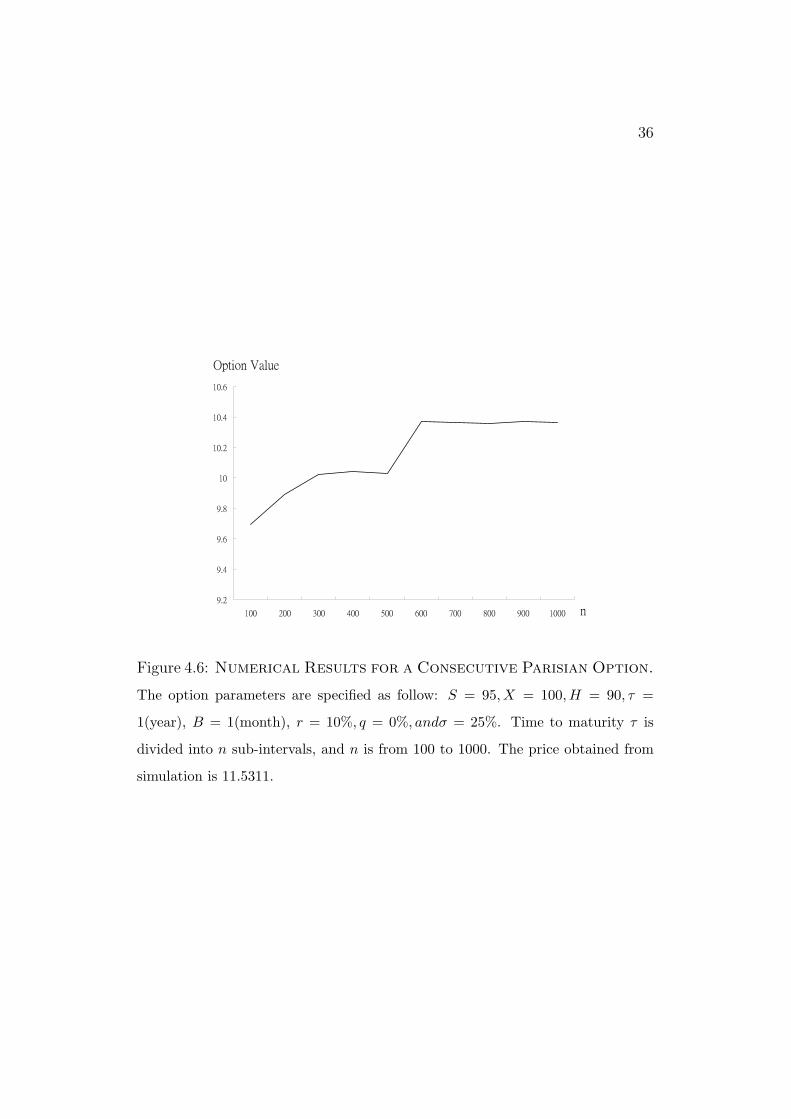
Figure 4.6: Numerical Results for a Consecutive Parisian Option.





37

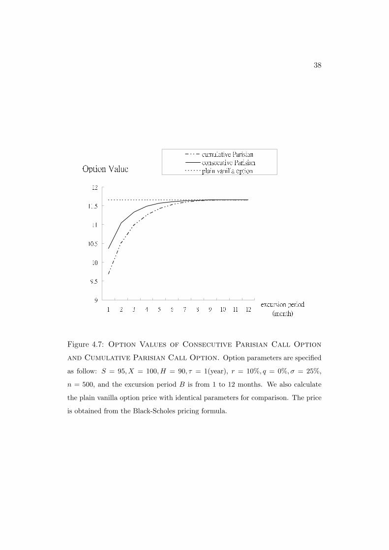
always has a higher premium than a cumulative Parisian option. Consecutive

and cumulative Parisian option values are increasing functions of the excur-

sion period B. When the length of the option excursion period approaches

its time to maturity τ , the value of a cumulative Parisian option and that of

a consecutive Parisian option will both approximate the value of the plain

vanilla option with identical parameters. Table 4.1 demonstrates that consec-

utive Parisian options always have a higher value than cumulative Parisian

options, as we have expected. Figure 4.7 shows the numerical results for a

consecutive Parisian call and a cumulative Parisian call with different excur-

sion periods. The value of a plain vanilla option with the same parameters

is obtained from the Black-Scholes formula.

38

Figure 4.7: Option Values of Consecutive Parisian Call Option

and Cumulative Parisian Call Option. Option parameters are specified

as follow: S = 95, X = 100, H = 90, τ = 1(year), r = 10%, q = 0%, σ = 25%,

n = 500, and the excursion period B is from 1 to 12 months. We also calculate

the plain vanilla option price with identical parameters for comparison. The price

is obtained from the Black-Scholes pricing formula.

Chapter 5

Conclusions

This thesis investigates the path-dependent Parisian type options. Efficient

and accurate pricing techniques are introduced. A cumulative Parisian op-

tion would be knocked-out or knocked-in if the price of its underlying asset

stays beyond the excursion level for a pre-determined cumulative period of

time. The knock-out or knock-in of a consecutive Parisian option would

be activated if price the underlying asset stays beyond the excursion level

consecutively for a pre-determined period of time.

We show that trinomial trees with auxiliary state vectors can be used

to price Parisian type options efficiently. A binomial branching technique

can be used to eliminate the problem with the fractional excursion period.

The pricing algorithm would be more accurate after we implement binomial

branches to adjust the tree. Characteristics of the Parisian type options are

also examined.

39

Bibliography

[1] Babbs, S. “Binomial Valuation of Lookback Options.” Journal of Eco-

nomic Dynamics & Control 24, 1499–1525.

[2] Duffie, D. Dynamic Asset Pricing Theory. Princeton: Princeton Uni-

versity Press, 2nd ed., 1996.

[3] Fusai, G. and Tagliani, A. “Pricing of Occupation Time Derivatives:

Continuous and Discrete Monitoring” Journal of Computational Finance

5(1), Fall 2001, 1–37.

[4] Haber, R. J., Schonbucher, P. J., and Wilmott, P. “Pricing

Parisian Options.” The Journal of Derivatives, Spring 1998, 71–79.

[5] Hsueh, L. P. and Liu, Y. A. “Step-Reset Options: Design and Val-

uation.” The Journal of Futures Markets 22(2), 2002, 155-171.

[6] Hull, J.Options, Futures, and Other Derivatives. 5th edition. Prentice-

Hall, 2002.

[7] Kwok, Y. K. and Lau, K. W. “Pricing Algorithms for Options with

Exotic Path-Dependence.” The Journal of Derivatives, Fall 2001, 28–38.

[8] Lyuu, Y. D. Financial Engineering and Computation: Principles,

Mathematics, Algorithms. Cambridge University Press, 2002.

40

41

[9] Ritchken, P. “On Pricing Barrier Options.” The Journal of Deriva-

tives, Winter 1995, 19–28.

[10] Tian, Y. S. “A Flexible Binomial Option Pricing Model.” The Journal

of Futures Markets, 19(7), 1999, 817–843.

pricing parisian-type options

Documents