PRIMES IN INTERVALS OF BOUNDED LENGTH

ANDREW GRANVILLE

Abstract. In April 2013, Yitang Zhang proved the existence of a finite bound B suchthat there are infinitely many pairs of distinct primes which differ by no more than B.This is a massive breakthrough, makes the twin prime conjecture look highly plausible(which can be re-interpreted as the conjecture that one can take B 2) and his workhelps us to better understand other delicate questions about prime numbers that hadpreviously seemed intractable. The original purpose of this talk was to discuss Zhang’sextraordinary work, putting it in its context in analytic number theory, and to sketcha proof of his theorem.

Zhang had even proved the result with B 70 000 000. Moreover, a co-operativeteam, polymath8, collaborating only on-line, had been able to lower the value of B to4680. Not only had they been more careful in several difficult arguments in Zhang’soriginal paper, they had also developed Zhang’s techniques to be both more powerfuland to allow a much simpler proof. Indeed the proof of Zhang’s Theorem, that will begiven in the write-up of this talk, is based on these developments.

In November, inspired by Zhang’s extraordinary breakthrough, James Maynard dra-matically slashed this bound to 600, by a substantially easier method. Both Maynard,and Terry Tao who had independently developed the same idea, were able to extendtheir proofs to show that for any given integer m ¥ 1 there exists a bound Bm suchthat there are infinitely many intervals of length Bm containing at least m distinctprimes. We will also prove this much stronger result herein, even showing that onecan take Bm e8m5.

If Zhang’s method is combined with the Maynard-Tao set up then it appears thatthe bound can be further reduced to 576. If all of these techniques could be pushed totheir limit then we would obtain B( B2) 12, so new ideas are still needed to havea feasible plan for proving the twin prime conjecture.

The article will be split into two parts. The first half, which appears here, wewill introduce the work of Zhang, Polymath8, Maynard and Tao, and explain theirarguments that allow them to prove their spectacular results. As we will discuss,Zhang’s main novel contribution is an estimate for primes in relatively short arithmeticprogressions. The second half of this article sketches a proof of this result; the Bulletinarticle will contain full details of this extraordinary work.

Part 1. Primes in short intervals

1. Introductionsec:intro

1.1. Intriguing questions about primes. Early on in our mathematical educationwe get used to the two basic rules of arithmetic, addition and multiplication. When we

1991 Mathematics Subject Classification. 11P32.To Yitang Zhang, for showing that one can, no matter what.

1

2 ANDREW GRANVILLE

define a prime number, simply in terms of the number’s multiplicative properties, wediscover a sequence of numbers, which is easily defined, yet difficult to gain a firm graspof, perhaps since the primes are defined in terms of what they are not (i.e. that theycannot be factored into two smaller integers)).

When one writes down the sequence of prime numbers:

2, 3, 5, 7, 11, 13, 17, 19, 23, 29, 31, 37, 41, 43, 47, 53, 59, 61, . . .

one sees that they occur frequently, but it took a rather clever construction of theancient Greeks to even establish that there really are infinitely many. Looking furtherat a list of primes, some patterns begin to emerge; for example, one sees that they oftencome in pairs:

3 and 5; 5 and 7; 11 and 13; 17 and 19; 29 and 31; 41 and 43; 59 and 61, . . .

One might guess that there are infinitely many such prime pairs. But this is an open,elusive question, the twin prime conjecture. Until recently there was little theoreticalevidence for it. All that one could say was that there was an enormous amount ofcomputational evidence that these pairs never quit; and that this conjecture (and variousmore refined versions) fit into an enormous network of conjecture, which build a beautifulelegant structure of all sorts of prime patterns. If the twin prime conjecture were falsethen the whole edifice would crumble.

The twin prime conjecture is certainly intriguing to both amateur and professionalmathematicians alike, though one might argue that it is an artificial question, since itasks for a very delicate additive property of a sequence defined by its multiplicativeproperties. Indeed, number theorists had struggled, until very recently, to identify anapproach to this question that seemed likely to make any significant headway. In thisarticle we will discuss these latest shocking developments. In the first few sections wewill take a leisurely stroll through the historical and mathematical background, so asto give the reader a sense of the great theorems that have been recently proved, from aperspective that will prepare the reader for the details of the proof.

1.2. Other patterns. Looking at the list of primes above we see other patterns thatbegin to emerge, for example, one can find four primes which have all the same digits,except the last one:

11, 13, 17 and 19; which is repeated with 101, 103, 107 and 109;

and one can find many more such examples – are there infinitely many? More simplyhow about prime pairs with difference 4:

3 and 7; 7 and 11; 13 and 17; 19 and 23; 37 and 41; 43 and 47; 67 and 71, . . . ;

or difference 10:

3 and 13; 7 and 17; 13 and 23; 19 and 29; 31 and 41; 37 and 47; 43 and 53, . . .?

Are there infinitely many such pairs? Such questions were probably asked back toantiquity, but the first clear mention of twin primes in the literature appears in a paper

PRIMES IN INTERVALS OF BOUNDED LENGTH 3

of de Polignac from 1849. In his honour we now call any integer h, for which there areinfinitely many prime pairs p, p h, a de Polignac number.1

Then there are the Sophie Germain pairs, primes p and q : 2p 1, which prove usefulin several simple algebraic constructions:2

2 and 5; 3 and 7; 5 and 11; 11 and 23; 23 and 47; 29 and 59; 41 and 83; . . . ;

Now we have spotted all sorts of patterns, we need to ask ourselves whether there is away of predicting which patterns can occur and which do not. Let’s start by looking atthe possible differences between primes: It is obvious that there are not infinitely manyprime pairs of difference 1, because one of any two consecutive integers must be even,and hence can only be prime if it equals 2. Thus there is just the one pair, 2 and 3, ofprimes with difference 1. One can make a similar argument for prime pairs with odddifference. Hence if h is an integer for which there are infinitely many prime pairs of theform p, q p h then h must be even. We have seen many examples, above, for eachof h 2, h 4 and h 10, and the reader can similarly construct lists of examples forh 6 and for h 8, and indeed for any other even h that takes her or his fancy. Thisleads us to bet on the generalized twin prime conjecture, which states that for any eveninteger 2k there are infinitely many prime pairs p, q p 2k.

What about prime triples? or quadruples? We saw two examples of prime quadruples ofthe form 10n 1, 10n 3, 10n 7, 10n 9, and believe that there are infinitely many.What about other patterns? Evidently any pattern that includes an odd differencecannot succeed. Are there any other obstructions? The simplest pattern that avoids anodd difference is n, n2, n4. One finds the one example 3, 5, 7 of such a prime triple,but no others. Further examination makes it clear why not: One of the three numbersis always divisible by 3. This is very similar to what happened with n, n 1; and onecan verify that, similarly, one of n, n 6, n 12, n 18, n 24 is always divisible by 5.The general obstruction can be described as follows:

For a given set of distinct integers a1 a2 . . . ak we say that prime p is anobstruction if p divides at least one of n a1, . . . , n ak, for every integer n. In otherwords, p divides

Ppnq pn a1qpn a2q . . . pn akqfor every integer n; which can be classified by the condition that the set a1, a2, . . . , akpmod pq includes all of the residue classes mod p. If no prime is an obstruction then wesay that x a1, . . . , x ak is an admissible set of forms.3.

1Some authors make a slightly different definition: That p and p h should also be consecutiveprimes.

2The group of reduced residues mod q is a cyclic group of order q1 2p, and therefore isomorphicto C2 Cp if p ¡ 2. Hence the order of each element in the group is either 1 (that is, 1 pmod qq), 2(that is, 1 pmod qq), p (the squares mod q) or 2p q 1. Hence g pmod qq generates the group ofreduced residues if and only if g is not a square mod q and g 1 pmod qq.

3Notice that a1, a2, . . . , ak pmod pq can occupy no more than k residue classes mod p and so, if p ¡ kthen p cannot be an obstruction. Hence, to check whether a given set A of k integers is admissible,one needs only find one residue class bp pmod pq, for each prime p ¤ k, which does not contain anyelement of A.

4 ANDREW GRANVILLE

In 1904 Dickson made the optimistic conjecture that if there is no such “obvious”obstruction to a set of linear forms being infinitely often prime, then they are infinitelyoften simultaneously prime. That is:

Conjecture: If xa1, . . . , xak is an admissible set of forms then there are infinitelymany integers n such that n a1, . . . , n ak are all prime numbers.

In this case, we call n a1, . . . , n ak a k-tuple of prime numbers.

To date, this has not been proven for any k ¡ 1 though, following Zhang’s work, webegin to get close for k 2. Indeed, Zhang has proved a weak variant of this conjecturefor k 2, as we shall see. Moreover Maynard

maynard[29], and Tao

tao[39], have gone on to prove

a weak variant for any k ¥ 2.

The above conjecture can be extended, as is, to all sets of k linear forms with integercoefficients in one variable (for example, the triple n, 2n 1, 3n 2), so long as weextend the notion of admissibility to also exclude the possible obstruction that two ofthe linear forms have different signs for all but finitely many n, (since, for example, nand 2 n, can never be simultaneously prime); some people call this the “obstructionat the ‘prime’, 1”. We can also extend the conjecture to more than one variable (forexample the set of forms m,m n,m 4n):

The prime k-tuplets conjecture: If a set of k linear forms in n variables is admis-sible then there are infinitely many sets of n integers such that when we substitute theseintegers into the forms we get a k-tuple of prime numbers.

There has been substantial recent progress on this conjecture. The famous breakthroughwas Green and Tao’s theorem

GT[19] for the k-tuple of linear forms in the two variables a

and d:

a, a d, a 2d, . . . , a pk 1qd(in other words, there are infinitely many k-term arithmetic progressions of primes.)Along with Ziegler, they went on to prove the prime k-tuplets conjecture for any ad-missible set of linear forms, provided no two satisfy a linear equation over the integers,GTZ[20]. What a remarkable theorem! Unfortunately these exceptions include many of thequestions we are most interested in; for example, p, q p2 satisfy the linear equationq p 2; and p, q 2p 1 satisfy the linear equation q 2p 1).

Finally, we also believe that the conjecture holds if we consider any admissible set ofk irreducible polynomials with integer coefficients, with any number of variables. Forexample we believe that n2 1 is infinitely often prime, and that there are infinitelymany prime triples m, n, m2 2n2.

1.3. The new results; primes in bounded intervals. In this section we stateZhang’s main theorem, as well as the improvement of Maynard and Tao, and discuss afew of the more beguiling consequences:

PRIMES IN INTERVALS OF BOUNDED LENGTH 5

Zhang’s main theorem: There exists an integer k such that the following is true: Ifx a1, . . . , x ak is an admissible set of forms then there are infinitely many integersn such that at least two of n a1, . . . , n ak are prime numbers.

Note that the result states that only two of the n ai are prime, not all (as would berequired in the prime k-tuplets conjecture). Zhang proved this result for a fairly largevalue of k, that is k 3500000, which has been reduced to k 105 by Maynard. Ofcourse if one could take k 2 then we would have the twin prime conjecture,4 butthe most optimistic plan at the moment, along the lines of Zhang’s proof, would yieldk 5.

To deduce that there are bounded gaps between primes from Zhang’s Theorem we needonly show the existence of an admissible set with k elements. This is not difficult,simply by letting the ai be the first k primes ¡ k.5 Hence we have proved:

Corollary 1.1 (Bounded gaps between primes). There exists a bound B such that thereare infinitely many integers pairs of prime numbers p q pB.

Finding the smallest B for a given k is a challenging question. The prime numbertheorem together with our construction above suggests that B ¤ kplog k Cq for someconstant C, but it is interesting to get better bounds. For Maynard’s k 105, Engelsmashowed that one can take B 600,6 and that this is best possible.

Our Corollary further implies

Corollary 1.2. There is an integer h, 0 h ¤ B such that there are infinitely manypairs of primes p, p h.

That is, some positive integer ¤ B is a de Polignac number. In fact one can go a littlefurther using Zhang’s main theorem, and deduce that if A is any admissible set of kintegers then there is an integer h P pAAq : ta b : a ¡ b P Au such that there areinfinitely many pairs of primes p, p h. One can find many beautiful consequences ofthis; for example, that a positive proportion of even integers are de Polignac numbers.

Next we state the Theorem of Maynard and of Tao:

The Maynard-Tao theorem: For any given integer m ¥ 2, there exists an integer ksuch that the following is true: If x a1, . . . , x ak is an admissible set of forms then

4And the generalized twin prime conjecture, and that there are infinitely many Sophie Germainpairs, and . . .

5This is admissible since none of the ai is 0 pmod pq for any p ¤ k, and the p ¡ k were handled inthe previous footnote.

6Sutherland’s website http://math.mit.edu/primegaps/ gives Engelsma’s admissible 105-tuple:0, 10, 12, 24, 28, 30, 34, 42, 48, 52, 54, 64, 70, 72, 78, 82, 90, 94, 100, 112, 114, 118, 120, 124, 132, 138, 148, 154,168, 174, 178, 180, 184, 190, 192, 202, 204, 208, 220, 222, 232, 234, 250, 252, 258, 262, 264, 268, 280, 288, 294,300, 310, 322, 324, 328, 330, 334, 342, 352, 358, 360, 364, 372, 378, 384, 390, 394, 400, 402, 408, 412, 418, 420,430, 432, 442, 444, 450, 454, 462, 468, 472, 478, 484, 490, 492, 498, 504, 510, 528, 532, 534, 538, 544, 558, 562,570, 574, 580, 582, 588, 594, 598, 600.

6 ANDREW GRANVILLE

there are infinitely many integers n such that at least m of n a1, . . . , n ak are primenumbers.

This includes and extends Zhang’s Theorem (which is the case k 2). The proof evenallows one make this explicit (we will obtain k ¤ e8m4, and Maynard improves this tok ¤ cm2e4m for some constant c ¡ 0).

Corollary 1.3 (Bounded intervals with m primes). For any given integer m ¥ 2, thereexists a bound Bm such that there are infinitely many intervals rx, xBms (with x P Z)which contain m prime numbers.

We will prove that one can take Bm e8m5 (and Maynard improves this to Bm cm3e4m for some constant c ¡ 0).

A Dickson k-tuple is a set of integers a1 . . . ak such that there are infinitely manyintegers for which n a1, n a2, . . . , n ak are each prime

Corollary 1.4. A positive proportion of m-tuples of integers are Dickson m-tuples.

Proof. With the notation as in the Maynard-Tao theorem let R ±p¤k p, select x to

be a large integer multiple of R and let N : tn ¤ x : pn,Rq 1u so that |N | φpRqRx.

Any subset of k elements of N is admissible, since it does not contain any integer 0pmod pq for each prime p ¤ k. There are

|N |k

such k-tuples. Each contains a Dickson

m-tuple by the Maynard-Tao theorem.

Now suppose that are T pxq Dickson m-tuples with 1 ¤ a1 . . . am ¤ x. Any such

m-tuple is a subset of exactly|N |mkm

of the k-subsets of N , and hence

T pxq |N | m

k m

¥|N |k

,

and therefore T pxq ¥ p|N |kqm pφpRqRkqm xm as desired.

This proof yields that, as a proportion of the m-tuples in N ,

T pxqL|N |m

¥ 1

L km

.

The m 2 case implies that at least 15460

th of the even integers are de Polignac numbers.

Zhang’s Theorem and the Maynard-Tao theorem each hold for any admissible k-tupleof linear forms (not just those of the form x a). With this we can prove several otheramusing consequences:

The last Corollary holds if we insist that the primes in the Dickson k-tuples areconsecutive primes.

There are infinitely many m-tuples of consecutive primes such that each pair in them-tuple differ from one another by just two digits when written in base 10.

PRIMES IN INTERVALS OF BOUNDED LENGTH 7

For any m ¥ 2 and coprime integers a and q, there are infinitely many intervalsrx, x qBms (with x P Z) which contain exactly m prime numbers, each a pmod qq.7

Let dn pn1pn where pn is the nth smallest prime. Fix m ¥ 1. There are infinitelymany n for which dn dn1 . . . dnm. There are also infinitely many n for whichdn ¡ dn1 ¡ . . . ¡ dnm. This was a favourite problem of Paul Erdos, though we donot see how to deduce such a result for other orderings of the dn.

1.4. Bounding the gaps between primes. A brief history. The young Gauss,examining Chernac’s table of primes up to one million, surmised that “the density ofprimes at around x is roughly 1 log x”. This was subsequently verified, as a consequenceof the prime number theorem. Therefore we are guaranteed that there are infinitely manypairs of primes p q with q p ¤ p1 εq log p for any fixed ε ¡ 0, which is not quite assmall a gap as we are hoping for! Nonetheless this raises the question: Fix c ¡ 0. Canwe even prove that

There are infinitely many pairs of primes p q with q p c log p ?

This follows for all c ¡ 1 by the prime number theorem, but it is not easy to provesuch a result for any particular value of c ¤ 1. The first such results were proved con-ditionally assuming the Generalized Riemann Hypothesis. This is surprising since theGeneralized Riemann Hypothesis was formulated to better understand the distributionof primes in arithmetic progressions, so why would it appear in an argument aboutshort gaps between primes? It is far from obvious by the argument used, and yet thisconnection deepened and broadened as the literature developed. We will discuss primesin arithmetic progressions in detail in the next section.

The first unconditional (though inexplicit) such result, bounding gaps between primes,was proved by Erdos in 1940 using the small sieve. In 1966, Bombieri and Davenport

bomdav[2]

substituted the Bombieri-Vinogradov theorem for the Generalized Riemann Hypothesisin earlier, conditional arguments, to prove this unconditionally for any c ¥ 1

2. The

Bombieri-Vinogradov Theorem is also a result about primes in arithmetic progressions(as we will discuss later). In 1988 Maier

maier[28] observed that one can easily modify this

to obtain any c ¥ 12eγ; and he further improved this, by combining the approaches of

Erdos and of Bombieri and Davenport, to obtain some bound a little smaller than 14, in

a technical tour-de-force.

The first big breakthrough occurred in 2005 when Goldston, Pintz and Yildirimgpy[15] were

able to show that there are infinitely many pairs of primes p q with q p c log p,for any given c ¡ 0. Indeed they extended their methods to show that, for any ε ¡ 0,there are infinitely many pairs of primes p q for which

q p plog pq12ε.It is their method which forms the basis of the discussion in this paper. Like Bombieriand Davenport, they showed that one can better understand small gaps between primes

7Thanks to Tristan Freiberg for pointing this out to me.

8 ANDREW GRANVILLE

by obtaining strong estimates on primes in arithmetic progressions, as in the Bombieri-Vinogradov Theorem. Even more, if one assumes a strong, but widely believed, conjec-ture about the equi-distribution of primes in arithmetic progressions, which extends theBombieri-Vinogradov Theorem, then one can show that there are infinitely many pairsof primes p q which differ by no more than 12 (that is, p q ¤ p 12)! In fact onecan take k 5 in Zhang’s theorem, and then apply the result to the admissible 5-tuple,t0, 2, 6, 8, 12u What an extraordinary statement! We know that if p q ¤ p 12then qp 2, 4, 6, 8, 10 or 12, and so at least one of these difference occurs infinitelyoften. That is, there exists a positive, even integer 2k ¤ 12 such that there are infinitelypairs of primes p, p 2k. It would be good to refine this further.

After Goldston, Pintz and Yildirim, most of the experts tried and failed to obtain enoughof an improvement of the Bombieri-Vinogradov Theorem to deduce the existence of somefinite bound B such that there are infinitely many pairs of primes that differ by no morethan B. To improve the Bombieri-Vinogradov Theorem is no mean feat and people havelonged discussed “barriers” to obtaining such improvements. In fact a technique hadbeen developed by Fouvry

fouvry[10], and by Bombieri, Friedlander and Iwaniec

bfi[3], but this

was neither powerful enough nor general enough to work in this circumstance.

Enter Yitang Zhang, an unlikely figure to go so much further than the experts, and tofind exactly the right improvement and refinement of the Bombieri-Vinogradov Theoremto establish the existence of the elusive bound B such that there are infinitely manypairs of primes that differ by no more than B. By all accounts, Zhang was a brilliantstudent in Beijing from 1978 to the mid-80s, finishing with a master’s degree, and thenworking on the Jacobian conjecture for his Ph.D. at Purdue, graduating in 1992. Hedid not proceed to a job in academia, working in odd jobs, such as in a sandwich shop,at a motel and as a delivery worker. Finally in 1999 he got a job at the Universityof New Hampshire as a lecturer (though with the same teaching load as tenure-trackfaculty). From time-to-time a lecturer devotes their energy to working on proving greatresults, but few have done so with such aplomb as Zhang. Not only did he prove agreat result, but he did so by improving technically on the experts, having importantkey ideas that they missed and developing a highly ingenious and elegant constructionconcerning exponential sums. Then, so as not to be rejected out of hand, he wrote hisdifficult paper up in such a clear manner that it could not be denied. Albert Einsteinworked in a patent office, Yitang Zhang in a Subway sandwich shop; both found time,despite the unrelated calls on their time and energy, to think the deepest thoughts inscience. Moreover Zhang’s breakthrough came at the relatively advanced age of 50 (ormore). Truly extraordinary.

After Zhang, a group of researchers decided to team up online to push the techniques,created by Zhang, to their limit. This was the eighth incarnation of the polymath project,which is an experiment to see whether this sort of collaboration can help researchdevelop beyond the traditional boundaries set by our academic culture. The originalbound of 70, 000, 000 was quickly reduced, and seemingly every few weeks, differentparts of Zhang’s argument could be improved, so that the bound came down in to thethousands. Moreover the polymath8 researchers found variants on Zhang’s argumentabout the distribution of primes in arithmetic progressions, that allow one to avoid some

PRIMES IN INTERVALS OF BOUNDED LENGTH 9

of the deeper ideas that Zhang used. These modifications enabled your author to givean accessible complete proof in this article.

After these clarifications of Zhang’s work, two researchers asked themselves whetherthe original “set-up” of Goldston, Pintz and Yildirim could be modified to get betterresults. James Maynard obtained his Ph.D. this summer at Oxford, writing one of thefinest theses in sieve theory of recent years. His thesis work equipped him perfectlyto question whether the basic structure of the proof could be improved. Unbeknownstto Maynard, at much the same time (late October), one of the world’s greatest livingmathematicians, Terry Tao, asked himself the same question. Both found, to theirsurprise, that a relatively minor variant made an enormous difference, and that it wassuddenly much easier to prove Zhang’s Main Theorem and to go far beyond, becauseone can avoid having to prove any difficult new results about primes in arithmeticprogressions. Moreover it is now not difficult to prove results about m primes in abounded interval, rather than just two.

2. The distribution of primes, divisors and prime k-tuplets

2.1. The prime number theorem. As we mentioned in the previous section, Gaussobserved, at the age of 16, that “the density of primes at around x is roughly 1 log x”,which leads quite naturally to the conjecture that

#tprimes p ¤ xu » x

2

dt

log t x

log xas xÑ 8.

(We use the symbol Apxq Bpxq for two functions A and B of x, to mean thatApxqBpxq Ñ 1 as x Ñ 8.) This was proved in 1896, the prime number theorem,and the integral provides a considerably more precise approximation to the number ofprimes ¤ x, than x log x. However, this integral is rather cumbersome to work with,and so it is natural to instead weight each prime with log p; that is we work with

Θpxq :¸

p primep¤x

log p

and the prime number theorem is equivalent to

Θpxq x as xÑ 8. (2.1) pnt2

2.2. The prime number theorem for arithmetic progressions, I. Any primedivisor of pa, qq is an obstruction to the primality of values of the polynomial qx a,and these are the only such obstructions. The prime k-tuplets conjecture thereforeimplies that if pa, qq 1 then there are infinitely many primes of the form qn a.This was first proved by Dirichlet in 1837. Once proved, one might ask for a more

10 ANDREW GRANVILLE

quantitative result. If we look at the primes in the arithmetic progressions pmod 10q:11, 31, 41, 61, 71, 101

3, 13, 23, 43, 53, 73, 83, 103

7, 17, 37, 47, 67, 97, 107

19, 29, 59, 79, 89, 109

then there seem to be roughly equal numbers in each, and this pattern persists as welook further out. Let φpqq denote the number of a pmod qq for which pa, qq 1, and sowe expect that

Θpx; q, aq :¸

p primep¤x

pa pmod qq

log p x

φpqq as xÑ 8.

This is the prime number theorem for arithmetic progressions and was first proved bysuitably modifying the proof of the prime number theorem.

The function φpqq was studied by Euler, who showed that it is multiplicative, that is

φpqq ¹peq

φppeq

(where peq means that pe is the highest power of prime p dividing q) and that φppeq pe pe1 for all e ¥ 1.

2.3. The prime number theorem and the Mobius function. Multiplicative func-tions lie at the heart of much of the theory of the distribution of prime numbers. One, inparticular, the Mobius function, µpnq, plays a prominent role. It is defined as µppq 1for every prime p, and µppmq 0 for every prime p and exponent m ¥ 2; the value atany given integer n is then deduced from the values at the prime powers, by multiplica-tivity: If n is squarefree then µpnq equals 1 or 1 depending on whether n has an evenor odd number of prime factors, respectively. One might guess that there are roughlyequal numbers of each, which one can phrase as the conjecture that

1

x

¸n¤x

µpnq Ñ 0 as nÑ 8.

This is a little more difficult to prove than it looks; indeed it is also equivalent to (pnt22.1).

That equivalence is proved using the remarkable identity

¸abn

µpaq log b #

log p if n pm, where p is prime,m ¥ 1;

0 otherwise.(2.2) VMidentity

For more on this connection see the forthcoming bookGS[18].

Primektuples

2.4. A quantitative prime k-tuplets conjecture. We are going to develop a heuris-tic to guesstimate the number of pairs of twin primes p, p 2 up to x. We start withGauss’s statement that “the density of primes at around x is roughly 1 log x. Hencethe probability that p is prime is 1 log x, and the probability that p 2 is prime is

PRIMES IN INTERVALS OF BOUNDED LENGTH 11

1 log x so, assuming that these events are independent, the probability that p and p2are simultaneously prime is

1

log x 1

log x 1

plog xq2 ;

and so we might expect about xplog xq2 pairs of twin primes p, p 2 ¤ x. Howeverthere is a problem with this reasoning, since we are implicitly assuming that the events“p is prime for an arbitrary integer p ¤ x”, and “p 2 is prime for an arbitrary integerp ¤ x”, can be considered to be independent. This is obviously false since, for example,if p is even then p 2 must also be.8 So, to correct for the non-independence modulosmall primes q, we determine the ratio of the probability that both p and p 2 are notdivisible by q, to the probabiliity that p and p1 are not divisible by q.

Now the probability that q divides an arbitrary integer p is 1q; and hence the probabilitythat p is not divisible by q is 1 1q. Therefore the probability that both of twoindependently chosen integers are not divisible by q, is p1 1qq2.

The probability that q does not divide either p or p 2, equals the probability thatp 0 or 2 pmod qq. If q ¡ 2 then p can be in any one of q 2 residue classes mod q,which occurs, for a randomly chosen p pmod qq, with probability 1 2q. If q 2 thenp can be in any just one residue class mod 2, which occurs with probability 12. Hencethe “correction factor” for divisibility by 2 is

p1 12q

p1 12q2 2,

whereas the “correction factor” for divisibility by any prime q ¡ 2 is

p1 2qq

p1 1qq2 .

Now divisibility by different small primes is independent, as we vary over values of n,by the Chinese Remainder Theorem, and so we might expect to multiply together allof these correction factors, corresponding to each “small” prime q. The question thenbecomes, what does “small” mean? In fact, it doesn’t matter much because the productof the correction factors over larger primes is very close to 1, and hence we can simplyextend the correction to be a product over all primes q. (More precisely, the infiniteproduct over all q, converges.) Hence we define the twin prime constant to be

C : 2¹

q primeq¥3

p1 2qq

p1 1qq2 1.3203236316,

and we conjecture that the number of prime pairs p, p 2 ¤ x is

Cx

plog xq2 .

8Also note that the same reasoning would tell us that there are xplog xq2 prime pairs p, p1 ¤ x.

12 ANDREW GRANVILLE

Computational evidence suggests that this is a pretty good guess. The analogous argu-ment implies the conjecture that the number of prime pairs p, p 2k ¤ x is

C¹p|kp¥3

p 1

p 2

x

plog xq2 .

This argument is easily modified to make an analogous prediction for any k-tuple: Givena1, . . . , ak, let Ωppq be the set of distinct residues given by a1, . . . , ak pmod pq, and thenlet ωppq |Ωppq|. None of the n ai is divisible by p if and only if n is in any one ofp ωppq residue classes mod p, and therefore the correction factor for prime p is

p1 ωppqpq

p1 1pqk .

Hence we predict that the number of prime k-tuplets n a1, . . . , n ak ¤ x is,

Cpaq x

plog xqk where Cpaq :¹p

p1 ωppqpq

p1 1pqk .

An analogous conjecture, via similar reasoning, can be made for the frequency of primek-tuplets of polynomial values in several variables. What is remarkable is that computa-tional evidence suggests that these conjectures do approach the truth, though this restson the rather shaky theoretical framework given here. A more convincing theoreticalframework based on the circle method (so rather more difficult) was given by Hardyand Littlewood

hardy[21], which we will discuss in the extended (Bulletin) article.

3. Uniformity in arithmetic progressions

3.1. When primes are first equi-distributed in arithmetic progressions. Thereis an important further issue when considering primes in arithmetic progressions: Inmany applications it is important to know when we are first guaranteed that the primesare more-or-less equi-distributed amongst the arithmetic progressions a pmod qq withpa, qq 1; that is

Θpx; q, aq x

φpqq for all pa, qq 1. (3.1) PNTaps

To be clear, here we want this to hold when x is a function of q, as q Ñ 8.

Extensive calculations give evidence that, for any ε ¡ 0, if q is sufficiently large and x ¥q1ε then the primes up to x are equi-distributed amongst the arithmetic progressions apmod qq with pa, qq 1, that is (

PNTaps3.1) holds. This is not only unproved at the moment,

also no one really has a plausible plan of how to show such a result. However the slightlyweaker statement that (

PNTaps3.1) holds for any x ¥ q2ε, can be shown to be true, assuming

the Generalized Riemann Hypothesis. This gives us a clear plan for proving such aresult, but one which has seen little progress in the last century!

The best unconditional results known are much weaker than we have hoped for, equidis-tribution only being proved once x ¥ eq

ε. This is the Siegel-Walfisz Theorem, and it

PRIMES IN INTERVALS OF BOUNDED LENGTH 13

can be stated in several (equivalent) ways with an error term: For any B ¡ 0 we have

Θpx; q, aq x

φpqq O

x

plog xqB

for all pa, qq 1. (3.2) SW1

Or: for any A ¡ 0 there exists B ¡ 0 such that if q plog xqA then

Θpx; q, aq x

φpqq"

1O

1

plog xqB*

for all pa, qq 1. (3.3) SW2

That x needs to be so large compared to q limited the number of applications of thisresult.

The great breakthough of the second-half of the twentieth century came in appreciatingthat for many applications, it is not so important that we know that equidistributionholds for every a with pa, qq 1, and every q up to some Q, but rather that this holdsfor most such q (with Q x12ε). It takes some juggling of variables to state theBombieri-Vinogradov Theorem: We are interested, for each modulus q, in the size ofthe largest error term

maxa mod qpa,qq1

Θpx; q, aq x

φpqq ,

or even

maxy¤x

maxa mod qpa,qq1

Θpy; q, aq y

φpqq .

The bounds 0 ¤ Θpx; q, aq ! xq

log x are trivial, the upper bound obtained by bounding

the possible contribution from each term of the arithmetic progression. (Throughout,the symbol “!”, as in “fpxq ! gpxq” means “there exists a constant c ¡ 0 such thatfpxq ¤ cgpxq.”) We would like to improve on the “trivial” upper bound, perhaps bya power of log x, but we are unable to do so for all q. However, what we can proveis that exceptional q are few and far between, and the Bombieri-Vinogradov Theoremexpresses this in a useful form. The first thing we do is add up the above quantitiesover all q ¤ Q x. The “trivial” upper bound is then

!¸q¤Q

x

qlog x ! xplog xq2.

The Bombieri-Vinogradov states that we can beat this trivial bound by an arbitrarypower of log x, provided Q is a little smaller than

?x:

The Bombieri-Vinogradov Theorem. For any given A ¡ 0 there exists a constantB BpAq, such that ¸

q¤Qmax

a mod qpa,qq1

Θpx; q, aq x

φpqq !A

x

plog xqA

where Q x12plog xqB.

In fact one can take B 2A 5; and one can also replace the summand here by theexpression above with the maximum over y (though we will not need to do this here).

14 ANDREW GRANVILLE

3.2. Breaking the x12-barrier. It is believed that estimates like that in the Bombieri-Vinogradov Theorem hold with Q significantly larger than

?x; indeed Elliott and Hal-

berstam conjecturedelliott[8] that one can take Q xc for any constant c 1:

The Elliott-Halberstam conjecture For any given A ¡ 0 and η, 0 η 12, we

have ¸q¤Q

maxa mod qpa,qq1

Θpx; q, aq x

φpqq ! x

plog xqA

where Q x12η.

However, it was shown infg-1[13] that one cannot go so far as to take Q xplog xqB.

This conjecture was the starting point for the work of Goldston, Pintz and Yıldırımgpy[15], that was used by Zhang

zhang[43] (which we give in detail in the next section). It can

be applied to obtain the following result, which we will prove.

gpy-thm Theorem 3.1 (Goldston-Pintz-Yıldırım).gpy[15] Let k ¥ 2, l ¥ 1 be integers, and 0

η 12, such that

1 2η ¡

1 1

2l 1

1 2l 1

k

. (3.4) thetal

Assume that the Elliott-Halberstam conjecture holds with Q x12η. If xa1, . . . , xakis an admissible set of forms then there are infinitely many integers n such that at leasttwo of n a1, . . . , n ak are prime numbers.

The conclusion here is exactly the statement of Zhang’s main theorem.

If the Elliott-Halberstam conjecture conjecture holds for some η ¡ 0 then select l tobe an integer so large that

1 1

2l1

?1 2η. Theorem

gpy-thm3.1 then implies Zhang’s

theorem for k p2l 1q2.

The Elliott-Halberstam conjecture seems to be too difficult to prove for now, butprogress has been made when restricting to one particular residue class: Fix integera 0. We believe that for any fixed η, 0 η 1

2, one has

¸q¤Q

pq,aq1

Θpx; q, aq x

φpqq ! x

plog xqA

where Q x12η, which follows from the Elliott-Halberstam conjecture (but is weaker).

The key to progress has been to notice that if one can“factor” the key terms here thenthe extra flexibility allows one to make headway. For example by factoring the modulusq as, say, dr where d and r are roughly some pre-specified sizes. The simplest classof integers q for which this can be done is the y-smooth integers, those integers whoseprime factors are all ¤ y. For example if we are given a y-smooth integer q and we wantq dr with d not much smaller than D, then we select d to be the largest divisor of q

PRIMES IN INTERVALS OF BOUNDED LENGTH 15

that is ¤ D and we see that Dy d ¤ D. This is precisely the class of moduli thatZhang considered.

The other “factorization” concerns the sum Θpx; q, aq. The terms of this sum can bewritten as a sum of products, as we saw in (

VMidentity2.2); in fact we will decompose this further,

partitioning the values of a and b into different ranges. This will be discussed in fulldetail in the accompanying article.

Zhangthm Theorem 3.2 (Yitang Zhang’s Theorem). There exist constants η, δ ¡ 0 such that forany given integer a, we have¸

q¤Qpq,aq1

q is ysmoothq squarefree

Θpx; q, aq x

φpqq !A

x

plog xqA (3.5) EHsmooth

where Q x12η and y xδ.

Zhangzhang[43] proved his Theorem for η2 δ 1

1168, and his argument works provided

414η 172δ 1. We will prove this result, by a somewhat simpler proof, provided162η90δ 1, and the more sophisticated proof of

polymath8[34] gives (

EHsmooth3.5) provided 43η27δ

1. We expect that this estimate holds for every η P r0, 12q and every δ P p0, 1s, but justproving it for any positive pair η, δ ¡ 0 is an extraordinary breakthrough that has anenormous effect on number theory, since it is such an applicable result (and technique).This is the technical result that truly lies at the heart of Zhang’s result about boundedgaps between primes, and sketching a proof of this is the focus of the second half of thecomplete paper (we will give a brief sketch at the end of this article).

4. Goldston-Pintz-Yıldırım’s argumentgpy-sec

We now give a version of the combinatorial argument of Goldston-Pintz-Yıldırımgpy[15],

which lies at the heart of the proof that there are bounded gaps between primes. (Hence-forth we will call it “the GPY argument”.)

4.1. The set up. Let H pa1 a2 . . . akq be an admissible k-tuple, and takex ¡ ak. Our goal is to select a weight for which weightpnq ¥ 0 for all n, such that

¸x n¤2x

weightpnq

k

i1

θpn aiq log 3x

¡ 0, (4.1) gpy1

where θpmq logm if m p is prime, and θpmq 0 otherwise. If we can do this thenthere must exist an integer n such that

weightpnq

k

i1

θpn aiq log 3x

¡ 0.

16 ANDREW GRANVILLE

In that case weightpnq 0 so that weightpnq ¡ 0, and therefore

k

i1

θpn aiq ¡ log 3x.

However each n ai ¤ 2x ak 2x x and so each θpn aiq log 3x. This impliesthat at least two of the θpn aiq are non-zero, that is, at least two of n a1, . . . , n akare prime.

A simple idea, but the difficulty comes in selecting the function weightpnq with theseproperties in such a way that we can evaluate the sum. Moreover in

gpy[15] they also

require that weightpnq is sensitive to when each n ai is “almost prime”. All of theseproperties can be acquired by using a construction championed by Selberg. In orderthat weightpnq ¥ 0 one can simply take it to be a square. Hence we select

weightpnq :

¸d|Ppnqd¤R

λpdq

2

,

where the sum is over the positive integers d that divide Ppnq, and

λpdq : µpdqG

log d

logR

,

where Gp.q is a measurable, bounded function, supported only on r0, 1s.9, and µ is theMobius function. Therefore λpdq is supported only on squarefree, positive integers, thatare ¤ R.

We can select Gptq p1 tqmm! to obtain the results of this section but it will pay,for our understanding of the Maynard-Tao construction, if we prove the GPY result formore general Gp.q.

4.2. Evaluating the sums over n. Now, expanding the above sum gives

¸d1,d2¤RD:rd1,d2s

λpd1qλpd2q

k

i1

¸x n¤2xD|Ppnq

θpn aiq log 3x¸

x n¤2xD|Ppnq

1

. (4.2) gpy2

Let ΩpDq be the set of congruence classes m pmod Dq for which D|P pmq; and let ΩipDqbe the set of congruence classes m P ΩpDq with pD,m aiq 1. Hence the parenthesesin the above line equals

k

i1

¸mPΩipDq

¸x n¤2x

nm pmod Dq

θpn aiq log 3x¸

mPΩpDq

¸x n¤2x

nm pmod Dq

1. (4.3) gpy3

Our first goal is to evaluate the sums over n. The final sum is easy; there are xDOp1qintegers in a given arithmetic progression with difference D, in an interval of length x.

9By supported only on we mean “can be non-zero only on”.

PRIMES IN INTERVALS OF BOUNDED LENGTH 17

The error term here is much smaller than the main term, and is easily shown to beirrelevant to the subsequent calculations.

Counting the number of primes in a given arithmetic progression with difference D, inan interval of length x. is much more difficult. We expect that (

PNTaps3.1) holds, so that each

Θp2x;D,m aiq Θpx;D,m aiq x

φpDq .

Here the error terms are larger and more care is needed. They can be handled bystandard techniques, provided that the error terms are smaller than the main terms byan arbitrarily large power of log x, at least on average. This shows why the Bombieri-Vinogradov Theorem is so useful, since it implies the needed estimate provided R x14op1q so that each D x12op1q. Going any further is difficult, so that the 1

4is an

important barrier. Goldston, Pintz and Yıldırım showed that if one can go just beyond14

then one can prove that there are bounded gaps between primes, but there did notseem to be any techniques available to them to do so.

For the purposes of the next part of this discussion let us not worry about the range inwhich such an estimate holds, nor about the size of the accumulated error terms, butrather make the substitution and see where it leads. First, though, we need to betterunderstand the sets ΩpDq and ΩipDq. Since they may be constructed using the ChineseRemainder Theorem from the sets with D prime, therefore if ωpDq : |ΩpDq| thenωp.q is a multiplicative function. Moreover each |Ωippq| ωppq 1, which we denote byωppq, and each |ΩipDq| ωpDq, extending ω to be a multiplicative function. Puttingthis altogether we obtain in (

gpy34.3) a main term of

kωpDq x

φpDq plog 3xqωpDq xD x

kωpDqφpDq plog 3xqωpDq

D

.

This is typically negative which explains why we cannot simply take our weights, λpdq,to all be positive. Substituting this in to (

gpy24.2) we obtain, in total, the sums

x

k ¸

d1,d2¤RD:rd1,d2s

λpd1qλpd2qωpDqφpDq plog 3xq

¸d1,d2¤RD:rd1,d2s

λpd1qλpd2qωpDqD

. (4.4) gpy4

The two sums over d1 and d2 in (gpy44.4) are not easy to evaluate: The use of the Mobius

function leads to many terms being positive, and many negative, so that there is, infact, a lot of cancelation. There are two techniques in analytic number theory thatallow one to get accurate estimates for such sums, when there is a lot of cancelation,one more analytic (

gpy[15]), the other more combinatorial (

sound[38],

ggpy[16]). We will discuss them

both, but only fully develop the latter.

18 ANDREW GRANVILLE

4.3. Evaluating the sums using Perron’s formula. Perron’s formula allows one tostudy inequalities using complex analysis:

1

2iπ

»Repsq2

ys

sds

$'&'%

1 if y ¡ 1;

12 if y 1;

0 if 0 y 1.

(Here the subscript “Repsq 2” means that we integrate along the line s : Repsq 2;that is s 2 it, with 8 t 8.) So to determine whether d R we simplycompute this integral with y Rd. (The special case, d R, has a negligible effecton our sums, and can be avoided by selecting R R Z). Hence the second sum in (

gpy44.4)

equals¸d1,d2¥1

D:rd1,d2s

λpd1qλpd2qωpDqD

1

2iπ

»Reps1q2

pRd1qs1s1

ds1 1

2iπ

»Reps2q2

pRd2qs2s2

ds2.

Re-organizing this we obtain

1

p2iπq2»

Reps1q2Reps2q2

¸

d1,d2¥1D:rd1,d2s

λpd1qλpd2qds11 d

s22

ωpDqD

Rs1s2 ds2

s2

ds1

s1

(4.5) 1stIntegral

We will compute the sum in the middle in the special case that λpdq µpdq, the moregeneral case following from a variant of this argument. Hence we have¸

d1,d2¥1

µpd1qµpd2qds11 d

s22

ωprd1, d2sqrd1, d2s . (4.6) 1stSum

The summand is a multiplicative function, which means that we can evaluate it prime-by-prime. For any given prime p, the summand is 0 if p2 divides d1 or d2 (sincethen µpd1q 0 or µpd2q 0). Therefore we have only four cases to consider: p -d1, d2; p|d1, p - d2; p - d1, p|d2; p|d1, p|d2, so the pth factor is

1 1

ps1 ωppq

p 1

ps2 ωppq

p 1

ps1s2 ωppq

p.

We have seen that ωppq k for all sufficiently large p so, in that case, the above becomes

1 k

p1s1 k

p1s2 k

p1s1s2 .

In the analytic approach, we compare the integrand to a (carefully selected) power of

the Riemann-zeta function, ζpsq. The pth factor of ζpsq is

1 1ps

1

so, as a first

approximation, the last line is roughly1 1

p1s1s2

k 1 1

p1s1

k 1 1

p1s2

k.

Substituting this back into (1stIntegral4.5) we obtain

1

p2iπq2» »

Reps1q2Reps2q2

ζp1 s1 s2qkζp1 s1qkζp1 s2qkGps1, s2q Rs1s2 ds2

s2

ds1

s1

.

PRIMES IN INTERVALS OF BOUNDED LENGTH 19

where

Gps1, s2q :¹

p prime

1 1

p1s1s2

k 1 1

p1s1

k 1 1

p1s2

k 1 ωppq

p1s1 ωppqp1s2

ωppqp1s1s2

.

The idea is to move both contours in the integral slightly to the left of Reps1q Reps2q 0, and show that the main contribution comes, via Cauchy’s Theorem, from the poleat s1 s2 0. This can be achieved using our understanding of the Riemann-zetafunction, and noting that

Gp0, 0q :¹

p prime

1 ωppq

p

1 1

p

k Cpaq 0.

Remarkably when one does the analogous calculation with the first sum in (gpy44.4), one

takes k 1 in place of k, and then

Gp0, 0q :¹

p prime

1 ωppq

p 1

1 1

p

pk1q Cpaq,

also. Since it is so unlikely that these two quite different products give the same constantby co-incidence, one can feel sure that the method is correct!

This was the technique used ingpy[15] and, although the outline of the method is quite

compelling, the details of the contour shifting can be complicated.

4.4. Evaluating the sums using Selberg’s combinatorial approach, I. As dis-cussed, the difficulty in evaluating the sums in (

gpy44.4) is that there are many positive

terms and many negative terms. In developing his upper bound sieve method, Selbergencountered a similar problem and dealt with it in a surprising way, using combinatorialidentities to remove this issue. The method rests on a reciprocity law : Suppose thatLpdq and Y prq are sequences of numbers, supported only on the squarefree integers. If

Y prq : µprq¸1

m: r|mLpmq for all r ¥ 1,

then

Lpdq µpdq¸1

n: d|nY pnq for all d ¥ 1

Here, and henceforth,¸1

denotes the restriction to squarefree integers that are ¤ R.

Let φω be the multiplicative function (defined here, only on squarefree integers) forwhich φωppq p ωppq. We apply the above reciprocity law with

Lpdq : λpdqωpdqd

and Y prq : yprqωprqφωprq .

Now since d1d2 Dpd1, d2q we have

λpd1qλpd2qωpDqD

Lpd1qLpd2q pd2, d2qωppd2, d2qq

20 ANDREW GRANVILLE

and therefore

S1 :¸1

d1,d2D:rd1,d2s

λpd1qλpd2qωpDqD

¸r,s

Y prqY psq¸1

d1,d2d1|r, d2|s

µpd1qµpd2q pd1, d2qωppd1, d2qq .

The summand (of the inner sum) is multiplicative and so we can work out its value,prime-by-prime. We see that if p|r but p - s (or vice-versa) then the sum is 1 1 0.Hence if the sum is non-zero then r s (as r and s are both squarefree). In that case,if p|r then the sum is 1 1 1 pωppq φωppqωppq. Hence the sum becomes

S1 ¸r

Y prq2φωprqωprq

¸r

yprq2ωprqφωprq . (4.7) squaresum

We will select

yprq : F

log r

logR

when r is squarefree, where F ptq is measurable and supported only on r0, 1s; and yprq 0otherwise. Hence we now have a sum with all positive terms so we do not have to fretabout complicated cancelations.

4.5. Sums of multiplicative functions. An important theme in analytic numbertheory is to understand the behaviour of sums of multiplicative functions, some beingeasier than others. Multiplicative functions f for which the fppq are fixed, or almostfixed, were the first class of non-trivial sums to be determined. Indeed from the Selberg-Delange theorem,10 one can deduce that¸

n¤x

gpnqn

κpgq plog xqkk!

, (4.8) SD

where

κpgq :¹

p prime

1 gppq

p gpp2q

p2 . . .

1 1

p

kwhen gppq is typically “sufficiently close” to some given positive integer k that the Eulerproduct converges. Moreover, by partial summation, one deduces that¸

n¤x

gpnqn

F

log n

log x

κpgqplog xqk

» 1

0

F ptq tk1

pk 1q!dt. (4.9) SD+

We apply this in the sum above, noting that here κpgq 1Cpaq, to obtain

CpaqS1 Cpaq¸r

ωprqφωprqF

log r

logR

2

plogRqk » 1

0

F ptq2 tk1

pk 1q!dt.

A similar calculation reveals that

Cpaqλpdq µpdq p1 vdqk» 1

vd

F ptq tk1

pk 1q!dt plogRqk,

where vd : log dlogR

.

10This also follows from the relatively easy proof of Theorem 1.1 ofIK[26].

PRIMES IN INTERVALS OF BOUNDED LENGTH 21

4.6. Selberg’s combinatorial approach, II. A completely analogous calculation,but now applying the reciprocity law with

Lpdq : λpdqωpdqφpdq and Y prq : yprqωprq

φωprq ,

yields that

S2 :¸1

d1,d2D:rd1,d2s

λpd1qλpd2qωpDqφpDq

¸r

yprq2ωprqφωprq . (4.10) solve2

We need to determine yprq in terms of the yprq, which we achieve by applying thereciprocity law twice:

yprq µprqφωprqωprq

¸d: r|d

ωpdqφpdq µpdq

d

ωpdq¸n: d|n

ypnqωpnqφωpnq

r

φprq¸n: r|n

ypnqφωpnrq

¸d: dr|nr

µpdrqωpdrqdrφpdrq ωpndq

r¸1

n: r|n

ypnqφpnq

r

φprq¸1

m: pm,rq1

ypmrqφpmq

» 1

log rlogR

F ptqdt logR,

where the last estimate was obtained by applying (SD+4.9) with k 1, and taking care

with the Euler product.

We now can insert this into (solve24.10), and apply (

SD+4.9) with k replaced by k 1, noting

that κpgq 1Cpaq, to obtain

CpaqS2 Cpaq¸r

yprq2ωprqφωprq plogRqk1

» 1

0

» 1

t

F puqdu2

tk2

pk 2q!dt.

4.7. Finding a positive difference; the proof of Theoremgpy-thm3.1. From these esti-

mate, we deduce that Cpaq times (gpy44.4) is asymptotic to xplog 3xqplogRqk times

klogR

log 3x» 1

0

» 1

t

F puqdu2

tk2

pk 2q!dt» 1

0

F ptq2 tk1

pk 1q!dt. (4.11) CollectedUp

Define

ρkpF q : k

» 1

0

» 1

t

F puqdu2

tk2

pk 2q!dtN» 1

0

F ptq2 tk1

pk 1q!dt. (4.12) Rhok

Assume that the Elliott-Halberstam conjecture holds with exponent 12 η, so that we

may take R ?Q. Hence we deduce that if

1

2

1

2 η

ρkpF q ¡ 1

for some F that satisfies the above hypotheses, then (CollectedUp4.11) implies that (

gpy44.4), and so

(gpy14.1), is ¡ 0

22 ANDREW GRANVILLE

We now need to select a suitable function F ptq to proceed. A good choice is F ptq p1tq``!

.Using the beta integral identity» 1

0

vk

k!

p1 vq``!

dv 1

pk ` 1q! ,

we obtain » 1

0

F ptq2 tk1

pk 1q!dt » 1

0

p1 tq2``!2

tk1

pk 1q!dt 1

pk 2`q!

2`

`

,

and» 1

0

» 1

t

F puqdu2

tk2

pk 2q!dt » 1

0

p1 tq`1

` 1

2tk2

pk 2q!dt 1

pk 2` 1q!

2` 2

` 1

.

Therefore (Rhok4.12) is ¡ 0 if (

thetal3.4) holds, and so we deduce Theorem

gpy-thm3.1.

In particular if the Elliott-Halberstam conjecture holds with exponent 12 η, then we

select ` to be a sufficiently large integer for which 1 2η ¡ 1 1

2`1

2. Selecting

k p2` 1q2 we deduce that for every admissible k-tuple, there are infinitely many nfor which the k-tuple, evaluated at n, contains two primes.

5. Zhang’s modifications of GPY

At the end of the previous section we saw that if the Elliott-Halberstam conjecture holdswith any exponent ¡ 1

2, then for every admissible k-tuple, there are infinitely many n

for which the k-tuple contains two primes. However the Elliott-Halberstam conjectureremains unproven.

In (EHsmooth3.5) we stated Zhang’s result, which breaks the

?x-barrier in such results, but at

the cost of restricting the moduli to being y-smooth, and restricting the arithmeticprogressions a pmod qq to having the same value of a as we vary over q . Can theGoldston-Pintz-Yıldırım argument be modified to handle these restrictions?

5.1. Averaging over arithmetic progressions. In the GPY argument we need esti-mates for the number of primes in the arithmetic progressions m ai pmod Dq wherem P ΩipDq. When using the Bombieri-Vinogradov Theorem, it does not matter thatm ai varies as we vary over D; but it does matter when employing Zhang’s TheoremZhangthm3.2.

Zhang realized that one can exploit the structure of the set OipDq ΩipDqai, since itis constructed from the Oippq with p|D using the Chinese Remainder Theorem, to getaround this issue:

Let νpDq denote the number of prime factors of (squarefree) D, so that τpDq 2νpDq.Any squarefree D can be written as rd1, d2s for 3νpDq pairs d1, d2, which means that we

PRIMES IN INTERVALS OF BOUNDED LENGTH 23

need an appropriate upper bound on

¤¸1

D¤Q3νpDq

¸bPOipDq

ΘpX;D, bq X

φpDq

where Q R2 and X x or 2x, for each i.

Let L be the lcm of all of the D in our sum. Then the set, OipLq, reduced mod D, gives|OipLq||OipDq| copies of OipDq and so

1

|OipDq|¸

bPOipDq

ΘpX;D, bq X

φpDq 1

|OipLq|¸

bPOipLq

ΘpX;D, bq X

φpDq .

Hence we need to divide and multiply by |OipDq| in each term of the above sum. Since|OipDq| ωpDq ¤ pk 1qνpDq, the above is therefore

¤¸1

D¤QτpDqA 1

|OipDq|¸

bPOipDq

ΘpX;D, bq X

φpDq

1

|OipLq|¸

bPOipLq

¸1

D¤QτpDqA

ΘpX;D, bq X

φpDq

¤ maxaPZ

¸1

D¤QpD,aq1

τpDqA ΘpX;D, aq X

φpDq

where 2A 3pk 1q.

It now needs a standard technical argument to bound this using TheoremZhangthm3.2: By

Cauchy’s Theorem, the square of this is

¤¸D¤Q

τpDq2AD

¸1

D¤QD

ΘpX;D, bq X

φpDq2

.

The first sum is bounded by pc logQq9k2 , and we have D|ΘpX;D, bq| ¤ pX Dq logX,trivially, and so

D

ΘpX;D, bq X

φpDq ! X logX.

The result now follows by applying TheoremZhangthm3.2.

5.2. Restricting the support to smooth integers. Zhang simply took the samecoefficients yprq as above, but now restricted to y-smooth integers; and called thisrestricted class of coefficients, zprq. Evidently the sum in (

squaresum4.7) with zprq in place of

yprq, is bounded above by the sum in (squaresum4.7). The sum in (

solve24.10) with zprq in place of

yprq, is a little more tricky, since we need a lower bound. Zhang proceeds by showingthat if L is sufficiently large and δ sufficiently small, then the two sums differ by onlya negligible amount. In particular we will prove Zhang’s Theorem when

162η 90δ 1.

Zhang’s argument here holds when L 863, k L2 and η 1pL 1q.

24 ANDREW GRANVILLE

It should be noted that Motohashi and Pintzmp[32] had already given an argument to

accomplish the goals of this section, in the hope that someone might prove an estimatelike (

EHsmooth3.5)!

6. Goldston-Pintz-Yıldırım in higher dimensional analysis

In the set-up in the argument of Goldston, Pintz and Yıldırım, we saw that we studythe divisors d of the product of the values of the k-tuple; that is

d|Ppnq pn a1q . . . pn akq.with d ¤ R.

The latest breakthrough stems from the idea of instead studying the k-tuples of divisorsd1, d2, . . . , dk of each individual element of the k-tuple; that is

d1|n a1, d2|n a2, . . . , dk|n ak.

Now, instead of d ¤ R, we take d1d2 . . . dk ¤ R.

6.1. The set up. One can proceed much as in the previous section, though technicallyit is easier to restrict our attention to when n is an appropriate congruence class modm where m is the product of the primes for which ωppq k. (because, if ωppq k thenp can only divide one n ai at a time). Hence we study

S0 :¸

rPΩpmq

¸nx

nr pmod mq

k

j1

θpn ajq h log 3x

¸di|nai for each i

λpd1, . . . , dkq

2

which upon expanding, as pdi,mq|pn ai,mq 1, equals

¸d1,...,dk¥1e1,...,ek¥1

pdiei,mq1 for each i

λpd1, . . . , dkqλpe1, . . . , ekq¸

rPΩpmq

¸nx

nr pmod mqrdi,eis|naifor each i

k

j1

θpn ajq h log 3x

.

Next notice that rdi, eis is coprime with rdj, ejs whenever i j, since their gcd dividespn ajq pn aiq, which divides m, and so equals 1 as pdiei,mq 1. Hence, inour internal sum, the values of n belong to an arithmetic progression with modulusm±

irdi, eis. Also notice that if n aj is prime then dj ej 1.

Therefore, ignoring error terms,

S0 ¸

1¤`¤k

ωpmqφpmqS2,` x h

ωpmqm

S1 x log 3x

where

S1 :¸

d1,...,dk¥1e1,...,ek¥1

pdi,ejq1 for ij

λpd1, . . . , dkqλpe1, . . . , ekq±i rdi, eis

PRIMES IN INTERVALS OF BOUNDED LENGTH 25

and

S2,` :¸

d1,...,dk¥1e1,...,ek¥1

pdi,ejq1 for ijd`e`1

λpd1, . . . , dkqλpe1, . . . , ekq±i φprdi, eisq

.

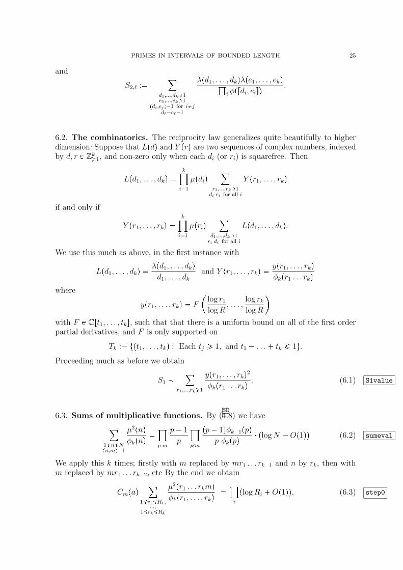
6.2. The combinatorics. The reciprocity law generalizes quite beautifully to higherdimension: Suppose that Lpdq and Y prq are two sequences of complex numbers, indexedby d, r P Zk¥1, and non-zero only when each di (or ri) is squarefree. Then

Lpd1, . . . , dkq k¹i1

µpdiq¸

r1,...,rk¥1di|ri for all i

Y pr1, . . . , rkq

if and only if

Y pr1, . . . , rkq k¹i1

µpriq¸

d1,...,dk¥1ri|di for all i

Lpd1, . . . , dkq.

We use this much as above, in the first instance with

Lpd1, . . . , dkq λpd1, . . . , dkqd1, . . . , dk

and Y pr1, . . . , rkq ypr1, . . . , rkqφkpr1 . . . rkq

where

ypr1, . . . , rkq F

log r1

logR, . . . ,

log rklogR

with F P Crt1, . . . , tks, such that that there is a uniform bound on all of the first orderpartial derivatives, and F is only supported on

Tk : tpt1, . . . , tkq : Each tj ¥ 1, and t1 . . . tk ¤ 1u.Proceeding much as before we obtain

S1 ¸

r1,...,rk¥1

ypr1, . . . , rkq2φkpr1 . . . rkq . (6.1) S1value

6.3. Sums of multiplicative functions. By (SD4.8) we have¸

1¤n¤Npn,mq1

µ2pnqφkpnq

¹p|m

p 1

p

¹p-m

pp 1qφk1ppqp φkppq plogN Op1qq (6.2) sumeval

We apply this k times; firstly with m replaced by mr1 . . . rk1 and n by rk, then withm replaced by mr1 . . . rk2, etc By the end we obtain

Cmpaq¸

1¤r1¤R1,...,

1¤rk¤Rk

µ2pr1 . . . rkmqφkpr1, . . . , rkq

¹i

plogRi Op1qq, (6.3) step0

26 ANDREW GRANVILLE

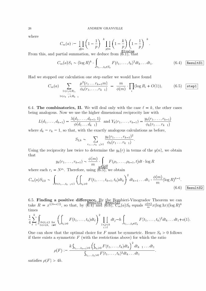
where

Cmpaq :¹p|m

1 1

p

k¹p-m

1 k

p

1 1

p

k.

From this, and partial summation, we deduce from (S1value6.1), that

CmpaqS1 plogRqk »t1,...,tkPTk

F pt1, . . . , tkq2dtk . . . dt1. (6.4) ResultS1

Had we stopped our calculation one step earlier we would have found

Cmpaq¸

1¤r1¤R1,...,

1¤rk1¤Rk1

µ2pr1 . . . rk1mqφkpr1, . . . , rk1q m

φpmq ¹i

plogRi Op1qq, (6.5) step1

6.4. The combinatorics, II. We will deal only with the case ` k, the other casesbeing analogous. Now we use the higher dimensional reciprocity law with

Lpd1, . . . , dk1q λpd1, . . . , dk1, 1qφpd1 . . . dk1q and Ykpr1, . . . , rk1q ykpr1, . . . , rk1q

φkpr1 . . . rk1qwhere dk rk 1, so that, with the exactly analogous calculations as before,

S2,k ¸

r1,...,rk1¥1

ykpr1, . . . , rk1q2φkpr1 . . . rk1q .

Using the reciprocity law twice to determine the ykprq in terms of the ypnq, we obtainthat

ykpr1, . . . , rk1q φpmqm

»t¥0

F pρ1, . . . , ρk1, tqdt logR

where each ri Nρi . Therefore, using (step16.5), we obtain

CmpaqS2,k »

0¤t1,...,tk1¤1

»tk¥0

F pt1, . . . , tk1, tkqdtk2

dtk1 . . . dt1 φpmqm

plogRqk1.

(6.6) ResultS2

6.5. Finding a positive difference. By the Bombieri-Vinogradov Theorem we can

take R x14op1q, so that, by (ResultS16.4) and (

ResultS26.6), CmpaqS0 equals ωpmq

mxplog 3xqplogRqk

times

1

4

k

`1

»0¤ti¤1 for

1¤i¤k, i`

»t`¥0

F pt1, . . . , tkqdt`2 ¹

1¤j¤ki`

dtjh»t1,...,tkPTk

F pt1, . . . , tkq2dtk . . . dt1op1q.

One can show that the optimal choice for F must be symmetric. Hence S0 ¡ 0 followsif there exists a symmetric F (with the restrictions above) for which the ratio

ρpF q :k³t1,...,tk1¥0

³tk¥0

F pt1, . . . , tkqdtk2

dtk1 . . . dt1³t1,...,tk¥0

F pt1, . . . , tkq2dtk . . . dt1 .

satisfies ρpF q ¡ 4h.

PRIMES IN INTERVALS OF BOUNDED LENGTH 27

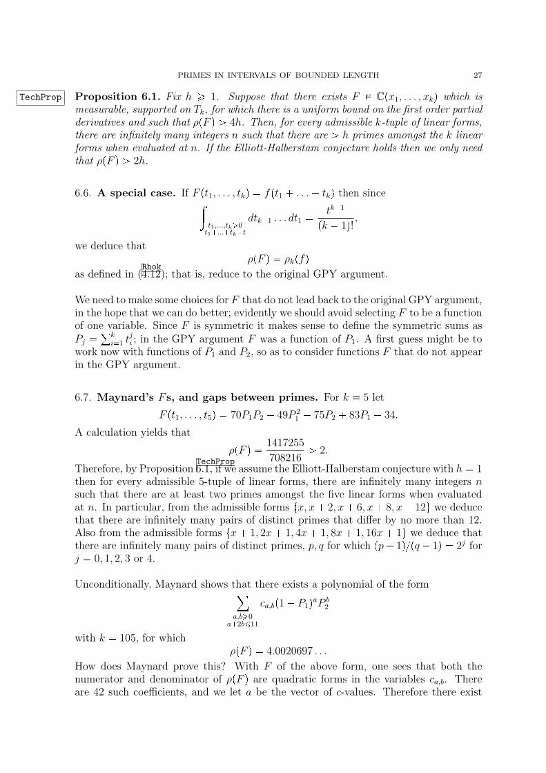
TechProp Proposition 6.1. Fix h ¥ 1. Suppose that there exists F P Cpx1, . . . , xkq which ismeasurable, supported on Tk, for which there is a uniform bound on the first order partialderivatives and such that ρpF q ¡ 4h. Then, for every admissible k-tuple of linear forms,there are infinitely many integers n such that there are ¡ h primes amongst the k linearforms when evaluated at n. If the Elliott-Halberstam conjecture holds then we only needthat ρpF q ¡ 2h.

6.6. A special case. If F pt1, . . . , tkq fpt1 . . . tkq then since»t1,...,tk¥0t1...tkt

dtk1 . . . dt1 tk1

pk 1q! ,

we deduce thatρpF q ρkpfq

as defined in (Rhok4.12); that is, reduce to the original GPY argument.

We need to make some choices for F that do not lead back to the original GPY argument,in the hope that we can do better; evidently we should avoid selecting F to be a functionof one variable. Since F is symmetric it makes sense to define the symmetric sums asPj

°ki1 t

ji ; in the GPY argument F was a function of P1. A first guess might be to

work now with functions of P1 and P2, so as to consider functions F that do not appearin the GPY argument.

6.7. Maynard’s F s, and gaps between primes. For k 5 let

F pt1, . . . , t5q 70P1P2 49P 21 75P2 83P1 34.

A calculation yields that

ρpF q 1417255

708216¡ 2.

Therefore, by PropositionTechProp6.1, if we assume the Elliott-Halberstam conjecture with h 1

then for every admissible 5-tuple of linear forms, there are infinitely many integers nsuch that there are at least two primes amongst the five linear forms when evaluatedat n. In particular, from the admissible forms tx, x 2, x 6, x 8, x 12u we deducethat there are infinitely many pairs of distinct primes that differ by no more than 12.Also from the admissible forms tx 1, 2x 1, 4x 1, 8x 1, 16x 1u we deduce thatthere are infinitely many pairs of distinct primes, p, q for which pp 1qpq 1q 2j forj 0, 1, 2, 3 or 4.

Unconditionally, Maynard shows that there exists a polynomial of the form¸a,b¥0

a2b¤11

ca,bp1 P1qaP b2

with k 105, for whichρpF q 4.0020697 . . .

How does Maynard prove this? With F of the above form, one sees that both thenumerator and denominator of ρpF q are quadratic forms in the variables ca,b. Thereare 42 such coefficients, and we let a be the vector of c-values. Therefore there exist

28 ANDREW GRANVILLE

easily calculable matrices M1 and M2 for which the numerator of F is aTM2a, and thedenominator is aTM1a. By the theory of Lagrangian multipliers, Maynard shows that

M11 M2a ρpF qa

so that ρpfq can be taken to be the largest eigenvalue ofM11 M2, and a the corresponding

eigenvector. These calculations are easily completed using a computer algebra packageand yield the result above.

By PropositionTechProp6.1 with h 1, we deduce that for every admissible 105-tuple of linear

forms, there are infinitely many integers n such that there are at least two primesamongst the 105 linear forms when evaluated at n.

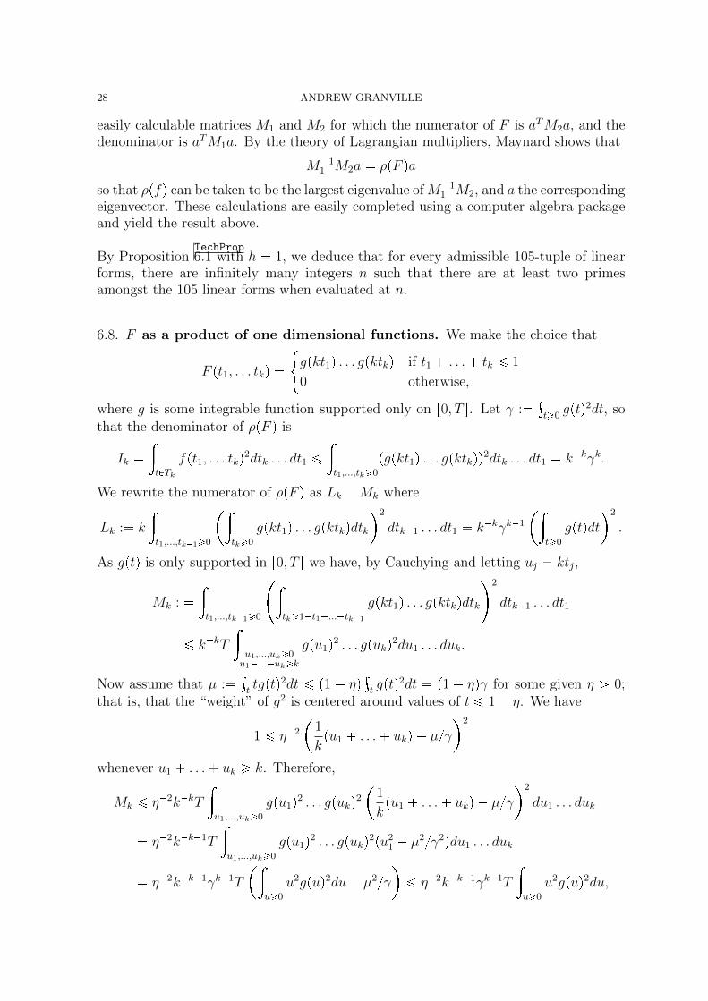
6.8. F as a product of one dimensional functions. We make the choice that

F pt1, . . . tkq #gpkt1q . . . gpktkq if t1 . . . tk ¤ 1

0 otherwise,

where g is some integrable function supported only on r0, T s. Let γ : ³t¥0

gptq2dt, sothat the denominator of ρpF q is

Ik »tPTk

fpt1, . . . tkq2dtk . . . dt1 ¤»t1,...,tk¥0

pgpkt1q . . . gpktkqq2dtk . . . dt1 kkγk.

We rewrite the numerator of ρpF q as Lk Mk where

Lk : k

»t1,...,tk1¥0

»tk¥0

gpkt1q . . . gpktkqdtk2

dtk1 . . . dt1 kkγk1

»t¥0

gptqdt2

.

As gptq is only supported in r0, T s we have, by Cauchying and letting uj ktj,

Mk : »t1,...,tk1¥0

»tk¥1t1...tk1

gpkt1q . . . gpktkqdtk2

dtk1 . . . dt1

¤ kkT»u1,...,uk¥0u1...uk¥k

gpu1q2 . . . gpukq2du1 . . . duk.

Now assume that µ : ³ttgptq2dt ¤ p1 ηq ³

tgptq2dt p1 ηqγ for some given η ¡ 0;

that is, that the “weight” of g2 is centered around values of t ¤ 1 η. We have

1 ¤ η2

1

kpu1 . . . ukq µγ

2

whenever u1 . . . uk ¥ k. Therefore,

Mk ¤ η2kkT»u1,...,uk¥0

gpu1q2 . . . gpukq2

1

kpu1 . . . ukq µγ

2

du1 . . . duk

η2kk1T

»u1,...,uk¥0

gpu1q2 . . . gpukq2pu21 µ2γ2qdu1 . . . duk

η2kk1γk1T

»u¥0

u2gpuq2du µ2γ¤ η2kk1γk1T

»u¥0

u2gpuq2du,

PRIMES IN INTERVALS OF BOUNDED LENGTH 29

by symmetry. We deduce that

ρpF q ¥³t¥0

gptqdt2 η2Tk

³u¥0

u2gpuq2du³t¥0

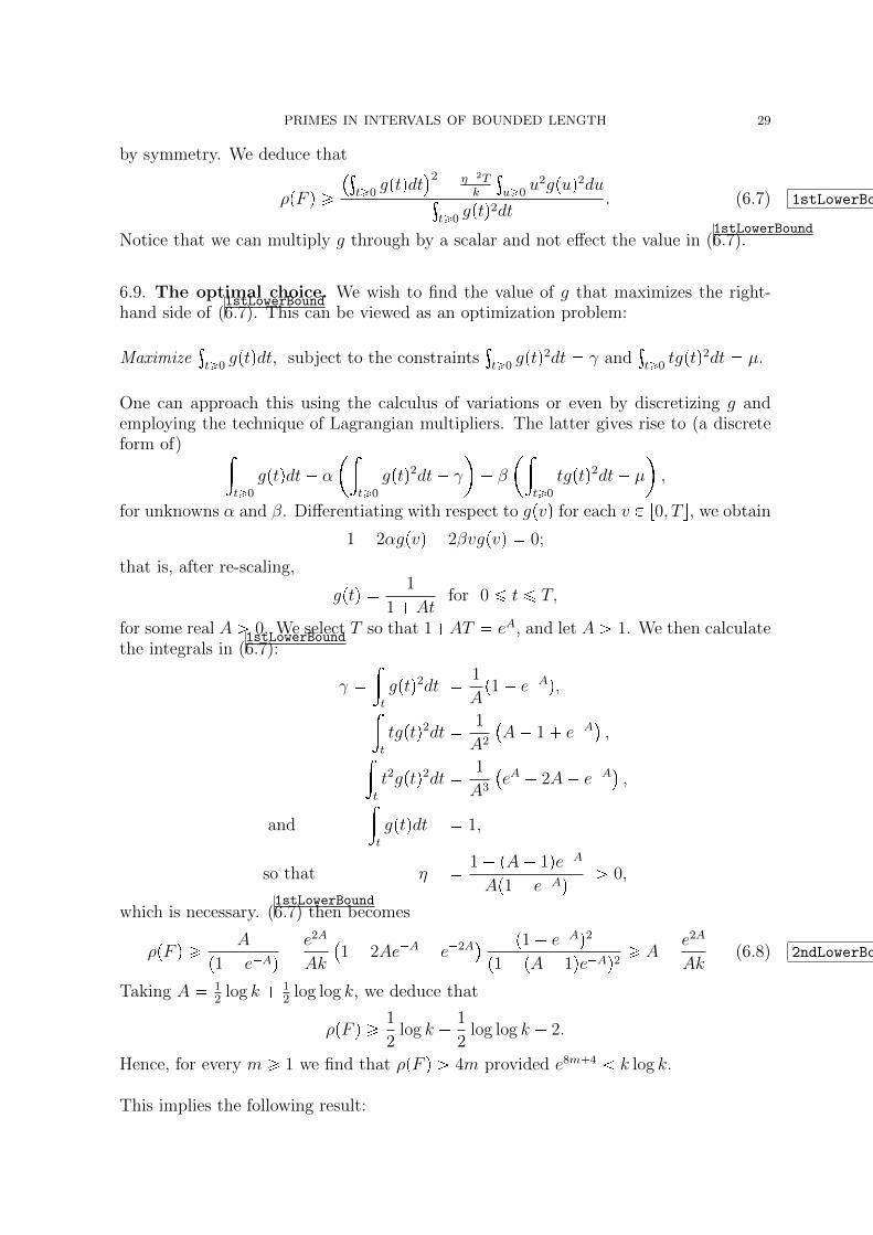
gptq2dt . (6.7) 1stLowerBound

Notice that we can multiply g through by a scalar and not effect the value in (1stLowerBound6.7).

6.9. The optimal choice. We wish to find the value of g that maximizes the right-hand side of (

1stLowerBound6.7). This can be viewed as an optimization problem:

Maximize³t¥0

gptqdt, subject to the constraints³t¥0

gptq2dt γ and³t¥0

tgptq2dt µ.

One can approach this using the calculus of variations or even by discretizing g andemploying the technique of Lagrangian multipliers. The latter gives rise to (a discreteform of) »

t¥0

gptqdt α

»t¥0

gptq2dt γ

β

»t¥0

tgptq2dt µ

,

for unknowns α and β. Differentiating with respect to gpvq for each v P r0, T s, we obtain

1 2αgpvq 2βvgpvq 0;

that is, after re-scaling,

gptq 1

1 Atfor 0 ¤ t ¤ T,

for some real A ¡ 0. We select T so that 1AT eA, and let A ¡ 1. We then calculatethe integrals in (

1stLowerBound6.7):

γ »t

gptq2dt 1

Ap1 eAq,»

t

tgptq2dt 1

A2

A 1 eA

,»

t

t2gptq2dt 1

A3

eA 2A eA

,

and

»t

gptqdt 1,

so that η 1 pA 1qeAAp1 eAq ¡ 0,

which is necessary. (1stLowerBound6.7) then becomes

ρpF q ¥ A

p1 eAq e2A

Ak

1 2AeA e2A

p1 eAq2p1 pA 1qeAq2 ¥ A e2A

Ak(6.8) 2ndLowerBound

Taking A 12

log k 12

log log k, we deduce that

ρpF q ¥ 1

2log k 1

2log log k 2.

Hence, for every m ¥ 1 we find that ρpF q ¡ 4m provided e8m4 k log k.

This implies the following result:

30 ANDREW GRANVILLE

Theorem 6.2. For any given integer m ¥ 2, let k be the smallest integer with k log k ¡e8m4. For any admissible k-tuple of linear forms L1, . . . , Lk there exists infinitely manyintegers n such that at least m of the Ljpnq, 1 ¤ j ¤ k are prime.

For any m ¥ 1, we let k be the smallest integer with k log k ¡ e8m4, so that k ¡ 10000;in this range it is known that πpkq ¤ k

log k4. Next we let x 2k log k ¡ 105 and, for

this range it is known that πpxq ¥ xlog x

p1 1log x

q. Hence

πp2k log kq πpkq ¥ 2k log k

logp2k log kq

1 1

logp2k log kq k

log k 4

and this is ¡ k for k ¥ 311 by an easy calculation. We therefore apply the theoremwith the k smallest primes ¡ k, which form an admissible set r1, 2k log ks, to obtain:

Corollary 6.3. For any given integer m ¥ 2, let Bm e8m5. There are infinitely manyintegers x for which there are at least m distinct primes within the interval rx, xBms.

By a slight modification of this construction, Maynard obtains Bm ! m3e4m inmaynard[29].

Part 2. Primes in arithmetic progressions; breaking the?x-barrier

Our goal, in the rest of the article, is to sketch the ideas behind the proof of Yitang’sextraordinary result, given in (

EHsmooth3.5), that primes are well-distributed on average in the

arithmetic progressions a pmod qq with q a little bigger than?x. We will see how this

question fits into a more general framework, as developed by Bombieri, Friedlander andIwaniec

bfi[3], so that Zhang’s results should also allow us to deduce analogous results for

interesting arithmetic sequences other than the primes.

To begin with we will need to discuss a key technique of analytic number theory, theidea of creating important sequences through convolutions:

7. Convolutions in number theory

The convolution of two functions f and g, written f g, is defined by

pf gqpnq :¸abn

fpaqgpbq,

for every integer n ¥ 1, where the sum is over all pairs of positive integers a, b whoseproduct is n. Hence if τpnq counts the number of divisors of n then

τ 1 1,

where 1 is the function with 1pnq 1 for every n ¥ 1. We already saw, in (VMidentity2.2), that

if Lpnq log n then µ L Λ, where Λpnq log p if n is a power of prime p, andΛpnq 0 otherwise. In the GPY argument we used that p1 µqpnq 0 if n ¡ 1.

PRIMES IN INTERVALS OF BOUNDED LENGTH 31

There is no better way to understand why convolutions are useful than to present afamous argument of Dirichlet, estimating the average of τpnq. Now , if n is squarefreeand has k prime factors then τpnq 2k, so we see that τpnq varies greatly dependingon the arithmetic structure of n, but the average is more stable:

1

x

¸n¤x

τpnq 1

x

¸n¤x

¸d|n

1 1

x

¸d|n

¸n¤xd|n

1 1

x

¸d¤x

xd

1

x

¸d¤x

xdOp1q

¸d¤x

1

dO

1

x

¸d¤x

1

.

One can approximate°d¤x

1d

by³x1dtt log x. Indeed the difference tends to a limit,

the Euler-Mascheroni constant γ : limNÑ8 11 1

2 . . . 1

N logN . Hence we have

proved that the integers up to x have log x Op1q divisors, on average, which is quiteremarkable for such a wildly fluctuating function.

Dirichlet studied this argument and noticed that when we approximate rxds by xdOp1q for large d, say for those d in px2, xs, then this is not really a very good ap-proximation, and gives a large cumulative error term, Opxq. However we know thatrxds 1 for each of these d, and so we can estimate this sum by x2Op1q, which ismuch more precise. In general we write n dm, where d and m are integers. Whend is small then we should fix d, and count the number of such m, with m ¤ xd (aswe did above); but when m is small, then we should fix m, and count the number of dwith d ¤ xm. In this way our sums are all over long intervals, which allows us to getan accurate approximation of their value:

1

x

¸n¤x

τpnq 1

x

¸n¤x

¸dmn

1 1

x

¸d¤?x

¸n¤xd|n

1 1

x

¸m ?x

¸n¤xm|n

1 1

x

¸d¤?x

¸m ?x

1

1

x

¸d¤?x

xdOp1q

1

x

¸m ?x

xmOp1q

1O

1?x

log x 2γ 1O

1?x

,

since°n¤N 1n logN γ Op1Nq, an extraordinary improvement upon the earlier

error term.

7.1. Vaughan’s identity. We will need a more convoluted identity than (VMidentity2.2) to prove

our estimates for primes in arithmetic progressions. There are several possible suitableidentities, the simplest of which is due to Vaughan

vaughan[40]:

Vaughan’s identity : Λ¥V µ U L µ U Λ V 1 µ¥U Λ¥V 1 (7.1) Vaughidentity

32 ANDREW GRANVILLE

where g¡W pnq gpnq if n ¡ W and gpnq 0 otherwise; and g g¤W g¡W . To verifythis identity, we manipulate the algebra of convolutions:

Λ¥V Λ Λ V pµ Lq Λ V p1 µq µ U L µ¥U L µ U Λ V 1 µ¥U Λ V 1

µ U L µ U Λ V 1 µ¥U pΛ 1 Λ V 1q,

8. Distribution in arithmetic progressionsGeneralBV

8.1. General sequences in arithmetic progressions. One can ask whether anygiven sequence pβpnqqn¥1 P C is well-distributed in arithmetic progressions modulo q.We begin by formulating an appropriate analogy to (

SW13.2), which should imply non-

trivial estimates in the range q ¤ plog xqA for any fixed A ¡ 0: We say that β satisfiesa Siegel-Walfisz condition if, for any fixed A ¡ 0, and whenever pa, qq 1, we have

¸n¤x

na pmod qq

βpnq 1

φpqq¸n¤x

pn,qq1

βpnq

!Aβx 1

2

plog xqA ,

with β β2 where, as usual,

β2 :¸n¤x

|βpnq|2 1

2

.

Using Cauchy’s inequality one can show that this assumption is “non-trivial” only forq plog xq2A; that is, when x is very large compared to q.

Using the large sieve, Bombieri, Friedlander and Iwaniecbfi[3] were able to prove two

results that are very surprising, given the weakness of the hypotheses. In the first theyshowed that if β satisfies a Siegel-Walfisz condition,11 then it is well-distributed foralmost all arithmetic progressions a pmod qq, for almost all q ¤ xplog xqB:

Theorem 8.1. Suppose that the sequence of complex numbers βpnq, n ¤ x satisfies aSiegel-Walfisz condition. For any A ¡ 0 there exists B BpAq ¡ 0 such that

¸q¤Q

¸a: pa,qq1

¸

na pmod qqβpnq 1

φpqq¸

pn,qq1

βpnq2

! β2 x

plog xqA

where Q xplog xqB.

The analogous result for Λpnq is known as the Barban-Davenport-Halberstam theoremand in that special case one can even obtain an asymptotic.

Before proceeding, let us assume, for the rest of this article, that we are given twosequences of complex numbers as follows:

11Their condition appears to be weaker than that assumed here, but it can be shown to be equivalent.

PRIMES IN INTERVALS OF BOUNDED LENGTH 33

αpmq, M m ¤ 2M and βpnq, N n ¤ 2N , with x13 N ¤ M ¤ x23 andMN ¤ x.

βpnq satisfies the Siegel-Walfisz condition. αpmq ! τpmqAplog xqB and βpnq ! τpnqAplog xqB (there inequalities are satisfied

by µ, 1,Λ, L and any convolutions of these sequences).

In their second result, Bombieri, Friedlander and Iwaniec, showed that rather generalconvolutions are well-distributed12 for all arithmetic progressions a pmod qq, for almostall q ¤ x12plog xqB.

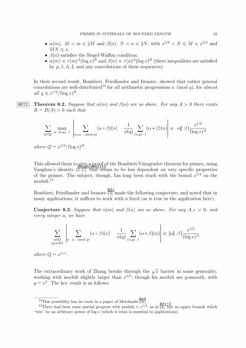
BFI2 Theorem 8.2. Suppose that αpmq and βpnq are as above. For any A ¡ 0 there existsB BpAq ¡ 0 such that

¸q¤Q

maxa: pa,qq1

¸

na pmod qqpα βqpnq 1

φpqq¸

pn,qq1

pα βqpnq ! αβ x12

plog xqA

where Q x12plog xqB.

This allowed them to give a proof of the Bombieri-Vinogradov theorem for primes, usingVaughan’s identity (

Vaughidentity7.1), that seems to be less dependent on very specific properties

of the primes. The subject, though, has long been stuck with the bound x12 on themoduli.13

Bombieri, Friedlander and Iwaniecbfi[3] made the following conjecture, and noted that in

many applications, it suffices to work with a fixed (as is true in the application here).

Conjecture 8.3. Suppose that αpmq and βpnq are as above. For any A, ε ¡ 0, andevery integer a, we have

¸q¤Q

pq,aq1

¸

na pmod qqpα βqpnq 1

φpqq¸

pn,qq1

pα βqpnq ! αβ x12

plog xqA

where Q x1ε.

The extraordinary work of Zhang breaks through the?x barrier in some generality,

working with moduli slightly larger than x12, though his moduli are y-smooth, withy xδ. The key result is as follows:

12This possibility has its roots in a paper of Motohashimot[31].

13There had been some partial progress with moduli ¡ x12, as inbfi-2[4], but no upper bounds which

“win” by an arbitrary power of log x (which is what is essential to applications).

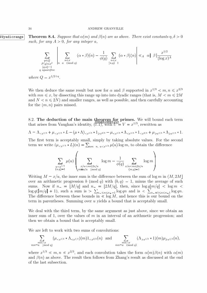
34 ANDREW GRANVILLE

BVdyadicrange Theorem 8.4. Suppose that αpmq and βpnq are as above. There exist constants η, δ ¡ 0such, for any A ¡ 0, for any integer a,

¸q¤Q

P pqq¤xδpq,aq1

q squarefree

¸n¤x

na pmod qq

pα βqpnq 1

φpqq¸n¤x

pn,qq1

pα βqpnq

!A αβ x12

plog xqA

where Q x12η.

We then deduce the same result but now for α and β supported in x13 m,n ¤ x23

with mn ¤ x, by dissecting this range up into into dyadic ranges (that is, M m ¤ 2Mand N n ¤ 2N) and smaller ranges, as well as possible, and then carefully accountingfor the pm,nq pairs missed.

8.2. The deduction of the main theorem for primes. We will bound each termthat arises from Vaughan’s identity, (

Vaughidentity7.1), with U V x13, rewritten as

Λ Λ x13 µ x13 L pµ Λq x13 1¥x23 µ x13 Λ x13 1 x23 µ¥x13 Λ¥x13 1.

The first term is acceptably small, simply by taking absolute values. For the secondterm we write pµ x13 Lqpnq

°umn, u x13 µpuq logm, to obtain the difference

¸u x13pu,qq1

µpuq

¸

xu m¤2xumau pmod qq

logm 1

φpqq¸

xu m¤2xupm,qq1

logm

Writing M xu, the inner sum is the difference between the sum of logm in pM, 2M sover an arithmetic progression b pmod qq with pb, qq 1, minus the average of suchsums. Now if n rMqs and n r2Mqs, then, since log qrmqs logm log qprmqs 1q, such a sum is ¡ °

n¤n¤n1 log qn and is °n1¤n¤n1 log qn.

The difference between these bounds in ! logM , and hence this is our bound on theterm in parentheses. Summing over u yields a bound that is acceptably small.

We deal with the third term, by the same argument as just above, since we obtain aninner sum of 1, over the values of m in an interval of an arithmetic progression; andthen we obtain a bound that is acceptably small.

We are left to work with two sums of convolutions:¸mnx

mna pmod qq

pµ x13 Λ x13qpmq1 x23pnq and¸mnx

mna pmod qq

pΛ¥x13 1qpmqµ¥x13pnq,

where x13 ! m,n ! x23, and each convolution takes the form αpmqβpnq with αpmqand βpnq as above. The result then follows from Zhang’s result as discussed at the endof the last subsection.

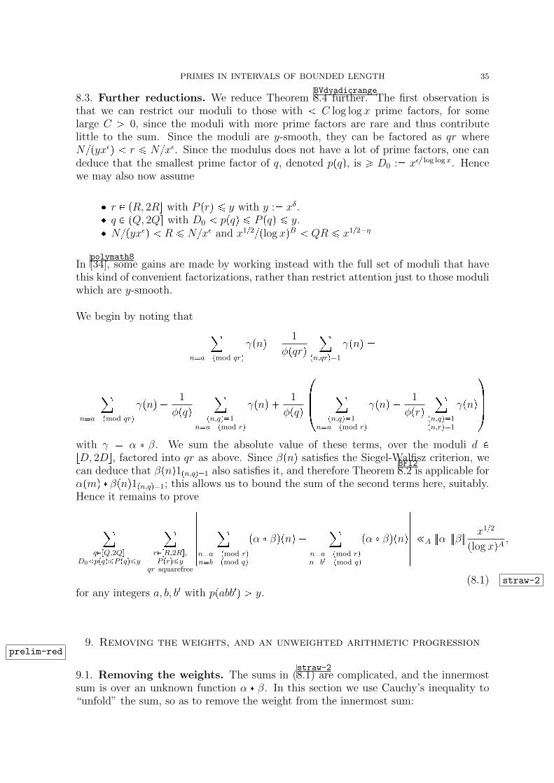
PRIMES IN INTERVALS OF BOUNDED LENGTH 35

8.3. Further reductions. We reduce TheoremBVdyadicrange8.4 further. The first observation is

that we can restrict our moduli to those with C log log x prime factors, for somelarge C ¡ 0, since the moduli with more prime factors are rare and thus contributelittle to the sum. Since the moduli are y-smooth, they can be factored as qr whereNpyxεq r ¤ Nxε. Since the modulus does not have a lot of prime factors, one candeduce that the smallest prime factor of q, denoted ppqq, is ¥ D0 : xε log log x. Hencewe may also now assume

r P pR, 2Rs with P prq ¤ y with y : xδ. q P pQ, 2Qs with D0 ppqq ¤ P pqq ¤ y. Npyxεq R ¤ Nxε and x12plog xqB QR ¤ x12η

Inpolymath8[34], some gains are made by working instead with the full set of moduli that have

this kind of convenient factorizations, rather than restrict attention just to those moduliwhich are y-smooth.

We begin by noting that ¸na pmod qrq

γpnq 1

φpqrq¸

pn,qrq1

γpnq

¸na pmod qrq

γpnq 1

φpqq¸

pn,qq1na pmod rq

γpnq 1

φpqq

¸

pn,qq1na pmod rq

γpnq 1

φprq¸

pn,qq1pn,rq1

γpnq

with γ α β. We sum the absolute value of these terms, over the moduli d PrD, 2Ds, factored into qr as above. Since βpnq satisfies the Siegel-Walfisz criterion, wecan deduce that βpnq1pn,qq1 also satisfies it, and therefore Theorem

BFI28.2 is applicable for

αpmq βpnq1pn,qq1; this allows us to bound the sum of the second terms here, suitably.Hence it remains to prove

¸qPrQ,2Qs

D0 ppqq¤P pqq¤y

¸rPrR,2Rs,P prq¤y

qr squarefree

¸

na pmod rqnb pmod qq

pα βqpnq ¸

na pmod rqnb1 pmod qq

pα βqpnq

!A αβ x12

plog xqA ,

(8.1) straw-2

for any integers a, b, b1 with ppabb1q ¡ y.

9. Removing the weights, and an unweighted arithmetic progressionprelim-red

9.1. Removing the weights. The sums in (straw-28.1) are complicated, and the innermost

sum is over an unknown function α β. In this section we use Cauchy’s inequality to“unfold” the sum, so as to remove the weight from the innermost sum:

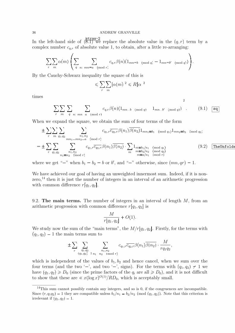
36 ANDREW GRANVILLE

In the left-hand side of (straw-28.1) we replace the absolute value in the pq, rq term by a

complex number cq,r of absolute value 1, to obtain, after a little re-arranging:

¸r

¸m

αpmq¸

q

¸n: mna pmod rq

cq,rβpnqp1mnb pmod qq 1mnb1 pmod qqq .

By the Cauchy-Schwarz inequality the square of this is

¤¸r

¸m

|αpmq|2 ¤ Rα2

times

¸r

¸m

¸q

¸n: mna pmod rq

cq,rβpnqp1mnb pmod qq 1mnb1 pmod qqq2

. (9.1) sq

When we expand the square, we obtain the sum of four terms of the form

¸r

¸m

¸q1,q2

¸n1,n2

mn1mn2a pmod rq

cq1,rcq2,rβpn1qβpn2q1mn1b1 pmod q1q1mn2b2 pmod q2q

¸r

¸q1,q2

¸n1,n2

n1n2 pmod rq

cq1,rcq2,rβpn1qβpn2q ¸m

1mb1n1 pmod q1qmb2n2 pmod q2qman1 pmod rq

(9.2) TheUnfolded

where we get “” when b1 b2 b or b1, and “” otherwise, since pmn, qrq 1.

We have achieved our goal of having an unweighted innermost sum. Indeed, if it is non-zero,14 then it is just the number of integers in an interval of an arithmetic progressionwith common difference rrq1, q2s.

9.2. The main terms. The number of integers in an interval of length M , from anarithmetic progression with common difference rrq1, q2s is

M

rrq1, q2s Op1q.

We study now the sum of the “main terms”, the Mrrq1, q2s. Firstly, for the terms withpq1, q2q 1 the main terms sum to

¸r

¸q1,q2

pq1,q2q1

¸n1,n2

n1n2 pmod rq

cq1,rcq2,rβpn1qβpn2q M

rq1q2

,

which is independent of the values of b1, b2 and hence cancel, when we sum over thefour terms (and the two ‘’, and two ‘’, signs). For the terms with pq1, q2q 1 wehave pq1, q2q ¥ D0 (since the prime factors of the qi are all ¥ D0), and it is not difficultto show that these are ! xplog xqOp1qRD0, which is acceptably small.

14This sum cannot possibly contain any integers, and so is 0, if the congruences are incompatible.Since pr, q1q2q 1 they are compatible unless b1n1 b2n2 pmod pq1, q2qq. Note that this criterion isirrelevant if pq1, q2q 1.

PRIMES IN INTERVALS OF BOUNDED LENGTH 37

9.3. The error terms and the advent of exponential sums. The “Op1q”s in (TheUnfolded9.2)

can add up to a total that is far too large. One can show that in most of the terms ofthe sum, the common difference of the arithmetic progression is larger than the lengthof the interval, so the correct count is either 0 or 1: It is hardly surprising that an errorterm of “Op1q” is too insensitive to help us.

To proceed, instead of approximating, we will give a precise formula for the number ofintegers in an arithmetic progression in an interval, using a sum of exponentials. Bythe Chinese Remainder Theorem, we can rewrite our triple of congruence conditions

m b1n1 pmod q1q, m b2n2 pmod q2q, m an1 pmod rqas one,

m m0pn1, n2q pmod qqwhere q rg`1`2, when there is a solution, which happens if and only if b1n1 b2n2

pmod gq, where g pq1, q2q and we now define `1 q1g, `2 q2g.

To identify whether m is in a given interval I, we use Fourier analysis. The discreteFourier transform is defined by

fphq :¸

b pmod qqfpbqeqphbq,

for any function f of period q. If f is any such function and Ip.q is the characteristicfunction for the interval pM, 2M s, then

¸mPI

fpmq 1

q

¸h pmod qq

Iphqfphq, (9.3) Plancherel

is an example of Plancherel’s formula. This has a “main term” at h 0 (which is the

same as the main term we found above, in that special case). The coefficients Iphq areeasily evaluated and bounded:

Iphq 2M

mM1

eqphmq eqp2hMq eqphMq 1

eqphq 1.

The numerator has absolute value ¤ 2 and, using the Taylor expansion, the denominatorhas absolute value |h|q. Hence

|Iphq| ! mintM, q|h|u,We apply (

Plancherel9.3) with f °

i ci1mai pmod qq, take absolute values, and use our bounds

for |Iphq|, to obtain¸i

ci

¸

mMmai pmod qq

1 M

q

!

¸0¤j¤J

Hj :2jqM

1

Hj

¸1¤|h|¤Hj

¸i

cieqpaihq . (9.4) ExponExpan

38 ANDREW GRANVILLE

The error terms in (TheUnfolded9.2) are bounded by

¸rR

¸g¤G

¸`1,`2Qgp`1,`2q1

¸

n1,n2Nn1n2 pmod rq

b1n1b2n2 pmod gq

βpn1qβpn2q

¸

mMmm0pn1,n2q pmod rg`1`2q

1 M

rg`1`2

which, by (ExponExpan9.4), is

!¸rR

¸g¤G

¸`1,`2Qgp`1,`2q1

¸0¤j¤J

Hj :2jGg

1

Hj

¸1¤|h|¤Hj

¸

n1,n2Nn1n2 pmod rq

n2pb2b1qn1 pmod gq

βpn1qβpn2qerg`1`2pm0pn1, n2qhq

.

We write n1 n, n2 n kr, replace the n2 variable with k, and define mkpnq m0pn1, n2q. To simplify matters shall proceed with r, g, k and j fixed, and then sumover these at the end, so we are reduced to studying

¸`1,`2Lp`1,`2q1

1

H

¸1¤|h|¤H

¸nN

pb2b1qnb1kr pmod gq

βpnqβpn krqerg`1`2pmkpnqhq

(9.5) ToBeBounded

where L Qg.

10. Linnik’s dispersion method

The proof of Zhang’s Theorem, and indeed of all the results in the literature of thistype, use Linnik’s dispersion method. The idea is to express the fact that n belongs toan arithmetic progression using Fourier analysis; summing up over n gives us a mainterm plus a sum of exponential sums, and then the challenge is to bound each of theseexponential sums.

Often the sums come with weights, and judicious use of Cauchying allows one to workwith an unweighted, but more complicated exponential sum. We will discuss bounds onexponential sums later in this section. These exponential sums are often Kloostermansums, which one needs to bound. Individual Kloosterman sums can often by suitablybounded by Weil’s or Deligne’s Theorem. However, sometimes one needs to get goodbounds on averages of Kloosterman sums, a question that was brilliantly attacked byDeshouillers and Iwaniec

DI83[7], using the (difficult) spectral theory of automorphic forms.

Indeed all previous work, breaking the?x barrier, such as

fi-2[12],

bfi[3]) uses these types

of estimates. One of the remarkable aspects of Zhang’s work is that he avoids thesepenible techniques, and the restrictions that come with them.

Zhang was able to use only existing bounds on Kloosterman sums to prove his Theorem,though he does use the sophisticated estimate of Birch and Bombieri from the appendix

PRIMES IN INTERVALS OF BOUNDED LENGTH 39

offi-3[14]. Polymath8 indicates how even this deeper result can be avoided, so that the

proof can be given using only “standard” estimates, which is what we do here.

10.1. Removing the weights again. To remove the β weights from (ToBeBounded9.5), we begin

by replacing the absolute value in (ToBeBounded9.5) by the appropriate complex number ch,`1,`2 of

absolute value 1, and re-organize to obtain¸nN

pb2b1qnb1kr pmod gq

βpnqβpn krq¸

`1,`2Lp`1,`2q1

1

H

¸1¤|h|¤H

ch,`1,`2erg`1`2pmkpnqhq. (10.1) PreCauchy

We now Cauchy on the outer sum, which allows us to peel off the β’s in the term¸n

|βpnqβpn krq|2 ¤¸n

|βpnq|4 β44,

times the more interesting term

¸n

¸

`1,`2Lp`1,`2q1

1

H

¸1¤|h|¤H

ch,`1,`2erg`1`2pmkpnqhq

2

.

We simply expand this sum, and take absolute values for each fixed h, j, `1, `2,m1,m2,to obtain

¤ 1

H2

¸1¤|h|,|j|¤Hi

¸`1,`2,m1,m2L

p`1,`2qpm1,m2q1

¸nN

pb2b1qnb1kr pmod gq

erg`1`2pmkpnqhqergm1m2pmkpnqjq

.Finally we have pure exponential sums, albeit horribly complicated.

10.2. Exponential sums with complicated moduli. If pr, sq 1 then there areintegers a, b for which

ar bs 1.

Note that although there are infinitely many possibilities for the pair of integers a, b,the values of a pmod sq and b mod r are uniquely defined. If we divide the previousequation by rs, and multiply by m, and then take ep.q of both sides, we obtain

erspmq espamq erpbmq.This allows us to write the exponential, in our last sum, explicitly. After some analysis,we find that our exponential sum take the form¸

nNna pmod qq

ed1

C1

n

ed2

C2

n kr

, (10.2) ExpSum

for some constants C1, C2 (where d1 rgr`1, `2s, d2 rm1,m2s and q divides g) whichdepend on many variables but are independent of n. With a change of variable n Ñqn a we transform this to another sum of the same shape but instead over all n in aninterval.

40 ANDREW GRANVILLE

10.3. Exponential sums: From the incomplete to the complete. We now havethe sum of the exponential of a function of n, over the integers in an interval. There aretypically many integers in this sum, so this is unlike what we encountered earlier (whenwe were summing 1). The terms of the sum are periodic of period dividing rd1, d2s andit is not difficult to sum the terms over a complete period. Hence we can restrict ourattention to “incomplete sums” where the sum does not include a complete period.

We can now employ (Plancherel9.3) once more. The coefficients Iphq are well understood, but the

fphq now take the form

¸n pmod qq

ed1

C1

n hn

ed2

C2

n∆ hn

,

a “complete” exponential sum.

The trick here is that we can factor the exponential into its prime factor exponentialsand then, by the Chinese Remainder Theorem, this sum equals the product over theprimes p dividing q, of the same sum but now over n pmod pq with the appropriateeppq. Hence we have reduced this question to asking for good bounds on exponentialsums of the form

¸n pmod pq

ep

a

n b

n∆ cn

.

Here we omit values of n for which a denominator is 0. As long as this does notdegenerate (for example, it would degenerate if p|a, b, c) then Weil’s Theorem impliesthat this is ¤ κp12, for some constant κ ¡ 0. Therefore the complete sum over npmod qq is ¤ κνpqqq12. This in turn allows us to bound our incomplete sum (

ExpSum10.2), and

to bound the term at the end of the previous section.

The calculations to put this into practice are onerous, and we shall omit these detailshere. At the end one finds that the bounds deduced are acceptably small if

x12 ¥ N ¡ xp2εq5

where ε ¡ 12η 7δ. However this is not quite good enough, since we need to be able totake N as small as x13.

We can try a modification of this proof, the most successful being where, before weCauchy equation (

PreCauchy10.1) we also fix the `1 variable. This variant allows us to extend our

range to all

N ¡ x13ε

where ε ¡ 143η 7

2δ. We are very close to the exponent 1

3, but it seems that we are

destined to just fail.

PRIMES IN INTERVALS OF BOUNDED LENGTH 41

11. Complete exponential sums: Combining information theGraham-Ringrose way

The “square-root cancellation” for incomplete exponential sums of the form |°n eqpfpnqq|for various moduli q, with the sum over n in an interval of length N q is not quitegood enough to obtain our results.

Graham and Ringrosegraham[17] proved that we can improve the (analogous) incomplete

character sum bounds when q is smooth. Here we follow Polymath8polymath8[34], who showed

how to modify the Graham-Ringrose argument to incomplete exponential sums. Thiswill allow us to reduce the size of N in the above argument and prove our result.

11.1. Formulating the improved incomplete exponential sum result. For con-venience we will write the entry of the exponential sum as fpnq, which should be thoughtof as taking the form an bpn∆q cn, though the argument is rather more general.We assume that N q, so that the Weil bound gives

¸n

eqpfpnqq ! τpqqAq12. (11.1) weil1

for some constant A which depends only on the degree of f .

In what follows we will assume that q is factored as q q1q2, and we will deduce that¸n

eqpfpnqq !

q

121 q

142

τpqqAplog qqN12. (11.2) vdc-1

If q is y-smooth then we let q1 be the largest divisor of q that is ¤ pqyq13 so that itmust be ¡ pqy2q13, and so q2 ¤ pqyq23. Hence the last bound implies

¸n

eqpfpnqq ! τpqqApqyq16plog qqN12.

It is this bound that we insert into the machinery of the previous section, and it allowsuse to extend our range to all

N ¡ x310ε

where ε is bounded below by a (positive) linear combination of η and δ. In order that

we can stretch the range down to all N ¡ x13 , this method requires that

162η 90δ 1.

11.2. Proof of (vdc-111.2). We may assume

q1 ¤ N ¤ q2

else if N q1 we have the trivial bound ¤ N pq1Nq12, and if N ¡ q2 then (weil111.1)

implies the result since q12 pq1q2q12 pq1Nq12.

42 ANDREW GRANVILLE

The main idea will be to reduce our incomplete exponential sum mod q, to a sum ofincomplete exponential sums mod q2. Now

eqpfpn kq1qq eq1pfpnqq2q eq2pfpn kq1qq1qso that, by a simple change of variable, we have¸

n

eqpfpnqq ¸n

eqpfpn kq1qqq ¸n

eq1pfpnqq2q eq2pfpn kq1qq1q.

Now, if we sum this over all k, 1 ¤ k ¤ K : tNq1u, then we have

K¸n

eqpfpnqq ¸n

eq1pfpnqq2qK

k1

eq2pfpn kq1qq1q,

and so K¸n

eqpfpnqq2

¤¸

n

K

k1

eq2pfpn kq1qq1q2

! N¸n

K

k1

eq2pfpn kq1qq1q2

N¸

1¤k,k1¤K

¸n

eq2pgk,k1pnqq,

where gk,k1pnq : pfpn kq1q fpn k1q1qqq1 pmod q2q if n kq1, n k1q1 P I, andgk,k1pnq : 0 otherwise. If k k1 then gk,kpnq 0, and so these terms contribute¤ KN2.

We now apply the bound of (weil111.1) taking f gk,k for k k1. Calculating the sum

yields (vdc-111.2).

11.3. Better results. Inpolymath8[34] the authors obtain better results using somewhat deeper

techniques.

By replacing the set of y-smooth integers by the much larger class of integers with divi-sors in a pre-specified interval (and such that those divisors have divisors in a differentpre-specified interval, etc., since one can iterate the proof in the previous section) theyimprove the restriction to

84η 48δ 1.

Following Zhang they also gained bounds on certain higher order convolutions (of theshape α 1 1 1), though here needing deeper exponential sum estimates, and werethen able to improve the restriction to (slightly better than)

43η 27δ 1.

11.4. Final remark. It is worth noting that one can obtain the same quality of resultsonly assuming a bound ! p23ε for the relevant exponential sums in finite fields.

PRIMES IN INTERVALS OF BOUNDED LENGTH 43

References

[1] E. Bombieri, On the large sieve, Mathematika 12 (1965), 201–225.[2] E. Bombieri and H. Davenport Small difference between prime numbers, Proc. Roy. Soc. Ser. A

293 (1966), 1-18.[3] E. Bombieri, J. Friedlander and H. IwaniecPrimes in arithmetic progressions to large moduli, Acta

Math. 156 (1986), no. 3-4, 203–251.[4] E. Bombieri, J. Friedlander and H. Iwaniec, Primes in arithmetic progressions to large moduli. II,

Math. Ann. 277 (1987), no. 3, 361–393.[5] E. Bombieri, J. Friedlander and H. Iwaniec, Primes in arithmetic progressions to large moduli. III,

J. Amer. Math. Soc. 2 (1989), no. 2, 215–224.

[6] P. Deligne, La conjecture de Weil. II, Publications Mathematiques de l’IHES 52 (1980), 137–252.[7] J.-M. Deshouillers and H. Iwaniec, Kloosterman Sums and Fourier Coefficients of Cusp Forms,

Inventiones mathematicae 70 (1982/83), 219-219.[8] P. D. T. A. Elliott and H. Halberstam, A conjecture in prime number theory, Symp. Math. 4

(1968), 59–72.[9] E. Fouvry, A new form of the error term in the linear sieve, Acta Arith., 37 (1980), 307–320.

[10] E. Fouvry, Autour du theoreme de Bombieri-Vinogradov, Acta Math. 152 (1984), no. 3-4, 219–244.[11] E. Fouvry and H. Iwaniec, On a theorem of Bombieri-Vinogradov type, Mathematika 27 (1980),

no. 2, 135–152 (1981).[12] E. Fouvry and H. Iwaniec, Primes in arithmetic progressions, Acta Arith. 42 (1983), no. 2, 197–

218.[13] J. Friedlander and A. Granville, Limitations to the equi-distribution of primes. I, Ann. of Math.

129 (1989), 363-382.[14] J. Friedlander and H. Iwaniec, Incomplete Kloosterman sums and a divisor problem, With an

appendix by Bryan J. Birch and Enrico Bombieri. Ann. of Math. (2) 121 (1985), no. 2, 319–350.[15] D. Goldston, J. Pintz and C. Yıldırım, Primes in tuples. I, Ann. of Math. 170 (2009), no. 2,

819–862.[16] D. Goldston, S. Graham, J. Pintz and C. Yıldırım, Small gaps between primes or almost primes,

Trans. Amer. Math. Soc. 361 (2009), no. 10, 5285–5330.[17] S. W. Graham and C. J. Ringrose, Lower bounds for least quadratic nonresidues, Analytic number

theory (Allerton Park, IL, 1989), 269–309, Progr. Math., 85, Birkhauser Boston, Boston, MA,1990.

[18] A. Granville and K. Soundararajan, Multiplicative number theory; the pretentious approach, toappear.

[19] B.J. Green and T. Tao, The primes contain arbitrarily long arithmetic progressions, Annals ofMathematics 167 (2008), 481-547.

[20] B.J. Green, T. Tao and T. ZieglerAn inverse theorem for the Gowers Us1rN s-norm, Annals ofMathematics 176 (2012), 1231-1372.

[21] G. H. Hardy and J. E. Littlewood, Some problems of “Partitio Numerorum”, III: On the expressionof a number as a sum of primes, Acta Math. 44 (1923), 1–70.

[22] D. R. Heath-Brown, Prime numbers in short intervals and a generalized Vaughan identity, Canad.J. Math. 34 (1982), no. 6, 1365–1377.

[23] H. A. Helfgott, Major arcs for Goldbach’s theorem, to appear.[24] D. Hensley and I. Richards, On the incompatibility of two conjectures concerning primes, Analytic

number theory (Proc. Sympos. Pure Math., Vol. XXIV, St. Louis Univ., St. Louis, Mo., 1972),pp. 123–127. Amer. Math. Soc., Providence, R.I., 1973.

[25] D. Hensley and I. Richards, Primes in intervals, Acta Arith. 25 (1973/74), 375–391.[26] H. Iwaniec and E. Kowalski, Analytic number theory, AMS Colloquium Publications, 53 (2004).[27] H. D. Kloosterman, On the representation of numbers in the form ax2 by2 cz2 dt2, Acta

Mathematica 49 (1926), pp. 407–464.[28] H. Maier, Small differences between prime numbers, Michigan Math. J. 35 (1988), 323344.[29] J. Maynard, Small gaps between primes, preprint.

44 ANDREW GRANVILLE

[30] L. J. Mordell, On a sum analogous to a Gauss’s sum, Quart. J. Math. Oxford Ser. 3 (1932),161–167.

[31] Y. Motohashi, An induction principle for the generalization of Bombieri’s Prime Number Theorem,Proc. Japan.. Acad. 52 (1976) 273-275.

[32] Y. Motohashi and J. Pintz, A smoothed GPY sieve, Bull. Lond. Math. Soc. 40 (2008), no. 2,298–310.

[33] J. Pintz, Polignac Numbers, Conjectures of Erdos on Gaps between Primes, Arithmetic Progres-sions in Primes, and the Bounded Gap Conjecture, preprint.

[34] D.H.J. Polymath, A new bound for small gaps between primes, preprint.[35] A. Schinzel, Remarks on the paper “Sur certaines hypotheses concernant les nombres premiers”,

Acta Arith. 7 (1961/1962) 1–8.[36] A. Selberg, On elementary methods in prime number-theory and their limitations, in Proc. 11th

Scand. Math. Cong. Trondheim (1949), Collected Works, Vol. I, 388397, Springer-Verlag, Berlin-Gottingen-Heidelberg, 1989.

[37] P. Shiu, A Brun-Titchmarsh theorem for multiplicative functions, J. Reine Angew. Math.313(1980), 161–170.

[38] K. Soundararajan, Small gaps between prime numbers: the work of Goldston-Pintz-Yildirim, Bull.Amer. Math. Soc. (N.S.) 44 (2007), no. 1, 1–18.

[39] T. Tao, private communication.[40] R. C. Vaughan, Sommes trigonometriques sur les nombres premiers, C. R. Acad. Sci. Paris Ser.

A 285 (1977), 981–983.[41] A. I. Vinogradov, The density hypothesis for Dirichlet L-series, Izv. Akad. Nauk SSSR Ser. Mat.

29 (1965), 903–934.[42] A. Weil, Numbers of solutions of equations in finite fields, Bulletin of the American Mathematical

Society 55 (1949), 497–508.[43] Y. Zhang, Bounded gaps between primes, to appear, Annals of Mathematics.

Departement de mathematiques et de statistiques, Universite de Montreal, MontrealQC H3C 3J7, Canada.

E-mail address: andrew@dms.umontreal.ca