Principal Component Analysis of Binary Data

by Iterated Singular Value Decomposition

Jan de Leeuw

Department of StatisticsUniversity of California Los Angeles

Abstract

The maximum likelihood estimates of a principal component analysis on the logitor probit scale are computed using majorization algorithms that iterate a sequenceof weighted or unweighted singular value decompositions. The relation with similarmethods in item response theory, roll call analysis, and binary choice analysis isdiscussed. The technique is applied to 2001 US House roll call data.

Key words: Multivariate Analysis, Factor Analysis, Binary Data, Item ResponseModels, Applications to Social Sciences

1 Introduction

Suppose P = {pij} is an n × m binary data matrix, i.e. a matrix with ele-ments equal to zero or one (representing yes/no, true/false, present/absent,agree/disagree). For the moment we suppose that P is complete, the case inwhich some elements are missing is discussed in a later section.

1 Jan de Leeuw, 8130 Math Sciences Bldg, Los Angeles, CA 90095-1554; phone(310)-825-9550; fax (310)-206-5658; email: deleeuw@stat.ucla.edu

Preprint submitted to Elsevier Science 9 June 2004

Table 1Binary data

discipline rows columns

political science legislators roll-calls

education students test items

systematic zoology species characteristics

ecology plants transects

archeology artefacts graves

sociology interviewees questions

There are many examples of such binary data in the sciences. We give a smallselection in Table 1, many more could be added.

Many different statistical techniques have been developed to analyze data ofthis kind. One important class is latent structure analysis (LSA), which in-cludes latent class analysis, latent trait analysis and various forms of factoranalysis for binary data. Alternatively, by recoding the data as a 2m table,log-linear decompositions and other approximations of the multivariate bi-nary distribution become available. There are also various forms of clusteranalysis which can be applied to binary data, usually by first computing somesort of similarity measure between rows and/or columns. And finally thereare variations of principal component analysis (PCA) specifically designed forbinary data, such as multiple correspondence analysis (MCA).

In this paper, we combine ideas of LSA, more particularly item response theoryand factor analysis of binary data, with PCA and MCA. This combinationproduces techniques with results that can be interpreted both in probabilisticand in geometric terms. Moreover, we propose algorithms that scale well, inthe sense that they can be fitted efficiently to large matrices.

Our algorithm is closely related to the logistic majorization algorithm pro-posed by Groenen et al. [2003]. We improve on their somewhat heuristicderivation, propose an alternative uniform logistic majorization, and a uni-form probit majorization.

2 Problem

The basic problem we solve in this paper is geometric. We want to representthe rows of the data matrix as points and the columns as hyperplanes in low-dimensional Euclidean space Rr, i.e. we want to make a drawing of our binary

2

matrix. Rows i are represented as points ai and the hyperplanes correspondingwith columns j are parametricized as vectors of slopes bj and as scalar inter-cepts cj. The parameter r is the dimensionality of the solution. It is usuallychosen to be equal to two, but drawings in different dimensionalities are alsopossible.

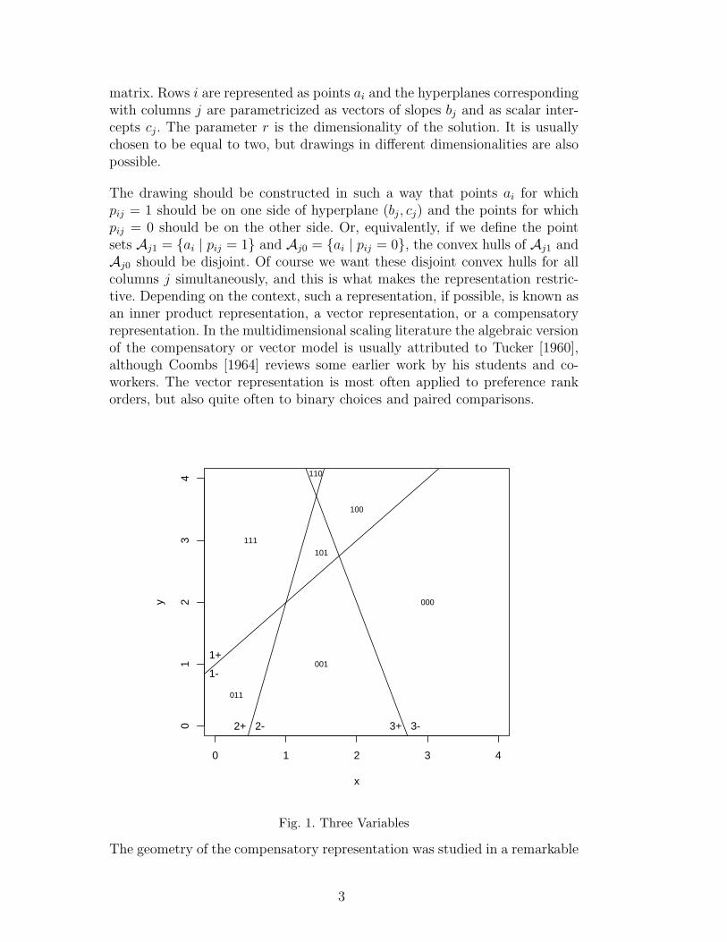
The drawing should be constructed in such a way that points ai for whichpij = 1 should be on one side of hyperplane (bj, cj) and the points for whichpij = 0 should be on the other side. Or, equivalently, if we define the pointsets Aj1 = {ai | pij = 1} and Aj0 = {ai | pij = 0}, the convex hulls of Aj1 andAj0 should be disjoint. Of course we want these disjoint convex hulls for allcolumns j simultaneously, and this is what makes the representation restric-tive. Depending on the context, such a representation, if possible, is known asan inner product representation, a vector representation, or a compensatoryrepresentation. In the multidimensional scaling literature the algebraic versionof the compensatory or vector model is usually attributed to Tucker [1960],although Coombs [1964] reviews some earlier work by his students and co-workers. The vector representation is most often applied to preference rankorders, but also quite often to binary choices and paired comparisons.

0 1 2 3 4

01

23

4

x

y

1+

1−

2+ 2− 3+ 3−

111

101

110

100

000

001

011

Fig. 1. Three Variables

The geometry of the compensatory representation was studied in a remarkable

3

monograph by Coombs and Kao [1955, especially Chapter 5], and the resultsare summarized in Coombs [1964, Chapter 12]. They show that m hyperplanes“in general position” in Rr will partition space into

τ(m, r) =r∑

k=0

(m

k

)

disjoint convex regions. Each region corresponds with a profile, i.e. a vector ofm zeroes and ones. Of the τ(m, r) regions there are 2m “open” regions, whichextend to infinity. Since in most actual data analysis situations n < τ(m, r) wedo not find all possible profiles (for a given set of hyperplanes) in our data, andsince profiles correspond with regions the position of each row point (again, fora given set of hyperplanes) is only partially determined by the data. A small

example, with three variables, is given in Figure 1. We see(

30

)+(

31

)+(

32

)= 7

regions, of which 6 are open. For these three variables, we can obtain perfectfit for any data matrix which does not contain the 010 profile.

The geometry of the compensatory model is different from that of multiplecorrespondence analysis (MCA). In the general form of MCA recently dis-cussed by De Leeuw [2003a] various measures of the size of a cloud of pointsin Rr are considered. Each column j of the data matrix defines a subset ofthe rows, those i for which pij = 1, corresponding to a cloud of points ai inthe drawing. Call them the hit-points. The drawing is then constructed insuch a way that the average over columns of the sizes of these clouds of hit-points is minimized. If cloud size is defined as squared distance to the centroidof the cloud this leads to multiple correspondence analysis [Greenacre, 1984,Gifi, 1990], a technique which is computationally relatively simple, because itrequires computation of just one single SVD. More complicated measures ofcloud size lead to more complicated optimization problems.

Thus in MCA we are satisfied if the clouds are small, not necessarily if theyare linearly separated. Aiming for a small cloud suggests that the hit-pointsare in a small sphere, and the miss-points are outside that sphere. There isa variation of the technique which uses what the French MCA school callsdedoublement. In that case we let the miss-points also define a cloud, andwe try to make both clouds small. This suggests two small disjoint spheres,and thus linear separation, which means that in the case of excellent fit MCAand the technique in this paper will be close. The difference between MCAwith and without dedoublement can be made more precise by using classicaltheorems of Guttman and Mosteller [De Leeuw, 2003a].

In algebraic terms, we want to find a solution to the system of strict inequalities

4

〈ai, bj〉 > cj ∀pij = 1, (1a)

〈ai, bj〉 < cj ∀pij = 0, (1b)

where 〈ai, bj〉 is the inner product of ai and bj. Coombs and Kao [1955] give asimple pencil-and-paper procedure to solve these inequalities in the case r = 2,assuming that such a solution actually exists.

In general the system of inequalities defined by the data will not have a perfectsolution. We have to find an approximate solution which is as good as possible,in the sense that it minimizes some loss function. Some simplifications areuseful before we discuss the loss function we use. By defining qij = 2pij − 1,i.e. qij = −1 if pij = 0 and qij = +1 if pij = 1, we can write the system in themore compact form qij(〈ai, bj〉−cj) > 0. By appending cj to bj and appending−1 to ai we can even write qij(〈ai, bj〉) > 0, where ai and bj now have r + 1elements. We collect them in an n × (r + 1) matrix of row scores A and inan m × (r + 1) matrix of column scores B. Now we can use the Hadamardproduct to rewrite our inequalities as Q ? AB′ > 0.

We fit a predicted matrix Π = {πij} to the observed binary data matrix P ={pij}. The predicted matrix Π is a function of A and B. More specifically, wedefine πij(A, B) = F (〈ai, bj〉, where F is some cumulative distribution functionsuch as the normal or logistic. Our computational problem is to minimize thedistance between P and Π(A, B) over (A, B), where distance is measured bythe loss function

D(A, B) = −n∑

i=1

m∑j=1

[pij log πij(A, B) + (1− pij) log(1− πij(A, B))]. (2a)

The distance interpretation comes from the fact that D(A, B) ≥ 0 with equal-ity if and only if pij = πij(A, B) for all i and j. Remember that we require thatthe last column of A has all elements equal to −1. If we drop this restriction,we still fit separating hyperplanes, but they are now located in Rr+1 and mustpass through the origin.

By assuming symmetry of F , i.e. F (−x) = 1 − F (x) for all x, and by usingthe fact that the pij are binary, we can also write

D(A, B) = −n∑

i=1

m∑j=1

log F (qij〈ai, bj〉). (2b)

The usual way to motivate loss function (2) is to assume that the pij areoutcomes of independent Bernoulli trials with probability of success πij =F (〈ai, bj〉). Then D is the negative log-likelihood, and minimizing D produces

5

maximum likelihood estimates. We do not emphasize this interpretation, sincewe do not think it is a realistic representation of actual data generating pro-cesses in any of the situations we are familiar with. Nevertheless, if you areso inclined, you can think of our computed points and lines as maximum like-lihood estimates. In any case, our loss function is a suitable way to measuredistance between the observed and expected frequencies, or, alternatively, ameasure how well the system of inequalities (1) is satisfied.

It is easy to see that if the system (1) has a solution, then minimizing D willfind it, and the minimum of D in that case will be zero. Conversely, we canonly make D converge to zero by letting (A, B) converge to a solution of (1).In fact what minimizing D is trying to achieve is

〈ai, bj〉 → ∞ ∀pij = 1, (3a)

〈ai, bj〉 → −∞ ∀pij = 0, (3b)

although it will generally not succeed in its goal. It can only do it perfectly ifthe system (1) is solvable. Using the analysis of Coombs and Kao [1955] we canmake these statements more precise. Of the 1

2(m2 + m + 2) regions defined by

m hyperplanes in two-space, there are 2m unbounded regions. All row pointsa in such an unbounded region will have the same profile, and moving themto infinity along the direction of recession of the region will make D smaller.

Define a matrix Λ with elements λij = F−1(πij). Then, we can write the basicrelationship we have to fit as Λ ≈ AB′. This expression shows that we aredealing with a rank r approximation problem of our data matrix on the F−1

scale, a problem that is solved by principal component analysis (PCA) or,equivalently, singular value decomposition (SVD), in the linear case in whichΛ is observed directly.

3 Algorithm

We develop a majorization algorithm for minimzing (2), based on boundingthe second derivative of the likelihood function. General information aboutmajorization algorithms is in De Leeuw [1994], Heiser [1995], Lange et al.[2000]. Majorization by bounding the second derivative is discussed in detailin Bohning and Lindsay [1988]. In the computer science literature majorizationis known as the variational method, or variational bounding [Jaakkola andJordan, 2000].

So far we have only assumed that the cdf F is symmetric. We now make an

6

additional assumption. Define the hazard function

h(x)∆=−d log F (x)

dx,

and assume there exists a function w ≥ 0 such that

− log F (x) ≤ − log F (y) + h(y)(x− y) +1

2w(y)(x− y)2 (4)

for all x and y. We say that w provides a quadratic majorization of log F . If wecan choose w(y) to be a constant, say w, then w provides a uniform quadraticmajorization. In Appendix A, we show that for uniform majorization of thelogistic cdf

w(y) ≡ 1

4,

for non-uniform majorization of the logistic cdf

w(y) =1− 2F (y)

2y,

and for uniform majorization of the normal cdf

w(y) ≡ 1.

The majorization of − log F can now be used to find a quadratic majorizationof the negative log-likelihood.

Theorem 1 Suppose A and A are n× p matrices of row scores and B and B

are m×p matrices of column scores. Define the n×m matrices wij∆= w(qij〈ai, bj〉),

hij∆= h(qij〈ai, bj〉), and zij

∆=〈ai, bj〉 − qij

hij

wij. Then

D(A, B) ≤ D(A, B)− 1

2

n∑i=1

m∑j=1

h2ij

wij

+1

2

n∑i=1

m∑j=1

wij(〈ai, bj〉 − zij)2.

PROOF. By completing the square we can also write (4) as

− log F (x) ≤ − log F (y) +1

2w(y)(x− (y − h(y)

w(y)))2 − 1

2

h2(y)

w(y). (6)

Now substitute qij〈ai, bj〉 for x and qij〈ai, bj〉 for y. Then

− log F (qij〈ai, bj〉) ≤ − log F (qij〈ai, bj〉)−1

2

h2(qij〈ai, bj〉)w(qij〈ai, bj〉)

+

+1

2w(qij〈ai, bj〉)(〈ai, bj〉 − (〈ai, bj〉 − qij

h(qij〈ai, bj〉)w(qij〈ai, bj〉)

))2. (7)

7

Sum over i and j to obtain the required result.

The algorithm works as follows. Start with some A(0) and B(0). Suppose A(k)

and B(k) are the current best solution. We update them to find a better solu-tion in two steps, similar to the E-step and the M-step in the EM-algorithm.

Algorithm 1 (Majorization)

Step k(1) Compute the matrices W (k), H(k)and Z(k) with elements

w(k)ij = w(qij〈a

(k)i , b

(k)j 〉),

h(k)ij = h(qij〈a

(k)i , b

(k)j 〉),

z(k)ij = 〈a(k)

i , b(k)j 〉 − qij

h(k)ij

w(k)ij

.

Step k(2) Solve the least squares matrix approximation problem

minA,B

n∑i=1

n∑j=1

w(k)ij (z

(k)ij − 〈ai, bj〉)2

by using the (weighted) SVD.

Theorem 2 The Majorization Algorithm 1 produces a decreasing sequenceD(A(k), B(k)) of loss function values, and all accumulation points of the se-quence (A(k), B(k)) of iterates are stationary points.

PROOF. This follows by applying general results on majorization algorithmsto Theorem 1.

4 Implementation Details

In the logistic case, we can choose if we want to use uniform on non-uniformmajorization. If we use uniform majorization, then the substeps of the algo-rithm are unweighted SVD’s. In an interpreted matrix language such as Ror Matlab the SVD is usually implemented in object code in a very efficientmanner, and consequently using uniform majorization seems a sensible choice.If we use non-uniform majorization we either have to write interpreted codefor the substeps, or we have to apply majorization a second time to approx-imate the weighted SVD by an unweighted one [Kiers, 1997, Groenen et al.,

8

2003]. This last strategy basically means we are using uniform majorizationin a roundabout way.

In our implementations of the algorithm so far, in the R language, we have al-ways chosen uniform approximation. This is mainly to avoid using interpretedcode as much as possible. Versions of the algorithm written in a compiled lan-guage such as C or FORTRAN could very well benefit from the more precisenon-uniform majorization. But even in the compiled case customized iterativemethods will probably have a hard time beating highly optimized SVD libraryroutines.

In our R implementation, the initial estimate for A and B is simply taken aszero. This start is obviously not a good one, and we may get some improvementby using MCA instead. But we have to remember that the SVD majorizationalgorithm converges very fast in the initial steps, and then slows down to itslinear (or even sublinear) rate, so the improvements of a very good start willpresumably be not very large.

Also observe that starting with A and B equal to zero means that the firstiteration computes the singular value decomposition of a matrix zij with ele-ment pij − 1

2. This will be often be close to the MCA solution, because MCA

also computes a singular value decomposition of a matrix of weighted andcentered pij.

If there are missing data then the matrix approximation problem becomes

minX,Y

∑{(z(k)

ij − 〈ai, bj〉)2 | (i, j) ∈ N},

where N is the subset of non-missing index pairs. We now use the classi-cal least squares augmentation trick, used in non-balanced ANOVA by Yatesand Wilkinson and in least squares factor analysis by Thomson and Harman.See De Leeuw [1994], De Leeuw and Michailidis [1999] for references and forfurther discussion of augmentation.

We define inner iterations in each iteration of our majorization algorithm toimpute the missing data. The inner iterations start with a

(k,0)i = a

(k)i and

b(k,0)j = b

(k)j .

z(k,`) =

z(k)ij if (i, j) ∈ N,

〈a(k,`)i , b

(k,`)j 〉 if (i, j) 6∈ N.

We then do an SVD to find A(k,`+1) and B(k,`+1), and continue the inner it-erations. Actually, in our R implementation we only perform a single inneriteration, which basically means that we always perform a singular value de-composition on Z(k,0) which is just our previous Z(k) with missing elementsimputed by setting them to the corresponding elements of the product of A(k)

and B(k).

9

It may not always be a good idea to do a complete SVD after computing a newZ or Z, even if we use an SVD algorithm that only computes p singular vectors.This will depend, again, on the precise nature of the computing environment,the uniformity of the majorization, and the restrictions on the parameters.

We could use an iterative SVD method such as the simultaneous iterationmethod proposed by Daugavet [1968], and perhaps more familiar as the NILES/NIPALSmethod [Wold, 1966a,b]. Only perform one or a small number of innermostiterations before updating H. This may ultimately lead to fewer computations.

Each NIPALS iteration

X ← HY (Y ′Y )−1,

Y ← H ′X(X ′X)−1,

basically requires two matrix multiplications, so even for big matrices it isquite inexpensive. To identify along the way, the iterations are typically im-plemented as

X ← orth(HY ),

Y ← H ′X,

where orth is an orthogonalization method such as Gram-Schmidt or QR. Thismakes the method identical to the Bauer-Rutishauser simultaneous iterationmethod, used in a similar context by Gifi [1990, page 98-99].

If an iterative SVD method is implemented, then we have to distinguish theouter iterations of the majorization algorithm, the inner iterations of the aug-mentation method to impute missing values, and the innermost iterations tocompute or improve the SVD. The number of inner and innermost iterationswill influence the amount of computation in an outer iteration and the con-vergence speed of the algortithm.

There is another straightforward block relaxation algorithm that can be usedto complement (or replace) our majorization technique. If we fix A at itscurrent value, then optimizing over bj is a straightforward logit or probit re-gression problem. Thus one cycle consists of solving n + m small logit orprobit regression problems, which are convex minimization problems with astraightforward globally convergent Newton-Raphson implementation. This isthe criss-cross regression algorithm used by researchers in generalized bilin-ear modeling [de Falguerolles and Francis, 1992, Gabriel, 1998, Van Eeuwijk,1995]. It has also been suggested by Poole [2001] for roll call analysis usingthe normal F .

In computer science, the work of Collins et al. [2002] extends PCA to theexponential family, using the fact that finding the optimal A for fixed B and

10

finding the optimal B for fixed A are generalized linear model regression prob-lems. Their development thus extends easily to Poisson and gamma versionsof PCA. Schein et al. [2003] combine the ideas in Tipping [1999] and Collinset al. [2002] in the logistic case. Thus they used fixed row scores ai and thenon-uniform majorization of the logistic cdf. The algorithm then uses blockrelaxation to optimize over blocks A and B.

From the theoretical point of view, this alternative algorithm uses more andsmaller blocks and will probably be slower and more likely to end up in anon-global minimum. On the other hand no majorization is involved and theNewton iterations will tend to be very precise and fast. It may be that thisblock regression algorithm can be used to refine the result of the majorizationalgorithm, but more research is necessary to compare the two.

5 Application Areas

In this section we try to give an overview of the various contexts in whichthe technique we discuss in this paper has occurred previously. As we shallsee, the history is complicated, because different areas of statistics and dataanalysis are not necessarily aware of each other’s work.

The multivariate compensatory model has been used for a long time in itemresponse theory (IRT). The logistic version, for example, has been studiedby Reckase [1997].

The main distinction we want to make in this section, however, is betweenfixed score and random score models, basically the same distinction as is madein factor analysis [Anderson and Rubin, 1956]. In fixed score models (whichwe have discussed so far) each row gets a parameter vector ai, and these“incidental” parameters are estimated along with the column parameters bj.In random score models rows are sampled from some distribution G, and therow parameters can be integrated out of the likelihood. Random score modelsare better behaved from a statistical point of view, but seems less appropriatein areas such as roll call analysis in which row parameters (legislator idealpoints) are really more interesting than column parameters (roll calls).

In Lawley [1944] a random score normal ogive model for the factor analysis ofbinary matrices was first proposed. Some other key references are the booksby Lord and Novick [1968, Chapter 16], Bartholomew [1987, Chapters 5 and6] and the articles by Takane and Leeuw [1987], Bock et al. [1988], McDonald[1997].

We can extend our majorization methods to optimize likelihood for random

11

score models. More work remains to be done on implementation in this case,but as Jaakkola and Jordan [2000] observe it allows us to replace MCMC [Mengand Schilling, 1996, Beguin and Glas, 2001] and other delicate approxima-tions [Bock et al., 1988, Bock and Schilling, 1997] by monotonically convergingmajorization algorithms.

There have been interesting recent related developments in multidimensionalroll call analysis. Let us first outline the basic way of thinking in the field [Clin-ton et al., 2003]. We work in Rr. Each legislator has an ideal point ai in thisspace and each roll call has both a yes-point uj and a no-point vj.

The utlities for legislator i to vote “yes” or “no” on roll call j have both a fixedand a random component. The fixed component is quadratic, that is squareddistance. Thus

ξ1ij

= −1

2‖ai − uj‖2 + ε1

ij,

ξ0

ij= −1

2‖ai − vj‖2 + ε0

ij.

This means that the legislator will vote “yes” if ξ1ij

> ξ0ij, i.e. if

〈ai, uj − vj〉 − cj > −(ε1ij − ε0

ij),

where cj = 12(‖uj‖2 − ‖vj‖2). If F is the cumulative probability distribution

of −(ε1ij − ε0

ij), then πij, the probability that legislator i will vote “yes” on rollcall j is simply F{〈ai, uj − vj〉− cj}, which is precisely the binary PCA repre-sentation we have studied so far. An identification analysis, using the secondderivatives of the likelihood function, has been published by Rivers [2003].There are also random legislator versions of this model [Bailey, 2001], and,similar to IRT, the field has been caught in the maelstrom of MCMC [Jack-man, 2000, 2001].

Both IRT and roll-call analysis are special cases of binary choice problems.There are many probabilistic version of the compensatory model for prefer-ential choice, which are reviewed very ably in Bockenholt and Gaul [1986]or Takane [1987]. We can use the utility formulation of the roll-call models toderive the paired comparison model in which individual i prefers j to `, whichwe also write as j >i `, if prob(j >i `) = F (〈ai, bj − b`〉). Applying majoriza-tion to this representation allows us to iteratively apply the constrained PCAtechniques of Takane and Hunter [2001], where we constrain the scores of pair(j, `) to be of the form bj − b`.

12

6 Examples

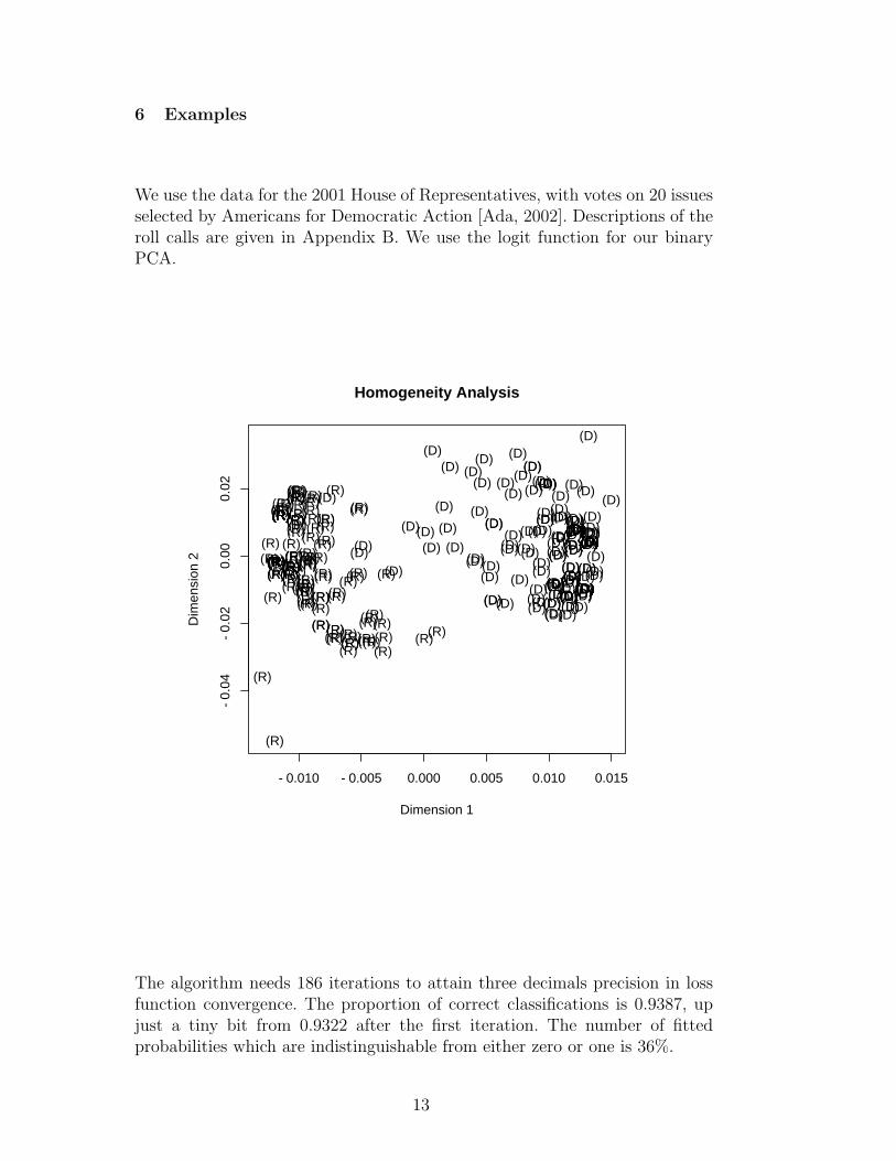
We use the data for the 2001 House of Representatives, with votes on 20 issuesselected by Americans for Democratic Action [Ada, 2002]. Descriptions of theroll calls are given in Appendix B. We use the logit function for our binaryPCA.

−0.010 −0.005 0.000 0.005 0.010 0.015

−0.

04−

0.02

0.00

0.02

Homogeneity Analysis

Dimension 1

Dim

ensi

on 2 (D)

(D)

(R)

(R)

(D)(D)

(R)

(D)

(R)

(D)

(R)

(D)(D)

(R)

(D)

(R)

(D)

(R)(R)

(R)

(D)

(D)

(R)

(D)

(D)

(D)

(R)

(R)

(D)

(D) (D)(R)

(R)

(R)(R)

(D)

(R)

(R)

(D)

(D)(D)

(D)

(D)

(R)

(D)(D)

(R)(R)

(R)(R)

(R)(R)(R)(R)(R)(R)

(R)

(D)

(D)(D)(D)

(D)(R)

(R)(R)

(D)(D)

(D)(D)

(R)(R)

(R)(D)

(D)(R)

(D)

(R)

(D)(D)(R)(R) (D)

(R)

(R)

(D)

(R)(D)

(D)(D)(R)

(R)

(D)

(D)(D)

(R)(R)

(R)

(D)

(D)

(R)

(D)

(D)

(D)(D)

(R)

(D)

(R)

(R)

(R)

(D)(R)

(R)(R)

(D)

(R) (D)(D)

(D)

(R)

(D)

(D)

(R) (D)(R)

(R)

(R)

(R)

(D)

(R)

(D)

(R)

(D)

(R)(R)(R)

(D)

(R)

(R)

(R)

(R)(D)

(I)

(R)(D)

(R)

(R)

(R)(R)

(D)

(R)

(R)

(R)

(D)

(R)

(D)

(D)

(R)

(D)

(R)

(R)

(D)

(R)

(R)(R)(R)

(R)

(D)

(R) (D)

(D)

(D)

(R) (D)(R)

(D)

(D)(D)(D)

(R)

(R)

(R)

(D)(R)

(R)

(R)

(R)

(D)(R)

(D)(R)

(R)(D)(D)

(D)

(R)(D)

(D)

(R)

(R)(R)

(D)

(R)

(D)(D)

(R)

(R)

(D)

(R)(R)

(D)

(D)

(D)

(R)(R)

(R)

(D)

(R)

(R)

(D)

(D)

(R)

(R)

(D)

(D)

(D)

(R)

(D)

(D)(R)

(R)

(D)

(D)

(D)

(R)(R)(R)

(D)

(R)

(D)(D)

(D)(R)

(D)

(D)

(D)(D)

(R)

(D)

(D)

(D)(D)(D)(D)

(D)

(R)(D)

(D)

(R)

(R)

(D)

(R)(D)

(D)

(D)(D)

(D)

(D)

(R)

(D)(D)

(R)

(R)

(R)

(D)

(D)(D)

(D)(D)

(R)

(R)

(D)

(R)

(D)

(D)

(D)(R)

(R)

(R)

(R)

(R)

(D)(D)

(D)(D)

(R)

(R)

(R)

(D)

(R)

(D)(D)(D)

(R)

(D)(D)

(R)

(D)

(R) (R)

(D)

(R)

(R)(R)

(R)

(D)(R)

(D)

(R)

(R)

(R)

(R)

(D)

(R)

(D)

(R)

(R)

(D)

(R)

(R)

(D)

(D)

(D)

(R)

(R)

(R)(R)

(D)

(D)

(R)

(D)

(R)

(D)

(R)(R)

(D)(D) (I)(D)

(D)(R)

(R)(R)

(D)

(D)

(R)

(D)(R)

(D)(R)(R)

(R)

(R)

(D)

(R)(R)

(D)

(R)

(R)

(R) (D)(R)

(D)

(D)(D)

(R)

(R)(R)

(D)

(D)

(R)

(R)

(D)

(D)(R)

(D)(D)

(R)

(D)

(R)

(R)

(R)

(D)

(D)

(R)

(D)

(R)

(R)

(R)

(D)

(D)

(R) (R)(D)

(R)(R)

(D)

(R)

(D)(D)

(D)(D)(D)

(R)

(D)(D)

(R)

(R)

(R)

(R)

(D)(R)

(D)

(D)

(R)

(D)(D)

(R)

(R)

(R)

(D)

(R)(R)(R)

(R)

(D)(D)(D)

(R)

(R)

The algorithm needs 186 iterations to attain three decimals precision in lossfunction convergence. The proportion of correct classifications is 0.9387, upjust a tiny bit from 0.9322 after the first iteration. The number of fittedprobabilities which are indistinguishable from either zero or one is 36%.

13

−0.05 0.00 0.05

−0.

25−

0.15

−0.

050.

000.

050.

10

Logistic PCA

Dimension 1

Dim

ensi

on 2

(D)

(D)

(R)

(R)

(D)(D)(R)

(D)(R)

(D)(R)

(D) (D)(R)

(D)(R)

(D)

(R)(R)

(R)

(D)

(D)

(R) (D)

(D)

(D)

(R)

(R)(D)

(D)(D)

(R)

(R)

(R)(R)

(D)

(R)

(R)

(D)

(D)

(D)

(D)

(D)

(R)(D)(D)

(R)(R)

(R)(R)

(R)(R)(R)(R)(R)(R)(R)

(D)

(D) (D) (D)

(D)(R)

(R)(R)(D)(D)

(D)(D)

(R)

(R)

(R) (D)

(D)

(R)

(D)

(R)

(D)(D)(R)(R)

(D)

(R)

(R)(D)

(R)(D)

(D)(D)

(R)

(R)(D)

(D)(D)

(R)

(R)

(R)

(D)(D)

(R)

(D)

(D)

(D)

(D)

(R)

(D)

(R)

(R)

(R)

(D)(R)

(R)

(R)(D)

(R)

(D)

(D)

(D)

(R)

(D)

(D)

(R) (D)(R)(R)

(R)(R)

(D)

(R)(D)

(R)

(D)(R)

(R)(R)

(D)

(R)

(R)

(R)(R)

(D)

(I)

(R)

(D)(R)

(R)

(R)

(R)

(D)

(R)

(R)

(R)(D)

(R)

(D)

(D)

(R)

(D)

(R)

(R)

(D)

(R)

(R)(R)(R)

(R)

(D)

(R)(D) (D)

(D)

(R) (D)(R)

(D)

(D)

(D)(D)

(R)

(R)

(R)

(D)

(R)

(R)

(R)

(R)

(D)

(R)

(D)(R)

(R)(D) (D)

(D)

(R)

(D)

(D)

(R)

(R)(R)

(D)

(R)

(D)(D)

(R)

(R)

(D)

(R)

(R)

(D)

(D)(D)

(R)(R)

(R)

(D)

(R)

(R)

(D)

(D)(R)

(R)

(D)

(D)

(D)(R)

(D)

(D)(R)

(R)

(D)

(D)

(D)

(R)

(R)(R)

(D)(R)

(D)(D)

(D)

(R)

(D)

(D)

(D)(D)

(R)(D)

(D)

(D)

(D)(D)(D)

(D)

(R)(D)(D)

(R)(R)

(D)

(R) (D)(D)

(D)(D)(D)

(D)(R)

(D) (D)

(R)

(R)(R)

(D)(D)

(D)

(D)(D)

(R)

(R)

(D)(R)

(D)

(D)(D)(R)

(R)(R)

(R)

(R)(D)

(D)

(D)(D)

(R)

(R)

(R)(D)(R)

(D)(D) (D)(R) (D)(D)(R)

(D)

(R) (R)

(D)(R)

(R)

(R)

(R)

(D)(R)

(D)

(R)

(R) (R)

(R)

(D)

(R) (D)

(R)

(R)

(D)

(R)

(R)

(D)

(D)(D)

(R)

(R)

(R)(R) (D) (D)

(R)

(D)

(R)

(D)(R)(R)

(D)(D) (I)(D)

(D)

(R)

(R)(R)

(D)

(D)

(R)(D)(R)

(D)

(R) (R)

(R)

(R)

(D)

(R)

(R)

(D)

(R)(R)

(R)(D)

(R) (D)

(D)(D)

(R)

(R)(R)

(D)

(D)(R)(R) (D)(D)

(R)

(D) (D)(R)

(D)

(R)

(R)

(R)

(D)

(D)

(R)

(D)

(R)

(R)

(R)

(D)

(D)(R) (R) (D)(R)(R)

(D)

(R)

(D)(D)

(D)

(D)(D)

(R)

(D)(D)(R)

(R)

(R)(R) (D)

(R)(D)

(D)(R)

(D)(D)

(R)

(R)

(R)(D)

(R)(R)

(R)

(R) (D)(D)(D)

(R)

(R)

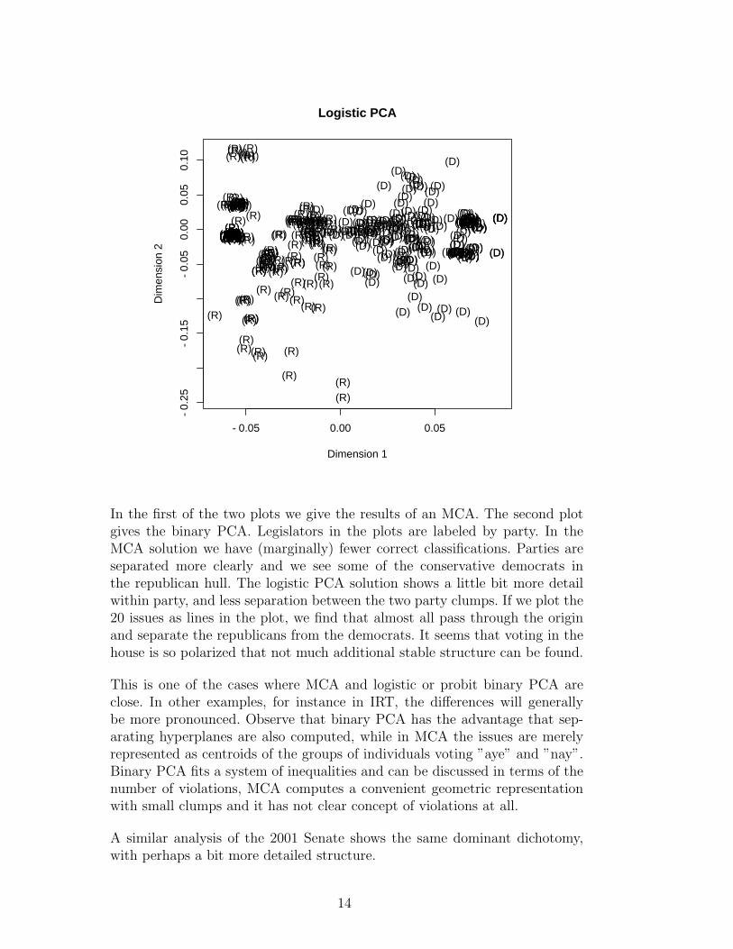
In the first of the two plots we give the results of an MCA. The second plotgives the binary PCA. Legislators in the plots are labeled by party. In theMCA solution we have (marginally) fewer correct classifications. Parties areseparated more clearly and we see some of the conservative democrats inthe republican hull. The logistic PCA solution shows a little bit more detailwithin party, and less separation between the two party clumps. If we plot the20 issues as lines in the plot, we find that almost all pass through the originand separate the republicans from the democrats. It seems that voting in thehouse is so polarized that not much additional stable structure can be found.

This is one of the cases where MCA and logistic or probit binary PCA areclose. In other examples, for instance in IRT, the differences will generallybe more pronounced. Observe that binary PCA has the advantage that sep-arating hyperplanes are also computed, while in MCA the issues are merelyrepresented as centroids of the groups of individuals voting ”aye” and ”nay”.Binary PCA fits a system of inequalities and can be discussed in terms of thenumber of violations, MCA computes a convenient geometric representationwith small clumps and it has not clear concept of violations at all.

A similar analysis of the 2001 Senate shows the same dominant dichotomy,with perhaps a bit more detailed structure.

14

7 Discussion and Conclusions

The logistic (and probit) forms of principal component analysis discussed inthis paper, and the corresponding majorization algorithms, seem to work well.Convergence is fast, and MCA provides a very good starting point. In the ex-amples we have analyzed they do not show great improvements over simplehomogeneity analysis, but this may very well be due to the extreme polariza-tion in US politics. In IRT, for example, it is well known that homogeneityanalysis (which is just a PCA of point correlations) gives results which can bequite different from those of simple logistic models. It will be a useful topic forfurther research to compare the two classes of techniques on different types ofexamples.

There are at least two additional interesting developments in the general ap-proach we have outlined here. Both are currently being tested. In the first weextend the logistic majorization method to general choice and ranking mod-els with multiple alternatives. This gives, for instance, a logistic version ofmultiple correspondence analysis for general sets of indicator matrices. In thesecond development logit and probit majorizations are used, in combinationwith the EM algorithm, to derive algorithms for random score versions of thevarious choice models. Although these new developments are largely untested,they seem to indicate that using quadratic majorization for choice models al-lows us to construct a very rich class of techniques. Compared with similarleast squares based techniques, such as the ones in Gifi [1990], they have theadvantage of of maximizing a Bernoulli likelihood and not requiring arbitrarynormalizations. They have the disadvantage of sometimes leading to partiallydegenerate solutions, in which points are moved to infinity to improve the fit.

8 Acknowledgments

Comments by George Michailides, Coen Bernaards, Doug Rivers, Yoshio Takane,Patrick Groenen, Jeff Lewis, Ulf Bockenholt and two anonymous reviewers onprevious versions of this paper have been very helpful.

15

A Logit and probit Bounds

A.1 The Logit Case

We first derive a result familiar from Bohning and Lindsay [1988], Lange et al.[2000]. Define

f(x) = −p log Ψ(x)− (1− p) log(1−Ψ(x)) = − log Ψ(qx),

where q = 2p− 1 and

Ψ(x) =1

1 + exp(−x).

Theorem 3 f is strictly convex on (0, 1) and has a uniformly bounded secondderivative satisfying 0 < f ′′(x) < 1

4.

PROOF. Simple calculation gives

f ′(x) = q(Ψ(qx)− 1),

f ′′(x) = Ψ(x)(1−Ψ(x)).

Clearly

0 < f ′′(x) <1

4for all 0 < x < 1, which is all we need.

This result can be improved by using a non-uniform bound due, independently,to Jaakkola and Jordan [2000] and Groenen et al. [2003]. The following resultshows the non-uniform bound is, in fact, sharper than the uniform one.

Theorem 4

log Ψ(x) ≥ log Ψ(y) + (1−Ψ(y))(x− y) +1− 2Ψ(y)

4y(x− y)2

≥ log Ψ(y) + (1−Ψ(y))(x− y)− 1

8(x− y)2.

PROOF. Let

f(x) = log Ψ(√

x)−√

x

2.

Then f is convex on x ≥ 0 and

f ′(x) =1− 2Ψ(

√x)

4√

x.

16

Convexity implies f(x) ≥ f(y) + f ′(y)(x− y), i.e.

log Ψ(√

x)−√

x

2≥ log Ψ(

√y)−

√y

2+

1− 2Ψ(√

y)

4√

y(x− y).

Collecting terms and changing variables gives

log Ψ(x) ≥ log Ψ(y) +x− y

2+

1− 2Ψ(y)

4y(x2 − y2),

which is, after some additional manipulation, the first inequality in the theo-rem.

The second inequality follows by a simple application of the mean value the-orem.

1− 2Ψ(y)

4y=

Ψ(−y)−Ψ(y)

4y=−2Ψ(ξ)(1−Ψ(ξ))y

4y=

= −1

2Ψ(ξ)(1−Ψ(ξ)) ≥ −1

8.

In Groenen et al. [2003] the authors look for a quadratic majorization of theform

log Ψ(x) ≥ log Ψ(y) + (1−Ψ(y))(x− y) + a(y)(x− y)2.

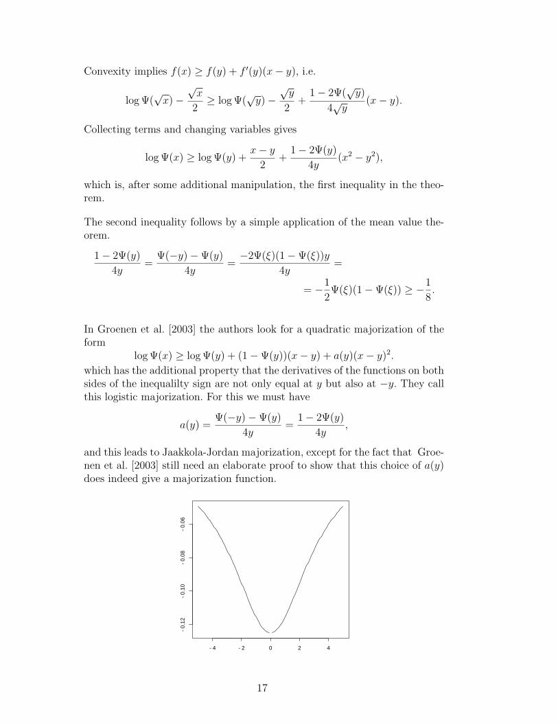
which has the additional property that the derivatives of the functions on bothsides of the inequalilty sign are not only equal at y but also at −y. They callthis logistic majorization. For this we must have

a(y) =Ψ(−y)−Ψ(y)

4y=

1− 2Ψ(y)

4y,

and this leads to Jaakkola-Jordan majorization, except for the fact that Groe-nen et al. [2003] still need an elaborate proof to show that this choice of a(y)does indeed give a majorization function.

−4 −2 0 2 4

−0.

12−

0.10

−0.

08−

0.06

x

boun

d (x

)

17

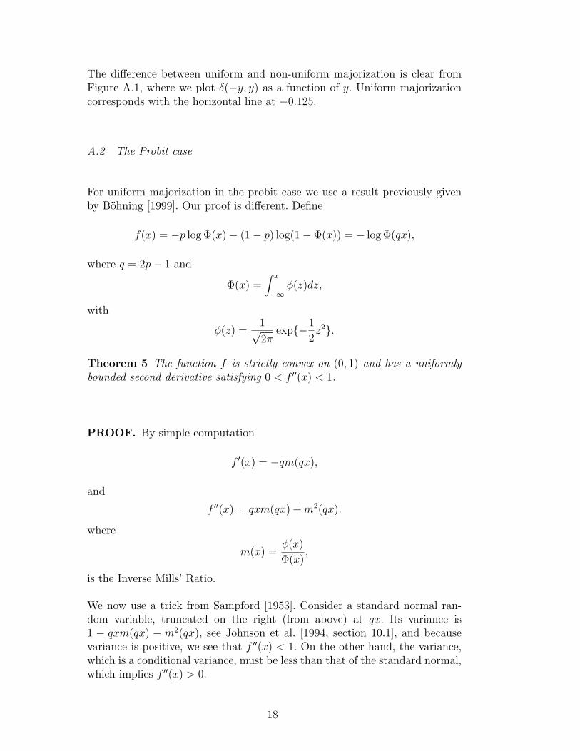
The difference between uniform and non-uniform majorization is clear fromFigure A.1, where we plot δ(−y, y) as a function of y. Uniform majorizationcorresponds with the horizontal line at −0.125.

A.2 The Probit case

For uniform majorization in the probit case we use a result previously givenby Bohning [1999]. Our proof is different. Define

f(x) = −p log Φ(x)− (1− p) log(1− Φ(x)) = − log Φ(qx),

where q = 2p− 1 and

Φ(x) =∫ x

−∞φ(z)dz,

with

φ(z) =1√2π

exp{−1

2z2}.

Theorem 5 The function f is strictly convex on (0, 1) and has a uniformlybounded second derivative satisfying 0 < f ′′(x) < 1.

PROOF. By simple computation

f ′(x) = −qm(qx),

and

f ′′(x) = qxm(qx) + m2(qx).

where

m(x) =φ(x)

Φ(x),

is the Inverse Mills’ Ratio.

We now use a trick from Sampford [1953]. Consider a standard normal ran-dom variable, truncated on the right (from above) at qx. Its variance is1 − qxm(qx) − m2(qx), see Johnson et al. [1994, section 10.1], and becausevariance is positive, we see that f ′′(x) < 1. On the other hand, the variance,which is a conditional variance, must be less than that of the standard normal,which implies f ′′(x) > 0.

18

A.3 Sharpest Quadratic majorization

The sharpest quadratic majorization [De Leeuw, 2003b] is obtained by defining

δ(x, y) =f(x)− f(y)− f ′(y)(x− y)

(x− y)2,

and then choosing the coefficient of the quadratic term in the majorization

f(x) ≥ f(y) + f ′(y)(x− y) + a(y)(x− y)2

as

a(y) = infx 6=y

δ(x, y).

In the logit case we know, from Theorem 4 that

δ(x, y) ≥ 1− 2Ψ(y)

4y,

and, from the proof, we have equality if and only if x2 = y2. Thus

infx 6=y

δ(x, y) = δ(−y, y) =1− 2Ψ(y)

4y,

and Jaakkola-Jordan majorization is sharp.

In the probit case (we conjecture that) δ(x, y) is increasing in x, and

infx6=y

δ(x, y) = limx→−∞

δ(x, y) = −1

2,

and uniform majorization is sharp.

19

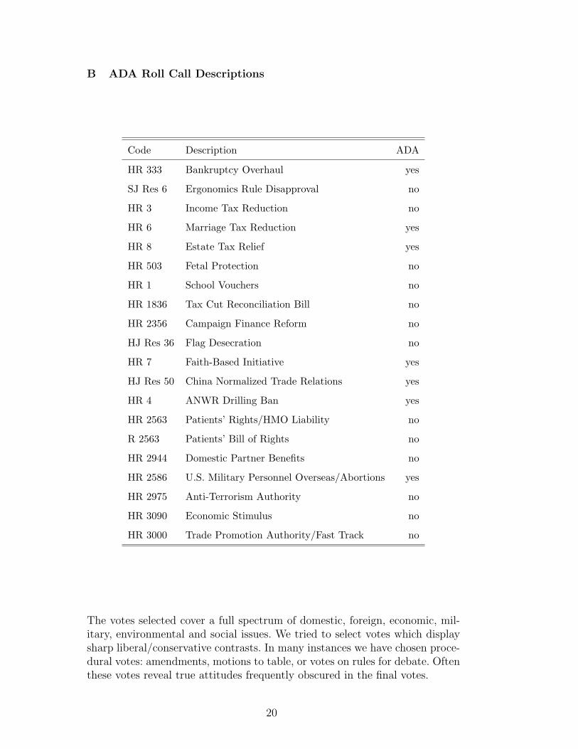
B ADA Roll Call Descriptions

Code Description ADA

HR 333 Bankruptcy Overhaul yes

SJ Res 6 Ergonomics Rule Disapproval no

HR 3 Income Tax Reduction no

HR 6 Marriage Tax Reduction yes

HR 8 Estate Tax Relief yes

HR 503 Fetal Protection no

HR 1 School Vouchers no

HR 1836 Tax Cut Reconciliation Bill no

HR 2356 Campaign Finance Reform no

HJ Res 36 Flag Desecration no

HR 7 Faith-Based Initiative yes

HJ Res 50 China Normalized Trade Relations yes

HR 4 ANWR Drilling Ban yes

HR 2563 Patients’ Rights/HMO Liability no

R 2563 Patients’ Bill of Rights no

HR 2944 Domestic Partner Benefits no

HR 2586 U.S. Military Personnel Overseas/Abortions yes

HR 2975 Anti-Terrorism Authority no

HR 3090 Economic Stimulus no

HR 3000 Trade Promotion Authority/Fast Track no

The votes selected cover a full spectrum of domestic, foreign, economic, mil-itary, environmental and social issues. We tried to select votes which displaysharp liberal/conservative contrasts. In many instances we have chosen proce-dural votes: amendments, motions to table, or votes on rules for debate. Oftenthese votes reveal true attitudes frequently obscured in the final votes.

20

References

Ada. 2001 Voting Record: Shattered Promise of Liberal Progress. ADA Today,57(1):1–17, March 2002.

T.W. Anderson and H. Rubin. Statistical inference in factor analysis. InJ. Neyman, editor, Proceedings of the Third Berkeley Symposium on Math-ematical Statistics and Probability, Volume 5, pages 111–150. University ofCalifornia Press, 1956.

M. Bailey. Ideal Point Estimation with a Small Number of Votes: A Random-Effects Approach. Political Analysis, 9(3):192–210, 2001.

D.J. Bartholomew. Latent Variable Models and Factor Analysis. Griffin, 1987.A.A. Beguin and C.W. Glas. MCMC Estimation and some Model-fit Analysis

of Multidimensional IRT Models. Psychometrika, 66:541–562, 2001.R.D. Bock, R. Gibbons, and E. Muraki. Full-information factor analysis.

Applied Psychological Measurement, 12:261–280, 1988.R.D. Bock and S. Schilling. High-Dimensional Full Information Factor Anal-

ysis. In M. Berkane, editor, Latent Cariable Modeling and Applications toCausality. Springer, 1997.

I. Bockenholt and W. Gaul. Analysis of Choice Behaviour via ProbabilisticIdeal Point and Vector Models. Applied Stochastic Models and Data Anal-ysis, 2:209–226, 1986.

D. Bohning. The Lower Bound Method in Probit Regression. ComputationalStatistics and Data Analysis, 30:13–17, 1999.

D. Bohning and B.G. Lindsay. Monotonicity of Quadratic-approximation Al-gorithms. Annals of the Institute of Statistical Mathematics, 40(4):641–663,1988.

J. Clinton, S. Jackman, and D. Rivers. The Statistical Analysis of Roll CallData. URL http://jackman.stanford.edu/papers/masterideal.pdf.2003.

M. Collins, S. Dasgupta, and R.E. Shapire. A generalization of principal com-ponent analysis to the exponential family. Advances in Neural InformationProcessing Systems, 14, 2002.

C. H. Coombs. A Theory of Data. Wiley, 1964.C.H. Coombs and R.C. Kao. Nonmetric Factor Analysis. Engineering Research

Bulletin 38, Engineering Research Institute, University of Michigan, AnnArbor, 1955.

V.A. Daugavet. Variant of the Stepped Exponential Method of Finding Someof the First Characteristics Values of a Symmetric Matrix. USSR Compu-tation and Mathematical Physics, 8(1):212–223, 1968.

A. de Falguerolles and B. Francis. Algorithmic Approaches for Fitting Bi-linear Models. In Y. Dodge and J. Whittaker, editors, COMPSTAT 1992,Heidelberg, Germany, 1992. Physika-Verlag.

J. De Leeuw. Block Relaxation Methods in Statistics. In H.H. Bock, W. Lenski,and M.M. Richter, editors, Information Systems and Data Analysis, Berlin,1994. Springer Verlag.

21

J. De Leeuw. Homogeneity Analysis of Pavings. URLhttp://jackman.stanford.edu/ideal/MeasurementConference/abstracts/homPeig.pdf.August 2003a.

J. De Leeuw. Quadratic Majorization. URLhttp://gifi.stat.ucla.edu/pub/quadmaj.pdf. 2003b.

J. De Leeuw and G. Michailidis. Block Relaxation Algorithms in Statistics.URL http://gifi.stat.ucla.edu/pub/block.pdf. 1999.

K.R. Gabriel. Generalized Bilinear Regression. Biometrika, 85:689–700, 1998.A. Gifi. Nonlinear multivariate analysis. Wiley, Chichester, England, 1990.M.J. Greenacre. Theory and applications of correspondence analysis. Aca-

demic Press, New York, New York, 1984.P.J.F. Groenen, P. Giaquinto, and H.L Kiers. Weighted Majorization Algo-

rithms for Weighted Least Squares Decomposition Models. Technical Re-port EI 2003-09, Econometric Institute, Erasmus University, Rotterdam,Netherlands, 2003.

W.J. Heiser. Convergent Computing by Iterative Majorization: Theory andApplications in Multidimensional Data Analysis. In W.J. Krzanowski,editor, Recent Advanmtages in Descriptive Multivariate Analysis. Oxford:Clarendon Press, 1995.

T.S. Jaakkola and M. I. Jordan. Bayesian parameter estimation via variationalmethods Bayesian Parameter Estimation via Variational Methods. Statisticsand Computing, 10:25–37, 2000.

S. Jackman. Estimation and Inference are Missing Data Problems: UnifyingSocial Science Statistics via Bayesian Simulation. Political Analysis, 8(4):307–332, 2000.

S. Jackman. Multidimensional Analysis of Roll Call Data via Bayesian Simu-lation: Identification, Estimation, Inference, and Model Checking. PoliticalAnalysis, 9(3):227–241, 2001.

N.L. Johnson, S. Kotz, and N. Balakrishnan. Continuous Univariate Distri-butions, Volume I. Wiley, second edition, 1994.

H.A.L. Kiers. Weighted Least Squares Fitting Using Iterative Ordinary LeastSquares Algorithms. Psychometrika, 62:251–266, 1997.

K. Lange, D.R. Hunter, and I. Yang. Optimization Transfer Using SurrogateObjective Functions. Journal of Computational and Graphical Statistics, 9:1–20, 2000.

D.N. Lawley. The Factorial Analysis of Multiple Item tests. Proceedings ofthe Royal Society of Edinburgh, 62-A:74–82, 1944.

F.M. Lord and M.R. Novick. Statistical Theories of Mental Test Scores.Addison-Wesley, 1968.

R.P. McDonald. Normal Ogive Multidimensional Model. In W.J. Van DerLinden and R.K. Hambleton, editors, Handbook of Item Response Theory.Springer, 1997.

X.-L. Meng and S. Schilling. Fitting Full-Information Item Factor AnalysisModels and an Empirical Investigation of Bridge Sampling. Journal of theAmerican Statistical Association, 91:1254–1267, 1996.

22

K.T. Poole. The geometry of multidimensional quadratic utility in models ofparliamentary roll call voting. Political Analysis, 9(3):211–226, 2001.

M.D. Reckase. A Linear Logistic Multidimensional Model. In W.J. Van DerLinden and R.K. Hambleton, editors, Handbook of Item Response Theory.Springer, 1997.

D. Rivers. Identification of multidimensional spatial voting models. URLhttp://jackman.stanford.edu/ideal/MeasurementConference/abstracts/river03.pdf.2003.

M.R. Sampford. Some Inequalities on Mill’s ratio and Related Functions.Annals of Mathematical Statistics, 24:130–132, 1953.

A.I. Schein, L.K. Saul, and L.H. Ungar. A generalized linear modelfor principal component analysis of binary data. In C.M. Bishopand B.J. Frey, editors, Proceedings of the Ninth InternationalWorkshop on Artificial Intelligence and Statistics, 2003. URLhttp://research.microsoft.com/conferences/aistats2003/proceedings/papers.htm.

Y. Takane. Analysis of Covariance Structures and Probabilistic Binary ChoiceData. Communication and Cognition, 20:45–62, 1987.

Y. Takane and M. Hunter. Constrained Principal Components Analysis: AComprehensive Theory. Applicable Algebra in Engineering, Communicationand Computing, 12:391–419, 2001.

Y. Takane and J. De Leeuw. On the relationship between item response theoryand factor analysis of discreticized variables. Psychometrika, 52:393–408,1987.

M. Tipping. Probabilistic Visualization of High-dimensional Binary Data.Advances in Neural Information Processing Systems, 11:592–598, 1999.

L.R. Tucker. Intra-individual and inter-individual multidimensionality. InH. Gulliksen and S. Messick, editors, Psychological Scaling: Theory and Ap-plications. Wiley, 1960.

F.A. Van Eeuwijk. Multiplicative Interaction in Generalized Linear Models.Biometrics, 51:1017–1032, 1995.

H. Wold. Estimation of Principal Components and Related Models by IterativeLeast Squares. In P.R. Krishnaiah, editor, Multivariate Analysis. AcademicPress, 1966a.

H. Wold. Nonlinear Estimation by Iterative Least Squares Procedures. InF.N. David, editor, Research Papers in Statistics. Festschrift for J. Neyman.Wiley, 1966b.

23