principles of distributed computing - eth z
TRANSCRIPT

Principles of
Distributed Computing
Roger [email protected]
Assistant: Christoph Lenzen ([email protected])
Spring 2010

2

Introduction
What is Distributed Computing?
In the last few decades, we have experienced an unprecedented growth in thearea of distributed systems and networks. Distributed computing now encom-passes many of the activities occurring in today’s computer and communicationsworld. Indeed, distributed computing appears in quite diverse application areas:Typical “old school” examples are parallel computers or the Internet. More re-cent application examples of distributed systems include peer-to-peer systems,sensor networks, or multi-core architectures.
These applications have in common that many processors or entities (oftencalled nodes) are active in the system at any moment. The nodes have certaindegrees of freedom: they may have their own hardware, their own code, andsometimes their own independent task. Nevertheless, the nodes may share com-mon resources and information and, in order to solve a problem that concernsseveral—or maybe even all—nodes, coordination is necessary.
Despite these commonalities, a peer-to-peer system, for example, is quitedifferent from a multi-core architecture. Due to such differences, many differ-ent models and parameters are studied in the area of distributed computing.In some systems, the nodes operate synchronously, and in other systems theyoperate asynchronously. There are simple homogeneous systems, and hetero-geneous systems where different types of nodes, potentially with different ca-pabilities, objectives etc., need to interact. There are different communicationtechniques: nodes may communicate by exchanging messages, or by means ofshared memory. Sometimes the communication infrastructure is tailor-made foran application, sometimes one has to work with any given infrastructure. Thenodes in a system sometimes work together to solve a global task, occasionallythe nodes are autonomous agents that have their own agenda and compete forcommon resources. Sometimes the nodes can be assumed to work correctly, attimes they may exhibit failures. In contrast to a single-node system, distributedsystems may still function correctly despite failures as other nodes can take overthe work of the failed nodes. There are different kinds of failures that can beconsidered: nodes may just crash, or they might exhibit an arbitrary, erroneousbehavior, maybe even to a degree where it cannot be distinguished from mali-cious (also known as Byzantine) behavior. It is also possible that the nodes dofollow the rules, however they tweak the parameters to get the most out of thesystem; in other words, the nodes act selfishly.
Apparently, there are many models (and even more combinations of models)that can be studied. We will not discuss them in greater detail now, but simply
3

4
define them when we use them. Towards the end of the course a general pictureshould emerge. Hopefully!
This course introduces the basic principles of distributed computing, high-lighting common themes and techniques. In particular, we study some of thefundamental issues underlying the design of distributed systems:
• Communication: Communication does not come for free; often communi-cation cost dominates the cost of local processing or storage. Sometimeswe even assume that everything but communication is free.
• Coordination: How can you coordinate a distributed system so that itperforms some task efficiently?
• Fault-tolerance: As mentioned above, one major advantage of a distrib-uted system is that even in the presence of failures the system as a wholemay survive.
• Locality: Networks keep growing. Luckily, global information is not alwaysneeded to solve a task, often it is sufficient if nodes talk to their neighbors.In this course, we will address the fundamental question in distributedcomputing whether a local solution is possible for a wide range of problems.
• Parallelism: How fast can you solve a task if you increase your computa-tional power, e.g., by increasing the number of nodes that can share theworkload? How much parallelism is possible for a given problem?
• Symmetry breaking: Sometimes some nodes need to be selected to or-chestrate the computation (and the communication). This is typicallyachieved by a technique called symmetry breaking.
• Synchronization: How can you implement a synchronous algorithm in anasynchronous system?
• Uncertainty: If we need to agree on a single term that fittingly describesthis course, it is probably “uncertainty”. As the whole system is distrib-uted, the nodes cannot know what other nodes are doing at this exactmoment, and the nodes are required to solve the tasks at hand despite thelack of global knowledge.
Finally, there are also a few areas that we will not cover in this course,mostly because these topics have become so important that they deserve andhave their own courses. Examples for such topics are distributed programming,software engineering, and also security and cryptography.
In summary, in this class we explore essential algorithmic ideas and lowerbound techniques, basically the “pearls” of distributed computing and networkalgorithms. We will cover a fresh topic every week.
Have fun!

Chapter 1
Vertex Coloring
1.1 Introduction
Vertex coloring is an infamous graph theory problem. It is also a useful toyexample to see the style of this course already in the first lecture. Vertex coloringdoes have quite a few practical applications, for example in the area of wirelessnetworks where coloring is the foundation of so-called TDMA MAC protocols.Generally speaking, vertex coloring is used as a means to break symmetries, oneof the main themes in distributed computing. In this chapter we will not reallytalk about vertex coloring applications but treat the problem abstractly. At theend of the class you probably learned the fastest (but not constant!) algorithmever! Let us start with some simple definitions and observations.
Problem 1.1 (Vertex Coloring). Given an undirected graph G = (V,E), assigna color cu to each vertex u ∈ V such that the following holds: e = (v, w) ∈E ⇒ cv 6= cw.
Remarks:
• Throughout this course, we use the terms vertex and node interchangeably.
• The application often asks us to use few colors! In a TDMA MAC protocol,for example, less colors immediately imply higher throughput. However,in distributed computing we are often happy with a solution which is sub-optimal. There is a tradeoff between the optimality of a solution (efficacy),and the work/time needed to compute the solution (efficiency).
3
1 2
3
Figure 1.1: 3-colorable graph with a valid coloring.
5

6 CHAPTER 1. VERTEX COLORING
Assumption 1.2 (Node Identifiers). Each node has a unique identifier, e.g.,its IP address. We usually assume that each identifier consists of only log n bitsif the system has n nodes.
Remarks:
• Sometimes we might even assume that the nodes exactly have identifiers1, . . . , n.
• It is easy to see that node identifiers (as defined in Assumption 1.2) solvethe coloring problem 1.1, but not very well (essentially requiring n colors).How many colors are needed at least is a well-studied problem.
Definition 1.3 (Chromatic Number). Given an undirected Graph G = (V,E),the chromatic number χ(G) is the minimum number of colors to solve Problem1.1.
To get a better understanding of the vertex coloring problem, let us first lookat a simple non-distributed (“centralized”) vertex coloring algorithm:
Algorithm 1 Greedy Sequential
1: while ∃ uncolored vertex v do2: color v with the minimal color (number) that does not conflict with the
already colored neighbors3: end while
Definition 1.4 (Degree). The number of neighbors of a vertex v, denoted byδ(v), is called the degree of v. The maximum degree vertex in a graph G definesthe graph degree ∆(G) = ∆.
Theorem 1.5 (Analysis of Algorithm 1). The algorithm is correct and termi-nates in n “steps”. The algorithm uses ∆ + 1 colors.
Proof: Correctness and termination are straightforward. Since each node has atmost ∆ neighbors, there is always at least one color free in the range 1, . . . ,∆+1.Remarks:
• In Definition 1.7 we will see what is meant by “step”.
• For many graphs coloring can be done with much less than ∆ + 1 colors.
• This algorithm is not distributed at all; only one processor is active at atime. Still, maybe we can use the simple idea of Algorithm 1 to define adistributed coloring subroutine that may come in handy later.
Now we are ready to study distributed algorithms for this problem. The fol-lowing procedure can be executed by every vertex v in a distributed coloringalgorithm. The goal of this subroutine is to improve a given initial coloring.

1.1. INTRODUCTION 7
Procedure 2 First FreeRequire: Node Coloring e.g., node IDs as defined in Assumption 1.2
Give v the smallest admissible color i.e., the smallest node color not used byany neighbor
Remarks:
• With this subroutine we have to make sure that two adjacent vertices arenot colored at the same time. Otherwise, the neighbors may at the sametime conclude that some small color c is still available in their neighbor-hood, and then at the same time decide to choose this color c.
Definition 1.6 (Synchronous Distributed Algorithm). In a synchronous al-gorithm, nodes operate in synchronous rounds. In each round, each processorexecutes the following steps:
1. Do some local computation (of reasonable complexity).
2. Send messages to neighbors in graph (of reasonable size).
3. Receive messages (that were sent by neighbors in step 2 of the same round).
Remarks:
• Any other step ordering is fine.
Algorithm 3 Reduce
1: Assume that initially all nodes have ID’s (Assumption 1.2)2: Each node v executes the following code3: node v sends its ID to all neighbors4: node v receives IDs of neighbors5: while node v has an uncolored neighbor with higher ID do6: node v sends “undecided” to all neighbors7: node v receives new decisions from neighbors8: end while9: node v chooses a free color using subroutine First Free (Procedure 2)
10: node v informs all its neighbors about its choice
31
100
5
31
2
5
Figure 1.2: Vertex 100 receives the lowest possible color.

8 CHAPTER 1. VERTEX COLORING
Definition 1.7 (Time Complexity). For synchronous algorithms (as defined in1.6) the time complexity is the number of rounds until the algorithm terminates.
Remarks:
• The algorithm terminates when the last processor has decided to termi-nate.
• To guarantee correctness the procedure requires a legal input (i.e., pairwisedifferent node IDs).
Theorem 1.8 (Analysis of Algorithm 3). Algorithm 3 is correct and has timecomplexity n. The algorithm uses ∆ + 1 colors.
Remarks:
• Quite trivial, but also quite slow.
• However, it seems difficult to come up with a fast algorithm.
• Maybe it’s better to first study a simple special case, a tree, and then gofrom there.
1.2 Coloring Trees
Lemma 1.9. χ(Tree) ≤ 2
Constructive Proof: If the distance of a node to the root is odd (even), colorit 1 (0). An odd node has only even neighbors and vice versa. If we assumethat each node knows its parent (root has no parent) and children in a tree, thisconstructive proof gives a very simple algorithm:
Algorithm 4 Slow Tree Coloring
1: Color the root 0, root sends 0 to its children2: Each node v concurrently executes the following code:3: if node v receives a message x (from parent) then4: node v chooses color cv = 1− x5: node v sends cv to its children (all neighbors except parent)6: end if
Remarks:
• With the proof of Lemma 1.9, Algorithm 4 is correct.
• How can we determine a root in a tree if it is not already given? We willfigure that out later.
• The time complexity of the algorithm is the height of the tree.
• If the root was chosen unfortunately, and the tree has a degenerated topol-ogy, the time complexity may be up to n, the number of nodes.
• Also, this algorithm does not need to be synchronous . . . !

1.2. COLORING TREES 9
Definition 1.10 (Asynchronous Distributed Algorithm). In the asynchronousmodel, algorithms are event driven (“upon receiving message . . . , do . . . ”). Pro-cessors cannot access a global clock. A message sent from one processor toanother will arrive in finite but unbounded time.
Remarks:
• The asynchronous model and the synchronous model (Definition 1.6) arethe cornerstone models in distributed computing. As they do not neces-sarily reflect reality there are several models in between synchronous andasynchronous. However, from a theoretical point of view the synchronousand the asynchronous model are the most interesting ones (because everyother model is in between these extremes).
• Note that in the asynchronous model, messages that take a longer pathmay arrive earlier.
Definition 1.11 (Time Complexity). For asynchronous algorithms (as definedin 1.6) the time complexity is the number of time units from the start of theexecution to its completion in the worst case (every legal input, every executionscenario), assuming that each message has a delay of at most one time unit.
Remarks:
• You cannot use the maximum delay in the algorithm design. In otherwords, the algorithm has to be correct even if there is no such delay upperbound.
Definition 1.12 (Message Complexity). The message complexity of a syn-chronous or asynchronous algorithm is determined by the number of messagesexchanged (again every legal input, every execution scenario).
Theorem 1.13 (Analysis of Algorithm 4). Algorithm 4 is correct. If each nodeknows its parent and its children, the (asynchronous) time complexity is the treeheight which is bounded by the diameter of the tree; the message complexity isn− 1 in a tree with n nodes.
Remarks:
• In this case the asynchronous time complexity is the same as the syn-chronous time complexity.
• Nice trees, e.g. balanced binary trees, have logarithmic height, that is wehave a logarithmic time complexity.
• This algorithm is not very exciting. Can we do better than logarithmic?!?
The following algorithm terminates in log∗ n time. Log-Star?! That’s the num-ber of logarithms (to the base 2) you need to take to get down to at least 2,starting with n:
Definition 1.14 (Log-Star).∀x ≤ 2 : log∗ x := 1 ∀x > 2 : log∗ x := 1 + log∗(log x)

10 CHAPTER 1. VERTEX COLORING
Remarks:
• Log-star is an amazingly slowly growing function. Log-star of all the atomsin the observable universe (estimated to be 1080) is 5! There are functionswhich grow even more slowly, such as the inverse Ackermann function,however, the inverse Ackermann function of all the atoms is 4. So log-starincreases indeed very slowly!
Here is the idea of the algorithm: We start with color labels that have log n bits.In each synchronous round we compute a new label with exponentially smallersize than the previous label, still guaranteeing to have a valid vertex coloring!But how are we going to do that?
Algorithm 5 “6-Color”
1: Assume that initially the vertices are legally colored. Using Assumption 1.2each label only has log n bits
2: The root assigns itself the label 0.3: Each other node v executes the following code (synchronously in parallel)4: send cv to all children5: repeat6: receive cp from parent7: interpret cv and cp as little-endian bit-strings: c(k), . . . , c(1), c(0)8: let i be the smallest index where cv and cp differ9: the new label is i (as bitstring) followed by the bit cv(i) itself
10: send cv to all children11: until cw ∈ 0, . . . , 5 for all nodes w
Example:
Algorithm 5 executed on the following part of a tree:
Grand-parent 0010110000 → 10010 → . . .Parent 1010010000 → 01010 → 111Child 0110010000 → 10001 → 001
Theorem 1.15 (Analysis of Algorithm 5). Algorithm 5 terminates in log∗ ntime.
Proof: A detailed proof is, e.g., in [Peleg 7.3]. In class we do a sketch of theproof.
Remarks:
• Colors 11∗ (in binary notation, i.e., 6 or 7 in decimal notation) will not bechosen, because the node will then do another round. This gives a totalof 6 colors (i.e., colors 0,. . . , 5).
• Can one reduce the number of colors in only constant steps? Note thatalgorithm 3 does not work (since the degree of a node can be much higherthan 6)! For fewer colors we need to have siblings monochromatic!
• Before we explore this problem we should probably have a second look atthe end game of the algorithm, the UNTIL statement. Is this algorithmtruly local?! Let’s discuss!

1.2. COLORING TREES 11
Algorithm 6 Shift Down
1: Root chooses a new (different) color from 0, 1, 22: Each other node v concurrently executes the following code:3: Recolor v with the color of parent
Lemma 1.16 (Analysis of Algorithm 6). Algorithm 6 preserves coloring legality;also siblings are monochromatic.
Now Algorithm 3 (Reduce) can be used to reduce the number of used colorsfrom six to three.
Algorithm 7 Six-2-Three
1: Each node v concurrently executes the following code:2: Run Algorithm 5 for log∗ n rounds.3: for x = 5, 4, 3 do4: Perform subroutine Shift down (Algorithm 6)5: if cv = x then6: choose new color cv ∈ 0, 1, 2 using subroutine First Free (Algorithm
2)7: end if8: end for
Theorem 1.17 (Analysis of Algorithm 7). Algorithm 7 colors a tree with threecolors in time O(log∗ n).
Remarks:
• The term O() used in Theorem 1.15 is called “big O” and is often usedin distributed computing. Roughly speaking, O(f) means “in the order off , ignoring constant factors and smaller additive terms.” More formally,for two functions f and g, it holds that f ∈ O(g) if there are constants x0
and c so that |f(x)| ≤ c|g(x)| for all x ≥ x0. For an elaborate discussionon the big O notation we refer to other introductory math or computerscience classes.
• As one can easily prove, a fast tree-coloring with only 2 colors is morethan exponentially more expensive than coloring with 3 colors. In a treedegenerated to a list, nodes far away need to figure out whether they arean even or odd number of hops away from each other in order to get a2-coloring. To do that one has to send a message to these nodes. Thiscosts time linear in the number of nodes.
• Also other lower bounds have been proved, e.g., any algorithm for 2-coloring the d-regular tree of radius r which runs in time at most 2r/3requires at least Ω(
√d) colors.
• The idea of this algorithm can be generalized, e.g., to a ring topology. Alsoa general graph with constant degree ∆ can be colored with ∆ + 1 colorsin O(log∗ n) time. The idea is as follows: In each step, a node comparesits label to each of its neighbors, constructing a logarithmic difference-tag

12 CHAPTER 1. VERTEX COLORING
Figure 1.3: Possible execution of Algorithm 7.
as in 6-color (Algorithm 5). Then the new label is the concatenation ofall the difference-tags. For constant degree ∆, this gives a 3∆-label inO(log∗ n) steps. Algorithm 3 then reduces the number of colors to ∆ + 1in 23∆ (this is still a constant for constant ∆!) steps.
• Recently, researchers have proposed other methods to break down longID’s for log-star algorithms. With these new techniques, one is able tosolve other problems, e.g., a maximal independent set in bounded growthgraphs in O(log∗ n) time. These techniques go beyond the scope of thiscourse.
• Unfortunately, coloring a general graph is not yet possible with this tech-nique. We will see another technique for that in Chapter 10. With thistechnique it is possible to color a general graph with ∆ + 1 colors inO(log n) time.
• A lower bound by Linial shows that many of these log-star algorithms areasymptotically (up to constant factors) optimal. This lower bound uses aninteresting technique. However, because of the one-topic-per-class policywe cannot look at it today.

Chapter 2
Leader Election
2.1 Anonymous Leader Election
Some algorithms (e.g. the slow tree coloring algorithm 4) ask for a special node,a so-called “leader”. Computing a leader is a most simple form of symmetrybreaking. Algorithms based on leaders do generally not exhibit a high degreeof parallelism, and therefore often suffer from poor time complexity. However,sometimes it is still useful to have a leader to make critical decisions in an easy(though non-distributed!) way.
The process of choosing a leader is known as leader election. Although leaderelection is a simple form of symmetry breaking, there are some remarkable issuesthat allow us to introduce notable computational models.
In this chapter we concentrate on the ring topology. The ring is the “dro-sophila” of distributed computing as many interesting challenges already revealthe root of the problem in the special case of the ring. Paying special attentionto the ring also makes sense from a practical point of view as some real worldsystems are based on a ring topology, e.g., the token ring standard for local areanetworks.
Problem 2.1 (Leader Election). Each node eventually decides whether it is aleader or not, subject to the constraint that there is exactly one leader.
Remarks:
• More formally, nodes are in one of three states: undecided, leader, notleader. Initially every node is in the undecided state. When leaving theundecided state, a node goes into a final state (leader or not leader).
Definition 2.2 (Anonymous). A system is anonymous if nodes do not haveunique identifiers.
Definition 2.3 (Uniform). An algorithm is called uniform if the number ofnodes n is not known to the algorithm (to the nodes, if you wish). If n isknown, the algorithm is called non-uniform.
Whether a leader can be elected in an anonymous system depends on whetherthe network is symmetric (ring, complete graph, complete bipartite graph, etc.)or asymmetric (star, single node with highest degree, etc.). Simplifying slightly,
13
14 CHAPTER 2. LEADER ELECTION
in this context a symmetric graph is a graph in which the extended neighborhoodof each node has the same structure. We will now show that non-uniformanonymous leader election for synchronous rings is impossible. The idea is thatin a ring, symmetry can always be maintained.
Lemma 2.4. After round k of any deterministic algorithm on an anonymousring, each node is in the same state sk.
Proof by induction: All nodes start in the same state. A round in a synchronousalgorithm consists of the three steps sending, receiving, local computation (seeDefinition 1.6). All nodes send the same message(s), receive the same mes-sage(s), do the same local computation, and therefore end up in the same state.
Theorem 2.5 (Anonymous Leader Election). Deterministic leader election inan anonymous ring is impossible.
Proof (with Lemma 2.4): If one node ever decides to become a leader (or anon-leader), then every other node does so as well, contradicting the problemspecification 2.1 for n > 1. This holds for non-uniform algorithms, and thereforealso for uniform algorithms. Furthermore, it holds for synchronous algorithms,and therefore also for asynchronous algorithms.
Remarks:
• Sense of direction is the ability of nodes to distinguish neighbor nodes inan anonymous setting. In a ring, for example, a node can distinguish theclockwise and the counterclockwise neighbor. Sense of direction does nothelp in anonymous leader election.
• Theorem 2.5 also holds for other symmetric network topologies (e.g., com-plete graphs, complete bipartite graphs, . . . ).
• Note that Theorem 2.5 does not hold for randomized algorithms; if nodesare allowed to toss a coin, symmetries can be broken.
2.2 Asynchronous Ring
We first concentrate on the asynchronous model from Definition 1.10. Through-out this section we assume non-anonymity; each node has a unique identifieras proposed in Assumption 1.2. Having ID’s seems to lead to a trivial leaderelection algorithm, as we can simply elect the node with, e.g., the highest ID.
Theorem 2.6 (Analysis of Algorithm 8). Algorithm 8 is correct. The timecomplexity is O(n). The message complexity is O(n2).
Proof: Let node z be the node with the maximum identifier. Node z sendsits identifier in clockwise direction, and since no other node can swallow it,eventually a message will arrive at z containing it. Then z declares itself tobe the leader. Every other node will declare non-leader at the latest whenforwarding message z. Since there are n identifiers in the system, each nodewill at most forward n messages, giving a message complexity of at most n2.We start measuring the time when the first node that “wakes up” sends itsidentifier. For asynchronous time complexity (Definition 1.11) we assume that
2.2. ASYNCHRONOUS RING 15
Algorithm 8 Clockwise
1: Each node v executes the following code:2: v sends a message with its identifier (for simplicity also v) to its clockwise
neighbor. If node v already received a message w with w > v, then nodev can skip this step; if node v receives its first message w with w < v, thennode v will immediately send v.
3: if v receives a message w with w > v then4: v forwards w to its clockwise neighbor5: v decides not to be the leader, if it has not done so already.6: else if v receives its own identifier v then7: v decides to be the leader8: end if
each message takes at most one time unit to arrive at its destination. After atmost n − 1 time units the message therefore arrives at node z, waking z up.Routing the message z around the ring takes at most n time units. Thereforenode z decides no later than at time 2n − 1. Every other node decides beforenode z.
Remarks:
• Note that in Algorithm 8 nodes need to distinguish between clockwiseand counterclockwise neighbors. In fact they do not: It is okay to simplysend your own identifier to any neighbor, and forward a message m to theneighbor you did not receive the message m from. So nodes only need tobe able to distinguish their two neighbors.
• Can we improve this algorithm?
Theorem 2.7 (Analysis of Algorithm 9). Algorithm 9 is correct. The timecomplexity is O(n). The message complexity is O(n log n).
Proof: Correctness is as in Theorem 2.6. The time complexity is O(n) sincethe node with maximum identifier z sends messages with round-trip times2, 4, 8, 16, . . . , 2 · 2k with k ≤ log(n + 1). (Even if we include the additionalwake-up overhead, the time complexity stays linear.) Proving the message com-plexity is slightly harder: if a node v manages to survive round r, no other nodein distance 2r (or less) survives round r. That is, node v is the only node in its2r-neighborhood that remains active in round r + 1. Since this is the same forevery node, less than n/2r nodes are active in round r+1. Being active in roundr costs 2 · 2 · 2r messages. Therefore, round r costs at most 2 · 2 · 2r · n
2r−1 = 8nmessages. Since there are only logarithmic many possible rounds, the messagecomplexity follows immediately.
Remarks:
• This algorithm is asynchronous and uniform as well.
• The question may arise whether one can design an algorithm with an evenlower message complexity. We answer this question in the next section.

16 CHAPTER 2. LEADER ELECTION
Algorithm 9 Radius Growth (For readability we provide pseudo-code only; fora formal version please consult [Attiya/Welch Alg. 3.1])
1: Each node v does the following:2: Initially all nodes are active. all nodes may still become leaders3: Whenever a node v sees a message w with w > v, then v decides to not be
a leader and becomes passive.4: Active nodes search in an exponentially growing neighborhood (clockwise
and counterclockwise) for nodes with higher identifiers, by sending out probemessages. A probe message includes the ID of the original sender, a bitwhether the sender can still become a leader, and a time-to-live number(TTL). The first probe message sent by node v includes a TTL of 1.
5: Nodes (active or passive) receiving a probe message decrement the TTL andforward the message to the next neighbor; if their ID is larger than the onein the message, they set the leader bit to zero, as the probing node doesnot have the maximum ID. If the TTL is zero, probe messages are returnedto the sender using a reply message. The reply message contains the ID ofthe receiver (the original sender of the probe message) and the leader-bit.Reply messages are forwarded by all nodes until they reach the receiver.
6: Upon receiving the reply message: If there was no node with higher IDin the search area (indicated by the bit in the reply message), the TTL isdoubled and two new probe messages are sent (again to the two neighbors).If there was a better candidate in the search area, then the node becomespassive.
7: If a node v receives its own probe message (not a reply) v decides to be theleader.
2.3 Lower Bounds
Lower bounds in distributed computing are often easier than in the standardcentralized (random access machine, RAM) model because one can argue aboutmessages that need to be exchanged. In this section we present a first lowerbound. We show that Algorithm 9 is asymptotically optimal.
Definition 2.8 (Execution). An execution of a distributed algorithm is a list ofevents, sorted by time. An event is a record (time, node, type, message), wheretype is “send” or “receive”.
Remarks:
• We assume throughout this course that no two events happen at exactlythe same time (or one can break ties arbitrarily).
• An execution of an asynchronous algorithm is generally not only deter-mined by the algorithm but also by a “god-like” scheduler. If more thanone message is in transit, the scheduler can choose which one arrives first.
• If two messages are transmitted over the same directed edge, then it issometimes required that the message first transmitted will also be receivedfirst (“FIFO”).
For our lower bound, we assume the following model:

2.3. LOWER BOUNDS 17
• We are given an asynchronous ring, where nodes may wake up at arbitrarytimes (but at the latest when receiving the first message).
• We only accept uniform algorithms where the node with the maximumidentifier can be the leader. Additionally, every node that is not theleader must know the identity of the leader. These two requirements canbe dropped when using a more complicated proof; however, this is beyondthe scope of this course.
• During the proof we will “play god” and specify which message in trans-mission arrives next in the execution. We respect the FIFO conditions forlinks.
Definition 2.9 (Open Schedule). A schedule is an execution chosen by thescheduler. A schedule for a ring is open if there is an open edge in the ring.An open (undirected) edge is an edge where no message traversing the edge hasbeen received so far.
The proof of the lower bound is by induction. First we show the base case:
Lemma 2.10. Given a ring R with two nodes, we can construct an open sched-ule in which at least one message is received. The nodes cannot distinguish thisschedule from one on a larger ring with all other nodes being where the openedge is.
Proof: Let the two nodes be u and v with u < v. Node u must learn theidentity of node v, thus receive at least one message. We stop the execution ofthe algorithm as soon as the first message is received. (If the first message isreceived by v, bad luck for the algorithm!) Then the other edge in the ring (onwhich the received message was not transmitted) is open. Since the algorithmneeds to be uniform, maybe the open edge is not really an edge at all, nobodycan tell. We could use this to glue two rings together, by breaking up thisimaginary open edge and connect two rings by two edges.
Lemma 2.11. By gluing together two rings of size n/2 for which we have openschedules, we can construct an open schedule on a ring of size n. If M(n/2)denotes the number of messages already received in each of these schedules, atleast 2M(n/2) + n/4 messages have to be exchanged in order to solve leaderelection.
Proof by induction: We divide the ring into two sub-rings R1 and R2 of sizen/2. These subrings cannot be distinguished from rings with n/2 nodes if nomessages are received from “outsiders”. We can ensure this by not schedulingsuch messages until we want to. Note that executing both given open scheduleson R1 and R2 “in parallel” is possible because we control not only the schedulingof the messages, but also when nodes wake up. By doing so, we make sure that2M(n/2) messages are sent before the nodes in R1 and R2 learn anything ofeach other!
Without loss of generality, R1 contains the maximum identifier. Hence, eachnode in R2 must learn the identity of the maximum identifier, thus at leastn/2 additional messages must be received. The only problem is that we cannotconnect the two sub-rings with both edges since the new ring needs to remainopen. Thus, only messages over one of the edges can be received. We “play

18 CHAPTER 2. LEADER ELECTION
god” and look into the future: we check what happens when we close only oneof these connecting edges. With the argument that n/2 new messages mustbe received, we know that there is at least one edge that will produce at leastn/4 more messages when being scheduled. This need not to be sent over theclosed link, but because they are caused by a message over this link, they cannotinvolve any message along the other open link in distance n/2. We schedule thisedge and the resulting n/4 messages, and leave the other open.
Lemma 2.12. Any uniform leader election algorithm for asynchronous ringshas at least message complexity M(n) ≥ n
4 (log n + 1).
Proof by induction: For simplicity we assume n being a power of 2. The basecase n = 2 works because of Lemma 2.10 which implies that M(2) ≥ 1 =24 (log 2 + 1). For the induction step, using Lemma 2.11 and the inductionhypothesis we have
M(n) = 2 ·M(n
2
)
+n
4
≥ 2 ·(n
8
(
logn
2+ 1))
+n
4
=n
4log n +
n
4=
n
4(log n + 1) .
2
Remarks:
• To hide the ugly constants we use the “big Omega” notation, the lowerbound equivalent of O(). A function f is in Ω(g) if there are constantsx0 and c > 0 such that |f(x)| ≥ c|g(x)| for all x ≥ x0. Again we referto standard text books for a formal definition. Rewriting Lemma 2.12 weget:
Theorem 2.13 (Asynchronous Leader Election Lower Bound). Any uniformleader election algorithm for asynchronous rings has Ω(n log n) message com-plexity.
2.4 Synchronous Ring
The lower bound relied on delaying messages for a very long time. Since this isimpossible in the synchronous model, we might get a better message complexityin this case. The basic idea is very simple: In the synchronous model, notreceiving a message is information as well! First we make some additionalassumptions:
• We assume that the algorithm is non-uniform (i.e., the ring size n isknown).
• We assume that every node starts at the same time.
• The node with the minimum identifier becomes the leader; identifiers areintegers.

2.4. SYNCHRONOUS RING 19
Algorithm 10 Synchronous Leader Election
1: Each node v concurrently executes the following code:2: The algorithm operates in synchronous phases. Each phase consists of n
time steps. Node v counts phases, starting with 0.3: if phase = v and v did not yet receive a message then4: v decides to be the leader5: v sends the message “v is leader” around the ring6: end if
Remarks:
• Message complexity is indeed n.
• But the time complexity is huge! If m is the minimum identifier it is m ·n.
• The synchronous start and the non-uniformity assumptions can be drop-ped by using a wake-up technique (upon receiving a wake-up message,wake up your clockwise neighbors) and by letting messages travel slowly.
• There are several lower bounds for the synchronous model: comparison-based algorithms or algorithms where the time complexity cannot be afunction of the identifiers have message complexity Ω(n log n) as well.
• In general graphs efficient leader election may be tricky. While time-optimal leader election can be done by parallel flooding-echo (see nextchapter), bounding the message complexity is generally more difficult.

20 CHAPTER 2. LEADER ELECTION

Chapter 3
Tree Algorithms
In this chapter we learn a few basic algorithms on trees, and how to constructtrees in the first place so that we can run these (and other) algorithms. Thegood news is that these algorithms have many applications, the bad news isthat this chapter is a bit on the simple side. But maybe that’s not really badnews?!
3.1 Broadcast
Definition 3.1 (Broadcast). A broadcast operation is initiated by a single pro-cessor, the source. The source wants to send a message to all other nodes inthe system.
Definition 3.2 (Distance, Radius, Diameter). The distance between two nodesu and v in an undirected graph G is the number of hops of a minimum pathbetween u and v. The radius of a node u is the maximum distance between uand any other node in the graph. The radius of a graph is the minimum radiusof any node in the graph. The diameter of a graph is the maximum distancebetween two arbitrary nodes.
Remarks:
• Clearly there is a close relation between the radius R and the diameter Dof a graph, such as R ≤ D ≤ 2R.
• The world is often fascinated by graphs with a small radius. For example,movie fanatics study the who-acted-with-whom-in-the-same-movie graph.For this graph it has long been believed that the actor Kevin Bacon hasa particularly small radius. The number of hops from Bacon even got aname, the Bacon Number. In the meantime, however, it has been shownthat there are “better” centers in the Hollywood universe, such as SeanConnery, Christopher Lee, Rod Steiger, Gene Hackman, or Michael Caine.The center of other social networks has also been explored, Paul Erdos forinstance is well known in the math community.
Theorem 3.3 (Broadcast Lower Bound). The message complexity of broadcastis at least n− 1. The source’s radius is a lower bound for the time complexity.
21

22 CHAPTER 3. TREE ALGORITHMS
Proof: Every node must receive the message.
Remarks:
• You can use a pre-computed spanning tree to do broadcast with tightmessage complexity. If the spanning tree is a breadth-first search spanningtree (for a given source), then the time complexity is tight as well.
Definition 3.4 (Clean). A graph (network) is clean if the nodes do not knowthe topology of the graph.
Theorem 3.5 (Clean Broadcast Lower Bound). For a clean network, the num-ber of edges is a lower bound for the broadcast message complexity.
Proof: If you do not try every edge, you might miss a whole part of the graphbehind it.
Remarks:
• This lower bound proof directly brings us to the well known flooding al-gorithm.
Algorithm 11 Flooding
1: The source (root) sends the message to all neighbors.2: Each other node v upon receiving the message the first time forwards the
message to all (other) neighbors.3: Upon later receiving the message again (over other edges), a node can dis-
card the message.
Remarks:
• If node v receives the message first from node u, then node v calls nodeu parent. This parent relation defines a spanning tree T . If the floodingalgorithm is executed in a synchronous system, then T is a breadth-firstsearch spanning tree (with respect to the root).
• More interestingly, also in asynchronous systems the flooding algorithmterminates after R time units, R being the radius of the source. However,the constructed spanning tree may not be a breadth-first search spanningtree.
3.2 Convergecast
Convergecast is the same as broadcast, just reversed: Instead of a root sendinga message to all other nodes, all other nodes send information to a root. Thesimplest convergecast algorithm is the echo algorithm:

3.3. BFS TREE CONSTRUCTION 23
Algorithm 12 Echo
Require: This algorithm is initiated at the leaves.1: A leave sends a message to its parent.2: If an inner node has received a message from each child, it sends a message
to the parent.
Remarks:
• Usually the echo algorithm is paired with the flooding algorithm, which isused to let the leaves know that they should start the echo process; thisis known as flooding/echo.
• One can use convergecast for termination detection, for example. If a rootwants to know whether all nodes in the system have finished some task, itinitiates a flooding/echo; the message in the echo algorithm then means“This subtree has finished the task.”
• Message complexity of the echo algorithm is n − 1, but together withflooding it is O(m), where m = |E| is the number of edges in the graph.
• The time complexity of the echo algorithm is determined by the depth ofthe spanning tree (i.e., the radius of the root within the tree) generatedby the flooding algorithm.
• The flooding/echo algorithm can do much more than collecting acknowl-edgements from subtrees. One can for instance use it to compute thenumber of nodes in the system, or the maximum ID (for leader election),or the sum of all values stored in the system, or a route-disjoint matching.
• Moreover, by combining results one can compute even fancier aggrega-tions, e.g., with the number of nodes and the sum one can compute theaverage. With the average one can compute the standard deviation. Andso on . . .
3.3 BFS Tree Construction
In synchronous systems the flooding algorithm is a simple yet efficient method toconstruct a breadth-first search (BFS) spanning tree. However, in asynchronoussystems the spanning tree constructed by the flooding algorithm may be far fromBFS. In this section, we implement two classic BFS constructions—Dijkstra andBellman-Ford—as asynchronous algorithms.
We start with the Dijkstra algorithm. The basic idea is to always add the“closest” node to the existing part of the BFS tree. We need to parallelize thisidea by developing the BFS tree layer by layer:
Theorem 3.6 (Analysis of Algorithm 13). The time complexity of Algorithm13 is O(D2), the message complexity is O(m + nD), where D is the diameterof the graph, n the number of nodes, and m the number of edges.
Proof: A broadcast/echo algorithm in Tp needs at most time 2D. Finding newneighbors at the leaves costs 2 time units. Since the BFS tree height is bounded

24 CHAPTER 3. TREE ALGORITHMS
Algorithm 13 Dijkstra BFS
1: The algorithm proceeds in phases. In phase p the nodes with distance p tothe root are detected. Let Tp be the tree in phase p. We start with T1 whichis the root plus all direct neighbors of the root. We start with phase p = 1:
2: repeat3: The root starts phase p by broadcasting “start p” within Tp.4: When receiving “start p” a leaf node u of Tp (that is, a node that was
newly discovered in the last phase) sends a “join p + 1” message to allquiet neighbors. (A neighbor v is quiet if u has not yet “talked” to v.)
5: A node v receiving the first “join p+1” message replies with “ACK” andbecomes a leaf of the tree Tp+1.
6: A node v receiving any further “join” message replies with “NACK”.7: The leaves of Tp collect all the answers of their neighbors; then the leaves
start an echo algorithm back to the root.8: When the echo process terminates at the root, the root increments the
phase9: until there was no new node detected
by the diameter, we have D phases, giving a total time complexity of O(D2).Each node participating in broadcast/echo only receives (broadcasts) at most 1message and sends (echoes) at most once. Since there are D phases, the cost isbounded by O(nD). On each edge there are at most 2 “join” messages. Repliesto a “join” request are answered by 1 “ACK” or “NACK” , which means that wehave at most 4 additional messages per edge. Therefore the message complexityis O(m + nD).
Remarks:
• The time complexity is not very exciting, so let’s try Bellman-Ford!
The basic idea of Bellman-Ford is even simpler, and heavily used in theInternet, as it is a basic version of the omnipresent border gateway protocol(BGP). The idea is to simply keep the distance to the root accurate. If aneighbor has found a better route to the root, a node might also need to updateits distance.
Algorithm 14 Bellman-Ford BFS
1: Each node u stores an integer du which corresponds to the distance from uto the root. Initially droot = 0, and du =∞ for every other node u.
2: The root starts the algorithm by sending “1” to all neighbors.3: if a node u receives a message “y” with y < du from a neighbor v then4: node u sets du := y5: node u sends “y + 1” to all neighbors (except v)6: end if
Theorem 3.7 (Analysis of Algorithm 14). The time complexity of Algorithm14 is O(D), the message complexity is O(nm), where D,n,m are defined as inTheorem 3.6.
Proof: We can prove the time complexity by induction. We claim that a nodeat distance d from the root has received a message “d” by time d. The root
3.4. MST CONSTRUCTION 25
knows by time 0 that it is the root. A node v at distance d has a neighbor uat distance d− 1. Node u by induction sends a message “d” to v at time d− 1or before, which is then received by v at time d or before. Message complexityis easier: A node can reduce its distance at most n − 1 times; each of thesetimes it sends a message to all its neighbors. If all nodes do this we have O(nm)messages.
Remarks:
• Algorithm 13 has the better message complexity and Algorithm 14 has thebetter time complexity. The currently best algorithm (optimizing both)needs O(m + n log3 n) messages and O(D log3 n) time. This “trade-off”algorithm is beyond the scope of this course.
3.4 MST Construction
There are several types of spanning trees, each serving a different purpose. Aparticularly interesting spanning tree is the minimum spanning tree (MST). TheMST only makes sense on weighted graphs, hence in this section we assume thateach edge e is assigned a weight ωe.
Definition 3.8 (MST). Given a weighted graph G = (V,E, ω), the MST of G isa spanning tree T minimizing ω(T ), where ω(G′) =
∑
e∈G′ ωe for any subgraphG′ ⊆ G.
Remarks:
• In the following we assume that no two edges of the graph have the sameweight. This simplifies the problem as it makes the MST unique; however,this simplification is not essential as one can always break ties by addingthe IDs of adjacent vertices to the weight.
• Obviously we are interested in computing the MST in a distributed way.For this we use a well-known lemma:
Definition 3.9 (Blue Edges). Let T be a spanning tree of the weighted graphG and T ′ ⊆ T a subgraph of T (also called a fragment). Edge e = (u, v) is anoutgoing edge of T ′ if u ∈ T ′ and v /∈ T ′ (or vice versa). The minimum weightoutgoing edge b(T ′) is the so-called blue edge of T ′.
Lemma 3.10. For a given weighted graph G (such that no two weights are thesame), let T denote the MST, and T ′ be a fragment of T . Then the blue edgeof T ′ is also part of T , i.e., T ′ ∪ b(T ′) ⊆ T .
Proof: For the sake of contradiction, suppose that in the MST T there is edgee 6= b(T ′) connecting T ′ with the remainder of T . Adding the blue edge b(T ′) tothe MST T we get a cycle including both e and b(T ′). If we remove e from thiscycle we still have a spanning tree, and since by the definition of the blue edgeωe > ωb(T ′), the weight of that new spanning tree is less than than the weightof T . We have a contradiction.

26 CHAPTER 3. TREE ALGORITHMS
Remarks:
• In other words, the blue edges seem to be the key to a distributed al-gorithm for the MST problem. Since every node itself is a fragment ofthe MST, every node directly has a blue edge! All we need to do is togrow these fragments! Essentially this is a distributed version of Kruskal’ssequential algorithm.
• At any given time the nodes of the graph are partitioned into fragments(rooted subtrees of the MST). Each fragment has a root, the ID of thefragment is the ID of its root. Each node knows its parent and its childrenin the fragment. The algorithm operates in phases. At the beginning of aphase, nodes know the IDs of the fragments of their neighbor nodes.
Algorithm 15 GHS (Gallager–Humblet–Spira)
1: Initially each node is the root of its own fragment. We proceed in phases:2: repeat3: All nodes learn the fragment IDs of their neighbors.4: The root of each fragment uses flooding/echo in its fragment to determine
the blue edge b = (u, v) of the fragment.5: The root sends a message to node u; while forwarding the message on the
path from the root to node u all parent-child relations are inverted suchthat u is the new temporary root of the fragment
6: node u sends a merge request over the blue edge b = (u, v).7: if node v also sent a merge request over the same blue edge b = (v, u)
then8: either u or v (whichever has the smaller ID) is the new fragment root9: the blue edge b is directed accordingly
10: else11: node v is the new parent of node u12: end if13: the newly elected root node informs all nodes in its fragment (again using
flooding/echo) about its identity14: until all nodes are in the same fragment (i.e., there is no outgoing edge)
Remarks:
• Algorithm 15 was stated in pseudo-code, with a few details not reallyexplained. For instance, it may be that some fragments are much largerthan others, and because of that some nodes may need to wait for others,e.g., if node u needs to find out whether neighbor v also wants to mergeover the blue edge b = (u, v). The good news is that all these details canbe solved. We can for instance bound the asynchronicity by guaranteeingthat nodes only start the new phase after the last phase is done, similarlyto the phase-technique of Algorithm 13.
Theorem 3.11 (Analysis of Algorithm 15). The time complexity of Algorithm15 is O(n log n), the message complexity is O(m log n).
Proof: Each phase mainly consists of two flooding/echo processes. In general,the cost of flooding/echo on a tree is O(D) time and O(n) messages. However,

3.4. MST CONSTRUCTION 27
the diameter D of the fragments may turn out to be not related to the diameterof the graph because the MST may meander, hence it really is O(n) time. Inaddition, in the first step of each phase, nodes need to learn the fragment ID oftheir neighbors; this can be done in 2 steps but costs O(m) messages. There area few more steps, but they are cheap. Altogether a phase costs O(n) time andO(m) messages. So we only have to figure out the number of phases: Initially allfragments are single nodes and hence have size 1. In a later phase, each fragmentmerges with at least one other fragment, that is, the size of the smallest fragmentat least doubles. In other words, we have at most log n phases. The theoremfollows directly.
Remarks:
• Algorithm 15 is called “GHS” after Gallager, Humblet, and Spira, three pi-oneers in distributed computing. Despite being quite simple the algorithmwon the prestigious Edsger W. Dijkstra Prize in Distributed Computingin 2004, among other reasons because it was one of the first (1983) non-trivial asynchronous distributed algorithms. As such it can be seen as oneof the seeds of this research area.
• We presented a simplified version of GHS. The original paper by Gallageret al. featured an improved message complexity of O(m + n log n).
• In 1987, Awerbuch managed to further improve the GHS algorithm to getO(n) time and O(m + n log n) message complexity, both asymptoticallyoptimal.
• The GHS algorithm can be applied in different ways. GHS for instancedirectly solves leader election in general graphs: The leader is simply thelast surviving root!
28 CHAPTER 3. TREE ALGORITHMS

Chapter 4
Distributed Sorting
“Indeed, I believe that virtually every important aspect ofprogramming arises somewhere in the context of sorting [and searching]!”
– Donald E. Knuth, The Art of Computer Programming
In this chapter we study a classic problem in computer science—sorting—from a distributed computing perspective. In contrast to an orthodox single-processor sorting algorithm, no node has access to all data, instead the to-be-sorted values are distributed. Distributed sorting then boils down to:
Definition 4.1 (Sorting). We choose a graph with n nodes v1, . . . , vn. Initiallyeach node stores a value. After applying a sorting algorithm, node vk stores thekth smallest value.
Remarks:
• What if we route all values to the same central node v, let v sort the valueslocally, and then route them to the correct destinations?! According to themessage passing model studied in the first few chapters this is perfectlylegal. With a star topology sorting finishes in O(1) time!
• Indeed, if we allow the All-to-All model of Chapter ?? we can even sortn values in a single round! So we need to make sure that we restrict ourmodel appropriately:
Definition 4.2 (Node Contention). In each step of a synchronous algorithm,each node can only send and receive O(1) messages containing O(1) values, nomatter how many neighbors the node has.
Remarks:
• Using Definition 4.2 sorting on a star graph takes linear time.
4.1 Array & Mesh
To get a better intuitive understanding of distributed sorting, we start with twosimple topologies, the array and the mesh. Let us begin with the array:
29

30 CHAPTER 4. DISTRIBUTED SORTING
Algorithm 16 Odd/Even Sort
1: Given an array of n nodes (v1, . . . , vn), each storing a value (not sorted).2: repeat3: Compare and exchange the values at nodes i and i + 1, i odd4: Compare and exchange the values at nodes i and i + 1, i even5: until done
Remarks:
• The compare and exchange primitive in Algorithm 16 is defined as follows:Let the value stored at node i be vi. After the compare and exchange nodei stores value min(vi, vi+1) and node i + 1 stores value max(vi, vi+1).
• How fast is the algorithm, and how can we prove correctness/efficiency?
• The most interesting proof uses the so-called 0-1 Sorting Lemma. It allowsus to restrict our attention to an input of 0’s and 1’s only, and works for any“oblivious comparison-exchange” algorithm. (Oblivious means: Whetheryou exchange two values must only depend on the relative order of thetwo values, and not on anything else.)
Lemma 4.3 (0-1 Sorting Lemma). If an oblivious comparison-exchange algo-rithm sorts all inputs of 0’s and 1’s, then it sorts arbitrary inputs.
Proof. We prove the opposite direction (does not sort arbitrary inputs ⇒ doesnot sort 0’s and 1’s). Assume that there is an input x = x1, . . . , xn that is notsorted correctly. Then there is a smallest value k such that the value at nodevk after running the sorting algorithm is strictly larger than the kth smallestvalue x(k). Define an input x∗
i = 0 ⇔ xi ≤ x(k), x∗i = 1 else. Whenever the
algorithm compares a pairs of 1’s or 0’s, it is not important whether it exchangesthe values or not, so we may simply assume that it does the same as on theinput x. On the other hand, whenever the algorithm compares some valuesx∗
i = 0 and x∗j = 1, this means that xi ≤ x(k) < xj . Therefore, in this case the
respective compare-exchange operation will do the same on both inputs. Weconclude that the algorithm will order x∗ the same way as x, i.e., the outputwith only 0’s and 1’s will also not be correct.
Theorem 4.4. Algorithm 16 sorts correctly in n steps.
Proof. Thanks to Lemma 4.3 we only need to consider an array with 0’s and1’s. Let j1 be the node with the rightmost (highest index) 1. If j1 is odd (even)it will move in the first (second) step. In any case it will move right in everyfollowing step until it reaches the rightmost node vn. Let jk be the node withthe kth rightmost 1. We show by induction that jk is not “blocked” anymore(constantly moves until it reaches destination!) after step k. We have alreadyanchored the induction at k = 1. Since jk−1 moves after step k − 1, jk getsa right 0-neighbor for each step after step k. (For matters of presentation weomitted a couple of simple details.)

4.1. ARRAY & MESH 31
Algorithm 17 Shearsort
1: We are given a mesh with m rows and m columns, m even, n = m2.2: The sorting algorithm operates in phases, and uses the odd/even sort algo-
rithm on rows or columns.3: repeat4: In the odd phases 1, 3, . . . we sort all the rows, in the even phases 2, 4, . . .
we sort all the columns, such that:5: Columns are sorted such that the small values move up.6: Odd rows (1, 3, . . . ,m− 1) are sorted such that small values move left.7: Even rows (2, 4, . . . ,m) are sorted such that small values move right.8: until done
Remarks:
• Linear time is not very exciting, maybe we can do better by using a dif-ferent topology? Let’s try a mesh (a.k.a. grid) topology first.
Theorem 4.5. Algorithm 17 sorts n values in√
n(log n+1) time in snake-likeorder.
Proof. Since the algorithm is oblivious, we can use Lemma 4.3. We show thatafter a row and a column phase, half of the previously unsorted rows will besorted. More formally, let us call a row with only 0’s (or only 1’s) clean, a rowwith 0’s and 1’s is dirty. At any stage, the rows of the mesh can be dividedinto three regions. In the north we have a region of all-0 rows, in the south all-1rows, in the middle a region of dirty rows. Initially all rows can be dirty. Sinceneither row nor column sort will touch already clean rows, we can concentrateon the dirty rows.
First we run an odd phase. Then, in the even phase, we run a peculiarcolumn sorter: We group two consecutive dirty rows into pairs. Since odd andeven rows are sorted in opposite directions, two consecutive dirty rows look asfollows:
00000 . . . 11111
11111 . . . 00000
Such a pair can be in one of three states. Either we have more 0’s than 1’s, ormore 1’s than 0’s, or an equal number of 0’s and 1’s. Column-sorting each pairwill give us at least one clean row (and two clean rows if “|0| = |1|”). Thenmove the cleaned rows north/south and we will be left with half the dirty rows.
At first glance it appears that we need such a peculiar column sorter. How-ever, any column sorter sorts the columns in exactly the same way (we are verygrateful to have Lemma 4.3!).
All in all we need 2 log m = log n phases to remain only with 1 dirty row inthe middle which will be sorted (not cleaned) with the last row-sort.

32 CHAPTER 4. DISTRIBUTED SORTING
Remarks:
• There are algorithms that sort in 3m + o(m) time on an m by m mesh(by diving the mesh into smaller blocks). This is asymptotically optimal,since a value might need to move 2m times.
• Such a√
n-sorter is cute, but we are more ambitious. There are non-distributed sorting algorithms such as quicksort, heapsort, or mergesortthat sort n values in (expected) O(n log n) time. Using our n-fold paral-lelism effectively we might therefore hope for a distributed sorting algo-rithm that sorts in time O(log n)!
4.2 Sorting Networks
In this section we construct a graph topology which is carefully manufacturedfor sorting. This is a deviation to previous chapters where we always had towork with the topology that was given to us. In many application areas (e.g.peer-to-peer networks, communication switches, systolic hardware) it is indeedpossible (in fact, crucial!) that an engineer can build the topology best suitedfor her application.
Definition 4.6 (Sorting Networks). A comparator is a device with two inputsx, y and two outputs x′, y′ such that x′ = min(x, y) and y′ = max(x, y). Weconstruct so-called comparison networks that consist of wires that connect com-parators (the output port of a comparator is sent to an input port of anothercomparator). Some wires are not connected to output comparators, and someare not connected to input comparators. The first are called input wires of thecomparison network, the second output wires. Given n values on the input wires,a sorting network ensures that the values are sorted on the output wires.
Remarks:
• The odd/even sorter explained in Algorithm 16 can be described as asorting network.
• Often we will draw all the wires on n horizontal lines (n being the “width”of the network). Comparators are then vertically connecting two of theselines.
• Note that a sorting network is an oblivious comparison-exchange network.Consequently we can apply Lemma 4.3 throughout this section. An ex-ample sorting network is depicted in Figure 4.1.
Definition 4.7 (Depth). The depth of an input wire is 0. The depth of acomparator is the maximum depth of its input wires plus one. The depth ofan output wire of a comparator is the depth of the comparator. The depth of acomparison network is the maximum depth (of an output wire).
Definition 4.8 (Bitonic Sequence). A bitonic sequence is a sequence of numbersthat first monotonically increases, and then monotonically decreases, or viceversa.

4.2. SORTING NETWORKS 33
Figure 4.1: A sorting network.
Remarks:
• < 1, 4, 6, 8, 3, 2 > or < 5, 3, 2, 1, 4, 8 > are bitonic sequences.
• < 9, 6, 2, 3, 5, 4 > or < 7, 4, 2, 5, 9, 8 > are not bitonic.
• Since we restrict ourselves to 0’s and 1’s (Lemma 4.3), bitonic sequenceshave the form 0i1j0k or 1i0j1k for i, j, k ≥ 0.
Algorithm 18 Half Cleaner
1: A half cleaner is a comparison network of depth 1, where we compare wirei with wire i + n/2 for i = 1, . . . , n/2 (we assume n to be even).
Lemma 4.9. Feeding a bitonic sequence into a half cleaner (Algorithm 18), thehalf cleaner cleans (makes all-0 or all-1) either the upper or the lower half ofthe n wires. The other half is bitonic.
Proof. Assume that the input is of the form 0i1j0k for i, j, k ≥ 0. If the midpointfalls into the 0’s, the input is already clean/bitonic and will stay so. If themidpoint falls into the 1’s the half cleaner acts as Shearsort with two adjacentrows, exactly as in the proof of Theorem 4.5. The case 1i0j1k is symmetric.
Algorithm 19 Bitonic Sequence Sorter
1: A bitonic sequence sorter of width n (n being a power of 2) consists of ahalf cleaner of width n, and then two bitonic sequence sorters of width n/2each.
2: A bitonic sequence sorter of width 1 is empty.
Lemma 4.10. A bitonic sequence sorter (Algorithm 19) of width n sorts bitonicsequences. It has depth log n.

34 CHAPTER 4. DISTRIBUTED SORTING
Proof. The proof follows directly from the Algorithm 19 and Lemma 4.9.
Remarks:
• Clearly we want to sort arbitrary and not only bitonic sequences! To dothis we need one more concept, merging networks.
Algorithm 20 Merging Network
1: A merging network of width n is a merger followed by two bitonic sequencesorters of width n/2. A merger is a depth-one network where we comparewire i with wire n− i + 1, for i = 1, . . . , n/2.
Remarks:
• Note that a merging network is a bitonic sequence sorter where we replacethe (first) half-cleaner by a merger.
Lemma 4.11. A merging network (Algorithm 20) merges two sorted input se-quences into one.
Proof. We have two sorted input sequences. Essentially, a merger does to twosorted sequences what a half cleaner does to a bitonic sequence, since the lowerpart of the input is reversed. In other words, we can use same argument asin Theorem 4.5 and Lemma 4.9: Again, after the merger step either the upperor the lower half is clean, the other is bitonic. The bitonic sequence sorterscomplete sorting.
Remarks:
• How do you sort n values when you are able to merge two sorted sequencesof size n/2? Piece of cake, just apply the merger recursively.
Algorithm 21 Batcher’s “Bitonic” Sorting Network
1: A batcher sorting network of width n consists of two batcher sorting net-works of width n/2 followed by a merging network of width n. (See Figure4.2.)
2: A batcher sorting network of width 1 is empty.
Theorem 4.12. A sorting network (Algorithm 21) sorts an arbitrary sequenceof n values. It has depth O(log2 n).
Proof. Correctness is immediate: at recursive stage k (k = 2, 4, 8, . . . , n) wemerge n/(2k) sorted sequences into n/k sorted sequences. The depth d(n) ofthe sorter of level n is the depth of a sorter of level n/2 plus the depth m(n)of a merger with width n. The depth of a sorter of level 1 is 0 since the sorteris empty. Since a merger of width n has the same depth as a bitonic sequencesorter of width n, we know by Lemma 4.10 that m(n) = log n. This gives arecursive formula for d(n) which solves to d(n) = 1
2 log2 n + 12 log n.

4.3. COUNTING NETWORKS 35
...
B[w
/2]
B[w
/2]
B[w
/2]
M[w
]
B[w]
.........
......
Figure 4.2: A batcher sorting network
Remarks:
• Simulating Batcher’s sorting network on an ordinary sequential computertakes time O(n log2 n). As said, there are sequential sorting algorithmsthat sort in asymptotically optimal time O(n log n). So a natural questionis whether there is a sorting network with depth O(log n). Such a networkwould have some remarkable advantages over sequential asymptoticallyoptimal sorting algorithms such as heapsort. Apart from being highlyparallel, it would be completely oblivious, and as such perfectly suited fora fast hardware solution. In 1983, Ajtai, Komlos, and Szemeredi presenteda celebrated O(log n) depth sorting network. (Unlike Batcher’s sortingnetwork the constant hidden in the big-O of the “AKS” sorting networkis too large to be practical, however.)
• It can be shown that Batcher’s sorting network and similarly others canbe simulated by a Butterfly network and other hypercubic networks, seenext Chapter.
• What if a sorting network is asynchronous?!? Clearly, using a synchronizerwe can still sort, but it is also possible to use it for something else. Checkout the next section!
4.3 Counting Networks
In this section we address distributed counting, a distributed service which canfor instance be used for load balancing.
Definition 4.13 (Distributed Counting). A distributed counter is a variablethat is common to all processors in a system and that supports an atomic test-and-increment operation. The operation delivers the system’s counter value tothe requesting processor and increments it.

36 Counting Networks
Remarks:
• A naive distributed counter stores the system’s counter value with a dis-tinguished central node. When other nodes initiate the test-and-incrementoperation, they send a request message to the central node and in turnreceive a reply message with the current counter value. However, with alarge number of nodes operating on the distributed counter, the centralprocessor will become a bottleneck. There will be a congestion of requestmessages at the central processor, in other words, the system will notscale.
• Is a scalable implementation (without any kind of bottleneck) of such adistributed counter possible, or is distributed counting a problem whichis inherently centralized?!?
• Distributed counting could for instance be used to implement a load bal-ancing infrastructure, i.e. by sending the job with counter value i (modulon) to server i (out of n possible servers).
Definition 4.14 (Balancer). A balancer is an asynchronous flip-flop whichforwards messages that arrive on the left side to the wires on the right, the firstto the upper, the second to the lower, the third to the upper, and so on.
Algorithm 22 Bitonic Counting Network.
1: Take Batcher’s bitonic sorting network of width w and replace all the com-parators with balancers.
2: When a node wants to count, it sends a message to an arbitrary input wire.3: The message is then routed through the network, following the rules of the
asynchronous balancers.4: Each output wire is completed with a “mini-counter.”5: The mini-counter of wire k replies the value “k + i · w” to the initiator of
the ith message it receives.
Definition 4.15 (Step Property). A sequence y0, y1, . . . , yw−1 is said to havethe step property, if 0 ≤ yi − yj ≤ 1, for any i < j.
Remarks:
• If the output wires have the step property, then with r requests, exactlythe values 1, . . . , r will be assigned by the mini-counters. All we need toshow is that the counting network has the step property. For that we needsome additional facts...
Facts 4.16. For a balancer, we denote the number of consumed messages on theith input wire with xi, i = 0, 1. Similarly, we denote the number of sent messageson the ith output wire with yi, i = 0, 1. A balancer has these properties:
(1) A balancer does not generate output-messages; that is, x0 + x1 ≥ y0 + y1
in any state.
(2) Every incoming message is eventually forwarded. In other words, if weare in a quiescent state (no message in transit), then x0 + x1 = y0 + y1.

37
(3) The number of messages sent to the upper output wire is at most onehigher than the number of messages sent to the lower output wire: in anystate y0 = ⌈(y0 + y1)/2⌉ (thus y1 = ⌊(y0 + y1)/2⌋).
Facts 4.17. If a sequence y0, y1, . . . , yw−1 has the step property,
(1) then all its subsequences have the step property.
(2) then its even and odd subsequences satisfy
w/2−1∑
i=0
y2i =
⌈
1
2
w−1∑
i=0
yi
⌉
and
w/2−1∑
i=0
y2i+1 =
⌊
1
2
w−1∑
i=0
yi
⌋
.
Facts 4.18. If two sequences x0, x1, . . . , xw−1 and y0, y1, . . . , yw−1 have the stepproperty,
(1) and∑w−1
i=0 xi =∑w−1
i=0 yi, then xi = yi for i = 0, . . . , w − 1.
(2) and∑w−1
i=0 xi =∑w−1
i=0 yi+1, then there exists a unique j (j = 0, 1, . . . , w−1) such that xj = yj + 1, and xi = yi for i = 0, . . . , w − 1, i 6= j.
Remarks:
• That’s enough to prove that a Merger preserves the step property.
Lemma 4.19. Let M [w] be a Merger of width w. In a quiescent state (no mes-sage in transit), if the inputs x0, x1, . . . , xw/2−1 resp. xw/2, xw/2+1, . . . , xw−1
have the step property, then the output y0, y1, . . . , yw−1 has the step property.
Proof. By induction on the width w.For w = 2: M [2] is a balancer and a balancer’s output has the step property
(Fact 4.16.3).For w > 2: Let z0, . . . , zw/2−1 resp. z′0, . . . , z
′w/2−1 be the output of the
upper respectively lower M [w/2] subnetwork. Since x0, x1, . . . , xw/2−1 andxw/2, xw/2+1, . . . , xw−1 both have the step property by assumption, their evenand odd subsequences also have the step property (Fact 4.17.1). By inductionhypothesis, the output of both M [w/2] subnetworks have the step property.
Let Z :=∑w/2−1
i=0 zi and Z ′ :=∑w/2−1
i=0 z′i. From Fact 4.17.2 we conclude that
Z = ⌈ 12∑w/2−1
i=0 xi⌉+ ⌊ 12∑w−1
i=w/2 xi⌋ and Z ′ = ⌊ 12∑w/2−1
i=0 xi⌋+ ⌈ 12∑w−1
i=w/2 xi⌉.Since ⌈a⌉+ ⌊b⌋ and ⌊a⌋+ ⌈b⌉ differ by at most 1 we know that Z and Z ′ differby at most 1.
If Z = Z ′, Fact 4.18.1 implies that zi = z′i for i = 0, . . . , w/2− 1. Therefore,the output of M [w] is yi = z⌊i/2⌋ for i = 0, . . . , w − 1. Since z0, . . . , zw/2−1 hasthe step property, so does the output of M [w] and the Lemma follows.
If Z and Z ′ differ by 1, Fact 4.18.2 implies that zi = z′i for i = 0, . . . , w/2−1,except a unique j such that zj and z′j differ by only 1, for j = 0, . . . , w/2 − 1.Let l := min(zj , z
′j). Then, the output yi (with i < 2j) is l + 1. The output
yi (with i > 2j + 1) is l. The output y2j and y2j+1 are balanced by the finalbalancer resulting in y2j = l + 1 and y2j+1 = l. Therefore M [w] preserves thestep property.

38 Counting Networks
A bitonic counting network is constructed to fulfill Lemma 4.19, i.e., thefinal output comes from a Merger whose upper and lower inputs are recursivelymerged. Therefore, the following Theorem follows immediately.
Theorem 4.20 (Correctness). In a quiescent state, the w output wires of abitonic counting network of width w have the step property.
Remarks:
• Is every sorting networks also a counting network? No. But surprisingly,the other direction is true!
Theorem 4.21 (Counting vs. Sorting). If a network is a counting networkthen it is also a sorting network, but not vice versa.
Proof. There are sorting networks that are not counting networks (e.g. odd/evensort, or insertion sort). For the other direction, let C be a counting networkand I(C) be the isomorphic network, where every balancer is replaced by acomparator. Let I(C) have an arbitrary input of 0’s and 1’s; that is, some ofthe input wires have a 0, all others have a 1. There is a message at C’s ith
input wire if and only if I(C)’s i input wire is 0. Since C is a counting network,all messages are routed to the upper output wires. I(C) is isomorphic to C,therefore a comparator in I(C) will receive a 0 on its upper (lower) wire ifand only if the corresponding balancer receives a message on its upper (lower)wire. Using an inductive argument, the 0’s and 1’s will be routed through I(C)such that all 0’s exit the network on the upper wires whereas all 1’s exit thenetwork on the lower wires. Applying Lemma 4.3 shows that I(C) is a sortingnetwork.
Remarks:
• We claimed that the counting network is correct. However, it is onlycorrect in a quiescent state.
Definition 4.22 (Linearizable). A system is linearizable if the order of thevalues assigned reflects the real-time order in which they were requested. Moreformally, if there is a pair of operations o1, o2, where operation o1 terminates be-fore operation o2 starts, and the logical order is “o2 before o1”, then a distributedsystem is not linearizable.
Lemma 4.23 (Linearizability). The bitonic counting network is not lineariz-able.
Proof. Consider the bitonic counting network with width 4 in Figure 4.3: As-sume that two inc operations were initiated and the corresponding messagesentered the network on wire 0 and 2 (both in light gray color). After hav-ing passed the second resp. the first balancer, these traversing messages “fallasleep”; In other words, both messages take unusually long time before they arereceived by the next balancer. Since we are in an asynchronous setting, thismay be the case.
In the meantime, another inc operation (medium gray) is initiated and entersthe network on the bottom wire. The message leaves the network on wire 2,and the inc operation is completed.

39
0
zzz
zzz
2
Figure 4.3: Linearizability Counter Example.
Strictly afterwards, another inc operation (dark gray) is initiated and entersthe network on wire 1. After having passed all balancers, the message will leavethe network wire 0. Finally (and not depicted in figure 4.3), the two light graymessages reach the next balancer and will eventually leave the network on wires1 resp. 3. Because the dark gray and the medium gray operation do conflictwith Definition 4.22, the bitonic counting network is not linearizable.
Remarks:
• Note that the example in Figure 4.3 behaves correctly in the quiescentstate: Finally, exactly the values 0, 1, 2, 3 are allotted.
• It was shown that linearizability comes at a high price (the depth growslinearly with the width).

40 Counting Networks

Chapter 5
Shared Memory
5.1 Introduction
In distributed computing, various different models exist. So far, the focus of thecourse was on loosely-coupled distributed systems such as the Internet, wherenodes asynchronously communicate by exchanging messages. The “opposite”model is a tightly-coupled parallel computer where nodes access a commonmemory totally synchronously—in distributed computing such a system is calleda Parallel Random Access Machine (PRAM).
A third major model is somehow between these two extremes, the sharedmemory model. In a shared memory system, asynchronous processes (or proces-sors) communicate via a common memory area of shared variables or registers:
Definition 5.1 (Shared Memory). A shared memory system is a system thatconsists of asynchronous processes that access a common (shared) memory. Aprocess can atomically access a register in the shared memory through a set ofpredefined operations. Apart from this shared memory, processes can also havesome local (private) memory.
Remarks:
• Various shared memory systems exist. A main difference is how they allowprocesses to access the shared memory. All systems can atomically reador write a shared register R. Most systems do allow for advanced atomicread-modify-write (RMW) operations, for example:
– test-and-set(R): t := R; R := 1; return t
– fetch-and-add(R, x): t := R; R := R + x; return t
– compare-and-swap(R, x, y): if R = x then R := y; return true; elsereturn false; endif;
– load-link/store-conditional: Load-link returns the current value ofthe specified register. A subsequent store-conditional to the sameregister will store a new value (and return true) only if no updateshave occurred to that register since the load-link. If any updateshave occurred, the store-conditional is guaranteed to fail (and returnfalse), even if the value read by the load-link has since been restored.
41

42 CHAPTER 5. SHARED MEMORY
• Maurice Herlihy suggested that the power of RMW operations can bemeasured with the so-called consensus-number : The consensus-number ofa RMW operation defines whether one can solve consensus for k processes.Test-and-set for instance has consensus-number 2 (one can solve consensuswith 2 processes, but not 3), whereas the consensus-number of compare-and-swap is infinite. In his 1991 paper, Maurice Herlihy proved the “uni-versality of consensus”, i.e., the power of a shared memory system is de-termined by the consensus-number. This insight had a remarkable theo-retical and practical impact. In practice for instance, hardware designersstopped developing shared memory systems supporting weak RMW oper-ations. Consequently, Maurice Herlihy was awarded the Dijkstra Prize inDistributed Computing in 2003.
• Many of the results derived in the message passing model have an equiva-lent in the shared memory model. Consensus for instance is traditionallystudied in the shared memory model.
• Whereas programming a message passing system is rather tricky (in partic-ular if fault-tolerance has to be integrated), programming a shared mem-ory system is generally considered easier, as programmers are given accessto global variables directly and do not need to worry about exchangingmessages correctly. Because of this, even distributed systems which phys-ically communicate by exchanging messages can often be programmedthrough a shared memory middleware, making the programmer’s life eas-ier.
• We will most likely find the general spirit of shared memory systems inupcoming multi-core architectures. As for programming style, the multi-core community seems to favor an accelerated version of shared memory,transactional memory.
• From a message passing perspective, the shared memory model is like abipartite graph: One one side you have the processes (the nodes) whichpretty much behave like nodes in the message passing model (asynchro-nous, maybe failures). On the other side you have the shared registers,which just work perfectly (no failures, no delay).
5.2 Mutual Exclusion
A classic problem in shared memory systems is mutual exclusion. We are givena number of processes which occasionally need to access the same resource. Theresource may be a shared variable, or a more general object such as a datastructure or a shared printer. The catch is that only one process at the time isallowed to access the resource. More formally:
Definition 5.2 (Mutual Exclusion). We are given a number of processes, eachexecuting the following code sections:<Entry> → <Critical Section> → <Exit> → <Remaining Code>A mutual exclusion algorithm consists of code for entry and exit sections, suchthat the following holds

5.2. MUTUAL EXCLUSION 43
• Mutual Exclusion: At all times at most one process is in the critical sec-tion.
• No deadlock: If some process manages to get to the entry section, latersome (possibly different) process will get to the critical section.
Sometimes we in addition ask for
• No lockout: If some process manages to get to the entry section, later thesame process will get to the critical section.
• Unobstructed exit: No process can get stuck in the exit section.
Using RMW primitives one can build mutual exclusion algorithms quite easily.Algorithm 23 shows an example with the test-and-set primitive.
Algorithm 23 Mutual Exclusion: Test-and-Set
Input: Shared register R := 0<Entry>1: repeat2: r := test-and-set(R)3: until r = 0
<Critical Section>4: . . .
<Exit>5: R := 0
<Remainder Code>6: . . .
Theorem 5.3. Algorithm 23 solves the mutual exclusion problem as in Defini-tion 5.2.
Proof. Mutual exclusion follows directly from the test-and-set definition: Ini-tially R is 0. Let pi be the ith process to successfully execute the test-and-set,where successfully means that the result of the test-and-set is 0. This happensat time ti. At time t′i process pi resets the shared register R to 0. Between tiand t′i no other process can successfully test-and-set, hence no other process canenter the critical section concurrently.
Proving no deadlock works similar: One of the processes loitering in theentry section will successfully test-and-set as soon as the process in the criticalsection exited.
Since the exit section only consists of a single instruction (no potential infi-nite loops) we have unobstructed exit.
Remarks:
• No lockout, on the other hand, is not given by this algorithm. Even withonly two processes there are asynchronous executions where always thesame process wins the test-and-set.
• Algorithm 23 can be adapted to guarantee fairness (no lockout), essentiallyby ordering the processes in the entry section in a queue.
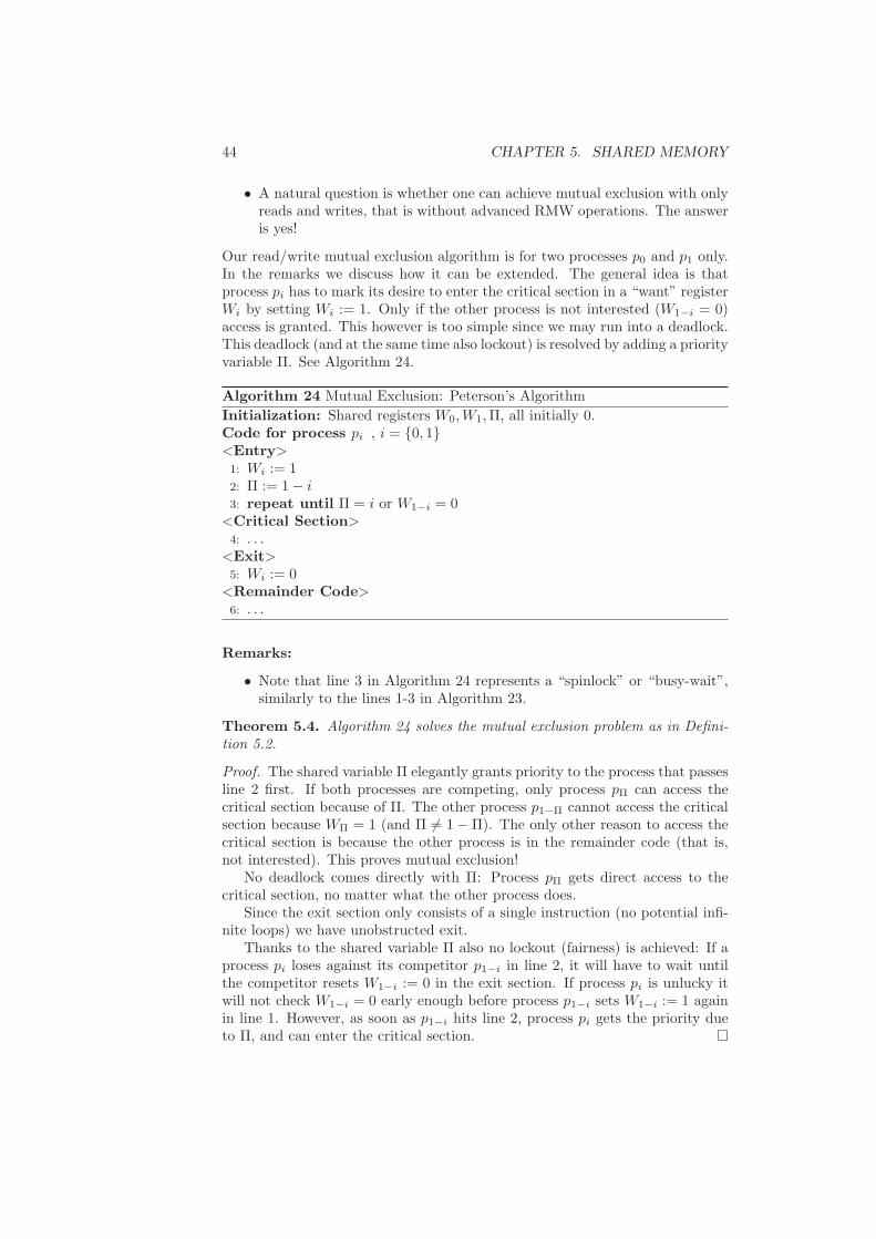
44 CHAPTER 5. SHARED MEMORY
• A natural question is whether one can achieve mutual exclusion with onlyreads and writes, that is without advanced RMW operations. The answeris yes!
Our read/write mutual exclusion algorithm is for two processes p0 and p1 only.In the remarks we discuss how it can be extended. The general idea is thatprocess pi has to mark its desire to enter the critical section in a “want” registerWi by setting Wi := 1. Only if the other process is not interested (W1−i = 0)access is granted. This however is too simple since we may run into a deadlock.This deadlock (and at the same time also lockout) is resolved by adding a priorityvariable Π. See Algorithm 24.
Algorithm 24 Mutual Exclusion: Peterson’s Algorithm
Initialization: Shared registers W0,W1,Π, all initially 0.Code for process pi , i = 0, 1<Entry>1: Wi := 12: Π := 1− i3: repeat until Π = i or W1−i = 0
<Critical Section>4: . . .
<Exit>5: Wi := 0
<Remainder Code>6: . . .
Remarks:
• Note that line 3 in Algorithm 24 represents a “spinlock” or “busy-wait”,similarly to the lines 1-3 in Algorithm 23.
Theorem 5.4. Algorithm 24 solves the mutual exclusion problem as in Defini-tion 5.2.
Proof. The shared variable Π elegantly grants priority to the process that passesline 2 first. If both processes are competing, only process pΠ can access thecritical section because of Π. The other process p1−Π cannot access the criticalsection because WΠ = 1 (and Π 6= 1− Π). The only other reason to access thecritical section is because the other process is in the remainder code (that is,not interested). This proves mutual exclusion!
No deadlock comes directly with Π: Process pΠ gets direct access to thecritical section, no matter what the other process does.
Since the exit section only consists of a single instruction (no potential infi-nite loops) we have unobstructed exit.
Thanks to the shared variable Π also no lockout (fairness) is achieved: If aprocess pi loses against its competitor p1−i in line 2, it will have to wait untilthe competitor resets W1−i := 0 in the exit section. If process pi is unlucky itwill not check W1−i = 0 early enough before process p1−i sets W1−i := 1 againin line 1. However, as soon as p1−i hits line 2, process pi gets the priority dueto Π, and can enter the critical section.

5.3. STORE & COLLECT 45
Remarks:
• Extending Peterson’s Algorithm to more than 2 processes can be done bya tournament tree, like in tennis. With n processes every process needs towin log n matches before it can enter the critical section. More precisely,each process starts at the bottom level of a binary tree, and proceeds tothe parent level if winning. Once winning the root of the tree it can enterthe critical section. Thanks to the priority variables Π at each node of thebinary tree, we inherit all the properties of Definition 5.2.
5.3 Store & Collect
5.3.1 Problem Definition
In this section, we will look at a second shared memory problem that has anelegant solution. Informally, the problem can be stated as follows. There aren processes p1, . . . , pn. Every process pi has a read/write register Ri in theshared memory where it can store some information that is destined for theother processes. Further, there is an operation by which a process can collect(i.e., read) the values of all the processes that stored some value in their register.
We say that an operation op1 precedes an operation op2 iff op1 terminatesbefore op2 starts. An operation op2 follows an operation op1 iff op1 precedesop2.
Definition 5.5 (Collect). There are two operations: A store(val) by processpi sets val to be the latest value of its register Ri. A collect operation returnsa view, a partial function V from the set of processes to a set of values, whereV (pi) is the latest value stored by pi, for each process pi. For a collect
operation cop, the following validity properties must hold for every process pi:
• If V (pi) = ⊥, then no store operation by pi precedes cop.
• If V (pi) = v 6= ⊥, then v is the value of a store operation sop of pi thatdoes not follow cop, and there is no store operation by pi that followssop and precedes cop.
Hence, a collect operation cop should not read from the future or miss apreceding store operation sop.
We assume that the read/write register Ri of every process pi is initializedto ⊥. We define the step complexity of an operation op to be the number ofaccesses to registers in the shared memory. There is a trivial solution to thecollect problem as shown by Algorithm 25.
Algorithm 25 Collect: Simple (Non-Adaptive) Solution
Operation store(val) (by process pi) :1: Ri := val
Operation collect:2: for i := 1 to n do3: V (pi) := Ri // read register Ri
4: end for

46 CHAPTER 5. SHARED MEMORY
Remarks:
• Algorithm 25 clearly works. The step complexity of every store operationis 1, the step complexity of a collect operation is n.
• At first sight, the step complexities of Algorithm 25 seem optimal. Becausethere are n processes, there clearly are cases in which a collect operationneeds to read all n registers. However, there are also scenarios in whichthe step complexity of the collect operation seems very costly. Assumethat there are only two processes pi and pj that have stored a value intheir registers Ri and Rj . In this case, a collect in principle only needsto read the registers Ri and Rj and can ignore all the other registers.
• Assume that up to a certain time t, k ≤ n processes have finished orstarted at least one operation. We call an operation op at time t adap-tive to contention if the step complexity of op only depends on k and isindependent of n.
• In the following, we will see how to implement adaptive versions of store
and collect.
5.3.2 Splitters
Algorithm 26 Splitter Code
Shared Registers: X : ⊥ ∪ 1, . . . , n; Y : booleanInitialization: X := ⊥; Y := false
Splitter access by process pi:1: X := i;2: if Y then3: return right4: else5: Y := true6: if X = i then7: return stop8: else9: return left
10: end if11: end if
To obtain adaptive collect algorithms, we need a synchronization primitive,called a splitter.
Definition 5.6 (Splitter). A splitter is a synchronization primitive with thefollowing characteristic. A process entering a splitter exits with either stop,left, or right. If k processes enter a splitter, at most one process exits withstop and at most k − 1 processes exit with left and right, respectively.
Hence, it is guaranteed that if a single process enters the splitter, then itobtains stop, and if two or more processes enter the splitter, then there isat most one process obtaining stop and there are two processes that obtain

5.3. STORE & COLLECT 47
k processors
at most 1
leftat most k−1
rightat most k−1
stop
Figure 5.1: A Splitter
different values (i.e., either there is exactly one stop or there is at least oneleft and at least one right). For an illustration, see Figure 5.1. The codeimplementing a splitter is given by Algorithm 26.
Lemma 5.7. Algorithm 26 correctly implements a splitter.
Proof. Assume that k processes enter the splitter. Because the first process thatchecks whether Y = true in line 2 will find that Y = false, not all processesreturn right. Next, assume that i is the last process that sets X := i. If i doesnot return right, it will find X = i in line 6 and therefore return stop. Hence,there is always a process that does not return left. It remains to show that atmost 1 process returns stop. For the sake of contradiction, assume pi and pj
are two processes that return stop and assume that pi sets X := i before pj setsX := j. Both processes need to check whether Y is true before one of themsets Y := true. Hence, they both complete the assignment in line 1 before thefirst one of them checks the value of X in line 6. Hence, by the time pi arrivesat line 6, X 6= i (pj and maybe some other processes have overwritten X bythen). Therefore, pi does not return stop and we get a contradiction to theassumption that both pi and pj return stop.
5.3.3 Binary Splitter Tree
Assume that we are given 2n − 1 splitters and that for every splitter S, thereis an additional shared variable ZS : ⊥ ∪ 1, . . . , n that is initialized to ⊥and an additional shared variable MS : boolean that is initialized to false. Wecall a splitter S marked if MS = true. The 2n − 1 splitters are arranged in acomplete binary tree of height n − 1. Let S(v) be the splitter associated witha node v of the binary tree. The store and collect operations are given byAlgorithm 27.
Theorem 5.8. Algorithm 27 correctly implements store and collect. Let kbe the number of participating processes. The step complexity of the first store
of a process pi is O(k), the step complexity of every additional store of pi isO(1), and the step complexity of collect is O(k).
Proof. Because at most one process can stop at a splitter, it is sufficient to showthat every process stops at some splitter at depth at most k − 1 ≤ n− 1 wheninvoking the first store operation to prove correctness. We prove that at mostk − i processes enter a subtree at depth i (i.e., a subtree where the root hasdistance i to the root of the whole tree). By definition of k, the number of
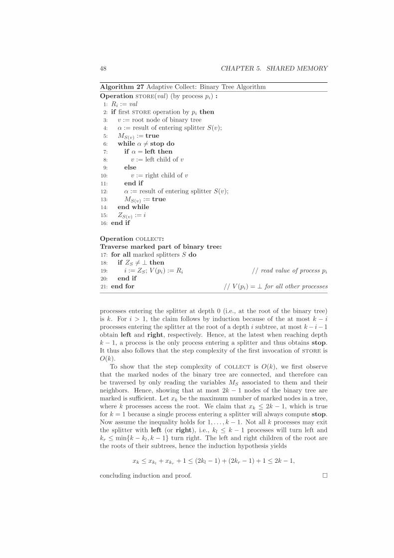
48 CHAPTER 5. SHARED MEMORY
Algorithm 27 Adaptive Collect: Binary Tree Algorithm
Operation store(val) (by process pi) :1: Ri := val2: if first store operation by pi then3: v := root node of binary tree4: α := result of entering splitter S(v);5: MS(v) := true6: while α 6= stop do7: if α = left then8: v := left child of v9: else
10: v := right child of v11: end if12: α := result of entering splitter S(v);13: MS(v) := true14: end while15: ZS(v) := i16: end if
Operation collect:Traverse marked part of binary tree:17: for all marked splitters S do18: if ZS 6= ⊥ then19: i := ZS ; V (pi) := Ri // read value of process pi
20: end if21: end for // V (pi) = ⊥ for all other processes
processes entering the splitter at depth 0 (i.e., at the root of the binary tree)is k. For i > 1, the claim follows by induction because of the at most k − iprocesses entering the splitter at the root of a depth i subtree, at most k− i− 1obtain left and right, respectively. Hence, at the latest when reaching depthk − 1, a process is the only process entering a splitter and thus obtains stop.It thus also follows that the step complexity of the first invocation of store isO(k).
To show that the step complexity of collect is O(k), we first observethat the marked nodes of the binary tree are connected, and therefore canbe traversed by only reading the variables MS associated to them and theirneighbors. Hence, showing that at most 2k − 1 nodes of the binary tree aremarked is sufficient. Let xk be the maximum number of marked nodes in a tree,where k processes access the root. We claim that xk ≤ 2k − 1, which is truefor k = 1 because a single process entering a splitter will always compute stop.Now assume the inequality holds for 1, . . . , k − 1. Not all k processes may exitthe splitter with left (or right), i.e., kl ≤ k − 1 processes will turn left andkr ≤ mink − kl, k − 1 turn right. The left and right children of the root arethe roots of their subtrees, hence the induction hypothesis yields
xk ≤ xkl+ xkr
+ 1 ≤ (2kl − 1) + (2kr − 1) + 1 ≤ 2k − 1,
concluding induction and proof.

5.3. STORE & COLLECT 49
left
right
Figure 5.2: 5× 5 Splitter Matrix
Remarks:
• The step complexities of Algorithm 27 are very good. Clearly, the stepcomplexity of the collect operation is asymptotically optimal. In orderfor the algorithm to work, we however need to allocate the memory for thecomplete binary tree of depth n−1. The space complexity of Algorithm 27therefore is exponential in n. We will next see how to obtain a polynomialspace complexity at the cost of a worse collect step complexity.
5.3.4 Splitter Matrix
Instead of arranging splitters in a binary tree, we arrange n2 splitters in an n×nmatrix as shown in Figure 5.2. The algorithm is analogous to Algorithm 27.The matrix is entered at the top left. If a process receives left, it next visitsthe splitter in the next row of the same column. If a process receives right, itnext visits the splitter in the next column of the same row. Clearly, the spacecomplexity of this algorithm is O(n2). The following theorem gives bounds onthe step complexities of store and collect.
Theorem 5.9. Let k be the number of participating processes. The step com-plexity of the first store of a process pi is O(k), the step complexity of everyadditional store of pi is O(1), and the step complexity of collect is O(k2).
Proof. Let the top row be row 0 and the left-most column be column 0. Let xi
be the number of processes entering a splitter in row i. By induction on i, weshow that xi ≤ k − i. Clearly, x0 ≤ k. Let us therefore consider the case i > 0.Let j be the largest column such that at least one process visits the splitter inrow i−1 and column j. By the properties of splitters, not all processes enteringthe splitter in row i− 1 and column j obtain left. Therefore, not all processesentering a splitter in row i− 1 move on to row i. Because at least one processes

50 CHAPTER 5. SHARED MEMORY
stays in every row, we get that xi ≤ k − i. Similarly, the number of processesentering column j is at most k − j. Hence, every process stops at the latest inrow k − 1 and column k − 1 and the number of marked splitters is at most k2.Thus, the step complexity of collect is at most O(k2). Because the longestpath in the splitter matrix is 2k, the step complexity of store is O(k).
Remarks:
• With a slightly more complicated argument, it is possible to show that thenumber of processes entering the splitter in row i and column j is at mostk − i− j. Hence, it suffices to only allocate the upper left half (includingthe diagonal) of the n× n matrix of splitters.
• The binary tree algorithm can be made space efficient by using a random-ized version of a splitter. Whenever returning left or right, a randomizedsplitter returns left or right with probability 1/2. With high probability,it then suffices to allocate a binary tree of depth O(log n).
• Recently, it has been shown that with a considerably more complicateddeterministic algorithm, it is possible to achieve O(k) step complexity andO(n2) space complexity.

Chapter 6
Shared Objects
6.1 Introduction
Assume that there is a common resource (e.g. a common variable or data struc-ture), which different nodes in a network need to access from time to time. Ifthe nodes are allowed to change the common object when accessing it, we needto guarantee that no two nodes have access to the object at the same time. Inorder to achieve this mutual exclusion, we need protocols that allow the nodesof a network to store and manage access to such a shared object. A simple andobvious solution is to store the shared object at a central location (see Algorithm28).
Algorithm 28 Shared Object: Centralized Solution
Initialization: Shared object stored at root node r of a spanning tree of thenetwork graph (i.e., each node knows its parent in the spanning tree).
Accessing Object: (by node v)1: v sends request up the tree2: request processed by root r (atomically)3: result sent down the tree to node v
Remarks:
• Algorithm 28 works. Instead of a spanning tree, one can use routing.
• It is however not very efficient. Assume that the object is accessed bya single node v repeatedly. Then we get a high message/time complex-ity. Instead v could store the object, or at least cache it. But then, incase another node w accesses the object, we might run into consistencyproblems.
• Alternative idea: The accessing node should become the new master ofthe object. The shared object then becomes mobile. There exist severalvariants of this idea. The simplest version is a home-based solution likein Mobile IP (see Algorithm 29).
51

52 CHAPTER 6. SHARED OBJECTS
Algorithm 29 Shared Object: Home-Based Solution
Initialization: An object has a home base (a node) that is known to everynode. All requests (accesses to the shared object) are routed through thehome base.
Accessing Object: (by node v)1: v acquires a lock at the home base, receives object.
Remarks:
• Home-based solutions suffer from the triangular routing problem. If twoclose-by nodes access the object on a rotating basis, all the traffic is routedthrough the potentially far away home-base.
6.2 Arrow and Friends
We will now look at a protocol (called the Arrow algorithm) that alwaysmoves the shared object to the node currently accessing it without creatingthe triangular routing problem of home-based solutions. The protocol runs ona precomputed spanning tree. Assume that the spanning tree is rooted at thecurrent position of the shared object. When a node u wants to access the sharedobject, it sends out a find request towards the current position of the object.While searching for the object, the edges of the spanning tree are redirectedsuch that in the end, the spanning tree is rooted at u (i.e., the new holder of theobject). The details of the algorithm are given by Algorithm 30. For simplicity,we assume that a node u only starts a find request if u is not currently theholder of the shared object and if u has finished all previous find requests (i.e.,it is not currently waiting to receive the object).
Remarks:
• The parent pointers in Algorithm 30 are only needed for the find operation.Sending the variable to u in line 13 or to w.successor in line 23 is doneusing routing (on the spanning tree or on the underlying network).
• When we draw the parent pointers as arrows, in a quiescent moment(where no “find” is in motion), the arrows all point towards the nodecurrently holding the variable (i.e., the tree is rooted at the node holdingthe variable)
• What is really great about the Arrow algorithm is that it works in acompletely asynchronous and concurrent setting (i.e., there can be manyfind requests at the same time).
Theorem 6.1. (Arrow, Analysis) In an asynchronous, steady-state, and con-current setting, a “find” operation terminates with message and time complexityD, where D is the diameter of the spanning tree.

6.2. ARROW AND FRIENDS 53
Algorithm 30 Shared Object: Arrow Algorithm
Initialization: As for Algorithm 28, we are given a rooted spanning tree. Eachnode has a pointer to its parent, the root r is its own parent. The variableis initially stored at r. For all nodes v, v.successor := null, v.wait := false.
Start Find Request at Node u:1: do atomically2: u sends “find by u” message to parent node3: u.parent := u4: u.wait := true5: end do
Upon w Receiving “Find by u” Message from Node v:6: do atomically7: if w.parent 6= w then8: w sends “find by u” message to parent9: w.parent := v
10: else11: w.parent := v12: if not w.wait then13: send variable to u // w holds var. but does not need it any more14: else15: w.successor := u // w will send variable to u a.s.a.p.16: end if17: end if18: end do
Upon w Receiving Shared Object:19: perform operation on shared object20: do atomically21: w.wait := false22: if w.successor 6= null then23: send variable to w.successor24: w.successor := null25: end if26: end do

54 CHAPTER 6. SHARED OBJECTS
Before proving Theorem 6.1, we prove the following lemma.
Lemma 6.2. An edge u, v of the spanning tree is in one of four states:
1.) Pointer from u to v (no message on the edge, no pointer from v to u)2.) Message on the move from u to v (no pointer along the edge)3.) Pointer from v to u (no message on the edge, no pointer from u to v)4.) Message on the move from v to u (no pointer along the edge)
Proof. W.l.o.g., assume that initially the edge u, v is in state 1. With amessage arrival at u (or if u starts a “find by u” request, the edge goes to state2. When the message is received at v, v directs its pointer to u and we aretherefore in state 3. A new message at v (or a new request initiated by v) thenbrings the edge back to state 1.
Proof of Theorem 6.1. Since the “find” message will only travel on a static tree,it suffices to show that it will not traverse an edge twice. Suppose for the sakeof contradiction that there is a first “find” message f that traverses an edgee = u, v for the second time and assume that e is the first edge that istraversed twice by f . The first time, f traverses e. Assume that e is firsttraversed from u to v. Since we are on a tree, the second time, e must betraversed from v to u. Because e is the first edge to be traversed twice, f mustre-visit e before visiting any other edges. Right before f reaches v, the edge eis in state 2 (f is on the move) and in state 3 (it will immediately return withthe pointer from v to u). This is a contradiction to Lemma 6.2.
Remarks:
• Finding a good tree is an interesting problem. We would like to have atree with low stretch, low diameter, low degree, etc.
• It seems that the Arrow algorithm works especially well when lots of “find”operations are initiated concurrently. Most of them will find a “close-by”node, thus having low message/time complexity. For the sake of simplicitywe analyze a synchronous system.
Theorem 6.3. (Arrow, Concurrent Analysis) Let the system be synchronous.Initially, the system is in a quiescent state. At time 0, a set S of nodes initiatesa “find” operation. The message complexity of all “find” operations is O(log |S|·m∗) where m∗ is the message complexity of an optimal (with global knowledge)algorithm on the tree.
Proof Sketch. Let d be the minimum distance of any node in S to the root.There will be a node u1 at distance d from the root that reaches the root ind time steps, turning all the arrows on the path to the root towards u1. Anode u2 that finds (is queued behind) u1 cannot distinguish the system froma system where there was no request u1, and instead the root was initiallylocated at u1. The message cost of u2 is consequentially the distance betweenu1 and u2 on the spanning tree. By induction the total message complexity isexactly as if a collector starts at the root and then “greedily” collects tokenslocated at the nodes in S (greedily in the sense that the collector always goestowards the closest token). Greedy collecting the tokens is not a good strategyin general because it will traverse the same edge more than twice in the worst

6.2. ARROW AND FRIENDS 55
case. An asymptotically optimal algorithm can also be translated into a depth-first-search collecting paradigm, traversing each edge at most twice. In anotherarea of computer science, we would call the Arrow algorithm a nearest-neighborTSP heuristic (without returning to the start/root though), and the optimalalgorithm TSP-optimal. It was shown that nearest-neighbor has a logarithmicoverhead, which concludes the proof.
Remarks:
• An average request set S on a not-too-bad tree gives usually a much betterbound. However, there is an almost tight log |S|/ log log |S| worst-caseexample.
• It was recently shown that Arrow can do as good in a dynamic setting(where nodes are allowed to initiate requests at any time). In particularthe message complexity of the dynamic analysis can be shown to have alog D overhead only, where D is the diameter of the spanning tree (notethat for logarithmic trees, the overhead becomes log log n).
• What if the spanning tree is a star? Then with Theorem 6.1, each find willterminate in 2 steps! Since also an optimal algorithm has message cost 1,the algorithm is 2-competitive. . . ? Yes, but because of its high degree thestar center experiences contention. . . It can be shown that the contentionoverhead is at most proportional to the largest degree ∆ of the spanningtree.
• Thought experiment: Assume a balanced binary spanning tree—by Theo-rem 6.1, the message complexity per operation is log n. Because a binarytree has maximum degree 3, the time per operation therefore is at most3 log n.
• There are better and worse choices for the spanning tree. The stretch ofan edge u, v is defined as distance between u and v in a spanning tree.The maximum stretch of a spanning tree is the maximum stretch over alledges. A few years ago, it was shown how to construct spanning trees thatare O(log n)-stretch-competitive.
What if most nodes just want to read the shared object? Then it doesnot make sense to acquire a lock every time. Instead we can use caching (seeAlgorithm 31).
Theorem 6.4. Algorithm 31 is correct. More surprisingly, the message com-plexity is 3-competitive (at most a factor 3 worse than the optimum).
Proof. Since the accesses do not overlap by definition, it suffices to show thatbetween two writes, we are 3-competitive. The sequence of accessing nodes isw0, r1, r2, . . . , rk, w1. After w0, the object is stored at w0 and not cachedanywhere else. All reads cost twice the smallest subtree T spanning the writew0 and all the reads since each read only goes to the first copy. The write w1
costs T plus the path P from w1 to T . Since any data management schememust use an edge in T and P at least once, and our algorithm uses edges in Tat most 3 times (and in P at most once), the theorem follows.

56 CHAPTER 6. SHARED OBJECTS
Algorithm 31 Shared Object: Read/Write Caching
• Nodes can either read or write the shared object. For simplicity we firstassume that reads or writes do not overlap in time (access to the object issequential).
• Nodes store three items: a parent pointer pointing to one of the neighbors(as with Arrow), and a cache bit for each edge, plus (potentially) a copy ofthe object.
• Initially the object is stored at a single node u; all the parent pointers pointtowards u, all the cache bits are false.
• When initiating a read, a message follows the arrows (this time: withoutinverting them!) until it reaches a cached version of the object. Then a copyof the object is cached along the path back to the initiating node, and thecache bits on the visited edges are set to true.
• A write at u writes the new value locally (at node u), then searches (follow theparent pointers and reverse them towards u) a first node with a copy. Deletethe copy and follow (in parallel, by flooding) all edge that have the cache flagset. Point the parent pointer towards u, and remove the cache flags.
Remarks:
• Concurrent reads are not a problem, also multiple concurrent reads andone write work just fine.
• What about concurrent writes? To achieve consistency writes need toinvalidate the caches before writing their value. It is claimed that thestrategy then becomes 4-competitive.
• Is the algorithm also time competitive? Well, not really: The optimalalgorithm that we compare to is usually offline. This means it knows thewhole access sequence in advance. It can then cache the object before therequest even appears!
• Algorithms on trees are often simpler, but have the disadvantage that theyintroduce the extra stretch factor. In a ring, for example, any tree hasstretch n− 1; so there is always a bad request pattern.

6.3. IVY AND FRIENDS 57
Algorithm 32 Shared Object: Pointer Forwarding
Initialization: Object is stored at root r of a precomputed spanning tree T (asin the Arrow algorithm, each node has a parent pointer pointing towardsthe object).
Accessing Object: (by node u)1: follow parent pointers to current root r of T2: send object from r to u3: r.parent := u; u.parent := u; // u is the new root
Algorithm 33 Shared Object: Ivy
Initialization: Object is stored at root r of a precomputed spanning tree T(as before, each node has a parent pointer pointing towards the object). Forsimplicity, we assume that accesses to the object are sequential.
Start Find Request at Node u:1: u sends “find by u” message to parent node2: u.parent := u
Upon v receiving “Find by u” Message:3: if v.parent = v then4: send object to u5: else6: send “find by u” message to v.parent7: end if8: v.parent := u // u will become the new root
6.3 Ivy and Friends
In the following we study algorithms that do not restrict communication to atree. Of particular interest is the special case of a complete graph (clique). Asimple solution for this case is given by Algorithm 32.
Remarks:
• If the graph is not complete, routing can be used to find the root.
• Assume that the nodes line up in a linked list. If we always choose thefirst node of the linked list to acquire the object, we have message/timecomplexity n. The new topology is again a linearly linked list. Pointerforwarding is therefore bad in a worst-case.
• If edges are not FIFO, it can even happen that the number of steps isunbounded for a node having bad luck. An algorithm with such a propertyis named “not fair,” or “not wait-free.” (Example: Initially we have thelist 4 → 3 → 2 → 1; 4 starts a find; when the message of 4 passes 3, 3itself starts a find. The message of 3 may arrive at 2 and then 1 earlier,thus the new end of the list is 2→ 1→ 3; once the message of 4 passes 2,the game re-starts.)
There seems to be a natural improvement of the pointer forwarding idea.Instead of simply redirecting the parent pointer from the old root to the newroot, we can redirect all the parent pointers of the nodes on the path visited

58 CHAPTER 6. SHARED OBJECTS
x3x1 x2 x4 x5x1
x2
x3
x4
x5
x0
x0
Figure 6.1: Reversal of the path x0, x1, x2, x3, x4, x5.
during a find message to the new root. The details are given by Algorithm 33.Figure 6.1 shows how the pointer redirecting affects a given tree (the right treeresults from a find request started at node x0 on the left tree).
Remarks:
• Also with Algorithm 33, we might have a bad linked list situation. How-ever, if the start of the list acquires the object, the linked list turns intoa star. As the following theorem will show, the search paths are not longon average. Since paths sometimes can be bad, we will need amortizedanalysis.
Theorem 6.5. If the initial tree is a star, a find request of Algorithm 33 needsat most log n steps on average, where n is the number of processors.
Proof. All logarithms in the following proof are to base 2. We assume thataccesses to the shared object are sequential. We use a potential function argu-ment. Let s(u) be the size of the subtree rooted at node u (the number of nodesin the subtree including u itself). We define the potential Φ of the whole treeT as (V is the set of all nodes)
Φ(T ) =∑
u∈V
log s(u)
2.
Assume that the path traversed by the ith operation has length ki, i.e., the ith
operation redirects ki pointers to the new root. Clearly, the number of stepsof the ith operation is proportional to ki. We are interested in the cost of mconsecutive operations,
∑mi=1 ki.
Let T0 be the initial tree and let Ti be the tree after the ith operation.Further, let ai = ki−Φ(Ti−1)+Φ(Ti) be the amortized cost of the ith operation.We have
m∑
i=1
ai =
m∑
i=1
(
ki − Φ(Ti−1) + Φ(Ti))
=
m∑
i=1
ki − Φ(T0) + Φ(Tm).
For any tree T , we have Φ(T ) ≥ log(n)/2. Because we assume that T0 is a star,we also have Φ(T0) = log(n)/2. We therefore get that
m∑
i=1
ai ≥m∑
i=1
ki.

6.3. IVY AND FRIENDS 59
Hence, it suffices to upper bound the amortized cost of every operation. Wethus analyze the amortized cost ai of the ith operation. Let x0, x1, x2, . . . , xki
be the path that is reversed by the operation. Further for 0 ≤ j ≤ ki, let sj bethe size of the subtree rooted at xj before the reversal. The size of the subtreerooted at x0 after the reversal is ski
and the size of the one rooted at xj afterthe reversal, for 1 ≤ j ≤ ki, is sj−sj−1 (see Figure 6.1). For all other nodes, thesizes of their subtrees are the same, therefore the corresponding terms cancelout in the ammortized cost ai. We can thus write ai as
ai = ki −
ki∑
j=0
1
2log sj
+
1
2log ski
+
ki∑
j=1
1
2log(sj − sj−1)
= ki +1
2·
ki−1∑
j=0
(
log(sj+1 − sj)− log sj
)
= ki +1
2·
ki−1∑
j=0
log
(
sj+1 − sj
sj
)
.
For 0 ≤ j ≤ ki−1, let αj = sj+1/sj . Note that sj+1 > sj and thus that αj > 1.Further note, that (sj+1 − sj)/sj = αj − 1. We therefore have that
ai = ki +1
2·
ki−1∑
j=0
log(αj − 1)
=
ki−1∑
j=0
(
1 +1
2log(αj − 1)
)
.
For α > 1, it can be shown that 1+log(α−1)/2 ≤ log α (see Lemma 6.6). Fromthis inequality, we obtain
ai ≤ki−1∑
j=0
log αj =
ki−1∑
j=0
logsj+1
sj=
ki−1∑
j=0
(log sj+1 − log sj)
= log ski− log s0 ≤ log n,
because ski= n and s0 ≥ 1. This concludes the proof.
Lemma 6.6. For α > 1, 1 + log(α− 1)/2 ≤ log α.
Proof. The claim can be verified by the following chain of reasoning:
0 ≤ (α− 2)2
0 ≤ α2 − 4α + 4
4(α− 1) ≤ α2
log2
(
4(α− 1))
≤ log2
(
α2)
2 + log2(α− 1) ≤ 2 log2 α
1 +1
2log2(α− 1) ≤ log2 α.

60 CHAPTER 6. SHARED OBJECTS
Remarks:
• Systems guys (the algorithm is called Ivy because it was used in a systemwith the same name) have some fancy heuristics to improve performanceeven more: For example, the root every now and then broadcasts its namesuch that paths will be shortened.
• What about concurrent requests? It works with the same argument asin Arrow. Also for Ivy an argument including congestion is missing (andmore pressing, since the dynamic topology of a tree cannot be chosen tohave low degree and thus low congestion as in Arrow).
• Sometimes the type of accesses allows that several accesses can be com-bined into one to reduce congestion higher up the tree. Let the tree inAlgorithm 28 be a balanced binary tree. If the access to a shared variablefor example is “add value x to the shared variable,” two or more accessesthat accidentally meet at a node can be combined into one. Clearly ac-cidental meeting is rare in an asynchronous model. We might be able touse synchronizers (or maybe some other timing tricks) to help meeting alittle bit.

Chapter 7
Dynamic Networks
Many large-scale distributed systems and networks are dynamic. In some net-works, e.g., peer-to-peer, nodes participate only for a short period of time, andthe topology can change at a high rate. In wireless ad-hoc networks, nodes aremobile and move around. In this chapter, we will study how to solve some basictasks if the network is dynamic. Under what conditions is it possible to computean accurate estimate of the size or some other property of the system? Howefficiently can information be disseminated reliably in the network? To whatextent does stability in the communication graph help solve these problems?
There are various reasons why networks can change over time and as a con-sequence, there also is a wide range of possible models for dynamic networks.Nodes might join or leave a distributed system. Some components or commu-nication links may fail in different ways. Especially if the network devices aremobile, the connectivity between them can change. Dynamic changes can occurconstantly or they might be infrequent enough so that the system can adapt toeach change individually.
We will look at a synchronous dynamic network model in which the graphcan change from round to round in a worst-case manner. To simplify things(and to make the problems we study well-defined), we assume that the set ofnodes in the network is fixed and does not change. However, we will makealmost no assumptions how the set of edges changes over time. We requiresome guarantees about the connectivity, apart from this, in each round, thecommunication graph is chosen in a worst-case manner by an adversary.
7.1 Synchronous Edge-Dynamic Networks
We model a synchronous dynamic network by a dynamic graph G = (V,E),where V is a static set of nodes, and E : N0 →
(
V2
)
is a function mapping a round
number r ∈ N0 to a set of undirected edges E(r). Here(
V2
)
:= u, v | u, v ∈ V is the set of all possible undirected edges over V .
Definition 7.1 (T -Interval Connectivity). A dynamic graph G = (V,E) issaid to be T -interval connected for T ∈ N if for all r ∈ N, the static graph
Gr,T :=(
V,⋂r+T−1
i=r E(r))
is connected. If G is 1-interval connected we say
that G is always connected.
61

62 CHAPTER 7. DYNAMIC NETWORKS
For simplicity, we restrict to deterministic algorithms. Nodes communicatewith each other using anonymous broadcast. At the beginning of round r, eachnode u decides what message to broadcast based on its internal state; at thesame time (and independently), the adversary chooses a set E(r) of edges forthe round. As in standard synchronous message passing, all nodes v for whichu, v ∈ E(r) receive the message broadcast by node u in round r and each nodecan perform arbitrary local computations upon receiving the messages from itsneighbors. We assume that all nodes in the network have a unique identifier(ID). In most cases, we will assume that messages are restricted to O(log n) bits.In these cases, we assume that node IDs can be represented using O(log n) bits,so that a constant number of node IDs and some additional information can betransmitted in a single message. We refer to the special case where all nodes arewoken up at once as synchronous start and to the general case as asynchronousstart.
We assume that each node in the network starts an execution of the protocolin an initial state which contains its own ID and its input. Additionally, nodesknow nothing about the network, and initially cannot distinguish it from anyother network.
7.2 Problem Definitions
In the context of this chapter, we study the following problems.
Counting. An algorithm is said to solve the counting problem if whenever it isexecuted in a dynamic graph comprising n nodes, all nodes eventually terminateand output n.
k-verification. Closely related to counting, the k-verification problem re-quires nodes to determine whether or not n ≤ k. All nodes begin with k astheir input, and must eventually terminate and output “yes” or “no”. Nodesmust output “yes” if and only if there are at most k nodes in the network.
k-token dissemination. An instance of k-token dissemination is a pair (V, I),where I : V → P (T ) assigns a set of tokens from some domain T to each node,and |⋃u∈V I(v)| = k. An algorithm solves k-token dissemination if for allinstances (V, I), when the algorithm is executed in any dynamic graph G =(V,E), all nodes eventually terminate and output
⋃
u∈V I(u). We assume thateach token in the nodes’ input is represented using O(log n) bits. Nodes may ormay not know k, depending on the context. Of particular interest is all-to-alltoken dissemination, a special case where k = n and each node initially knowsexactly one token, i.e., |I(u)| = 1 for all nodes u.
k-committee election. As an useful step towards solving counting and to-ken dissemination, we consider a problem called k-committee election. In thisproblem, nodes must partition themselves into sets, called committees, such that
a) the size of each committee is at most k and
b) if k ≥ n, then there is just one committee containing all nodes.

7.3. BASIC INFORMATION DISSEMINATION 63
Each committee has a unique committee ID, and the goal is for all nodes toeventually terminate and output a committee ID such that the two conditionsare satisfied.
7.3 Basic Information Dissemination
To start, let us study how a single piece of information is propagated througha dynamic network. We assume that we have a dynamic network graph G withn nodes such that G is always connected (G is 1-interval connected as definedin Definition 7.1). Further assume that there is a single piece of information(token), which is initially known by a single node.
Theorem 7.2. Assume that there is a single token in the network. Furtherassume that at time 0 at least one node knows the token and that once theyknow the token, all nodes broadcast it in every round. In a 1-interval connectedgraph G = (V,E) with n nodes, after r ≤ n−1 rounds, at least r+1 nodes knowthe token. Hence, in particular after n− 1 rounds, all nodes know the token.
Proof. We can proof the theorem by induction on r. Let T (r) be the set ofnodes that know the token after r rounds. We need to show that for all r ≥ 0,|T (r)| ≥ min r + 1, n. Because we assume that at time 0 at least one nodeknows the token, clearly, |T (0)| ≥ 1. For the induction step, assume that afterr rounds, |T (r)| ≥ min r + 1, n. If T (r) = V , we have |T (r + 1)| ≥ |T (r)| = nand we are done. Otherwise, we have V \T (r) 6= ∅. Therefore, by the 1-intervalconnectivity assumption, there must be two nodes u ∈ T (r) and v ∈ V \ T (r)such that u, v ∈ E(r + 1). Hence, in round r + 1, node v gets the token antherefore |T (r + 1)| ≥ |T (r)|+ 1 ≥ min r + 2, n.
Remarks:
• Note that Theorem 7.2 only shows that after n− 1 rounds all nodes knowthe token. If the nodes do not know n or an upper bound on n, they donot know if all nodes know the token.
• We can apply the above techniques also if there is more than one tokenin the network, provided that tokens form a totally-ordered set and nodesforward the smallest (or biggest) token they know. It is then guaranteedthat the smallest (resp. biggest) token in the network will be known by allnodes after at most n− 1 rounds. Note, however, that in this case nodesdo not know when they know the smallest or biggest token.
The next theorem shows that essentially, for the general asynchronous startcase, 1-interval connectivity does not suffice to obtain anything better than whatis stated by the above theorem. If nodes do not know n or an upper bound onn initially, they cannot find n.
Theorem 7.3. Counting is impossible in 1-interval connected graphs with asyn-chronous start.
Proof. Suppose by way of contradiction that A is a protocol for counting whichrequires at most t(n) rounds in 1-interval connected graphs of size n. Let n′ =

64 CHAPTER 7. DYNAMIC NETWORKS
max t(n) + 1, n + 1. We will show that the protocol cannot distinguish a staticline of length n from a dynamically changing line of length n′.
Given a sequence A = a1 . . . am, let shift(A, r) denote the cyclic left-shiftof A in which the first r symbols (r ≥ 0) are removed from the beginning ofthe sequence and appended to the end. Consider an execution in a dynamicline of length n′, where the line in round r is composed of two adjacent sectionsA Br, where A = 0 . . . (n − 1) remains static throughout the execution,and B(r) = shift(n . . . (n′ − 1), r) is left-shifted by one in every round. Thecomputation is initiated by node 0 and all other nodes are initially asleep. Weclaim that the execution of the protocol in the dynamic graph G = A B(r)is indistinguishable in the eyes of nodes 0, . . . , n − 1 from an execution of theprotocol in the static line of length n (that is, the network comprising sectionA alone). This is proven by induction on the round number, using the fact thatthroughout rounds 0, . . . , t(n)− 1 none of the nodes in section A ever receives amessage from a node in section B: although one node in section B is awakenedin every round, this node is immediately removed and attached at the end ofsection B, where it cannot communicate with the nodes in section A. Thus,the protocol cannot distinguish the dynamic graph A from the dynamic graphA B(r), and it produces the wrong output in one of the two graphs.
Remark:
• The above impossibility result extends to all problems introduced in Sec-tion 7.2 as long as we do not assume that the nodes know n or an upperbound on n.
In light of the impossibility result of Theorem 7.3, let us now first considerthe synchronous start case where all nodes start the protocol at time 0 (withround 1). We first look at the case where there is no bound on the messagesize and describe a simple linear-time protocol for counting (and token dissem-ination). The protocol is extremely simple, but it demonstrates some of theideas used in some of the later algorithms, where we eliminate the large mes-sages using a stability assumption (T -interval connectivity) which allows nodesto communicate with at least one of their neighbors for at least T rounds.
In the simple protocol, all nodes maintain a set A containing all the IDs theyhave collected so far. In every round, each node broadcasts A and adds any IDsit receives. Nodes terminate when they first reach a round r in which |A| ≤ r.
A← self ;for r = 1, 2, . . . do
broadcast A;receive B1, . . . , Bs from neighbors;A← A ∪B1 ∪ . . . ∪Bs;if |A| ≤ r then terminate and output |A|;
end
Algorithm 1: Counting in linear time using large messages
Before analyzing Algorithm 1, let us fix some notation that will help to argueabout the algorithms we will study. If x is a variable of an algorithm, let xu(r)be the value of the variable x at node u after r rounds (immediately before thebroadcast operation of round r+1). For instance in Algorithm 1, Au(r) denotesthe set of IDs of node u at the end of the rth iteration of the for-loop.

7.3. BASIC INFORMATION DISSEMINATION 65
Lemma 7.4. Assume that we are given an 1-interval connected graph G =(V,E) and that all nodes in V execute Algorithm 1. If all nodes together startat time 0, we have |Au(r)| ≥ r + 1 for all u ∈ V and r < n.
Proof. We prove the lemma by induction on r. We clearly have |Au(0)| = 1 forall u because initially each node includes its own ID in A. Hence, the lemma istrue for r = 0.
For the induction step, assume that the claim of the lemma is true for somegiven r < n− 1 for all dynamic graphs G. Let A′
u(r +1) be the set of identifiersknown by node u if all nodes start the protocol at time 1 (instead of 0) and runit for r rounds. By the induction hypothesis, we have |A′
u(r +1)| ≥ r +1. If thealgorithm is started at time 0 instead of time 1, the set of identifiers in Au(r+1)is exactly the union of all the identifiers known by the nodes in A′
u(r+1) after thefirst round (at time 1). This includes all the nodes in A′
u(r + 1) as well as theirneighbors in the first round. If |A′
u(r+1)| ≥ r+2, we also have |Au(r+1)| ≥ r+2and we are done. Otherwise, by 1-interval connectivity, there must at least beone node v ∈ V \A′
u(r + 1) for which there is an edge to a node in A′u(r + 1) in
round 1. We therefore have |Au(r + 1)| ≥ |A′u(r + 1)|+ 1 ≥ r + 2.
Theorem 7.5. In an 1-interval connected graph G, Algorithm 1 terminates atall nodes after n rounds and output n.
Proof. Follows directly from Lemma 7.4. For all nodes u, |Au(r)| ≥ r + 1 > rfor all r < n and |Au(n)| = |Au(n− 1)| = n.
Lemma 7.6. Assume that we are given a 2-interval connected graph G = (V,E)and that all nodes in V execute Algorithm 1. If node u is waken up and startsthe algorithm at time t, it holds that have |Au(t+2r)| ≥ r +1 for all 0 ≤ r < n.
Proof. The proof follows along the same lines as the proof of Lemma 7.4 (seeexercises).
Remarks:
• Because we did not bound the maximal message size and because everynode receives information (an identifier) from each other node, Algorithm1 can be used to solve all the problems defined in Section 7.2. For thetoken dissemination problem, the nodes also need to attach a list of allknown tokens to all messages
• As a consequence of Theorem 7.3, 1-interval connectivity does not sufficeto compute the number of nodes n in a dynamic network if nodes startasynchronously. It turns out that in this case, we need a slightly strongerconnectivity assumption. If the network is 2-interval connected insteadof 1-interval connected, up to a constant factor in the time complexity,the above results can also be obtained in the asynchronous start case (seeexercises).
• For the remainder of the chapter, we will only consider the simpler syn-chronous start case. For T ≥ 2, all discussed results that hold for T -interval connected networks with synchronous start also hold for asyn-chronous start with the same asymptotic bounds.
66 CHAPTER 7. DYNAMIC NETWORKS
7.4 Small Messages
We now switch to the more interesting (and more realistic) case where in eachround, each node can only broadcast a message of O(log n) bits. We will firstshow how to use k-committee election to solve counting. We first describe howto obtain a good upper bound on n. We will then see that the same algorithmcan also be used to find n exactly and to solve token dissemination.
7.4.1 k-Verification
The counting algorithm works by successive doubling: at each point the nodeshave a guess k for the size of the network, and attempt to verify whether or notk ≥ n. If it is discovered that k < n, the nodes double k and repeat; if k ≥ n,the nodes halt and output the count.
Suppose that nodes start out in a state that represents a solution to k-committee election: each node has a committee ID, such that no more than knodes have the same ID, and if k ≥ n then all nodes have the same committee ID.The problem of checking whether k ≥ n is then equivalent to checking whetherthere is more than one committee: if k ≥ n there must be one committee only,and if k < n there must be more than one. Nodes can therefore check if k ≥ nby executing a simple k-round protocol that checks if there is more than onecommittee in the graph.
The k-verification protocol Each node has a local variable x , which isinitially set to 1. While xu = 1, node u broadcasts its committee ID. If it hearsfrom some neighbor a different committee ID from its own, or the special value⊥, it sets xu ← 0 and broadcasts ⊥ in all subsequent rounds. After k rounds,all nodes output the value of their x variable.
Lemma 7.7. If the initial state of the execution represents a solution to k-committee election, at the end of the k-verification protocol each node outputs 1iff k ≥ n.
Proof. First suppose that k ≥ n. In this case there is only one committee inthe graph; no node ever hears a committee ID different from its own. After krounds all nodes still have x = 1, and all output 1.
Next, suppose k < n. We can show that after the ith round of the protocol,at least i nodes in each committee have x = 0. In any round of the protocol,consider a cut between the nodes that belong to a particular committee andstill have x = 1, and the rest of the nodes, which either belong to a differentcommittee or have x = 0. From 1-interval connectivity, there is an edge inthe cut, and some node u in the committee that still has xu = 1 hears eithera different committee ID or ⊥. Node u then sets xu ← 0, and the number ofnodes in the committee that still have x = 1 decreases by at least one. Sinceeach committee initially contains at most k nodes, after k rounds all nodes inall committees have x = 0, and all output 0.
7.4.2 k-Committee Election
We can solve k-committee in O(k2) rounds as follows. Each node u stores twolocal variables, committeeu and leaderu. A node that has not yet joined a

7.4. SMALL MESSAGES 67
leader ← self ;committee ← ⊥;for i = 0, . . . , k do
// Polling phase
if committee = ⊥ thenmin active ← self ; // The node nominates itself for selection
elsemin active ← ⊥;
endfor j = 0, . . . , k − 1 do
broadcast min active;receive x1, . . . , xs from neighbors;min active ← min min active, x1, . . . , xs;
end// Update leader
leader ← min leader ,min active;// Selection phase
if leader = self then// Leaders invite the smallest ID they heard
invitation ← (self ,min active);else
// Non-leaders do not invite anybody
invitation ← ⊥endfor j = 0, . . . , k − 1 do
broadcast invitation;receive y1, . . . , ys from neighbors;invitation ← min invitation, y1, . . . , ys ; // (in lexicographic
order)
end// Join the leader’s committee, if invited
if invitation = (leader , self ) thencommittee = leader ;
end
endif committee = ⊥ then
committee ← self ;end
Algorithm 2: k-committee in always-connected graphs

68 CHAPTER 7. DYNAMIC NETWORKS
committee is called active, and a node that has joined a committee is inactive.Once nodes have joined a committee they do not change their choice.
Initially all nodes consider themselves leaders, but throughout the protocol,any node that hears an ID smaller than its own adopts that ID as its leader.The protocol proceeds in k cycles, each consisting of two phases, polling andselection.
1. Polling phase: for k−1 rounds, all nodes propagate the ID of the smallestactive node of which they are aware.
2. Selection phase: in this phase, each node that considers itself a leaderselects the smallest ID it heard in the previous phase and invites thatnode to join its committee. An invitation is represented as a pair (x, y),where x is the ID of the leader that issued the invitation, and y is the IDof the invited node. All nodes propagate the smallest invitation of whichthey are aware for k − 1 (invitations are sorted in lexicographic order, sothe invitations issued by the smallest node in the network will win outover other invitations. It turns out, though, that this is not necessary forcorrectness; it is sufficient for each node to forward an arbitrary invitationfrom among those it received).
At the end of the selection phase, a node that receives an invitation to joinits leader’s committee does so and becomes inactive. (Invitations issuedby nodes that are not the current leader can be accepted or ignored; this,again, does not affect correctness.)
At the end of the k cycles, any node u that has not been invited to join acommittee outputs committeeu = u. The details are given in Algorithm 2.
Lemma 7.8. Algorithm 2 solves the k-committee problem in O(k2) rounds in1-interval connected networks.
Proof. The time complexity is immediate. To prove correctness, we show thatafter the protocol ends, the values of the local committeeu variables constitutea valid solution to k-committee.
1. In each cycle, each node invites at most one node to join its committee.After k cycles at most k nodes have joined any committee. Note that thefirst node invited by a leader u to join u’s committee is always u itself.Thus, if after k cycles node u has not been invited to join a committee, itfollows that u did not invite any other node to join its committee; when itforms its own committee in the last line of the algorithm, the committee’ssize is 1.
2. Suppose that k ≥ n, and let u be the node with the smallest ID in thenetwork. Following the polling phase of the first cycle, all nodes v haveleaderv = u for the remainder of the protocol. Thus, throughout theexecution, only node u issues invitations, and all nodes propagate u’sinvitations. Since k ≥ n rounds are sufficient for u to hear the ID of theminimal active node in the network, in every cycle node u successfullyidentifies this node and invites it to join u’s committee. After k cycles, allnodes will have joined.

7.5. MORE STABLE GRAPHS 69
Remark:
• The protocol can be modified easily to solve all-to-all token disseminationif k ≥ n. Let tu be the token node u received in its input (or ⊥ if node udid not receive a token). Nodes attach their tokens to their IDs, and sendpairs of the form (u, tu) instead of just u. Likewise, invitations now containthe token of the invited node, and have the structure (leader , (u, tu)). Themin operation disregards the token and applies only to the ID. At the endof each selection phase, nodes extract the token of the invited node, andadd it to their collection. By the end of the protocol every node has beeninvited to join the committee, and thus all nodes have seen all tokens.
7.5 More Stable Graphs
S ← ∅;for i = 0, . . . , ⌈k/T ⌉ − 1 do
for r = 0, . . . , 2T − 1 doif S 6= A then
t← min (A \ S);broadcast t;S ← S ∪ t
endreceive t1, . . . , ts from neighbors;A← A ∪ t1, . . . , ts
endS ← ∅
endreturn A
Procedure disseminate(A, T, k)
In this section we show that in T -interval connected graphs the computationcan be sped up by a factor of T . To do this we employ a neat pipelining effect,using the temporarily stable subgraphs that T -interval connectivity guarantees;this allows us to disseminate information more quickly. Basically, because weare guaranteed that some edges and paths persist for T rounds, it suffices tosend a particular ID or token only once in T rounds to guarantee progress.Other rounds can then be used for different tokens. For convenience we assumethat the graph is 2T -interval connected for some T ≥ 1.
Procedure disseminate gives an algorithm for exchanging at least T piecesof information in n rounds when the dynamic graph is 2T -interval connected.The procedure takes three arguments: a set of tokens A, the parameter T , anda guess k for the size of the graph. If k ≥ n, each node is guaranteed to learnthe T smallest tokens that appeared in the input to all the nodes.
The execution of procedure disseminate is divided into ⌈k/T ⌉ phases, eachconsisting of 2T rounds. During each phase, each node maintains the set A oftokens it has already learned and a set S of tokens it has already broadcastin the current phase (initially empty). In each round of the phase, the nodebroadcasts the smallest token it has not yet broadcast in the current phase,then adds that token to S.

70 CHAPTER 7. DYNAMIC NETWORKS
We refer to each iteration of the inner loop as a phase. Since a phase lasts2T rounds and the graph is 2T -interval connected, there is some connectedsubgraph that exists throughout the phase. Let G′
i be a connected subgraphthat exists throughout phase i, for i = 0, . . . , ⌈k/T ⌉ − 1. We use disti(u, v) todenote the distance between nodes u, v ∈ V in G′
i.Let Kt(r) denote the set of nodes that know token t by the beginning of
round r, that is, Kt(r) = u ∈ V | t ∈ Au(r). In addition, let I be the set ofT smallest tokens in
⋃
u∈V Au(0). Our goal is to show that when the protocolterminates we have Kt(r) = V for all t ∈ I.
For a node u ∈ V , a token t ∈ P , and a phase i, we define tdisti(u, t) to bethe distance of u from the nearest node in G′
i that knows t at the beginning ofphase i:
tdist(u, t) := min disti(u, v) | v ∈ Kt(2T · i) .
Here and in the sequel, we use the convention that min ∅ :=∞. For convenience,we use Si
u(r) := Su(2T · i + r) to denote the value of Su in round r of phasei. Similarly we denote Ai
u(r) := Au(2T · i + r) and Kit(r) := Kt(2T · i + r).
Correctness hinges on the following property.
Lemma 7.9. For any node u ∈ V , token t ∈ ⋃v∈V Av(0), and round r suchthat tdisti(u, t) ≤ r ≤ 2T , either t ∈ Si
u(r + 1) or Su(r + 1) includes at least(r − tdisti(u, t)) tokens that are smaller than t.
Proof. By induction on r. For r = 0 the claim is immediate.Suppose the claim holds for round r − 1 of phase i, and consider round
r ≥ tdisti(u, t). If r = tdisti(u, t), then r − tdisti(u, t) = 0 and the claimholds trivially. Thus, suppose that r > tdisti(u, t). Hence, r − 1 ≥ tdisti(u, t),and the induction hypothesis applies: either t ∈ Si
u(r) or Siu(r) includes at least
(r − 1− tdisti(u, t)) tokens that are smaller than t. In the first case we are done,since Si
u(r) ⊆ Siu(r+1); thus, assume that t 6∈ Si
u(r), and Siu(r) includes at least
(r − 1− tdisti(u, t)) tokens smaller than t. However, if Siu(r) includes at least
(r − tdisti(u, t)) tokens smaller than t, then so does Siu(r + 1), and the claim is
again satisfied; thus we assume that Siu(r) includes exactly (r − 1− tdisti(u, t))
tokens smaller than t.It is sufficient to prove that min
(
Aiu(r) \ Si
u(r))
≤ t: if this holds, then
in round r node u broadcasts min(
Aiu(r) \ Si
u(r))
, which is either t or a to-ken smaller than t; thus, either t ∈ Si
u(r + 1) or Siu(r + 1) includes at least
(r − tdisti(u, t)) tokens smaller than t, and the claim holds.First we handle the case where tdisti(u, t) = 0. In this case, t ∈ Ai
u(0) ⊆Ai
u(r). Since we assumed that t 6∈ Siu(r) we have t ∈ Ai
u(r) \ Siu(r), which
implies that min(
Aiu(r) \ Si
u(r))
≤ t.Next suppose that tdisti(u, t) > 0. Let x ∈ Ki
t(0) be a node such thatdisti(u, x) = tdist(u, t) (such a node must exist from the definition of tdisti(u, t)),and let v be a neighbor of u along the path from u to x in Gi, such thatdisti(v, x) = disti(u, x)−1 < r. From the induction hypothesis, either t ∈ Si
v(r)or Si
v(r) includes at least (r − 1− tdisti(v, t)) = (r − tdisti(u, t)) tokens that aresmaller than t. Since the edge between u and v exists throughout phase i, nodeu receives everything v sends in phase i, and hence Si
v(r) ⊆ Aiu(r). Finally,
because we assumed that Siu(r) contains exactly (r − 1− tdisti(u, t)) tokens
smaller than t, and does not include t itself, we have min(
Aiu(r) \ Si
u(r))
≤ t,as desired.

7.5. MORE STABLE GRAPHS 71
Using Lemma 7.9 we can show: correct.
Lemma 7.10. If k ≥ n, at the end of procedure disseminate the set Au ofeach node u contains the T smallest tokens.
Proof. Let Ndi (t) := u ∈ V | tdisti(u, t) ≤ d denote the set of nodes at dis-
tance at most d from some node that knows t at the beginning of phase i, andlet t be one of the T smallest tokens.
From Lemma 7.9, for each node u ∈ NTi (t), either t ∈ Si
u(2T +1) or Siu(2T +
1) contains at least 2T − T = T tokens that are smaller than t. But t is oneof the T smallest tokens, so the second case is impossible. Therefore all nodesin N
Ti (t) know token t at the end of phase i. Because Gi is connected we have
|NTi (t)| ≥ min n− |Ki(t)|, T; that is, in each phase T new nodes learn t, until
all the nodes know t. Since there are no more than k nodes and we have ⌈k/T ⌉phases, at the end of the last phase all nodes know t.
To solve counting and token dissemination with up to n tokens, we useProcedure disseminate to speed up the k-committee election protocol fromAlgorithm 2. Instead of inviting one node in each cycle, we can use disseminateto have the leader learn the IDs of the T smallest nodes in the polling phase,and use procedure disseminate again to extend invitations to all T smallestnodes in the selection phase. Thus, in O(k +T ) rounds we can increase the sizeof the committee by T .
Theorem 7.11. It is possible to solve k-committee election in O(k + k2/T )rounds in T -interval connected graphs. When used in conjunction with the k-verification protocol, this approach yields O(n+n2/T )-round protocols for count-ing all-to-all token dissemination.
Remarks:
• The same result can also be achieved for the asynchronous start case, aslong as T ≥ 2.
• The described algorithm is based on the assumptions that all nodes knowT (or that they have a common lower bound on T ). At the cost of alog-factor, it is possible to drop this assumption and adapt to the actualinterval-connectivity T .
• It is not known whether the bound of Theorem 7.11 is tight. It can beshown that it is tight for a restricted class of protocols (see exercises).
• If we make additional assumptions about the stable subgraphs that areguaranteed for intervals of length T , the bound in Theorem 7.11 can beimproved. E.g., if intervals of length T induce a stable k-vertex connectedsubgraph, the complexity can be improved to O(n + n2/(kT )).

72 CHAPTER 7. DYNAMIC NETWORKS

Chapter 8
Peer-to-Peer Computing
“Indeed, I believe that virtually every important aspect ofprogramming arises somewhere in the context of [sorting and] searching!”
– Donald E. Knuth, The Art of Computer Programming
8.1 Introduction
Unfortunately, the term peer-to-peer (P2P) is ambiguous, used in a variety ofdifferent contexts, such as:
• In popular media coverage, P2P is often synonymous to software or proto-cols that allow users to “share” files, often of dubious origin. In the earlydays, P2P users mostly shared music, pictures, and software; nowadaysbooks, movies or tv shows have caught on. P2P file sharing is immenselypopular, currently at least half of the total Internet traffic is due to P2P!
• In academia, the term P2P is used mostly in two ways. A narrow viewessentially defines P2P as the “theory behind file sharing protocols”. Inother words, how do Internet hosts need to be organized in order to delivera search engine to find (file sharing) content efficiently? A popular termis “distributed hash table” (DHT), a distributed data structure that im-plements such a content search engine. A DHT should support at least asearch (for a key) and an insert (key, object) operation. A DHT has manyapplications beyond file sharing, e.g., the Internet domain name system(DNS).
• A broader view generalizes P2P beyond file sharing: Indeed, there is agrowing number of applications operating outside the juridical gray area,e.g., P2P Internet telephony a la Skype, P2P mass player games on videoconsoles connected to the Internet, P2P live video streaming as in Zattooor StreamForge, or P2P social storage such as Wuala. So, again, what isP2P?! Still not an easy question... Trying to account for the new applica-tions beyond file sharing, one might define P2P as a large-scale distributedsystem that operates without a central server bottleneck. However, with
73
74 CHAPTER 8. PEER-TO-PEER COMPUTING
this definition almost everything we learn in this course is P2P! More-over, according to this definition early-day file sharing applications suchas Napster (1999) that essentially made the term P2P popular would notbe P2P! On the other hand, the plain old telephone system or the worldwide web do fit the P2P definition...
• From a different viewpoint, the term P2P may also be synonymous forprivacy protection, as various P2P systems such as Freenet allow publish-ers of information to remain anonymous and uncensored. (Studies showthat these freedom-of-speech P2P networks do not feature a lot of contentagainst oppressive governments; indeed the majority of text documentsseem to be about illicit drugs, not to speak about the type of content inaudio or video files.)
In other words, we cannot hope for a single well-fitting definition of P2P, assome of them even contradict. In the following we mostly employ the academicviewpoints (second and third definition above). In this context, it is generallybelieved that P2P will have an influence on the future of the Internet. The P2Pparadigm promises to give better scalability, availability, reliability, fairness,incentives, privacy, and security, just about everything researchers expect froma future Internet architecture. As such it is not surprising that new “clean slate”Internet architecture proposals often revolve around P2P concepts.
One might naively assume that for instance scalability is not an issue intoday’s Internet, as even most popular web pages are generally highly available.However, this is not really because of our well-designed Internet architecture,but rather due to the help of so-called overlay networks: The Google website forinstance manages to respond so reliably and quickly because Google maintains alarge distributed infrastructure, essentially a P2P system. Similarly companieslike Akamai sell “P2P functionality” to their customers to make today’s userexperience possible in the first place. Quite possibly today’s P2P applicationsare just testbeds for tomorrow’s Internet architecture.
8.2 Architecture Variants
Several P2P architectures are known:
• Client/Server goes P2P: Even though Napster is known to the be first P2Psystem (1999), by today’s standards its architecture would not deserve thelabel P2P anymore. Napster clients accessed a central server that managedall the information of the shared files, i.e., which file was to be found onwhich client. Only the downloading process itself was between clients(“peers”) directly, hence peer-to-peer. In the early days of Napster theload of the server was relatively small, so the simple Napster architecturemade a lot of sense. Later on, it became clear that the server wouldeventually be a bottleneck, and more so an attractive target for an attack.Indeed, eventually a judge ruled the server to be shut down, in otherwords, he conducted a juridical denial of service attack.
• Unstructured P2P: The Gnutella protocol is the anti-thesis of Napster,as it is a fully decentralized system, with no single entity having a globalpicture. Instead each peer would connect to a random sample of other
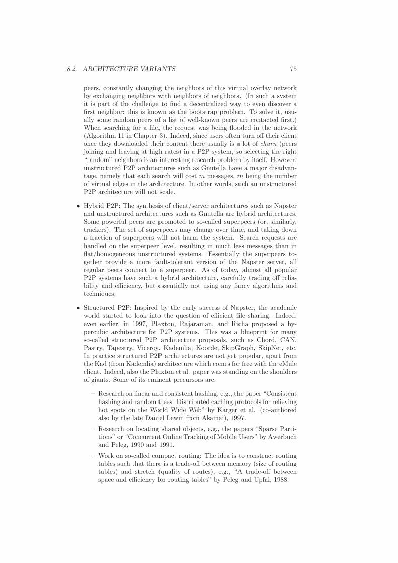
8.2. ARCHITECTURE VARIANTS 75
peers, constantly changing the neighbors of this virtual overlay networkby exchanging neighbors with neighbors of neighbors. (In such a systemit is part of the challenge to find a decentralized way to even discover afirst neighbor; this is known as the bootstrap problem. To solve it, usu-ally some random peers of a list of well-known peers are contacted first.)When searching for a file, the request was being flooded in the network(Algorithm 11 in Chapter 3). Indeed, since users often turn off their clientonce they downloaded their content there usually is a lot of churn (peersjoining and leaving at high rates) in a P2P system, so selecting the right“random” neighbors is an interesting research problem by itself. However,unstructured P2P architectures such as Gnutella have a major disadvan-tage, namely that each search will cost m messages, m being the numberof virtual edges in the architecture. In other words, such an unstructuredP2P architecture will not scale.
• Hybrid P2P: The synthesis of client/server architectures such as Napsterand unstructured architectures such as Gnutella are hybrid architectures.Some powerful peers are promoted to so-called superpeers (or, similarly,trackers). The set of superpeers may change over time, and taking downa fraction of superpeers will not harm the system. Search requests arehandled on the superpeer level, resulting in much less messages than inflat/homogeneous unstructured systems. Essentially the superpeers to-gether provide a more fault-tolerant version of the Napster server, allregular peers connect to a superpeer. As of today, almost all popularP2P systems have such a hybrid architecture, carefully trading off relia-bility and efficiency, but essentially not using any fancy algorithms andtechniques.
• Structured P2P: Inspired by the early success of Napster, the academicworld started to look into the question of efficient file sharing. Indeed,even earlier, in 1997, Plaxton, Rajaraman, and Richa proposed a hy-percubic architecture for P2P systems. This was a blueprint for manyso-called structured P2P architecture proposals, such as Chord, CAN,Pastry, Tapestry, Viceroy, Kademlia, Koorde, SkipGraph, SkipNet, etc.In practice structured P2P architectures are not yet popular, apart fromthe Kad (from Kademlia) architecture which comes for free with the eMuleclient. Indeed, also the Plaxton et al. paper was standing on the shouldersof giants. Some of its eminent precursors are:
– Research on linear and consistent hashing, e.g., the paper “Consistenthashing and random trees: Distributed caching protocols for relievinghot spots on the World Wide Web” by Karger et al. (co-authoredalso by the late Daniel Lewin from Akamai), 1997.
– Research on locating shared objects, e.g., the papers “Sparse Parti-tions” or “Concurrent Online Tracking of Mobile Users” by Awerbuchand Peleg, 1990 and 1991.
– Work on so-called compact routing: The idea is to construct routingtables such that there is a trade-off between memory (size of routingtables) and stretch (quality of routes), e.g., “A trade-off betweenspace and efficiency for routing tables” by Peleg and Upfal, 1988.
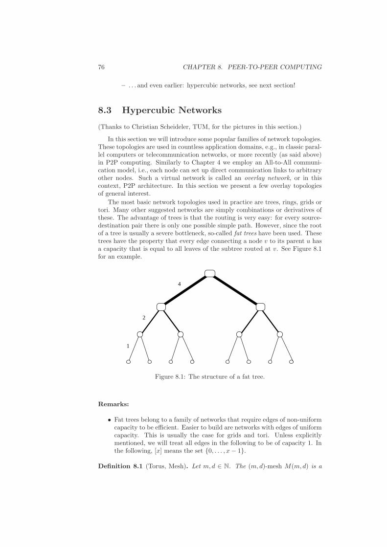
76 CHAPTER 8. PEER-TO-PEER COMPUTING
– . . . and even earlier: hypercubic networks, see next section!
8.3 Hypercubic Networks
(Thanks to Christian Scheideler, TUM, for the pictures in this section.)
In this section we will introduce some popular families of network topologies.These topologies are used in countless application domains, e.g., in classic paral-lel computers or telecommunication networks, or more recently (as said above)in P2P computing. Similarly to Chapter 4 we employ an All-to-All communi-cation model, i.e., each node can set up direct communication links to arbitraryother nodes. Such a virtual network is called an overlay network, or in thiscontext, P2P architecture. In this section we present a few overlay topologiesof general interest.
The most basic network topologies used in practice are trees, rings, grids ortori. Many other suggested networks are simply combinations or derivatives ofthese. The advantage of trees is that the routing is very easy: for every source-destination pair there is only one possible simple path. However, since the rootof a tree is usually a severe bottleneck, so-called fat trees have been used. Thesetrees have the property that every edge connecting a node v to its parent u hasa capacity that is equal to all leaves of the subtree routed at v. See Figure 8.1for an example.
2
1
4
Figure 8.1: The structure of a fat tree.
Remarks:
• Fat trees belong to a family of networks that require edges of non-uniformcapacity to be efficient. Easier to build are networks with edges of uniformcapacity. This is usually the case for grids and tori. Unless explicitlymentioned, we will treat all edges in the following to be of capacity 1. Inthe following, [x] means the set 0, . . . , x− 1.
Definition 8.1 (Torus, Mesh). Let m, d ∈ N. The (m, d)-mesh M(m, d) is a

8.3. HYPERCUBIC NETWORKS 77
graph with node set V = [m]d and edge set
E =
(a1, . . . , ad), (b1, . . . , bd) | ai, bi ∈ [m],d∑
i=1
|ai − bi| = 1
.
The (m, d)-torus T (m, d) is a graph that consists of an (m, d)-mesh and addi-tionally wrap-around edges from nodes (a1, . . . , ai−1,m, ai+1, . . . , ad) to nodes(a1, . . . , ai−1, 1, ai+1, . . . , ad) for all i ∈ 1, . . . , d and all aj ∈ [m] with j 6= i.In other words, we take the expression ai − bi in the sum modulo m prior tocomputing the absolute value. M(m, 1) is also called a line, T (m, 1) a cycle,and M(2, d) = T (2, d) a d-dimensional hypercube. Figure 8.2 presents a lineararray, a torus, and a hypercube.
011010
110
100
000 001
101
111
M(2,3)
0 1 2
M( ,1)m
−1m
01
02
00 10
11
12
03
20
21
22
13
30
31
32
23 33
(4,2)T
Figure 8.2: The structure of M(m, 1), T (4, 2), and M(2, 3).
Remarks:
• Routing on mesh, torus, and hypercube is trivial. On a d-dimensionalhypercube, to get from a source bitstring s to a target bitstring d one onlyneeds to fix each “wrong” bit, one at a time; in other words, if the sourceand the target differ by k bits, there are k! routes with k hops.
• The hypercube can directly be used for a structured P2P architecture. Itis trivial to construct a distributed hash table (DHT): We have n nodes,n for simplicity being a power of 2, i.e., n = 2d. As in the hypercube, eachnode gets a unique d-bit ID, and each node connects to d other nodes,i.e., the nodes that have IDs differing in exactly one bit. Now we use aglobally known hash function f , mapping file names to long bit strings;SHA-1 is popular in practice, providing 160 bits. Let fd denote the first dbits (prefix) of the bitstring produced by f . If a node is searching for filename X, it routes a request message f(X) to node fd(X). Clearly, nodefd(X) can only answer this request if all files with hash prefix fd(X) havebeen previously registered at node fd(X).
• There are a few issues which need to be addressed before our DHT works,in particular churn (nodes joining and leaving without notice). To dealwith churn the system needs some level of replication, i.e., a number ofnodes which are responsible for each prefix such that failure of some nodes
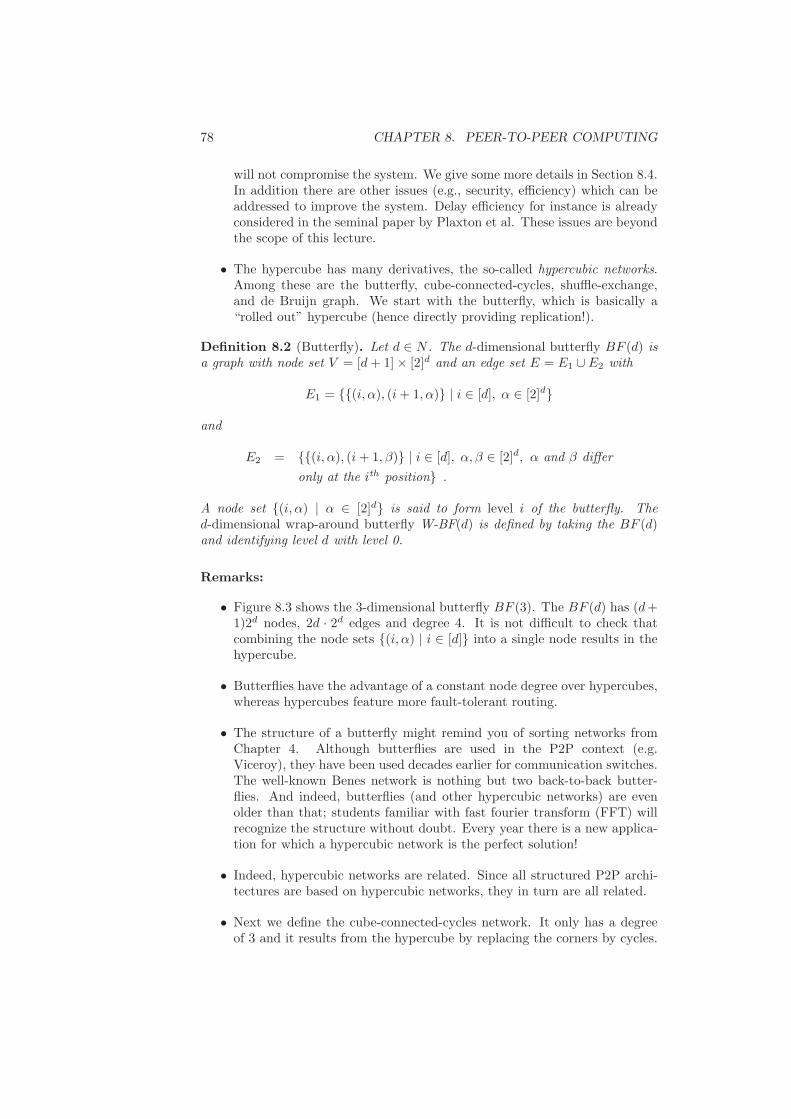
78 CHAPTER 8. PEER-TO-PEER COMPUTING
will not compromise the system. We give some more details in Section 8.4.In addition there are other issues (e.g., security, efficiency) which can beaddressed to improve the system. Delay efficiency for instance is alreadyconsidered in the seminal paper by Plaxton et al. These issues are beyondthe scope of this lecture.
• The hypercube has many derivatives, the so-called hypercubic networks.Among these are the butterfly, cube-connected-cycles, shuffle-exchange,and de Bruijn graph. We start with the butterfly, which is basically a“rolled out” hypercube (hence directly providing replication!).
Definition 8.2 (Butterfly). Let d ∈ N . The d-dimensional butterfly BF (d) isa graph with node set V = [d + 1]× [2]d and an edge set E = E1 ∪ E2 with
E1 = (i, α), (i + 1, α) | i ∈ [d], α ∈ [2]d
and
E2 = (i, α), (i + 1, β) | i ∈ [d], α, β ∈ [2]d, α and β differ
only at the ith position .
A node set (i, α) | α ∈ [2]d is said to form level i of the butterfly. Thed-dimensional wrap-around butterfly W-BF(d) is defined by taking the BF (d)and identifying level d with level 0.
Remarks:
• Figure 8.3 shows the 3-dimensional butterfly BF (3). The BF (d) has (d+1)2d nodes, 2d · 2d edges and degree 4. It is not difficult to check thatcombining the node sets (i, α) | i ∈ [d] into a single node results in thehypercube.
• Butterflies have the advantage of a constant node degree over hypercubes,whereas hypercubes feature more fault-tolerant routing.
• The structure of a butterfly might remind you of sorting networks fromChapter 4. Although butterflies are used in the P2P context (e.g.Viceroy), they have been used decades earlier for communication switches.The well-known Benes network is nothing but two back-to-back butter-flies. And indeed, butterflies (and other hypercubic networks) are evenolder than that; students familiar with fast fourier transform (FFT) willrecognize the structure without doubt. Every year there is a new applica-tion for which a hypercubic network is the perfect solution!
• Indeed, hypercubic networks are related. Since all structured P2P archi-tectures are based on hypercubic networks, they in turn are all related.
• Next we define the cube-connected-cycles network. It only has a degreeof 3 and it results from the hypercube by replacing the corners by cycles.
8.3. HYPERCUBIC NETWORKS 79
000 100010 110001 101011 111
1
2
0
3
Figure 8.3: The structure of BF(3).
000 001 010 011 100 101 110 111
2
1
0
(110,1)
(011,2)
(101,1)
(001,2)
(001,1)
(001,0)(000,0)
(100,0)
(100,1)
(100,2)
(000,2)
(000,1)
(010,1)
(010,0)
(010,2)
(110,2)
(110,0) (111,0)
(111,1)
(111,2)
(011,1)
(011,0)
(101,2)
(101,0)
Figure 8.4: The structure of CCC(3).
Definition 8.3 (Cube-Connected-Cycles). Let d ∈ N . The cube-connected-cycles network CCC(d) is a graph with node set V = (a, p) | a ∈ [2]d, p ∈ [d]and edge set
E =
(a, p), (a, (p + 1)mod d) | a ∈ [2]d, p ∈ [d]
∪
(a, p), (b, p) | a, b ∈ [2]d, p ∈ [d], a = b except for ap
.
Remarks:
• Two possible representations of a CCC can be found in Figure 8.4.
• The shuffle-exchange is yet another way of transforming the hypercubicinterconnection structure into a constant degree network.
Definition 8.4 (Shuffle-Exchange). Let d ∈ N . The d-dimensional shuffle-exchange SE(d) is defined as an undirected graph with node set V = [2]d andan edge set E = E1 ∪ E2 with
E1 = (a1, . . . , ad), (a1, . . . , ad) | (a1, . . . , ad) ∈ [2]d, ad = 1− ad

80 CHAPTER 8. PEER-TO-PEER COMPUTING
andE2 = (a1, . . . , ad), (ad, a1, . . . , ad−1) | (a1, . . . , ad) ∈ [2]d .
Figure 8.5 shows the 3- and 4-dimensional shuffle-exchange graph.
000 001
100
010
101
011
110 111 0000 0001
0010 0011
0100 0101
0110 0111
1000 1001
1010 1011
1100 1101
1110 1111
SE(3) SE(4)
E
E1
2
Figure 8.5: The structure of SE(3) and SE(4).
Definition 8.5 (DeBruijn). The b-ary DeBruijn graph of dimension d DB(b, d)is an undirected graph G = (V,E) with node set V = v ∈ [b]d and edge setE that contains all edges v, w with the property that w ∈ (x, v1, . . . , vd−1) :x ∈ [b], where v = (v1, . . . , vd).
010
100
001
110
1111100
01
000101
011
10
Figure 8.6: The structure of DB(2, 2) and DB(2, 3).
Remarks:
• Two examples of a DeBruijn graph can be found in Figure 8.6. TheDeBruijn graph is the basis of the Koorde P2P architecture.
• There are some data structures which also qualify as hypercubic networks.An obvious example is the Chord P2P architecture, which uses a slightlydifferent hypercubic topology. A less obvious (and therefore good) exam-ple is the skip list, the balanced binary search tree for the lazy programmer:
Definition 8.6 (Skip List). The skip list is an ordinary ordered linked list ofobjects, augmented with additional forward links. The ordinary linked list is thelevel 0 of the skip list. In addition, every object is promoted to level 1 withprobability 1/2. As for level 0, all level 1 objects are connected by a linked list.In general, every object on level i is promoted to the next level with probability1/2. A special start-object points to the smallest/first object on each level.

8.3. HYPERCUBIC NETWORKS 81
Remarks:
• Search, insert, and delete can be implemented in O(log n) expected timein a skip list, simply by jumping from higher levels to lower ones whenovershooting the searched position. Also, the amortized memory cost ofeach object is constant, as on average an object only has two forwardpointers.
• The randomization can easily be discarded, by deterministically promotinga constant fraction of objects of level i to level i + 1, for all i. Wheninserting or deleting, object o simply checks whether its left and rightlevel i neighbors are being promoted to level i + 1. If none of them is,promote object o itself. Essentially we establish a MIS on each level, henceat least every third and at most every second object is promoted.
• There are obvious variants of the skip list, e.g., the skip graph. Insteadof promoting only half of the nodes to the next level, we always promoteall the nodes, similarly to a balanced binary tree: All nodes are part ofthe root level of the binary tree. Half the nodes are promoted left, andhalf the nodes are promoted right, on each level. Hence on level i we havehave 2i lists (or, more symmetrically: rings) of about n/2i objects. Thisis pretty much what we need for a nice hypercubic P2P architecture.
• One important goal in choosing a topology for a network is that it has asmall diameter. The following theorem presents a lower bound for this.
Theorem 8.7. Every graph of maximum degree d > 2 and size n must have adiameter of at least ⌈(log n)/(log(d− 1))⌉ − 2.
Proof. Suppose we have a graph G = (V,E) of maximum degree d and sizen. Start from any node v ∈ V . In a first step at most d other nodes can bereached. In two steps at most d · (d−1) additional nodes can be reached. Thus,in general, in at most k steps at most
1 +
k−1∑
i=0
d · (d− 1)i = 1 + d · (d− 1)k − 1
(d− 1)− 1≤ d · (d− 1)k
d− 2
nodes (including v) can be reached. This has to be at least n to ensure that vcan reach all other nodes in V within k steps. Hence,
(d− 1)k ≥ (d− 2) · nd
⇔ k ≥ logd−1((d− 2) · n/d) .
Since logd−1((d − 2)/d) > −2 for all d > 2, this is true only if k ≥⌈(log n)/(log(d− 1))⌉ − 2.
Remarks:
• In other words, constant-degree hypercubic networks feature an asymp-totically optimal diameter.
82 CHAPTER 8. PEER-TO-PEER COMPUTING
• There are a few other interesting graph classes, e.g., expander graphs (anexpander graph is a sparse graph which has high connectivity properties,that is, from every not too large subset of nodes you are connected toa larger set of nodes), or small-world graphs (popular representations ofsocial networks). At first sight hypercubic networks seem to be related toexpanders and small-world graphs, but they are not.
8.4 DHT & Churn
As written earlier, a DHT essentially is a hypercubic structure with nodes havingidentifiers such that they span the ID space of the objects to be stored. Wedescribed the straightforward way how the ID space is mapped onto the peersfor the hypercube. Other hypercubic structures may be more complicated: Thebutterfly network, for instance, may directly use the d+1 layers for replication,i.e., all the d + 1 nodes with the same ID are responsible for the same hashprefix. For other hypercubic networks, e.g., the pancake graph (see exercises),assigning the object space to peer nodes may be more difficult.
In general a DHT has to withstand churn. Usually, peers are under control ofindividual users who turn their machines on or off at any time. Such peers joinand leave the P2P system at high rates (“churn”), a problem that is not existentin orthodox distributed systems, hence P2P systems fundamentally differ fromold-school distributed systems where it is assumed that the nodes in the systemare relatively stable. In traditional distributed systems a single unavailablenode is a minor disaster: all the other nodes have to get a consistent view of thesystem again, essentially they have to reach consensus which nodes are available.In a P2P system there is usually so much churn that it is impossible to have aconsistent view at any time.
Most P2P systems in the literature are analyzed against an adversary thatcan crash a fraction of random peers. After crashing a few peers the systemis given sufficient time to recover again. However, this seems unrealistic. Thescheme sketched in this section significantly differs from this in two major as-pects. First, we assume that joins and leaves occur in a worst-case manner. Wethink of an adversary that can remove and add a bounded number of peers; itcan choose which peers to crash and how peers join. We assume that a joiningpeer knows a peer which already belongs to the system. Second, the adversarydoes not have to wait until the system is recovered before it crashes the nextbatch of peers. Instead, the adversary can constantly crash peers, while the sys-tem is trying to stay alive. Indeed, the system is never fully repaired but alwaysfully functional. In particular, the system is resilient against an adversary thatcontinuously attacks the “weakest part” of the system. The adversary could forexample insert a crawler into the P2P system, learn the topology of the system,and then repeatedly crash selected peers, in an attempt to partition the P2Pnetwork. The system counters such an adversary by continuously moving theremaining or newly joining peers towards the sparse areas.
Clearly, we cannot allow the adversary to have unbounded capabilities. Inparticular, in any constant time interval, the adversary can at most add and/orremove O(log n) peers, n being the total number of peers currently in the sys-tem. This model covers an adversary which repeatedly takes down machines bya distributed denial of service attack, however only a logarithmic number of ma-

8.4. DHT & CHURN 83
chines at each point in time. The algorithm relies on messages being deliveredtimely, in at most constant time between any pair of operational peers, i.e., thesynchronous model. Using the trivial synchronizer this is not a problem. Weonly need bounded message delays in order to have a notion of time which isneeded for the adversarial model. The duration of a round is then proportionalto the propagation delay of the slowest message.
In the remainder of this section, we give a sketch of the system: For sim-plicity, the basic structure of the P2P system is a hypercube. Each peer is partof a distinct hypercube node; each hypercube node consists of Θ(log n) peers.Peers have connections to other peers of their hypercube node and to peers ofthe neighboring hypercube nodes.1 Because of churn, some of the peers have tochange to another hypercube node such that up to constant factors, all hyper-cube nodes own the same number of peers at all times. If the total number ofpeers grows or shrinks above or below a certain threshold, the dimension of thehypercube is increased or decreased by one, respectively.
The balancing of peers among the hypercube nodes can be seen as a dynamictoken distribution problem on the hypercube. Each node of the hypercube has acertain number of tokens, the goal is to distribute the tokens along the edges ofthe graph such that all nodes end up with the same or almost the same numberof tokens. While tokens are moved around, an adversary constantly inserts anddeletes tokens. See also Figure 8.7.
Figure 8.7: A simulated 2-dimensional hypercube with four nodes, each consist-ing of several peers. Also, all the peers are either in the core or in the peripheryof a node. All peers within the same node are completely connected to eachother, and additionally, all peers of a node are connected to the core peers of theneighboring nodes. Only the core peers store data items, while the peripheralpeers move between the nodes to balance biased adversarial changes.
In summary, the P2P system builds on two basic components: i) an algo-rithm which performs the described dynamic token distribution and ii) an in-formation aggregation algorithm which is used to estimate the number of peersin the system and to adapt the dimension of the hypercube accordingly:
Theorem 8.8 (DHT with Churn). We have a fully scalable, efficient P2P
1Having a logarithmic number of hypercube neighbor nodes, each with a logarithmic num-ber of peers, means that each peers has Θ(log2
n) neighbor peers. However, with some addi-tional bells and whistles one can achieve Θ(log n) neighbor peers.

84 CHAPTER 8. PEER-TO-PEER COMPUTING
system which tolerates O(log n) worst-case joins and/or crashes per constanttime interval. As in other P2P systems, peers have O(log n) neighbors, and theusual operations (e.g., search, insert) take time O(log n).
Remarks:
• Indeed, handling churn is only a minimal requirement to make a P2Psystem work. Later studies proposed more elaborate architectures whichcan also handle other security issues, e.g., privacy or Byzantine attacks.
• It is surprising that unstructured (in fact, hybrid) P2P systems dominatestructured P2P systems in the real world. One would think that structuredP2P systems have advantages, in particular their efficient logarithmic datalookup. On the other hand, unstructured P2P networks are simpler, inparticular in light of non-exact queries.

Chapter 9
Social Networks
Distributed computing is applicable in various contexts. This lecture exemplar-ily studies one of these contexts, social networks, an area of study whose originsdate back a century. To give you a first impression, consider Figure 9.1.
inst2
34
5
6
7
8
9
10
11
12
13
14
1516
1718
19
20
21
22
23
24
25
26
27
28
29
30
31
32
33
admin
Figure 9.1: This graph shows the social relations between the members of akarate club, studied by anthropologist Wayne Zachary in the 1970s. Two people(nodes) stand out, the instructor and the administrator of the club, both happento have many friends among club members. At some point, a dispute causedthe club to split into two. Can you predict how the club partitioned? (If not,just search the Internet for Zachary and Karate.)
85

86 CHAPTER 9. SOCIAL NETWORKS
9.1 Small-World Networks
Back in 1929, Frigyes Karinthy published a volume of short stories that pos-tulated that the world was “shrinking” because human beings were connectedmore and more. Some claim that he was inspired by radio network pioneerGuglielmo Marconi’s 1909 Nobel Prize speech. Despite physical distance, thegrowing density of human “networks” renders the actual social distance smallerand smaller. As a result, it is believed that any two individuals can be connectedthrough at most five (or so) acquaintances, i.e., within six hops.
• The topic was hot in the 1960s. For instance, in 1964, Marshall McLuhancoined the metaphor “Global Village”. He wrote: “As electrically con-tracted, the globe is no more than a village”. He argues that due to thealmost instantaneous reaction times of new (“electric”) technologies, eachindividual inevitably feels the consequences of his actions and thus auto-matically deeply participates in the global society. McLuhan understoodwhat we now can directly observe – real and virtual world are moving to-gether. He realized that the transmission medium, rather than the trans-mitted information is at the core of change, as expressed by his famousphrase “the medium is the message”.
• This idea has been followed ardently in the 1960s by several sociologists,first by Michael Gurevich, later by Stanley Milgram. Milgram wanted toknow the average path length between two “random” humans, by usingvarious experiments, generally using randomly chosen individuals fromthe US Midwest as starting points, and a stockbroker living in a suburbof Boston as target. The starting points were given name, address, oc-cupation, plus some personal information about the target. They wereasked to send a letter to the target. However, they were not allowed todirectly send the letter, rather, they had to pass it to somebody they knewon first-name basis and that they thought to have a higher probability toknow the target person. This process was repeated, until somebody knewthe target person, and could deliver the letter. Shortly after starting theexperiment, letters have been received. Most letters were lost during theprocess, but if they arrived, the average path length was about 5.5. Theobservation that the entire population is connected by short acquaintancechains got later popularized by the terms “six degrees of separation” and“small world”.
• Statisticians tried to explain Milgram’s experiments, by essentially giv-ing network models that allowed for short diameters, i.e., each node isconnected to each other node by only a few hops. Until today there is athriving research community in statistical physics that tries to understandnetwork properties that allow for “small world” effects.
• One of the keywords in this area are power-law graphs, networks werenode degrees are distributed according to a power-law distribution, i.e.the number of nodes with degree δ is proportional to δ−α, for some α > 1.Such power-law graphs have been witnessed in many application areas,apart from social networks also in the web, or in Biology or Physics.

9.1. SMALL-WORLD NETWORKS 87
• Obviously, two power-law graphs might look and behave completely dif-ferently, even if α and the number of edges is exactly the same.
One well-known model towards this end is the Watts-Strogatz model. Wattsand Strogatz argued that social networks should be modeled by a combination oftwo networks: As the basis we take a network that has a large cluster coefficient. . .
Definition 9.1. The cluster coefficient of a network is defined by the probabilitythat two friends of a node are likely to be friends as well, summing up over allthe nodes.
. . . , then we augment such a graph with random links, every node for in-stance points to a constant number of other nodes, chosen uniformly at random.This augmentation represents acquaintances that connect nodes to parts of thenetwork that would otherwise be far away.
Remarks:
• Without further information, knowing the cluster coefficient is of ques-tionable value: Assume we arrange the nodes in a grid. Technically, ifwe connect each node to its four closest neighbors, the graph has clustercoefficient 0, since there are no triangles; if we instead connect each nodewith its eight closest neighbors, the cluster coefficient is 3/7. The clus-ter coefficient is quite different, even though both networks have similarcharacteristics.
This is interesting, but not enough to really understand what is going on. ForMilgram’s experiments to work, it is not sufficient to connect the nodes in acertain way. In addition, the nodes themselves need to know how to forwarda message to one of their neighbors, even though they cannot know whetherthat neighbor is really closer to the target. In other words, nodes are notjust following physical laws, but they make decisions themselves. In contrastto those mathematicians that worked on the problem earlier, Jon Kleinbergunderstood that Milgram’s experiment essentially shows that social networksare “navigable”, and that one can only explain it in terms of a greedy routing.
In particular, Kleinberg set up an artificial network with nodes on a gridtopology, plus some additional random links per node. In a quantitative studyhe showed that the random links need a specific distance distribution to allowfor efficient greedy routing. This distribution marks the sweet spot for anynavigable network.
Definition 9.2 (Augmented Grid). We take n = m2 nodes (i, j) ∈ V =
1, . . . ,m2 that are identified with the lattice points on an m × m grid. Wedefine the distance between two nodes (i, j) and (k, ℓ) as d
(
(i, j), (k, ℓ))
=|k − i| + |ℓ − j| as the distance between them on the m × m lattice. The net-work is modeled using a parameter α ≥ 0. Each node u has a directed edge toevery lattice neighbor. These are the local contacts of a node. In addition, eachnode also has an additional random link (the long-range contact). For all uand v, the long-range contact of u points to node v with probability proportionalto d(u, v)−α, i.e., with probability d(u, v)−α/
∑
w∈V \u d(u,w)−α. Figure 9.2illustrates the model.

88 CHAPTER 9. SOCIAL NETWORKS
Figure 9.2: Augmented grid with m = 6
Remarks:
• The network model has the following geographic interpretation: nodes(individuals) live on a grid and know their neighbors on the grid. Further,each node has some additional acquaintances throughout the network.
• The parameter α controls how the additional neighbors are distributedacross the grid. If α = 0, long-range contacts are chosen uniformly atrandom (as in the Watts-Strogatz model). As α increases, long-rangecontacts become shorter on average. In the extreme case, if α → ∞, alllong-range contacts are to immediate neighbors on the grid.
• It can be shown that as long as α ≤ 2, the diameter of the resultinggraph is polylogarithmic in n (polynomial in log n) with high probability.In particular, if the long-range contacts are chosen uniformly at random(α = 0), the diameter is O(log n).
Since the augmented grid contains random links, we do not know anythingfor sure about how the random links are distributed. In theory, all links couldpoint to the same node! However, this is almost certainly not the case. Formallythis is captured by the term with high probability.
Definition 9.3 (With High Probability). Some probabilistic event is said tooccur with high probability (w.h.p.), if it happens with a probability p ≥ 1 −1/nc, where c is a constant. The constant c may be chosen arbitrarily, but it isconsidered constant with respect to Big-O notation.
9.1. SMALL-WORLD NETWORKS 89
Remarks:
• For instance, a running time bound of c log n or ec! log n + 5000c withprobability at least 1−1/nc would be O(log n) w.h.p., but a running timeof nc would not be O(n) w.h.p. since c might also be 50.
• This definition is very powerful, as any polynomial (in n) number of state-ments that hold w.h.p. also holds w.h.p. at the same time, regardless ofany dependencies between random variables!
Theorem 9.4. The diameter of the augmented grid with α = 0 is O(log n) withhigh probability.
Proof Sketch. For simplicity, we will only show that we can reach a node wstarting from some node v. However, it can be shown that (essentially) eachof the intermediate claims holds with high probability, which then by meansof the union bound yields that all of the claims hold simultaneously with highprobability for all pairs of nodes (see exercises).
Let Ng be the ⌈log n⌉-hop neighborhood of v on the grid, containing Ω(log2 n)nodes. Each of the nodes in Ng has a random link, probably leading to distantparts of the graph. As long as we have reached only o(n) nodes, any newrandom link will with probability 1− o(1) lead to a node for which none of itsgrid neighbors has been visited yet. Thus, in expectation we find almost |Ng|new nodes whose neighbors are “fresh”. Using their grid links, we will reach(4−o(1))|Ng| more nodes within one more hop. If bad luck strikes, it could stillhappen that many of these links lead to a few nodes, already visited nodes, ornodes that are very close to each other. But that is very unlikely, as we havelots of random choices! Indeed, it can be shown that not only in expectation,but with high probability (5− o(1))|Ng| many nodes are reached this way (seeexercises).
Because all these shiny new nodes have (so far unused) random links, wecan repeat this reasoning inductively, implying that the number of nodes growsby (at least) a constant factor for every two hops. Thus, after O(log n) hops,we will have reached n/ log n nodes (which is still small compared to n). Fi-nally, consider the expected number of links from these nodes that enter the(log n)-neighborhood of some target node w with respect to the grid. Since thisneighborhood consists of Ω(log2 n) nodes, in expectation Ω(log n) links comeclose enough to w. This is large enough to almost guarantee that this happens(see exercises). Summing everything up, we still used merely O(log n) hops intotal to get from v to w.
This shows that for α = 0 (and in fact for all α ≤ 2), the resulting networkhas a small diameter. Recall however that we also wanted the network to benavigable. For this, we consider a simple greedy routing strategy (Algorithm 34.
Algorithm 34 Greedy Routing
1: while not at destination do2: go to a neighbor which is closest to destination (considering grid distance
only)3: end while

90 CHAPTER 9. SOCIAL NETWORKS
Lemma 9.5. In the augmented grid, Algorithm 34 finds a routing path of lengthat most 2(m− 1) ∈ O(
√n).
Proof. Because of the grid links, there is always a neighbor which is closer tothe destination. Since with each hop we reduce the distance to the target atleast by one in one of the two grid dimensions, we will reach the destinationwithin 2(m− 1) steps.
This is not really what Milgram’s experiment promises. We want to knowhow much the additional random links speed up the process. To this end, wefirst need to understand how likely it is that two nodes u and v are connectedby a random link in terms of n and their distance d(u, v).
Lemma 9.6. Node u’s random link leads to a node v with probability
• Θ(1/(d(u, v)αm2−α)) if α < 2.
• Θ(1/(d(u, v)2 log n)) if α = 2,
• Θ(1/d(u, v)α) if α > 2.
Moreover, if α > 2, the probability to see a link of length at least d is inΘ(1/dα−2).
Proof. For α 6= 2, we have that
∑
w∈V \u
1
d(u,w)α∈
m∑
r=1
Θ(r)
rα= Θ
(∫ m
r=1
1
rα−1dr
)
= Θ
([
r2−α
2− α
]m
1
)
.
If α < 2, this gives Θ(m2−α), if α > 2, it is in Θ(1). If α = 2, we get
∑
w∈V \u
1
d(u,w)α∈
m∑
r=1
Θ(r)
r2= Θ(1) ·
m∑
r=1
1
r= Θ(log m) = Θ(log n).
Multiplying with d(u, v)α yields the first three bounds.For the last statement, compute
∑
w∈Vd(u,v)≥d
Θ(1/d(u, v)α) = Θ
(∫ m
r=d
r
rαdr
)
= Θ
([
r2−α
2− α
]m
d
)
= Θ(1/dα−2).
Remarks:
• For α 6= 2, this is bad news for the greedy routing algorithm, as it willtake nΩ(1) = mΩ(1) expected steps to reach the destination. This is dis-appointing, we were hoping for something polylogarithmic.
• If α < 2, in distance m(2−α)/3 to the target are m2(2−α)/3 many nodes.Thus it takes Θ(m(2−α)/3) links in expectation to find a link that comesthat close to the destination. Without finding such a link, we have to goat least this far using grid links only.

9.1. SMALL-WORLD NETWORKS 91
• If α > 2, it takes Θ(m(α−2)/(α−1)) steps until we see a link of lengthat least m1/(α−1) in expectation. Without such links, it takes at leastm/m1/(α−1) = m(α−2)/(α−1) steps to travel a distance of m.
• Any algorithm that uses only the information on long-range contacts thatit can collect at the so far visited nodes cannot be faster.
• However, the case α = 2 looks more promising.
Definition 9.7 (Phase). Consider routing from a node u to a node v andassume that we are at some intermediate node w. We say that we are in phasej at node w if the lattice distance d(w, v) to the target node v is between 2j <d(w, v) ≤ 2j+1.
Remarks:
• Enumerating the phases in decreasing order is useful, as notation becomesless cumbersome.
• There are ⌈log m⌉ ∈ O(log n) phases.
Lemma 9.8. Assume that we are in phase j at node w when routing from u tov. The probability for getting to phase j − 1 in one step is at least Ω(1/ log n).
Proof. Let Bj be the set of nodes x with d(x, v) ≤ 2j . We get from phase jto phase j − 1 if the long-range contact of node w points to some node in Bj .Note that we always make progress while following the greedy routing path.Therefore, we have not seen node w before and the long-range contact of wpoints to a random node that is independent of anything seen on the path fromu to w.
For all nodes x ∈ Bj , we have d(w, x) ≤ d(w, v)+d(x, v) ≤ 2j+1 +2j < 2j+2.Hence, for each node x ∈ Bj , the probability that the long-range contact of wpoints to x is Ω(1/22j+4 log n). Further, the number of nodes in Bj is at least(2j)2/2 = 22j−1. Hence, the probability that some node in Bj is the long rangecontact of w is at least
Ω
(
|Bj | ·1
22j+4 log n
)
= Ω
(
22j−1
22j+4 log n
)
= Ω
(
1
log n
)
.
Theorem 9.9. Consider the greedy routing path from a node u to a node v onan augmented grid with parameter α = 2. The expected length of the path isO(log2 n).
Proof. We already observed that the total number of phases is O(log n) (thedistance to the target is halved when we go from phase j to phase j − 1). Ateach point during the routing process, the probability of proceeding to the nextphase is at least Ω(1/ log n). Let Xj be the number of steps in phase j. Becausethe probability for ending the phase is Ω(1/ log n) in each step, in expectationwe need O(log n) steps to proceed to the next phase, i.e., E[Xj ] ∈ O(log n). LetX =
∑
j Xj be the total number of steps of the routing process. By linearity ofexpectation, we have
E[X] =∑
j
E[Xj ] ∈ O(log2 n).

92 CHAPTER 9. SOCIAL NETWORKS
9.2 Propagation Studies
In networks, nodes may influence each other’s behavior and decisions. There aremany applications where nodes influence their neighbors, e.g. they may impacttheir opinions, or they may bias what products they buy, or they may pass ona disease.
On a beach (modeled as a line segment), it is best to place an ice creamstand right in the middle of the segment, because you will be able to “control”the beach most easily. What about the second stand, where should it settle?The answer generally depends on the model, but assuming that people will buyice cream from the stand that is closer, it should go right next to the first stand.
Rumors can spread astoundingly fast through social networks. Tradition-ally this happens by word of mouth, but with the emergence of the Internetand its possibilities new ways of rumor propagation are available. People writeemail, use instant messengers or publish their thoughts in a blog. Many factorsinfluence the dissemination of rumors. It is especially important where in a net-work a rumor is initiated and how convincing it is. Furthermore the underlyingnetwork structure decides how fast the information can spread and how manypeople are reached. More generally, we can speak of diffusion of information innetworks. The analysis of these diffusion processes can be useful for viral mar-keting, e.g. to target a few influential people to initiate marketing campaigns.A company may wish to distribute the rumor of a new product via the mostinfluential individuals in popular social networks such as Facebook. A secondcompany might want to introduce a competing product and has hence to selectwhere to seed the information to be disseminated. Rumor spreading is quitesimilar to our ice cream stand problem.
More formally, we may study propagation problems in graphs. Given agraph, and two players. Let the first player choose a seed node u1; afterwardslet the second player choose a seed node u2, with u2 6= u1. The goal of the gameis to maximize the number of nodes that are closer to one’s own seed node.
In many graphs it is an advantage to choose first. In a star graph for instancethe first player can choose the center node of the star, controlling all but onenode. In some other graphs, the second player can at least score even. But isthere a graph where the second player has an advantage?
Theorem 9.10. In a two player rumor game where both players select one nodeto initiate their rumor in the graph, the first player does not always win.
Proof. See Figure 9.3 for an example where the second player will always win,regardless of the decision the first player. If the first player chooses the node x0
in the center, the second player can select x1. Choice x1 will be outwitted by x2,and x2 itself can be answered by z1. All other strategies are either symmetric,or even less promising for the first player.

9.2. PROPAGATION STUDIES 93
x1x2
y2
y1
z1
x0
y2
z2
Figure 9.3: Counter example.

94 CHAPTER 9. SOCIAL NETWORKS

Chapter 10
Maximal Independent Set
In this chapter we present a highlight of this course, a fast maximal independentset (MIS) algorithm. The algorithm is the first randomized algorithm that westudy in this class. In distributed computing, randomization is a powerful andtherefore omnipresent concept, as it allows for relatively simple yet efficientalgorithms. As such the studied algorithm is archetypal.
A MIS is a basic building block in distributed computing, some other prob-lems pretty much follow directly from the MIS problem. At the end of thischapter, we will give two examples: matching and vertex coloring (see Chapter1).
10.1 MIS
Definition 10.1 (Independent Set). Given an undirected Graph G = (V,E)an independent set is a subset of nodes U ⊆ V , such that no two nodes in Uare adjacent. An independent set is maximal if no node can be added withoutviolating independence. An independent set of maximum cardinality is calledmaximum.
2
1
2
Figure 10.1: Example graph with 1) a maximal independent set (MIS) and 2)a maximum independent set (MaxIS).
95

96 CHAPTER 10. MAXIMAL INDEPENDENT SET
Remarks:
• Computing a maximum independent set (MaxIS) is a notoriously difficultproblem. It is equivalent to maximum clique on the complementary graph.Both problems are NP-hard, in fact not approximable within n
1
2−ǫ.
• In this course we concentrate on the maximal independent set (MIS) prob-lem. Please note that MIS and MaxIS can be quite different, indeed e.g.on a star graph the MIS is Θ(n) smaller than the MaxIS (cf. Figure 10.1).
• Computing a MIS sequentially is trivial: Scan the nodes in arbitrary order.If a node u does not violate independence, add u to the MIS. If u violatesindependence, discard u. So the only question is how to compute a MISin a distributed way.
Algorithm 35 Slow MIS
Require: Node IDsEvery node v executes the following code:
1: if all neighbors of v with larger identifiers have decided not to join the MISthen
2: v decides to join the MIS3: end if
Remarks:
• Not surprisingly the slow algorithm is not better than the sequential algo-rithm in the worst case, because there might be one single point of activityat any time. Formally:
Theorem 10.2 (Analysis of Algorithm 35). Algorithm 35 features a time com-plexity of O(n) and a message complexity of O(m).
Remarks:
• This is not very exciting.
• There is a relation between independent sets and node coloring (Chapter1), since each color class is an independent set, however, not necessarily aMIS. Still, starting with a coloring, one can easily derive a MIS algorithm:We first choose all nodes of the first color. Then, for each additional colorwe add “in parallel” (without conflict) as many nodes as possible. Thusthe following corollary holds:
Corollary 10.3. Given a coloring algorithm that needs C colors and runs intime T , we can construct a MIS in time C + T .
Remarks:
• Using Theorem 1.17 and Corollary 10.3 we get a distributed determinis-tic MIS algorithm for trees (and for bounded degree graphs) with timecomplexity O(log∗ n).

10.2. FAST MIS FROM 1986 97
• With a lower bound argument one can show that this deterministic MISalgorithm for rings is asymptotically optimal.
• There have been attempts to extend Algorithm 5 to more general graphs,however, so far without much success. Below we present a radically dif-ferent approach that uses randomization. Please note that the algorithmand the analysis below is not identical with the algorithm in Peleg’s book.
10.2 Fast MIS from 1986
Algorithm 36 Fast MIS
The algorithm operates in synchronous rounds, grouped into phases.A single phase is as follows:1) Each node v marks itself with probability 1
2d(v) , where d(v) is the current
degree of v.2) If no higher degree neighbor of v is also marked, node v joins the MIS. Ifa higher degree neighbor of v is marked, node v unmarks itself again. (If theneighbors have the same degree, ties are broken arbitrarily, e.g., by identifier).3) Delete all nodes that joined the MIS and their neighbors, as they cannotjoin the MIS anymore.
Remarks:
• Correctness in the sense that the algorithm produces an independent setis relatively simple: Steps 1 and 2 make sure that if a node v joins theMIS, then v’s neighbors do not join the MIS at the same time. Step 3makes sure that v’s neighbors will never join the MIS.
• Likewise the algorithm eventually produces a MIS, because the node withthe highest degree will mark itself at some point in Step 1.
• So the only remaining question is how fast the algorithm terminates. Tounderstand this, we need to dig a bit deeper.
Lemma 10.4 (Joining MIS). A node v joins the MIS in step 2 with probabilityp ≥ 1
4d(v) .
Proof: Let M be the set of marked nodes in step 1. Let H(v) be the set ofneighbors of v with higher degree, or same degree and higher identifier. Usingindependence of the random choices of v and nodes in H(v) in Step 1 we get
P [v /∈ MIS|v ∈M ] = P [∃w ∈ H(v), w ∈M |v ∈M ]
= P [∃w ∈ H(v), w ∈M ]
≤∑
w∈H(v)
P [w ∈M ] =∑
w∈H(v)
1
2d(w)
≤∑
w∈H(v)
1
2d(v)≤ d(v)
2d(v)=
1
2.

98 CHAPTER 10. MAXIMAL INDEPENDENT SET
Then
P [v ∈ MIS] = P [v ∈ MIS|v ∈M ] · P [v ∈M ] ≥ 1
2· 1
2d(v).
2
Lemma 10.5 (Good Nodes). A node v is called good if
∑
w∈N(v)
1
2d(w)≥ 1
6.
Otherwise we call v a bad node. A good node will be removed in Step 3 withprobability p ≥ 1
36 .
Proof: Let node v be good. Intuitively, good nodes have lots of low-degreeneighbors, thus chances are high that one of them goes into the independentset, in which case v will be removed in step 3 of the algorithm.
If there is a neighbor w ∈ N(v) with degree at most 2 we are done: WithLemma 10.4 the probability that node w joins the MIS is at least 1
8 , and ourgood node will be removed in Step 3.
So all we need to worry about is that all neighbors have at least degree 3:
For any neighbor w of v we have 12d(w) ≤ 1
6 . Since∑
w∈N(v)
1
2d(w)≥ 1
6there is a
subset of neighbors S ⊆ N(v) such that1
6≤∑
w∈S
1
2d(w)≤ 1
3
We can now bound the probability that node v will be removed. Let thereforeR be the event of v being removed. Again, if a neighbor of v joins the MIS inStep 2, node v will be removed in Step 3. We have
P [R] ≥ P [∃u ∈ S, u ∈ MIS]
≥∑
u∈S
P [u ∈ MIS]−∑
u,w∈S;u6=w
P [u ∈ MIS and w ∈ MIS] .
For the last inequality we used the inclusion-exclusion principle truncatedafter the second order terms. Let M again be the set of marked nodes afterStep 1. Using P [u ∈M ] ≥ P [u ∈ MIS] we get
P [R] ≥∑
u∈S
P [u ∈ MIS]−∑
u,w∈S;u6=w
P [u ∈M and w ∈M ]
≥∑
u∈S
P [u ∈ MIS]−∑
u∈S
∑
w∈S
P [u ∈M ] · P [w ∈M ]
≥∑
u∈S
1
4d(u)−∑
u∈S
∑
w∈S
1
2d(u)
1
2d(w)
≥∑
u∈S
1
2d(u)
(
1
2−∑
w∈S
1
2d(w)
)
≥ 1
6
(
1
2− 1
3
)
=1
36.
2

10.2. FAST MIS FROM 1986 99
Remarks:
• We would be almost finished if we could prove that many nodes are goodin each phase. Unfortunately this is not the case: In a star-graph, forinstance, only a single node is good! We need to find a work-around.
Lemma 10.6 (Good Edges). An edge e = (u, v) is called bad if both u and vare bad; else the edge is called good. The following holds: At any time at leasthalf of the edges are good.
Proof: For the proof we construct a directed auxiliary graph: Direct each edgetowards the higher degree node (if both nodes have the same degree direct ittowards the higher identifier). Now we need a little helper lemma before we cancontinue with the proof.
Lemma 10.7. A bad node has outdegree at least twice its indegree.
Proof: For the sake of contradiction, assume that a bad node v does not haveoutdegree at least twice its indegree. In other words, at least one third of theneighbor nodes (let’s call them S) have degree at most d(v). But then
∑
w∈N(v)
1
2d(w)≥∑
w∈S
1
2d(w)≥∑
w∈S
1
2d(v)≥ d(v)
3
1
2d(v)=
1
6
which means v is good, a contradiction. 2
Continuing the proof of Lemma 10.6: According to Lemma 10.7 the number ofedges directed into bad nodes is at most half the number of edges directed outof bad nodes. Thus, the number of edges directed into bad nodes is at mosthalf the number of edges. Thus, at least half of the edges are directed into goodnodes. Since these edges are not bad, they must be good.
Theorem 10.8 (Analysis of Algorithm 36). Algorithm 36 terminates in ex-pected time O(log n).
Proof: With Lemma 10.5 a good node (and therefore a good edge!) will bedeleted with constant probability. Since at least half of the edges are good(Lemma 10.6) a constant fraction of edges will be deleted in each phase.
More formally: With Lemmas 10.5 and 10.6 we know that at least halfof the edges will be removed with probability at least 1/36. Let R be thenumber of edges to be removed. Using linearity of expectation we know thatE [R] ≥ m/72, m being the total number of edges at the start of a phase. Nowlet p := P [R ≤ E [R] /2]. Bounding the expectation yields
E [R] =∑
r
P [R = r] · r ≤ p · E [R] /2 + (1− p) ·m.
Solving for p we get
p ≤ m− E [R]
m− E [R] /2<
m− E [R] /2
m≤ 1− 1/144.
In other words, with probability at least 1/144 at least m/144 edges are removedin a phase. After expected O(log m) phases all edges are deleted. Since m ≤ n2
and thus O(log m) = O(log n) the Theorem follows. 2

100 CHAPTER 10. MAXIMAL INDEPENDENT SET
Remarks:
• With a bit of more math one can even show that Algorithm 36 terminatesin time O(log n) “with high probability”.
• The presented algorithm is a simplified version of an algorithm by MichaelLuby, published 1986 in the SIAM Journal of Computing. Around thesame time there have been a number of other papers dealing with the sameor related problems, for instance by Alon, Babai, and Itai, or by Israeliand Itai. The analysis presented here takes elements of all these papers,and from other papers on distributed weighted matching. The analysis inthe book by David Peleg is different, and only achieves O(log2 n) time.
• Though not as incredibly fast as the log∗-coloring algorithm for trees, thisalgorithm is very general. It works on any graph, needs no identifiers, andcan easily be made asynchronous.
• Surprisingly, much later, there have been half a dozen more papers pub-lished, with much worse results!! In 2002, for instance, there was a paperwith linear running time, improving on a 1994 paper with cubic runningtime, restricted to trees!
• In 2009, Metivier, Robson, Saheb-Djahromi and Zemmari found a slightlydifferent (and simpler) way to compute a MIS in the same logarithmictime:
10.3 Fast MIS from 2009
Algorithm 37 Fast MIS 2
The algorithm operates in synchronous rounds, grouped into phases.A single phase is as follows:1) Each node v chooses a random value r(v) ∈ [0, 1] and sends it to itsneighbors.2) If r(v) < r(w) for all neighbors w ∈ N(v), node v enters the MIS andinforms its neighbors.3) If v or a neighbor of v entered the MIS, v terminates (v and all edgesadjacent to v are removed from the graph), otherwise v enters the next phase.
Remarks:
• Correctness in the sense that the algorithm produces an independent setis simple: Steps 1 and 2 make sure that if a node v joins the MIS, thenv’s neighbors do not join the MIS at the same time. Step 3 makes surethat v’s neighbors will never join the MIS.
• Likewise the algorithm eventually produces a MIS, because the node withthe globally smallest value will always join the MIS, hence there is progress.
• So the only remaining question is how fast the algorithm terminates. Tounderstand this, we need to dig a bit deeper.

10.3. FAST MIS FROM 2009 101
• Our proof will rest on a simple, yet powerful observation about expectedvalues of random variables that may not be independent :
Theorem 10.9 (Linearity of Expectation). Let Xi, i = 1, . . . , k denote randomvariables, then
E
[
∑
i
Xi
]
=∑
i
E [Xi] .
Proof. It is sufficient to prove E [X + Y ] = E [X]+E [Y ] for two random variablesX and Y , because then the statement follows by induction. Since
P [(X,Y ) = (x, y)] = P [X = x] · P [Y = y|X = x]
= P [Y = y] · P [X = x|Y = y]
we get that
E [X + Y ] =∑
(X,Y )=(x,y)
P [(X,Y ) = (x, y)] · (x + y)
=∑
X=x
∑
Y =y
P [X = x] · P [Y = y|X = x] · x
+∑
Y =y
∑
X=x
P [Y = y] · P [X = x|Y = y] · y
=∑
X=x
P [X = x] · x +∑
Y =y
P [Y = y] · y
= E [X] + E [Y ] .
Remarks:
• How can we prove that the algorithm only needs O(log n) phases in expec-tation? It would be great if this algorithm managed to remove a constantfraction of nodes in each phase. Unfortunately, it does not.
• Instead we will prove that the number of edges decreases quickly. Again,it would be great if any single edge was removed with constant probabilityin Step 3. But again, unfortunately, this is not the case.
• Maybe we can argue about the expected number of edges to be removedin one single phase? Let’s see: A node v enters the MIS with probability1/(d(v) + 1), where d(v) is the degree of node v. By doing so, not onlyare v’s edges removed, but indeed all the edges of v’s neighbors as well –generally these are much more than d(v) edges. So there is hope, but weneed to be careful: If we do this the most naive way, we will count thesame edge many times.
• How can we fix this? The nice observation is that it is enough to countjust some of the removed edges. Given a new MIS node v and a neighborw ∈ N(v), we count the edges only if r(v) < r(x) for all x ∈ N(w). Thislooks promising. In a star graph, for instance, only the smallest randomvalue can be accounted for removing all the edges of the star.
102 CHAPTER 10. MAXIMAL INDEPENDENT SET
Lemma 10.10 (Edge Removal). In a single phase, we remove at least half ofthe edges in expectation.
Proof: To simplify the notation, at the start of our phase, the graph is simplyG = (V,E). Suppose that a node v joins the MIS in this phase, i.e., r(v) < r(w)for all neighbors w ∈ N(v). If in addition we have r(v) < r(x) for all neighborsx of a neighbor w of v, we call this event (v → w). The probability of event(v → w) is at least 1/(d(v) + d(w)), since d(v) + d(w) is the maximum numberof nodes adjacent to v or w (or both). As v joins the MIS, all edges (w, x) willbe removed; there are d(w) of these edges.
In order to count the removed edges, we need to weight events properly.Whether we remove the edges adjacent to w because of event (v → w) is a
random variable X(v→w). If event (v → w) occurs, X(v→w) has the value d(w),if not it has the value 0. For each edge v, w we have two such variables, theevent X(v→w) and X(w→v). Due to Theorem 10.9, the expected value of thesum X of all these random variables is at least
E [X] =∑
v,w∈E
E[X(v→w)] + E[X(w→v)]
=∑
v,w∈E
P [Event (v → w)] · d(w) + P [Event (w → v)] · d(v)
≥∑
v,w∈E
d(w)
d(v) + d(w)+
d(v)
d(w) + d(v)
=∑
v,w∈E
1 = |E|.
In other words, in expectation all edges are removed in a single phase?!?Probably not. This means that we still counted some edges more than once.Indeed, for an edge v, w ∈ E our random variable X includes the edge if theevent (u → v) happens, but X also includes the edge if the event (x → w)happens. So we may have counted the edge v, w twice. Fortunately however,not more than twice, because at most one event (· → v) and at most one event(· → w) can happen. If (u → v) happens, we know that r(u) < r(w) for allw ∈ N(v); hence another (u′ → v) cannot happen because r(u′) > r(u) ∈ N(v).Therefore the random variable X must be divided by 2. In other words, inexpectation at least half of the edges are removed.
Remarks:
• This enables us to follow a bound on the expected running time of Algo-rithm 37 quite easily.
Theorem 10.11 (Expected running time of Algorithm 37). Algorithm 37 ter-minates after at most 3 log4/3 m + 1 ∈ O(log n) phases in expectation.
Proof: The probability that in a single phase at least a quarter of all edgesare removed is at least 1/3. For the sake of contradiction, assume not. Thenwith probability less than 1/3 we may be lucky and many (potentially all) edgesare removed. With probability more than 2/3 less than 1/4 of the edges areremoved. Hence the expected fraction of removed edges is strictly less than1/3 · 1 + 2/3 · 1/4 = 1/2. This contradicts Lemma 10.10.

10.3. FAST MIS FROM 2009 103
Hence, at least every third phase is “good” and removes at least a quarterof the edges. To get rid of all but two edges we need log4/3 m good phases inexpectation. The last two edges will certainly be removed in the next phase.Hence a total of 3 log4/3 m + 1 phases are enough in expectation.
Remarks:
• Sometimes one expects a bit more of an algorithm: Not only should theexpected time to terminate be good, but the algorithm should alwaysterminate quickly. As this is impossible in randomized algorithms (afterall, the random choices may be “unlucky” all the time!), researchers oftensettle for a compromise, and just demand that the probability that thealgorithm does not terminate in the specified time can be made absurdlysmall. For our algorithm, this can be deduced from Lemma 10.10 andanother standard tool, namely Chernoff’s Bound.
Definition 10.12 (W.h.p.). We say that an algorithm terminates w.h.p. (withhigh probability) within O(t) time if it does so with probability at least 1− 1/nc
for any choice of c ≥ 1. Here c may affect the constants in the Big-O notationbecause it is considered a “tunable constant” and usually kept small.
Definition 10.13 (Chernoff’s Bound). Let X =∑k
i=1 Xi be the sum of kindependent 0− 1 random variables. Then Chernoff’s bound states that w.h.p.
|X − E[X]| ∈ O(
log n +√
E[X] log n)
.
Corollary 10.14 (Running Time of Algorithm 37). Algorithm 37 terminatesw.h.p. in O(log n) time.
Proof: In Theorem 10.11 we used that independently of everything that hap-pened before, in each phase we have a constant probability p that a quar-ter of the edges are removed. Call such a phase good. For some constantsC1 and C2, let us check after C1 log n + C2 ∈ O(log n) phases, in how manyphases at least a quarter of the edges have been removed. In expectation,these are at least p(C1 log n + C2) many. Now we look at the random variable
X =∑C1 log n+C2
i=1 Xi, where the Xi are independent 0 − 1 variables being onewith exactly probability p. Certainly, if X is at least x with some probabil-ity, then the probability that we have x good phases can only be larger (if noedges are left, certainly “all” of the remaining edges are removed). To X wecan apply Chernoff’s bound. If C1 and C2 are chosen large enough, they willovercome the constants in the Big-O from Chernoff’s bound, i.e., w.h.p. it holdsthat |X − E[X]| ≤ E[X]/2, implying X ≥ E[X]/2. Choosing C1 large enough,we will have w.h.p. sufficiently many good phases, i.e., the algorithm terminatesw.h.p. in O(log n) phases.
Remarks:
• The algorithm can be improved a bit more even. Drawing random realnumbers in each phase for instance is not necessary. One can achievethe same by sending only a total of O(log n) random (and as many non-random) bits over each edge.
• One of the main open problems in distributed computing is whether onecan beat this logarithmic time, or at least achieve it with a deterministicalgorithm.

104 CHAPTER 10. MAXIMAL INDEPENDENT SET
• Let’s turn our attention to applications of MIS next.
10.4 Applications
Definition 10.15 (Matching). Given a graph G = (V,E) a matching is asubset of edges M ⊆ E, such that no two edges in M are adjacent (i.e., whereno node is adjacent to two edges in the matching). A matching is maximalif no edge can be added without violating the above constraint. A matching ofmaximum cardinality is called maximum. A matching is called perfect if eachnode is adjacent to an edge in the matching.
Remarks:
• In contrast to MaxIS, a maximum matching can be found in polynomialtime (Blossom algorithm by Jack Edmonds), and is also easy to approxi-mate (in fact, already any maximal matching is a 2-approximation).
• An independent set algorithm is also a matching algorithm: Let G =(V,E) be the graph for which we want to construct the matching. Theauxiliary graph G′ is defined as follows: for every edge in G there is a nodein G′; two nodes in G′ are connected by an edge if their respective edgesin G are adjacent. A (maximal) independent set in G′ is a (maximal)matching in G, and vice versa. Using Algorithm 37 directly produces aO(log n) bound for maximal matching.
• More importantly, our MIS algorithm can also be used for vertex coloring(Problem 1.1):
Algorithm 38 General Graph Coloring
1: Given a graph G = (V,E) we virtually build a graph G′ = (V ′, E′) asfollows:
2: Every node v ∈ V clones itself d(v)+1 times (v0, . . . , vd(v) ∈ V ′), d(v) beingthe degree of v in G.
3: The edge set E′ of G′ is as follows:4: First all clones are in a clique: (vi, vj) ∈ E′, for all v ∈ V and all 0 ≤ i <
j ≤ d(v)5: Second all ith clones of neighbors in the original graph G are connected:
(ui, vi) ∈ E′, for all (u, v) ∈ E and all 0 ≤ i ≤ min(d(u), d(v)).6: Now we simply run (simulate) the fast MIS Algorithm 37 on G′.7: If node vi is in the MIS in G′, then node v gets color i.
Theorem 10.16 (Analysis of Algorithm 38). Algorithm 38 (∆ + 1)-colors anarbitrary graph in O(log n) time, with high probability, ∆ being the largest degreein the graph.
Proof: Thanks to the clique among the clones at most one clone is in the MIS.And because of the d(v)+1 clones of node v every node will get a free color! Therunning time remains logarithmic since G′ has O
(
n2)
nodes and the exponentbecomes a constant factor when applying the logarithm.

10.4. APPLICATIONS 105
Remarks:
• This solves our open problem from Chapter 1.1!
• Together with Corollary 10.3 we get quite close ties between (∆ + 1)-coloring and the MIS problem.
• However, in general Algorithm 38 is not the best distributed algorithm forO(∆)-coloring. For fast distributed vertex coloring please check Kotha-palli, Onus, Scheideler, Schindelhauer, IPDPS 2006. This algorithm isbased on a O(log log n) time edge coloring algorithm by Grable and Pan-conesi, 1997.
• Computing a MIS also solves another graph problem on graphs of boundedindependence.
Definition 10.17 (Bounded Independence). G = (V,E) is of bounded inde-pendence, if each neighborhood contains at most a constant number of indepen-dent (i.e., mutually non-adjacent) nodes.
Definition 10.18 ((Minimum) Dominating Sets). A dominating set is a subsetof the nodes such that each node is in the set or adjacent to a node in the set.A minimum dominating set is a dominating set containing the least possiblenumber of nodes.
Remarks:
• In general, finding a dominating set less than factor log n larger than anminimum dominating set is NP-hard.
• Any MIS is a dominating set: if a node was not covered, it could join theindependent set.
• In general a MIS and a minimum dominating sets have not much in com-mon (think of a star). For graphs of bounded independence, this is differ-ent.
Corollary 10.19. On graphs of bounded independence, a constant-factor ap-proximation to a minimum dominating set can be found in time O(log n) w.h.p.
Proof: Denote by M a minimum dominating set and by I a MIS. Since M is adominating set, each node from I is in M or adjacent to a node in M . Sincethe graph is of bounded independence, no node in M is adjacent to more thanconstantly many nodes from I. Thus, |I| ∈ O(|M |). Therefore, we can computea MIS with Algorithm 37 and output it as the dominating set, which takesO(log n) rounds w.h.p.

106 CHAPTER 10. MAXIMAL INDEPENDENT SET

Chapter 11
Locality Lower Bounds
In Chapter 1, we looked at distributed algorithms for coloring. In particular,we saw that rings and rooted trees can be colored with 3 colors in log∗ n+O(1)rounds. In this chapter, we will reconsider the distributed coloring problem. Wewill look at a classic lower bound by Nathan Linial that shows that the result ofChapter 1 is tight: Coloring rings (and rooted trees) indeed requires Ω(log∗ n)rounds. In particular, we will prove a lower bound for coloring in the followingsetting:
• We consider deterministic, synchronous algorithms.
• Message size and local computations are unbounded.
• We assume that the network is a directed ring with n nodes.
• Nodes have unique labels (identifiers) from 1 to n.
Remarks:
• A generalization of the lower bound to randomized algorithms is possible.Unfortunately, we will however not have time to discuss this.
• Except for restricting to deterministic algorithms, all the conditions abovemake a lower bound stronger. Any lower bound for synchronous algo-rithms certainly also holds for asynchronous ones. A lower bound that istrue if message size and local computations are not restricted is clearly alsovalid if we require a bound on the maximal message size or the amountof local computations. Similarly also assuming that the ring is directedand that node labels are from 1 to n (instead of choosing IDs from a moregeneral domain) strengthen the lower bound.
• Instead of directly proving that 3-coloring a ring needs Ω(log∗ n) rounds,we will prove a slightly more general statement. We will consider deter-ministic algorithms with time complexity r (for arbitrary r) and derive alower bound on the number of colors that are needed if we want to prop-erly color an n-node ring with an r-round algorithm. A 3-coloring lowerbound can then be derived by taking the smallest r for which an r-roundalgorithm needs 3 or fewer colors.
107

108 CHAPTER 11. LOCALITY LOWER BOUNDS
Algorithm 39 Synchronous Algorithm: Canonical Form
1: In r rounds: send complete initial state to nodes at distance at most r2: // do all the communication first3: Compute output based on complete information about r-neighborhood4: // do all the computation in the end
11.1 Locality
Let us for a moment look at distributed algorithms more generally (i.e., notonly at coloring and not only at rings). Assume that initially, all nodes onlyknow their own label (identifier) and potentially some additional input. Asinformation needs at least r rounds to travel r hops, after r rounds, a node vcan only learn about other nodes at distance at most r. If message size and localcomputations are not restricted, it is in fact not hard to see, that in r rounds,a node v can exactly learn all the node labels and inputs up to distance r.As shown by the following lemma, this allows to transform every deterministicr-round synchronous algorithm into a simple canonical form.
Lemma 11.1. If message size and local computations are not bounded, everydeterministic, synchronous r-round algorithm can be transformed into an algo-rithm of the form given by Algorithm 39 (i.e., it is possible to first communicatefor r rounds and then do all the computations in the end).
Proof. Consider some r-round algorithm A. We want to show that A can bebrought to the canonical form given by Algorithm 39. First, we let the nodescommunicate for r rounds. Assume that in every round, every node sends itscomplete state to all of its neighbors (remember that there is no restriction onthe maximal message size). By induction, after r rounds, every node knows theinitial state of all other nodes at distance at most i. Hence, after r rounds, anode v has the combined initial knowledge of all the nodes in its r-neighborhood.We want to show that this suffices to locally (at node v) simulate enough ofAlgorithm A to compute all the messages that v receives in the r communicationrounds of a regular execution of Algorithm A.
Concretely, we prove the following statement by induction on i. For allnodes at distance at most r − i + 1 from v, node v can compute all messagesof the first i rounds of a regular execution of A. Note that this implies that vcan compute all the messages it receives from its neighbors during all r rounds.Because v knows the initial state of all nodes in the r-neighborhood, v canclearly compute all messages of the first round (i.e., the statement is true fori = 1). Let us now consider the induction step from i to i+1. By the inductionhypothesis, v can compute the messages of the first i rounds of all nodes inits (r − i + 1)-neighborhood. It can therefore compute all messages that arereceived by nodes in the (r − i)-neighborhood in the first i rounds. This is ofcourse exactly what is needed to compute the messages of round i + 1 of nodesin the (r − i)-neighborhood.

11.1. LOCALITY 109
Remarks:
• It is straightforward to generalize the canonical form to randomized algo-rithms: Every node first computes all the random bits it needs throughoutthe algorithm. The random bits are then part of the initial state of a node.
Definition 11.2 (r-hop view). We call the collection of the initial states of allnodes in the r-neighborhood of a node v, the r-hop view of v.
Remarks:
• Assume that initially, every node knows its degree, its label (identifier)and potentially some additional input. The r-hop view of a node v thenincludes the complete topology of the r-neighborhood (excluding edgesbetween nodes at distance r) and the labels and additional inputs of allnodes in the r-neighborhood.
Based on the definition of an r-hop view, we can state the following corollaryof Lemma 11.1.
Corollary 11.3. A deterministic r-round algorithm A is a function that mapsevery possible r-hop view to the set of possible outputs.
Proof. By Lemma 11.1, we know that we can transform Algorithm A to thecanonical form given by Algorithm 39. After r communication rounds, everynode v knows exactly its r-hop view. This information suffices to compute theoutput of node v.
Remarks:
• Note that the above corollary implies that two nodes with equal r-hopviews have to compute the same output in every r-round algorithm.
• For coloring algorithms, the only input of a node v is its label. The r-hopview of a node therefore is its labeled r-neighborhood.
• Since we only consider rings, r-hop neighborhoods are particularly simple.The labeled r-neighborhood of a node v (and hence its r-hop view) ina directed ring is simply a (2r + 1)-tuple (ℓ−r, ℓ−r+1, . . . , ℓ0, . . . , ℓr) ofdistinct node labels where ℓ0 is the label of v. Assume that for i > 0, ℓi
is the label of the ith clockwise neighbor of v and ℓ−i is the label of theith counterclockwise neighbor of v. A deterministic coloring algorithm fordirected rings therefore is a function that maps (2r + 1)-tuples of nodelabels to colors.
• Consider two r-hop views Vr = (ℓ−r, . . . , ℓr) and V ′r = (ℓ′−r, . . . , ℓ
′r). If
ℓ′i = ℓi+1 for −r ≤ i ≤ r − 1 and if ℓ′r 6= ℓi for −r ≤ i ≤ r, the r-hop viewV ′
r can be the r-hop view of a clockwise neighbor of a node with r-hop viewVr. Therefore, every algorithm A that computes a valid coloring needs toassign different colors to Vr and V ′
r. Otherwise, there is a ring labeling forwhich A assigns the same color to two adjacent nodes.

110 CHAPTER 11. LOCALITY LOWER BOUNDS
11.2 The Neighborhood Graph
We will now make the above observations concerning colorings of rings a bitmore formal. Instead of thinking of an r-round coloring algorithm as a functionfrom all possible r-hop views to colors, we will use a slightly different perspective.Interestingly, the problem of understanding distributed coloring algorithms canitself be seen as a classical graph coloring problem.
Definition 11.4 (Neighborhood Graph). For a given family of network graphsG, the r-neighborhood graph Nr(G) is defined as follows. The node set of Nr(G)is the set of all possible labeled r-neighborhoods (i.e., all possible r-hop views).There is an edge between two labeled r-neighborhoods Vr and V ′
r if Vr and V ′r
can be the r-hop views of two adjacent nodes.
Lemma 11.5. For a given family of network graphs G, there is an r-roundalgorithm that colors graphs of G with c colors iff the chromatic number of theneighborhood graph is χ(Nr(G)) ≤ c.
Proof. We have seen that a coloring algorithm is a function that maps everypossible r-hop view to a color. Hence, a coloring algorithm assigns a color toevery node of the neighborhood graph Nr(G). If two r-hop views Vr and V ′
r canbe the r-hop views of two adjacent nodes u and v (for some labeled graph inG), every correct coloring algorithm must assign different colors to Vr and V ′
r.Thus, specifying an r-round coloring algorithm for a family of network graphsG is equivalent to coloring the respective neighborhood graph Nr(G).
Remarks:
• If an algorithm is non-uniform, i.e., the nodes know n, we can see this ashaving different neighborhood graphs for different values of n (as opposedto a disconnected neighborhood graph).
• This does not make much of a difference for coloring algorithms on thering, as we are interested in neighborhoods that are much smaller than n.
Instead of directly defining the neighborhood graph for directed rings, wedefine directed graphs Bk,n that are closely related to the neighborhood graph.Let k and n be two positive integers and assume that n ≥ k. The node set ofBk,n contains all k-tuples of increasing node labels ([n] = 1, . . . , n):
V [Bk,n] =
(α1, . . . , αk) : αi ∈ [n], i < j → αi < αj
(11.1)
For α = (α1, . . . , αk) and β = (β1, . . . , βk) there is a directed edge from α to βiff
∀i ∈ 1, . . . , k − 1 : βi = αi+1. (11.2)
Lemma 11.6. Viewed as an undirected graph, the graph B2r+1,n is a subgraphof the r-neighborhood graph of directed n-node rings with node labels from [n].
Proof. The claim follows directly from the observations regarding r-hop viewsof nodes in a directed ring from Section 11.1. The set of k-tuples of increasingnode labels is a subset of the set of k-tuples of distinct node labels. Two nodesof B2r+1,n are connected by a directed edge iff the two corresponding r-hopviews are connected by a directed edge in the neighborhood graph. Note that

11.2. THE NEIGHBORHOOD GRAPH 111
if there is an edge between α and β in Bk,n, α1 6= βk because the node labels inα and β are increasing.
To determine a lower bound on the number of colors an r-round algorithmneeds for directed n-node rings, it therefore suffices to determine a lower boundon the chromatic number of B2r+1,n. To obtain such a lower bound, we needthe following definition.
Definition 11.7 (Diline Graph). The directed line graph (diline graph) DL(G)of a directed graph G = (V,E) is defined as follows. The node set of DL(G) isV [DL(G)] = E. There is a directed edge
(
(w, x), (y, z))
between (w, x) ∈ E and(y, z) ∈ E iff x = y, i.e., if the first edge ends where the second one starts.
Lemma 11.8. If n > k, the graph Bk+1,n can be defined recursively as follows:
Bk+1,n = DL(Bk,n).
Proof. The edges of Bk,n are pairs of k-tuples α = (α1, . . . , αk) and β =(β1, . . . , βk) that satisfy Conditions (11.1) and (11.2). Because the last k − 1labels in α are equal to the first k − 1 labels in β, the pair (α, β) can be rep-resented by a (k + 1)-tuple γ = (γ1, . . . , γk+1) with γ1 = α1, γi = βi−1 = αi
for 2 ≤ i ≤ k, and γk+1 = βk. Because the labels in α and the labels in βare increasing, the labels in γ are increasing as well. The two graphs Bk+1,n
and DL(Bk,n) therefore have the same node sets. There is an edge betweentwo nodes (α1, β1
) and (α2, β2) of DL(Bk,n) if β
1= α2. This is equivalent to
requiring that the two corresponding (k + 1)-tuples γ1
and γ2
are neighbors inBk+1,n, i.e., that the last k labels of γ
1are equal to the first k labels of γ
2.
The following lemma establishes a useful connection between the chromaticnumbers of a directed graph G and its diline graph DL(G).
Lemma 11.9. For the chromatic numbers χ(G) and χ(DL(G)) of a directedgraph G and its diline graph, it holds that
χ(
DL(G))
≥ log2
(
χ(G))
.
Proof. Given a c-coloring ofDL(G), we show how to construct a 2c coloring of G.The claim of the lemma then follows because this implies that χ(G) ≤ 2χ(DL(G)).
Assume that we are given a c-coloring of DL(G). A c-coloring of the dilinegraph DL(G) can be seen as a coloring of the edges of G such that no twoadjacent edges have the same color. For a node v of G, let Sv be the set ofcolors of its outgoing edges. Let u and v be two nodes such that G contains adirected edge (u, v) from u to v and let x be the color of (u, v). Clearly, x ∈ Su
because (u, v) is an outgoing edge of u. Because adjacent edges have differentcolors, no outgoing edge (v, w) of v can have color x. Therefore x 6∈ Sv. Thisimplies that Su 6= Sv. We can therefore use these color sets to obtain a vertexcoloring of G, i.e., the color of u is Su and the color of v is Sv. Because thenumber of possible subsets of [c] is 2c, this yields a 2c-coloring of G.
Let log(i) x be the i-fold application of the base-2 logarithm to x:
log(1) x = log2 x, log(i+1) x = log2(log(i) x).

112 CHAPTER 11. LOCALITY LOWER BOUNDS
Remember from Chapter 1 that
log∗ x = 1 if x ≤ 2, log∗ x = 1 + mini : log(i) x ≤ 2.
For the chromatic number of Bk,n, we obtain
Lemma 11.10. For all n ≥ 1, χ(B1,n) = n. Further, for n ≥ k ≥ 2, χ(Bk,n) ≥log(k−1) n.
Proof. For k = 1, Bk,n is the complete graph on n nodes with a directed edgefrom node i to node j iff i < j. Therefore, χ(B1,n) = n. For k > 2, the claimfollows by induction and Lemmas 11.8 and 11.9.
This finally allows us to state a lower bound on the number of rounds neededto color a directed ring with 3 colors.
Theorem 11.11. Every deterministic, distributed algorithm to color a directedring with 3 or less colors needs at least (log∗ n)/2− 1 rounds.
Proof. Using the connection between Bk,n and the neighborhood graph for di-rected rings, it suffices to show that χ(B2r+1,n) > 3 for all r < (log∗ n)/2 − 1.
From Lemma 11.10, we know that χ(B2r+1,n) ≥ log(2r) n. To obtain log(2r) n ≤2, we need r ≥ (log∗ n)/2−1. Because log2 3 < 2, we therefore have log(2r) n > 3if r < log∗ n/2− 1.
Corollary 11.12. Every deterministic, distributed algorithm to compute anMIS of a directed ring needs at least log∗ n/2−O(1) rounds.
Remarks:
• It is straightforward to see that also for a constant c > 3, the number ofrounds needed to color a ring with c or less colors is log∗ n/2−O(1).
• There basically (up to additive constants) is a gap of a factor of 2 betweenthe log∗ n+O(1) upper bound of Chapter 1 and the log∗ n/2−O(1) lowerbound of this chapter. It is possible to show that the lower bound istight, even for undirected rings (for directed rings, this will be part of theexercises).
• The presented lower bound is due to Nathan Linial. The lower bound isalso true for randomized algorithms. The generalization for randomizedalgorithms was done by Moni Naor.
• Alternatively, the lower bound can also be presented as an application ofRamsey’s theory. Ramsey’s theory is best introduced with an example:Assume you host a party, and you want to invite people such that thereare no three people who mutually know each other, and no three peoplewhich are mutual strangers. How many people can you invite? This isan example of Ramsey’s theorem, which says that for any given integer c,and any given integers n1, . . . , nc, there is a Ramsey number R(n1, . . . , nc),such that if the edges of a complete graph with R(n1, . . . , nc) nodes arecolored with c different colors, then for some color i the graph containssome complete subgraph of color i of size ni. The special case in the partyexample is looking for R(3, 3).

11.2. THE NEIGHBORHOOD GRAPH 113
• Ramsey theory is more general, as it deals with hyperedges. A normaledge is essentially a subset of two nodes; a hyperedge is a subset of knodes. The party example can be explained in this context: We have(hyper)edges of the form i, j, with 1 ≤ i, j ≤ n. Choosing n sufficientlylarge, coloring the edges with two colors must exhibit a set S of 3 edgesi, j ⊂ v1, v2, v3, such that all edges in S have the same color. To proveour coloring lower bound using Ramsey theory, we form all hyperedges ofsize k = 2r+1, and color them with 3 colors. Choosing n sufficiently large,there must be a set S = v1, . . . , vk+1 of k + 1 identifiers, such that allk + 1 hyperedges consisting of k nodes from S have the same color. Notethat both v1, . . . , vk and v2, . . . , vk+1 are in the set S, hence there willbe two neighboring views with the same color. Ramsey theory shows thatin this case n will grow as a power tower (tetration) in k. Thus, if n is solarge that k is smaller than some function growing like log∗ n, the coloringalgorithm cannot be correct.
• The neighborhood graph concept can be used more generally to studydistributed graph coloring. It can for instance be used to show that witha single round (every node sends its identifier to all neighbors) it is possibleto color a graph with (1 + o(1))∆2 lnn colors, and that every one-roundalgorithm needs at least Ω(∆2/ log2 ∆ + log log n) colors.
• One may also extend the proof to other problems, for instance one mayshow that a constant approximation of the minimum dominating set prob-lem on unit disk graphs costs at least log-star time.
• Using r-hop views and the fact that nodes with equal r-hop views have tomake the same decisions is the basic principle behind almost all localitylower bounds (in fact, we are not aware of a locality lower bound that doesnot use this principle). Using this basic technique (but a completely dif-ferent proof otherwise), it is for instance possible to show that computingan MIS (and many other problems) in a general graph requires at leastΩ(√
log n/ log log n) and Ω(log ∆/ log log ∆) rounds.

114 CHAPTER 11. LOCALITY LOWER BOUNDS

Chapter 12
Synchronizers
So far, we have mainly studied synchronous algorithms because generally, asyn-chronous algorithms are often more difficult to obtain and it is substantiallyharder to reason about asynchronous algorithms than about synchronous ones.For instance, computing a BFS tree (cf. Chapter 3) efficiently requires muchmore work in an asynchronous system. However, many real systems are notsynchronous and we therefore have to design asynchronous algorithms. In thischapter, we will look at general simulation techniques, called synchronizers, thatallow to run a synchronous algorithm in an asynchronous environment.
12.1 Basics
A synchronizer generates sequences of clock pulses at each node of the networksatisfying the condition given by the following definition.
Definition 12.1 (valid clock pulse). We call a clock pulse generated at a nodev valid if it is generated after v received all the messages of the synchronousalgorithm sent to v by its neighbors in the previous pulses.
Given a mechanism that generates the clock pulses, a synchronous algorithmis turned into an asynchronous algorithm in an obvious way: As soon as the ith
clock pulse is generated at node v, v performs all the actions (local computationsand sending of messages) of round i of the synchronous algorithm.
Theorem 12.2. If all generated clock pulses are valid according to Definition12.1, the above method provides an asynchronous algorithm that behaves exactlythe same way as the given synchronous algorithm.
Proof. When the ith pulse is generated at a node v, v has sent and receivedexactly the same messages and performed the same local computations as inthe first i− 1 rounds of the synchronous algorithm.
The main problem when generating the clock pulses at a node v is that v can-not know what messages its neighbors are sending to it in a given synchronousround. Because there are no bounds on link delays, v cannot simply wait “longenough” before generating the next pulse. In order satisfy Definition 12.1, nodeshave to send additional messages for the purpose of synchronization. The total
115

116 CHAPTER 12. SYNCHRONIZERS
complexity of the resulting asynchronous algorithm depends on the overheadintroduced by the synchronizer. For a synchronizer S, let T (S) and M(S) bethe time and message complexities of S for each generated clock pulse. As wewill see, some of the synchronizers need an initialization phase. We denote thetime and message complexities of the initialization by Tinit(S) and Minit(S),respectively. If T (A) and M(A) are the time and message complexities of thegiven synchronous algorithm A, the total time and message complexities Ttot
and Mtot of the resulting asynchronous algorithm then become
Ttot = Tinit(S)+T (A)·(1+T (S)) and Mtot = Minit(S)+M(A)+T (A)·M(S),
respectively.
Remarks:
• Because the initialization only needs to be done once for each network, wewill mostly be interested in the overheads T (S) and M(S) per round ofthe synchronous algorithm.
Definition 12.3 (Safe Node). A node v is safe with respect to a certain clockpulse if all messages of the synchronous algorithm sent by v in that pulse havealready arrived at their destinations.
Lemma 12.4. If all neighbors of a node v are safe with respect to the currentclock pulse of v, the next pulse can be generated for v.
Proof. If all neighbors of v are safe with respect to a certain pulse, v has receivedall messages of the given pulse. Node v therefore satisfies the condition ofDefinition 12.1 for generating a valid next pulse.
Remarks:
• In order to detect safety, we require that all algorithms send acknowl-edgements for all received messages. As soon as a node v has receivedan acknowledgement for each message that it has sent in a certain pulse,it knows that it is safe with respect to that pulse. Note that sendingacknowledgements does not increase the asymptotic time and messagecomplexities.
12.2 Synchronizer α
Algorithm 40 Synchronizer α (at node v)
1: wait until v is safe2: send SAFE to all neighbors3: wait until v receives SAFE messages from all neighbors4: start new pulse
Synchronizer α is very simple. It does not need an initialization. Using ac-knowledgements, each node eventually detects that it is safe. It then reports thisfact directly to all its neighbors. Whenever a node learns that all its neighborsare safe, a new pulse is generated. Algorithm 40 formally describes synchronizerα.

12.3. SYNCHRONIZER β 117
Theorem 12.5. The time and message complexities of synchronizer α per syn-chronous round are
T (α) = O(1) and M(α) = O(m).
Proof. Communication is only between neighbors. As soon as all neighbors ofa node v become safe, v knows of this fact after one additional time unit. Forevery clock pulse, synchronizer α sends at most four additional messages overevery edge: Each of the nodes may have to acknowledge a message and reportssafety.
Remarks:
• Synchronizer α was presented in a framework, mostly set up to have acommon standard to discuss different synchronizers. Without the frame-work, synchronizer α can be explained more easily:
1. Send message to all neighbors, include round information i and actualdata of round i (if any).
2. Wait for message of round i from all neighbors, and go to next round.
• Although synchronizer α allows for simple and fast synchronization, itproduces awfully many messages. Can we do better? Yes.
12.3 Synchronizer β
Algorithm 41 Synchronizer β (at node v)
1: wait until v is safe2: wait until v receives SAFE messages from all its children in T3: if v 6= ℓ then4: send SAFE message to parent in T5: wait until PULSE message received from parent in T6: end if7: send PULSE message to children in T8: start new pulse
Synchronizer β needs an initialization that computes a leader node ℓ and aspanning tree T that is rooted at ℓ. As soon as all nodes are safe, this informationis propagated to ℓ by means of a convergecast. The leader then broadcasts thisinformation to all nodes. The details of synchronizer β are given in Algorithm41.
Theorem 12.6. The time and message complexities of synchronizer β per syn-chronous round are
T (β) = O(diameter(T )) ≤ O(n) and M(β) = O(n).
The time and message complexities for the initialization are
Tinit(β) = O(n) and Minit(β) = O(m + n log n).

118 CHAPTER 12. SYNCHRONIZERS
Proof. Because the diameter of T is at most n − 1, the convergecast and thebroadcast together take at most 2n − 2 time units. Per clock pulse, the syn-chronizer sends at most 2n− 2 synchronization messages (one in each directionover each edge of T ).
With an improvement (due to Awerbuch) of the GHS algorithm (Algorithm15) you saw in Chapter 3, it is possible to construct an MST in time O(n)with O(m+n log n) messages in an asynchronous environment. Once the tree iscomputed, the tree can be made rooted in time O(n) with O(n) messages.
Remarks:
• We now got a time-efficient synchronizer (α) and a message-efficient syn-chronizer (β), it is only natural to ask whether we can have the best ofboth worlds. And, indeed, we can. How is that synchronizer called? Quiteobviously: γ .
12.4 Synchronizer γ
Figure 12.1: A cluster partition of a network: The dashed cycles specify theclusters, cluster leaders are black, the solid edges are the edges of the intraclustertrees, and the bold solid edges are the intercluster edges
Synchronizer γ can be seen as a combination of synchronizers α and β. In theinitialization phase, the network is partitioned into clusters of small diameter.In each cluster, a leader node is chosen and a BFS tree rooted at this leadernode is computed. These trees are called the intracluster trees. Two clustersC1 and C2 are called neighboring if there are nodes u ∈ C1 and v ∈ C2 forwhich (u, v) ∈ E. For every two neighboring clusters, an intercluster edge ischosen, which will serve for communication between these clusters. Figure 12.1illustrates this partitioning into clusters. We will discuss the details of how toconstruct such a partition in the next section. We say that a cluster is safe ifall its nodes are safe.

12.4. SYNCHRONIZER γ 119
Synchronizer γ works in two phases. In a first phase, synchronizer β isapplied separately in each cluster by using the intracluster trees. Wheneverthe leader of a cluster learns that its cluster is safe, it reports this fact to allthe nodes in the clusters as well as to the leaders of the neighboring clusters.Now, the nodes of the cluster enter the second phase where they wait untilall the neighboring clusters are known to be safe and then generate the nextpulse. Hence, we essentially apply synchronizer α between clusters. A detaileddescription is given by Algorithm 42.
Algorithm 42 Synchronizer γ (at node v)
1: wait until v is safe2: wait until v receives SAFE messages from all children in intracluster tree3: if v is not cluster leader then4: send SAFE message to parent in intracluster tree5: wait until CLUSTERSAFE message received from parent6: end if7: send CLUSTERSAFE message to all children in intracluster tree8: send NEIGHBORSAFE message over all intercluster edges of v9: wait until v receives NEIGHBORSAFE messages from all adjacent inter-
cluster edges and all children in intracluster tree10: if v is not cluster leader then11: send NEIGHBORSAFE message to parent in intracluster tree12: wait until PULSE message received from parent13: end if14: send PULSE message to children in intracluster tree15: start new pulse
Theorem 12.7. Let mC be the number of intercluster edges and let k be themaximum cluster radius (i.e., the maximum distance of a leaf to its clusterleader). The time and message complexities of synchronizer γ are
T (γ) = O(k) and M(γ) = O(n + mC).
Proof. We ignore acknowledgements, as they do not affect the asymptotic com-plexities. Let us first look at the number of messages. Over every intraclus-ter tree edge, exactly one SAFE message, one CLUSTERSAFE message, oneNEIGHBORSAFE message, and one PULSE message is sent. Further, oneNEIGHBORSAFE message is sent over every intercluster edge. Because thereare less than n intracluster tree edges, the total message complexity thereforeis at most 4n + 2mC = O(n + mC).
For the time complexity, note that the depth of each intracluster treeis at most k. On each intracluster tree, two convergecasts (the SAFE andNEIGHBORSAFE messages) and two broadcasts (the CLUSTERSAFE andPULSE messages) are performed. The time complexity for this is at most 4k.There is one more time unit needed to send the NEIGHBORSAFE messagesover the intercluster edges. The total time complexity therefore is at most4k + 1 = O(k).

120 CHAPTER 12. SYNCHRONIZERS
12.5 Network Partition
We will now look at the initialization phase of synchronizer γ. Algorithm 43describes how to construct a partition into clusters that can be used for syn-chronizer γ. In Algorithm 43, B(v, r) denotes the ball of radius r around v, i.e.,B(v, r) = u ∈ V : d(u, v) ≤ r where d(u, v) is the distance between u andv. The algorithm has a parameter ρ > 1. The clusters are constructed sequen-tially. Each cluster is started at an arbitrary node that has not been includedin a cluster. Then the cluster radius is grown as long as the cluster grows by afactor more than ρ.
Algorithm 43 Cluster construction
1: while unprocessed nodes do2: select an arbitrary unprocessed node v;3: r := 0;4: while |B(v, r + 1)| > ρ|B(v, r)| do5: r := r + 16: end while7: makeCluster(B(v, r)) //all nodes in B(v, r) are now processed8: end while
Remarks:
• The algorithm allows a trade-off between the cluster diameter k (and thusthe time complexity) and the number of intercluster edges mC (and thusthe message complexity). We will quantify the possibilities in the nextsection.
• Two very simple partitions would be to make a cluster out of every singlenode or to make one big cluster that contains the whole graph. We thenget synchronizers α and β as special cases of synchronizer γ.
Theorem 12.8. Algorithm 43 computes a partition of the network graph intoclusters of radius at most logρ n. The number of intercluster edges is at most(ρ− 1) · n.
Proof. The radius of a cluster is initially 0 and does only grow as long as itgrows by a factor larger than ρ. Since there are only n nodes in the graph, thiscan happen at most logρ n times.
To count the number of intercluster edges, observe that an edge can onlybecome an intercluster edge if it connects a node at the boundary of a clusterwith a node outside a cluster. Consider a cluster C of size |C|. We know thatC = B(v, r) for some v ∈ V and r ≥ 0. Further, we know that |B(v, r + 1)| ≤ρ · |B(v, r)|. The number of nodes adjacent to cluster C is therefore at most|B(v, r + 1) \ B(v, r)| ≤ ρ · |C| − |C|. Hence, the number of intercluster edgesadjacent to C is at most (ρ − 1) · |C|. Summing over all clusters, we get thatthe total number of intercluster edges is at most (ρ− 1) · n.
Corollary 12.9. Using ρ = 2, Algorithm 43 computes a clustering with clusterradius at most log2 n and with at most n intercluster edges.

12.5. NETWORK PARTITION 121
Corollary 12.10. Using ρ = n1/k, Algorithm 43 computes a clustering withcluster radius at most k and at most O(n1+1/k) intercluster edges.
Remarks:
• Algorithm 43 describes a centralized construction of the partitioning ofthe graph. For ρ ≥ 2, the clustering can be computed by an asynchronousdistributed algorithm in time O(n) with O(m+n log n) (reasonably sized)messages (showing this will be part of the exercises).
• It can be shown that the trade-off between cluster radius and number ofintercluster edges of Algorithm 43 is asymptotically optimal. There aregraphs for which every clustering into clusters of radius at most k requiresn1+c/k intercluster edges for some constant c.
The above remarks lead to a complete characterization of the complexity ofsynchronizer γ.
Corollary 12.11. The time and message complexities of synchronizer γ persynchronous round are
T (γ) = O(k) and M(γ) = O(n1+1/k).
The time and message complexities for the initialization are
Tinit(γ) = O(n) and Minit(γ) = O(m + n log n).
Remarks:
• The synchronizer idea and the synchronizers discussed in this chapter aredue to Baruch Awerbuch.
• In Chapter 3, you have seen that by using flooding, there is a very simplesynchronous algorithm to compute a BFS tree in time O(D) with mes-sage complexity O(m). If we use synchronizer γ to make this algorithmasynchronous, we get an algorithm with time complexity O(n + D log n)and message complexity O(m+n log n+D ·n) (including the initializationphase).
• The synchronizers α, β, and γ achieve global synchronization, i.e., ev-ery node generates every clock pulse. The disadvantage of this is thatnodes that do not participate in a computation also have to participate inthe synchronization. In many computations (e.g. in a BFS construction),many nodes only participate for a few synchronous rounds. An improvedsynchronizer due to Awerbuch and Peleg can exploit such a scenario andachieves time and message complexity O(log3 n) per synchronous round(without initialization).
• It can be shown that if all nodes in the network need to generate all pulses,the trade-off of synchronizer γ is asymptotically optimal.

122 CHAPTER 12. SYNCHRONIZERS
• Partitions of networks into clusters of small diameter and coverings of net-works with clusters of small diameters come in many variations and havevarious applications in distributed computations. In particular, apart fromsynchronizers, algorithms for routing, the construction of sparse spanningsubgraphs, distributed data structures, and even computations of localstructures such as a MIS or a dominating set are based on some kind ofnetwork partitions or covers.

Chapter 13
Stabilization
A large branch of research in distributed computing deals with fault-tolerance.Being able to tolerate a considerable fraction of failing or even malisciously be-having (“Byzantine”) nodes while trying to reach consensus (on e.g. the outputof a function) among the nodes that work properly is crucial for building reli-able systems. However, consensus protocols require that a majority of the nodesremains non-faulty all the time.
Can we design a distributed system that survives transient (short-lived)failures, even if all nodes are temporarily failing? In other words, can we builda distributed system that repairs itself ?
13.1 Self-Stabilization
Definition 13.1 (Self-Stabilization). A distributed system is self-stabilizing if,starting from an arbitrary state, it is guaranteed to converge to a legitimatestate. If the system is in a legitimate state, it is guaranteed to remain there,provided that no further faults happen. A state is legitimate if the state satisfiesthe specifications of the distributed system.
Remarks:
• What kind of transient failures can we tolerate? An adversary can crashnodes, or make nodes behave Byzantine. Indeed, temporarily an adversarycan do harm in even worse ways, e.g. by corrupting the volatile memoryof a node (without the node noticing), or by corrupting messages on thefly (without anybody noticing). However, as all failures are transient,eventually all nodes must work correctly again, that is, crashed nodesget resurrected, Byzantine nodes stop being malicious, messages are beingdelivered reliably, and the memory of the nodes is secure.
• Clearly, the read only memory (ROM) must be taboo at all times forthe adversary. No system can repair itself if the program code itself orconstants are corrupted. The adversary can only corrupt the variables inthe volatile random access memory (RAM).
123

124 CHAPTER 13. STABILIZATION
Definition 13.2 (Time Complexity). The time complexity of a self-stabilizingsystem is the time that passed after the last (transient) failure until the systemhas converged to a legitimate state again, staying legitimate.
Remarks:
• Self-stabilization enables a distributed system to recover from a transientfault regardless of its nature. A self-stabilizing system does not have tobe initialized as it eventually (after convergence) will behave correctly.
• Self-stabilization was introduced in a paper by Edsger W. Dijkstra in 1974,in the context of a token ring network. A token ring is an early form oflocal area network where nodes are arranged in a ring, communicating bya token. The system is correct if there is exactly one token in the ring.
• Let’s have a look at one of Dijkstra’s simple solutions. Given an orientedring, we simply call the clockwise neighbor parent (p), and the counter-clockwise neighbor child (c). Also, there is a leader node v0. Every node vis in a state S(v) ∈ 0, 1, . . . , n, perpetually informing its child about itsstate. The token is implicitly passed on by nodes switching state. Uponnoticing a change of the parent state S(p), node v executes the followingcode:
Algorithm 44 Self-stabilizing Token Ring
1: if v = v0 then2: if S(v) = S(p) then3: S(v) := S(v) + 1 (mod n)4: end if5: else6: S(v) := S(p)7: end if
Theorem 13.3. Algorithm 44 stabilizes correctly.
Proof: As long as some nodes or edges are faulty, anything can happen. In self-stabilization, we only consider the system after it is correct (at time t0, howeverstarting in an arbitrary state).
Every node apart from leader v0 will always attain the state of its parent.It may happen that one node after the other will learn the current state of theleader. In this case the system stabilizes after the leader increases its state atmost n time units after time t0. It may however be that the leader increases itsstate even if the system is not stable, e.g. because its parent or parent’s parentaccidentally had the same state at time t0.
The leader will increase its state possibly multiple times without reachingstability, however, at some point the leader will reach state s, a state that noother node had at time t0. (Since there are n nodes and n states, this willeventually happen.) At this point the system must stabilize because the leadercannot push for s + 1 (mod n) until every node (including its parent) has s.
After stabilization, there will always be only one node changing its state,i.e., the system remains in a legitimate state.

13.1. SELF-STABILIZATION 125
Remarks:
• For his work Dijkstra received the 2002 ACM PODC Influential PaperAward. Dijkstra passed away shortly after receiving the award. WithDijkstra being such an eminent person in distributed computing (e.g. con-currency, semaphores, mutual exclusion, deadlock, finding shortest pathsin graphs, fault-tolerance, self-stabilization), the award was renamed Eds-ger W. Dijkstra Prize in Distributed Computing.
• Although one might think the time complexity of the algorithm is quitebad, it is asymptotically optimal.
• It can be a lot of fun designing self-stabilizing algorithms. Let us tryto build a system, where the nodes organize themselves as a maximalindependent set (MIS, Chapter 10):
Algorithm 45 Self-stabilizing MIS
Require: Node IDsEvery node v executes the following code:
1: do atomically2: Join MIS if no neighbor with larger ID joins MIS3: Send (node ID, MIS or not MIS) to all neighbors4: end do
Remarks:
• Note that the main idea of Algorithm 45 is from Algorithm 35, Chapter 10.
• As long as some nodes are faulty, anything can happen: Faulty nodes mayfor instance decide to join the MIS, but report to their neighbors thatthey did not join the MIS. Similarly messages may be corrupted duringtransport. As soon as the system (nodes, messages) is correct, however,the system will converge to a MIS. (The arguments are the same as inChapter 10).
• Self-stabilizing algorithms always run in an infinite loop, because transientfailures can hit the system at any time. Without the infinite loop, an ad-versary can always corrupt the solution “after” the algorithm terminated.
• The problem of Algorithm 45 is its time complexity, which may be linearin the number of nodes. This is not very exciting. We need somethingbetter! Since Algorithm 45 was just the self-stabilizing variant of the slowMIS Algorithm 35, maybe we can hope to “self-stabilize” some of our fastalgorithms from Chapter 10?
• Yes, we can! Indeed there is a general transformation that takes anylocal algorithm (efficient but not fault-tolerant) and turns it into a self-stabilizing algorithm, keeping the same level of efficiency and efficacy. Wepresent the general transformation below.
126 CHAPTER 13. STABILIZATION
Theorem 13.4 (Transformation). We are given a deterministic local algorithmA that computes a solution of a given problem in k synchronous communicationrounds. Using our transformation, we get a self-stabilizing system with timecomplexity k. In other words, if the adversary does not corrupt the system for ktime units, the solution is stable. In addition, if the adversary does not corruptany node or message closer than distance k from a node u, node u will be stable.
Proof: In the proof, we present the transformation. First, however, we need tobe more formal about the deterministic local algorithm A. In A, each node ofthe network computes its decision in k phases. In phase i, node u computesits local variables according to its local variables and received messages of theearlier phases. Then node u sends its messages of phase i to its neighbors.Finally node u receives the messages of phase i from its neighbors. The set oflocal variables of node u in phase i is given by Li
u. (In the very first phase, nodeu initializes its local variables with L1
u.) The message sent from node u to nodev in phase i is denoted by mi
u,v. Since the algorithm A is deterministic, node u
can compute its local variables Liu and messages mi
u,∗ of phase i from its stateof earlier phases, by simply applying functions fL and fm. In particular,
Liu = fL(u,Li−1
u ,mi−1∗,u ), for i > 1, and (13.1)
miu,v = fm(u, v, Li
u), for i ≥ 1. (13.2)
The self-stabilizing algorithm needs to simulate all the k phases of the localalgorithm A in parallel. Each node u stores its local variables L1
u, . . . , Lku as well
as all messages received m1∗,u, . . . ,mk
∗,u in two tables in RAM. For simplicity,
each node u also stores all the sent messages m1u,∗, . . . ,m
ku,∗ in a third table. If
a message or a local variable for a particular phase is unknown, the entry in thetable will be marked with a special value ⊥ (“unknown”). Initially, all entriesin the table are ⊥.
Clearly, in the self-stabilizing model, an adversary can choose to changetable values at all times, and even reset these values to ⊥. Our self-stabilizingalgorithm needs to constantly work against this adversary. In particular, eachnode u runs these two procedures constantly:
• For all neighbors: Send each neighbor v a message containing the completerow of messages of algorithmA, that is, send the vector (m1
u,v, . . . ,mku,v) to
neighbor v. Similarly, if neighbor u receives such a vector from neighborv, then neighbor u replaces neighbor v’s row in the table of incomingmessages by the received vector (m1
v,u, . . . ,mkv,u).
• Because of the adversary, node u must constantly recompute its localvariables (including the initialization) and outgoing message vectors usingFunctions (13.1) and (13.2) respectively.
The proof is by induction. Let N i(u) be the i-neighborhood of node u (thatis, all nodes within distance i of node u). We assume that the adversary has notcorrupted any node in Nk(u) since time t0. At time t0 all nodes in Nk(u) willcheck and correct their initialization. Following Equation (13.2), at time t0 allnodes in Nk(u) will send the correct message entry for the first round (m1
∗,∗) toall neighbors. Asynchronous messages take at most 1 time unit to be received

13.1. SELF-STABILIZATION 127
at a destination. Hence, using the induction with Equations (13.1) and (13.2)it follows that at time t0 + i, all nodes in Nk−i(u) have received the correctmessages m1
∗,∗, . . . ,mi∗,∗. Consequently, at time t0 + k node u has received all
messages of local algorithm A correctly, and will compute the same result valueas in A. 2
Remarks:
• Using our transformation (also known as “local checking”), designing self-stabilizing algorithms just turned from art to craft.
• As we have seen, many local algorithms are randomized. This brings twoadditional problems. Firstly, one may not exactly know how long thealgorithm will take. This is not really a problem since we can simplysend around all the messages needed, until the algorithm is finished. Thetransformation of Theorem 13.4 works also if nodes just send all messagesthat are not ⊥. Secondly, we must be careful about the adversary. Inparticular we need to restrict the adversary such that a node can producea reproducible sufficiently long string of random bits. This can be achievedby storing the sufficiently long string along with the program code in theread only memory (ROM). Alternatively, the algorithm might not storethe random bit string in its ROM, but only the seed for a random bitgenerator. We need this in order to keep the adversary from reshufflingrandom bits until the bits become “bad”, and the expected (or with highprobability) efficacy or efficiency guarantees of the original local algorithmA cannot be guaranteed anymore.
• Since most local algorithms have only a few communication rounds, andonly exchange small messages, the memory overhead of the transformationis usually bearable. In addition, information can often be compressed in asuitable way so that for many algorithms message size will remain polylog-arithmic. For example, the information of the fast MIS algorithm (Algo-rithm 37) consists of a series of random values (one for each round), plustwo boolean values per round. These boolean values represent whether thenode joins the MIS, or whether a neighbor of the node joins the MIS. Theorder of the values tells in which round a decision is made. Indeed, theseries of random bits can even be compressed just into the random seedvalue, and the neighbors can compute the random values of each roundthemselves.
• There is hope that our transformation as well gives good algorithms formobile networks, that is for networks where the topology of the networkmay change. Indeed, for deterministic local approximation algorithms,this is true: If the adversary does not change the topology of a node’sk-neighborhood in time k, the solution will locally be stable again.
• For randomized local approximation algorithms however, this is not thatsimple. Assume for example, that we have a randomized local algorithmfor the dominating set problem. An adversary can constantly switch thetopology of the network, until it finds a topology for which the randombits (which are not really random because these random bits are in ROM)give a solution with a bad approximation ratio. By defining a weaker

128 CHAPTER 13. STABILIZATION
adversarial model, we can fix this problem. Essentially, the adversaryneeds to be oblivious, in the sense that it cannot see the solution. Then itwill not be possible for the adversary to restart the random computationif the solution is “too good”.
• Self-stabilization is the original approach, and self-organization may be thegeneral theme, but new buzzwords pop up every now and then, e.g. self-configuration, self-management, self-regulation, self-repairing, self-heal-ing, self-optimization, self-adaptivity, or self-protection. Generally allthese are summarized as “self-*”. One computing giant coined the term“autonomic computing” to reflect the trend of self-managing distributedsystems.
13.2 Advanced Stabilization
We finish the chapter with a non-trivial example beyond self-stabilization, show-ing the beauty and potential of the area: In a small town, every evening eachcitizen calls all his (or her) friends, asking them whether they will vote for theDemocratic or the Republican party at the next election.1 In our town citizenslisten to their friends, and everybody re-chooses his or her affiliation accordingto the majority of friends.2 Is this process going to “stabilize” (in one way oranother)?
Remarks:
• Is eventually everybody voting for the same party? No.
• Will each citizen eventually stay with the same party? No.
• Will citizens that stayed with the same party for some time, stay withthat party forever? No.
• And if their friends also constantly root for the same party? No.
• Will this beast stabilize at all?!? Yes!
Theorem 13.5 (Dems & Reps). Eventually every citizen is rooting for thesame party every other day.
Proof: To prove that the opinions eventually become fixed or cycle every otherday, think of each friendship between citizens as a pair of (directed) edges, onein each direction. Let us say an edge is currently “bad” if the party of theadvising friend differs from the next-day’s party of the advised friend. In otherwords, the edge is bad if the advisor was in the minority. An edge that is notbad, is “good”.
Consider the out-edges of citizen c on day t, during which (say) c roots forthe Democrats. Assume that during day t, g out-edges of c are good, and bout-edges are bad. Note that g + b is the degree of c. Since g out-edges weregood, g friends of c root for the Democrats on day t+1. Likewise, b friends of croot for the Republicans on day t+1. In other words, on the evening of day t+1
1We are in the US, and as we know from The Simpsons, you “throw your vote away” ifyou vote for somebody else. As a consequence our example has two parties only.
2Assume for the sake of simplicity that everybody has an odd number of friends.
13.2. ADVANCED STABILIZATION 129
citizen c will receive g recommendations for Democrats, and b for Republicans.We distinguish two cases:
• g > b: In this case, citizen c will still (or again) root for the Democrats onday t + 2. Note that in this case, on day t + 1, exactly g in-edges of c aregood, and exactly b in-edges are bad. In other words, the number of badout-edges on day t is exactly the number of bad in-edges on day t + 1.
• g < b: In this case, citizen c will root for the Republicans on day t + 2.Note that in this case, on day t + 1, exactly b in-edges of c are good, andexactly g in-edges are bad. In other words, the number of bad out-edgeson day t was exactly the number of good in-edges on day t + 1 (and viceversa). Since citizen c is rooting for the Republicans, the number of badout-edges on day t was strictly larger than the number of bad in-edges onday t + 1.
We account for every edge as out-edge on day t, and as in-edge on day t + 1.Since in both of the above cases the number of bad edges do not increase, thetotal number of bad edges B cannot increase. In fact, if any node switches itsparty from day t to t + 2, we know that the total number of bad edges strictlydecreases. But B cannot decrease forever. Once B hits its minimum, the systemstabilizes in the sense that every citizen will either stick with his or her partyforever or flip-flop every day – the system “stabilizes”. 2
Remarks:
• The model can be generalized considerably by, for example, adding weightsto vertices (meaning some citizens’ opinions are more important thanothers), allowing loops (citizens who consider their own current opinionsas well), allowing tie-breaking mechanisms, and even allowing differentthresholds for party changes.
• How long does it take until the system stabilizes?
• Some of you may be reminded of Conway’s Game of Life: We are given aninfinite two-dimensional grid of cells, each of which is in one of two possiblestates, dead or alive. Every cell interacts with its eight neighbors. In eachround, the following transitions occur: Any live cell with fewer than twolive neighbors dies, as if caused by lonelyness. Any live cell with morethan three live neighbors dies, as if by overcrowding. Any live cell withtwo or three live neighbors lives on to the next generation. Any dead cellwith exactly three live neighbors is “born” and becomes a live cell. Theinitial pattern constitutes the “seed” of the system. The first generationis created by applying the above rules simultaneously to every cell in theseed, births and deaths happen simultaneously, and the discrete momentat which this happens is sometimes called a tick. (In other words, eachgeneration is a pure function of the one before.) The rules continue tobe applied repeatedly to create further generations. John Conway figuredthat these rules were enough to generate interesting situations, including“breeders” with create “guns” which in turn create “gliders”. As such Lifein some sense answers an old question by John von Neumann, whetherthere can be a simple machine that can build copies of itself. In fact Lifeis Turing complete, that is, as powerful as any computer.

130 CHAPTER 13. STABILIZATION
Figure 13.1: A “glider gun”. . .
Figure 13.2: . . . in action.