Principles of longitudinal beam diagnostics

with coherent radiation

Oliver Grimm and Peter Schmuser, DESY

April 24, 2006

The FLASH facility requires novel techniques to characterize the longitudinal charge dis-tribution of the electron bunches that drive the free-electron laser. Bunch features well below30 µm need to be resolved. One technique is based on the measurement of the far-infrared ra-diation spectrum and reconstruction of the bunch shape through Fourier analysis. Currently,experiments using synchrotron, transition and diffraction radiation are operating at FLASH,studying the emission spectra with various instruments. This report describes the basic physics,the measurement principles, and gives explicit mathematical derivations. References to morecomprehensive discussions of practical problems and experiments are listed.

After a brief introduction in Sect. 1, the radiation spectrum emitted by an electron bunch iscalculated in Sect. 2 in far-field approximation. The technique to reconstruct the bunch shapefrom the spectrum and its basic limitations are then explained in Sect. 3. Practical examples aregiven. Some additional material is collected in the appendices.

The typical radiation pulse duration ranges from less than 100 femtoseconds to several pi-coseconds. Conventional bolometric radiation detectors are far too slow to resolve these shortpulses. It is therefore not the instantaneous power that is relevant, but the energy within a pulse.The letter U refers in this report to an energy per unit area, resulting from time integration ofthe Poynting vector. Frequency is always given as cycle frequency, not angular frequency. TheFourier transform of a function is distinguished from the function itself only by the argument.All calculations are done in SI units.

1 Introduction to coherent radiation diagnostics

The principle of coherent radiation diagnostics is outlined in this introductory section for thespecial case of synchrotron radiation from circular motion. The angle-integrated energy spectrumof a single relativistic electron with energy Ee moving one turn on a circle with radius R is givenby1 [Jack99]

dW

dλ=

√3e2

2ε0

γλc

λ3

∞∫λc/λ

K5/3(x)dx with γ =Ee

mec2, λc =

4πR

3γ3. (1)

K5/3 is a modified Bessel function. A bunch of N electrons does not simply radiate N timesthis spectral energy but the spectrum is enhanced towards long wavelengths due to coherentemission by a progressively larger fraction of all electrons (see Eq. (6) in the next section). Forwavelengths much longer than the bunch length, the bunch behaves as a single macro-particlewith charge −N e, and the radiated power scales with N2.

1It should be noted that Eq. (1) is not valid if the electron traverses only a short arc of a circle [Sal97].

1

TESLA FEL 2006-03

0

2000

4000

6000

8000

Cha

rge

dens

ity (

a.u.

)

–100 0 100 200 300 400 500 600

z (µm)

|For

m fa

ctor

|

20 40 60 80 100 120 140 160 180 200

λ (µm)

1

10−1

10−2

10−3

10−4

10−5

Figure 1 Bunch shapes (left) and absolute magnitude of the corresponding form factors (right).The Gaussian has σ=50 µm. The two shapes with a leading peak and a long tail are computedusing a parametrization from [Gel03]. Such bunch shapes are typical for the effect of a magneticbunch compressor. The form factors are computed according to Eq. (5).

The coherence effect is illustrated for the three electron bunch shapes that are shown in Fig. 1.The figure also shows the corresponding form factors, to be defined in the next section, thatdetermine the coherent amplification. The computed synchrotron radiation spectra for a bunchcharge of 1 nC are plotted in Fig. 2. The electron energy is 130 MeV, the radius of curvatureis 1.6 m. The spectrum is significantly enhanced in the far-infrared region, and the form of thespectrum depends on the bunch shape. To what extent the bunch shape can be reconstructedfrom such a spectrum is considered in detail in Sect. 3.1. It is obvious that already the totalemitted energy contains information on the longitudinal extension of the bunch.

In practice, the measured spectrum depends not only on the bunch shape, but also on modi-fications resulting from the suppression of long wavelengths due to cut-off effects in the vacuumchamber, diffraction during radiation transport and frequency-dependent detector response, ren-dering the reconstruction process quite a demanding task.

2 Radiation spectrum from an electron bunch

The electric field in time-domain produced by a bunch of N electrons is given by the superpo-sition of the fields from the individual electrons,

�E(t) =N∑

i=1

�Ei(t).

The spectrum can be calculated by Fourier transformation. The Fourier transform pair2 used inthis report is defined as

�E(ν) =

∞∫−∞

�E(t)e−2πiνt dt and �E(t) =

∞∫−∞

�E(ν)e2πiνt dν. (2)

We assume that the time-dependence of the individual field contributions from differentelectrons is identical, except for time-delays corresponding to their spatial separations. Call

2If the angular frequency ω is used instead of 2πν, a factor 1/√

2π has to be included in front of both integrals.

2

Spe

ctra

l Ene

rgy

(J/m

)

λ (m)

10

1

10−1

10−2

10−2

10−3

10−3

10−4

10−4

10−5

10−5

10−6

10−6

10−710−710−8

Figure 2 Synchrotron radiation by 130 MeV electrons in a magnet with 1.6 m bending radius.The spectral energy for a bunch charge of 1 nC is shown as a function of wavelength accordingto Eq. (6). The bunch shapes from Fig. 1 are used. At wavelengths above (10-100) µm a strongenhancement is observed in comparison with the incoherent emission (dashed curve).

�E1(t) the field produced by a suitably chosen reference electron, then the field of electron i is�Ei(t) = �E1(t + Δti). The Fourier transform of the total field reads

�E(ν) =

∞∫−∞

∑i

�Ei(t)e−2πiνtdt =∑

i

∞∫−∞

�E1(t + Δti)e−2πiνtdt =∑

i

∞∫−∞

�E1(t)e−2πiν(t−Δti)dt

=∑

i

e2πiνΔti

∞∫−∞

�E1(t)e−2πiνtdt = �E1(ν)∑

i

e2πiνΔti . (3)

In this equation, the origin of the radiation field is of no importance, it could for example beproduced by relativistic electrons that are deflected in a magnetic field (synchrotron radiation)or that cross the boundary between two media of different dielectric properties (transition ra-diation). What matters is the same time-domain behaviour of all particles, meaning that theelectrons are uncorrelated. The present treatment is not applicable to non-stationary situationswhere the radiation pulse emitted by an electron may be modified by the previously emittedradiation from other electrons. This happens for example at the edge of a magnetic field (see[Sal97] for details). In such cases the assumption of identical pulse shapes is no longer justified.

The energy spectrum in the far-field is calculated in Appendix A, Eq. (18):

dU

dν=⟨

2ε0c∣∣∣ �E(ν)

∣∣∣2⟩ .

The angle brackets indicate the ensemble average which must be taken since �E(ν) is the fieldresulting from one particular microscopic distribution of particles while dU/dν is a macroscopicquantity.

3

For an electron bunch of arbitrary shape, as depicted in Fig. 3, the time delay betweenelectron i and the reference electron 1 is Δti = (Ri − R1)/c. The basic assumption that allelectrons contribute the same electric field pulse in time-domain except for a time delay definesa far-field condition. In effect, this requires the two unit vectors �n and �ni in Fig. 3 to be parallel.Since �ri + Ri�ni = R1�n,

Ri = R1 �n · �ni − �ni · �ri ≈ R1 − �n · �ri.

The time delay can thus be written as

Δti = −�n · �ri/c = −�k · �ri/(c k), where �k =2πλ

�n.

�k is the wave vector, pointing from the reference electron to the observation point. The timedelay Δti leads to a phase shift between the electromagnetic waves emitted from electron i andthe reference electron 1 given by 2πcΔti/λ = −�k ·�ri . The wavelength-dependent energy densityspectrum3 becomes

dU

dλ=

2ε0c2

λ2

⟨∣∣∣∣∣ �E1(�k)∑

i

e−i�k·�ri

∣∣∣∣∣2⟩

=(

dU

dλ

)1

⟨∣∣∣∣∣∑

i

e−i�k·�ri

∣∣∣∣∣2⟩

where(dU

dλ

)1

=2ε0c

2

λ2

∣∣∣ �E1(�k)∣∣∣2

is the spectrum radiated by a single electron. Evaluation of the ensemble average yields

⟨∣∣∣∣∣∑

i

e−i�k·�ri

∣∣∣∣∣2⟩

=

⟨(∑i

e−i�k·�ri

)·⎛⎝∑

j

ei�k·�rj

⎞⎠⟩

=N∑

i=1

1 +

⟨N∑

i=1

N∑j=1j �=i

e−i�k·�ri · ei�k·�rj

⟩= N +

⟨N∑

i=1

e−i�k·�ri

⟩⟨N∑

j=1j �=i

ei�k·�rj

⟩

We now define the normalized three-dimensional particle density distribution by

S3D(�r) =1N

⟨N∑

i=1

δ(�r − �ri)

⟩=

1N − 1

⟨N∑

j=1j �=i

δ(�r − �rj)

⟩.

The equality of the two ensemble averages follows from the fact that the probability distributionsof N and N -1 electrons are identical due to our assumption of uncorrelated electrons. With thisdefinition of the particle density the above ensemble average can be written as

⟨∣∣∣∣∣∑

i

e−i�k·�ri

∣∣∣∣∣2⟩

= N + N(N − 1)∫

S3D(�r)e−i�k·�rd�r ·∫

S3D(�s)ei�k·�sd�s.

3From the requirement |(dU/dν)dν| = |(dU/dλ)dλ|, it follows that dU/dλ = c/λ2(dU/dν).

4

PRi

R1�ri

�n

�ni

θz

x

Figure 3 Designations used for describing coherent radiation from a bunch of electrons. Thedistance to the observation point P is assumed to be large compared to the size of the bunch.Therefore the unit vector �ni pointing from electron i to P is nearly parallel to �n which pointsfrom the reference electron 1 at the origin to P.

The three-dimensional bunch form factor is defined as the Fourier transform of the three-dimensional normalized particle density distribution

F3D(�k) =∫

S3D(�r)e−i�k·�r d�r. (4)

The effect of a finite transverse size will be discussed in Sect. 3.4. Note, however, that exper-imentally transverse and longitudinal size effects cannot be separated. Sufficient focusing ofthe electron beam is necessary to suppress transverse effects and to obtain a high longitudinalsensitivity. In the following, only the longitudinal form factor

F (λ) =

∞∫−∞

S(z)e−2πiz/λ dz (5)

is considered, where the longitudinal charge distribution is the projection of the three-dimensionaldistribution onto the z axis: S(z) =

∫S3D(�r) dxdy. It derives from Eq. (4) if �k is along the z

direction. Using this form factor the radiation spectrum becomes

dU

dλ=(

dU

dλ

)1

(N + N(N − 1) |F (λ)|2

). (6)

The first term is the incoherent part, proportional the number N of electrons. The second partaccounts for coherent emission and is proportional to N(N − 1) ≈ N2.

The theoretical possibility for a three dimensional (tomographic) bunch shape reconstructionis contained in the freedom of choosing the projection axis. This choice, however, is usuallystrongly limited by the emission characteristics of the relativistic source, being often tightlycollimated in the forward direction. A definite - and within certain limits adjustable - observationangle can be achieved with Cerenkov radiation.

3 Reconstruction of the bunch charge distribution

3.1 Kramers-Kronig relation for phase reconstruction

The reconstruction of the longitudinal particle density distribution S(z) by inverse Fourier trans-formation is not directly possible because only the magnitude of the form factor can be measured

5

through Eq. (6) but not its phase. The Kramers-Kronig relation4 can be utilized to determinethe phase within certain limitations. The application of the Kramers-Kronig technique to longi-tudinal bunch shape diagnostics was first suggested by Lai and Sievers [Lai97]. The derivationgiven here follows the principles outlined in [Woo72].

Since a time shift of the bunch profile results only in an unimportant overall phase factor5

and the electron bunches are of finite length, the time profile can always be shifted such thatS(z) = 0 for z < 0 without loss of generality. Now the definition of the form factor is extendedto the complex frequency domain by defining a complex frequency

ν = νr + i νi

The exponential function eiαν with a real coefficient α is an analytic function of ν. This can beseen by writing

eiαν = u(νr, νi) + iv(νr, νi), u(νr, νi) = cos(ανr)e−ανi , v(νr, νi) = sin(ανr)e−ανi ,

and obtaining

∂u

∂νr= −α sin(ανr)e−ανi =

∂v

∂νi,

∂u

∂νi= −α cos(ανr)e−ανi = − ∂v

∂νr.

These are the Cauchy-Riemann equations. Since the partial derivatives are also continuous, theexponential is analytic. In the form factor integral

F (ν) =

∞∫0

S(z)e−2πiνz/c dz (7)

the exponential is multiplied with a real function S(z) that does not depend on ν, therefore theform factor F (ν) is also analytic in the entire complex frequency plane.

The Kramers-Kronig relation connects the real and imaginary part of an analytic function.In many cases, for example for the complex refractive index, either the real or imaginary partcan be measured and the relation can then be used directly to deduce the other part. In thepresent context, however, neither the real nor the imaginary part of the form factor is accessiblebut only its magnitude. The determination of the phase requires a particular treatment.

We write

F (ν) = ρ(ν)eiΘ(ν)

with real functions ρ(ν) ≥ 0 and Θ(ν), and take the logarithm:

ln F (ν) = ln ρ(ν) + iΘ(ν).

4In most general terms, the Kramers-Kronig relation connects the real and imaginary part of a responsefunction of a linear, causal system [Toll56]. The connection to the bunch shape reconstruction problem is madeby writing Eq. (3) as �E(ν) = NF3D(ν) �E1(ν): �E1(ν) is the stimulus, �E(ν) the response, and NF3D(ν) the responsefunction. This identification might appear far-fetched, but conceptually the stimulus can be identified with thecause for radiation emission, e.g. the magnetic field for synchrotron radiation or refractive-index changes fortransition radiation. Then �E(ν) is the response of the bunch to this stimulus.

5An overall phase is equivalent to a shift of the longitudinal profile because�∞−∞ S(z) exp(2πi(Δz− z)/λ) dz =

�∞−∞ S(z + Δz) exp(−2πiz/λ) dz. This shift is unobservable since the arrival time of the bunch is in principle not

accessible via a frequency-domain approach due to the time integration from −∞ to +∞.

6

ν0

-i

νr

i νi

SSC

LSC

Figure 4 Integration contour C for evaluating the Kramers-Kronig relations by using theresidue theorem. The integral over the large semicircle LSC vanishes in the limit of an infiniteradius.

The two Cauchy-Riemann equations for F (ν) require that(∂ρ

∂νr− ρ

∂Θ∂νi

)cos Θ =

(∂ρ

∂νi+ ρ

∂Θ∂νr

)sin Θ ∧

(∂ρ

∂νi+ ρ

∂Θ∂νr

)cos Θ =

(− ∂ρ

∂νr+ ρ

∂Θ∂νi

)sin Θ.

By multiplying the first equation with cos Θ and the second with sinΘ and then subtractingboth, the terms in brackets are found to vanish individually.6 These are just the Cauchy-Riemannequations for ln F (ν). Therefore, as long as ρ(ν) does not vanish, also the logarithm is analytic.This property is used in the following derivations. The effect of zeros in the form factor isconsidered in Sect. 3.3.

The magnitude ρ(ν) of the form factor can be derived from the power spectrum Eq. (6)for real positive frequencies. A severe problem arises because the form factor vanishes at highfrequencies, as the bunch shape can only contain structures of finite width. The logarithm willthen diverge. For this reason an auxiliary function f(ν) is defined by

f(ν) =(ν0ν − i2) ln F (ν)(ν2 − i2)(ν0 − ν)

, |f(ν)| =|ν0ν − i2|

√ln2 ρ(ν) + Θ2(ν)

|ν2 − i2| · |ν0 − ν| ,

where i in italics is defined by i = i s−1 to be dimensionally correct. The function f(ν) is aproduct of analytic functions and as such analytic, except at the isolated singularities at ν = ν0

and ν = ±i.The residue theorem will now be applied for the closed clockwise contour C shown in Fig. 4:∮C

f(ν) dν =∮C

(ν0ν − i2) ln F (ν)(ν + i)(ν − i)(ν0 − ν)

dν = −2πi(iν0 + i2) ln F (−i)

2i(ν0 + i)= −iπ ln F (−i). (8)

Due to the assumption that ρ(ν) does not vanish, the integrand has only one pole at ν = −i insidethe contour. The contour integral can be broken down into integrals over the large semicircleLSC, over the small semicircle SSC and a principal value integral over the real axis, indicatedby P:

∮C

f(ν) dν =∫

LSC

f(ν) dν +∫

SSC

f(ν) dν + P∞∫

−∞f(νr) dνr. (9)

6Thanks to H. Delsim-Hashemi for pointing this out to us.

7

The prerequisite that S(z) = 0 for z < 0 assures that only positive z values appear in Eq. (7).This implies that the form factor F (ν) is bounded in the lower half plane (νi < 0) by virtueof the real part of the exponential, exp(2πνiz/c): it vanishes for νi → −∞. It also vanishes for|νr| → ∞ for all practical cases, since the charge distribution will not contain infinitely finestructures, as was already mentioned above. It can thus be assumed that ρ(ν) drops faster thansome negative power at large |ν|,

ρ(ν) < b|ν|−α for |ν| → ∞,

with an exponent α > 0. This implies that the contour integral over the large semicircle LSC inthe lower half complex plane vanishes in the limit of an infinite radius:

lim|ν|→∞

∣∣∣∣∣∣∫

LSC

f(ν) dν

∣∣∣∣∣∣ ≤ lim|ν|→∞

π∫0

|f(ν)| |ν| dϕ = lim|ν|→∞

παν0 ln |ν||ν| = 0 (ν = |ν|eiϕ). (10)

The integral over the small semicircle, which is centered at the real frequency ν0 > 0, can beevaluated by writing f(ν) = g(ν)/(ν0 − ν), where g(ν) is a continuous function in the vicinityof ν0, and by setting ν0 − ν = ε eiϕ. In the limit ε → 0 one obtains

∫SSC

f(ν) dν ≈ g(ν0)∫

SSC

1ν0 − ν

dν = g(ν0)

0∫π

1εeiϕ

εeiϕ i dϕ = iπg(ν0) = iπ ln F (ν0). (11)

Inserting the results from Eq. (8), Eq. (10) and Eq. (11) into Eq. (9) yields

P∞∫

−∞f(νr) dνr + iπ ln F (ν0) = −iπ ln F (−i).

We take the real part of this equation and use the fact that F (−i) is a real number, which followsfrom Eq. (7). Then, by dropping the index r as from now on only real frequencies are involved,

Θ(ν0) =1πP

∞∫−∞

(νν0 − i2) ln ρ(ν)(ν2 − i2)(ν0 − ν)

dν.

The integration can be restricted to positive frequencies by using the property of the complexform factor Eq. (7) that F ∗(ν) = F (−ν) for real ν and hence ρ(−ν) = ρ(ν), which implies

0∫−∞

(νν0 − i2) ln ρ(ν)(ν2 − i2)(ν0 − ν)

dν =

∞∫0

(−νν0 − i2) ln ρ(ν)(ν2 − i2)(ν0 + ν)

dν.

The result is

Θ(ν0) =2ν0

πP

∞∫0

ln ρ(ν)ν20 − ν2

dν.

The singularity at ν0 can be removed by subtracting the vanishing quantity

2ν0

πP

∞∫0

ln ρ(ν0)ν20 − ν2

dν =2ν0 ln ρ(ν0)

πlimε→0

⎛⎝ ν0−ε∫

0

1ν20 − ν2

dν +

∞∫ν0+ε

1ν20 − ν2

dν

⎞⎠

8

=ln ρ(ν0)

πlimε→0

(ln

ν0 + ν

ν0 − ν

∣∣∣∣ν0−ε

0

+ lnν0 + ν

ν − ν0

∣∣∣∣∞

ν0+ε

)= 0.

Finally, the Kramers-Kronig relation for phase reconstruction of the form factor becomes

Θ(ν0) =2ν0

π

∞∫0

ln(ρ(ν)/ρ(ν0))ν20 − ν2

dν. (12)

There is indeed no longer a singularity at ν = ν0, as can be verified by a Taylor expansion ofln ρ(ν) about ν0 (unless ρ(ν0) vanishes, in which case the phase is meaningless).

The longitudinal bunch charge distribution follows from the inverse Fourier integral Eq. (5)

S(z) =1c

∞∫−∞

F (ν)e2πiνz/cdν =1c

∞∫0

(F (ν)e2πiνz/c + F (−ν)e−2πiνz/c

)dν

=1c

∞∫0

(F (ν)e2πiνz/c + F ∗(ν)e−2πiνz/c

)dν

Hence

S(z) =2c

∞∫0

ρ(ν) cos(

2πν

cz + Θ(ν)

)dν. (13)

The integration extends over all frequencies from zero to infinity. As any measurement will coveronly a limited range, suitable extrapolations to small and large frequencies are usually neededin practice.

The normalized time profile St(t) of the electron bunch follows by using z = ct, valid forhighly relativistic particles:

St(t) = 2

∞∫0

ρ(ν) cos (2πν t + Θ(ν)) dν. (14)

3.2 Practical examples for bunch shape reconstructions

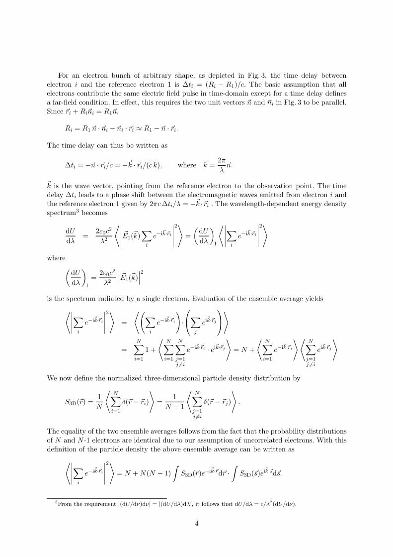
To illustrate the applicability of the phase reconstruction technique, examples are given in Fig. 5for three bunch shapes: a Gaussian with σz=300 µm, a double Gaussian with σz,1=50 µm andσz,2=300 µm, and a bunch with a Gaussian head (σz=50µm) and an exponential tail (1 mmdecay length). The form factors were calculated for 500 frequencies between a lower value of100 GHz or 400 GHz, respectively, and an upper value of 5 THz. Using the absolute values of thetheoretical form factors, the phases were determined according to Eq. (12) and the shapes werereconstructed with Eq. (13). A simple low-frequency extrapolation ρ(ν) = exp(−αν2) was used,with α chosen to join smoothly the data at 100 GHz or 400 GHz, respectively. No high-frequencyextrapolation was applied. As can be seen from the figure, the reconstruction works well for allshapes if the lower frequency cut-off of 100 GHz is used. However, severe distortions occur for alower frequency limit at 400 GHz, except for the 300 µm simple Gaussian bunch for which theGaussian extrapolation is obviously very good.

9

−3 −2 −1 0 1 2 30

200

400

600

800

1000

1200

1400

1600

1800

2000

Longitudinal Position (mm)

Cha

rge

dens

ity (

a.u.

)

−3 −2 −1 0 1 2 30

500

1000

1500

2000

2500

Longitudinal Position (mm)

Cha

rge

dens

ity (

a.u.

)

Figure 5 Original (dash-dot) and reconstructed (solid) bunch shapes. The low-frequency ex-trapolation is ρ(ν) = exp(−αν2), joined at 100 GHz on the top and at 400 GHz on the bottom.The curves are shifted horizontally such that their maximum values coincide.

10

Low- and high-frequency extrapolations are considered in more detail in [Fro05], the effectof measurement noise is studied in [Men05].

If additional time-domain data on the bunch shape are available from an instrument withthe resolution function I(t), the experimentally measured shape Smeas(t) is related to the trueshape S(t) by a convolution integral,

Smeas(t) =∫

S(t′)I(t − t′) dt′.

In frequency domain this is written as the product of the Fourier transforms,

Smeas(ν) = F (ν)I(ν),

where Eq. (7) has been used. The Fourier transform of the measured shape is almost equalto the form factor if I(ν) is close to unity. In this case, the low-frequency extrapolation canbe replaced by measured data. Assuming for the resolution function a Gaussian with widthσinstr, the measuring instrument will act as a low-pass filter, with I(ν) dropping to 1/e atthe frequency c/(

√2πσinstr). For a streak camera with 200 fs rms resolution, for example, this

frequency is 800 GHz.

3.3 On zeros in the form factor

An essential prerequisite in the Kramers-Kronig analysis is the absence of zeros in the form factor.This is true for a Gaussian bunch whose form factor is also of Gaussian shape and vanishesnowhere in the complex ν plane. However, already a truncated Gaussian charge distributionpossesses a form factor containing zeros. The existence of zeros can therefore not be excludedfor realistic bunch shapes.

Suppose the form factor has a simple zero at some complex frequency in the lower half plane,μ = μr + iμi with μi < 0. Then the new function

F (ν) = F (ν) · ν − μ∗

ν − μ

will be nonzero at ν = μ. It will be shown below that F (ν) and F (ν) have the same magnitudeon the real axis.

Let us now admit an arbitrary number zeros of the form factor and label them by μn. A newform factor without zeros is defined by

F (ν) = F (ν)∏n

Bn(ν) with Bn(ν) =ν − μ∗

n

ν − μn.

We have shifted all zeros μn of the original form factor into the product which is called theBlaschke product7. The magnitude of each term is

|Bn(ν)| =

√|ν|2 + |μn|2 − 2(νrμn,r − νiμn,i)|ν|2 + |μn|2 − 2(νrμn,r + νiμn,i)

.

On the real frequency axis (νi=0) the form factor magnitude is not changed by the Blaschkeproduct since |Bn(ν)|=1, and therefore ρ(ν) = |F (ν)| = |F (ν)|. Furthermore, |Bn(ν)| < 1 in the

7The Blaschke product obviously cannot remove zeros which are on the real frequency axis. Such zeros of theform factor where ρ(ν) = 0, however, do not contribute to the reconstructed bunch shape according to Eq. (13).

11

lower half plane (νi < 0), so F (ν) remains bounded. The Kramers-Kronig treatment can thusbe applied to the new, zeroless form factor F (ν). For a rigorous proof that indeed all zeros ofthe form factor can be absorbed into the Blaschke product see the references quoted in [Toll56].

On the real frequency axis the Blaschke product has unity modulus and can therefore beexpressed as a phase factor exp(iΘB(ν)). The real phase is given by

ΘB(ν) =∑n

arctan(Bn(ν))(Bn(ν))

=∑

n

arctan2μn,i(ν − μn,r)

(ν − μn,r)2 − μ2n,i

. (15)

This Blaschke phase is a monotonic function of frequency. To see this consider a single termBn(ν) and suppress the subscript n for brevity:

ddν

(2μi(ν − μr)

(ν − μr)2 − μ2i

)= −2μi

(ν − μr)2 + μ2i(

(ν − μr)2 − μ2i

)2 > 0 for μi < 0.

Hence also dΘB/dν > 0 for all real frequencies ν, provided the imaginary part of μ is negative.A further restriction on the contribution from the Blaschke product results from a symmetry

of the complex form factor that follows from Eq. (7): F ∗(−ν∗) = F (ν). A zero located at μrequires always another one at −μ∗ (mirrored at the imaginary frequency axis). The phasecontribution from such a pair is

Θpair(ν) = arctan4νμi

(ν2 − |μ|2)

ν4 + |μ|4 − 2ν2μ2r − 6ν2μ2

i

.

If |μ| � |ν|, Θpair(ν) ≈ 4μiν/|μ|2. A contribution proportional to frequency corresponds, ac-cording to Eq. (13), to a mere shift of the reconstructed profile, given here by 2cμi/(π|μ|2). Forthis reason, only complex zeros which are not too far away from the frequency range used forthe reconstruction contribute to the bunch shape.

We have seen that the Blaschke product leaves the function ρ(ν) invariant on the real axis.Therefore it is not possible to deduce the Blaschke contribution from a measurement of theabsolute value of the form factor. This is the deeper reason why the phase of the form factor andthereby the bunch shape cannot be uniquely reconstructed from spectral intensity measurementsonly. The Kramers-Kronig phase Eq. (12) is sometimes referred to as the canonical phase or theminimal phase.

To investigate the influence of zeros in the form factor we consider a σz =300 µm Gaussian witha superimposed sinusoidal oscillation. The mathematical procedure is described in AppendixD. The form factor is found to contain infinitely many zeros in the lower half of the complexfrequency plane. The Blaschke phase has been computed numerically, see Fig. 10 in the Appen-dix. Here we restrict our analysis to a computation of the Kramers-Kronig phase Eq. (12) anddisregard the zeros in the form factor. Fig. 6 shows that the original particle distribution is wellreproduced if just the Kramers-Kronig phase is used in Eq. (13) and the Blaschke phase is ig-nored. The modification of the bunch shape by the Blaschke phase is not very important and hasin practice certainly much less influence than the uncertainties which are due to measurementerrors and the low- and high-frequency extrapolations of the measured spectral data.

3.4 Transverse size effects

The form factor for a general three-dimensional charge distribution was calculated in Sect. 2 infar-field approximation, see Eq. (4). Assuming for illustrative purposes that the charge distrib-

12

−1 −0.5 0 0.5 10

200

400

600

800

1000

1200

1400

1600

Longitudinal Position (mm)

Cha

rge

dens

ity (

a.u.

)

Figure 6 Original (dash-dot) and reconstructed (solid) bunch shape for a Gaussian with asuperimposed sinusoidal oscillation. A low-frequency extrapolation ρ(ν) = exp(−αν2) is joinedat 100 GHz.

ution can be written in product form8, the form factor can also be factorized. For the case of alongitudinal and transverse Gaussian distribution with rotational symmetry about the z axis,

S3D(x, y, z) =1

2πσ2t

exp(−x2 + y2

2σ2t

)1√

2πσz

exp(− z2

2σ2z

),

evaluating Eq. (4) yields

F3D(kx, ky, kz) =1√

2πσz

12πσ2

t

∞∫∫∫−∞

exp(− z2

2σ2z

− x2 + y2

2σ2t

− i (kxx + kyy + kzz))

dxdydz

= exp(−σ2

zk2z

2

)exp

(−σ2

t (k2x + k2

y)2

), (16)

where√k2

x + k2y =

2πλ

sin θ, kz =2πλ

cos θ,

for an observation angle θ with respect to the z axis. This three-dimensional form factor is plottedin Fig. 7 for four values of σt and two values of θ. The form factor is reduced to 1/e of its maximumvalue (obtained for an infinitely thin line bunch) for a transverse size σt = λ/(

√2π sin θ).

8This is a good assumption in a straight linac for relativistic electrons with no longitudinal motion anddecoupled transverse betatron oscillations. However, if bunch compressors with magnetic chicanes are installed,as for FLASH, this factorization is not necessarily possible.

13

10 20 30 40 50 60 700

0.1

0.2

0.3

0.4

0.5

0.6

0.7

0.8

0.9

1

λ/σz

For

m fa

ctor

mag

nitu

de

σt=0, θ=100 mrad

σt=20σ

z, θ=100 mrad

σt=50σ

z, θ=100 mrad

σt=100σ

z, θ=10 mrad

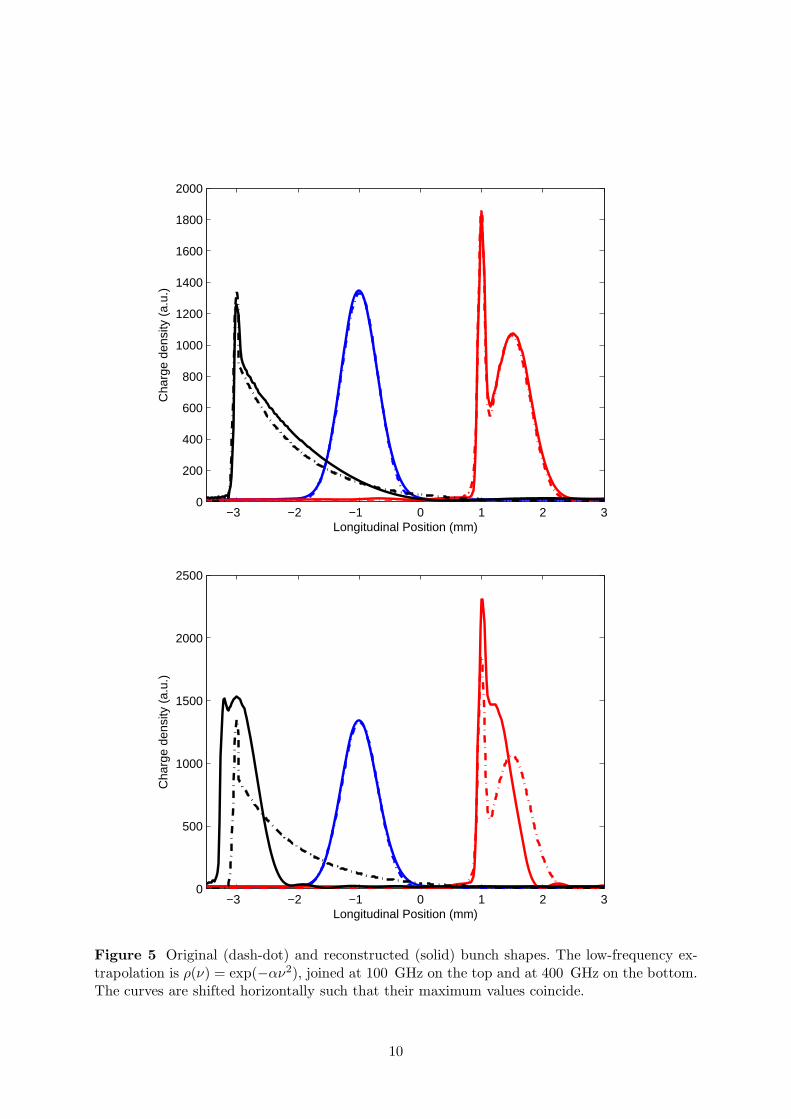
Figure 7 Influence of the transverse bunch size σt on the form factor after Eq. (16).

Eq. (16) shows that the transverse contribution to the form factor is determined by σt sin θ,the longitudinal contribution by σz cos θ. For small angles, transverse effects are strongly sup-pressed. This is generally the case for radiation from highly relativistic electrons which is in-evitably strongly collimated, typical opening angles being θ ≈ 1/γ � 1 for transition or syn-chrotron radiation.

This suppression effect can also be seen from Fig. 3: the path length difference from electron1 and electron i to the observation point P is given by �n · �ri = xi sin θ + zi cos θ, showing againthe weak influence of the transverse size for small angles. This argument is valid in generalfor any charge distribution, also if it cannot be factorized. Although the form factor is ratherinsensitive to the transverse structure of the electron bunch, the bunches should nevertheless bewell focused if fine details of the longitudinal charge distribution shall be resolved.

A Derivation of the frequency spectrum

The energy density spectrum dU/dν (in units of J/(Hzm2)) at a given position9 is related tothe power density dU/dt through

Utotal =

∞∫0

dU

dνdν =

∞∫−∞

dU

dtdt, (17)

9As the unit indicates, this and the following quantities are taken per unit area, thus they should read in fulld2U/dνdA. The differential dA is suppressed for brevity, as well as the variable �r: �E(�r, t) ≡ �E(t), etc.

14

where Utotal is the energy density (in units of J/m2). The power density is the absolute magnitudeof the Poynting vector �S(t), [�S]=W/m2, which in free space is [Jack99]

�S(t) =1μ0

�E(t)× �B(t) = ε0c((�E(t))2�n(t) − (�E(t)·�n(t))�E(t)

).

For the second equation the relation �B(t) = 1c�n(t)× �E(t) has been used which is valid in general

for the radiation of a single accelerated charge, with �n(t) the unit vector from the position of thecharge at retarded time to the observation point. At large distance from the source, the secondterm on the right side is absent since then �E(t) is perpendicular to �n(t). With this far-fieldcondition,

Utotal = ε0c

∞∫−∞

∣∣∣ �E(t)∣∣∣2 dt = ε0c

∞∫−∞

∣∣∣∣∣∣∞∫

−∞

�E(ν)e2πiνtdν

∣∣∣∣∣∣2

dt

= ε0c

∞∫−∞

∞∫−∞

�E(ν)e2πiνtdν ·∞∫

−∞

�E∗(ν ′)e−2πiν′tdν ′dt

= ε0c

∞∫∫−∞

�E(ν)· �E∗(ν ′)∞∫

−∞e−2πi(ν′−ν)tdtdνdν ′

= ε0c

∞∫∫−∞

�E(ν)· �E∗(ν ′)δ(ν ′ − ν)dνdν ′ = ε0c

∞∫−∞

| �E(ν)|2dν = 2ε0c

∞∫0

| �E(ν)|2dν.

In the last step �E∗(−ν) = �E(ν) was used, valid since �E(t) is real. Comparing with Eq. (17),

dU

dν= 2ε0c| �E(ν)|2. (18)

B Basic operation principle of an interferometer

One standard instrument for measuring frequency spectra is the interferometer. The basic op-eration principle of such a device is described in this section for the example of a Michelsoninterferometer. It is in essence a proof of the Wiener-Khinchin theorem.

The layout of a Michelson interferometer with the relations of electric field before and afterthe beam splitter is sketched in Fig. 8. A perfect splitter is assumed, dividing the incoming powerin two equal parts. Thus the electric field amplitudes of the two outgoing beams are smaller bya factor of

√2 than the incoming. Due to the symmetric beam splitter characteristic, on average

half the intensity is reflected back to the source, as will be shown below.The time dependent electric field reaching the detector Eout(t) is therefore related to the

incoming field Ein(t) by

Eout(t) =Ein(t)√

4+

Ein(t − 2Δx/c)√4

.

A slow detector that integrates the instantaneous intensity over the radiation pulse will measurean energy Uout as function of mirror displacement Δx (the interferogram) given by

Uout(Δx) =

∞∫−∞

ε0c |Eout(t)|2 dt

15

��������������

��������������

��������������������������������

Detector

Ein(t)

Ein(t)√2

Ein(t)√2

Ein(t− 2Δxc

)√2

Ein(t)√4

+ Ein(t− 2Δxc

)√4

Δx

Figure 8 Sketch of the electric field relations in an interferometer

= ε0c

∞∫−∞

E2in(t)4

+E2

in(t − 2Δx/c)4

+12Ein(t)Ein(t − 2Δx/c) dt

=Uin

2+

ε0c

2

∞∫−∞

∞∫−∞

Ein(ν)e2πiνtdν

∞∫−∞

Ein(ν ′)e2πiν′(t−2Δx/c)dν ′ dt

=Uin

2+

ε0c

2

∞∫−∞

∞∫−∞

Ein(ν)Ein(ν ′)e−4πiν′Δx/c

∞∫−∞

e2πi(ν+ν′)t dt dν ′dν

=Uin

2+

ε0c

2

∞∫−∞

∞∫−∞

Ein(ν)Ein(ν ′)e−4πiν′Δx/c δ(ν + ν ′) dν ′dν

=Uin

2+

ε0c

2

∞∫−∞

Ein(ν)Ein(−ν)e4πiνΔx/c dν

=Uin

2+

ε0c

2

∞∫−∞

|Ein(ν)|2 e4πiνΔx/c dν

=Uin

2+

14

∞∫−∞

(dU

dν

)in

e4πiνΔx/c dν (from Eq. (18))

=Uin

2+

12

∞∫0

(dU

dν

)in

cos(

4πνΔx

c

)dν. (19)

16

The Fourier transform relation between Ein(ν) and Ein(t) is defined through Eq. (2). The lastline follows from the symmetry of (dU/dν)in. The units of Uout(Δx) and Uin are J/m2.

Apart from the constant offset at Uin/2, the interferogram is the cosine Fourier transformof the incoming frequency spectrum which can therefore be recovered by the inverse transform.The Fourier transforms are real, therefore no phase-retrieval problems occur as for the bunchshape reconstruction in Sect. 3.1.

The integral averaged over Δx vanishes, so the detector sees only half of the incomingintensity, the other half is reflected back to the source.

A Martin-Puplett interferometer works along the same principles, but no radiation thatenters the device is going back to the source10, allowing an easy removal of intensity fluctuations.The difference interferogram of the two detectors shows no offset. Consult [Fro05] for detailedinformation on theoretical background and on practicalities.

C Interferogram of a Gaussian bunch

The form factor F (λ) of a Gaussian line bunch with normalized longitudinal charge distribution

S(z) =1√2πσ

exp(− z2

2σ2

)is, from Eq. (5),

F (λ) = exp(−2π2σ2

λ2

).

In the following, the number of particles is assumed to be large so that the coherent part of thetotal emission spectrum Eq. (6) dominates.

Taking first a single-electron spectrum (dU/dλ)in independent of λ, for example from tran-sition radiation, the interferogram from Eq. (19) will be Gaussian,

Uout(Δx) − Uin

2∼ exp

(− Δx2

2(σ/

√2)2)

,

with a width a factor of√

2 smaller than the width of the charge distribution.As second example the spectrum of synchrotron radiation from circular motion is used. In

the forward direction for long wavelengths11 λ � λc it is given by [Jack99](dU

dλ

)in

=31/3e2

2ε0

1d2λ2

(Γ(2/3)

π

)2(πR

λ

)2/3

∼ λ− 83 ,

where Γ denotes the Gamma function and d is the distance to the observation point. Here, theinterferogram will be

Uout(Δx) − Uin

2∼

∞∫0

ν2/3 exp(−4π2σ2ν2

c2

)cos(

4πνΔx

c

)dν.

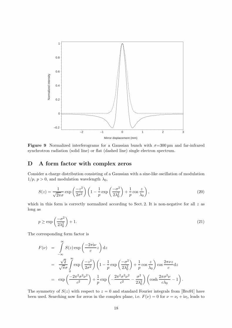
This cannot be evaluate analytically. In Fig. 9, a comparison of this case with that of a flatsingle electron spectrum for a Gaussian bunch with σ=300 µm is shown. A dip appears forthe synchrotron radiation case and the full width at half maximum is decreased by about 30%compared to the flat spectrum.

10However, since linearly polarized radiation is needed, an input polarizer is used. For unpolarized radiation,half of the intensity is still lost, but independent of the mirror position Δx.

11For the parameters used in Fig. 2, λc = 409 nm.

17

–0.2

0

0.2

0.4

0.6

0.8

1

Nor

mal

ized

inte

nsity

–2 –1 0 1 2 3

Mirror displacement (mm)

Figure 9 Normalized interferograms for a Gaussian bunch with σ=300 µm and far-infraredsynchrotron radiation (solid line) or flat (dashed line) single electron spectrum.

D A form factor with complex zeros

Consider a charge distribution consisting of a Gaussian with a sine-like oscillation of modulation1/p, p > 0, and modulation wavelength λ0,

S(z) =1√2πσ

exp(−z2

2σ2

)(1 − 1

pexp

(−σ2

2λ20

)+

1p

cosz

λ0

), (20)

which in this form is correctly normalized according to Sect. 2. It is non-negative for all z aslong as

p ≥ exp(−σ2

2λ20

)+ 1. (21)

The corresponding form factor is

F (ν) =

∞∫−∞

S(z) exp(−2πiν

cz

)dz

=√

2√πσ

∞∫0

exp(−z2

2σ2

)(1 − 1

pexp

(−σ2

2λ20

)+

1p

cosz

λ0

)cos

2πνz

cdz

= exp(−2π2σ2ν2

c2

)+

1p

exp(−2π2σ2ν2

c2− σ2

2λ20

)(cosh

2πσ2ν

cλ0− 1)

.

The symmetry of S(z) with respect to z = 0 and standard Fourier integrals from [Bro91] havebeen used. Searching now for zeros in the complex plane, i.e. F (ν) = 0 for ν = νr + iνi, leads to

18

the condition

1 − p exp(

σ2

2λ20

)= cosh

2πσ2ν

cλ0,

or, using the abbreviation α=2πσ2/(cλ0) and the relation cosh αν=(eαν + e−αν)/2,

2 − 2p exp(

σ2

2λ20

)= eα(νr+iνi) + e−α(νr+iνi)

= eανr (cos ανi + i sin ανi) + e−ανr (cos ανi − i sin ανi) .

The left-hand side of this equation is real, so(eανr − e−ανr

)sinανi = 0(

eανr + e−ανr)cos ανi = 2 − 2p exp

(σ2

2λ20

)≤ − exp

(−σ2

2λ20

)(22)

must hold for any complex zero, where the inequality is due to the restriction Eq. (21).Solutions for sinανi=0 require thus cos ανi=-1 or ανi = (2m + 1)π with m an integer, and

additionally that the right-hand side of Eq. (22) is smaller than -2, as the minimum value of thesum in brackets on the right is +2. If this is fulfilled, then

νr =1α

ln

(p exp

(σ2

2λ20

)(1 ±

√1 − 2

pexp

(−σ2

2λ20

))− 1

). (23)

In case the second term under the root is much smaller than unity, this expression can besimplified by expanding the root to first order for the positive sign or to second order for thenegative sign, yielding

νr ≈ ±(

cλ0 ln 2p2πσ2

+c

4πλ0

).

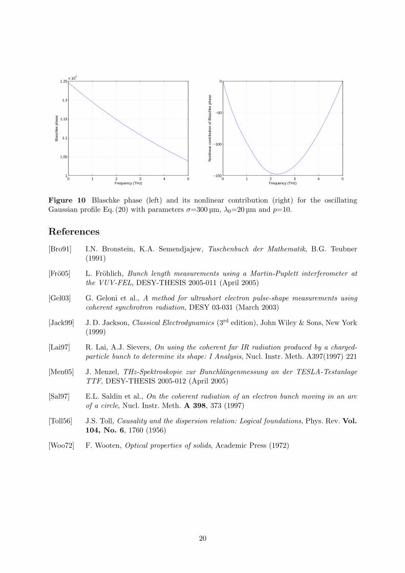
As an example, the oscillating Gaussian plotted in Fig. 5 has σ=300 µm, λ0=20µm and p=10,so that the approximation holds well and zeros occur for νr=±1.2 THz. The Blaschke phaseEq. (15) for this case and its nonlinear contribution are plotted in Fig. 10. The first 2000 zerosin the negative complex plane were included in this calculation. Increasing the number of zerosfurther increases the phase itself, but does not change the nonlinear contribution significantlyanymore. This behaviour was found in Sect. 3.3: zeros far away from the real axis contributeonly linearly to the phase.

If the right-hand side of Eq. (22) lies between -2 and 0, Eq. (23) does not yield a real result.In this case zeros of the form factor are located on the imaginary axis, νr=0, at

νi = ± 1α

arccos(

1 − p exp(

σ2

2λ20

))+

2πm

αfor any integer m.

For every allowed parameter set σ, λ0 and p there will therefore be either one or two valuesof νr for which an infinite number of zeros occur for values of νi given above.

Acknowledgments

Useful discussions with Evgeni Saldin, helping in clarifying several essential points, are greatlyacknowledged.

19

0 1 2 3 4 51

1.05

1.1

1.15

1.2

1.25x 10

4

Frequency (THz)

Bla

schk

e ph

ase

0 1 2 3 4 5−150

−100

−50

0

Frequency (THz)

Non

linea

r co

ntrib

utio

n of

Bla

schk

e ph

ase

Figure 10 Blaschke phase (left) and its nonlinear contribution (right) for the oscillatingGaussian profile Eq. (20) with parameters σ=300 µm, λ0=20 µm and p=10.

References

[Bro91] I.N. Bronstein, K.A. Semendjajew, Taschenbuch der Mathematik, B.G. Teubner(1991)

[Fro05] L. Frohlich, Bunch length measurements using a Martin-Puplett interferometer atthe VUV-FEL, DESY-THESIS 2005-011 (April 2005)

[Gel03] G. Geloni et al., A method for ultrashort electron pulse-shape measurements usingcoherent synchrotron radiation, DESY 03-031 (March 2003)

[Jack99] J.D. Jackson, Classical Electrodynamics (3rd edition), John Wiley & Sons, New York(1999)

[Lai97] R. Lai, A.J. Sievers, On using the coherent far IR radiation produced by a charged-particle bunch to determine its shape: I Analysis, Nucl. Instr. Meth. A397(1997) 221

[Men05] J. Menzel, THz-Spektroskopie zur Bunchlangenmessung an der TESLA-TestanlageTTF, DESY-THESIS 2005-012 (April 2005)

[Sal97] E.L. Saldin et al., On the coherent radiation of an electron bunch moving in an arcof a circle, Nucl. Instr. Meth. A 398, 373 (1997)

[Toll56] J.S. Toll, Causality and the dispersion relation: Logical foundations, Phys. Rev. Vol.104, No. 6, 1760 (1956)

[Woo72] F. Wooten, Optical properties of solids, Academic Press (1972)

20