prioritization of onshore pipeline systems for integrity ... · risk-based optimization of pipeline...
TRANSCRIPT

JJJ AN CENTRE FOR ENGNEERlNG RESEARCH NC
2UO Clerk Pead
Edmonton Aibcrta Conoda T6N i H2
Gi (403) 450-33GD Fcx (403) 450-3700
Prioritization of Onshore Pipeline Systems for Integrity Maintenance
PIRAMID Technical Reference Manual No 41
Confidential to C-FERs Pipeline Program Participants
Prepared by M J Stephens MSc PEng
November 1996 Centre For Engineering Research Inc Project 95007
CENTRE FOR ENGINEERING RESEARCH INC
Prioritization of Onshore Pipeline Systems for Integrity Maintenance
PIRAMID Technical Reference Manual No 41
Confidential to C-FERs Pipeline Program Participants
Prepared by M J Stephens MSc PEng
November 1996 Project 95007
PERMIT TO PRACTICE CENTRE FOR ENGINEERING RESEARCH INC
Signature ~~ Date -~0(1ljif
PERMIT NUMBER P4487 The Association of Professional Engineers
Geologists and Geophysicists of Alberta
CENTRE FOR ENGINEERING RESEARCH INC
NOTICE
Restriction on Disclosure
This report describes the methodology and findings of a contract research project carried by the Centre For Engineering Research Inc on behalf of the Pipeline Program Participants All data analyses and conclusions are proprietary to C-FER This material contained in this report may not be disclosed or used in whole or in part except in accordance with the terms of the Joint Industry Project Agreement The report contents may not be reproduced in whole or in part or be transferred in any form without also including a complete reference to the source document
CENTRE FOR ENGINEERING RESEARCH INC
TABLE OF CONTENTS
Notice Table of Contents ii List of Figures and Tables IV
Executive Summary v
10 INTRODUCTION 1
11 Background 1 12 Objective and Scope 1
20 THE PRIORITIZATION METHOD 3
21 Overview 3 22 Model Components 4
221 System Definition 4 222 Probability Estimation 4 223 Consequence Evaluation 5 224 Risk Estimation and Ranking 5
30 SYSTEM DEFINITION 7
31 Introduction 7 32 Pipeline Attributes 7
40 PROBABILITY ESTIMATION 8
4 I Introduction 8 42 Probability Estimation Model 8
421 General 8 422 Baseline Failure Rates 9 423 Failure Mode Factor 10 424 Failure Rate Modification Factors 11
4241 External Metal Loss Corrosion 11 4242 Internal Metal Loss Corrosion 15 4243 Mechanical Damage 17
42431 Overview 17 42432 Probability of Interference 17 42433 Probability of Failure Given Interference 21 42434 Model Scale Factor 23
4244 Ground Movement 23 4245 Environmentally Induced Crack-Like Defects
(stress corrosion cracking) 25 4246 Mechanically Induced Crack-Like Defects (metal fatigue) 28 4247 Other Causes 31
II
CENTRE FOR ENGINEERING RESEARCH INC
Table of Contents
50 CONSEQUENCE EVALUATION 32
51 Introduction 32 52 Consequence Evaluation Influence Diagram Node Parameters 32
52 l Failure Mode 32 522 Equivalent Volume 33 523 Interruption Cost 33 524 Loss 34
524l Node Parameter 34 5242 Equivalent Costs 34
60 RISK ESTIMATION AND SEGMENT RANKING 36
61 Introduction 36 62 Risk Calculation Model 36 63 Risk Ranking Model 37
70 SUMMARY38
80 REFERENCES40
iii
CENTRE FOR ENGINEERING RESEARCH INC
LIST OF FIGURES AND TABLES
Figure 21
Figure 22
Figure 41
Figure 51
Figure 61
Framework for risk-based optimization of pipeline integrity maintenance activities
Flow chart for pipeline system prioritization
Fault tree model for mechanical interference
Basic node influence diagram for consequence evaluation
Output format for segment risk ranking
Table 31
Table 41
Pipeline segment attributes for prioritization
Reference baseline failure rates and relative failure mode factors by cause for buried pipelines
Segment attributes required by Equivalent Volume node to characterize environmental sensitivity of spill site
lV
Table 51
CErITRE FOR ENGINEERING RESEARCH INC
EXECUTIVE SUMMARY
The Centre For Engineering Research Inc (C-FER) is conducting a JOIlt industry research program directed at the optimization of pipeline integrity maintenance activities using a riskshybased approach This document describes the system prioritization model that has been developed to estimate the level of operating risk associated with all segments within a pipeline system This model forms the basis for one of the modules in the software suite PIRAMID (Pipeline Risk Analysis for Maintenance and Integrity Decisions)
The pipeline system prioritization approach involves the analysis of segment-specific pipeline attributes to produce firstly an estimate of the probability of failure associated with individual segments as a function of failure cause and secondly an estimate of the potentiaJ consequences of segment failure in terms of three distinct consequence components (ie life safety environmental damage and economic impact) The model then combines the cause-specific failure probability estimates with a global measure of the loss potential associated with the different consequence components into a single measure of operating risk for each pipeline segment Segments are then ranked according to the estimated level of risk the intention being to identify (or target) potentially high risk segments for subsequent detailed decision analysis at the maintenance optimization stage of the pipeline maintenance planning process
Key steps in the pipeline system prioritization process are summarized as follows
Probability Estimation
The annual probability of failure of each segment within the operating system is calculated for each significant failure cause from baseline historical failure rate estimates which are adjusted to reflect the impact of line-specific attribute sets The specific failure causes addressed are metal loss corrosion (externaJ and internal) outside force (mechanical damage and ground movement) crack-like defects (stress corrosion cracking and seam weld fatigue cracks) and other
Baseline failure rates for a given pipeline type (ie gas or liquid) are obtained from statistical analysis of historical pipeline incident data which yield estimates of the annuaJ number of failure incidents per unit line length The baseline failure rates are then converted to line-specific estimates using failure rate modification factors that depend on the attributes of the line segment in question The failure rate modification factors are calculated from the values of selected segment attributes using algorithms developed from statistical analysis of pipeline incident data andor anaJytical models supplemented where necessary by judgement The resulting lineshyspecific failure rates are then converted to failure probability estimates by multiplying each failure rate by the length of the corresponding line segment
v
CENTRE FOR ENGINEERING RESEARCH INC
Executive Summary
Consequence Analysis
The consequences of failure associated with a given segment are estimated using analytical models The approach assumes that the consequences of pipeline failure are fully represented by three parameters the total cost as a measure of the economic loss the number offatalities as a measure of losses in life and the residual spill volume (after initial clean-up) as a measure of the long term environmental impact The consequence assessment approach involves modelling the release of product from the pipeline determination of the likely hazard types and their relative likelihood of occurrence estimation of the hazard intensity at different locations and calculation of the number of fatalities the residual spill volume and the total cost
The three distinct consequence measures calculated using the models are combined into a single measure of the total loss potential associated with line failure by converting fatality estimates and residual spill volume estimates into equivalent costs This conversion is carried out based on the so-called willingness to pay concept which involves making an estimate of the amount of money that society would be willing to pay to avoid a particular adverse outcome
Risk Estimation and Ranking
Multiplication of the segment-specific failure probability estimate for a given failure cause by the associated combined loss estimate (a financial cost estimate including the cost equivalent of human fatalities and residual spill volume) produces an estimate of operating risk defined as the expected annual loss associated with a given segment of pipeline for the failure cause in question Summation of the risk estimates for all failure causes associated with a given segment gives an estimate of the total expected annual loss associated with segment operation Dividing these segment risk estimates by the corresponding segment length yields normalized risk estimates that allow comparison of calculated risks between segments of different lengths These causeshyspecific and combined-cause risk estimates form the basis for a quantitative ranking of all segments identified within a given pipeline system
vi
CENTRE FOR ENGINEERING RESEARCH INC
10 INTRODUCTION
11 Background
This document constitutes one of the deliverables associated C-FER s joint industry program on risk-based optimization of pipeline integrity maintenance activities The goal of this program is to develop models and software tools that can assist pipeline operators in making optimal decisions regarding integrity maintenance activities for a given pipeline or pipeline segment The software resulting from this joint industry program is called PIRAMID (Pipeline Risk Analysis for Maintenance and Inspection Decisions) This document is part of the technical reference manual for the program
Implementation of a risk-balted approach to maintenance planning as envisioned in this program requires quantitative estimates of both the probability of line failure and the adverse consequences associated with line failure should it occur There is considerable uncertainty associated with the assessment of both the probability and consequences of line failure To find the optimal set of integrity maintenance actions in the presence of this uncertainty a probabilistic optimization methodology based on the use of decision influence diagrams has been adopted The basis for and development of this decision analysis approach is described in PIRAMID Technical Reference Manual No 12 (Stephens et al 1995) Application of the influence diagram based decision analysis approach to onshore pipeline systems is described in PIRAMID Technical Reference Manual No 32 (Stephens et al 1996)
Given the level of effort associated with the decision influence diagram approach to maintenance optimization it is considered impractical and inefficient to carry out such a detailed analysis of candidate maintenance activities for all failure causes associated with each segment within a pipeline system Alternatively it is desirable to develop a pipeline system prioritization model that will estimate the level of operating risk associated with each segment within the system and to use this risk estimate as a basis for ranking segments This segment ranking will serve to identify segments within the system with a potentially unacceptable level of operating risk with the intent that the high risk segments so identified can then be subjected to the more detailed analysis implicit in the decision influence diagram approach referred to above
12 Objective and Scope
This document describes the system prioritization model that has been developed to estimate the level of operating risk associated with all segments within a pipeline system The approach involves the analysis of segment-specific pipeline attributes to produce firstly an estimate of the failure rate associated with individual segments as a function of failure cause and secondly an estimate of the potential consequences of segment failure in terms of three distinct consequence components (ie life safety environmental damage and economic impact) The model will then
CENTRE FOR ENGINEERING RESEARCH INC
Introduction
combine the cause-specific failure rate estimates with a global measure of the loss potential associated with the different consequence components into a single measure of operating risk for each pipeline segment and then rank each segment by failure cause according to the calculated level of risk This model will therefore serve as a screening tool that will help pipeline operating companies identify potentially high risk segments for subsequent detailed analysis using the decision analysis tools that are currently being developed under this project
The basic structure of the prioritization model described herein is based on the methodology developed in PIRAMID Technical Reference Manual No 12 (Stephens et al 1995) This document provides a detailed technical description of the prioritization approach and the underlying basis for the calculation of failure probabilities individual and combined consequence components and operating risk
2
CENTRE FOR ENGINEERING RESEARCH INC
20 THE PRIORITIZATION METHOD
21 Overview
The framework for the pipeline integrity maintenance optimization as developed under this project is summarized in Figure 21 The first significant stage in the maintenance optimization process is to prioritize segments within a given pipeline system with respect to the need for integrity maintenance action Specifically the system prioritization stage is intended to rank segments based on the estimated level of operating risk associated with significant failure causes where risk is defined as the product of the probability of line failure and a global measure of the adverse consequences of failure To this end pipeline characteristics (or attributes) must be evaluated to produce firstly a line-specific estimate of the failure probability for each segment within the system as a function of failure cause (eg metal loss corrosion mechanical damage ground movement crack-like defects etc) and secondly an estimate of the potential consequences of segment failure in terms of three distinct consequence components life safety environmental damage and economic impact Cause-specific failure probability estimates are then multiplied by a global measure of the loss potential associated with the different consequence components to produce a single measure of operating risk for all failure causes associated with each segment Segments can then be ranked by failure cause according to the estimated level of risk This cause specific segment ranking will serve to identify (or target) potentially high risk segments for subsequent detailed decision analysis at the maintenance optimization stage where the optimal strategy for managing the risk associated with a specific failure cause can be determined
The steps associated with the prioritization process described above are summarized in the flowchart shown in Figure 22 The calculation process outlined in the flowchart can be divided into four distinct specificationcalculation modules that perform the following functions
bull System Definition defines the pipeline system to be analysed by specifying the segments to be considered and defining the attributes necessary to fully characterize each distinct section within each analysis segment
bull Probability Estimation estimates the line-specific probability of failure by failure cause for each distinct section within each analysis segment
bull Consequence Evaluation estimates the line-specific consequences of failure for each distinct section within each analysis segment
bull Risk Estimation and Ranking calculates the operating risk associated with each segment within the system on a cause by cause basis and ranks the segments by the calculated level of operating risk on either a cause-by-cause or a combined cause basis
An expanded description of each functional module is given in the following sections
3
CENTRE FOR ENGINEERING RESEARCH INC
The Prioritization Method
22 Model Components
221 System Definition
The extent of the pipeline system to be evaluated must first be defined To this end the pipeline system is divided into appropriate segments that can be treated as individual units with respect to integrity maintenance For each segment the attributes that effect the probability and consequences of line failure are specified Each segment should be as uniform as possible with respect to the attributes that affect pipe integrity (eg age material properties coating type and environmental conditions) Alternatively the segments may correspond to portions of the line for which the integrity maintenance actions being considered can be implemented (eg if pigging is considered then a segment must be piggable and have pig traps at both ends) The preferred approach is subdivision by attribute commonality because the segment risk ranking results will then apply equally to all points along each segment Where subdivision according to criteria other than attribute commonality is adopted the segment ranking results will reflect an averaging process that accounts for variations in failure rates and failure consequences along the length of segments
A detailed discussion of the System Definition model information requirements is given m Section 30
222 Probability Estimation
The annual probability of failure of each segment within the operating system is calculated for each significant failure cause from baseline historical failure rate estimates which are adjusted to reflect the impact of line-specific attribute sets The specific failure causes addressed are metal loss corrosion (external and internal) outside force (mechanical damage and ground movement) crack-like defects (stress corrosion cracking and seam weld fatigue cracks) and other
Baseline failure rates for a given pipeline type (ie gas or liquid) are obtained from statistical analysis of historical pipeline incident data which yield estimates of the annual number of failure incidents per unit line length The baseline failure rates are then converted to line-specific estimates using failure rate modification factors that depend on the attributes of the line segment in question The failure rate modification factors are calculated from the values of selected segment attributes using algorithms developed from statistical analysis of pipeline incident data andlor analytical models supplemented where necessary by judgement The resulting lineshyspecific failure rates are then converted to failure probability estimates by multiplying each failure rate by the length of the corresponding line segment
A detailed discussion of the calculation process associated with the Probability Estimation model is given in Section 40
4
CENTRE FOR ENGINEERING RESEARCH INC
The Prioritization Method
223 Consequence Evaluation
The consequences of failure associated with a given segment are estimated using analytical models The approach assumes that the consequences of pipeline failure are fully represented by three parameters the total cost as a measure of the economic loss the number offatalities as a measure of losses in life and the residual spill volume (after initial clean-up) as a measure of the long term environmental impact The consequence assessment approach involves modelling the release of product from the pipeline determination of the likely hazard types and their relative likelihood of occurrence estimation of the hazard intensity at different locations and calculation of the number of fatalities the residual spill volume and the total cost The consequence models employed in the prioritization process have been adapted from the models previously developed for use in the decision analysis model based on influence diagrams (see PIRAMID Technical Reference Manual No 32 Stephens et al 1996)
The hazard types considered in the modelling process include both the immediate hazards associated with line failure (eg jetpool fires vapour cloud fires or explosions and toxic or asphyxiating clouds) as well as the long term environmental hazards associated with persistent liquid spills Fatality estimation based on the hazard characterization models reflects the population density associated with a given land use and takes into account the effect of shelter andor escape on survivability Estimation of residual spill volume takes into account the product clean-up potential associated with the spill site and incorporates a factor that adjusts the volume measure to reflect both the environmental damage potential of the spilled product as well as the damage sensitivity of the environment in the vicinity of the spill site The total cost estimate includes the direct costs associated with line failure including the cost of lost product line repair and service interruption and the costs that are dependent on the type of release hazard including the cost of property damage spill clean-up and fatality compensation
The three distinct consequence measures calculated using the models are combined into a single measure of the total loss potential associated with line failure by converting fatality estimates and residual spill volume estimates into equivalent costs This conversion is carried out based on the so-called willingness to pay concept which involves making an estimate of the amount of money that society would be willing to pay to avoid a particular adverse outcome
A detailed discussion of the calculation process associated with the Consequence Evaluation model is given in Section 50
224 Risk Estimation and Ranking
Multiplication of the segment-specific failure probability estimate for a given failure cause by the associated combined loss estimate (a financial cost estimate including the cost equivalent of human fatalities and residual spill volume) produces an estimate of operating risk defined as the expected annual Joss associated with a given segment of pipeline for the failure cause in question Summation of the risk estimates for all failure causes associated with a given segment gives an
5
CENTRE FOR ENGINEERING RESEARCH INC
The Prioritization Method
estimate of the total expected annual loss associated with segment operation Dividing these segment risk estimates by the corresponding segment length yields normalized risk estimates that allow comparison of calculated risks between segments of different lengths These causeshyspecific and combined-cause risk estimates form the basis for a quantitative ranking of all segments identified within a given pipeline system
A detailed discussion of the calculation process associated with the Risk Estimation and Segment Ranking model is given in Section 60
6
CENTRE FOR ENGINEERJNG RESEARCH INC
Figures
CENTRE FOR ENGINEERING RESEARCH INC
System Definition
Divide pipeline system into segments
System Prioritization
Conduct risk assessment for each segment and rank segments according to the risk level
i shy
Maintenance Optimization
Determine optimal integrity maintenance strategy for each targeted segment
Refinement of System Prioritization bull
Develop alternate ranking of targeted segments based on cost of risk reduction I
i
Maintenance Implementation f Implement Optimal Maintenance Strategy on Targeted Segments
I Repeat for all
segments
I
Figure 21 Framework for risk-based optimization of pipeiine integrity maintenance activities
CENTRE FOR ENGINEERING RESEARCH INC
I Select Segment -
+ Define Segment Attributes
+ Identify Failure I Identify Failure Hazards I
Causes I
+ + + Estimated Failure Quantify Quantify Quantify
Probability for Financial Life Safety Environmental Each Potential Consequences Consequences Consequences Failure Cause of Failure of Failure of Failure
t t Quantify Total Combined Loss Associated With IFailure
I
Evaluated Components of Risk Repeat for all Associated With Each Failure Cause Segments
Repeat for Each Segment Identified for Prioritization
Rank Segments and Associated Failure Causes by Estimated Level of Risk
Figure 22 Flow chart for pipeline system prioritization
CENTRE FOR ENGINEERING RESEARCH INC
30 SYSTEM DEFINITION
31 Introduction
The pipeline system is defined by specifying the pipeline segments that are to be analysed and the required line attributes along the length of each analysis segment This information will be processed to produce a description of each analysis segment that identifies consecutive sections within each segment (where a section is defined as a length of pipeline over which the attribute values do not vary) and defines the attribute set associated with each section
32 Pipeline Attributes
The specific pipeline attributes that have been chosen as a basis for segment prioritization are summarized in Table 31 The chosen attributes involve two overlapping sub-sets one associated with parameters that have been shown to have an impact on the rate and hence the probability ofline failure and the other with parameters that are known to significantly influence the consequences of line failure should it occur Table 31 identifies the specific attributes associated with each sub-set Note that the total number of attributes that must be defined for each segment in a given system depends on the type of product (ie natural gas HVP liquid or L VP liquid) being transported in the line and whether or not the environmental impact of persistent liquid product spills is to be considered in the consequence evaluation
Note also that the attribute set employed for probability estimation and consequence evaluation at the prioritization stage is not intended to be comprehensive (eg the pipeline literature suggests that line-specific failure rates are influenced by attributes not considered in the prioritization model) A restricted attribute set has purposely been employed at the system prioritization stage to limit the information requirements associated with the system prioritization activity In addition it is noted that the impact of additional factors on the probability and consequences offailure are addressed at the subsequent maintenance optimization stage where a more detailed estimate of operating risk is calculated as part of the formal decision analysis process conducted for the segments targeted by the initial risk ranking at the prioritization stage
7
CENTRE FOR ENGlNEERlNG RESEARCH INC
Tables
No Attribute Description Attribute Units Input Required for Required for f~-~-~=~~A~nalv~bullrls~P~re~fe~roen~ces~c-~~~--l Name ext (int) Type Probability Consequence Natural Gas HVP liquids LVP llaulds Included
Estimation Estimation only only consider env su ress env
1 f~e~_QlJ~~~f~~ _-------------- ___ fe~Q_i_~-- mm (m) 1- S1 ____________ X X X X xccmiddotmiddotmiddotmiddotmiddotmiddot 2 Pipe wau Thickness __ ~~~~ ~_mm~~(~)__ ~~sectI=-- xx X __xx ____ Xx ______ --~--middot------ llt _
1
3 ~H~-~~~YY_i~-i~-~j_~~-2~-~- ----- ------- _____ fP~Y~-~- _--~~Pa)_ s1 _ 1
_
1
A X 4 fP~ sect9~X ~~1 ~~-12YP~ __ __sect~~YP~-- --52 X ______ _________ ______ X xc +middotmiddotmiddotmiddotmiddotmiddotmiddotmiddotmiddotmiddotmiddotmiddotxbull _1 s _flip~-~-Q~IY~ ____________ _____ -----~~~YP-1 ----~----- s2 ~------------ ----------I ~ ~ X middot---------~-----------i--t~=-~~~iliion Profii6 E~~~ie ______ ~~~--- ~~ -middot-------- x -~--- -------- x----- IImiddot---- middot---middot- middotmiddotmiddot-middotmiddotmiddotmiddotmiddot-middotmiddot middot-middot-middotmiddot--middot-middotmiddot I ~ QP-~~ifo~i~~~~~~--~-r~iiie-~ -- - --- -------- -- Pres-sPrOIDe-- ~J~~J__ c1 bullmiddot--middotmiddotmiddot-x----bull----~x__ ___~x_ _ x ______ - _ ____ ____ _ 9 lt2P~~~i9 f~~1_r~ -~~~9-~ ------middot-middot-- __________ ____ ____ _ff~~-~~~Jl~ --~-~_(Paj_ __8~1__ 1_____ Xcc--middot---middotmiddotmiddotmiddottmiddotmiddotmiddotmiddot-middot x-- 1__ bullx~ -middotmiddot-middot-middot _ _ middotmiddotmiddotmiddotmiddotmiddotmiddotmiddot-middotmiddotmiddotmiddotmiddot tmiddotmiddotmiddotmiddot-middot 110 g_~_~_ul~ti~ ~lllb_~_r _ltl___P__r~-~~~~~t~-------- ________ _PfeuroJ~~~Y~~- s1 __ __ x x x ___________ _ 11 9perltgttn9T_~rl1-~f~~~-rf________________ ___ __________ 1-in~~P _~J5L__ S1 _1 _____ x x 1 x lmiddotmiddotmiddotmiddotmiddotmiddotmiddotmiddotmiddotmiddotmiddotmiddotmiddotmiddotmiddotmiddotmiddotmiddotmiddotmiddotImiddotmiddotmiddotmiddotmiddotbullmiddotmiddotmiddotmiddotmiddotmiddotmiddotmiddotmiddotmiddot 12 _P~9_9-1E flo_~ B_a~~i~f_l_q~f_l_lt~~--~2~_qiection)_____ ________ FlowAate _____ ~~ __8_1_ X X X 13 ~-r1~_y9_1111feurol(P~~~~f_l~2~-9lii~_cae_~~tyL_ __ CapFraction ~ltpoundnJ S1 X X X ______ ___ _ 14 (li~lif_)_Q__ ~_~tteurolfl~ __~~1~~(ptS_~f_l~_2~()_f_f_l_~if_l~~~-~l_(ll_e ------~ 2Jr~~_n $1 x -----~--------- xx ---- ---------- ------- r-- middotx----------shy15 fro9_l_1_c~Tra11spo_rtation_Distanceurol ___________~n~D_ls_t -~f~Tl 51 ___________ _____ X A
~ ~J~~~-~rplusmnc~~i~n~10~-u~~---- -f~~r~ ~~-1~~) ---~-1-__ 1
--=~----middot- ____ -X__ i---------- _-~-=~~-- ---------x- ---i-shy- ~---middot--~~ _fi~~~~-i~~ci~~t~~lu~~-- _ -~-~o--~~-d- bi~)- --~1~_ _________ __ ~--bullI-- middot~c----middot-middot-middotmiddotmiddotl --middotmiddot-middotmiddotmiddot~------ ~middot--middotmiddotmiddot--middot--
1
20 Tiin~ _() --~~-~- sectl()pp~J~~~~-ifle of ~ete~I~~__ _Ti~~sect~-- _hrs (SepoundL S1 X X _~-------------- X _____ 1 ___________ )( ________ _
21 Q~e~l_i_lt_y~~ Cover m St X _______ ___ ____ __ c_____ _____xx_ 22 ~i~~ent Land Use _ ~ci~~-c $2 X X X 1~3 _A_C_Y__ ~_c_c~~~-~_iiy_ AOWaccess --middotmiddot-middot---- -------s2- -----x-- ---- --- ----- ----- ---- - ---middotmiddotmiddotmiddotbullxbullmiddotmiddotmiddotmiddotmiddotmiddotmiddot bullmiddotmiddotmiddotmiddotmiddotmiddotmiddotmiddotmiddotmiddotmiddotmiddotmiddotmiddotxbullbullmiddotmiddotmiddotmiddotmiddotmiddotmiddotmiddotmiddotmiddot 24 ROW condition ________ _ ~w_-_Co__~- - -- - --=sect_________ i--------- --x- ------ -- _-_middot__-_-_middot_middot--
1 __ ----middotI----- --l--C _-middotmiddot I ~
25 B9~Patipoundlf~~g~~~~Y _______ ---~~e~t ____sect5_____ x _______ r-- x _____ _ ~~ _N~~~9-~~-2l~ fi~sectP~~~--~Y~~_l_l____ --------------- _____ ______ -~~~-- ~---- $2 r---------middot-xc-middot-middotmiddot-middot middotmiddot--middotmiddotmiddotmiddot-middotmiddotmiddotmiddotmiddotmiddotmiddotmiddotmiddotmiddotmiddot __ 11 bullbullbullxbull- 1bullbullbullbullbullbullbullbullbullbullbullbullbullbullbull x +middotmiddotmiddotmiddotmiddotmiddotmiddotmiddotmiddotmiddotmiddotmiddotmiddotgtmiddotmiddotmiddotmiddotmiddotmiddot middotmiddotmiddotmiddotmiddotmiddotmiddot xbull 21 -~-~()~~if19TYE~L~~~fl~rpound~1f3~1_11~- ______ _gr~_iQ_ --middot-s2~-- x _ )( ___________ llt ______________x_middot--middotmiddotmiddot-middot middotmiddotmiddotmiddotmiddot--- ---middotmiddotmiddot-- ~- __ _ 28 ~~~ iiJlg T~~~~_i__f1_g~~~~9~~stics ______ _~~~- 52-- imiddotmiddotmiddotmiddotmiddotmiddot -)(middot ___ middot- xmiddotmiddot---middotmiddotmiddotmiddotmiddot- bullbull 29 _0~lfH_~~ _sectg_i_~g_r_rg_~_yi_t_y_ ___ ___ ___ SoilCorrode ____ _~S~2~+------cx~middot- ___ __ _ _ __ _ x0 _ 1________ --+middot-middotmiddotmiddot-middotmiddotmiddotmiddotmiddotmiddotmiddotmiddotmiddotmiddotmiddotmiddotmiddot-middotmiddotmiddotmiddotmiddotmiddotmiddotmiddotmiddotmiddot +middotmiddotmiddot-middotmiddotmiddotmiddotmiddotmiddotmiddotmiddotmiddotmiddotmiddotx 1 30 sect9_C ft~~ti~l __~E0poundV~9Jfl6f) ---------- 99~_o~e1~~_ ---- --11-~s2c-+--bullc---middot - _ - middot-middot ---middot-- ---middot-------middot xbull--middotmiddot---- ---middot-middotmiddot----middot x - IC--middotmiddotmiddot-middotmiddotmiddotmiddotmiddot--middotmiddotmiddotmiddotmiddotmiddotmiddotmiddot-middotmiddotmiddotmiddot I -middotmiddotmiddotmiddotx I 31 sect~l~~l _fl_i~ C~~nl TYP(l________________ ExtCoalin9 ______ _______ X X X __ ___ _______ ________ ---~X------------32 ~X1_eml P_ipe_ Coaflng Co_ndition __9oatCond _ middot--middot----middot- _ _ ______ X X X33 c31hOdicmiddotp~1ec1n-Le~e1middot------- CPLeve --+ - bullbullmiddotmiddotmiddot-middotmiddotmiddotmiddotmiddotmiddotmiddotmiddot+middotmiddotmiddotmiddotmiddot-middotmiddotmiddotmiddotmiddotmiddotmiddotmiddotmiddot +middotmiddotmiddotmiddotmiddot-middot- -----l ---x7---l---xbull----J x 34 ~e15~__ ()_f__ 9~_ti_0_9_sect_~~~~f)9_____ CoatShield -------~-----~I-middot-middotmiddot-middot cmiddot--middot-middot-middot --+middotmiddot--middotmiddotmiddot ltx-+middotmiddotmiddotmiddotmiddotmiddotmiddotmiddotmiddotmiddotmiddotmiddotmiddotmiddotmiddotccxmiddotmiddotmiddotmiddotmiddotmiddotmiddotmiddot middotmiddotmiddotmiddotmiddotmiddotmiddotmiddotmiddotmiddotmiddotmiddotmiddotmiddot xmiddotmiddotmiddotmiddotmiddotmiddotmiddot 1
35 f r~~~1(~ __ sect_l(l_~ll__~l(_r_~ence pound S~~19 lt~hmiddotmiddotmiddot bull __ __ _ ln_te_rtcer_e_noe~middott-------- jmiddot ___ c + iimiddotmiddotmiddotmiddot middotJ -middotmiddotmiddot- __ II------ f _~- ___ __ __ -_-- _X __ XX shy36 ~r9~_c_t_c()_~~(J-~iYY _ __ ___ ProdCorrode --~~middot ---middotmiddotmiddotmiddotmiddotmiddotmiddot- bullmiddotmiddotmiddotmiddotmiddotmiddotmiddotmiddotmiddotmiddotmiddotmiddotmiddotImiddotmiddotmiddotmiddotmiddotmiddotmiddotmiddot __ 1 ____ -- 1 A ~ _ X 37 sect~ound Movemen1 Potent~~L middot -- ---------- GfidMovPol s X 3s Pip~_ r~~ __P_~_f11_i~Jt_Y~D ~_11~ ~0~~~~0~- -----~~-------~- __ ~~_rtwrtFaa11P__ -~t-__--middotmiddot---bull---middotfbullmiddotmiddotmiddotmiddotmiddotE~middotmiddotmiddotmiddotmiddotbull-bull lbull===middotmiddotmiddotmiddot~-middotmiddotmiddot--bull=+--x~- r-----middot__-xbull-middot-middotmiddotmiddot +-----middot-middot-- x--_------middotmiddot- Imiddot-middot -_middotmiddot--_middot--middotmiddotmiddotmiddotmiddotmiddotmiddotmiddotmiddotmiddotmiddotmiddot-middotmiddotmiddotmiddotmiddotmiddotmiddot-middotmiddotmiddot-bullmiddot-bull--bullmiddotmiddotbullxbullbull- 8 139 secturltl0__ 1_1__t_r _l_ll_i~i_J1 ~Om 1 shymiddotmiddot-middotmiddotmiddotmiddotmiddotmiddotmiddotmiddotmiddot middotmiddotmiddotmiddotmiddotmiddotmiddotmiddotmiddotmiddotmiddotmiddotmiddotmiddotmiddotmiddotmiddotmiddot ------ DrkWater -middotmiddot--middotmiddotmiddotmiddotmiddotmiddotmiddotmiddotmiddotmiddotmiddotmiddotmiddotmiddotmiddotmiddot t-middot----i_____ ---------- X -------middotmiddot-middot 40 Orif)kif)_g__ W_~t_er _w_i_thin_S km
middotmiddotmiddotmiddot-middotmiddotmiddotmiddotmiddotmiddotmiddotmiddotmiddotmiddotmiddotmiddotmiddotmiddotmiddot- x-------middot--- -middot-middotmiddotbull-middotmiddot-middotmiddotmiddotmiddotmiddotmiddotmiddotmiddotmiddotmiddotmiddotmiddot -- +middotmiddotmiddotmiddotmiddotmiddotmiddotmiddot middotmiddotmiddotmiddotmiddotmiddotmiddotmiddot bullbullmiddotmiddotmiddotmiddotmiddotmiddotmiddotmiddotmiddotmiddotmiddotmiddotmiddotmiddotmiddotmiddotmiddotmiddotmiddotmiddotmiddotmiddotmiddotmiddotmiddot i-1-----shy41 Q1b_~~-~-~ifr ~t~~-~m- 0thWater
---1-1-~-t---- - x42 ~sect~-~-~ ~~t_hjn 5 km _____ _Qi_rsect~p~sure_ ~~middot-middot-middot~middot-middotmiddotmiddotmiddot-middotmiddotmiddotmiddotmiddotmiddotmiddotmiddotmiddotmiddotmiddotmiddotmiddotmiddotmiddotmiddotmiddot x
43 Sensilive Environment within 10 km SensEnviro -middot-middot --middot~ -+middotmiddotmiddotmiddotmiddotmiddotmiddotmiddotmiddotmiddotmiddotmiddotmiddotmiddotmiddotmiddotmiddotmiddotmiddot-middot-middot-middotmiddotmiddotmiddot --------x-----shy44 sensitlve GroumiddotnciWaiemiddotrw1111n-10 km -- senSGnctwtr - x
Attribute Data Input Type 81 all consecutive sections delineated by KP start amp KP end defined by numeric value 82 all consecutive sections delineated by KP star1 amp KP end defined by text string from predefined choice list Ci continuously varying quantity defined by numeric values at KP reference locations
Table 31 Pipeline segment attributes for prioritization
CENTRE FOR ENGINEERING RESEARCH INC
40 PROBABILITY ESTIMATION
41 Introduction
An estimate is required of the annual probability of failure for each section within each analysis segment as a function of failure cause In addition since the consequences of line failure will depend on the mode of failure (ie leak or rupture) because the failure mode will affect product release and hazard characteristics (see Section 50) it is also necessary to estimate failure probability as a function of failure mode The required mode- and cause-specific failure probabilities can be calculated from baseline failure rate estimates adjusted to reflect the impact of line specific attribute sets
Baseline failure rate estimates for a given pipeline product (ie gas or liquid) can be estimated from historical pipeline incident data These baseline failure rates can be converted to sectionshyspecific estimates using failure rate modification factors that are defined by failure mode and failure cause as a function of selected pipeline section attributes The failure rate modification factors are calculated from the section attributes using algorithms developed from the analysis of historical pipeline incident data and expert judgement The resulting section-specific failure rates can subsequently be converted into failure probability estimates by multiplying each failure rate by the length of the corresponding section
42 Probability Estimation Model
421 General
The annual probability of failure Pf for each section j within each analysis segment i as a function of failure mode k and failure cause I can be calculated from the following
(41]
where Rf1 = the failure rate associated with section j of segment i
for failure mode k and failure cause l
= the length of section j within segment i (km)
and
Rf1 = Rfb MF1AFJI (per kmbullyear) (42]
where Rjb =the baseline failure rate for failure cause l (per kmbullyear)
8
CENTRE FOR ENGINEERING RESEARCH INC
Probability Estimation
=the relative probability or mode factor for failure mode k associated with cause I and
= the failure rate modification factor for section j of segment i associated with failure cause I
The specific failure modes (index k) considered by the probability estimation model are
bull small leaks(k = I)
bull large leaks (k = 2) and
bull ruptures (k = 3)
The significant failure causes (index I) addressed by the probability estimation model are
bull external metal loss corrosion (l = 1)
bull internal metal loss corrosion (I= 2)
bull mechanical damage (I= 3)
bull ground movement (I= 4)
bull environmentally induced crack-like defects specifically stress corrosion cracking (l = 5)
bull mechanically induced crack-like defects specifically seam weld fatigue (I= 6) and
bull other (I= 7)
422 Baseline Failure Rates
The failure rate is defined as the annual number of incidents involving loss of containment divided by the length of pipeline in operation for the year in which incidents are reported The baseline failure rate Rjb is defined herein as the average failure rate for a reference line segment associated with a particular pipeline system operating company or industry sector (ie gas or liquid) It is intended to reflect average conditions relating to construction operation and maintenance practices For a given pipeline system these baseline failure rate estimates are best obtained from operating company data if the system exposure (ie the total length and age of the system) is sufficient to yield a statistically significant number of failure incidents In the absence of appropriate company or system specific data an estimate of the baseline failure rate can be obtained from historical pipeline incident and exposure data gathered and published by government regulatory agencies industry associations and consultants
In a previous related project (see Appendix B Stephens et al 1996) a review of onshore pipeline incident data and statistical summary reports was carried out to facilitate the development of a set of reference failure rates that could be taken to be representative of natural gas crude oil and petroleum product pipelines as a whole Allowing for differences in the incident reporting requirements associated with the different reporting agencies and reeognizing that in the context of the risk estimation approach adopted herein we are interested in rate estimates that include
9
CENTRE FOR ENGINEERING RESEARCH INC
Probability Estimation
small leaks which are often not reported the review supports a reference failure rate of approximately I x 1 ff3 per kmbullyr for both gas and liquid product pipelines
The reference failure rate cited above is a combined failure cause estimate As part of another related project (Stephens et al 1995) estimates of the relative probabilities of failure for each significant failure cause were obtained for natural gas and liquid product pipelines based on data compiled by Canadian and American regulatory agencies The data supports the following relative probability estimates for both gas and liquid lines
Failure Cause Relative Probability
External Metal Loss Corrosion 30
Internal Metal Loss Corrosion 5
Mechanical Damage 30
Ground Movement (see note)
Environmentally Induced Cracks (see note) (stress corrosion cracking)
Mechanically Induced Cracks (see note) (metal fatigue)
Other 20 (excluding mechanical components)
Note values either not available for cause as defined or too low to be significant in a general context
Multiplying the reference failure rates by the relative failure probability estimates tabulated above leads to the cause-specific baseline failure rate summarized in Table 41 Note that baseline values are not tabulated for causes involving ground movement and crack-like defects This reflects the assumption that these failure causes are highly location or line specific (as opposed to being a common problem for all pipelines) and the associated failure rates are therefore not adequately characterized using the adjusted baseline failure rate approach described above Instead an approach to probability estimation that keys on the specific attributes of the line in question will be employed for these failure causes The specific approach adopted for each of the three excepted failure causes will be described in the sections of the report that develop their respective attribute factor algorithms
423 Failure Mode Factor
The relative probability of failure by small leak large leak or rupture will depend on the failure mechanism being considered For example metal loss corrosion failures are predominantly small leaks (ie pin holes) whereas mechanical damage failures resulting from excavation equipment typically involve a greater percentage of large leaks and ruptures
IO
CENTRE FOR ENGINEERING RESEARCH INC
Probability Estimation
In the context of this project the distinction between the three failure modes is tied to the hole size or more explicitly the equivalent circular hole diameter Pipeline failure rate summaries that report failure mode data by equivalent hole size (eg Fearnehough 1985 and EGIG 1993) typically define the transition from small leak to large leak by an equivalent hole diameter of 20 mm and the transition between large leak and rupture by an equivalent diameter ranging from 80 mm (Fearnehough 1985) to the line diameter (EGIG 1993) Based on this approach to failure mode distinction the above references suggest relative failure mode probabilities for gas transmission pipelines in the following ranges
Failure Cause Small Leak Large Leak Runture
Corrosion 85 to 95 5 to 10 Oto5
External Interference 20to 25 50 to 55 20to30
Ground Movement 10 to 20 35 to 45 35 to 45
Construction Defects I Material Failure 55 to 70 25 to 35 5 to IO
Other I Unknown 70 to 90 5 to 15 5 to 15
In the absence of similar failure mode data for liquid product lines it is suggested that the above range estimates be assumed to apply to both gas and liquid product lines Reference failure mode probability estimates based on this assumption are summarized in Table 41
424 Failure Rate Modification Factors
The algorithms required to define the failure rate modification factor AFJI for each significant failure cause l for a given section j of segment i are developed in the following sections
4241 External Metal Loss Corrosion
Pipeline failure associated with external metal loss corrosion is typically the result of a loss of coating protection at locations where the surrounding soil environment supports a corrosion reaction The factors that affect the susceptibility of a line to external corrosion include the type and condition of the coating system the level of cathodic protection and the corrosivity of the surrounding soil medium Also the corrosivity of the environment and the general condition of the coating system are significantly affected by the operating temperature of the pipeline because high temperatures promote coating decay and accelerate chemical reactions Because external corrosion is a time dependent mechanism the extent of corrosion damage and its propensity to cause line failure will be significantly influenced by the duration of exposure (ie the line age) and the thickness of the pipe wall that must be penetrated by the growing corrosion feature
l I
CENTRE FOR ENGINEERING RESEARCH INC
Probability Estimation
The failure rate modification factor developed to reflect the impact of these factors on the baseline external metal loss failure rate is
[43]
where KEc = model scaling factor A =line pipe age t = line pipe wall thickness T = line operating temperature
= soil corrosivity factor Fse = cathodic Protection factor FCP
FCT = coating type factor and = coating condition factor Fee
The core relationship involving line age A wall thickness t and operating temperature T (line attributes LineAge Pipe Wall and LineTemp in Table 3 I) was developed from a multiple linear regression analysis of failure rate data on hydrocarbon liquid pipelines operating in California published by the California State Fire Marshall (CSFM 1993) It should be noted that the actual relationship derived from the California pipeline incident data involved line diameter rather than wall thickness The diameter term was translated into a wall thickness term (which in the context of corrosion failure is considered to be the more relevant parameter) by assuming that wall thickness is directly proportional to line diameter
The soil corrosivity factor Fsc (line attribute SoilCorrode in Table 31) is an index that scales the rate modification factor over a range that reflects the impact of variations in soil corrosivity on the corrosion failure rate The index multiplier associated with each value of the soil corrosivity attribute is given by the following
~ Soil Corrosivity Resistivity (ohmbullcml Soil Draina~e - Texture
033 low gt 10000 excessively drained - coarse texture
067 below average 5000 - 10000 well drained - moderately coarse texture or poorly drained - coarse texture
10 average 2000 5000 well drained - moderately fine texture or poorly drained - moderately coarse texture or
very poorly drained with high steady water table
23 above average 1000- 2000 well drained - fine texture or poorly drained - moderately fine texture or
very poorly drained with fluctuating water table
33 high lt 1000 poorly drained - fine texture or mucks peats with fluctuating water table
12
CENTRE FOR ENGINEERING RESEARCH INC
Probability Estimation
The order of magnitude range was established based on the results of corrosion metal loss tests conducted on steel pipe samples buried in soils of various resistivities as reported by Crews (1976) The corrosivity categories and corresponding resistivity ranges (together with descriptions of characteristic soil conditions) were adapted from those developed by Miller et al (1981) as a basis for ranking the underground corrosion potential based on soil surveys
The cathodic protection factor FCP (line attribute CPlevel in Table 31) is an index that scales the rate modification factor over a range that reflects the impact of varying degrees of cathodic protection system effectiveness on corrosion failure rate The index multiplier associated with each value of the cathodic protection level attribute is given by the following
~ 05
10
30
50
Cathodic Protection Level
above average
average
below average
no cathodic protection
Characterization
adequate voltage uniform level
adequate average voltage some variability
inadequate voltage andor high variability
The order of magnitude range was established primarily based on the failure rate data reported by the CSFM (1993) which indicates a failure rate approximately five times higher for unprotected pipe The 05 and 30 factors were introduced based on judgement to reflect the fact that the five fold reduction in failure rate is an average value which therefore applies to pipelines having average cathodic protection levels and that some allowance should be made for above and below average conditions
Note that the impact of two additional line attributes the presence of coating shielding (attribute CoatShield in Table 31) and electrical interference (attribute Interference in Table 31) are tied to the cathodic protection factor The assumption implicit in the model developed herein is that if either shielding or interference exists then the cathodic protection factor will be set equal to the no protection state (FCP index = 50) to reflect the adverse effect of these characteristics on the overall effectiveness of the cathodic protection system
The coating type factor Fer (line attribute Ext Coat in Table 3 I) is an index that scales the rate modification factor to reflect the impact of different coating types on corrosion failure rate The index multiplier associated with each coating type is given by the following
Coating Type Eor 05 polyethylene I epoxy
10 coal tar
20 Asphalt
13
CENTRE FOR ENGINEERING RESEARCH INC
Probability Estimation
40 tape coat
80 none (bare pipe)
The reference coating types and the index multipliers were adapted from a study by Keifner et al (1990) wherein index factors are cited based on the perceived track record of generic coating types
The coating condition factor Fee (line attribute CoatCond in Table 31) is an index that scales the rate modification factor to reflect the impact of the condition of the external coating on corrosion failure rate The index multiplier associated with each condition state is given by the following
Coating Condition Lr 05 above average
10 average
20 below average
The coating condition states and associated indices were selected so that when taken together with the coating type factor described above the product of the two coating factor indices will yield a set of multipliers that are similar to those proposed by Keifner et al (1990) for the different coating types identified
The model scale factor KEC serves to adjust the failure rate modification factor to a value of unity for the external corrosion reference segment defined as the line segment associated with the reference value of all line attributes that influence the external metal loss failure rate estimate The intention is that the baseline failure rate for external corrosion should apply directly to the reference segment (hence the need for a corresponding attribute modification factor of I) The expression for Kee is obtained by first rearranging Equation 43 and setting AF= 10 to give
[44]
The value of external corrosion model scale factor is calculated using Equation [44] by substituting the values of all parameters that are associated with the reference segment The reference segment parameter values should be developed in conjunction with the baseline failure rate estimate (see Section 422) on a pipeline system operating company or industry basis depending on the intended application of the model
14
CENTRE FOR ENGINEERING RESEARCH INC
Probability Estimation
Based on a review of incident data summaries in the public domain the following reference values are suggested as default values for the external corrosion reference segment
bull line age LineAge = 38 years
bull wall thickness Pipe Wall =582 mm
bull operating temperature LineTemp = 366deg C
bull soil corrosivity SoiICorrode =Average (F5c = 10)
bull cathodic protection CPlevel =Average (Fcr = 10)
bull coating type ExtCoating =Coal Tar (Fer= 10) and
bull coating condition CoatCond =Average (Fcc = 10)
The corresponding model scale factor is Kc = 169 x 10
4242 Internal Metal Loss Corrosion
Pipeline failure associated with internal metal loss corrosion is primarily influenced by the corrosivity of the transported product Like external corrosion internal corrosion is a time dependent mechanism the extent of corrosion damage and its propensity to cause line failure will therefore be significantly influenced by the duration of exposure (ie the line age) and the thickness of the pipe wall that must be penetrated by the growing corrosion feature
The failure rate modification factor developed to reflect the impact of these factors on the baseline internal metal loss failure rate is
[45]
where K1c = model scaling factor A = line pipe age t = line pipe wall thickness and
Fc = product corrosivity factor
The core relationship involving line age A (line attribute LineAge in Table 31) and wall thickness t (line attribute Pipe Wall in Table 31) was inferred from the model developed for external corrosion which suggests that the failure rate is directly proportional to line age and inversely proportional to wall thickness The line operating temperature term was dropped because the effect of temperature on the failure rate is covered under the broadly defined measure of product corrosivity
The product corrosivity factor F1c (line attribute Prod Corrode in Table 3 l) is an index that scales the rate modification factor over a range that reflects the impact of variations in product
15
CENTRE FOR ENGINEERING RESEARCH INC
Probability Estimation
corrosivity on corrosion failure rate The index multiplier associated with each value of the product corrosivity attribute is given by the following
Product Corrosivit) Growth Rate (mmyr) Elpound 004 negligible lt002
02 low 002 to 01
LO moderate 01to05
50 high 05 to 25
250 extreme gt 25
The index range was established based on the simple assumption that if the corrosion growth rate is essentially constant and failure rate has been shown to be inversely proportional to wall thickness then it follows that the failure rate will be directly proportional to pit depth growth rate The index multipliers are therefore directly proportional to the assumed growth rates for each product category The corrosion growth rate ranges associated with each product category are consistent with values that are generally accepted in the process piping industry
The model scale factor K1c serves to adjust the failure rate modification factor to a value of unity for the internal corrosion reference segment defined as the line segment associated with the reference value of all line attributes that influence the external metal loss failure rate estimate The intention is that the baseline failure rate for internal corrosion should apply directly to the reference segment (hence the need for a corresponding attribute modification factor of 1) The expression for K1c is obtained by first rearranging Equation [ 45] and setting AF= 10 to give
[46]Kie= (A)
- Fpc t
The value of internal corrosion model scale factor is calculated using Equation [46] by substituting the values of all parameters that are associated with the reference segment The reference segment parameter values should be developed in conjunction with the baseline failure rate estimate (see Section 422) on a pipeline system operating company or industry basis depending on the intended application of the model
Based on a review of incident data summaries in the public domain the following reference values are suggested as default values for the internal corrosion reference segment
bull line age LineAge = 38 years
bull wall thickness PipeWall = 582 mm and
bull product corrosivity ProdCorrode =Moderate (Fpc =10)
16
CENTRE FOR ENGINEERING RESEARCH INC
Probability Estimation
The corresponding model scale factor is K1c = 153 x I ff
4243 Mechanical Damage
42431 Overview
Mechanical damage incidents are typically caused by construction or excavation equipment working in the area of the pipeline The potential for line failure due to damage inflicted by this type of equipment depends on both the likelihood of mechanical interference and the subsequent likelihood of pipe failure given interference The factors that affect the susceptibility of a line to mechanical interference include 1) the level of constructionexcavation activity on or near the right-of-way which is influenced by the type of land use adjacent to the right-of-way and the presence of line crossings and 2) the degree to which line burial depth right-of-way condition and signage first call systems and line patrols reduce the potential for impact given activity The potential for line failure given interference will depend on the type of equipment involved in the incident (ie the level of force applied and configuration of the indentor) and the resistance of the pipe to a puncture type failure which is largely dependent on the thickness of the pipe wall and the strength of the line pipe material
The failure rate modification factor developed to reflect the influence of these factors on the baseline mechanical damage failure rate is
[47]
where PHrr is the relative probability of mechanical interference PFH is the probability of line failure given interference and KMD is the model scaling factor
42432 Probability of Interference
The relationship developed to estimate the relative probability of mechanical interference (ie the probability relative to the industry wide historical average value) is given by
[48]
where RAcr =relative probability of construction activity
PDPT =probability of inadequate cover depth
PMRK = probability of inadequate line marking
PCAU = probability of inadequate dig notification and response system
PACC = probability of accidental impact with marked andor located line
PLT = probability that patrol fails to detect activity (patrol interval too long) and
PJ)ET = probability that patrol fails to detect activity (patrol personnel miss indication)
17
CENTRE FOR ENGINEERING RESEARCH INC
Probability Estimation
The basic relationships that describe the relative probability of mechanical interference as given by Equation (48] were obtained using the fault tree analysis method A fault tree is a deductive model that can be constructed to identify the logical combinations of basic events leading to the main accidental event or top event being analysed in this case the occurrence of mechanical interference It can be used to estimate the probability of the top event (mechanical interference) from the probabilities of the basic events (see for example McCormick 1981) The probability estimation approach adopted herein assumes that all basic events defined in the model are independent of one another
The specific fault tree that was developed to model mechanical interference is shown in Figure 3 1 The first level of branching in the tree indicates that a hit occurs if I) there is excavation activity at the pipeline location 2) the contractor fails to avoid the pipeline and 3) the operating companys right-of-way patrols fail to detect the activity and prevent the damage These events must all be true for the hit to occur and therefore they are connected with a soshycalled AND gate (ie events must co-exist and probabilities are therefore multiplicative) Gate 2 states that excavation to pipeline location occurs if there is construction activity along the pipeline AND the excavation depth is deeper than the pipeline burial depth Gate 3 indicates that the contractor will fail to avoid the pipeline if he is unaware of its presence or if he is aware of the pipeline but either ignores the warnings or simply hits the line by accident (these events need not all be true for the contractor to fail to avoid the pipeline hence the use of a so-called OR gate which implies that the probabilities are additive) It is assumed that signage and a one-call systems are both used as warning mechanisms Therefore Gate 5 states that both of these warning methods must be inadequate for the contractor to be unaware of the presence of the pipeline Finally gate 4 indicates that the right-of-way patrols will fail to detect the activity if the interval between patrols is sufficiently long for the activity to start and the damage to occur between two patrols OR if the patrol personnel fail to detect the activity
The probabilities associated with representative states of all basic events required to specify the fault tree shown in Figure 31 are defined as follows
The basic event associated with construction activity is defined by an annual probability of construction activity per unit length of pipeline relative to the activity level for a typical pipeline (ie a relative rate estimate) This relative rate of construction activity RAcr is given by
(49]
The land use factor Fw (line attribute AdjLand in Table 31) is an index that scales RAcr to reflect the influence of different land use types on construction activity level The land use types and index multiplier associated with each type are given by the following
18
CENTRE FOR ENGINEERING RESEARCH INC
Probability Estimation
Eu_ Adjacent Land Use Type
20 Commercial I Industrial
50 Residential - urban
20 Residential - rural
05 Agricultural
01 Parkland - forestedother
005 Remote - forestedother
The index multipliers were established subjectively based on judgement to reflect the perceived variations in activity level associated with the specified land use types (Note that the primary consideration employed in assigning index multiplier values was population density)
The crossing factor FXJvc (line attribute Crossing in Table 31) is an index that scales RACT to reflect the impact of pipeline crossings on construction activity level The crossing types and index multiplier associated with each type are given by the following
Crossing I Special Terrain Type E= LO None (typical cross country)
100 Road I Rail
100 River I Stream
01 Bog I Muskeg I Marsh I Swamp
01 Lake
LO Aerial
The index multipliers were established subjectively based on judgement to reflect the perceived variations in activity level associated with specific crossing and terrain types
The probability that the depth of cover is insufficient to prevent contact where construction activity crosses the pipeline as defined by the basic event P0 Pr is given by
-(04512Pon - d bull [410]
19
CENTRE FOR ENGINEERING RESEARCH lNC
Probability Estimation
where d is the depth of pipeline burial in metres (line attribute Cover in Table 31) The form of Equation [410] was adapted from a model proposed by Kiefner (1990) and the numerator value was chosen such that the calculated rate of reduction in impact frequency with increased burial depth is consistent with the trend exhibited by historical data reported by the European Gas Pipeline Incident Group (EGIG 1993) assuming that hit frequencies are proportional to the reported failure frequencies
The probability that the line markings (ie general right-of-way condition andor signage) are not adequate to make the contractor aware of the presence of a pipeline as defined by the basic event PMRK is given by
Right-of-way Condition I Signage~ 01 Excellent
02 Above average
03 Average
06 Below average
09 Poor
The probability estimates associated with each right-of-way conditionsignage state (line attribute ROWcond in Table 31) were established subjectively based on judgement to reflect the perceived variations in effectiveness associated with the specified marking levels
The probability that the dig notification and response system will not be adequate to make the contractor aware of the presence of a pipeline as defined by the basic event PcAw is given by
Notification I Response System ~ 025 One-call system (high awareness level)
05 One-call system (average awareness level)
075 One-call system (low awareness level)
10 None
The probability estimates associated with each one-call system state (line attribute Notify in Table 31) were established subjectively based on judgement to reflect the perceived variations in effectiveness associated with the specified levels of dig notification and response
The probability that the contractor will ignore the line markings or simply fail to miss the pipeline during excavation work as defined by the basic event PAccbull is assumed to be a random
20
CENTRE FOR ENGINEERING RESEARCH INC
Probability Estimation
parameter that is not correlated to specific line attributes It will be characterized by its mean value which is subjectively estimated to be approximately 10 (ie PKc= 01)
The probability that the interval between right-of-way patrols will be sufficient for construction activity to start and lead to damage between patrols as defined by the basic event P1NT is estimated based on the following assumptions that the average elapsed time from the start of construction mobilization (visible to patrol personnel) and activity causing failure is 24 hours and that construction activity is possible 5 days per week Given these assumptions the nonshydetect probabilities as a function of patrol frequency (line attribute ROW patrol in Table 31) are as follows
Patrol Frequency 4r (30-1 )30 =10 Monthly (or less frequently)
(10-1)10 = 09 Bi-weekly
(5-1)5 = 08 Weekly
(5-2)5 = 06 Twice per week
(5-3)5 = 04 Three or more times week
Finally the probability that right-of-way patrol personnel will fail to detect activity having the potential to cause line damage during a patrol as defined by the basic event PDET is assumed to be a random parameter that is not correlated to specific line attributes It will be characterized by its mean value which is subjectively estimated to be approximately 5 (ie Pvrr = 005)
42433 Probability of Failure Given Interference
Given a mechanical interference event the probability of failure PnH is equal to the probability that the load L will exceed the pipe wall resistance R at the location of impact This can be written as
fttH = P(L gt R) = P(R - L lt 0) [ 411]
If as a first order approximation the uncertainty associated with both the applied load and the pipe resistance are characterized by assuming that both parameters are normally distributed and therefore fully described by a mean value micro and a standard deviation a then a solution to Equation [4l J] is given by
[412]
21
CENTRE FOR ENGINEERING RESEARCH INC
Probability Estimation
= the mean value of the applied load = the standard deviation of the applied load = the mean value of the pipe resistance = the standard deviation of the pipe resistance and
ltIgt is the standard normal distribution function
The magnitude of the applied load is a function of the weight of the constructionexcavation equipment impacting the pipeline Based on an estimate of the weight distribution of excavation equipment operating in North America obtained by C-FER from industry and assuming that the impact force in kN is equal to 563 times the excavator weight in tonnes (Spiekhout I 995) the applied load can be characterized by the following
microL 164 kN [413a]
a-L = 738 (cov = 45) [413b]
A pipeline impact resistance model developed from full-scale tests on line pipe by Spiekhout (1995) is given by
R =1(48St 2 )+ f3 [414]
where S = pipe body yield strength (line attribute Pipe Yield in Table 31 ) t =pipe wall thickness (line attribute PipeWall in Table 31)
and A and f3 are random variables that can be estimated from regression analysis of test results and model predictions
Based on this model and representative assumptions about the variability in pipe yield strength and wall thickness it can be shown that the pipe resistance is characterized by
[415a]
112 ) 2 2) 2 2 2 ]crR = [(48micro5micro CfJ +VJ48micro cr 5 +(2microJ48micro 5 ) er +ermicro [415b]
wheremicro = mean value of pipe yield strength =IIS a- = standard deviation of pipe yield strength = 007 S micro = mean value of pipe wall thickness = t a = standard deviation of pipe wall thickness = 001 t micro =mean value of A =073 0) = standard deviation of A =00 micro3 = mean value of f3 = 170 (kN) and
013 = standard deviation of f3 = 34 (kN)
22
CENTRE FOR ENGINEERING RESEARCH INC
Probability Estimation
The probability of line failure given impact can therefore be estimated from Equation (412] using Equation (413] for the load parameters and Equation [415] for the resistance parameters
42434 Model Scale Factor
The model scale factor Kvv serves to adjust the failure rate modification factor to a value of unity for the mechanical damage reference segment defined as the line segment associated with the reference value of all line attributes that influence the mechanical damage failure rate estimate The intention is that the baseline failure rate for mechanical damage should apply directly to the reference segment (hence the need for a corresponding attribute modification factor of 1) The expression for K0 is obtained by first rearranging Equation 47 and setting AF= 10 to give
(416]
The value of the mechanical damage model scale factor is calculated using Equations (48] [412] and (416] by substituting the values of all parameters that are associated with the reference segment The reference segment parameter values should be developed in conjunction with the baseline failure rate estimate (see Section 422) on a pipeline system operating company or industry basis depending on the intended application of the model
Based on a review of incident data summaries in the public domain the following reference values are suggested as default values for the mechanical damage reference segment
bull land use type AdjLand =assume a blended value Fw = 10
bull crossing I special terrain Crossing = None (typical) FXING = 10
bull depth of cover Cover =09m
bull probability of inadequate line marking ROWcond = Average PMRK= 10
bull probability of inadequate one-call Notify =Average system Pcm= 05
bull probability of accidental impact with located line = constant PAcc= 01
bull probability that patrol interval too long ROWpatrol =Bi-weekly P7 = 09
bull probability that patrol personnel miss indication =constant PJa = 005
bull pipe wall thickness PipeWall = 582 mm and
bull pipe body yield strength bull Pipe Yield = 241 MPa (Grade B)
The corresponding model scale factor is K0 = 617 x IO
4244 Ground Movement
Pipeline failure can occur as a result of ground movement caused by for example subsidence frost heave thaw settlement slope movement and seismic activity The potential for line failure
23
CENTRE FOR ENGINEERING RESEARCH INC
Probability Estimation
due to ground movement depends on both the likelihood and extent of movement and the subsequent likelihood of pipe failure given ground movement Failures due to ground movement events are highly location and pipeline specific and therefore probability estimation based on historical incident rates adjusted by selected line attributes is not considered appropriate Alternatively an approach based entirely on location specific information is employed Specifically pipeline failure associated with ground movement will be addressed by directly specifying estimates of both the probability of a ground movement event and the probability of line failure given event occurrence These estimates will be inferred directly from the corresponding line attributes
The failure rate modification factor developed to reflect this approach is
[417]
where RMv =annual rate of significant ground movement events PFiu =probability of pipe failure given movement event and F1NT =pipe joint factor
Note that for the reasons stated above this parameter will be multiplied by a fixed baseline failure rate estimate of unity hence the calculated value of AF represents the estimated failure rate due to ground movement
The rate of occurrence of a significant ground movement event RMv (line attribute GndMovPot in Table 31) is given by
Rate Estimate (events I km year)
000001 Negligible ($ I in I00000)
00001 Low (l in I0000)
0001 Moderate (1 in 000)
001 High (I in JOO)
01 Extreme (2 1 in IO)
The rate estimates associated with each category were established subjectively based on judgement to provide a usable range of values that should be sufficient to characterize most situations of interest Note that for line sections containing a single significant ground movement site the rate estimate would be the annual event probability divided by the section length
The probability of pipeline failure given ground movement PAM (line attribute GndFailPot in Table 31 ) is given by
24
CENTRE FOR ENGINEERING RESEARCH INC
Probability Estimation
EfM 001
Failure Probability (per event)
Low (S l in 100)
01 Moderate (I in IO)
10 High (I in 1)
Again the probability estimates associated with each category were established subjectively based on judgement to provide a usable range of values that should be sufficient to characterize situations of interest
The pipe joint factor F1NT (line attribute JointType in Table 31) is an index that modifies the estimate of the probability of failure given movement to reflect the impact of girth weld quality The index multiplier associated with each joint type is given by the following
Joint Type ~ 05 High quality weld
10 Average quality weld
20 Poor quality weld
50 Mechanical joint
The index multiplier associated with each joint type was established subjectively based on judgement to reflect the perceived effect on failure probability of variations in the strength and ductility of different joint types
4245 Environmentally Induced Crack-Like Defects (stress corrosion cracking)
At the current stage of program development pipeline failure associated with environmentally induced crack-like defects will be restricted to address stress corrosion cracking (SCC) only SCC tends to occur in highly stressed regions of pipe that are also experiencing external metal loss corrosion The factors that are thought to affect the susceptibility of a line to sec include all of the factors that influence the lines susceptibility to external metal loss corrosion plus a soil environment conducive to SCC an operating pressure that generates a hoop stress in excess of the so-called threshold stress for sec and the presence of a cyclic component to the hoop stress
The failure rate modification factor developed to reflect the impact of these factors on the rate of sec failure is
25
CENTRE FOR ENGfNEERING RESEARCH INC
Probability Estimation
= [AFfor external metaI lass corrosion ] Fscc FTH FsR FcPF (418]
where Fscc = sec potential factor
FTH = threshold stress factor
FR = stress range factor and
FCPF = supplemental cathodic protection factor
The premise implicit in Equation [418] is that the SCC failure rate will be proportional to the external metal loss corrosion failure rate on the basis that an environment conducive to external metal loss corrosion must exist before SCC can develop This suggests further that the baseline failure rate that is to be multiplied by the attribute factor defined above is that corresponding to external metal loss corrosion Given these assumptions the SCC specific attribute factors listed above therefore serve to define an SCC failure rate as some fractional multiple of the external metal loss corrosion rate It is aumed that given the current lack of consensus on the mechanisms of sec initiation and growth in line pipe this simplistic and potentially conservative approach to failure rate estimation for the purposes of segment ranking represents a prudent interim strategy
The sec potential factor FSCC (line attribute SCCPot in Table 31) is an index that modifies the metal loss corrosion factor to reflect the impact of soil environment (eg water chemistry and pH) on the SCC failure rate The index multiplier associated with each condition state is given by the following
Lee SCC Potential
00 no potential
01 unlikely potential
05 likely potential
10 definite potential
The SCC potential condition states and associated indices were selected so that if the soil environment is not conducive to sec then the sec failure rate will be zero and if the soil is definitely conducive to sec then the failure rate estimate will (depending on other factors) be equal to the metal loss corrosion failure rate Intermediate index multipliers have been introduced to acknowledge a finite sec failure potential in the absence of the information necessary to characterize the SCC potential of the soil environment
26
CENTRE FOR ENGINEERING RESEARCH INC
Probability Estimation
The threshold stress factor Frn is an index that modifies the metal loss corrosion factor to reflect the impact of hoop stress level on the SCC failure rate The hoop stress level is defined in terms of a stress ratio given by
PD StressRatio = -- [419]
2 t S
where P =line operating pressure (line attribute Press in Table 31) D =pipe diameter (line attribute PipeDiameter in Table 31) t =pipe wall thickness (line attribute PipeWall in Table 31) and s =pipe body yield stress (line attribute Pipe Yield in Table 31)
The index multiplier associated with each condition state is given by the following
StressRatio
00 lt05
05 05 to 06
10 gt06
The threshold stress condition states and associated indices were selected to acknowledge that the generally recognized threshold for the initiation of sec is a hoop stress level of between 50 and 60 of the pipe body yield strength (Beavers and Thompson 1995) For hoop stress levels below 50 the threshold index multiplier is 00 implying that the sec failure potential is essentially zero The uncertainty associated with the threshold stress level is reflected by an index multiplier of 05 for stress levels in the transition range
The stress range factor FsR (from line attribute PressRange in Table 31) is an index that modifies the metal loss corrosion factor to reflect the impact of cyclic hoop stresses on the SCC failure rate The index multiplier associated with each condition state is given by the following
Pressure Range fSli 00 00
10 gt00
The stress range factor as defined simply acknowledges that SCC growth requires a non-zero hoop stress range (Beavers and Thompson 1995)
The supplemental cathodic protection factor FCPF is an index that modifies the metal loss corrosion factor to reflect the impact of cathodic protection on the SCC failure rate The index
27
CENTRE FOR ENGINEERING RESEARCH INC
Probability Estimation
multiplier associated with each value of the cathodic protection level attribute (line attribute CPievel in Table 31) is given by the following
Cathodic Protection Level CharacterizationEra 10 above average adequate voltage uniform level
10 average adequate average voltage some variability
10 below average inadequate voltage andor high variability
00 no cathodic protection
The supplemental cathodic protection factor serves to acknowledge that SCC growth does not occur outside a finite voltage potential range that will not occur naturally on a line without cathodic protection (Beavers and Thompson 1995)
4246 Mechanically Induced Crack-Like Defects (metal fatigue)
At the current stage of program development pipeline failure associated with mechanically induced crack-like defects is restricted to the consideration of seam weld fatigue cracks only Seam weld fatigue tends to occur in susceptible seam welds (ie seams with significant starter defects) that are also undergoing significant stress fluctuations due to line pressure variations andor external loads The factors that are thought to affect the susceptibility of a pipeline to seam weld fatigue are primarily seam weld type effective stress range and number of stress cycles Failures due to seam weld fatigue are considered highly pipeline specific and therefore probability estimation based on historical incident rates adjusted by selected line attributes is not considered appropriate Alternatively an approach based entirely on location specific information is employed
The failure rate modification factor developed to reflect the impact of significant factors on the rate of seam weld failure is
[420]
where PswF =probability of seam weld fatigue failure Nw = effective number of seam welds per unit line length
Note that for the reasons stated above this parameter will be multiplied by a fixed baseline failure rate estimate of unity hence the calculated value of AF represents the estimated failure rate due to seam weld fatigue
28
CENTRE FOR ENGINEERING RESEARCH INC
Probability Estimation
The probability of seam weld fatigue failure PswF is equal to the probability that the number of load cycles NL will exceed the number of cycles associated with failure at the corresponding stress range N This can be written as
[421]
If the number of load cycles is treated as a deterministic quantity and the uncertainty associated with the fatigue life of the weld is characterized by a log normal probability distribution (Albrecht 1983) then the solution to Equation [421] is given by
(422]
where log(NJ =the log of the number of applied load cycles micromiddot = the mean value of the log of the fatigue life of the weld seam aglNbulli = the standard deviation of the log of the fatigue life of the weld seam and
ltP is the standard normal distribution function
The number of applied load or pressure cycles is a specified pipeline characteristic (see line attribute PressCycle in Table 31)
The fatigue life of a weldment N is typically expressed by a relationship of the form
log(NR)= b-m log(S) [423]
where b and m are random variables that can be estimated from regression analysis of fatigue test results and S is the stress range perpendicular to the weldment axis which is given by
PDs =- [424] 2t
where P =the operating pressure range (line attribute PressRange in Table 31) D =pipe diameter (line attribute PipeDiameter in Table 3 I) and t =pipe wall thickness (line attribute PipeWall in Table 31)
Note that where the primary component of cyclic stress is not caused by fluctuating line pressure (say for example where external loads at road crossings are significant) an equivalent operating pressure range P can be specified for the PressRange attribute (see Table 31) that takes the
form
[425]
29
CENTRE FOR ENGINEERING RESEARCH INC
Probability Estimation
where s is the maximum stress range perpendicular to the weldment axis due to the loading mechanism in question
Based on this model and assuming that a typical line pipe seam weld corresponds to an AASHTO weldment category C it can be shown (see for example Albrecht 1983) that the fatigue life of the weld is characterized by
[426a]
wheremicro = the mean value of b = 1268 microm =the mean value of m= 3097 and
a 10(N) =a constant= 0158 [426b]
The probability of fatigue failure for a typical seam weld can therefore be estimated from Equation [422] using the load resistance parameters given in Equation [426]
To account for the detrimental effect of poor seam weld quality on fatigue strength it 1s suggested that the actual stress range S be replaced by an effective stress range s given by
[427]
where F5
M is a seam weld factor that reflects the reduction in fatigue life caused by the increased size of starter defects associated with problematic welding processes
The seam weld factor FM associated with each value of seam weld type (line attribute Seam Type in Table 31) is given by the following
Seam Weld Type ~ 10 None (seamless)
10 High quality weld
08 Suspect weld
06 Poor quality weld
The seam weld factor range (10 to 06) is taken directly from the CSA pipeline code clause dealing with the effect of longitudinal joint type on allowable operating pressure (clause 4334 CSA Z662-I 994) An intermediate or suspect weld category has been introduced to characterize problematic welds (eg pre l 970 electric resistance welds) and the corresponding seam weld factor has been set half way between the upper and lower bound values
30
CENTRE FOR ENGINEERING RESEARCH INC
Probability Estimation
Finally to account for the fact that the model developed above considers only a single weldment a multiplier is required to convert the probability of failure per seam weld into a probability of failure per unit line length (see Equation [420]) Assuming that each pipe joint seam weld constitutes a distinct weldment and assuming further an average joint length of approximately 10 m this implies that there are on the order of I 00 fatigue susceptible weldments per kilometre of pipeline hence
[428]
4247 Other Causes
The other causes category is included in the prioritization model to reflect the background failure rate associated with causes that are not typically addressed by maintenance programs intended to maintain the integrity of aging pipelines In the context of this project it is assumed to be independent of specific line attributes and therefore a constant value This implies that the failure rate modification factor for failure by other causes is given by
AF=l0 [429]
31
CENIRE FOR ENGlNEERING RESEARCH INC
Figures and Tables
Excavation to pipeline location
Pipeline hit by excavator
Contractor fails to avoid pipeline
ContractorInadequate unaware ofConstruction depth of pipelineactivity cover
Inadequate markings
Operator ROW patrols fail to detect activity
Interval Patrol fails Contractor between
ignores to detect patrols too warnings activitylong
Output event AND gate 0 CJ OR gate Basic eventCJ 0
Figure 41 Fault tree model for mechanical interference
CENTRE FOR ENGINEERING RESEARCH INC
Failure Cause Baseline Failure Rate
Mode Factor
(incidentskm yr) small leak large leak rupture
External Metal Loss Corrosion
30 x lff4 085 010 005
Internal Metal Loss Corrosion
05 x 10 085 010 005
Mechanical Damage
30x lff4 025 050 025
Ground Movement
not applicable 020 040 040
Environmental Cracks (SCC)
not applicable 060 030 01
Mechanical Cracks (fatigue)
not applicable 06 03 01
Other Causes
20 x ff 08 01 01
Table 4 J Reference baseline failure rates and relative failure mode factors by cause for buried pipelines
CENTRE FOR ENGINEERING RESEARCH INC
50 CONSEQUENCE EVALUATION
51 Introduction
An estimate is required of the consequences of line failure for each section within each analysis segment as a function of the mode of line failure The consequences are calculated for each failure mode using analytical models that have been developed to evaluate product release characteristics and hazard areas and use this information to calculate quantitative measures of the life safety impact the environmental impact and the financial impact of line failure The three distinct consequence components are then combined into a single measure of the loss potential associated with each failure scenario
Consequence evaluation and combination 1s carried out for each analysis segment using algorithms that have already been developed and implemented within the framework of an influence diagram that was designed for decision analysis for further details refer to PIRAMID Technical Reference Manual No 32 (Stephens et al 1996) The influence diagram that forms the basis for the consequence evaluation model used for system prioritization is a modified and somewhat simplified version of the influence diagram described in the report referenced above
The simplified consequence evaluation influence diagram used for prioritization is shown in Figure 51 This influence diagram can be solved to obtain estimates of the three main consequence measures Number of Fatalities Equivalent Residual Spill Volume and Total Cost as well as the combined consequence measure referred to herein as Loss as a function of Failure Mode (ie small leak large leak and rupture) and Failure Section (ie attribute consistent sections along the length of the line segment) Note a detailed discussion of the steps involved in specifying and solving an influence diagram is given in PIRAMID Technical Reference Manual No 21 (Nessim and Hong 1995)
The following section of this report contains a technical description of the node parameters associated with the consequence evaluation influence diagram shown in Figure 51 that differ from those in the decision analysis influence diagram developed previously The reader is directed to PIRAMID Technical Reference Manual No 32 for a technical description of all other common node parameters
52 Consequence Evaluation Influence Diagram Node Parameters
521 Failure Mode
The Failure Mode node is a modified version of the Pipe Peiformance node in the original decision influence diagram (see Technical Reference Manual No 32) The name change reflects
32
CENTRE FOR ENGINEERING RESEARCH INC
Consequence Evaluation
the fact that the four valid states associated with the original node parameter (ie safe small leak large leak and rupture) have been revised down to three with the safe state being eliminated This reflects the fact that the consequences of the safe state (ie no failure) are not relevant to the prioritization model and consequences associated with the no failure state (ie the Maintenance Cost node) have therefore been eliminated
522 Equivalent Volume
The Equivalent Volume node in the original decision influence diagram (see Technical Reference Manual No 32) has been modified to reduce the number of line attributes that must be specified to characterize the environmental damage sensitivity of the spill site The reduced attribute set is shown in Table 5 1 together with the attributes that have been eliminated from the list and defined internally by representative default values In addition the node has been revised such that the additional required node parameter inputs (ie the reference spill product and the reference spill site damage index) are specified by global model default values
523 Interruption Cost
The Interruption Cost node in the original decision influence diagram (see Technical Reference Manual No 32) has been modified to calculate unit product transport costs microcanbull from the following relationship
[51]
where micro is the unit transport cost in dollars per unit volume per unit distance and Tdi is the transport distance associated with products passing through the line segment in question This calculation approach allows for the definition of universal unit transport cost estimates by product type that are independent of segment length and therefore globally applicable to the pipeline system as a whole The unit cost estimates microaao can therefore be specified by global
model default values The required segment specific data TJ is obtained directly from the data structure generated at the System Definition stage of model specification (see line attribute TransDist in Table 31)
In addition the node has been modified such that the remaining segment specific node parameter input data (ie the tendered volume vs line capacity and the billing abatement threshold) are also obtained directly from the data structure generated at the System Definition stage of model specification (see line attributes CapFraction and BAT in Table 31)
33
CENTRE FOR ENGINEERING RESEARCH INC
Consequence Evaluation
524 Loss
5241 Node Parameter
The Loss node is a new node that serves to convert the number of fatalities estimate and the equivalent residual spill volume estimate into equivalent dollars and to then add these quantities to the total cost estimate to produce a combined measure of the total loss associated with line failure in so-called equivalent dollar units This conversion is carried out based on the so-called willingness to pay concept which involves making an estimate of the amount of money that the pipeline operator or society as a whole would be willing to pay to avoid a particular adverse outcome Using this approach the cost equivalent of a human fatality can estimated by determining the amount of money that the operator (or society) would be willing to pay to avoid the loss of a statistical life Similarly an estimate can be made of the amount of money that the operator (or society) would be willing to pay to avoid the long-term environmental damage associated with the spill of a reference volume of a specific product at a specific reference location
The algorithm employed to calculate the node parameter which is total loss estimate Loss for each mode of failure k on each sectionj along each segment i is given by
[52]
where c = mean value of the total cost
ii =mean value of the number offatalities
v = mean value of the equivalent volume
= equivalent cost of one human fatality and
= equivalent cost of a unit residual spill volume of reference product at the reference spill location
5242 Equivalent Costs
As indicated previously the equivalent cost of human fatalities and equivalent spill volumes can be estimated using the willingness to pay (WTP) approach As developed in the economics literature and summarized by Rusin and Savvides-Gellerson (1987) the VTP approach when applied to the value of human life takes into account an individuals desire to improve their probability of survival by estimating what the individual would be willing to pay for a marginal reduction in their probability of death Specifically the WTP method measures the value of goods and services that an individual would be willing to forego in order to obtain a reduction in the probability of accidental loss of life By averaging this measure across all people exposed to a risk or a potential change in risk an estimate of the value of a statistical life is obtained
34
CENTRE FOR ENGINEERING RESEARCH INC
Consequence Evaluation
In the Rusin and Savvides-Gellerson study cited above a review of economic studies undertaken by various government agencies and consulting firms led the authors to adopt an estimate of $2 million dollars as the value of reducing the risk of death by an amount such that we expect one less death at the reduced risk level This monetary value is suggested here as a default estimate of the equivalent cost of one human fatality in the absence of a formal evaluation of this cost by the user of the prioritization method
Similarly the WTP approach can be applied to equivalent spill volumes wherein an estimate can be obtained of the value of goods and services that an individual would be willing to forego in order to obtain a reduction (or to prevent an increase) in the probability of long-term environmental damage resulting from a unit volume of reference product spilled at a reference location Given the implicit variability in the actual and perceived impact of different spill products on different environments it is difficult to come up with a broadly applicable estimate of the equivalent cost (in $m3
) of an equivalent spill volume this quantity is highly operator and location specific
To provide a point of reference for environmental damage cost equivalents consider the following A hypothetical environmental damage assessment case presented by Desvousges et al (1989) indicates an equivalent cost in the range of $20000m to $200000m for a diesel oil spill (with a residual spill volume of approximately JOO m3
) in an environmentally sensitive recreational area Note that the low end of the cited cost range considers site restoration costs only whereas the high end of the range reflects the additional loss-of-use value and the so-called non-use value of the damaged resources to people far removed from the spill site who would be willing to pay to simply know that the environmental resource exists and that it is available for use if desired
As another example the state of Washington has developed a spill damage compensation formula for estimating public resource damages for oils spills into state waters (Geselbracht and Logan 1993) This formula assigns a damage cost that falls within a range of $260m to $13000m ($1USgal to $50USgal) depending on the product damage potential and resource vulnerability
Based on the cited examples an equivalent unit cost for equivalent spill volumes referenced to an environmentally sensitive spill location could easily be on the order of thousands or tens-ofshythousands of dollars A monetary value of $10000 is suggested here as a default estimate of the equivalent cost of a cubic metre of equivalent spill volume (referenced to an environmentally sensitive location) in the absence of a formal evaluation of this cost by the user of the prioritization method
35
CENTRE FOR ENGINEERlNG RESEARCH lNC
Figures and Tables
---
---T----- I
j l j -
I -- shy -Lr - --- ------shy ------
--shy
Dependence Key
Conditional Functional
- - -
Figure 51 Basic node influence diagram for consequence evaluation
CENTRE FOR ENGINEERING RESEARCH INC
Pipeline Segment Attribute Defined No Input Required
by (specified internally using a
ProQram User representative attribute value)
Adjacent Land Use x Near Field Terrain x Significant Far Field Terrain Character Same as Near Field Terrain
Natural Surface Containment None
Distance to Surface Water x Surface Topography Rolling Terrain (slopes 5 to 50 )
Annual Rainfall 800 mmyr
Flood Potential flood return period 20 yrs
Confining Layer Thickness 3 to 10 m
Confining Layer Conductivity medium ( 1 Oe-4 to 1 Oe-6 emfs) )
Aquifer Conductivity medium (10e-2 to 10e-4 emfs)
Drinking Water within 5km x
Other Water within 5km x middotshyLand Use within 5krn x -------shy----~--
Sensitive Environment within 1 Okm - ------middotmiddot ----shyx
-- ------shy -- shy - --------shy
Sensitive Groundwater within 1 Okm x
Table 51 Segment attributes required by Equivalent Volume node to eharacterize environmental damage sensitivity of spill site
CENTRE FOR ENGINEERING RESEARCH INC
60 RISK ESTIMATION AND SEGMENT RANKING
61 Introduction
Multiplication of the segment-specific failure probability estimate for a given failure cause by the associated combined loss estimate produces an estimate of operating risk defined as the expected annual loss ExpLoss associated with a given segment of pipeline for the failure cause in question Summation of the risk estimates for all failure causes associated with a given segment gives an estimate of the total expected annual loss associated with segment operation Dividing these segment risk estimates by the corresponding segment length yields normalized risk estimates ExpLoss that allow comparison of calculated risks between segments of different lengths These cause-specific and combined-cause risk estimates form the basis for a quantitative ranking of all segments identified within a given pipeline system
62 Risk Calculation Model
The expected annual loss ExpLoss associated with each failure cause I for each analysis segment i is given by
Ns Nm
ExpLoss = L ExpLossijkl ($I year) [61] j=1 k=-1
where ExpLossjkl
Pfu1 = probability of failure for section j of segment i associated with failure mode k and failure cause I (failures I year)
Lossj =combined loss associated with failure on section j of segment i resulting from failure mode k ($I failure)
Ns =number of sections in segment and
Nm =number of failure modes= 3
The expected annual loss associated with each analysis segment for all failure causes combined is
calculated from the following
Ne
ExpLoss = L ExpLoss ($ I year) [62] fccJ
36
CENTRE FOR ENGINEERING RESEARCH INC
Risk Estimation and Segment Ranking
where Ne =number of failure causes =7
The expected annual loss on a per km basis ExpLoss is be calculated from the per segment
quantities ExpLoss as follows
on a cause-by-cause basis
ExpLossExpLoss ($ I kmbullyear) (63]
Lseg
and for the all causes combined case
bull ExpLossExpLoss =-~-~ ($ I kmbullyear) (64]
Lseg
where Lseg = length of Segment i (km)
63 Risk Ranking Model
The probability weighted or expected loss estimates calculated as described in the previous section form the basis for the ranking of all specified segments The basic intention is to rank each segment by failure cause to target high risk segments and associated failure causes for subsequent maintenance decision analysis The option also exists to rank segments on a combined cause basis which will provide a global measure of risk exposure for each segment The form of the risk ranking output generated by the prioritization model is illustrated in Figure 61
37
CENTRE FOR ENGINEERING RESEARCH lNC
Figures
~oop 13 External Corrosion -shy M--~- ---shy
9999 2 Loop 13 sec 8678 3 Loop 8 Ground Movement 8000 4 Loop 12 External Corrosion 6699 5 Loop 1 External Corrosion 5010 6 Loop2 External Corrosion 500() 7 Loop 2 Mechanical Damage 4400 8 Loop 3 Afechancial Damage 9 Loop 13 Mechanical Damage
12 Internal Corrosion
Figure 61 Output format for segment risk ranking
CENTRE FOR ENGINEERING RESEARCH INC
70 SUMMARY
The system prioritization stage is intended to identify segments within a pipeline system that may present an unacceptable level of operating risk To this end pipeline characteristics (or attributes) are evaluated to produce a line-specific estimate of the failure rate for each segment within the system as a function of failure cause (eg metal loss corrosion mechanical damage ground movement crack-like defects) and an estimate is made of the potential consequences of segment failure in terms of three distinct consequence components (ie life safety environmental damage and economic impact) Cause-specific failure rates are then combined with a global measure of the loss potential associated with the different consequence components to produce a single measure of operating risk for all failure causes associated with each segment Segments are then ranked according to the estimated level of risk the intention being to identify (or target) potentially high risk segments for subsequent detailed decision analysis at the maintenance optimization stage of the pipeline maintenance planning process
In the context of the prioritization model developed herein the components of operating risk are estimated as follows
The probability of line failure is given by
[41]
where RfJ = the failure rate associated with section j of segment i for failure mode k and failure cause I and
Lsecu =the length of sectionj within segment i (km)
The segment specific failure rate is given by
[42]
where Rfb =the baseline failure rate for failure model (per kmbullyear)
MFkl = the relative probability or mode factor for failure mode k associated with cause I and
AFJI = the failure rate modification factor for section j of segment i associated with failure cause I
A combined measure of the consequences of line failure is given by
($ per incident) [52]
38
CENTRE FOR ENGINEERING RESEARCH INC
Summary
where c = mean value of the total cost
n = mean value of the number of fatalities
v = mean value of the equivalent volume
a =equivalent cost of a human fatality and
=equivalent cost of a unit residual spill volume of reference product at the reference spill location
The operating risk per segment is given by the probability weighted or expected Loss which on a cause-by-cause basis is given by
Ns Nm
ExpLossil = 2 ExpLossjkl ($I year) [61] jo=l k=I
where ExpLoss
and Pfkl =probability of failure for section j of segment i associated with failure mode k and failure cause I (failures I year)
Lossi = eombined loss associated with failure on section j of segment i resulting from failure mode k ($I failure)
Ns = number of sections in segment I and
Nm =number of failure modes= 3
The normalized operating risk expressed on a per unit length basis is given by
bull ExpLoss1ExpLossil =-~-~ ($ I kmbullyear) [63]Lseg
where Lsec = the length of segment i (km)1
39
CENTRE FOR ENGINEERING RESEARCH [NC
80 REFERENCES
Albrecht P 1983 S-N Fatigue Reliability Analysis of Highway Bridges Probabilistic Fracture Mechanics and Fatigue Methods Applications for Structural Design and Maintenance ASTM STP 798 J M Bloom and J C Ekvall Eds American Society for Testing and Materials pp 184 - 204
Beavers A and Thompson N G 1995 Effects of Coatings on SCC of Pipelines New Developments Proceedings of the Fourteenth International Conference on Offshore Mechanics and Arctic Engineering Vol V pp 249 - 254
Crews D L 1976 Interpretation of Pitting Corrosion Data from Statistical Prediction Interval calculations Galvanic and Pitting Corrosion - Field and Laboratory Studies ASTM STP 576 American Society for Testing and Materials pp 217 - 230
CSA Z662-94 1994 Oil and Gas Pipeline Systems - Oil and Gas Industry Systems Canadian Standards Association Ontario September
CSFM 1993 Hazardous Liquid Pipeline Risk Assessment Prepared for the California State Fire Marshal by EDM Services Inc Simi Valley CA
Desvousges W H Dunford R W and Domanico J L 1989 Measuring Natural Resource Damages An Economic Appraisal Prepared for the American Petroleum Institute by the Research Triangle Institute Research Triangle Park NC
EGIG 1993 Gas Pipeline Incidents Report 1970-1992 European Gas Pipeline Incident Data Group
Feamehough G D 1985 The Control of Risk in Gas Transmission Pipeline Institute of Chemical Engineers Symposium Series No 93 pp 25 - 44
Geselbracht L and Logan R 1993 Washingtons Marine Oil Spill Compensation Schedule shySimplified Resource Damage Assessment Proceedings of the 1993 International Oil Spill Conference (Prevention Preparedness Response) Tampa March-April
Kiefner J F Vieth P H Orban J E and Feder P I 1990 Methods for Prioritizing Pipeline Maintenance and Rehabilitation American Gas Association
McCormick M J 1981 Reliability and Risk Analysis Academic Press Inc New York
Miller F P Foss J E and Wolf D C 1981 Soil Surveys Their Synthesis Confidence Limits and Utilization for Corrosion Assessment of Soil Underground Corrosion ASTM STP 741 Edward Escalante Ed American Society for Testing and Materials pp 3 - 23
40
CENTRE FOR ENGINEERING RESEARCH INC
References
Nessim M A and Hong HP 1995 Probabilistic Decision Analysis Using Influence Diagrams - PIRAMID Technical Reference Manual No 21 Confidential to C-FERs Pipeline Program Participants C-FER Report 94022 October
Rusin M and Savvides-Gellerson E 1987 The Safety of Interstate Liquid Pipelines An Evaluation of Present Levels and Proposals for Change American Petroleum Institute Research Study 040 July
Spiekhout J 1995 A New Design Philosophy for Gas Transmission Pipelines - Designing for Gouge-Resistance and Puncture-Resistance
Stephens M J Nessim M A and Chen Q 1995 A Methodology for Risk-Based Optimization of Pipeline Integrity Maintenance Activities - PIRAMID Technical Reference Manual No 12 Confidential to C-FER s Pipeline Program Participants C-FER Report 94006 October
Stephens M J Nessim M A and Chen Q 1996 Probabilistic Assessment of Onshore Pipeline Failure Consequences PIRAMID Technical Reference Manual No 32 Confidential to C-FERs Pipeline Program Participants C-FER Report 94035 November
41
- Piramid Technical Reference manaul No 41
-

CENTRE FOR ENGINEERING RESEARCH INC
LIST OF FIGURES AND TABLES
Figure 21
Figure 22
Figure 41
Figure 51
Figure 61
Framework for risk-based optimization of pipeline integrity maintenance activities
Flow chart for pipeline system prioritization
Fault tree model for mechanical interference
Basic node influence diagram for consequence evaluation
Output format for segment risk ranking
Table 31
Table 41
Pipeline segment attributes for prioritization
Reference baseline failure rates and relative failure mode factors by cause for buried pipelines
Segment attributes required by Equivalent Volume node to characterize environmental sensitivity of spill site
lV
Table 51
CErITRE FOR ENGINEERING RESEARCH INC
EXECUTIVE SUMMARY
The Centre For Engineering Research Inc (C-FER) is conducting a JOIlt industry research program directed at the optimization of pipeline integrity maintenance activities using a riskshybased approach This document describes the system prioritization model that has been developed to estimate the level of operating risk associated with all segments within a pipeline system This model forms the basis for one of the modules in the software suite PIRAMID (Pipeline Risk Analysis for Maintenance and Integrity Decisions)
The pipeline system prioritization approach involves the analysis of segment-specific pipeline attributes to produce firstly an estimate of the probability of failure associated with individual segments as a function of failure cause and secondly an estimate of the potentiaJ consequences of segment failure in terms of three distinct consequence components (ie life safety environmental damage and economic impact) The model then combines the cause-specific failure probability estimates with a global measure of the loss potential associated with the different consequence components into a single measure of operating risk for each pipeline segment Segments are then ranked according to the estimated level of risk the intention being to identify (or target) potentially high risk segments for subsequent detailed decision analysis at the maintenance optimization stage of the pipeline maintenance planning process
Key steps in the pipeline system prioritization process are summarized as follows
Probability Estimation
The annual probability of failure of each segment within the operating system is calculated for each significant failure cause from baseline historical failure rate estimates which are adjusted to reflect the impact of line-specific attribute sets The specific failure causes addressed are metal loss corrosion (externaJ and internal) outside force (mechanical damage and ground movement) crack-like defects (stress corrosion cracking and seam weld fatigue cracks) and other
Baseline failure rates for a given pipeline type (ie gas or liquid) are obtained from statistical analysis of historical pipeline incident data which yield estimates of the annuaJ number of failure incidents per unit line length The baseline failure rates are then converted to line-specific estimates using failure rate modification factors that depend on the attributes of the line segment in question The failure rate modification factors are calculated from the values of selected segment attributes using algorithms developed from statistical analysis of pipeline incident data andor anaJytical models supplemented where necessary by judgement The resulting lineshyspecific failure rates are then converted to failure probability estimates by multiplying each failure rate by the length of the corresponding line segment
v
CENTRE FOR ENGINEERING RESEARCH INC
Executive Summary
Consequence Analysis
The consequences of failure associated with a given segment are estimated using analytical models The approach assumes that the consequences of pipeline failure are fully represented by three parameters the total cost as a measure of the economic loss the number offatalities as a measure of losses in life and the residual spill volume (after initial clean-up) as a measure of the long term environmental impact The consequence assessment approach involves modelling the release of product from the pipeline determination of the likely hazard types and their relative likelihood of occurrence estimation of the hazard intensity at different locations and calculation of the number of fatalities the residual spill volume and the total cost
The three distinct consequence measures calculated using the models are combined into a single measure of the total loss potential associated with line failure by converting fatality estimates and residual spill volume estimates into equivalent costs This conversion is carried out based on the so-called willingness to pay concept which involves making an estimate of the amount of money that society would be willing to pay to avoid a particular adverse outcome
Risk Estimation and Ranking
Multiplication of the segment-specific failure probability estimate for a given failure cause by the associated combined loss estimate (a financial cost estimate including the cost equivalent of human fatalities and residual spill volume) produces an estimate of operating risk defined as the expected annual loss associated with a given segment of pipeline for the failure cause in question Summation of the risk estimates for all failure causes associated with a given segment gives an estimate of the total expected annual loss associated with segment operation Dividing these segment risk estimates by the corresponding segment length yields normalized risk estimates that allow comparison of calculated risks between segments of different lengths These causeshyspecific and combined-cause risk estimates form the basis for a quantitative ranking of all segments identified within a given pipeline system
vi
CENTRE FOR ENGINEERING RESEARCH INC
10 INTRODUCTION
11 Background
This document constitutes one of the deliverables associated C-FER s joint industry program on risk-based optimization of pipeline integrity maintenance activities The goal of this program is to develop models and software tools that can assist pipeline operators in making optimal decisions regarding integrity maintenance activities for a given pipeline or pipeline segment The software resulting from this joint industry program is called PIRAMID (Pipeline Risk Analysis for Maintenance and Inspection Decisions) This document is part of the technical reference manual for the program
Implementation of a risk-balted approach to maintenance planning as envisioned in this program requires quantitative estimates of both the probability of line failure and the adverse consequences associated with line failure should it occur There is considerable uncertainty associated with the assessment of both the probability and consequences of line failure To find the optimal set of integrity maintenance actions in the presence of this uncertainty a probabilistic optimization methodology based on the use of decision influence diagrams has been adopted The basis for and development of this decision analysis approach is described in PIRAMID Technical Reference Manual No 12 (Stephens et al 1995) Application of the influence diagram based decision analysis approach to onshore pipeline systems is described in PIRAMID Technical Reference Manual No 32 (Stephens et al 1996)
Given the level of effort associated with the decision influence diagram approach to maintenance optimization it is considered impractical and inefficient to carry out such a detailed analysis of candidate maintenance activities for all failure causes associated with each segment within a pipeline system Alternatively it is desirable to develop a pipeline system prioritization model that will estimate the level of operating risk associated with each segment within the system and to use this risk estimate as a basis for ranking segments This segment ranking will serve to identify segments within the system with a potentially unacceptable level of operating risk with the intent that the high risk segments so identified can then be subjected to the more detailed analysis implicit in the decision influence diagram approach referred to above
12 Objective and Scope
This document describes the system prioritization model that has been developed to estimate the level of operating risk associated with all segments within a pipeline system The approach involves the analysis of segment-specific pipeline attributes to produce firstly an estimate of the failure rate associated with individual segments as a function of failure cause and secondly an estimate of the potential consequences of segment failure in terms of three distinct consequence components (ie life safety environmental damage and economic impact) The model will then
CENTRE FOR ENGINEERING RESEARCH INC
Introduction
combine the cause-specific failure rate estimates with a global measure of the loss potential associated with the different consequence components into a single measure of operating risk for each pipeline segment and then rank each segment by failure cause according to the calculated level of risk This model will therefore serve as a screening tool that will help pipeline operating companies identify potentially high risk segments for subsequent detailed analysis using the decision analysis tools that are currently being developed under this project
The basic structure of the prioritization model described herein is based on the methodology developed in PIRAMID Technical Reference Manual No 12 (Stephens et al 1995) This document provides a detailed technical description of the prioritization approach and the underlying basis for the calculation of failure probabilities individual and combined consequence components and operating risk
2
CENTRE FOR ENGINEERING RESEARCH INC
20 THE PRIORITIZATION METHOD
21 Overview
The framework for the pipeline integrity maintenance optimization as developed under this project is summarized in Figure 21 The first significant stage in the maintenance optimization process is to prioritize segments within a given pipeline system with respect to the need for integrity maintenance action Specifically the system prioritization stage is intended to rank segments based on the estimated level of operating risk associated with significant failure causes where risk is defined as the product of the probability of line failure and a global measure of the adverse consequences of failure To this end pipeline characteristics (or attributes) must be evaluated to produce firstly a line-specific estimate of the failure probability for each segment within the system as a function of failure cause (eg metal loss corrosion mechanical damage ground movement crack-like defects etc) and secondly an estimate of the potential consequences of segment failure in terms of three distinct consequence components life safety environmental damage and economic impact Cause-specific failure probability estimates are then multiplied by a global measure of the loss potential associated with the different consequence components to produce a single measure of operating risk for all failure causes associated with each segment Segments can then be ranked by failure cause according to the estimated level of risk This cause specific segment ranking will serve to identify (or target) potentially high risk segments for subsequent detailed decision analysis at the maintenance optimization stage where the optimal strategy for managing the risk associated with a specific failure cause can be determined
The steps associated with the prioritization process described above are summarized in the flowchart shown in Figure 22 The calculation process outlined in the flowchart can be divided into four distinct specificationcalculation modules that perform the following functions
bull System Definition defines the pipeline system to be analysed by specifying the segments to be considered and defining the attributes necessary to fully characterize each distinct section within each analysis segment
bull Probability Estimation estimates the line-specific probability of failure by failure cause for each distinct section within each analysis segment
bull Consequence Evaluation estimates the line-specific consequences of failure for each distinct section within each analysis segment
bull Risk Estimation and Ranking calculates the operating risk associated with each segment within the system on a cause by cause basis and ranks the segments by the calculated level of operating risk on either a cause-by-cause or a combined cause basis
An expanded description of each functional module is given in the following sections
3
CENTRE FOR ENGINEERING RESEARCH INC
The Prioritization Method
22 Model Components
221 System Definition
The extent of the pipeline system to be evaluated must first be defined To this end the pipeline system is divided into appropriate segments that can be treated as individual units with respect to integrity maintenance For each segment the attributes that effect the probability and consequences of line failure are specified Each segment should be as uniform as possible with respect to the attributes that affect pipe integrity (eg age material properties coating type and environmental conditions) Alternatively the segments may correspond to portions of the line for which the integrity maintenance actions being considered can be implemented (eg if pigging is considered then a segment must be piggable and have pig traps at both ends) The preferred approach is subdivision by attribute commonality because the segment risk ranking results will then apply equally to all points along each segment Where subdivision according to criteria other than attribute commonality is adopted the segment ranking results will reflect an averaging process that accounts for variations in failure rates and failure consequences along the length of segments
A detailed discussion of the System Definition model information requirements is given m Section 30
222 Probability Estimation
The annual probability of failure of each segment within the operating system is calculated for each significant failure cause from baseline historical failure rate estimates which are adjusted to reflect the impact of line-specific attribute sets The specific failure causes addressed are metal loss corrosion (external and internal) outside force (mechanical damage and ground movement) crack-like defects (stress corrosion cracking and seam weld fatigue cracks) and other
Baseline failure rates for a given pipeline type (ie gas or liquid) are obtained from statistical analysis of historical pipeline incident data which yield estimates of the annual number of failure incidents per unit line length The baseline failure rates are then converted to line-specific estimates using failure rate modification factors that depend on the attributes of the line segment in question The failure rate modification factors are calculated from the values of selected segment attributes using algorithms developed from statistical analysis of pipeline incident data andlor analytical models supplemented where necessary by judgement The resulting lineshyspecific failure rates are then converted to failure probability estimates by multiplying each failure rate by the length of the corresponding line segment
A detailed discussion of the calculation process associated with the Probability Estimation model is given in Section 40
4
CENTRE FOR ENGINEERING RESEARCH INC
The Prioritization Method
223 Consequence Evaluation
The consequences of failure associated with a given segment are estimated using analytical models The approach assumes that the consequences of pipeline failure are fully represented by three parameters the total cost as a measure of the economic loss the number offatalities as a measure of losses in life and the residual spill volume (after initial clean-up) as a measure of the long term environmental impact The consequence assessment approach involves modelling the release of product from the pipeline determination of the likely hazard types and their relative likelihood of occurrence estimation of the hazard intensity at different locations and calculation of the number of fatalities the residual spill volume and the total cost The consequence models employed in the prioritization process have been adapted from the models previously developed for use in the decision analysis model based on influence diagrams (see PIRAMID Technical Reference Manual No 32 Stephens et al 1996)
The hazard types considered in the modelling process include both the immediate hazards associated with line failure (eg jetpool fires vapour cloud fires or explosions and toxic or asphyxiating clouds) as well as the long term environmental hazards associated with persistent liquid spills Fatality estimation based on the hazard characterization models reflects the population density associated with a given land use and takes into account the effect of shelter andor escape on survivability Estimation of residual spill volume takes into account the product clean-up potential associated with the spill site and incorporates a factor that adjusts the volume measure to reflect both the environmental damage potential of the spilled product as well as the damage sensitivity of the environment in the vicinity of the spill site The total cost estimate includes the direct costs associated with line failure including the cost of lost product line repair and service interruption and the costs that are dependent on the type of release hazard including the cost of property damage spill clean-up and fatality compensation
The three distinct consequence measures calculated using the models are combined into a single measure of the total loss potential associated with line failure by converting fatality estimates and residual spill volume estimates into equivalent costs This conversion is carried out based on the so-called willingness to pay concept which involves making an estimate of the amount of money that society would be willing to pay to avoid a particular adverse outcome
A detailed discussion of the calculation process associated with the Consequence Evaluation model is given in Section 50
224 Risk Estimation and Ranking
Multiplication of the segment-specific failure probability estimate for a given failure cause by the associated combined loss estimate (a financial cost estimate including the cost equivalent of human fatalities and residual spill volume) produces an estimate of operating risk defined as the expected annual Joss associated with a given segment of pipeline for the failure cause in question Summation of the risk estimates for all failure causes associated with a given segment gives an
5
CENTRE FOR ENGINEERING RESEARCH INC
The Prioritization Method
estimate of the total expected annual loss associated with segment operation Dividing these segment risk estimates by the corresponding segment length yields normalized risk estimates that allow comparison of calculated risks between segments of different lengths These causeshyspecific and combined-cause risk estimates form the basis for a quantitative ranking of all segments identified within a given pipeline system
A detailed discussion of the calculation process associated with the Risk Estimation and Segment Ranking model is given in Section 60
6
CENTRE FOR ENGINEERJNG RESEARCH INC
Figures
CENTRE FOR ENGINEERING RESEARCH INC
System Definition
Divide pipeline system into segments
System Prioritization
Conduct risk assessment for each segment and rank segments according to the risk level
i shy
Maintenance Optimization
Determine optimal integrity maintenance strategy for each targeted segment
Refinement of System Prioritization bull
Develop alternate ranking of targeted segments based on cost of risk reduction I
i
Maintenance Implementation f Implement Optimal Maintenance Strategy on Targeted Segments
I Repeat for all
segments
I
Figure 21 Framework for risk-based optimization of pipeiine integrity maintenance activities
CENTRE FOR ENGINEERING RESEARCH INC
I Select Segment -
+ Define Segment Attributes
+ Identify Failure I Identify Failure Hazards I
Causes I
+ + + Estimated Failure Quantify Quantify Quantify
Probability for Financial Life Safety Environmental Each Potential Consequences Consequences Consequences Failure Cause of Failure of Failure of Failure
t t Quantify Total Combined Loss Associated With IFailure
I
Evaluated Components of Risk Repeat for all Associated With Each Failure Cause Segments
Repeat for Each Segment Identified for Prioritization
Rank Segments and Associated Failure Causes by Estimated Level of Risk
Figure 22 Flow chart for pipeline system prioritization
CENTRE FOR ENGINEERING RESEARCH INC
30 SYSTEM DEFINITION
31 Introduction
The pipeline system is defined by specifying the pipeline segments that are to be analysed and the required line attributes along the length of each analysis segment This information will be processed to produce a description of each analysis segment that identifies consecutive sections within each segment (where a section is defined as a length of pipeline over which the attribute values do not vary) and defines the attribute set associated with each section
32 Pipeline Attributes
The specific pipeline attributes that have been chosen as a basis for segment prioritization are summarized in Table 31 The chosen attributes involve two overlapping sub-sets one associated with parameters that have been shown to have an impact on the rate and hence the probability ofline failure and the other with parameters that are known to significantly influence the consequences of line failure should it occur Table 31 identifies the specific attributes associated with each sub-set Note that the total number of attributes that must be defined for each segment in a given system depends on the type of product (ie natural gas HVP liquid or L VP liquid) being transported in the line and whether or not the environmental impact of persistent liquid product spills is to be considered in the consequence evaluation
Note also that the attribute set employed for probability estimation and consequence evaluation at the prioritization stage is not intended to be comprehensive (eg the pipeline literature suggests that line-specific failure rates are influenced by attributes not considered in the prioritization model) A restricted attribute set has purposely been employed at the system prioritization stage to limit the information requirements associated with the system prioritization activity In addition it is noted that the impact of additional factors on the probability and consequences offailure are addressed at the subsequent maintenance optimization stage where a more detailed estimate of operating risk is calculated as part of the formal decision analysis process conducted for the segments targeted by the initial risk ranking at the prioritization stage
7
CENTRE FOR ENGlNEERlNG RESEARCH INC
Tables
No Attribute Description Attribute Units Input Required for Required for f~-~-~=~~A~nalv~bullrls~P~re~fe~roen~ces~c-~~~--l Name ext (int) Type Probability Consequence Natural Gas HVP liquids LVP llaulds Included
Estimation Estimation only only consider env su ress env
1 f~e~_QlJ~~~f~~ _-------------- ___ fe~Q_i_~-- mm (m) 1- S1 ____________ X X X X xccmiddotmiddotmiddotmiddotmiddotmiddot 2 Pipe wau Thickness __ ~~~~ ~_mm~~(~)__ ~~sectI=-- xx X __xx ____ Xx ______ --~--middot------ llt _
1
3 ~H~-~~~YY_i~-i~-~j_~~-2~-~- ----- ------- _____ fP~Y~-~- _--~~Pa)_ s1 _ 1
_
1
A X 4 fP~ sect9~X ~~1 ~~-12YP~ __ __sect~~YP~-- --52 X ______ _________ ______ X xc +middotmiddotmiddotmiddotmiddotmiddotmiddotmiddotmiddotmiddotmiddotmiddotxbull _1 s _flip~-~-Q~IY~ ____________ _____ -----~~~YP-1 ----~----- s2 ~------------ ----------I ~ ~ X middot---------~-----------i--t~=-~~~iliion Profii6 E~~~ie ______ ~~~--- ~~ -middot-------- x -~--- -------- x----- IImiddot---- middot---middot- middotmiddotmiddot-middotmiddotmiddotmiddotmiddot-middotmiddot middot-middot-middotmiddot--middot-middotmiddot I ~ QP-~~ifo~i~~~~~~--~-r~iiie-~ -- - --- -------- -- Pres-sPrOIDe-- ~J~~J__ c1 bullmiddot--middotmiddotmiddot-x----bull----~x__ ___~x_ _ x ______ - _ ____ ____ _ 9 lt2P~~~i9 f~~1_r~ -~~~9-~ ------middot-middot-- __________ ____ ____ _ff~~-~~~Jl~ --~-~_(Paj_ __8~1__ 1_____ Xcc--middot---middotmiddotmiddotmiddottmiddotmiddotmiddotmiddot-middot x-- 1__ bullx~ -middotmiddot-middot-middot _ _ middotmiddotmiddotmiddotmiddotmiddotmiddotmiddot-middotmiddotmiddotmiddotmiddot tmiddotmiddotmiddotmiddot-middot 110 g_~_~_ul~ti~ ~lllb_~_r _ltl___P__r~-~~~~~t~-------- ________ _PfeuroJ~~~Y~~- s1 __ __ x x x ___________ _ 11 9perltgttn9T_~rl1-~f~~~-rf________________ ___ __________ 1-in~~P _~J5L__ S1 _1 _____ x x 1 x lmiddotmiddotmiddotmiddotmiddotmiddotmiddotmiddotmiddotmiddotmiddotmiddotmiddotmiddotmiddotmiddotmiddotmiddotmiddotmiddotImiddotmiddotmiddotmiddotmiddotbullmiddotmiddotmiddotmiddotmiddotmiddotmiddotmiddotmiddotmiddot 12 _P~9_9-1E flo_~ B_a~~i~f_l_q~f_l_lt~~--~2~_qiection)_____ ________ FlowAate _____ ~~ __8_1_ X X X 13 ~-r1~_y9_1111feurol(P~~~~f_l~2~-9lii~_cae_~~tyL_ __ CapFraction ~ltpoundnJ S1 X X X ______ ___ _ 14 (li~lif_)_Q__ ~_~tteurolfl~ __~~1~~(ptS_~f_l~_2~()_f_f_l_~if_l~~~-~l_(ll_e ------~ 2Jr~~_n $1 x -----~--------- xx ---- ---------- ------- r-- middotx----------shy15 fro9_l_1_c~Tra11spo_rtation_Distanceurol ___________~n~D_ls_t -~f~Tl 51 ___________ _____ X A
~ ~J~~~-~rplusmnc~~i~n~10~-u~~---- -f~~r~ ~~-1~~) ---~-1-__ 1
--=~----middot- ____ -X__ i---------- _-~-=~~-- ---------x- ---i-shy- ~---middot--~~ _fi~~~~-i~~ci~~t~~lu~~-- _ -~-~o--~~-d- bi~)- --~1~_ _________ __ ~--bullI-- middot~c----middot-middot-middotmiddotmiddotl --middotmiddot-middotmiddotmiddot~------ ~middot--middotmiddotmiddot--middot--
1
20 Tiin~ _() --~~-~- sectl()pp~J~~~~-ifle of ~ete~I~~__ _Ti~~sect~-- _hrs (SepoundL S1 X X _~-------------- X _____ 1 ___________ )( ________ _
21 Q~e~l_i_lt_y~~ Cover m St X _______ ___ ____ __ c_____ _____xx_ 22 ~i~~ent Land Use _ ~ci~~-c $2 X X X 1~3 _A_C_Y__ ~_c_c~~~-~_iiy_ AOWaccess --middotmiddot-middot---- -------s2- -----x-- ---- --- ----- ----- ---- - ---middotmiddotmiddotmiddotbullxbullmiddotmiddotmiddotmiddotmiddotmiddotmiddot bullmiddotmiddotmiddotmiddotmiddotmiddotmiddotmiddotmiddotmiddotmiddotmiddotmiddotmiddotxbullbullmiddotmiddotmiddotmiddotmiddotmiddotmiddotmiddotmiddotmiddot 24 ROW condition ________ _ ~w_-_Co__~- - -- - --=sect_________ i--------- --x- ------ -- _-_middot__-_-_middot_middot--
1 __ ----middotI----- --l--C _-middotmiddot I ~
25 B9~Patipoundlf~~g~~~~Y _______ ---~~e~t ____sect5_____ x _______ r-- x _____ _ ~~ _N~~~9-~~-2l~ fi~sectP~~~--~Y~~_l_l____ --------------- _____ ______ -~~~-- ~---- $2 r---------middot-xc-middot-middotmiddot-middot middotmiddot--middotmiddotmiddotmiddot-middotmiddotmiddotmiddotmiddotmiddotmiddotmiddotmiddotmiddotmiddot __ 11 bullbullbullxbull- 1bullbullbullbullbullbullbullbullbullbullbullbullbullbullbull x +middotmiddotmiddotmiddotmiddotmiddotmiddotmiddotmiddotmiddotmiddotmiddotmiddotgtmiddotmiddotmiddotmiddotmiddotmiddot middotmiddotmiddotmiddotmiddotmiddotmiddot xbull 21 -~-~()~~if19TYE~L~~~fl~rpound~1f3~1_11~- ______ _gr~_iQ_ --middot-s2~-- x _ )( ___________ llt ______________x_middot--middotmiddotmiddot-middot middotmiddotmiddotmiddotmiddot--- ---middotmiddotmiddot-- ~- __ _ 28 ~~~ iiJlg T~~~~_i__f1_g~~~~9~~stics ______ _~~~- 52-- imiddotmiddotmiddotmiddotmiddotmiddot -)(middot ___ middot- xmiddotmiddot---middotmiddotmiddotmiddotmiddot- bullbull 29 _0~lfH_~~ _sectg_i_~g_r_rg_~_yi_t_y_ ___ ___ ___ SoilCorrode ____ _~S~2~+------cx~middot- ___ __ _ _ __ _ x0 _ 1________ --+middot-middotmiddotmiddot-middotmiddotmiddotmiddotmiddotmiddotmiddotmiddotmiddotmiddotmiddotmiddotmiddot-middotmiddotmiddotmiddotmiddotmiddotmiddotmiddotmiddotmiddot +middotmiddotmiddot-middotmiddotmiddotmiddotmiddotmiddotmiddotmiddotmiddotmiddotmiddotx 1 30 sect9_C ft~~ti~l __~E0poundV~9Jfl6f) ---------- 99~_o~e1~~_ ---- --11-~s2c-+--bullc---middot - _ - middot-middot ---middot-- ---middot-------middot xbull--middotmiddot---- ---middot-middotmiddot----middot x - IC--middotmiddotmiddot-middotmiddotmiddotmiddotmiddot--middotmiddotmiddotmiddotmiddotmiddotmiddotmiddot-middotmiddotmiddotmiddot I -middotmiddotmiddotmiddotx I 31 sect~l~~l _fl_i~ C~~nl TYP(l________________ ExtCoalin9 ______ _______ X X X __ ___ _______ ________ ---~X------------32 ~X1_eml P_ipe_ Coaflng Co_ndition __9oatCond _ middot--middot----middot- _ _ ______ X X X33 c31hOdicmiddotp~1ec1n-Le~e1middot------- CPLeve --+ - bullbullmiddotmiddotmiddot-middotmiddotmiddotmiddotmiddotmiddotmiddotmiddot+middotmiddotmiddotmiddotmiddot-middotmiddotmiddotmiddotmiddotmiddotmiddotmiddotmiddot +middotmiddotmiddotmiddotmiddot-middot- -----l ---x7---l---xbull----J x 34 ~e15~__ ()_f__ 9~_ti_0_9_sect_~~~~f)9_____ CoatShield -------~-----~I-middot-middotmiddot-middot cmiddot--middot-middot-middot --+middotmiddot--middotmiddotmiddot ltx-+middotmiddotmiddotmiddotmiddotmiddotmiddotmiddotmiddotmiddotmiddotmiddotmiddotmiddotmiddotccxmiddotmiddotmiddotmiddotmiddotmiddotmiddotmiddot middotmiddotmiddotmiddotmiddotmiddotmiddotmiddotmiddotmiddotmiddotmiddotmiddotmiddot xmiddotmiddotmiddotmiddotmiddotmiddotmiddot 1
35 f r~~~1(~ __ sect_l(l_~ll__~l(_r_~ence pound S~~19 lt~hmiddotmiddotmiddot bull __ __ _ ln_te_rtcer_e_noe~middott-------- jmiddot ___ c + iimiddotmiddotmiddotmiddot middotJ -middotmiddotmiddot- __ II------ f _~- ___ __ __ -_-- _X __ XX shy36 ~r9~_c_t_c()_~~(J-~iYY _ __ ___ ProdCorrode --~~middot ---middotmiddotmiddotmiddotmiddotmiddotmiddot- bullmiddotmiddotmiddotmiddotmiddotmiddotmiddotmiddotmiddotmiddotmiddotmiddotmiddotImiddotmiddotmiddotmiddotmiddotmiddotmiddotmiddot __ 1 ____ -- 1 A ~ _ X 37 sect~ound Movemen1 Potent~~L middot -- ---------- GfidMovPol s X 3s Pip~_ r~~ __P_~_f11_i~Jt_Y~D ~_11~ ~0~~~~0~- -----~~-------~- __ ~~_rtwrtFaa11P__ -~t-__--middotmiddot---bull---middotfbullmiddotmiddotmiddotmiddotmiddotE~middotmiddotmiddotmiddotmiddotbull-bull lbull===middotmiddotmiddotmiddot~-middotmiddotmiddot--bull=+--x~- r-----middot__-xbull-middot-middotmiddotmiddot +-----middot-middot-- x--_------middotmiddot- Imiddot-middot -_middotmiddot--_middot--middotmiddotmiddotmiddotmiddotmiddotmiddotmiddotmiddotmiddotmiddotmiddot-middotmiddotmiddotmiddotmiddotmiddotmiddot-middotmiddotmiddot-bullmiddot-bull--bullmiddotmiddotbullxbullbull- 8 139 secturltl0__ 1_1__t_r _l_ll_i~i_J1 ~Om 1 shymiddotmiddot-middotmiddotmiddotmiddotmiddotmiddotmiddotmiddotmiddot middotmiddotmiddotmiddotmiddotmiddotmiddotmiddotmiddotmiddotmiddotmiddotmiddotmiddotmiddotmiddotmiddotmiddot ------ DrkWater -middotmiddot--middotmiddotmiddotmiddotmiddotmiddotmiddotmiddotmiddotmiddotmiddotmiddotmiddotmiddotmiddotmiddot t-middot----i_____ ---------- X -------middotmiddot-middot 40 Orif)kif)_g__ W_~t_er _w_i_thin_S km
middotmiddotmiddotmiddot-middotmiddotmiddotmiddotmiddotmiddotmiddotmiddotmiddotmiddotmiddotmiddotmiddotmiddotmiddot- x-------middot--- -middot-middotmiddotbull-middotmiddot-middotmiddotmiddotmiddotmiddotmiddotmiddotmiddotmiddotmiddotmiddotmiddot -- +middotmiddotmiddotmiddotmiddotmiddotmiddotmiddot middotmiddotmiddotmiddotmiddotmiddotmiddotmiddot bullbullmiddotmiddotmiddotmiddotmiddotmiddotmiddotmiddotmiddotmiddotmiddotmiddotmiddotmiddotmiddotmiddotmiddotmiddotmiddotmiddotmiddotmiddotmiddotmiddotmiddot i-1-----shy41 Q1b_~~-~-~ifr ~t~~-~m- 0thWater
---1-1-~-t---- - x42 ~sect~-~-~ ~~t_hjn 5 km _____ _Qi_rsect~p~sure_ ~~middot-middot-middot~middot-middotmiddotmiddotmiddot-middotmiddotmiddotmiddotmiddotmiddotmiddotmiddotmiddotmiddotmiddotmiddotmiddotmiddotmiddotmiddotmiddot x
43 Sensilive Environment within 10 km SensEnviro -middot-middot --middot~ -+middotmiddotmiddotmiddotmiddotmiddotmiddotmiddotmiddotmiddotmiddotmiddotmiddotmiddotmiddotmiddotmiddotmiddotmiddot-middot-middot-middotmiddotmiddotmiddot --------x-----shy44 sensitlve GroumiddotnciWaiemiddotrw1111n-10 km -- senSGnctwtr - x
Attribute Data Input Type 81 all consecutive sections delineated by KP start amp KP end defined by numeric value 82 all consecutive sections delineated by KP star1 amp KP end defined by text string from predefined choice list Ci continuously varying quantity defined by numeric values at KP reference locations
Table 31 Pipeline segment attributes for prioritization
CENTRE FOR ENGINEERING RESEARCH INC
40 PROBABILITY ESTIMATION
41 Introduction
An estimate is required of the annual probability of failure for each section within each analysis segment as a function of failure cause In addition since the consequences of line failure will depend on the mode of failure (ie leak or rupture) because the failure mode will affect product release and hazard characteristics (see Section 50) it is also necessary to estimate failure probability as a function of failure mode The required mode- and cause-specific failure probabilities can be calculated from baseline failure rate estimates adjusted to reflect the impact of line specific attribute sets
Baseline failure rate estimates for a given pipeline product (ie gas or liquid) can be estimated from historical pipeline incident data These baseline failure rates can be converted to sectionshyspecific estimates using failure rate modification factors that are defined by failure mode and failure cause as a function of selected pipeline section attributes The failure rate modification factors are calculated from the section attributes using algorithms developed from the analysis of historical pipeline incident data and expert judgement The resulting section-specific failure rates can subsequently be converted into failure probability estimates by multiplying each failure rate by the length of the corresponding section
42 Probability Estimation Model
421 General
The annual probability of failure Pf for each section j within each analysis segment i as a function of failure mode k and failure cause I can be calculated from the following
(41]
where Rf1 = the failure rate associated with section j of segment i
for failure mode k and failure cause l
= the length of section j within segment i (km)
and
Rf1 = Rfb MF1AFJI (per kmbullyear) (42]
where Rjb =the baseline failure rate for failure cause l (per kmbullyear)
8
CENTRE FOR ENGINEERING RESEARCH INC
Probability Estimation
=the relative probability or mode factor for failure mode k associated with cause I and
= the failure rate modification factor for section j of segment i associated with failure cause I
The specific failure modes (index k) considered by the probability estimation model are
bull small leaks(k = I)
bull large leaks (k = 2) and
bull ruptures (k = 3)
The significant failure causes (index I) addressed by the probability estimation model are
bull external metal loss corrosion (l = 1)
bull internal metal loss corrosion (I= 2)
bull mechanical damage (I= 3)
bull ground movement (I= 4)
bull environmentally induced crack-like defects specifically stress corrosion cracking (l = 5)
bull mechanically induced crack-like defects specifically seam weld fatigue (I= 6) and
bull other (I= 7)
422 Baseline Failure Rates
The failure rate is defined as the annual number of incidents involving loss of containment divided by the length of pipeline in operation for the year in which incidents are reported The baseline failure rate Rjb is defined herein as the average failure rate for a reference line segment associated with a particular pipeline system operating company or industry sector (ie gas or liquid) It is intended to reflect average conditions relating to construction operation and maintenance practices For a given pipeline system these baseline failure rate estimates are best obtained from operating company data if the system exposure (ie the total length and age of the system) is sufficient to yield a statistically significant number of failure incidents In the absence of appropriate company or system specific data an estimate of the baseline failure rate can be obtained from historical pipeline incident and exposure data gathered and published by government regulatory agencies industry associations and consultants
In a previous related project (see Appendix B Stephens et al 1996) a review of onshore pipeline incident data and statistical summary reports was carried out to facilitate the development of a set of reference failure rates that could be taken to be representative of natural gas crude oil and petroleum product pipelines as a whole Allowing for differences in the incident reporting requirements associated with the different reporting agencies and reeognizing that in the context of the risk estimation approach adopted herein we are interested in rate estimates that include
9
CENTRE FOR ENGINEERING RESEARCH INC
Probability Estimation
small leaks which are often not reported the review supports a reference failure rate of approximately I x 1 ff3 per kmbullyr for both gas and liquid product pipelines
The reference failure rate cited above is a combined failure cause estimate As part of another related project (Stephens et al 1995) estimates of the relative probabilities of failure for each significant failure cause were obtained for natural gas and liquid product pipelines based on data compiled by Canadian and American regulatory agencies The data supports the following relative probability estimates for both gas and liquid lines
Failure Cause Relative Probability
External Metal Loss Corrosion 30
Internal Metal Loss Corrosion 5
Mechanical Damage 30
Ground Movement (see note)
Environmentally Induced Cracks (see note) (stress corrosion cracking)
Mechanically Induced Cracks (see note) (metal fatigue)
Other 20 (excluding mechanical components)
Note values either not available for cause as defined or too low to be significant in a general context
Multiplying the reference failure rates by the relative failure probability estimates tabulated above leads to the cause-specific baseline failure rate summarized in Table 41 Note that baseline values are not tabulated for causes involving ground movement and crack-like defects This reflects the assumption that these failure causes are highly location or line specific (as opposed to being a common problem for all pipelines) and the associated failure rates are therefore not adequately characterized using the adjusted baseline failure rate approach described above Instead an approach to probability estimation that keys on the specific attributes of the line in question will be employed for these failure causes The specific approach adopted for each of the three excepted failure causes will be described in the sections of the report that develop their respective attribute factor algorithms
423 Failure Mode Factor
The relative probability of failure by small leak large leak or rupture will depend on the failure mechanism being considered For example metal loss corrosion failures are predominantly small leaks (ie pin holes) whereas mechanical damage failures resulting from excavation equipment typically involve a greater percentage of large leaks and ruptures
IO
CENTRE FOR ENGINEERING RESEARCH INC
Probability Estimation
In the context of this project the distinction between the three failure modes is tied to the hole size or more explicitly the equivalent circular hole diameter Pipeline failure rate summaries that report failure mode data by equivalent hole size (eg Fearnehough 1985 and EGIG 1993) typically define the transition from small leak to large leak by an equivalent hole diameter of 20 mm and the transition between large leak and rupture by an equivalent diameter ranging from 80 mm (Fearnehough 1985) to the line diameter (EGIG 1993) Based on this approach to failure mode distinction the above references suggest relative failure mode probabilities for gas transmission pipelines in the following ranges
Failure Cause Small Leak Large Leak Runture
Corrosion 85 to 95 5 to 10 Oto5
External Interference 20to 25 50 to 55 20to30
Ground Movement 10 to 20 35 to 45 35 to 45
Construction Defects I Material Failure 55 to 70 25 to 35 5 to IO
Other I Unknown 70 to 90 5 to 15 5 to 15
In the absence of similar failure mode data for liquid product lines it is suggested that the above range estimates be assumed to apply to both gas and liquid product lines Reference failure mode probability estimates based on this assumption are summarized in Table 41
424 Failure Rate Modification Factors
The algorithms required to define the failure rate modification factor AFJI for each significant failure cause l for a given section j of segment i are developed in the following sections
4241 External Metal Loss Corrosion
Pipeline failure associated with external metal loss corrosion is typically the result of a loss of coating protection at locations where the surrounding soil environment supports a corrosion reaction The factors that affect the susceptibility of a line to external corrosion include the type and condition of the coating system the level of cathodic protection and the corrosivity of the surrounding soil medium Also the corrosivity of the environment and the general condition of the coating system are significantly affected by the operating temperature of the pipeline because high temperatures promote coating decay and accelerate chemical reactions Because external corrosion is a time dependent mechanism the extent of corrosion damage and its propensity to cause line failure will be significantly influenced by the duration of exposure (ie the line age) and the thickness of the pipe wall that must be penetrated by the growing corrosion feature
l I
CENTRE FOR ENGINEERING RESEARCH INC
Probability Estimation
The failure rate modification factor developed to reflect the impact of these factors on the baseline external metal loss failure rate is
[43]
where KEc = model scaling factor A =line pipe age t = line pipe wall thickness T = line operating temperature
= soil corrosivity factor Fse = cathodic Protection factor FCP
FCT = coating type factor and = coating condition factor Fee
The core relationship involving line age A wall thickness t and operating temperature T (line attributes LineAge Pipe Wall and LineTemp in Table 3 I) was developed from a multiple linear regression analysis of failure rate data on hydrocarbon liquid pipelines operating in California published by the California State Fire Marshall (CSFM 1993) It should be noted that the actual relationship derived from the California pipeline incident data involved line diameter rather than wall thickness The diameter term was translated into a wall thickness term (which in the context of corrosion failure is considered to be the more relevant parameter) by assuming that wall thickness is directly proportional to line diameter
The soil corrosivity factor Fsc (line attribute SoilCorrode in Table 31) is an index that scales the rate modification factor over a range that reflects the impact of variations in soil corrosivity on the corrosion failure rate The index multiplier associated with each value of the soil corrosivity attribute is given by the following
~ Soil Corrosivity Resistivity (ohmbullcml Soil Draina~e - Texture
033 low gt 10000 excessively drained - coarse texture
067 below average 5000 - 10000 well drained - moderately coarse texture or poorly drained - coarse texture
10 average 2000 5000 well drained - moderately fine texture or poorly drained - moderately coarse texture or
very poorly drained with high steady water table
23 above average 1000- 2000 well drained - fine texture or poorly drained - moderately fine texture or
very poorly drained with fluctuating water table
33 high lt 1000 poorly drained - fine texture or mucks peats with fluctuating water table
12
CENTRE FOR ENGINEERING RESEARCH INC
Probability Estimation
The order of magnitude range was established based on the results of corrosion metal loss tests conducted on steel pipe samples buried in soils of various resistivities as reported by Crews (1976) The corrosivity categories and corresponding resistivity ranges (together with descriptions of characteristic soil conditions) were adapted from those developed by Miller et al (1981) as a basis for ranking the underground corrosion potential based on soil surveys
The cathodic protection factor FCP (line attribute CPlevel in Table 31) is an index that scales the rate modification factor over a range that reflects the impact of varying degrees of cathodic protection system effectiveness on corrosion failure rate The index multiplier associated with each value of the cathodic protection level attribute is given by the following
~ 05
10
30
50
Cathodic Protection Level
above average
average
below average
no cathodic protection
Characterization
adequate voltage uniform level
adequate average voltage some variability
inadequate voltage andor high variability
The order of magnitude range was established primarily based on the failure rate data reported by the CSFM (1993) which indicates a failure rate approximately five times higher for unprotected pipe The 05 and 30 factors were introduced based on judgement to reflect the fact that the five fold reduction in failure rate is an average value which therefore applies to pipelines having average cathodic protection levels and that some allowance should be made for above and below average conditions
Note that the impact of two additional line attributes the presence of coating shielding (attribute CoatShield in Table 31) and electrical interference (attribute Interference in Table 31) are tied to the cathodic protection factor The assumption implicit in the model developed herein is that if either shielding or interference exists then the cathodic protection factor will be set equal to the no protection state (FCP index = 50) to reflect the adverse effect of these characteristics on the overall effectiveness of the cathodic protection system
The coating type factor Fer (line attribute Ext Coat in Table 3 I) is an index that scales the rate modification factor to reflect the impact of different coating types on corrosion failure rate The index multiplier associated with each coating type is given by the following
Coating Type Eor 05 polyethylene I epoxy
10 coal tar
20 Asphalt
13
CENTRE FOR ENGINEERING RESEARCH INC
Probability Estimation
40 tape coat
80 none (bare pipe)
The reference coating types and the index multipliers were adapted from a study by Keifner et al (1990) wherein index factors are cited based on the perceived track record of generic coating types
The coating condition factor Fee (line attribute CoatCond in Table 31) is an index that scales the rate modification factor to reflect the impact of the condition of the external coating on corrosion failure rate The index multiplier associated with each condition state is given by the following
Coating Condition Lr 05 above average
10 average
20 below average
The coating condition states and associated indices were selected so that when taken together with the coating type factor described above the product of the two coating factor indices will yield a set of multipliers that are similar to those proposed by Keifner et al (1990) for the different coating types identified
The model scale factor KEC serves to adjust the failure rate modification factor to a value of unity for the external corrosion reference segment defined as the line segment associated with the reference value of all line attributes that influence the external metal loss failure rate estimate The intention is that the baseline failure rate for external corrosion should apply directly to the reference segment (hence the need for a corresponding attribute modification factor of I) The expression for Kee is obtained by first rearranging Equation 43 and setting AF= 10 to give
[44]
The value of external corrosion model scale factor is calculated using Equation [44] by substituting the values of all parameters that are associated with the reference segment The reference segment parameter values should be developed in conjunction with the baseline failure rate estimate (see Section 422) on a pipeline system operating company or industry basis depending on the intended application of the model
14
CENTRE FOR ENGINEERING RESEARCH INC
Probability Estimation
Based on a review of incident data summaries in the public domain the following reference values are suggested as default values for the external corrosion reference segment
bull line age LineAge = 38 years
bull wall thickness Pipe Wall =582 mm
bull operating temperature LineTemp = 366deg C
bull soil corrosivity SoiICorrode =Average (F5c = 10)
bull cathodic protection CPlevel =Average (Fcr = 10)
bull coating type ExtCoating =Coal Tar (Fer= 10) and
bull coating condition CoatCond =Average (Fcc = 10)
The corresponding model scale factor is Kc = 169 x 10
4242 Internal Metal Loss Corrosion
Pipeline failure associated with internal metal loss corrosion is primarily influenced by the corrosivity of the transported product Like external corrosion internal corrosion is a time dependent mechanism the extent of corrosion damage and its propensity to cause line failure will therefore be significantly influenced by the duration of exposure (ie the line age) and the thickness of the pipe wall that must be penetrated by the growing corrosion feature
The failure rate modification factor developed to reflect the impact of these factors on the baseline internal metal loss failure rate is
[45]
where K1c = model scaling factor A = line pipe age t = line pipe wall thickness and
Fc = product corrosivity factor
The core relationship involving line age A (line attribute LineAge in Table 31) and wall thickness t (line attribute Pipe Wall in Table 31) was inferred from the model developed for external corrosion which suggests that the failure rate is directly proportional to line age and inversely proportional to wall thickness The line operating temperature term was dropped because the effect of temperature on the failure rate is covered under the broadly defined measure of product corrosivity
The product corrosivity factor F1c (line attribute Prod Corrode in Table 3 l) is an index that scales the rate modification factor over a range that reflects the impact of variations in product
15
CENTRE FOR ENGINEERING RESEARCH INC
Probability Estimation
corrosivity on corrosion failure rate The index multiplier associated with each value of the product corrosivity attribute is given by the following
Product Corrosivit) Growth Rate (mmyr) Elpound 004 negligible lt002
02 low 002 to 01
LO moderate 01to05
50 high 05 to 25
250 extreme gt 25
The index range was established based on the simple assumption that if the corrosion growth rate is essentially constant and failure rate has been shown to be inversely proportional to wall thickness then it follows that the failure rate will be directly proportional to pit depth growth rate The index multipliers are therefore directly proportional to the assumed growth rates for each product category The corrosion growth rate ranges associated with each product category are consistent with values that are generally accepted in the process piping industry
The model scale factor K1c serves to adjust the failure rate modification factor to a value of unity for the internal corrosion reference segment defined as the line segment associated with the reference value of all line attributes that influence the external metal loss failure rate estimate The intention is that the baseline failure rate for internal corrosion should apply directly to the reference segment (hence the need for a corresponding attribute modification factor of 1) The expression for K1c is obtained by first rearranging Equation [ 45] and setting AF= 10 to give
[46]Kie= (A)
- Fpc t
The value of internal corrosion model scale factor is calculated using Equation [46] by substituting the values of all parameters that are associated with the reference segment The reference segment parameter values should be developed in conjunction with the baseline failure rate estimate (see Section 422) on a pipeline system operating company or industry basis depending on the intended application of the model
Based on a review of incident data summaries in the public domain the following reference values are suggested as default values for the internal corrosion reference segment
bull line age LineAge = 38 years
bull wall thickness PipeWall = 582 mm and
bull product corrosivity ProdCorrode =Moderate (Fpc =10)
16
CENTRE FOR ENGINEERING RESEARCH INC
Probability Estimation
The corresponding model scale factor is K1c = 153 x I ff
4243 Mechanical Damage
42431 Overview
Mechanical damage incidents are typically caused by construction or excavation equipment working in the area of the pipeline The potential for line failure due to damage inflicted by this type of equipment depends on both the likelihood of mechanical interference and the subsequent likelihood of pipe failure given interference The factors that affect the susceptibility of a line to mechanical interference include 1) the level of constructionexcavation activity on or near the right-of-way which is influenced by the type of land use adjacent to the right-of-way and the presence of line crossings and 2) the degree to which line burial depth right-of-way condition and signage first call systems and line patrols reduce the potential for impact given activity The potential for line failure given interference will depend on the type of equipment involved in the incident (ie the level of force applied and configuration of the indentor) and the resistance of the pipe to a puncture type failure which is largely dependent on the thickness of the pipe wall and the strength of the line pipe material
The failure rate modification factor developed to reflect the influence of these factors on the baseline mechanical damage failure rate is
[47]
where PHrr is the relative probability of mechanical interference PFH is the probability of line failure given interference and KMD is the model scaling factor
42432 Probability of Interference
The relationship developed to estimate the relative probability of mechanical interference (ie the probability relative to the industry wide historical average value) is given by
[48]
where RAcr =relative probability of construction activity
PDPT =probability of inadequate cover depth
PMRK = probability of inadequate line marking
PCAU = probability of inadequate dig notification and response system
PACC = probability of accidental impact with marked andor located line
PLT = probability that patrol fails to detect activity (patrol interval too long) and
PJ)ET = probability that patrol fails to detect activity (patrol personnel miss indication)
17
CENTRE FOR ENGINEERING RESEARCH INC
Probability Estimation
The basic relationships that describe the relative probability of mechanical interference as given by Equation (48] were obtained using the fault tree analysis method A fault tree is a deductive model that can be constructed to identify the logical combinations of basic events leading to the main accidental event or top event being analysed in this case the occurrence of mechanical interference It can be used to estimate the probability of the top event (mechanical interference) from the probabilities of the basic events (see for example McCormick 1981) The probability estimation approach adopted herein assumes that all basic events defined in the model are independent of one another
The specific fault tree that was developed to model mechanical interference is shown in Figure 3 1 The first level of branching in the tree indicates that a hit occurs if I) there is excavation activity at the pipeline location 2) the contractor fails to avoid the pipeline and 3) the operating companys right-of-way patrols fail to detect the activity and prevent the damage These events must all be true for the hit to occur and therefore they are connected with a soshycalled AND gate (ie events must co-exist and probabilities are therefore multiplicative) Gate 2 states that excavation to pipeline location occurs if there is construction activity along the pipeline AND the excavation depth is deeper than the pipeline burial depth Gate 3 indicates that the contractor will fail to avoid the pipeline if he is unaware of its presence or if he is aware of the pipeline but either ignores the warnings or simply hits the line by accident (these events need not all be true for the contractor to fail to avoid the pipeline hence the use of a so-called OR gate which implies that the probabilities are additive) It is assumed that signage and a one-call systems are both used as warning mechanisms Therefore Gate 5 states that both of these warning methods must be inadequate for the contractor to be unaware of the presence of the pipeline Finally gate 4 indicates that the right-of-way patrols will fail to detect the activity if the interval between patrols is sufficiently long for the activity to start and the damage to occur between two patrols OR if the patrol personnel fail to detect the activity
The probabilities associated with representative states of all basic events required to specify the fault tree shown in Figure 31 are defined as follows
The basic event associated with construction activity is defined by an annual probability of construction activity per unit length of pipeline relative to the activity level for a typical pipeline (ie a relative rate estimate) This relative rate of construction activity RAcr is given by
(49]
The land use factor Fw (line attribute AdjLand in Table 31) is an index that scales RAcr to reflect the influence of different land use types on construction activity level The land use types and index multiplier associated with each type are given by the following
18
CENTRE FOR ENGINEERING RESEARCH INC
Probability Estimation
Eu_ Adjacent Land Use Type
20 Commercial I Industrial
50 Residential - urban
20 Residential - rural
05 Agricultural
01 Parkland - forestedother
005 Remote - forestedother
The index multipliers were established subjectively based on judgement to reflect the perceived variations in activity level associated with the specified land use types (Note that the primary consideration employed in assigning index multiplier values was population density)
The crossing factor FXJvc (line attribute Crossing in Table 31) is an index that scales RACT to reflect the impact of pipeline crossings on construction activity level The crossing types and index multiplier associated with each type are given by the following
Crossing I Special Terrain Type E= LO None (typical cross country)
100 Road I Rail
100 River I Stream
01 Bog I Muskeg I Marsh I Swamp
01 Lake
LO Aerial
The index multipliers were established subjectively based on judgement to reflect the perceived variations in activity level associated with specific crossing and terrain types
The probability that the depth of cover is insufficient to prevent contact where construction activity crosses the pipeline as defined by the basic event P0 Pr is given by
-(04512Pon - d bull [410]
19
CENTRE FOR ENGINEERING RESEARCH lNC
Probability Estimation
where d is the depth of pipeline burial in metres (line attribute Cover in Table 31) The form of Equation [410] was adapted from a model proposed by Kiefner (1990) and the numerator value was chosen such that the calculated rate of reduction in impact frequency with increased burial depth is consistent with the trend exhibited by historical data reported by the European Gas Pipeline Incident Group (EGIG 1993) assuming that hit frequencies are proportional to the reported failure frequencies
The probability that the line markings (ie general right-of-way condition andor signage) are not adequate to make the contractor aware of the presence of a pipeline as defined by the basic event PMRK is given by
Right-of-way Condition I Signage~ 01 Excellent
02 Above average
03 Average
06 Below average
09 Poor
The probability estimates associated with each right-of-way conditionsignage state (line attribute ROWcond in Table 31) were established subjectively based on judgement to reflect the perceived variations in effectiveness associated with the specified marking levels
The probability that the dig notification and response system will not be adequate to make the contractor aware of the presence of a pipeline as defined by the basic event PcAw is given by
Notification I Response System ~ 025 One-call system (high awareness level)
05 One-call system (average awareness level)
075 One-call system (low awareness level)
10 None
The probability estimates associated with each one-call system state (line attribute Notify in Table 31) were established subjectively based on judgement to reflect the perceived variations in effectiveness associated with the specified levels of dig notification and response
The probability that the contractor will ignore the line markings or simply fail to miss the pipeline during excavation work as defined by the basic event PAccbull is assumed to be a random
20
CENTRE FOR ENGINEERING RESEARCH INC
Probability Estimation
parameter that is not correlated to specific line attributes It will be characterized by its mean value which is subjectively estimated to be approximately 10 (ie PKc= 01)
The probability that the interval between right-of-way patrols will be sufficient for construction activity to start and lead to damage between patrols as defined by the basic event P1NT is estimated based on the following assumptions that the average elapsed time from the start of construction mobilization (visible to patrol personnel) and activity causing failure is 24 hours and that construction activity is possible 5 days per week Given these assumptions the nonshydetect probabilities as a function of patrol frequency (line attribute ROW patrol in Table 31) are as follows
Patrol Frequency 4r (30-1 )30 =10 Monthly (or less frequently)
(10-1)10 = 09 Bi-weekly
(5-1)5 = 08 Weekly
(5-2)5 = 06 Twice per week
(5-3)5 = 04 Three or more times week
Finally the probability that right-of-way patrol personnel will fail to detect activity having the potential to cause line damage during a patrol as defined by the basic event PDET is assumed to be a random parameter that is not correlated to specific line attributes It will be characterized by its mean value which is subjectively estimated to be approximately 5 (ie Pvrr = 005)
42433 Probability of Failure Given Interference
Given a mechanical interference event the probability of failure PnH is equal to the probability that the load L will exceed the pipe wall resistance R at the location of impact This can be written as
fttH = P(L gt R) = P(R - L lt 0) [ 411]
If as a first order approximation the uncertainty associated with both the applied load and the pipe resistance are characterized by assuming that both parameters are normally distributed and therefore fully described by a mean value micro and a standard deviation a then a solution to Equation [4l J] is given by
[412]
21
CENTRE FOR ENGINEERING RESEARCH INC
Probability Estimation
= the mean value of the applied load = the standard deviation of the applied load = the mean value of the pipe resistance = the standard deviation of the pipe resistance and
ltIgt is the standard normal distribution function
The magnitude of the applied load is a function of the weight of the constructionexcavation equipment impacting the pipeline Based on an estimate of the weight distribution of excavation equipment operating in North America obtained by C-FER from industry and assuming that the impact force in kN is equal to 563 times the excavator weight in tonnes (Spiekhout I 995) the applied load can be characterized by the following
microL 164 kN [413a]
a-L = 738 (cov = 45) [413b]
A pipeline impact resistance model developed from full-scale tests on line pipe by Spiekhout (1995) is given by
R =1(48St 2 )+ f3 [414]
where S = pipe body yield strength (line attribute Pipe Yield in Table 31 ) t =pipe wall thickness (line attribute PipeWall in Table 31)
and A and f3 are random variables that can be estimated from regression analysis of test results and model predictions
Based on this model and representative assumptions about the variability in pipe yield strength and wall thickness it can be shown that the pipe resistance is characterized by
[415a]
112 ) 2 2) 2 2 2 ]crR = [(48micro5micro CfJ +VJ48micro cr 5 +(2microJ48micro 5 ) er +ermicro [415b]
wheremicro = mean value of pipe yield strength =IIS a- = standard deviation of pipe yield strength = 007 S micro = mean value of pipe wall thickness = t a = standard deviation of pipe wall thickness = 001 t micro =mean value of A =073 0) = standard deviation of A =00 micro3 = mean value of f3 = 170 (kN) and
013 = standard deviation of f3 = 34 (kN)
22
CENTRE FOR ENGINEERING RESEARCH INC
Probability Estimation
The probability of line failure given impact can therefore be estimated from Equation (412] using Equation (413] for the load parameters and Equation [415] for the resistance parameters
42434 Model Scale Factor
The model scale factor Kvv serves to adjust the failure rate modification factor to a value of unity for the mechanical damage reference segment defined as the line segment associated with the reference value of all line attributes that influence the mechanical damage failure rate estimate The intention is that the baseline failure rate for mechanical damage should apply directly to the reference segment (hence the need for a corresponding attribute modification factor of 1) The expression for K0 is obtained by first rearranging Equation 47 and setting AF= 10 to give
(416]
The value of the mechanical damage model scale factor is calculated using Equations (48] [412] and (416] by substituting the values of all parameters that are associated with the reference segment The reference segment parameter values should be developed in conjunction with the baseline failure rate estimate (see Section 422) on a pipeline system operating company or industry basis depending on the intended application of the model
Based on a review of incident data summaries in the public domain the following reference values are suggested as default values for the mechanical damage reference segment
bull land use type AdjLand =assume a blended value Fw = 10
bull crossing I special terrain Crossing = None (typical) FXING = 10
bull depth of cover Cover =09m
bull probability of inadequate line marking ROWcond = Average PMRK= 10
bull probability of inadequate one-call Notify =Average system Pcm= 05
bull probability of accidental impact with located line = constant PAcc= 01
bull probability that patrol interval too long ROWpatrol =Bi-weekly P7 = 09
bull probability that patrol personnel miss indication =constant PJa = 005
bull pipe wall thickness PipeWall = 582 mm and
bull pipe body yield strength bull Pipe Yield = 241 MPa (Grade B)
The corresponding model scale factor is K0 = 617 x IO
4244 Ground Movement
Pipeline failure can occur as a result of ground movement caused by for example subsidence frost heave thaw settlement slope movement and seismic activity The potential for line failure
23
CENTRE FOR ENGINEERING RESEARCH INC
Probability Estimation
due to ground movement depends on both the likelihood and extent of movement and the subsequent likelihood of pipe failure given ground movement Failures due to ground movement events are highly location and pipeline specific and therefore probability estimation based on historical incident rates adjusted by selected line attributes is not considered appropriate Alternatively an approach based entirely on location specific information is employed Specifically pipeline failure associated with ground movement will be addressed by directly specifying estimates of both the probability of a ground movement event and the probability of line failure given event occurrence These estimates will be inferred directly from the corresponding line attributes
The failure rate modification factor developed to reflect this approach is
[417]
where RMv =annual rate of significant ground movement events PFiu =probability of pipe failure given movement event and F1NT =pipe joint factor
Note that for the reasons stated above this parameter will be multiplied by a fixed baseline failure rate estimate of unity hence the calculated value of AF represents the estimated failure rate due to ground movement
The rate of occurrence of a significant ground movement event RMv (line attribute GndMovPot in Table 31) is given by
Rate Estimate (events I km year)
000001 Negligible ($ I in I00000)
00001 Low (l in I0000)
0001 Moderate (1 in 000)
001 High (I in JOO)
01 Extreme (2 1 in IO)
The rate estimates associated with each category were established subjectively based on judgement to provide a usable range of values that should be sufficient to characterize most situations of interest Note that for line sections containing a single significant ground movement site the rate estimate would be the annual event probability divided by the section length
The probability of pipeline failure given ground movement PAM (line attribute GndFailPot in Table 31 ) is given by
24
CENTRE FOR ENGINEERING RESEARCH INC
Probability Estimation
EfM 001
Failure Probability (per event)
Low (S l in 100)
01 Moderate (I in IO)
10 High (I in 1)
Again the probability estimates associated with each category were established subjectively based on judgement to provide a usable range of values that should be sufficient to characterize situations of interest
The pipe joint factor F1NT (line attribute JointType in Table 31) is an index that modifies the estimate of the probability of failure given movement to reflect the impact of girth weld quality The index multiplier associated with each joint type is given by the following
Joint Type ~ 05 High quality weld
10 Average quality weld
20 Poor quality weld
50 Mechanical joint
The index multiplier associated with each joint type was established subjectively based on judgement to reflect the perceived effect on failure probability of variations in the strength and ductility of different joint types
4245 Environmentally Induced Crack-Like Defects (stress corrosion cracking)
At the current stage of program development pipeline failure associated with environmentally induced crack-like defects will be restricted to address stress corrosion cracking (SCC) only SCC tends to occur in highly stressed regions of pipe that are also experiencing external metal loss corrosion The factors that are thought to affect the susceptibility of a line to sec include all of the factors that influence the lines susceptibility to external metal loss corrosion plus a soil environment conducive to SCC an operating pressure that generates a hoop stress in excess of the so-called threshold stress for sec and the presence of a cyclic component to the hoop stress
The failure rate modification factor developed to reflect the impact of these factors on the rate of sec failure is
25
CENTRE FOR ENGfNEERING RESEARCH INC
Probability Estimation
= [AFfor external metaI lass corrosion ] Fscc FTH FsR FcPF (418]
where Fscc = sec potential factor
FTH = threshold stress factor
FR = stress range factor and
FCPF = supplemental cathodic protection factor
The premise implicit in Equation [418] is that the SCC failure rate will be proportional to the external metal loss corrosion failure rate on the basis that an environment conducive to external metal loss corrosion must exist before SCC can develop This suggests further that the baseline failure rate that is to be multiplied by the attribute factor defined above is that corresponding to external metal loss corrosion Given these assumptions the SCC specific attribute factors listed above therefore serve to define an SCC failure rate as some fractional multiple of the external metal loss corrosion rate It is aumed that given the current lack of consensus on the mechanisms of sec initiation and growth in line pipe this simplistic and potentially conservative approach to failure rate estimation for the purposes of segment ranking represents a prudent interim strategy
The sec potential factor FSCC (line attribute SCCPot in Table 31) is an index that modifies the metal loss corrosion factor to reflect the impact of soil environment (eg water chemistry and pH) on the SCC failure rate The index multiplier associated with each condition state is given by the following
Lee SCC Potential
00 no potential
01 unlikely potential
05 likely potential
10 definite potential
The SCC potential condition states and associated indices were selected so that if the soil environment is not conducive to sec then the sec failure rate will be zero and if the soil is definitely conducive to sec then the failure rate estimate will (depending on other factors) be equal to the metal loss corrosion failure rate Intermediate index multipliers have been introduced to acknowledge a finite sec failure potential in the absence of the information necessary to characterize the SCC potential of the soil environment
26
CENTRE FOR ENGINEERING RESEARCH INC
Probability Estimation
The threshold stress factor Frn is an index that modifies the metal loss corrosion factor to reflect the impact of hoop stress level on the SCC failure rate The hoop stress level is defined in terms of a stress ratio given by
PD StressRatio = -- [419]
2 t S
where P =line operating pressure (line attribute Press in Table 31) D =pipe diameter (line attribute PipeDiameter in Table 31) t =pipe wall thickness (line attribute PipeWall in Table 31) and s =pipe body yield stress (line attribute Pipe Yield in Table 31)
The index multiplier associated with each condition state is given by the following
StressRatio
00 lt05
05 05 to 06
10 gt06
The threshold stress condition states and associated indices were selected to acknowledge that the generally recognized threshold for the initiation of sec is a hoop stress level of between 50 and 60 of the pipe body yield strength (Beavers and Thompson 1995) For hoop stress levels below 50 the threshold index multiplier is 00 implying that the sec failure potential is essentially zero The uncertainty associated with the threshold stress level is reflected by an index multiplier of 05 for stress levels in the transition range
The stress range factor FsR (from line attribute PressRange in Table 31) is an index that modifies the metal loss corrosion factor to reflect the impact of cyclic hoop stresses on the SCC failure rate The index multiplier associated with each condition state is given by the following
Pressure Range fSli 00 00
10 gt00
The stress range factor as defined simply acknowledges that SCC growth requires a non-zero hoop stress range (Beavers and Thompson 1995)
The supplemental cathodic protection factor FCPF is an index that modifies the metal loss corrosion factor to reflect the impact of cathodic protection on the SCC failure rate The index
27
CENTRE FOR ENGINEERING RESEARCH INC
Probability Estimation
multiplier associated with each value of the cathodic protection level attribute (line attribute CPievel in Table 31) is given by the following
Cathodic Protection Level CharacterizationEra 10 above average adequate voltage uniform level
10 average adequate average voltage some variability
10 below average inadequate voltage andor high variability
00 no cathodic protection
The supplemental cathodic protection factor serves to acknowledge that SCC growth does not occur outside a finite voltage potential range that will not occur naturally on a line without cathodic protection (Beavers and Thompson 1995)
4246 Mechanically Induced Crack-Like Defects (metal fatigue)
At the current stage of program development pipeline failure associated with mechanically induced crack-like defects is restricted to the consideration of seam weld fatigue cracks only Seam weld fatigue tends to occur in susceptible seam welds (ie seams with significant starter defects) that are also undergoing significant stress fluctuations due to line pressure variations andor external loads The factors that are thought to affect the susceptibility of a pipeline to seam weld fatigue are primarily seam weld type effective stress range and number of stress cycles Failures due to seam weld fatigue are considered highly pipeline specific and therefore probability estimation based on historical incident rates adjusted by selected line attributes is not considered appropriate Alternatively an approach based entirely on location specific information is employed
The failure rate modification factor developed to reflect the impact of significant factors on the rate of seam weld failure is
[420]
where PswF =probability of seam weld fatigue failure Nw = effective number of seam welds per unit line length
Note that for the reasons stated above this parameter will be multiplied by a fixed baseline failure rate estimate of unity hence the calculated value of AF represents the estimated failure rate due to seam weld fatigue
28
CENTRE FOR ENGINEERING RESEARCH INC
Probability Estimation
The probability of seam weld fatigue failure PswF is equal to the probability that the number of load cycles NL will exceed the number of cycles associated with failure at the corresponding stress range N This can be written as
[421]
If the number of load cycles is treated as a deterministic quantity and the uncertainty associated with the fatigue life of the weld is characterized by a log normal probability distribution (Albrecht 1983) then the solution to Equation [421] is given by
(422]
where log(NJ =the log of the number of applied load cycles micromiddot = the mean value of the log of the fatigue life of the weld seam aglNbulli = the standard deviation of the log of the fatigue life of the weld seam and
ltP is the standard normal distribution function
The number of applied load or pressure cycles is a specified pipeline characteristic (see line attribute PressCycle in Table 31)
The fatigue life of a weldment N is typically expressed by a relationship of the form
log(NR)= b-m log(S) [423]
where b and m are random variables that can be estimated from regression analysis of fatigue test results and S is the stress range perpendicular to the weldment axis which is given by
PDs =- [424] 2t
where P =the operating pressure range (line attribute PressRange in Table 31) D =pipe diameter (line attribute PipeDiameter in Table 3 I) and t =pipe wall thickness (line attribute PipeWall in Table 31)
Note that where the primary component of cyclic stress is not caused by fluctuating line pressure (say for example where external loads at road crossings are significant) an equivalent operating pressure range P can be specified for the PressRange attribute (see Table 31) that takes the
form
[425]
29
CENTRE FOR ENGINEERING RESEARCH INC
Probability Estimation
where s is the maximum stress range perpendicular to the weldment axis due to the loading mechanism in question
Based on this model and assuming that a typical line pipe seam weld corresponds to an AASHTO weldment category C it can be shown (see for example Albrecht 1983) that the fatigue life of the weld is characterized by
[426a]
wheremicro = the mean value of b = 1268 microm =the mean value of m= 3097 and
a 10(N) =a constant= 0158 [426b]
The probability of fatigue failure for a typical seam weld can therefore be estimated from Equation [422] using the load resistance parameters given in Equation [426]
To account for the detrimental effect of poor seam weld quality on fatigue strength it 1s suggested that the actual stress range S be replaced by an effective stress range s given by
[427]
where F5
M is a seam weld factor that reflects the reduction in fatigue life caused by the increased size of starter defects associated with problematic welding processes
The seam weld factor FM associated with each value of seam weld type (line attribute Seam Type in Table 31) is given by the following
Seam Weld Type ~ 10 None (seamless)
10 High quality weld
08 Suspect weld
06 Poor quality weld
The seam weld factor range (10 to 06) is taken directly from the CSA pipeline code clause dealing with the effect of longitudinal joint type on allowable operating pressure (clause 4334 CSA Z662-I 994) An intermediate or suspect weld category has been introduced to characterize problematic welds (eg pre l 970 electric resistance welds) and the corresponding seam weld factor has been set half way between the upper and lower bound values
30
CENTRE FOR ENGINEERING RESEARCH INC
Probability Estimation
Finally to account for the fact that the model developed above considers only a single weldment a multiplier is required to convert the probability of failure per seam weld into a probability of failure per unit line length (see Equation [420]) Assuming that each pipe joint seam weld constitutes a distinct weldment and assuming further an average joint length of approximately 10 m this implies that there are on the order of I 00 fatigue susceptible weldments per kilometre of pipeline hence
[428]
4247 Other Causes
The other causes category is included in the prioritization model to reflect the background failure rate associated with causes that are not typically addressed by maintenance programs intended to maintain the integrity of aging pipelines In the context of this project it is assumed to be independent of specific line attributes and therefore a constant value This implies that the failure rate modification factor for failure by other causes is given by
AF=l0 [429]
31
CENIRE FOR ENGlNEERING RESEARCH INC
Figures and Tables
Excavation to pipeline location
Pipeline hit by excavator
Contractor fails to avoid pipeline
ContractorInadequate unaware ofConstruction depth of pipelineactivity cover
Inadequate markings
Operator ROW patrols fail to detect activity
Interval Patrol fails Contractor between
ignores to detect patrols too warnings activitylong
Output event AND gate 0 CJ OR gate Basic eventCJ 0
Figure 41 Fault tree model for mechanical interference
CENTRE FOR ENGINEERING RESEARCH INC
Failure Cause Baseline Failure Rate
Mode Factor
(incidentskm yr) small leak large leak rupture
External Metal Loss Corrosion
30 x lff4 085 010 005
Internal Metal Loss Corrosion
05 x 10 085 010 005
Mechanical Damage
30x lff4 025 050 025
Ground Movement
not applicable 020 040 040
Environmental Cracks (SCC)
not applicable 060 030 01
Mechanical Cracks (fatigue)
not applicable 06 03 01
Other Causes
20 x ff 08 01 01
Table 4 J Reference baseline failure rates and relative failure mode factors by cause for buried pipelines
CENTRE FOR ENGINEERING RESEARCH INC
50 CONSEQUENCE EVALUATION
51 Introduction
An estimate is required of the consequences of line failure for each section within each analysis segment as a function of the mode of line failure The consequences are calculated for each failure mode using analytical models that have been developed to evaluate product release characteristics and hazard areas and use this information to calculate quantitative measures of the life safety impact the environmental impact and the financial impact of line failure The three distinct consequence components are then combined into a single measure of the loss potential associated with each failure scenario
Consequence evaluation and combination 1s carried out for each analysis segment using algorithms that have already been developed and implemented within the framework of an influence diagram that was designed for decision analysis for further details refer to PIRAMID Technical Reference Manual No 32 (Stephens et al 1996) The influence diagram that forms the basis for the consequence evaluation model used for system prioritization is a modified and somewhat simplified version of the influence diagram described in the report referenced above
The simplified consequence evaluation influence diagram used for prioritization is shown in Figure 51 This influence diagram can be solved to obtain estimates of the three main consequence measures Number of Fatalities Equivalent Residual Spill Volume and Total Cost as well as the combined consequence measure referred to herein as Loss as a function of Failure Mode (ie small leak large leak and rupture) and Failure Section (ie attribute consistent sections along the length of the line segment) Note a detailed discussion of the steps involved in specifying and solving an influence diagram is given in PIRAMID Technical Reference Manual No 21 (Nessim and Hong 1995)
The following section of this report contains a technical description of the node parameters associated with the consequence evaluation influence diagram shown in Figure 51 that differ from those in the decision analysis influence diagram developed previously The reader is directed to PIRAMID Technical Reference Manual No 32 for a technical description of all other common node parameters
52 Consequence Evaluation Influence Diagram Node Parameters
521 Failure Mode
The Failure Mode node is a modified version of the Pipe Peiformance node in the original decision influence diagram (see Technical Reference Manual No 32) The name change reflects
32
CENTRE FOR ENGINEERING RESEARCH INC
Consequence Evaluation
the fact that the four valid states associated with the original node parameter (ie safe small leak large leak and rupture) have been revised down to three with the safe state being eliminated This reflects the fact that the consequences of the safe state (ie no failure) are not relevant to the prioritization model and consequences associated with the no failure state (ie the Maintenance Cost node) have therefore been eliminated
522 Equivalent Volume
The Equivalent Volume node in the original decision influence diagram (see Technical Reference Manual No 32) has been modified to reduce the number of line attributes that must be specified to characterize the environmental damage sensitivity of the spill site The reduced attribute set is shown in Table 5 1 together with the attributes that have been eliminated from the list and defined internally by representative default values In addition the node has been revised such that the additional required node parameter inputs (ie the reference spill product and the reference spill site damage index) are specified by global model default values
523 Interruption Cost
The Interruption Cost node in the original decision influence diagram (see Technical Reference Manual No 32) has been modified to calculate unit product transport costs microcanbull from the following relationship
[51]
where micro is the unit transport cost in dollars per unit volume per unit distance and Tdi is the transport distance associated with products passing through the line segment in question This calculation approach allows for the definition of universal unit transport cost estimates by product type that are independent of segment length and therefore globally applicable to the pipeline system as a whole The unit cost estimates microaao can therefore be specified by global
model default values The required segment specific data TJ is obtained directly from the data structure generated at the System Definition stage of model specification (see line attribute TransDist in Table 31)
In addition the node has been modified such that the remaining segment specific node parameter input data (ie the tendered volume vs line capacity and the billing abatement threshold) are also obtained directly from the data structure generated at the System Definition stage of model specification (see line attributes CapFraction and BAT in Table 31)
33
CENTRE FOR ENGINEERING RESEARCH INC
Consequence Evaluation
524 Loss
5241 Node Parameter
The Loss node is a new node that serves to convert the number of fatalities estimate and the equivalent residual spill volume estimate into equivalent dollars and to then add these quantities to the total cost estimate to produce a combined measure of the total loss associated with line failure in so-called equivalent dollar units This conversion is carried out based on the so-called willingness to pay concept which involves making an estimate of the amount of money that the pipeline operator or society as a whole would be willing to pay to avoid a particular adverse outcome Using this approach the cost equivalent of a human fatality can estimated by determining the amount of money that the operator (or society) would be willing to pay to avoid the loss of a statistical life Similarly an estimate can be made of the amount of money that the operator (or society) would be willing to pay to avoid the long-term environmental damage associated with the spill of a reference volume of a specific product at a specific reference location
The algorithm employed to calculate the node parameter which is total loss estimate Loss for each mode of failure k on each sectionj along each segment i is given by
[52]
where c = mean value of the total cost
ii =mean value of the number offatalities
v = mean value of the equivalent volume
= equivalent cost of one human fatality and
= equivalent cost of a unit residual spill volume of reference product at the reference spill location
5242 Equivalent Costs
As indicated previously the equivalent cost of human fatalities and equivalent spill volumes can be estimated using the willingness to pay (WTP) approach As developed in the economics literature and summarized by Rusin and Savvides-Gellerson (1987) the VTP approach when applied to the value of human life takes into account an individuals desire to improve their probability of survival by estimating what the individual would be willing to pay for a marginal reduction in their probability of death Specifically the WTP method measures the value of goods and services that an individual would be willing to forego in order to obtain a reduction in the probability of accidental loss of life By averaging this measure across all people exposed to a risk or a potential change in risk an estimate of the value of a statistical life is obtained
34
CENTRE FOR ENGINEERING RESEARCH INC
Consequence Evaluation
In the Rusin and Savvides-Gellerson study cited above a review of economic studies undertaken by various government agencies and consulting firms led the authors to adopt an estimate of $2 million dollars as the value of reducing the risk of death by an amount such that we expect one less death at the reduced risk level This monetary value is suggested here as a default estimate of the equivalent cost of one human fatality in the absence of a formal evaluation of this cost by the user of the prioritization method
Similarly the WTP approach can be applied to equivalent spill volumes wherein an estimate can be obtained of the value of goods and services that an individual would be willing to forego in order to obtain a reduction (or to prevent an increase) in the probability of long-term environmental damage resulting from a unit volume of reference product spilled at a reference location Given the implicit variability in the actual and perceived impact of different spill products on different environments it is difficult to come up with a broadly applicable estimate of the equivalent cost (in $m3
) of an equivalent spill volume this quantity is highly operator and location specific
To provide a point of reference for environmental damage cost equivalents consider the following A hypothetical environmental damage assessment case presented by Desvousges et al (1989) indicates an equivalent cost in the range of $20000m to $200000m for a diesel oil spill (with a residual spill volume of approximately JOO m3
) in an environmentally sensitive recreational area Note that the low end of the cited cost range considers site restoration costs only whereas the high end of the range reflects the additional loss-of-use value and the so-called non-use value of the damaged resources to people far removed from the spill site who would be willing to pay to simply know that the environmental resource exists and that it is available for use if desired
As another example the state of Washington has developed a spill damage compensation formula for estimating public resource damages for oils spills into state waters (Geselbracht and Logan 1993) This formula assigns a damage cost that falls within a range of $260m to $13000m ($1USgal to $50USgal) depending on the product damage potential and resource vulnerability
Based on the cited examples an equivalent unit cost for equivalent spill volumes referenced to an environmentally sensitive spill location could easily be on the order of thousands or tens-ofshythousands of dollars A monetary value of $10000 is suggested here as a default estimate of the equivalent cost of a cubic metre of equivalent spill volume (referenced to an environmentally sensitive location) in the absence of a formal evaluation of this cost by the user of the prioritization method
35
CENTRE FOR ENGINEERlNG RESEARCH lNC
Figures and Tables
---
---T----- I
j l j -
I -- shy -Lr - --- ------shy ------
--shy
Dependence Key
Conditional Functional
- - -
Figure 51 Basic node influence diagram for consequence evaluation
CENTRE FOR ENGINEERING RESEARCH INC
Pipeline Segment Attribute Defined No Input Required
by (specified internally using a
ProQram User representative attribute value)
Adjacent Land Use x Near Field Terrain x Significant Far Field Terrain Character Same as Near Field Terrain
Natural Surface Containment None
Distance to Surface Water x Surface Topography Rolling Terrain (slopes 5 to 50 )
Annual Rainfall 800 mmyr
Flood Potential flood return period 20 yrs
Confining Layer Thickness 3 to 10 m
Confining Layer Conductivity medium ( 1 Oe-4 to 1 Oe-6 emfs) )
Aquifer Conductivity medium (10e-2 to 10e-4 emfs)
Drinking Water within 5km x
Other Water within 5km x middotshyLand Use within 5krn x -------shy----~--
Sensitive Environment within 1 Okm - ------middotmiddot ----shyx
-- ------shy -- shy - --------shy
Sensitive Groundwater within 1 Okm x
Table 51 Segment attributes required by Equivalent Volume node to eharacterize environmental damage sensitivity of spill site
CENTRE FOR ENGINEERING RESEARCH INC
60 RISK ESTIMATION AND SEGMENT RANKING
61 Introduction
Multiplication of the segment-specific failure probability estimate for a given failure cause by the associated combined loss estimate produces an estimate of operating risk defined as the expected annual loss ExpLoss associated with a given segment of pipeline for the failure cause in question Summation of the risk estimates for all failure causes associated with a given segment gives an estimate of the total expected annual loss associated with segment operation Dividing these segment risk estimates by the corresponding segment length yields normalized risk estimates ExpLoss that allow comparison of calculated risks between segments of different lengths These cause-specific and combined-cause risk estimates form the basis for a quantitative ranking of all segments identified within a given pipeline system
62 Risk Calculation Model
The expected annual loss ExpLoss associated with each failure cause I for each analysis segment i is given by
Ns Nm
ExpLoss = L ExpLossijkl ($I year) [61] j=1 k=-1
where ExpLossjkl
Pfu1 = probability of failure for section j of segment i associated with failure mode k and failure cause I (failures I year)
Lossj =combined loss associated with failure on section j of segment i resulting from failure mode k ($I failure)
Ns =number of sections in segment and
Nm =number of failure modes= 3
The expected annual loss associated with each analysis segment for all failure causes combined is
calculated from the following
Ne
ExpLoss = L ExpLoss ($ I year) [62] fccJ
36
CENTRE FOR ENGINEERING RESEARCH INC
Risk Estimation and Segment Ranking
where Ne =number of failure causes =7
The expected annual loss on a per km basis ExpLoss is be calculated from the per segment
quantities ExpLoss as follows
on a cause-by-cause basis
ExpLossExpLoss ($ I kmbullyear) (63]
Lseg
and for the all causes combined case
bull ExpLossExpLoss =-~-~ ($ I kmbullyear) (64]
Lseg
where Lseg = length of Segment i (km)
63 Risk Ranking Model
The probability weighted or expected loss estimates calculated as described in the previous section form the basis for the ranking of all specified segments The basic intention is to rank each segment by failure cause to target high risk segments and associated failure causes for subsequent maintenance decision analysis The option also exists to rank segments on a combined cause basis which will provide a global measure of risk exposure for each segment The form of the risk ranking output generated by the prioritization model is illustrated in Figure 61
37
CENTRE FOR ENGINEERING RESEARCH lNC
Figures
~oop 13 External Corrosion -shy M--~- ---shy
9999 2 Loop 13 sec 8678 3 Loop 8 Ground Movement 8000 4 Loop 12 External Corrosion 6699 5 Loop 1 External Corrosion 5010 6 Loop2 External Corrosion 500() 7 Loop 2 Mechanical Damage 4400 8 Loop 3 Afechancial Damage 9 Loop 13 Mechanical Damage
12 Internal Corrosion
Figure 61 Output format for segment risk ranking
CENTRE FOR ENGINEERING RESEARCH INC
70 SUMMARY
The system prioritization stage is intended to identify segments within a pipeline system that may present an unacceptable level of operating risk To this end pipeline characteristics (or attributes) are evaluated to produce a line-specific estimate of the failure rate for each segment within the system as a function of failure cause (eg metal loss corrosion mechanical damage ground movement crack-like defects) and an estimate is made of the potential consequences of segment failure in terms of three distinct consequence components (ie life safety environmental damage and economic impact) Cause-specific failure rates are then combined with a global measure of the loss potential associated with the different consequence components to produce a single measure of operating risk for all failure causes associated with each segment Segments are then ranked according to the estimated level of risk the intention being to identify (or target) potentially high risk segments for subsequent detailed decision analysis at the maintenance optimization stage of the pipeline maintenance planning process
In the context of the prioritization model developed herein the components of operating risk are estimated as follows
The probability of line failure is given by
[41]
where RfJ = the failure rate associated with section j of segment i for failure mode k and failure cause I and
Lsecu =the length of sectionj within segment i (km)
The segment specific failure rate is given by
[42]
where Rfb =the baseline failure rate for failure model (per kmbullyear)
MFkl = the relative probability or mode factor for failure mode k associated with cause I and
AFJI = the failure rate modification factor for section j of segment i associated with failure cause I
A combined measure of the consequences of line failure is given by
($ per incident) [52]
38
CENTRE FOR ENGINEERING RESEARCH INC
Summary
where c = mean value of the total cost
n = mean value of the number of fatalities
v = mean value of the equivalent volume
a =equivalent cost of a human fatality and
=equivalent cost of a unit residual spill volume of reference product at the reference spill location
The operating risk per segment is given by the probability weighted or expected Loss which on a cause-by-cause basis is given by
Ns Nm
ExpLossil = 2 ExpLossjkl ($I year) [61] jo=l k=I
where ExpLoss
and Pfkl =probability of failure for section j of segment i associated with failure mode k and failure cause I (failures I year)
Lossi = eombined loss associated with failure on section j of segment i resulting from failure mode k ($I failure)
Ns = number of sections in segment I and
Nm =number of failure modes= 3
The normalized operating risk expressed on a per unit length basis is given by
bull ExpLoss1ExpLossil =-~-~ ($ I kmbullyear) [63]Lseg
where Lsec = the length of segment i (km)1
39
CENTRE FOR ENGINEERING RESEARCH [NC
80 REFERENCES
Albrecht P 1983 S-N Fatigue Reliability Analysis of Highway Bridges Probabilistic Fracture Mechanics and Fatigue Methods Applications for Structural Design and Maintenance ASTM STP 798 J M Bloom and J C Ekvall Eds American Society for Testing and Materials pp 184 - 204
Beavers A and Thompson N G 1995 Effects of Coatings on SCC of Pipelines New Developments Proceedings of the Fourteenth International Conference on Offshore Mechanics and Arctic Engineering Vol V pp 249 - 254
Crews D L 1976 Interpretation of Pitting Corrosion Data from Statistical Prediction Interval calculations Galvanic and Pitting Corrosion - Field and Laboratory Studies ASTM STP 576 American Society for Testing and Materials pp 217 - 230
CSA Z662-94 1994 Oil and Gas Pipeline Systems - Oil and Gas Industry Systems Canadian Standards Association Ontario September
CSFM 1993 Hazardous Liquid Pipeline Risk Assessment Prepared for the California State Fire Marshal by EDM Services Inc Simi Valley CA
Desvousges W H Dunford R W and Domanico J L 1989 Measuring Natural Resource Damages An Economic Appraisal Prepared for the American Petroleum Institute by the Research Triangle Institute Research Triangle Park NC
EGIG 1993 Gas Pipeline Incidents Report 1970-1992 European Gas Pipeline Incident Data Group
Feamehough G D 1985 The Control of Risk in Gas Transmission Pipeline Institute of Chemical Engineers Symposium Series No 93 pp 25 - 44
Geselbracht L and Logan R 1993 Washingtons Marine Oil Spill Compensation Schedule shySimplified Resource Damage Assessment Proceedings of the 1993 International Oil Spill Conference (Prevention Preparedness Response) Tampa March-April
Kiefner J F Vieth P H Orban J E and Feder P I 1990 Methods for Prioritizing Pipeline Maintenance and Rehabilitation American Gas Association
McCormick M J 1981 Reliability and Risk Analysis Academic Press Inc New York
Miller F P Foss J E and Wolf D C 1981 Soil Surveys Their Synthesis Confidence Limits and Utilization for Corrosion Assessment of Soil Underground Corrosion ASTM STP 741 Edward Escalante Ed American Society for Testing and Materials pp 3 - 23
40
CENTRE FOR ENGINEERING RESEARCH INC
References
Nessim M A and Hong HP 1995 Probabilistic Decision Analysis Using Influence Diagrams - PIRAMID Technical Reference Manual No 21 Confidential to C-FERs Pipeline Program Participants C-FER Report 94022 October
Rusin M and Savvides-Gellerson E 1987 The Safety of Interstate Liquid Pipelines An Evaluation of Present Levels and Proposals for Change American Petroleum Institute Research Study 040 July
Spiekhout J 1995 A New Design Philosophy for Gas Transmission Pipelines - Designing for Gouge-Resistance and Puncture-Resistance
Stephens M J Nessim M A and Chen Q 1995 A Methodology for Risk-Based Optimization of Pipeline Integrity Maintenance Activities - PIRAMID Technical Reference Manual No 12 Confidential to C-FER s Pipeline Program Participants C-FER Report 94006 October
Stephens M J Nessim M A and Chen Q 1996 Probabilistic Assessment of Onshore Pipeline Failure Consequences PIRAMID Technical Reference Manual No 32 Confidential to C-FERs Pipeline Program Participants C-FER Report 94035 November
41
- Piramid Technical Reference manaul No 41
-

CENTRE FOR ENGINEERING RESEARCH INC
10 INTRODUCTION
11 Background
This document constitutes one of the deliverables associated C-FER s joint industry program on risk-based optimization of pipeline integrity maintenance activities The goal of this program is to develop models and software tools that can assist pipeline operators in making optimal decisions regarding integrity maintenance activities for a given pipeline or pipeline segment The software resulting from this joint industry program is called PIRAMID (Pipeline Risk Analysis for Maintenance and Inspection Decisions) This document is part of the technical reference manual for the program
Implementation of a risk-balted approach to maintenance planning as envisioned in this program requires quantitative estimates of both the probability of line failure and the adverse consequences associated with line failure should it occur There is considerable uncertainty associated with the assessment of both the probability and consequences of line failure To find the optimal set of integrity maintenance actions in the presence of this uncertainty a probabilistic optimization methodology based on the use of decision influence diagrams has been adopted The basis for and development of this decision analysis approach is described in PIRAMID Technical Reference Manual No 12 (Stephens et al 1995) Application of the influence diagram based decision analysis approach to onshore pipeline systems is described in PIRAMID Technical Reference Manual No 32 (Stephens et al 1996)
Given the level of effort associated with the decision influence diagram approach to maintenance optimization it is considered impractical and inefficient to carry out such a detailed analysis of candidate maintenance activities for all failure causes associated with each segment within a pipeline system Alternatively it is desirable to develop a pipeline system prioritization model that will estimate the level of operating risk associated with each segment within the system and to use this risk estimate as a basis for ranking segments This segment ranking will serve to identify segments within the system with a potentially unacceptable level of operating risk with the intent that the high risk segments so identified can then be subjected to the more detailed analysis implicit in the decision influence diagram approach referred to above
12 Objective and Scope
This document describes the system prioritization model that has been developed to estimate the level of operating risk associated with all segments within a pipeline system The approach involves the analysis of segment-specific pipeline attributes to produce firstly an estimate of the failure rate associated with individual segments as a function of failure cause and secondly an estimate of the potential consequences of segment failure in terms of three distinct consequence components (ie life safety environmental damage and economic impact) The model will then
CENTRE FOR ENGINEERING RESEARCH INC
Introduction
combine the cause-specific failure rate estimates with a global measure of the loss potential associated with the different consequence components into a single measure of operating risk for each pipeline segment and then rank each segment by failure cause according to the calculated level of risk This model will therefore serve as a screening tool that will help pipeline operating companies identify potentially high risk segments for subsequent detailed analysis using the decision analysis tools that are currently being developed under this project
The basic structure of the prioritization model described herein is based on the methodology developed in PIRAMID Technical Reference Manual No 12 (Stephens et al 1995) This document provides a detailed technical description of the prioritization approach and the underlying basis for the calculation of failure probabilities individual and combined consequence components and operating risk
2
CENTRE FOR ENGINEERING RESEARCH INC
20 THE PRIORITIZATION METHOD
21 Overview
The framework for the pipeline integrity maintenance optimization as developed under this project is summarized in Figure 21 The first significant stage in the maintenance optimization process is to prioritize segments within a given pipeline system with respect to the need for integrity maintenance action Specifically the system prioritization stage is intended to rank segments based on the estimated level of operating risk associated with significant failure causes where risk is defined as the product of the probability of line failure and a global measure of the adverse consequences of failure To this end pipeline characteristics (or attributes) must be evaluated to produce firstly a line-specific estimate of the failure probability for each segment within the system as a function of failure cause (eg metal loss corrosion mechanical damage ground movement crack-like defects etc) and secondly an estimate of the potential consequences of segment failure in terms of three distinct consequence components life safety environmental damage and economic impact Cause-specific failure probability estimates are then multiplied by a global measure of the loss potential associated with the different consequence components to produce a single measure of operating risk for all failure causes associated with each segment Segments can then be ranked by failure cause according to the estimated level of risk This cause specific segment ranking will serve to identify (or target) potentially high risk segments for subsequent detailed decision analysis at the maintenance optimization stage where the optimal strategy for managing the risk associated with a specific failure cause can be determined
The steps associated with the prioritization process described above are summarized in the flowchart shown in Figure 22 The calculation process outlined in the flowchart can be divided into four distinct specificationcalculation modules that perform the following functions
bull System Definition defines the pipeline system to be analysed by specifying the segments to be considered and defining the attributes necessary to fully characterize each distinct section within each analysis segment
bull Probability Estimation estimates the line-specific probability of failure by failure cause for each distinct section within each analysis segment
bull Consequence Evaluation estimates the line-specific consequences of failure for each distinct section within each analysis segment
bull Risk Estimation and Ranking calculates the operating risk associated with each segment within the system on a cause by cause basis and ranks the segments by the calculated level of operating risk on either a cause-by-cause or a combined cause basis
An expanded description of each functional module is given in the following sections
3
CENTRE FOR ENGINEERING RESEARCH INC
The Prioritization Method
22 Model Components
221 System Definition
The extent of the pipeline system to be evaluated must first be defined To this end the pipeline system is divided into appropriate segments that can be treated as individual units with respect to integrity maintenance For each segment the attributes that effect the probability and consequences of line failure are specified Each segment should be as uniform as possible with respect to the attributes that affect pipe integrity (eg age material properties coating type and environmental conditions) Alternatively the segments may correspond to portions of the line for which the integrity maintenance actions being considered can be implemented (eg if pigging is considered then a segment must be piggable and have pig traps at both ends) The preferred approach is subdivision by attribute commonality because the segment risk ranking results will then apply equally to all points along each segment Where subdivision according to criteria other than attribute commonality is adopted the segment ranking results will reflect an averaging process that accounts for variations in failure rates and failure consequences along the length of segments
A detailed discussion of the System Definition model information requirements is given m Section 30
222 Probability Estimation
The annual probability of failure of each segment within the operating system is calculated for each significant failure cause from baseline historical failure rate estimates which are adjusted to reflect the impact of line-specific attribute sets The specific failure causes addressed are metal loss corrosion (external and internal) outside force (mechanical damage and ground movement) crack-like defects (stress corrosion cracking and seam weld fatigue cracks) and other
Baseline failure rates for a given pipeline type (ie gas or liquid) are obtained from statistical analysis of historical pipeline incident data which yield estimates of the annual number of failure incidents per unit line length The baseline failure rates are then converted to line-specific estimates using failure rate modification factors that depend on the attributes of the line segment in question The failure rate modification factors are calculated from the values of selected segment attributes using algorithms developed from statistical analysis of pipeline incident data andlor analytical models supplemented where necessary by judgement The resulting lineshyspecific failure rates are then converted to failure probability estimates by multiplying each failure rate by the length of the corresponding line segment
A detailed discussion of the calculation process associated with the Probability Estimation model is given in Section 40
4
CENTRE FOR ENGINEERING RESEARCH INC
The Prioritization Method
223 Consequence Evaluation
The consequences of failure associated with a given segment are estimated using analytical models The approach assumes that the consequences of pipeline failure are fully represented by three parameters the total cost as a measure of the economic loss the number offatalities as a measure of losses in life and the residual spill volume (after initial clean-up) as a measure of the long term environmental impact The consequence assessment approach involves modelling the release of product from the pipeline determination of the likely hazard types and their relative likelihood of occurrence estimation of the hazard intensity at different locations and calculation of the number of fatalities the residual spill volume and the total cost The consequence models employed in the prioritization process have been adapted from the models previously developed for use in the decision analysis model based on influence diagrams (see PIRAMID Technical Reference Manual No 32 Stephens et al 1996)
The hazard types considered in the modelling process include both the immediate hazards associated with line failure (eg jetpool fires vapour cloud fires or explosions and toxic or asphyxiating clouds) as well as the long term environmental hazards associated with persistent liquid spills Fatality estimation based on the hazard characterization models reflects the population density associated with a given land use and takes into account the effect of shelter andor escape on survivability Estimation of residual spill volume takes into account the product clean-up potential associated with the spill site and incorporates a factor that adjusts the volume measure to reflect both the environmental damage potential of the spilled product as well as the damage sensitivity of the environment in the vicinity of the spill site The total cost estimate includes the direct costs associated with line failure including the cost of lost product line repair and service interruption and the costs that are dependent on the type of release hazard including the cost of property damage spill clean-up and fatality compensation
The three distinct consequence measures calculated using the models are combined into a single measure of the total loss potential associated with line failure by converting fatality estimates and residual spill volume estimates into equivalent costs This conversion is carried out based on the so-called willingness to pay concept which involves making an estimate of the amount of money that society would be willing to pay to avoid a particular adverse outcome
A detailed discussion of the calculation process associated with the Consequence Evaluation model is given in Section 50
224 Risk Estimation and Ranking
Multiplication of the segment-specific failure probability estimate for a given failure cause by the associated combined loss estimate (a financial cost estimate including the cost equivalent of human fatalities and residual spill volume) produces an estimate of operating risk defined as the expected annual Joss associated with a given segment of pipeline for the failure cause in question Summation of the risk estimates for all failure causes associated with a given segment gives an
5
CENTRE FOR ENGINEERING RESEARCH INC
The Prioritization Method
estimate of the total expected annual loss associated with segment operation Dividing these segment risk estimates by the corresponding segment length yields normalized risk estimates that allow comparison of calculated risks between segments of different lengths These causeshyspecific and combined-cause risk estimates form the basis for a quantitative ranking of all segments identified within a given pipeline system
A detailed discussion of the calculation process associated with the Risk Estimation and Segment Ranking model is given in Section 60
6
CENTRE FOR ENGINEERJNG RESEARCH INC
Figures
CENTRE FOR ENGINEERING RESEARCH INC
System Definition
Divide pipeline system into segments
System Prioritization
Conduct risk assessment for each segment and rank segments according to the risk level
i shy
Maintenance Optimization
Determine optimal integrity maintenance strategy for each targeted segment
Refinement of System Prioritization bull
Develop alternate ranking of targeted segments based on cost of risk reduction I
i
Maintenance Implementation f Implement Optimal Maintenance Strategy on Targeted Segments
I Repeat for all
segments
I
Figure 21 Framework for risk-based optimization of pipeiine integrity maintenance activities
CENTRE FOR ENGINEERING RESEARCH INC
I Select Segment -
+ Define Segment Attributes
+ Identify Failure I Identify Failure Hazards I
Causes I
+ + + Estimated Failure Quantify Quantify Quantify
Probability for Financial Life Safety Environmental Each Potential Consequences Consequences Consequences Failure Cause of Failure of Failure of Failure
t t Quantify Total Combined Loss Associated With IFailure
I
Evaluated Components of Risk Repeat for all Associated With Each Failure Cause Segments
Repeat for Each Segment Identified for Prioritization
Rank Segments and Associated Failure Causes by Estimated Level of Risk
Figure 22 Flow chart for pipeline system prioritization
CENTRE FOR ENGINEERING RESEARCH INC
30 SYSTEM DEFINITION
31 Introduction
The pipeline system is defined by specifying the pipeline segments that are to be analysed and the required line attributes along the length of each analysis segment This information will be processed to produce a description of each analysis segment that identifies consecutive sections within each segment (where a section is defined as a length of pipeline over which the attribute values do not vary) and defines the attribute set associated with each section
32 Pipeline Attributes
The specific pipeline attributes that have been chosen as a basis for segment prioritization are summarized in Table 31 The chosen attributes involve two overlapping sub-sets one associated with parameters that have been shown to have an impact on the rate and hence the probability ofline failure and the other with parameters that are known to significantly influence the consequences of line failure should it occur Table 31 identifies the specific attributes associated with each sub-set Note that the total number of attributes that must be defined for each segment in a given system depends on the type of product (ie natural gas HVP liquid or L VP liquid) being transported in the line and whether or not the environmental impact of persistent liquid product spills is to be considered in the consequence evaluation
Note also that the attribute set employed for probability estimation and consequence evaluation at the prioritization stage is not intended to be comprehensive (eg the pipeline literature suggests that line-specific failure rates are influenced by attributes not considered in the prioritization model) A restricted attribute set has purposely been employed at the system prioritization stage to limit the information requirements associated with the system prioritization activity In addition it is noted that the impact of additional factors on the probability and consequences offailure are addressed at the subsequent maintenance optimization stage where a more detailed estimate of operating risk is calculated as part of the formal decision analysis process conducted for the segments targeted by the initial risk ranking at the prioritization stage
7
CENTRE FOR ENGlNEERlNG RESEARCH INC
Tables
No Attribute Description Attribute Units Input Required for Required for f~-~-~=~~A~nalv~bullrls~P~re~fe~roen~ces~c-~~~--l Name ext (int) Type Probability Consequence Natural Gas HVP liquids LVP llaulds Included
Estimation Estimation only only consider env su ress env
1 f~e~_QlJ~~~f~~ _-------------- ___ fe~Q_i_~-- mm (m) 1- S1 ____________ X X X X xccmiddotmiddotmiddotmiddotmiddotmiddot 2 Pipe wau Thickness __ ~~~~ ~_mm~~(~)__ ~~sectI=-- xx X __xx ____ Xx ______ --~--middot------ llt _
1
3 ~H~-~~~YY_i~-i~-~j_~~-2~-~- ----- ------- _____ fP~Y~-~- _--~~Pa)_ s1 _ 1
_
1
A X 4 fP~ sect9~X ~~1 ~~-12YP~ __ __sect~~YP~-- --52 X ______ _________ ______ X xc +middotmiddotmiddotmiddotmiddotmiddotmiddotmiddotmiddotmiddotmiddotmiddotxbull _1 s _flip~-~-Q~IY~ ____________ _____ -----~~~YP-1 ----~----- s2 ~------------ ----------I ~ ~ X middot---------~-----------i--t~=-~~~iliion Profii6 E~~~ie ______ ~~~--- ~~ -middot-------- x -~--- -------- x----- IImiddot---- middot---middot- middotmiddotmiddot-middotmiddotmiddotmiddotmiddot-middotmiddot middot-middot-middotmiddot--middot-middotmiddot I ~ QP-~~ifo~i~~~~~~--~-r~iiie-~ -- - --- -------- -- Pres-sPrOIDe-- ~J~~J__ c1 bullmiddot--middotmiddotmiddot-x----bull----~x__ ___~x_ _ x ______ - _ ____ ____ _ 9 lt2P~~~i9 f~~1_r~ -~~~9-~ ------middot-middot-- __________ ____ ____ _ff~~-~~~Jl~ --~-~_(Paj_ __8~1__ 1_____ Xcc--middot---middotmiddotmiddotmiddottmiddotmiddotmiddotmiddot-middot x-- 1__ bullx~ -middotmiddot-middot-middot _ _ middotmiddotmiddotmiddotmiddotmiddotmiddotmiddot-middotmiddotmiddotmiddotmiddot tmiddotmiddotmiddotmiddot-middot 110 g_~_~_ul~ti~ ~lllb_~_r _ltl___P__r~-~~~~~t~-------- ________ _PfeuroJ~~~Y~~- s1 __ __ x x x ___________ _ 11 9perltgttn9T_~rl1-~f~~~-rf________________ ___ __________ 1-in~~P _~J5L__ S1 _1 _____ x x 1 x lmiddotmiddotmiddotmiddotmiddotmiddotmiddotmiddotmiddotmiddotmiddotmiddotmiddotmiddotmiddotmiddotmiddotmiddotmiddotmiddotImiddotmiddotmiddotmiddotmiddotbullmiddotmiddotmiddotmiddotmiddotmiddotmiddotmiddotmiddotmiddot 12 _P~9_9-1E flo_~ B_a~~i~f_l_q~f_l_lt~~--~2~_qiection)_____ ________ FlowAate _____ ~~ __8_1_ X X X 13 ~-r1~_y9_1111feurol(P~~~~f_l~2~-9lii~_cae_~~tyL_ __ CapFraction ~ltpoundnJ S1 X X X ______ ___ _ 14 (li~lif_)_Q__ ~_~tteurolfl~ __~~1~~(ptS_~f_l~_2~()_f_f_l_~if_l~~~-~l_(ll_e ------~ 2Jr~~_n $1 x -----~--------- xx ---- ---------- ------- r-- middotx----------shy15 fro9_l_1_c~Tra11spo_rtation_Distanceurol ___________~n~D_ls_t -~f~Tl 51 ___________ _____ X A
~ ~J~~~-~rplusmnc~~i~n~10~-u~~---- -f~~r~ ~~-1~~) ---~-1-__ 1
--=~----middot- ____ -X__ i---------- _-~-=~~-- ---------x- ---i-shy- ~---middot--~~ _fi~~~~-i~~ci~~t~~lu~~-- _ -~-~o--~~-d- bi~)- --~1~_ _________ __ ~--bullI-- middot~c----middot-middot-middotmiddotmiddotl --middotmiddot-middotmiddotmiddot~------ ~middot--middotmiddotmiddot--middot--
1
20 Tiin~ _() --~~-~- sectl()pp~J~~~~-ifle of ~ete~I~~__ _Ti~~sect~-- _hrs (SepoundL S1 X X _~-------------- X _____ 1 ___________ )( ________ _
21 Q~e~l_i_lt_y~~ Cover m St X _______ ___ ____ __ c_____ _____xx_ 22 ~i~~ent Land Use _ ~ci~~-c $2 X X X 1~3 _A_C_Y__ ~_c_c~~~-~_iiy_ AOWaccess --middotmiddot-middot---- -------s2- -----x-- ---- --- ----- ----- ---- - ---middotmiddotmiddotmiddotbullxbullmiddotmiddotmiddotmiddotmiddotmiddotmiddot bullmiddotmiddotmiddotmiddotmiddotmiddotmiddotmiddotmiddotmiddotmiddotmiddotmiddotmiddotxbullbullmiddotmiddotmiddotmiddotmiddotmiddotmiddotmiddotmiddotmiddot 24 ROW condition ________ _ ~w_-_Co__~- - -- - --=sect_________ i--------- --x- ------ -- _-_middot__-_-_middot_middot--
1 __ ----middotI----- --l--C _-middotmiddot I ~
25 B9~Patipoundlf~~g~~~~Y _______ ---~~e~t ____sect5_____ x _______ r-- x _____ _ ~~ _N~~~9-~~-2l~ fi~sectP~~~--~Y~~_l_l____ --------------- _____ ______ -~~~-- ~---- $2 r---------middot-xc-middot-middotmiddot-middot middotmiddot--middotmiddotmiddotmiddot-middotmiddotmiddotmiddotmiddotmiddotmiddotmiddotmiddotmiddotmiddot __ 11 bullbullbullxbull- 1bullbullbullbullbullbullbullbullbullbullbullbullbullbullbull x +middotmiddotmiddotmiddotmiddotmiddotmiddotmiddotmiddotmiddotmiddotmiddotmiddotgtmiddotmiddotmiddotmiddotmiddotmiddot middotmiddotmiddotmiddotmiddotmiddotmiddot xbull 21 -~-~()~~if19TYE~L~~~fl~rpound~1f3~1_11~- ______ _gr~_iQ_ --middot-s2~-- x _ )( ___________ llt ______________x_middot--middotmiddotmiddot-middot middotmiddotmiddotmiddotmiddot--- ---middotmiddotmiddot-- ~- __ _ 28 ~~~ iiJlg T~~~~_i__f1_g~~~~9~~stics ______ _~~~- 52-- imiddotmiddotmiddotmiddotmiddotmiddot -)(middot ___ middot- xmiddotmiddot---middotmiddotmiddotmiddotmiddot- bullbull 29 _0~lfH_~~ _sectg_i_~g_r_rg_~_yi_t_y_ ___ ___ ___ SoilCorrode ____ _~S~2~+------cx~middot- ___ __ _ _ __ _ x0 _ 1________ --+middot-middotmiddotmiddot-middotmiddotmiddotmiddotmiddotmiddotmiddotmiddotmiddotmiddotmiddotmiddotmiddot-middotmiddotmiddotmiddotmiddotmiddotmiddotmiddotmiddotmiddot +middotmiddotmiddot-middotmiddotmiddotmiddotmiddotmiddotmiddotmiddotmiddotmiddotmiddotx 1 30 sect9_C ft~~ti~l __~E0poundV~9Jfl6f) ---------- 99~_o~e1~~_ ---- --11-~s2c-+--bullc---middot - _ - middot-middot ---middot-- ---middot-------middot xbull--middotmiddot---- ---middot-middotmiddot----middot x - IC--middotmiddotmiddot-middotmiddotmiddotmiddotmiddot--middotmiddotmiddotmiddotmiddotmiddotmiddotmiddot-middotmiddotmiddotmiddot I -middotmiddotmiddotmiddotx I 31 sect~l~~l _fl_i~ C~~nl TYP(l________________ ExtCoalin9 ______ _______ X X X __ ___ _______ ________ ---~X------------32 ~X1_eml P_ipe_ Coaflng Co_ndition __9oatCond _ middot--middot----middot- _ _ ______ X X X33 c31hOdicmiddotp~1ec1n-Le~e1middot------- CPLeve --+ - bullbullmiddotmiddotmiddot-middotmiddotmiddotmiddotmiddotmiddotmiddotmiddot+middotmiddotmiddotmiddotmiddot-middotmiddotmiddotmiddotmiddotmiddotmiddotmiddotmiddot +middotmiddotmiddotmiddotmiddot-middot- -----l ---x7---l---xbull----J x 34 ~e15~__ ()_f__ 9~_ti_0_9_sect_~~~~f)9_____ CoatShield -------~-----~I-middot-middotmiddot-middot cmiddot--middot-middot-middot --+middotmiddot--middotmiddotmiddot ltx-+middotmiddotmiddotmiddotmiddotmiddotmiddotmiddotmiddotmiddotmiddotmiddotmiddotmiddotmiddotccxmiddotmiddotmiddotmiddotmiddotmiddotmiddotmiddot middotmiddotmiddotmiddotmiddotmiddotmiddotmiddotmiddotmiddotmiddotmiddotmiddotmiddot xmiddotmiddotmiddotmiddotmiddotmiddotmiddot 1
35 f r~~~1(~ __ sect_l(l_~ll__~l(_r_~ence pound S~~19 lt~hmiddotmiddotmiddot bull __ __ _ ln_te_rtcer_e_noe~middott-------- jmiddot ___ c + iimiddotmiddotmiddotmiddot middotJ -middotmiddotmiddot- __ II------ f _~- ___ __ __ -_-- _X __ XX shy36 ~r9~_c_t_c()_~~(J-~iYY _ __ ___ ProdCorrode --~~middot ---middotmiddotmiddotmiddotmiddotmiddotmiddot- bullmiddotmiddotmiddotmiddotmiddotmiddotmiddotmiddotmiddotmiddotmiddotmiddotmiddotImiddotmiddotmiddotmiddotmiddotmiddotmiddotmiddot __ 1 ____ -- 1 A ~ _ X 37 sect~ound Movemen1 Potent~~L middot -- ---------- GfidMovPol s X 3s Pip~_ r~~ __P_~_f11_i~Jt_Y~D ~_11~ ~0~~~~0~- -----~~-------~- __ ~~_rtwrtFaa11P__ -~t-__--middotmiddot---bull---middotfbullmiddotmiddotmiddotmiddotmiddotE~middotmiddotmiddotmiddotmiddotbull-bull lbull===middotmiddotmiddotmiddot~-middotmiddotmiddot--bull=+--x~- r-----middot__-xbull-middot-middotmiddotmiddot +-----middot-middot-- x--_------middotmiddot- Imiddot-middot -_middotmiddot--_middot--middotmiddotmiddotmiddotmiddotmiddotmiddotmiddotmiddotmiddotmiddotmiddot-middotmiddotmiddotmiddotmiddotmiddotmiddot-middotmiddotmiddot-bullmiddot-bull--bullmiddotmiddotbullxbullbull- 8 139 secturltl0__ 1_1__t_r _l_ll_i~i_J1 ~Om 1 shymiddotmiddot-middotmiddotmiddotmiddotmiddotmiddotmiddotmiddotmiddot middotmiddotmiddotmiddotmiddotmiddotmiddotmiddotmiddotmiddotmiddotmiddotmiddotmiddotmiddotmiddotmiddotmiddot ------ DrkWater -middotmiddot--middotmiddotmiddotmiddotmiddotmiddotmiddotmiddotmiddotmiddotmiddotmiddotmiddotmiddotmiddotmiddot t-middot----i_____ ---------- X -------middotmiddot-middot 40 Orif)kif)_g__ W_~t_er _w_i_thin_S km
middotmiddotmiddotmiddot-middotmiddotmiddotmiddotmiddotmiddotmiddotmiddotmiddotmiddotmiddotmiddotmiddotmiddotmiddot- x-------middot--- -middot-middotmiddotbull-middotmiddot-middotmiddotmiddotmiddotmiddotmiddotmiddotmiddotmiddotmiddotmiddotmiddot -- +middotmiddotmiddotmiddotmiddotmiddotmiddotmiddot middotmiddotmiddotmiddotmiddotmiddotmiddotmiddot bullbullmiddotmiddotmiddotmiddotmiddotmiddotmiddotmiddotmiddotmiddotmiddotmiddotmiddotmiddotmiddotmiddotmiddotmiddotmiddotmiddotmiddotmiddotmiddotmiddotmiddot i-1-----shy41 Q1b_~~-~-~ifr ~t~~-~m- 0thWater
---1-1-~-t---- - x42 ~sect~-~-~ ~~t_hjn 5 km _____ _Qi_rsect~p~sure_ ~~middot-middot-middot~middot-middotmiddotmiddotmiddot-middotmiddotmiddotmiddotmiddotmiddotmiddotmiddotmiddotmiddotmiddotmiddotmiddotmiddotmiddotmiddotmiddot x
43 Sensilive Environment within 10 km SensEnviro -middot-middot --middot~ -+middotmiddotmiddotmiddotmiddotmiddotmiddotmiddotmiddotmiddotmiddotmiddotmiddotmiddotmiddotmiddotmiddotmiddotmiddot-middot-middot-middotmiddotmiddotmiddot --------x-----shy44 sensitlve GroumiddotnciWaiemiddotrw1111n-10 km -- senSGnctwtr - x
Attribute Data Input Type 81 all consecutive sections delineated by KP start amp KP end defined by numeric value 82 all consecutive sections delineated by KP star1 amp KP end defined by text string from predefined choice list Ci continuously varying quantity defined by numeric values at KP reference locations
Table 31 Pipeline segment attributes for prioritization
CENTRE FOR ENGINEERING RESEARCH INC
40 PROBABILITY ESTIMATION
41 Introduction
An estimate is required of the annual probability of failure for each section within each analysis segment as a function of failure cause In addition since the consequences of line failure will depend on the mode of failure (ie leak or rupture) because the failure mode will affect product release and hazard characteristics (see Section 50) it is also necessary to estimate failure probability as a function of failure mode The required mode- and cause-specific failure probabilities can be calculated from baseline failure rate estimates adjusted to reflect the impact of line specific attribute sets
Baseline failure rate estimates for a given pipeline product (ie gas or liquid) can be estimated from historical pipeline incident data These baseline failure rates can be converted to sectionshyspecific estimates using failure rate modification factors that are defined by failure mode and failure cause as a function of selected pipeline section attributes The failure rate modification factors are calculated from the section attributes using algorithms developed from the analysis of historical pipeline incident data and expert judgement The resulting section-specific failure rates can subsequently be converted into failure probability estimates by multiplying each failure rate by the length of the corresponding section
42 Probability Estimation Model
421 General
The annual probability of failure Pf for each section j within each analysis segment i as a function of failure mode k and failure cause I can be calculated from the following
(41]
where Rf1 = the failure rate associated with section j of segment i
for failure mode k and failure cause l
= the length of section j within segment i (km)
and
Rf1 = Rfb MF1AFJI (per kmbullyear) (42]
where Rjb =the baseline failure rate for failure cause l (per kmbullyear)
8
CENTRE FOR ENGINEERING RESEARCH INC
Probability Estimation
=the relative probability or mode factor for failure mode k associated with cause I and
= the failure rate modification factor for section j of segment i associated with failure cause I
The specific failure modes (index k) considered by the probability estimation model are
bull small leaks(k = I)
bull large leaks (k = 2) and
bull ruptures (k = 3)
The significant failure causes (index I) addressed by the probability estimation model are
bull external metal loss corrosion (l = 1)
bull internal metal loss corrosion (I= 2)
bull mechanical damage (I= 3)
bull ground movement (I= 4)
bull environmentally induced crack-like defects specifically stress corrosion cracking (l = 5)
bull mechanically induced crack-like defects specifically seam weld fatigue (I= 6) and
bull other (I= 7)
422 Baseline Failure Rates
The failure rate is defined as the annual number of incidents involving loss of containment divided by the length of pipeline in operation for the year in which incidents are reported The baseline failure rate Rjb is defined herein as the average failure rate for a reference line segment associated with a particular pipeline system operating company or industry sector (ie gas or liquid) It is intended to reflect average conditions relating to construction operation and maintenance practices For a given pipeline system these baseline failure rate estimates are best obtained from operating company data if the system exposure (ie the total length and age of the system) is sufficient to yield a statistically significant number of failure incidents In the absence of appropriate company or system specific data an estimate of the baseline failure rate can be obtained from historical pipeline incident and exposure data gathered and published by government regulatory agencies industry associations and consultants
In a previous related project (see Appendix B Stephens et al 1996) a review of onshore pipeline incident data and statistical summary reports was carried out to facilitate the development of a set of reference failure rates that could be taken to be representative of natural gas crude oil and petroleum product pipelines as a whole Allowing for differences in the incident reporting requirements associated with the different reporting agencies and reeognizing that in the context of the risk estimation approach adopted herein we are interested in rate estimates that include
9
CENTRE FOR ENGINEERING RESEARCH INC
Probability Estimation
small leaks which are often not reported the review supports a reference failure rate of approximately I x 1 ff3 per kmbullyr for both gas and liquid product pipelines
The reference failure rate cited above is a combined failure cause estimate As part of another related project (Stephens et al 1995) estimates of the relative probabilities of failure for each significant failure cause were obtained for natural gas and liquid product pipelines based on data compiled by Canadian and American regulatory agencies The data supports the following relative probability estimates for both gas and liquid lines
Failure Cause Relative Probability
External Metal Loss Corrosion 30
Internal Metal Loss Corrosion 5
Mechanical Damage 30
Ground Movement (see note)
Environmentally Induced Cracks (see note) (stress corrosion cracking)
Mechanically Induced Cracks (see note) (metal fatigue)
Other 20 (excluding mechanical components)
Note values either not available for cause as defined or too low to be significant in a general context
Multiplying the reference failure rates by the relative failure probability estimates tabulated above leads to the cause-specific baseline failure rate summarized in Table 41 Note that baseline values are not tabulated for causes involving ground movement and crack-like defects This reflects the assumption that these failure causes are highly location or line specific (as opposed to being a common problem for all pipelines) and the associated failure rates are therefore not adequately characterized using the adjusted baseline failure rate approach described above Instead an approach to probability estimation that keys on the specific attributes of the line in question will be employed for these failure causes The specific approach adopted for each of the three excepted failure causes will be described in the sections of the report that develop their respective attribute factor algorithms
423 Failure Mode Factor
The relative probability of failure by small leak large leak or rupture will depend on the failure mechanism being considered For example metal loss corrosion failures are predominantly small leaks (ie pin holes) whereas mechanical damage failures resulting from excavation equipment typically involve a greater percentage of large leaks and ruptures
IO
CENTRE FOR ENGINEERING RESEARCH INC
Probability Estimation
In the context of this project the distinction between the three failure modes is tied to the hole size or more explicitly the equivalent circular hole diameter Pipeline failure rate summaries that report failure mode data by equivalent hole size (eg Fearnehough 1985 and EGIG 1993) typically define the transition from small leak to large leak by an equivalent hole diameter of 20 mm and the transition between large leak and rupture by an equivalent diameter ranging from 80 mm (Fearnehough 1985) to the line diameter (EGIG 1993) Based on this approach to failure mode distinction the above references suggest relative failure mode probabilities for gas transmission pipelines in the following ranges
Failure Cause Small Leak Large Leak Runture
Corrosion 85 to 95 5 to 10 Oto5
External Interference 20to 25 50 to 55 20to30
Ground Movement 10 to 20 35 to 45 35 to 45
Construction Defects I Material Failure 55 to 70 25 to 35 5 to IO
Other I Unknown 70 to 90 5 to 15 5 to 15
In the absence of similar failure mode data for liquid product lines it is suggested that the above range estimates be assumed to apply to both gas and liquid product lines Reference failure mode probability estimates based on this assumption are summarized in Table 41
424 Failure Rate Modification Factors
The algorithms required to define the failure rate modification factor AFJI for each significant failure cause l for a given section j of segment i are developed in the following sections
4241 External Metal Loss Corrosion
Pipeline failure associated with external metal loss corrosion is typically the result of a loss of coating protection at locations where the surrounding soil environment supports a corrosion reaction The factors that affect the susceptibility of a line to external corrosion include the type and condition of the coating system the level of cathodic protection and the corrosivity of the surrounding soil medium Also the corrosivity of the environment and the general condition of the coating system are significantly affected by the operating temperature of the pipeline because high temperatures promote coating decay and accelerate chemical reactions Because external corrosion is a time dependent mechanism the extent of corrosion damage and its propensity to cause line failure will be significantly influenced by the duration of exposure (ie the line age) and the thickness of the pipe wall that must be penetrated by the growing corrosion feature
l I
CENTRE FOR ENGINEERING RESEARCH INC
Probability Estimation
The failure rate modification factor developed to reflect the impact of these factors on the baseline external metal loss failure rate is
[43]
where KEc = model scaling factor A =line pipe age t = line pipe wall thickness T = line operating temperature
= soil corrosivity factor Fse = cathodic Protection factor FCP
FCT = coating type factor and = coating condition factor Fee
The core relationship involving line age A wall thickness t and operating temperature T (line attributes LineAge Pipe Wall and LineTemp in Table 3 I) was developed from a multiple linear regression analysis of failure rate data on hydrocarbon liquid pipelines operating in California published by the California State Fire Marshall (CSFM 1993) It should be noted that the actual relationship derived from the California pipeline incident data involved line diameter rather than wall thickness The diameter term was translated into a wall thickness term (which in the context of corrosion failure is considered to be the more relevant parameter) by assuming that wall thickness is directly proportional to line diameter
The soil corrosivity factor Fsc (line attribute SoilCorrode in Table 31) is an index that scales the rate modification factor over a range that reflects the impact of variations in soil corrosivity on the corrosion failure rate The index multiplier associated with each value of the soil corrosivity attribute is given by the following
~ Soil Corrosivity Resistivity (ohmbullcml Soil Draina~e - Texture
033 low gt 10000 excessively drained - coarse texture
067 below average 5000 - 10000 well drained - moderately coarse texture or poorly drained - coarse texture
10 average 2000 5000 well drained - moderately fine texture or poorly drained - moderately coarse texture or
very poorly drained with high steady water table
23 above average 1000- 2000 well drained - fine texture or poorly drained - moderately fine texture or
very poorly drained with fluctuating water table
33 high lt 1000 poorly drained - fine texture or mucks peats with fluctuating water table
12
CENTRE FOR ENGINEERING RESEARCH INC
Probability Estimation
The order of magnitude range was established based on the results of corrosion metal loss tests conducted on steel pipe samples buried in soils of various resistivities as reported by Crews (1976) The corrosivity categories and corresponding resistivity ranges (together with descriptions of characteristic soil conditions) were adapted from those developed by Miller et al (1981) as a basis for ranking the underground corrosion potential based on soil surveys
The cathodic protection factor FCP (line attribute CPlevel in Table 31) is an index that scales the rate modification factor over a range that reflects the impact of varying degrees of cathodic protection system effectiveness on corrosion failure rate The index multiplier associated with each value of the cathodic protection level attribute is given by the following
~ 05
10
30
50
Cathodic Protection Level
above average
average
below average
no cathodic protection
Characterization
adequate voltage uniform level
adequate average voltage some variability
inadequate voltage andor high variability
The order of magnitude range was established primarily based on the failure rate data reported by the CSFM (1993) which indicates a failure rate approximately five times higher for unprotected pipe The 05 and 30 factors were introduced based on judgement to reflect the fact that the five fold reduction in failure rate is an average value which therefore applies to pipelines having average cathodic protection levels and that some allowance should be made for above and below average conditions
Note that the impact of two additional line attributes the presence of coating shielding (attribute CoatShield in Table 31) and electrical interference (attribute Interference in Table 31) are tied to the cathodic protection factor The assumption implicit in the model developed herein is that if either shielding or interference exists then the cathodic protection factor will be set equal to the no protection state (FCP index = 50) to reflect the adverse effect of these characteristics on the overall effectiveness of the cathodic protection system
The coating type factor Fer (line attribute Ext Coat in Table 3 I) is an index that scales the rate modification factor to reflect the impact of different coating types on corrosion failure rate The index multiplier associated with each coating type is given by the following
Coating Type Eor 05 polyethylene I epoxy
10 coal tar
20 Asphalt
13
CENTRE FOR ENGINEERING RESEARCH INC
Probability Estimation
40 tape coat
80 none (bare pipe)
The reference coating types and the index multipliers were adapted from a study by Keifner et al (1990) wherein index factors are cited based on the perceived track record of generic coating types
The coating condition factor Fee (line attribute CoatCond in Table 31) is an index that scales the rate modification factor to reflect the impact of the condition of the external coating on corrosion failure rate The index multiplier associated with each condition state is given by the following
Coating Condition Lr 05 above average
10 average
20 below average
The coating condition states and associated indices were selected so that when taken together with the coating type factor described above the product of the two coating factor indices will yield a set of multipliers that are similar to those proposed by Keifner et al (1990) for the different coating types identified
The model scale factor KEC serves to adjust the failure rate modification factor to a value of unity for the external corrosion reference segment defined as the line segment associated with the reference value of all line attributes that influence the external metal loss failure rate estimate The intention is that the baseline failure rate for external corrosion should apply directly to the reference segment (hence the need for a corresponding attribute modification factor of I) The expression for Kee is obtained by first rearranging Equation 43 and setting AF= 10 to give
[44]
The value of external corrosion model scale factor is calculated using Equation [44] by substituting the values of all parameters that are associated with the reference segment The reference segment parameter values should be developed in conjunction with the baseline failure rate estimate (see Section 422) on a pipeline system operating company or industry basis depending on the intended application of the model
14
CENTRE FOR ENGINEERING RESEARCH INC
Probability Estimation
Based on a review of incident data summaries in the public domain the following reference values are suggested as default values for the external corrosion reference segment
bull line age LineAge = 38 years
bull wall thickness Pipe Wall =582 mm
bull operating temperature LineTemp = 366deg C
bull soil corrosivity SoiICorrode =Average (F5c = 10)
bull cathodic protection CPlevel =Average (Fcr = 10)
bull coating type ExtCoating =Coal Tar (Fer= 10) and
bull coating condition CoatCond =Average (Fcc = 10)
The corresponding model scale factor is Kc = 169 x 10
4242 Internal Metal Loss Corrosion
Pipeline failure associated with internal metal loss corrosion is primarily influenced by the corrosivity of the transported product Like external corrosion internal corrosion is a time dependent mechanism the extent of corrosion damage and its propensity to cause line failure will therefore be significantly influenced by the duration of exposure (ie the line age) and the thickness of the pipe wall that must be penetrated by the growing corrosion feature
The failure rate modification factor developed to reflect the impact of these factors on the baseline internal metal loss failure rate is
[45]
where K1c = model scaling factor A = line pipe age t = line pipe wall thickness and
Fc = product corrosivity factor
The core relationship involving line age A (line attribute LineAge in Table 31) and wall thickness t (line attribute Pipe Wall in Table 31) was inferred from the model developed for external corrosion which suggests that the failure rate is directly proportional to line age and inversely proportional to wall thickness The line operating temperature term was dropped because the effect of temperature on the failure rate is covered under the broadly defined measure of product corrosivity
The product corrosivity factor F1c (line attribute Prod Corrode in Table 3 l) is an index that scales the rate modification factor over a range that reflects the impact of variations in product
15
CENTRE FOR ENGINEERING RESEARCH INC
Probability Estimation
corrosivity on corrosion failure rate The index multiplier associated with each value of the product corrosivity attribute is given by the following
Product Corrosivit) Growth Rate (mmyr) Elpound 004 negligible lt002
02 low 002 to 01
LO moderate 01to05
50 high 05 to 25
250 extreme gt 25
The index range was established based on the simple assumption that if the corrosion growth rate is essentially constant and failure rate has been shown to be inversely proportional to wall thickness then it follows that the failure rate will be directly proportional to pit depth growth rate The index multipliers are therefore directly proportional to the assumed growth rates for each product category The corrosion growth rate ranges associated with each product category are consistent with values that are generally accepted in the process piping industry
The model scale factor K1c serves to adjust the failure rate modification factor to a value of unity for the internal corrosion reference segment defined as the line segment associated with the reference value of all line attributes that influence the external metal loss failure rate estimate The intention is that the baseline failure rate for internal corrosion should apply directly to the reference segment (hence the need for a corresponding attribute modification factor of 1) The expression for K1c is obtained by first rearranging Equation [ 45] and setting AF= 10 to give
[46]Kie= (A)
- Fpc t
The value of internal corrosion model scale factor is calculated using Equation [46] by substituting the values of all parameters that are associated with the reference segment The reference segment parameter values should be developed in conjunction with the baseline failure rate estimate (see Section 422) on a pipeline system operating company or industry basis depending on the intended application of the model
Based on a review of incident data summaries in the public domain the following reference values are suggested as default values for the internal corrosion reference segment
bull line age LineAge = 38 years
bull wall thickness PipeWall = 582 mm and
bull product corrosivity ProdCorrode =Moderate (Fpc =10)
16
CENTRE FOR ENGINEERING RESEARCH INC
Probability Estimation
The corresponding model scale factor is K1c = 153 x I ff
4243 Mechanical Damage
42431 Overview
Mechanical damage incidents are typically caused by construction or excavation equipment working in the area of the pipeline The potential for line failure due to damage inflicted by this type of equipment depends on both the likelihood of mechanical interference and the subsequent likelihood of pipe failure given interference The factors that affect the susceptibility of a line to mechanical interference include 1) the level of constructionexcavation activity on or near the right-of-way which is influenced by the type of land use adjacent to the right-of-way and the presence of line crossings and 2) the degree to which line burial depth right-of-way condition and signage first call systems and line patrols reduce the potential for impact given activity The potential for line failure given interference will depend on the type of equipment involved in the incident (ie the level of force applied and configuration of the indentor) and the resistance of the pipe to a puncture type failure which is largely dependent on the thickness of the pipe wall and the strength of the line pipe material
The failure rate modification factor developed to reflect the influence of these factors on the baseline mechanical damage failure rate is
[47]
where PHrr is the relative probability of mechanical interference PFH is the probability of line failure given interference and KMD is the model scaling factor
42432 Probability of Interference
The relationship developed to estimate the relative probability of mechanical interference (ie the probability relative to the industry wide historical average value) is given by
[48]
where RAcr =relative probability of construction activity
PDPT =probability of inadequate cover depth
PMRK = probability of inadequate line marking
PCAU = probability of inadequate dig notification and response system
PACC = probability of accidental impact with marked andor located line
PLT = probability that patrol fails to detect activity (patrol interval too long) and
PJ)ET = probability that patrol fails to detect activity (patrol personnel miss indication)
17
CENTRE FOR ENGINEERING RESEARCH INC
Probability Estimation
The basic relationships that describe the relative probability of mechanical interference as given by Equation (48] were obtained using the fault tree analysis method A fault tree is a deductive model that can be constructed to identify the logical combinations of basic events leading to the main accidental event or top event being analysed in this case the occurrence of mechanical interference It can be used to estimate the probability of the top event (mechanical interference) from the probabilities of the basic events (see for example McCormick 1981) The probability estimation approach adopted herein assumes that all basic events defined in the model are independent of one another
The specific fault tree that was developed to model mechanical interference is shown in Figure 3 1 The first level of branching in the tree indicates that a hit occurs if I) there is excavation activity at the pipeline location 2) the contractor fails to avoid the pipeline and 3) the operating companys right-of-way patrols fail to detect the activity and prevent the damage These events must all be true for the hit to occur and therefore they are connected with a soshycalled AND gate (ie events must co-exist and probabilities are therefore multiplicative) Gate 2 states that excavation to pipeline location occurs if there is construction activity along the pipeline AND the excavation depth is deeper than the pipeline burial depth Gate 3 indicates that the contractor will fail to avoid the pipeline if he is unaware of its presence or if he is aware of the pipeline but either ignores the warnings or simply hits the line by accident (these events need not all be true for the contractor to fail to avoid the pipeline hence the use of a so-called OR gate which implies that the probabilities are additive) It is assumed that signage and a one-call systems are both used as warning mechanisms Therefore Gate 5 states that both of these warning methods must be inadequate for the contractor to be unaware of the presence of the pipeline Finally gate 4 indicates that the right-of-way patrols will fail to detect the activity if the interval between patrols is sufficiently long for the activity to start and the damage to occur between two patrols OR if the patrol personnel fail to detect the activity
The probabilities associated with representative states of all basic events required to specify the fault tree shown in Figure 31 are defined as follows
The basic event associated with construction activity is defined by an annual probability of construction activity per unit length of pipeline relative to the activity level for a typical pipeline (ie a relative rate estimate) This relative rate of construction activity RAcr is given by
(49]
The land use factor Fw (line attribute AdjLand in Table 31) is an index that scales RAcr to reflect the influence of different land use types on construction activity level The land use types and index multiplier associated with each type are given by the following
18
CENTRE FOR ENGINEERING RESEARCH INC
Probability Estimation
Eu_ Adjacent Land Use Type
20 Commercial I Industrial
50 Residential - urban
20 Residential - rural
05 Agricultural
01 Parkland - forestedother
005 Remote - forestedother
The index multipliers were established subjectively based on judgement to reflect the perceived variations in activity level associated with the specified land use types (Note that the primary consideration employed in assigning index multiplier values was population density)
The crossing factor FXJvc (line attribute Crossing in Table 31) is an index that scales RACT to reflect the impact of pipeline crossings on construction activity level The crossing types and index multiplier associated with each type are given by the following
Crossing I Special Terrain Type E= LO None (typical cross country)
100 Road I Rail
100 River I Stream
01 Bog I Muskeg I Marsh I Swamp
01 Lake
LO Aerial
The index multipliers were established subjectively based on judgement to reflect the perceived variations in activity level associated with specific crossing and terrain types
The probability that the depth of cover is insufficient to prevent contact where construction activity crosses the pipeline as defined by the basic event P0 Pr is given by
-(04512Pon - d bull [410]
19
CENTRE FOR ENGINEERING RESEARCH lNC
Probability Estimation
where d is the depth of pipeline burial in metres (line attribute Cover in Table 31) The form of Equation [410] was adapted from a model proposed by Kiefner (1990) and the numerator value was chosen such that the calculated rate of reduction in impact frequency with increased burial depth is consistent with the trend exhibited by historical data reported by the European Gas Pipeline Incident Group (EGIG 1993) assuming that hit frequencies are proportional to the reported failure frequencies
The probability that the line markings (ie general right-of-way condition andor signage) are not adequate to make the contractor aware of the presence of a pipeline as defined by the basic event PMRK is given by
Right-of-way Condition I Signage~ 01 Excellent
02 Above average
03 Average
06 Below average
09 Poor
The probability estimates associated with each right-of-way conditionsignage state (line attribute ROWcond in Table 31) were established subjectively based on judgement to reflect the perceived variations in effectiveness associated with the specified marking levels
The probability that the dig notification and response system will not be adequate to make the contractor aware of the presence of a pipeline as defined by the basic event PcAw is given by
Notification I Response System ~ 025 One-call system (high awareness level)
05 One-call system (average awareness level)
075 One-call system (low awareness level)
10 None
The probability estimates associated with each one-call system state (line attribute Notify in Table 31) were established subjectively based on judgement to reflect the perceived variations in effectiveness associated with the specified levels of dig notification and response
The probability that the contractor will ignore the line markings or simply fail to miss the pipeline during excavation work as defined by the basic event PAccbull is assumed to be a random
20
CENTRE FOR ENGINEERING RESEARCH INC
Probability Estimation
parameter that is not correlated to specific line attributes It will be characterized by its mean value which is subjectively estimated to be approximately 10 (ie PKc= 01)
The probability that the interval between right-of-way patrols will be sufficient for construction activity to start and lead to damage between patrols as defined by the basic event P1NT is estimated based on the following assumptions that the average elapsed time from the start of construction mobilization (visible to patrol personnel) and activity causing failure is 24 hours and that construction activity is possible 5 days per week Given these assumptions the nonshydetect probabilities as a function of patrol frequency (line attribute ROW patrol in Table 31) are as follows
Patrol Frequency 4r (30-1 )30 =10 Monthly (or less frequently)
(10-1)10 = 09 Bi-weekly
(5-1)5 = 08 Weekly
(5-2)5 = 06 Twice per week
(5-3)5 = 04 Three or more times week
Finally the probability that right-of-way patrol personnel will fail to detect activity having the potential to cause line damage during a patrol as defined by the basic event PDET is assumed to be a random parameter that is not correlated to specific line attributes It will be characterized by its mean value which is subjectively estimated to be approximately 5 (ie Pvrr = 005)
42433 Probability of Failure Given Interference
Given a mechanical interference event the probability of failure PnH is equal to the probability that the load L will exceed the pipe wall resistance R at the location of impact This can be written as
fttH = P(L gt R) = P(R - L lt 0) [ 411]
If as a first order approximation the uncertainty associated with both the applied load and the pipe resistance are characterized by assuming that both parameters are normally distributed and therefore fully described by a mean value micro and a standard deviation a then a solution to Equation [4l J] is given by
[412]
21
CENTRE FOR ENGINEERING RESEARCH INC
Probability Estimation
= the mean value of the applied load = the standard deviation of the applied load = the mean value of the pipe resistance = the standard deviation of the pipe resistance and
ltIgt is the standard normal distribution function
The magnitude of the applied load is a function of the weight of the constructionexcavation equipment impacting the pipeline Based on an estimate of the weight distribution of excavation equipment operating in North America obtained by C-FER from industry and assuming that the impact force in kN is equal to 563 times the excavator weight in tonnes (Spiekhout I 995) the applied load can be characterized by the following
microL 164 kN [413a]
a-L = 738 (cov = 45) [413b]
A pipeline impact resistance model developed from full-scale tests on line pipe by Spiekhout (1995) is given by
R =1(48St 2 )+ f3 [414]
where S = pipe body yield strength (line attribute Pipe Yield in Table 31 ) t =pipe wall thickness (line attribute PipeWall in Table 31)
and A and f3 are random variables that can be estimated from regression analysis of test results and model predictions
Based on this model and representative assumptions about the variability in pipe yield strength and wall thickness it can be shown that the pipe resistance is characterized by
[415a]
112 ) 2 2) 2 2 2 ]crR = [(48micro5micro CfJ +VJ48micro cr 5 +(2microJ48micro 5 ) er +ermicro [415b]
wheremicro = mean value of pipe yield strength =IIS a- = standard deviation of pipe yield strength = 007 S micro = mean value of pipe wall thickness = t a = standard deviation of pipe wall thickness = 001 t micro =mean value of A =073 0) = standard deviation of A =00 micro3 = mean value of f3 = 170 (kN) and
013 = standard deviation of f3 = 34 (kN)
22
CENTRE FOR ENGINEERING RESEARCH INC
Probability Estimation
The probability of line failure given impact can therefore be estimated from Equation (412] using Equation (413] for the load parameters and Equation [415] for the resistance parameters
42434 Model Scale Factor
The model scale factor Kvv serves to adjust the failure rate modification factor to a value of unity for the mechanical damage reference segment defined as the line segment associated with the reference value of all line attributes that influence the mechanical damage failure rate estimate The intention is that the baseline failure rate for mechanical damage should apply directly to the reference segment (hence the need for a corresponding attribute modification factor of 1) The expression for K0 is obtained by first rearranging Equation 47 and setting AF= 10 to give
(416]
The value of the mechanical damage model scale factor is calculated using Equations (48] [412] and (416] by substituting the values of all parameters that are associated with the reference segment The reference segment parameter values should be developed in conjunction with the baseline failure rate estimate (see Section 422) on a pipeline system operating company or industry basis depending on the intended application of the model
Based on a review of incident data summaries in the public domain the following reference values are suggested as default values for the mechanical damage reference segment
bull land use type AdjLand =assume a blended value Fw = 10
bull crossing I special terrain Crossing = None (typical) FXING = 10
bull depth of cover Cover =09m
bull probability of inadequate line marking ROWcond = Average PMRK= 10
bull probability of inadequate one-call Notify =Average system Pcm= 05
bull probability of accidental impact with located line = constant PAcc= 01
bull probability that patrol interval too long ROWpatrol =Bi-weekly P7 = 09
bull probability that patrol personnel miss indication =constant PJa = 005
bull pipe wall thickness PipeWall = 582 mm and
bull pipe body yield strength bull Pipe Yield = 241 MPa (Grade B)
The corresponding model scale factor is K0 = 617 x IO
4244 Ground Movement
Pipeline failure can occur as a result of ground movement caused by for example subsidence frost heave thaw settlement slope movement and seismic activity The potential for line failure
23
CENTRE FOR ENGINEERING RESEARCH INC
Probability Estimation
due to ground movement depends on both the likelihood and extent of movement and the subsequent likelihood of pipe failure given ground movement Failures due to ground movement events are highly location and pipeline specific and therefore probability estimation based on historical incident rates adjusted by selected line attributes is not considered appropriate Alternatively an approach based entirely on location specific information is employed Specifically pipeline failure associated with ground movement will be addressed by directly specifying estimates of both the probability of a ground movement event and the probability of line failure given event occurrence These estimates will be inferred directly from the corresponding line attributes
The failure rate modification factor developed to reflect this approach is
[417]
where RMv =annual rate of significant ground movement events PFiu =probability of pipe failure given movement event and F1NT =pipe joint factor
Note that for the reasons stated above this parameter will be multiplied by a fixed baseline failure rate estimate of unity hence the calculated value of AF represents the estimated failure rate due to ground movement
The rate of occurrence of a significant ground movement event RMv (line attribute GndMovPot in Table 31) is given by
Rate Estimate (events I km year)
000001 Negligible ($ I in I00000)
00001 Low (l in I0000)
0001 Moderate (1 in 000)
001 High (I in JOO)
01 Extreme (2 1 in IO)
The rate estimates associated with each category were established subjectively based on judgement to provide a usable range of values that should be sufficient to characterize most situations of interest Note that for line sections containing a single significant ground movement site the rate estimate would be the annual event probability divided by the section length
The probability of pipeline failure given ground movement PAM (line attribute GndFailPot in Table 31 ) is given by
24
CENTRE FOR ENGINEERING RESEARCH INC
Probability Estimation
EfM 001
Failure Probability (per event)
Low (S l in 100)
01 Moderate (I in IO)
10 High (I in 1)
Again the probability estimates associated with each category were established subjectively based on judgement to provide a usable range of values that should be sufficient to characterize situations of interest
The pipe joint factor F1NT (line attribute JointType in Table 31) is an index that modifies the estimate of the probability of failure given movement to reflect the impact of girth weld quality The index multiplier associated with each joint type is given by the following
Joint Type ~ 05 High quality weld
10 Average quality weld
20 Poor quality weld
50 Mechanical joint
The index multiplier associated with each joint type was established subjectively based on judgement to reflect the perceived effect on failure probability of variations in the strength and ductility of different joint types
4245 Environmentally Induced Crack-Like Defects (stress corrosion cracking)
At the current stage of program development pipeline failure associated with environmentally induced crack-like defects will be restricted to address stress corrosion cracking (SCC) only SCC tends to occur in highly stressed regions of pipe that are also experiencing external metal loss corrosion The factors that are thought to affect the susceptibility of a line to sec include all of the factors that influence the lines susceptibility to external metal loss corrosion plus a soil environment conducive to SCC an operating pressure that generates a hoop stress in excess of the so-called threshold stress for sec and the presence of a cyclic component to the hoop stress
The failure rate modification factor developed to reflect the impact of these factors on the rate of sec failure is
25
CENTRE FOR ENGfNEERING RESEARCH INC
Probability Estimation
= [AFfor external metaI lass corrosion ] Fscc FTH FsR FcPF (418]
where Fscc = sec potential factor
FTH = threshold stress factor
FR = stress range factor and
FCPF = supplemental cathodic protection factor
The premise implicit in Equation [418] is that the SCC failure rate will be proportional to the external metal loss corrosion failure rate on the basis that an environment conducive to external metal loss corrosion must exist before SCC can develop This suggests further that the baseline failure rate that is to be multiplied by the attribute factor defined above is that corresponding to external metal loss corrosion Given these assumptions the SCC specific attribute factors listed above therefore serve to define an SCC failure rate as some fractional multiple of the external metal loss corrosion rate It is aumed that given the current lack of consensus on the mechanisms of sec initiation and growth in line pipe this simplistic and potentially conservative approach to failure rate estimation for the purposes of segment ranking represents a prudent interim strategy
The sec potential factor FSCC (line attribute SCCPot in Table 31) is an index that modifies the metal loss corrosion factor to reflect the impact of soil environment (eg water chemistry and pH) on the SCC failure rate The index multiplier associated with each condition state is given by the following
Lee SCC Potential
00 no potential
01 unlikely potential
05 likely potential
10 definite potential
The SCC potential condition states and associated indices were selected so that if the soil environment is not conducive to sec then the sec failure rate will be zero and if the soil is definitely conducive to sec then the failure rate estimate will (depending on other factors) be equal to the metal loss corrosion failure rate Intermediate index multipliers have been introduced to acknowledge a finite sec failure potential in the absence of the information necessary to characterize the SCC potential of the soil environment
26
CENTRE FOR ENGINEERING RESEARCH INC
Probability Estimation
The threshold stress factor Frn is an index that modifies the metal loss corrosion factor to reflect the impact of hoop stress level on the SCC failure rate The hoop stress level is defined in terms of a stress ratio given by
PD StressRatio = -- [419]
2 t S
where P =line operating pressure (line attribute Press in Table 31) D =pipe diameter (line attribute PipeDiameter in Table 31) t =pipe wall thickness (line attribute PipeWall in Table 31) and s =pipe body yield stress (line attribute Pipe Yield in Table 31)
The index multiplier associated with each condition state is given by the following
StressRatio
00 lt05
05 05 to 06
10 gt06
The threshold stress condition states and associated indices were selected to acknowledge that the generally recognized threshold for the initiation of sec is a hoop stress level of between 50 and 60 of the pipe body yield strength (Beavers and Thompson 1995) For hoop stress levels below 50 the threshold index multiplier is 00 implying that the sec failure potential is essentially zero The uncertainty associated with the threshold stress level is reflected by an index multiplier of 05 for stress levels in the transition range
The stress range factor FsR (from line attribute PressRange in Table 31) is an index that modifies the metal loss corrosion factor to reflect the impact of cyclic hoop stresses on the SCC failure rate The index multiplier associated with each condition state is given by the following
Pressure Range fSli 00 00
10 gt00
The stress range factor as defined simply acknowledges that SCC growth requires a non-zero hoop stress range (Beavers and Thompson 1995)
The supplemental cathodic protection factor FCPF is an index that modifies the metal loss corrosion factor to reflect the impact of cathodic protection on the SCC failure rate The index
27
CENTRE FOR ENGINEERING RESEARCH INC
Probability Estimation
multiplier associated with each value of the cathodic protection level attribute (line attribute CPievel in Table 31) is given by the following
Cathodic Protection Level CharacterizationEra 10 above average adequate voltage uniform level
10 average adequate average voltage some variability
10 below average inadequate voltage andor high variability
00 no cathodic protection
The supplemental cathodic protection factor serves to acknowledge that SCC growth does not occur outside a finite voltage potential range that will not occur naturally on a line without cathodic protection (Beavers and Thompson 1995)
4246 Mechanically Induced Crack-Like Defects (metal fatigue)
At the current stage of program development pipeline failure associated with mechanically induced crack-like defects is restricted to the consideration of seam weld fatigue cracks only Seam weld fatigue tends to occur in susceptible seam welds (ie seams with significant starter defects) that are also undergoing significant stress fluctuations due to line pressure variations andor external loads The factors that are thought to affect the susceptibility of a pipeline to seam weld fatigue are primarily seam weld type effective stress range and number of stress cycles Failures due to seam weld fatigue are considered highly pipeline specific and therefore probability estimation based on historical incident rates adjusted by selected line attributes is not considered appropriate Alternatively an approach based entirely on location specific information is employed
The failure rate modification factor developed to reflect the impact of significant factors on the rate of seam weld failure is
[420]
where PswF =probability of seam weld fatigue failure Nw = effective number of seam welds per unit line length
Note that for the reasons stated above this parameter will be multiplied by a fixed baseline failure rate estimate of unity hence the calculated value of AF represents the estimated failure rate due to seam weld fatigue
28
CENTRE FOR ENGINEERING RESEARCH INC
Probability Estimation
The probability of seam weld fatigue failure PswF is equal to the probability that the number of load cycles NL will exceed the number of cycles associated with failure at the corresponding stress range N This can be written as
[421]
If the number of load cycles is treated as a deterministic quantity and the uncertainty associated with the fatigue life of the weld is characterized by a log normal probability distribution (Albrecht 1983) then the solution to Equation [421] is given by
(422]
where log(NJ =the log of the number of applied load cycles micromiddot = the mean value of the log of the fatigue life of the weld seam aglNbulli = the standard deviation of the log of the fatigue life of the weld seam and
ltP is the standard normal distribution function
The number of applied load or pressure cycles is a specified pipeline characteristic (see line attribute PressCycle in Table 31)
The fatigue life of a weldment N is typically expressed by a relationship of the form
log(NR)= b-m log(S) [423]
where b and m are random variables that can be estimated from regression analysis of fatigue test results and S is the stress range perpendicular to the weldment axis which is given by
PDs =- [424] 2t
where P =the operating pressure range (line attribute PressRange in Table 31) D =pipe diameter (line attribute PipeDiameter in Table 3 I) and t =pipe wall thickness (line attribute PipeWall in Table 31)
Note that where the primary component of cyclic stress is not caused by fluctuating line pressure (say for example where external loads at road crossings are significant) an equivalent operating pressure range P can be specified for the PressRange attribute (see Table 31) that takes the
form
[425]
29
CENTRE FOR ENGINEERING RESEARCH INC
Probability Estimation
where s is the maximum stress range perpendicular to the weldment axis due to the loading mechanism in question
Based on this model and assuming that a typical line pipe seam weld corresponds to an AASHTO weldment category C it can be shown (see for example Albrecht 1983) that the fatigue life of the weld is characterized by
[426a]
wheremicro = the mean value of b = 1268 microm =the mean value of m= 3097 and
a 10(N) =a constant= 0158 [426b]
The probability of fatigue failure for a typical seam weld can therefore be estimated from Equation [422] using the load resistance parameters given in Equation [426]
To account for the detrimental effect of poor seam weld quality on fatigue strength it 1s suggested that the actual stress range S be replaced by an effective stress range s given by
[427]
where F5
M is a seam weld factor that reflects the reduction in fatigue life caused by the increased size of starter defects associated with problematic welding processes
The seam weld factor FM associated with each value of seam weld type (line attribute Seam Type in Table 31) is given by the following
Seam Weld Type ~ 10 None (seamless)
10 High quality weld
08 Suspect weld
06 Poor quality weld
The seam weld factor range (10 to 06) is taken directly from the CSA pipeline code clause dealing with the effect of longitudinal joint type on allowable operating pressure (clause 4334 CSA Z662-I 994) An intermediate or suspect weld category has been introduced to characterize problematic welds (eg pre l 970 electric resistance welds) and the corresponding seam weld factor has been set half way between the upper and lower bound values
30
CENTRE FOR ENGINEERING RESEARCH INC
Probability Estimation
Finally to account for the fact that the model developed above considers only a single weldment a multiplier is required to convert the probability of failure per seam weld into a probability of failure per unit line length (see Equation [420]) Assuming that each pipe joint seam weld constitutes a distinct weldment and assuming further an average joint length of approximately 10 m this implies that there are on the order of I 00 fatigue susceptible weldments per kilometre of pipeline hence
[428]
4247 Other Causes
The other causes category is included in the prioritization model to reflect the background failure rate associated with causes that are not typically addressed by maintenance programs intended to maintain the integrity of aging pipelines In the context of this project it is assumed to be independent of specific line attributes and therefore a constant value This implies that the failure rate modification factor for failure by other causes is given by
AF=l0 [429]
31
CENIRE FOR ENGlNEERING RESEARCH INC
Figures and Tables
Excavation to pipeline location
Pipeline hit by excavator
Contractor fails to avoid pipeline
ContractorInadequate unaware ofConstruction depth of pipelineactivity cover
Inadequate markings
Operator ROW patrols fail to detect activity
Interval Patrol fails Contractor between
ignores to detect patrols too warnings activitylong
Output event AND gate 0 CJ OR gate Basic eventCJ 0
Figure 41 Fault tree model for mechanical interference
CENTRE FOR ENGINEERING RESEARCH INC
Failure Cause Baseline Failure Rate
Mode Factor
(incidentskm yr) small leak large leak rupture
External Metal Loss Corrosion
30 x lff4 085 010 005
Internal Metal Loss Corrosion
05 x 10 085 010 005
Mechanical Damage
30x lff4 025 050 025
Ground Movement
not applicable 020 040 040
Environmental Cracks (SCC)
not applicable 060 030 01
Mechanical Cracks (fatigue)
not applicable 06 03 01
Other Causes
20 x ff 08 01 01
Table 4 J Reference baseline failure rates and relative failure mode factors by cause for buried pipelines
CENTRE FOR ENGINEERING RESEARCH INC
50 CONSEQUENCE EVALUATION
51 Introduction
An estimate is required of the consequences of line failure for each section within each analysis segment as a function of the mode of line failure The consequences are calculated for each failure mode using analytical models that have been developed to evaluate product release characteristics and hazard areas and use this information to calculate quantitative measures of the life safety impact the environmental impact and the financial impact of line failure The three distinct consequence components are then combined into a single measure of the loss potential associated with each failure scenario
Consequence evaluation and combination 1s carried out for each analysis segment using algorithms that have already been developed and implemented within the framework of an influence diagram that was designed for decision analysis for further details refer to PIRAMID Technical Reference Manual No 32 (Stephens et al 1996) The influence diagram that forms the basis for the consequence evaluation model used for system prioritization is a modified and somewhat simplified version of the influence diagram described in the report referenced above
The simplified consequence evaluation influence diagram used for prioritization is shown in Figure 51 This influence diagram can be solved to obtain estimates of the three main consequence measures Number of Fatalities Equivalent Residual Spill Volume and Total Cost as well as the combined consequence measure referred to herein as Loss as a function of Failure Mode (ie small leak large leak and rupture) and Failure Section (ie attribute consistent sections along the length of the line segment) Note a detailed discussion of the steps involved in specifying and solving an influence diagram is given in PIRAMID Technical Reference Manual No 21 (Nessim and Hong 1995)
The following section of this report contains a technical description of the node parameters associated with the consequence evaluation influence diagram shown in Figure 51 that differ from those in the decision analysis influence diagram developed previously The reader is directed to PIRAMID Technical Reference Manual No 32 for a technical description of all other common node parameters
52 Consequence Evaluation Influence Diagram Node Parameters
521 Failure Mode
The Failure Mode node is a modified version of the Pipe Peiformance node in the original decision influence diagram (see Technical Reference Manual No 32) The name change reflects
32
CENTRE FOR ENGINEERING RESEARCH INC
Consequence Evaluation
the fact that the four valid states associated with the original node parameter (ie safe small leak large leak and rupture) have been revised down to three with the safe state being eliminated This reflects the fact that the consequences of the safe state (ie no failure) are not relevant to the prioritization model and consequences associated with the no failure state (ie the Maintenance Cost node) have therefore been eliminated
522 Equivalent Volume
The Equivalent Volume node in the original decision influence diagram (see Technical Reference Manual No 32) has been modified to reduce the number of line attributes that must be specified to characterize the environmental damage sensitivity of the spill site The reduced attribute set is shown in Table 5 1 together with the attributes that have been eliminated from the list and defined internally by representative default values In addition the node has been revised such that the additional required node parameter inputs (ie the reference spill product and the reference spill site damage index) are specified by global model default values
523 Interruption Cost
The Interruption Cost node in the original decision influence diagram (see Technical Reference Manual No 32) has been modified to calculate unit product transport costs microcanbull from the following relationship
[51]
where micro is the unit transport cost in dollars per unit volume per unit distance and Tdi is the transport distance associated with products passing through the line segment in question This calculation approach allows for the definition of universal unit transport cost estimates by product type that are independent of segment length and therefore globally applicable to the pipeline system as a whole The unit cost estimates microaao can therefore be specified by global
model default values The required segment specific data TJ is obtained directly from the data structure generated at the System Definition stage of model specification (see line attribute TransDist in Table 31)
In addition the node has been modified such that the remaining segment specific node parameter input data (ie the tendered volume vs line capacity and the billing abatement threshold) are also obtained directly from the data structure generated at the System Definition stage of model specification (see line attributes CapFraction and BAT in Table 31)
33
CENTRE FOR ENGINEERING RESEARCH INC
Consequence Evaluation
524 Loss
5241 Node Parameter
The Loss node is a new node that serves to convert the number of fatalities estimate and the equivalent residual spill volume estimate into equivalent dollars and to then add these quantities to the total cost estimate to produce a combined measure of the total loss associated with line failure in so-called equivalent dollar units This conversion is carried out based on the so-called willingness to pay concept which involves making an estimate of the amount of money that the pipeline operator or society as a whole would be willing to pay to avoid a particular adverse outcome Using this approach the cost equivalent of a human fatality can estimated by determining the amount of money that the operator (or society) would be willing to pay to avoid the loss of a statistical life Similarly an estimate can be made of the amount of money that the operator (or society) would be willing to pay to avoid the long-term environmental damage associated with the spill of a reference volume of a specific product at a specific reference location
The algorithm employed to calculate the node parameter which is total loss estimate Loss for each mode of failure k on each sectionj along each segment i is given by
[52]
where c = mean value of the total cost
ii =mean value of the number offatalities
v = mean value of the equivalent volume
= equivalent cost of one human fatality and
= equivalent cost of a unit residual spill volume of reference product at the reference spill location
5242 Equivalent Costs
As indicated previously the equivalent cost of human fatalities and equivalent spill volumes can be estimated using the willingness to pay (WTP) approach As developed in the economics literature and summarized by Rusin and Savvides-Gellerson (1987) the VTP approach when applied to the value of human life takes into account an individuals desire to improve their probability of survival by estimating what the individual would be willing to pay for a marginal reduction in their probability of death Specifically the WTP method measures the value of goods and services that an individual would be willing to forego in order to obtain a reduction in the probability of accidental loss of life By averaging this measure across all people exposed to a risk or a potential change in risk an estimate of the value of a statistical life is obtained
34
CENTRE FOR ENGINEERING RESEARCH INC
Consequence Evaluation
In the Rusin and Savvides-Gellerson study cited above a review of economic studies undertaken by various government agencies and consulting firms led the authors to adopt an estimate of $2 million dollars as the value of reducing the risk of death by an amount such that we expect one less death at the reduced risk level This monetary value is suggested here as a default estimate of the equivalent cost of one human fatality in the absence of a formal evaluation of this cost by the user of the prioritization method
Similarly the WTP approach can be applied to equivalent spill volumes wherein an estimate can be obtained of the value of goods and services that an individual would be willing to forego in order to obtain a reduction (or to prevent an increase) in the probability of long-term environmental damage resulting from a unit volume of reference product spilled at a reference location Given the implicit variability in the actual and perceived impact of different spill products on different environments it is difficult to come up with a broadly applicable estimate of the equivalent cost (in $m3
) of an equivalent spill volume this quantity is highly operator and location specific
To provide a point of reference for environmental damage cost equivalents consider the following A hypothetical environmental damage assessment case presented by Desvousges et al (1989) indicates an equivalent cost in the range of $20000m to $200000m for a diesel oil spill (with a residual spill volume of approximately JOO m3
) in an environmentally sensitive recreational area Note that the low end of the cited cost range considers site restoration costs only whereas the high end of the range reflects the additional loss-of-use value and the so-called non-use value of the damaged resources to people far removed from the spill site who would be willing to pay to simply know that the environmental resource exists and that it is available for use if desired
As another example the state of Washington has developed a spill damage compensation formula for estimating public resource damages for oils spills into state waters (Geselbracht and Logan 1993) This formula assigns a damage cost that falls within a range of $260m to $13000m ($1USgal to $50USgal) depending on the product damage potential and resource vulnerability
Based on the cited examples an equivalent unit cost for equivalent spill volumes referenced to an environmentally sensitive spill location could easily be on the order of thousands or tens-ofshythousands of dollars A monetary value of $10000 is suggested here as a default estimate of the equivalent cost of a cubic metre of equivalent spill volume (referenced to an environmentally sensitive location) in the absence of a formal evaluation of this cost by the user of the prioritization method
35
CENTRE FOR ENGINEERlNG RESEARCH lNC
Figures and Tables
---
---T----- I
j l j -
I -- shy -Lr - --- ------shy ------
--shy
Dependence Key
Conditional Functional
- - -
Figure 51 Basic node influence diagram for consequence evaluation
CENTRE FOR ENGINEERING RESEARCH INC
Pipeline Segment Attribute Defined No Input Required
by (specified internally using a
ProQram User representative attribute value)
Adjacent Land Use x Near Field Terrain x Significant Far Field Terrain Character Same as Near Field Terrain
Natural Surface Containment None
Distance to Surface Water x Surface Topography Rolling Terrain (slopes 5 to 50 )
Annual Rainfall 800 mmyr
Flood Potential flood return period 20 yrs
Confining Layer Thickness 3 to 10 m
Confining Layer Conductivity medium ( 1 Oe-4 to 1 Oe-6 emfs) )
Aquifer Conductivity medium (10e-2 to 10e-4 emfs)
Drinking Water within 5km x
Other Water within 5km x middotshyLand Use within 5krn x -------shy----~--
Sensitive Environment within 1 Okm - ------middotmiddot ----shyx
-- ------shy -- shy - --------shy
Sensitive Groundwater within 1 Okm x
Table 51 Segment attributes required by Equivalent Volume node to eharacterize environmental damage sensitivity of spill site
CENTRE FOR ENGINEERING RESEARCH INC
60 RISK ESTIMATION AND SEGMENT RANKING
61 Introduction
Multiplication of the segment-specific failure probability estimate for a given failure cause by the associated combined loss estimate produces an estimate of operating risk defined as the expected annual loss ExpLoss associated with a given segment of pipeline for the failure cause in question Summation of the risk estimates for all failure causes associated with a given segment gives an estimate of the total expected annual loss associated with segment operation Dividing these segment risk estimates by the corresponding segment length yields normalized risk estimates ExpLoss that allow comparison of calculated risks between segments of different lengths These cause-specific and combined-cause risk estimates form the basis for a quantitative ranking of all segments identified within a given pipeline system
62 Risk Calculation Model
The expected annual loss ExpLoss associated with each failure cause I for each analysis segment i is given by
Ns Nm
ExpLoss = L ExpLossijkl ($I year) [61] j=1 k=-1
where ExpLossjkl
Pfu1 = probability of failure for section j of segment i associated with failure mode k and failure cause I (failures I year)
Lossj =combined loss associated with failure on section j of segment i resulting from failure mode k ($I failure)
Ns =number of sections in segment and
Nm =number of failure modes= 3
The expected annual loss associated with each analysis segment for all failure causes combined is
calculated from the following
Ne
ExpLoss = L ExpLoss ($ I year) [62] fccJ
36
CENTRE FOR ENGINEERING RESEARCH INC
Risk Estimation and Segment Ranking
where Ne =number of failure causes =7
The expected annual loss on a per km basis ExpLoss is be calculated from the per segment
quantities ExpLoss as follows
on a cause-by-cause basis
ExpLossExpLoss ($ I kmbullyear) (63]
Lseg
and for the all causes combined case
bull ExpLossExpLoss =-~-~ ($ I kmbullyear) (64]
Lseg
where Lseg = length of Segment i (km)
63 Risk Ranking Model
The probability weighted or expected loss estimates calculated as described in the previous section form the basis for the ranking of all specified segments The basic intention is to rank each segment by failure cause to target high risk segments and associated failure causes for subsequent maintenance decision analysis The option also exists to rank segments on a combined cause basis which will provide a global measure of risk exposure for each segment The form of the risk ranking output generated by the prioritization model is illustrated in Figure 61
37
CENTRE FOR ENGINEERING RESEARCH lNC
Figures
~oop 13 External Corrosion -shy M--~- ---shy
9999 2 Loop 13 sec 8678 3 Loop 8 Ground Movement 8000 4 Loop 12 External Corrosion 6699 5 Loop 1 External Corrosion 5010 6 Loop2 External Corrosion 500() 7 Loop 2 Mechanical Damage 4400 8 Loop 3 Afechancial Damage 9 Loop 13 Mechanical Damage
12 Internal Corrosion
Figure 61 Output format for segment risk ranking
CENTRE FOR ENGINEERING RESEARCH INC
70 SUMMARY
The system prioritization stage is intended to identify segments within a pipeline system that may present an unacceptable level of operating risk To this end pipeline characteristics (or attributes) are evaluated to produce a line-specific estimate of the failure rate for each segment within the system as a function of failure cause (eg metal loss corrosion mechanical damage ground movement crack-like defects) and an estimate is made of the potential consequences of segment failure in terms of three distinct consequence components (ie life safety environmental damage and economic impact) Cause-specific failure rates are then combined with a global measure of the loss potential associated with the different consequence components to produce a single measure of operating risk for all failure causes associated with each segment Segments are then ranked according to the estimated level of risk the intention being to identify (or target) potentially high risk segments for subsequent detailed decision analysis at the maintenance optimization stage of the pipeline maintenance planning process
In the context of the prioritization model developed herein the components of operating risk are estimated as follows
The probability of line failure is given by
[41]
where RfJ = the failure rate associated with section j of segment i for failure mode k and failure cause I and
Lsecu =the length of sectionj within segment i (km)
The segment specific failure rate is given by
[42]
where Rfb =the baseline failure rate for failure model (per kmbullyear)
MFkl = the relative probability or mode factor for failure mode k associated with cause I and
AFJI = the failure rate modification factor for section j of segment i associated with failure cause I
A combined measure of the consequences of line failure is given by
($ per incident) [52]
38
CENTRE FOR ENGINEERING RESEARCH INC
Summary
where c = mean value of the total cost
n = mean value of the number of fatalities
v = mean value of the equivalent volume
a =equivalent cost of a human fatality and
=equivalent cost of a unit residual spill volume of reference product at the reference spill location
The operating risk per segment is given by the probability weighted or expected Loss which on a cause-by-cause basis is given by
Ns Nm
ExpLossil = 2 ExpLossjkl ($I year) [61] jo=l k=I
where ExpLoss
and Pfkl =probability of failure for section j of segment i associated with failure mode k and failure cause I (failures I year)
Lossi = eombined loss associated with failure on section j of segment i resulting from failure mode k ($I failure)
Ns = number of sections in segment I and
Nm =number of failure modes= 3
The normalized operating risk expressed on a per unit length basis is given by
bull ExpLoss1ExpLossil =-~-~ ($ I kmbullyear) [63]Lseg
where Lsec = the length of segment i (km)1
39
CENTRE FOR ENGINEERING RESEARCH [NC
80 REFERENCES
Albrecht P 1983 S-N Fatigue Reliability Analysis of Highway Bridges Probabilistic Fracture Mechanics and Fatigue Methods Applications for Structural Design and Maintenance ASTM STP 798 J M Bloom and J C Ekvall Eds American Society for Testing and Materials pp 184 - 204
Beavers A and Thompson N G 1995 Effects of Coatings on SCC of Pipelines New Developments Proceedings of the Fourteenth International Conference on Offshore Mechanics and Arctic Engineering Vol V pp 249 - 254
Crews D L 1976 Interpretation of Pitting Corrosion Data from Statistical Prediction Interval calculations Galvanic and Pitting Corrosion - Field and Laboratory Studies ASTM STP 576 American Society for Testing and Materials pp 217 - 230
CSA Z662-94 1994 Oil and Gas Pipeline Systems - Oil and Gas Industry Systems Canadian Standards Association Ontario September
CSFM 1993 Hazardous Liquid Pipeline Risk Assessment Prepared for the California State Fire Marshal by EDM Services Inc Simi Valley CA
Desvousges W H Dunford R W and Domanico J L 1989 Measuring Natural Resource Damages An Economic Appraisal Prepared for the American Petroleum Institute by the Research Triangle Institute Research Triangle Park NC
EGIG 1993 Gas Pipeline Incidents Report 1970-1992 European Gas Pipeline Incident Data Group
Feamehough G D 1985 The Control of Risk in Gas Transmission Pipeline Institute of Chemical Engineers Symposium Series No 93 pp 25 - 44
Geselbracht L and Logan R 1993 Washingtons Marine Oil Spill Compensation Schedule shySimplified Resource Damage Assessment Proceedings of the 1993 International Oil Spill Conference (Prevention Preparedness Response) Tampa March-April
Kiefner J F Vieth P H Orban J E and Feder P I 1990 Methods for Prioritizing Pipeline Maintenance and Rehabilitation American Gas Association
McCormick M J 1981 Reliability and Risk Analysis Academic Press Inc New York
Miller F P Foss J E and Wolf D C 1981 Soil Surveys Their Synthesis Confidence Limits and Utilization for Corrosion Assessment of Soil Underground Corrosion ASTM STP 741 Edward Escalante Ed American Society for Testing and Materials pp 3 - 23
40
CENTRE FOR ENGINEERING RESEARCH INC
References
Nessim M A and Hong HP 1995 Probabilistic Decision Analysis Using Influence Diagrams - PIRAMID Technical Reference Manual No 21 Confidential to C-FERs Pipeline Program Participants C-FER Report 94022 October
Rusin M and Savvides-Gellerson E 1987 The Safety of Interstate Liquid Pipelines An Evaluation of Present Levels and Proposals for Change American Petroleum Institute Research Study 040 July
Spiekhout J 1995 A New Design Philosophy for Gas Transmission Pipelines - Designing for Gouge-Resistance and Puncture-Resistance
Stephens M J Nessim M A and Chen Q 1995 A Methodology for Risk-Based Optimization of Pipeline Integrity Maintenance Activities - PIRAMID Technical Reference Manual No 12 Confidential to C-FER s Pipeline Program Participants C-FER Report 94006 October
Stephens M J Nessim M A and Chen Q 1996 Probabilistic Assessment of Onshore Pipeline Failure Consequences PIRAMID Technical Reference Manual No 32 Confidential to C-FERs Pipeline Program Participants C-FER Report 94035 November
41
- Piramid Technical Reference manaul No 41
-
CENTRE FOR ENGINEERING RESEARCH INC
Introduction
combine the cause-specific failure rate estimates with a global measure of the loss potential associated with the different consequence components into a single measure of operating risk for each pipeline segment and then rank each segment by failure cause according to the calculated level of risk This model will therefore serve as a screening tool that will help pipeline operating companies identify potentially high risk segments for subsequent detailed analysis using the decision analysis tools that are currently being developed under this project
The basic structure of the prioritization model described herein is based on the methodology developed in PIRAMID Technical Reference Manual No 12 (Stephens et al 1995) This document provides a detailed technical description of the prioritization approach and the underlying basis for the calculation of failure probabilities individual and combined consequence components and operating risk
2
CENTRE FOR ENGINEERING RESEARCH INC
20 THE PRIORITIZATION METHOD
21 Overview
The framework for the pipeline integrity maintenance optimization as developed under this project is summarized in Figure 21 The first significant stage in the maintenance optimization process is to prioritize segments within a given pipeline system with respect to the need for integrity maintenance action Specifically the system prioritization stage is intended to rank segments based on the estimated level of operating risk associated with significant failure causes where risk is defined as the product of the probability of line failure and a global measure of the adverse consequences of failure To this end pipeline characteristics (or attributes) must be evaluated to produce firstly a line-specific estimate of the failure probability for each segment within the system as a function of failure cause (eg metal loss corrosion mechanical damage ground movement crack-like defects etc) and secondly an estimate of the potential consequences of segment failure in terms of three distinct consequence components life safety environmental damage and economic impact Cause-specific failure probability estimates are then multiplied by a global measure of the loss potential associated with the different consequence components to produce a single measure of operating risk for all failure causes associated with each segment Segments can then be ranked by failure cause according to the estimated level of risk This cause specific segment ranking will serve to identify (or target) potentially high risk segments for subsequent detailed decision analysis at the maintenance optimization stage where the optimal strategy for managing the risk associated with a specific failure cause can be determined
The steps associated with the prioritization process described above are summarized in the flowchart shown in Figure 22 The calculation process outlined in the flowchart can be divided into four distinct specificationcalculation modules that perform the following functions
bull System Definition defines the pipeline system to be analysed by specifying the segments to be considered and defining the attributes necessary to fully characterize each distinct section within each analysis segment
bull Probability Estimation estimates the line-specific probability of failure by failure cause for each distinct section within each analysis segment
bull Consequence Evaluation estimates the line-specific consequences of failure for each distinct section within each analysis segment
bull Risk Estimation and Ranking calculates the operating risk associated with each segment within the system on a cause by cause basis and ranks the segments by the calculated level of operating risk on either a cause-by-cause or a combined cause basis
An expanded description of each functional module is given in the following sections
3
CENTRE FOR ENGINEERING RESEARCH INC
The Prioritization Method
22 Model Components
221 System Definition
The extent of the pipeline system to be evaluated must first be defined To this end the pipeline system is divided into appropriate segments that can be treated as individual units with respect to integrity maintenance For each segment the attributes that effect the probability and consequences of line failure are specified Each segment should be as uniform as possible with respect to the attributes that affect pipe integrity (eg age material properties coating type and environmental conditions) Alternatively the segments may correspond to portions of the line for which the integrity maintenance actions being considered can be implemented (eg if pigging is considered then a segment must be piggable and have pig traps at both ends) The preferred approach is subdivision by attribute commonality because the segment risk ranking results will then apply equally to all points along each segment Where subdivision according to criteria other than attribute commonality is adopted the segment ranking results will reflect an averaging process that accounts for variations in failure rates and failure consequences along the length of segments
A detailed discussion of the System Definition model information requirements is given m Section 30
222 Probability Estimation
The annual probability of failure of each segment within the operating system is calculated for each significant failure cause from baseline historical failure rate estimates which are adjusted to reflect the impact of line-specific attribute sets The specific failure causes addressed are metal loss corrosion (external and internal) outside force (mechanical damage and ground movement) crack-like defects (stress corrosion cracking and seam weld fatigue cracks) and other
Baseline failure rates for a given pipeline type (ie gas or liquid) are obtained from statistical analysis of historical pipeline incident data which yield estimates of the annual number of failure incidents per unit line length The baseline failure rates are then converted to line-specific estimates using failure rate modification factors that depend on the attributes of the line segment in question The failure rate modification factors are calculated from the values of selected segment attributes using algorithms developed from statistical analysis of pipeline incident data andlor analytical models supplemented where necessary by judgement The resulting lineshyspecific failure rates are then converted to failure probability estimates by multiplying each failure rate by the length of the corresponding line segment
A detailed discussion of the calculation process associated with the Probability Estimation model is given in Section 40
4
CENTRE FOR ENGINEERING RESEARCH INC
The Prioritization Method
223 Consequence Evaluation
The consequences of failure associated with a given segment are estimated using analytical models The approach assumes that the consequences of pipeline failure are fully represented by three parameters the total cost as a measure of the economic loss the number offatalities as a measure of losses in life and the residual spill volume (after initial clean-up) as a measure of the long term environmental impact The consequence assessment approach involves modelling the release of product from the pipeline determination of the likely hazard types and their relative likelihood of occurrence estimation of the hazard intensity at different locations and calculation of the number of fatalities the residual spill volume and the total cost The consequence models employed in the prioritization process have been adapted from the models previously developed for use in the decision analysis model based on influence diagrams (see PIRAMID Technical Reference Manual No 32 Stephens et al 1996)
The hazard types considered in the modelling process include both the immediate hazards associated with line failure (eg jetpool fires vapour cloud fires or explosions and toxic or asphyxiating clouds) as well as the long term environmental hazards associated with persistent liquid spills Fatality estimation based on the hazard characterization models reflects the population density associated with a given land use and takes into account the effect of shelter andor escape on survivability Estimation of residual spill volume takes into account the product clean-up potential associated with the spill site and incorporates a factor that adjusts the volume measure to reflect both the environmental damage potential of the spilled product as well as the damage sensitivity of the environment in the vicinity of the spill site The total cost estimate includes the direct costs associated with line failure including the cost of lost product line repair and service interruption and the costs that are dependent on the type of release hazard including the cost of property damage spill clean-up and fatality compensation
The three distinct consequence measures calculated using the models are combined into a single measure of the total loss potential associated with line failure by converting fatality estimates and residual spill volume estimates into equivalent costs This conversion is carried out based on the so-called willingness to pay concept which involves making an estimate of the amount of money that society would be willing to pay to avoid a particular adverse outcome
A detailed discussion of the calculation process associated with the Consequence Evaluation model is given in Section 50
224 Risk Estimation and Ranking
Multiplication of the segment-specific failure probability estimate for a given failure cause by the associated combined loss estimate (a financial cost estimate including the cost equivalent of human fatalities and residual spill volume) produces an estimate of operating risk defined as the expected annual Joss associated with a given segment of pipeline for the failure cause in question Summation of the risk estimates for all failure causes associated with a given segment gives an
5
CENTRE FOR ENGINEERING RESEARCH INC
The Prioritization Method
estimate of the total expected annual loss associated with segment operation Dividing these segment risk estimates by the corresponding segment length yields normalized risk estimates that allow comparison of calculated risks between segments of different lengths These causeshyspecific and combined-cause risk estimates form the basis for a quantitative ranking of all segments identified within a given pipeline system
A detailed discussion of the calculation process associated with the Risk Estimation and Segment Ranking model is given in Section 60
6
CENTRE FOR ENGINEERJNG RESEARCH INC
Figures
CENTRE FOR ENGINEERING RESEARCH INC
System Definition
Divide pipeline system into segments
System Prioritization
Conduct risk assessment for each segment and rank segments according to the risk level
i shy
Maintenance Optimization
Determine optimal integrity maintenance strategy for each targeted segment
Refinement of System Prioritization bull
Develop alternate ranking of targeted segments based on cost of risk reduction I
i
Maintenance Implementation f Implement Optimal Maintenance Strategy on Targeted Segments
I Repeat for all
segments
I
Figure 21 Framework for risk-based optimization of pipeiine integrity maintenance activities
CENTRE FOR ENGINEERING RESEARCH INC
I Select Segment -
+ Define Segment Attributes
+ Identify Failure I Identify Failure Hazards I
Causes I
+ + + Estimated Failure Quantify Quantify Quantify
Probability for Financial Life Safety Environmental Each Potential Consequences Consequences Consequences Failure Cause of Failure of Failure of Failure
t t Quantify Total Combined Loss Associated With IFailure
I
Evaluated Components of Risk Repeat for all Associated With Each Failure Cause Segments
Repeat for Each Segment Identified for Prioritization
Rank Segments and Associated Failure Causes by Estimated Level of Risk
Figure 22 Flow chart for pipeline system prioritization
CENTRE FOR ENGINEERING RESEARCH INC
30 SYSTEM DEFINITION
31 Introduction
The pipeline system is defined by specifying the pipeline segments that are to be analysed and the required line attributes along the length of each analysis segment This information will be processed to produce a description of each analysis segment that identifies consecutive sections within each segment (where a section is defined as a length of pipeline over which the attribute values do not vary) and defines the attribute set associated with each section
32 Pipeline Attributes
The specific pipeline attributes that have been chosen as a basis for segment prioritization are summarized in Table 31 The chosen attributes involve two overlapping sub-sets one associated with parameters that have been shown to have an impact on the rate and hence the probability ofline failure and the other with parameters that are known to significantly influence the consequences of line failure should it occur Table 31 identifies the specific attributes associated with each sub-set Note that the total number of attributes that must be defined for each segment in a given system depends on the type of product (ie natural gas HVP liquid or L VP liquid) being transported in the line and whether or not the environmental impact of persistent liquid product spills is to be considered in the consequence evaluation
Note also that the attribute set employed for probability estimation and consequence evaluation at the prioritization stage is not intended to be comprehensive (eg the pipeline literature suggests that line-specific failure rates are influenced by attributes not considered in the prioritization model) A restricted attribute set has purposely been employed at the system prioritization stage to limit the information requirements associated with the system prioritization activity In addition it is noted that the impact of additional factors on the probability and consequences offailure are addressed at the subsequent maintenance optimization stage where a more detailed estimate of operating risk is calculated as part of the formal decision analysis process conducted for the segments targeted by the initial risk ranking at the prioritization stage
7
CENTRE FOR ENGlNEERlNG RESEARCH INC
Tables
No Attribute Description Attribute Units Input Required for Required for f~-~-~=~~A~nalv~bullrls~P~re~fe~roen~ces~c-~~~--l Name ext (int) Type Probability Consequence Natural Gas HVP liquids LVP llaulds Included
Estimation Estimation only only consider env su ress env
1 f~e~_QlJ~~~f~~ _-------------- ___ fe~Q_i_~-- mm (m) 1- S1 ____________ X X X X xccmiddotmiddotmiddotmiddotmiddotmiddot 2 Pipe wau Thickness __ ~~~~ ~_mm~~(~)__ ~~sectI=-- xx X __xx ____ Xx ______ --~--middot------ llt _
1
3 ~H~-~~~YY_i~-i~-~j_~~-2~-~- ----- ------- _____ fP~Y~-~- _--~~Pa)_ s1 _ 1
_
1
A X 4 fP~ sect9~X ~~1 ~~-12YP~ __ __sect~~YP~-- --52 X ______ _________ ______ X xc +middotmiddotmiddotmiddotmiddotmiddotmiddotmiddotmiddotmiddotmiddotmiddotxbull _1 s _flip~-~-Q~IY~ ____________ _____ -----~~~YP-1 ----~----- s2 ~------------ ----------I ~ ~ X middot---------~-----------i--t~=-~~~iliion Profii6 E~~~ie ______ ~~~--- ~~ -middot-------- x -~--- -------- x----- IImiddot---- middot---middot- middotmiddotmiddot-middotmiddotmiddotmiddotmiddot-middotmiddot middot-middot-middotmiddot--middot-middotmiddot I ~ QP-~~ifo~i~~~~~~--~-r~iiie-~ -- - --- -------- -- Pres-sPrOIDe-- ~J~~J__ c1 bullmiddot--middotmiddotmiddot-x----bull----~x__ ___~x_ _ x ______ - _ ____ ____ _ 9 lt2P~~~i9 f~~1_r~ -~~~9-~ ------middot-middot-- __________ ____ ____ _ff~~-~~~Jl~ --~-~_(Paj_ __8~1__ 1_____ Xcc--middot---middotmiddotmiddotmiddottmiddotmiddotmiddotmiddot-middot x-- 1__ bullx~ -middotmiddot-middot-middot _ _ middotmiddotmiddotmiddotmiddotmiddotmiddotmiddot-middotmiddotmiddotmiddotmiddot tmiddotmiddotmiddotmiddot-middot 110 g_~_~_ul~ti~ ~lllb_~_r _ltl___P__r~-~~~~~t~-------- ________ _PfeuroJ~~~Y~~- s1 __ __ x x x ___________ _ 11 9perltgttn9T_~rl1-~f~~~-rf________________ ___ __________ 1-in~~P _~J5L__ S1 _1 _____ x x 1 x lmiddotmiddotmiddotmiddotmiddotmiddotmiddotmiddotmiddotmiddotmiddotmiddotmiddotmiddotmiddotmiddotmiddotmiddotmiddotmiddotImiddotmiddotmiddotmiddotmiddotbullmiddotmiddotmiddotmiddotmiddotmiddotmiddotmiddotmiddotmiddot 12 _P~9_9-1E flo_~ B_a~~i~f_l_q~f_l_lt~~--~2~_qiection)_____ ________ FlowAate _____ ~~ __8_1_ X X X 13 ~-r1~_y9_1111feurol(P~~~~f_l~2~-9lii~_cae_~~tyL_ __ CapFraction ~ltpoundnJ S1 X X X ______ ___ _ 14 (li~lif_)_Q__ ~_~tteurolfl~ __~~1~~(ptS_~f_l~_2~()_f_f_l_~if_l~~~-~l_(ll_e ------~ 2Jr~~_n $1 x -----~--------- xx ---- ---------- ------- r-- middotx----------shy15 fro9_l_1_c~Tra11spo_rtation_Distanceurol ___________~n~D_ls_t -~f~Tl 51 ___________ _____ X A
~ ~J~~~-~rplusmnc~~i~n~10~-u~~---- -f~~r~ ~~-1~~) ---~-1-__ 1
--=~----middot- ____ -X__ i---------- _-~-=~~-- ---------x- ---i-shy- ~---middot--~~ _fi~~~~-i~~ci~~t~~lu~~-- _ -~-~o--~~-d- bi~)- --~1~_ _________ __ ~--bullI-- middot~c----middot-middot-middotmiddotmiddotl --middotmiddot-middotmiddotmiddot~------ ~middot--middotmiddotmiddot--middot--
1
20 Tiin~ _() --~~-~- sectl()pp~J~~~~-ifle of ~ete~I~~__ _Ti~~sect~-- _hrs (SepoundL S1 X X _~-------------- X _____ 1 ___________ )( ________ _
21 Q~e~l_i_lt_y~~ Cover m St X _______ ___ ____ __ c_____ _____xx_ 22 ~i~~ent Land Use _ ~ci~~-c $2 X X X 1~3 _A_C_Y__ ~_c_c~~~-~_iiy_ AOWaccess --middotmiddot-middot---- -------s2- -----x-- ---- --- ----- ----- ---- - ---middotmiddotmiddotmiddotbullxbullmiddotmiddotmiddotmiddotmiddotmiddotmiddot bullmiddotmiddotmiddotmiddotmiddotmiddotmiddotmiddotmiddotmiddotmiddotmiddotmiddotmiddotxbullbullmiddotmiddotmiddotmiddotmiddotmiddotmiddotmiddotmiddotmiddot 24 ROW condition ________ _ ~w_-_Co__~- - -- - --=sect_________ i--------- --x- ------ -- _-_middot__-_-_middot_middot--
1 __ ----middotI----- --l--C _-middotmiddot I ~
25 B9~Patipoundlf~~g~~~~Y _______ ---~~e~t ____sect5_____ x _______ r-- x _____ _ ~~ _N~~~9-~~-2l~ fi~sectP~~~--~Y~~_l_l____ --------------- _____ ______ -~~~-- ~---- $2 r---------middot-xc-middot-middotmiddot-middot middotmiddot--middotmiddotmiddotmiddot-middotmiddotmiddotmiddotmiddotmiddotmiddotmiddotmiddotmiddotmiddot __ 11 bullbullbullxbull- 1bullbullbullbullbullbullbullbullbullbullbullbullbullbullbull x +middotmiddotmiddotmiddotmiddotmiddotmiddotmiddotmiddotmiddotmiddotmiddotmiddotgtmiddotmiddotmiddotmiddotmiddotmiddot middotmiddotmiddotmiddotmiddotmiddotmiddot xbull 21 -~-~()~~if19TYE~L~~~fl~rpound~1f3~1_11~- ______ _gr~_iQ_ --middot-s2~-- x _ )( ___________ llt ______________x_middot--middotmiddotmiddot-middot middotmiddotmiddotmiddotmiddot--- ---middotmiddotmiddot-- ~- __ _ 28 ~~~ iiJlg T~~~~_i__f1_g~~~~9~~stics ______ _~~~- 52-- imiddotmiddotmiddotmiddotmiddotmiddot -)(middot ___ middot- xmiddotmiddot---middotmiddotmiddotmiddotmiddot- bullbull 29 _0~lfH_~~ _sectg_i_~g_r_rg_~_yi_t_y_ ___ ___ ___ SoilCorrode ____ _~S~2~+------cx~middot- ___ __ _ _ __ _ x0 _ 1________ --+middot-middotmiddotmiddot-middotmiddotmiddotmiddotmiddotmiddotmiddotmiddotmiddotmiddotmiddotmiddotmiddot-middotmiddotmiddotmiddotmiddotmiddotmiddotmiddotmiddotmiddot +middotmiddotmiddot-middotmiddotmiddotmiddotmiddotmiddotmiddotmiddotmiddotmiddotmiddotx 1 30 sect9_C ft~~ti~l __~E0poundV~9Jfl6f) ---------- 99~_o~e1~~_ ---- --11-~s2c-+--bullc---middot - _ - middot-middot ---middot-- ---middot-------middot xbull--middotmiddot---- ---middot-middotmiddot----middot x - IC--middotmiddotmiddot-middotmiddotmiddotmiddotmiddot--middotmiddotmiddotmiddotmiddotmiddotmiddotmiddot-middotmiddotmiddotmiddot I -middotmiddotmiddotmiddotx I 31 sect~l~~l _fl_i~ C~~nl TYP(l________________ ExtCoalin9 ______ _______ X X X __ ___ _______ ________ ---~X------------32 ~X1_eml P_ipe_ Coaflng Co_ndition __9oatCond _ middot--middot----middot- _ _ ______ X X X33 c31hOdicmiddotp~1ec1n-Le~e1middot------- CPLeve --+ - bullbullmiddotmiddotmiddot-middotmiddotmiddotmiddotmiddotmiddotmiddotmiddot+middotmiddotmiddotmiddotmiddot-middotmiddotmiddotmiddotmiddotmiddotmiddotmiddotmiddot +middotmiddotmiddotmiddotmiddot-middot- -----l ---x7---l---xbull----J x 34 ~e15~__ ()_f__ 9~_ti_0_9_sect_~~~~f)9_____ CoatShield -------~-----~I-middot-middotmiddot-middot cmiddot--middot-middot-middot --+middotmiddot--middotmiddotmiddot ltx-+middotmiddotmiddotmiddotmiddotmiddotmiddotmiddotmiddotmiddotmiddotmiddotmiddotmiddotmiddotccxmiddotmiddotmiddotmiddotmiddotmiddotmiddotmiddot middotmiddotmiddotmiddotmiddotmiddotmiddotmiddotmiddotmiddotmiddotmiddotmiddotmiddot xmiddotmiddotmiddotmiddotmiddotmiddotmiddot 1
35 f r~~~1(~ __ sect_l(l_~ll__~l(_r_~ence pound S~~19 lt~hmiddotmiddotmiddot bull __ __ _ ln_te_rtcer_e_noe~middott-------- jmiddot ___ c + iimiddotmiddotmiddotmiddot middotJ -middotmiddotmiddot- __ II------ f _~- ___ __ __ -_-- _X __ XX shy36 ~r9~_c_t_c()_~~(J-~iYY _ __ ___ ProdCorrode --~~middot ---middotmiddotmiddotmiddotmiddotmiddotmiddot- bullmiddotmiddotmiddotmiddotmiddotmiddotmiddotmiddotmiddotmiddotmiddotmiddotmiddotImiddotmiddotmiddotmiddotmiddotmiddotmiddotmiddot __ 1 ____ -- 1 A ~ _ X 37 sect~ound Movemen1 Potent~~L middot -- ---------- GfidMovPol s X 3s Pip~_ r~~ __P_~_f11_i~Jt_Y~D ~_11~ ~0~~~~0~- -----~~-------~- __ ~~_rtwrtFaa11P__ -~t-__--middotmiddot---bull---middotfbullmiddotmiddotmiddotmiddotmiddotE~middotmiddotmiddotmiddotmiddotbull-bull lbull===middotmiddotmiddotmiddot~-middotmiddotmiddot--bull=+--x~- r-----middot__-xbull-middot-middotmiddotmiddot +-----middot-middot-- x--_------middotmiddot- Imiddot-middot -_middotmiddot--_middot--middotmiddotmiddotmiddotmiddotmiddotmiddotmiddotmiddotmiddotmiddotmiddot-middotmiddotmiddotmiddotmiddotmiddotmiddot-middotmiddotmiddot-bullmiddot-bull--bullmiddotmiddotbullxbullbull- 8 139 secturltl0__ 1_1__t_r _l_ll_i~i_J1 ~Om 1 shymiddotmiddot-middotmiddotmiddotmiddotmiddotmiddotmiddotmiddotmiddot middotmiddotmiddotmiddotmiddotmiddotmiddotmiddotmiddotmiddotmiddotmiddotmiddotmiddotmiddotmiddotmiddotmiddot ------ DrkWater -middotmiddot--middotmiddotmiddotmiddotmiddotmiddotmiddotmiddotmiddotmiddotmiddotmiddotmiddotmiddotmiddotmiddot t-middot----i_____ ---------- X -------middotmiddot-middot 40 Orif)kif)_g__ W_~t_er _w_i_thin_S km
middotmiddotmiddotmiddot-middotmiddotmiddotmiddotmiddotmiddotmiddotmiddotmiddotmiddotmiddotmiddotmiddotmiddotmiddot- x-------middot--- -middot-middotmiddotbull-middotmiddot-middotmiddotmiddotmiddotmiddotmiddotmiddotmiddotmiddotmiddotmiddotmiddot -- +middotmiddotmiddotmiddotmiddotmiddotmiddotmiddot middotmiddotmiddotmiddotmiddotmiddotmiddotmiddot bullbullmiddotmiddotmiddotmiddotmiddotmiddotmiddotmiddotmiddotmiddotmiddotmiddotmiddotmiddotmiddotmiddotmiddotmiddotmiddotmiddotmiddotmiddotmiddotmiddotmiddot i-1-----shy41 Q1b_~~-~-~ifr ~t~~-~m- 0thWater
---1-1-~-t---- - x42 ~sect~-~-~ ~~t_hjn 5 km _____ _Qi_rsect~p~sure_ ~~middot-middot-middot~middot-middotmiddotmiddotmiddot-middotmiddotmiddotmiddotmiddotmiddotmiddotmiddotmiddotmiddotmiddotmiddotmiddotmiddotmiddotmiddotmiddot x
43 Sensilive Environment within 10 km SensEnviro -middot-middot --middot~ -+middotmiddotmiddotmiddotmiddotmiddotmiddotmiddotmiddotmiddotmiddotmiddotmiddotmiddotmiddotmiddotmiddotmiddotmiddot-middot-middot-middotmiddotmiddotmiddot --------x-----shy44 sensitlve GroumiddotnciWaiemiddotrw1111n-10 km -- senSGnctwtr - x
Attribute Data Input Type 81 all consecutive sections delineated by KP start amp KP end defined by numeric value 82 all consecutive sections delineated by KP star1 amp KP end defined by text string from predefined choice list Ci continuously varying quantity defined by numeric values at KP reference locations
Table 31 Pipeline segment attributes for prioritization
CENTRE FOR ENGINEERING RESEARCH INC
40 PROBABILITY ESTIMATION
41 Introduction
An estimate is required of the annual probability of failure for each section within each analysis segment as a function of failure cause In addition since the consequences of line failure will depend on the mode of failure (ie leak or rupture) because the failure mode will affect product release and hazard characteristics (see Section 50) it is also necessary to estimate failure probability as a function of failure mode The required mode- and cause-specific failure probabilities can be calculated from baseline failure rate estimates adjusted to reflect the impact of line specific attribute sets
Baseline failure rate estimates for a given pipeline product (ie gas or liquid) can be estimated from historical pipeline incident data These baseline failure rates can be converted to sectionshyspecific estimates using failure rate modification factors that are defined by failure mode and failure cause as a function of selected pipeline section attributes The failure rate modification factors are calculated from the section attributes using algorithms developed from the analysis of historical pipeline incident data and expert judgement The resulting section-specific failure rates can subsequently be converted into failure probability estimates by multiplying each failure rate by the length of the corresponding section
42 Probability Estimation Model
421 General
The annual probability of failure Pf for each section j within each analysis segment i as a function of failure mode k and failure cause I can be calculated from the following
(41]
where Rf1 = the failure rate associated with section j of segment i
for failure mode k and failure cause l
= the length of section j within segment i (km)
and
Rf1 = Rfb MF1AFJI (per kmbullyear) (42]
where Rjb =the baseline failure rate for failure cause l (per kmbullyear)
8
CENTRE FOR ENGINEERING RESEARCH INC
Probability Estimation
=the relative probability or mode factor for failure mode k associated with cause I and
= the failure rate modification factor for section j of segment i associated with failure cause I
The specific failure modes (index k) considered by the probability estimation model are
bull small leaks(k = I)
bull large leaks (k = 2) and
bull ruptures (k = 3)
The significant failure causes (index I) addressed by the probability estimation model are
bull external metal loss corrosion (l = 1)
bull internal metal loss corrosion (I= 2)
bull mechanical damage (I= 3)
bull ground movement (I= 4)
bull environmentally induced crack-like defects specifically stress corrosion cracking (l = 5)
bull mechanically induced crack-like defects specifically seam weld fatigue (I= 6) and
bull other (I= 7)
422 Baseline Failure Rates
The failure rate is defined as the annual number of incidents involving loss of containment divided by the length of pipeline in operation for the year in which incidents are reported The baseline failure rate Rjb is defined herein as the average failure rate for a reference line segment associated with a particular pipeline system operating company or industry sector (ie gas or liquid) It is intended to reflect average conditions relating to construction operation and maintenance practices For a given pipeline system these baseline failure rate estimates are best obtained from operating company data if the system exposure (ie the total length and age of the system) is sufficient to yield a statistically significant number of failure incidents In the absence of appropriate company or system specific data an estimate of the baseline failure rate can be obtained from historical pipeline incident and exposure data gathered and published by government regulatory agencies industry associations and consultants
In a previous related project (see Appendix B Stephens et al 1996) a review of onshore pipeline incident data and statistical summary reports was carried out to facilitate the development of a set of reference failure rates that could be taken to be representative of natural gas crude oil and petroleum product pipelines as a whole Allowing for differences in the incident reporting requirements associated with the different reporting agencies and reeognizing that in the context of the risk estimation approach adopted herein we are interested in rate estimates that include
9
CENTRE FOR ENGINEERING RESEARCH INC
Probability Estimation
small leaks which are often not reported the review supports a reference failure rate of approximately I x 1 ff3 per kmbullyr for both gas and liquid product pipelines
The reference failure rate cited above is a combined failure cause estimate As part of another related project (Stephens et al 1995) estimates of the relative probabilities of failure for each significant failure cause were obtained for natural gas and liquid product pipelines based on data compiled by Canadian and American regulatory agencies The data supports the following relative probability estimates for both gas and liquid lines
Failure Cause Relative Probability
External Metal Loss Corrosion 30
Internal Metal Loss Corrosion 5
Mechanical Damage 30
Ground Movement (see note)
Environmentally Induced Cracks (see note) (stress corrosion cracking)
Mechanically Induced Cracks (see note) (metal fatigue)
Other 20 (excluding mechanical components)
Note values either not available for cause as defined or too low to be significant in a general context
Multiplying the reference failure rates by the relative failure probability estimates tabulated above leads to the cause-specific baseline failure rate summarized in Table 41 Note that baseline values are not tabulated for causes involving ground movement and crack-like defects This reflects the assumption that these failure causes are highly location or line specific (as opposed to being a common problem for all pipelines) and the associated failure rates are therefore not adequately characterized using the adjusted baseline failure rate approach described above Instead an approach to probability estimation that keys on the specific attributes of the line in question will be employed for these failure causes The specific approach adopted for each of the three excepted failure causes will be described in the sections of the report that develop their respective attribute factor algorithms
423 Failure Mode Factor
The relative probability of failure by small leak large leak or rupture will depend on the failure mechanism being considered For example metal loss corrosion failures are predominantly small leaks (ie pin holes) whereas mechanical damage failures resulting from excavation equipment typically involve a greater percentage of large leaks and ruptures
IO
CENTRE FOR ENGINEERING RESEARCH INC
Probability Estimation
In the context of this project the distinction between the three failure modes is tied to the hole size or more explicitly the equivalent circular hole diameter Pipeline failure rate summaries that report failure mode data by equivalent hole size (eg Fearnehough 1985 and EGIG 1993) typically define the transition from small leak to large leak by an equivalent hole diameter of 20 mm and the transition between large leak and rupture by an equivalent diameter ranging from 80 mm (Fearnehough 1985) to the line diameter (EGIG 1993) Based on this approach to failure mode distinction the above references suggest relative failure mode probabilities for gas transmission pipelines in the following ranges
Failure Cause Small Leak Large Leak Runture
Corrosion 85 to 95 5 to 10 Oto5
External Interference 20to 25 50 to 55 20to30
Ground Movement 10 to 20 35 to 45 35 to 45
Construction Defects I Material Failure 55 to 70 25 to 35 5 to IO
Other I Unknown 70 to 90 5 to 15 5 to 15
In the absence of similar failure mode data for liquid product lines it is suggested that the above range estimates be assumed to apply to both gas and liquid product lines Reference failure mode probability estimates based on this assumption are summarized in Table 41
424 Failure Rate Modification Factors
The algorithms required to define the failure rate modification factor AFJI for each significant failure cause l for a given section j of segment i are developed in the following sections
4241 External Metal Loss Corrosion
Pipeline failure associated with external metal loss corrosion is typically the result of a loss of coating protection at locations where the surrounding soil environment supports a corrosion reaction The factors that affect the susceptibility of a line to external corrosion include the type and condition of the coating system the level of cathodic protection and the corrosivity of the surrounding soil medium Also the corrosivity of the environment and the general condition of the coating system are significantly affected by the operating temperature of the pipeline because high temperatures promote coating decay and accelerate chemical reactions Because external corrosion is a time dependent mechanism the extent of corrosion damage and its propensity to cause line failure will be significantly influenced by the duration of exposure (ie the line age) and the thickness of the pipe wall that must be penetrated by the growing corrosion feature
l I
CENTRE FOR ENGINEERING RESEARCH INC
Probability Estimation
The failure rate modification factor developed to reflect the impact of these factors on the baseline external metal loss failure rate is
[43]
where KEc = model scaling factor A =line pipe age t = line pipe wall thickness T = line operating temperature
= soil corrosivity factor Fse = cathodic Protection factor FCP
FCT = coating type factor and = coating condition factor Fee
The core relationship involving line age A wall thickness t and operating temperature T (line attributes LineAge Pipe Wall and LineTemp in Table 3 I) was developed from a multiple linear regression analysis of failure rate data on hydrocarbon liquid pipelines operating in California published by the California State Fire Marshall (CSFM 1993) It should be noted that the actual relationship derived from the California pipeline incident data involved line diameter rather than wall thickness The diameter term was translated into a wall thickness term (which in the context of corrosion failure is considered to be the more relevant parameter) by assuming that wall thickness is directly proportional to line diameter
The soil corrosivity factor Fsc (line attribute SoilCorrode in Table 31) is an index that scales the rate modification factor over a range that reflects the impact of variations in soil corrosivity on the corrosion failure rate The index multiplier associated with each value of the soil corrosivity attribute is given by the following
~ Soil Corrosivity Resistivity (ohmbullcml Soil Draina~e - Texture
033 low gt 10000 excessively drained - coarse texture
067 below average 5000 - 10000 well drained - moderately coarse texture or poorly drained - coarse texture
10 average 2000 5000 well drained - moderately fine texture or poorly drained - moderately coarse texture or
very poorly drained with high steady water table
23 above average 1000- 2000 well drained - fine texture or poorly drained - moderately fine texture or
very poorly drained with fluctuating water table
33 high lt 1000 poorly drained - fine texture or mucks peats with fluctuating water table
12
CENTRE FOR ENGINEERING RESEARCH INC
Probability Estimation
The order of magnitude range was established based on the results of corrosion metal loss tests conducted on steel pipe samples buried in soils of various resistivities as reported by Crews (1976) The corrosivity categories and corresponding resistivity ranges (together with descriptions of characteristic soil conditions) were adapted from those developed by Miller et al (1981) as a basis for ranking the underground corrosion potential based on soil surveys
The cathodic protection factor FCP (line attribute CPlevel in Table 31) is an index that scales the rate modification factor over a range that reflects the impact of varying degrees of cathodic protection system effectiveness on corrosion failure rate The index multiplier associated with each value of the cathodic protection level attribute is given by the following
~ 05
10
30
50
Cathodic Protection Level
above average
average
below average
no cathodic protection
Characterization
adequate voltage uniform level
adequate average voltage some variability
inadequate voltage andor high variability
The order of magnitude range was established primarily based on the failure rate data reported by the CSFM (1993) which indicates a failure rate approximately five times higher for unprotected pipe The 05 and 30 factors were introduced based on judgement to reflect the fact that the five fold reduction in failure rate is an average value which therefore applies to pipelines having average cathodic protection levels and that some allowance should be made for above and below average conditions
Note that the impact of two additional line attributes the presence of coating shielding (attribute CoatShield in Table 31) and electrical interference (attribute Interference in Table 31) are tied to the cathodic protection factor The assumption implicit in the model developed herein is that if either shielding or interference exists then the cathodic protection factor will be set equal to the no protection state (FCP index = 50) to reflect the adverse effect of these characteristics on the overall effectiveness of the cathodic protection system
The coating type factor Fer (line attribute Ext Coat in Table 3 I) is an index that scales the rate modification factor to reflect the impact of different coating types on corrosion failure rate The index multiplier associated with each coating type is given by the following
Coating Type Eor 05 polyethylene I epoxy
10 coal tar
20 Asphalt
13
CENTRE FOR ENGINEERING RESEARCH INC
Probability Estimation
40 tape coat
80 none (bare pipe)
The reference coating types and the index multipliers were adapted from a study by Keifner et al (1990) wherein index factors are cited based on the perceived track record of generic coating types
The coating condition factor Fee (line attribute CoatCond in Table 31) is an index that scales the rate modification factor to reflect the impact of the condition of the external coating on corrosion failure rate The index multiplier associated with each condition state is given by the following
Coating Condition Lr 05 above average
10 average
20 below average
The coating condition states and associated indices were selected so that when taken together with the coating type factor described above the product of the two coating factor indices will yield a set of multipliers that are similar to those proposed by Keifner et al (1990) for the different coating types identified
The model scale factor KEC serves to adjust the failure rate modification factor to a value of unity for the external corrosion reference segment defined as the line segment associated with the reference value of all line attributes that influence the external metal loss failure rate estimate The intention is that the baseline failure rate for external corrosion should apply directly to the reference segment (hence the need for a corresponding attribute modification factor of I) The expression for Kee is obtained by first rearranging Equation 43 and setting AF= 10 to give
[44]
The value of external corrosion model scale factor is calculated using Equation [44] by substituting the values of all parameters that are associated with the reference segment The reference segment parameter values should be developed in conjunction with the baseline failure rate estimate (see Section 422) on a pipeline system operating company or industry basis depending on the intended application of the model
14
CENTRE FOR ENGINEERING RESEARCH INC
Probability Estimation
Based on a review of incident data summaries in the public domain the following reference values are suggested as default values for the external corrosion reference segment
bull line age LineAge = 38 years
bull wall thickness Pipe Wall =582 mm
bull operating temperature LineTemp = 366deg C
bull soil corrosivity SoiICorrode =Average (F5c = 10)
bull cathodic protection CPlevel =Average (Fcr = 10)
bull coating type ExtCoating =Coal Tar (Fer= 10) and
bull coating condition CoatCond =Average (Fcc = 10)
The corresponding model scale factor is Kc = 169 x 10
4242 Internal Metal Loss Corrosion
Pipeline failure associated with internal metal loss corrosion is primarily influenced by the corrosivity of the transported product Like external corrosion internal corrosion is a time dependent mechanism the extent of corrosion damage and its propensity to cause line failure will therefore be significantly influenced by the duration of exposure (ie the line age) and the thickness of the pipe wall that must be penetrated by the growing corrosion feature
The failure rate modification factor developed to reflect the impact of these factors on the baseline internal metal loss failure rate is
[45]
where K1c = model scaling factor A = line pipe age t = line pipe wall thickness and
Fc = product corrosivity factor
The core relationship involving line age A (line attribute LineAge in Table 31) and wall thickness t (line attribute Pipe Wall in Table 31) was inferred from the model developed for external corrosion which suggests that the failure rate is directly proportional to line age and inversely proportional to wall thickness The line operating temperature term was dropped because the effect of temperature on the failure rate is covered under the broadly defined measure of product corrosivity
The product corrosivity factor F1c (line attribute Prod Corrode in Table 3 l) is an index that scales the rate modification factor over a range that reflects the impact of variations in product
15
CENTRE FOR ENGINEERING RESEARCH INC
Probability Estimation
corrosivity on corrosion failure rate The index multiplier associated with each value of the product corrosivity attribute is given by the following
Product Corrosivit) Growth Rate (mmyr) Elpound 004 negligible lt002
02 low 002 to 01
LO moderate 01to05
50 high 05 to 25
250 extreme gt 25
The index range was established based on the simple assumption that if the corrosion growth rate is essentially constant and failure rate has been shown to be inversely proportional to wall thickness then it follows that the failure rate will be directly proportional to pit depth growth rate The index multipliers are therefore directly proportional to the assumed growth rates for each product category The corrosion growth rate ranges associated with each product category are consistent with values that are generally accepted in the process piping industry
The model scale factor K1c serves to adjust the failure rate modification factor to a value of unity for the internal corrosion reference segment defined as the line segment associated with the reference value of all line attributes that influence the external metal loss failure rate estimate The intention is that the baseline failure rate for internal corrosion should apply directly to the reference segment (hence the need for a corresponding attribute modification factor of 1) The expression for K1c is obtained by first rearranging Equation [ 45] and setting AF= 10 to give
[46]Kie= (A)
- Fpc t
The value of internal corrosion model scale factor is calculated using Equation [46] by substituting the values of all parameters that are associated with the reference segment The reference segment parameter values should be developed in conjunction with the baseline failure rate estimate (see Section 422) on a pipeline system operating company or industry basis depending on the intended application of the model
Based on a review of incident data summaries in the public domain the following reference values are suggested as default values for the internal corrosion reference segment
bull line age LineAge = 38 years
bull wall thickness PipeWall = 582 mm and
bull product corrosivity ProdCorrode =Moderate (Fpc =10)
16
CENTRE FOR ENGINEERING RESEARCH INC
Probability Estimation
The corresponding model scale factor is K1c = 153 x I ff
4243 Mechanical Damage
42431 Overview
Mechanical damage incidents are typically caused by construction or excavation equipment working in the area of the pipeline The potential for line failure due to damage inflicted by this type of equipment depends on both the likelihood of mechanical interference and the subsequent likelihood of pipe failure given interference The factors that affect the susceptibility of a line to mechanical interference include 1) the level of constructionexcavation activity on or near the right-of-way which is influenced by the type of land use adjacent to the right-of-way and the presence of line crossings and 2) the degree to which line burial depth right-of-way condition and signage first call systems and line patrols reduce the potential for impact given activity The potential for line failure given interference will depend on the type of equipment involved in the incident (ie the level of force applied and configuration of the indentor) and the resistance of the pipe to a puncture type failure which is largely dependent on the thickness of the pipe wall and the strength of the line pipe material
The failure rate modification factor developed to reflect the influence of these factors on the baseline mechanical damage failure rate is
[47]
where PHrr is the relative probability of mechanical interference PFH is the probability of line failure given interference and KMD is the model scaling factor
42432 Probability of Interference
The relationship developed to estimate the relative probability of mechanical interference (ie the probability relative to the industry wide historical average value) is given by
[48]
where RAcr =relative probability of construction activity
PDPT =probability of inadequate cover depth
PMRK = probability of inadequate line marking
PCAU = probability of inadequate dig notification and response system
PACC = probability of accidental impact with marked andor located line
PLT = probability that patrol fails to detect activity (patrol interval too long) and
PJ)ET = probability that patrol fails to detect activity (patrol personnel miss indication)
17
CENTRE FOR ENGINEERING RESEARCH INC
Probability Estimation
The basic relationships that describe the relative probability of mechanical interference as given by Equation (48] were obtained using the fault tree analysis method A fault tree is a deductive model that can be constructed to identify the logical combinations of basic events leading to the main accidental event or top event being analysed in this case the occurrence of mechanical interference It can be used to estimate the probability of the top event (mechanical interference) from the probabilities of the basic events (see for example McCormick 1981) The probability estimation approach adopted herein assumes that all basic events defined in the model are independent of one another
The specific fault tree that was developed to model mechanical interference is shown in Figure 3 1 The first level of branching in the tree indicates that a hit occurs if I) there is excavation activity at the pipeline location 2) the contractor fails to avoid the pipeline and 3) the operating companys right-of-way patrols fail to detect the activity and prevent the damage These events must all be true for the hit to occur and therefore they are connected with a soshycalled AND gate (ie events must co-exist and probabilities are therefore multiplicative) Gate 2 states that excavation to pipeline location occurs if there is construction activity along the pipeline AND the excavation depth is deeper than the pipeline burial depth Gate 3 indicates that the contractor will fail to avoid the pipeline if he is unaware of its presence or if he is aware of the pipeline but either ignores the warnings or simply hits the line by accident (these events need not all be true for the contractor to fail to avoid the pipeline hence the use of a so-called OR gate which implies that the probabilities are additive) It is assumed that signage and a one-call systems are both used as warning mechanisms Therefore Gate 5 states that both of these warning methods must be inadequate for the contractor to be unaware of the presence of the pipeline Finally gate 4 indicates that the right-of-way patrols will fail to detect the activity if the interval between patrols is sufficiently long for the activity to start and the damage to occur between two patrols OR if the patrol personnel fail to detect the activity
The probabilities associated with representative states of all basic events required to specify the fault tree shown in Figure 31 are defined as follows
The basic event associated with construction activity is defined by an annual probability of construction activity per unit length of pipeline relative to the activity level for a typical pipeline (ie a relative rate estimate) This relative rate of construction activity RAcr is given by
(49]
The land use factor Fw (line attribute AdjLand in Table 31) is an index that scales RAcr to reflect the influence of different land use types on construction activity level The land use types and index multiplier associated with each type are given by the following
18
CENTRE FOR ENGINEERING RESEARCH INC
Probability Estimation
Eu_ Adjacent Land Use Type
20 Commercial I Industrial
50 Residential - urban
20 Residential - rural
05 Agricultural
01 Parkland - forestedother
005 Remote - forestedother
The index multipliers were established subjectively based on judgement to reflect the perceived variations in activity level associated with the specified land use types (Note that the primary consideration employed in assigning index multiplier values was population density)
The crossing factor FXJvc (line attribute Crossing in Table 31) is an index that scales RACT to reflect the impact of pipeline crossings on construction activity level The crossing types and index multiplier associated with each type are given by the following
Crossing I Special Terrain Type E= LO None (typical cross country)
100 Road I Rail
100 River I Stream
01 Bog I Muskeg I Marsh I Swamp
01 Lake
LO Aerial
The index multipliers were established subjectively based on judgement to reflect the perceived variations in activity level associated with specific crossing and terrain types
The probability that the depth of cover is insufficient to prevent contact where construction activity crosses the pipeline as defined by the basic event P0 Pr is given by
-(04512Pon - d bull [410]
19
CENTRE FOR ENGINEERING RESEARCH lNC
Probability Estimation
where d is the depth of pipeline burial in metres (line attribute Cover in Table 31) The form of Equation [410] was adapted from a model proposed by Kiefner (1990) and the numerator value was chosen such that the calculated rate of reduction in impact frequency with increased burial depth is consistent with the trend exhibited by historical data reported by the European Gas Pipeline Incident Group (EGIG 1993) assuming that hit frequencies are proportional to the reported failure frequencies
The probability that the line markings (ie general right-of-way condition andor signage) are not adequate to make the contractor aware of the presence of a pipeline as defined by the basic event PMRK is given by
Right-of-way Condition I Signage~ 01 Excellent
02 Above average
03 Average
06 Below average
09 Poor
The probability estimates associated with each right-of-way conditionsignage state (line attribute ROWcond in Table 31) were established subjectively based on judgement to reflect the perceived variations in effectiveness associated with the specified marking levels
The probability that the dig notification and response system will not be adequate to make the contractor aware of the presence of a pipeline as defined by the basic event PcAw is given by
Notification I Response System ~ 025 One-call system (high awareness level)
05 One-call system (average awareness level)
075 One-call system (low awareness level)
10 None
The probability estimates associated with each one-call system state (line attribute Notify in Table 31) were established subjectively based on judgement to reflect the perceived variations in effectiveness associated with the specified levels of dig notification and response
The probability that the contractor will ignore the line markings or simply fail to miss the pipeline during excavation work as defined by the basic event PAccbull is assumed to be a random
20
CENTRE FOR ENGINEERING RESEARCH INC
Probability Estimation
parameter that is not correlated to specific line attributes It will be characterized by its mean value which is subjectively estimated to be approximately 10 (ie PKc= 01)
The probability that the interval between right-of-way patrols will be sufficient for construction activity to start and lead to damage between patrols as defined by the basic event P1NT is estimated based on the following assumptions that the average elapsed time from the start of construction mobilization (visible to patrol personnel) and activity causing failure is 24 hours and that construction activity is possible 5 days per week Given these assumptions the nonshydetect probabilities as a function of patrol frequency (line attribute ROW patrol in Table 31) are as follows
Patrol Frequency 4r (30-1 )30 =10 Monthly (or less frequently)
(10-1)10 = 09 Bi-weekly
(5-1)5 = 08 Weekly
(5-2)5 = 06 Twice per week
(5-3)5 = 04 Three or more times week
Finally the probability that right-of-way patrol personnel will fail to detect activity having the potential to cause line damage during a patrol as defined by the basic event PDET is assumed to be a random parameter that is not correlated to specific line attributes It will be characterized by its mean value which is subjectively estimated to be approximately 5 (ie Pvrr = 005)
42433 Probability of Failure Given Interference
Given a mechanical interference event the probability of failure PnH is equal to the probability that the load L will exceed the pipe wall resistance R at the location of impact This can be written as
fttH = P(L gt R) = P(R - L lt 0) [ 411]
If as a first order approximation the uncertainty associated with both the applied load and the pipe resistance are characterized by assuming that both parameters are normally distributed and therefore fully described by a mean value micro and a standard deviation a then a solution to Equation [4l J] is given by
[412]
21
CENTRE FOR ENGINEERING RESEARCH INC
Probability Estimation
= the mean value of the applied load = the standard deviation of the applied load = the mean value of the pipe resistance = the standard deviation of the pipe resistance and
ltIgt is the standard normal distribution function
The magnitude of the applied load is a function of the weight of the constructionexcavation equipment impacting the pipeline Based on an estimate of the weight distribution of excavation equipment operating in North America obtained by C-FER from industry and assuming that the impact force in kN is equal to 563 times the excavator weight in tonnes (Spiekhout I 995) the applied load can be characterized by the following
microL 164 kN [413a]
a-L = 738 (cov = 45) [413b]
A pipeline impact resistance model developed from full-scale tests on line pipe by Spiekhout (1995) is given by
R =1(48St 2 )+ f3 [414]
where S = pipe body yield strength (line attribute Pipe Yield in Table 31 ) t =pipe wall thickness (line attribute PipeWall in Table 31)
and A and f3 are random variables that can be estimated from regression analysis of test results and model predictions
Based on this model and representative assumptions about the variability in pipe yield strength and wall thickness it can be shown that the pipe resistance is characterized by
[415a]
112 ) 2 2) 2 2 2 ]crR = [(48micro5micro CfJ +VJ48micro cr 5 +(2microJ48micro 5 ) er +ermicro [415b]
wheremicro = mean value of pipe yield strength =IIS a- = standard deviation of pipe yield strength = 007 S micro = mean value of pipe wall thickness = t a = standard deviation of pipe wall thickness = 001 t micro =mean value of A =073 0) = standard deviation of A =00 micro3 = mean value of f3 = 170 (kN) and
013 = standard deviation of f3 = 34 (kN)
22
CENTRE FOR ENGINEERING RESEARCH INC
Probability Estimation
The probability of line failure given impact can therefore be estimated from Equation (412] using Equation (413] for the load parameters and Equation [415] for the resistance parameters
42434 Model Scale Factor
The model scale factor Kvv serves to adjust the failure rate modification factor to a value of unity for the mechanical damage reference segment defined as the line segment associated with the reference value of all line attributes that influence the mechanical damage failure rate estimate The intention is that the baseline failure rate for mechanical damage should apply directly to the reference segment (hence the need for a corresponding attribute modification factor of 1) The expression for K0 is obtained by first rearranging Equation 47 and setting AF= 10 to give
(416]
The value of the mechanical damage model scale factor is calculated using Equations (48] [412] and (416] by substituting the values of all parameters that are associated with the reference segment The reference segment parameter values should be developed in conjunction with the baseline failure rate estimate (see Section 422) on a pipeline system operating company or industry basis depending on the intended application of the model
Based on a review of incident data summaries in the public domain the following reference values are suggested as default values for the mechanical damage reference segment
bull land use type AdjLand =assume a blended value Fw = 10
bull crossing I special terrain Crossing = None (typical) FXING = 10
bull depth of cover Cover =09m
bull probability of inadequate line marking ROWcond = Average PMRK= 10
bull probability of inadequate one-call Notify =Average system Pcm= 05
bull probability of accidental impact with located line = constant PAcc= 01
bull probability that patrol interval too long ROWpatrol =Bi-weekly P7 = 09
bull probability that patrol personnel miss indication =constant PJa = 005
bull pipe wall thickness PipeWall = 582 mm and
bull pipe body yield strength bull Pipe Yield = 241 MPa (Grade B)
The corresponding model scale factor is K0 = 617 x IO
4244 Ground Movement
Pipeline failure can occur as a result of ground movement caused by for example subsidence frost heave thaw settlement slope movement and seismic activity The potential for line failure
23
CENTRE FOR ENGINEERING RESEARCH INC
Probability Estimation
due to ground movement depends on both the likelihood and extent of movement and the subsequent likelihood of pipe failure given ground movement Failures due to ground movement events are highly location and pipeline specific and therefore probability estimation based on historical incident rates adjusted by selected line attributes is not considered appropriate Alternatively an approach based entirely on location specific information is employed Specifically pipeline failure associated with ground movement will be addressed by directly specifying estimates of both the probability of a ground movement event and the probability of line failure given event occurrence These estimates will be inferred directly from the corresponding line attributes
The failure rate modification factor developed to reflect this approach is
[417]
where RMv =annual rate of significant ground movement events PFiu =probability of pipe failure given movement event and F1NT =pipe joint factor
Note that for the reasons stated above this parameter will be multiplied by a fixed baseline failure rate estimate of unity hence the calculated value of AF represents the estimated failure rate due to ground movement
The rate of occurrence of a significant ground movement event RMv (line attribute GndMovPot in Table 31) is given by
Rate Estimate (events I km year)
000001 Negligible ($ I in I00000)
00001 Low (l in I0000)
0001 Moderate (1 in 000)
001 High (I in JOO)
01 Extreme (2 1 in IO)
The rate estimates associated with each category were established subjectively based on judgement to provide a usable range of values that should be sufficient to characterize most situations of interest Note that for line sections containing a single significant ground movement site the rate estimate would be the annual event probability divided by the section length
The probability of pipeline failure given ground movement PAM (line attribute GndFailPot in Table 31 ) is given by
24
CENTRE FOR ENGINEERING RESEARCH INC
Probability Estimation
EfM 001
Failure Probability (per event)
Low (S l in 100)
01 Moderate (I in IO)
10 High (I in 1)
Again the probability estimates associated with each category were established subjectively based on judgement to provide a usable range of values that should be sufficient to characterize situations of interest
The pipe joint factor F1NT (line attribute JointType in Table 31) is an index that modifies the estimate of the probability of failure given movement to reflect the impact of girth weld quality The index multiplier associated with each joint type is given by the following
Joint Type ~ 05 High quality weld
10 Average quality weld
20 Poor quality weld
50 Mechanical joint
The index multiplier associated with each joint type was established subjectively based on judgement to reflect the perceived effect on failure probability of variations in the strength and ductility of different joint types
4245 Environmentally Induced Crack-Like Defects (stress corrosion cracking)
At the current stage of program development pipeline failure associated with environmentally induced crack-like defects will be restricted to address stress corrosion cracking (SCC) only SCC tends to occur in highly stressed regions of pipe that are also experiencing external metal loss corrosion The factors that are thought to affect the susceptibility of a line to sec include all of the factors that influence the lines susceptibility to external metal loss corrosion plus a soil environment conducive to SCC an operating pressure that generates a hoop stress in excess of the so-called threshold stress for sec and the presence of a cyclic component to the hoop stress
The failure rate modification factor developed to reflect the impact of these factors on the rate of sec failure is
25
CENTRE FOR ENGfNEERING RESEARCH INC
Probability Estimation
= [AFfor external metaI lass corrosion ] Fscc FTH FsR FcPF (418]
where Fscc = sec potential factor
FTH = threshold stress factor
FR = stress range factor and
FCPF = supplemental cathodic protection factor
The premise implicit in Equation [418] is that the SCC failure rate will be proportional to the external metal loss corrosion failure rate on the basis that an environment conducive to external metal loss corrosion must exist before SCC can develop This suggests further that the baseline failure rate that is to be multiplied by the attribute factor defined above is that corresponding to external metal loss corrosion Given these assumptions the SCC specific attribute factors listed above therefore serve to define an SCC failure rate as some fractional multiple of the external metal loss corrosion rate It is aumed that given the current lack of consensus on the mechanisms of sec initiation and growth in line pipe this simplistic and potentially conservative approach to failure rate estimation for the purposes of segment ranking represents a prudent interim strategy
The sec potential factor FSCC (line attribute SCCPot in Table 31) is an index that modifies the metal loss corrosion factor to reflect the impact of soil environment (eg water chemistry and pH) on the SCC failure rate The index multiplier associated with each condition state is given by the following
Lee SCC Potential
00 no potential
01 unlikely potential
05 likely potential
10 definite potential
The SCC potential condition states and associated indices were selected so that if the soil environment is not conducive to sec then the sec failure rate will be zero and if the soil is definitely conducive to sec then the failure rate estimate will (depending on other factors) be equal to the metal loss corrosion failure rate Intermediate index multipliers have been introduced to acknowledge a finite sec failure potential in the absence of the information necessary to characterize the SCC potential of the soil environment
26
CENTRE FOR ENGINEERING RESEARCH INC
Probability Estimation
The threshold stress factor Frn is an index that modifies the metal loss corrosion factor to reflect the impact of hoop stress level on the SCC failure rate The hoop stress level is defined in terms of a stress ratio given by
PD StressRatio = -- [419]
2 t S
where P =line operating pressure (line attribute Press in Table 31) D =pipe diameter (line attribute PipeDiameter in Table 31) t =pipe wall thickness (line attribute PipeWall in Table 31) and s =pipe body yield stress (line attribute Pipe Yield in Table 31)
The index multiplier associated with each condition state is given by the following
StressRatio
00 lt05
05 05 to 06
10 gt06
The threshold stress condition states and associated indices were selected to acknowledge that the generally recognized threshold for the initiation of sec is a hoop stress level of between 50 and 60 of the pipe body yield strength (Beavers and Thompson 1995) For hoop stress levels below 50 the threshold index multiplier is 00 implying that the sec failure potential is essentially zero The uncertainty associated with the threshold stress level is reflected by an index multiplier of 05 for stress levels in the transition range
The stress range factor FsR (from line attribute PressRange in Table 31) is an index that modifies the metal loss corrosion factor to reflect the impact of cyclic hoop stresses on the SCC failure rate The index multiplier associated with each condition state is given by the following
Pressure Range fSli 00 00
10 gt00
The stress range factor as defined simply acknowledges that SCC growth requires a non-zero hoop stress range (Beavers and Thompson 1995)
The supplemental cathodic protection factor FCPF is an index that modifies the metal loss corrosion factor to reflect the impact of cathodic protection on the SCC failure rate The index
27
CENTRE FOR ENGINEERING RESEARCH INC
Probability Estimation
multiplier associated with each value of the cathodic protection level attribute (line attribute CPievel in Table 31) is given by the following
Cathodic Protection Level CharacterizationEra 10 above average adequate voltage uniform level
10 average adequate average voltage some variability
10 below average inadequate voltage andor high variability
00 no cathodic protection
The supplemental cathodic protection factor serves to acknowledge that SCC growth does not occur outside a finite voltage potential range that will not occur naturally on a line without cathodic protection (Beavers and Thompson 1995)
4246 Mechanically Induced Crack-Like Defects (metal fatigue)
At the current stage of program development pipeline failure associated with mechanically induced crack-like defects is restricted to the consideration of seam weld fatigue cracks only Seam weld fatigue tends to occur in susceptible seam welds (ie seams with significant starter defects) that are also undergoing significant stress fluctuations due to line pressure variations andor external loads The factors that are thought to affect the susceptibility of a pipeline to seam weld fatigue are primarily seam weld type effective stress range and number of stress cycles Failures due to seam weld fatigue are considered highly pipeline specific and therefore probability estimation based on historical incident rates adjusted by selected line attributes is not considered appropriate Alternatively an approach based entirely on location specific information is employed
The failure rate modification factor developed to reflect the impact of significant factors on the rate of seam weld failure is
[420]
where PswF =probability of seam weld fatigue failure Nw = effective number of seam welds per unit line length
Note that for the reasons stated above this parameter will be multiplied by a fixed baseline failure rate estimate of unity hence the calculated value of AF represents the estimated failure rate due to seam weld fatigue
28
CENTRE FOR ENGINEERING RESEARCH INC
Probability Estimation
The probability of seam weld fatigue failure PswF is equal to the probability that the number of load cycles NL will exceed the number of cycles associated with failure at the corresponding stress range N This can be written as
[421]
If the number of load cycles is treated as a deterministic quantity and the uncertainty associated with the fatigue life of the weld is characterized by a log normal probability distribution (Albrecht 1983) then the solution to Equation [421] is given by
(422]
where log(NJ =the log of the number of applied load cycles micromiddot = the mean value of the log of the fatigue life of the weld seam aglNbulli = the standard deviation of the log of the fatigue life of the weld seam and
ltP is the standard normal distribution function
The number of applied load or pressure cycles is a specified pipeline characteristic (see line attribute PressCycle in Table 31)
The fatigue life of a weldment N is typically expressed by a relationship of the form
log(NR)= b-m log(S) [423]
where b and m are random variables that can be estimated from regression analysis of fatigue test results and S is the stress range perpendicular to the weldment axis which is given by
PDs =- [424] 2t
where P =the operating pressure range (line attribute PressRange in Table 31) D =pipe diameter (line attribute PipeDiameter in Table 3 I) and t =pipe wall thickness (line attribute PipeWall in Table 31)
Note that where the primary component of cyclic stress is not caused by fluctuating line pressure (say for example where external loads at road crossings are significant) an equivalent operating pressure range P can be specified for the PressRange attribute (see Table 31) that takes the
form
[425]
29
CENTRE FOR ENGINEERING RESEARCH INC
Probability Estimation
where s is the maximum stress range perpendicular to the weldment axis due to the loading mechanism in question
Based on this model and assuming that a typical line pipe seam weld corresponds to an AASHTO weldment category C it can be shown (see for example Albrecht 1983) that the fatigue life of the weld is characterized by
[426a]
wheremicro = the mean value of b = 1268 microm =the mean value of m= 3097 and
a 10(N) =a constant= 0158 [426b]
The probability of fatigue failure for a typical seam weld can therefore be estimated from Equation [422] using the load resistance parameters given in Equation [426]
To account for the detrimental effect of poor seam weld quality on fatigue strength it 1s suggested that the actual stress range S be replaced by an effective stress range s given by
[427]
where F5
M is a seam weld factor that reflects the reduction in fatigue life caused by the increased size of starter defects associated with problematic welding processes
The seam weld factor FM associated with each value of seam weld type (line attribute Seam Type in Table 31) is given by the following
Seam Weld Type ~ 10 None (seamless)
10 High quality weld
08 Suspect weld
06 Poor quality weld
The seam weld factor range (10 to 06) is taken directly from the CSA pipeline code clause dealing with the effect of longitudinal joint type on allowable operating pressure (clause 4334 CSA Z662-I 994) An intermediate or suspect weld category has been introduced to characterize problematic welds (eg pre l 970 electric resistance welds) and the corresponding seam weld factor has been set half way between the upper and lower bound values
30
CENTRE FOR ENGINEERING RESEARCH INC
Probability Estimation
Finally to account for the fact that the model developed above considers only a single weldment a multiplier is required to convert the probability of failure per seam weld into a probability of failure per unit line length (see Equation [420]) Assuming that each pipe joint seam weld constitutes a distinct weldment and assuming further an average joint length of approximately 10 m this implies that there are on the order of I 00 fatigue susceptible weldments per kilometre of pipeline hence
[428]
4247 Other Causes
The other causes category is included in the prioritization model to reflect the background failure rate associated with causes that are not typically addressed by maintenance programs intended to maintain the integrity of aging pipelines In the context of this project it is assumed to be independent of specific line attributes and therefore a constant value This implies that the failure rate modification factor for failure by other causes is given by
AF=l0 [429]
31
CENIRE FOR ENGlNEERING RESEARCH INC
Figures and Tables
Excavation to pipeline location
Pipeline hit by excavator
Contractor fails to avoid pipeline
ContractorInadequate unaware ofConstruction depth of pipelineactivity cover
Inadequate markings
Operator ROW patrols fail to detect activity
Interval Patrol fails Contractor between
ignores to detect patrols too warnings activitylong
Output event AND gate 0 CJ OR gate Basic eventCJ 0
Figure 41 Fault tree model for mechanical interference
CENTRE FOR ENGINEERING RESEARCH INC
Failure Cause Baseline Failure Rate
Mode Factor
(incidentskm yr) small leak large leak rupture
External Metal Loss Corrosion
30 x lff4 085 010 005
Internal Metal Loss Corrosion
05 x 10 085 010 005
Mechanical Damage
30x lff4 025 050 025
Ground Movement
not applicable 020 040 040
Environmental Cracks (SCC)
not applicable 060 030 01
Mechanical Cracks (fatigue)
not applicable 06 03 01
Other Causes
20 x ff 08 01 01
Table 4 J Reference baseline failure rates and relative failure mode factors by cause for buried pipelines
CENTRE FOR ENGINEERING RESEARCH INC
50 CONSEQUENCE EVALUATION
51 Introduction
An estimate is required of the consequences of line failure for each section within each analysis segment as a function of the mode of line failure The consequences are calculated for each failure mode using analytical models that have been developed to evaluate product release characteristics and hazard areas and use this information to calculate quantitative measures of the life safety impact the environmental impact and the financial impact of line failure The three distinct consequence components are then combined into a single measure of the loss potential associated with each failure scenario
Consequence evaluation and combination 1s carried out for each analysis segment using algorithms that have already been developed and implemented within the framework of an influence diagram that was designed for decision analysis for further details refer to PIRAMID Technical Reference Manual No 32 (Stephens et al 1996) The influence diagram that forms the basis for the consequence evaluation model used for system prioritization is a modified and somewhat simplified version of the influence diagram described in the report referenced above
The simplified consequence evaluation influence diagram used for prioritization is shown in Figure 51 This influence diagram can be solved to obtain estimates of the three main consequence measures Number of Fatalities Equivalent Residual Spill Volume and Total Cost as well as the combined consequence measure referred to herein as Loss as a function of Failure Mode (ie small leak large leak and rupture) and Failure Section (ie attribute consistent sections along the length of the line segment) Note a detailed discussion of the steps involved in specifying and solving an influence diagram is given in PIRAMID Technical Reference Manual No 21 (Nessim and Hong 1995)
The following section of this report contains a technical description of the node parameters associated with the consequence evaluation influence diagram shown in Figure 51 that differ from those in the decision analysis influence diagram developed previously The reader is directed to PIRAMID Technical Reference Manual No 32 for a technical description of all other common node parameters
52 Consequence Evaluation Influence Diagram Node Parameters
521 Failure Mode
The Failure Mode node is a modified version of the Pipe Peiformance node in the original decision influence diagram (see Technical Reference Manual No 32) The name change reflects
32
CENTRE FOR ENGINEERING RESEARCH INC
Consequence Evaluation
the fact that the four valid states associated with the original node parameter (ie safe small leak large leak and rupture) have been revised down to three with the safe state being eliminated This reflects the fact that the consequences of the safe state (ie no failure) are not relevant to the prioritization model and consequences associated with the no failure state (ie the Maintenance Cost node) have therefore been eliminated
522 Equivalent Volume
The Equivalent Volume node in the original decision influence diagram (see Technical Reference Manual No 32) has been modified to reduce the number of line attributes that must be specified to characterize the environmental damage sensitivity of the spill site The reduced attribute set is shown in Table 5 1 together with the attributes that have been eliminated from the list and defined internally by representative default values In addition the node has been revised such that the additional required node parameter inputs (ie the reference spill product and the reference spill site damage index) are specified by global model default values
523 Interruption Cost
The Interruption Cost node in the original decision influence diagram (see Technical Reference Manual No 32) has been modified to calculate unit product transport costs microcanbull from the following relationship
[51]
where micro is the unit transport cost in dollars per unit volume per unit distance and Tdi is the transport distance associated with products passing through the line segment in question This calculation approach allows for the definition of universal unit transport cost estimates by product type that are independent of segment length and therefore globally applicable to the pipeline system as a whole The unit cost estimates microaao can therefore be specified by global
model default values The required segment specific data TJ is obtained directly from the data structure generated at the System Definition stage of model specification (see line attribute TransDist in Table 31)
In addition the node has been modified such that the remaining segment specific node parameter input data (ie the tendered volume vs line capacity and the billing abatement threshold) are also obtained directly from the data structure generated at the System Definition stage of model specification (see line attributes CapFraction and BAT in Table 31)
33
CENTRE FOR ENGINEERING RESEARCH INC
Consequence Evaluation
524 Loss
5241 Node Parameter
The Loss node is a new node that serves to convert the number of fatalities estimate and the equivalent residual spill volume estimate into equivalent dollars and to then add these quantities to the total cost estimate to produce a combined measure of the total loss associated with line failure in so-called equivalent dollar units This conversion is carried out based on the so-called willingness to pay concept which involves making an estimate of the amount of money that the pipeline operator or society as a whole would be willing to pay to avoid a particular adverse outcome Using this approach the cost equivalent of a human fatality can estimated by determining the amount of money that the operator (or society) would be willing to pay to avoid the loss of a statistical life Similarly an estimate can be made of the amount of money that the operator (or society) would be willing to pay to avoid the long-term environmental damage associated with the spill of a reference volume of a specific product at a specific reference location
The algorithm employed to calculate the node parameter which is total loss estimate Loss for each mode of failure k on each sectionj along each segment i is given by
[52]
where c = mean value of the total cost
ii =mean value of the number offatalities
v = mean value of the equivalent volume
= equivalent cost of one human fatality and
= equivalent cost of a unit residual spill volume of reference product at the reference spill location
5242 Equivalent Costs
As indicated previously the equivalent cost of human fatalities and equivalent spill volumes can be estimated using the willingness to pay (WTP) approach As developed in the economics literature and summarized by Rusin and Savvides-Gellerson (1987) the VTP approach when applied to the value of human life takes into account an individuals desire to improve their probability of survival by estimating what the individual would be willing to pay for a marginal reduction in their probability of death Specifically the WTP method measures the value of goods and services that an individual would be willing to forego in order to obtain a reduction in the probability of accidental loss of life By averaging this measure across all people exposed to a risk or a potential change in risk an estimate of the value of a statistical life is obtained
34
CENTRE FOR ENGINEERING RESEARCH INC
Consequence Evaluation
In the Rusin and Savvides-Gellerson study cited above a review of economic studies undertaken by various government agencies and consulting firms led the authors to adopt an estimate of $2 million dollars as the value of reducing the risk of death by an amount such that we expect one less death at the reduced risk level This monetary value is suggested here as a default estimate of the equivalent cost of one human fatality in the absence of a formal evaluation of this cost by the user of the prioritization method
Similarly the WTP approach can be applied to equivalent spill volumes wherein an estimate can be obtained of the value of goods and services that an individual would be willing to forego in order to obtain a reduction (or to prevent an increase) in the probability of long-term environmental damage resulting from a unit volume of reference product spilled at a reference location Given the implicit variability in the actual and perceived impact of different spill products on different environments it is difficult to come up with a broadly applicable estimate of the equivalent cost (in $m3
) of an equivalent spill volume this quantity is highly operator and location specific
To provide a point of reference for environmental damage cost equivalents consider the following A hypothetical environmental damage assessment case presented by Desvousges et al (1989) indicates an equivalent cost in the range of $20000m to $200000m for a diesel oil spill (with a residual spill volume of approximately JOO m3
) in an environmentally sensitive recreational area Note that the low end of the cited cost range considers site restoration costs only whereas the high end of the range reflects the additional loss-of-use value and the so-called non-use value of the damaged resources to people far removed from the spill site who would be willing to pay to simply know that the environmental resource exists and that it is available for use if desired
As another example the state of Washington has developed a spill damage compensation formula for estimating public resource damages for oils spills into state waters (Geselbracht and Logan 1993) This formula assigns a damage cost that falls within a range of $260m to $13000m ($1USgal to $50USgal) depending on the product damage potential and resource vulnerability
Based on the cited examples an equivalent unit cost for equivalent spill volumes referenced to an environmentally sensitive spill location could easily be on the order of thousands or tens-ofshythousands of dollars A monetary value of $10000 is suggested here as a default estimate of the equivalent cost of a cubic metre of equivalent spill volume (referenced to an environmentally sensitive location) in the absence of a formal evaluation of this cost by the user of the prioritization method
35
CENTRE FOR ENGINEERlNG RESEARCH lNC
Figures and Tables
---
---T----- I
j l j -
I -- shy -Lr - --- ------shy ------
--shy
Dependence Key
Conditional Functional
- - -
Figure 51 Basic node influence diagram for consequence evaluation
CENTRE FOR ENGINEERING RESEARCH INC
Pipeline Segment Attribute Defined No Input Required
by (specified internally using a
ProQram User representative attribute value)
Adjacent Land Use x Near Field Terrain x Significant Far Field Terrain Character Same as Near Field Terrain
Natural Surface Containment None
Distance to Surface Water x Surface Topography Rolling Terrain (slopes 5 to 50 )
Annual Rainfall 800 mmyr
Flood Potential flood return period 20 yrs
Confining Layer Thickness 3 to 10 m
Confining Layer Conductivity medium ( 1 Oe-4 to 1 Oe-6 emfs) )
Aquifer Conductivity medium (10e-2 to 10e-4 emfs)
Drinking Water within 5km x
Other Water within 5km x middotshyLand Use within 5krn x -------shy----~--
Sensitive Environment within 1 Okm - ------middotmiddot ----shyx
-- ------shy -- shy - --------shy
Sensitive Groundwater within 1 Okm x
Table 51 Segment attributes required by Equivalent Volume node to eharacterize environmental damage sensitivity of spill site
CENTRE FOR ENGINEERING RESEARCH INC
60 RISK ESTIMATION AND SEGMENT RANKING
61 Introduction
Multiplication of the segment-specific failure probability estimate for a given failure cause by the associated combined loss estimate produces an estimate of operating risk defined as the expected annual loss ExpLoss associated with a given segment of pipeline for the failure cause in question Summation of the risk estimates for all failure causes associated with a given segment gives an estimate of the total expected annual loss associated with segment operation Dividing these segment risk estimates by the corresponding segment length yields normalized risk estimates ExpLoss that allow comparison of calculated risks between segments of different lengths These cause-specific and combined-cause risk estimates form the basis for a quantitative ranking of all segments identified within a given pipeline system
62 Risk Calculation Model
The expected annual loss ExpLoss associated with each failure cause I for each analysis segment i is given by
Ns Nm
ExpLoss = L ExpLossijkl ($I year) [61] j=1 k=-1
where ExpLossjkl
Pfu1 = probability of failure for section j of segment i associated with failure mode k and failure cause I (failures I year)
Lossj =combined loss associated with failure on section j of segment i resulting from failure mode k ($I failure)
Ns =number of sections in segment and
Nm =number of failure modes= 3
The expected annual loss associated with each analysis segment for all failure causes combined is
calculated from the following
Ne
ExpLoss = L ExpLoss ($ I year) [62] fccJ
36
CENTRE FOR ENGINEERING RESEARCH INC
Risk Estimation and Segment Ranking
where Ne =number of failure causes =7
The expected annual loss on a per km basis ExpLoss is be calculated from the per segment
quantities ExpLoss as follows
on a cause-by-cause basis
ExpLossExpLoss ($ I kmbullyear) (63]
Lseg
and for the all causes combined case
bull ExpLossExpLoss =-~-~ ($ I kmbullyear) (64]
Lseg
where Lseg = length of Segment i (km)
63 Risk Ranking Model
The probability weighted or expected loss estimates calculated as described in the previous section form the basis for the ranking of all specified segments The basic intention is to rank each segment by failure cause to target high risk segments and associated failure causes for subsequent maintenance decision analysis The option also exists to rank segments on a combined cause basis which will provide a global measure of risk exposure for each segment The form of the risk ranking output generated by the prioritization model is illustrated in Figure 61
37
CENTRE FOR ENGINEERING RESEARCH lNC
Figures
~oop 13 External Corrosion -shy M--~- ---shy
9999 2 Loop 13 sec 8678 3 Loop 8 Ground Movement 8000 4 Loop 12 External Corrosion 6699 5 Loop 1 External Corrosion 5010 6 Loop2 External Corrosion 500() 7 Loop 2 Mechanical Damage 4400 8 Loop 3 Afechancial Damage 9 Loop 13 Mechanical Damage
12 Internal Corrosion
Figure 61 Output format for segment risk ranking
CENTRE FOR ENGINEERING RESEARCH INC
70 SUMMARY
The system prioritization stage is intended to identify segments within a pipeline system that may present an unacceptable level of operating risk To this end pipeline characteristics (or attributes) are evaluated to produce a line-specific estimate of the failure rate for each segment within the system as a function of failure cause (eg metal loss corrosion mechanical damage ground movement crack-like defects) and an estimate is made of the potential consequences of segment failure in terms of three distinct consequence components (ie life safety environmental damage and economic impact) Cause-specific failure rates are then combined with a global measure of the loss potential associated with the different consequence components to produce a single measure of operating risk for all failure causes associated with each segment Segments are then ranked according to the estimated level of risk the intention being to identify (or target) potentially high risk segments for subsequent detailed decision analysis at the maintenance optimization stage of the pipeline maintenance planning process
In the context of the prioritization model developed herein the components of operating risk are estimated as follows
The probability of line failure is given by
[41]
where RfJ = the failure rate associated with section j of segment i for failure mode k and failure cause I and
Lsecu =the length of sectionj within segment i (km)
The segment specific failure rate is given by
[42]
where Rfb =the baseline failure rate for failure model (per kmbullyear)
MFkl = the relative probability or mode factor for failure mode k associated with cause I and
AFJI = the failure rate modification factor for section j of segment i associated with failure cause I
A combined measure of the consequences of line failure is given by
($ per incident) [52]
38
CENTRE FOR ENGINEERING RESEARCH INC
Summary
where c = mean value of the total cost
n = mean value of the number of fatalities
v = mean value of the equivalent volume
a =equivalent cost of a human fatality and
=equivalent cost of a unit residual spill volume of reference product at the reference spill location
The operating risk per segment is given by the probability weighted or expected Loss which on a cause-by-cause basis is given by
Ns Nm
ExpLossil = 2 ExpLossjkl ($I year) [61] jo=l k=I
where ExpLoss
and Pfkl =probability of failure for section j of segment i associated with failure mode k and failure cause I (failures I year)
Lossi = eombined loss associated with failure on section j of segment i resulting from failure mode k ($I failure)
Ns = number of sections in segment I and
Nm =number of failure modes= 3
The normalized operating risk expressed on a per unit length basis is given by
bull ExpLoss1ExpLossil =-~-~ ($ I kmbullyear) [63]Lseg
where Lsec = the length of segment i (km)1
39
CENTRE FOR ENGINEERING RESEARCH [NC
80 REFERENCES
Albrecht P 1983 S-N Fatigue Reliability Analysis of Highway Bridges Probabilistic Fracture Mechanics and Fatigue Methods Applications for Structural Design and Maintenance ASTM STP 798 J M Bloom and J C Ekvall Eds American Society for Testing and Materials pp 184 - 204
Beavers A and Thompson N G 1995 Effects of Coatings on SCC of Pipelines New Developments Proceedings of the Fourteenth International Conference on Offshore Mechanics and Arctic Engineering Vol V pp 249 - 254
Crews D L 1976 Interpretation of Pitting Corrosion Data from Statistical Prediction Interval calculations Galvanic and Pitting Corrosion - Field and Laboratory Studies ASTM STP 576 American Society for Testing and Materials pp 217 - 230
CSA Z662-94 1994 Oil and Gas Pipeline Systems - Oil and Gas Industry Systems Canadian Standards Association Ontario September
CSFM 1993 Hazardous Liquid Pipeline Risk Assessment Prepared for the California State Fire Marshal by EDM Services Inc Simi Valley CA
Desvousges W H Dunford R W and Domanico J L 1989 Measuring Natural Resource Damages An Economic Appraisal Prepared for the American Petroleum Institute by the Research Triangle Institute Research Triangle Park NC
EGIG 1993 Gas Pipeline Incidents Report 1970-1992 European Gas Pipeline Incident Data Group
Feamehough G D 1985 The Control of Risk in Gas Transmission Pipeline Institute of Chemical Engineers Symposium Series No 93 pp 25 - 44
Geselbracht L and Logan R 1993 Washingtons Marine Oil Spill Compensation Schedule shySimplified Resource Damage Assessment Proceedings of the 1993 International Oil Spill Conference (Prevention Preparedness Response) Tampa March-April
Kiefner J F Vieth P H Orban J E and Feder P I 1990 Methods for Prioritizing Pipeline Maintenance and Rehabilitation American Gas Association
McCormick M J 1981 Reliability and Risk Analysis Academic Press Inc New York
Miller F P Foss J E and Wolf D C 1981 Soil Surveys Their Synthesis Confidence Limits and Utilization for Corrosion Assessment of Soil Underground Corrosion ASTM STP 741 Edward Escalante Ed American Society for Testing and Materials pp 3 - 23
40
CENTRE FOR ENGINEERING RESEARCH INC
References
Nessim M A and Hong HP 1995 Probabilistic Decision Analysis Using Influence Diagrams - PIRAMID Technical Reference Manual No 21 Confidential to C-FERs Pipeline Program Participants C-FER Report 94022 October
Rusin M and Savvides-Gellerson E 1987 The Safety of Interstate Liquid Pipelines An Evaluation of Present Levels and Proposals for Change American Petroleum Institute Research Study 040 July
Spiekhout J 1995 A New Design Philosophy for Gas Transmission Pipelines - Designing for Gouge-Resistance and Puncture-Resistance
Stephens M J Nessim M A and Chen Q 1995 A Methodology for Risk-Based Optimization of Pipeline Integrity Maintenance Activities - PIRAMID Technical Reference Manual No 12 Confidential to C-FER s Pipeline Program Participants C-FER Report 94006 October
Stephens M J Nessim M A and Chen Q 1996 Probabilistic Assessment of Onshore Pipeline Failure Consequences PIRAMID Technical Reference Manual No 32 Confidential to C-FERs Pipeline Program Participants C-FER Report 94035 November
41
- Piramid Technical Reference manaul No 41
-

CENTRE FOR ENGINEERING RESEARCH INC
The Prioritization Method
estimate of the total expected annual loss associated with segment operation Dividing these segment risk estimates by the corresponding segment length yields normalized risk estimates that allow comparison of calculated risks between segments of different lengths These causeshyspecific and combined-cause risk estimates form the basis for a quantitative ranking of all segments identified within a given pipeline system
A detailed discussion of the calculation process associated with the Risk Estimation and Segment Ranking model is given in Section 60
6
CENTRE FOR ENGINEERJNG RESEARCH INC
Figures
CENTRE FOR ENGINEERING RESEARCH INC
System Definition
Divide pipeline system into segments
System Prioritization
Conduct risk assessment for each segment and rank segments according to the risk level
i shy
Maintenance Optimization
Determine optimal integrity maintenance strategy for each targeted segment
Refinement of System Prioritization bull
Develop alternate ranking of targeted segments based on cost of risk reduction I
i
Maintenance Implementation f Implement Optimal Maintenance Strategy on Targeted Segments
I Repeat for all
segments
I
Figure 21 Framework for risk-based optimization of pipeiine integrity maintenance activities
CENTRE FOR ENGINEERING RESEARCH INC
I Select Segment -
+ Define Segment Attributes
+ Identify Failure I Identify Failure Hazards I
Causes I
+ + + Estimated Failure Quantify Quantify Quantify
Probability for Financial Life Safety Environmental Each Potential Consequences Consequences Consequences Failure Cause of Failure of Failure of Failure
t t Quantify Total Combined Loss Associated With IFailure
I
Evaluated Components of Risk Repeat for all Associated With Each Failure Cause Segments
Repeat for Each Segment Identified for Prioritization
Rank Segments and Associated Failure Causes by Estimated Level of Risk
Figure 22 Flow chart for pipeline system prioritization
CENTRE FOR ENGINEERING RESEARCH INC
30 SYSTEM DEFINITION
31 Introduction
The pipeline system is defined by specifying the pipeline segments that are to be analysed and the required line attributes along the length of each analysis segment This information will be processed to produce a description of each analysis segment that identifies consecutive sections within each segment (where a section is defined as a length of pipeline over which the attribute values do not vary) and defines the attribute set associated with each section
32 Pipeline Attributes
The specific pipeline attributes that have been chosen as a basis for segment prioritization are summarized in Table 31 The chosen attributes involve two overlapping sub-sets one associated with parameters that have been shown to have an impact on the rate and hence the probability ofline failure and the other with parameters that are known to significantly influence the consequences of line failure should it occur Table 31 identifies the specific attributes associated with each sub-set Note that the total number of attributes that must be defined for each segment in a given system depends on the type of product (ie natural gas HVP liquid or L VP liquid) being transported in the line and whether or not the environmental impact of persistent liquid product spills is to be considered in the consequence evaluation
Note also that the attribute set employed for probability estimation and consequence evaluation at the prioritization stage is not intended to be comprehensive (eg the pipeline literature suggests that line-specific failure rates are influenced by attributes not considered in the prioritization model) A restricted attribute set has purposely been employed at the system prioritization stage to limit the information requirements associated with the system prioritization activity In addition it is noted that the impact of additional factors on the probability and consequences offailure are addressed at the subsequent maintenance optimization stage where a more detailed estimate of operating risk is calculated as part of the formal decision analysis process conducted for the segments targeted by the initial risk ranking at the prioritization stage
7
CENTRE FOR ENGlNEERlNG RESEARCH INC
Tables
No Attribute Description Attribute Units Input Required for Required for f~-~-~=~~A~nalv~bullrls~P~re~fe~roen~ces~c-~~~--l Name ext (int) Type Probability Consequence Natural Gas HVP liquids LVP llaulds Included
Estimation Estimation only only consider env su ress env
1 f~e~_QlJ~~~f~~ _-------------- ___ fe~Q_i_~-- mm (m) 1- S1 ____________ X X X X xccmiddotmiddotmiddotmiddotmiddotmiddot 2 Pipe wau Thickness __ ~~~~ ~_mm~~(~)__ ~~sectI=-- xx X __xx ____ Xx ______ --~--middot------ llt _
1
3 ~H~-~~~YY_i~-i~-~j_~~-2~-~- ----- ------- _____ fP~Y~-~- _--~~Pa)_ s1 _ 1
_
1
A X 4 fP~ sect9~X ~~1 ~~-12YP~ __ __sect~~YP~-- --52 X ______ _________ ______ X xc +middotmiddotmiddotmiddotmiddotmiddotmiddotmiddotmiddotmiddotmiddotmiddotxbull _1 s _flip~-~-Q~IY~ ____________ _____ -----~~~YP-1 ----~----- s2 ~------------ ----------I ~ ~ X middot---------~-----------i--t~=-~~~iliion Profii6 E~~~ie ______ ~~~--- ~~ -middot-------- x -~--- -------- x----- IImiddot---- middot---middot- middotmiddotmiddot-middotmiddotmiddotmiddotmiddot-middotmiddot middot-middot-middotmiddot--middot-middotmiddot I ~ QP-~~ifo~i~~~~~~--~-r~iiie-~ -- - --- -------- -- Pres-sPrOIDe-- ~J~~J__ c1 bullmiddot--middotmiddotmiddot-x----bull----~x__ ___~x_ _ x ______ - _ ____ ____ _ 9 lt2P~~~i9 f~~1_r~ -~~~9-~ ------middot-middot-- __________ ____ ____ _ff~~-~~~Jl~ --~-~_(Paj_ __8~1__ 1_____ Xcc--middot---middotmiddotmiddotmiddottmiddotmiddotmiddotmiddot-middot x-- 1__ bullx~ -middotmiddot-middot-middot _ _ middotmiddotmiddotmiddotmiddotmiddotmiddotmiddot-middotmiddotmiddotmiddotmiddot tmiddotmiddotmiddotmiddot-middot 110 g_~_~_ul~ti~ ~lllb_~_r _ltl___P__r~-~~~~~t~-------- ________ _PfeuroJ~~~Y~~- s1 __ __ x x x ___________ _ 11 9perltgttn9T_~rl1-~f~~~-rf________________ ___ __________ 1-in~~P _~J5L__ S1 _1 _____ x x 1 x lmiddotmiddotmiddotmiddotmiddotmiddotmiddotmiddotmiddotmiddotmiddotmiddotmiddotmiddotmiddotmiddotmiddotmiddotmiddotmiddotImiddotmiddotmiddotmiddotmiddotbullmiddotmiddotmiddotmiddotmiddotmiddotmiddotmiddotmiddotmiddot 12 _P~9_9-1E flo_~ B_a~~i~f_l_q~f_l_lt~~--~2~_qiection)_____ ________ FlowAate _____ ~~ __8_1_ X X X 13 ~-r1~_y9_1111feurol(P~~~~f_l~2~-9lii~_cae_~~tyL_ __ CapFraction ~ltpoundnJ S1 X X X ______ ___ _ 14 (li~lif_)_Q__ ~_~tteurolfl~ __~~1~~(ptS_~f_l~_2~()_f_f_l_~if_l~~~-~l_(ll_e ------~ 2Jr~~_n $1 x -----~--------- xx ---- ---------- ------- r-- middotx----------shy15 fro9_l_1_c~Tra11spo_rtation_Distanceurol ___________~n~D_ls_t -~f~Tl 51 ___________ _____ X A
~ ~J~~~-~rplusmnc~~i~n~10~-u~~---- -f~~r~ ~~-1~~) ---~-1-__ 1
--=~----middot- ____ -X__ i---------- _-~-=~~-- ---------x- ---i-shy- ~---middot--~~ _fi~~~~-i~~ci~~t~~lu~~-- _ -~-~o--~~-d- bi~)- --~1~_ _________ __ ~--bullI-- middot~c----middot-middot-middotmiddotmiddotl --middotmiddot-middotmiddotmiddot~------ ~middot--middotmiddotmiddot--middot--
1
20 Tiin~ _() --~~-~- sectl()pp~J~~~~-ifle of ~ete~I~~__ _Ti~~sect~-- _hrs (SepoundL S1 X X _~-------------- X _____ 1 ___________ )( ________ _
21 Q~e~l_i_lt_y~~ Cover m St X _______ ___ ____ __ c_____ _____xx_ 22 ~i~~ent Land Use _ ~ci~~-c $2 X X X 1~3 _A_C_Y__ ~_c_c~~~-~_iiy_ AOWaccess --middotmiddot-middot---- -------s2- -----x-- ---- --- ----- ----- ---- - ---middotmiddotmiddotmiddotbullxbullmiddotmiddotmiddotmiddotmiddotmiddotmiddot bullmiddotmiddotmiddotmiddotmiddotmiddotmiddotmiddotmiddotmiddotmiddotmiddotmiddotmiddotxbullbullmiddotmiddotmiddotmiddotmiddotmiddotmiddotmiddotmiddotmiddot 24 ROW condition ________ _ ~w_-_Co__~- - -- - --=sect_________ i--------- --x- ------ -- _-_middot__-_-_middot_middot--
1 __ ----middotI----- --l--C _-middotmiddot I ~
25 B9~Patipoundlf~~g~~~~Y _______ ---~~e~t ____sect5_____ x _______ r-- x _____ _ ~~ _N~~~9-~~-2l~ fi~sectP~~~--~Y~~_l_l____ --------------- _____ ______ -~~~-- ~---- $2 r---------middot-xc-middot-middotmiddot-middot middotmiddot--middotmiddotmiddotmiddot-middotmiddotmiddotmiddotmiddotmiddotmiddotmiddotmiddotmiddotmiddot __ 11 bullbullbullxbull- 1bullbullbullbullbullbullbullbullbullbullbullbullbullbullbull x +middotmiddotmiddotmiddotmiddotmiddotmiddotmiddotmiddotmiddotmiddotmiddotmiddotgtmiddotmiddotmiddotmiddotmiddotmiddot middotmiddotmiddotmiddotmiddotmiddotmiddot xbull 21 -~-~()~~if19TYE~L~~~fl~rpound~1f3~1_11~- ______ _gr~_iQ_ --middot-s2~-- x _ )( ___________ llt ______________x_middot--middotmiddotmiddot-middot middotmiddotmiddotmiddotmiddot--- ---middotmiddotmiddot-- ~- __ _ 28 ~~~ iiJlg T~~~~_i__f1_g~~~~9~~stics ______ _~~~- 52-- imiddotmiddotmiddotmiddotmiddotmiddot -)(middot ___ middot- xmiddotmiddot---middotmiddotmiddotmiddotmiddot- bullbull 29 _0~lfH_~~ _sectg_i_~g_r_rg_~_yi_t_y_ ___ ___ ___ SoilCorrode ____ _~S~2~+------cx~middot- ___ __ _ _ __ _ x0 _ 1________ --+middot-middotmiddotmiddot-middotmiddotmiddotmiddotmiddotmiddotmiddotmiddotmiddotmiddotmiddotmiddotmiddot-middotmiddotmiddotmiddotmiddotmiddotmiddotmiddotmiddotmiddot +middotmiddotmiddot-middotmiddotmiddotmiddotmiddotmiddotmiddotmiddotmiddotmiddotmiddotx 1 30 sect9_C ft~~ti~l __~E0poundV~9Jfl6f) ---------- 99~_o~e1~~_ ---- --11-~s2c-+--bullc---middot - _ - middot-middot ---middot-- ---middot-------middot xbull--middotmiddot---- ---middot-middotmiddot----middot x - IC--middotmiddotmiddot-middotmiddotmiddotmiddotmiddot--middotmiddotmiddotmiddotmiddotmiddotmiddotmiddot-middotmiddotmiddotmiddot I -middotmiddotmiddotmiddotx I 31 sect~l~~l _fl_i~ C~~nl TYP(l________________ ExtCoalin9 ______ _______ X X X __ ___ _______ ________ ---~X------------32 ~X1_eml P_ipe_ Coaflng Co_ndition __9oatCond _ middot--middot----middot- _ _ ______ X X X33 c31hOdicmiddotp~1ec1n-Le~e1middot------- CPLeve --+ - bullbullmiddotmiddotmiddot-middotmiddotmiddotmiddotmiddotmiddotmiddotmiddot+middotmiddotmiddotmiddotmiddot-middotmiddotmiddotmiddotmiddotmiddotmiddotmiddotmiddot +middotmiddotmiddotmiddotmiddot-middot- -----l ---x7---l---xbull----J x 34 ~e15~__ ()_f__ 9~_ti_0_9_sect_~~~~f)9_____ CoatShield -------~-----~I-middot-middotmiddot-middot cmiddot--middot-middot-middot --+middotmiddot--middotmiddotmiddot ltx-+middotmiddotmiddotmiddotmiddotmiddotmiddotmiddotmiddotmiddotmiddotmiddotmiddotmiddotmiddotccxmiddotmiddotmiddotmiddotmiddotmiddotmiddotmiddot middotmiddotmiddotmiddotmiddotmiddotmiddotmiddotmiddotmiddotmiddotmiddotmiddotmiddot xmiddotmiddotmiddotmiddotmiddotmiddotmiddot 1
35 f r~~~1(~ __ sect_l(l_~ll__~l(_r_~ence pound S~~19 lt~hmiddotmiddotmiddot bull __ __ _ ln_te_rtcer_e_noe~middott-------- jmiddot ___ c + iimiddotmiddotmiddotmiddot middotJ -middotmiddotmiddot- __ II------ f _~- ___ __ __ -_-- _X __ XX shy36 ~r9~_c_t_c()_~~(J-~iYY _ __ ___ ProdCorrode --~~middot ---middotmiddotmiddotmiddotmiddotmiddotmiddot- bullmiddotmiddotmiddotmiddotmiddotmiddotmiddotmiddotmiddotmiddotmiddotmiddotmiddotImiddotmiddotmiddotmiddotmiddotmiddotmiddotmiddot __ 1 ____ -- 1 A ~ _ X 37 sect~ound Movemen1 Potent~~L middot -- ---------- GfidMovPol s X 3s Pip~_ r~~ __P_~_f11_i~Jt_Y~D ~_11~ ~0~~~~0~- -----~~-------~- __ ~~_rtwrtFaa11P__ -~t-__--middotmiddot---bull---middotfbullmiddotmiddotmiddotmiddotmiddotE~middotmiddotmiddotmiddotmiddotbull-bull lbull===middotmiddotmiddotmiddot~-middotmiddotmiddot--bull=+--x~- r-----middot__-xbull-middot-middotmiddotmiddot +-----middot-middot-- x--_------middotmiddot- Imiddot-middot -_middotmiddot--_middot--middotmiddotmiddotmiddotmiddotmiddotmiddotmiddotmiddotmiddotmiddotmiddot-middotmiddotmiddotmiddotmiddotmiddotmiddot-middotmiddotmiddot-bullmiddot-bull--bullmiddotmiddotbullxbullbull- 8 139 secturltl0__ 1_1__t_r _l_ll_i~i_J1 ~Om 1 shymiddotmiddot-middotmiddotmiddotmiddotmiddotmiddotmiddotmiddotmiddot middotmiddotmiddotmiddotmiddotmiddotmiddotmiddotmiddotmiddotmiddotmiddotmiddotmiddotmiddotmiddotmiddotmiddot ------ DrkWater -middotmiddot--middotmiddotmiddotmiddotmiddotmiddotmiddotmiddotmiddotmiddotmiddotmiddotmiddotmiddotmiddotmiddot t-middot----i_____ ---------- X -------middotmiddot-middot 40 Orif)kif)_g__ W_~t_er _w_i_thin_S km
middotmiddotmiddotmiddot-middotmiddotmiddotmiddotmiddotmiddotmiddotmiddotmiddotmiddotmiddotmiddotmiddotmiddotmiddot- x-------middot--- -middot-middotmiddotbull-middotmiddot-middotmiddotmiddotmiddotmiddotmiddotmiddotmiddotmiddotmiddotmiddotmiddot -- +middotmiddotmiddotmiddotmiddotmiddotmiddotmiddot middotmiddotmiddotmiddotmiddotmiddotmiddotmiddot bullbullmiddotmiddotmiddotmiddotmiddotmiddotmiddotmiddotmiddotmiddotmiddotmiddotmiddotmiddotmiddotmiddotmiddotmiddotmiddotmiddotmiddotmiddotmiddotmiddotmiddot i-1-----shy41 Q1b_~~-~-~ifr ~t~~-~m- 0thWater
---1-1-~-t---- - x42 ~sect~-~-~ ~~t_hjn 5 km _____ _Qi_rsect~p~sure_ ~~middot-middot-middot~middot-middotmiddotmiddotmiddot-middotmiddotmiddotmiddotmiddotmiddotmiddotmiddotmiddotmiddotmiddotmiddotmiddotmiddotmiddotmiddotmiddot x
43 Sensilive Environment within 10 km SensEnviro -middot-middot --middot~ -+middotmiddotmiddotmiddotmiddotmiddotmiddotmiddotmiddotmiddotmiddotmiddotmiddotmiddotmiddotmiddotmiddotmiddotmiddot-middot-middot-middotmiddotmiddotmiddot --------x-----shy44 sensitlve GroumiddotnciWaiemiddotrw1111n-10 km -- senSGnctwtr - x
Attribute Data Input Type 81 all consecutive sections delineated by KP start amp KP end defined by numeric value 82 all consecutive sections delineated by KP star1 amp KP end defined by text string from predefined choice list Ci continuously varying quantity defined by numeric values at KP reference locations
Table 31 Pipeline segment attributes for prioritization
CENTRE FOR ENGINEERING RESEARCH INC
40 PROBABILITY ESTIMATION
41 Introduction
An estimate is required of the annual probability of failure for each section within each analysis segment as a function of failure cause In addition since the consequences of line failure will depend on the mode of failure (ie leak or rupture) because the failure mode will affect product release and hazard characteristics (see Section 50) it is also necessary to estimate failure probability as a function of failure mode The required mode- and cause-specific failure probabilities can be calculated from baseline failure rate estimates adjusted to reflect the impact of line specific attribute sets
Baseline failure rate estimates for a given pipeline product (ie gas or liquid) can be estimated from historical pipeline incident data These baseline failure rates can be converted to sectionshyspecific estimates using failure rate modification factors that are defined by failure mode and failure cause as a function of selected pipeline section attributes The failure rate modification factors are calculated from the section attributes using algorithms developed from the analysis of historical pipeline incident data and expert judgement The resulting section-specific failure rates can subsequently be converted into failure probability estimates by multiplying each failure rate by the length of the corresponding section
42 Probability Estimation Model
421 General
The annual probability of failure Pf for each section j within each analysis segment i as a function of failure mode k and failure cause I can be calculated from the following
(41]
where Rf1 = the failure rate associated with section j of segment i
for failure mode k and failure cause l
= the length of section j within segment i (km)
and
Rf1 = Rfb MF1AFJI (per kmbullyear) (42]
where Rjb =the baseline failure rate for failure cause l (per kmbullyear)
8
CENTRE FOR ENGINEERING RESEARCH INC
Probability Estimation
=the relative probability or mode factor for failure mode k associated with cause I and
= the failure rate modification factor for section j of segment i associated with failure cause I
The specific failure modes (index k) considered by the probability estimation model are
bull small leaks(k = I)
bull large leaks (k = 2) and
bull ruptures (k = 3)
The significant failure causes (index I) addressed by the probability estimation model are
bull external metal loss corrosion (l = 1)
bull internal metal loss corrosion (I= 2)
bull mechanical damage (I= 3)
bull ground movement (I= 4)
bull environmentally induced crack-like defects specifically stress corrosion cracking (l = 5)
bull mechanically induced crack-like defects specifically seam weld fatigue (I= 6) and
bull other (I= 7)
422 Baseline Failure Rates
The failure rate is defined as the annual number of incidents involving loss of containment divided by the length of pipeline in operation for the year in which incidents are reported The baseline failure rate Rjb is defined herein as the average failure rate for a reference line segment associated with a particular pipeline system operating company or industry sector (ie gas or liquid) It is intended to reflect average conditions relating to construction operation and maintenance practices For a given pipeline system these baseline failure rate estimates are best obtained from operating company data if the system exposure (ie the total length and age of the system) is sufficient to yield a statistically significant number of failure incidents In the absence of appropriate company or system specific data an estimate of the baseline failure rate can be obtained from historical pipeline incident and exposure data gathered and published by government regulatory agencies industry associations and consultants
In a previous related project (see Appendix B Stephens et al 1996) a review of onshore pipeline incident data and statistical summary reports was carried out to facilitate the development of a set of reference failure rates that could be taken to be representative of natural gas crude oil and petroleum product pipelines as a whole Allowing for differences in the incident reporting requirements associated with the different reporting agencies and reeognizing that in the context of the risk estimation approach adopted herein we are interested in rate estimates that include
9
CENTRE FOR ENGINEERING RESEARCH INC
Probability Estimation
small leaks which are often not reported the review supports a reference failure rate of approximately I x 1 ff3 per kmbullyr for both gas and liquid product pipelines
The reference failure rate cited above is a combined failure cause estimate As part of another related project (Stephens et al 1995) estimates of the relative probabilities of failure for each significant failure cause were obtained for natural gas and liquid product pipelines based on data compiled by Canadian and American regulatory agencies The data supports the following relative probability estimates for both gas and liquid lines
Failure Cause Relative Probability
External Metal Loss Corrosion 30
Internal Metal Loss Corrosion 5
Mechanical Damage 30
Ground Movement (see note)
Environmentally Induced Cracks (see note) (stress corrosion cracking)
Mechanically Induced Cracks (see note) (metal fatigue)
Other 20 (excluding mechanical components)
Note values either not available for cause as defined or too low to be significant in a general context
Multiplying the reference failure rates by the relative failure probability estimates tabulated above leads to the cause-specific baseline failure rate summarized in Table 41 Note that baseline values are not tabulated for causes involving ground movement and crack-like defects This reflects the assumption that these failure causes are highly location or line specific (as opposed to being a common problem for all pipelines) and the associated failure rates are therefore not adequately characterized using the adjusted baseline failure rate approach described above Instead an approach to probability estimation that keys on the specific attributes of the line in question will be employed for these failure causes The specific approach adopted for each of the three excepted failure causes will be described in the sections of the report that develop their respective attribute factor algorithms
423 Failure Mode Factor
The relative probability of failure by small leak large leak or rupture will depend on the failure mechanism being considered For example metal loss corrosion failures are predominantly small leaks (ie pin holes) whereas mechanical damage failures resulting from excavation equipment typically involve a greater percentage of large leaks and ruptures
IO
CENTRE FOR ENGINEERING RESEARCH INC
Probability Estimation
In the context of this project the distinction between the three failure modes is tied to the hole size or more explicitly the equivalent circular hole diameter Pipeline failure rate summaries that report failure mode data by equivalent hole size (eg Fearnehough 1985 and EGIG 1993) typically define the transition from small leak to large leak by an equivalent hole diameter of 20 mm and the transition between large leak and rupture by an equivalent diameter ranging from 80 mm (Fearnehough 1985) to the line diameter (EGIG 1993) Based on this approach to failure mode distinction the above references suggest relative failure mode probabilities for gas transmission pipelines in the following ranges
Failure Cause Small Leak Large Leak Runture
Corrosion 85 to 95 5 to 10 Oto5
External Interference 20to 25 50 to 55 20to30
Ground Movement 10 to 20 35 to 45 35 to 45
Construction Defects I Material Failure 55 to 70 25 to 35 5 to IO
Other I Unknown 70 to 90 5 to 15 5 to 15
In the absence of similar failure mode data for liquid product lines it is suggested that the above range estimates be assumed to apply to both gas and liquid product lines Reference failure mode probability estimates based on this assumption are summarized in Table 41
424 Failure Rate Modification Factors
The algorithms required to define the failure rate modification factor AFJI for each significant failure cause l for a given section j of segment i are developed in the following sections
4241 External Metal Loss Corrosion
Pipeline failure associated with external metal loss corrosion is typically the result of a loss of coating protection at locations where the surrounding soil environment supports a corrosion reaction The factors that affect the susceptibility of a line to external corrosion include the type and condition of the coating system the level of cathodic protection and the corrosivity of the surrounding soil medium Also the corrosivity of the environment and the general condition of the coating system are significantly affected by the operating temperature of the pipeline because high temperatures promote coating decay and accelerate chemical reactions Because external corrosion is a time dependent mechanism the extent of corrosion damage and its propensity to cause line failure will be significantly influenced by the duration of exposure (ie the line age) and the thickness of the pipe wall that must be penetrated by the growing corrosion feature
l I
CENTRE FOR ENGINEERING RESEARCH INC
Probability Estimation
The failure rate modification factor developed to reflect the impact of these factors on the baseline external metal loss failure rate is
[43]
where KEc = model scaling factor A =line pipe age t = line pipe wall thickness T = line operating temperature
= soil corrosivity factor Fse = cathodic Protection factor FCP
FCT = coating type factor and = coating condition factor Fee
The core relationship involving line age A wall thickness t and operating temperature T (line attributes LineAge Pipe Wall and LineTemp in Table 3 I) was developed from a multiple linear regression analysis of failure rate data on hydrocarbon liquid pipelines operating in California published by the California State Fire Marshall (CSFM 1993) It should be noted that the actual relationship derived from the California pipeline incident data involved line diameter rather than wall thickness The diameter term was translated into a wall thickness term (which in the context of corrosion failure is considered to be the more relevant parameter) by assuming that wall thickness is directly proportional to line diameter
The soil corrosivity factor Fsc (line attribute SoilCorrode in Table 31) is an index that scales the rate modification factor over a range that reflects the impact of variations in soil corrosivity on the corrosion failure rate The index multiplier associated with each value of the soil corrosivity attribute is given by the following
~ Soil Corrosivity Resistivity (ohmbullcml Soil Draina~e - Texture
033 low gt 10000 excessively drained - coarse texture
067 below average 5000 - 10000 well drained - moderately coarse texture or poorly drained - coarse texture
10 average 2000 5000 well drained - moderately fine texture or poorly drained - moderately coarse texture or
very poorly drained with high steady water table
23 above average 1000- 2000 well drained - fine texture or poorly drained - moderately fine texture or
very poorly drained with fluctuating water table
33 high lt 1000 poorly drained - fine texture or mucks peats with fluctuating water table
12
CENTRE FOR ENGINEERING RESEARCH INC
Probability Estimation
The order of magnitude range was established based on the results of corrosion metal loss tests conducted on steel pipe samples buried in soils of various resistivities as reported by Crews (1976) The corrosivity categories and corresponding resistivity ranges (together with descriptions of characteristic soil conditions) were adapted from those developed by Miller et al (1981) as a basis for ranking the underground corrosion potential based on soil surveys
The cathodic protection factor FCP (line attribute CPlevel in Table 31) is an index that scales the rate modification factor over a range that reflects the impact of varying degrees of cathodic protection system effectiveness on corrosion failure rate The index multiplier associated with each value of the cathodic protection level attribute is given by the following
~ 05
10
30
50
Cathodic Protection Level
above average
average
below average
no cathodic protection
Characterization
adequate voltage uniform level
adequate average voltage some variability
inadequate voltage andor high variability
The order of magnitude range was established primarily based on the failure rate data reported by the CSFM (1993) which indicates a failure rate approximately five times higher for unprotected pipe The 05 and 30 factors were introduced based on judgement to reflect the fact that the five fold reduction in failure rate is an average value which therefore applies to pipelines having average cathodic protection levels and that some allowance should be made for above and below average conditions
Note that the impact of two additional line attributes the presence of coating shielding (attribute CoatShield in Table 31) and electrical interference (attribute Interference in Table 31) are tied to the cathodic protection factor The assumption implicit in the model developed herein is that if either shielding or interference exists then the cathodic protection factor will be set equal to the no protection state (FCP index = 50) to reflect the adverse effect of these characteristics on the overall effectiveness of the cathodic protection system
The coating type factor Fer (line attribute Ext Coat in Table 3 I) is an index that scales the rate modification factor to reflect the impact of different coating types on corrosion failure rate The index multiplier associated with each coating type is given by the following
Coating Type Eor 05 polyethylene I epoxy
10 coal tar
20 Asphalt
13
CENTRE FOR ENGINEERING RESEARCH INC
Probability Estimation
40 tape coat
80 none (bare pipe)
The reference coating types and the index multipliers were adapted from a study by Keifner et al (1990) wherein index factors are cited based on the perceived track record of generic coating types
The coating condition factor Fee (line attribute CoatCond in Table 31) is an index that scales the rate modification factor to reflect the impact of the condition of the external coating on corrosion failure rate The index multiplier associated with each condition state is given by the following
Coating Condition Lr 05 above average
10 average
20 below average
The coating condition states and associated indices were selected so that when taken together with the coating type factor described above the product of the two coating factor indices will yield a set of multipliers that are similar to those proposed by Keifner et al (1990) for the different coating types identified
The model scale factor KEC serves to adjust the failure rate modification factor to a value of unity for the external corrosion reference segment defined as the line segment associated with the reference value of all line attributes that influence the external metal loss failure rate estimate The intention is that the baseline failure rate for external corrosion should apply directly to the reference segment (hence the need for a corresponding attribute modification factor of I) The expression for Kee is obtained by first rearranging Equation 43 and setting AF= 10 to give
[44]
The value of external corrosion model scale factor is calculated using Equation [44] by substituting the values of all parameters that are associated with the reference segment The reference segment parameter values should be developed in conjunction with the baseline failure rate estimate (see Section 422) on a pipeline system operating company or industry basis depending on the intended application of the model
14
CENTRE FOR ENGINEERING RESEARCH INC
Probability Estimation
Based on a review of incident data summaries in the public domain the following reference values are suggested as default values for the external corrosion reference segment
bull line age LineAge = 38 years
bull wall thickness Pipe Wall =582 mm
bull operating temperature LineTemp = 366deg C
bull soil corrosivity SoiICorrode =Average (F5c = 10)
bull cathodic protection CPlevel =Average (Fcr = 10)
bull coating type ExtCoating =Coal Tar (Fer= 10) and
bull coating condition CoatCond =Average (Fcc = 10)
The corresponding model scale factor is Kc = 169 x 10
4242 Internal Metal Loss Corrosion
Pipeline failure associated with internal metal loss corrosion is primarily influenced by the corrosivity of the transported product Like external corrosion internal corrosion is a time dependent mechanism the extent of corrosion damage and its propensity to cause line failure will therefore be significantly influenced by the duration of exposure (ie the line age) and the thickness of the pipe wall that must be penetrated by the growing corrosion feature
The failure rate modification factor developed to reflect the impact of these factors on the baseline internal metal loss failure rate is
[45]
where K1c = model scaling factor A = line pipe age t = line pipe wall thickness and
Fc = product corrosivity factor
The core relationship involving line age A (line attribute LineAge in Table 31) and wall thickness t (line attribute Pipe Wall in Table 31) was inferred from the model developed for external corrosion which suggests that the failure rate is directly proportional to line age and inversely proportional to wall thickness The line operating temperature term was dropped because the effect of temperature on the failure rate is covered under the broadly defined measure of product corrosivity
The product corrosivity factor F1c (line attribute Prod Corrode in Table 3 l) is an index that scales the rate modification factor over a range that reflects the impact of variations in product
15
CENTRE FOR ENGINEERING RESEARCH INC
Probability Estimation
corrosivity on corrosion failure rate The index multiplier associated with each value of the product corrosivity attribute is given by the following
Product Corrosivit) Growth Rate (mmyr) Elpound 004 negligible lt002
02 low 002 to 01
LO moderate 01to05
50 high 05 to 25
250 extreme gt 25
The index range was established based on the simple assumption that if the corrosion growth rate is essentially constant and failure rate has been shown to be inversely proportional to wall thickness then it follows that the failure rate will be directly proportional to pit depth growth rate The index multipliers are therefore directly proportional to the assumed growth rates for each product category The corrosion growth rate ranges associated with each product category are consistent with values that are generally accepted in the process piping industry
The model scale factor K1c serves to adjust the failure rate modification factor to a value of unity for the internal corrosion reference segment defined as the line segment associated with the reference value of all line attributes that influence the external metal loss failure rate estimate The intention is that the baseline failure rate for internal corrosion should apply directly to the reference segment (hence the need for a corresponding attribute modification factor of 1) The expression for K1c is obtained by first rearranging Equation [ 45] and setting AF= 10 to give
[46]Kie= (A)
- Fpc t
The value of internal corrosion model scale factor is calculated using Equation [46] by substituting the values of all parameters that are associated with the reference segment The reference segment parameter values should be developed in conjunction with the baseline failure rate estimate (see Section 422) on a pipeline system operating company or industry basis depending on the intended application of the model
Based on a review of incident data summaries in the public domain the following reference values are suggested as default values for the internal corrosion reference segment
bull line age LineAge = 38 years
bull wall thickness PipeWall = 582 mm and
bull product corrosivity ProdCorrode =Moderate (Fpc =10)
16
CENTRE FOR ENGINEERING RESEARCH INC
Probability Estimation
The corresponding model scale factor is K1c = 153 x I ff
4243 Mechanical Damage
42431 Overview
Mechanical damage incidents are typically caused by construction or excavation equipment working in the area of the pipeline The potential for line failure due to damage inflicted by this type of equipment depends on both the likelihood of mechanical interference and the subsequent likelihood of pipe failure given interference The factors that affect the susceptibility of a line to mechanical interference include 1) the level of constructionexcavation activity on or near the right-of-way which is influenced by the type of land use adjacent to the right-of-way and the presence of line crossings and 2) the degree to which line burial depth right-of-way condition and signage first call systems and line patrols reduce the potential for impact given activity The potential for line failure given interference will depend on the type of equipment involved in the incident (ie the level of force applied and configuration of the indentor) and the resistance of the pipe to a puncture type failure which is largely dependent on the thickness of the pipe wall and the strength of the line pipe material
The failure rate modification factor developed to reflect the influence of these factors on the baseline mechanical damage failure rate is
[47]
where PHrr is the relative probability of mechanical interference PFH is the probability of line failure given interference and KMD is the model scaling factor
42432 Probability of Interference
The relationship developed to estimate the relative probability of mechanical interference (ie the probability relative to the industry wide historical average value) is given by
[48]
where RAcr =relative probability of construction activity
PDPT =probability of inadequate cover depth
PMRK = probability of inadequate line marking
PCAU = probability of inadequate dig notification and response system
PACC = probability of accidental impact with marked andor located line
PLT = probability that patrol fails to detect activity (patrol interval too long) and
PJ)ET = probability that patrol fails to detect activity (patrol personnel miss indication)
17
CENTRE FOR ENGINEERING RESEARCH INC
Probability Estimation
The basic relationships that describe the relative probability of mechanical interference as given by Equation (48] were obtained using the fault tree analysis method A fault tree is a deductive model that can be constructed to identify the logical combinations of basic events leading to the main accidental event or top event being analysed in this case the occurrence of mechanical interference It can be used to estimate the probability of the top event (mechanical interference) from the probabilities of the basic events (see for example McCormick 1981) The probability estimation approach adopted herein assumes that all basic events defined in the model are independent of one another
The specific fault tree that was developed to model mechanical interference is shown in Figure 3 1 The first level of branching in the tree indicates that a hit occurs if I) there is excavation activity at the pipeline location 2) the contractor fails to avoid the pipeline and 3) the operating companys right-of-way patrols fail to detect the activity and prevent the damage These events must all be true for the hit to occur and therefore they are connected with a soshycalled AND gate (ie events must co-exist and probabilities are therefore multiplicative) Gate 2 states that excavation to pipeline location occurs if there is construction activity along the pipeline AND the excavation depth is deeper than the pipeline burial depth Gate 3 indicates that the contractor will fail to avoid the pipeline if he is unaware of its presence or if he is aware of the pipeline but either ignores the warnings or simply hits the line by accident (these events need not all be true for the contractor to fail to avoid the pipeline hence the use of a so-called OR gate which implies that the probabilities are additive) It is assumed that signage and a one-call systems are both used as warning mechanisms Therefore Gate 5 states that both of these warning methods must be inadequate for the contractor to be unaware of the presence of the pipeline Finally gate 4 indicates that the right-of-way patrols will fail to detect the activity if the interval between patrols is sufficiently long for the activity to start and the damage to occur between two patrols OR if the patrol personnel fail to detect the activity
The probabilities associated with representative states of all basic events required to specify the fault tree shown in Figure 31 are defined as follows
The basic event associated with construction activity is defined by an annual probability of construction activity per unit length of pipeline relative to the activity level for a typical pipeline (ie a relative rate estimate) This relative rate of construction activity RAcr is given by
(49]
The land use factor Fw (line attribute AdjLand in Table 31) is an index that scales RAcr to reflect the influence of different land use types on construction activity level The land use types and index multiplier associated with each type are given by the following
18
CENTRE FOR ENGINEERING RESEARCH INC
Probability Estimation
Eu_ Adjacent Land Use Type
20 Commercial I Industrial
50 Residential - urban
20 Residential - rural
05 Agricultural
01 Parkland - forestedother
005 Remote - forestedother
The index multipliers were established subjectively based on judgement to reflect the perceived variations in activity level associated with the specified land use types (Note that the primary consideration employed in assigning index multiplier values was population density)
The crossing factor FXJvc (line attribute Crossing in Table 31) is an index that scales RACT to reflect the impact of pipeline crossings on construction activity level The crossing types and index multiplier associated with each type are given by the following
Crossing I Special Terrain Type E= LO None (typical cross country)
100 Road I Rail
100 River I Stream
01 Bog I Muskeg I Marsh I Swamp
01 Lake
LO Aerial
The index multipliers were established subjectively based on judgement to reflect the perceived variations in activity level associated with specific crossing and terrain types
The probability that the depth of cover is insufficient to prevent contact where construction activity crosses the pipeline as defined by the basic event P0 Pr is given by
-(04512Pon - d bull [410]
19
CENTRE FOR ENGINEERING RESEARCH lNC
Probability Estimation
where d is the depth of pipeline burial in metres (line attribute Cover in Table 31) The form of Equation [410] was adapted from a model proposed by Kiefner (1990) and the numerator value was chosen such that the calculated rate of reduction in impact frequency with increased burial depth is consistent with the trend exhibited by historical data reported by the European Gas Pipeline Incident Group (EGIG 1993) assuming that hit frequencies are proportional to the reported failure frequencies
The probability that the line markings (ie general right-of-way condition andor signage) are not adequate to make the contractor aware of the presence of a pipeline as defined by the basic event PMRK is given by
Right-of-way Condition I Signage~ 01 Excellent
02 Above average
03 Average
06 Below average
09 Poor
The probability estimates associated with each right-of-way conditionsignage state (line attribute ROWcond in Table 31) were established subjectively based on judgement to reflect the perceived variations in effectiveness associated with the specified marking levels
The probability that the dig notification and response system will not be adequate to make the contractor aware of the presence of a pipeline as defined by the basic event PcAw is given by
Notification I Response System ~ 025 One-call system (high awareness level)
05 One-call system (average awareness level)
075 One-call system (low awareness level)
10 None
The probability estimates associated with each one-call system state (line attribute Notify in Table 31) were established subjectively based on judgement to reflect the perceived variations in effectiveness associated with the specified levels of dig notification and response
The probability that the contractor will ignore the line markings or simply fail to miss the pipeline during excavation work as defined by the basic event PAccbull is assumed to be a random
20
CENTRE FOR ENGINEERING RESEARCH INC
Probability Estimation
parameter that is not correlated to specific line attributes It will be characterized by its mean value which is subjectively estimated to be approximately 10 (ie PKc= 01)
The probability that the interval between right-of-way patrols will be sufficient for construction activity to start and lead to damage between patrols as defined by the basic event P1NT is estimated based on the following assumptions that the average elapsed time from the start of construction mobilization (visible to patrol personnel) and activity causing failure is 24 hours and that construction activity is possible 5 days per week Given these assumptions the nonshydetect probabilities as a function of patrol frequency (line attribute ROW patrol in Table 31) are as follows
Patrol Frequency 4r (30-1 )30 =10 Monthly (or less frequently)
(10-1)10 = 09 Bi-weekly
(5-1)5 = 08 Weekly
(5-2)5 = 06 Twice per week
(5-3)5 = 04 Three or more times week
Finally the probability that right-of-way patrol personnel will fail to detect activity having the potential to cause line damage during a patrol as defined by the basic event PDET is assumed to be a random parameter that is not correlated to specific line attributes It will be characterized by its mean value which is subjectively estimated to be approximately 5 (ie Pvrr = 005)
42433 Probability of Failure Given Interference
Given a mechanical interference event the probability of failure PnH is equal to the probability that the load L will exceed the pipe wall resistance R at the location of impact This can be written as
fttH = P(L gt R) = P(R - L lt 0) [ 411]
If as a first order approximation the uncertainty associated with both the applied load and the pipe resistance are characterized by assuming that both parameters are normally distributed and therefore fully described by a mean value micro and a standard deviation a then a solution to Equation [4l J] is given by
[412]
21
CENTRE FOR ENGINEERING RESEARCH INC
Probability Estimation
= the mean value of the applied load = the standard deviation of the applied load = the mean value of the pipe resistance = the standard deviation of the pipe resistance and
ltIgt is the standard normal distribution function
The magnitude of the applied load is a function of the weight of the constructionexcavation equipment impacting the pipeline Based on an estimate of the weight distribution of excavation equipment operating in North America obtained by C-FER from industry and assuming that the impact force in kN is equal to 563 times the excavator weight in tonnes (Spiekhout I 995) the applied load can be characterized by the following
microL 164 kN [413a]
a-L = 738 (cov = 45) [413b]
A pipeline impact resistance model developed from full-scale tests on line pipe by Spiekhout (1995) is given by
R =1(48St 2 )+ f3 [414]
where S = pipe body yield strength (line attribute Pipe Yield in Table 31 ) t =pipe wall thickness (line attribute PipeWall in Table 31)
and A and f3 are random variables that can be estimated from regression analysis of test results and model predictions
Based on this model and representative assumptions about the variability in pipe yield strength and wall thickness it can be shown that the pipe resistance is characterized by
[415a]
112 ) 2 2) 2 2 2 ]crR = [(48micro5micro CfJ +VJ48micro cr 5 +(2microJ48micro 5 ) er +ermicro [415b]
wheremicro = mean value of pipe yield strength =IIS a- = standard deviation of pipe yield strength = 007 S micro = mean value of pipe wall thickness = t a = standard deviation of pipe wall thickness = 001 t micro =mean value of A =073 0) = standard deviation of A =00 micro3 = mean value of f3 = 170 (kN) and
013 = standard deviation of f3 = 34 (kN)
22
CENTRE FOR ENGINEERING RESEARCH INC
Probability Estimation
The probability of line failure given impact can therefore be estimated from Equation (412] using Equation (413] for the load parameters and Equation [415] for the resistance parameters
42434 Model Scale Factor
The model scale factor Kvv serves to adjust the failure rate modification factor to a value of unity for the mechanical damage reference segment defined as the line segment associated with the reference value of all line attributes that influence the mechanical damage failure rate estimate The intention is that the baseline failure rate for mechanical damage should apply directly to the reference segment (hence the need for a corresponding attribute modification factor of 1) The expression for K0 is obtained by first rearranging Equation 47 and setting AF= 10 to give
(416]
The value of the mechanical damage model scale factor is calculated using Equations (48] [412] and (416] by substituting the values of all parameters that are associated with the reference segment The reference segment parameter values should be developed in conjunction with the baseline failure rate estimate (see Section 422) on a pipeline system operating company or industry basis depending on the intended application of the model
Based on a review of incident data summaries in the public domain the following reference values are suggested as default values for the mechanical damage reference segment
bull land use type AdjLand =assume a blended value Fw = 10
bull crossing I special terrain Crossing = None (typical) FXING = 10
bull depth of cover Cover =09m
bull probability of inadequate line marking ROWcond = Average PMRK= 10
bull probability of inadequate one-call Notify =Average system Pcm= 05
bull probability of accidental impact with located line = constant PAcc= 01
bull probability that patrol interval too long ROWpatrol =Bi-weekly P7 = 09
bull probability that patrol personnel miss indication =constant PJa = 005
bull pipe wall thickness PipeWall = 582 mm and
bull pipe body yield strength bull Pipe Yield = 241 MPa (Grade B)
The corresponding model scale factor is K0 = 617 x IO
4244 Ground Movement
Pipeline failure can occur as a result of ground movement caused by for example subsidence frost heave thaw settlement slope movement and seismic activity The potential for line failure
23
CENTRE FOR ENGINEERING RESEARCH INC
Probability Estimation
due to ground movement depends on both the likelihood and extent of movement and the subsequent likelihood of pipe failure given ground movement Failures due to ground movement events are highly location and pipeline specific and therefore probability estimation based on historical incident rates adjusted by selected line attributes is not considered appropriate Alternatively an approach based entirely on location specific information is employed Specifically pipeline failure associated with ground movement will be addressed by directly specifying estimates of both the probability of a ground movement event and the probability of line failure given event occurrence These estimates will be inferred directly from the corresponding line attributes
The failure rate modification factor developed to reflect this approach is
[417]
where RMv =annual rate of significant ground movement events PFiu =probability of pipe failure given movement event and F1NT =pipe joint factor
Note that for the reasons stated above this parameter will be multiplied by a fixed baseline failure rate estimate of unity hence the calculated value of AF represents the estimated failure rate due to ground movement
The rate of occurrence of a significant ground movement event RMv (line attribute GndMovPot in Table 31) is given by
Rate Estimate (events I km year)
000001 Negligible ($ I in I00000)
00001 Low (l in I0000)
0001 Moderate (1 in 000)
001 High (I in JOO)
01 Extreme (2 1 in IO)
The rate estimates associated with each category were established subjectively based on judgement to provide a usable range of values that should be sufficient to characterize most situations of interest Note that for line sections containing a single significant ground movement site the rate estimate would be the annual event probability divided by the section length
The probability of pipeline failure given ground movement PAM (line attribute GndFailPot in Table 31 ) is given by
24
CENTRE FOR ENGINEERING RESEARCH INC
Probability Estimation
EfM 001
Failure Probability (per event)
Low (S l in 100)
01 Moderate (I in IO)
10 High (I in 1)
Again the probability estimates associated with each category were established subjectively based on judgement to provide a usable range of values that should be sufficient to characterize situations of interest
The pipe joint factor F1NT (line attribute JointType in Table 31) is an index that modifies the estimate of the probability of failure given movement to reflect the impact of girth weld quality The index multiplier associated with each joint type is given by the following
Joint Type ~ 05 High quality weld
10 Average quality weld
20 Poor quality weld
50 Mechanical joint
The index multiplier associated with each joint type was established subjectively based on judgement to reflect the perceived effect on failure probability of variations in the strength and ductility of different joint types
4245 Environmentally Induced Crack-Like Defects (stress corrosion cracking)
At the current stage of program development pipeline failure associated with environmentally induced crack-like defects will be restricted to address stress corrosion cracking (SCC) only SCC tends to occur in highly stressed regions of pipe that are also experiencing external metal loss corrosion The factors that are thought to affect the susceptibility of a line to sec include all of the factors that influence the lines susceptibility to external metal loss corrosion plus a soil environment conducive to SCC an operating pressure that generates a hoop stress in excess of the so-called threshold stress for sec and the presence of a cyclic component to the hoop stress
The failure rate modification factor developed to reflect the impact of these factors on the rate of sec failure is
25
CENTRE FOR ENGfNEERING RESEARCH INC
Probability Estimation
= [AFfor external metaI lass corrosion ] Fscc FTH FsR FcPF (418]
where Fscc = sec potential factor
FTH = threshold stress factor
FR = stress range factor and
FCPF = supplemental cathodic protection factor
The premise implicit in Equation [418] is that the SCC failure rate will be proportional to the external metal loss corrosion failure rate on the basis that an environment conducive to external metal loss corrosion must exist before SCC can develop This suggests further that the baseline failure rate that is to be multiplied by the attribute factor defined above is that corresponding to external metal loss corrosion Given these assumptions the SCC specific attribute factors listed above therefore serve to define an SCC failure rate as some fractional multiple of the external metal loss corrosion rate It is aumed that given the current lack of consensus on the mechanisms of sec initiation and growth in line pipe this simplistic and potentially conservative approach to failure rate estimation for the purposes of segment ranking represents a prudent interim strategy
The sec potential factor FSCC (line attribute SCCPot in Table 31) is an index that modifies the metal loss corrosion factor to reflect the impact of soil environment (eg water chemistry and pH) on the SCC failure rate The index multiplier associated with each condition state is given by the following
Lee SCC Potential
00 no potential
01 unlikely potential
05 likely potential
10 definite potential
The SCC potential condition states and associated indices were selected so that if the soil environment is not conducive to sec then the sec failure rate will be zero and if the soil is definitely conducive to sec then the failure rate estimate will (depending on other factors) be equal to the metal loss corrosion failure rate Intermediate index multipliers have been introduced to acknowledge a finite sec failure potential in the absence of the information necessary to characterize the SCC potential of the soil environment
26
CENTRE FOR ENGINEERING RESEARCH INC
Probability Estimation
The threshold stress factor Frn is an index that modifies the metal loss corrosion factor to reflect the impact of hoop stress level on the SCC failure rate The hoop stress level is defined in terms of a stress ratio given by
PD StressRatio = -- [419]
2 t S
where P =line operating pressure (line attribute Press in Table 31) D =pipe diameter (line attribute PipeDiameter in Table 31) t =pipe wall thickness (line attribute PipeWall in Table 31) and s =pipe body yield stress (line attribute Pipe Yield in Table 31)
The index multiplier associated with each condition state is given by the following
StressRatio
00 lt05
05 05 to 06
10 gt06
The threshold stress condition states and associated indices were selected to acknowledge that the generally recognized threshold for the initiation of sec is a hoop stress level of between 50 and 60 of the pipe body yield strength (Beavers and Thompson 1995) For hoop stress levels below 50 the threshold index multiplier is 00 implying that the sec failure potential is essentially zero The uncertainty associated with the threshold stress level is reflected by an index multiplier of 05 for stress levels in the transition range
The stress range factor FsR (from line attribute PressRange in Table 31) is an index that modifies the metal loss corrosion factor to reflect the impact of cyclic hoop stresses on the SCC failure rate The index multiplier associated with each condition state is given by the following
Pressure Range fSli 00 00
10 gt00
The stress range factor as defined simply acknowledges that SCC growth requires a non-zero hoop stress range (Beavers and Thompson 1995)
The supplemental cathodic protection factor FCPF is an index that modifies the metal loss corrosion factor to reflect the impact of cathodic protection on the SCC failure rate The index
27
CENTRE FOR ENGINEERING RESEARCH INC
Probability Estimation
multiplier associated with each value of the cathodic protection level attribute (line attribute CPievel in Table 31) is given by the following
Cathodic Protection Level CharacterizationEra 10 above average adequate voltage uniform level
10 average adequate average voltage some variability
10 below average inadequate voltage andor high variability
00 no cathodic protection
The supplemental cathodic protection factor serves to acknowledge that SCC growth does not occur outside a finite voltage potential range that will not occur naturally on a line without cathodic protection (Beavers and Thompson 1995)
4246 Mechanically Induced Crack-Like Defects (metal fatigue)
At the current stage of program development pipeline failure associated with mechanically induced crack-like defects is restricted to the consideration of seam weld fatigue cracks only Seam weld fatigue tends to occur in susceptible seam welds (ie seams with significant starter defects) that are also undergoing significant stress fluctuations due to line pressure variations andor external loads The factors that are thought to affect the susceptibility of a pipeline to seam weld fatigue are primarily seam weld type effective stress range and number of stress cycles Failures due to seam weld fatigue are considered highly pipeline specific and therefore probability estimation based on historical incident rates adjusted by selected line attributes is not considered appropriate Alternatively an approach based entirely on location specific information is employed
The failure rate modification factor developed to reflect the impact of significant factors on the rate of seam weld failure is
[420]
where PswF =probability of seam weld fatigue failure Nw = effective number of seam welds per unit line length
Note that for the reasons stated above this parameter will be multiplied by a fixed baseline failure rate estimate of unity hence the calculated value of AF represents the estimated failure rate due to seam weld fatigue
28
CENTRE FOR ENGINEERING RESEARCH INC
Probability Estimation
The probability of seam weld fatigue failure PswF is equal to the probability that the number of load cycles NL will exceed the number of cycles associated with failure at the corresponding stress range N This can be written as
[421]
If the number of load cycles is treated as a deterministic quantity and the uncertainty associated with the fatigue life of the weld is characterized by a log normal probability distribution (Albrecht 1983) then the solution to Equation [421] is given by
(422]
where log(NJ =the log of the number of applied load cycles micromiddot = the mean value of the log of the fatigue life of the weld seam aglNbulli = the standard deviation of the log of the fatigue life of the weld seam and
ltP is the standard normal distribution function
The number of applied load or pressure cycles is a specified pipeline characteristic (see line attribute PressCycle in Table 31)
The fatigue life of a weldment N is typically expressed by a relationship of the form
log(NR)= b-m log(S) [423]
where b and m are random variables that can be estimated from regression analysis of fatigue test results and S is the stress range perpendicular to the weldment axis which is given by
PDs =- [424] 2t
where P =the operating pressure range (line attribute PressRange in Table 31) D =pipe diameter (line attribute PipeDiameter in Table 3 I) and t =pipe wall thickness (line attribute PipeWall in Table 31)
Note that where the primary component of cyclic stress is not caused by fluctuating line pressure (say for example where external loads at road crossings are significant) an equivalent operating pressure range P can be specified for the PressRange attribute (see Table 31) that takes the
form
[425]
29
CENTRE FOR ENGINEERING RESEARCH INC
Probability Estimation
where s is the maximum stress range perpendicular to the weldment axis due to the loading mechanism in question
Based on this model and assuming that a typical line pipe seam weld corresponds to an AASHTO weldment category C it can be shown (see for example Albrecht 1983) that the fatigue life of the weld is characterized by
[426a]
wheremicro = the mean value of b = 1268 microm =the mean value of m= 3097 and
a 10(N) =a constant= 0158 [426b]
The probability of fatigue failure for a typical seam weld can therefore be estimated from Equation [422] using the load resistance parameters given in Equation [426]
To account for the detrimental effect of poor seam weld quality on fatigue strength it 1s suggested that the actual stress range S be replaced by an effective stress range s given by
[427]
where F5
M is a seam weld factor that reflects the reduction in fatigue life caused by the increased size of starter defects associated with problematic welding processes
The seam weld factor FM associated with each value of seam weld type (line attribute Seam Type in Table 31) is given by the following
Seam Weld Type ~ 10 None (seamless)
10 High quality weld
08 Suspect weld
06 Poor quality weld
The seam weld factor range (10 to 06) is taken directly from the CSA pipeline code clause dealing with the effect of longitudinal joint type on allowable operating pressure (clause 4334 CSA Z662-I 994) An intermediate or suspect weld category has been introduced to characterize problematic welds (eg pre l 970 electric resistance welds) and the corresponding seam weld factor has been set half way between the upper and lower bound values
30
CENTRE FOR ENGINEERING RESEARCH INC
Probability Estimation
Finally to account for the fact that the model developed above considers only a single weldment a multiplier is required to convert the probability of failure per seam weld into a probability of failure per unit line length (see Equation [420]) Assuming that each pipe joint seam weld constitutes a distinct weldment and assuming further an average joint length of approximately 10 m this implies that there are on the order of I 00 fatigue susceptible weldments per kilometre of pipeline hence
[428]
4247 Other Causes
The other causes category is included in the prioritization model to reflect the background failure rate associated with causes that are not typically addressed by maintenance programs intended to maintain the integrity of aging pipelines In the context of this project it is assumed to be independent of specific line attributes and therefore a constant value This implies that the failure rate modification factor for failure by other causes is given by
AF=l0 [429]
31
CENIRE FOR ENGlNEERING RESEARCH INC
Figures and Tables
Excavation to pipeline location
Pipeline hit by excavator
Contractor fails to avoid pipeline
ContractorInadequate unaware ofConstruction depth of pipelineactivity cover
Inadequate markings
Operator ROW patrols fail to detect activity
Interval Patrol fails Contractor between
ignores to detect patrols too warnings activitylong
Output event AND gate 0 CJ OR gate Basic eventCJ 0
Figure 41 Fault tree model for mechanical interference
CENTRE FOR ENGINEERING RESEARCH INC
Failure Cause Baseline Failure Rate
Mode Factor
(incidentskm yr) small leak large leak rupture
External Metal Loss Corrosion
30 x lff4 085 010 005
Internal Metal Loss Corrosion
05 x 10 085 010 005
Mechanical Damage
30x lff4 025 050 025
Ground Movement
not applicable 020 040 040
Environmental Cracks (SCC)
not applicable 060 030 01
Mechanical Cracks (fatigue)
not applicable 06 03 01
Other Causes
20 x ff 08 01 01
Table 4 J Reference baseline failure rates and relative failure mode factors by cause for buried pipelines
CENTRE FOR ENGINEERING RESEARCH INC
50 CONSEQUENCE EVALUATION
51 Introduction
An estimate is required of the consequences of line failure for each section within each analysis segment as a function of the mode of line failure The consequences are calculated for each failure mode using analytical models that have been developed to evaluate product release characteristics and hazard areas and use this information to calculate quantitative measures of the life safety impact the environmental impact and the financial impact of line failure The three distinct consequence components are then combined into a single measure of the loss potential associated with each failure scenario
Consequence evaluation and combination 1s carried out for each analysis segment using algorithms that have already been developed and implemented within the framework of an influence diagram that was designed for decision analysis for further details refer to PIRAMID Technical Reference Manual No 32 (Stephens et al 1996) The influence diagram that forms the basis for the consequence evaluation model used for system prioritization is a modified and somewhat simplified version of the influence diagram described in the report referenced above
The simplified consequence evaluation influence diagram used for prioritization is shown in Figure 51 This influence diagram can be solved to obtain estimates of the three main consequence measures Number of Fatalities Equivalent Residual Spill Volume and Total Cost as well as the combined consequence measure referred to herein as Loss as a function of Failure Mode (ie small leak large leak and rupture) and Failure Section (ie attribute consistent sections along the length of the line segment) Note a detailed discussion of the steps involved in specifying and solving an influence diagram is given in PIRAMID Technical Reference Manual No 21 (Nessim and Hong 1995)
The following section of this report contains a technical description of the node parameters associated with the consequence evaluation influence diagram shown in Figure 51 that differ from those in the decision analysis influence diagram developed previously The reader is directed to PIRAMID Technical Reference Manual No 32 for a technical description of all other common node parameters
52 Consequence Evaluation Influence Diagram Node Parameters
521 Failure Mode
The Failure Mode node is a modified version of the Pipe Peiformance node in the original decision influence diagram (see Technical Reference Manual No 32) The name change reflects
32
CENTRE FOR ENGINEERING RESEARCH INC
Consequence Evaluation
the fact that the four valid states associated with the original node parameter (ie safe small leak large leak and rupture) have been revised down to three with the safe state being eliminated This reflects the fact that the consequences of the safe state (ie no failure) are not relevant to the prioritization model and consequences associated with the no failure state (ie the Maintenance Cost node) have therefore been eliminated
522 Equivalent Volume
The Equivalent Volume node in the original decision influence diagram (see Technical Reference Manual No 32) has been modified to reduce the number of line attributes that must be specified to characterize the environmental damage sensitivity of the spill site The reduced attribute set is shown in Table 5 1 together with the attributes that have been eliminated from the list and defined internally by representative default values In addition the node has been revised such that the additional required node parameter inputs (ie the reference spill product and the reference spill site damage index) are specified by global model default values
523 Interruption Cost
The Interruption Cost node in the original decision influence diagram (see Technical Reference Manual No 32) has been modified to calculate unit product transport costs microcanbull from the following relationship
[51]
where micro is the unit transport cost in dollars per unit volume per unit distance and Tdi is the transport distance associated with products passing through the line segment in question This calculation approach allows for the definition of universal unit transport cost estimates by product type that are independent of segment length and therefore globally applicable to the pipeline system as a whole The unit cost estimates microaao can therefore be specified by global
model default values The required segment specific data TJ is obtained directly from the data structure generated at the System Definition stage of model specification (see line attribute TransDist in Table 31)
In addition the node has been modified such that the remaining segment specific node parameter input data (ie the tendered volume vs line capacity and the billing abatement threshold) are also obtained directly from the data structure generated at the System Definition stage of model specification (see line attributes CapFraction and BAT in Table 31)
33
CENTRE FOR ENGINEERING RESEARCH INC
Consequence Evaluation
524 Loss
5241 Node Parameter
The Loss node is a new node that serves to convert the number of fatalities estimate and the equivalent residual spill volume estimate into equivalent dollars and to then add these quantities to the total cost estimate to produce a combined measure of the total loss associated with line failure in so-called equivalent dollar units This conversion is carried out based on the so-called willingness to pay concept which involves making an estimate of the amount of money that the pipeline operator or society as a whole would be willing to pay to avoid a particular adverse outcome Using this approach the cost equivalent of a human fatality can estimated by determining the amount of money that the operator (or society) would be willing to pay to avoid the loss of a statistical life Similarly an estimate can be made of the amount of money that the operator (or society) would be willing to pay to avoid the long-term environmental damage associated with the spill of a reference volume of a specific product at a specific reference location
The algorithm employed to calculate the node parameter which is total loss estimate Loss for each mode of failure k on each sectionj along each segment i is given by
[52]
where c = mean value of the total cost
ii =mean value of the number offatalities
v = mean value of the equivalent volume
= equivalent cost of one human fatality and
= equivalent cost of a unit residual spill volume of reference product at the reference spill location
5242 Equivalent Costs
As indicated previously the equivalent cost of human fatalities and equivalent spill volumes can be estimated using the willingness to pay (WTP) approach As developed in the economics literature and summarized by Rusin and Savvides-Gellerson (1987) the VTP approach when applied to the value of human life takes into account an individuals desire to improve their probability of survival by estimating what the individual would be willing to pay for a marginal reduction in their probability of death Specifically the WTP method measures the value of goods and services that an individual would be willing to forego in order to obtain a reduction in the probability of accidental loss of life By averaging this measure across all people exposed to a risk or a potential change in risk an estimate of the value of a statistical life is obtained
34
CENTRE FOR ENGINEERING RESEARCH INC
Consequence Evaluation
In the Rusin and Savvides-Gellerson study cited above a review of economic studies undertaken by various government agencies and consulting firms led the authors to adopt an estimate of $2 million dollars as the value of reducing the risk of death by an amount such that we expect one less death at the reduced risk level This monetary value is suggested here as a default estimate of the equivalent cost of one human fatality in the absence of a formal evaluation of this cost by the user of the prioritization method
Similarly the WTP approach can be applied to equivalent spill volumes wherein an estimate can be obtained of the value of goods and services that an individual would be willing to forego in order to obtain a reduction (or to prevent an increase) in the probability of long-term environmental damage resulting from a unit volume of reference product spilled at a reference location Given the implicit variability in the actual and perceived impact of different spill products on different environments it is difficult to come up with a broadly applicable estimate of the equivalent cost (in $m3
) of an equivalent spill volume this quantity is highly operator and location specific
To provide a point of reference for environmental damage cost equivalents consider the following A hypothetical environmental damage assessment case presented by Desvousges et al (1989) indicates an equivalent cost in the range of $20000m to $200000m for a diesel oil spill (with a residual spill volume of approximately JOO m3
) in an environmentally sensitive recreational area Note that the low end of the cited cost range considers site restoration costs only whereas the high end of the range reflects the additional loss-of-use value and the so-called non-use value of the damaged resources to people far removed from the spill site who would be willing to pay to simply know that the environmental resource exists and that it is available for use if desired
As another example the state of Washington has developed a spill damage compensation formula for estimating public resource damages for oils spills into state waters (Geselbracht and Logan 1993) This formula assigns a damage cost that falls within a range of $260m to $13000m ($1USgal to $50USgal) depending on the product damage potential and resource vulnerability
Based on the cited examples an equivalent unit cost for equivalent spill volumes referenced to an environmentally sensitive spill location could easily be on the order of thousands or tens-ofshythousands of dollars A monetary value of $10000 is suggested here as a default estimate of the equivalent cost of a cubic metre of equivalent spill volume (referenced to an environmentally sensitive location) in the absence of a formal evaluation of this cost by the user of the prioritization method
35
CENTRE FOR ENGINEERlNG RESEARCH lNC
Figures and Tables
---
---T----- I
j l j -
I -- shy -Lr - --- ------shy ------
--shy
Dependence Key
Conditional Functional
- - -
Figure 51 Basic node influence diagram for consequence evaluation
CENTRE FOR ENGINEERING RESEARCH INC
Pipeline Segment Attribute Defined No Input Required
by (specified internally using a
ProQram User representative attribute value)
Adjacent Land Use x Near Field Terrain x Significant Far Field Terrain Character Same as Near Field Terrain
Natural Surface Containment None
Distance to Surface Water x Surface Topography Rolling Terrain (slopes 5 to 50 )
Annual Rainfall 800 mmyr
Flood Potential flood return period 20 yrs
Confining Layer Thickness 3 to 10 m
Confining Layer Conductivity medium ( 1 Oe-4 to 1 Oe-6 emfs) )
Aquifer Conductivity medium (10e-2 to 10e-4 emfs)
Drinking Water within 5km x
Other Water within 5km x middotshyLand Use within 5krn x -------shy----~--
Sensitive Environment within 1 Okm - ------middotmiddot ----shyx
-- ------shy -- shy - --------shy
Sensitive Groundwater within 1 Okm x
Table 51 Segment attributes required by Equivalent Volume node to eharacterize environmental damage sensitivity of spill site
CENTRE FOR ENGINEERING RESEARCH INC
60 RISK ESTIMATION AND SEGMENT RANKING
61 Introduction
Multiplication of the segment-specific failure probability estimate for a given failure cause by the associated combined loss estimate produces an estimate of operating risk defined as the expected annual loss ExpLoss associated with a given segment of pipeline for the failure cause in question Summation of the risk estimates for all failure causes associated with a given segment gives an estimate of the total expected annual loss associated with segment operation Dividing these segment risk estimates by the corresponding segment length yields normalized risk estimates ExpLoss that allow comparison of calculated risks between segments of different lengths These cause-specific and combined-cause risk estimates form the basis for a quantitative ranking of all segments identified within a given pipeline system
62 Risk Calculation Model
The expected annual loss ExpLoss associated with each failure cause I for each analysis segment i is given by
Ns Nm
ExpLoss = L ExpLossijkl ($I year) [61] j=1 k=-1
where ExpLossjkl
Pfu1 = probability of failure for section j of segment i associated with failure mode k and failure cause I (failures I year)
Lossj =combined loss associated with failure on section j of segment i resulting from failure mode k ($I failure)
Ns =number of sections in segment and
Nm =number of failure modes= 3
The expected annual loss associated with each analysis segment for all failure causes combined is
calculated from the following
Ne
ExpLoss = L ExpLoss ($ I year) [62] fccJ
36
CENTRE FOR ENGINEERING RESEARCH INC
Risk Estimation and Segment Ranking
where Ne =number of failure causes =7
The expected annual loss on a per km basis ExpLoss is be calculated from the per segment
quantities ExpLoss as follows
on a cause-by-cause basis
ExpLossExpLoss ($ I kmbullyear) (63]
Lseg
and for the all causes combined case
bull ExpLossExpLoss =-~-~ ($ I kmbullyear) (64]
Lseg
where Lseg = length of Segment i (km)
63 Risk Ranking Model
The probability weighted or expected loss estimates calculated as described in the previous section form the basis for the ranking of all specified segments The basic intention is to rank each segment by failure cause to target high risk segments and associated failure causes for subsequent maintenance decision analysis The option also exists to rank segments on a combined cause basis which will provide a global measure of risk exposure for each segment The form of the risk ranking output generated by the prioritization model is illustrated in Figure 61
37
CENTRE FOR ENGINEERING RESEARCH lNC
Figures
~oop 13 External Corrosion -shy M--~- ---shy
9999 2 Loop 13 sec 8678 3 Loop 8 Ground Movement 8000 4 Loop 12 External Corrosion 6699 5 Loop 1 External Corrosion 5010 6 Loop2 External Corrosion 500() 7 Loop 2 Mechanical Damage 4400 8 Loop 3 Afechancial Damage 9 Loop 13 Mechanical Damage
12 Internal Corrosion
Figure 61 Output format for segment risk ranking
CENTRE FOR ENGINEERING RESEARCH INC
70 SUMMARY
The system prioritization stage is intended to identify segments within a pipeline system that may present an unacceptable level of operating risk To this end pipeline characteristics (or attributes) are evaluated to produce a line-specific estimate of the failure rate for each segment within the system as a function of failure cause (eg metal loss corrosion mechanical damage ground movement crack-like defects) and an estimate is made of the potential consequences of segment failure in terms of three distinct consequence components (ie life safety environmental damage and economic impact) Cause-specific failure rates are then combined with a global measure of the loss potential associated with the different consequence components to produce a single measure of operating risk for all failure causes associated with each segment Segments are then ranked according to the estimated level of risk the intention being to identify (or target) potentially high risk segments for subsequent detailed decision analysis at the maintenance optimization stage of the pipeline maintenance planning process
In the context of the prioritization model developed herein the components of operating risk are estimated as follows
The probability of line failure is given by
[41]
where RfJ = the failure rate associated with section j of segment i for failure mode k and failure cause I and
Lsecu =the length of sectionj within segment i (km)
The segment specific failure rate is given by
[42]
where Rfb =the baseline failure rate for failure model (per kmbullyear)
MFkl = the relative probability or mode factor for failure mode k associated with cause I and
AFJI = the failure rate modification factor for section j of segment i associated with failure cause I
A combined measure of the consequences of line failure is given by
($ per incident) [52]
38
CENTRE FOR ENGINEERING RESEARCH INC
Summary
where c = mean value of the total cost
n = mean value of the number of fatalities
v = mean value of the equivalent volume
a =equivalent cost of a human fatality and
=equivalent cost of a unit residual spill volume of reference product at the reference spill location
The operating risk per segment is given by the probability weighted or expected Loss which on a cause-by-cause basis is given by
Ns Nm
ExpLossil = 2 ExpLossjkl ($I year) [61] jo=l k=I
where ExpLoss
and Pfkl =probability of failure for section j of segment i associated with failure mode k and failure cause I (failures I year)
Lossi = eombined loss associated with failure on section j of segment i resulting from failure mode k ($I failure)
Ns = number of sections in segment I and
Nm =number of failure modes= 3
The normalized operating risk expressed on a per unit length basis is given by
bull ExpLoss1ExpLossil =-~-~ ($ I kmbullyear) [63]Lseg
where Lsec = the length of segment i (km)1
39
CENTRE FOR ENGINEERING RESEARCH [NC
80 REFERENCES
Albrecht P 1983 S-N Fatigue Reliability Analysis of Highway Bridges Probabilistic Fracture Mechanics and Fatigue Methods Applications for Structural Design and Maintenance ASTM STP 798 J M Bloom and J C Ekvall Eds American Society for Testing and Materials pp 184 - 204
Beavers A and Thompson N G 1995 Effects of Coatings on SCC of Pipelines New Developments Proceedings of the Fourteenth International Conference on Offshore Mechanics and Arctic Engineering Vol V pp 249 - 254
Crews D L 1976 Interpretation of Pitting Corrosion Data from Statistical Prediction Interval calculations Galvanic and Pitting Corrosion - Field and Laboratory Studies ASTM STP 576 American Society for Testing and Materials pp 217 - 230
CSA Z662-94 1994 Oil and Gas Pipeline Systems - Oil and Gas Industry Systems Canadian Standards Association Ontario September
CSFM 1993 Hazardous Liquid Pipeline Risk Assessment Prepared for the California State Fire Marshal by EDM Services Inc Simi Valley CA
Desvousges W H Dunford R W and Domanico J L 1989 Measuring Natural Resource Damages An Economic Appraisal Prepared for the American Petroleum Institute by the Research Triangle Institute Research Triangle Park NC
EGIG 1993 Gas Pipeline Incidents Report 1970-1992 European Gas Pipeline Incident Data Group
Feamehough G D 1985 The Control of Risk in Gas Transmission Pipeline Institute of Chemical Engineers Symposium Series No 93 pp 25 - 44
Geselbracht L and Logan R 1993 Washingtons Marine Oil Spill Compensation Schedule shySimplified Resource Damage Assessment Proceedings of the 1993 International Oil Spill Conference (Prevention Preparedness Response) Tampa March-April
Kiefner J F Vieth P H Orban J E and Feder P I 1990 Methods for Prioritizing Pipeline Maintenance and Rehabilitation American Gas Association
McCormick M J 1981 Reliability and Risk Analysis Academic Press Inc New York
Miller F P Foss J E and Wolf D C 1981 Soil Surveys Their Synthesis Confidence Limits and Utilization for Corrosion Assessment of Soil Underground Corrosion ASTM STP 741 Edward Escalante Ed American Society for Testing and Materials pp 3 - 23
40
CENTRE FOR ENGINEERING RESEARCH INC
References
Nessim M A and Hong HP 1995 Probabilistic Decision Analysis Using Influence Diagrams - PIRAMID Technical Reference Manual No 21 Confidential to C-FERs Pipeline Program Participants C-FER Report 94022 October
Rusin M and Savvides-Gellerson E 1987 The Safety of Interstate Liquid Pipelines An Evaluation of Present Levels and Proposals for Change American Petroleum Institute Research Study 040 July
Spiekhout J 1995 A New Design Philosophy for Gas Transmission Pipelines - Designing for Gouge-Resistance and Puncture-Resistance
Stephens M J Nessim M A and Chen Q 1995 A Methodology for Risk-Based Optimization of Pipeline Integrity Maintenance Activities - PIRAMID Technical Reference Manual No 12 Confidential to C-FER s Pipeline Program Participants C-FER Report 94006 October
Stephens M J Nessim M A and Chen Q 1996 Probabilistic Assessment of Onshore Pipeline Failure Consequences PIRAMID Technical Reference Manual No 32 Confidential to C-FERs Pipeline Program Participants C-FER Report 94035 November
41
- Piramid Technical Reference manaul No 41
-

CENTRE FOR ENGINEERING RESEARCH INC
30 SYSTEM DEFINITION
31 Introduction
The pipeline system is defined by specifying the pipeline segments that are to be analysed and the required line attributes along the length of each analysis segment This information will be processed to produce a description of each analysis segment that identifies consecutive sections within each segment (where a section is defined as a length of pipeline over which the attribute values do not vary) and defines the attribute set associated with each section
32 Pipeline Attributes
The specific pipeline attributes that have been chosen as a basis for segment prioritization are summarized in Table 31 The chosen attributes involve two overlapping sub-sets one associated with parameters that have been shown to have an impact on the rate and hence the probability ofline failure and the other with parameters that are known to significantly influence the consequences of line failure should it occur Table 31 identifies the specific attributes associated with each sub-set Note that the total number of attributes that must be defined for each segment in a given system depends on the type of product (ie natural gas HVP liquid or L VP liquid) being transported in the line and whether or not the environmental impact of persistent liquid product spills is to be considered in the consequence evaluation
Note also that the attribute set employed for probability estimation and consequence evaluation at the prioritization stage is not intended to be comprehensive (eg the pipeline literature suggests that line-specific failure rates are influenced by attributes not considered in the prioritization model) A restricted attribute set has purposely been employed at the system prioritization stage to limit the information requirements associated with the system prioritization activity In addition it is noted that the impact of additional factors on the probability and consequences offailure are addressed at the subsequent maintenance optimization stage where a more detailed estimate of operating risk is calculated as part of the formal decision analysis process conducted for the segments targeted by the initial risk ranking at the prioritization stage
7
CENTRE FOR ENGlNEERlNG RESEARCH INC
Tables
No Attribute Description Attribute Units Input Required for Required for f~-~-~=~~A~nalv~bullrls~P~re~fe~roen~ces~c-~~~--l Name ext (int) Type Probability Consequence Natural Gas HVP liquids LVP llaulds Included
Estimation Estimation only only consider env su ress env
1 f~e~_QlJ~~~f~~ _-------------- ___ fe~Q_i_~-- mm (m) 1- S1 ____________ X X X X xccmiddotmiddotmiddotmiddotmiddotmiddot 2 Pipe wau Thickness __ ~~~~ ~_mm~~(~)__ ~~sectI=-- xx X __xx ____ Xx ______ --~--middot------ llt _
1
3 ~H~-~~~YY_i~-i~-~j_~~-2~-~- ----- ------- _____ fP~Y~-~- _--~~Pa)_ s1 _ 1
_
1
A X 4 fP~ sect9~X ~~1 ~~-12YP~ __ __sect~~YP~-- --52 X ______ _________ ______ X xc +middotmiddotmiddotmiddotmiddotmiddotmiddotmiddotmiddotmiddotmiddotmiddotxbull _1 s _flip~-~-Q~IY~ ____________ _____ -----~~~YP-1 ----~----- s2 ~------------ ----------I ~ ~ X middot---------~-----------i--t~=-~~~iliion Profii6 E~~~ie ______ ~~~--- ~~ -middot-------- x -~--- -------- x----- IImiddot---- middot---middot- middotmiddotmiddot-middotmiddotmiddotmiddotmiddot-middotmiddot middot-middot-middotmiddot--middot-middotmiddot I ~ QP-~~ifo~i~~~~~~--~-r~iiie-~ -- - --- -------- -- Pres-sPrOIDe-- ~J~~J__ c1 bullmiddot--middotmiddotmiddot-x----bull----~x__ ___~x_ _ x ______ - _ ____ ____ _ 9 lt2P~~~i9 f~~1_r~ -~~~9-~ ------middot-middot-- __________ ____ ____ _ff~~-~~~Jl~ --~-~_(Paj_ __8~1__ 1_____ Xcc--middot---middotmiddotmiddotmiddottmiddotmiddotmiddotmiddot-middot x-- 1__ bullx~ -middotmiddot-middot-middot _ _ middotmiddotmiddotmiddotmiddotmiddotmiddotmiddot-middotmiddotmiddotmiddotmiddot tmiddotmiddotmiddotmiddot-middot 110 g_~_~_ul~ti~ ~lllb_~_r _ltl___P__r~-~~~~~t~-------- ________ _PfeuroJ~~~Y~~- s1 __ __ x x x ___________ _ 11 9perltgttn9T_~rl1-~f~~~-rf________________ ___ __________ 1-in~~P _~J5L__ S1 _1 _____ x x 1 x lmiddotmiddotmiddotmiddotmiddotmiddotmiddotmiddotmiddotmiddotmiddotmiddotmiddotmiddotmiddotmiddotmiddotmiddotmiddotmiddotImiddotmiddotmiddotmiddotmiddotbullmiddotmiddotmiddotmiddotmiddotmiddotmiddotmiddotmiddotmiddot 12 _P~9_9-1E flo_~ B_a~~i~f_l_q~f_l_lt~~--~2~_qiection)_____ ________ FlowAate _____ ~~ __8_1_ X X X 13 ~-r1~_y9_1111feurol(P~~~~f_l~2~-9lii~_cae_~~tyL_ __ CapFraction ~ltpoundnJ S1 X X X ______ ___ _ 14 (li~lif_)_Q__ ~_~tteurolfl~ __~~1~~(ptS_~f_l~_2~()_f_f_l_~if_l~~~-~l_(ll_e ------~ 2Jr~~_n $1 x -----~--------- xx ---- ---------- ------- r-- middotx----------shy15 fro9_l_1_c~Tra11spo_rtation_Distanceurol ___________~n~D_ls_t -~f~Tl 51 ___________ _____ X A
~ ~J~~~-~rplusmnc~~i~n~10~-u~~---- -f~~r~ ~~-1~~) ---~-1-__ 1
--=~----middot- ____ -X__ i---------- _-~-=~~-- ---------x- ---i-shy- ~---middot--~~ _fi~~~~-i~~ci~~t~~lu~~-- _ -~-~o--~~-d- bi~)- --~1~_ _________ __ ~--bullI-- middot~c----middot-middot-middotmiddotmiddotl --middotmiddot-middotmiddotmiddot~------ ~middot--middotmiddotmiddot--middot--
1
20 Tiin~ _() --~~-~- sectl()pp~J~~~~-ifle of ~ete~I~~__ _Ti~~sect~-- _hrs (SepoundL S1 X X _~-------------- X _____ 1 ___________ )( ________ _
21 Q~e~l_i_lt_y~~ Cover m St X _______ ___ ____ __ c_____ _____xx_ 22 ~i~~ent Land Use _ ~ci~~-c $2 X X X 1~3 _A_C_Y__ ~_c_c~~~-~_iiy_ AOWaccess --middotmiddot-middot---- -------s2- -----x-- ---- --- ----- ----- ---- - ---middotmiddotmiddotmiddotbullxbullmiddotmiddotmiddotmiddotmiddotmiddotmiddot bullmiddotmiddotmiddotmiddotmiddotmiddotmiddotmiddotmiddotmiddotmiddotmiddotmiddotmiddotxbullbullmiddotmiddotmiddotmiddotmiddotmiddotmiddotmiddotmiddotmiddot 24 ROW condition ________ _ ~w_-_Co__~- - -- - --=sect_________ i--------- --x- ------ -- _-_middot__-_-_middot_middot--
1 __ ----middotI----- --l--C _-middotmiddot I ~
25 B9~Patipoundlf~~g~~~~Y _______ ---~~e~t ____sect5_____ x _______ r-- x _____ _ ~~ _N~~~9-~~-2l~ fi~sectP~~~--~Y~~_l_l____ --------------- _____ ______ -~~~-- ~---- $2 r---------middot-xc-middot-middotmiddot-middot middotmiddot--middotmiddotmiddotmiddot-middotmiddotmiddotmiddotmiddotmiddotmiddotmiddotmiddotmiddotmiddot __ 11 bullbullbullxbull- 1bullbullbullbullbullbullbullbullbullbullbullbullbullbullbull x +middotmiddotmiddotmiddotmiddotmiddotmiddotmiddotmiddotmiddotmiddotmiddotmiddotgtmiddotmiddotmiddotmiddotmiddotmiddot middotmiddotmiddotmiddotmiddotmiddotmiddot xbull 21 -~-~()~~if19TYE~L~~~fl~rpound~1f3~1_11~- ______ _gr~_iQ_ --middot-s2~-- x _ )( ___________ llt ______________x_middot--middotmiddotmiddot-middot middotmiddotmiddotmiddotmiddot--- ---middotmiddotmiddot-- ~- __ _ 28 ~~~ iiJlg T~~~~_i__f1_g~~~~9~~stics ______ _~~~- 52-- imiddotmiddotmiddotmiddotmiddotmiddot -)(middot ___ middot- xmiddotmiddot---middotmiddotmiddotmiddotmiddot- bullbull 29 _0~lfH_~~ _sectg_i_~g_r_rg_~_yi_t_y_ ___ ___ ___ SoilCorrode ____ _~S~2~+------cx~middot- ___ __ _ _ __ _ x0 _ 1________ --+middot-middotmiddotmiddot-middotmiddotmiddotmiddotmiddotmiddotmiddotmiddotmiddotmiddotmiddotmiddotmiddot-middotmiddotmiddotmiddotmiddotmiddotmiddotmiddotmiddotmiddot +middotmiddotmiddot-middotmiddotmiddotmiddotmiddotmiddotmiddotmiddotmiddotmiddotmiddotx 1 30 sect9_C ft~~ti~l __~E0poundV~9Jfl6f) ---------- 99~_o~e1~~_ ---- --11-~s2c-+--bullc---middot - _ - middot-middot ---middot-- ---middot-------middot xbull--middotmiddot---- ---middot-middotmiddot----middot x - IC--middotmiddotmiddot-middotmiddotmiddotmiddotmiddot--middotmiddotmiddotmiddotmiddotmiddotmiddotmiddot-middotmiddotmiddotmiddot I -middotmiddotmiddotmiddotx I 31 sect~l~~l _fl_i~ C~~nl TYP(l________________ ExtCoalin9 ______ _______ X X X __ ___ _______ ________ ---~X------------32 ~X1_eml P_ipe_ Coaflng Co_ndition __9oatCond _ middot--middot----middot- _ _ ______ X X X33 c31hOdicmiddotp~1ec1n-Le~e1middot------- CPLeve --+ - bullbullmiddotmiddotmiddot-middotmiddotmiddotmiddotmiddotmiddotmiddotmiddot+middotmiddotmiddotmiddotmiddot-middotmiddotmiddotmiddotmiddotmiddotmiddotmiddotmiddot +middotmiddotmiddotmiddotmiddot-middot- -----l ---x7---l---xbull----J x 34 ~e15~__ ()_f__ 9~_ti_0_9_sect_~~~~f)9_____ CoatShield -------~-----~I-middot-middotmiddot-middot cmiddot--middot-middot-middot --+middotmiddot--middotmiddotmiddot ltx-+middotmiddotmiddotmiddotmiddotmiddotmiddotmiddotmiddotmiddotmiddotmiddotmiddotmiddotmiddotccxmiddotmiddotmiddotmiddotmiddotmiddotmiddotmiddot middotmiddotmiddotmiddotmiddotmiddotmiddotmiddotmiddotmiddotmiddotmiddotmiddotmiddot xmiddotmiddotmiddotmiddotmiddotmiddotmiddot 1
35 f r~~~1(~ __ sect_l(l_~ll__~l(_r_~ence pound S~~19 lt~hmiddotmiddotmiddot bull __ __ _ ln_te_rtcer_e_noe~middott-------- jmiddot ___ c + iimiddotmiddotmiddotmiddot middotJ -middotmiddotmiddot- __ II------ f _~- ___ __ __ -_-- _X __ XX shy36 ~r9~_c_t_c()_~~(J-~iYY _ __ ___ ProdCorrode --~~middot ---middotmiddotmiddotmiddotmiddotmiddotmiddot- bullmiddotmiddotmiddotmiddotmiddotmiddotmiddotmiddotmiddotmiddotmiddotmiddotmiddotImiddotmiddotmiddotmiddotmiddotmiddotmiddotmiddot __ 1 ____ -- 1 A ~ _ X 37 sect~ound Movemen1 Potent~~L middot -- ---------- GfidMovPol s X 3s Pip~_ r~~ __P_~_f11_i~Jt_Y~D ~_11~ ~0~~~~0~- -----~~-------~- __ ~~_rtwrtFaa11P__ -~t-__--middotmiddot---bull---middotfbullmiddotmiddotmiddotmiddotmiddotE~middotmiddotmiddotmiddotmiddotbull-bull lbull===middotmiddotmiddotmiddot~-middotmiddotmiddot--bull=+--x~- r-----middot__-xbull-middot-middotmiddotmiddot +-----middot-middot-- x--_------middotmiddot- Imiddot-middot -_middotmiddot--_middot--middotmiddotmiddotmiddotmiddotmiddotmiddotmiddotmiddotmiddotmiddotmiddot-middotmiddotmiddotmiddotmiddotmiddotmiddot-middotmiddotmiddot-bullmiddot-bull--bullmiddotmiddotbullxbullbull- 8 139 secturltl0__ 1_1__t_r _l_ll_i~i_J1 ~Om 1 shymiddotmiddot-middotmiddotmiddotmiddotmiddotmiddotmiddotmiddotmiddot middotmiddotmiddotmiddotmiddotmiddotmiddotmiddotmiddotmiddotmiddotmiddotmiddotmiddotmiddotmiddotmiddotmiddot ------ DrkWater -middotmiddot--middotmiddotmiddotmiddotmiddotmiddotmiddotmiddotmiddotmiddotmiddotmiddotmiddotmiddotmiddotmiddot t-middot----i_____ ---------- X -------middotmiddot-middot 40 Orif)kif)_g__ W_~t_er _w_i_thin_S km
middotmiddotmiddotmiddot-middotmiddotmiddotmiddotmiddotmiddotmiddotmiddotmiddotmiddotmiddotmiddotmiddotmiddotmiddot- x-------middot--- -middot-middotmiddotbull-middotmiddot-middotmiddotmiddotmiddotmiddotmiddotmiddotmiddotmiddotmiddotmiddotmiddot -- +middotmiddotmiddotmiddotmiddotmiddotmiddotmiddot middotmiddotmiddotmiddotmiddotmiddotmiddotmiddot bullbullmiddotmiddotmiddotmiddotmiddotmiddotmiddotmiddotmiddotmiddotmiddotmiddotmiddotmiddotmiddotmiddotmiddotmiddotmiddotmiddotmiddotmiddotmiddotmiddotmiddot i-1-----shy41 Q1b_~~-~-~ifr ~t~~-~m- 0thWater
---1-1-~-t---- - x42 ~sect~-~-~ ~~t_hjn 5 km _____ _Qi_rsect~p~sure_ ~~middot-middot-middot~middot-middotmiddotmiddotmiddot-middotmiddotmiddotmiddotmiddotmiddotmiddotmiddotmiddotmiddotmiddotmiddotmiddotmiddotmiddotmiddotmiddot x
43 Sensilive Environment within 10 km SensEnviro -middot-middot --middot~ -+middotmiddotmiddotmiddotmiddotmiddotmiddotmiddotmiddotmiddotmiddotmiddotmiddotmiddotmiddotmiddotmiddotmiddotmiddot-middot-middot-middotmiddotmiddotmiddot --------x-----shy44 sensitlve GroumiddotnciWaiemiddotrw1111n-10 km -- senSGnctwtr - x
Attribute Data Input Type 81 all consecutive sections delineated by KP start amp KP end defined by numeric value 82 all consecutive sections delineated by KP star1 amp KP end defined by text string from predefined choice list Ci continuously varying quantity defined by numeric values at KP reference locations
Table 31 Pipeline segment attributes for prioritization
CENTRE FOR ENGINEERING RESEARCH INC
40 PROBABILITY ESTIMATION
41 Introduction
An estimate is required of the annual probability of failure for each section within each analysis segment as a function of failure cause In addition since the consequences of line failure will depend on the mode of failure (ie leak or rupture) because the failure mode will affect product release and hazard characteristics (see Section 50) it is also necessary to estimate failure probability as a function of failure mode The required mode- and cause-specific failure probabilities can be calculated from baseline failure rate estimates adjusted to reflect the impact of line specific attribute sets
Baseline failure rate estimates for a given pipeline product (ie gas or liquid) can be estimated from historical pipeline incident data These baseline failure rates can be converted to sectionshyspecific estimates using failure rate modification factors that are defined by failure mode and failure cause as a function of selected pipeline section attributes The failure rate modification factors are calculated from the section attributes using algorithms developed from the analysis of historical pipeline incident data and expert judgement The resulting section-specific failure rates can subsequently be converted into failure probability estimates by multiplying each failure rate by the length of the corresponding section
42 Probability Estimation Model
421 General
The annual probability of failure Pf for each section j within each analysis segment i as a function of failure mode k and failure cause I can be calculated from the following
(41]
where Rf1 = the failure rate associated with section j of segment i
for failure mode k and failure cause l
= the length of section j within segment i (km)
and
Rf1 = Rfb MF1AFJI (per kmbullyear) (42]
where Rjb =the baseline failure rate for failure cause l (per kmbullyear)
8
CENTRE FOR ENGINEERING RESEARCH INC
Probability Estimation
=the relative probability or mode factor for failure mode k associated with cause I and
= the failure rate modification factor for section j of segment i associated with failure cause I
The specific failure modes (index k) considered by the probability estimation model are
bull small leaks(k = I)
bull large leaks (k = 2) and
bull ruptures (k = 3)
The significant failure causes (index I) addressed by the probability estimation model are
bull external metal loss corrosion (l = 1)
bull internal metal loss corrosion (I= 2)
bull mechanical damage (I= 3)
bull ground movement (I= 4)
bull environmentally induced crack-like defects specifically stress corrosion cracking (l = 5)
bull mechanically induced crack-like defects specifically seam weld fatigue (I= 6) and
bull other (I= 7)
422 Baseline Failure Rates
The failure rate is defined as the annual number of incidents involving loss of containment divided by the length of pipeline in operation for the year in which incidents are reported The baseline failure rate Rjb is defined herein as the average failure rate for a reference line segment associated with a particular pipeline system operating company or industry sector (ie gas or liquid) It is intended to reflect average conditions relating to construction operation and maintenance practices For a given pipeline system these baseline failure rate estimates are best obtained from operating company data if the system exposure (ie the total length and age of the system) is sufficient to yield a statistically significant number of failure incidents In the absence of appropriate company or system specific data an estimate of the baseline failure rate can be obtained from historical pipeline incident and exposure data gathered and published by government regulatory agencies industry associations and consultants
In a previous related project (see Appendix B Stephens et al 1996) a review of onshore pipeline incident data and statistical summary reports was carried out to facilitate the development of a set of reference failure rates that could be taken to be representative of natural gas crude oil and petroleum product pipelines as a whole Allowing for differences in the incident reporting requirements associated with the different reporting agencies and reeognizing that in the context of the risk estimation approach adopted herein we are interested in rate estimates that include
9
CENTRE FOR ENGINEERING RESEARCH INC
Probability Estimation
small leaks which are often not reported the review supports a reference failure rate of approximately I x 1 ff3 per kmbullyr for both gas and liquid product pipelines
The reference failure rate cited above is a combined failure cause estimate As part of another related project (Stephens et al 1995) estimates of the relative probabilities of failure for each significant failure cause were obtained for natural gas and liquid product pipelines based on data compiled by Canadian and American regulatory agencies The data supports the following relative probability estimates for both gas and liquid lines
Failure Cause Relative Probability
External Metal Loss Corrosion 30
Internal Metal Loss Corrosion 5
Mechanical Damage 30
Ground Movement (see note)
Environmentally Induced Cracks (see note) (stress corrosion cracking)
Mechanically Induced Cracks (see note) (metal fatigue)
Other 20 (excluding mechanical components)
Note values either not available for cause as defined or too low to be significant in a general context
Multiplying the reference failure rates by the relative failure probability estimates tabulated above leads to the cause-specific baseline failure rate summarized in Table 41 Note that baseline values are not tabulated for causes involving ground movement and crack-like defects This reflects the assumption that these failure causes are highly location or line specific (as opposed to being a common problem for all pipelines) and the associated failure rates are therefore not adequately characterized using the adjusted baseline failure rate approach described above Instead an approach to probability estimation that keys on the specific attributes of the line in question will be employed for these failure causes The specific approach adopted for each of the three excepted failure causes will be described in the sections of the report that develop their respective attribute factor algorithms
423 Failure Mode Factor
The relative probability of failure by small leak large leak or rupture will depend on the failure mechanism being considered For example metal loss corrosion failures are predominantly small leaks (ie pin holes) whereas mechanical damage failures resulting from excavation equipment typically involve a greater percentage of large leaks and ruptures
IO
CENTRE FOR ENGINEERING RESEARCH INC
Probability Estimation
In the context of this project the distinction between the three failure modes is tied to the hole size or more explicitly the equivalent circular hole diameter Pipeline failure rate summaries that report failure mode data by equivalent hole size (eg Fearnehough 1985 and EGIG 1993) typically define the transition from small leak to large leak by an equivalent hole diameter of 20 mm and the transition between large leak and rupture by an equivalent diameter ranging from 80 mm (Fearnehough 1985) to the line diameter (EGIG 1993) Based on this approach to failure mode distinction the above references suggest relative failure mode probabilities for gas transmission pipelines in the following ranges
Failure Cause Small Leak Large Leak Runture
Corrosion 85 to 95 5 to 10 Oto5
External Interference 20to 25 50 to 55 20to30
Ground Movement 10 to 20 35 to 45 35 to 45
Construction Defects I Material Failure 55 to 70 25 to 35 5 to IO
Other I Unknown 70 to 90 5 to 15 5 to 15
In the absence of similar failure mode data for liquid product lines it is suggested that the above range estimates be assumed to apply to both gas and liquid product lines Reference failure mode probability estimates based on this assumption are summarized in Table 41
424 Failure Rate Modification Factors
The algorithms required to define the failure rate modification factor AFJI for each significant failure cause l for a given section j of segment i are developed in the following sections
4241 External Metal Loss Corrosion
Pipeline failure associated with external metal loss corrosion is typically the result of a loss of coating protection at locations where the surrounding soil environment supports a corrosion reaction The factors that affect the susceptibility of a line to external corrosion include the type and condition of the coating system the level of cathodic protection and the corrosivity of the surrounding soil medium Also the corrosivity of the environment and the general condition of the coating system are significantly affected by the operating temperature of the pipeline because high temperatures promote coating decay and accelerate chemical reactions Because external corrosion is a time dependent mechanism the extent of corrosion damage and its propensity to cause line failure will be significantly influenced by the duration of exposure (ie the line age) and the thickness of the pipe wall that must be penetrated by the growing corrosion feature
l I
CENTRE FOR ENGINEERING RESEARCH INC
Probability Estimation
The failure rate modification factor developed to reflect the impact of these factors on the baseline external metal loss failure rate is
[43]
where KEc = model scaling factor A =line pipe age t = line pipe wall thickness T = line operating temperature
= soil corrosivity factor Fse = cathodic Protection factor FCP
FCT = coating type factor and = coating condition factor Fee
The core relationship involving line age A wall thickness t and operating temperature T (line attributes LineAge Pipe Wall and LineTemp in Table 3 I) was developed from a multiple linear regression analysis of failure rate data on hydrocarbon liquid pipelines operating in California published by the California State Fire Marshall (CSFM 1993) It should be noted that the actual relationship derived from the California pipeline incident data involved line diameter rather than wall thickness The diameter term was translated into a wall thickness term (which in the context of corrosion failure is considered to be the more relevant parameter) by assuming that wall thickness is directly proportional to line diameter
The soil corrosivity factor Fsc (line attribute SoilCorrode in Table 31) is an index that scales the rate modification factor over a range that reflects the impact of variations in soil corrosivity on the corrosion failure rate The index multiplier associated with each value of the soil corrosivity attribute is given by the following
~ Soil Corrosivity Resistivity (ohmbullcml Soil Draina~e - Texture
033 low gt 10000 excessively drained - coarse texture
067 below average 5000 - 10000 well drained - moderately coarse texture or poorly drained - coarse texture
10 average 2000 5000 well drained - moderately fine texture or poorly drained - moderately coarse texture or
very poorly drained with high steady water table
23 above average 1000- 2000 well drained - fine texture or poorly drained - moderately fine texture or
very poorly drained with fluctuating water table
33 high lt 1000 poorly drained - fine texture or mucks peats with fluctuating water table
12
CENTRE FOR ENGINEERING RESEARCH INC
Probability Estimation
The order of magnitude range was established based on the results of corrosion metal loss tests conducted on steel pipe samples buried in soils of various resistivities as reported by Crews (1976) The corrosivity categories and corresponding resistivity ranges (together with descriptions of characteristic soil conditions) were adapted from those developed by Miller et al (1981) as a basis for ranking the underground corrosion potential based on soil surveys
The cathodic protection factor FCP (line attribute CPlevel in Table 31) is an index that scales the rate modification factor over a range that reflects the impact of varying degrees of cathodic protection system effectiveness on corrosion failure rate The index multiplier associated with each value of the cathodic protection level attribute is given by the following
~ 05
10
30
50
Cathodic Protection Level
above average
average
below average
no cathodic protection
Characterization
adequate voltage uniform level
adequate average voltage some variability
inadequate voltage andor high variability
The order of magnitude range was established primarily based on the failure rate data reported by the CSFM (1993) which indicates a failure rate approximately five times higher for unprotected pipe The 05 and 30 factors were introduced based on judgement to reflect the fact that the five fold reduction in failure rate is an average value which therefore applies to pipelines having average cathodic protection levels and that some allowance should be made for above and below average conditions
Note that the impact of two additional line attributes the presence of coating shielding (attribute CoatShield in Table 31) and electrical interference (attribute Interference in Table 31) are tied to the cathodic protection factor The assumption implicit in the model developed herein is that if either shielding or interference exists then the cathodic protection factor will be set equal to the no protection state (FCP index = 50) to reflect the adverse effect of these characteristics on the overall effectiveness of the cathodic protection system
The coating type factor Fer (line attribute Ext Coat in Table 3 I) is an index that scales the rate modification factor to reflect the impact of different coating types on corrosion failure rate The index multiplier associated with each coating type is given by the following
Coating Type Eor 05 polyethylene I epoxy
10 coal tar
20 Asphalt
13
CENTRE FOR ENGINEERING RESEARCH INC
Probability Estimation
40 tape coat
80 none (bare pipe)
The reference coating types and the index multipliers were adapted from a study by Keifner et al (1990) wherein index factors are cited based on the perceived track record of generic coating types
The coating condition factor Fee (line attribute CoatCond in Table 31) is an index that scales the rate modification factor to reflect the impact of the condition of the external coating on corrosion failure rate The index multiplier associated with each condition state is given by the following
Coating Condition Lr 05 above average
10 average
20 below average
The coating condition states and associated indices were selected so that when taken together with the coating type factor described above the product of the two coating factor indices will yield a set of multipliers that are similar to those proposed by Keifner et al (1990) for the different coating types identified
The model scale factor KEC serves to adjust the failure rate modification factor to a value of unity for the external corrosion reference segment defined as the line segment associated with the reference value of all line attributes that influence the external metal loss failure rate estimate The intention is that the baseline failure rate for external corrosion should apply directly to the reference segment (hence the need for a corresponding attribute modification factor of I) The expression for Kee is obtained by first rearranging Equation 43 and setting AF= 10 to give
[44]
The value of external corrosion model scale factor is calculated using Equation [44] by substituting the values of all parameters that are associated with the reference segment The reference segment parameter values should be developed in conjunction with the baseline failure rate estimate (see Section 422) on a pipeline system operating company or industry basis depending on the intended application of the model
14
CENTRE FOR ENGINEERING RESEARCH INC
Probability Estimation
Based on a review of incident data summaries in the public domain the following reference values are suggested as default values for the external corrosion reference segment
bull line age LineAge = 38 years
bull wall thickness Pipe Wall =582 mm
bull operating temperature LineTemp = 366deg C
bull soil corrosivity SoiICorrode =Average (F5c = 10)
bull cathodic protection CPlevel =Average (Fcr = 10)
bull coating type ExtCoating =Coal Tar (Fer= 10) and
bull coating condition CoatCond =Average (Fcc = 10)
The corresponding model scale factor is Kc = 169 x 10
4242 Internal Metal Loss Corrosion
Pipeline failure associated with internal metal loss corrosion is primarily influenced by the corrosivity of the transported product Like external corrosion internal corrosion is a time dependent mechanism the extent of corrosion damage and its propensity to cause line failure will therefore be significantly influenced by the duration of exposure (ie the line age) and the thickness of the pipe wall that must be penetrated by the growing corrosion feature
The failure rate modification factor developed to reflect the impact of these factors on the baseline internal metal loss failure rate is
[45]
where K1c = model scaling factor A = line pipe age t = line pipe wall thickness and
Fc = product corrosivity factor
The core relationship involving line age A (line attribute LineAge in Table 31) and wall thickness t (line attribute Pipe Wall in Table 31) was inferred from the model developed for external corrosion which suggests that the failure rate is directly proportional to line age and inversely proportional to wall thickness The line operating temperature term was dropped because the effect of temperature on the failure rate is covered under the broadly defined measure of product corrosivity
The product corrosivity factor F1c (line attribute Prod Corrode in Table 3 l) is an index that scales the rate modification factor over a range that reflects the impact of variations in product
15
CENTRE FOR ENGINEERING RESEARCH INC
Probability Estimation
corrosivity on corrosion failure rate The index multiplier associated with each value of the product corrosivity attribute is given by the following
Product Corrosivit) Growth Rate (mmyr) Elpound 004 negligible lt002
02 low 002 to 01
LO moderate 01to05
50 high 05 to 25
250 extreme gt 25
The index range was established based on the simple assumption that if the corrosion growth rate is essentially constant and failure rate has been shown to be inversely proportional to wall thickness then it follows that the failure rate will be directly proportional to pit depth growth rate The index multipliers are therefore directly proportional to the assumed growth rates for each product category The corrosion growth rate ranges associated with each product category are consistent with values that are generally accepted in the process piping industry
The model scale factor K1c serves to adjust the failure rate modification factor to a value of unity for the internal corrosion reference segment defined as the line segment associated with the reference value of all line attributes that influence the external metal loss failure rate estimate The intention is that the baseline failure rate for internal corrosion should apply directly to the reference segment (hence the need for a corresponding attribute modification factor of 1) The expression for K1c is obtained by first rearranging Equation [ 45] and setting AF= 10 to give
[46]Kie= (A)
- Fpc t
The value of internal corrosion model scale factor is calculated using Equation [46] by substituting the values of all parameters that are associated with the reference segment The reference segment parameter values should be developed in conjunction with the baseline failure rate estimate (see Section 422) on a pipeline system operating company or industry basis depending on the intended application of the model
Based on a review of incident data summaries in the public domain the following reference values are suggested as default values for the internal corrosion reference segment
bull line age LineAge = 38 years
bull wall thickness PipeWall = 582 mm and
bull product corrosivity ProdCorrode =Moderate (Fpc =10)
16
CENTRE FOR ENGINEERING RESEARCH INC
Probability Estimation
The corresponding model scale factor is K1c = 153 x I ff
4243 Mechanical Damage
42431 Overview
Mechanical damage incidents are typically caused by construction or excavation equipment working in the area of the pipeline The potential for line failure due to damage inflicted by this type of equipment depends on both the likelihood of mechanical interference and the subsequent likelihood of pipe failure given interference The factors that affect the susceptibility of a line to mechanical interference include 1) the level of constructionexcavation activity on or near the right-of-way which is influenced by the type of land use adjacent to the right-of-way and the presence of line crossings and 2) the degree to which line burial depth right-of-way condition and signage first call systems and line patrols reduce the potential for impact given activity The potential for line failure given interference will depend on the type of equipment involved in the incident (ie the level of force applied and configuration of the indentor) and the resistance of the pipe to a puncture type failure which is largely dependent on the thickness of the pipe wall and the strength of the line pipe material
The failure rate modification factor developed to reflect the influence of these factors on the baseline mechanical damage failure rate is
[47]
where PHrr is the relative probability of mechanical interference PFH is the probability of line failure given interference and KMD is the model scaling factor
42432 Probability of Interference
The relationship developed to estimate the relative probability of mechanical interference (ie the probability relative to the industry wide historical average value) is given by
[48]
where RAcr =relative probability of construction activity
PDPT =probability of inadequate cover depth
PMRK = probability of inadequate line marking
PCAU = probability of inadequate dig notification and response system
PACC = probability of accidental impact with marked andor located line
PLT = probability that patrol fails to detect activity (patrol interval too long) and
PJ)ET = probability that patrol fails to detect activity (patrol personnel miss indication)
17
CENTRE FOR ENGINEERING RESEARCH INC
Probability Estimation
The basic relationships that describe the relative probability of mechanical interference as given by Equation (48] were obtained using the fault tree analysis method A fault tree is a deductive model that can be constructed to identify the logical combinations of basic events leading to the main accidental event or top event being analysed in this case the occurrence of mechanical interference It can be used to estimate the probability of the top event (mechanical interference) from the probabilities of the basic events (see for example McCormick 1981) The probability estimation approach adopted herein assumes that all basic events defined in the model are independent of one another
The specific fault tree that was developed to model mechanical interference is shown in Figure 3 1 The first level of branching in the tree indicates that a hit occurs if I) there is excavation activity at the pipeline location 2) the contractor fails to avoid the pipeline and 3) the operating companys right-of-way patrols fail to detect the activity and prevent the damage These events must all be true for the hit to occur and therefore they are connected with a soshycalled AND gate (ie events must co-exist and probabilities are therefore multiplicative) Gate 2 states that excavation to pipeline location occurs if there is construction activity along the pipeline AND the excavation depth is deeper than the pipeline burial depth Gate 3 indicates that the contractor will fail to avoid the pipeline if he is unaware of its presence or if he is aware of the pipeline but either ignores the warnings or simply hits the line by accident (these events need not all be true for the contractor to fail to avoid the pipeline hence the use of a so-called OR gate which implies that the probabilities are additive) It is assumed that signage and a one-call systems are both used as warning mechanisms Therefore Gate 5 states that both of these warning methods must be inadequate for the contractor to be unaware of the presence of the pipeline Finally gate 4 indicates that the right-of-way patrols will fail to detect the activity if the interval between patrols is sufficiently long for the activity to start and the damage to occur between two patrols OR if the patrol personnel fail to detect the activity
The probabilities associated with representative states of all basic events required to specify the fault tree shown in Figure 31 are defined as follows
The basic event associated with construction activity is defined by an annual probability of construction activity per unit length of pipeline relative to the activity level for a typical pipeline (ie a relative rate estimate) This relative rate of construction activity RAcr is given by
(49]
The land use factor Fw (line attribute AdjLand in Table 31) is an index that scales RAcr to reflect the influence of different land use types on construction activity level The land use types and index multiplier associated with each type are given by the following
18
CENTRE FOR ENGINEERING RESEARCH INC
Probability Estimation
Eu_ Adjacent Land Use Type
20 Commercial I Industrial
50 Residential - urban
20 Residential - rural
05 Agricultural
01 Parkland - forestedother
005 Remote - forestedother
The index multipliers were established subjectively based on judgement to reflect the perceived variations in activity level associated with the specified land use types (Note that the primary consideration employed in assigning index multiplier values was population density)
The crossing factor FXJvc (line attribute Crossing in Table 31) is an index that scales RACT to reflect the impact of pipeline crossings on construction activity level The crossing types and index multiplier associated with each type are given by the following
Crossing I Special Terrain Type E= LO None (typical cross country)
100 Road I Rail
100 River I Stream
01 Bog I Muskeg I Marsh I Swamp
01 Lake
LO Aerial
The index multipliers were established subjectively based on judgement to reflect the perceived variations in activity level associated with specific crossing and terrain types
The probability that the depth of cover is insufficient to prevent contact where construction activity crosses the pipeline as defined by the basic event P0 Pr is given by
-(04512Pon - d bull [410]
19
CENTRE FOR ENGINEERING RESEARCH lNC
Probability Estimation
where d is the depth of pipeline burial in metres (line attribute Cover in Table 31) The form of Equation [410] was adapted from a model proposed by Kiefner (1990) and the numerator value was chosen such that the calculated rate of reduction in impact frequency with increased burial depth is consistent with the trend exhibited by historical data reported by the European Gas Pipeline Incident Group (EGIG 1993) assuming that hit frequencies are proportional to the reported failure frequencies
The probability that the line markings (ie general right-of-way condition andor signage) are not adequate to make the contractor aware of the presence of a pipeline as defined by the basic event PMRK is given by
Right-of-way Condition I Signage~ 01 Excellent
02 Above average
03 Average
06 Below average
09 Poor
The probability estimates associated with each right-of-way conditionsignage state (line attribute ROWcond in Table 31) were established subjectively based on judgement to reflect the perceived variations in effectiveness associated with the specified marking levels
The probability that the dig notification and response system will not be adequate to make the contractor aware of the presence of a pipeline as defined by the basic event PcAw is given by
Notification I Response System ~ 025 One-call system (high awareness level)
05 One-call system (average awareness level)
075 One-call system (low awareness level)
10 None
The probability estimates associated with each one-call system state (line attribute Notify in Table 31) were established subjectively based on judgement to reflect the perceived variations in effectiveness associated with the specified levels of dig notification and response
The probability that the contractor will ignore the line markings or simply fail to miss the pipeline during excavation work as defined by the basic event PAccbull is assumed to be a random
20
CENTRE FOR ENGINEERING RESEARCH INC
Probability Estimation
parameter that is not correlated to specific line attributes It will be characterized by its mean value which is subjectively estimated to be approximately 10 (ie PKc= 01)
The probability that the interval between right-of-way patrols will be sufficient for construction activity to start and lead to damage between patrols as defined by the basic event P1NT is estimated based on the following assumptions that the average elapsed time from the start of construction mobilization (visible to patrol personnel) and activity causing failure is 24 hours and that construction activity is possible 5 days per week Given these assumptions the nonshydetect probabilities as a function of patrol frequency (line attribute ROW patrol in Table 31) are as follows
Patrol Frequency 4r (30-1 )30 =10 Monthly (or less frequently)
(10-1)10 = 09 Bi-weekly
(5-1)5 = 08 Weekly
(5-2)5 = 06 Twice per week
(5-3)5 = 04 Three or more times week
Finally the probability that right-of-way patrol personnel will fail to detect activity having the potential to cause line damage during a patrol as defined by the basic event PDET is assumed to be a random parameter that is not correlated to specific line attributes It will be characterized by its mean value which is subjectively estimated to be approximately 5 (ie Pvrr = 005)
42433 Probability of Failure Given Interference
Given a mechanical interference event the probability of failure PnH is equal to the probability that the load L will exceed the pipe wall resistance R at the location of impact This can be written as
fttH = P(L gt R) = P(R - L lt 0) [ 411]
If as a first order approximation the uncertainty associated with both the applied load and the pipe resistance are characterized by assuming that both parameters are normally distributed and therefore fully described by a mean value micro and a standard deviation a then a solution to Equation [4l J] is given by
[412]
21
CENTRE FOR ENGINEERING RESEARCH INC
Probability Estimation
= the mean value of the applied load = the standard deviation of the applied load = the mean value of the pipe resistance = the standard deviation of the pipe resistance and
ltIgt is the standard normal distribution function
The magnitude of the applied load is a function of the weight of the constructionexcavation equipment impacting the pipeline Based on an estimate of the weight distribution of excavation equipment operating in North America obtained by C-FER from industry and assuming that the impact force in kN is equal to 563 times the excavator weight in tonnes (Spiekhout I 995) the applied load can be characterized by the following
microL 164 kN [413a]
a-L = 738 (cov = 45) [413b]
A pipeline impact resistance model developed from full-scale tests on line pipe by Spiekhout (1995) is given by
R =1(48St 2 )+ f3 [414]
where S = pipe body yield strength (line attribute Pipe Yield in Table 31 ) t =pipe wall thickness (line attribute PipeWall in Table 31)
and A and f3 are random variables that can be estimated from regression analysis of test results and model predictions
Based on this model and representative assumptions about the variability in pipe yield strength and wall thickness it can be shown that the pipe resistance is characterized by
[415a]
112 ) 2 2) 2 2 2 ]crR = [(48micro5micro CfJ +VJ48micro cr 5 +(2microJ48micro 5 ) er +ermicro [415b]
wheremicro = mean value of pipe yield strength =IIS a- = standard deviation of pipe yield strength = 007 S micro = mean value of pipe wall thickness = t a = standard deviation of pipe wall thickness = 001 t micro =mean value of A =073 0) = standard deviation of A =00 micro3 = mean value of f3 = 170 (kN) and
013 = standard deviation of f3 = 34 (kN)
22
CENTRE FOR ENGINEERING RESEARCH INC
Probability Estimation
The probability of line failure given impact can therefore be estimated from Equation (412] using Equation (413] for the load parameters and Equation [415] for the resistance parameters
42434 Model Scale Factor
The model scale factor Kvv serves to adjust the failure rate modification factor to a value of unity for the mechanical damage reference segment defined as the line segment associated with the reference value of all line attributes that influence the mechanical damage failure rate estimate The intention is that the baseline failure rate for mechanical damage should apply directly to the reference segment (hence the need for a corresponding attribute modification factor of 1) The expression for K0 is obtained by first rearranging Equation 47 and setting AF= 10 to give
(416]
The value of the mechanical damage model scale factor is calculated using Equations (48] [412] and (416] by substituting the values of all parameters that are associated with the reference segment The reference segment parameter values should be developed in conjunction with the baseline failure rate estimate (see Section 422) on a pipeline system operating company or industry basis depending on the intended application of the model
Based on a review of incident data summaries in the public domain the following reference values are suggested as default values for the mechanical damage reference segment
bull land use type AdjLand =assume a blended value Fw = 10
bull crossing I special terrain Crossing = None (typical) FXING = 10
bull depth of cover Cover =09m
bull probability of inadequate line marking ROWcond = Average PMRK= 10
bull probability of inadequate one-call Notify =Average system Pcm= 05
bull probability of accidental impact with located line = constant PAcc= 01
bull probability that patrol interval too long ROWpatrol =Bi-weekly P7 = 09
bull probability that patrol personnel miss indication =constant PJa = 005
bull pipe wall thickness PipeWall = 582 mm and
bull pipe body yield strength bull Pipe Yield = 241 MPa (Grade B)
The corresponding model scale factor is K0 = 617 x IO
4244 Ground Movement
Pipeline failure can occur as a result of ground movement caused by for example subsidence frost heave thaw settlement slope movement and seismic activity The potential for line failure
23
CENTRE FOR ENGINEERING RESEARCH INC
Probability Estimation
due to ground movement depends on both the likelihood and extent of movement and the subsequent likelihood of pipe failure given ground movement Failures due to ground movement events are highly location and pipeline specific and therefore probability estimation based on historical incident rates adjusted by selected line attributes is not considered appropriate Alternatively an approach based entirely on location specific information is employed Specifically pipeline failure associated with ground movement will be addressed by directly specifying estimates of both the probability of a ground movement event and the probability of line failure given event occurrence These estimates will be inferred directly from the corresponding line attributes
The failure rate modification factor developed to reflect this approach is
[417]
where RMv =annual rate of significant ground movement events PFiu =probability of pipe failure given movement event and F1NT =pipe joint factor
Note that for the reasons stated above this parameter will be multiplied by a fixed baseline failure rate estimate of unity hence the calculated value of AF represents the estimated failure rate due to ground movement
The rate of occurrence of a significant ground movement event RMv (line attribute GndMovPot in Table 31) is given by
Rate Estimate (events I km year)
000001 Negligible ($ I in I00000)
00001 Low (l in I0000)
0001 Moderate (1 in 000)
001 High (I in JOO)
01 Extreme (2 1 in IO)
The rate estimates associated with each category were established subjectively based on judgement to provide a usable range of values that should be sufficient to characterize most situations of interest Note that for line sections containing a single significant ground movement site the rate estimate would be the annual event probability divided by the section length
The probability of pipeline failure given ground movement PAM (line attribute GndFailPot in Table 31 ) is given by
24
CENTRE FOR ENGINEERING RESEARCH INC
Probability Estimation
EfM 001
Failure Probability (per event)
Low (S l in 100)
01 Moderate (I in IO)
10 High (I in 1)
Again the probability estimates associated with each category were established subjectively based on judgement to provide a usable range of values that should be sufficient to characterize situations of interest
The pipe joint factor F1NT (line attribute JointType in Table 31) is an index that modifies the estimate of the probability of failure given movement to reflect the impact of girth weld quality The index multiplier associated with each joint type is given by the following
Joint Type ~ 05 High quality weld
10 Average quality weld
20 Poor quality weld
50 Mechanical joint
The index multiplier associated with each joint type was established subjectively based on judgement to reflect the perceived effect on failure probability of variations in the strength and ductility of different joint types
4245 Environmentally Induced Crack-Like Defects (stress corrosion cracking)
At the current stage of program development pipeline failure associated with environmentally induced crack-like defects will be restricted to address stress corrosion cracking (SCC) only SCC tends to occur in highly stressed regions of pipe that are also experiencing external metal loss corrosion The factors that are thought to affect the susceptibility of a line to sec include all of the factors that influence the lines susceptibility to external metal loss corrosion plus a soil environment conducive to SCC an operating pressure that generates a hoop stress in excess of the so-called threshold stress for sec and the presence of a cyclic component to the hoop stress
The failure rate modification factor developed to reflect the impact of these factors on the rate of sec failure is
25
CENTRE FOR ENGfNEERING RESEARCH INC
Probability Estimation
= [AFfor external metaI lass corrosion ] Fscc FTH FsR FcPF (418]
where Fscc = sec potential factor
FTH = threshold stress factor
FR = stress range factor and
FCPF = supplemental cathodic protection factor
The premise implicit in Equation [418] is that the SCC failure rate will be proportional to the external metal loss corrosion failure rate on the basis that an environment conducive to external metal loss corrosion must exist before SCC can develop This suggests further that the baseline failure rate that is to be multiplied by the attribute factor defined above is that corresponding to external metal loss corrosion Given these assumptions the SCC specific attribute factors listed above therefore serve to define an SCC failure rate as some fractional multiple of the external metal loss corrosion rate It is aumed that given the current lack of consensus on the mechanisms of sec initiation and growth in line pipe this simplistic and potentially conservative approach to failure rate estimation for the purposes of segment ranking represents a prudent interim strategy
The sec potential factor FSCC (line attribute SCCPot in Table 31) is an index that modifies the metal loss corrosion factor to reflect the impact of soil environment (eg water chemistry and pH) on the SCC failure rate The index multiplier associated with each condition state is given by the following
Lee SCC Potential
00 no potential
01 unlikely potential
05 likely potential
10 definite potential
The SCC potential condition states and associated indices were selected so that if the soil environment is not conducive to sec then the sec failure rate will be zero and if the soil is definitely conducive to sec then the failure rate estimate will (depending on other factors) be equal to the metal loss corrosion failure rate Intermediate index multipliers have been introduced to acknowledge a finite sec failure potential in the absence of the information necessary to characterize the SCC potential of the soil environment
26
CENTRE FOR ENGINEERING RESEARCH INC
Probability Estimation
The threshold stress factor Frn is an index that modifies the metal loss corrosion factor to reflect the impact of hoop stress level on the SCC failure rate The hoop stress level is defined in terms of a stress ratio given by
PD StressRatio = -- [419]
2 t S
where P =line operating pressure (line attribute Press in Table 31) D =pipe diameter (line attribute PipeDiameter in Table 31) t =pipe wall thickness (line attribute PipeWall in Table 31) and s =pipe body yield stress (line attribute Pipe Yield in Table 31)
The index multiplier associated with each condition state is given by the following
StressRatio
00 lt05
05 05 to 06
10 gt06
The threshold stress condition states and associated indices were selected to acknowledge that the generally recognized threshold for the initiation of sec is a hoop stress level of between 50 and 60 of the pipe body yield strength (Beavers and Thompson 1995) For hoop stress levels below 50 the threshold index multiplier is 00 implying that the sec failure potential is essentially zero The uncertainty associated with the threshold stress level is reflected by an index multiplier of 05 for stress levels in the transition range
The stress range factor FsR (from line attribute PressRange in Table 31) is an index that modifies the metal loss corrosion factor to reflect the impact of cyclic hoop stresses on the SCC failure rate The index multiplier associated with each condition state is given by the following
Pressure Range fSli 00 00
10 gt00
The stress range factor as defined simply acknowledges that SCC growth requires a non-zero hoop stress range (Beavers and Thompson 1995)
The supplemental cathodic protection factor FCPF is an index that modifies the metal loss corrosion factor to reflect the impact of cathodic protection on the SCC failure rate The index
27
CENTRE FOR ENGINEERING RESEARCH INC
Probability Estimation
multiplier associated with each value of the cathodic protection level attribute (line attribute CPievel in Table 31) is given by the following
Cathodic Protection Level CharacterizationEra 10 above average adequate voltage uniform level
10 average adequate average voltage some variability
10 below average inadequate voltage andor high variability
00 no cathodic protection
The supplemental cathodic protection factor serves to acknowledge that SCC growth does not occur outside a finite voltage potential range that will not occur naturally on a line without cathodic protection (Beavers and Thompson 1995)
4246 Mechanically Induced Crack-Like Defects (metal fatigue)
At the current stage of program development pipeline failure associated with mechanically induced crack-like defects is restricted to the consideration of seam weld fatigue cracks only Seam weld fatigue tends to occur in susceptible seam welds (ie seams with significant starter defects) that are also undergoing significant stress fluctuations due to line pressure variations andor external loads The factors that are thought to affect the susceptibility of a pipeline to seam weld fatigue are primarily seam weld type effective stress range and number of stress cycles Failures due to seam weld fatigue are considered highly pipeline specific and therefore probability estimation based on historical incident rates adjusted by selected line attributes is not considered appropriate Alternatively an approach based entirely on location specific information is employed
The failure rate modification factor developed to reflect the impact of significant factors on the rate of seam weld failure is
[420]
where PswF =probability of seam weld fatigue failure Nw = effective number of seam welds per unit line length
Note that for the reasons stated above this parameter will be multiplied by a fixed baseline failure rate estimate of unity hence the calculated value of AF represents the estimated failure rate due to seam weld fatigue
28
CENTRE FOR ENGINEERING RESEARCH INC
Probability Estimation
The probability of seam weld fatigue failure PswF is equal to the probability that the number of load cycles NL will exceed the number of cycles associated with failure at the corresponding stress range N This can be written as
[421]
If the number of load cycles is treated as a deterministic quantity and the uncertainty associated with the fatigue life of the weld is characterized by a log normal probability distribution (Albrecht 1983) then the solution to Equation [421] is given by
(422]
where log(NJ =the log of the number of applied load cycles micromiddot = the mean value of the log of the fatigue life of the weld seam aglNbulli = the standard deviation of the log of the fatigue life of the weld seam and
ltP is the standard normal distribution function
The number of applied load or pressure cycles is a specified pipeline characteristic (see line attribute PressCycle in Table 31)
The fatigue life of a weldment N is typically expressed by a relationship of the form
log(NR)= b-m log(S) [423]
where b and m are random variables that can be estimated from regression analysis of fatigue test results and S is the stress range perpendicular to the weldment axis which is given by
PDs =- [424] 2t
where P =the operating pressure range (line attribute PressRange in Table 31) D =pipe diameter (line attribute PipeDiameter in Table 3 I) and t =pipe wall thickness (line attribute PipeWall in Table 31)
Note that where the primary component of cyclic stress is not caused by fluctuating line pressure (say for example where external loads at road crossings are significant) an equivalent operating pressure range P can be specified for the PressRange attribute (see Table 31) that takes the
form
[425]
29
CENTRE FOR ENGINEERING RESEARCH INC
Probability Estimation
where s is the maximum stress range perpendicular to the weldment axis due to the loading mechanism in question
Based on this model and assuming that a typical line pipe seam weld corresponds to an AASHTO weldment category C it can be shown (see for example Albrecht 1983) that the fatigue life of the weld is characterized by
[426a]
wheremicro = the mean value of b = 1268 microm =the mean value of m= 3097 and
a 10(N) =a constant= 0158 [426b]
The probability of fatigue failure for a typical seam weld can therefore be estimated from Equation [422] using the load resistance parameters given in Equation [426]
To account for the detrimental effect of poor seam weld quality on fatigue strength it 1s suggested that the actual stress range S be replaced by an effective stress range s given by
[427]
where F5
M is a seam weld factor that reflects the reduction in fatigue life caused by the increased size of starter defects associated with problematic welding processes
The seam weld factor FM associated with each value of seam weld type (line attribute Seam Type in Table 31) is given by the following
Seam Weld Type ~ 10 None (seamless)
10 High quality weld
08 Suspect weld
06 Poor quality weld
The seam weld factor range (10 to 06) is taken directly from the CSA pipeline code clause dealing with the effect of longitudinal joint type on allowable operating pressure (clause 4334 CSA Z662-I 994) An intermediate or suspect weld category has been introduced to characterize problematic welds (eg pre l 970 electric resistance welds) and the corresponding seam weld factor has been set half way between the upper and lower bound values
30
CENTRE FOR ENGINEERING RESEARCH INC
Probability Estimation
Finally to account for the fact that the model developed above considers only a single weldment a multiplier is required to convert the probability of failure per seam weld into a probability of failure per unit line length (see Equation [420]) Assuming that each pipe joint seam weld constitutes a distinct weldment and assuming further an average joint length of approximately 10 m this implies that there are on the order of I 00 fatigue susceptible weldments per kilometre of pipeline hence
[428]
4247 Other Causes
The other causes category is included in the prioritization model to reflect the background failure rate associated with causes that are not typically addressed by maintenance programs intended to maintain the integrity of aging pipelines In the context of this project it is assumed to be independent of specific line attributes and therefore a constant value This implies that the failure rate modification factor for failure by other causes is given by
AF=l0 [429]
31
CENIRE FOR ENGlNEERING RESEARCH INC
Figures and Tables
Excavation to pipeline location
Pipeline hit by excavator
Contractor fails to avoid pipeline
ContractorInadequate unaware ofConstruction depth of pipelineactivity cover
Inadequate markings
Operator ROW patrols fail to detect activity
Interval Patrol fails Contractor between
ignores to detect patrols too warnings activitylong
Output event AND gate 0 CJ OR gate Basic eventCJ 0
Figure 41 Fault tree model for mechanical interference
CENTRE FOR ENGINEERING RESEARCH INC
Failure Cause Baseline Failure Rate
Mode Factor
(incidentskm yr) small leak large leak rupture
External Metal Loss Corrosion
30 x lff4 085 010 005
Internal Metal Loss Corrosion
05 x 10 085 010 005
Mechanical Damage
30x lff4 025 050 025
Ground Movement
not applicable 020 040 040
Environmental Cracks (SCC)
not applicable 060 030 01
Mechanical Cracks (fatigue)
not applicable 06 03 01
Other Causes
20 x ff 08 01 01
Table 4 J Reference baseline failure rates and relative failure mode factors by cause for buried pipelines
CENTRE FOR ENGINEERING RESEARCH INC
50 CONSEQUENCE EVALUATION
51 Introduction
An estimate is required of the consequences of line failure for each section within each analysis segment as a function of the mode of line failure The consequences are calculated for each failure mode using analytical models that have been developed to evaluate product release characteristics and hazard areas and use this information to calculate quantitative measures of the life safety impact the environmental impact and the financial impact of line failure The three distinct consequence components are then combined into a single measure of the loss potential associated with each failure scenario
Consequence evaluation and combination 1s carried out for each analysis segment using algorithms that have already been developed and implemented within the framework of an influence diagram that was designed for decision analysis for further details refer to PIRAMID Technical Reference Manual No 32 (Stephens et al 1996) The influence diagram that forms the basis for the consequence evaluation model used for system prioritization is a modified and somewhat simplified version of the influence diagram described in the report referenced above
The simplified consequence evaluation influence diagram used for prioritization is shown in Figure 51 This influence diagram can be solved to obtain estimates of the three main consequence measures Number of Fatalities Equivalent Residual Spill Volume and Total Cost as well as the combined consequence measure referred to herein as Loss as a function of Failure Mode (ie small leak large leak and rupture) and Failure Section (ie attribute consistent sections along the length of the line segment) Note a detailed discussion of the steps involved in specifying and solving an influence diagram is given in PIRAMID Technical Reference Manual No 21 (Nessim and Hong 1995)
The following section of this report contains a technical description of the node parameters associated with the consequence evaluation influence diagram shown in Figure 51 that differ from those in the decision analysis influence diagram developed previously The reader is directed to PIRAMID Technical Reference Manual No 32 for a technical description of all other common node parameters
52 Consequence Evaluation Influence Diagram Node Parameters
521 Failure Mode
The Failure Mode node is a modified version of the Pipe Peiformance node in the original decision influence diagram (see Technical Reference Manual No 32) The name change reflects
32
CENTRE FOR ENGINEERING RESEARCH INC
Consequence Evaluation
the fact that the four valid states associated with the original node parameter (ie safe small leak large leak and rupture) have been revised down to three with the safe state being eliminated This reflects the fact that the consequences of the safe state (ie no failure) are not relevant to the prioritization model and consequences associated with the no failure state (ie the Maintenance Cost node) have therefore been eliminated
522 Equivalent Volume
The Equivalent Volume node in the original decision influence diagram (see Technical Reference Manual No 32) has been modified to reduce the number of line attributes that must be specified to characterize the environmental damage sensitivity of the spill site The reduced attribute set is shown in Table 5 1 together with the attributes that have been eliminated from the list and defined internally by representative default values In addition the node has been revised such that the additional required node parameter inputs (ie the reference spill product and the reference spill site damage index) are specified by global model default values
523 Interruption Cost
The Interruption Cost node in the original decision influence diagram (see Technical Reference Manual No 32) has been modified to calculate unit product transport costs microcanbull from the following relationship
[51]
where micro is the unit transport cost in dollars per unit volume per unit distance and Tdi is the transport distance associated with products passing through the line segment in question This calculation approach allows for the definition of universal unit transport cost estimates by product type that are independent of segment length and therefore globally applicable to the pipeline system as a whole The unit cost estimates microaao can therefore be specified by global
model default values The required segment specific data TJ is obtained directly from the data structure generated at the System Definition stage of model specification (see line attribute TransDist in Table 31)
In addition the node has been modified such that the remaining segment specific node parameter input data (ie the tendered volume vs line capacity and the billing abatement threshold) are also obtained directly from the data structure generated at the System Definition stage of model specification (see line attributes CapFraction and BAT in Table 31)
33
CENTRE FOR ENGINEERING RESEARCH INC
Consequence Evaluation
524 Loss
5241 Node Parameter
The Loss node is a new node that serves to convert the number of fatalities estimate and the equivalent residual spill volume estimate into equivalent dollars and to then add these quantities to the total cost estimate to produce a combined measure of the total loss associated with line failure in so-called equivalent dollar units This conversion is carried out based on the so-called willingness to pay concept which involves making an estimate of the amount of money that the pipeline operator or society as a whole would be willing to pay to avoid a particular adverse outcome Using this approach the cost equivalent of a human fatality can estimated by determining the amount of money that the operator (or society) would be willing to pay to avoid the loss of a statistical life Similarly an estimate can be made of the amount of money that the operator (or society) would be willing to pay to avoid the long-term environmental damage associated with the spill of a reference volume of a specific product at a specific reference location
The algorithm employed to calculate the node parameter which is total loss estimate Loss for each mode of failure k on each sectionj along each segment i is given by
[52]
where c = mean value of the total cost
ii =mean value of the number offatalities
v = mean value of the equivalent volume
= equivalent cost of one human fatality and
= equivalent cost of a unit residual spill volume of reference product at the reference spill location
5242 Equivalent Costs
As indicated previously the equivalent cost of human fatalities and equivalent spill volumes can be estimated using the willingness to pay (WTP) approach As developed in the economics literature and summarized by Rusin and Savvides-Gellerson (1987) the VTP approach when applied to the value of human life takes into account an individuals desire to improve their probability of survival by estimating what the individual would be willing to pay for a marginal reduction in their probability of death Specifically the WTP method measures the value of goods and services that an individual would be willing to forego in order to obtain a reduction in the probability of accidental loss of life By averaging this measure across all people exposed to a risk or a potential change in risk an estimate of the value of a statistical life is obtained
34
CENTRE FOR ENGINEERING RESEARCH INC
Consequence Evaluation
In the Rusin and Savvides-Gellerson study cited above a review of economic studies undertaken by various government agencies and consulting firms led the authors to adopt an estimate of $2 million dollars as the value of reducing the risk of death by an amount such that we expect one less death at the reduced risk level This monetary value is suggested here as a default estimate of the equivalent cost of one human fatality in the absence of a formal evaluation of this cost by the user of the prioritization method
Similarly the WTP approach can be applied to equivalent spill volumes wherein an estimate can be obtained of the value of goods and services that an individual would be willing to forego in order to obtain a reduction (or to prevent an increase) in the probability of long-term environmental damage resulting from a unit volume of reference product spilled at a reference location Given the implicit variability in the actual and perceived impact of different spill products on different environments it is difficult to come up with a broadly applicable estimate of the equivalent cost (in $m3
) of an equivalent spill volume this quantity is highly operator and location specific
To provide a point of reference for environmental damage cost equivalents consider the following A hypothetical environmental damage assessment case presented by Desvousges et al (1989) indicates an equivalent cost in the range of $20000m to $200000m for a diesel oil spill (with a residual spill volume of approximately JOO m3
) in an environmentally sensitive recreational area Note that the low end of the cited cost range considers site restoration costs only whereas the high end of the range reflects the additional loss-of-use value and the so-called non-use value of the damaged resources to people far removed from the spill site who would be willing to pay to simply know that the environmental resource exists and that it is available for use if desired
As another example the state of Washington has developed a spill damage compensation formula for estimating public resource damages for oils spills into state waters (Geselbracht and Logan 1993) This formula assigns a damage cost that falls within a range of $260m to $13000m ($1USgal to $50USgal) depending on the product damage potential and resource vulnerability
Based on the cited examples an equivalent unit cost for equivalent spill volumes referenced to an environmentally sensitive spill location could easily be on the order of thousands or tens-ofshythousands of dollars A monetary value of $10000 is suggested here as a default estimate of the equivalent cost of a cubic metre of equivalent spill volume (referenced to an environmentally sensitive location) in the absence of a formal evaluation of this cost by the user of the prioritization method
35
CENTRE FOR ENGINEERlNG RESEARCH lNC
Figures and Tables
---
---T----- I
j l j -
I -- shy -Lr - --- ------shy ------
--shy
Dependence Key
Conditional Functional
- - -
Figure 51 Basic node influence diagram for consequence evaluation
CENTRE FOR ENGINEERING RESEARCH INC
Pipeline Segment Attribute Defined No Input Required
by (specified internally using a
ProQram User representative attribute value)
Adjacent Land Use x Near Field Terrain x Significant Far Field Terrain Character Same as Near Field Terrain
Natural Surface Containment None
Distance to Surface Water x Surface Topography Rolling Terrain (slopes 5 to 50 )
Annual Rainfall 800 mmyr
Flood Potential flood return period 20 yrs
Confining Layer Thickness 3 to 10 m
Confining Layer Conductivity medium ( 1 Oe-4 to 1 Oe-6 emfs) )
Aquifer Conductivity medium (10e-2 to 10e-4 emfs)
Drinking Water within 5km x
Other Water within 5km x middotshyLand Use within 5krn x -------shy----~--
Sensitive Environment within 1 Okm - ------middotmiddot ----shyx
-- ------shy -- shy - --------shy
Sensitive Groundwater within 1 Okm x
Table 51 Segment attributes required by Equivalent Volume node to eharacterize environmental damage sensitivity of spill site
CENTRE FOR ENGINEERING RESEARCH INC
60 RISK ESTIMATION AND SEGMENT RANKING
61 Introduction
Multiplication of the segment-specific failure probability estimate for a given failure cause by the associated combined loss estimate produces an estimate of operating risk defined as the expected annual loss ExpLoss associated with a given segment of pipeline for the failure cause in question Summation of the risk estimates for all failure causes associated with a given segment gives an estimate of the total expected annual loss associated with segment operation Dividing these segment risk estimates by the corresponding segment length yields normalized risk estimates ExpLoss that allow comparison of calculated risks between segments of different lengths These cause-specific and combined-cause risk estimates form the basis for a quantitative ranking of all segments identified within a given pipeline system
62 Risk Calculation Model
The expected annual loss ExpLoss associated with each failure cause I for each analysis segment i is given by
Ns Nm
ExpLoss = L ExpLossijkl ($I year) [61] j=1 k=-1
where ExpLossjkl
Pfu1 = probability of failure for section j of segment i associated with failure mode k and failure cause I (failures I year)
Lossj =combined loss associated with failure on section j of segment i resulting from failure mode k ($I failure)
Ns =number of sections in segment and
Nm =number of failure modes= 3
The expected annual loss associated with each analysis segment for all failure causes combined is
calculated from the following
Ne
ExpLoss = L ExpLoss ($ I year) [62] fccJ
36
CENTRE FOR ENGINEERING RESEARCH INC
Risk Estimation and Segment Ranking
where Ne =number of failure causes =7
The expected annual loss on a per km basis ExpLoss is be calculated from the per segment
quantities ExpLoss as follows
on a cause-by-cause basis
ExpLossExpLoss ($ I kmbullyear) (63]
Lseg
and for the all causes combined case
bull ExpLossExpLoss =-~-~ ($ I kmbullyear) (64]
Lseg
where Lseg = length of Segment i (km)
63 Risk Ranking Model
The probability weighted or expected loss estimates calculated as described in the previous section form the basis for the ranking of all specified segments The basic intention is to rank each segment by failure cause to target high risk segments and associated failure causes for subsequent maintenance decision analysis The option also exists to rank segments on a combined cause basis which will provide a global measure of risk exposure for each segment The form of the risk ranking output generated by the prioritization model is illustrated in Figure 61
37
CENTRE FOR ENGINEERING RESEARCH lNC
Figures
~oop 13 External Corrosion -shy M--~- ---shy
9999 2 Loop 13 sec 8678 3 Loop 8 Ground Movement 8000 4 Loop 12 External Corrosion 6699 5 Loop 1 External Corrosion 5010 6 Loop2 External Corrosion 500() 7 Loop 2 Mechanical Damage 4400 8 Loop 3 Afechancial Damage 9 Loop 13 Mechanical Damage
12 Internal Corrosion
Figure 61 Output format for segment risk ranking
CENTRE FOR ENGINEERING RESEARCH INC
70 SUMMARY
The system prioritization stage is intended to identify segments within a pipeline system that may present an unacceptable level of operating risk To this end pipeline characteristics (or attributes) are evaluated to produce a line-specific estimate of the failure rate for each segment within the system as a function of failure cause (eg metal loss corrosion mechanical damage ground movement crack-like defects) and an estimate is made of the potential consequences of segment failure in terms of three distinct consequence components (ie life safety environmental damage and economic impact) Cause-specific failure rates are then combined with a global measure of the loss potential associated with the different consequence components to produce a single measure of operating risk for all failure causes associated with each segment Segments are then ranked according to the estimated level of risk the intention being to identify (or target) potentially high risk segments for subsequent detailed decision analysis at the maintenance optimization stage of the pipeline maintenance planning process
In the context of the prioritization model developed herein the components of operating risk are estimated as follows
The probability of line failure is given by
[41]
where RfJ = the failure rate associated with section j of segment i for failure mode k and failure cause I and
Lsecu =the length of sectionj within segment i (km)
The segment specific failure rate is given by
[42]
where Rfb =the baseline failure rate for failure model (per kmbullyear)
MFkl = the relative probability or mode factor for failure mode k associated with cause I and
AFJI = the failure rate modification factor for section j of segment i associated with failure cause I
A combined measure of the consequences of line failure is given by
($ per incident) [52]
38
CENTRE FOR ENGINEERING RESEARCH INC
Summary
where c = mean value of the total cost
n = mean value of the number of fatalities
v = mean value of the equivalent volume
a =equivalent cost of a human fatality and
=equivalent cost of a unit residual spill volume of reference product at the reference spill location
The operating risk per segment is given by the probability weighted or expected Loss which on a cause-by-cause basis is given by
Ns Nm
ExpLossil = 2 ExpLossjkl ($I year) [61] jo=l k=I
where ExpLoss
and Pfkl =probability of failure for section j of segment i associated with failure mode k and failure cause I (failures I year)
Lossi = eombined loss associated with failure on section j of segment i resulting from failure mode k ($I failure)
Ns = number of sections in segment I and
Nm =number of failure modes= 3
The normalized operating risk expressed on a per unit length basis is given by
bull ExpLoss1ExpLossil =-~-~ ($ I kmbullyear) [63]Lseg
where Lsec = the length of segment i (km)1
39
CENTRE FOR ENGINEERING RESEARCH [NC
80 REFERENCES
Albrecht P 1983 S-N Fatigue Reliability Analysis of Highway Bridges Probabilistic Fracture Mechanics and Fatigue Methods Applications for Structural Design and Maintenance ASTM STP 798 J M Bloom and J C Ekvall Eds American Society for Testing and Materials pp 184 - 204
Beavers A and Thompson N G 1995 Effects of Coatings on SCC of Pipelines New Developments Proceedings of the Fourteenth International Conference on Offshore Mechanics and Arctic Engineering Vol V pp 249 - 254
Crews D L 1976 Interpretation of Pitting Corrosion Data from Statistical Prediction Interval calculations Galvanic and Pitting Corrosion - Field and Laboratory Studies ASTM STP 576 American Society for Testing and Materials pp 217 - 230
CSA Z662-94 1994 Oil and Gas Pipeline Systems - Oil and Gas Industry Systems Canadian Standards Association Ontario September
CSFM 1993 Hazardous Liquid Pipeline Risk Assessment Prepared for the California State Fire Marshal by EDM Services Inc Simi Valley CA
Desvousges W H Dunford R W and Domanico J L 1989 Measuring Natural Resource Damages An Economic Appraisal Prepared for the American Petroleum Institute by the Research Triangle Institute Research Triangle Park NC
EGIG 1993 Gas Pipeline Incidents Report 1970-1992 European Gas Pipeline Incident Data Group
Feamehough G D 1985 The Control of Risk in Gas Transmission Pipeline Institute of Chemical Engineers Symposium Series No 93 pp 25 - 44
Geselbracht L and Logan R 1993 Washingtons Marine Oil Spill Compensation Schedule shySimplified Resource Damage Assessment Proceedings of the 1993 International Oil Spill Conference (Prevention Preparedness Response) Tampa March-April
Kiefner J F Vieth P H Orban J E and Feder P I 1990 Methods for Prioritizing Pipeline Maintenance and Rehabilitation American Gas Association
McCormick M J 1981 Reliability and Risk Analysis Academic Press Inc New York
Miller F P Foss J E and Wolf D C 1981 Soil Surveys Their Synthesis Confidence Limits and Utilization for Corrosion Assessment of Soil Underground Corrosion ASTM STP 741 Edward Escalante Ed American Society for Testing and Materials pp 3 - 23
40
CENTRE FOR ENGINEERING RESEARCH INC
References
Nessim M A and Hong HP 1995 Probabilistic Decision Analysis Using Influence Diagrams - PIRAMID Technical Reference Manual No 21 Confidential to C-FERs Pipeline Program Participants C-FER Report 94022 October
Rusin M and Savvides-Gellerson E 1987 The Safety of Interstate Liquid Pipelines An Evaluation of Present Levels and Proposals for Change American Petroleum Institute Research Study 040 July
Spiekhout J 1995 A New Design Philosophy for Gas Transmission Pipelines - Designing for Gouge-Resistance and Puncture-Resistance
Stephens M J Nessim M A and Chen Q 1995 A Methodology for Risk-Based Optimization of Pipeline Integrity Maintenance Activities - PIRAMID Technical Reference Manual No 12 Confidential to C-FER s Pipeline Program Participants C-FER Report 94006 October
Stephens M J Nessim M A and Chen Q 1996 Probabilistic Assessment of Onshore Pipeline Failure Consequences PIRAMID Technical Reference Manual No 32 Confidential to C-FERs Pipeline Program Participants C-FER Report 94035 November
41
- Piramid Technical Reference manaul No 41
-

CENTRE FOR ENGINEERING RESEARCH INC
Probability Estimation
Eu_ Adjacent Land Use Type
20 Commercial I Industrial
50 Residential - urban
20 Residential - rural
05 Agricultural
01 Parkland - forestedother
005 Remote - forestedother
The index multipliers were established subjectively based on judgement to reflect the perceived variations in activity level associated with the specified land use types (Note that the primary consideration employed in assigning index multiplier values was population density)
The crossing factor FXJvc (line attribute Crossing in Table 31) is an index that scales RACT to reflect the impact of pipeline crossings on construction activity level The crossing types and index multiplier associated with each type are given by the following
Crossing I Special Terrain Type E= LO None (typical cross country)
100 Road I Rail
100 River I Stream
01 Bog I Muskeg I Marsh I Swamp
01 Lake
LO Aerial
The index multipliers were established subjectively based on judgement to reflect the perceived variations in activity level associated with specific crossing and terrain types
The probability that the depth of cover is insufficient to prevent contact where construction activity crosses the pipeline as defined by the basic event P0 Pr is given by
-(04512Pon - d bull [410]
19
CENTRE FOR ENGINEERING RESEARCH lNC
Probability Estimation
where d is the depth of pipeline burial in metres (line attribute Cover in Table 31) The form of Equation [410] was adapted from a model proposed by Kiefner (1990) and the numerator value was chosen such that the calculated rate of reduction in impact frequency with increased burial depth is consistent with the trend exhibited by historical data reported by the European Gas Pipeline Incident Group (EGIG 1993) assuming that hit frequencies are proportional to the reported failure frequencies
The probability that the line markings (ie general right-of-way condition andor signage) are not adequate to make the contractor aware of the presence of a pipeline as defined by the basic event PMRK is given by
Right-of-way Condition I Signage~ 01 Excellent
02 Above average
03 Average
06 Below average
09 Poor
The probability estimates associated with each right-of-way conditionsignage state (line attribute ROWcond in Table 31) were established subjectively based on judgement to reflect the perceived variations in effectiveness associated with the specified marking levels
The probability that the dig notification and response system will not be adequate to make the contractor aware of the presence of a pipeline as defined by the basic event PcAw is given by
Notification I Response System ~ 025 One-call system (high awareness level)
05 One-call system (average awareness level)
075 One-call system (low awareness level)
10 None
The probability estimates associated with each one-call system state (line attribute Notify in Table 31) were established subjectively based on judgement to reflect the perceived variations in effectiveness associated with the specified levels of dig notification and response
The probability that the contractor will ignore the line markings or simply fail to miss the pipeline during excavation work as defined by the basic event PAccbull is assumed to be a random
20
CENTRE FOR ENGINEERING RESEARCH INC
Probability Estimation
parameter that is not correlated to specific line attributes It will be characterized by its mean value which is subjectively estimated to be approximately 10 (ie PKc= 01)
The probability that the interval between right-of-way patrols will be sufficient for construction activity to start and lead to damage between patrols as defined by the basic event P1NT is estimated based on the following assumptions that the average elapsed time from the start of construction mobilization (visible to patrol personnel) and activity causing failure is 24 hours and that construction activity is possible 5 days per week Given these assumptions the nonshydetect probabilities as a function of patrol frequency (line attribute ROW patrol in Table 31) are as follows
Patrol Frequency 4r (30-1 )30 =10 Monthly (or less frequently)
(10-1)10 = 09 Bi-weekly
(5-1)5 = 08 Weekly
(5-2)5 = 06 Twice per week
(5-3)5 = 04 Three or more times week
Finally the probability that right-of-way patrol personnel will fail to detect activity having the potential to cause line damage during a patrol as defined by the basic event PDET is assumed to be a random parameter that is not correlated to specific line attributes It will be characterized by its mean value which is subjectively estimated to be approximately 5 (ie Pvrr = 005)
42433 Probability of Failure Given Interference
Given a mechanical interference event the probability of failure PnH is equal to the probability that the load L will exceed the pipe wall resistance R at the location of impact This can be written as
fttH = P(L gt R) = P(R - L lt 0) [ 411]
If as a first order approximation the uncertainty associated with both the applied load and the pipe resistance are characterized by assuming that both parameters are normally distributed and therefore fully described by a mean value micro and a standard deviation a then a solution to Equation [4l J] is given by
[412]
21
CENTRE FOR ENGINEERING RESEARCH INC
Probability Estimation
= the mean value of the applied load = the standard deviation of the applied load = the mean value of the pipe resistance = the standard deviation of the pipe resistance and
ltIgt is the standard normal distribution function
The magnitude of the applied load is a function of the weight of the constructionexcavation equipment impacting the pipeline Based on an estimate of the weight distribution of excavation equipment operating in North America obtained by C-FER from industry and assuming that the impact force in kN is equal to 563 times the excavator weight in tonnes (Spiekhout I 995) the applied load can be characterized by the following
microL 164 kN [413a]
a-L = 738 (cov = 45) [413b]
A pipeline impact resistance model developed from full-scale tests on line pipe by Spiekhout (1995) is given by
R =1(48St 2 )+ f3 [414]
where S = pipe body yield strength (line attribute Pipe Yield in Table 31 ) t =pipe wall thickness (line attribute PipeWall in Table 31)
and A and f3 are random variables that can be estimated from regression analysis of test results and model predictions
Based on this model and representative assumptions about the variability in pipe yield strength and wall thickness it can be shown that the pipe resistance is characterized by
[415a]
112 ) 2 2) 2 2 2 ]crR = [(48micro5micro CfJ +VJ48micro cr 5 +(2microJ48micro 5 ) er +ermicro [415b]
wheremicro = mean value of pipe yield strength =IIS a- = standard deviation of pipe yield strength = 007 S micro = mean value of pipe wall thickness = t a = standard deviation of pipe wall thickness = 001 t micro =mean value of A =073 0) = standard deviation of A =00 micro3 = mean value of f3 = 170 (kN) and
013 = standard deviation of f3 = 34 (kN)
22
CENTRE FOR ENGINEERING RESEARCH INC
Probability Estimation
The probability of line failure given impact can therefore be estimated from Equation (412] using Equation (413] for the load parameters and Equation [415] for the resistance parameters
42434 Model Scale Factor
The model scale factor Kvv serves to adjust the failure rate modification factor to a value of unity for the mechanical damage reference segment defined as the line segment associated with the reference value of all line attributes that influence the mechanical damage failure rate estimate The intention is that the baseline failure rate for mechanical damage should apply directly to the reference segment (hence the need for a corresponding attribute modification factor of 1) The expression for K0 is obtained by first rearranging Equation 47 and setting AF= 10 to give
(416]
The value of the mechanical damage model scale factor is calculated using Equations (48] [412] and (416] by substituting the values of all parameters that are associated with the reference segment The reference segment parameter values should be developed in conjunction with the baseline failure rate estimate (see Section 422) on a pipeline system operating company or industry basis depending on the intended application of the model
Based on a review of incident data summaries in the public domain the following reference values are suggested as default values for the mechanical damage reference segment
bull land use type AdjLand =assume a blended value Fw = 10
bull crossing I special terrain Crossing = None (typical) FXING = 10
bull depth of cover Cover =09m
bull probability of inadequate line marking ROWcond = Average PMRK= 10
bull probability of inadequate one-call Notify =Average system Pcm= 05
bull probability of accidental impact with located line = constant PAcc= 01
bull probability that patrol interval too long ROWpatrol =Bi-weekly P7 = 09
bull probability that patrol personnel miss indication =constant PJa = 005
bull pipe wall thickness PipeWall = 582 mm and
bull pipe body yield strength bull Pipe Yield = 241 MPa (Grade B)
The corresponding model scale factor is K0 = 617 x IO
4244 Ground Movement
Pipeline failure can occur as a result of ground movement caused by for example subsidence frost heave thaw settlement slope movement and seismic activity The potential for line failure
23
CENTRE FOR ENGINEERING RESEARCH INC
Probability Estimation
due to ground movement depends on both the likelihood and extent of movement and the subsequent likelihood of pipe failure given ground movement Failures due to ground movement events are highly location and pipeline specific and therefore probability estimation based on historical incident rates adjusted by selected line attributes is not considered appropriate Alternatively an approach based entirely on location specific information is employed Specifically pipeline failure associated with ground movement will be addressed by directly specifying estimates of both the probability of a ground movement event and the probability of line failure given event occurrence These estimates will be inferred directly from the corresponding line attributes
The failure rate modification factor developed to reflect this approach is
[417]
where RMv =annual rate of significant ground movement events PFiu =probability of pipe failure given movement event and F1NT =pipe joint factor
Note that for the reasons stated above this parameter will be multiplied by a fixed baseline failure rate estimate of unity hence the calculated value of AF represents the estimated failure rate due to ground movement
The rate of occurrence of a significant ground movement event RMv (line attribute GndMovPot in Table 31) is given by
Rate Estimate (events I km year)
000001 Negligible ($ I in I00000)
00001 Low (l in I0000)
0001 Moderate (1 in 000)
001 High (I in JOO)
01 Extreme (2 1 in IO)
The rate estimates associated with each category were established subjectively based on judgement to provide a usable range of values that should be sufficient to characterize most situations of interest Note that for line sections containing a single significant ground movement site the rate estimate would be the annual event probability divided by the section length
The probability of pipeline failure given ground movement PAM (line attribute GndFailPot in Table 31 ) is given by
24
CENTRE FOR ENGINEERING RESEARCH INC
Probability Estimation
EfM 001
Failure Probability (per event)
Low (S l in 100)
01 Moderate (I in IO)
10 High (I in 1)
Again the probability estimates associated with each category were established subjectively based on judgement to provide a usable range of values that should be sufficient to characterize situations of interest
The pipe joint factor F1NT (line attribute JointType in Table 31) is an index that modifies the estimate of the probability of failure given movement to reflect the impact of girth weld quality The index multiplier associated with each joint type is given by the following
Joint Type ~ 05 High quality weld
10 Average quality weld
20 Poor quality weld
50 Mechanical joint
The index multiplier associated with each joint type was established subjectively based on judgement to reflect the perceived effect on failure probability of variations in the strength and ductility of different joint types
4245 Environmentally Induced Crack-Like Defects (stress corrosion cracking)
At the current stage of program development pipeline failure associated with environmentally induced crack-like defects will be restricted to address stress corrosion cracking (SCC) only SCC tends to occur in highly stressed regions of pipe that are also experiencing external metal loss corrosion The factors that are thought to affect the susceptibility of a line to sec include all of the factors that influence the lines susceptibility to external metal loss corrosion plus a soil environment conducive to SCC an operating pressure that generates a hoop stress in excess of the so-called threshold stress for sec and the presence of a cyclic component to the hoop stress
The failure rate modification factor developed to reflect the impact of these factors on the rate of sec failure is
25
CENTRE FOR ENGfNEERING RESEARCH INC
Probability Estimation
= [AFfor external metaI lass corrosion ] Fscc FTH FsR FcPF (418]
where Fscc = sec potential factor
FTH = threshold stress factor
FR = stress range factor and
FCPF = supplemental cathodic protection factor
The premise implicit in Equation [418] is that the SCC failure rate will be proportional to the external metal loss corrosion failure rate on the basis that an environment conducive to external metal loss corrosion must exist before SCC can develop This suggests further that the baseline failure rate that is to be multiplied by the attribute factor defined above is that corresponding to external metal loss corrosion Given these assumptions the SCC specific attribute factors listed above therefore serve to define an SCC failure rate as some fractional multiple of the external metal loss corrosion rate It is aumed that given the current lack of consensus on the mechanisms of sec initiation and growth in line pipe this simplistic and potentially conservative approach to failure rate estimation for the purposes of segment ranking represents a prudent interim strategy
The sec potential factor FSCC (line attribute SCCPot in Table 31) is an index that modifies the metal loss corrosion factor to reflect the impact of soil environment (eg water chemistry and pH) on the SCC failure rate The index multiplier associated with each condition state is given by the following
Lee SCC Potential
00 no potential
01 unlikely potential
05 likely potential
10 definite potential
The SCC potential condition states and associated indices were selected so that if the soil environment is not conducive to sec then the sec failure rate will be zero and if the soil is definitely conducive to sec then the failure rate estimate will (depending on other factors) be equal to the metal loss corrosion failure rate Intermediate index multipliers have been introduced to acknowledge a finite sec failure potential in the absence of the information necessary to characterize the SCC potential of the soil environment
26
CENTRE FOR ENGINEERING RESEARCH INC
Probability Estimation
The threshold stress factor Frn is an index that modifies the metal loss corrosion factor to reflect the impact of hoop stress level on the SCC failure rate The hoop stress level is defined in terms of a stress ratio given by
PD StressRatio = -- [419]
2 t S
where P =line operating pressure (line attribute Press in Table 31) D =pipe diameter (line attribute PipeDiameter in Table 31) t =pipe wall thickness (line attribute PipeWall in Table 31) and s =pipe body yield stress (line attribute Pipe Yield in Table 31)
The index multiplier associated with each condition state is given by the following
StressRatio
00 lt05
05 05 to 06
10 gt06
The threshold stress condition states and associated indices were selected to acknowledge that the generally recognized threshold for the initiation of sec is a hoop stress level of between 50 and 60 of the pipe body yield strength (Beavers and Thompson 1995) For hoop stress levels below 50 the threshold index multiplier is 00 implying that the sec failure potential is essentially zero The uncertainty associated with the threshold stress level is reflected by an index multiplier of 05 for stress levels in the transition range
The stress range factor FsR (from line attribute PressRange in Table 31) is an index that modifies the metal loss corrosion factor to reflect the impact of cyclic hoop stresses on the SCC failure rate The index multiplier associated with each condition state is given by the following
Pressure Range fSli 00 00
10 gt00
The stress range factor as defined simply acknowledges that SCC growth requires a non-zero hoop stress range (Beavers and Thompson 1995)
The supplemental cathodic protection factor FCPF is an index that modifies the metal loss corrosion factor to reflect the impact of cathodic protection on the SCC failure rate The index
27
CENTRE FOR ENGINEERING RESEARCH INC
Probability Estimation
multiplier associated with each value of the cathodic protection level attribute (line attribute CPievel in Table 31) is given by the following
Cathodic Protection Level CharacterizationEra 10 above average adequate voltage uniform level
10 average adequate average voltage some variability
10 below average inadequate voltage andor high variability
00 no cathodic protection
The supplemental cathodic protection factor serves to acknowledge that SCC growth does not occur outside a finite voltage potential range that will not occur naturally on a line without cathodic protection (Beavers and Thompson 1995)
4246 Mechanically Induced Crack-Like Defects (metal fatigue)
At the current stage of program development pipeline failure associated with mechanically induced crack-like defects is restricted to the consideration of seam weld fatigue cracks only Seam weld fatigue tends to occur in susceptible seam welds (ie seams with significant starter defects) that are also undergoing significant stress fluctuations due to line pressure variations andor external loads The factors that are thought to affect the susceptibility of a pipeline to seam weld fatigue are primarily seam weld type effective stress range and number of stress cycles Failures due to seam weld fatigue are considered highly pipeline specific and therefore probability estimation based on historical incident rates adjusted by selected line attributes is not considered appropriate Alternatively an approach based entirely on location specific information is employed
The failure rate modification factor developed to reflect the impact of significant factors on the rate of seam weld failure is
[420]
where PswF =probability of seam weld fatigue failure Nw = effective number of seam welds per unit line length
Note that for the reasons stated above this parameter will be multiplied by a fixed baseline failure rate estimate of unity hence the calculated value of AF represents the estimated failure rate due to seam weld fatigue
28
CENTRE FOR ENGINEERING RESEARCH INC
Probability Estimation
The probability of seam weld fatigue failure PswF is equal to the probability that the number of load cycles NL will exceed the number of cycles associated with failure at the corresponding stress range N This can be written as
[421]
If the number of load cycles is treated as a deterministic quantity and the uncertainty associated with the fatigue life of the weld is characterized by a log normal probability distribution (Albrecht 1983) then the solution to Equation [421] is given by
(422]
where log(NJ =the log of the number of applied load cycles micromiddot = the mean value of the log of the fatigue life of the weld seam aglNbulli = the standard deviation of the log of the fatigue life of the weld seam and
ltP is the standard normal distribution function
The number of applied load or pressure cycles is a specified pipeline characteristic (see line attribute PressCycle in Table 31)
The fatigue life of a weldment N is typically expressed by a relationship of the form
log(NR)= b-m log(S) [423]
where b and m are random variables that can be estimated from regression analysis of fatigue test results and S is the stress range perpendicular to the weldment axis which is given by
PDs =- [424] 2t
where P =the operating pressure range (line attribute PressRange in Table 31) D =pipe diameter (line attribute PipeDiameter in Table 3 I) and t =pipe wall thickness (line attribute PipeWall in Table 31)
Note that where the primary component of cyclic stress is not caused by fluctuating line pressure (say for example where external loads at road crossings are significant) an equivalent operating pressure range P can be specified for the PressRange attribute (see Table 31) that takes the
form
[425]
29
CENTRE FOR ENGINEERING RESEARCH INC
Probability Estimation
where s is the maximum stress range perpendicular to the weldment axis due to the loading mechanism in question
Based on this model and assuming that a typical line pipe seam weld corresponds to an AASHTO weldment category C it can be shown (see for example Albrecht 1983) that the fatigue life of the weld is characterized by
[426a]
wheremicro = the mean value of b = 1268 microm =the mean value of m= 3097 and
a 10(N) =a constant= 0158 [426b]
The probability of fatigue failure for a typical seam weld can therefore be estimated from Equation [422] using the load resistance parameters given in Equation [426]
To account for the detrimental effect of poor seam weld quality on fatigue strength it 1s suggested that the actual stress range S be replaced by an effective stress range s given by
[427]
where F5
M is a seam weld factor that reflects the reduction in fatigue life caused by the increased size of starter defects associated with problematic welding processes
The seam weld factor FM associated with each value of seam weld type (line attribute Seam Type in Table 31) is given by the following
Seam Weld Type ~ 10 None (seamless)
10 High quality weld
08 Suspect weld
06 Poor quality weld
The seam weld factor range (10 to 06) is taken directly from the CSA pipeline code clause dealing with the effect of longitudinal joint type on allowable operating pressure (clause 4334 CSA Z662-I 994) An intermediate or suspect weld category has been introduced to characterize problematic welds (eg pre l 970 electric resistance welds) and the corresponding seam weld factor has been set half way between the upper and lower bound values
30
CENTRE FOR ENGINEERING RESEARCH INC
Probability Estimation
Finally to account for the fact that the model developed above considers only a single weldment a multiplier is required to convert the probability of failure per seam weld into a probability of failure per unit line length (see Equation [420]) Assuming that each pipe joint seam weld constitutes a distinct weldment and assuming further an average joint length of approximately 10 m this implies that there are on the order of I 00 fatigue susceptible weldments per kilometre of pipeline hence
[428]
4247 Other Causes
The other causes category is included in the prioritization model to reflect the background failure rate associated with causes that are not typically addressed by maintenance programs intended to maintain the integrity of aging pipelines In the context of this project it is assumed to be independent of specific line attributes and therefore a constant value This implies that the failure rate modification factor for failure by other causes is given by
AF=l0 [429]
31
CENIRE FOR ENGlNEERING RESEARCH INC
Figures and Tables
Excavation to pipeline location
Pipeline hit by excavator
Contractor fails to avoid pipeline
ContractorInadequate unaware ofConstruction depth of pipelineactivity cover
Inadequate markings
Operator ROW patrols fail to detect activity
Interval Patrol fails Contractor between
ignores to detect patrols too warnings activitylong
Output event AND gate 0 CJ OR gate Basic eventCJ 0
Figure 41 Fault tree model for mechanical interference
CENTRE FOR ENGINEERING RESEARCH INC
Failure Cause Baseline Failure Rate
Mode Factor
(incidentskm yr) small leak large leak rupture
External Metal Loss Corrosion
30 x lff4 085 010 005
Internal Metal Loss Corrosion
05 x 10 085 010 005
Mechanical Damage
30x lff4 025 050 025
Ground Movement
not applicable 020 040 040
Environmental Cracks (SCC)
not applicable 060 030 01
Mechanical Cracks (fatigue)
not applicable 06 03 01
Other Causes
20 x ff 08 01 01
Table 4 J Reference baseline failure rates and relative failure mode factors by cause for buried pipelines
CENTRE FOR ENGINEERING RESEARCH INC
50 CONSEQUENCE EVALUATION
51 Introduction
An estimate is required of the consequences of line failure for each section within each analysis segment as a function of the mode of line failure The consequences are calculated for each failure mode using analytical models that have been developed to evaluate product release characteristics and hazard areas and use this information to calculate quantitative measures of the life safety impact the environmental impact and the financial impact of line failure The three distinct consequence components are then combined into a single measure of the loss potential associated with each failure scenario
Consequence evaluation and combination 1s carried out for each analysis segment using algorithms that have already been developed and implemented within the framework of an influence diagram that was designed for decision analysis for further details refer to PIRAMID Technical Reference Manual No 32 (Stephens et al 1996) The influence diagram that forms the basis for the consequence evaluation model used for system prioritization is a modified and somewhat simplified version of the influence diagram described in the report referenced above
The simplified consequence evaluation influence diagram used for prioritization is shown in Figure 51 This influence diagram can be solved to obtain estimates of the three main consequence measures Number of Fatalities Equivalent Residual Spill Volume and Total Cost as well as the combined consequence measure referred to herein as Loss as a function of Failure Mode (ie small leak large leak and rupture) and Failure Section (ie attribute consistent sections along the length of the line segment) Note a detailed discussion of the steps involved in specifying and solving an influence diagram is given in PIRAMID Technical Reference Manual No 21 (Nessim and Hong 1995)
The following section of this report contains a technical description of the node parameters associated with the consequence evaluation influence diagram shown in Figure 51 that differ from those in the decision analysis influence diagram developed previously The reader is directed to PIRAMID Technical Reference Manual No 32 for a technical description of all other common node parameters
52 Consequence Evaluation Influence Diagram Node Parameters
521 Failure Mode
The Failure Mode node is a modified version of the Pipe Peiformance node in the original decision influence diagram (see Technical Reference Manual No 32) The name change reflects
32
CENTRE FOR ENGINEERING RESEARCH INC
Consequence Evaluation
the fact that the four valid states associated with the original node parameter (ie safe small leak large leak and rupture) have been revised down to three with the safe state being eliminated This reflects the fact that the consequences of the safe state (ie no failure) are not relevant to the prioritization model and consequences associated with the no failure state (ie the Maintenance Cost node) have therefore been eliminated
522 Equivalent Volume
The Equivalent Volume node in the original decision influence diagram (see Technical Reference Manual No 32) has been modified to reduce the number of line attributes that must be specified to characterize the environmental damage sensitivity of the spill site The reduced attribute set is shown in Table 5 1 together with the attributes that have been eliminated from the list and defined internally by representative default values In addition the node has been revised such that the additional required node parameter inputs (ie the reference spill product and the reference spill site damage index) are specified by global model default values
523 Interruption Cost
The Interruption Cost node in the original decision influence diagram (see Technical Reference Manual No 32) has been modified to calculate unit product transport costs microcanbull from the following relationship
[51]
where micro is the unit transport cost in dollars per unit volume per unit distance and Tdi is the transport distance associated with products passing through the line segment in question This calculation approach allows for the definition of universal unit transport cost estimates by product type that are independent of segment length and therefore globally applicable to the pipeline system as a whole The unit cost estimates microaao can therefore be specified by global
model default values The required segment specific data TJ is obtained directly from the data structure generated at the System Definition stage of model specification (see line attribute TransDist in Table 31)
In addition the node has been modified such that the remaining segment specific node parameter input data (ie the tendered volume vs line capacity and the billing abatement threshold) are also obtained directly from the data structure generated at the System Definition stage of model specification (see line attributes CapFraction and BAT in Table 31)
33
CENTRE FOR ENGINEERING RESEARCH INC
Consequence Evaluation
524 Loss
5241 Node Parameter
The Loss node is a new node that serves to convert the number of fatalities estimate and the equivalent residual spill volume estimate into equivalent dollars and to then add these quantities to the total cost estimate to produce a combined measure of the total loss associated with line failure in so-called equivalent dollar units This conversion is carried out based on the so-called willingness to pay concept which involves making an estimate of the amount of money that the pipeline operator or society as a whole would be willing to pay to avoid a particular adverse outcome Using this approach the cost equivalent of a human fatality can estimated by determining the amount of money that the operator (or society) would be willing to pay to avoid the loss of a statistical life Similarly an estimate can be made of the amount of money that the operator (or society) would be willing to pay to avoid the long-term environmental damage associated with the spill of a reference volume of a specific product at a specific reference location
The algorithm employed to calculate the node parameter which is total loss estimate Loss for each mode of failure k on each sectionj along each segment i is given by
[52]
where c = mean value of the total cost
ii =mean value of the number offatalities
v = mean value of the equivalent volume
= equivalent cost of one human fatality and
= equivalent cost of a unit residual spill volume of reference product at the reference spill location
5242 Equivalent Costs
As indicated previously the equivalent cost of human fatalities and equivalent spill volumes can be estimated using the willingness to pay (WTP) approach As developed in the economics literature and summarized by Rusin and Savvides-Gellerson (1987) the VTP approach when applied to the value of human life takes into account an individuals desire to improve their probability of survival by estimating what the individual would be willing to pay for a marginal reduction in their probability of death Specifically the WTP method measures the value of goods and services that an individual would be willing to forego in order to obtain a reduction in the probability of accidental loss of life By averaging this measure across all people exposed to a risk or a potential change in risk an estimate of the value of a statistical life is obtained
34
CENTRE FOR ENGINEERING RESEARCH INC
Consequence Evaluation
In the Rusin and Savvides-Gellerson study cited above a review of economic studies undertaken by various government agencies and consulting firms led the authors to adopt an estimate of $2 million dollars as the value of reducing the risk of death by an amount such that we expect one less death at the reduced risk level This monetary value is suggested here as a default estimate of the equivalent cost of one human fatality in the absence of a formal evaluation of this cost by the user of the prioritization method
Similarly the WTP approach can be applied to equivalent spill volumes wherein an estimate can be obtained of the value of goods and services that an individual would be willing to forego in order to obtain a reduction (or to prevent an increase) in the probability of long-term environmental damage resulting from a unit volume of reference product spilled at a reference location Given the implicit variability in the actual and perceived impact of different spill products on different environments it is difficult to come up with a broadly applicable estimate of the equivalent cost (in $m3
) of an equivalent spill volume this quantity is highly operator and location specific
To provide a point of reference for environmental damage cost equivalents consider the following A hypothetical environmental damage assessment case presented by Desvousges et al (1989) indicates an equivalent cost in the range of $20000m to $200000m for a diesel oil spill (with a residual spill volume of approximately JOO m3
) in an environmentally sensitive recreational area Note that the low end of the cited cost range considers site restoration costs only whereas the high end of the range reflects the additional loss-of-use value and the so-called non-use value of the damaged resources to people far removed from the spill site who would be willing to pay to simply know that the environmental resource exists and that it is available for use if desired
As another example the state of Washington has developed a spill damage compensation formula for estimating public resource damages for oils spills into state waters (Geselbracht and Logan 1993) This formula assigns a damage cost that falls within a range of $260m to $13000m ($1USgal to $50USgal) depending on the product damage potential and resource vulnerability
Based on the cited examples an equivalent unit cost for equivalent spill volumes referenced to an environmentally sensitive spill location could easily be on the order of thousands or tens-ofshythousands of dollars A monetary value of $10000 is suggested here as a default estimate of the equivalent cost of a cubic metre of equivalent spill volume (referenced to an environmentally sensitive location) in the absence of a formal evaluation of this cost by the user of the prioritization method
35
CENTRE FOR ENGINEERlNG RESEARCH lNC
Figures and Tables
---
---T----- I
j l j -
I -- shy -Lr - --- ------shy ------
--shy
Dependence Key
Conditional Functional
- - -
Figure 51 Basic node influence diagram for consequence evaluation
CENTRE FOR ENGINEERING RESEARCH INC
Pipeline Segment Attribute Defined No Input Required
by (specified internally using a
ProQram User representative attribute value)
Adjacent Land Use x Near Field Terrain x Significant Far Field Terrain Character Same as Near Field Terrain
Natural Surface Containment None
Distance to Surface Water x Surface Topography Rolling Terrain (slopes 5 to 50 )
Annual Rainfall 800 mmyr
Flood Potential flood return period 20 yrs
Confining Layer Thickness 3 to 10 m
Confining Layer Conductivity medium ( 1 Oe-4 to 1 Oe-6 emfs) )
Aquifer Conductivity medium (10e-2 to 10e-4 emfs)
Drinking Water within 5km x
Other Water within 5km x middotshyLand Use within 5krn x -------shy----~--
Sensitive Environment within 1 Okm - ------middotmiddot ----shyx
-- ------shy -- shy - --------shy
Sensitive Groundwater within 1 Okm x
Table 51 Segment attributes required by Equivalent Volume node to eharacterize environmental damage sensitivity of spill site
CENTRE FOR ENGINEERING RESEARCH INC
60 RISK ESTIMATION AND SEGMENT RANKING
61 Introduction
Multiplication of the segment-specific failure probability estimate for a given failure cause by the associated combined loss estimate produces an estimate of operating risk defined as the expected annual loss ExpLoss associated with a given segment of pipeline for the failure cause in question Summation of the risk estimates for all failure causes associated with a given segment gives an estimate of the total expected annual loss associated with segment operation Dividing these segment risk estimates by the corresponding segment length yields normalized risk estimates ExpLoss that allow comparison of calculated risks between segments of different lengths These cause-specific and combined-cause risk estimates form the basis for a quantitative ranking of all segments identified within a given pipeline system
62 Risk Calculation Model
The expected annual loss ExpLoss associated with each failure cause I for each analysis segment i is given by
Ns Nm
ExpLoss = L ExpLossijkl ($I year) [61] j=1 k=-1
where ExpLossjkl
Pfu1 = probability of failure for section j of segment i associated with failure mode k and failure cause I (failures I year)
Lossj =combined loss associated with failure on section j of segment i resulting from failure mode k ($I failure)
Ns =number of sections in segment and
Nm =number of failure modes= 3
The expected annual loss associated with each analysis segment for all failure causes combined is
calculated from the following
Ne
ExpLoss = L ExpLoss ($ I year) [62] fccJ
36
CENTRE FOR ENGINEERING RESEARCH INC
Risk Estimation and Segment Ranking
where Ne =number of failure causes =7
The expected annual loss on a per km basis ExpLoss is be calculated from the per segment
quantities ExpLoss as follows
on a cause-by-cause basis
ExpLossExpLoss ($ I kmbullyear) (63]
Lseg
and for the all causes combined case
bull ExpLossExpLoss =-~-~ ($ I kmbullyear) (64]
Lseg
where Lseg = length of Segment i (km)
63 Risk Ranking Model
The probability weighted or expected loss estimates calculated as described in the previous section form the basis for the ranking of all specified segments The basic intention is to rank each segment by failure cause to target high risk segments and associated failure causes for subsequent maintenance decision analysis The option also exists to rank segments on a combined cause basis which will provide a global measure of risk exposure for each segment The form of the risk ranking output generated by the prioritization model is illustrated in Figure 61
37
CENTRE FOR ENGINEERING RESEARCH lNC
Figures
~oop 13 External Corrosion -shy M--~- ---shy
9999 2 Loop 13 sec 8678 3 Loop 8 Ground Movement 8000 4 Loop 12 External Corrosion 6699 5 Loop 1 External Corrosion 5010 6 Loop2 External Corrosion 500() 7 Loop 2 Mechanical Damage 4400 8 Loop 3 Afechancial Damage 9 Loop 13 Mechanical Damage
12 Internal Corrosion
Figure 61 Output format for segment risk ranking
CENTRE FOR ENGINEERING RESEARCH INC
70 SUMMARY
The system prioritization stage is intended to identify segments within a pipeline system that may present an unacceptable level of operating risk To this end pipeline characteristics (or attributes) are evaluated to produce a line-specific estimate of the failure rate for each segment within the system as a function of failure cause (eg metal loss corrosion mechanical damage ground movement crack-like defects) and an estimate is made of the potential consequences of segment failure in terms of three distinct consequence components (ie life safety environmental damage and economic impact) Cause-specific failure rates are then combined with a global measure of the loss potential associated with the different consequence components to produce a single measure of operating risk for all failure causes associated with each segment Segments are then ranked according to the estimated level of risk the intention being to identify (or target) potentially high risk segments for subsequent detailed decision analysis at the maintenance optimization stage of the pipeline maintenance planning process
In the context of the prioritization model developed herein the components of operating risk are estimated as follows
The probability of line failure is given by
[41]
where RfJ = the failure rate associated with section j of segment i for failure mode k and failure cause I and
Lsecu =the length of sectionj within segment i (km)
The segment specific failure rate is given by
[42]
where Rfb =the baseline failure rate for failure model (per kmbullyear)
MFkl = the relative probability or mode factor for failure mode k associated with cause I and
AFJI = the failure rate modification factor for section j of segment i associated with failure cause I
A combined measure of the consequences of line failure is given by
($ per incident) [52]
38
CENTRE FOR ENGINEERING RESEARCH INC
Summary
where c = mean value of the total cost
n = mean value of the number of fatalities
v = mean value of the equivalent volume
a =equivalent cost of a human fatality and
=equivalent cost of a unit residual spill volume of reference product at the reference spill location
The operating risk per segment is given by the probability weighted or expected Loss which on a cause-by-cause basis is given by
Ns Nm
ExpLossil = 2 ExpLossjkl ($I year) [61] jo=l k=I
where ExpLoss
and Pfkl =probability of failure for section j of segment i associated with failure mode k and failure cause I (failures I year)
Lossi = eombined loss associated with failure on section j of segment i resulting from failure mode k ($I failure)
Ns = number of sections in segment I and
Nm =number of failure modes= 3
The normalized operating risk expressed on a per unit length basis is given by
bull ExpLoss1ExpLossil =-~-~ ($ I kmbullyear) [63]Lseg
where Lsec = the length of segment i (km)1
39
CENTRE FOR ENGINEERING RESEARCH [NC
80 REFERENCES
Albrecht P 1983 S-N Fatigue Reliability Analysis of Highway Bridges Probabilistic Fracture Mechanics and Fatigue Methods Applications for Structural Design and Maintenance ASTM STP 798 J M Bloom and J C Ekvall Eds American Society for Testing and Materials pp 184 - 204
Beavers A and Thompson N G 1995 Effects of Coatings on SCC of Pipelines New Developments Proceedings of the Fourteenth International Conference on Offshore Mechanics and Arctic Engineering Vol V pp 249 - 254
Crews D L 1976 Interpretation of Pitting Corrosion Data from Statistical Prediction Interval calculations Galvanic and Pitting Corrosion - Field and Laboratory Studies ASTM STP 576 American Society for Testing and Materials pp 217 - 230
CSA Z662-94 1994 Oil and Gas Pipeline Systems - Oil and Gas Industry Systems Canadian Standards Association Ontario September
CSFM 1993 Hazardous Liquid Pipeline Risk Assessment Prepared for the California State Fire Marshal by EDM Services Inc Simi Valley CA
Desvousges W H Dunford R W and Domanico J L 1989 Measuring Natural Resource Damages An Economic Appraisal Prepared for the American Petroleum Institute by the Research Triangle Institute Research Triangle Park NC
EGIG 1993 Gas Pipeline Incidents Report 1970-1992 European Gas Pipeline Incident Data Group
Feamehough G D 1985 The Control of Risk in Gas Transmission Pipeline Institute of Chemical Engineers Symposium Series No 93 pp 25 - 44
Geselbracht L and Logan R 1993 Washingtons Marine Oil Spill Compensation Schedule shySimplified Resource Damage Assessment Proceedings of the 1993 International Oil Spill Conference (Prevention Preparedness Response) Tampa March-April
Kiefner J F Vieth P H Orban J E and Feder P I 1990 Methods for Prioritizing Pipeline Maintenance and Rehabilitation American Gas Association
McCormick M J 1981 Reliability and Risk Analysis Academic Press Inc New York
Miller F P Foss J E and Wolf D C 1981 Soil Surveys Their Synthesis Confidence Limits and Utilization for Corrosion Assessment of Soil Underground Corrosion ASTM STP 741 Edward Escalante Ed American Society for Testing and Materials pp 3 - 23
40
CENTRE FOR ENGINEERING RESEARCH INC
References
Nessim M A and Hong HP 1995 Probabilistic Decision Analysis Using Influence Diagrams - PIRAMID Technical Reference Manual No 21 Confidential to C-FERs Pipeline Program Participants C-FER Report 94022 October
Rusin M and Savvides-Gellerson E 1987 The Safety of Interstate Liquid Pipelines An Evaluation of Present Levels and Proposals for Change American Petroleum Institute Research Study 040 July
Spiekhout J 1995 A New Design Philosophy for Gas Transmission Pipelines - Designing for Gouge-Resistance and Puncture-Resistance
Stephens M J Nessim M A and Chen Q 1995 A Methodology for Risk-Based Optimization of Pipeline Integrity Maintenance Activities - PIRAMID Technical Reference Manual No 12 Confidential to C-FER s Pipeline Program Participants C-FER Report 94006 October
Stephens M J Nessim M A and Chen Q 1996 Probabilistic Assessment of Onshore Pipeline Failure Consequences PIRAMID Technical Reference Manual No 32 Confidential to C-FERs Pipeline Program Participants C-FER Report 94035 November
41
- Piramid Technical Reference manaul No 41
-

CENTRE FOR ENGINEERING RESEARCH lNC
Probability Estimation
where d is the depth of pipeline burial in metres (line attribute Cover in Table 31) The form of Equation [410] was adapted from a model proposed by Kiefner (1990) and the numerator value was chosen such that the calculated rate of reduction in impact frequency with increased burial depth is consistent with the trend exhibited by historical data reported by the European Gas Pipeline Incident Group (EGIG 1993) assuming that hit frequencies are proportional to the reported failure frequencies
The probability that the line markings (ie general right-of-way condition andor signage) are not adequate to make the contractor aware of the presence of a pipeline as defined by the basic event PMRK is given by
Right-of-way Condition I Signage~ 01 Excellent
02 Above average
03 Average
06 Below average
09 Poor
The probability estimates associated with each right-of-way conditionsignage state (line attribute ROWcond in Table 31) were established subjectively based on judgement to reflect the perceived variations in effectiveness associated with the specified marking levels
The probability that the dig notification and response system will not be adequate to make the contractor aware of the presence of a pipeline as defined by the basic event PcAw is given by
Notification I Response System ~ 025 One-call system (high awareness level)
05 One-call system (average awareness level)
075 One-call system (low awareness level)
10 None
The probability estimates associated with each one-call system state (line attribute Notify in Table 31) were established subjectively based on judgement to reflect the perceived variations in effectiveness associated with the specified levels of dig notification and response
The probability that the contractor will ignore the line markings or simply fail to miss the pipeline during excavation work as defined by the basic event PAccbull is assumed to be a random
20
CENTRE FOR ENGINEERING RESEARCH INC
Probability Estimation
parameter that is not correlated to specific line attributes It will be characterized by its mean value which is subjectively estimated to be approximately 10 (ie PKc= 01)
The probability that the interval between right-of-way patrols will be sufficient for construction activity to start and lead to damage between patrols as defined by the basic event P1NT is estimated based on the following assumptions that the average elapsed time from the start of construction mobilization (visible to patrol personnel) and activity causing failure is 24 hours and that construction activity is possible 5 days per week Given these assumptions the nonshydetect probabilities as a function of patrol frequency (line attribute ROW patrol in Table 31) are as follows
Patrol Frequency 4r (30-1 )30 =10 Monthly (or less frequently)
(10-1)10 = 09 Bi-weekly
(5-1)5 = 08 Weekly
(5-2)5 = 06 Twice per week
(5-3)5 = 04 Three or more times week
Finally the probability that right-of-way patrol personnel will fail to detect activity having the potential to cause line damage during a patrol as defined by the basic event PDET is assumed to be a random parameter that is not correlated to specific line attributes It will be characterized by its mean value which is subjectively estimated to be approximately 5 (ie Pvrr = 005)
42433 Probability of Failure Given Interference
Given a mechanical interference event the probability of failure PnH is equal to the probability that the load L will exceed the pipe wall resistance R at the location of impact This can be written as
fttH = P(L gt R) = P(R - L lt 0) [ 411]
If as a first order approximation the uncertainty associated with both the applied load and the pipe resistance are characterized by assuming that both parameters are normally distributed and therefore fully described by a mean value micro and a standard deviation a then a solution to Equation [4l J] is given by
[412]
21
CENTRE FOR ENGINEERING RESEARCH INC
Probability Estimation
= the mean value of the applied load = the standard deviation of the applied load = the mean value of the pipe resistance = the standard deviation of the pipe resistance and
ltIgt is the standard normal distribution function
The magnitude of the applied load is a function of the weight of the constructionexcavation equipment impacting the pipeline Based on an estimate of the weight distribution of excavation equipment operating in North America obtained by C-FER from industry and assuming that the impact force in kN is equal to 563 times the excavator weight in tonnes (Spiekhout I 995) the applied load can be characterized by the following
microL 164 kN [413a]
a-L = 738 (cov = 45) [413b]
A pipeline impact resistance model developed from full-scale tests on line pipe by Spiekhout (1995) is given by
R =1(48St 2 )+ f3 [414]
where S = pipe body yield strength (line attribute Pipe Yield in Table 31 ) t =pipe wall thickness (line attribute PipeWall in Table 31)
and A and f3 are random variables that can be estimated from regression analysis of test results and model predictions
Based on this model and representative assumptions about the variability in pipe yield strength and wall thickness it can be shown that the pipe resistance is characterized by
[415a]
112 ) 2 2) 2 2 2 ]crR = [(48micro5micro CfJ +VJ48micro cr 5 +(2microJ48micro 5 ) er +ermicro [415b]
wheremicro = mean value of pipe yield strength =IIS a- = standard deviation of pipe yield strength = 007 S micro = mean value of pipe wall thickness = t a = standard deviation of pipe wall thickness = 001 t micro =mean value of A =073 0) = standard deviation of A =00 micro3 = mean value of f3 = 170 (kN) and
013 = standard deviation of f3 = 34 (kN)
22
CENTRE FOR ENGINEERING RESEARCH INC
Probability Estimation
The probability of line failure given impact can therefore be estimated from Equation (412] using Equation (413] for the load parameters and Equation [415] for the resistance parameters
42434 Model Scale Factor
The model scale factor Kvv serves to adjust the failure rate modification factor to a value of unity for the mechanical damage reference segment defined as the line segment associated with the reference value of all line attributes that influence the mechanical damage failure rate estimate The intention is that the baseline failure rate for mechanical damage should apply directly to the reference segment (hence the need for a corresponding attribute modification factor of 1) The expression for K0 is obtained by first rearranging Equation 47 and setting AF= 10 to give
(416]
The value of the mechanical damage model scale factor is calculated using Equations (48] [412] and (416] by substituting the values of all parameters that are associated with the reference segment The reference segment parameter values should be developed in conjunction with the baseline failure rate estimate (see Section 422) on a pipeline system operating company or industry basis depending on the intended application of the model
Based on a review of incident data summaries in the public domain the following reference values are suggested as default values for the mechanical damage reference segment
bull land use type AdjLand =assume a blended value Fw = 10
bull crossing I special terrain Crossing = None (typical) FXING = 10
bull depth of cover Cover =09m
bull probability of inadequate line marking ROWcond = Average PMRK= 10
bull probability of inadequate one-call Notify =Average system Pcm= 05
bull probability of accidental impact with located line = constant PAcc= 01
bull probability that patrol interval too long ROWpatrol =Bi-weekly P7 = 09
bull probability that patrol personnel miss indication =constant PJa = 005
bull pipe wall thickness PipeWall = 582 mm and
bull pipe body yield strength bull Pipe Yield = 241 MPa (Grade B)
The corresponding model scale factor is K0 = 617 x IO
4244 Ground Movement
Pipeline failure can occur as a result of ground movement caused by for example subsidence frost heave thaw settlement slope movement and seismic activity The potential for line failure
23
CENTRE FOR ENGINEERING RESEARCH INC
Probability Estimation
due to ground movement depends on both the likelihood and extent of movement and the subsequent likelihood of pipe failure given ground movement Failures due to ground movement events are highly location and pipeline specific and therefore probability estimation based on historical incident rates adjusted by selected line attributes is not considered appropriate Alternatively an approach based entirely on location specific information is employed Specifically pipeline failure associated with ground movement will be addressed by directly specifying estimates of both the probability of a ground movement event and the probability of line failure given event occurrence These estimates will be inferred directly from the corresponding line attributes
The failure rate modification factor developed to reflect this approach is
[417]
where RMv =annual rate of significant ground movement events PFiu =probability of pipe failure given movement event and F1NT =pipe joint factor
Note that for the reasons stated above this parameter will be multiplied by a fixed baseline failure rate estimate of unity hence the calculated value of AF represents the estimated failure rate due to ground movement
The rate of occurrence of a significant ground movement event RMv (line attribute GndMovPot in Table 31) is given by
Rate Estimate (events I km year)
000001 Negligible ($ I in I00000)
00001 Low (l in I0000)
0001 Moderate (1 in 000)
001 High (I in JOO)
01 Extreme (2 1 in IO)
The rate estimates associated with each category were established subjectively based on judgement to provide a usable range of values that should be sufficient to characterize most situations of interest Note that for line sections containing a single significant ground movement site the rate estimate would be the annual event probability divided by the section length
The probability of pipeline failure given ground movement PAM (line attribute GndFailPot in Table 31 ) is given by
24
CENTRE FOR ENGINEERING RESEARCH INC
Probability Estimation
EfM 001
Failure Probability (per event)
Low (S l in 100)
01 Moderate (I in IO)
10 High (I in 1)
Again the probability estimates associated with each category were established subjectively based on judgement to provide a usable range of values that should be sufficient to characterize situations of interest
The pipe joint factor F1NT (line attribute JointType in Table 31) is an index that modifies the estimate of the probability of failure given movement to reflect the impact of girth weld quality The index multiplier associated with each joint type is given by the following
Joint Type ~ 05 High quality weld
10 Average quality weld
20 Poor quality weld
50 Mechanical joint
The index multiplier associated with each joint type was established subjectively based on judgement to reflect the perceived effect on failure probability of variations in the strength and ductility of different joint types
4245 Environmentally Induced Crack-Like Defects (stress corrosion cracking)
At the current stage of program development pipeline failure associated with environmentally induced crack-like defects will be restricted to address stress corrosion cracking (SCC) only SCC tends to occur in highly stressed regions of pipe that are also experiencing external metal loss corrosion The factors that are thought to affect the susceptibility of a line to sec include all of the factors that influence the lines susceptibility to external metal loss corrosion plus a soil environment conducive to SCC an operating pressure that generates a hoop stress in excess of the so-called threshold stress for sec and the presence of a cyclic component to the hoop stress
The failure rate modification factor developed to reflect the impact of these factors on the rate of sec failure is
25
CENTRE FOR ENGfNEERING RESEARCH INC
Probability Estimation
= [AFfor external metaI lass corrosion ] Fscc FTH FsR FcPF (418]
where Fscc = sec potential factor
FTH = threshold stress factor
FR = stress range factor and
FCPF = supplemental cathodic protection factor
The premise implicit in Equation [418] is that the SCC failure rate will be proportional to the external metal loss corrosion failure rate on the basis that an environment conducive to external metal loss corrosion must exist before SCC can develop This suggests further that the baseline failure rate that is to be multiplied by the attribute factor defined above is that corresponding to external metal loss corrosion Given these assumptions the SCC specific attribute factors listed above therefore serve to define an SCC failure rate as some fractional multiple of the external metal loss corrosion rate It is aumed that given the current lack of consensus on the mechanisms of sec initiation and growth in line pipe this simplistic and potentially conservative approach to failure rate estimation for the purposes of segment ranking represents a prudent interim strategy
The sec potential factor FSCC (line attribute SCCPot in Table 31) is an index that modifies the metal loss corrosion factor to reflect the impact of soil environment (eg water chemistry and pH) on the SCC failure rate The index multiplier associated with each condition state is given by the following
Lee SCC Potential
00 no potential
01 unlikely potential
05 likely potential
10 definite potential
The SCC potential condition states and associated indices were selected so that if the soil environment is not conducive to sec then the sec failure rate will be zero and if the soil is definitely conducive to sec then the failure rate estimate will (depending on other factors) be equal to the metal loss corrosion failure rate Intermediate index multipliers have been introduced to acknowledge a finite sec failure potential in the absence of the information necessary to characterize the SCC potential of the soil environment
26
CENTRE FOR ENGINEERING RESEARCH INC
Probability Estimation
The threshold stress factor Frn is an index that modifies the metal loss corrosion factor to reflect the impact of hoop stress level on the SCC failure rate The hoop stress level is defined in terms of a stress ratio given by
PD StressRatio = -- [419]
2 t S
where P =line operating pressure (line attribute Press in Table 31) D =pipe diameter (line attribute PipeDiameter in Table 31) t =pipe wall thickness (line attribute PipeWall in Table 31) and s =pipe body yield stress (line attribute Pipe Yield in Table 31)
The index multiplier associated with each condition state is given by the following
StressRatio
00 lt05
05 05 to 06
10 gt06
The threshold stress condition states and associated indices were selected to acknowledge that the generally recognized threshold for the initiation of sec is a hoop stress level of between 50 and 60 of the pipe body yield strength (Beavers and Thompson 1995) For hoop stress levels below 50 the threshold index multiplier is 00 implying that the sec failure potential is essentially zero The uncertainty associated with the threshold stress level is reflected by an index multiplier of 05 for stress levels in the transition range
The stress range factor FsR (from line attribute PressRange in Table 31) is an index that modifies the metal loss corrosion factor to reflect the impact of cyclic hoop stresses on the SCC failure rate The index multiplier associated with each condition state is given by the following
Pressure Range fSli 00 00
10 gt00
The stress range factor as defined simply acknowledges that SCC growth requires a non-zero hoop stress range (Beavers and Thompson 1995)
The supplemental cathodic protection factor FCPF is an index that modifies the metal loss corrosion factor to reflect the impact of cathodic protection on the SCC failure rate The index
27
CENTRE FOR ENGINEERING RESEARCH INC
Probability Estimation
multiplier associated with each value of the cathodic protection level attribute (line attribute CPievel in Table 31) is given by the following
Cathodic Protection Level CharacterizationEra 10 above average adequate voltage uniform level
10 average adequate average voltage some variability
10 below average inadequate voltage andor high variability
00 no cathodic protection
The supplemental cathodic protection factor serves to acknowledge that SCC growth does not occur outside a finite voltage potential range that will not occur naturally on a line without cathodic protection (Beavers and Thompson 1995)
4246 Mechanically Induced Crack-Like Defects (metal fatigue)
At the current stage of program development pipeline failure associated with mechanically induced crack-like defects is restricted to the consideration of seam weld fatigue cracks only Seam weld fatigue tends to occur in susceptible seam welds (ie seams with significant starter defects) that are also undergoing significant stress fluctuations due to line pressure variations andor external loads The factors that are thought to affect the susceptibility of a pipeline to seam weld fatigue are primarily seam weld type effective stress range and number of stress cycles Failures due to seam weld fatigue are considered highly pipeline specific and therefore probability estimation based on historical incident rates adjusted by selected line attributes is not considered appropriate Alternatively an approach based entirely on location specific information is employed
The failure rate modification factor developed to reflect the impact of significant factors on the rate of seam weld failure is
[420]
where PswF =probability of seam weld fatigue failure Nw = effective number of seam welds per unit line length
Note that for the reasons stated above this parameter will be multiplied by a fixed baseline failure rate estimate of unity hence the calculated value of AF represents the estimated failure rate due to seam weld fatigue
28
CENTRE FOR ENGINEERING RESEARCH INC
Probability Estimation
The probability of seam weld fatigue failure PswF is equal to the probability that the number of load cycles NL will exceed the number of cycles associated with failure at the corresponding stress range N This can be written as
[421]
If the number of load cycles is treated as a deterministic quantity and the uncertainty associated with the fatigue life of the weld is characterized by a log normal probability distribution (Albrecht 1983) then the solution to Equation [421] is given by
(422]
where log(NJ =the log of the number of applied load cycles micromiddot = the mean value of the log of the fatigue life of the weld seam aglNbulli = the standard deviation of the log of the fatigue life of the weld seam and
ltP is the standard normal distribution function
The number of applied load or pressure cycles is a specified pipeline characteristic (see line attribute PressCycle in Table 31)
The fatigue life of a weldment N is typically expressed by a relationship of the form
log(NR)= b-m log(S) [423]
where b and m are random variables that can be estimated from regression analysis of fatigue test results and S is the stress range perpendicular to the weldment axis which is given by
PDs =- [424] 2t
where P =the operating pressure range (line attribute PressRange in Table 31) D =pipe diameter (line attribute PipeDiameter in Table 3 I) and t =pipe wall thickness (line attribute PipeWall in Table 31)
Note that where the primary component of cyclic stress is not caused by fluctuating line pressure (say for example where external loads at road crossings are significant) an equivalent operating pressure range P can be specified for the PressRange attribute (see Table 31) that takes the
form
[425]
29
CENTRE FOR ENGINEERING RESEARCH INC
Probability Estimation
where s is the maximum stress range perpendicular to the weldment axis due to the loading mechanism in question
Based on this model and assuming that a typical line pipe seam weld corresponds to an AASHTO weldment category C it can be shown (see for example Albrecht 1983) that the fatigue life of the weld is characterized by
[426a]
wheremicro = the mean value of b = 1268 microm =the mean value of m= 3097 and
a 10(N) =a constant= 0158 [426b]
The probability of fatigue failure for a typical seam weld can therefore be estimated from Equation [422] using the load resistance parameters given in Equation [426]
To account for the detrimental effect of poor seam weld quality on fatigue strength it 1s suggested that the actual stress range S be replaced by an effective stress range s given by
[427]
where F5
M is a seam weld factor that reflects the reduction in fatigue life caused by the increased size of starter defects associated with problematic welding processes
The seam weld factor FM associated with each value of seam weld type (line attribute Seam Type in Table 31) is given by the following
Seam Weld Type ~ 10 None (seamless)
10 High quality weld
08 Suspect weld
06 Poor quality weld
The seam weld factor range (10 to 06) is taken directly from the CSA pipeline code clause dealing with the effect of longitudinal joint type on allowable operating pressure (clause 4334 CSA Z662-I 994) An intermediate or suspect weld category has been introduced to characterize problematic welds (eg pre l 970 electric resistance welds) and the corresponding seam weld factor has been set half way between the upper and lower bound values
30
CENTRE FOR ENGINEERING RESEARCH INC
Probability Estimation
Finally to account for the fact that the model developed above considers only a single weldment a multiplier is required to convert the probability of failure per seam weld into a probability of failure per unit line length (see Equation [420]) Assuming that each pipe joint seam weld constitutes a distinct weldment and assuming further an average joint length of approximately 10 m this implies that there are on the order of I 00 fatigue susceptible weldments per kilometre of pipeline hence
[428]
4247 Other Causes
The other causes category is included in the prioritization model to reflect the background failure rate associated with causes that are not typically addressed by maintenance programs intended to maintain the integrity of aging pipelines In the context of this project it is assumed to be independent of specific line attributes and therefore a constant value This implies that the failure rate modification factor for failure by other causes is given by
AF=l0 [429]
31
CENIRE FOR ENGlNEERING RESEARCH INC
Figures and Tables
Excavation to pipeline location
Pipeline hit by excavator
Contractor fails to avoid pipeline
ContractorInadequate unaware ofConstruction depth of pipelineactivity cover
Inadequate markings
Operator ROW patrols fail to detect activity
Interval Patrol fails Contractor between
ignores to detect patrols too warnings activitylong
Output event AND gate 0 CJ OR gate Basic eventCJ 0
Figure 41 Fault tree model for mechanical interference
CENTRE FOR ENGINEERING RESEARCH INC
Failure Cause Baseline Failure Rate
Mode Factor
(incidentskm yr) small leak large leak rupture
External Metal Loss Corrosion
30 x lff4 085 010 005
Internal Metal Loss Corrosion
05 x 10 085 010 005
Mechanical Damage
30x lff4 025 050 025
Ground Movement
not applicable 020 040 040
Environmental Cracks (SCC)
not applicable 060 030 01
Mechanical Cracks (fatigue)
not applicable 06 03 01
Other Causes
20 x ff 08 01 01
Table 4 J Reference baseline failure rates and relative failure mode factors by cause for buried pipelines
CENTRE FOR ENGINEERING RESEARCH INC
50 CONSEQUENCE EVALUATION
51 Introduction
An estimate is required of the consequences of line failure for each section within each analysis segment as a function of the mode of line failure The consequences are calculated for each failure mode using analytical models that have been developed to evaluate product release characteristics and hazard areas and use this information to calculate quantitative measures of the life safety impact the environmental impact and the financial impact of line failure The three distinct consequence components are then combined into a single measure of the loss potential associated with each failure scenario
Consequence evaluation and combination 1s carried out for each analysis segment using algorithms that have already been developed and implemented within the framework of an influence diagram that was designed for decision analysis for further details refer to PIRAMID Technical Reference Manual No 32 (Stephens et al 1996) The influence diagram that forms the basis for the consequence evaluation model used for system prioritization is a modified and somewhat simplified version of the influence diagram described in the report referenced above
The simplified consequence evaluation influence diagram used for prioritization is shown in Figure 51 This influence diagram can be solved to obtain estimates of the three main consequence measures Number of Fatalities Equivalent Residual Spill Volume and Total Cost as well as the combined consequence measure referred to herein as Loss as a function of Failure Mode (ie small leak large leak and rupture) and Failure Section (ie attribute consistent sections along the length of the line segment) Note a detailed discussion of the steps involved in specifying and solving an influence diagram is given in PIRAMID Technical Reference Manual No 21 (Nessim and Hong 1995)
The following section of this report contains a technical description of the node parameters associated with the consequence evaluation influence diagram shown in Figure 51 that differ from those in the decision analysis influence diagram developed previously The reader is directed to PIRAMID Technical Reference Manual No 32 for a technical description of all other common node parameters
52 Consequence Evaluation Influence Diagram Node Parameters
521 Failure Mode
The Failure Mode node is a modified version of the Pipe Peiformance node in the original decision influence diagram (see Technical Reference Manual No 32) The name change reflects
32
CENTRE FOR ENGINEERING RESEARCH INC
Consequence Evaluation
the fact that the four valid states associated with the original node parameter (ie safe small leak large leak and rupture) have been revised down to three with the safe state being eliminated This reflects the fact that the consequences of the safe state (ie no failure) are not relevant to the prioritization model and consequences associated with the no failure state (ie the Maintenance Cost node) have therefore been eliminated
522 Equivalent Volume
The Equivalent Volume node in the original decision influence diagram (see Technical Reference Manual No 32) has been modified to reduce the number of line attributes that must be specified to characterize the environmental damage sensitivity of the spill site The reduced attribute set is shown in Table 5 1 together with the attributes that have been eliminated from the list and defined internally by representative default values In addition the node has been revised such that the additional required node parameter inputs (ie the reference spill product and the reference spill site damage index) are specified by global model default values
523 Interruption Cost
The Interruption Cost node in the original decision influence diagram (see Technical Reference Manual No 32) has been modified to calculate unit product transport costs microcanbull from the following relationship
[51]
where micro is the unit transport cost in dollars per unit volume per unit distance and Tdi is the transport distance associated with products passing through the line segment in question This calculation approach allows for the definition of universal unit transport cost estimates by product type that are independent of segment length and therefore globally applicable to the pipeline system as a whole The unit cost estimates microaao can therefore be specified by global
model default values The required segment specific data TJ is obtained directly from the data structure generated at the System Definition stage of model specification (see line attribute TransDist in Table 31)
In addition the node has been modified such that the remaining segment specific node parameter input data (ie the tendered volume vs line capacity and the billing abatement threshold) are also obtained directly from the data structure generated at the System Definition stage of model specification (see line attributes CapFraction and BAT in Table 31)
33
CENTRE FOR ENGINEERING RESEARCH INC
Consequence Evaluation
524 Loss
5241 Node Parameter
The Loss node is a new node that serves to convert the number of fatalities estimate and the equivalent residual spill volume estimate into equivalent dollars and to then add these quantities to the total cost estimate to produce a combined measure of the total loss associated with line failure in so-called equivalent dollar units This conversion is carried out based on the so-called willingness to pay concept which involves making an estimate of the amount of money that the pipeline operator or society as a whole would be willing to pay to avoid a particular adverse outcome Using this approach the cost equivalent of a human fatality can estimated by determining the amount of money that the operator (or society) would be willing to pay to avoid the loss of a statistical life Similarly an estimate can be made of the amount of money that the operator (or society) would be willing to pay to avoid the long-term environmental damage associated with the spill of a reference volume of a specific product at a specific reference location
The algorithm employed to calculate the node parameter which is total loss estimate Loss for each mode of failure k on each sectionj along each segment i is given by
[52]
where c = mean value of the total cost
ii =mean value of the number offatalities
v = mean value of the equivalent volume
= equivalent cost of one human fatality and
= equivalent cost of a unit residual spill volume of reference product at the reference spill location
5242 Equivalent Costs
As indicated previously the equivalent cost of human fatalities and equivalent spill volumes can be estimated using the willingness to pay (WTP) approach As developed in the economics literature and summarized by Rusin and Savvides-Gellerson (1987) the VTP approach when applied to the value of human life takes into account an individuals desire to improve their probability of survival by estimating what the individual would be willing to pay for a marginal reduction in their probability of death Specifically the WTP method measures the value of goods and services that an individual would be willing to forego in order to obtain a reduction in the probability of accidental loss of life By averaging this measure across all people exposed to a risk or a potential change in risk an estimate of the value of a statistical life is obtained
34
CENTRE FOR ENGINEERING RESEARCH INC
Consequence Evaluation
In the Rusin and Savvides-Gellerson study cited above a review of economic studies undertaken by various government agencies and consulting firms led the authors to adopt an estimate of $2 million dollars as the value of reducing the risk of death by an amount such that we expect one less death at the reduced risk level This monetary value is suggested here as a default estimate of the equivalent cost of one human fatality in the absence of a formal evaluation of this cost by the user of the prioritization method
Similarly the WTP approach can be applied to equivalent spill volumes wherein an estimate can be obtained of the value of goods and services that an individual would be willing to forego in order to obtain a reduction (or to prevent an increase) in the probability of long-term environmental damage resulting from a unit volume of reference product spilled at a reference location Given the implicit variability in the actual and perceived impact of different spill products on different environments it is difficult to come up with a broadly applicable estimate of the equivalent cost (in $m3
) of an equivalent spill volume this quantity is highly operator and location specific
To provide a point of reference for environmental damage cost equivalents consider the following A hypothetical environmental damage assessment case presented by Desvousges et al (1989) indicates an equivalent cost in the range of $20000m to $200000m for a diesel oil spill (with a residual spill volume of approximately JOO m3
) in an environmentally sensitive recreational area Note that the low end of the cited cost range considers site restoration costs only whereas the high end of the range reflects the additional loss-of-use value and the so-called non-use value of the damaged resources to people far removed from the spill site who would be willing to pay to simply know that the environmental resource exists and that it is available for use if desired
As another example the state of Washington has developed a spill damage compensation formula for estimating public resource damages for oils spills into state waters (Geselbracht and Logan 1993) This formula assigns a damage cost that falls within a range of $260m to $13000m ($1USgal to $50USgal) depending on the product damage potential and resource vulnerability
Based on the cited examples an equivalent unit cost for equivalent spill volumes referenced to an environmentally sensitive spill location could easily be on the order of thousands or tens-ofshythousands of dollars A monetary value of $10000 is suggested here as a default estimate of the equivalent cost of a cubic metre of equivalent spill volume (referenced to an environmentally sensitive location) in the absence of a formal evaluation of this cost by the user of the prioritization method
35
CENTRE FOR ENGINEERlNG RESEARCH lNC
Figures and Tables
---
---T----- I
j l j -
I -- shy -Lr - --- ------shy ------
--shy
Dependence Key
Conditional Functional
- - -
Figure 51 Basic node influence diagram for consequence evaluation
CENTRE FOR ENGINEERING RESEARCH INC
Pipeline Segment Attribute Defined No Input Required
by (specified internally using a
ProQram User representative attribute value)
Adjacent Land Use x Near Field Terrain x Significant Far Field Terrain Character Same as Near Field Terrain
Natural Surface Containment None
Distance to Surface Water x Surface Topography Rolling Terrain (slopes 5 to 50 )
Annual Rainfall 800 mmyr
Flood Potential flood return period 20 yrs
Confining Layer Thickness 3 to 10 m
Confining Layer Conductivity medium ( 1 Oe-4 to 1 Oe-6 emfs) )
Aquifer Conductivity medium (10e-2 to 10e-4 emfs)
Drinking Water within 5km x
Other Water within 5km x middotshyLand Use within 5krn x -------shy----~--
Sensitive Environment within 1 Okm - ------middotmiddot ----shyx
-- ------shy -- shy - --------shy
Sensitive Groundwater within 1 Okm x
Table 51 Segment attributes required by Equivalent Volume node to eharacterize environmental damage sensitivity of spill site
CENTRE FOR ENGINEERING RESEARCH INC
60 RISK ESTIMATION AND SEGMENT RANKING
61 Introduction
Multiplication of the segment-specific failure probability estimate for a given failure cause by the associated combined loss estimate produces an estimate of operating risk defined as the expected annual loss ExpLoss associated with a given segment of pipeline for the failure cause in question Summation of the risk estimates for all failure causes associated with a given segment gives an estimate of the total expected annual loss associated with segment operation Dividing these segment risk estimates by the corresponding segment length yields normalized risk estimates ExpLoss that allow comparison of calculated risks between segments of different lengths These cause-specific and combined-cause risk estimates form the basis for a quantitative ranking of all segments identified within a given pipeline system
62 Risk Calculation Model
The expected annual loss ExpLoss associated with each failure cause I for each analysis segment i is given by
Ns Nm
ExpLoss = L ExpLossijkl ($I year) [61] j=1 k=-1
where ExpLossjkl
Pfu1 = probability of failure for section j of segment i associated with failure mode k and failure cause I (failures I year)
Lossj =combined loss associated with failure on section j of segment i resulting from failure mode k ($I failure)
Ns =number of sections in segment and
Nm =number of failure modes= 3
The expected annual loss associated with each analysis segment for all failure causes combined is
calculated from the following
Ne
ExpLoss = L ExpLoss ($ I year) [62] fccJ
36
CENTRE FOR ENGINEERING RESEARCH INC
Risk Estimation and Segment Ranking
where Ne =number of failure causes =7
The expected annual loss on a per km basis ExpLoss is be calculated from the per segment
quantities ExpLoss as follows
on a cause-by-cause basis
ExpLossExpLoss ($ I kmbullyear) (63]
Lseg
and for the all causes combined case
bull ExpLossExpLoss =-~-~ ($ I kmbullyear) (64]
Lseg
where Lseg = length of Segment i (km)
63 Risk Ranking Model
The probability weighted or expected loss estimates calculated as described in the previous section form the basis for the ranking of all specified segments The basic intention is to rank each segment by failure cause to target high risk segments and associated failure causes for subsequent maintenance decision analysis The option also exists to rank segments on a combined cause basis which will provide a global measure of risk exposure for each segment The form of the risk ranking output generated by the prioritization model is illustrated in Figure 61
37
CENTRE FOR ENGINEERING RESEARCH lNC
Figures
~oop 13 External Corrosion -shy M--~- ---shy
9999 2 Loop 13 sec 8678 3 Loop 8 Ground Movement 8000 4 Loop 12 External Corrosion 6699 5 Loop 1 External Corrosion 5010 6 Loop2 External Corrosion 500() 7 Loop 2 Mechanical Damage 4400 8 Loop 3 Afechancial Damage 9 Loop 13 Mechanical Damage
12 Internal Corrosion
Figure 61 Output format for segment risk ranking
CENTRE FOR ENGINEERING RESEARCH INC
70 SUMMARY
The system prioritization stage is intended to identify segments within a pipeline system that may present an unacceptable level of operating risk To this end pipeline characteristics (or attributes) are evaluated to produce a line-specific estimate of the failure rate for each segment within the system as a function of failure cause (eg metal loss corrosion mechanical damage ground movement crack-like defects) and an estimate is made of the potential consequences of segment failure in terms of three distinct consequence components (ie life safety environmental damage and economic impact) Cause-specific failure rates are then combined with a global measure of the loss potential associated with the different consequence components to produce a single measure of operating risk for all failure causes associated with each segment Segments are then ranked according to the estimated level of risk the intention being to identify (or target) potentially high risk segments for subsequent detailed decision analysis at the maintenance optimization stage of the pipeline maintenance planning process
In the context of the prioritization model developed herein the components of operating risk are estimated as follows
The probability of line failure is given by
[41]
where RfJ = the failure rate associated with section j of segment i for failure mode k and failure cause I and
Lsecu =the length of sectionj within segment i (km)
The segment specific failure rate is given by
[42]
where Rfb =the baseline failure rate for failure model (per kmbullyear)
MFkl = the relative probability or mode factor for failure mode k associated with cause I and
AFJI = the failure rate modification factor for section j of segment i associated with failure cause I
A combined measure of the consequences of line failure is given by
($ per incident) [52]
38
CENTRE FOR ENGINEERING RESEARCH INC
Summary
where c = mean value of the total cost
n = mean value of the number of fatalities
v = mean value of the equivalent volume
a =equivalent cost of a human fatality and
=equivalent cost of a unit residual spill volume of reference product at the reference spill location
The operating risk per segment is given by the probability weighted or expected Loss which on a cause-by-cause basis is given by
Ns Nm
ExpLossil = 2 ExpLossjkl ($I year) [61] jo=l k=I
where ExpLoss
and Pfkl =probability of failure for section j of segment i associated with failure mode k and failure cause I (failures I year)
Lossi = eombined loss associated with failure on section j of segment i resulting from failure mode k ($I failure)
Ns = number of sections in segment I and
Nm =number of failure modes= 3
The normalized operating risk expressed on a per unit length basis is given by
bull ExpLoss1ExpLossil =-~-~ ($ I kmbullyear) [63]Lseg
where Lsec = the length of segment i (km)1
39
CENTRE FOR ENGINEERING RESEARCH [NC
80 REFERENCES
Albrecht P 1983 S-N Fatigue Reliability Analysis of Highway Bridges Probabilistic Fracture Mechanics and Fatigue Methods Applications for Structural Design and Maintenance ASTM STP 798 J M Bloom and J C Ekvall Eds American Society for Testing and Materials pp 184 - 204
Beavers A and Thompson N G 1995 Effects of Coatings on SCC of Pipelines New Developments Proceedings of the Fourteenth International Conference on Offshore Mechanics and Arctic Engineering Vol V pp 249 - 254
Crews D L 1976 Interpretation of Pitting Corrosion Data from Statistical Prediction Interval calculations Galvanic and Pitting Corrosion - Field and Laboratory Studies ASTM STP 576 American Society for Testing and Materials pp 217 - 230
CSA Z662-94 1994 Oil and Gas Pipeline Systems - Oil and Gas Industry Systems Canadian Standards Association Ontario September
CSFM 1993 Hazardous Liquid Pipeline Risk Assessment Prepared for the California State Fire Marshal by EDM Services Inc Simi Valley CA
Desvousges W H Dunford R W and Domanico J L 1989 Measuring Natural Resource Damages An Economic Appraisal Prepared for the American Petroleum Institute by the Research Triangle Institute Research Triangle Park NC
EGIG 1993 Gas Pipeline Incidents Report 1970-1992 European Gas Pipeline Incident Data Group
Feamehough G D 1985 The Control of Risk in Gas Transmission Pipeline Institute of Chemical Engineers Symposium Series No 93 pp 25 - 44
Geselbracht L and Logan R 1993 Washingtons Marine Oil Spill Compensation Schedule shySimplified Resource Damage Assessment Proceedings of the 1993 International Oil Spill Conference (Prevention Preparedness Response) Tampa March-April
Kiefner J F Vieth P H Orban J E and Feder P I 1990 Methods for Prioritizing Pipeline Maintenance and Rehabilitation American Gas Association
McCormick M J 1981 Reliability and Risk Analysis Academic Press Inc New York
Miller F P Foss J E and Wolf D C 1981 Soil Surveys Their Synthesis Confidence Limits and Utilization for Corrosion Assessment of Soil Underground Corrosion ASTM STP 741 Edward Escalante Ed American Society for Testing and Materials pp 3 - 23
40
CENTRE FOR ENGINEERING RESEARCH INC
References
Nessim M A and Hong HP 1995 Probabilistic Decision Analysis Using Influence Diagrams - PIRAMID Technical Reference Manual No 21 Confidential to C-FERs Pipeline Program Participants C-FER Report 94022 October
Rusin M and Savvides-Gellerson E 1987 The Safety of Interstate Liquid Pipelines An Evaluation of Present Levels and Proposals for Change American Petroleum Institute Research Study 040 July
Spiekhout J 1995 A New Design Philosophy for Gas Transmission Pipelines - Designing for Gouge-Resistance and Puncture-Resistance
Stephens M J Nessim M A and Chen Q 1995 A Methodology for Risk-Based Optimization of Pipeline Integrity Maintenance Activities - PIRAMID Technical Reference Manual No 12 Confidential to C-FER s Pipeline Program Participants C-FER Report 94006 October
Stephens M J Nessim M A and Chen Q 1996 Probabilistic Assessment of Onshore Pipeline Failure Consequences PIRAMID Technical Reference Manual No 32 Confidential to C-FERs Pipeline Program Participants C-FER Report 94035 November
41
- Piramid Technical Reference manaul No 41
-

CENTRE FOR ENGINEERING RESEARCH INC
Probability Estimation
EfM 001
Failure Probability (per event)
Low (S l in 100)
01 Moderate (I in IO)
10 High (I in 1)
Again the probability estimates associated with each category were established subjectively based on judgement to provide a usable range of values that should be sufficient to characterize situations of interest
The pipe joint factor F1NT (line attribute JointType in Table 31) is an index that modifies the estimate of the probability of failure given movement to reflect the impact of girth weld quality The index multiplier associated with each joint type is given by the following
Joint Type ~ 05 High quality weld
10 Average quality weld
20 Poor quality weld
50 Mechanical joint
The index multiplier associated with each joint type was established subjectively based on judgement to reflect the perceived effect on failure probability of variations in the strength and ductility of different joint types
4245 Environmentally Induced Crack-Like Defects (stress corrosion cracking)
At the current stage of program development pipeline failure associated with environmentally induced crack-like defects will be restricted to address stress corrosion cracking (SCC) only SCC tends to occur in highly stressed regions of pipe that are also experiencing external metal loss corrosion The factors that are thought to affect the susceptibility of a line to sec include all of the factors that influence the lines susceptibility to external metal loss corrosion plus a soil environment conducive to SCC an operating pressure that generates a hoop stress in excess of the so-called threshold stress for sec and the presence of a cyclic component to the hoop stress
The failure rate modification factor developed to reflect the impact of these factors on the rate of sec failure is
25
CENTRE FOR ENGfNEERING RESEARCH INC
Probability Estimation
= [AFfor external metaI lass corrosion ] Fscc FTH FsR FcPF (418]
where Fscc = sec potential factor
FTH = threshold stress factor
FR = stress range factor and
FCPF = supplemental cathodic protection factor
The premise implicit in Equation [418] is that the SCC failure rate will be proportional to the external metal loss corrosion failure rate on the basis that an environment conducive to external metal loss corrosion must exist before SCC can develop This suggests further that the baseline failure rate that is to be multiplied by the attribute factor defined above is that corresponding to external metal loss corrosion Given these assumptions the SCC specific attribute factors listed above therefore serve to define an SCC failure rate as some fractional multiple of the external metal loss corrosion rate It is aumed that given the current lack of consensus on the mechanisms of sec initiation and growth in line pipe this simplistic and potentially conservative approach to failure rate estimation for the purposes of segment ranking represents a prudent interim strategy
The sec potential factor FSCC (line attribute SCCPot in Table 31) is an index that modifies the metal loss corrosion factor to reflect the impact of soil environment (eg water chemistry and pH) on the SCC failure rate The index multiplier associated with each condition state is given by the following
Lee SCC Potential
00 no potential
01 unlikely potential
05 likely potential
10 definite potential
The SCC potential condition states and associated indices were selected so that if the soil environment is not conducive to sec then the sec failure rate will be zero and if the soil is definitely conducive to sec then the failure rate estimate will (depending on other factors) be equal to the metal loss corrosion failure rate Intermediate index multipliers have been introduced to acknowledge a finite sec failure potential in the absence of the information necessary to characterize the SCC potential of the soil environment
26
CENTRE FOR ENGINEERING RESEARCH INC
Probability Estimation
The threshold stress factor Frn is an index that modifies the metal loss corrosion factor to reflect the impact of hoop stress level on the SCC failure rate The hoop stress level is defined in terms of a stress ratio given by
PD StressRatio = -- [419]
2 t S
where P =line operating pressure (line attribute Press in Table 31) D =pipe diameter (line attribute PipeDiameter in Table 31) t =pipe wall thickness (line attribute PipeWall in Table 31) and s =pipe body yield stress (line attribute Pipe Yield in Table 31)
The index multiplier associated with each condition state is given by the following
StressRatio
00 lt05
05 05 to 06
10 gt06
The threshold stress condition states and associated indices were selected to acknowledge that the generally recognized threshold for the initiation of sec is a hoop stress level of between 50 and 60 of the pipe body yield strength (Beavers and Thompson 1995) For hoop stress levels below 50 the threshold index multiplier is 00 implying that the sec failure potential is essentially zero The uncertainty associated with the threshold stress level is reflected by an index multiplier of 05 for stress levels in the transition range
The stress range factor FsR (from line attribute PressRange in Table 31) is an index that modifies the metal loss corrosion factor to reflect the impact of cyclic hoop stresses on the SCC failure rate The index multiplier associated with each condition state is given by the following
Pressure Range fSli 00 00
10 gt00
The stress range factor as defined simply acknowledges that SCC growth requires a non-zero hoop stress range (Beavers and Thompson 1995)
The supplemental cathodic protection factor FCPF is an index that modifies the metal loss corrosion factor to reflect the impact of cathodic protection on the SCC failure rate The index
27
CENTRE FOR ENGINEERING RESEARCH INC
Probability Estimation
multiplier associated with each value of the cathodic protection level attribute (line attribute CPievel in Table 31) is given by the following
Cathodic Protection Level CharacterizationEra 10 above average adequate voltage uniform level
10 average adequate average voltage some variability
10 below average inadequate voltage andor high variability
00 no cathodic protection
The supplemental cathodic protection factor serves to acknowledge that SCC growth does not occur outside a finite voltage potential range that will not occur naturally on a line without cathodic protection (Beavers and Thompson 1995)
4246 Mechanically Induced Crack-Like Defects (metal fatigue)
At the current stage of program development pipeline failure associated with mechanically induced crack-like defects is restricted to the consideration of seam weld fatigue cracks only Seam weld fatigue tends to occur in susceptible seam welds (ie seams with significant starter defects) that are also undergoing significant stress fluctuations due to line pressure variations andor external loads The factors that are thought to affect the susceptibility of a pipeline to seam weld fatigue are primarily seam weld type effective stress range and number of stress cycles Failures due to seam weld fatigue are considered highly pipeline specific and therefore probability estimation based on historical incident rates adjusted by selected line attributes is not considered appropriate Alternatively an approach based entirely on location specific information is employed
The failure rate modification factor developed to reflect the impact of significant factors on the rate of seam weld failure is
[420]
where PswF =probability of seam weld fatigue failure Nw = effective number of seam welds per unit line length
Note that for the reasons stated above this parameter will be multiplied by a fixed baseline failure rate estimate of unity hence the calculated value of AF represents the estimated failure rate due to seam weld fatigue
28
CENTRE FOR ENGINEERING RESEARCH INC
Probability Estimation
The probability of seam weld fatigue failure PswF is equal to the probability that the number of load cycles NL will exceed the number of cycles associated with failure at the corresponding stress range N This can be written as
[421]
If the number of load cycles is treated as a deterministic quantity and the uncertainty associated with the fatigue life of the weld is characterized by a log normal probability distribution (Albrecht 1983) then the solution to Equation [421] is given by
(422]
where log(NJ =the log of the number of applied load cycles micromiddot = the mean value of the log of the fatigue life of the weld seam aglNbulli = the standard deviation of the log of the fatigue life of the weld seam and
ltP is the standard normal distribution function
The number of applied load or pressure cycles is a specified pipeline characteristic (see line attribute PressCycle in Table 31)
The fatigue life of a weldment N is typically expressed by a relationship of the form
log(NR)= b-m log(S) [423]
where b and m are random variables that can be estimated from regression analysis of fatigue test results and S is the stress range perpendicular to the weldment axis which is given by
PDs =- [424] 2t
where P =the operating pressure range (line attribute PressRange in Table 31) D =pipe diameter (line attribute PipeDiameter in Table 3 I) and t =pipe wall thickness (line attribute PipeWall in Table 31)
Note that where the primary component of cyclic stress is not caused by fluctuating line pressure (say for example where external loads at road crossings are significant) an equivalent operating pressure range P can be specified for the PressRange attribute (see Table 31) that takes the
form
[425]
29
CENTRE FOR ENGINEERING RESEARCH INC
Probability Estimation
where s is the maximum stress range perpendicular to the weldment axis due to the loading mechanism in question
Based on this model and assuming that a typical line pipe seam weld corresponds to an AASHTO weldment category C it can be shown (see for example Albrecht 1983) that the fatigue life of the weld is characterized by
[426a]
wheremicro = the mean value of b = 1268 microm =the mean value of m= 3097 and
a 10(N) =a constant= 0158 [426b]
The probability of fatigue failure for a typical seam weld can therefore be estimated from Equation [422] using the load resistance parameters given in Equation [426]
To account for the detrimental effect of poor seam weld quality on fatigue strength it 1s suggested that the actual stress range S be replaced by an effective stress range s given by
[427]
where F5
M is a seam weld factor that reflects the reduction in fatigue life caused by the increased size of starter defects associated with problematic welding processes
The seam weld factor FM associated with each value of seam weld type (line attribute Seam Type in Table 31) is given by the following
Seam Weld Type ~ 10 None (seamless)
10 High quality weld
08 Suspect weld
06 Poor quality weld
The seam weld factor range (10 to 06) is taken directly from the CSA pipeline code clause dealing with the effect of longitudinal joint type on allowable operating pressure (clause 4334 CSA Z662-I 994) An intermediate or suspect weld category has been introduced to characterize problematic welds (eg pre l 970 electric resistance welds) and the corresponding seam weld factor has been set half way between the upper and lower bound values
30
CENTRE FOR ENGINEERING RESEARCH INC
Probability Estimation
Finally to account for the fact that the model developed above considers only a single weldment a multiplier is required to convert the probability of failure per seam weld into a probability of failure per unit line length (see Equation [420]) Assuming that each pipe joint seam weld constitutes a distinct weldment and assuming further an average joint length of approximately 10 m this implies that there are on the order of I 00 fatigue susceptible weldments per kilometre of pipeline hence
[428]
4247 Other Causes
The other causes category is included in the prioritization model to reflect the background failure rate associated with causes that are not typically addressed by maintenance programs intended to maintain the integrity of aging pipelines In the context of this project it is assumed to be independent of specific line attributes and therefore a constant value This implies that the failure rate modification factor for failure by other causes is given by
AF=l0 [429]
31
CENIRE FOR ENGlNEERING RESEARCH INC
Figures and Tables
Excavation to pipeline location
Pipeline hit by excavator
Contractor fails to avoid pipeline
ContractorInadequate unaware ofConstruction depth of pipelineactivity cover
Inadequate markings
Operator ROW patrols fail to detect activity
Interval Patrol fails Contractor between
ignores to detect patrols too warnings activitylong
Output event AND gate 0 CJ OR gate Basic eventCJ 0
Figure 41 Fault tree model for mechanical interference
CENTRE FOR ENGINEERING RESEARCH INC
Failure Cause Baseline Failure Rate
Mode Factor
(incidentskm yr) small leak large leak rupture
External Metal Loss Corrosion
30 x lff4 085 010 005
Internal Metal Loss Corrosion
05 x 10 085 010 005
Mechanical Damage
30x lff4 025 050 025
Ground Movement
not applicable 020 040 040
Environmental Cracks (SCC)
not applicable 060 030 01
Mechanical Cracks (fatigue)
not applicable 06 03 01
Other Causes
20 x ff 08 01 01
Table 4 J Reference baseline failure rates and relative failure mode factors by cause for buried pipelines
CENTRE FOR ENGINEERING RESEARCH INC
50 CONSEQUENCE EVALUATION
51 Introduction
An estimate is required of the consequences of line failure for each section within each analysis segment as a function of the mode of line failure The consequences are calculated for each failure mode using analytical models that have been developed to evaluate product release characteristics and hazard areas and use this information to calculate quantitative measures of the life safety impact the environmental impact and the financial impact of line failure The three distinct consequence components are then combined into a single measure of the loss potential associated with each failure scenario
Consequence evaluation and combination 1s carried out for each analysis segment using algorithms that have already been developed and implemented within the framework of an influence diagram that was designed for decision analysis for further details refer to PIRAMID Technical Reference Manual No 32 (Stephens et al 1996) The influence diagram that forms the basis for the consequence evaluation model used for system prioritization is a modified and somewhat simplified version of the influence diagram described in the report referenced above
The simplified consequence evaluation influence diagram used for prioritization is shown in Figure 51 This influence diagram can be solved to obtain estimates of the three main consequence measures Number of Fatalities Equivalent Residual Spill Volume and Total Cost as well as the combined consequence measure referred to herein as Loss as a function of Failure Mode (ie small leak large leak and rupture) and Failure Section (ie attribute consistent sections along the length of the line segment) Note a detailed discussion of the steps involved in specifying and solving an influence diagram is given in PIRAMID Technical Reference Manual No 21 (Nessim and Hong 1995)
The following section of this report contains a technical description of the node parameters associated with the consequence evaluation influence diagram shown in Figure 51 that differ from those in the decision analysis influence diagram developed previously The reader is directed to PIRAMID Technical Reference Manual No 32 for a technical description of all other common node parameters
52 Consequence Evaluation Influence Diagram Node Parameters
521 Failure Mode
The Failure Mode node is a modified version of the Pipe Peiformance node in the original decision influence diagram (see Technical Reference Manual No 32) The name change reflects
32
CENTRE FOR ENGINEERING RESEARCH INC
Consequence Evaluation
the fact that the four valid states associated with the original node parameter (ie safe small leak large leak and rupture) have been revised down to three with the safe state being eliminated This reflects the fact that the consequences of the safe state (ie no failure) are not relevant to the prioritization model and consequences associated with the no failure state (ie the Maintenance Cost node) have therefore been eliminated
522 Equivalent Volume
The Equivalent Volume node in the original decision influence diagram (see Technical Reference Manual No 32) has been modified to reduce the number of line attributes that must be specified to characterize the environmental damage sensitivity of the spill site The reduced attribute set is shown in Table 5 1 together with the attributes that have been eliminated from the list and defined internally by representative default values In addition the node has been revised such that the additional required node parameter inputs (ie the reference spill product and the reference spill site damage index) are specified by global model default values
523 Interruption Cost
The Interruption Cost node in the original decision influence diagram (see Technical Reference Manual No 32) has been modified to calculate unit product transport costs microcanbull from the following relationship
[51]
where micro is the unit transport cost in dollars per unit volume per unit distance and Tdi is the transport distance associated with products passing through the line segment in question This calculation approach allows for the definition of universal unit transport cost estimates by product type that are independent of segment length and therefore globally applicable to the pipeline system as a whole The unit cost estimates microaao can therefore be specified by global
model default values The required segment specific data TJ is obtained directly from the data structure generated at the System Definition stage of model specification (see line attribute TransDist in Table 31)
In addition the node has been modified such that the remaining segment specific node parameter input data (ie the tendered volume vs line capacity and the billing abatement threshold) are also obtained directly from the data structure generated at the System Definition stage of model specification (see line attributes CapFraction and BAT in Table 31)
33
CENTRE FOR ENGINEERING RESEARCH INC
Consequence Evaluation
524 Loss
5241 Node Parameter
The Loss node is a new node that serves to convert the number of fatalities estimate and the equivalent residual spill volume estimate into equivalent dollars and to then add these quantities to the total cost estimate to produce a combined measure of the total loss associated with line failure in so-called equivalent dollar units This conversion is carried out based on the so-called willingness to pay concept which involves making an estimate of the amount of money that the pipeline operator or society as a whole would be willing to pay to avoid a particular adverse outcome Using this approach the cost equivalent of a human fatality can estimated by determining the amount of money that the operator (or society) would be willing to pay to avoid the loss of a statistical life Similarly an estimate can be made of the amount of money that the operator (or society) would be willing to pay to avoid the long-term environmental damage associated with the spill of a reference volume of a specific product at a specific reference location
The algorithm employed to calculate the node parameter which is total loss estimate Loss for each mode of failure k on each sectionj along each segment i is given by
[52]
where c = mean value of the total cost
ii =mean value of the number offatalities
v = mean value of the equivalent volume
= equivalent cost of one human fatality and
= equivalent cost of a unit residual spill volume of reference product at the reference spill location
5242 Equivalent Costs
As indicated previously the equivalent cost of human fatalities and equivalent spill volumes can be estimated using the willingness to pay (WTP) approach As developed in the economics literature and summarized by Rusin and Savvides-Gellerson (1987) the VTP approach when applied to the value of human life takes into account an individuals desire to improve their probability of survival by estimating what the individual would be willing to pay for a marginal reduction in their probability of death Specifically the WTP method measures the value of goods and services that an individual would be willing to forego in order to obtain a reduction in the probability of accidental loss of life By averaging this measure across all people exposed to a risk or a potential change in risk an estimate of the value of a statistical life is obtained
34
CENTRE FOR ENGINEERING RESEARCH INC
Consequence Evaluation
In the Rusin and Savvides-Gellerson study cited above a review of economic studies undertaken by various government agencies and consulting firms led the authors to adopt an estimate of $2 million dollars as the value of reducing the risk of death by an amount such that we expect one less death at the reduced risk level This monetary value is suggested here as a default estimate of the equivalent cost of one human fatality in the absence of a formal evaluation of this cost by the user of the prioritization method
Similarly the WTP approach can be applied to equivalent spill volumes wherein an estimate can be obtained of the value of goods and services that an individual would be willing to forego in order to obtain a reduction (or to prevent an increase) in the probability of long-term environmental damage resulting from a unit volume of reference product spilled at a reference location Given the implicit variability in the actual and perceived impact of different spill products on different environments it is difficult to come up with a broadly applicable estimate of the equivalent cost (in $m3
) of an equivalent spill volume this quantity is highly operator and location specific
To provide a point of reference for environmental damage cost equivalents consider the following A hypothetical environmental damage assessment case presented by Desvousges et al (1989) indicates an equivalent cost in the range of $20000m to $200000m for a diesel oil spill (with a residual spill volume of approximately JOO m3
) in an environmentally sensitive recreational area Note that the low end of the cited cost range considers site restoration costs only whereas the high end of the range reflects the additional loss-of-use value and the so-called non-use value of the damaged resources to people far removed from the spill site who would be willing to pay to simply know that the environmental resource exists and that it is available for use if desired
As another example the state of Washington has developed a spill damage compensation formula for estimating public resource damages for oils spills into state waters (Geselbracht and Logan 1993) This formula assigns a damage cost that falls within a range of $260m to $13000m ($1USgal to $50USgal) depending on the product damage potential and resource vulnerability
Based on the cited examples an equivalent unit cost for equivalent spill volumes referenced to an environmentally sensitive spill location could easily be on the order of thousands or tens-ofshythousands of dollars A monetary value of $10000 is suggested here as a default estimate of the equivalent cost of a cubic metre of equivalent spill volume (referenced to an environmentally sensitive location) in the absence of a formal evaluation of this cost by the user of the prioritization method
35
CENTRE FOR ENGINEERlNG RESEARCH lNC
Figures and Tables
---
---T----- I
j l j -
I -- shy -Lr - --- ------shy ------
--shy
Dependence Key
Conditional Functional
- - -
Figure 51 Basic node influence diagram for consequence evaluation
CENTRE FOR ENGINEERING RESEARCH INC
Pipeline Segment Attribute Defined No Input Required
by (specified internally using a
ProQram User representative attribute value)
Adjacent Land Use x Near Field Terrain x Significant Far Field Terrain Character Same as Near Field Terrain
Natural Surface Containment None
Distance to Surface Water x Surface Topography Rolling Terrain (slopes 5 to 50 )
Annual Rainfall 800 mmyr
Flood Potential flood return period 20 yrs
Confining Layer Thickness 3 to 10 m
Confining Layer Conductivity medium ( 1 Oe-4 to 1 Oe-6 emfs) )
Aquifer Conductivity medium (10e-2 to 10e-4 emfs)
Drinking Water within 5km x
Other Water within 5km x middotshyLand Use within 5krn x -------shy----~--
Sensitive Environment within 1 Okm - ------middotmiddot ----shyx
-- ------shy -- shy - --------shy
Sensitive Groundwater within 1 Okm x
Table 51 Segment attributes required by Equivalent Volume node to eharacterize environmental damage sensitivity of spill site
CENTRE FOR ENGINEERING RESEARCH INC
60 RISK ESTIMATION AND SEGMENT RANKING
61 Introduction
Multiplication of the segment-specific failure probability estimate for a given failure cause by the associated combined loss estimate produces an estimate of operating risk defined as the expected annual loss ExpLoss associated with a given segment of pipeline for the failure cause in question Summation of the risk estimates for all failure causes associated with a given segment gives an estimate of the total expected annual loss associated with segment operation Dividing these segment risk estimates by the corresponding segment length yields normalized risk estimates ExpLoss that allow comparison of calculated risks between segments of different lengths These cause-specific and combined-cause risk estimates form the basis for a quantitative ranking of all segments identified within a given pipeline system
62 Risk Calculation Model
The expected annual loss ExpLoss associated with each failure cause I for each analysis segment i is given by
Ns Nm
ExpLoss = L ExpLossijkl ($I year) [61] j=1 k=-1
where ExpLossjkl
Pfu1 = probability of failure for section j of segment i associated with failure mode k and failure cause I (failures I year)
Lossj =combined loss associated with failure on section j of segment i resulting from failure mode k ($I failure)
Ns =number of sections in segment and
Nm =number of failure modes= 3
The expected annual loss associated with each analysis segment for all failure causes combined is
calculated from the following
Ne
ExpLoss = L ExpLoss ($ I year) [62] fccJ
36
CENTRE FOR ENGINEERING RESEARCH INC
Risk Estimation and Segment Ranking
where Ne =number of failure causes =7
The expected annual loss on a per km basis ExpLoss is be calculated from the per segment
quantities ExpLoss as follows
on a cause-by-cause basis
ExpLossExpLoss ($ I kmbullyear) (63]
Lseg
and for the all causes combined case
bull ExpLossExpLoss =-~-~ ($ I kmbullyear) (64]
Lseg
where Lseg = length of Segment i (km)
63 Risk Ranking Model
The probability weighted or expected loss estimates calculated as described in the previous section form the basis for the ranking of all specified segments The basic intention is to rank each segment by failure cause to target high risk segments and associated failure causes for subsequent maintenance decision analysis The option also exists to rank segments on a combined cause basis which will provide a global measure of risk exposure for each segment The form of the risk ranking output generated by the prioritization model is illustrated in Figure 61
37
CENTRE FOR ENGINEERING RESEARCH lNC
Figures
~oop 13 External Corrosion -shy M--~- ---shy
9999 2 Loop 13 sec 8678 3 Loop 8 Ground Movement 8000 4 Loop 12 External Corrosion 6699 5 Loop 1 External Corrosion 5010 6 Loop2 External Corrosion 500() 7 Loop 2 Mechanical Damage 4400 8 Loop 3 Afechancial Damage 9 Loop 13 Mechanical Damage
12 Internal Corrosion
Figure 61 Output format for segment risk ranking
CENTRE FOR ENGINEERING RESEARCH INC
70 SUMMARY
The system prioritization stage is intended to identify segments within a pipeline system that may present an unacceptable level of operating risk To this end pipeline characteristics (or attributes) are evaluated to produce a line-specific estimate of the failure rate for each segment within the system as a function of failure cause (eg metal loss corrosion mechanical damage ground movement crack-like defects) and an estimate is made of the potential consequences of segment failure in terms of three distinct consequence components (ie life safety environmental damage and economic impact) Cause-specific failure rates are then combined with a global measure of the loss potential associated with the different consequence components to produce a single measure of operating risk for all failure causes associated with each segment Segments are then ranked according to the estimated level of risk the intention being to identify (or target) potentially high risk segments for subsequent detailed decision analysis at the maintenance optimization stage of the pipeline maintenance planning process
In the context of the prioritization model developed herein the components of operating risk are estimated as follows
The probability of line failure is given by
[41]
where RfJ = the failure rate associated with section j of segment i for failure mode k and failure cause I and
Lsecu =the length of sectionj within segment i (km)
The segment specific failure rate is given by
[42]
where Rfb =the baseline failure rate for failure model (per kmbullyear)
MFkl = the relative probability or mode factor for failure mode k associated with cause I and
AFJI = the failure rate modification factor for section j of segment i associated with failure cause I
A combined measure of the consequences of line failure is given by
($ per incident) [52]
38
CENTRE FOR ENGINEERING RESEARCH INC
Summary
where c = mean value of the total cost
n = mean value of the number of fatalities
v = mean value of the equivalent volume
a =equivalent cost of a human fatality and
=equivalent cost of a unit residual spill volume of reference product at the reference spill location
The operating risk per segment is given by the probability weighted or expected Loss which on a cause-by-cause basis is given by
Ns Nm
ExpLossil = 2 ExpLossjkl ($I year) [61] jo=l k=I
where ExpLoss
and Pfkl =probability of failure for section j of segment i associated with failure mode k and failure cause I (failures I year)
Lossi = eombined loss associated with failure on section j of segment i resulting from failure mode k ($I failure)
Ns = number of sections in segment I and
Nm =number of failure modes= 3
The normalized operating risk expressed on a per unit length basis is given by
bull ExpLoss1ExpLossil =-~-~ ($ I kmbullyear) [63]Lseg
where Lsec = the length of segment i (km)1
39
CENTRE FOR ENGINEERING RESEARCH [NC
80 REFERENCES
Albrecht P 1983 S-N Fatigue Reliability Analysis of Highway Bridges Probabilistic Fracture Mechanics and Fatigue Methods Applications for Structural Design and Maintenance ASTM STP 798 J M Bloom and J C Ekvall Eds American Society for Testing and Materials pp 184 - 204
Beavers A and Thompson N G 1995 Effects of Coatings on SCC of Pipelines New Developments Proceedings of the Fourteenth International Conference on Offshore Mechanics and Arctic Engineering Vol V pp 249 - 254
Crews D L 1976 Interpretation of Pitting Corrosion Data from Statistical Prediction Interval calculations Galvanic and Pitting Corrosion - Field and Laboratory Studies ASTM STP 576 American Society for Testing and Materials pp 217 - 230
CSA Z662-94 1994 Oil and Gas Pipeline Systems - Oil and Gas Industry Systems Canadian Standards Association Ontario September
CSFM 1993 Hazardous Liquid Pipeline Risk Assessment Prepared for the California State Fire Marshal by EDM Services Inc Simi Valley CA
Desvousges W H Dunford R W and Domanico J L 1989 Measuring Natural Resource Damages An Economic Appraisal Prepared for the American Petroleum Institute by the Research Triangle Institute Research Triangle Park NC
EGIG 1993 Gas Pipeline Incidents Report 1970-1992 European Gas Pipeline Incident Data Group
Feamehough G D 1985 The Control of Risk in Gas Transmission Pipeline Institute of Chemical Engineers Symposium Series No 93 pp 25 - 44
Geselbracht L and Logan R 1993 Washingtons Marine Oil Spill Compensation Schedule shySimplified Resource Damage Assessment Proceedings of the 1993 International Oil Spill Conference (Prevention Preparedness Response) Tampa March-April
Kiefner J F Vieth P H Orban J E and Feder P I 1990 Methods for Prioritizing Pipeline Maintenance and Rehabilitation American Gas Association
McCormick M J 1981 Reliability and Risk Analysis Academic Press Inc New York
Miller F P Foss J E and Wolf D C 1981 Soil Surveys Their Synthesis Confidence Limits and Utilization for Corrosion Assessment of Soil Underground Corrosion ASTM STP 741 Edward Escalante Ed American Society for Testing and Materials pp 3 - 23
40
CENTRE FOR ENGINEERING RESEARCH INC
References
Nessim M A and Hong HP 1995 Probabilistic Decision Analysis Using Influence Diagrams - PIRAMID Technical Reference Manual No 21 Confidential to C-FERs Pipeline Program Participants C-FER Report 94022 October
Rusin M and Savvides-Gellerson E 1987 The Safety of Interstate Liquid Pipelines An Evaluation of Present Levels and Proposals for Change American Petroleum Institute Research Study 040 July
Spiekhout J 1995 A New Design Philosophy for Gas Transmission Pipelines - Designing for Gouge-Resistance and Puncture-Resistance
Stephens M J Nessim M A and Chen Q 1995 A Methodology for Risk-Based Optimization of Pipeline Integrity Maintenance Activities - PIRAMID Technical Reference Manual No 12 Confidential to C-FER s Pipeline Program Participants C-FER Report 94006 October
Stephens M J Nessim M A and Chen Q 1996 Probabilistic Assessment of Onshore Pipeline Failure Consequences PIRAMID Technical Reference Manual No 32 Confidential to C-FERs Pipeline Program Participants C-FER Report 94035 November
41
- Piramid Technical Reference manaul No 41
-

CENTRE FOR ENGINEERING RESEARCH INC
Probability Estimation
The probability of seam weld fatigue failure PswF is equal to the probability that the number of load cycles NL will exceed the number of cycles associated with failure at the corresponding stress range N This can be written as
[421]
If the number of load cycles is treated as a deterministic quantity and the uncertainty associated with the fatigue life of the weld is characterized by a log normal probability distribution (Albrecht 1983) then the solution to Equation [421] is given by
(422]
where log(NJ =the log of the number of applied load cycles micromiddot = the mean value of the log of the fatigue life of the weld seam aglNbulli = the standard deviation of the log of the fatigue life of the weld seam and
ltP is the standard normal distribution function
The number of applied load or pressure cycles is a specified pipeline characteristic (see line attribute PressCycle in Table 31)
The fatigue life of a weldment N is typically expressed by a relationship of the form
log(NR)= b-m log(S) [423]
where b and m are random variables that can be estimated from regression analysis of fatigue test results and S is the stress range perpendicular to the weldment axis which is given by
PDs =- [424] 2t
where P =the operating pressure range (line attribute PressRange in Table 31) D =pipe diameter (line attribute PipeDiameter in Table 3 I) and t =pipe wall thickness (line attribute PipeWall in Table 31)
Note that where the primary component of cyclic stress is not caused by fluctuating line pressure (say for example where external loads at road crossings are significant) an equivalent operating pressure range P can be specified for the PressRange attribute (see Table 31) that takes the
form
[425]
29
CENTRE FOR ENGINEERING RESEARCH INC
Probability Estimation
where s is the maximum stress range perpendicular to the weldment axis due to the loading mechanism in question
Based on this model and assuming that a typical line pipe seam weld corresponds to an AASHTO weldment category C it can be shown (see for example Albrecht 1983) that the fatigue life of the weld is characterized by
[426a]
wheremicro = the mean value of b = 1268 microm =the mean value of m= 3097 and
a 10(N) =a constant= 0158 [426b]
The probability of fatigue failure for a typical seam weld can therefore be estimated from Equation [422] using the load resistance parameters given in Equation [426]
To account for the detrimental effect of poor seam weld quality on fatigue strength it 1s suggested that the actual stress range S be replaced by an effective stress range s given by
[427]
where F5
M is a seam weld factor that reflects the reduction in fatigue life caused by the increased size of starter defects associated with problematic welding processes
The seam weld factor FM associated with each value of seam weld type (line attribute Seam Type in Table 31) is given by the following
Seam Weld Type ~ 10 None (seamless)
10 High quality weld
08 Suspect weld
06 Poor quality weld
The seam weld factor range (10 to 06) is taken directly from the CSA pipeline code clause dealing with the effect of longitudinal joint type on allowable operating pressure (clause 4334 CSA Z662-I 994) An intermediate or suspect weld category has been introduced to characterize problematic welds (eg pre l 970 electric resistance welds) and the corresponding seam weld factor has been set half way between the upper and lower bound values
30
CENTRE FOR ENGINEERING RESEARCH INC
Probability Estimation
Finally to account for the fact that the model developed above considers only a single weldment a multiplier is required to convert the probability of failure per seam weld into a probability of failure per unit line length (see Equation [420]) Assuming that each pipe joint seam weld constitutes a distinct weldment and assuming further an average joint length of approximately 10 m this implies that there are on the order of I 00 fatigue susceptible weldments per kilometre of pipeline hence
[428]
4247 Other Causes
The other causes category is included in the prioritization model to reflect the background failure rate associated with causes that are not typically addressed by maintenance programs intended to maintain the integrity of aging pipelines In the context of this project it is assumed to be independent of specific line attributes and therefore a constant value This implies that the failure rate modification factor for failure by other causes is given by
AF=l0 [429]
31
CENIRE FOR ENGlNEERING RESEARCH INC
Figures and Tables
Excavation to pipeline location
Pipeline hit by excavator
Contractor fails to avoid pipeline
ContractorInadequate unaware ofConstruction depth of pipelineactivity cover
Inadequate markings
Operator ROW patrols fail to detect activity
Interval Patrol fails Contractor between
ignores to detect patrols too warnings activitylong
Output event AND gate 0 CJ OR gate Basic eventCJ 0
Figure 41 Fault tree model for mechanical interference
CENTRE FOR ENGINEERING RESEARCH INC
Failure Cause Baseline Failure Rate
Mode Factor
(incidentskm yr) small leak large leak rupture
External Metal Loss Corrosion
30 x lff4 085 010 005
Internal Metal Loss Corrosion
05 x 10 085 010 005
Mechanical Damage
30x lff4 025 050 025
Ground Movement
not applicable 020 040 040
Environmental Cracks (SCC)
not applicable 060 030 01
Mechanical Cracks (fatigue)
not applicable 06 03 01
Other Causes
20 x ff 08 01 01
Table 4 J Reference baseline failure rates and relative failure mode factors by cause for buried pipelines
CENTRE FOR ENGINEERING RESEARCH INC
50 CONSEQUENCE EVALUATION
51 Introduction
An estimate is required of the consequences of line failure for each section within each analysis segment as a function of the mode of line failure The consequences are calculated for each failure mode using analytical models that have been developed to evaluate product release characteristics and hazard areas and use this information to calculate quantitative measures of the life safety impact the environmental impact and the financial impact of line failure The three distinct consequence components are then combined into a single measure of the loss potential associated with each failure scenario
Consequence evaluation and combination 1s carried out for each analysis segment using algorithms that have already been developed and implemented within the framework of an influence diagram that was designed for decision analysis for further details refer to PIRAMID Technical Reference Manual No 32 (Stephens et al 1996) The influence diagram that forms the basis for the consequence evaluation model used for system prioritization is a modified and somewhat simplified version of the influence diagram described in the report referenced above
The simplified consequence evaluation influence diagram used for prioritization is shown in Figure 51 This influence diagram can be solved to obtain estimates of the three main consequence measures Number of Fatalities Equivalent Residual Spill Volume and Total Cost as well as the combined consequence measure referred to herein as Loss as a function of Failure Mode (ie small leak large leak and rupture) and Failure Section (ie attribute consistent sections along the length of the line segment) Note a detailed discussion of the steps involved in specifying and solving an influence diagram is given in PIRAMID Technical Reference Manual No 21 (Nessim and Hong 1995)
The following section of this report contains a technical description of the node parameters associated with the consequence evaluation influence diagram shown in Figure 51 that differ from those in the decision analysis influence diagram developed previously The reader is directed to PIRAMID Technical Reference Manual No 32 for a technical description of all other common node parameters
52 Consequence Evaluation Influence Diagram Node Parameters
521 Failure Mode
The Failure Mode node is a modified version of the Pipe Peiformance node in the original decision influence diagram (see Technical Reference Manual No 32) The name change reflects
32
CENTRE FOR ENGINEERING RESEARCH INC
Consequence Evaluation
the fact that the four valid states associated with the original node parameter (ie safe small leak large leak and rupture) have been revised down to three with the safe state being eliminated This reflects the fact that the consequences of the safe state (ie no failure) are not relevant to the prioritization model and consequences associated with the no failure state (ie the Maintenance Cost node) have therefore been eliminated
522 Equivalent Volume
The Equivalent Volume node in the original decision influence diagram (see Technical Reference Manual No 32) has been modified to reduce the number of line attributes that must be specified to characterize the environmental damage sensitivity of the spill site The reduced attribute set is shown in Table 5 1 together with the attributes that have been eliminated from the list and defined internally by representative default values In addition the node has been revised such that the additional required node parameter inputs (ie the reference spill product and the reference spill site damage index) are specified by global model default values
523 Interruption Cost
The Interruption Cost node in the original decision influence diagram (see Technical Reference Manual No 32) has been modified to calculate unit product transport costs microcanbull from the following relationship
[51]
where micro is the unit transport cost in dollars per unit volume per unit distance and Tdi is the transport distance associated with products passing through the line segment in question This calculation approach allows for the definition of universal unit transport cost estimates by product type that are independent of segment length and therefore globally applicable to the pipeline system as a whole The unit cost estimates microaao can therefore be specified by global
model default values The required segment specific data TJ is obtained directly from the data structure generated at the System Definition stage of model specification (see line attribute TransDist in Table 31)
In addition the node has been modified such that the remaining segment specific node parameter input data (ie the tendered volume vs line capacity and the billing abatement threshold) are also obtained directly from the data structure generated at the System Definition stage of model specification (see line attributes CapFraction and BAT in Table 31)
33
CENTRE FOR ENGINEERING RESEARCH INC
Consequence Evaluation
524 Loss
5241 Node Parameter
The Loss node is a new node that serves to convert the number of fatalities estimate and the equivalent residual spill volume estimate into equivalent dollars and to then add these quantities to the total cost estimate to produce a combined measure of the total loss associated with line failure in so-called equivalent dollar units This conversion is carried out based on the so-called willingness to pay concept which involves making an estimate of the amount of money that the pipeline operator or society as a whole would be willing to pay to avoid a particular adverse outcome Using this approach the cost equivalent of a human fatality can estimated by determining the amount of money that the operator (or society) would be willing to pay to avoid the loss of a statistical life Similarly an estimate can be made of the amount of money that the operator (or society) would be willing to pay to avoid the long-term environmental damage associated with the spill of a reference volume of a specific product at a specific reference location
The algorithm employed to calculate the node parameter which is total loss estimate Loss for each mode of failure k on each sectionj along each segment i is given by
[52]
where c = mean value of the total cost
ii =mean value of the number offatalities
v = mean value of the equivalent volume
= equivalent cost of one human fatality and
= equivalent cost of a unit residual spill volume of reference product at the reference spill location
5242 Equivalent Costs
As indicated previously the equivalent cost of human fatalities and equivalent spill volumes can be estimated using the willingness to pay (WTP) approach As developed in the economics literature and summarized by Rusin and Savvides-Gellerson (1987) the VTP approach when applied to the value of human life takes into account an individuals desire to improve their probability of survival by estimating what the individual would be willing to pay for a marginal reduction in their probability of death Specifically the WTP method measures the value of goods and services that an individual would be willing to forego in order to obtain a reduction in the probability of accidental loss of life By averaging this measure across all people exposed to a risk or a potential change in risk an estimate of the value of a statistical life is obtained
34
CENTRE FOR ENGINEERING RESEARCH INC
Consequence Evaluation
In the Rusin and Savvides-Gellerson study cited above a review of economic studies undertaken by various government agencies and consulting firms led the authors to adopt an estimate of $2 million dollars as the value of reducing the risk of death by an amount such that we expect one less death at the reduced risk level This monetary value is suggested here as a default estimate of the equivalent cost of one human fatality in the absence of a formal evaluation of this cost by the user of the prioritization method
Similarly the WTP approach can be applied to equivalent spill volumes wherein an estimate can be obtained of the value of goods and services that an individual would be willing to forego in order to obtain a reduction (or to prevent an increase) in the probability of long-term environmental damage resulting from a unit volume of reference product spilled at a reference location Given the implicit variability in the actual and perceived impact of different spill products on different environments it is difficult to come up with a broadly applicable estimate of the equivalent cost (in $m3
) of an equivalent spill volume this quantity is highly operator and location specific
To provide a point of reference for environmental damage cost equivalents consider the following A hypothetical environmental damage assessment case presented by Desvousges et al (1989) indicates an equivalent cost in the range of $20000m to $200000m for a diesel oil spill (with a residual spill volume of approximately JOO m3
) in an environmentally sensitive recreational area Note that the low end of the cited cost range considers site restoration costs only whereas the high end of the range reflects the additional loss-of-use value and the so-called non-use value of the damaged resources to people far removed from the spill site who would be willing to pay to simply know that the environmental resource exists and that it is available for use if desired
As another example the state of Washington has developed a spill damage compensation formula for estimating public resource damages for oils spills into state waters (Geselbracht and Logan 1993) This formula assigns a damage cost that falls within a range of $260m to $13000m ($1USgal to $50USgal) depending on the product damage potential and resource vulnerability
Based on the cited examples an equivalent unit cost for equivalent spill volumes referenced to an environmentally sensitive spill location could easily be on the order of thousands or tens-ofshythousands of dollars A monetary value of $10000 is suggested here as a default estimate of the equivalent cost of a cubic metre of equivalent spill volume (referenced to an environmentally sensitive location) in the absence of a formal evaluation of this cost by the user of the prioritization method
35
CENTRE FOR ENGINEERlNG RESEARCH lNC
Figures and Tables
---
---T----- I
j l j -
I -- shy -Lr - --- ------shy ------
--shy
Dependence Key
Conditional Functional
- - -
Figure 51 Basic node influence diagram for consequence evaluation
CENTRE FOR ENGINEERING RESEARCH INC
Pipeline Segment Attribute Defined No Input Required
by (specified internally using a
ProQram User representative attribute value)
Adjacent Land Use x Near Field Terrain x Significant Far Field Terrain Character Same as Near Field Terrain
Natural Surface Containment None
Distance to Surface Water x Surface Topography Rolling Terrain (slopes 5 to 50 )
Annual Rainfall 800 mmyr
Flood Potential flood return period 20 yrs
Confining Layer Thickness 3 to 10 m
Confining Layer Conductivity medium ( 1 Oe-4 to 1 Oe-6 emfs) )
Aquifer Conductivity medium (10e-2 to 10e-4 emfs)
Drinking Water within 5km x
Other Water within 5km x middotshyLand Use within 5krn x -------shy----~--
Sensitive Environment within 1 Okm - ------middotmiddot ----shyx
-- ------shy -- shy - --------shy
Sensitive Groundwater within 1 Okm x
Table 51 Segment attributes required by Equivalent Volume node to eharacterize environmental damage sensitivity of spill site
CENTRE FOR ENGINEERING RESEARCH INC
60 RISK ESTIMATION AND SEGMENT RANKING
61 Introduction
Multiplication of the segment-specific failure probability estimate for a given failure cause by the associated combined loss estimate produces an estimate of operating risk defined as the expected annual loss ExpLoss associated with a given segment of pipeline for the failure cause in question Summation of the risk estimates for all failure causes associated with a given segment gives an estimate of the total expected annual loss associated with segment operation Dividing these segment risk estimates by the corresponding segment length yields normalized risk estimates ExpLoss that allow comparison of calculated risks between segments of different lengths These cause-specific and combined-cause risk estimates form the basis for a quantitative ranking of all segments identified within a given pipeline system
62 Risk Calculation Model
The expected annual loss ExpLoss associated with each failure cause I for each analysis segment i is given by
Ns Nm
ExpLoss = L ExpLossijkl ($I year) [61] j=1 k=-1
where ExpLossjkl
Pfu1 = probability of failure for section j of segment i associated with failure mode k and failure cause I (failures I year)
Lossj =combined loss associated with failure on section j of segment i resulting from failure mode k ($I failure)
Ns =number of sections in segment and
Nm =number of failure modes= 3
The expected annual loss associated with each analysis segment for all failure causes combined is
calculated from the following
Ne
ExpLoss = L ExpLoss ($ I year) [62] fccJ
36
CENTRE FOR ENGINEERING RESEARCH INC
Risk Estimation and Segment Ranking
where Ne =number of failure causes =7
The expected annual loss on a per km basis ExpLoss is be calculated from the per segment
quantities ExpLoss as follows
on a cause-by-cause basis
ExpLossExpLoss ($ I kmbullyear) (63]
Lseg
and for the all causes combined case
bull ExpLossExpLoss =-~-~ ($ I kmbullyear) (64]
Lseg
where Lseg = length of Segment i (km)
63 Risk Ranking Model
The probability weighted or expected loss estimates calculated as described in the previous section form the basis for the ranking of all specified segments The basic intention is to rank each segment by failure cause to target high risk segments and associated failure causes for subsequent maintenance decision analysis The option also exists to rank segments on a combined cause basis which will provide a global measure of risk exposure for each segment The form of the risk ranking output generated by the prioritization model is illustrated in Figure 61
37
CENTRE FOR ENGINEERING RESEARCH lNC
Figures
~oop 13 External Corrosion -shy M--~- ---shy
9999 2 Loop 13 sec 8678 3 Loop 8 Ground Movement 8000 4 Loop 12 External Corrosion 6699 5 Loop 1 External Corrosion 5010 6 Loop2 External Corrosion 500() 7 Loop 2 Mechanical Damage 4400 8 Loop 3 Afechancial Damage 9 Loop 13 Mechanical Damage
12 Internal Corrosion
Figure 61 Output format for segment risk ranking
CENTRE FOR ENGINEERING RESEARCH INC
70 SUMMARY
The system prioritization stage is intended to identify segments within a pipeline system that may present an unacceptable level of operating risk To this end pipeline characteristics (or attributes) are evaluated to produce a line-specific estimate of the failure rate for each segment within the system as a function of failure cause (eg metal loss corrosion mechanical damage ground movement crack-like defects) and an estimate is made of the potential consequences of segment failure in terms of three distinct consequence components (ie life safety environmental damage and economic impact) Cause-specific failure rates are then combined with a global measure of the loss potential associated with the different consequence components to produce a single measure of operating risk for all failure causes associated with each segment Segments are then ranked according to the estimated level of risk the intention being to identify (or target) potentially high risk segments for subsequent detailed decision analysis at the maintenance optimization stage of the pipeline maintenance planning process
In the context of the prioritization model developed herein the components of operating risk are estimated as follows
The probability of line failure is given by
[41]
where RfJ = the failure rate associated with section j of segment i for failure mode k and failure cause I and
Lsecu =the length of sectionj within segment i (km)
The segment specific failure rate is given by
[42]
where Rfb =the baseline failure rate for failure model (per kmbullyear)
MFkl = the relative probability or mode factor for failure mode k associated with cause I and
AFJI = the failure rate modification factor for section j of segment i associated with failure cause I
A combined measure of the consequences of line failure is given by
($ per incident) [52]
38
CENTRE FOR ENGINEERING RESEARCH INC
Summary
where c = mean value of the total cost
n = mean value of the number of fatalities
v = mean value of the equivalent volume
a =equivalent cost of a human fatality and
=equivalent cost of a unit residual spill volume of reference product at the reference spill location
The operating risk per segment is given by the probability weighted or expected Loss which on a cause-by-cause basis is given by
Ns Nm
ExpLossil = 2 ExpLossjkl ($I year) [61] jo=l k=I
where ExpLoss
and Pfkl =probability of failure for section j of segment i associated with failure mode k and failure cause I (failures I year)
Lossi = eombined loss associated with failure on section j of segment i resulting from failure mode k ($I failure)
Ns = number of sections in segment I and
Nm =number of failure modes= 3
The normalized operating risk expressed on a per unit length basis is given by
bull ExpLoss1ExpLossil =-~-~ ($ I kmbullyear) [63]Lseg
where Lsec = the length of segment i (km)1
39
CENTRE FOR ENGINEERING RESEARCH [NC
80 REFERENCES
Albrecht P 1983 S-N Fatigue Reliability Analysis of Highway Bridges Probabilistic Fracture Mechanics and Fatigue Methods Applications for Structural Design and Maintenance ASTM STP 798 J M Bloom and J C Ekvall Eds American Society for Testing and Materials pp 184 - 204
Beavers A and Thompson N G 1995 Effects of Coatings on SCC of Pipelines New Developments Proceedings of the Fourteenth International Conference on Offshore Mechanics and Arctic Engineering Vol V pp 249 - 254
Crews D L 1976 Interpretation of Pitting Corrosion Data from Statistical Prediction Interval calculations Galvanic and Pitting Corrosion - Field and Laboratory Studies ASTM STP 576 American Society for Testing and Materials pp 217 - 230
CSA Z662-94 1994 Oil and Gas Pipeline Systems - Oil and Gas Industry Systems Canadian Standards Association Ontario September
CSFM 1993 Hazardous Liquid Pipeline Risk Assessment Prepared for the California State Fire Marshal by EDM Services Inc Simi Valley CA
Desvousges W H Dunford R W and Domanico J L 1989 Measuring Natural Resource Damages An Economic Appraisal Prepared for the American Petroleum Institute by the Research Triangle Institute Research Triangle Park NC
EGIG 1993 Gas Pipeline Incidents Report 1970-1992 European Gas Pipeline Incident Data Group
Feamehough G D 1985 The Control of Risk in Gas Transmission Pipeline Institute of Chemical Engineers Symposium Series No 93 pp 25 - 44
Geselbracht L and Logan R 1993 Washingtons Marine Oil Spill Compensation Schedule shySimplified Resource Damage Assessment Proceedings of the 1993 International Oil Spill Conference (Prevention Preparedness Response) Tampa March-April
Kiefner J F Vieth P H Orban J E and Feder P I 1990 Methods for Prioritizing Pipeline Maintenance and Rehabilitation American Gas Association
McCormick M J 1981 Reliability and Risk Analysis Academic Press Inc New York
Miller F P Foss J E and Wolf D C 1981 Soil Surveys Their Synthesis Confidence Limits and Utilization for Corrosion Assessment of Soil Underground Corrosion ASTM STP 741 Edward Escalante Ed American Society for Testing and Materials pp 3 - 23
40
CENTRE FOR ENGINEERING RESEARCH INC
References
Nessim M A and Hong HP 1995 Probabilistic Decision Analysis Using Influence Diagrams - PIRAMID Technical Reference Manual No 21 Confidential to C-FERs Pipeline Program Participants C-FER Report 94022 October
Rusin M and Savvides-Gellerson E 1987 The Safety of Interstate Liquid Pipelines An Evaluation of Present Levels and Proposals for Change American Petroleum Institute Research Study 040 July
Spiekhout J 1995 A New Design Philosophy for Gas Transmission Pipelines - Designing for Gouge-Resistance and Puncture-Resistance
Stephens M J Nessim M A and Chen Q 1995 A Methodology for Risk-Based Optimization of Pipeline Integrity Maintenance Activities - PIRAMID Technical Reference Manual No 12 Confidential to C-FER s Pipeline Program Participants C-FER Report 94006 October
Stephens M J Nessim M A and Chen Q 1996 Probabilistic Assessment of Onshore Pipeline Failure Consequences PIRAMID Technical Reference Manual No 32 Confidential to C-FERs Pipeline Program Participants C-FER Report 94035 November
41
- Piramid Technical Reference manaul No 41
-
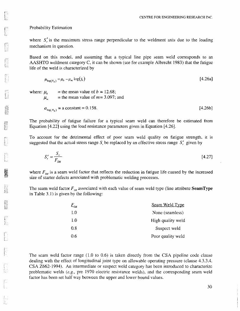
CENTRE FOR ENGINEERING RESEARCH INC
Probability Estimation
Finally to account for the fact that the model developed above considers only a single weldment a multiplier is required to convert the probability of failure per seam weld into a probability of failure per unit line length (see Equation [420]) Assuming that each pipe joint seam weld constitutes a distinct weldment and assuming further an average joint length of approximately 10 m this implies that there are on the order of I 00 fatigue susceptible weldments per kilometre of pipeline hence
[428]
4247 Other Causes
The other causes category is included in the prioritization model to reflect the background failure rate associated with causes that are not typically addressed by maintenance programs intended to maintain the integrity of aging pipelines In the context of this project it is assumed to be independent of specific line attributes and therefore a constant value This implies that the failure rate modification factor for failure by other causes is given by
AF=l0 [429]
31
CENIRE FOR ENGlNEERING RESEARCH INC
Figures and Tables
Excavation to pipeline location
Pipeline hit by excavator
Contractor fails to avoid pipeline
ContractorInadequate unaware ofConstruction depth of pipelineactivity cover
Inadequate markings
Operator ROW patrols fail to detect activity
Interval Patrol fails Contractor between
ignores to detect patrols too warnings activitylong
Output event AND gate 0 CJ OR gate Basic eventCJ 0
Figure 41 Fault tree model for mechanical interference
CENTRE FOR ENGINEERING RESEARCH INC
Failure Cause Baseline Failure Rate
Mode Factor
(incidentskm yr) small leak large leak rupture
External Metal Loss Corrosion
30 x lff4 085 010 005
Internal Metal Loss Corrosion
05 x 10 085 010 005
Mechanical Damage
30x lff4 025 050 025
Ground Movement
not applicable 020 040 040
Environmental Cracks (SCC)
not applicable 060 030 01
Mechanical Cracks (fatigue)
not applicable 06 03 01
Other Causes
20 x ff 08 01 01
Table 4 J Reference baseline failure rates and relative failure mode factors by cause for buried pipelines
CENTRE FOR ENGINEERING RESEARCH INC
50 CONSEQUENCE EVALUATION
51 Introduction
An estimate is required of the consequences of line failure for each section within each analysis segment as a function of the mode of line failure The consequences are calculated for each failure mode using analytical models that have been developed to evaluate product release characteristics and hazard areas and use this information to calculate quantitative measures of the life safety impact the environmental impact and the financial impact of line failure The three distinct consequence components are then combined into a single measure of the loss potential associated with each failure scenario
Consequence evaluation and combination 1s carried out for each analysis segment using algorithms that have already been developed and implemented within the framework of an influence diagram that was designed for decision analysis for further details refer to PIRAMID Technical Reference Manual No 32 (Stephens et al 1996) The influence diagram that forms the basis for the consequence evaluation model used for system prioritization is a modified and somewhat simplified version of the influence diagram described in the report referenced above
The simplified consequence evaluation influence diagram used for prioritization is shown in Figure 51 This influence diagram can be solved to obtain estimates of the three main consequence measures Number of Fatalities Equivalent Residual Spill Volume and Total Cost as well as the combined consequence measure referred to herein as Loss as a function of Failure Mode (ie small leak large leak and rupture) and Failure Section (ie attribute consistent sections along the length of the line segment) Note a detailed discussion of the steps involved in specifying and solving an influence diagram is given in PIRAMID Technical Reference Manual No 21 (Nessim and Hong 1995)
The following section of this report contains a technical description of the node parameters associated with the consequence evaluation influence diagram shown in Figure 51 that differ from those in the decision analysis influence diagram developed previously The reader is directed to PIRAMID Technical Reference Manual No 32 for a technical description of all other common node parameters
52 Consequence Evaluation Influence Diagram Node Parameters
521 Failure Mode
The Failure Mode node is a modified version of the Pipe Peiformance node in the original decision influence diagram (see Technical Reference Manual No 32) The name change reflects
32
CENTRE FOR ENGINEERING RESEARCH INC
Consequence Evaluation
the fact that the four valid states associated with the original node parameter (ie safe small leak large leak and rupture) have been revised down to three with the safe state being eliminated This reflects the fact that the consequences of the safe state (ie no failure) are not relevant to the prioritization model and consequences associated with the no failure state (ie the Maintenance Cost node) have therefore been eliminated
522 Equivalent Volume
The Equivalent Volume node in the original decision influence diagram (see Technical Reference Manual No 32) has been modified to reduce the number of line attributes that must be specified to characterize the environmental damage sensitivity of the spill site The reduced attribute set is shown in Table 5 1 together with the attributes that have been eliminated from the list and defined internally by representative default values In addition the node has been revised such that the additional required node parameter inputs (ie the reference spill product and the reference spill site damage index) are specified by global model default values
523 Interruption Cost
The Interruption Cost node in the original decision influence diagram (see Technical Reference Manual No 32) has been modified to calculate unit product transport costs microcanbull from the following relationship
[51]
where micro is the unit transport cost in dollars per unit volume per unit distance and Tdi is the transport distance associated with products passing through the line segment in question This calculation approach allows for the definition of universal unit transport cost estimates by product type that are independent of segment length and therefore globally applicable to the pipeline system as a whole The unit cost estimates microaao can therefore be specified by global
model default values The required segment specific data TJ is obtained directly from the data structure generated at the System Definition stage of model specification (see line attribute TransDist in Table 31)
In addition the node has been modified such that the remaining segment specific node parameter input data (ie the tendered volume vs line capacity and the billing abatement threshold) are also obtained directly from the data structure generated at the System Definition stage of model specification (see line attributes CapFraction and BAT in Table 31)
33
CENTRE FOR ENGINEERING RESEARCH INC
Consequence Evaluation
524 Loss
5241 Node Parameter
The Loss node is a new node that serves to convert the number of fatalities estimate and the equivalent residual spill volume estimate into equivalent dollars and to then add these quantities to the total cost estimate to produce a combined measure of the total loss associated with line failure in so-called equivalent dollar units This conversion is carried out based on the so-called willingness to pay concept which involves making an estimate of the amount of money that the pipeline operator or society as a whole would be willing to pay to avoid a particular adverse outcome Using this approach the cost equivalent of a human fatality can estimated by determining the amount of money that the operator (or society) would be willing to pay to avoid the loss of a statistical life Similarly an estimate can be made of the amount of money that the operator (or society) would be willing to pay to avoid the long-term environmental damage associated with the spill of a reference volume of a specific product at a specific reference location
The algorithm employed to calculate the node parameter which is total loss estimate Loss for each mode of failure k on each sectionj along each segment i is given by
[52]
where c = mean value of the total cost
ii =mean value of the number offatalities
v = mean value of the equivalent volume
= equivalent cost of one human fatality and
= equivalent cost of a unit residual spill volume of reference product at the reference spill location
5242 Equivalent Costs
As indicated previously the equivalent cost of human fatalities and equivalent spill volumes can be estimated using the willingness to pay (WTP) approach As developed in the economics literature and summarized by Rusin and Savvides-Gellerson (1987) the VTP approach when applied to the value of human life takes into account an individuals desire to improve their probability of survival by estimating what the individual would be willing to pay for a marginal reduction in their probability of death Specifically the WTP method measures the value of goods and services that an individual would be willing to forego in order to obtain a reduction in the probability of accidental loss of life By averaging this measure across all people exposed to a risk or a potential change in risk an estimate of the value of a statistical life is obtained
34
CENTRE FOR ENGINEERING RESEARCH INC
Consequence Evaluation
In the Rusin and Savvides-Gellerson study cited above a review of economic studies undertaken by various government agencies and consulting firms led the authors to adopt an estimate of $2 million dollars as the value of reducing the risk of death by an amount such that we expect one less death at the reduced risk level This monetary value is suggested here as a default estimate of the equivalent cost of one human fatality in the absence of a formal evaluation of this cost by the user of the prioritization method
Similarly the WTP approach can be applied to equivalent spill volumes wherein an estimate can be obtained of the value of goods and services that an individual would be willing to forego in order to obtain a reduction (or to prevent an increase) in the probability of long-term environmental damage resulting from a unit volume of reference product spilled at a reference location Given the implicit variability in the actual and perceived impact of different spill products on different environments it is difficult to come up with a broadly applicable estimate of the equivalent cost (in $m3
) of an equivalent spill volume this quantity is highly operator and location specific
To provide a point of reference for environmental damage cost equivalents consider the following A hypothetical environmental damage assessment case presented by Desvousges et al (1989) indicates an equivalent cost in the range of $20000m to $200000m for a diesel oil spill (with a residual spill volume of approximately JOO m3
) in an environmentally sensitive recreational area Note that the low end of the cited cost range considers site restoration costs only whereas the high end of the range reflects the additional loss-of-use value and the so-called non-use value of the damaged resources to people far removed from the spill site who would be willing to pay to simply know that the environmental resource exists and that it is available for use if desired
As another example the state of Washington has developed a spill damage compensation formula for estimating public resource damages for oils spills into state waters (Geselbracht and Logan 1993) This formula assigns a damage cost that falls within a range of $260m to $13000m ($1USgal to $50USgal) depending on the product damage potential and resource vulnerability
Based on the cited examples an equivalent unit cost for equivalent spill volumes referenced to an environmentally sensitive spill location could easily be on the order of thousands or tens-ofshythousands of dollars A monetary value of $10000 is suggested here as a default estimate of the equivalent cost of a cubic metre of equivalent spill volume (referenced to an environmentally sensitive location) in the absence of a formal evaluation of this cost by the user of the prioritization method
35
CENTRE FOR ENGINEERlNG RESEARCH lNC
Figures and Tables
---
---T----- I
j l j -
I -- shy -Lr - --- ------shy ------
--shy
Dependence Key
Conditional Functional
- - -
Figure 51 Basic node influence diagram for consequence evaluation
CENTRE FOR ENGINEERING RESEARCH INC
Pipeline Segment Attribute Defined No Input Required
by (specified internally using a
ProQram User representative attribute value)
Adjacent Land Use x Near Field Terrain x Significant Far Field Terrain Character Same as Near Field Terrain
Natural Surface Containment None
Distance to Surface Water x Surface Topography Rolling Terrain (slopes 5 to 50 )
Annual Rainfall 800 mmyr
Flood Potential flood return period 20 yrs
Confining Layer Thickness 3 to 10 m
Confining Layer Conductivity medium ( 1 Oe-4 to 1 Oe-6 emfs) )
Aquifer Conductivity medium (10e-2 to 10e-4 emfs)
Drinking Water within 5km x
Other Water within 5km x middotshyLand Use within 5krn x -------shy----~--
Sensitive Environment within 1 Okm - ------middotmiddot ----shyx
-- ------shy -- shy - --------shy
Sensitive Groundwater within 1 Okm x
Table 51 Segment attributes required by Equivalent Volume node to eharacterize environmental damage sensitivity of spill site
CENTRE FOR ENGINEERING RESEARCH INC
60 RISK ESTIMATION AND SEGMENT RANKING
61 Introduction
Multiplication of the segment-specific failure probability estimate for a given failure cause by the associated combined loss estimate produces an estimate of operating risk defined as the expected annual loss ExpLoss associated with a given segment of pipeline for the failure cause in question Summation of the risk estimates for all failure causes associated with a given segment gives an estimate of the total expected annual loss associated with segment operation Dividing these segment risk estimates by the corresponding segment length yields normalized risk estimates ExpLoss that allow comparison of calculated risks between segments of different lengths These cause-specific and combined-cause risk estimates form the basis for a quantitative ranking of all segments identified within a given pipeline system
62 Risk Calculation Model
The expected annual loss ExpLoss associated with each failure cause I for each analysis segment i is given by
Ns Nm
ExpLoss = L ExpLossijkl ($I year) [61] j=1 k=-1
where ExpLossjkl
Pfu1 = probability of failure for section j of segment i associated with failure mode k and failure cause I (failures I year)
Lossj =combined loss associated with failure on section j of segment i resulting from failure mode k ($I failure)
Ns =number of sections in segment and
Nm =number of failure modes= 3
The expected annual loss associated with each analysis segment for all failure causes combined is
calculated from the following
Ne
ExpLoss = L ExpLoss ($ I year) [62] fccJ
36
CENTRE FOR ENGINEERING RESEARCH INC
Risk Estimation and Segment Ranking
where Ne =number of failure causes =7
The expected annual loss on a per km basis ExpLoss is be calculated from the per segment
quantities ExpLoss as follows
on a cause-by-cause basis
ExpLossExpLoss ($ I kmbullyear) (63]
Lseg
and for the all causes combined case
bull ExpLossExpLoss =-~-~ ($ I kmbullyear) (64]
Lseg
where Lseg = length of Segment i (km)
63 Risk Ranking Model
The probability weighted or expected loss estimates calculated as described in the previous section form the basis for the ranking of all specified segments The basic intention is to rank each segment by failure cause to target high risk segments and associated failure causes for subsequent maintenance decision analysis The option also exists to rank segments on a combined cause basis which will provide a global measure of risk exposure for each segment The form of the risk ranking output generated by the prioritization model is illustrated in Figure 61
37
CENTRE FOR ENGINEERING RESEARCH lNC
Figures
~oop 13 External Corrosion -shy M--~- ---shy
9999 2 Loop 13 sec 8678 3 Loop 8 Ground Movement 8000 4 Loop 12 External Corrosion 6699 5 Loop 1 External Corrosion 5010 6 Loop2 External Corrosion 500() 7 Loop 2 Mechanical Damage 4400 8 Loop 3 Afechancial Damage 9 Loop 13 Mechanical Damage
12 Internal Corrosion
Figure 61 Output format for segment risk ranking
CENTRE FOR ENGINEERING RESEARCH INC
70 SUMMARY
The system prioritization stage is intended to identify segments within a pipeline system that may present an unacceptable level of operating risk To this end pipeline characteristics (or attributes) are evaluated to produce a line-specific estimate of the failure rate for each segment within the system as a function of failure cause (eg metal loss corrosion mechanical damage ground movement crack-like defects) and an estimate is made of the potential consequences of segment failure in terms of three distinct consequence components (ie life safety environmental damage and economic impact) Cause-specific failure rates are then combined with a global measure of the loss potential associated with the different consequence components to produce a single measure of operating risk for all failure causes associated with each segment Segments are then ranked according to the estimated level of risk the intention being to identify (or target) potentially high risk segments for subsequent detailed decision analysis at the maintenance optimization stage of the pipeline maintenance planning process
In the context of the prioritization model developed herein the components of operating risk are estimated as follows
The probability of line failure is given by
[41]
where RfJ = the failure rate associated with section j of segment i for failure mode k and failure cause I and
Lsecu =the length of sectionj within segment i (km)
The segment specific failure rate is given by
[42]
where Rfb =the baseline failure rate for failure model (per kmbullyear)
MFkl = the relative probability or mode factor for failure mode k associated with cause I and
AFJI = the failure rate modification factor for section j of segment i associated with failure cause I
A combined measure of the consequences of line failure is given by
($ per incident) [52]
38
CENTRE FOR ENGINEERING RESEARCH INC
Summary
where c = mean value of the total cost
n = mean value of the number of fatalities
v = mean value of the equivalent volume
a =equivalent cost of a human fatality and
=equivalent cost of a unit residual spill volume of reference product at the reference spill location
The operating risk per segment is given by the probability weighted or expected Loss which on a cause-by-cause basis is given by
Ns Nm
ExpLossil = 2 ExpLossjkl ($I year) [61] jo=l k=I
where ExpLoss
and Pfkl =probability of failure for section j of segment i associated with failure mode k and failure cause I (failures I year)
Lossi = eombined loss associated with failure on section j of segment i resulting from failure mode k ($I failure)
Ns = number of sections in segment I and
Nm =number of failure modes= 3
The normalized operating risk expressed on a per unit length basis is given by
bull ExpLoss1ExpLossil =-~-~ ($ I kmbullyear) [63]Lseg
where Lsec = the length of segment i (km)1
39
CENTRE FOR ENGINEERING RESEARCH [NC
80 REFERENCES
Albrecht P 1983 S-N Fatigue Reliability Analysis of Highway Bridges Probabilistic Fracture Mechanics and Fatigue Methods Applications for Structural Design and Maintenance ASTM STP 798 J M Bloom and J C Ekvall Eds American Society for Testing and Materials pp 184 - 204
Beavers A and Thompson N G 1995 Effects of Coatings on SCC of Pipelines New Developments Proceedings of the Fourteenth International Conference on Offshore Mechanics and Arctic Engineering Vol V pp 249 - 254
Crews D L 1976 Interpretation of Pitting Corrosion Data from Statistical Prediction Interval calculations Galvanic and Pitting Corrosion - Field and Laboratory Studies ASTM STP 576 American Society for Testing and Materials pp 217 - 230
CSA Z662-94 1994 Oil and Gas Pipeline Systems - Oil and Gas Industry Systems Canadian Standards Association Ontario September
CSFM 1993 Hazardous Liquid Pipeline Risk Assessment Prepared for the California State Fire Marshal by EDM Services Inc Simi Valley CA
Desvousges W H Dunford R W and Domanico J L 1989 Measuring Natural Resource Damages An Economic Appraisal Prepared for the American Petroleum Institute by the Research Triangle Institute Research Triangle Park NC
EGIG 1993 Gas Pipeline Incidents Report 1970-1992 European Gas Pipeline Incident Data Group
Feamehough G D 1985 The Control of Risk in Gas Transmission Pipeline Institute of Chemical Engineers Symposium Series No 93 pp 25 - 44
Geselbracht L and Logan R 1993 Washingtons Marine Oil Spill Compensation Schedule shySimplified Resource Damage Assessment Proceedings of the 1993 International Oil Spill Conference (Prevention Preparedness Response) Tampa March-April
Kiefner J F Vieth P H Orban J E and Feder P I 1990 Methods for Prioritizing Pipeline Maintenance and Rehabilitation American Gas Association
McCormick M J 1981 Reliability and Risk Analysis Academic Press Inc New York
Miller F P Foss J E and Wolf D C 1981 Soil Surveys Their Synthesis Confidence Limits and Utilization for Corrosion Assessment of Soil Underground Corrosion ASTM STP 741 Edward Escalante Ed American Society for Testing and Materials pp 3 - 23
40
CENTRE FOR ENGINEERING RESEARCH INC
References
Nessim M A and Hong HP 1995 Probabilistic Decision Analysis Using Influence Diagrams - PIRAMID Technical Reference Manual No 21 Confidential to C-FERs Pipeline Program Participants C-FER Report 94022 October
Rusin M and Savvides-Gellerson E 1987 The Safety of Interstate Liquid Pipelines An Evaluation of Present Levels and Proposals for Change American Petroleum Institute Research Study 040 July
Spiekhout J 1995 A New Design Philosophy for Gas Transmission Pipelines - Designing for Gouge-Resistance and Puncture-Resistance
Stephens M J Nessim M A and Chen Q 1995 A Methodology for Risk-Based Optimization of Pipeline Integrity Maintenance Activities - PIRAMID Technical Reference Manual No 12 Confidential to C-FER s Pipeline Program Participants C-FER Report 94006 October
Stephens M J Nessim M A and Chen Q 1996 Probabilistic Assessment of Onshore Pipeline Failure Consequences PIRAMID Technical Reference Manual No 32 Confidential to C-FERs Pipeline Program Participants C-FER Report 94035 November
41
- Piramid Technical Reference manaul No 41
-

CENTRE FOR ENGINEERING RESEARCH INC
Consequence Evaluation
In the Rusin and Savvides-Gellerson study cited above a review of economic studies undertaken by various government agencies and consulting firms led the authors to adopt an estimate of $2 million dollars as the value of reducing the risk of death by an amount such that we expect one less death at the reduced risk level This monetary value is suggested here as a default estimate of the equivalent cost of one human fatality in the absence of a formal evaluation of this cost by the user of the prioritization method
Similarly the WTP approach can be applied to equivalent spill volumes wherein an estimate can be obtained of the value of goods and services that an individual would be willing to forego in order to obtain a reduction (or to prevent an increase) in the probability of long-term environmental damage resulting from a unit volume of reference product spilled at a reference location Given the implicit variability in the actual and perceived impact of different spill products on different environments it is difficult to come up with a broadly applicable estimate of the equivalent cost (in $m3
) of an equivalent spill volume this quantity is highly operator and location specific
To provide a point of reference for environmental damage cost equivalents consider the following A hypothetical environmental damage assessment case presented by Desvousges et al (1989) indicates an equivalent cost in the range of $20000m to $200000m for a diesel oil spill (with a residual spill volume of approximately JOO m3
) in an environmentally sensitive recreational area Note that the low end of the cited cost range considers site restoration costs only whereas the high end of the range reflects the additional loss-of-use value and the so-called non-use value of the damaged resources to people far removed from the spill site who would be willing to pay to simply know that the environmental resource exists and that it is available for use if desired
As another example the state of Washington has developed a spill damage compensation formula for estimating public resource damages for oils spills into state waters (Geselbracht and Logan 1993) This formula assigns a damage cost that falls within a range of $260m to $13000m ($1USgal to $50USgal) depending on the product damage potential and resource vulnerability
Based on the cited examples an equivalent unit cost for equivalent spill volumes referenced to an environmentally sensitive spill location could easily be on the order of thousands or tens-ofshythousands of dollars A monetary value of $10000 is suggested here as a default estimate of the equivalent cost of a cubic metre of equivalent spill volume (referenced to an environmentally sensitive location) in the absence of a formal evaluation of this cost by the user of the prioritization method
35
CENTRE FOR ENGINEERlNG RESEARCH lNC
Figures and Tables
---
---T----- I
j l j -
I -- shy -Lr - --- ------shy ------
--shy
Dependence Key
Conditional Functional
- - -
Figure 51 Basic node influence diagram for consequence evaluation
CENTRE FOR ENGINEERING RESEARCH INC
Pipeline Segment Attribute Defined No Input Required
by (specified internally using a
ProQram User representative attribute value)
Adjacent Land Use x Near Field Terrain x Significant Far Field Terrain Character Same as Near Field Terrain
Natural Surface Containment None
Distance to Surface Water x Surface Topography Rolling Terrain (slopes 5 to 50 )
Annual Rainfall 800 mmyr
Flood Potential flood return period 20 yrs
Confining Layer Thickness 3 to 10 m
Confining Layer Conductivity medium ( 1 Oe-4 to 1 Oe-6 emfs) )
Aquifer Conductivity medium (10e-2 to 10e-4 emfs)
Drinking Water within 5km x
Other Water within 5km x middotshyLand Use within 5krn x -------shy----~--
Sensitive Environment within 1 Okm - ------middotmiddot ----shyx
-- ------shy -- shy - --------shy
Sensitive Groundwater within 1 Okm x
Table 51 Segment attributes required by Equivalent Volume node to eharacterize environmental damage sensitivity of spill site
CENTRE FOR ENGINEERING RESEARCH INC
60 RISK ESTIMATION AND SEGMENT RANKING
61 Introduction
Multiplication of the segment-specific failure probability estimate for a given failure cause by the associated combined loss estimate produces an estimate of operating risk defined as the expected annual loss ExpLoss associated with a given segment of pipeline for the failure cause in question Summation of the risk estimates for all failure causes associated with a given segment gives an estimate of the total expected annual loss associated with segment operation Dividing these segment risk estimates by the corresponding segment length yields normalized risk estimates ExpLoss that allow comparison of calculated risks between segments of different lengths These cause-specific and combined-cause risk estimates form the basis for a quantitative ranking of all segments identified within a given pipeline system
62 Risk Calculation Model
The expected annual loss ExpLoss associated with each failure cause I for each analysis segment i is given by
Ns Nm
ExpLoss = L ExpLossijkl ($I year) [61] j=1 k=-1
where ExpLossjkl
Pfu1 = probability of failure for section j of segment i associated with failure mode k and failure cause I (failures I year)
Lossj =combined loss associated with failure on section j of segment i resulting from failure mode k ($I failure)
Ns =number of sections in segment and
Nm =number of failure modes= 3
The expected annual loss associated with each analysis segment for all failure causes combined is
calculated from the following
Ne
ExpLoss = L ExpLoss ($ I year) [62] fccJ
36
CENTRE FOR ENGINEERING RESEARCH INC
Risk Estimation and Segment Ranking
where Ne =number of failure causes =7
The expected annual loss on a per km basis ExpLoss is be calculated from the per segment
quantities ExpLoss as follows
on a cause-by-cause basis
ExpLossExpLoss ($ I kmbullyear) (63]
Lseg
and for the all causes combined case
bull ExpLossExpLoss =-~-~ ($ I kmbullyear) (64]
Lseg
where Lseg = length of Segment i (km)
63 Risk Ranking Model
The probability weighted or expected loss estimates calculated as described in the previous section form the basis for the ranking of all specified segments The basic intention is to rank each segment by failure cause to target high risk segments and associated failure causes for subsequent maintenance decision analysis The option also exists to rank segments on a combined cause basis which will provide a global measure of risk exposure for each segment The form of the risk ranking output generated by the prioritization model is illustrated in Figure 61
37
CENTRE FOR ENGINEERING RESEARCH lNC
Figures
~oop 13 External Corrosion -shy M--~- ---shy
9999 2 Loop 13 sec 8678 3 Loop 8 Ground Movement 8000 4 Loop 12 External Corrosion 6699 5 Loop 1 External Corrosion 5010 6 Loop2 External Corrosion 500() 7 Loop 2 Mechanical Damage 4400 8 Loop 3 Afechancial Damage 9 Loop 13 Mechanical Damage
12 Internal Corrosion
Figure 61 Output format for segment risk ranking
CENTRE FOR ENGINEERING RESEARCH INC
70 SUMMARY
The system prioritization stage is intended to identify segments within a pipeline system that may present an unacceptable level of operating risk To this end pipeline characteristics (or attributes) are evaluated to produce a line-specific estimate of the failure rate for each segment within the system as a function of failure cause (eg metal loss corrosion mechanical damage ground movement crack-like defects) and an estimate is made of the potential consequences of segment failure in terms of three distinct consequence components (ie life safety environmental damage and economic impact) Cause-specific failure rates are then combined with a global measure of the loss potential associated with the different consequence components to produce a single measure of operating risk for all failure causes associated with each segment Segments are then ranked according to the estimated level of risk the intention being to identify (or target) potentially high risk segments for subsequent detailed decision analysis at the maintenance optimization stage of the pipeline maintenance planning process
In the context of the prioritization model developed herein the components of operating risk are estimated as follows
The probability of line failure is given by
[41]
where RfJ = the failure rate associated with section j of segment i for failure mode k and failure cause I and
Lsecu =the length of sectionj within segment i (km)
The segment specific failure rate is given by
[42]
where Rfb =the baseline failure rate for failure model (per kmbullyear)
MFkl = the relative probability or mode factor for failure mode k associated with cause I and
AFJI = the failure rate modification factor for section j of segment i associated with failure cause I
A combined measure of the consequences of line failure is given by
($ per incident) [52]
38
CENTRE FOR ENGINEERING RESEARCH INC
Summary
where c = mean value of the total cost
n = mean value of the number of fatalities
v = mean value of the equivalent volume
a =equivalent cost of a human fatality and
=equivalent cost of a unit residual spill volume of reference product at the reference spill location
The operating risk per segment is given by the probability weighted or expected Loss which on a cause-by-cause basis is given by
Ns Nm
ExpLossil = 2 ExpLossjkl ($I year) [61] jo=l k=I
where ExpLoss
and Pfkl =probability of failure for section j of segment i associated with failure mode k and failure cause I (failures I year)
Lossi = eombined loss associated with failure on section j of segment i resulting from failure mode k ($I failure)
Ns = number of sections in segment I and
Nm =number of failure modes= 3
The normalized operating risk expressed on a per unit length basis is given by
bull ExpLoss1ExpLossil =-~-~ ($ I kmbullyear) [63]Lseg
where Lsec = the length of segment i (km)1
39
CENTRE FOR ENGINEERING RESEARCH [NC
80 REFERENCES
Albrecht P 1983 S-N Fatigue Reliability Analysis of Highway Bridges Probabilistic Fracture Mechanics and Fatigue Methods Applications for Structural Design and Maintenance ASTM STP 798 J M Bloom and J C Ekvall Eds American Society for Testing and Materials pp 184 - 204
Beavers A and Thompson N G 1995 Effects of Coatings on SCC of Pipelines New Developments Proceedings of the Fourteenth International Conference on Offshore Mechanics and Arctic Engineering Vol V pp 249 - 254
Crews D L 1976 Interpretation of Pitting Corrosion Data from Statistical Prediction Interval calculations Galvanic and Pitting Corrosion - Field and Laboratory Studies ASTM STP 576 American Society for Testing and Materials pp 217 - 230
CSA Z662-94 1994 Oil and Gas Pipeline Systems - Oil and Gas Industry Systems Canadian Standards Association Ontario September
CSFM 1993 Hazardous Liquid Pipeline Risk Assessment Prepared for the California State Fire Marshal by EDM Services Inc Simi Valley CA
Desvousges W H Dunford R W and Domanico J L 1989 Measuring Natural Resource Damages An Economic Appraisal Prepared for the American Petroleum Institute by the Research Triangle Institute Research Triangle Park NC
EGIG 1993 Gas Pipeline Incidents Report 1970-1992 European Gas Pipeline Incident Data Group
Feamehough G D 1985 The Control of Risk in Gas Transmission Pipeline Institute of Chemical Engineers Symposium Series No 93 pp 25 - 44
Geselbracht L and Logan R 1993 Washingtons Marine Oil Spill Compensation Schedule shySimplified Resource Damage Assessment Proceedings of the 1993 International Oil Spill Conference (Prevention Preparedness Response) Tampa March-April
Kiefner J F Vieth P H Orban J E and Feder P I 1990 Methods for Prioritizing Pipeline Maintenance and Rehabilitation American Gas Association
McCormick M J 1981 Reliability and Risk Analysis Academic Press Inc New York
Miller F P Foss J E and Wolf D C 1981 Soil Surveys Their Synthesis Confidence Limits and Utilization for Corrosion Assessment of Soil Underground Corrosion ASTM STP 741 Edward Escalante Ed American Society for Testing and Materials pp 3 - 23
40
CENTRE FOR ENGINEERING RESEARCH INC
References
Nessim M A and Hong HP 1995 Probabilistic Decision Analysis Using Influence Diagrams - PIRAMID Technical Reference Manual No 21 Confidential to C-FERs Pipeline Program Participants C-FER Report 94022 October
Rusin M and Savvides-Gellerson E 1987 The Safety of Interstate Liquid Pipelines An Evaluation of Present Levels and Proposals for Change American Petroleum Institute Research Study 040 July
Spiekhout J 1995 A New Design Philosophy for Gas Transmission Pipelines - Designing for Gouge-Resistance and Puncture-Resistance
Stephens M J Nessim M A and Chen Q 1995 A Methodology for Risk-Based Optimization of Pipeline Integrity Maintenance Activities - PIRAMID Technical Reference Manual No 12 Confidential to C-FER s Pipeline Program Participants C-FER Report 94006 October
Stephens M J Nessim M A and Chen Q 1996 Probabilistic Assessment of Onshore Pipeline Failure Consequences PIRAMID Technical Reference Manual No 32 Confidential to C-FERs Pipeline Program Participants C-FER Report 94035 November
41
- Piramid Technical Reference manaul No 41
-
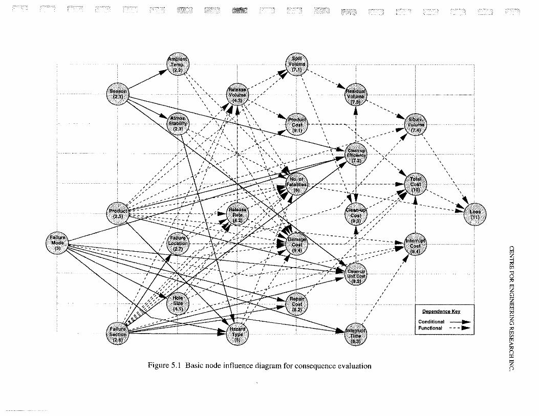

CENTRE FOR ENGINEERING RESEARCH INC
Risk Estimation and Segment Ranking
where Ne =number of failure causes =7
The expected annual loss on a per km basis ExpLoss is be calculated from the per segment
quantities ExpLoss as follows
on a cause-by-cause basis
ExpLossExpLoss ($ I kmbullyear) (63]
Lseg
and for the all causes combined case
bull ExpLossExpLoss =-~-~ ($ I kmbullyear) (64]
Lseg
where Lseg = length of Segment i (km)
63 Risk Ranking Model
The probability weighted or expected loss estimates calculated as described in the previous section form the basis for the ranking of all specified segments The basic intention is to rank each segment by failure cause to target high risk segments and associated failure causes for subsequent maintenance decision analysis The option also exists to rank segments on a combined cause basis which will provide a global measure of risk exposure for each segment The form of the risk ranking output generated by the prioritization model is illustrated in Figure 61
37
CENTRE FOR ENGINEERING RESEARCH lNC
Figures
~oop 13 External Corrosion -shy M--~- ---shy
9999 2 Loop 13 sec 8678 3 Loop 8 Ground Movement 8000 4 Loop 12 External Corrosion 6699 5 Loop 1 External Corrosion 5010 6 Loop2 External Corrosion 500() 7 Loop 2 Mechanical Damage 4400 8 Loop 3 Afechancial Damage 9 Loop 13 Mechanical Damage
12 Internal Corrosion
Figure 61 Output format for segment risk ranking
CENTRE FOR ENGINEERING RESEARCH INC
70 SUMMARY
The system prioritization stage is intended to identify segments within a pipeline system that may present an unacceptable level of operating risk To this end pipeline characteristics (or attributes) are evaluated to produce a line-specific estimate of the failure rate for each segment within the system as a function of failure cause (eg metal loss corrosion mechanical damage ground movement crack-like defects) and an estimate is made of the potential consequences of segment failure in terms of three distinct consequence components (ie life safety environmental damage and economic impact) Cause-specific failure rates are then combined with a global measure of the loss potential associated with the different consequence components to produce a single measure of operating risk for all failure causes associated with each segment Segments are then ranked according to the estimated level of risk the intention being to identify (or target) potentially high risk segments for subsequent detailed decision analysis at the maintenance optimization stage of the pipeline maintenance planning process
In the context of the prioritization model developed herein the components of operating risk are estimated as follows
The probability of line failure is given by
[41]
where RfJ = the failure rate associated with section j of segment i for failure mode k and failure cause I and
Lsecu =the length of sectionj within segment i (km)
The segment specific failure rate is given by
[42]
where Rfb =the baseline failure rate for failure model (per kmbullyear)
MFkl = the relative probability or mode factor for failure mode k associated with cause I and
AFJI = the failure rate modification factor for section j of segment i associated with failure cause I
A combined measure of the consequences of line failure is given by
($ per incident) [52]
38
CENTRE FOR ENGINEERING RESEARCH INC
Summary
where c = mean value of the total cost
n = mean value of the number of fatalities
v = mean value of the equivalent volume
a =equivalent cost of a human fatality and
=equivalent cost of a unit residual spill volume of reference product at the reference spill location
The operating risk per segment is given by the probability weighted or expected Loss which on a cause-by-cause basis is given by
Ns Nm
ExpLossil = 2 ExpLossjkl ($I year) [61] jo=l k=I
where ExpLoss
and Pfkl =probability of failure for section j of segment i associated with failure mode k and failure cause I (failures I year)
Lossi = eombined loss associated with failure on section j of segment i resulting from failure mode k ($I failure)
Ns = number of sections in segment I and
Nm =number of failure modes= 3
The normalized operating risk expressed on a per unit length basis is given by
bull ExpLoss1ExpLossil =-~-~ ($ I kmbullyear) [63]Lseg
where Lsec = the length of segment i (km)1
39
CENTRE FOR ENGINEERING RESEARCH [NC
80 REFERENCES
Albrecht P 1983 S-N Fatigue Reliability Analysis of Highway Bridges Probabilistic Fracture Mechanics and Fatigue Methods Applications for Structural Design and Maintenance ASTM STP 798 J M Bloom and J C Ekvall Eds American Society for Testing and Materials pp 184 - 204
Beavers A and Thompson N G 1995 Effects of Coatings on SCC of Pipelines New Developments Proceedings of the Fourteenth International Conference on Offshore Mechanics and Arctic Engineering Vol V pp 249 - 254
Crews D L 1976 Interpretation of Pitting Corrosion Data from Statistical Prediction Interval calculations Galvanic and Pitting Corrosion - Field and Laboratory Studies ASTM STP 576 American Society for Testing and Materials pp 217 - 230
CSA Z662-94 1994 Oil and Gas Pipeline Systems - Oil and Gas Industry Systems Canadian Standards Association Ontario September
CSFM 1993 Hazardous Liquid Pipeline Risk Assessment Prepared for the California State Fire Marshal by EDM Services Inc Simi Valley CA
Desvousges W H Dunford R W and Domanico J L 1989 Measuring Natural Resource Damages An Economic Appraisal Prepared for the American Petroleum Institute by the Research Triangle Institute Research Triangle Park NC
EGIG 1993 Gas Pipeline Incidents Report 1970-1992 European Gas Pipeline Incident Data Group
Feamehough G D 1985 The Control of Risk in Gas Transmission Pipeline Institute of Chemical Engineers Symposium Series No 93 pp 25 - 44
Geselbracht L and Logan R 1993 Washingtons Marine Oil Spill Compensation Schedule shySimplified Resource Damage Assessment Proceedings of the 1993 International Oil Spill Conference (Prevention Preparedness Response) Tampa March-April
Kiefner J F Vieth P H Orban J E and Feder P I 1990 Methods for Prioritizing Pipeline Maintenance and Rehabilitation American Gas Association
McCormick M J 1981 Reliability and Risk Analysis Academic Press Inc New York
Miller F P Foss J E and Wolf D C 1981 Soil Surveys Their Synthesis Confidence Limits and Utilization for Corrosion Assessment of Soil Underground Corrosion ASTM STP 741 Edward Escalante Ed American Society for Testing and Materials pp 3 - 23
40
CENTRE FOR ENGINEERING RESEARCH INC
References
Nessim M A and Hong HP 1995 Probabilistic Decision Analysis Using Influence Diagrams - PIRAMID Technical Reference Manual No 21 Confidential to C-FERs Pipeline Program Participants C-FER Report 94022 October
Rusin M and Savvides-Gellerson E 1987 The Safety of Interstate Liquid Pipelines An Evaluation of Present Levels and Proposals for Change American Petroleum Institute Research Study 040 July
Spiekhout J 1995 A New Design Philosophy for Gas Transmission Pipelines - Designing for Gouge-Resistance and Puncture-Resistance
Stephens M J Nessim M A and Chen Q 1995 A Methodology for Risk-Based Optimization of Pipeline Integrity Maintenance Activities - PIRAMID Technical Reference Manual No 12 Confidential to C-FER s Pipeline Program Participants C-FER Report 94006 October
Stephens M J Nessim M A and Chen Q 1996 Probabilistic Assessment of Onshore Pipeline Failure Consequences PIRAMID Technical Reference Manual No 32 Confidential to C-FERs Pipeline Program Participants C-FER Report 94035 November
41
- Piramid Technical Reference manaul No 41
-

CENTRE FOR ENGINEERING RESEARCH INC
Summary
where c = mean value of the total cost
n = mean value of the number of fatalities
v = mean value of the equivalent volume
a =equivalent cost of a human fatality and
=equivalent cost of a unit residual spill volume of reference product at the reference spill location
The operating risk per segment is given by the probability weighted or expected Loss which on a cause-by-cause basis is given by
Ns Nm
ExpLossil = 2 ExpLossjkl ($I year) [61] jo=l k=I
where ExpLoss
and Pfkl =probability of failure for section j of segment i associated with failure mode k and failure cause I (failures I year)
Lossi = eombined loss associated with failure on section j of segment i resulting from failure mode k ($I failure)
Ns = number of sections in segment I and
Nm =number of failure modes= 3
The normalized operating risk expressed on a per unit length basis is given by
bull ExpLoss1ExpLossil =-~-~ ($ I kmbullyear) [63]Lseg
where Lsec = the length of segment i (km)1
39
CENTRE FOR ENGINEERING RESEARCH [NC
80 REFERENCES
Albrecht P 1983 S-N Fatigue Reliability Analysis of Highway Bridges Probabilistic Fracture Mechanics and Fatigue Methods Applications for Structural Design and Maintenance ASTM STP 798 J M Bloom and J C Ekvall Eds American Society for Testing and Materials pp 184 - 204
Beavers A and Thompson N G 1995 Effects of Coatings on SCC of Pipelines New Developments Proceedings of the Fourteenth International Conference on Offshore Mechanics and Arctic Engineering Vol V pp 249 - 254
Crews D L 1976 Interpretation of Pitting Corrosion Data from Statistical Prediction Interval calculations Galvanic and Pitting Corrosion - Field and Laboratory Studies ASTM STP 576 American Society for Testing and Materials pp 217 - 230
CSA Z662-94 1994 Oil and Gas Pipeline Systems - Oil and Gas Industry Systems Canadian Standards Association Ontario September
CSFM 1993 Hazardous Liquid Pipeline Risk Assessment Prepared for the California State Fire Marshal by EDM Services Inc Simi Valley CA
Desvousges W H Dunford R W and Domanico J L 1989 Measuring Natural Resource Damages An Economic Appraisal Prepared for the American Petroleum Institute by the Research Triangle Institute Research Triangle Park NC
EGIG 1993 Gas Pipeline Incidents Report 1970-1992 European Gas Pipeline Incident Data Group
Feamehough G D 1985 The Control of Risk in Gas Transmission Pipeline Institute of Chemical Engineers Symposium Series No 93 pp 25 - 44
Geselbracht L and Logan R 1993 Washingtons Marine Oil Spill Compensation Schedule shySimplified Resource Damage Assessment Proceedings of the 1993 International Oil Spill Conference (Prevention Preparedness Response) Tampa March-April
Kiefner J F Vieth P H Orban J E and Feder P I 1990 Methods for Prioritizing Pipeline Maintenance and Rehabilitation American Gas Association
McCormick M J 1981 Reliability and Risk Analysis Academic Press Inc New York
Miller F P Foss J E and Wolf D C 1981 Soil Surveys Their Synthesis Confidence Limits and Utilization for Corrosion Assessment of Soil Underground Corrosion ASTM STP 741 Edward Escalante Ed American Society for Testing and Materials pp 3 - 23
40
CENTRE FOR ENGINEERING RESEARCH INC
References
Nessim M A and Hong HP 1995 Probabilistic Decision Analysis Using Influence Diagrams - PIRAMID Technical Reference Manual No 21 Confidential to C-FERs Pipeline Program Participants C-FER Report 94022 October
Rusin M and Savvides-Gellerson E 1987 The Safety of Interstate Liquid Pipelines An Evaluation of Present Levels and Proposals for Change American Petroleum Institute Research Study 040 July
Spiekhout J 1995 A New Design Philosophy for Gas Transmission Pipelines - Designing for Gouge-Resistance and Puncture-Resistance
Stephens M J Nessim M A and Chen Q 1995 A Methodology for Risk-Based Optimization of Pipeline Integrity Maintenance Activities - PIRAMID Technical Reference Manual No 12 Confidential to C-FER s Pipeline Program Participants C-FER Report 94006 October
Stephens M J Nessim M A and Chen Q 1996 Probabilistic Assessment of Onshore Pipeline Failure Consequences PIRAMID Technical Reference Manual No 32 Confidential to C-FERs Pipeline Program Participants C-FER Report 94035 November
41
- Piramid Technical Reference manaul No 41
-