PRISAD: A Partitioned Rendering Infrastructure forScalable Accordion Drawing (Extended Version)

James Slack∗† Kristian Hildebrand∗†‡ Tamara Munzner∗†

ABSTRACT

We present PRISAD, the first generic rendering infrastructure forinformation visualization applications that use the accordion draw-ing technique: rubber-sheet navigation with guaranteed visibilityfor marked areas of interest. Our new rendering algorithms arebased on the partitioning of screen-space, which allows us to handledense dataset regions correctly. The algorithms in previous workled to incorrect visual representations because of overculling, and toinefficiencies due to overdrawing multiple items in the same region.Our pixel-based drawing infrastructure guarantees correctness byeliminating overculling, and improves rendering performance withtight bounds on overdrawing.

PRITree and PRISeq are applications built on PRISAD, withthe feature sets of TreeJuxtaposer and SequenceJuxtaposer, respec-tively. We describe our PRITree and PRISeq dataset traversal al-gorithms, which are used for efficient rendering, culling, and lay-out of datasets within the PRISAD framework. We also discussPRITree node marking techniques, which offer order-of-magnitudeimprovements to both memory and time performance versus pre-vious range storage and retrieval techniques. Our PRITree im-plementation features a five-fold increase in rendering speed fornon-trivial tree structures, and also reduces memory requirementsin some real-world datasets by up to eight times, so we are ableto handle trees of several million nodes. PRISeq renders fif-teen times faster and handles datasets twenty times larger thanprevious work. The software is available as open source fromhttp://olduvai.sourceforge.net.

CR Categories: I.3.6 [Computer Graphics]: Methodology andTechniques—Graphics data structures and data types;

Keywords: Focus+Context, Information Visualization, Real TimeRendering, Progressive Rendering

INTRODUCTION

PRISAD, our Partitioned Rendering Infrastructure for Scalable Ac-cordion Drawing, is a generic Accordion Drawing (AD) infrastruc-ture for rendering and navigating large datasets. AD is a visual-ization technique that features rubber-sheet navigation and guaran-teed visibility of selected nodes. Rubber-sheet navigation involvesthe user-guided action of stretching on-screen regions of interest; astretched region has more screen real estate in which to draw moreunoccluded geometric items from the same world-space region.When a region is stretched, the nailed-down borders of the win-dow prevent data from being pushed off-screen and AD squishesdata in appropriate regions, as shown in Figure 1.

Guaranteed visibility of data, represented by geometric objectson screen, is trivial with small datasets. The topological structure

∗e-mail:{jslack,hilde,tmm}@cs.ubc.ca†University of British Columbia‡Bauhaus University Weimar

polar

bears

sealsspotted

black bearslouisiana

harbor

american

polar

bears

seals spotted

black bears

louisiana

harbor

american

Figure 1: Left: A tree dataset drawn with uniformly allocated spacefor each vertical node width and horizontal node height. Right:When navigating by stretching a rubber-sheet surface, the distor-tions allocate more screen-space to some regions of nodes and otherregions are squished into less screen-space.

of the tree shown in Figure 1, and colors for each node, are visi-ble without navigation. However, when the size of the dataset be-comes large, as in Figure 2, AD must guarantee the visibility ofall marked regions. A brute-force drawing algorithm, which wouldrender every node in the dataset, does not offer sufficient renderingperformance for animating such large datasets, especially with ourguaranteed visibility requirements.

As data is never pushed off-screen with AD navigation, we canalways map data from its infinite-precision world-space position toour finite-precision dataset representation in screen space. AD nav-igation leads to compressing regions of many data items to subtenda small screen-space region, yielding high depth complexity. Toachieve scalable rendering performance for large datasets, we mustefficiently reduce the amount of overdrawing in dense screen-spaceregions where drawing a subset of geometric data objects is suffi-cient to represent the entire region. Culling the correct data in denseregions is particularly difficult when we must guarantee the visibil-ity of important features at all times. A correct drawing with nooverculling is visually indistinguishable from the brute-force ren-dering where every item is drawn. We need both marked node vis-ibility, and a proper representation of the dataset in every distortedregion of screen space.

We present our generic PRISAD infrastructure, and two applica-tions built on it, both of which use Java with the GL4Java graphicslibrary. PRITree implements the feature set of TreeJuxtaposer forvisually comparing hierarchies [11], and PRISeq has the functional-ity of SequenceJuxtaposer for visualizing multiple aligned genomicsequences [16]. Our contributions include:

• Time-Efficient Generic Rendering: PRISAD tightly boundsoverdrawing in dense, complex regions by separating pixel-based partitioning from application-specific rendering ac-tions.

• Correct Generic Rendering: PRISAD eliminates overculling,so no misleading gaps appear in the dataset picture.

• Space-Efficient Marking: PRITree computes and storesmarked regions of trees in structures capable of determin-ing marking characteristics quickly, eliminating the need forcaching marking properties for each node.

• Space-Efficient Traversal: PRITree traversal algorithms fordrawing and picking exploit the dataset topology, instead ofadding a memory-expensive external data structure.

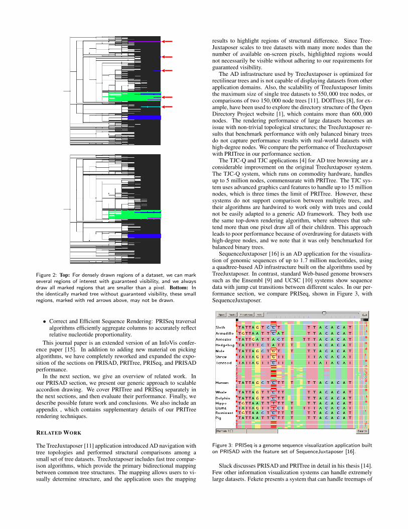
Figure 2: Top: For densely drawn regions of a dataset, we can markseveral regions of interest with guaranteed visibility, and we alwaysdraw all marked regions that are smaller than a pixel. Bottom: Inthe identically marked tree without guaranteed visibility, these smallregions, marked with red arrows above, may not be drawn.

• Correct and Efficient Sequence Rendering: PRISeq traversalalgorithms efficiently aggregate columns to accurately reflectrelative nucleotide proportionality.

This journal paper is an extended version of an InfoVis confer-ence paper [15]. In addition to adding new material on pickingalgorithms, we have completely reworked and expanded the expo-sition of the sections on PRISAD, PRITree, PRISeq, and PRISADperformance.

In the next section, we give an overview of related work. Inour PRISAD section, we present our generic approach to scalableaccordion drawing. We cover PRITree and PRISeq separately inthe next sections, and then evaluate their performance. Finally, wedescribe possible future work and conclusions. We also include anappendix , which contains supplementary details of our PRITreerendering techniques.

RELATED WORK

The TreeJuxtaposer [11] application introduced AD navigation withtree topologies and performed structural comparisons among asmall set of tree datasets. TreeJuxtaposer includes fast tree compar-ison algorithms, which provide the primary bidirectional mappingbetween common tree structures. The mapping allows users to vi-sually determine structure, and the application uses the mapping

results to highlight regions of structural difference. Since Tree-Juxtaposer scales to tree datasets with many more nodes than thenumber of available on-screen pixels, highlighted regions wouldnot necessarily be visible without adhering to our requirements forguaranteed visibility.

The AD infrastructure used by TreeJuxtaposer is optimized forrectilinear trees and is not capable of displaying datasets from otherapplication domains. Also, the scalability of TreeJuxtaposer limitsthe maximum size of single tree datasets to 550,000 tree nodes, orcomparisons of two 150,000 node trees [11]. DOITrees [8], for ex-ample, have been used to explore the directory structure of the OpenDirectory Project website [1], which contains more than 600,000nodes. The rendering performance of large datasets becomes anissue with non-trivial topological structures; the TreeJuxtaposer re-sults that benchmark performance with only balanced binary treesdo not capture performance results with real-world datasets withhigh-degree nodes. We compare the performance of TreeJuxtaposerwith PRITree in our performance section.

The TJC-Q and TJC applications [4] for AD tree browsing are aconsiderable improvement on the original TreeJuxtaposer system.The TJC-Q system, which runs on commodity hardware, handlesup to 5 million nodes, commensurate with PRITree. The TJC sys-tem uses advanced graphics card features to handle up to 15 millionnodes, which is three times the limit of PRITree. However, thesesystems do not support comparison between multiple trees, andtheir algorithms are hardwired to work only with trees and couldnot be easily adapted to a generic AD framework. They both usethe same top-down rendering algorithm, where subtrees that sub-tend more than one pixel draw all of their children. This approachleads to poor performance because of overdrawing for datasets withhigh-degree nodes, and we note that it was only benchmarked forbalanced binary trees.

SequenceJuxtaposer [16] is an AD application for the visualiza-tion of genomic sequences of up to 1.7 million nucleotides, usinga quadtree-based AD infrastructure built on the algorithms used byTreeJuxtaposer. In contrast, standard Web-based genome browserssuch as the Ensembl [9] and UCSC [10] systems show sequencedata with jump cut transitions between different scales. In our per-formance section, we compare PRISeq, shown in Figure 3, withSequenceJuxtaposer.

Figure 3: PRISeq is a genome sequence visualization application builton PRISAD with the feature set of SequenceJuxtaposer [16].

Slack discusses PRISAD and PRITree in detail in his thesis [14].Few other information visualization systems can handle extremelylarge datasets. Fekete presents a system that can handle treemaps of

one million nodes [6]. While AD could in theory be implementedwithin an existing toolkit such as the InfoVis Toolkit [5], its fo-cus on generality rather than scalable accordion drawing precludesachieving the performance we describe here. The Tulip systemfor graph drawing [2] is quite general and its data structures werecarefully designed for scalability. However, it would be very dif-ficult to adapt Tulip for general accordion drawing, especially dueto our guaranteed visibility requirements for rendering. The Jazzand Piccolo zoomable user interface toolkits [3] also provide sup-port for multi-scale navigation through arbitrarily large 2D surfaces,but not guaranteed visibility of landmarks or rubber-sheet naviga-tion. NicheWorks [17], a graph visualization application that laysout nodes radially, is capable of displaying graphs of up to 50,000nodes with real time manipulation, and its performance decreaseslinearly with dataset size. In contrast, PRISAD provides constantrendering performance for datasets.

PRISAD

PRISAD provides support for navigation, culling, drawing, pick-ing, and marking. Applications must be designed to interact withthe generic PRISAD infrastructure to benefit from its capabilities.The interplay of control flow between PRISAD-enabled applica-tions and the components provided by this infrastructure is shownin Figure 4. We distinguish between a pre-processing discretizationstage that operates entirely in world-space, and the rendering stepthat runs for each drawn frame where computations are handled inscreen-space coordinates. PRISAD-enabled applications must sup-port the following functions:

• laying out the dataset as a collection of geometric objects inworld space

• gridding each geometric object between its four enclosinggrid lines

• seeding the partitioned ranges for drawing in priority order• drawing representative geometric object for each range,

through selection or aggregation

The generic PRISAD components handle the remaining actions:• initializing binary trees holding horizontal and vertical grid

lines• mapping between geometric objects and grid lines• partitioning grid lines into adjacent ranges based on screen-

space positions• progressively controlling rendering for realtime performance

PRISADApplication

World-space discretization

Laying out

Gridding

Initializing

Mapping

RenderingS, τ

S ranges

Queue

Object

Seeding

Drawing

Partitioning

ProgressiveRendering

World-spacediscretization

Screen-spacerendering

PRISADApplication

Screen-space rendering

Laying out

Gridding

(x, y) size

Initializing

Mapping

S, node

{S , S } X Y

Seeding

Drawing

Partitioning

ProgressiveRendering

World-spacediscretization

Screen-spacerendering

Figure 4: Left: Initialization of a dataset in PRISAD applicationsrequires a world-space discretization phase, which must generateseveral generic components from application-specific dataset struc-tures. Right: The rendering phase separates partitioning from draw-ing, which simplifies application drawing effort for faster pixel-basedrendering performance.

Split Line Hierarchy

The link between discretization in world space and rendering inscreen space is the grid of lines that keeps track of the stretching andsquishing of navigation actions. Figure 1 shows the deformationof a small tree, with this malleable two-dimensional grid structureexplicitly indicated as an overlay on the rendered picture of the tree.A split line is a dividing line of that 2D grid structure; split linespartition the space in which the geometric objects are drawn andare used to map world-space regions onto screen regions.

A

B

C

D

E

F

Figure 5: A split line hierarchy is both a binary tree structure thatprovides a linear ordering and a hierarchical subdivision of areas. Forinstance, the region for split line B is bounded by its parent regionD, and B separates its bounded descendants A and C.

Figure 5 shows that a split line hierarchy provides both a linearordering of the lines, and a recursive subdivision of spatial regions.Each split line may be moved independently in its region, and weuse a relative offset for the position of a split line in its bounded re-gion. Moving a split line affects the absolute, screen-space positionof both the moving split line and all of its split line hierarchy de-scendants. All AD implementations achieve O(log n) performancefor computing the absolute positions of split lines using similar hi-erarchies, when any position is required by the rendering algorithm.However, since we cache absolute positions of nodes, and only re-quire absolute positions for O(p) split lines, for p pixels on screen,the amortized per-frame cost of world-to-screen computation is alsoO(p).

We use minimal memory overhead by decoupling the grid intoseparate horizontal and vertical split line hierarchies, as proposedby TJC [4]. In contrast, the original TreeJuxtaposer system uses aquadtree data structure for partitioning in both directions simulta-neously, and the memory required to maintain that data structure isthe primary limitation of its scalability.

World-space discretization

The pre-processing phase of discretization occurs in world space.The application lays out the dataset as a collection of geometricobjects, and passes information about the size of split line hierarchyneeded to contain it to PRISAD for grid initialization. The griddingphase finds the four bounding split lines that enclose each geometricobject, and if needed PRISAD will record the bidirectional mappingbetween these split lines and geometric object in a lookup table.For each of the four world-space discretization steps, we refer toFigures 6 and 7 for illustrative examples in PRITree and PRISeqwith a small dataset.

Laying out The spatial layout of a dataset; that is, the world-space position of the geometric objects that comprise the whole,is determined by the application. For instance, layout in PRITree,shown in Figure 6a, uses a standard horizontal rectilinear tree lay-out method. Edges are drawn with T-shaped lines and nodes aredrawn as points at the junction of the T, with leaves right-alignedon the side of the screen. PRISeq positions pre-aligned genomic se-quences in the vertical direction, shown in Figure 7a, displaying thenucleotides from left to right as color-coded boxes that represent thebases A, C, G, or T . The two applications presented here have non-overlapping layouts for geometric objects. Our generic PRISAD

14578

3

620

a) Laying out

5

4b) Initializing

14578

3

620

c) Gridding

1 114 425 537 748 85

3

620

012345

d) Mapping

Figure 6: World-space discretization for trees. The map on the rightof d) shows the association between split lines on the left and leaveson the right.

A A C C

A C C C

G G C G

a) Laying out

3

4b) Initializing

A A C C

A C C C

G G C G

c) Gridding d) Mapping (lazy evaluation later)

Figure 7: World-space discretization for sequences. Mapping is per-formed lazily as needed later, during rendering, to reduce the appli-cation startup time.

infrastructure could in theory handle object overlap, but that wouldadd complexity to the application-specific drawing phase.

Initializing After layout, the application calculates how manysplit lines are required in each direction, to allow navigation at theappropriate granularity for the geometric structure. This calculationis straightforward for both PRITree and PRISeq, as shown in Fig-ures 6b and 7b. For trees, we want one split line between each leafin the vertical direction, and one between each layer from the rootto the leaves horizontally. For sequences, we need one split line be-tween each nucleotide box. The PRISAD infrastructure can createand initialize the two split line hierarchies after being supplied withthe required sizes by the application.

Gridding In PRISAD, gridding is the specification of whichfour split lines enclose a world-space geometric object on the top,bottom, left, and right sides. In PRITree, the space required byeach leaf edge is uniform in one direction, with one edge betweeneach pair of equally-spaced split lines. However, horizontal edgelengths, and the vertical extent of the interior node edges, dependon the tree topology, as shown in Figure 6c. For PRISeq, in Fig-ure 7c, the nucleotide boxes are all of uniform size in world space,so gridding is straightforward.

Mapping The final discretization step provides a constant-timebidirectional lookup function to map between the enclosing split-lines and the geometric objects. In PRISeq, there is no need to ex-plicitly calculate or store extra information because of the regulargrid structure inherent in the horizontal sequence rows and verti-cal columns of aligned nucleotides. However, we make use of thePRISAD mapping infrastructure when we perform the first scenerendering. Instead of mapping at initialization, which becomes slowfor large datasets, we map as part of the application-specific draw-

ing stage. This means, as shown in Figure 7d, that no mapping isdone in the PRISeq world-space discretization stages. Details abouthow we map aggregated columns of nucleotides are in the PRISeqsection.

In PRITree, the layout is more complex, so the relationship be-tween tree nodes and split lines must be explicitly recorded beforethe first rendering. Figure 6d shows the table stored by PRISADthat provides O(1) access from a leaf node to the split line assignedto it, and vice versa from a split line to its attached leaf node. Inte-rior nodes are not mapped to split lines, since screen-space render-ing operations that require the bidirectional mapping operate onlyon the leaves of the dataset. This mapping allows for constant-timebidirectional lookup: leaves can be found near a given screen-spaceposition, and likewise on-screen positions can be found given a leafobject from the topology.

Screen-space rendering

PRISAD rendering occurs in screen space, and again the controlflow bounces between the infrastructure and the application. First,partitioning an entire split line hierarchy creates a list of ranges thatcover small screen-space areas of roughly equal size. Seeding thenallows the application to impose an order of drawing by turningthe range list into a priority queue. The infrastructure has optionalsupport for progressively rendering the prioritized queue, checkingfor interaction or animation events at regular intervals. Finally, theapplication is responsible for determining a single geometric objectto draw for each range in the queue. Figure 8 shows a small PRITreeexample.

All previous AD infrastructures, which are tightly coupled toapplication-specific algorithms, perform partitioning during draw-ing using a top-down approach. They begin ordered rendering byenqueuing a single root object, and recursively enqueue its de-scendants until some stopping criteria are satisfied. Determin-ing whether it is safe to terminate the recursion requires complexapplication-specific calculations, in particular because of the guar-anteed visibility requirement. Generalizing this top-down hierar-chical approach at the infrastructure level would be difficult, evenfor applications with highly regular structure such as the grid-basedlayout of aligned sequence data. The key innovation of PRISAD isseparating screen-space partitioning, which can be handled generi-cally, from the drawing that must be done by the application. Ourapplication-specific drawing algorithms are simple, are executed abounded number of times linear in the number of partitions, anddo not require computation of screen-space positions to guaranteecoverage of specific pixels.

We note that because accordion drawing is explicitly based ondiscretization, the classical topological definition of rubber-sheetgeometry as a homeomorphic transformation does not hold [13]. Ahomeomorphism is a bijective, continuous function with a contin-uous inverse, whereas the discretization that we carry out in orderto efficiently handle large datasets is of course not continuous. Wenevertheless use the term rubber-sheet navigation in describing ADbecause it captures the feel of the interface.

Partitioning The main idea of PRISAD is to partition the datasetinto screen-space regions of roughly equal size before drawing anygeometric objects. This partition computation involves a binarysearch traversal of the split line hierarchy. It relies on the screen-space positions of the grid lines, and thus must be recomputed eachtime that any navigation action occurs. After partitioning, the re-sulting screen-space regions are either smaller than a target size, orcontain only one geometric object to draw. Each region is boundedby split lines, so partitioning returns a list of split line ranges. Fig-ure 8a shows the PRITree partitioning of the leaf set {1,2,3,4,5}into the queue of ranges, {[1,2], [3,4], [5]}. The segmentation isbased only on the position of the tree leaves with respect to vertical

12 [1,2]

[3,4][5]

{[1,2],[3,4],[5]}Queue of ranges

345

a) Partitioning12 [1,2]

[3,4][5]

{[1,2], , } [3,4] [5]

{ , ,[1,2]} [3,4] [5] Ordered queue

345

b) Seeding12 [1,2]

[3,4][5]

[3,4]

{ ,[1,2]} [5] Ordered queue

345

c) Drawing (path up from leaf)

Figure 8: Screen-space rendering for trees. The lines to the right ofthe tree demarcate screen-space regions, and navigation will changewhich objects fall into them.

screen-space regions. This example illustrates that the partitioningdoes not need to match the hierarchical structure of the topologicaltree: the subtree with leaves 4 and 5 is split across multiple ranges,and the [3,4] split line range contains leaves from multiple topolog-ical subtrees.

An application developer must determine which of the two hier-archy directions to partition for the rendering phase. With PRITree,we observe that the dense structure of topological leaves in the ver-tical direction is ideal for culling, whereas the horizontal directionlacks uniform, traversable structure; thus, we partition so that theprimary rendering direction is horizontal. In contrast, for PRISeqthe primary rendering direction is vertical. Many nucleotides in acolumn are expected to be identical, because the rows of multiplegene sequences are aligned. We exploit this property to save timeand space by run-length encoding in the vertical direction, as de-scribed in the PRISeq section.

Seeding and Progressive Rendering The output from the parti-tion stage is a list of ranges. The seeding stage allows applicationsto transform that list into a queue, specifying the order in which todraw items when progressive rendering support is enabled. Withdatasets small enough to render quickly, the entire scene can bedrawn in a single frame and drawing order is irrelevant, applica-tions can disable progressive rendering. The dotted line in Figure 4represents this pass-through case. However, the PRISAD infras-tructure offers support for guaranteed frame rate rendering to en-sure that each frame finishes within a bounded amount of time, withrendering spread across multiple frames. In this case, drawing or-der is visible to the user and the application can impose its ownsemantics. For example, to ensure visibility of landmarks duringanimated transitions of datasets, we render a representative objectfor each marked region first in PRITree and PRISeq, and we alsomove objects selected by the user for resizing to the front of the ren-der queue. For example, if the subtree containing the leaves [4,5]is marked as in Figure 8b, we would reorder the partition queue Pas {[3,4], [5], [1,2]} since the marked leaves of 4 and 5 should bedrawn before the other unmarked leaves.

Even if progressive rendering is unnecessary, seeding is stillrequired to ensure that drawings are correct to avoid overcullingmarked regions. Seeding prevents the rendering errors shown inFigure 2. Our sections on marking for PRITree and PRISeq de-scribe how marked areas are enqueued in the PRITree and PRISeq

seeding phases, respectively, to ensure guaranteed visibility.Drawing In the drawing phase, one geometric object from each

enqueued object range is drawn. For trees, one leaf node is se-lected from each range, and the full or partial path from the leaf uptowards the root is drawn. Figure 8c shows the effect of drawingfrom leaf 4 to the root as a thick line along the path. For sequences,aggregation in the horizontal directions occurs as needed to create arepresentative box for a range, and the entire column is drawn withthe minimal number of boxes using run-length encoding. The fol-lowing sections describe application-specific drawing approachesin more detail.

PRITREE

In the previous section, we discussed the generic infrastructure forworld-space discretization and screen-space rendering, includingexamples of PRITree. In this section, we discuss more details oftree traversal for rendering, creation and traversal of data structuresfor guaranteed visibility of marked groups, and support for effi-ciently picking geometric objects near the cursor.

Rendering: Leaf Selection

A

B

CDE

a

b

c

dA

B

C

L

LLL

s

ii+1k

Figure 9: Left: Each partitioned range of leaves in P = {[A], [B], [C,E]}must render only one path from some leaf in its range to the root;we only draw tree edges marked in dark grey and always render theleaf paths in ranges with a single leaf. Sub-pixel partitions are shownas alternating colored regions. When deciding on a leaf in [C,E], wemust choose either D or E, or else the internal node b would not berendered. Right: Our selection traversal processes paths from theshaded partition to all subtrees with leaves in that range larger thanτ . The black edges represent traversal paths and dark grey edgesstop the traversal from processing subtrees of extent larger than τ .

In the drawing phase, the application is given a split line range,and must determine which geometric object to draw from the set ofobjects attached to those grid lines. For trees, the choice is whichleaf to select, and the path from that leaf up to the root is drawn. Thepath drawing can safely terminate early when a path segment thathas already been drawn is encountered. The selection of the leaf foreach range is the most important run-time decision for our drawingalgorithm. A poor leaf choice would lead to incorrect overculling,where a misleading gap appears in the drawing. Figure 9 Left showsthree ranges, with the selected leaves and their upward paths drawnin dark grey and culled objects in black. In this example, note thatselecting leaf C could lead to a visible gap because the interior edgeb would not be drawn.

Selecting a safe leaf from a range requires traversing the topo-logical tree dataset and using the split lines associated with topo-logical tree edges to quickly determine screen-space distances. Ourleaf selection algorithm terminates after at most two partial upwardtraversals from a leaf toward the root. We ascend from the first leafin the range until we find an internal node whose vertical edge islarger than the screen-space extent of the partition. We then jumpto the first leaf in the next subtree over, and if we are still within

the partition we again ascend until we find an edge larger than thepartition size. We choose the leaf belonging to the leftmost of thesetwo candidate edges.

Working through the example shown in Figure 9 Right for therange [Ls,Lk] illustrates why this algorithm works. We denote themaximum vertical screen-space extent of a partition as τ , shown asthe green filled-in area; Appendix A presents a detailed justificationfor setting τ to one-quarter of a pixel. Our selection traversal startsat the first leaf node Ls in the range. We ascend to the ancestors ofLs until we find the first internal node larger than τ , which is A; thesize of A is the sum of the sizes of leaves under A. It follows that thesize of B, the child of A on the path to Ls, is not as large as τ , so weknow that we can draw the subtree under B as line of a single pixel.One point of caution about rendering B as a single pixel width line:if the path under B to Ls crosses between two pixels, a jagged linewill be displayed. In Appendix , we show that these jagged linesdo not matter with τ smaller than one-quarter pixel, and how suchpaths cause gaps in TreeJuxtaposer rendering. We will draw theleaf path from the starting node Ls if no other subtree that is largerthan τ can be drawn by drawing a path from Ls to B.

We locate the next leaf to ascend, Li+1, by finding the node adja-cent to Li, the maximum leaf under A; our mapping process gives usO(1) lookup time for Li+1 following the ordering of leaves mappedto split lines. Lookup of Li from A is also O(1) since subtrees keepreferences to their minimum and maximum leaves. Our algorithmcontinues by ascending from Li+1 because this leaf is still in therange [Ls, Lk]. Similar to finding B, the ascent finds C to be the up-permost node not as large as τ . However, the pixel-high path fromLi+1 to C would be shorter than the path from Ls to B, so we keepLs as the representative leaf rather than switching to Li+1. Finally,the maximum leaf under the parent of C is outside the range [Ls,Lk], so our algorithm terminates, choosing to draw the path from Lsto the root; in fact, any leaf in [Ls, Li] is a good choice.

By using τ in our ascent termination criterion, we limit the num-ber of necessary ascents to at most two per leaf range. A subtreelarger than τ would exit the leaf range on at least one of the twopossible sides of the range. Leaf selection, and thus drawing, islinear in the number of partitions; that is, in the number of verticalpixels.

Our leaf selection algorithm has many possible safe choices forrepresentative leaves, so we have no guarantees that leaves corre-sponding to a marked group will be chosen. We explicitly seed thequeue with ranges of marked objects to ensure guaranteed visibility,as we describe next.

Marked Groups

In PRISAD, marked groups are sets of geometric items that shouldbe drawn in a specified color. These groups might contain com-puted differences, or user selections. Each tree node has a uniquekey in our topological structure. Keys are assigned by a pre-ordertraversal, so every complete subtree of the topology is a single, con-tinuous range of keys, with the root node key smaller than all otherkeys, as shown on the tree layout in Figure 6a. For each markedgroup, we store the ranges in a binary search tree structure, whichallows us to search the list of all marks for any node in O(log r)time, for r marked ranges. Instead of storing every individual nodein the search tree, we store ranges of marked nodes, and concatenateany adjacent marked node ranges if possible. This look-up is muchmore efficient than the O(rn) cost of TreeJuxtaposer, where n isthe number nodes of the dataset. Although TreeJuxtaposer cachedthe last computed group after each marking action, Figure 16 showsthat the cost of color look-up before caching is very slow in a worst-case marking situation.

To provide visual landmarks during animated transitions, ourprogressive rendering algorithm draws a skeleton representing

Figure 10: Left: A fully rendered tree scene with several coloredmarks. Right: The skeleton view of the same tree, with each markedgroup represented as a path from node to root.

marked groups before drawing the rest of the scene. TreeJuxtaposeralso renders marked groups before unmarked objects, but there isno guarantee of finishing in one frame if the marked regions con-tain large ranges. Unlike TreeJuxtaposer, PRITree progressive ren-dering only draws a single leaf path from any leaf in the markedrange to the root, for each marked range. This sparse marking, asshown in Figure 10, draws enough of each range to quickly por-tray a useful skeleton of marks at low cost, and also guarantees thatsub-pixel width subtrees are not culled out of the scene. The timeto render a skeletal path is O(h) for a subtree of height h, which isusually at most O(log(n)), versus O(n) for a subtree containing nnodes. With this improvement, we also render skeletal paths for allmarked groups in the first frame.

Picking

Picking is the inverse problem from rendering, namely going froma screen-space region representing a cursor picking area to a geo-metric object. Just as with rendering, providing realtime respon-siveness becomes more difficult as dataset size grows. Many ofthe tree edges in PRITree are skinny, so the the well-known Fitts’Law [7] effect holds that small targets can be irritatingly difficult toselect. The obvious solution is allowing a small picking fuzz re-gion around objects to be considered as a hit. However, fuzz aloneis not sufficient: backtracking is a robust solution to the problem.The quadtree-based picking of TreeJuxtaposer and TJC-Q did notsupport backtracking, and picking could fail in sparse regions whena quadtree cell was empty, even though an adjacent cell within thepicking fuzz region had a pickable tree node

PRITree picking is a descent-based technique with backtracking,described in pseudocode in Figure 11. We find a child node, Nk, ofsome tree node N, that is enough within the picking fuzz of the cur-sor, M, and store adjacent sibling tree nodes, Nk−1 and Nk+1, forlater backtracking if we choose the wrong child node. When we donot find a tree node with our choice in the path, we begin using thecontents of the stack. Since our PRITree layout technique fills theentire grid, such that subtree roots cover the extent of their leaves inthe direction of SY , our style of picking does not rely on descendingthe exact subtree that is above M. We may be “off-by-one” in eitherdirection safely, because if a backtrack is necessary, the only pos-sible subtree to examine would be the one geometrically adjacentsubtree in the SY direction.

This method works just as well as other descent methods whenregions are dense, because we can guarantee to find a close enoughnode anywhere within the picking fuzz range in a dense region,and we approach M the further we descend in the hierarchy. Anexample of a sparse case where backtracking is necessary is whena very narrow subtree is adjacent to a very wide subtree. In thiscase, the narrow subtree is hard to pick, so most often a picking

Picking Functioninput: mouse screen position M = (X ,Y )

root TreeNode T = (kids,cell) wherekids = {T0,T1, . . . ,Tn−1}cell = (Xmin,Xmax,Ymin,Ymax)

output: picked TreeNode T(X ,Y ), a node close to (X ,Y )

stack S← /0S.push Twhile S 6= /0

N← S.popif (X ,Y ) over edge of N

return N // return NxMin← N.cell.Xminif N.isLea f () or N.cell.bounds(Y ) or xMin > X

continue // throw away Nk← BinarySearch( N.kids, Y )if k > 0

S.push Nk−1if k < n−1

S.push Nk+1S.push Nk

end whilereturn /0 // no node picked

Figure 11: PRITree Picking: descend tree under node T until a treenode close to mouse coordinates (X ,Y ) is found. Stack S is used forbacktracking if a descent is unable to find a tree edge; at each stepof the descent, two siblings of Nk, the next node to be checked, arepushed onto S. All screen-space distance functions: BinarySearch;N.cell.bounds(Y ); M over edge of N, apply a picking fuzz.

algorithm may select the wide subtree and give up even when thecursor is very close to the narrow subtree.

When the cursor is in a wide subtree, but is too far to pick anynode in that subtree, we know that the cursor must be verticallybetween some node in the subtree and one of the siblings of thesubtree. The sibling of the subtree that is vertically opposite thecursor is not pickable, so we know that for any backtracked de-scent, at most one sibling that we cache in the stack is useful. Also,when backtracking, we know that we will backtrack to exactly theappropriate sibling we need to find the cursor. This is true because abacktrack means that the cursor is vertically further than the pickingfuzz away from the edges of the subtree that define the bounds of itsdrawn tree edges. Only ascending to the node that bounds the cursoron the opposite side will continue the picking descent. Therefore,although our algorithm always caches both siblings, when possi-ble, we follow at most two paths in the entire tree if the cursor isin regions where nodes are sparse; it is cheaper to cache first, anddetermine if the siblings are appropriate later.

Our overall complexity depends on the branching factors ofthe nodes involved, since a binary search is required at a cost ofO(log c), where c is the maximum branching factor. For pathsthat descend into dense regions, we incur the costs of traversingthe height of our tree, which is O(H), for a tree of maximum heightH. Therefore, our overall picking complexity is O(H ∗ log c).

PRISEQ

The PRISeq partitioning exploits the probability of vertical coher-ence in a column of nucleotides, as discussed in the section onPRISAD screen space rendering. Our goal is a rendering algorithmwith complexity that depends on the number of pixels as opposedto the dataset size. In PRITree, culling occurs in only one direc-

tion: leaves are culled, and the drawing strategy hinges on cullingby careful selection along a leaf path. In PRISeq, we need to cull inboth directions. We aggregate information about the entire regionencompassed by a split line to draw a representative object for it.These representatives are computed at most once, by caching theresults of lazy evaluation.

Rendering: Column Aggregation

We aggregate across multiple columns according to the split linehierarchy. Recall that split lines encompass regions of space, withlines higher in the hierarchy subtending larger regions, and thatthe partitioning respects this hierarchical structure. SequenceJux-taposer selects a nucleotide in a region at random for every frame,giving a misleading visual indicator of nucleotide density and caus-ing flicker during transitions due to the lack of frame-to-frame co-herence. Since the sequence layout introduced by SequenceJuxta-poser uses filled rectangles in a packed grid, our partitioning stop-ping criterion τ for PRISeq can be set to terminate partitioningcolumns at one pixel resolution.

Our PRISeq representative object reflects the density of nu-cleotides in the region in question; specifically, we find the mostfrequently occurring nucleotide in the region and use its color.Representatives are recursively computed and cached, so findinga higher-level split line automatically populates the cache with itsdescendants. We break ties with random selection from the candi-date colors, but the true nucleotide counts are propagated upwardsso that the selection does not bias its ancestors, and so that the se-lection persists across frames due to the caching. Figure 12 showsa small example. After the representative objects are computed foreach row of an aggregate column, our previously described run-length encoding strategy is used to minimize rendering time andsave storage space.

SeqA A A C C

k k+1 k+2 k+3

SeqB A C C C

SeqC G G C G

SeqA A C

SeqB A C

SeqC G G

[k, k+1] [k+2, k+3]

SeqA C

SeqB C

SeqC G

[k, k+3]

Figure 12: PRISeq recursively aggregates information for columns en-compassed by split lines to determine which nucleotide color shouldbe used for the representative object. Left: No aggregation is per-formed at the highest magnification since every nucleotide is visible.Rendering column k+2 requires drawing only a single vertical rectan-gle since C is in every sequence for that column. Center: For columnrange [k, k +1], SeqB has a tie, so A is randomly chosen but the truecounts are propagated upwards. Right: When aggregating all fourcolumns, C is found to occur most frequently for SeqB.

Aggregating a single region encompassed by a split line has aone time cost of O(r), where r is the number of nucleotides in therange. We could precompute the aggregation for the entire splitline hierarchy in the mapping stage of world-space discretization,in the empty step in Figure 7d, but we instead save time and spaceby lazy evaluation that fills the mapping cache. The runtime costfor drawing a frame where all aggregated columns are found in thecache is O(h∗v) where h is the number of horizontal pixels and v isthe number of vertical pixels, because there are at most h columns,drawing a column requires at most O(v) work, and cache lookuptime is constant. The number of sequences or nucleotides may farexceed the number of vertical or horizontal pixels, but our aggre-gation method for PRISeq renders only O(p) geometric objects inO(p) time, where p is the number of on-screen pixels and p = h∗v.

Marked Groups

Similar to PRITree, marked groups in PRISeq are given seedingpriority over the rest of the dataset. Each partitioned region inPRISeq that contains a marked item is drawn with an additionalcolored rectangle across some vertical range of the culled area. Re-gions that are horizontally adjacent are rendered with a continuousmarked area. We store each marked region type in PRITree as aseparate marking tree. The marking trees use a standard binary treelibrary, and store continuous ranges of nucleotides that are markedfor that region type.

We enqueue marks in our rendering queue by processing ourmarking trees in nucleotide, then sequence order. For each markednucleotide range, we find the culling regions that a mark belongs to,which may be several nucleotides long, and several sequences high.After we find the horizontal ranges for each mark, we determine ifany mark is adjacent to the last culling region, and append adjacentregions until we find a marking discontinuity.

Our marked region drawing is much faster than rendering themarks with the rest of the dataset, since we draw marks as contin-uous rectangles of the same marking color. Since we cull marks inboth directions, we achieve O(h∗v) rendering time for h horizontaland v vertical screen pixels. The search for marks itself depends onthe current marking state. Each marked range search takes O(log k)time for k marked ranges, which indicates that total marked rangerendering is O(h∗v+k∗ log k), since we search each marked rangefor a culled region. In practice, this upper bound is quite liberal:we typically perform fewer than k searches, and would only drawat most k marked ranges with a brute force approach. We chose ourmethod because it renders fewer geometric objects, and is capableof rendering O(h∗ v) marks on with interactive frame rates.

Picking

The partitioning of nucleotides produces a screen-space division ofculled geometric objects in the horizontal direction. To assist inpicking visible on-screen objects, we also partition the vertical splitline component of PRISeq into ranges of sequences that subtend thesame pixel. By having a partitioned split line hierarchy in both di-rections, PRISeq picking becomes a binary search for a small pick-ing region around the cursor position in the horizontal and verticaldirections. Since our rendering process uses the same partitions todetermine what to draw for each rectangular culled range, we canuse the same descent operation for picking to ensure that what wesee is what we pick.

PRISAD PERFORMANCE

This section shows how our applications, PRITree and PRISeqwhich use our generic AD infrastructure, compare with functionallysimilar applications. Therefore, although we would like to comparePRITree with the performance of TJC, which can render datasetswith three times the number of tree nodes as PRITree, we can onlyassert how TJC would fare using our test datasets. It is worth men-tioning that the performance of TJC on binary trees [4] is available,but as we show in the following section on PRITree, using datasetswith different characteristics, especially real-world examples, maynot be as fast or as memory efficient.

PRITree vs. TreeJuxtaposer

In this section, we evaluate the performance of PRITree (PT) us-ing TreeJuxtaposer (TJ) performance for identical actions as ourbenchmark. All performance tests were performed using a 3.0 GHzPentium IV processor, Java 1.4.2 04-b05 HotSpot runtime environ-ment with a maximum heap of 1.8 gigabytes, GL4Java v1.4 graph-ics libraries, and an nVidia Quadro FX 3000 video chipset, running

twm in XFree86 version 4.3.99.902. The window size was set to640 by 480 pixels, and timing results were output by millisecond-accurate Java system functions, and averaged from several manu-ally prompted redrawings of each tested dataset.

First, we compare the performance of both applications withrespect to rendering a series of synthetic and large, real-worlddatasets. Our analysis of both total scene rendering time and mem-ory consumption shows that we do not lose performance by switch-ing from application-specific algorithms to the generic infrastruc-ture of PRISAD; on the contrary, we achieve a speed-up. We theninvestigate the worst-case marking performance on the comparisonof large datasets.

The space of all possible trees is vast and hard to classify. We usetwo sequences of synthetic data that bound the degree of nodes: bal-anced binary trees, and star trees: the bushiest possible trees whereall nodes but one are leaves, attached to a single root node. Forreal-world datasets we chose two pairs of large comparable trees:the InfoVis 2003 contest classification trees (IVC) [12], each withover 190,000 nodes; and two Open Directory Project categoriza-tion trees (ODP) [1], from March and June 2004, each with over480,000 nodes.

Figure 13: Our real-world application performance testing datasets.Top: Comparison of two InfoVis 2003 contest classification trees,each with over 190,000 nodes. Bottom: Two OpenDirectory Projectcategorization trees, each with over 480,000 nodes, with some markedsubtrees. There are over 30,000 differences between these two trees,which makes this rendering very slow with differences enabled.

Results

The top of Figure 14 shows that both TJ and PT rendering timeperformance on star trees is comparable with a small number ofnodes. Once the star trees include more leaves than available ver-tical screen pixels, PT culls efficiency while TJ continues to renderthe entire dataset. Star trees of 130,000 nodes take one second forTJ to render, while any star tree larger than 4000 nodes rendersin 50 ms. TJ performs poorly with bushy trees, since when theroot node is larger than one pixel, TJ will draw all of its children.PT quickly reaches a constant-time plateau with star trees, showingthat PRISAD has succeeded in setting strict limits in the numberof leaves to draw through partitioning: the number of leaves ren-dered is at most four times the number of vertical pixels on screen.Although the TJC system was not tested on this type of graph, therendering algorithm used means that it is likely to exhibit similarpoor behavior for the star tree case as TJ.

The center of Figure 14 shows again that rendering time perfor-mance is identical between PT and TJ until graphs of larger than4000 are rendered. The performance of binary trees in PT becomessub-linear after a threshold number of nodes. Again, when PT ren-ders datasets with four times the number of leaves as vertical pixels,it only renders that many more nodes for every doubling in size ofthe balanced binary trees. This progression of drawing a constantnumber of leaves more for every doubling in dataset size is exactlythe graph of O(log n), for trees with n nodes. The graph doesnot remain linear in the semi-log plot due to the increased heightof traversal necessary to find the first large subtree from each leafduring the rendering traversal. A more favorable dataset for PTwould have a larger branching factor to reduce that depth of traver-sal. Also, note that the TJ trendline has some peculiar features: therendering time for a binary tree of 262,143 nodes is faster than atree of less than half its size. This downturn illustrates the over-culling problem in TJ, where large binary trees are incorrectly ren-dered with gaps.

The bar graph on the bottom of Figure 14 shows how PT and TJreact with real-world datasets, after the first scene has been drawn.IVC includes many high-degree internal nodes, and the slow per-formance of TJ during the contest comparison is primarily relatedto the overdrawing of dense regions. PT is capable of renderinga single IVC tree over five times faster than TJ. For IVC on bothapplications, the rendering time appears to be approximately dou-ble for tree comparisons. PT renders two ODP trees much slowerunder comparison due to the very large number of differences be-tween trees; there are 30,000 differences due a great number ofsparse leaf changes between the datasets, all of which are renderedfor guaranteed visibility. Since there are relatively few local differ-ences, marked group look-up and rendering is not a huge cost forIVC, when compared to ODP. It is also interesting to note that therendering time of TJ for IVC comparison is less than twice the ren-dering time for a single IVC tree, which may be related to how TJcaches marked nodes.

In Figure 15 top, we see that the binary and star trees series bothconsume linear amounts of memory, but with different constants.The PT memory performance comparison reveals that PT is easilycapable of loading star trees four times larger, or binary trees threetimes larger, than TJ. In the bottom of Figure 15, we note that for thecontest comparison, PT is about five times as efficient as TJ. Also,the footprint of PT from single trees to comparisons is very close todouble, while TJ consumes about four times the memory for com-parisons of the IVC dataset. This means that since our methodsof storing marked nodes is the major difference between these twoapplications once the grid layout methods are normalized, that ourPT marked node storage is far more efficient than methods used byTJ. Considering the number of marked nodes in the ODP datasetcomparison that causes it to render very slowly, this is a surprisingresult of the memory efficiency of PRITree.

Rendering times: star trees

1

10

100

1000

10000

9 65 513 4,097 32,769 262,145 2,097,153

Dataset size (# tree nodes, log scale)

Tim

e (m

s, lo

g sc

ale)

PRITreeTreeJuxtaposer

Rendering times: balanced binary trees

0

50

100

150200

250

300

350

400

15 127 1,023 8,191 65,535 524,287 4,194,303

Dataset size (# tree nodes, log scale)Ti

me

(ms)

PRITreeTreeJuxtaposer

Rendering Times: PRITree vs. TreeJuxtaposer

147

824

387

1496

275

1593

0

500

1000

1500

2000

PRITree TreeJuxtaposer

Tim

e (m

s)

Contest Contest CompOpenDir OpenDir Comp

Figure 14: Top: Rendering times for PRITree and TreeJuxtaposerwith star trees. Both applications render efficiently until 4000 nodes,after which PRITree remains constant and TreeJuxtaposer remainslinear. Center: Rendering times for PRITree and TreeJuxtaposerwith balanced binary trees. Applications diverge at 8000 nodes, wherePRITree becomes nearly logarithmic until 0.5 million nodes but is stillsublinear afterward, and TreeJuxtaposer begins to have rendering er-rors and therefore inconsistent performance times. Bottom: Render-ing times for PRITree and TreeJuxtaposer with real-world datasets.PRITree is much faster even with the OpenDir dataset that has morethan double the nodes of the Contest dataset, but becomes very slowwith the OpenDir comparison with over 30,000 guaranteed visibilitymarks. The rendering time for the first frame of a comparison isignored to allow TreeJuxtaposer to cache marks.

Finally, in Figure 16, we see that the performance of PRITree isorders of magnitude faster than TreeJuxtaposer immediately aftermarking. The first scene drawn after marking with TreeJuxtaposermust recompute colors for each node in the topology, which re-quires linear traversal through a list of all marked nodes. PRITreedoes not cache marks for nodes, which gives slower post-markingperformance, but only a small one-time cost for computing the col-ors for all nodes. By not caching the marks in PRITree, we decrease

Memory footprint

0200400600800

100012001400160018002000

0 1,048,576 2,097,152 3,145,728 4,194,304

Dataset size (# tree nodes)

Mem

ory

(MB

)

PRITree BinaryPRITree StarTreeJuxtaposer BinaryTreeJuxtaposer Star

Memory Footprint: PRITree vs. TreeJuxtaposer

153

433322

1581

476

985

0

500

1000

1500

2000

PRITree TreeJuxtaposer

Mem

ory

(MB

)

Contest Contest CompOpenDir OpenDir Comp

Figure 15: Top: The memory footprints of binary and star syntheticdatasets with PRITree and TreeJuxatposer. PRITree is four timesmore efficient with star trees and three times more efficient withbinary trees. Bottom: Memory footprints of real world datasets, In-foVis Contest and OpenDirectory, with PRITree and TreeJuxtaposer.PRITree is three times more efficient with single trees and five timesmore efficient with comparisons. TreeJuxtaposer could not load theOpenDirectory dataset, so this efficiency analysis is conservative.

our memory footprint, leading to better scalability.

PRISeq vs. SequenceJuxtaposer

The result of using the PRISAD framework is order-of-magnitudeimprovements in both time and space for PRISeq (PS) comparedto SequenceJuxtaposer (SJ). PS can handle datasets of 6400 se-quences of 6400 nucleotides each, for a total of 40 million nu-cleotides, which is a twenty-fold improvement over the 1.7 mil-lion nucleotide limit of SJ. Rendering a dataset of 44 species with17,000 nucleotides, for a total of 740,000 nucleotides, takes 7 sec-onds with SJ [16]. PS can render the same dataset in less than onehalf-second.

Action / Application TreeJuxtaposer PRITreeFirst Scene Unmarked 115 0.27Subsequent Scenes Unmarked 1.5 0.27First Scene Marked 130 2.5Subsequent Scenes Marked 1.5 0.55

Figure 16: The marking time performance, in seconds, for a classifi-cation tree from the InfoVis 2003 contest [12].

FUTURE WORK AND CONCLUSIONS

Many users have requested editing functionality for trees, whichwould require modifying PRISAD to support dynamic rather thanstatic data. Adding internal logging capabilities to PRISAD wouldalso benefit users who wish to undo actions, replay their activi-ties, or load a previously saved navigation state. Finally, we wouldlike to combine PRITree and PRISeq to allow biologists to explorethe interplay between genomic data and hypothesized evolutionarytrees.

We have presented PRISAD, a partitioned rendering infrastruc-ture for scalable accordion drawing. Our infrastructure is thefirst to provide a generic interface to the accordion drawing fea-tures of rubber-sheet navigation and guaranteed visibility of markednodes. Additionally, PRISAD tightly bounds overdrawing withpixel-based rendering constraints; all partitioning terminates at aknown pixel-based value and the application-specific algorithmsare prohibited from further partitioning. These constraints yieldbounded rendering time performance for several tree sizes andtopologies evaluated in comparison to TreeJuxtaposer performance.PRITree and PRISeq are applications built on PRISAD that dupli-cate the feature sets of TreeJuxtaposer and SequenceJuxtaposer, re-spectively. A detailed comparison of PRITree and TreeJuxtaposer,using the IVC dataset, shows an improvement of three to four timesmore efficient memory usage, and five times faster rendering. Ournew data structures and algorithms for marking groups in PRITreeyield an order of magnitude speed increase. PRISeq provides order-of-magnitude improvements for both rendering speed and mem-ory usage. PRITree and PRISeq are open source and available forsource or binary download at http://olduvai.sf.net.

ACKNOWLEDGEMENTS

Funding was provided by NSF/DEB-0121651/0121682,NSERC/RGPIN 262047-03, and Hildebrand was supportedby the German Academic Exchange Service. We thank CiaranLlachlan Leavitt for comments on paper drafts.

REFERENCES

[1] Open Directory Project [WWW document] http://www.dmoz.org/ (ac-cessed 21 October 2005).

[2] Auber D. Tulip - a huge graph visualization framework. In: MutzelP, Junger M (Eds). Graph Drawing Software, Mathematics and Visu-alization series. Springer-Verlag: London, 2003; 105–126.

[3] Bederson B, Grosjean J, Meyer J. Toolkit design for interactive struc-tured graphics. IEEE Transactions on Software Engineering 2004;30(8): 535–546 .

[4] Beermann D, Munzner T, Humphreys G. Scalable, robust visualiza-tion of very large trees. Seventh Eurographics / IEEE Visualizationand Graphics Technical Committee Symposium on Visualization (Eu-roVis) 2005 (Leeds, UK), IEEE Computer Society Press, 2005; 37–44.

[5] Fekete JD. The InfoVis Toolkit. Tenth IEEE Symposium on Infor-mation Visualization 2004 (Austin, Texas), IEEE Computer SocietyPress, 2004; 167–174.

[6] Fekete JD, Plaisant C. Interactive information visualization of a mil-lion items. Eighth IEEE Symposium on Information Visualization2002 (Boston, Massachusetts), IEEE Computer Society Press, 2002;117–124.

[7] Fitts P. The information capacity of the human motor system in con-trolling the amplitude of movement. Journal of Experimental Psy-chology 1954; 47: 381–391 .

[8] Heer J, Card S. DOITrees revisited: scalable, space-constrained visu-alization of hierarchical data. Advanced Visual Interfaces 2004 (Gal-lipoli, Italy), ACM Press, 2004; 421–424.

[9] Hubbard T et al. The Ensembl genome database project. Nucleic AcidsResearch 2002; 30(1): 38–41 .

[10] Kent WJ, Sugnet CW, Furey TS, Roskin KM, Pringle TH, Zahler AM,Haussler D. The human genome browser at UCSC. Genome Research2002; 12: 996–1006 .

[11] Munzner T, Guimbretiere F, Tasiran S, Zhang L, Zhou Y. TreeJux-taposer: Scalable tree comparison using Focus+Context with guaran-teed visibility. ACM Transactions on Graphics (Proceedings of ACMSIGGRAPH 2003) 2003; 22(3): 453–462 .

[12] Plaisant C, Fekete JD. InfoVis 2003 contest [WWW document]http://www.cs.umd.edu/hcil/iv03contest/ (accessed 8 July 2003).

[13] Sarkar M, Reiss S. Manipulating screen space with StretchTools: Vi-sualizing large structures on small screens. Technical Report CS-92-42, Department of Computer Science, Brown University, 1992.

[14] Slack J. A partitioned rendering infrastructure for stable accordionnavigation. Master’s thesis, University of British Columbia, 2005.

[15] Slack J, Hildebrand K, Munzner T. PRISAD: A Partitioned RenderingInfrastructure for Scalable Accordion Drawing. Eleventh IEEE Sym-posium on Information Visualization 2005 (Minneapolis, Minnesota),IEEE Computer Society Press, 2005; 41–48.

[16] Slack J, Hildebrand K, Munzner T, John KS. SequenceJuxtaposer:Fluid navigation for large-scale sequence comparison in context.German Conference on Bioinformatics 2004 (Bielefeld, Germany),Gesellschaft fur Informatik, 2004; 37–42.

[17] Wills GJ. NicheWorks: Interactive Visualization of Very LargeGraphs. Computational and Graphical Statistics 1999; 8(2): 190–212 .

APPENDIX PRITREE TRAVERSAL DETAILS

Leaf overculling

The primary focus of previous tree rendering applications, such asTreeJuxtaposer and TJC, is to minimize the number of branchesdrawn for a subtree beneath a node, rather than minimizing theglobal number of nodes drawn. Attempts by these applications toprevent overdrawing fail for some complex topologies, as demon-strated by the evaluation of TreeJuxtaposer in Section . Overdraw-ing between topologically partitioned components is the major in-efficiency of top-down partitioning and rendering. Top-down ap-proaches do not consider overlaps of adjacent topologies, which insome datasets renders ten times the number of leaves than there arevertical screen pixels.

Our PRITree rendering begins by drawing tree scenes startingfrom the set of all leaf nodes, and then proceeding bottom-up, ortoward the root node. The leaf nodes are partitioned in a separateprocess from the drawing algorithm, which simplifies the entire ren-dering algorithm. We can partition and draw simple paths from theleaves to the root provided that it is still possible to correctly ren-der the entire scene, which means no visible differences from thebrute-force drawing of every node. In this section, we show that themaximum size for partitioning leaf ranges, to prevent overculling atthe leaves and without exact pixel arithmetic, is half the width of apixel.

If τ , the maximum partition size of leaf ranges, is set to onepixel, then we may underdraw nodes at the leaf level, which thenpropagates rendering errors to nodes higher in the topology. Whenboth adjacent leaf ranges draw outside of a shared pixel, as shownin Figure 17, gaps may appear in many places throughout the topol-ogy. One solution to this problem would be to perform exact pixelarithmetic to ensure each dense leaf region is subdivided until everyleaf range is contained within some pixel.

Our solution, which does not use exact pixel arithmetic, guaran-tees rendering in every pixel for leaf ranges by using τ of smallerthan one-half pixel. As shown in Figure 18, a smaller τ guaran-tees rendering into each pixel in the set of all leaves. However, thisis only a solution for complete rendering of dense regions of leafnodes; the complexities of bottom-up rendering are discussed next.

R

R

R

L

L

m-1

m

m+1

k

k+1

Figure 17: If τ is too large, then rendering gaps are visible throughoutthe tree topology. The adjacent leaf ranges Lk and Lk+1 render asingle leaf, which may be in pixels adjacent to pixel row Rm, ratherthan in row Rn itself which would be left blank.

R

R

R

L

L

m-1

m

m+1

k

k+1

Figure 18: Restricting τ to less than one-half pixel prevents gaps inrendering the set of leaves at the expense of overdrawing. Othergaps in rendering are also prevented by our tree traversal.

Hierarchical overculling

After AD partitions the split line hierarchy to form a set of consec-utive, non-overlapping leaf ranges, PRITree rendering draws oneleaf path per leaf range. The leaf path consists of every ancestor,along the path to the root, of one carefully selected leaf in eachrange. Selecting the wrong leaf will result in drawing errors, whichwe refer to as hierarchical overculling. Unlike leaf overculling, wemay notice these drawing errors in sparsely populated regions ofleaf nodes.

Consider a path of tree nodes, P, drawn from a leaf toward theroot, which is entirely contained in a given pixel row. P may beculled and not drawn if another path of nodes, Q, from the sameleaf range, may be drawn over the entire length of P. If both P andQ terminate at a common node, R, in the topology, then the subtreeof nodes under R between P and Q can be culled to the same pathon-screen path; this logic is similar to the subtree culling argumentsused in TJC [4].

The more difficult case occurs when P and Q do not terminateat the same node. To determine which of P or Q is the better forrendering, we must traverse, as described in Section , to find thelongest of these two paths. The termination criteria of the subtreewidth for P and Q, which we call ψ , is at least as large as τ in orderto guarantee a strict bound of two ascents per leaf range. However,if we also apply the restriction that the sum of τ and ψ is less thanone-half pixel, then we may use a similar argument from the previ-ous section that filled all rendering gaps in the range of all leaves.Consider the following equations, where p is the with of a pixel:

ψ ≥ τ → ψ− τ ≥ 0 (1)

τ +ψ < p/2 → p/2− τ −ψ > 0 (2)p/2−2τ > 0 → τ < p/4 (3)

maximize τ → τ = p/4→ ψ > p/4 (4)

where (3) is the addition of our restrictions, (1) and (2). Since wealso want to minimize the number of partitions, we maximize thesize of τ to give us (4). This final solution tells us that with our re-strictions, we have optimal solutions of τ and ψ , which means thatwe render up to four times the number of leaves as there are verti-cal pixels on-screen and each leaf range tree ascent requires at mosttwo traversals. The advantage of this result is that we do not haveto perform exact pixel arithmetic on adjacent subtrees, which wouldbecome costly for complicated tree datasets. Instead, we have a ren-dering result that depends only on the number of on-screen pixels,which reduces the cost of rendering complex and dense datasets.