probabilistic seismic demand model for california...

Probabilistic Seismic Demand Model forCalifornia Highway Bridges

Kevin Mackie1 AM ASCEBozidar Stojadinovic2 AM ASCE

Abstract

A performance-based seismic design method enables designers to evaluate a graduated suite of

performance levels for a structure in a given hazard environment. The Pacific Earthquake Engi-

neering Center is developing a framework for performance-based seismic design. One component

of this framework is a probabilistic seismic demand model for a class of structures in an urban

region with a well-defined seismic hazard exposure. A probabilistic seismic demand model relates

ground motion Intensity Measures to structural Demand Measures. It is formulated by statisti-

cally analyzing the results of a suite of non-linear time-history analyses of typical structures under

expected earthquakes in the urban region. An example of a probabilistic seismic demand model

for typical highway bridges in California is presented. It was formulated using a portfolio of 80

recorded ground motions and a portfolio of 108 bridges generated by varying bridge design pa-

rameters. The sensitivity of the demand models to variation of bridge design parameters is also

discussed. Trends derived from this sensitivity study provide designers with a unique tool to assess

the effect of seismicity and design parameters on bridge performance.

1Graduate Student, University of California, Berkeley, Department of Civil & Env. Engineering2Assistant Professor, University of California, Berkeley, Department of Civil & Env. Engineering, 721 Davis Hall

#1710, Berkeley, CA 94720-1710, e-mail: [email protected]

1

Keywords

performance-based design, seismic hazard intensity measures, structural demand measures, prob-

abilistic seismic design model, reinforced concrete bridges

2

INTRODUCTION

Performance-based design provides a means for structures to be designed to meet an array of

graduated performance objectives in a specific hazard environment. Dealing with multiple perfor-

mance objectives, each comprising a performance level at a seismic hazard level, requires a design

framework significantly more complex than traditional seismic design frameworks. Recent im-

plementations of performance-based design frameworks, such as FEMA-273 [FEMA-273 96] and

Vision 2000 [SEAOC 95], account for location-specific seismic hazards in a probabilistic manner,

where the graduated arrays of performance levels are based on deterministic estimates of structural

capacities. A consistent probability-based approach, where uncertainties in the demand and ca-

pacity sides are considered simultaneously, has only been fully implemented recently in the SAC

Steel Project [FEMA-350 00] to design steel moment frame buildings.

The Pacific Earthquake Engineering Research Center (PEER) is developing a consistent probability-

based framework for seismic performance-based design and evaluation. This framework draws on

results from the SAC Steel Project, but is substantially more general. Performance objectives

are defined in terms of socio-economic Decision Variables (DV) and annual probabilities that such

variables will exceed specified limit values in a seismic hazard environment of the urban region and

site under consideration. However, a general probabilistic model directly relating Decision Vari-

ables to seismic hazard Intensity Measures (IM) is too complex. Instead, the PEER performance-

based design framework utilizes the Joint Probability Theorem to de-aggregate various sources of

randomness and uncertainty. Thus, the mean annual frequency of a DV exceeding limit value z is

[Cornell 00]:

νDV (z) =Z

y

ZxGDV jDM(zjy) dGDMjIM(yjx) j dλIM(x)j: (1)

The kernel of the double integral in Equation 1 comprises three probabilistic models:

GDV jDM(zjy) is a capacity model, predicting the probability of exceeding the value of a Decision

Variable z, given a value of a Demand Measure (DM) y;

GDMjIM(yjx) is a demand model, predicting the probability of exceeding value of a Demand

Measure y, given a value of a seismic hazard Intensity Measure (IM) x;

dλIM(x) is a seismic hazard model, predicting the probability of exceeding the value of a seismic

3

hazard Intensity Measure (IM) x in a given seismic hazard environment.

Such de-aggregation is possible only if the three models involved are mutually independent, and if

the capacity and demand models are independent of the seismic hazard environment. Furthermore,

the intermediate variables IM, DM and DV should be chosen such that probability conditioning

is not carried over from one model to the next. Finally, the models should be efficient, meaning

that the dispersion between the model and the data is small and constant over the entire range

of model variables. Design of a good de-aggregated performance-based design framework is not

easy [Cornell 00]. However, such a de-aggregated approach is to performance-based design what

object-oriented approach is to programming: it enables de-coupling of a large problem into inde-

pendent units. Such units can be designed separately and used interchangeably, making it easier to

develop a general performance-based framework for seismic design and evaluation.

The hazard and performance de-aggregation process described above is depicted in Figure 1

for the case of a highway overpass bridge. First, seismic hazards, evaluated using a regional

hazard model, are expressed using Intensity Measures. A demand model, built for this class of

bridges, is then used to correlate hazard Intensity Measures to structural Demand Measures for this

bridge. Next, a capacity model is used to relate structural Demand Measures to Decision Variables.

Decision Variables describe the performance of a typical overpass bridge after an earthquake in

terms of its function in a traffic network in an urban region such as the San Francisco Bay Area.

The results of a performance-based evaluation of an overpass bridge in the San Francisco Bay Area

are mean annual probabilities of exceeding set values of a chosen suite of Decision Variables.

A probabilistic seismic demand model (PSDM hereafter) for typical California highway bridges

is presented in this paper. The fundamentals of developing a PSDM, such as the choice of ground

motions and their Intensity Measures, and the choice of bridge design parameters and structural

Demand Measures, are presented first. Sample PSDMs for a two-span single-bent highway over-

pass are derived and explored next. A discussion of how to formulate highway overpass PSDMs

and how to incorporate them into PEER’s performance-based seismic design framework concludes

this paper.

4

PROBABILISTIC SEISMIC DEMAND MODEL

A PSDM is a result of probabilistic seismic demand analysis. Probabilistic seismic demand anal-

ysis (PSDA), as defined in [Shome 98], is the coupling of probabilistic seismic hazard analysis

(PSHA) and nonlinear structural analysis. PSDA is done to estimate the probabilities of exceeding

discrete levels of structural demand measures in a postulated seismic hazard environment, i.e. to

formulate a structural demand hazard curve [Luco 01].

Nowadays, probabilistic seismic evaluation is routinely done as a part of performance-based

design of important and expensive structures such as the new East Bay Bridge across the San Fran-

cisco Bay. In such projects, a complex non-linear model of the structure is typically subjected

to a large number of real and artificial ground motions to estimate the required probabilities of

exceeding predetermined values of a set of project-specific Decision Variables. Such computation-

ally intensive approaches are applicable to unique structures only, and cannot be used in routine

performance-based design.

A de-aggregated performance-based design framework (Equation 1) is a practical alternative.

One step in this framework is a PSDA used to formulate a PSDM that applies to an entire urban

region, rather than to a unique location; applies to an array of possible Decision Variables, rather

than a single one; and applies to a class of structures, rather than to a unique structure. Such

PSDMs are quite general. The procedure used to formulate them has four aspects: choice of

ground motions, definition of the class of structures, formulation of a non-linear analysis model,

and choice of Intensity Measure and Demand Measure pairs to describe the model. Formulation of

PSDMs for typical California two-span single-column-bent highway overpass bridges will be used

to illustrate such PSDA procedure.

Ground Motions for PSDA

Customary probabilistic seismic hazard analysis yields hazard curves that relate measures of ground

motion intensity, such as peak ground acceleration, to earthquake (moment) magnitude (Mw) and

epicentral distance (R) for an urban region. Such hazard curves, also called attenuation curves,

are usually conditioned on local soil type. They are computed using an elastic single-degree-

of-freedom system model to compute the required spectral quantities for a suite of measured or

5

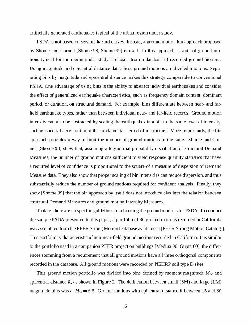
artificially generated earthquakes typical of the urban region under study.

PSDA is not based on seismic hazard curves. Instead, a ground motion bin approach proposed

by Shome and Cornell [Shome 98, Shome 99] is used. In this approach, a suite of ground mo-

tions typical for the region under study is chosen from a database of recorded ground motions.

Using magnitude and epicentral distance data, these ground motions are divided into bins. Sepa-

rating bins by magnitude and epicentral distance makes this strategy comparable to conventional

PSHA. One advantage of using bins is the ability to abstract individual earthquakes and consider

the effect of generalized earthquake characteristics, such as frequency domain content, dominant

period, or duration, on structural demand. For example, bins differentiate between near- and far-

field earthquake types, rather than between individual near- and far-field records. Ground motion

intensity can also be abstracted by scaling the earthquakes in a bin to the same level of intensity,

such as spectral acceleration at the fundamental period of a structure. More importantly, the bin

approach provides a way to limit the number of ground motions in the suite. Shome and Cor-

nell [Shome 98] show that, assuming a log-normal probability distribution of structural Demand

Measures, the number of ground motions sufficient to yield response quantity statistics that have

a required level of confidence is proportional to the square of a measure of dispersion of Demand

Measure data. They also show that proper scaling of bin intensities can reduce dispersion, and thus

substantially reduce the number of ground motions required for confident analysis. Finally, they

show [Shome 99] that the bin approach by itself does not introduce bias into the relation between

structural Demand Measures and ground motion Intensity Measures.

To date, there are no specific guidelines for choosing the ground motions for PSDA. To conduct

the sample PSDA presented in this paper, a portfolio of 80 ground motions recorded in California

was assembled from the PEER Strong Motion Database available at [PEER Strong Motion Catalog ].

This portfolio is characteristic of non-near-field ground motions recorded in California. It is similar

to the portfolio used in a companion PEER project on buildings [Medina 00, Gupta 00], the differ-

ences stemming from a requirement that all ground motions have all three orthogonal components

recorded in the database. All ground motions were recorded on NEHRP soil type D sites.

This ground motion portfolio was divided into bins defined by moment magnitude Mw and

epicentral distance R, as shown in Figure 2. The delineation between small (SM) and large (LM)

magnitude bins was at Mw = 6:5. Ground motions with epicentral distance R between 15 and 30

6

km were grouped into a small distance (SR) bin, while ground motions with R > 30 km were in

the large distance (LR) bin. Ground motions with epicentral distance R smaller than 15 km were

intentionally omitted to eliminate the near-field effects from this PSDA study. The portfolio was

chosen so that each bin contains 20 motions, distributed as uniformly as possible within each bin

(Figure 2).

Class of Structures for PSDA

The second component of a PSDA is the definition of a class of structures to be analyzed. A class of

structures is defined by structural topology, typical structural components, and methods of design.

Sample structures are instantiations of a class defined by specific geometry and design parameters.

The goal of PSDA is to produce a PSDM that enables design parameter sensitivity investigations.

The PSDA presented in this paper is conducted for a class of typical new California highway

overpass bridges. Such bridges are constructed using reinforced concrete and designed according

to Caltrans’ Bridge Design Specification and Seismic Design Criteria [Caltrans 99] which incor-

porate recommendations from ATC-32 [Council 96]. Longitudinal structural configurations for

bridges in this class are shown in Figure 3. They are: single-span, two-span, and three-span over-

passes (including abutments) and stand-alone components of multi-span viaducts divided at ex-

pansion joints. In the transverse direction, typical California overpasses have single, two-column

or multi-column bents (Figure 3). At abutments and expansion joints these bridges have varying

degrees of restraint (shear keys and/or rubber bearing pads, for example). Common to all bridges

is a Type I integral pile shaft foundation extending into a column with a uniform cross-section, and

a continuous superstructure, as designed by Caltrans [Yashinsky 00]. In this study it was assumed

that new bridge columns develop plastic hinges in flexure rather than failing in shear, consistent

with the displacement-based capacity design approach used by Caltrans.

A two-span single-column bent highway overpass bridge class was chosen to demonstrate

PSDA in this paper (Figure 4). While actual bridge designs would be governed by Caltrans criteria,

members of this bridge class were generated by varying ten bridge design parameters. They are:

degree of skew, span length, span to column height ratio, steel and concrete nominal strengths,

amount of longitudinal and transverse column reinforcement, ratio of column diameter to super-

7

structure depth, soil properties at pile shafts, and bridge weight. These parameters are defined in

Figure 4 and listed in Table 1 together with ranges of their variation used in this study.

A base bridge configuration defined by zero angle of skew, two equal 18.2 m (60 ft) spans, a

7.6 m (30 ft) high single-column bent, with a 1.6 m (5.25 ft) diameter circular column that has 2%

longitudinal and 0.7% transverse reinforcement, and a Type I pile shaft foundation on a NEHRP

class D soil site. A suite of 108 different two-span overpass bridges was generated by varying

design parameters from the base configuration, one at a time. Such parameter variation was done

to cover the entire parameter space, even though it may generate a few uncommon bridge designs.

Nonlinear Analysis for PSDA

Nonlinear analysis is the third component of PSDA. The importance of choosing a nonlinear anal-

ysis tool and understanding its limitations cannot be underestimated. This tool should enable suf-

ficiently accurate modeling of the class of structures under investigation, perform stable nonlinear

time-history analysis of the structure, and enable easy extraction and post-process various struc-

tural response quantities after an analysis. More importantly, this analysis tool must be calibrated

to give a level of confidence in the response quantities it produces.

Nonlinear analysis of the sample PSDA presented in this paper was done using PEER’s OpenSees

platform [McKenna 00, OpenSees ]. A nonlinear model for the base bridge configuration was

developed first. The columns and pile shafts were modeled using a three-dimensional flexibility-

based nonlinear beam-column element with fiber cross sections. This element provides a nonlinear

model for flexure and axial load effects, while effects of shear and torsion are modeled linearly,

using initial uncracked stiffness. The circular column cross-sections have perimeter longitudinal

bars and spiral confinement. A simple elastic-plastic material with a post-yield (hardening) stiff-

ness equal to 1.5% of pre-yield stiffness was used to model all reinforcement steel. Concrete con-

fined by the spirals was modeled using a Kent-Scott-Park stress-strain relation, with the maximum

confined concrete strength determined using Mander’s confinement model [Kent 71, Mander 88].

Soil-structure interaction in pile shaft foundations was modeled using bi-linear springs at vary-

ing depths over the pile shaft length, as in [Fenves 98]. The properties of these p-y springs were

determined using soil parameters and recommendations from API [Institute 93]. P�∆ effects were

8

included in the analysis to capture the effect of tall columns and relatively heavy bridge decks. The

bridge deck was designed as a typical Caltrans box section for a three-lane wide roadway. During

the nonlinear analyses, the deck was assumed to remain elastic. Thus, it was modeled as a linear

elastic beam, but with a cracked section stiffness.

The abutments were modeled using nonlinear elastic-perfectly plastic spring-gap elements,

which directly account for gap opening and closing. The longitudinal direction resistance of

the abutment was derived from the stiffness of elastomeric bearing pads on seat-type abutments

[Priestley 96]. The abutment stiffness model ignored the embankment and soil inertial effects.

Instead, a passive earth pressure of the backwall, set at 370 KPa (7.7 ksf) according to the Cal-

trans procedure [Goel 97] which includes an empirical pile resistance estimate of 0.7 kN/m/pile

(40kips/in/pile) [Maroney 94a], was used. The initial seat gap was assumed to be 15.2 cm (6

in). Therefore, the longitudinal participation of the abutment will occur only under large bridge

deformations. The abutment model in the transverse direction has a similar stiffness as in the lon-

gitudinal direction, provided by the shear keys, wing-walls and piles, but is activated immediately

(there is a zero-length gap).

Initial analyses showed that the response of short-span bridges is dominated by the dynamic

response of the approach embankment and abutment. In order to make the bridge model more

realistic, spring properties derived above were “softened” by a factor of 2. Such softening also

addresses the discrepancy between the Caltrans-recommended stiffness and the tri-linear abutment

stiffness envelope observed in large scale abutment tests [Maroney 94b]. More advanced bridge

models should incorporate more complex abutment models, including soil mass inertia and soil-

pile interaction and embankment soils, such as the soil slice model [Wissawapaisal 00].

Nonlinear models for each one of the 108 bridges in this PSDA were made by changing the

bridge design parameters in a computer script that generated individual OpenSees input files.

Modal analyses were performed first, using bridge models with simple supports at abutments to

exclude their effect to compute bridge fundamental transverse and longitudinal periods as con-

trolled by the column only. Nonlinear time-history analyses were conducted by running a suite of

80 ground motions, unscaled and divided into four bins as discussed above, through each one of

the 108 bridge models. A database of bridge response quantities was generated by post-processing

the results of the time-history analyses.

9

Intensity Measures and Demand Measures for PSDA

A PSDM relates ground motion Intensity Measures to structure-class-specific Demand Measures.

Thus, the choice of IM–DM pairs in the demand model is critical for a successful PSDA. An

optimal PSDM should be practical, sufficient, effective and efficient, as described below.

An IM–DM pair in a demand model is practical if it makes engineering sense and if it can

be easily derived from available ground motion measurements (for IMs) and nonlinear analysis

response quantities (for DMs). Good correlations between computer model results and existing

experimental data lend further credibility to the model.

From the standpoint of the performance-based design framework (Equation 1), it is important

that both Intensity and Demand Measures are not statistically dependent on ground motion charac-

teristics, such as moment magnitude and epicentral distance. Otherwise, de-aggregation can not be

achieved. Demand models with such conditional statistical independence are said to be sufficient.

Effectiveness of a demand model is a measure of how readily it yields itself to use in a de-

aggregated performance-based design framework. Assuming that ground motion Intensity Mea-

sures have a log-normal distribution [Shome 98], an effective demand model should have a corre-

sponding exponential form:

DM = a (IM)b (2)

or, equivalently

log(DM) = A+B log(IM) (3)

making a log-log plot of the IM–DM relation specified by this demand model a straight line.

More importantly, such a log-log linear (or piece-wise linear) demand model makes it possible to

evaluate the integrals in the de-aggregated performance-based design framework (Equation 1) in

closed form and to cast the entire framework in an LRFD format. This was accomplished for steel

moment frames in the SAC Joint Venture Steel Project [FEMA-350 00, Cornell 01] and proved to

be crucial for wide adoption of probabilistic performance-based design in practice.

A PSDM is derived by correlating Intensity Measures for ground motions in the ground motion

portfolio and Demand Measures for the structure computed using nonlinear time-history analysis.

A linear regression analysis of the logarithms of the IM–DM data gives coefficients A and B in

Equations 2 and 3, and produces a line through the cloud of IM–DM data in a log-log plot as

10

shown in Figure 5. Dispersion δ of the IM–DM data with respect to the regression fit, defined as

the standard deviation of the logarithm of regression residuals for Demand Measure [Shome 98]

(Figure 5), measures the variability of DM given IM. An efficient demand model has small dis-

persion, thus requiring a smaller number of different non-linear time-history analyses to compute

coefficients A and B with the same confidence.

Selecting an Intensity and Demand Measure pair for a practical, sufficient, effective and effi-

cient PSDM is not easy. The traditional relation between Peak Ground Acceleration and structural

response is practical, but is neither efficient nor effective. A number of Intensity Measure–Demand

Measure pairs presented in the literature in recent years have been aimed at performance-based de-

sign of buildings. Thus, a principal milestone in the development of a PSDM for highway overpass

bridges is the search for an optimal Intensity and Demand Measure pair for this class of structures.

The search for an optimal IM–DM pair is best done with the aid of computers. This enables

consideration of a large number of Intensity and Demand measure combinations. The ground

motion Intensity Measures used in this study are shown in Table 2. These measures range from

conventional spectral quantities, across duration and energy-related quantities, to characteristics

of the ground motion frequency spectra. Each Intensity Measure is ground motion specific, yet

independent of the bridge model. Intensity Measures for the selected ground motion records were

computed in advance and stored in a database.

Bridge Demand Measures were chosen from a recently developed PEER database of exper-

imental results for concrete bridge components [Hose 00, PEER Capacity Catalog ]. These De-

mand Measures, listed in Table 3, span from global ones, such as bridge drift ratio, to intermediate

ones, such as cross-section curvature, to local ones, such as steel and concrete strain. The OpenSees

bridge model is programmed to output a record of Demand Measures after each time-history analy-

sis. This record is also stored in a database. After completing 80 response-history analyses for each

of the 108 bridges, the resulting database can be searched enabling arbitrary paring of Intensity and

Demand Measures and pair-to-pair comparison.

11

SAMPLE PSDA

Development of a PSDM is illustrated in this sample PSDA. The class of structures under consid-

eration is a two-span single-bent straight highway overpass bridge. The base bridge has no skew

at the abutments. Each span is 18.2 m (60 ft) long. The bent comprises a single 7.6 m (30 ft) tall

column, measured from the soil surface. This column has a 1.6 m (5.25 ft) diameter circular cross

section with 2% longitudinal and 0.7% transverse reinforcement. The column foundation is an

integral Type I pile shaft. This base bridge is on a NEHRP class D soil site. The ground motions

used in this PSDA were the 80 ground motions classified into four bins shown in Figure 2. These

motions were not scaled in intensity or modified in any way. They were arbitrarily oriented so that

the fault-normal component was applied in the longitudinal direction of the bridge.

The scope of parameter variation presented herein was intentionally reduced to fit the format of

this paper. Only two ground motion Intensity Measures were considered. They are Sd1;ln and Sd1;tr,

elastic 5%-damping Spectral Displacements at the fundamental longitudinal and transverse periods

of the bridge, respectively (Table 2). Only six Demand Measures were considered. They are:

bridge displacement ductility, bridge column curvature ductility, and bridge residual displacement

in both transverse and longitudinal directions each (Table 3). Lastly, only 10 different bridges

are considered by varying three design parameters, namely span to column height, longitudinal

column reinforcement, and ratio of column diameter to superstructure depth with respect to the

base bridge configuration (Table 4). Only one parameter was varied from the base configuration at

a time, while the other two were kept constant.

Modal analysis of the 10 bridge models yields the periods of the first two elastic vibration

modes listed in Table 4. The first two mode shapes were practically identical for all 10 considered

bridges. The first mode shape is dominated by longitudinal deck motion accompanied by small

deck rotations near the abutments. The second mode shape is dominated by simple transverse

motion of the deck. The longitudinal and transverse periods for each of the bridges were used to

compute the Intensity Measures Sd1;ln and Sd1;tr for the 80 ground motions involved. Following

modal analyses, 800 nonlinear time-history analyses were done using the OpenSees finite element

model. The Demand Measures from these analyses were computed and stored in the database for

longitudinal and the transverse bridge directions independently.

12

Resulting PSDMs

Different PSDMs are shown in Figures 6 through 18. In each of these figures, the data is plotted in

log-log scale, with the Demand Measure on the abscissa and the Intensity Measure on the ordinate.

This is a standard method for plotting any IM–DM relationship (stemming from a push-over curve

axis designation) even though the Demand Measure is regarded as the dependent variable. A

regression analysis of the data yields coefficients A and B of Equation 3 listed in Table 5. Also

listed are values of dispersion δ for each regression analysis to characterize the efficiency of the

probabilistic seismic demand model. In this example, only a single linear fit to the data was made.

Smaller dispersion can be achieved using a bi- or tri-linear fit not performed in this example.

Model Comparison

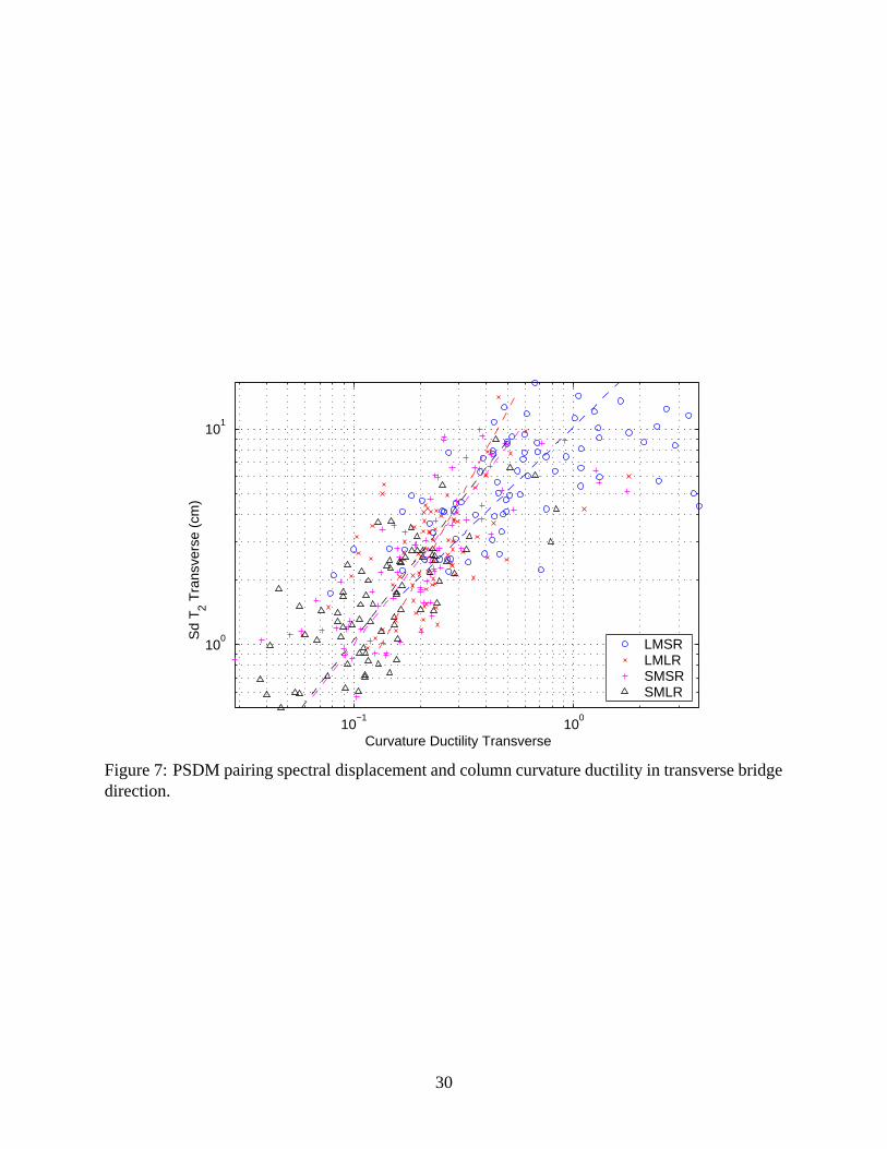
This PSDM pairs Spectral Displacement at the fundamental period of the bridge as the Intensity

Measure and bridge column Curvature Ductility as the Demand Measure. PSDMs for longitudi-

nal and transverse directions of the base bridge are shown in Figures 6 and 7, respectively. Data

regressions were done separately for each of the four ground motion bins shown in Figure 2. As

expected, more intense ground motions induce larger column curvature demands (the large magni-

tude, small distance bin). Single-line fitting (Equation 3) produces a good PSDM, with dispersions

δ ranging between 0.20 and 0.43. Thus, the Spectral Displacement–Column Curvature demand

model is an effective and efficient model, but may not be practical from a design standpoint.

A PSDM comprising Spectral Displacement and column Displacement Ductility is shown in

Figures 8 and 9, respectively. The Demand Measure in this model (column displacement ductil-

ity) was chosen because it is more practical for design than curvature ductility. This model was

intended to capture the effect of inelastic shear deformation on the performance of the bridge. Al-

beit, the beam-column element used in this implementation of the OpenSees includes only elastic

shear deformation, enabling a direct relation between column curvature and column displacement.

Thus, the quality of this PSDM is similar to the PSDM examined above. This example illustrates

the need for careful consideration of the analysis tools used for PSDA. The resulting PSDMs will

only be as good as the analytical models used to compute them.

A third PSDM pairs Spectral Displacement with a column Residual Displacement Index (RDI

13

in Table 3). RDI measures the amount of residual inelastic deformation of the structure after an

earthquake. The model is shown in Figures 10 and 11. Data in this model has a huge scatter, not

only between bins but also within each bin. Values of dispersion of each regression line are on

the order of 0.80, two to three times larger than for the two PSDMs discussed above. Such large

scatter makes this model ineffective and inefficient, even though it has a well-defined meaning for

bridge design. This example shows how to evaluate the quality of PSDMs.

Design Parameter Sensitivity

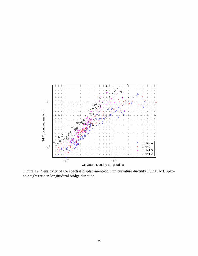
A good PSDM my be used as a design tool for discovering how changes in different design param-

eters affect the performance of a bridge. The Spectral Displacement–Column Curvature Demand

PSDM will be used in the following.

The effects of variation of the bridge span-to-column height ratio (span fixed, height determined

by ratio) are shown in Figures 12 and 13, all ground motions included. Evidently, as the span-to-

column height ratio is increased (i.e. the bridge is becoming more squat, and more stiff compared

to the base configuration, going from left to right across the graphs) column curvature ductility

Demand Measure increases for constant values of Spectral Displacement Intensity Measure. The

slope of the linear regression fit is steeper for smaller the span-to-height ratios, meaning that stiffer

bridges have a higher rate of increase of curvature demand with the increase of bridge span-to-

column height ration. However, the fundamental period of a stiffer bridge will be shorter, leading

to smaller values of Spectral Displacement Intensity Measure. Therefore, given the range of bridge

periods considered, increasing bridge stiffness by reducing the span-to-column height ratio results

in either no net gain, or even a loss of performance. To a designer this would suggest alternate

methods are required for reducing column ductility demand.

The effects of varying the column diameter are examined using PSDMs in Figures 14 and 15,

using the column diameter-to-superstructure depth ratio as the design parameter. In contrast to the

span-to-column height parameter, increasing bridge stiffness by increasing the column diameter

has the direct effect of lowering curvature ductility demand (stiffness increases from right to left

in the graphs). Dispersions δ are on the order of 0.25 and insensitive to variation of the design

parameter. Therefore, changing column diameter is a better way to decrease column curvature

demand.

14

Variation of the amount of longitudinal reinforcing steel in the column is examined using PS-

DMs shown in Figures 16 and 17. Stiffening and strengthening the column by providing more steel

has a similar effect as increasing column diameter. As expected, more reinforcement reduces duc-

tility demand for more intense motions when the response of the column becomes inelastic, while

adding reinforcement has a negligible effect for low-intensity ground motions when the column is

elastic. In contrast, the effect of changing column diameter was evident at all ground motion inten-

sity levels. The PSDMs show that performance improvement rate saturates as more reinforcement

is added. The reduction in curvature demand obtained by increasing the amount of longitudinal

reinforcement from 1% to 2% is significantly larger than the reduction obtained by increasing the

amount of steel from 3% to 4%. Also of note is the magnitude of dispersion δ. It depends on the

amount of reinforcement, being the largest for ρ = 1%. This suggests that more heavily reinforced

columns have more uniform behavior across the range of ground motions considered in this study.

Finally, effect of abutment modeling is examined in Figure 18, for transverse bridge direction

only. Two bridge models are used to generate PSDMs in this figure. One model utilizes springs

whose stiffness was computed using abutment stiffness data. This model was used for other PS-

DMs in this example. The other model has roller supports instead of springs, assuming abutments

do not participate in bridge response. As expected, abutment participation adds strength to the

bridge and reduces demand at any given ground motion intensity level. Unfortunately, these PS-

DMs can not be used to determine which abutment model is more realistic: more field test data is

needed to calibrate abutment models.

CONCLUSION

Probabilistic seismic demand models for typical California highway overpass bridges were pre-

sented in this paper. They were developed using probabilistic seismic demand analysis for a class

of real structures. Using a class of realistic structures, rather than a somewhat artificial single-

degree-of-freedom system model, is a fundamental extension of PSDA. While preparing for PSDA

an analyst should consider the following issues:

1. Choice of ground motion Intensity Measures and structural Demand Measures should be

made to produce a practical, sufficient, effective and efficient PSDM. Guidelines for making

15

such choices are as yet scarce.

2. Reducing the dispersion in PSDMs is a high-priority task, since it directly affects the number

of ground motions and time history analyses required to compute PSDM parameters.

3. When choosing the ground motions for PSDA, care should be taken to avoid bias, yet to

accurately represent the seismicity of the region for which PSDMs are being developed.

4. Understanding the capabilities and shortcomings of the tool used to model and analyze the

structure is essential for proper interpretation of PSDMs.

5. A class of structures is represented by a base structure and a number of instantiations devel-

oped by varying a set of design parameters. Therefore, good design of the base structure and

prudent choice of design parameters are essential for successful development of PSDMs.

6. The computational effort required to develop PSDMs for a class of structures and the com-

plexity of the database required to track the results of a large number of analyses should not

be underestimated. Task scheduling, database and visualization tools should be designed and

implemented with care.

Probabilistic seismic demand models for a class of structures provide information about the

probability of exceeding critical levels of chosen structural demand measures in a given seismic

hazard environment. Standing alone, PSDMs are, essentially, structural demand hazard curves.

Given that they are developed for a class of structures, they provide information on how variations

of structural design parameters change the expected demand on the structure. Such sensitivity data

can be used to efficiently design structures for performance. The stand-alone value of PSDMs is

further increased when they are used in a performance-based seismic design framework, such as

the one developed by PEER. In such design frameworks, PSDMs are coupled with ground motion

intensity models on one side and structural element fragility models on the other side to yield

probabilities of exceeding structural performance levels for a structure in a given seismic hazard

environment.

Probabilistic seismic demand models presented in this paper can be improved in several differ-

ent ways. One aspect is the improvement of bridge models, such as improved modeling of column

16

shear response and better abutment models. Another aspect is the investigation of how sensitive

the models are to the choice of ground motions (near-field vs. far-field) and local soil conditions. A

third way of improving PSDMs is by focusing on measures that evaluate the ability of the bridge to

fulfill its function after an earthquake. Three sample function-related overpass Demand Measures

are: 1) enforcement of a 30 km/h speed limit and a 10-metric-ton axis weight limit for a period of 6

weeks; 2) closure of one-half of bridge lanes for a period shorter than 2 weeks; and 3) maintenance

of bridge traffic at current levels after an after-shock that produces no more than 10 cm spectral

displacement at first transverse period of the bridge. Such function-related Demand Measures en-

able a more direct evaluation of a bridge within a transportation network in an urban area, and

better modeling of performance of such networks after earthquakes. Work on these improvements

is ongoing.

ACKNOWLEDGMENT

This work is supported by the Earthquake Engineering Research Centers Program of the National

Science Foundation under Award Number EEC-9701568 as PEER Project #312-2000 “Seismic

Demands for Performance-Based Seismic Design of Bridges”. The authors gratefully acknowledge

this support. The opinions presented in this paper are solely those of the authors and do not

necessarily represent the views of the sponsors. The authors are also grateful to Professor C. Allin

Cornell and a group of his graduate students at Stanford University for enlightening discussions

about PSDMs.

17

APPENDIX: REFERENCES

[Caltrans 99] Caltrans,. Seismic Design Criteria. California Department of

Transportation, 1.1 edition, July 1999.

[Cornell 00] Cornell, C. A. and Krawinkler, H. . “Progress and challenges

in seismic performance assessment.” PEER Center News, 3(2),

Spring 2000.

[Cornell 01] Cornell, C. A. , Jalayer, F. , Hamburger, R. O. , and Foutch, D. A.

. “The probabilistic basis for the 2000 SAC/FEMA steel mo-

ment frame guidelines.” ASCE, Journal of Structural Engineer-

ing, 2001. In press.

[Council 96] Council, A. T. . “Improved seismic design criteria for california

bridges.”. Report ATC-32, 1996. Palo Alto, CA.

[FEMA-273 96] NEHRP guidelines for the seismic rehabilitation of buildings.

Federal Emergency Management Agency (FEMA), Washington

D.C., fema-273 edition, 1996.

[FEMA-350 00] Recommended Seismic Design Criteria for New Steel Moment-

Frame Buildings. Federal Emergency Management Agency

(FEMA), Washington D.C., fema-350 edition, July 2000.

[Fenves 98] Fenves, G. L. and Ellery, M. . “Behavior and failure analysis of

a multiple-frame highway bridge in the 1994 Northridge earth-

quake.” Technical Report 98/08, PEER, University of California,

Berkeley, 1998.

[Goel 97] Goel, R. K. and Chopra, A. . “Evaluation of bridge abutment

capacity and stiffness during earthquakes.” Earthquake Spectra,

13(1):1–23, February 1997.

18

[Gupta 00] Gupta, A. and Krawinkler, H. . “Behavior of ductile of SRMFs at

various hazard levels.” ASCE Journal of Structural Engineering,

126(ST1):98–107, January 2000.

[Hose 00] Hose, Y. , Silva, P. , and Seible, F. . “Development of a perfor-

mance evaluation database for concrete bridge components and

systems under simulated seismic loads.” EERI Earthquake Spec-

tra, 16(2):413–442, April 2000.

[Institute 93] Institute, A. P. . “Recommended practice for planning, designing,

and constructing fixed offshore platform: Load and resistance

factor design.”. Technical Report RP2A-LRFD, 1993. Washing-

ton D.C.

[Kent 71] Kent, D. C. and Park, R. . “Flexural members with confined con-

crete.” Journal of Structural Engineering, 97(ST7):1969–1990,

July 1971.

[Kramer 96] Kramer, S. L. . Geotechnical Earthquake Engineering. Prentice

Hall, Upper Saddle River, NJ, 1996.

[Luco 01] Luco, N. , Cornell, C. A. , and Yeo, G. L. . “Annual limit-state

frequencies for partially-inspected earthquake-damaged build-

ings.” In 8th International Conference on Structural Safety and

Reliability, International Association for Structural Safety and

Reliability (IASSAR), Denmark, 2001. In press.

[Mander 88] Mander, J. B. , Priestley, M. J. N. , and Park, R. . “Theoretical

stress-strain model for confined concrete.” Journal of the Struc-

tural Engineering, 114(ST8):1804–1826, August 1988.

[Maroney 94a] Maroney, B. , Kutter, B. , Romstad, K. , Chai, Y. H. , and Van-

derbilt, E. . “Interpretation of large scale bridge abutment test

19

results.” In 3rd Annual Seismic Research Workshop, Caltrans,

Sacramento, CA, 1994.

[Maroney 94b] Maroney, B. H. and Chair, Y. H. . “Seismic design and retrofitting

of reinforced concrete bridges.” In 2nd International. Work-

shop, pages 255–276, Earthquake Commission of New Zealand,

Queenstown, New Zealand, 1994.

[McKenna 00] McKenna, F. and Fenves, G. L. . “An object-oriented software de-

sign for parallel structural analysis.” In Advanced Technology in

Structural Engineering, Proceedings, Structures Congress 2000,

ASCE, Washington, D. C., 2000.

[Medina 00] Medina, R. and Krawinkler, H. . “Seismic demands for

performance-based design.” Internal PEER Technical Report,

November 2000.

[OpenSees ] http://www.opensees.org,. Web page.

[PEER Capacity Catalog ] http://www.structures.ucsd.edu/PEER/Capacity

Catalog/capacity catalog.html,. Web page.

[PEER Strong Motion Catalog ] http://peer.berkeley.edu/smcat,. Web page.

[Priestley 96] Priestley, M. J. N. , Seible, F. , and Calvi, G. M. . Seismic Design

and Retrofit of Bridges. John Wiley and Sons, Inc., New York,

NY, 1996.

[SEAOC 95] SEAOC,. Vision 2000: A framework for performance based

design. Structural Engineers Association of California, Sacra-

mento, CA, 1995.

[Shome 98] Shome, N. , Cornell, C. A. , Bazzurro, P. , and Caraballo, J. E.

. “Earthquakes, records, and nonlinear responses.” EERI Earth-

quake Spectra, 14(3):467–500, June 1998.

20

[Shome 99] Shome, N. and Cornell, C. A. . “Probabilistic seismic demand

analysis of nonlinear structures.” Reliability of Marine Struc-

tures Report RMS–35, Department of Civil and Environmental

Engineering, Stanford University, Stanford, CA, 1999.

[Wissawapaisal 00] Wissawapaisal, C. and Aschheim, M. . “Modeling the transverse

response of short bridges subjected to earthquakes.” Technical

Report 00-05, Mid-America Earthquake Center, University of

Illinois, Urbana-Champaign, IL, September 2000.

[Yashinsky 00] Yashinsky, M. and Ostrom, T. . “Caltrans’ new seismic design

criteria for bridges.” EERI Earthquake Spectra, 16(1):285–307,

February 2000.

21

LIST OF FIGURE CAPTIONS

Figure 1: PEER performance-based design framework

Figure 2: Ground motion portfolio divided into bins

Figure 3: Members of a highway overpass bridge class of structures

Figure 4: Design parameters for a two-span overpass bridge

Figure 5: Dispersion of IM–DM data with respect to a regression fit (Equation 2)

Figure 6: PSDM pairing spectral displacement and column curvature ductility in longitudinal

bridge direction

Figure 7: PSDM pairing spectral displacement and column curvature ductility in transverse bridge

direction

Figure 8: PSDM pairing spectral displacement and column residual displacement index in lon-

gitudinal bridge direction

Figure 9: PSDM pairing spectral displacement and column displacement ductility in transverse

bridge direction

Figure 10: PSDM pairing spectral displacement and column residual displacement index in lon-

gitudinal bridge direction

Figure 11: PSDM pairing spectral displacement and residual displacement index in transverse

bridge direction

Figure 12: Sensitivity of the spectral displacement–column curvature ductility PSDM wrt. span-

to-height ratio in longitudinal bridge direction

Figure 13: Sensitivity of the spectral displacement–column curvature ductility PSDM wrt. span-

to-height ratio in transverse bridge direction

Figure 14: Sensitivity of the spectral displacement–column curvature ductility PSDM wrt. column

diameter in longitudinal bridge direction


diameter in transverse bridge direction


longitudinal reinforcement ratio in longitudinal bridge direction


22

longitudinal reinforcement ratio in transverse bridge direction

Figure 18: Sensitivity of the spectral displacement–column curvature ductility PSDM wrt. abut-

ment model in transverse bridge direction

23

0 5 10 15 20 25 30 35-0.1

-0.05

0

0.05

0.1

0.15

time [sec]

acce

lera

tion

[g]

DemandModel

IntensityMeasures

DemandMeasures

CapacityModel

Hazard Performance

DecisionVariables

Figure 1: PEER performance-based design framework.

24

0 10 20 30 40 50 60 70

5.8

6

6.2

6.4

6.6

6.8

LMLR

SMLR

LMSR

SMSR

Ground Motion Bins

Distance R (km)

Mom

ent M

agni

tude

M

Figure 2: Ground motion portfolio divided into bins.

25

xxxxxxxxxxxxxxxxxxxxxxxxxxxxxxxxxxxxxxxxxxxxxxxxxxxxxxxxxxxxxxxxxxxxxxxxxxxxxxxxxxxxxxxxxxxxxxxxxxxxxxxxxxxxxxxxxxxxxxxxxxxxxxxxxxxxxxxxxxxxxxxxxxxxxxxxxxxx

xxxxxxxxxxxxxxxxxxxxxxxxxxxxxxxxxxxxxxxxxxxxxxxxxxxxxxxxxxxxxxxxxxxxxxxxxxxxxxxxxxxxxxxxxxxxxxxxxxxxxxxxxxxxxxxxxxxxxxxxxxxxxxxxxxxxxxxxxxxxxxxxxxxxxxxxxxxxxxxxxxxxxxxxxxxxxxxxxxxxxxxxxx

xxxxxxxxxxxxxxxxxxxxxxxxxxxxxxxxxxxxxxxxxxxxxxxxxxxxxxxxxxxxxxxxxxxxxxxxxxxxxx

xxxxxxxxxxxxxxxxxxxxxxxxxxxxxxxxxxxxxxxxxxxx








Figure 3: Members of a highway overpass bridge class of structures.

26

xxxxxxxxxxxxxxxxxxxxxxxxxxxxxxxxxxxxxxxxxxxxxxxxxxxxxxxxxxxxxxxxxxxxxxxxxxxxxxxxxxxxxxxxxxxxxxxxxxxxxxxxxxxxxxxxxxxxxxxx

xxxxxxxxxxxxxxxxxxxxxxxxxxxxxxxxxxxxxxxxxxxxxxxxxxxxxxxxxxxxxxxxxxxxxxxxxxxxxxxxxxxxxxxxxxxxxxxxxxxxxxxxxxxxxxxxxxxxxxxxxxxxxxxxxxxxxxxxxxxxxxxxxxxxxxxxxxxxxxxxxxxxxxxx

Dc

2L

H

DsKab Kab

Ksoil

xxxxxxxxxxxx

xxxxxxxxx

xxxxxxxxx

xxxxxxxxxxxxxxxx

xxxxxxxxx

xxxxxxxxxxxx

xxxxxxxxxxxx

xxxxxxxxx

A-A

A A

Figure 4: Design parameters for a two-span overpass bridge.

27

Inte

nsity

Mea

sure

Demand Measure

δ δ

Equation (3

)

Figure 5: Dispersion of IM–DM data with respect to a regression fit (Equation 2).

28

10−1

100

100

101

Curvature Ductility Longitudinal

Sd

T 1 Lon

gitu

dina

l (cm

)

LMSRLMLRSMSRSMLR

Figure 6: PSDM pairing spectral displacement and column curvature ductility in longitudinalbridge direction.

29

10−1

100

100

101

Curvature Ductility Transverse

Sd

T 2 Tra

nsve

rse

(cm

)

LMSRLMLRSMSRSMLR

Figure 7: PSDM pairing spectral displacement and column curvature ductility in transverse bridgedirection.

30

10−1

100

100

101

Displacement Ductility Longitudinal

Sd

T 1 Lon

gitu

dina

l (cm

)

LMSRLMLRSMSRSMLR

Figure 8: PSDM pairing spectral displacement and column displacement ductility in longitudinalbridge direction.

31

10−1

100

100

101

Displacement Ductility Transverse

Sd

T 2 Tra

nsve

rse

(cm

)

LMSRLMLRSMSRSMLR

Figure 9: PSDM pairing spectral displacement and column displacement ductility in transversebridge direction.

32

10−4

10−3

10−2

10−1

100

101

RDI Longitudinal

Sd

T 1 Lon

gitu

dina

l (cm

)

LMSRLMLRSMSRSMLR

Figure 10: PSDM pairing spectral displacement and column residual displacement index in longi-tudinal bridge direction.

33

10−3

10−2

10−1

100

101

RDI Transverse

Sd

T 2 Tra

nsve

rse

(cm

)

LMSRLMLRSMSRSMLR

Figure 11: PSDM pairing spectral displacement and column residual displacement index in trans-verse bridge direction.

34

10−1

100

100

101


Sd

T 1 Lon

gitu

dina

l (cm

)

L/H=2.4L/H=2 L/H=1.5L/H=1.2

Figure 12: Sensitivity of the spectral displacement–column curvature ductility PSDM wrt. span-to-height ratio in longitudinal bridge direction.

35

10−1

100

100

101


Sd

T 2 Tra

nsve

rse

(cm

)

L/H=2.4L/H=2 L/H=1.5L/H=1.2

Figure 13: Sensitivity of the spectral displacement–column curvature ductility PSDM wrt. span-to-height ratio in transverse bridge direction.

36

10−1

100

101

100

101


Sd

T 1 Lon

gitu

dina

l (cm

)

Dc/Ds=0.67Dc/Ds=0.75Dc/Ds=1 Dc/Ds=1.3

Figure 14: Sensitivity of the spectral displacement–column curvature ductility PSDM wrt. columndiameter in longitudinal bridge direction.

37

10−2

10−1

100

100

101


Sd

T 2 Tra

nsve

rse

(cm

)

Dc/Ds=0.67Dc/Ds=0.75Dc/Ds=1 Dc/Ds=1.3

Figure 15: Sensitivity of the spectral displacement–column curvature ductility PSDM wrt. columndiameter in transverse bridge direction.

38

10−1

100

101

100

101


Sd

T 1 Lon

gitu

dina

l (cm

)

ρs,ln=0.01

ρs,ln=0.02

ρs,ln=0.03

ρs,ln=0.04

Figure 16: Sensitivity of the spectral displacement–column curvature ductility PSDM wrt. columnlongitudinal reinforcement ratio in longitudinal bridge direction.

39

10−1

100

101

100

101


Sd

T 2 Tra

nsve

rse

(cm

)

ρs,ln=0.01

ρs,ln=0.02

ρs,ln=0.03

ρs,ln=0.04

Figure 17: Sensitivity of the spectral displacement–column curvature ductility PSDM wrt. columnlongitudinal reinforcement ratio in transverse bridge direction.

40

10−1

100

101

102


Aria

s In

tens

ity T

rans

vers

e (c

m/s

)

No abutmentAbutment

Figure 18: Sensitivity of the spectral displacement–column curvature ductility PSDM wrt. abut-ment model in transverse bridge direction.

41

LIST OF TABLE CAPTIONS

Figure 1: Parameter variation ranges for a two-span overpass bridge

Figure 2: Ground motion Intensity Measures considered in this study (source: [Kramer 96])

Figure 3: Bridge Demand Measures considered in this study

Figure 4: Bridge first (longitudinal) and second (transverse) mode periods

Figure 5: Regression coefficients A and B (Equation 3) and dispersion δ for data in Figures 6

through 17

42

Table 1: Parameter variation ranges for a two-span overpass bridge.

Description Parameter Range

Degree of skew α 0–π=3 rad

Span length L 18–55 m (60–180 ft)

Span-to-column height ratio L=H 1.2–2.4

Column-to-superstructure dimension ratio Dc=Ds 0.67-1.33

Reinforcement nominal yield strength fy 470–655 MPa (68–95 ksi)

Concrete nominal strength f 0c 20–55 MPa (3–8 ksi)

Column longitudinal reinforcement ratio ρs;l 1–4%

Column transverse reinforcement ratio ρs;t 0.4–1.0%

Soil stiffness based on NEHRP groups Ksoil A, B, C, D

Additional bridge dead load Wda 10-100% self-weight

43

Table 2: Ground motion Intensity Measures considered in this study (source: [Kramer 96]).

Intensity Measure Description/equation

Arias Intensity Is =π2g

R ∞0 u2

g(t) dt

Velocity Intensity Iv =R ∞

0u2

g(t)jug(t)j

dt

Cumulative absolute velocity IjAj =R ∞

0 jug(t)j dt

Cumulative absolute displacement IjV j =R ∞

0 jug(t)j dt

Frequency ratio 1 FR1 = ug;max=ug;max

Frequency ratio 2 FR2 = ug;max=ug;max

Strong motion duration Td = 0:02e0:74M +0:3R

RMS acceleration arms =q

1Td

R Td0 u2

g(t) dt

Characteristic intensity Ic = a1:5rmsT

1:5d

Effective peak acceleration EPA = 0:4 Sa;avgj0:50:1

Effective peak velocity EPV = 0:4 Sv;avgj0:50:1

Effective peak displacement EPD = 0:4 Sd;avgj0:50:1

Spectral quantities Sd = Sv=ω = Sa=ω2

Epicentral distance R

Moment magnitude M

44

Table 3: Bridge Demand Measures considered in this study

Demand Measure Equation

Peak steel strain εs;max

Peak concrete strain εc;max

Peak column curvature φmax

Curvature ductility µφ = φmax=φy

Displacement ductility µ∆ = umax=uy

Drift ratio γ = umax=H

Residual deformation index RDI = uresidual=uy

Plastic rotation θp = (umax�uy)=H

Hysteretic energy HE =H

F du

Normalized hysteretic energy NHE = HE=(Fyuy)

45

Table 4: Bridge first (longitudinal) and second (transverse) mode periods.

Bridge configuration T1;l [sec] T1;t [sec]

1 Base bridge 0.56 0.35

2 L=H = 2:0 0.65 0.37

3 L=H = 1:5 0.81 0.38

4 L=H = 1:2 0.97 0.39

5 Dc=Ds = 0:67 0.64 0.36

6 Dc=Ds = 1:0 0.41 0.33

7 Dc=Ds = 1:3 0.33 0.30

8 ρs;l = 0:01 0.59 0.35

9 ρs;l = 0:03 0.54 0.35

10 ρs;l = 0:04 0.53 0.35

46

Table 5: Regression coefficients A and B (Equation 3) and dispersion δ for data in Figures 6through 17.

Figure A;B;δLine 1 Line 2 Line 3 Line 4

6a -2.28, 1.05, 0.43 -2.14, 0.73, 0.20 -2.33, 0.89, 0.22 -2.38, 0.93, 0.24

7 -2.34, 1.01, 0.42 -2.01, 0.53, 0.30 -2.31, 0.76, 0.30 -2.34, 0.76, 0.26

8 -2.17, 0.79, 0.20 -2.19, 0.72, 0.17 -2.36, 0.81, 0.16 -2.42, 0.85, 0.16

9 -2.00, 0.67, 0.26 -1.90, 0.46, 0.26 -2.21, 0.68, 0.24 -2.26, 0.63, 0.23

10 -5.30, 0.92, 0.63 -5.06, 0.83, 0.81 -5.38, 0.63, 0.98 -4.95, 0.32, 0.91

11 -5.84, 1.22, 0.77 -4.62, 0.53, 0.61 -4.92, 0.53, 0.73 -4.56, 0.56, 0.77

12b -2.24, 1.26, 0.23 -2.44, 1.26, 0.24 -2.46, 0.96, 0.25 -2.84, 1.01, 0.18

13 -2.13, 1.18, 0.32 -2.34, 1.01, 0.28 -2.50, 0.93, 0.25 -2.85, 0.96, 0.25

14c -2.32, 1.47, 0.27 -2.24, 1.26, 0.23 -2.44, 1.08, 0.18 -2.86, 1.01, 0.19

15 -2.14, 1.19, 0.30 -2.13, 1.18, 0.32 -2.48, 1.05, 0.26 -3.06, 1.10, 0.25

16d -2.10, 1.42, 0.37 -2.24, 1.26, 0.23 -2.29, 1.14, 0.15 -2.30, 1.04, 0.13

17 -2.04, 1.36, 0.33 -2.13, 1.18, 0.32 -2.20, 1.02, 0.26 -2.33, 1.00, 0.21

aLines 1, 2, 3, and 4 correspond to LMSR, LMLR, SMSR, and SMLR ground motion bins, respectively.bLines 1, 2, 3, and 4 correspond to L=H = 2.4, 2.0, 1.5, and 1.2, respectively.cLines 1, 2, 3, and 4 correspond to Dc=Ds = 0.75, 0.67, 1.0, and 1.3, respectively.dLines 1, 2, 3, and 4 correspond to ρ s;l = 0.02, 0.01, 0.03, and 0.04, respectively.

47

probabilistic seismic demand model for california...

Documents