probability & random variables
TRANSCRIPT
Principles of Communications I (Fall, 2007) Probability & Random Variables
NCTU EE 1
Probability & Random Variables Motivations:
Both messages (signals) & noises are random in nature
Some definitions: (a) random variable (r.v.): one random quantity (b) random sequence: sequence of random variable (c) random process: a (continuous-time) function whose value (at any time instant) is
a r.v.
Probability Space
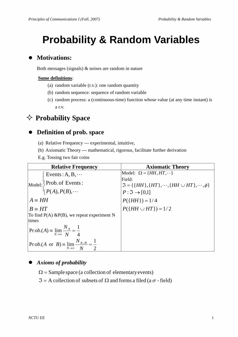
Definition of prob. space (a) Relative Frequency --- experimental, intuitive, (b) Axiomatic Theory --- mathematical, rigorous, facilitate further derivation E.g. Tossing two fair coins
Relative Frequency Axiomatic Theory
Model:⎪⎩
⎪⎨
⎧
L
L
),(),(:Events of Prob.
B, A, :Events
BPAP
HTBHHA
≡≡
To find P(A) &P(B), we repeat experiment N times
41lim).(Pr =≡
∞→ NN
Aob A
N
21lim)or .(Pr =≡ ∪
∞→ NNBAob BA
N
Model: },,{ LHTHH=Ω Field:
},},{,},{},{{ φLL HTHHHTHH ∪=ℑ
2/1})({4/1})({
]1,0[:
=∪=
→ℑ
HTHHPHHP
P
Axioms of probability
field)- (a filed a forms and of subsets of collectionA events) elementary of collection (a space Sample
σΩ=ℑ=Ω
Principles of Communications I (Fall, 2007) Probability & Random Variables
NCTU EE 2
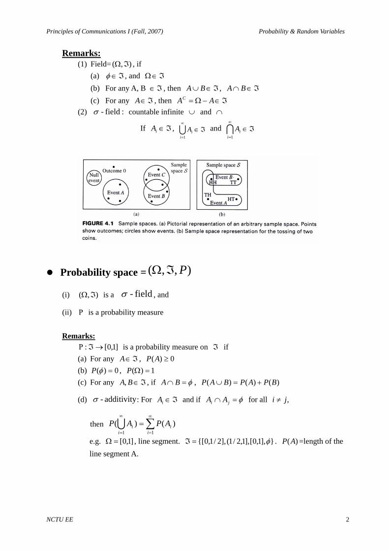
Remarks: (1) Field= ),( ℑΩ , if
(a) ℑ∈φ , and ℑ∈Ω (b) For any A, B ℑ∈ , then ℑ∈∪ BA , ℑ∈∩ BA (c) For any ℑ∈A , then ℑ∈−Ω= AAC
(2) :field- σ countable infinite ∪ and ∩
If ℑ∈iA , ℑ∈∞
=U
1iiA and ℑ∈
∞
=I
1iiA
Probability space = ),,( PℑΩ
(i) ),( ℑΩ is a field- σ , and
(ii) Ρ is a probability measure
Remarks: ]1,0[: →ℑΡ is a probability measure on ℑ if
(a) For any ℑ∈A , 0)( ≥AP (b) 0)( =φP , 1)( =ΩP (c) For any ℑ∈BA, , if φ=∩ BA , )()()( BPAPBAP +=∪
(d) additivity- σ : For ℑ∈iA and if φ=∩ ji AA for all ,ji ≠
then ∑∞
=
∞
=
=11
)()(i
ii
i APAP U
e.g. ]1,0[=Ω , line segment. }],1,0[],1,2/1(],2/1,0{[ φ=ℑ . )(AP =length of the line segment A.
Principles of Communications I (Fall, 2007) Probability & Random Variables
NCTU EE 3
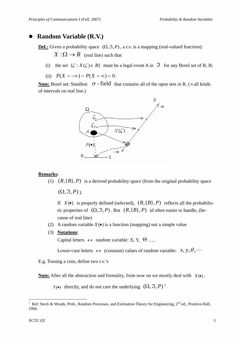
Random Variable (R.V.) Def.: Given a probability space ),,( PℑΩ , a r.v. is a mapping (real-valued function):
RX →Ω: (real line) such that
(i) the set })(:{ BX ∈ζζ must be a legal event A in ℑ for any Borel set of R, B;
(ii) 0)()( =∞==−∞= XPXP .
Note: Borel set: Smallest field- σ that contains all of the open sets in R. (≈ all kinds of intervals on real line.)
Remarks:
(1) )},{,( PBR is a derived probability space (from the original probability space
),,( PℑΩ ).
If )(•X is properly defined (selected), )},{,( PBR reflects all the probabilis-tic properties of ),,( PℑΩ . But )},{,( PBR id often easier to handle, (be-cause of real line)
(2) A random variable )(•X is a function (mapping) not a simple value (3) Notations:
Capital letters ↔ random variable: X, Y, Θ…..
Lower-case letters ↔ (constant) values of random variable: L,,, θyx
E.g. Tossing a coin, define two r.v.’s Note: After all the abstraction and formality, from now on we mostly deal with )(•X ,
)(•Y directly, and do not care the underlying ),,( PℑΩ 1
1 Ref: Stock & Woods, Prob., Random Processes, and Estimation Theory for Engineering, 2nd ed., Prentice-Hall, 1994.
Principles of Communications I (Fall, 2007) Probability & Random Variables
NCTU EE 4
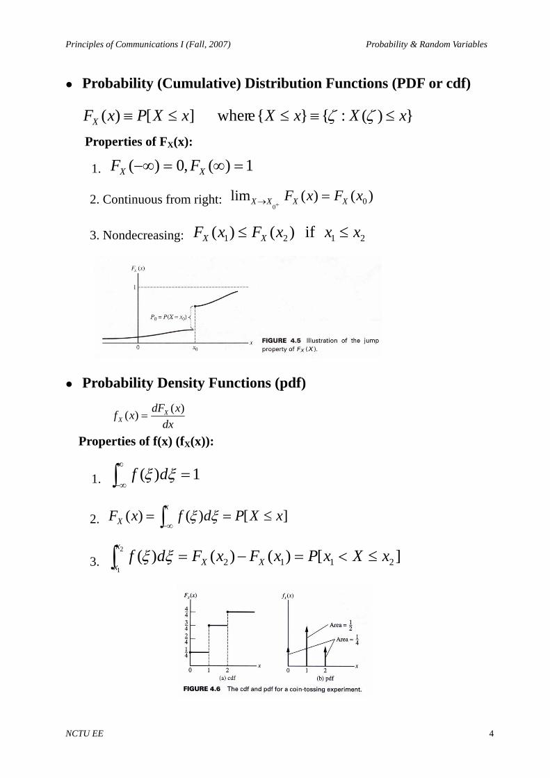
Probability (Cumulative) Distribution Functions (PDF or cdf)
})(:{}{ e wher][)( xXxXxXPxFX ≤≡≤≤≡ ζζ
Properties of FX(x):
1. 1)(,0)( =∞=−∞ XX FF
2. Continuous from right: )()(lim 00
xFxF XXXX =+→
3. Nondecreasing: 2121 if )()( xxxFxF XX ≤≤
Probability Density Functions (pdf)
dxxdFxf X
X)()( =
Properties of f(x) (fX(x)):
1. 1)( =∫∞
∞−ξξ df
2. ][)()( xXPdfxFx
X ≤== ∫ ∞− ξξ
3. ][)()()( 21122
1
xXxPxFxFdf XX
x
x≤<=−=∫ ξξ
Principles of Communications I (Fall, 2007) Probability & Random Variables
NCTU EE 5
Some common pdf’s
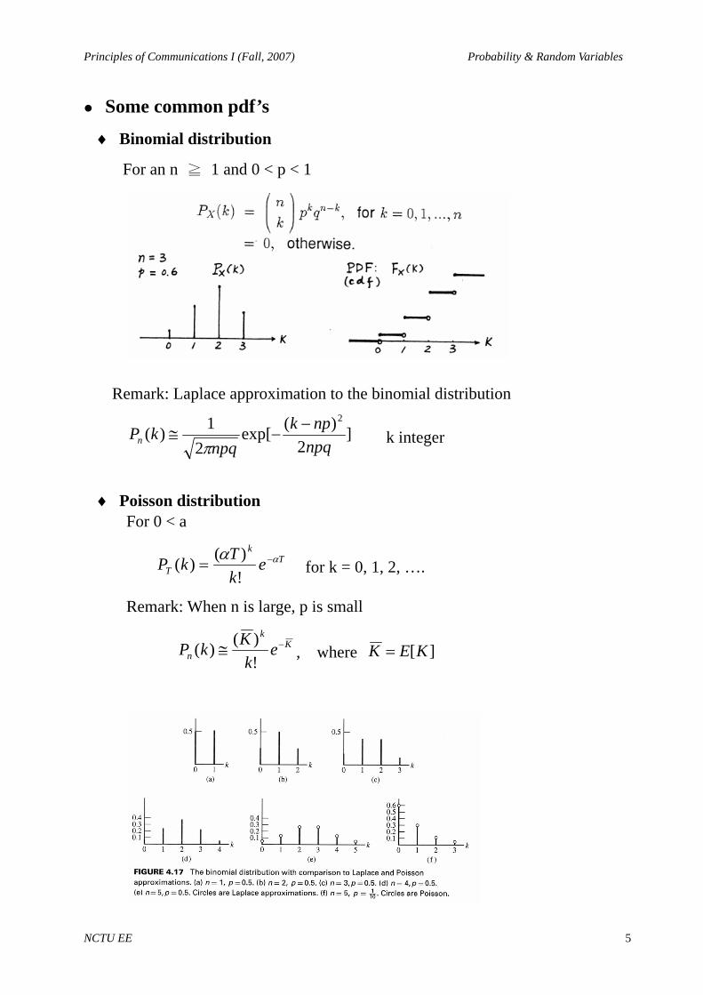
♦ Binomial distribution
For an n ≧ 1 and 0 < p < 1
Remark: Laplace approximation to the binomial distribution
]2
)(exp[2
1)(2
npqnpk
npqkPn
−−≅
π k integer
♦ Poisson distribution
For 0 < a
Tk
T ekTkP αα −=!)()( for k = 0, 1, 2, ….
Remark: When n is large, p is small
Kk
n ek
KkP −≅!)()( , where ][KEK =
Principles of Communications I (Fall, 2007) Probability & Random Variables
NCTU EE 6
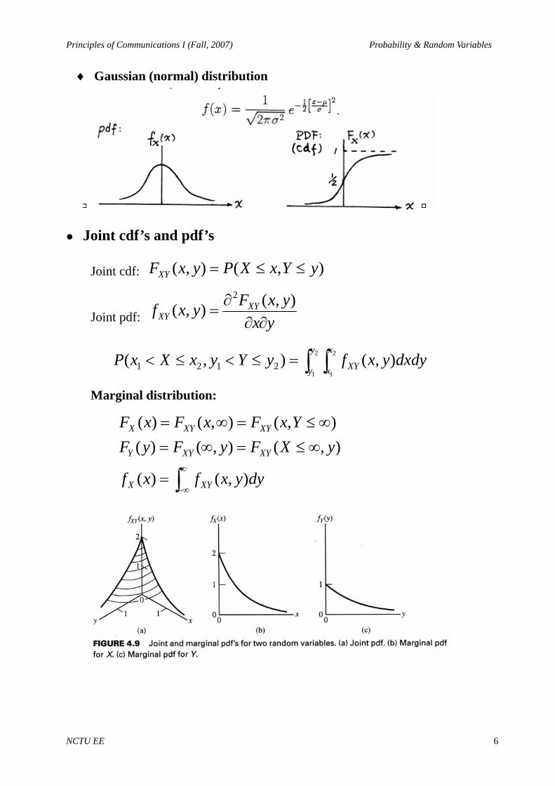
♦ Gaussian (normal) distribution
Joint cdf’s and pdf’s
Joint cdf: ),(),( yYxXPyxFXY ≤≤=
Joint pdf: yxyxFyxf XY
XY ∂∂∂
=),(),(
2
∫ ∫=≤<≤< 2
1
2
1
),(),( 2121
y
y
x
x XY dxdyyxfyYyxXxP
Marginal distribution:
∫∞
∞−=
∞≤=∞=∞≤=∞=
dyyxfxf
yXFyFyFYxFxFxF
XYX
XYXYY
XYXYX
),()(
),(),()(),(),()(
Principles of Communications I (Fall, 2007) Probability & Random Variables
NCTU EE 7
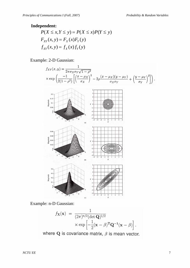
Independent:
)()(),()()(),(
)()(),(
yfxfyxfyFxFyxF
yYPxXPyYxXP
YXXY
YXXY
==
≤≤=≤≤
Example: 2-D Gaussian:
Example: n-D Gaussian:
Principles of Communications I (Fall, 2007) Probability & Random Variables
NCTU EE 8
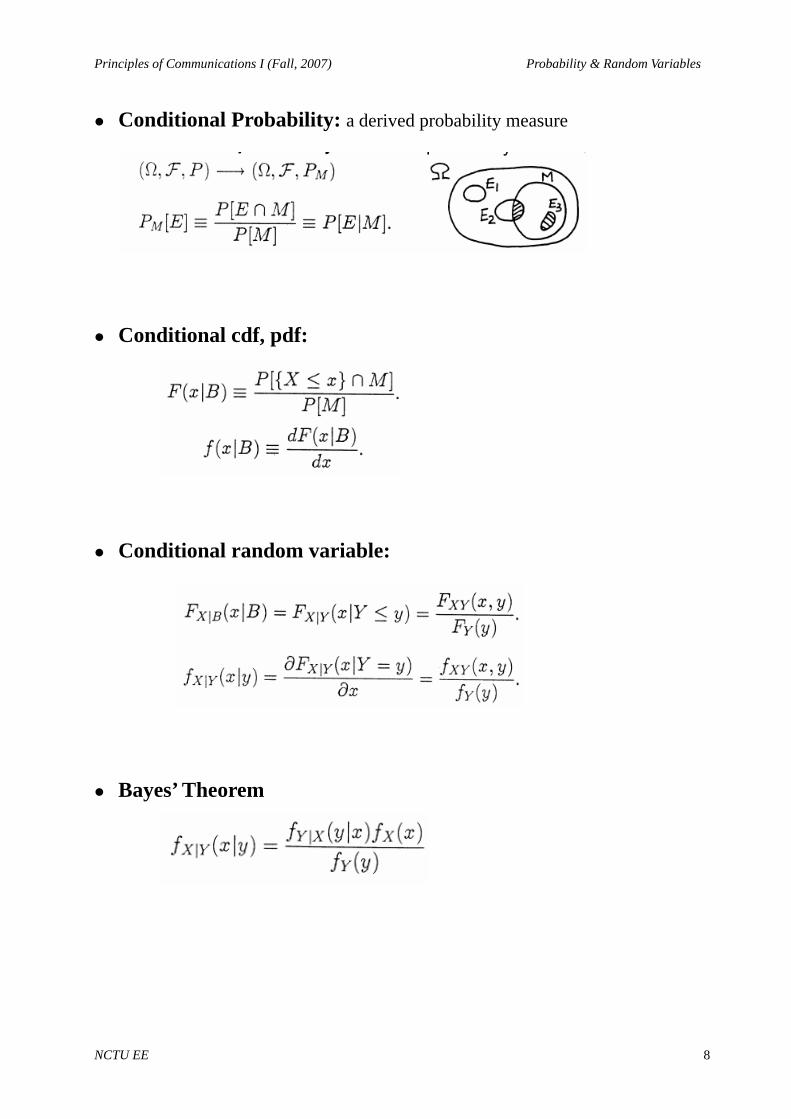
Conditional Probability: a derived probability measure
Conditional cdf, pdf:
Conditional random variable:
Bayes’ Theorem
Principles of Communications I (Fall, 2007) Probability & Random Variables
NCTU EE 9
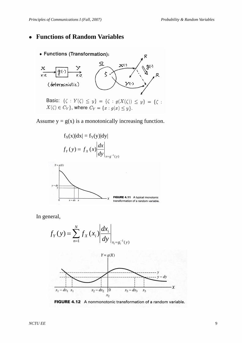
Functions of Random Variables
Assume y = g(x) is a monotonically increasing function.
fX(x)|dx| = fY(y)|dy|
)(1
)()(ygx
XY dydxxfyf
−=
=
In general,
∑= = −
=N
n ygx
iiXY
iidydxxfyf
1 )(1
)()(
Principles of Communications I (Fall, 2007) Probability & Random Variables
NCTU EE 10
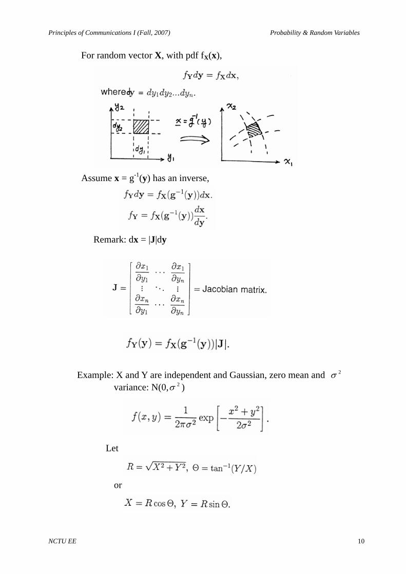
For random vector X, with pdf fX(x),
Assume x = g-1(y) has an inverse,
Remark: dx = |J|dy
Example: X and Y are independent and Gaussian, zero mean and 2σ variance: N(0, 2σ )
Let
or
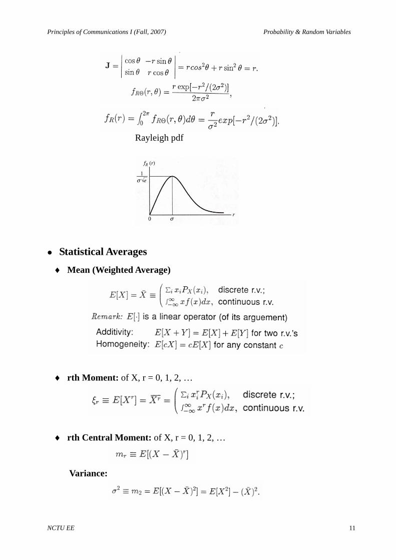
Principles of Communications I (Fall, 2007) Probability & Random Variables
NCTU EE 11
Rayleigh pdf
Statistical Averages
♦ Mean (Weighted Average)
♦ rth Moment: of X, r = 0, 1, 2, …
♦ rth Central Moment: of X, r = 0, 1, 2, …
Variance:
Principles of Communications I (Fall, 2007) Probability & Random Variables
NCTU EE 12
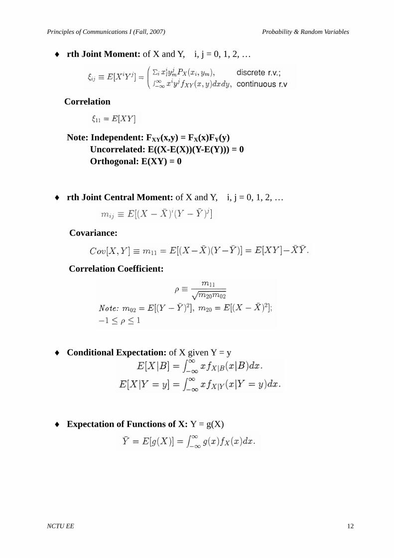
♦ rth Joint Moment: of X and Y, i, j = 0, 1, 2, …
Correlation
Note: Independent: FXY(x,y) = FX(x)FY(y) Uncorrelated: E((X-E(X))(Y-E(Y))) = 0 Orthogonal: E(XY) = 0
♦ rth Joint Central Moment: of X and Y, i, j = 0, 1, 2, …
Covariance:
Correlation Coefficient:
♦ Conditional Expectation: of X given Y = y
♦ Expectation of Functions of X: Y = g(X)
Principles of Communications I (Fall, 2007) Probability & Random Variables
NCTU EE 13
♦ Moment Generating Functions
♦ Characteristic Functions
Principles of Communications I (Fall, 2007) Probability & Random Variables
NCTU EE 14
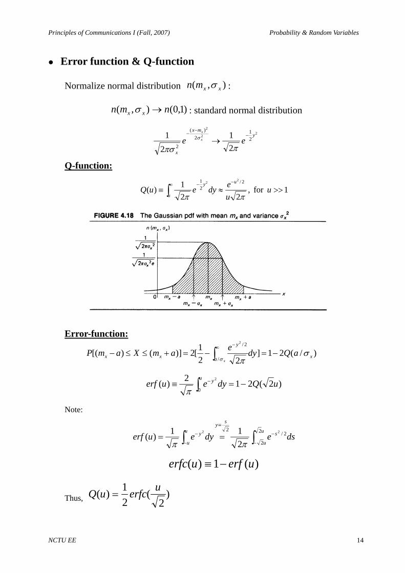
Error function & Q-function
Normalize normal distribution ),( xxmn σ :
)1,0(),( nmn xx →σ : standard normal distribution
22
2
21
2)(
2 21
21 y
mx
x
ee x
x−
−−
→ππσ
σ
Q-function:
1for ,22
1)(2/
21 2
2
>>≈≡−∞ −
∫ uuedyeuQ
u
u
y
ππ
Error-function:
)2(212)(0
2
uQdyeuerfu y −=≡ ∫ −
π
Note:
∫∫ −
−
≡
−
− ==u
u
s
syu
u
y dsedyeuerf2
2
2/2 22
211)(ππ
)(1)( uerfuerfc −≡
Thus, )2
(21)( uerfcuQ =
)/(21]22
1[2)]()[(/
2/2
xa
y
xx aQdyeamXamPx
σπσ
−=−=+≤≤− ∫∞ −