probability theory

Module #19 – Probability

Probability Theory

Slides for a Course Based on the TextSlides for a Course Based on the TextDiscrete Mathematics & Its ApplicationsDiscrete Mathematics & Its Applications (6 (6thth

Edition) Kenneth H. Rosen Edition) Kenneth H. Rosen based on slides by based on slides by

Michael P. Frank and Andrew W. MooreMichael P. Frank and Andrew W. Moore


Terminology• A (stochastic) A (stochastic) experimentexperiment is a procedure that is a procedure that

yields one of a given set of possible outcomesyields one of a given set of possible outcomes• The The sample spacesample space SS of the experiment is the of the experiment is the

set of possible outcomes.set of possible outcomes.• An event is a An event is a subsetsubset of sample space. of sample space.• A random variable is a function that assigns a A random variable is a function that assigns a

real value to each outcome of an experimentreal value to each outcome of an experimentNormally, a probability is related to an experiment or a trial.

Let’s take flipping a coin for example, what are the possible outcomes?

Heads or tails (front or back side) of the coin will be shown upwards.After a sufficient number of tossing, we can “statistically” concludethat the probability of head is 0.5.In rolling a dice, there are 6 outcomes. Suppose we want to calculate the prob. of the event of odd numbers of a dice. What is that probability?


Random Variables

• A A “random variable”“random variable” VV is any variable whose is any variable whose value is unknown, or whose value depends on value is unknown, or whose value depends on the precise situation.the precise situation.– E.g.E.g., the number of students in class today, the number of students in class today– Whether it will rain tonight (Boolean variable)Whether it will rain tonight (Boolean variable)

• The proposition The proposition VV==vvii may have an uncertain may have an uncertain

truth value, and may be assigned a truth value, and may be assigned a probability.probability.

Module #19 – ProbabilityExample 10

• A fair coin is flipped 3 times. Let A fair coin is flipped 3 times. Let SS be the sample space of 8 be the sample space of 8 possible outcomes, and let possible outcomes, and let XX be a random variable that assignees be a random variable that assignees to an outcome the number of heads in this outcome. to an outcome the number of heads in this outcome.

• Random variable Random variable X X is a functionis a function XX::SS → → XX((SS), ), where where XX((SS)={0, 1, 2, 3} is the range of )={0, 1, 2, 3} is the range of X, X, which is the number the number of heads, andof heads, andSS={ ={ (TTT), (TTH), (THH), (HTT), (HHT), (HHH), (THT), (HTH)(TTT), (TTH), (THH), (HTT), (HHT), (HHH), (THT), (HTH) } }

• X(TTT) = 0 X(TTT) = 0 X(TTH) = X(HTT) = X(THT) = 1X(TTH) = X(HTT) = X(THT) = 1X(HHT) = X(THH) = X(HTH) = 2X(HHT) = X(THH) = X(HTH) = 2X(HHH) = 3X(HHH) = 3

• The The probability distribution (pdf) of random variableprobability distribution (pdf) of random variable XX is given by is given by P(X=3) = 1/8, P(X=2) = 3/8, P(X=1) = 3/8, P(X=0) = 1/8. P(X=3) = 1/8, P(X=2) = 3/8, P(X=1) = 3/8, P(X=0) = 1/8.


Experiments & Sample Spaces

• A (stochastic) A (stochastic) experimentexperiment is any process by which is any process by which a given random variable a given random variable VV gets assigned some gets assigned some particularparticular value, and where this value is not value, and where this value is not necessarily known in advance.necessarily known in advance.– We call it the “actual” value of the variable, as We call it the “actual” value of the variable, as

determined by that particular experiment.determined by that particular experiment.• The The sample spacesample space SS of the experiment is just of the experiment is just

the domain of the random variable, the domain of the random variable, SS = dom[ = dom[VV]]..• The The outcomeoutcome of the experiment is the specific of the experiment is the specific

value value vvii of the random variable that is selected. of the random variable that is selected.


Events

• An An eventevent EE is any set of possible outcomes in is any set of possible outcomes in SS……– That is, That is, EE SS = = domdom[[VV]]..

• E.g., the event that “less than 50 people show up for our next E.g., the event that “less than 50 people show up for our next class” is represented as the set class” is represented as the set {1, 2, …, 49}{1, 2, …, 49} of values of the of values of the variable variable VV = (# of people here next class) = (# of people here next class)..

• We say that event We say that event EE occursoccurs when the actual value when the actual value of of VV is in is in EE, which may be written , which may be written VVEE..– Note that Note that VVEE denotes the proposition (of uncertain denotes the proposition (of uncertain

truth) asserting that the actual outcome (value of truth) asserting that the actual outcome (value of VV) ) will be one of the outcomes in the set will be one of the outcomes in the set EE..


Probabilities

• We write P(A) as “the fraction of possible We write P(A) as “the fraction of possible worlds in which A is true”worlds in which A is true”


Visualizing A

Event space of all possible worlds

Its area is 1Worlds in which A is False

Worlds in which A is true

P(A) = Area ofreddish oval


Probability

• The The probabilityprobability p p = Pr[= Pr[EE] ] [0,1] [0,1] of an event of an event EE is is a real number representing our degree of certainty a real number representing our degree of certainty that that EE will occur. will occur.– If If Pr[Pr[EE] = 1] = 1, then , then EE is absolutely certain to occur, is absolutely certain to occur,

• thus thus VVEE has the truth value has the truth value TrueTrue..– If If Pr[Pr[EE] = 0] = 0, then , then EE is absolutely certain is absolutely certain not not to occur,to occur,

• thus thus VVEE has the truth value has the truth value FalseFalse..– If If Pr[Pr[EE] = ] = ½½, then we are , then we are maximally uncertainmaximally uncertain about about

whether whether EE will occur; that is, will occur; that is, • VVEE and and VVEE are considered are considered equally likelyequally likely..

– How do we interpret other values of How do we interpret other values of pp??Note: We could also define probabilities for more general propositions, as well as events.


Four Definitions of Probability

• Several alternative definitions of probability Several alternative definitions of probability are commonly encountered:are commonly encountered:– Frequentist, Bayesian, Laplacian, AxiomaticFrequentist, Bayesian, Laplacian, Axiomatic

• They have different strengths & They have different strengths & weaknesses, philosophically speaking.weaknesses, philosophically speaking.– But fortunately, they coincide with each other But fortunately, they coincide with each other

and work well together, in the majority of cases and work well together, in the majority of cases that are typically encountered.that are typically encountered.


Probability: Frequentist Definition

• The probability of an event The probability of an event EE is the limit, as is the limit, as nn→∞→∞,, of of the fraction of times that we find the fraction of times that we find VVEE over the course over the course of of nn independent repetitions of (different instances of) independent repetitions of (different instances of) the same experiment.the same experiment.

• Some problems with this definition: Some problems with this definition: – It is only well-defined for experiments that can be It is only well-defined for experiments that can be

independently repeated, infinitely many times! independently repeated, infinitely many times! • or at least, if the experiment can be repeated in principle, or at least, if the experiment can be repeated in principle, e.g.e.g., over , over

some hypothetical ensemble of (say) alternate universes.some hypothetical ensemble of (say) alternate universes.

– It can never be measured exactly in finite time!It can never be measured exactly in finite time!

• Advantage:Advantage: It’s an objective, mathematical definition. It’s an objective, mathematical definition.

n

nE EV

n

lim:]Pr[


Probability: Bayesian Definition• Suppose a rational, profit-maximizing entity Suppose a rational, profit-maximizing entity RR is is

offered a choice between two rewards:offered a choice between two rewards:– Winning Winning $1$1 if and only if the event if and only if the event EE actually occurs. actually occurs.– Receiving Receiving pp dollars (where dollars (where pp[0,1][0,1]) unconditionally.) unconditionally.

• If If RR can honestly state that he is completely can honestly state that he is completely indifferent between these two rewards, then we say indifferent between these two rewards, then we say that that RR’s probability for ’s probability for EE is is pp, that is, , that is, PrPrRR[[EE] :] :≡≡ pp..

• Problem:Problem: It’s a subjective definition; depends on the It’s a subjective definition; depends on the reasoner reasoner RR, and his knowledge, beliefs, & rationality., and his knowledge, beliefs, & rationality.– The version above additionally assumes that the utility of The version above additionally assumes that the utility of

money is linear.money is linear.• This assumption can be avoided by using “utils” (utility units) This assumption can be avoided by using “utils” (utility units)

instead of dollars.instead of dollars.


Probability: Laplacian Definition

• First, assume that all individual outcomes in the First, assume that all individual outcomes in the sample space are sample space are equally likelyequally likely to each other to each other……– Note that this term still needs an operational definition!Note that this term still needs an operational definition!

• Then, the probability of any event Then, the probability of any event EE is given by, is given by, Pr[Pr[EE] = |] = |EE|/||/|SS||. . Very simple!Very simple!

• Problems:Problems: Still needs a definition for Still needs a definition for equally likelyequally likely, , and depends on the existence of and depends on the existence of somesome finite sample finite sample space space SS in which all outcomes in in which all outcomes in SS are, in fact, are, in fact, equally likely.equally likely.


Probability: Axiomatic Definition• Let Let pp be any total function be any total function pp::SS→[0,1]→[0,1] such that such that

∑∑ss pp((ss) = 1) = 1..

• Such a Such a pp is called a is called a probability distributionprobability distribution..• Then, theThen, the probability under p probability under p

of any event of any event EESS is just: is just:• Advantage: Advantage: Totally mathematically well-defined!Totally mathematically well-defined!

– This definition can even be extended to apply to infinite This definition can even be extended to apply to infinite sample spaces, by changing sample spaces, by changing ∑∑→→∫∫, and calling , and calling pp a a probability density functionprobability density function or a probability or a probability measuremeasure..

• Problem: Problem: Leaves operational meaning unspecified.Leaves operational meaning unspecified.

Es

spEp )(:][


The Axioms of Probability

• 0 <= P(A) <= 10 <= P(A) <= 1

• P(True) = 1P(True) = 1

• P(False) = 0P(False) = 0

• P(A or B) = P(A) + P(B) - P(A and B)P(A or B) = P(A) + P(B) - P(A and B)


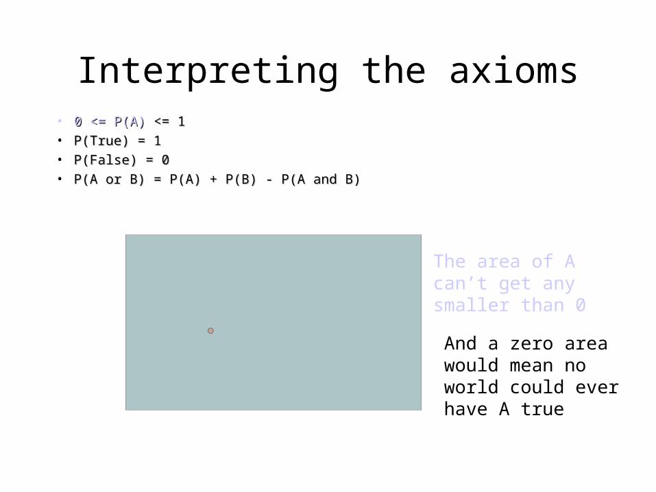
Interpreting the axioms• 0 <= P(A) 0 <= P(A) <= 1<= 1




The area of A can’t get any smaller than 0

And a zero area would mean no world could ever have A true


Interpreting the axioms• 0 <= 0 <= P(A) <= 1P(A) <= 1




The area of A can’t get any bigger than 1

And an area of 1 would mean all worlds will have A true


Interpreting the axioms

• 0 <= P(A) <= 10 <= P(A) <= 1



• P(P(AA or or BB) = P() = P(AA) + P() + P(BB) - P() - P(AA and and BB))

A

B


Theorems from the Axioms

• 0 <= P(A) <= 1, P(True) = 1, P(False) = 00 <= P(A) <= 1, P(True) = 1, P(False) = 0• P(P(AA or or BB) = P() = P(AA) + P() + P(BB) - P() - P(AA and and BB))

From these we can prove:From these we can prove:

P(not A) = P(~A) = 1-P(A)P(not A) = P(~A) = 1-P(A)

• How?How?


Another important theorem

• 0 <= P(A) <= 1, P(True) = 1, P(False) = 00 <= P(A) <= 1, P(True) = 1, P(False) = 0• P(P(AA or or BB) = P() = P(AA) + P() + P(BB) - P() - P(AA and and BB))

From these we can prove:From these we can prove:

P(A) = P(A ^ B) + P(A ^ ~B)P(A) = P(A ^ B) + P(A ^ ~B)

• How?How?


Probability of an event EThe probability of an event E is the sum of the The probability of an event E is the sum of the

probabilities of the outcomes in E. That isprobabilities of the outcomes in E. That is

Note that, if there are n outcomes in the event E, Note that, if there are n outcomes in the event E, that is, if E = {athat is, if E = {a11,a,a22,…,a,…,ann} then} then

p(E) p(s)

sE

p(E) p(

i1

n

ai)


Example

• What is the probability that, if we flip a coin What is the probability that, if we flip a coin three times, that we get an odd number of three times, that we get an odd number of tails?tails?

((TTTTTT), (TTH), (), (TTH), (TTHH), (HTT), (HHHH), (HTT), (HHTT), (HHH), ), (HHH), (THT), (H(THT), (HTTH)H)

Each outcome has probability 1/8,Each outcome has probability 1/8,

p(odd number of tails) = 1/8+1/8+1/8+1/8 = ½ p(odd number of tails) = 1/8+1/8+1/8+1/8 = ½


Visualizing Sample Space

• 1.1. ListingListing– S = {Head, Tail}S = {Head, Tail}

• 2.2. Venn Diagram Venn Diagram

• 3.3. Contingency TableContingency Table

• 4.4. Decision Tree DiagramDecision Tree Diagram


SS

TailTail

HHHH

TTTT

THTHHTHT

Sample SpaceSample SpaceS = {HH, HT, TH, TT}S = {HH, HT, TH, TT}

Venn Diagram

OutcomeOutcome

Experiment: Toss 2 Coins. Note Faces.Experiment: Toss 2 Coins. Note Faces.

Event Event


22ndnd CoinCoin11stst CoinCoin HeadHead TailTail TotalTotal

HeadHead HHHH HTHT HH, HTHH, HT

TailTail THTH TTTT TH, TTTH, TT

TotalTotal HH,HH, THTH HT,HT, TTTT SS

Contingency Table


S = {HH, HT, TH, TT}S = {HH, HT, TH, TT} Sample SpaceSample Space

OutcomeOutcomeSimpleSimpleEvent Event (Head on(Head on1st Coin)1st Coin)


Tree Diagram

Outcome Outcome

S = {HH, HT, TH, TT}S = {HH, HT, TH, TT} Sample SpaceSample Space


TT

HH

TT

HH

TT

HHHH

HTHT

THTH

TTTT

HH


Discrete Random Variable

– Possible values (outcomes) are discretePossible values (outcomes) are discrete• E.g., natural number (0, 1, 2, 3 etc.)E.g., natural number (0, 1, 2, 3 etc.)

– Obtained by CountingObtained by Counting– Usually Finite Number of ValuesUsually Finite Number of Values

• But could be infinite (must be “countable”)But could be infinite (must be “countable”)


Discrete Probability Distribution ( also called probability mass function (pmf) )

1.1.List of All possible [List of All possible [xx, , pp((xx)] pairs)] pairs– xx = Value of Random Variable (Outcome) = Value of Random Variable (Outcome)– pp((xx) = Probability Associated with Value) = Probability Associated with Value

2.2.Mutually Exclusive (No Overlap)Mutually Exclusive (No Overlap)

3.3.Collectively Exhaustive (Nothing Left Out)Collectively Exhaustive (Nothing Left Out)

4. 0 4. 0 pp((xx) ) 1 1

5. 5. pp((xx) = 1) = 1


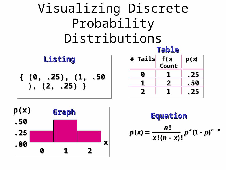
Visualizing Discrete Probability Distributions

{ (0, .25), (1, .50), (2, .25) }{ (0, .25), (1, .50), (2, .25) }{ (0, .25), (1, .50), (2, .25) }{ (0, .25), (1, .50), (2, .25) }

ListingListingTableTable

GraphGraph EquationEquation

# # TailsTails f(xf(x))CountCount

p(xp(x))

00 11 .25.2511 22 .50.5022 11 .25.25

pp xxnn

xx nn xxpp ppxx nn xx(( ))

!!

!! (( )) !!(( ))

11

.00.00

.25.25

.50.50

00 11 22xx

p(x)p(x)


Mutually Exclusive Events

• Two events Two events EE11, , EE22 are called are called mutually mutually

exclusiveexclusive if they are disjoint: if they are disjoint: EE11EE22 = = – Note that two mutually exclusive events Note that two mutually exclusive events cannot cannot

both occurboth occur in the same instance of a given in the same instance of a given experiment.experiment.

• For mutually exclusive events,For mutually exclusive events,Pr[Pr[EE11 EE22] = Pr[] = Pr[EE11] + Pr[] + Pr[EE22]]..


Exhaustive Sets of Events

• A set A set EE = { = {EE11, , EE22, …}, …} of events in the sample of events in the sample

space space SS is called is called exhaustiveexhaustive iff . iff .• An exhaustive set An exhaustive set EE of events that are all mutually of events that are all mutually

exclusive with each other has the property thatexclusive with each other has the property that

SEi

.1]Pr[ iE


Elementary Probability Rules

• P(~A) + P(A) = 1P(~A) + P(A) = 1• P(B) = P(B ^ A) + P(B ^ ~A)P(B) = P(B ^ A) + P(B ^ ~A)


Bernoulli Trials

• Each performance of an experiment with Each performance of an experiment with only two possible outcomes is called a only two possible outcomes is called a Bernoulli trialBernoulli trial..

• In general, a possible outcome of a In general, a possible outcome of a Bernoulli trial is called a Bernoulli trial is called a successsuccess or a or a failurefailure..

• If p is the probability of a success and q is If p is the probability of a success and q is the probability of a failure, then p+q=1.the probability of a failure, then p+q=1.


Probability of k successes in n independent Bernoulli trials.

The probability of k successes in n The probability of k successes in n independent Bernoulli trials, with independent Bernoulli trials, with probability of success p and probability of probability of success p and probability of failure q = 1-p is C(n,k)pfailure q = 1-p is C(n,k)pkkqqn-kn-k


ExampleA coin is biased so that the probability of heads is 2/3. A coin is biased so that the probability of heads is 2/3.

What is the probability that exactly four heads come up What is the probability that exactly four heads come up when the coin is flipped seven times, assuming that the when the coin is flipped seven times, assuming that the flips are independent?flips are independent?

The number of ways that we can get four heads is: C(7,4) The number of ways that we can get four heads is: C(7,4) = 7!/4!3!= 7*5 = 35= 7!/4!3!= 7*5 = 35

The probability of getting four heads and three tails is The probability of getting four heads and three tails is (2/3)(2/3)44(1/3)(1/3)3= 3= 16/316/377

p(4 heads and 3 tails) is C(7,4) p(4 heads and 3 tails) is C(7,4) (2/3)(2/3)44(1/3)(1/3)33 = 35*16/3 = 35*16/377 = = 560/2187560/2187


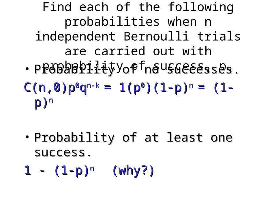
Find each of the following probabilities when n independent Bernoulli trials are carried out

with probability of success, p.

• Probability of no successes.Probability of no successes.

C(n,0)pC(n,0)p00qqn-k n-k = 1(p= 1(p00)(1-p))(1-p)n n = (1-p)= (1-p)n n

• Probability of at least one success.Probability of at least one success.

1 - (1-p)1 - (1-p)n n (why?)(why?)


Find each of the following probabilities when n independent Bernoulli trials are carried out

with probability of success, p.

• Probability of at most one success.Probability of at most one success.

Means there can be no successes or one Means there can be no successes or one successsuccess

C(n,0)pC(n,0)p00qqn-0 n-0 +C(n,1)p+C(n,1)p11qqn-1 n-1

(1-p)(1-p)nn + np(1-p) + np(1-p)n-1n-1

• Probability of at least two successes.Probability of at least two successes.

1 -1 - (1-p)(1-p)nn - np(1-p) - np(1-p)n-1n-1


A coin is flipped until it comes ups tails. The probability the coin comes up tails is p.

• What is the probability that the experiment What is the probability that the experiment ends after n flips, that is, the outcome ends after n flips, that is, the outcome consists of n-1 heads and a tail?consists of n-1 heads and a tail?

(1-p)(1-p)n-1n-1pp


Probability vs. Odds• You may have heard the term “odds.”You may have heard the term “odds.”

– It is widely used in the gambling community.It is widely used in the gambling community.

• This is not the same thing as probability!This is not the same thing as probability!– But, it is very closely related.But, it is very closely related.

• The The odds in favorodds in favor of an event of an event EE means the means the relative relative probability of probability of EE compared with its complement compared with its complement EE. .

OO((EE) :) :≡ Pr(≡ Pr(EE)/Pr()/Pr(EE))..– E.g.E.g., if , if pp((EE) = 0.6) = 0.6 then then pp((EE) = 0.4) = 0.4 and and OO((EE) = 0.6/0.4 = 1.5) = 0.6/0.4 = 1.5..

• Odds are conventionally written as a ratio of integers.Odds are conventionally written as a ratio of integers.– E.g.E.g., , 3/23/2 or or 3:23:2 in above example. “Three to two in favor.” in above example. “Three to two in favor.”

• The The odds againstodds against EE just means just means 1/1/OO((EE)). . “2 to 3 against”“2 to 3 against”

Exercise:Express theprobabilityp as a functionof the odds in favor O.


Example 1: Balls-and-Urn• Suppose an urn contains 4 blue balls and 5 red balls.Suppose an urn contains 4 blue balls and 5 red balls.• An example An example experiment: experiment: Shake up the urn, reach in Shake up the urn, reach in

(without looking) and pull out a ball.(without looking) and pull out a ball.• A A random variablerandom variable VV: Identity of the chosen ball.: Identity of the chosen ball.• The The sample space sample space SS: The set of: The set of

all possible values of all possible values of VV::– In this case, In this case, SS = { = {bb11,…,,…,bb99}}

• An An eventevent EE: “The ball chosen is: “The ball chosen isblue”: blue”: EE = { ______________ } = { ______________ }

• What are the odds in favor of What are the odds in favor of EE??• What is the probability of What is the probability of EE? ?

b1 b2

b3

b4

b5

b6

b7

b8

b9


Independent Events

• Two events E,F are called independent if Pr[EF] = Pr[E]·Pr[F].

• Relates to the product rule for the number of ways of doing two independent tasks.

• Example: Flip a coin, and roll a die.Pr[(coin shows heads) (die shows 1)] =

Pr[coin is heads] × Pr[die is 1] = ½×1/6 =1/12.


Example

Suppose a red die and a blue die are rolled. The sample space:

1 2 3 4 5 6 1 x x x x x x 2 x x x x x x 3 x x x x x x 4 x x x x x x 5 x x x x x x 6 x x x x x x

Are the events sum is 7 and the blue die is 3 independent?


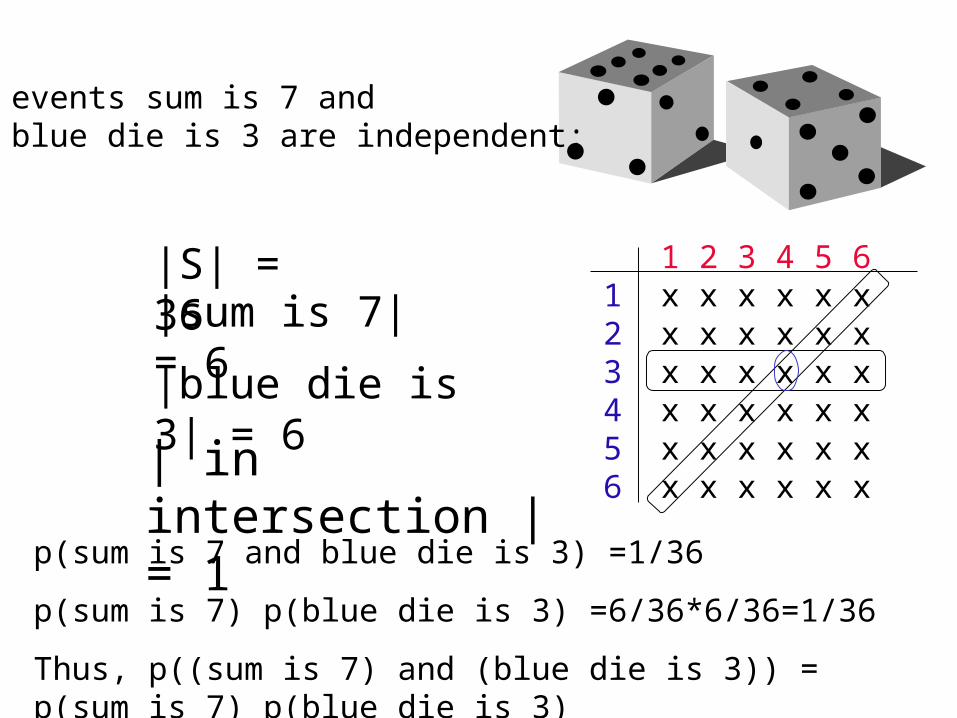
|S| = 36 1 2 3 4 5 6 1 x x x x x x 2 x x x x x x 3 x x x x x x 4 x x x x x x 5 x x x x x x 6 x x x x x x

|sum is 7| = 6

|blue die is 3| = 6

| in intersection | = 1

p(sum is 7 and blue die is 3) =1/36

p(sum is 7) p(blue die is 3) =6/36*6/36=1/36

Thus, p((sum is 7) and (blue die is 3)) = p(sum is 7) p(blue die is 3)

The events sum is 7 and the blue die is 3 are independent:


Conditional Probability

• Let Let EE,,FF be any events such that be any events such that Pr[Pr[FF]>0]>0..• Then, the Then, the conditional probabilityconditional probability of of EE given given FF, ,

written written Pr[Pr[EE||FF]], is defined as , is defined as Pr[Pr[EE||FF] :] :≡ ≡ Pr[Pr[EEFF]/Pr[]/Pr[FF]]..

• This is what our probability that This is what our probability that EE would turn out would turn out to occur should be, if we are given to occur should be, if we are given only only the the information that information that FF occurs. occurs.

• If If EE and and FF are independent then are independent then Pr[Pr[EE||FF] = Pr[] = Pr[EE]].. Pr[Pr[EE||FF] = Pr[] = Pr[EEFF]/Pr[]/Pr[FF] = Pr[] = Pr[EE]]×Pr[×Pr[FF]/Pr[]/Pr[FF] = Pr[] = Pr[EE]]


Visualizing Conditional Probability

• If we are given that event If we are given that event FF occurs, then occurs, then– Our attention gets restricted to the subspace Our attention gets restricted to the subspace FF..

• Our Our posteriorposterior probability for probability for EE (after seeing (after seeing FF)) correspondscorrespondsto the to the fractionfraction of of FF where where EEoccurs also.occurs also.

• Thus, Thus, pp′(′(EE)=)=pp((EE∩∩FF)/)/pp((FF).).

Entire sample space S

Event FEvent EEventE∩F


• Suppose I choose a single letter out of the 26-letter English alphabet, totally at random.– Use the Laplacian assumption on the sample space {a,b,..,z}.– What is the (prior) probability

that the letter is a vowel?• Pr[Vowel] = __ / __ .

• Now, suppose I tell you that the letter chosen happened to be in the first 9 letters of the alphabet.– Now, what is the conditional (or

posterior) probability that the letteris a vowel, given this information?

• Pr[Vowel | First9] = ___ / ___ .

Conditional Probability Example

a b c

de fghi

j

k

l

mn

o

p q

r

s

tu

v

w

xy

z

1st 9lettersvowels

Sample Space S


Example

• What is the probability that, if we flip a coin three times, that we get an odd number of tails (=event E), if we know that the event F, the first flip comes up tails occurs?

(TTT), (TTH), (THH), (HTT), (HHT), (HHH), (THT), (HTH)

Each outcome has probability 1/4,

p(E |F) = 1/4+1/4 = ½, where E=odd number of tailsor p(E|F) = p(EF)/p(F) = 2/4 = ½For comparison p(E) = 4/8 = ½ E and F are independent, since p(E |F) = Pr(E).


Prior and Posterior Probability• Suppose that, before you are given any information about the

outcome of an experiment, your personal probability for an event E to occur is p(E) = Pr[E].– The probability of E in your original probability distribution p is called

the prior probability of E.• This is its probability prior to obtaining any information about the outcome.

• Now, suppose someone tells you that some event F (which may overlap with E) actually occurred in the experiment.– Then, you should update your personal probability for event E to occur,

to become p′(E) = Pr[E|F] = p(E∩F)/p(F).• The conditional probability of E, given F.

– The probability of E in your new probability distribution p′ is called the posterior probability of E.

• This is its probability after learning that event F occurred.

• After seeing F, the posterior distribution p′ is defined by letting

p′(v) = p({v}∩F)/p(F) for each individual outcome vS.

probability theory

Education