problem solving examples

ECE 1010 ECE Problem Solving I

Chapter 3: Problem Solving Examples 3–46

Problem Solving Examples

Chapter 3 of the text contains a problem solving example in thearea of speech signal analysis. In this section we will first con-sider this particular problem. Next we will briefly investigate theMATLAB signal processing toolbox, which is an extension tothe MATLAB core. The signal processing toolbox is alsoincluded in the student edition.

Statistical Measurements of a Speech Utterance

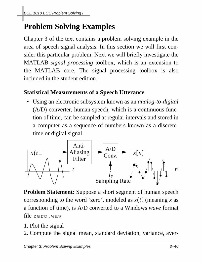
• Using an electronic subsystem known as an analog-to-digital(A/D) converter, human speech, which is a continuous func-tion of time, can be sampled at regular intervals and stored ina computer as a sequence of numbers known as a discrete-time or digital signal

Problem Statement: Suppose a short segment of human speechcorresponding to the word ‘zero’, modeled as (meaning x asa function of time), is A/D converted to a Windows wave formatfile zero.wav

1. Plot the signal2. Compute the signal mean, standard deviation, variance, aver-

x t( )

t

Anti-Aliasing

Filter

A/DConv. x n[ ]

nfs

Sampling Rate

x t( )



age power, average magnitude, and number of zero crossingsNote: Average power, although not formally defined yet in

this course, is just

Input/Output Description: A block diagram description of theproblem requirements is the following

Sample/Hand Calculation: Since the wav file we must processcontains thousands of samples, a sample calculation will be per-formed using a short ‘made-up’ record of data:

• Mean

x2

n[ ] N⁄n 1=N∑

zero.wav

SoundRecord

MA

TL

AB

Impl

emen

tatio

n signal std. dev.signal mean

signal avg. power

signal avg. magnitude

signal zero crossings

signal plot

signal variance

x n[ ] 0.5 1.2 2– 0.8=

mean x( ) µ 0.5 1.2 2–( ) 0.8+ + +4

---------------------------------------------------- 0.125= = =



• Variance (standard deviation is )

• Average power

• Average magnitude

• Zero crossings count (by inspection)

MATLAB Solution: To formulate the MATLAB solution we forthe most part can use standard functions we are already familiarwith. Two areas of concern are:

1. How do we import a wav file into the MATLAB work space,2. Develop an algorithm to count the zero crossings

• To import a wav file we will use one of the MATLAB soundfunctions

» help wavread

WAVREAD Read Microsoft WAVE (".wav") sound file.

Y=WAVREAD(FILE) reads a WAVE file specified by the

string FILE, returning the sampled data in Y. The ".wav"

extension is appended if no extension is given. Ampli-

σ

var x( ) σ2=

0.5 µ–( )21.2 µ–( )2

2– µ–( )20.8 µ–( )2

+ + +3

--------------------------------------------------------------------------------------------------------------------- 2.0891==

average power 0.52

1.22

2–( )20.8

2+ + +

4--------------------------------------------------------------- 1.5825= =

average magnitude 0.5 1.2 2– 0.8+ + +4

----------------------------------------------------------- 1.125= =

zero crossings 2=



tude values are in the range [-1,+1].

[Y,FS,BITS]=WAVREAD(FILE) returns the sample rate

(FS) in Hertz and the number of bits per sample (BITS)

used to encode the data in the file. (more help avail-

able, but not listed here)

• To count the number of zero crossings we form a new vectory that is the product of x and x delayed by one index or sam-ple value, i.e.,

• When a product is negative we know that the original signaleither went from + to - or - to +; the find() function canhelp us here

• The length function can then be used to determine thenumber of entries that find returns, and hence the number ofzero crossings in the data record x

• The MATLAB script file% The MATLAB script file speak_zero.m

% Begin by loading the wav file

x = wavread(‘zero.wav’);

%

%Display numerical results

fprintf('Digit Statistics \n\n');

fprintf('mean: %f \n', mean(x));

fprintf('standard deviation: %f \n', std(x));

fprintf('variance: %f \n', std(x)^2);

y 1( ) x 1( )x 2( )=

y 2( ) x 2( )x 3( )=

y 3( ) x 3( )x 4( )=

…



fprintf('average power: %f \n', mean(x.^2));

fprintf('average magnitude: %f \n', mean(abs(x)));

prod = x(1:length(x)-1).*x(2:length(x));

crossings = length(find(prod<0));

fprintf('zero crossings: %.0f \n', crossings);

plot(x); grid;

title('Speech Waveform of the Word Zero','fontsize',16);

ylabel('Amplitude','fontsize',14);

xlabel('Sequence Index','fontsize',14);

• Results form the test vector (we comment out wavread)» x = [0.5 1.2 -2 0.8];

» speak_zero

Digit Statistics

mean: 0.125000

standard deviation: 1.445395

variance: 2.089167

average power: 1.582500

average magnitude: 1.125000

zero crossings: 2

1 1.5 2 2.5 3 3.5 4-2

-1.5

-1

-0.5

0

0.5

1

1.5Speech Waveform of the Word Zero

Am

plitu

de

Sequence Index



• Now run with the real data» speak_zero

Digit Statistics

mean: 0.005810

standard deviation: 0.250013

variance: 0.062507

average power: 0.062533

average magnitude: 0.176845

zero crossings: 586

0 1000 2000 3000 4000 5000 6000 7000 8000 9000 10000-1

-0.8

-0.6

-0.4

-0.2

0

0.2

0.4

0.6

0.8

1Speech Waveform of the Word Zero

Am

plitu

de

Sequence Index


Chapter 3: Writing MATLAB Functions 3–52

Writing MATLAB Functions

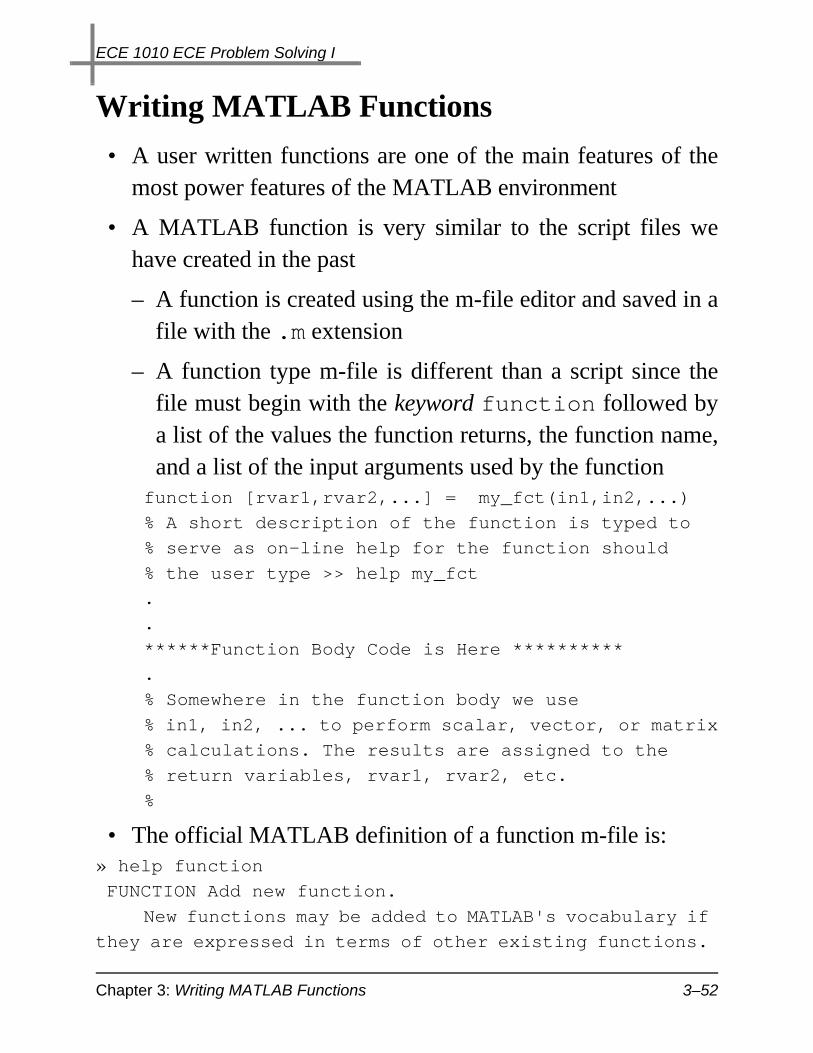
• A user written functions are one of the main features of themost power features of the MATLAB environment

• A MATLAB function is very similar to the script files wehave created in the past

– A function is created using the m-file editor and saved in afile with the .m extension

– A function type m-file is different than a script since thefile must begin with the keyword function followed bya list of the values the function returns, the function name,and a list of the input arguments used by the function

function [rvar1,rvar2,...] = my_fct(in1,in2,...)

% A short description of the function is typed to

% serve as on-line help for the function should

% the user type >> help my_fct

.

.

******Function Body Code is Here **********

.

% Somewhere in the function body we use

% in1, in2, ... to perform scalar, vector, or matrix

% calculations. The results are assigned to the

% return variables, rvar1, rvar2, etc.

%

• The official MATLAB definition of a function m-file is:» help function

FUNCTION Add new function.

New functions may be added to MATLAB's vocabulary if

they are expressed in terms of other existing functions.



The commands and functions that comprise the new func-

tion must be put in a file whose name defines the name

of the new function, with a filename extension of '.m'.

At the top of the file must be a line that contains the

syntax definition for the new function. For example, the

existence of a file on disk called STAT.M with:

function [mean,stdev] = stat(x)

n = length(x);

mean = sum(x) / n;

stdev = sqrt(sum((x - mean).^2)/n);

defines a new function called STAT that calculates the

mean and standard deviation of a vector. The variables

within the body of the function are all local variables.

See SCRIPT for procedures that work globally on the

work-space.

• A particular caution in defining your own functions is tomake sure that your names do not conflict with any of MAT-LAB’s predefined functions

• The m-file name must be the same as the function name, e.g.,my_fct is saved as my_fct.m

• All variables created and used within a function are local tothat function, and will be destroyed when you are done usingthe function

• Likewise the only MATLAB workspace variables that thefunction has knowledge of are those that are passed into it viathe input parameter list, i.e., in1, in2, etc.,



Example: A common function used in signals and systems prob-lem solving is a function for generating a rectangular pulse

• We would like to create a new function rect(t) that allowsto input a vector (a scalar version would trivial and not asuseful) of time samples t and returns the corresponding func-tional values function x = rect(t)

% RECT x = rect(t): A function that is defined

% to be 1 on [-0.5,0.5] and 0 otherwise.

% Initialize a vector with zeros in it that is

% the same length as the input vetor t:

x = zeros(size(t));

% Create an index vector that holds the indices

% of t where abs(t) <= 0.5:

set1 = find(abs(t) <= 0.5);

% Use set1 to change the corresponding values

% of x from zero to one:

x(set1) = ones(size(set1));

% We are finished!

• Now we need to test the function and see if it performs asexpected

– Check the on-line help» help rect

t

rect t( )

rect t( ) 1, t12---≤

0, otherwise

=1

-0.5 0.5

rect t( )



RECT x = rect(t): A function that is defined

to be 1 on [-0.5,0.5] and 0 otherwise.

– Run a test vector into the function and plot the results» t = -2:.01:2;

» x = rect(t);

» plot(t,x); grid;

» axis([-2 2 -.1 1.1])

» title('The rect Function in Action', ...

'fontsize',18)

» ylabel('x(t)','fontsize',16)

» xlabel('t','fontsize',16)

-2 -1.5 -1 -0.5 0 0.5 1 1.5 2

0

0.2

0.4

0.6

0.8

1

The rect Function in Action

x(t)

t



Example: Practice! p. 108 (2)

Develop and test (plot results for a test vector input) user writtenfunctions to compute the following:

2. ramp(x) defined as

• This function can be constructed as a simple modification tothe rect functionfunction x = ramp(t)

% RAMP x = ramp(t): A function that is defined

% to be t for t >= 0 and 0 otherwise.

% Initialize a vector with zeros in it that is

% the same length as the input vetor t:

x = zeros(size(t));

% Create an index vector that holds the indices

% of t where t >= 0:

set1 = find(t >= 0);

% Use set1 to change the corresponding values

% of x from zero to t:

x(set1) = t(set1);

% We are finished!

• Test the function:

– On-line help:» help rect

RAMP x = ramp(t): A function that is defined

to be t on t >=0 and 0 otherwise.

ramp x( ) x, x 0≥0, otherwise

=



– Pass a test vector through» t = -2:.01:2;

» x = ramp(t);

» plot(t,x); grid;

» title('The ramp Function in Action','fontsize',18)

» ylabel('ramp(t)','fontsize',16)

» xlabel('t','fontsize',16)

-2 -1.5 -1 -0.5 0 0.5 1 1.5 20

0.2

0.4

0.6

0.8

1

1.2

1.4

1.6

1.8

2The ramp Function in Action

ram

p(t)

t


Chapter 3: Functions for Random Number Generation 3–58

Functions for Random Number Generation

• Engineering problem solving, in particular, simulation basedproblem solving, typically requires the use of random num-ber generators to allow the construction of repeated trialstype experiments

• Applications in electrical engineering include:

– Noise in communication, signal processing, and controlsystem signals

– Fading characteristics in a space, mobile, or indoor wire-less communication channel

– The random arrival of packets in a communication network

– The variation in parameter values in electrical networksdue to manufacturing imperfections; integrated circuitcomponents and lumped elements, others

– The duration of voice calls in a telephone switch or cell ina cellular telephone system

– many, many others

Uniform Random Numbers

• Depending upon the processes (physics) involved with theproblem the distribution of values the random number gener-ator produces is of great interest



• The most simplistic random number generators produce uni-form random numbers, that is numbers uniformly distrib-uted over the interval

• The MATLAB function rand produces numbers that areuniformly distributed over the interval

• A random number sequence is really only pseudo random,that is the random number sequence eventually repeats itself

• The starting point of the random sequence in controlled bythe seed value; in MATLAB the initial seed value 0

• For a given seed value the random number generator pro-duces the same sequence of numbers

Table 3.11: Features of rand

Call Mode Description

rand(n) Generates an matrix of number uniform on .

rand(n,m) Generates an matrix of number uniform on .

rand(‘seed’,n) Sets the seed value.

rand(‘seed’) Returns the current seed value.

a b,[ ]

0 1,[ ]

n n×0 1,

n m×0 1,



Example: Call rand three times

» rn1 = rand(10,1); rn2 = rand(10,1);

» rand('seed',0); rn3 = rand(10,1);

» [rn1 rn2 rn3]

ans =

0.2190 0.5297 0.2190

0.0470 0.6711 0.0470

0.6789 0.0077 0.6789

0.6793 0.3834 0.6793

0.9347 0.0668 0.9347

0.3835 0.4175 0.3835

0.5194 0.6868 0.5194

0.8310 0.5890 0.8310

0.0346 0.9304 0.0346

0.0535 0.8462 0.0535

– Note: In the above we see that the first and third sequencesare identical by virtue of the fact that both use the sameseed

• The MATLAB statistics tool box supplies many types of ran-dom number generators, all of which can be investigated bytyping randtool at the MATLAB prompt

• Numbers uniform on the interval can be transformed tonumbers uniform on using the transformation

(3.2)

Example: Find the approximate distribution of two resistors in aparallel connection assuming that they each have measured val-ues which vary uniformly about their nominal values by

0 1,[ ]a b,[ ]

x b a–( ) r a+⋅=

5%±



• Let ohms and ohms

• In actuality is uniform on the interval and is uniform on

The Statistics Toolbox Function Randtool

R2 5%±R3

R1R2

R1 R2+------------------ ?%±=

R1 5%± Resistors in Parallel

R1 10 000,= R2 5 000,=

R1 9500 10500,[ ]R2 4750 5250,[ ]



• Compute 50,000 trials and histogram the results» n = 50000;

» r1 = rand(n,1)*(10500-9500)+9500;

» r2 = rand(n,1)*(5250-4750)+4750;

» r3 = r1.*r2./(r1+r2);

» hist(r3,20)

» title('Histogram of Random Resistor Values in

Parallel','fontsize',16)

» ylabel('Occurrence R1 || R2','fontsize',14)

» xlabel('Range of R3 Values','fontsize',14)

• Clearly the resulting is not uniformly distributed (prob-lem left for ECE 3610)

3150 3200 3250 3300 3350 3400 3450 35000

500

1000

1500

2000

2500

3000

3500

4000Histogram of Random Resistor Values in Parallel

Occ

urre

nce

of R

1 ||

R2

Range of R3 Values

#Trials = 50,000

R3




Give the MATLAB statements to generate 10 random numbersbetween -20 and -10. Check your answers by executing the codeand printing the results.

» uni3 = rand(10,1)*(-10 + 20) + -20;

» uni3

uni3 =

-16.9991

-14.6655

-12.4649

-17.7156

-16.6365

-10.0437

-15.1421

-12.5393

-18.4294

-12.7613

Gaussian Random Numbers

• Another popular distribution is Gaussian or normal randomnumbers

• Here the density of numbers follows a bell shaped curve ofthe form

x x( ) 1

2πσx2

-----------------e

x mx–( )2–

2σx2

-------------------------

∞ x ∞< <–,=



• The center of the bell is located at , which is the mean ofthe random numbers, while the spread or variation of the ran-dom numbers about the mean is given by (the variance is

)

– It can be shown that 68% of the numbers fall within theinterval , while 99% fall within

• The MATLAB function for producing normal random num-bers (no special toolbox required) is randn

• If r is normal with zero mean and unity variance we can cre-ate a random sequence with mean and variance via thetransformation

(3.3)


Use MATLAB to generate 1,000 normal random number valueswith the and . Calculate the mean andvariance, and plot the data set histogram using 25 bins.

Table 3.12:

Call Mode Description

randn(n) Generates an matrix of normal random numbers having zero mean and unity variance.

randn(n,m) Generates an matrix of normal random numbers having zero mean and unity variance.

mx

σxσx

2

mx σx± mx 3σx±

n n×

n m×

mx σx2

x σxr mx+=

mx 5.5–= σx 1.25=



» x = 1.25*randn(1000,1) - 5.5;

» mean(x)

ans = -5.4957

» std(x)

ans = 1.2326

» hist(x,25)

» title('Histogram of x Normal with mean = -5.5, std =

1.25','fontsize',16)

» ylabel('Occurrence of x','fontsize',14)

» xlabel('Range of x Values','fontsize',14)

– Note: To better approximate a bell shaped distributionmore trials are needed

-10 -9 -8 -7 -6 -5 -4 -3 -20

10

20

30

40

50

60

70

80

90

100Histogram of x Normal with mean = -5.5, std = 1.25

Occ

urre

nce

of x

Range of x Values

#Trials = 1,000

problem solving examples

Documents