proceedings of the sixth seminar for homogenization … of the sixth seminar for homogenization and...
TRANSCRIPT

Proceedings of the Sixth Seminar for Homogenization and Quality Control in Climatological Databases
(Budapest, Hungary, 26 – 30 May 2008)
Climate Data and Monitoring WCDMP-No. 76
WMO-TD No. 1576

PROCEEDINGS OF THE SIXTH SEMINAR
FOR HOMOGENIZATION AND QUALITY
CONTROL IN CLIMATOLOGICAL DATABASES
Organized by Hungarian Meteorological Service (HMS)
jointly with the
MEETING OF
COST-ES0601 (HOME) ACTION
MANAGEMENT COMMITTEE AND WORKING GROUPS
Budapest, Hungary, 26 - 30 May 2008
Organized by the Hungarian Meteorological Service
Supported by EU/COST-ES0601 Action, WMO, HMS
Edited by M. Lakatos, T. Szentimrey, Z. Bihari and S. Szalai

PREFACE
The Hungarian Meteorological Service and the World Meteorological Organisation have
organized Seminar for homogenisation and quality control in climatological databases for
the 6th time. COST Action ES0601, Advances in Homogenisation Methods of Climate
Series: an Integrated Approach (HOME) was the main sponsor and co-organizer this time.
This Action makes regular and planned development of the homogenisation methods
possible. The seminar was an open meeting giving a good occasion for information
exchange between the participants of the HOME project and other researchers of
homogenisation community.
The 31 Seminar‟s presentations followed the structure of the COST Action. The 1st
Working Group (WG1) deals with the inventory of homogenisation methods, and the
preparation of a benchmark dataset for the other working groups, WG2 has a task of break
point detection, WG3 the correction of time series and WG4 the work with the daily data.
The last working group, WG5 deals with the recommendation of the best available
homogenisation method.
The organisational circumstances, topics and the high scientific level of
presentations show a clear positive shift in the administrative and scientific development of
homogenisation procedures. First, the data management issue appeared on the European
level, officially. It is clear, that the development of data availability and common or at least
comparable management methods are not a national tasks, but have to be solved on the
international level with participation of national data holders and international donor
organisation(s). Wide range of countries presented their homogenisation efforts during the
seminar. Unfortunately, not all countries are able to develop, or even to adopt
homogenisation methods by their own resources. Therefore, further support is required,
especially for the countries without homogenized database.
Secondly, many different meteorological parameters were objects of homogenisation
procedures at the presentations. It is very positive, but the scientific basis needs further
development and enlargement. All measured meteorological parameters should be
involved in the homogenisation on a climatologically and mathematically well established
basis.
Many daily based homogenisation methods were presented, which is very
beneficial and have been among the recommendations since the very long time.
Furthermore, the COST Action pays attention to the wider availability of homogenisation
methods.
We can detect many positive scientific and administrative features at the
homogenisation procedures. The accent should be made on transboundary developments
now. Large international projects, like Climate Data Regional Climate Centre, South-
European Drought Management Centre, Climate of the Carpathian Region, etc. apply
homogenisation methods, but they need further, practically applicable homogenisation
procedure developments. Our task is keeping these existing tendencies alive in the future,
and in that case we can be optimistic.
Sándor Szalai

CONTENTS
Methodological questions of series comparison ......................................................................
Tamás Szentimrey ............................................................................................................... 1
Experiences with quality control and homogenization of daily series
of various meteorological elements in the Czech Republic 1961-2007 ..................................
P. Štěpánek and P. Zahradníček ........................................................................................ 8
Quantifying efficiency of homogenisation methods ...............................................................
Peter Domonkos ................................................................................................................. 20
Understanding inter-site temperature differences at the KNMI terrain in De Bilt (the
Netherlands).............................................................................................................................
Theo Brandsma .................................................................................................................. 33
Detected Inhomogeneities In Wind Direction And Speed Data From Ireland ........................
Predrag Petrović and Mary Curley.................................................................................. 41
A method for daily temperature data interpolation and quality control based on the selected
past events ...............................................................................................................................
Gregor Vertačnik ............................................................................................................... 53
Air humidity in Cracow in the period 1863-2007 – daily data quality control and
homogenization methods .........................................................................................................
Agnieszka Wypych and Katarzyna Piotrowicz .............................................................. 60
Homogenization of water vapour data from Vaisala radiosondes and older (marz, rkz) used
in Polish aerological service ....................................................................................................
Barbara Brzóska ................................................................................................................ 68
Homogenization of Italian precipitation series ........................................................................
Andrea Toreti, Franco Desiato, Guido Fioravanti, Walter Perconti ............................ 76
Homogenisation of temperature time series in Croatia ...........................................................
Dubravka Rasol, Tanja Likso, Janja Milković ............................................................... 85
Towards the assessment of inhomogeneities of climate data series, resulting from the
automation of the observing network in Mainland Portugal ...................................................
Mendes M., Nunes L., Viterbo P., Neto J. ....................................................................... 94
Homogenization of daily data series for extreme climate indeces calculation........................
Lakatos, M., Szentimrey, T., Bihari, Z., Szalai, S. ........................................................ 100
Programme ........................................................................................................................ 110
List of participants ............................................................................................................. 113

1
METHODOLOGICAL QUESTIONS OF SERIES COMPARISON
Tamás Szentimrey
Hungarian Meteorological Service, H-1525, P.O. Box 38, Budapest, Hungary,
1. INTRODUCTION
The aim of the homogenization procedures is to detect the inhomogeneities and to correct the
series. In practice there are absolute and relative methods applied for this purpose. However
the application of absolute methods is very problematic and hazardous since the separation of
climate change signal and the inhomogeneity signal is essentially impossible. Relative
methods can be applied if there are more station series given, which can be compared
mutually. The methodology of comparison is related to the following questions: reference
series creation, difference series constitution, multiple comparisons of series etc. These topics
are very important for detection as well as for correction, because the efficient comparison of
series can increase both the significance and the power. The development of efficient
comparison methods can be based on the examination of the spatial covariance structure of
data series. Consequently the statistical spatiotemporal modelling is also a key question of
data series homogenization. The adequate comparison, break point detection and correction
procedures are depending on the statistical model.
2. GENERAL FORM OF ADDITIVE MODEL
In case of relative methods a general form of additive model for more monthly series
belonging to the same month in a small climate region can be written as follows,
)()()()( ttIHEttX jjjj .,n,, t,N ,,j 21;21 , (1)
where )(t is the common and unknown climate change signal (temporal trend), jE are the
spatial expected values (spatial trend), )(tIH j are the inhomogeneity signals and )(tj are
normal white noise series. The signal t is a fixed parameter without any assumption about
the shape. The type of inhomogeneity tIH is in general a ‟step-like function‟ with unknown
break points T and shifts 01 TIHTIH , and 0nIH is assumed in general.
Consequently the expected values are,
)()()(E tIHEttX jjj .,n,, t,N ,,j 21;21 .
The inhomogeneity can be written as linear function of the shifts, jjj ttIH νTT , so from
model (1) the following form can be obtained,
)()()( T ttEttX jjjjj νT .,n,, t,N ,,j 21;21 , (2)
where tjT is the vector of one break point functions, and jν is the vector of shifts at the
break points.

2
The above additive (linear) model (2) may be written also in vector form,
tttt ενTE1X nt ,...,1 (3)
where tXtXt N,.....,1
T X , NEE ,.....,1
T E , ttt NN
TT
11 ,..., TeTeT ,
TTT
1 ,.., Nννν , vector 1 is identically one, and the normal distributed vector variables
C0ε ,,..,T
1 Nttt N nt ,...,1 are totally independent in time. The spatial
covariance matrix C may be an arbitrary covariance matrix which describes the spatial
structure of the series and it can have a key role in the methodology of comparison.
3. COMPARISON OF SERIES FOR DETECTION AND CORRECTION
According to the model (1), (2), (3) the expected values of examined series are,
)()()(E tIHEttX jjj .,n,, t,N ,,j 21;21 , (4)
that are covered with normal white noise series,
C0ε ,,.....,T
1 Nttt N nt ,...,1 ,
where the vector variables tε nt ,...,1 are totally independent in time, and matrix C is
the spatial covariance matrix between the stations. This station covariance matrix C may
have a key role in methodology of comparison of series.
The aim of the homogenization procedure is to detect the inhomogeneities and to correct the
series. During the procedure the series can be compared mutually and the role of series – that
may be candidate or reference ones – is changing in the course of procedure. The reference
series are not assumed to be homogeneous at the correct examinations! The significance and
the power of the procedures can be defined according to the probabilities of type of errors.
Type one error means the detection of false or superfluous inhomogeneity while type two
error means neglecting some real inhomogeneity.
The problem of comparison of series is related to the following questions: reference series
creation, difference series constitution, multiple comparisons of series etc. These topics are
very important for detection as well as for correction, because the efficient comparison of
series can increase both the significance and the power. The development of efficient
comparison methods can be based on the examination of the spatial covariance structure of
data series. The maximum likelihood methods also take into account the mentioned spatial
covariance structure (section 4.2).
3.1 Difference series constitution
At the examinations the main problem arises from the fact that the shape of the common
climate change signal is unknown. Therefore so-called difference series are examined in order
to filter out the climate change signal )(t .
Let us use the following notations, )(tX j , ,N,,j 21N is the chosen candidate series
and the other series )(tX i , ji j \NN- are the references.
The simple difference series by pairs are, tXtXtZ ijj ji -N .
However the difference series constitution can be formulated in more general way as well,
namely
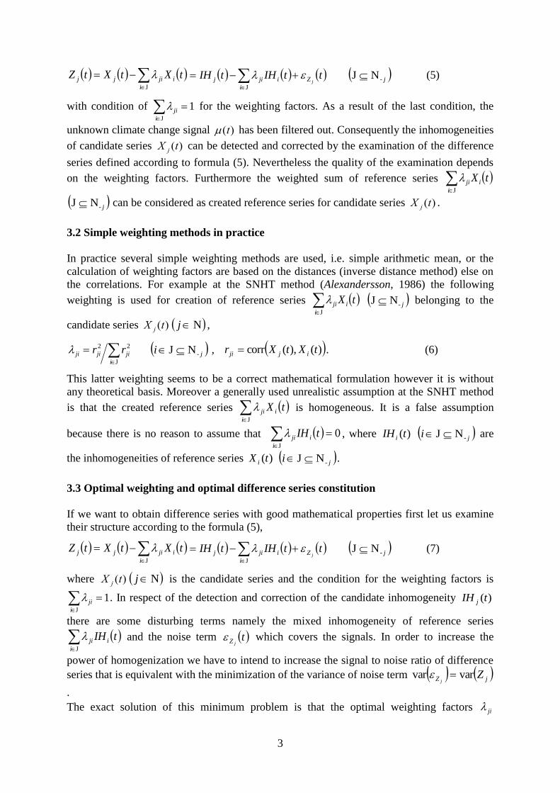
3
Ji
ijijj tXtXtZ ttIHtIHjZ
i
ijij J
j-NJ (5)
with condition of 1J
i
ji for the weighting factors. As a result of the last condition, the
unknown climate change signal )(t has been filtered out. Consequently the inhomogeneities
of candidate series )(tX j can be detected and corrected by the examination of the difference
series defined according to formula (5). Nevertheless the quality of the examination depends
on the weighting factors. Furthermore the weighted sum of reference series tX i
i
jiJ
j-NJ can be considered as created reference series for candidate series )(tX j .
3.2 Simple weighting methods in practice
In practice several simple weighting methods are used, i.e. simple arithmetic mean, or the
calculation of weighting factors are based on the distances (inverse distance method) else on
the correlations. For example at the SNHT method (Alexandersson, 1986) the following
weighting is used for creation of reference series tX i
i
jiJ
j-NJ belonging to the
candidate series )(tX j Nj ,
J
22
i
jijiji rr ji -NJ , )(),(corr tXtXr ijji . (6)
This latter weighting seems to be a correct mathematical formulation however it is without
any theoretical basis. Moreover a generally used unrealistic assumption at the SNHT method
is that the created reference series Ji
iji tX is homogeneous. It is a false assumption
because there is no reason to assume that 0J
i
iji tIH , where )(tIH i ji -NJ are
the inhomogeneities of reference series )(tX i ji -NJ .
3.3 Optimal weighting and optimal difference series constitution
If we want to obtain difference series with good mathematical properties first let us examine
their structure according to the formula (5),
Ji
ijijj tXtXtZ ttIHtIHjZ
i
ijij J
j-NJ (7)
where )(tX j Nj is the candidate series and the condition for the weighting factors is
1J
i
ji . In respect of the detection and correction of the candidate inhomogeneity )(tIH j
there are some disturbing terms namely the mixed inhomogeneity of reference series
Ji
iji tIH and the noise term tjZ which covers the signals. In order to increase the
power of homogenization we have to intend to increase the signal to noise ratio of difference
series that is equivalent with the minimization of the variance of noise term jZ Zj
varvar
.
The exact solution of this minimum problem is that the optimal weighting factors ji

4
ji -NJ written in vector form are,
11C1
cC1cCλ
1
J,J
T
J,
1
J,J
T
J,
1
J,JJ,
1 j
jj (8)
where J,jc is the candidate-reference covariance vector and J,JC is the reference-reference
covariance matrix (Cressie, 1991; Szentimrey, 1999, 2007b). It can be seen that the
covariance matrix C uniquely determines the optimum weighting factors that minimize the
variance, and the optimal difference series created in this manner can be applied efficiently
for the detection and correction procedures. Changing the combinations of the reference series
tX i ji -NJ altogether 12 1 N optimally weighted difference series can be
constituted for a chosen candidate series )(tX j .
Remark 1
We call the attention to the connection with the spatial interpolation techniques built in GIS.
The optimal weighting factors J,jλ are just the ordinary kriging weighting factors when the
candidate (predictand) )(tX j is interpolated with reference series (predictors)
ji itX -NJ)( . Consequently, the optimal difference series are theoretically identical
with the interpolation error series of ordinary kriging. Practically at the homogenization the
necessary covariance matrix C can be estimated on the basis of data series while the ordinary
kriging methods built in GIS cannot efficiently use the data series for modelling the necessary
statistical parameters (Szentimrey, 2007b).
Remark 2
The missing data completion or filling the gaps is also an interpolation problem at the
homogenization. In accordance with the optimal difference series formula the following
interpolation is suggested for missing value completion,
J
ˆ
i
iijijj EtXEtX (9)
where tX jˆ is the interpolated candidate series value and the values tX i ji -NJ are
the reference ones, the weighting factors ji ji -NJ are calculated according to (8),
furthermore jE , iE ji -NJ are the spatial expected values by model (1). These optimal
interpolation parameters minimize the RMSE, and this procedure is built in the MASH
method for missing data completion (Szentimrey, 1999).
Remark 3
We mention if we substitute the generalized-least-squares estimation of unknown climate
change signal t into the formula of linear regression between predictand )(tX j and
predictors ji itX -NJ)( then also the above introduced optimal difference series is
obtained with minimal variance (Szentimrey, 2007b).
4. APPLICATION OF OPTIMAL DIFFERENCE SERIES FOR DETECTION AND
CORRECTION
As a consequence of the mixed inhomogeneities of difference series (7) we have to examine
more optimal difference series in order to estimate and separate the appropriate

5
inhomogeneities for the candidate series. Various strategies and procedures can be
implemented for this purpose.
4.1 Iteration procedures
A typical iteration procedure is the MASH algorithm (Szentimrey, 1999, 2007a). At this
procedure a so-called optimal difference series system is examined during one iteration steps.
The system elements are optimal difference series and created without common reference
series what makes possible to detect and separate the inhomogeneities for the chosen
candidate series. The outline of one iteration step is as follows.
1. To choose the candidate series.
2. Series comparison: constitution of optimal difference series system.
3. Multiple break points detection for difference series based on hypothesis tests:
point estimations, confidence intervals.
4. Estimation of shifts of difference series: point estimations, confidence intervals.
5. Analysis of results: separation of break points and shifts for candidate series.
6. Correction of candidate series based on the above results.
During the procedure the iteration steps 1-6 are repeated and each series can be examined
many times! As it can be seen the optimal difference series have a key role at this procedure.
As regards the correction part we emphasize that almost all the methods use point estimation
for the correction factors at the detected break points. The MASH procedure is an exception
because the correction factors are estimated also on the basis of confidence intervals.
4.2 Maximum Likelihood procedures
Another possibility is to apply the maximum likelihood principle. Nevertheless in this case
also certain optimal difference series are examined implicitly. But first let us see the structure
of maximum likelihood estimation.
We use again the model (2), (3) that is,
tttt ενTE1X nt ,...,1 (10)
where the vector variables tε C0,N nt ,...,1 are totally independent in time. We
assume spatial covariance matrix C is known and inverse 1C exists.
Then the basic minimum tasks to obtain the maximum likelihood estimations for various
parameters in case of normal distribution are as follows.
i, Maximum likelihood estimation for νE,,t , if tT (breaks) are given:
n
t
ttttttt
1
1T
,min νTE1XCνTE1X
νE
,
ii, Maximum likelihood estimation for νTE ,,, tt , if the total number of break points K
is given:
n
t
tttttttt
1
1T
,min νTE1XCνTE1X
νTE
,,
iii, Bayesian approach (model selection), penalized likelihood methods,

6
if the total number of break points K is also estimated:
K
n
t
pentttttt
tt
K1
1T
,
minmin νTE1XCνTE1X
νTE
,,
where the penalty terms IHKK ppenpen depend on IHp and IHp is some „a priori‟
probability of break at each time 1.1 .,n,t and each station. Some examples for „a priori‟
probabilities applied in practice: 1
1
1
e
epIH (Akaike),
1
1
1
n
npIH (Schwarz),
1
1
1
n
n
n
n
IH
n
np (Caussinus-Lyazrhi).
According to the minimum task i, this correction model can be applied if the break points
tT .,n,t .1 are known and we want to give maximum likelihood estimations for the shifts
ν . This estimation is the so-called generalized-least-squares estimation of the shifts. If we use
the identity matrix I instead of C then we obtain the least-squares estimation which was
implemented by Caussinus and Mestre, 2004.
Returning to the relation of maximum likelihood estimation and the optimal difference series,
let us consider the following special optimal difference series,
tXtXtZ i
Ni
jijj
j
-
Nj ,...,1 ,
where the weighting factors are optimal according to formula (8).
Hereinafter let us denote the above optimal series in vector form:
ttZtZt N XΛIZ T
1 ,....., nt ,...,1 .
Theorem (without proof)
In case of arbitrary inhomogeneity terms νT ,,...,1 ntt :
n
t
ttttttt
1
1T
,min νTE1XCνTE1X
E
n
t
cccc tttt1
1TνTΛIZCνTΛIZ Z (11)
where ZZZ ttc and TTT ttc are centered values,
and 1
ZC is a generalized inverse of ZC that is the covariance matrix of tZ .
The concept of generalized inverse means, that ZZZZ CCCC 1 , in spite of the fact that ZC is
a singular matrix since the optimal difference series NjtZ j ,...,1 are linearly dependent.
Essentially the formula (11) can be obtained by the substitution of the generalized-least-
squares estimations of E,t .
As a consequence of this theorem the minimum tasks i, ii, iii, can be rewritten also with the
optimal difference series tZ .
i, Maximum likelihood estimation for ν , if tT (breaks) are given:
7
n
t
cccc tttt1
1Tmin νTΛIZCνTΛIZ Zν
ii, Maximum likelihood estimation for νT ,t , if the total number of break points K is
given:
n
t
cccc ttttt
1
1Tmin νTΛIZCνTΛIZ Z
νT ,
iii, Bayesian approach (model selection), penalized likelihood methods,
if the total number of break points K is also estimated:
K
n
t
cccc pentttttK
1
1Tminmin νTΛIZCνTΛIZ Z
νT ,
CONCLUSION
The solutions of the minimum tasks for ν (i, ii, iii,) and tT (ii, iii,) are functions of the
optimal difference series ntt ,...,1Z . That means the maximum likelihood methods also
perform series comparison and examine implicitly optimal difference series!
References
Alexandersson, H., 1986: “A homogeneity test applied to precipitation data”, Int. J. Climatology 6: 661-675.
Caussinus, H, Mestre, O. 2004: “Detection and correction of artificial shifts in climate series.” Appl. Statist., 53,
Part 3, pp. 405-425.
Cressie, N., 1991: “Statistics for Spatial Data.”, Wiley, New York, 900p.
Mestre, O., 1999: “Step-by-step procedures for choosing a model with change-points”, Proceedings of the
Second Seminar for Homogenization of Surface Climatological Data, Budapest, Hungary; WMO, WCDMP-
No. 41, pp. 15-25.
Szentimrey, T., 1999: “Multiple Analysis of Series for Homogenization (MASH)”, Proceedings of the Second
Seminar for Homogenization of Surface Climatological Data, Budapest, Hungary; WMO, WCDMP-No. 41,
pp. 27-46.
Szentimrey, T., 2007a: “Manual of homogenization software MASHv3.02”, Hungarian Meteorological Service,
p. 61.
Szentimrey, T, Bihari, Z., Szalai,S., 2007b: “Comparison of geostatistical and meteorological interpolation
methods (what is what?)”, Spatial Interpolation for climate data - the use of GIS in climatology and
meteorology, Edited by Hartwig Dobesch, Pierre Dumolard and Izabela Dyras, 2007, ISTE ltd., London, UK,
284pp, ISBN 978-1-905209-70-5, pp.45-56

8
EXPERIENCES WITH QUALITY CONTROL AND
HOMOGENIZATION OF DAILY SERIES
OF VARIOUS METEOROLOGICAL ELEMENTS IN THE CZECH
REPUBLIC 1961-2007
P. Štěpánek and P. Zahradníček
Czech Hydrometeorological Institute, Regional Office Brno, Czech Republic,
Phone: +420-541 421 033,
Abstract
Quality control and homogenization has to be undertaken prior to any data analysis in order to
eliminate any erroneous values and inhomogeneities in time series. In this work we describe and then
apply our own approach to data quality control, combining several methods: (i) by applying limits
derived from interquartile ranges (ii) by analyzing difference series between candidate and
neighbouring stations and (iii) by comparing the series values tested with “expected” values –
technical series created by means of statistical methods for spatial data (e.g. IDW, kriging).
Because of the presence of noise in series, statistical homogeneity tests render results with some
degree of uncertainty. In this work, the use of various statistical tests and reference series made it
possible to increase considerably the number of homogeneity test results for each series and thus to
assess homogeneity more reliably. Inhomogeneities were corrected on a daily scale.
These methodological approaches are demonstrated by use of the daily data of various
meteorological elements measured in the area of the Czech Republic. Series were processed by means
of developed ProClimDB and AnClim software (www.climahom.eu).
INTRODUCTION
In recent years considerable attention has been devoted to the analysis of daily data. Prior
to analysis, the need to homogenize data and check their quality arises (Brandsma, 2000,
Vincent et al. 2002, Wijngaard et al. 2003, Petrovic 2004, Della-Marta 2006 and others).
Several kinds of problem have to be taken into consideration in the course of data processing,.
These involve selection of a proper method for homogenization with regard to the data used,
i.e. fulfilling all the conditions necessary to applying selected tests of relative homogeneity
(e.g. normal distribution), creation of reference series (defining selection criteria), adjustment
of inhomogeneities revealed, completion of missing values, and others. To date, no widely
accepted homogenization approach has appeared that could be generalized and applied to a
wider range of meteorological elements and different climatic regions. However, such
approaches are needed. The creation of a general method of homogenization is also the main
goal of the ongoing COST project ES0601, planned to culminate in 2011.
Because of presence of noise in series, statistical homogeneity tests render results with
some degree of uncertainty. In this work, the use of various statistical tests and types of
reference series made it possible to increase considerably the number of homogeneity tests
results for each series tested and thus to assess homogeneity more reliably.
Considering quality control, the lack of a generally accepted methodology is even more
profound than in the case of homogenization. Without treating outliers, homogenization and
analysis may render misleading results. We therefore devoted consierable time to the
9
methodology of detecting outliers, something that could moreover be automated to process
large datasets of daily (subdaily) values.
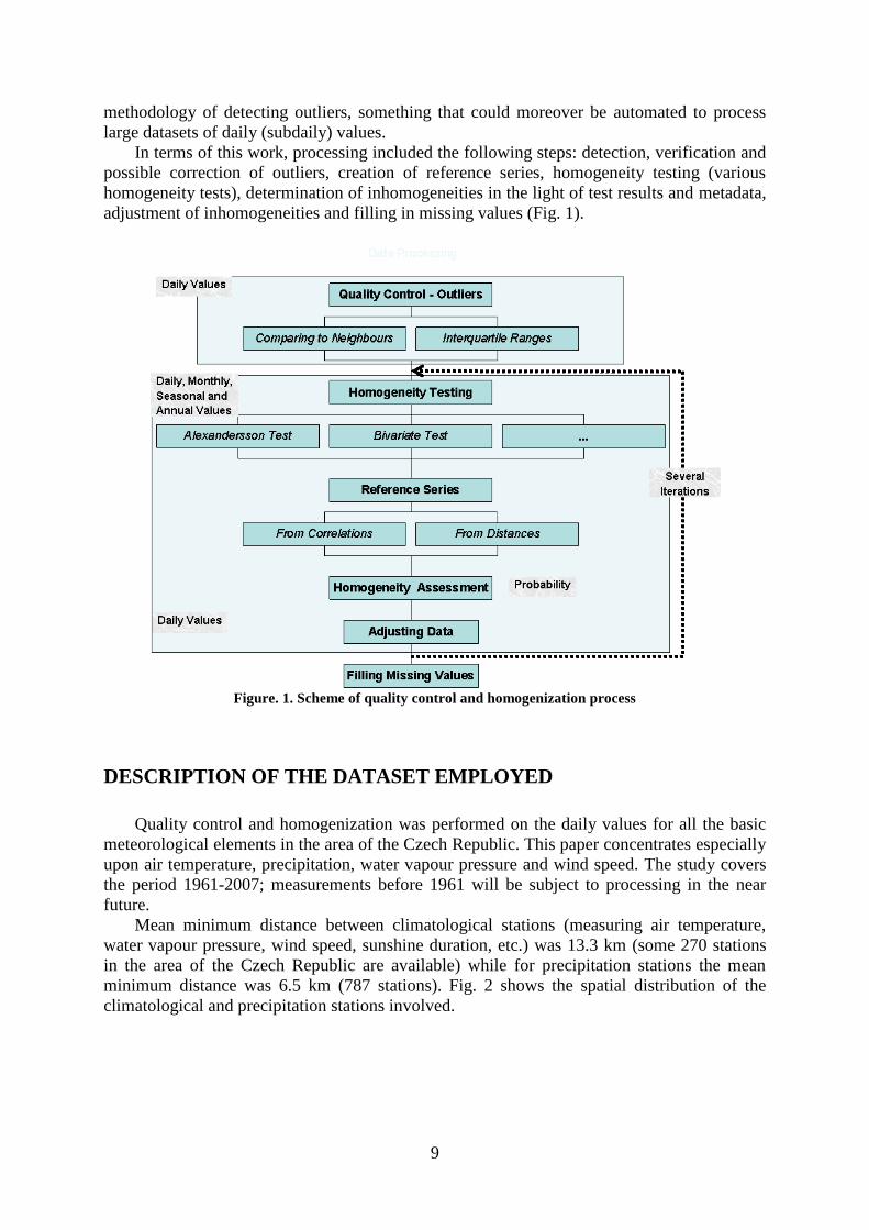
In terms of this work, processing included the following steps: detection, verification and
possible correction of outliers, creation of reference series, homogeneity testing (various
homogeneity tests), determination of inhomogeneities in the light of test results and metadata,
adjustment of inhomogeneities and filling in missing values (Fig. 1).
Figure. 1. Scheme of quality control and homogenization process
DESCRIPTION OF THE DATASET EMPLOYED
Quality control and homogenization was performed on the daily values for all the basic
meteorological elements in the area of the Czech Republic. This paper concentrates especially
upon air temperature, precipitation, water vapour pressure and wind speed. The study covers
the period 1961-2007; measurements before 1961 will be subject to processing in the near
future.
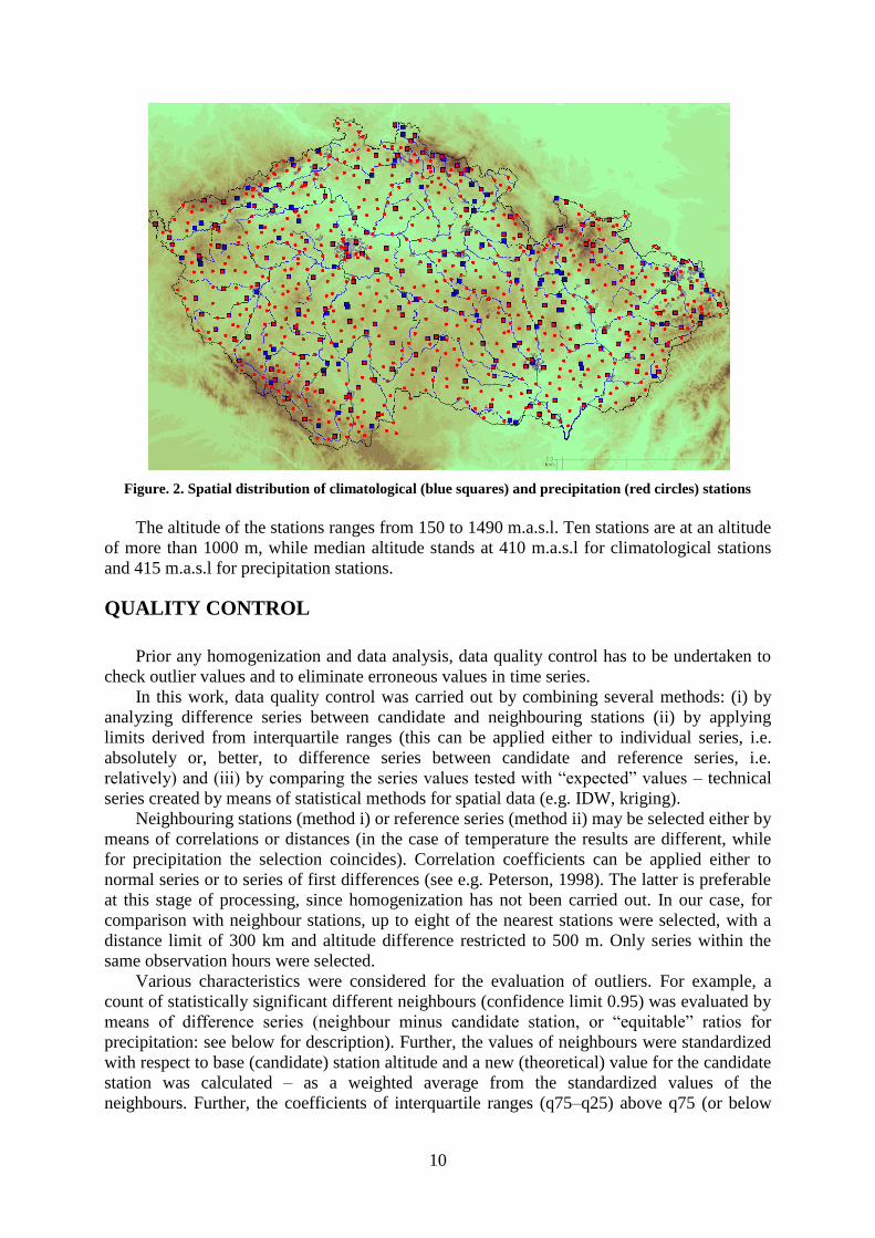
Mean minimum distance between climatological stations (measuring air temperature,
water vapour pressure, wind speed, sunshine duration, etc.) was 13.3 km (some 270 stations
in the area of the Czech Republic are available) while for precipitation stations the mean
minimum distance was 6.5 km (787 stations). Fig. 2 shows the spatial distribution of the
climatological and precipitation stations involved.
10
Figure. 2. Spatial distribution of climatological (blue squares) and precipitation (red circles) stations
The altitude of the stations ranges from 150 to 1490 m.a.s.l. Ten stations are at an altitude
of more than 1000 m, while median altitude stands at 410 m.a.s.l for climatological stations
and 415 m.a.s.l for precipitation stations.
QUALITY CONTROL
Prior any homogenization and data analysis, data quality control has to be undertaken to
check outlier values and to eliminate erroneous values in time series.
In this work, data quality control was carried out by combining several methods: (i) by
analyzing difference series between candidate and neighbouring stations (ii) by applying
limits derived from interquartile ranges (this can be applied either to individual series, i.e.
absolutely or, better, to difference series between candidate and reference series, i.e.
relatively) and (iii) by comparing the series values tested with “expected” values – technical
series created by means of statistical methods for spatial data (e.g. IDW, kriging).
Neighbouring stations (method i) or reference series (method ii) may be selected either by
means of correlations or distances (in the case of temperature the results are different, while
for precipitation the selection coincides). Correlation coefficients can be applied either to
normal series or to series of first differences (see e.g. Peterson, 1998). The latter is preferable
at this stage of processing, since homogenization has not been carried out. In our case, for
comparison with neighbour stations, up to eight of the nearest stations were selected, with a
distance limit of 300 km and altitude difference restricted to 500 m. Only series within the
same observation hours were selected.
Various characteristics were considered for the evaluation of outliers. For example, a
count of statistically significant different neighbours (confidence limit 0.95) was evaluated by
means of difference series (neighbour minus candidate station, or “equitable” ratios for
precipitation: see below for description). Further, the values of neighbours were standardized
with respect to base (candidate) station altitude and a new (theoretical) value for the candidate
station was calculated – as a weighted average from the standardized values of the
neighbours. Further, the coefficients of interquartile ranges (q75–q25) above q75 (or below

11
q25) were evaluated (calculated from the standardized neighbour values), and applied to
candidate station value; this was done in order to assess similarity of neighbour values used
with regard to the test value: the more values of neighbours are similar, the higher the value of
the coefficient becomes.
The final decision on removing outliers was based on a combination of factors: the
percentage of the count of significantly different neighbours (for automation of quality
control, 75% was applied); the probability of median of all neighbours-base differences or
ratios (for automation CDF>0.95, normal distribution, was taken); difference between base
station value and median calculated from standardized neighbours values, expressed as
probability (for automation CDF>0.95 applied again); coefficient of interquartile range – base
station value compared to standardized neighbours values (considering coefficient of IQR of
more than 3 for automation); difference between expected value and median calculated from
original values of neighbours divided by standard deviation of base station (CDF<0.9 with
respect to automation), and finally, after automatic selection applying the limits mentioned,
by visual (subjective) comparison of the standardized values of neighbours with the candidate
station values. Fig. 3 shows an example of the parameter settings for calculation in
ProClimDB software and final output for decision-making about outliers.
Further details on the quality control process may be found in the documentation for
ProClimDB software (Ńtěpánek, 2008).
Figure 3. Setting the ProClimDB software for outlier values evaluation. Top (two-way processing:
selection of neighbours and calculation of characteristics for evaluation of outliers). Bottom: example of
output with auxiliary characteristics for quality control evaluation.
HOMOGENIZATION
Although daily values were the subject of processing in this work, detection of
inhomogeneities was performed using monthly means (or sums in the case of precipitation).
Inhomogeneities are easier to detect in monthly series because they involve less noise than
daily values. Moreover, daily values for some meteorological elements (e.g. air temperature)
are dependent, so application of common statistical tests is difficult. Transformation of daily

12
precipitation sums to normal distribution is not easy either, even where possible, and there are
certain drawbacks to such processing, for example fewer values available for analysis when
omitting zero values).
The relative homogeneity tests applied were: Standard Normal Homogeneity Test
[SNHT] (Alexandersson, 1986, 1995); the Maronna and Yohai bivariate test (Potter, 1981);
and the Easterling and Peterson test (Easterling, Peterson, 1995). Reference series calculations
were based on distances from the five nearest stations, with a distance limit of 300 km and an
altitude difference limit of 500 m. The power for weights (inverse distance) for temperature
and water vapour pressure was taken as 1, for wind speed as 2 and for precipitation as 3.
Neighbouring station values were standardized to average and standard deviation of candidate
station. An example of parameter settings for the calculation of reference series by means of
ProClimDB software is shown in Fig. 4. Detection of inhomogeneities was performed for
series to a maximum duration of 40 years, while the overlap for two consecutive periods was
10 years (requirements of SNHT tests for one shift). The tests were applied on monthly as
well as seasonal and annual averages (sums).
Figure 4. Settings for calculation of reference series in ProClimDB software, air temperature (left) and
precipitation (right)
The main criterion for determining a year of inhomogeneity was the probability of
detection of a given year, i.e. the ratio between the count of detections for a given year from
all test results for a given station (using type of reference series, range of tests applied,
monthly, seasonal and annual series) and the count of all theoretically possible detections.
Further details of reference series creation and testing may be found in Ńtěpánek et al. (2007).
After evaluation of detected breaks and comparison with metadata, a final decision on
correction of inhomogeneities was made. Data were corrected on a daily scale. Adjustment of
such inhomogeneities was addressed by means of a reference series calculated from the
weighted average over the five nearest stations (weights as inverse distance and with a power
of 0.5 for temperature, water vapour pressure and with a power of 1 for precipitation and wind
speed), applying standardization of neighbour station series to average and standard deviation
of candidate station. Reference series for inhomogeneity corrections were calculated on a
daily scale, five years before and after a break.
We created our own correction method, an adaptation of a method for the correction of
regional climate model outputs by Déqué (2007), itself based on assumptions similar to those
implicit in methods described by Trewin and Trevitt (1996) and Della-Marta (2006), which
apply variable correction according to individual percentiles (or deciles). Our process is based
on comparison of percentiles (empirical distribution) of differences (or ratios) between

13
candidate and reference series before and after a break. Percentiles are estimated from
candidate series and values for differences of candidate and references series are taken from
the same time (date). Each month is processed individually, but also taking into account the
values of adjacent months before and after it to ensure smoother passage from one month to
another. Candidate – reference differences for individual percentiles are then differenced
before and after a break and smoothed by low-pass filter to obtain a final adjustment based on
a given percentile (see Fig. 5 for illustration). Values (before a break) are then adjusted in
such a way that we find a value for the candidate series before a break (interpolating between
two percentile values if needed) and the corresponding correction factor, which is then
applied to the value to be adjusted. Special treatment is needed for outlier values at the ends
of distributions.
Figure 5. Deriving corrections for individual percentiles from differences between candidate and
reference series before and after a break
Various characteristics were analyzed before applying the adjustments: the increment of
correlation coefficients between candidate and reference series after adjustments; any change
of standard deviation in differences before and after the change; presence of linear trends, etc.
In the event of any doubt, the adjustments were not applied.
The above-mentioned steps (homogeneity testing, evaluation and correction of
inhomogeneities detected) were performed in several iterations. At each iteration, more
precise results were obtained. Missing values were filled in only after homogenization and
adjustment of inhomogeneities in the series. The reason for this was that the new values were
estimated from data not influenced by possible shifts in the series. Moreover, when missing
data are filled in before homogenization, they may influence inhomogeneity detection in a
negative way.
QUALITY CONTROL RESULTS
Various meteorological elements were subject to thorough quality control according to
the methodology described in section 3. An optimal set of parameters was found for each
meteorological element (by cross-validation). For temperature this was, for example,
standardization to altitude (for each day individually), power of weight (reciprocal value of
distance) of 1, trimmed mean (applying 0.2 and 0.8 percentiles), no regression correction and
outliers check (CDF=0.99). For precipitation, water vapour pressure and wind speed, trimmed
mean was not applied; power of weights was taken as 3 for precipitation, 2 for wind and 1 for
water vapour pressure. Moreover, for precipitation, transformation of values was applied to
obtain a comparable value not dependent upon the mode of division (i.e. X/Y or Y/X have the
same distance from 1).
-6.0
-5.0
-4.0
-3.0
-2.0
-1.0
0.0
1.0
2.0
3.0
4.0
5.0
6.0
0.0
01
0.0
55
0.1
10
0.1
64
0.2
18
0.2
73
0.3
27
0.3
82
0.4
36
0.4
90
0.5
45
0.5
99
0.6
53
0.7
08
0.7
62
0.8
16
0.8
71
0.9
25
0.9
79
Percentile
Tem
pera
ture
/°C
Differences
Smoothed
-6.0
-5.0
-4.0
-3.0
-2.0
-1.0
0.0
1.0
2.0
3.0
4.0
5.0
6.0
0.0
01
0.0
55
0.1
10
0.1
64
0.2
18
0.2
73
0.3
27
0.3
82
0.4
36
0.4
90
0.5
45
0.5
99
0.6
53
0.7
08
0.7
62
0.8
16
0.8
71
0.9
25
0.9
79
Percentile
Tem
pera
ture
/°C
Before break
After break

14
It is important to analyze only measured values in a quality control check; in derivatives
of them such as daily averages, errors are already masked to some extent. This fact is well
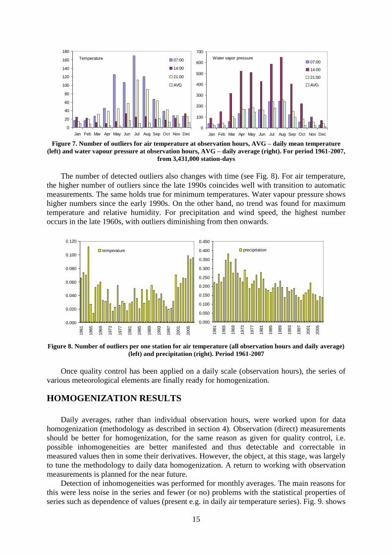
illustrated in Figs. 6 and 7. For air temperature, more outliers were detected in the morning
and evening measurements (probably associated with steeper gradients). The same is true of
relative humidity and wind speed. On the other hand, water vapour pressure shows more
outliers for the 14:00 observation hour compared to morning or evening measurements. In all
these cases, the number of outliers detected in daily mean values is the lowest and in monthly
averages it would be even worse, i.e. only the largest outliers would then be detected.
Figure 6. Number of outliers for air temperature (T) at observation hours 07:00, 14:00, 21:00, AVG –
daily average; daily maximum temperature (TMA), daily minimum temperature (TMI), daily ground
minimum temperature (TPM); water vapour pressure (E), relative humidity (H), wind speed (F). For
period 1961-2007, from 3,431,000 station-days.
The number of detected outliers differs considerably between the various meteorological
elements, e.g. for relative humidity the number is ten times higher than that for air
temperature. The number of outliers for sunshine duration (not shown on the plot) is similar to
that for minimum temperature (1022). For precipitation, this is almost 8000, for new snow
about half of this and for snow depth about a third (however, there are about four times more
precipitation stations than climatological stations).
The number of outliers has clear annual cycle. For most of the elements, a higher number
of outliers was detected in summer months than in winter months (see Figure 7). For air
temperature and minimum temperature, the maximum occurs in July, for water vapour
pressure in August, for wind speed in August. For precipitation there are two maxima per
year, in the summer months and then in January and December, while during spring and
autumn a lower number of outliers was detected. In contrast, sunshine duration shows a
higher number of outliers in January and December, new snow in December (zero in summer
of course) and snow depth in November and April.
Air temperature, as has already been shown (Fig. 6), exhibits more errors in daily
minimum (or ground minimum) temperature compared to maximum temperature, but the
ratios change considerably in the course of the year. While in summer months the number of
detected outliers for minimum or ground minimum temperatures is much higher (e.g. ten
times so in July), in the winter months the number is the same; the number of maximum
temperature outliers does not change very much in the course of the year.
0
200
400
600
800
1000
1200
T_07:0
0
T_14:0
0
T_21:0
0
T_A
VG
TM
A
TM
I
TP
M
0
2000
4000
6000
8000
10000
12000
14000
16000
18000
E_07:0
0
E_14:0
0
E_21:0
0
E_A
VG
H_07:0
0
H_14:0
0
H_21:0
0
H_A
VG
F_07:0
0
F_14:0
0
F_21:0
0
F_A
VG
15
Figure 7. Number of outliers for air temperature at observation hours, AVG – daily mean temperature
(left) and water vapour pressure at observation hours, AVG – daily average (right). For period 1961-2007,
from 3,431,000 station-days
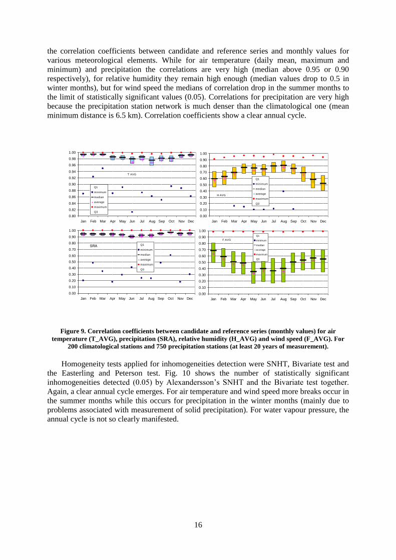
The number of detected outliers also changes with time (see Fig. 8). For air temperature,
the higher number of outliers since the late 1990s coincides well with transition to automatic
measurements. The same holds true for minimum temperatures. Water vapour pressure shows
higher numbers since the early 1990s. On the other hand, no trend was found for maximum
temperature and relative humidity. For precipitation and wind speed, the highest number
occurs in the late 1960s, with outliers diminishing from then onwards.
Figure 8. Number of outliers per one station for air temperature (all observation hours and daily average)
(left) and precipitation (right). Period 1961-2007
Once quality control has been applied on a daily scale (observation hours), the series of
various meteorological elements are finally ready for homogenization.
HOMOGENIZATION RESULTS
Daily averages, rather than individual observation hours, were worked upon for data
homogenization (methodology as described in section 4). Observation (direct) measurements
should be better for homogenization, for the same reason as given for quality control, i.e.
possible inhomogeneities are better manifested and thus detectable and correctable in
measured values then in some their derivatives. However, the object, at this stage, was largely
to tune the methodology to daily data homogenization. A return to working with observation
measurements is planned for the near future.
Detection of inhomogeneities was performed for monthly averages. The main reasons for
this were less noise in the series and fewer (or no) problems with the statistical properties of
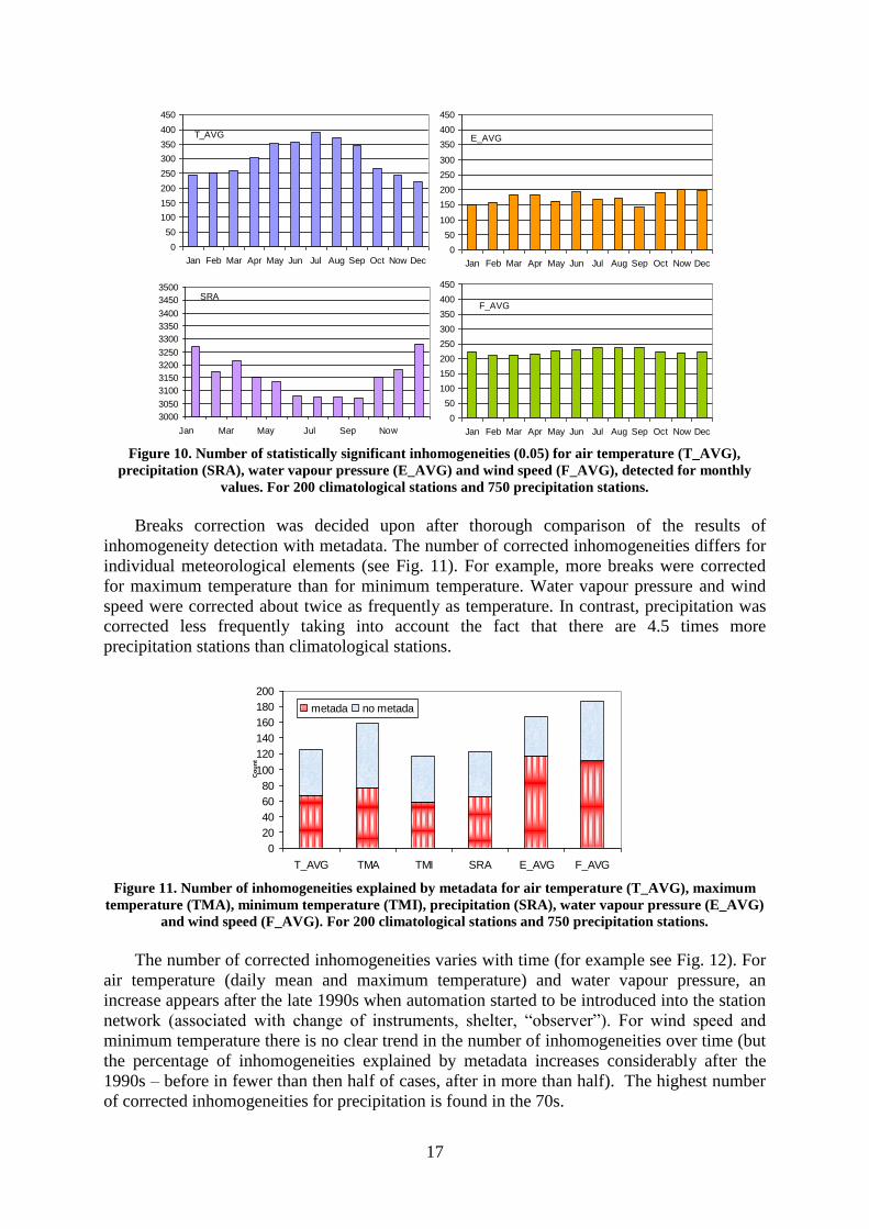
series such as dependence of values (present e.g. in daily air temperature series). Fig. 9. shows
Temperature
0
20
40
60
80
100
120
140
160
180
Jan Feb Mar Apr May Jun Jul Aug Sep Oct Nov Dec
07:00
14:00
21:00
AVG
Water vapor pressure
0
100
200
300
400
500
600
700
Jan Feb Mar Apr May Jun Jul Aug Sep Oct Nov Dec
07:00
14:00
21:00
AVG
0.000
0.050
0.100
0.150
0.200
0.250
0.300
0.350
0.400
0.450
1961
1965
1969
1973
1977
1981
1985
1989
1993
1997
2001
2005
precipitation
0.000
0.020
0.040
0.060
0.080
0.100
0.120
1961
1965
1969
1973
1977
1981
1985
1989
1993
1997
2001
2005
temperature
16
the correlation coefficients between candidate and reference series and monthly values for
various meteorological elements. While for air temperature (daily mean, maximum and
minimum) and precipitation the correlations are very high (median above 0.95 or 0.90
respectively), for relative humidity they remain high enough (median values drop to 0.5 in
winter months), but for wind speed the medians of correlation drop in the summer months to
the limit of statistically significant values (0.05). Correlations for precipitation are very high
because the precipitation station network is much denser than the climatological one (mean
minimum distance is 6.5 km). Correlation coefficients show a clear annual cycle.
Figure 9. Correlation coefficients between candidate and reference series (monthly values) for air
temperature (T_AVG), precipitation (SRA), relative humidity (H_AVG) and wind speed (F_AVG). For
200 climatological stations and 750 precipitation stations (at least 20 years of measurement).
Homogeneity tests applied for inhomogeneities detection were SNHT, Bivariate test and
the Easterling and Peterson test. Fig. 10 shows the number of statistically significant
inhomogeneities detected (0.05) by Alexandersson‟s SNHT and the Bivariate test together.
Again, a clear annual cycle emerges. For air temperature and wind speed more breaks occur in
the summer months while this occurs for precipitation in the winter months (mainly due to
problems associated with measurement of solid precipitation). For water vapour pressure, the
annual cycle is not so clearly manifested.
0.80
0.82
0.84
0.86
0.88
0.90
0.92
0.94
0.96
0.98
1.00
Jan Feb Mar Apr May Jun Jul Aug Sep Oct Nov Dec
Q1
minimum
median
average
maximum
Q3
T AVG
0.00
0.10
0.20
0.30
0.40
0.50
0.60
0.70
0.80
0.90
1.00
Jan Feb Mar Apr May Jun Jul Aug Sep Oct Nov Dec
Q1
minimum
median
average
maximum
Q3
SRA
0.00
0.10
0.20
0.30
0.40
0.50
0.60
0.70
0.80
0.90
1.00
Jan Feb Mar Apr May Jun Jul Aug Sep Oct Nov Dec
Q1
minimum
median
average
maximum
Q3
H AVG
0.00
0.10
0.20
0.30
0.40
0.50
0.60
0.70
0.80
0.90
1.00
Jan Feb Mar Apr May Jun Jul Aug Sep Oct Nov Dec
Q1
minimum
median
av erage
maximum
Q3
F AVG
17
Figure 10. Number of statistically significant inhomogeneities (0.05) for air temperature (T_AVG),
precipitation (SRA), water vapour pressure (E_AVG) and wind speed (F_AVG), detected for monthly
values. For 200 climatological stations and 750 precipitation stations.
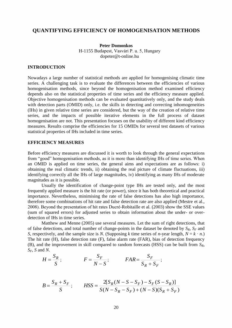
Breaks correction was decided upon after thorough comparison of the results of
inhomogeneity detection with metadata. The number of corrected inhomogeneities differs for
individual meteorological elements (see Fig. 11). For example, more breaks were corrected
for maximum temperature than for minimum temperature. Water vapour pressure and wind
speed were corrected about twice as frequently as temperature. In contrast, precipitation was
corrected less frequently taking into account the fact that there are 4.5 times more
precipitation stations than climatological stations.
Figure 11. Number of inhomogeneities explained by metadata for air temperature (T_AVG), maximum
temperature (TMA), minimum temperature (TMI), precipitation (SRA), water vapour pressure (E_AVG)
and wind speed (F_AVG). For 200 climatological stations and 750 precipitation stations.
The number of corrected inhomogeneities varies with time (for example see Fig. 12). For
air temperature (daily mean and maximum temperature) and water vapour pressure, an
increase appears after the late 1990s when automation started to be introduced into the station
network (associated with change of instruments, shelter, “observer”). For wind speed and
minimum temperature there is no clear trend in the number of inhomogeneities over time (but
the percentage of inhomogeneities explained by metadata increases considerably after the
1990s – before in fewer than then half of cases, after in more than half). The highest number
of corrected inhomogeneities for precipitation is found in the 70s.
0
50
100
150
200
250
300
350
400
450
Jan Feb Mar Apr May Jun Jul Aug Sep Oct Now Dec
T_AVG
3000
3050
3100
3150
3200
3250
3300
3350
3400
3450
3500
Jan Mar May Jul Sep Now
SRA
0
50
100
150
200
250
300
350
400
450
Jan Feb Mar Apr May Jun Jul Aug Sep Oct Now Dec
F_AVG
0
50
100
150
200
250
300
350
400
450
Jan Feb Mar Apr May Jun Jul Aug Sep Oct Now Dec
E_AVG
0
20
40
60
80
100
120
140
160
180
200
T_AVG TMA TMI SRA E_AVG F_AVG
Co
un
t
metada no metada

18
Figure 12. Number of corrected inhomogeneities for air temperature for individual years, divided into the
number of unexplained breaks (no metadata), explained by metadata (metadata) and associated with
automation (metadadata – AMS). For 200 climatological stations
An annual cycle is also clearly manifested in the correction of inhomogeneities (data
corrected on a daily scale as described in section 4). Considering the absolute values of
corrections, the degrees of adjustment were higher during the summer months for air
temperature and water vapour pressure, while for wind speed slightly lower adjustments were
made in the summer months compared with those of winter. For precipitation, major
corrections (ratios) were applied in winter months. After correction, correlation coefficients
increased mainly in the summer months (air temperature, water vapour pressure and also wind
speed).
Future work will lead to the application of observation hour measurements for
homogenization, not just daily averages. On preliminary comparison, the results achieved
(homogenized daily data) should differ only negligibly from the results obtained by
application of observation hours, so a start can be made on using the currently acquired series
for various data analyses requiring homogeneous daily data, e.g. studies of extremes.
CONCLUSIONS
The current work presents a methodology for outlier detection and series homogenization
for various meteorological elements in the area of the Czech Republic in the period 1961-
2007.
A method for outlier detection that could be automated to the greatest extent was a
priority, since millions of values had to be processed for each meteorological element. Such a
method was finally found and successfully applied. It utilizes a combination of several
methods for outlier detection. No one method alone was found adequate; only a combination
leads to satisfying results – the discovery of real outliers and suppression of fault alarms.
Parameters (the settings appropriate to the methods) had to be found individually for each
meteorological element.
In the outlier detection itself, errors must be sought in straight, measured data rather than
merely daily averages or even monthly averages (sums), since outliers are masked to a greater
or lesser extent in the latter. Errors in measurement tend to occur more frequently in certain
parts of the year, generally in the summer months.
A clear annual cycle also emerged in several of the characteristics of the inhomogeneities
detected. For example, air temperature inhomogeneities occur mainly in the summer months
and the same holds for the amount of corrections applied, while in the case of precipitation
0
2
4
6
8
10
12
1961
1963
1965
1967
1969
1971
1973
1975
1977
1979
1981
1983
1985
1987
1989
1991
1993
1995
1997
1999
2001
2003
2005
2007
Co
un
t
no metadata
metadata
metadata - AMS

19
more inhomogeneities were detected in the winter months (associated with solid precipitation
measurements); the corrections applied were also higher in the winter months. Automation of
measurements had very strong influence on the homogeneity of station time series (and even
the occurrence of outliers) in terms of most of the meteorological elements (with the
exception of minimum temperature, precipitation and wind speed). Fortunately, automation
was introduced successively into the station network so it was possible to detect it and make
corrections without major problems.
The data processing for this work was carried out by means of ProClimDB software for
processing whole datasets (finding outliers, combining series, creating reference series,
preparing data for homogeneity testing, etc.) and AnClim software for homogeneity testing
(http://www.climahom.eu). Further development of the software, e.g. connection with R
software, is ongoing.
Further steps in quality control and homogenization will lead to analysis of individual
observation hours and also historical data.
Acknowledgements The authors would like to acknowledge the financial support of the Grant Agency of the Czech
Republic for project no. 205/08/1619 and the European Commission for Contract No. 037005.
References Alexandersson, A. (1986): A homogeneity test applied to precipitation data. Journal of Climatology, 6, 661–675.
Alexandersson, A. (1995): Homogenity testing, multiple breaks and trends. In: Proc. 6th Int. Meeting on Stat.
Climatology, Galway, Ireland, 439–441.
Brandsma, T. (2000): Weather-type dependent homogenization of daily Zwanenburg/De Bilt temperature series.
http://www.met.hu/omsz.php?almenu_id=omsz&pid=seminars&pri=6&mpx=1&sm0=0&tfi=brandsma
Della-Marta, P. M., Wanner, H. (2006): A Method of Homogenizing the Extremes and Mean of Daily
Temperature Measurements. Journal of Climate, 19, 4179-4197.
Déqué, M. (2007): Frequency of precipitation and temperature extremes over France in an anthropogenic
scenario: model results and statistical correction according to observed values. Global and Planetary
Change, 57, 16-26.
Easterling, D. R., Peterson, T. C. (1995): A new method for detecting undocumented discontinuities in
climatological time series. International Journal of Climatology, 15, 369–377.
Peterson, T. C. (1998): Homogeneity adjustments of in situ atmospheric climate data: a review. International
Journal of Climatology, 18, 1493–1517.
Petrovic, P. (2004): Detecting of inhomogeneities in time series using Real Precision Metod. In: Fourth seminar
for homogenization and quality control in climatological databases (Budapest, Hungary, 6-10 October 2003),
WCDMP-No. 56. WMO, Geneva, 79–88.
Potter, K.W. (1981): Illustration of a New Test for Detecting a Shift in Mean in Precipitation Series. Mon. Wea.
Rev., 109, 2040-2045.
Ńtěpánek, P., Řezníĉková, L., Brázdil, R. (2007): Homogenization of daily air pressure and temperature series
for Brno (Czech Republic) in the period 1848–2005 In: Proceedings of the Fifth seminar for homogenization
and quality control in climatological databases (Budapest, 29 May – 2 June 2006), WCDMP. WMO,
Genova. (submitted)
Ńtěpánek, P. (2008): ProClimDB – software for processing climatological datasets. CHMI, regional office Brno.
http://www.climahom.eu/ProcData.html
Trewin, B.C., Trevitt A.C.F. (1996) The development of composite temperature records. Int J Climatol 16:1227–
1242.
Vincent, L. A., X. Zhang, B. R. Bonsal, and W. D. Hogg (2002): Homogenization of daily temperatures over
Canada. Journal of Climate, 15, 1322-1334.
Wijngaard, J. B. , Klein Tank, A. M. G. , Können, G. P. (2003): Homogenity of 20th century European daily
temperature and precipitation series. Int. J. Climatol., 23, 679–692
20
QUANTIFYING EFFICIENCY OF HOMOGENISATION METHODS
Peter Domonkos
H-1155 Budapest, Vasvári P. u. 5, Hungary
INTRODUCTION
Nowadays a large number of statistical methods are applied for homogenising climatic time
series. A challenging task is to evaluate the differences between the efficiencies of various
homogenisation methods, since beyond the homogenisation method examined efficiency
depends also on the statistical properties of time series and the efficiency measure applied.
Objective homogenisation methods can be evaluated quantitatively only, and the study deals
with detection parts (OMID) only, i.e. the skills in detecting and correcting inhomogeneities
(IHs) in given relative time series are considered, but the way of the creation of relative time
series, and the impacts of possible iterative elements in the full process of dataset
homogenisation are not. This presentation focuses on the usability of different kind efficiency
measures. Results comprise the efficiencies for 15 OMIDs for several test datasets of various
statistical properties of IHs included in time series.
EFFICIENCY MEASURES
Before efficiency measures are discussed it is worth to look through the general expectations
from “good” homogenisation methods, as it is more than identifying IHs of time series. When
an OMID is applied on time series, the general aims and expectations are as follows: i)
obtaining the real climatic trends, ii) obtaining the real picture of climate fluctuations, iii)
identifying correctly all the IHs of large magnitudes, iv) identifying as many IHs of moderate
magnitudes as it is possible.
Usually the identification of change-point type IHs are tested only, and the most
frequently applied measure is the hit rate (or power), since it has both theoretical and practical
importance. Nevertheless, minimising the rate of false detections has also high importance,
therefore some combinations of hit rate and false detection rate are also applied (Mestre et al.,
2008). Beyond the presentation of hit rates Ducré-Robitaille et al. (2003) show the SSE values
(sum of squared errors) for adjusted series to obtain information about the under- or over-
detection of IHs in time series.
Matthew and Menne (2005) use several measures. Let the sum of right detections, that
of false detections, and total number of change-points in the dataset be denoted by SR, SF and
S, respectively, and the sample size is N. (Supposing k time series of n-year length, N = k · n.)
The hit rate (H), false detection rate (F), false alarm rate (FAR), bias of detection frequency
(B), and the improvement in skill compared to random forecasts (HSS) can be built from SR,
SF, S and N.
S
SH R ;
SN
SF F
;
FR
F
SS
SFAR
;
S
SSB FR ;
))(()(
)]()([2
FRFR
RFFR
SSSNSSNS
SSSSSNSHSS

21
The diversity of efficiency measures can be reasoned by the fact that efficiency depends on
the purpose of the homogenisation, as well as on the statistical characteristics of time series.
In addition, even such simple concepts as “right detection” and “false detection” are not
absolutely objective, because their definitions need subjective decisions about the tolerance in
lapse of timings (j) and magnitudes (m). We apply arbitrary, but reasonable choices for the
estimation of efficiencies. In this study the H, FAR, and three further measures are applied.
Two of the latter three (EA and EB, see below) are for evaluating detection skill, while the
third one (ET) is dedicated to control the impact of OMIDs on the reliability of linear trend
estimations.
S
SSE FR
A
kS
kSSE FR
B
The conception of EA is that the importance of finding real IHs and avoiding false detections
is practically the same. However, in case of low number of factual IHs, EA can easily be
negative, even if only a few false detections occurred. In contrast, this inconvenience cannot
happen with EB. In case of a pure white noise the target value of (1 - EB) equals with the
probability of first type error in hypothesis testing for the existence of homogeneous or
inhomogenous character of time series. In case of large number of large IHs in time series EB
shows similar values to EA. With moderate intensity of IHs EB is always substantially higher
than EA, but just because of the systematic character of (EB - EA), the rank order among
OMIDs is not affected by the choice between EA and EB.
For controlling the reliability of trend estimations, the difference between the mean
bias of trend estimations for homogenised time series (f), and that for time series without
homogenisation (f0) is calculated:
0
0
f
ffET
ET shows the improvement in preciseness of trend estimations owing to homogenisation. In
this study the trend estimations for the whole (100-year long) time series, and those for the
last 50 year sections are evaluated.
Definitions for calculating detection skill:
• In the detection process IH magnitudes are expressed in the proportion of the
estimated standard deviation of noise (se*) in the examined time series.
Te ss 2R1* if R > 0
Te ss * if R 0 ,
where R denotes 1-year lag autocorrelation, and sT means the empirical standard deviation of
the time series. The application of the unit se* is reasoned by the fact that during the detection
process the factual standard deviation of noise process (se) is known only for simulated time
series, while for time series from observations this characteristic is unknown. In contrast, se*
can easily be calculated for any time series. se* is usually higher than se, but never higher than
sT. Thus se* is a better estimation of se, than sT would be.
• In calculating EA or EB factual IHs only with m > mo magnitudes are considered, and
mo is 2 or 3 in this study.
• Right detection: A shift with m 1.5 for mo = 2 (m 2 for mo = 3) is detected with
maximum j =1 time lapse.

22
• False detection: A shift with m 1.5 for mo = 2 (m 2 for mo = 3) is detected at year j,
but there is no shift of the same direction than the detected one with m > 0 within the (j-2,j+2)
period.
Considering that individual efficiency measures may reflect only some special features of
OMIDs instead of their efficiency in a broader sense, some combinations of different kind
measures, especially the combination of detection skill and skill in trend estimations might be
beneficial. Domonkos (2006a) introduced such an efficiency measure (“general efficiency”),
but we admit that such a measure is rather complicated and its structure is based on subjective
decisions. In this presentation the general efficiency is not used.
HOMOGENISATION METHODS EXAMINED
Fifteen OMIDs are examined in the presentation, all of them are the same as those were used
in Domonkos (2006a). In this paper basic parameterisations are used only, thus Caussinus -
Mestre method and MASH are represented here only with one-one version. Details about
method parameterisation, handling of outliers and the way of detecting multiple IHs can be
found in Domonkos (2006a, 2006b). The fifteen OMIDs are listed here in alphabetical order.
a) Bayesian test (Ducré-Robitaille et al., 2003) with penalised maximum likelihood method
for calculating number of change-points (Caussinus and Lyazrhi, 1997; Mestre, 2004) [Bay]
b) Bayesian test (Ducré-Robitaille et al., 2003) with serial correlation analysis (Sneyers,
1999) [Ba1]
c) Buishand-test [Bu1] (maximum of the absolute values of accumulated anomalies,
Buishand, 1982)
d) Buishand-test [Bu2] (difference between maximum and minimum values of accumulated
anomalies, Buishand, 1982)
e) Caussinus - Mestre method [C-M] (Caussinus and Mestre, 2004)
f) Easterling-Peterson test [E-P] (Easterling and Peterson, 1995)
g) Mann-Kendall test [M-K] (Aesawy and Hasanean, 1998)
h) Multiple Analysis of Series for Homogenisation [MAS] (Szentimrey, 1999)
i) Multiple Linear Regression [MLR] (Vincent, 1998)
j) Pettitt-test [Pet] (Pettitt, 1979)
k) Standard Normal Homogeneity Test for shifts only [SNH] (Alexandersson, 1986)
l) Standard Normal Homogeneity Test for shifts and trends [SNT] (Alexandersson and
Moberg, 1997)
m) t-test [tt1] (Ducré-Robitaille et al., 2003)
n) t-test [tt2] (Kyselý and Domonkos, 2006)
o) Wilcoxon Rank Sum test [WRS] (Karl and Williams, 1987)
DATASETS FOR EFFICIENCY TESTING
Efficiency of OMIDs strongly depends on the statistical properties of IHs in datasets
examined. Therefore the creation of proper datasets has crucial importance in the test
procedure. In Domonkos (2006a) a dataset was developed in which the statistical properties of
IHs highly resemble that of observed temperature time series in Hungary. More precisely, the
resemblance is valid for relative time series with at least 0.4 autocorrelation, and the relative
time series are derived from the observed data field by Peterson and Easterling (1994). This
presentation uses again that dataset, but together with four other datasets, since one aim of the
study is to compare the performances of efficiency measures in different tasks. Each dataset

23
comprises 10,000 one hundred year long relative time series. The time series are built from a
standard white noise and artificially inserted IHs. In the creation of test datasets IH
magnitudes are expressed with their proportion to se. Because of the difference in the applied
unit magnitudes here are denoted with m’.
The IH properties in the five datasets are as follows.
a) “1 IH only”: One IH is included in each time series. Its type is change-point, the timing (j)
is 40 or 60, and m’ = 3.
b) “1+4 IHs”: Five change-points are included, one with j = 40 and m’ = 3, while the others
are with random timing and a fixed magnitude, m’ = 1.5. Minimum distance between adjacent
IHs and from the endpoints of the series is 4 years.
c) “EXP, m‟< 6”: The mean frequency occurrence is one IH per decade, but IH-frequencies in
individual time series may deviate from the average. All the IHs are change-points, their signs
(positive or negative), timings and magnitudes are random. Magnitudes (m’) are between 0
and 6, they are exponentially distributed for m’ > 1, and equally distributed for m’ < 1. In the
below formula q is a random variable with equal distribution between 0 and 1.
)36.0(8.2 ' qem if q 0.36
qm 36.0
1' if q < 0.36
d) “EXP, m‟< 2”: It is similar to “EXP, m‟< 6”, some parameters differ only. The mean
frequency occurrence is one IH per decade again. All the IHs are change-points, their signs
(positive or negative), timings and magnitudes are random. Magnitudes (m’) are between 0
and 2, they are exponentially distributed for m’ > 1, and equally distributed for m’ < 1. Since
all the IH magnitudes are smaller than 2, their appearance is similar to common noise. For this
dataset EA cannot be applied, as the denominator of the formula would be zero.
)59.0(69.1' qem if q 0.59
qm 59.0
1' if q < 0.59
e) “HU standard”: A complex structure of randomly distributed IHs of different types
(change-points, platform-like IH-pairs, trends) and magnitudes. The title “HU standard” refers
to the high resemblance of the statistical properties of IHs between this dataset on one hand,
and relative time series with at least 0.4 first order autocorrelation, derived from an observed
Hungarian temperature dataset, on the other hand. (High autocorrelation in relative time series
is an indicator of substantial pollution by IHs, see e.g. Sneyers, 1999.)
The mean frequency of IHs is about 3 per decade, but most of them have short duration
and small magnitude. The decline of frequency with growing magnitudes is considerably
faster for m < 2.9 magnitudes, than in case of EXP, m‟< 6. As a result of this difference in the
magnitude distribution, there are much less IHs of 1.5 < m < 4 in HU standard, than in EXP,
m‟< 6, in spite of the fact, that the frequency of all IHs is higher in HU standard. See more
details about the properties of this dataset in Domonkos (2006a).
RESULTS
Fig. 1 presents the detection skills for the OMIDs examined. It comprises eight parts (fig.
1a…1h) differing in the test dataset or mo parameter applied. Usually formula EA (for dataset

24
EXP, m‟< 2 the EB) was used. Results show that i) Detection skill is almost always positive
(number of correct identification is usually larger, than that of false detection for each OMID
examined); ii) Differences according to test dataset characteristics are often larger, than
according to different OMIDs; iii) If results for each specific dataset - OMID pair are
compared, detection skill is always higher with large IHs (mo = 3), than for moderate and high
IHs together (mo = 2), with one exception only (dataset EXP, m‟< 2 with M-K); iv) Rank
order of skills are hardly affected by the arbitrary choice of mo; v) For dataset “1 IH only”
detection skills are higher, than for other datasets (except for tt1), despite the fact that mo = 2
is applied with “1 IH only”, since the size of the IH magnitude does not allow the application
of the higher threshold.
Comparing the results for individual OMIDs, it can be find that C-M, E-P and MAS
usually perform better, than the other methods, particularly with datasets HU standard and
EXP, m‟< 6. In contrast, C-M and MAS are the poorest when there is no IH of substantial size
in the time series (dataset EXP, m‟< 2).
Figure 1. Detection skills for individual OMIDs. Striped: C-M, filled: MAS, dotted: E-P.
a) dataset “1 IH only”, mo = 2.
Figure 1b. Dataset “1+4 IH”, mo = 2
0
25
50
75
100
MLR Bay SNH Ba1 WRS Bu2 Bu1 tt2 E-P C-M MAS SNT Pet tt1 M-K
EA[%]
-10
15
40
65
90
E-P tt2 Bay SNH Ba1 C-M MAS Bu1 WRS Bu2 Pet MLR SNT tt1 M-K
EA[%]

25
Figure 1c. Dataset “EXP, m‟< 6”, mo = 2
Figure 1d. Dataset “EXP, m‟< 6”, mo = 3
Figure 1e. Dataset “EXP, m‟< 2”, mo = 2
0
25
50
75
100
C-M MAS Ba1 E-P Bay SNH tt2 Bu2 Bu1 WRS tt1 Pet MLR SNT M-K
EA[%]
-10
15
40
65
90
MAS E-P C-M Ba1 Bay SNH tt2 tt1 Bu2 Bu1 WRS MLR Pet SNT M-K
EA[%]
0
25
50
75
100
tt1 SNT E-P tt2 Bu1 Pet MLR SNH Bay WRS Bu2 Ba1 M-K MAS C-M
EB[%]

26
Figure 1f. Dataset “EXP, m‟< 2”, mo = 3
Figure 1g. Dataset “HU standard”, mo = 2
Figure 1h. Dataset “HU standard”, mo = 3
0
25
50
75
100
tt1 SNT Bu1 Pet E-P tt2 SNH Bu2 Bay WRS Ba1 MLR MAS M-K C-M
EB[%]
0
25
50
75
100
C-M MAS E-P Ba1 MLR Bay SNH SNT Bu2 Bu1 tt2 tt1 WRS Pet M-K
EA[%]
0
25
50
75
100
MAS C-M E-P Ba1 MLR Bay SNH SNT Bu1 tt1 Bu2 tt2 WRS Pet M-K
EA[%]
27
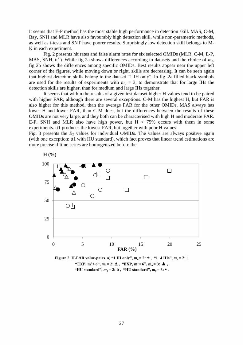
It seems that E-P method has the most stable high performance in detection skill. MAS, C-M,
Bay, SNH and MLR have also favourably high detection skill, while non-parametric methods,
as well as t-tests and SNT have poorer results. Surprisingly low detection skill belongs to M-
K in each experiment.
Fig. 2 presents hit rates and false alarm rates for six selected OMIDs (MLR, C-M, E-P,
MAS, SNH, tt1). While fig 2a shows differences according to datasets and the choice of mo,
fig 2b shows the differences among specific OMIDs. Best results appear near the upper left
corner of the figures, while moving down or right, skills are decreasing. It can be seen again
that highest detection skills belong to the dataset “1 IH only”. In fig. 2a filled black symbols
are used for the results of experiments with mo = 3, to demonstrate that for large IHs the
detection skills are higher, than for medium and large IHs together.
It seems that within the results of a given test dataset higher H values tend to be paired
with higher FAR, although there are several exceptions. C-M has the highest H, but FAR is
also higher for this method, than the average FAR for the other OMIDs. MAS always has
lower H and lower FAR, than C-M does, but the differences between the results of these
OMIDs are not very large, and they both can be characterised with high H and moderate FAR.
E-P, SNH and MLR also have high power, but H < 75% occurs with them in some
experiments. tt1 produces the lowest FAR, but together with poor H values.
Fig. 3 presents the ET values for individual OMIDs. The values are always positive again
(with one exception: tt1 with HU standard), which fact proves that linear trend estimations are
more precise if time series are homogenized before the
Figure 2. H-FAR value-pairs. a) “1 IH only”, mo = 2: + , “1+4 IHs”, mo = 2: ٱ,
“EXP, m‟< 6”, mo = 2: , “EXP, m‟< 6”, mo = 3: ▲ ,
“HU standard”, mo = 2: o , “HU standard”, mo = 3: • .
0
25
50
75
100
0 5 10 15 20 25
H (%)
FAR (%)
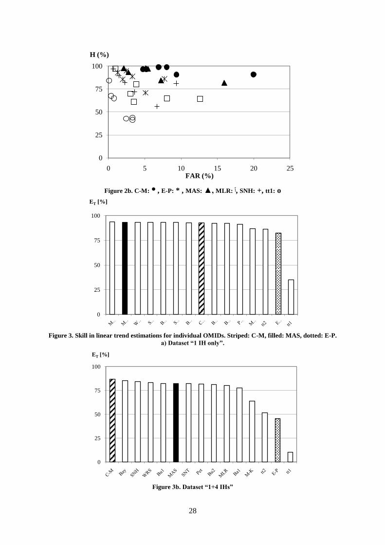
28
Figure 2b. C-M: • , E-P: * , MAS: ▲, MLR: ٱ, SNH: +, tt1: o
Figure 3. Skill in linear trend estimations for individual OMIDs. Striped: C-M, filled: MAS, dotted: E-P.
a) Dataset “1 IH only”.
Figure 3b. Dataset “1+4 IHs”
0
25
50
75
100
0 5 10 15 20 25
H (%)
FAR (%)
0
25
50
75
100
ET [%]
0
25
50
75
100
ET [%]

29
Figure 3c. Dataset “EXP, m‟< 6”
Figure 3d. Dataset “EXP, m‟< 2”
Figure 3e. Dataset “HU standard”
0
25
50
75
100
C-M Bay MAS SNH Bu1 WRS Ba1 Bu2 MLR SNT Pet tt2 M-K E-P tt1
ET [%]
0
25
50
75
100
C-M Bay SNH WRS Bu1 SNT MAS Pet MLR Bu2 Ba1 M-K tt2 E-P tt1
ET [%]
-10
15
40
65
90
C-M MLR Bay MAS SNH WRS Bu1 SNT Pet Bu2 Ba1 M-K tt2 E-P tt1
ET [%]

30
calculation of trends. The five parts of the figure (fig. 3a…3e) are for the five test datasets
applied. Results for different datasets have several common
Characteristics, particularly if the very special case of “1 IH only” is excluded from the
comparisons. Results show that 10-11 OMIDs produce rather similar ET values, while the last
4 ones always have much poorer results. The poorest trend detection skills always belong to
the tt1, E-P, tt2 and M-K. The rank order has similarities also among the best OMIDs. C-M is
always the best according to ET values, the rank of Bay is always 2 or 3, that of SNH is 3-5,
while that of MAS,
Bu1 and WRS is always between 3 and 7. ET values of MLR are usually slightly lower, than
that of several other OMIDs, but in case of HU standard MLR has the second highest skill.
This special feature of the results for MLR may be in connection with the fact that HU
standard is the only test dataset used in this study which contains linear change type IHs
beyond change-points.
DISCUSSION
Efficiencies of fifteen OMIDs were estimated using different efficiency measures and five
different test datasets. The picture is mixed, since the efficiencies strongly depend on the
efficiency measures and test datasets applied. However, several common features were found
among the different kind results. The dependence of the rank order of OMID efficiencies is
strong on the efficiency measure, but moderate only on the test dataset characteristics (with
some exceptions, whose occurrences are rather unlikely in real climatic datasets). The rank
order of skills in trend estimations turned out to be surprisingly independent from test datasets
used. On the other hand, the performances and ranks for a specified OMID are often markedly
different according to different efficiency characteristics, i.e. a specific OMID may perform
very different skills in hit rate, false alarm rate and reliability of trend estimation, the most
striking examples were mentioned in the previous section. The following principles may help
to obtain a general evaluation of OMID efficiencies:
• Various characteristics (hit rate, false alarm rate, etc.) must be evaluated together,
• If the role of one factor (e.g. false alarm rate) is overemphasized, it may result in
misleading consequences. In fact an uncovered IH has very similar impact on the reliability of
climate variability investigations, to the one that can be caused by a false IH of the same
magnitude.
• Since homogenisation procedures often contain iterations, the impacts of iterations on
the growing or abatement of detection errors should also be considered, but it is beyond the
scope of the present study. We note that the performance of detection skill (both the hit rate
and the false alarm rate) likely has higher practical importance, than that of the ET values has,
since detection errors may influence harmfully the forthcoming results of iterations. On the
other hand, low ET values are also indications of certain type detection errors, therefore such a
large negative difference that was experienced with E-P relative to the performance of most
OMIDs, is an indication of limited appropriateness, in spite of high EA and EB values.
• Unified evaluation for the results of various test dataset and parameterization
applications is advantageous.
Our results show that C-M and MAS usually perform better, than the other OMIDs,
and it is particularly valid for dataset “HU standard” which is close to a real, observed dataset.
This finding is not a surprise, since these two methods were developed to detect multiple IHs
without hierarchic algorithm, while some hierarchic way of detection process cannot be
avoided using the other OMIDs. The drawback of hierarchic detection was analysed e.g. by
Menne and Williams (2005), so our results confirm only the superiority of direct methods for
detecting multiple IHs. The results also confirm the theory that non-parametric OMIDs are

31
less powerful in comparison with other OMIDs, although there are some exceptions for this
rule.
It was found that MAS and C-M have clearly higher detection skills in datasets those
mimic observed climatic time series with considerable pollution by IHs (i.e. with at least 0.4
serial correlation in relative time series), and C-M is always the best method according to ET
values. However, the superiority of these OMIDs is not uniform; other “common” OMIDs
sometimes perform better. We name this phenomenon inverse rank order. The main cases of
inverse order are as follows: i) Only one IH exists in the time series (all the evaluated skills),
2) Detection skill is relatively poor when there are several IHs in the time series, but non of
them has large magnitude (in our experiments, when m’ is smaller than 2 for each IH), 3) C-
M (and in some experiments MAS) has slightly higher FAR, than most of the examined
OMIDs have, 4) Trend detection skill is often slightly poorer with MAS, than with Bay and
SNH.
It must be stressed that in spite of the occurrences of inverse rank order, MAS and C-
M are highly recommended for practical use, particularly, because they very often provide the
highest skill, and even in cases of inverse rank orders their efficiencies are not low. On the
other hand, it can be stated that Bay, SNH and MLR are also rather good OMIDs. What is
more, in some specific tasks those have methodological connection with homogeneity
investigations the application of some OMIDs with not very high efficiencies can be the most
advantageous. For instance, in detecting climatic jumps, E-P seems to be an outstandingly
good OMID, because of its uniformly high detection skill in various test datasets.
To reduce the chance of false detection with C-M and MAS, we mention two
opportunities: i) Although both C-M and MAS have inner test to decide about homogeneous
or inhomogeneous character of time series, they tend to detect more false IHs than several
other OMIDs, when there are very few or small IHs only in the time series examined.
Therefore time series with multiple IHs of considerable magnitudes should be preselected
before the application of C-M or MAS. There is also a problematic point, that during the
iterations, if OMIDs are applied repeatedly on the same time series, the chance of false
detection may increase. ii) Another possibility is to introduce optimised parameterisations, as
it was shown in Domonkos (2006a).
Finally we note that further experiments are needed with the use of various test
datasets and efficiency measures, to obtain a more complete picture about OMID efficiencies.
CONCLUSIONS
• Results of efficiency calculations strongly depend on the efficiency measures applied.
Therefore a profound evaluation of the efficiencies for individual OMIDs needs the combined
use of several efficiency measures.
• Efficiencies of individual OMIDs are almost always positive what proves that
homogenised time series are more usable for climate variability investigations, than raw time
series.
• The results of this study confirm that parametric OMIDs usually perform better, than
non-parametric OMIDs, and the highest skills are usually experienced with OMIDs capable of
detecting multiple IHs in a direct (non-hierarchic) way. Two direct OMIDs exist: C-M and
MAS. Their practical use is highly recommended.
• The usefulness of individual OMIDs depends on the statistical properties of time
series. Further examinations of OMID efficiencies are needed relying on experiments with
more various test datasets and parameterizations of efficiency measures, in order to obtain
more exact information about the practical usefulness of OMIDs.

32
Acknowledgements: The research was partly funded by the COST ES0601 project.
References Aesawy, A.M. and Hasanean, H.M., 1998: Annual and seasonal climatic analysis of surface air temperature
variations at six southern Mediterranean stations. Theor. Appl. Climatol. 61, 55-68.
Alexandersson, H. 1986: A homogeneity test applied to precipitation data. J. Climatol. 6, 661-675.
Alexandersson, H. and Moberg, A. 1997: Homogenization of Swedish temperature data. Part I: Homogeneity
test for linear trends. Int. J. Climatol. 17, 25-34.
Buishand, T.A. 1982: Some methods for testing the homogeneity of rainfall records. J. Hydrology 58, 11-27.
Caussinus, H. and Lyazrhi, F. 1997: Choosing a linear model with a random number of change-points and
outliers. Ann. Inst. Statist. Math. 49/4, 761-775.
Caussinus, H. and Mestre, O. 2004: Detection and correction of artificial shifts in climate series. J. Roy. Stat.
Soc. Series C 53, 405-425.
Domonkos, P. 2006a: Testing of homogenisation methods: purposes, tools and problems of implementation.
Proceedings of the 5th
Seminar and Quality Control in Climatological Databases, CD, 126-145.
Domonkos, P. 2006b: Application of objective homogenization methods: Inhomogeneities in time series of
temperature and precipitation. Időjárás 110, 63-87.
Ducré-Robitaille, J-F., Vincent, L.A. and Boulet, G. 2003: Comparison of techniques for detection of
discontinuities in temperature series. Int. J. Climatol. 23, 1087-1101.
Easterling, D.R. and Peterson, T.C. 1995: A new method for detecting undocumented discontinuities in
climatological time series. Int. J. Climatol. 15, 369-377.
Karl, T.R. and Williams Jr, C.N. 1987: An approach to adjusting climatological time series for discontinuous
inhomogeneities. J. Climate Appl. Meteor. 26, 1744-1763.
Kyselý, J. and Domonkos, P. 2006: Recent increase in persistence of atmospheric circulation over Europe:
comparison with long-term variations since 1881. Int. J. Climatol. 26, 461-483.
Menne, M.J. and Williams Jr, C.N. 2005: Detection of undocumented changepoints using multiple test statistics
and composite reference series. J. Climate 18, 4271-4286.
Mestre, O. 2004: Correcting climate series using ANOVA technique. Fourth Seminar for Homogenization and
Quality Control in Climatological Databases, WCDMP 56, WMO-TD 1236, 93-96.
Mestre, O., Domonkos P., Lebarbier, E., Picard, F. and Robin, S. 2008: Comparison of change-point detection
methods in the mean of Gaussian processes. In: Sixth Seminar for Homogenization and Quality Control
in Climatological Databases (in press).
Peterson, T.C. and Easterling, D.R. 1994: Creation of homogeneous composite climatological reference series.
Int. J. Climatol. 14, 671-679.
Pettitt, A.N. 1979: A non-parametric approach to the change-point problem. Applied Statistics 28,126-135.
Sneyers, R., 1999: Homogenizing time series of climatological observations. Second Seminar for
Homogenization of Surface Climatological Data. Hungarian Met. Serv., Budapest, 5-14.
Szentimrey, T. 1999: Multiple Analysis of Series for Homogenization (MASH). Second Seminar for
Homogenization of Surface Climatological Data. WCDMP 41, WMO-TD, 1962, WMO, Geneva, 27-
46.
Vincent, L.A. 1998: A technique for the identification of inhomogeneities in Canadian temperature series. J.
Climate 11, 1094-1104.

33
UNDERSTANDING INTER-SITE TEMPERATURE DIFFERENCES AT
THE KNMI TERRAIN IN DE BILT (THE NETHERLANDS)
Theo Brandsma
Royal Netherlands Meteorological Institute (KNMI), PO Box 201,
3730 AE De Bilt, the Netherlands, Tel: +31 302206911, Fax: +31 302210407,
Abstract
From May 2003 through June 2005 a field experiment was carried out at the KNMI terrain in De Bilt.
At five sites, including the operational site, temperature and wind speed were measured at a height of
1.5 m every minute, using identical instruments. The temperature differences between the sites have
been studied in connection with the wind speed differences and operationally measured weather
variables. During the experiment (in October 2004) a renovation of the nature area just west of the
operational temperature screen took place. The renovation introduced an inhomogeneity in the
temperature time series at the operational site. The inter-site temperature differences are largest in
summer and smallest in winter. Except for the most enclosed site, these temperature differences have
opposite signs for daily maximum and minimum temperatures. As could be expected, the magnitudes
of the differences strongly depend on the weather conditions. The understanding of these dependencies
is an important condition for improving the homogenization of daily temperature series.
INTRODUCTION
Temperature measurements are often an object of debate. Questions arise whether the
measurements are representative for the area that the stations are supposed to represent, or
whether the temperature time series are homogeneous enough to allow studies of climate
trends and climate variability. Meteorologists mostly emphasize the first question while
climatologists are generally more concerned about the second question.
In this context, thermometer exposure and siting are important. WMO (1996) states: “In order
to achieve representative results when comparing thermometer readings at different places
and at different times, a standardized exposure of the screen and, hence, of the thermometer
itself is also indispensable. For general meteorological work, the observed temperature should
be representative of the free air conditions surrounding the stations over as large an area as
possible, at a height of between 1.25 and 2 m above ground level. The height above the
ground level is specified because large vertical temperature gradients may exist in the lowest
layers of the atmosphere. The best site for the measurements is, therefore, over level ground,
freely exposed to sunshine and wind and not shielded by, or close to, trees, buildings and
other obstructions.” From this statement it is obvious that sheltering, and changes in
sheltering due to e.g. growth of trees or relocation are undesirable for air temperature
measurements.
The present study aims at quantifying the possible effects of sheltering on temperature
measurements. These effects have been studied at the local scale of the KNMI-terrain in De
Bilt in a two-year experiment by comparing five different sites. Other causes that may affect
temperature series, e.g., urbanization and reclamation of land, are not taken into account. The
effect of urbanization on the temperature series of the De Bilt is discussed in Brandsma et al.
(2003).

34
This paper summarizes some of the results of the experiment in De Bilt. An extensive
description of the instrumental setup and calibration can be found in Brandsma (2004) that
presents the results of the first year of the measurements.
BACKGROUND AND METHODOLOGY
Background
The particular exposure problems in De Bilt are illustrated in Figure 1. The figure shows the
location of the operational thermometer screen De Bilt 260 (DB260) at the instruments field
of KNMI. The first problem originates from the lines of trees that run from south of DB260 to
north-northeast. The present height of the trees varies from about 20 to 30 meter. Because the
thermometer screen at DB260 is amply within the range of 8-12 times the obstacle height,
local effects may affect the temperature measurements. The predominant southwesterly flow
further attributes to this problem. In addition, in 2–3 years before the start of the experiment,
the area west of DB260 (the green hatched area) had been transformed into nature. During the
period May 2003–September 2004 the bushes in the nature area had heights up to 2 to 3 m at
a distance of only 12 m from DB260, thus creating an extra shelter effect. In October 2004 the
nature area has been renovated completely (see Figure 2), introducing an inhomogeneity in
the measurements during the experiment.
Figure 1: Location of the operational site (DB260) and the 4 parallel sites (Test1-Test4) at the
KNMI terrain in De Bilt. Light green is grass cover and dark green trees. The white area that
runs from mid bottom to top right consists mainly of vegetable gardens. The KNMI buildings are
in gray (left from the vegetable gardens). The green hatched area represents a nature area.

35
The second problem deals with long-term homogeneity. At 27 August 1951 the operational
thermometer screen was moved from location Test1 to the current DB260 location. It is
known that this relocation, combined with a change in screen type and a minor relocation on
16 September 1950 caused a jump downwards in the maximum temperatures, especially in
the summer. The change in screen type was accompanied by parallel measurements. We
digitized and analyzed these data and found that the screen transition partly explains the
downward dump in summer maximum temperature. Unfortunately, no parallel measurements
were performed for the relocation, making it difficult to correct for the jump, especially for
the daily series. Moreover, since the relocation in 1951 the height of the line of trees increased
considerably. The height of the line of trees varied at that time between 5 and 25 m, indicating
a gradual growth of the trees between that time and present.
0 90 180 270 360
Wind direction (
0
10
20
30
40
0
10
20
30
40
0
10
20
30
40
Ob
sta
cle
altitu
de ()
Test2 site
DB260 site
Test4 siteTest3 site
Test1 site
Figure 3: Obstacle altitude as a function of wind direction at the operational site DB260 and the
4 parallel locations
Test4
DB260
Figure 2: Aerial photo of the measurement field after the renovation of the nature area
west of DB260 in October 2004. The arrows point to two new bodies of water.

36
Figure 4: Instruments at the operational site DB260. To the left the KNMI multi-plate
radiation shield for measuring temperature and to the right the cup anemometer. Both
instruments operate at 1.5 m above ground level. The 4 parallel locations are equipped with the
same instruments.
Figure 1 shows the position of the current operational site DB260 and the four selected
experimental parallel locations indicated by TestN (N = 1,…,4). Test1 is located at the
historical operational site; Test2 (the current back-up site) is situated 30 m from DB260 at
118, and Test3 at 50 m from DB260 at 118. Test4 is situated about 220 m east of DB260
near the operational wind mast, which measures wind direction and speed at 20 m height.
Besides the large barrier of trees that runs from south of DB260 to north-northeast, there is
also a shallow barrier between the vegetable gardens and the KNMI terrain (see Figure 1).
The distance of Test3 to the barrier equals 23 m (perpendicular to the barrier). The barrier
consists of a 2 m high permeable fence. Behind the fence, there are garden houses with a
height of 2–3 m scattered over the vegetable gardens.
Figure 3 shows the obstacle altitude for each site. The figure clearly shows that Test1 is the
most enclosed location and Test4 the most open location. This is also reflected in the annual
cycle of the percentage of shade hours (not shown). During winter, Test1 is in the shade for
almost the whole day, while for Test4 this only happens for a small fraction (< 13%) of the
day.
Instrumental setup All 5 locations are equipped with identical instruments and sensors. Figure 4 shows the
instruments at DB260. Air temperature is measured at 1.5 m above ground level in naturally
ventilated KNMI multi-plate radiation shields. The standard measurement uncertainty of the
sensors is 0.1C but this is reduce to about 0.03C by correcting the data with the calibration
curves.
Wind speed is measured at each site with cup anemometers on top of a pole (see Figure 4) at
the same height as the air temperature measurements (1.5 m). The anemometers are situated at
a distance of 4 m northeast of the thermometerscreens. The standard uncertainty of the
sensors is 0.5 m/s. As for temperature, a higher accuracy was obtained by correcting the
measurements with the calibration data.

37
Besides the experimental temperature and wind speed measurements also the following
operational 10-minute measurements at the KNMI terrain are stored and used: wind direction,
actual total cloud cover and total cloud cover in the last 30 minutes (both with ceilometer), air
pressure reduced to mean sea level, precipitation duration, mean precipitation intensity, direct
radiation, diffuse radiation, global radiation, grass minimum temperature at 10 cm, and
horizontal visibility.
Methodology
The differences between the 5 locations are studied by comparing the air temperature
differences T(SiteX – Test4), where SiteX stands for the Test1, Test2, Test3 and DB260
sites. Test4 is used as the reference site. This site is likely not affected by the renovation of
the nature area and is also a candidate future operational location. In this paper we focus on
the monthly mean temperature differences between the 5 locations from May 2003 – June
2005 and on the diurnal temperature cycle differences. Special attention is given to the impact
of the renovation of the nature area.
RESULTS
Maximum temperature. Figure 5 shows the monthly means of the daily maximum temperature
differences T. The temperature differences are largest in the summer half year and may
amount to 0.4-0.5C for Test1 and DB260 (summer 2003). Before the renovation of the
nature area in October 2004, T for DB260 and Test 1 are comparable, while after the
renovation DB260 is close to Test2 and Test3. Keep in mind that that the temperature at Test1
and the reference Test4 are probably not affected by the renovation.
May Jun Jul Aug Sep Oct Nov Dec Jan Feb Mar Apr May Jun Jul Aug Sep Oct Nov Dec Jan Feb Mar Apr May Jun
-0.3
-0.2
-0.1
0.0
0.1
0.2
0.3
0.4
0.5
T
(C
)
Test1
Test2
Test3
DB260
2004 2005
Daily maximum temperature (SiteX - Test4)
2003
Figure 5: Monthly means of the daily maximum temperature differences T between SiteX and Test4 for
the period May 2003–June 2005
Minimum temperature. Figure 6 shows the monthly means of the daily minimum temperature
differences T. Compared to Figure 5 it is noteworthy that the sign of T changed, except for
Test1. Test1 is warmer than Test4, both in the maximum and minimum temperature, where
the relative warmth is largest for the minimum temperature. After de renovation, T for
DB260, Test2 and Test3 are all close to zero. This suggests that the renovation influenced all
of these three sites.

38
May Jun Jul Aug Sep Oct Nov Dec Jan Feb Mar Apr May Jun Jul Aug Sep Oct Nov Dec Jan Feb Mar Apr May Jun
-0.8
-0.6
-0.4
-0.2
0.0
0.2
0.4
0.6
0.8
1.0
1.2
T
(C
)
Test1
Test2
Test3
DB260
2004 2005
Daily minimum temperature (SiteX - Test4)
2003
Figure 6: Same as Figure 5 but now for daily minimum temperature
0 6 12 18 24
0 6 12 18 24
hour
-0.8
-0.6
-0.4
-0.2
0.0
0.2
0.4-0.8
-0.6
-0.4
-0.2
0.0
0.2
0.4
T
(C
)
May/June 2004 May/June 2005
Winter 2004 Winter 2005
Test1
Test2
Test3
DB260
Figure 7: Mean diurnal temperature cycle differences between SiteX and Test4 for (a) winter 2004 (DJF),
(b) winter 2005 (after the renovation), (c) May-June 2004, and May-June 2005 (after the renovation)
Diurnal temperature cycle differences. Figure 7 presents the mean diurnal temperature cycle
differences between siteX and Test4. Note the behavior of Test1, especially in the summer,
during sunrise and sunset. Because the site is in the shade during sunrise and sunset,
temperatures at these times are lower than that of the other sites. Note also the decrease in the
diurnal cycle differences with respect to Test4 for DB260, Test2 and Test3 after the
renovation (especially for the May/June period). After the renovation, the diurnal cycle
differences for DB260, Test2 and Test3 are almost identical, especially during daytime.
Diurnal temperature cycle differences as a function of windspeed and cloudiness. Figure 8
presents the mean diurnal temperature cycle differences between siteX and Test4 in summer
for 4 combinations of windspeed W and cloudiness N (cloud cover fraction). The figure
clearly shows that the inter-site temperature differences strongly depend on the prevailing
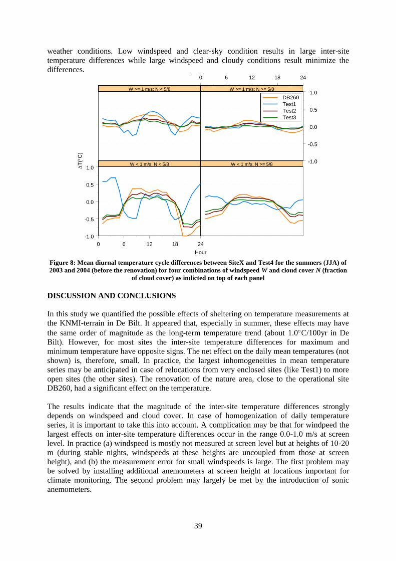
39
weather conditions. Low windspeed and clear-sky condition results in large inter-site
temperature differences while large windspeed and cloudy conditions result minimize the
differences.
Figure 8: Mean diurnal temperature cycle differences between SiteX and Test4 for the summers (JJA) of
2003 and 2004 (before the renovation) for four combinations of windspeed W and cloud cover N (fraction
of cloud cover) as indicted on top of each panel
DISCUSSION AND CONCLUSIONS
In this study we quantified the possible effects of sheltering on temperature measurements at
the KNMI-terrain in De Bilt. It appeared that, especially in summer, these effects may have
the same order of magnitude as the long-term temperature trend (about 1.0C/100yr in De
Bilt). However, for most sites the inter-site temperature differences for maximum and
minimum temperature have opposite signs. The net effect on the daily mean temperatures (not
shown) is, therefore, small. In practice, the largest inhomogeneities in mean temperature
series may be anticipated in case of relocations from very enclosed sites (like Test1) to more
open sites (the other sites). The renovation of the nature area, close to the operational site
DB260, had a significant effect on the temperature.
The results indicate that the magnitude of the inter-site temperature differences strongly
depends on windspeed and cloud cover. In case of homogenization of daily temperature
series, it is important to take this into account. A complication may be that for windpeed the
largest effects on inter-site temperature differences occur in the range 0.0-1.0 m/s at screen
level. In practice (a) windspeed is mostly not measured at screen level but at heights of 10-20
m (during stable nights, windspeeds at these heights are uncoupled from those at screen
height), and (b) the measurement error for small windspeeds is large. The first problem may
be solved by installing additional anemometers at screen height at locations important for
climate monitoring. The second problem may largely be met by the introduction of sonic
anemometers.
0 6 12 18 24
0 6 12 18 24
Hour
-1.0
-0.5
0.0
0.5
1.0-1.0
-0.5
0.0
0.5
1.0
T
(C
)
W < 1 m/s; N < 5/8 W < 1 m/s; N >= 5/8
W >= 1 m/s; N < 5/8 W >= 1 m/s; N >= 5/8
DB260
Test1
Test2
Test3
Summer (JJA) 2003-2004

40
Improvement of our understanding of inter-site temperature differences may enable the
modeling them. In case of De Bilt there are certain aspects that are likely important and
should be studied further. First, the non-uniformity of the KNMI-terrain may affect
downstream sites by daytime advection. Especially the vegetable gardens seem to have
energy balances different from those of the surrounding grassland. This results in different
Bowen ratios (sensible heat flux/latent heat flux). Second, local stability differences are most
important during nighttime stable conditions (small wind speeds, clear sky) when inversions
develop, causing low temperatures near the ground. Differences in wind speed between the
locations may then cause different strengths of the inversion, resulting in higher temperatures
at the location with the larger wind speed. Third, screen ventilation differences are especially
important during the day when radiation errors increase with decreasing wind speed. Fourth,
small sky-view factors restrict radiation. This is mainly important at the Test1 location. Fifth,
local differences in soil type and groundwater levels between the locations may affect the
energy balance and may cause differences in observed temperatures. It is known that at the
Test4 site groundwater levels are shallower than at the other sites. Especially in dry summers
this may result in local differences in the Bowen ratio. Finally, instrumental errors may play a
role, though these are minimized here by the calibration procedures.
References
Brandsma, T., G.P. Können and H.R.A. Wessels, 2003. Empirical estimation of the effect of urban heat
advection on the temperature series of De Bilt (The Netherlands). International Journal of Climatology
23, 829-845.
Brandsma, T., 2004. Parallel air temperature measurements at the KNMI-terrain in De Bilt (the Netherlands)
May 2003 – April 2005, Interim report, KNMI-Publication 207, KNMI, De Bilt, the Netherlands.
WMO, 1996. Guide to Meteorological Instruments and Methods of Observation, WMO-No.8, Geneva,
Switzerland.

41
DETECTED INHOMOGENEITIES IN WIND DIRECTION AND SPEED
DATA FROM IRELAND
Predrag Petrović1 and Mary Curley
2
1Republic Hydrometeorological Institute of Serbia, Kneza Vińeslava 66, Belgrade, Serbia,
tel. +381/11/3050-803, [email protected], 2Met Éireann, Glasnevin Hill, Glasnevin, Dublin, tel. +3531/8065530,
INHOMOGENEITIES OF WIND DATA
Detection of inhomogeneities in wind direction and speed data is a specific problem. First,
instead of a single element, a pair of elements must be examined simultaneoulsy. None of the
existing detection methods deal with more than one element at a time. Second, averaged
values in series seem to contain insufficient information about examined weather element.
Since some changes might occur only in certain ranges of values, consideration of
distributions as an alternative solution gives some previously unavailable information about
changes in series.
Another difficulty with wind direction and speed data is the proper approach to various
calculations. Wind series are coupled into a pair of completely different elements with
different type and range of values, which are azimuth and speed. While wind speed could be
treated as any scalar, wind direction data are limited to a fixed range of 360 degrees. Thus,
wind data are defined in polar coordinates, which cannot be processed in homogenisation
without some conversion of values or adaptation of existing methods. Neither splitting wind
data to a pair of north and east component seems to be a satisfactory solution (Petrović, 2008).
Therefore, a new method had to be used as an alternative solution.
The ReDistribution Method (Petrović, 2004) deals with distributions of values instead of
mean or extreme values. Hence, some additional information about changes in series are
revealed. The ReDistribution Method is based on calculation of changes in frequencies of
values by subranges between two distributions, generated from subsets with fixed moving
window length. The intercomparison between two consecutive distributions detect
significancy of changes and hence inhomogeneities.
One of the advantages of the method is its ability to process data with small gaps, infrequent
error occurence (i.e. typing errors) or outliers. Since such data appear in a very small number
(once in hundreds of thousands of records or even less), their influence on data distribution
values is practically insignificant. Average values might be greatly influenced by outliers,
which appear to be a disadvantage, because of the rigorous needs for accurate data. Thus,
even suspicious or incomplete data might be used with a very small risk of uncertainties.

42
AVAILABLE DATASET
A good example of using this method is given by examination of wind direction and speed
datasets from Ireland. These datasets are hourly wind direction and speed values from 13
stations located countrywide (Figure 1), covering different periods beginning between 1939
and 1954 up to end of 2007 (Table 1).
A large number of metadata was also available and used for verification of this analysis.
Figure 1. Locations of stations in Ireland with available wind data
Station latitude (N) longitude (W) altitude (m) start date
Birr 53.1 7.9 73 01.10.1954
Casement Aerodrome 53.3 6.4 94 01.01.1964
Claremorris 53.7 9.0 71 01.01.1950
Clones 54.2 7.2 89 01.01.1951
Cork Airport 51.8 8.5 154 01.01.1962
Dublin Airport 53.4 6.2 71 01.11.1941
Kilkenny 52.7 7.3 66 01.06.1957
Malin Head 55.4 7.3 22 01.05.1955
Mullingar 53.5 7.4 104 01.01.1950
Roche's Point 51.8 8.2 43 01.12.1955
Rosslare 52.3 6.3 26 01.12.1956
Shannon Airport 52.7 8.9 6 01.09.1945
Valentia Observatory 51.9 10.2 11 01.10.1939
Table 1. List of stations in Ireland with available wind data

43
THE PROCEDURE FOR DETECTION OF INHOMOGENEITIES
Initial settings
The ReDistribution Method requires initial settings that depend upon some summary
information. To establish a number of categories for counts, it is necessary to review a range
of values and overall value resolution Wind direction data have a 10-degree resolution, or 37
possible values (36 values for direction plus one for calms). Wind speed range is from 0 to 63
knots with resolution of 1 knot. Since values over 50 knots are very rare, this value can be
considered for the top of the range.
The best results from the method are obtained with 10-20 categories throughout the whole
range. More categories would produce higher noise levels, while a lesser number of
categories weakens the precision features of the method. Thus, there are 19 categories set for
wind direction (18 for direction by 20 degrees plus one for calms) and 18 categories for wind
speed (16 subranges by 3 knots, one for speed over 51 knots and one for calms).
Another initial setting of the ReDistribution Method is the moving data window length. To
avoid seasonal changes, it is best to use a whole number of years. To avoid taking into
account a year that might feature some extreme situations (i.e. extreme values, prevailing
wind direction more present than usual), a minimum of two years is the least acceptable
choice for a start. However, the method has to be re-run at least once more, but with longer
data window length. This returns lower noise level and more precise peaks of ReDistribution
Index (RDI) values in temporal scale for detection of break points. The greater the number of
different runs, the more reliable the information returned from the method. Still, too long
window will diminish break points that appear in time shorter than the window length.
In the case of Irish data, 2-year moving window runs produced quite high noise level.
Additional runs were of 4-year and 6-year windows, which reduced noise to an acceptable
level and confirmed detected break points.
Although the ReDistribution Method is capable of dealing with sub-daily values, it is time
consuming and it is recommended to calculate daily distributions first. Calculations using
daily distribution values save a lot of time wasted in hourly values without any significant
loss of power of the method that still indicate break points in daily resolution. This procedure
requires recalculations of counted values into relative values (percentages) in order to get
valid results.
Selection of RDI peak values as break points
The ReDistribution Method may calculate the RDI values for more than one series at a time.
In this case, the RDI values are derived from two series, wind direction and speed. It is an
important feature of the method, because detected break points might be more or less certain,
and also explained by some presumed cause, depending on their (non)simultaneous
occurence. If the peaks are more or less at the same point in time, the detected break point is
more certain and even more accurate in temporal scale. Non-simultaneous RDI peaks more
rely on the magnitude and signal/noise ratio.

44
Magnitudes of RDI peaks indicate the possibility and accuracy of detected break points. If the
RDI value is over 0.125, the break is quite certain (Figure 3, point 2). Smaller peaks of RDI,
but still over 0.100 might indicate a possible break (Figure 2, point 2). Even smaller RDI peak
values might be a break point, but only if the peaks from two series are simultaneous and
significantly higher than the noise level (Figure 2 and 1).
Differences in time between detected break points and their causes are in a great accordance
with RDI peak magnitudes. High RDI values return the break point information with very
high precision (up to daily resolution, even the very day of change). When dealing with small
Figure 3. Examples of RDI peaks; possible break with RDI > 0.100 and break of wind speed
only (1) and ceratin break with RDI > 0.125 (2) (Birr, 6-year moving window)
Figure 2. Examples of RDI peaks; simultaneous peaks of both series over noise level (1), peak of
series below 0.100 but over noise level (2) and peak of wind direction series only (3) (Shannon
Airport, 6-year moving window)

45
RDI peaks, differences in time between the detected break and its cause might be quite large
(even a couple of years). Such low magnitudes might even question the significance of the
detected break and thus consider series as homogenuous at that point.
Finally, detected break points have to be considered according to its type and verified by
metadata or any other source of information, which might include simultaneous breaks from
different weather elements or results from any other reliable homogeneity test. Further
examination of detected break points should be considered as a part of a homogenisation
(correction of values) procedure.
TYPES OF BREAK POINTS ACCORDING TO POSSIBLE CAUSES
Main types of inhomogeneities
There are three main types of inhomogeneities:
Both direction and speed affected at the same time (Figure 3, point 2; Figure 2, point 1). This
type of inhomogeneity is generally caused by one or more following reasons: change of
instrument type, relocation of a measurement site, abrupt change of station surroundings, even
change of observer.
Wind direction only (no break point with wind speed) (Figure 1, point 3). Causes for this type
of inhomogeneity include: change of instrument orientation or functionality (usually wind
vane orientation, change of friction or inertia), misorientation of instrument (false orientation,
i.e. according to magnetic instead of geographical north) and change of precision (number of
wind rose directions). This is a quite rare type of inhomogeneity because there are very few
situations in which only wind direction is affected by the change.
Wind speed only (no break point with wind direction) (Figure 3, point 1). Breaks only in wind
speed series are generally caused by change of instrument calibration, functionality (usually
friction in mechanism associated with wind cups), change of threshold for initialization of an
instrument, change of precision (including measurement units). Other causes for changes in
wind speed only are mentioned with the first main type of inhomogeneity.
TYPES OF INHOMOGENEITIES IN WIND DIRECTION SERIES
Present experience gained with the ReDistribution
Method has given several types of inhomogeneities
in wind direction series. Examples of these types are
given from processing wind data from Ireland.
Shifting distribution of directions (Figure 4) is a type
of change where distributions from one sector of
directions (up to half a circle) move to another,
different or even opposite sector. It is generally
caused by a change in station surroundings or
relocation of instrument. The example of Valentia
wind direction break in 1950 corresponds to
metadata information of building a balloon filling
hut south of the measurement site in 1947. This
event reduced frequencies of southern winds and
slightly increased northern wind frequencies. The
0
2
4
6
8
10
12
36
2
4
6
8
10
12
14
16
18
20
22
24
26
28
30
32
34
1950
1956
Figure 4. Shifting distribution of directions
(Valentia, 1950)

46
redistribution of wind direction frequencies is
associated mainly with low wind speeds,
indicating change of local winds, while high
wind speeds were still had the same
distribution by directions. Since the magnitude
of change is quite low (RDI is 0.100), and no
other breaks were detected close to this one,
the change of surroundings appears to have
taken effect on wind direction data a few years
later.
Widening / narrowing of wind rose (Figure 5)
is a type of change where frequencies of
prevailing wind directions become lower /
higher, making wind rose appear widened /
narrowed. This is another type of change caused by changes in instrument environ-ment, but
also an instrument replacement, which is featured with the given example of Shannon in
1991. A new instrument was placed on a different mast, some distance away from the
previous location, hence the change of location took effect on data.
Spreading / contracting of wind rose (Figure 6) is
a type of change where all frequencies become
evenly higher / lower. The most probable cause is
an instrument being replaced by one with lower /
higher initialization threshold. Such changes
frequently occur when mechanical anemometers
are replaced by a new generation of wind
instruments during automation of a station. This
type of change usually has a small magnitude and
it might be quite uncertain in time. An example of
introducing an AWS in Kilkenny during 1998
shows such type of change.
Moving of prevailing wind (Figure 7) is a type of
change where prevailing wind is being redirected
by an angle, while other directions remain
generally the same. This is due to change in
measurement site environment, emerging or
removing an obstacle near the instrument. Also,
the reason could also be an instrument
replacement, like in a given example of Clones in
1997.
Other types of inhomogeneities associated with
wind direction were not found in the wind
datasets from Ireland. These include:
Rotation of a wind rose (Petrović, 2004) is a type
of change where all frequencies seem to be shifted
by an angle. The cause for this type is usually a misorientation of an instrument which is
corrected at certain point in time.
''Starry'' wind rose (Petrović, 2004) is a type of change where some directions are just missing
or not sufficiently present in the distribution of direcions. This is equal to low precision
measurements (or measurement unit) problem, where new instrument introduces more wind
0
2
4
6
8
10
12
36
2
4
6
8
10
12
14
16
18
20
22
24
26
28
30
32
34
1991
1997
Figure 5. Narrowing of wind rose
(Shannon, 1991)
0
2
4
6
8
10
12
36
2
4
6
8
10
12
14
16
18
20
22
24
26
28
30
32
34
1997
2003
Figure 6. Spreading of wind rose
(Kilkenny, 1997)
0
2
4
6
8
10
12
36
2
4
6
8
10
12
14
16
18
20
22
24
26
28
30
32
34
1997
2003
Figure 7. Moving of prevailing wind
(Clones, 1997)

47
direction classes than old measurements (i.e. changing a number of wind directions from 8 to
16 or more).
Irregular redistribution (Petrović, 2004) is any other type of change that is neither described
here, nor easy to detect any pattern of change. The causes for this heavy distortion of a wind
rose include change of surroundings, relocation of a measurement site or errorneous mixed-up
dataset.
TYPES OF INHOMOGENEITIES IN WIND SPEED SERIES
The ReDistribution Method has detected break points in wind speed series that could be
sorted by several types.
Shift up (Figure 8) is one of the most frequent type
of changes, moving maximum distribution
frequencies to higher values of wind speed. Lower
values are less frequent, while higher values of wind
speed are more present in the dataset. The cause for
this type of break is generally an instrument replaced
by one with different calibration. The given example
of Malin Head, 1962, shows how wind speed
distribution affected by instrument malfunction.
Older instrument readings returned a continuous
variation between zero and the true wind speed
values, occasionally stopping the instrument
working properly.
Shift down (Figure 9) is as frequent a type of change
as the previously described shift up type. Here,
maximum distribution frequencies are moved to
lower wind speed. Higher values are less frequent,
while values lower than the most frequent wind
speed are more featured in the dataset. The cause for
this type of break is the same as the cause for shift
up type. An example from Claremorris at the
beginning of 1968, gives a good example of the
effect of instrument overhaul in May 1967 which
caused changes in the of wind speed distributions.
Calms up (Figure 10) is a type of change that
increases the number of calms, while other wind
speed frequencies are practically unchanged. The
cause for this type of change is the increase of
threshold for instrument initialization, which is
generally due to enhanced friction. However, the
reason could not be instrument sheltering by
obstacles, because such change would distort the air
flow at the instrument position. The break point in
Claremorris, 1958, suggested such a problem with
the anemometer. There are reports in the metadata
that the instrument was insensitive to winds below 4
knots and due to this the instrument was overhaul in
0
2
4
6
8
10
12
14
16
18
0 3 6 9 12 15 18 21 24 27 30 33 36 39 42 45 48 51
1962
1968
Figure 8. Shift up of wind speed
distribution (Malin Head, 1962)
0
5
10
15
20
25
0 3 6 9 12 15 18 21 24 27 30 33 36 39 42 45 48 51
1968
1974
Figure 9. Shift down of wind speed
distributions (Claremorris, 1968)
0
5
10
15
20
25
0 3 6 9 12 15 18 21 24 27 30 33 36 39 42 45 48 51
1958
1964
Figure 10. Calms up (Claremorris, 1958)

48
1967. During the overhaul bad corrosion was discovered which explains the fact that the
instrument had become less sensitive. Sometimes this type of break might come up with shift
down type, having the same cause of change.
Calms down / calms out (Figure 11) is a type of change that reduces number of calms to near
zero values. This is due to introduction of an instrument with much lower initialization
threshold. This is often featured in introduction of AWS, like in a given example of
Claremorris, 1995.
Measurement unit (Figure 12) is a type of change featured as ''gaps'' in some categories of
wind speed. This is due to conversion of measurement unit, like in a given example of Dublin
Airport, 1944, where knots were introduced after Beaufort scale estimates.
Irregular redistribution (Petrović, 2004) is any other type of change that is neither described
here, nor easy to detect any pattern of change. The causes for such breaks include change of
surroundings, relocation of a measurement site, instrument malfunction or erroneous mixed-
up dataset. Such changes were not found in the data sets from Ireland.
HOMOGENISATION POSSIBILITIES
The ReDistribution Method is primarily a break point detection tool. Since it is based on
comparison between consecutive distributions of values instead of mean values, present
homogenisation tools and methods are of a little use. This method has to develop a new
approach to homogenisation in order to establish proper corrections for distributions of
values.
Present homogenisation methods usually return a certain value as a correction factor for the
inhomogenuous data subset. Additive correction factor could be positive or negative, but
negative correction returns some values to undefined (negative) range. Hence, present
methods are not applicable to elements that are defined for no negative values, such as wind
speed. This factor can also be multiplicative, which avoids such error, but disturbs
0
5
10
15
20
25
30
35
0 3 6 9 12 15 18 21 24 27 30 33 36 39 42 45 48 51
1944
1946
Figure 12. Change of measurement unit
(estimates to measurements, Dublin
Airport, 1944)
Figure 11. Calms down / calms out
(Claremorris, 1995)
0
5
10
15
20
25
30
0 3 6 9 12 15 18 21 24 27 30 33 36 39 42 45 48 51
1995
2001

49
distributions. Wind speed data are often inhomogenuous by subranges of values (i.e. low and
initialization threshold values), thus such correction would produce more erroneous data at
subranges that were not previously affected by inhomogeneity.
On the other hand, wind direction as azimuth value is an element with strictly defined range
of values from 0 to 360 degrees, with ability to switch from one limit of range to another by
definition (when crossing north direction). So far, there are no homogenisation tools that
could correct such values. Secondly, wind direction and speed are quite independent one from
another, while inhomogeneities frequently affect both series at the same time, especially when
a change on surroundings or instrumentation occurs.
As mentioned, some inhomogeneities of wind speed affect only a subrange of values.
Homogenisation tool must use a method for correction of distributions. In general, overall
distributions are easy to homogenise by applying a correction related to distribution of values.
The real problem is to go to the source values and apply an established correction. That
correction must be a set of correction values applicable by categories of values, bearing in
mind that sum of all occurences must be preserved.
Any possible homogenisation must incorporate mathematical tools that would consider
distribution (i.e. probability density function) instead of adding / multiplying all
homogenising values. An investigation of such correction function is in the plans for future
work on development of the ReDistribution Method.
RESULTS
NUMBER OF DETECTED BREAKS
Investigation of wind direction and
speed data sets from Ireland by using
the ReDistribution Method was quite
successful. Nearly half of all detected
break points were confirmed by
metadata (Table 2). Metadata for
anemometers is currently being
digitized in Met Éireann. Hence more
metadata may be available in the
future (e.g. calibration details). Thus it
may be possible to confirm more of the breaks in the future.
ACCURACY OF BREAK POINT DETECTION
The accuracy of break point detection improves with higher RDI peak values. The highest
RDI peak value is 0.186 (Birr, 1998), strongly indicating redistribution of wind speed value
coming from the instrument replacement (introduction of AWS). This break is also detected
with very short difference between the indicated break point and true change. In this case, the
precision of break detection was only four days (detected 20th
June 1998, true change 24th
June 1998). However, the shortest difference was only two days (Claremorris: detected 10th
September 1995, true change 12th
September 1995).
On the contrary, low RDI values of under 0.100 are generally suspicious breaks and these
might be taken for real breaks only after metadata confirmation. The lowest RDI break
recognised as a break point is 0.087 (Dublin Airport, 1994). In such cases, the differences
between detected and confirmed break extend to 6 months and more.
type of break
number of
detected breaks
confirmed by
metadata
wind direction 27 12
wind speed 47 20
wind direction and speed 19 9
wind direction only 8 3
wind speed only 28 11
total 55 23
Table 2. Overall number of detected and confirmed
break points in wind data sets from Ireland

50
Some RDI temporal changes return double or multiple peaks of almost the same magnitude in
a period of time shorter that the data window length. It is not necessary to pick up the highest
value as the break point, but the closest one to the true break, if metadata are available. Such
cases indicate problems with observational data that occur for a certain period in time (i.e.
period between instrument malfunction and its service, multiple breaks in time shorter than
the power of the method may detect).
METADATA
Metadata information was available for much of the wind data from Ireland. However there
were some periods without metadata records and also some of the data had not yet been
digitized. It was presumed that there were no important changes during this time, but there is
a possibility that some of the metadata is incomplete Metadata were quite valuable when they
contained the exact date and information about the changes on the measurement site. Such
metadata are of major importance when the method has to be tested and verified.
There were also some cases when metadata did not match completely the returned results.
Also, some of the metadata has not yet been examined/digitised (e.g. calibration lists). It is
necessary to examine this data in order to get the most complete information possible. In this
work such cases were left as not confirmed breaks.
UNCERTAINTIES
Low RDI peaks often return many uncertain break points. Bearing in mind given causes, the
next question is the importance of these breaks. Although some of the low RDI peaks are the
true breaks, it is difficult to decide whether such break point might be neglected and treat
series as homogenuous at that point.
Gradual changes (trends) are not certainly detected by the ReDistribution Method. It is also
difficult to detect slow redistributions of wind direction and / or speed which might be due to
gradual changes (i.e. tree growth, increase of friction in instruments). For the time being, such
changes were suspected in periods with increased RDI noise level. Further development of the
method will show whether this assumption is correct.
COMPARISON WITH KNOWN METHODS (SNHT)
Since there were no methods for detection of inhomogeneities in wind direction data,
comparison of the ReDistribution Method is made only with wind speed data. The
comparison method for detection was chosen to be Standard Normal Homogeneity Test
(SNHT). The hourly data were recalculated to the monthly and annual resolution before they
were processed. Data gaps were not filled in order not to bias any result returned from the
SNHT and thus make a correct comparison of the two detection methods.
The comparison of the results returned that from 47 detected break points using
ReDistribution Method, 20 were also detected by SNHT. On the other hand, SNHT has not
detected any new break point that was undetected by the ReDistribution Method. Although
SNHT has also detected some minor breaks, some major breaks with high RDI values (up to
0.162, Mullingar, June 1996) were not detected by the comparison method. This might be the
case with periods with increased RDI values (as it was in the mentioned case). However the
SNHT depends on homogeneous reference series with high correlation between the reference
and candidate series and it is not very suitable for use with Irish wind data.

51
Differences in time between detected break points from both methods were not significant in
annual resolution. SNHT has no ability to detect breaks in any finer than monthly resolution.
Since the ReDistribution Method has returned better results than SNHT, it is highly
recommended for further use.
PLANS FOR THE FUTURE
Present experience with the ReDistribution Method has established a basis in break point
detection with respect to the causes of inhomogeneities. However, these basis have to be
extended with more experience with the method (more data coupled with metadata).
The construction of surrogate wind data sets might show the true power of the detection
method. However, most inhomogeneities are coming from measurement problems, while
climatic signal (if any detected or suspected) is highly suppressed by the method, making
difficult to detect gradual changes. Therefore, surrogate wind data sets must include a ''given''
climatic singnal, ''cleaned'' from instrumentation problems in order to examine possibilities
for climatic signal detection.
Since the ReDistribution Method is capable of operating with more than one series at a time,
introduction of wind gusts as the third element is also planned. Naturally, wind gusts must be
strictly defined (10-minute, hourly or daily maximum wind speed) for the whole dataset, but
this is not necessary for the method in general. Amongst other features, wind gusts depend on
roughness by directions of the surrounding terrain, which will make calculations a bit more
difficult. As the first step, it is planned to introduce wind gusts with an approximation of
evenly distributed roughness from all directions.
The ReDistribution Method might also have a variation that would substitute
intercomparisons between subsequent distributions with distributions from two different
measurement sites. That variation would make the ReDistribution Method capable to work as
a parallel, relative method.
Also, the ReDistribution Method is applicable to some other weather elements. Sometimes,
these elements might not have any climatological sense (i.e. visibility ranges), while any
inhomogeneity detected with such series might discover a valuable metadata information (i.e.
change of observer). Such break points might help in full investigation of inhomogeneities of
other elements that occur at approximately the same time.
Finally, the possibilities for making a correction method based on distributions is being
considered. The initial work would be based on a redistribution matrix calculated from the
changes in distributions and establishing a correction function applicable to the whole dataset.
Such method would make the ReDistribution more complete.
CONCLUSIONS
The ReDistribution Method is the inhomogeneity detection method with a wide set of
possibilities. It is also able to detect inhomogeneities with very high precision in certain cases.
Amongst other features, the method also considers the causes of inhomogeneities as crucial
information.
Whilst present experience of the ReDistribution Method returns, in general very good results,
further experience of the method will lead to even better results in determining the causes of
inhomogeneities. A wider use of the method is the best way for obtaining more experience
with data from other climate regions (i.e. climate regions with periodic winds) or data that
have special and presently uninvestigated causes for inhomogeneities.

52
Accuracy of the ReDistribution Method might be better determined after more processed data
is compared and verified with metadata. Some basic principles are already given, while
quantitative relations might be established with more detected and verified break points.
Correction method based on distributions has to be developed and tested with the detection
method. Corrections that would be detected have to be compared to corrections delivered
from other, classical homogenisation methods.
Finally, metadata must be as complete as possible, even with additions delivered from the
ReDistribution Method findings, if necessary (Petrović, 2007).
Acknowledgements Authors would like to thank Sean Bonner and Michael McDonnell from Met Éireann for their
great efforts in browsing through metadata, and Ivana Tońić from Institute for Meteorology,
University of Belgrade, for additional efforts in working with SNHT.
References Aguilar, E., Auer, I., Brunet, M., Peterson, T. C., Wieringa, J., 2003: Guidelines on climate data and
homogenization, WMO, WCDMP-No. 53
Alexandersson, H. Alexandersson H, Moberg A. 1997: Homogenization of Swedish temperature data. Part I:
Homogeneity test for linear trends. Int. J. Climatol. 17: 25-34
Petrović, P. 2004: Detecting of inhomogeneities in time series using Real Precision Method, Fourth Seminar For
Homogenization And Quality Control In Climatological Databases (Budapest, Hungary, 6-10. October
2003); WMO, WCDMP-No. 56, pp. 79-88
Petrović, P. 2007: The search for metadata 'hidden' in recordsets, 6th
ECSN Data Management Workshop
(presentation), Vienna, 20 – 22 November 2007.
Petrović, P. 2008: Detection of inhomogeneities in wind direction and speed data, Fifth Seminar For
Homogenization And Quality Control In Climatological Databases (Budapest, Hungary, 29 May – 2
June 2006); OMSZ (CD), pp. 73-80

53
A METHOD FOR DAILY TEMPERATURE DATA INTERPOLATION
AND QUALITY CONTROL BASED ON THE SELECTED PAST
EVENTS
Gregor Vertačnik
Environmental Agency of the Republic of Slovenia, Ljubljana, Slovenia,
tel: +386 1 4784 581, fax: +386 1 4784 054, [email protected]
Abstract
A method for daily interpolation of temperature at classical climate stations, based on the selected past
events, is discussed. The method was developed due to unsuitable results obtained by simple
interpolation methods in some cases. The basis of the method is the selection of reference data set
from the reference period. The reference data set consists of temperature data from the target and
reference stations in days that are similar to the target day. The similarity is calculated as weighted
Euclidean distance, considering spatial correlation and spatiotemporal evolution. The reference data
set is used in the interpolation procedure with the final result being a combination of estimations based
on each of the reference stations. Preliminary tests have shown more or less significant reduction of
the standard error compared to the case when all the data from the reference period is used for the
interpolation. However, we have found it is impossible to infer on local phenomena in some cases,
resulting in a still considerable error. Incorporation of other types of meteorological data and data from
the target station should thus further improve the results.
INTRODUCTION
Simple methods for daily temperature data quality control and completion at a meteorological
station are usually based on measurements at nearby stations and the corresponding climate
normals. Station climatology used for the data interpolation is the same regardless of the
weather situation (e.g. sunny, rainy, windy). However, in complex terrain, like in Slovenia, air
temperature frequently varies significantly on a short distance, depending on the weather type.
An example of such a case is presented in Fig. 1, where strong precipitation gradient led to
strong temperature gradient. Among the most frequent cases, when the horizontal temperature
gradient is particularly strong is, when föhn wind is blowing (e.g. bora from the northeast or
Karavanke föhn from the north to northwest). Föhn causes pronounced temperature difference
between the windward and the leeward side of the mountain barrier. Diurnal temperature
range can also be very different on a particular day from region to region. As the spatial
density of the network of temperature stations is not sufficient for straightforward
interpolation in some cases, taking the weather situation into account can improve the
interpolation result noticeably. In this manner we can infer for example on strong temperature
inversion from the temperature data at nearby stations although the microclimate at the target
station is not comparable to any of the nearby stations.
For this reason we have developed a more sophisticated method which is based on the
selection of measurements according to the weather situation.
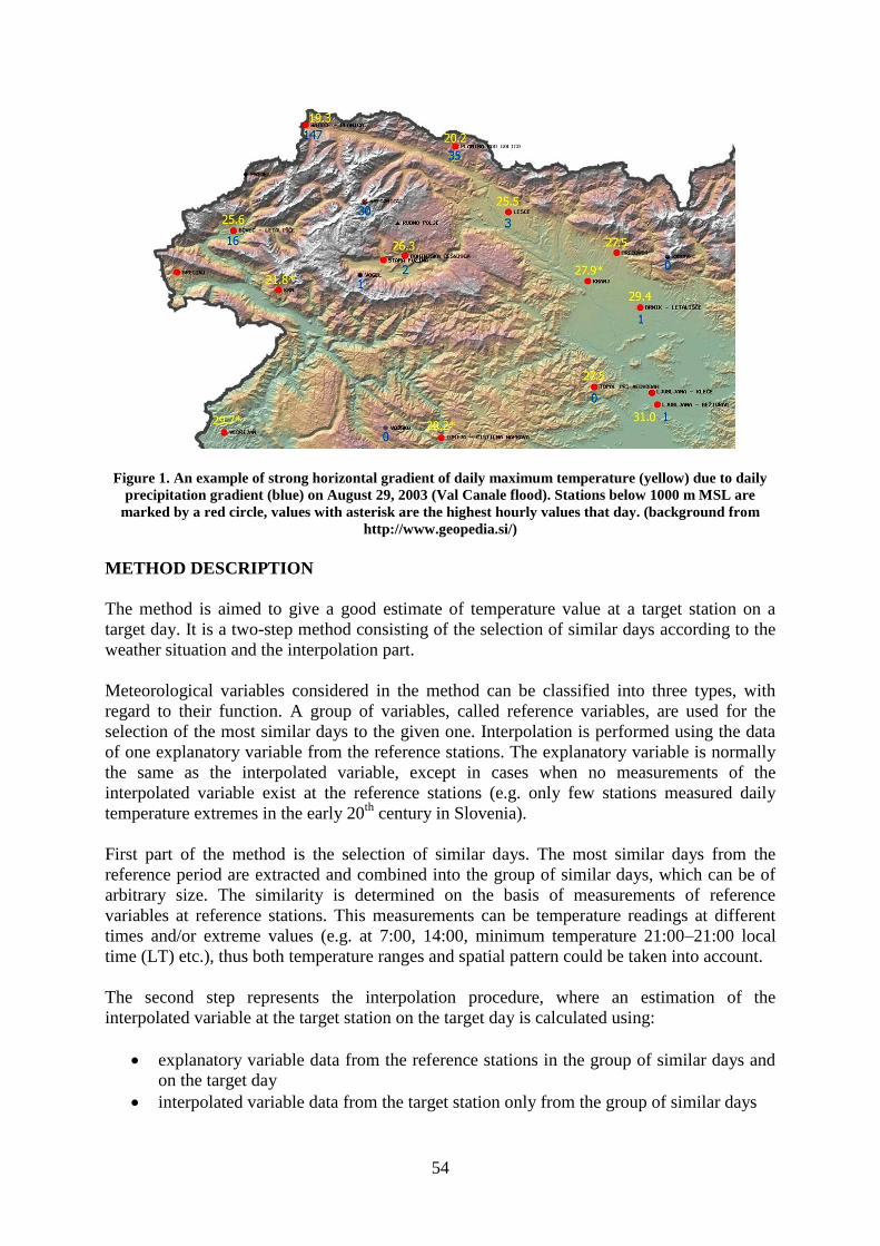
54
Figure 1. An example of strong horizontal gradient of daily maximum temperature (yellow) due to daily
precipitation gradient (blue) on August 29, 2003 (Val Canale flood). Stations below 1000 m MSL are
marked by a red circle, values with asterisk are the highest hourly values that day. (background from
http://www.geopedia.si/)
METHOD DESCRIPTION
The method is aimed to give a good estimate of temperature value at a target station on a
target day. It is a two-step method consisting of the selection of similar days according to the
weather situation and the interpolation part.
Meteorological variables considered in the method can be classified into three types, with
regard to their function. A group of variables, called reference variables, are used for the
selection of the most similar days to the given one. Interpolation is performed using the data
of one explanatory variable from the reference stations. The explanatory variable is normally
the same as the interpolated variable, except in cases when no measurements of the
interpolated variable exist at the reference stations (e.g. only few stations measured daily
temperature extremes in the early 20th
century in Slovenia).
First part of the method is the selection of similar days. The most similar days from the
reference period are extracted and combined into the group of similar days, which can be of
arbitrary size. The similarity is determined on the basis of measurements of reference
variables at reference stations. This measurements can be temperature readings at different
times and/or extreme values (e.g. at 7:00, 14:00, minimum temperature 21:00–21:00 local
time (LT) etc.), thus both temperature ranges and spatial pattern could be taken into account.
The second step represents the interpolation procedure, where an estimation of the
interpolated variable at the target station on the target day is calculated using:
explanatory variable data from the reference stations in the group of similar days and
on the target day
interpolated variable data from the target station only from the group of similar days

55
As explanatory and interpolated variables can be different, it is possible, for example, to
estimate the maximum temperature at the target station considering the values at 14:00 LT at
the reference stations.
Group of similar days
The group of similar days is constructed by using weighted Euclidean distance between all the
considered temperature measurements at reference stations on the target and a candidate day.
Weighting is done through Pearson correlation coefficients between the series of the reference
variables at the reference stations and the interpolated variable at the target station. Although
more appropriate weights can be found, we decided to use correlation-based weights as the
iterative process searching the optimal weights could be very time-consuming. Days with the
smallest Euclidean distance are selected into a group of similar days.
A special issue is a construction of a measure for the degree of similarity, since at least two
kinds of similarity can be specified in our case, regarding:
1) Absolute values (similar air mass)
2) Spatiotemporal pattern (similar weather phenomena)
An example showing the difference between the types is presented in Fig. 2.
Figure 2. Measured temperature time series (T0) on Rudno polje (Pokljuka) 18–19 July, 2007, and
arbitrary similar series (T1 - similar absolute values, T2 - similar temporal pattern)
Since the computation of the optimal weights would be very time-consuming, we decided to
use simple basic weighs, which are used in further computation:
s,v
s,v
s,v
1 (1)
where s,v denotes Pearson correlation coefficient between the series of variable v at
reference station s and the series of the interpolated variable at the target station. Eq. (1)
6
8
10
12
14
16
18
20
22
24
26
28
18:00 21:00 0:00 3:00 6:00 9:00 12:00 15:00 18:00 21:00 0:00
time
tem
pe
ratu
re [
°C]
T0 T1 T2

56
satisfies two fundamental conditions: the weight is 0 when the correlation coefficient is 0 and
infinity when the correlation coefficient equals 1. Besides, reference stations with very high
(~0.9) correlation coefficient have many times higher weight than those with weak or
moderate correlation coefficient (~0.5).
To consider the second type of aforementioned similarity (spatiotemporal similarity), we need
to calculate average temperature deviation of the candidate day from the target day:
s,v
p
s,v
s,v s,v
D,s,vd,s,vp
s,v
d,dev
TT
1
1
(2)
where s,v represents standard deviation of the temperature series in the reference period, d
indicates a candidate and D the target day. Since all the considered temperature variables do
not have the same variance (e.g. daily minimum temperature in Ljubljana is less variable than
daily maximum temperature), normalised (by s,v ) variables are used. Weighting is done by
using the power 1p of the basic weights.
When the average deviation is obtained, we can calculate the normalised weighted Euclidean
distance between a candidate and the target day:
s,v
p
s,v
s,v s,v
D,s,vd,s,v
devd,dev
s,v
D,s,vd,s,v
dev
p
s,v
d
TTk
TTk
E2
2
22
1
(3)
where devk determines the influence of each type of the aforementioned similarities. Weights
are, as in Eq. (2), powers of the basic weights.
Interpolation
Two basic ideas were used for the interpolation part of the method. First of all, a link between
(target station S , interpolated variable i ) and (reference station s , explanatory variable e ) is
established using the data from the group of similar days. In this way we calculate the average
difference, s,D , for each combination target station–reference station:
days.simd
s,d,eS,d,i
s,D
s,D TTn
1 (4)
where s,Dn counts the number of considered similar days for reference station s and the target
day D . It is worth a remark that s,Dn may differ from station to station, as some data ( s,d,eT )
in the group of similar days could be missing.

57
The differences serves as an input for the final equation, which gives us the interpolated
value:
s
p
s,es,D
s
s,Ds,D,e
p
s,es,D
S,D,in
Tn
T3
3
(5)
The sum of the temperature at a reference station and the difference s,D represents a single
estimation for the interpolated value. All the estimations are weighted by the correlation term
( 3p
s,e ) and the number of considered days from the group of similar days ( s,Dn ) to obtain the
interpolated value. The latter term is added to balance the influence of reference stations on
the interpolation result in cases with a lot of missing data. By the reduction of available
measurements which are used to determine the difference in Eq. (4) the uncertainty of the
calculated difference increases, therefore it is better to minimize the influence of stations with
sparse data.
Near-optimal values of parameters 1p , 2p , 3p , devk and the number of similar days were found
by an ensemble run with each member having different combination of the parameter values.
The combination with the minimum standard error of the interpolated series was determined
as the best choice. The procedure was carried out for each case separately.
Example of use of the method
An interpolation of daily minimum air temperature at Ljubljana airport in the period 2003–
2007, based on the reference period 1995–2002, will be discussed as an example of the
method. Computer programme selected five best-correlated stations, whereas the explanatory
variable was also daily minimum air temperature. For the gropu of similar days we considered
temperatures at 21:00 LT the day before, at 7:00 LT and 14:00 LT on the given day and the
minimum and maximum temperatures. The parameters 1p and 2p were set to 1, while 3p
was set to 2. The results of the most simple method with monthly correction factors used on
the data from the whole reference period at meteorological station Ljubljana (best-correlated,
17 km SSE of the target station) are added for comparison.
The first interesting detail in the presented case, which is worth of analysis, is the role of the
devk factor. In Fig. 3 we can see the monotonous reducing of the standard error as devk is
increasing. In other words, the best result is obtained when only the second kind of similarity
(similar temperature range and spatial pattern) is taken into account.

58
Figures 3 and 4. Dependence of the standard error to devk (left) and comparison of the standard error
through year between the methods (right)
Another question, which has not been discussed yet, is the optimal size of the group of similar
days and the number of days from the reference period to be considered for each target day.
Some testing revealed a huge difference from case to case, meaning that the magnitude of
sample error (large when only few days are considered) and the error caused by the inclusion
of “non-similar” days (limiting to the most simple methods) is very different for each case.
Results for 20 and 200 days for the presented case are shown in Fig. 4.
If we take a look inside a part of the interpolated series, we can notice some systematic
difference between the simplest method and the method discussed in this paper (Fig. 5). The
former method is better in most days, though the error remains quite high in some days.
Figure 5. Comparison of the measured and the interpolated series for March 2004
CONCLUSION
The method described in the paper is able to decrease the interpolation error, but the lack of
other meteorological data still prevents it to make an adequate estimation of the temperature
when there is a local phenomenon at the target station we can not infer on using only
available temperature data. Such cases are the main reason for the large part of the variance
being unexplained. Thus, inclusion of other meteorological data from the reference as well as
1.09
1.1
1.11
1.12
1.13
1.14
1.15
1.16
1.17
0 0.2 0.4 0.6 0.8 1
k dev
sta
nd
ard
err
or
[°C
]
00.20.40.60.8
11.21.41.61.8
22.22.4
Ja
n
Fe
b
Ma
r
Ap
r
Ma
y
Ju
n
Ju
l
Au
g
Se
p
Oct
No
v
De
c
month
sta
nd
ard
err
or
[°C
]
20 sim. days 200 sim. days Ljubljana only, all days
-16
-14
-12
-10
-8
-6
-4
-2
0
2
4
6
8
1 3 5 7 9 11 13 15 17 19 21 23 25 27 29 31
day
tem
pe
ratu
re [
°C]
measured 20 sim. days 200 sim. days Ljubljana only, all days

59
from the target station (if possible) would probably result in further significant reduction of
the error.
Another issue which has to be solved or at least minimized is the choice of the model‟s
parameter values. There is no simple answer to weighting factors, the size of the group of
similar days and variables to be included. Test runs have shown that at least some of the
optimal parameters differ strongly from case to case, while in most cases inclusion of more
variables and stations yields better results. Iterative process could minimize the problem but
then the method could become time-inefficient.
The most significant disadvantage or restriction of the method is the necessity of using more
or less homogenous series at nearby stations. Artificial jumps and temperature trends can
otherwise seriously influence both the choice of the most similar days and the interpolation
results. On the other hand this problem is marginal for quality control where small
interpolation error is not of big importance.
References
Meteorological digital archive of the Environmental Agency of the Republic of Slovenia

60
AIR HUMIDITY IN CRACOW IN THE PERIOD 1863-2007 – DAILY
DATA QUALITY CONTROL AND HOMOGENIZATION METHODS
Agnieszka Wypych, Katarzyna Piotrowicz
Institute of Geography and Spatial Management, Jagielonian University,
Gronostajowa 7, 30-387 Krakow, Poland, 12 664-53-25, 12 664-53-85,
[email protected]; [email protected]
INTRODUCTION
Air humidity, in other words water vapour content in the air, is characterized by
various factors. They include, among others: relative humidity, vapour pressure, moisture
deficit, dew point temperature or specific and absolute humidity. Air humidity is one of the
more important weather and climate components. It plays a key role in defining the climate
conditions of a given area. Water vapour content in the air has a decisive influence on
evaporation intensity, occurrence of precipitation and certain phenomena, such as fog.
Variations of humidity parameters over several years are very seldom analysed
(Dubicka et al. 2003, Wypych 2003). This is caused, among others, by lack of long-term
hygrometric or psychrometric measurements. The impact of urban areas on the annual and
spatial variability of air humidity has been researched much more frequently (Ackerman
1987, Hage 1975, Holmer, Eliasson 1999, Lee 1991). Relatively short series of measurements
(3-10 years) have been used for this purpose (Chandler 1967, Murinova 1978, Unger 1999).
The research station of the Institute of Geography and Spatial Management of the
Jagiellonian University in Krakow, Poland, was established in 1792. It has got one of the
longest, regular series of measurements and observations of various meteorological elements
conducted in the same location. The complete documentation of the station, together with the
metadata, constitutes unique research material.
The only measurement series to have undergone homogeneity testing thus far are
series of air temperature, atmospheric pressure and precipitation (Twardosz 1997, Ustrnul
1997). The homogeneity of air humidity parameters has not been investigated, mainly due to
the methodical difficulties related to the analysis of numerical material.
The paper presents the stages and the methods used in order to examine the quality of
Krakow‟s air humidity measurement series. Daily values of selected air humidity parameters
calculated on the basis of psychometric measurements were verified.
DATA SOURCES
Air humidity measurements in Krakow commenced at the time of the station‟s
creation. Initially, hair hygrometers were implemented, including a Saussure hygrometer,
which operated until 1830. Since 1834, all measurements have been carried out by means of
an August psychrometer. Thermometers are located in a Stevenson shelter next to a window
with NNW exposure, second floor level (12 m AGL) of the Śniadecki College building in the
Botanical Garden of the Jagiellonian University (Fig. 1). Alas, from 1856 until November
1862, there is a gap in measurements of meteorological elements under analysis. Within the
last 145 years (1863-2007), all observations of water vapour content in the air have been
uninterruptedly performed in the same location and using consistently the same method, three
or four times per every 24 hours (Tab. 1).
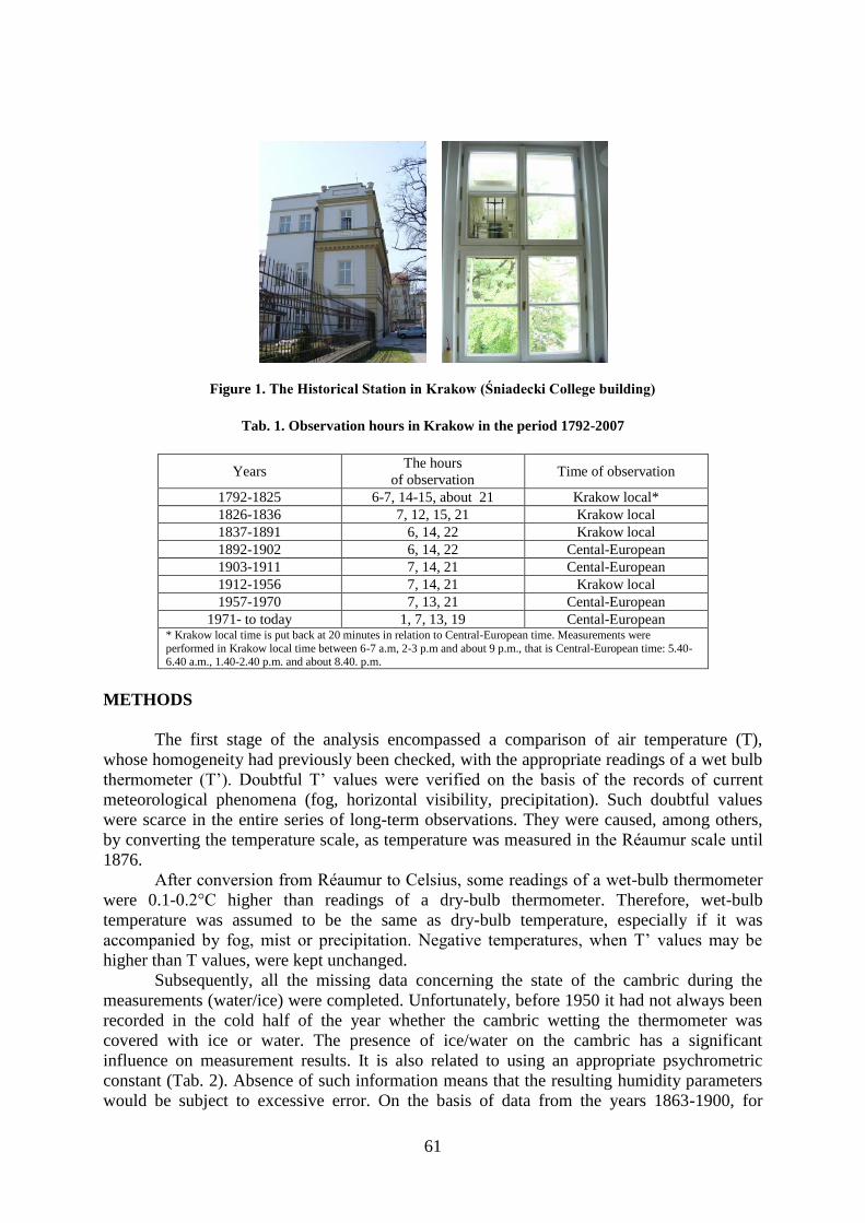
61
Figure 1. The Historical Station in Krakow (Śniadecki College building)
Tab. 1. Observation hours in Krakow in the period 1792-2007
Years The hours
of observation Time of observation
1792-1825 6-7, 14-15, about 21 Krakow local* 1826-1836 7, 12, 15, 21 Krakow local 1837-1891 6, 14, 22 Krakow local 1892-1902 6, 14, 22 Cental-European 1903-1911 7, 14, 21 Cental-European 1912-1956 7, 14, 21 Krakow local 1957-1970 7, 13, 21 Cental-European
1971- to today 1, 7, 13, 19 Cental-European * Krakow local time is put back at 20 minutes in relation to Central-European time. Measurements were
performed in Krakow local time between 6-7 a.m, 2-3 p.m and about 9 p.m., that is Central-European time: 5.40-6.40 a.m., 1.40-2.40 p.m. and about 8.40. p.m.
METHODS
The first stage of the analysis encompassed a comparison of air temperature (T),
whose homogeneity had previously been checked, with the appropriate readings of a wet bulb
thermometer (T‟). Doubtful T‟ values were verified on the basis of the records of current
meteorological phenomena (fog, horizontal visibility, precipitation). Such doubtful values
were scarce in the entire series of long-term observations. They were caused, among others,
by converting the temperature scale, as temperature was measured in the Réaumur scale until
1876.
After conversion from Réaumur to Celsius, some readings of a wet-bulb thermometer
were 0.1-0.2°C higher than readings of a dry-bulb thermometer. Therefore, wet-bulb
temperature was assumed to be the same as dry-bulb temperature, especially if it was
accompanied by fog, mist or precipitation. Negative temperatures, when T‟ values may be
higher than T values, were kept unchanged.
Subsequently, all the missing data concerning the state of the cambric during the
measurements (water/ice) were completed. Unfortunately, before 1950 it had not always been
recorded in the cold half of the year whether the cambric wetting the thermometer was
covered with ice or water. The presence of ice/water on the cambric has a significant
influence on measurement results. It is also related to using an appropriate psychrometric
constant (Tab. 2). Absence of such information means that the resulting humidity parameters
would be subject to excessive error. On the basis of data from the years 1863-1900, for

62
relative air humidity the estimated error for extreme T‟ values was ±3.6-4.4% (Fig. 2). It is
slightly higher for positive temperatures of the wet-bulb thermometer and this is why relative
humidity could be overestimated even by 4.4%. For negative T‟ values, relative humidity
would be underestimated up to ca. 3.6%.
Tab. 2. Psychrometric formulas used to calculate air humidity parameters
(Robitzsch 1949; modified)
ice water
e – vapour pressure; E – saturation vapour pressure; T – air temperature; T‟ – wet-bulb
temperature
Figure 2. Difference (%) between relative air humidity values counted using „ice formulas” and „water
formulas” (-5t5°C) (Krakow 1863-1900)
To prevent such differences in calculations, the frequency of occurrence of ice and
water on the cambric for individual air temperatures was estimated. For that purpose, a series
of measurements from 1971-2000 was used, when the condition of the cambric was
conscientiously recorded and when thermal and air humidity conditions in Krakow were very
diverse. This 30-year period included both extremely warm winters, e.g. in 1972/73, when T‟
was seldom covered with ice, and very severe ones (e.g. 1962/63) when temperature was very
often below 0°C.
Psychrometric patterns permit the presence of ice or water on the cambric when the
wet-bulb temperature is from -10°C to 8°C. In Krakow, from 1971-2000, at three observation
times ice was always (100%) reported on the cambric when T was below -4°C and with
declining frequency until 4°C (0.4%) (Fig. 3). Water appeared on the cambric for
temperatures T from -4°C (0.4%) to 4°C (96.6%). For temperatures above 4°C, the bulb of the
wet-bulb thermometer was always wet with water (Fig. 3).
-5
-4
-3
-2
-1
0
1
2
3
4
5
<-5.0;-4.0) <-4.0;-3.0) <-3.0;-2.0) <-2.0;-1.0) <-1.0;0.0) 0.0 (0.0;1.0> (1.0;2.0> (2.0;3.0> (3.0;4.0> (4.0;5.0>
temperature (oC)
diffe
ren
ce
(%
)
)'(7060,0' TTETe
'235
'4366,7
10107,6' T
T
ET
)'(7946,0' TTETe
'5,265
'5,9
10107,6' T
T
ET

63
Figure 3. Frequency of ice/water cambric state (Krakow 1971-2000)
Those results enable us to fill in missing cambric status information and reduce the
miscalculation of relative humidity to ±1.5%. It has been assumed that for air temperatures
T<-3.0°C, cambric on the bulb of the wet-bulb thermometer was covered with ice, similarly
for temperatures in the range -3.0°C<T<-2.0°C when T‟<-2.0°C. Presence of water on the
cambric was assumed for air temperatures T>2.0°C while all temperatures in the range -
1.9°C≤T≤1.9°C were compared with current weather conditions. Current synoptic situation
and cloud cover were taken into account, and 24h time series of air temperature was analysed
on the basis of hygrograms. Ice on the cambric was reported for all days when temperatures
remained below zero.
Psychometric models, identical for the entire series, were used to calculate the value of
air humidity parameters (Rojecki 1959). On the basis of readings of T and T‟, they help obtain
values of four humidity parameters: vapour pressure, relative humidity, saturation deficit and
dew point temperature. At further stages of homogeneity testing of series of data only relative
humidity was investigated as it is the most frequently analysed humidity parameter. It might
be assumed that if relative humidity proves homogeneous, other humidity parameters will be
homogeneous, too, because they had been calculated on the basis of the same T and T‟ values.
The results obtained in consequence were compared with the values read from
hygrograms and the readings of the hair hygrometer. At the same time as psychrometric
measurements, relative humidity was measured using a hygrometer or hygrograph. Extreme
cases, which gave rise to doubts, were analysed with regard to the records about the state of
the atmosphere: circulation conditions, the occurrence of foehn and some atmospheric
phenomena. Krakow is exposed several times a year to effects of operation of foehn in the
Tatra Mountains which are some 80 km away in a straight line. Krakow‟s relative humidity
was then even ca. 15%.
RESULTS
The performed homogeneity tests (modified form of SNHT Alexandersson –
Stepanek, 2007) did not find any cases which would clearly indicate that the series was not
homogeneous. The controversial values identified in the analysis were subjected to further
verification. To achieve that, archival records of measurements and meteorological
observations were used. Corrections of numerical data were not performed. The content of air
vapour in the air is a resultant of the interaction of numerous factors and processes, which
need to be taken into account before correcting the values. In light of the lack other objective
possibilities of verification of air humidity in Krakow, the analysed data were considered as
relatively homogeneous.
0%
20%
40%
60%
80%
100%
<-5.0;-4.0) <-4.0;-3.0) <-3.0;-2.0) <-2.0;-1.0) <-1.0;0.0) 0.0 (0.0;1.0> (1.0;2.0> (2.0;3.0> (3.0;4.0> (4.0;5.0>
temperature (oC)
frequency

64
Figure 4a shows long-term mean annual relative air humidity in Krakow in the years
1863-2007. Values have been calculated on the basis of observation times averages (as the
arithmetic mean of 3 daily readings).
The turn of the 20th
century saw a marked decline in Krakow‟s relative air humidity
(Wypych 2007). The mean annual relative humidity in that period ranged from 85% in 1871
to 72% in 1911. Until the 1960s, relative humidity stood at ca. 79% and did not undergo
significant changes on a year-on-year basis. Then a marked drop of this meteorological
element was observed. At the turn of the 21st century, average annual relative humidity was
ca. 70% and was the lowest since the beginning of the period under analysis. To make sure
that fluctuations in relative humidity were related to fluctuations of Krakow‟s climate and not
to the non-homogeneous quality of the series of data, results were compared with long-term
air temperature variation and urban development.
Figure 4. Mean annual relative air humidity and air temperature in Krakow in the period 1863-2007
Until the beginning of the 20th
century, the station was located outside the city, to the
east. At that time Krakow‟s industrial function was weak. From 1792 until 1900, city area
changed only slightly, from ca. 5 to 8.9 km2 (Matuszko et al. 2004). The number of
inhabitants changed to a much higher extent – it rose from 10,100 in 1785 to more than
85,000 in 1900. Now the city has a population of ca. 800,000 inhabitants living on an area of
327,000 km2. The years 1918–1939 brought a gradual rise in Krakow‟s economic and urban
growth, with the greatest changes occurring after the Second World War. The 1950s saw the
establishment of a centre of heavy industry with a steel mill and residential area with services
to the east of the city – Nowa Huta.
y = -0,063x + 81,834
60
70
80
90
100
1860 1870 1880 1890 1900 1910 1920 1930 1940 1950 1960 1970 1980 1990 2000
(%)a) Relative air humidity
y = 0,014x + 7,467
4,0
6,0
8,0
10,0
12,0
1860 1870 1880 1890 1900 1910 1920 1930 1940 1950 1960 1970 1980 1990 2000
(oC) b) Air temperature
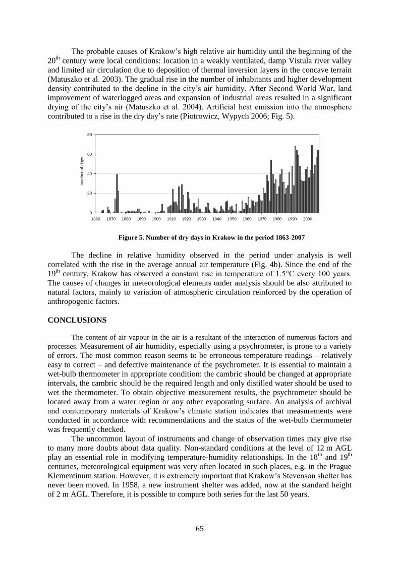
65
The probable causes of Krakow‟s high relative air humidity until the beginning of the
20th
century were local conditions: location in a weakly ventilated, damp Vistula river valley
and limited air circulation due to deposition of thermal inversion layers in the concave terrain
(Matuszko et al. 2003). The gradual rise in the number of inhabitants and higher development
density contributed to the decline in the city‟s air humidity. After Second World War, land
improvement of waterlogged areas and expansion of industrial areas resulted in a significant
drying of the city‟s air (Matuszko et al. 2004). Artificial heat emission into the atmosphere
contributed to a rise in the dry day‟s rate (Piotrowicz, Wypych 2006; Fig. 5).
Figure 5. Number of dry days in Krakow in the period 1863-2007
The decline in relative humidity observed in the period under analysis is well
correlated with the rise in the average annual air temperature (Fig. 4b). Since the end of the
19th
century, Krakow has observed a constant rise in temperature of 1.5°C every 100 years.
The causes of changes in meteorological elements under analysis should be also attributed to
natural factors, mainly to variation of atmospheric circulation reinforced by the operation of
anthropogenic factors.
CONCLUSIONS
The content of air vapour in the air is a resultant of the interaction of numerous factors and
processes. Measurement of air humidity, especially using a psychrometer, is prone to a variety
of errors. The most common reason seems to be erroneous temperature readings – relatively
easy to correct – and defective maintenance of the psychrometer. It is essential to maintain a
wet-bulb thermometer in appropriate condition: the cambric should be changed at appropriate
intervals, the cambric should be the required length and only distilled water should be used to
wet the thermometer. To obtain objective measurement results, the psychrometer should be
located away from a water region or any other evaporating surface. An analysis of archival
and contemporary materials of Krakow‟s climate station indicates that measurements were
conducted in accordance with recommendations and the status of the wet-bulb thermometer
was frequently checked.
The uncommon layout of instruments and change of observation times may give rise
to many more doubts about data quality. Non-standard conditions at the level of 12 m AGL
play an essential role in modifying temperature-humidity relationships. In the 18th
and 19th
centuries, meteorological equipment was very often located in such places, e.g. in the Prague
Klementinum station. However, it is extremely important that Krakow‟s Stevenson shelter has
never been moved. In 1958, a new instrument shelter was added, now at the standard height
of 2 m AGL. Therefore, it is possible to compare both series for the last 50 years.
0
20
40
60
80
1860 1870 1880 1890 1900 1910 1920 1930 1940 1950 1960 1970 1980 1990 2000
num
ber
of
days

66
Changed times of readings are especially important for summer humidity
measurements. Heino (1994) proved that evening and morning observation times have the
greatest importance. Differences in calculations of the mean daily relative humidity may reach
3-4%. In Krakow, reading times in periods of air humidity measurements changed eight
times, with the greatest differences relating to the evening reading (180 minutes).
Another important factor affecting the quality of available source material are the
surroundings of the meteorological station. The Krakow station has never changed location.
When observations were started, the area was located on the outskirts of the city, enclosed
only by scattered buildings. Now, due to the city‟s dynamic growth, it is situated in the centre,
at the crossroads of busy arterial roads. Additionally, it is within the Botanical Garden
founded in 1783. With the passage of time, the garden expanded (from 2.4 to 9.6 hectares)
and its development changed too – the number and diversity of species grown there rose as
well.
Due to potential measurement and calculation errors described, results obtained should
be appropriately verified. Quite often it is not possible on account of new observation times
and station‟s environment. Therefore, existing air humidity variation studies have been in
general based on short series which provide a relative guarantee of homogeneity. However,
they are not sufficiently representative to define development trends.
Global climate change, widely discussed in recent years, can be described only thanks
to in-depth studies aimed at an analysis of long-term variation of basic meteorological
elements. The big-city location of meteorological stations which have long measurement
sequences leads to error-prone readings, with the error being related to the dynamic change in
local conditions. Studies based on data from relocated stations also raise a variety of concerns
– on account of more or less successful attempts at standardization of material.
An in-depth analysis of source material, which encompasses 145 years of
meteorological observations carried out without a break in one place in Krakow, enables to
say that data available is relatively homogenous. With such a long-term series of data, ranging
from the beginnings of instrumental measurement, it is impossible to completely avoid certain
inhomogeneities. However, any attempts at data improvement could be erroneous and destroy
the originality and substantive value of the series.
Acknowledgements This study was supported by a grant from the Ministry of Science and Higher Education (No
N306 049 32/3237).
References
Ackerman B., 1987, Climatology of Chicago area urban-rural differences in humidity, Journal of Climate &
Applied Meteorology, 26 (3), 427-430.
Chandler T.J., 1967, Absolute and relative humidities in towns, Bull. Am. Met. Soc., 48, 394-399.
Dubicka M., Rosiński D., Szymanowski M., 2003, The influence of urban environment on air humidity in
Wrocław, Acta Universitatis Wratislaviensis, Studia Geograficzne, 75, 504-527.
Hage K.D., 1975, Urban-rural humidity differences, Journal Applied Meteorology, 14, 1277-1283.
Heino R., 1994, Changes of relative air humidity in Finland, [in:] Climate variations in Central Europe, R. Heino
(Ed.) Proceedings of the European Workshop on Climate Variations, Finland, 314-320.
Holmer B., Eliasson I., 1999, Urban-rural vapour pressure differences and their role in the development of urban
heat Island, International Journal of Climatology, 19 (9), 989-1009.
Lee D.O., 1991, Urban-rural humidity differences in London, International Journal of Climatology, 11 (5), 577-
582.
Matuszko D., Piotrowicz K., Twardosz R., 2003, The relationship between temperature, cloudiness and
precipitation in Cracow at the time of rapid growth, Prace Geograficzne, 112, IGiGP UJ, 69-80.
Matuszko D., Twardosz R., Piotrowicz K., 2004, Relationships between cloudiness, precipitation and air
temperature, Geographia Polonica, 77, 1, 9-17.

67
Murinova G., 1978, The influence of the town on the air humidity in Bratislava, Contributions of the
Geophysical Institute, Slovak Academy of Sciences, Series of Meteorology, 2, 193-206.
Piotrowicz K., Wypych A., 2006, Long-term variations in the number of hot, very hot and sultry days in
Kraków, Papers on Global Change IGBP, 13, 43-58.
Robitzsch M., 1949, Ausfürlische Tafeln zur Berechnung der Luftfeuchtigkeit, Leipzig.
Rojecki A., 1959, Tablice psychrometryczne, Wydawnictwa Komunikacyjne, Warszawa.
Stepanek, P., 2007, AnClim - software for time series analysis (for Windows). Dept. of Geography, Fac. of
Natural Sciences, Masaryk University, Brno. 1.47 MB.
Twardosz R., 1997, Homogenizacja serii pomiarów opadów atmosferycznych na stacji meteorologicznej w
Krakowie [Homogenization of the precipitation measurement series for Cracow meteorological station],
[in:] Wahania klimatu Krakowa (1792-1995), J. Trepińska (Ed.), IG UJ, Kraków, 89-95.
Unger J., 1999, Urban-rural air humidity differences in Szeged, Hungary, International Journal of Climatology,
19, 1509-1515.
Ustrnul Z., 1997, Uzupełnienie i weryfikacja danych krakowskiej serii pomiarów za lata 1792-1825 [Completing
and verification of Cracow measurement data series for the 1792-1825], [in:] Wahania klimatu Krakowa
(1792-1995), J. Trepińska (Ed.), IG UJ, Kraków, 79-88.
Wypych A., 2003, Long-term course of the relative air humidity in Cracow (1901-2000), Acta Universitatis
Wratislaviensis, Studia Geograficzne, 75, 171-179.
Wypych A., 2007, Wilgotność powietrza [Air humidity], [in:] Klimat Krakowa w XX wieku, D. Matuszko (Ed.),
IGiGP UJ, Kraków, 113-125.

68
HOMOGENIZATION OF WATER VAPOUR DATA FROM VAISALA
RADIOSONDES AND OLDER (MARZ, RKZ) USED IN POLISH
AEROLOGICAL SERVICE
Barbara Brzóska
Institute of Meteorology and Water Management, Centre of Aerology, Poland,
Abstract
The water vapour content in the atmosphere has got fundamental meaning for the ozone
chemistry and photochemical processes of its destruction. Thus the research of its variability is of
crucial importance, particularly in the levels of upper troposphere and lower stratosphere (UTLS).
Another important issue is to investigate the processes of water vapour transport through the
troposphere. The most reliable source of information on the relative humidity (RH) the results of the
radiosonde measurements conducted in Poland since the 30-ties of the 20th century. Unfortunately, the
numerous changes of radiosonde types influence the homogeneity of the RH series. The registers of
RH obtained from the simple humidity sensors (MARZ, RKZ) used in Polish aerological service till
the 90-ties are somewhat greater than the data from the following period. Since 1992 in Poland
Vaisala radiondes are used to measure RH in the profile of atmosphere. However, the change of the
radiosonde type in June 1999 (RS-80A to RS-90) caused the break of homogeneity of the series.
For correction of RS-80A's relative humidity (RH) data series, four methods have been used,
available in the literature. The correction equations result from comparison of measurements of
different sensors or of laboratory measurements. The results of the comparisons show that the method
evaluated in Lindenberg (Germany) for dr Leiterer‟s team, is the best one for our series correction
purposes.
For correction of MARZ‟s and RKZ‟s relative humidity data series (measurements from
before 1992), method dr Leiterer‟s team from Lindenberg have been used. Values of RH with
correction expending more reliability, but still the data series are not homogeneous in all isobaric
levels in troposphere.
INTRODUCTION
Water vapour is measured in the atmosphere from multiple platforms with a large variety
of sensors. The instruments developed in more recent years. The measurement of upper
tropospheric water vapour by radiosondes is, however, fraught with numerous problems. In
the stratosphere, the most commonly used in situ water vapour measurement instruments have
shown significant biases between each other. As a result of correlative measurement
programs, special intercomparison activities and algorithm improvements, discrepancies
between measurement systems have been better quantified.
HUMIDITY CORRECTION METHODS FOR RS-80A RADIOSONDE
In the first step of homogenisation, data from Vaisala radiosondes was smoothed
using a 12-month moving average. The figure 1 presented the humidity row and smoothed
series for three polish radiosounding stations – Leba, Legionowo and Wroclaw.

69
Figure 1. Humidity series for Leba, Legionowo and Wroclaw for row (left) and smoothed (right) data
For correction of RS-80A's humidity series, four methods have been used, available at
literature. The correction equations are results of comparison of measurements from different
sensors or of laboratory measurements. Two of correction methods depend not only on
temperature, but also on actual humidity. One of these methods (Leiterer, 2002), taking into
account climatological data (Lindenberg, Germany), seems to be best one. Only this
correction „repairs‟ acceptably, smaller values of humidity, detected by RS-80A radiosonde.
Applied correction formulas have been inserted in Appendix A.
The Figure 2 shows humidity series for Leba (January 1992 – December 2007),
Legionowo (July 1993 - December 2007) and Wroclaw (January 1993 - December 2007) at
00 UT for uncorrected and corrected series using the all correction methods.
Humidity series looks better with, than without correction. It seems that majority
corrective methods rest on simple shift to part of highest value only. They behave better in
bottom tropospheric levels and worst heigher. The corrective methods dependent on more of
factor have been checked much better than dependent on only temperature. The „Wang‟ and
„Leiterer‟ methods, especially in the UTLS region, where underestimated values of humidity
from RS-80A have increased after correction, making the series less inhomogeneous than
1992 1994 1996 1998 2000 2002 2004 2006 2008
200
250
300
400
500
700
850
925
1000
Leba humidity uncorrected
time [years]
pre
ssure
[hP
a]
RS-80A RS-90,92
0
10
20
30
40
50
60
70
80
90
100
1994 1996 1998 2000 2002 2004 2006 2008
200
250
300
400
500
700
850
925
1000
Legionowo humidity uncorrected
time [years]
pre
ssure
[hP
a]
RS-80A RS-90,92
0
10
20
30
40
50
60
70
80
90
100
1993 1995 1997 1999 2001 2003 2005 2007
200
250
300
400
500
700
850
925
1000
Wroclaw humidity uncorrected
time [years]
pre
ssure
[hP
a]
RS-80A RS-90,92
0
10
20
30
40
50
60
70
80
90
100
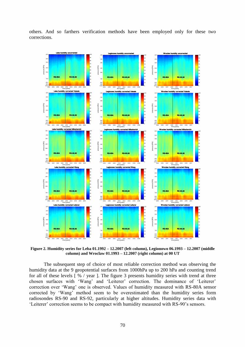
70
others. And so farthers verification methods have been employed only for these two
corrections.
Figure 2. Humidity series for Leba 01.1992 – 12.2007 (left column), Legionowo 06.1993 – 12.2007 (middle
column) and Wroclaw 01.1993 – 12.2007 (right column) at 00 UT
The subsequent step of choice of most reliable correction method was observing the
humidity data at the 9 geopotential surfaces from 1000hPa up to 200 hPa and counting trend
for all of these levels [ % / year ]. The figure 3 presents humidity series with trend at three
chosen surfaces with „Wang‟ and „Leiterer‟ correction. The dominance of „Leiterer‟
correction over „Wang‟ one is observed. Values of humidity measured with RS-80A sensor
corrected by „Wang‟ method seem to be overestimated than the humidity series form
radiosondes RS-90 and RS-92, particularly at higher altitudes. Humidity series data with
„Leiterer‟ correction seems to be compact with humidity measured with RS-90‟s sensors.
1992 1994 1996 1998 2000 2002 2004 2006 2008
200
250
300
400
500
700
850
925
1000
Leba humidity uncorrected
time [years]
pre
ssure
[hP
a]
RS-80A RS-90,92
0
10
20
30
40
50
60
70
80
90
100
1994 1996 1998 2000 2002 2004 2006 2008
200
250
300
400
500
700
850
925
1000
Legionowo humidity uncorrected
time [years]
pre
ssure
[hP
a]
RS-80A RS-90,92
0
10
20
30
40
50
60
70
80
90
100
1993 1995 1997 1999 2001 2003 2005 2007
200
250
300
400
500
700
850
925
1000
Wroclaw humidity uncorrected
time [years]
pre
ssure
[hP
a]
RS-80A RS-90,92
0
10
20
30
40
50
60
70
80
90
100
1992 1994 1996 1998 2000 2002 2004 2006 2008
200
250
300
400
500
700
850
925
1000
Leba humidity corrected Vaisala
time [years]
pre
ssure
[hP
a]
RS-80A RS-90,92
0
10
20
30
40
50
60
70
80
90
100
1994 1996 1998 2000 2002 2004 2006 2008
200
250
300
400
500
700
850
925
1000
Legionowo humidity corrected Vaisala
time [years]
pre
ssure
[hP
a]
RS-80A RS-90,92
0
10
20
30
40
50
60
70
80
90
100
1993 1995 1997 1999 2001 2003 2005 2007
200
250
300
400
500
700
850
925
1000
Wroclaw humidity corrected Vaisala
time [years]
pre
ssure
[hP
a]
RS-80A RS-90,92
0
10
20
30
40
50
60
70
80
90
100
1992 1994 1996 1998 2000 2002 2004 2006 2008
200
250
300
400
500
700
850
925
1000
Leba humidity corrected Miloshevich
time [years]
pre
ssure
[hP
a]
RS-80A RS-90,92
0
10
20
30
40
50
60
70
80
90
100
1994 1996 1998 2000 2002 2004 2006 2008
200
250
300
400
500
700
850
925
1000
Legionowo humidity corrected Miloshevich
time [years]
pre
ssure
[hP
a]
RS-80A RS-90,92
0
10
20
30
40
50
60
70
80
90
100
1993 1995 1997 1999 2001 2003 2005 2007
200
250
300
400
500
700
850
925
1000
Wroclaw humidity corrected Miloshevich
time [years]
pre
ssure
[hP
a]
RS-80A RS-90,92
0
10
20
30
40
50
60
70
80
90
100
1992 1994 1996 1998 2000 2002 2004 2006 2008
200
250
300
400
500
700
850
925
1000
Leba humidity corrected Wang
time [years]
pre
ssure
[hP
a]
RS-80A RS-90,92
0
10
20
30
40
50
60
70
80
90
100
1994 1996 1998 2000 2002 2004 2006 2008
200
250
300
400
500
700
850
925
1000
Legionowo humidity corrected Wang
time [years]
pre
ssure
[hP
a]
RS-80A RS-90,92
0
10
20
30
40
50
60
70
80
90
100
1993 1995 1997 1999 2001 2003 2005 2007
200
250
300
400
500
700
850
925
1000
Wroclaw humidity corrected Wang
time [years]
pre
ssure
[hP
a]
RS-80A RS-90,92
0
10
20
30
40
50
60
70
80
90
100
1992 1994 1996 1998 2000 2002 2004 2006 2008
200
250
300
400
500
700
850
925
1000
Leba humidity corrected Leiterer
time [years]
pre
ssure
[hP
a]
RS-80A RS-90,92
0
10
20
30
40
50
60
70
80
90
100
1994 1996 1998 2000 2002 2004 2006 2008
200
250
300
400
500
700
850
925
1000
Legionowo humidity corrected Leiterer
time [years]
pre
ssure
[hP
a]
RS-80A RS-90,92
0
10
20
30
40
50
60
70
80
90
100
1993 1995 1997 1999 2001 2003 2005 2007
200
250
300
400
500
700
850
925
1000
Wroclaw humidity corrected Leiterer
time [years]
pre
ssure
[hP
a]
RS-80A RS-90,92
0
10
20
30
40
50
60
70
80
90
100
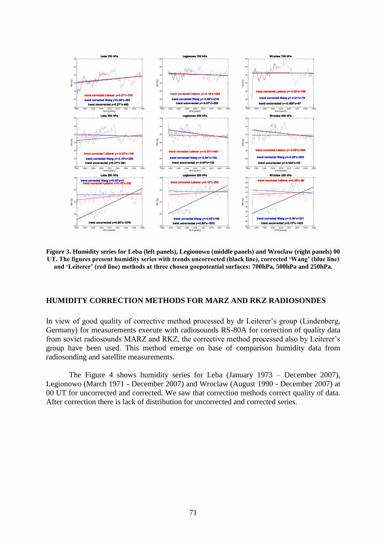
71
Figure 3. Humidity series for Leba (left panels), Legionowo (middle panels) and Wroclaw (right panels) 00
UT. The figures present humidity series with trends uncorrected (black line), corrected „Wang‟ (blue line)
and „Leiterer‟ (red line) methods at three chosen goepotential surfaces: 700hPa, 500hPa and 250hPa.
HUMIDITY CORRECTION METHODS FOR MARZ AND RKZ RADIOSONDES
In view of good quality of corrective method processed by dr Leiterer‟s group (Lindenberg,
Germany) for measurements execute with radiosounds RS-80A for correction of quality data
from soviet radiosounds MARZ and RKZ, the corrective method processed also by Leiterer‟s
group have been used. This method emerge on base of comparison humidity data from
radiosonding and satellite measurements.
The Figure 4 shows humidity series for Leba (January 1973 – December 2007),
Legionowo (March 1971 - December 2007) and Wroclaw (August 1990 - December 2007) at
00 UT for uncorrected and corrected. We saw that correction methods correct quality of data.
After correction there is lack of distribution for uncorrected and corrected series.
1992 1994 1996 1998 2000 2002 2004 2006 200835
40
45
50
55
60
65
trend uncorrected y=0.27*x-490
trend corrected Wang y=0.26*x-464
trend corrected Leiterer y=0.21*x-376
Leba 700 hPa
time [years]
RH
[%
]
1992 1994 1996 1998 2000 2002 2004 2006 200835
40
45
50
55
60
65
trend uncorrected y=-0.07*x+200
trend corrected Wang y=-0.08*x+219
trend corrected Leiterer y=-0.12*x+293
Legionowo 700 hPa
time [years]
RH
[%
]
1992 1994 1996 1998 2000 2002 2004 2006 200835
40
45
50
55
60
65
trend uncorrected y=-0.005*x+67
trend corrected Wang y=-0.01*x+79
trend corrected Leiterer y=-0.05*x+165
Wroclaw 700 hPa
time [years]
RH
[%
]
1992 1994 1996 1998 2000 2002 2004 2006 200825
30
35
40
45
50
55
trend uncorrected y=0.21*x-381
trend corrected Wang y=-0.10*x+235
trend corrected Leiterer y=-0.03*x+109
Leba 500 hPa
time [years]
RH
[%
]
1992 1994 1996 1998 2000 2002 2004 2006 200825
30
35
40
45
50
55
trend uncorrected y=-0.04*x+130
trend corrected Wang y=-0.34*x+732
trend corrected Leiterer y=-0.30*x+651
Legionowo 500 hPa
time [years]
RH
[%
]
1992 1994 1996 1998 2000 2002 2004 2006 200825
30
35
40
45
50
55
trend uncorrected y=-0.004*x+53
trend corrected Wang y=-0.29*x+633
trend corrected Leiterer y=-0.26*x+560
Wroclaw 500 hPa
time [years]
RH
[%
]
1992 1994 1996 1998 2000 2002 2004 2006 200820
25
30
35
40
trend uncorrected y=0.80*x-1579
trend corrected Wang y=0.02*x+3 trend corrected Leiterer y=0.18*x-336
Leba 250 hPa
time [years]
RH
[%
]
1992 1994 1996 1998 2000 2002 2004 2006 200820
25
30
35
40
trend uncorrected y=0.80*x-1572
trend corrected Wang y=-0.03*x+88
trend corrected Leiterer y=0.12*x-200
Legionowo 250 hPa
time [years]
RH
[%
]
1992 1994 1996 1998 2000 2002 2004 2006 200820
22
24
26
28
30
32
34
36
38
40
trend uncorrected y=0.73*x-1422
trend corrected Wang y=-0.09*x+221
trend corrected Leiterer y=0.06*x-96
Wroclaw 250 hPa
time [years]
RH
[%
]

72
Figure 5. Humidity series for Leba, Legionowo and Wroclaw at 00 UT for uncorrected (left column) and
corrected (right column) data
The next step was observing the humidity data at the 5 geopotential surfaces from
1000hPa up to 400 hPa and counting trend for all of these levels [ % / year ]. The figure 5
presents humidity series with trend at three chosen surfaces. Humidity series looks better
with, than without correction. Unfortunately, received results have exerted, that employed
corrective method, it does not eliminate completely the differences among data from soviet
and Finnish radiosounds. Results are different for each geopotential level and each station
however, it get no completelely similar series. Additional opposite sign of trend of humidity
from soviet and finnish radiosounds on many surfaces have been visible, that makes
impossible obtainment of similar series. In final effect still has been show that series of
measurement of humidity is uncontinuous at change of sensor.
1973 1977 1981 1985 1989 1993 1997 2001 2005
400
500
700
850
925
1000
Leba humidity uncorrected
time [years]
pre
ssure
[hP
a]
MARZ, RKZ Vaisala
30
40
50
60
70
80
90
100
1973 1977 1981 1985 1989 1993 1997 2001 2005
400
500
700
850
925
1000
Leba humidity corrected
time [years]
pre
ssure
[hP
a]
MARZ, RKZ Vaisala
30
40
50
60
70
80
90
100
1971 1975 1979 1983 1987 1991 1995 1999 2003 2007
400
500
700
850
925
1000
Legionowo humidity uncorrected
time [years]
pre
ssure
[hP
a]
MARZ, RKZ Vaisala
30
40
50
60
70
80
90
100
1971 1975 1979 1983 1987 1991 1995 1999 2003 2007
400
500
700
850
925
1000
Legionowo humidity corrected
time [years]
pre
ssure
[hP
a]
MARZ, RKZ Vaisala
30
40
50
60
70
80
90
100
1991 1994 1998 2002 2006
400
500
700
850
925
1000
Wroclaw humidity uncorrected
time [years]
pre
ssure
[hP
a]
MARZ,RKZ Vaisala
30
40
50
60
70
80
90
100
1991 1994 1998 2002 2006
400
500
700
850
925
1000
Wroclaw humidity corrected
time [years]
pre
ssure
[hP
a]
MARZ,RKZ Vaisala
30
40
50
60
70
80
90
100

73
Figure 6. Humidity series for Leba (left panels), Legionowo (middle panels) and Wroclaw (right panels) 00
UT. The figures present humidity series with trends uncorrected (black line) and corrected (red line) data
at three chosen goepotential surfaces: 700hPa, 500hPa and 400hPa.
CONCLUSIONS
o For homogenisation of humidity data from Vaisala radiosounds (RS-80A, RS-90 and
RS-92) four correction methods have been chosen for correction data from RS-80A
radiosounds.
o Two methods („Wang‟ and „Leiterer‟) were submitted for further studies.
o Analyses of humidity trends on different goepotential surfaces show dominance of
„Leirerer‟ correction over „Wang‟ one.
o For homogenisation of humidity data from soviet (MARZ and RKZ) and Finnish (RS-
80A, RS-90 and RS-92) radiosounds the correction methods execute by Leiterer‟s
group have been chosen for correction data from soviet radiosounds.
o Adopted method ameliorates quality of data however, there is still not so good so as
data after correction can become subject climatic analyses.
APPENDIX A: MATHEMATICAL BACKGROUND
The RS80-A is subject to several sources of measurement error, and correction of the
individual measurement errors is an alternative approach for correcting RS80-A data that is
under development. A "temperature-dependence error" is caused by using a linear
approximation in the data processing algorithm to represent the actual non-linear temperature
dependence of the sensor calibration, and is, in general, the largest RS80-A measurement
error at cold temperatures.
1970 1975 1980 1985 1990 1995 2000 2005 201035
40
45
50
55
60
65
70
75
trend uncorrected y=-0.41*x+874
trend corrected y=0.03*x+1
Leba 700 hPa
time [years]
RH
[%
]
1970 1975 1980 1985 1990 1995 2000 2005 201035
40
45
50
55
60
65
70
75
trend uncorrected y=-0.39*x+841
trend corrected y=-0.04*x+140
Legionowo 700 hPa
time [years]
RH
[%
]
1990 1992 1994 1996 1998 2000 2002 2004 2006 200835
40
45
50
55
60
65
70
75
trend uncorrected y=-0.31*x+668
trend corrected y=-0.02*x+99
Wroclaw 700 hPa
time [years]
RH
[%
]
1970 1975 1980 1985 1990 1995 2000 2005 201025
30
35
40
45
50
55
60
65
70
trend uncorrected y=-0.50*x+1048
trend corrected y=-0.02*x+87
Leba 500 hPa
time [years]
RH
[%
]
1970 1975 1980 1985 1990 1995 2000 2005 201025
30
35
40
45
50
55
60
65
70
trend uncorrected y=-0.57*x+1191
trend corrected y=-0.07*x+175
Legionowo 400 hPa
time [years]
RH
[%
]
1990 1992 1994 1996 1998 2000 2002 2004 2006 200825
30
35
40
45
50
55
60
65
70
trend uncorrected y=-0.48*x+1014
trend corrected y=-0.17*x+387
Wroclaw 500 hPa
time [years]
RH
[%
]
1970 1975 1980 1985 1990 1995 2000 2005 201025
30
35
40
45
50
55
60
65
70
trend uncorrected y=-0.57*x+1174
trend corrected y=0.045*x-48
Leba 400 hPa
time [years]
RH
[%
]
1970 1975 1980 1985 1990 1995 2000 2005 201025
30
35
40
45
50
55
60
65
70
trend uncorrected y=-0.49*x+1026
trend corrected y=-0.10*x+244
Legionowo 500 hPa
time [years]
RH
[%
]
1990 1992 1994 1996 1998 2000 2002 2004 2006 200825
30
35
40
45
50
55
60
65
70
trend uncorrected y=-0.53*x+1110
trend corrected y=-0.13*x+293
Wroclaw 400 hPa
time [years]
RH
[%
]
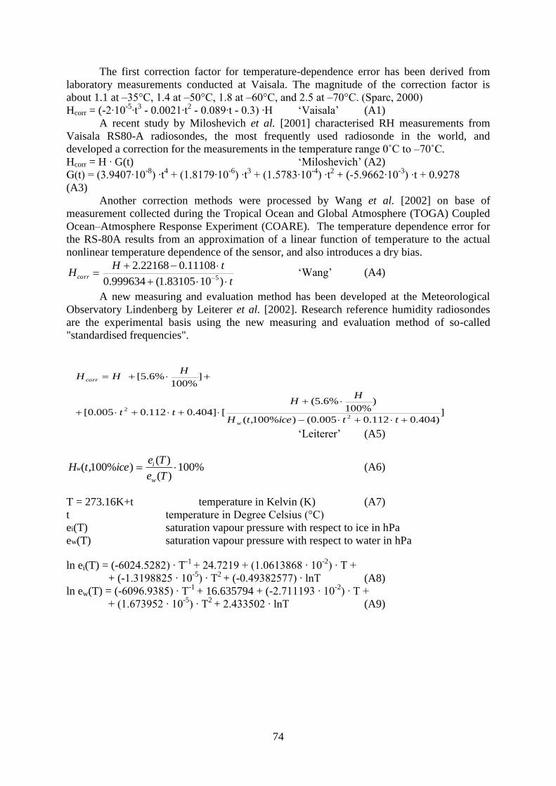
74
The first correction factor for temperature-dependence error has been derived from
laboratory measurements conducted at Vaisala. The magnitude of the correction factor is
about 1.1 at –35°C, 1.4 at –50°C, 1.8 at –60°C, and 2.5 at –70°C. (Sparc, 2000)
Hcorr = (-2∙10-5
∙t3 - 0.0021∙t
2 - 0.089∙t - 0.3) ∙H „Vaisala‟ (A1)
A recent study by Miloshevich et al. [2001] characterised RH measurements from
Vaisala RS80-A radiosondes, the most frequently used radiosonde in the world, and
developed a correction for the measurements in the temperature range 0˚C to –70˚C.
Hcorr = H ∙ G(t) „Miloshevich‟ (A2)
G(t) = (3.9407∙10-8
) ∙t4 + (1.8179∙10
-6) ∙t
3 + (1.5783∙10
-4) ∙t
2 + (-5.9662∙10
-3) ∙t + 0.9278
(A3)
Another correction methods were processed by Wang et al. [2002] on base of
measurement collected during the Tropical Ocean and Global Atmosphere (TOGA) Coupled
Ocean–Atmosphere Response Experiment (COARE). The temperature dependence error for
the RS-80A results from an approximation of a linear function of temperature to the actual
nonlinear temperature dependence of the sensor, and also introduces a dry bias.
t
tHHcorr
)1083105.1(999634.0
11108.022168.25
„Wang‟ (A4)
A new measuring and evaluation method has been developed at the Meteorological
Observatory Lindenberg by Leiterer et al. [2002]. Research reference humidity radiosondes
are the experimental basis using the new measuring and evaluation method of so-called
"standardised frequencies".
„Leiterer‟ (A5)
%100)(
)()%100,(
Te
TeicetH
w
iw (A6)
T = 273.16K+t temperature in Kelvin (K) (A7)
t temperature in Degree Celsius (°C)
ei(T) saturation vapour pressure with respect to ice in hPa
ew(T) saturation vapour pressure with respect to water in hPa
ln ei(T) = (-6024.5282) ∙ T-1
+ 24.7219 + (1.0613868 ∙ 10-2
) ∙ T +
+ (-1.3198825 ∙ 10-5
) ∙ T2
+ (-0.49382577) ∙ lnT (A8)
ln ew(T) = (-6096.9385) ∙ T-1
+ 16.635794 + (-2.711193 ∙ 10-2
) ∙ T +
+ (1.673952 ∙ 10-5
) ∙ T2
+ 2.433502 ∙ lnT (A9)
])404.0112.0005.0()%100,(
)%100
%6.5(
[]404.0112.0005.0[
]%100
%6.5[
2
2
tticetH
HH
tt
HHH
w
corr

75
References
SPARC Assessment of Upper Troposheric and Stratospheric Water Vapour, December 2000, WCRP-113,
WMO/TD No.1043, SPARC Report No.2.
Miloshevich, L. M., et al.: “Characterization and correction of relative humidity measurements from Vaisala
RS80-A radiosondes at cold temperatures”; Journal of Atmospheric and Oceanic Technology, vol.18,
February 2001.
Wang, J., et al.: “Corrections of humidity measurement errors from the Vaisala RS80 radiosonde - Application to
TOGA COARE Data”; Journal of Atmospheric and Oceanic Technology, vol.19, July 2002.
Leiterer, U., et al.: "Method for correction of RS80 A – Humicap humidity profiles"; 2002.
Leiterer, U., et al.: “Correction Method for RS80-A Humicap Humidity Profiles and Their Validation by Lidar
Backscattering Profiles in Tropical Cirrus Clouds”; Journal of Atmospheric and Oceanic Technology,
vol.22, January 2005
Soden, B.J. and J.R. Lanzante; 1996: An assessment of satellite and radiosonde climatologies of upper-
tropospheric water vapor. J. Climate, 9, 1235-1250.

76
HOMOGENIZATION OF ITALIAN PRECIPITATION SERIES
Andrea Toreti1,2,3
, Franco Desiato1, Guido Fioravanti
1, Walter Perconti
1
1 ISPRA, Istituto Superiore per la Protezione e la Ricerca Ambientale (ex APAT),
2 Institute of Geography, Climatology and Meteorology, University of Bern,
3 Oeschger Centre for Climate Change Research (OCCR) and National Centre of Competence
in Research on Climate (NCCR Climate), University of Bern, tel: +390650072567,
fax: +390650072657
INTRODUCTION
The analysis of precipitation series is crucial in the assessment of climate change in the
Mediterranean area, in order to understand its impacts on ecosystems and human activities,
and to provide reliable information for the definition of adaptation strategies. In this context
the Italian Research Institute for the Environment – ISPRA (formerly National Environmental
Agency APAT) developed a computerized system for the collection and elaboration of
statistical data on the Italian climate, denominated SCIA (Desiato et al., 2007). In this system
rough data, coming from national and regional meteorological networks, are collected and
quality checked; the outputs, e.g. ten-daily, monthly and annual indicators, are available on
the web site: www.scia.sinanet.apat.it.
In this study a set of 59 stations (fig. 1), belonging to the Air Force Weather Service
and some regional environmental agencies and characterized by temporal continuity and high
quality, was selected. Data underwent a quality control procedure and outliers were discarded;
afterwards monthly series were elaborated. Time series of climatic variables, as temperature
and precipitation, may be affected by non-climatic factors, that can hide or alter the climatic
signal; therefore, a 3-step homogenization procedure was applied to monthly series.
Figure 1. Map of the 59 stations
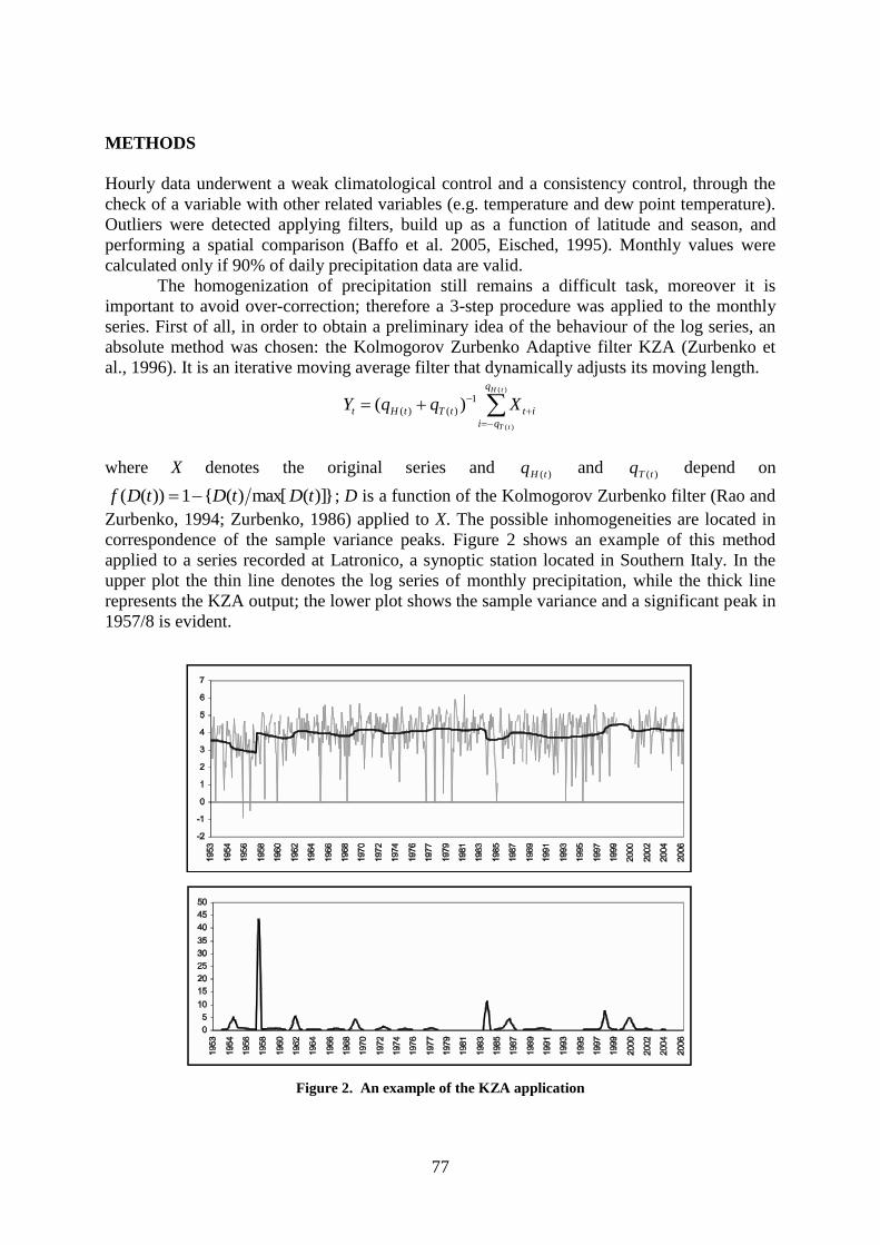
77
METHODS
Hourly data underwent a weak climatological control and a consistency control, through the
check of a variable with other related variables (e.g. temperature and dew point temperature).
Outliers were detected applying filters, build up as a function of latitude and season, and
performing a spatial comparison (Baffo et al. 2005, Eisched, 1995). Monthly values were
calculated only if 90% of daily precipitation data are valid.
The homogenization of precipitation still remains a difficult task, moreover it is
important to avoid over-correction; therefore a 3-step procedure was applied to the monthly
series. First of all, in order to obtain a preliminary idea of the behaviour of the log series, an
absolute method was chosen: the Kolmogorov Zurbenko Adaptive filter KZA (Zurbenko et
al., 1996). It is an iterative moving average filter that dynamically adjusts its moving length.
)(
)(
1
)()( )(tH
tT
q
qi
ittTtHt XqqY
where X denotes the original series and )(tHq and )(tTq depend on
})](max[)({1))(( tDtDtDf ; D is a function of the Kolmogorov Zurbenko filter (Rao and
Zurbenko, 1994; Zurbenko, 1986) applied to X. The possible inhomogeneities are located in
correspondence of the sample variance peaks. Figure 2 shows an example of this method
applied to a series recorded at Latronico, a synoptic station located in Southern Italy. In the
upper plot the thin line denotes the log series of monthly precipitation, while the thick line
represents the KZA output; the lower plot shows the sample variance and a significant peak in
1957/8 is evident.
Figure 2. An example of the KZA application

78
The second step involves a modified version of the well-known Standard Normal
Homogeneity Test (Alexandersson and Moberg, 1997). A moving window approach was
implemented, using a window length of 12 years, but discarding the inhomogeneities detected
in the first/last four years. The modified SNHT was applied to the log ratio series, building up
the reference series with at least three stations, chosen using the best correlation criterion
(Peterson and Easterling, 1994) and putting some geographical limitations.
The identified shifts underwent the third step of our procedure: the Multi Response
Permutation Procedure MRPP (Easterling and Peterson, 1994; Mielke et al., 1981). It is non
parametric and it was implemented choosing a window length of 96 values (centred at the
inhomogeneity point). It is based on a standardized version of the following statistic and on a
partition of K elements in g subgroups:
g
i
iiC1
, KnC ii
Where ni denotes the cardinality of the i-th subgroup, i the average distance (using the
Euclidean distance) for all elements belonging to the i-th subgroup. Figure 3 illustrates an
example: the synoptic station Enna in Sicily before (red line) and after (grey line) the
homogenization, indeed an inhomogeneity was detected by the procedure in November 1964.
Figure 3. Enna series before (red line) and after (grey line) the homogenization
RESULTS
After the homogenization of the 59 monthly precipitation series, they were transformed in
standardized anomaly series (Jones and Hulme, 1996), using as reference period 1971 – 2000.
Afterwards, annual and seasonal series were calculated; the former considering the year from
December to November, the latter applying the meteorological definition of seasons. Finally,
the series were aggregated, in order to achieve three series for the following sub-areas:
Northern, Central and Southern Italy. In the case of annual series no significant trends were
identified. On the contrary, Northern winter series has a decreasing trend since 1961 and
Centre winter series is characterized by a positive trend since 1998 (it might be confirmed in
next years, when more data will be available).
The same calculations were carried out also for the original series, trying to understand
the impact of the homogenization on the final output, which was used for trend identification
and further climatological analysis. As for annual standardized series, absolute values of
differences (between homogenized and original series) do not overcome 0.5, with greatest
values in Central Italy and smallest values in Southern Italy (fig. 4 and fig. 5).

79
Figure 4. Comparison of annual standardized series before and after the homogenization
Figure 5. Boxplot of the differences between original and homogenized annual series
In Northern Italy there are not great differences between homogeneous and original series,
especially during autumn (fig. 6, fig. 7 and fig. 8); all values belong to (-0.5, 0.3).

80
Figure 6. Comparison of seasonal standardized series, before and after homogenization in Northern Italy
(winter and spring)
Figure 7. Comparison of seasonal standardized series, before and after homogenization in Northern Italy
(summer and autumn)

81
Figure 8.Boxplot of the differences between original and homogenized seasonal series in Northern Italy
In Central Italy differences are small, but winter 2000 with a value of about 0.6; spring
values, with three exceptions, are concentrated around zero (fig. 9, fig.10 and fig. 11).
Figure 9. Comparison of seasonal standardized series, before and after homogenization in Central Italy
(winter and spring)

82
Figure 10..Comparison of seasonal standardized series, before and after homogenization in Central Italy
(summer and autumn)
Figure 11. Boxplot of the differences between original and homogenized seasonal series in Central Italy
Finally, in Southern Italy there are not remarkable differences, except some high values, as
summer 1999 (with a value of about 1) and winter 1996 (with a value of about 0.6). Figures
12, 13 and 14 show these results.
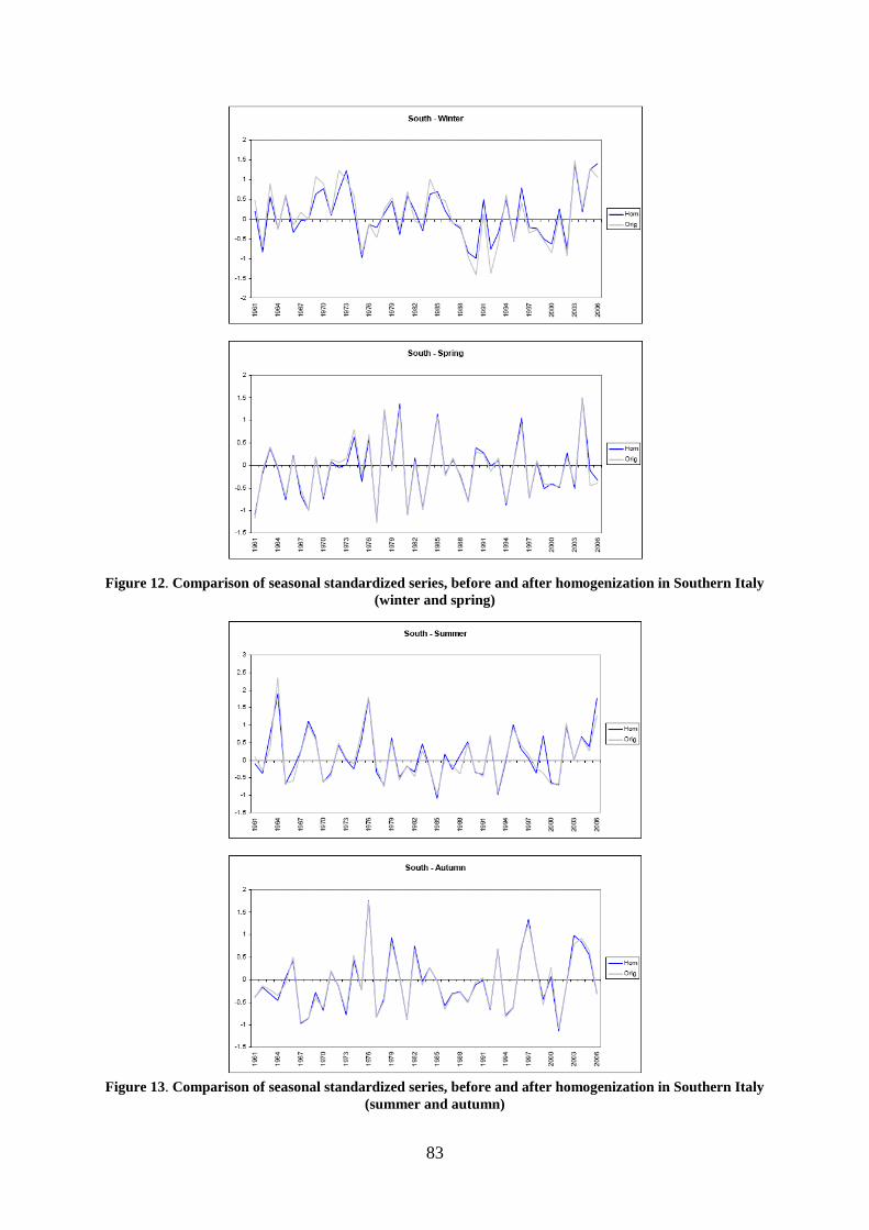
83
Figure 12. Comparison of seasonal standardized series, before and after homogenization in Southern Italy
(winter and spring)
Figure 13. Comparison of seasonal standardized series, before and after homogenization in Southern Italy
(summer and autumn)

84
Figure 14. Boxplot of the differences between original and homogenized seasonal series in Southern Italy
CONCLUSIONS
In order to obtain a set of high quality precipitation series for climatological analysis, 59
monthly series well distributed over the Italian territory were homogenized applying a three
steps procedure: KZA, modified SNHT and MRPP. The application of these different
methods should avoid overcorrection, preserving the true climatic signal. However, it is
important to underline that the homogenization of precipitation is still a tricky question. Our
ongoing research concerns the investigation of other methods, the introduction of pairwise
comparison in the procedure and the homogenization of daily series.
References
Alexandersson H, Moberg A. 1997. Homogenization of Swedish temperature data. Part I: homogeneity test for
linear trends. International Journal of Climatology 17: 25-34.
Baffo F, Suatoni B, Desiato F. 2005. Indicatori climatici: i controlli di validità e la ricerca dei valori errati.
Bollettino Geofisico 1-2, anno XXVIII: 31-41.
Desiato F, Lena F, Toreti A. 2007. SCIA: a system for a better knowledge of the Italian climate. Bollettino di
Geofisica Teorica ed Applicata 48: 351-358.
Easterling DR, Peterson TC. 1994. A new method for detecting undocumented discontinuities in climatological
series. International Journal of Climatology 15: 369-377.
Eisched JK, Baker CB, Karl TR, Diaz HF. 1995. The quality control of long-term climatological data using
objective data analysis. Journal of Applied Meteorology 34: 2787-2795.
Jones PD, Hulme M. 1996. Calculating regional climatic time series for temperature and precipitation: methods
and illustrations. International Journal of Climatology 16: 361-377.
Mielke PW, Berry KJ, Brier GW. 1981. Application of multi-response permutation procedure for examining
seasonal changes in monthly mean sea level pressure patterns. Monthly Weather Review 190: 120-126.
Peterson TC, Easterling DR. 1994. Creation of homogenous composite climatological reference series.
International Journal of Climatology 14: 671-679.
Rao ST, Zurbenko IG. 1994. Detecting and tracking changes in ozone air quality. Journal of the Air and Waste
Management Association 44: 1089-1092.
Zurbenko IG. 1986. The Spectral Analysis of Time Series. North Holland, USA, 248 pp.
Zurbenko I, Porter PS, Rao ST, Ku JY, Gui R, Eskridge RE. 1996. Detecting discontinuities in time series of
upper air data: development and demonstration of an adaptive filter technique. Journal of Climate 9:
3548-3560.

85
HOMOGENISATION OF TEMPERATURE TIME SERIES IN
CROATIA
Dubravka Rasol, Tanja Likso, Janja Milković
DHMZ, Griĉ 3, HR-10 000 Zagreb, Croatia,
Abstract
The use of homogenized meteorological data time series is very important for all climate analyses
because artificial shifts can cause misleading conclusions that do not correspond to real climate
changes. Until recently, the homogenization of Croatian meteorological data series was carried out
only sporadically. However, since Croatia joined the HOME COST Action ES0601, we have started
dealing more intensively with the issue of homogenization.
This paper outlines the preliminary results of homogenization of some Croatian temperature data
series. Two methods of homogenization were used and the results were compared. One of the methods
used was Multiple Analysis of Series for Homogenization - MASH v3.02 and the other one was
Standard Normal Homogeneity Test - SNHT applied with the AnClim software. Those two methods
were applied on the data series from nine stations situated in the northwestern part of Croatia. Both
methods gave similar results in detecting break points with quite a high accordance with the existing
metadata. Furthermore, three stations were chosen for comparison of homogenized data series.
Differences between values obtained by each method were negligible, but more detailed analysis of
those results is required in the future.
INTRODUCTION
Homogeneous time series of climatic elements are essential for all studies concerning climate
variability. Inhomogeneities caused by station relocation, instrumentation changes, changes in
methods of calculating monthly means, etc. (e.g. Peterson and Easterling 1994; Jones 1995)
can mask real trends and variability. In practice, it is difficult to preserve the permanence of
all observation elements. Because of that many long-term time series contain inhomogeneities
that must be adjusted before any comprehensive analysis for climatic variations
(Alexandersson 1986; Karl and Williams 1987; Peterson and Easterling 1994; Jones 1995;
Heino 1997; Peterson et al. 1998).
The intention of this paper is to compare two different homogenization methods Multiple
Analysis of Series for Homogenization (MASH) and Standard Normal Homogeneity Test
(SNHT) in order to evaluate the effectiveness of the procedures for breakpoints detection and
time series adjustment.
Homogenisation in Croatia
Until recently, the homogenisation of Croatian meteorological data series was carried out only
sporadically (Volaric 1982, Juras 1993, Likso 2004). Lately, in the Meteorological and
Hydrological Serivce (MHC) of Croatia none of the methods of homogenisation is applied
operationally. Recently meteorologists from the MHS have joined the COST Action ES0601 -
Advances in homogenisation methods of climate series: an integrated approach (HOME,
2007-2011), and also have started a bilateral cooperation with the Hungarian Meteorological
Service the project "Harmonization of homogenisation and interpolation methods"
(2007-2009). As a consequence meteorologists in Croatia have started dealing more
intensively with the issue of homogenization.
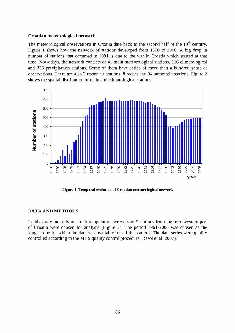
86
Croatian meteorological network
The meteorological observations in Croatia date back to the second half of the 19th
century.
Figure 1 shows how the network of stations developed from 1850 to 2000. A big drop in
number of stations that occurred in 1991 is due to the war in Croatia which started at that
time. Nowadays, the network consists of 41 main meteorological stations, 116 climatological
and 336 precipitation stations. Some of them have series of more than a hundred years of
observations. There are also 2 upper-air stations, 8 radars and 34 automatic stations. Figure 2
shows the spatial distribution of main and climatological stations.
Figure 1. Temporal evolution of Croatian meteorological network
DATA AND METHODS
In this study monthly mean air temperature series from 9 stations from the northwestern part
of Croatia were chosen for analysis (Figure 2). The period 1961-2006 was chosen as the
longest one for which the data was available for all the stations. The data series were quality
controlled according to the MHS quality control procedure (Rasol et al. 2007).
0
100
200
300
400
500
600
700
800
1850
1880
1925
1948
1951
1954
1957
1960
1963
1966
1969
1972
1975
1978
1981
1984
1987
1990
1993
1996
1999
2002
2005
year
Nu
mb
er
of
sta
tio
ns

87
Figure 2. Spatial distribution of main (red) and climatological (black) stations and the list of stations
chosen for this study
Break points were found and data was homogenized with two methods for relative
homogeneity testing and the results obtained by each method were compared.
One method used here for the homogenization of temperature data is Multiple Analysis of
Series for Homogenization, developed by Tamas Szentimrey in the Hungarian Meteorological
Service (Szentimrey 1994, 1995, 1996). That procedure does not assume a reference series is
homogeneous. Break points are detected and adjusted through mutual comparisons of series
within the same climatic area. The candidate series is chosen from the available time series
and the remaining series are considered as reference series. Several difference series are
constructed from the candidate and weighted reference series.
The other method is described in Alexandersson (1986) and Alexandersson and Moberg
(1997), known as the Standard Normal Homogeneity Test applied with the AnClim software
(Stepanek, 2005). This procedure requires a homogeneous reference series. The reference
series should ideally consist of meteorological data from several stations where the climate
variations resemble those at the test station. Reference station should be located in a region
with the same climatic characteristics as the test station. The number of reference stations
should be large enough to eliminate eventual inhomogeneities in the reference data. In
general, reference series have been constructed as a weighted average of the data from
reference stations. The weight factors are the correlation coefficients between the test series
and the series from reference stations.
As the testing was performed on the temperature time series, the differences between test and
reference series were considered. The SNHT test is based on the likelihood ratio test with the
assumption that there is at most one break point in the series. The test for a single shift cannot
properly handle series with many break points (Alexanderson and Moberg 1997). In this
paper, if a break point was detected, it was adjusted by calculating an adjustment factor (the
Bjelovar
Karlovac
Koprivnica
Krizevci
Sisak
Slavonski Brod
Zagreb Gric
Zagreb Maksimir
Varazdin

88
difference between the test series and the reference series). The test was repeated to detect
further break points, until the series is considered homogeneous. For a homogeneous time
series, the test statistic should not exceed a critical t-value on a specified confidence level.
RESULTS
Table 1 shows the breakpoints detected by MASH and SNHT. Quite a lot of breakpoints were
found by both methods. The years for which there is a justification for the breakpoint in the
metadata are bolded. Both methods detected all, from metadata known breakpoints, as well as
additional ones. The accordance between mentioned procedures for breakpoint detection was
very high. There were some minor changes found in the metadata that were not detected, but
we can not be sure that those changes could really cause significant breaks in data series.
Table 1: Breakpoints detected by MASH (blue) and SNHT (red)
Bjelovar 1969 1981 1983 1989 1998 2001 2003 2004
1969 1983 1989 1998 2001 2004
Karlovac 1992 1993 1994 1999 2000 2001
1965 1984 1992 2000 2001
Koprivnica 1964 1967 1999
1965 1967 1980 1998
Krizevci 1980 1982 1984 1994 1995 2000
1981 1986 1993 1997 2000
Sisak 1964 1969 1971 1984 1989 1996
1964 1969 1979 1984 1996 2001
Slavonski Brod 1969 1974 1986 1991 1994 1996
1969 1986 1991 1996 1998
Zagreb Gric 1982 1989 1992 1998
1967 1972 1984
Zagreb Maksimir 1981 1987 1989 1991 2002
1981 1991 1995 2002
Varazdin 1971 2000
1970 1987 1989 2000
Figure 3 shows the results of adjusting with MASH and SNHT method for Zagreb Gric
station. Zagreb Gric temperature series is almost homogeneous, there were some very small
changes in series but none of the breakpoints have justification in metadata.
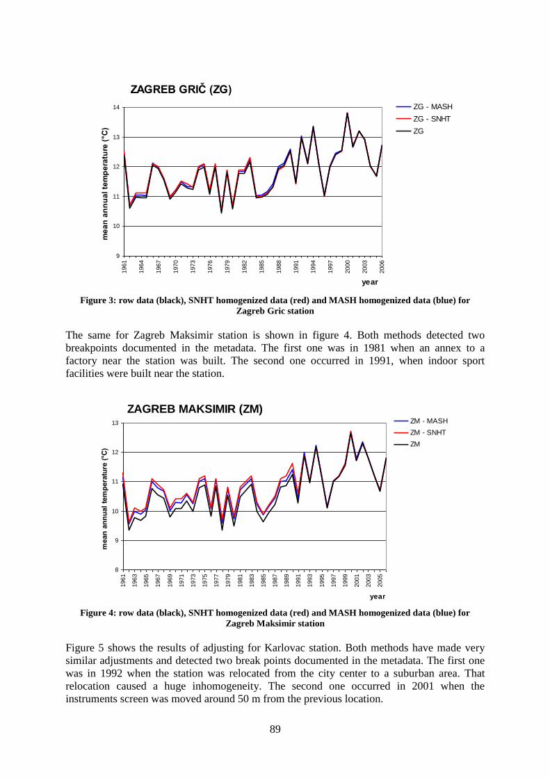
89
Figure 3: row data (black), SNHT homogenized data (red) and MASH homogenized data (blue) for
Zagreb Gric station
The same for Zagreb Maksimir station is shown in figure 4. Both methods detected two
breakpoints documented in the metadata. The first one was in 1981 when an annex to a
factory near the station was built. The second one occurred in 1991, when indoor sport
facilities were built near the station.
Figure 4: row data (black), SNHT homogenized data (red) and MASH homogenized data (blue) for
Zagreb Maksimir station
Figure 5 shows the results of adjusting for Karlovac station. Both methods have made very
similar adjustments and detected two break points documented in the metadata. The first one
was in 1992 when the station was relocated from the city center to a suburban area. That
relocation caused a huge inhomogeneity. The second one occurred in 2001 when the
instruments screen was moved around 50 m from the previous location.
ZAGREB GRIČ (ZG)
9
10
11
12
13
14
1961
1964
1967
1970
1973
1976
1979
1982
1985
1988
1991
1994
1997
2000
2003
2006
year
me
an
an
nu
al
tem
pe
ratu
re (
°C)
ZG - MASH
ZG - SNHT
ZG
ZAGREB MAKSIMIR (ZM)
8
9
10
11
12
13
1961
1963
1965
1967
1969
1971
1973
1975
1977
1979
1981
1983
1985
1987
1989
1991
1993
1995
1997
1999
2001
2003
2005
year
mean
an
nu
al
tem
pera
ture
(°C
)
ZM - MASH
ZM - SNHT
ZM
90
Figure 5: row data (black), SNHT homogenized data (red) and MASH homogenized data (blue) for
Karlovac station
The differences between the MASH homogenized and SNHT homogenized series (Figure 6),
for all three stations are very small, mostly less than 0.1°C and the largest is 0.2°C what is
still very good accordance. From this it cannot be said which method would be better to use.
Figure 6: Differences between MASH and SNHT homogenized for Zagreb Gric (violet) Zagreb Maksimir
(orange) and Karlovac (green) stations
Figure 7 up shows the place where Karlovac station was situated until 1992, it was in the
middle of the city with the high urban impact, and the figure 7 down shows the new position
after the relocation in 1992. The green arrow shows the position of the instruments screen in
the period from 1992 to 2001 and the red one the position after 2001 which is around 50 m
from the previous one. It is obvious that the position after 1992 is completely different, being
out in the fields and far from any urban impact.
KARLOVAC (KA)
8
9
10
11
12
13
1961
1964
1967
1970
1973
1976
1979
1982
1985
1988
1991
1994
1997
2000
2003
2006
year
me
an
an
nu
al
tem
pe
ratu
re (
°C)
KA - MASH
KA - SNHT
KA
-0.25
-0.2
-0.15
-0.1
-0.05
0
0.05
0.1
0.15
0.2
0.25
1961
1964
1967
1970
1973
1976
1979
1982
1985
1988
1991
1994
1997
2000
2003
2006
year
dif
fere
nc
es
(°C
)
ZG
KA
ZM
91
Figure 7: Position of the Karlovac station until 1992 (up) and after 1992 (down)
Figure 8 shows differences between yearly mean temperatures at Karlovac station and at all
reference stations. There is a big drop in 1992 and another one in 2001. It is obvious that after
relocation temperatures at Karlovac station became higher what is in accordance with the
location differences.

92
Figure 8: Differences between yearly mean temperatures at Karlovac station and at all reference stations
Trends
To get an impression of the difference between using original and homogenized data linear
trends for Karlovac station are shown in figure 9. The slope of homogenized data is much
steeper what shows the importance of homogenization of meteorological time series.
Figure 8: Linear trends for row and homogenized temperature time series for Karlovac station
CONCLUSIONS
Both MASH and SNHT methods for all studied stations detected all breakpoints known from
metadata, as well as some other undocumented discontinuities. The differences between
homogenized series obtained by each method were negligible. For Karlovac station it is still
to be discussed if it is better to homogenize the series according to the most recent data or the
data before the relocation in 1992. The question to be addressed is which part of the series is
more representative for the region so the more detailed analysis of the presented results is
required in the future.
KARLOVAC (KA)
8
9
10
11
12
13
1961
1963
1965
1967
1969
1971
1973
1975
1977
1979
1981
1983
1985
1987
1989
1991
1993
1995
1997
1999
2001
2003
2005
year
me
an
an
nu
al te
mp
era
ture
(°C
)
KA - MASH
KA - SNHT
KA
Linear (KA - SNHT)
Linear (KA - MASH)
Linear (KA)
year
Tem
per
atu
re d
iffe
ren
ces
(°C
)

93
Acknowledgements
Authors would like to thank Tamas Szentimrey for his valuable help regarding the MASH
homogenization method. This study was supported by the Ministry of Science, Education and
Sports of Croatia (project: "Harmonization of homogenization and interpolation methods")
and the Hypo Alpe-Adria bank d.d. donation "Ten for ten".
References
Alexandersson, H.,1986: A homogeneity test applied to precipitation data. Int. J. of Climatology, 6, 661-675.
Easterling D.R. and Peterson, T.C.1995: A new method of detecting undocumented discontinuities in
climatological time series, Int. J. of Climatology, 15, 369-377
Heino, R., 1997: Metadata and their role in homogenization. First Seminar for Homogenization of Surface
Climatological Data, Budapest, Hungary, Hungarian Meteorological Service, 5-8.
Jones, P.D., 1995: The instrumental data record: Its accuracy and use in attempts to identify the "CO2" signal.
Analyses of Climate Variability, H. von Storch, and H. Navarra, Eds., Springer, 53-75.
Juras, J., 1993: Homogeneity of the old meteorological series. Prace Geograficzne, 95, 93-98
Karl, T.R., and C.N. Williams Jr., 1987: An approach to adjusting climatological time series for discontinuous
inhomogeneities. J. Climate Appl. Meteor., 26, 1744-1763.
Likso, T., 2003: Inhomogeneities in temperature time series in CroatiaCroatian Meteorological Journal, 38, 3-9.
Peterson, T.C. and Easterling D.R., 1994: Creation of a homogeneous composite climatological reference series.
Int. J. of Climatology, 14, 671-679.
Peterson, T.C. and Coauthors, 1998: Homogeneity adjustments of in situ atmospheric climate data: A review.
Int. J. of Climatology, 18, 1493-1517.
Rasol, D., Ńantić, A., Milković, J. 2007: Climatological data quality control in Croatia, 6th
ESCN Data
Management Workshop, 20th
-22nd
November 2007, Vienna
Stepanek, P., 2007: AnClim - software for time series analysis (for Windows). Dept. of Geography, Fac. of
Natural Sciences, Masaryk University, Brno. 1.47 MB.
Szentimrey, T., 2006: Multiple Analysis of Series for Homogenization (MASH v3.01), software & user manual
Volarić, B., 1982: Homogenost nizova oborine na otocima srednje Dalmacije, Radovi, 22, Geofiziĉki zavod,
Zagreb, 51 pp

94
TOWARDS THE ASSESSMENT OF INHOMOGENEITIES OF
CLIMATE DATA SERIES, RESULTING FROM THE AUTOMATION
OF THE OBSERVING NETWORK IN MAINLAND PORTUGAL
Mendes M., Nunes L., Viterbo P., Neto J.
Instituto de Meteorologia, Rua C do Aeroporto, 1749-077 Lisboa, Portugal,
Tel: (351) 218447000, Fax: (351) 218402370
INTRODUCTION
Climate data series are based on meteorological observations, following a set of rules, with
regard to type of instruments, exposure, representativeness of station location and data
recording procedures, amongst others. The history and evolution of observing networks show
examples of a variety of changes, for instance, changes on instrument type, on instrument
performance (calibration) and data procedures.
In recent years, Portugal, following a global trend, introduced changes in meteorological
observation methods, especially due to the automation of the data acquisition and
transmission procedures. Parallel observations with co-located conventional and automatic
instruments in several sites, result in sets of overlapping data for various meteorological
elements, now available for analysis.
In the present work, we study possible impacts on time series continuity originated by
changes in observation procedures.
The present work plans to extend studies developed for the maximum temperature for two
locations and years (Nunes, 1996) and for minimum and maximum temperatures and
precipitation for a pair of years (Silva, 2001), by characterizing significant differences
between automated and conventional stations in space and time. With the extended series of
records analysed here, based on a set of 30 sites, we can start to estimate the impact of
observation changes on climate series and monthly values. Comparisons with 1961-1990
Normal values and statistical indices were made to evaluate the significance of differences
between both series.
DATA
The data used were acquired from 30 stations chosen from the Portuguese Network, in places
were there was a overlap exposure of both automated and conventional systems, for periods
ranging from 5 to 10 years.
In Figure 1 we can observe the station spatial distribution, type, and climatic classification.
Principal or synoptic stations, operated by professional personnel and for synoptic hours, are
represented in black. Simpler stations, operated by volunteers with a more basic background
in observing procedures, are represented in blue. The observing time in this station type is 09
UTC.
The climatic classification assured a relatively good special resolution and representativeness.
Table 1 represents the overlapping period for each station and the date of beginning of
operations for the conventional stations.
It is possible to observe that the overlapping periods are different for different stations and
one can evaluate the importance of the present work from the date of the beginning of some
of the Conventional Weather Station (CWS), which, in some cases, date from the 19th
century.

95
Parameters presented in the present work are air temperature at 09 UTC (T009), minimum
(Tmin) and maximum (Tmax) air temperatures, recorded between 09-09 UTC.
MISSING DATA
One of the most significant problems that the present study faced was related to missing data.
In fact, both systems had a significant number of missing data. In the Automatic Weather
Stations (AWS) the problem is related to power supply and data communications. On the
other hand, in CWS the problem is related to the decreasing number of professional personnel
handling the principal stations. Overall, data failure is lower for principal stations than in the
simple stations. The main factor for this difference is related with power supply in simple
stations, which are solar powered. In winter days, the exposure of the solar panels is shorter,
therefore, the batteries have a lower autonomy.
METHODOLOGY
Statistics, such as average, standard deviation, root mean square error (RMSE), and
correlation coefficients, were computed for both automated and conventional series, as well as
for the difference between them.
To compare these indices, statistical tests were made, especially over the mean values. A
subjective analysis was made over the stability of the differences and the spatial distribution
of the bias during the overlapping periods, based on visual inspection of results.
For climatic purposes, it became necessary to compare monthly data, retrieved from both
series. Mean and extreme values were compared trough statistical testing for significance
Table 1. Stations and overlapping periods
Nr. Begin
CWS
Overlap
start
Overlap
end
End CWS
531 07/1922 07/1997 12/2006
535 01/1836 07/1999 12/2007
541 11/1988 07/1997 12/2007
543 07/1969 06/1998 02/2006 02/2006
548 04/1995 06/1998 12/2007
551 11/2005 11/2006 12/2007
557 01/1869 01/2002 12/2007
558 04/1995 06/1997 12/2007
560 04/1991 06/1997 12/2007
562 01/1873 07/1997 04/2004 04/2004
567 02/1992 06/1997 12/2007
568 01/1931 01/1998 12/2007
570 05/1985 05/1998 12/2007
571 01/1932 06/1997 12/2007
575 03/1931 06/1998 12/2007
579 01/1982 06/1997 12/2007
605 08/1967 06/1998 12/2007
611 01/1879 01/2000 12/2007
619 01/1980 07/1997 12/2007
632 01/1924 01/2000 12/2007
635 01/1932 01/2000 11/2001 11/2001
685 01/1954 06/1998 08/2002 08/2002
702 10/1980 07/1998 12/2007
744 05/1977 05/1997 08/2007
770 01/1924 05/1997 12/2007
783 11/1933 05/1997 12/2006
812 01/1948 01/2000 12/2007
835 01/1927 05/1997 12/2007
850 05/1963 05/1997 06/2007
864 06/1982 05/1997 12/2004
Figure 1. Distribution of the station type and
climatic classification
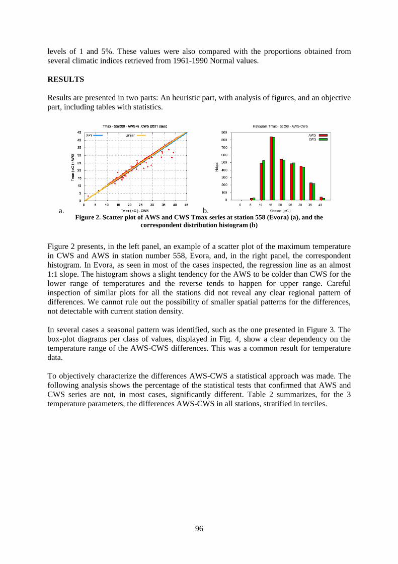
96
levels of 1 and 5%. These values were also compared with the proportions obtained from
several climatic indices retrieved from 1961-1990 Normal values.
RESULTS
Results are presented in two parts: An heuristic part, with analysis of figures, and an objective
part, including tables with statistics.
Figure 2 presents, in the left panel, an example of a scatter plot of the maximum temperature
in CWS and AWS in station number 558, Evora, and, in the right panel, the correspondent
histogram. In Evora, as seen in most of the cases inspected, the regression line as an almost
1:1 slope. The histogram shows a slight tendency for the AWS to be colder than CWS for the
lower range of temperatures and the reverse tends to happen for upper range. Careful
inspection of similar plots for all the stations did not reveal any clear regional pattern of
differences. We cannot rule out the possibility of smaller spatial patterns for the differences,
not detectable with current station density.
In several cases a seasonal pattern was identified, such as the one presented in Figure 3. The
box-plot diagrams per class of values, displayed in Fig. 4, show a clear dependency on the
temperature range of the AWS-CWS differences. This was a common result for temperature
data.
To objectively characterize the differences AWS-CWS a statistical approach was made. The
following analysis shows the percentage of the statistical tests that confirmed that AWS and
CWS series are not, in most cases, significantly different. Table 2 summarizes, for the 3
temperature parameters, the differences AWS-CWS in all stations, stratified in terciles.
a. b. Figure 2. Scatter plot of AWS and CWS Tmax series at station 558 (Evora) (a), and the
correspondent distribution histogram (b)

97
Figures 3 and 4 display examples of the seasonal evolution of the differences and their
dependency on classes of values,, respectively.
In the T009 case, more than 50% of the bias values are on the 3rd
tercile, corresponding to
positive values. On the other hand, minimum and maximum temperatures have the larger
percentage values over the 2nd
tercile that correspond to the central values, near zero.
In the statistical tests corresponding to overall monthly averages and monthly series,
calculated when possible, the global results show, in more than 60% of the test values,
differences between the overall monthly averages and the monthly data series of AWS and
CWS that are not significant (Table 3).
Table 3. Percentage of non-significant differences of
overall monthy average and monthly series at 99%
significance level
Daily time series Montlhy time series
T009 Tmax Tmin T009 Tmax Tmin
Table 2. Distribution of AWS-CWS
differences in tercile values
Jan 87 83 93 96 92 100
Feb 87 90 93 95 93 100
Var Nr.cases 1st T 2
ndT 3
rd T Mar 90 93 97 100 96 100
T009 30 23% 23% 53% Apr 83 97 90 97 100 98
Tmax 30 23% 43% 33% May 83 97 100 98 100 100
Tmin 30 30% 53% 17% Jun 80 97 93 97 97 100
Jul 80 97 90 97 100 98
Aug 63 97 87 91 100 96
Sep 67 97 87 90 100 96
Oct 80 93 93 99 98 94
Nov 80 87 93 96 94 100
Dec 83 80 93 93 97 96
Anomalies of the AWS and CWS with respect to the 1961-1990 monthly normals show a
very similar behaviour of the two observation systems, i.e., the test values were
rejected/accepted with similar threshold values. This fact is shown in Tables 4a to 4c.
Table 4 reveals that that in the latest years, all the three studied temperatures have higher
values than the 1961-1990 normals. This fact is shown by the larger number of significant
Figure 3. Box-plot of the monthly percentiles
of the differences of Tmin of station 579
(Lisboa)
Figure 4. Box and whiskers representation of
of Tmin AWS-CWS differences by classes of
values of station 543 (Viana do Castelo).
Boxes represent the 25 to 75 percentile,
whiskers at 5 and 95 percentile and the black
line is the median
98
differences between AWS (CWS) and normals for positive anomalies (rejections of the
hypothesis of statistical equal values).
The following step was to test the differences for extreme values. Climatic indices (WMO
Nr.100, 1983) such as the 10th
an 90th
percentiles of the minimum and maximum temperatures
(TNpp and TXpp, 1961-1990 Normal values), the cold days (CD, Tmin<-10ºC), tropical
nights (TN, Tmin>20ºC), warm days WD, Tmax>20ºC), summer days (SD, Tmax>25ºC),
tropical days 1 (TD1, Tmax>30ºC) and tropical days 2 (TD2, Tmax>35ºC).
We assessed if the proportion of days above or below the indices between AWS and CWS
series was significantly different. Table 5 shows, for more than 90% of months, proportions
are not significantly different at the 1% significance level.
Table 4. Contingency tables with the number of rejected months of AWS and CWS series when
compared with 1961-1990 Normal values: (a) T009, (b) Tmax and (c) Tmin
CWS
a T009 Rej(-) 1 5 10 90 95 99 Rej(+)
AW
S
Rej(-) 68 9 4 9 3 0 1 0
1 10 9 3 4 1 0 0 0
5 4 4 4 6 6 1 0 1
10 11 12 5 58 21 1 2 3
90 3 6 5 64 115 8 16 15
95 0 0 0 8 20 7 8 9
99 1 1 0 5 34 10 10 20
Rej(+) 1 3 1 10 39 17 64 307
CWS
b Tmax Rej(-) 1 5 10 90 95 99 Rej(+)
AW
S
Rej(-) 24 2 0 1 1 0 0 0
1 5 5 0 2 0 0 0 0
5 0 3 2 5 0 1 0 0
10 5 6 4 52 11 2 0 0
90 1 2 0 31 72 3 10 9
95 2 0 0 0 16 2 4 2
99 0 0 0 3 14 14 20 12
Rej(+) 0 0 0 1 10 4 24 154
CWS
c Tmin Rej(-) 1 5 10 90 95 99 Rej(+)
AW
S
Rej(-) 42 7 1 2 0 0 0 0
1 6 6 2 5 0 0 0 0
5 0 3 3 9 0 0 0 0
10 11 2 4 58 25 0 0 0
90 3 4 1 10 80 14 10 2
95 1 0 0 2 5 6 6 6
99 1 0 0 4 3 1 16 20
Rej(+) 1 0 0 1 3 1 5 133
Table 5. Percentage of months that rejected proportions between AWS and CWS indices were
significantly different at 1% confidence level
Jan Feb Mar Apr May Jun Jul Aug Sep Oct Nov Dec
Tm
in
CD 100 100 100 100 100 100 100 100 100 100 100 100
TN 100 100 100 100 100 100 100 97 100 100 100 100
TN10 100 100 100 100 100 97 100 90 93 93 97 97
TN90 97 97 97 100 100 97 100 100 97 97 100 100
Tm
ax
WD 97 97 97 97 97 100 100 100 100 97 97 100
SD 100 100 100 97 97 100 100 93 100 97 97 100
TD1 100 100 100 97 97 97 100 100 97 100 100 100
TD2 100 100 100 100 100 97 97 100 100 100 100 100
TX10 97 93 100 97 100 100 97 97 97 93 93 97
TX90 97 93 97 100 100 97 100 100 100 97 97 93
In order to determine in an objective way the pattern of each difference, we devised an
heuristic method to detect the existence of dependency of differences on classes of values. For
each parameter, differences were stratified in classes of values and a box and whiskers
representation created for each class (see Figure 4 as an example). In such a figure, a linear
increase (decrease) with class of values can be idealized as a straight line with positive
(negative) slope; ±σ/(xmax- xmin), where sigma, xmax, and xmin are, respectively, the sample

99
standard deviation, minimum value and maximum value. In the following we refer to this as
the reference slope. Next we compute the linear fits to the dependency of each of the 10, 25,
50, 75 and 90th
percentiles with class of values, obtaining in this way 5 slopes for each
variable. If two of the absolute values of the slopes were higher the reference slope, the
parameter difference was considered value-dependent. Tables 6a-b show the percentage of
cases in which the slope value was higher than the reference slope, for positive values (+m)
and negative values (-m). Table 6c, summarizes the absolute number of cases that are value-
dependent (Val) and non value-dependent (NVal). Overall, results from Table 6, suggest that
the number of cases that are value-dependent (Val) are between 15 and 30% of the total
number of cases. It is interesting to note, on panels (A) and (B) of Table 6, that the slopes of
minimum and maximum temperatures have opposite sign.
Table 6. (A) Percentage of negative slopes that are lower than the reference slope; (B)
Percentage of positive slopes that are higher than the reference slope; (C) Absolute number of
cases classified as value-dependent (Val) and non value-dependent(NVal)
A B C
-m p10 p25 p50 p75 p90
+m p10 p25 p50 p75 p90 Val NVal
T009 18 4 4 0 4
T009 7 7 14 21 14 T009 6 22
Tmax 4 0 0 0 0
Tmax 14 18 18 21 25 Tmax 8 20
Tmin 21 11 14 14 21
Tmin 0 0 0 0 0 Tmin 5 23
CONCLUSIONS
Overall, for meteorological surveillance and monthly reporting, the main operational use of
data at IM, the differences between AWS and CWS are not significant. Most of the tests
reveal that for daily or monthly data, differences are acceptable and do not compromise
continuity of the data series. We identified patterns on some of the differences shown, which
can lead to a statistical or algorithm correction. The value-dependent differences are very
likely related to exposure factors such as the effect of the different type of shelters/screens
used to cover the AWS and CWS sensors (Perry et al, 2007).
Nevertheless, if the goal is to study long series of data, its extremes and tendencies, the raw
data needs to be corrected prior to the merge of the time series.
References
Nunes L. (1996), Aquisição, processamento, análise e validação de dados meteorológicos: Sistemas Clássico
versus Sistemas automáticos – o caso da temperatura do ar, Dissertação de Mestrado, Mestrado em
Ciências Geofísicas, especialização em Meteorologia, da Faculdade de Ciências da Universidade de Lisboa
Perry M.C., Prior M.J. e Parker D.E. (2007), An assessment of the suitability of a plastic thermometer screen for
climatic data collection, International journal of climatology, 2007, vol. 27, nº2, pág. 267-276
Silva P. (2001), Comparação Estações Clássicas vs. Estações Automáticas – Ponto de vista da Climatologia,
Relatório de Estágio Profissionalizante, Licenciatura em Ciências Geofísicas, variante
Meteorologia/Oceanografia, pela Faculdade de Ciências da Universidade de Lisboa
WMO-Nr. 100, Guide to Climatological Practices, 1983
100
HOMOGENIZATION OF DAILY DATA SERIES FOR EXTREME
CLIMATE INDECES CALCULATION
Lakatos, M., Szentimrey, T., Bihari, Z., Szalai, S.
Hungarian Meteorological Service,
INTRODUCTION
Extreme climate indices calculations require at least daily resolution of homogeneous time
series. In many cases the characteristics of the estimated linear trends are unambiguously
unlike on the original and homogenized time series. It is a frequent occurrence that the sign of
the slope implies decreasing or increasing on the data with artificial breaks, while the fitted
trend to homogenized data implies adverse character.
The ECA&D indices and some other special temperature and precipitation indices of our own
development were built in to the Climate Database of the Hungarian Meteorological Service.
Long term daily maximum, minimum temperature and daily precipitation sums series were
homogenized and the climate indices series based on daily data has been derived and analyzed
for the period 1901-2007. The extreme climate indices calculation results and the fitted linear
trend statistics were tested on the original as well as on the homogenized daily data series.
The differences are exposed in this paper.
DATA AND METHOD
Deriving the extreme climate indices the gaps in the data series and the inhomogeneities
caused problems. Therefore the homogenization of observation series is crucial to get correct
consequences on changes of extremes.
The necessity of homogenization is demonstrated in Figs. 1 and 2 which show the annual
number of frost days (daily minimum temperature < 0°C) for Szeged station in original and
the homogenized daily minimum temperatures. Both the magnitude and the sign of the
estimated linear trend are different in the two cases.
Figure 1. Annual number of frost days with the ten-years moving average for Szeged station in the period
of 1901-2007 using the original data
40
50
60
70
80
90
100
110
120
130
140
1901 1911 1921 1931 1941 1951 1961 1971 1981 1991 2001
Nu
mb
er o
f fr
ost
da
ys
Szeged original data Trend= 1.8 days/decade
101
Figure 2. Annual number of frost days with the ten-years moving average for Szeged station in the period
of 1901-2007 using the homogenized data
The computations implemented in this work are based on long term daily data in the period of
1901-2007. Daily maximum and minimum temperatures of 15 observation stations and daily
precipitation sum of 58 precipitation stations were taken into account in the analysis. In the
preparation phase the homogenization and quality control of the daily measurements were
carried out. The homogenization of daily data was performed with the procedure MASH
(Multiple Analysis of Series for Homogenization) (Szentimrey, 1999).
The main features of MASHv3.02 (Szentimrey, 2007)
The software consists of two parts.
Part 1: Quality control, missing data completion and homogenization of monthly series:
Relative homogeneity test procedure.
Step by step procedure: the role of series (candidate or reference series) changes step by step
in the course of the procedure.
Additive (e.g. temperature) or multiplicative (e.g. precipitation) model can be used depending
on the climate elements.
Providing the homogeneity of the seasonal and annual series as well.
Metadata (probable dates of break points) can be used automatically.
Homogenization and quality control (QC) results can be evaluated on the basis of verification
tables generated automatically during the procedure.
Part 2: Homogenization of daily series:
Based on the detected monthly inhomogeneities.
Including quality control (QC) and missing data completion for daily data. The quality control
results can be evaluated by test tables generated automatically during the procedure.
VERIFICATION OF THE HOMOGENIZATION RESULTS AND QUALITY
CONTROL
During the execution of MASH procedure the quality control and homogenization test results
e.g. detected errors, degree of inhomogeneity, number of break points, estimated corrections
and certain verification results are documented in the automatically generated tables which
make the evaluation efficient. The Tables 1-3 contains the homogeneity test results for the
different meteorological elements which were analyzed in this work. In the case of daily
minimum temperature series the degree of inhomogeneity of the stations are high values,
40
50
60
70
80
90
100
110
120
130
140
1901 1911 1921 1931 1941 1951 1961 1971 1981 1991 2001
Nu
mb
er o
f fr
ost
da
yss
Szeged homogenized dataTrend= -1 days/decade

102
multiples of the critical value even in average. The test statistics proximate the critical value
after homogenization (Table 1.). Lower but still high degree of inhomogeneity is typical of
the daily maximum temperatures (Table 2.). The MASH procedure reduced the test statistics
in the case of daily maximum temperatures substantially. The inhomogeneity of the raw
precipitation data series is less, although the MASH procedure more decreased the test
statistics (Table 3.).
Table 1. Test results for daily minimum temperatures
VERIFICATION OF HOMOGENIZATION (MINIMUM)
TEST STATISTICS for ANNUAL SERIES (OUTPUT of MASH)
Critical value (significance level 0.05): 21.73
Test Statistics Before Homogenization(TSB)
Station TSB Station TSB Station TSB
5 2024.83 12 1232.54 13 843.11
10 735.77 3 644.61 15 631.40
6 617.90 1 579.59 2 496.33
7 438.06 8 390.13 11 384.80
4 317.23 14 309.52 9 99.56
AVERAGE:649.69
Test Statistics After Homogenization(TSA)
Station TSA Station TSA Station TSA
14 36.56 2 35.15 13 31.27
4 30.55 1 30.02 8 29.43
9 28.10 5 27.74 3 24.01
6 23.30 7 22.87 10 22.37
12 22.09 15 21.68 11 17.68
AVERAGE: 26.85
Table 2. Test results for daily maximum temperatures
VERIFICATION OF HOMOGENIZATION (MAXIMUM)
TEST STATISTICS for ANNUAL SERIES (OUTPUT of MASH)
Critical value (significance level 0.05): 21.73
Test Statistics Before Homogenization(TSB)
Station TSB Station TSB Station TSB
12 1106.40 6 1031.97 5 488.03
8 360.65 13 314.53 7 311.95
11 284.94 10 206.09 1 158.15
14 145.63 4 135.56 2 133.73
15 130.89 9 79.72 3 46.26
AVERAGE:328.97
Test Statistics After Homogenization(TSA)
Station TSA Station TSA Station TSA
1 60.91 7 49.90 5 44.96
2 44.82 14 34.28 8 32.99
6 31.73 9 28.31 11 25.28
10 22.59 3 21.89 13 21.44
15 21.21 4 20.36 12 19.39
AVERAGE: 32.00

103
Table 3. Test results for daily precipitation
VERIFICATION OF HOMOGENIZATION (PRECIPITATION)
TEST STATISTICS for ANNUAL SERIES (OUTPUT of MASH)
Critical value (significance level 0.05): 21.73
Test Statistics Before Homogenization(TSB)
Station TSB Station TSB Station TSB
13 175.11 10 170.34 27 137.97
17 110.87 3 81.79 20 80.32
4 76.88 18 60.28 1 59.43
56 17.15 36 15.07 24 11.06
AVERAGE: 43.10
Test Statistics After Homogenization(TSA)
Station TSA Station TSA Station TSA
2 66.34 18 59.33 37 54.23
58 51.60 20 51.54 51 48.02
1 44.91 44 43.98 52 43.85
8 15.27 56 14.62 36 12.82
AVERAGE: 29.13
The quality control part of the MASH demonstrates the detected errors. The Table 4 points a
rough error in May 1941 on Kecskemét station. These very low daily maximum values
appear as extremes in the original data. Extreme high daily minimum temperatures were
registered in the climatological database in Túrkeve station to the date 18-19 February 1907
(Table 5.). The MASH quality control part detected the mistaken daily data. In case of
precipitation we present only the summary of results in the Table 6.
Table 4. Quality Control results of daily maximum temperatures
Maximum temperature (1901-2007)
Result of automatic Quality Control By MASH
Total number of errors: 3319
Maximal positive error: 12.35
Minimal negative error: -20.91
Example: Kecskemét(46401), 26-31 May 1941
48101 47100 46401 58104 55706 64704 44121
1941 525 22.4 24.6 26.0 24.6 24.8 24.2 25.3
1941 526 23.9 23.8 2.4 24.0 24.0 23.8 25.6
1941 527 24.2 24.2 2.4 25.6 23.3 23.8 22.8
1941 528 26.9 26.6 2.7 28.2 26.7 25.4 27.8
1941 529 25.8 24.0 2.4 27.0 26.5 24.6 24.2
1941 530 24.7 24.6 2.5 25.5 24.0 22.4 23.8
1941 531 25.0 25.2 2.7 26.5 25.8 25.4 25.9
1941 6 1 22.1 21.5 21.0 19.7 17.6 18.8 22.8
Table 5. Quality Control results of daily minimum temperatures
Minimum temperature (1901-2007)
Result of automatic Quality Control by MASH
Total number of errors: 2058
Maximal positive error: 14.03
Minimal negative error: -10.55
Example: Túrkeve(55706), 18-19 February 1907
48101 47100 46401 58104 55706 64704 44121

104
1907 217 -9.0 -13.0 -16.4 -10.8 -15.0 -17.9 -10.50
1907 218 -6.0 -5.1 -10.0 -3.9 5.0 -7.2 -5.50
1907 219 -1.5 -2.5 -6.4 -4.6 10.6 -13.2 -0.60
1907 220 -1.0 -1.5 -2.4 -0.1 -0.2 -1.9 -0.40
Table 6. Quality Control results of daily precipitation sum
Precipitation (1901-2007)
Result of automatic Quality Control by MASH
Total number of errors: 854
Maximal positive error: 84.0
Minimal negative error: -33.4
CLIMATE INDICES Extreme climate indices calculation started in the frame of project named „Regional Climate
Modeling” 2005 – 2007 (NKFP-3A/082/2004, National Office for Research and Technology)
in Hungary. The index definitions mainly are based on the ECA&D and Climdex definitions.
The indices listed in the Table 7-9 were calculated in the climate database of The Hungarian
meteorological Service. All of them were derived on original as well as on homogenized,
quality controlled and complemented daily data. The changes raised in the extreme index
series are estimated by linear trend fitting in three, partly overlapping time periods: 1901-
2007, 1961-2007 and 1976-2007. The longest period goes back to the beginning of the 20th
century to detect long term changes; the period from the mid 20th
century turns up in IPCC
reports, therefore that interval is analyzed. The last 30 years is chosen, because that is the
most intense warming period, and it mostly characterizes the present climate.
Table 7. Extreme warm temperature indices in the climate database of HMS
Index/unit Warm extremes
txx / °C absolute Tmax
dtx25/day summer days Tmax > 25 °C
dtx30e/day hot days Tmax ≥30 °C
dtx35e/day very hot days Tmax ≥35 °C
dtn20/day tropical nights Tmin > 20 °C
ditxgnr/day heat wave duration index
ditgnr90/day warm spell days
itxgnr90/day maximum duration of warm spell
TN90p /% Tmin > 90th percentile of normal period
TX90/% Tmax > 90th percentile of normal period
Table 8. Extreme cold temperature indices in the climate database of HMS
Index/unit Cold extremes
tnn/°C absolute Tmin
dtn0/days frost days Tmin < 0°C
itn0x/days maximum number of frost days Tmin < 0°C
t17s/°C heating degree days
dtx0/day ice days Tmax < 0°C
ditnlnr/day cold wave duration index
ditlnr10/day cold spell days
itnlnr10/day maximum duration of cold spell
TN10p /% Tmin < 10th percentile of normal period
TX10p /% Tmax < 10th percentile of normal period

105
Table 9. Extreme precipitation climate indices in the climate database of HMS
Index/unit Precipitation
rs/mm precipitation sum
dr1/day number of wet days
r1a/mm/day mean wet-day precipitation
ir1xd/day length of longest dry period R <1 mm
ir1xw/day length of longest wet period R ≥ 1 mm
dr5/day number of days R ≥ 5 mm
dr10 day number of days R≥ 10 mm
dr20/ day number of days R≥ 20 mm
rx1/mm naximum daily sum
rx5/mm naximum sum in 5 days long period
pr95gnr/% proportion of prec. days R> 95% of normal period in the total annual precipitation
pr99gnr/% proportion of prec. days R> 99% of normal period in the total annual precipitation
The estimation of trend values and testing of theirs significance are performed both on
original while complemented data and on quality controlled, complemented and homogenized
data. The MASH method was used for the data quality control, completion and for
homogenization. In the Fig. 3 the changes of two indices based on daily minimum: TN10p
(Tmin < 10th percentile of the 1961-1990 normal) and TN90p (Tmin > 90th percentile of
1961-1990 normal) are shown. The significant changes on 0.9 confidence level are colored
according to the sign of the slope. The coloration of the cells indicates the significant
increasing (red) and decreasing (blue) trends on the original and on the homogenized data.
The decreasing tendency is dominant in the case of index TN10p, but there is inexplicable
increasing on Szeged station in all the examined period. Kecskemét and Debrecen also show
increased values on the longest series from 1901-2007. The adverse characteristics of the
changes are caused by the artificial breaks in the data series. The positive values are
eliminated after homogenization. The less extremely cold days rather agree with the global
changes. Similarly in the case of index TN90p the presence of the wrong data and
inhomogeneites result significant decreasing on the stations Kecskemét, Szeged and Debrecen
from the beginning of the 20th
century to 2007. The higher than the 90th
percentile minimum
temperatures are reassuringly dominant at all the stations and period.
TN10p orig 1901-2007 1961-2007 1976-2007
Sopron -15.5 -11.1 -4.5
Szombathely -0.5 -6.5 -6.7
Keszthely -1.3 -7.6 -4.7
Mosonmagyaróvár 2.3 2.6 0.4
Siófok -23.9 -7.7 -8.5
Pécs 1.2 -4.7 -5.2
Baja -11.6 -5.4 -7.6
Kalocsa -8.5 0.0 -2.7
Kecskemét 5.8 -2.0 -2.9
Szeged 6.1 9.4 8.2
Túrkeve -1.4 -14.0 -19.4
Miskolc -10.3 -5.2 -5.7
Debrecen 9.6 -0.6 -3.9
Nyíregyháza -9.8 -5.6 -7.3
Budapest -15.7 -4.9 -6.9
TN10p homogenized 1901-2007 1961-2007 1976-2007
Sopron -7.3 -6.3 -6.4
Szombathely -4.5 -5.3 -6.0
Keszthely -4.0 -2.8 -3.6
Mosonmagyaróvár -3.8 -3.3 -3.3
Siófok -7.8 -6.2 -7.7
Pécs -5.4 -4.9 -5.4
Baja -6.0 -3.8 -5.4
Kalocsa -5.6 -1.5 -4.4
Kecskemét -3.4 -2.0 -3.5
Szeged -2.2 0.0 -0.5
Túrkeve -5.1 -6.2 -11.4
Miskolc -6.7 -3.9 -5.7
Debrecen -2.5 -2.8 -5.3
Nyíregyháza -6.1 -4.3 -6.1
Budapest -6.2 -4.9 -6.6
106
Figure 3. Percentage change of the original and homogenized extreme indices based on daily minimum
temperature for 15 Hungarian stations in three different time intervals
Figure 4. Percentage change of the original and homogenized extreme indices based on daily maximum
temperature for 15 Hungarian stations in three different time intervals
TN90p orig 1901-2007 1961-2007 1976-2007
Sopron 15.3 17.8 10.6
Szombathely 5.8 14.4 13.8
Keszthely 6.1 14.1 11.6
Mosonmagyaróvár -0.2 0.0 3.8
Siófok 21.0 16.5 17.4
Pécs -1.2 11.8 12.4
Baja 13.1 12.7 13.9
Kalocsa 9.0 8.0 11.5
Kecskemét -6.2 8.8 10.7
Szeged -3.9 -2.5 -1.0
Túrkeve 6.7 24.0 28.9
Miskolc 11.6 10.9 12.1
Debrecen -7.8 5.9 8.9
Nyíregyháza 10.0 9.6 11.8
Budapest 14.5 10.4 13.8
TN90p homogenized 1901-2007 1961-2007 1976-2007
Sopron 6.4 10.4 10.2
Szombathely 10.0 11.8 12.2
Keszthely 7.9 9.1 9.4
Mosonmagyaróvár 8.6 9.0 9.3
Siófok 8.0 13.8 15.4
Pécs 8.1 11.5 12.2
Baja 9.0 10.4 11.2
Kalocsa 7.1 9.4 13.0
Kecskemét 7.7 9.1 11.2
Szeged 8.6 10.5 11.0
Túrkeve 10.4 5.6 9.3
Miskolc 8.1 9.2 12.1
Debrecen 10.7 9.3 11.2
Nyíregyháza 6.3 6.7 9.0
Budapest 5.9 9.7 12.8
TX10p orig 1901-2007 1961-2007 1976-2007
Sopron -9.4 -8.1 -10.0
Szombathely -5.1 -8.2 -7.6
Keszthely -6.9 -5.2 -5.7
Mosonmagyaróvár -6.3 -4.4 -4.1
Siófok -4.3 -4.6 -5.0
Pécs -1.6 -4.5 -3.9
Baja -5.3 -1.9 -2.9
Kalocsa -5.7 -3.5 -7.4
Kecskemét -5.8 -4.2 -5.3
Szeged -8.7 -3.9 -5.7
Túrkeve -11.7 2.8 -3.1
Miskolc -7.3 -4.0 -6.8
Debrecen -6.2 -3.1 -5.0
Nyíregyháza -3.6 -2.4 -6.0
Budapest -5.0 -2.6 -6.1
TX10p homogenized 1901-2007 1961-2007 1976-2007
Sopron -5.9 -7.1 -8.9
Szombathely -4.8 -5.9 -6.2
Keszthely -5.1 -5.3 -5.6
Mosonmagyaróvár -5.5 -5.1 -4.8
Siófok -6.9 -6.0 -5.8
Pécs -4.2 -3.8 -4.2
Baja -5.7 -4.6 -5.7
Kalocsa -4.3 -3.6 -6.6
Kecskemét -5.2 -3.8 -5.7
Szeged -4.2 -4.1 -4.8
Túrkeve -3.6 -4.1 -8.8
Miskolc -3.6 -3.0 -6.3
Debrecen -4.4 -3.3 -5.2
Nyíregyháza -5.7 -4.3 -6.7
Budapest -5.1 -3.9 -7.8
TX90p orig 1901-2007 1961-2007 1976-2007
Sopron 11.4 13.0 14.3
Szombathely 9.4 12.9 12.7
Keszthely 7.9 9.9 12.1
Mosonmagyaróvár 5.7 10.3 10.7
Siófok -0.7 11.7 13.7
Pécs 2.7 10.5 9.2
Baja 5.6 8.5 8.3
Kalocsa 5.2 10.9 15.1
Kecskemét 4.6 11.0 10.9
Szeged 10.7 11.3 13.6
Túrkeve 6.0 0.9 7.0
Miskolc 6.5 10.0 12.0
Debrecen 7.0 8.1 8.7
Nyíregyháza 0.8 7.7 12.4
Budapest 3.5 6.9 9.5
TX90p homogenized 1901-2007 1961-2007 1976-2007
Sopron 8.8 11.3 13.0
Szombathely 8.7 10.0 10.7
Keszthely 7.1 9.8 12.0
Mosonmagyaróvár 5.5 11.3 12.1
Siófok 2.4 12.8 14.8
Pécs 5.9 9.9 9.3
Baja 7.2 12.1 12.8
Kalocsa 4.1 10.9 14.3
Kecskemét 4.4 9.9 10.7
Szeged 7.5 11.8 12.3
Túrkeve 6.0 9.2 14.6
Miskolc 4.0 8.5 11.2
Debrecen 5.3 8.3 9.1
Nyíregyháza 3.3 9.8 13.0
Budapest 4.3 8.8 12.1
107
In the Fig. 4 the changes of the indices TX10p and TX90p are shown. Both of them are
calculated with using daily maximum temperatures. The differences between original and
homogenized changes are less apparent than in Fig. 3, but the necessity of homogenization is
obvious.
The columns in the Fig. 5 indicate also the degree and the trend of the indices which
were examined in this study. Note that in many cases not only the degree but the sign of the
estimated trend are discrepant. The diagrams are consistent with the test statistics introduced
in the section 3. The degree of inhomogeneity of the indices based on daily minima is large,
especially in the periods 1901-2007, but artificial breaks also were founded in the subsequent
periods.
Figure 5. Comparative chart of the change arise in the series of TN10p and TN90p extreme climate indices
for 15 Hungarian stations in three different time intervals
The precipitation is more variable climatological element than the temperature in time and in
space as well. The extreme precipitation index which were examined in this paper is the
proportion of precipitation days R> 95% of the 1961-1990 periods in the total annual
precipitation (R95pTOT). The variability is manifested in Fig 6. which contains the changes
of R95pTOT in the examined periods. The significant tendencies confirm that the fraction of
the short term precipitation in the yearly sum is increased near to the present, but the measure
of the changes is variant. The differences of the fitted original trend and homogenized trend
are not so obvious than in the case of temperature. It follows from the fact that the MASH
procedure is more cautious in the case of precipitation data.
-25 -15 -5 5 15 25
Sopron
Szombathely
Keszthely
Mosonmagyaróvár
Siófok
Pécs
Baja
Kalocsa
Kecskemét
Szeged
Túrkeve
Miskolc
Debrecen
Nyíregyháza
Budapest
Sopron
Szombathely
Keszthely
Mosonmagyaróvár
Siófok
Pécs
Baja
Kalocsa
Kecskemét
Szeged
Túrkeve
Miskolc
Debrecen
Nyíregyháza
Budapest
1901-2007 %
Tn90p
-25 -15 -5 5 15 25
Sopron
Szombathely
Keszthely
Mosonmagyaróvár
Siófok
Pécs
Baja
Kalocsa
Kecskemét
Szeged
Túrkeve
Miskolc
Debrecen
Nyíregyháza
Budapest
Sopron
Szombathely
Keszthely
Mosonmagyaróvár
Siófok
Pécs
Baja
Kalocsa
Kecskemét
Szeged
Túrkeve
Miskolc
Debrecen
Nyíregyháza
Budapest
1976-2007 %
Tn10p
Tn90p
-25 -15 -5 5 15 25
Sopron
Szombathely
Keszthely
Mosonmagyaróvár
Siófok
Pécs
Baja
Kalocsa
Kecskemét
Szeged
Túrkeve
Miskolc
Debrecen
Nyíregyháza
Budapest
Sopron
Szombathely
Keszthely
Mosonmagyaróvár
Siófok
Pécs
Baja
Kalocsa
Kecskemét
Szeged
Túrkeve
Miskolc
Debrecen
Nyíregyháza
Budapest
1961-2007 %
Tn10p
Tn90p
Tn10p
108
Figure 6. Changes of R95pTOT extreme precipitation index for 58 Hungarian stations in three different
time intervals
CONCLUSION
The majority of long data series is inhomogeneous, and often contains shifts in the mean or in
the variance due to site-relocations, changes in instrumentation or in observing practices.
Amongst the observation series there are good quality data as well, but sorting them out
requires the execution of a homogenization procedure first. Neglecting the inhomogeneous
series causes a huge loss of valuable information. Long term daily maximum, minimum
R95pTOT (%) homo orig homo orig homo orig
1901-2007 1901-2007 1961-2007 1961-2007 1976-2007 1976-2007
Sopron -0.3 -1.0 3.3 3.2 6.9 6.8
Fertőszentmiklós 2.1 2.0 0.3 0.5 7.3 7.2
Szombathely 4.2 1.3 -0.4 -0.4 0.4 0.6
Felsőszölnök 3.0 -3.2 -0.9 -0.9 -3.1 -3.1
Mosonmagyaróvár -3.3 -1.5 -2.7 -2.1 9.3 9.9
Ravazd 1.2 -2.8 1.5 1.6 6.7 6.8
Pér 3.3 3.1 2.5 3.6 -0.1 0.0
Beled 1.7 2.1 -1.8 -0.9 6.8 8.1
Bakonyszentkirály 0.5 2.0 2.6 2.8 10.1 10.3
Kemenesszentmárton -0.5 2.3 -3.9 -5.5 4.7 4.2
Kerta 1.2 0.7 -7.3 -7.3 5.7 5.6
Bakonybél 4.2 4.1 1.1 1.3 10.9 11.0
Városlőd 0.9 4.1 -1.0 3.9 4.3 6.0
Herend -3.5 -2.7 -1.8 -1.9 0.7 0.6
Türje 0.8 0.5 -6.0 -6.1 3.7 3.6
Sümeg 0.7 0.6 -3.2 -3.2 6.2 6.0
Nagyvázsony 1.2 -2.8 -2.2 -2.3 3.4 3.4
Keszthely -1.2 -0.8 1.3 1.8 1.7 1.0
Balatonkeresztúr -5.2 -4.1 1.7 2.4 2.3 3.0
Marcali 3.9 5.8 -0.3 -0.3 6.0 6.1
Mernye 8.5 8.4 1.2 1.2 6.6 7.3
Iharos -6.6 -6.9 -5.1 -5.1 -3.0 -3.0
Rinyakovácsi -4.2 -4.7 -1.4 -1.2 -0.7 -0.5
Márianosztra 1.8 1.8 -2.7 -2.6 7.2 7.3
Kápolnásnyék -6.2 -6.7 1.5 1.5 5.1 5.1
Balatonalmádi -2.2 -3.9 -6.0 -7.9 -8.5 -8.4
Siófok 1.5 0.8 2.6 2.2 0.6 0.4
Tab -0.9 -0.6 -0.5 1.0 2.8 3.6
Pincehely -0.6 -0.6 4.7 4.5 19.3 19.3
Tengelic 3.1 4.5 5.6 6.1 9.3 9.8
Gölle -2.6 -1.6 -1.8 -2.1 13.5 13.5
Szálka 13.3 13.7 4.0 4.2 11.0 11.1
Pécs 6.5 5.0 6.1 6.1 12.2 12.0
Pásztó -3.7 -0.7 -2.8 -2.4 3.9 4.4
Budapest 1.8 1.6 1.1 1.1 4.4 4.2
Tápiószele 0.4 0.7 -0.2 0.0 2.1 2.6
Kecskemét-kült -0.9 -1.0 3.5 4.0 6.8 7.8
Kalocsa Öregcsertő 2.6 2.4 4.1 3.8 15.4 14.3
Baja 1.4 1.3 4.7 4.2 14.7 14.9
Felsőszentiván 6.4 5.7 3.7 2.2 14.9 15.0
Miskolc -0.2 0.4 2.0 1.4 5.0 5.5
Bogács -3.8 -3.9 0.3 0.3 3.1 3.1
Poroszló -1.7 0.4 0.4 0.0 6.9 3.0
Fegyvernek -5.3 -5.4 -6.3 -7.2 -4.7 -4.6
Túrkeve 8.9 8.8 8.7 8.8 13.3 13.5
Cibakháza 1.2 0.5 4.9 4.9 1.9 1.9
Kunszentmárton 3.3 4.2 -2.1 -2.2 3.0 3.2
Kondoros 5.7 5.5 0.5 0.9 6.9 7.6
Szeged 1.5 1.1 3.9 4.6 1.3 2.1
Karcsa 3.2 2.5 3.1 3.4 -0.7 -1.9
Nyíregyháza 1.6 1.2 3.5 3.5 7.9 7.7
Téglás Hadháztéglás 5.3 3.0 9.1 9.5 7.0 7.3
Hajdúszoboszló 8.4 7.7 4.1 4.2 5.9 6.0
Debrecen 7.7 7.2 6.2 6.7 6.5 6.8
Méhkerék 9.9 11.1 8.2 8.2 -0.8 -1.0
Battonya 4.6 4.5 1.3 1.3 5.6 5.7
Nyírmada 3.1 3.0 4.6 4.6 -0.2 -0.2
Vásárosnamény 7.9 7.6 0.3 1.5 3.4 3.4
109
temperature and daily precipitation sums series were homogenized and the extreme climate
indices series were derived and analyzed in the period of 1901-2007, 1961-2007 and 1976-
2007 in this paper. In many cases the changes of indices series according to original data and
homogenized data implies adverse character. According to our investigations the importance
of homogenization is undeniable in climate change studies.
References
Aguilar, E., I. Auer, M. Brunet, T.C. Peterson and J. Wieringa, 2003: Guidelines on climate metadata and
homogenization. In WCDMP No. 53 – WMO/TD-No. 1186.
Alexander, L.V., X. Zhang, T.C. Peterson, J. Caesar, B. Gleason, A.M.G. Klein Tank, M. Haylock, D. Collins,
B. Trewin, F. Rahimzadeh, A. Tagipour, P. Ambenje, K. Rupa Kumar, J. Revadekar and G. Griffiths,
2006: Global observed changes in daily climate extremes of temperature and precipitation. In J. Geophys.
Res.,111, doi:10.1029/2005JD006290.
Alexander, L.V. and Arblaster, J.M. 2009: Assessing trends in observed and modelled climate extremes over
Australia in relation to future projections. In Int. J. Climatol. 29, 417–435 pp.
van Engelen, A., Klein Tank, A., van der Schrier, G. and Klok, L., 2008: European Climate Assessment &
Dataset (ECA&D) Report 2008, In "Towards an operational system for assessing observed changes in
climate extremes". KNMI, De Bilt, The Netherlands, 68pp
Frich, P., L.V. Alexander, P. Della-Marta, B. Gleason, M. Haylock, A.M.G. Klein Tank, and T. Peterson, 2002:
Observed coherent changes in climatic extremes during 2nd half of the 20th century. In Climate Research
19: 193-212.
Hirschi, M., P. Stepanek, S.I. Seneviratne, O.B. Christensen and CECILIA WP4 members, 2008: CECILIA
climate indices: Analysis of temperature extremes in Central and Eastern Europe. In General Assembly of
the European Geosciences Union (EGU), EGU2008-A-09640.
IPCC, 2007: Climate Change 2007. The Scientific Basis, Contribution of Working Group Ito the Fourth
Assessment Report of the Intergovernmental Panel on Climate Change (IPCC). Solomon, S., D. Qin, M.
Manning, Z. Chen, M. Marquis, K.B. Averyt, M. Tignor and H.L. Miller (eds.), Cambridge University
Press, UK, pp946.
Szentimrey, T., 1999: Multiple Analysis of Series for Homogenization (MASH). In Proceedings of the Second
Seminar for Homogenization of Surface Climatological Data, WMO, WCDMP-No. 41: 27-46.
Szentimrey, T., 2007: Manual of homogenization software MASHv3.02, Hungarian Meteorological Service, p.
61.
Wijngaard J. B., Klein Tank A. M. G., Konnen G. P., 2003: Homogeneity of 20th century european daily
temperature and precipitation series. In Int. J. Climatol., 23: 679-692.

110
PROGRAMME
BUDAPEST, HUNGARY
26 – 30 MAY 2008
Venue:
The Headquarters of the Hungarian Meteorological Service (1 Kitaibel Pál street, Budapest)
Monday, 26 May
8:30-9:30 Registration
9:30-12:00
Openning addresses by
the President of HMS
the Organizers
Introduction about COST HOME
Monday is dedicated to specific results obtained within COST HOME
WG1:
Aguilar, E. (SE): Results of WG1, Bibliography
Venema, V. (DE): Results of WG1, Benchmark dataset
Lunch break
13:30-18:00
WG2-3:
Mestre, O., Domonkos, P., Lebarbier, P., Picard, F., Robin, S. (FR, HU):
Comparison of change-point detection methods in the mean of Gaussian processes
Prohom, M. (ES): Steps followed to create a climate dataset for Catalonia and
Andorra (18th
-21st centuries). Analysis of Catalan, Andorran and French temperature
series from the early 20th
century to the present using different homogenisation
approaches
Menne, M. (US): Automated Homogenization of Monthly Temperature Series via
Pairwise Comparisons
Szentimrey, T. (HU): Methodological questions of series comparison
WG4:
Gruber, C., Auer, I. (AT): Comparison of daily homogenization methods using parallel
measurements for evaluation
Stepanek, P.,Zahradníĉek, P. (CZ): Experiences with homogenization of daily and
monthly series of air temperature, precipitation and relative humidity in the Czech
Republic, 1961-2007
18:00 Welcome party

111
Tuesday, 27 May
9:00-17:00
WG2-3 Round Table and presentations, discussions(with participation of non Cost members):
Jourdain, S., Mestre, O. (FR): Use and misuse of absolute homogeneity tests
Grimvall, A., Sirisack, S., Burauskaite-Harju, A., Wahlin, K. (SE): Unifying mixed linear
models and the MASH algorithm for breakpoint detection
Brázdil, R., Stepanek, P., Macková, J. (CZ): Homogenisation of Brno climatic series 1799-
2007: Example of the use of early instrumental records
Venema, V., Mestre, O., Rust, H.W. (DE, FR): Inhomogeneities in temperature records
deceive long-range dependence estimators
Domonkos, P. (HU): Quantifying efficiency of homogenisation methods
Guijarro, J.A. (ES): Climatol 2: Interactive and automatic R functions for homogenisation
of climatological series
Bari, B. (MA): Breakpoints detection in Temperature Time Series in Morocco using the
Ellipse Test
Lizuma, L., Protopopova, V., Briede, A. (LV): Experience regarding detecting
inhomogeneities in temperature time series using MASH Lunch break: 12:00-13:30
Wednesday, 28 May
9:00-12:00
WG4 Round Table and presentations, discussions (with participation of non Cost
members):
Stepanek, P., Zahradníĉek, P. (CZ): Quality control of daily data on example of Central
European series of air temperature, relative humidity and precipitation
Aguilar, E., Brunet, M., Sigró, J. (ES): Different approaches for the homogenisation of the
Spanish Daily Temperature Series
Brandsma, T. (NL): Understanding inter-site temperature differences at the KNMI terrain
in De Bilt (the Netherlands)
Petrović, P., Curley, M. (RS, IE): Detected Inhomogeneities In Wind Direction And Speed
Data From Ireland
Lunch break
13:30-18:00
Management Committee of COST HOME
19:00 Seminar banquet

112
Thursday, 29 May
9:00-12:00
Vertaĉnik, G. (SI): A method for daily temperature data interpolation and quality control
based on the selected past events
Li, Z. and co-authors (CN): Effects of site-change and urbanisation in the Beijing
temperature series 1977-2006
Wypych, A., Piotrowicz, K. (PL): Air humidity in Cracow (Poland) in the period 1863-
2007 – daily data quality control and homogenization methods
Brzóska, B. (PL): Homogenization of water vapour data from Vaisala radiosondes and
older (MARZ, RKZ) used in Polish aerological service
Toreti, A., Desiato, F., Fioravanti, G., Perconti, W. (IT): Homogenization of Italian
precipitation series
Lunch break
13:30-17:00
Cheval, S., Szentimrey, T., Manea, A. (RO, HU), : Homogenization of monthly
temperature series in Romania (1901-2005) using metadata
Wieczorek, A.M., Jourdain, S., Desmaizières, L., Grimal, D., Tamburini, A. (FR): Monthly
Air Temperature Homogenization over France
Rasol, D., Likso, T., Milkovic, J. (HR): Homogenisation of temperature time series in
Croatia
Mendes, M., Neto, J., Silva, Á., Nunes, L., Viterbo, P. (PT): Characterization of data sets
for the assessment of inhomogeneities of climate data series, resulting from the
automation of the observing network in Mainland Portugal
Adamczyk, R., Lupikasza, E. (PL): Comparison of re-analysis gridded and station
cloudiness data over Europe
Lakatos, M., Szentimrey, T., Bihari, Z., Szalai, S. (HU): Homogenization of daily data
series for extreme climate indeces calculation
Friday, 30 May Excursion to Hollókő
Meeting point: HMS, 1, Kitaibel P. street at 7:45

113
LIST OF PARTICIPANTS
AUSTRALIA
ROGER STONE
University of Southern Queensland
AUSTRIA
INGEBORG AUER
Zentralanstalt für Meteorologie und
Geodynamik
CHRISTINE GRUBER
Zentralanstalt für Meteorologie und
Geodynamik
LEOPOLD HAIMBERGER
BULGARIA
TANIA MARINOVA
National Institute of Meteorology and
Hydrology, Bulgarian Academy of
Sciences
Tania [email protected]
ALEXANDROV VESSELIN
CHINA
LI ZHEN
Institute of Atmospheric Physics
CROATIA
TANJA LIKSO
Meteorological and Hydrological Service
of Croatia
JANJA MILKOVIĆ
Meteorological and Hydrological Service
of Croatia
DUBRAVKA RASOL
Meteorological and Hydrological Service
of Croatia
ANA ŃANTIĆ
Meteorological and Hydrological Service
of Croatia
CZECH REPUBLIC
RUDOLF BRÁZDIL
Institute of Geography, Masaryk
University, Brno
PETR ŃTĚPÁNEK
Czech Hydrometeorological Institute
CYPRUS
FOKIANOS KONSTANTINOS
FINLAND
TIETAVAINEN HANNA
HEIKKI TUOMENVIRTA

114
FRANCE
VALERIE DAUX
OLIVIER MESTRE
Météo-France
ANNE-MARIE WIECZOREK
METEO-FRANCE
GERMANY
VICTOR VENEMA
Meteorologisches Institut Universitaet
Bonn
GERHARD MÜLLER-WESTERMEIER
Deutscher Wetterdienst
GREECE
ATHANASSIOS ARGIRIOU
GEORGE KALOGERAS
Hellenic National Meteorological Service
HUNGARY
ZITA BIHARI
Hungarian Meterological Service
PETER DOMONKOS
MÓNIKA LAKATOS
Hungarian Meterological Service
SÁNDOR SZALAI
Hungarian Meterological Service
TAMÁS SZENTIMREY
Hungarian Meterological Service
IRELAND
SEAN BONNER
Met Éireann
MARY CURLEY
Met Éireann
MICHAEL MCDONNELL
Met Éireann
PROF. JOHN SWEENEY
Department of Geography
National University of Ireland, Maynooth
ITALY
FIORELLA ACQUAOTTA
University of Turin
MICHELE BRUNETTI
Institute of Atmospheric Sciences and
Climate, Bologna
SIMONA FRATIANNI
University of Turin
MAURIZIO MAUGERI
TERESA NANNI
SILVIA UGHETTO
CNMCA-ITALY
ANDREA TORETI
APAT / UNIBERN
LATVIA
ARGITA BRIEDE
LITA LIZUMA

115
Latvian Environment, Geology and
Meteorology Agency
MOROCCO
DRISS BARI
Chef Adjoint du Service de Banque de
données et Climatologie Direction
Régionale Météorologique du Centre
Casablanca
NETHERLANDS
THEO BRANDSMA
Royal Netherlands Meteorological Institute
ALBERT KLEIN TANK
Royal Netherlands Meteorological Institute
NORWAY
LARS ANDRESEN
Norwegian Meteorological Institute
OYVIND NORDLI
Norwegian Meteorological Institute
POLAND
ROMANA ADAMCZYK
University of Silesia, Faculty of Earth
Sciences, Department of Climatology
BARBARA BRZÓSKA
Institute of Meteorology and Water
Management Centre of Aerology
JANUSZ FILIPIAK
University of Gdansk
EWA ŁUPIKASZA
University of Silesia, Faculty of Earth
Sciences, Department of Climatology
MIROSLAW MIETUS
KATARZYNA PIOTROWICZ
Institute of Geography and Spatial
Management, Jagiellonian University
ZSUZSANNA VÍZI
Nicolaus Copernicus University
AGNIESZKA WYPYCH
Institute of Geography and Spatial
Management, Jagiellonian University
PORTUGAL
MANUEL MENDES
Instituto de Meteorologia
ANA MONTEIRO
LUIS NUNES
Instituto de Meteorologia
ROMANIA
CONSTANTA BORONEANT
SORIN CHEVAL
SERBIA
PREDRAG PETROVIĆ
Republic Hydrometeorological Service of
Serbia

116
SLOVAKIA
OLIVER BOCHNÍĈEK
Slovak Hydrometeorological Institute
PETER KAJABA
Slovak Hydrometeorological Institute
JOZEF PECHO
Slovak Hydrometeorological Institute
SLOVENIA
MIHA DEMŃAR
University of Ljubljana, Faculty of
Mathematics and Physics
GREGOR VERTAĈNIK
Environmental Agency of the Republic of
Slovenia
SPAIN
ENRIC AGUILAR
University Rovira i Virgili de Tarragona
JOSÉ ANTONIO GUIJARRO
Agencia Estatal de Meteorología
MARC PROHOM
SWEDEN
ANDERS GRIMVALL
Linköping University
AGNE BURAUSKAITE-HARJU
Linköping University
HANS LINDERHOLM
University of Gothenburg
SWITZERLAND
MISCHA CROCI-MASPOLI
PAUL DELLA-MARTA
FRANZ GUNTHER KUGLITSCH
Oeschger Centre for Climate Change
Research, University of Bern
UNITED KINGDOM
ROBERT ALLAN
Met Office Hadley Centre
PHILLIP JONES
USA
MATTHEW MENNE
NOAA/National Climatic Data Center

For more information, please contact:
World Meteorological Organization
Observing and Information Systems DepartmentTel.: +41 (0) 22 730 82 68 – Fax: +41 (0) 22 730 80 21
E-mail: [email protected]
7 bis, avenue de la Paix – P.O. Box 2300 – CH 1211 Geneva 2 – Switzerland
www.wmo.int