process appendix – she transmission plc and sp ... - ofgem
TRANSCRIPT

1
Process Appendix – SHE Transmission plc and SP Transmission

2
CONTENTS
1. Introduction ................................................................................................................................................... 5
2. Alignment with BS EN 60812 ......................................................................................................................... 6
2.1. Application of FMEA to derive probability of failure .............................................................................. 6
2.2. Step (b): Define system boundaries for analysis..................................................................................... 7
2.3. Step (c): Understand system requirements and function....................................................................... 8
2.4. Step (d): Define failure / success criteria ................................................................................................ 8
2.5. Step (e): Determine each item’s failure modes and their failure effects ............................................... 9
2.6. Step (f): Summarise each failure effect ................................................................................................ 15
2.7. Step (h): Determine system failure severity classes ............................................................................. 16
2.8. Step (i): Establish item’s failure mode severity..................................................................................... 17
2.9. Step (j): Determine item’s failure mode and effect frequencies .......................................................... 18
2.10. Step (k): Determine failure mode frequencies ............................................................................... 20
3. Methodology Overview ............................................................................................................................... 21
3.1. Assets .................................................................................................................................................... 21
3.2. Material Failure Mode .......................................................................................................................... 21
3.3. Probability of Detection ........................................................................................................................ 22
3.4. Probability of Consequence .................................................................................................................. 22
4. Treatment of Uncertainty ............................................................................................................................ 23
5. FMEA ............................................................................................................................................................ 23
5.1. Understanding Failure Cause types on TO assets ................................................................................. 23
5.2. Failure Modes ....................................................................................................................................... 25
5.3. Detecting Failure Modes ....................................................................................................................... 25
5.3.1. Consequence of Failure Modes .................................................................................................. 26
5.4. Probability of Failure P(F) ..................................................................................................................... 27
5.4.1. Initial Ageing Rate ....................................................................................................................... 27
5.4.2. Anticipated Asset Life ................................................................................................................. 27
5.4.3. Average Life ................................................................................................................................ 28
5.4.4. Factors which may influence Probability of Failure.................................................................... 28
5.4.5. Mapping End of Life Modifier to Probability of Failure .............................................................. 30

3
6. Calculating Probability of Failure ................................................................................................................. 31
6.1. Determination of c ................................................................................................................................ 32
6.2. Determination of k ................................................................................................................................ 32
6.3. Calibration against very low observed failure rates ............................................................................. 33
6.4. End of Life ............................................................................................................................................. 33
6.4.1. Derivation of the Initial EoL indicator, EoL1. ............................................................................... 34
6.4.2. The Ageing Mechanism .............................................................................................................. 35
6.4.3. Derivation of the Intermediate EoL indicator, EoL2, ................................................................... 37
6.5. Forecasting Probability of Failure ......................................................................................................... 38
6.5.1. Final Ageing Rate ........................................................................................................................ 39
6.5.2. Ageing Reduction Factor ............................................................................................................ 40
6.6. Circuit breaker factors and EoL calculations ......................................................................................... 41
6.6.1. Factors which may influence Probability of Failure.................................................................... 41
6.7. Transformer and Reactor Factors and EoL calculation ......................................................................... 42
6.7.1. Factors which may influence Probability of Failure.................................................................... 43
6.7.2. Derivation of Tx EoLDGA ............................................................................................................... 43
6.7.3. Derivation of Tx EoLFFA ................................................................................................................ 43
6.8. Cable Factors and EoL calculation ........................................................................................................ 45
6.8.1. Factors which may influence Probability of Failure.................................................................... 45
6.9. Overhead Line Factors and EoL calculation .......................................................................................... 46
6.9.1. Conductors ................................................................................................................................. 47
6.9.2. Derivation of the Conductor Initial EoL indicator, EoL1. ............................................................. 47
6.9.3. Factors which may influence Probability of Failure.................................................................... 47
6.9.4. Derivation of the Conductor Intermediate EoL indicator, EoL2, ................................................. 48
6.9.5. Derivation of the Conductor Final EoL indicator, EoLy0 .............................................................. 49
6.9.6. Fittings ........................................................................................................................................ 49
6.9.7. Derivation of the Fittings Initial EoL indicator, EoLC. .................................................................. 49
6.9.8. Factors which may influence Probability of Failure.................................................................... 50
6.9.9. Derivation of Fittings - Final EoL indicator, EoLy0 ....................................................................... 50
6.9.10. Towers ........................................................................................................................................ 52

4
6.9.11. Steelwork EoL indicator .............................................................................................................. 52
6.9.11.1. Derivation of Steelwork EoLA and EoLB .................................................................................. 52
6.9.11.2. Derivation of Steelwork EoL indicator EoLC............................................................................ 53
6.9.11.3. Derivation of Steelwork EoLS .................................................................................................. 53
6.9.12. Foundation EoL indicator ........................................................................................................... 54
6.9.12.1. Derivation of the Foundation EoL indicator ........................................................................... 54
6.9.12.2. Foundation Interim EoL indicator .......................................................................................... 55
6.9.13. Steel Tower EoL indicator ........................................................................................................... 56
7. Report findings ............................................................................................................................................. 57
8. Table of Figures ................................................................................................Error! Bookmark not defined.

5
1. INTRODUCTION
This document provides supplemental information on how SP Transmission and SHE Transmission plc
implement the methodology laid out within the Common Methodology (hereinafter referred to as “the
Methodology”).
SHE Transmission and SP Transmission’s Implementation of the Methodology (hereinafter referred to as “the
Implementation”) is aligned with the requirements set out in BS EN 60812: Analysis techniques for system
reliability – Procedure for failure mode and effects analysis. This will be demonstrated in detail in Section 2.
The remainder of this document will provide further details on the Implementation. For ease of navigation, it
follows as far as possible the same layout as Sections 1 and 2 of the Methodology. Where a part of these
sections is not referred to below, it is to be assumed that there is no deviation from, or further information to
be added to, the Methodology.

6
2. ALIGNMENT WITH BS EN 60812
This Section provides the background on how the probability of failure of assets will be determined by this
Implementation. Ofgem have requested that probability of failure (PoF) is determined from first principles
using Failure Mode Effect Analysis (FMEA).
This Implementation is aligned with the requirements set out in BS EN 60812: Analysis techniques for system
reliability – Procedure for failure mode and effects analysis (hereinafter referred to as “BS EN 60812”).
Correspondingly, this Section describes how the process used follows the steps needed to perform FMEA as
presented in BS EN 60812.
The steps needed to perform FMEA are illustrated in Figure 2.1
Figure 2.1 - Steps needed to perform FMEA and determine Probability of Failure
BS EN 60812 states that FMEA is preferably applied during the design stage as a means of cost effectively
removing or mitigating against potential failure modes for new assets. However, electrical transmission assets
are of a mature design and have a proven reliability history. Recognising this, the Implementation has been
specifically selected to reflect that it is used to derive the probability of failure curve for mature assets with
significant operating history.
As shown in, Figure 2.1 the first step is to determine whether FMEA or FMECA is required. Ofgem require that
monetised asset risk is determined; therefore, the Implementation includes the determination of the
consequences of failure and asset criticality, i.e. FMECA is required. However, the Criticality determination is
explained in detail in the Methodology and, as such, this document presents only those steps directly linked to
determining the probability of failure, i.e. steps (b) to (k).
2.1. APPLICATION OF FMEA TO DERIVE PROBABILITY OF FAILURE
BS EN 60812 states that “The FMEA effort applied to the complex products might be very extensive”. One of
the key objectives in determining the approach to implementing the methodology was to ensure that Ofgem’s
requirement for a common approach to reporting Network Output Measures is achieved in an economically
efficient manner.
BS EN 60812 also states that the program plan describing the FMEA analysis “should contain the following
points:
Clear definition of the specific purposes of the analysis and the expected results;

7
The scope of the present analysis in terms of how the FMEA should focus on certain design elements.
The scope should reflect the design maturity, elements of the design that may be considered to be a
risk because they perform a critical function or because of the immaturity of the technology used; and
Participation of design experts in the analysis.
The approach to the implementation of FMEA has been adopted to ensure that the purpose of the analysis
and the scope is directly aligned to meeting the requirements of the common methodology whilst
representing optimum economic efficiency. This implementation of FMEA utilises the existing knowledge,
experience and historical data relating to the key condition related failure causes for the assets over their
lifetime. It takes account of relevant inspection and test protocols to detect these key failure causes.
Workshops have been held with transmission engineers to supplement this information in order to identify
any additional failure causes, operational stresses and inspection and test protocols that may be relevant for
transmission assets.
The scope of the implementation is limited to the following lead assets, as identified in Section 1 of the
Methodology:
1. Circuit breakers
2. Transformers
3. Reactors
4. Underground cables
5. Overhead lines
a. Conductors
b. Fittings
c. Towers
2.2. STEP (B): DEFINE SYSTEM BOUNDARIES FOR ANALYSIS
BS EN 60812 states that a number of specific items “need to be included into the information on the system
structure”. This includes information on:
“different system elements with their characteristics, performances, roles and functions”;
“redundancy level and nature of redundancies”;
“position and importance of the system within the whole facility”;
This implementation is applied to electrical transmission assets that are of a mature design and have a proven
reliability history. As such, the characteristics, performances and functions of the assets are well understood.
Similarly, the redundancy level and the position and importance of individual assets within the overall
transmission network is recognised and well documented.
BS EN 60812 states “The system boundary forms the physical and functional interface between the system and
its environment, including other systems with which the analysis system interacts. The definition of the system
boundary for the analysis should correspond to the boundary as defined for design and maintenance”.
In this implementation, the asset is considered to represent the most economically efficient level for defining
the system.
BS EN 60812 states “It is important to determine the indenture level in the system that will be used for the
analysis. For example, the system can be broken down by function or into subsystems, replaceable units or
individual components. Ground rules for selecting the system indenture levels for analysis depend on the
results desired and the availability of design information. The following guidelines are useful.
The highest level within the system is selected from the design concept and specified output
requirements

8
The lowest level within the system at which the analysis is effective is that level for which information
is available to establish a definition and description of functions. The selection of the appropriate
system level is influenced by previous experience. Less detailed analysis may be justified for a system
based on a mature design, with a good reliability, maintainable and safety record. Conversely, greater
details and a correspondingly lower system level are indicated for any newly designed system or a
system with unknown reliability history.
The specified or intended maintenance and repair level may be a valuable guide in determining the
lower system levels.”
The Implementation is conducted at the asset level, i.e. at the “system level” in FMEA terms. This is considered
to be the appropriate level for assets that are of a mature design and have a proven reliability history, as is the
case for electricity transmission assets which have good reliability, maintenance and safety records. This also
corresponds to conducting analysis at the level at which maintenance and repairs are conducted, i.e. at the
“system level”.
Full analysis of both failure rates and outcomes at a lower (sub-component) level is not always economically
efficient for mature assets. However, it is essential that all potential failures of sub-components are taken into
consideration in the analysis. Specifically, the failure causes are considered at the sub-component level, but
the failure effects are captured at the system level. This requires careful analysis of the detection methods to
ensure nothing is missed. This is discussed further in Section 5.2.
2.3. STEP (C): UNDERSTAND SYSTEM REQUIREMENTS AND FUNCTION
BS EN 60812 states “The status of the different operating conditions of the system should be specified, as well
as the changes in the configuration or position of the system and its components during the different
operational phases.”
Thus, in order to understand the requirements for the system (i.e. the asset), FMEA requires that the status of
the different operating conditions of the system be specified, together with any changes in configuration of
the position of the system and its components during the different operational phases. This is used to define
the requirements for, say, the minimum levels of performance (e.g. in terms of reliability or safety) being
achieved.
This Implementation relates to assets that are of a mature design and have a proven reliability history;
therefore, the knowledge and understanding of the system requirements are well defined. The system
requirements are clearly documented for each asset in the form of its functional specification in terms of
voltage withstand, current carrying capacity, number of operations, environmental operating conditions, etc.
BS EN 60812 states “The environmental conditions of the system should be specified, including ambient
conditions and those created by other systems in the vicinity.”
The environmental conditions of the assets are well known and understood, specifically the physical location
and the situation for each asset (i.e. whether it is indoors or outdoors). Information is also collected on the
environmental conditions. This information is used, alongside other criteria, to determine the rate of
degradation of assets over time and to derive asset health. See Section 2.10 for further information.
2.4. STEP (D): DEFINE FAILURE / SUCCESS CRITERIA
The analysis is concerned with the “failure” of physical assets. Transmission assets are designed and operated
with the aim of avoiding failures which result in supply loss and are therefore typically replaced before such
failures occur. Such decisions are made by considering the ability of the asset to perform its design function
adequately. These types of failure criteria can be broadly defined as “the failure of the asset to perform its
designated function”. This definition is consistent with the definition of “Functional Failure” which is used in

9
Reliability Centred Maintenance1 which states that “A Functional Failure is defined as the inability of any asset
to fulfil a function to a standard of performance which is acceptable to the user”.
More specifically, electrical assets are required to fulfil a number of functions in the form of electrical,
mechanical, operational, safety and environmental capability. This definition leads to the following set of
failure criteria for all asset categories:
Failure criteria
Electrical The asset fails to perform its designated electrical function (e.g. voltage withstand,
current carrying capacity)
Mechanical The asset fails to perform its designated mechanical function (e.g. suspension of a
conductor)
Operational The asset fails to perform its designated operational function (e.g. responding to trip
commands or tap-change instructions)
Safety The asset fails to perform its designated safety function (e.g. shutters, interlocks,
earthing)
Environmental The asset fails to perform its designated environmental function (e.g. preventing
release of gas or oil)
Table 2.1 - Failure Criteria
Each of these failures will manifest itself in many different ways and at different times. The following section
analyses the specific failure modes of each asset category to ensure that all potential failures have been
considered and that adequate detection methods exits to enable these failures to be identified.
2.5. STEP (E): DETERMINE EACH ITEM’S FAILURE MODES AND THEIR FAILURE EFFECTS
BS EN 60812 provides some general failure modes as shown in Table 2.2, to be considered when determining
the failure modes and their failure effects.
Failure Mode
1 Failure during operation
2 Failure to operate at a prescribed time
3 Failure to cease operation at a prescribed time
4 Premature operation
Table 2.2 - General Failure Modes (from BS EN 60812)
BS EN 60812 states “Virtually every type of failure mode can be classified into one or more of these categories.
However, these general failure modes categories are too broad in scope for definitive analysis; consequently,
the list needs to be expanded to make the categories more specific.
It is important that evaluation of all items within the system boundaries at the lowest level commensurately
with the objectives of the analysis is undertaken to identify all potential failure modes. Investigation to
determine possible failure causes and also failure effects on subsystem and system function can then be
undertaken.
“To assist this function typical failure mode data can be sought from the following areas:
a for new items, reference can be made to other items with similar function and structure and to the
results of tests performed on them under appropriate stress levels;
1 Reliability Centred Maintenance, John Mowbray, 1997 – see page 47

10
b for new items, the design intent and detailed functional analysis yields the potential failure modes and
their causes. This method is preferred to the one in a), because the stresses and the operation itself
might be different from the similar items. An example of this situation may be the use of a signal
processor different than the one used in the similar design;
c for items in use, in-service records and failure data may be consulted;
d potential failure modes can be deduced from functional and physical parameters typical of the
operation of the item.”
BS EN 60812 also states that “Failure causes may be determined from analysis of field failures “. As this
Implementation is applied to mature assets that have been in operation over many years, service records and
failure data have been used to identify the failure modes. Specifically, the National Equipment Defect
Reporting Scheme (NEDeRS®) has been used to identify failure causes. NEDeRS® combines experience of users
regarding defects occurring on electrical equipment and associated components and enables appropriate
action to be taken. The defects reported include those discovered during inspection after delivery, in
commissioning, in operation and during maintenance.
The process used to apply NEDeRS® information to deriving the failure modes and their failure effects is
illustrated in Figure 2.2 .
Figure 2.2 - Process used to identify PoF curve using historical data
The types of defects recorded within NEDeRS® fall into one or more of the following categories:
Dangerous Incident Notice (DIN): the standard form of notification of an incident which resulted or
could have resulted in a fatality or serious injury;
Suspension of Operating Practice (SOP): a notification of a suspension or change in some operational
practice or procedure
National Equipment Defect Report (NEDeR): a defect or operational problem related to an item of
plant that is not considered to meet the criteria of a DIN; and
Defect: a deficiency that is not sufficiently severe to warrant a DIN, SOP or NEDeR, but which is
worthy of recording;
Table 2.3 provides an extract showing selected failure areas (i.e. failure item or sub-component at which
failures are recorded), as reported in NEDERs®, by asset class. This information is shown in its entirety in
Appendix A of this Document.

11
Failure Area Asset Class
Cir
cuit
Bre
aker
s
Tran
s-
form
ers
Rea
cto
rs
Cab
les
OH
L:
Co
nd
uct
ors
OH
L: F
itti
ngs
OH
L: T
ow
ers
Actuator
Arc Contact Assembly
Auxiliary Wiring
Blast Tube
Breather
Busbar Chamber
Busbar/
Bandjoint
Bushing
Cable
Cable Box
Cable Termination
.. .. .. .. .. .. .. ..
Isolating contact /
Auxiliary contact
Joggle Chamber
Key Interlock
LV Chamber
Main Tank/Chamber
Mechanism/
Mechanical
.. .. .. .. .. .. .. ..
Pipework
Porcelain
.. .. .. .. .. .. .. ..
Spouts/
Shutters
Stress Cone
Tapchanger Tank
.. .. .. .. .. .. .. ..
Vacuum Interrupter
Voltage Transformer
Table 2.3 - Failure Items by Asset Class
NEDeRS® contains a total of 40 potential failure causes. Table 2.3 demonstrates the complex relationship that
exists between failure cause and failure area (i.e. sub-component), i.e. each failure cause can potentially affect
a large number of sub-components. This is presented in the form of a matrix showing the linkage between
failure cause and sub-component for a sample data sub-set in Table 2.4. This information is shown in its
entirety in Appendix A of this Document.

12
Failure Area
Failure Cause
Act
uat
or
Arc
co
nta
ct
asse
mb
ly
Au
xilia
ry W
irin
g
Bla
st T
ub
e
Bre
ath
er
Bu
sbar
Ch
amb
er
Cab
le
Term
inat
ion
Jogg
le C
ham
ber
Key
Inte
rlo
ck
Mec
han
ism
/Mec
han
ical
Po
wer
Su
pp
ly
Mo
de
Accidental contact
Auxiliary - short circuit
Connector failure
Contacts not made properly
Contamination of internal parts
Electronic hardware
failure/malfunction
Environment
Faulty design
Faulty installation
Faulty manufacture
Ferro resonance
Interlock
Lightning
Loss of Vacuum
Lubrication of components
Mechanical
Oil Contamination
Overload
Oxidation
Partial discharge activity
Water/Moisture Ingress
Wind/gale
Accidental contact
Table 2.4 - Failure Causes by Failure Area
BS EN 60812 states that “A failure effect is the consequence of a failure mode in terms of the operation,
function or status of a system.”
There are a number of potential reasons for an asset to fail; these failures are referred to as functional failures
and relate to the inability of the asset to adequately perform its intended function. Hence, functional failures
are not solely limited to failure events that result in an interruption to supply.
Any failure has the potential to affect the ability of assets to function as required. Table 2.5 summarises the
primary functions of lead assets.

13
Asset Class Operation, Function, Status Failure Criteria
Circuit Breakers
Insulate
Conduct
Interrupt
Electrical, Operational, Safety, Environmental
Transformers
Insulate
Conduct
Transform
Electrical, Operational, Safety, Environmental
Reactors
Insulate
Conduct
Provide reactance
Electrical, Operational, Safety, Environmental
Underground Cables Insulate
Conduct
Electrical, Safety, Environmental
Overhead Lines (Conductors) Conduct
Mechanical Support
Electrical, Mechanical
Overhead Lines (Fittings) Insulate
Mechanical Support
Electrical, Mechanical
Overhead Lines (Towers) Mechanical Support Mechanical, Safety
Table 2.5 - Operation, Function and Status of Lead Assets
BS EN 60812 states that “the way in which the failure is detected and the means by which the user or
maintainer is made aware of the failure” should be determined.
There is a number of different detection methods employed to detect failures of transmission network assets
(i.e. when the asset fails to perform its required function). These detection methods can be classified as
follows:
System protection
On-line monitoring
Supervisory system
Maintenance
Measurement
Visual inspection
There is a direct linkage between the detection method and the failure effect. Any failure resulting in the
activation of system protection leads to the isolation of the asset from the remainder of the network and, in
some circumstances, could lead to a loss of supply. The nature of some failures detected by routine
maintenance or visual inspection, however, means the asset can remain in service until such a time that the
repair is carried out.
The linkage between the detection method and the failure effect is highlighted in Table 2.6. These effects take
into consideration the failure compensating provisions that are in place to prevent or reduce the effect of the
failure mode, as within BS EN 60812.

14
Detection Method
Failure Effect Category
Syst
em
Pro
tect
ion
On
-Lin
e M
on
ito
rin
g
Sup
ervi
sory
Sys
tem
Mai
nte
nan
ce
Mea
sure
men
t
Vis
ual
Insp
ect
ion
No unplanned outage, no planned outage required.
No damage caused to the system.
No unplanned outage, planned outage required.
No damage caused to the system.
Unplanned outage. Any damage to the system is
limited, and repairs can be undertaken within a few
days.
Unplanned outage, requires extensive repair, which
typically takes one to two weeks.
Unplanned outage, catastrophic damage has
occurred. Repair / replacement takes an extensive
period of time (several weeks or months)
Table 2.6 - Detection Methods
In this context, the term ‘outage’ refers to the asset being ‘taken out of service’. This could be as a result of
the activation of system protection (i.e. an unplanned outage), or the isolation of the asset while repairs are
undertaken (i.e. a planned outage).
The use of these categories to define the failure effects ensures alignment with the way that failures have
been recorded. The categories also used to define the failure modes, see Section 2.6. This has the advantage
of enabling the probability of failure curve for each of these failure modes to be calibrated against historical
fault records.

15
2.6. STEP (F): SUMMARISE EACH FAILURE EFFECT
The failure effects are summarised in Table 2.7
Table 2.7 - Failure Effects
Circuit Breakers
1 A failure that does not cause an unplanned outage. Repairs can be undertaken without taking the asset out of
service.
2 The circuit breaker fails to operate when called to do so, resulting in a larger unplanned outage than would be
expected. Investigation and repairs may be required before the device can be returned to service.
3 A failure that causes an unplanned outage which can be repaired. The duration of the repair exceeds 24 hours
but is less than 10 days.
4
A failure that causes an unplanned outage and extensive damage. Where repairs are possible the duration of
any works will exceed 10 days, or the failure will result in the retirement of the failed asset and require the
installation of a new replacement asset.
Transformers
1 A failure that does not cause an unplanned outage. Repairs can be undertaken without taking the asset out of
service.
2 A failure that does not cause an unplanned outage, but requires a planned outage for repairs to be undertaken.
The duration of the repair is three days or less.
3 A failure that causes an unplanned outage which can be repaired. However, the duration of the repair exceeds
three days but is less than 10 days.
4 A failure that causes an unplanned outage which causes extensive damage. Where repairs are possible, the
duration exceeds 10 days. Alternatively, the failure requires the installation of a new asset.
Reactors
1 A failure that causes an unplanned outage which can be repaired and returned to service within three days.
2 A failure that causes an unplanned outage which can be repaired. However, the duration of the repair exceeds
three days but is less than 10 days.
3 Major: A failure that causes an unplanned outage which causes extensive damage. Where repairs are possible,
the duration exceeds 10 days. Alternatively, the failure requires the installation of a new asset.
Underground cables
1 A failure that does not cause an unplanned outage. The repair can be conducted in a planned manner, using a
planned outage.
2 A failure causing an unplanned outage.
Overhead lines – conductors
1 A failure that requires a repair; however does not either cause or require an outage.
2 A failure that does not cause an unplanned outage, but requires a planned outage for repairs to be undertaken.
3 A failure that causes an unplanned outage, but can be repaired within a week.
4 A failure that causes an unplanned outage and repair takes more than a week or the asset needs to be
replaced.
Overhead lines - fittings
1 Failure does not cause an outage and repair can be undertaken without an outage
2 Failure does not cause an unplanned outage, but requires a planned outage for repair.
3 Failure causes an unplanned outage.
Overhead lines - towers
1 Failure does not cause an outage and repair can be undertaken without an outage
2 Failure does not cause an unplanned outage, but requires a planned outage for repair.
3 Failure causes an unplanned outage.

16
2.7. STEP (H): DETERMINE SYSTEM FAILURE SEVERITY CLASSES
BS EN 60812 states that “Severity is an assessment of the significance of the failure mode’s effect on item
operation.”
The Standard also provides some general guidance on severity classification via the examples listed in Table
2.8
Severity Classification Consequences
Catastrophic
A failure mode which could potentially result in the failure of the
system’s primary functions and therefore cause serious damage to the
system and its environment and/or personal injury
Critical
A failure mode which could potentially result in the failure of the
system’s primary functions and therefore cause serious damage to the
system and its environment, but which does not constitute a serious
threat to life or injury.
Marginal
A failure mode, which could potentially degrade system performance
function(s) without appreciable damage to system or threat to life or
injury.
Insignificant
A failure mode, which could potentially degrade system performance
function(s) but will cause no damage to the system and does not
constitute a threat to life.
Table 2.8 - BS EN 60812 Illustrative Example of Severity Classification

17
2.8. STEP (I): ESTABLISH ITEM’S FAILURE MODE SEVERITY
The failure effects as listed in Section 2.6 can be mapped directly onto these failure severity classifications, as
shown below. The failure severity of the failure modes considered in this implementation is shown in Table
2.9.
Failure Mode Failure Severity
Cir
cuit
Bre
ake
rs
1 A failure that can be repaired, does not cause or require a planned outage Defect
2
A circuit breaker fails to operate when called to do so, resulting in a larger unplanned
outage than would be expected. Investigation and repairs may be required before the
device can be returned to service.
Minor
3 A failure that causes an unplanned outage which can be repaired the duration of the
repair exceeds 24 hours but is less than 10 days. Significant
4
A failure that causes an unplanned outage and extensive damage. Where repairs are
possible the duration of any works will exceed 10 days, or the failure will result in the
retirement of the failed asset and require the installation of a new replacement asset.
Major
Tran
sfo
rmer
s
1 A failure that causes an unplanned outage which can be repaired and returned to
service within three days. Minor
2 A failure that causes an unplanned outage which can be repaired. However, the
duration of the repair exceeds three days but is less than 10 days. Significant
3
Major: A failure that causes an unplanned outage which causes extensive damage.
Where repairs are possible, the duration exceeds 10 days. Alternatively, the failure
requires the installation of a new asset.
Major
Rea
cto
rs
1 A failure that causes an unplanned outage which can be repaired and returned to
service within three days. Minor
2 A failure that causes an unplanned outage which can be repaired. However, the
duration of the repair exceeds three days but is less than 10 days. Significant
3
A failure that causes an unplanned outage which causes extensive damage. Where
repairs are possible, the duration exceeds 10 days. Alternatively, the failure requires
the installation of a new asset.
Major
Cab
les 1
A failure that does not cause an unplanned outage. The repair can be conducted in a
planned manner, using a planned outage. Minor
2 A failure causing an unplanned outage. Major
Ove
rhea
d li
ne
s –
con
du
cto
rs
1 A failure that requires a repair however does not either cause or require an outage. Defect
2 A failure that does not cause an unplanned outage, but requires a planned outage for
repairs to be undertaken. Minor
3 A failure that causes an unplanned outage, but can be repaired within a week. Significant
4 A failure that causes an unplanned outage and repair takes more than a week, or the
asset needs to be replaced.
Major
Ove
rhea
d
lines
-
fitt
ings
1 Failure does not cause an outage and repair can be undertaken without an outage Minor
2 Failure does not cause an unplanned outage, but requires a planned outage for repair. Significant
3 Failure causes an unplanned outage. Major
Ove
rhea
d
lines
-
tow
ers
1 Failure does not cause an outage and repair can be undertaken without an outage Minor
2 Failure does not cause an unplanned outage, but requires a planned outage for repair. Significant
3 Failure causes an unplanned outage. Major
Table 2.9 - Failure Mode Severity

18
2.9. STEP (J): DETERMINE ITEM’S FAILURE MODE AND EFFECT FREQUENCIES
The following approach has been adopted in order to determine the failure mode effect frequency;
Determine the general form or shape of the failure effect frequency distribution curve;
Express the failure effect frequency mathematically so that values can be derived for individual assets.
This has been achieved via the following two stages:
o Express the shape of the curve using a mathematical expression
o Determine the absolute values of the failure effect frequency and ultimately the failure
mode frequencies. This is described in Section 0.
In order to determine the general form of the failure effect frequency curve, the failure causes have been sub-
divided into the following categories
Failures that are linked to degradation and asset deterioration, i.e. time based failures
Failures not linked to degradation and deterioration, i.e. which are not related to time. These can be
further sub-divided as follows:
o Those related to ‘internal’ issues associated with the asset itself, such as those linked to
manufacturer/model issues, design, installation, maintenance and obsolescence.
o Those related to ‘external’ issues such as lightning or other weather related events.
An example of this mapping is provided in Table 2.10. This information is shown in its entirety in Appendix A of
this Document.
Fault Cause
Failure categorisation
Time Based Non-Time Based
(Condition) (Internal) (External)
Accidental contact
Connector failure
Faulty design
Mechanical
Oil contamination
Oxidation
Wind/gale
Table 2.10 - Failure Categorisation by Cause
General reliability theory2 suggests that there are six failure patterns that occur in practice, as summarised in
Table 2.11.
Practical experience suggests that:
Non-time based failures (by definition) are random failures, and occur at a consistent level over the
life of the asset.
Time-based failures follow the ‘wear out’ pattern, i.e. the probability of failure increases over time.
Combining these two elements together, as illustrated in Figure 2.3 therefore provides an estimate of the form
of the failure effects frequency curve. This indicates that there is an initial phase where the rate of failure is at
a constant low level, with failures then increasing as the asset reaches the end of its life. Analysis shows that
all the identified fault causes lead to one or more of the specified failure categories.
2 Reliability Centred Maintenance, John Mowbray, 1997

19
This does not preclude that a sub-set of the population may exhibit infant mortality or initial break-in patterns
of failure in addition to the ‘wear out’ curve. However, the curve shown in Figure 2.3 is considered to best
describe the failure effects frequency curve of an asset population as a whole.
No. Failure Pattern Description
1 Bathtub
A high probability of failure when the equipment
is new, followed by a low level of random failures,
and followed by a sharp increase in failures at the
end of its life.
2 Wear out A low level of random failures, followed by a
sharp increase in failures at the end of its life.
3 Fatigue A gradually increasing level of failures over the
course of the equipment’s life.
4 Initial break-in period A very low level of failure followed by a sharp rise
to a constant level
5 Random
A consistent level of random failures over the life
of the equipment with no pronounced increases
or decreased related to the life of the equipment.
6 Infant mortality A high initial failure rate followed by a random
level of failures
Table 2.11 - Six Patterns of Failure
Figure 2.3 - Form of the Probability of Failure Curve
This Implementation links probability of failure to asset condition. This approach is a key step in the process as
it enables the probability of failure curve to be calibrated against historical failure records and takes account of
operating experience and knowledge. More information on the mathematical expression of the Probability of
Failure Curve can be found in Section 5.4.

20
2.10. STEP (K): DETERMINE FAILURE MODE FREQUENCIES
As described above, the concept of the End of Life Indicator is used to embody all of the factors that may
influence each failure mode’s probability of failure. The detail of the End of Life Indicator formulation is
different for each asset class, reflecting the different information and the different types of degradation
processes. There is, however, an underlying structure for all asset groups as outlined below:
For a specific asset, an initial (age related) End of Life Indicator is calculated using knowledge and experience
of its performance and expected lifetime, taking account of factors such as original specification,
manufacturer, operational experience and operating conditions (duty, proximity to coast, etc.). Further details
are given in Section 5.4 and the Company Specific Appendices.
Information that is indicative of condition is used to create additional 'factors' that modify the initial End of Life
Indicator. This includes information that cannot be directly related to specific degradation processes, such as
factors relating to fault / defect history and reliability issues associated with specific equipment types (e.g.
different manufacturers). It also includes information related to specific degradation processes that identify
potential end of life conditions (e.g. corrosion), but is not generally considered sufficient to provide a definitive
indication of asset condition independently of other information. Whilst this information is not used to
provide a specific End of Life Indicator, it can be used to define a minimum value for the asset (see Section
5.4).
Where condition information related to specific degradation process can be used to identify end of life
conditions with a high degree of confidence (e.g. dissolved gas analysis of transformer oil provides a definitive
indication of the health of the transformer regardless of other information available), this is used to directly
derive an End of Life Indicator for the asset. This could include condition information derived from specific
tests or very detailed visual condition information obtained from helicopter inspections of overhead lines.
Where appropriate, the values derived from such tests can be used in preference to the modified age based
End of Life Indicator described above. Further details are found in Section 5.4
In summary, the current End of Life Indicator of an individual asset is determined by comparing the values
derived for intermediate End of Life Indicators. This can be represented by the schematic in Figure 2.4

21
Figure 2.4 - Derivation of Current End of Life Indicator
The derivation of each of the components in Figure 2.4 is described in more detail in Section 6.
3. METHODOLOGY OVERVIEW
3.1. ASSETS
In order to ascertain the overall level of risk, the methodology will calculate Asset Risk for lead assets only, namely:
1. Circuit Breakers
2. Transformers
3. Reactors
4. Underground Cable
5. Overhead Lines
a. Conductor
b. Fittings
c. Towers
Whilst each TO owns a small <132kV asset base, lead assets are deemed by Ofgem to be those operating at 132kV and above.
3.2. MATERIAL FAILURE MODE
The failure criteria for each asset is a state that prevents the achievement specified requirement and function. By implication, any state that does not prevent or impede the achievement of the specified requirement and function is not regarded as a failure. This Implementation of the Methodology considers only the condition-related failure modes with measurable effects on the specified requirement and function.
Age
Average Life
Duty
Location
Situation
Environment
LSE Factor
Expected Life
Duty Factor
EoL1

22
The Implementation allows for up to five condition-related failure modes and each failure mode is defined according the severity of the consequences. In order to adequately assess the effect or criticality of each failure mode (in accordance with Section 5.2.9 of EN 60812), these definitions are specific to each asset class and are defined in the relevant section
3.3. PROBABILITY OF DETECTION
The probability of detecting and acting upon the failure mode is already covered in the definition of the failure modes and the use of actual data on the number of failures to calibrate the model (i.e. if a failure mode if usually detected early then this will reflected in the fact that more of the failures will be in the category addressed by planned outages.
3.4. PROBABILITY OF CONSEQUENCE
As stated in the common methodology, this function is used when a failure mode is mapped to multiple effects. However, as this deployment of the methodology considers only the condition-related failure modes with measurable effects on the specified requirement and function, there is a one-to-one mapping from failure mode to effect and, therefore, this is not required.

23
4. TREATMENT OF UNCERTAINTY
The modelling of asset degradation and failure involves a degree of uncertainty. This is especially the case with
transmission assets, which are inherently very reliable and do not always produce clear indicators of
degradation or incipient failure. It is therefore essential that any methodology is fully tested and any source of
uncertainty fully documented.
The degradation models described in this Implementation contain a number of non-linear elements (in the
form of caps, collars or discontinuous functions). Therefore, the actual level of uncertainty in the results will
depend to some degree on the input data; for some results, the output will be highly certain and for others
(especially at the extremes of the model boundaries), the output will be less certain.
To enable uncertainty to be determined, the following principles must be adopted regarding input data:
All input data and calibration data will be referenced to its source, wherever possible.
Where input data or calibration data is estimated (rather than sourced directly) the process by which
the estimate was reached will be documented.
The uncertainty or confidence level should be stated for each input parameter.
Provided the above records are kept, it will then be possible to carry out the sensitivity testing and assessment
of uncertainty described in the Methodology.
5. FMEA
As stated within BS 60812, “The lowest level within the system at which the analysis is effective is that level for
which information is available… Less detailed analysis may be justified for a system based on a mature design,
with a good reliability, maintainability and safety record”. This deployment of FMEA is a flexible and practical
implementation of theory which has been shown to align with BS 60812.
It is not a top down approach, but a system level approach (e.g., transformer) rather than a sub-component
level approach (e.g., tapchanger selector). The advantage of this approach is that the same failure mode
effects are still considered without the level of uncertainty required for sub-component level analysis.
This system level approach looks at failure modes and their effects, whilst the subcomponent level approach
looks at the causes of these failure modes. This subcomponent level approach necessitates a degree of
assumption as it requires the operator to define the most likely failure modes (and effects) for each failure
cause.
5.1. UNDERSTANDING FAILURE CAUSE TYPES ON TO ASSETS
BS 60812 states:
“The identification and description of failure causes is not always necessary for all failure modes identified in
the analysis. Identification and description of failure causes, as well as suggestions for their mitigation should
be done on the basis of the failure effects and their severity. The more severe the effects of failure modes, the
more accurately failure causes should be identified and described. Otherwise, the analyst may dedicate
unnecessary effort on the identification of failure causes of such failure modes that have no or a very minor
effect on system functionality.”
In line with the Standard and as discussed in Section 2.2, this Implementation does not require the
documentation of all failure causes for each failure mode. As electrical assets are based on mature designs
with many years of experience of the assets in service, the failure causes are well researched and understood,

24
with many years worth of publications, failure investigations and in-service experience of most designs. As
such, mitigations for these failure causes are also relatively mature and have resulted in proven design
changes, or the ability to detect these failure causes before they lead to catastrophic failure of the asset. This
methodology takes this ability to detect the failure causes into consideration when defining the data used to
calculate the probability of failure. By providing a flexible framework for the probability of failure calculation,
the methodology can take account of any variation in failure causes and detection methods between different
asset designs.
Although the potential failure causes could be identified and documented for every failure mode for every
asset type, this is considered to be unnecessary effort for a mature and well understood asset base. In
addition, a significant number of the failure causes will be exhibited in the same way and have the same
severity of their effect e.g. a gassing transformer may be caused by a high resistance connection, movement of
the winding, failure of the insulation etc., but all have the potential to result the same failure effect e.g. a
Buchholz trip which requires further investigation. Only after investigation will the actual cause of the failure
be evident, so the use of field data to define the failure rates for the each of the failure effects and related
failure modes is considered to give a more reliable output, as stated in BS 60812:
“Failure causes may be determined from analysis of field failures or failures in test units. When the design is
new and without precedent, failure causes may be established by eliciting the opinion of experts.”

25
5.2. FAILURE MODES
As discussed in Section 0, this Implementation includes the ability to model several failure modes. The failure
modes are grouped in the same way as the common methodology, with the failure modes may be defined as:
Defect: A failure that can be repaired with a planned outage and returned to service within 24 hours.
Minor failure: A failure that causes an unplanned outage which can be repaired and returned to
service within 24 hours.
Significant failure: A failure that causes an unplanned outage which can be repaired; the duration of
the repair exceeds 24 hours but is less than 10 days.
Major failure: A failure that causes an unplanned outage which causes extensive damage. Where
repairs are possible, the duration exceeds 10 days. Alternatively, the failure requires the installation
of a new asset.
The failure modes will also be inherently considered at the level below these groupings so that consideration
of the severity (consequence) of failure, and failure rates can be aligned to actual failure data. Examples for a
transformer are shown below:
Defect e.g. External damage to transformer
Minor Failure e.g. Buchholz trip – no evident fault
Significant Failure
e.g. Bushing or tapchanger failure requiring replacement of component
Major Failure e.g. Winding failure requiring replacement of asset
The failure modes considered in this methodology, along with their effects and failure rates, are designed to
be completely flexible so that they can be aligned with the actual failure modes experienced for an asset group
and aligned with actual failure data. For example, failure modes used in transmission may be calibrated
differently to those used for distribution assets in cases where inherently different management strategies are
applied.
5.3. DETECTING FAILURE MODES
The standard states that “For each failure mode, the analyst should determine the way in which the failure is
detected and the means by which the user or maintainer is made aware of the failure.”
As the failure modes are defined at system level in this Implementation and directly linked to the failure
effects, the some of the failure modes will be detected if an outage occurs, others will be detected during
inspection, maintenance or testing of the asset, and these detection methods will generally be aligned with
the data included in determination of the asset condition. As such the End of Life and Probability of Failure can
be directly linked through the inclusion of the appropriate measurement data.

26
5.3.1. CONSEQUENCE OF FAILURE MODES
As stated above, only the failure modes with measurable effects on the specified requirement and function are
considered. The failure modes are summarised according to the severity of the failure effect.
The failure severity classifications used in the Implementation are shown in Table 5.1
Severity
Classification Consequences
Defect
A failure that causes no damage to the system or the environment. The failure does not
constitute a threat to life or injury. The asset can remain operational while awaiting repair.
The asset does not need to be taken out of service for any repairs which typically can be
undertaken as part of routine maintenance activities.
Minor
A failure that results in minimal damage to the system or environment is minimal. The failure
does not constitute any appreciable increased threat to life or injury. The repair can typically
be undertaken within a short period (within three days), and may require the asset to be taken
out of service.
Significant
A failure that results in the asset being taken out of service until the repair can be effected.
The damage to the system is minimal. The failure constitutes a modest increased threat to life
or injury and of damage to the environment. The asset can usually be repaired, but the repair
typically exceeds three days but is less than 10 days.
Major
A failure that results in extensive damage to the system and the environment. There is an
appreciable increased threat to life or injury. If the asset can be repaired, the repair takes
several weeks or months. In many cases, the asset must be replaced.
Table 5.1 - Severity Classifications
These failures represent the broad classification of failures based on experience and operational knowledge.
Applying the process described in Section 2.5 shows that every potential failure area of every asset class
results in a detectable fault in at least one of the above severity classifications.
This technique of summarising consequences according to the severity of each failure mode has two
advantages:
Only those failure modes with material effects are included, avoiding any unnecessary analysis of
failure modes that do not have material effects, and;
Direct alignment with the failure severity classification, thereby reducing any uncertainty in the
mapping of failure effect to failure severity.
This approach has been found to give accurate, reproducible results using generally available data and as a
result has been widely adopted throughout the industry both within Great Britain and overseas. For further
information on this approach, see Section 6.2.

27
5.4. PROBABILITY OF FAILURE P(F)
5.4.1. INITIAL AGEING RATE
The Initial Ageing Rate is needed to determine the rate of change of the EoL Indicator. The standard approach
adopted is to estimate the time for the EoL Indicator to move from 0.5 (i.e. a new asset) to 5.5 (the end of an
asset's anticipated life and the point at which the probability of failure starts to rise significantly (see Section
2.9 for further details). By definition, the time (t2 − t1) in Equation 6 is the Anticipated Life of the asset as
defined in Section 5.4.2.
The Modified Anticipated Life of an asset varies depending both on the asset type and its operating conditions.
Therefore, a different value must be calculated for each individual asset based on its Modified Anticipated Life,
as follows:
𝐵𝑖 = ln (EoL𝑀𝐴𝐿
𝐸𝑂𝐿𝑁𝑒𝑤
) ∙1
𝐴𝐴𝐿𝑖
Equation 1
where:
EoLMAL = EoL Indicator of the asset when it reaches its Modified Anticipated Life (set to 5.5)
𝐸𝑂𝐿New = EoL Indicator of a new asset (normally set to 0.5)
AALi = Anticipated Asset Life, i (as determined using Equation 2)
5.4.2. ANTICIPATED ASSET LIFE
The Anticipated Asset Life is the age of an asset, in years, at which it would be first expected to observe
significant deterioration (defined as a EoL of 5.5), taking into consideration location and/or duty in addition to
the asset type. It is derived from the Average Life (see Section 5.4.3) of the asset and varies depending on the
operating conditions for the asset as follows:
AALi =AALN,i
FDuty,i ∙ FLoc,i
Equation 2
where:
AALN,i = Average Life of asset i
FDuty,i = Duty Factor of asset i
FLoc,i = Location Factor of asset i
28
5.4.3. AVERAGE LIFE
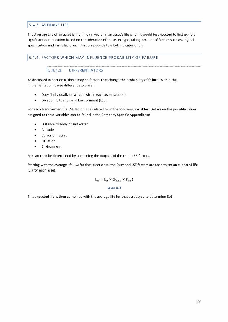
The Average Life of an asset is the time (in years) in an asset's life when it would be expected to first exhibit
significant deterioration based on consideration of the asset type, taking account of factors such as original
specification and manufacturer. This corresponds to a EoL Indicator of 5.5.
5.4.4. FACTORS WHICH MAY INFLUENCE PROBABILITY OF FAILURE
5.4.4.1. DIFFERENTIATORS
As discussed in Section 0, there may be factors that change the probability of failure. Within this
Implementation, these differentiators are:
Duty (individually described within each asset section)
Location, Situation and Environment (LSE)
For each transformer, the LSE factor is calculated from the following variables (Details on the possible values
assigned to these variables can be found in the Company Specific Appendices):
Distance to body of salt water
Altitude
Corrosion rating
Situation
Environment
FLSE can then be determined by combining the outputs of the three LSE factors.
Starting with the average life (LA) for that asset class, the Duty and LSE factors are used to set an expected life
(LE) for each asset.
LE = LA × (FLSE × FDY)
Equation 3
This expected life is then combined with the average life for that asset type to determine EoL1.

29
5.4.4.2. MODIFIERS
Modifiers change the rate at which an asset’s Probability of Failure increases. Within this Implementation,
these modifiers are:
Visual Condition
Defects
Family Reliability
Test Results
Operational restrictions
Each asset will have its own suite of modifiers; these are described in more detail in the asset specific sections
of this document and the Company Specific Appendices. Additionally, any modifiers which are Company
Specific will be described within the Company Specific Appendices.
Visual External Condition Factors
The observed condition of the transformer is evaluated through visual assessment by operational staff. Several
components of the transformer are assessed individually and assigned a condition. Condition is assessed on a
1-5 scale (1 = satisfactory, 5 = immediate replacement required). Each component’s condition is weighted
differently based on the significance of the component. These components are combined to produce an
overall scale and a Condition factor is produced.
Defects
The defect module searches the input data defect list to identify any defects associated with each asset. The
defects, in the form of stock phrases, automatically populate a defects calibration table against which users
assign a defect severity score. Once the calibration table has been set, the defect module calculates a defect
score for each asset, and uses this score to determine a defect factor, which can be overridden by a poor
defect history exception report. As with the condition factor outlined above, it is possible to set minimum HIs
for any identified defects, where this has taken place the model will identify any minimum EoL indices, and set
them aside for use later in the process.
Family Reliability
Family Reliability is determined using the TO’s own experience of assets in operation. Each family is assigned a
reliability rating (from 1-4, with 1 being Very Reliable and 4 being Very Unreliable) which then generates a
reliability factor.
Test Results
Where tests have been undertaken, the results (pass, suspect or fail) for each test type are used to derive
individual test factors (and if desired minimum EoL indices) and are then combined in order to produce an
overall test factor. The overall test factor is included in the formation of modifying factor FV1, while any
defined minimum EoL indices are set aside for use later in the process.
Operational Restrictions
When a significant issue is identified regarding a family of transformers, an Operator can issue a NEDeR which
notifies all other operators. This is called an Operational Restriction, or OR. Each OR is assigned a severity,
which then generates an Operational Restriction factor.
For assets which have more than one OR assigned to them, it is the largest factor (or most serious OR) which is
passed through to form the overall OR factor.

30
5.4.5. MAPPING END OF LIFE MODIFIER TO PROBABILITY OF FAILURE
As discussed in previous Sections, this Implementation uses this asset-specific information; from both intrusive
and non-intrusive inspections to derive a series of modifiers and differentiators which are then used to
produce an overall End of Life Modifier. From that, the asset’s failure mode frequency or Probability of Failure
(PoF) is derived (this is described in more detail in the asset-specific sections of this document). The
relationship between the condition related probability of failure and time is shown schematically in Figure 2.3.

31
6. CALCULATING PROBABILITY OF FAILURE
As shown in Figure 2.3, the relationship between the condition related probability of failure and time is not
linear. An asset can accommodate significant degradation with very little effect on the risk of failure.
Conversely, once the degradation becomes significant or widespread, the risk of failure rapidly increases. The
use of a standard relationship between PoF and asset health means that End of Life Indicators for all different
types of assets (transformers, cables, switchgear, OHLs) have a consistent meaning. The significance of any
individual End of Life Indicator value or the distribution of values for a population can be immediately
appreciated. Comparisons between different assets and different asset groups can be made directly.
The approach adopted recognises that deterioration and failure results not just from the ageing process but is
influenced by events external to the item, e.g. environmental condition or poor installation.
The following two functions were considered as a means of expressing the probability of failure distribution
curve mathematically:
An exponential function, which gives a rapid risk in the probability of failure as the Health Index value
increases, i.e. as the deterioration approaches the point of failure.
A cubic expression (i.e. the first three terms of a Taylor series for an exponential function).
Mathematical modelling3 using simulated data indicates that the use of an exponential function provides a
predicted failure rate that generally falls in the range of the simulated predictions up to about year 15. After
this time, the function starts to give predicted failure rates that are too high. A better approach is considered
to be a hybrid form of the cubic function as shown in Equation 44. This allows for the probability of failure to
be constant for low value End of Life Indicators (i.e. for assets in good condition) before increasing rapidly as
the End of Life Indicator increases (i.e. as the item begins to significantly degrade). The cubic function is
considered to model asset behaviour more closely than the exponential.
A threshold level (EoLlim, a calibration value) determines the point at which probability of failure is derived
using the cubic expression. Up to the limit defined by EoLlim, the probability of failure is set at a constant
value; above EoLlim the cubic relationship applies.
PoF = k ∙ (1 + (EoL ∙ c) +(EoL∙c)2
2!+
(EoL∙c)3
3!) where EoL > EoLlim
and
PoF = k ∙ (1 + (𝐸𝑂𝐿lim ∙ c) +(EoLlim∙c)2
2!+
(EoLIlim∙c)3
3!) where EoL ≤ 𝐸𝑂𝐿lim
Equation 4
where:
PoF = probability of failure
𝐸𝑂𝐿 = End of Life Indicators
k & c = constants
3 “Applying Markov Decision Processes in Asset Management” (M Black) - PhD Thesis,(2003) 4 "Comparing probabilistic methods for the asset management of distributed items" (M Black, AT Brint and JR Brailsford) - ASCE J. Infrastructure Systems (2005)

32
EoLlim = EoL Indicator limit below which the probability of failure is constant.
The value of c fixes the relative values of the probability of failure for different modifiers (i.e. the slope of the
curve) and k determines the absolute value; both constants are calibration values which are set for each asset
class and for each failure mode. Further information on determining the values for c and k is found in Sections
6.1 and 6.2 respectively.
This implementation has the benefit of being able to describe a situation where the PoF rises more rapidly as
asset condition degrades, but at a more controlled rate than a full exponential function would describe. The
End of Life modifier limit (EoLlim) represents the point at which there starts to be a direct relationship between
the End of Life modifier and an increasing PoF. The PoF associated with modifiers below this limit relate to
installation issues or random events.
6.1. DETERMINATION OF C
The value of c is the same for all Asset Categories and has been selected such that the PoF for an asset in the
worst condition is ten times higher than the PoF of a new asset.
The value of c can be determined by assigning the relative probability of failure values for two EoL indicator
values (generally EoL = 10 and EoL = EoLlim). Development of the modelling system and experience (gained
over twelve years of deployment) with the use of the hybrid EoL / PoF relationship has shown that an
appropriate value of c is 1.086; this equates to a ratio of EoL = 10 to EoL = 4 of approximately 10.
6.2. DETERMINATION OF K
The values for k (i.e. by failure mode and asset class) are determined using data on historic failure rate data.
The value of k in Equation 5 is derived by consideration of:
the expected number of functional failures per annum (i.e. across all the failure modes);
the Indicator distribution for the asset category; and
the volume of assets in the asset category.
For linear assets, the number of functional failures per kilometre per annum is used in the derivation of 𝑘; ie
PoF is determined on a per length basis. The calibration process ensures that for each Asset Class, the total
expected number of failures matches of the current asset population matches the number of expected
functional failures resulting from the above analysis. Typically, the observed failure rate provides the lower
bound for the number of expected functional failures and the number of replaced assets in a given year plus
the observed failure rate provides the upper bound.
An estimate of the actual value can be derived from the Implementation itself, by taking the sum of the
observed failure rate and the estimated PoF of all replaced assets. The actual value chosen may be derived
from expert judgement, preferably supported by analysis of the condition of replaced assets. Where
Implementation-produced failure rates are not supported by direct field evidence, such data should be used as
the basis of review and benchmarking wherever possible.
Thus, the value of k is calculated as follows:
k ∙ ∑ (1 + EoLi ∙ c +(EoLi ∙ c)2
2!+
(EoLi ∙ c)3
3!)
n
i=1
= (Expected no. of failures per annum)I
Equation 5

33
where:
n = the number of assets in asset group I
6.3. CALIBRATION AGAINST VERY LOW OBSERVED FAILURE RATES
The electricity industry recognises that one of the most challenging aspects in modelling the performance of
transmission assets is their very high reliability5. While there may be numerous records of “defects” or “minor
failures”, evidence of “major failures” may not exist and the observed failure rate for a particular asset
category by particular network operators may tend towards zero. This potentially leads to an inaccurate
determination of asset condition risk.
Given this widely-recognised problem (and the resulting lack of data available to each network operator), the
IEC White Paper on “Strategic asset management of power networks”6 recommends that “a standardized set
of functions to which to fit historical data could be specified, together with a method for determining which
particular function to use for a given data set, considering environment and load conditions. This would
dramatically improve the accuracy of service life estimation across businesses and allow benchmarking and
comparison of various approaches”. This is the approach taken by in this Implementation, but it is of course
dependent on the effective exchange of industry-wide data to enable effective calibration and benchmarking.
Fortunately, such exchanges do exist, including industry-wide reliability assessments, such as EPRI’s Industry-
Wide Substation Equipment Performance and Failure Database7 or UMS’s International Transmission
Operations & Maintenance Study8. Where failure rates are not supported by direct field evidence, such data
should be used as the basis of review and benchmarking wherever possible.
The values of k by asset class and failure mode are presented in Company Specific Appendices. These values
have been calculated using historic failure rates (where available). Where no failures have occurred over this
time period, it is necessary to estimate the “expected” failure rate as described above.
6.4. END OF LIFE
End of life (EoL) can be defined as when the condition related probability of failure becomes unacceptable. It
may be difficult to define unacceptable PoF, and indeed it may vary from asset to asset. However, as the
importance of the asset increases, the limit of acceptable PoF will fall. With the sharply rising EoL / PoF
relationship (see Figure 2), it would be expected that EoL will be when the EoL indicator reaches a value
somewhere between 6 and 10. Typically, end of life is defined as an EoL indicator of 7 or greater.
The condition of the overall asset population is monitored to ensure that replacement/refurbishment volumes
are sufficient to maintain sustainable levels of reliability performance, to manage site operational issues
associated with safety risks and to maintain or improve environmental performance. Aspects such as strategic
spares holdings and refurbishment capabilities are managed to ensure these sustainable levels of reliability
performance are maintained and to maintain or improve safety and environmental performance.
Although transmission assets are often complex, multi-component items of plant, within this Implementation
each is considered as an individual self-contained ‘system’ on a per asset basis.
5 Section 5.1.3 of CIGRE TB 422 Transmission Asset Risk Management (August 2010) 6 http://www.iec.ch/whitepaper/pdf/iecWP-assetmanagement-LR-en.pdf 7 http://www.epri.com/abstracts/Pages/ProductAbstract.aspx?ProductId=000000000001020010 8 http://www.umsgroup.com/Americas/What-we-do/Learning-Consortia/ITOMS

34
Asset management information is fed into the Implementation in order to produce a EoL indicator for each
asset, which is referred to as EoL(Y0). It is from this ‘system’ EoL indicator a probability of failure, (PoF), is
calculated for a number of defined failure modes.
Figure 6.1 - Implementation Overview
6.4.1. DERIVATION OF THE INITIAL EOL INDICATOR, EOL1.
The initial EoL indicator is based around the age of an asset in relation to the estimated average expected
service life which could be reasonably anticipated. This calculation stage does not take into account any
condition, defect, inspection or testing information, and simply provides an impression of the likely EoL of an
asset given its age, where it is located and its approximate work load. The first stage of the calculation is
shown below.
Figure 6.2 - Initial EoL indicator, EoL(1)
Asset Management Information
EoL1
Maximum Modmin
EoL2
EoLy0
Differentiators
Modifiers
PoFy0
Age
Average Life
Duty
Location
Situation
Environment
Duty Factor
LSE Factor
Expected LifeInitial Aging
Rate
Initial Indicator, EOL1

35
It should be noted that the derivation of all factors are TO Specific and subject to testing and validation during
the implementation of the methodology within the individual TOs.
6.4.2. THE AGEING MECHANISM
The model contains an ageing mechanism, which attempts to estimate the likely future EoL indices for each
asset, referred to as EoLyn, which is used to project the future PoF of each asset being considered. The rate of
change of the EoL Indicator is non-linear. The degradation processes involved (e.g., corrosion) are accelerated
by the products of the process, hence the rate of deterioration increases as the processes proceed.
Section 5.2.9 of BS EN 60812-2006 provides some guidance on the determination of this relationship:
“…besides published information regarding the failure rate, it is very important to consider the operational
profile (environmental, mechanical, and/or electrical stresses applied) of each component that contribute to its
probability of occurrence. This is because the component failure rates, and consequently failure rate of the
failure mode under consideration, in most cases increase proportionally with the increase of applied stresses
with the power law relationship or exponentially.”
Although the standard recommends that failure rates should be derived from field failure data, there is little
useful published data on electrical asset failure rates, especially at transmission level.
Nevertheless, most network owners have many years of experience of asset operation and so it is this
experience and historical data that is used primarily to determine this relationship. Through the electricity
industry’s Strategic Technology Programme, it was observed that electrical asset failure rates correlated with
asset health according to a semi-Markov relationship9, leading to an exponential function that for a given
asset, can be written as follows:
EoLt2 = 𝐸𝑜𝐿t1 ∙ exp {B ∙ (t2 − t1)}
Equation 6
where:
𝐸𝑜𝐿t2 = EoL Indicator at time t2
EoLt1 = EoL Indicator at time t1
B = Ageing rate (see Section 5.4 for details)
(t2 − t1) = Time taken for the asset to move from EoLt1 to EoLt2
The Initial Indicator of each asset is derived using its Initial Ageing Rate (Section 5.4.1 for further details) and
its current age (this corresponds to the time taken for the asset to move from the Indicator of a new asset to
its Initial Indicator) by the making the following substitutions into Equation 2:
EoL1,i = EoLNew ∙ exp{β1,i ∙ Agei}
Equation 7
9 “Using Modelling to Understand and Improve CBRM” STP project reference 4167 , AT Brint, JR Brailsford and D Hughes (2006).

36
where:
EoL1,i = Initial Indicator of asset i
𝐸𝑂𝐿New = Indicator of a new asset (normally set to 0.5)
β1,i = Initial Ageing Rate of asset i (see Section 5.4.1)
The Initial Indicator is capped at a value of 5.5 to reflect the fact that age alone should not be sufficient to
indicate that an asset has reached end of life; EoL can only be achieved when there is condition related
information indi
cating significant degradation10.
The methodology also calculates an ‘initial aging rate’, ‘b’, for each asset which is used as an input to the
ageing mechanism outlined below which is employed for any future asset EoL indicator estimation. The
standard EoL(y0) module also calculates the number of years it will take each asset to reach a EoL of 10, the EoL
indicator which is defined as the “end of life”.
We determine the EoL indicator in future years using the following equation:
𝐸𝑜𝐿𝑦(𝑛) = 𝐸𝑜𝐿𝑦(0)𝑒𝑏∆𝑇
Equation 8
where ∆T = time between years 0 and n.
This is initially determined using the expected life of the asset as ∆T, and the maximum and minimum EoLs as
EoL(yn) and EoL(y0) respectively. With all other variables known, b can then be calculated.
On an individual asset basis, the methodology firstly considers each asset’s age in order to determine whether
an ageing rate reduction factor should be included in the future EoL indicator estimation calculation. For
example, where an asset has reached near to end-of-life with no indications of problems, it is more likely to
live longer than initially expected and so the ageing rate reduction factor should be included.
Once this has been determined, all the information is available to produce a future EoL indicator. Having made
this estimation for each of the subcomponent parts of the larger system, the Implementation re-combines the
EoL indices to produce an estimated future system EoL indicator for each asset.
10
This only applies in year 0; EoL can be achieved in future years when there is no condition information.

37
6.4.3. DERIVATION OF THE INTERMEDIATE EOL INDICATOR, EOL2,
The second calculation stage, i.e. to find EoL2, introduces more specific asset information pertaining to
observed condition, inspection surveys, maintenance test results and operators experience of each asset.
Some typical modifiers, including EoL1 from the previous stage, are shown in Figure 6.3 below.
Figure 6.3- Intermediate EoL indicator EoL2
Modifiers specific to each asset type are identified in asset specific sections of this Section.
Condition
Defect History
Generic Reliability
Oil Condition
Operational Restrictions
Test Results
Factor Value (FV1)
EoL1
AFM Score
Leakage History
EoL2

38
6.5. FORECASTING PROBABILITY OF FAILURE
The information above can also be used to determine an approximate rate of deterioration and, therefore, to estimate future asset EoL indices, which can be seen in Figure 6.4 below.
Figure 6.4 - Forecasting Probability of Failure
The current EoL Indicator profile of a group of assets provides a 'snapshot' of the current condition of those
assets. It is also possible through the application of Equation 6 to predict how these assets will behave in the
future; i.e. how the EoL Indicator will change going forwards. In order to do so, it is first necessary to
determine the Final Ageing Rate and the Ageing Reduction Factor for the asset. Once these are known,
Equation 9 is used to calculate the EoL Indicator for any asset in any future year tYN, as follows:
EoLYn,1 = maximum (EoLY0,i ∙ exp {βfinal,i ∙ (tYN − tY0)
Fage,i
} , 𝐸𝑂𝐿YN,max)
Equation 9
where:
EoLYN,i = Future Health Index of asset i in future year YN
Bfinal,i = Final Ageing Rate of asset i (see Section 0for details)
Fage,i = Ageing Reduction Factor for asset i (see Section 6.5.2 for details)
(tYN − tY0) = Number of years over which the asset moves from EoLY0,i to EoLYN,i
EoLYN,max = Maximum allowable value for the Future Indicator; typically set to 15.
Where an Indicator is derived for multiple sub-components, the Future Indicator is derived by ageing each
component to derive the EoL Indicator of the individual sub-components in the future year; these are then re-
combined to produce the future overall EoL Indicator.
Asset Age
Initial Ageing Rate, b
EoLy0Recalculated
Ageing Rate, b’
Ageing Rate Reduction
Factor
Asset Ageing Rate, B
Future EoL
Future Year
EoLy0

39
6.5.1. FINAL AGEING RATE
For assets that are new and/or in good condition, the Future Health Index is determined using the Initial
Ageing Rate. This prevents very slow ageing of an asset due to very good condition results, which would
otherwise result in an unrealistic time for the asset to reach its end of life.
These assets are identified as those with a Current Health Index below a defined threshold or those younger
than a defined age limit.
Thus, when Agei < Agerecalc or EoLY0,i ≤ EoLrecalc:
βfinal,i = β1,i
Equation 10
where:
Agei = Current age of asset i
Agerecalc = Age limit for recalculating the ageing rate
EoLrecalc = Maximum EoL Indicator for using the Initial Ageing Rate
For other assets, the Final Ageing Rate is determined using the asset’s Current Health Index, as shown in Error! R
eference source not found..
βfinal,i = maximum [ln (
HIY0
HINew)
Agei
, β1,i. βratio]
Equation 11
where:
βratio = Maximum ratio between the Final Ageing Rate and the Initial Ageing Rate.
The ratio between the Initial Ageing Rate and the Final Ageing Rate is limited to prevent very rapid ageing of an
asset due to very poor condition results or reliability issues that would otherwise result in an unrealistic time
for the asset to reach its end of life. The maximum ratio is a calibration value and is typically set to a value of
2.

40
6.5.2. AGEING REDUCTION FACTOR
The Ageing Reduction Factor accounts for the increased life expectancy of an asset as it grows older; i.e. it
slows the ageing process for assets that have started to age. This is necessary to model the effect of scheduling
increasingly intensive or frequent maintenance as an asset approaches the end of its life. The relationship
between EoL Indicator and the Ageing Reduction Factor is shown in Figure 6.5.
Figure 6.5 - Ageing Reduction Factor Lookup
where:
Fage,lower = Lower threshold for the Ageing Reduction Factor
Fage,upper = Upper threshold for the Ageing Reduction Factor
𝐸𝑜𝐿lower = Value of Indicator below which the lower threshold for the Ageing Reduction Factor
is used
EoLupper = Value of Indicator above which the upper threshold for the Ageing Reduction Factor
is used
If the EoL Indicator of the asset is between EoLlower and EoLupper, the Ageing Reduction Factor varies linearly
as described by Equation 12.
Fage = Fage,lower + (EoLY0 − EoLlower
EoLupper − EoLlower
) . (Fage,upper − Fage,lower)
Equation 12
The relationship between EoL Indicator and Ageing Reduction Factor is set via a calibration table which defines
points 1 to 4 shown in Figure 6.5. The values used to define the Ageing Reduction Factor in all of the models
were determined empirically from historical records and are shown in Table 6.1.
EoLLOWER EoLUPPER Indicator

41
Point
(See Figure 6.5) EoL Indicator
Ageing Reduction
Factor
1 0.5 1.0
2 2.0 1.0
3 5.5 1.5
4 15.0 1.5
Table 6.1- Ageing Reduction Factor Calibration Values
The failure effect frequency directly maps to the failure mode frequency, due to the way that the failure
effects and failure modes have been categorised.
As highlighted previously, the value of 𝑐 fixes the relative values of the probability of failure for different
health indices (i.e. the slope of the curve) whilst 𝑘 determines the absolute value; both constants are
calibration values which are set for each asset class and for each failure mode. Given the importance of these
parameters in estimating the asset PoF, it is essential that these parameters are subject to rigorous testing,
calibration and review.
6.6. CIRCUIT BREAKER FACTORS AND EOL CALCULATIONS
The following sections of this document provide an overview of the transmission Circuit Breaker model design.
The process for determining the Circuit Breaker EoL Indicator is shown in Figure 2.4. For each stage in the EoL
indicator derivation, the overview will identify and name all of the component parts of each derivation and
provide a high level explanation of what the component parts represent. Specific factor values can be found in
the Company Specific Appendices.
6.6.1. FACTORS WHICH MAY INFLUENCE PROBABILITY OF FAILURE
The following is a list of factors which may influence the Probability of Failure:
Duty (FDY)
Oil Condition
SF6 Condition
SF6 Leakage
The EoL2 module combines the overall condition factor, defect history factor, generic reliability factor, overall
SOP factor, overall test result factor, SF6 condition factor and the SF6 leakage history factor in order to
determine modifying factor ‘FV1’. This is then multiplied with EoL1 from the previous calculation stage to
determine EoL2.

42
6.7. TRANSFORMER AND REACTOR FACTORS AND EOL CALCULATION
Transformers are assigned an Asset EoL indicator (EoL) according to their known condition and the service
history of other similar transformers
The EoL of the overall transformer population is monitored to ensure that replacement/refurbishment
volumes are sufficient to maintain sustainable levels of reliability performance, to manage site operational
issues associated with safety risks and to maintain or improve environmental performance in terms of oil
leakage. Aspects such as strategic spares holdings and refurbishment capabilities are managed to ensure
these sustainable levels of reliability performance are maintained and to maintain or improve safety and
environmental performance.
Within this methodology, transmission transformers are considered as ‘systems’ which are made up of 2
components; a transformer (Tx), and a tapchanger (TC). Each component is considered to be an individual
asset, with a clearly defined linkage.
For each component of a transformer system, End of Life Modifiers are generated before an overall system EoL
indicator is created.
Figure 6.6 - Transformer System Methodology Overview
The Transformer System EoL indicator is defined as follows:
𝑇𝑥𝑆𝑦𝑠𝑡𝑒𝑚𝐸𝑜𝐿(𝑦0) = 𝑚𝑎𝑥(𝑇𝑥𝐸𝑜𝐿(𝑦0), 𝑇𝑐𝐸𝑜𝐿(𝑦0))
Equation 13
Where 𝑇𝑥𝐸𝑜𝐿(𝑦0) = 𝑚𝑎𝑥(𝐸𝑜𝐿𝐷𝐺𝐴, 𝐸𝑜𝐿𝐹𝐹𝐴, 𝐸𝑜𝐿𝑀𝑂𝐷)
Equation 14
And:
Asset Management Information
System EoLy0
EOL TXy0
PoFy0
EOL TCy0
EOL TXyn
EOL TCyn
System EoLyn PoFyn
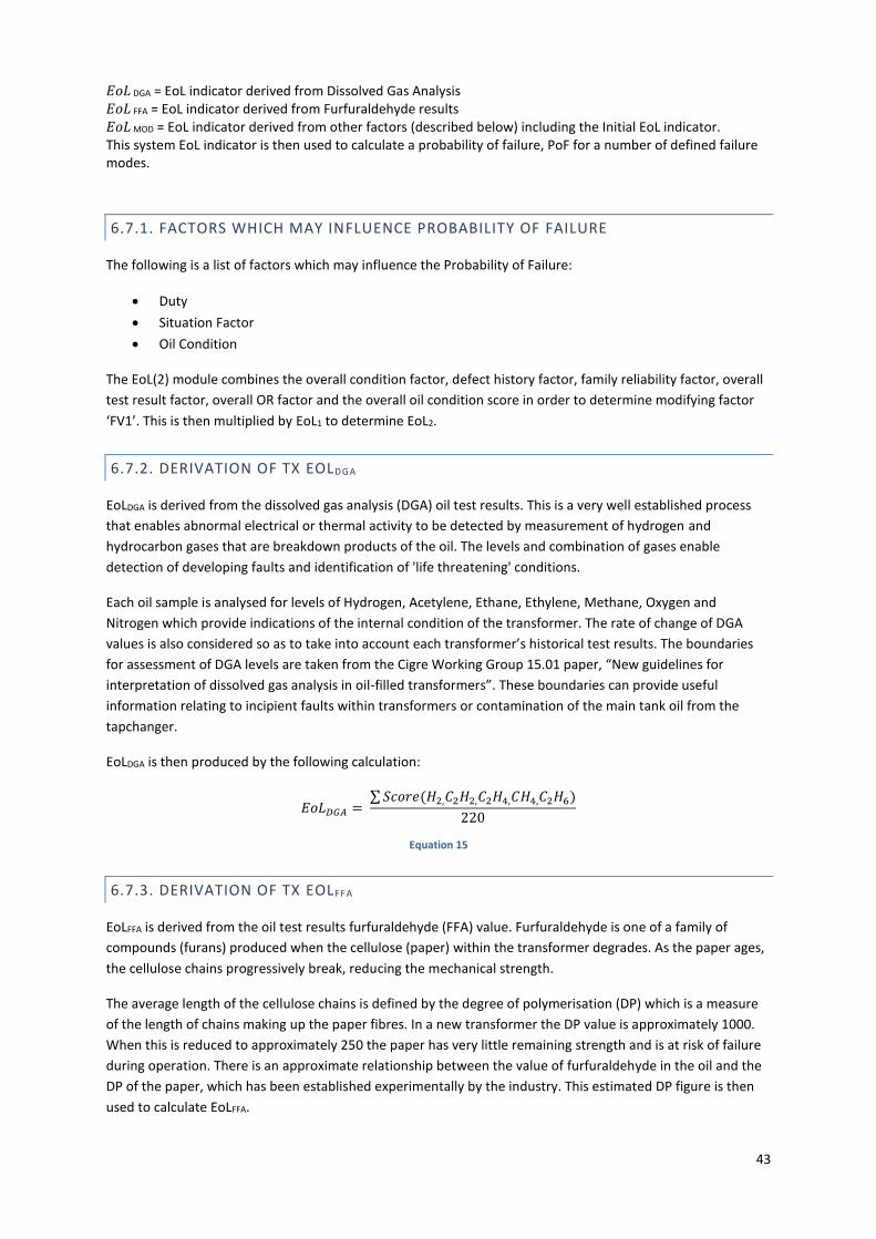
43
𝐸𝑜𝐿 DGA = EoL indicator derived from Dissolved Gas Analysis 𝐸𝑜𝐿 FFA = EoL indicator derived from Furfuraldehyde results 𝐸𝑜𝐿 MOD = EoL indicator derived from other factors (described below) including the Initial EoL indicator. This system EoL indicator is then used to calculate a probability of failure, PoF for a number of defined failure modes.
6.7.1. FACTORS WHICH MAY INFLUENCE PROBABILITY OF FAILURE
The following is a list of factors which may influence the Probability of Failure:
Duty
Situation Factor
Oil Condition
The EoL(2) module combines the overall condition factor, defect history factor, family reliability factor, overall
test result factor, overall OR factor and the overall oil condition score in order to determine modifying factor
‘FV1’. This is then multiplied by EoL1 to determine EoL2.
6.7.2. DERIVATION OF TX EOLDGA
EoLDGA is derived from the dissolved gas analysis (DGA) oil test results. This is a very well established process
that enables abnormal electrical or thermal activity to be detected by measurement of hydrogen and
hydrocarbon gases that are breakdown products of the oil. The levels and combination of gases enable
detection of developing faults and identification of 'life threatening' conditions.
Each oil sample is analysed for levels of Hydrogen, Acetylene, Ethane, Ethylene, Methane, Oxygen and
Nitrogen which provide indications of the internal condition of the transformer. The rate of change of DGA
values is also considered so as to take into account each transformer’s historical test results. The boundaries
for assessment of DGA levels are taken from the Cigre Working Group 15.01 paper, “New guidelines for
interpretation of dissolved gas analysis in oil-filled transformers”. These boundaries can provide useful
information relating to incipient faults within transformers or contamination of the main tank oil from the
tapchanger.
EoLDGA is then produced by the following calculation:
𝐸𝑜𝐿𝐷𝐺𝐴 = ∑ 𝑆𝑐𝑜𝑟𝑒(𝐻2,𝐶2𝐻2,𝐶2𝐻4,𝐶𝐻4,𝐶2𝐻6)
220
Equation 15
6.7.3. DERIVATION OF TX EOLFFA
EoLFFA is derived from the oil test results furfuraldehyde (FFA) value. Furfuraldehyde is one of a family of
compounds (furans) produced when the cellulose (paper) within the transformer degrades. As the paper ages,
the cellulose chains progressively break, reducing the mechanical strength.
The average length of the cellulose chains is defined by the degree of polymerisation (DP) which is a measure
of the length of chains making up the paper fibres. In a new transformer the DP value is approximately 1000.
When this is reduced to approximately 250 the paper has very little remaining strength and is at risk of failure
during operation. There is an approximate relationship between the value of furfuraldehyde in the oil and the
DP of the paper, which has been established experimentally by the industry. This estimated DP figure is then
used to calculate EoLFFA.

44
Failures involving multi-component systems such as the transformer system under consideration may be
regarded as completely interdependent, and therefore links in a ‘system chain’. This is the underlying principle
behind the derivation of the final present day transformer system EoL indicator EoLy0, which is generated from
the larger of the transformer EoLy0 and its associated tapchanger EoLy0.
𝐸𝑜𝐿(𝑦0) = 𝑚𝑎𝑥(𝑇𝑥𝐸𝑜𝐿(𝑦0), 𝑇𝑐𝐸𝑜𝐿(𝑦0)).
Equation 16

45
6.8. CABLE FACTORS AND EOL CALCULATION
Cables are assigned an Asset EoL indicator (EoL) according to their known condition and the service history of
other similar cables.
Within this methodology, transmission cables are considered as number of discrete cable lengths (or
‘component’) which together form a distinct circuit.
For each component of cable circuit asset management information is fed into the model in order to produce a
component EoL indicator, referred to as EoLy0, before an overall system EoL indicator is created. This system
EoL indicator is then used to calculate a probability of failure, PoF for a number of defined failure modes.
There are three separate models within the main underground cable model reflecting the following types of
construction;
Oil
Non-pressurised
Submarine cable
Each model uses a similar format, though certain condition points are ‘construction’ dependent and only used
within that model as a factor.
The models contain an ageing mechanism, which attempts to estimate the likely future EoL indices for each
cable to as EoLyn. These future EoL estimations are combined in an identical fashion to the present day EoL
calculation, so as to derive an overall cable future EoL, and it is this which is used to project future PoF of each
of the cables being considered.
6.8.1. FACTORS WHICH MAY INFLUENCE PROBABILITY OF FAILURE
The following is a list of factors which may influence the Probability of Failure:
Duty
Location, Situation and Environment (LSE)
For each cable the LSE factor is calculated from a situation factor and an installation factor, as shown in Figure 6.7 below.
Figure 6.7 - LSE factor
For submarine cables the LSE is determined using the following variables:
Cable route topology
Cable situation factor
Wind/wave factor
Combined wave and current energy factor

46
The combination of these variables determines an overall LSE factor (FLSE) using the following equation:
𝐹𝐿𝑆𝐸 = 𝑚𝑎𝑥(𝐹𝑇 , 𝐹𝑆, 𝐹𝑊 , 𝐹𝐸)
Equation 17
Starting with the average life (LA) for that asset class, the Duty and LSE factors are used to set an expected life (LE) for each asset.
𝐿𝐸 = 𝐿𝐴 × (𝐹𝐿𝑆𝐸 × 𝐹𝐷𝑌)
Equation 18
Leak History
The leak history information for a particular circuit is used to determine a leak history factor and an associated
minimum EoL for each circuit. The leak history is derived from information on the volume of top-ups over a
ten year period.
Fault rate
The fault rate information for a circuit will be used to determine a Fault rate factor and derive a minimum EoL,
as shown below.
The EoL2 module combines the defect history factor, generic reliability factor, overall test result factor, leak
history factor and the fault rate factor in order to determine modifying factor ‘FV1’. This is then multiplied by
EoL1 to determine EoL2.
6.9. OVERHEAD LINE FACTORS AND EOL CALCULATION
OHL assets are assigned an Asset EoL indicator (EoL) according to their known condition, the known condition
of associated components and the service history of other similar conductors, fittings and towers.
Within this methodology, three Lead Asset types are considered separately however they can be viewed in
combination, representative of an entire circuit.
Conductors
Fittings
Towers
Figure 6.8 - OHL System Overview
In addition to the ‘per asset’ EoL indices described above, the models will include summary information by
route for towers, and circuit name for spans.
EoL Steel Tower
EoL Conductor
EoL Fittings/Insulaors
EoL Steelwork
EoL Foundation
Per tower
Per circuitPer forward span
Per circuitPer tower
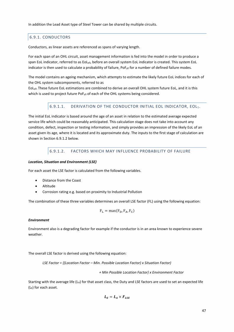
47
In addition the Lead Asset type of Steel Tower can be shared by multiple circuits.
6.9.1. CONDUCTORS
Conductors, as linear assets are referenced as spans of varying length.
For each span of an OHL circuit, asset management information is fed into the model in order to produce a
span EoL indicator, referred to as EoLy0, before an overall system EoL indicator is created. This system EoL
indicator is then used to calculate a probability of failure, PoFy0 for a number of defined failure modes.
The model contains an ageing mechanism, which attempts to estimate the likely future EoL indices for each of
the OHL system subcomponents, referred to as
EoLy0. These future EoL estimations are combined to derive an overall OHL system future EoL, and it is this
which is used to project future PoFy0 of each of the OHL systems being considered.
6.9.1.1. DERIVATION OF THE CONDUCTOR INITIAL EOL INDICATOR, EOL1.
The initial EoL indicator is based around the age of an asset in relation to the estimated average expected
service life which could be reasonably anticipated. This calculation stage does not take into account any
condition, defect, inspection or testing information, and simply provides an impression of the likely EoL of an
asset given its age, where it is located and its approximate duty. The inputs to the first stage of calculation are
shown in Section 6.9.1.2 below.
6.9.1.2. FACTORS WHICH MAY INFLUENCE PROBABILITY OF FAILURE
Location, Situation and Environment (LSE)
For each asset the LSE factor is calculated from the following variables.
Distance from the Coast
Altitude
Corrosion rating e.g. based on proximity to Industrial Pollution
The combination of these three variables determines an overall LSE factor (FL) using the following equation:
FL = max(FD, FA, FC)
Environment
Environment also is a degrading factor for example if the conductor is in an area known to experience severe
weather.
The overall LSE factor is derived using the following equation:
LSE Factor = {(Location Factor – Min. Possible Location Factor) x Situation Factor)
+ Min Possible Location Factor} x Environment Factor
Starting with the average life (LA) for that asset class, the Duty and LSE factors are used to set an expected life
(LE) for each asset.
𝑳𝑬 = 𝑳𝑨 × 𝑭𝑳𝑺𝑬

48
6.9.1.3. DERIVATION OF THE CONDUCTOR INTERMEDIATE EOL INDICATOR,
EOL2,
The second calculation stage, i.e. to find EoL2, introduces more specific asset information pertaining to
observed condition, test results and operators’ experience of each asset. The typical inputs, including EoL1
from the previous stage, are shown in Figure 6.9 - Intermediate EoL indicator EoL.
Figure 6.9 - Intermediate EoL indicator EoL2
Condition
The condition of the various components of an asset provide a measure of the degradation processes which
may be occurring, and therefore the EoL of the asset. The helicopter assessment of steel tower overhead lines
includes a visual assessment of the conductor span.
Defect History
The number of defects experienced on the span over the previous 5 years (including those that have been
repaired are identified. Each defect will then be assigned a severity rating (using a scale of 1 to 4, where 4 is
the most severe) via a calibration table.
Infra-red Test Results
Helicopter inspections of the Over Head Lines are used to identify hot joints on conductors. This information
will be used to derive an infra-red test factor and a minimum EoL value via calibration tables as shown below.
Where tests have been undertaken, the results (either pass, suspect or fail) for each test type are used to
derive individual test factors (and if desired minimum EoL indices) and are then combined in order to produce
an overall test factor. The overall test factor is included in the formation of modifying factor FV1, while any
defined minimum EoL indices are set aside for use later in the process.
Condition
Defect History
Infra-Red Test Results
Tate Joints
Corman Test Results
Conductor Sampling
Factor Value (FV1)
EoL1
EoL2

49
Cormon Test Results
Cormon testing measures the extent of corrosion on ACSR conductors, and can be used to derive a EoL
indicator independently of any other information on condition or age.
The test results are used to derive a Cormon EoL indicator via a calibration table of the form shown below.
The tests are conducted on a span or number of spans and the results are then applied to the whole circuit.
The test results are converted to a score, e.g. 1-4.
Conductor Sampling
Conductor sampling determines the extent of corrosion a sample of the overhead conductor, which is
considered to provide a representative indication of the EoL of the circuit. The results can be used to derive a
EoL indicator independently of any other information on condition or age.
The test results are used to derive a Conductor Sampling EoL indicator via a calibration table of the form
shown below. The tests results are conducted on a span or number of spans and then applied to the whole
circuit. The test results are converted to a score, e.g. 1-5.
6.9.1.4. DERIVATION OF THE CONDUCTOR FINAL EOL INDICATOR, EOLY0
The final stage of the conductor present day EoL indicator, EoLY0, compares each individual factors
intermediate EoL indicator as shown below:
Figure 6.10 - Conductor Final EoL indicator, EoLCond
6.9.2. FITTINGS
To attach, insulate and join conductor spans various fittings and insulators are used. Over the course of the
lifetime of these assets an EoL indicator needs to be calculated (on a per circuit and a per tower basis) as
summarised in the schematic diagram below.
6.9.2.1. DERIVATION OF THE FITTINGS INITIAL EOL INDICATOR, EOLC.
The initial EoL indicator is based around the age of an asset in relation to the estimated average expected
service life which could be reasonably anticipated. This calculation stage does not take into account any
Maximum Modmin
EoL2
EoLCond

50
condition, defect, inspection or testing information, and simply provides an impression of the likely EoL of an
asset given its age, where it is located and its approximate work load. The inputs to the first stage of
calculation are shown in Section below.
6.9.2.2. FACTORS WHICH MAY INFLUENCE PROBABILITY OF FAILURE
Location, Situation and Environment (LSE)
For each asset the LSE factor is calculated from the following variables.
Distance from the Coast
Altitude
Corrosion rating e.g. based on proximity to Industrial Pollution
The combination of these two variables determines an overall LSE factor (FLSE) using the following equation:
The overall LSE factor is derived using the following equation:
LSE Factor = ((Location Factor – Min. Possible Location Factor) x Situation Factor) + Min Possible Location
Factor) x Environment Factor
Starting with the average life (LA) for that asset class, the Duty and LSE factors are used to set an expected life
(LE) for each asset.
𝑳𝑬 = 𝑳𝑨 × 𝑭𝑳𝑺𝑬
6.9.2.3. DERIVATION OF FITTINGS - FINAL EOL INDICATOR, EOLY0
The second calculation stage, i.e. to find EoLY0, introduces more specific asset information pertaining to
observed condition, test results and operators’ experience of each asset. The typical inputs, including EoLC
from the previous stage, are shown in Figure 6.11.
Figure 6.11 - Final EoL indicator
EoLA
EoLFitEoLB
EoLC

51
Condition
Where reliable and robust information provides definitive information on asset condition, the information is
used to directly derive a condition based EoL indicator. This is depicted in the schematic diagram shown
below.
Figure 6.12 - Derivation of condition based EoL Indices for fittings
A number of individual condition points are assessed or rated using a pre-defined scale (typically 1 to 4 or 1 to
5). Each condition rating is then assigned a condition score via a calibration table. Each condition point has its
own specific calibration table for defining the condition score.
Condition Score Calibration
EoLa and EoLb are two possible values for the condition based EoL indicator derived by combining the
individual condition scores in two different ways. This ensures that a ‘worst case’ EoL indicator is derived
regardless of whether the fittings have only one element in very poor condition or a number of elements in
moderately poor condition.
EoLa is the highest of the condition scored divided by a calibration value, whilst EOLb is the sum of the three
highest condition scores divided by a second calibration value. Where condition scores are not provided, a
default condition score is applied.
Condition 1
EoLACondition 2
Condition 3
Condition n
EoLB

52
6.9.3. TOWERS
The steel tower EoL indicator is formed from a combination of a steelwork EoL and a tower foundation EoL
indices.
The Tower EoL indicator is defined as follows:
𝐸𝑜𝐿(𝑇) = 𝑤𝑒𝑖𝑔ℎ𝑡𝑒𝑑 𝑎𝑣𝑒𝑟𝑎𝑔𝑒(𝑇𝑜𝑤𝑒𝑟 𝑆𝑡𝑒𝑒𝑙𝑤𝑜𝑟𝑘 𝐸𝑜𝐿𝑦0, 𝑇𝑜𝑤𝑒𝑟 𝐹𝑜𝑢𝑛𝑑𝑎𝑡𝑖𝑜𝑛𝑠 𝐸𝑜𝐿𝑦0)
6.9.4. STEELWORK EOL INDICATOR
6.9.4.1. DERIVATION OF STEELWORK EOLA AND EOLB
The first stage of the steel work EoL indicator is derived using the observed condition information collated
from surveys and inspections, as shown below.
Figure 6.13 - Derivation of initial steelwork indicators
Observed condition scores taken from inspection or condition assessments and the year in which the condition
assessments took place are entered into the model. Each condition point is assigned a condition score via a
series of calibration lookup tables. Condition points include scores for the tower legs, step bolts, bracings,
crossarms, peak, paintwork.
EoLA is derived from the worst of the condition points found, while EoLB is derived using the sum of the
condition points scores divided by a calibration ‘divider’. This creates two EoL indices which represent the
Tower Leg Rating
Step Bolt Rating
Bracings Rating
Crossarms Rating
Peak Rating
Paintwork Rating
Tower Leg Factor
Step Bolt Factor
Bracings Factor
Crossarms Factor
Peak Factor
Paintwork Factor
EoLA
EoLB

53
condition of the tower steelwork in the year of condition assessment; the Implementation will then age these
EoL indices to the present year.
6.9.4.2. DERIVATION OF STEELWORK EOL INDICATOR EOLC
An ‘age based’ EoL indicator, EoLC, is derived from the asset age, last painting date and the expected service
life of the tower as shown in Figure 6.14 below. This is only used
i. if no inspection data is available to derive EoLA and EoLB, or
ii. to provide boundaries for the HIs derived from inspection data.
Figure 6.14 - Steelwork EoL indicator EoL(c)
The assets age is taken from the date of tower construction and where it exists, the date at which the tower
was last painted. If a tower has been painted then the expected life of the tower will be set via calibration to
an expected life associated with the paint system, typically in the region of 15 years. If the tower has not been
painted the year of construction is used against an expected life which is associated with the original tower
steelwork galvanising, a calibration value typically set at around 30 years.
6.9.4.3. DERIVATION OF STEELWORK EOLS
The final tower steelwork EoL indicator, EoLS, which represents the present day overall condition of the tower
steelwork is determined from EoLA, EoLB and EoLC as depicted below.
Figure 6.15 - Tower Steelwork EoLS
Where detailed condition assessment information is not available, the model will not be able to calculate EoLA
or EoLB, and therefore EoLS will equal EoLC.
Last Painting Date
Date of Construction
Age
Average Life
Location
Expected Life
EoLC
EoLS
EoLBEoLA EoLC

54
Where detailed condition information is available the final tower steelwork EoL indicator, EoLS, will be the
maximum of EoLA and EoLB. In the event that the condition assessment identifies that the tower steel work in
an as new condition, then the model will use EoLC to modify the EoL indicator depending upon the age of the
tower up to a calibratable limits which is typically set at an EoL of around 1.5.
6.9.5. FOUNDATION EOL INDICATOR
6.9.5.1. DERIVATION OF THE FOUNDATION EOL INDICATOR
The Implementation calculates an EoL indicator for each set of tower foundations for each tower position. The
model uses information relating to the type of foundation, the environment in which the foundation is
situated, along with more specific foundation test results and inspection information. The first stage of EoL
indicator calculation determines the foundation initial EoL indicator, which is shown in below.
Figure 6.16 - Initial Foundation EoL indicator, EoLF1
The overall location factor for foundations is either derived from the specific soil test results indicated in Figure
6 or from an overall soil type factor. If neither are available the factor defaults to a neutral value of 1.
Date of Construction
Age
Average Life
Location
Expected Life
EoLF1
Foundation Type
Soil Redox Potential Factor
Soil Resistivity Factor
Soil pH Factor
Soil Type Factor
Soil Redox Potential
Soil Type
Soil pH
Soil Resistivity

55
6.9.5.2. FOUNDATION INTERIM EOL INDICATOR
The second calculation stage, i.e. to find EoL2, introduces more specific asset information pertaining to
observed condition, inspection surveys, maintenance test results and operators experience. The inputs,
including the Foundation EoL1 from the previous calculation stage, are shown below.
Figure 6.17 - Interim Foundation EoL indicator EoLF2
Within this stage of the foundation EoL indicator derivation, the results of asset specific tests carried out on
tower foundations are used to modify the initial foundation EoL indicator.
This interim foundation EoL can be overridden by foundation ratings assigned to foundations which have been
excavated and inspected (within defined calibration limits). The override will only take place on the condition
that the date at which the excavated rating has been assigned is after the date when the foundation was last
routinely inspected/tested. The EoL indicator which results from this mechanism is assigned for the year in
which the excavation took place.
Where excavations and repairs have been undertaken, and the date of the completed works is later than the
latest date of any condition assessment, then the test data will not be used in the creation of the foundation
EoL indicator. Instead the EoL indicator will be based upon a calibration value which reflects the EoL of the
asset once the repairs have been completed (at the time of completion) and aged to the present year as
before.
Factor Value
EoLF1
TDR/TECO Factor
Polarisation Resistance
Factor
Inspection Factor
TDR/TECO Results
Inspection Date
Inspection Rating
Polarisation Resistance
Measurements
EoLF2

56
6.9.6. STEEL TOWER EOL INDICATOR
The Steel Tower EoL indicator is formed from the combination of the Tower Steelwork EoL indicator and the
Foundation EoL Indicator, as shown below.
Figure 6.18 - Steel Tower EoL indicator
Once each of the input heath indices have been created, the Steel Tower EoL indicator is formed by taking a
weighted average of both the tower steelwork and the foundation EoL indices. This weighted average is
subject to a minimum EoL indicator override which is determined by calibration values. Traditionally the
weighting applied to the tower steelwork to foundation is in the region of 1:3, however this ratio can be
changed as part of a calibration review.
EoLT
EoLF2 EoLS

57
7. REPORT FINDINGS
The analysis described so far is only credible if it is documented, understood and the findings are known to be
meaningful. Section 5.4 of EN 60812 provides guidance on the scope and content of FMEA reporting, which
should include a detailed record of the analysis used and a summary of the failure effect identified.
The implementation by SP Transmission/SHE Transmission uses a managed computing tool to provide clear,
auditable documentation of the precise calculation steps used in the analysis.
Figure 7.1 Example algorithm view on SP Transmission/SHE Transmission modelling environment