processing, analysis, and general evaluation of well-driller logs

U.S. Department of the InteriorU.S. Geological Survey

Scientific Investigations Report 2008 –5184

National Water Availability and Use Pilot Program

Processing, Analysis, and General Evaluation of Well-Driller Logs for Estimating Hydrogeologic Parameters of the Glacial Sediments in a Ground-Water Flow Model of the Lake Michigan Basin

41°

42°

43°

44°

45°

46°

90° 89° 88° 87° 86° 85° 84° 83° 82°

SAGIN

AW B

AY

LAKEMICHIGAN

GREE

N BAY

Base from U.S. Geological Survey digital data 1:100,000 1983. Universal Transverse Mercator projection, Zone 16, Standard parallel 0° (Equator), Central meridian 87° W,North American Datum 1983

70 140 MILES

70 140 KILOMETERS0

0

ILLINOIS

INDIANA

MICHIGAN

WISCONSIN

OHIO

1

25

50

75

100

EXPLANATIONEquivalent horizontal hydraulic conductivity, in feet per day


By Leslie D. Arihood

National Water Availability and Use Pilot Program

Scientific Investigations Report 2008–5184

U.S. Department of the InteriorU.S. Geological Survey

U.S. Department of the InteriorDIRK KEMPTHORNE, Secretary

U.S. Geological SurveyMark D. Myers, Director

U.S. Geological Survey, Reston, Virginia: 2009

For product and ordering information: World Wide Web: http://www.usgs.gov/pubprod Telephone: 1-888-ASK-USGSFor more information on the USGS--the Federal source for science about the Earth, its natural and living resources, natural hazards, and the environment: World Wide Web: http://www.usgs.gov Telephone: 1-888-ASK-USGS

Any use of trade, product, or firm names is for descriptive purposes only and does not imply endorsement by the U.S. Government.

Although this report is in the public domain, permission must be secured from the individual copyright owners to reproduce any copyrighted materials contained within this report.

Suggested citation: Arihood, L.D., 2009, Processing, analysis, and general evaluation of well-driller records for estimating hydrogeologic parameters of the glacial sediments in a ground-water flow model of the Lake Michigan Basin: Scientific Investiga-tions Report 2008-5184, 26 p.

ISBN 1-411-32302-5

iii

ContentsAbstract ...........................................................................................................................................................1Introduction.....................................................................................................................................................2

Purpose and Scope ..............................................................................................................................2Geologic Setting ....................................................................................................................................2

Processing of Well-Log Data .......................................................................................................................5Evaluation of Well-Log Data ................................................................................................................5Calculation of Equivalent Horizontal and Vertical Hydraulic Conductivities for the

Glacial Layers of the Model ...................................................................................................5Calculation of Aquifer Hydraulic Conductivity from Well-Log Specific-Capacity Data ..........10Compilation of Water-Level Calibration Data from Well Logs .....................................................11Estimation of Thickness and Hydraulic Conductivity for Glacial Sediments beneath

Lake Michigan........................................................................................................................14Analysis of Well-Log Data ..........................................................................................................................15Comparison of Hydrogeologic Products Derived from Well-Log Data with Other

Hydrogeologic Products ...............................................................................................................20Summary and Conclusions .........................................................................................................................24References Cited..........................................................................................................................................25

Figures 1. Study area of the Lake Michigan ground-water model and boundary of the

Lake Michigan Basin. ...................................................................................................................3 2. Thickness of Quaternary Period sediments in the study area of the Lake Michigan

ground-water model. ....................................................................................................................4 3. Distribution of logs from drilled wells used to generate hydraulic conductivity

and water-level data for the glacial layers of the Lake Michigan Basin ground- water-flow model. .........................................................................................................................6

4. Flow chart for processing well-log lithologies into grids of horizontal and vertical hydraulic conductivity. .................................................................................................................7

5. Relation between lithology-based equivalent hydraulic conductivity and the percentage of aquifer material in the model layer. .................................................................9

6. Flow chart for the processing of well-log water levels into model-calibration data for the Lake Michigan ground-water-flow model. .......................................................12

7. Estimated thickness of glacial sediments beneath Lake Michigan. Estimates based on data from Soller and Packard (1998), Colgan and Principato (1998), and National Oceanic and Atmospheric Administration (2005). .........................................15

8. Distribution of equivalent horizontal hydraulic conductivity for layer 1 of the model based on assumed hydraulic conductivity of 1 foot per day for nonaquifer material and 100 feet per day for aquifer material. ...............................................................16

9. Distribution of equivalent vertical hydraulic conductivity for layer 1 of the model based on assumed vertical hydraulic conductivity of 0.001 foot per day for nonaquifer material and 10 feet per day for aquifer material. ............................................17

iv

Figures–Continued

10. Distribution of horizontal hydraulic conductivity calculated from well-log derived specific-capacity data for aquifers in layer 1 of the ground-water-flow model ..............19

11. Distribution of equivalent horizontal hydraulic conductivity for layer 1 from this study and surface geology from Fullerton and others (2003) ..............................................21

12. Distribution of equivalent horizontal hydraulic conductivity for layer 1 from this study and generalized ground-water availability for a part of northern Indiana (Indiana Department of Natural Resources, 1980) ................................................................22

13. Distribution of equivalent horizontal hydraulic conductivity distribution for layer 1 of the model and flow-duration ratios for a part of northern Indiana .............................23

Tables 1. Amount of surface area of the Lake Michigan ground-water model covered by

individual sediment textures and sediment texture classifications .....................................4 2. Comparison of median horizontal hydraulic conductivity calculated using specific

capacity data from Indiana and Michigan .............................................................................11 3. Kriging parameters used to interpolate ground-water-level surfaces in Indiana,

Michigan, and Wisconsin for the Lake Michigan ground-water-flow model ..................13 4. Median horizontal hydraulic conductivity for different sediment texture classes

calculated from specific-capacity data from Indiana, Michigan, and Wisconsin for model layers 1, 2, and 3 of a ground-water-flow model of the Lake Michigan Basin. .................................................................................................................18

v

Conversion Factors

Inch/Pound to SI

Multiply By To obtain

Length

inch (in.) 2.54 centimeter (cm)

inch (in.) 25.4 millimeter (mm)

foot (ft) 0.3048 meter (m)

mile (mi) 1.609 kilometer (km)

Area

square mile (mi2) 259.0 hectare (ha)

square mile (mi2) 2.590 square kilometer (km2)

Flow rate

gallon per minute (gal/min) 0.06309 liter per second (L/s)

Hydraulic conductivity

foot per day (ft/d) 0.3048 meter per day (m/d)

Transmissivity*

foot squared per day (ft2/d) 0.09290 meter squared per day (m2/d)

SI to Inch/Pound

Multiply By To obtain

Length

centimeter (cm) 0.3937 inch (in.)

millimeter (mm) 0.03937 inch (in.)

meter (m) 3.281 foot (ft)

kilometer (km) 0.6214 mile (mi)

Area

hectare (ha) 0.003861 square mile (mi2)

square kilometer (km2) 0.3861 square mile (mi2)

Flow rate

liter per second (L/s) 15.85 gallon per minute (gal/min)

Hydraulic conductivity

meter per day (m/d) 3.281 foot per day (ft/d)

Transmissivity*

meter squared per day (m2/d) 10.76 foot squared per day (ft2/d)

Horizontal coordinate information is referenced to the North American Datum of 1983 (NAD 83)

*Transmissivity: The standard unit for transmissivity is cubic foot per day per square foot times foot of aquifer thickness [(ft3/d)/ft2]ft. In this report, the mathematically reduced form, foot squared per day (ft2/d), is used for convenience.

vi

Abbreviations

AML ARC Macro Language

ASCII American Standard Code for Information Exchange

DEM Digital elevation model

GWSI Ground Water Site Inventory

K Equivalent horizontal hydraulic conductivity

KZ Equivalent vertical hydraulic conductivity

KSC Horizontal hydraulic conductivity derived from water-well log specific-capacity data

T Transmissivity, in foot squared per day


AbstractIn 2005, the U.S. Geological Survey began a pilot study

for the National Water Availability and Use Program to assess the availability of water and water use in the Great Lakes Basin. Part of the study involves constructing a ground-water flow model for the Lake Michigan part of the Basin. Most ground-water flow occurs in the glacial sediments above the bedrock formations; therefore, adequate representa-tion by the model of the horizontal and vertical hydraulic con-ductivity of the glacial sediments is important to the accuracy of model simulations. This work processed and analyzed well records to provide the hydrogeologic parameters of horizontal and vertical hydraulic conductivity and ground-water levels for the model layers used to simulated ground-water flow in the glacial sediments. The methods used to convert (1) lithology descriptions into assumed values of horizontal and vertical hydraulic conductivity for entire model layers, (2) aquifer-test data into point values of horizontal hydraulic conductivity, and (3) static water levels into water-level calibration data are presented.

A large data set of about 458,000 well driller well logs for monitoring, observation, and water wells was available from three statewide electronic data bases to characterize hydrogeologic parameters. More than 1.8 million records of lithology from the well logs were used to create a lithologic-based representation of horizontal and vertical hydraulic conductivity of the glacial sediments. Specific-capacity data from about 292,000 well logs were converted into horizontal hydraulic conductivity values to determine specific values of horizontal hydraulic conductivity and its aerial variation. About 396,000 well logs contained data on ground-water lev-els that were assembled into a water-level calibration data set.

A lithology-based distribution of hydraulic conductivity was created by use of a computer program to convert well-log lithology descriptions into aquifer or nonaquifer categories and to calculate equivalent horizontal and vertical hydraulic conductivities (K and K

Z, respectively) for each of the glacial

layers of the model. The K was based on an assumed value

of 100 ft/d (feet per day) for aquifer materials and 1 ft/d for nonaquifer materials, whereas the equivalent K

Z was based on

an assumed value of 10 ft/d for aquifer materials and 0.001 ft/d for nonaquifer materials. These values were assumed for convenience to determine a relative contrast between aquifer and nonaquifer materials. The point values of K and K

Z from

wells that penetrate at least 50 percent of a model layer were interpolated into a grid of values. The K distribution was based on an inverse distance weighting equation that used an expo-nent of 2. The K

Z distribution used inverse distance weighting

with an exponent of 4 to represent the abrupt change in KZ that

commonly occurs between aquifer and nonaquifer materials.The values of equivalent hydraulic conductivity for

aquifer sediments needed to be adjusted to actual values in the study area for the ground-water flow modeling. The specific-capacity data (discharge, drawdown, and time data) from the well logs were input to a modified version of the Theis equa-tion to calculate specific capacity based horizontal hydraulic conductivity values (K

SC). The K

SC values were used as a guide

for adjusting the assumed value of 100 ft/d for aquifer deposits to actual values used in the model.

Water levels from well logs were processed to improve reliability of water levels for comparison to simulated water levels in a model layer during model calibration. Water levels were interpolated by kriging to determine a composite water-level surface. The difference between the kriged surface and individual water levels was used to identify outlier water levels.

Examination of the well-log lithology data in map form revealed that the data were not only useful for model input, but also were useful for understanding the glacial hydrogeology of a multistate area. The distribution of K and K

Z provided a

three-dimensional view of aquifer and confining systems. The distribution of K

SC revealed an aerial difference from state to

state and a relation to glacial sediment texture. Median KSC

was larger for Indiana (264 ft/d) than for Michigan (89 ft/d) or Wisconsin (48 ft/d). The difference could be related to past glacial processes. A pattern in K

SC was observed with sedi-

ment texture. Aquifers within sediment textures deposited

By Leslie D. Arihood

2 Processing, Analysis, and General Evaluation of Well-Driller Logs for Estimating Hydrogeologic Parameters

under a higher energy environment, for example, outwash textures, had higher values of K

SC than those deposited under a

lower energy environment.

IntroductionAt the request of Congress, the U.S. Geological Survey

is assessing the availability and use of the Nation’s water resources. In 2005, the U.S. Geological Survey established a program called the National Water Availability andUse (U.S. Geological Survey, 2002). The program is designed to characterize how much surface and ground water is currently available, how water availability is chang-ing, and how much water will be available in the future. The Great Lakes Basin was chosen as a pilot study area. Methods developed during the pilot study are intended to best evaluate the resource and deliver accurate and timely information to planners at local, regional, and national levels.

Part of the study involves constructing a ground-water model for the Lake Michigan part of the Basin. Mandle and Kontis (1992, p. 92) found that most ground-water flow for the northern Midwest United States, which includes the Lake Michigan Basin west of Lake Michigan, occurs in the glacial sediments as opposed to the underlying bedrock. There-fore, adequate representation by the model of the horizontal and vertical hydraulic conductivity of the glacial sediments is important to the accuracy of model flow simulations. Adequate representation of the glacial sediments is difficult because of their extreme heterogeneity. The occurrence of interbedded sand and gravel deposits within the fine grained glacial sediments is difficult to predict. Many observation points are required to define the extent of intermittent zones of aquifer and nonaquifer sediments. Neff and others (2005, p. 7) explained the improvement in using the lithology information from well logs to better represent geology beneath the surface. Abundant data that can provide information on hydraulic conductivity, as well as ground-water levels, are available from well driller well logs that were provided to state regulatory agencies. The monitoring-, observation-, and water-well logs have been computerized by the states, stored in statewide data bases, and are available for processing and analysis by com-puter programs to provide data for model construction.

Purpose and Scope

This report documents the process of converting informa-tion from about 458,000 electronic well logs from the state data bases of Michigan, Wisconsin, and Indiana into data useful for construction of a regional ground-water model for the Lake Michigan Basin. The report first establishes the use and limitations of well logs in hydrogeologic studies, and then explains how lithologic descriptions recorded by drillers onto well logs were converted into hydraulic conductivities. The procedures are explained for converting specific-capacity data

(well pumpage rate, time, and water-level drawdown data) into values of horizontal hydraulic conductivity and for charac-terizing the horizontal hydraulic conductivities of different hydrogeologic units. A quality-control procedure to eliminate outlier water-level data from a well-log data set to be used as model-calibration data also is presented. No well-log data were available for the glacial sediments beneath Lake Michi-gan, therefore, the procedure for estimating glacial thickness and the horizontal and vertical hydraulic conductivities of the sediments beneath the lake is explained.

Results of the well-log processing are illustrated, ana-lyzed, and compared to similar hydrogeologic products as a qualitative method to evaluate the accuracy of well-log data. Distributions of the well-log derived values of horizontal and vertical hydraulic conductivity are illustrated across three states for the top layer (layer 1) of the ground-water model. Patterns in the distributions are described and analyzed. The distributions are compared to surface-geology and ground-water availability maps and a type of flow-duration map as a way to qualitatively evaluate the accuracy of the hydraulic conductivity distributions. This comparison process revealed that well-log based products have potential advantages over conventional products like surface geology maps to determine hydrologic parameters, and those advantages are presented.

Geologic Setting

The 181,000 mi2 study area covers nearly all of Michi-gan and parts of Wisconsin and Indiana (fig. 1). The study area corresponds to the area of the Lake Michigan ground-water model currently (2008) being constructed as another part of the pilot study on water availability and use. Although northeastern Illinois is included in the modeled area, hydrau-lic conductivity data for that area were not derived from well logs. Data for Illinois were derived from another model being constructed by the Illinois State Water Survey for northeastern Illinois (Lin and others, 2008). No well logs were analyzed for Ohio or the Canadian parts of the ground-water model. Hydraulic conductivity, to be discussed in the modeling report, was instead based on texture classes defined by Fullerton and others (2003) or Soller and Packard (1998).

The study area is overlain by glacial sediments depos-ited by four glaciations, which created mostly flat to gently rolling topography (Weist, 1978, p. J3). Although glacial sediments cover the study area, in some areas those sedi-ments are reworked into different deposits, such as allu-vium. Glacial sediments can be as much as 1,100 ft thick in Michigan (Weist, 1978, p. J3) but usually are less than 200 ft thick (fig. 2). The glacial sediments at the surface consist of several textures, but fine grained sediments dominate (table 1). The distribution of the textures is shown in a surface geol-ogy map presented later in the report. A description of the regional surficial aquifer system within the glacial sediments is provided by Coon and Sheets (2006, p. 7–8). The glacial sediments overlie mostly consolidated sedimentary formations

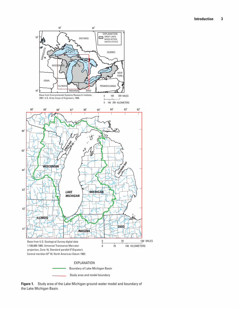
Introduction 3

Figure 1. Study area of the Lake Michigan ground-water model and boundary of the Lake Michigan Basin.

Base from U.S. Geological Survey digital data1:100,000 1983. Universal Transverse Mercatorprojection, Zone 16, Standard parallel 00 (Equator),

EXPLANATION

Boundary of Lake Michigan Basin

WISCONSIN

ILLINOIS

INDIANA

MICHIGAN

OHIO

LAKE MICHIGAN

900 890 880 870 860 850 840 830 820

460

450

440

430

420

410

Central meridian 870 W, North American Datum 1983

GREEN

BAY

SAGIN

AW B

AY

Study area and model boundary

WISCONSIN

I

ILLINOIS

INDIANA OHIO

PENNSYLVANIA

NEWYORK

ONTARIO

QUEBEC

MIN

NES

OTA

IOWA

EXPLANATION

KILOMETERS

MILES0 100 200

0 100 200

GREAT LAKES BASIN WITHIN UNITED STATES

Base from Environmental Systems Research Institute, 2001; U.S. Army Corps of Engineers, 1998.

CANADAU.S.A

MI CHIG AN

900800

500

400

70 140 MILES

70 140 KILOMETERS0

0


ranging in age from Jurassic to Precambrian Period (Sheets and Simonson, 2006, p. 4). The major bedrock feature is the deep sedimentary basin in Michigan (Weist, 1978, p. J3) that is reflected in the area of thick Quaternary Period sediments shown in figure 2. Additional information on the bedrock for-mations can be found in Sheets and Simonson (2006).

Figure 2. Thickness of Quaternary Period sediments in the study area of the Lake Michigan ground-water model.

Table 1. Amount of surface area of the Lake Michigan ground-water model covered by individual sediment textures and sediment texture classifications.

[Data from Fullerton and others, 2003]

Sediment texture

Area covered by asediment

texture (percent)

Sediment texture classification

Till 55.9 Fine grained

Coarse1 24.6 Coarse grained

Lake sediments 17.5 Fine grained

Peat and muck 1.5 Fine grained

Loess 0.5 Fine grained1Outwash, ice contact forms, sand, colluvium, alluvium

70 140 MILES

70 140 KILOMETERS0

0

Thickness from 0 toless than 50 ft






Water body

No data

EXPLANATION

Sediment thickness from Soller and Packard, 1998

460

450

440

430

420

410

900 890 880 870 860 850 840 830 820

Base from U.S. Geological Survey digital data1:100,000 1983. Universal Transverse Mercatorprojection, Zone 16, Standard parallel 00 (Equator),Central meridian 870 W, North American Datum 1983

Processing of Well-Log Data 5

Processing of Well-Log DataThis section begins by providing a qualitative evalua-

tion of data from all available well driller reports (well logs) for use in hydrogeologic interpretations, then describes the processing of data from well logs into hydrogeologic infor-mation useful for ground-water modeling. The methods used to convert (1) lithology descriptions into assumed values of horizontal and vertical hydraulic conductivity for entire model layers, (2) pump-test data into point values of horizontal hydraulic conductivity, and (3) static water levels into water-level calibration data are presented. Hydraulic conductivities for the glacial sediments beneath Lake Michigan also were required for the ground-water model, but well logs do not exist in that area. An alternate method for estimating horizontal and vertical hydraulic conductivity for Lake Michigan sediments is explained.

Evaluation of Well-Log Data

Data recorded on well logs from monitoring, observation, and water wells may not be thought as reliable as those col-lected by geologists or hydrologists who are typically guided by training programs or a quality-assurance plan during data collection. Still, the data can potentially be useful when other data are not available. For example, Fowler and Arihood (1998, sheet 1) used well-log water-level data to indicate general ground-water flow direction and water-level altitude for St. Joseph County in northern Indiana. By comparison, the mean absolute error between 46 water levels measured in 1990–1992 by U.S. Geological Survey staff (Bayless and Ari-hood, 1996) and a kriged water-level surface created from the well-log data was 4 ft. Horizontal hydraulic conductivity from a study area in northeastern Illinois calculated from driller-col-lected specific-capacity data (12 ft/d) compared favorably with values calculated from professionally supervised aquifer tests (8 ft/d) and ground-water model calibration (17 ft/d) (Kay and others, 2006). The following evaluation is a qualitative one that discusses the limitations of well-log data and the general approach of typical driller practice in well-log data collection.

Well logs can provide aerially extensive hydrogeologic information. However, as with all data sets, sources of errors need to be considered. Errors in location of the well log can result in misplaced lithologies and incorrect altitudes for those lithologies. Errors in location also result in incorrect altitudes for ground-water levels. The potential for sampling bias from water-well logs is present because wells are drilled only until they reach aquifer material that can yield sufficient water. Aquifers at higher or lower altitudes with possibly dif-ferent characteristics are not sampled. Interpolation between points where aquifers yield sufficient water could result in the impression that all aquifers in the area are transmissive, yet the area may contain generally low-yielding aquifers. In addition, the low-yielding aquifers, if encountered, are not reported. These limitations to well-log information need to be consid-

ered during the interpretation of the data. The large quantity of well-log data may help to reduce the influence of occasional errors, but in areas with few well logs, the uncertainty in inter-pretation increases.

Well-log data are recorded by well drillers who gener-ally are not required by an organization to follow specific procedures in data collection. Therefore, questions can arise as to the quality of data collected by drillers. During a series of ground-water availability studies by the U.S. Geological Survey during the 1970’s and 1980’s (for example, Lapham, 1981), project hydrologists decided to interview about 15 to 20 well drillers in four central Indiana counties about their data-collection practices. Information was acquired about how each driller recorded lithologies, static water levels, and specific-capacity data. Although some drillers used unac-ceptable practices, such as completing the well log long after drilling the well, the majority of drillers followed timely and reasonable procedures, such as waiting until a true static water level had developed before recording the static water level for the well. The impression from the interviews was that the typical driller exhibited a desire to provide accurate informa-tion and recorded data in a manner approaching that used by a geologist or hydrologist. The driller sometimes demonstrated the same desire as a scientist to accurately record his findings. In addition, the driller may be driven by economic interests in having to justify well placement on the basis of drilling records. That is, it may be difficult to sell a deep well when shallow wells have been successfully established.

Calculation of Equivalent Horizontal and Vertical Hydraulic Conductivities for the Glacial Layers of the Model

Well logs provided about 458,000 observation points with more than 1.8 million records of lithology (fig. 3). The well logs have become computerized and stored in statewide computerized data bases. The well logs from Wisconsin (Wis-consin Geological and Natural History Survey, 2004), Michi-gan (Michigan Department of Environmental Quality, 2003), and Indiana (Indiana Department of Natural Resources, 2002) were obtained for processing in 2006 and 2007 by computer programs into information useful for ground-water modeling.

Well-log processing used ARC Macro Language pro-gramming (AML) available in ArcInfo software (Environ-mental Systems Research Institute, 2003) and consisted of several steps that are illustrated in figure 4. The well-log data bases were obtained as two files formatted as American Standard Code for Information Interchange (ASCII) for each state. The first file contained basic well-site information, such as owner name, X-Y coordinates of the well, well depth, aquifer-test data, and water level. This file was converted into a point coverage. The second file was the record of lithologies recorded by the well drillers. The second file was converted into an INFO data base, which was then read by a second AML program that automatically converted driller lithology


Figure 3. Distribution of logs from drilled wells used to generate hydraulic conductivity and water-level data for the glacial layers of the Lake Michigan Basin ground-water-flow model.


Figure 4. Flow chart for processing well-log lithologies into grids of horizontal and vertical hydraulic conductivity.

ASCII file of lithologies

ASCII file of well-site information

(x-y, depth, water level)

INFO file oflithologies

INFO file of standardizedlithologies and aquifer

classifications

Point coverageof well-site information

Point coverage of all well-log information

Lithologyinterpretation

checks

County coverage 1

County coverage 2

County coverage 3

Remainingcounty coverages

Calculate equivalent horizontal and vertical hydraulic conductivities for eachlayer of the ground-water flow model using assumed values for the

hydraulic conductivity of aquifer, nonaquifer, and unknown aquifer type

Combine county covers to one statewide cover

Interpolate point cover values with Inverse Distance Weighting

to generate a statewide grid

Grid values input to model-calibration

process

Grid maps used forqualitative analysis

of hydrogeology

Statewide water-welllog database


descriptions into standard U.S. Geological Survey Ground-Water Site Inventory Sys tem (GWSI) lithology codes (Mathey, 1989, p. 2–110). The program searches for key phrases that describe lithology, such as sand, clay, or silt, and compares the phrases to lithology text strings in an interpretation file that converts the driller text into a GWSI lithology. The second AML program searches the phrases for as many as three lithology descriptors to determine the best match to a GWSI code, which can have as many as three lithology descriptors. The AML also classified each lithology into either aquifer or nonaquifer material. After the interpretation, the lithology records were checked for lithology descriptions that could not be interpreted because of misspellings or new lithology phrases not referenced in the interpretation file. Additional lithology text strings were added to the interpretation file so that the undefined lithology records could be converted to GWSI lithologies. Errors in the lithology record, such as gaps in the lithology record or the appearance of glacial lithology in a bedrock section of the well log, resulted in eliminating the well record from the statewide coverage. On average, about 5 percent of the well logs were deleted from each original state well-log data base. The INFO lithology file was joined to the well-site information point coverage, and then subdivided into individual county coverages. Further processing is done on single county coverages, because data for an individual well can be accessed during subsequent programming more rapidly if the data are in a county coverage rather than in one set of the entire state.

The lithology records in the county coverages were con-verted by a third AML program into an equivalent, or effective horizontal and vertical hydraulic conductivity for each well site for specified thicknesses of the glacial sediments. The specified thicknesses correspond to the predefined thicknesses of glacial-sediment layers used in the ground-water model. The glacial sediments are represented in the model by three layers: a maximum 100-ft thick layer 1, a maximum 200-ft thick layer 2, and a layer 3 that accounts for all remaining glacial thickness. These layer thicknesses were used to provide a relatively even division of the glacial sediments in the major-ity of the modeled area and to provide an opportunity to vary the hydraulic conductivity with depth. Some areas have thin glacial sediments, therefore, a value of horizontal and vertical hydraulic conductivity is calculated at a well site for less than the 100- or 200-ft thickness and possibly for fewer than three layers.

The program calculates equivalent horizontal and vertical hydraulic conductivities (referred to subsequently as K and KZ) for the predefined layers on the basis of percentage of aquifer and nonaquifer material in each layer. The equivalent K is based on an assumed value of 100 ft/day for aquifer mate-rial and 1 ft/day for nonaquifer material, whereas the equiva-lent KZ is based on an assumed value of 10 ft/day for aquifer material and 0.001 ft/day for nonaquifer material. These val-ues are assumed for convenience to determine a relative con-trast between aquifer and nonaquifer material. The calculation of equivalent horizontal and vertical hydraulic conductivity for

each glacial layer of the model uses the following equations (DeWeist, 1965, p. 231–232):

(1)

(2)

where K = equivalent horizontal hydraulic conductivity

for a model layer K

Z = equivalent vertical hydraulic conductivity

for a model layer Ki = assumed horizontal hydraulic conductivity

of the ith lithology record within the layer Ki

z = assumed vertical hydraulic conductivity of

the ith lithology record within the model layer

ti = thickness of the ith lithology record within the model layer

i = the ith lithology record, and n = total number of lithology records within the

model layer.

After equivalent hydraulic conductivities have been calculated for well sites in each county, the county coverages are rejoined into a statewide coverage. Sites without lithology records were eliminated from the statewide coverage.

To further explain the relation between the equivalent hydraulic conductivities, assumed values of hydraulic conduc-tivity, and quantity of aquifer / nonaquifer material, the rela-tion is illustrated in figure 5. The K value is proportional to the thickness of aquifer material present within the model layer. For a 100-ft layer that is 50 percent aquifer material (50 ft of aquifer), K is 50 percent of the maximum value (100 ft/d), or 50 ft/d. The proportional relation can be applied to other assumed ranges for horizontal hydraulic conductivity of aqui-fer material, such as 1 to 1000 ft/d. That is, the distribution of horizontal hydraulic conductivity does not have to be recalcu-lated from the well-log record; a simple multiplication can be applied to the distribution of values. The K

Z is not proportional

to the percentage of aquifer material, but is strongly influenced by the value chosen for vertical hydraulic conductivity of the nonaquifer material. The lower the value for vertical hydraulic conductivity of nonaquifer material, the more quickly K

Z for

the model layer decreases in value as the percentage of aquifer material decreases from 100 percent. If a different value for vertical hydraulic conductivity of nonaquifer material is cho-sen during model calibration, then K

Z has to be recalculated.

According to equation 2, the recalculation requires values for

∑

∑

=

==n

iiz

i

n

i

i

Z

Kt

tK

1

1

∑

∑

=

=

×= n

i

i

n

i

ii

t

KtK

1

1)(


thicknesses of aquifer and nonaquifer material (other values in equation 2 are known or given), which can be obtained from the equivalent horizontal hydraulic conductivity. For example, if the model layer is 100 ft thick at a model cell and aquifer material has an assumed horizontal hydraulic conductivity of 100 ft/d, and if K at a model node is 75 ft/d, then the thickness of nonaquifer material is 25 ft and aquifer material thickness is 75 ft. A value for vertical hydraulic conductivity is assumed, and the remaining unknown, K

Z, can be calculated.

Several additional details associated with the calculation of hydraulic conductivities are provided to help understand the processing of well logs:

1. The value of assumed hydraulic conductivity for a lithol-ogy record is determined by a file that defines all GWSI lithology codes to be aquifer, nonaquifer, or undefined lithology, such as drift. For undefined lithologies, the geo-metric mean of the equivalent horizontal hydraulic con-ductivity of aquifer and nonaquifer material is assigned to the lithology record. Because aquifer material has an assumed horizontal hydraulic conductivity of 100 ft/d and nonaquifer material has an assumed horizontal hydraulic

conductivity 1 ft/d, then the assigned horizontal hydraulic conductivity for the undefined lithology is approximately 10 ft/d.

2. The model design uses three layers (1, 2, and 3) to repre-sent the glacial sediments. Where glacial sediments range from 1 to 100 ft thick, layer 1 has a thickness equal to the glacial thickness. Where glacial sediments are from 101 to 300 ft thick, layer 1 has a thickness of 100 ft and layer 2 has a thickness equal to the remainder of the glacial thickness. Where glacial sediments are in excess of 300 ft thick, layer 1 extends from the land surface to 100 ft; layer 2 extends from 100 ft to 300 ft below land surface; and layer 3 extends from 300 ft below land surface to the depth where the glacial sediments contact the top of bedrock.

3. A lithology record (for example, clay 85 to 120 ft) may begin in one layer and end in the layer below. For that case, the lithology record, along with the associated hydraulic conductivity, is split proportionally between the two layers.

Figure 5. Relation between lithology-based equivalent hydraulic conductivity and the percentage of aquifer material in the model layer.

0

20

40

60

80

100

0 20 40 60 80 1000.001

0.01

0.1

1

10

Equivalent horizontalhydraulic conductivity, K

Equivalent verticalhydraulic conductivity, Kz

CALC

ULAT

ED E

QUIV

ALEN

T HO

RIZO

NTA

LHY

DRAU

LIC

CON

DUCT

IVIT

Y, IN

FEE

T PE

R DA

Y

CALC

ULAT

ED E

QUIV

ALEN

T VE

RTIC

ALHY

DRAU

LIC

CON

DUCT

IVIT

Y, IN

FEE

T PE

R DA

Y

AQUIFER MATERIAL, IN PERCENT


4. A penetration depth into each model layer, expressed as a percentage, was calculated for each well. Wells that penetrate to a depth equal to or greater than 50 percent of a layer were selected from the coverage of equivalent hydraulic conductivity and used to create the continuous distributions of hydraulic conductivity.

5. Hydraulic conductivities are calculated only for that part of the lithology record that is below the driller-measured water level. In a few wells, the water level is greater than 100 ft deep, meaning that layer 1 is dry and calculated hydraulic conductivities are 0 ft/d. If no water-level value is available for the well, then the equivalent hydraulic conductivities are based on all lithology records within a layer. This decision should not noticeably alter the distri-butions because 85 percent of the wells have water-level data and the water table is usually close to the surface in fine grained sediments, which comprises most of the area. The near-surface water table is evidenced by the general need for tile drainage and the high surface-water levels in borrow pits along interstate highways.

6. In areas where the glacial sediments are thicker than 300 ft and a third glacial layer is present, the thickness of the third glacial layer is defined as the thickness from 300 ft below ground to the depth of bedrock as defined by the well log. If the well is not drilled to bedrock, then an estimated thickness of model layer 3 is determined by use of an interpolated value of bedrock surface altitude from a bedrock-surface map constructed in another one of the water-availability set of studies (David Lampe, U.S. Geological Survey, written commun., 2006). The percent penetration of the well into the third layer is based on the actual or estimated layer thickness.

7. If the well extends through a layer bottom, this process also computes an altitude of the layer bottom at each well. If a layer has zero thickness, then the altitude of that layer is assigned the same value as the bottom altitude of the first layer above with a finite thickness. For example, if layer 3 is zero thickness, and layer 2 is 50 ft thick with a bottom altitude of 650 ft, then the bottom altitude of layer 3 is also 650 ft. The altitude of the bedrock surface would also be 650 ft. During model construction, layer 3 would be given a small thickness of 0.2 ft so that the layer is continuous.

Calculation of Aquifer Hydraulic Conductivity from Well-Log Specific-Capacity Data

Values of horizontal hydraulic conductivity for aquifer material also were calculated directly from about 292,000 well logs by use of the specific-capacity data (well discharge, duration of pumping, and water-level drawdown) and are referred to as K

SC. The calculated K

SC provided an estimate of

horizontal hydraulic conductivity. The modeling process used the estimate as a guide for adjusting the assumed K value of 100 ft/d to actual values used in calculating a lithology-based K for a model layer. The process of converting pump-test, or specific-capacity data, into K

SC is presented.

Well discharge, duration of pumping, and water-level drawdown for each well were input to a modified form of the Theis equation shown below (Prudic, 1991, p. 11) to deter-mine an aquifer transmissivity, T. Because T appears on both sides of equation 3, an iterative process was used to calculate T by use of an initial value of 500 ft2/d. The process stops after several iterations when the difference between the old estimate and new estimate for T becomes less than 5 ft2/d, and the last new estimate is used. The value of T was adjusted for the effect of partial penetration by the well screen into the aquifer by use of a method described by Butler (1957, p. 160). Values of K

SC were calculated by dividing T by the thickness of satu-

rated aquifer material penetrated by the well, which provides a conservative estimate for K

SC. Well loss was not accounted for

because there were no available data to analyze well loss, and the well was assumed 100 percent efficient. It was assumed that, in whole, the gravel pack around the well screen compen-sated for the additional drawdown caused by turbulent flow through the well screen and in the well casing. The calculation of T from specific-capacity data is often done, and two alterna-tive, computerized methods are referenced for convenience: (Bradbury and Rothschild, 1985; McLin, 2005).

(3)

where T = transmissivity, in feet squared per day, Q = well discharge, in gallons per minute, s = drawdown, in feet, r = well radius, in feet, S = storage coefficient (dimensionless), and t = time, in days.

Equation 3 requires values for storage coefficient, well diameter, and screen length. Well logs often do not have all of these data (and almost never have storage coefficient), there-fore estimates need to be determined. If screen length data was missing, then a screen length of 5 ft was assumed when pumping rate was less than 200 gal/min, and a screen length of 20 ft was assumed if the pumping rate was greater than or

−−

=

TtSr

sQT e 4

log577.0**32.152


equal to 200 gal/min. If well diameter data was missing, then a well diameter of 4 inches was assumed when pumping rate was less than 200 gal/min, and a well diameter of 8 inches was assumed if pumping rate was greater than or equal to 200 gal/min. If the well was confined, then the storage coefficient was assumed to be 0.0001; if the well was unconfined, then the storage coefficient was assumed to be 0.15. These values are well within ranges suggested by Freeze and Cherry (1979, p. 60–61), and their difference from actual values should not significantly affect the calculation of T (Prudic, 1991, p. 12). Confined or unconfined conditions were deter-mined by observing if the pumping level for the water surface was above or below the top of the aquifer, respectively.

Calculation of horizontal hydraulic conductivity from transmissivity requires a value for well discharge. Well dis-charge could be generated by a submersible pump, an air line (air flow from a compressor), or other methods, like a bailer. Because different pumping methods might result in different values for K

SC, a comparison was made between K

SC values

calculated using data from different methods of pumping. Table 2 presents the results of the effect from different pump-ing methods on median values of K

SC for wells in Michigan

(Michigan Department of Environmental Quality, 2005) and Indiana (Indiana Department of Natural Resources, 2002). Sample size for each glacial texture was large, always greater than 1,000 samples. The values are for sites where the pump-ing method was known and do not include all of the sites with specific-capacity data. The table shows that median K

SC for the

air flow method is greater than that for the submersible pump method in Indiana, however, the opposite is true in Michi-gan. A rank-sum test (Helsel and Hirsch, 1995) was done on the individual state data sets and confirmed that the air flow method of pumping produces larger values of K

SC in the Indi-

ana data and smaller values in Michigan (p > 0.999). Because it is not known which method of pumping produces a more representative value of K

SC, and because the median K

SC using

all methods of pumping is between the median KSC

for air flow and submersible pumping, the data from all pumping methods were used in the analysis of patterns in K

SC for the three states.

Table 2. Comparison of median horizontal hydraulic conductivity calculated using specific capacity data from Indiana and Michigan.

[ft/d, feet per day; (1,625), number of samples; data from Michigan Depart-ment of Environmental Quality (2005) and Indiana Department of Natural Resources (2002)]

Method of pumping

Median horizontal hydraulic

conductivityin Indiana

(ft/d)

Median horizontal hydraulic

conductivityin Michigan

(ft/d)All 177 (6,425) 18.7 (162,496)

Air flow 226 (2,076) 14.2 (50,455)

Submersible pump 143 (976) 37.0 (12,471)

Compilation of Water-Level Calibration Data from Well Logs

About 396,000 water-level values (one value per well log collected at the time of well construction) are available from the state well-log data bases for the Lake Michigan ground-water model area. In some areas, the well-log water-level data are the only source of information on water surfaces of the various aquifers. Such a large data set should provide many reliable water levels to aid in model calibration. In fact, Fowler and Arihood (1998, sheet 1) used well-log water-level data to indicate general ground-water flow direction and water-level altitude for St. Joseph County in northern Indiana. Water levels measured by U.S. Geological Survey (Bayless and Ari-hood, 1996) were on the average (mean absolute error) 4 ft from a kriged water-level surface created from the driller data, which is sufficient accuracy for model calibration data. How-ever, appropriate screening techniques were used to eliminate inaccurate and inconsistent data.

All well logs that contained a depth to static water level from land surface were processed into a coverage and evalu-ated for accuracy and consistency. The process of selecting water-level data for model calibration is illustrated in figure 6. A static water-level altitude was calculated by subtracting the depth to the static water level from the land-surface altitude. Land-surface altitude typically is recorded on the well log along with the depth to static water level. If land-surface altitude was not recorded, then a value interpolated from a 30-meter digital elevation model (DEM) was substituted for the missing altitude data. Substituted values of altitude repre-sented less than 1 percent of the data set, except for the data from Wisconsin. Land-surface altitude data were not available from the well logs; therefore, all altitude data from Wiscon-sin (86,000 values) were derived from the DEM. The error in land-surface altitude will vary depending on the method used to determine altitude. Altitudes commonly are estimated from topographic maps. The author examined the potential error in altitudes estimated from topographic maps by comparing estimated altitudes with surveyed values for 35 well sites. The mean absolute error for altitudes estimated from a topographic map was 1.68 ft. The root mean square error for altitudes based on DEM data was estimated to be 8.01 ft (American Society for Photogrammetry and Remote Sensing, 2007, p. 106).

Although well-log water levels can be helpful, many water levels in the data set are expected to contain significant measurement and location error and should be eliminated from the set of calibration water levels. A method was developed for quality assurance of well-log water levels. The method used kriging to determine a water-level surface, and then used the difference between the kriged surface and water levels from a well log to identify and eliminate outlier water levels.


A kriging interpolator available in ArcInfo, version 8.3 (Environmental Systems Research Institute, 2003) was used to estimate a water-level surface grid that had grid cells every 2,000 ft. Kriging was used to improve the estimation of water levels by taking advantage of the spatial correlation existing

Figure 6. Flow chart for the processing of well-log water levels into model-calibration data for the Lake Michigan ground-water-flow model.

between water-level measurements. Ordinary kriging (McBrat-ney and Webster, 1986) was applied to the individual water-level data sets from each state by use of the kriging parameters shown in table 3. Included in the table is the mathematical function used to fit the semi-variance data. Kriging was applied to the individual state data sets, but trends in popula-tion distributions between each state were not considered.

Cover containing all well-log information

Reduced cover containing depth to water level and land-surface data DEM provides missing

land-surface values(water-level altitude calculated)

Water-level altitudesurface interpolated from point values of water-level altitude by ordinary kriging

Point values of water-level altitude subtracted from kriged water-level surface

Differences between individual water levels and kriged surface sorted by magnitude

Water levels having consistent differences fromkriged water-level surface are kept for model calibration

Remaining water-level values assigned to a model layer on the basis of well depth and used to compare to simulated values calculated for the same model layer


Lack of consideration of the trends probably introduced error in the estimates, but the errors were not considered signifi-cant relative to the use of the water-level surface, which was to eliminate outlier water levels. As explained in the next paragraph, only large differences between individual measure-ments and the kriged water-level surface were used to identify outliers.

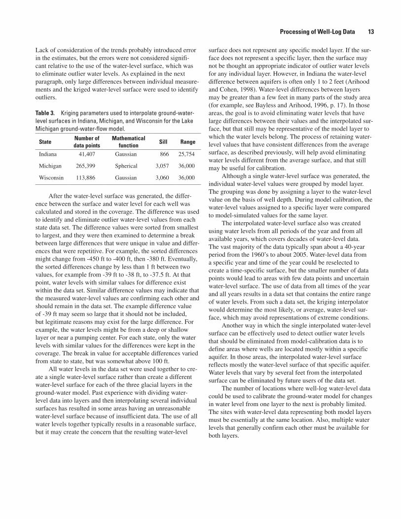
Table 3. Kriging parameters used to interpolate ground-water-level surfaces in Indiana, Michigan, and Wisconsin for the Lake Michigan ground-water-flow model.

StateNumber of data points

Mathematical function

Sill Range

Indiana 41,407 Gaussian 866 25,754

Michigan 265,399 Spherical 3,057 36,000

Wisconsin 113,886 Gaussian 3,060 36,000

After the water-level surface was generated, the differ-ence between the surface and water level for each well was calculated and stored in the coverage. The difference was used to identify and eliminate outlier water-level values from each state data set. The difference values were sorted from smallest to largest, and they were then examined to determine a break between large differences that were unique in value and differ-ences that were repetitive. For example, the sorted differences might change from -450 ft to -400 ft, then -380 ft. Eventually, the sorted differences change by less than 1 ft between two values, for example from -39 ft to -38 ft, to -37.5 ft. At that point, water levels with similar values for difference exist within the data set. Similar difference values may indicate that the measured water-level values are confirming each other and should remain in the data set. The example difference value of -39 ft may seem so large that it should not be included, but legitimate reasons may exist for the large difference. For example, the water levels might be from a deep or shallow layer or near a pumping center. For each state, only the water levels with similar values for the differences were kept in the coverage. The break in value for acceptable differences varied from state to state, but was somewhat above 100 ft.

All water levels in the data set were used together to cre-ate a single water-level surface rather than create a different water-level surface for each of the three glacial layers in the ground-water model. Past experience with dividing water-level data into layers and then interpolating several individual surfaces has resulted in some areas having an unreasonable water-level surface because of insufficient data. The use of all water levels together typically results in a reasonable surface, but it may create the concern that the resulting water-level

surface does not represent any specific model layer. If the sur-face does not represent a specific layer, then the surface may not be thought an appropriate indicator of outlier water levels for any individual layer. However, in Indiana the water-level difference between aquifers is often only 1 to 2 feet (Arihood and Cohen, 1998). Water-level differences between layers may be greater than a few feet in many parts of the study area (for example, see Bayless and Arihood, 1996, p. 17). In those areas, the goal is to avoid eliminating water levels that have large differences between their values and the interpolated sur-face, but that still may be representative of the model layer to which the water levels belong. The process of retaining water-level values that have consistent differences from the average surface, as described previously, will help avoid eliminating water levels different from the average surface, and that still may be useful for calibration.

Although a single water-level surface was generated, the individual water-level values were grouped by model layer. The grouping was done by assigning a layer to the water-level value on the basis of well depth. During model calibration, the water-level values assigned to a specific layer were compared to model-simulated values for the same layer.

The interpolated water-level surface also was created using water levels from all periods of the year and from all available years, which covers decades of water-level data. The vast majority of the data typically span about a 40-year period from the 1960’s to about 2005. Water-level data from a specific year and time of the year could be reselected to create a time-specific surface, but the smaller number of data points would lead to areas with few data points and uncertain water-level surface. The use of data from all times of the year and all years results in a data set that contains the entire range of water levels. From such a data set, the kriging interpolator would determine the most likely, or average, water-level sur-face, which may avoid representations of extreme conditions.

Another way in which the single interpolated water-level surface can be effectively used to detect outlier water levels that should be eliminated from model-calibration data is to define areas where wells are located mostly within a specific aquifer. In those areas, the interpolated water-level surface reflects mostly the water-level surface of that specific aquifer. Water levels that vary by several feet from the interpolated surface can be eliminated by future users of the data set.

The number of locations where well-log water-level data could be used to calibrate the ground-water model for changes in water level from one layer to the next is probably limited. The sites with water-level data representing both model layers must be essentially at the same location. Also, multiple water levels that generally confirm each other must be available for both layers.


Estimation of Thickness and Hydraulic Conductivity for Glacial Sediments beneath Lake Michigan

Few data sources (and no well logs) were available to help provide information on thickness and horizontal and vertical hydraulic conductivity of the sediments beneath Lake Michigan. Therefore, the values of thickness and hydraulic conductivity for sediments beneath Lake Michigan are inferred from existing map information and, to a large degree, based on what could be considered reasonable by study hydrologists. These values may require adjustment during model calibra-tion.

Different data sources for thickness of sediments were used for different parts of the lake bottom. For the southern half of Lake Michigan (see fig. 2 for extent), work presented by Soller and Packard (1998) was used to estimate the thickness of lacustrine clay and till. For the northern half of Lake Michigan, a shaded relief map (Colgan and Principato, 1998) and a discussion of the geomorphology of the lakebed (National Oceanic and Atmospheric Administration, 2005) were used to estimate the thickness and hydrologic character-istics of the glacial sediments. East of Green Bay, Wis. and for two isolated areas of alluvial fan/deltaic deposition, the glacial sediments were modeled as a sequence of sand over nonaqui-fer materials. In areas where Colgan and Principato (1998) interpreted smoothly varying lake bottom topography, it was assumed that the map indicated deposition of sand and silt. In areas where the map showed highly variable lake bottom topography, it was assumed that the map reflected bedrock surface control of the lake bottom. For areas of highly variable lake bottom topography, it was assumed that a 10 ft thick clay deposit was the only glacial sediment covering bedrock. For the entire near-lakeshore area, the underlying clay and tills were assumed to be capped by sand deposits derived from flu-vial sources. The resulting thickness map is shown in figure 7.

Equivalent hydraulic conductivity values (K and KZ) were

assigned based upon the composition of the materials within each mapping area. For clay and till, K = 1 ft/d and K

Z = 0.1

ft/d; for sand, K = 100 ft/d and KZ = 10 ft/d. For areas mapped

as being capped by sand, such as around the lake perimeter, the sand deposits were assumed to represent 25 percent of the total thickness of the glacial sediments. For example, where sediments were mapped as 100 ft thick, sand and clay thick-ness were assumed to be 25 ft and 75 ft, respectively. The assumption of 25 percent sand deposits ensured that there was always a sand and clay mixture, regardless of the total thick-ness of glacial sediments. The resulting horizontal hydraulic conductivity distribution is shown in the next section.

Analysis of Well-Log DataThe processing of well logs was originally intended

to provide distributions of horizontal and vertical hydraulic conductivity for a ground-water model. The values associated with the distributions were manipulated by the calibration process to obtain final values while maintaining the relative differences in the distribution. During the processing, obser-vations of the well-log data in map form indicated additional benefits that accrue from this analysis in the understanding of the hydrogeology of a multistate area. The distributions of K and K

Z data provide a three-dimensional view of aquifer and

confining systems and the distribution of specific-capacity-based hydraulic conductivity reveal aerial differences from state to state in horizontal hydraulic conductivity of sand and gravel deposits.

The point values of K and KZ calculated from the well-

log lithology records for each layer were used as input to an interpolation program within ArcInfo to estimate a grid of values for hydraulic conductivity for each state data set. The K distribution was based on an inverse distance weighting equa-tion shown below (Isaaks and Srivastava, 1989, p. 258–259). According to Isaaks and Srivastava (1989, p. 259), as the value of the exponent p becomes greater, the closest input value has greater influence on the estimated value. The K distribution was calculated with an exponent of 2, which is commonly used (Sheppard, 1968). The K

Z distribution used an exponent

of 4 on the log of vertical hydraulic conductivity to better represent the abrupt change in K

Z that occurs between aquifer

and nonaquifer materials. The distributions were calculated for each state, and then the individual state distributions and the distribution beneath Lake Michigan were merged together to construct a single distribution of K and K

Z for each model

layer. The K and KZ distributions for layer 1, the most continu-

ous layer, are shown in figures 8 and 9, respectively. The fig-ures show the K and K

Z distributions based on assumed values

for aquifer and nonaquifer materials, but the distributions also reflect the total amount of aquifer and nonaquifer material in the first layer of the model. The grids are based on well logs that penetrate at least 50 percent of the layer thickness.

(4)

where

ν̂ = estimated value, νi

= input value, i = ith input value, n = last input value, d = distance between the input value and the

point of estimation, and p = exponent.

∑

∑

=

== n

ip

i

n

iip

i

d

νdν

1

1

1

1

ˆ

Analysis of Well-Log Data 15

The distributions shown in the previous two figures provided the pattern of change in hydraulic conductivity for the ground-water model. Final values of hydraulic conductiv-ity associated with the distribution were determined during model calibration. For calibration, the original values of hydraulic conductivity were to be expanded from those in the grids (1–100 ft/d) to a wider range that was more effective in

matching observed values of ground-water levels and flows. In addition, the modeled area was divided into zones representing different glacial environments. The addition of zones provided the flexibility of using different multipliers for hydraulic conductivity in areas that may have a consistently higher or lower value because of glacial setting. Final details about the expansion and zonation will be discussed in the future modeling report.

Figure 7. Estimated thickness of glacial sediments beneath Lake Michigan. Estimates based on data from Soller and Packard (1998), Colgan and Principato (1998), and National Oceanic and Atmospheric Administration (2005).

EXPLANATION

10

100

200

300

440

GREE

N BAY

42

43

44

45

46

87 86 85 84880 0 0 0 0

0

0

0

0

0

0 70 140 210 MILES

0 70 140 210 KILOMETERS

Sediment thickness, in feet

LAKEMICHIGAN



Figure 8. Distribution of equivalent horizontal hydraulic conductivity for layer 1 of the model based on assumed hydraulic conductivity of 1 foot per day for nonaquifer material and 100 feet per day for aquifer material.

ILLINOIS

INDIANA

MICHIGAN

WISCONSIN

OHIO(no data)

(no data)

1

25

50

75

100

41

42

43

44

45

46

90 89 88 87 86 85 84 83 82

EXPLANATION

0 0 0 0 0 0 0 0 0

0

0

0

0

0

0

SAGIN

AW B

AY

Equivalent horizontal hydraulic conductivity, in feet per day

LAKEMICHIGAN


GREE

N BAY

70 140 MILES

70 140 KILOMETERS0

0


Figure 9. Distribution of equivalent vertical hydraulic conductivity for layer 1 of the model based on assumed vertical hydraulic conductivity of 0.001 foot per day for nonaquifer material and 10 feet per day for aquifer material.

Vertical hydraulic conductivity, in feet per day

Less than or equal to 0.01

Greater than 0.01 andless than or equal to 0.1



EXPLANATION

ILLINOIS

INDIANA

MICHIGAN

WISCONSIN

OHIO

LAKEMICHIGAN

900 890 880 870 860 850840 830 820

460

450

440

430

420

410


(no data)

(no data)

70 140 MILES

70 140 KILOMETERS0

0


Table 4. Median horizontal hydraulic conductivity for different sediment texture classes calculated from specific-capacity data from Indiana, Michigan, and Wisconsin for model layers 1, 2, and 3 of a ground-water-flow model of the Lake Michigan Basin.

[ft/d, feet per day; —, no data]

Glacial textureat the surface

Horizontal hydraulic conductivity in Indiana (ft/d)

Horizontal hydraulic conductivity in Michigan (ft/d)

Horizontal hydraulic conductivity in Wisconsin (ft/d)

Model layer 1Coarse 200 35 25

Till 98 28 22

Fine grained stratified 74 12 29

Model layer 2Coarse 240 18 12

Till 130 16 16

Fine grained stratified 56 6.6 22

Model layer 3Coarse — 7.7 0.73

Till — 6.3 7.8

Fine grained stratified — 6.3 —

Patterns can be seen in the distributions of hydraulic conductivity. Patterns of high and low K over large areas are evident within each state, such as the high values in northwest-ern Indiana and the low values southwest of Saginaw Bay in Michigan (fig. 8). Patterns also continue across state boundar-ies, such as the southwest-to-northeast set of linear features in northern Indiana and southeastern Michigan (fig. 8). High val-ues of K

Z appear in the same areas in figure 9 as seen in figure

8, but the extent of high values is more limited in figure 9 than in figure 8. The limited extent of high values is related to the calculation of K

Z. An area can have mostly aquifer material,

but a thin layer of nonaquifer material within the aquifer can significantly lower the overall value of K

Z calculated for the

model layer. About 270,000 point values of K

SC also were mapped and

observed for patterns. Using inverse distance weighting with an exponent of 2, distributions of K

SC were generated from the

specific-capacity data for individual states, and the state distri-butions were merged into a single distribution for the three-state area (fig. 10). Figures 8 and 10 both show values for hori-zontal hydraulic conductivity, but they differ in the volume of material that they represent. Figure 8 is the equivalent hydrau-lic conductivity for model layer 1, which consists of aquifer and nonaquifer material. Figure 10 provides an estimate of the hydraulic conductivity of aquifer material within layer 1. In figure 8, horizontal hydraulic conductivity of aquifer material is assumed to be 100 ft/d, whereas in figure 10 the horizontal hydraulic conductivity of aquifer material is calculated from specific capacity data. Extremely high values of greater than 10,000 ft/d for K

SC were calculated for a few sites, but the

distribution shown does not exceed 1,000 ft/d because that number is considered a realistic maximum value. Median K

SC

values decrease from Indiana (264 ft/d) to Michigan (89 ft/d) to Wisconsin (48 ft/d). The decline could be related to past glacial processes. Kevin Kincare (U.S. Geological Survey, oral

commun., 2006) described the glaciers as melting in place in Michigan. Such melting may have allowed nonaquifer material to settle in with the aquifer material and resulted in low hori-zontal hydraulic conductivities for aquifer material in Michi-gan. Meltwater may have been more active in Indiana, generat-ing high energy flows and resulting in cleaner aquifer material in Indiana. Some correlation can be seen between areas of high horizontal hydraulic conductivity and current drainage ways in Indiana (fig. 10). More hydrogeologic investigation is required to confirm this general observation.

A relation was found between KSC

and sediment texture. The point data for K

SC were grouped by the surface geology

texture class (defined by Soller and Packard, 1998) within which the well resides, and the median value was calculated for each texture class, layer, and state (table 4). Median values are used to avoid the influence of extremely high values that can noticeably influence the computation of average val-ues. Median values also help to eliminate the influence of extremely high or low values of horizontal hydraulic conduc-tivity caused by errors in data collection techniques. Again, K

SC values in Indiana are greater than those in the other two

states. In addition, the percentage difference between the values associated with the different textures in Indiana and Michigan are greater than those in Wisconsin for layer 1. For example, in model layer 1, the difference between median K

SC

from areas of till to areas of coarse grained sediments is 104 percent for Indiana, 25 percent for Michigan, and 14 percent for Wisconsin. Higher values are found in areas where surface geology textures consist of coarse grained sediments. Coarse grained sediments are associated with a high energy environ-ment present during their deposition. Similar values were found for the three textures in Wisconsin. Except for Indiana, the values for the three textures decrease with depth, reflecting possibly the greater compression and decrease in pore size of

the sediments with depth.


Figure 10. Distribution of horizontal hydraulic conductivity calculated from well-log derived specific-capacity data for aquifers in layer 1 of the ground-water-flow model.

Horizontal hydraulic conductivity, in feet per day

EXPLANATION

WISCONSIN

ILLINOIS

INDIANA

MICHIGAN

OHIO

10

250

500

750

1000

460

450

440

430

420

410

900 890 880870 860 850 840 830 820

LAKEMICHIGAN


(no data)(no data)

70 140 MILES

70 140 KILOMETERS0

0


Comparison of Hydrogeologic Products Derived from Well-Log Data with Other Hydrogeologic Products

The map of equivalent horizontal hydraulic conductivity of model layer 1, hereinafter termed K map, prepared by this study (fig. 8) is compared to three hydrogeologic products: a surface geology map of the study area, a ground-water avail-ability map for Indiana, and a map that shows flow-duration ratios (the 20-percent flow duration divided by the 90-percent flow duration) for northern Indiana. The comparisons indicate similarities between the map of K and the three published maps, as well as potential advantages that accrue to the K map. The similarities indicate additional uses of the map of K in interpreting ground- and surface-water hydrology.

The patterns of fine and coarse grained sediments shown on the map of K (fig. 8) and the occurrences of those sedi-ments on the surface geology map are similar (fig. 11). For example, a large area of coarse grained sediments is present in northwestern Indiana on both maps in fig. 11. In addition, a fine grained area is shown southwest of Green Bay in both parts of the figure. The K map shows additional, three-dimen-sional information that is not evident on the surface geology map. The surface geology map depicts a patchy deposit of coarse grained sediments in north-central Wisconsin, but the K map indicates that the coarse grained sediments are more aerially extensive and continue beneath the patchy loamy till. The surface geology map also shows surficial coarse and fine grained stratified sediments that rim and extend southwest of Saginaw Bay, but the K map suggests that fine grained sediments dominate the upper part of glacial sediments in the same area.

In figure 12, the K map for northern Indiana is presented alongside a ground-water availability map that shows potential yields to properly constructed large-diameter wells penetrating the full thickness of aquifers (Indiana Department of Natural Resources, Division of Water, 1980, p. 33). The ground-water availability map is based on maximum well yields reported in an area. The blue and green areas along the top of the ground-water availability map correspond to areas of high yield and also correspond favorably to the darkest area of red on the northern border of the K map (fig. 12). The dark red areas represent high K values, but they also represent a high percent-age of sand and gravel (fig. 12), which could be the reason for the high yields. The correspondence suggests that the K map could possibly be used in combination with other indicators of ground-water availability. The correspondence between high ground-water availability and darker red areas is not exact, possibly because well-yield data may not have been available to define an area on the ground-water availability map as high yield. A correspondence between areas with lower values of K

and low well yields also can be seen in figure 12. The low-yielding brown and yellow areas in the southwestern corner of the ground-water availability map correspond to near-white areas of the K map.

The information in figure 12 or figure 8 (K distribution of the entire study area) could be combined with the specific capacity-based horizontal hydraulic conductivity information in figure 10 for additional ground-water availability informa-tion. That is, for two areas of equally high K values (equally high percentages of sand and gravel), the area indicated in figure 10 as having higher horizontal hydraulic conductivity would probably yield greater amounts of water to wells.

The last qualitative comparison between well-log based products and published maps will demonstrate a correspon-dence between the K distribution and low-flow statistics. Figure 13 shows the distribution of K overlain by areas of equal flow duration ratio for northern Indiana (Arihood and Glatfelter, 1991, Plate 1). Flow-duration ratio was defined as the 20-percent flow duration at a streamflow-gaging site divided by the 90-percent flow duration. Flow duration ratio was mapped for Indiana by calculating the ratio for all the qualifying streamflow gaging stations in Indiana, then transferring the ratios to the watershed areas associated with the gages. The flow-duration ratio data is used in a regres-sion equation (Arihood and Glatfelter, 1991, p. 9) to estimate the 7-day, 10-year low flow at any point along a stream not affected by flow regulation. Low values of flow-duration ratio are related to areas predominately containing sand and gravel (Arihood and Glatfelter, 1991, p. 8). As can be seen in figure 13, the red areas of the K map along the northern boundary of the state are those with high percentages of sand and gravel, and they correspond to areas with low values of flow-duration ratio. The large red area in northwestern Indiana is associated with the lowest flow-duration ratio value of 3. In addition, the near-white areas in the southeastern and southwestern corners of the K map correspond to areas on the flow-duration map where base flow is so limited that the 7-day 10-year low flow is sometimes zero. The near-white areas not only show where ground water may not be sufficiently available, but, in con-trast, show where surface-water supplies could be developed because they have a high percentage of surface runoff and low percentage of recharge to ground water.

Comparison of Hydrogeologic Products Derived from Well-Log Data with Other Hydrogeologic Products 21

Figu

re 1

1.

Dist

ribut

ion

of e

quiv

alen

t hor

izont

al h

ydra

ulic

con

duct

ivity

for l

ayer

1 fr

om th

is s

tudy

and

sur

face

geo

logy

from

Ful

lerto

n an

d ot

hers

(200

3).

Clay

ey ti

ll

Loam

y til

l

Fine

gra

ined

stra

tifie

d

Med

ium

gra

ined

stra

tifie

d

Coar

se g

rain

edst

ratif

ied

Orga

nic

EXPL

ANAT

ION

EXPL

ANAT

ION

GREEN BAY

SAGINAW BAY

WIS

CON

SIN

ILLI

NO

IS

IND

IAN

AMIC

HIG

AN

OH

IO

WIS

CON

SIN

ILLI

NO

IS

IND

IAN

A

MIC

HIG

AN O

HIO

1 25

50 75

100

Horiz

onta

l hyd

raul

ic c

ondu

ctiv

ity,

in fe

et p

er d

ay

460

450

440

430

420

410

890

880

870

860

850

840

830

820

900

900

890

880

870

86

0

85

0

84

0

83

0

82

0

460

450

440

430

420

410

Dist

ribut

ion

of e

quiv

alen

t hor

izont

al h

ydra

ulic

con

duct

ivity

in

laye

r 1 o

f the

gro

und-

wat

er m

odel

bas

ed o

n w

ell-l

og li

thol

ogie

sGe

olog

y of

sur

ficia

l dep

osits

(Ful

lerto

n an

d ot

hers

, 200

3)

Base

from

U.S

. Geo

logi

cal S

urve

y di

gita

l dat

a1:

100,

000

1983

. Uni

vers

al T

rans

vers

e M

erca

tor

proj

ectio

n, Z

one

16, S

tand

ard

para

llel 0

0 (E

quat

or),

Cent

ral m

erid

ian

870

W, N

orth

Am

eric

an D

atum

198

3

Base

from

U.S

. Geo

logi

cal S

urve

y di

gita

l dat

a1:

100,

000

1983

. Uni

vers

al T

rans

vers

e M

erca

tor

proj

ectio

n, Z

one

16, S

tand

ard

para

llel 0

0 (E

quat

or),

Cent

ral m

erid

ian

870

W, N

orth

Am

eric

an D

atum

198

3

Fine

gra

ined

mat

eria

l

Coar

se g

rain

ed m

ater

ial

7014

0 M

ILES

7014

0 K

ILOM

ETER

S00

7014

0 M

ILES

7014

0 K

ILOM

ETER

S00


Figu

re 1

2.

Dist

ribut

ion

of e

quiv

alen

t hor

izont

al h

ydra

ulic

con

duct

ivity

for l

ayer

1 fr

om th

is s

tudy

and

gen

eral

ized

grou

nd-w

ater

ava

ilabi

lity

for a

par

t of n

orth

ern

Indi

ana

(Indi

ana

Depa

rtmen

t of N

atur

al R

esou

rces

, 198

0).

EXPL

ANAT

ION

Max

imum

wel

l yie

lds,

in g

allo

ns p

er m

inut

e

10 100

200

400

600

50

grea

ter t

han

1,00

0

4052

30

4115

4137

30

8722

3087

8637

3086

1585

5230

8530

8507

30

1020

3040

M

ILES

1020

3040

KIL

OMET

ERS

00

4052

30

4115

4137

30

8722

3087

8637

3086

1585

5230

8530

8507

30

1020

3040

M

ILES

1020

3040

KIL

OMET

ERS

00

EXPL

ANAT

ION

Gene

raliz

ed g

roun

d-w

ater

ava

ilabi

lity

(from

Indi

ana

Depa

rtmen

t of N

atur

al R

esou

rces

, 198

0, p

. 33)

Equi

vale

nt h

orizo

ntal

hyd

raul

ic c

ondu

ctiv

ity fo

r lay

er 1

of t

he g

roun

d-w

ater

mod

el

Horiz

onta

l hyd

raul

ic c

ondu

ctiv

ity,

in fe

et p

er d

ay1 25 50 75 10

0

Base

from

U.S

. Geo

logi

cal S

urve

y di

gita

l dat

a1:

100,

000

1983

. Uni

vers

al T

rans

vers

e M

erca

tor

proj

ectio

n, Z

one

16, S

tand

ard

para

llel 0

0 (E

quat

or),

Cent

ral m

erid

ian

870

W, N

orth

Am

eric

an D

atum

198

3

low

per

cent

age

of s

and

and

grav

el

high

per

cent

age

of s

and

and

grav

el

Comparison of Hydrogeologic Products Derived from Well-Log Data with Other Hydrogeologic Products 23

Figure 13. Distribution of equivalent horizontal hydraulic conductivity distribution for layer 1 of the model and flow-duration ratios for a part of northern Indiana.

10

55

15

1020

3

3

3

105

10

25

20

20 10

10

10

10

00

0

5

5

15 25

20

5

5 5

Boundary line forflow duration ratio

10 20 30 40 MILES

10 20 30 40 KILOMETERS0

0

EXPLANATION

870 22’ 30’’ 870 860 37’ 30’’ 860 15’ 850 52’ 30’’ 850 30’ 850 07’ 30’’

410 37’ 30’’

410 15’

400 52’ 30’’

Equivalent horizontal hydraulic conductivity, in feet per day

1

25

50

75

100


3 Flow-duration ratio. Ifvalue is 0, then the 7-day 10-year low flow = 0

Flow duration ratios from Arihood and Glatfelter, 1991, plate 1

Low percentage sand and gravel

High percentage of sand and gravel

Low values of flow-duration ratio also are related to watersheds with high base flows, which, in turn, are related to high rates of ground-water recharge. Because of its correspon-dence to flow-duration ratio, the K map could also possibly be used as an indicator of ground-water recharge. Ground-water recharge is often determined by a regression equation that uses surface geology as an independent variable because surface-

geologic information is readily available. However, Neff and others (2005, p. 7) explained the improvement in using the lithology information from well logs to better represent geology beneath the surface. The K distribution in figure 13 represents geologic composition beneath the surface, and its use as a basin characteristic may improve the prediction of recharge. Other possibilities may exist to improve the results


of regression estimation of other hydrologic parameters when-ever surface geology is used as an independent variable. For example, flow quantity, such as 10-year low flow, or water-quality characteristics could be estimated using K values.

Well logs may provide additional sources of informa-tion useful to water availability and use. Coon and Sheets (2006) estimated the volume of ground water available in the Great Lakes Basin. To estimate the volume of ground water in glacial sediments, the characteristics of surficial aquifers (thickness, extent, and composition) from the Great Lakes study area were used (Coon and Sheets, 2006, p. 12). If a well-log data base were available for a future study area, then the K distribution could be constructed for the area. The volume of aquifer material within the distribution could be calculated by available software, and then the volume of water available in the aquifer material could be calculated using an assumed storage coefficient. The volume of water calculation would be based on more detailed data than was done by Coon and Sheets (2006, p. 12). Water use is often recorded on well logs. Although water-use data from well logs were not used in this study, future studies might benefit from those data. Well-log records will not document all water use in a region, but they may provide a satisfactory sample of water use, or at least, an indication of water use that could supplement other data. The usefulness of water-use data from well logs would be based on the quality and completeness of data from any given area.

Summary and ConclusionsIn 2005, the U.S. Geological Survey established a pro-

gram called the National Water Availability and Use.The Great Lakes Basin was chosen as a pilot study area where methods were to be developed to best evaluate water resources. Part of the pilot study involves constructing a ground-water model for the Lake Michigan part of the Basin. Most ground-water flow occurs in the glacial sediments; there-fore, adequate representation by the model of the horizontal and vertical hydraulic conductivity of the glacial sediments is important to the accuracy of model simulations. About 458,000 well driller logs were available in computerized form to help characterize hydraulic conductivity of the glacial sedi-ments. Computer programs were written to process well-log information into representations of the equivalent horizontal and vertical hydraulic conductivity distribution for the glacial layers of the model. In addition, the specific-capacity data was converted into horizontal hydraulic conductivity data that could be used during ground-water modeling as a guide for adjustment of equivalent horizontal hydraulic conductiv-ity distributions, and well-log water levels were processed to assemble a water-level calibration data set.

A lithology-based distribution of equivalent hydraulic conductivity was created by first automatically converting well-log lithology descriptions into aquifer or nonaquifer cat-egories, and then calculating equivalent horizontal and vertical

hydraulic conductivities (K and KZ, respectively) for predeter-

mined thicknesses of glacial sediments. The equivalent K was based on an assumed value of 100 ft/d for aquifer material and 1 ft/d for nonaquifer material, whereas the equivalent K

Z was

based on an assumed value of 10 ft/d for aquifer material and 0.001 ft/d for nonaquifer material. These values were assumed for convenience to determine a relative contrast between aqui-fer and nonaquifer sediments. The point values of K and K

Z

from wells that penetrate at least 50 percent of a model layer were interpolated into a continuous distribution. Each K dis-tribution was based on an inverse distance weighting equation that used an exponent of 2, which is commonly used. The K

Z

distribution used an exponent of 4, which helped to represent the abrupt change in K

Z that often occurs between aquifer and

nonaquifer materials.The assumed values of hydraulic conductivity for aquifer

sediments needed to be adjusted to actual values that occur in the study area. The specific-capacity data (discharge, draw-down, and time data) from driller well logs were used with a modified version of the Theis equation that corrects for partial penetration of the aquifer to calculate horizontal hydraulic conductivities (K

SC). The K

SC values were used as a guide dur-

ing ground-water modeling to adjust the assumed value of 100 ft/d for aquifer deposits to actual values used in the modeling.

A method was developed to obtain potentially more reli-able water levels from well logs for comparison with simu-lated water levels in a model layer during model calibration. The method uses kriging of the water-level data to determine a water-level surface, and then uses the difference between the kriged surface and individual water levels to identify outlier water levels.

Examination of the well-log data in map form revealed that the data was not only useful for model input, but useful in understanding the hydrogeology of a multistate area. The distribution of K and K

Z provide a three-dimensional view of

aquifer and confining systems. The distribution of specific-capacity based hydraulic conductivity reveals an aerial dif-ference from state to state and a relation to sediment texture. Patterns in high and low hydraulic conductivity over large areas are evident within a state, such as the high hydraulic conductivity in northwestern Indiana and the low hydraulic conductivity southwest of Saginaw Bay in Michigan. Patterns also continue across state boundaries, such as the southwest-to-northeast set of linear features in northern Indiana and southeastern Michigan. Median K

SC are larger in Indiana

(264 ft/d) and relatively smaller in Michigan (89 ft/d) and Wis-consin (48 ft/d). This difference could be related to past glacial processes. Another pattern in K

SC was observed with sediment

texture. Aquifers within sediment textures deposited under a higher energy environment, for example, outwash textures, had higher values of K

SC than those deposited under a lower

energy environment.

References Cited 25

The products derived from well-log data appear similar to published maps and possibly convey more information than available in the published maps. The patterns of fine and coarse grained sediments shown on the distribution of K for model layer 1 (K map) and the surface geology map are simi-lar. In areas where the two maps differ, the difference may be related to the content of geologic deposits beneath the surface. In an area where the surface geology map shows a mixture of fine and coarse grained sediments, the K map shows that fine grained sediments dominate the glacial sediments. Areas of high and low well yield on a ground-water availability map for Indiana correspond to areas of high and low percent-ages of sand and gravel on the K map for the same area. The correspondence suggests that a K map could be a supporting indicator of ground-water availability. A flow-duration ratio map (20-percent flow duration divided by the 90-percent duration) indirectly maps the amount of sand and gravel in glacial deposits in Indiana. Areas that have low values of the flow-duration ratio and high percentages of sand and gravel correspond to areas of high sand and gravel percentage on the K map.

The similarities between the K map and hydrogeologic maps suggest uses of the map data beyond the generation of input data to a ground-water model that are beneficial to the understanding of ground-water availability. Areas of high K (high percentages of sand and gravel) are related to high rates of ground-water recharge and ground-water availability. Ground-water recharge is often determined by a regression equation that uses surface geology as an independent variable because surface-geology information is readily available. But the entire thickness of geologic materials beneath the surface determine recharge rates, and a K map based on well logs pen-etrating 100 ft or more of the glacial sediments better repre-sents overall geologic composition. Data from a K map could be used as a basin characteristic to improve the prediction of recharge or any low or high flow statistic, such as the 7-day, 10-year low flow or the 10-year flood.

References Cited

American Society for Photogrammetry and Remote Sensing, 2007, The DEM user’s manual, second edition, chapter 4, Digital elevation technologies and applications, Edited by David F. Maune: Bethesda, Maryland, p. 99–118.

Arihood, L.D., and Glatfelter, D.R., 1991, Method for estimat-ing low-flow characteristics of ungaged streams, in Indiana: U.S. Geological Survey Water-Supply Paper 2372, 18 p.

Arihood, L.D., and Cohen, D.A., 1998, Geohydrology and simulated ground-water flow in northwestern Elkhart County, Indiana: U.S. Geological Survey Water-Resources Investigations Report 97–4204, 47 p.

Bayless, E.R., and Arihood L.D., 1996, Hydrogeology and simulated ground-water flow through the unconsolidated aquifers of northeastern St. Joseph County, Indiana: U.S. Geological Survey Water-Resources Investigations Report 95–4225, 47 p.

Bradbury, K.R., and Rothschild, E.R., 1985, A computerized technique for estimating the hydraulic conductivity of aqui-fers from specific capacity data: Ground Water, v. 23, no. 2, p. 240–246.

Butler, S.S., 1957, Engineering Hydrology: Engle wood Cliffs, N. J., Prentice-Hall, Inc., 356 p.

Colgan, P.M., and Principato, S., 1998, Distribution of glacial landforms and sediments in Wiscon sin, and the Upper Peninsula of Michigan: an application of GIS to glacial geology: Poster for the North Central Geological Society of America in Columbus, Ohio, accessed August 8, 2006, at: http://www.casdn.neu.edu/~geology/ department/staff/colgan/poster/POSTER.htm

Coon, W.F., and Sheets, R.A., 2006, Estimate of ground-water in storage in the Great Lakes Basin, United States, 2006: U.S. Geological Survey Scientific Investigations Report 2006–5180, 19 p.

DeWeist, R.J.M., 1965, Geohydrology: New York, John Wiley and Sons, 366 p.

Environmental Systems Research Institute, 2003, ArcInfo, ver-sion 8.3: Redlands, Calif.

Fowler, K.K., and Arihood, L.D., 1998, Geohydrology and quality of ground water in unconsolidated aquifers near South Bend, Indiana: U.S. Geological Survey Water-Resources Investigations Report 98–4139, 3 sheets, accessed November 6, 2008, at http://in.water.usgs.gov/newreports/

Freeze, R.A., and Cherry, J.A., 1979, Groundwater: Engle-wood Cliffs, N.J., Prentice-Hall, 604 p.

http://www.casdn.neu.edu/

http://www.casdn.neu.edu/

http://in.water.usgs.gov/newreports/

http://in.water.usgs.gov/newreports/


Fullerton, D.S., Bush, C.A., and Pennell, J.N., 2003, Map of surficial deposits and materials in the Eastern and Central United States (east of 1020 west longitude): U.S. Geological Survey Geologic Investigations Series I–2789, 46 p.

Helsel, D.R., and Hirsch, R.M., 1995, Statistical methods in water resources: New York, Elsevier Science Publishing Company, Inc., 529 p.

Indiana Department of Natural Resources, Division of Water, 1980, The Indiana water resource, availability, uses, and needs: Indiana Department of Natural Resources, Gover-nor’s Water Resources Study Commission, 508 p.

Indiana Department of Natural Resources, Division of Water, Water Rights and Use Section, Water Well Record Data-base, 2002: accessed July 22, 2008, at http://www.in.gov/dnr/water/7067.htm

Isaaks, E.H., and Srivastava, R.M., 1989, An introduction to applied geostatistics: New York, Oxford University Press, 561 p.

Kay, R.T., Arihood, L.D., Arnold, T.L., and Fowler, K.K., 2006, Hydrogeology, water use, and simulated ground-water flow and availability in Campton Township, Kane County, Illinois: U.S. Geological Survey Scientific Investigation Report 2006–5076, 99 p.

Lapham, W.W., 1981, Ground-water resources of the White River Basin, Madison County, Indiana: U.S. Geological Survey Water-Resources Investigations 81–35, 112 p.

Lin, Y.F., Walker, D., and Meyer, S., undated, Groundwa-ter flow models of Northeastern Illinois, a case study for building MODFLOW models with GIS: Illinois State Water Survey, 3 sheets, accessed on May 15, 2008 at http://www.sws.uiuc.edu/gws/docs/GFMNI-2003.pdf

Mandle, R.J., and Kontis, A.L., 1992, Simulation of regional ground-water flow in the Cambrian-Ordovician aquifer sys-tem in the northern Midwest United States: U.S. Geological Survey Professional Paper 1405–C, 97 p.

Mathey, S.B., ed., 1989, National water information system user’s manual, v. 2, chap. 4., Ground-Water Site Inventory Sys tem: U.S. Geological Survey Open-File Report 89–597, 281 p.

McBratney, A.B., and Webster, Richard, 1986, Choosing functions for semi-variograms of soil properties and fitting them to sampling estimates: Journal of Soil Science, v. 37, p. 617–639.

McLin, S.G., 2005, Estimating aquifer transmissivity from specific capacity using MATLAB: Ground Water, v. 43, no. 4, p. 611–614.

Michigan Department of Environmental Quality, 2005, Michi-gan glacial landsystems: accessed 2005, at http://www.mcgi.state.mi.us/mgdl/?rel=thext&action=thmname&cid=19&cat=Glacial+Landsystems

Michigan Department of Environmental Quality, 2003, Wellogic, statewide ground water database (SGWD): Lan-sing, Mich., Michigan Department of Environmental Qual-ity, (continuously updated), accessed September 20, 2005, at http://www.mcgi.state.mi.us/mgdl/?rel=thext &action=thmname&cid=2&cat=Drinking+Water+Wells.

National Oceanic and Atmospheric Administration, 2005, Lake Michigan geomorphology: accessed August 8, 2006, at http://www.ngdc.noaa.gov/mgg/greatlakes/lakemich_cdrom/html/geomorph.htm

Neff, B.P., Day, S.M., Piggott, A.R., and Fuller, L.M., 2005, Base flow in the Great Lakes Basin: U.S. Geological Survey Scientific Investigations Report 2005–5217, 23 p.

Prudic, D.E., 1991, Estimates of hydraulic con ductivity from aquifer-test analysis and specific-capacity data, Gulf Coast Regional Aquifer Sys tems, south-central United States: U.S. Geological Survey Water-Resources Investigations Report 90–4121, 38 p.

Sheets, R.A., and Simonson, L.A., 2006, Compilation of regional ground-water divides for principal aquifers corre-sponding to the Great Lakes Basin, United States: U.S. Geo-logical Survey Scientific Investigations Report 2006–5102, 23 p.

Sheppard, Donald, 1968, A two-dimensional interpolation function for irregularly-spaced data: Proceedings of the 1968 ACM National Conference, p. 517-524, accessed at http://portal.acm.org/citation.cfm?doid=800186.810616

Soller, D.R. and Packard, P.H., 1998, Digital representation of a map showing the thickness and character of Quaternary sediments in the glaciated United States east of the Rocky Mountains: U.S. Geological Digital Data Series DDS–38.

U.S. Geological Survey, 2002, Concepts for national assess-ment of water availability and use: U.S. Geological Survey Circular 1223, 34 p.

Weist, W.G., 1978, Summary appraisals of the Nation’s ground-water resources—Great Lakes Region: U.S. Geolog-ical Survey Professional Paper 813–J, 30 p.

Wisconsin Geological and Natural History Survey, 2004, wiscLITH: A digital lithologic and stratigraphic database of Wisconsin geology: Madison, Wis., Wisconsin Geological and Natural History Survey Open-File Report 2003–05, 39 p.

http://www.in.gov/dnr/water/3595.htm

http://www.in.gov/dnr/water/3595.htm

http://www.sws.uiuc.edu/gws/docs/GFMNI-2003.pdf

http://www.sws.uiuc.edu/gws/docs/GFMNI-2003.pdf

http://www.mcgi.state.mi.us/mgdl/?rel=thext&action=thmname&cid=19&cat=Glacial+Landsystems



http://www.mcgi.state.mi.us/mgdl/?rel=thext

http://www.mcgi.state.mi.us/mgdl/?rel=thext

http://www.ngdc.noaa.gov/mgg/greatlakes/lakemich_cdrom/html/geomorph.htm

http://www.ngdc.noaa.gov/mgg/greatlakes/lakemich_cdrom/html/geomorph.htm

http://portal.acm.org/citation.cfm?doid=800186.810616

Arihood—Processing, A

nalysis, and General Evaluation of W

ell-Driller Logs for Estim

ating Hydrogeologic Param

eters —Scientific Investigations Report 2008-5184

Printed on recycled paper

processing, analysis, and general evaluation of well-driller logs

Documents