processing module for the development of an artificial retina · processing module for the...

UNIVERSIDADE TECNICA DE LISBOAINSTITUTO SUPERIOR TECNICO

Processing Module for theDevelopment of an Artificial

Retina

Sergio Martins, n. 48117Sergio Capela , n. 48124

LICENCIATURA EM ENGENHARIA ELECTROTECNICA E DE

COMPUTADORES

Relatorio de Trabalho Final de Curso

205/2005/M

Orientador: Professor Leonel Sousa

Junho de 2005

i

Acknowledgements

We would like to thank everyone that helped us to develop this work with special

regard to our project supervisor, Prof. Leonel Sousa and our INESC-ID colleagues Pedro

Tomas e Jose Germano for their support and guidance.

We also present our appreciations to Prof. Borges de Almeida for his precious help in

Neural Networks, and to Markus Bongard from UMH which helped us in the understand-

ing of the experimental data files.

iii

Abstract

Loss of vision is a well known disability that has a profound impact on modern society.

With the rise of new technologies and the growing knowledge about the works of the

human visual system, efforts are being made to attenuate the difficulties that blind people

encounter in a society which relies heavily on visual stimuli.

The purpose of this work is the development of a processing module with the capability

of adjustment to approximate real experimental data. Therefore, it is intended to be able

to generate electric signals in response to light stimulation, to provide a suitable stimula-

tion of the visual cortex in the brain and thus giving some sense of visual rehabilitation

to profoundly blind people.

With that purpose, accurate models and algorithms for the response of the retina, due

to a visual stimulus, and for the generation of impulses capable of stimulating the visual

cortex are proposed and analyzed. The proposed models and algorithms are supervised

learning systems trained with experimental data.

Keywords

Retina Model, Spike Events, Neural Networks.

v

Resumo

Perda de visao e uma bem conhecida deficiencia que tem um profundo impacto na

sociedade moderna. Com o aparecimento de novas tecnologias e com o conhecimento cres-

cente acerca do funcionamento do sistema visual humano, esforcos estao a ser empregues

de maneira a diminuir as dificuldades encontradas por pessoas cegas numa sociedade que

se baseia em grande parte nos estımulos visuais.

O objectivo deste trabalho e o desenvolvimento de um modulo de processamento capaz

de se ajustar a dados obtidos experimentalmente. Pretende-se desta maneira ganhar

a capacidade de geracao de estımulos que possam ser eficazmente aplicados ao cortex

cerebral, dando assim alguma sensacao de visao a pessoas cegas.

De maneira a atingir tal fim sao propostos e analisados possıveis modelos para a

resposta visual da retina e consequente criacao de impulsos capazes de estimular o cortex

visual. Os modelos propostos sao sistemas de aprendizagem supervisionada treinados com

dados experimentais.

Palavras Chave

Modelo da Retina, Spike Events, Redes Neuronais.

Contents

1 Introduction 1

1.1 Outline of this work and main goals . . . . . . . . . . . . . . . . . . . . . . 1

1.2 Report organization . . . . . . . . . . . . . . . . . . . . . . . . . . . . . . . 2

2 Background 5

2.1 Deterministic Model . . . . . . . . . . . . . . . . . . . . . . . . . . . . . . 5

2.1.1 Early Layers . . . . . . . . . . . . . . . . . . . . . . . . . . . . . . . 5

2.1.2 Neuromorphic Pulse Coding . . . . . . . . . . . . . . . . . . . . . . 7

2.2 Stochastic Model . . . . . . . . . . . . . . . . . . . . . . . . . . . . . . . . 9

2.3 Neural Events and Spike Sorting . . . . . . . . . . . . . . . . . . . . . . . . 11

2.4 Neural Networks . . . . . . . . . . . . . . . . . . . . . . . . . . . . . . . . 13

2.4.1 Gradient optimization . . . . . . . . . . . . . . . . . . . . . . . . . 14

2.4.2 Error control, adaptive steps and moment . . . . . . . . . . . . . . 14

3 Deterministic Model Neural Network 17

3.1 Model Linearization and Simplifications . . . . . . . . . . . . . . . . . . . . 17

3.2 Implementing the Model . . . . . . . . . . . . . . . . . . . . . . . . . . . . 20

3.2.1 The neural network . . . . . . . . . . . . . . . . . . . . . . . . . . . 20

3.2.2 The minimum search based algorithm . . . . . . . . . . . . . . . . . 22

3.3 Experimental Results . . . . . . . . . . . . . . . . . . . . . . . . . . . . . . 23

4 Stochastic Model Neural Network 29

4.1 Model Linearization and Simplifications . . . . . . . . . . . . . . . . . . . . 29

4.2 Implementing the Model . . . . . . . . . . . . . . . . . . . . . . . . . . . . 31

4.2.1 The neural network . . . . . . . . . . . . . . . . . . . . . . . . . . . 31

4.2.2 The minimum search based algorithm . . . . . . . . . . . . . . . . . 32

4.3 Experimental Results . . . . . . . . . . . . . . . . . . . . . . . . . . . . . . 34

5 Comparison and Analysis of the Models 39

5.1 Error Evaluation . . . . . . . . . . . . . . . . . . . . . . . . . . . . . . . . 39

vii

viii CONTENTS

5.1.1 Spike number errors . . . . . . . . . . . . . . . . . . . . . . . . . . 39

5.1.2 Metric errors . . . . . . . . . . . . . . . . . . . . . . . . . . . . . . 40

5.1.3 Mean Squared Error (MSE) . . . . . . . . . . . . . . . . . . . . . . 41

5.2 Error Analysis and Discussion . . . . . . . . . . . . . . . . . . . . . . . . . 42

6 Conclusions 45

6.1 Future work . . . . . . . . . . . . . . . . . . . . . . . . . . . . . . . . . . . 46

A Human Visual System 47

A.1 The Human Eye . . . . . . . . . . . . . . . . . . . . . . . . . . . . . . . . . 47

A.2 An Overview of the Retina . . . . . . . . . . . . . . . . . . . . . . . . . . . 48

A.3 Parallel Pathways and Color Vision . . . . . . . . . . . . . . . . . . . . . . 49

A.4 LGN and Visual Cortex . . . . . . . . . . . . . . . . . . . . . . . . . . . . 50

A.5 Key Notions . . . . . . . . . . . . . . . . . . . . . . . . . . . . . . . . . . . 51

B Filter Analysis 53

B.1 Flash Stimulus . . . . . . . . . . . . . . . . . . . . . . . . . . . . . . . . . 53

B.2 Impulse Stimulus . . . . . . . . . . . . . . . . . . . . . . . . . . . . . . . . 54

List of Figures

1.1 Schematic representation of the Cortical Visual Neuroprosthesis [2]. . . . . 2

2.1 Model with space-time separability [2]. . . . . . . . . . . . . . . . . . . . . 6

2.2 Complete model for simulating the human visual system [2]. . . . . . . . . 7

2.3 Integrate and fire schema for the Neuromorphic Pulse Coding [2]. . . . . . 7

2.4 Updated Integrate and fire schema for the Neuromorphic Pulse Coding [2]. 8

2.5 Stochastic model [4]. . . . . . . . . . . . . . . . . . . . . . . . . . . . . . . 9

2.6 Multi-electrode array. . . . . . . . . . . . . . . . . . . . . . . . . . . . . . . 12

3.1 Linearized rectifier . . . . . . . . . . . . . . . . . . . . . . . . . . . . . . . 18

3.2 Cross-correlation analysis . . . . . . . . . . . . . . . . . . . . . . . . . . . . 19

3.3 Error surface of the metric in function of ρA and γ parameters. . . . . . . . 23

3.4 Deterministic model spike results for flash stimulus. . . . . . . . . . . . . . 24

3.5 Deterministic model neural network results for flash stimulus. . . . . . . . 25

3.6 Deterministic model spike results for impulse stimulus. . . . . . . . . . . . 27

3.7 Deterministic model neural network results for impulse stimulus. . . . . . . 28

4.1 Heaviside approximation. . . . . . . . . . . . . . . . . . . . . . . . . . . . . 30

4.2 Error surface of the metric. . . . . . . . . . . . . . . . . . . . . . . . . . . . 33

4.3 Stochastic model spike results for flash stimulus. . . . . . . . . . . . . . . . 35

4.4 Stochastic model neural network results for flash stimulus. . . . . . . . . . 36

4.5 Stochastic model spike results for impulse stimulus. . . . . . . . . . . . . . 37

4.6 Stochastic model neural network results for impulse stimulus. . . . . . . . . 38

5.1 Percentage error for spike counts. . . . . . . . . . . . . . . . . . . . . . . . 40

5.2 Cross spike errors for the predicted trains. . . . . . . . . . . . . . . . . . . 41

5.3 Mean Square Error of the artificial neuronal network adaptation. . . . . . . 42

A.1 Schematic representation of the human eye [11]. . . . . . . . . . . . . . . . 47

A.2 Traversal section of the retina [11]. . . . . . . . . . . . . . . . . . . . . . . 48

A.3 The human visual pathways [12]. . . . . . . . . . . . . . . . . . . . . . . . 50

ix

x LIST OF FIGURES

A.4 Receptive field center-surround organization. . . . . . . . . . . . . . . . . . 52

B.1 Impulsive and frequency response. . . . . . . . . . . . . . . . . . . . . . . . 54

B.2 Impulsive and frequency response. . . . . . . . . . . . . . . . . . . . . . . . 54

List of Tables

3.1 Deterministic model, flash stimulus parameters. . . . . . . . . . . . . . . . 26

3.2 Deterministic model, impulse stimulus parameters. . . . . . . . . . . . . . 26

4.1 Stochastic model, flash stimulus parameters. . . . . . . . . . . . . . . . . . 34

4.2 Stochastic model, impulse stimulus parameters. . . . . . . . . . . . . . . . 38

5.1 Statistical properties of the errors. . . . . . . . . . . . . . . . . . . . . . . . 42

xi

xii LIST OF TABLES

Acronyms

CGC Contrast Gain Control

CORTIVIS Cortical Visual Neuroprosthesis for the Blind

DoG Difference of Gaussians

EM Expectation-Maximization

LGN Lateral Geniculate Nucleus

LMS Least Mean Square

MSE Mean Squared Error

NEV Neural Events

NN Artificial Neural Network

PCA Principal Components Analysis

UMH Miguel Hernndez University

xiii

xiv ACRONYMS

Chapter 1

Introduction

The work presented in this report was developed in the scope of the European project

Cortical Visual Neuroprosthesis for the Blind (CORTIVIS) [1]. It is finan-

cially supported by the Commission of the European Communities under the designation

QLK6-CT-2001-00279, specific RTD programme ”Quality of Life and Management of

Living Resources”.

This chapter presents the main goals and objectives of this work. It also summarizes

the work made and its main specifications. At the end of the chapter the general structure

of this report is presented.

1.1 Outline of this work and main goals

In the present, blindness is a burden because modern society is deeply raised in a world

of visual stimuli and as such, it relies heavily in the ability of sight that most people do

have. Effective treatments for profoundly blind people due to degeneration of the retina,

nerves and brain are not yet a reality and work in this area is of interest to decrease the

gap that exists between today’s world and people with this kind of limitation.

The CORTIVIS European project aims to develop prototypes in the field of visual

rehabilitations and to demonstrate the feasibility of a cortical neuroprosthesis, interfaced

with the visual cortex, as a means through which a limited but useful visual sense may

be restored to profoundly blind people. The full restoration of vision appears to be

impossible; however the capability of shape discrimination and object localization could

suffice in many of the day by day tasks, resulting in a substantial improvement in the

standard of living of blind and visually impaired persons.

This type of visual prosthesis is composed by the blocks depicted in fig. 1.1. In this

figure, it can be seen that an image capture device appears at first, in order to acquire

the visual stimulus. Attained the image it is necessary to process and encode it. These

1

2 CHAPTER 1. INTRODUCTION

tasks are made by the Visual Encoding main module, where all the necessary processing

is performed and spike events are generated to stimulate the visual cortex cells through

a microelectrode array. Having the proper stimulation it is needed to transfer it to the

cells. For that purpose a wireless link is assigned to connect the outside to the inside

of the human head. Once inside, the corresponding stimulation is applied to the cortex

through a microelectrode array.

On the context of this work, a classification of the blocks can be made regarding to the

environments, outside the human head or inside the human head, in which the modules

are comprised. Being the final result intended for this work a system that is able to learn

from experimental data (spike patterns), the modules inside the human head and the

wireless link are of minor importance.

VisualStimulus

Image capture

Visual Encoding

Serial Link

(sender)

Serial Link

(Receiver)

Electrode Stimulator

Inside Human Head

Visual Cortex Cells

Electrical stimulus for microelectrode array

Outside Human Head

Figure 1.1: Schematic representation of the Cortical Visual Neuroprosthesis [2].

This project was based on previously proposed models, from which certain parame-

ters are automatically adjustable by a Artificial Neural Network (NN). The purpose of

such system was to approximate the experimental data without compromising the overall

generalization, and by taking advantage of the knowledge of the biological systems. At

a glance this work follows a new approach of mapping the models directly in Artificial

Neural Networks.

1.2 Report organization

There are five chapters in the report, including this introduction. The second chapter,

the one that follows, presents the background needed and around which, all this work is

1.2. REPORT ORGANIZATION 3

based. There two models already studied on other papers, like [2], [3] and [4], and their

architectures are briefly presented . With such presentation, the main building blocks

of each of the models are described in a mathematical perspective. The desired output

of these models is introduced through the explanation of the recorded data files format,

NEV files, which carry information about the experimental occurrence times of neuronal

events. As a last topic, Artificial Neural Network (NN) theory is conveyed to fundament

the techniques latter used for the development of supervised learning systems.

The third and fourth chapters discuss the designed learning systems based on NN. The

chapters follow a unified structure for the different models of the background. The idea

is to ”make” the models themselves NNs. For that transformation, the various simplifica-

tions assumed in the work are introduced in both chapters, as well as the correspondent

mathematical formulation for designing and implementing the NNs. A supplementary

algorithm, named the minimum search algorithm, is proposed for dealing with the spike

generator mechanisms, which are discrete by nature and represent several problems for

the NN. Simulations results conclude the chapters.

In the fifth chapter a comparative analysis between the two different models considered

in this work is made and the corresponding advantages and drawbacks are discussed. A

experimental analysis evaluation is performed, based on real data provided by CORTIVIS

partners.

Chapter six concludes the report and points to directions for continuing this work in

the future.

4 CHAPTER 1. INTRODUCTION

Chapter 2

Background

In this chapter we introduce the foundations in which this work relies. For this purpose

two well known models are presented, and the subject of Neural Events (NEV) and Spike

Sorting are introduced. A brief biological description of the systems in which these models

are based can be found in appendix A.

Both models are briefly described in what follows. For a detailed analysis see [2], [3]

and [4] and for a comparison of the models refer to [5].

2.1 Deterministic Model

The operation of the parallel channels of the human visual system is very complex.

They process visual stimulus on four dimensions, 3-D on space and 1-D on time. Two

phases can be considered on this, according with the present model: the Early Layers,

responsible for signal processing and the Neuromorphic Pulse Coding, which translates the

output of the first block into spike events capable of exciting the visual cortex cells. These

modules are based in a collection of spatial and temporal filters and a non-linear block (the

Contrast Gain Control (CGC)) for the Early Layers and a scheme of integrate-and-fire

for the pulse coding.

2.1.1 Early Layers

The retina neural model adopted in this approach is illustrated in fig. 2.1, which

consists in a band-pass spatial filter, S(x), followed by a high-pass time filter, T (t), and

a simple rectification over the result. Assuming space-time separability:

S(x) =a+

2πσ+

e− ‖x‖2

2σ2+ − a−

2πσ−e− ‖x‖2

2σ2− . (2.1)

5

6 CHAPTER 2. BACKGROUND

DoG High-Pass

StimulusI(x,t)

Rectification

Firing RateF(t)

S(x) T (t )

Figure 2.1: Model with space-time separability [2].

This model assumes that neural response is a combination of the center and surround

receptive field, and that the sensibility of each field is described by a Gaussian distribution

(eq. 2.1). However, since the surround receptive field is generally delayed in relation to

the center receptive field, a delay block can be added, making the model represented in

figure 2.1 non space-time separable.

After filtering in space, the signal is convoluted with a temporal first order high pass

filter, represented by eq. 2.2,

T (t) = δ(t)− αH(t)e−αt, (2.2)

where H(t) represents the Heaviside step function and α−1 is the decay time constant of

the response. A linear combination of the high pass filtered signal and the non-filtered

signal may be introduced as an adjustment of the appropriate time response on a particular

receptive field as in fig. 2.2.

Another improvement in this model is the introduction of a Contrast Gain Control

mechanism. This improvement exerts a strong modulatory effect in the responses acting

as an adaptive contrast gain control mechanism. It consists in a low-pass filter with the

following impulsive response:

hLP (t) = Be−tτ , (2.3)

where B and τ represent the strength and the time constant of the CGC, followed by a

non-linear function described as:

g(x, t) =1

1 + [v(x, t).H(v(x, t)

)]4

. (2.4)

The result is finally rectified applying the function:

Fi(x, t) = φH(y(x, t) + θ)[y(x, t) + θ]. (2.5)

To extend this model to the chromatic domain, one only needs to replicate the stimulus

input over the RGB channels, and consider independent filters for the three basic color

components. Then, before the temporal high-pass filtering, a weighted combination is

2.1. DETERMINISTIC MODEL 7

performed over the three.

A final representation of the complete model is depicted in figure 2.2.

kS1(r)

kS2(r)kS1(r)

kS2(r)

Visual Stimulus

kS 1(r)

kS 2(r)

Space filtering

kSL PR 2(t ) k SLPR 1(t )kSLPG 2(t ) kSLPG 1(t )k SLPB 2(t ) kSLPB 1(t )

Delay

Delay

Delay +

+

+

+ + x

Fi(r,t)

Low PassNon LinearHigh Pass

Time filtering

Contrast G

ain Control

αT

βT

m(r,t)

l(r,t)

u(r,t)

v(r,t)

y(r,t)

g(r,t)

mB

mG

mR

sR(r,t) sG(r,t) sB(r,t)

Figure 2.2: Complete model for simulating the human visual system [2].

2.1.2 Neuromorphic Pulse Coding

A simple, but not very flexible, solution for the pulse coding is depicted in fig. 2.3. The

idea is to integrate-and-fire the signal produced by the early layers, which corresponds to

the firing rate, into a neural pulse representation.

Early Layers

Firing Rate(fR)

Action potential(Paction)

Spike Event

(E)

VisualStimulus

+

-

Neuromorphic Pulse Coding

γFeedback potential(Pfeedback)

λφ

Figure 2.3: Integrate and fire schema for the Neuromorphic Pulse Coding [2].

The equations that describe the schema in fig. 2.3 are:

Pfeedback(x, t) = γ · E(x, t), (2.6)

Paction(x, t) =

∫ t

0

[fR(x, τ)− Pfeedback(x, τ)]dτ (2.7)

E(x, t) = λ ·H(Paction(x, t)− φ) (2.8)


where λ modulates the height of the pulse, φ defines the threshold for a spike to occur and

H is the Heaviside function. Some enhancements to this model have been introduced:

• a leakage factor in the integrator;

• a spike height modulation factor.

The purpose of the first one is to eliminate spikes anticipation errors because of an

action potential residuum (resulting from a remaining action potential not strong enough

to produce a spike event). Another advantage observed is the elimination of possible

random spikes originated by random noise. The spike height modulation factor will affect

the amplitude of the spike proportional to the first derivative of the action potential. Thus

a strong stimulus will generate higher spike avoiding a delay for the cells to understand

that stimulus. Rewriting the previous equations in order to include these enhancements

result in:

E(x, t) = λ · [ρc · Pstrong(x, t) + ρD] ·H(Paction(x, t)− φ) (2.9)

Pstrong(x, t) =∂

∂tPaction ·H(

∂

∂tPaction(x, t)) (2.10)

P ′A(x, t) = Paction(x, t)−

∫ t

0

ρA · P ′A + ρBdτ (2.11)

An updated representation, comprising the above equations, is shown in fig. 2.4, where

ρA and ρB are adjustable parameters of the first modification, as ρC and ρD are to the

later.

Early Layers

Firing Rate(fR)

Action potential (Paction)

Spike Event

(E)

VisualStimulus

+

-

Neuromorphic Pulse Coding

Feedback potential(Pfeedback)

γ

+ρA

ρB

-

+ +

x

ρc∂/∂t

λφ

+

ρD

Figure 2.4: Updated Integrate and fire schema for the Neuromorphic Pulse Coding [2].

2.2. STOCHASTIC MODEL 9

2.2 Stochastic Model

With this model, an attempt to resemble some random characteristics observed in

retina’s experimental responses is made. This is an important issue, mainly due to the

interpretation of the spike train elicited by certain visual stimulus. First it is known that

the presentation of identical stimulus originates different spike trains, secondly, different

light stimulus can originate similar spike responses. These observations corresponds to

the effects known in the literature as the variability and ambiguity of the neural response

[4].

To accomplish this variability, the model includes noise sources, in particular two

Gaussian noise sources. This model is only temporal, nevertheless, it could be easily

extended to include a spacial dimension, particularly if the assumption of separability is

made.

Figure 2.5: Stochastic model [4].

The first operation is a stimulus filtering through a linear filter F (t) to produce the

generator potential g(t) as depicted in fig. 2.5. The filter function F (t) is related in a

large extent with the occurrence of firing events and most of the model’s parameters

are gathered there. The filter is synthesized using a linear combination of orthonormal

functions,

F (t) =N∑

j=1

kjfj(t), (2.12)

where the use of distorted sinus functions form a basis for the construction of the filter:

fj(t) =

{sin(πj(2 t

τf− ( t

τf)2)), 0 ≤ t ≤ τf

0 , otherwise. (2.13)


The use of these basis functions contrasts with the Fourier basis by the necessity of a

lower number of them to achieve an accurate filter.

Convolving the stimulus s(t) with the filter F (t) gives g(t):

g(t) =

∫ t

−∞s(τ)F (t− τ)dτ. (2.14)

The filter F (t) identifies what feature the cell reports by asking to what extent the

visual stimulus follows the filter response. As the resemblance gets higher so does g(t).

In this work fifteen different components of the type (2.13) were used to synthesize F (t)

which corresponds to N = 15 in equation (2.12).

Thereafter, g(t) gets summed with a noise component a(t) and a feedback signal p(t)

giving rise to the signal h(t). As depicted in fig. 2.5 this signal enters in a threshold

function and originates the spike events. The threshold function consists of three main

parts. The first one compares the signal h(t) with a threshold level θ, and has the

following form δ(h(t)− θ). These delta spikes should happen only when the signal crosses

the threshold θ in the upward direction and, for that purpose, the inclusion of a second

term of the form H(h(t)) is made, where H(t) is the usual Heaviside function and the dot

above h(t) designates the signal derivative with respect to time.

The inclusion of the feedback signal P (t) is due to take in account the refractoriness

of the ganglion cells after a firing event. After each firing, a negative after-potential is

triggered and added to the generator potential g(t), lowering the signal h(t) immediately

after firing. The after potential P (t) has the form:

P (t) = Be−tτp , (2.15)

where B and τp are respectively the strength and time decaying constant present in the

feedback branch.

The output signal is thus computed by applying eq. 2.16:

r(t) = δ(h(t)− θ)h(t)H(h(t)), (2.16)

where the component h(t) is included as a gain control element.

With the inclusion of this feedback loop in the equations, the following generator

potential is achieved:

h(t) = g(t) + a(t) +

∫ t

−∞r(τ)(1 + b(τ))P (t− τ)dτ. (2.17)

The output spike train appears as a series of delta functions,

2.3. NEURAL EVENTS AND SPIKE SORTING 11

ρ(t) = Σδ(t− ti). (2.18)

Equation (2.18) is termed the neural response.

Summarizing the above presentation, a linear filter F (t) sets the overall time scale of

the fluctuations in the generator potential g(t). A fraction of those transients will cross

the threshold θ determining the sparseness of firing events in the neuron’s response. As

the threshold gets crossed, in an upward direction, an after-potential immediately reduces

the input to the spike generator by an amount B. Case the potential continues to rise

by more than this amount, subsequent spikes can be fired, thus, the parameter B, along

with the threshold θ, controls the number of spikes fired in an event.

The trial-to-trial variability of event timings is simulated by the Gaussian noise source

a(t) which adds to g(t) and by the shape of the filter F (t), which sets the overall time

scale of the firing process. The spike number variability results from both σa and the

amount of noise injected by the after-potential following each spike, B · σb.

Both noise sources follow a Gaussian distribution with zero mean and a standard

deviation of σa, σb, respectively.

2.3 Neural Events and Spike Sorting

NEV stands for Neural Events which are related to the firing times of neural action

potentials. These type of events can be recorded using multi-electrode arrays.

Several experiments have been made in Miguel Hernndez University (UMH) and the

results were made available in the private pages of [1]1, with the purpose of developing

a retina model. For that intent, and particularly for the data used in this work, a real

retina was sectioned and the consequent recording of its response, to an external visual

stimulus, was made with the array. An example of such array (10x10 electrode in this

case, although there are some with 25x25) is portrayed in figure 2.6.

The output of such experiments is stored in NEV files. A large variety of information

is registered, such as, timestamps of the spike events, action potential responses for each

spike, among other technical information.

Each electrode can acquire multi-unit activity, because each one is affected by a group

of cells, not necessarily of the same type. Thus studying the response of a single one is not

possible unless some kind of pre-processing is performed first. This type of pre-processing

is called spike-sorting.

From the activity recorded it can be seen that there are several different types of action

potential. They differ in many aspects, such as the sign of the higher peak, the ratio of

1Access to the information of these pages must be requested by email or any other contact available.


Figure 2.6: Multi-electrode array.

the two major peaks and the overall time scale of the curve. Assuming that each distinct

shape of responses corresponds to a kind of ganglion cell (ON-type, OFF-type, ON-OFF)

it is important to classify each response. A method that has shown good results is the

Principal Components Analysis (PCA). It consists in the extraction of several ordered

orthogonal vectors, with the direction of greater variance, which is obtained computing

the eigenvectors of the covariance matrix of the data.

Having the data represented by the first k components, we cross upon a Cluster Analy-

sis problem, which can be solved by several algorithms, such as K-Means or Expectation-

Maximization (EM) as in [6].

K-Means is probably the simplest approach to this problem. It consists in defining

the clusters locations as the mean of the data within each cluster, using for example a

Euclidean distance. This method ignores the distribution of data within clusters, which

is only relevant if the data is not well separated.

On the other hand, EM tries to capture the statistical distribution of data, model-

ing each cluster with a Gaussian centered on that cluster. The main advantage of this

algorithm is that it quantifies the certainty of classification and it deals well with long

variabilities.

In the specific case of the data supplied by UMH, an offline treatment of the spikes

recorded on each electrode was made, and the activity sorted according to their waveform

shape and assigned to neuronal ”units”. The final result alongside with two stimulus

markers, ANALOG1RISE and ANALOG2RISE as designated in the files, was enclosed

in ASCII files. The stimulus markers convey information about the stimuli used during

the experiment and thus can be used for its reconstruction. The specific mean of these

markers depends on the stimuli.

2.4. NEURAL NETWORKS 13

These ASCII files are organized according to the following format:

• Unit numbers are given as electrode identifier.unit, e.g. 40.2 means electrode 40,

unit 2.

• the stimulation is coded marked as ANALOG1RISE, ANALOG2RISE.

• the ASCII files have a multicolumn layout. In one line the columns have the following

meaning:

– first column holds the timestamp in seconds, while the second one provides the

corresponding identified unit if available; all following columns are holding the

analog waveform (in mV) of the extracellular registered signal at the timestamp

of column 1 for the identified unit of column 2,

– in case of trigger rows, the second column identifies the signal and the first

corresponds to the timestamp.

More information about these files can be found in [1].

2.4 Neural Networks

Artificial Neural Networks (NN) are supervised learning systems with biologic foun-

dations, related to the operation of the brain. They have already a comprehensible and

thorough theoretical support and development [7].

In this work, NN are used to adjust parameters of the earlier presented models, in order

to approximate experimental results, provided by UMH in the conditions already referred

in section 2.3. In classic NN, a construction unit, like the Adaline or the Rosenblatts

Perceptron, is used to construct various levels, each one containing one or more of those

units and linking the inputs to the outputs. These construction units have weights that

are adjustable through analytic techniques which are based on a error measure, usually the

Mean Squared Error (MSE), that gets minimized by applying a gradient minimization

method. There is a widely known implementing technique which goes by the name of

backpropagation and it is most useful for feed-forward networks (networks that have no

feedback, or simply, that have no connections that loop). The term is an abbreviation for

”backwards propagation of errors”. Backpropagation requires that the transfer function

used by the artificial neurons be differentiable [8].

The use of models employing neural networks was already tried with success to learn

how to reproduce neural activity recorded in NEV files [6]. However, in this work we

depart from the classic networks and, having the models in consideration, we take a


different approach, namely, the models themselves were transformed in Artificial Neural

Network (NN). Despite that, all the traditional methods of NN, such as error control

and adaptive steps and the Least Mean Square (LMS) method, were used to ensure the

overall functioning of the networks. These are now introduced as background to NN.

2.4.1 Gradient optimization

The main goal of NN is to adjust the weights in a manner that a specific input leads

to a desired output (pattern). Training is based on a minimization algorithm, usually a

gradient method, which consists in iteratively adapting the weights w of the network, by

small steps with size η, towards the negative direction of the gradient of a functional J

to be minimized.

W(n + 1) = W(n)− η · ∇J(n). (2.19)

A common computation method is the back-propagation rule, which can be derived by

the application of a chain rule of differentiation.

The gradient method is exact in nature, however there is an alternative called the Least

Mean Square which gains in speed but looses in exactness. It is a gradient estimations

method. This method has a major inconvenience as it can make the convergence to a

minimum unstable.

2.4.2 Error control, adaptive steps and moment

One of the difficulties of NN is the choice of the step η. Adaptive steps tries to solve

this problem by introducing an independent and variable η for each one of the network

weights. This could introduce high steps that can be undesirable. To solve this problem,

error control is made in each iteration by reducing the steps, thus withdrawing in the

iterative process, whenever a increase of the cost function succeeds.

The implementation is made by considering an independent step ηi(n) for each weight

ωi(n). In every iteration the weights are adapted by following the rule:

ηi(n) =

{u · ηi(n− 1) , gi(n)gi(n− 1) > 0

d · ηi(n− 1) , gi(n)gi(n− 1) > 0(2.20)

2.4. NEURAL NETWORKS 15

where gi are the gradients in relation to the i’th weight and the u and d are given by,

u = 1 + δu

d = 1 + δd

(2.21)

being δu ≈ δd ¿ 1.

This method is used alongside with the moment. The moment preserving technique

is an acceleration method of the learning process of a NN. It consists in filtering the

gradient vector by using a filter with low pass characteristics.

4W(n) = −ηg(n) + α∆W(n− 1) (2.22)

The moment α introduces inertia in the gradient attenuating oscillations.

Chapter 3

Deterministic Model Neural

Network

From this point forward a new approach is proposed and described, in which a depart

from the static property of parameters, present in the models previously described, is

made. This is achieved by using Artificial Neural Networks capable of tuning the overall

response of the models.

For that purpose, the models themselves are transformed in NN. The various steps

that were evolved in such a transformation are further discussed and analyzed in the

sections that follow.

3.1 Model Linearization and Simplifications

One of the difficulties in NN is that the model must be differentiable. This is not

verified in the deterministic model presented in chapter 2.1. There, it is mentioned the

presence of a rectifier, synthesized with Heaviside functions and also a integrate-and-fire

scheme for spike generation. The first being not differentiable because of the Heaviside

functions and the later being discrete, constitute problems to the operation of the models

NN.

An attempt to linearize the rectifier equation 2.5 was made, in order to resolve the

above problems. The idea was to add two functions resulting in R(t) = t + |t|, but this

version is not yet differentiable because of |t|. To overcome this problem, the absolute

value of t is replaced by t2√t2+a2 . The results follow in the form of equations,

17

18 CHAPTER 3. DETERMINISTIC MODEL NEURAL NETWORK

f(x, t) = φ ·R(u(x, t)− θ) (3.1)

R(t) =1

2·(

t +t2√

t2 + a2

)(3.2)

where f(x, t) is the output of the linearized rectifier. The constant a in R(t) is a tunable

parameter that defines the degree of approximation obtained in relation to the original

half wave rectifier.

−10 −8 −6 −4 −2 0 2−0.5

0

0.5

1

1.5

2Rectifier Approximation

x

R(x

)

Desired Rectifiera=0.1a=0.3a=0.7a=1.0

Figure 3.1: Linearized rectifier

A visual representation of the linearized rectifier is given in fig. 3.1, where the sig-

nificance of parameter a is evident. As it can be seen, as a decreases the degree of

approximation increases and in the limit, when a → 0, the two functions are identical. To

make the linearized rectifier equivalent to eq. 2.5, φ and θ were included in the following

form: φ ·R(t− θ).

For the integrate-and-fire scheme, such a simple solution will not suffice, and so, the

model is cut as in chapter 2.1. The transformation to a NN was applied only to the early

layers and for the rest of the model, a minimum search based algorithm was developed and

applied. This algorithm scans a n-dimensional space to find a minimum. It is described

in detail in the next section, where the specific search space is defined.

Another source of possible complications is the CGC, since it introduces a feedback

cycle. This feedback was not considered because it was regarded as not worth it. In fact

this feedback acts mainly as an automatic gain control mechanism which does not change

significantly the final results.

3.1. MODEL LINEARIZATION AND SIMPLIFICATIONS 19

Another critical issue which needs some attention is the existing lag between the cell

response and the model response. This happens because the model doesn’t takes in

account that the cells don’t have a immediate reaction to the stimulus. Because of this

the stimulus must be aligned with the response, in order to have an operational NN. With

that purpose, a cross-correlation analysis (see fig.3.2) on the data has to be preformed

prior to the training.

The cross-correlation analysis can not be performed directly on the experimental data

because of its discrete nature. A simple workaround is to filter the experimental spike

events with a low-pass filter, preserving the information about the time of occurrence and

the density of activity. A simple Hanning window (eq. 3.3) was chosen with this purpose.

w[k + 1] = 0.5 ·(

1− cos

(2π

k

n− 1

)), k = 0, ..., n− 1. (3.3)

where n times the sampling period gives the length of the window.

The cross-correlation was then made over the stimulus and the estimated firing rate,

originating several peaks around the origin. With that analysis, the phase lag can be

identified, from the temporal position of the first peak seen in fig.3.2, and the signals

aligned.

0 0.1 0.2 0.3 0.4 0.50

1

2

3

4

5

6

7

8

9

Time [s]

Cro

ss C

orre

latio

n A

mpl

itude

Figure 3.2: Cross-correlation analysis

This simple method did not suffice for all cases, since there were several aspects that

had influence in the lag estimation, such as, the filter used, in this case the Hanning

window length, the cell response and the stimuli characteristics. In fact, there is not an

optimal solution to the alignment problem because of all that dependencies, and so the

results must be manually verified. This manual verification may lead to small changes in

the estimated lag in order to improve results.


3.2 Implementing the Model

As it was mentioned in the last section (3.1), the complete model was cut and trans-

formed in a hybrid model, with a NN for the early layer and a minimum search based

algorithm which uses the metric proposed in [9].

3.2.1 The neural network

The main task in designing the NN is the calculus of the derivatives of signals present

in the model. These signals are the convolution results throughout the model,

m(x, t) =

∫r(τx, t)S(x− τx)∂τx (3.4)

u(x, t) =

∫ t

0

m(x, τ)T (t− τ)∂τ (3.5)

where S(x) refers to equation 2.1 and T (t) to equation 2.2. r(τx, t) is the input signal.

The neural events can be taken from the experimental results, however, since the NN

is applied only to the early layers, an estimate of the instantaneous firing rate has to be

performed. This firing rate is estimated by applying a low pass filtering to the spikes with

a Hanning window, because the firing rate characteristic is what sets the spike events. As

the spike events result from an integration, convolving the events with an appropriate filter

(low pass) gives the strength of the firing rate, that gave rise to the events themselves.

The length of the window was empirically adjusted and varies according to the needs of

the training. A common value of this length was 64 ms.

The Mean Squared Error is used as a cost function. The error itself is the difference

between the output of the net and the desired signal taken as the estimate referred above.

e(t) = f(t)− d(t) (3.6)

Differentiating in order to the parameters of interest:

• In order to θ,

∂C(t)

∂θ= −2 · e(t) · φ ·R′(u(x, t)− θ) (3.7)

• In order to φ,

∂C(t)

∂φ= 2 · e(t) ·R(u(x, t)− θ) (3.8)

3.2. IMPLEMENTING THE MODEL 21

• In order to α,

∂C(t)

∂α= 2 · e(t) · φ ·R′(u(x, t)− θ) · ∂u(x, t)

∂α∂u(x, t)

∂α=

∫ t

0

m(x, τ)(α · (t− τ)− 1) · e−α(t−τ)∂τ

(3.9)

• In order to a generic variable of S(x), ε,

∂C(t)

∂ε= 2 · e(t) · φ ·R′(u(x, t)− θ) ·

∫ t

0

T (τ)∂m(x, t− τ)

∂ε∂τ

∂m(x, t)

∂ε=

∫r(τx, t)

∂S(x− τx)

∂ε∂τx

(3.10)

• Specifying for each of the parameters of S(x),

∂S(x)

∂σ+

=a

2πσ5+

(‖x‖2 − 2σ2+)e

− ‖x‖22σ2

+ (3.11)

∂S(x)

∂σ−= − b

2πσ5−(‖x‖2 − 2σ2

−)e− ‖x‖2

2σ2− (3.12)

∂S(x)

∂a+

=1

2πσ2+

e− ‖x‖2

2σ2+ (3.13)

∂S(x)

∂a−= − 1

2πσ2−e− ‖x‖2

2σ2− (3.14)

where R(t) is the linearized rectifier and R′(t) = ∂R(t)∂t

.

With all the above formulas, the gradient is calculated by applying:

~∇J =∂C

∂α~eα +

∂C

∂θ~eθ +

∂C

∂φ~eφ. (3.15)

For the training itself, and due to the length of data, there was a preference in using the

LMS training method. Each pattern was defined as a period of the stimulus, because all

the stimuli were periodic and a long time interval of inactivity succeeded each stimulation,

which in turn, makes the data breakable in independent temporal slices. Due to the LMS

oscillatory convergence, the error control mechanisms were discarded and appropriate

adaptive steps were used, respecting the following condition δu < δd (see eq. 2.21).


3.2.2 The minimum search based algorithm

The estimation of the integrate-and-fire schema (fig. 2.4) was restricted to ρA and γ.

This option was taken because ρC and ρD only modulate the amplitude of the spike (and

since the experimental results does not gives any information about it, it was assumed

they all had the same size) and because ρB only adds a constant factor to the integral,

influencing the corresponding discharge rate.

In order to assess ρA and γ, some measure of adequacy is needed. For this measure a

metric based on [9] was implemented. The metric in question is very different from the

usual metrics for error measuring and was specially designed for the comparison of neural

events: the comparison is based on the relative distances between spikes present in both

trains, cross spike intervals. It is an iterative algorithm that assigns different costs to

the addition, removal and dislocation of spikes, until both trains are equal, giving then

a result for the transformation. There are two others metrics of similar algorithms but

with different notions of distance (see [9] for details): one of those is based only in spike

counts, and the error is only the difference of the number of spikes but, because of the

poor performance stated in [9] it was put aside immediately; the other one had similar

results, although a different concept was used, intervals between spike events within each

of the trains (inter spike intervals), and not cross spike intervals, are used. The cross

spike intervals metric was chosen because it makes a direct error measure between the

two spike trains in evaluation, and as such, with the absolute timing of the spikes being

important, and not only the relative time interval between two spikes in one train.

This makes the metric algorithm relevant, and so we present it here. Having two spike

trains, Sa = {a1, a2, ..., am} and Sb = {a1, a2, ..., an}, with m and n spikes respectively,

the iterations relies on the following function,

Gspikei,j = min{ Gspike

i−1,j + 1, Gspikei,j−1 + 1, Gspike

i−1,j−1 + q | ai − bj |} (3.16)

where Gspikei,j denotes the distance between a spike trains composed of the first i spikes of

Sa and the first j spikes of Sb.

The algorithm can be seen as the generator of a matrix, with i rows and j columns,

where each cell depends on the above and on the left cells. The last cell Gspiken,m represents

the desired distance. Thus, there is a bi-dimensional space (ρa and γ) and an error

measure between spike trains, from which a minimum is to be extracted.

Fig. 3.3 represents this space and denotes a valley of low error values from which a

minimum must be extracted. For achieving this minimum value an iterative approach

was used. First, some limits can be imposed to the space, in fact both have to be positive

and ρa can not be higher than 1 (100%). Having imposed those limits, a first minimum

3.3. EXPERIMENTAL RESULTS 23

0 10 20 30 0

0.1

0.2

0

20

40

60

80

LeakageFactor

Threshold

Err

or

Figure 3.3: Error surface of the metric in function of ρA and γ parameters.

is found by searching the space in a fine enough manner. Subsequent refinement is then

performed around it by finding another minimum in a subspace of the initial one. This is

repeated until, in the last of the subspaces, the error value is almost constant.

The relation between this two parameters (ρa and γ) is very flexible, as a similar firing

rate estimation can still produce reasonable results. This is due to the absence of an

absolute minimum as seen by the curved valley in fig. 3.3. Another aspect that must be

taken in account is that the metric is of great importance, hence, the cost definitions of

each of the elementary operations (addition, removal and displacement of a spike) must be

well defined. This is due to the large variations of the minimum with the elementary costs

of operations. However, these can be adjusted by varying the parameter q of eq. 3.16,

which expresses the precision of temporal coding, thus deciding the preferable operation.

For example, as q takes the value of 0.01 ms−1, the cost of removing the spike is below

the cost of displacing the spike by more than q−1 = 100 ms.

3.3 Experimental Results

After describing the implementation, it is now time to present some experimental

results. Since the main goal of this works is the generation of spike trains with some

kind of resemblance to the experimental ones, lets start by showing them side by side. In

fig. 3.4, one can see the stimulus, the experimental spikes and the predicted spikes, both

in fig. 3.4(a) and fig. 3.4(b).


0 2 4 6 8 100

0.5

1

Stim

ulus

0 2 4 6 8 10

0.5

1T

arge

t

0 2 4 6 8 10

0.5

1

Out

put

0 2 4 6 8 10

Time [s]

(a) Spike trains comparison (the predicted and the pretended).

4.8 4.9 5 5.1 5.20

0.5

1

Stim

ulus

4.8 4.9 5 5.1 5.2

0.5

1

Tar

get

4.8 4.9 5 5.1 5.2

0.5

1

Out

put

4.8 4.9 5 5.1 5.2

Time [s]

(b) More detailed view of the spike response in one stimulusperiod.

Figure 3.4: Deterministic model spike results for flash stimulus.

The stimulus is homogeneous in space with a temporal square wave characteristic

with a 15% duty cycle (15% of the stimulus period is onset with a constant value and the

remaining time it is offset with a zero value). The onset stimuli corresponds to a white

flash on a black background, making it a high contrast stimulation. The homogeneous

characteristics of the used signals make the spatial filtering worthless, since it does not

have any direct influence in the results and only behaves as a gain factor. As a result

this filter was discarded and the correspondent NN weights were not trained making

m(x, t) = r(x, t) = r(t) in eq.3.4.


From the first figure, differences between the trains are evident, nevertheless, there is

some resemblance between them. In fact, observing the spikes from a nearer perspective,

fig. 3.4(b), it can be seen that the model is able to reproduce most of the features present,

which are related to the estimated parameters. The spike sparseness is related to the time

decay rate of the high pass filter (eq. 2.2), as it sets the strength evolution of the firing

rate of the cell. The amount of activity recorded, another important feature, is dependent

on several parameters, such as, the ones found by the minimum search algorithm (γ and

ρA) and the φ of the NN. These parameters define how much, how long and how many is

lost in the integration process that fires spikes.

The occurrence of both first spikes, in the expected and the experimental, denotes

the good alignment achieved by the correlation analysis, but some times a finer manual

tunning is necessary. Figure 3.5 depicts the intermediate result provided by the NN in

the approximation of the estimated firing rate. Given the lack of flexibility of the model,

a good overall performance was denoted by the results for this specific stimulus.

4.8 4.9 5 5.1 5.20

1

2

3

4

5

6

Time [s]

Am

plitu

de

StimulusNN OutputTarget Firing Rate

(a) Neuronal approximation results.

0 50 100 150 200 250−2

0

2

4

6

8

10

12

14

Wei

ghts

Val

ues

Epochs

(b) Weights evolution.

Figure 3.5: Deterministic model neural network results for flash stimulus.

It is worth to mention all the relevant information about the results in fig. 3.4 and

fig. 3.5, such as, the ASCII file with NEV data, the electrode and unit (see section 2.3),

and the parameters obtained. This information is contained in table 3.1, where the file is

in the first row of the table as also the electrode and unit pair used. The following two

lines of the table presents the trained parameters and the last line provide some important

parameters like the Hanning window size, the cost q, associated with the displacement

of spikes, the delay of the response and the a parameter which represents the degree of

approximation for the linearized rectifier.


Simulation Information for results presented in fig. 3.4 and fig. 3.5:Data file : 21052003 rabbit flash newlocation001.txt (electrode 9 / unit 4)Model Parameters:

early layers: θ = −0.001 φ = 5.048 α = 13.841integrate and fire: γ = 22.929 ρA = 0.026

Extraneous Parameters:delay = 55ms window = 64ms a = 0.01 q = 0.01ms−1

Table 3.1: Deterministic model, flash stimulus parameters.

Different stimulus have to be applied, to verify the model validity. Taking as the

stimulus a square wave with a much lower duty cycle, less then 1% and near impulse,

the same experiments were performed. The results in fig. 3.6 and fig. 3.7 were not as

good as the ones observed in the previous figures. In fact, the training resulted only in

a gain adjustment (φ), because the limited duration of the stimulus inhibits significative

changes in the output with the variation of the other two parameters, α and θ, furthermore

training the θ for this specific stimuli resulted in negative values and firing rates, which is

not theoretically possible. In such cases the θ value was reset to zero. As the experimental

results exhibit spikes outside this duration, the model is also unable to reproduce those

spikes. Information about the simulation is presented in table 3.2.

The importance of the q value in the metric is easily seen with this last kind of

stimulus. In fact, making q → 0 (the cost for displacing a spike is almost null), the

relative distance of the spikes loses relevance regarding to the number of spikes. As a

consequence the minimum will be found when the number of predicted spikes is the same

as the experimental ones, despite of different time positions. On the other hand, if the

cost of displacing a spike is to high, the minimum will appear for exact matching positions

of the spikes times, which is hard for the model to achieve and will probably lead to the

removal of all the spikes.

Simulation Information for results presented in fig. 3.6 and fig. 3.7:Data file : 21052003 rabbit flash newlocation031.txt (electrode 9 / unit 4)Model Parameters:

early layers: θ = −0.001 φ = 4.918 α = 1.339integrate and fire: γ = 13.716 ρA = 0.047

Extraneous Parameters:delay = 52ms window = 64ms a = 0.01 q = 0.15ms−1

Table 3.2: Deterministic model, impulse stimulus parameters.

The type of stimuli used to attain the experimental responses is described in detail on


the private pages of [1]. The flash stimulus correspond to the full-field flashes where the

complete stimulation area is illuminated with a spatial color constant stimulus, while the

impulse stimulus is a special form of the full-field stimulation where the display time of

flashes is short in duration.

6 8 10 12 140

0.5

1

Stim

ulus

6 8 10 12 14

0.5

1

Tar

get

6 8 10 12 14

0.5

1

Out

put

6 8 10 12 14

Time [s]


6.65 6.7 6.75 6.8 6.85 6.90

0.5

1

Stim

ulus

6.65 6.7 6.75 6.8 6.85 6.9

0.5

1

Tar

get

6.65 6.7 6.75 6.8 6.85 6.9

0.5

1

Out

put

6.65 6.7 6.75 6.8 6.85 6.9

Time [s]


Figure 3.6: Deterministic model spike results for impulse stimulus.


6.65 6.7 6.75 6.8 6.85 6.90

1

2

3

4

5

6

Time [s]

Am

plitu

de

StimulusNN OutputTarget Firing Rate


0 50 100 150 200 250−1

0

1

2

3

4

5

6

Wei

ghts

Val

ues

Epochs


Figure 3.7: Deterministic model neural network results for impulse stimulus.

Chapter 4

Stochastic Model Neural Network

This chapter presents the work performed for the stochastic model, following an ap-

proach similar to the adopted for the deterministic model.

As in chapter 3 the simplifications are presented and the overall performance of the

NN is introduced along side with some results.

4.1 Model Linearization and Simplifications

As in the previous chapter, some simplifications were necessary. Basically, having in

account the model as presented in section 2.2, similar problems arose in the spike gener-

ation mechanism. However, the process used to circumvent the problem was different. A

linearization over the whole model was performed, including the spike mechanism. This

option was made with the intention of having just a NN as the model and not a junction

of a NN with a minimum search algorithm, as in chapter 3.

This process originated some doubts, in respect to the performance of the NN, because

of the simplifications needed and the feedback branch present in the model. First, the

simplifications only approximate the model, and so, their influence is present and cannot

always be disregarded, especially, as the approximation is made over a discrete space

into a continuous equivalent. Furthermore, in the feedback branch, an infinite impulse

response filter is present, inserting memory in the whole system and causing problems in

the derivative process needed for the NN implementation.

For the implementation itself, the non linear rectifier block in model of figure 2.5

must have a continuous output making the gradient calculus possible. By looking to the

eq. 2.16 of the rectifier, the h(t) can be discarded since it only defines the amplitude of the

spikes and this information is absent in the experimental data. Thus we have a continuous

function which brings some implementation issues. One of these issues results from the

use of a sampling period needed in the implementation. A discrete equivalent used for

29

30 CHAPTER 4. STOCHASTIC MODEL NEURAL NETWORK

eq. 2.16 was:

r(n) = H(h(n)− θ) ·H(θ − h(n− 1)). (4.1)

This equation is responsible for the rise of a spike event whenever the current input

is higher than the threshold θ and the previous is lower (it exercises a logic conjunc-

tion of both conditions). This discrete function is feasible and the respective continuous

equivalent used is differentiable,

r(t) = I(h(t)− θ) · I(

θ −∫ t

0

h(τ)D(t− τ)∂τ

), (4.2)

where,

I(t) =1

2+

1

πarctan(a · t), (4.3)

D(t) = −δ(t) +4

Ts

e−2Ts·t (4.4)

D(t) is an all pass filter that introduces a delay equal to Ts seconds. This filter is

merely formal, since the discrete implementation will only include an unit sample delay.

The constant a in I(t) is a tunable parameter that defines the degree of approximation

obtained in relation to the original r(t) (see fig.4.1).

−1 −0.5 0 0.5 10

0.2

0.4

0.6

0.8

1

x

I (x)

Heaviside Approximation

Heavisidea=10a=30a=50a=100

Figure 4.1: Heaviside approximation.

As all other blocks from eq. 2.12 to eq. 2.17 are already linear and differentiable, there

are no more changes needed.


4.2 Implementing the Model

Several aspects of the implementation are common to the ones presented in sections

3.1 and 3.2, namely, the stimuli reconstruction, the firing rate estimation and the NN

training methods. For that reason, they will not be focused in this chapter.

4.2.1 The neural network

The model signals, as presented in figure 2.5, are described by the following equations:

g(t) =

∫ t

0

s(τ)F (t− τ)∂τ (4.5)

r(t) = I(h(t)− θ) · I(θ −∫ t

0

h(τ)D(t− τ)∂τ) (4.6)

p(t) =

∫ t

0

r(τ)P (t− τ)∂τ (4.7)

h(t) = g(t) + p(t) (4.8)

Their derivatives are:

• In order to the filter’s coefficients:

∂C

∂kj

= 2 · e(t) · ∂r(t)

∂kj

∂r(t)

∂kj

=∂h(t)

∂kj

·[I ′(h(t)− θ) · I

(θ −

∫ t

0


)

− I(h(t)− θ) · I ′(

θ −∫ t

0


)]

∂h(t)

∂kj

=∂g(t)

∂kj

+∂p(t)

∂kj

=

∫ t

0

s(τ) · fj(t− τ)∂τ +

∫ t

0

∂r(τ)

∂kj

P (t− τ)∂τ

(4.9)


• In order to θ:

∂C

∂θ= 2 · e(t) · ∂r(t)

∂θ

∂r(t)

∂θ=

(∂h(t)

∂θ− 1

) [I ′(h(t)− θ) · I

(θ −

∫ t

0


)

− I(h(t)− θ) · I ′(

θ −∫ t

0


)]

∂h(t)

∂θ=

∂p(t)

∂θ=

∫ t

0

∂r(τ)

∂θP (t− τ)∂τ

(4.10)

• In order to a generic variable of P (t), ε:

∂C

∂ε= 2 · e(t) · ∂r(t)

∂ε

∂r(t)

∂ε=

∂h(t)

∂ε·[I ′(h(t)− θ) · I

(θ −

∫ t

0


)

− I(h(t)− θ) · I ′(

θ −∫ t

0


)]

∂h(t)

∂ε=

∂p(t)

∂ε=

∫ t

0

r(τ)∂P (t− τ)

∂ε∂τ +

∫ t

0

∂r(τ)

∂εP (t− τ)∂τ

(4.11)

• Specifying for each of the parameters of P (t),

∂P (t)

∂B= e

− tτp (4.12)

∂P (t)

∂τp

=B · tτp

· e− tτp (4.13)

where I(t) is the linearized rectifier and I ′(t) = ∂I(t)∂t

.

With all the above formulas, the gradient is calculated by applying:

~∇J =15∑

j=1

∂C

∂kj

~ekj+

∂C

∂θ~eθ +

∂C

∂B~eB +

∂τp

∂φ~eτp . (4.14)

4.2.2 The minimum search based algorithm

Despite the already introduced approach, where the whole model is a NN, the hy-

pothesis of splitting it in a similar manner as in the deterministic model was taken in

account. In such implementation the NN became much simpler, since it is composed only


by the filter F (t). Picking up eq. 4.9, the terms which follow 2 · e(t) are replaced by the

derivatives of the filter itself, resulting in:

∂C

∂kj

= 2 · e(t) ·∫ t

0

s(τ) · fj(t− τ)∂τ. (4.15)

In this case all the general concepts, presented in the corresponding section of 3.2,

hold even with the augmented search space. This new search space is defined by the B,

τp and θ constants of the rectifier block and its feedback branch (see equations 2.15 and

2.16) and the used metric is the same.

Although the graphical analysis of this 3-dimensional search space is not direct, since

it would involve a 4-dimensional representation, it is worthwhile to have a graphical

representation for a better understanding of the error evolution with variation of the

parameters. To surpass the dimensional problem, each one of the three parameters is set

constant while the other two varies. The result of such analysis is depicted in fig. 4.2.

Figure 4.2: Error surface of the metric.

The same type of behavior as in the integrate-and-fire scheme is observed, as the

presence of curved valleys is preserved.

It is worth mentioning that in order to use this algorithm, a estimation of the input

to the spike generator mechanism is needed. As in the deterministic model, a convolution

between a Hanning window and the experimental data was performed. This method gave

the firing rate estimate in the deterministic model but is also suitable as an approximation

of the generation potential g(t), because it relates the events with the potential activity

timing and the most relevant feature of the firing rate is its strength through time.


4.3 Experimental Results

As expected, the results obtained by the application of NN to the model revealed

some important problems. Every trials in the training procedure resulted in an almost

immediate convergence to nearby weight values, independent of the respective initializa-

tions. This indicates the presence of local minima and suggests an very irregular cost

surface. This was a direct result of the complexity added with the inclusion of an infinite

impulse response filter in the feedback branch and the approximation made for the spike

generation mechanism.

To deal with that problem, the respective source (the rectifier and feedback branch

NN) was discarded. In its place and once more, the use of a minimum search algorithm

has proven worthy both in results, as seen in fig. 4.3, and simplicity.

The presented results follow the same structure used for the deterministic model, so

that an experimental comparison between their performance can be easily achieved. The

data and parameters are in tables 4.1 and 4.2 and follow the description made in the

experimental results of the last chapter. The NN parameters are deferred to appendix B

since they do not convey an intuitive notion about the filter properties. The data file

and the corresponding electrode and unit used are referred in the first row of the tables.

The second row of the table states the minimums found for the spike generator. The last

row shows important constants used, like the Hanning window size, the q parameter of

the metric, already explained, and the τF that defines the time length of filter F (t) basis

functions (see eq. 2.12 and eq. 2.13).

Starting by the square wave with a duty cycle of 15% for the stimulus, and analyzing

the overall results in fig. 4.3, the predicted spikes have a good alignment with the desired

ones, considering that no special pre-processing was made in order to achieve this, which

indicates a remarkable adaptability of the filter. On the other hand, zooming on one period

of the stimulus, even though the number of spikes is similar in both trains, the relative

location between them is not very accurate. This lack of accuracy can be explained by

observing the results in fig. 4.4. The NN revealed serious problems in trying to reproduce

the target generator potential, although all weights converged as depicted in fig. 4.4(b).

Simulation Information for results presented in in fig. 4.3 and fig. 4.4:Data file : 21052003 rabbit flash newlocation001.txt (electrode 9 / unit 4)Model Parameters:

spike mechanism: θ = 1.852 B = −18.376 τP = 0.001Extraneous Parameters:

τF = 500ms window = 64ms a = 100 q = 0.10ms−1

Table 4.1: Stochastic model, flash stimulus parameters.


0 2 4 6 8 100

0.5

1

Stim

ulus

0 2 4 6 8 10

0.5

1

Tar

get

0 2 4 6 8 10

0.5

1

Out

put

0 2 4 6 8 10

Time [s]


4.5 5 5.5 60

0.5

1

Stim

ulus

4.5 5 5.5 6

0.5

1

Tar

get

4.5 5 5.5 6

0.5

1

Out

put

4.5 5 5.5 6

Time [s]


Figure 4.3: Stochastic model spike results for flash stimulus.

In respect to the impulse stimulus responses, a better but undervalued response is

attained for the filter as seen in fig. 4.6. This happens because the stimulus periodicity is

not exactly as expected, in fact, some significant variability is present in the onset portion

of the impulse stimulus. Moreover, it can be detected two principal onset time lengths

of 10 and 20 ms. As a consequence, the network will underestimate or overestimate the

response because of the filter’s dependence on the onset time length (F (t) is a low pass

filter as detailed in appendix B).

The alignment shown in fig. 4.5(b) is not as good than those of the deterministic


4.5 5 5.5 6−1

0

1

2

3

4

5

6

Time [s]

Am

plitu

de

StimulusNN OutputTarget Generator Potential


0 50 100 150 200 250−0.1

−0.05

0

0.05

0.1

Wei

ghts

Val

ues

Epochs


Figure 4.4: Stochastic model neural network results for flash stimulus.

model but no pre-processing was applied for that specific purpose. This can be seen as

an advantage and another important benefit is that the model’s response is not cropped

by the stimulus onset time, which makes it able to predict spikes that the deterministic

model can not. This is expected to exert a big influence on the performance analysis of

the two models.

The original model, as presented in section 2.2, includes two gaussian noise sources

that were not included. The sole purpose of such sources is to resemble the variability

and the ambiguity of the neural code. These sources can not be included in the training

process as they are ”external” to the model, but could be introduced in a later performance

analysis, in order to see their influence in approximating real data variability.


15 16 17 18 19 20 21 220

0.5

1

Stim

ulus

15 16 17 18 19 20 21 22

0.5

1T

arge

t

15 16 17 18 19 20 21 22

0.5

1

Out

put

15 16 17 18 19 20 21 22

Time [s]


15.5 15.55 15.6 15.65 15.7 15.75 15.8 15.850

0.5

1

Stim

ulus

15.5 15.55 15.6 15.65 15.7 15.75 15.8 15.85

0.5

1

Tar

get

15.5 15.55 15.6 15.65 15.7 15.75 15.8 15.85

0.5

1

Out

put

15.5 15.55 15.6 15.65 15.7 15.75 15.8 15.85

Time [s]


Figure 4.5: Stochastic model spike results for impulse stimulus.


15.5 15.55 15.6 15.65 15.7 15.75 15.8 15.85−1

0

1

2

3

4

5

Time [s]

Am

plitu

de

StimulusNN OutputTarget Generator Potential


0 50 100 150 200 250−0.1

−0.05

0

0.05

0.1

Wei

ghts

Val

ues

Epochs


Figure 4.6: Stochastic model neural network results for impulse stimulus.

Simulation Information for results presented in in fig. 4.5 and fig. 4.6:Data file : 21052003 rabbit flash newlocation031.txt (electrode 9 / unit 4)Model Parameters:

spike mechanism: θ = 1.168 B = −17.078 τP = 0.003Extraneous Parameters:

τF = 500ms window = 64ms a = 100 q = 0.10ms−1

Table 4.2: Stochastic model, impulse stimulus parameters.

Chapter 5

Comparison and Analysis of the

Models

To evaluate both models performance the results must be put side by side and some

error measure has to be performed. It is this error measure that will provide some insight

about the difficulties that each model finds when trying to adapt to the experimental

data.

The error measures used are based in spike counts, the metric presented on section 3.2

and the Mean Squared Error (MSE). The first two are used directly with the spike trains

and the last one takes the NN results and compares them with the firing rate estimations.

5.1 Error Evaluation

The errors described in the next three sections are calculated using individual mea-

sures between the predicted and the experimental counterpart of each trial. Each trial

is composed by 4 successive patterns like the ones used for the NN training. With this

trials the number of error values is reduced and can be easily visualized in graphics.

5.1.1 Spike number errors

For the first error, the number of spikes obtained through simulation is subtracted

from the number of experimental spikes and then divided by the same value. With this

simple operation a percentage error, EC , is found with ease by the following equations:

39

40 CHAPTER 5. COMPARISON AND ANALYSIS OF THE MODELS

Np =

∫ρp(t)dt (5.1)

EC =|Ns −Ne|

Ne

× 100% (5.2)

where the subscripts s and e of N denote the number of predicted and the number of

experimental spikes. ρp is the neural response function of eq. 2.18.

Despite its simplicity, this simple percentage serves as a first glimpse of the models

efficiency. In fact, as several studies point out that the number of spikes and the time lag

between the first two spikes in an event is what conveys the major part of the information

[10], this is a good starting point to measure the discrepancy between the models predicted

spikes and the experimental spikes.

Figure 5.1 shows a plot of the percentage errors for the predicted number of spikes.

Both models are taken into account as well as the different stimuli used.

0 5 10 15 200

20

40

60

80

100

Pattern

Err

or

Deterministic ModelStochastic Model

(a) Flash stimulus.

0 5 10 15 20 250

20

40

60

80

100

Pattern

Err

or


(b) Impulse stimulus.

Figure 5.1: Percentage error for spike counts.

Again, it is evident the worse performance of the deterministic model when applying

an impulse stimulus. For the flashes both models achieve a good prediction and the

deterministic one performs slightly better than the stochastic model.

5.1.2 Metric errors

As a second indicator the values of the cross spike metric of section 3.2 are used. The

q constant is set to 0.01ms−1 as to certify that the same error conditions are used for all

the simulations. The cross spike errors are displayed in fig. 5.2.

5.1. ERROR EVALUATION 41

0 5 10 15 200

10

20

30

40

50

Pattern

Err

or


(a) Flash stimulus.

0 5 10 15 20 250

10

20

30

40

50

Pattern

Err

or



Figure 5.2: Cross spike errors for the predicted trains.

As in the spike count error, the same kind of observations can be made. The stochastic

model has better overall results, despite the good performance of the deterministic model

for the flashes stimuli. The error variability also increases for the impulse stimuli as it

did in the last error measure.

5.1.3 Mean Squared Error (MSE)

So far, only the output of the models was used. That is not enough for the performance

analysis of the Artificial Neural Networks. To have acceptable measures for the NN

performance, the desired output must be used, that is, the firing rate estimation has to

appear in the error calculation.

Having the output of the NN and the firing rate estimation, the MSE is used to

evaluate the performance of the network. This measure can be defined by:

MSE =1

N

N∑n=1

(f ′r(n)− fr(n))2

(5.3)

where f ′r(t) is the NN predicted firing rate and fr(t) is the estimated firing rate.

The evolution of the performance is similar in both the MSE for the NN and the

previous error measures in which the spike events are directly used (the same general

features can be observed in fig. 5.3).

A more detailed analysis must be performed as to discuss the advantages and draw-

backs of the different models as well as some possible improvement solutions.


0 5 10 15 200

0.2

0.4

0.6

0.8

1

Pattern

Err

or


(a) Flash stimulus.

0 5 10 15 20 250

0.2

0.4

0.6

0.8

1

Pattern

Err

or



Figure 5.3: Mean Square Error of the artificial neuronal network adaptation.

5.2 Error Analysis and Discussion

Taking some statistics over the errors presented in last section.

Deterministic Model Stochastic ModelFlash Impulse Flash Impulse

EC µ 6.244 62.340 13.986 23.210σ 6.082 11.428 8.024 14.127

Metric µ 11.914 27.436 17.375 17.005σ 2.028 6.628 3.248 5.316

MSE µ 0.164 0.566 0.287 0.182σ 0.047 0.162 0.070 0.079

Table 5.1: Statistical properties of the errors.

Table 5.2 presents the mean and the standard deviation over the error values obtained

in the last section. It is evident the loss of efficiency for the deterministic model in the case

of impulse stimuli, as its mean errors increase in a much more drastic manner as those

observed for the stochastic model. This is due to the already referred problem of the

model response limitation to the short onset time length of the stimulus. Nevertheless

the spike events are there and have an explanation, especially as they exhibit a very

regular behavior which is easily seen by the second peak observed of fig. 3.2 of the cross

correlation analysis.

This observed peak is a typical event for high contrast full field stimulations, the ones

used in this work, that corresponds to a ganglion cell network effect. When the full field

stimulus is presented to the retina, the ganglion cell network becomes globally stimulated

evoking a first response. This stimulus originates lateral and vertical processes in all cells

5.2. ERROR ANALYSIS AND DISCUSSION 43

of the retina, so depending of the active connection pathways and the stimulus signal,

some additional late activity peaks may occur. This must be taken in account for a correct

biological retina model and in the present case, it is not.

An attempt to diminish that error could be performed by including delayed versions

of the stimulus at the model’s input. However such a solution lacks in flexibility because

each cell has its own network position.

The stochastic model deals well with that effect, denoting the F (t) filter (eq. 2.12)

flexibility in following the experimental results, as long as its time length is long enough to

cover those effects. The flexibility offered by the filter have the disadvantage in allowing

overfit to experimental data, making the model less generalizable. Another benefit of this

model is that no pre-processing is needed, in contrast to the deterministic. It is thus,

not susceptible to errors that arise from applying methods such as the cross correlation

analysis. One interesting particularity was the low pass characteristic of the F (t) filter

(as concluded in appendix B), since the deterministic model has a high pass temporal

filter instead.

The errors from a simple count of the spikes and from the metric can also be compared,

since in the limit where q → 0 the two are identical. On the other hand, as q rises the

relative spike time positions gains importance face to the simple count of spikes. This is

seen for the stochastic model where a increase on the count error percentage, from flash

stimuli to impulse stimuli, leads to a decrease of the metric error.

This enforces a deeper analysis about the value of q used for the error measure and

the one used for the minimum search algorithm. For the experimental q, a prior analysis

was made in order to have intuition about the displacement between the spikes. It makes

sense to have different values of q according to the necessities of each model and char-

acteristics of each stimulus. A particular case is the one that exhibit the worst results

(deterministic model, impulse stimuli, fig. 3.6), because if q were smaller, the model would

try to compensate the outside stimulus spikes by firing them inside the onset scope of

the stimulus. However, this may not be the preferable solution from the biologic point

of view. The q value used in this chapter was always the same to assure the coherence

between the error measures.

At last the MSE used to evaluate the NN performance confirmed all the above results.

The deterministic model had both the minimum and the maximum error value, in fact,

its neural network had the best performance when adjusting itself to the estimated firing

rate originated by flash stimuli despite its weak flexibility face to the stochastic model.

The standard deviations present in table 5.2 reveal a higher variability of the obtained

responses when the impulse stimuli is applied which is due to the already mentioned onset

different time lengths present. The stochastic model is also more stable which is seen by


the smaller changes in its mean errors standard deviations.

Chapter 6

Conclusions

The first step in the rehabilitation of visual impaired persons is the understanding of

the human visual system and the involved biological processes. This lead to the develop-

ment of models capable of reproducing the neural coding of the retina with the purpose

of creating visual neuroprosthesis.

This work focused on two models, which require some prior knowledge about its pa-

rameters. To reduce this a priori knowledge necessity Artificial Neural Networks were

introduced. However instead of using the traditional concept of a NN, the topology of the

models was embedded in the NN itself. The new approach has the advantages of a small

number of adjustable weights, a reduced complexity of the NN, it also prevents some

overfitting problems and, above all that, it retains the models insight on the biological

systems. Thus it is possible to relate the adjusted weights to the models, in contrast to

classical Artificial Neural Network.

Such solution, however, encounters problems in dealing with the discrete events,

namely from the neural coding (spike events), since Artificial Neural Networks rely on

the continuous and differentiable properties of their internal signals. A simplistic solu-

tion, entitled the minimum search algorithm, was adopted for dealing with such discrete

spaces. This solution uses directly the experimental spike events times to measure the

error present in the predicted responses and it does so by using a cross spike metric [9],

that takes in account the number of predicted spikes as well as their position in time.

With the developed system, neural responses were well predicted even with only an

approximate procedure to predict the firing rate. Despite the similar characteristics of

the stimuli, as they both were square temporal waves (space homogeneous signals) only

differing in their duty cycle, the models capabilities became evident.

The deterministic model proved to be able of predicting the responses in which the

observed events where contained in the time interval of the stimulus onset. On the other

hand, as it failed to predict spikes outside that interval, a high error for short duration

45

46 CHAPTER 6. CONCLUSIONS

stimulus was found. In such cases, the stochastic model revealed a better performance by

maintaining the prediction errors close in value.

The different behaviors of the models were explained by analyzing their structure. The

deterministic relies in a half wave rectified high pass filtering and so it can not replicate

experimental results that are outside the temporal scope of the stimulus presented as

input. On the other hand, the stochastic model is not so affected by the stimuli temporal

scope, where the flexibility of its filter along with its temporal length has a major influence

on predicting such results. Furthermore, by the inclusion of two appropriate noise sources,

the stochastic model can be improved to resemble the variability and the ambiguity of

the neural code. This feature can be easily included in the integrate and fire schema of

the deterministic model as well.

The stochastic model presented a more regular behavior since it did not had a signif-

icant error variation relatively to the stimulus applied, however the resulting stochastic

model filter revealed a dependency on the stimuli, as the filters obtained for flash stimulus

and impulse stimuli were different. The discrepancy in the filters is due to the limited

number of stimuli used and reveals an overfit to the experimental data.

6.1 Future work

Obvious directions for future work include extending the results to a wider set of

stimuli with a more complex temporal behavior and spatial characteristics. Such selection

of stimulus would allow to evaluate the performance of the deterministic model spatial

filter and to extend the stochastic model with a spatial dimension. The use of a wide set

of different stimuli would be an important step for validating the models analyzed in this

work.

Different solutions for the learning mechanisms should also be considered, specially

with the encountered difficulties in dealing with discrete events. Genetic algorithms are

a possibility, since they are not limited to differentiable models neither to particular cost

functions. Such algorithms could also be used together with Artificial Neural Networks.

The evaluation of different retina models is also of interest, since it could bring new

improvements regarding the two models already analyzed.

Appendix A

Human Visual System

The human visual system is based on a series of optical and neural transformations.

To understand how these transformations can be mapped into the models described in

this report, insights on the works of the biological visual system are needed. The sole

purpose of this appendix is to provide these insights to the reader. The references used

are [11], [12], [13], [2] and [6].

A.1 The Human Eye

To achieve this goal a schematic representation of the eye, fig. A.1, must be compre-

hended and analyzed. From simple observation, similarities with real record cameras are

visible. The first one is that the eye has a lens that enables focus and an iris that controls

the quantity of light entering throw the lens. The focus is controlled by the contraction

or extension of the ciliary body.

��

Figure A.1: Schematic representation of the human eye [11].

47

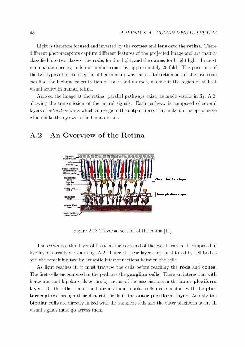
48 APPENDIX A. HUMAN VISUAL SYSTEM

Light is therefore focused and inverted by the cornea and lens onto the retina. There

different photoreceptors capture different features of the projected image and are mainly

classified into two classes: the rods, for dim light, and the cones, for bright light. In most

mammalian species, rods outnumber cones by approximately 20-fold. The positions of

the two types of photoreceptors differ in many ways across the retina and in the fovea one

can find the highest concentration of cones and no rods, making it the region of highest

visual acuity in human retina.

Arrived the image at the retina, parallel pathways exist, as made visible in fig. A.2,

allowing the transmission of the neural signals. Each pathway is composed of several

layers of retinal neurons which converge to the output fibers that make up the optic nerve

which links the eye with the human brain.

A.2 An Overview of the Retina

��

��

Figure A.2: Traversal section of the retina [11].

The retina is a thin layer of tissue at the back end of the eye. It can be decomposed in

five layers already shown in fig. A.2. Three of these layers are constituted by cell bodies

and the remaining two by synaptic interconnections between the cells.

As light reaches it, it must traverse the cells before reaching the rods and cones.

The first cells encountered in the path are the ganglion cells. There an interaction with

horizontal and bipolar cells occurs by means of the associations in the inner plexiform

layer. On the other hand the horizontal and bipolar cells make contact with the pho-

toreceptors through their dendritic fields in the outer plexiform layer. As only the

bipolar cells are directly linked with the ganglion cells and the outer plexiform layer, all

visual signals must go across them.

A.3. PARALLEL PATHWAYS AND COLOR VISION 49

Another class of cells seen in the figure at the top of the page is the amacrine cells.

These only have identifiable dendrites, which connect in the inner plexiform layer, and

function as inhibitory cells on the axon terminals of bipolar cells, thus managing their

output to ganglion cells. They also perform dedicated tasks concerned with shaping

and control of ganglion cell responses. An interesting observation is that direct synapses

from bipolar cells are a minority of all synapses of ganglion cells and so many traditional

presentations of the retina underweight the importance of amacrine cells.

A.3 Parallel Pathways and Color Vision

As the retina is stimulated by light, one type of bipolar cell hyperpolarizes, and the

other depolarizes. The distinction, created at the first retinal synapse, is propagated

throughout the visual system.

This gives rise to the classification of bipolar cells as ON or OFF, which occur in

approximately equal numbers. The classes of ON and OFF bipolars are each fur-

ther subdivided in order to provide separate channels for high-frequency (transient) and

low-frequency (sustained) information. However it is important to notice that there are

no dedicated cones at the other extremity of the visual system, instead the output of

each cone is tapped by several bipolar cell types to provide many parallel channels, each

communicating a different version of the cone’s output to the inner retina.

Another thing that should be noticed is the non-chromatically behavior of the bipolar

cells, preventing the retina from discriminating among wavelengths. As a consequence

a single type of cone cannot create color vision and its output is a single signal, which

can vary only on magnitude. For that reason, a cone’s signal to the brain is inevitable

ambiguous and to surpass that the outputs of at least two cones must be compared.

In order to compare the outputs, two types of cones are needed, one reporting on long

wavelengths and one on short; by comparing their outputs, the retina can create a single

signal that reflects the spectral compositions of the stimulus. The synaptic connections

of the inner retina are arranged so that the outputs of some ganglion cells compare the

responses of the short-wavelength-sensitive cones with those of the long-wavelength cones.

Most amacrine and all ganglion cells receive their main bipolar cell synapses from

cone bipolars, but retinas work in starlight as well as daylight, and this range is created

by a division of labor between cones and rods. Signals originating in rod photorecep-

tors reach the retinal ganglion cells via an indirect rout using as its final path the axon

terminals of the cone bipolar cells. By synapsing on the axon of the cone bipolar cells,

the rod pathway gains access to the elaborate circuitry of the cone pathway, including

its associated amacrine circuitry.


A.4 LGN and Visual Cortex

The upside-down pattern evidenced in the retinal image is preserved as neurons from

the retina connect to the Lateral Geniculate Nucleus (LGN) through the optic nerve, and

is still further preserved along the cortex. Despite the stereo vision that humans have,

two eyes; the brain does not keep the information of the two retinas separate. Instead,

it splits the world into left and right visual fields. As the outputs of each eye leave the

retina, a separation occurs. The nasal (toward the nose) half of each eye’s visual field

crosses from one side to the other at the optic chiasm and the temporal half (towards

the temple) remains on the same side as the eye-of-origin. This splitting and crossing

re-organizes the retinal outputs so that the left hemisphere process information from the

right visual field and the right hemisphere processes information from the left visual field.

Figure A.3: The human visual pathways [12].

From the optic chiasm the signal travels through the optic track and reaches the LGN

- see fig. A.3. The signal is also sent to the midbrain for eye muscles control.

A.5. KEY NOTIONS 51

Retinal ganglion cells come in two sorts: M (magnocellular, or parasol) and P (par-

vocellular, or midget). P cells exhibit color-opponent responses evidence by their firing

dependency in the wavelength of light in their receptive fields. M cells do not exhibit

this property but are responsible for the transient responses firing action potentials when

a stimulus is introduced, but with a fading characteristic with the immutability of the

same. P cells, meanwhile, give sustained responses to stimuli in their receptive field.

The division of M and P pathways becomes anatomically evident in the LGN. While

the receptive fields of LGN neurons look a lot like retinal ganglion cells, the LGN does re-

organize these circuits into distinct layers. It is also there that a type of signal processing

of extreme importance happens: a non-linear amplification. This amplification is used

as a mean to compensate the delay between the detection of the visual stimulus in the

retina’s photoreceptors and the arrival of the signal to the visual cortex.

As the signal leaves the LGN it is transported into the primary visual cortex, V1.

Because the signal is still separated in two, there are two correspondent V1s in each

person (left and right hemispheres). There are approximately 30 visual areas after V1;

some of them seem to be specialized for processing a certain aspect of visual information,

like motion, color and shapes.

In the primary visual cortex there are three main types of cells; simple, complex and

end-stopped. Their receptive fields are very different of the concentric ones observed in

the ganglion cells of the retina or the neurons in the LGN. The cells who belong to

the first type respond to a light/dark edge (contrast); the complex ones are direction-

selective or motion sensitive; the end-stopped cells exhibit length summation and are

motion sensitive.

A.5 Key Notions

The retinal ganglion cells represent the output of the retina by firing action potentials.

These electrical spikes are responsible for the transmission of information in the brain.

Spikes are all-or-none, discrete, stereotyped events that occur above a certain threshold-

level input. A refractory period is present preventing the neuron from firing consecutive

action potentials. It is the firing rate of the neuron that represents information about

stimulus intensity within each neuron.

Retinal ganglion cells fire action potentials in response to certain types of retinal

stimulation. For this to happen, a part of the retina ganglion cells, named receptive fields,

must be stimulated. Most retinal cells have concentric (or center-surround) receptive

fields. These receptive fields are mostly divided in two parts (center/surround), one of

which is excitatory (ON), the other inhibitory (OFF), as shown in the graphics of fig. A.4.


Figure A.4: Receptive field center-surround organization.

For an On/OFF center/surround cell, a spot of light shown on the inside (center) of

the receptive field will elicit spikes, while light falling on the outside ring (surround) will

suppress firing below the baseline rate. The opposite is true for an OFF/ON cell. Though,

visual neurons are not limited to the above, and indeed exhibit interdependency, as the

activity of a given neuron is affected by those who are nearby. In fact when a ganglion

cell fires action potentials, it also inhibits the firing of lateral ganglion cells. The same

type of comportment is present in the LGN with the addition of a non linearity.

Appendix B

Filter Analysis

In this appendix two filters will be described and analyzed in a brief manner. Both

filters follow the equations:

F (t) =N∑

j=1

kjfj(t),

fj(t) =

{sin(πj(2 t

τf− ( t

τf)2)), 0 ≤ t ≤ τf

0 , otherwise.

and they only differ in the kj weights. They both concern to the stochastic model.

B.1 Flash Stimulus

The weights adjusted by the NN were the following:

k1 = −0.00072 k6 = −0.00675 k11 = −0.00118

k2 = 0.01163 k7 = −0.00435 k12 = 0.00283

k3 = 0.02566 k8 = −0.00234 k13 = −0.00395

k4 = 0.01349 k9 = 0.00107 k14 = 0.00370

k5 = 0.00625 k10 = 0.00185 k15 = −0.00496

With the combination of the 15 weights kj above, the filter was reconstructed allowing

to illustrate its impulsive and frequency response, which are depicted in fig. B.1.

From the figure analysis, the most important characteristic to extract is the low pass

behavior of this filter.

53

54 APPENDIX B. FILTER ANALYSIS

0 0.1 0.2 0.3 0.4 0.5−0.04

−0.02

0

0.02

0.04

0.06

Time [s]

Am

plitu

de

(a) Impulsive Response

10−3

10−2

10−1

−80

−60

−40

−20

0

20

Frequency (kHz)

Mag

nitu

de (

dB)

(b) Frequency Response

Figure B.1: Impulsive and frequency response.

B.2 Impulse Stimulus

The weights adjusted by the NN, for an impulse stimulus input, are presented next:

k1 = 0.10212 k6 = −0.05600 k11 = 0.02150

k2 = 0.08494 k7 = −0.03255 k12 = 0.00473

k3 = 0.05066 k8 = −0.00003 k13 = −0.00159

k4 = 0.04769 k9 = −0.01508 k14 = 0.00005

k5 = 0.00057 k10 = −0.00126 k15 = 0.00159

With the combination of the 15 weights kj above, the filter was reconstructed allowing

to illustrate its impulsive and frequency response, which are depicted in fig. B.2. Again

the low pass characteristic is evident.

0 0.1 0.2 0.3 0.4 0.5−0.1

0

0.1

0.2

0.3

0.4

Time [s]

Am

plitu

de

(a) Impulsive Response

10−3

10−2

10−1

−80

−60

−40

−20

0

20

40

Frequency (kHz)

Mag

nitu

de (

dB)

(b) Frequency Response

Figure B.2: Impulsive and frequency response.

References

[1] Cortical Visual Neuroprosthesis for the Blind - CORTIVIS.

http://cortivis.umh.es.

[2] Pedro F. Z. Tomas, Bio-Inspired Processing Module for the Development of an Arti-

ficial Retina. Lisbon, Instituto Superior Tecnico, 2003.

[3] Justin Keat, Pamela Reinagel, R. Clay Reid and Markus Meister, ”Population coding

of motion patterns in the early visual system”, vol. 30. Springer-Verlag, 2001.

[4] Justin Keat, Pamela Reinagel and R. Clay Reid and Markus Meister, ”Predicting

Every Spike: A Model for the Responses of Visual Neurons”, vol. 187. Cell Press,

2001.

[5] J. C. Martins and Leonel A. Sousa, Performance Comparison of Bio-inspired Com-

putational Retina Models. 2005.

[6] Jose A. H. Germano and Ricardo M. S. Baptista, Development of a Bio-Inspired

Model with Configurable Implementation. Lisbon, Instituto Superior Tecnico, 2004.

[7] Simon Haykin, Neural Networks: A Comprehensive Foundation. Prentice-Hall, 1999.

[8] Fernando M. Silva, Redes Neuronais e Aprendizagem Automatica - Acetatos . Seccao

de Folhas da Associacao de Estudantes do Instituto Superior Tecnico.

[9] Jonathan D. Victor, and Keith P. Purpura, ”Nature and Precision of Temporal Cod-

ing in Visual Cortex: A Metric-Space Analysis”, vol. 76. New York, The American

Physiologicam Society, 1996.

[10] M. J. Berry, D. K. Warland, and M. Meister, ”The Structure and Precision of Retinal

Spike Trains”, vol. 94. New York, Neurobiology, Proc. Natl. Acad. Sci. USA, 1997.

[11] Human Eye and Artificial Retina Implants.

http://remort.wz.cz/retina/.

55

56 REFERENCES

[12] Visual Pathways.

http://www.cog.brown.edu/courses/cg0001/lectures/visualpaths.html

http://www.ruf.rice.edu/ pomeran/AlumniCollege2004Imagelist.htm.

[13] Richard H. Masland, The Fundamental Plan of the Retina, vol. 4.

processing module for the development of an artificial retina · processing module for the...

Documents