production and operation managements forecasting professor jiang zhibin dr. geng na...
TRANSCRIPT

Production and Operation ManagementsProduction and Operation Managements
ForecastingProfessor JIANG Zhibin
Dr. GENG [email protected]
1391704834013917048340
Department of Industrial Engineering & LogisticsDepartment of Industrial Engineering & Logistics ManagementManagement
Shanghai Jiao Tong UniversityShanghai Jiao Tong University

What is forecasting?• Forecasting is the process of predicting the future;
What do you want to forecast?• Your future
• Career
• Marriage
• House price
• Stock
• …
Why forecast?
How forecast??

Introduction(1)
Why forecast in a business factory?All business planning is based on a forecast;
What a factory should forecast?Factors affecting the future success of a firm-
Sales of existing productsCustomer demand patterns for new products;Needs and availabilities of raw materials;Changing skills of workers;Interest rates;Capacity requirements;International policies;
Marketing and production make the most use of forecasting methods.Marketing needs to forecast for both new products and existing products;Sales forecasts are used for production planning

Introduction(2)
Examples of benefiting from good forecasting and paying price from poor one:
Detroit make slow respond to customer tastes in automobiles from heavy gas guzzlers to smaller and more fuel efficient ones during 1960’s, such that it suffered much when OPEC oil embargoing in late 1970 speed up the trend of shifting to smaller cars. Compaq Computer became a market leader in the early 1980s by properly predicating consumer demand for portable version of the IBM PC; Ford Motor’s early success and later demise
•It predicated that customer would want a simpler, less expensive, and easier to be maintained car, and developed its Model T car that dominated the market;•However, later, did not see that customer tired of the open Model T design, and failed to forecast the customer’s desire for other designs that almost caused the end of a firm that has monopolized the industry only a few years ago.
ForecastingForecasting
•Contents•The Time Horizon in Forecasting;
•Subjective Foresting Methods;
•Objective Forecasting Methods;
•Evaluating Forecast
•Notation Conventions;
•Methods for Forecasting Stationary Series;
•Trend-Based Methods;
•Methods for Seasonal Series;

The Time Horizon in Forecasting
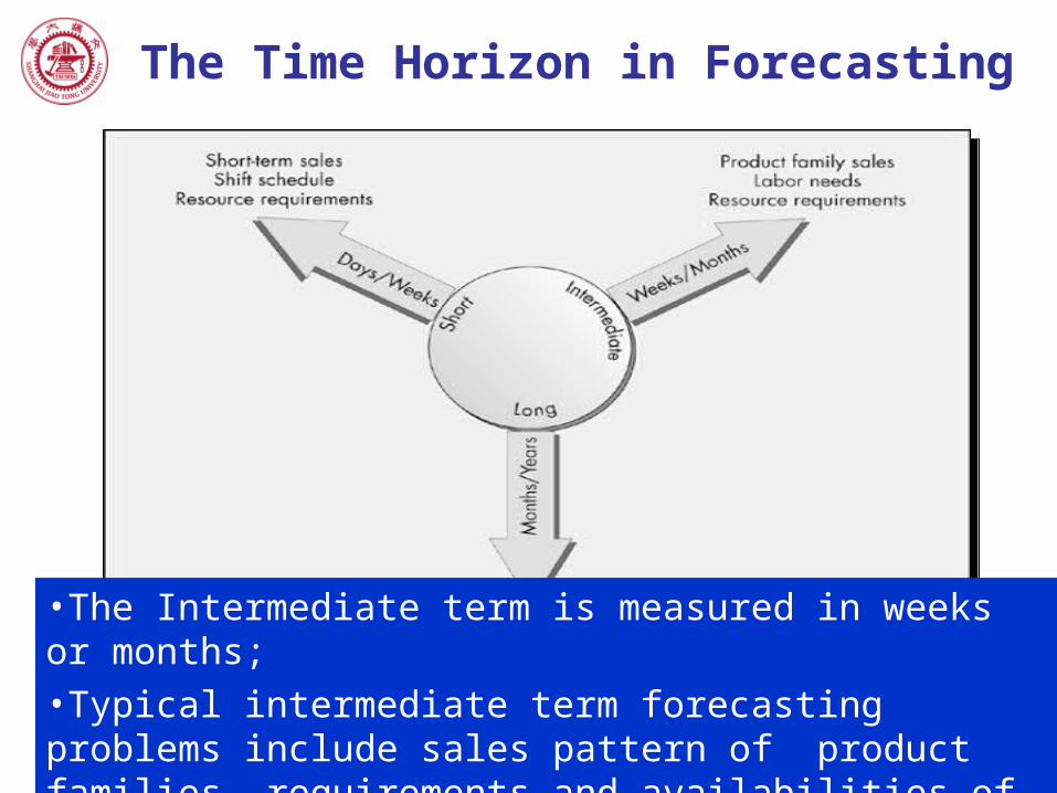
Fig.2-1 Forecast Horizons in Operation Planning

The Time Horizon in Forecasting
Fig.2-1 Forecast Horizons in Operation Planning
•The Short-term forecasting is required for day-to-day planning;
•Measured usually in day or weeks;
•Required for inventory management, production plan, and resource requirement planning, and shift scheduling
The Time Horizon in Forecasting
Fig.2-1 Forecast Horizons in Operation Planning
•The Intermediate term is measured in weeks or months;
•Typical intermediate term forecasting problems include sales pattern of product families, requirements and availabilities of workers, and resource requirements.

The Time Horizon in Forecasting
Fig.2-1 Forecast Horizons in Operation Planning
•The long term is measured in months or years;
•It is one part of the overall firm’s manufacturing strategy;
•Problems for long term forecasting include long term capacity planning; long term sales patterns, and growth trend.
•One of example is long term planning of capacity.

Classification of Forecasts
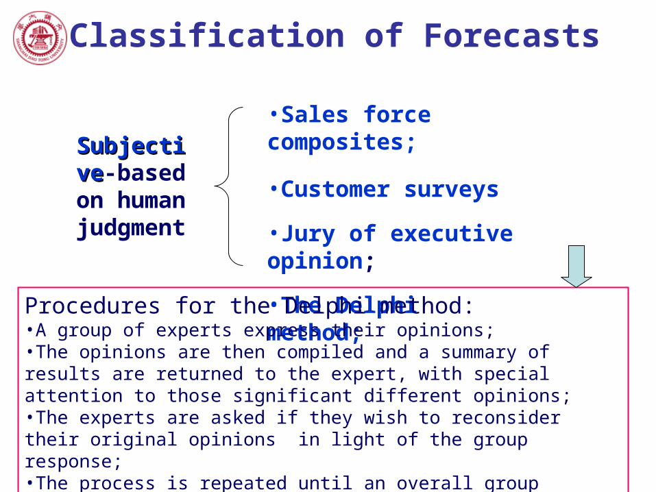
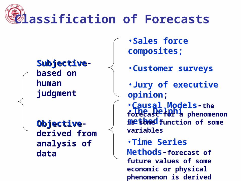
SubjectiveSubjective-based on human judgment
ObjectiveObjective-derived from analysis of data
•Sales force composites;
•Customer surveys
•Jury of executive opinion;
•The Delphi method;•Causal Models-the forecast for a phenomenon is some function of some variables
•Time Series Methods-forecast of future values of some economic or physical phenomenon is derived from a collection of their past observations

Classification of Forecasts
SubjectiveSubjective-based on human judgment
•Sales force composites;
•Customer surveys
•Jury of executive opinion;
•The Delphi method;
•Sale force is in a good position to see changes in their preferences;•Numbers of the sale force submit sales estimates of the products they sell in the next year;•Sales manager aggregate individual estimates

Classification of Forecasts
SubjectiveSubjective-based on human judgment
•Sales force composites;
•Customer surveys
•Jury of executive opinion;
•The Delphi method;
•It can signal the future trends and shifting preference patterns;•Survey and sampling plans must ensure statistically unbiased resulting data and representative of the customer base;

Classification of Forecasts
SubjectiveSubjective-based on human judgment
•Sales force composites;
•Customer surveys
•Jury of executive opinion;
•The Delphi method;
•Expert’s opinion is the only source of information for forecasting, when no past historic data, as with new products;•The approach is to combine the opinions of experts to derive a forecast;•Two ways for the combination.
•One is to have individual responsible for preparing for the forecast interview the executive directly and develop a forecast from the result of the interview;•Another is to require the executive to meet as a group and come to consensus.

Classification of Forecasts
SubjectiveSubjective-based on human judgment
•Sales force composites;
•Customer surveys
•Jury of executive opinion;
•The Delphi method;•Named for the Delphic oracle of ancient Greece who had power to predicate the future;•Based on collecting the opinion of experts like jury of executive opinion;•However, in different manner in which individual opinions are combined in order to overcome some of the inherent shortcoming of group dynamics;
The personalities of some group members overshadow others
Classification of Forecasts
SubjectiveSubjective-based on human judgment
•Sales force composites;
•Customer surveys
•Jury of executive opinion;
•The Delphi method;Procedures for the Delphi method:•A group of experts express their opinions;•The opinions are then compiled and a summary of results are returned to the expert, with special attention to those significant different opinions;•The experts are asked if they wish to reconsider their original opinions in light of the group response;•The process is repeated until an overall group consensus is reached;
Classification of Forecasts
SubjectiveSubjective-based on human judgment
ObjectiveObjective-derived from analysis of data
•Sales force composites;
•Customer surveys
•Jury of executive opinion;
•The Delphi method;•Causal Models-the forecast for a phenomenon is some function of some variables
•Time Series Methods-forecast of future values of some economic or physical phenomenon is derived from a collection of their past observations
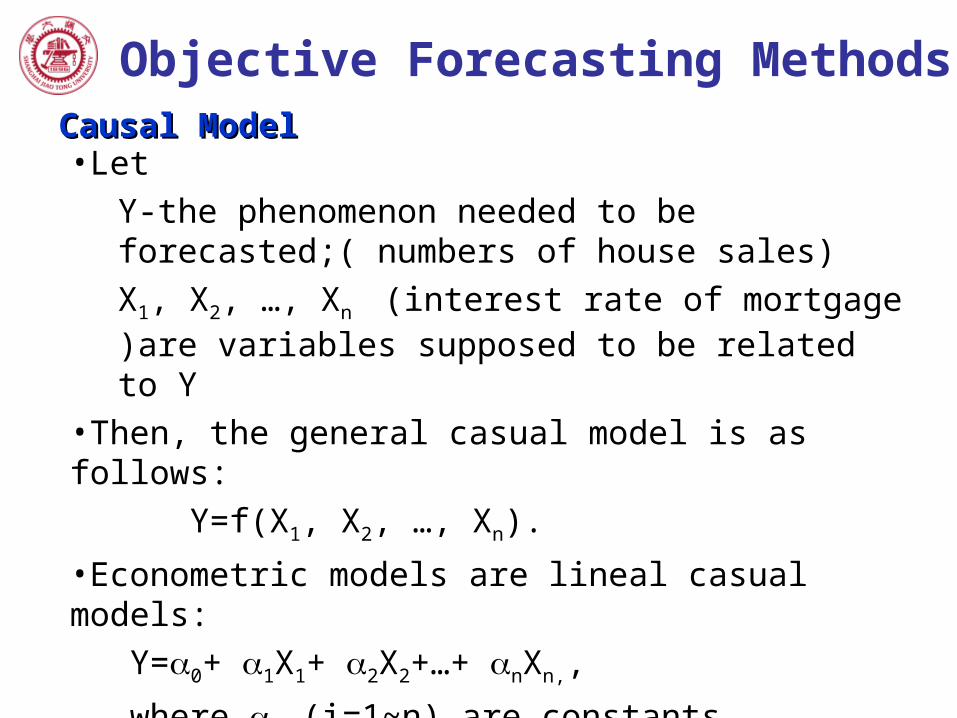
Objective Forecasting MethodsCausal ModelCausal Model•Let
Y-the phenomenon needed to be forecasted;( numbers of house sales)
X1, X2, …, Xn (interest rate of mortgage )are variables supposed to be related to Y
•Then, the general casual model is as follows:
Y=f(X1, X2, …, Xn).
•Econometric models are lineal casual models:
Y=0+ 1X1+ 2X2+…+ nXn,,
where i (i=1~n) are constants.
•The method of least squares is most commonly used for finding estimators of these constants.

Objective Forecasting Methods
Causal ModelCausal ModelAssume we have the past data (xi, yi), i=1~n; and the the causal model is simply as Y=a+bX. Define
2
1
( , ) [ ( )]n
i ii
g a b y a bx
as the sum of the squares of the distances from line a+bX to data points yi. We may choose a and b to minimize g, by letting
0g
a
1 1
12 0
n n
i i i ii i
y a bx a y bx y bxn
1 1
21
1 1
0
n n
i i ini i
i i i n ni
i ii i
x y y xy a bx x b
x x x
0
g
b

Objective Forecasting Methods
Causal ModelCausal Model 2
1
( , ) [ ( )]n
i ii
g a b y a bx
0g
a
a y bx
1 1 1 1
2 2
1 1 1 1
n n n n
i i i i i ixyi i i i
n n n nxx
i i i ii i i i
x y y x n x y ny xS
bSx x x n x nx x
0g
b
2 2; ( )n n n n n
xy i i i i xx i ii i i i i
S n x y x y S n x x 1 1
; ;n n
i ii i
x x y yn n

Objective Forecasting MethodsTime Series Methods-Time Series Methods-•The idea is that information can be inferred from the pattern of past observations and can be used to forecast future values of the series.•Try to isolate the following patterns that arise most often.
Trend-the tendency of a time series, usually a stable growth or decline, either linear (a line) or nonlinear (described as nonlinear function, e. g. a quadratic or exponential curve) Seasonality-Variation of a series related to seasonal changes and repeated every season.Cycles-Cyclic variation similar to seasonality, except that the length and the magnitude may change, usually associated with economic variation.Randomness-No recognizable pattern to the data.

Objective Forecasting Methods
Fig. 2-2 Time Series Patterns

Evaluating Forecast
The forecast error et in period t is the difference between the forecast value for that period and the actual demand for that period.
t t te F D
The three measures for evaluating forecasting accuracy during n period
2
1
1 n
ii
MSE en
•MAD: The mean absolute deviation, preferred method;•MSE: The mean squared error;•MAPE: The mean absolute percentage error (MAPE)
1
1| |
n
ii
MAD en
1
1[ | / |] 100
n
i ii
MAPE e Dn

Example 2.1
Artel, a manufacturer of SRAMs (static random access memories), has production plants in Austin, Texas, and Sacramento, California. The managers of these plants are asked to forecast production yields (measured in percent) one week ahead for their plants. Based on six weekly forecasts, the firm’s management wishes to determine which manager is more successful at predicting his plant’s yields. The results of their predictions are given in the following table.
Evaluating Forecast
Week P1 O1 |E1| |E1/O1| P2 O2 |E2| |E2/O2|1 92 88 4 0.0455 96 91 5 0.05492 87 88 1 0.0114 89 89 0 0.00003 95 97 2 0.0206 92 90 2 0.02224 90 83 7 0.0843 93 90 3 0.03335 88 91 3 0.0330 90 86 4 0.04656 93 93 0 0.0000 85 89 4 0.0449
Evaluating Forecast
Example 2.1Example 2.1
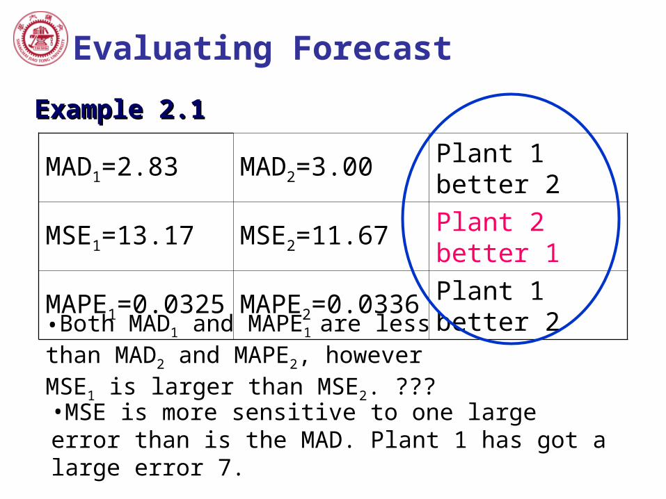
MAD1=2.83 MAD2=3.00 Plant 1 better 2
MSE1=13.17 MSE2=11.67 Plant 2 better 1
MAPE1=0.0325 MAPE2=0.0336 Plant 1 better 2
•Both MAD1 and MAPE1 are less than MAD2 and MAPE2, however MSE1 is larger than MSE2. ???•MSE is more sensitive to one large error than is the MAD. Plant 1 has got a large error 7.
Evaluating Forecast
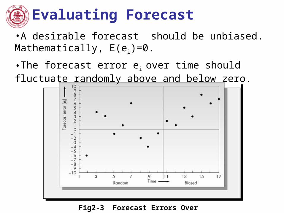
Fig2-3 Forecast Errors Over Time
•A desirable forecast should be unbiased. Mathematically, E(ei)=0.
•The forecast error ei over time should fluctuate randomly above and below zero.
Notation Convention
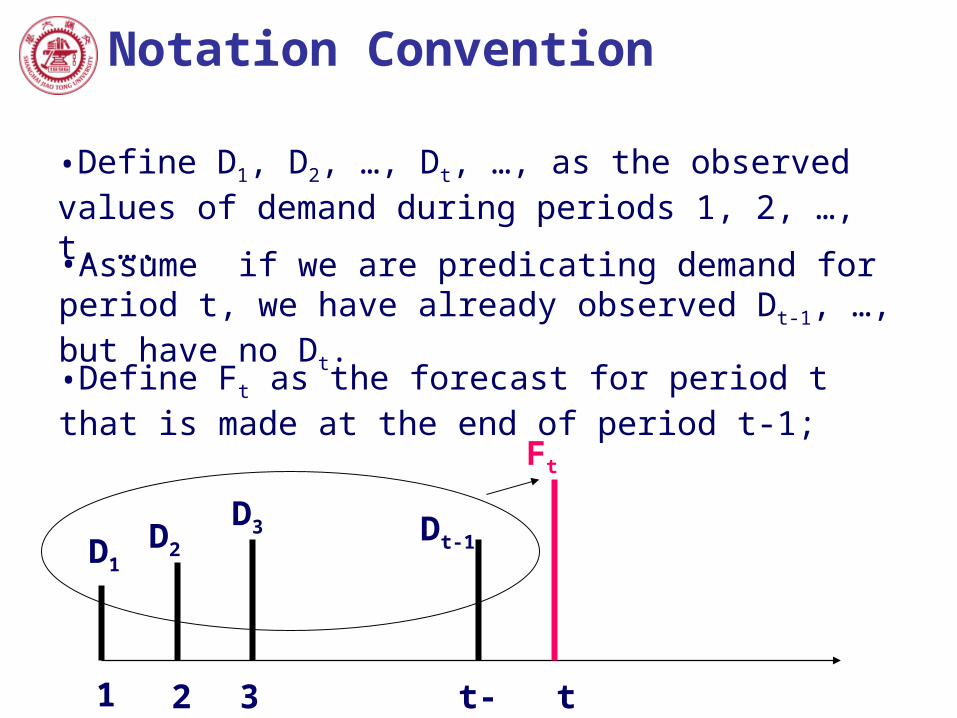
•Define D1, D2, …, Dt, …, as the observed values of demand during periods 1, 2, …, t, …..
•Assume if we are predicating demand for period t, we have already observed Dt-1, …, but have no Dt.
•Define Ft as the forecast for period t that is made at the end of period t-1;
1 2 3 t-1 t
D1D2
D3 Dt-1
Ft

Notation Convention
•The above is one-step-ahead forecast-they are made for predicating the demand only in the next period.
•A time series forecast is actually obtained by weighting the past data
1 1 1 20
, ,
m
t t i t i t ti
F D for some set of weights L
1 2 3 t-1 t
D1D2
D3 Dt-1
Ft

Methods of Forecasting Stationary Series
Stationary time series: each observation can be represented by a constant plus a random fluctuation.
t tD where = an unknown constant corresponding to mean of the series;= the random error with mean zero and variation 2.
•Methods:
Moving average;
Exponential SmoothingSimple
Holt
Winters

Methods of Forecasting Stationary Series
Moving Average-A moving average of order N is simply the arithmetic average of the most recent N observations (one-step-ahead), denoted as MA(N).
1 21
1 1( )
N
t t i t t t Ni
F D D D DN N
L
1 2 3 t-1 t
D1D2
Dt-N Dt-1
Ft
Dt-2……N past data
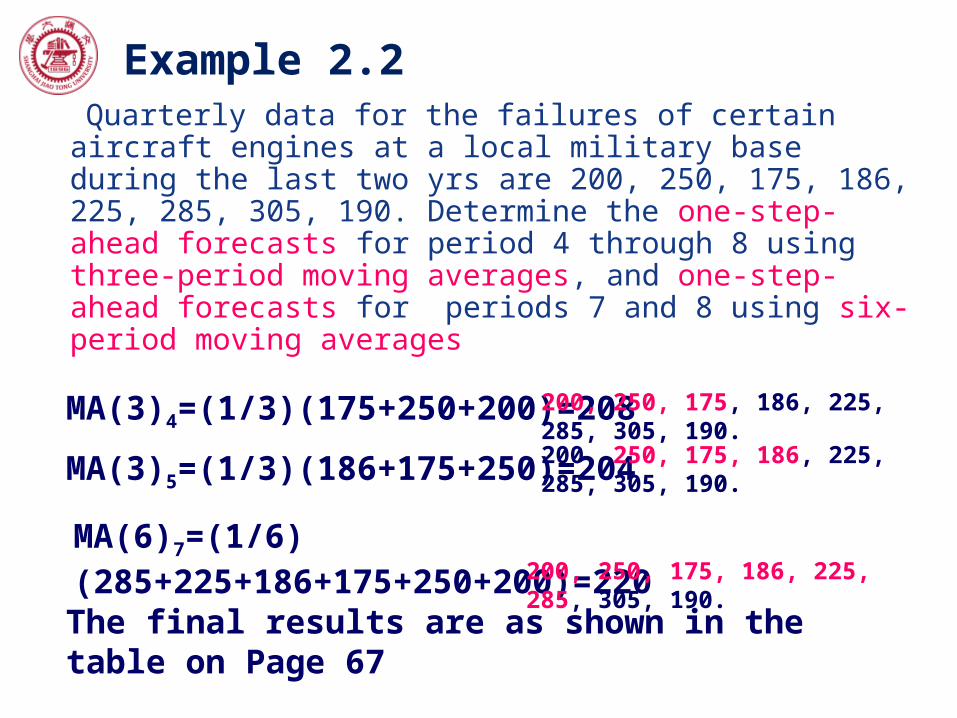
Example 2.2 Quarterly data for the failures of certain aircraft engines
at a local military base during the last two yrs are 200, 250, 175, 186, 225, 285, 305, 190. Determine the one-step-ahead forecasts for period 4 through 8 using three-period moving averages, and one-step-ahead forecasts for periods 7 and 8 using six-period moving averages
MA(3)4=(1/3)(175+250+200)=208
MA(3)5=(1/3)(186+175+250)=204
MA(6)7=(1/6)(285+225+186+175+250+200)=220
The final results are as shown in the table on Page 67
200, 250, 175, 186, 225, 285, 305, 190.
200, 250, 175, 186, 225, 285, 305, 190.
200, 250, 175, 186, 225, 285, 305, 190.
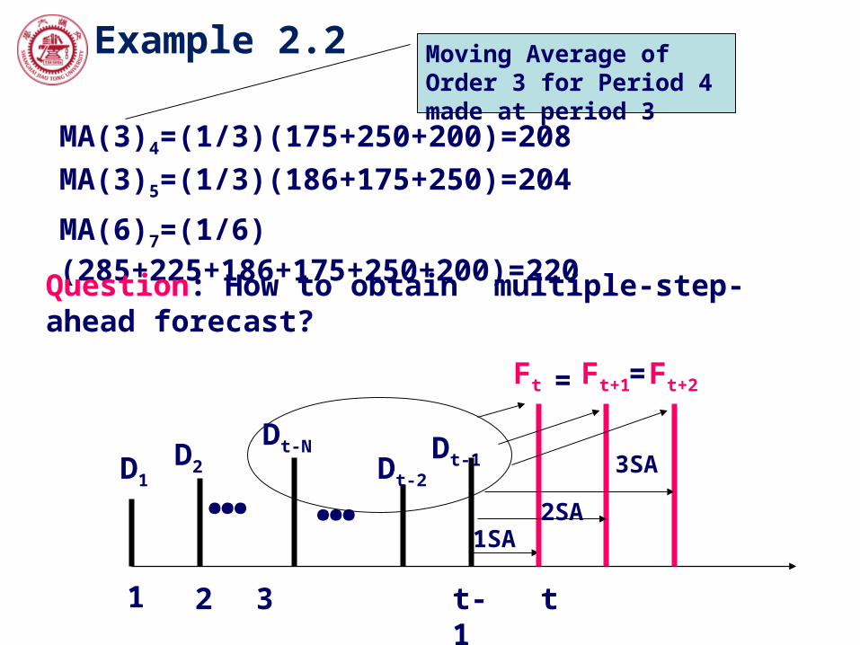
Example 2.2
MA(3)4=(1/3)(175+250+200)=208
MA(3)5=(1/3)(186+175+250)=204
MA(6)7=(1/6)(285+225+186+175+250+200)=220
Question: How to obtain multiple-step-ahead forecast?
1 2 3 t-1 t
D1D2
Dt-N Dt-1Dt-2……
Ft
1SA
Ft+1
2SA
Ft+2
3SA
= =
Moving Average of Order 3 for Period 4 made at period 3

Methods of Forecasting Stationary Series
1 21
1 1( )
N
t t i t t t Ni
F D D D DN N
L
1 1 1 2 11
1
1 1[ ]
1 1( ) ( )
N
t t i tt t t t N t Ni
N
t t N t i t ti
N
t N
F D D DN N
D D D F D DN
D D D
N
D
L
•Calculate Ft+1 based on Ft-simplify the calculation
Only need to calculate the difference between the most recent demands and the demand N period ahead for updating the forecast.
Methods of Forecasting Stationary Series
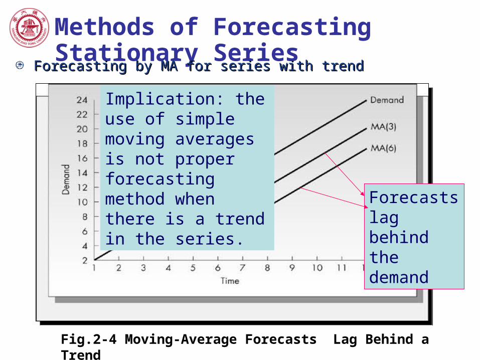
Forecasting by MA for series with trendForecasting by MA for series with trend
Fig.2-4 Moving-Average Forecasts Lag Behind a Trend
Implication: the use of simple moving averages is not proper forecasting method when there is a trend in the series.
Forecasts lag behind the demand
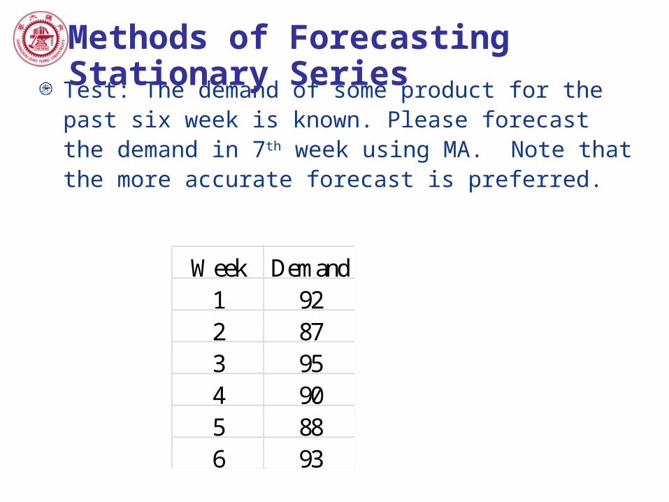
Test: The demand of some product for the past six week is known. Please forecast the demand in 7th week using MA. Note that the more accurate forecast is preferred.
Methods of Forecasting Stationary Series
Week Demand1 922 873 954 905 886 93
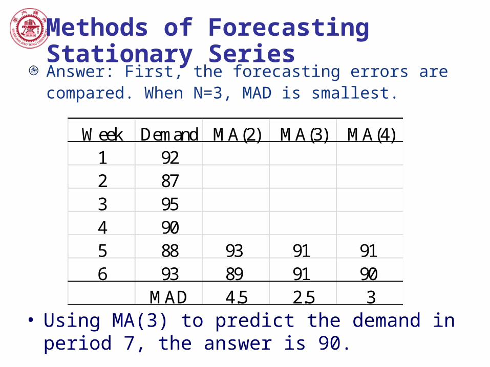
Answer: First, the forecasting errors are compared. When N=3, MAD is smallest.
Methods of Forecasting Stationary Series
Week Demand MA(2) MA(3) MA(4)1 922 873 954 905 88 93 91 916 93 89 91 90
MAD 4.5 2.5 3
• Using MA(3) to predict the demand in period 7, the answer is 90.

Methods of Forecasting Stationary Series
Exponential Smoothing-Exponential Smoothing-the current forecast is weighted average of the last forecast and the last value of demand.
1 1
( ) (1 )(Last forecast)
(1 )t t t
new forecast current observation of demand
F D F
where 0<1 is the smoothing constant, which determines the relative weight placed on the last observation of demand, while 1- is weight placed on the last forecast.
1 1 1 1 1 1 1(1 ) ( )t t t t t t t tF D F F F D F e
The forecast in any period t is the forecast in period t-1 minus some fraction of the observed forecast error in period t-1

Methods of Forecasting Stationary Series
Exponential Smoothing-Exponential Smoothing-the current forecast is weighted average of the last forecast and the last value of demand.
1 1(1 )t t tF D F
where 0<1 is the smoothing constant, which determines the relative weight placed on the last observation of demand, while 1- is weight placed on the last forecast.
1 1 1 1 1 1 1(1 ) ( )t t t t t t t tF D F F F D F e
1 2 2(1 )t t tF D F
21 2 2 1
0
(1 ) (1 ) ... (1 )it t t t t i
i
F D D F D

Fig.2-5 Weights in Exponential Smoothing
The older of a past data, the smaller of its contribution to the forecast for a future period.
(1 )
0.1
i

Example 2.3 Consider Example 2.2, in which the observed number of failures
over a two yrs period are 200, 250, 175, 186, 225, 285, 305, 190. We will now forecast using exponential smoothing. We assume that the forecast for period 1 was 200, and suppose that =0.1
F2= ES(0.1)2= D1+(1- 1)F1=0.1200+(1-0.1) 200=200
F3= ES(0.1)3= D2+(1- 1)F2=0.1250+(1-0.1) 200=205
•Since ES requires that at each stage we need the previous forecast, it is not obvious how to get the method started.
•We may assume that the initial forecast is equal to the initial value of demand.
•However, this approach has a serious drawback?

Methods of Forecasting Stationary Series
Fig.2-6 Exponential Smoothing for Different Values of Alpha
Smaller turns out a stable forecast, while larger results in better track of series

Methods of Forecasting Stationary Series
Comparing of ES and MA
Similarities• Both methods are based on assumption that underlying
demand is stationary .
• Both methods depend on a single parameters.
• Both methods will lag behind a trend if one exits.
Differences• MA is better than EA in that it needs only past N data, while
EA needs all the past data;

Trend –Based Methods
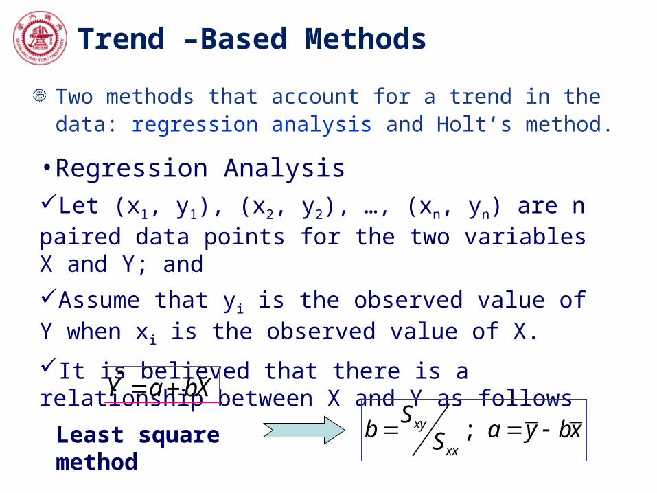
Two methods that account for a trend in the data: regression analysis and Holt’s method.
•Regression AnalysisLet (x1, y1), (x2, y2), …, (xn, yn) are n paired data points for the two variables X and Y; and
Assume that yi is the observed value of Y when xi is the observed value of X.
It is believed that there is a relationship between X and Y as follows
Y a bX
• Represents the predicated value of Y;• a and b are chosen to minimize the sum of squared distance between regression line and the data point
Trend –Based Methods
Two methods that account for a trend in the data: regression analysis and Holt’s method.
•Regression AnalysisLet (x1, y1), (x2, y2), …, (xn, yn) are n paired data points for the two variables X and Y; and
Assume that yi is the observed value of Y when xi is the observed value of X.
It is believed that there is a relationship between X and Y as follows
Y a bX
;xy
xx
Sb a y bxS Least square
method

Methods of Forecasting Trend Series
Fig 2-7 An Example of a Regression Line
Y a bX (i, Di)
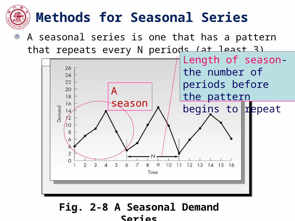
Methods for Seasonal Series
A seasonal series is one that has a pattern that repeats every N periods (at least 3).
Fig. 2-8 A Seasonal Demand Series
Length of season-the number of periods before the pattern begins to repeat
A season

Methods for Seasonal SeriesHow to represent seasonality?
•Seasonal factor-A set of multipliers ct, 1 t N, ct=N;
•ct represents the average amount that the demand in tth period of the season is above or below the average.•For example: if c3=1.25 and c5=0.6, then the demand in the 3rd period is 25 percent above the average demand; while demand in the 5th period is 40 percent below the average demand.

Methods of Forecasting Stationary Seasonal Series
Seasonal Factors for Stationary Seasonal Series (No trend)Compute the sample mean of all data(A minimum of two seasons of date is required): mDivide each observation by sample mean the seasonal factors of observed data for each period in each season: SFi,j=Dij/m ( Dij-the observed dada for period j in season i, total H seasons)Average the factors for the same periods within each season the seasonal factor:
Multiplying the sample mean by a seasonal factor the forecast of demand in the corresponding period of the season.
1
1 H
j iji
SF SFH

Methods of Forecasting Stationary Seasonal Series
Wk1 Wk2 Wk3 Wk4Monday 16. 2 17. 3 14. 6 16. 1Tuesday 12. 2 11. 5 13. 1 11. 8
Wednesday 14. 2 15 13 12. 9Thursday 17. 3 17. 6 16. 9 16. 6Friday 22. 5 23. 5 21. 9 24. 3
Monday 0. 977169Tuesday 0. 739726
Wednesday 0. 838661Thursday 1. 041096
Friday 1. 403349
Wk1 Wk2 Wk3 Wk4Monday 0. 986301 1. 053272 0. 888889 0. 980213Tuesday 0. 74277 0. 700152 0. 797565 0. 718417
Wednesday 0. 864536 0. 913242 0. 791476 0. 785388Thursday 1. 053272 1. 071537 1. 028919 1. 010654Friday 1. 369863 1. 430746 1. 333333 1. 479452
Monday 16. 05Tuesday 12. 15
Wednesday 13. 775Thursday 17. 1
Friday 23. 05
Avg=16.42516.425*0.977169=16.05

Methods of Forecasting Trend Seasonal Series
•Deseaonalized- Get seasonality away;
•Make forecast on deseaonalized data;
•Get seasonality back
A more complex time series: Trend + Seasonality
Seasonal Decomposition Using Moving Averages
Seasonal Decomposition Using Moving Averages
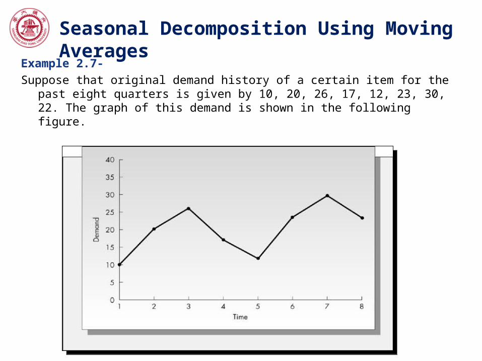
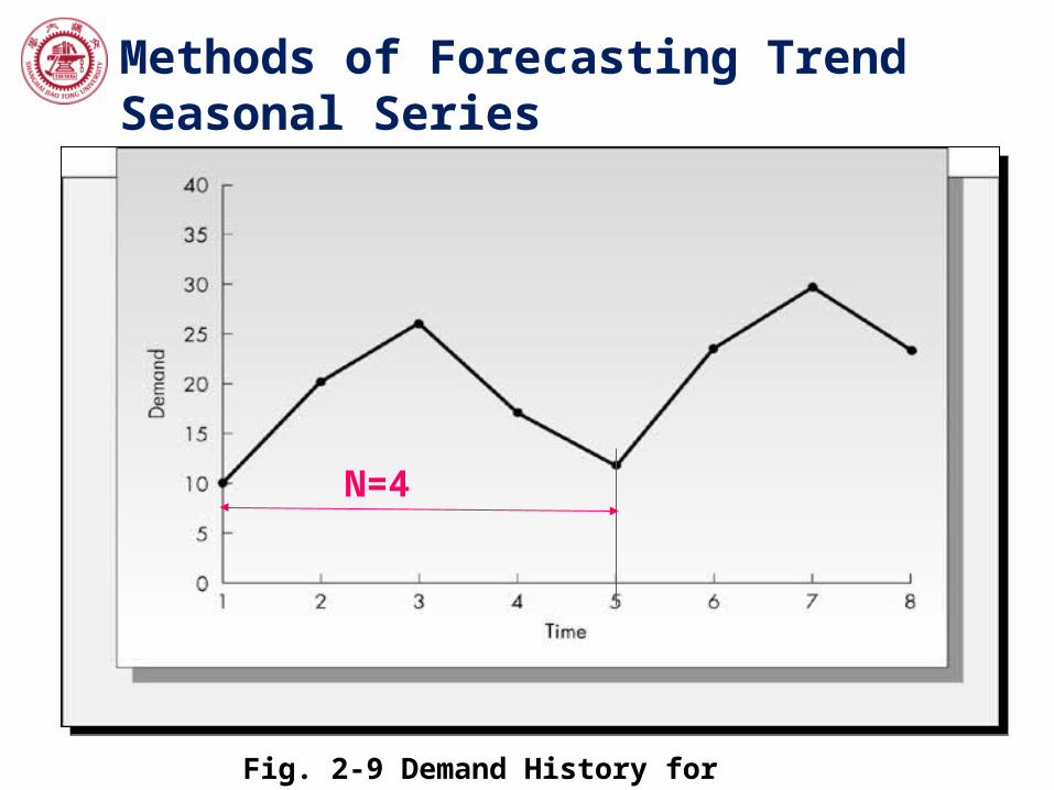
Example 2.7-
Suppose that original demand history of a certain item for the past eight quarters is given by 10, 20, 26, 17, 12, 23, 30, 22. The graph of this demand is shown in the following figure.

Methods of Forecasting Trend Seasonal Series
Procedures:• Draw the demand curves and estimate the season
length N;• Computer the moving average MA(N);• Centralize the moving averages;• Get the centralized MA values back on period;
• Calculate seasonal factors, and make sure of ct=N. • Divide each observation by the appropriate seasonal
factor to obtain the deseasonalized demand• Forecast is made based on deseasonalized demand.• Final forecast is obtained by multiplying the forecast
(with no seasonality) with seasonal factors.
Methods of Forecasting Trend Seasonal Series
Fig. 2-9 Demand History for Example 2.7
N=4

Methods of Forecasting Trend Seasonal Series
Procedures: Draw the demand curves and estimate the season
length N; Computer the moving average MA(N); Centralize the moving averages; Get the centralized MA values back on period; Calculate seasonal factors, and make sure of ct=N. Divide each observation by the appropriate seasonal
factor to obtain the deseasonalized demand Forecast is made based on deseasonalized demand. Final forecast is obtained by multiplying the forecast
(with no seasonality) with seasonal factors.
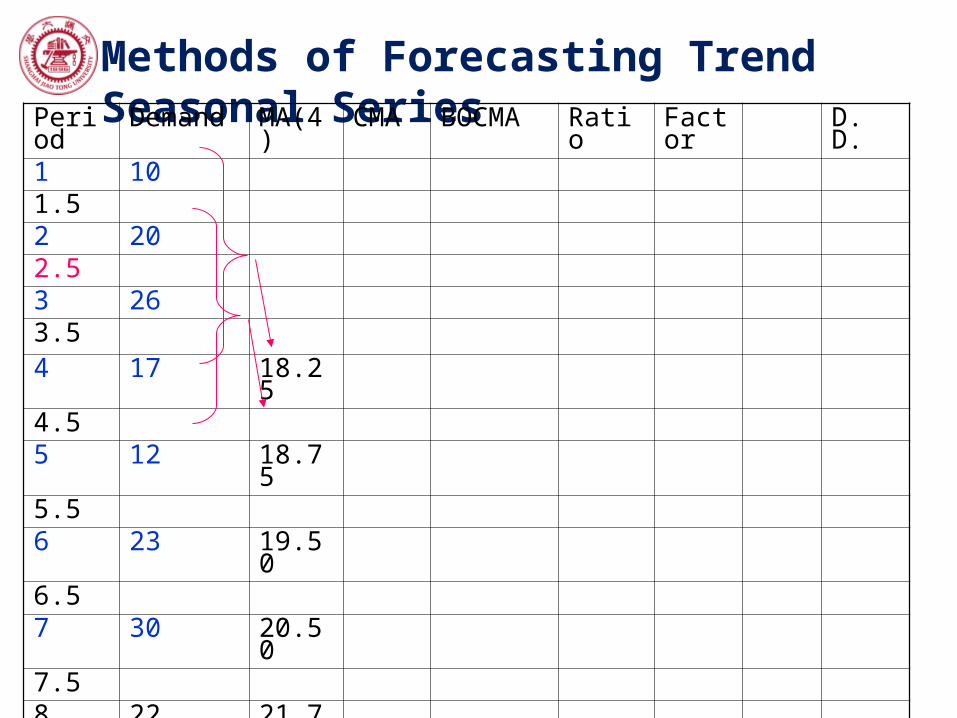
Methods of Forecasting Trend Seasonal SeriesPeriod Demand MA(4) CMA BOCMA Ratio Factor D. D.
1 10
1.5
2 20
2.5
3 26
3.5
4 17 18.25
4.5
5 12 18.75
5.5
6 23 19.50
6.5
7 30 20.50
7.5
8 22 21.75

Methods of Forecasting Trend Seasonal Series
Procedures:• Draw the demand curves and estimate the season
length N;• Computer the moving average MA(N);• Centralize the moving averages;• Get the centralized MA values back on period;
• Calculate seasonal factors, and make sure of ct=N. • Divide each observation by the appropriate seasonal
factor to obtain the deseasonalized demand• Forecast is made based on deseasonalized demand.
• Final forecast is obtained by multiplying the forecast (with no seasonality) with seasonal factors.

Methods of Forecasting Trend Seasonal SeriesPeriod Demand MA(4) CMA BOCMA Ratio Factor D. D.
1 10
1.5
2 20
2.5 18.25
3 26
3.5 18.75
4 17 18.25
4.5 19.50
5 12 18.75
5.5 20.50
6 23 19.50
6.5 21.75
7 30 20.50
7.5
8 22 21.75
Since 18.25 is calculated by moving demand of periods 1, 2, 3, and 4. The center of these period is 2.5

Methods of Forecasting Trend Seasonal Series
Procedures:• Draw the demand curves and estimate the season
length N;• Computer the moving average MA(N);• Centralize the moving averages;• Get the centralized MA values back on period;
• Calculate seasonal factors, and make sure of ct=N. • Divide each observation by the appropriate seasonal
factor to obtain the deseasonalized demandForecast is made based on deseasonalized demand.
• Final forecast is obtained by multiplying the forecast (with no seasonality) with seasonal factors.

Methods of Forecasting Trend Seasonal SeriesPeriod Demand MA(4) CMA BOCMA Ratio Factor D. D.
1 10
1.5
2 20
2.5 18.25
3 26 18.5
3.5 18.75
4 17 18.25 19.125
4.5 19.50
5 12 18.75 20.00
5.5 20.50
6 23 19.50 21.125
6.5 21.75
7 30 20.50
7.5
8 22 21.75
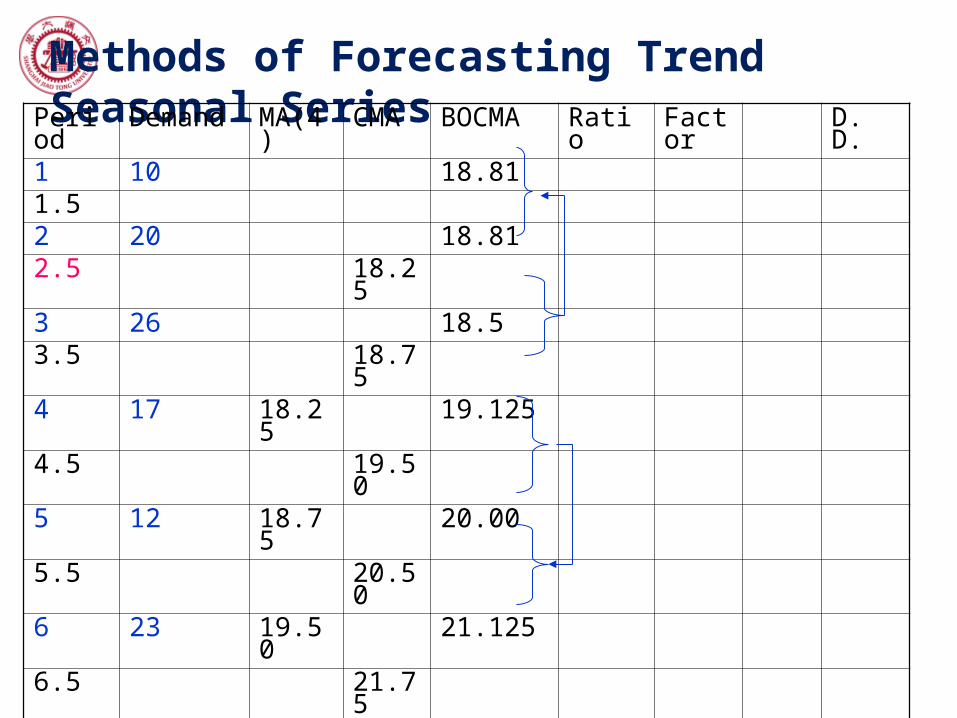
Methods of Forecasting Trend Seasonal SeriesPeriod Demand MA(4) CMA BOCMA Ratio Factor D. D.
1 10 18.81
1.5
2 20 18.81
2.5 18.25
3 26 18.5
3.5 18.75
4 17 18.25 19.125
4.5 19.50
5 12 18.75 20.00
5.5 20.50
6 23 19.50 21.125
6.5 21.75
7 30 20.50 20.56
7.5
8 22 21.75 20.56

Methods of Forecasting Trend Seasonal Series
Seasonal Decomposition Using Moving Averages-Example 2.7•Draw the demand curves and estimate the season length N;•Computer the moving average MA(N);•Centralize the moving averages;•Get the centralized MA values back on period;•Calculate seasonal factors, and make sure of ct=N. •Divide each observation by the appropriate seasonal factor to obtain the deseasonalized demand Forecast is made based on deseasonalized demand.
•Final forecast is obtained by multiplying the forecast (with no seasonality) with seasonal factors.

Methods of Forecasting Trend Seasonal SeriesPeriod Demand MA(4) CMA BOCMA Ratio Factor D. D.
1 10 18.81 0.532 0.566 0.558
1.5
2 20 18.81 1.063 1.076 1.061
2.5 18.25
3 26 18.5 1.405 1.434 1.415
3.5 18.75
4 17 18.25 19.125 0.888 0.979 0.966
4.5 19.50
5 12 18.75 20.00 0.6
5.5 20.50
6 23 19.50 21.125 1.089
6.5 21.75
7 30 20.50 20.56 1.463
7.5
8 22 21.75 20.56 1.070
Modify factors: 0.5664/(0.566+1.076+1.434+0.979)
10/18.81
(0.532+0.60)/2
Ratio- the demand over centered MA

Methods of Forecasting Trend Seasonal Series
Seasonal Decomposition Using Moving Averages-Example 2.7•Draw the demand curves and estimate the season length N;•Computer the moving average MA(N);•Centralize the moving averages;•Get the centralized MA values back on period;•Calculate seasonal factors, and make sure of ct=N. •Divide each observation by the appropriate seasonal factor to obtain the deseasonalized demand Forecast is made based on deseasonalized demand.
•Final forecast is obtained by multiplying the forecast (with no seasonality) with seasonal factors.
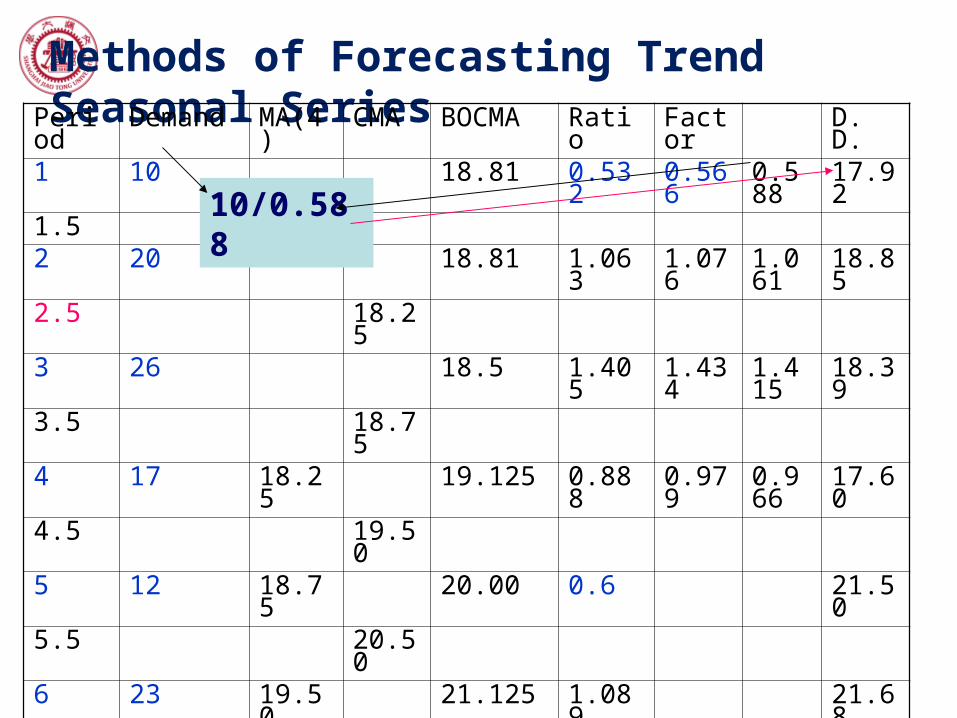
Methods of Forecasting Trend Seasonal SeriesPeriod Demand MA(4) CMA BOCMA Ratio Factor D. D.
1 10 18.81 0.532 0.566 0.588 17.92
1.5
2 20 18.81 1.063 1.076 1.061 18.85
2.5 18.25
3 26 18.5 1.405 1.434 1.415 18.39
3.5 18.75
4 17 18.25 19.125 0.888 0.979 0.966 17.60
4.5 19.50
5 12 18.75 20.00 0.6 21.50
5.5 20.50
6 23 19.50 21.125 1.089 21.68
6.5 21.75
7 30 20.50 20.56 1.463 21.22
7.5
8 22 21.75 20.56 1.070 22.77
10/0.588

Methods of Forecasting Trend Seasonal Series
Seasonal Decomposition Using Moving Averages-Example 2.7•Draw the demand curves and estimate the season length N;•Computer the moving average MA(N);•Centralize the moving averages;•Get the centralized MA values back on period;•Calculate seasonal factors, and make sure of ct=N. •Divide each observation by the appropriate seasonal factor to obtain the deseasonalized demand Forecast is made based on deseasonalized demand.
•Final forecast is obtained by multiplying the forecast (with no seasonality) with seasonal factors.

Methods of Forecasting Trend Seasonal Series
Forecast made on Deseasonalized demand by MA
• MA(6) for period 9=20.52 (without seasonality);
• Forecast for period: 20.520.558=11.45 (with seasonality)
D. D.17.92
18.85
18.39
17.60
21.50
21.68
21.22
22.77
Q
How to forecast demand for period 10, 11, 12?
F10= MA(6) of 2-step-head=F9=20.52
F10×SF2=20.52× 1.061=21.77

Methods of Forecasting Trend Seasonal Series
• Forecast made on Deseasonalized demand by regressionBy regression analysis over D. D., obtain:
Dt=16.8+0.7092t
By substituting t=9 through 12, obtain forecasts (without seasonality): 23.18, 23.89, 24.60 and 25.31;
By multiplying seasonal factors, obtain forecast in the future periods 9 through 12: 12.93, 25.35, 34.81, and 24.45.

ForecastingForecasting
Contents•The Time Horizon in Forecasting;
•Subjective Foresting Methods;
•Objective Forecasting Methods;
•Evaluating Forecast
•Notation Conventions;
•Methods for Forecasting Stationary Series;
•Trend-Based Methods;
•Methods for Seasonal Series;

Homework for Chapter 2:
Q13, Q24, Q34
In two weeks

Website for downloading the slides:
cc.sjtu.edu.cn
Choose “精品课程”Search for “生产计划与控制”Click “教学资料”Click “教学课件” .

The End!