production cross section in using soft electron -tagging
TRANSCRIPT

Measurement of the tt Production Cross Section in pp Collisions at√s=1.96 TeV
using Soft Electron b-Tagging
T. Aaltonen,24 J. Adelman,14 T. Akimoto,56 B. Alvarez Gonzalezt,12 S. Amerioz,44 D. Amidei,35 A. Anastassov,39
A. Annovi,20 J. Antos,15 G. Apollinari,18 A. Apresyan,49 T. Arisawa,58 A. Artikov,16 W. Ashmanskas,18
A. Attal,4 A. Aurisano,54 F. Azfar,43 W. Badgett,18 A. Barbaro-Galtieri,29 V.E. Barnes,49 B.A. Barnett,26
P. Barriabb,47 P. Bartos,15 V. Bartsch,31 G. Bauer,33 P.-H. Beauchemin,34 F. Bedeschi,47 D. Beecher,31 S. Behari,26
G. Bellettiniaa,47 J. Bellinger,60 D. Benjamin,17 A. Beretvas,18 J. Beringer,29 A. Bhatti,51 M. Binkley,18
D. Biselloz,44 I. Bizjakff ,31 R.E. Blair,2 C. Blocker,7 B. Blumenfeld,26 A. Bocci,17 A. Bodek,50 V. Boisvert,50
G. Bolla,49 D. Bortoletto,49 J. Boudreau,48 A. Boveia,11 B. Braua,11 A. Bridgeman,25 L. Brigliadoriy,6
C. Bromberg,36 E. Brubaker,14 J. Budagov,16 H.S. Budd,50 S. Budd,25 S. Burke,18 K. Burkett,18 G. Busettoz,44
P. Bussey,22 A. Buzatu,34 K. L. Byrum,2 S. Cabrerav,17 C. Calancha,32 M. Campanelli,36 M. Campbell,35
F. Canelli14,18 A. Canepa,46 B. Carls,25 D. Carlsmith,60 R. Carosi,47 S. Carrillon,19 S. Carron,34 B. Casal,12
M. Casarsa,18 A. Castroy,6 P. Catastinibb,47 D. Cauzee,55 V. Cavalierebb,47 M. Cavalli-Sforza,4 A. Cerri,29
L. Cerritop,31 S.H. Chang,28 Y.C. Chen,1 M. Chertok,8 G. Chiarelli,47 G. Chlachidze,18 F. Chlebana,18 K. Cho,28
D. Chokheli,16 J.P. Chou,23 G. Choudalakis,33 S.H. Chuang,53 K. Chungo,18 W.H. Chung,60 Y.S. Chung,50
T. Chwalek,27 C.I. Ciobanu,45 M.A. Cioccibb,47 A. Clark,21 D. Clark,7 G. Compostella,44 M.E. Convery,18
J. Conway,8 M. Cordelli,20 G. Cortianaz,44 C.A. Cox,8 D.J. Cox,8 F. Crescioliaa,47 C. Cuenca Almenarv,8
J. Cuevast,12 R. Culbertson,18 J.C. Cully,35 D. Dagenhart,18 M. Datta,18 T. Davies,22 P. de Barbaro,50
S. De Cecco,52 A. Deisher,29 G. De Lorenzo,4 M. Dell’Orsoaa,47 C. Deluca,4 L. Demortier,51 J. Deng,17
M. Deninno,6 P.F. Derwent,18 A. Di Cantoaa,47 G.P. di Giovanni,45 C. Dionisidd,52 B. Di Ruzzaee,55
J.R. Dittmann,5 M. D’Onofrio,4 S. Donatiaa,47 P. Dong,9 J. Donini,44 T. Dorigo,44 S. Dube,53 J. Efron,40
A. Elagin,54 R. Erbacher,8 D. Errede,25 S. Errede,25 R. Eusebi,18 H.C. Fang,29 S. Farrington,43 W.T. Fedorko,14
R.G. Feild,61 M. Feindt,27 J.P. Fernandez,32 C. Ferrazzacc,47 R. Field,19 G. Flanagan,49 R. Forrest,8 M.J. Frank,5
M. Franklin,23 J.C. Freeman,18 I. Furic,19 M. Gallinaro,52 J. Galyardt,13 F. Garberson,11 J.E. Garcia,21
A.F. Garfinkel,49 P. Garosibb,47 K. Genser,18 H. Gerberich,25 D. Gerdes,35 A. Gessler,27 S. Giagudd,52
V. Giakoumopoulou,3 P. Giannetti,47 K. Gibson,48 J.L. Gimmell,50 C.M. Ginsburg,18 N. Giokaris,3 M. Giordaniee,55
P. Giromini,20 M. Giunta,47 G. Giurgiu,26 V. Glagolev,16 D. Glenzinski,18 M. Gold,38 N. Goldschmidt,19
A. Golossanov,18 G. Gomez,12 G. Gomez-Ceballos,33 M. Goncharov,33 O. Gonzalez,32 I. Gorelov,38
A.T. Goshaw,17 K. Goulianos,51 A. Greselez,44 S. Grinstein,23 C. Grosso-Pilcher,14 R.C. Group,18 U. Grundler,25
J. Guimaraes da Costa,23 Z. Gunay-Unalan,36 C. Haber,29 K. Hahn,33 S.R. Hahn,18 E. Halkiadakis,53 B.-Y. Han,50
J.Y. Han,50 F. Happacher,20 K. Hara,56 D. Hare,53 M. Hare,57 S. Harper,43 R.F. Harr,59 R.M. Harris,18 M. Hartz,48
K. Hatakeyama,51 C. Hays,43 M. Heck,27 A. Heijboer,46 J. Heinrich,46 C. Henderson,33 M. Herndon,60 J. Heuser,27
S. Hewamanage,5 D. Hidas,17 C.S. Hillc,11 D. Hirschbuehl,27 A. Hocker,18 S. Hou,1 M. Houlden,30 S.-C. Hsu,29
B.T. Huffman,43 R.E. Hughes,40 U. Husemann,61 M. Hussein,36 J. Huston,36 J. Incandela,11 G. Introzzi,47
M. Ioridd,52 A. Ivanov,8 E. James,18 D. Jang,13 B. Jayatilaka,17 E.J. Jeon,28 M.K. Jha,6 S. Jindariani,18
W. Johnson,8 M. Jones,49 K.K. Joo,28 S.Y. Jun,13 J.E. Jung,28 T.R. Junk,18 T. Kamon,54 D. Kar,19 P.E. Karchin,59
Y. Katom,42 R. Kephart,18 W. Ketchum,14 J. Keung,46 V. Khotilovich,54 B. Kilminster,18 D.H. Kim,28 H.S. Kim,28
H.W. Kim,28 J.E. Kim,28 M.J. Kim,20 S.B. Kim,28 S.H. Kim,56 Y.K. Kim,14 N. Kimura,56 L. Kirsch,7 S. Klimenko,19
B. Knuteson,33 B.R. Ko,17 K. Kondo,58 D.J. Kong,28 J. Konigsberg,19 A. Korytov,19 A.V. Kotwal,17 M. Kreps,27
J. Kroll,46 D. Krop,14 N. Krumnack,5 M. Kruse,17 V. Krutelyov,11 T. Kubo,56 T. Kuhr,27 N.P. Kulkarni,59
M. Kurata,56 S. Kwang,14 A.T. Laasanen,49 S. Lami,47 S. Lammel,18 M. Lancaster,31 R.L. Lander,8 K. Lannons,40
A. Lath,53 G. Latinobb,47 I. Lazzizzeraz,44 T. LeCompte,2 E. Lee,54 H.S. Lee,14 S.W. Leeu,54 S. Leone,47
J.D. Lewis,18 C.-S. Lin,29 J. Linacre,43 M. Lindgren,18 E. Lipeles,46 A. Lister,8 D.O. Litvintsev,18 C. Liu,48 T. Liu,18
N.S. Lockyer,46 A. Loginov,61 M. Loretiz,44 L. Lovas,15 D. Lucchesiz,44 C. Lucidd,52 J. Lueck,27 P. Lujan,29
P. Lukens,18 G. Lungu,51 L. Lyons,43 J. Lys,29 R. Lysak,15 D. MacQueen,34 R. Madrak,18 K. Maeshima,18
K. Makhoul,33 T. Maki,24 P. Maksimovic,26 S. Malde,43 S. Malik,31 G. Mancae,30 A. Manousakis-Katsikakis,3
F. Margaroli,49 C. Marino,27 C.P. Marino,25 A. Martin,61 V. Martink,22 M. Martınez,4 R. Martınez-Balların,32
arX
iv:1
002.
3783
v2 [
hep-
ex]
12
Apr
201
0

2
T. Maruyama,56 P. Mastrandrea,52 T. Masubuchi,56 M. Mathis,26 M.E. Mattson,59 P. Mazzanti,6 K.S. McFarland,50
P. McIntyre,54 R. McNultyj ,30 A. Mehta,30 P. Mehtala,24 A. Menzione,47 P. Merkel,49 C. Mesropian,51 T. Miao,18
N. Miladinovic,7 R. Miller,36 C. Mills,23 M. Milnik,27 A. Mitra,1 G. Mitselmakher,19 H. Miyake,56 S. Moed,23
N. Moggi,6 M.N. Mondragonn,18 C.S. Moon,28 R. Moore,18 M.J. Morello,47 J. Morlock,27 P. Movilla Fernandez,18
J. Mulmenstadt,29 A. Mukherjee,18 Th. Muller,27 R. Mumford,26 P. Murat,18 M. Mussiniy,6 J. Nachtmano,18
Y. Nagai,56 A. Nagano,56 J. Naganoma,56 K. Nakamura,56 I. Nakano,41 A. Napier,57 V. Necula,17 J. Nett,60
C. Neuw,46 M.S. Neubauer,25 S. Neubauer,27 J. Nielseng,29 L. Nodulman,2 M. Norman,10 O. Norniella,25
E. Nurse,31 L. Oakes,43 S.H. Oh,17 Y.D. Oh,28 I. Oksuzian,19 T. Okusawa,42 R. Orava,24 K. Osterberg,24
S. Pagan Grisoz,44 C. Pagliarone,55 E. Palencia,18 V. Papadimitriou,18 A. Papaikonomou,27 A.A. Paramonov,14
B. Parks,40 S. Pashapour,34 J. Patrick,18 G. Paulettaee,55 M. Paulini,13 C. Paus,33 T. Peiffer,27 D.E. Pellett,8
A. Penzo,55 T.J. Phillips,17 G. Piacentino,47 E. Pianori,46 L. Pinera,19 K. Pitts,25 C. Plager,9 L. Pondrom,60
O. Poukhov∗,16 N. Pounder,43 F. Prakoshyn,16 A. Pronko,18 J. Proudfoot,2 F. Ptohosi,18 E. Pueschel,13
G. Punziaa,47 J. Pursley,60 J. Rademackerc,43 A. Rahaman,48 V. Ramakrishnan,60 N. Ranjan,49 I. Redondo,32
P. Renton,43 M. Renz,27 M. Rescigno,52 S. Richter,27 F. Rimondiy,6 L. Ristori,47 A. Robson,22 T. Rodrigo,12
T. Rodriguez,46 E. Rogers,25 S. Rolli,57 R. Roser,18 M. Rossi,55 R. Rossin,11 P. Roy,34 A. Ruiz,12 J. Russ,13
V. Rusu,18 B. Rutherford,18 H. Saarikko,24 A. Safonov,54 W.K. Sakumoto,50 O. Salto,4 L. Santiee,55 S. Sarkardd,52
L. Sartori,47 K. Sato,18 A. Savoy-Navarro,45 P. Schlabach,18 A. Schmidt,27 E.E. Schmidt,18 M.A. Schmidt,14
M.P. Schmidt∗,61 M. Schmitt,39 T. Schwarz,8 L. Scodellaro,12 A. Scribanobb,47 F. Scuri,47 A. Sedov,49 S. Seidel,38
Y. Seiya,42 A. Semenov,16 L. Sexton-Kennedy,18 F. Sforzaaa,47 A. Sfyrla,25 S.Z. Shalhout,59 T. Shears,30
P.F. Shepard,48 M. Shimojimar,56 S. Shiraishi,14 M. Shochet,14 Y. Shon,60 I. Shreyber,37 A. Simonenko,16
P. Sinervo,34 A. Sisakyan,16 A.J. Slaughter,18 J. Slaunwhite,40 K. Sliwa,57 J.R. Smith,8 F.D. Snider,18 R. Snihur,34
A. Soha,8 S. Somalwar,53 V. Sorin,36 T. Spreitzer,34 P. Squillaciotibb,47 M. Stanitzki,61 R. St. Denis,22 B. Stelzer,34
O. Stelzer-Chilton,34 D. Stentz,39 J. Strologas,38 G.L. Strycker,35 J.S. Suh,28 A. Sukhanov,19 I. Suslov,16
T. Suzuki,56 A. Taffardf ,25 R. Takashima,41 Y. Takeuchi,56 R. Tanaka,41 M. Tecchio,35 P.K. Teng,1 K. Terashi,51
J. Thomh,18 A.S. Thompson,22 G.A. Thompson,25 E. Thomson,46 P. Tipton,61 P. Ttito-Guzman,32
S. Tkaczyk,18 D. Toback,54 S. Tokar,15 K. Tollefson,36 T. Tomura,56 D. Tonelli,18 S. Torre,20 D. Torretta,18
P. Totaroee,55 S. Tourneur,45 M. Trovatocc,47 S.-Y. Tsai,1 Y. Tu,46 N. Turinibb,47 F. Ukegawa,56 S. Vallecorsa,21
N. van Remortelb,24 A. Varganov,35 E. Vatagacc,47 F. Vazquezn,19 G. Velev,18 C. Vellidis,3 M. Vidal,32 R. Vidal,18
I. Vila,12 R. Vilar,12 T. Vine,31 M. Vogel,38 I. Volobouevu,29 G. Volpiaa,47 P. Wagner,46 R.G. Wagner,2
R.L. Wagner,18 W. Wagnerx,27 J. Wagner-Kuhr,27 T. Wakisaka,42 R. Wallny,9 S.M. Wang,1 A. Warburton,34
D. Waters,31 M. Weinberger,54 J. Weinelt,27 W.C. Wester III,18 B. Whitehouse,57 D. Whitesonf ,46 A.B. Wicklund,2
E. Wicklund,18 S. Wilbur,14 G. Williams,34 H.H. Williams,46 P. Wilson,18 B.L. Winer,40 P. Wittichh,18
S. Wolbers,18 C. Wolfe,14 T. Wright,35 X. Wu,21 F. Wurthwein,10 S. Xie,33 A. Yagil,10 K. Yamamoto,42
J. Yamaoka,17 U.K. Yangq,14 Y.C. Yang,28 W.M. Yao,29 G.P. Yeh,18 K. Yio,18 J. Yoh,18 K. Yorita,58 T. Yoshidal,42
G.B. Yu,50 I. Yu,28 S.S. Yu,18 J.C. Yun,18 L. Zanellodd,52 A. Zanetti,55 X. Zhang,25 Y. Zhengd,9 and S. Zucchelliy,6
(CDF Collaboration†)1Institute of Physics, Academia Sinica, Taipei, Taiwan 11529, Republic of China
2Argonne National Laboratory, Argonne, Illinois 604393University of Athens, 157 71 Athens, Greece
4Institut de Fisica d’Altes Energies, Universitat Autonoma de Barcelona, E-08193, Bellaterra (Barcelona), Spain5Baylor University, Waco, Texas 76798
6Istituto Nazionale di Fisica Nucleare Bologna, yUniversity of Bologna, I-40127 Bologna, Italy7Brandeis University, Waltham, Massachusetts 02254
8University of California, Davis, Davis, California 956169University of California, Los Angeles, Los Angeles, California 90024
10University of California, San Diego, La Jolla, California 9209311University of California, Santa Barbara, Santa Barbara, California 93106
12Instituto de Fisica de Cantabria, CSIC-University of Cantabria, 39005 Santander, Spain13Carnegie Mellon University, Pittsburgh, PA 15213
14Enrico Fermi Institute, University of Chicago, Chicago, Illinois 6063715Comenius University, 842 48 Bratislava, Slovakia; Institute of Experimental Physics, 040 01 Kosice, Slovakia
16Joint Institute for Nuclear Research, RU-141980 Dubna, Russia17Duke University, Durham, North Carolina 27708
18Fermi National Accelerator Laboratory, Batavia, Illinois 6051019University of Florida, Gainesville, Florida 32611
20Laboratori Nazionali di Frascati, Istituto Nazionale di Fisica Nucleare, I-00044 Frascati, Italy

3
21University of Geneva, CH-1211 Geneva 4, Switzerland22Glasgow University, Glasgow G12 8QQ, United Kingdom
23Harvard University, Cambridge, Massachusetts 0213824Division of High Energy Physics, Department of Physics,
University of Helsinki and Helsinki Institute of Physics, FIN-00014, Helsinki, Finland25University of Illinois, Urbana, Illinois 61801
26The Johns Hopkins University, Baltimore, Maryland 2121827Institut fur Experimentelle Kernphysik, Universitat Karlsruhe, 76128 Karlsruhe, Germany
28Center for High Energy Physics: Kyungpook National University,Daegu 702-701, Korea; Seoul National University, Seoul 151-742,
Korea; Sungkyunkwan University, Suwon 440-746,Korea; Korea Institute of Science and Technology Information,
Daejeon 305-806, Korea; Chonnam National University, Gwangju 500-757,Korea; Chonbuk National University, Jeonju 561-756, Korea
29Ernest Orlando Lawrence Berkeley National Laboratory, Berkeley, California 9472030University of Liverpool, Liverpool L69 7ZE, United Kingdom
31University College London, London WC1E 6BT, United Kingdom32Centro de Investigaciones Energeticas Medioambientales y Tecnologicas, E-28040 Madrid, Spain
33Massachusetts Institute of Technology, Cambridge, Massachusetts 0213934Institute of Particle Physics: McGill University, Montreal, Quebec,
Canada H3A 2T8; Simon Fraser University, Burnaby, British Columbia,Canada V5A 1S6; University of Toronto, Toronto, Ontario,
Canada M5S 1A7; and TRIUMF, Vancouver, British Columbia, Canada V6T 2A335University of Michigan, Ann Arbor, Michigan 48109
36Michigan State University, East Lansing, Michigan 4882437Institution for Theoretical and Experimental Physics, ITEP, Moscow 117259, Russia
38University of New Mexico, Albuquerque, New Mexico 8713139Northwestern University, Evanston, Illinois 6020840The Ohio State University, Columbus, Ohio 4321041Okayama University, Okayama 700-8530, Japan
42Osaka City University, Osaka 588, Japan43University of Oxford, Oxford OX1 3RH, United Kingdom
44Istituto Nazionale di Fisica Nucleare, Sezione di Padova-Trento, zUniversity of Padova, I-35131 Padova, Italy45LPNHE, Universite Pierre et Marie Curie/IN2P3-CNRS, UMR7585, Paris, F-75252 France
46University of Pennsylvania, Philadelphia, Pennsylvania 1910447Istituto Nazionale di Fisica Nucleare Pisa, aaUniversity of Pisa,
bbUniversity of Siena and ccScuola Normale Superiore, I-56127 Pisa, Italy48University of Pittsburgh, Pittsburgh, Pennsylvania 15260
49Purdue University, West Lafayette, Indiana 4790750University of Rochester, Rochester, New York 14627
51The Rockefeller University, New York, New York 1002152Istituto Nazionale di Fisica Nucleare, Sezione di Roma 1,
ddSapienza Universita di Roma, I-00185 Roma, Italy53Rutgers University, Piscataway, New Jersey 08855
54Texas A&M University, College Station, Texas 7784355Istituto Nazionale di Fisica Nucleare Trieste/Udine,
I-34100 Trieste, eeUniversity of Trieste/Udine, I-33100 Udine, Italy56University of Tsukuba, Tsukuba, Ibaraki 305, Japan
57Tufts University, Medford, Massachusetts 0215558Waseda University, Tokyo 169, Japan
59Wayne State University, Detroit, Michigan 4820160University of Wisconsin, Madison, Wisconsin 53706
61Yale University, New Haven, Connecticut 06520
We present a measurement of the top quark pair production cross section in pp collisions at√s=1.96 TeV using a data sample corresponding to 1.7 fb−1 of integrated luminosity collected with
the Collider Detector at Fermilab. We reconstruct tt events in the lepton+jets channel, consistingof eν+jets and µν+jets final states. The dominant background is the production of W bosonsin association with multiple jets. To suppress this background, we identify electrons from thesemileptonic decay of heavy-flavor jets (‘soft electron tags’). From a sample of 2196 candidateevents, we obtain 120 tagged events with a background expectation of 51± 3 events, correspondingto a cross section of σtt = 7.8± 2.4 (stat)± 1.6 (syst)± 0.5 (lumi) pb. We assume a top-quark massof 175 GeV/c2. This is the first measurement of the tt cross section with soft electron tags in RunII of the Tevatron.

4
PACS numbers: 12.38.Qk, 13.20.He, 13.85.Lg, 14.65.Ha
I. INTRODUCTION
The top quark is the most massive fundamental parti-cle observed to date, and has been studied by the CDFand D0 collaborations since its discovery in 1995 [1]. Thett production cross section has been measured in each ofthe three canonical final states: qq′b qq′b [2], qq′b `νb [3–5], and ¯νb `νb [6] (` = e, µ, and q = u, d, c, s). Inthese measurements, different combinations of b-quarkidentification (‘tagging’) and kinematic information [3]have been used to suppress backgrounds. Tagging of b-quarks has been accomplished by identifying the long life-time of the hadron with secondary vertex reconstructionor with displaced tracks [4] or through soft muons fromsemileptonic decay [5]. Along with measurements of thetop-quark mass [7] and many other properties of the topquark, a consistent picture of the top quark as the thirdgeneration standard model (SM) isospin partner of thebottom quark emerges.
The Fermilab Tevatron produces top quarks, typicallyin pairs, by colliding pp at
√s = 1.96 TeV. The tt pro-
duction cross section calculated at next-to-leading orderis 6.7± 0.8 pb [8] assuming mt = 175 GeV/c2, where theuncertainty is dominated by the choice of renormalizationand factorization scales. At the Tevatron, approximately85% of tt production is via quark-antiquark annihilationand 15% is via gluon-gluon fusion. The measurement ofthe production cross section is important first as a testof perturbative QCD, but also as a platform from whichto study other top-quark properties. Moreover, measur-ing the tt cross section in its various final states is animportant consistency test of the SM and might high-
∗Deceased†With visitors from aUniversity of Massachusetts Amherst,Amherst, Massachusetts 01003, bUniversiteit Antwerpen, B-2610Antwerp, Belgium, cUniversity of Bristol, Bristol BS8 1TL,United Kingdom, dChinese Academy of Sciences, Beijing 100864,China, eIstituto Nazionale di Fisica Nucleare, Sezione di Cagliari,09042 Monserrato (Cagliari), Italy, fUniversity of CaliforniaIrvine, Irvine, CA 92697, gUniversity of California Santa Cruz,Santa Cruz, CA 95064, hCornell University, Ithaca, NY 14853,iUniversity of Cyprus, Nicosia CY-1678, Cyprus, jUniversity Col-lege Dublin, Dublin 4, Ireland, kUniversity of Edinburgh, Edin-burgh EH9 3JZ, United Kingdom, lUniversity of Fukui, FukuiCity, Fukui Prefecture, Japan 910-0017 mKinki University, Higashi-Osaka City, Japan 577-8502 nUniversidad Iberoamericana, Mex-ico D.F., Mexico, oUniversity of Iowa, Iowa City, IA 52242,pQueen Mary, University of London, London, E1 4NS, Eng-land, qUniversity of Manchester, Manchester M13 9PL, Eng-land, rNagasaki Institute of Applied Science, Nagasaki, Japan,sUniversity of Notre Dame, Notre Dame, IN 46556, tUniversityde Oviedo, E-33007 Oviedo, Spain, uTexas Tech University, Lub-bock, TX 79609, vIFIC(CSIC-Universitat de Valencia), 46071 Va-lencia, Spain, wUniversity of Virginia, Charlottesville, VA 22904,xBergische Universitat Wuppertal, 42097 Wuppertal, Germany,ffOn leave from J. Stefan Institute, Ljubljana, Slovenia,
light contributions to a particular decay channel fromnew physics.
In this paper, we present a measurement of the tt pro-duction cross section in the lepton plus ≥ 3 jets finalstate. The dominant background in this channel is theproduction of a W boson associated with several jets. Tosuppress this background, we use a soft electron tagger(SLTe) to identify the semileptonic decay of heavy-flavor(HF). Heavy-flavor refers to the product of the fragmen-tation of a bottom or charm quark.
Soft electron tagging is a challenging method of iden-tifying b-jets because the semileptonic branching frac-tion (BF) is approximately 20% − BF(b → eνX) andBF(b→ c→ eνX) each contribute approximately 10% −and because electron identification is complicated by thepresence of a surrounding jet. The algorithm is able todistinguish electromagnetic showers from hadronic show-ers by using a shower-maximum detector embedded inthe electromagnetic calorimeter. This detector has a highenough resolution that it can determine the transverseshape and position of electron showers and yet be unaf-fected by nearby activity. Additionally, γ → e+e− con-versions due to material interactions provide a significantbackground, which we suppress using a combination ofgeometric and kinematic requirements. Nevertheless, thesoft electron technique is interesting because it is com-plementary to other b-tagging techniques and because itis a useful technique for other analyses.
This is the first measurement of the tt cross sectionwith soft electron tags in Run II of the Tevatron. A pre-vious measurement at
√s = 1.8 TeV combined secondary
vertex tagging, soft muon, and soft electron tagging [9].We organize this paper as follows: Sec. II describes
aspects of the CDF detector salient to this analysis. Sec-tion III describes the implementation of the SLTe. Wediscuss the SLTe tagging efficiency in tt events in Sec. IV.Section V describes the calculation of the background totagged electrons in HF jets, including conversion elec-trons and hadrons. In Sec. VI, we tune the SLTe taggerin a bb control sample. This ensures the tagger’s valid-ity in high-momentum b-jets, such as those found in ttevents. Section VII reports the cross section measure-ment, including the event selection and signal and back-ground estimation. Finally, in Sec. VIII we present ourresults and conclusions.
II. THE CDF DETECTOR
CDF II is a multi-purpose, azimuthally and forward-backward symmetric detector designed to study pp col-lisions at the Tevatron. An illustration of the detectoris shown in Fig. 1. We use a cylindrical coordinate sys-tem where z points along the proton direction, φ is theazimuthal angle about the beam axis, and θ is the po-
5
lar angle to the proton beam direction. We define thepseudorapidity η ≡ − ln tan(θ/2).
The tracking system consists of silicon microstrip de-tectors and an open-cell drift chamber immersed in a 1.4T solenoidal magnetic field. The silicon microstrip detec-tors provide precise charged particle tracking in the radialrange from 1.5 − 28 cm. The silicon detectors are dividedinto three different subcomponents, comprised of eighttotal layers. Layer00 (L00) [10] is a single-sided silicondetector mounted directly on the beampipe. The siliconvertex detector (SVXII) [11] consists of five double-sidedsensors with radial range up to 10.6 cm. The intermedi-ate silicon layer (ISL) [12] is composed of two layers ofdouble-sided silicon, extending coverage up to |η| < 2.0.The drift chamber, referred to as the central outer tracker(COT) [13], consists of 96 layers of sense wires groupedin 8 alternating superlayers of axial and stereo wires,covering a radial range from 40 to 140 cm. The recon-structed trajectories of COT tracks are extrapolated intothe silicon detectors, and the track is refit using the ad-ditional hits in the silicon detectors. In combination, theCOT and silicon detectors provide excellent tracking upto |η| ≤ 1.1. The transverse momentum (pT ) resolution,σ(pT )/pT , is approximately 0.07% pT [GeV/c]−1 whenhits from the SVXII and ISL are included.
Beyond the solenoid lie the electromagnetic andhadronic calorimeters, with coverage up to |η| ≤ 3.6.The calorimeters have a projective geometry with a seg-mentation of ∆η ≈ 0.1 and ∆φ ≈ 15◦ in the central(|η| ≤ 1.1) region. The central electromagnetic calorime-ter (CEM) [14] consists of > 18 radiation lengths (X0)of lead-scintillator sandwich and contains wire and stripchambers embedded at the expected shower maximum(∼ 6X0). The wire and strip chambers are collectivelyreferred to as the central shower-maximum (CES) cham-bers and provide measurements of the transverse electro-magnetic shower shape along the r − φ and z directionswith a resolution of 1 and 2 mm, respectively. The centralhadronic calorimeter (CHA) [15] consists of ∼ 4.7 interac-tion lengths of alternating lead-scintillator layers at nor-mal incidence. Measured in units of GeV, the CEM hasan energy resolution, σ(E)/E = 13.5%/
√E sin(θ)⊕ 2%,
and the CHA has an energy resolution, σ(E)/E =
50%/√E.
Muon chambers [16] consist of layers of drift tubes sur-rounding the calorimeter. The central muon detector(CMU) is cylindrical and covers a pseudorapidity range|η| < 0.63. The central muon upgrade (CMP) is a box-shaped set of drift chambers located beyond the CMUand separated by more than three interaction lengthsof steel. Muons which produce hits in both the CMUand CMP are called CMUP. The central muon extension(CMX) extends the muon coverage up to |η| ≤ 1.
Gaseous Cherenkov luminosity counters (CLC) [17]provide the luminosity measurement with a ± 6% rela-tive uncertainty.
CDF uses a three-level trigger system to select eventsto be recorded to tape. The first two levels perform a lim-
ited set of reconstruction with dedicated hardware, andthe third level is a software trigger performing speed-optimized event reconstruction algorithms. The triggersused in this analysis include electron, muon, and jet trig-gers at different transverse energy thresholds. The elec-tron triggers require the coincidence of a track with anelectromagnetic cluster in the central calorimeter. Themuon triggers require a track that points to hits in themuon chambers. The jet triggers require calorimeterclusters with uncorrected ET above a specified thresh-old.
III. SOFT ELECTRON TAGGING
The SLTe algorithm uses the COT and silicon trackers,central calorimeter and, in particular, the central showermaximum chambers to identify electrons embedded injets from semileptonic decays of HF quarks. The taggingalgorithm is ‘track-based’ - as opposed to ‘jet-based’ - inthat we consider every track in the event that meets cer-tain criteria as a candidate for tagging. Such tracks arerequired to be well-measured by the COT and to extrapo-late to the CES. This requirement forces the track to have|η| less than 1.2. We require that the track pT is greaterthan 2 GeV/c. We consider only tracks that originateclose to the primary vertex: |d0| < 0.3 cm, |z0| < 60 cm,and |z0−zvtx| < 5 cm, where d0 is the impact parameter,that is the distance of closest approach in the transverseplane, with respect to the beamline. The z position ofthe track at closest approach to the beamline is z0, andzvtx is the reconstructed z position of the primary ver-tex. Tracks must also pass a jet-matching requirement,
which is that they are within ∆R ≡√
∆η2 + ∆φ2 ≤ 0.4from the axis of a jet with transverse energy ET greaterthan 20 GeV. Jets are clustered with a fixed-cone al-gorithm with a cone of size ∆R ≤ 0.4. Jet energiesare corrected for detector response, multiple interactions,and un-instrumented regions of the detector [18]. Fi-nally, tracks must also pass a conversion filter describedin Sec. V A. Although we have not explicitly requiredtracks to have silicon hits, the conversion filter insiststhat tracks with a high number of ‘missing’ silicon hitsmust be discarded. We consider tracks which meet all ofthe above criteria as SLTe candidates.
Candidate tracks are passed through the SLTe algo-rithm which uses information from both the calorimeterand CES detectors. The algorithm is designed to iden-tify low-pT electrons [19] embedded in high-ET jets whilestill maintaining a high identification efficiency for high-pT electrons. This is particularly important for taggingtt events, although the SLTe algorithm is not specific tothis final state. Figure 2 shows the pT shape of candi-date SLTe electrons in the CDF II detector from a bottomquark, charm quark, and photon conversions in pythia[20] tt Monte Carlo (MC) simulated events. Even in ttevents, the electron spectrum from b-jets peaks at low pTbut extends more than a decade in scale. Electrons from

6
FIG. 1: Illustration of the CDF II detector.
[GeV/c]T Track peSLT5 10 15 20 25 30 35 40 45 50
Norm
alize
d Un
its
0
0.1
0.2
0.3
0.4
0.5
Bottom Electron
Charm Electron
Conversion Electron
Eventst Distribution of Electrons in tTp
FIG. 2: Transverse momentum distribution of candidateSLTe tracks in jets in pythia tt MC simulated events.Distributions for electrons from a bottom quark, charmquark, and photon conversions are normalized to unity
to emphasize the relative difference in the shapes.
charm decay in tt events are principally due to cascadedecays, but some direct charm production occurs throughthe hadronic decay of the W boson.
The SLTe candidate tracks are extrapolated to thefront face of the calorimeter to seed an electromagneticcluster in the CEM. The two calorimeter towers adja-cent in η-space closest to the extrapolated point are usedin the cluster. A candidate SLTe must have an elec-tromagnetic shower that satisfies 0.6 < EEM/p < 2.5and EHad/EEM < 0.2, where EEM and EHad are thetotal electromagnetic and hadronic energies in the clus-ter, respectively, and p is the momentum of the elec-tron track. The EEM/p requirement selects electromag-netic showers which have approximately the same en-ergy as the track (as expected from electrons), while theEHad/EEM requirement suppresses late-developing (typ-ically hadronic) showers. These requirements were tunedin simulated tt events and are looser than for typicalhigh-ET electrons because the presence of photons andhadrons from the nearby jet distorts the energy deposi-tion. Figure 3 shows the calorimeter variables for candi-date SLTe tracks in pythia tt simulation.
Next, the SLTe algorithm uses the track extrapolationto seed a wire cluster and strip cluster in the CES. Welimit the number of strips and wires in the clusters toseven each in order to minimize the effects of the sur-rounding environment. At least two wires (strips) withenergy above a 80 (120) MeV threshold must be present,

7
/pEME0 1 2 3 4 5 6 7 8 9 10
Norm
alize
d Un
its
0
0.02
0.04
0.06
0.08
0.1
0.12
Eventst tracks in teCandidate SLT
(a)
Bottom ElectronsCharm Electrons
EM/EHadE0 0.2 0.4 0.6 0.8 1 1.2 1.4 1.6 1.8 2
Norm
alize
d Un
its
0
0.05
0.1
0.15
0.2
0.25
0.3
0.35 Eventst tracks in teCandidate SLT
(b)
Bottom ElectronsCharm Electrons
FIG. 3: (a) EEM/p and (b) EHad/EEM for candidate SLTe tracks from HF decay in pythia tt MC simulated events.Selection criteria for the distributions are shown with arrows.
# of Wires Above Threshold1 2 3 4 5 6 7
Norm
alize
d Un
its
0
0.05
0.1
0.15
0.2
0.25
0.3
0.35
0.4
(a)
ElectronsHadrons
wire2!
0 5 10 15 20 25 30
Norm
alize
d Un
its
0
0.05
0.1
0.15
0.2
0.25
(b)
Ove
rflow
ElectronsHadrons
[cm]wire"-6 -4 -2 0 2 4 6
Norm
alize
d Un
its0
0.05
0.1
0.15
0.2
0.25
0.3
(c)
ElectronsHadrons
# of Strips Above Threshold1 2 3 4 5 6 7
Norm
alize
d Un
its
0
0.05
0.1
0.15
0.2
0.25
0.3
0.35
0.4
(d)
ElectronsHadrons
strip2!
0 5 10 15 20 25 30
Norm
alize
d Un
its
0
0.05
0.1
0.15
0.2
0.25
(e)
Ove
rflow
ElectronsHadrons
[cm]strip"-6 -4 -2 0 2 4 6
Norm
alize
d Un
its
0
0.05
0.1
0.15
0.2
0.25
0.3
(f)
ElectronsHadrons
FIG. 4: (a) Number of wires above threshold, (b) χ2wire, (c) ∆wire, (d) Number of strips above threshold, (e) χ2
strip,
and (f) ∆strip for SLTe tracks from a sample of conversion electrons and from a sample of hadrons in jet-triggeredevents. The last bin of the χ2 distribution and the first and last bins of the ∆ distribution are the integral of theunderflow/overflow. Arrows indicate the location of the wire and strip requirement for tagging. CES variables are
combined to form a likelihood-ratio discriminant.
or the track is not tagged. This requirement suppresseslow-pT hadrons that have a late developing shower in theCEM. Two discriminant quantities determined from theCES are used to distinguish electrons from hadrons. Oneis a χ2 comparison between the transverse shower profileof the SLTe candidate and the profile measured with test-beam electrons. The other is the distance ∆, measuredin cm, between the extrapolated track and the position
of the cluster energy centroid. Each type of discriminantis determined for the wire and strip chambers separately.
We construct a likelihood-ratio discriminant by usingthe χ2 and ∆ distributions from pure samples of elec-trons and hadrons as templates. The electron sample isselected by triggering on a ET > 8 GeV electron froma photon conversion (γ → e+e−) and using the partnerelectron. For this sample, the conversion filter require-

8
ment is inverted, and the jet-matching requirement isignored. To prevent a bias from overlapping electromag-netic showers, photon conversions in which both electronsshare a tower are not considered. The hadron sample isselected through events that pass a 50 GeV jet triggerand identifying generic tracks in jets away from the trig-ger jet. In both samples, the purity is over 98%.
The distributions for the CES wire chamber and stripchamber discriminants from each sample are shown inFig. 4. The relative difference in shapes between thewire and strip distributions is due to the different energythresholds used, and the slightly different resolution dueto the differing technology.
The likelihood-ratio is formed by binning the electronand hadron templates in a normalized 4-dimensional his-togram to preserve the correlations between the four vari-ables, χ2
wire, χ2strip, ∆wire, and ∆strip, creating probability
distribution functions for both signal and background.We use them to derive a likelihood ratio according to theformula:
L ≡ Si
Si +Bi(1)
where Si and Bi are the value of the probability dis-tribution functions in the ith bin of signal and back-ground templates, respectively. We tag a candidate trackif L > 0.55. Two other operating points (> 0.65 and> 0.75) were also studied for this analysis, but the for-mer point was found to give the best expected combinedstatistical and systematic uncertainty on the tt cross sec-tion. Table I summarizes the requirements for a candi-date SLTe track to be tagged.
We measure the tagging efficiency − that is, the num-ber of tracks that are tagged divided by the number ofall candidate tracks − with the combination of calorime-ter, wire/strip, and L requirements in various samples.Figure 5 shows this tagging efficiency for the electronsample (∼ 60% at L > 0.55) and the hadron sample(∼ 1.1% at L > 0.55) as a function of the likelihood-ratio requirement. Note that because the hadron samplehas not been corrected for the small contamination byelectrons, the hadron tagging efficiency should only beconsidered an upper bound. This correction is discussedlater in Sec. V B. Also note that value of the likelihood-ratio does not extend to 1.0. This is an artifact of thefour variables chosen for the likelihood. Hadrons occupythe entire phase-space of possible values for χ2
wire/strip
and ∆wire/strip, so that the background probability dis-tribution function is never zero.
IV. SLTe TAGGING EFFICIENCY IN JETS
An important feature of the SLTe algorithm is the tag-ging efficiency dependence on the environment. In theprevious section we described the per-track tagging effi-ciency for a sample of isolated conversion electrons where
0.6 < EEM/p < 2.5EHad/EEM < 0.2
≥ 2 wires above threshold in CES cluster≥ 2 strips above threshold in CES cluster
CES L > 0.55
TABLE I: Summary of requirements for tagging acandidate SLTe track.
Likelihood Requirement0 0.1 0.2 0.3 0.4 0.5 0.6 0.7 0.8 0.9 1
Likelihood Requirement0 0.1 0.2 0.3 0.4 0.5 0.6 0.7 0.8 0.9 1
Tagg
ing
Effic
ienc
y0
0.1
0.2
0.3
0.4
0.5
0.6
0.7
0.8
ElectronsHadrons
FIG. 5: Tagging efficiency for electrons from photonconversions (where each leg occupies different
calorimeter towers) and hadrons in events triggered ona 50 GeV jet as a function of the likelihood-ratio
requirement.
each leg is incident on a different calorimeter tower. How-ever, the tagging efficiency for electrons from semilep-tonic b decay with the same kinematic characteristics asthe conversion electrons is markedly lower. This is due tothe nearby jet which distorts the electromagnetic showerdetected in the calorimeter. In general, the calorimetervariables, EEM/p and EHad/EEM, are strongly affectedby the jet, whereas the CES variables - that is the χ2
and ∆ variables as well as the number of wires and stripsin the CES cluster - have a much weaker dependence.
For the SLTe algorithm, we introduce the isolationvariable, ISLT, defined as the scalar sum of the pT oftracks which point to the calorimeter cluster divided bythe candidate track pT : ΣclstpT /pT . This variable is use-ful at quantifying the degree to which the local environ-ment should affect the electron’s electromagnetic shower,and hence the identification variables. An isolated SLTe
track has ISLT identically equal to 1.0, whereas for a non-isolated track, ISLT > 1.0.
In order to measure the SLTe tagging efficiency of softelectrons in jets, we rely on a combination of MC simula-
9
tion and data-driven techniques. We study the calorime-ter and the CES discriminants, which both enter theSLTe algorithm, separately. Although the calorimetervariables have a strong dependence on the local envi-ronment, they are well-modeled in the MC simulation.However, the CES variables, on the whole, are poorlymodeled in the simulation due to the presence of earlyoverlapping hadronic showers.
We study the modeling of the SLTe calorimeter-baseddiscriminants in a sample of conversion electrons recon-structed in jets. This sample is constructed by identify-ing an electron and its conversion partner while both areclose to a jet (∆R ≤ 0.4). We select such conversionsin data triggered on a 50 GeV jet and a kinematicallycomparable dijet MC simulation sample. We use themissing silicon layer variable, described in Sec. V A, toenhance the conversion electron content in the sample.This is done by requiring that the track associated withthe conversion partner is expected to have, but does nothave, hits in at least three silicon layers. The conversionpartner is used as a probe to compare the efficiency ofthe combined calorimeter requirements in both data andsimulated samples as a function of pT and ISLT. We seevery good agreement in the general trend between bothsamples, as shown in Fig. 6, from which we derive a 2.5%relative systematic uncertainty (integrating over all bins)to cover the difference between data and simulation. Thecomparison between kinematically and environmentallysimilar samples is important to validate the behavior ofthe simulation modeling.
To account for the mis-modeling of the CES-based dis-criminants, we measure the tagging efficiency of candi-date SLTe tracks directly in data and apply it to can-didate SLTe tracks in the simulation that have alreadypassed the calorimeter-based requirements. The effi-ciency is parameterized as a three-dimensional matrixin pT , η, and ISLT to account for the correlations be-tween the three variables. This matrix is constructedout of the pure conversion electron sample used to createthe likelihood-ratio templates. The validity of the tagmatrix is then verified in a sample of electrons from Zboson decays and in a bb sample, as described in Sec. VI.A 3% relative systematic uncertainty − derived from theagreement within the conversion sample and with theZ → e+e− sample − is applied to the tag-matrix predic-tion.
Applying the matrix as a weight on each candidateSLTe track identified in the simulated events, we findthat the tagging efficiency for electrons from HF jets intt events is approximately 40% per electron track (SeeSec. VI). This is calculated by identifying candidate SLTe
tracks in tt events matched to electrons from HF jetsin the simulation. For those electrons which pass thecalorimeter requirements, the tag matrix determines theexpected tagging probability.
V. SLTe TAGGING BACKGROUNDS
The two principal backgrounds to SLTe tagging arereal electrons from photon conversions and misidentifiedelectrons from charged hadrons (e.g. π, K, p). Althoughthe tagging probability is very low for hadrons, the highmultiplicity of such tracks makes their contribution non-negligible. Conversion electrons are much more abundantthan electrons from HF jets. In tt events, three times asmany candidate tracks are due to conversion electronsthan to electrons from semileptonic decay of HF. Theirremoval is essential to effective b-tagging. Additionally,there is a small contribution from Dalitz decays of π0, η,and J/ψ. In this section we discuss the estimation of theconversion electron and hadronic backgrounds.
A. Conversions
The primary procedure for conversion electron rejec-tion relies on identifying the partner leg. We identifyan SLTe tagged track as a conversion if, when combinedwith another nearby track in the event, the pair has thegeometric characteristics of a photon conversion. In par-ticular, the ∆ cot(θ) between the tracks as well as thedistance between the tracks when they are parallel in ther − φ plane must be small. However, for low-pT conver-sion electrons in jets, this requirement fails to identifythe partner leg more than 40% of the time. The primaryreason for this is that the track reconstruction algorithmsbegin to fail at very low pT ∼ 500 MeV/c. The asymmet-ric energy sharing between conversion legs exacerbatesthis effect.
To recover conversion electrons when the partner leg isnot found, we use the fact that conversions are producedthrough interactions in the material. We extrapolate thecandidate track’s helix through the silicon detectors andidentify silicon detector channels where no hit is found.If a track is missing hits on each side of more than threedouble-sided silicon layers, then it is identified as a con-version (at most six missing layers is possible [21]). Fig-ure 7 shows the reconstructed radius of conversion, Rconv,versus the number of missing silicon layers for conver-sion electrons with both legs tagged by the SLTe in aninclusive sample of ET > 8 GeV electrons. Althoughhigh Rconv values are suppressed because of the impactparameter requirement, there is a clear correlation be-tween missing silicon layers and the Rconv. For SLTe
candidates, we combine both the standard partner-track-finding algorithm with the missing silicon layer algorithmso that if a tag fails either, we reject it as a conversionelectron.
We measure the conversion ID efficiency in data bydecomposing the algorithm into a partner-track-findingcomponent and a missing silicon layer component. Weuse the missing silicon layer templates to measure thepartner-track-finding component efficiency, and we use asample of conversions with both legs SLTe tagged to mea-

10
[GeV/c]TTrack p2 4 6 8 10 12 14 16 18 20
Effic
ienc
y
0.5
0.6
0.7
0.8
0.9
1
1.1Isolated Conversion Electrons
Jet Data
Jet MC(a)
[GeV/c]TTrack p2 4 6 8 10 12 14 16 18 20
Effic
ienc
y
0.1
0.2
0.3
0.4
0.5
0.6
0.7
0.8
0.9Non-Isolated Conversion Electrons
Jet Data
Jet MC(b)
FIG. 6: Efficiency of the calorimeter requirements on an untagged conversion electron as a function of the track pT ,for both isolated (a) and non-isolated (b) tracks. Error bars reflect statistical uncertainties from both data and MC.We use the overall agreement to derive a 2.5% relative systematic uncertainty on the calorimeter requirements of the
SLTe tagger.
[cm]convR0 5 10 15 20 25 30 35 40 45 50
# M
issin
g SI
Lay
ers
0
1
2
3
4
5
6
0
1
2
3
4
5
6
Conversions from Inclusive Electron Dataset
FIG. 7: Number of missing silicon layers versus thereconstructed radius of conversion for conversion
electrons found in an inclusive (ET > 8 GeV) electronsample. Tracks tagged by the SLTe algorithm are
rejected as conversions if they have more than threemissing silicon layers.
sure the missing silicon layer component efficiency. Wecombine the efficiencies, accounting for their correlation.
We use an in situ process of building templates for themissing silicon layer variable for conversions and prompttracks directly within the sample of interest to fit forthe total conversion content before and after rejection.The in situ nature of the template construction is impor-tant because conversion identification depends stronglyon kinematics and geometry that can vary across dif-
ferent samples. The conversion template is constructedfrom conversions where both legs are tagged by the SLTe,and the prompt track template is constructed from trackswhere the SLTe requirements have been inverted, result-ing in a nearly 100% pure hadronic sample.
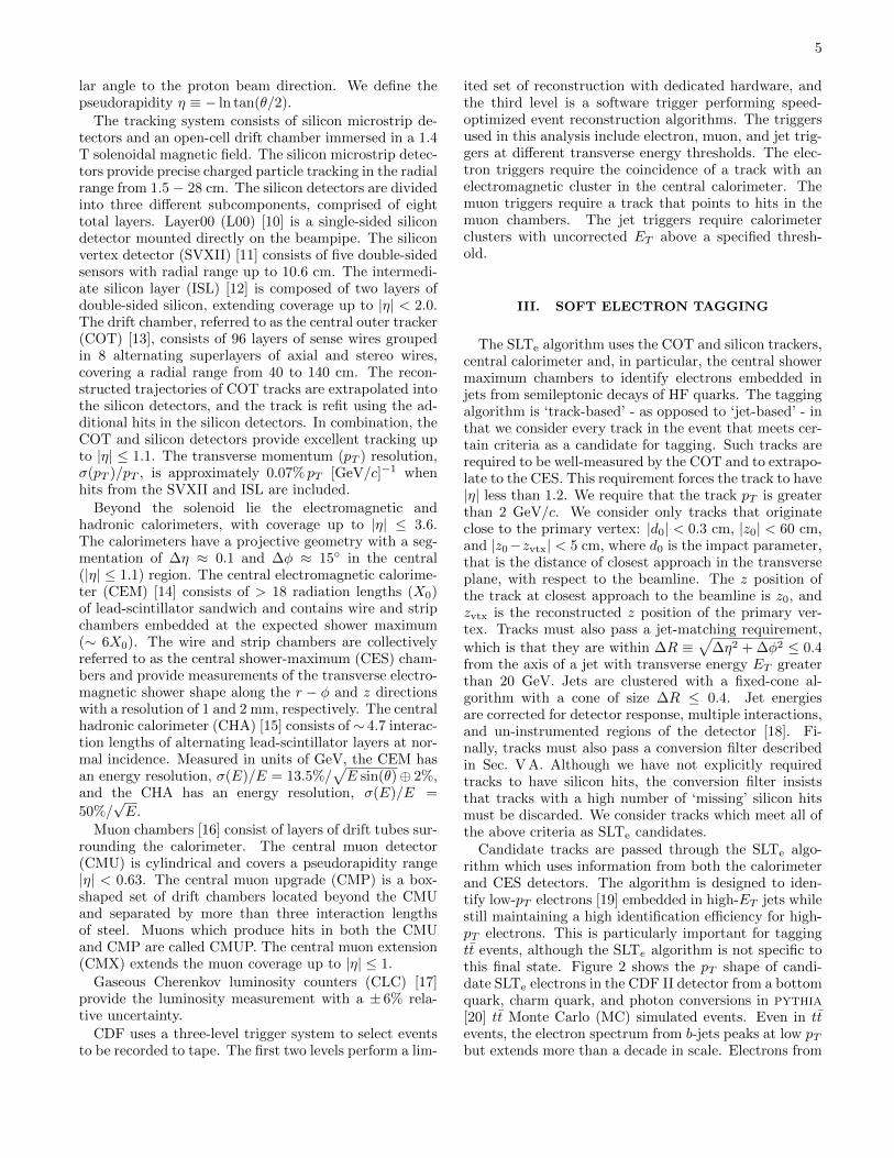
A fit for the conversion component of SLTe tags inevents triggered on a 20 GeV jet is shown in Fig. 8. Inthe fit, only those electrons with hits in six expected sil-icon layers is considered. Those tracks with fewer thansix expected layers are used as a consistency check, and asystematic uncertainty is assigned to the geometric biasincurred from this requirement. The dearth of trackswith four or five missing layers is an artifact of the CDFtrack reconstruction algorithm, which requires that atleast three silicon hits must be added to any track ornone will be added. The goodness-of-fit is limited bysystematic biases in the template construction which con-tribute the dominant systematic uncertainties to the ef-ficiency measurement. Such biases include correlationsbetween track finding and missing silicon layers, model-ing of prompt electrons (including HF decay) by prompthadrons, geometric dependencies, and sample contami-nation.
We find that the conversion identification efficiency isoverestimated in MC simulation relative to data. Wecharacterize the difference by a multiplicative scale fac-tor (SF), defined as the ratio of efficiencies measured indata and simulation. Because the conversion identifica-tion efficiency depends strongly on the underlying photonenergy spectrum, it is important for the SF measurementto compare energetically similar samples. Therefore, wemeasure the SF in events triggered by a jet with ET > 20,50, 70, and 100 GeV and compare to MC simulated dijet
11
Missing Silicon Layers0 1 2 3 4 5 6
Tags
/Miss
ing
Laye
r
02000400060008000
100001200014000160001800020000
Missing Silicon Layers0 1 2 3 4 5 6
Tags
/Miss
ing
Laye
r
02000400060008000
100001200014000160001800020000 Jet 20 Dataset
Electron TagsConversionsPrompts
FIG. 8: Fit for the conversion and prompt component ofSLTe tags before conversion removal in events triggeredon a ET > 20 GeV jet. The goodness-of-fit is limited by
systematic biases in the template construction and isaccounted for in the final SF measurement.
[GeV/c]TTrack p2 3 4 5 6 7 8 9 10 11 12
[GeV/c]TTrack p2 3 4 5 6 7 8 9 10 11 12
Effic
ienc
y/Sc
ale
Fact
or
0.20.30.40.50.60.70.80.9
11.11.2
Efficiency: Jet20 DataEfficiency: Jet20 MCEfficiency SF
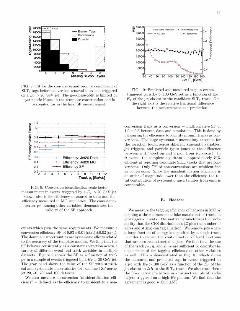
FIG. 9: Conversion identification scale factormeasurement in events triggered by a ET > 20 GeV jet.Shown also is the efficiency measured in data and the
efficiency measured in MC simulation. The consistencyacross pT , among other variables, demonstrates the
validity of the SF approach.
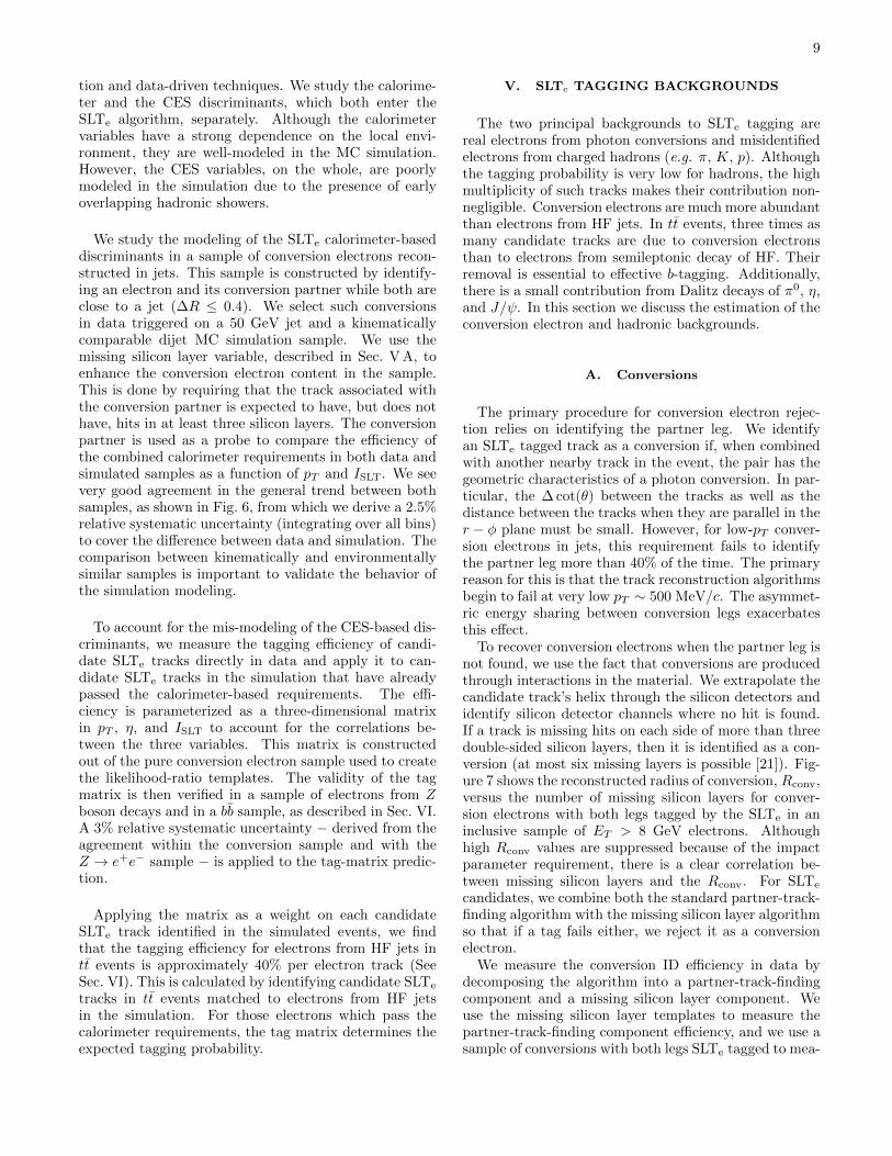
events which pass the same requirements. We measure aconversion efficiency SF of 0.93±0.01 (stat)±0.02 (syst).The dominant uncertainties are systematic effects relatedto the accuracy of the template models. We find that theSF behaves consistently as a constant correction across avariety of different event and track variables in multipledatasets. Figure 9 shows the SF as a function of trackpT in a sample of events triggered by a ET > 20 GeV jet.The gray band shows the value of the SF with statisti-cal and systematic uncertainties for combined SF acrossjet 20, 50, 70, and 100 datasets.
We also measure a conversion ‘misidentification effi-ciency’ − defined as the efficiency to misidentify a non-
[GeV]TJet E20 40 60 80 100 120 140 160 180 200
Tags
0
5000
10000
15000
20000
25000
30000
35000
40000
Frac
tiona
l Diff
eren
ce
-0.4
-0.2
0
0.2
0.4Fake Matrix Prediction
Jet 100 Data
(Pred-Meas)/Pred
5% Systematic±
FIG. 10: Predicted and measured tags in eventstriggered on a ET > 100 GeV jet as a function of theET of the jet closest to the candidate SLTe track. On
the right axis is the relative fractional differencebetween the measurement and prediction.
conversion track as a conversion − multiplicative SF of1.0 ± 0.3 between data and simulation. This is done bymeasuring the efficiency to identify prompt tracks as con-versions. The large systematic uncertainty accounts forthe variation found across different kinematic variables,jet triggers, and particle types (such as the differencebetween a HF electron and a pion from Ks decay). Intt events, the complete algorithm is approximately 70%efficient at rejecting candidate SLTe tracks that are con-versions. Only 7% of non-conversions are misidentifiedas conversions. Since the misidentification efficiency isan order of magnitude lower than the efficiency, the to-tal contribution of systematic uncertainties from each iscomparable.
B. Hadrons
We measure the tagging efficiency of hadrons in MC bydefining a three-dimensional fake matrix out of tracks injet-triggered events. The matrix parameterizes the prob-ability that the CES discriminants (L plus the number ofwires and strips) can tag a hadron. We remove jets wherea large fraction of energy is deposited by a single track,in order to reduce the contamination of hard electronsthat are also reconstructed as jets. We find that the useof the track pT , η, and ISLT are sufficient to describe thedependence of the tagging efficiency on other variablesas well. This is demonstrated in Fig. 10, which showsthe measured and predicted tags in events triggered ona jet with ET > 100 GeV as a function of the ET of thejet closest in ∆R to the SLTe track. We also cross-checkthe fake-matrix prediction in a distinct sample of tracksin jets triggered on a high-ET photon. We find that theagreement is good within ±5%.

12
Before tagging, the tracks in the jet samples are al-most purely hadronic; however, after tagging, we mustcorrect for the electron contamination when we estimatethe total efficiency to tag a hadronic track. Three classesof electrons are present in the sample: conversion elec-trons, HF electrons, and other sources (primarily Dalitzdecay of π0). The conversion electron contamination isestimated by measuring the efficiency and misidentifica-tion efficiency of the conversion filter in the jet samples.Using this information in combination with the numberof tracks before and after conversion removal determinesthe remaining conversion content. The HF electron con-tamination is estimated using correlations between theSLTe tags and b-tags from a secondary vertex algorithm,SecVtx [22]. We use SecVtx to enhance the HF con-tent of the jet sample. Using MC simulation to estimatethe expected size of this enhancement, we can extrap-olate back to the original, pre-SecVtx tag HF compo-nent. The remaining contribution of electrons from othersources is small and estimated with the MC simulation.
We find that 35 ± 3% of the tags in the jet-triggeredsample are electrons. This estimate is verified by measur-ing the SLTe tagging efficiency for charged pions from Ks
decay. By subtracting the electron contamination fromthe fake-matrix prediction, we find that, on average, 0.5%of hadronic tracks in tt events produce a fake SLTe tag.
VI. TUNING IN bb SAMPLE
As a validation of the measured efficiency of the tag-ger, we measure the jet tagging efficiency in a highly en-riched sample of bb events. Events are selected throughan 8 GeV electron or muon trigger, and we require thatboth the jet close to the lepton (∆R ≤ 0.4) and the re-coiling (away) jet have a SecVtx tag. We measure theper-jet efficiency to find at least one SLTe tag in the awayjet. This efficiency is measured to be 4.4± 0.1 (stat) (%)in simulation and 4.3± 0.1 (stat) (%) in data.
The efficiency is calculated in simulation by taking allof the candidate tracks in the jet that pass the calorime-ter requirements and using either the tag matrix for elec-trons or the fake matrix for hadrons to determine a tag-ging probability. If a track is identified as a conversion,then the tagging probability is rescaled according to theconversion efficiency or mis-identification efficiency SF.We tune the tag matrix with a multiplicative factor of0.98 ± 0.03 to get the simulation to agree with data,where the systematic uncertainty is assigned to cover ajet-ET dependence in the difference. The difference inthe prediction and measurement is due to isolation ef-fects of the jet environment not already accounted forby the ISLT parameterization, specifically the presenceof neutral hadrons. Figure 11 shows the predicted andmeasured tags in the combined 8 GeV electron and muontrigger samples as a function of the pT of the SLTe tagafter the tuning. Statistical uncertainties from the dataand simulation are added in quadrature and shown on
[GeV/c]T Track peSLT2 4 6 8 10 12 14 16 18 20
Tags
/1.0
GeV
/c
0
200
400
600
800
1000
1200
[GeV/c]T Track peSLT2 4 6 8 10 12 14 16 18 20
Tags
/1.0
GeV
/c
0
200
400
600
800
1000
1200
Ove
rflow
SLT TagsHF ElectronsConversion ElectronsFake Electrons
8 GeV Lepton Datasets EventseSLT
FIG. 11: Predicted and measured tags as a function ofthe SLTe track pT in a bb enhanced sample constructed
from inclusive electron and muon triggered events.Shown are contributions from fake tags, conversionelectron tags, and HF electron tags. Simulation and
data statistical uncertainties are combined inquadrature and shown together on the data points only.
the data points.By combining the tag matrix, fake matrix, conversion
identification and mis-identification efficiency SFs, andthe correction for the jet environment, we estimate thetagging efficiency of data from simulation. Figure 12shows the efficiency to tag a HF electron and a hadronin simulated tt events as a function of the track pT andthe jet ET . While the tagging efficiency for electrons issteady as a function of the track pT , it decreases as afunction of the jet ET because of the decreasing isolationat high-ET .
VII. CROSS SECTION MEASUREMENT
The tt production cross section is determined with theequation
σ =N −B
εttAtt
∫Ldt
(2)
where N is the number of tagged events, B is the ex-pected background, εtt and Att are the signal efficiencyand acceptance, respectively and
∫Ldt is the integrated
luminosity. In this section, we describe the measurementof each of these quantities.
A. Event Selection and Expectation
We select tt events in the lepton+jets decay channelthrough an inclusive lepton trigger which requires anelectron (muon) with ET > 18 GeV (pT > 18 GeV/c).

13
[GeV/c]T Track peSLT2 4 6 8 10 12 14 16 18
HF E
lect
ron
Effic
ienc
y
0
0.1
0.2
0.3
0.4
0.5
0.6 Tagging EfficiencyeSLT
Hadr
on E
fficie
ncy
0
0.005
0.01
HF ElectronsHadrons
(a)
[GeV]TJet E20 30 40 50 60 70 80 90 100 110 120
HF E
lect
ron
Effic
ienc
y
0
0.1
0.2
0.3
0.4
0.5
0.6 Tagging EfficiencyeSLT
Hadr
on E
fficie
ncy
0
0.005
0.01HF ElectronsHadrons
(b)
FIG. 12: Predicted efficiency to tag an electron from semileptonic decay of HF and a hadron candidate SLTe trackin tt events as a function of the track pT (a) and corrected jet ET (b). The left axis indicates the tagging efficiency
for the electrons and the right axis indicates the tagging efficiency for the hadrons.
Corrected tt Acceptance (%)Lepton 1 jet 2 jets 3 jets 4 jets ≥ 5 jetsCEM 0.163± 0.003 0.862± 0.011 1.403± 0.017 1.493± 0.018 0.519± 0.007
CMUP 0.089± 0.002 0.477± 0.009 0.788± 0.015 0.826± 0.015 0.284± 0.006CMX 0.042± 0.001 0.220± 0.005 0.353± 0.008 0.381± 0.008 0.130± 0.003Total 0.295± 0.005 1.559± 0.024 2.543± 0.039 2.700± 0.041 0.932± 0.015
TABLE II: Corrected tt acceptance in the lepton+jets decay channel. We have required HT > 250 GeV for eventswith ≥ 3 jets and 6ET > 30 GeV. Combined statistical and systematic uncertainties are shown.
After triggering, we further require that events con-tain an isolated electron (muon) with ET > 20 GeV(pT > 20 GeV/c) in the central region (|η| < 1.1). Werefer to this lepton as the primary lepton, to distinguishit from the soft lepton tag. The isolation of the primarylepton is defined as the transverse energy in the calorime-ter surrounding the lepton in a cone of ∆R ≤ 0.4 − butnot including the lepton ET itself − divided by the elec-tron (muon) ET (pT ). The lepton is considered isolatedif the isolation is less than 0.1. Note that this isolationdefinition is different than the isolation variable, ISLT,which is used with the SLTe algorithm.
We reject cosmic ray muons, conversion electrons, andZ bosons. Only one primary lepton is allowed to bereconstructed in the lepton+jets sample, and the fla-vor of that lepton must be consistent with the triggerpath. More details regarding this event selection canbe found in Ref. [5]. An inclusive W boson sample isconstructed by requiring high missing transverse energy,6ET > 30 GeV. We suppress background events by requir-ing HT > 250 GeV when three or more jets are present.We define HT as the scalar sum of the transverse energyof the primary lepton, jets, and 6ET .
In total, using events collected from February 2002through March 2007 corresponding to an integrated lu-minosity of
∫Ldt = 1.7± 0.1 fb−1, we find 2196 ‘pretag’
events with ≥ 3 jets after the event selection described.
We apply the SLTe algorithm to this sample and find 120‘tag’ events with ≥ 3 jets with at least one SLTe, of whichfive have two SLTe tags. Out of 120 events, 48 have aSecVtx tag present, in agreement with the expected 45such double tags.
We use pythia MC simulation with mt = 175 GeV/c2
to simulate top-quark pair-production. By default,all MC simulated samples are generated with theCTEQ5L [23] parton distribution functions (PDF), andthe program EvtGen [24] is used to decay the parti-cle species. We measure Att by counting the number ofevents that pass the lepton+jets event selection describedabove divided by the total number of events generated.We do not restrict the decay channel at the generatorlevel, so it is possible for some signal from other decaychannels [25] to be reconstructed and categorized as lep-ton+jets. We then correct the acceptance with variousscale factors to account for differences between simula-tion modeling and data. These scale factors result fromdifferences in modeling of the lepton identification andisolation components, as well as corrections for require-ments imposed on data but not the simulation, includingthe trigger efficiency, the position of the primary vertexalong z, and the quality of the lepton track. The totalacceptance for tt events after corrections is 6.2%, compa-rable with the acceptance of other analyses in this finalstate [3–5]. A breakdown of the corrected acceptance by

14
jet multiplicity and W lepton type is shown in Table II.Scaling the acceptance by the tt production cross section(assumed here to be 6.7 pb) and integrated luminosityyields a total pre-tag event expectation of 716.7 ± 44.4events, where the dominant uncertainties result from theuncertainty on the luminosity and the acceptance correc-tions.
Finally, we measure the efficiency to find at least oneSLTe tag in events that pass the event selection by ap-plying the calorimeter requirements, tag matrix, fake ma-trix, and conversion efficiency scale factors to candidatetracks. Assuming σtt = 6.7 pb, and
∫Ldt = 1.7 fb−1, we
expect 59.2 ± 5.0 events after tagging in the ≥ 3 jet re-gion. This corresponds to a per-event tagging efficiencyof εtt = 8.3%.
B. Background Estimation and SampleComposition
We consider three categories of background in the iden-tification of tt events. The first category, whose contri-bution is derived from MC simulation, includes the pro-duction of WW , WZ, ZZ∗ (where one Z can be pro-duced off-shell), single top quark production, Z in asso-ciation with jets, and Drell-Yan in association with jets.These backgrounds have a small uncertainty on the pro-duction cross section or contribute sufficiently little tothe total background that a large uncertainty has littleeffect. For diboson production, we use pythia generatedsamples scaled by their respective theoretical cross sec-tions to estimate their contribution to the pretag and tagsamples. The estimate for single top quark productionuses a combination of madevent [26] for generation andpythia for showering, and is calculated separately for s-and t-channel processes again using the theoretical crosssections. Z+jets and Drell-Yan+jets use an alpgen [27]and pythia combination, where alpgen is used for thegeneration and pythia is used for the showering. Thecross section is scaled to match the measured Z+jetscross section with an additional 1.2 ± 0.2 correction tomatch the measured jet multiplicity spectrum. Table IIIlists the cross sections used for each process.
The second category consists of background from mul-tijet production, called QCD. We estimate the QCD con-tribution by releasing the 6ET requirement and fitting thetotal 6ET distribution to templates for the backgroundsand signal. To model the QCD 6ET spectrum, we usetwo samples: a pythia bb dijet sample, and a data sam-ple with an ET > 20 GeV electron candidate that failsat least two electron ID requirements. This sample isprincipally composed of multijet events with a similartopology to those that fake a high-ET electron. We fitfor the fraction of QCD events in the sample by fixingthe tt and MC simulation-driven background normaliza-tions, and varying the W+jets and QCD template nor-malizations separately. The total QCD contribution hasvirtually no dependence on the assumed tt cross section.
We also include a 15% systematic uncertainty due to thereal electron contamination in the electron-like sample.Table IV shows the measured fits for the fraction of pre-tag events with 6ET > 30 GeV that are due to pretag and
tag QCD events, FQCDpre and FQCD
tag , respectively. Theresult of the fit in the pretag region for ≥ 3 tags is shownin Fig. 13.
[GeV]TE0 20 40 60 80 100 120
Even
ts/6
.0 G
eV
050
100150200250300350400450
[GeV]TE0 20 40 60 80 100 120
Even
ts/6
.0 G
eV
050
100150200250300350400450
QCD Template Fit-1 Ldt=1.7 fb!
3 Jets)"Data (Pretag: tt
QCD TemplateW+JetsZ+JetsDrell-YanSingle TopWW/WZ/ZZ
FIG. 13: QCD fit for pretag events with ≥ 3 jets.W+jet and QCD templates are allowed to float.
The third category and largest background is the pro-duction of W bosons in association with multiple jets.We use a combination of simulation and data-driven tech-niques to measure this background. We use alpgen asthe generator of the W+multijet datasets and pythiafor fragmentation and showering.
The W+jet normalization is determined by assumingthat all pretag data events, not already accounted forby tt or by the first two background categories, must beW+jets. The tag estimate is derived from the pretag es-timate by assuming that the tagging efficiency measuredin MC simulation for separate HF categories is accurateand only the relative amount of HF needs adjustment.The equations below elucidate this procedure:
NpreW = Npre
data −NpreMC −N
preQCD −N
prett (3)
N tag
W+bb= Npre
W (ε2bF2b + ε1bF1b) (4)
N tagW+cc = Npre
W (ε2cF2c + ε1cF1c) (5)
N tagW+LF = Npre
W ε0b,0c(1− F2b − F1b − F2c − F1c) (6)
where N tag and Npre are the number of tag and pretagevents for various signal and background components,and LF refers to light-flavor. The tagging efficiencies, ε,are measured in separate HF categories, where the sub-script designates the number of reconstructed jets in anevent identified as a b− or c− jet with information fromthe generator. For bookkeeping purposes, the presenceof a b-jet supersedes the presence of a c-jet. The HF frac-tions, F , designate the fraction of W+jet events for eachHF category.
While both the HF efficiencies and HF fractions are

15
Process Cross Section×BF (pb) GeneratorWW 12.4± 0.25 [28] pythiaWZ 3.96± 0.06 [28] pythiaZZ∗ 2.12± 0.15 [28] pythia
single top (s-channel) 0.29± 0.02 [29] madevent+pythiasingle top (t-channel) 0.66± 0.03 [29] madevent+pythia
Z+Jets 308± 51 [30] alpgen+pythiaDrell-Yan+Jets 2882± 480 [30] alpgen+pythia
TABLE III: Cross sections and generators used for the MC-simulation-derived backgrounds. The production ofsingle top, Z+jets and Drell-Yan+jets is constrained to decay (semi-)leptonically at generator level. The cross
sections for these processes are multiplied by the leptonic branching fraction. The decay of the diboson simulation,however, remains unconstrained, and the full production cross section is quoted.
1 Jet 2 Jets ≥ 3 JetsFQCDpre (%) 3.7± 6.0 4.6± 0.6 9.2± 1.5
FQCDtag (%) 0.045± 0.011 0.10± 0.02 0.28± 0.14
TABLE IV: Summary of the fraction of the pretagsample due to pretag and tag QCD events for different
jet multiplicies.
Fraction 1 Jet 2 Jets 3 Jets ≥ 4 JetsF1b 0.8± 0.3 1.6± 0.6 3.0± 1.1 3.7± 1.4F2b — 1.0± 0.4 2.2± 0.8 3.5± 1.3F1c 5.8± 1.6 9.1± 2.6 10.2± 3.3 12.1± 3.9F2c — 1.5± 0.6 3.4± 1.3 6.3± 2.3
TABLE V: Heavy-flavor fractions multiplied by theK-factor for W+jet events. Uncertainties are dominatedby the agreement of the K-factor across jet bins and the
Q2 scale. All numbers are shown in units of %.
measured in MC simulation, the fractions are calibratedby a single, multiplicative K-factor, K = 1.0 ± 0.4, de-rived from a data/MC comparison of multijet events withHF enhanced by a SecVtx tag. The systematic uncer-tainty is dominated by the contribution from varying the
1 Jet 2 Jets 3 Jets ≥ 4 Jetsε0b,0c 0.92± 0.06 1.89± 0.11 3.01± 0.17 4.24± 0.24ε1b 3.33± 0.16 4.39± 0.22 5.43± 0.29 6.80± 0.36ε2b — 6.72± 0.33 7.26± 0.37 9.55± 0.45ε1c 1.61± 0.09 2.50± 0.14 3.46± 0.20 4.78± 0.28ε2c — 3.11± 0.17 4.17± 0.23 5.58± 0.30
TABLE VI: SLTe tagging efficiency for different classesof HF in W+jet events. Uncertainties shown include allSLTe tagging systematic uncertainties. All numbers are
shown in units of %.
Q2 of the samples and the agreement of the K-factoracross jet multiplicities. Phase-space overlap of jets sim-ulated by alpgen and pythia is accounted for by allow-ing alpgen to simulate those HF jets well-separated inη−φ space and allowing pythia to simulate the rest [31].Tables V and VI show the measured values for the HFfractions and efficiencies, respectively.
C. Measurement and Uncertainties
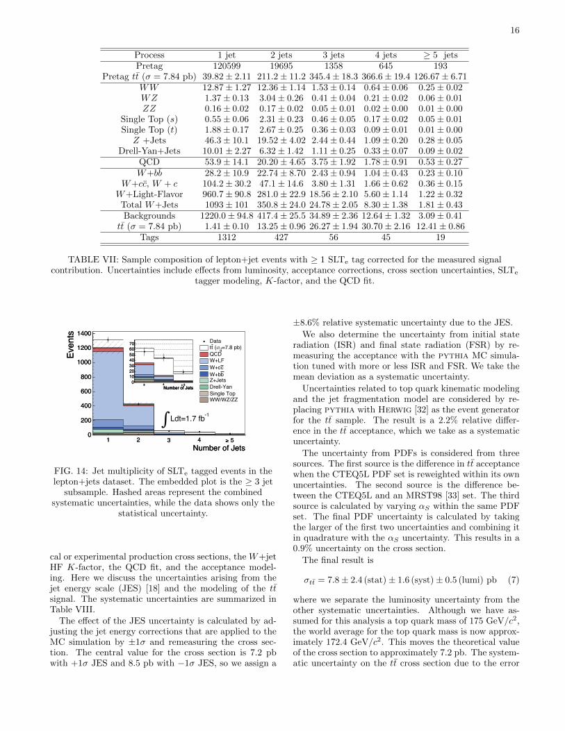
Although the W+jets background depends explicitlyon the assumed value of σtt (see Eq. 3), we can solvealgebraically for the cross section, resulting in a centralvalue of 7.8 ± 2.4 pb, where the statistical uncertaintyis determined through error propagation and is verifiedwith pseudo-experiments. The final sample compositionis shown in Table VII and is shown graphically in Fig. 14.This table shows the tt expectation for the measuredcross section along with the background estimates cor-rected for the signal contribution. The observed numberof pretag events and the expected number of pretag ttevents is also presented.
The combined systematic uncertainties due to the lu-minosity, acceptance, background cross sections, SLTe
tagging, K-factor, and QCD fit are given in the table.Note that some of the background contributions − inparticular, the W+jets components − are negatively cor-related with each other, and this is reflected in the sys-tematic uncertainties presented.
Figure 15 show the SLTe tag pT distribution and theevent HT distribution in the ≥ 3 jet region.
In the previous sections, we have described system-atic uncertainties related to the SLTe tagger and thebackground estimations. The tagger uncertainties derivefrom the calorimeter variable modeling, the tag- and fake-matrix predictions, the conversion (mis-)identificationscale factors, and the jet environment correction fromthe b-jet tuning. Each of the tagger uncertainties areuncorrelated because they have been derived in sepa-rate samples with distinct measurement techniques. Thebackground uncertainties are derived from the theoreti-
16
Process 1 jet 2 jets 3 jets 4 jets ≥ 5 jetsPretag 120599 19695 1358 645 193
Pretag tt (σ = 7.84 pb) 39.82± 2.11 211.2± 11.2 345.4± 18.3 366.6± 19.4 126.67± 6.71WW 12.87± 1.27 12.36± 1.14 1.53± 0.14 0.64± 0.06 0.25± 0.02WZ 1.37± 0.13 3.04± 0.26 0.41± 0.04 0.21± 0.02 0.06± 0.01ZZ 0.16± 0.02 0.17± 0.02 0.05± 0.01 0.02± 0.00 0.01± 0.00
Single Top (s) 0.55± 0.06 2.31± 0.23 0.46± 0.05 0.17± 0.02 0.05± 0.01Single Top (t) 1.88± 0.17 2.67± 0.25 0.36± 0.03 0.09± 0.01 0.01± 0.00Z +Jets 46.3± 10.1 19.52± 4.02 2.44± 0.44 1.09± 0.20 0.28± 0.05
Drell-Yan+Jets 10.01± 2.27 6.32± 1.42 1.11± 0.25 0.33± 0.07 0.09± 0.02QCD 53.9± 14.1 20.20± 4.65 3.75± 1.92 1.78± 0.91 0.53± 0.27W+bb 28.2± 10.9 22.74± 8.70 2.43± 0.94 1.04± 0.43 0.23± 0.10
W+cc, W + c 104.2± 30.2 47.1± 14.6 3.80± 1.31 1.66± 0.62 0.36± 0.15W+Light-Flavor 960.7± 90.8 281.0± 22.9 18.56± 2.10 5.60± 1.14 1.22± 0.32Total W+Jets 1093± 101 350.8± 24.0 24.78± 2.05 8.30± 1.38 1.81± 0.43Backgrounds 1220.0± 94.8 417.4± 25.5 34.89± 2.36 12.64± 1.32 3.09± 0.41
tt (σ = 7.84 pb) 1.41± 0.10 13.25± 0.96 26.27± 1.94 30.70± 2.16 12.41± 0.86Tags 1312 427 56 45 19
TABLE VII: Sample composition of lepton+jet events with ≥ 1 SLTe tag corrected for the measured signalcontribution. Uncertainties include effects from luminosity, acceptance corrections, cross section uncertainties, SLTe
tagger modeling, K-factor, and the QCD fit.
Number of Jets1 2 3 4 5!
Even
ts
0
200
400
600
800
1000
1200
1400
Number of Jets1 2 3 4 5!
Even
ts
0
200
400
600
800
1000
1200
1400Data
=7.8 pb)tt" (ttQCDW+LF
cW+cbW+b
Z+JetsDrell-YanSingle TopWW/WZ/ZZ
-1 Ldt=1.7 fb#
Number of Jets3 4 5!
Number of Jets3 4 5!
010203040506070
Number of Jets3 4 5!
010203040506070
FIG. 14: Jet multiplicity of SLTe tagged events in thelepton+jets dataset. The embedded plot is the ≥ 3 jet
subsample. Hashed areas represent the combinedsystematic uncertainties, while the data shows only the
statistical uncertainty.
cal or experimental production cross sections, the W+jetHF K-factor, the QCD fit, and the acceptance model-ing. Here we discuss the uncertainties arising from thejet energy scale (JES) [18] and the modeling of the ttsignal. The systematic uncertainties are summarized inTable VIII.
The effect of the JES uncertainty is calculated by ad-justing the jet energy corrections that are applied to theMC simulation by ±1σ and remeasuring the cross sec-tion. The central value for the cross section is 7.2 pbwith +1σ JES and 8.5 pb with −1σ JES, so we assign a
±8.6% relative systematic uncertainty due to the JES.
We also determine the uncertainty from initial stateradiation (ISR) and final state radiation (FSR) by re-measuring the acceptance with the pythia MC simula-tion tuned with more or less ISR and FSR. We take themean deviation as a systematic uncertainty.
Uncertainties related to top quark kinematic modelingand the jet fragmentation model are considered by re-placing pythia with Herwig [32] as the event generatorfor the tt sample. The result is a 2.2% relative differ-ence in the tt acceptance, which we take as a systematicuncertainty.
The uncertainty from PDFs is considered from threesources. The first source is the difference in tt acceptancewhen the CTEQ5L PDF set is reweighted within its ownuncertainties. The second source is the difference be-tween the CTEQ5L and an MRST98 [33] set. The thirdsource is calculated by varying αS within the same PDFset. The final PDF uncertainty is calculated by takingthe larger of the first two uncertainties and combining itin quadrature with the αS uncertainty. This results in a0.9% uncertainty on the cross section.
The final result is
σtt = 7.8± 2.4 (stat)± 1.6 (syst)± 0.5 (lumi) pb (7)
where we separate the luminosity uncertainty from theother systematic uncertainties. Although we have as-sumed for this analysis a top quark mass of 175 GeV/c2,the world average for the top quark mass is now approx-imately 172.4 GeV/c2. This moves the theoretical valueof the cross section to approximately 7.2 pb. The system-atic uncertainty on the tt cross section due to the error

17
[GeV/c]T Track peSLT5 10 15 20 25 30 35 40
Tags
/2.0
GeV
/c
0
10
20
30
40
50
60
[GeV/c]T Track peSLT5 10 15 20 25 30 35 40
Tags
/2.0
GeV
/c
0
10
20
30
40
50
60-1 Ldt=1.7 fb!
Data=7.8)
tt" (tt
QCDW+LF
cW+cbW+b
Z+JetsDrell-YanSingle TopWW/WZ/ZZ
(a)
[GeV]TEvent H250 300 350 400 450 500 550 600 650 700
Even
ts/2
5 G
eV
0
5
10
15
20
25
30
[GeV]TEvent H250 300 350 400 450 500 550 600 650 700
Even
ts/2
5 G
eV
0
5
10
15
20
25
30-1 Ldt=1.7 fb!
Data=7.8)
tt" (tt
QCDW+LF
cW+cbW+b
Z+JetsDrell-YanSingle TopWW/WZ/ZZ
(b)
FIG. 15: (a) pT distribution of SLTe tags in lepton+jet events with ≥ 3 jets. (b) HT distribution of SLTe taggedevents with ≥ 3 jets.
Source Relative Uncertaintyon σtt (%)
Jet Energy Scale 8.4QCD Fit 5.0K-factor 3.0
Herwig/pythia 2.2Acceptance Corrections 1.6
Background Cross Section 0.6PDFs 0.9FSR 0.6ISR 0.5
Conversion ID Efficiency SFs 10.7Fake Matrix 7.8
Calorimeter Modeling 7.7Tag Matrix 6.8
Jet Environment Correction 5.4Total Tagger Uncertainty 17.6
Total 20.6
TABLE VIII: Summary of systematic uncertainties.
on the top-quark mass is small, and leaves the result un-changed.
VIII. CONCLUSIONS
We have performed the first measurement ofthe tt production cross section with SLTe tagsin Run II of the Tevatron. This measurement,σtt = 7.8 ± 2.4 (stat) ± 1.6 (syst) ± 0.5 (lumi) pb, is
consistent with the theoretical value [8], σtt = 6.7 ± 0.8pb (mt = 175 GeV/c2), as well as the current CDFaverage [34], σtt = 7.02 ± 0.63 pb. While statisticallylimited, this measurement demonstrates the consistencyof the top quark production cross section in the lep-ton+jets final state with soft electron b-tagging. Thismeasurement also provides an experimental basis forinvestigating other high-pT physics measurements withthe soft electron tagging technique.
Acknowledgments
We thank the Fermilab staff and the technical staffsof the participating institutions for their vital contribu-tions. This work was supported by the U.S. Departmentof Energy and National Science Foundation; the ItalianIstituto Nazionale di Fisica Nucleare; the Ministry ofEducation, Culture, Sports, Science and Technology ofJapan; the Natural Sciences and Engineering ResearchCouncil of Canada; the National Science Council of theRepublic of China; the Swiss National Science Founda-tion; the A.P. Sloan Foundation; the Bundesministeriumfur Bildung und Forschung, Germany; the World ClassUniversity Program, the National Research Foundationof Korea; the Science and Technology Facilities Coun-cil and the Royal Society, UK; the Institut National dePhysique Nucleaire et Physique des Particules/CNRS;the Russian Foundation for Basic Research; the Minis-terio de Ciencia e Innovacion, and Programa Consolider-Ingenio 2010, Spain; the Slovak R&D Agency; and theAcademy of Finland.
[1] F. Abe et al. (CDF Collaboration), Phys. Rev. Lett. 74,2626 (1995);
S. Abachi et al. (D0 Collaboration), Phys. Rev. Lett. 74,2632 (1995).

18
[2] T. Aaltonen et al. (CDF Collaboration), Phys. Rev. D76, 072009 (2007);V.M. Abazov et al. (D0 Collaboration),arXiv.org:0911.4286 [hep-ex], FERMILAB-PUB-09-592-E.
[3] D. Acosta et al. (CDF Collaboration), Phys. Rev. D 72,052003 (2005);V.M. Abazov et al. (D0 Collaboration), Phys. Rev. D 76,092007 (2007).
[4] A. Abulencia et al. (CDF Collaboration), Phys. Rev. Lett97, 082004 (2006);A. Abulencia et al. (CDF Collaboration), Phys. Rev. D74, 072006 (2006);V.M. Abazov et al. (D0 Collaboration), Phys. Lett. B626, 35 (2005).
[5] D. Acosta et al. (CDF Collaboration), Phys. Rev. D 72,032002 (2005);T. Aaltonen et al. (CDF Collaboration), Phys. Rev. D79, 052007 (2009).
[6] D. Acosta et al. (CDF Collaboration), Phys. Rev. Lett.93, 142001 (2004);V.M. Abazov et al. (D0 Collaboration), Phys. Rev. D 76,052006 (2007).
[7] Tevatron Electroweak Working Group, arXiv:0808.1089v1 [hep-ex], FERMILAB-TM-2413-E.
[8] M. Cacciari, S. Frixione, M. Mangano, P. Nason, and G.Ridolfi, J. High Energy Phys. 0809 (2008) 127;N. Kidonakis and R. Vogt, Phys. Rev. D 78, 074005(2008);S. Moch and P. Uwer, Nucl. Phys. Proc. Suppl. 183, 75-80 (2008).
[9] F. Abe et al. (CDF Collaboration), Phys. Rev. Lett. 80,2773 (1998).
[10] C. Hill et al. (CDF Collaboration), Nucl. Instrum. Meth-ods Phys. Res., Sect. A 530, 1 (2004).
[11] A. Sill et al. (CDF Collaboration), Nucl. Instrum. Meth-ods Phys. Res., Sect. A 447, 1 (2000).
[12] A. Affolder et al. (CDF Collaboration), Nucl. Instrum.Methods Phys. Res., Sect. A 453, 84 (2000).
[13] T. Affolder et al. (CDF Collaboration), Nucl. Instrum.Methods Phys. Res., Sect. A 526, 249 (2004).
[14] L. Balka et al. (CDF Collaboration), Nucl. Instrum.Methods Phys. Res., Sect. A 267, 272 (1988).
[15] S. Bertolucci et al. (CDF Collaboration), Nucl. Instrum.Methods Phys. Res., Sect. A 267, 301 (1988).
[16] G. Ascoli et al. (CDF Collaboration), Nucl. Instrum.Methods Phys. Res., Sect. A 268, 33 (1998).
[17] D. Acosta et al. (CDF Collaboration), Nucl. Instrum.Methods Phys. Res., Sect. A 494, 57 (2002).
[18] A. Bhatti et al. (CDF Collaboration), Nucl. Instrum.Methods Phys. Res., Sect. A 566, 2 (2006).
[19] We characterize the transverse energy of soft electrons bythe track pT , rather than the more typical calorimetricET , because of the presence of the jet.
[20] T. Sjostrand, S. Mrenna, and P. Skands, J. High EnergyPhys. 0605 (2006) 026. We use pythia version 6.216.
[21] Although L00 is used for track reconstruction, it is onlyone-sided and excluded from the the conversion-findingalgorithm. The last layer of the ISL is also too far forwardto be fiducial for SLTe tracks. Therefore, a total of atmost six layers may be missing for any given SLTe track.
[22] D. Acosta et al. (CDF Collaboration), Phys. Rev. D 71,052003 (2005).
[23] J. Pumplin, D. Stump, J. Huston, H. Lai, P. Nadolsky,and W. Tung, J. High Energy Phys. 0207 (2002) 012.
[24] D.J. Lange et al., Nucl. Instrum. Methods Phys. Res.,Sect. A 462, 152 (2001).
[25] The dilepton channel − where both W bosons decay lep-tonically − contributes 2−3% of the total event selectionas one lepton may escape identification.
[26] J. Alwall et al., J. High Energy Phys. 0709 (2007) 028.We use madevent version 4.211.
[27] M.L. Mangano, M. Moretti, F. Piccinini, R. Pittau, andA.D. Polosa, J. High Energy Phys. 0307 (2003) 001. Weuse alpgen version 2.10 prime.
[28] J.M. Campbell and R.K. Ellis, Phys. Rev. D 60, 113006(1999).
[29] G. Jikia and S. Slabospitsky, Phys. Lett. B 295, 136(1992).
[30] D. Acosta et al. (CDF Collaboration), Phys. Rev. Lett94, 091803 (2005).
[31] D. Sherman, Ph.D. thesis, Harvard University, 2007.[32] G. Corcella et. al., J. High Energy Phys. 01 (2001) 010.
We use Herwig version 6.510.[33] A.D. Martin, R.G. Roberts, W.J. Stirling, and R.S.
Thorne, Eur. Phys. J. C 4, 463 (1998).[34] The CDF Collaboration, CDF Conference Note
9448 (2008): http://www-cdf.fnal.gov/physics/new/
top/confNotes/