Productivity, Networks and Input-Output Structure ∗

Harald Fadinger† Christian Ghiglino ‡ Mariya Teteryatnikova§

July 2015

Abstract

We consider a multi-sector general equilibrium model with IO linkages, sector-specific productivi-

ties and tax rates. Using tools from network theory, we investigate how the IO structure interacts with

productivities and taxes in the determination of aggregate income. Employing a statistical approach,

we show that aggregate income is a simple function of the first and second moments of the distribution

of the IO multipliers, sectoral productivities and sectoral tax rates. We then estimate the parameters

of the model to fit their joint empirical distribution, allowing these to vary with income per capita.

We find an important difference between rich and medium-low-income countries. Poor countries

have more extreme distributions of IO multipliers than rich economies: there are a few high-multiplier

sectors, while most sectors have very low multipliers; in contrast, rich countries have more sectors

with intermediate multipliers. Moreover, the correlations of these with productivities and tax rates

are positive in poor countries, while being negative in rich ones. The estimated model predicts cross-

country income differences extremely well, also out-of-sample (up to 97% of the variation in relative

income per capita). We also perform a number of counterfactuals. First, we “impose” the dense IO

structure of the U.S. on low- and middle-income countries and find a large damaging effect, up to 80

%. Second, we assume that sectoral IO multipliers and productivities are uncorrelated and find that

low-income countries would lose up to 50% of their per capita income while high-income countries

would gain. Finally, optimal taxation results suggest that poor countries would gain up to 30% in

terms of per capita income if they moved to a tax system that taxes high-multiplier sectors less.

KEY WORDS: input-output structure, networks, productivity, cross-country income differences

JEL CLASSIFICATION: O11, O14, O47, C67, D85

∗We thank Dominick Bartelme, Johannes Boehm, Antonio Ciccone, Yuriy Gorodnichenko, seminar participants at theUniversities of Mannheim and Vienna and at the 2015 SED meeting for useful comments and suggestions. We also thankSusana Parraga Rodriguez for excellent research assistance.†University of Mannheim. Email: harald.fadinger@uni-mannheim.de.‡University of Essex. Email:cghig@essex.ac.uk.§University of Vienna. Email: mariya.teteryatnikova@univie.ac.at.

1 Introduction

One of the fundamental debates in economics is about how important differences in factor endowments

– such as physical or human capital stocks – are relative to aggregate productivity differences in terms

of explaining cross-country differences in income per capita. The standard approach to address this

question is to specify an aggregate production function for value added (e.g., Caselli, 2005) . Given data

on aggregate income and factor endowments and the imposed mapping between endowments and income,

one can back out productivity differences as a residual that explains differences between predicted and

actual income. However, this standard approach ignores that GDP aggregates value added of many

economic activities which are connected to each other through input-output linkages.1 In contrast, a

literature in development economics initiated by Hirschman (1958) has long emphasized that economic

structure is of first-order importance to understand cross-country income differences.2

Consider, for example, a productivity increase in the Transport sector. This reduces the price of

transport services and thereby increases productivity in sectors that use transport services as an input

(e.g., Mining). Increased productivity in Mining in turn increases productivity of the Steel sector by

reducing the price of iron ore, which in turn increases the productivity of the Transport Equipment

sector. In a second-round effect, the productivity increase in Transport Equipment in turn improves

productivity of the Transport sector and so on. Thus, input-output (IO) linkages between sectors lead

to multiplier effects. The IO multiplier of a sector summarizes all these intermediate effects and measures

by how much aggregate income will change if productivity of this sector changes by one percent. The

size of the sectoral multiplier effect depends to a large extent on the number of sectors to which a given

sector supplies and the intensity with which its output is used as an input by the other sectors.3 We

document that there are large differences in IO multipliers across sectors – e.g., most infrastructure

sectors, such as Transport and Energy, have high multipliers because they are used as inputs by many

other sectors,4 while a sector such as Textiles – which does not provide inputs to many sectors – has a

low multiplier. As a consequence, low productivities in different sectors will have very distinct effects on

aggregate income, depending on the size of the sectoral IO multiplier.

1An important exception that highlights sectoral TFP differences is the recent work on dual economies. This literaturefinds that productivity gaps between rich and poor countries are much more pronounced in agriculture than in manufacturingor service sectors and this fact together with the much larger value added or employment share of agriculture in poorcountries can explain an important fraction of cross-country income differences.

2More recent contributions highlighting the role of economic structure for aggregate income are Ciccone, 2002 and Jones,2011 a,b.

3The intensity of input use is measured by the IO coefficient, which states the cents spent on that input per dollar ofoutput produced. There are also higher-order effects, which depend on the number and the IO coefficients of the sectors towhich the sectors that use the initial sector’s output as an input supply.

4The view that infrastructure sectors are of crucial importance for aggregate outcomes has also been endorsed by theWorld Bank. In 2010, the World Bank positioned support for infrastructure as a strategic priority in creating growthopportunities and targeting the poor and vulnerable. Infrastructure projects have become the single largest business linefor the World Bank Group, with $26 billion in commitments and investments in 2011 (World Bank Group InfrastructureUpdate FY 2012-2015).

1

In this paper, we address the question how differences in economic structure across countries – as

captured by IO linkages between sectors – affect cross-country differences in aggregate income per capita.

To this end, we combine data from the World Input-Output Database (Timmer, 2012) and the Global

Trade Analysis project (GTAP Version 6), in order to construct a unique dataset of IO tables, sectoral

total factor productivities and sectoral tax rates for a large cross section of countries in the year 2005.5

With this data at hand, we investigate how the IO structure interacts with sectoral TFP differences

and taxes to determine aggregate per capita income. First, we document that in all countries there is a

relatively small set of sectors which have very large IO multipliers and whose performance thus crucially

affects aggregate outcomes. Moreover, despite this regularity, we also find that there do exist substantial

differences in the network characteristics of IO linkages between poor and rich countries. In particular,

low-income countries typically have a very small number of average and high-multiplier sectors, while

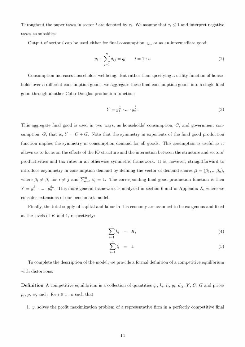
high-income countries have a more dense input-output network. To visualize these differences, in Figure

1 we plot a graphical representation of the IO matrices of two countries: Uganda (a very poor country

with a per capita GDP of 964 PPP dollars in 2005) and the U.S. (a major industrialized economy with a

per capita GDP of around 42,500 PPP dollars in 2005). The columns of the IO matrix are the producing

sectors, while the rows are the sectors whose output is used as an input. Thus, a dot in the matrix

indicates that the column sector uses some of the row sector’s output as an input and a blank space

indicates that there is no significant connection between the two sectors.6

Figure 1: IO-matrices by country: Uganda (left), USA (right)

By comparing the matrices it is apparent that in Uganda there are only four sectors which supply

5We have data on sectoral TFPs and tax rates for 37 countries and data on IO tables for 70 countries.6Data are from GTAP version 6, see the data appendix for details. The figure plots IO coefficients defined as cents of

industry j output (row j) used per dollar of output of industry i (column i). To make the figure more readable, we onlyplot linkages with at least 2 cents per dollar of output.

2

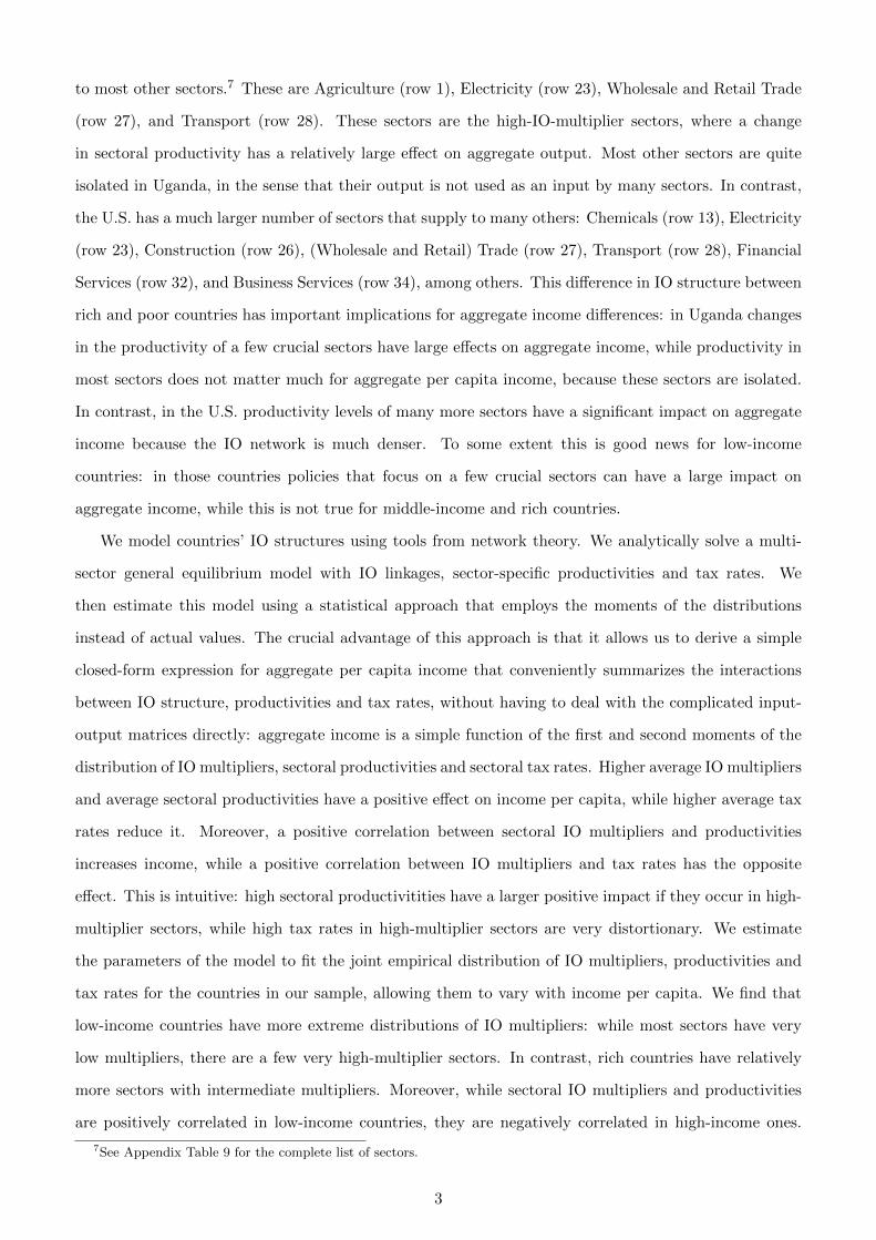
to most other sectors.7 These are Agriculture (row 1), Electricity (row 23), Wholesale and Retail Trade

(row 27), and Transport (row 28). These sectors are the high-IO-multiplier sectors, where a change

in sectoral productivity has a relatively large effect on aggregate output. Most other sectors are quite

isolated in Uganda, in the sense that their output is not used as an input by many sectors. In contrast,

the U.S. has a much larger number of sectors that supply to many others: Chemicals (row 13), Electricity

(row 23), Construction (row 26), (Wholesale and Retail) Trade (row 27), Transport (row 28), Financial

Services (row 32), and Business Services (row 34), among others. This difference in IO structure between

rich and poor countries has important implications for aggregate income differences: in Uganda changes

in the productivity of a few crucial sectors have large effects on aggregate income, while productivity in

most sectors does not matter much for aggregate per capita income, because these sectors are isolated.

In contrast, in the U.S. productivity levels of many more sectors have a significant impact on aggregate

income because the IO network is much denser. To some extent this is good news for low-income

countries: in those countries policies that focus on a few crucial sectors can have a large impact on

aggregate income, while this is not true for middle-income and rich countries.

We model countries’ IO structures using tools from network theory. We analytically solve a multi-

sector general equilibrium model with IO linkages, sector-specific productivities and tax rates. We

then estimate this model using a statistical approach that employs the moments of the distributions

instead of actual values. The crucial advantage of this approach is that it allows us to derive a simple

closed-form expression for aggregate per capita income that conveniently summarizes the interactions

between IO structure, productivities and tax rates, without having to deal with the complicated input-

output matrices directly: aggregate income is a simple function of the first and second moments of the

distribution of IO multipliers, sectoral productivities and sectoral tax rates. Higher average IO multipliers

and average sectoral productivities have a positive effect on income per capita, while higher average tax

rates reduce it. Moreover, a positive correlation between sectoral IO multipliers and productivities

increases income, while a positive correlation between IO multipliers and tax rates has the opposite

effect. This is intuitive: high sectoral productivitities have a larger positive impact if they occur in high-

multiplier sectors, while high tax rates in high-multiplier sectors are very distortionary. We estimate

the parameters of the model to fit the joint empirical distribution of IO multipliers, productivities and

tax rates for the countries in our sample, allowing them to vary with income per capita. We find that

low-income countries have more extreme distributions of IO multipliers: while most sectors have very

low multipliers, there are a few very high-multiplier sectors. In contrast, rich countries have relatively

more sectors with intermediate multipliers. Moreover, while sectoral IO multipliers and productivities

are positively correlated in low-income countries, they are negatively correlated in high-income ones.

7See Appendix Table 9 for the complete list of sectors.

3

Similarly, IO multipliers and tax rates are positively correlated in poor countries and negatively correlated

in rich ones.

With the parameter estimates in hand, we use our closed-form expression for income per capita

as a function of IO structure to predict income differences across countries. In contrast to standard

development accounting, where the model is exactly identified, this provides an over-identification test

because parameter estimates have been obtained using data on IO multipliers, productivities and taxes

only. We find that our model predicts cross-country income differences extremely well both within the

sample of countries that we have used to estimate the parameter values and also out of sample, i.e.,

in the full Penn World Tables sample (around 150 countries). Our model predicts up to 97% of the

cross-country variation in relative income per capita, which is extremely large compared to standard

development accounting. Moreover, our model with IO linkages does much better in terms of predicting

income differences than a model that just averages estimated sectoral productivities and ignores IO

structure. In fact, such a model actually over-predicts cross-country income differences. The reason is

that the large sectoral TFP differences that we observe in the data are mitigated by the IO structure,

since very low productivity sectors tend to be isolated in low- and middle-income countries. Thus, if we

measure aggregate productivity levels as an average of sectoral productivities, income levels of middle-

and low-income countries would be significantly lower than they actually are.

Moreover, we perform a number of counterfactuals. First, we impose the IO structure of the U.S.

on all countries, which forces them to use the relatively dense U.S. IO network. We find that the U.S.

IO structure would significantly reduce income of low- and middle-income countries. For a country

at 40% of the U.S. income level (e.g., Mexico) per capita income would decline by around 40% and

income reductions would amount to up to 80 % for the world’s poorest economies (e.g., Congo). The

intuition for this result is that poor countries tend to have higher than average relative productivity

levels (relative to those of the U.S. in the same sector) in precisely those sectors that have higher IO

multipliers.8 This implies that they do relatively well given their really low productivity levels in some

sectors. Consequently, if we impose the much denser IO structure of the U.S. on poor countries – which

would make their really bad sectors much more connected to the rest of the economy – they would be

significantly poorer.

Second, we impose that sectoral IO multipliers and productivities are uncorrelated. This scenario

would again hurt low-income countries, which would lose up to 50% of their per capita income, because

they have above average productivity levels in high-multiplier sectors. By contrast, high-income countries

would gain up to 50% in terms of income per capita, since they tend to have below average productivity

8An important exception is Agriculture, which, in low-income countries, has a high IO multiplier and a below-averageproductivity level.

4

levels in high-multiplier sectors.9

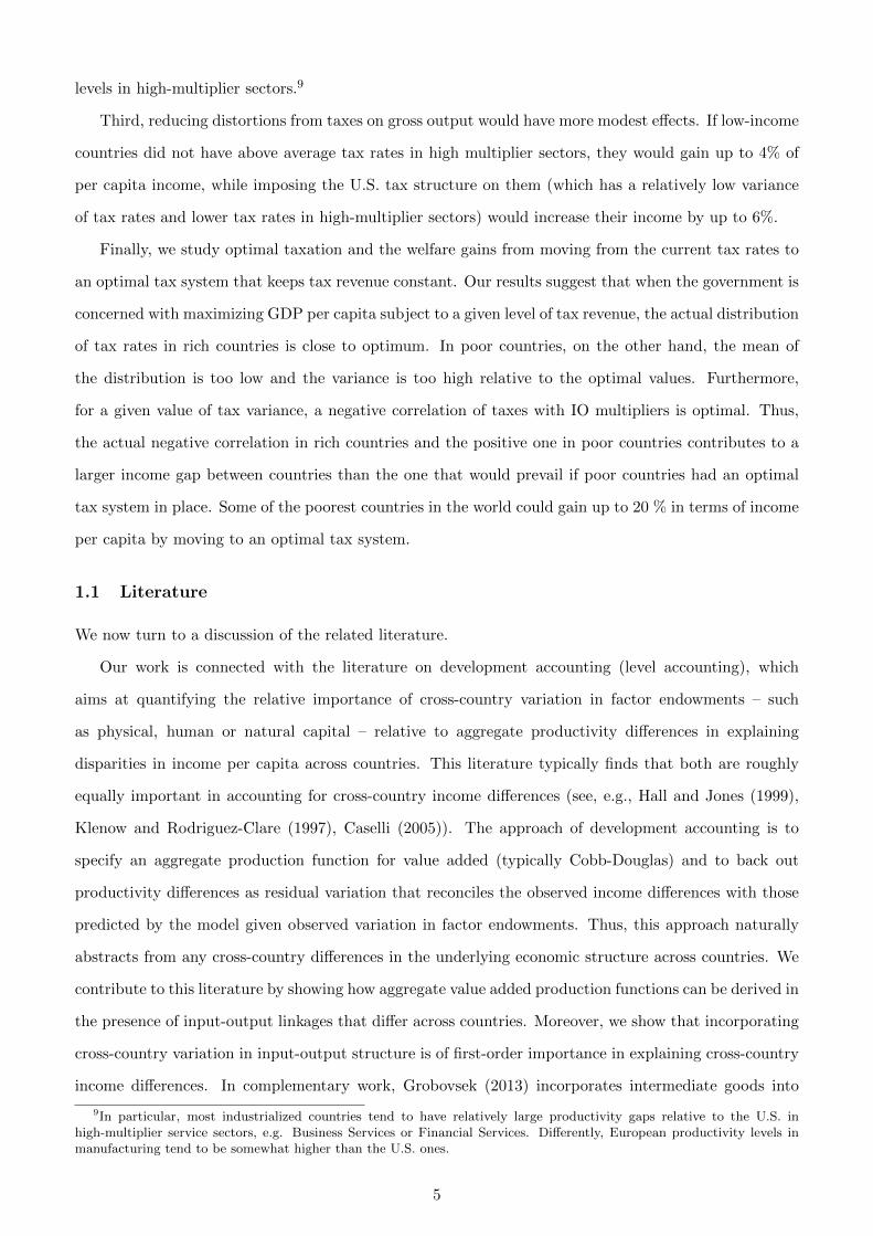
Third, reducing distortions from taxes on gross output would have more modest effects. If low-income

countries did not have above average tax rates in high multiplier sectors, they would gain up to 4% of

per capita income, while imposing the U.S. tax structure on them (which has a relatively low variance

of tax rates and lower tax rates in high-multiplier sectors) would increase their income by up to 6%.

Finally, we study optimal taxation and the welfare gains from moving from the current tax rates to

an optimal tax system that keeps tax revenue constant. Our results suggest that when the government is

concerned with maximizing GDP per capita subject to a given level of tax revenue, the actual distribution

of tax rates in rich countries is close to optimum. In poor countries, on the other hand, the mean of

the distribution is too low and the variance is too high relative to the optimal values. Furthermore,

for a given value of tax variance, a negative correlation of taxes with IO multipliers is optimal. Thus,

the actual negative correlation in rich countries and the positive one in poor countries contributes to a

larger income gap between countries than the one that would prevail if poor countries had an optimal

tax system in place. Some of the poorest countries in the world could gain up to 20 % in terms of income

per capita by moving to an optimal tax system.

1.1 Literature

We now turn to a discussion of the related literature.

Our work is connected with the literature on development accounting (level accounting), which

aims at quantifying the relative importance of cross-country variation in factor endowments – such

as physical, human or natural capital – relative to aggregate productivity differences in explaining

disparities in income per capita across countries. This literature typically finds that both are roughly

equally important in accounting for cross-country income differences (see, e.g., Hall and Jones (1999),

Klenow and Rodriguez-Clare (1997), Caselli (2005)). The approach of development accounting is to

specify an aggregate production function for value added (typically Cobb-Douglas) and to back out

productivity differences as residual variation that reconciles the observed income differences with those

predicted by the model given observed variation in factor endowments. Thus, this approach naturally

abstracts from any cross-country differences in the underlying economic structure across countries. We

contribute to this literature by showing how aggregate value added production functions can be derived in

the presence of input-output linkages that differ across countries. Moreover, we show that incorporating

cross-country variation in input-output structure is of first-order importance in explaining cross-country

income differences. In complementary work, Grobovsek (2013) incorporates intermediate goods into

9In particular, most industrialized countries tend to have relatively large productivity gaps relative to the U.S. inhigh-multiplier service sectors, e.g. Business Services or Financial Services. Differently, European productivity levels inmanufacturing tend to be somewhat higher than the U.S. ones.

5

a two-sector model with intermediates and finds that poor countries have much lower productivities

in intermediate compared to final production, which can potentially explain a substantial portion of

cross-country income differences.

The importance of intermediate linkages and IO multipliers for aggregate income differences has been

highlighted by Fleming (1955), Hirschmann (1958), and, more recently, by Ciccone (2002) and Jones

(2011 a,b). The last two authors emphasize that if the intermediate share in gross output is sizable,

there exist large multiplier effects: small firm (or industry-level) productivity differences or distortions

that lead to misallocation of resources across sectors or plants can add up to large aggregate effects.

These authors make this point in a purely theoretical context. While our setup in principle allows

for a mechanism whereby intermediate linkages amplify small sectoral productivity differences, we find

that there is little empirical evidence for this channel: cross-country sectoral productivity differences

estimated from the data are even larger than aggregate ones and the sparse IO structure of low-income

countries helps to mitigate the impact of very low productivity levels in some sectors on aggregate

outcomes.

Our finding that sectoral productivity differences between rich and poor countries are larger than

aggregate ones is instead similar to those of the literature on dual economies and sectoral productivity

gaps in agriculture (Caselli, 2005; Restuccia, Yang, and Zhu, 2008; Chanda and Dalgaard, 2008; Vollrath,

2009, Gollin et al., 2014). Also closely related to our work – which focuses on changes in the IO

structure as countries’ income level increases – a literature on structural transformation emphasizes

sectoral productivity gaps and transitions from agriculture to manufacturing and services as a reason

for cross-country income differences (see, e.g., Duarte and Restuccia, 2010 for a recent contribution).

However, this literature abstracts from intermediate linkages between industries.

In terms of modeling approach, our paper adopts the framework of the multi-sector real business cycle

model with IO linkages of Long and Plosser (1983); in addition we model the input-output structure

as a network, quite similarly to the setup of Acemoglu et. al. (2012). In contrast to these studies,

which deal with the relationship between sectoral productivity shocks and aggregate fluctuations, we are

interested in the question how sectoral productivity levels interact with the IO structure to determine

aggregate income levels. Moreover, while the aforementioned papers are mostly theoretical, we provide

a comprehensive empirical study of the impact of cross-country differences in IO structure on income.

Other recent related contributions are Oberfield (2014) and Carvalho and Voigtlander (2014), who

develop an abstract theory of endogenous input-output network formation, and Boehm (2014), who

focuses on the role of contract enforcement on aggregate productivity differences in a quantitative struc-

tural model with IO linkages. Differently from these papers, we do not try to model the IO structure

6

as arising endogenously and we take sectoral productivity differences as exogenous. Instead, we aim at

understanding how given differences in IO structure and sectoral productivities translate into aggregate

income differences.

The number of empirical studies investigating cross-country differences in IO structure is quite lim-

ited. In the most comprehensive study up to that date, Chenery, Robinson, and Syrquin (1986) find that

the intermediate input share of manufacturing increases with industrialization and – consistent with our

evidence – that input-output matrices become less sparse as countries industrialize. Most closely related

to our paper is the contemporaneous work by Bartelme and Gorodnichenko (2014). They also collect

data on IO tables for many countries and investigate the relationship between IO linkages and aggregate

income. In reduced form regressions of aggregate input-output multipliers on income per worker, they

find a positive correlation between the two variables. Moreover, they investigate how distortions affect

IO linkages and income levels. Differently from the present paper, they do not use data on sectoral pro-

ductivities and tax rates and they do not use network theory to represent IO tables. As a consequence,

they do not investigate how differences in the distribution of multipliers and their correlations with

productivities and tax rates impact on aggregate income, which is the focus of our work. Furthermore,

they do not address the question of optimal taxation given the IO structure, while we do.

The outline of the paper is as follows. The next section describes our dataset and present some

descriptive statistics. In the following section, we lay out our theoretical model and derive an expression

for aggregate GDP in terms of the IO network characteristics. Subsequently, we turn to the estimation

and model fit and finally, we present a number of counterfactual results. The final section presents our

conclusion.

2 Dataset and descriptive analysis

2.1 Data

IO tables measure the flow of intermediate products between different plants or establishments, both

within and between sectors. The ji’th entry of the IO table is the value of output from establishments in

industry j that is purchased by different establishments in industry i for use in production.10 Dividing

the flow of industry j to industry i by gross output of industry i, one obtains the IO coefficient γji,

which states the cents of industry j output used in the production of each dollar of industry i output.

To construct a dataset of input-output tables for a range of high- and low-income countries and

to compute sectoral total factor productivities, tax rates and countries’ aggregate income and factor

10Intermediate output must be traded between establishments in order to be recorded in the IO table, while flows thatoccur within a given plant are not measured.

7

endowments, we combine information from three datasets: the World Input-Output Database (WIOD,

Timmer, 2012), the Global Trade Analysis Project (GTAP version 6, Dimaranan, 2006), and the Penn

World Tables, Version 7.1 (PWT 7.1, Heston et al., 2012).11

The first dataset, WIOD, contains IO data for 39 countries classified into 35 sectors in the year 2005.

The list of countries and sectors is provided in Appendix Tables 7 and 9. WIOD data also provides all

the information necessary to compute gross-output-based sectoral total factor productivity: real gross

output, real sectoral capital and labor inputs, Purchasing Power Parity price indices for sectoral gross

output and sectoral factor payments to labor and capital. Moreover, WIOD provides information on

sectoral net tax rates (taxes minus subsidies) on gross output. The second dataset, GTAP version

6, contains data for 70 countries and 37 sectors in the year 2004. We use GTAP data to get more

information about IO tables of low-income countries and we construct IO coefficients for all 70 countries.

Finally, the third dataset, PWT 7.1, includes data on income per capita in PPP, aggregate physical

capital stocks and labor endowments for 155 countries in the year 2005. In our analysis, PWT data is

used to make out-of-sample predictions with our model.

2.2 IO structure

To begin with, we provide some descriptive analysis of the input-output structure of the set of countries

in our data. To this end, we consider the sample of countries from the GTAP database. First, we

sum IO multipliers of all sectors to compute the aggregate IO multiplier. While a sectoral multiplier

indicates the change in aggregate income caused by a one percent change in productivity of one sector,

the aggregate IO multiplier tells us by how much aggregate income changes due to a one percent change

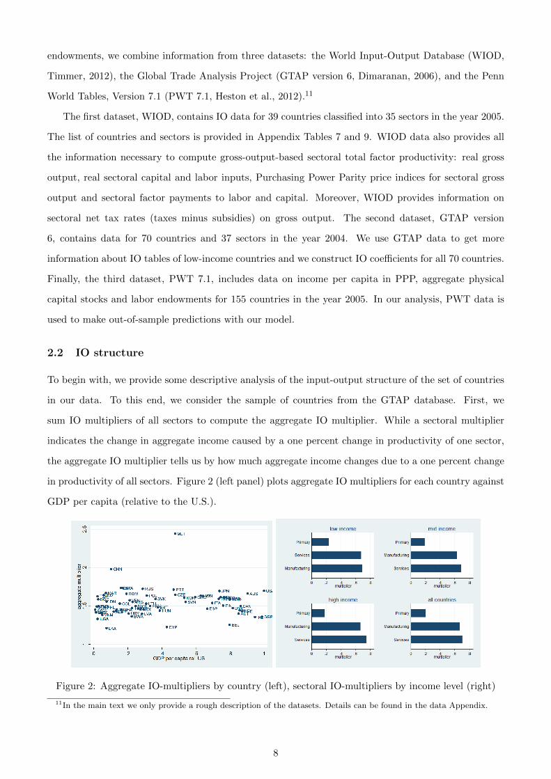
in productivity of all sectors. Figure 2 (left panel) plots aggregate IO multipliers for each country against

GDP per capita (relative to the U.S.).

Figure 2: Aggregate IO-multipliers by country (left), sectoral IO-multipliers by income level (right)

11In the main text we only provide a rough description of the datasets. Details can be found in the data Appendix.

8

We observe that aggregate multipliers for the GTAP sample average around 1.6 and are uncorrelated

with the level of income. This implies that a one percent increase in productivity of all sectors raises

per capita income by around 1.6 percent on average.12

Next, we compute separately the aggregate IO multipliers for the three major sector categories:

primary sectors (which include Agriculture, Coal, Oil and Gas Extraction and Mining), manufacturing

and services. Figure 2 (right panel) plots these multipliers by income level. Here, we divide countries

into low income (less than 10,000 PPP Dollars of per capita income), middle income (10,000-20,000 PPP

Dollars of per capita income) and high income (more than 20,000 PPP Dollars of per capita income).

We find that multipliers are largest in services (around 0.65 on average), slightly lower in manufac-

turing (around 0.62) and smallest in primary sectors (around 0.2). As before, the level of income does

not play an important role in this result: the comparison is similar for countries at all levels of income

per capita.13 We conclude that at the aggregate-economy level or for major sectoral aggregates there

are no systematic differences in IO structure across countries.

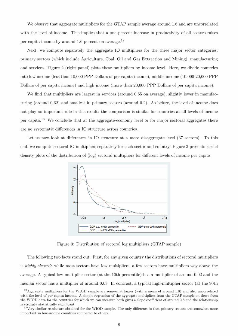
Let us now look at differences in IO structure at a more disaggregate level (37 sectors). To this

end, we compute sectoral IO multipliers separately for each sector and country. Figure 3 presents kernel

density plots of the distribution of (log) sectoral multipliers for different levels of income per capita.

Figure 3: Distribution of sectoral log multipliers (GTAP sample)

The following two facts stand out. First, for any given country the distributions of sectoral multipliers

is highly skewed : while most sectors have low multipliers, a few sectors have multipliers way above the

average. A typical low-multiplier sector (at the 10th percentile) has a multiplier of around 0.02 and the

median sector has a multiplier of around 0.03. In contrast, a typical high-multiplier sector (at the 90th

12Aggregate multipliers for the WIOD sample are somewhat larger (with a mean of around 1.8) and also uncorrelatedwith the level of per capita income. A simple regression of the aggregate multipliers from the GTAP sample on those fromthe WIOD data for the countries for which we can measure both gives a slope coefficient of around 0.8 and the relationshipis strongly statistically significant

13Very similar results are obtained for the WIOD sample. The only difference is that primary sectors are somewhat moreimportant in low-income countries compared to others.

9

percentile) has a multiplier of around 0.065, while a sector at the 99th percentile has a multiplier of

around 0.134.

Second, the distribution of multipliers in low-income countries is more skewed towards the extremes

than it is in high-income countries. In poor countries, almost all sectors have very low multipliers and a

few sectors have very high multipliers. Differently, in rich countries the distribution of sectoral multipliers

has significantly more mass in the center.

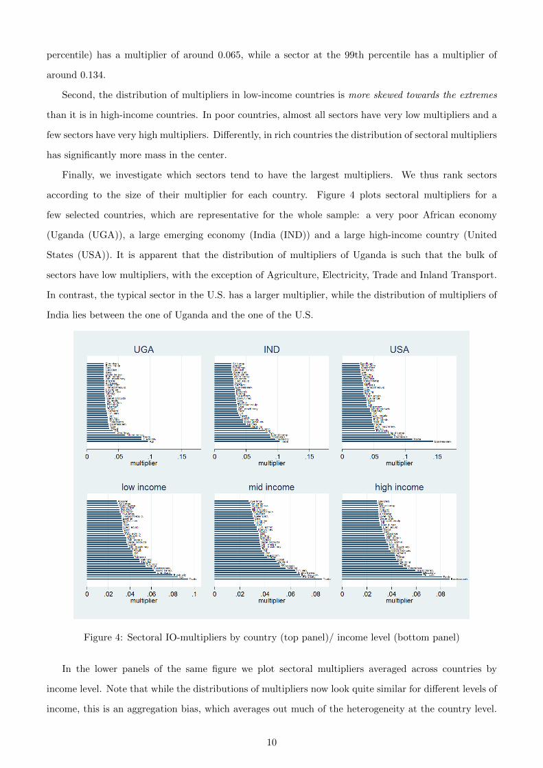
Finally, we investigate which sectors tend to have the largest multipliers. We thus rank sectors

according to the size of their multiplier for each country. Figure 4 plots sectoral multipliers for a

few selected countries, which are representative for the whole sample: a very poor African economy

(Uganda (UGA)), a large emerging economy (India (IND)) and a large high-income country (United

States (USA)). It is apparent that the distribution of multipliers of Uganda is such that the bulk of

sectors have low multipliers, with the exception of Agriculture, Electricity, Trade and Inland Transport.

In contrast, the typical sector in the U.S. has a larger multiplier, while the distribution of multipliers of

India lies between the one of Uganda and the one of the U.S.

Figure 4: Sectoral IO-multipliers by country (top panel)/ income level (bottom panel)

In the lower panels of the same figure we plot sectoral multipliers averaged across countries by

income level. Note that while the distributions of multipliers now look quite similar for different levels of

income, this is an aggregation bias, which averages out much of the heterogeneity at the country level.

10

From this Figure we see that in low-income countries the sectors with the highest multipliers are Trade,

Electricity, Agriculture, Chemicals, and Inland Transport. Turning to the set of middle- and high-income

countries, the most important sectors in terms of multipliers are Trade, Electricity, Business Services,

Inland Transport and Financial Services.

Thus, overall the sectors with the highest multipliers are mostly service sectors. Agriculture is

one notable exception for countries with an income level below 10,000 PPP dollars, where agricultural

products are an input to many sectors. Moreover, in low-income countries Chemicals and Petroleum

Refining tend to have a large multiplier, too. In general though, typical manufacturing sectors have

intermediate multipliers (around 0.04). Finally, the sectors with the lowest multipliers are also mostly

services: Apparel, Air Transport, Water Transport, Gas Distribution and Dwellings (Owner-occupied

houses). Given the large number of sectors with low multipliers, the specific sectors differ more across

income groups. The figures for individual countries confirm the overall picture.

2.3 Productivities and taxes

We now provide some descriptive evidence on sectoral total factor productivity (TFPs) relative to the

U.S., tax rates as well as their correlations with sectoral multipliers. Here, we use the countries in the

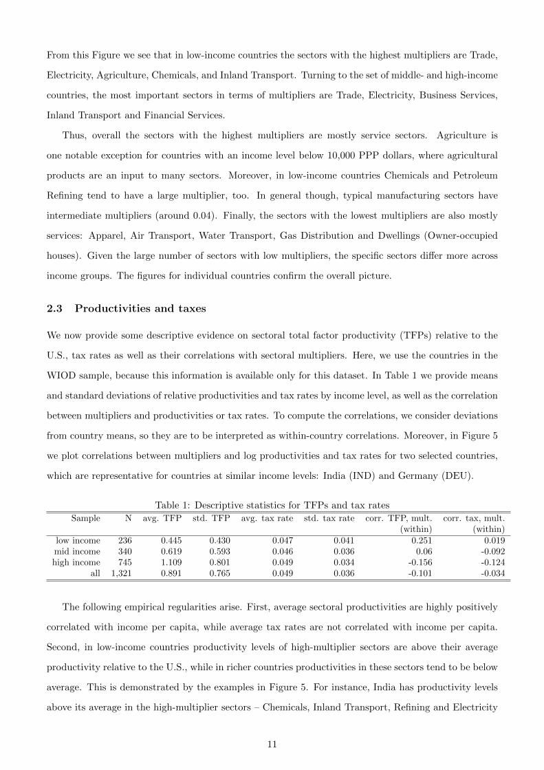
WIOD sample, because this information is available only for this dataset. In Table 1 we provide means

and standard deviations of relative productivities and tax rates by income level, as well as the correlation

between multipliers and productivities or tax rates. To compute the correlations, we consider deviations

from country means, so they are to be interpreted as within-country correlations. Moreover, in Figure 5

we plot correlations between multipliers and log productivities and tax rates for two selected countries,

which are representative for countries at similar income levels: India (IND) and Germany (DEU).

Table 1: Descriptive statistics for TFPs and tax rates

Sample N avg. TFP std. TFP avg. tax rate std. tax rate corr. TFP, mult. corr. tax, mult.(within) (within)

low income 236 0.445 0.430 0.047 0.041 0.251 0.019mid income 340 0.619 0.593 0.046 0.036 0.06 -0.092high income 745 1.109 0.801 0.049 0.034 -0.156 -0.124

all 1,321 0.891 0.765 0.049 0.036 -0.101 -0.034

The following empirical regularities arise. First, average sectoral productivities are highly positively

correlated with income per capita, while average tax rates are not correlated with income per capita.

Second, in low-income countries productivity levels of high-multiplier sectors are above their average

productivity relative to the U.S., while in richer countries productivities in these sectors tend to be below

average. This is demonstrated by the examples in Figure 5. For instance, India has productivity levels

above its average in the high-multiplier sectors – Chemicals, Inland Transport, Refining and Electricity

11

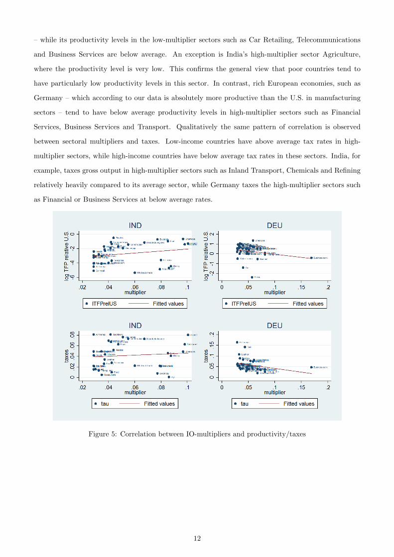
– while its productivity levels in the low-multiplier sectors such as Car Retailing, Telecommunications

and Business Services are below average. An exception is India’s high-multiplier sector Agriculture,

where the productivity level is very low. This confirms the general view that poor countries tend to

have particularly low productivity levels in this sector. In contrast, rich European economies, such as

Germany – which according to our data is absolutely more productive than the U.S. in manufacturing

sectors – tend to have below average productivity levels in high-multiplier sectors such as Financial

Services, Business Services and Transport. Qualitatively the same pattern of correlation is observed

between sectoral multipliers and taxes. Low-income countries have above average tax rates in high-

multiplier sectors, while high-income countries have below average tax rates in these sectors. India, for

example, taxes gross output in high-multiplier sectors such as Inland Transport, Chemicals and Refining

relatively heavily compared to its average sector, while Germany taxes the high-multiplier sectors such

as Financial or Business Services at below average rates.

Figure 5: Correlation between IO-multipliers and productivity/taxes

12

3 Theoretical framework

3.1 Model

In this section we present our theoretical framework, which will be used in the remainder of our analysis.

Consider a static multi-sector economy with taxes. n competitive sectors each produce a distinct good

that can be used either for final consumption or as an input for production. The technology of sector

i ∈ 1 : n is Cobb-Douglas with constant returns to scale. Namely, the output of sector i, denoted by qi,

is

qi = Λi(kαi l

1−αi

)1−γi dγ1i1i d

γ2i2i · ... · d

γnini , (1)

where Λi is the exogenous total factor productivity of sector i, ki and li are the quantities of capital and

labor used by sector i and dji is the quantity of good j used in production of good i (intermediate goods

produced by sector j).14 The exponent γji ∈ [0, 1) represents the share of good j in the production

technology of firms in sector i, and γi =∑n

j=1 γji ∈ (0, 1) is the total share of intermediate goods in

gross output of sector i. Parameters α, 1−α ∈ (0, 1) are shares of capital and labor in the remainder of

the inputs (value added).

Given the Cobb-Douglas technology in (1) and competitive factor markets, γji’s also correspond to

the entries of the IO matrix, measuring the value of spending on input j per dollar of production of good

i.15 We denote this IO matrix by Γ. Then the entries of the j’th row of matrix Γ represent the values of

spending on a given input j per dollar of production of each sector in the economy. On the other hand,

the elements of the i’th column of matrix Γ are the values of spending on inputs from each sector in the

economy per dollar of production of a given good i.16

Resources in the economy are allocated with distortions. In this paper distortions are regarded as

sector-specific proportional taxes on gross output. For the main part of the analysis we consider taxes

as exogenous reductions in firms’ revenue, and the total revenue from taxation is spent on government

expenditures. Then in the last section we endogenize taxes by addressing the problem of optimal taxation.

14In section 6 and Appendix A we consider the case of an open economy, where sectors’ production technology employsboth domestic and imported intermediate goods.

15Strictly speaking, the entries in the IO matrix have to be adjusted for taxes. To see this, consider sector i’s first-ordercondition with respect to output of sector j, which is given by: (1− τi)γjipiqi = pjdji. Thus, the empirical IO coefficients(demand of sector i for sector j per dollar of sector i’s output) in basic prices pi ≡ pi(1 − τi) (excluding transport costs

and taxes) are given by IObji =pjdjipiqi

=pj(1−τj)djipi(1−τi)qi

= γji(1 − τj). Consequently, the IO coefficient of the using sector i inbasic prices depends negatively on the tax rate in the supplying sector j. Next, consider the empirical IO coefficients inuser prices (including taxes and transport costs): IOuji =

pjdjipiqi

= γji(1 − τi). Thus, the IO coefficient of sector i in userprices depends negatively on its own tax rate τi. To the extent that taxes correspond to actual observable tax rates on grossoutput, we can adjust empirical IO coefficients for them. However, if taxes represent unmeasured distortions or wedges, weare unable to correct IO coefficients for their impact. However, in footnote 23 below we explain that unmeasured distortionsdo not systematically bias IO multipliers as long as IO coefficients are measured in user prices and production functionsare Cobb-Douglas.

16According to our notation, the sum of elements in the i’th column of matrix Γ is equal to γi, the total intermediateshare of sector i.

13

Throughout the paper taxes in sector i are denoted by τi. We assume that τi ≤ 1 and interpret negative

taxes as subsidies.

Output of sector i can be used either for final consumption, yi, or as an intermediate good:

yi +n∑j=1

dij = qi i = 1 : n (2)

Consumption increases households’ wellbeing. But rather than specifying a utility function of house-

holds over n different consumption goods, we aggregate these final consumption goods into a single final

good through another Cobb-Douglas production function:

Y = y1n1 · ... · y

1nn . (3)

This aggregate final good is used in two ways, as households’ consumption, C, and government con-

sumption, G, that is, Y = C + G. Note that the symmetry in exponents of the final good production

function implies the symmetry in consumption demand for all goods. This assumption is useful as it

allows us to focus on the effects of the IO structure and the interaction between the structure and sectors’

productivities and tax rates in an otherwise symmetric framework. It is, however, straightforward to

introduce asymmetry in consumption demand by defining the vector of demand shares β = (β1, .., βn),

where βi 6= βj for i 6= j and∑n

i=1 βi = 1. The corresponding final good production function is then

Y = yβ11 · ... · y

βnn . This more general framework is analyzed in section 6 and in Appendix A, where we

consider extensions of our benchmark model.

Finally, the total supply of capital and labor in this economy are assumed to be exogenous and fixed

at the levels of K and 1, respectively:

n∑i=1

ki = K, (4)

n∑i=1

li = 1. (5)

To complete the description of the model, we provide a formal definition of a competitive equilibrium

with distortions.

Definition A competitive equilibrium is a collection of quantities qi, ki, li, yi, dij , Y , C, G and prices

pi, p, w, and r for i ∈ 1 : n such that

1. yi solves the profit maximization problem of a representative firm in a perfectly competitive final

14

good’s market:

max{yi}

py1n1 · ... · y

1nn −

n∑i=1

piyi,

taking {pi}, p as given.

2. {dij}, ki, li solve the profit maximization problem of a representative firm in the perfectly com-

petitive sector i for i ∈ 1 : n:

max{dij},ki,li

(1− τi)piΛi(kαi l

1−αi

)1−γi dγ1i1i d

γ2i2i · ... · d

γnini −

n∑j=1

pjdji − rki − wli,

taking {pi} as given (τi and Λi are exogenous).

3. Households’ budget constraint determines C: C = w + rK.

4. Government’s budget constraint determines G: G =∑n

i=1 τipiqi.

5. Markets clear:

(a) r clears the capital market:∑n

i=1 ki = K,

(b) w clears the labor market:∑n

i=1 li = 1,

(c) pi clears the sector i’s market: yi +∑n

j=1 dij = qi,

(d) p clears the final good’s market: Y = C +G.

6. Production function for qi is qi = Λi(kαi l

1−αi

)1−γi dγ1i1i d

γ2i2i · ... · d

γnini .

7. Production function for Y , is Y = y1n1 · ... · y

1nn .

Note that households’and government consumption are simply determined by the budget constraints,

so that there is no decision for the households or government to be made. Moreover, the total production

of the aggregate final good, Y , which is equal to∑n

i=1 piyi due to the Cobb-Douglas technology in a

competitive final good’s market, represents GDP (total value added) per capita.

3.2 Equilibrium

The following proposition characterizes the equilibrium value of the logarithm of GDP per capita, which

we later refer to equivalently as aggregate output or aggregate income or value added of the economy.

15

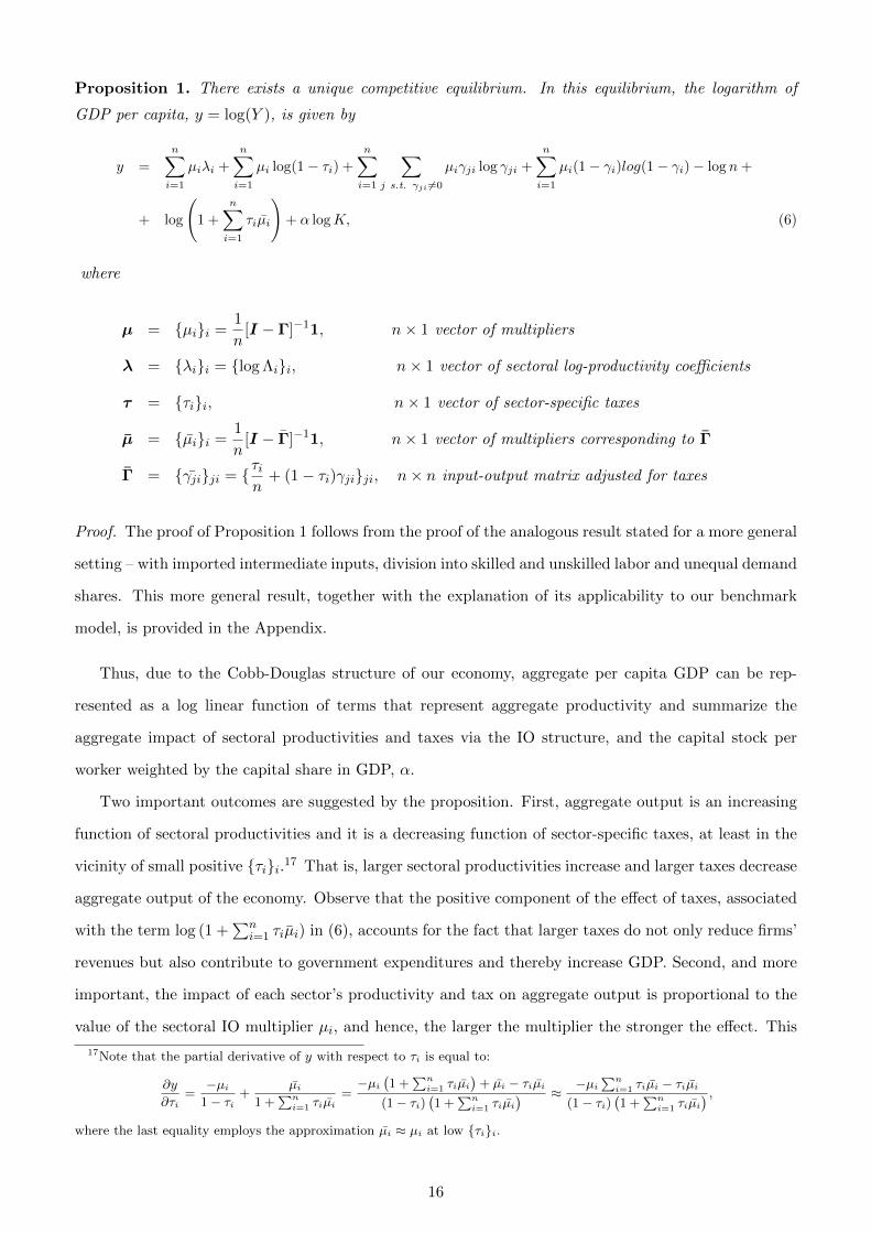
Proposition 1. There exists a unique competitive equilibrium. In this equilibrium, the logarithm of

GDP per capita, y = log(Y ), is given by

y =

n∑i=1

µiλi +

n∑i=1

µi log(1− τi) +

n∑i=1

∑j s.t. γji 6=0

µiγji log γji +

n∑i=1

µi(1− γi)log(1− γi)− log n+

+ log

(1 +

n∑i=1

τiµi

)+ α logK, (6)

where

µ = {µi}i =1

n[I − Γ]−11, n× 1 vector of multipliers

λ = {λi}i = {log Λi}i, n× 1 vector of sectoral log-productivity coefficients

τ = {τi}i, n× 1 vector of sector-specific taxes

µ = {µi}i =1

n[I − Γ]−11, n× 1 vector of multipliers corresponding to Γ

Γ = {γji}ji = {τin

+ (1− τi)γji}ji, n× n input-output matrix adjusted for taxes

Proof. The proof of Proposition 1 follows from the proof of the analogous result stated for a more general

setting – with imported intermediate inputs, division into skilled and unskilled labor and unequal demand

shares. This more general result, together with the explanation of its applicability to our benchmark

model, is provided in the Appendix.

Thus, due to the Cobb-Douglas structure of our economy, aggregate per capita GDP can be rep-

resented as a log linear function of terms that represent aggregate productivity and summarize the

aggregate impact of sectoral productivities and taxes via the IO structure, and the capital stock per

worker weighted by the capital share in GDP, α.

Two important outcomes are suggested by the proposition. First, aggregate output is an increasing

function of sectoral productivities and it is a decreasing function of sector-specific taxes, at least in the

vicinity of small positive {τi}i.17 That is, larger sectoral productivities increase and larger taxes decrease

aggregate output of the economy. Observe that the positive component of the effect of taxes, associated

with the term log (1 +∑n

i=1 τiµi) in (6), accounts for the fact that larger taxes do not only reduce firms’

revenues but also contribute to government expenditures and thereby increase GDP. Second, and more

important, the impact of each sector’s productivity and tax on aggregate output is proportional to the

value of the sectoral IO multiplier µi, and hence, the larger the multiplier the stronger the effect. This

17Note that the partial derivative of y with respect to τi is equal to:

∂y

∂τi=−µi

1− τi+

µi1 +

∑ni=1 τiµi

=−µi

(1 +

∑ni=1 τiµi

)+ µi − τiµi

(1− τi)(1 +

∑ni=1 τiµi

) ≈−µi

∑ni=1 τiµi − τiµi

(1− τi)(1 +

∑ni=1 τiµi

) ,where the last equality employs the approximation µi ≈ µi at low {τi}i.

16

means that the positive effect of higher sectoral productivity and the negative effect of a higher tax on

aggregate output are stronger in sectors with larger multipliers.18

The vector of sectoral multipliers, in turn, is determined by the features of the IO matrix through

the Leontief inverse, [I − Γ]−1.19 The interpretation and properties of this matrix as well as a simpler

representation of the vector of multipliers are discussed in the next section. We show that sectoral

multipliers can be directly expressed in terms of simple characteristics of the IO structure of the economy

and have a straightforward interpretation as a measure of sectors’ centrality in the IO network. Namely,

larger IO multipliers correspond to sectors that are more central in a well-defined sense. Then in view

of Proposition 1, this implies that the impact of sectoral productivities and taxes on aggregate output

of the economy tends to be stronger for sectors that are located more centrally in the IO network.

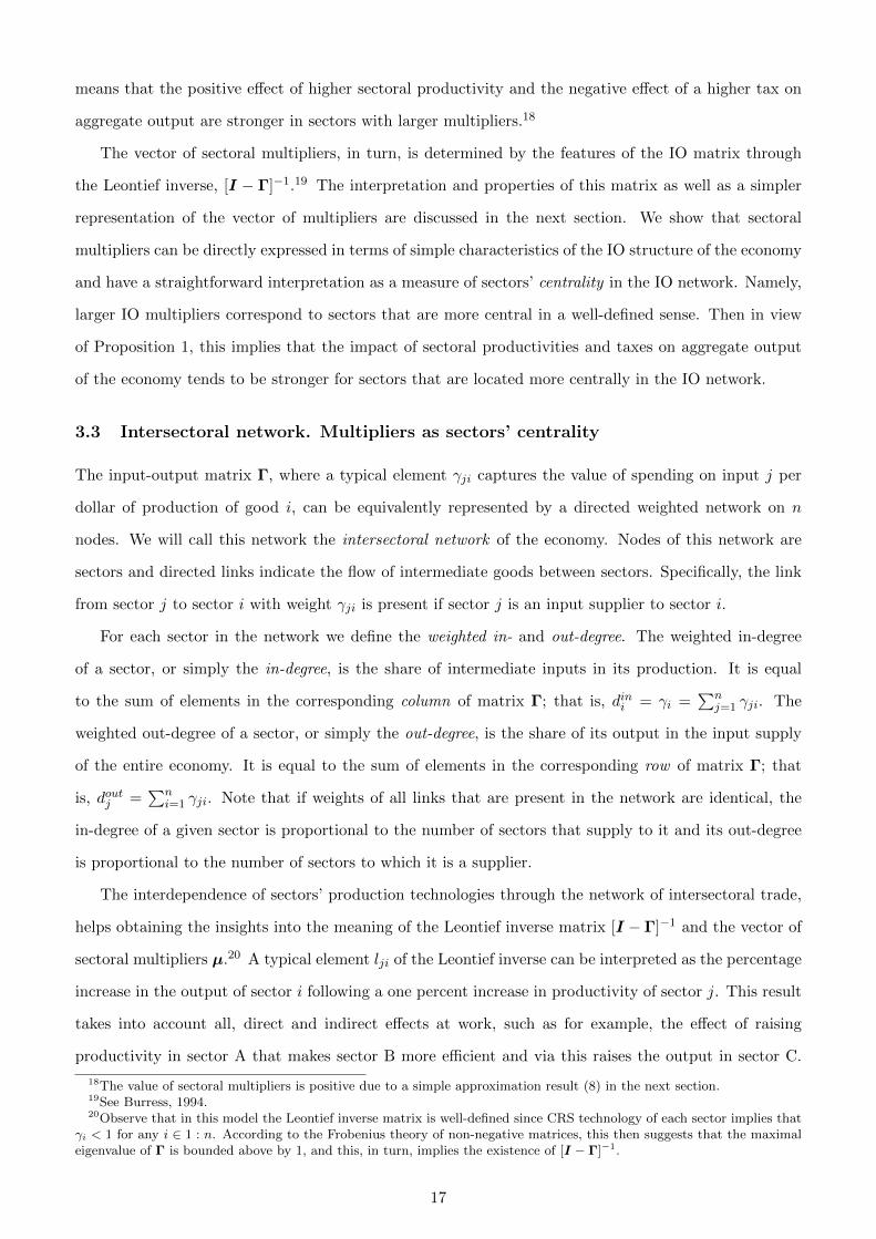
3.3 Intersectoral network. Multipliers as sectors’ centrality

The input-output matrix Γ, where a typical element γji captures the value of spending on input j per

dollar of production of good i, can be equivalently represented by a directed weighted network on n

nodes. We will call this network the intersectoral network of the economy. Nodes of this network are

sectors and directed links indicate the flow of intermediate goods between sectors. Specifically, the link

from sector j to sector i with weight γji is present if sector j is an input supplier to sector i.

For each sector in the network we define the weighted in- and out-degree. The weighted in-degree

of a sector, or simply the in-degree, is the share of intermediate inputs in its production. It is equal

to the sum of elements in the corresponding column of matrix Γ; that is, dini = γi =∑n

j=1 γji. The

weighted out-degree of a sector, or simply the out-degree, is the share of its output in the input supply

of the entire economy. It is equal to the sum of elements in the corresponding row of matrix Γ; that

is, doutj =∑n

i=1 γji. Note that if weights of all links that are present in the network are identical, the

in-degree of a given sector is proportional to the number of sectors that supply to it and its out-degree

is proportional to the number of sectors to which it is a supplier.

The interdependence of sectors’ production technologies through the network of intersectoral trade,

helps obtaining the insights into the meaning of the Leontief inverse matrix [I − Γ]−1 and the vector of

sectoral multipliers µ.20 A typical element lji of the Leontief inverse can be interpreted as the percentage

increase in the output of sector i following a one percent increase in productivity of sector j. This result

takes into account all, direct and indirect effects at work, such as for example, the effect of raising

productivity in sector A that makes sector B more efficient and via this raises the output in sector C.

18The value of sectoral multipliers is positive due to a simple approximation result (8) in the next section.19See Burress, 1994.20Observe that in this model the Leontief inverse matrix is well-defined since CRS technology of each sector implies that

γi < 1 for any i ∈ 1 : n. According to the Frobenius theory of non-negative matrices, this then suggests that the maximaleigenvalue of Γ is bounded above by 1, and this, in turn, implies the existence of [I − Γ]−1.

17

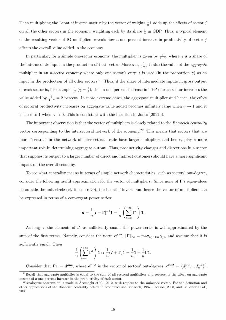
Then multiplying the Leontief inverse matrix by the vector of weights 1n1 adds up the effects of sector j

on all the other sectors in the economy, weighting each by its share 1n in GDP. Thus, a typical element

of the resulting vector of IO multipliers reveals how a one percent increase in productivity of sector j

affects the overall value added in the economy.

In particular, for a simple one-sector economy, the multiplier is given by 11−γ , where γ is a share of

the intermediate input in the production of that sector. Moreover, 11−γ is also the value of the aggregate

multiplier in an n-sector economy where only one sector’s output is used (in the proportion γ) as an

input in the production of all other sectors.21 Thus, if the share of intermediate inputs in gross output

of each sector is, for example, 12 (γ = 1

2), then a one percent increase in TFP of each sector increases the

value added by 11−γ = 2 percent. In more extreme cases, the aggregate multiplier and hence, the effect

of sectoral productivity increases on aggregate value added becomes infinitely large when γ → 1 and it

is close to 1 when γ → 0. This is consistent with the intuition in Jones (2011b).

The important observation is that the vector of multipliers is closely related to the Bonacich centrality

vector corresponding to the intersectoral network of the economy.22 This means that sectors that are

more ”central” in the network of intersectoral trade have larger multipliers and hence, play a more

important role in determining aggregate output. Thus, productivity changes and distortions in a sector

that supplies its output to a larger number of direct and indirect customers should have a more significant

impact on the overall economy.

To see what centrality means in terms of simple network characteristics, such as sectors’ out-degree,

consider the following useful approximation for the vector of multipliers. Since none of Γ’s eigenvalues

lie outside the unit circle (cf. footnote 20), the Leontief inverse and hence the vector of multipliers can

be expressed in terms of a convergent power series:

µ =1

n[I − Γ]−11 =

1

n

(+∞∑k=0

Γk

)1.

As long as the elements of Γ are sufficiently small, this power series is well approximated by the

sum of the first terms. Namely, consider the norm of Γ, ‖Γ‖∞ = maxi,j∈1:n γji, and assume that it is

sufficiently small. Then

1

n

(+∞∑k=0

Γk

)1 ≈ 1

n(I + Γ)1 =

1

n1 +

1

nΓ1.

Consider that Γ1 = dout, where dout is the vector of sectors’ out-degrees, dout =(dout1 , .., doutn

)′.

21Recall that aggregate multiplier is equal to the sum of all sectoral multipliers and represents the effect on aggregateincome of a one percent increase in the productivity of each sector.

22Analogous observation is made in Acemoglu et al., 2012, with respect to the influence vector. For the definition andother applications of the Bonacich centrality notion in economics see Bonacich, 1987, Jackson, 2008, and Ballester et al.,2006.

18

This leads to the following simple representation of the vector of multipliers:

µ ≈ 1

n1 +

1

ndout, (7)

so that for any sector i,

µi ≈1

n+

1

ndouti , i = 1 : n. (8)

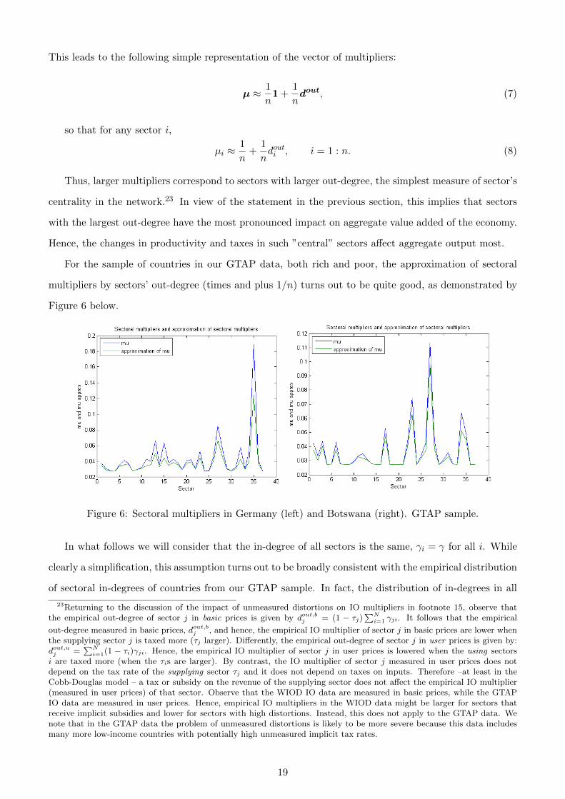
Thus, larger multipliers correspond to sectors with larger out-degree, the simplest measure of sector’s

centrality in the network.23 In view of the statement in the previous section, this implies that sectors

with the largest out-degree have the most pronounced impact on aggregate value added of the economy.

Hence, the changes in productivity and taxes in such ”central” sectors affect aggregate output most.

For the sample of countries in our GTAP data, both rich and poor, the approximation of sectoral

multipliers by sectors’ out-degree (times and plus 1/n) turns out to be quite good, as demonstrated by

Figure 6 below.

Figure 6: Sectoral multipliers in Germany (left) and Botswana (right). GTAP sample.

In what follows we will consider that the in-degree of all sectors is the same, γi = γ for all i. While

clearly a simplification, this assumption turns out to be broadly consistent with the empirical distribution

of sectoral in-degrees of countries from our GTAP sample. In fact, the distribution of in-degrees in all

23Returning to the discussion of the impact of unmeasured distortions on IO multipliers in footnote 15, observe thatthe empirical out-degree of sector j in basic prices is given by dout,bj = (1 − τj)

∑Ni=1 γji. It follows that the empirical

out-degree measured in basic prices, dout,bj , and hence, the empirical IO multiplier of sector j in basic prices are lower whenthe supplying sector j is taxed more (τj larger). Differently, the empirical out-degree of sector j in user prices is given by:dout,uj =

∑Ni=1(1 − τi)γji. Hence, the empirical IO multiplier of sector j in user prices is lowered when the using sectors

i are taxed more (when the τis are larger). By contrast, the IO multiplier of sector j measured in user prices does notdepend on the tax rate of the supplying sector τj and it does not depend on taxes on inputs. Therefore –at least in theCobb-Douglas model – a tax or subsidy on the revenue of the supplying sector does not affect the empirical IO multiplier(measured in user prices) of that sector. Observe that the WIOD IO data are measured in basic prices, while the GTAPIO data are measured in user prices. Hence, empirical IO multipliers in the WIOD data might be larger for sectors thatreceive implicit subsidies and lower for sectors with high distortions. Instead, this does not apply to the GTAP data. Wenote that in the GTAP data the problem of unmeasured distortions is likely to be more severe because this data includesmany more low-income countries with potentially high unmeasured implicit tax rates.

19

countries is strongly peaked around the mean value, which suggests that on the demand side sectors

are rather homogeneous, i.e., they use intermediate goods in approximately equal proportions.24 This is

in sharp contrast with the observed distribution of sectoral out-degrees that puts most weight on small

values of out-degrees but also assigns a non-negligible weight to the out-degrees that are way above the

average, displaying a fat tail. That is, on the supply side sectors are rather heterogenous: relatively few

sectors supply their product to a large number of sectors in the economy, while many sectors supply

to just a few. Figure 13 in the Appendix provides an illustration of empirical distributions of in- and

out-degree for different levels of income per capita.

Note that the fat-tail nature of out-degree distribution is also inherent to the distribution of sectoral

multipliers. Moreover, according to both distributions, the proportion of sectors with very low and very

high out-degree and multiplier is larger in low-income countries. This similarity between the distribution

of sectoral out-degrees and multipliers is consistent with the derived relationship (8) between douti and

µi for each sector.

3.4 Expected aggregate output

To estimate the model we use a statistical approach that allows us to represent aggregate income as

a simple function of the first and second moments of the distribution of the IO multipliers, sectoral

productivities and sectoral tax rates. The distribution of multipliers, or sectors’ centralities, captures

the properties of the intersectoral network in each country, while the correlation between the distribution

of multipliers and productivities and between multipliers and distortions captures the interaction of the

input-output structure with sectoral productivities and distortions.

In the next section, we show that the joint distribution of sectoral multipliers, productivities (relative

to the U.S.) and taxes (µi,Λreli , τi) is close to log-Normal, so that the joint distribution of log’s of

the corresponding variables, (log(µi), log(Λreli ), log(τi)) is Normal.25 Here i refers to the sector and

Λreli = ΛiΛUSi

. In particular, the fact that the distribution of µi is log-Normal means that while the largest

probability is assigned to relatively low values of a multiplier, a non-negligible weight is assigned to high

values, too. That is, the distribution is positively skewed, or possesses a fat right tail. Empirically, we

find that this tail is fatter and hence, the variance and the mean of µi are larger in countries with lower

income.26

Given the log-Normal distribution of (µi,Λreli , τi), the expected value of the aggregate output in

24Note that essentially the same assumption of constant in-degree (γi = 1) is employed in Acemoglu et al., 2012, and inCarvalho et al., 2010.

25To be precise, the distribution of (log(µi), log(Λreli ), log(τi)) is a truncated trivariate Normal, where log(µi) is censoredfrom below at a certain a > 0. This is taken into account in our empirical analysis. However, the difference from a usual,non-truncated Normal distribution turns out to be inessential. Therefore, for simplicity of exposition, in this section werefer to the distribution of (log(µi), log(Λreli ), log(τi)) as Normal and to the distribution of (µi,Λ

reli , τi) as log-Normal.

26See the distribution parameter estimates in the next section.

20

each country can be evaluated using the expression for y in (6). We first impose a few simplifying

assumptions. First, we consider that for each sector i of a given country, the triple (µi,Λreli , τi) is drawn

from the same trivariate log-Normal distribution, as estimated for this country. Second, we assume that

all variables on the right-hand side of (6), apart from µi, Λreli and τi, are not random. Moreover, all

non-zero elements of the input-output matrix Γ are the same, that is, γji = γ for any i and j whenever

γji > 0, and the in-degree γi = γ for all i.27 Third, to simplify the analysis of the benchmark model,

we omit the positive term with taxes, log (1 +∑n

i=1 τiµi), on the right-hand side of (6). It is easy to

show that such modification means treating distortions as pure waste, rather than taxes contributing to

government budget. In section 6, we implement “full” estimation of the model, including the omitted

term, and show that the difference between treating distortions as a pure waste or taxes is not empirically

relevant. Furthermore, we regard the values of {τi}i as sufficiently small, which allows approximating

log(1 − τi) with −τi. Finally, in order to express a sectoral log-productivity coefficient λi in terms of

the relative productivity Λreli , we use an approximation λi = log(Λi) ≈ Λreli +(log(ΛUSi )− 1

), which,

strictly speaking, is only good when Λi is sufficiently close to ΛUSi .

Under these assumptions, the expression for the aggregate output y in (6) simplifies and can be

written as:

y =

n∑i=1

µiΛreli −

n∑i=1

µiτi +

n∑i=1

µiγ log(γ) + log(1− γ)− log n+α log(K)− (1 + γ) +

n∑i=1

µi log(ΛUSi ). (9)

The expected aggregate output, E(y), is then equal to :

E(y) = n(E(µ)E(Λrel) + cov(µ,Λrel)− E(µ)E(τ)− cov(µ, τ)

)+ (1 + γ)(γ log(γ)− 1) +

+ log(1− γ)− log n+ α log(K) + E(µ)n∑i=1

log(ΛUSi

). (10)

From this expression, we see that higher expected multipliers E(µ) lead to larger expected income

E(y) for the same fixed levels of E(Λrel), E(τ) and covariances, as soon as E(Λrel) > E(τ), which

holds empirically for most countries. Moreover, since aggregate value added depends positively on the

covariance term cov(µ,Λrel), higher relative productivities have a larger impact if they occur in sectors

with higher multipliers. Similarly, higher tax rates reduce aggregate income by more if they are set in

sectors with higher multipliers, as indicated by cov(µ, τ).

The expression for expected aggregate income in (10) can be written in terms of the parameters of

27These conditions on γji and γ allow us to express∑j s.t. γji 6=0 µiγji log γji as µiγ log(γ) since the number of non-zero

elements in each column of Γ is equal to γγ

, and∑ni=1 µi(1− γi)log(1− γi) = log(1− γ) since

∑ni=1 µi(1− γi) = 1′[I −Γ] ·

1n

[I−Γ]−11 = 1n1′1 = 1. Moreover,

∑ni=1 µi ≈ 1+γ because from (8) it follows that

∑ni=1 µi ≈ 1+

∑ni=1 d

outi

n= 1+

∑ni=1 d

ini

n

and dini = γi = γ for all i.

21

the normally distributed (log(µ), log(Λrel), log(τ)), by means of the relationships between Normal and

log-Normal distributions:28

E(y) = n(emµ+mΛ+1/2(σ2

µ+σ2Λ)+σµ,Λ − emµ+mτ+1/2(σ2

µ+σ2τ )+σµ,τ

)+ (1 + γ)(γ log(γ)− 1) +

+ log(1− γ)− log n+ α log(K) + emµ+1/2σ2µ

n∑i=1

log(ΛUSi

), (13)

where mµ, mΛ, mτ are the means and σ2µ, σ2

Λ, σ2τ and σµ,Λ and σµ,τ are the elements of the variance-

covariance matrix of the Normal distribution.

This is the ultimate expression that we use in the empirical analysis of the benchmark model in

section 4 below.

4 Empirical analysis

In this section we estimate the parameters of the Normal distribution of (log(µ), log(Λrel), log(τ)) for

the sample of countries for which we have data and evaluate the predicted aggregate income in these

countries (relative to the one of the U.S.). In order to predict relative rather than absolute output, we

use equation (13) differenced with the value of predicted aggregate income for the U.S.

4.1 Structural estimation

The vector of log multipliers, log relative productivities and log tax rates Z = (log(µ), log(Λrel), log(τ))

is drawn from a (truncated) trivariate Normal distribution.29

The vector of parameters to be estimated using Maximum Likelihood estimation is Θ = (m,Σ),

where m is the vector of means and Σ denotes the variance-covariance matrix. In order to allow for

structure, productivity and taxes to differ across countries we model both m and Σ as linear functions

of x = log(GDP per capita).

First, we estimate the statistical model on the WIOD sample (35 sectors, 39 countries). We find that

mµ is decreasing in log(GDP per capita), while σµ is not a significant function of per capita GDP for

28These relationships are:

E(µ) = emµ+1/2σ2µ , E(Λrel) = emΛ+1/2σ2

Λ , E(τ) = emτ+1/2σ2τ , (11)

cov(µ,Λ) = emµ+mΛ+1/2(σ2µ+σ2

Λ) · (eσµ,Λ − 1) , cov(µ, τ) = emµ+mτ+1/2(σ2µ+σ2

τ ) · (eσµ,τ − 1) (12)

29The formula for the truncated trivariate Normal, where log(µ) is censored from below at a is given by f(Z|log(µ) ≥a) = 1√

(2Π)3|Σ|exp[−1/2(Z−m)′Σ−1(Z−m)]/(1−F (a)), where F (a) =

∫ a−∞

1

σµ√

(2Π)exp[−1/2(log(µ)−mµ)2/σ2

µ]d log(µ)

is the cumulative marginal distribution of log(µ) and where

m =

mµ

mΛ

mτ

,Σ =

σ2µ ρµΛσµσΛ ρµτσµστ

ρµΛσµσΛ σ2Λ ρΛτσΛστ

ρµτσµστ ρΛτσΛστ σ2τ

(14)

.

22

this sample. We thus restrict the second parameter to be constant in the reported estimates. The point

estimates and standard errors of all parameters are summarized in Table 2. mµ is decreasing in log(GDP

per capita) with a slope of around -0.08. The log of σ2µ is around -0.642. Hence, in the WIOD sample

poor countries have a distribution of log multipliers with a slightly higher average than rich countries

but with the same dispersion, implying that the distribution of the level of multipliers has a larger mean

and a larger variance in poor countries (see formulas in footnote 30). Average log productivity, mΛ is

strongly increasing in log GDP per capita (with a slope of around 1.3), while the standard deviation of

log productivity, σΛ is a decreasing function of the same variable. This implies that rich countries have

higher average log productivity levels and less variation (relative to the U.S.) across sectors than poor

countries. Similarly, average log taxes, mτ , are slightly increasing in log(GDP per capita) (with a slope

of 0.09), whereas the variability of tax rates, as described by log(σ2τ ), is decreasing with income. Finally,

note that the correlation between log multipliers and log productivity, ρµΛ, is a decreasing function

of log(GDP per capita). Similarly, the correlation between log multipliers and log distortions, ρµτ is

also decreasing in per capita income. These correlations imply that poor countries have above average

productivity levels and taxes in sectors with higher multipliers, while rich countries have productivities

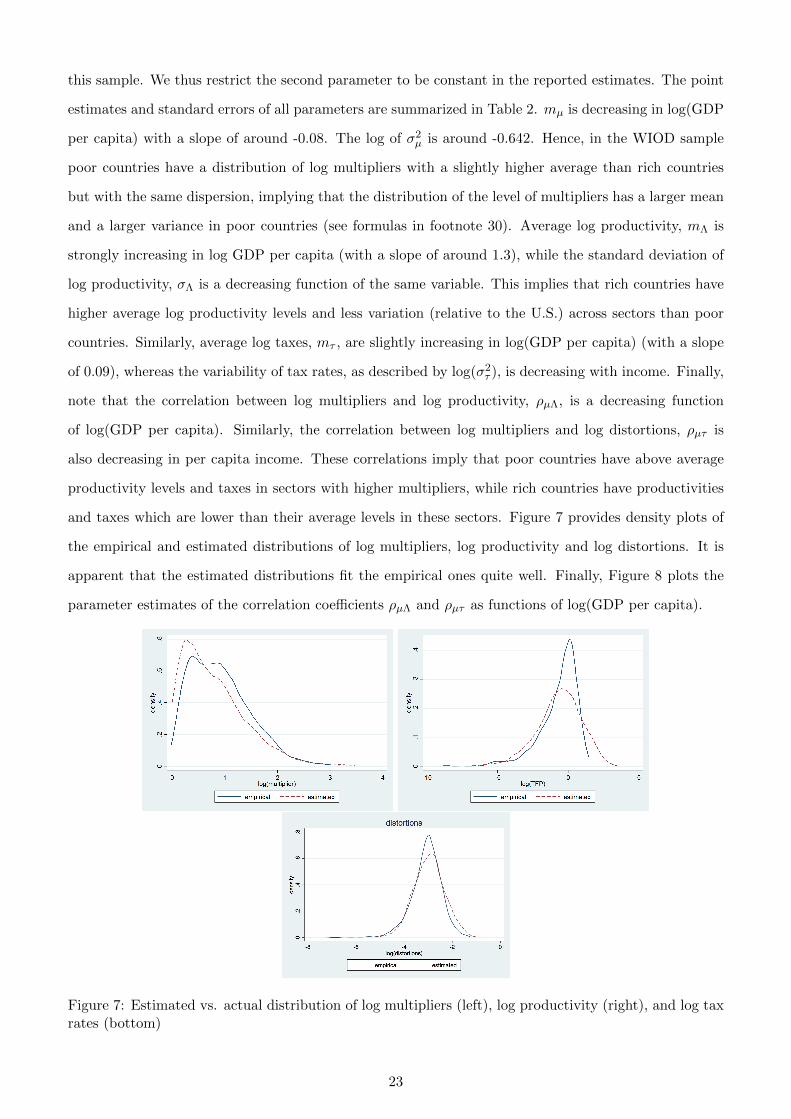
and taxes which are lower than their average levels in these sectors. Figure 7 provides density plots of

the empirical and estimated distributions of log multipliers, log productivity and log distortions. It is

apparent that the estimated distributions fit the empirical ones quite well. Finally, Figure 8 plots the

parameter estimates of the correlation coefficients ρµΛ and ρµτ as functions of log(GDP per capita).

Figure 7: Estimated vs. actual distribution of log multipliers (left), log productivity (right), and log taxrates (bottom)

23

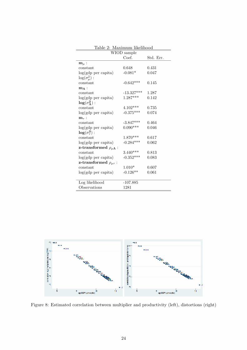
Table 2: Maximum likelihoodWIOD sample

Coef. Std. Err.mµ :constant 0.648 0.431log(gdp per capita) -0.081* 0.047log(σ2

µ) :constant -0.642*** 0.145mΛ :constant -13.327*** 1.287log(gdp per capita) 1.287*** 0.142log(σ2

Λ) :constant 4.102*** 0.735log(gdp per capita) -0.375*** 0.074mτ :constant -3.847*** 0.464log(gdp per capita) 0.090*** 0.046log(σ2

τ ) :constant 1.870*** 0.617log(gdp per capita) -0.284*** 0.062z-transformed ρµΛ :constant 3.440*** 0.813log(gdp per capita) -0.352*** 0.083z-transformed ρµτ :constant 1.010* 0.607log(gdp per capita) -0.126** 0.061

Log likelihood -107.885Observations 1281

Figure 8: Estimated correlation between multiplier and productivity (left), distortions (right)

24

To obtain more information on the IO structure of low-income countries, we now re-estimate our

statistical model on the GTAP sample (37 sectors, 70 countries). For these countries, we only have

information on IO multipliers but not on productivity levels and taxes. Therefore, we estimate a uni-

variate Normal distribution for mµ and σµ. Table 3 reports the results. We find that mµ is now an

insignificant function of income and we therefore report the estimate for constant mµ. In contrast, for

the larger sample the standard deviation of log multipliers, σµ is now significantly smaller for rich than

for poor countries. This implies that both the mean and the standard deviation of the corresponding

distributions of multipliers are larger in poor countries than in rich ones: in poor countries the average

sector has a larger multiplier and there is more mass in the right tail of the distribution. We summarize

these empirical findings below.

Table 3: Maximum LikelihoodGTAP sample

Coef. Std. Err.mµ :constant -3.274*** 0.072

log(σµ2) :

constant 0.328*** 0.029log(GDP per capita) -0.008*** 0.003

Log likelihood 10,069.322Observations 2,553

Summary of estimation results:

1. The estimated distribution of IO multipliers has a larger variance and more mass in the right tail

in poor countries compared to rich ones.

2. The estimated distribution of productivities has a lower mean and a larger variance in poor countries

compared to rich ones.

3. The estimated distribution of tax rates has a lower mean and a larger variance in poor countries

compared to rich ones.

4. IO multipliers and productivities correlate positively in poor countries and negatively in rich ones.

5. IO multipliers and tax rates correlate positively in poor countries and negatively in rich ones.

4.2 Predicting cross-country income differences

With the parameter estimates Θ in hand, we now use equation (13) (differenced relative to the U.S.) to

predict income per capita relative to the U.S.30 We compare our baseline model which features country-

30The expression for E(y) for the truncated distribution of (µi,Λreli , τi) is somewhat more complicated and less intuitive.

However, the results for aggregate income using a truncated normal distribution for µ are very similar to the estimation of

25

specific IO linkages, sectoral productivity differences and taxes with three simple alternatives. The first

one, which we label the ’naive model’, has no IO structure, no productivity differences and no taxes,

so that y = E(y) = αlog(K). The second model, in contrast, has sectoral productivity differences but

no IO linkages. It is easy to show that under the assumption that sectoral productivities follow a log-

Normal distribution predicted log income in the this model is given by E(y) = emΛ+0.5∗σ2Λ + α log(K) +

1n

∑ni=1(log(ΛUSi ))−1.31 The third alternative model features sectoral productivity differences, taxes and

IO linkages but keeps the IO structure constant for all countries (by restricting the mean and the variance

of the distribution of multipliers to be independent of per capita GDP in the estimation). In addition

to the estimated parameter values Θ, we need to calibrate a few other parameters. As standard, we set

(1− α), the labor income share in GDP, equal to 2/3. Moreover, we set γ, the share of intermediates in

gross output, equal to 0.5, which corresponds to the average level in the WIOD dataset. Finally, we set

n equal to 35, which corresponds to the number of sectors in the WIOD dataset.

To evaluate model fit, we provide the following tests: first, we regress income per capita relative to

the U.S. predicted by the model on actual data for GDP per capita relative to the U.S. If the model

fits perfectly the estimate for the intercept should be zero, while the regression slope and the R-squared

should equal unity. Second, as a graphical measure for the goodness of fit, we also plot predicted income

per capita relative to the U.S. against actual relative income. Note that these statistics provide over-

identification tests for our model since there is no intrinsic reason for the model to fit data on relative

per capita income: we have not tried to match income data in order to estimate the parameters of the

distribution of IO multipliers, productivities or taxes. Instead, we have just allowed the joint distribution

of these parameters to vary with the level of income per capita.

The results for the first test are reported in Table 4. In column (1), we report statistics for the

’naive’ model. In column (2), we report results for the model with productivity differences but no IO

structure. In column (3) we report results for the baseline model (13), where we take the parameter

estimates as estimated from the WIOD data (using parameters for the distribution of multipliers from

Table 2 above). In column (4), we force the distribution of multipliers to be the same across countries

by restricting both mµ and σ2µ to be constant. Finally, in column (5) we report results for the baseline

model when the distribution of multipliers is estimated from the GTAP dataset (using parameters for

the distribution of multipliers from Table 3).

We now present the results of this exercise. The ’naive’ model fails in predicting relative income

across countries (column (1)). As is well known, a model without productivity differences predicts too

little variation in income per capita across countries. Still, in the WIOD sample, which consists mostly

(13) and we therefore use the formulas for the non-truncated distribution. The details can be provided by the authors.31Y =

∏ni=1 Λ

1/ni (K)α, hence y = 1

n

∑ni=1 λi + α log(K). Using our approximation for productivity relative to the U.S.,

taking expectations and assuming that Λi follows a log-Normal distribution, we obtain the above formula.

26

of high-income countries, it does relatively well: the intercept is 0.426, the slope coefficient is 0.735 and

the R-squared is 0.888. The simple model with productivity differences but no IO linkages (column

(2)) performs better but it generates too much variation in income compared to the data, implying

that aggregate productivity differences estimated from sectoral data are larger than what is necessary to

generate the observed differences in income: the intercept is -0.155, the slope coefficient is 0.929 and the

R-squared is 0.865. We now move to the first specification with IO structure. In column (3) we report

results for the baseline model with the IO structure estimated from WIOD data. This model indeed

performs better than the one without IO structure: the intercept is no longer statistically different from

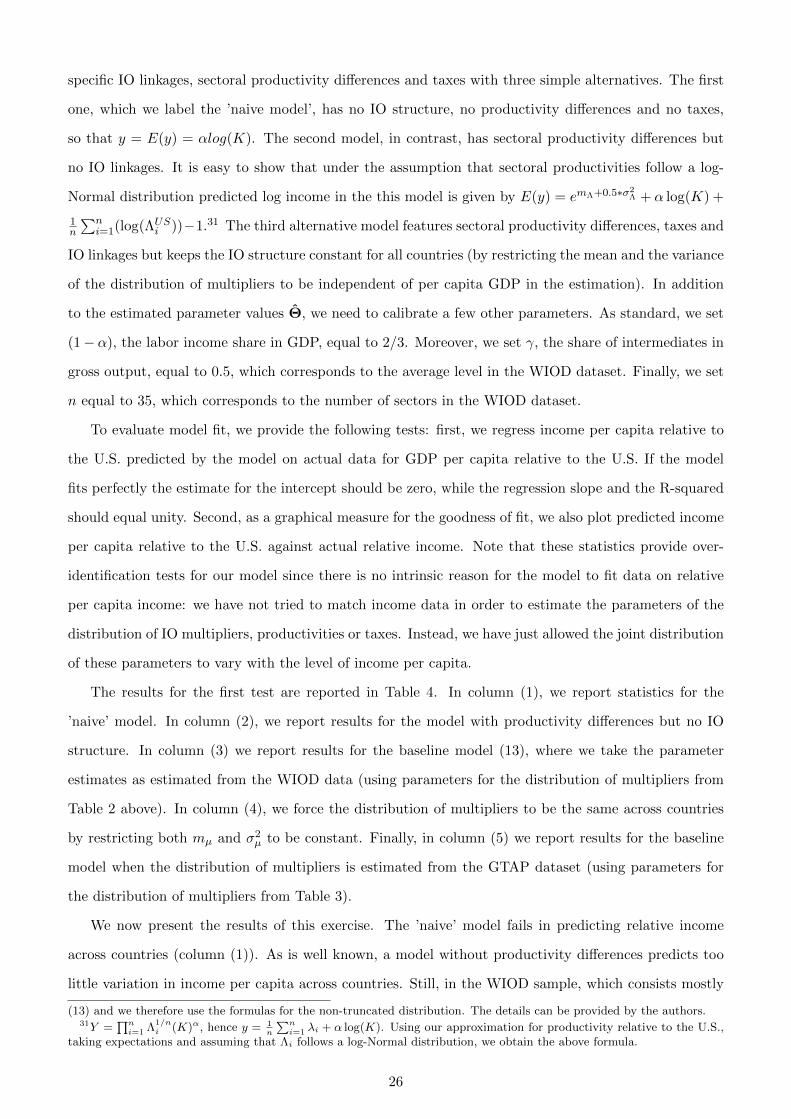
zero, the slope coefficient equals 0.922 and the R-squared is 0.853. A visual comparison of actual vs.

predicted relative income in Figure 9 confirms the substantially better fit of the model with IO linkages

compared to the one without IO structure, which underpredicts relative income levels of most countries.

Next, we test if cross-country differences in IO structure are part of the explanation of improved fit. In

column (4) we restrict the coefficients of mµ and σ2µ to be the same for all countries but we continue to

allow for cross-country differences in the correlation between productivity and IO structure as well as in

the correlation between taxes and IO structure. We find that this model fits the data much worse than

the one with income-varying IO structure: the intercept is 0.225, the slope coefficient drops to 0.843

and the R-squared to 0.738, thus indicating that cross-country differences in IO structure are important

for predicting differences in income across countries. Finally, in column (5) we use the estimated IO

structure from the GTAP sample in our baseline IO model. The GTAP data is more informative about

cross-country differences in IO structure than the WIOD data because it includes a much larger sample

of low- and middle-income countries, which allows estimating differences in structure across countries

much more precisely. The above estimates from the GTAP data indicate that poorer countries have a

distribution of multipliers with a significantly fatter right tail compared to rich countries. Using these

estimates, we find that the size of the intercept drops to 0.007 and is not statistically different from

zero, while the slope coefficient is equal to 0.901 and the R-squared is 0.834 Thus, this specification

outperforms both the model without IO structure and the one with constant IO structure in terms of

predicting income differences and performs comparably to the one where the IO structure is estimated

from the WIOD data.

Observe that there are three main factors that determine the improved fit of the baseline model with

IO structure compared to the model without IO structure: first, the difference in the IO structure between

high and low-income countries, where poor countries in the sample have only a few highly connected

sectors and many sectors that are relatively isolated, while rich countries have more intermediately

connected sectors; second, the fact that in contrast to rich countries poor economies have higher than

27

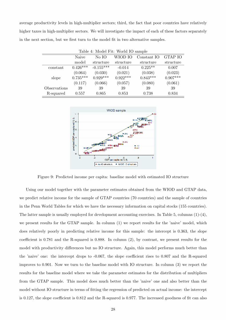
average productivity levels in high-multiplier sectors; third, the fact that poor countries have relatively

higher taxes in high-multiplier sectors. We will investigate the impact of each of these factors separately

in the next section, but we first turn to the model fit in two alternative samples.

Table 4: Model Fit: World IO sample

Naive No IO WIOD IO Constant IO GTAP IOmodel structure structure structure structure

constant 0.426*** -0.155*** -0.014 0.225** 0.007(0.064) (0.030) (0.021) (0.038) (0.023)

slope 0.735*** 0.929*** 0.922*** 0.843*** 0.907***(0.117) (0.066) (0.057) (0.080) (0.061)

Observations 39 39 39 39 39R-squared 0.557 0.865 0.853 0.738 0.834

Figure 9: Predicted income per capita: baseline model with estimated IO structure

Using our model together with the parameter estimates obtained from the WIOD and GTAP data,

we predict relative income for the sample of GTAP countries (70 countries) and the sample of countries

in the Penn World Tables for which we have the necessary information on capital stocks (155 countries).

The latter sample is usually employed for development accounting exercises. In Table 5, columns (1)-(4),

we present results for the GTAP sample. In column (1) we report results for the ’naive’ model, which

does relatively poorly in predicting relative income for this sample: the intercept is 0.363, the slope

coefficient is 0.781 and the R-squared is 0.888. In column (2), by contrast, we present results for the

model with productivity differences but no IO structure. Again, this model performs much better than

the ’naive’ one: the intercept drops to -0.067, the slope coefficient rises to 0.807 and the R-squared

improves to 0.901. Now we turn to the baseline model with IO structure. In column (3) we report the

results for the baseline model where we take the parameter estimates for the distribution of multipliers

from the GTAP sample. This model does much better than the ’naive’ one and also better than the

model without IO structure in terms of fitting the regression of predicted on actual income: the intercept

is 0.127, the slope coefficient is 0.812 and the R-squared is 0.977. The increased goodness of fit can also

28

be seen from Figure 10, left panel, where we plot predicted income against actual income for the baseline

model and the model without IO structure. While the second considerably underpredicts income for

most countries, the model with IO structure is extremely close to the 45 degree line. Only for the poorest

countries it overpredicts their relative income somewhat. Finally, in column (4) we report results for

the baseline model where the estimates of the IO structure are derived from the WIOD sample: we now

get the intercept of 0.084, the slope coefficient of 0.808 and the R-squared of 0.962. Thus, this model

performs slightly worse than the one where we have used the GTAP IO structure because it predicts

somewhat smaller differences in IO structure across countries.

Finally, we discuss the results for the Penn World Tables sample (columns (5)-(8)). Here the perfor-

mance of the ’naive’ model is again quite poor and it strongly overpredicts income for poor countries,

indicating that productivity differences matter for explaining aggregate income differences. In column

(5) the intercept is 0.342 and the slope coefficient is 0.823 with an R-squared of 0.831. In column

(6) we report results for the model without IO structure, which has a negative intercept (-0.037), an

even smaller slope coefficient of 0.759 and an R-squared of 0.894. This model is again outperformed by

our baseline model with the GTAP IO structure: the slope coefficient for this model is 0.775 and the

R-squared increases substantially to 0.966. Thus, the model performs quite well in predicting relative

income across countries, even in a sample that is much larger than the one from which we have estimated

the parameters of the model. The good fit can also be seen clearly from the right panel of Figure 10,

where most data points are extremely close to the 45 degree line. Again, the model overpredicts relative

income levels somewhat for very low-income countries. Finally, in column (8), we report results for the

baseline model when estimating the IO structure from the WIOD sample. This model does slightly

worse than the previous one, but still performs better than the model without IO structure: the slope

coefficient is 0.763, and the R-squared is 0.953. We conclude that including an IO structure into the

model helps to substantially improve model fit. To wrap up, we now present a summary of our findings.

Summary of model fit:

1. The baseline model with estimated IO structure performs substantially better in terms of predicting

cross-country income differences than a model without technology differences (which underestimates

income differences) and a model with technology differences but without IO structure (which over-

estimates income differences).

2. The baseline model with IO structure estimated from GTAP data performs slightly better than the

same model with IO structure estimated from WIOD data.

3. The above results hold for three different samples of countries: the WIOD dataset (39 countries),

the GTAP dataset (70 countries) and the Penn World Tables dataset (155 countries).

29

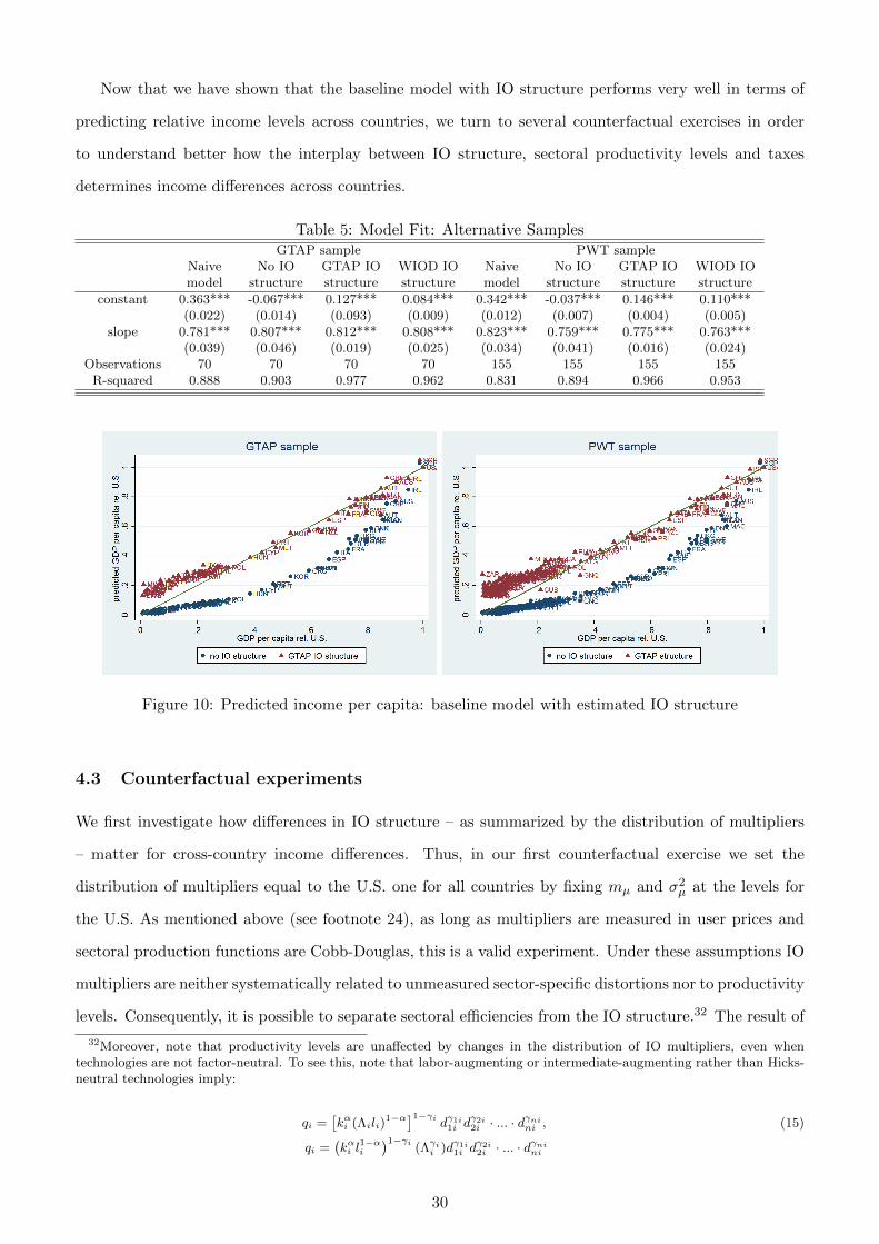
Now that we have shown that the baseline model with IO structure performs very well in terms of

predicting relative income levels across countries, we turn to several counterfactual exercises in order

to understand better how the interplay between IO structure, sectoral productivity levels and taxes

determines income differences across countries.

Table 5: Model Fit: Alternative SamplesGTAP sample PWT sample

Naive No IO GTAP IO WIOD IO Naive No IO GTAP IO WIOD IOmodel structure structure structure model structure structure structure

constant 0.363*** -0.067*** 0.127*** 0.084*** 0.342*** -0.037*** 0.146*** 0.110***(0.022) (0.014) (0.093) (0.009) (0.012) (0.007) (0.004) (0.005)

slope 0.781*** 0.807*** 0.812*** 0.808*** 0.823*** 0.759*** 0.775*** 0.763***(0.039) (0.046) (0.019) (0.025) (0.034) (0.041) (0.016) (0.024)

Observations 70 70 70 70 155 155 155 155R-squared 0.888 0.903 0.977 0.962 0.831 0.894 0.966 0.953

Figure 10: Predicted income per capita: baseline model with estimated IO structure

4.3 Counterfactual experiments

We first investigate how differences in IO structure – as summarized by the distribution of multipliers

– matter for cross-country income differences. Thus, in our first counterfactual exercise we set the

distribution of multipliers equal to the U.S. one for all countries by fixing mµ and σ2µ at the levels for

the U.S. As mentioned above (see footnote 24), as long as multipliers are measured in user prices and

sectoral production functions are Cobb-Douglas, this is a valid experiment. Under these assumptions IO

multipliers are neither systematically related to unmeasured sector-specific distortions nor to productivity

levels. Consequently, it is possible to separate sectoral efficiencies from the IO structure.32 The result of

32Moreover, note that productivity levels are unaffected by changes in the distribution of IO multipliers, even whentechnologies are not factor-neutral. To see this, note that labor-augmenting or intermediate-augmenting rather than Hicks-neutral technologies imply:

qi =[kαi (Λili)

1−α]1−γi dγ1i1i d

γ2i2i · ... · d

γnini , (15)

qi =(kαi l

1−αi

)1−γi (Λγii )dγ1i1i d

γ2i2i · ... · d

γnini

30

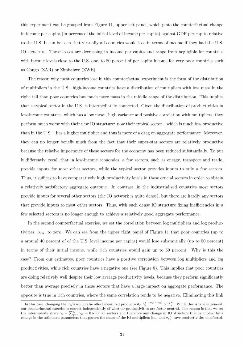
this experiment can be grasped from Figure 11, upper left panel, which plots the counterfactual change

in income per capita (in percent of the initial level of income per capita) against GDP per capita relative

to the U.S. It can be seen that virtually all countries would lose in terms of income if they had the U.S.

IO structure. These losses are decreasing in income per capita and range from negligible for countries

with income levels close to the U.S. one, to 80 percent of per capita income for very poor countries such

as Congo (ZAR) or Zimbabwe (ZWE).

The reason why most countries lose in this counterfactual experiment is the form of the distribution

of multipliers in the U.S.: high-income countries have a distribution of multipliers with less mass in the

right tail than poor countries but much more mass in the middle range of the distribution. This implies

that a typical sector in the U.S. is intermediately connected. Given the distribution of productivities in

low-income countries, which has a low mean, high variance and positive correlation with multipliers, they

perform much worse with their new IO structure: now their typical sector – which is much less productive

than in the U.S. – has a higher multiplier and thus is more of a drag on aggregate performance. Moreover,

they can no longer benefit much from the fact that their super-star sectors are relatively productive

because the relative importance of these sectors for the economy has been reduced substantially. To put

it differently, recall that in low-income economies, a few sectors, such as energy, transport and trade,

provide inputs for most other sectors, while the typical sector provides inputs to only a few sectors.

Thus, it suffices to have comparatively high productivity levels in those crucial sectors in order to obtain

a relatively satisfactory aggregate outcome. In contrast, in the industrialized countries most sectors

provide inputs for several other sectors (the IO network is quite dense), but there are hardly any sectors

that provide inputs to most other sectors. Thus, with such dense IO structure fixing inefficiencies in a

few selected sectors is no longer enough to achieve a relatively good aggregate performance.

In the second counterfactual exercise, we set the correlation between log multipliers and log produc-

tivities, ρµΛ, to zero. We can see from the upper right panel of Figure 11 that poor countries (up to

a around 40 percent of of the U.S. level income per capita) would lose substantially (up to 50 percent)

in terms of their initial income, while rich countries would gain up to 60 percent. Why is this the

case? From our estimates, poor countries have a positive correlation between log multipliers and log

productivities, while rich countries have a negative one (see Figure 8). This implies that poor countries

are doing relatively well despite their low average productivity levels, because they perform significantly

better than average precisely in those sectors that have a large impact on aggregate performance. The

opposite is true in rich countries, where the same correlation tends to be negative. Eliminating this link

In this case, changing the γji’s would also affect measured productivity Λ(1−α)(1−γi)i or Λγii . While this is true in general,

our counterfactual exercise is correct independently of whether productivities are factor neutral. The reason is that we setthe intermediate share γi =

∑Nj=1 γji = 0.5 for all sectors and therefore any change in IO structure that is implied by a

change in the estimated parameters that govern the shape of the IO multipliers (mµ and σµ) leave productivities unaffected.

31

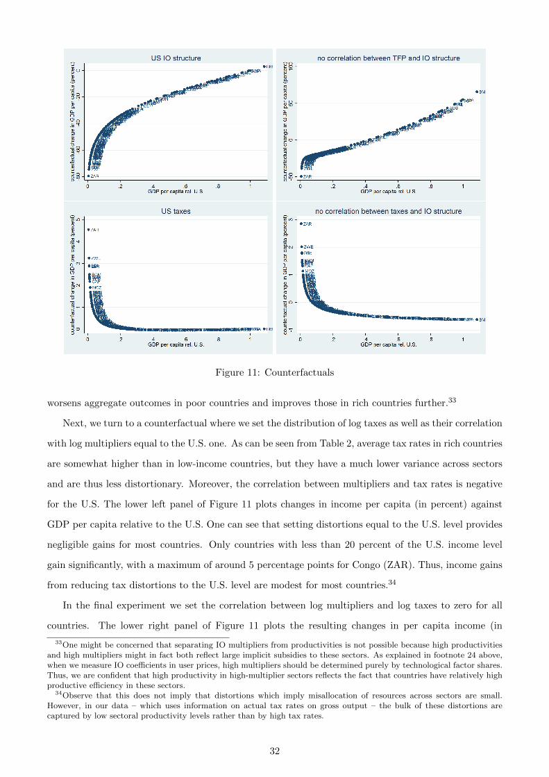
Figure 11: Counterfactuals

worsens aggregate outcomes in poor countries and improves those in rich countries further.33

Next, we turn to a counterfactual where we set the distribution of log taxes as well as their correlation

with log multipliers equal to the U.S. one. As can be seen from Table 2, average tax rates in rich countries

are somewhat higher than in low-income countries, but they have a much lower variance across sectors

and are thus less distortionary. Moreover, the correlation between multipliers and tax rates is negative

for the U.S. The lower left panel of Figure 11 plots changes in income per capita (in percent) against

GDP per capita relative to the U.S. One can see that setting distortions equal to the U.S. level provides

negligible gains for most countries. Only countries with less than 20 percent of the U.S. income level

gain significantly, with a maximum of around 5 percentage points for Congo (ZAR). Thus, income gains

from reducing tax distortions to the U.S. level are modest for most countries.34

In the final experiment we set the correlation between log multipliers and log taxes to zero for all

countries. The lower right panel of Figure 11 plots the resulting changes in per capita income (in

33One might be concerned that separating IO multipliers from productivities is not possible because high productivitiesand high multipliers might in fact both reflect large implicit subsidies to these sectors. As explained in footnote 24 above,when we measure IO coefficients in user prices, high multipliers should be determined purely by technological factor shares.Thus, we are confident that high productivity in high-multiplier sectors reflects the fact that countries have relatively highproductive efficiency in these sectors.

34Observe that this does not imply that distortions which imply misallocation of resources across sectors are small.However, in our data – which uses information on actual tax rates on gross output – the bulk of these distortions arecaptured by low sectoral productivity levels rather than by high tax rates.

32

percent) against GDP relative to the U.S. level. Again, income changes resulting from this experiment

are relatively small. Poor countries – which empirically exhibit a positive correlation between multipliers

and distortions– experience small increases in income (up to 3 percentage points for Congo (ZAR)), while

rich countries – which empirically have a negative correlation between multipliers and tax rates – lose

around one percentage point of income per capita.

Summary of counterfactual experiments:

1. Imposing the dense IO structure of the U.S. on poor economies would reduce their income levels by

up to 80 percent because the typical sector, which has a lower productivity than the high-multiplier

sectors in these economies, would become more connected.

2. If poor economies did not have above-average productivity levels in high-multiplier sectors, their

income levels would be reduced by up to 40 percent.

3. Imposing the distribution of tax rates of the U.S. on poor economies would lead to moderate income

gains of up to 5 percent.

4. If poor economies did not have above-average tax levels in high-multiplier sectors, their income

levels would increase by up to 3 percent.

5 Optimal taxation

The theoretical model employed for the analysis so far considers tax rates as exogenously given and

wasteful. In this section we introduce an active role for the government and address the problem of

optimal taxation. To do that, in principle we should specify the objective function of the government or

social planner which is to be maximized by the choice of tax rates. However, given that in this model,

the market allocation is Pareto-optimal, an unconstrained planner would choose zero taxation. We

thus analyze the problem of optimal taxation for exogenously specified government expenditures. The

appealing feature of analyzing such “semi-optimal” taxation schemes is that they are much less dependent

on the specific welfare function. Indeed, as long as welfare increases with individual consumption C, any

welfare function would generate the same outcome for exogenously fixed government consumption G. In

short we will designate this analysis as GDP per capita maximization with exogenous G.

Importantly, optimal taxes will be obtained via a statistical approach in line with the rest of the

paper. As before it is assumed that sectoral IO multipliers, taxes and productivities are drawn from

a trivariate log-Normal distribution. The optimization task is then to maximize the expected value of

GDP through an appropriate choice of the mean, variance and covariance of the tax distribution, keeping

33

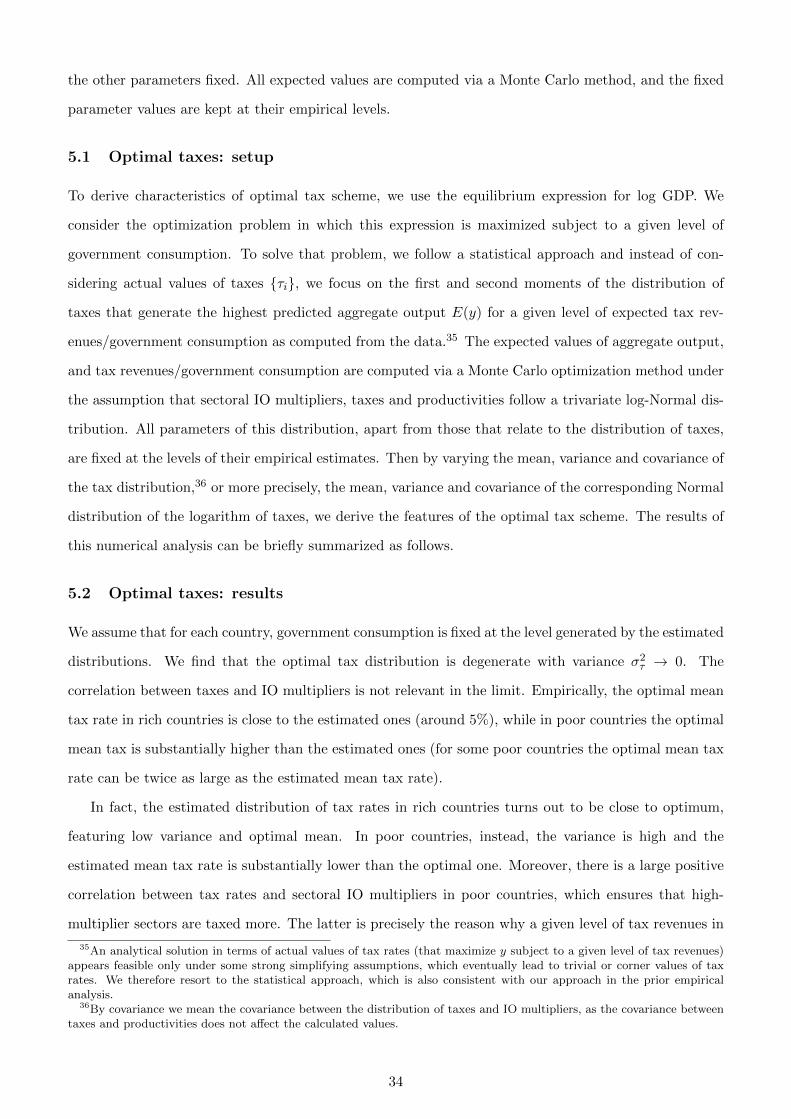
the other parameters fixed. All expected values are computed via a Monte Carlo method, and the fixed

parameter values are kept at their empirical levels.

5.1 Optimal taxes: setup

To derive characteristics of optimal tax scheme, we use the equilibrium expression for log GDP. We

consider the optimization problem in which this expression is maximized subject to a given level of

government consumption. To solve that problem, we follow a statistical approach and instead of con-

sidering actual values of taxes {τi}, we focus on the first and second moments of the distribution of

taxes that generate the highest predicted aggregate output E(y) for a given level of expected tax rev-

enues/government consumption as computed from the data.35 The expected values of aggregate output,

and tax revenues/government consumption are computed via a Monte Carlo optimization method under

the assumption that sectoral IO multipliers, taxes and productivities follow a trivariate log-Normal dis-

tribution. All parameters of this distribution, apart from those that relate to the distribution of taxes,

are fixed at the levels of their empirical estimates. Then by varying the mean, variance and covariance of

the tax distribution,36 or more precisely, the mean, variance and covariance of the corresponding Normal

distribution of the logarithm of taxes, we derive the features of the optimal tax scheme. The results of

this numerical analysis can be briefly summarized as follows.

5.2 Optimal taxes: results

We assume that for each country, government consumption is fixed at the level generated by the estimated

distributions. We find that the optimal tax distribution is degenerate with variance σ2τ → 0. The

correlation between taxes and IO multipliers is not relevant in the limit. Empirically, the optimal mean

tax rate in rich countries is close to the estimated ones (around 5%), while in poor countries the optimal

mean tax is substantially higher than the estimated ones (for some poor countries the optimal mean tax

rate can be twice as large as the estimated mean tax rate).

In fact, the estimated distribution of tax rates in rich countries turns out to be close to optimum,

featuring low variance and optimal mean. In poor countries, instead, the variance is high and the

estimated mean tax rate is substantially lower than the optimal one. Moreover, there is a large positive

correlation between tax rates and sectoral IO multipliers in poor countries, which ensures that high-

multiplier sectors are taxed more. The latter is precisely the reason why a given level of tax revenues in

35An analytical solution in terms of actual values of tax rates (that maximize y subject to a given level of tax revenues)appears feasible only under some strong simplifying assumptions, which eventually lead to trivial or corner values of taxrates. We therefore resort to the statistical approach, which is also consistent with our approach in the prior empiricalanalysis.

36By covariance we mean the covariance between the distribution of taxes and IO multipliers, as the covariance betweentaxes and productivities does not affect the calculated values.

34

poor countries can be reached with a lower mean tax rate than prescribed in optimum. Indeed, under the

optimal tax scheme all sectors should be taxed evenly, and then raising the same amount of tax revenues

requires a higher mean tax. Still, we find that the distortion loss associated with high (optimal) mean

tax is small compared to the loss associated with taxing high-multiplier sectors more. The left panel of

Figure 12 plots welfare gains (in terms of percentage gains in GDP) of moving to a uniform tax rate

that generates the same revenue as the current tax system against GDP per capita. The welfare gains

are basically zero for all high-income countries but they can rise to up to 30% of GDP for some of the

poorest countries in the world. This is consistent with our previous counterfactuals which showed that

poor countries would gain most from moving to the U.S. parameters of the tax distribution. However,

in that experiment gains were much smaller since taxes were considered as wasteful.

Figure 12: Optimal taxation

We also perform a more unusual experiment. Indeed, as there might be other reasons why tax rates

cannot be uniform, we want to explore the role of the covariance between taxes and IO multipliers for the

outcome. We set the variance of the tax rate distribution to be equal to the actual estimated value and

examine the role of choosing the optimal correlation between the distribution of tax rates and sectoral

IO multipliers and the mean tax rates that keep tax revenue constant. We find that the optimal tax

distribution has negative correlation with sectoral IO multipliers, so that consistently with the findings of

our empirical analysis, more central sectors should be taxed less. The right panel of Figure 12 plots the

percentage gains in GDP per capita of moving to the optimal correlation between taxes and multipliers

that keeps tax revenue constant. Again, welfare gains are substantial for very poor countries. Moreover,

moving to a negative correlation between taxes and multipliers and increasing average tax rates would

imply gains which are almost as large as those of moving to a uniform tax rate.

Finally, in unreported simulations we have considered government expenditure to enter households’

utility in a Cobb-Douglas fashion. The results were very similar to those of the model that takes

government expenditure as given.

35

6 Robustness checks

In this section, we report the results of a number of robustness checks in order to show that our findings

do not hinge on the specific restrictions imposed on the baseline model. We consider the following

extensions. First, we estimate parameters using the approximated distribution of multipliers, where we

employ the representation of multipliers in terms of sectoral out-degrees. Second, we allow for skilled

and unskilled labor as separate production factors. Third, we generalize the final demand structure and

introduce expenditure shares that differ across countries and sectors. Fourth, we generalize the model by

introducing imported intermediate inputs. Finally, we consider taxes as government revenue instead of

treating them as wasteful. We then show that none of these generalizations changes the basic conclusions

of the baseline model. The formulas for aggregate income implied by these more general models as well

as detailed derivations can be found in the Appendix.

6.1 Approximation of multipliers

We first provide results when estimating the distribution of log multipliers from a first and second-

order approximation, instead of using the actual empirical distribution of log multipliers. Following the

discussion in section 3.3, the first-order approximation of multipliers is µ ≈ 1n + 1

nΓ1, while the second-

order approximation is µ ≈ 1n + 1

nΓ1+ 1nΓ21. The first-order approximation abstracts from higher-order

interconnectedness and only considers direct outward linkages (weighted out-degrees), while the second-

order approximation also considers second-order interconnectedness (the weighted out-degree of sectors

to which each sector delivers).

Empirically, there is little difference between the actual distribution of multipliers and the esti-

mated distribution using the first and second-order approximation, as can be seen from Figure 14 in

the Appendix. Columns (1) and (2) of Table 6 report model fit results for the first- and second-order

approximation. It is apparent that the difference in performance between the models is relatively small.

The intercepts are now -0.106 and -0.133 and the slope coefficients are 0.989 and 0.974, respectively, for

the first- and second-order approximation, compared to -0.014 and 0.922 for the baseline model with IO

structure estimated on the WIOD sample. Observe also that the first-order approximation, which is most

consistent with the formula for aggregate income (13), performs slightly better than the second-order

approximation, indicating that modeling second-order interconnectedness does not help to improve our

understanding how differences in countries’ IO structure affect aggregate income.

36

6.2 Cross-country differences in demand structure

So far we have abstracted from cross-country differences in the final demand structure, which also have

an impact on sectoral multipliers because sectors with larger final expenditure shares will have a larger

impact on GDP. In the next robustness check, we thus consider a more general demand structure. More

specifically, we model the production function for the aggregate final good as Y = yβ11 · ... · y

βnn , where βi

is allowed to be country-sector-specific. The advantage of this specification is that it picks up differences

in the final demand structure that may have an impact on aggregate income. The drawback is that

now multipliers become functions of both differences in the IO structure and differences in final demand.

Thus, this specification does not allow one to differentiate between the two channels. The vector of

sectoral multipliers is now defined as µ = {µi}i = [I −Γ]−1β, where β = (β1, .., βn)′. Its interpretation,

however, is identical to the one before: each sectoral multiplier µi reveals how a change in productivity

(or taxes) of sector i affects the overall value added in the economy.

The results for this model can be found in column (3) of Table 6. The intercept is now -0.12 and the

slope coefficient is 0.901, which is somewhat worse than the performance of our baseline model. This

indicates that – within the context of our model – modeling differences in the final demand structure

does not help to understand differences in aggregate income. The reason seems to be that modeling

differences in final demand structure introduces additional noise in the multiplier data, which makes it

harder to estimate the systematic features of inter-industry linkages.

6.3 Skilled labor

Next, we split aggregate ”labor” endowments into skilled and unskilled labor. Namely, let the technology

of each sector i ∈ 1 : n in every country be described by the following Cobb-Douglas function:

qi = Λi

(kαi u

δi s

1−α−δi

)1−γi−σidγ1i

1i dγ2i2i · ... · d

γnini , (16)

where si and ui denote the amounts of skilled and unskilled labor used by sector i, γi =∑n

j=1 γji is

the share of intermediate goods in the total input use of sector i and α, δ, 1 − α − δ ∈ (0, 1) are the

respective shares of capital, unskilled and skilled labor in the remainder of the inputs. The total supply

of skilled and unskilled labor in the economy is fixed at the exogenous levels of S and U , respectively. We

define skilled labor as the number of hours worked by workers with at least some tertiary education and

we define unskilled labor as the number of hours worked by workers with less than tertiary education.

Information on skilled and unskilled labor inputs is from WIOD. We calibrate δ = 1/6 to fit the college

skill premium of the U.S. Results are provided in column (4) of Table 6. The intercept is -0.055 and the

slope coefficient is 0.943, which is very close to the baseline model. We conclude that the results are not

37

sensitive to the definition of labor endowments.

6.4 Imported intermediates

So far we have abstracted from international trade and we have assumed that all goods have to be pro-

duced domestically. Here, we instead allow for both domestically produced and imported intermediates.

We thus assume that sectoral production functions are given by:

qi = Λi(kαi l

1−αi

)1−γi−σi dγ1i1i d

γ2i2i · ... · d

γnini · f

σ1i1i f

σ2i2i · ... · f

σnini , (17)

where dji are domestically produced intermediate inputs and fji are imported intermediate inputs.

Domestic and imported intermediate inputs are assumed to be imperfectly substitutable, and γji, σji

denote the shares of domestic and imported intermediates, respectively, in the value of sectoral gross

output. We change the construction of the IO tables accordingly by separating domestically produced

from imported intermediates and then re-estimating the distribution of IO multipliers.

The results for fitting the model with this specification are given in column (5) of Table 6. The slope

coefficient is now 1.004, which is even closer to one than with the baseline specification. The intuition

for why results remain very similar comes from the fact that most important, high-multiplier sectors

tend to be services, which are effectively non-traded. Therefore, allowing for trade does not change the

statistical distribution of multipliers and the implied predicted income in every country very much. We

thus conclude that our results are quite robust to allowing for trade in intermediates.

6.5 Taxes as government revenue

As a final robustness check, we rebate tax revenues collected by the government lump sum to households

instead of considering them as wasted. The results for this model are presented in column (6) of Table

6. We find that the results are basically equivalent to those in the baseline model: the intercept is 0.017

and not statistically different from zero, while the slope coefficient is 0.920. Thus, rebating government

revenue to households does not make a difference. We therefore conclude that our baseline model is

pretty robust to a number of extensions and alternative assumptions.

7 Conclusions

In this paper we have studied the role of input-output structure of the economy and its interaction

with sectoral productivities and tax distortions in explaining income differences across countries. In

contrast to the typical approach in the literature on development accounting and on dual economies

and structural transformation, we model input-output linkages between sectors and the difference in

38

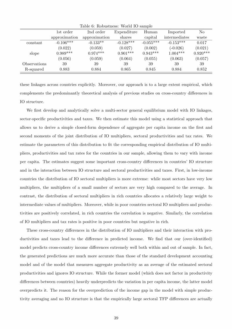
Table 6: Robustness: World IO sample

1st order 2nd order Expenditure Human Imported Noapproximation approximation shares capital intermediates waste

constant -0.106*** -0.133** -0.128*** -0.055*** -0.153*** 0.017(0.022) (0.059) (0.027) (0.002) (-0.026) (0.021)

slope 0.989*** 0.974*** 0.901*** 0.943*** 1.004*** 0.920***(0.056) (0.059) (0.064) (0.055) (0.063) (0.057)

Observations 39 39 39 39 39 39R-squared 0.883 0.884 0.865 0.845 0.884 0.852

these linkages across countries explicitly. Moreover, our approach is to a large extent empirical, which

complements the predominantly theoretical analysis of previous studies on cross-country differences in

IO structure.

We first develop and analytically solve a multi-sector general equilibrium model with IO linkages,

sector-specific productivities and taxes. We then estimate this model using a statistical approach that

allows us to derive a simple closed-form dependence of aggregate per capita income on the first and

second moments of the joint distribution of IO multipliers, sectoral productivities and tax rates. We

estimate the parameters of this distribution to fit the corresponding empirical distribution of IO multi-

pliers, productivities and tax rates for the countries in our sample, allowing them to vary with income

per capita. The estimates suggest some important cross-country differences in countries’ IO structure

and in the interaction between IO structure and sectoral productivities and taxes. First, in low-income

countries the distribution of IO sectoral multipliers is more extreme: while most sectors have very low

multipliers, the multipliers of a small number of sectors are very high compared to the average. In

contrast, the distribution of sectoral multipliers in rich countries allocates a relatively large weight to

intermediate values of multipliers. Moreover, while in poor countries sectoral IO multipliers and produc-

tivities are positively correlated, in rich countries the correlation is negative. Similarly, the correlation

of IO multipliers and tax rates is positive in poor countries but negative in rich.

These cross-country differences in the distribution of IO multipliers and their interaction with pro-

ductivities and taxes lead to the difference in predicted income. We find that our (over-identified)

model predicts cross-country income differences extremely well both within and out of sample. In fact,

the generated predictions are much more accurate than those of the standard development accounting

model and of the model that measures aggregate productivity as an average of the estimated sectoral

productivities and ignores IO structure. While the former model (which does not factor in productivity

differences between countries) heavily underpredicts the variation in per capita income, the latter model

overpredicts it. The reason for the overprediction of the income gap in the model with simple produc-

tivity averaging and no IO structure is that the empirically large sectoral TFP differences are actually

39

mitigated by the IO structure. In paticular, as very low-productivity sectors in poor countries tend to

be badly connected, they are not that relevant for the aggregate economy.

Our counterfactual experiments suggest that if we impose the much denser IO structure of the U.S.

on poor countries and thereby increase the overall significance of their worst-productivity sectors, the

per capita income of these countries could decline by as much as 80%. That is, given the very low

productivity levels of many sectors in poor countries, having these sectors largely isolated effectively

benefits these economies. Similarly, eliminating the correlation of sectoral multipliers and productivities

would hurt poor countries but benefit the rich ones, due to the fact that the correlation of multipliers and

productivities is positive in poor countries and negative in rich ones. At last, reducing distortions from

taxes on gross output would improve the aggregate economic performance of poor countries; however,

the associated per capita income changes would be relatively small.

Finally, we study the problem of optimal taxation and analyze the welfare gains from moving to

an optimal tax system in all countries, while keeping tax revenues constant. Our findings suggest that

when the government aims at maximizing GDP per capita for a given level of tax revenue, the actual

distribution of tax rates is close to optimum in rich countries, but in poor countries, the mean of the

distribution is too low and the variance is too high relative to the optimum. We also find that for a

given value of tax variance, a negative correlation of taxes with IO multipliers is optimal, which once

again suggests a relative advantage of the tax scheme implemented in rich countries. We find that some

of the poorest countries in the world could gain up to 20% in terms of income per capita by moving to

an optimal tax system, while benefits for the rich countries would be negligible.

40

References

[1] Arbex, M. and F. S. Perobelli (2010), Solow Meets Leontief: Economic Growth and Energy Con-sumption,Energy Economics, 32 (1), 43-53.

[2] Acemoglu, D., Carvalho V.M., Ozdaglar A., and A. Tahbaz-Salehi (2012), “The Network Origins ofAggregate Fluctuations,”Econometrica, 80 (5), 1977-2016.

[3] Banerjee, A. V. and E. Duflo (2005), Growth Theory through the Lens of Development Economics,in Philippe Aghion and Steven A. Durlauf, eds., Handbook of Economic Growth, New York: NorthHolland, 473-552.

[4] Ballester,C., A. Calvo-Armengol, and Y. Zenou (2006), “Who’s Who in Networks. Wanted: TheKey Player,”Econometrica, 74, 1403-1417.

[5] Bartelme, D. (2014), Linkages and Economic Development, U.C. Berkeley, unpublished manuscript.

[6] Basu, S. (1995), Intermediate Goods and Business Cycles: Implications for Productivity and Wel-fare, American Economic Review, 85 (3), 512-531.

[7] Bonacich, P. (1987), “Power and Centrality: A Family of Measures,”American Journal of Sociology,92, 1170-1182.

[8] Boehm, J. (2013), The Impact of Contract Enforcement Costs on Outsourcing and Aggregate Pro-ductivity, LSE, unpublished manuscript.

[9] Burress, D. (1994), “Homeomorphism Between Leontief and Cobb-Douglas Input-Output Mod-els,”Economics Letters, 44, 49-53.

[10] Carvalho, V.M. (2010), “Aggregate Fluctuations and the Network Structure of IntersectoralTrade,”Working Paper.

[11] Carvalho, V.M. and N. Voigtlander (2014), “Input diffusion and the evolution of production net-works,”National Bureau of Economic Research.

[12] Caselli, F. (2005), Accounting for Cross-Country Income Differences, in Philippe Aghion and StevenA. Durlauf, eds., Handbook of Economic Growth, New York: North Holland, 679-741.

[13] Chenery, H., S. Robinson, and M. Syrquin (1986), Industrialization and Growth: A ComparativeStudy, New York, Oxford University Press.

[14] Ciccone, A. (2002), Input Chains and Industrialization, Review of Economic Studies, 69 (3), 565-587.

[15] Dimaranan, B., ed.(2006), Global Trade, Assistance, and Production: The GTAP 6 Data Base,Center for Global Trade Analysis, Purdue University

[16] Dupor, B. (1999), Aggregation and Irrelevance in Multi-Sector Models,Journal of Monetary Eco-nomics, 43 (2), 391-409.

[17] Easterly, W. (1993), How Much Do Distortions A Growth?, Journal of Monetary Economics, 32(2), 187-212.

[18] Fleming, M. (1955), External Economies and the Doctrine of Balanced Growth, Economic Journal,65, 241-256. 733-772.

[19] Gabaix, X. (2011), The Granular Origins of Aggregate Fluctuations, Econometrica, 79, 733-772.

[20] Gabaix, X., and R. Ibragimov (2011), “Rank-1/2: A Simple Way to Improve the OLS Estimationof Tail Exponents,”Journal of Business and Economic Statistics, 29, 24-39.

41

[21] Gollin, D., Lagakos D., and M. Waugh (2013), Agricultural Productivity Differences across Coun-tries, American Economic Review, 104(5), 165-170.

[22] Grobovsek, J. (2013), Development Accounting with Intermediate Goods, University of Edinburgh,unpublished manuscript.

[23] Hall, R. and C. I. Jones (1999), Why Do Some Countries Produce So Much More Output PerWorker Than Others?, Quarterly Journal of Economics, 114 (1), 83-116.

[24] Heston, A., R. Summers and B. Aten (2012), Penn World Table Version 7.1, Center for InternationalComparisons of Production, Income and Prices at the University of Pennsylvania

[25] Hirschman, A.O. (1958), ”The Strategy of Economic Development,” New Haven, CT: Yale Univer-sity Press.

[26] Horvath, M. T.K. (1998), Cyclicality and Sectoral Linkages: Aggregate Fluctuations from Indepen-dent Sectoral Shocks, Review of Economic Dynamics, 1 (4), 781-808.

[27] Hsieh, C.-T. and P.J. Klenow (2009), Misallocation and Manufacturing TFP in China and India,Quarterly Journal of Economics, 124 (4), 1403-1448.

[28] Hulten, C. R. (1978), Growth Accounting with Intermediate Inputs, Review of Economic Studies,45 (3), 511–518.

[29] Jackson, M.O. (2008), “Social and Economic Networks,”Princeton, NJ: Princeton University Press.

[30] Jones, I. Charles (2011a), “Intermediate Goods and Weak Links in the Theory of Economic Devel-opment”American Economic Journal: Macroeconomics, 3 (2), 1-28.

[31] Jones, I. Charles (2011b), “Misallocation, Input-Output Economics, and Economic Growth”Version2.0. Prepared for the 10th World Congress of the Econometric Society meeting in Shanghai.

[32] Klenow, P. and A. Rodriguez-Clare (1997), The Neoclassical Revival in Growth Economics: Has ItGone Too Far?, in Ben Bernanke and Julio Rotemberg, eds., NBER Macroeconomics Annual.

[33] Leontief, W. (1936), Quantitative Input and Output Relations in the Economic System of the UnitedStates, Review of Economics and Statistics, 18 (3), 105-125.

[34] Long, J. B. and C. I. Plosser (1983), Real Business Cycles, Journal of Political Economy, 91 (1),39-69.

[35] Miller, R. E. and P. D. Blair (2009), Input-Output Analysis: Foundations and Extensions, 2ndedition. Cambridge University Press.

[36] Oberfield, E. (2013), Business Networks, Production Chains, and Productivity: A Theory of Input-Output Architecture, Princeton, unpublished manuscript.

[37] Parente, S. L. and E. C. Prescott (1999), Monopoly Rights: A Barrier to Riches, American EconomicReview, 89 (5), 1216-1233.

[38] Restuccia, D., D. Yang and X. Zhu (2008), Agriculture and aggregate productivity: A quantitativecross-country analysis, Journal of Monetary Economics, 55 (2), 234-250.

[39] Timmer, M., ed. (2012), The World Input-Output Database (WIOD): Contents, Sources andMethod”, WIOD Working Paper Number 1

[40] Vollrath, D. (2009), How important are dual economy effects for aggregate productivity?, Journalof Development Economics, 88(2), 325-334.

42

Appendix A: Extensions of the benchmark model

7.1 Skilled labor

Consider the economy of our benchmark model where we introduce the distinction between skilled and

unskilled labor. This distinction implies that the technology of each sector i ∈ 1 : n in every country

can be described by the following Cobb-Douglas function:

qi = Λi

(kαi u

δi s

1−α−δi

)1−γi−σidγ1i

1i dγ2i2i · ... · d

γnini , (18)

where si and ui denote the amounts of skilled and unskilled labor used by sector i, γi =∑n

j=1 γji is the

share of intermediate goods in the total input use of sector i and α, δ, 1−α−δ ∈ (0, 1) are the respective

shares of capital, unskilled and skilled labor in the remainder of the inputs. The total supply of skilled

and unskilled labor in the economy is fixed at the exogenous levels of S and U , respectively.

In this case, the logarithm of the value added per capita, y = log (Y/(U + S)), is given by the

expression (28) of Proposition 2, adopted to our framework here. In fact, it is only slightly different from

the expression for y in our benchmark model (cf. Proposition 1), where δ = 0 and the total supply of

labor is normalized to 1. With skilled and unskilled labor, the aggregate output per capita is given by:

y =n∑i=1

µiλi +n∑i=1

µi log(1− τi) +n∑i=1

∑j s.t. γji 6=0

µiγji log γji +n∑i=1

µi(1− γi)log(1− γi)− log n+

+ log

(1 +

n∑i=1

τiµi

)+ α logK + δ logU + (1− α− δ) logS − log(U + S).

Then the approximate representation of y is also similar to the corresponding representation of y in the

benchmark model (cf. (9)):

y =

n∑i=1

µiΛreli −

n∑i=1

µiτi +

n∑i=1

µiγ log(γ) + log(1− γ)− log n+ α log(K) +

+ δ logU + (1− α− δ) logS − log(U + S)− (1 + γ) +

n∑i=1

µi log(ΛUSi ), (19)

where the same assumptions and notation as before apply.

We now employ this representation of y to find the predicted value of aggregate output E(y). Note

that since the new framework, with skilled and unskilled labor, does not modify the definition of the

sectoral multipliers, the distribution of the triple (µi,Λreli , τi) in every country remains the same. It is a

trivariate log-Normal distribution with parametersm and Σ that have been estimated for our benchmark

model. Using these parameters, together with the equations (11) – (12) (see footnote 28), we derive the

43

expression for the predicted aggregate output E(y) in terms of the estimated parameters:

E(y) = n(emµ+mΛ+1/2(σ2

µ+σ2Λ)+σµ,Λ − emµ+mτ+1/2(σ2

µ+σ2τ )+σµ,τ

)+ (1 + γ)(γ log(γ)− 1) +

+ log(1− γ)− log n+ α log(K) + δ logU + (1− α− δ) logS − log(U + S) + (20)

+ emµ+1/2σ2µ

n∑i=1

log(ΛUSi

). (21)

This equation for the predicted aggregate output is analogous to the equation (13) that we employed in

our estimation of the benchmark model.

7.2 Sector-specific expenditure shares

Consider now the economy that is identical to our benchmark economy in all but demand shares for final

goods. Namely, let us generalize the production function for the aggregate final good to accommodate

arbitrary, sector-specific demand shares:

Y = yβ11 · ... · y

βnn ,

where βi ≥ 0 for all i and∑n

i=1 βi = 1. As before, suppose that this aggregate final good is fully allocated

to households’ consumption and government spending, that is, Y = C +G.

Using the generic expression for the aggregate output (28) of Proposition 2 and adopting this ex-

pression to the case of our economy here, we obtain the following formula for y:

y =

n∑i=1

µiλi +

n∑i=1

µi log(1− τi) +

n∑i=1

∑j s.t. γji 6=0

µiγji log γji +

n∑i=1

µi(1− γi)log(1− γi) +

+n∑i=1

βi log(βi) + log

(1 +

n∑i=1

τiµi

)+ α logK.

In this formula the vector of sectoral multipliers is defined differently than before, to account for the

arbitrary demand shares. The new vector of multipliers is µ = {µi}i = [I − Γ]−1β. Its interpretation,

however, is identical to the one before: each sectoral multiplier µi reveals how a change in productivity

(or distortion) of sector i affects the overall value added in the economy.

Given this expression for y, we now derive the approximate representation of the aggregate output to

be used in our empirical analysis. For this purpose, we employ the same set of simplifying assumptions

44

as before, which results in:

y =

n∑i=1

µiΛreli −

n∑i=1

µiτi +

n∑i=1

µiγ log(γ) + log(1− γ) +

n∑i=1

βi log(βi) + α log(K)−

− (1 + γ) +

n∑i=1

µi log(ΛUSi ). (22)

Following the same procedure as earlier, we use this expression to find the predicted value of y. First,

we estimate the distribution of the triple (µi,Λreli , τi) in every country. We find that even though the

definition of sectoral multipliers is now different from the one in our benchmark model, the distribution

of (µi,Λreli , τi) is still log-Normal.37 Then, using the estimates of the parameters of this distribution, m

and Σ, together with the equations (11) – (12) (see footnote 28), we find the predicted aggregate output

E(y) as a function of these parameters:38

E(y) = n(emµ+mΛ+1/2(σ2

µ+σ2Λ)+σµ,Λ − emµ+mτ+1/2(σ2

µ+σ2τ )+σµ,τ

)+ (1 + γ)(γ log(γ)− 1) + log(1− γ) +

+n∑i=1

βi log(βi) + α log(K) + emµ+1/2σ2µ

n∑i=1

log(ΛUSi

). (23)

The resulting expression for E(y) is similar to (13) in our benchmark model.

7.3 Imported intermediates

Another extension of the benchmark model allows for trade between countries. The traded goods are used

as inputs in production of the n competitive sectors, so that both domestic and imported intermediate

goods are employed in sectors’ production technology. Then the output of sector i is determined by the

following production function:

qi = Λi(kαi l

1−αi

)1−γi−σi dγ1i1i d

γ2i2i · ... · d

γnini · f

σ1i1i f

σ2i2i · ... · f

σnini , (24)

where dji is the quantity of the domestic good j used by sector i, and fji is the quantity of the imported

intermediate good j used by sector i. The imported intermediate goods are assumed to be different, so

that domestic and imported goods are not perfect substitutes. Also, with a slight abuse of notation,

we assume that there are n different intermediate goods that can be imported.39 The exponents γji,

σji ∈ [0, 1) represent the respective shares of domestic and imported good j in the technology of firms

in sector i, and γi =∑n

j=1 γji, σi =∑n

j=1 σji ∈ (0, 1) are the total shares of domestic and imported

intermediate goods, respectively.

37In fact, differently from the benchmark model, the distribution is ”exactly” log-Normal and not truncated log-Normalas it was before.

38As before, we also assume for simplicity that all other variables on the right-hand side of (22) are non-random.39This is consistent with the specification of input-output tables in our data.

45

As in our benchmark economy, each domestically produced good can be used for final consumption,

yi, or as an intermediate good, and all final consumption goods are aggregated into a single final good

through a Cobb-Douglas production function, Y = y1n1 · ... · y

1nn . Now, in case of an open economy

considered here, the aggregate final good is used not only for households’ consumption and government

spending but also for export to the rest of the world; that is, Y = C +G+X. The exports pay for the

imported intermediate goods and are defined by the balanced trade condition:

X =

n∑i=1

n∑j=1

pjfji, (25)

where pj is the exogenous world price of the imported intermediate goods. Note that the balanced trade

condition is reasonable to impose if we consider our static model as describing the steady state of the

model.

The aggregate output y is determined by the equation (28) of Proposition 2, adopted to our framework

here:

y =1∑n

i=1 µi(1− γi − σi)

( n∑i=1

µiλi +n∑i=1

µi log(1− τi) +n∑i=1

∑j s.t. γji 6=0

µiγji log γji +

+

n∑i=1

∑j s.t.σji 6=0

µiσji log σji −n∑i=1

n∑j=1

µiσji log pj +

n∑i=1

µi(1− γi − σi)log(1− γi − σi)− log n

)+

+ log

(1 +

n∑i=1

τiµi +n∑i=1

(1− τi)σiµi

)+ α logK,

where vector {µi}i = 1n [I − Γ]−11 is a vector of multipliers corresponding to Γ and Γ = {γji}ji =

{ 1nτi + 1

n(1− τi)σi + (1− τi)γji}ji is an input-output matrix adjusted for taxes and shares of imported

intermediate goods.40

In the empirical analysis we use an approximate representation of the aggregate output, where a

range of simplifying assumptions is imposed. First, to be able to compare the results with the results

of the benchmark model, we employ the same assumptions on in-degree, elements of matrix Γ and

distortions as earlier. In particular, distortions are treated as pure waste, which simplifies the definition

of matrix Γ, so that Γ = {γji}ji = { 1nσi+γji}ji, and this results in term log (1 +

∑ni=1 σiµi) instead of a

longer term log (1 +∑n

i=1 τiµi +∑n

i=1(1− τi)σiµi) in the above expression for y.41 Second, in the new

framework with open economies we also impose some conditions on imports. We assume that the total

share of imported intermediate goods used by any sector of a country is sufficiently small and identical

40Observe that(I − Γ

)−1exists because the maximal eigenvalue of Γ is bounded above by 1. The latter is implied by

the Frobenius theory of non-negative matrices, that says that the maximal eigenvalue of Γ is bounded above by the largestcolumn sum of Γ, which in our case is smaller than 1:

∑nj=1

(1nτi + 1

n(1− τi)σi + (1− τi)γji

)= τi+ (1− τi)σi+ (1− τi)γi =

τi + (1− τi)(σi + γi) < 1 for any σi + γi < 1 and any τi < 1.41Details are available from the authors.

46

across sectors, that is, σi = σ for any sector i.42 We also regard any non-zero elements of the vector of

import shares of sector i as the same, equal to σi (such that∑

j s.t.σji 6=0 σi = σ). Then we obtain the

following approximation for the aggregate output y:

y =1

(1− σ(1 + γ))

( n∑i=1

µiΛreli −

n∑i=1

µiτi +n∑i=1

µiγ log γ +n∑i=1

µiσ log σi −

−n∑i=1

µiσi∑

j s.t.σji 6=0

log pj − log n

)+ log(1− γ − σ) + σ (1 + γ + σ) + α logK −

− 1 + γ

(1− σ(1 + γ))+

1

(1− σ(1 + γ))

n∑i=1

µi log(ΛUSi ).

Now, using equations (11) – (12) (see footnote 28)for the parameters of the trivariate log-Normal

distribution of (µi,Λreli , τi), we can derive the predicted aggregate output E(y):

E(y) =n

(1− σ(1 + γ))

(emµ+mΛ1/2(σ2

µ+σ2Λ)+σµ,Λ − emµ+mτ+1/2(σ2

µ+σ2τ )+σµ,τ

)+

+1

(1− σ(1 + γ))

n∑i=1

σ log σi − σin∑

j=1,j s.t. σji 6=0

log pj + log(ΛUSi )

emµ+1/2σ2µ +

+(1 + γ)γ log γ

(1− σ(1 + γ))− log n

(1− σ(1 + γ))+ log(1− γ − σ) + σ (1 + γ + σ) + α log(K)− 1 + γ

(1− σ(1 + γ)).

We bring this expression to data and evaluate predicted output in all countries of our data sample. We

note, however, that the vector of world prices of the imported intermediates {pj}nj=1 is not provided in

the data. Then to make the comparison of aggregate income in different countries possible, we assume

that for any sector i, the value of σi∑n

j=1,j s.t. σji 6=0 log pj is the same across countries, so that this term

cancels out when the difference in countries’ predicted output is considered. For this purpose we assume

that in all countries, the vector of shares of the imported intermediate goods used by sector i is the same

and that all countries face the same vector of prices of the imported intermediate goods {pj}nj=1.

7.4 Taxes as government revenue

As a final extension, consider our benchmark model in which taxes are regarded not as waste but as

government revenue. This means that taxes do not only decrease aggregate income through a reduction in

firms’ revenues but they also increase it through an increase in government expenditures. Therefore, (9)

used for the estimation in the benchmark model should contain an additional term log (1 +∑n

i=1 τiµi),

which is positive and increasing in taxes. In approximation at small taxes, when log (1 +∑n

i=1 τiµi) ≈42This allows approximating log

(1 +

∑ni=1 σiµi

)with σ

∑ni=1 µi = σ (1 + γ + σ), where the equality follows from µi ≈

µi+1n

∑nj=1

1nσj . The latter, in turn, is a result of the approximation of {µi}i by the first elements of the convergent power

series 1n

(∑+∞k=0 Γ

k)

1 and the analogous approximation for {µi}ni=1 (see section 3.3).

47

∑ni=1 τiµi, this leads to

y =

n∑i=1

µiΛreli +

n∑i=1

µiγ log(γ) + log(1− γ)− log n+ α log(K)− (1 + γ) +

+

n∑i=1

µi log(ΛUSi ) +1

n2

n∑i=1

τ2i +

n∑i=1

∑j 6=i

τiτj

. (26)

The predicted aggregate output, E(y), is then equal to:

E(y) = n(emµ+mΛ+1/2(σ2

µ+σ2Λ)+σµ,Λ − γ2emµ+mτ+1/2(σ2

µ+σ2τ )+σµ,τ

)+ (1 + γ)(γ log(γ)− 1) +

+ log(1− γ)− log n+ α log(K) + emµ+1/2σ2µ

n∑i=1

log(ΛUSi

)+

+

(1

n− γ)e2mτ+σ2

τ

(eσ

2τ + n− 1

), (27)

where as before, we employed equations (11) – (12) (see footnote 28) and the new relevant equation

var(τ) =(eσ

2τ − 1

)e2mτ+σ2

τ for the relationship between the parameters of the Normal and log-Normal

distributions.43

Appendix B: Proofs for the benchmark model and its extensions

Proposition 1 and formulas for aggregate output stated in Appendix A are particular cases of Proposition

2 that applies in a generic setting – with open economies, division into skilled and unskilled labor and

unequal demand shares. A brief description of this economy, as well as Proposition 2 and its proof are

provided below.

• The technology of each of n competitive sectors is Cobb-Douglas with constant returns to scale.

Namely, the output of sector i, denoted by qi, is

qi = Λi

(kαi u

δi s

1−α−δi

)1−γi−σidγ1i

1i dγ2i2i · ... · d

γnini · f

σ1i1i f

σ2i2i · ... · f

σnini ,

where si and ui are the amounts of skilled and unskilled labor, dji is the quantity of the domestic

good j and fji is the quantity of the imported good j used by sector i. γi =∑n

j=1 γji and

σi =∑n

j=1 σji are the respective shares of domestic and imported intermediate goods in the total

input use of sector i and α, δ, 1− α − δ are the respective shares of capital, unskilled and skilled

labor in the remainder of the inputs.

43In calculating E(τiτj) for i 6= j, we also employed the assumption that random draws of τi are independent acrosssectors.

48

• A good produced by sector i can be used for final consumption, yi, or as an intermediate good:

yi +

n∑j=1

dij = qi i = 1 : n

• Final consumption goods are aggregated into a single final good through another Cobb-Douglas

production function:

Y = yβ11 · ... · y

βnn ,

where βi ≥ 0 for all i and∑n

i=1 βi = 1.

• This aggregate final good can itself be used in one of three ways, as households’ consumption,

government expenditures or as export to the rest of the world:

Y = C +G+X.

• Exports pay for the imported intermediate goods, and we impose a balanced trade condition:

X =

n∑i=1

n∑j=1

pjfji,

where pj is the exogenous world price of the imported intermediate goods.

• Households finance their consumption through income:

C = wUU + wSS + rK.

• Government finances its expenditures through tax revenues:

G =

n∑i=1

τipiqi.

• The total supply of physical capital, unskilled and skilled labor are fixed at the exogenous levels

of K, U and S, respectively:

n∑i=1

ki = K,

n∑i=1

ui = U,

n∑i=1

si = S.

49

For this ”generic” economy, the competitive equilibrium with distortions is defined by analogy with the

definition in section 3.1. The solution is described by Proposition 2.

Proposition 2. There exists a unique competitive equilibrium. In this equilibrium, the logarithm of

GDP per capita, y = log (Y/(U + S)), is given by

y =1∑n

i=1 µi(1− γi − σi)

[n∑i=1

µiλi +

n∑i=1

µi log(1− τi) +

n∑i=1

∑j s.t.γij 6=0

µiγji log γji +

n∑i=1

∑j s.t.σij 6=0

µiσji log σji −

−n∑i=1

n∑j=1

µiσji log pj +

n∑i=1

βilogβi +

n∑i=1

µi(1− γi − σi)log(1− γi − σi)

]+ log

(1 +

n∑i=1

τiµi +

n∑i=1

(1− τi)σiµi

)+

+α logK + δlogU + (1− α− δ)logS − log(U + S). (28)

where

µ = {µi}i = [I − Γ]−1β, n× 1 vector of multipliers

λ = {λi}i = {log Λi}i, n× 1 vector of sectoral log-productivity coefficients

µ = {µi}i = [I − Γ]−1β, n× 1 vector of multipliers corresponding to Γ

Γ = {γji}ji = {βjτi + βj(1− τi)σi + (1− τi)γji}ji, n× n input-output matrix adjusted for taxes and trade

Proof. Part I: Calculation of logwU .

Consider the profit maximization problems of a representative firm in the final goods market and in each

sector. For a representative firm in the final goods market the FOCs allocate to each good a spending

share that is proportional to the good’s demand share βi:

piyi = βiY = βi(C +G+X) = βi(wUU + wSS + rK) + βi

n∑i=1

τipiqi + βi

n∑i=1

n∑j=1

pjmji ∀i ∈ 1 : n

where the price of the final good is normalized to 1, p = 1. For a firm in sector i the FOCs are:

(1− τi)α(1− γi − σi)piqir

= ki (29)

(1− τi)δ(1− γi − σi)piqiwU

= ui (30)

(1− τi)(1− α− δ)(1− γi − σi)piqiwS

= si (31)

(1− τi)γjipiqipj

= dji j ∈ 1 : n (32)

(1− τi)σjipiqipj

= fji j ∈ 1 : n (33)

Substituting the left-hand side of these equations for the values of ki, ui, si, {dji} and {fji} in firm i’s

50

log-production technology and simplifying the obtained expression, we derive:

δ logwU =1

1− γi − σi

(λi + log(1− τi) + log pi −

n∑j=1

γji log pj +∑

j s.t. γji 6=0

γji log γji −

−n∑j=1

σji log pj +∑

j s.t. σji 6=0

σji log σji

)− α log r − (1− α− δ) log(wS) +

+ log(1− γi − σi) + α log(α) + δ log δ + (1− α− δ) log(1− α− δ) (34)

Next, we use FOCs (29) – (33) and market clearing conditions for labor and capital to express r and

wS in terms of wU :

wU =1

Uδ

n∑i=1

(1− τi)(1− γi − σi)(piqi) (35)

wS =1

S(1− α− δ)

n∑i=1

(1− τi)(1− γi − σi)(piqi) =wUU

S

1− α− δδ

(36)

r =1

Kα

n∑i=1

(1− τi)(1− γi − σi)(piqi) =wuU

K

α

δ(37)

Substituting these values of r and wS in (34) we obtain:

logwU =1

1− γi − σi

(λi + log(1− τi) + log pi −

n∑j=1

γji log pj +∑

j s.t. γji 6=0

γji log γji −n∑j=1

σji log pj +

+∑

j s.t. σji 6=0

σji log σji

)+ α logK − (1− δ) logU + (1− α− δ) logS + log(1− γi − σi) + log δ

Multiplying this equation by the ith element of the vector µ′Z = β′1′[I − Γ′]−1 · Z, where Z is a

diagonal matrix with Zii = 1− γi − σi, and summing over all sectors i gives

n∑i=1

µi(1− γi − σi) logwU =n∑i=1

µiλi +n∑i=1

µi log(1− τi) +n∑i=1

βi log pi +n∑i=1

∑j s.t. γji 6=0

µiγji log γji −

−n∑j=1

µiσji log pj +∑

j s.t. σji 6=0

µiσji log σji +n∑i=1

µi(1− γi − σi) log(1− γi − σi) +

+

n∑i=1

µi(1− γi − σi) (α logK − (1− δ) logU + (1− α− δ) logS + log δ)

Next, we use the relation between the price of the final good p (normalized to 1) and prices of each sector

goods, derived from a profit maximization of the final good firm that has Cobb-Douglas technology.44

44Profit maximization of the final good’s firm implies that ∂Y∂yi

= pip

. On the other hand, since Y = yβ11 · ... · yβnn , we

have ∂Y∂yi

= βiYyi

. Hence, βiYyi

= pip

, or yi = βipYpi

. Substituting this in the production technology of the firm in final goodmarket, we obtain:

Y =

n∏i=1

(βipY

pi

)βi= pY

n∏i=1

(βi

1

pi

)βi.

51

This relation implies that∏ni=1 (pi)

βi =∏ni=1 (βi)

βi , so that∑n

i=1 βi log pi =∑n

i=1 βi log βi, and the

above equation becomes:

logwU =1∑n

i=1 µi(1− γi − σi)

[ n∑i=1

µiλi +n∑i=1

µi log(1− τi) +n∑i=1

βi log βi +n∑i=1

∑j s.t. γji 6=0

µiγji log γji −

−n∑j=1

µiσji log pj +∑

j s.t. σji 6=0

µiσji log σji +

n∑i=1

µi(1− γi − σi) log(1− γi − σi)]

+

+ α logK − (1− δ) logU + (1− α− δ) logS + log δ (38)

Part II: Calculation of y.

Recall that our ultimate goal is to find y = log (Y/(U + S)) = log (C +G+X)− log(U + S). From the

households’ and government budget constraints and from the balanced trade condition, C + G + X =

wUU + wSS + rK +∑n

i=1 τipiqi +∑n

i=1

∑nj=1 pjfji, where in the last term, pjfji = (1 − τi)σjipiqi

(cf. (33)). Below we show that piqi can be expressed as a product of wUU + wSS + rK and another

term that involves distortions and structural characteristics. Then using (36) and (37), we obtain the

representation of C +G+X as a product of wU and another term determined by exogenous variables.

This representation, together with (38), will then allow us to solve for y.

Consider the resource constraint for sector j, with both sides multiplied by pj :

pjyj +

n∑i=1

pjdji = pjqj

Using FOCs of the profit maximization problem of the final good’s firm and a firm in sector i, this can

be written as:

βjY +

n∑i=1

(1− τi)γjipiqi = pjqj

or

βj(wUU + wSS + rK) +

n∑i=1

[βjτi + (1− τi)γji] piqi + βj

n∑i=1

n∑j=1

(1− τi)σjipiqi = pjqj .

Using the fact that∑n

j=1 σji = σi and combining terms, we obtain:

βj(wUU + wSS + rK) +

n∑i=1

[βjτi + βj(1− τi)σi + (1− τi)γji] piqi = pjqj .

Denote by aj = pjqj and by γji = βjτi+βj(1−τi)σi+(1−τi)γji. Then the above equation in the matrix

form is:

(wUU + wSS + rK)β + Γa = a

So, p∏ni=1

(βi

1pi

)βi= 1. Now, since we used the normalization p = 1, it must be that

∏ni=1 (pi)

βi =∏ni=1 (βi)

βi .

52

where β = (β1, .., βn)′, Γ = {γji}ji and a = {aj}j . Hence,

a = (I − Γ)−1 (wUU + wSS + rK)β = (wUU + wSS + rK)µ

where µ =(I − Γ

)−1β.45 So, ai = piqi = (wUU + wSS + rK)µi and therefore,

Y = C +G+X = wUU + wSS + rK +

n∑i=1

τipiqi +

n∑i=1

n∑j=1

(1− τi)σjipiqi =

= (wUU + wSS + rK)

(1 +

n∑i=1

τiµi +

n∑i=1

(1− τi)σiµi

)

Using (36) and (37), this leads to

Y =wUU

δ

(1 +

n∑i=1

τiµi +n∑i=1

(1− τi)σiµi

).

so that

y = log Y − log(U + S) = logwU + logU + log

(1 +

n∑i=1

τiµi +n∑i=1

(1− τi)σiµi

)− log δ − log(U + S).

Finally, substituting logwU with (38) yields our result:

y =1∑n

i=1 µi(1− γi − σi)

[n∑i=1

µiλi +

n∑i=1

µi log(1− τi) +

n∑i=1

∑j s.t.γij 6=0

µiγji log γji +

n∑i=1

∑j s.t.σij 6=0

µiσji log σji −

−n∑i=1

n∑j=1

µiσji log pj +

n∑i=1

µi(1− γi − σi)log(1− γi − σi) +

n∑i=1

βilogβi

]+ log

(1 +

n∑i=1

τiµi +

n∑i=1

(1− τi)σiµi

)+

+α logK + δlogU + (1− α− δ)logS − log(U + S).

This completes the proof.

Application of Proposition 2 to the case of the benchmark economy:

Proof. (Proposition 1) In case of our benchmark economy, we assume that: i) there is no distinction

between skilled and unskilled labor, so that δ = 1−α and the total supply of labor is normalized to 1; ii)

demand shares for all final goods are the same, that is, βi = 1n for all i; iii) the economies are closed, so

that no imported intermediate goods are used in sectors’ production, that is, σji = 0 for all i, j ∈ 1 : n

45Notice that(I − Γ

)−1exists because the sum of elements in each column of Γ is less than 1:∑n

j=1 (βjτi + βj(1− τi)σi + (1− τi)γji) = τi + (1 − τi)σi + (1 − τi)γi = τi + (1 − τi)(σi + γi) < 1 for any σi + γi < 1and any τi < 1.

53

and σi = 0 for all i. This simplifies the expression for y in Proposition 2 and produces:

y =1∑n

i=1 µi(1− γi)

n∑i=1

µiλi +

n∑i=1

µi log(1− τi) +

n∑i=1

∑j s.t. γji 6=0

µiγji log γji +

n∑i=1

µi(1− γi)log(1− γi)− log n

+

+ log

(1 +

n∑i=1

τiµi

)+ α logK,

Now, observe that∑n

i=1 µi(1− γi) = 1′[I −Γ] · 1n [I −Γ]−11 = 1

n1′1 = 1. Then the expression simplifies

even further and leads to the result of Proposition 1:

y =

n∑i=1

µiλi +

n∑i=1

µi log(1− τi) +

n∑i=1

∑j s.t. γji 6=0

µiγji log γji +

n∑i=1

µi(1− γi)log(1− γi)− log n+

+ log

(1 +

n∑i=1

τiµi

)+ α logK,

where

µ = {µi}i =1

n[I − Γ]−11, n× 1 vector of multipliers

λ = {λi}i = {log Λi}i, n× 1 vector of sectoral log-productivity coefficients

τ = {τi}i, n× 1 vector of sector-specific taxes

µ = {µi}i =1

n[I − Γ]−11, n× 1 vector of multipliers corresponding to Γ

Γ = {γji}ji = {τin

+ (1− τi)γji}ji, n× n input-output matrix adjusted for taxes

Appendix C: Data construction

WIOD: IO tables are available in current national currency at basic prices and are separated into do-

mestically produced and imported intermediates. In our main specification, IO coefficients are defined

as the value of domestically produced plus imported intermediates divided by the value of gross output

at basic prices. Basic prices exclude taxes and transport margins. In the robustness checks, domestic IO

coefficients are defined as the value of domestically produced intermediates divided by the value of gross

output, and IO coefficients for imported intermediates are defined as the value of imported intermediates

divided by the value of gross output. The IO tables also provide separate information about net taxes

(taxes minus subsidies) on gross output. These comprise the following: non-deductible value added tax

(VAT); taxes on products, except VAT and import taxes; subsidies on products; taxes and duties on

imports excluding VAT.

WIOD data also includes socio-economic accounts that are defined consistently with the IO tables.

54

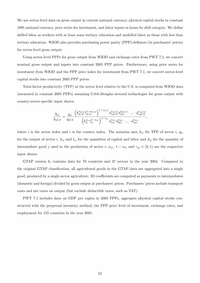
We use sector-level data on gross output in current national currency, physical capital stocks in constant

1995 national currency, price series for investment, and labor inputs in hours by skill category. We define

skilled labor as workers with at least some tertiary education and unskilled labor as those with less than

tertiary education. WIOD also provides purchasing power parity (PPP)-deflators (in purchasers’ prices)

for sector-level gross output.

Using sector-level PPPs for gross output from WIOD and exchange rates from PWT 7.1, we convert

nominal gross output and inputs into constant 2005 PPP prices. Furthermore, using price series for

investment from WIOD and the PPP price index for investment from PWT 7.1, we convert sector-level

capital stocks into constant 2005 PPP prices.

Total factor productivity (TFP) at the sector level relative to the U.S. is computed from WIOD data

(measured in constant 2005 PPPs) assuming Cobb-Douglas sectoral technologies for gross output with

country-sector-specific input shares:

ΛicΛiUS

=qicqiUS

(kαiUSiUS l1−αiUSiUS

)1−γiUSdγ1iUS

1iUS dγ2iUS2ci · ... · dγniUSniUS(

kαicic l1−αicic

)1−γicdγ1ic

1ic dγ2ic2ci · ... · d

γnicnic

,

where i is the sector index and c is the country index. The notation uses Λic for TFP of sector i, qic

for the output of sector i, kic and lic for the quantities of capital and labor and dji for the quantity of

intermediate good j used in the production of sector i; αic, 1 − αic and γji ∈ [0, 1) are the respective

input shares.

GTAP version 6, contains data for 70 countries and 37 sectors in the year 2004. Compared to

the original GTAP classification, all agricultural goods in the GTAP data are aggregated into a single

good, produced by a single sector agriculture. IO coefficients are computed as payments to intermediates

(domestic and foreign) divided by gross output at purchasers’ prices. Purchasers’ prices include transport

costs and net taxes on output (but exclude deductible taxes, such as VAT).

PWT 7.1 includes data on GDP per capita in 2005 PPPs, aggregate physical capital stocks con-

structed with the perpetual inventory method, the PPP price level of investment, exchange rates, and

employment for 155 countries in the year 2005.

55

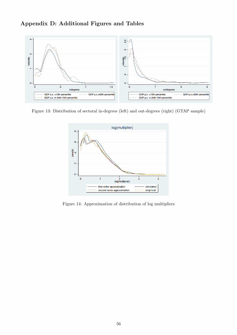
Appendix D: Additional Figures and Tables

Figure 13: Distribution of sectoral in-degrees (left) and out-degrees (right) (GTAP sample)

Figure 14: Approximation of distribution of log multipliers

56

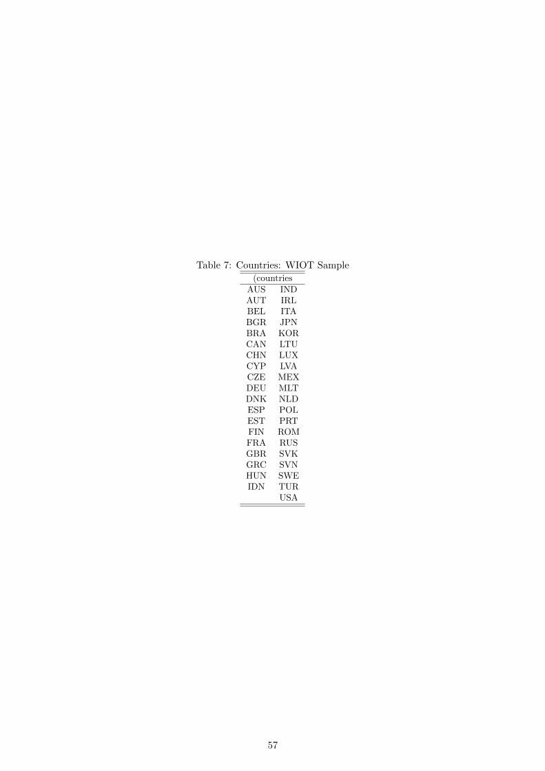
Table 7: Countries: WIOT Sample

(countriesAUS INDAUT IRLBEL ITABGR JPNBRA KORCAN LTUCHN LUXCYP LVACZE MEXDEU MLTDNK NLDESP POLEST PRTFIN ROMFRA RUSGBR SVKGRC SVNHUN SWEIDN TUR

USA

57

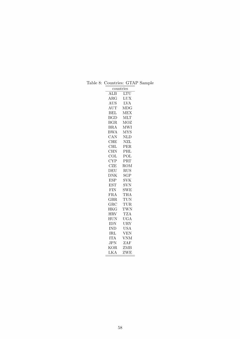
Table 8: Countries: GTAP Sample

countriesALB LTUARG LUXAUS LVAAUT MDGBEL MEXBGD MLTBGR MOZBRA MWIBWA MYSCAN NLDCHE NZLCHL PERCHN PHLCOL POLCYP PRTCZE ROMDEU RUSDNK SGPESP SVKEST SVNFIN SWEFRA THAGBR TUNGRC TURHKG TWNHRV TZAHUN UGAIDN URYIND USAIRL VENITA VNMJPN ZAFKOR ZMBLKA ZWE

58

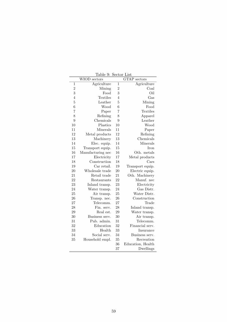
Table 9: Sector ListWIOD sectors GTAP sectors

1 Agriculture 1 Agriculture2 Mining 2 Coal3 Food 3 Oil4 Textiles 4 Gas5 Leather 5 Mining6 Wood 6 Food7 Paper 7 Textiles8 Refining 8 Apparel9 Chemicals 9 Leather

10 Plastics 10 Wood11 Minerals 11 Paper12 Metal products 12 Refining13 Machinery 13 Chemicals14 Elec. equip. 14 Minerals15 Transport equip. 15 Iron16 Manufacturing nec 16 Oth. metals17 Electricity 17 Metal products18 Construction 18 Cars19 Car retail. 19 Transport equip.20 Wholesale trade 20 Electric equip.21 Retail trade 21 Oth. Machinery22 Restaurants 22 Manuf. nec23 Inland transp. 23 Electricity24 Water transp. 24 Gas Distr.25 Air transp. 25 Water Distr.26 Transp. nec. 26 Construction27 Telecomm. 27 Trade28 Fin. serv. 28 Inland transp.29 Real est. 29 Water transp.30 Business serv. 30 Air transp.31 Pub. admin. 31 Telecomm.32 Education 32 Financial serv.33 Health 33 Insurance34 Social serv. 34 Business serv.35 Household empl. 35 Recreation

36 Education, Health37 Dwellings

59