Professor John ZietlowMBA 621

Professor John ZietlowMBA 621

Spring 2006Spring 2006

Stock And Bond ValuationStock And Bond Valuation

Chapter 4Chapter 4

Valuation FundamentalsValuation Fundamentals

• Value of any financial asset is the PV of future cash flows– Bonds: PV of promised interest & principal payments– Stocks: PV of all future dividends– Patents, trademarks: PV of future royalties

• Valuation is the process linking risk & return– Output of process is asset’s expected market price

• A key input is the required [expected] return on an asset– Defined as the return an arms-length investor would require

for an asset of equivalent risk– Debt securities: risk-free rate plus risk premium(s)

• Required return for stocks found using CAPM or other asset pricing model – Beta determines risk premium: higher beta, higher reqd return

The Basic Valuation ModelThe Basic Valuation Model

• Can express price of any asset at time 0, P0, mathematically as Equation 4.1:

• Where:

P0 = Price of asset at time 0 (today)

CFt = cash flow expected at time t

r = discount rate, reflecting asset’s risk

n = number of discounting periods (usually years)

)1.4.(Eq)r +(1

CF + . . . + )r +(1

CF + )r +(1

CF = P nn

22

11

0

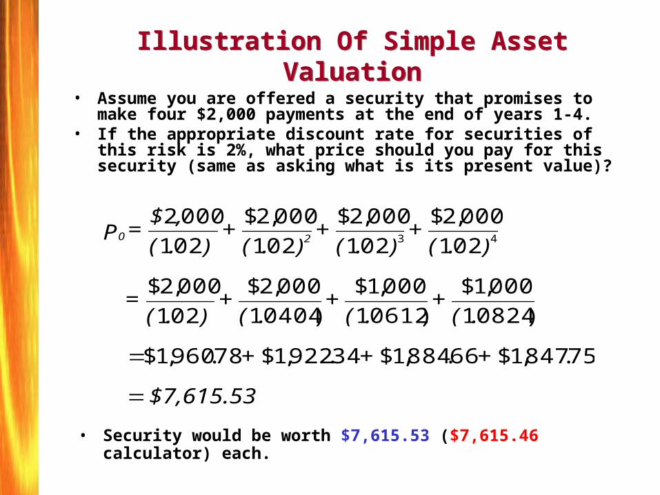
Illustration Of Simple Asset ValuationIllustration Of Simple Asset Valuation

• Assume you are offered a security that promises to make four $2,000 payments at the end of years 1-4.

• If the appropriate discount rate for securities of this risk is 2%, what price should you pay for this security (same as asking what is its present value)?

$7,615.53

+++

.( +

.( +

.( +

).( =

).( +

).( +

).( +

).(

,$ = P 20

75.847,1$66.884,1$34.922,1$78.960,1$

)08241

000,1$

)06121

000,1$

)04041

000,2$

021

000,2$

021

000,2$

021

000,2$

021

000,2$

021

000243

• Security would be worth $7,615.53 ($7,615.46 calculator) each.

Illustration Of Bond Valuation Using U.S. Treasury Securities

Illustration Of Bond Valuation Using U.S. Treasury Securities

• The simplest debt instruments to value are U.S. Treasury securities since there is no default risk.

• Instead of r, the discount rate to use, rf, is the pure cost of borrowing.

• Assume you are asked to value two Treasury securities, when rf is 1.75 percent (r = 0.0175):

– A (pure discount) Treasury bill with a $1,000 face value that matures in three months, and

– A 1.75% coupon rate Treasury note, also with a $1,000 face value, that matures in three years.

• For the T-Bill, three months is one-quarter year (n=0.25)• For 3-year bond, n = 3

Illustration Of Bond Valuation Using U.S. Treasury Securities (Continued)

Illustration Of Bond Valuation Using U.S. Treasury Securities (Continued)

• The 3-month T-Bill pays no interest; return comes from difference between purchase price and maturity value.

• 3-year T-Note makes two end-of-year $17.5 coupon payments (CF1=CF2=$17.5), plus end-of-year 3 payment of interest plus principal (CF3 = $1,017.5)

• Can value both with variation of Equation 4.1:

$1,000=$965.9+ $16.9 + $17.2 =

1.0175

$1,017.5 +

1.0175

$17.5+

1.0175

$17.5 = P

$995.67=1.0043466

$1,000=

1.0175

$1,000=

r +1CF = P

32NoteT

0.250.250.25

BillT

Bond Valuation FundamentalsBond Valuation Fundamentals

• Most U.S. corporate bonds: – Pay interest at a fixed coupon interest rate– Have an initial maturity of 10 to 30 years, and – Have a par value (also called face or principal value) of

$1,000 that must be repaid at maturity. • The Sun Company, on January 3, 2004, issues a 5 percent

coupon interest rate, 10‑year bond with a $1,000 par value– Assume annual interest payments for simplicity– Will value later assuming semi-annual coupon payments

• Investors in Sun Company’s bond thus receive the contractual right to: – $50 coupon interest (C) paid at the end of each year and – The $1,000 par value (Par) at the end of the tenth year.

• Assume required return, r, also equal to 5%

• The price of Sun Company’s bond, P0, making ten (n=10) annual coupon interest payments (C = $50), plus returning $1,000 principal (Par) at end of year 10, determined as:

Bond Valuation Fundamentals (Continued)Bond Valuation Fundamentals (Continued)

00.000,1$05.

050,1$

05.

50$

05.

50$

05.

50$

05.

50$

05.

50$

05.

50$

05.

50$

05.

50$

05.

50$

10987

6543

=)(1

+)(1

+ )(1

+)(1

+

)(1

+ )(1

+)(1

+ )(1

+ )(1

+ )(1

= P 20

• So this bond would be selling at par value of $1,000

• Bond’s value has two separable parts:

(1) PV of stream of annual interest payments, t=1 to t=10

(2) PV of principal repayment at end of year 10.• Can thus also value bond as the PV of an annuity plus the

PV of a single cash flow using PVFA and PVF from tables.

P0 = C x (PVFA5%,10yr) + Par x (PVF5%,10yr)

= $50 (7.7220) + $1,000 (0.6139) = $1,000.00

• Bonds with a few cash flows can be valued with Eq 4.1; for bonds with many cash flows, use PVFA/PVF factors, calculator or Excel.

Bond Valuation Fundamentals (Continued)Bond Valuation Fundamentals (Continued)

Bond Values If Required Return Is Not Equal To The Coupon Rate

Bond Values If Required Return Is Not Equal To The Coupon Rate

• Whenever the required return on a bond (r) differs from its coupon interest rate, the bond's value will differ from its par, or face, value.

– Will only sell at par if r = coupon rate

• When r is greater than the coupon interest rate, P0 will be less than par value, and the bond will sell at a discount.

– For Sun, if r >5%, P0 will be less than $1,000

• When r is below the coupon interest rate, P0 will be greater than par, and the bond will sell at a premium.

– For Sun, if r <5%, P0 will be greater than $1,000

• Exercise: Value Sun Company, 10-year, 5% coupon rate bond if required return, r =6% and again if r = 4%.

Bond Values If Required Return Is Not Equal To The Coupon Rate (Continued)

Bond Values If Required Return Is Not Equal To The Coupon Rate (Continued)

• Value Sun Company bond if r = 6%

P0 = $50 x (PVFA6%,10yr) + Par x (PVF6%,10yr)

= $50 (7.3601) + $1,000 (0.5584) = $926.405 approx

• Bond sells at a discount of $1,000 - $926.405 = $73.595• Value Sun Company bond if r = 4%

P0 = C x (PVFA4%,10yr) + Par x (PVF4%,10yr)

= $50 (8.1109) + $1,000 (0.6756) = $1081.145 approx

• Bond sells at a premium of $1,081.45 - $1,000 = $81.45• Premiums & discounts change systematically as r changes

0 1 2 3 4 5 6 7 8

Required Return, r (%)

Mar

ket

Val

ue

of

Bo

nd

P0 ($

)

1,200

1,100

1,081

926900

800

Premium

Par

Discount

Bond Value & Required Return, Sun Company’s 5 % Coupon Rate, 10-year, $1,000 Par, January 1, 2004 Issue Paying Annual Interest

Bond Value & Required Return, Sun Company’s 5 % Coupon Rate, 10-year, $1,000 Par, January 1, 2004 Issue Paying Annual Interest

1,000

The Dynamics Of Bond Valuation Changes For Different Times To Maturity

The Dynamics Of Bond Valuation Changes For Different Times To Maturity

• Whenever r is different from the coupon interest rate, the time to maturity affects bond value – even if the required return remains constant until maturity.

• The shorter is n, the less responsive is P0 to changes in r. Assume r falls from 5% to 4%

– For n=8 years, P0 rises from $1,000 to $1,067.33, or 6.73%

– For n=3 years, P0 rises from $1,000 to $1,027.75, or 2.775%

• Same relationship if r rises from 5% to 6%, though percentage declines in price less than increases (maximum decline is 100%, increase unlimited)

– For n=8 years, P0 falls from $1,000 to $937.89, or 6.21%

– For n=3 years, P0 falls from $1,000 to $973.25, or 2.675%

• Even if r doesn’t change, premiums and discounts will decline towards par as bond nears maturity.

Time to maturity (years)

Mar

ket

Val

ue

of B

ond

P0 ($

)Relation Between Time to Maturity, Required Return & Bond Value,

Sun Company’s 5%, 10-year, $1,000 Par Issue Paying Annual InterestRelation Between Time to Maturity, Required Return & Bond Value,

Sun Company’s 5%, 10-year, $1,000 Par Issue Paying Annual Interest

Premium Bond, Required Return, r = 4%

Par-Value Bond, Required Return, r = 5%

Discount Bond, Required Return, r = 6%

10 9 8 7 6 5 4 3 2 1 0

M

1,100

1,0811,067.3

1,050

1,027.75

1,000

926

900

950

Relationship Between Bond Prices & Yields, Bonds Of

Differing Current Maturities But Same 6.5% Coupon Rates Relationship Between Bond Prices & Yields, Bonds Of

Differing Current Maturities But Same 6.5% Coupon Rates

Bond Prices and Yields

$0

$500

$1,000

$1,500

$2,000

1 2 3 4 5 6 7 8 9 10 11 12 13 14 15

Yield to maturity, %

Bon

d P

rice

2-year bond 10-year bond

Semi-Annual Bond Interest PaymentsSemi-Annual Bond Interest Payments

• Most bonds pay interest semi-annually rather than annually• Can easily modify basic valuation formula; divide both

coupon payment (C) and discount rate (r) by 2, as in Eq 4.3:

• In Eq 4.3, C is the annual coupon payment, so C/2 is the semi-annual payment.

• r is the annual required return, so r/2 is the semi-annual discount rate.

• n is the number of years, so there are 2n semi-annual payments.

)3.4.()

21(

000,12....

)2

1(

2

)2

1(

2

)2

1(

2Pr2321

Eqr

C

r

C

r

C

r

C

icen

• Value a T-Bond with a par value of $1,000 that matures in exactly 2 years and pays a 4% coupon if r = 4.4% per year.

• Insert known variables into Equation 4.3: C = $40, so C/2 = $20, r = 0.044, so r/2 = 0.022, n = 2, so 2n = 4:

Valuing A Bond With Semi-Annual Bond Interest Payments

Valuing A Bond With Semi-Annual Bond Interest Payments

43.992$97.934$74.18$15.19$57.19$

)022.1(

020,1$

)022.1(

20$

)022.1(

20$

)022.1(

20$

2044.0

1

000,1240$

2044.0

1

240$

2044.0

1

240$

2044.0

1

240$

432

43210

P

The Importance And Calculation Of Yield To Maturity

The Importance And Calculation Of Yield To Maturity

• Yield to Maturity (YTM) is the rate of return investors earn if they buy the bond at P0 and hold it until maturity.

• The YTM on a bond selling at par (P0 = Par) will always equal the coupon interest rate.

– When P0 Par, the YTM will differ from the coupon rate.

• YTM is the discount rate that equates the PV of a bond’s cash flows with its price. If P0, CFs, n known, can find YTM

– Use T-Bond with n=2 years, 2n=4, C/2=$20, P0=$992.43

• The YTM can be found by trial and error, calculator or with spreadsheet program (Excel).

432

21

020,1$

21

20$

21

20$

21

20$43.992$

rrrr

The Fisher Effect And Expected InflationThe Fisher Effect And Expected Inflation

• The relationship between nominal (observed) and real (inflation-adjusted) interest rates and expected inflation called the Fisher Effect (or Fisher Equation).

• Fisher said the nominal rate (r) is approximately equal to the real rate of interest (a) plus a premium for expected inflation (i).– If real rate equals 3% (a = 0.03) and expected inflation

equals 2% (i = 0.02):

r a + i 0.03 + 0.02 0.05 5%

• The true Fisher Effect is multiplicative, rather than additive:

(1+r) = (1+a)(1+i) = (1.03)(1.02) = 1.0506; so r = 5.06%

The Term Structure Of Interest RatesThe Term Structure Of Interest Rates

• At any point in time, will be a systematic relationship between YTM and maturity for securities of a given risk

– Usually, yields on long-term securities higher than short-term

– Generally look at risk-free Treasury debt securities

• Relationship between yield and maturity called the Term Structure of Interest Rates

– Graphical depiction called a Yield Curve

• Yield curves normally upwards-sloping (long yields > short)

– Can be flat or even inverted during times of financial stress

• Won’t cover term structure in depth, but three principal “expectations” theories explain term structure:

– Pure expectations hypothesis: YC embodies prediction

– Liquidity premium theory: Investors must be paid more to invest L-T

– Preferred habitat hypothesis: Investors prefer maturity zones, so different supply and demand characteristics in sub-sectors

Yield Curves for US Treasury SecuritiesYield Curves for US Treasury Securities

2

4

6

8

10

12

14

16

5 10 15 20 30

Years to Maturity

Inte

res

t R

ate

%

August 1996

October 1993

May 1981

January 1995

1 3

Yield Curve, March 23, 2006From www.cnnfn.com

Yield Curve, March 23, 2006From www.cnnfn.com

                     

% %

Years to maturity

Changes In The Shape And Level Of Treasury Yield Curve During Early October 1998

Changes In The Shape And Level Of Treasury Yield Curve During Early October 1998

3.7

3.9

4.1

4.3

4.5

4.7

4.9

5.1

5 10 30

Maturity in Years

Yie

ld %

October 9

October 8

October 2

1

Equity ValuationEquity Valuation

• As will be discussed in chapter 5, the required return on common stock is based on its beta, derived from the CAPM

– Valuing CS is the most difficult, both practically & theoretically

– Preferred stock valuation is much easier (the easiest of all) ^

• Disequilibrium: Whenever investors feel the expected return, r, is not equal to the required return, r, prices will react:

– If exp return declines or reqd return rises, stock price will fall

– If exp return rises or reqd return declines, stock price will rise

• Asset prices can change for reasons besides their own risk

– Changes in asset’s liquidity, tax status can change price

– Changes in market risk premium can change all asset values

• Most dramatic change in market risk: Russian default Fall 98

– Caused required return on all risky assets to rise, price to fall

Bond Risk Premiums, February 97-November 98Bond Risk Premiums, February 97-November 98

0

100

200

300

400

500

600

High-yield BondYields less yieldon 10-yearTreasurys inbasis points

9897

Preferred Stock ValuationPreferred Stock Valuation

• PS is an equity security that is expected to pay a fixed annual dividend over its (assumed infinite) life.

• Preferred stock’s market price, P0, equals next period’s dividend payment, Dt+1, divided by the discount rate, r, appropriate for securities of its risk class:

• A share of PS paying a $2.30 per share annual dividend and with a required return of 11% would thus be worth $20.91:

r

D = P 1t

0

%0.1111.091.20$

30.2$1 == =P

D = r

0

t

share= =r

D = P t

0 /91.20$11.0

30.2$1

• Formula can be rearranged to compute required return, if price and dividend known:

Common Stock ValuationCommon Stock Valuation

• Basic formula for valuing a share of stock easy to state; P0 is equal to the present value of the expected stock price at end of period 1, plus dividends received, as in Eq 4.4:

)4.4.Eq()r1(

DPP 11

0

• But how to determine P1? This is the PV of expected stock price P2, plus dividends. P2 in turn, the PV of P3 plus dividends, and so on.

• Repeating this logic over and over, find that today’s price equals PV of the entire dividend stream the stock will pay in the future, as in Eq 4.5:

)5.4.Eq(....)r1(

D

)r1(

D

)r1(

D

)r1(

D

)r1(

DP

55

44

33

2

210

The Zero Growth Valuation ModelThe Zero Growth Valuation Model

• To value common stock, must make assumption about growth of future dividends.

• Simplest approach, the zero growth model, assumes a constant, non-growing dividend stream:

D1 = D2 = ... = D• Plugging constant value D into Eq 4.5, valuation formula

reduces to simple equation for a perpetuity:

• Assume the dividend of Disco Company is expected to remain at $1.75/share indefinitely, and the required return on Disco’s stock is 15%. P0 is determined to be $11.67 as:

r

DP 0

67.11$15.0

75.1$0

r

DP

The Constant Growth Valuation ModelThe Constant Growth Valuation Model

• The most widely used simple stock valuation formula, the constant growth model, assumes dividends will grow at a constant rate, g, that is less than the required return (g<r).

• If dividends grow at a constant rate forever, can value stock as a growing perpetuity. Denoting next year’s dividend as D1:

• This is commonly called the Gordon Growth Model, after Myron Gordon, who popularized model in the 1960s.

• The Gordon Company’s dividends have grown by 7% per year, reaching $1.40 per share. This growth is expected to continue, so D1=$1.40 x 1.07=$1.498. If required return is 15%:

6.4.10 Eq

gr

DP

73.18$08.0

498.1$

07.015.0

498.1$10

gr

DP

Valuing Common Stock Using The Variable Growth Model

Valuing Common Stock Using The Variable Growth Model

• Because future growth rates might change, need to consider a variable growth rate model that allows for a change in the dividend growth rate.

• Let g1 = the initial, higher growth rate and g2 = the lower, subsequent growth rate, and assume a single shift in growth rates from g1 to g2.

• Model can be generalized for two or more changes in growth rates, but keep simple now.

• For a single change in growth rates, can use four-step valuation procedure:

Valuing Common Stock Using The Variable Growth Model (Continued)

Valuing Common Stock Using The Variable Growth Model (Continued)

• Step 1: Find the value of the dividends at the end of each year, Dt, during the initial high-growth phase.

• Step 2: Find the PV of the dividends during this high-growth phase, and sum the discounted cash flows.

• Step 3: Using the Gordon growth model, (a) find the value of the stock at the end of the high-growth phase using the next period’s dividend (after one year’s growth at g2). – (b) Then compute PV of this price by discounting back to

time 0.

• Step 4: Determine the value of the stock today (P0) by adding the PV of the stock price computed in step 3 to the sum of the discounted dividend payments from step 2.

An Example Of Stock Valuation Using The Variable Growth Model

An Example Of Stock Valuation Using The Variable Growth Model

• Estimate the current (end‑of‑2003) value of Morris Industries' common stock, P0 = P2003 , using the four‑step procedure presented above, and assuming the following:– The most recent (2003) annual dividend payment of Morris

Industries was $4 per share. – The firm's financial manager expects that these dividends

will increase at a 8 percent annual rate, g1 , over the next three years (2004, 2005, and 2006).

– At the end of the three years (end of 2006) the firm's mature product line is expected to result in a slowing of the dividend growth rate to 5 percent per year forever (noted as g2).

– The firm's required return, r , is 12 percent.

An Example Of Stock Valuation Using The Variable Growth Model (Continued)

An Example Of Stock Valuation Using The Variable Growth Model (Continued)

• Step 1: Compute the value of dividends in 2004, 2005, and 2006 as (1+g1)=1.08 times the previous year’s dividend:

Div2004= Div2003 x (1+g1) = $4 x 1.08 = $4.32

Div2005= Div2004 x (1+g1) = $4.32 x 1.08 = $4.67

Div2006= Div2005 x (1+g1) = $4.67 x 1.08 = $5.04

• Step 2: Find the PV of these three dividend payments:

PV of Div2004= Div2004 (1+r) = $ 4.32 (1.12) = $3.86

PV of Div2005= Div2005 (1+r)2 = $ 4.67 (1.12)2 = $3.72

PV of Div2006= Div2006 (1+r)3 = $ 5.04 (1.12)3 = $3.59

Sum of discounted dividends = $3.86 + $3.72 + $3.59 = $11.17

An Example Of Stock Valuation Using The Variable Growth Model (Continued)

An Example Of Stock Valuation Using The Variable Growth Model (Continued)

• Step 3: Find the value of the stock at the end of the initial growth period (P2006) using constant growth model.

• To do this, calculate next period dividend by multiplying D2006 by 1+g2, the lower constant growth rate:

D2007 = D2006 x (1+ g2) = $ 5.04 x (1.05) = $5.292

• Then use D2007=$5.292, g =0.05, r =0.12 in Gordon model:

60.75$0.07

292.5$

0.05 -0.12

292.5$76 = = =

g -rD = P

2

200200

• Next, find the PV of this stock price by discounting P2006 by (1+r)3.

81.53$405.1

60.75$

)12.1(

60.75$

)1( 336 = = =

rP =PV 200

An Example Of Stock Valuation Using The Variable Growth Model (Continued)

An Example Of Stock Valuation Using The Variable Growth Model (Continued)

• Step 4: Finally, add the PV of the initial dividend stream (found in Step 2) to the PV of stock price at the end of the initial growth period (P2006):

P2003 = $11.17 + $53.81 = $64.98

• The current (end-of-year 2003) stock price is thus $64.98 per share.

Other Approaches To Common Stock Valuation

Other Approaches To Common Stock Valuation

• Book value: simply the net assets per share available to common stockholders after liabilities (and PS) paid in full; equals total common equity on the balance sheet– Assumes assets can be sold at book value, so may over-estimate

realizable value• Liquidation value: is the actual net amount per share likely to be

realized upon liquidation & payment of liabilities– More realistic than book value, but doesn’t consider firm’s value as

a going concern• Price/Earnings (P/E) multiples: reflects the amount investors will

pay for each dollar of earnings per share– P/E multiples differ between & within industries– Especially helpful for privately-held firms (think of how many

shares will issue as go public, multiply that by P/E for industry to get market value for all new shares)