Profiling and scalability of the high resolution

NCEP model for Weather and Climate Simulations

Phani R, Sahai A. K, Suryachandra Rao A, Jeelani SMD

Indian Institute of Tropical Meteorology

Dr. Homi Bhabha Road, Pashan, Pune

e-mail: rphani@tropmet.res.in

Abstract—Coupled climate modeling has become one of the

most challenging fields with the development of multicore

architectures and its importance in daily weather and climate

predictions. At IITM, ‘PRITHVI’ cluster (~70TF), NCEP

Climate Forecast System (CFS) and its atmospheric

component (GFS) have been installed on IBM Power6

architecture. Here, we investigate the scalability of the MPI-

OPenMP hybrid models (CFS, GFS) and the limitations of

hybrid spectral models when going to high resolutions. Also,

this paper looks into the performance and scaling with these

two models (CFS, GFS) on the TeraFLOP cluster, varying the

threads and describes the preliminary results for the high resolution simulations.

Keywords-CFS; GFS; scalability; profiling

I. INTRODUCTION

With the advancement of science and multi-core

architectures in High Performance Computing (HPC), the

need and expectation of accurate weather and climate

predictions for the Government agencies and agricultural

organizations have increased. One of the daunting

challenges for the weather forecasters and climate modelers

is to have better scalable models [1-3]. Efforts are being

made to improve weather forecast by running the models at

high resolution with more sophisticated physics and

radiation calls which is of very high cost. Apart from this,

ensemble technique which is now being used for the

seasonal and climate predictions in-turn make the

experiments highly computationally expensive. Presently,

on an IBM Power6, Global Forecast System (GFS) model

with T574 spectral resolution (27 KM), takes ~24 minutes

for a one day simulation on 128 cores, which is time

consuming. We look at this issue how it can be scaled by

varying the MPI tasks and the OpenMP threads. Also, the

recent innovations on increasing the density of cores in each

node/chip, the challenge lies in scaling the model on these

architectures with the variation in the MPI and OpenMP

tasks.

The speed up and the model performance are two main

issues which are very much governed by the system

architectures [4,5]. The speedup can be improved by

increasing the number of MPI tasks or the OpenMP threads

in the MPI-OpenMP parallel implementation of the model.

Recent results suggest that the work sharing between the

cores in the MPI-OpenMP parallel implementation results in

much improved performance and consumes less

communication and I/O bandwidth [2]. With this, the multi-

core architectures have gained much significance for

running hybrid MPI-OpenMP models on these architectures

[2,5,6]. In this paper, we look into the Climate Forecast

System (CFS) model and its atmospheric component Global

Forecast System (GFS) model, their performance on the

IBM Power 6 „PRITHVI‟. We confine our results for three

different spectral resolutions CFS T382, T126 and GFS

T574. We look at the scalability problem of GFS T574 by

varying the number of threads and CFS T382 scalability by

varying the number of cores. Also, the high-resolution

model (GFS T382) is compared with the low resolution

model (GFS T126) and we look closely at the variations in

these simulations.

II. THE MODEL

The NCEP Climate Forecast System (CFS) version 2

[7] is a fully coupled ocean-land-atmosphere dynamical

seasonal prediction model installed on „PRITHVI‟ (IITM)

under the Ministry of Earth Sciences (MOES) and NCEP

MOU. This model is an operational version of NCEP

released recently. At IITM, the CFS model is being run at

two different resolutions T382 (~35 KM), T126 (~100KM)

for the seasonal and extended range prediction. The

atmospheric component of the CFS is the GFS model,

includes both the global analysis and forecast components,

which implies that GFS can also be used for the weather

forecast. The Oceanic component of the CFS is the

MoM4p0 and land-surface model is of NAOH.

Interoperability is achieved with the ocean, atmosphere, sea-

ice and the land-surface components being coupled with the

Earth System Modelling Framework (ESMF) coupler and

runs on the Multiple Program Multiple Data (MPMD)

paradigm.

978-1-4673-2371-0/12/$31.00 ©2012 IEEE

A. Ocean Model

NCEP CFS model contains the Mom4P0 ocean model

[8] which is a finite difference version of the ocean

primitive equations configured under the Boussinesq and

hydrostatic approximations. The model uses the tripolar grid

with the latitude typically taken at 65°N and the other two

grids are at poles situated over land which will not have any

consequences for running the numerical ocean model. The

horizontal layout is a staggered Arakawa B grid and

geometric height is in the vertical. The model has a varying

resolution in the meridonal direction with 0.25° between

10°S and 10°N, gradually increasing to 0.5° poleward of

30°N and 30°S and the zonal direction with 0.5° resolution.

The time-step for this ocean model was 1800 seconds.

Running the CFS model is different from GFS model, CFS

has to be allocated few processors for the ocean component

to run while for the GFS it was not required. For example, if

the model has been allocated 128 cores with 60 cores to the

ocean, GFS runs on 67 cores with one core being allocated

to the coupler.

B. Atmospheric Model

GFS is global atmospheric numerical weather prediction

model developed by NCEP-NOAA [9,10]. This is a spectral

triangular model with hybrid MPI-OpenMP parallel

implementation and has 64 levels in the vertical direction.

Domain decomposition and data communication depend on

the numerical methods used in the model. Most of the

Atmospheric models are three dimensional and the domain

decomposition can be up to three dimensions. Because of its

domain dependent computations, like cloud microphysics,

parameterization schemes NCEP GFS model is a three-

dimensional model with one-dimensional decomposition.

This makes the limitation for the GFS model in the

maximum number of tasks to the number in the latitudes but

can have usage of OpenMP threads.

In the paper, we discuss the GFS T574 (~27KM) along

with the CFS T382 (~35KM) models. For each of these

resolutions, forecast simulations have been done for 8 days

and the total runtimes have been averaged to 1 day. Both the

models have been run in forecast mode with 6 hourly

outputs and the time-step for CFS was 600 seconds while

for GFS was 120 seconds. In the last part of our paper, we

compare the GFS T126 with the GFS T382 results by giving

an observed SST forcing. Simulation for the GFS T126

(Forced Sea Surface Temperature (SST)) and GFS T382

(Forced SST) have been performed for 55 years and 40

years respectively, and the time taken for each of these runs

are 21 days and 48 days respectively on 128 cores.

III. THE SYSTEM

Prithvi‟s IBM Power6 processors support Simultaneous

Multithreading (SMT) which is one of the multi-core

technology on which the hybrid models are supposed to

giver better performance. SMT is a processor technology

that allows two separate instruction streams (threads) to run

concurrently on the same physical processor, improving

overall throughput. On “PRITHVI”, there are 117 nodes

with 128 GB of memory and each node is equipped with 16

Power6 processors, or 32 physical cores. With SMT

switched on, there are 64 logical cores (virtual cpus). Since

each node runs its own operating system, they can be

rebooted or repaired independently from the others,

resulting in higher availability of the overall. It should be

noted that only the 32 physical cores within each node have

direct access to the memory. Also, the total number of cores

for a hybrid model to run in each node can be a maximum of

64 on IBM Power6 architecture. Due to this reason we can

vary the OpenMP threads to a maximum of 32 and a

minimum of 2 MPI tasks in each node. IBM‟s MPI and

LAPI are being used for parallel communication while the

Infiband network is Qlogic.

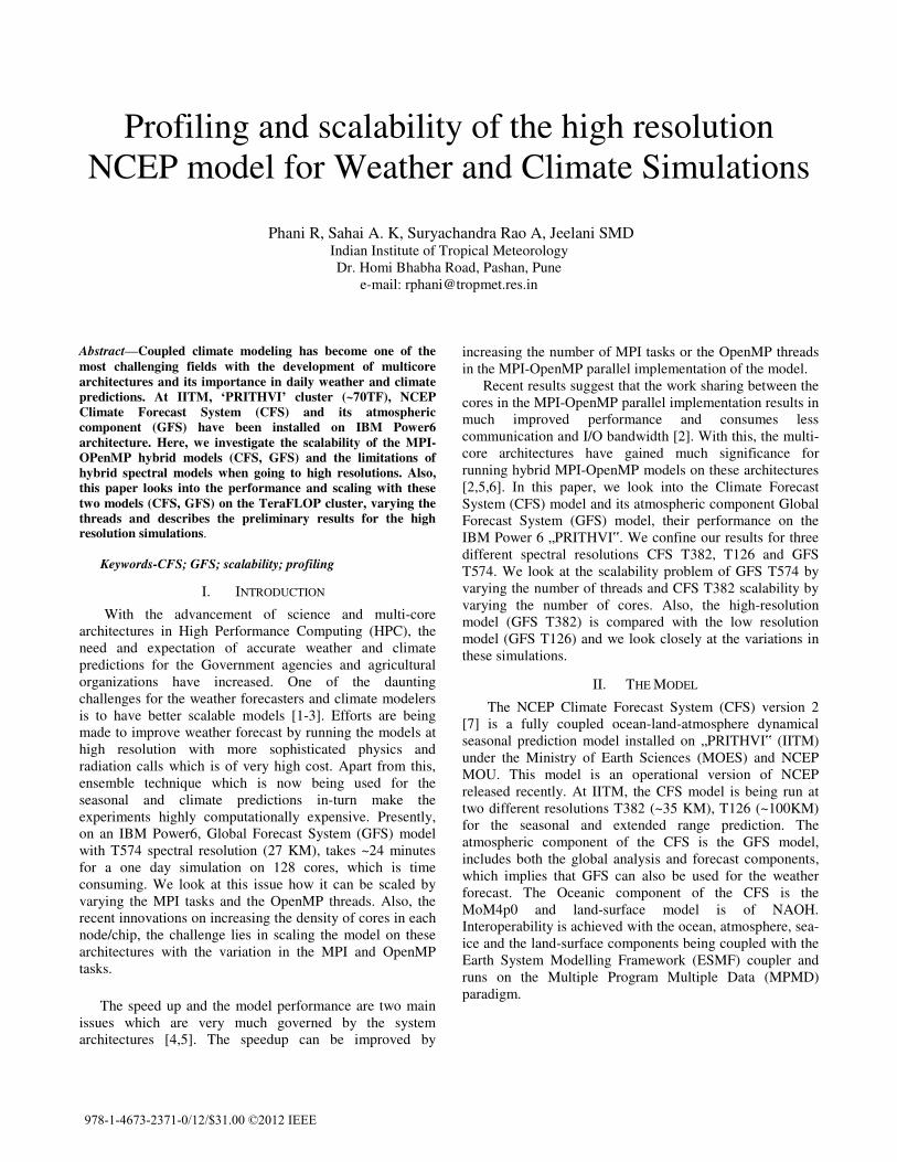
Figure 1. GFS scalability plot for MPI tasks 128 and 400 by varying

the threads.

IV. EFFICIENCY OF THREADING

Climate model involves solving the Navier-Strokes

dynamical equations at each grid-point by different

methods. Out of the finite difference, finite volume, finite

element, spectral element and spectral method, spectral

method gives good exponential convergence (for smooth

solution) and the elimination of pole problems when using

spherical coordinates. The main disadvantage of using the

spectral method is the occurrence of Gibbs phenomena and

the limitation of the spectral truncations. The climate

models which we have presented here, CFS and GFS are

also a part of them. When running CFS, or the GFS, the

atmospheric model spectral dynamical core supports 1D

decomposition over latitude. For this reason, we cannot

increase the number of MPI tasks in running the model

beyond the spectral truncation. For example, if we are

working on GFS T574 spectral resolution, it means that the

spectral triangular truncations are 574 and the number of

MPI tasks cannot be larger than 574. The other option is to

run the climate models with OpenMP threads and we have

performed experiments by varying the OpenMP threads on

different cores rather than running on the same core. There

was an apprehension that running threads on different cores

in a multi-core architecture can increase the performance

rather than on a single core. We address this question by

performing this experiment on our multi-core „PRITHVI‟

system that allows threading to run on virtual and physical

cores concurrently. Our aim is to run the model by varying

the OpenMP threads within each node and look into the

scalability issues.

V. RESULTS AND DISCUSSIONS

Hybrid model scalability performance can be better

understood by varying the MPI and the OpenMP threads.

Initial experiment was performed on the GFS T574

atmospheric model in varying the OpenMP threads. In this

experiment, the total MPI tasks have been fixed and

increased the OpenMP threads in each node from 1 to 32,

thereby decreasing the MPI tasks in each node from 64 to 2

(1 OpenMP thread has 64 MPI tasks, 2 threads have 32 MPI

tasks, 8 threads have 8 MPI tasks, 16 OpenMP threads have

4 MPI tasks in each node). Two experiments have been

performed on this model with MPI task equal to 128 and the

other with MPI tasks equal to 400 and varying the OpenMP

threads. For example, with 400 MPI tasks and 8 OpenMP

threads, the model has been run on 3200 cores ~ 50 nodes ~

30TF.

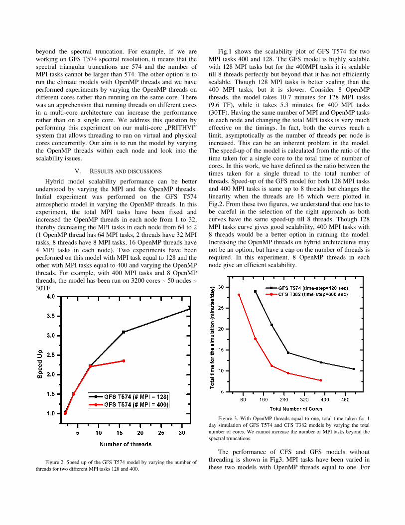
Figure 2. Speed up of the GFS T574 model by varying the number of

threads for two different MPI tasks 128 and 400.

Fig.1 shows the scalability plot of GFS T574 for two

MPI tasks 400 and 128. The GFS model is highly scalable

with 128 MPI tasks but for the 400MPI tasks it is scalable

till 8 threads perfectly but beyond that it has not efficiently

scalable. Though 128 MPI tasks is better scaling than the

400 MPI tasks, but it is slower. Consider 8 OpenMP

threads, the model takes 10.7 minutes for 128 MPI tasks

(9.6 TF), while it takes 5.3 minutes for 400 MPI tasks

(30TF). Having the same number of MPI and OpenMP tasks

in each node and changing the total MPI tasks is very much

effective on the timings. In fact, both the curves reach a

limit, asymptotically as the number of threads per node is

increased. This can be an inherent problem in the model.

The speed-up of the model is calculated from the ratio of the

time taken for a single core to the total time of number of

cores. In this work, we have defined as the ratio between the

times taken for a single thread to the total number of

threads. Speed-up of the GFS model for both 128 MPI tasks

and 400 MPI tasks is same up to 8 threads but changes the

linearity when the threads are 16 which were plotted in

Fig.2. From these two figures, we understand that one has to

be careful in the selection of the right approach as both

curves have the same speed-up till 8 threads. Though 128

MPI tasks curve gives good scalability, 400 MPI tasks with

8 threads would be a better option in running the model.

Increasing the OpenMP threads on hybrid architectures may

not be an option, but have a cap on the number of threads is

required. In this experiment, 8 OpenMP threads in each

node give an efficient scalability.

Figure 3. With OpenMP threads equal to one, total time taken for 1

day simulation of GFS T574 and CFS T382 models by varying the total

number of cores. We cannot increase the number of MPI tasks beyond the

spectral truncations.

The performance of CFS and GFS models without

threading is shown in Fig3. MPI tasks have been varied in

these two models with OpenMP threads equal to one. For

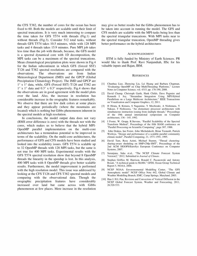
the CFS T382, the number of cores for the ocean has been

fixed to 60. Both the models are scalable until their limit of

spectral truncations. It is very much interesting to compare

the time taken for GFS T574 with threads (Fig.1) and

without threads (Fig.3). Consider 512 total tasks, without

threads GFS T574 takes 10.5 minutes, while with 128 MPI

tasks and 4 threads takes 15.9 minutes. Pure MPI job takes

less time than the job with threads, because, the GFS model

is a spectral dynamical core with 1D decomposition, the

MPI tasks can be a maximum of the spectral truncations.

Mean climatological precipitation plots were shown in Fig.4

for the Indian subcontinent in which GFS (forced SST)

T126 and T382 spectral resolutions are compared with the

observations. The observations are from Indian

Meteorological Department (IMD) and the GPCP (Global

Precipitation Climatology Project). The IMD and GPCP are

1° x 1° data, while, GFS (Forced SST) T126 and T382 are

1° x 1° data and 0.3° x 0.3° respectively. Fig.4 shows that

the observations are in good agreement with the model plots

over the land. Also, the increase in resolution has

considerable increase in the orographic features remarkably.

We observe that there are few dark colors at some places

and they appear periodically (where the mountains are

located) which is nothing but Gibbs phenomenon inherent in

the spectral models at high resolution.

In conclusions, the model output data does not vary

(RMS error difference is zero) with the threads nor with the

cores, which makes us to believe that the hybrid MPI-

OpenMP parallel implementation on the multi-core

architectures has a tremendous potential to be improved in

terms of the scalability. On the multi-core architectures, the

performance of GFS and CFS models have been studied and

looked into the scalability issues. GFS T574 is scalable up

to 32 OpenMP threads with 128 MPI tasks, but the same is

not true for 400 MPI tasks. Experimental results with the

GFS T574 spectral resolution show that beyond 8 OpenMP

threads the linearity in the speedup is lost. In this analysis,

400 MPI tasks with 8 OpenMP threads give better scalable

results. Furthermore, the model improvement is performed

with the high resolution model. This issue was addressed by

looking at the CFS T126 and CFS T382 spectral models and

comparing with the observational data. Though the

orographic precipitation features have considerably

increased over land but came across with Gibbs

phenomenon at few places. Mere increase in the resolution

may give us better results but the Gibbs phenomenon has to

be taken into account in running the model. The GFS and

CFS models are scalable with the MPI-tasks being less than

the spectral triangular truncations. With MPI tasks near to

the spectral triangular truncation, OpenMP threading gives

better performance on the hybrid architectures

ACKNOWLEDGMENT

IITM is fully funded by Ministry of Earth Sciences. PR would like to thank Prof. Ravi Nanjundiah, IISc for his valuable inputs and Rajan, IBM.

REFERENCES

[1] Chunhua Liao, Zhenying Liu, Lei Huang and Barbara Chapman,

“Evaluating OpenMP on Chip MultiThreading Platforms,” Lecture Notes in Computer Science, vol. 4315, pp. 178-190, 2008.

[2] David Champ, Christoph Garth, Hank Childs, Dave Pugmire and Kenneth I. Joy, “Streamline Integration Using MPI-Hybrid Parallelism on a Large Multicore Architecture,” IEEE Transactions on Visualization and Computer Graphics, 12, 2011.

[3] H Hirata, K Kimura, S Nagamine, Y Mochizuki, A Nishimura, Y Nakase, T Nishizawa, “An elementary processor architecture with simultaneous instruction issuing from multiple threads,” Proceedings of the 19th annual international symposium on Computer architecture, 136 - 145, 1992.

[4] I Foster, W. Gropp, R.Stevens, “Parallel Scalability of the Spectral Transform Method", Proceedings of the fifth SIAM conference on "Parallel Processing on Scientific Computing”, page 307, 1988.

[5] John Drakea, Ian Foster, John Michalakesb, Brian Toonenb, Patrick Worleya, "Design and performance of a scalable parallel community climate model", Parallel Computing, 21, 1571-1591, 1995.

[6] David Tam, Reza Azimi, Michael Stumm, “Thread clustering: sharing-aware sheduling on SMP-CMp-SMT”, Proceedings of the 2nd ACM SIGOPS/EuroSys European Conference on Computer Systems, 2007.

[7] Suranjana, Saha et.al., “The NCEP Climate Forecast System Version2,” 2012, Submitted to Journal of Climate.

[8] Stephen Griffies M. Harrison, Ronald C. Pacanowski and Antony Rosati, “A technical guide to MoM4,” GFDL Ocean Group Technical Report 5, NOAA, 2004.

[9] NCEP NOAA: Envoronomental Modelling Center, “The GFS Atmospheric model” NCEP Office Note 442, Global Climate and Weather Modelling Branch, EMC, Camp Springs, Maryland, 2003.

[10] Han J, H-L Pan, Revision and Convection of Vertical Diffusion in the NCEP Global Forecast System, Weather and Forecasting, 2011, 26,520-533.

Figure 4. Mean Climatological precipitation plot for a) GFS T126 (forced Sea Surface Temperature (SST)) for 55 years at 384 x 190 grid resolution b) GFS

T382 (forced SST) for 40 years at 1152 x 576 grid resolution c) IMD station observational data at 360 x 180 grid resolution d) GPCP observational data at

360 x 180 grid resolution.