progress in physics, 2/2014
DESCRIPTION
Publications on advanced studies in theoretical and experimental physics, including related themes from mathematics.TRANSCRIPT

PROGRESS
2014 Volume 10
“All scientists shall have the right to present their scientificresearch results, in whole or in part, at relevant scientificconferences, and to publish the same in printedscientific journals, electronic archives, and any othermedia.” — Declaration of Academic Freedom, Article 8
ISSN 1555-5534
The Journal on Advanced Studies in Theoretical and Experimental Physics,including Related Themes from Mathematics
IN PHYSICS
Issue 2
The Journal on Advanced Studies in Theoretical and Experimental Physics, including Related Themes from Mathematics
PROGRESS IN PHYSICSA quarterly issue scientific journal, registered with the Library of Congress (DC, USA). This journal is peer reviewed and included in the ab-
stracting and indexing coverage of: Mathematical Reviews and MathSciNet (AMS, USA), DOAJ of Lund University (Sweden), Zentralblatt MATH
(Germany), Scientific Commons of the University of St. Gallen (Switzerland), Open-J-Gate (India), Referativnyi Zhurnal VINITI (Russia), etc.
Electronic version of this journal:
http://www.ptep-online.com
Editorial Board
Dmitri Rabounski, Editor-in-Chief
Florentin Smarandache, Assoc. Editor
Larissa Borissova, Assoc. Editor
Editorial Team
Gunn Quznetsov
Andreas Ries
Ebenezer Chifu
Felix Scholkmann
Pierre Millette
Postal Address
Department of Mathematics and Science,
University of New Mexico,
705 Gurley Ave., Gallup, NM 87301, USA
Copyright c© Progress in Physics, 2014
All rights reserved. The authors of the ar-
ticles do hereby grant Progress in Physics
non-exclusive, worldwide, royalty-free li-
cense to publish and distribute the articles in
accordance with the Budapest Open Initia-
tive: this means that electronic copying, dis-
tribution and printing of both full-size ver-
sion of the journal and the individual papers
published therein for non-commercial, aca-
demic or individual use can be made by any
user without permission or charge. The au-
thors of the articles published in Progress in
Physics retain their rights to use this journal
as a whole or any part of it in any other pub-
lications and in any way they see fit. Any
part of Progress in Physics howsoever used
in other publications must include an appro-
priate citation of this journal.
This journal is powered by LATEX
A variety of books can be downloaded free
from the Digital Library of Science:
http://www.gallup.unm.edu/∼smarandache
ISSN: 1555-5534 (print)
ISSN: 1555-5615 (online)
Standard Address Number: 297-5092
Printed in the United States of America
April 2014 Vol. 10, Issue 2
CONTENTS
Rabounski D. and Borissova L. General Relativity Theory Explains the Shnoll Effect
and Makes Possible Forecasting Earthquakes and Weather Cataclysms . . . . . . . . . . . . 63
Hansson J. On the Origin of Elementary Particle Masses . . . . . . . . . . . . . . . . . . . . . . . . . . . . . 71
Lehnert B. Extended Analysis of the Casimir Force . . . . . . . . . . . . . . . . . . . . . . . . . . . . . . . . . . 74
Silva P. R. Proton-Electron Mass Ratio: A Geometric Inference . . . . . . . . . . . . . . . . . . . . . . . 77
Silva P. R. Memory of Living Beings and Its Three Characteristic Times . . . . . . . . . . . . . . . 79
Reiter E. S. New Experiments Call for a Continuous Absorption Alternative to Quantum
Mechanics — The Unquantum Effect . . . . . . . . . . . . . . . . . . . . . . . . . . . . . . . . . . . . . . . . . . 82
Khalaf A. M. and Altalhi F. A. Staggering Phenomenon in Gamma Transitional Ener-
gies over Spin for Negative Parity States of Octupole Vibrational Nuclear Bands . . . 89
Silva N. P. A Model for the Expansion of the Universe . . . . . . . . . . . . . . . . . . . . . . . . . . . . . . . 93
Germano M. Binding Energy and Equilibrium of Compact Objects . . . . . . . . . . . . . . . . . . . 98
Ogiba F. Addendum to “Phenomenological Derivation of the Schrodinger Equation” . . . 108
Dumitru S. Views about “Oxford Questions”. Wave Functions Collapse and Schrodin-
ger’s Cat: Are They Real Scientific Topics or Simple Fictions? . . . . . . . . . . . . . . . . . . 111
Daywitt W. C. The Electron and Proton Planck-Vacuum Coupling Forces and the Dirac
Equation . . . . . . . . . . . . . . . . . . . . . . . . . . . . . . . . . . . . . . . . . . . . . . . . . . . . . . . . . . . . . . . . . . . 114
Robitaille P.-M. Further Insight Relative to Cavity Radiation II: Gedanken Experiments
and Kirchhoff’s Law . . . . . . . . . . . . . . . . . . . . . . . . . . . . . . . . . . . . . . . . . . . . . . . . . . . . . . . . 116
Silva P. R. Electrical Conductivity of Metals: A New Look at this Subject . . . . . . . . . . . . . 121
Robitaille P.-M. On the Equation which Governs Cavity Radiation . . . . . . . . . . . . . . . . . . . 126

Information for Authors and Subscribers
Progress in Physics has been created for publications on advanced studies in
theoretical and experimental physics, including related themes from mathe-
matics and astronomy. All submitted papers should be professional, in good
English, containing a brief review of a problem and obtained results.
All submissions should be designed in LATEX format using Progress in
Physics template. This template can be downloaded from Progress in Physics
home page http://www.ptep-online.com. Abstract and the necessary informa-
tion about author(s) should be included into the papers. To submit a paper,
mail the file(s) to the Editor-in-Chief.
All submitted papers should be as brief as possible. We accept brief pa-
pers, no larger than 8 typeset journal pages. Short articles are preferable.
Large papers can be considered in exceptional cases to the section Special
Reports intended for such publications in the journal. Letters related to the
publications in the journal or to the events among the science community can
be applied to the section Letters to Progress in Physics.
All that has been accepted for the online issue of Progress in Physics is
printed in the paper version of the journal. To order printed issues, contact
the Editors.
This journal is non-commercial, academic edition. It is printed from pri-
vate donations. (Look for the current author fee in the online version of the
journal.)

Issue 2 (April) PROGRESS IN PHYSICS Volume 10 (2014)
LETTERS TO PROGRESS IN PHYSICS
General Relativity Theory Explains the Shnoll Effect and Makes Possible
Forecasting Earthquakes and Weather Cataclysms
Dmitri Rabounski and Larissa Borissova
E-mails: [email protected]; [email protected]
The Shnoll effect manifests itself in the fine structure of the noise registered in very sta-
ble processes, where the magnitude of signal and the average noise remain unchanged.
It is found in the periodic fluctuation of the fine structure of the noise according to the
cosmic cycles connected with stars, the Sun, and the Moon. The Shnoll effect is ex-
plained herein, employing the framework of General Relativity, as the twin/entangled
synchronization states of the observer’s reference frame. The states are repeated while
the observer travels, in common with the Earth, through the cosmic grid of the geodesic
synchronization paths that connect his local reference frame with the reference frames
of other cosmic bodies. These synchronization periods match the periods that are man-
ifested due to the Shnoll effect, regardless of which process produces the noise. These
synchronization periods are expected to exist in the noise of natural processes of any
type (physics, biology, social, etc.) as well as in such artificial processes as computer-
software random-number generation. This conclusion accords with what was registered
according the Shnoll effect. The theory not only explains the Shnoll effect but also al-
lows for forecasting fluctuations in the stock exchange market, fluctuations of weather,
earthquakes, and other cataclysms.
1 The whole truth about the Shnoll effect
Fundamental misunderstandings of the Shnoll effect can be
found in published articles as reported by journalists and sci-
entists. Therefore, now is a good time to tell the whole truth
about the Shnoll effect, to dot all the i’s and to cross all the t’s.
We express our deep appreciation to Prof. Simon Shnoll, with
whom we have enjoyed many years of friendly acquaintance
and scientific collaboration.
The principal error in understanding the Shnoll effect is
that some people think it is a periodical fluctuation of the
magnitude of the signal that is measured. This is incorrect,
since the magnitude of the signal and the average noise re-
main the same during the long-term measurements done by
Shnoll and his workgroup. Further, such processes are specif-
ically chosen for the study that are very stable in time. Simply
put, nothing allegedly changes in the experiments which con-
tinue during days, months, and even years. The subject of
the measurement is the fine structure of the noise registered
in stable processes.
Every process contains noise. The noise originates due
to the influence of random factors and satisfies the Gaussian
distribution (i.e., the Gauss continuous distribution function
of the probability of the measured value between any two
moments of time). Gaussian distribution is attributed to any
random process, such as noise, and is based on the averag-
ing and smoothing of the noise fluctuation measured during
a long enough interval of time. Nevertheless, if considering
very small intervals of time, the real noise has a bizarre struc-
ture of the probability distribution function, which differs for
each interval of time. Each of these real functions being con-
sidered “per se” cannot be averaged to a Gaussian curve. This
is what Shnoll called the fine structure of noise and is the ob-
ject of research studies originally conducted by Simon Shnoll,
commencing in 1951–1954 to this day.
So, the magnitude of noise is measured in a very stable
process during a long enough duration of time (days, months,
and even years). Then the full row of the measured data is
taken under study. The full duration of time is split into small
intervals. A histogram of the probability distribution function
is then created for each of the small intervals. Each inter-
val of time has its own bizarre distribution function (form of
the histogram) that differs from Gaussian function. Never-
theless, Shnoll found that “paired histograms,” which have a
very similar (almost identical) form, exist along the row of the
measured data. That is, the histogram created for each inter-
val of time has its own “twin” which has a similar form. The
similar form was found in the histograms which were regis-
tered with the following periods of repetition connected with
stars, the Sun, and the Moon:
• 24 hours = 1440 min (solar day);
• 365 days = 525 600 min (calendar year);
• 23 hours, 56 min = 1436 min (stellar day);
• 365 days, 6 hours, 9 min = 525 969 min (stellar year);
• 24 hours, 50 min = 1490 min (lunar day);
• 27 days, 7 hours, 43 min = 39 343 min (lunar month);
• 31 days, 19 hours, 29 min = 45 809 min (period of the
lunar evection).
D. Rabounski and L. Borissova. General Relativity Theory Explains the Shnoll Effect 63

Volume 10 (2014) PROGRESS IN PHYSICS Issue 2 (April)
Also, aside as the similar forms of histograms, appearance
the mirrored forms of histograms was registered by Shnoll
with periods of:
• 720 min (half of the calendar/solar day);
• 182 days, 12 hours = 262 800 min (half of the calen-
dar/solar year).
Shnoll called this phenomenon the “palindrome effect”. It is
one of Shnoll’s newest findings: despite his having started
the research studies in 1951, the possibility of the appearance
of the mirrored forms of histograms only came to his atten-
tion in 2004. The “palindrome effect” was first registered in
December 2007. Aside from these two periods of the “palin-
dromes”, a number of other palindrome cycles were found.
However, certain circumstances have not allowed a continua-
tion of these studies in full force yet.
As was shown by Shnoll after many experiments done
synchronously at different locations from South Pole to North
Pole, an appearance of the similar form (or the mirrored form)
of the histograms does not depend on the geographical lati-
tude, but depends only on the geographical longitude, i.e., the
same local time at the point of observation. In other words,
the Shnoll effect is manifested equally at any location on the
Earth’s surface, according to the local time, meaning the same
locations of the celestial objects in the sky with respect to the
visible horizon.
It is significant that the process producing the noise that
we measure can be absolutely anything. Initially, in 1951,
Shnoll started his research studies from measurements of the
speed of chemical reactions in the aqueous solutions of pro-
teins. Then many other biochemical processes attracted his
attention. After decades of successful findings, he focused on
such purely physical processes as α-decay and β-decay of the
atomic nuclei. It was shown that not only all the random natu-
ral processes of different origins, but even artificial processes
as random-number generation by computer software manifest
the Shnoll effect. In other words, this is a fundamental effect.
That in a nutshell is the whole truth about the Shnoll ef-
fect. A detailed history of these research studies can be found
in Shnoll’s book [1], which also contains hundreds of refer-
ences to the primary publications on this theme commencing
in the 1950s to this day. A brief description of the Shnoll
effect can also be found in his short presentation of 2006 [2].
A theoretical explanation of the Shnoll effect on the basis
of General Relativity follows. But first, we need to explain
two important misunderstandings which are popular among
the general public.
2 The two most popular mistakes in the understandings
of General Relativity
There are two main mistakes in the understanding of General
Relativity. These mistakes originate due to the popular ex-
planations of the theory provided by the reporters and other
writers unfamiliar with the details of Riemannian geometry.
The first is the prejudice that an absolute reference frame
allegedly is impossible according to Einstein’s theory. The
second is the prejudice that Einstein’s theory allegedly “pro-
hibits” speeds of information transfer faster than the speed of
light, including the instantaneous transfer of information.
These two prejudices originate due to the superficial ex-
planation of Einstein’s theory, which can be encountered in
the majority of books on the subject. The superficial explana-
tion limits the reader by the historical path in which Special
Relativity and General Relativity were created, and by the
simplest analysis of the basics of the theory of space-time-
matter. As a result, the aforementioned two prejudices be-
came widely popular among laymen as well as among the
scientists who did not study the special aspects of Einstein’s
theory connected with these two problems.
Nevertheless there are a number of fundamental research
studies that cover the aforementioned two problems in detail.
While these research results may be unknown to reporters or
the majority of the scientific community, relativists who work
in the field of reference frames and observable quantities have
long been aware of them.
So, in 1944 Abraham Zelmanov published his massive
theoretical study [3], where he first determined physical ob-
servable quantities as the projections of four-dimensional
quantities onto the line of time and the three-dimensional
spatial section of the observer’s reference frame. His mathe-
matical apparatus for calculating physically observable quan-
tities in the space-time of General Relativity then became
known as the theory of chronometric invariants [4, 5]. Roger
Penrose, Kip Thorne, and Stephen Hawking as young re-
searchers visited Zelmanov in Sternberg Astronomical Insti-
tute (Moscow), and listened to his presentations about physi-
cal reference frames and observable quantities at his seminar.
In particular, Zelmanov showed [3] that an absolute reference
frame is allowed in a finite closed universe, if such a reference
frame is linked to the global rotation or the global deforma-
tion of the universe.
Later, Zelmanov’s followers also voiced, in their scientific
presentations, the possibility of an absolute reference frame in
a finite closed universe.
It should be noted that an absolute reference frame is im-
possible in the space-time of Special Relativity. This is be-
cause Special Relativity considers the simplified version of
the four-dimensional pseudo-Riemannian space (space-time),
which is always infinite, and also is free of curvature, rota-
tion, and deformation. Therefore, an absolute reference frame
is allowed only in the space-time of General Relativity, and
only in those cosmological models where the universe exists
as a finite closed volume of space, which rotates or deforms
as a whole.
The second of the aforementioned prejudices claim that
Einstein’s theory allegedly “prohibits” the particles which
travel faster than light. This claim is not true. The theoretical
possibility of faster-than-light particles — tachyons — was
64 D. Rabounski and L. Borissova. General Relativity Theory Explains the Shnoll Effect

Issue 2 (April) PROGRESS IN PHYSICS Volume 10 (2014)
first considered in 1958 by Frank Tangherlini, in the space-
time of Special Relativity. He presented this theoretical re-
search in his PhD thesis [6] prepared under the supervision
of Sidney Drell and Leonard Schiff, in the Department of
Physics at Stanford University. A similar theory of tachyons
in the framework of Special Relativity was suggested, inde-
pendently of Tanglerlini, in 1979 by Torgny Sjodin [7] (he
was a Swedish scientist working in Theoretical Physics De-
partment at Vrije Universiteit in Brussels). The most impor-
tant surveys on tachyons such as [8,9] referred to Tangherlini.
Tachyons were first illuminated in the journal publications on
the theory of relativity in a principal paper of 1960 [10], au-
thored by Jakov Terletski. Then a more detailed paper [11]
was published in 1962 by Bilaniuk, Deshpande, and Sudar-
shan. The term “tachyons” first appeared later, in 1967 by
Gerald Feinberg [12]. See the newest historical survey and
analysis of this problem in [13]. Detailed consideration of
tachyons in the space-time of General Relativity was included
in our books [14, 15].
The main problem with tachyons is that they cannot be
registered by means of direct experimentation by a regular
observer [16]. Really, regular observers synchronize their
reference frames by light signals. In this case, as was already
pointed out by Einstein, the speed of light is the ultimate max-
imum speed that can be registered by an observer: in this case
superluminal displacements cannot be registered. More pre-
cisely, in reference frames synchronized by light signals, any
superluminal displacement will still be registered as a light
signal. See [16] or §1.15 of our book [14] for details. This
problem arises not from the ideology of Einstein’s theory (as
many people erroneously think), but only from the general
theory of physical experiments.
So, as was explained by international experts on reference
frames, an absolute reference frame is allowed in the space-
time of General Relativity, in a finite closed universe, if such
a reference frame is linked to the global rotation or the global
deformation of the universe. But an absolute reference frame
is impossible in the space (space-time) of Special Relativity,
because the space is infinite, and is free of rotation and defor-
mation.
Faster-than-light particles (tachyons) are allowed in the
space (space-time) of both Special Relativity and General
Relativity. But superluminal speeds of such particles can-
not be registered by a regular observer because his reference
frame is synchronized to others by light signals. Such an ob-
server will register any superluminal motion as motion with
the speed of light.
Aside from the tachyon problem, there is also the problem
of the instant transfer of information. We mean the instant
transfer of information without applying quantum mechanics
methods (we call it non-quantum teleportation). This prob-
lem was first investigated by us, in 1991–1995. These theo-
retical results were first published in 2001, in the first edition
of our book [14]. A short explanation of the theory can also
be found in our presentation [17].
The know-how of our theoretical research was that we
considered the four-dimensional pseudo-Riemannian space
(the space-time of General Relativity) without any limitations
pre-imposed on the space geometry according to physical
sense or philosophical concepts. In other words, we stud-
ied the space-time of General Relativity “per se”. We found
that, in addition to the regular state of space-time, a fully de-
generate state is possible. From the point of view of a regular
observer, whose home is our regular space-time, the fully de-
generate space-time appears as a point: all four-dimensional
(space-time) intervals, all three-dimensional intervals, and all
intervals of time are zero therein. We therefore called the
fully degenerate space-time zero-space. But this fact does
not mean that zero-space is nonsense. Once the observer en-
ters zero-space, he sees that the space and time intervals are
nonzero therein.
We showed that zero-space is inhabited by light-like par-
ticles which are similar to regular photons. We called these
particles zero-particles. Zero-particles travel in zero-space
with the speed of light. But their motion is perceived by
a regular observer as instantaneous displacement. This is
one of the effects of relativity theory, which is due to the
space-time geometry. We only see that particles travel in-
stantaneously while they travel at the speed of light in their
home space (zero-space), which appears to us, the external
observers, as the space wherein all intervals of time and all
three-dimensional intervals are zero.
We also showed that the regular relation between energy
and momentum is not true for zero-particles. Zero-particles
bear the properties of virtual photons, which are known from
Quantum Electrodynamics (i.e., they transfer interactions be-
tween regular particles). This means that zero-particles play
the role of virtual photons, which are material carriers of in-
teraction between regular particles of our world.
Zero-space as a whole is connected to our regular space-
time in every point: at every point of our regular space-time,
we have full access to any location inside zero-space. Once
a regular photon has entered into such a zero-space “gate”
at one location of our regular space, it can be instantly con-
nected to another regular photon which has entered into a sim-
ilar “gate” at another location. This is a way for non-quantum
teleportation of photons.
We also showed that zero-particles manifest themselves
as standing light waves (stopped light) while zero-space as a
whole is filled with the global system of the standing light
waves (the world-hologram). This matches with what Lene
Hau registered in the frozen light experiment [18, 19]: there,
a light beam being stopped is “stored” in atomic vapor, re-
maining invisible to the observer until that moment of time
when it is set free again in its regularly “travelling state”. The
complete theory of stopped light according to General Rel-
ativity was first given in 2011, in our presentations [20, 21],
then again in 2012, in the third edition of our book [14]. The
D. Rabounski and L. Borissova. General Relativity Theory Explains the Shnoll Effect 65

Volume 10 (2014) PROGRESS IN PHYSICS Issue 2 (April)
obtained theoretical results mean that the frozen light exper-
iment pioneered at Harvard by Lene Hau is an experimental
“foreword” to the discovery of zero-particles and, hence, a
way for non-quantum teleportation.
Until recently, teleportation has had an explanation given
only by Quantum Mechanics [22]. It was previously achieved
only in the strict quantum way: e.g., quantum teleportation of
photons, in 1998 [23], and of atoms, in 2004 [24, 25]. Now
the situation changes: with our theory we can find physical
conditions for non-quantum teleportation of photons, which
is not due to the probabilistic laws of Quantum Mechanics
but according to the laws of General Relativity following the
space-time geometry.
Thus, the instant transfer of information is allowed in the
space-time of General Relativity (though the real speeds of
the particles do not exceed the velocity of light). But this is
impossible in the space-time of Special Relativity, because it
is free of rotation and a gravitational field (whereas by con-
trast, the main physical condition of zero-space is a strong
gravitational potential or a near-light-speed rotation).
Of course, the general reader cannot find all these im-
portant details in general-purpose books explaining Einstein’s
theory. Special skills in Riemannian geometry are needed to
understand what has been written in the special publications
that we surveyed herein. It is not surprising, therefore, that
the majority of people are still puzzled by the aforementioned
prejudices and misunderstandings about Einstein’s theory.
3 General Relativity Theory explains the Shnoll effect:
the scanning of the world-hologram along the Earth’s
path in the cosmos
As we shall set forth, the instantaneous synchronization of re-
mote reference frames in our Universe via non-quantum tele-
portation has a direct connection with the Shnoll effect.
First, let us understand what is the Shnoll effect in terms
of the theory of relativity.
The form of a histogram obtained as a result from a series
of measurements of noise (note that the average magnitude
of the noise remains the same) shows the fine structure of
the countdown of the measured value, according to the struc-
ture of the physical coordinates and of the physical time of
the observer. It does not matter which type of processes pro-
duces the registered noise; only the physical reference frame
of the observer is substantial. In other words, the form of the
histogram’s resulting measurement of noise shows the fine
structure of the physical coordinates and of the physical time
of the observer. If two histograms’ resulting measurements
of noise taken at two different time intervals have the same
form, then two of these different states of the same system
that generates the noise are synchronized to each other. If
these two synchronized states appear periodically in the mo-
ments of time associated with the same coordinates of a cos-
mic body on the celestial sphere, the two synchronized states
are also synchronized with the cosmic body.
Therefore, we arrive at the following conclusion. In terms
of relativity theory, the Shnoll effect means that the reference
frame of a terrestrial observer is somehow synchronized with
remote cosmic bodies. This synchronization is done at each
moment of time with respect to coordinates connected with
stars (cycles of the stellar day and the sidereal year), and with
respect to the coordinates connected with the Sun (cycles of
the solar day and the calendar year). Also, the synchroniza-
tion condition (the form of the histogram) is repeated in the
reversed mode in time at each of two opposite points in the
Earth’s orbit around the Sun, and at each of two opposite
points of the observer’s location with respect to stars (due
to the daily rotation of the Earth): this is the “palindrome ef-
fect”, including the half-year and half-day palindromes.
Now the second question arises. How is this synchroniza-
tion accomplished? Regularly, and according to the initial
suggestion of Einstein (which was introduced in the frame-
work of Special Relativity), reference frames are synchro-
nized by light signals. But in the case of experiments where
the Schnoll effect was registered, the noise source and the
measurement equipment were located in a laboratory build-
ing under a massive roof. So the laboratory is surely isolated
from light signals and other (low-magnitude) electromagnetic
radiations which come from stars. . . The answer comes from
General Relativity.
First, as is known from General Relativity, two remote
reference frames can be synchronized through the shortest
path (known as geodesic line) connecting them in the space
(space-time). A geodesic path can be paved between any two
points at every fixed moment of time. If these points oscil-
late with respect to each other, the synchronized states are re-
peated with the period of the oscillation. In terms of a regular
terrestrial observer, who is located on the surface of the Earth,
this means that his reference frame can be synchronized with
the reference frame of a celestial object, which is located in
the depths of the cosmos, at any moment of time. Each single
state (moment of time) of the synchronization has twin states
of synchronization. The twin states are repeated due to the
daily rotation and to the yearly rotation of the observer (at
his location on the Earth’s surface) with respect to stars∗, with
respect to the Sun, and also due to his cyclic motion with re-
spect to the Moon. Thus the respective cycles of repetition of
the synchronized twin states of the observer’s reference frame
(the cycles of appearance of the similar forms of histograms)
must exist. The cycles of repetition of the twin states are, with
precision, to the nearest minute:
∗This refers to the International Celestial Reference System, which is
the standard celestial coordinate system centered at the barycentre of the So-
lar System, with axes that are fixed with respect to objects in far-reaches
of the cosmos. These coordinates are approximately the same as the equato-
rial coordinates on the celestial sphere. The International Celestial Reference
System is defined by the measured positions of more than two hundred extra-
galactic objects (mainly quasars). It is the standard stellar reference system
accepted by the International Astronomical Union.
66 D. Rabounski and L. Borissova. General Relativity Theory Explains the Shnoll Effect

Issue 2 (April) PROGRESS IN PHYSICS Volume 10 (2014)
• Solar day (24 hours= 1440 min), the period of daily ro-
tation of the terrestrial observer together with the Earth
with respect to the Sun;
• Calendar year (365 days = 525 600 min), the period
of orbital revolution of the terrestrial observer together
with the Earth around the Sun;
• Sidereal (stellar) day: 23 hours, 56 min = 1436 min. It
is the period of daily rotation of the terrestrial observer,
together with the Earth with respect to stars;
• Sidereal (stellar) year: 365 days, 6 hours, 9 min =
525 969 min. It is the period of orbital revolution of
the terrestrial observer, together with the Earth around
the Sun with respect to stars;
• Lunar day (24 hours, 50 min = 1490 min), the period
between two observed moonrises. It is longer than a
24-hour solar day, because the Moon revolves around
the Earth in the same direction that the Earth rotates
around her own axis;
• Sidereal month: 27 days, 7 hours, 43 min = 39 343
min. It is the period of the Moon’s revolution around
the Earth with respect to stars;
• Period of the lunar evection (31 days, 19 hours, 29 min
= 45 809 min), which is the period of the oscillatory
deviation of the Moon’s orbit from its average position
with respect to the Earth.
Also, the cycles of reverse synchronization (appearance of the
mirrored forms of histograms, that means the “palindrome
effect”) shall exist according to the half-periods:
• Half of the solar day (12 hours = 720 min);
• Half of the calendar year (182 days, 12 hours= 262 800
min);
• Half of the stellar day (11 hours, 58 min = 718 min);
• Half of the sidereal year (182 days, 15 hours, 5 min =
262 985 min);
• Half of the lunar day (12 hours, 25 min = 745 min);
• Half of the sidereal month (13 days, 15 hours, 52 min
= 19 672 min);
• Half-period of the lunar evection (15 days, 21 hours, 45
min = 22 905 min).
Also there exist a number of other periods of appearance of
the synchronized states of the observer’s reference frame (ap-
pearance of the similar form of histograms), which manifest
cyclic synchronization with some other celestial objects. We
do not discuss them herein because of brevity of this presen-
tation.
Second. Synchronization is possible not only of light sig-
nals or other electromagnetic signals moving at the speed of
light. Instant synchronization of remote reference frames is
possible in the space-time of General Relativity [14,17]. This
can be done through zero-space — the fully degenerate space-
time. It will appear to a regular observer as a point; that is the
necessary condition of non-quantum teleportation at any dis-
tance in our world. Therefore the “non-quantum teleportation
channel” is constantly allowed between any two points of our
space. Zero-particles — the particles that are hosted by zero-
space — are material carriers in non-quantum teleportation.
Zero-particles are standing light waves (i.e. stopped light),
thus zero-space is filled with a global system of standing light
waves — the world-hologram of non-quantum teleportation
channels. According to space topology, there is univalent
mapping of zero-space (the world-hologram) onto our reg-
ular space (our universe). This means that the local physical
reference frame of a terrestrial observer, travelling together
with the Earth in the cosmos, “scans” the world-hologram of
teleportation channels.
Each point of the Earth’s surface, including the observer’s
location, makes a daily revolution around the Earth’s centre.
The Earth revolves around the Sun at a speed of 30 km/sec.
The Sun revolves, at a speed of 250 km/sec, around the centre
of our Galaxy called the Milky Way. As a result, the observer
located on the surface of the Earth travels in the Galaxy along
the highly elongated double helix (which is like the DNA he-
lix), through the cosmic grid of the “stargates” into the non-
quantum teleportation channels which instantly synchronize
his local reference frame with stars, the Sun, and other cosmic
objects. Because of the cycles of the turbinal motion of the
observer, each single stargate has its own twin respectively
to the periods of the motion. The states of the observer’s
reference frame at these twin locations, due to entering into
the same teleportation channel, are not only synchronized but
also entangled with each other.∗
The moments of a terrestrial observer’s entering into the
gate of the same teleportation channel are the same as the mo-
ments of repetition of the twin synchronized states of his local
reference frame. Therefore, it is obvious that the appearance
of the similar forms of histograms (and the appearance of the
mirrored forms of histograms) manifests not only the syn-
chronized (and, respectively, — reverse synchronized) twin
states of the observer’s reference frame, but also that these
states are entangled with each other.
Such a synchronization occurs regardless of whether the
observer sees the sky or is isolated in a laboratory building. It
is done by zero-particles through zero-space, independently
of the obstacles that can be met by electromagnetic signals in
our regular space.
Recall, the Shnoll effect is periodic repetition of a similar
form (or mirrored forms) of the histograms’ resulting mea-
surement of noise. Most of the periods that are expected
according to the theory and listed above coincide with the
periods registered by Shnoll and his workgroup [1]. These
are the solar day (1440 min), the stellar day (1436 min), the
calendar year (525 600 min), the stellar year (525 969 min),
∗In a sense similar to the quantum entangled states, according to Quan-
tum Mechanics.
D. Rabounski and L. Borissova. General Relativity Theory Explains the Shnoll Effect 67

Volume 10 (2014) PROGRESS IN PHYSICS Issue 2 (April)
the lunar day (1490 min), the lunar month (registered as the
“near-27-day period”), and the period of the lunar evection
(45 809 min). The mirrored forms of histograms were regis-
tered with periods of half of a solar day (720 min), and half of
the calendar year (262 800 min), while analysis of the mea-
surements is still under development. Nevertheless, there are
enough coincidences of the theory with Shnoll’s experimen-
tal data.
We therefore conclude that the Shnoll effect manifests the
scanning of the world-hologram of the non-quantum telepor-
tation channels along the Earth’s path in the cosmos. So, the
Shnoll effect has been explained according to General Rela-
tivity Theory.
It is important to understand the following: to find entan-
gled moments of time (the “gates” into the same teleportation
channel in the cosmos), it does not matter which stable pro-
cess (which type of processes) produces the random noise that
we register. Not only natural processes, but also the processes
such as random-number generation by a computer’s software
will show the Shnoll effect, as well as such social phenomena
as fluctuations in the stock exchange market. This means that
the theoretical explanation that is given here on the basis of
General Relativity provides a theoretical ground for a wide
range of fundamental effects in physics, biology, geophysics,
social behaviour and other fields of science. This fact leads
us to a number of important sequels and applications, which
can be achieved from further research studies of the Shnoll
effect.
4 Forecasting earthquakes and other cataclysms on the
basis of the scanning of the Earth’s path in the cosmos
So, we have arrived at a conclusion that the Shnoll effect is
a fundamental effect, which is explained according to Gen-
eral Relativity. Therefore, we expect the Shnoll effect to be
found not just in noise that the terrestrial observer registers
in such processes as biochemical reactions or nuclear decay.
The noise of other terrestrial processes which have natural
and artificial origin should also show the Shnoll effect. Be-
cause practical applications are important, the following im-
portant types of noise should be taken into account:
• Random mass migrations of people;
• Fluctuations in the stock exchange market;
• Fluctuations of the sickness rate among the masses of
people, animals, and plants;
• Fluctuations of social unrest (local conflicts, etc.)
• Fluctuations of the Earth’s crust — earthquakes;
• Fluctuations of weather (weather events and weather
cataclysms);
• and many others.
Here within we’ve touched so far only on the last two items
on this list. These are earthquakes and weather.
Our planet Earth is so large that earthquakes can be con-
sidered as the noise fluctuations of the Earth’s crust, while
weather events and weather cataclysms are the noise fluctu-
ations in the atmosphere. Therefore, this is a proper back-
ground where the Shnoll effect should be manifested.
Indeed, there is a huge scientific study that shows the
statistical behaviour of background earthquakes and weather
events [26–32]. The study was done in the 1930–1940’s.
It was conducted by Nikolai Morozov, Hon. Member of the
USSR Academy of Sciences.∗
Morozov and his assistants analysed the observational
data about the background earthquakes and weather events
that were collected at all the world-known weather observato-
ries and seismic stations of the world (located from the equa-
tor to the extreme north and south). The observational data
were recorded throughout all periods of the systematic scien-
tific observations, during the second half of the 19th century
and the first half of the 20th century, which has then been
accessed from yearbooks of the observatories and stations.
In addition to the statistical behaviour of the background
earthquakes and weather events, Morozov found that air tem-
perature, barometric pressure, humidity and other geophys-
ical parameters depend on the height of the centre of our
Galaxy (and other compact star clusters in our Galaxy) above
the horizon. In other words, the weather factors depend on
the stellar (sidereal) time at the point of observations. As a
result, Morozov arrived at the following fundamental conclu-
sion. All previous forecasts of earthquakes and weather cata-
clysms did not give satisfying results because the forecasters
took into account only the influence of the Sun and Moon on
the Earth’s crust and the atmosphere (which influences were
dated according to solar time), while the influence of objects
in the farther-reaches of the cosmos, such as the centre of
our Galaxy and other (as visible and invisible) compact stel-
lar clusters, which are dated according to the stellar (sidereal)
time, were not taken into account.
We can therefore say that Morozov’s geophysical studies
show that we can surely consider micro-earthquakes as ran-
dom noise, which always exist in the Earth’s crust. The same
is true about weather where random noise is nothing but small
fluctuations of air temperature, barometric pressure, humid-
ity, etc.
A confirmation of the conclusion follows from Shnoll’s
experiments. Already by the 1980s, synchronous fluctuations
of forms of the histograms (the Shnoll effect) were registered
on the basis of seismic observations [33]. This means, ac-
cording to our theoretical explanation herein, that the twin en-
tangled synchronization states of the local physical reference
frame of the terrestrial observer (the Shnoll effect, according
to General Relativity) coincide with the seismic noise regis-
tered in the Earth’s crust.
∗This study was not continued after the death of its author, Prof. Moro-
zov, in 1946.
68 D. Rabounski and L. Borissova. General Relativity Theory Explains the Shnoll Effect

Issue 2 (April) PROGRESS IN PHYSICS Volume 10 (2014)
Therefore, proceeding from our theoretical explanation of
the Shnoll effect, we can forecast how, where, and when pow-
erful earthquakes will appear in the Earth’s crust; how, where,
and when weather cataclysms will occur in the atmosphere.
Essentially, here’s how to go about doing it.
Two things are needed to understand this method. First,
we need to understand that every real observer has his own
local physical reference frame. The physical reference frame
consists of real coordinate grids spanning over the real phys-
ical bodies around him (his real reference bodies), and also
of the real clocks that are fixed on the real coordinate grids.∗
In the case of a terrestrial observer (us, for instance), the real
coordinate grids and clocks are connected with the physical
environment around us. Therefore, noise fluctuations of the
environment mean noise fluctuations of the real physical mea-
surement units of the observer.
Second, as follows from the theory of physical observable
quantities in General Relativity, if the fine structure of noises
in two physical reference frames match with each other, these
two reference frames are synchronized with each other.
Therefore, as we’ve shown above, the Shnoll effect mani-
fests the twin/entangled states of the local physical reference
frame of the observer. These twin/entangled states are in-
stantly synchronized with each other, along with other cos-
mic bodies located along the entire synchronization path in
the cosmos. If their physical reference frames are synchro-
nized at a very close frequency, a resonance of noise fluctu-
ations occurs. In this case, concerning seismic noise, a pow-
erful earthquake occurs in the background of the noise from
micro-earthquakes (that exist continuously and everywhere in
the Earth’s crust). Concerning the weather, this means that a
weather cataclysm occurs in the background of noise fluctua-
tions of the weather.
In other words, if one or more of the powerful cosmic
bodies appear on the same path of synchronization with a
terrestrial observer, noise fluctuations of these cosmic bod-
ies become synchronized with the background noise of the
observer’s physical reference frame. A resonance occurs in
the physical reference frame of the observer that is the local
environment in the point of his observation. The background
noise of the environment experiences a huge fluctuation: i.e.,
a powerful earthquake, a weather cataclysm, etc.
Thank to Morozov’s geophysical studies we conclude that
the Sun and the Moon are not the main “synchronizers” that
cause a significant resonance in the physical reference frame
of a terrestrial observer. We must therefore take into account
the convergence of several “celestial synchronizers” of the
Solar System and our Galaxy in one synchronization path.
Therefore, all that is required for forecasting earthquakes
and weather cataclysms, according to our theoretical expla-
nation of the Shnoll effect, is as follows.
∗See details about physical reference frames, and about physical observ-
able quantities in Zelmanov’s publications [3–5], or in our books [14, 15].
1. First step — daily registrations of the basic noise fluc-
tuations in different environments at different locations
on the Earth. Analysis of the measurements, according
to the histogram techniques that were used by Shnoll,
in order to fix the details of the periods as determined
by the Shnoll effect. In other words, this is the “scan-
ning” of the local space of the planet in order to create
the complex map of the background noise fluctuations
of different environments of the Earth, according to so-
lar time and stellar time;
2. Second step — creating a detailed list of the more or
less powerful cosmic sources, which can be the main
“synchronizers” affecting the physical reference frame
of a terrestrial observer. The stellar (sidereal) coordi-
nates of the cosmic sources, and their ephemerides will
be needed in the third stage of the forecasting;
3. Third step — determining the moments of time when
these celestial synchronizers converge on the same syn-
chronization path, that is, their crossing the celestial
meridian (hour circle) at approximately the same mo-
ment of time as the point of observation, then compar-
ing these with the moments of time of the noise fluc-
tuations registered due to the Shnoll effect (in the first
step). As a result we will find those celestial synchro-
nizers whose synchronization with the terrestrial envi-
ronment produces the most powerful effect;
4. Fourth step — calculate further convergences of the
most powerful synchronizers at every location on the
Earth’s surface. As a result, by taking into account the
delay time of interaction rate in the respective terres-
trial environment (the ground, the atmosphere, etc.),
we will be able to forecast where and when the reso-
nant states will occur in the Earth’s crust (earthquakes)
and in the atmosphere (weather cataclysms).
Forecasting the other events of the above list such as ran-
dom mass migrations of people, fluctuations in the stock ex-
change market, fluctuations of the sickness rate, fluctuations
of social unrest, and others, is possible analogously. The
events predicted according to this method may have differ-
ent periods of delay from the synchronization moment. The
delay time depends on inertia in the medium that is being
affected: the Earth’s crust, atmosphere, interaction in the so-
cial medium, etc. Therefore, despite this, the moments of the
resonant synchronization are the same for all processes that
are registered at the point of observation; the resonant fluc-
tuations will appear at different moments of time in different
environments (including the technogenic environments and
the social medium). Nevertheless the method of forecasting
remains consistent for all the events around us.
So, forecasting powerful earthquakes and weather cata-
clysms is possible on the basis of our theoretical explanation
of the Shnoll effect. Other practical applications of the the-
D. Rabounski and L. Borissova. General Relativity Theory Explains the Shnoll Effect 69

Volume 10 (2014) PROGRESS IN PHYSICS Issue 2 (April)
ory and experiment are also possible, but they are outside the
scope of this short communication.
Acknowledgements
The authors are grateful to Prof. Simon Shnoll and his wife,
Prof. Maria Kondrashova, for years of fruitful scientific col-
laboration and friendly acquaintance. We are also thankful to
Prof. Joseph Hafele and Patrick Ivers for a discussion of these
issues and useful tips.
Submitted on January 25, 2014 / Accepted on January 27, 2014
References
1. Shnoll S. E. Cosmophysical Factors in Stochastic Processes. American
Research Press, Rehoboth (NM, USA), 2012.
2. Shnoll S. E. Changes in the fine structure of stochastic distributions as
a consequence of space-time fluctuations. Progress in Physics, 2006,
v. 2, issue 2, 39–45.
3. Zelmanov A. Chronometric Invariants. Dissertation, 1944. American
Research Press, Rehoboth (NM, USA), 2006.
4. Zelmanov A. L. Chronometric invariants and accompanying frames of
reference in the General Theory of Relativity. Soviet Physics Doklady,
1956, vol. 1, 227–230 (translated from Doklady Academii Nauk USSR,
1956, vol. 107, no. 6, 815–818).
5. Zelmanov A. L. On the relativistic theory of an anisotropic inhomo-
geneous universe. A 1957 Cosmogony Meeting thesis. The Abraham
Zelmanov Journal, 2008, vol. 1, 33–63.
6. Tangherlini F. R. The velocity of light in uniformly moving frame.
A dissertation. Stanford University, 1958. The Abraham Zelmanov
Journal, 2009, vol. 2, 44–110.
7. Sjodin T. Synchronization in special relativity and related theories.
Nuovo Cimento B, 1979, v. 51, 229–246.
8. Recami E. Classical tachyons and possible applications. Rivista del
Nuovo Cimento, 1986, vol. 9, 1–178.
9. Liberati S., Sonego S., and Visser M. Faster-than-c signals, special rel-
ativity, and causality. Annals of Physics, 2002, vol. 298, 151–185.
10. Terletski Ya. P. The causality principle and the second law of thermody-
namics. Soviet Physics Doklady, 1961, vol. 5, 782–785 (translated from
Doklady Academii Nauk USSR, 1960, vol. 133, no. 2, 329–332).
11. Bilaniuk O.-M. P., Deshpande V. K., and Sudarshan E. C. G. “Meta” rel-
ativity. American Journal of Physics, 1962, vol. 30, no. 10, 718–723.
12. Feinberg G. Possibility of faster-than light particles. Physical Review,
1967, vol. 159, no. 5, 1089–1105.
13. Malykin G. B. and Malykin E. G. Tangherlini’s dissertation and its sig-
nificance for physics of the 21th century. The Abraham Zelmanov Jour-
nal, 2009, vol. 2, 121–143.
14. Rabounski D. and Borissova L. Particles Here and beyond the Mir-
ror. Third expanded edition. American Research Press, Rehoboth (NM,
USA), 2012. Re-printed in French as: Rabounski D. et Borissova L.
Particules de l’Univers et au dela du Miroir. Traduit de l’anglais par
Patrick Marquet, American Research Press, Rehoboth (NM, USA),
2012.
15. Borissova L. and Rabounski D. Fields, Vacuum, and the Mirror Uni-
verse. Svenska fysikarkivet, Stockholm, 2009. Re-printed in French as:
Borissova L. et Rabounski D. Champs, Vide, et Univers miroir. Traduit
de l’anglais par Patrick Marquet, American Research Press, Rehoboth
(NM, USA), 2010.
16. Rabounski D. A blind pilot: who is a super-luminal observer? Progress
in Physics, 2008, v. 4, issue 2, 171.
17. Borissova L. and Rabounski D. On the possibility of instant displace-
ments in the space-time of General Relativity. Progress in Physics,
2005, v. 1, issue 1, 17–19.
18. Hau L. V. Frozen light. Scientific American, 17 July 2001, v. 285, no. 1,
52–59.
19. Hau L. V. Frozen light. Scientific American Special Edition “The Edge
of Physics”, 31 May 2003, 44–51.
20. Rabounski D. and Borissova L. A theory of frozen light according to
General Relativity. A presentation delivered at the 2011 APS March
Meeting, held in March 21–25, 2011, in Dallas, Texas.
21. Rabounski D. and Borissova L. A theory of frozen light according to
General Relativity. The Abraham Zelmanov Journal, 2011, v. 4, 3–27.
22. Bennett C. H., Brassard G., Crepeau C., Jozsa R., Peres A., and Woot-
ters W. K. Teleporting an unknown quantum state via dual classical
and Einstein-Podolsky-Rosen channels. Physical Review Letters, 1993,
v. 70, 1895–1899.
23. Boschi D., Branca S., De Martini F., Hardy L., and Popescu S. Exper-
imental realization of teleporting an unknown pure quantum state via
dual classical and Einstein-Podolsky-Rosen Channels. Physical Review
Letters, 1998, v. 80, 1121–1125.
24. Riebe M., Haffner H., Roos C. F., Hansel W., Benhelm J., Lancas-
ter G. P. T., Korber T. W., Becher C., Schmidt-Kaler F., James D. F. V.,
and Blatt R. Deterministic quantum teleportation with atoms. Nature,
2004, v. 429, 734–736.
25. Barrett M. D., Chiaverini J., Schaetz T., Britton J., Itano W. M.,
Jost J. D., Knill E., Langer C., Leibfried D., Ozeri R., and Wine-
land D. J. Deterministic quantum teleportation of atomic qubits. Nature,
2004, v. 429, 737–739.
26. Morozov N. A. On the possibility of a scientific prognosis of weather.
Bulletin de l’Academie des Sciences de l’URSS, Serie geographique et
geophisique, 1944, tome VIII, no. 2–3, 63–71.
27. Morozov N. A. Influence of the central body of the galaxy and its other
dark super-suns on the geophysical and meteorological phenomena that
appear around us. Archive of Russian Academy of Sciences, fund 543
(personal fund of N. A. Morozov, Hon. Member of the USSR Academy
of Sciences), folder 01, file 72 (188 pages).
28. Morozov N. A. On the cosmic factors affecting the frequency of earth-
quakes. Ibidem, file 96 (461 pages).
29. Morozov N. A. On the celestial influences on the frequency of earth-
quakes. Ibidem, file 98 (297 pages).
30. Morozov N. A. On the influence of the cosmic effects on the frequency
of earthquakes. Ibidem, file 99 (110 pages).
31. Morozov N. A. Earthquakes: the cosmic studies. Ibidem, file 100
(282 pages).
32. Morozov N. A. Basics of Theoretical Meteorology and Geophysics.
Manuscript of the book. Ibidem, files 128–139.
33. Shnoll S. E. Private communications with the authors.
70 D. Rabounski and L. Borissova. General Relativity Theory Explains the Shnoll Effect

Issue 2 (April) PROGRESS IN PHYSICS Volume 10 (2014)
On the Origin of Elementary Particle Masses
Johan Hansson
Department of Physics, LuleåUniversity of Technology, SE-971 87 Luleå, Sweden.
The oldest enigma in fundamental particle physics is: Where do the observed masses
of elementary particles come from? Inspired by observation of the empirical particle
mass spectrum we propose that the masses of elementary particles arise solely due to
the self-interaction of the fields associated with a particle. We thus assume that the
mass is proportional to the strength of the interaction of the field with itself. A simple
application of this idea to the fermions is seen to yield a mass for the neutrino in line
with constraints from direct experimental upper limits and correct order of magnitude
predictions of mass separations between neutrinos, charged leptons and quarks. The
neutrino interacts only through the weak force, hence becomes light. The electron in-
teracts also via electromagnetism and accordingly becomes heavier. The quarks also
have strong interactions and become heavy. The photon is the only fundamental parti-
cle to remain massless, as it is chargeless. Gluons gain mass comparable to quarks, or
slightly larger due to a somewhat larger color charge. Including particles outside the
standard model proper, gravitons are not exactly massless, but very light due to their
very weak self-interaction. Some immediate and physically interesting consequences
arise: i) Gluons have an effective range ∼1 fm, physically explaining why QCD has
finite reach; ii) Gravity has an effective range ∼100 Mpc coinciding with the largest
known structures, the cosmic voids; iii) Gravitational waves undergo dispersion even in
vacuum, and have all five polarizations (not just the two of m = 0), which might explain
why they have not yet been detected.
The standard model of particle physics [1–4] is presently our
most fundamental tested [5] description of nature. Within the
standard model there are some 18 parameters (several more if
neutrinos are non-massless) which cannot be predicted but
must be supplied by experimental data in a global best-fit
fashion. There are coupling constants, mixing parameters,
and, above all, values for the different fundamental particle
masses. The theory is silent on where and how these param-
eters arise, and even more speculative theories, such as string
theory, have so far not been able to predict (postdict) their
values. Even if the Higgs particle is confirmed, and the Higgs
mechanism [6] is validated in one form or another, it still does
not explain “the origin of mass” as often erroneously stated.
Unknown/incalculable parameters for particle masses are in
the Higgs model replaced by equally unknown/incalculable
coupling constants to the Higgs field; the higher the coupling,
the larger the mass, while no coupling to the Higgs field gives
massless particles like the photon and gluons. So nothing is
gained in the fundamental understanding of masses. Fifteen
of the free parameters in the standard model are due to the
Higgs. Thirteen of them are in the fermion sector, and the
Higgs interactions with the fermions are not gauge invariant
so their strengths are arbitrary. So to make progress we must
understand masses.
There is no hope of predicting elementary masses from re-
normalized quantum field theory as the very process of renor-
malization itself forever hides any physical mass-generating
mechanism; the renormalized masses are taken as the exper-
imentally measured values, i.e. any possible physical con-
nection for predicting particle masses is lost. But surely, na-
ture herself is not singular, the infinities appearing in quantum
field theory instead arising from the less-than-perfect formu-
lation of the theory. If a truly non-perturbative description of
nature would be found it might be possible to calculate par-
ticle masses from first principles, but we still seem far from
such a description.
In this article we will instead take a more phenomenolog-
ical approach, but still be able to deduce a number of physical
results and some interesting consequences.
From standard (perturbative) quantum field theory, the lo-
west order contribution to the self-mass is [7] (see Fig. 1)
∆m = α
∫
u γµK(1, 2)γµ u eipx12 δ(s212) d4x, (1)
where the loop integral is logarithmically UV divergent ∝log( 1
r) as the cut-off radius r → 0.∗ So (in perturbation the-
ory) the contribution is divergent but as all gauge fields di-
verge in the same way, the quotients are finite. (Another way
would be to assume that there exists a “shortest length” in
nature that would serve as a natural cut-off and give finite in-
tegrals.) As an aside, as all expressions are relativistically
invariant the usual relativistic factor γ = 1/√
1 − v2/c2 is au-
tomatic if v , 0, i.e. if we are not in the rest frame of the
particle.
∗Also for a classical electron of radius r, ∆m = Cα ∝ α, but there the
coefficient is linearly divergent C ∝ 1/r. Additionally, the classical result is
exact, i.e. non-perturbative.
Johan Hansson. On the Origin of Elementary Particle Masses 71

Volume 10 (2014) PROGRESS IN PHYSICS Issue 2 (April)
Fig. 1: Feynman diagram for self-mass contribution from a gauge
field (squiggly line). Each vertex contributes one charge factor√α ∝ q.
We will thus imagine the following pragmatic scenario:
a quantum field without any charges corresponds to a mass-
less particle; when charges, q, are attached the mass is m ∝q2 ∝ α, where α is the relevant coupling constant. This sig-
nificantly reduces the number of ad hoc parameters. Also, the
lagrangian can still be completely massless (as in the Higgs
scenario), preserving attractive features such as gauge invari-
ance that would be broken by explicit mass terms, the gener-
ation of mass being a secondary physical phenomenon.
So we get
m(electron) ∝ αQED (2)
m(quark) ∝ αQCD (3)
m(neutrino) ∝ αQFD (4)
where the dominating coupling constant is αQED for quantum
electrodynamics, αQCD for quantum chromodynamics (strong
interactions) and αQFD for quantum flavordynamics (weak in-
teractions).
If we now assume that all gauge fields give a contribution
of roughly the same order of magnitude, so that the propor-
tionality factors cancel up to a constant of order unity (coming
from the different gauge groups), we get results for the quo-
tients of elementary masses without having to know the exact
(non-perturbative) contribution. Using the observed mass for
the electron, and αQED ∼ 137−1, αQCD ∼ 1, we get
m(quark) ≃ 50 MeV, (5)
(although physical quark masses are notoriously hard to de-
fine [8]) and pretending as if we knew nothing of the elec-
troweak theory (in order not to get entangled with the Higgs
mechanism again), using the old Fermi theory for weak inter-
actions (or quantum flavordynamics, QFD) as appropriate for
the low energies where observations of physical masses are
actually made, using the physical coupling derived from typi-
cal scattering cross sections or decay rates (τ−1 ∝ α2) , we get,
using τ−1QFD∼ 106s−1 (e.g. µ → eνµνe) and τ−1
QED∼ 1016s−1
(e.g. π0 → γγ),
m(neutrino) ≃ 0.5 × 10⁻⁵MeV ≃ 5 eV. (6)
This is a prediction resulting from our simple assumption,
compatible with upper limits from direct experiments, where-
as in the Higgs model no predictions of masses are possible
(being connected to free parameters).
We see that we immediately get the right hierarchy of
masses, with the right magnitudes, which is encouraging con-
sidering the approximations made.
A clear indication of the relative effect of QED compared
to QCD is seen in the case of pions: π+ and π− both have mass
139.6 MeV, while the neutral pion π0 has a mass of 135 MeV.
The small difference ∆m = 4.6 MeV, attributable to QED,
predicts a charge radius ∼1 fm, consistent with scattering ex-
periments using pions.
One issue still remaining is why not m(Z) ∼ m(neutrino)
or m(W) ∼ m(electron). We take it as a sign that the interme-
diate vector bosons W and Z really are not fundamental, but
instead are composite [9, 10].
If we, disregarding renormalization issues, also include
the graviton as the force carrier of gravity (which is expected
to hold for weak gravitational fields) we see that QCD, QFD
and gravity all should disappear exponentially at sufficiently
large distances due to the non-zero physical masses of their
force carrier particles, only electromagnetism (QED) having
truly infinite reach as the physical mass of the photon is equal
to zero, as the photon carries no charge. The range can be
estimated by the Yukawa theory potential e−λmc/~/r, giving
λcuto f f ≃ ~/mc. This gives for the gluon with bare mass zero
(in the lagrangian), but physical mass m(gluon) , 0, the value
λcuto f f (QCD) ≃ 0.3 fm, which explains why QCD is only
active within nuclei, although the bare mass m = 0 naively
would give infinite reach as its coupling to the Higgs is zero.
Despite what many thinks, this problem has not been solved
[11].
For gravity, the same calculation leads to λcuto f f (gravity)
≃ 3×10⁸ light-years, or 100 Mpc, which happens to coincide
with the largest known structures in the universe, the cosmic
voids [12]. The corresponding graviton mass is
m(graviton) ≃ 5 × 10⁻³² eV, (7)
well in line with the experimental upper limits [13]. Another
thing to keep in mind is that if/when gravity decouples, it will
appear as if the universe accelerates when going from the cou-
pled (decelerating) to the uncoupled (coasting) regime where
distance ≥ λcuto f f (gravity), perhaps making dark energy su-
perfluous as explanation for cosmic “acceleration” [14, 15].
If masses really originate in this way it might be possible to
include other interactions but the gravitational in an “equiva-
lence principle”, hence perhaps opening the door to a unified
description of all interactions.
The relation m(graviton) , 0 has other peculiar effects:
gravitational waves of different wavelengths (energies) would
travel at different velocities, smearing them out, the longer
the wavelength, the larger the effect. Also, not being strictly
massless, gravitons (spin s=2) should have 2s + 1 = 5 po-
larization states instead of the two conventionally assumed
helicity states if massless. This might be why gravitational
waves hitherto have escaped detection, as it would scramble
their signature.
72 Johan Hansson. On the Origin of Elementary Particle Masses

Issue 2 (April) PROGRESS IN PHYSICS Volume 10 (2014)
If we, just for the moment, tentatively reintroduce the per-
turbative running of coupling “constants” (renormalization
group) we obtain m(graviton) → ∞ as r → 0 implying that
(quantum) gravity gets a dynamical cutoff for small separa-
tions, as an increasingly more massive quantum is harder to
exchange, effectively making the interaction of gravity disap-
pear in that limit, perhaps showing a way out of the ultraviolet
divergencies of quantum gravity in a way reminiscent of how
massive vector bosons cured the Fermi theory.
We have not addressed the known replication of particles
into three generations of seemingly identical, but more mas-
sive, variants, the most exactly studied from an experimental
standpoint being the three charged leptons, i.e. (e, µ, τ), the
electron and its heavier “cousins” the muon and tauon.∗
A straightforward way would be to introduce some “gen-
eration charge” or quantum number, make e.g. a power-law
ansatz and fit to the observed values of the charged leptons
and deduce the masses of neutrinos and quarks in the higher
generations. That would, however, not bring us any closer to
a true understanding.
A more promising way could be to assume that the sta-
ble elementary particles of the first generation are exact soli-
ton solutions to the relevant quantum field theory, or its dual
[16], whereas unstable higher generation elementary particles
would be solitary wave (particle-like, but not stable) solutions
to the said quantum field theory. Unfortunately, there are no
known exact 3+1 dimensional soliton solutions to quantum
field theories, with non-trivial soliton scattering [16]. An-
other avenue would be to explore if Thom’s “catastrophe the-
ory” [17] (or other more general theories of bifurcation) ap-
plied to particle physics could spontaneously reproduce mul-
tiple generations, as it is known to include stable/unstable
multiple solutions. Thom’s theory states that all possible sud-
den jumps between the simplest attractors – points – are de-
termined by the elementary catstrophes, and the equilibrium
states of any dynamical system can in principle be described
as attractors. As one attractor gives way for another the sta-
bility of the system may be preserved, but often it is not. It
could be capable to generate masses spontaneously in a dif-
ferent and novel way compared to the Higgs mechanism. The
different charges, i.e. coupling constants, could define the
control surface, whereas the actual physical mass would de-
fine the behavior surface. Sudden bifurcations could signify
decay of previously stable elementary particles.
To summarize, our simple and physically compelling as-
sumption that particle masses are solely due to self-interact-
ions: i) Directly and simply gives the correct mass hierar-
chy between neutrinos, electrons and quarks. ii) Reduces the
number of ad hoc parameters in the standard model. iii) Qual-
∗Are there additional generations? Data on the decay width of the Z
indicate that there at least cannot be any additional light neutrinos. A fourth
neutrino would have to be very massive > mZ/2 ≃ 45 GeV. One might well
ask if the generation structure is a true aspect of nature, or just a result of our
incomplete understanding of the weak interaction [10].
itatively explains why the photon is the only massless funda-
mental particle, why QCD has short range, and why neutrinos
are not strictly massless. iv) Gives testable predictions, e.g.
regarding gravitons (gravitational waves).
Submitted on January 22, 2014 / Accepted on January 23, 2014
References
1. Glashow S. L. Nucl. Phys., 1961, v. 22, 579.
2. Weinberg S. Phys. Rev. Lett., 1967, v. 19, 1264.
3. Salam A. in Svartholm N., ed. Elementary Particle Physics: Relativistic
Groups and Analyticity, Eight Nobel Symposium. Almqvist and Wik-
sell, 1968, p. 367.
4. Fritzsch H., Gell-Mann M., Leutwyler H. Phys. Lett. B, 1973, v. 47,
365.
5. Cahn R. N., Goldhaber G. The Experimental Foundations of Particle
Physics, 2nd ed. Cambridge University Press, Cambridge, 2009.
6. Higgs P. Phys. Rev. Lett., 1964, v. 13, 508.
7. Feynman R. P. Phys. Rev., 1949, v. 76, 769.
8. Hansson J. Can. J. Phys., 2002, v. 80, 1093. arXiv: hep-ph/0208137.
9. D’Souza I. A., Kalman C. S. Preons. World Scientific, Singapore, 1992.
10. Dugne J.-J., Fredriksson S., Hansson J. Europhys. Lett., 2002, v. 60,
188. arXiv: hep-ph/0208135.
11. Clay Mathematics Institute Millennium Prize Problem: Yang-Mills,
http://www.claymath.org/millennium/Yang-Mills-Theory/.
12. Lindner U. et al. Astron. Astrophys., 1995, v. 301, 329.
13. Goldhaber A. S., Nieto M. M. Rev. Mod. Phys., 2010, v. 82, 939.
14. Riess A. et al. Astr. J., 1998, v. 116, 1009.
15. Perlmutter S. et al. Ap. J., 1999, v. 517, 565.
16. Manton N.S. Nonlinearity, 2008, v. 21, T221.
17. Thom R. Stabilite Structurelle et Morphogenese: Essai d’une Theorie
Generale des Modeles. Benjamin, 1972. English trans. by Fowler D. H.
Structural Stability and Morphogenesis: An Outline of a Theory of
Models. Benjamin, 1975.
Johan Hansson. On the Origin of Elementary Particle Masses 73

Volume 10 (2014) PROGRESS IN PHYSICS Issue 2 (April)
Extended Analysis of the Casimir Force
Bo Lehnert
Alfven Laboratory, Royal Institute of Technology, SE-10044 Stockholm, Sweden. E-mail: [email protected]
There are several arguments for the conventional form of the Zero Point Energy fre-
quency spectrum to be put in doubt. It has thus to be revised into that of a self-consistent
system in statistical equilibrium where the total energy density and the equivalent pres-
sure become finite. An extended form of the Casimir force is thereby proposed to be
used as a tool for determining the local magnitude of the same pressure. This can
be done in terms of measurements on the force between a pair polished plane plates
consisting of different metals, the plates having very small or zero air gaps. This corre-
sponds to the largest possible Casimir force. Even then, there may arise problems with
other adhering forces, possibly to be clarified in further experiments.
1 Introduction
The vacuum is not merely an empty space. Due to quantum
theory, there is a non-zero level of the ground state, the Zero
Point Energy (ZPE) as described by Schiff [1] among others.
An example of the related spectrum of vacuum fluctuations
was given by Casimir [2], who predicted that two metal plates
will attract each other when being separated by a sufficiently
small air gap. This prediction was first confirmed experimen-
tally by Lamoreaux [3].
In a number of investigations the author has called atten-
tion to the importance of ZPE in connection with fundamental
physics, on both the microscopic and the macroscopic scales.
This applies to revised quantum electrodynamics and its re-
lation to massive elementary particle models [4–6], as well
as to attempts of explaining the concepts of dark energy and
dark matter of the expanding universe [7, 8].
This paper presents an extended analysis of the ZPE fre-
quency spectrum and its effect on the Casimir force, thereby
leading to proposed experimental investigations on the fea-
tures of the same spectrum.
2 Frequency spectrum of the Zero Point Energy
The local Zero Point Energy density has to become derivable
from the frequency spectrum of an ensemble of ZPE photons.
Such a procedure has to be conducted in the same standard
way as for statistical systems in general, as described by Ter-
letskii [9] and Kennard [10] among others.
For a “gas” of ZPE photons the number of field oscilla-
tions per unit volume in the range (ν, ν+ dν) becomes
dn =8π
c3ν2 dν. (1)
This number can also be conceived to represent the various
“rooms” to be populated by the photon frequency distribution.
In finding the corresponding self-consistent and fully de-
termined contribution to the ZPE energy density, two points
have to be taken into account:
The quantized energy of every single photon is
E0 =12hν.
The photon population of the frequency states has to be
adapted to a statistical equilibrium, under the constraint
of a finite and given total energy density. The latter
corresponds to an average energy E0 =12hν per photon
with a related average frequency ν.
Due to these points, the contribution to the energy density
within the range (ν, ν+ dν) becomes [7, 8]
du =4πh
c3ν3 exp
(
−ν
ν
)
. (2)
Here the Boltzmann factor
PB = exp
(
−E0
E0
)
= exp
(
−ν
ν
)
(3)
is due to the probability of the various photon states in statis-
tical equilibrium.
In the present isotropic state, the contribution to the pres-
sure becomes dp= du/3. The local ZPE pressure then has the
total integrated value
p0 =8πhν4
c3(4)
as obtained from relation (2).
In the earlier conventional analysis, the factor (3) has been
missing, thus resulting in an infinite total ZPE energy den-
sity and pressure. Several investigators, such as Riess and
Turner [11] as well as Heitler [12], have thrown doubt upon
such an outcome. Attempts to circumambulate this irrelevant
result by introducing cutoff frequencies either at the Planck
length or at an arbitrary energy of 100 GeV, are hardly accept-
able. This omission does not only debouch into a physically
unacceptable result, but also represents an undetermined and
not self-consistent statistical system [7, 8].
3 Experimental possibilities
The average frequency ν appearing in the factor (3) is an im-
portant but so far not determined basic parameter. It may have
a characteristic value in the environment of the Earth, or even
of our galaxy. It should therefore be investigated if this para-
74 Bo Lehnert. Extended Analysis of the Casimir Force

Issue 2 (April) PROGRESS IN PHYSICS Volume 10 (2014)
meter can be determined from experiments. This would re-
quire earlier experiments on the Casimir force to be extended.
Two options are here proposed for such investigations, all us-
ing polished plane metal plates:
Air gaps of a smaller width than those in earlier ex-
periments, but being larger than the electromagnetic
skin depth of the plates, would extend the measurable
range. Thereby the insertion of insulating material of
very small thickness may be tested.
The largest possible Casimir force is expected to oc-
cur at a vanishing air gap. In this case the skin depth
of the plates acts as an equivalent air gap. Even at
this maximum Casimir force, other surface and stick-
ing mechanisms such as by Van der Waals’ forces may
interfere with the measurements. To eliminate at least
part of these difficulties, any magnetic alloy should be
avoided as plate material in the first place. Further, as
pointed out by N. Abramson [13] and G. Brodin [14],
plates of different materials should be chosen to avoid
microscopic matching of the metal structures. Possi-
ble choices of plate material are Ag, Cu, Au, Al, Mg,
Mo, W, Zn, Ni, Cd, Sb, and Bi in order of decreasing
electric conductivity.
As a device for measurement of the Casimir force, a weight-
ing machine with two horizontal plates is proposed, in which
the weight of the upper plate is outbalanced and a vertical
Casimir force can be recorded.
4 The Casimir force
The Casimir force arises from the difference in pressure on
the out- and insides of the metal plates. Whereas the full ZPE
pressure acts at their outsides, there is a reduced pressure act-
ing on their insides, due to the boundary condition which sorts
out all frequencies below a limit ν. The latter corresponds to
wavelengths larger than λ= c/ν, as being further specified for
the two options defined in Sec. 3. The net Casimir pressure
thus becomes
p =
∞∫
0
dp −
∞∫
ν
dp =4πh
3c3
ν∫
0
ν3 exp
(
−ν
ν
)
dν (5)
due to the distribution (2). With x= ν/ν and x= ν/ν expres-
sion (5) obtains the form
p = p0Π (x) (6)
where p0 is given by (4) and
Π =
x∫
0
x3 exp (−x) dx =
= 1 −
(
1 + x +1
2x2 +
1
6x3
)
exp (−x) . (7)
4.1 Plates with an air gap
The first option concerns an air gap of the width a, being sub-
stantially larger than the skin depth of the plates at relevant
frequencies. Then the frequencies smaller than ν= c/2a and
wavelengths larger than λ= 2a are excluded. In the limit of
x≪ 1, Π then approaches the value x4/24, and the net pres-
sure becomes
p πhc
48a4(8)
being proportional to 1/a4 as earlier shown by Casimir [2].
For arbitrary values of x= c/2aν, the Casimir pressure (6)
can then for various gap widths be studied as a function of
ν. The set of obtained values of p then leads to information
about the average frequency ν, within the limits of application
of this option.
4.2 Plates with zero air gap
With the second option of a vanishing air gap, the sum of
the skin depths at each plate plays the role of a total air gap.
Using two plates of different metals having the electric con-
ductivities σ1 and σ2, their skin depths at the frequency ν
become [15]
(δ1, δ2) =1√πµ0ν
(
1√σ1
,1√σ2
)
. (9)
The total skin depth can then be written as
δ1 + δ2 =2√πµ0ν
1√σ12
(10)
where
σ12 =4σ1σ2
σ1 + σ2 + 2√σ1σ2
. (11)
In the limiting case where half a wavelength λ/2= c/2ν is
equal to the total skin depth (10), the corresponding frequency
limit becomes
ν =µ0πc
2σ12
16. (12)
Since λ varies as 1/ν and δ1 + δ2 as 1/√ν, it is seen that all
frequencies ν less than ν are excluded by the boundary condi-
tion. Thus ν represents the Casimir frequency limit, as in the
analogous case of a nonzero air gap.
With p0 given by (4), p and Π by (6) and (7), ν by (12),
and x= ν/ν, the Casimir pressure p is obtained as a function
of the average frequency ν for a given effective conductiv-
ity (11) of a pair of plates. Examples are given by (Ag/Cu,
Ni/Cd, Sb/Bi) for which σ12 = (60.5, 14.1, 1.26)× 106 A/Vm
and ν= (134, 31.2, 2.79)×1016 s−1 and λ= (2.23, 9.60, 107)×10−10 m, respectively. The dependence of p on ν for the three
examples of metal plate combinations are demonstrated in
Fig. 1. The left-hand part of the figure relates to large val-
ues of x for which p nearly includes the full pressure (4), and
Bo Lehnert. Extended Analysis of the Casimir Force 75

Volume 10 (2014) PROGRESS IN PHYSICS Issue 2 (April)
1014
1016
1018
1020
10-5
100
105
1010
1015
ν [s−1]
p[N
/m
2]
Ag/Cu
Ni/Cd
Sb/Bi
Fig. 1: Casimir pressure p as a function of the ZPE average fre-
quency ν for the three metal plate combinations Ag/Cu, Ni/Cd, and
Sb/Bi.
for which there is a vanishing difference between the vari-
ous plate combinations. The right-hand part of the same fig-
ure corresponds on the other hand to small x for which there
is a difference due to the various values of resistivity and ν.
This part leads to a pressure p having the asymptotic limit
(πh/3c3) ν4 at large ν. To extend the range of resistivity de-
pendent Casimir pressures in respect to ν, plates with even
lower values of σ12 would have to be used. Provided that the
Casimir force is the dominant one, the measured pressure p
should thus be related to the same value of the average fre-
quency ν, then being independent of the choice of metal com-
binations. This would, in its turn, lead to an identification
of ν.
5 Conclusions
There are strong arguments for the frequency spectrum of
the Zero Point Energy to be determined by means of a self-
consistent system of statistical equilibrium in which there is
a finite total pressure and a related finite average frequency.
To investigate this state, an extended experimental analysis is
proposed, based on the largest possible Casimir force which
occurs on a pair of metal plates separated by a very small
or even vanishing air gap. Provided that these forces be-
come much stronger than those due to other possible adhering
mechanisms, the proposed measurements may give an esti-
mate of the average frequency defined in Section 2.
Submitted on January 30, 2014 / Accepted on February 7, 2014
References
1. Schiff L. I. Quantum Mechanics. McGraw-Hill Book Comp. Inc., New
York-Toronto-London, 1949, Ch. IV, Sec. 13.
2. Casimir H. B. G. On the attraction between two perfectly conducting
plates. Proc. K. Ned. Akad. Wet., 1948, v. 51, 793–795.
3. Lamoreaux S. K. Demonstration of the Casimir force in the 0.6 to 6 µm
Range. Phys. Rev. Lett., 1997, v. 78, 5–8.
4. Lehnert B. Revised Quantum Electrodynamics. In Dvoeglazov
V. V. (ed), Contemporary Fundamental Physics. Nova Science Publish-
ers, Inc., New York, 2013.
5. Lehnert B. Potentialities of revised quantum electrodynamics. Progress
in Physics, 2013, v. 4, 48–52.
6. Lehnert B. Mass-radius relations of Z and Higgs-like bosons. Progress
in Physics, 2013, v. 10, 5–7.
7. Lehnert B. On dark energy and dark matter of the expanding universe.
Progress in Physics, 2009, v. 2, 77–82.
8. Lehnert B. Dark energy and dark matter as due to zero point energy.
Journal of Plasma Physics, 2013, v. 79, 324–334.
9. Terletskii Ya. P. Statistical Physics. North-Holland, Amsterdam and
London, 1971, Ch. VI.
10. Kennard E. H. Kinetic Theory of Gases. McGraw-Hill Book Comp.,
Inc., First edition, New York and London, 1938, Sec. 226.
11. Riess A. G. and Turner M. S. From slowdown to speed-up. Scientific
American, February 2004, 50–55.
12. Heitler W. The Quantum Theory of Radiation. Oxford: Clarendon
Press, 1954, pp. 57 and 326.
13. Abramson N. Private communication 2012.
14. Brodin G. Private communication 2012.
15. Stratton J.A. Electromagnetic Theory. McGraw-Hill Book Comp., Inc.,
New York and London, 1941, p. 504.
76 Bo Lehnert. Extended Analysis of the Casimir Force

Issue 2 (April) PROGRESS IN PHYSICS Volume 10 (2014)
Proton-Electron Mass Ratio: A Geometric Inference
Paulo R. Silva
Departamento de Fısica (Retired Associate Professor), Universidade Federal de Minas Gerais, Brazil
E-mail: [email protected]
In this paper we propose that the inertial masses of the proton and of the electron can be
associated to volumes of the unit cells of hyper-cubic lattices constructed in the momen-
tum space. The sizes of the edges of these cells are given by the Planck’s momentum
in the case of the electron, and by a modified Planck’s momentum in the case of the
proton. We introduce a “conservation of information principle” in order to obtain the
wave function which leads to this modified momentum. This modification is attributed
to the curvature of the space-time, and in doing this, the concept of the entropy of a
black hole has been considered. The obtained proton-electron mass ratio reproduces
various results of the literature, and compares well with the experimental findings.
1 Introduction
The volumes of certain associated symmetric spaces have
been used as a means to estimate the proton-electron mass
ratio, besides the ratios among leptons and mesons masses
[1–7]. Some of these papers [1–4] claim to present more
consistent physical interpretations of the particles mass ra-
tio, obtained through these geometric approaches. As was
pointed out by Gonzalez-Martin, Smilga [1,4] obtained a vol-
ume factor from the decomposition of SO(3, 3) with respect to
the product group SO(3, 1) × SO(2). He calculated this vol-
ume factor that when compared with the volume factor of the
electron furnishes a proton-electron mass ratio very close to
known experimental result. The same evaluation was done
earlier by Wyler [7].
In this work we intend to pursue further on this subject,
by associating the masses of the proton and of the electron to
the volumes of unit cells in the momentum space, with each
unit cell having its appropriate size. For appropriate size we
mean that, the unit cell edge associated to the electron mass
is given by a characteristic momentum of the Planck’s scale.
On the other hand the unit cell related to the proton mass is
also evaluated with the aid of a Planck’s scale momentum,
but modified by the curvature of the space-time. The rea-
son to establish such differences is that the electron is usually
described through Quantum Electrodynamics (QED) [8], an
abelian field theory. Meanwhile the proton is described by
Quantum Chromodynamics (QCD) [9], a non-abelian field
theory, and we propose that this feature introduces a curvature
in space-time modifying the size of the cell of the momentum
space.
2 A conjecture about the conservation of the informa-
tion
If we consider a black hole of radius r, its entropy is given by
the well known Bekenstein-Hawking [10–12] formula
S =A
4=πr2
L2Pl
, (1)
where LPl is Planck’s length.
Let us write a “law of the conservation of the information”
in the form
S + I = C. (2)
In (2), C is a constant. Now we propose to associate the quan-
tity of information, I, to the logarithm of a density of proba-
bilityΨ2, whereΨ is a wave function associated to this curved
space-time. We have
πr2
L2Pl
+ ln(Ψ2) = C. (3)
Equation (3) leads to
Ψ = Ψ0 exp
−
π r2
L2Pl
. (4)
In order to better examine the content ofΨ it is convenient
to interpret it as a ground-state wave function of a kind of one-
dimensional harmonic oscillator. Inserting this function and
its second derivative in a Schrodinger equation for a particle
of mass M, we have
−
~2
2M
π2r2
L4Pl
Ψ +~
2
2M
π
L2Pl
Ψ + VΨ = ǫ0Ψ. (5)
Making the identification of the “r-squared” and the “inde-
pendent of r” terms, we have
1
2
~2π
2
ML4Pl
r2 =1
2kr2 = V(r) (6)
and~
2π
2ML2Pl
= ǫ0 =1
2~ω. (7)
By taking
LPl =~
MPl
and M ≡ MPl, (8)
we get
~ω = πMPl c2 = <p> c (9)
Paulo R. Silva. Proton-Electron Mass Ratio: A Geometric Inference 77

Volume 10 (2014) PROGRESS IN PHYSICS Issue 2 (April)
with
<p> = πMPl c. (10)
We interpret (10) as the size of the unit cell in the curved
momentum space. Equation (9) can be seen as the difference
in energy levels in the curved space, namely ~ω being related
to the emission (absorption) of a boson of momentum <p>.
3 Estimate of the proton-electron mass ratio
As was pointed out by Wesson [13], Einstein’s Equivalence
Principle (EEP) may be a direct consequence of an extra di-
mension. Yet according to Wesson, a null path in five space-
time dimensions (5-D) can describe a massive particle which
usually lives in four dimensions. This null path conditions in
5-D can encompass both the gravitational mass of this par-
ticle (related to its Schwarzschild radius) as well its inertial
mass (related to its Compton length).
Partially inspired in Wesson work [13], we will assume
that particle masses are tied to some type of unit cell in a
five-dimensional momentum space lattice. First let us con-
sider the electron. The field theory which deals with the elec-
tron is the (abelian) QED [8]. We imagine that the amount of
inertial mass of the electron (me) is proportional to the five-
dimensional volume of the unit cell in the momentum space
lattice, which size is given by the Planck’s characteristic mo-
mentum, namely
p = MPl c, (11)
and
V5 = p5 = (MPl c)5. (12)
Therefore we write
me = KV5 = K (MPl c)5. (13)
On the other hand the proton is a hadron which structure
is described by QCD [9,14], a non-abelian field theory. QCD
has in common with General Relativity (GR), the fact that
both are known to be non-linear theories. It seems that in
evaluating the proton mass, a curved space-time must be con-
sidered. This leads to a modified size of the unit cell in the
momentum space lattice. Looking at the wave function given
by (4) and the structure of energy levels implied by it, we have
obtained <p> given by (10). But the curvature of a space
seems not to be displayed by a mathematical object such as a
volume. Then we propose that the inertial mass of the proton
mp is proportional to a five-surface area in the curved momen-
tum space lattice, this surface area being a derivative from a
six-volume. Therefore we write
<V6> = <p>6 (14)
<S 5> =d<V6>
d<p>= 6<p>5 (15)
and
mp = K <S 5> = K 6π5 (MPl c)5. (16)
In writing (16) we have used (10), and considered that the
proportionality constant K is the same as that used in deter-
mining the electron mass. By comparing (13) and (16), we
finally obtainmp
me
= 6π5≈ 1836.12. (17)
The ratio given by (17) has been previously obtained by var-
ious authors, and compares relatively well with the experi-
mental values (please see [1,3,4] and references cited in those
papers).
Submitted on January 21, 2014 / Accepted on February 6, 2014
References
1. Gonzalez-Martin G. arXiv: physics/0009066.
2. Gonzalez-Martin G. arXiv: physics/0405094.
3. Gonzalez-Martin G. Revista Mexicana de Fisica, 2003, v. 49 (3), 118.
4. Smilga W. arXiv: gen-ph/0505040v3.
5. Lenz F. Phys. Rev., 1951, v. 82, 554.
6. Good J. Phys. Lett. A, 1970, v. 33, 383.
7. Wyler A. C. R. Acad. Sc. Paris, 1971, v. 217A, 186.
8. Ryder L. H. Quantum Field Theory. Cambridge Univ. Press, Cam-
bridge, 1992.
9. Wilczek F. Phys. Today, 2000 (August), 22.
10. Bekenstein J. D. Phys. Rev.D, 1973, v. 7, 2333.
11. Hawking S. Comm. Math. Phys., 1975, v. 43, 199.
12. Damour T. arXiv: hep-th/0401160.
13. Wesson P. S. arXiv: gen-ph/1301.0033v1.
14. Moriyasu K. An Elementary Primer For Gauge Theory. World Scien-
tific, Singapore, 1983.
78 Paulo R. Silva. Proton-Electron Mass Ratio: A Geometric Inference

Issue 2 (April) PROGRESS IN PHYSICS Volume 10 (2014)
Memory of Living Beings and Its Three Characteristic Times
Paulo R. SilvaDepartamento de Fısica (Retired Associate Professor), ICEx, Universidade Federal de Minas Gerais, Brazil
E-mail: [email protected]
In this study we first evaluate the time between collisions related to the transport prop-erties in liquid water, provided by the protons motion tied to the hydrogen bonds. Aswater is an essential substance for the establishment of life in the living beings, wetake this time as the basic unit to measure some kinds of retention time related to theirmemory. Besides this, integration is an important feature associated to the operation ofthe memory. Then we consider two possible ways of doing integration and an averagebetween them. One of these characteristic times, the Darwin time, is given by addingover the N basic units which forms the memory. The other possibility, the recent time,is obtained by considering a kind of time-like random walk running over the N basicunits. Finally we perform a geometric average between these two times and call it gen-erations’ time. As a means to estimate these characteristic times, we take the number ofprotons contained in a volume of water compatible with the dimensions of the portionof the brain responsible by its memory.
1 Introduction
It seems that water is fundamental to the flourishing of life[1], and the hydrogen-bond kinetics [2] plays an importantrole in the establishment of the transport properties of thisliquid. Besides this, living beings which exhibit the propertyof to replicate, must have this feature encoded in its memory.In electronic computers, electrical currents are the agents re-sponsible for writing or deleting the information stored in itsmemory. In this paper we propose that, in the living beingscase, the protonic currents do this job. In order to accomplishthis we will treat protonic currents in close analogy with theelectrical currents in metals.
First we will evaluate the averaged time between colli-sions for protonic currents and after we will use this time inan integration sense, in order to find characteristic times ofpersistency of the information registered in the living beingsmemories. By integration sense we mean that we are lookingfor physical properties which depend on the whole system,a kind of cooperative effect, or an emergent property of thecollective of particles.
2 Electrical conductivity through protons
Drude formula for the electrical conductivity of metals can bewritten as
σ =e2nτM, (1)
where e is the quantum of electric charge, n is the numberof charge carriers per unit of volume, τ is the average timebetween collisions and M is the mass of the charge carriers.
Besides this in reference [3], starting from Landauer’sparadigm: conduction is transmission [4], the relation for theelectrical conductivity can be put in the form
σ =e2
πℏℓ0. (2)
where ℓ0 is the size of the channel of conduction. In the caseof the charge carrier being the proton, the maximum conduc-tivity is reached when the length, ℓ0, becomes equal to thereduced Compton wavelength of it, namely
ℓ0 =ℏ
Mc. (3)
Inserting equation (3) into equation (2) we get
σmax =e2Mcπℏ2 . (4)
Making the identification between the two relations forthe electrical conductivity, namely equating equation (1) toequation (4), and solving for τ, we obtain for the maximumtime between collisions the expression
τmax = τ =M2cnπℏ2 . (5)
It would be worth to evaluate numerically equation (5). Inorder to do this we consider that water molecules in the liq-uid state are relatively closed packed. Therefore by takingn = 1029 m−3, which seems to be an acceptable number forn, we get
τ = 2.7 × 10⁻⁷ s. (6)
This time interval is seven orders of magnitude greater thanthe time between collisions of electrons in metallic copper atroom temperature [5].
3 Hydrogen bond and the transport properties of liquidwater
As far we know, protonic currents have not been directly mea-sured in water. Indeed, equation (5) for the maximum timebetween collisions, does not show explicit dependency on thequantum of electric charge e.
Paulo R. Silva. Memory of Living Beings and Its Three Characteristic Times 79

Volume 10 (2014) PROGRESS IN PHYSICS Issue 2 (April)
Meanwhile, from equation (27) of reference [5], we have
λ2F = λC ℓ . (7)
In equation (7), λF, λC and ℓ, are respectively the Fermiand Compton wavelengths and the mean free path of the par-ticle responsible by the transport property in water. Besidesthis, Luzar and Chandler [2] pointed out that: “In the hydro-gen — bond definition employed by them, two water molec-ules separated by less than 3.5Å can be either bond or notbonded, depending upon their relative orientations. At largeseparations, a bond cannot be formed.” This informationcomes from the first coordination shell of water, as measuredby its oxygen-oxygen radial distribution function. We willidealize a lattice of water molecules, and by considering itsFermi length λF = 3.5Å, and by taking λC equal to the reducedCompton length of the proton, we obtain from equation (7)
ℓ = 6.2 × 10⁻⁴ m. (8)
Equation (8) is an estimate of the proton mean free path inwater. If we write
ℓ = VFτ (9)
where VF is a kind of Fermi velocity of the system and solvingfor VF, we find after using equations (6) and (8)
VF ≈ 2300 m/s. (10)
We observe that this value of VF is comparable with the speedof sound in water, approximately 1500 m/s. Therefore thistime between collisions estimated for the proton motion per-forming the hydrogen bond in water seems to make somesense.
4 Three characteristic times tied to the living beings
Recently Max Tegmark [6] published a paper entitled Con-sciousness as a State of Matter. Tegmark was inspired in awork by Giulio Tononi [7]: Consciousness as Integrated In-formation: A Provisional Manifesto. According to Tegmark[6], Tononi [7] stated that for an information processing sys-tem to be conscious, it needs to have two distinct properties:
1. Have the ability to store a long amount of information;2. This information must be integrated into unified whole.Besides this, as was pointed out by Tegmark [6]: “Natural
selection suggests that self-reproducing information process-ing systems will evolve integration if it is useful for them,regardless of whether they are conscious or not”. In this workwe are interested in look at the integrated effects with respectto time intervals, taking in account the great number N of ba-sic units which compose the whole. By whole, we considerfor instance, a substantial part of the brain of a living beingresponsible by its memory. We assume that the characteris-tic times are measured in terms of units of time-base. Thisunit will be taking as the time between collisions of the pro-tons motion, related to the transport properties of water andassociated to the hydrogen-bond dynamics.
4.1 Integrated time: first possibility
Let us to take a time-like string of N unit cells or basic units.We suppose that the time elapsed, τR, for the informationsweep the whole string can be computed by considering akind of Brownian motion on this time-like string. Then wecan write
τR = N12 τ. (11)
Eighteen grams of liquid water occupies a volume of approxi-mately 18 cm3 and contains 2NA protons, where NA stands forAvogrado number. We assume that this volume correspondsto a portion of the human brain compatible with the size ofthe region of memory storage. As a means to estimate τR, letus put numbers in (11) and we get
τR = (2NA)12 τ ≈ 3 × 10⁵ s. (12)
The time interval, given by equation (12), corresponds ap-proximately to the duration of 3.5 days and perhaps can beassociated to the recent memory of the human brain. If thevolume of the memory’s device is ten times smaller, namely1.8 cm3, the value of τR is reduced to approximately one day.
As a means of comparison, we cite a statement quoted ina paper by S. Mapa and H. E. Borges [8] that a type of mem-ory which they call working memory, may persist by one ormore hours. Meanwhile, with chemical aids this time can beextended, as we can find in the words of Yassa and collab-orators [9]: “We report for the first time a specific effect ofcaffeine on reducing forgetting over 24 hours”.
4.2 Integrated time: second possibility
Another possibility to consider for the integrated time is as-suming that the overall time is the sum over the basic timeunits. Thinking in this way it is possible to write
τD = Nτ . (13)
If we take (2NA)/10 protons of 1.8 grams of water, we obtainfor τD,
τD ≈ 3.2 × 10¹⁶ ≈ 109 years. (14)
We will call τD the Darwin’s time. This choice can bebased in the following reasoning. According to Joyce [10]:“The oldest rocks that provide clues to life’s distant past are3.6 × 109 years old and by that time cellular life seems al-ready to be established!” Another interesting paper about theorigins of life can be found in reference [11].
4.3 Third characteristic time
The two characteristic times we have discussed before wereassociated by us to the recent memory time τR (order of mag-nitude of one day) and the Darwin’s time τD (order of magni-tude of one billion of years), this last one related to the estab-lishment of life on earth. We judge interesting to consider an-
80 Paulo R. Silva. Memory of Living Beings and Its Three Characteristic Times

Issue 2 (April) PROGRESS IN PHYSICS Volume 10 (2014)
other characteristic time corresponding to the geometric av-erage of the two times we just described. We write
τG = (τDτR)12 = N
34 τ . (15)
Inserting N = 1.2×10²³, the number of protons containedin 1.8 cm3 of water and the unit of time interval τ = 2.7 ×10⁻⁷ s in equation (15), we obtain for the generations’ timeτD the value
τG = 1700 years. (16)
If we estimate a mean lifetime of the human beings as 70years, the above number corresponds to approximately 24generations.
5 Analogy with the polymer physics
Two characteristic times we have described in this paper canbe thought in analogy with polymer physics [12]. In fourdimensions, the scaling relation of polymers reproduces thatof a single random walk.
If we think about a time-like string of time-length τD,composed by “monomers” having the duration of a unit-timeτ, we have after N steps the relation
τR = (τDτ)12 = N
12 τ . (17)
We remember that τD is given by equation (13). Thereforethe Darwin’s time τD corresponds to the time-length of thestring and the recent time τR looks similar to the end to enddistance (equivalent to the gyration radius of polymers).
6 Concluding remarks
This work has been developed through two steps. In the firstone, an averaged time τ between collisions was calculated,taking in account the proton current associated to the hydro-gen bond in liquid water. As the human body, in particular itsbrain, is constituted in great extension by this liquid, it seemsthat any physical process occurring in it must consider therelevancy of water in supporting this task. Perhaps the abovereasoning could be extended to all living beings. The falsifi-ability of the calculated τ was verified by obtaining a kind ofFermi velocity which is comparable to the sound velocity inliquid water.
In the second step we considered an important propertyof memory, namely its integrability. By taking a number N ofhydrogen bonds contained in a volume of water representa-tive of the memory device of the living beings, we was able toassociate two characteristic times to them. The integrabilitygiven by simple addition of unit-base time gives the Darwintime which grows linearly with N. Another kind of integra-tion, a time-like random walk, leads to the recent memorytime which grows with the square root of N. An intermediatetime interval given by the geometric average of the last twoones was also evaluated and we call it generation’s time.
Although this work may sound very speculative, we thinkthat it perhaps could inspire other more robust research on thepresent subject.
Submitted on February 9, 2014 / Accepted on February 13, 2014
References1. Atteberry J. Why is water vital to life? 10 August 2010. http://
science.howstuffworks.com/environmental/earth/geophysics/water-vital-to-life.html.
2. Luzar A., and Chandler D. Hydrogen-bond kinetics in liquid water. Na-ture, v. 379, 4 January 1996, 55–57.
3. Silva P. R., Sampaio M., Nassif C., Nemes M. C. Phys. Lett. A, v. 358,2006, 358–362.
4. Landauer R. IBMJ Res. Dev., 1957, issue 1, 223.
5. Silva P.R. Electrical conductivity of metals: a new look at this subject.viXra: 1209.0071 (2012).
6. Tegmark M. Consciousness as a state of matter. arXiv: 1401.1219.
7. Tononi G. Consciousness as integrated information: a provisional man-ifesto. Biol. Bull., 2008, 215–216. http://www.biobull.org/content/215/3/216.full.
8. Mapa S. and Borges H. E. Modelagem de um mecanismo paraformacao e evocacao de memorias em criaturas artificiais. http://www.dca.fee.unicamp.br/∼gudwin/courses/IA889/2011/IA889-05.pdf
9. Borota D., Murray E., Kiceli G., Chang A., Watabe J. M., Ly M.,Toscano J. P., Yassa M. A. Post-study caffeine administration enhancesmemory consolidation in humans. Nature Neuroscience, 2014, v. 17,201–203.
10. Joyce G. F. RNA evolution and the origin of life. Nature, 16March 1989, v. 338, 217–224. http://www.its.caltech.edu/∼bch176/Joyce1989.pdf
11. Damineli A. and Damineli D. S. C. Origens da vida. EstudosAvancados, 2007, v. 21(59), 263–284. http://dx.doi.org /10.1590/S0103-40142007000100022
12. De Gennes P.-G. Scaling Concepts in Polymer Physics. Cornell Univer-sity Press, Ithaca (N.Y.), 1979.
Paulo R. Silva. Memory of Living Beings and Its Three Characteristic Times 81

Volume 10 (2014) PROGRESS IN PHYSICS Issue 2 (April)
New Experiments Call for a Continuous Absorption Alternative to QuantumMechanics – The Unquantum Effect
Eric S. Reiter251 Nelson Avenue, 94044 Pacifica, CA, USA. E-mail: [email protected]
A famous beam-split coincidence test of the photon model was performed with γ-raysinstead of visible light. A similar test was performed to split α-rays. In both tests, co-incidence rates greatly exceed chance, leading to an unquantum effect. In contradictionto quantum theory and the photon model, these new results are strong evidence of thelong abandoned accumulation hypothesis, also known as the loading theory. Attentionis drawn to assumptions applied to past key experiments that led to quantum mechan-ics. The history of the loading theory is outlined, and a few key experiment equationsare derived, now free of wave-particle duality. Quantum theory usually works becausethere is a subtle difference between quantized and thresholded absorption.
1 Introduction
Since Einstein’s photoelectric work of 1905, quantum me-chanics (QM) has endured despite its bizarre implications be-cause no strong experimental evidence has been put forth torefute it. Such new evidence is presented in detail here.
By QM and the photon model, a singly emitted photonof energy h νL must not trigger two coincident detections in abeam-split coincidence test (see p. 50 in [1] and p. 39 in [2])where h is Planck’s constant of action, and νL is frequencyof the electromagnetic wave. Beam-split coincidence testsof past have seemingly confirmed QM by measuring only anaccidental chance coincidence rate [3–6].
Here, new beam-split coincidence experiments use γ-raysinstead of visible light. The detectors employed have high“energy” resolution, whereby their pulse-height is propor-tional to νL. The γ-ray detection-pulses were within a full-height window, indicating we are not dealing with frequencydown-conversion.
To measure such an unquantum effect implies that afraction of pre-loaded energy was present in the detectormolecules preceding the event of an incoming classical pulseof radiant energy. It is called the accumulation hypothesis orthe loading theory [7–12] (see p. 47 in [12]). The pre-loadedenergy came from previous absorption that did not yet fill upto a threshold. The unquantum tests give us a choice: weeither give up an always-applicable particle-energy conser-vation, or give up energy conservation altogether. We upholdenergy conservation.
A beam-split coincidence test compares an expectedchance coincidence rate Rc to a measured experimental co-incidence rate Re. Prior tests [3–6] all gave Re/Rc = 1. Pastauthors admitted that exceeding unity would contradict QM.These unquantum experiments are the only tests known to re-veal Re/Rc > 1. This clearly contradicts the one-to-one “Bornrule” probability prediction of QM.
It is counterintuitive to attempt to contradict the photonmodel with what was thought to be the most particle-like
form of light, γ-rays. Prior tests have only pitted QM againstan overly classical model that did not consider a pre-loadedstate. A beam-split coincidence test with γ-rays is fair to boththe loading theory and photon theory. The loading theorytakes h as a maximum. This idea of action allowed belowh is algebraically equivalent to “Planck’s second theory” of1911 [9, 10, 14, 15]. There, Planck took action as a propertyof matter, not light (see p. 136 in [10]). The unquantum ef-fect implies that it was a false assumption to think h is dueto a property of light. The loading theory assumes light isquantized at energy h νL only at the instant of emission, butthereafter spreads classically.
Similar new beam-split tests with α-rays, contradictingQM with Re/Rc > 1, are also described herein. This is im-portant because both matter and light display wave-particleduality, and its resolution requires experiment and theory forboth.
2 Gamma-ray beam-split tests
In a test of unambiguous distinction between QM and theloading theory, the detection mechanism must adequatelyhandle both time and energy in a beam-split coincidence testwith two detectors, as shown in the following analysis. Sur-prisingly, discussions of pulse “energy” (height) resolutionhave not been addressed in past tests [3–6] which were per-formed with visible light, and one test with x-rays. Refer-ring to Fig. 1 we will analyze a photomultiplier tube (PMT)pulse-height response to monochromatic visible light [16]. Asingle channel analyzer (SCA) is a filter instrument that out-puts a window of pulse heights ∆Ewindow to be measured; LLis lower level and UL is upper level (italic symbols denotenotation in figures). If we set LL to less than half Emean, onecould argue we favored the loading theory, because a down-conversion might take place that would record coincidencesin both detectors. Also, if LL were set too low, one couldargue we were recording false coincidences due to noise. Ifwe set LL higher than half Emean, one could argue we were
82 Eric S. Reiter. New Experiments Call for a Continuous Absorption Alternative to Quantum Mechanics

Issue 2 (April) PROGRESS IN PHYSICS Volume 10 (2014)
Fig. 1: PMT pulse-height response. Data according to [16].
unfair to the loading theory by eliminating too many pulsesthat would have caused coincidences. Therefore a fair test re-quires high pulse-height resolution: Emean ≫ ∆Ewindow. Thiscriterion is not possible with a PMT or any visible light detec-tor, but is easily met with γ-rays and scintillation detectors.
A high photoelectric effect detector-efficiency for the cho-sen γ-ray frequency was judged to enhance the unquantum ef-fect, and this proved true. The single 88 keV γ-ray emitted inspontaneous decay from cadmium-109 (109Cd), and detectedwith NaI(Tl) scintillators fit this criterion (see p. 717 [17]) andworked well. All radioisotopes used were low-level license-exempt.
A γ test of July 5, 2004 (see Fig. 6 in [18]) will be de-scribed in detail, and others briefly. After spontaneous de-cay by electron capture, 109Cd becomes stable 109Ag. 109Cdalso emits an x-ray, far below LL. We know that only oneγ is emitted at a time, from a coincidence test with the γsource placed between two facing detectors that cover closeto 4π solid angle (see p. 693 [19]). That test only revealed thechance rate, measured by
Rc = R1 R2 τ , (1)
where R1 and R2 are the singles rates from each detector, andτ is the chosen time window within which coincident eventsare counted.
The test was performed with two detectors like thoseshown in Fig. 2, each being an NaI(Tl) crystal coupled to aPMT. The 109Cd source was inside a tin collimator placed di-rectly in front of detector #1, a custom made 4 mm thick 40 ×40 mm crystal. Directly behind detector #1 was detector #2,a 1.5′′ Bicron NaI-PMT. We call this thin-and-thick detectorarrangement tandem geometry. This test was performed in-side a lead shield [20] that lowered the background rate 1/31.Referring to Fig. 3, components for each of the two detectorchannels are an Ortec 460 shaping amplifier, an Ortec 551SCA, and an HP 5334 counter. For each detector channel,singles rates R1 and R2 were measured by calculating (counterpulses)/(test duration). A four channel Lecroy LT344 digital
Fig. 2: Two γ-ray detectors in tandem geometry; a demonstratorunit. Detector #1 was used with other components for data shown.
storage oscilloscope (DSO) with histogram software, moni-tored the analog pulses from each shaping amplifier on Ch1(channel 1) and Ch2, and from the timing pulse outputs fromeach SCA on Ch3 and Ch4. Stored images of each triggeredanalog pulse assured that the number of misshaped pulses waswell below 1%. Misshaped pulses can occur from pulse over-lap and cosmic rays. This DSO can update pulse-height Eand time difference ∆t histograms after each triggered sweep.To assure exceeding particle-energy conservation, LL on eachSCA window was set to ∼ 2/3 of the 109Cd γ characteristicpulse-height.
Data for this test is mostly from Fig. 4, a screen capturefrom the DSO. A control test with no source present is ∆t his-togram trace B of 16 counts/40.1 ks = 0.0004/s, a backgroundrate to be subtracted. With τ taken as 185 ns, the chance ratefrom Eq. 1 was (291/s)(30/s)(185 ns) = Rc = 0.0016/s. Fromtrace A and numbers on Fig. 4, Re = 295/5.5 ks − 0.0004/s= 0.053/s. The unquantum effect was Re/Rc = 33.5 timesgreater than chance. The described test is not some specialcase. Much critical scrutiny [18, 20] was taken to eliminatepossible sources of artifact, including: faulty instruments,contamination by 113Cd in the 109Cd, fluorescence effects,cosmic rays, possibility of discovering stimulated emission,pile-up errors, and PMT artifacts. Hundreds of similar testsand repeats of various form have successfully defied QM.These tests include those with different sources (57Co, 241Am,pair-annihilation γ from 22Na [21], 54Mn, 137Cs) and differentdetectors (NaI, high purity germanium, bismuth germinate,CsI), different geometries, and different collimator materials.
109Cd was prepared in two chemical states of matter (seeFig. 11 in [18]). A salt state was prepared by evaporating anisotope solution. A metal state was prepared by electroplatingthe isotope in solution onto the end of a platinum wire. Theunquantum effect from the salt state was 5 times greater than
Eric S. Reiter. New Experiments Call for a Continuous Absorption Alternative to Quantum Mechanics 83

Volume 10 (2014) PROGRESS IN PHYSICS Issue 2 (April)
Fig. 3: γ-ray coincidence experiment.
from the metal state. This discovery measures how chemistryaffects nuclear electron capture in isotope decay. We theorizethat γ from the salt-crystaline source are more coherent andthat the unquantum effect is enhanced by coherent waves. Thesingles spectrum did not measurably change with this chem-ical state change, so this sensitivity is due to the unquantumeffect. A similar effect was reported [22] but was not nearlyas sensitive or simple.
The unquantum effect is sensitive to distance (see Fig.8–9 in [18]). A longer γwavelength from 241Am shows an en-hanced unquantum effect when placed closer to the detectors,while a shorter γ wavelength from 137Cs shows an enhancedeffect when placed farther from the detector. Therefore, wecan see how the spreading cone of a classical γ defines an areathat matches the size of the microscopic scatterer (electron).We can measure how the short spatial and temporal qualitiesof a classical spreading γ wave-packet trigger the unquantumeffect.
In addition to tandem geometry, a beam-split geometrywas explored successfully. Different materials were testedto split an energy-fraction of a classical γ to one side, whilethe remaining ray passed through (see Fig. 12 in [18]). Thisbeam-split geometry was developed into a spectroscopywhereby the pulse-height spectrum of the second detectorwas expanded. A non-shifted spectrum-peak indicates elasticRayleigh scattering. A shifted spectrum-peak indicates non-elastic Compton scattering.
In beam-split geometry, crystals of silicon and germa-nium were explored with an apertured γ path to obtain angleresolution (see Fig. 13 in [18]). The unquantum effect var-
Fig. 4: γ-ray ∆t from DSO.
ied with crystal orientation to reveal a new form of crystal-lography. This was not Bragg reflection from atomic planes,but rather from periodicity smaller than inter-atomic distance,perhaps electron-orbital structure.
The unquantum effect is sensitive to temperature of thebeam-splitter (see Fig. 18 in [18]). A liquid nitrogen cooledslab of aluminum delivered a 50% greater unquantum effect,as expected.
Magnetic effects were explored with coincident deflectedpulse-height analysis (see Fig. 14–16 in [18]) in beam-splitgeometry. A ferrite scatterer in a magnetic gap revealed en-hanced Rayleigh scattering, indicating a stiff scatterer, as onewould expect. A diamagnetic scatterer in a magnetic gaprevealed enhanced Compton scattering, indicating a flexiblescatterer, as expected.
The unquantum effect’s increase/decrease response toseveral physical variables in the direction that made physicalsense solidifies its fundamental validity. Each of the abovementioned modes of unquantum measurement represents auseful exciting discovery.
There is a simple way to measure the unquantum effectwith a single NaI-PMT detector and a pulse-height analyzer[20]. Measure the 109Cd sum-peak’s count rate within a pre-set ∆E window that is set at twice 88 keV, and compare tochance. The result approached chance × 2.
Our most impressive γ-split test [21] used 22Na emitting apositron that annihilates into two 511 keV γ. The decay alsoemits a stronger γ that was caught in a third detector. In thistriple-coincidence test Rc = R1 R2 R3 τ12 τ23. Only one fromeach pair of annihilation γ-rays were then captured by twodetectors in tandem. Here Re/Rc = 963. Energy = h ν is stilltrue as a threshold value, but these experiments say there areno photons.
84 Eric S. Reiter. New Experiments Call for a Continuous Absorption Alternative to Quantum Mechanics

Issue 2 (April) PROGRESS IN PHYSICS Volume 10 (2014)
Fig. 5: α-split test in vacuum chamber.
3 Alpha-ray beam-split tests241Am in spontaneous decay emits a single 5.5 MeV α-rayand a 59.6 keV γ. An α is a helium nucleus. This soundslike a particle, but consider a helium nuclear matter-wave. Ifthe wave was probabilistic, the particle would go one wayor another, and coincidence rates would only approximatechance. I performed hundreds of various tests in four vacuumchamber rebuilds. Two silicon Ortec surface barrier detec-tors with adequate pulse-height resolution were employed ina circuit nearly identical to Fig. 3. Fig. 5 shows the detectorsand pre-amplifiers in the vacuum chamber. These tests wereperformed under computer CPU control by a program writ-ten in QUICKBASIC to interact with the DSO through a GPIBinterface. Both SCA LL settings were at 1/3 of the charac-teristic α pulse-height, because it was found that an α-splitusually maintains particle-energy conservation. The coinci-dence time-window was τ = 100 ns. The ∆t histograms ofFig. 6 were from DSO screen captures.
Data of Fig. 6-a was a two hour control test with the twodetectors at right angles to each other and the 241Am cen-trally located. Only the chance rate was measured, assuringthat only one α was emitted at a time. This arrangement isadequate, and 4π solid angle capture is not practical with α.Any sign of a peak is a quick way to see if chance is exceeded.Background tests of up to 48 hours with no source gave a zerocoincidence count.
Data of Fig. 6-b (Nov. 13, 2006) was from the arrange-ment of Fig. 5 using two layers of 24 carat gold leaf overthe front of detector #1. Mounted on the rim of detector #2were 241Am sources, shaded to not affect detector #2. Everyanalog detector pulse in coincidence was perfectly shaped.Rc = 9.8×10⁻⁶/s, and Re/Rc = 105 times greater than chance.
From collision experiments, the α requires ∼ 7 MeV pernucleon to break into components, and even more for gold[17]. It would take 14 MeV to create two deuterons. The onlyenergy available is from the α’s 5.5 MeV kinetic energy. So
Fig. 6: α-ray ∆t plots.
Fig. 7: Coincident α pulse-height pairs,
for any model of nuclear splitting there is not enough energyto cause a conventional nuclear split. Also plotted from theCPU program and data from the test of Fig. 6-b is data re-plotted in Fig. 7. Fig. 7 depicts pulse heights plotted as dotson a two dimensional graph to show coincident pulse heightsfrom both detectors. The transmitted and reflected pulse-height singles spectra were carefully pasted into the figure.We can see that most of the a pulses (dots) are near the half-height marks; α usually splits into two lower kinetic-energyHe matter-waves. Six dots, circled, clearly exceeded particle-energy conservation. Counting just these 6, we still exceedchance: Re/Rc = 3.97. This is a sensational contradiction ofQM because it circumvents the argument that a particle-likesplit, such as splitting into two deuterons, is somehow still atplay.
In search for alternative explanations, we found none andconclude: an α matter-wave can split and continuous absorp-tion can fill a pre-loaded state of He up to a detection thresh-
Eric S. Reiter. New Experiments Call for a Continuous Absorption Alternative to Quantum Mechanics 85

Volume 10 (2014) PROGRESS IN PHYSICS Issue 2 (April)
old. Also, the α-split test demonstrates how the loading the-ory applies to historical interference and diffraction tests withelectrons, neutrons, and atoms [23, 24]. Several other mate-rials were tested in transmission and reflection geometries toreveal the usefulness of this matter-wave unquantum effect inmaterial science [21]. It is not necessary to use gold to exceedchance, but many materials tested just gave chance.
4 History of the loading theory and its misinterpretation
A believable report of such disruptive experimental resultsrequires an accompanying historical and theoretical analysis.
Lenard [7, 8] recognized a pre-loaded state in the photo-electric (PE) effect with his trigger hypothesis. Most physi-cists ignored this idea in favor of Einstein’s light quanta [25]because the PE equation worked. Planck (see Eq. 14 in [9],and p. 161 in [10]) explored a loading theory in a derivation ofhis black body law that recognized continuous absorption andexplosive emission. Sommerfeld and Debye [11] exploredan electron speeding up in a spiral around a nucleus duringresonant light absorption. Millikan (see p. 253 in [13] de-scribed the loading theory, complete with its pre-loaded statein 1947, but assumed that its workings were “terribly difficultto conceive.” In the author’s extensive search, physics liter-ature thereafter only treats a crippled version of the loadingtheory with no consideration of a pre-loaded state.
Most physics textbooks (e.g. [26], p. 79) and literature(e.g. [27]) routinely use photoelectric response time as evi-dence that the loading theory is not workable. Effectively,students are taught to think there is no such thing as a pre-loaded state. Using a known light intensity, they calculatethe time an atom-sized absorber needs to soak up enough en-ergy to emit an electron. One finds a surprisingly long ac-cumulation time (the longest response time). They claim nosuch long response time is observed, and often quote ∼ 1 ns,the shortest response time from the 1928 work of Lawrenceand Beams [28] (L&B). Such arguments unfairly compare ashortest experimental response time with a longest calculatedresponse time. An absorber pre-loaded to near threshold ex-plains the shortest response times. The longest response timefrom L&B was ∼ 60 ns. L&B did not report their light inten-sity, so it is not fair to compare their results to an arbitrary cal-culation. Energy conservation must be upheld, so an appro-priate calculation is to measure the longest response time andthe light intensity, assume the loading theory starting from anunloaded state, and calculate the effective size of the loadingcomplex. The loading theory was the first and obvious modelconsidered for our earliest experiments in modern physics.There is no excuse for the misrepresentation outlined here.
5 A workable loading theory
For brevity, the theory is elaborated for the charge matter-wave. If we develop three principles, we will find they explainboth the quantum and unquantum experiments [29]:
1. de Broglie’s wavelength equation is modified to thewavelength of a beat or standing-wave envelope-func-tion of Ψ;
2. Planck’s constant h, electron charge e, and mass con-stants like the electron mass me are maximum thresh-olds whereby emission is quantized but absorption iscontinuous and thresholded;
3. Ratios h/e, e/m, h/m, in our equations are conservedas the matter-wave expands and thins-out.
In de Broglie’s derivation of his famous wavelength equa-tion (see. p. 3 in [30])
λΨ =h
me vp, (2)
he devised a frequency equation
hνΨ = me c2, (3)
and a velocity equation
vp VΨ = c2. (4)
For equations (2–4), subscript Ψ is for either a matter-wave or a probabilistic wave, λΨ is the phase wavelength, νΨthe phase frequency, vp the particle velocity, VΨ the phasevelocity, and me the electron mass. Equations (3) and (4)remain widely accepted, but have serious problems. Equa-tion (3) is only true when using νL instead of νΨ to calculatea mass equivalent. If we measure vp, λΨ, and me for mat-ter diffraction, equation (3) fails. Our experimental equationsuse h associated with kinetic energy, or momentum, not mass-equivalent energy.
As for equation (4), one might attempt to extract it fromthe Lorentz transformation equation of time by dimensionalanalysis, but its derivation independent of equations (2) or (3)has not been found by the author. Nevertheless, it describesan infinite VΨ in any particle’s rest frame. Many physicists useequation (4) to justify the probability interpretation of QM,(see p. 89 in [31]) but this leads to “spooky action at a dis-tance” we are all well aware of.
A much more reasonable frequency equation is the PE ef-fect equation hνL =
1/2 mev2p, with the work function not yet
encountered. It is very reasonable to understand that some-thing about charge is oscillating at the frequency of its emittedlight, but just how to replace νL with a charge frequency re-quires insight. Recall the Balmer or Rydberg equation of thehydrogen spectrum in terms of frequency in its simplest form:νL = νΨ2 − νΨ1. Here νΨ is frequency of a non-probabilistic Ψmatter-wave. The hydrogen atom is telling us that the re-lationship between νL and νΨ is about difference-frequenciesand beats. Consider that this difference-frequency propertyis fundamental to free charge as well as atomically boundcharge. Beats, constructed from superimposing two sinewaves are understood from a trigonometric identity to equal
86 Eric S. Reiter. New Experiments Call for a Continuous Absorption Alternative to Quantum Mechanics

Issue 2 (April) PROGRESS IN PHYSICS Volume 10 (2014)
an averaged Ψ wave modulated by a modulator wave M, asgraphed in Fig. 8. If we take M as the coupling of light tocharge we see that there are two beats per modulator wave,and we can write a relationship between light frequency andthe frequency of charge beats: 2νL = νg. Group velocity iscommonly substituted for particle velocity, so vp = vg. Sub-stituting the last two equations into the PE equation makeshνg = mev
2g. Groups are periodic, so we apply νg = vg/λg to
derive a wavelength equation (principle 1):
λg =h
me vg. (5)
Notice that both the PE equation and equation (5) haveh/me. Recall several equations applicable to so-called “waveproperties of particles”: Lorentz force, PE, Compton effect,Aharonov-Bohm effect, others. They all have ratios like e/m,h/m, h/e. Examining h/me ≡ Qh/m, if action is less thanh and mass is less than me and the proportion is conserved,we would not be able to tell if those values went below ourthresholds (h,m, e) while the charge-wave spreads out anddiffracts (principles 2 & 3). Therefore we can write equation(5) as λg = Qh/m/vg and the PE equation as νL =
1/2 Qm/h vg2.
At threshold, mgroup = me and at sub-threshold we use Qratios to emphasize wave nature (Q for quotient). To under-stand the PE effect without photons, visualize the pre-loadedstate in the Qm/h ratio. Energy loads up to threshold and anelectron is emitted explosively (principle 2); thereafter, thecharge-wave can spread classically.
The Compton effect is often claimed to require QM treat-ment. A classical treatment is in Compton and Allison’s book(see p. 232 in [12]) based upon a Bragg grating of envelopesfrom standing de Broglie waves. However, the envelopeswere weak. If charge structures were inherently composed ofbeats of length d, it would naturally create a plausible Bragggrating. Use the Bragg diffraction equation λL = 2d sin(ϕ/2),where ϕ is deflection angle. Substitute for d, λg from equation(5). Solve for vg and insert into the Doppler shift equation∆λL/λL = (vg/c) sin(ϕ/2). Simplify using the trigonometricidentity sin2 θ = [1 − cos(2θ)]/2 and Qh/m to yield
∆λL =Qh/m
c(1 − cos(ϕ)),
the Compton effect equation.Also related to the Compton effect are popular accounts
of the test by Bothe and Geiger. The measured coincidencerate was not a one-to-one particle-like effect as often claimed,but rather the coincidence rate was ∼ 1/11 [32].
What about quantized charge experiments? Measure-ments of e are performed upon ensembles of many atoms,such as in the Millikan oil drop experiment, and earlier byJ. J. Thompson. Granted, electron detectors go click, but thatis the same threshold effect demonstrated by the unquantumα-split experiments. From evidence of charge diffraction
Fig. 8: Illustration of the concept of matter and antimatter. (a) Twopositron beats. (b) Two electron beats.
alone, it was a poor assumption to think charge was alwaysquantized at e. Charge, capable of spreading out as a wavewith a fixed e/me ratio for any unit of volume, loading up,and detected at threshold e, would remain consistent with ourobservations. Furthermore, the electron need not be relativelysmall. Chemists performing Electron Spin Resonance mea-surements often model the electron to be as large as a ben-zene ring. A QM electron would predict a smeared-out ESRspectrum.
The following is a list of famous experiments and prin-ciples re-analyzed with this newly developed Loading The-ory (LT) by the author [29]: PE effect, Compton effect, shotnoise, black body theory, spin, elementary charge quantiza-tion, charge & atom diffraction, uncertainty principle, ex-clusion principle, Bothe-Geiger experiment, Compton-Simonexperiment, and the nature of antimatter, as envisioned inFig. 8. The LT visualizes these fundamental issues, now freeof wave-particle duality.
The LT supported by the unquantum effect easily resolvesthe enigma of the double-slit experiment. The wave of light ormatter would load-up, and show itself as a click at a threshold.
These realizations lead to matter having two states: (1) acontained wave in a particle state, and (2) a spreading matter-wave that is not a particle at all, yet carries the wave-formmatching a loading-up particle. One may protest by quot-ing experiments in support of QM, such as giant moleculediffraction, EPR tests, and quantum cryptography. My anal-ysis of major flaws in such tests, and elaboration of topicsoutlined here, are freely viewable from my posted essays andat www.unquantum.net.
Submitted on October 11, 2013 / Accepted on February 23, 2014
References1. Bohr N. Atomic physics and human knowledge. John Wiley and Sons
Inc, New York, 1958.
2. Heisenberg W. The physical principles of the quantum theory. DoverPublications, Dover, 1930.
3. Givens M. P. An experimental study of the quantum nature of x-rays.Philosophical Magazine, 1946, v. 37, 335–346.
4. Brannen E., Ferguson H. The question of correlation between photonsin coherent light rays. Nature, 1956, v. 4531, 481–482.
Eric S. Reiter. New Experiments Call for a Continuous Absorption Alternative to Quantum Mechanics 87
Volume 10 (2014) PROGRESS IN PHYSICS Issue 2 (April)
5. Clauser J. F. Experimental distinction between the quantum and classi-cal field theoretic predictions for the photoelectric effect. Physical Re-view D, 1974, v. 9, 853–860.
6. Grainger P., Roger G., Aspect A. A new light on single photon inter-ferences. Annals of the New York Academy of Sciences, 1986, v. 480,98–107.
7. Lenard P. On cathode rays. Nobel lecture, Nobel Lectures, Physics1901-1921, Elsevier Publishing Company, Amsterdam, 1967.
8. Lenard P. Ueber die lichtelektrische Wirkung. Annalen der Physik,1902, v. 313(5), 149–198.
9. Planck M. Eine neue Strahlungshypothese. Verhandlungen derDeutschen Physikalischen Gesellschaft, 1911, v. 13, 138–148.Reprinted in: Physikalische Abhandlungen und Vortrage, Carl Schutte& Co, Berlin, 1958, v. 2, 249–259.
10. Planck M. The theory of heat radiation. Masius, M. (transl.) P. Blak-iston’s Son & Co., Philadelphia, 1914.
11. Debye P., Sommerfeld A. Theorie des lichtelektrischen Effektes vomStandpunkt des Wirkungsquantums. Annalen der Physik, 1913, v. 41,872–930.
12. Compton A., Allison S. K. X-rays in theory and experiment. Van Nos-trand, New York, 1935.
13. Millikan R.A. Electrons (+ and −) protons photons neutrons mesotronsand cosmic rays. University of Chicago Press, 1947.
14. Kuhn T. S. Black-body theory and the quantum discontinuity, 1894–1912. Oxford University Press, 1978, (see p. 235–264).
15. Whittaker E. A history of the theories of aether and electricity: the mod-ern theories 1900–1926. Thomas Nelson and Sons, London, Edinburg,1953, (see p. 103)
16. Flyckt S.-O., Mamonier C. Photomultiplier tubes principles and appli-cations. Philips Photonics, Brive, France, 2002.
17. Evans R. The atomic nucleus. Tata McGraw Hill Publishing CompanyLimited, Bombay, New Delhi, 1955.
18. Reiter E. S. Photon violation spectroscopy. viXra: 1203.0094.
19. Knoll G. Radiation detection and measurement. John Wiley and Sons,Inc., New York, 1979.
20. Reiter E. S. A serious challenge to quantization. viXra: 1203.0092.
21. Reiter E. S. Particle violation spectroscopy. viXra: 1204.0032.
22. Kraushaar J. J., Wilson E. D., Bainbridge K. T. Comparison of the val-ues of the disintegration constant of Be7 in Be, BeO, and BeF2. Physi-cal Review, 1953, v. 90, 610–614.
23. Estermann I., Frisch R., Stern O. Monochromasierung der de Broglie-Wellen von Molekularstrahlen. Zeitschrift fuer Physik, 1932, v. A73,348–365.
24. Berman P. R. Atom interferometry. Academic Press, San Diego, Lon-don, Boston, New York, Sydney, Tokyo, Toronto, 1997.
25. Einstein A. On a heuristic point of view concerning the productionand transformation of light (title translated). Annalen der Physik, 1905,v. 17, 132–148.
26. Eisberg R. Fundamentals of modern physics. John Wiley and Sons, Inc.,New York, 1961.
27. Gluck P., Saering B. No time lag in the photoelectric effect. The PhysicsTeacher, 2010, v. 48, 285–286.
28. Lawrence E., Beams J. The element of time in the photoelectric effect.Physical Review, 1928, v. 32, 478–485.
29. Reiter E. S. An understanding of the particle-like property of light andcharge. viXra: 1203.0077.
30. de Broglie L. An introduction to the study of wave mechanics.E. P. Dutton, New York, 1930.
31. Born M. Atomic physics, fifth edition. Hafner Publishing Co., NewYork, 1951.
32. Shankland R. S. An apparent failure of the photon theory of scattering.Physical Review, 1936, v. 49, 8–13.
88 Eric S. Reiter. New Experiments Call for a Continuous Absorption Alternative to Quantum Mechanics

Issue 2 (April) PROGRESS IN PHYSICS Volume 10 (2014)
Staggering Phenomenon in Gamma Transitional Energies over Spin for NegativeParity States of Octupole Vibrational Nuclear Bands
A.M. Khalaf1 and F.A. Altalhi21Physics Department, Faculty of Science, Al-Azhar University, Cairo, Egypt. E-mail: ali [email protected]
2Department of Science, Tabuk University, Ministry of Higher Education, Kingdom of Saudi Arabia. E-mail: [email protected]
The negative parity states of octupole vibrational bands in Tungsten and Osmium nucleihave perturbed structure. To explore the ∆I = 1 staggering, we plotted the gammatransitional energy over spin (EGOS) versus I2. Such a plot exhibit large deviation froma linear I(I+1) dependence E(I) = A[I(I+1)]+B[I(I+1)]2 and effectively splits into twodifferent curves for odd and even spin states and a staggering pattern is found. The odd-spin members Iπ = 1−, 3−, 5−, . . . were displaced relatively to the even-spin membersIπ = 2−, 4−, 6−, . . . i.e. the odd levels do not lie at the energies predicted by the purerotator fit to the even levels, but all of them lie systematically above or all of them liesystematically below the predicted energies because the odd-spin states can be alignedcompletely, while the even-spin states can only be aligned partially. Also the ∆I = 1staggering effect has been clearly investigated by examining the usual backbeding plot.
1 Introduction
The properties of nuclear rotational bands built on octupoledegrees of freedom have been extensively studied within var-ious microscopic as will as macroscopic model approachesin nuclear structure [1–6]. It is will known that heavy nucleihave low-lying Kπ = 0− octupole deformed bands [7,8]. The-oretical works of such bands have been presented in frame-work of cranked random phase approximation (RPA) [9, 10],the collective model [5], the interacting boson model (IBM)[3, 11], the variable moment of inertia (VMI) model [12] andthe alpha particle cluster model [4, 13]. The IBM and the ex-otic cluster models address the existence of negative paritybands with Kπ , 0−.
Several staggering effects are known in nuclear spectros-copy. The ∆I = 2 staggering has been observed and inter-preted in superdeformed (SD) nuclei [14–22], where the lev-els with I = I0 + 2, I0 + 6, I0 + 10, . . . are displaced relativelyto the levels with I = I0, I0 + 4, I0 + 8, . . ., i.e. the level withangular momentum I is displaced relatively to its neighborswith angular momentum I ± 2. There is another kind of stag-gering happening in SD odd-A nuclei, the ∆I = 1 signaturesplitting in signature partners pairs [23].
The ∆I = 1 Staggering in odd normal deformed (ND) nu-clei is familiar for a long time [24–28], where the rotationalbands with K = 1/2 separate into signature partners, i.e. thelevels with I = 3/2, 7/2, 11/2, . . . are displaced relatively tothe levels with I = 1/2, 5/2, 9/2, . . .. In this paper, we willinvestigate another type of ∆I = 1 energy staggering occur-ring in the negative parity octupole bands of even-even nu-clei, where the levels with odd spin Iπ = 1−, 3−, 5−, . . . aredisplaced relatively to the levels with even spin Iπ = 2−, 4−,6−, . . .. This is more strikingly revealed when one makes theusual backbending plot of the energies in which the kine-matic moment of inertia is plotted against the square of ro-tational frequency. The negative parity octupole band breaks
into even and odd-spin bands with, however, very little back-bending tendency.
2 Outline of the Theory of ∆I = 1 Energy Staggering
To analyze the ∆I = 1 energy staggering in collective bands,several tests have been considered in the literature. In ouranalysis, the basic staggering parameter is the gamma tran-sitional energy over spin (EGOS=Eγ(I)/I) of the transitionalenergies in a ∆I = 1, where E(I) is the energy of the state ofthe spin I, and Eγ(I) denotes the dipole transition energy
Eγ(I) = E(I) − E(I − 1). (1)
The level energies in a band can be more realistic parameter-ize by two-term rotational formula as a reference
E(I) = A[I(I + 1)] + B[I(I + 1)]2. (2)
The first two-term represents the perfect purely collectiverigid rotational energy, where A denotes the inertial param-eter A = ℏ/2J (where J is the kinematic moment of inertia).The introduction of the second term is based on the assump-tion that, on rotation, the moment of inertia of the nucleusincreases as does the quadratic function of the square of theangular velocity of rotation of the nucleus.
It is interesting to discuss the energy levels by plottingEGOS against spin. This is not helpful to identify the struc-ture of the nucleus, but also to see clearly changes as a func-tion of spin. For pure rotator, the energies of the yrast statesare:
E(I) = A[I(I + 1)]. (3)
Then the E2 γ-ray energies are given by
Eγ(I) = A[4I − 2] (4)
which yield
EGOS = A(4 − 2
I
). (5)
Khalaf A.M. and Altalhi F.A. Staggering Phenomenon in Gamma Transitional Energies over Spin for Negative Parity States 89

Volume 10 (2014) PROGRESS IN PHYSICS Issue 2 (April)
Table 1: The adopted best model parameters A and B for our selected octupole vibrational bands.
178W 180W 176Os 178Os 180Os 182OsA (keV) 13.637 13.027 9.665 10.083 11.796 9.491B (eV) -13.821 -8.517 -2.223 -3.032 -8.607 0.140
In units of A, EGOS evolves from 3 for I = 2 up to 4 for highI, and so gradually increasing and asymptotic function of I.
EGOS for our proposed reference formula (2) is given by
EGOS = 2A + 4BI2. (6)
The EGOS when plotted against I2, it represent a straight lineof intercept 2A and slope 4B. Practically, the plot splits intotwo different curves for the odd and even spin states respec-tively. To see fine variation in the plot (EGOS & I2), we usethe staggering parameter
e(I) = EGOS −(2A + 4BI2
)ref
(7)
where the unknown A and B are determined by minimizingthe function F
F(I, A, B) =∑
I
|e(I)|2. (8)
The summation over spin in equation (8) is taken in step of∆I = 1. The function F has a minimum value when all itspartial derivatives with respect to A and B vanish (∂F/∂A =0, ∂F/∂B = 0), this leads to
2nA + 4∑
I
I2B =∑
I
EGOS (I) (9)
2∑
I
I2A + 4∑
I
I4B =∑
I
I2EGOS (I) (10)
where n is the number of data points.The behavior of the octupole band is most clearly illus-
trated by a conventional backbending plot. For each ∆I = 2value, the effective nuclear kinematic moment of inertia isplotted versus the square of the rotational frequency. If weconsider the variation of the kinematic moment of inertia J(1)
with angular momentum I, we can write
2J(1)
ℏ2 =4I − 2
E(I) − E(I − 2). (11)
Lets us define the rotational frequency ℏω as a derivativeof the energy E(I) with respect to the angular momentum[I(I + 1)]1/2,
ℏω =dE
d[I(I + 1)]1/2 (12)
usually we adopt the relation
(ℏω)2 =4(I2 − I + 1)(2J(1)/ℏ2)2 . (13)
3 Numerical Calculation and Discusion
Our selected octupole bands are namely: 178W, 180W, 176Os,178Os, 180Os and 182Os. The optimized model parameters Aand B for each nucleus have been adjusted by using a com-puer simulation search program to fit the calculated theoret-ical energies Ecal(Ii), with the corresponding experimentalones Eexp(Ii). The procedure of fitting is repeated for sev-eral trail values A and B to minimize the standard quantity χwhich represent the root mean square deviation
χ =
1N
N∑i=1
(Eexp(Ii) − ECal(Ii)Eexp(Ii)
)21/2
where N is the number of data points and ∆Eexp(Ii) are theexperimental errors. The best optimized parameters are listedin table (1). The negative parity octupole bands have sev-eral interesting characteristics, the most obvious of which isthe staggering effect. In this paper the ∆I = 1 staggeringis evident on a plot of staggering parameter e(I) against I2
and illustrated in figure (1), the band effectively splits into anodd- and even-spin sequence with a slight favoring in energyfor the odd-spin states. In terms of an alignment of the an-gular momentum of the octupole vibration, the odd energyfavoring can be understood since the odd-spin states can bealigned completely (I ∼ R + 3, where R = 0, 2, 4, . . . is thecollective rotation), while the even spins can only be alignedpartially (I ∼ R + 2). As expected from a good rotor model,the γ-ray transition energy Eγ(I) increases with increasing theangular momentum I. It is found in some rotational deformednuclei that the transition energy decreases with increasing I,this anomalous behavior is called nuclear backbending. Inorder to represent this backbending, one prefers to plot twicethe kinematic moment of inertia 2J(1)/ℏ2 versus the square ofthe rotational frequency (ℏω)2. Figure (2) shows the back-bending plot for our selected octupole bands. It is seen thatthe bands are essentially separate into odd and even spin se-quences which shows the effects of rotation alignment. Theincrease in Coriolis effects is due to the lowering of the Fermilevel, then these effects depress the odd spin states relativeto the even spin states. When the Coriolis effects are largecompered with the octupole correlations effected through theresidual interaction, it becomes inappropriate to identify thesebands as octupole bands (decoupled two quasiparticle bands).These are bands in which the intrinsic spin has been alignedwith the rotational spin through the decoupling action of theCoriolis force.
90 Khalaf A.M. and Altalhi F.A. Staggering Phenomenon in Gamma Transitional Energies over Spin for Negative Parity States

Issue 2 (April) PROGRESS IN PHYSICS Volume 10 (2014)
Fig. 1: The odd-even ∆I = 1 energy staggering parameters e(I)versus I2 for negative parity states of octupole vibrational bands indoubly even nuclei 178,180W and 176,178,180,182Os.
Fig. 2: Plot of twice Kinematic moment of inertia 2J(1) against thesquare of the rotational frequency (ℏω)2 for the negative parity bandsin 178,180W and 176,178,180,182Os isotopes.
4 Conclusion
In negative parity octupole bands of even-even W/Os nuclei,the levels with odd spins Iπ = 1−, 3−, 5−, ... are displaced rel-atively to the levels with even spins Iπ = 2−, 4−, 6−, .... Theeffect is called ∆I = 1 staggering and its magnitude is clearlylarger than the experimental errors. The phase and amplitudeof the splitting is due to rotation particle Corialis coupling.Our proposed two terms formula provided us with informa-tion about the effective moment of inertia.
Submitted on February 11, 2014 / Accepted on February 23, 2014
References1. Ahmed I. and Butler B.M. Octupole Shapes in Nuclei Annual Review
of Nuclear and Particle Science, 1993, v. 43, 71–814.
2. Denisov V.Yu. and Dzyublik A.Ya. Collective states of even-even andodd nuclei with β2, β3, ..., βN deformations. Nuclear Physics, 1995,v. A589 17–57.
3. Zamfir N.V. and Kusnezov D. Octupole Correlations in the Transitionaloctinides and the spdf interacting boson Model. Physical Review, 2001,v. C63 054306–054315 and Octupole Correlations in U and Pu Nuclei.Physical Review, 2001, v. C67 014305–014313.
4. Shneidman T.M., et al. Cluster interpretation of parity splitting in al-ternating parity bands. Physics Letters, 2002, v. B526 322–328, andCluster interpretation of properties of alternating parity bands in heavynuclei. Physical Review, 2003, v. C67 014313–014325.
5. Minkov N., et al. Parity shift and beat staggering structure of octupolebands in a collective model for quadrupole–octupole-deformed nuclei.Journal of Physics G: Nuclear and Particle Physics, 2006, v. 32 497–510.
6. Hinde D. and Dasgupta M. Insights into the dynamics of fusion formingheavy elements. Nuclear Physics, 2007, v. A787 176–183.
7. Butler P.A. and Nazarewicz W. Intrinsic reflection asymmetry in atomicnuclei. Review of Modern Physics, 1996, v. 68 349–421.
8. Stefan Frauendorf. Spontaneous symmetry breaking in rotating nuclei.Review of Modern Physics, 2001, v. 73 463–514.
9. Ward D. et al. Rotational bands in 238U. Nuclear Physics, 1996, v. A60088–110.
10. Hackman G. High-spin properties of octupole bands in 240Pu and248Cm. Physical Review, 1998, v. C57 R1056–R1059.
11. Cottle P.D. and Zamfir N.V. Octupole states in deformed actinide nu-clei with the interacting boson approximation. Physical Review, 1998,v. C58 1500–1514.
12. Lenis D. and Dennis Bonatsos. Parameter-free solution of the BohrHamiltonian for actinides critical in the octupole mode. Physics Let-ters, 2006, v. B633 474–478.
13. Buck B., Merchant A.C. and Perez S.M. Negative parity bands ineven–even isotopes of Ra, Th, U and Pu. Journal of Physics G: Nu-clear and Particle Physics, 2008, v. 35 085101–085102.
14. Flibotte S., et al. ∆I= 4 bifurcation in a superdeformed band: Evidencefor a C4 symmetry band. Physical Review Letters, 1993, v. 71 4299–4302.
15. Cederwall B, et al. New features of superdeformed bands in 194Hg.Physica Scripta, 1994, v. 72 3150–3153.
16. Haslip1 D.S., Flibotte1 S. and de France G. ∆I= 4 Bifurcation in Identi-cal Superdeformed Bands. Physical Review Letters, 1997, v. 78 3447–3450.
17. Hamamoto I. and Mottleson B. Superdeformed rotational bands in thepresence of 44Y deformation. Physics Letters, 1994, v. B333 294–298.
18. Pavlichenkov I.M. and Flibotte S. C4 symmetry and bifurcation in su-perdeformed bands. Physical Review, 1995, v. C51 R460–R464.
19. Khalaf A.M., Taha M.M., and Kotb M. Studies of Superdeformationin Gadolinium Nuclei Using Three-Parameters Rotational Formula.Progress in Physics, 2012, v. 8 (4), 39–44.
20. Khalaf A.M. and Sirag M.M. Analysis of ∆I = 2 Staggering in NuclearSuperdeformed Rotational Bands. Egypt Journal of Physics, 2004, v. 35(2), 359–375.
21. Sirag M.M. Reexamination of ∆I = 2 Energy Staggering in NuclearSuperdeformed Rotational Bands. Egypt Journal of Physics, 2007, v. 38(1), 1–14.
22. Madiha D. Okasha. ∆I=2 Nuclear Staggering in Superdeformed Rota-tional Bands. Progress in Physics, 2014, v. 10 (1), 41–44.
Khalaf A.M. and Altalhi F.A. Staggering Phenomenon in Gamma Transitional Energies over Spin for Negative Parity States 91

Volume 10 (2014) PROGRESS IN PHYSICS Issue 2 (April)
23. Khalaf A.M., et al. ∆I = 1 Signature Splitting in Signature Partners ofOdd Mass Superdeformed Nuclei. Progress in Physics, 2013, v. 9 (3),39–43.
24. Stephens F.S. Spin alignment in superdeformed rotational bands. Nu-clear Physics, 1990, v. A520 c91–c104.
25. Toki H. and Faessler A. Asymmetric rotor model for decoupled bandsin transitional odd-mass nuclei. Nuclear Physics, 1975, v. A253 231–252.
26. Khalaf A.M. High Spin Properties in Deformed Nuclei Using WeakCoupling Model. Indian Journal of pure and Applied Physics, 1986,v. 24 469–471.
27. Khalaf A.M. Nuclear Backbending and Evidence for Particle Core Cou-pling in Even-Even Nuclei. Indian Journal of pure and Applied Physics,1986, v. 24 530–535.
28. Khalaf A.M. and Hegazi A.N. Theoretical Investigation of PotentialSpectra for Axially Symetric Nuclei. Proceedings of the Mathematicaland Physical Society of Egypt, 1984, v. 57 (2), 95–104.
92 Khalaf A.M. and Altalhi F.A. Staggering Phenomenon in Gamma Transitional Energies over Spin for Negative Parity States

Issue 2 (April) PROGRESS IN PHYSICS Volume 10 (2014)
A Model for the Expansion of the Universe
Nilton Penha SilvaDepartmento de Fısica (Retired Professor), Universidade Federal de Minas Gerais, Belo Horizonte, MG, Brazil
Email: [email protected]
One introduces an ansatz for the expansion factor a(t) = e(H(t)t−H0T0)/β for our Universein the spirit of the FLRW model; β is a constant to be determined. Considering thatthe ingredients acting on the Universe expansion (t > 4 × 10¹² s ≈ 1.3 × 10⁻⁵ Gyr) aremainly matter (baryons plus dark matter) and dark energy, one uses the current mea-sured values of Hubble constant H0, the Universe current age T0, matter density param-eter Ωm(T0) and dark energy parameter ΩΛ(T0) together with the Friedmann equationsto find β = 0.5804 and that our Universe may have had a negative expansion accelera-tion up to the age T⋆ = 3.214 Gyr (matter era) and positive after that (dark energy era),leading to an eternal expansion. An interaction between matter and dark energy is foundto exist. The deceleration q(t) has been found to be q(T⋆) = 0 and q(T0) = −0.570.
1 Introduction
The Cosmological Principle states that the Universe is spa-tially homogeneous and isotropic on sufficiently large scale[1–4] and [7]. This is expressed by the Friedmann spacetimemetric:
ds2 = ℜ2(t) dψ2+ℜ2(t) f 2k (ψ)
(dθ2 + sin2θ dϕ2
)−c2dt2, (1)
where ψ, θ and ϕ are comoving space coordinates (0 ≤ ψ ≤π, 0 ≤ θ ≤ π, 0 ≤ ϕ ≤ 2π), t is the proper time shown byany observer clock in the comoving system. ℜ(t) is the scalefactor in units of distance; actually ℜ(t) is the radius of cur-vature of the Universe. The proper time t may be identifiedwith the cosmic time. In terms of the usual expansion factor
a(t) =ℜ(t)ℜ(T0)
, (2)
being T0 the current age of the Universe, equation (1) be-comes
ds2 = ℜ2(T0) a2(t)(dψ2 + f 2
k (ψ)(dθ2 + sin2θ dϕ2
))− c2dt2,
(3)
f 2k (ψ) assumes the following expressions:
f 2k (ψ)
f 21 (ψ) = sin2ψ (closed Universe)
f 20 (ψ) = ψ2 (flat Universe)f 2−1(ψ) = sinh2ψ (open Universe)
(4)
The expansion process one will be considering here is the onestarted by the time of 4 × 10¹² s ≈ 1.3×10⁻⁵ Gyr when the socalled matter era began. Right before that, the Universe wentthrough the so called radiation era. In this paper one consid-ers only the role of the matter (baryonic and non-baryonic)and the dark energy.
2 Einstein’s field equations
Let one uses Einstein’s Field Equations [5], with the inclusionof the Λ “cosmological constant” term.
Gµν = Rµν −12gµν R =
8πGc4
(Tµν + TΛµν
)(5)
where gµν is the metric tensor, Rµν is the Ricci tensor, R is theRicci scalar curvature, Tµν is the energy-momentum tensor,and, TΛµν the dark-energy-momentum tensor,
TΛµν = ρΛc2gµν, (6)
ρΛ =Λc2
8πG; (7)
Λ is the “cosmological constant”, which will be here allowedto vary with time. The metric tensor for the metric above,equation (3), is
(gµν) =
ℜ2(t) 0 0 0
0 ℜ2(t) f 2k (ψ) 0 0
0 0 ℜ2(t) f 2k (ψ)sin2θ 0
0 0 0 −c2
(8)
where
ℜ(t) = ℜ(T0) a(t). (9)
The Ricci tensor is given by
Rµν = ∂λΓλµν − ∂νΓλµλ + Γ
ηµνΓ
ληλ − Γ
ηµλΓ
λην (10)
where the Christoffel symbols Γλµν are
Γλµν =12gλσ
(∂µgσν + ∂νgσµ − ∂σgµν
). (11)
The Ricci scalar curvature is given by
R = gµνRµν , (12)
Nilton Penha Silva. A Model for the Expansion of the Universe 93

Volume 10 (2014) PROGRESS IN PHYSICS Issue 2 (April)
and the energy-momentum tensor is
Tµν =(ρm +
1c2 pm
)uµuν + pmgµν , (13)
where ρm is the matter density and pm is the matter pressure,both only time dependent. By making straightforward calcu-lations, one gets
R = 6
kℜ2(T0)a2(t)
+1c2
( a(t)a(t)
)2
+a(t)a(t)
= 6
K(t) +1c2
( a(t)a(t)
)2
+a(t)a(t)
. (14)
Here K(t) is Gaussian curvature at cosmic time t:
K(t) =kℜ2(t)
=k
ℜ2(T0) a2(t). (15)
The Einstein’s field equations are
Gii =8πGc4
(Tii + TΛii
)↔
−c2K(t) +
(a(t)a(t)
)2
+ 2a(t)a(t)
= 8πG(
1c2 pm − ρΛ
) (16)
andGtt =
8πGc4
(Ttt + TΛtt
)↔
3
c2K(t) +(
a(t)a(t)
)2 = 8πG (ρm + ρΛ)
(17)
where i = (ψ, θ, ϕ); all off-diagonal terms are null. The equa-tion of state for dark energy is
pΛ = −ρΛc2. (18)
Simple manipulation of equations above leads to
a(t)a(t)
= −4πG3
(ρm + 3
1c2 pm − 2ρΛ
), (19)
(a(t)a(t)
)2
+ c2K(t) =8πG
3(ρm + ρΛ) . (20)
Equations (19-20) are known as Friedmann equations. Hav-ing in account that
a(t)a(t)= H(t), (21)
a(t)a(t)
= H(t) + H2(t), (22)
where H(t) is time dependent Hubble parameter, and thatpressure pm = 0 (matter is treated as dust), one has
H(t) + H2(t) =8πG
3
(−1
2ρm + ρΛ
), (23)
c2K(t) + H2(t) =8πG
3(ρm + ρΛ) , (24)
orH(t)H2(t)
+ 1 =1ρcrit
(−1
2ρm + ρΛ
), (25)
c2K(t)H2(t)
+ 1 =1ρcrit
(ρm + ρΛ) , (26)
where
ρcrit =3H2(t)8πG
(27)
is the so called critical density. From equations (25-26) oneobtains, after simple algebra,
ρm =1
4πG
(c2K(t) − H(t)
), (28)
ρΛ =1
4πG
(12
c2K(t) +32
H2(t) + H(t)), (29)
or,
Ωm =
(23
c2K(t)H2(t)
− 23
H(t)H2(t)
), (30)
ΩΛ =
(13
c2K(t)H2(t)
+23
H(t)H2(t)
+ 1), (31)
where Ωm = ρm/ρcrit and ΩΛ = ρΛ/ρcrit are, respectively, thecosmological matter and dark energy density parameters.
The Ricci scalar curvature stands as
R = 6(K(t) +
1c2
(2H2(t) + H(t)
)). (32)
3 The ansatz
Now let one introduces the following ansatz for the expansionfactor:
a(t) = e(H(t)t − H0T0)/β (33)
where T0 is the current age of the Universe, H0 = H(T0)is the Hubble constant, and β is a constant parameter to bedetermined. From equations (21-23) one obtains
H(t) = H0
(t
T0
)β−1
(34)
H(t) = H(t)1t
(β − 1) . (35)
By inserting equations (34-35) into equation (25) one has:
β − 1H0t
(t
T0
)1−β+ 1 =
1ρcrit
(−1
2ρm + ρΛ
)(36)
β − 1H0T0
(t
T0
)−β= −1
2Ωm + ΩΛ − 1 (37)
94 Nilton Penha Silva. A Model for the Expansion of the Universe

Issue 2 (April) PROGRESS IN PHYSICS Volume 10 (2014)
Fig. 1: a(t) = e1β
((t
T0
)β−1
)H0T0
Fig. 2: H(t) = H0
(t
T0
)β−1
Since β is assumed to be a constant, and, thatΩm(T0), ΩΛ(T0)and H(T0) = H0 are measured quantities, one has for t = T0,
β − 1H0T0
= −12Ωm(T0) + ΩΛ(T0) − 1 (38)
which solved for β gives
β = 1 + H0T0
(−1
2Ωm(T0) + ΩΛ(T0) − 1
)= 0.5804. (39)
where
H0 = 69.32 kms−1Mpc−1 = 0.0709 Gyr−1,
T0 = 13.772 Gyr,
Ωm(T0) = 0.2865 and ΩΛ(T0) = 0.7135 [6].The plot of the expansion acceleration
a(t) =(H(t) + H2(t)
)a(t) (40)
as function of t = age of the Universe reveals that for t < T⋆,the acceleration is negative and for t > T⋆, the acceleration ispositive. See Figure (4). This means that when the Universeis younger than T⋆, the regular gravitation overcomes darkenergy, and after T⋆, dark energy overcomes gravitation. Theresult is an eternal positive accelerated expansion after T⋆ =3.214 Gyr. See ahead.
Fig. 3: a(t) = a(t) H0
(t
T0
)β−1
Fig. 4: a(t) = a(t)(H0
(t
T0
)β − (1 − β) 1T0
)H0
(t
T0
)β−1
Fig. 5: q(t) = −(1 + 1
H0T0(β − 1)
(t
T0
)−β)In fact, by setting equation (40) to zero and just solving it
for t,
H(t)1t
(β − 1) + H2(t) = 0, (41)
one gets
t = T⋆ = T0
(1 − βH0T0
) 1β
= 3.214 Gyr . (42)
From equation (26), one writes
c2kℜ2(t)H2(t)
= Ωm + ΩΛ − 1. (43)
The known recently measured values of Ωm(T0) and ΩΛ(T0)[6] do not allow one to say, from above equation, that the
Nilton Penha Silva. A Model for the Expansion of the Universe 95

Volume 10 (2014) PROGRESS IN PHYSICS Issue 2 (April)
Fig. 6: Left hand side of equation (43) is plotted for some values ofℜ(T0). At the current Universe age T0 = 13.772 Gyr, the right sideof the referred equation has the margin of error equal to ±0.0191.
Fig. 7: Gaussian curvature K(t) = k
(ℜ(T0)a(t))2 and Ricci scalar cur-
vature R(t) = 6(K(t) + 1
c2 H(t)(2H(t) + 1
t (β − 1)))
.
Universe is clearly flat (k = 0). The referred measured valueshave a margin of error:
ΩΛ(T0) = 0.7135+0.0095−0.0096
Ωm(T0) = 0.2865+0.0096−0.0095
Considering also the margin of errors of the other measuredparameters [6], one cannot distinguish between k = 1, −1 or0. The match between both sides of equations (43) requiresthat, the today’s curvature radius of the Universe beℜ(T0) >100 Gyr, in the context of this paper. See Figure (6).
The so called deceleration parameter is
q(t) = − a(t)a(t)a2(t)
= −(
H(t)H2(t)
+ 1)
= −1 + β − 1
H0T0
(t
T0
)−β(44)
which, at current Universe age is q(T0) = −0.570. See Figure(5).
The expansion scalar factor a(t), Hubble parameter H(t),expansion speed a(t), expansion acceleration a(t), and the de-celeration parameter q(t) are plotted in Figures (1-5).
Fig. 8: Matter and dark energy density parameters fork = 1, 0,−1: Ωm(t) = 2
3H2(t)
(c2K(t) − (β − 1) H(t)
t
); ΩΛ(t) =
13H2(t)
(c2K(t) + 2 (β − 1) H(t)
t + 3H2(t)). The radius of curvature is
taken asℜ(T0) = 102 Gly.
Fig. 9: Matter and dark energy densities for k = 1, 0,−1: 6sssmmmρm(t) = 2
8πG
(c2K(t) − (β − 1) H(t)
t
);
ρΛ(t) = 18πG
(c2K(t) + 2 (β − 1) H(t)
t + 3H2(t)).
The radius of curvature is taken asℜ(T0) = 102 Gly.
The sequence of Figures (7-10) shows the Gaussian K(t)and R curvatures, matter density parameter Ωm(t), dark en-ergy density parameter ΩΛ(t), matter density ρm(t), dark en-ergy density ρΛ(t) and cosmological dark energy Λ(t).
The time derivatives of ρΛ(t) and ρm(t) reveal interestingdetail of the model in question:
ρm + 3H(ρm +
1c2 pm
)= ρm + 3Hρm = −Q (45)
ρΛ + 3H(ρΛ +
1c2 pΛ
)= ρΛ = Q (46)
Q = 2H(
1t2 (β − 2)(β − 1) + 3H − c2K
)(47)
where pm = 0 and pΛ = −ρΛc2. This implies that
ρm + ρΛ = −3Hρm. (48)
The two perfect fluids interact with each other. In Figure (11)one shows the plots for ρm, ρΛ and ρm + ρΛ as functions ofcosmic time.
96 Nilton Penha Silva. A Model for the Expansion of the Universe

Issue 2 (April) PROGRESS IN PHYSICS Volume 10 (2014)
Fig. 10: Dark energy Λ(t), in units of cm−2 for k = 1, 0,−1.Λ(t) = 1
c2 8πG ρΛ(t). The radius of curvature is taken as ℜ(T0) =102 Gly. The result for Λ(t) satisfies the following inequality:|Λ| < 10−42cm−2 [4].
Fig. 11: Time derivatives of ρΛ, ρm and of the sum ρΛ + ρm fork = 1, 0,−1. The radius of curvature is taken asℜ(T0) = 102 Gly.
4 Conclusion
The expression for the expansion factor a(t) = eH0T0β
((t
T0
)β−1
),
where β = 0.5804, constitutes a model for the expansion ofthe Universe for t > 4 × 10¹²s ≈ 1.3 × 10⁻⁵Gyr in whichgravity dominates up to the Universe age of T∗ = 3.214 Gyrand after that dark energy overcomes gravity and that persistsforever. The acceleration of expansion is negative in the firstpart (matter era) and positive after that (dark energy era). Themathematical expressions for dark energy and matter densi-ties indicate a clear interaction between the two perfect fluids(dark energy and matter). The classical deceleration parame-ter q(t) is found to have the value q(T0) = −0.570 for the cur-rent Universe age and the current radius of curvature shouldbeℜ(T0) > 100 Gly.
Submitted on March 2, 2014 / Accepted on March 4, 2014
References1. Raine, D. An Introduction to the Science Of Cosmology. Institute of
Physics Publishing Ltd, 2001.
2. Peacock, J.A. Cosmological Physics. Cambridge University Press,1999.
3. Harrison, E.R. Cosmology: The Science of the Universe. CambridgeUniversity Press, 2nd ed. 2000.
4. Islam J.N. An Introduction to Mathematical Cosmology. CambridgeUniversity Press. 2002.
5. Baryshev, Y.V. Expanding space: The root of conceptual problems ofthe cosmological physics. arXiv: gr-qc/0810.0153. 2008
6. Bennett, C.L. et al. Nine-Year Wilkinson Microwave Anisotropy Probe(WMAP) Observations: Final Maps and Results. arXiv: astro-ph.CO.2013.
7. Ellis, G.F.R. et al. Relativistic Cosmology. Cambridge University Press,2012.
Nilton Penha Silva. A Model for the Expansion of the Universe 97

Volume 10 (2014) PROGRESS IN PHYSICS Issue 2 (April)
Binding Energy and Equilibrium of Compact Objects
Massimo Germano
Department of Basic and Applied Sciences for Engineering (SBAI), University of Rome “La Sapienza”,
Via Antonio Scarpa 14 00162, Rome, Italy. E-mail: [email protected]
The theoretical analysis of the existence of a limit mass for compact astronomic ob-
jects requires the solution of the Einstein’s equations of general relativity together with
an appropriate equation of state. Analytical solutions exist in some special cases like
the spherically symmetric static object without energy sources that is here considered.
Solutions, i.e. the spacetime metrics, can have a singular mathematical form (the so
called Schwarzschild metric due to Hilbert) or a nonsingular form (original work of
Schwarzschild). The former predicts a limit mass and, consequently, the existence of
black holes above this limit. Here it is shown that, the original Schwarzschild met-
ric permits compact objects, without mass limit, having reasonable values for central
density and pressure. The lack of a limit mass is also demonstrated analytically just
imposing reasonable conditions on the energy-matter density, of positivity and decreas-
ing with radius. Finally the ratio between proper mass and total mass tends to 2 for
high values of mass so that the binding energy reaches the limit m (total mass seen by a
distant observer). As it is known the negative binding energy reduces the gravitational
mass of the object; the limit of m for the binding energy provides a mechanism for stable
equilibrium of any amount of mass to contrast the gravitational collapse.
1 Introduction to nonsingular Schwarzschild metric
The fate of extremely compact objects in the universe is ruled
by the particular solutions of the Einstein’s equations. As it
is true that no all the mathematical theorems and statements
have a corresponding meaning in the physical world, at the
same time there is not a general rule, other than the verifi-
cation by means of experimental and observational data, to
establish, a priori, which mathematical solution must be dis-
carded and which must be accepted.
In the case of the basic static model for compact objects,
in the theory up to date the collapse is ruled by a specific so-
lution (called Schwarzschild solution but not given explicitly
by Schwarzschild, coming from the Hilbert’s interpretation
instead) that contains mathematical and thus physical singu-
larities leading to a mass limit for ordinary compact objects
and to the consequent black hole hypothesis (generalization
to rotating or charged objects contains as well the features of
singularity and horizon surface and it is not necessary in this
context).
However, a different interpretation of the solution (non-
singular), particularly the original Schwarzschild solution,
cannot be excluded if the completely different consequences
(the nonexistence of mass limit and thus of black holes) are
not yet demonstrated to be inconsistent with observational
data.
1.1 Possible solutions to the static problem
Karl Schwarzschild in 1916 [1, eq. 14, page 194] gave an ex-
act solution in vacuum to Einstein’s field equation determin-
ing the line element for systems with static spherical symme-
try (in units such that c = G = 1):
ds2 =
(
1− αR(r)
)
dt2− dR(r)2
1− αR(r)
−R(r)2(
dθ2 + sin2θ dφ2)
, (1)
where α is a constant depending on the value of the mass, that
can be obtained from the newtonian limit, and
R(r) = (r3 + σ)1/3 (2)
where σ (indicated with ρ in the original article) is a sec-
ond constant to be determined and r is the same radial vari-
able of the spherically symmetric Minkowski spacetime. Ma-
thematically, there are two possible solutions that satisfy Ein-
stein’s field equation in vacuum (Rµν = 0): one is given by
the class of infinite values of R(r) such that
R(r) = (|r − r0|n + αn)1/n(3)
with arbitrary r0 and r , r0, the other is given by setting
R(r) = r. (4)
It is worth to note that all the solutions of the class (3) can
be obtained one from another by means of a simple coordi-
nate transformation as must be in general relativity, while the
solution (4) cannot be obtained from (3) and viceversa with
a simple coordinate transformation. So, since the actual so-
lution must be of course unique, the actual solution must be
chosen among the form (3) and the form (4). At this stage,
the only request that Rµν = 0 cannot discriminate about these
solutions, additional considerations must be examined: in the
98 Massimo Germano. Binding Energy and Equilibrium of Compact Objects

Issue 2 (April) PROGRESS IN PHYSICS Volume 10 (2014)
following it will be shown that, since R(r) is related to the
Gaussian curvature, it cannot be set equal to the radial co-
ordinate r as in (4) because this brings to unphysical conse-
quences.
The choices made, for example, by Schwarzschild [1]
(r0 = 0, r > r0, n = 3), by Brillouin [2] (r0 = 0, r > r0,
n = 1) and by Droste [3] (r0 = α, r > r0, n = 1) belong to
the class of solutions of the first kind (3); all the solutions of
this class share the same constant α in the denominator (or,
like in the Droste’s solution, the additional condition for va-
lidity that r > α) that prevents the metric to become singular
and to change signature so that they could be called a class of
“nonsingular” solutions.
The other possibility is the “singular” solution (4), due
to the contribution by Hilbert [4], leading to the so called
“Schwarzschild Solution”, that from now on will be called
Schwarzschild-Hilbert or “singular” solution, that sets n = 1,
r0 = α in (3), so that σ = 0 in (2) i.e. R = r; this is simi-
lar to the Droste’s solution but with no limitation on r so that
0 6 r 6 ∞. The line element in this case is the well known
Schwarzschild (-Hilbert) metric
ds2 =
(
1 − αr
)
dt2 − dr2
1 − αr
− r2(
dθ2 + sin2θ dφ2)
, (5)
where r is (supposed to be) the usual radial coordinates (but
it is actually related to the Gaussian curvature as it will be
shown later) running from zero to infinity and α is determined
from the Newtonian potential in the limit r → ∞, so that
α = 2m where m is the mass in geometrized units while its
complete expression would be m = GM/c2.
The consequences of the line element (5) are well known,
among them the existence of an “event horizon”, a not remov-
able singularity in r = 0, the change in the sign of the g00 and
g11 elements of the metric when 0 6 r 6 2m and the existence
of a mass limit for equilibrium of massive neutron cores [5]
and the consequent black hole hypothesis.
There is an open question about if there is an actual differ-
ence between all these solutions, leading to different physical
consequences. An example of this discussion can be find on
references [6–8].
The present article will not enter deep into the question,
instead it must be intended as a contribute for understanding
the possible physical consequences, on compact objects, ap-
plying the nonsingular metric (1 and 2).
1.2 Some characteristics of the Schwarzschild metric
This article, will start from a “nonsingular” solution, the one
given by K. Schwarzschild [1] (1 and 2) (from now on, sim-
ply, Schwarzschild solution), that set (eq. 13 in [1])
σ = α3 = 8m3 (6)
so that the line element of the Schwarzschild Solution (1),
using the coordinate r, becomes
ds2 =
(
1 −α
(r3 + σ)1/3
)
dt2 −r4(r3 + σ)−4/3
1 − α
(r3 + σ)1/3
dr2−
− (r3 + σ)2/3(
dθ2 + sin2θdφ2)
,
(7)
where σ has been explicitly left in order to compare all the
subsequent formulas for this Schwarzschild metric (7) to the
ones derived from the Schwarzschild-Hilbert metric (5), by
simply setting σ = 0.
A first glance at the metric (7) indicates that there is no
singularity at r = 2m, no “event horizon” and no change of
sign (and of nature of the light cone) in the g00 and g11 ele-
ments of the metric. The “problem” has been moved to the
origin r = 0 with the choice σ = α3. Moreover, the behavior
of Schwarzschild metric, at the origin, is totally different from
the one of Schwarzschild-Hilbert metric: in this latter, indeed,
the presence of r in the denominator produces a mathemati-
cal, and consequently physical, not removable singularity, in
the former there is just a smooth vanishing of the g00 and g11
metric elements, since in Schwarzschild metric (7)
limr→0g00 = 0; lim
r→0g11 = 0. (8)
It worths to note that the expression of the “time” element
g00 in the limit r → 0 is analogous to the limit r → 2m of the
same element in metric (5), so that there is a coordinate time
(time measured by a distant observer) going to infinite while
a radially ingoing object would approach r = 0.
Both singular (4) and nonsingular (3) class of solutions
give similar results in the weak field limit, that is the limit
where all the experimental proofs for general relativity are
performed. For example, Schwarzschild, applied his metric
(7) to solve the problem of the observed anomaly in the per-
ihelion of Mercury. He found the exact solution ( [1] eq.18
p.195) and noticed that the approximate Einstein’s solution is
the exact one by substituting the Einstein radial coordinate r
with (r3+α3)1/3 = r(1+α3/r3)1/3; since the term within paren-
thesis differs from 1 by a quantity of the order of 10−12, the
actual level of precision of the measurements cannot make a
distinction between the two kind of metrics. Quite a different
behavior appears in the strong field limit as it will be shown
later.
1.3 Different nature of r and different centers of spheri-
cal symmetry for the two kind of metrics
The further analysis to discriminate among these two kind
of metrics involves the nature of the r coordinate that repre-
sents two very different quantities in the two metrics. In effect
can be demonstrated that, in the Schwarzschild metric (1), r
is the usual radial coordinate analogue of the coordinate in
Massimo Germano. Binding Energy and Equilibrium of Compact Objects 99

Volume 10 (2014) PROGRESS IN PHYSICS Issue 2 (April)
Minkowski space and r = 0 is the actual center of the config-
uration with a finite curvature: in the derivation of metric (1),
Schwarzschild never changes the nature of r (see [1] eq.7)
that corresponds to the radial coordinate of the Minkowski
space. r = 0 corresponds to the center of the distribution and
this is demonstrated if one looks at a curvature invariant, the
Kretschmann scalar, that is maximized at r = 0 as it is re-
quired. In effect, considering the nonsingular Schwarzschild
solution, its expression is
Rkr = RµνλξRµνλξ =
12α2
(
r3 + α3)2
(9)
that has a maximum finite value in r = 0 of Rkr(0) = 12/α4.
At the same time, the Gaussian Curvature is defined by
KS =R1212
g=
1
R2=
1
(r3 + α3)2/3(10)
so that for r = 0⇒ KS = 1/α2 so KS is finite at the center.
On the other side, the r of the Schwarzschild-hilbert met-
ric (5) it is not the radial coordinate neither a distance at all
but it is, actually, the square of the inverse of the Gaussian
curvature of a spherically symmetric geodesic surface in the
spatial section of the spacetime manifold because
KS H =R1212
g=
1
r2. (11)
Where are the centers of spherical distribution for the two
kind of metric? The answer to this question can be given
by the quantity that represents the proper distance Rp(r) =∫
g11dr.
In the Schwarzschild-Hilbert case (5),
Rp(r) =
∫
g11dr =
∫
1√
1 − αr
dr =
=√
r√
r − α + α ln[
2(√
r +√
r − α)]
+C
(12)
where C is a constant. The center rc of the distribution is
found setting the proper distance equal to zero (Rp(rc) = 0)
that happens for rc = α and C = −α ln(
2√α)
. Finally the
expression for the proper distance is
Rp(r) =√
r√
r − α + α ln
( √r +√
r − α√α
)
. (13)
So, in the Schwarzschild-Hilbert metric α ≡ 2m < r 6 ∞,
while the range of the proper distance is 0 6 Rp 6 ∞, there is
no meaning for r 6 2m coherently with its nature connected
with the Gaussian curvature and the center of the distribution
is rc = 2m.
This means that, if is given a Minkowski spacetime, whe-
re E3 is its Euclidean space, the center of the spherical sym-
metry is rc = 0 and r coincides with the proper distance Rp
and with the radius of Gaussian curvature RG, r = Rp = RG,
considering the metric manifold M3, that is the spatial part
of Schwarzschild-Hilbert spacetime, then the central point
Rp(rc) = 0 corresponds to the point rc = 2m in E3 that is
any point on a spherical surface centered in r = 0 with radius
r = 2m. Only in this way there is a one to one correspondence
between all points of E3 and M3.
In the Schwarzschild case (7) instead,
Rp(r) =
∫
g11dr =
∫
√
√
√
√
√
√
√r4
(
r3 + α3)− 4
3
1 − α(
r3 + α3)
13
dr =
=(
r3 + α3)− 1
3 ×√
(
r3 + α3)
43 − α
(
r3 + α3)
+
+α ln
[
2(
r3 + α3)
16+ 2
√
(
r3 + α3)
13 − α
]
+C.
(14)
The center of the distribution rc if found setting Rp(rc) = 0
that is for rc = 0 and C = −α ln(
2√α)
so that the expression
for the proper distance is
Rp(r) =(
r3 + α3)− 1
3
√
(
r3 + α3)
43 − α
(
r3 + α3)
+
+α ln
(
r3 + α3)
16+
√
(
r3 + α3)
13 − α
√α
.
(15)
In conclusion, in Schwarzschild metric (1) r is the actual
radial coordinate that goes from 0 to∞ (whole manifold) and
r = 0 is recognized to be the center where the Kretschmann
scalar is maximized (9) and the Gaussian Curvature KS (r) =
1/R(r)2 is finite since it goes from KS (0) = 1/α2 to KS (∞) =
0. In Schwarzschild-Hilbert metric, (5) instead, r has nothing
to do with the radial coordinate or distance but it is actually
related to the Gaussian curvature KS H = 1/r2 and it is defined
only from 2m to ∞ as recognized by Droste [3].
2 Metric inside matter and equilibrium equations
Let’s consider a mass of degenerate matter (without source of
energy [9]) in a finite volume, the full treatment consists in
solving Einstein’s equations (equilibrium equations) together
with an appropriate equation of state for the matter. There are
well known studies dedicated to the analysis of equilibrium in
the strong field limit, for massive compact objects in the envi-
ronment of the singular Schwarzschild-Hilbert metric, where
neutron massive cores of neutron stars have been considered,
imposing different equations of state for the neutron matter.
Anyway, all these different equations of state, from the pi-
oneer and fundamental work of Oppenheimer and Volkoff [5]
to the more realistic models [10] [11], share an important
common characteristic: all these models, applied to the sin-
gular metric (5), predict some theoretical upper limit to a
100 Massimo Germano. Binding Energy and Equilibrium of Compact Objects

Issue 2 (April) PROGRESS IN PHYSICS Volume 10 (2014)
mass in equilibrium due to the intrinsic relativistic effect of
the metric itself, and a consequent final collapse above this
limit. The difference between these approaches regards the
value of the limit that can change from 0.7 solar masses in
the Oppenheimer-Volkoff (O-V) model to few solar masses
in the other models [12]. Above these limits nothing can stop
the object from the final collapse inside its “Schwarzschild”
radius 2m and then, because of the changing of sign, up to
a not avoidable final singularity, where curvature reaches an
infinite value and the known physics meets its limits.
In this article, one of these models will be considered, in
particular the O-V model in the environment of the nonsin-
gular Schwarzschild metric (7) in the form valid inside the
matter. The O-V model is not quite realistic because it con-
siders the neutrons as a Fermi gas; however, no matter which
model is considered, all the models predict a limit to the mass
because of the singular metric, while it will be shown that in a
nonsingular metric even the O-V model, that otherwise gives
the sharper limit to the mass (≈ 0.7 of solar mass), does not
show it, instead it gives the equilibrium radius for any value
of the mass.
The procedure will follow the original one given by Op-
penheimer and Volkoff so that the results can be directly com-
pared. The difference will be that the nonsingular Schwarz-
schild metric inside matter will be applied instead of the sin-
gular one and the equations derived from the latter can be
obtained from the former setting σ = 0.
Let’s consider the static metric (7) with spherical symme-
try, valid in empty space and set the g00 and g11 elements in
the general exponential form:
ds2 = eν(r)dt2 − eλ(r)dr2 −(
r3 + σ)2/3 (
dθ2 + sin2θdφ2)
. (16)
Solving Einstein’s equations (see Appendix A) the metric
inside the matter is found:
ds2=
1− 2m(r)(
r3 + 8m3)1/3
dt2−r4
(
r3 + 8m3)−4/3
1− 2m(r)(
r3 + 8m3)1/3
dr2 −
−(
r3 + 8m3)2/3 (
dθ2 + sin2θdφ2)
.
(17)
The system of equilibrium equations becomes:
dp(r)
dr= −
(p(r) + (r))[
m(r) + 4π(
r3 + σ)
p(r)]
(
r3 + σ)4/3
r2
1 − 2m(r)(
r3 + σ)1/3
dm(r)
dr= 4π(r)r2
. (18)
where σ = 8m3 and
m(r) =1
2
(
r3 + 8m3)1/3
1 − e−λr4
(
r3 + 8m3)4/3
.
If one setsσ = 0 in the first equation of (18), then the Tolman-
Oppenheimer-Volkoff equation (A-4) can be obtained; equa-
tions (18) together with an equation of state = (p) consti-
tute the system to be integrated.
3 Equation of state and numerical integration
Following the procedure by Oppenheimer and Volkoff [5],
the matter is considered to consist of particles with rest mass
µ0 obeying Fermi statistics, neglecting thermal energy and
forces between them; the equation of state can be put in the
parametric form
= K (sinh(t) − t) ,
p =1
3K (sinh(t) − 8 sinh(t/2) + 3t) ,
where K = πµ40c5(4h3 and t = 4 log( p/µ0c+ [1+ ( p/µ0c)2]1/2)
where p is the maximum momentum in the Fermi distribution
related to the proper particle density N/V = 8π p3/(3h3).
Setting K = 1/4π the units of length a and of mass b are
fixed such that, for neutron gas,
a =1
π
(
h
µ0c
)2/3c
(µ0G)1/2= 1.36 × 106cm (19)
and b = c2a/G = 1.83 × 1034g.
Finally the system of adimensional equations, renaming
the adimensional mass m(r) ≡ u(r), to be integrated are
du
dr= r2 (sinh(t) − t)
dt
dr= − 4(sinh(t) − 2 sinh(t/2))
r3 + 8m3
r2
[
(
r3 + 8m3)1/3− 2u
]
×
×
[
13
(
r3 + 8m3)
(sinh(t) + 8 sinh(t/2) + 3t) + u]
cosh(t) − 4 cosh(t/2) + 3
. (20)
This system is the analogous of the system integrated by
Oppenheimer and Volkoff ( [5], Eqs. 18 and 19) which can
be obtained setting σ ≡ α3 ≡ 8m3 = 0.
The procedure followed by Oppenheimer and Volkoff first
fixes the value t0 for the parameter t when r = 0 (determin-
ing central energy density and pressure), then the equations
in [5] are numerically integrated for several finite values of
t0. Another boundary condition can be obtained setting of
u(0) ≡ u0 = 0. The equations are integrated till a value of
r = rb for which t (and consequently the pressure) drops to 0,
representing the border radius of the matter distribution; the
corresponding value u(rb) = m is then, the value of the mass
that can stay in equilibrium with a radius rb and the imposed
central density.
In the original paper (O-V) the first 4 results for t0 equal
to 1, 2, 3 and 4 are reported in a table (table I in [5], reported
Massimo Germano. Binding Energy and Equilibrium of Compact Objects 101
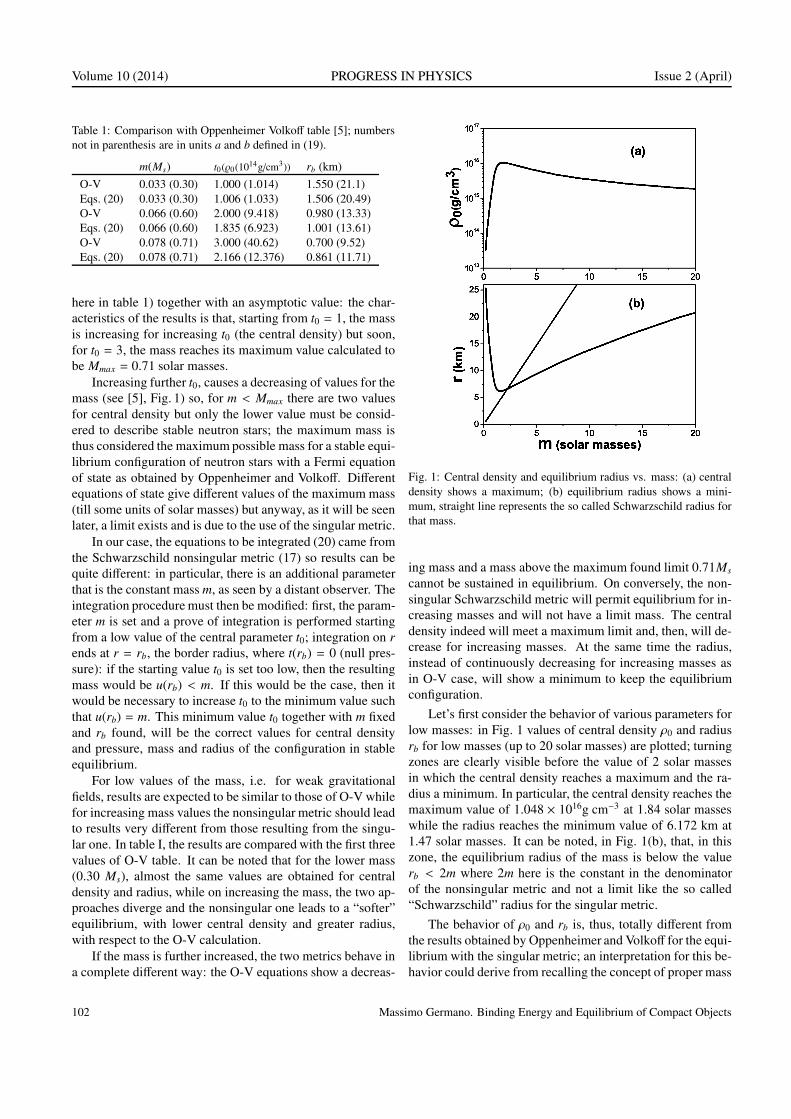
Volume 10 (2014) PROGRESS IN PHYSICS Issue 2 (April)
Table 1: Comparison with Oppenheimer Volkoff table [5]; numbers
not in parenthesis are in units a and b defined in (19).
m(Ms) t0(0(1014g/cm3)) rb (km)
O-V 0.033 (0.30) 1.000 (1.014) 1.550 (21.1)
Eqs. (20) 0.033 (0.30) 1.006 (1.033) 1.506 (20.49)
O-V 0.066 (0.60) 2.000 (9.418) 0.980 (13.33)
Eqs. (20) 0.066 (0.60) 1.835 (6.923) 1.001 (13.61)
O-V 0.078 (0.71) 3.000 (40.62) 0.700 (9.52)
Eqs. (20) 0.078 (0.71) 2.166 (12.376) 0.861 (11.71)
here in table 1) together with an asymptotic value: the char-
acteristics of the results is that, starting from t0 = 1, the mass
is increasing for increasing t0 (the central density) but soon,
for t0 = 3, the mass reaches its maximum value calculated to
be Mmax = 0.71 solar masses.
Increasing further t0, causes a decreasing of values for the
mass (see [5], Fig. 1) so, for m < Mmax there are two values
for central density but only the lower value must be consid-
ered to describe stable neutron stars; the maximum mass is
thus considered the maximum possible mass for a stable equi-
librium configuration of neutron stars with a Fermi equation
of state as obtained by Oppenheimer and Volkoff. Different
equations of state give different values of the maximum mass
(till some units of solar masses) but anyway, as it will be seen
later, a limit exists and is due to the use of the singular metric.
In our case, the equations to be integrated (20) came from
the Schwarzschild nonsingular metric (17) so results can be
quite different: in particular, there is an additional parameter
that is the constant mass m, as seen by a distant observer. The
integration procedure must then be modified: first, the param-
eter m is set and a prove of integration is performed starting
from a low value of the central parameter t0; integration on r
ends at r = rb, the border radius, where t(rb) = 0 (null pres-
sure): if the starting value t0 is set too low, then the resulting
mass would be u(rb) < m. If this would be the case, then it
would be necessary to increase t0 to the minimum value such
that u(rb) = m. This minimum value t0 together with m fixed
and rb found, will be the correct values for central density
and pressure, mass and radius of the configuration in stable
equilibrium.
For low values of the mass, i.e. for weak gravitational
fields, results are expected to be similar to those of O-V while
for increasing mass values the nonsingular metric should lead
to results very different from those resulting from the singu-
lar one. In table I, the results are compared with the first three
values of O-V table. It can be noted that for the lower mass
(0.30 Ms), almost the same values are obtained for central
density and radius, while on increasing the mass, the two ap-
proaches diverge and the nonsingular one leads to a “softer”
equilibrium, with lower central density and greater radius,
with respect to the O-V calculation.
If the mass is further increased, the two metrics behave in
a complete different way: the O-V equations show a decreas-
Fig. 1: Central density and equilibrium radius vs. mass: (a) central
density shows a maximum; (b) equilibrium radius shows a mini-
mum, straight line represents the so called Schwarzschild radius for
that mass.
ing mass and a mass above the maximum found limit 0.71Ms
cannot be sustained in equilibrium. On conversely, the non-
singular Schwarzschild metric will permit equilibrium for in-
creasing masses and will not have a limit mass. The central
density indeed will meet a maximum limit and, then, will de-
crease for increasing masses. At the same time the radius,
instead of continuously decreasing for increasing masses as
in O-V case, will show a minimum to keep the equilibrium
configuration.
Let’s first consider the behavior of various parameters for
low masses: in Fig. 1 values of central density ρ0 and radius
rb for low masses (up to 20 solar masses) are plotted; turning
zones are clearly visible before the value of 2 solar masses
in which the central density reaches a maximum and the ra-
dius a minimum. In particular, the central density reaches the
maximum value of 1.048 × 10¹⁶g cm−3 at 1.84 solar masses
while the radius reaches the minimum value of 6.172 km at
1.47 solar masses. It can be noted, in Fig. 1(b), that, in this
zone, the equilibrium radius of the mass is below the value
rb < 2m where 2m here is the constant in the denominator
of the nonsingular metric and not a limit like the so called
“Schwarzschild” radius for the singular metric.
The behavior of ρ0 and rb is, thus, totally different from
the results obtained by Oppenheimer and Volkoff for the equi-
librium with the singular metric; an interpretation for this be-
havior could derive from recalling the concept of proper mass
102 Massimo Germano. Binding Energy and Equilibrium of Compact Objects

Issue 2 (April) PROGRESS IN PHYSICS Volume 10 (2014)
Mp, linked to the concept of gravitational binding energy EB:
the total mass m, i.e. the mass seen by a distant observer,
is defined by m =∫ rb
04π(r)r2dr but if one integrates the
energy-density over the proper “local” volume, the proper
mass Mp of the system can be defined.
The proper volume element dτ is defined from dτ2 =
gi jdxidx j where i, j = 1, 2, 3 are only spatial coordinates.
The proper volume from the O-V singular metric (5) then is
dτS = 4πr2(1 − 2m/r)−1/2dr and the proper volume from the
actual Schwarzschild nonsingular metric (7) dτNS = 4πr2(1−2m/(r3 +σ)1/3)−1/2dr; coherently can be defined respectively
as two proper masses MP:
MPS =
∫ rb
0
4πr2(1 − 2m/r)−1/2dr (21)
and
MPNS =
∫ rb
0
4πr2(1 − 2m/(r3 + σ)1/3)−1/2dr. (22)
The physical meaning of proper mass is connected with
the difference MP − m = EB where EB is the gravitational
binding energy ( [13] p. 126). In Fig. 2 the completely differ-
ent behavior of the binding energy is shown, in the cases of
singular solution and nonsingular solution: in the first case,
the binding energy increases dramatically (together with the
increasing of the central density to unphysical values) and
above the maximum mass limit of about 0.7 solar masses the
function becomes multivalued.
On the other side, in the nonsingular case, the binding
energy increases smoothly with increasing mass and does not
indicate any mass limit. In Fig. 2 only low mass values are re-
ported but it will be shown later that, in the nonsingular case,
the binding energy for higher mass values increases linearly
with the mass and, considering that the ratio MP/m in Fig. 3
tends→ 2, the binding energy tends to the value m of the rest
mass.
Central (0) and average AV ≡ M/( 43πr3
b) densities have
a similar behavior: starting from values of 0(0.184Ms) =
3.29 × 10¹³g/cm3 and AV (0.184Ms) = 5.40 × 10¹²g/cm3,
reaching the maximum values of 0(1.84Ms) = 1.0476 ×10¹⁶g/cm3 and AV (2.30Ms) = 3.688× 10¹⁵g/cm3 and finally
reaching the values for the last considered mass, 0(3.68 ×10⁶Ms) = 1.243×10¹⁰g/cm3 and AV (3.68×10⁶Ms) = 8.687×10⁹g/cm3.
Behavior evidences the presence of a maximum for both
the densities and a decreasing for increasing masses: the cen-
tral density converges to the average density values which
decrease because volume grows with radius with an higher
power than the mass.
Integration of the system (20) admits solution with an
equilibrium radius for any amount of mass: in Fig. 3, higher
values of mass are considered till, as an example, a value
around 4 million of solar masses as it is supposed to be con-
centrated in the Milky Way’s center.
Fig. 2: Gravitational binding energy vs. mass: comparison between
Oppenheimer-Volkoff results [5] (multivalued line with circles) and
this article results (squares).
Fig. 3: Ratio between proper mass and mass vs. mass logarithm:
limit tends to value 2 corresponding to an efficiency of 100% of
mass conversion in gravitational binding energy
Together with the density decreasing with mass, there is
another peculiar behavior, the one referred to the ratio of
proper mass on mass: in Fig. 3 it is shown that this ratio tends
to the value 2, meaning that there ia a 100% efficiency in con-
verting mass into binding energy. The total mass of the com-
pact object includes both the rest-mass energy and the nega-
tive binding energy so that the mass of the collapsed object
is smaller than the sum of the component particles [14]. For
neutron stars this mass deficit can be as large as 25% [15] but
here it increases till 100% above 1 thousand of solar masses
(depending on the equation of state) and this can be the mech-
anism to support stable equilibrium for such objects.
4 Inequality for nonexistance of a limit mass
Numerical results show that there is not a mass limit for equi-
librium. This result can be seen also analytically trying to
find an upper limit for the mass, independently from the spe-
cific equation of state. This limit exists in the case of singular
Massimo Germano. Binding Energy and Equilibrium of Compact Objects 103

Volume 10 (2014) PROGRESS IN PHYSICS Issue 2 (April)
metric and it is possible to see that this limit does not exist
in the case of nonsingular metric following the procedure ex-
pressed, for example, by R.M. Wald [13, p. 130].
A first less sharp limit exists for the singular metric as
necessary condition for the metric to be static: a metric is
said to be static if it is stationary and, in addition, exists a
spacelike hypersurface Σ (orthogonal to the timelike Killing
vector field ξα); in order for Σ to be spacelike the necessary
condition for staticity is that the radial element of the metric
g11 would be greater than zero (in the following calculation,
it will be used the Wald notation of g11 ≡ h(r) and g00 ≡ f (r),
with the Suffix S to indicate the expression from the singular
metric and NS for the nonsingular one).
So for the two metrics (5) and (7) it will be
hS (r) =
(
1 − 2m(r)
r
)−1
(23)
and
hNS (r) = r4(
r3 + σ)−4/3
(
1 − 2m(r)
(r3 + σ)1/3
)−1
. (24)
The necessary condition for stability implies that, for a
given mass M and equilbrium radius rb, h(rb) > 0 so, it
clearly requires a limit for M only in the singular case, that
is M < rb/2 (eq. 6.2.32 in [13]) while, in the nonsingular
case, hNS (rb) > 0 is always satisfied for any value of M and
rb (considering that σ ≡ 8M3).
This limit for M (for the singular metric) can be sharpened
using the condition g00 ≡ f (r) > 0 that imposes the Killing
field ξα to be timelike everywhere. The term f (r) has the
form, for the singular and nonsingular metric, respectively
fS (r) =
(
1 − 2m(r)
r
)
fNS (r) =
(
1 − 2m(r)
(r3 + σ)1/3
)
. (25)
Since f (r) must be greater than zero everywhere, it could
seem that it would be necessary to know the specific equation
of state for matter but, actually, the only conditions that must
be assumed are very basic i.e. the density must be such that
> 0 and d/dr 6 0 while there is no need for whatsoever
assumption about pressure P.
Applying these conditions, the following inequalities are
obtained (see Appendix B): in the singular case it is found an
upper mass limit
M 64
9rb , (26)
in the nonsingular case, instead, the following inequality is
found:
1 −
8M3
r3b+ 8M3
13
>1
9
1 −8M3
r3b+ 8M3
. (27)
Since it is always true that 0 6 8M3/(r3b+ 8M3) 6 1, the
inequality for the nonsingular case (27), i.e. the condition of
stability, is always satisfied for any values of both M and rb so
that there is no upper limit for the mass, to have equilibrium,
whatever would be the, reasonable, equation of state.
5 Conclusions
In conclusion, the application of the class of nonsingular sta-
tic spherically symmetric metrics (particularly the Schwarz-
schild solution [1]) to the problem of hydrostatic equilibrium
gives completely different solutions from those of the singular
case. In this latter, there is a mass limit (whose value depends
from the specific state equation) for dense cores of degen-
erate matter: above this limit, nothing can stop the config-
uration from a final gravitational collapse with formation of
event horizon and inner physical singularity. In the case of
nonsingular metric (that does not include the possibility of
an event horizon) instead, the equilibrium is always reached
whatever would be the amount of mass.
The application with a Fermi gas state equation, as in
the Oppenheimer-Volkoff work [5], shows that central den-
sity has the same behavior, for increasing mass, than average
density i.e. a maximum (with reasonable physical value), be-
fore reaching the 2 solar masses and then a decreasing. The
equilibrium radius of the system shows a minimum before
the 2 solar masses then grows with increasing masses but re-
maining well below the so called “Schwarzschild radius” for
that mass which, in the nonsingular metric environment, is
not the dimension of an event horizon but only a parameter
connecting the general relativistic metric with the newtonian
one. Proper mass of the system tends to the limit of twice
the mass. This means that the negative binding energy tends
to the limit of m counterbalancing the gravitational mass m.
This is a mechanism that can stop gravitational collapsing and
that can sustain stable equilibrium.
Considering experimental observations, weak field expe-
riments give same results, within errors, for the singular and
nonsingular metrics, while for strong fields, the nonsingular
metric admits stable configuration of greater amount of mass
while singular metrics admits black hole formation. Few ob-
servational, indirect, evidences for black holes existence have
been performed in years but it seems that an alternative hy-
pothesis of very compact degenerate matter configurations,
permitted by nonsingular metrics, could be compatible with
observations: let’s consider, for example, a single nonrotating
compact object of 9.2 solar masses (m=1 in units of (19)), in
the singular metric, it would be a black hole, no matter of
which state equation is used, and a “Schwarzschild radius”
rs = 27.17 km would define the horizon event whose sur-
face would have an infinite gravitational redshift and would
surround a pointlike singularity.
The application of nonsingular metric (with a Fermi equa-
tion of state) instead, would give a very compact object, of
104 Massimo Germano. Binding Energy and Equilibrium of Compact Objects

Issue 2 (April) PROGRESS IN PHYSICS Volume 10 (2014)
radius rb = 13.23km, made by ordinary (degenerate) matter
with a central density 0 = 13.23 × 10¹⁵g/cm3; the density
value is not far from the ordinary nuclear density, moreover a
more realistic state equation would keep density value within
reasonable physical limit.
Gravitational redshift factor f =√−g11 (the ratio be-
tween wavelength observed at infinity and wavelength emit-
ted at distance r) at the surface of the matter configuration
would be f = 1.165. This redshift would correspond, in the
black hole case, to a redshift of a photon emitted ad distance
r = rs f 2/( f 2 − 1) = 3.8rs. This difference, theoretically,
could be observable but total luminosity would be so faint not
to permit direct observations while indirect observations due
to, for example, the accretion disk surrounding these com-
pact objects, would be very similar. The existence of com-
pact massive (several solar masses) objects could justify why
observed emissions from individuated neutron stars and black
hole candidates are so similar [16] despite the totally different
characteristics of a hard surface and an event horizon.
Recent observations involving magnetic fields of quasars
also put in doubt the existence of inner super-massive black
holes [17]. It must be remarked that at the state of the art there
is still no observational proof of a black hole event horizon
[18].
Lack of single compact objects of very great mass it is
due more to mechanism of formation of such object than to
some mass limit, anyway in the galactic’s centers there is
gravitational evidence for compact objects of millions of so-
lar masses. Let’s resume how it would be such an object in
the nonsingular model with a Fermi gas state equation (others
EOS would not change the qualitative features): considering
an object 3.6 millions of solar masses, it would have a radius
of about 58, 000 km that is the half percent of its estimated
“Schwarzschild radius” in the black hole hypothesis, a cen-
tral density 0 = 1.24 × 10¹⁰g/cm3 and a central pressure
P0 = 7.3 × 10¹⁶ Pa both smoothly decreasing outward.
Sagittarius A, the radio point source associated with the
dark mass located at the center of the Milky Way, is the best
studied black hole candidate to date, but till now has not be
possible to verify or to exclude the presence of a horizon [19].
The horizon existence has been inferred because a surface
emission, to remain undetected, would require large radiative
efficiencies, greater than 99.6% [20] anyway, this is actually
the phenomenon predicted by the application of nonsingular
metric, because, as seen in Fig. 3, the limit value of 2 for the
ratio MP/M means an efficiency limit of about 100%. This
could be justified, actually, by a not exotic object having a
hard surface, emissions and gravitational effects compatible
with observations, and that could be permitted because the
contribution of the negative binding energy.
Submitted on February 16, 2014 / Accepted on February 24, 2014
References
1. Schwarzschild K. Uber das Gravitationsfeld eines Massenpunktes nach
der Einsteinschen Theorie (On the Gravitational Field of a Mass Point
According to Einstein’s Theory), Sitzungsber. Preuss. Akad. Wiss.,
Phys. Math. Kl., 1916, v. 1916a, 189–196.
2. Brillouin M. The singular points of Einstein’s universe. J. Phys. Ra-
dium, 1923, v. 23, 43–46.
3. Droste J. The field of a single centre in Einstein’s theory. Ned. Acad.
Wet., 1917, v. 19, 197–215.
4. Hilbert D. Die Grundlagen der Phisik. Nachr. Ges. Wis. Gottingen
Math. Phys. Kl., 1915, 395–407.
5. Oppenheimer J.R., Volkoff G.M. On massive neutron cores. Phys. Rev.,
1939, v. 55, 374–381.
6. Crothers S.J. The Schwarzschild solution and its implications for grav-
itational waves: part I. Progress in Physics, 2005, v. 2, 3–12.
7. Abrams L.S. Black holes: the legacy of Hilbert’s error. Can. J. Phys.,
1989, v. 67, 919–934.
8. Stavroulakis N. On a paper by J. Smaller and B. Temple. Ann. Fond. de
Broglie, 2002, v. 27(3), 511–519.
9. Landau L. On the theory of stars. Physik. Zeits. Sowjetunion, 1932, v. 1,
285–288.
10. Rhoades C.E., Ruffini R. Maximum mass of a neutron star. Phys. Rev.
Lett., 1974, v. 32, 324–327.
11. Srinivasan G. The maximum mass of neutron stars. Bull. Astr. Soc. In-
dia., 2002, v. 30, 523–547.
12. Hartle J.B., Sabbadini A.G. The equation of state and bounds on the
mass of nonrotating neutron star. Astrophys. J., 1977, v. 213, 831–835.
13. Wald R.M. General Relativity. The University of Chicago Press,
Chicago, 1984.
14. Alecian E., Morsink S.M. The effect of neutron star gravitational bind-
ing energy on gravitational radiation-driven mass-transfer binaries. As-
trophys. J., 2004, v. 614, 914–921.
15. Cook G.B., Shapiro S.L., Teukolsky S.A. Rapidly rotating neutron
stars in general relativity realistic equation of state. Astrophis. J., 1994,
v. 424, 823–845.
16. Ed. Maccarone J., Fender R. P., Ho L.C. From X-ray Binaries to
Quasars: Black Holes on all Mass Scales. Springer, the Netherlands,
2005.
17. Schild R.E., Leiter D.J. Black hole or MECO? decided by a thin lumi-
nous ring structure deep within Quasar Q0957+561. J. of Cosmology,
2010, v. 6, 1400–1437.
18. Abramowicz M.A., Kluzniak W., Lasota, J.P. No observational proof
of black hole event-horizon. Astronomy and Astrophysics, 2002, v. 396,
L31–L34.
19. Broderick A.E., Narayan R. On the Nature of the Compact Dark Mass
at the Galactic Center. Astrophys. J., 2006, v. 638 (1), L21–L24.
20. Broderick A.E., Loeb A., Narayan R. The event horizon of Sagitarius
A. Astrophys. J., 2009, v. 701, 1357–1366.
21. Tolman R.C. Relativity Thermodynamics and Cosmology. University
Press, Oxford, 1934.
Massimo Germano. Binding Energy and Equilibrium of Compact Objects 105

Volume 10 (2014) PROGRESS IN PHYSICS Issue 2 (April)
Appendix A
The only non vanishing components of the Einstein Tensor G
are G00, G1
1and G2
2= G3
3. Considering a matter that supports
no transverse stresses and has no mass motion then the energy
momentum components are [21] T 11= T 2
2= T 3
3= −p and
T 00= where p is the pressure and is the macroscopic
energy density measured in proper coordinates. So Einstein’s
equations are
G00 = 8πT 0
0 = 8π = e−λ[
λ′r2
r3 + σ− r4
(r3 + σ)2−
−4rσ
(r3 + σ)2
]
+1
(r3 + σ)2/3
(T00)
G11 = 8πT 1
1 = 8πp = e−λ[
ν ′r2
r3 + σ+
r4
(r3 + σ)2
]
−
− 1
(r3 + σ)2/3
(T11)
G22 = 8πT 2
2 = e−λ[
(ν ′ − λ′)r2
2(r3 + σ)−λ′ν ′
4+ν ′ 2
4+
+2rσ
(r3 + σ)2+ν ′′
2
]
+1
(r3 + σ)2/3
(T22)
where p, , λ and ν are functions of r and the primes indi-
cates a differentiation with respect to r. Since T 11= T 2
2then
(T 11− T 2
2) × 2/r = 0 and from equations (T00) it is easy to
verify that
d
dr
(
−T 11
)
+(
T 00 − T 1
1
) ν ′
2=
(
T 11 − T 2
2
) 2
r= 0 (A-1)
so that this latter equation can be read
dp
dr= −
p +
2ν ′. (A-2)
Equations (T00), (T11) and (A-2) constitute the system of
equations to be solved and correspond to the ones in Oppen-
heimer Volkoff article [5, Eqs. 4,3 and 5] if σ is set equal to 0;
an opportune equation of state = (p) must also be included
in the system.
Eliminating ν ′ in (T11) and (A-2), the hydrostatic equi-
librium equation in exponential form is
dp
dr= − p +
2×
×[
8πp eλ(r3 + σ)
r2+ eλ
(r3 + σ)1/3
r2− r2
(r3 + σ)
]
.
(A-3)
If it is set σ = 0 and the singular metric (5) (inside the
matter) is considered where eλ(r) = (1 − 2m(r)/r)−1 (and con-
sequently m(r) = 12r(1−e−λ)) then the Tolman-Oppenheimer-
Volkoff equilibrium equation is obtained
dp
dr= −
(p(r) + (r))[
m(r) + 4πr3 p(r)]
r2
(
1 −2m(r)
r
) . (A-4)
In our case (A-3) instead, it is possible to give the correct
physical meaning to m(r) setting, for the nonsingular metric
inside the matter,
eλ(r) =(r3 + σ)−4/3
1 − 2m(r)
(r3 + σ)1/3
r4; (A-5)
in effect, at the border r = rb there will be continuity with the
metric in vacuum (7) and (6) so that
eλ(rb) = eλ =r4(r3 + 8m3)−4/3
1 − 2m
(r3 + 8m3)1/3
and m(rb) will assume its value m as seen by an external ob-
server
m(rb) =1
2
(
r3b+8m3
)1/3
1−e−λr4
b(
r3b+8m3
)4/3
= m. (A-6)
Finally the Schwarzschild metric inside the matter (in conti-
nuity with (7) where it is set α = 2m(r) and σ = 8m3 so that
σ = α3 outside the matter) will be
ds2 =
1 − 2m(r)(
r3 + 8m3)1/3
dt2−
−r4
(
r3 + 8m3)−4/3
1 − 2m(r)(
r3 + 8m3)1/3
dr2−
−(
r3 + 8m3)2/3 (
dθ2 + sin2θdφ2)
.
(A-7)
So, with eλ(r) given by (A-5), the equilibrium equation
(A-3) (that is the merging of the two Einstein’s equations
(T11) and (A-2)) and the other Einstein’s equation (T00) will
become respectively
dp(r)
dr= −
(p(r) + (r))[
m(r) + 4π(r3 + σ)p(r)]
(
r3 + σ)4/3
r2
1 − 2m(r)(
r3 + σ)1/3
dm(r)
dr= 4π(r)r2
, (A-8)
where σ = 8m3.
106 Massimo Germano. Binding Energy and Equilibrium of Compact Objects

Issue 2 (April) PROGRESS IN PHYSICS Volume 10 (2014)
Appendix B
Pressure P can be eliminated from Einstein’s equations con-
sidering that G11− G2
2= 0, this, together with the definition
of h(r) (23) leads to the following equation for the singular
metric (using the notation by Wald, eq. 6.2.34 in [13])
d
dr
r−1hS (r)−1/2d f
1/2
S(r)
dr
=
=[
fS (r)hS (r)]1/2 d
dr
[
m(r)
r3
]
(B-1)
while, for the nonsingular metric
d
dr
[
(r3 + σ)−1/3hNS (r)−1/2 d fNS (r)1/2
dr
]
=
=(r3 + σ)2/3
r2
[
fNS (r)hNS (r)]1/2 d
dr
[
m(r)
r3 + σ
]
.
(B-2)
The right sides for both equations are proportional to the
derivative with respect to r of the average density, so because
the condition d/dr 6 0, the left sides must be both less or
equivalent to 0. Integrating the inequalities for the left sides,
inward from the border rb to a generic radius r we obtain
1
rh1/2
S(r)
d fS (r)1/2
dr>
M
r3b
, (B-3)
1
(r3 + σ)1/3h1/2
NS(r)
d f1/2
NS(r)
dr>
M
r3b+ σ. (B-4)
These inequalities can be integrated again inward from
rb to 0. The condition d/dr 6 0 implies that m(r) cannot be
smaller than the value it would have for a uniform density star
so, for the singular case, m(r) > Mr3/r3b
and, for the nonsin-
gular one, m(r) > M(r3+σ)/(r3b+σ), so that inequalities (B-3
and B-4) become: for the singular case (Wald, eq. 6.2.39)
f1/2
S(0) 6
3
2
(
1 − 2M
rb
)1/2
− 1
2(B-5)
and for the nonsingular case
f1/2
NS(0) 6
3
2
1 − 2M
(r3b+ σ)1/3
1/2
− 1
2
1 − 2Mσ2/3
r3b+ σ
(B-6)
(as usual for σ = 0 the two cases are equivalent). Finally, the
condition f 1/2(0) > 0 implies that, for the singular case, the
necessary condition for staticity involves a maximum limit
for the mass: from (B-5)
M 64
9rb . (B-7)
For the nonsingular case instead, the stability condition
implies, from (B-6) and inserting the value σ ≡ 8m3, the
inequality
1 −
8M3
r3b+ 8M3
13
>1
9
1 −8M3
r3b+ 8M3
. (B-8)
Massimo Germano. Binding Energy and Equilibrium of Compact Objects 107

Volume 10 (2014) PROGRESS IN PHYSICS Issue 2 (April)
Addendum to “Phenomenological Derivation of the Schrodinger Equation”
Fernando OgibaE-mail: [email protected]
This addendum to the article [1] is crucial for understanding how the complex effective
action, despite its derivation based on classical concepts, prevents quantal particles to
move along extreme action trajectories. The reason relates to homogenous, isotropic
and unpredictable impulses received from the environment. These random impulses al-
lied to natural obedience to the dynamical principle imply that such particles are perma-
nently and randomly passing from an extreme action trajectory to another; all of them
belonging to the ensemble given by the stochastic Hamilton-Jacobi-Bohm equation.
Also, to correct a wrong interpretation concerning energy conservation, it is shown that
the remaining energy due to these permanent particle-medium interactions (absorption-
emission phenomena) is the so-called quantum potential.
1 Introduction
The central subject of the article [1] is: Quantal particles
(such as electrons), due to its interactions with the environ-
ment, move in accordance with the complex effective action
S e f f = S + i~
2ln P (1)
which was obtained following the classical Hamilton’s dy-
namical principle but considering the motion as a whole, that
is, taking averages. The resulting canonical equations coin-
cide with those extracted from the Schrodinger equation writ-
ing ψ=√
P exp (iS/~), namely:
∂S
∂t+∇S · ∇S
2m+ V + Q = 0 (2)
and∂P
∂t+ ∇ ·
(
P∇S
m
)
= 0 , (3)
where
Q =~
2
8m
∇P · ∇P
P2− ~
2
4m
∇ · ∇P
P(4)
is the quantum potential which, visibly, is the remaining en-
ergy of two distinct concurrent phenomena.
The main motivation for writing this addendum concerns
the result∫
P
(
i~
2
1
P
∂P
∂t
)
d3r = 0 (5)
which is not the expression of energy conservation, as argued
in connection with Eg. 23 of the article. In true, the null value
of this average means that the involved energy (the enclosed
quantity) does not remain in the particle; it is radiation, as will
be shown. In doing this, it is necessary to explain how Q — as
an energy resulting from the particle-medium interactions —
agrees with the energy conservation required by the so-called
quantum equilibrium.
Also, in the mentioned article the meaning of the effec-
tive action (1) is not so clear. It was derived supposing a
particle over a possible trajectory; what, in view of the re-
sults, must be true. On the other hand, a continuous trajec-
tory of elementary particles is an experimentally discredited
concept. So, there must be a link between these two oppos-
ing points of view. In true, there is, as will be seen. Indeed,
it will be shown that quantal particles occupies, sequentially
and instantly, just one point over different trajectories which
are randomically chosen in the ensemble (2). This means that
quantal particles don’t move along extreme action trajectories
but occupy trajectories (permited by the dynamical principle)
just for a moment.
The interacting medium — primarily responsible for
quantum effects — is the zero-point field (ZPF) which, ac-
cording to the classical description of the Casimir’s experi-
ment, is viewed as a homogeneous and isotropic distribution
of electromagnetic waves pervading all space. As the phases
of these waves are randomically distributed in the range
[0, 2π], then electrical charged particles (balanced or not) are
permanently receiving unpredictable impulses. This has two
main consequences: First, the accelerated charged particles
radiate all the absorbed energy. Second, the unpredictable im-
pulses prevent quantal particles to follow predictable paths.
Even so, the overall motion obeys the Hamilton’s principle
which is founded on trajectories. How can all this happen?
2 The quantum potential and the ensemble of virtual
trajectories
The answer to the above question lay in the fact that the nat-
ural behavior of any moving particle, at any time, is obeying
the classical dynamical principle. This must be interpreted as
follows: In the absence of random forces, they move along
extreme action trajectories. However, in the case of parti-
cles which are significantly affected by the ZPF the situation
is drastically modified. Indeed, homogeneous, isotropic and
random forces (including beck reaction forces) are not part of
the traditional classical description of the motion.
Here, it will be proved that the quantal motion occurs as
follows: Immediately before any particle-field random inter-
108 Fernando Ogiba. Addendum to “Phenomenological Derivation of the Schrodinger Equation”

Issue 2 (April) PROGRESS IN PHYSICS Volume 10 (2014)
action the particle is over a given trajectory (obedience to
the dynamical principle), but upon receiving an unpredictable
impulse it is withdrawing from this trajectory to an unpre-
dictable place. Again, in the new position it continues obey-
ing the dynamical principle; that is, the particle is over an-
other trajectory. As this is a permanent process, then the parti-
cle occupies these possible trajectories only instantly (virtual
trajectories). In a sense, we can say that the unpredictable
impulse has created initial conditions (arbitrary) for a new
trajectory.
In the light of the foregoing, at each position actually oc-
cupied by the particle pass an infinite number of such virtual
trajectories. This assumption is in agreement with the fol-
lowing facts: First, Eq. (2) represents an ensemble of unpre-
dictable trajectories; P(x, t) — preserving its uniqueness —
can take any value at x. Moreover, ∇P is not deterministic.
Second, energy and momentum in quantum mechanics are in-
dependent of coordinates. This means that everywhere there
are equivalent ensembles of partial derivatives ∂S/∂t and ∇S
— requiring continuous virtual functions S — which on av-
erage give the corresponding observed quantities. This state-
ment implies the same uncertainty everywhere (non locality).
Thirty, Probability density, classically, is defined over trajec-
tories; it is canonically conjugate to the action function S (this
remains valid in the equations above). Over extreme action
trajectories ∂P/∂t = 0 (we know where the particle is at the
time t). Therefore, if ∂P/∂t , 0, then it means that the particle
was “banned” from its trajectory.
To formally prove that the trajectories represented by the
virtual ensemble (2) are instantly visited by the particle, it is
necessary finding a valid expression which leads to the idea
that such trajectories (or momenta ∇S ) are randomly chosen
(or induced) where the particle is. This is better made after
knowing the meaning of the quantum potential.
If a moving particle is not actuated by random forces,
then, given the potential V and the initial conditions, we can
predict its extreme action trajectory. However, the presence
of random forces — exactly like that found in the ZPF —
modify this classical way to see the motion. This rupture re-
lates to the fact that now there is only a probability of finding
the particle at a given position at the time t.
Whenever a particle is removed from a given position by
random forces, the probability of find it there is diminished.
Consequently, as probability is a conserved quantity, this de-
crease of probability leads to the emergence of an outgoing
compensatory probability current. Formally, following stan-
dard techniques and considering the ZPF properties, at each
position there is a diffusion of probability density currents
(Pv), in such a way that
∂P
∂t+ ∇ · (Pv) = 0 . (6)
In true, Pv represents all possible local outflows of mat-
ter whose velocities v have the directions of the vectors ∇P.
Therefore, all currents obey
Pv = α∇P, (7)
where α is a proportionality factor, to be determined.
Being the matter-field interaction conservative, then there
is no net momentum transfer to the particle. This implies that
the average probability density current is zero, i.e.
∫
P (Pv) d3r =
∫
P (α∇P) d3r = 0 . (8)
Integrating the second form by parts and considering that
P → 0 at infinity, we find that its null value is plenty satis-
fied if α is a constant. In true, it is an imaginary diffusion
constant because there is no effective dislocation of matter in
all directions (this is a single-particle description). In fact, in
accordance with the imaginary part of the effective action (1),
the unpredictable impulses received by the particle are given
by
mv = ∇(
i~
2ln P
)
= i~
2
∇P
P, (9)
which, compared with (7), implies that α = i~/2m.
The consequent average kinetic energy induced by the
ZPF on the particle is
〈TZPF〉 =∫
P
(
1
2m |v|2
)
d3r , (10)
which considering (9), reads
〈TZPF〉 =~
2
8m
∫
(∇P)2
Pd3r. (11)
However, the implicated acceleration makes the electrical
charge radiates. So, we must appeal to the general rule con-
cerning accelerated charged particles, namely: The change in
the kinetic energy in the absorption-emission process is equal
to the work done by the field minus the radiated energy. This
is the energy conservation implicit in the determination of the
Abraham-Lorentz back reaction force.
Therefore, varying the average kinetic energy, that is, tak-
ing the functional derivative of (11) with respect to P, we find
that the remaining energy due to particle-field interactions is
δ〈TZPF〉 =~
2
8m
(
∇P · ∇P
P2− 2∇ · ∇P
P
)
, (12)
where, therefore, the first term relates to absorption of radia-
tion, and the second to emission.
Coincidentally, this remaining energy is the quantum po-
tential (4) which, therefore, is the expression of the required
energy conservation implied in the so-called quantum equi-
librium.
At this point we have sufficient valid information to prove
that extreme action trajectories are randomly chosen at each
position actually occupied by the particle.
Fernando Ogiba. Addendum to “Phenomenological Derivation of the Schrodinger Equation” 109

Volume 10 (2014) PROGRESS IN PHYSICS Issue 2 (April)
Indeed, the probability density conservation (6), consid-
ering (9), reads
∂P
∂t+ i~
2m∇2P = 0 , (13)
which has the shape of a diffusion equation; local diffusion
of probability density currents or virtual outflows of matter at
the actual particle position.
The validity of this equation is unquestionable. In fact, it
is absolutely equivalent to Eq. (3), or
∂(ψ∗ψ)
∂t+ i~
2m∇ · (ψ∗ ∇ψ − ψ∇ψ∗) = 0 , (14)
as can be proven from |∇ψ|2 = −ψ∗∇ψ and the parameterized
forms of S and P in terms of ψ.
Very important, the equations (13) and (3) represent the
same diffusion at each position x actually occupied. Equiv-
alently, these two ways of expressing probability conserva-
tion contain implicitly all possibilities for the particle flow at
x. As Eq. (3) expresses this in terms of ∇S , then ∇S must
represent all possible momenta at x. However, as these par-
tial derivatives require continuous action functions, then there
pass multiple virtual trajectories. One of them infallibly will
be occupied, but only for a moment because in the next posi-
tion the same phenomenon is repeated.
In this sence, the obedience to the dynamical principle,
implicit in the effective action (1), is traduced as follows: At
a given time the particle is over a trajectory represented by the
action S (real part), but at this very moment there is a choice
for the next motion, which is dictated by the probability de-
pendent local action (imaginary part). In other words, the
imaginary part chose the next action function (S ) represent-
ing another trajectory to be occupied during an infinitesimal
time; and so on.
Now, it is possible to correct the interpretation given to
(5) in the article [1]. Just rewrite Eq. (13) in the energy form
i~
2
1
P
∂P
∂t=~
2
4m
∇ · ∇P
P, (15)
which implies that
∫
all
P
(
i~
2
1
P
∂P
∂t
)
d3r =
∫
all
P
(
~2
4m
∇ · ∇P
P
)
d3r = 0 . (16)
Being the second member of (15) the emitted energy of
the balance (12), then the result (5) means that the involved
energy doesn’t remain in the particle.
3 Conslusion
The subsequent particle’s positions, randomly chosen in the
interactions, are on different trajectories. Therefore, there are
continuous trajectories, but never followed by quantal parti-
cles. They simply represent the obedience to the mechanical
principle, regardless of where the particle is. Nevertheless, as
these virtual trajectories are inherent to the Schrodinger pic-
ture, then it is expected that they — properly determined and
used as statistical tools - can give the same predictions. How-
ever, the convenience of such procedure needs to be better
discussed.
On the other hand, were highlighted permanent emissions
and absorptions of radiation, meaning that particles are actu-
ated by forces and back reaction forces, which, on average,
are zero. This explains why the interactions become trans-
parent in the quantum description. Nevertheless, speculating,
these permanent absorptions and emissions of electromag-
netic waves (a delicate asymmetry accompanying particles
everywhere) may be important to interpret certain properties
of matter.
Submitted on March 3, 2014 / Accepted on March 11, 2014
References
1. Ogiba F. Phenomenological derivation of the Schrodinger equation.
Prog. Phys., 2011, no.4, 25–28.
110 Fernando Ogiba. Addendum to “Phenomenological Derivation of the Schrodinger Equation”

Issue 2 (April) PROGRESS IN PHYSICS Volume 10 (2014)
Views about the “Oxford Questions”. Wave Function Collapse
and Schrodinger’s Cat:
Are They Real Scientific Topics or Plain Fictions?
Spiridon Dumitru
Department of Physics (retired), “Transilvania” University, B-dul Eroilor 29, 500036 Brasov, Romania
E-mail: [email protected]
Motivated by the recently published “Oxford Questions” we review the foundational
character of the wave function collapse theme. We show that the respective theme, as
well as its twin analogue represented by the Schrodinger’s cat problem, are not real
scientific topics but plain and rather trivial fictions. Consequently, we suggest that the
related items of the “Oxford Questions” have to be perceived with some epistemic cau-
tion.
1 Introduction
The newly diffused The Oxford Questions on the Foundations
of Quantum Physics [1], known also as “Oxford Questions,
aims to formulate “a list of main open questions about the
foundations of quantum physics”. Within the respective list,
the issue “whether or not the ‘collapse of the wave packet’ is
a physical process” is approached in “several Oxford Ques-
tions: in particular, 1b, 2a, 2c, 3a, 3c and 5a”. The issue is
mainly brought into attention in 3c: “How can the progressive
collapse of the wave function be experimentally monitored?”.
It is expected that, in the future, the Oxford Questions
will stimulate more or less extensive studies in both advanced
and pedagogic research. Previous to these studies, it is im-
portant to examine the correctness of the items gathered in
the Oxford Questions, particularly the ones pertaining to the
above-mentioned quantum collapse. Such an examination is
intended in this short paper, by using some ideas noted in
some of our recent works. Section 2 is focused on the theme
of Wave Function Collapse. Additionally, in Section 3, we
examine the case of Schrodinger’s Cat Thought Experiment
which in fact is a twin analogue of the Wave Function Col-
lapse. We find that both the Wave Function Collapse and the
Schrodinger’s Cat Thought Experiment are not real scientific
topics but only pure fictions.
The present paper ends in Section 4 with some closing
thoughts, particularly with the suggestion that, for real sci-
ence, the invalidated Oxford Questions items have to be re-
garded as needless.
2 On the wave function collapse
Historically speaking, the Wave Function Collapse concept
was brought into scientific debate by the conflict between the
following two suppositions:
s1 The old opinion that a Quantum Measurement of a
(sub)atomic observable should be regarded as a sin-
gle sampling (trial) which gives a unique deterministic
value.
s2 The agreement, enforced by theoretical considerations,
is such that to describe such an observable one should
resort to probabilistic (non-deterministic) entities
represented by an operator together with a wave func-
tion.
To avoid conflict between suppositions s1 and s2 it was
in diffused the thesis that, during a Quantum Measurement,
the corresponding wave function collapses into a particular
eigenfunction associated with a unique (deterministic) eigen-
value of the implied operator. Such a thesis has led to the
Wave Function Collapse concept regarded as a true dogma.
The respective concept was assumed, in different ways and
degrees, within a large number of mainstream publications
(see [2–8] and references therein). But, as a rule, the pre-
viously mentioned assumptions were (and still are) not ac-
companied with adequate elucidations concerning the initial
correctness of the alluded concept in relation to the natural
themes of Quantum Mechanics.
Now, explicitly or implicitly, the Oxford Questions [1] put
forward the problems:
p1 Whether or not the “collapse of the wave packet” is a
physical process.
p2 How can the progressive collapse of the wave function
be experimentally monitored?
p3 According to which theoretical scheme, justified by
physical reality alone, can a Wave Function Collapse be
described properly? (This is in the situation [6] where
a whole “zoo of collapse models” have already been
invented.
In order to generate significant remarks on the above-
mentioned Oxford Questions problems p1–p3, now we wish
to bring into attention some ideas prefigured and to a certain
extent argued in our recent paper [9, 10]. We mainly pointed
out the ephemeral character (i.e. caducity) of the Wave Func-
tion Collapse concept. Basically our argumentations are
grounded on the following indubitable facts. Mathematically,
a quantum observable (described by a corresponding opera-
Spiridon Dumitru. Views about “Oxford Questions” 111

Volume 10 (2014) PROGRESS IN PHYSICS Issue 2 (April)
tor) is a true random variable. Then, in a theoretical frame-
work, such a variable must be regarded as endowed with a
spectra of eigenvalues. For a given quantum state/system the
mentioned eigenvalues are associated with particular proba-
bilities incorporated within the wave function of the men-
tioned state/system. Consequently, from an experimental per-
spective, a measurement of a quantum observable requires an
adequate number of samplings finished through a significant
statistical group of data/outcomes. That is why one can con-
clude that the supposition s1 of the Wave Function Collapse
concept appears as a false premise while the whole respective
concept proves oneself to be a useless fiction.
The previously noted conclusion can be consolidated in-
directly by mentioning the quantum-classical probabilistic
similarity (see [11–14]) among quantum mechanical observ-
ables and macroscopic random variables, studied within the
thermodynamic theory of fluctuations. On the whole, a mac-
roscopic random variable is characterized by a continuous
spectra of values associated with an intrinsic probability den-
sity. Then, for measuring a macroscopic random variable, a
single experimental sampling delivering a unique value (re-
sult) is worthless. Such a sampling is not described as a col-
lapse of the mentioned probability density. Similarly, a quan-
tum measurement must not be represented as a wave func-
tion collapse. Moreover, a true experimental evaluation of
a macroscopic random variable requires an adequate lot of
samplings finished through a statistical set of individual re-
sults. A plausible model for a theoretical description of the
alluded evaluation can be done [14–16] through an informa-
tion transmission process. In the respective model, the mea-
sured system appears as an information source while the mea-
suring device plays the role of an information transmission
channel to the recorder of measurement data. As part of the
mentioned measuring process, the quantum mechanical oper-
ators (describing quantum observables) preserve their mathe-
matical expressions. Additionally, the transmission to the the
recorder of quantum probabilistic attributes is described by
means of linear transformations for probability density and
current(associated with the corresponding wave function).
Taking into account the above mentioned indubitable ar-
guments, we think that in natural perception the “collapse of
the wave function” cannot be considered as a physical pro-
cess. Consequently, the Wave Function Collapse concept
does not have the qualities of a real scientific topic, it be-
ing only a purely trivial and worthless fiction. Moreover, the
above noted problems p2 and p3 make no sense. That is why
the further studies expected to be raised by the Oxford Ques-
tions would be more appropriate if ignoring all the elements
regarding the Wave Function Collapse concept.
3 As regards the Schrodinger’s cat
Subsidiarily to the above considerations about the Wave
Function Collapse concept, some remarks can be brought into
question [9] concerning the famous Schrodinger’s Cat
Thought Experiment. The essential element in the respective
experiment is represented by a single decay of a radioactive
atom (which, through some macroscopic machinery, kills the
cat). But the individual lifetime of a single decaying atom
is a random variable. That is why the mentioned killing de-
cay is in fact a twin analogue of the above mentioned single
sampling taken into account in supposition s1 of the Wave
Functions Collapse concept. So, the previous considerations
reveal the notifiable fact that is useless (even forbidden) to
design experiments or actions that rely solely on a single de-
terministic sampling of a random variable (such is the decay
lifetime). Accordingly, the Schrodinger’s Cat Thought Ex-
periment appears as a twin analogue of the Wave Functions
Collapse i.e. as a fiction (figment) and a deontology without
any real scientific value.
The previously mentioned fictional character of the
Schrodinger’s Cat Thought Experiment can be argued once
more by observation [9] that it is possible to imagine a macro-
scopic thought-experiment completely analogous with Shro-
dinger’s quantum one. Within the respective analogue, a
cousin of Schrodinger’s cat can be killed through launching a
single macroscopic ballistic projectile. More specifically, the
killing macroscopic machinery is activated by the reaching of
the projectile in a probable hitting point. But the respective
point has characteristics of a true macroscopic (non-quantum)
random variable. Consequently, the launching of a single pro-
jectile is a false premise, similar to the supposition s1 of the
Wave Function Collapse concept. Add here the known fact
that within the practice of traditional artillery (operating only
with macroscopic ballistic projectiles but not with propelled
missiles) designed for an expected destruction of a military
objective, one uses a considerable (statistical) number of pro-
jectiles but not a single one. So the whole situation with a
macroscopic killing projectile is completely analogous with
the Schrodinger’s Cat Thought Experiment which uses a sin-
gle quantum radioactive decay. Therefore, the acknowledged
classical experiment makes clear once more the fictional char-
acter of the Schrodinger’s Cat Thought Experiment.
According to the above-noted remarks, certain things
must be regarded as being worthless, i.e. allegations such
as: ”the Schrodinger’s cat thought experiment remains a top-
ical touchstone for all interpretations of quantum mechan-
ics”. Note that such or similar allegations can be found in
many science popularization texts, e.g. in the ones dissemi-
nated via the Internet.
4 Closing thoughts
Through the contents of the previous sections, we have
brought into attention a few significant remarks regarding the
themes of the Wave Function Collapse and the Schrodinger’s
Cat Thought Experiment. Through the respective remarks,
we argue that the mentioned themes are not real scientific
112 Spiridon Dumitru. Views about “Oxford Questions”

Issue 2 (April) PROGRESS IN PHYSICS Volume 10 (2014)
topics but pure and trivial fictions. So we find that the Ox-
ford Questions have an important, prolonged drawback and,
consequently, their invalidated items have to be regarded as
needless things for science.
Submitted on February 27, 2014 / Accepted on March 12, 2014
References
1. Briggs G.A.D., Butterfield J.N., Zeilinger A. The Oxford Questions on
the foundations of quantum physics. Proc. Royal Soc. A, 2013, v.469,
20130299; arXiv:1307.1310.
2. Stamatescu I.-O. Wave function collapse. In: Compendium of Quantum
Physics, Springer, 2009, 813–822.
3. Ghirardi C. Collapse theories. The Stanford Encyclopedia of Philoso-
phy. Winter 2011 Edition, http://plato.stanford.edu/archives/win2011
4. Omnes R. Decoherence and wave function collapse. Foundations of
Physics, 2011, v.41, 1857–1880; arXiv: 1105.0831.
5. Weinberg S. Collapse of the state vector. Phys. Rev. A, 2012, v.85,
062116; arXiv: 1109.6462.
6. Bassi A., Lochan K., Satin S., Singh T.P., and Ulbricht H. Models
of wave-function collapse, underlying theories, and experimental tests.
arXiv: 1204.4325.
7. Cowan C.W., Tumulka R. Epistemology of wave function collapse in
quantum physics. arXiv: 1307.0827.
8. Bassi A., Ulbricht H. Collapse models: from theoretical foundations to
experimental verifications. arXiv:1401.6314.
9. Dumitru S. Caducity of idea about wave function collapse as well new
views on Schrodinger’s cat and quantum measurements. Progress in
Physics, 2013, v.9, no.2, 63–68.
10. Dumitru S. Annotations regarding the Oxford Questions. arXiv:
1311.2581.
11. Dumitru S. Fluctuations and thermodynamic inequalities. Physica
Scripta, 1974, v.10, 101–103.
12. Dumitru S. The Planck and Boltzmann constants as similar generic in-
dicators of stochasticity: some conceptual implications of quantum-
nonquantum analogies. Physics Essays, 1993, v.6, 5–20.
13. Dumitru S., Boer A. Fluctuations in the presence of fields — phe-
nomenological Gaussian approximation and a class of thermodynamic
inequalities. Phys. Rev. E, 2001, v.64, 021108; arXiv: cond-mat/
0011444.
14. Dumitru S. Reconsideration of the uncertainty relations and quan-
tum measurements, Progress in Physics, 2008, v.4, no.2, 50–68;
arXiv:1205.3892.
15. Dumitru S. Phenomenological theory of recorded fluctuations. Physics
Letters A, 1974, v.48, 109–110.
16. Dumitru S., Boer A. On the measurements regarding random ob-
servables. Romanian Journal of Physics, 2008, v.53, 1111–1116;
http://www.nipne.ro/rjp/2008 53 9-10.html
Spiridon Dumitru. Views about “Oxford Questions” 113

Volume 10 (2014) PROGRESS IN PHYSICS Issue 2 (April)
The Electron and Proton Planck-Vacuum Coupling Forces
and the Dirac Equation
William C. Daywitt
National Institute for Standards and Technology (retired), Boulder, Colorado, U.S.A.
E-mail: [email protected]
This short paper derives the electron and proton Planck-vacuum coupling forces so that
both the electron and proton, and their antiparticles, possess a Compton radius and obey
the Dirac equation.
1 Introduction
The Dirac equation can be expressed as [1] [2]
e2∗
(
i∂
∂ct+ αα · i∇
)
ψ = mc2βψ (1)
where in the Planck vacuum (PV) theory the coefficients e2∗
and mc2 are particle-PV coupling constants associated with
the polarization and curvature forces
(±e∗)(−e∗)
r2= ∓
e2∗
r2and
mm∗G
r∗r=
mc2
r(2)
where (±e∗) and mc2 are the charge and rest mass energy of
the free-space Dirac particles and (−e∗) refers to the separate
Planck particles making up the PV continuum. G is Newton’s
gravitational constant, m∗ and r∗ are the mass and Compton
radius of the Planck particles, and e∗ is the massless bare
charge. The ‘Dirac particles’ refer in the present paper to
the electron and proton and their respective antiparticles.
The coupling constants in (1) and (2) are presently asso-
ciated with the rest-frame coupling forces [3]
F(r) = ∓e2∗
r2−
mc2
r(3)
but there is a problem. The negative polarization force in (3)
is due to the positive charge in (±e∗) of (2) and yields the
equation
−e2∗
(
i∂
∂ct+ αα · i∇
)
ψ = mc2βψ (4)
which, because of the negative sign, is not a Dirac equation.
Thus these coupling forces do not lead to a Dirac particle in
the positron and proton cases — nor can they produce their
corresponding Compton radii rc = e2∗/mc2 from (3), where
F(rc) must vanish. So there is something wrong with these
coupling forces and, to resolve the problem, it is necessary to
look more closely at the foundation of the PV theory.
2 Single superforce
The two observations: “investigations point towards a com-
pelling idea, that all nature is ultimately controlled by the ac-
tivities of a single superforce”, and “[a living vacuum] holds
the key to a full understanding of the forces of nature” ; come
from Paul Davies’ popular 1984 book [4, p.104] entitled “Su-
perforce: The Search for a Grand Unified Theory of Nature”.
This living vacuum consists of a “seething ferment of virtual
particles”, and is “alive with throbbing energy and vitality”.
These statements form the foundation of the PV theory [5] [6]
that, among other things, derives the primary constants as-
sociated with Newton’s constant G (= e2∗/m
2∗), Planck’s re-
duced constant ~ (= e2∗/c), and the fine structure constant
α (= e2/e2∗).
The single-superforce idea is taken here to mean that the
superforces associated with General relativity [5] and the
Newton and Coulomb forces have the same magnitude. In
particular it is assumed that
m2∗G
r2∗
=c4
G= (±)
e2∗
r2∗
(5)
where the first, second, and third ratios are the superforces for
Newton’s gravitational force and General relativity, and the
free-space forces and superforces associated with the Cou-
lomb force.
Equating the first and second ratios in (5) leads to
c4
G= (±)
m∗c2
r∗(6)
where, since c4 and G are positive-definite constants, the neg-
ative sign in (6) must refer to some other aspect of the ratio
— this other aspect is the c4/G association with the two-term
particle-PV coupling forces. Equating the second and third
ratios in (5) and using (6) yields
(±)m∗c
2
r∗= (±)
e2∗
r2∗
(7)
both sides of which are coupling forces.
Equating the first and third ratios in (5) gives
G =e2∗
m2∗
(8)
as the definition of the secondary constant G in terms of the
primary constants e2∗ and m2
∗.
114 William C. Daywitt. The Electron and Proton Planck-Vacuum Coupling Forces and the Dirac Equation

Issue 2 (April) PROGRESS IN PHYSICS Volume 10 (2014)
Using the curvature and polarization forces in (7), the
two-term coupling forces take the form
F(r∗) = (±)e2∗
r2∗
(±)m∗c
2
r∗(9)
where the proper choice of the plus and minus signs leads to
coupling forces consistent with the existence of a Compton
radius. Thus the proper choice is
F(r∗) = ±
(
e2∗
r2∗
−m∗c
2
r∗
)
(10)
defining coupling forces that vanish at the Compton radius
(r∗ = e2∗/m∗c
2) of the Planck particle. The vanishing of (10)
reveals a basic property of the PV state that establishes how
the stable free-space particle interacts with the vacuum — i.e.,
via a two-term coupling force that generates a characteristic
Compton radius (rc = e2∗/mc2) for the particle.
For the free-space electron and proton and their antipar-
ticles, the results of the previous paragraph suggest that their
coupling forces should be
F(r) = ±
(
e2∗
r2−
mec2
r
)
=
electron
positron(11)
and
F(r) = ∓
(
e2∗
r2−
mpc2
r
)
=
proton
antiproton(12)
where the plus and minus signs correspond to the particles
indicated on the right of the braces, and the subscripts ‘e’
and ‘p’ refer to the electron and proton respectively. These
coupling forces replace the problematic forces in (3). The
radius r in these equations is the radius from the free-space
Dirac particle to the separate particles of the PV.
The vanishing of equations (10)–(12) leads to the impor-
tant string of Compton relations
remec2 = rpmpc2 = r∗m∗c2 = e2
∗ (= c~) (13)
relating the Dirac particles to the Planck particles.
3 Conclusions and comments
The forces (11) and (12) vanish at the electron and proton,
and their respective antiparticle, Compton radii
re =e2∗
mec2and rp =
e2∗
mpc2(14)
and lead to the Dirac equations
±e2∗
(
i∂
∂ct+ αα · i∇
)
ψ = ±mc2βψ . (15)
Dividing through by ±mc2 gives
rc
(
i∂
∂ct+ αα · i∇
)
ψ = βψ (16)
where the Compton radius rc (= e2∗/mc2) and m now represent
any of the Dirac particles (rc = re, rp).
The particle-PV potential energy associated with the cou-
pling forces in (11) and (12) is defined as
V(r) = −
∫ r
rc
|F(r)| dr (17)
for r 6 rc, resulting in (using (13))
V(r)
mc2=
rc
r− 1 − ln
rc
r(18)
where V(rc) = 0. The potential increases as the Dirac-particle
cores (±e∗,m) are approached (as r decreases), making the
negative energy vacuum susceptible to free-space (where the
cores reside) perturbations. This susceptibility leads to an
internal vacuum structure for the Dirac particles; where, in
the “The Dirac Proton and its Structure” calculations [6] [7],
quantitative confirmation for the preceding Dirac-particle cal-
culations is provided.
Submitted on March 6, 2014 / Accepted on March 17, 2014
References
1. Daywitt W.C. Understanding the Dirac Equation and the Electron-
Vacuum System. Progress in Physics, 2013, no. 4, 78.
2. Daywitt W.C. The Electron-Vacuum Coupling Force in the Dirac
Electron Theory and its Relation to the Zitterbewegung. Progress in
Physics, 2013, no. 3, 25.
3. Daywitt W.C. Particles and Antiparticles in the Planck Vacuum Theory.
Progress in Physics, 2011, no. 1, 55.
4. Davies P. Superforce: the Search for a Grand Unified Theory of Nature.
Simon and Schuster, Inc., New York, 1984.
5. Daywitt W.C. The Planck Vacuum. Progress in Physics, 2009, no. 1,
20. See also www.planckvacuum.com.
6. Daywitt W.C. The Proton and its Structure. This paper has been sub-
mitted the the Canadian “Applied Physics Research” Journal for publi-
cation. See also www.planckvacuum.com.
7. Barut A.O. and Bracken A.J. Zitterbewegung and the Internal Geome-
try of the Electron. Phys. Rev. D, 1981, v. 23, no. 10.
William C. Daywitt. The Electron and Proton Planck-Vacuum Coupling Forces and the Dirac Equation 115

Volume 10 (2014) PROGRESS IN PHYSICS Issue 2 (April)
Further Insight Relative to Cavity Radiation II:
Gedanken Experiments and Kirchhoff’s Law
Pierre-Marie Robitaille
Department of Radiology, The Ohio State University, 395 W. 12th Ave, Columbus, Ohio 43210, USA.
E-mail: [email protected]
Kirchhoff’s law of thermal emission states that cavity radiation must always be black,
or normal, irrespective of the nature of the walls. Arbitrary cavity radiation must be
solely dependent upon the equilibrium temperature and the frequency of observation.
Despite such theoretical claims, it is well established that laboratory blackbodies are
not constructed from arbitrary materials, but rather from nearly perfect absorbers of
radiation over the frequency of interest. In the laboratory, arbitrary cavities do not
contain black radiation. This experimental fact stands in direct conflict with Kirchhoff’s
formulation. Nonetheless, Kirchhoff’s law of thermal emission endures, in part, due to
Gedanken experiments whose errors in logic are difficult to ascertain. In this work,
thought experiments are discussed in order to expose some logical shortcomings. It will
be demonstrated that Kirchhoff’s law cannot be supported in this context.
If a space be entirely surrounded by bodies of the
same temperature, so that no rays can penetrate
through them, every pencil in the interior of the
space must be so constituted, in regard to its quality
and intensity, as if it had proceeded from a perfectly
black body of the same temperature, and must there-
fore be independent of the form and nature of the
bodies, being determined by temperature alone. . .
In the interior therefore of an opake red-hot body
of any temperature, the illumination is always the
same, whatever be the constitution of the body in
other respects.Gustav Robert Kirchhoff, 1860 [1]
1 Introduction
Recently, the validity of Kirchhoff’s law [1, 2] and the uni-
versality of the laws of thermal emission [3–6] have been
brought into question [7–13]. This reformulation of an estab-
lished thermodynamic principle has repercussions throughout
the fields of physics and astronomy. The issues at hand not
only concern our understanding of the nature of the stars [14]
and the microwave background [15], but also the universal-
ity endowed upon Boltzmann’s and Planck’s constants [12].
Thus, although 150 years have passed since Kirchhoff’s law
was formulated [1,2], it is appropriate to carefully reconsider
its authenticity. In this respect, the author has argued against
the validity of this law of thermal emission [7–13].
Stewart’s law [16], not Kirchhoff’s [1, 2], properly ac-
counts for the equivalence between emissivity and absorptiv-
ity in thermal equilibrium. Unlike his contemporaries [1,2,6],
Stewart [16] does not require that all radiation within cavities
be black, or normal. In this work, the variable nature of cav-
ity radiation is affirmed by addressing a Gedanken experiment
which is often invoked to justify Kirchhoff’s law, either in the
classroom or within textbooks.
2 Experiment I: Two ideal cavities
In this experiment, two cavities of the same dimensions are
imagined to exist in an empty universe at the same tempera-
ture (see Fig. 1A). In order to ensure that the heat contained
within each cavity cannot escape, let us surround the exterior
of these enclosures with an adiabatic wall. The interior of
each cavity is then placed under vacuum to prevent convec-
tive processes. The inner surface of the first enclosure (cavity
1) is comprised of an ideal, or perfect, emitter (Emissivity
(ǫ)= 1, Reflectivity (ρ)= 0; at the frequency of interest). The
interior of cavity 2 is constructed from an ideal, or perfect,
reflector (ǫ = 0, ρ= 1; at the frequency of interest). For ped-
agogical purposes, a perfectly adiabatic structure is selected
for the inner wall of cavity 2. The cavities are in temperature
equilibrium with a third object in the same universe, which is
also surrounded by an adiabatic wall.
The physics community currently maintains that, under
these conditions, both cavities must contain black radiation,
in accordance with Kirchhoff’s law [1,2], despite the fact that
the second cavity, being fully adiabatic, acts as a perfect re-
flector and, hence, is unable to emit a single photon. How can
it be argued that cavity 2 is filled with black radiation?
Let the two cavities come into contact with one another
and place a small hole between them, as displayed in Fig. 1B.
When this occurs, photons must cross from cavity 1 (perfectly
emitting) into cavity 2 (perfectly reflective). Yet, if cavity 2
is devoid of black radiation, it will not be able to transfer a
photon back into the first cavity. As a result, since the first
cavity would be losing net photons into the second cavity, its
energy content or temperature would drop. Conversely, the
energy content of the second cavity would rise. This cannot
be permitted according to the zeroth law of thermodynamics,
since all three objects are already at the same temperature.
Consequently, it is argued that the perfectly reflecting cavity
116 Pierre-Marie Robitaille. Additional Thought Experiments Refuting Kirchhoff’s Law

Issue 2 (April) PROGRESS IN PHYSICS Volume 10 (2014)
Fig. 1: Schematic representation of our thought experiments. A)
Two cavities are presented. Cavity 1 is constructed from a perfect
emitter (ǫ = 1, ρ= 0) surrounded by an adiabatic wall. Cavity 2 rep-
resents a perfect reflector (ǫ = 0, ρ= 1). In this case, we assume that
both the inner lining and the outer wall are fully adiabatic. B) The
cavities displayed in A are brought together and a small hole is made
between them in order to permit radiation to flow from one enclosure
into the other. C) Two cavities are presented which again have been
brought in contact with one another. The inner surface of cavity 1 is
constructed from graphite, or soot, and is assumed to act as a perfect
emitter (ǫ = 1, ρ= 0). The inner surface of cavity 2 is constructed
from silver which is assumed to act as a perfectly reflector (ǫ = 0,
ρ= 1). Both cavities are surrounded by adiabatic walls. However,
when the two cavities are brought together, the adiabatic walls be-
tween them are removed. This allows for direct thermal contact of
the two inner surfaces. A small hole is included to permit radiation
to move from one enclosure into the other.
must have contained black radiation all along, such that ra-
diative equilibrium could always be maintained and that the
temperature of the cavities can remain intact.
The error in such arguments must be found in permitting
net energy to be transferred from cavity 1 into cavity 2. This
cannot be allowed, simply based on the zeroth law of thermo-
dynamics, if both cavities are said to be at the same tempera-
ture. A logical misstep must have been made in this thought
experiment. The two cavities must not have been properly
conceived.
The problem can be attributed to the inner surface of the
second cavity and in the fact that both cavities must be sur-
rounded by an adiabatic wall to prevent the emission of pho-
tons into the surrounding empty universe. This was central
to maintaining the energy/temperature stability of each sub-
system.
In designing the second cavity from a perfectly adiabatic
wall, a physical regimen has been adopted which has no rela-
tionship to the best reflectors. Adiabatic walls are immune to
all thermal processes. As a consequence, scientists who in-
voke their use in this setting, fail to recognize that such walls
cannot be characterized with a temperature. Thus, if Kirch-
hoff’s law is invalid and there are actually no photons within
cavity 2, one cannot even set a temperature for the second sys-
tem. By default, adiabatic walls cannot store energy within
themselves. Namely, in addition to being perfectly reflective,
they cannot support thermal conduction or electron flow. This
stands in direct opposition to the known properties of the best
reflectors and real heat shields.∗
In reality, all good reflectors are also good conductors. As
a case in point, silver constitutes a very efficient reflector in
the infrared, but it is also one of the best electrical and thermal
conductors.†
Since the formulation of a law of physics must depend
upon the proper characterization of the physical world, one
must be careful not to invoke a mathematical or physical reg-
imen which has lost all relation to reality. The use of a fully
adiabatic perfectly reflecting cavity has not allowed for suffi-
cient degrees of freedom in which to store energy, as it cannot
sustain any phonons within its walls. The only degree of free-
dom which might be available to such a cavity would rest in
its ability to contain a radiation field. However, can cavity
2 actually have the ability to spontaneously generate such a
field, despite its complete lack of phonons and perfect reflec-
tion, simply driven by a law of physics which is currently
under question?
As cavity 2 is perfectly reflecting, the proper conclusion
remains that it cannot self-generate a single photon. Thus, it
should initially be devoid of a radiation field. Because it also
cannot hold any energy in its adiabatic walls, cavity 2 cannot
be characterized by any temperature.
Consequently, at the beginning of the experiment, cavity
2 cannot be in thermal equilibrium with cavity 1. Therefore,
cavity 1 is allowed to transfer photons into cavity 2, simply
because there is no thermal equilibrium initially. The temper-
ature of cavity 1 must drop, as it pumps photons into cavity 2.
Thus, cavity 1 falls out of thermal equilibrium with the third
object, and Kirchhoff’s law has not been proven.
Obviously, there are shortcomings in cavity 2. As such,
the cavities should be redesigned, such that the validity of
Kirchhoff’s law can be assessed from a slightly different per-
spective.
∗Superconducting magnets for MRI utilize heat shields in their interior
that may well represent the closest example of an adiabatic shield in na-
ture. Such shields are typically made from a highly reflective and conductive
metal. They are suspended in the interior of the cryostat using very thin
and insulating fiberglass rods which act to help eliminate all conductive ther-
mal contact between the shield and other portions of the magnet system (i.e.
the liquid helium Dewar containing the magnet windings, other heat shields,
the liquid nitrogen Dewar, the outer casing of the magnet, etc.). These heat
shields are typically suspended in a vacuum environment. This is done in
order to minimize any convective contact between the shield and the rest of
the magnet.†Silver is amongst the best conductors with a resistivity of only ∼ 1.6 ×
10−8 Ω m at 300 K and of ∼ 0.001 × 10⁻⁸ Ω m at 4 K [17]. It is also an
excellent reflector in the infrared, our frequency range of interest.
Pierre-Marie Robitaille. Additional Thought Experiments Refuting Kirchhoff’s Law 117

Volume 10 (2014) PROGRESS IN PHYSICS Issue 2 (April)
3 Experiment II: Two cavities in thermal contact
Once again, each cavity is surrounded, under vacuum, with
an adiabatic wall such that heat radiation cannot be lost into
the universe and the temperature of each cavity can be main-
tained. As before, these two cavities are in temperature equi-
librium with a third object in the same universe, which is also
surrounded by an adiabatic wall.
The inner surface of cavity 1, the perfectly emitting cav-
ity, will be constructed from graphite, or soot. These mate-
rials are known to be very good physical examples of black-
bodies in the laboratory [18–21]. Departure from physical
reality will consist solely in assuming that the emissivity of
the inner surface is perfect (ǫ = 1, ρ= 0).
Silver will be used to line the inner surface of cavity 2.
This metal is perhaps the best known reflector in the labo-
ratory. In parallel fashion, a single departure is made from
physical reality, namely in assuming that the reflectivity of
the silver interior will be perfect (ǫ = 0, ρ= 1), much like the
second cavity in section 2.
Each cavity has a total energy which is now equal to the
sum of the energy it contains in the photons it encloses and
in the phonons which exists in its walls.∗ In this sense, each
cavity is given access to only two possible degrees of free-
dom: 1) the vibrational/phonon system in its walls and 2) the
radiation field.
Since the systems must be in thermal equilibrium, net
conduction is forbidden in accordance with the requirements
set forth by Max Planck [6, p. 23].
Let us now bring the two cavities together. But this time,
before making the small hole, let us remove the adiabatic
outer wall from that section of the cavities which come into
direct contact. In this manner, thermal conduction can occur
between the two cavities, if necessary. Finally, let us make
the small hole and permit cavity 1 to transfer a photon into
cavity 2 (see Fig. 1C).
Under these conditions, if a photon from cavity 1 enters
cavity 2, an identical quantum of energy instantly propagates
from the second perfectly reflecting cavity, through conduc-
tion and phonon action, into the walls of the first cavity. In
a sense, cavity 1 has instantly converted this phonon into the
photon it just expelled. As a result, cavity 1 has simply acted
as a transformer of energy. It has taken phonon energy from
cavity 2, created a photon, and sent energy back into cavity 2.
Cavity 1 has not lost any net photons. The total energy of each
system does not change and the zeroth law is not violated.
Thus, when a small hole is made between the two enclo-
sures, each cavity eventually becomes filled with blackbody
radiation when thermal equilibrium is reestablished. This
conclusion has previously been demonstrated mathematically
[9] and was recognized long ago in the laboratory. The net
∗For the purpose of this discussion, the energy associated with the elec-
trons in conduction bands, or any other degree of freedom, can be neglected,
as these do not provide additional insight into this problem.
result is that no net energy has been exchanged. The temper-
ature does not change, and no laws of thermodynamics have
been violated. Yet, for the period of time when photon and
phonon transfer was occurring, the entire system fell out of
thermal equilibrium, even if temperature equilibrium was be-
ing maintained. Eventually however, thermal equilibrium is
re-established and both cavities are filled with black radiation.
Over the course of this experiment, something very im-
portant has occurred in cavity 2. The energy which this cav-
ity contained has been redistributed amongst its two degrees
of freedom. Although the net temperature of cavity 2 has not
changed, phonon energy has been lost to the radiation field.
This simple observation has consequences in physics, as it
signifies that the law of equipartition which characterizes so
much of statistical thermodynamics cannot hold. The energy
of a system is not necessarily distributed equally between all
of its available degrees of freedom.
It could be argued, of course, that a behavior has been de-
manded from real materials which can never exist. This is a
question of how closely physical reality can be modeled. Is
it a more grievous error to assume 1) that a perfectly adia-
batic cavity can exist, a material which cannot emit photons,
cannot sustain conduction in any form, or be associated with
any temperature, or 2) that graphite and silver come to rep-
resent two ‘perfect’ examples of emissivity and reflectivity,
respectively?
Relative to this question, it is clear that the construction
of a perfectly reflecting cavity from an ideally adiabatic wall
(Experiment I) constitutes the greater departure from physi-
cal reality. Adiabatic surfaces, with their inability to emit any
photons and their incapability of sustaining thermal or elec-
trical conduction simply are not approached by anything in
nature. It is impossible to state that a truly adiabatic wall is at
any given temperature, as temperature in the physical world
must be associated with energy content and adiabatic walls
contain none. They represent a convenient intellectual con-
cept and offer very little relative to properly modeling physi-
cal reality. For this reason, their use results in the finding that
all cavities must be filled with blackbody radiation, even if
their walls lack the physical ability to emit a single photon.
Obviously, a logical conflict has been produced which high-
lights that our model has deviated too far from physical real-
ity. As a result, it is unlikely that such a model (Experiment
I) provides a proper proving ground relative to the validity of
Kirchhoff’s formulation.
Conversely, it is known that laboratory blackbodies con-
structed from graphite, or soot (carbon black, lampblack),
can reach rather high emissivities over certain frequencies
[18–21]. The requirement that these materials can come to
have an emissivity of 1 is very close to reality. At the same
time, silver can manifest an excellent reflectivity over certain
frequencies. Silver surfaces are the best reflectors known. As
a result, the assumption that silver can exhibit a reflectivity
of 1, is not very far from experimental fact. In this regard,
118 Pierre-Marie Robitaille. Additional Thought Experiments Refuting Kirchhoff’s Law

Issue 2 (April) PROGRESS IN PHYSICS Volume 10 (2014)
it must be concluded that Experiment II constitutes a much
better representation of nature. It is known that laboratory
blackbodies are always made from near perfect emitters of
radiation, like graphite or soot [10, 11]. They are never made
of excellent reflectors, such as silver [10, 11].
The silver cavity was initially devoid of any radiation,
precisely because it can emit none. It is only when it is
placed in contact with a perfectly absorbing cavity, that the
energy contained in its vibrational degrees of freedom can be
transformed into a radiation field. This directly highlights that
Kirchhoff’s formulation cannot be correct. We do not find an
equal ability to construct blackbody cavities in the laboratory
irrespective of the nature of the walls. Silver cavities cannot
hold black radiation unless they have been subjected to the
action of a perfect absorber [9].
4 Conclusions
When properly analyzed, Gedanken experiments reveal that
Kirchhoff’s law of the thermal emission cannot be valid. The
proper analysis of cavity radiation must be open to realistic
treatments of energy balance within real materials. When
this is correctly accomplished, cavity radiation becomes ab-
solutely dependent on the nature of the enclosure. Phonon
transfer can balance photon transfer. As such, Kirchhoff’s law
holds no validity, either mathematically, in the experimental
setting, or in the context of thought experiments [7–13]. Cav-
ity radiation is not always black, but is absolutely dependent
on the nature of the enclosure. As demonstrated in Experi-
ment II, two cavities can be at the same temperature, but not
contain identical radiation. The introduction of black radia-
tion into opaque enclosures absolutely depends on the pres-
ence, or action, of a perfect emitter. Based on this presenta-
tion, the constants of Planck and Boltzmann are not univer-
sal [12].
Beyond Kirchhoff’s law, the analysis of cavity radiation
leads to the conclusion that the equipartition theorem cannot
be valid across all systems. The amount of energy associated
with a given degree of freedom at temperature equilibrium
is not necessarily equal to that contained in all other degrees
of freedom. The zeroth law of thermodynamics, by which
temperature is defined, is not concerned with radiation fields,
but simply temperature equilibrium. If two objects are at the
same temperature, they are by definition in thermal equilib-
rium, provided that their is no net emission, conduction, and
convection taking place in the systems of interest.
In Experiment II, a system is initially placed under tem-
perature and thermal equilibrium. It then is allowed to remain
under temperature equilibrium, while it temporarily falls out
of thermal equilibrium, as the small hole is created to en-
able the exchange of phonons and photons. At any time, if
the two cavities are physically separated and the hole filled,
they would immediately regain both temperature and thermal
equilibrium. At that point, the second cavity would contain
an arbitrary number of photons and not black radiation. It is
only if cavity 1 is given sufficient time to act that cavity II
will contain black radiation. However, the action of the first
cavity was absolutely critical to this transformation. A per-
fect emitter had to be present. It is not simply a question of
time, but of physical action by a perfect emitter.
Experiment II is indicating that it is not necessarily pos-
sible to equilibrate the energy contained within the degrees
of freedom within real materials. Under these conditions,
equipartition cannot hold. Equipartition requires that all de-
grees of freedom have the same ability to contain energy. This
cannot be correct. The most compelling example is illustrated
by the hydrogen and hydroxyl bonding systems within wa-
ter [14]. The force constants in these two systems are dras-
tically different. As a result, the hydrogen bonding system
is likely to be filled with energy at temperatures just above
absolute zero (∼3K). This is the reason, in fact, why the mi-
crowave background which surrounds the Earth does not vary
in intensity in response to seasonal changes [14]. Equiparti-
tion is also invalid in the photosphere, where dramatic differ-
ences in the energy content of the translational and vibrational
degrees of freedom are likely to exist [22].
Throughout his treatise on heat radiation [6], Max Planck
invoked a carbon particle, which he surmised to act as a sim-
ple catalyst (see [10] for a detailed review). However, he in-
serted a perfect emitter into his cavity. This particle could
then fill the cavity with black radiation, provided that it was
placed in physical contact with the energy source to be con-
verted. It did not matter how much carbon was inserted, as
this only governs the time involved. For this reason, when
Planck introduced the carbon particle into his cavity [6], it
was as if he had lined it completely with carbon [10]. He had
not demonstrated that all cavities contained black radiation,
only that all perfectly emitting cavities are black.
Acknowledgment
Sylvain Brechet is recognized for valuable insight relative
to phonon transfer during conduction. Luc Robitaille is ac-
knowledged for the preparation of Fig. 1.
The first draft of this work was completed at the home
of Professor Lawrence J. Berliner immediately following a
discussion which took place at my poster (H1.00227 — The
Sun on Trial) during the APS March Meeting. Larry and his
wife Barbara are recognized for their unceasing encourage-
ment and for welcoming me into their Denver home.
Dedication
This work is dedicated to my father, Noel Antoine Robitaille
(born on December 22, 1929). He devoted his life to the prac-
tice of family and emergency medicine, delivering over 800
babies and tending the medical needs of the communities in
which he resided, both in Canada and Iowa. He retired on
August 30, 2013, at the age of nearly 84, after having, for
Pierre-Marie Robitaille. Additional Thought Experiments Refuting Kirchhoff’s Law 119

Volume 10 (2014) PROGRESS IN PHYSICS Issue 2 (April)
many years, served at his small clinic in LaPorte City and
making visits to the local nursing home. A few years ago,
as he walked with nostalgia in the cemetery of his village, he
recalled how so many buried there were once his patients and
friends. His daughter-in-law, to help lighten the atmosphere,
had inquired: “So Noel, do you think you were a good doc-
tor?”
In February 2014, he passed the 50 year anniversary of
receiving the rare privilege, as a white man, to be named an
honorary Indian Chief — “Kitchitouagegki”. He was the first
named by any of the Three First Nations: The Council of
Three Fires (Ojibway, Odawa, and Potawatomi). In describ-
ing the honor conferred upon him, Allen Toulouse recalled,
“His presence contributed to reducing the infant mortality
rate of the Sagamok First Nation (Reducing the number of
deaths during pregnancy for both the mothers and their ba-
bies). He also made many actions to improve the conditions
of the people of Sagamok — including having running water
and wells installed in the reserve in the early 1960s” [23]. It
appears that his elevation to Chief represents “the first official
case of a First Nation bestowing this honor upon a Caucasian
medical doctor in North-American history” [23].
Fig. 2: Noel Antoine Robitaille, honorary chief “Kitchitouagegki”.
Photo courtesy of Allen Toulouse and Christine Robitaille.
Submitted on: March 17, 2014 / Accepted on: March 19, 2014
First published online on: March 19, 2014
References
1. Kirchhoff G. Uber das Verhaltnis zwischen dem Emissionsvermogen
und dem Absorptionsvermogen der Korper fur Warme und Licht.
Poggendorfs Annalen der Physik und Chemie, 1860, v. 109, 275–301.
(English translation by F. Guthrie: Kirchhoff G. On the relation be-
tween the radiating and the absorbing powers of different bodies for
light and heat. Phil. Mag., 1860, ser. 4, v. 20, 1–21).
2. Kirchhoff G. Uber den Zusammenhang zwischen Emission und Ab-
sorption von Licht und Warme. Monatsberichte der Akademie der Wis-
senschaften zu Berlin, sessions of Dec. 1859, 1860, 783–787.
3. Wien W. Uber die Energieverteilung in Emissionspektrum eines
schwarzen Korpers. Ann. Phys., 1896, v. 58, 662–669.
4. Stefan J. Uber die Beziehung zwischen der Warmestrahlung
und der Temperatur. Sitzungsberichte der mathematisch naturwis-
senschaftlichen Classe der kaiserlichen Akademie der Wissenschaften,
Wien 1879, v. 79, 391–428.
5. Planck M. Uber das Gesetz der Energieverteilung im Normalspektrum.
Annalen der Physik, 1901, v. 4, 553–563.
6. Planck M. The theory of heat radiation. P. Blakiston’s Son & Co.,
Philadelphia, PA, 1914.
7. Robitaille P.-M. On the validity of Kirchhoff’s law of thermal emission.
IEEE Trans. Plasma Sci., 2003, v. 31, no. 6, 1263–1267.
8. Robitaille P.M. Robitaille P. M. L. An analysis of universality in black-
body radiation. Progr. Phys., 2006, v. 2, 22–23; arXiv:physics 0507007.
9. Robitaille P.-M. A critical analysis of universality and Kirchhoff’s law:
A return to Stewart’s law of thermal emission. Progr. Phys., 2008, v. 3,
30–35.
10. Robitaille P.-M. Blackbody radiation and the carbon particle. Progr.
Phys., 2008, v. 3, 36–55.
11. Robitaille P.-M. Kirchhoff’s law of thermal emission: 150 Years. Progr.
Phys., 2009, v. 4, 3–13.
12. Robitaille P.-M. Blackbody radiation and the loss of universality: Im-
plications for Planck’s formulation and Boltzmann’s constant. Progr.
Phys., 2009, v. 4, 14–16.
13. Robitaille P.-M. Further Insight Relative to Cavity Radiation: A
Thought Experiment Refuting Kirchhoff’s Law. Progr. Phys., 2014,
v. 10(1), 38–40.
14. Robitaille P.-M. Water, hydrogen bonding, and the microwave back-
ground. Progr. Phys., 2009, v. 2, L5–L8.
15. Robitaille P.-M. Fourty lines of evidence for condensed matter — The
Sun on trial: Liquid metallic hydrogen as a solar building block. Progr.
Phys., 2013, v. 4, 90–142.
16. Stewart B. An account of some experiments on radiant heat, involv-
ing an extension of Prevost’s theory of exchanges. Trans. Royal Soc.
Edinburgh, 1858, v. 22, no. 1, 1–20.
17. Electrical Resistivity of Pure Metals. In, CRC Handbook of Chemistry
and Physics, 2013–2014, CRC Press, Baca Raton, FL, p. 12–42.
18. Touloukian Y.S., DeWitt D.P. Thermal radiative properties of nonmetal-
lic solids. Vol. 8 in: Thermophysical Properties of Matter, IFI/Plenum,
New York, 1972.
19. Burchell T.D. Thermal properties and nuclear energy applications. In:
Graphite and Precursors, Gordon and Breach Science Publishers, Am-
sterdam, The Netherlands, 2001, 87–109.
20. Harris L. The optical properties of metal blacks and carbon blacks. MIT
and The Eppley Foundation for Research, Monograph Ser., 1, New
Port, R.I., Dec. 1967.
21. Pierson H.O. Handbook of Carbon, Graphite, Diamond and Fullerenes.
Noyes Publications, Park Ridge, NJ, 1993, p. 109.
22. Robitaille P.-M. On the Temperature of the Photosphere: Energy Parti-
tion in the Sun. Progr. Phys., 2011, v. 3, 89–92.
23. Toulouse A. Sagamok Anishinabek News, Dec. 2013, p. 13.
http://issuu.com/sagamok/docs/sagamok news december digital versi
(Accessed online 3/8/2013).
120 Pierre-Marie Robitaille. Additional Thought Experiments Refuting Kirchhoff’s Law

Issue 2 (April) PROGRESS IN PHYSICS Volume 10 (2014)
Electrical Conductivity of Metals: A New Look at this Subject
Paulo Roberto SilvaDepartmento de Fısica (Retired Associate Professor), ICEx, Universidade Federal de Minas Gerais,
Belo Horizonte, MG, Brazil. E-mail: [email protected]
Various parameters tied to the electrical conductivity of typical metals are estimatedand are expressed in terms of universal constants. It happens that they are close tothose found in metallic copper at room temperature. The fact that the realization ofthe model occurs at room temperature is explained by using the Landauer’s erasureprinciple. The averaged collision time of the electron of conduction is also thought as aparticle lifetime. Finally an analogy is established between the motion of the electron ofconduction and the cosmological constant problem, where a spherical surface of radiusequal to the electron mean free path has been thought as a surface horizon for the chargecarriers.
1 Introduction
Highly purified water is a bad electrical conductor. However,the addition of small amounts of sodium chloride (NaCl) tothis liquid, can increase its electrical conductivity in a sub-stantial way. At the ambient temperature (295K), the wa-ter’s dielectric constant of 80, permits the Na+ and Cl- ionsto move freely through the liquid and this feature can ac-count for the change in its conductive behavior. It seemsthat the concentration of free charge carriers has the mostrelevant role in determining the electrical conductivity of thesubstances. But what to say about electrical conductivity inmetals? Isolated metallic atoms have their inner electronsbelonging to closed shells and hence tightly bound to theircorresponding atomic nucleus. However the electrons of theouter most shell are weakly bonded to its respective nucleus.When arranged in a crystal lattice structure, the bond weak-ness of these outer electrons is enhanced due to the interac-tions among neighbor atoms of the lattice, so that the elec-trons of conduction are free to travel through the whole crys-tal. Resistance to their motion is due to the thermal vibrations(phonons) and defects provoked by the presence of impuritiesand lattice dislocations. In a perfect crystal at zero absolutetemperature, these free electrons can be described by usingthe quantum mechanical formalism of the Bloch waves [1,2].The concentration of free electrons plays an important role inthe description of the electrical conductivity in metals.
2 Evaluation of typical parameters tied to the electrical
conductivity of metals
A possible way to estimate the concentration of conductionelectrons in a typical good metal will be next presented. Analternative form to estimate the Casimir force between twoparallel uncharged metallic plates separated by a close dis-tance d was developed in reference [3]. There, we consideredthe cutting of a cubic cavity of edge d in a metallic block.We imagined that the free electrons in metal as a gas of non-relativistic particles confined by the vacuum pressure in theinterior of a cubic box of edge equal to d. On the other hand
as was pointed out by Jaffe [12], the Casimir force can becalculated without reference to the vacuum fluctuations, andlike other observable effects in QED, it vanishes as the finestructure constant α goes to zero.
In reference [3], we treated a non-relativistic Fermi gasconfined by the vacuum pressure B and found the relation
Bd3 =25
Eav , (1)
where Eav stands for the average energy of the gas. Mean-while it is convenient to consider that an equivalent way totreat the problem is by taking in account the electromagneticinteraction through the dependence of the energy levels of thesystem on the fine structure constant α. We reproduce heresome steps of the reasons outlined in reference [3]. One ofthe simplest models which exhibits energy levels dependenceon the fine structure α is the Bohr atom, namely
En = −α2mc2
2n2= −
E1
n2. (2)
By taking the maximum occupied energy level equal to N2 , we
get the maximum energy EM of the system
EM = −4E1
N2. (3)
The average energy could be estimated as
EF =2N
∫ N2
1(−) E1 n−2dn =
2N
E12 − N
N. (4)
In the limit, as N ≫ 1, we have
Eav = − 2E1
N. (5)
Now let us estimate the vacuum pressure. We have
Bd3 = −25α2mc2
N=
25
Eav . (6)
Paulo Roberto Silva. Electrical Conductivity of Metals: A New Look at this Subject 121

Volume 10 (2014) PROGRESS IN PHYSICS Issue 2 (April)
By taking p0 =αmc
2 and λ0 =hp0= 2hαmc
, it is possible tomake the choice
N =d
λ0=αmcd
2h. (7)
Inserting equation (7) into equation (6), we obtain
B = −8
5παπ2~c
d4. (8)
Therefore we notice that by making the choice indicated byequation (7), the explicit dependence of B on the electronmass m and on the maximum quantum number N has dis-appeared. The alternative way we have used in order to treatthe Casimir force problem, permit us to calculate a typicaldensity of charge carriers in good metals. Let us write
nd3 =4π3
N3 3! = 8πN3 . (9)
In equation (9), we have considered the volume of a sphere inthe N-space, and the possible number of permutations amongthe Nx, Ny and Nz quantum numbers. Putting equation (7)into equation (9) we obtain
n = π
(
αmc
h
)3. (10)
Numerical evaluation of equation (10) gives n = 8.56 ×1028 m−3, which could be compared with 8.45×1028 m−3, thedensity of charge carriers in metallic copper [1, 2]. Mean-while the Fermi energy of metals could be expressed as [1,4]
EF =h2
8m
(
3n
π
)23
. (11)
Inserting equation (10) into equation (11), we get
EF =3
23
8α2mc2. (12)
Numerical estimate of equation (12) gives EF = 7.07 eV,which naturally is very close to the value found in metalliccopper.
In order to proceed further, let us compute the electricalconductivity of a typical good metal. To do this we first sup-pose that we have n scatters per unit of volume and by con-sidering a prism shaped tube having longitudinal size equalto the electron mean free path ℓ, width ℓF equal to half ofthe Fermi wavelength of the electron, and thickness ℓC equalto half of its Compton wavelength. If we consider that theelectrical conductivity always happens in a regime of chargeneutrality, the number of scatters per unit of volume will beequal to the number density of charge carriers, and we canwrite
nℓFℓCℓ = nh
2mvF
h
2mcvFτ = 1. (13)
In equation (13), ℓC stands for the wavelength of a pho-ton with a momentum related to the creation of a electron-positron pair and this corresponds to a minimum thickness ofthe prism, which also implies in a maximum τ, the averagetime between collisions. From equation (13) we obtain therelation
nτ =m2c
π2~2. (14)
Now, Drude formula for the electrical conductivityσ is givenby ( Kittel [1])
σ =e2nτ
m. (15)
Inserting nτ of equation (14) into equation (15), we obtain
σ =e2mc
π2~2. (16)
Numerical estimate of the electrical resistivity ρ, gives ρ =1σ= 1.57 × 10⁻⁸Ωm which can be compared with the resis-
tivity of the metallic copper measured at the temperature of295 K, namely ρcopper = 1.70 × 10⁻⁸Ωm. From equation (10)and equation (14) we also obtain the averaged time betweencollisions
τ =1α3
4h
πmc2. (17)
Numerical estimate of equation (17) gives τ = 2.65× 10⁻¹⁴s.This umber must be compared with the value estimated ofτcopper = 2.5 × 10⁻¹⁴s, for copper at the room temperature asquoted by Allen [2]. It is also interesting to write formulasfor the Fermi velocity vF and the electron mean free path ℓ.We have
vF =
(
2EF
m
)12
=3
13
2αc, (18)
and
ℓ = vFτ =3
13 2h
α2πmc. (19)
These relations for the quantities associated to the electricalconduction in typical metals are exhibited in table 1, as welltheir respective numerical estimates and are also comparedwith the corresponding ones quoted for copper at the roomtemperature.
3 Realization at the room temperature: a possible expla-
nation
It is an intriguing question why a model describing the elec-trical conductivity of a typical good metal just realizes itselfin copper crystals at room temperature. The answer to thisquestion could be elaborated through these reasons.
• As was pointed out by Jacobs [9], Landauer’s era-sure principle [8] states that: whenever a single bit ofinformation is erased, the entropy in the environmentto which the information storing system is connectedmust increase at least kB ln 2, where kB is the Boltz-mann’s constant;
122 Paulo Roberto Silva. Electrical Conductivity of Metals: A New Look at this Subject

Issue 2 (April) PROGRESS IN PHYSICS Volume 10 (2014)
• A free electron in a metal travels in average a distanceequal to its mean free path, with a constant velocity vF ,until to collide with the ionic vibrations (phonons). Inthe collision process, the free electron looses its mem-ory.
We think that we may associate to the Fermi energy EF , astring of length equal to its Fermi wavelength, composed byunit cells having a length equal to the Compton wavelengthof the electron. Let us to introduce a quasi-particle with amass-energy µc2 defined as
µc2 = EF
vF
c. (20)
As we can see from equation (20), this quasi-particle has amass-energy equal to the Fermi energy divided by the numberof cells in the string. Defining
∆F = ∆U − T∆S =12µc2− kB ln 2 . (21)
And after making the requirement that
∆F |T=T⋆ = 0 , (22)
we obtain the relation
E3F =
(
kBT⋆)2
2 (ln 2)2 mc2 . (23)
Putting EF = 7.1eV (table 1) and mc2 = 0.511MeV in equa-tion (23) and solving for kBT⋆, we find
kBT⋆ = 26 meV (24)
The above number for the characteristic temperature T⋆ mustbe compared with kBTRoom = 25 meV. Therefore the ob-tained result for the characteristic temperature given by equa-tion (24) seems to make sense to the fact that the realizationof the model for the electrical conductivity of good metals tohappen for copper crystals at the room temperature.
4 Three characteristic lenghts and the grow of a poly-
mer chain
In a paper dealing with the cosmological constant problem[6], the time evolution of the universe world line was com-pared with the growing of a polymer chain by making useof a Flory-like free energy. It is possible to think the electronmean free path as the length of a polymer chain, composed bymonomers of size equal to the Compton wavelength of elec-tron. Within this analogy, the radius of gyration of the chain isidentified with the Fermi wavelength of electron. We consideras in the de Gennes derivation [7] two contributions for theFlory’s free energy. The first term which goes proportionalto N2
Rd , corresponds to a repulsive-like monomer-monomer in-teraction. A second term which comes from an entropic con-tribution, namely a logarithm of a Gaussian distribution (a
signature of a random walk process) goes as R2
(NλC )2 . We write
F =N2λd
C
Rd+
R2
Nλ2C
, (25)
where F is a Flory-like free energy, λC is the Compton length,N is the number of monomers in the chain, and d is the space-time dimension. Setting ℓ = NλC and minimizing equation(25) relative to R, we obtain for the radius of gyration Rg therelation
Rg = ℓ3
2+d λd−12+d
C. (26)
We identify Rg(d = 4) with the Fermi length of the electron,λF . We have
λF = (ℓλC)12 . (27)
We observe that equation (27) , relating the three charac-teristics lengths of the problem, agrees with the upper boundto the electron mean free path found in reference [13]. Pleasesee equation (21) of the cited reference. It is worth to no-tice that the agreement between both calculations occurs justwhen the radius of gyration is evaluated in the space-time di-mension d = 4.
5 High temperature behaviour of the collision time
It would be interesting to evaluate a relation expressing thehigh temperature behavior of the collision time appearing inthe Drude formula for the electrical conductivity. By consid-ering a viscous force which depends linearly on the velocity,the power dissipated by this force can be written as
dE
dt= −Fviscousv = −
1τ
pv . (28)
The power dissipated by this viscous force acting on thecharge carrier will appear as an increasing in the internal en-ergy of the lattice and we write
dU
dt= −
dE
dt=
1τ
pv . (29)
By taking
p =~
2Rand vdt = dR , (30)
where the first relation in equation (30) comes from the un-certainty principle, we get
dU =~
2τdR
R. (31)
Performing the integration of equation (31) between the limitsR0 =
~
mcand R1 =
~
mvF, we obtain
∆U =~
2τln
c
vF. (32)
Now, let us consider an entropy variation given by
∆S = kB ln 2D = DkB ln 2 . (33)
Paulo Roberto Silva. Electrical Conductivity of Metals: A New Look at this Subject 123

Volume 10 (2014) PROGRESS IN PHYSICS Issue 2 (April)
In equation (33), we have written an entropy variation similarto that considered in applying the Landauer’s erasure princi-ple [8], but here putting D = 4, by taking in account the fourdimensions of the space-time. Taking the extremum of thefree energy, namely writing
∆F = ∆U − T∆S = 0 , (34)
and solving for τ, we have
τ =~
8kBTln
c
vF. (35)
In the case of copper(
vF = 1.57 × 10⁶m s−1)
at the room tem-perature (T = 300 K), we find
τcopper (300 K) = 2.4 × 10⁻¹⁴s. (36)
As we can see in table 1, the result of equation (36) is veryclose to the room temperature mean collision time of the elec-trons of conduction in copper, as quoted in the literature.
6 Average collision time as a particle lifetime
There are two characteristics linear momenta that we can as-sociate to the free electrons responsible for the electrical con-ductivity in good metals. They are: the Fermi momentummvF and the Compton momentum mc. By taking into accountthat the free electron has a fermionic character, we will writea non-linear Dirac-like equation describing the “motion” ofthis particle. We have
∂Ψ
∂x−
1c
∂Ψ
∂t=
mvF
~Ψ −
mc
~|Ψ⋆Ψ| Ψ . (37)
We see that equation (37) contains only first order derivativesof the field Ψ. Besides this, the field Ψ has not a spinorialcharacter. Making the two sides of equation (37) equal tozero and solving for |Ψ⋆Ψ|, we get
|Ψ⋆Ψ| =vF
c=
313
2α . (38)
In obtaining equation (38), we also used the result for vFshown in table 1. On the other hand in the collision process,the free electron loss its memory. We may think that this fea-ture looks similar to the annihilation of a particle- antiparticlepair, each of mass-energy equal to EF . Putting this thing in aform of the uncertainty principle yields
2EF∆t =h
2or
hν
2= 2EF . (39)
Solving equation (39) for ν, we get
ν =1∆t= 4
EF
h=
323
2hα2mc2. (40)
By combining the results of equation (38) and equation(40)we obtain the line width Γ tied to the “particle” decay
Γ = ν |Ψ⋆Ψ| =3
4hα3mc2 . (41)
Finally the “particle” lifetime τ is given by
τ =1Γ=
4h
3α3mc2. (42)
Comparing τ giving by equation (42) with the time betweencollisions shown in table 1, we verify that the present resultdisplays the number 3 in the denominator, instead of the num-ber π which appears in table 1.
Table 1: Formulas related to the electrical conductivity of typicalmetals, in terms of universal constants (this work). Numerical esti-mates of them are compared with those quoted for Copper at roomtemperature.
Formula Numericalestimates
Copper at room tem-peratures
n = π(
αmch
)38.56× 1028 m−3 8.45×1028 m−3 [1,2]
EF =3
23
8 α2mc2 7.07 eV 7.0 eV [1]
ρ = 1σ= π
2~
2
e2mc1.57× 10−8Ωm 1.70×10⁻⁸Ωm [1,2]
τ = 1α3
4hπmc2 2.65 × 10⁻¹⁴ s 2.5×10⁻¹⁴ s [2,5]
vF =3
13
2 αc 1.6× 10⁶ m s−1 1.6 × 10⁶ m s−1 [1]
ℓ = 313 2hα2πmc
419Å 400Å [5]
7 Analogy with the cosmological constant problem
In this section we assume, for simplicity, that ~ = c = kB = 1.One worth point we can consider now is the analogy that canbe made with the cosmological constant problem. Hsu andZee [10] have proposed an effective action Ae f f as a means todeal with the cosmological constant problem. They wrote
Ae f f = −
ΛL4 +M4
P
Λ
+ independent of Λ-terms, (43)
where MP is the Planck mass, L is the radius of the eventhorizon of the universe and Λ is the cosmological constant.Taking the extremum of this action they got
Λ =
(
MP
L
)2
. (44)
124 Paulo Roberto Silva. Electrical Conductivity of Metals: A New Look at this Subject

Issue 2 (April) PROGRESS IN PHYSICS Volume 10 (2014)
We could think Ae f f above as a four-dimensional representa-tion of a kind of free energy, where the first term plays therole of the internal energy and the second one is related to theentropy S . The absolute temperature is taken to be equal toone. We propose that
Ω ∼ exp
M4P
Λ
(45)
withS = lnΩ. (46)
On the other hand, there is a proposal [11] that the universecan be considered as a black hole with its entropy being eval-uated by counting the number of cells contained in the areaof its event horizon (the holographic principle), namely
S universe ∼
(
L
LP
)2
= L2 M2P . (47)
By considering the two equivalent ways of the entropy evalu-ation, from equation (46) and equation (47) relations, we canwrite
L2 M2P =
M4P
Λ, (48)
which reproduces the results of Hsu and Zee [10], please seeequation (44). Turning to the problem of the electrical con-ductivity in good metals, let us consider for instance in a cop-per crystal an electron of the conduction band which just suf-fered a collision. In the absence of an external electric field,all the directions in the space have equal probability to be cho-sen in a starting new free flight. Therefore if we take a spherecentered at the point where the electron has been scattered,with a radius equal to the electron mean free path, the surfaceof this sphere may be considered as an event horizon for thephenomena. Any electron starting from this center will be onaverage scattered when striking the event horizon, loosing thememory of its previous free flight. Besides this, all the latticesites of the metallic crystal are treated on equal footing, dueto the translational symmetry of the system. Based on theprevious discussion and inspired on the black hole physics,let us to define the entropy related on the event horizon forthe electron of conduction in metals. We write
S Metal = π
(
ℓ
w
)2
, (49)
where ℓ is the electron mean free path and w is the equivalentto the Planck length of the problem. It is possible to writean action analogous to that of Hsu and Zee [10], in order todescribe the electrical conductivity in metals. We have
AMetal ∼
(
ΛMℓ4 +
1Λw4
)
. (50)
Making the equality between the two ways of writing the en-tropy, namely equaling the entropy of a surface horizon of
radius ℓ and ultra-violet cutoff w with the last term of equa-tion(50), we get
π
(
ℓ
w
)2
=1ΛMw4
, (51)
which leads toΛ
(− 14 )
M= π
14 (ℓw)
12 . (52)
Upon to identifyΛ(− 14 )
Mwith the Fermi wavelength of the elec-
tron λF and w with its Compton wavelength λC , we obtain
λF = π14 (ℓλC)
12 . (53)
Relation (53) must be compared with equation (27).
Submitted on March 14, 2014 / Accepted on March 17, 2014
References
1. Kittel C. Introduction to Solid State Physics. 5th Ed, Wiley, 1976,Chapter 6.
2. Allen P.B. Electrical Conductivity. The Physics Teacher, v. 17(6),September 1979, 362–366.
3. Silva P.R. Casimir force: an alternative treatment. arXiv: 0901.0908.
4. Tipler P.A. Modern Physics. Worth Pub. Inc., New York, 1978, Chap-ter 9.
5. Halliday D. et al. Fundamentals of Physics, 3th Edition, Extended Ver-sion, Wiley, 1988, Chapter 28.
6. Silva P.R. Cosmological constant and polymer physics. Braz. J. Phys.,2008, v. 38, 587–590; arXiv: 0812.4007.
7. de Gennes P-G. Scaling Concepts in Polymer Physics. Cornell Univer-sity Press, 1979, Chapter 1.
8. Landauer R. IBM J. Res. Develop., 1961, v. 5, 183.
9. Jacobs K. arXiv: quant-ph/0512105.
10. Hsu S. and Zee A. arXiv: hep-ph/0406142.
11. Susskind L. The world as a hologram. arXiv: hep-th/9409089.
12. Jaffe R.L. Phys. Rev. D, 2005, v. 72, 021301.
13. Silva P.R. et al. Quantum conductance and electric resistivity. Phys.
Lett. A, 2006, v. 358, 358–362.
Paulo Roberto Silva. Electrical Conductivity of Metals: A New Look at this Subject 125

Volume 10 (2014) PROGRESS IN PHYSICS Issue 2 (April)
LETTERS TO PROGRESS IN PHYSICS
On the Equation which Governs Cavity Radiation
Pierre-Marie Robitaille
Department of Radiology, The Ohio State University, 395 W. 12th Ave, Columbus, Ohio 43210, USA
E-mail: [email protected]
In this work, the equation which properly governs cavity radiation is presented. Given
thermal equilibrium, the radiation contained within an arbitrary cavity depends upon the
nature of its walls, in addition to its temperature and its frequency of observation. With
this realization, the universality of cavity radiation collapses. The constants of Planck
and Boltzmann can no longer be viewed as universal.
Science enhances the moral value of life, because it
furthers a love of truth and reverence. . .
Max Planck, Where is Science Going? 1932 [1]
When Max Planck formulated his law [2, 3], he insisted that
cavity radiation must always be black or normal, as first pro-
posed by Gustav Robert Kirchhoff [4,5]. The laws of thermal
emission [2–7] were considered universal in nature. Based
on Kirchhoff’s law [4, 5], cavity radiation was said to be in-
dependent of the nature of the walls and determined solely
by temperature and frequency. Provided that the cavity walls
were opaque, the radiation which it contained was always of
the same nature [2–5]. All cavities, even those made from
arbitrary materials, were endowed with this property.
Cavity radiation gained an almost mystical quality and
Planck subsequently insisted that his equation had overar-
ching consequences throughout physics. The constants con-
tained within his formulation, those of Planck and Boltzmann
(h and k), became fundamental to all of physics, leading to the
development of Planck length, Planck mass, Planck time, and
Planck temperature [3, p. 175].
However, it can be demonstrated that cavity radiation is
not universal, but depends on the nature of the cavity itself [8–
15]. As such, the proper equation governing cavity radiation
is hereby presented.
It is appropriate to begin this derivation by simply consid-
ering Kirchhoff’s law [4, 5]
ǫν
κν
= f (T, ν) , (1)
where f (T, ν) is the function provided by Max Planck [2]. As
Eq. 1 was hypothesized to be applicable to all cavities, we can
adopt the limits of two extremes, namely the perfect absorber
and the perfect reflector.
First, the condition under which Kirchhoff’s law is often
presented, the perfectly absorbing cavity, can be considered
(emissivity (ǫ)= 1, absorptivity (κ)= 1, reflectivity (ρ)= 0; at
the frequency of interest, ν). In setting κ to 1, it is apparent
that the mathematical form of the Eq. 1 remains valid.
Second, if a perfectly reflecting cavity is utilized (ǫ = 0,
κ= 0, ρ= 1), it is immediately observed that, in setting κ to 0,
Kirchhoff’s law becomes undefined. This simple mathemat-
ical test indicates that arbitrary cavities cannot be black, as
Kirchhoff’s law cannot be valid over all conditions. The prob-
lem arises because reflection has not been properly included
in Kirchhoff’s formulation. In this respect, it is possible to
invoke Stewart’s law of thermal emission [16] which states
that, under conditions of thermal equilibrium, the emissivity
and absorptivity are equal
ǫν = κν . (2)
It is recognized that, for any material, the sum of the emis-
sivity and reflectivity is always equal to 1. This constitutes
another formulation of Stewart’s law [10, 16] which can also
be expressed in terms of absorptivity
ǫν + ρν = κν + ρν = 1 . (3)
As such, let us substitute these relations into Kirchhoff’s
law (Eq. 1). This mathematical operation is permitted in this
exceptional case, since Stewart’s law (Eqs. 2, 3) is valid under
conditions of thermal equilibrium. The effects of reflection
are inserted into Kirchhoff’s law. In so doing, the possibility
that Eq. 1 can become undefined, when absorptivity is equal
to 0, is removed, as reflectivity will be equal to 1. Hence, the
following is obtained:
ǫν + ρν
κν + ρν= f (T, ν) . (4)
Since, κν + ρν can be set to 1, with rearrangement, the
law for arbitrary cavity radiation under conditions of thermal
equilibrium, can be obtained. This law is now properly de-
pendent on the nature of the cavity walls, because it includes
the reflectivity observed in real materials
ǫν = f (T, ν) − ρν . (5)
Dedication
This work is dedicated to our mothers on whose knees we
learn the most important lesson: love.
Submitted on: March 25, 2014 / Accepted on: March 26, 2014
First published online on: March 26, 2014
126 Pierre-Marie Robitaille. On the Equation which Governs Cavity Radiation

Issue 2 (April) PROGRESS IN PHYSICS Volume 10 (2014)
References
1. Planck M. The new science — 3 complete works: Where is science
going? The universe in the light of modern physics; The philosophy
of physics. [Translated from the German by James Murphy and W.H.
Johnston], Meridian Books, New York, 1959.
2. Planck M. Uber das Gesetz der Energieverteilung im Normalspektrum.
Annalen der Physik, 1901, v. 4, 553–563.
3. Planck M. The theory of heat radiation. P. Blakiston’s Son & Co.,
Philadelphia, PA, 1914.
4. Kirchhoff G. Uber das Verhaltnis zwischen dem Emissionsvermogen
und dem Absorptionsvermogen. der Korper fur Warme und Licht.
Poggendorfs Annalen der Physik und Chemie, 1860, v. 109, 275–301.
(English translation by F. Guthrie: Kirchhoff G. On the relation be-
tween the radiating and the absorbing powers of different bodies for
light and heat. Phil. Mag., 1860, ser. 4, v. 20, 1–21).
5. Kirchhoff G. Uber den Zusammenhang zwischen Emission und Ab-
sorption von Licht und. Warme. Monatsberichte der Akademie der Wis-
senschaften zu Berlin, sessions of Dec. 1859, 1860, 783–787.
6. Wien W. Uber die Energieverteilung in Emissionspektrum eines
schwarzen Korpers. Ann. Phys., 1896, v. 58, 662–669.
7. Stefan J. Uber die Beziehung zwischen der Warmestrahlung
und der Temperature. Sitzungsberichte der mathematischnatur wis-
senschaftlichen Classe der kaiserlichen Akademie der Wissenschaften,
Wien 1879, v. 79, 391–428.
8. Robitaille P.-M. On the validity of Kirchhoff’s law of thermal emission.
IEEE Trans. Plasma Sci., 2003, v. 31, no. 6, 1263–1267.
9. Robitaille P.M. Robitaille P. M. L. An analysis of universality in
blackbody radiation. Progr. Phys., 2006, v. 2, 22–23; arXiv: physics
0507007.
10. Robitaille P.-M. A critical analysis of universality and Kirchhoff’s law:
A return to Stewart’s law of thermal emission. Progr. Phys., 2008, v. 3,
30–35.
11. Robitaille P.-M. Blackbody radiation and the carbon particle. Progr.
Phys., 2008, v. 3, 36–55.
12. Robitaille P.-M. Kirchhoff’s law of thermal emission: 150 Years. Progr.
Phys., 2009, v. 4, 3–13.
13. Robitaille P.-M. Blackbody radiation and the loss of universality: Im-
plications for Planck’s formulation and Boltzmann’s constant. Progr.
Phys., 2009, v. 4, 14–16.
14. Robitaille P.-M. Further Insight Relative to Cavity Radiation: A
Thought Experiment Refuting Kirchhoff’s Law. Progr. Phys., 2014,
v. 10(1), 38–40.
15. Robitaille P.-M. Further Insight Relative to Cavity Radiation II:
Gedanken Experiments and Kirchhoff’s Law. Progr. Phys., 2014,
v. 10(2), 116–120.
16. Stewart B. An account of some experiments on radiant heat, involv-
ing an extension of Prevost’s theory of exchanges. Trans. Royal Soc.
Edinburgh, 1858, v. 22, no. 1, 1–20.
Pierre-Marie Robitaille. On the Equation which Governs Cavity Radiation 127

Volume 10 (2014) PROGRESS IN PHYSICS Issue 2 (April)
128

Progress in Physics is an American scientific journal on advanced studies in physics, registered with the Library of Congress (DC, USA): ISSN 1555-5534 (print version) and ISSN 1555-5615 (online version). The journal is peer reviewed and listed in the abstracting and indexing coverage of: Mathemati-cal Reviews of the AMS (USA), DOAJ of Lund University (Sweden), Zentral-blatt MATH (Germany), Scientific Commons of the University of St.Gallen (Switzerland), Open-J-Gate (India), Referential Journal of VINITI (Russia), etc. Progress in Physics is an open-access journal published and distributed in accordance with the Budapest Open Initiative: this means that the electronic copies of both full-size version of the journal and the individual papers publis-hed therein will always be acessed for reading, download, and copying for any user free of charge. The journal is issued quarterly (four volumes per year).
Electronic version of this journal: http://www.ptep-online.com
Editorial board: Dmitri Rabounski (Editor-in-Chief), Florentin Smarandache,Larissa Borissova
Editorial team: Gunn Quznetsov, Andreas Ries, Ebenezer Chifu,Felix Scholkmann, Pierre Millette
Postal address: Department of Mathematics and Science, University of New Mexico, 705 Gurley Avenue, Gallup, NM 87301, USA
Printed in the United States of America