progressive point set surfaces - stanford university

Submitted for review

Progressive Point Set Surfaces

Shachar Fleishman and Daniel Cohen-OrTel Aviv University

andMarc AlexaTU Darmstadt

andClaudio T. SilvaAT&T Labs

Progressive point set surfaces (PPSS) are a multilevel point-based surface representation. They

combine the usability of multilevel scalar displacement maps (e.g. compression, filtering, model-ing) with the generality of point-based surface representations (i.e. no fixed homology group or

continuity class). The multiscale nature of PPSS fosters the idea of point-based modeling. The

basic building block for the construction of PPSS is a projection operator, which maps points inthe proximity of the shape onto local polynomial surface approximations. The projection operatorallows the computing of displacements from smoother to more detailed levels. Based on the prop-erties of the projection operator we derive an algorithm to construct a base point set. Starting

from this base point set, a refinement rule using the projection operator constructs a PPSS fromany given manifold surface.

Categories and Subject Descriptors: I.3.5 [Computer Graphics]: Computational Geometry and Object Model-ing: Object hierarchies, Boundary representations; G.1.2 [Mathematics of Computing]: Approximation: Ap-proximation of surfaces and contours

General Terms: Algorithms

Additional Key Words and Phrases: Moving least squares, Point-based modeling, Surface representation andreconstruction

1. INTRODUCTION

Point sets are emerging as a surface representation. The particular appeal of point setsis their generality: every shape can be represented by a set of points on its boundary,where the degree of accuracy typically depends only on the number of points. Point setsdo not have a fixed continuity class or are limited to certain homology groups as in mostother surface representations. Polygonal meshes, in particular, have a piecewise linearC0 geometry, resulting in an unnatural appearance. To overcome the continuity problem,research has been devoted to image space smoothing techniques (e.g. Gouraud shading),or procedures to smooth the model’s geometry such as subdivision surfaces.

To define a manifold from the set of points, the inherent spatial interrelation amongthe points is exploited as implicit connectivity information. A mathematical definition oralgorithm attaches a topology and a geometric shape to the set of points. This is non-trivialsince it is unclear what spacing of points represents connected or disconnected pieces ofthe surface. Moreover, most surfaces are manifold, which limits the possibilities of usingfunctions for global interpolation or approximation. Recently, Levin gave a definition of amanifold surface from a set of points [Levin 2000], which was used in [Alexa et al. 2001]

ACM Journal Name, Vol. V, No. N, Month 20YY, Pages 1–0??.


2 · S. Fleishman, M. Alexa, D. Cohen-Or, C.T. Silva

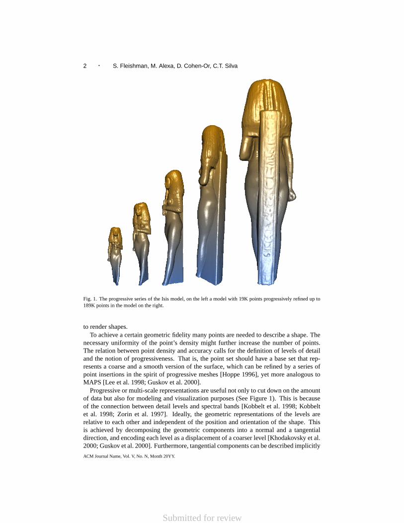
Fig. 1. The progressive series of the Isis model, on the left a model with 19K points progressively refined up to189K points in the model on the right.

to render shapes.To achieve a certain geometric fidelity many points are needed to describe a shape. The

necessary uniformity of the point’s density might further increase the number of points.The relation between point density and accuracy calls for the definition of levels of detailand the notion of progressiveness. That is, the point set should have a base set that rep-resents a coarse and a smooth version of the surface, which can be refined by a series ofpoint insertions in the spirit of progressive meshes [Hoppe 1996], yet more analogous toMAPS [Lee et al. 1998; Guskov et al. 2000].

Progressive or multi-scale representations are useful not only to cut down on the amountof data but also for modeling and visualization purposes (See Figure 1). This is becauseof the connection between detail levels and spectral bands [Kobbelt et al. 1998; Kobbeltet al. 1998; Zorin et al. 1997]. Ideally, the geometric representations of the levels arerelative to each other and independent of the position and orientation of the shape. Thisis achieved by decomposing the geometric components into a normal and a tangentialdirection, and encoding each level as a displacement of a coarser level [Khodakovsky et al.2000; Guskov et al. 2000]. Furthermore, tangential components can be described implicitly

ACM Journal Name, Vol. V, No. N, Month 20YY.


Progressive Point Set Surfaces · 3

by the refinement rule so that a single scalar per point is sufficient to encode the shape. Notethat this also leads to an efficient geometry compression scheme.

This approach has been described and analyzed for mesh geometry using subdivisiontechniques by [Guskov et al. 2000; Lee et al. 2000]. Based on the method of moving leastsquares (MLS) presented in [Alexa et al. 2001; Levin 2000], in this paper we define aprojection operator and a refinement rule. Together, they allow us to refine a given basepoint set towards a reference point set (input model). The projection operator defines alocal tangential coordinate frame, which allows us to specify the position of inserted points,with a scalar representing the normal component. The tangential components are definedby the refinement rule. As such, the scheme is reminiscent of subdivision techniques formeshes.

Based on the properties of the refinement process we develop a simplification scheme forpoint sets to construct a base point set, which represents a smoother version of the originalshape. The base point set is then refined by point insertion to add levels of detail. Thesurface could be refined adaptively creating point sets with densities varying with respect,say, to the viewing parameters or the local geometric behavior of the surface. In this paperwe:

—introduce a point-based modeling technique that is based on the MLS projection mech-anism.

—present a progressive scheme for point set surfaces, where the levels of an object repre-sent both coarse–to–fine and smooth–to–detailed hierarchy.

—use a local operator that allows accurate computation of local differential surface prop-erties.

—apply an encoding scheme for compressing progressive point sets surfaces.

In Section 2, we proceed with a presentation of related work. We define the MLS surfaceand how to compute it in Section 3. In Section 4, we describe the progressive point setsurfaces in detail. Section 5 describes how a progressive point set surface is encoded anddiscusses its efficiency. Results are shown in Section 6. We end with a discussion on theprogressive point set surface and conclude in Sections 7 and 8.

2. RELATED WORK

Our work is related to the recent research efforts in developing point-based representa-tions for shapes [Grossman and Dally 1998; Pauly and Gross 2001; Pfister et al. 2000;Rusinkiewicz and Levoy 2000]. Most of the mentioned techniques are targeted at fast pro-cessing and rendering of large point-sampled geometry. Our techniques are focused onadvancing the “modeling” of primitives with points. In this respect our work fits into thefield of Digital Geometry Processing(DGP) [Desbrun et al. 1999; Guskov et al. 1999;Guskov et al. 2000; Lee et al. 1998; Taubin 1995], which aims at extending standard signalprocessing concepts to the manifold surface domain. In [Pauly and Gross 2001], Paulyand Gross have shown how to extend these techniques to point-based representations bycollecting sets of points to patches, over which the points define an irregularly sampledfunction. Most approaches for meshes also construct a multiresolution representation byprogressively refining a base domain and exploiting the connection of the refinement levelsto spectral properties. Meshes are generally composed of two parts: the connectivity of themesh; and the geometry (i.e., the position of the vertices). Few DGP techniques can be




directly applied to such a representation (one example is the pioneering work presented in[Taubin 1995]). DGP algorithms require parameterization of the surface, which could berepresented in mesh form as a subdivision surface [Lee et al. 1998; Kobbelt et al. 1999;Eck et al. 1995].

A recent work related to our surface representation is the work of Carr et al. [Carr et al.2001] which reconstructs 3D objects by fitting a global radial basis function (RBF) to pointclouds. An RBF forms a solid model of an object, allowing analytic evaluation of surfacenormal, direct rendering and iso-surface extraction, similar to the properties of the surfacerepresentation we use.

Several different hierarchical representations have been proposed for geometric objects.Object simplification [Cignoni et al. 1994; Cohen et al. 1996; He et al. 1996; Hoppe et al.1993; Zhou et al. 1997] is often used to generate a hierarchical representation, which couldbe used for many purposes, e.g. rendering [Duchaineau et al. 1997; El-Sana and Varshney1999; Xia et al. 1997].

A leading technique for representing hierarchical meshes isProgressive Meshes[Hoppe1996], a mesh representation of varying resolution where a series of edge-split operationsprogressively refines a base mesh up to the original resolution of the source. This repre-sentation motivates solutions to mesh simplification, progressive transmission and load-ing from a disk or from a remote server. A number of mesh compression and streamingtechniques are based on this concept [Cohen-Or et al. 1999; Pajarola and Rossignac 2000;Taubin et al. 1998]. For a recent survey of mesh simplification and compression techniquessee [Gotsman et al. 2001].

Subdivision surfaces [Kobbelt and Schroder 1998; Kobbelt 2000; Zorin et al. 1996;1997] are defined by a topological refinement operator and a smoothing rule. Given amesh of arbitrary topology, they refine the mesh towards a smooth limit surface. Pointset surfaces are similar to subdivision surfaces, in that it is possible to add points to thedefined smooth surface without additional information. However, to describe an arbitrarysurface using subdivision techniques, inserted points need to be displaced. Normal Meshes[Guskov et al. 2000] as well as Displaced Subdivision Surfaces [Lee et al. 2000] demon-strate this idea of a multi resolution subdivision mesh where vertices are displaced by asingle scalar value in the normal direction. These approaches are attractive since a singlescalar value is easier to manipulate or store. The underlying concept could be understoodas decomposing the surface representation into a tangential and a normal component (see[Guskov et al. 2000]). Note that we use the same idea, however without coding the tangen-tial component explicitly as the mesh connectivity but implicitly as point proximity.

3. MLS SURFACES

The MLS surfaceSP of a set of pointsP = pi,pi ∈ R3, i ∈ 1, . . . , N is definedimplicitly by a projection operator. To project a pointr ontoSP two steps are necessary:First, a local reference domainH is computed. Then, a local bivariate polynomial is fittedoverH to the point set. More precisely, the local reference domainH = x|〈n,x〉 −D =0,x ∈ R3,n ∈ R3, ‖n‖ = 1 is determined by minimizing

N∑i=1

(〈n,pi − r− tn〉)2 e−‖pi−r−tn‖2/h2(1)

in all normal directionsn and offsetst.




Letqi be the projection ofpi ontoH, andfi the height ofpi over H, i.efi = n·(pi−q).The polynomial approximationg is computed by minimizing the weighted least squareserror

N∑i=1

(g(xi, yi)− fi)2e−‖pi−r−tn‖2/h2

. (2)

The projection ofr is given by

MLS(r) = r + (t + g(0, 0))n. (3)

Formally, the surfaceSP is the set of points (Ω ⊂ <) that project onto themselves. In thisdefinition,h is the anticipated spacing of the points. Thus, the point set together with anadequately chosen value forh defines the surface. As part of the projection procedure, wenot only determine the position on the surface where a point projects to, but we also obtainhigh-order derivative information analytically, which can be used to accurately determinenormal, curvature, etc. In the following,SX will generally be the surface with respect to apoint setX defined by the above procedure. We will call this the MLS-surface ofX.

4. PROGRESSIVE POINT SET SURFACES

First, we give an overview of the concept of progressive point set surfaces and then explainthe details in the following sections.

Given a reference (input) point setR = ri defining a reference surfaceSR. The pointsetR is reduced by removing points to form a base point setP0 ⊂ R. This base point setdefines a surfaceSP0 which differs fromSR. Next, we will resample the surface addingmore points so that the difference between our surface andSR decrease.

The base point setP0 is refined by inserting additional points yielding the setP1. Therefinement operator first inserts points independent of the reference setR, which meansP1 6⊂ R. Then, the inserted points are displaced so that the difference between the surfacesdecreases, i.e.d(SP1 , SR) < d(SP0 , SR).

This process is repeated to generate a sequence of point setsPi with increasing size anddecreasing difference to the reference surface. A progressive point set surfaces is definedas the MLS surface ofP = P0, P1, . . .. Where each point setPi is encoded by the (scalar)displacements of inserted points, yielding a compact representation of the progressive pointset surface.

In the following we explain the necessary steps for this procedure in detail.

4.1 The refinement operator

Let R be the reference point set as before andP be the point set to refine. The setP isrefined by generating additional pointsA = aj, which are sampled in the local neigh-borhoods of thepi.

More specifically, let the local reference domainHp(pi) of a pointpi (see Figure 2a) bedetermined as the local minimum of Eq. (1) with respect to the points inP . The referenceplaneHp(pi) is sampled regularly at intervalsρ, yielding a set of(u, v) coordinates for thepointsa′j on the plane. These points are placed in the neighborhood of the surface using thepolynomialg = gp(pi) (defined by Eq. (2) ), yielding the set of pointsaj = (u, v, g(u, v)).

To find and encode the positions of the additional points, the planeHp(aj) of aj is com-puted, and then two local polynomial fits are computed on the basis of the given reference




i

a’

a

H (p )ip

g (p )p i

p

(a)

H (a)p

ap

ar

a

∆

(b)

Fig. 2. An illustration of the point set refinement process: (a) a new pointa is generated in the neighborhoodof the surface of the current level (the blue points). The reference planeHp(pi) and polynomialgp(pi) of pi

are computed. By scanning the neighborhood ofpi, a new pointa′ onHp(pi) is generated and projected on thepolynomialgp(pi). In (b), a is projected onMLSp (the blue curve) by computing its reference planeHp(a)and polynomialgp(a). Next,a is projected again onSR (defined by the black points) using the same referenceplane, but with the appropriate polynomialgr(a). Finally, the detail value∆ = ar − ap is computed.




Fig. 3. Close-ups of smooth renderings for different levels in the hierarchy of a PPSS. Thebase level of a PPSS defines a smooth surface, which is here visualized by upsamplingthe smooth surface by adding points without displacing them to fit the detailed originalsurface. Note that higher levels add these details to the PPSS representation.

domainHp(aj): The first polynomialgp is with respect to the points inP and the second,gr, is with respect to the points inR. The height of a pointaj is given asgr(0, 0), i.e. onthe local polynomial fit to the points in the reference set (see Figure 2b).

Since the coordinate(u, v) is generated implicitly by specifying the regular samplingparameterρ, only the height has to be encoded. Based on Eq. (3, the height ofaj can beexpressed as the difference:

∆ = gr(0, 0)− gp(0, 0). (4)

Since the distance betweengr andgp is significantly smaller than the distance betweengr

and the reference plane, the∆ can be efficiently encoded.The regular sampling pattern has to be adapted to avoid oversampling and sampling of

empty regions. We introduce two criteria for deciding whether to insert a point. A pointai

is inserted only if

(1) none of the already inserted pointsP ∪ aj, j < i is closer thanρ and

(2) it is in the convex hull of points inP closer thanh or, more formally, iff ai ∈CHpi|‖pi − ai‖ < h.

The first criterion avoids oversampling, and the second aims at detecting boundaries ofthe manifold by defining the extent of the local neighborhood.

The sampling parameterρ can be used to specify the refinement convergence. Ifρ ishalved in every refinement step the number of points approximately quadruples from onepoint set to the next. However,ρ can also be used to adapt the sampling density to theapplication needs, e.g. visible regions of the surface or local curvature if piecewise linearapproximations are needed.

As the point density increases from one refinement level to the next, alsoh should beadapted. We adapth to the change inρ, for example, ifρ is halved in every step, so ish.We assume, however, that a suitableh is given for the base point set. This is discussed inthe following section.




4.2 Constructing the base point set

The refinement operator uses local reference domains on the basis of the reduced pointset to compute polynomial fits to the reference point set. This requires the local referencedomain of a pointpi with respect to the points inP and to the points inR to be about thesame. We use this requirement as a criterion for reducing the reference point set to the basepoint set.

Given a neighborhood sizeh and a maximum deviationε, let Qi be the point set whichresults from removing the points in ah-neighborhood aroundri, i.e.

Qi = rk|‖rk − ri‖ > h. (5)

A point ri can be used in the base point set if its original reference domainHi|R is close tothe reference domainHi|Qi

with respect to the reduced point setQi. More specifically, thedistance betweenHi|R andHi|Qi

is measured as the 2-norm of the difference of the fourscalars (three normal components, one offset) defining the reference domain (see Section3).

In practice, the points inR are visited in random order. Ifri can be included inP0,all points in theh-neighborhood aroundri are discarded for inclusion inP0. The processterminates once all points are tested.

5. THE PPSS ENCODING

Figure 4 illustrates the magnitudes of the displacements of the progressive set. Observingthat the vast majority of the displacements are of small magnitudes gives raise to a spaceefficient encoding scheme. To create an encoding ofPi+1 givenPi, we perform the routinedescribed in Section 4.1. New points are generated and projected both onSPi

and onSR.The difference between the two projections is thedisplacementdenoted by∆. Since thedistance between the two surfaces is small, the displacements are merely the details of thesurface and can be encoded in a small number of bits.

To decodePi+1, a reverse procedure is applied. New points are generated as described inthe encoding procedure. For each pointr, the reference plane and polynomial are computedusing Eqns. (1),(2). Then the point is projected using a modified Eq. (3) as follows:

MLS(r) = r + (t + g(0, 0) + ∆)n. (6)

For efficient storage, we quantize the displacement values to a user-specified accuracy.An error bound defines the maximal tolerated error with respect to the diagonal of theobject’s bounding box. The range of the displacements and the error bound defines thenumber of bits required to properly represent the displacements. Recall that the decodingprocedure is highly dependent on performing the exact same procedure that the encoderperformed. Quantizing the values and reconstructing them creates minor differences thatmay lead to somewhat different sets of points that are added to each level. If this occurs theencoder and decoder may no longer be synchronized. Therefore, in the encoding processthe displacements are quantized to guarantee that the decoder generates the exact set ofpoints that is encoded.

6. RESULTS

We have implemented the progressive point set representation as described in the previoussections and applied it to several models. Table I summarizes the results by showing the




0%

0.21%

Fig. 4. A color-coding of the magnitude of the displacement for the Venus model. Note that smooth regionshave small displacements, while regions containing fine detail need larger displacements The magnitude of thedisplacements essentially corresponds to the energy in the respective frequency band.

bits / displacementPoints (error10−4)

Name Points in P0 0.001 0.01 0.1 0.5

Dragon 437K 16K 9.7 6.6 3.4 2.4(0.026) (0.044) (0.29) (1.6)

Isis 187K 9K 9.9 6.9 4.7 1.8(0.01) (0.04) (0.31) (1.9)

Venus 134K 7K 9.2 8.3 5.5 3.0(0.08) (0.13) (0.27) (1.2)

Dino 56K 4K 10.9 8.1 4.9 2.9(0.25) (0.24) (0.35) (0.97)

Table I. Achieved bit-rates for given error bounds. The user can specify an error bound on the displacement values.Depending on the error bound, a quantization scheme is chosen, which influences the number of bits necessary toencode the displacements. The small number of quantization levels typically results in a systematically smallererror as compared to the error bound (shown in parenthesis).




Inserted Bits / Total Total Average errorpoints ∆ points size b/p (10−4)476370 2.3 493142 139K 3.66 2.7472330 2.4 489102 144K 3.77 1.6440907 3.5 457679 192K 4.92 0.29439652 6.6 456424 364K 8.06 0.044439840 9.7 456612 534K 11.1 0.026

Table II. A comparison of the size vs. accuracy for the Dragon model. Each line shows the size of the model asa function of the number of bits used for quantization of the displacement values. The base point set contains16772 points compressed to37.4 bits / point.

VenusDinosaur

DragonIsis

0

0.5

1

1.5

2

2.5

2 4 6 8 10 12 14 16

Err

or

Bits / Point

Rate Distortion Curve

Fig. 5. Rate distortion curve: shows a comparison of size vs. accuracy achievable with our compression method.The error is measured on a scale of10−4 of the bounding box of the model.




average number of bits per displacement required with respect to error tolerance. Theerror is expressed with respect to the diagonal of the bounding box of the given model.Note that the error is merely subject to the quantization applied to the displacements. Ourexperiments as shown in Table II and Figures 5 and 7 suggest that an average of five bits perpoint yields a pleasing visual quality. The base point setP0 is compressed by triangulatingthe points using the BPA [Bernardini et al. 1999] and applying a mesh compression tool[Gotsman et al. 2001].

Table II shows the compression achieved by varying the number of bits for the displace-ment values. We measured the accuracy of the reconstructed model in the spirit of Metro[Ciampalini et al. 1997], i.e. by sampling distances in normal direction. To measure thedistance between an MLS surfaceS1 defined by a set of pointsP1 and the reference MLSsurfaceS defined byP , we sample arbitrary points in the neighborhood ofS1, and use theMLS projection procedure to project each point onS1 and onS. The average differencebetween the two projections is the error.

We compared the PPSS based compression techniqe with techniques for multiresolutionmesh compression. In particular, we have used Khodakovsky’s mesh compression tech-nique [Khodakovsky et al. 2000] to generate meshes with increasing accuracy with respectto a reference mesh. The vertices of the reference mesh were used to build a PPSS. Sincewe do not have connectivity information the BPA was used to generate meshes from thepoint sets. The resulting meshes have been compared to the reference using Metro. Fig-ure 6 shows a visualization of the results. Note that the PPSS does not fit the piecewiselinear geometry of the reference mesh (as the mesh compression technique) but the MLS-surface defined by the vertices. This adds some bias to the resulting error for the PPSS.

Figure 7, show a series of progressively refined point sets, where the shaded images arerendered by an upsampling procedure [Alexa et al. 2001], which requires no displacements.The rendering performs a local refinement of the surface around each point of the model.The images in the second column of Figure 8 are rendered with the above upsamplingmethod and the images in the third column are rendered using the OpenGLTM glPointSizefunction. Since the MLS surface is continuous and smooth, the quality of the upsampledrenderings is higher than a splat rendering.

7. DISCUSSION

As in other multilevel shape representations, the levels essentially correspond to differentbands in the spectrum of the shape. The Gaussian weight function leads to a Gaussianfiltering of the shape (compare Eqns. (1) and (2) ). The spatial radiush of the filter is in-versely related to the Gaussian in the frequency domain. Thus, the base point set representsthe shape with the most relative energy in the low frequency bands, while the refinementlevels add higher frequency bands (see the shape hierarchy in Figure 1, and the details inFigure 3). The projection operator allows us to compute the scalar displacement necessaryto lift a point from one level to the next. The displacements are with respect to local frames(as in [Kobbelt et al. 2000]). The magnitude of this displacement is, thus, a measure of theenergy in the respective frequency band. This is illustrated with color codes in Figure 4.

Recently, Kalaiah and Varshney introduced an effective method for rendering pointprimitives that requires the computation of the principal curvatures and a local coordinateframe for each point [Kalaiah and Varshney 2001]. This approach is natural for the MLSsurface representation since it requires a local coordinate frame and the principal curvature




103K e=0.0038 516K e=0.002741K e=0.008

41K e=0.03 94K e=0.011 197K e=0.0042

Fig. 6. Comparison of meshes using Metro. The top row displays several steps during the refinement processof Khodakovsky’s algorithm. The numbers below the figures show their size and mean error with respect of thebounding box of the object, as reported by the I.E.I-CNR Metro tool. The bottom row displays three meshesreconstructed from a PPSS and compared to the input mesh. Note that the PPSS does not fit the reference meshbut rather the smooth MLS-surface over the vertices. The point sets are triangulated using BPA to be able to applyMetro. Color ranges from blue to green with respect to the error.




Fig. 7. A progressive series of the Venus and Dragon models.

for each. During the MLS projection procedure a local coordinate frame is computed, andthe principal curvatures can be estimated directly from Eq. (2).

8. CONCLUSIONS

Our technique has several unique features. First of all, it works directly on points, avoidingthe need to triangulate the source point set, and the costly remeshing of the surface intosubdivision connectivity. This is especially important for large and detailed datasets. An-other important property of our technique is its locality. This leads to a numerical stablecomputation, linear time and space complexity, small memory footprint, which permits towork on large objects. Furthermore, progressive point set representations lead to a com-pression scheme, where the dynamic range of the error decreases with each level in thehierarchy. As shown above, at each level it is possible to upsample the surface from thesparse representation.

The lack of connectivity in the representation could also be the source of shortcomings.As shown in [Amenta et al. 1998], there are limits on surface samplings which can beproven to define a given surface. That is, our approach might need a relatively dense baseset to resolve possible ambiguities in the modeling of certain complex surfaces. Moreover,it is considerably easier to handle discontinuities by triangulated models.

A considerable amount of research has been devoted to developing and optimizing the“mesh-base world”. Many advanced methods require a local parameterization and localdifferential properties. The MLS projection procedure inherently has these qualities, forexample, texture synthesis on surfaces [Turk 2001; Wei and Levoy 2001]. We believe thatthe importance of point set representation and of MLS surfaces in particular is likely toplay an increasing role in 3D modeling.

ACKNOWLEDGMENTS

The datasets by courtesy of Cyberware and the Stanford 3D scanning repository.This paper would not be possible without the many people who made their software

available: Fausto Bernardini for his implementation of the Ball-Pivoting Algorithm; IgorGuskov, Andrei Khodakovsky, Peter Schroeder, and Wim Sweldens for their remeshing




and compression code; Craig Gotsman and Virtue Ltd for “Optimizer”; and The VisualComputing Group of CNR-Pisa for Metro. We would like to thank Wagner Correa for helpthroughout this project.

REFERENCES

ALEXA , M., BEHR, J., COHEN-OR, D., FLEISHMAN , S., LEVIN , D., AND SILVA , C. T. 2001. Point setsurfaces.IEEE Visualization 2001, 21–28. ISBN 0-7803-7200-x.

AMENTA , N., BERN, M., AND KAMVYSSELIS, M. 1998. A new voronoi-based surface reconstruction algo-rithm. Proceedings of SIGGRAPH 98, 415–422. ISBN 0-89791-999-8. Held in Orlando, Florida.

BERNARDINI, F., MITTLEMAN , J., RUSHMEIER, H., SILVA , C., AND TAUBIN , G. 1999. The ball-pivoting al-gorithm for surface reconstruction.IEEE Transactions on Visualization and Computer Graphics 5,4 (October- December), 349–359. ISSN 1077-2626.

CARR, J. C., BEATSON, R. K., CHERRIE, J. B., MITCHELL , T. J., FRIGHT, W. R., MCCALLUM , B. C.,ANDEVANS, T. R. 2001. Reconstruction and representation of 3d objects with radial basis functions.Proceedingsof SIGGRAPH 2001, 67–76. ISBN 1-58113-292-1.

CIAMPALINI , A., CIGNONI, P., MONTANI , C., AND SCOPIGNO, R. 1997. Multiresolution decimation basedon global error.The Visual Computer 13,5, 228–246. ISSN 0178-2789.

CIGNONI, P., FLORIANI , L. D., MONTONI, C., PUPPO, E., AND SCOPIGNO, R. 1994. Multiresolution model-ing and visualization of volume data based on simplicial complexes.1994 Symposium on Volume Visualization,19–26. ISBN 0-89791-741-3.

COHEN, J., VARSHNEY, A., MANOCHA, D., TURK, G., WEBER, H., AGARWAL , P., FREDERICK P. BROOKS,J., AND WRIGHT, W. 1996. Simplification envelopes.Proceedings of SIGGRAPH 96, 119–128. ISBN0-201-94800-1. Held in New Orleans, Louisiana.

COHEN-OR, D., LEVIN , D., AND REMEZ, O. 1999. Progressive compression of arbitrary triangular meshes.IEEE Visualization ’99, 67–72. ISBN 0-7803-5897-X. Held in San Francisco, California.

DESBRUN, M., MEYER, M., SCHRODER, P., AND BARR, A. H. 1999. Implicit fairing of irregular meshesusing diffusion and curvature flow.Proceedings of SIGGRAPH 99, 317–324. ISBN 0-20148-560-5. Held inLos Angeles, California.

DUCHAINEAU , M. A., WOLINSKY, M., SIGETI, D. E., MILLER , M. C., ALDRICH, C., AND M INEEV-WEINSTEIN, M. B. 1997. Roaming terrain: Real-time optimally adapting meshes.IEEE Visualization ’97,81–88. ISBN 0-58113-011-2.

ECK, M., DEROSE, T. D., DUCHAMP, T., HOPPE, H., LOUNSBERY, M., AND STUETZLE, W. 1995. Multires-olution analysis of arbitrary meshes.Proceedings of SIGGRAPH 95, 173–182. ISBN 0-201-84776-0. Held inLos Angeles, California.

EL-SANA , J. AND VARSHNEY, A. 1999. Generalized view-dependent simplification.Computer GraphicsForum 18,3 (September), 83–94. ISSN 1067-7055.

GOTSMAN, C., GUMHOLD , S., AND KOBBELT, L. 2001. Simplification and compression of 3d meshes. InEuropean Summer School on Principles of Multiresolution in Geometric Modelling (PRIMUS), Munich.

GROSSMAN, J. P.AND DALLY , W. J. 1998. Point sample rendering.Eurographics Rendering Workshop 1998,181–192. ISBN 3-211-83213-0. Held in Vienna, Austria.

GUSKOV, I., SWELDENS, W., AND SCHRODER, P. 1999. Multiresolution signal processing for meshes.Pro-ceedings of SIGGRAPH 99, 325–334. ISBN 0-20148-560-5. Held in Los Angeles, California.

GUSKOV, I., V IDIMCE , K., SWELDENS, W., AND SCHRODER, P. 2000. Normal meshes.Proceedings ofSIGGRAPH 2000, 95–102. ISBN 1-58113-208-5.

HE, T., HONG, L., VARSHNEY, A., AND WANG, S. W. 1996. Controlled topology simplification.IEEE Trans-actions on Visualization and Computer Graphics 2,2 (June). ISSN 1077-2626.

HOPPE, H. 1996. Progressive meshes.Proceedings of SIGGRAPH 96, 99–108. ISBN 0-201-94800-1. Held inNew Orleans, Louisiana.

HOPPE, H., DEROSE, T., DUCHAMP, T., MCDONALD , J., AND STUETZLE, W. 1993. Mesh optimization.Proceedings of SIGGRAPH 93, 19–26. ISBN 0-201-58889-7. Held in Anaheim, California.

KALAIAH , A. AND VARSHNEY, A. 2001. Differential point rendering. InRendering Techniques, S. J. Gortlerand K. Myszkowski, Eds. Springer-Verlag.

KHODAKOVSKY, A., SCHRODER, P.,AND SWELDENS, W. 2000. Progressive geometry compression.Proceed-ings of SIGGRAPH 2000, 271–278. ISBN 1-58113-208-5.

KOBBELT, L. 2000. sqrt(3) subdivision.Proceedings of SIGGRAPH 2000, 103–112. ISBN 1-58113-208-5.KOBBELT, L., CAMPAGNA , S.,AND SEIDEL, H.-P. 1998. A general framework for mesh decimation.Graphics

Interface ’98, 43–50. ISBN 0-9695338-6-1.KOBBELT, L., CAMPAGNA , S., VORSATZ, J.,AND SEIDEL, H.-P. 1998. Interactive multi-resolution modeling

on arbitrary meshes.Proceedings of SIGGRAPH 98, 105–114. ISBN 0-89791-999-8. Held in Orlando, Florida.KOBBELT, L. AND SCHRODER, P. 1998. A multiresolution framework for variational subdivision.ACM Trans-

actions on Graphics 17,4 (October), 209–237. ISSN 0730-0301.KOBBELT, L. P., BAREUTHER, T., AND SEIDEL, H.-P. 2000. Multiresolution shape deformations for meshes

with dynamic vertex connectivity.Computer Graphics Forum 19,3 (August), 249–260. ISSN 1067-7055.KOBBELT, L. P., VORSATZ, J., LABSIK , U., AND SEIDEL, H.-P. 1999. A shrink wrapping approach to remesh-

ing polygonal surfaces.Computer Graphics Forum 18,3 (September), 119–130. ISSN 1067-7055.LEE, A., MORETON, H., AND HOPPE, H. 2000. Displaced subdivision surfaces.Proceedings of SIGGRAPH

2000, 85–94. ISBN 1-58113-208-5.




LEE, A., SWELDENS, W., SCHRODER, P., COWSAR, L., AND DOBKIN , D. 1998. Maps: Multiresolutionadaptive parameterization of surfaces.Proceedings of SIGGRAPH 98, 95–104. ISBN 0-89791-999-8. Held inOrlando, Florida.

LEVIN , D. 2000. Mesh-independent surface interpolation. Tech. rep., Tel-Aviv University.http://www.math.tau.ac.il/˜ levin.

PAJAROLA, R. AND ROSSIGNAC, J. 2000. Compressed progressive meshes.IEEE Transactions on Visualizationand Computer Graphics 6,1 (January - March), 79–93. ISSN 1077-2626.

PAULY, M. AND GROSS, M. 2001. Spectral processing of point-sampled geometry.Proceedings of SIGGRAPH2001, 379–386. ISBN 1-58113-292-1.

PFISTER, H., ZWICKER, M., VAN BAAR , J., AND GROSS, M. 2000. Surfels: Surface elements as renderingprimitives. Proceedings of SIGGRAPH 2000, 335–342. ISBN 1-58113-208-5.

RUSINKIEWICZ, S. AND LEVOY, M. 2000. Qsplat: A multiresolution point rendering system for large meshes.Proceedings of SIGGRAPH 2000, 343–352. ISBN 1-58113-208-5.

TAUBIN , G. 1995. A signal processing approach to fair surface design.Proceedings of SIGGRAPH 95, 351–358.ISBN 0-201-84776-0. Held in Los Angeles, California.

TAUBIN , G., GUEZIEC, A., HORN, W., AND LAZARUS, F. 1998. Progressive forest split compression.Pro-ceedings of SIGGRAPH 98, 123–132. ISBN 0-89791-999-8. Held in Orlando, Florida.

TURK, G. 2001. Texture synthesis on surfaces.Proceedings of SIGGRAPH 2001, 347–354. ISBN 1-58113-292-1.

WEI, L.-Y. AND LEVOY, M. 2001. Texture synthesis over arbitrary manifold surfaces.Proceedings of SIG-GRAPH 2001, 355–360. ISBN 1-58113-292-1.

X IA , J. C., EL-SANA , J., AND VARSHNEY, A. 1997. Adaptive real-time level-of-detail-based rendering forpolygonal models.IEEE Transactions on Visualization and Computer Graphics 3,2 (April - June). ISSN1077-2626.

ZHOU, Y., CHEN, B., AND KAUFMAN , A. E. 1997. Multiresolution tetrahedral framework for visualizingregular volume data.IEEE Visualization ’97, 135–142. ISBN 0-58113-011-2.

ZORIN, D., SCHRODER, P., AND SWELDENS, W. 1996. Interpolating subdivision for meshes with arbitrarytopology.Proceedings of SIGGRAPH 96, 189–192. ISBN 0-201-94800-1. Held in New Orleans, Louisiana.

ZORIN, D., SCHRODER, P.,AND SWELDENS, W. 1997. Interactive multiresolution mesh editing.Proceedingsof SIGGRAPH 97, 259–268. ISBN 0-89791-896-7. Held in Los Angeles, California.




Fig. 8. Two intermediate representations of the Venus model in the hierarchy. On the left we show the set ofpoints. In the middle, the set of points are rendered by splatting using OpenGLTM . The images on the right arerendered using an MLS upsampling procedure, requiring no additional data.


progressive point set surfaces - stanford university

Documents