Project 1-44 (1)

Measuring Tire-Pavement Noise at the Source:

Precision and Bias Statement

July 14, 2011

Prepared for:

National Cooperative Highway Research Program Transportation Research Board of The National Academies

Prepared by:

Dr. Paul R. Donavan Illingworth & Rodkin, Inc.

Petaluma, CA 94952

Dana M. Lodico, P.E., INCE Bd. Cert. Lodico Acoustics LLC Englewood, CO 80112

ACKNOWLEDGMENT OF SPONSORSHIP This work was sponsored by the American Association of State Highway and Transportation Officials, in cooperation with the Federal Highway Administration, and was conducted in the National Cooperative Highway Research Program, which is administered by the Transportation Research Board of the National Academies.

DISCLAIMER

This is an uncorrected draft as submitted by the research agency. The opinions and conclusions expressed or implied in the report are those of the research agency. They are not necessarily those of the Transportation Research Board, the National Academies, or the program sponsors.

TABLE OF CONTENTS SUMMARY ....................................................................................................................................1

CHAPTER 1 BACKGROUND ............................................................................................................................2 Findings from NCHRP 1-44 Project ...................................................................................2 Other Findings Since the Completion of NCHRP 1-44 Project........................................3 Literature Review...........................................................................................................3 OBSI Comparative Testing ............................................................................................4 “Precision” and “Bias” .........................................................................................................5 CHAPTER 2 RESEARCH APPROACH............................................................................................................6 Research Objectives and Scope ...........................................................................................6 Approach ...............................................................................................................................6 Task 1: Collect and Evaluate Information.....................................................................6 Task 2: Plan and Conduct Initial Test Studies...............................................................6 Task 3: Evaluate Comparative Testing Among OBSI Users .........................................7 Task 4: Conduct Further Testing to Address Reproducibility and Bias ........................7 Task 5: Investigate Methods for Calibration of OBSI Measurement Systems...............7 Task 6: Develop Proposed Revisions to OBSI Procedures ...........................................7 Report Organization .............................................................................................................8 CHAPTER 3 TEST PROGRAMS .......................................................................................................................9 Test Track Measurements....................................................................................................9 Facilities Equipment ......................................................................................................9 Test Procedures and Conditions ..................................................................................10 Laboratory Measurements.................................................................................................11 Wind Tunnel Testing ....................................................................................................11 Road-wheel Simulator Testing .....................................................................................13 CHAPTER 4 RESEARCH FINDINGS.............................................................................................................15 Temperature ........................................................................................................................15 Discussion of Results ...................................................................................................16 Validation of Temperature Correction Results............................................................16 Assessment of Air Density Correction .........................................................................17 Pass-by Measurements and Air Temperature..............................................................19 Pavement Temperature ................................................................................................20 Test Tires .............................................................................................................................22 Tire Comparisons.........................................................................................................23 Tire Hardiness .............................................................................................................27

Tire Loading.................................................................................................................29 Other Tire Parameters .................................................................................................30 Test Parameters ..................................................................................................................34 Location .......................................................................................................................34 Background Noise ........................................................................................................37 Reflecting Objects ........................................................................................................39 Test Speed ....................................................................................................................39 Horizontal Curves ........................................................................................................40 Vertical Curves ............................................................................................................42 Environmental Conditions .................................................................................................42 Wind .............................................................................................................................42 Pavement Dampness ....................................................................................................45 Instrumentation...................................................................................................................47 OBSI Measuring Equipment ........................................................................................47 OBSI System Calibration .............................................................................................48 Vehicle/Operator Effects ....................................................................................................48 Repeatability and Reproducibility ....................................................................................50 Controlled Testing Repeatability .................................................................................50 On-road Testing Repeatability.....................................................................................51 On-road Testing Reproducibility .................................................................................52 CHAPTER 5 PRECISION AND BIAS STATEMENTS .................................................................................53 CHAPTER 6 PROPOSED REVISIONS TO THE PROCEDURE ................................................................55 CHAPTER 7 RECOMMENDATIONS AND SUGGESTED RESEARCH ..................................................56 Test Procedure Implementation ........................................................................................56 Continuing Test Procedure Refinement .......................................................................56 Use of Tire Noise Road-Wheel Simulators ..................................................................56 Coordination with Other Tire/Pavement Noise Assessment Procedures ......................56 Suggested Research.............................................................................................................57 REFERENCES.............................................................................................................................58 ATTACHMENT 1: Revised Proposed Standard Method of Test for Measurement of Tire/Pavement Noise Using the On-Board Sound Intensity Method (OBSI) .............................................................AT-1

APPENDIX A: Factors in OBSI Precision and Bias..............................................................................Attached CD APPENDIX B: The Effect of Air Density on OBSI Measurement........................................................Attached CD APPENDIX C: Test Track Measurement Program................................................................................Attached CD APPENDIX D: Laboratory Measurement Program: Tire Noise Dynamometer Tests...........................Attached CD APPENDIX E: Laboratory Measurement Program: Wind Tunnel Tests ..............................................Attached CD APPENDIX F: Summary of Comparative OBSI Testing Rodeos.........................................................Attached CD

LIST OF FIGURES Figure 1: Pontiac G6 installed in GMAL ....................................................................................12 Figure 2: Vertical dual probe fixture installed on the Chevrolet Impala and ideal fixture

installed on the opposite side of the vehicle ...............................................................12 Figure 3: Plan view of the test vehicle defining negative and positive crosswind (yaw)

directions......................................................................................................................12 Figure 4: Test vehicle installed in on the tire noise chassis dynamometer setup for drive axis measurements ........................................................................................13 Figure 5: Overall OBSI levels for test tire TT#5 versus temperature for all test periods ...........15 Figure 6: Overall Passby levels at 25 feet versus air temperature for September and December test periods ...........................................................................................19 Figure 7: Pavement temperature versus air pavements during the February, March,

September, and December tests of tire TT#5...............................................................20 Figure 8: Overall OBSI levels for test tire TT#5 versus pavement temperature for all test periods.........................................................................................................21 Figure 9: Overall OBSI levels for the eleven new test tires .......................................................23 Figure 10: Overall OBSI levels for new SRTT tires versus TT#5 ...............................................24 Figure 11: Overall OBSI levels for the six older test tires and new tire TT#5 .............................25 Figure 12: Overall OBSI levels for Older SRTT tires versus TT#5.............................................26 Figure 13: Overall OBSI levels for all 16 test tires versus TT#5 ................................................27 Figure 14: Overall OBSI levels for all test tires versus tire durometer hardness number ............28 Figure 15: Overall OBSI levels for tire TT#5 with varied tire loading ........................................29 Figure 16: Average temperature adjusted OBSI levels for TT#5 for each month of testing........30 Figure 17: Overall OBSI level increase from initial to final testing.............................................32 Figure 18: Example of OBSI level variation with location in a test pavement ............................35 Figure 19: Difference in OBSI level created by a ½ second change in start position (44

ft) for 5 second average for different profiles of OBSI versus position as a function of the difference in OBSI level in the profile ................................................36

Figure 20: Difference in OBSI level created by a 0.2 second change in start position (17.6 ft) for 5 second average for different profiles of OBSI versus position as a

function of the difference in OBSI level in the profile ................................................36 Figure 21: PI index criteria compared to baseline PI index levels on the smooth and

coarse dynamometer surfaces ......................................................................................38 Figure 22: Sites for evaluation of horizontal curves with PCC site and AC site..........................41 Figure 23: One-third octave band spectra comparison of straight and curved roadway sections..........................................................................................................41 Figure 24: Sound intensity and pressure levels for vehicles at 60 mph and 0º yaw ....................43

Figure 25: Overall sound intensity and pressure levels as a function of yaw angle ...........................................................................................................................43 Figure 26: Increase in sound intensity levels above tire noise alone created by wind

background noise effects for overall, 400, and 500 Hz bands .....................................44 Figure 27: ⅓ octave band OBSI level on Section S4 (½” porous OGAC) for visibly damp and dry conditions..............................................................................................46 Figure 28: ⅓ octave band OBSI level on Section S8 (½” porous PFC ) for visibly damp and dry conditions..............................................................................................46 Figure 29: Overall OBSI levels for the two test teams with and without test tires

switched .......................................................................................................................49 Figure 30: Overall OBSI levels for repeat runs over three baseline times ..................................50

LIST OF TABLES Table 1: Data quality criteria and recommended parameter limits ..............................................3 Table 2: Test configurations and conditions for on-road measurements ...................................11 Table 3: Averages of ranges and standard deviation of uncorrected and corrected OBSI

data...............................................................................................................................17 Table 4: Average of ranges and standard deviations of uncorrected and corrected OBSI data using the air density correction for TT#5...................................................18 Table 5: Averages of range and standard deviation of uncorrected and corrected OBSI data for air and pavement temperature ..............................................................22 Table 6: Tires used in test track OBSI measurements ...............................................................22 Table 7: Ranges in OBSI level across all pavements, averaged over all pavements, and standard deviations for different tire groupings ....................................................25 Table 8 Test tire tread depth measured in January 2011...........................................................33 Table 9: OBSI levels and level differences for test speeds of 59, 60 and 61 mph.....................39 Table 10: Run-to-Run level variation for February testing..........................................................51 Table 11: Test-to-test level variation for on-road testing.............................................................52 Table 12: Calculated uncertainty and limit of repeatability for test procedure............................54

AUTHOR ACKNOWLEDGEMENTS The research reported here in was performed under NCHRP Project 1-44(1) by Illingworth & Rodkin, Inc., Petaluma, California; Dr. Paul Donavan was the principal investigator. Lodico Acoustics, LLC, Denver, Colorado served as a subcontractor for all phases of this research and participated in data acquisition and analysis. Chris Peters and Carrie Janello, also of Illingworth & Rodkin, Inc, assisted in the test track field work and data analysis. The authors acknowledge the assistance provided by Matt Seare and Kyle Taylor of the Hyundai·Kia America Technical Center, Inc. in the use of the Hyundai·Kia Proving Ground for the test track measurement programs. Liaison the use of these facilities was provided by Bruce Rymer of Caltrans. The authors also acknowledge the assistance provided by Alan Parrett and James Zunich of the General Motors Proving Ground in Milford, Michigan, in the use of General Motors wind tunnel and tire noise dynamometer for the laboratory test portions of this research as well as the assistance of staffs of these facilities in performing the testing.

SUMMARY MEASURING TIRE-PAVEMENT NOISE AT THE SOURCE: PRECISION AND BIAS STATMENT The research performed under NCHRP 1-44, “Measuring Tire-Pavement Noise at the Source”, recommended a procedure for measuring tire-pavement noise using the on-board sound intensity (OBSI) method. The objectives of the research performed in the NCHRP Project 1-44 (1) “Measuring Tire-Pavement Noise at the Source: Precision and Bias Statement” were to develop and recommend modifications to the recommended method of test and to determine the precision and bias statements for this method. This was accomplished through a series of test track measurements completed in four events spanning a 10 month period and through laboratory measurements conducted on a tire noise dynamometer with replica road surfaces and in an aero-acoustic wind tunnel. The results of four comparative OBSI test “rodeos” were also analyzed to examine test team-to-team variability. Recommendations to reduce uncertainty in the OBSI measurements were developed and incorporated in a revised Method of Test. These are enumerated in Chapter 6 and summarized here. A temperature correction of -0.04 dB/ºF is recommended to be applied to sound intensity data acquired with the analyzer set to standard conditions of 68ºF (20ºC) and 101.3 kPa atmospheric pressure effectively normalizing the reported levels to these conditions. In order to identify contamination from background noise due to other noise sources, a frequency dependent pressure to intensity (PI) index ranging from 2.5 to 5 dB was developed. A criterion of being 15 inches or more from sound reflecting surfaces was recommended. Crosswind conditions were also recommended to be no greater than 8 mph. Criteria for determining when test tires should be retired were determined. Tolerances on the data acquisition start location were defined at ±10 ft (0.23 seconds at 60 mph) and the vehicle speed tolerance was set to ±1 mph. Air temperature was restricted to a range from 40 to 100ºF. Tire loading was revised downward to 800±100 lbs from the previously recommended nominal of 850 lbs and probe fore/aft separation changed to 8¼ inches centered on the axis of rotation of the tire instead of being defined by determination of the more ambiguous tire contact patch. In addition to these changes, the existing requirements in the procedure were confirmed. Based on the recommended revised OBSI Method of Test, uncertainties and limits on precision and bias were developed. Precision was considered in two parts. For repeatability, a single operator testing on the same pavement under the same environmental conditions within a single test session, the uncertainty was determined to be ±0.2 dB with a limit of 0.6 dB. Precision reproducibility for multiple test teams measuring under the same environmental conditions or a single test team measuring over multiple days was determined to be ±0.4 dB with a limit of 1.1 dB. Bias resulting from longer periods of time between tests or from site to site was determined to be ±0.5 dB with a limit of 1.4 dB.

1

CHAPTER 1 BACKGROUND In 2008, research was completed on the NCHRP Project 1-44, entitled “Measuring Tire-Pavement Noise at the Source”. The final report was subsequently published as NCHRP Report 6301. The objectives of this project were to (1) develop rational procedures for measuring tire-pavement noise at the source and (2) demonstrate the applicability of the procedures through testing of in-service pavements. This work resulted in the “Proposed Method of Test for Measurement of Tire-Pavement Noise Using the On-Board Sound Intensity (OBSI) Method”1. The results of this research were also largely incorporated into an American Association of State Highway Transportation Officials (AASHTO) provisional Standard Method of Test entitled “Measurement of Tire/Pavement Using the On-Board Sound Intensity (OBSI) Method” TP76-11 (proposed). As the number of practitioners of the OBSI method grew and more comparative testing took place, interest developed in documenting the precision and bias of the procedure. NCHRP Project 1-44 (1), “Measuring Tire-Pavement Noise at the Source: Precision and Bias Statement” was initiated to address this need with the resultant objective of developing a precision and bias statement for the test method reported in NCHRP Report 6301. Findings from NCHRP 1-44 Project In addition to developing and demonstrating rational procedures for measuring tire-pavement noise at the source, Project 1-44 research also included an initial investigation into precision repeatability, precision reproducibility and bias issues. The evaluation of test parameters included sound intensity probe configuration and orientation, variations in location of the probes, test speed, tire inflation pressure, tire loading, temperature, and the use of different test vehicles. Run-to-run repeatability was also documented for consecutive test runs or repeats, as was reproducibility from day to day. In these parameter investigations, the ranges of variable values were defined to be perturbations around a defined vehicle type, tire, and instrumentation system in a baseline condition. This testing identified OBSI probe location in the vertical direction, vehicle speed, and vehicle loading to be greatest causes of variation for the ranges and parameters evaluated. Within reasonable limits, probe distance from the tire, probe fore/aft location, and tire inflation pressure were found not to be critical. Based on these results, parameter limits were established for the OBSI procedure. Table 1 summarizes the parameter limits and criteria for the test procedure. Based on the initial investigation into precision and bias issues, a number of recommendations for further research were identified including the effects of large temperature ranges, the effects of other environmental conditions, and the need for comparative testing between different operators and measurement systems. With the selection of the ASTM Standard Reference Test Tire (SRTT)2, issues of tire-to-tire variation and tire performance over time were also identified as areas deserving further investigation. These are addressed in Project 1-44(1).

2

Table 1: Data Quality Criteria and Recommended Parameter Limits

Parameter Data Quality Criteria Run to Run Range, Overall A-Wtd OBSI level

Within 1 dB

Run to Run Range, ⅓ Octave Band Levels

Within 2 dB

Coherence > 0.8 for frequencies below 4000 Hz PI Index < 5 dB for data reported as valid

Parameter Parameter Limits Probe Location, Vertical 75 ± 6 mm (3 ± ¼ in.) above pavement Vehicle Test speed 97 ± 1 km/h (60 ± 1 mph) Tire Inflation Pressure (Cold) 207 ± 14 kPa (30 ± 2 psi) Wheel Load 385 ± 45 kg (850 ± 100 lbs) Probe Location, Fore/Aft 200 ± 13 mm (8 ± ½ in.) Probe Distance from Tire Sidewall 100 ± 13 mm (4 ± ½ in.)

Other Findings Literature Review Summary The literature review conducted as part of the NCHRP Project 1-44 included historical information regarding precision and bias for at the source tire-pavement noise measurements and are documented in NCHRP Report 6301. Since that time, more information has been added to the technical literature on parameters that affect tire noise generation and measurement. As described below, recent literature has focused on temperature effects, pavement variations over a test section, and test tire variables. Previous investigations of the effects of temperature on OBSI level have generally found that tire/pavement noise decreases with increasing temperature and that this relationship depends on tire and the pavement3,4,5. Generally, these data were obtained for a limited range of temperature or are composite of data not necessarily taken to solely address temperature effects. Temperature affects the measurement of sound intensity due to the finite difference approximation used in its computation that includes the density of air, which is determined largely by air temperature and barometric pressure. Although theoretically a correction for air density should be made, it has not been demonstrated experimentally in the literature whether applying the correction improves or detracts from the precision of the sound intensity measurement. In terms of the effect of pavement variation within a given test section, it is thought that significant variation in the noise of a pavement over short distances could display itself as higher than usual (greater than 1 dB) run-to-run variation due to OBSI results being sensitive to wheel path tracking and start/stop location accuracy. Variations of several dB in OBSI level have been reported to occur locally for some pavements over the standardized sampling distance of 440 ft6,7,8. Some researchers have also noted that variations of several dB can also occur in and out of a worn wheel path.

3

It has become increasingly clear through the literature that test tire differences introduce variability9. Generally, tires exhibiting more wear and aging, as measured by tire durometer hardness and tread depth, produced higher OBSI levels. The results of one in-depth study that measured OBSI levels with simulated increases in durometer hardness and with variations in tread depth10 was largely inconclusive as the effects varied with tire type and test methods and test facilities used. This research indicated that the development of any such wear relationships should cover a wide range of pavements and be specific to a given test tire design (the SRTT was not included)10. Research specific to the SRTT tire found no consistent difference in OBSI level between new tires and those with up to about 1,200 miles and 2½ years of age11. Further, no consistent difference was found for tires ranging in durometer hardness from 62 to 66. The tire-to-tire variation was about 0.5 dB on average for four new tires measured on six AC and PCC pavements with a range as high as 1.1 dB for one of the pavements. In one study, conducted on a road-wheel simulator with a smooth asphalt replica surface, new SRTT tires with minimal break in were 1 dB higher in level on average than one-year old tires with about 300 miles accumulated12. However, tire durometer hardness was not measured as part of this experiment. OBSI Comparative Testing Concurrent with the research in NCHRP 1-44 (1), the Tire/Pavement Noise Research Consortium Pooled Fund TPF-5(135) sponsored four sets of comparative testing (rodeos) between OBSI users13,14,15,16. The first set of testing was conducted at the test track of the National Center for Asphalt Technology (NCAT), the second at the General Motors Desert Proving Ground in Yuma, AZ, the third on in-service roads in the vicinity of Austin, TX, and the fourth on in-service roads near the town of Elkin, NC. Detailed results of the comparative tests are described in the individual project reports13,14,15,16. This section gives a brief summary of the overall results of the comparative tests relevant to this current project (see Appendix F for further details). The measurements for all four rodeos were performed within the limits of the recommended method of test from the NCHRP Report 6301. For the comparative testing near Austin, the results from three test teams fell within a maximum range of 2.0 dB for all of the test sections with an average range of 1.3 dB. The initial comparison among the four test teams in Elkin, NC resulted in an average difference from test section to section across the teams of 1.3 dB, with a standard deviation of 0.5 dB, and a maximum difference for any one pavement of 2.3 dB. A similar rodeo conducted in Mesa, AZ9 produced a maximum range of 2.2 dB with an average range of 1.3 dB for four test teams on nine pavement surfaces. These average differences are consistent with the Yuma, AZ and NCAT comparisons, although a larger (1.1 dB) standard deviation was encountered at NCAT due to discrete tire/pavement interactions13. Earlier research found a range of 0.8 dB with a standard deviation of 0.3 dB for ten consecutive runs with the same equipment configuration and test tire/vehicle combination on a stud damaged concrete and smooth asphalt pavement1. The differences seen in the rodeos are likely due to a combination of environmental, tire, loading, and vehicle/operator variables.

4

The largest source of variation was found to be due to tires. However, from these limited data sets of the rodeos, no clear correlation between tire hardness, tread depth, age and tire-pavement level were identified. In the comparative testing, test tire loading ranged from about 700 lbs to 930 lbs for different vehicles under baseline conditions; however no clear trend with loading could be established. As a group, the results suggest that this variable may not be independent of other vehicle and/or tire parameters. Applying increasing load to a single vehicle typically results in increases in tire/pavement noise as demonstrated in the Yuma, AZ rodeo, NCHRP Project 1-441, and the results for this research reported in Chapter 4. In the comparative testing, as well as previous research1 and results from the literature3,4,5, small but fairly consistent effects of temperature were observed over relatively small temperature ranges. These effects generally display the expected trend of decreased noise level with increasing temperature. Because of the relatively small temperature gradients involved compared to the uncertainties in other factors, temperature effects for the SRTT tire could not be thoroughly analyzed from the comparative tests. In the comparative testing, two instances of damp pavement were encountered. In the Texas testing, damp pavement was suspected to be a cause of some variation, but not conclusively demonstrated. In the NCAT testing, visible dampness was of no consequence even for porous pavements. “Precision” and “Bias” The purpose of this research was to develop a precision and bias statement for the “Proposed Method of Test for Measurement of Tire-Pavement Noise Using the On-Board Sound Intensity (OBSI) Method”, included in the NCHRP Report 630. Based on the definitions provided in the ASTM Standard Practice for Preparing Precision and Bias Statements for Test Methods for Construction Materials17, “precision” is defined as variation for a single operator (repeatability) and variation between laboratories when testing the same material (reproducibility), in this case pavement. “Bias” is defined as the systemic error inherent in the test method. For purposes of application to this research project, precision is considered as uncertainty that occurs for a pavement measured under the same conditions made in a short time interval, two hours for instance. Bias is defined as the uncertainty that occurs over a longer time interval or from one site to another and is not accounted for in the test procedure either by limits or corrections. Precision and bias statements are developed in Chapter 5 and further details are provided in Appendix A.

5

CHAPTER 2 RESEARCH APPROACH Research Objectives and Scope The objective of this research was to develop a precision and bias statement for the OBSI test method that was developed and demonstrated in the NCHRP Project 1-441. Supporting objectives were to identify any further parameter controls that would reduce the uncertainty in results obtained with the procedure and to update the proposed method of test accordingly. The research was to experimentally and analytically assess variables that could decrease measurement uncertainty. These included the environmental effects of temperature over a large range, pavement moisture, and ambient wind conditions, tire parameters including tire-to-tire variation, loading, and aging effects, variation across users, roadway geometries, and noise contamination from other sources and reflective surfaces. Approach The research included the following tasks: Task 1: Collect and Evaluate Information Although much of the historical information regarding precision and bias for at the source tire-pavement noise measurements was collected during the NCHRP Project 1-44, additional findings had been reported and were available in the literature. This material was reviewed for consistency in this project. This information was used to define gaps in the existing knowledge, identify the most critical needs for additional research, and to define the test plans described in Task 2. Task 2: Plan and Conduct Initial Test Studies Planning and conducting tests to evaluate the precision repeatability issues identified in Task 1 and to determine the precision reproducibility and bias limits was split into two tasks, Task 2 and 4. The initial testing in Task 2 included OBSI measurements conducted in test track and laboratory environments. All test track measurements were performed at the Hyundai-Kia Proving Ground in California City, CA, in the Mojave Desert. This location was chosen because of the extremes of temperature under which testing could be conducted over a yearly seasonal cycle and the availability of large number of special surfaces designed to represent in pavements in common use. The laboratory measurements were conducted at General Motors facilities in Michigan which included a tire noise dynamometer with smooth and coarse replica road surfaces and an aero-acoustic wind tunnel. The initial test track measurements of Task 2 focused on measuring eleven new SRTT test tires to examine new tire variability and to serve a baselines for follow-up testing, measuring a range of older, in-service tire tires, measuring OBSI under a range of cooler temperatures (February and March), and

6

examining run-to-run repeatability and team-to-team reproducibility. Tests on the road-wheel simulator were conducted to examine run-to-run repeatability under very controlled conditions, tire warm-up, small variations in speed, the effect of reflecting objects, the effect of nearby background noise sources, and the increase in noise for drive tires under level and up-grade cruise conditions. Wind tunnel tests were conducted to determine limits on crosswind conditions for the OBSI measurement procedure and to examine wind-induced vehicle background noise levels.

Task 3: Evaluate Comparative Testing among OBSI Users Over the course of the project, four OBSI rodeos were held as sponsored by the Pooled Fund TPF-5(135) 13,14,15,16. The research team participated in each of these events and analyzed the results for use in this project. These rodeos occurred in four different locations in the country and involved a total of seven different measurement teams. The data produced by these events provided additional information on variability due to instrumentation, operators, vehicles, tires, and procedures. Based on results of Tasks 1 through 3, a work plan for the remaining research was developed and executed. Task 4: Conduct Further Testing to Address Reproducibility and Bias Tests were conducted on the test track facilities of the Hyundai-Kia Proving Ground. The tested was conducted in two sessions; one under warm to hot conditions in late September and one under cool to cold conditions in mid December. The hot weather testing concentrated primarily on the effects of temperature on the OBSI measurements. The cool weather testing included continuation of the temperature variation study, re-testing of the 11 tires evaluating the effects of accelerated ageing, in-use service, test reproducibility over a one year span, and the effect of the wheel width. In the both the hot and cool weather test sessions, limited pass-by testing for the different temperatures was also conducted to form a more complete understanding of the effect of temperature on tire noise generation independent of the OBSI method. On-highway testing was also conducted to evaluate horizontal curvature effects. Task 5: Investigate Methods for Calibration of OBSI Measurement Systems To enable OBSI users to validate their sound intensity measurement system, methods of performing complete end-to-end checks or calibrations were explored. There are currently no commercially available devices to do this task. The existing standards for sound intensity measurement only address the probe components in terms of sound pressure measurement and residual indicated sound intensity. Under this task, the feasibility of using a device(s) to perform at least relative comparisons between OBSI systems was investigated and recommendations were developed. Task 6: Develop Proposed Revisions to OBSI Procedure Revisions to the current proposed OBSI procedure were developed based on the research performed in this project and were incorporated into a revised proposed method of test

7

provided in Attachment 1. This report documents the research conducted, the proposed revised OBSI procedure, and precision and bias statements. Report Organization The remainder of this report consists of five additional chapters, references, an attached proposed revised standard method of test for OBSI, and five appendices. In Chapter 3, the test track and laboratory test programs are described with the results of this testing presented throughout Chapter 4 under the topics of the effects temperature, test tires, test parameters, environmental conditions, instrumentation, and vehicle/operator differences on the OBSI repeatability and reproducibility. In Chapter 5, precision and bias statements are developed based on the findings of Chapter 4. To enable these precision and bias statements, revisions to the proposed standard method of test are presented in Chapter 6. Recommendations and suggested research resulting from this project are discussed in Chapter 7 in regard to implementing the test procedure, coordination with other tire-pavement noise measurement procedures, and additional related research. The proposed revised standard method of test is also included as Attachment 1 at the end of the main body of the report. Appendix A provides reviews of earlier NCHRP research and the relevant literature and a definition of precision and bias as it applies to OBSI. Appendix B describes the effect of air density on OBSI measurements theoretically and empirically. Appendix C provides a detailed description of the test track measurements and the results of the tests conducted in February and March while Appendix D and E provide similar information of the tire noise dynamometer and wind tunnel testing, respectively. Appendix F includes descriptions and summaries of the OBSI comparative testing that occurred during the time of this research.

8

CHAPTER 3 TEST PROGRAMS The test program included measurements made on-road using a test track and in laboratories under more controlled conditions. The test track measurements addressed temperature effects, test repeatability, tire-to-tire variability over different parameters (e.g., hardness, age, mileage, etc), and other test parameters. Laboratory measurements, conducted in a wind tunnel environment and on a tire noise dynamometer, primarily evaluated the effects of background noise from wind and other noise sources on OBSI measurements. These measurement programs are summarized in this chapter with more thorough details provided in Appendices C, D, and E for the test track, dynamometer, and wind tunnel testing, respectively. Test Track Measurements OBSI measurements were conducted at the Hyundai Kia (H·K) Motors California Proving Grounds (HATCHI), near California City, California. This facility has a variety of pavement types specifically designed to replicate many of the pavement type types in use in southern California and included both asphalt and Portland cement concrete pavements. Previous testing had shown that SRTT OBSI levels range from 92.6 to 104.6 dBA for 15 of the H·K surfaces18. The testing was conducted on ten of these pavements in four sessions in 2010; February 9th through 12th, March 15th through 18th, September 27th through 28th, and December 13th through 16th. Facilities and Equipment Ten pavement surfaces were tested representing a variety of design categories and covering a range in the noise level of about 10 dB. The test sections included eight AC pavements and two PCC pavements. The AC pavements consisted of two dense-graded asphalt concrete (DGAC) pavements with maximum aggregate sizes of ⅜” and ¾” (⅜” DGAC and ¾” DGAC, respectively) , an open-graded asphalt concrete (OGAC) pavement, an AC pavement that had been sand blasted and ground (Sand Blast), a slurry-sealed surface (Slurry Seal), a chip seal pavement (Chip Seal) with a maximum aggregate size of ¾”, an AC of fine aggregate producing an “ultra smooth” surface (Ultra Smooth) and an AC pavement intended to be porous, but as constructed was not porous (Porous). The PCC surfaces included one longitudinal tine texture (Long. Tine PCC) and one with diagonal broom texture (Broom PCC). For propriety reasons, further construction details of these pavements were not provided by H·K, however, photographs of the test surfaces are provided in Appendix C. A total of 17 tires were used in the test track measurements. Eleven of these were new tires obtained in the fall of 2009. These tires are referred as test tires TT#1 through TT#11. The durometer hardness of the new tires all fell within the range specified in the ASTM International F 2493 of 64 ± 22. The other tires had been in-service as test tires and were provided by several OBSI practitioners. The in-service tires all had accrued

9

some mileage and were 1 to 3 years older than the new tires. These tires generally had higher hardness numbers, most of which were not within the range given by ASTM F 2493. More details for the test tires and their applications in the research are provided in Chapter 4. All seventeen tires were tested with a 2004 Chevrolet Malibu V6 (Car 1) that was used throughout all of the test track measurements. In the February tests, a 4 cylinder 2010 Chevrolet Malibu (Car 2) was used as part of separate “team” that used a different data acquisition system and different vehicle and analyzer operators to evaluate reproducibility between teams for the same tires. Both vehicles had right rear wheel loads of about 770 lbs, including the OBSI equipment and operators. Test Procedures and Conditions Test Procedures. All testing followed the measurement protocol “Proposed Method of Test for Measurement of Tire-Pavement Noise Using the On-Board Sound Intensity (OBSI) Method”1. Testing was conducted with a baseline load consisting of two people and the OBSI instrumentation. Measurements were made using the vertical dual probe configuration as used in earlier testing and at a test speed of 60 mph. Instrumentation systems consisted of phased-matched microphone and preamplifiers whose signals were acquired with a five-channel commercial analog to digital converter that also powered the microphones and provided signal conditioning. The unit interfaced to a laptop computer that used commercial software to produce ⅓ octave band sound levels and narrow band, Fourier transform (FFT) levels. For the AC pavements, 5-second averages were made on each surface while, on the shorter PCC pavements, the averaging time was reduced to 4 seconds. This shorter averaging time was found not to increase the run-to-run variation over that experienced for the AC pavements and, although not in strict compliance of the Proposed Method of Test, this modification presented no evidence that it compromised the precision and bias of the results over those obtained with the longer averaging time. Vehicle speed was maintained using the vehicle cruise control and monitored throughout each test run using GPS units with 0.1 mph readouts of speed. The position of start point for acquiring data at each test section was signaled to the analyzer operator with a audible impulse produced by an optical sensor mounted on the OBSI fixture and triggered by a reflective traffic cones. During the course of the measurements, the overall level of the trailing edge probe was observed and recorded. The time signal from each microphone, the coherence, and PI index were also monitored during data acquisition. Test Configurations. More than 750 combinations of pavements, tires, vehicle, and test temperatures were measured, with more than 2250 individual runs. The tire/vehicle test matrix including the date of testing, the temperature range, and items tested is summarized in Table 2. For each test event, all ten pavements were measured for each tire. Of the eleven new tires, TT#5 was used as the primary test tire and measurements on it were repeated after three or less intermediate measurements on other tires. This provided data on OBSI level versus time and temperature, as well as a moving reference such that the test tires always had a comparison tire measured under mostly similar conditions. Occasional repeat measurements were also conducted using the secondary

10

test tire, Tire TT#9. In addition to the range of new and in-service tires, cases of added weight and altered speed were also included in the matrix.

Table 2: Test configurations and conditions for on-road measurements

Test Event Temperature

Range, ºF Items Tested

Tires TT#1- #11 – new tire baselines Feb 2010 – Car 1 40-61

TT#5 repeats & temperature variation

Feb 2010 – Car 2 43-59 Tires TT#5 & TT#9 comparisons to Car 1

Mar 2010 – Car 1 62-77 In-service tires, TT#5 repeats & load variation

Sept 2010 – Car 1 72-104 Tire TT#5 & TT#9 temperature variation

Tires TT#1- #11 – aged tires, wheel width Dec 2010 – Car 1 41-69

TT#5 repeats & temperature variation

Laboratory Measurements Laboratory measurements were conducted in a wind tunnel environment and on a road-wheel simulator. The wind tunnel tests were conducted to evaluate of the effects of wind-induced noise on the OBSI measurement as generated by the probe, fixture, test tire and vehicle. The road-wheel testing was conducted to evaluate run-to-run variation, the effect of added background noise, the effect of reflections, and vehicle operating parameters. Wind Tunnel Testing Measurements were conducted in the General Motors Aerodynamics Laboratory (GMAL) automotive wind tunnel. This facility features low values for inflow turbulence (~ 0.6%) and the ability to accurately reproduce wind effects on full-size vehicles for yaw angles (simulated cross-wind conditions) up to ± 20 degrees at wind speeds to as much as 150 mph. GMAL is an aero-acoustic wind tunnel achieving noise levels of 58 dB or less in all individual ⅓ octave bands at 60 mph. Figure 1 shows the test vehicle placement in the wind tunnel. Measurements were conducted using the vertical dual probe OBSI fixture used throughout the project and with a special (ideal) single probe holder designed to eliminate self noise. Two test vehicles were used, a Pontiac G6 and a Chevrolet Impala. Photographs of the dual probe configuration and of the ideal fixture are shown in Figure 2. The majority of the testing involved measuring sound intensity and sound pressure levels under a matrix of wind conditions. These included wind speeds of 35, 45, 60, and 70 mph at 0º yaw and for yaw angles varying in two-degree increments between -14 and +14 degrees for 60 mph. The convention used for defining positive and negative

11

Figure 1: Pontiac G6 installed in GMAL

Figure 2: Vertical dual probe fixture installed on the Chevrolet Impala (left) and ideal fixture installed on the opposite side of the vehicle (right)

crosswind/yaw directions for the probe and test vehicle are shown in Figure 3. Noise generated by the test vehicle underbodies was isolated with the ideal probe on the opposite side of the vehicle from the OBSI fixture. Additional testing was performed to isolate and diagnose noise generated by air flow around the OBSI fixture and probes and

Direction of Travel

“+” Crosswind Direction

“–” Crosswind Direction

OBSI Fixture

Direction of Travel

“+” Crosswind Direction

“–” Crosswind Direction

OBSI Fixture Figure 3: Plan view of the test vehicle defining negative and positive crosswind (yaw) directions

12

to evaluate windscreen attachment methods. The full test matrix and more details of the wind tunnel testing and results are provided in Appendix E. Road-wheel Simulator Testing The road-wheel simulator or tire noise chassis dynamometer is a facility at the GM Milford Proving Ground (MPG) designed specifically for tire noise testing. It consists of two independent 10-ft diameter rolls, arranged such both tires on a single automotive axle can be tested at the same time or individually. The available surfaces replicate two of the pavements currently in use at the MPG, a “smooth road” which is fine aggregate DGAC pavement and a “stud damaged concrete” (SDC) which is an exposed aggregate PCC pavement constructed to simulate wear by studded snow tires. The epoxy surfaces affixed to the dynamometer were made from castings of the actual test track surfaces. Details of this facility and test description are provided in Appendix D. The tire noise dynamometer can be operated such that it drives the tires or that the vehicle itself drives the dynamometer when the drive axle is placed on the road-wheel simulator. The road-wheel is housed in a semi-anechoic chamber (Figure 4) with a controlled environment producing air temperature consistently in the range of 64 to 66º F.

Figure 4: Test vehicle installed in on the tire noise chassis dynamometer setup for drive axis measurements The testing was performed using a 2010 Chevrolet Malibu. On the right rear wheel position, testing on the smooth road surface was done primarily with TT#9. Limited data with TT #5 was also obtained for the baseline configuration. To test on the SDC surface, the left rear wheel position was required and the testing on the left rear wheel was done using an older SRTT tire that had been used for pass-by testing in this same wheel position. This same tire was also used on the smooth road surface in the left front wheel position for measurements made on the drive axle of the test vehicle. For most of the test conditions, speed was maintained at 60.5 mph (97.4 km/h) as set by the chassis dynamometer. Vehicle loading included only the weight of the OBSI instrumentation, providing an estimated loading of the right rear position test tire of 697 lbs based on

13

measurements made in conjunction with test track testing completed in February. The instrumentation and installation was identical to that used in the on-road measurements. The primary objectives of the tire noise dynamometer testing were to document the effect of background noise and reflections from nearby objects. Repeat baseline measurements were conducted to define test variability using this highly controlled facility. Additional evaluations included examining the variation in OBSI level due to small increments of test speed, the fall-off in level when the probes are moved to more outboard distances, the effect of the microphone windscreens and methods of securing them, and the differences in level when the tire is driven by vehicle versus free rolling.

14

CHAPTER 4 RESEARCH FINDINGS In this chapter, all of the sources of measurement uncertainty are discussed along with the applicable findings from the test and analytical work conducted in this project. Detailed information on the test track, wind tunnel, and tire-noise dynamometer testing and test results are provided in Appendices C, D, and E. Detailed analysis of the temperature effects on tire noise generation and OBSI measurements are presented in Appendix B and summaries of the OBSI comparative testing referred to in this chapter are presented in Appendix F. Temperature Prior to reviewing the results regarding other parameters, it is important to first consider the effect of temperature. As shown in Table 2, testing was conducted throughout periods in February, March, September, and December over the course of several days using two primary test tires, TT#5 and TT#9. Testing began in the very early morning and continuing to the evening in order to obtain wide temperature range. For TT#5, average temperatures ranged from 40 to 101°F. For TT#9, the temperatures ranged from 41 to 104°F, although a much smaller data set was gathered. The results of the measurements on tires TT#5 are plotted in Figure 5, against air temperature for each pavement. These data include 370 data points (37 points for each pavement) over a temperature range from 40 to 101ºF.

y = -0.03x + 96.93

R2 = 0.64

y = -0.04x + 101.87

R2 = 0.83

y = -0.07x + 109.49

R2 = 0.89

y = -0.04x + 103.16

R2 = 0.85

y = -0.05x + 103.87

R2 = 0.84

y = -0.02x + 102.42

R2 = 0.69

y = -0.04x + 105.24

R2 = 0.91

y = -0.01x + 99.02

R2 = 0.33

y = -0.04x + 101.68

R2 = 0.95

y = -0.03x + 102.90

R2 = 0.80

92

94

96

98

100

102

104

106

108

30 40 50 60 70 80 90 100 110

Air Temperature, Deg F

So

un

d I

nte

nsi

ty L

evel

, dB

A

Ultra Smooth

Slurry Seal

Chip Seal

Porous

Sand Blast

Broom PCC

Long. Tine PCC

3/8" DGAC

OGAC

3/4" DGAC

Figure 5: Overall OBSI levels for test tire TT#5 versus temperature for all test periods

15

Discussion of Results Consistent with data in the literature3,4,5 and the results from NCHRP Project 1-441, downward trends with increasing temperature were found for both tires for all pavements, with slopes varying by pavement type. On average for all pavements, the OBSI level decreased at a slope of 0.039 dB/°F for TT#5 using the typical assumption of linear relationships between tire noise level and temperature. Although it can be considered that a logarithmic relationship between tire noise and temperature may be more appropriate (see Appendix B for details), a linear assumption was used as a logarithmic regression did not appear to further improve the fit of data and the differences in the coefficient of determination (R2) values were small. For TT#5, the slopes for each pavement surface were typically in the range of 0.025 to 0.052 dB/°F with the exception of the chip seal and 3/8” DGAC pavements, which resulted in slopes of 0.068 and 0.015 dB/°F, respectively. The PCC rates fell within the AC pavements range, with one on the higher end and one on the lower end. Similar rates (with low R2 values) were found for the SRTT tire at much higher air temperatures in the earlier research1. The earlier research also found that the spectra for temperature changes increased or decreased with temperature in a uniform manner so that it was not considered in the analysis. Validation of Temperature Correction Results As seen from Figure 5, the temperature gradients vary with pavement. These data do not indicate the applicability of multiple adjustments based on specific pavement groupings. For the purposes of the test procedure, it is also not tenable to have specific temperature gradient adjustments for individual pavements. Realizing this, the issue is whether a single, average correction will be beneficial when applied to a full range of pavement types. To assess the validity of the calculated air temperature correction, a linear rate of 0.039 dB/°F (which was calculated using the TT#5 data only) was applied in order to normalize all of the TT#5 and TT#9 data to a common temperature of 70°F. For the TT#9 data (including data from both vehicles), pavement specific temperature corrections, as calculated for each pavement based on the TT#5 results, were also applied and the results were compared to those for the more generalized correction factor. For each pavement, the range and standard deviation of the measured OBSI levels for all test temperatures was calculated separately for the data of TT#5 and TT#9. These pavement ranges and averages were then averaged for all pavements for each tire. The performance of the temperature correction was then tested by comparing these pavement averages for range and standard deviation with and without the correction applied. The average of ranges and standard deviations of the uncorrected and corrected data for both tires is shown in Table 3. As expected, the temperature adjustment reduced the average of ranges and standard deviations for both data sets. Use of the pavement specific corrections further reduced the average range slightly, from 1.6 dB to 1.4 dB for TT#9, with the standard deviation dropping slightly from 0.5 dB to 0.4 dB. As would be expected, the pavements with specific slopes differing most from the general 0.039 dB/°F

16

slope (e.g., the chip seal and 3/8” DGAC) resulted in the largest difference between the use of the pavement specific and general corrections.

Table 3: Average of ranges and standard deviations of uncorrected and corrected OBSI data

Uncorrected for Air Temperature

Corrected for Air Temperature

Test Tire Average of Ranges, dB

Average of Standard

Deviations, dB

Average of Ranges, dB

Average of Standard

Deviations, dB

TT#5 2.9 0.9 1.7 0.4

TT#9 2.3 0.7 1.6 0.5

These results indicate that even though the rates are different for each pavement, applying the general adjustment helps to reduce the variations between measurements almost as much as the pavement specific adjustment. Also, the temperature normalization improved the TT#9 data, even though the data set originated from measurements made on another test tire. Based on this analysis, the 0.039 dB/º F rate will be used in the analysis of the remainder of the test results when the influence of temperature is evaluated. Assessment of Air Density Correction Unlike sound pressure, sound intensity is not a directly measured acoustic quantity. It is determined using a finite difference calculation and is based on the sound pressures at two closely spaced points. Fundamentally, there is no inherent dependence of sound intensity on air density or air acoustic impedance as it is only related to the sound power output of a noise source. In implementing the finite difference approximation for determining (“measuring”) sound intensity, a term of 1/ρ is introduced where ρ is the density of air. To properly account for air density at the time of the measurement, values of ambient temperature and atmospheric pressure can be input directly into the analyzer (or calculation of sound intensity) as specified in the proposed method of test1 or the sound intensity levels output from the analyzer can be corrected during post processing using the following relationship:

I

t, For

x B.

L = 10●Log (Ii/Iref) –10●Log (Tm/To) + 10●Log (Pm/Po) where IL is actual sound intensity level, 10●Log (Ii/Iref) is the sound intensity level indicated by the analyzer (without temperature and pressure inputs), Tm is the temperature at the time of the measurement, To is the temperature used by the analyzer for its standard condition, Pm is the atmospheric pressure at the time of the measuremenand Po is the atmospheric pressure used by the analyzer for its standard condition.further derivation, explanations, and validation of this correction, see Appendi The sound power output for mechanisms associated with tire noise also has some dependence on ρ and c, the speed of sound (discussion provided in Appendix B). Taking

17

these into account, the effect of ρ in the measurement of tire noise using OBSI becomes even less than indicated above. As a result, although theoretically a correction for air density should be made, it is not clear whether applying the correction improves the precision of the sound intensity measurement and whether any density corrections are necessary. Because of the uncertainty of the application of an air density correction, OBSI data was collected in this research without adjusting to ambient temperature and pressure at the time of the data acquisition. Density correction factors were later determined relative to analyzer reference conditions of 68º F and 101.325 kPa and were found to average -0.14 dB with a range from -0.45 to +0.24 dB. In consideration of the use of the air density adjustments, the uncorrected and temperature corrected OBSI results for TT#5 and TT#9 were assessed both with and without the addition of the air density adjustment. In the case of the temperature corrected data with the air density adjustment, the resulting temperature corrections were slightly different from those calculated without the air density correction (0.043 dB/ºF as opposed to the 0.039 dB/ºF slope noted previously). In this case, the data was first corrected to (air density) conditions of 68º F and 101.325 kPa, and then the 0.043 dB/ºF temperature correction was applied to the data to normalize it to 68ºF. The average of ranges and standard deviations for the uncorrected and corrected data for TT#5 is shown in Table 4. Unlike the temperature adjustment, the air density “correction” did not improve the average of ranges or standard deviations of the data. Similar trends were seen with TT#9, with the average range and standard deviations increasing with the use of the air density “correction”. This suggests that more consistent OBSI levels will be achieved if all data were taken using a standardized analyzer reference condition, such as 68º F and 101.325 kPa, and then applying the temperature adjustment of 0.040 dB/ºF (rounded from 0.039 dB/ºF) developed in this research. In this case, it would be required to ultimately report OBSI levels relative to this reference condition along with uncorrected data referenced to the conditions under which the measurement was made.

Table 4: Average of ranges and standard deviations of uncorrected and corrected OBSI data using the air density correction for TT#5

Uncorrected for Air Temperature

Corrected for Air Temperature

Average of Ranges, dB

Average of Standard

Deviations, dB

Average of Range,

dB

Average of Standard

Deviations, dB

Without Air Density Correction 2.9 0.9 1.7 0.4

With Air Density Correction 3.2 1.0 2.0 0.5

18

Pass-by Measurements and Air Temperature Pass-by measurements were made in conjunction with the OBSI measurements during the September and December testing (as time allowed) providing additional support for the temperature corrections discussed previously. Pass-by measurements were made on three of the pavements surfaces, the Chip Seal, Porous, and Broom PCC pavements over a temperature range of 50 to 102ºF. For the PCC pavement, measurements were made with the test vehicle traveling in both directions across the section. The results of the measurements are plotted in Figure 6, against air temperature for each pavement. Consistent with the OBSI measurements and data in the literature, downward trends with increasing temperatures were found for all pavements, with slopes varying by pavement type. For Broom PCC, the pass-by slopes were very similar to the OBSI slope; 0.024 and 0.028 dB/ºF for the pass-by data as compared to 0.025 dB/ºF for the OBSI data. However, the two AC pavements resulted in lower slopes for the pass-by data; 0.043 versus 0.068 dB/ºF for Chip Seal and 0.024 versus 0.040 dB/ºF for Porous.

y = -0.04x + 80.17

R2 = 0.88

y = -0.03x + 78.36

R2 = 0.71

y = -0.02x + 77.38

R2 = 0.54

y = -0.02x + 73.45

R2 = 0.67

69

70

71

72

73

74

75

76

77

78

79

80

30 40 50 60 70 80 90 100 110

Air Temperature, Deg F

Pas

s-b

y S

ou

nd

Pre

ssu

re L

eve

l, d

BA

Broom PCC L-R

Broom PCC R-L

Chip Seal

Porous

Figure 6: Overall Passby levels at 25 feet versus air temperature for September and December test periods

Consistent with the AC pavement results, analysis regarding the sound power output of tire noise sources as a function of temperature suggests that pass-by sound pressure should have less of a dependence on temperature than does OBSI data. Similar differences between OBSI and wayside variations with temperature are consistent with the results of the 10-year long I-80 Davis pavement aging study19, which also found OBSI results to have a higher variation with temperature than wayside results for an AC pavement.

19

These results indicate: 1) the downward trend of noise level with increasing temperature is not limited to at-the-source tire/pavement noise measurement techniques consistent with previous literature4; 2) temperature corrections for OBSI should not be applied to measurements made using other techniques such as wayside/pass-by or sound pressure based Close Proximity data; 3) these limited data do not support separate temperature gradients for AC and PCC. Pavement Temperature During the course of the test track measurements, the surface temperature of each test pavement was measured along with OBSI levels. In general, the pavement temperatures followed the air temperature as shown in Figure 7 for the test events in all four months.

Over a day’s cycle, the pavement temperatures increased fairly uniformly with air temperature early in the day. However, the pavement temperatures tended to increase at higher rate as the day progressed, apparently due to heating by the sun. Later in the day, the pavement temperatures decreased at a faster rate than the air temperature as the sun was less directly overhead. Late in the day, the pavement temperatures often dropped below those of the air. On overcast days, the difference between air and pavement temperature was less. Because of these different air and pavement temperature cycles, considerable scatter was seen in the pavement versus air temperature plot of Figure 7. In some cases due to the solar effects, range in the pavement temperatures was 20 to 30ºF for the same air temperature.

35

45

55

65

75

85

95

105

115

125

135

35 45 55 65 75 85 95 105

Air Temperature, Deg F

Pav

eme

nt

Tem

pe

ratu

re, D

eg F

Ultra Smooth

Slurry Seal

Chip Seal

Porous

Sand Blast

Broom PCC

Long. Tine PCC

3/8" DGAC

OGAC

3/4" DGAC

Figure 7: Pavement temperature versus of air pavements during the February, March, September, and December tests of tire TT#5

20

With the scatter in the air versus pavement temperatures, it is unclear whether adjusting OBSI data for air or pavement temperature data would provide the greater reduction in uncertainty. In Figure 8, OBSI levels are plotted against the pavement temperatures

measured at the time of each test conducted in the four test months with no adjustments applied to the OBSI data. As with air temperature, these results show OBSI levels decreasing with increasing pavement temperature which is also consistent with the literature3,4. Other than including a wider temperature range, these results appear similar to those for air temperature (shown in Figure 5). The trends between pavements are similar although the slopes of the linear regression lines tend to be lower than for the air temperature data. Also the coefficients of determination (R2) values are generally lower for the pavement temperature results. Similar to the air temperature correction discussed in the earlier section, use of individual gradients as corrections for each pavement or pavement grouping would be problematic for application to generally unknown pavements. For pavement temperature, the average gradient was 0.028 dB/ºF with a standard deviation of 0.011 dB/ºF.

y = -0.05x + 108.49

R2 = 0.86

y = -0.03x + 101.08

R2 = 0.84

y = -0.02x + 96.53

R2 = 0.62

y = -0.03x + 101.28

R2 = 0.80

y = -0.03x + 104.70

R2 = 0.83

y = -0.04x + 103.15

R2 = 0.80

y = -0.01x + 99.09

R2 = 0.50

y = -0.03x + 102.57

R2 = 0.78

y = -0.02x + 102.37

R2 = 0.64

y = -0.02x + 102.11

R2 = 0.61

92

94

96

98

100

102

104

106

108

35 45 55 65 75 85 95 105 115 125 135

Pavement Temperature, Deg F

So

un

d In

ten

sity

Lev

el,

dB

A

Ultra Smooth

Slurry Seal

Chip Seal

Porous

Sand Blast

Broom PCC

Long. Tine PCC

3/8" DGAC

OGAC

3/4" DGAC

Figure 8: Overall OBSI levels for test tire TT#5 versus pavement temperature for all test periods

The average pavement temperature gradient was applied to the OBSI data on a pavement-by-pavement basis. The average of ranges and standard deviations of OBSI levels was determined as done for Table 3 with and without the pavement temperature correction applied. These values are reported in Table 5 along with the results for no temperature correction and the average air temperature corrected results. These results show that correcting the OBSI levels for pavement temperature reduced the uncertainty in the levels as indicated by a reduction in the average of ranges from 2.9 dB to 2.1 dB and a reduction

21

in the average of standard deviations by 0.4 dB. However, these improvements were not as much as those resulting from the air temperature correction shown in Table 5.

Table 5: Average of Ranges and Standard Deviations of Uncorrected and Corrected OBSI Data for Air and Pavement Temperature

Uncorrected for Temperature

Corrected for Air Temperature Only

Corrected for Pavement Temperature Only

Average of Ranges

Average of Standard

Deviations

Average of Ranges

Average of Standard

Deviations

Average of Ranges

Average of Standard

Deviations 2.9 dB 0.9 dB 1.7 dB 0.4 dB 2.1 dB 0.5 dB

These findings indicate that a pavement temperature correction is less desirable than an air temperature correction. Further, acquiring air temperature data in field situations is safer than stopping alongside a busy highway to measure pavement temperature. Test Tires The tires included in the test sessions are listed in Table 6 with their designation, build date, average durometer hardness at the start and completion of the 2010 testing, and application. Tires TT#1 through TT#11 are those acquired for this research and all

Table 6: Tires used in test track OBSI measurements

Tire Designation

Build Date

Avg Durometer February

2010

Avg Durometer

January 2011

Application

TT#1 4608 64 68 IR mileage tire - right rear TT#2 4608 65 70 IR mileage tire - right front TT#3 4608 62 64 Accelerating aging test tire TT#4 4608 65 66 Accelerating aging test tire TT#5 4608 63 65 Primary 1-44-1 test tire TT#6 4608 63 68 IR mileage tire - left front TT#7 4608 64 65 Reference tire (low use) TT#8 4608 64 64 Wheel width (7.0 inches) TT#9 4608 64 65 Secondary 1-44-1 test tire TT#10 4608 63 64 Wheel width (7.0 inches) TT#11 4608 64 69 IR mileage tire - left rear SRTT #1 4305 68 Caltrans primary test tire SRTT #2 4305 70 Pooled Fund primary test tire SRTT #3 4307 64 IR Secondary test tire ACPA 0806 68 ACPA current test tire Transtec 4206 70 Transtec current test tire Passby RR 2906 68 Caltrans passby test tire (right rear)

22

have a build date of November 2008 (i.e. week 46, year 08). This group of tires enabled the evaluation of the range in OBSI performance from tires built in at similar times. The hardness of these all fell within the range specified in the ASTM International F 2493 of 64 ± 2 when measured with an ambient temperature of 74 to 77º F, within the allowed range of 73.4 ± 3.6º F. When the tires were first received, they were tested in a temperature range from 68 to 69º F slightly below the specified range. In those measurements, the initial hardness numbers were 1.7 higher than those reported in Table 6 indicating some sensitivity to measurement temperature. At the completion of testing, the hardness of 7 of the 11 tires (measured in January 2011) remained within the ASTM F 2493 range. However, the four accumulated mileage tires had higher hardness numbers that no longer fell within the ASTM F 2493 range. The six in-service tires were 1 to 3 years older than the new tires and five out of six of these tires had higher hardness numbers than the new tires and were not within the range allowed in ASTM F 2493. Tire Comparisons New Tires. The OBSI levels of 11 new tires were all measured in the February test session. These levels are all normalized to 58º F (the average temperature occurring over the measurements) and are presented in Figure 9. Considering each pavement

individually, the range in OBSI levels produced by the eleven tires was from 0.7 to 1.6 dB. The average of the ranges for all pavements was 1.1 dB with a standard deviation of 0.3 dB. However, when considering only tests done with tire TT#5 in the February and March periods, the range for each pavement was from 0.2 to 1.4 dB with an average of ranges across pavements of 0.7 dB and a standard deviation of 0.3 dB. This indicates that test reproducibility is improved on average by 0.4 dB by using the same tire.

94

95

96

97

98

99

100

101

102

103

104

105

106

107

UltraSmooth

SlurrySeal

ChipSeal

Porous SandBlast

BroomPCC

Long.TinePCC

3/8"DGAC

OGAC 3/4"DGAC

So

un

d In

ten

sity

Lev

el, d

BA

TT#1 TT#2 TT#3 TT#4

TT#5 TT#6 TT#7 TT#8

TT#9 TT#10 TT#11

Figure 9: Overall OBSI levels for the eleven new test tires

23

Figure 9 shows inconsistency between the relative performance of individual tires across the different pavements. That is, no tire consistently results in the lowest or highest levels from pavement to pavement and rank ordering of tires is somewhat different from one pavement to the next. To examine this further, the performance of all of the other new tires were compared against those of TT#5, as shown in Figure 10 for all of the test

surfaces. Lines defining the average offset between the tires are also shown. These offsets range from 0.2 dB lower than TT#5 for TT#6 and TT#7 to 0.4 dB higher. These are small compared to the variation seen for individual pavements. For the 3/8” DGAC pavement, the levels for TT#5 are consistently higher than all the other pavements by 0.1 to 1.2 dB. For Chip Seal, this is reversed with the levels for TT#5 being consistently lower than all the other pavements by 0.1 to 1.2 dB. This indicates that the difference between tires is a function of the combination of tire and pavement and not just the tire. Therefore, making “corrections” based on average differences between tires on some set of pavements will not necessarily reduce the uncertainty due to tire variation.

93

94

95

96

97

98

99

100

101

102

103

104

105

106

107

94 95 96 97 98 99 100 101 102 103 104 105 106

Tire TT#5 Sound Intensity Level, dBA

So

un

d In

ten

sity

Lev

el, d

BA

TT#1

TT#2

TT#3

TT#4

TT#6

TT#7

TT#8

TT#9

TT#10

TT#11

3/8" DGAC

Chip Seal

Figure 10: Overall OBSI levels for new SRTT tires versus TT#5 (with lines of average offset)

Old and New Tires. The overall levels for the 6 older (used) tires are shown in Figure 11 along with TT#5, all normalized to 58º F. As a group, the levels for the older tires are on average 0.4 dB higher than for the new tires when averaged across all pavements. However, the average range in level for the smaller set of old tires is lower than that of the new tires, 0.9 dB versus 1.1 dB even though the standard deviations are essentially equal with calculated values of 0.35 and 0.34 dB, respectively. When the old and new tires are considered together as a group, the ranges and standard deviations increase notably as shown in Table 7 in part, due to the difference of averages between the groupings. Therefore when newer and older tires are used in comparative testing, the

24

expected difference increases by 0.4 to 0.7 dB. Given the average range of about 1.6 dB for the combined

94

95

96

97

98

99

100

101

102

103

104

105

106

107

UltraSmooth

SlurrySeal

ChipSeal

Porous SandBlast

BroomPCC

Long.TinePCC

3/8"DGAC

OGAC 3/4"DGAC

So

un

d In

ten

sit

y L

eve

l, d

BA

ACPA SRTT 1 SRTT 2

SRTT 3 Passby RR TGI

TT#5 (New)

Figure 11: Overall OBSI levels for the six older test tires and new tire TT#5

Table 7: Ranges in OBSI level across all pavements, averaged over all pavements, and standard deviations for different tire groupings

Group Range for All Pavements, dB

Average Range, dB

Standard Deviation, dB

All Tires 1.1 to 2.2 1.6 0.43 New Tires 0.7 to 1.6 1.1 0.30 Old Tires 0.3 to 1.5 0.9 0.35 tires, differences of almost 2 dB could occur due to tire differences alone for mixed old and new tires. The overall OBSI levels normalized to 58°F are plotted for the all of the old tires against the TT#5 average levels in Figure 12 and lines defining the average offset between the tires are also shown. These offsets are all positive with the range from 0.2 dB for the Passby RR tires to 1.0 dB for SRTT 3 and average offset being 0.5 dB. For the older tires, the range in offset is slightly greater than the new tires, 0.8 dB for the older tires versus 0.6 dB for the newer ones. For the older tires, the scatter for the different pavements is slightly smaller than the new tires (1.2 dB versus 1.4 dB) which could be due the smaller sample of older tires. As with the new tires, the rank ordering of tires changes with pavement although there is more consistency for some tires. For example, SRTT 3 generally produced higher levels and Passby RR generally produced lower levels. The newer tire TT#5 generally produced the lowest level of all seven tires except on the two PCC pavements. From the data of Figure 12, it appears introducing a tire correction based on all of the pavements would reduce some of the differences measured between tires from pavement to pavement. This reduction was demonstrated in

25

93

94

95

96

97

98

99

100

101

102

103

104

105

106

107

94 95 96 97 98 99 100 101 102 103 104 105 106

Tire TT#5 Sound Intensity Level, dBA

So

un

d I

nte

nsi

ty L

evel

, dB

A

ACPA

SRTT 1

SRTT 2

SRTT 3

Passby RR

Transtec

Figure 12: Overall OBSI levels for older SRTT tires versus TT#5 (with lines of average offset)

the NC Rodeo results in which the average team to team variation was reduced from 1.2 dB to 0.9 dB by adjusting levels for tire differences based on their rank ordering across the test pavements. The linear regression lines shown in Figure 13 for all of the old and new tires generally follow the 1-to-1 slope with individual slopes ranging from 0.88 to 1.08. The spread generally increases with decreasing level and is fairly large, up to 2.3 dB for the Ultra Smooth AC pavement. This is consistent with the comparative testing results discussed in Chapter 3 and with the observation that tire differences tend to dominate the generation of tire noise on pavements producing lower levels while the pavement roughness characteristics dominate for those producing higher levels20. Closer examination of Figure 13 reveals that the tires with the small slopes defining the “fan-out” at lower levels are from the group of older tires. Conversely, the new tires tend to have slopes more nearly equal to 1 and do not demonstrate this fanning out behavior. Similar behavior was also noted in the results of the Mesa Rodeo conducted in 20089. Figures 10 and 12 show that the range in tire age resulted in a total difference in average offset of 1.2 dB. Considering the new tires only or the old tires only, this range is 0.6 dB and 0.8 dB, respectively, with the offset between groups being 0.4 dB with the older tires producing higher levels. Also Figure 11 shows that the older tires tend to have a larger range amongst themselves for quieter pavements and are more consistently louder than new tires for these pavements. These observations suggest that using new tires may be preferred to eliminate some of these uncertainties. However, a working definition for “new” tire as well as a suggested replacement cycle needs to be developed.

26

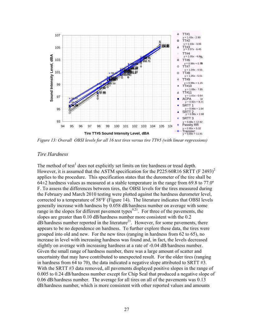
94.78

99.21

104.80

100.59100.44

101.27

102.71

97.88

98.98

101.33

94.78

99.21

104.80

100.59100.44

101.27

102.71

97.88

98.98

101.33

94.78

99.21

104.80

100.59100.44

101.27

102.71

97.88

98.98

101.33

94.78

99.21

104.80

100.59100.44101.27

102.71

97.88

98.98

101.33

94.78

99.21

104.80

100.59100.44101.27

102.71

97.88

98.98

101.33

94.78

99.21

104.80

100.59100.44101.27

102.71

97.88

98.98

101.33 y = 1.07x - 6.45

R2 = 0.99

y = 1.01x - 0.64

R2 = 0.96

y = 1.04x - 4.55

R2 = 1.00

93

95

97

99

101

103

105

107

94 95 96 97 98 99 100 101 102 103 104 105 106

Tire TT#5 Sound Intensity Level, dBA

So

un

d In

ten

sity

Le

vel

, dB

A

TT#1

TT#2

TT#3

TT#4

TT#6

TT#7

TT#8

TT#9

TT#10

TT#11

ACPA

SRTT 1

SRTT 2

SRTT 3

Passby RR

Transtec

y = 1.03x - 2.90

y = 0.95x + 5.32

y = 1.03x - 3.05

y = 1.07x - 6.45

y = 1.05x - 4.84

y = 0.99x + 0.76

y = 1.04x - 4.55

y = 1.05x - 5.01

y = 0.99x + 1.15

y = 1.08x - 7.85

y = 1.01x - 0.64

y = 0.92x + 8.21

y = 0.99x + 1.64

y = 0.98x + 2.68

y = 0.88x + 12.92

y = 0.89x + 11.81

Figure 13: Overall OBSI levels for all 16 test tires versus tire TT#5 (with linear regressions)

Tire Hardness The method of test1 does not explicitly set limits on tire hardness or tread depth. However, it is assumed that the ASTM specification for the P225/60R16 SRTT (F 2493)2 applies to the procedure. This specification states that the durometer of the tire shall be 64±2 hardness values as measured at a stable temperature in the range from 69.8 to 77.0º F. To assess the differences between tires, the OBSI levels for the tires measured during the February and March 2010 testing were plotted against the hardness durometer level, corrected to a temperature of 58°F (Figure 14). The literature indicates that OBSI levels generally increase with hardness by 0.058 dB/hardness number on average with some range in the slopes for different pavement types9,21. For three of the pavements, the slopes are greater than 0.10 dB/hardness number more consistent with the 0.2 dB/hardness number reported in the literature21. However, for some pavements, there appears to be no dependence on hardness. To further explore these data, the tires were grouped into old and new. For the new tires (ranging in hardness from 62 to 65), no increase in level with increasing hardness was found and, in fact, the levels decreased slightly on average with increasing hardness at a rate of -0.04 dB/hardness number. Given the small range of hardness number, there was a large amount of scatter and uncertainty that may have contributed to unexpected result. For the older tires (ranging in hardness from 64 to 70), the data indicated a negative slope attributed to SRTT #3. With the SRTT #3 data removed, all pavements displayed positive slopes in the range of 0.005 to 0.24 dB/hardness number except for Chip Seal that produced a negative slope of 0.06 dB/hardness number. The average for all tires on all of the pavements was 0.13 dB/hardness number, which is more consistent with other reported values and amounts

27

y = -0.04x + 107.73

R2 = 0.09

y = 0.05x + 99.79

R2 = 0.08

y = 0.07x + 96.65

R2 = 0.25

y = 0.02x + 99.48

R2 = 0.02

y = 0.02x + 99.97

R2 = 0.01

y = 0.02x + 99.61

R2 = 0.03

y = 0.06x + 96.00

R2 = 0.11

y = 0.12x + 91.34

R2 = 0.48

y = 0.12x + 90.11

R2 = 0.25

y = 0.11x + 88.04

R2 = 0.25

92

94

96

98

100

102

104

106

108

61 62 63 64 65 66 67 68 69 70 71

Durometer Hardness Number

So

un

d In

ten

sit

y L

evel

, dB

A

Ultra Smooth

Slurry Seal

Chip Seal

Porous

Sand Blast

Broom PCC

Long. Tine PCC

3/8" DGAC

OGAC

3/4" DGAC

Figure 14: Overall OBSI levels for all test tires versus tire durometer hardness number

to an overall average increase of about 0.3 dB for tires with hardness numbers increasing from 68 to 70. At the time of the December tests, the hardness of all eleven new tires had increased as shown by the January 2011 results in Table 5. The largest increases were for the in-service tires for which increases ranged from 3.9 to 5.0 durometer hardness. The hardness for these four tires then fell outside of the 66 hardness number limit specified in the ASTM specification while all of the other tires remained within the specification. As a group, the increase in OBSI levels for the in-service tires was greater than the other tires averaging 0.7 dB versus 0.4 dB. Given the average hardness number increase of 4.6 for these four tires, the average rate of increase in OBSI level with hardness is 0.15 dB/hardness number. However, the increase in level for the right side in-service tires was much lower than the left side (an average of 0.2 dB for the right versus 1.2 dB for left). Considering only right side tires, there was no trend of OBSI level increase and durometer hardness number increase. From this research, a consistent correlation between tire hardness and tire/pavement level could not be identified. As a group, the new tires tested in February and March had lower durometer hardness numbers and produced lower OBSI levels than the older tires. However, it is not clear if restricting test tires at or below a specific hardness number would reduce variation. Hardness for all four in-service tires increased significantly (4.8), however, the trends between hardness and OBSI varied between right side and left side tires. It could be concluded that for newer SRTT tires, the rubber durometer hardness number may not be an important parameter, but as a tire ages, hardness may become an important variable. Therefore, setting some limit on hardness (and other tire

28

aging parameters) would limit measurement uncertainty to the values obtained in this research. Tire Loading The AASHTO Test Method procedure (TP-76) does not limit tire loading, but the earlier research1 recommended that loading be limited to 850 ± 100 lb. Tire loading effects on OBSI results were evaluated incrementally using the TT#5 test tire during the March test series (Table 2). Weight was added to the trunk of the vehicle to result in increased loading on the right rear wheel (where the OBSI instrumentation is attached) by 100, 150, and 200 lbs above the baseline wheel load of 770 lbs. Temperatures during these measurements ranged from 64 to 75°F. The results of these measurements, shown in Figure 15, indicate a small, but consistent increase of OBSI level with increased wheel

load for all pavement types that averages 0.16 dB/100 lb. Using temperature corrected data, the average increase for the TT#5 data was 0.23 dB/100 lb. These results are similar to those of the earlier research, which found an increase of about 0.2 dB/100 lbs for added trunk weight (equivalent to about 60 lbs added wheel load) for the SRTT tire (without temperature corrections). The levels for each load case and pavement were also normalized to the baseline loading of 771 using the average loading rate without temperature corrections. Without the loading normalization, the average loading increase from 771 to 971 lbs resulted in a 0.40 dB increase in OBSI level. With the normalization, the average difference was reduced to 0.04 dB. This indicates that correcting for loading should reduce the variation created by loading differences.

y = 0.00x + 103.50

R2 = 0.67

y = 0.00x + 100.10

R2 = 0.91

y = 0.00x + 100.27

R2 = 0.25

y = 0.00x + 100.07

R2 = 0.07

y = 0.00x + 98.97

R2 = 0.18

y = 0.00x + 98.71

R2 = 0.87

y = 0.00x + 97.60

R2 = 0.28

y = 0.00x + 97.94

R2 = 0.11

y = 0.00x + 97.03

R2 = 0.06

y = 0.00x + 91.27

R2 = 0.80

92

94

96

98

100

102

104

106

750 800 850 900 950 1000

Test Tire Loading, lbs

So

un

d In

ten

sity

Lev

el, d

BA

Ultra Smooth

Slurry Seal

Chip Seal

Porous

Sand Blast

Broom PCC

Long. Tine PCC

3/8" DGAC

OGAC

3/4" DGAC

Figure 15: Overall OBSI levels for tire TT#5 with varied tire loading

29

Increased loading on tire TT#9 mounted on the Malibu rental car in February and on the TGI tire mounted on the IR Malibu in March resulted in an average increase in OBSI level of 0.09 dB/100 lbs and 0.18 dB/100 lbs, respectively. Since rates are defined by only two loadings, there is more uncertainty in these data than those defined by the incremental data shown in Figure 15. However, on average, the rates defined with the TT#9 and TGI tires are very similar to those for TT#5. In the comparative tests, loading ranged from about 700 lbs to 930 lbs for individual test teams. In some cases, the more lightly loaded cars produced lower OBSI levels than heavier cars and in some cases not. Added weight and tire loading to baseline conditions generally increased noise level for Yuma tests, but the results displayed considerable scatter. As a group, the results suggest that this variable may not be independent of other vehicle and/or tire parameters. Further details of the comparative testing are provided in Appendix F. Other Tire Parameters Several other parameters were evaluated in the follow-up testing in December. The performance of the primary and secondary test tires was examined for all of the test events in test track measurements. Figure 16 presents the OBSI levels measured for each pavement averaged over the tests performed in each of the four measurement months.

93

94

95

96

97

98

99

100

101

102

103

104

105

106

107

Feb Avg March Avg Sept Avg Dec Avg

So

un

d In

ten

sity

Lev

el, d

BA

Ultra Smooth

Slurry Seal

Chip Seal

Porous

Sand Blast

Broom PCC

Long. Tine PCC

3/8" DGAC

OGAC

3/4" DGAC

Figure 16: Average temperature adjusted OBSI levels for TT#5 for each month of testing

These values are adjusted for temperature of 68ºF. Parameters not accounted for include pavement aging, change in tire hardness/aging, and pavement temperature. For eight of the ten pavements, the OBSI levels are within a 1 dB for all of the test track

30

measurements. For Chip Seal, an increase of 1.7 dB was measured between the September and December testing. In December, some raveling of the pavement had occurred that may have contributed to the higher level. The December levels were less than 1 dB higher than the February levels. For the ⅜ inch DGAC, variation of 1½ dB occurred with the highest level occurring in September. This pavement had a temperature gradient of 0.013 dB/ºF (see Figure 5) which is well below average so that the correction contributed to the higher variation indicated in Figure 16. On average across all pavements, the increase determined between February and December was 0.2 dB with a standard deviation of 0.25 dB. Even with fewer data points, the trends for the secondary test tire, TT#9, were similar to those for TT#5. In addition to the parameters discussed in the previous section, several other tire parameters including tire aging and wheel width were identified as possibly influencing OBSI results. To assess these tire parameters, the 11 new tires used in this project were subject to a variety of conditions between the February and December tests as follows:

TT#7 was used as a reference test tire and was stored under dark, no light conditions for the entire period between tests

TT#5 and TT#9 were used as the primary and secondary test tires, respectively and used throughout the on-road and laboratory testing with the majority of the test mileage accumulated on TT#5

TT#1, TT#2, TT#6, and TT#11 remained on the IR Malibu for the entire period between February and December accumulating about 11,000 miles of normal usage

TT#3 and TT#4 were subjected to heat cycles of up to 139º on a daily basis throughout the summer months to increase tire hardness and were not used in any other testing

TT#8 and TT#10 were stored under the same conditions as TT#7 but were remounted on 6.5 inch wide wheels (7 inch wide wheels used for all other tires).

The average increase in OBSI level of each tire between the February and December testing corrected to a temperature of 70ºF is shown in Figure 17. In-Service Mileage Accumulation. The tires with accumulated mileage clearly displayed the effect of usage in terms of their physical parameters. As discussed in a previous section, these tires increased hardness numbers by 4 to 5 compared to the more typical increases of about 1 to 2. The tread depth was also reduced more on these tires than for the other tires. For the front, drive axle tires, the worn depth was 5.2 mm and 5.6 mm for the driver side tire (LF) and the passenger side tire (RF), respectively compared to the nominal new depth of 8 mm. The rear tires (RR and LR) were considerably less affected, both at about 7.2 mm, likely due to the lower loading on these tires. The OBSI results shown in Figure 17 are quite mixed. The driver side tires both displayed significant increases in level compared to all other tires. However, the increase for the passenger side tires was minimal and similar to the other tires which were also used on this side of the vehicle. The driver side tires were always tested and mounted on that

31

0.30.2

1.1

1.5

0.1

0.50.6

0.4 0.4

0.6

0.4

0.0

0.5

1.0

1.5

2.0

2.5

3.0

Mile

age

RR - TT#1

Mile

age

RF - TT#2

Mile

age

LF -

TT#6

Mile

age

LR -

TT# 11

Accele

rate

d Agin

g - T

T#3

Accele

rate

d Agin

g - T

T#4

Whe

el W

idth

- TT#8

Whe

el W

idth

- TT#1

0

Test T

ire A

- TT#5

Test T

ire B

- TT#9

Refer

ence

(Low

Use

) - T

T#7

Incr

ease

in O

BS

I Lev

el, d

B

Figure 17: Overall OBSI level increase from initial(February) to final (December) testing

side of the car. Because no driver side control tire was used, the results for this side of the vehicle could not be validated. Comparison of the side-to-side data, revealed no trend to suggest that the decreased tread depth for both front tires produces measurable differences in the OBSI levels. Averaging the increase for all four tires produces an increase of 0.8 dB that may be related to the increased hardness of these tires, however, with the side-to-side differences, it is difficult validate such a conclusion. The result of this trial determined that an in-service life of about 10 months and 11,000 miles produces changes in hardness and tread depth that could affect the results if the tire is used in a test. Wheel Width. As indicated by Figure 17, change in OBSI level produced by the two tires (TT#8 and TT#10) mounted on 6.5 inches wheels was virtually identical to the test and reference tires. In terms of OBSI level, the tires on the narrower wheel produced average levels within 0.2 dB of the of the other right side tires measured in December. Accelerated Aging. The tires exposed to heat cycles throughout the course of summer months also produced some mixed results. The tire hardness for tires TT#3 and TT#4 increased by 2 and 1 hardness numbers, respectively. Figure 17 shows that the increase in level was actually greater for TT#4, however, both are in the range of the other right side tires. Generally, this heat exposure produced a marginal increase in hardness. Tread Depth. At the beginning of the project, the eleven new test tires all had tread depths of nominally 8 mm (equal to or greater than the ASTM specification of 7.97 mm). After the completion of the December testing, tread depths were measured and the results are shown in Table 8. For low usage tires, TT#3, 4, 7, 8, and 10, the tread depths

32

Table 8: Test tire tread depth measured in January 2011

Tire TT#

1 TT#

2 TT#

3 TT#

4 TT#

5 TT#

6 TT#

7 TT#

8 TT#

9 TT#10

TT#11

Depth, mm

7.2 5.2 8.1 8.0 7.8 5.6 8.0 8.1 7.8 7.9 7.2

remained at or above the ASTM specified value of 8 mm except for TT#10. The tread depths of the four in-service tires (TT#1, 2, 6, and 11) were below this specification with the front tires displaying considerable more tread loss while the loss for the lightly loaded rear tires was only about 0.8 mm after 11,000 miles of use. For TT#5, the estimated mileage of 1,300 produced a reduction in tread depth of about 0.2 mm. For TT#9, the estimated mileage of 1,000 miles also produced a reduction in tread depth of about 0.2 mm. For the other tires (other than the in-service tires), there was essentially no reduction in tread depth after an accumulated mileage of less than 75 miles. Limits on Test Tires. February testing showed that older tires that had been in service produced 0.5 dB higher levels on average than newer tires. This suggests that some limit on tires usage and age should be considered. This research did not provide a clear quantitative definition and criterion for defining when a tire is too “old”. Generally as usage increased, tread depth became less and tires became harder. The older tires used in this study were 1 to 3 years older than the eleven new tires. The older tires displayed no trend in OBSI level with build date possibly because of the sample size used. It was noted previously that relative performance of the new tires was not consistent suggesting that each tire reacts slightly differently to each pavement. As these individual tires age, such inconsistencies are expected to continue as demonstrated for the older tires tested in February and March. Also, the effect of aging variables such as hardness, tread depth, time since construction, and mileage, may not be consistent from tire-to-tire. This would make developing a single or multiple criteria for identifying when a tire should not be used quite problematic. To avoid increased (or increasing) uncertainty with aging tires, a combination of factors could be considered based on hardness, tread depth, mileage, and years since construction or years in service. Exceeding any one criterion may not be sufficient to retire the tire, but exceeding several criteria would be sufficient. Hardness versus noise performance results for the older tires (between 68 and 70 hardness), showed an increase in OBSI level with increasing hardness. This would suggest 68 as a recommended maximum hardness number. Regarding tread depth, when the depth reached 7.2 mm, at least some tires displayed higher noise levels. For mileage, some tires displayed higher levels after 11,000 miles, but others up to 1,300 miles did not. Therefore, limiting mileage to some value between 1,300 and 11,000 these may be appropriate. SRTT#1 and SRTT#2 have both been in service since 2006 (i.e. about 4 years at the time of the February tests). Under this approach, a tire that has more than two of the attributes of 1) being in-service for more than 4 years, 2) having more than 11,000 miles, 3) having hardness number of greater 68, or 4) tread depth less than 7.2 mm would be retired.

33

Test Parameters Location The positioning of the test vehicle during a test run, including the location at which the five-second data acquisition begins and the position of the test tire in the wheel path, can be a source of variation from run-to-run of a single test team or from one measurement team to another. Because the magnitude of the effect of either of these variables depends on the pavement section being tested, it cannot be quantified without a prior knowledge of the site. However, some insight into these issues can be obtained by analyzing OBSI data that has been collected on other sites displaying variability and by evaluating some hypothetical cases. Data Acquisition Start Location. The pavements tested at the H·K Proving Ground were constructed to be as uniform as possible. As a result, the effect of variation in start location was minimal. In order to consider the worse case, OBSI data collected for a Caltrans project on I-5 in Sacramento were considered7. In this project, 0.7 miles of PCC freeway were overlaid with new open graded rubber asphalt concrete (RAC[O]). Initially, the this segment was tested in three sections of 440 ft corresponding to 5 seconds of transit time at 60 mph. The difference in level between sections was measured to be 2½ dB which was greater than that measured for other pavements of the same construction project. Differences in the sounds produced inside the test vehicle as it passed over this pavement were clearly audible. Recordings of the sound pressure signals from OBSI probe were recorded for the entire length of the project and were later re-analyzed using a “fast” averaging time (1/8 second exponential average) to obtain sound intensity level as a function of time (and corresponding distance). The result of this analysis is shown in Figure 18 for a time period of 20 seconds. With this shorter analysis time, variation in OBSI level is shown to be about 7 dB excluding the slap identified in Figure 18. More typically, this type of variation is about 1 to 2 dB with maximum variations up to 4 dB. The fast averaging time data of Figure 18 were further analyzed to produce a moving five-second energy average to simulate different start times for data acquisition. The data were summed on an energy basis into 5 second time blocks and then time was incremented by 0.1 second and the 5-second summation repeated for the length of the data from 0.6 seconds to 20 seconds (also shown in Figure 18). To evaluate the effect of start location, different points along the moving average curve were examined. As an example, if the variation in start time was 0.5 seconds (44 ft at 60 mph), the difference in OBSI level between starting at 2.0 seconds and 2.5 seconds is 0.4 dB. The largest variation occurs at near 12 seconds where audible slap is or is not included in the average and the difference in 5-second average level is 0.7 dB for a 0.5 second variation in start time. This maximum run-to-run variation that could be produced by the start variation corresponds to a standard deviation of 0.5 dB for two passes and 0.4 dB for three passes. This is within the limits required in both the NCHRP proposed procedure and the AASHTO 10-76 procedure. If a second team made measurements along this project, as along as the start position was specified to ±22 ft and the slap at the end were avoided,

34

96

97

98

99

100

101

102

103

104

105

106

107

108

0 1 2 3 4 5 6 7 8 9 10 11 12 13 14 15 16 17 18 19 20

Time, seconds

So

un

d In

ten

sity

Lev

el, d

BA

OBSI Fast Response Averaging

Moving 5 Second AveragePCC RAC(O)

Audible Slap

Figure 18: Example of OBSI level variation with location in a test pavement

the maximum difference between the two teams due to variation in the start location would be 0.5 dB or less. The pavement segment included in the data shown in Figure 18 was measured in three sections over the length of the project. For each section, multiple passes were made and averaged together. The data acquisition for each start point was initiated visually based on roadside landmarks. The variation between the averages for each section was greater than 2 dB as would be expected considering sections from 2.5 to 7.5 seconds and 9.5 to 14.5 seconds. The variations between passes over these sections were typically less than 0.4 dB with one section having a maximum range of 1.0 dB with a standard deviation of 0.5 dB all within the current procedure requirements. Start location was also evaluated analytically for different theoretical OBSI profiles including an instantaneous increase mid-way through the 5-second section, alternating levels every 0.4 seconds, steadily increasing level throughout the section, and instantaneous increases and decreases in the last 0.4 seconds of the section. The variations in 5-second average OBSI levels were found to be a function of the level difference between the different portions of the pavement and of the noise “profile”. For all cases, as the difference in level within section increases, the variation increases. For the “dip” at the end case, the variation in level is the greatest of the five cases as shown in Figure 19. If the starting point for data can be maintained to a variation of about 0.2 seconds, or 17.6 ft, the variation is reduced by more than half as shown in Figure 20. With this amount of control of start location, the variation 5-second OBSI average level is 0.5 dB or less for differences in pavement of 6 dB for all noise profile scenarios. It is expected that differences of 6 dB would be clearly audible inside the test vehicle.

35

-3.0

-2.5

-2.0

-1.5

-1.0

-0.5

0.0

0.5

1.0

1.5

2.0

0 1 2 3 4 5 6 7 8 9 10

Sound Intensity Level Change, dB

So

un

d In

ten

sity

Lev

el D

iffe

ren

ce, d

B

Mid Step0.4s AlternatingEnd StepRampEnd Dip

Figure 19: Difference in OBSI level created by a ½ second change in start position (44 ft) for 5 second average for different profiles of OBSI versus position as a function of the difference in OBSI level in the profile

-3.0

-2.5

-2.0

-1.5

-1.0

-0.5

0.0

0.5

1.0

1.5

2.0

0 1 2 3 4 5 6 7 8 9 10

Sound Intensity Level Change, dB

So

un

d I

nte

nsi

ty L

evel

Dif

fere

nce

, d

B

Mid Step0.4s AlternatingEnd StepRampEnd Dip

Figure 20: Difference in OBSI level created by a 0.2 second change in start position (17.6 ft) for 5 second average for different profiles of OBSI versus position as a function of the difference in OBSI level in the profile

36

As a field data point, in the North Carolina Comparative Testing16 it was found that varying the position of the start of data acquisition by the length of the test cars produced variations of 0.3 dB or less which was within the variation of the repeat baselines. In regard to the OBSI procedure, for a single team testing a section of pavement, the current requirements on run-to-run variation are sufficient. However, by requiring that the start of data acquisition occur within 20 ft or 0.23 seconds relative an identified start point, the potential for variation would be further reduced. Wheel Path. OBSI levels for tires within and outside the wheel path vary with the pavement. Differences between OBSI level for the wheel path and lane center represent the maximum differences that may be encountered for those pavements22,23. For ten pavements (including both HMA and PCC), the average difference between the lane center and wheel path was 1.1 dB with a standard deviation of 0.74 dB. The range was from 0 dB for a 6 month old HMA pavement to 2.4 dB for 5 year old grooved, visually damaged PCC. For run-to-run variation, if the test tire was wandering during the pass over the pavement, wheel path variation would be identified by applying the existing criteria in the OBSI test procedures. For reproducibility, it is important that the same position of the test tire relative to the wheel path be maintained in all testing. The wheel path appears to be about 2½ to 3 ft wide based on photos accompanying the wheel path/lane center data. It should be possible to maintain the test tire close enough in the wheel path to avoid the differences measured between the lane center and wheel path. Slight variation within the wheel path may be possible, however this is difficult to document. In the North Carolina Rodeo16, two teams tested with their vehicle centered and not quite centered in the lane of travel for 12 pavements. The average differences were 0.3 and 0.2 dB which was about the same as that for repeated baseline tests. Based on these findings, tighter control of the test tire position within the wheel path does not appear to be necessary. However, tire position with respect to wheel path should be reported as part of the test results. Background Noise For on-road OBSI measurements, the primary background noise concern is the influence of other on-road vehicles near the test tire during data acquisition. The effects of varying levels of background noise were assessed in detail in the tire noise dynamometer testing. With increasing levels of background noise, the measured sound intensity levels decrease because the net energy coming from the test tire is cancelled by the net energy from the background source flowing toward the tire. In this situation, the PI index increases in level because the sound pressure (the sum of both the tire noise and the background noise) increases and the net sound intensity decreases. Similarly, the effect of background noise on the OBSI level is greatest when the source is directly opposite the test tire on a line perpendicular to the axis of rotation, such as when the tire or other noise source of another vehicle is directly opposite the test tire. As the tire/noise source of the adjacent vehicle moves forward or rearward of the test tire, the effect on the OBSI level diminishes rapidly due to the directivity of the sound intensity probe. The tire noise dynamometer tests showed that the sound pressure level of the background noise directly opposite of the test tire must be 10 dB or more below the sound pressure level of the

37

tire/pavement noise source to achieve an error of less than 0.5 dB. For application to 5-second OBSI measurements, both the noise level produced by other vehicles (or noise sources) and the duration of time in which the tire/noise source is directly opposite the test tire are needed to determine the effect of background noise. As neither of these variables may be known, run-to-run variation and sound intensity direction are proposed to identify background contamination. As for all reported data, the run-to-run variation is required to be 1 dB or less. Use of this requirement should be sufficient to identify any contamination that would potentially influence the results. However, if possibility of contamination occurs during any one run of a data set, that run should be repeated in order to obtain at least two runs meeting this criterion. In more severe cases of contamination, the direction of the sound intensity vector would be negative. Also, the effect of background noise will produce increases in the PI index. Based on the initial tire noise dynamometer testing, a tentative criterion would be to limit the PI index to about 1 dB greater than the PI index measured on the dynamometer in the absence of background noise. This criterion was explored further and the frequency dependent criteria are shown in Figure 21 along with the baseline OBSI levels measured

0

1

2

3

4

5

6

400 500 630 800 1000 1250 1600 2000 2500 3150 4000 5000

1/3 Octave Band Center Frequency, Hz

PI

Ind

ex, d

B

Smooth Surface Leading EdgeSmooth Surface Trailing EdgeCoarse Surface Leading EdgeCoarse Surface Trailing EdgePI Index Criteria

Figure 21: PI index criteria compared to baseline PI index levels on the smooth and coarse dynamometer surfaces

on the dynamometer with the smooth and coarse surfaces. By applying these criteria to the background noise data from the dynamometer, resulting errors range from about 0.8 to 1.5 dB in individual one-third octave bands which is within the limit allowed for individual bands in the current procedure. For overall A-weighted level, the error should be no greater than about 1 dB. To test their feasibility, these criteria were applied to 18

38

data sets containing 20 to 50 individual runs in each set for which background noise was known not to be an issue. For most of these data runs, the criteria were met for both the leading and trailing edge OBSI levels. In a few cases, the criteria were exceeded in the 400 and 5000 Hz bands. A very few runs exceeded the criteria, however, these runs were obviously outliers compared to the other runs and should be eliminated. These tighter criteria on PI index will allow an acceptable error due to background noise while not rejecting many more runs than would occur based on the current frequency independent criteria. Reflecting Objects The effects of reflections from nearby surfaces were also evaluated in the tire noise dynamometer testing. For these tests, a large plywood “wall” was placed opposite and parallel to the sidewall of the test tire at various distances. These tests determined that maintaining a separation of 14½ inches or greater between the tire sidewall and reflecting object provided an error of less 0.3 dB for either the smooth or coarse surface. Therefore, a separation of 15 inches appears to be an appropriate criterion. Test Speed During the December 2010 test track measurements, the effects of speed variation were examined by testing at 59 and 61 mph for all the test pavements. The measurements were completed within a 2½ hour time period on December 15th using the primary test tire, TT#5. During the testing, the temperature ranged from 56 to 58º F and no temperature compensation was applied to the results summarized in Table 9. On average, the increase in OBSI level due to increasing speed from 59 to 61 mph was 0.42 dB or 0.21 dB/mph consistent with the results of earlier research1. It is also comparable to the speed gradients of 0.22 and 0.25 dB/mph that were measured on the tire noise dynamometer under very controlled conditions. For individual pavements, the effect of speed varies considerably

Table 9: OBSI levels and level differences for test speeds of 59, 60, and 61 mph

OBSI Level (dBA) at Nominal Test Speed (mph)

Difference in OBSI Level (dB) for Indicated Speed Differences (mph) Test Section

59 60 61 60-59 61-60 61-59 Ultra Smooth 95.1 95.3 95.1 0.2 -0.2 0.1 Slurry Seal 99.2 99.7 99.4 0.5 -0.4 0.1 Chip Seal 104.9 106.0 105.5 1.1 -0.4 0.6 Porous 100.6 101.0 101.3 0.4 0.2 0.7 Sand Blast 100.8 101.6 101.7 0.8 0.1 0.9 Burlap PCC 100.4 100.3 100.5 -0.1 0.2 0.1 Long. Tine PCC 102.5 102.9 103.0 0.3 0.1 0.4 3/8" DGAC 98.1 98.1 98.4 0.0 0.4 0.4 OGAC 98.8 98.8 99.1 0.1 0.3 0.3 3/4" DGAC 100.5 100.7 101.0 0.2 0.3 0.5

Average 0.36 0.06 0.42 Standard Deviation 0.35 0.29 0.27

39

from 0.05 to 0.45 dB/mph. There appears to be no consistent trend between pavements to allow any grouping of the pavements. As a result, an adjustment for all pavements could be considered based on average gradient of 0.21 dB/mph with the knowledge that this would introduce an uncertainty of ±0.27 dB within the speed range of 59 to 60 mph. The results shown in Table 9 indicate that the average difference in OBSI levels due to a ±1 mph change in speed are smaller than the 0.5 dB difference in sets for the same tire tested within a 4º F temperature range over a several day period (see section “On-Road Testing Reproducibility”). Therefore, maintaining the existing test speed requirement of 60 ±1 mph appears to be adequate. The standard deviations shown in Table 9 for ±1 mph speed change and variation between pavements suggest that adjustments within this range would not improve the certainty of the measurements. Adjustments to compensate for a speed change beyond ±1 mph will likely degrade measurement certainty even further given the range of speed gradients displayed for these pavements and for the twelve pavements measured in earlier research1. Horizontal Curves The effect of side forces acting on tires operating in a curved path have been documented in the literature. Sandberg estimated that side forces create increases in tire noise level by 1 to 7 dB depending on the circumstance24. Also, increases of 2 to 10 dB have been measured for ribbed truck tires operating at low speed on a 110 ft radius circular path25. During comparative OBSI testing at the General Motors Proving Ground in Yuma, AZ, data on a 400 ft radius vehicle turn-around loop was collected for comparison to the same pavement on the straightaway portion of the “smooth” asphalt test track26. The loop was banked and had a recommended speed of 35 mph; testing was done at 30 mph. The curved/banked section produced levels that were on average 3.5 dB higher than the straightaway with the largest differences occurring in the one-third octave bands above 800 Hz. This extreme case of both curvature and banking demonstrated the potential for either of these parameters to produce higher tire/pavement noise levels in a situation where lateral force was quite apparent to the vehicle occupants. To examine the effect of curvature under more moderate conditions, two locations on State Route 58 near the Hyundai-Kia Proving Ground were measured in conjunction with the test track measurements and are shown in Figure 22. One site was on the longitudinally tined PCC mainline and the other site was on HMA off-ramp and both were tested at 60 mph. For these cases, OBSI level increases of 0.6 dB and 0.4 dB were measured on the curved portion for the PCC and HMA sites, respectively, as shown in Figure 23. For the PCC site, the curvature was less than the HMA site, however some lateral force was experienced in the curve. The pavement was also found to be somewhat variable in OBSI level (on the order of 1 dB) and it could not be concluded that the difference is entirely due to curvature. It is suspected that the increases below 1000 Hz were more due to pavement variation than curvature. For the off-ramp site, the curvature and lateral force were greater and eight pairs of data were taken with standard deviations of 0.1 to 0.2 dB from run-to-run compared to 0.4 to 0.7 dB for the PCC site. At the ramp site, the increases in level occurred in the one-third octave bands above 800 Hz and were

40

Figure 22: Sites for evaluation of horizontal curves with PCC site (left) and AC site (right)

Straight Section

Curved Section

Straight Section

Curved Section

Straight Section

Curved Section

Straight Section

Curved Section

75

80

85

90

95

100

105

400 500 630 800 1000 1250 1600 2000 2500 3150 4000 5000

1/3 Octave Band Center Frequency, Hz

So

un

d In

ten

sit

y L

evel

, dB

A

LT Straight (107.2 dBA)

LT Curved (107.8 dBA)

AC Straight (101.3 dBA)

AC Curved (101.7 dBA)

Figure 23: One-third octave band spectra comparison of straight and curved roadway sections

more consistent with the earlier results. The results of these curvature tests were not conclusive in terms of developing strict criteria to apply to the OBSI procedure. Generally, the difference in OBSI level was on the order of test-to-test reproducibility and expected variation from site-to-site for nominally the same pavement. Further, the increase in OBSI level is likely due to increases in lateral forces acting on the tire. These forces are function of both horizontal

41

curvature and pavement banking making a single criterion problematic. The current requirement in the procedure that the test section be “nominally straight” appears to be sufficient given the small differences measurements where lateral forces were clearly present. A possible modification to the requirement would be to add the phrase “so as not to produce any perceivable lateral force” as determined subjectively. Vertical Curves The effect of torque applied to the test tire by a drive axle that occurs due to over-coming road-load losses and ascending a grade was evaluated during the tire noise dynamometer testing (see details in Appendix D). In this testing, the drive axle of the front-wheel drive test vehicle was placed on the tire noise dynamometer and OBSI levels measured for this position. Testing was then done with the tire freewheeling (engine off, tires driven by the dynamometer), with the engine on supplying torque to the test tires to maintain steady cruise conditions, and with additional torque applied to the tires to overcome a 2% grade. The results indicated a 0.5 dB increase in overall OBSI level between the no-load and road-load case, and 1.1 dB between no-load and incline-load. This finding supports the requirement in the OBSI test procedure that only non-driven axles of the test vehicle should be used. Because the effects of torque would also occur under braking for a non-driven tire, measurement under free-rolling conditions should be added as part of the procedure. Environmental Conditions This section discusses the effects of wind and moisture on the OBSI measurements. The effect of temperature is discussed earlier in this Chapter. Wind One source of background noise and related inaccuracies in OBSI measurements is the noise induced by air flow passing the over and around the OBSI fixture, probes, and test vehicle. The proposed method of test using OBSI1 does not set limits on wind conditions. To gain further understanding of possible wind noise contamination effects in isolation and to determine if and what limits on crosswind conditions are necessary for the OBSI measurement procedure, measurements were conducted in the General Motors Aeroacoustic wind tunnel. The measured wind induced background sound intensity levels (IL) and sound pressure levels (SPL) were compared to a tire/pavement noise source level calculated as an average of five of quieter pavements (labeled ‘AC Pavement’ in Figures 24 and 25, also see Appendix E). As an example, Figure 24 shows the ⅓ octave band SPL and IL levels on two test vehicles at 60 mph and 0 degrees yaw with the dual probe fixture, compared to the AC Pavement OBSI levels. These results are similar for the two vehicles. The background wind noise IL was more than 10 dB below the tire-pavement noise level in all frequency bands, which would result in increases 0.4 dB or less in the individual ⅓ octave band IL levels for AC Pavement.

42

55

60

65

70

75

80

85

90

95

400 500 630 800 1000 1250 1600 2000 2500 3150 4000 5000

1/3 Octave Band Center Frequency, Hz

So

un

d I

nte

nsi

ty L

evel

, dB

AG6, SPL

Impala, SPL

G6, IL

Impala, IL

AC Pavement

Figure 24: Sound intensity and pressure levels for test vehicles at 60 mph and 0º yaw

As shown in Figure 25, overall wind noise levels are lowest at a yaw angle of -6 degrees and highest for +14 degree yaw. For both vehicles, the overall sound intensity levels were more than 10 dB below the AC Pavement levels for all yaw angles, therefore crosswind conditions of up to 14 degrees would be acceptable for testing when considering the overall A-Weighted OBSI level.

70

75

80

85

90

95

100

14 12 10 8 6 4 2 0 -2 -4 -6 -8 -10 -12 -14

Yaw Angle, degrees

So

un

d L

evel

, d

BA

G6, SPL

Impala, SPL

G6, IL

Impala, IL

AC Pavement

Figure 25: Overall sound intensity and pressure levels as a function of yaw angle

43

Wind noise levels relative to AC Pavement OBSI levels were also considered for individual ⅓ octave bands from -14 to +14 degrees yaw in 2 degree increment steps. This analysis indicated that the highest contamination occurred in the 400 and 500 Hz bands. For the bands centered at 400 and 500 Hz, wind induced background noise levels were less than 10 dB above the AC Pavement levels for yaw angles greater than 0. To quantify the error that could be expected to AC Pavement OBSI levels, the wind noise IL measured at each yaw angle for each vehicle was added to the AC Pavement level. The level due to AC Pavement alone was then subtracted from this summed level to determine the resultant error. The results of these calculations are shown in Figure 26 for the overall A-weighted levels and the 400 and 500 Hz band levels for both vehicles.

From Figure 26, the change in the overall OBSI for AC Pavement due to background wind noise was 0.3 dB or less in all yaw angles. In the 500 Hz band, the background noise with the Impala resulted in a 0.5 dB increase in the OBSI level starting at +4 degrees yaw and increased to 1 dB at +14 degrees yaw. In the 400 Hz band, the full range of positive yaw angle could not be evaluated due to ‘drop outs’ in the sound intensity level, however, up to +8 degrees, the measurement error did not exceed 0.5 dB. The errors due to the background wind noise were higher with the G6. In the 500 Hz band, the G6 background noise resulted in a 0.5 dB increase in the OBSI level starting at +4 degrees yaw, 1 dB at +8 degrees yaw, and 2 dB at +14 degrees yaw. For 400 Hz, the G6 resulted in a 0.5 dB increase OBSI level starting at +2 degrees yaw, 1 dB at +6 degrees yaw, and reaching 1.8 dB at +10 and +12 degrees yaw.

0

1

2

3

4

5

14 12 10 8 6 4 2 0 -2 -4 -6 -8 -10 -12 -14

Yaw Angle, degrees

In

crea

se i

n S

ou

nd

In

ten

sity

Lev

el,

dB

G6, Overall

G6, 500 Hz

G6, 400 Hz

Impala, Overall

Impala, 500 Hz

Impala, 400 Hz

Figure 26: Increase in sound intensity levels above tire noise alone created by wind background noise effects for overall, 400, and 500 Hz bands

In the proposed method of test, run-to-run variability of 1 dB for the overall a-weighed OBSI level and 2 dB for the individual one-third octave band are set and extreme cases were at or below this limit for all conditions. Based on Figure 26, a conservative limit on crosswind condition could be set at +8 degrees yaw, or 8 mph, for wind in the direction

44

from the probe to the test vehicle considering the possible accumulation of other sources of error. Based on an analysis of the PI index with respect to the influences of wind induced background noise on OBSI measurement, it appears that tighter limits on the PI index may account for crosswind conditions in which the wind induced background noise is found to affect OBSI measurement levels. The results of the wind tunnel testing indicate that limits should be addressed on an individual 1/3-octave band case with particular attention paid to the 400, 500, and 5,000 Hz bands. Recommendations limiting the PI index which take into account the results described here as well as the results from other testing throughout the study, are discussed later in this Chapter. Pavement Dampness In the literature24, persisting effect of damp porous pavement is documented up to 18 hours after rainfall even when the pavement appears to be dry. In the ISO 11819-2 standard defining the close proximity method of on-bound tire noise measurement27, it is required to check for moisture in the porous pavement if rain has occurred within 2 days of the testing. In the proposed method of test, this requirement is also stated. For OBSI users, this requirement has been of concern as it cannot always be confirmed that a specific segment of roadway did or did not receive rainfall if rain was in the general vicinity. Further, a 2-day restriction will limit the time when a pavement can be tested. For non-porous pavements, the requirement is that the pavement appears dry. Because of these concerns, a more definitive limit on porous pavement moisture was examined. During NCAT comparative testing, measurements were made on two porous pavements 1) when the were visually damp from rain occurring on the previous day, 2) when the pavements appeared visually dry later that day, and 3) two days later when pavements were completely dry (with no rain occurring for the previous three days). As shown in Figure 27 for the first pavement, the overall OBSI levels were essentially the same for the three conditions. In ⅓ octave bands, above 1000 Hz, differences of as much as 2 dB occur, however, the levels are higher when the pavement is completely dry. If moisture were affecting the sound absorptive properties of the pavement, it would be expected to occur in these frequencies and it would be expected that the damp levels would be higher24. For the second pavement shown in Figure 28, the overall levels were higher for the dry condition by 0.7 dB and the effect on higher frequencies is mixed. The change in overall level is determined by the frequency bands from 630 to 1000 Hz, which are generally controlled by pavement surface roughness and not by pavement porosity. The increase in level would be even greater if the difference in temperature were taken into account (61º and 65º F for the damp conditions, and73º F for the dry conditions). Similar behaviors were also noted at a 45 mph test speed. Although the effect of porous pavement dampness on OBSI level was different than expected (increase with dry conditions), the results from the NCAT testing re-enforce the requirement that porous pavement should be given sufficient time to dry after rain before measurements are made. Two days for drying is specified in the current proposed

45

method of test and this appears to be overly cautious. The requirement could be reduced to 24 hours with no appearance of dampness.

65

70

75

80

85

90

95

100

105

400 500 630 800 1000 1250 1600 2000 2500 3150 4000 5000

1/3 Octave Band Center Frequency, Hz

So

un

d I

nte

ns

ity

Le

vel,

dB

A

S4 Damp - 103.1 dBA

S4 Repeat - 103.2 dBA

S4 Dry - 102.9 dBA

Figure 27: ⅓ octave band OBSI level on Section S4 (½” porous OGAC ) for visibly damp and dry conditions

65

70

75

80

85

90

95

100

105

400 500 630 800 1000 1250 1600 2000 2500 3150 4000 5000

1/3 Octave Band Center Frequency, Hz

So

un

d In

ten

sity

Lev

el, d

BA

S8 Damp - 102.1 dBA

S8 Repeat - 102.1 dBA

S8 Dry - 102.8 dBA

Figure 28: ⅓ octave band OBSI level on Section S8 (½” porous PFC ) for visibly damp and dry conditions

46

Instrumentation OBSI Measuring Equipment The measurement of sound intensity is documented in two standards of the American National Standards Institute (ANSI) 28,29. These cover the instruments for measuring sound intensity28 and the methods for determining the sound power of noise sources using sound intensity29. Instruments are also covered in an International Electrotechnical Commission (IEC) Standard30 which is similar to the ANSI standard. The ANSI standard for sound intensity28 identifies a number of requirements on the instrumentation and their performance relative to sound pressure measurements and to the relationship between sound pressure and sound intensity under specific conditions. The stated operating temperature range of the measurements is 5º to 40ºC (41º to 104º F). The standard does not provide an overall uncertainty of the measurement if the standard is followed as it “depends on many factors”31. However, it provides tolerances on sound intensity measurements for plane waves incident on a probe at the reference direction (the line established by the two microphones of the probe for the positive direction). Under plane conditions, the tolerance for a Class 1 system is ±0.7 dB between one-third octave bands centered at 315 to 1250 Hz, ±1.0 dB for 1600 to 2000 Hz, and ±1.4 dB for 2500 to 5000 Hz. The ANSI standard for sound power determination29 states uncertainties with standard deviations of 2.0 dB between 250 and 500 Hz, and 1.5 dB between 1000 and 4000 Hz for sound power determined with sound intensity. These values are higher than those for the sound intensity measurement alone due the added uncertainties in defining the average sound intensity on a surface enclosing the source. There are no temperature or other environmental requirements specified in the standard. The standards provide little information on the uncertainty that could be expected in the OBSI measurement as the sound field is not ideal and does not contain only plane waves. Therefore, measurement uncertainty needs to be examined within the context of the OBSI measurements and it was addressed in the test track measurements and results of OBSI comparative testing. The elements that comprise an OBSI instrumentation system can however be considered individually for their uncertainties. Specifications provided by several suppliers of the sound intensity microphone pairs, microphone amplifiers, and calibrators were reviewed for accuracy and operating range. The operating ranges for microphones are typically between -10º and 50º C with a gradient of -0.002 dB/º C. The frequency response uncertainties are ±1.0 dB over the range of the OBSI measurement. The operating temperature ranges for preamplifiers are greater and the frequency response uncertainties range from ±0.2 dB to ±0.5 dB. This performance is valid up to 95% relative humidity. For sound pressure calibrators, the uncertainty at reference conditions (20º to 23º C temperature and 101.3 kPa atmospheric pressure) is typically ±0.2 dB. For larger ranges in temperature (-10º and 50º C) and pressure (65 kPa to 108 kPa), these uncertainties are increase by 0.1 to 0.2 dB. There is also some sensitivity to relative humidity such that most suppliers state an operating range from 10% to 90% RH with a gradient on the order of 0.001 dB/% RH. In practice, although these uncertainties could produce a significant “stack-up” of

47

uncertainties, effects of these uncertainties generally appear to be minor. Bench-top comparisons between different systems exposed to the same sound field showed differences consistently about 0.2 dB or less using the same calibrator and pressure and temperature settings. The Test Track measurements showed a 0.1 dB difference for the two instrumentation systems of the same model number, but different microphones, preamplifiers, and sound intensity processors. In comparison tests, sound pressure calibrators have produced differences of 0.2 dB, this falls within the range typically specified by calibrator suppliers. To minimize uncertainties due to instrumentation, the proposed revisions test procedure set limits on temperature from 40º to 100ºF. These are at slight variance with those specified in the ANSI standard28 of 5º to 40ºC (41º to 104ºF). The proposed lower limit is considered as a rounded number from the temperature scale conversion. Also, testing in this research was successful accomplished as low as 40ºF. The proposed high temperature was reduced due to testing in earlier research conducted in Mesa, AZ1 and in the September 2010 testing. In both cases, problems with instrument were encountered when the air temperature exceeded about 100ºF. Under these conditions, the microphone and preamplifiers surface temperatures were measured to be about 120ºF and the signals produced by the probes generated input overloads in the sound intensity processor such that further testing was not possible. This could only be remedied by allowing the probes to cool in air-conditioned garage space. OBSI System Calibration As noted earlier, there is no calibration standard for sound intensity measurement. The ANSI standard for sound power determination from sound intensity measurements requires overall sound intensity measurement system verification using a reference sound source26. Under this procedure, the sound power of the source of known level is determined using the methods specified in the standard. This is basically an indirect method of a sound intensity calibration and the tolerances are large (± 1.5 dB for 800 to 5000 Hz) for the purposes of OBSI instrumentation validation. There is one commercially available device that does an actual sound intensity level by inserting a metal screen between two microphones making up a sound intensity probe. In this device, the same sound field is generated in the coupler with a small loudspeaker in which random noise can be input. The metal screen then induces a phase shift between the microphones and simulating a progressive sound wave between the microphones for which a sound intensity-like level is generated. Such a device was used in the bench-top temperature/pressure study (reported in Appendix B). Using a controlled voltage input to the device, stable pseudo sound intensity levels were generated over a period of months. This coupler could in principle be used a basis for a system for comparing sound intensity levels obtained by different OBSI users under bench-top conditions. However, a stable input signal would have to be verified and maintained. Also the “calibration” would only be relative among users and not absolute. Further, although the coupler appears to be stable itself, there are variations from coupler to coupler. Vehicle/Operator Effects

48

Vehicle and operator effects were assessed during the on-road track testing and throughout the comparative testing events. The results of both the test track and comparative testing are within the limits of the proposed method of test and are similar to the earlier results1, which indicated small bias for similar vehicles. The February test track measurements were conducted by two different test teams each using their own test vehicle, test tire, instrumentation, driver, and instrumentation operator. The two instrumentation systems were similar and had been compared previously in a bench-top calibration and were found to produce overall levels within 0.1 dB of each other and differences for individual one-third octave bands ranging from 0.1 to 0.4 dB for the 400 to 5000 Hz bands. In the test track measurements, an initial comparison was conducted followed by a comparison in which the two teams swapped test tires. For the ten pavements, the maximum average difference between the team/ tire combinations was 0.2 dB as shown in Figure 29, mostly due to tire differences. The

results of this controlled comparison with the same instrumentation (comparable to within 0.1 dB), the same tire loading for two different cars, the same section start point trigger signals, same vintage of test tires, and vehicle speed monitoring should produce less variation than would be expected in other less controlled OBSI comparative testing.

94

95

96

97

98

99

100

101

102

103

104

105

106

107

UltraSmooth

SlurrySeal

Chip Seal Porous SandBlast

BroomPCC

Long.Tine PCC

3/8"DGAC

OGAC 3/4"DGAC

So

un

d In

ten

sity

Le

vel,

dB

A

I&R Malibu Tire TT#9 Rental Malibu Tire TT#5

I&R Malibu Tire TT#5 Rental Malibu Tire TT#9

Figure 29: Overall OBSI levels for the two test teams with and without test tires switched

Once tire and temperature differences were taken into account in the comparative testing, differences due to measurement systems and operational issues between teams were found to be minimal. Differences between test teams were found to be attributable to tire loading, although the results were generally inconsistent and displayed considerable scatter. In the Yuma comparison testing, bench-top testing of different instrumentation was found to be within 0.2 dB. The North Carolina comparative tests could not identify

49

consistent bias between teams using similar instrumentation and data acquisition setups, even with a variety of vehicle makes, models, and loading. The average differences between teams was found to be smaller than the differences between repeat baselines, suggesting that, on average, no significant differences between the procedures used by each team, the three different test vehicles, the instrumentation systems, or the tire loading occurred. Repeatability and Reproducibility The issue of repeatability was assessed under controlled laboratory conditions and for on-road conditions through analysis of consecutive passes made using the same vehicle/tire combination. Reproducibility was assessed through comparison of on-road data, using the same vehicle/tire combination over the course of the study. Controlled Testing Repeatability To identify the repeatability that could be expected under ‘ideal’ conditions, baseline measurements were repeated on the smooth and rough surfaces on the road wheel simulator. For these measurements, the tire was driven by the dyno at a constant test speed of 60.5 mph. Per the road wheel simulator protocol, measurements were made after approximately 5 minutes to allow the tire to reach a constant operating temperature. Measurements were made in three blocks with the dyno shutdown and restarted between the blocks. Within each block nine data samples were acquired in groups of three with each sample being a five second linear average as specified in the proposed method of test1. The overall A-weighted levels for these measurements are shown in Figure 30 for TT#5 on the smooth surface.

99

99.5

100

100.5

101

101.5

102

1 2 3 4 5 6 7 8 9 1 2 3 4 5 6 7 8 9 1 2 3 4 5 6 7 8 9

Sample Number

Ove

rall

So

un

d I

nte

nsi

ty L

evel

, d

BA

Baseline Period #1 Baseline Period #2 Baseline Period #3

Figure 30: Overall OBSI levels for repeat runs over three baseline times

50

For the smooth road surface, the variation in levels for individual data points for TT#5 was found to be small with an overall range of less than 0.3 dB and a standard deviation of 0.07 dB. For TT#9 on the smooth surface, a range of 0.2 dB occurred with a standard deviation of 0.07 dB. For the individual one-third octave band levels, the average range was 0.6 dB with an average standard deviation of 0.17 dB for TT#5 and the average range was 0.5 dB with an average standard deviation of 0.13 dB for TT#9. A similar series of baseline measurements was conducted on the coarse road surface at the left rear wheel position using the passby SRTT. For these measurements, the range in baseline levels was 0.3 dB with a standard deviation of 0.1 dB. Once stable operating parameters were achieved, the typical range in overall OBSI level was about 0.3 dB with a standard deviation less than 0.1 dB for both test surfaces. Limited variation in OBSI level occurred because test speed, environmental conditions, and wheel path were highly controlled and stop/start timing was not an issue. It would not be reasonable to expect that such low variation could be maintained for on-road conditions. On-road Testing Repeatability As part of the earlier research1, ten or more consecutive passes were measured and compared to assess on-road run-to-run repeatability. Testing occurred over a period of 50 minutes and an air temperature range of 2º F. The total range in overall A-weighted OBSI levels for the SRTT tire on both the AC and PCC pavements was 0.8 dB, with standard deviations of 0.3. The run-to-run variations of the individual passes were examined in this research in the February test track measurements and were found to be generally small. First, the range of the overall level from run-to-run for each tire and each pavement was identified resulting in 180 three run data sets. For each pavement, the average, maximum, and minimum of the ranges were determined and are presented in Table 10. These data indicate an average run-to-run variation of 0.1 to 0.3 dB and a maximum range for all pavements and tires of 0.9 dB (similar to the maximum range reported in the earlier research1. The maximum standard deviation for any surface and tire combination was 0.5

Table 10: Run-to-run level variation for February testing

Pavement Average

Range, dB Maximum Range, dB

Minimum Range, dB

Ultra Smooth 0.3 0.9 0.1 Slurry Seal 0.2 0.5 0.0 Chip Seal 0.3 0.6 0.1 Porous 0.1 0.3 0.0 Sand Blast 0.2 0.4 0.0 Burlap PCC 0.2 0.4 0.1 Long. Tine PCC 0.3 0.8 0.0 3/8" DGAC 0.1 0.3 0.1 OGAC 0.1 0.3 0.0

51

with an average of 0.3 and standard deviation of 0.1. The results for the range in run-to-run variation indicate that a 1 dB requirement is achievable and that a run-to-run variation of about 0.5 dB should be achievable. Results for the standard deviation of run-to-run levels support a requirement for a maximum limit of 0.6 with more typical standard deviations being about 0.3. On-road Testing Reproducibility To assess reproducibility, the variations between three-run data sets measured using TT#5 over three days of testing in February (temperature range of 55 to 59ºF) as well as over the course of the study were examined for TT#5. The measurements over the course of the study included a temperature range of 40 to 101º F and extended over 10 months in which mileage and aging occurred on both the test tire and the pavement surface. Table 11 shows the maximum range and standard deviation of test-to-test variation for each pavement after temperature corrections were applied for both comparisons. The

February testing resulted in maximum test-to-test ranges of 0.2 to 1.2 dB, with standard deviations of 0.1 to 0.4. For all testing conducted, the maximum range for any pavement was 2.6 dB and maximum standard deviation for any surface was 0.8 dB.

Table 11: Test-to-test OBSI level variation for on-road testing

February (55-59ºF) All Testing (40-101ºF) Pavement Range,

dB Standard

Deviation, dBRange,

dB Standard

Deviation, dBUltra Smooth 0.5 0.2 1.6 0.5 Slurry Seal 0.5 0.2 1.5 0.4 Chip Seal 1.1 0.4 2.6 0.8 Porous 0.9 0.3 1.4 0.3 Sand Blast 0.5 0.2 2.1 0.5 Burlap PCC 0.4 0.2 1.7 0.4 Long. Tine PCC 1.2 0.4 1.2 0.3 3/8" DGAC 0.3 0.1 2.3 0.7 OGAC 0.4 0.2 0.9 0.2 3/4" DGAC 0.2 0.1 1.4 0.3

Average 0.5 0.2 1.7 0.4

These results indicate that about a 1 dB variation in levels may be achievable for measurements over the course of a several days conducted within a reasonable temperature range (~5ºF). However, even with application of the temperature correction, comparison testing when small differences are expected is best conducted within similar temperature ranges (~10ºF) unless temperature is the variable being tested.

52

CHAPTER 5 DEVELOPMENT OF PRECISION AND BIAS STATEMENTS “Precision” is defined as variation for a single operator (repeatability) and variation between laboratories when testing the same material (reproducibility), in this case pavement, and “bias” is defined as the systemic error inherent in the test method. For this research, precision is considered as uncertainty that occurs for a pavement measured under the same conditions made in a short time interval, two hours for instance. Bias is defined as the uncertainty that occurs over a longer time interval or from one site to another and is not accounted for in the test procedure either by limits or corrections. For example, temperature differences, tire age, and pavement age are sources of bias. The approach to assessing uncertainty in experimental data used in this analysis is based on the international standard ISO 572532,33. Based on these references, the uncertainty and the limit of repeatability, reproducibility, or bias associated with observed values can be calculated with a probability of 95 percent as follows: U = 2 * σ, where U is uncertainty and σ is the standard deviation from the mean l = 2.8 * σ, where l is the limit of repeatability, reproducibility, or bias Precision and bias were defined and calculated using the data sets indicated below.

1) Precision repeatability a. Definition - The uncertainty of the results for a single operator testing on a

pavement surface under the same environmental conditions over a relatively short time interval

b. Data - On-road test results made with TT#5 in February within 5º F temperature range.

2) Precision reproducibility

a. Definition - The uncertainty between test tires/teams for a given pavement under the same environmental conditions made within a short time interval or for a single operator over a multi-day test period

b. Data Set 1 - On-road test results made with TT#5 in February and March c. Data Set 2 - The 16 different SRTT test tires that were tested while

mounted on the right rear wheel of the test vehicle during the February and March testing

3) Bias

a. Definition - The uncertainty occurring over a longer time interval or from one site to another that is not accounted for in the test procedure

b. Data - Test results made during all on-road testing with TT#5, including tests in February, March, September, and December with the recommended temperature adjustment.

53

The uncertainty and limit of repeatability, reproducibility, and bias were calculated for each of the conditions listed above. The uncertainty was used to define the precision and bias in the test procedure. The results of these calculations are shown in Table 12.

Table 12: Calculated Uncertainty and Limit of Repeatability for Test Procedure

Uncertainty, dB Limit, dB

Repeatability ± 0.2 (0.4 total) 0.6 Reproducibility ± 0.4 (0.8 total) 1.1 Bias ± 0.5 (1.0 total) 1.4

The limits of reproducibility were compared to the comparative testing results to validate the results of the calculations. The average ranges for the comparative tests were about 1.3 dB, which is slightly higher than the limit of reproducibility (1.1 dB). However, these comparative testing results do not take into account the recommended limits or corrections recommended in this research. Therefore, it seems reasonable to expect slightly lower ranges with some modification of the test procedure.

54

CHAPTER 6 PROPOSED REVISIONS TO THE PROCEDURE Based on the findings of this research, several changes to the test method are recommended. The following is a summary of the recommended changes:

Require that test tire hardness, wheel width, and groove (tread) depth fall within the specifications indicated in ASTM F 2493 P225/60R16 for new tires.

Change the tire loading specification from 850±100 lbs to 800±100 lbs, to better align with the range of vehicles used in current OBSI testing.

Add criteria to indicate when a test tire is considered inappropriate for use and should be replaced (with a new SRTT).

Define the position of the leading and trailing edge probes fore/aft by a probe separation of 8¼ inches centered on the axis of rotation of the tire (to avoid ambiguity of defining the edges of the contact patch) and remove Figure 2.

Remove the air density correction and require that standard values of 68°F (20°C) and 1 atm be entered into the analyzer for all testing.

Require measurement of air temperatures every half hour or less to detect changes of ±2°F and that testing is further restricted to be within a temperature range from 40 to 100°F and recommend (not require) measurement of pavement temperature.

Recommend that tests be conducted when crosswind wind speed is 8 mph or less in the wind direction from the probe to the test vehicle (see Figure 3).

Require that atmospheric pressure be determined for the test period Require that reflective surfaces be located at a distance of 15 inches or greater

from the tire sidewall. Add a new section entitled “Vehicle Operation” addressing start location, tire

path, and test vehicle speed. Require start location to be within ±10 feet relative to the identified start point. Require that testing to be conducted with the test tire in the wheel path or

otherwise to document and report tire position. Require that test vehicle speed be maintained within ±1 mph of the nominal test

speed. Require frequency dependent PI index data quality criteria. Specify an air temperature correction of 0.04 dB/º F to normalize the overall A-

weighted OBSI levels to a standardized air temperature of 68ºF (20ºC). Require only temperature corrected OBSI data to be reported along with the

correction factor. Require that atmospheric pressure be reported. Require that OBSI levels uncorrected for temperature, tire hardness, tire loading,

and location of the start point are recorded. Add revised precision and bias statements.

The test procedure revised to reflect these recommended changes is presented as Attachment 1.

55

CHAPTER 7

RECOMMENDATIONS AND SUGGESTED RESEARCH

Based on the findings of this research, recommendations for the implementation of the test procedure and other recommendations are provided in this section. Test Procedure Implementation The proposed revisions to the test procedure outlined in Chapter 6 should be reconciled with the current draft AASHTO OBSI procedure. Also, the findings of this research should be communicated to other standards organizations (ASTM and SAE) involved in developing OBSI procedures. Continuing Test Procedure Refinement This research has recommended changes to define and reduce the limits of the precision bias of the OBSI procedure. Because of the complexity and interactions between individual test tires, pavements, and other variables, better understanding of the influence of these items on the precision and bias is necessary. This can be accomplished through thoroughly documented comparative testing following the recommended procedure. Particular emphasis should be applied to test tires because they contribute most to uncontrolled variation. Statistical correlations between tire hardness, tread depth, age, loading, and tire/pavement noise level should be investigated. Further, the recommended criteria for test tire retirement should be assessed to determine if the recommended limits are sufficiently restrictive to reduce variability between tires or if they more strict than necessary. Further, a periodic review of the choice of the SRTT for consistency of noise generation both for single tires over time and for the population of new tires should be conducted. In addition, roadway specific issues such as the effect of roadway curvature, banking, and tire position relative to the wheel path should be investigated to determine if more quantitative controls are necessary to achieve less uncertainty. Use of Tire Noise Road-Wheel Simulators The majority of the testing for this project was conducted on-road. However, the OBSI testing conducted on the road-wheel simulator and on-road over the replicated pavement surfaces demonstrated sufficient correlation to consider such facilities in future work. Parameters such as test tire variation and aging, test speed, wheel load, inflation pressure, wheel alignment and temperature should be evaluated using a road-wheel simulator allowing more controlled testing. Coordination with Other Tire/Pavement Noise Assessment Procedures Statistical Isolated Pass-by (SIP) and Continuous-Flow Traffic Time Integrated (CTIM) methods are two procedures describing methods of determining the influence of pavements on vehicle noise at locations adjacent to a roadway (e.g., “wayside” locations,

56

representative of communities adjacent to highways) under various in-situ highway traffic conditions. Coordinating the development of these procedures with OBSI methods is an important aspect of implementing the OBSI method and generating increasing understanding of relation of on-board and wayside techniques. To facilitate comparison of SIP and CTIM and OBSI, these wayside procedures should undergo similar analysis to that presented in this study to develop precision and bias statements. Suggested Research The following topics of research are suggested based on the findings of this project:

Investigate tire variation to determine the influence of parameters that may affect noise generation and could be controlled in the test procedure.

Verify the findings and recommendations of this research on several porous pavements.

Conduct testing to further identify differences between test teams that might be controlled through the test procedure.

Conduct parameter testing under a laboratory setting to further isolate variations with variables such as test speed, test tires, inflation pressure, wheel alignment, and wheel load.

Investigate the effect of site-specific variables on CTIM and SIP measurements to identify the more important variables and set limits.

Develop a method for relative calibration of complete sound intensity measurement systems.

57

REFERENCES 1. Donavan, P. and Lodico, D., “Measuring Tire-Pavement Noise at the Source”,

NCHRP Report 630, Transportation Research Board, Washington, D.C., 2009. 2. F2493 Standard Specification of P225/60R16 Radial Standard Reference Test Tire,

ASTM International, 100 Barr Harbor Drive, West Conshohocken, PA. 3. Sandberg, U., “Semi-Generic Temperature Corrections for Tyre/Road Noise”,

Proceedings of Inter-Noise 2004, Istanbul, Turkey, August 2004. 4. Anfosso-Lédée, F., and Pichaud, Y.. “Temperature Effect of Tyre-Road Noise”,

Applied Acoustics 68 (2007) 1-6, June 2006. 5. Bendtsen, H., Lu, Q., and Kohler, E., “Temperature Influence on Road Traffic Noise:

California OBSI Measurement Study”, draft report of the Danish Road Institute, the University of California Pavement Research Center, Dynatest, and Caltrans (contact Bruce Rymer, Caltrans for availability).

6. Thornton, W., Bernard, R., Hanson, D., and Scofield, L., “Acoustical Variability of Existing Pavements”, Proceedings of Noise-Con 2004, Baltimore, Maryland, July 2004.

7. Donavan, P., “Illingworth & Rodkin Updates”, Proceedings of the FHWA Tire/Pavement Noise Strategic Planning Workshop, Purdue University, Indianapolis, IN, April 2006.

8. Rasmussen, R., Mun, E., Karamihas, S., and Chang, G., “Relating Pavement Texture to Tire-Pavement Noise”, Proceedings of Inter-Noise 2006, Honolulu, Hawaii, December 2006.

9. Donavan, P., “Comparison of OBSI Measurements for Four Research Teams: the Mesa Rodeo”, California Department of Transportation, Division of Environmental Analysis, Sacramento, CA, prepared by Illingworth & Rodkin, Inc., Petaluma, CA, January 2006.

10. Sandberg, U. and Glaeser, K., Effect of Tyre Wear on Noise Emission and Rolling Resistance”, Proceedings of Inter-Noise 2008, Shanghai, China, October 2008.

11. Donavan, P., “Use of the ATSM Standard Reference Test Tire as a Benchmark for On-Board Tire/Pavement Noise Measurement”, SAE Paper 2009-01-2108, Society of Automotive Engineers Noise and Vibration Conference Proceedings, St. Charles, Illinois, May 2009.

12. Moore, D., “SRTT Noise Variability”, presentation to the ISO Working Group 33 of the ISO Procedure 11819, Acoustics – Measurement of the Influence of Road Surfaces on Traffic Noise, International Organization for Standardization, Geneva, Switzerland.

13. Donavan, P.R., “Pavement Acoustics Testing at NCAT: OBSI, Sound Propagation, and Comparative Measurements”, prepared for the Washington State Department of Transportation under Agreement Y-10704 and Tire/Pavement Noise Research Consortium Pooled Fund TPF-5(135), by Illingworth & Rodkin, Inc., Petaluma CA, August 2010.

14. Donavan, P.R., “Comparative OBSI Testing at the General Motors Proving Ground in Yuma”, prepared for the Washington State Department of Transportation under Agreement Y-10704 and Tire/Pavement Noise Research Consortium Pooled Fund TPF-5(135), by Illingworth & Rodkin, Inc., Petaluma CA, August 2010.

58

15. Lodico, D., “Comparison OBSI Testing near Austin, TX: TxDOT Rodeo”, Prepared for the Texas Department of Transportation, the Washington State Department of Transportation under Agreement Y-10704, and Tire/Pavement Noise Research Consortium Pooled Fund TPF-5(135), by Illingworth & Rodkin, Inc., Petaluma CA, July 2010.

16. Donavan, P.R., “Comparative OBSI Testing in North Carolina: The North Carolina Rodeo”, prepared for the Washington State Department of Transportation under Agreement Y-10704 and Tire/Pavement Noise Research Consortium Pooled Fund TPF-5(135), by Illingworth & Rodkin, Inc., Petaluma CA, March 2011.

17. ASTM International, “Standard Practice for Preparing Precision and Bias Statements for Test Methods for Construction Materials”, ASTM C 670-03, ASTM International, West Conshohocken, Pennsylvania, 2003.

18. Donavan, P. and Lodico, D., “Tire/Pavement Noise of Test Track Surfaces Designed to Replicate California Highways”, Proceedings of Inter-Noise 2009, Ottawa, Ontario, Canada, August 2009.

19. Lodico, Dana M., and Reyff, James A., "Long-term noise performance of open graded asphalt concrete (OGAC) - Results of 10-year long study", Noise Control Engineering J., Volume 57, Issue 2, pp. 84-93 (March 2009).

20. Rasmussen, R., Bernhard, R., Sandberg, U., and Mun, E., “The Little Book of Quieter Pavements”, Report No. FHWA-IF-08-004, prepared by the Transtec Group, Inc., Austin TX, for the Federal Highway Administration, Office of Pavement Technology, Washington, DC, July 2007.

21. Sandberg, U., “Influence of Tyre Rubber Hardness on Tyre/Road Noise Emission”, Proceedings of INTERNOISE 2007, Istanbul, Turkey, August 2007.

22. Donavan, P. and Rymer, B., “Effects of Aging on Tire/Pavement Noise Generation for Concrete Pavements of Different Textures”, Compendium of Papers, TRB 90th Annual Meeting, Washington, D.C., January 2011.

23. Donavan, P., “Tire Noise Generation and Propagation over Non-Porous Asphalt Pavements”, Compendium of Papers, TRB 90th Annual Meeting, Washington, D.C., January 2011.

24. Sandberg, U., and Ejsmont, J., The Tyre/Road Noise Reference Book, INFORMEX, Ejsmont & Sandberg Handelsbolag, Harg, SE-59040 Kisa, Sweden, 2002, p.483-484.

25. Donavan, P.R., “Examination of Tire/Road Noise at Frequencies above 630 Hertz”, The Proceeding of InterNoise 2002, Dearborn, MI, USA, August 2002

26. Donavan, P.R., “Comparative OBSI Testing at the General Motors Proving Ground in Yuma”, prepared for the Washington State Department of Transportation under Agreement Y-10704 and Tire/Pavement Noise Research Consortium Pooled Fund TPF-5(135), by Illingworth & Rodkin, Inc., Petaluma CA, August 2010.

27. International Standard ISO 11819-2, “Acoustics – Measurement of the Influence of Road Surfaces on Traffic Noise – Part 2: The Close Proximity Method”, International Organization of Standardization, Geneva, Switzerland, 2000.

28. American National Standard ANSI S1.9-1996, “Instruments for the Measurement of Sound Intensity”, American National Standards Institute, Inc. administered by the Acoustical Society of America, New York, NY, 1996 (reaffirmed 2006).

29. American National Standard ANSI S12.12-1992, “Engineering Method for the Determination of Sound Power Levels of Noise Sources Using Sound Intensity”,

59

60

30. International Electrotechnical Commission Standard IEC 61043, “Instruments for the Measurement of Sound Intensity”, IEC, Geneva Switzerland, 1993.

31. Jacobsen, F., “On the Uncertainty in Measurement of Sound Power Using Sound Intensity”, Noise Control Eng. J. 55(1), 2007 Jan-Feb.

32. International Standard ISO 5725, “Part 1 to 6 Accuracy Trueness and Precision of Measurement Methods and Results”, International Organization of Standardization, Geneva, Switzerland, 1994.

33. Ageron, T., Pardo, L., Berthou, C., Ficheux, S., and Perruchet, C., “Experimental approach for evaluating uncertainties associated with vehicle noise according to ISO 5725”, Noise Control Engineering Journal, 2006.

NCHRP Project 1-44 (1): Measuring Tire-Pavement Noise at the Source:

Precision and Bias Statement

Attachment 1

PROPOSED REVISED STANDARD METHOD OF TEST FOR

MEASUREMENT OF TIRE/PAVEMENT NOISE USING THE ON-BOARD SOUND INTENSITY

METHOD (OBSI)

AT-1

PROPOSED STANDARD METHOD OF TEST FOR

DISCLAIMER The proposed revised test method is a recommendation of the staff at Illingworth & Rodkin, Inc and Lodico Acoustics, LLC. The test method has not been approved by NCHRP or by any AASHTO Committee or formally accepted for the AASHTO specifications. MEASUREMENT OF TIRE/PAVEMENT NOISE USING THE ON-BOARD SOUND INTENSITY METHOD (OBSI)

1. Scope

1.1 This document defines the procedures for measuring tire/pavement noise using the on-board sound intensity (OBSI) method.

1.2 OBSI measurements at the source can be used to characterize the in-service noise

performance of pavements.

1.3 This procedure is anticipated to change as experience increases and additional research allows for the establishment of testing variables over a larger data set.

1.4 This standard does not purport to address all of the safety problems, if any, associated

with its use. It is the responsibility of the user of this standard to establish appropriate safety and health practices and determine the applicability of regulatory limitations prior to use.

2. Referenced Documents

2.1 ASTM Standards

2.1.1 F2493 Standard Specification of P225/60R16 Radial Standard Reference Test Tire

2.2 ANSI Standards

2.2.1 ANSI S1.9-1996 (R2006): Instruments for the Measurement of Sound Intensity

2.2.2 ANSI S1.40-2006: American National Standard Specifications and Verification

Procedures for Sound Calibrators

2.2.3 ANSI S1.11 Specification for Octave-Band and Fractional-Octave-Band Analog and Digital Filters

3. Terminology

AT-2

3.1 Sound intensity – the instantaneous product of acoustic pressure and acoustic particle velocity at a point with the direction of propagation defined by the particle velocity vector. It corresponds to the acoustic energy flow through a unit area and has the units of Watts per square meter.

3.2 Sound intensity level – ten times the logarithm of the time averaged sound intensity

divided by the reference sound intensity (Iref) of 1 x 10-12 watts per square meter (10*Log(I/Iref)).

3.3 Coherence – a measure of the linear dependency of two signals with a value of 0 being

no dependency, and a value of 1 being prefect linear dependence. Mathematically, it is the magnitude of the cross-spectrum between two signals squared divided the product of the auto-spectrum of both signals.

3.4 PIindex – the sound intensity to sound pressure level index defined by subtracting the

sound intensity level from the sound pressure level. 4. Summary of Method

4.1 A method is described to measure tire/pavement noise from a standard test tire using a sound intensity probe that is installed directly on a test vehicle using an appropriate fixture. Data is acquired over a 440 ft section of pavement at a steady test speed. Where possible, a test speed of 60 mph is used with alternative speeds of 35 and 45 mph depending on local conditions and regulations. Sound intensity levels are measured at the leading and trailing edge contact patch of the test tire, either simultaneously or consecutively, and a minimum of two runs for each probe location are made. Data is acquired for ⅓ octave bands centered at 400 to 5000 Hz and checked to ensure that data quality criteria are met. The results from the leading and trailing edge positions for each run are averaged together and then the tire averages for individual runs are averaged, resulting in the overall A-weighted OBSI level and ⅓ octave band levels that are reported for each pavement section.

5. Significance and Use

5.1 This test method defines procedures to quantify tire/pavement noise levels very near the noise source and in isolation from other vehicle noises.

5.2 Using the method and the specified standard test tire, measurements can be compared

across different pavements and among different users of the method.

5.3 The method can also be used to compare the tire/pavement noise generation of different tires, including truck tires, if the intent of the measurements is to compare tire noise generation on some defined set of pavements.

6. Equipment

6.1 Acoustic Instrumentation

AT-3

6.1.1 The sound intensity level shall be measured using a sound intensity meter or

equivalent measurement system meeting the requirements of ANSI S1.9-1996 (R 2006) and requirements of ANSI S1.11.

6.1.2 The sound intensity probe shall consist of two ½” phased matched condenser

microphones installed on two ½” microphone preamplifiers. These shall be attached to a plastic probe holder that provides a 16mm center-to-center spacing of the microphones as measured from the center of the microphone diaphragms resulting in a “side-by-side” SI probe configuration. The midpoint between these microphones shall be used in positioning the probe. The microphones shall be protected from airflow using a spherical foam windscreen approximately 3½” in diameter.

6.1.3 Acoustic calibration of the entire data acquisition system shall be performed with a

sound calibrator that fulfils the requirements of ANSI S1.40 Class 0 or Class 1.

6.2 Non-Acoustic Instrumentation

6.2.1 Air and surface temperatures shall be measured with a device with an overall accuracy of ±1.8° F.

6.2.2 Wind speed shall be measured with a device capable with an overall accuracy of

±5%

6.2.3 Tire inflation pressure shall be measured with a device with an overall accuracy of ±1 psi.

6.2.4 Vehicle speed shall be measured with a device with an overall accuracy of ±1

mph. Vehicle speedometers may be used if independently calibrated by a device with an overall accuracy of ±1 mph.

6.3 Test Tire

6.3.1 Measurements shall be conducted using the ASTM F 2493 P225/60R16 (16 inch) Standard Reference Test Tire (SRTT). Note that in order to be in adherence with ASTM F 2493 P225/60R16, the hardness of new test tires must be 64 ± 2 when measured with an ambient temperature of 73.4 ± 3.6º F. The test tire must be mounted with a wheel width of 6.5± 0.5 inches. Once in use, tire hardness must be measured and recorded within a month of each test.

6.3.2 Test tires shall be operated in only one rotational direction for the test life of the tire. The test tire shall be mounted on the right side of the test vehicle unless special circumstance requires testing in the left wheel path. The test tire shall be mounted on a non-driven axle for free-rolling operation.

AT-4

6.3.3 The test tire shall be inflated to a pressure of 30±2 psi cold.

6.3.4 The test tire shall be loaded with the existing, unloaded weight of the vehicle plus personnel and equipment to perform the testing unless specified otherwise in the test plan. Loading of the test tire shall be 800±100 lbs.

6.3.5 The test tire shall be replaced when two or more of the following conditions

occur:

6.3.5.1 The test tire has been in service for more than four years 6.3.5.2 The test tire has accumulated mileage greater 7,000 miles 6.3.5.3 The durometer hardness number of the tire is greater than 68 6.3.5.4 The average tread depth is less than 7.2 mm

6.4 Test Vehicle

6.4.1 The test vehicle shall provide a non-driven, non-steering tire/wheel mounting location.

6.4.2 The tire and wheel at the test position shall rotate freely without extraneous noise

of any kind. 7. Measuring Procedure

7.1 Probe Location

7.1.1 Sound intensity shall be measured at two points, one opposite the leading edge of the contact patch and one opposite the trailing edge (Figure 1)

7.1.2 The measurement point for the leading edge probe shall be 4⅛ inches forward of

the centerline of tire rotation. The trailing edge probe shall be located 4⅛ inches aft of the centerline of tire rotation providing a total probe separation of 8¼ inches.

7.1.3 The measurement points shall be 3±¼ inches above the ground with the test

vehicle on a flat surface

7.1.4 Measurements shall be made in a plane surface parallel to the sidewall of the tire with the measurement plane 4±½ inches from the tire sidewall at the measurement location.

7.1.5 The probe shall be supported by a fixture capable of maintaining it in the

specified position for the duration of the test. The fixture shall be designed to minimize extraneous noise and wind turbulence. Measurements of the leading

AT-5

Tire Contact Patch:

SI Probe Locations

4 in.

3 in.

Side View

Top View

Leading EdgeTrailing Edge

Tire Contact Patch:

SI Probe Locations

4 in.

3 in.

Side View

Top View

Leading EdgeTrailing Edge

Figure A-1: OBSI probe locations relative to test tire and pavement surface

Figure 1: OBSI probe locations relative to test tire and pavement surface

7.2 Acoustic Calibration

7.2.1 Prior to each set of measurements, the sound intensity probes and measurement system shall be calibrated with the acoustic calibrator. At the end of each set measurements or after 4 hours (whichever is shorter), the calibration shall be repeated. If the second calibration differs from the first by more than ±0.2 dB, the set shall be repeated.

7.2.2 Standard values of 68ºF (20°C) air temperature and 1 atm barometric pressure

shall be entered into the analyzer for proper calculation of sound intensity prior to OBSI measurement and used for all testing. (Corrections to account for actual temperature are specified in Section 8)

7.3 Environmental Conditions

7.3.1 Pavement dampness - The pavement shall be dry. For known non-porous

pavements, this criterion shall be followed from visual inspection. For porous pavements, testing shall not be conducted on the pavement if it is known that rain has occurred in the vicinity of the test site within 48 hours.

7.3.2 Temperature – Air temperature shall be measured at the beginning of the OBSI

measurement set and every half-hour thereafter, or sooner if environmental conditions are rapidly changing, such that changes of ±2°F are detected. Testing shall be restricted to a temperature range from 40 to 100°F unless the purpose of

AT-6

the testing is intended to evaluate the effects of temperature. If feasible, pavement temperature should be measured on same cycle defined for air temperature

7.3.3 Wind speed and direction - Wind speed and direction shall be monitored and

noted for the test period. Crosswind speeds of 8 mph or more in the wind direction from the probe to the test vehicle should be avoided. Data validity checks shall be used to identify when wind conditions have adverse effects on the OBSI measurement.

7.3.4 Atmospheric pressure – Atmospheric pressure shall be determined for the time of

test by direct measurement, by use of nearby meteorological data, or by other means.

7.4 Test Section

7.4.1 The test section shall have the same nominal material and surfacing for its length. 7.4.2 The test section shall be free of debris to the extent possible. 7.4.3 The test section shall be nominally straight so as not to produce any perceivable

lateral force and free of dips and swells. 7.4.4 Any reflective surfaces shall be located at a minimum of 15 inches or greater from

the location of the tire sidewall in the test section. 7.4.5 The start of data acquisition shall occur within ±10 ft relative to the identified

start point. 7.4.6 Testing should be conducted with the test tire positioned in the wheel path. If

testing is conducted outside of the wheel path, the location of the tire on the test section shall be documented and reported.

7.5 Acoustic Data Acquisition

7.5.1 Sound intensity shall be measured using a “linear average” (energy average) over a specific time interval. An averaging time of 5 seconds is be used for a test speed of 60 mph. For 45 mph, the averaging time is 6.7 seconds. For 35 mph, it is 8.6 seconds. If the pavement sections are too short to allow this or if it is suspected that the pavement is not consistent throughout the specified section, shorter period times are allowable as long as all Data Quality Criteria are met.

7.5.2 The mean sound pressure level of the probe microphone pair and coherence of the

sound pressure signals between the microphone pair shall be measured. Microphone signals shall also be recorded for additional post-processing if required.

7.5.3 OBSI and other acoustic data shall be acquired at minimum for the ⅓ octave

bands centered at 400 to 5000 Hz.

7.5.4 Microphone signals shall be filtered by the A-weighting spectrum shape at the input to the analyzer.

AT-7

7.5.5 A minimum of two measurements each for the leading and trailing edge probe

locations shall be made for each section of pavement tested. It is recommended that three or more measurements of each section be performed. If data quality criteria are not met for at least two of the runs, the measurements shall be repeated until they are.

7.6 Data Quality Criteria

7.6.1 Audio monitoring - The sound pressure signals shall be acoustically and/or visually monitored as they are acquired. Any unusual noises such as rattles, excessive wind noise, stones embedded in the tire tread, etc. shall be observed and the cause of such noises shall be identified and remedied.

7.6.2 The direction of the sound intensity shall be positive for all data reported as valid.

Positive direction is defined as sound propagating away from the test tire.

7.6.3 The PIindex shall be equal to or less than the values given in Table 1 and greater than –1 dB in all ⅓ octave bands for all data reported as valid.

Table 1: Maximum allowed PIindex values for reported data Freq. 400 500 630 800 1000 1250 1600 2000 2500 3150 4000 5000 Level 5 4.5 3.5 2.5 2.5 2.5 2.5 3.0 3.0 3.0 3.0 4.5

7.6.4 Coherence – The ordinary coherence between the two microphones comprising the probe shall be greater than 0.8 for all frequencies below 4000 Hz.

7.6.5 Overall A-weighted sound intensity levels for measurements made of the same

pavement section shall be within 1 dBA. The range in sound intensity level between runs shall be less than 2 dB in all ⅓ octave bands for all data reported as valid.

8. Data Processing

8.1 OBSI data shall be processed into levels representing the combination of the noise sources at the leading and trailing edge of the contact patch. If a single probe is used, multiple runs shall be averaged together arithmetically for the leading and trailing edges separately. The leading and trailing averages shall then be averaged on an energy basis. If dual probes are used, the level of the two probes shall be averaged on an energy basis for each run. The energy averages for individual runs shall then be averaged together arithmetically.

8.2 A linear air temperature correction of 0.04 dB/º F shall be used to normalize the overall

A-weighted OBSI levels to a standardized air temperature of 68ºF (20ºC) using the equation:

AT-8

ILnorm = ILmeas + 0.04(Tmeas - 68ºF)

Where ILmeas is the sound intensity measured by the analyzer set to 68ºF, Tmeas is the temperature at the time of the test in ºF, and ILnorm is the OBSI level to be reported as the corrected level. Both corrected and uncorrected data shall be documented. No attempt shall be made to correct the individual ⅓ octave band data.

9. Data Reporting

9.1 The specific acoustic data reported shall depend on the specific needs of the test as defined in the test plan and final report. As a minimum, the following tire/pavement average data shall be reported for each pavement section tested: overall A-weighted OBSI level summed over the frequency bands from 400 to 5,000 Hz corrected for temperature with correction value noted; ⅓ octave band levels for frequency bands from 400 to 5,000 Hz corrected for temperature with correction value noted.

9.2 Any exceptions to this stated OBSI procedure must be reported.

9.3 Other information that shall be reported include: air and pavement temperature range

during testing, atmospheric pressure during testing, location and description of the test pavement, the location of the start point ±10 ft, the date of the measurement, period of the performance of the measurements, and test speed.

9.4 Additional information to be recorded shall include: wind conditions during the

measurements, coherence, PIindex, probe configuration, tire hardness, tire loading, test vehicle make and model, and overall A-weighted OBSI level and ⅓ octave band levels over the frequency bands from 400 to 5,000 Hz uncorrected for temperature.

10. Precision and Bias

10.1 Precision 10.1.1 Repeatability - The uncertainty of the results of this test method for a single

operator testing a given pavement under similar wind and humidity conditions, within a temperature range of 5ºF, and within a time period of 2 hours is ± 0.2 dB. The limit of repeatability is 0.6 dB.

10.1.2 Reproducibility – The uncertainty for a single operator testing over a multiple day test period is ± 0.4 dB. The limit of reproducibility is 1.1 dB.

10.1.3 Test Tire Reproducibility – The uncertainty between test tires under similar wind and humidity conditions, within a temperature range of 5ºF, and within a time period of 2 hours is ± 0.4 dB. The limit of test tire reproducibility is 1.1 dB.

10.2 Bias – The uncertainty occurring over a longer time interval or from one site to another

that is not accounted for in the test procedure is ± 0.5 dB. The limit of bias is 1.4 dB.

AT-9

AT-10

NCHRP Project 1-44 (1): Measuring Tire-Pavement Noise at the Source:

Precision and Bias Statement

APPENDIX A

Factors in OBSI Precision and Bias

APPENDIX A

Factors in OBSI Precision and Bias

TABLE OF CONTENTS

Page SUMMARY OF FINDINGS FROM EARLIER NCHRP RESEARCH........................ A-1 DEFINITIONS OF “PRECISION” AND “BIAS”......................................................... A-2 LITERATURE REVIEW ............................................................................................... A-3 REFERENCES..……… ............................................................................................... ..A-5

SUMMARY OF FINDINGS FROM EARLIER NCHRP RESEARCH The objectives of the earlier NCHRP research project1 were to (1) develop rational procedures for measuring tire-pavement noise at the source and (2) demonstrate the applicability of the procedures through testing of in-service pavements. Based on the results of a literature review, technical issues resulting from evaluation testing of candidate methods, and practical non-acoustical considerations, the on-board sound intensity (OBSI) method was selected for further development into an at-the-source tire-pavement noise procedure. To develop, enhance, and evaluate the OBSI procedure, testing was conducted to examine the effect of measurement variables on the repeatability of data obtained using a draft procedure and to demonstrate the applicability of the OBSI method to characterizing the in-service noise performance of pavements. At the conclusion of the research, the “Proposed Method of Test for Measurement of Tire-Pavement Noise Using the On-Board Sound Intensity (OBSI) Method” was developed1. As discussed above, a portion of the earlier research1 included an initial investigation into precision repeatability and reproducibility and bias issues. The evaluation of test parameters included sound intensity probe configuration and orientation, variations in location of the probes, test speed, tire inflation pressure, tire loading, temperature, and the use of different test vehicles. Run-to-run repeatability was also documented for consecutive test runs or repeats, as was reproducibility from day to day. In these parameter investigations, the ranges of variable values were defined to be perturbations around a defined vehicle type, tire, and instrumentation system in a baseline condition. This testing identified OBSI probe location in the vertical direction, vehicle speed, and vehicle loading to be greatest causes of variation for the ranges and parameters evaluated. Within reasonable limits, probe distance from the tire, probe fore/aft location, and tire inflation pressure were found not to be critical. Based on these results, parameter limits were established for the OBSI procedure. Table 1 summarizes the parameter limits and criteria included in the test procedure, based on the results of the earlier research1.

Table 1: Data Quality Criteria and Recommended Parameter Limits

Parameter Data Quality Criteria Run to Run Range, Overall A-Wtd OBSI level

Within 1 dB

Run to Run Range, ⅓ Octave Band Levels

Within 2 dB

Coherence > 0.8 for frequencies below 4000 Hz PI Index < 5 dB for data reported as valid

Parameter Parameter Limits Probe Location, Vertical 75 ± 6 mm (3 ± ¼ in.) above pavement Vehicle Test speed 97 ± 1 km/h (60 ± 1 mph) Tire Inflation Pressure (Cold) 207 ± 14 kPa (30 ± 2 psi) Wheel Load 385 ± 45 kg (850 ± 100 lbs) Probe Location, Fore/Aft 200 ± 13 mm (8 ± ½ in.) Probe Distance from Tire Sidewall 100 ± 13 mm (4 ± ½ in.)

A1

Based on the initial investigation into precision and bias issues undertaken in the previous research1, a number of recommendations for further research were identified. Once the ASTM Standard Reference Test Tire (SRTT)2 was identified as the standard test tire in the draft procedure, further investigation of the tire-to-tire variation and tire performance over time were identified as issues requiring further investigation. The effects of temperature over a larger range than that encountered in the project and ranges in other environmental conditions were also identified as research needs. To address the issue of different users obtaining similar OBSI levels on the same pavement under the same environmental conditions, comparative testing or “rodeos” were recommended. Finally, the potential effects of roadway geometry and nearby other noise sources such as truck tires were cited as areas for further investigation. DEFINITIONS OF “PRECISION” AND “BIAS” The purpose of this research is to develop a precision and bias statement for the “Proposed Method of Test for Measurement of Tire-Pavement Noise Using the On-Board Sound Intensity (OBSI) Method” included in the NCHRP Report 6301. To explore sources of uncertainty in OBSI measurements more rigorously, it is helpful to define the terms of “precision” and “bias” based on the definitions provided in the ASTM Standard Practice for Preparing Precision and Bias Statements for Test Methods for Construction Materials3. For the term precision, this document cites two components: variation for a single operator, and variation between laboratories when testing the same material (pavement). These are also often referred to as repeatability and reproducibility, respectively. Bias is then systemic error inherent in the test method. For purposes of application to this research project, precision is considered as uncertainty that occurs for a pavement measured under the same conditions made in a short time interval, two hours for instance. Bias is then taken to be uncertainty that occurs over a longer time interval or from one site to another and is not accounted for in the test procedure either by limits or corrections. As an example, test tires can have implications for both precision and bias. For reproducibility precision, differences in the condition of the tire from one OBSI user to another can introduce measurement uncertainty. For testing by one team over a period of six months, changes in tire performance due to aging and wear would introduce a bias uncertainty within the limits that these parameters are controlled in the test procedure. Based on the earlier research, the results of comparative testing, and some of the precision and bias issues mentioned in the ISO Close Proximity draft standard4, preliminary lists of sources of uncertainty were developed as part of the working plan and are presented below. For each, there is an indication as whether it falls into precision – repeatability (RP), precision – reproducibility (RD), or bias (B). It will be noted that for some variables, there are several influences. The sources of uncertainty are roughly ordered in observed importance and/or likelihood of occurrence with the elements within each category also ordered.

A2

SOURCE OF MEASUREMENT UNCERTAINTY

1. Variation of environmental variables a. Temperature (air, pavement, tire) - B

2. Variation of tire properties a. Temperature – RP b. Loading - RD c. Durometer - RD & B d. Tire-to-tire manufacturer variability - RD e. Inflation pressure - RD f. Tread depth - RD & B g. Wear - RD & B

3. Test speed control – RP & RD 4. Pavement characteristics (these will vary from pavement-to-pavement)

a. Variability in stop/start position - RP b. Lateral tracking (e.g. in/out of wheel path) - RP c. Pavement stability - RP

5. Instrumentation differences a. Analyzers - RD b. Microphone & preampfliers - RD c. Calibrators - RD d. Air density adjustments - RD

6. Probe configuration and orientation - RD 7. Site geometry/other factors

a. Proximity of other vehicles (e.g. heavy trucks with noisy tires) - RP b. Proximity of reflecting objects - B c. Horizontal curvature - B d. Grades – B e. Banking - B

8. Test vehicle differences a. Other background noises (e.g. brake drag, wheel bearings, gear whine,

etc.) - RD b. Vehicle weight - RD c. Tire alignment - RD d. Tire torque - RD

9. System set-up repeatability (e.g. fixture geometry, probe location, etc.) - RD 10. Random (sampling) error - RP 11. Instrumentation tolerances

a. Calibrator specification/repeatability - RP b. Analyzer specification/repeatability - RP

LITERATURE REVIEW An extensive literature review was conducted as part of the earlier research1, which included historical information regarding precision and bias for at the source tire-pavement noise measurements. Again, the detailed results of the earlier research are

A3

described in the NCHRP Report 6301 and associated Appendices. Since that time, more has been added to the technical literature on parameters that affect tire noise generation and measurement. In the area of environmental variables, temperature has claimed the most attention in recent literature. It has been found that temperature can affect OBSI tire/pavement noise measurements through changes in tire noise generation and in the actual measurement of sound intensity. Previous investigations have generally found that tire/pavement noise decreases with increasing temperature and that this relationship depends on tire and the pavement5,6,7. Generally, these data were obtained for a limited range of temperature or are composite of data not necessarily taken to solely address temperature effects. Temperature affects the measurement of sound intensity due to the finite difference approximation used in its computation that includes the density of air. Density is determined largely by air temperature and barometric pressure. Although theoretically such corrections should be made in the instrumentation setup or afterwards in terms of a calculable constant offset, it remains an open question as to whether or not applying the correction improves or detracts from the precision of the sound intensity measurement particularly when they are made in the presence of flow. A number of researchers have assessed the effect of pavement variation within a given test section. If there is significant variation in the noise of pavement over short distances, it is thought that this could display itself as higher than usual (greater than 1 dB) run-to-run variation due OBSI results being sensitive to wheel path tracking and start/stop location accuracy. Variations of several dB in OBSI level have been reported to occur locally for some pavements over the standardized sampling distance of 440 ft8,9,10. Further, some researchers have also noted that variations of several dB can also occur in and out of a worn wheel path. From the OBSI rodeo in Mesa11, it was clear that the test tire used by each team introduced variability. Indicators of tire wear and aging were noted as measured by tire durometer hardness and tread depth. Generally, the tires with more indicated wear and aging produced the higher OBSI levels. The effect of wear on tire/pavement noise levels has been recently reported based on artificially aging of samples of four different type designs, none of which were the SRTT. Increases in durometer hardness were simulated by exposing tires to elevated temperatures for prolonged periods of time while tread depth was removed using an Uneven Wear Machine operated to produce even tread wear12. The results of this work were largely inconclusive as the effects varied with tire type and test methods and test facilities used. The research did indicate that the development of any such wear relationships should be specific to a given test tire design and cover a wide range of pavements. Specific OBSI evaluations of SRTT tires for the effect of tire age, rubber durometer, and variation from tire-to-tire have also been reported13. In this research, it was found that between new tires and those with up to about 1,200 miles and 2½ years of age, there was no consistent difference. Further, for tires ranging in durometer hardness from 62 to 66, no consistent difference was found. The tire-to-tire variation was about 0.5 dB on average for four new tires measured on six AC and PCC pavements with a range as high as 1.1 dB for one of the pavements. In a

A4

A5

study conducted by General Motors Corporation, two sets of four tires were measured on a roadwheel simulator with a smooth asphalt replica surface14. One set consisted of new SRTT tires with minimal break-in and the second set included one year old tires with about 300 miles accumulated. In this study, the new tires were 1 dB higher in level on average with a total range of 1 dB while the year old tires had a range of 1.3 dB. Unfortunately, tire durometer hardness was not measured as part of this experiment. In order to define precision and bias as it relates to the test tire, further research is needed to identify the limits on tire aging and wear indicators and to assess the range of nominally identical tires over a wider range of pavement surfaces. REFERENCES

1 Donavan, P. and Lodico, D., “Measuring Tire-Pavement Noise at the Source”, NCHRP Report 630, Transportation Research Board, Washington, D.C., 2009. 2 F2493 Standard Specification of P225/60R16 Radial Standard Reference Test Tire, ASTM International, 100 Barr Harbor Drive, West Conshohocken, PA. 3 ASTM International, “Standard Practice for Preparing Precision and Bias Statements for Test Methods for Construction Materials”, ASTM C 670-03, ASTM International, West Conshohocken, Pennsylvania, 2003. 4 International Organization of Standardization. “ISO/CD 11819-2. Acoustics – Method for measuring the influence of road surfaces on traffic noise – Part 2: the close-proximity method”, Working Draft, ISO, Geneva, Switzerland, 2000. 5 Sandberg, U., “Semi-Generic Temperature Corrections for Tyre/Road Noise”, Proceedings of Inter-Noise 2004, Istanbul, Turkey, August 2004. 6 Anfosso-Lédée, F., and Pichaud, Y.. “Temperature Effect of Tyre-Road Noise”, Applied Acoustics 68 (2007) 1-6, June 2006. 7 Bendtsen, H., Lu, Q., and Kohler, E., “Temperature Influence on Road Traffic Noise: California OBSI Measurement Study”, draft report of the Danish Road Institute, the University of California Pavement Research Center, Dynatest, and Caltrans (contact Bruce Rymer, Caltrans for availability). 8 Thornton, W., Bernard, R., Hanson, D., and Scofield, L., “Acoustical Variability of Existing Pavements”, Proceedings of Noise-Con 2004, Baltimore, Maryland, July 2004. 9 Donavan, P., “Illingworth & Rodkin Updates”, Proceedings of the FHWA Tire/Pavement Noise Strategic Planning Workshop, Purdue University, Indianapolis, IN, April 2006. 10 Rasmussen, R., Mun, E., Karamihas, S., and Chang, G., “Relating Pavement Texture to Tire-Pavement Noise”, Proceedings of Inter-Noise 2006, Honolulu, Hawaii, December 2006. 11 Donavan, P., “Comparison of OBSI Measurements for Four Research Teams: the Mesa Rodeo”, California Department of Transportation, Division of Environmental Analysis, Sacramento, CA, prepared by Illingworth & Rodkin, Inc., Petaluma, CA, January 2006. 12 Sandberg, U. and Glaeser, K., Effect of Tyre Wear on Noise Emission and Rolling Resistance”, Proceedings of Inter-Noise 2008, Shanghai, China, October 2008. 13 Donavan, P., “Use of the ATSM Standard Reference Test Tire as a Benchmark for On-Board Tire/Pavement Noise Measurement”, SAE Paper 2009-01-2108, Society of

A6

Automotive Engineers Noise and Vibration Conference Proceedings, St. Charles, Illinois, May 2009. 14 Moore, D., “SRTT Noise Variability”, presentation to the ISO Working Group 33 of the ISO Procedure 11819, Acoustics – Measurement of the Influence of Road Surfaces on Traffic Noise, International Organization for Standardization, Geneva, Switzerland.

NCHRP Project 1-44 (1): Measuring Tire-Pavement Noise at the Source:

Precision and Bias Statement

APPENDIX B

The Effect of Air Density on OBSI Measurement

APPENDIX B

The Effect of Air Density on OBSI Measurement

TABLE OF CONTENTS

Page AIR DENSITY AND THE MEASUREMENT OF SOUND INTENSITY................... B-1 BENCH-TOP VALIDATION TESTING ...................................................................... B-4 THE EFFECT OF AIR DENSITY ON OBSI MEASUREMENT................................. B-9 REFERENCES..……… ............................................................................................. ..B-12

AIR DENSITY AND THE MEASUREMENT OF SOUND INTENSITY At any given point in a sound field, the instantaneous sound intensity vector is given as: )()( ttp uI (1)

Where I is the instantaneous intensity vector and u is the instantaneous acoustic velocity vector and p is the instantaneous acoustic (scalar) pressure. Typically, time average sound intensity is the only quantity of concern: )()( ttp uI (2) And < I > then represents the average intensity vector at the given point. It should be noted that I (time average now assumed) is related to the power sound of a noise source through the expression:

∫s I · dS = W (3)

where S is a surface that entirely encloses the source. It should be noted that W is a characteristic of the noise source and that the relationship between W and I are not dependent on any other variable such as temperature or air density. Thus, for a given (steady) source, the sound intensity is not a function of temperature and air density. In order to measure sound intensity, acoustic pressure can easily be measured with a microphone and conventional methods. However, the measurement of acoustic velocity is problematic. To estimate u, Euler’s equation can be used: p(t) + ρ 0/)( ttu (4) in which p(t) is the gradient of the pressure field in each direction and ρ is the density of air. It will be noted that this is simply an expression of Newton’s Second Law, F=ma. Restating this expression for a given direction r, rp / ρ ( ur/t ) (5)

Solving this equation for ur then becomes:

ur = - (1/ρ) ∫p/r dt (6)

If the sound pressures, p1 and p2, are measured simultaneously at two closely spaced

points 1 and 2 separated by Δr the term ∫p/r in the above integral can approximated by:

ur ≈ - (1/ρ) ∫ (p2-p1)/Δr dt (7)

B1

which is referred to as the finite difference approximation used to determine sound intensity. Using ur as given above in Eq. (7) and time averaged sound intensity from Eq. (2), the equation for sound intensity becomes:

< Ir > = < [(p1+p2)/2] ● (-1/ρ Δr) ∫ (p2-p1) dt (8)

In modern analyzers, this finite difference approximation of sound intensity is implemented in two methods. In some analyzers, the calculation is done directly on the time signal where the difference and sum are determined using some rms averaging time. The signals themselves can be filtered into (typically) one-third octave bands and the sound intensity determined in each band. Alternatively, sound intensity can be determined in the frequency domain using Fourier transforms of the two pressure signals. This expression can be shown to give: Ir (ω) = (-1/ ω ρ Δr) ● Im{G12(ω)} (9)

where Im{G12(ω} is the imaginary part of the cross-spectrum of the two pressures at points 1 and 2. Using this FFT approach, the time averaging is performed by averaging the results of successive FFTs each representing some finite time window. One-third octave band results are then approximated by summing the level at individual frequencies over the limits specified for individual bands. In both the time and frequency domain approaches, the measured sound intensity is seen to be inversely related to density. From Eq. (5), it is seen that the density term represents the mass of air between the microphones that it is accelerated by the change in pressure. It should be noted that in these expressions, neither the speed of sound nor the acoustic impedance of air is factor as the expression for sound intensity at a point as it deals with local acoustic quantities and not the propagation of sound. Further, if the density of air changes, this change effects the local acoustic velocity and not the forcing function, p/r. As a result, if the value of ρ is not changed for the measurement to reflect the actual measurement conditions, the intensity measured using Eq. (8) will be in error as the acoustic velocity will change to accommodate the change in density. For a source with a fixed sound power output, the product of ρ and ur remain a constant. So if the density for the measurement (ρm) increases, the measured value of ur (ur

m) will decrease. Thus, for some reference condition of ρ (ρo):

ρo uro = ρm ur

m where ur

o is the acoustic velocity for the reference condition. The acoustic velocity for the reference then is then:

uro = ur

m (ρm/ρo)

Without the use of the actual value of ρm at the time of the measurement, the erroneous value of ur is related to the reference velocity ur

o by the ratio ρm/ρo which, in turn, givesthe value of the sound intensity at the reference condition as:

B2

Io = Ii (ρm/ρo) (10)

Where Ii is the sound intensity indicated by the analyzer obtained with the improper value of ρ. As discussed previously, since the physical sound power of the source is assumed constant, the intensity measured at a point remains constant and hence, the factor (ρm/ρo) is used to restore indicated sound intensity to its value at the reference onditions.

pressure in order to calculate the sound intensity. his is done using the ideal gas law:

ρ = P/(R● T) (11)

he ed that

re (i.e.

ution of water vapor term is

nored as it results in a very small partial pressure.

sing Eq. (11), the ratio ρm/ρo can be expressed in terms of P and T in Eq. (10) as:

Io = Ii ● (Pm To)/(Po Tm) (12)

y convention, sound intensity level is given by:

IL = 10●Log (Ir/Iref) (13)

rence sound intensity of 10-12 N/m●s. Substituting Io into Eq. (13) to Eq. (13) for Ir

IL = 10●Log ((Ii 1 Log (Pm/Po) (Pm To)/(Po Tm))/Iref) (14)

r:

IL = 10●Log (Ii ) + 10●Log (Pm/Po) + 10●Log (To/Tm) – 10●Log (Iref)

IL = 10●Log (Ii/Iref) –10●Log (Tm/To) + 10●Log (Pm/Po) (15)

c To implement Eq. (10), commercial analyzers for measuring sound intensity typically allow for input of air temperature andT

where P is the absolute (non-dynamic) pressure, T is absolute temperature, and R is tspecific gas constant for dry air. Specific reference values for T and P are uscorrespond to a reference air density and these values are the default for the measurement. These reference values typically are a standard atmospheric pressure of 101.325 kPa and a standard temperature of 20°C expressed in absolute temperatu293.16). It should be noted that when moisture is present in the air (i.e. relative humidity), the density is actually made of two parts, one for dry air and one for thedensity of water vapor. In most analyzers, the contribig U

B

where Iref is the refein

0●

O

B3

The expression given by Eq. (15) can be seen to provide the expected behavior. If the measurement temperature increases above the reference temperature, IiL will increase if the value of ρ is not updated to reflect the decreased density and this will be offset by theterm 10●Log (T

ecreases for the measurement below

, IiL will also increase if the value of ρ is not updated to reflect the decreased density

reference values for pressure (Po) and temperature o). To implement corrections properly, it is necessary to know the reference values and

to the

of the tests. The temperature ranges ncountered were from 64.4 to 90ºF and pressure from 101.851 to 101.140 kPa producing

n

r is

case, e correction reduces the slope of the regression through the data points to near zero, in

r,

m/To). If the atmospheric pressure dPo

and this will be offset by the term 10●Log (Pm/Po). Different analyzers may use different(Tuse these in Eq. (15). BENCH-TOP TESTING VALIDATION To illustrate the use of the behavior of measured sound intensity as a function of temperature and pressure and application of corrections, a series of bench-top experiments were performed over the course of several days. The sound intensity for these tests was generated by G.R.A.S. Type 51AB Intensity Calibrator. This deviceprescribes a given pressure on the two microphones used together as a sound intensity probe with a resistance in between the microphones to produce a constant pressure gradient. Pink noise was supplied to the calibrator using the signal generator of a Larson Davis 3000 Real Time Analyzer. The resultant sound intensity was measured using a Brüel Kjaer Pulse analyzer. Using 5 second linear averages, repeated measurements werefound to have a standard deviation of 0.1 dB and repeating measurements after shutting down all equipment and recalibrating was found to produce an average difference of 0.1 dB for measurements taken within 8 minutes of each other. No changes were madeanalyzer input values for either temperature or pressure were made during the course of any of the measurements throughout the daysea range in density of 1.155 to 1.217 kg/m3. The resultant sound intensity levels summed for the one-third octave band levels betwee400 and 5000 Hz are shown in Figures E1, E2, and E3 plotted against density, pressure, and temperature, respectively. There are several issues of note from these plots. First, the range of sound intensity level is not great, only 0.6 dB. Also, at any parameter value, there is a range of about 0.3 dB. However, for each parameter, the expected behavioseen. For density, as the parameter increase in value, the sound intensity decreases. For pressure, increases also produce decreasing sound intensity level. For temperature, increases produce increasing values of sound intensity level. Using Eq. (15) and Pulse reference values of Po = 101.325 kPa and To= 20º C (293.16º K), the indicated values of sound intensity were corrected and are shown in Figures E4, E5, and E6. In eachthother words, adjusts the indicated sound intensity to actual (constant) intensity. Before using an analyzer to applying corrections during the sound intensity measurements, it may be advisable to validate the internal processing of the analyzer to verify the corrections are properly made. Using the G.R.A.S. sound intensity calibrato

B4

further bench-top testing was performed. In this case, the measurements were all made under the same physical air density conditions, however, the input values for P and T

y = -2.80x + 85.29

R2 = 0.33

81.5

81.6

81.7

81.8

81.9

82.0

82.1

82.2

82.3

1.15 1.16 1.17 1.18 1.19 1.2 1.21 1.22

Air Density, kg/m3

Figure B

So

un

d In

ten

sity

Lev

el, d

BA

1: Indicated overall sound intensity levels for pink noise generated

using a constant output sound intensity calibrator for varying values of air density

y = -0.29x + 111.15

R2 = 0.22

81.5

81.6

81.7

81.8

81.9

82.0

82.1

82.2

82.3

101.1 101.2 101.3 101.4 101.5 101.6 101.7 101.8 101.9

Atmospheric Pressure, kPa

Figure B2: Indicated o

So

un

d I

nte

nsi

ty L

evel

, d

BA

verall sound intensity levels for pink noise generated

using a constant output sound intensity calibrator for varying values of barometric pressure

B5

y = 0.01x + 81.46

R2 = 0.33

81.5

81.6

81.7

81.8

81.9

82.0

82.1

82.2

82.3

60 65 70 75 80 85 90 95

Temperature, OF

So

un

d I

nte

ns

ity

Lev

el,

dB

A

Figure B3: Indicated overall sound intensity levels for pink noise generated using a constant output sound intensity calibrator for varying values of temperature

y = -2.80x + 85.29

R2 = 0.33

y = 0.87x + 80.88

R2 = 0.05

81.5

81.6

81.7

81.8

81.9

82.0

82.1

82.2

82.3

1.15 1.16 1.17 1.18 1.19 1.2 1.21 1.22

Air Density, kg/m3

So

un

d In

ten

sity

Lev

el,

dB

A

Measured

Corrected

Figure B4: Indicated & corrected overall sound intensity levels for pink noise generated using a constant output sound intensity calibrator for varying values of air density

B6

y = -0.29x + 111.15

R2 = 0.22

y = 0.09x + 72.87

R2 = 0.03

81.5

81.6

81.7

81.8

81.9

82.0

82.1

82.2

82.3

101.1 101.2 101.3 101.4 101.5 101.6 101.7 101.8 101.9

Atmospheric Pressure, kPa

So

un

d I

nte

ns

ity

Le

ve

l, d

BA

Measured

Corrected

Figure B5: Indicated & corrected overall sound intensity levels for pink noise generated using a constant output sound intensity calibrator for varying values of atmospheric pressure

y = 0.01x + 81.46

R2 = 0.33

y = -0.00x + 82.06

R2 = 0.04

81.5

81.6

81.7

81.8

81.9

82.0

82.1

82.2

82.3

60 65 70 75 80 85 90 95

Temperature, OF

So

un

d In

ten

sity

Lev

el, d

BA

Measured

Corrected

Figure B6: Indicated & corrected overall sound intensity levels for pink noise generated using a constant output sound intensity calibrator for varying values of temperature

B7

were changed and resultant indicated sound intensity recorded. In this case, the acoustic particle velocity physically remains the same, but the indicted sound intensity increases to match the change in density. As a result, the expression given in Eq. (10) also applies where ρm becomes the value of ρ input to the analyzer. This testing was performed for both the B&K Pulse system and Larson Davis 3000 producing the results shown in Figure E7 and E8, respectively, of measured and corrected sound intensity level versus density calculated from the T and P parameters input to the analyzers. These parameters

y = -3.85x + 97.94

R2 = 0.97

y = -0.23x + 93.56

R2 = 0.10

92

92

93

93

94

94

95

95

0.80 0.90 1.00 1.10 1.20 1.30 1.40 1.50 1.60

Air Density, kg/m3

So

un

d In

ten

sity

Lev

el, d

BA

Measured

Corrected

Figure B7: Indicated & corrected overall sound intensity levels for pink noise generated using a constant output sound intensity calibrator for constant air density and varying temperature and pressure input values in the B&K Pulse Analyzer

ranged from 0º to 40º C for temperature and from 813 to 1213 hPa for pressure. As expected, the indicated, or “measured”, sound intensity levels decrease with increase density values. In both analyzers, the erroneous sound intensity values generated in the instrumentation by inputting different values for T and P are corrected by applying Eq. (15). That is, once corrected, the sound intensity levels essentially show no dependence on density. This indicates that for both of these analyzers, proper adjustments will be made to account for density changes when the measurement values for T and P are entered at the time of the test. THE EFFECT OF AIR DENSITY ON OBSI MEASUREMENT In the above analysis, it is assumed that the sound power of the source remains constant and independent of density and temperature. In applying sound intensity to tire noise measurement using the OBSI method, this assertion may not be valid for measurements made on the same pavement surface, but under different environmental conditions. First,

B8

y = -4.00x + 97.01

R2 = 0.99

y = -0.13x + 92.42

R2 = 0.20

92

92

92

92

92

93

93

93

93

93

0.80 0.90 1.00 1.10 1.20 1.30 1.40

Air Density, kg/m3

So

un

d In

ten

sity

Lev

el, d

BA

Measured

Corrected

Figure B8: Indicated & corrected overall sound intensity levels for pink noise generated using a constant output sound intensity calibrator for constant air density and varying temperature and pressure input values in the Larson Davis 3000 Analyzer

it has been shown by many researchers that tire/pavement noise generation generally decreases with increasing temperature as was demonstrated in the NCHRP 1-44 Project and others. This finding is not restricted to OBSI data, but has been documented in statistical pass-by data as well and is suspected to be a factor in time averaged traffic noise measurement. As a result, the sound power level produced by a given tire on a given pavement is (typically) expected to decrease with increasing temperature. The second reason is that theoretically, the sound power level for most of the source models that are ascribed to tire noise are directly related to air density. Tire noise source mechanisms are generally divided into two categories, vibration of elements of the tire, e.g. sidewall, tread element, and tread band vibration, and aerodynamic, air displacement mechanisms. For all the theoretical models predicting sound power from vibrating surfaces such as pulsating spheres, baffled and unbaffled pistons, the sound power is directly related to air density and speed of sound, together referred to as the character impedance of air. As an example, the sound power of a baffled, rigid piston is given as:

W = (ρck2/4π)●QH2 (16)

Where k is the acoustic wave number defined to be k=2π/λ and λ is the acoustic wavelength. The term QH is the source strength defined by the velocity amplitude of the piston and its surface area. Acoustic wavelength is determined by the frequency of oscillation and the speed of sound by λ= c/f. Assuming that the motion of the piston is

B9

not affected by the speed of sound, in other words, the motion of surface is not dependent on the surrounding medium, and noting that k=2πf/c, Eq. (16) can be rewritten as:

W = (ρπf 2/c)●QH2 (17)

The sound power is then shown to depend on term ρ/c only (aside from frequency). The speed of sound is given by:

c = P/1.4 (18)

substituting the expression for ρ from Eq. (11):

c = 1.183 RT (19) Substituting the expression ρ into Eq. (16) and the expression of c of Eq. (17):

W = (P/(RT)1½) ● (πf 2/1.183)●QH2 (20)

This expression implies that if P remains constant, the sound power level would decrease at a rate of 15 ● Log(T). In the same manner as used to produce Eq. (15), the sound power level of tire/pavement noise based on a vibration source is given by:

PWL = 10●Log (Wo/Wref) + 10●Log (Pm/Po) – 15●Log (Tm/To)) (21) Where Wo is the source sound power at the given reference To and Po and PWL is the sound power level measured under the Tm and Pm conditions. This expression alone has some interesting implications. Using this type of source representation, theoretically, as the air temperature increases, the sound power output of the tire decreases in addition to any reduction of vibration of the tire structure. In other words, to determine the effect of air temperature on vibration mechanisms, 15●Log (Tm/To) should be added to the measured data. Further, 10●Log (Pm/Po) should be subtracted regardless of type of noise measurement, i.e. pressure or intensity. Previous studies attempted to relate tire noise to temperature have not included any dependence on the atmospheric pressure and this may contribute to the range of relationships reported in the literature. Aside from the issue of atmospheric pressure, assuming that the strength of the vibration of the tire does decrease with increased temperature an additional term should be added to Eq. (21). Based on the research reported in the literature, this term is taken to be linear in the form of X dB/degree resulting in a correction term of –X●(Tm–To) where X is the unknown dependence of the source strength QH

2 on temperature:

PWL = 10●Log (Wo/Wref) + 10●Log (Pm/Po) – 15●Log (Tm/To)) – X●(Tm–To) (22) From Eq. (3), the sound intensity at some point in the sound field of the tire will be directly related to the sound power with terms to account for the surface area enclosing the tire and any directivity factors associated with the measurement point relative to other

B10

points in the sound field. Within some constant, the measured sound intensity can be expressed in the same form as Eq. (22):

IL = 10●Log (Io/Iref) + 10●Log (Pm/Po) – 15●Log (Tm/To)) – X●(Tm–To) (23) From purposes of comparing one pavement surface to another or the performance of one pavement over time, Pm and Tm may not be the same from one measurement to the next and it then becomes necessary to correct the measured sound intensity to a standard pressure and temperature defined by To and Po. Rewriting Eq. (23) in terms of the sound intensity level at the standard conditions:

10●Log (Io/Iref) = IL – 10●Log (Pm/Po) + 15●Log (Tm/To)) + X●(Tm–To) (24) In this equation, IL is actual sound intensity determined with the values of temperature and pressure at the time of the measurement and corresponds to the sound intensity level in the left side of Eq. (15). Substituting that expression into Eq. (24) using the indicated sound intensity when the values of temperature and pressure not changed, the sound intensity that would be measured at the standard conditions becomes:

10●Log (Io/Iref) = 10●Log (Ii/Iref) – 10●Log (Tm/To) + 10●Log (Pm/Po) – 10●Log (Pm/Po) + 15●Log (Tm/To)) + X●(Tm–To) (25)

In this expression, the terms with the pressure ratio cancel and temperature ratio terms can be consolidated to yield:

10●Log (Io/Iref) = 10●Log (Ii/Iref) + 5●Log (Tm/To)) + X●(Tm–To) (26) Use of this expression in OBSI measurement is quite appealing. With the pressure terms canceling, the need to measure or otherwise determine atmospheric pressure at the time of the measurement is eliminated. Also, any uncertainty with a pressure correction is removed. Further, the dependence on temperature ratio is reduced by a factor of two over that of Eq. (15) resulting less uncertainty regarding temperature. Use of Eq. (26) in OBSI measurement would require that a standard reporting temperature be agreed upon and that the values for both pressure and temperature input to an analyzer would be the same regardless of the actual measurement conditions. Eq. (26) would also apply for aerodynamic source mechanisms. For all three source types, mass fluctuation (monopole, such a Helmholtz resonator or tread air-pumping), force fluctuation (dipole, such as Aeolian tone generated by flow around a cylinder), and fluctuating shear stresses (quadrupole, such as jet noise), the sound power produced is also directly related to ρ/c. For tire mechanisms as air-pumping from grooves or cavities in the tire or pavement, the source is mass injection/oscillation corresponding to a monopole source. The expression of sound power for this type of source is:

Wmonopole ρL2U4/c (27)

B11

B12

As a result, the above discussion for vibration related sources also applies to aerodynamic related sources, or virtually all potential tire noise mechanisms. The analysis leading to Eq. (26) are theoretical and based on assumptions regarding the nature of tire noise source mechanisms. Before applying as a standardized method of normalizing OBSI data for different temperatures, research is needed to verify that its use will actually reduce variation in comparing data taken at one temperature to data taken at other temperatures. REFERENCES

Encyclopedia of Acoustics, Volume 1 and 4, edited by M. Crocker, John Wiley & Sons, Inc., 1997, New York, NY. Theoretical Acoustics, P. Morse and U. Ingard, Mcgraw-Hill Book Company, 1968, New York, NY. Noise and Vibration Control Engineering, edited by L. Beranek, and I. Ver, John Wiley & Sons, Inc., 1992, New York, NY. Fundamentals of Acoustics, L. Kinsler and A. Frey, John Wiley & Sons, Inc., 2nd Edition, 1962, New York, NY. Compressible-Fluid Dynamics, P. Thompson, Mcgraw-Hill Book Company, 1972, New York, NY.

NCHRP Project 1-44 (1): Measuring Tire-Pavement Noise at the Source:

Precision and Bias Statement

APPENDIX C

Test Track Measurement Program in February and March 2010

APPENDIX C

Test Track Measurement Program in February and March 2010

TABLE OF CONTENTS

Page INTRODUCTION .................................................................................................... C-1 DESCRIPTION OF THE MEASUREMENTS.............................................................. C-1 Facilities and Equipment .................................................................................... C-1 Test Track ............................................................................................... C-1 Test Tires ............................................................................................... C-1 Test Vehicles........................................................................................... C-3 Test Procedures and Conditions…. .................................................................... C-3 Test Procedures....................................................................................... C-3 Environmental Conditions ...................................................................... C-4 Test Configurations................................................................................. C-5 TEST RESULTS AND DISCUSSION .......................................................................... C-6 Run-to-Run Consistency..................................................................................... C-6 Test Vehicle/Operator......................................................................................... C-7

Temperature……….... ........................................................................................ C-8 Tire Comparisons……….................................................................................. C-10 New Tires.............................................................................................. C-10 Old and New Tires................................................................................ C-11

Tire Loading ......................................................................................... C-13 Tire Hardness.. .................................................................................................. C-14

SUMMARY………………………………………………………………….………..C-16 REFERENCES……… ................................................................................................. C-17

INTRODUCTION The initial sets of test track measurements conducted in February and March of 2010 were directed at conducting baseline measurements of the multiple new SRTT tires to be used throughout the course of the project, obtaining on-board sound intensity (OBSI) data for a cooler range of temperature conditions, assessing test repeatability, and evaluating other test parameters as time allowed. To address tire-to-tire variability, the test matrix included 11 new tires and tires that have been in service for varying periods of time and amounts of usage. This initial measurement program and the results obtained are presented in this Appendix. The results of later testing conducted in September and December 2010 are reported in the main body of the report. DESCRIPTION OF THE MEASUREMENTS OBSI measurements were conducted at the Hyundai Kia Motors California Proving Grounds (HATCHI), near Mojave, California. This facility was known to have a variety of pavement types specifically designed to re-produce many of the pavement type types in use in southern California and previous testing has shown that the ASTM Standard Reference Test Tire (SRTT) OBSI levels range from 92.6 to 104.6 for 15 of their surfaces1. These surfaces included both asphalt concrete (AC) and portland cement concrete (PCC) pavements. The initial testing was conducted in two sessions, the first from February 9th through 12th, 2010, and the second from March 15th through 18th, 2010. Facilities and Equipment Test Track Ten pavement surfaces were tested representing a variety of design categories and covering a range in the noise level of about 10 dB. The test sections included eight AC pavements and two PCC pavements. The AC pavements consisted of two dense-graded asphalt concrete (DGAC) pavements with maximum aggregate sizes of ⅜” and ¾” (⅜” DGAC and ¾” DGAC, respectively) , an open-graded asphalt concrete (OGAC) pavement, an AC pavement that had been sand blasted and ground (Sand Blast), a slurry-sealed surface (Slurry Seal), a chip seal pavement (Chip Seal) with maximum ¾” aggregate, an AC of fine aggregate producing an “ultra smooth” surface (Ultra Smooth) and an AC pavement intended to be porous, but in fact, not porous (Porous). The PCC surfaces included one longitudinal tine texture (Long. Tine PCC) and one with diagonal broom texture (Broom PCC). For propriety reasons, further construction details of these pavements were not provided by H·K, however, photographs of each of the test pavements are shown in Figure C1. Test Tires The list of tires included in the test sessions are shown in Table C1 with their designation, build data, average durometer hardness, and application. Tires TT#1 through TT#11 were purchased new for this work and all have a build date of November 2008 (i.e. week

C1

⅜” DGAC ¾” DGAC

Chip Seal Sand Blasted

OGAC Ultra Smooth

Slurry Seal Porous*

Broom PCC Long. Tine PCC

Figure C1: Test pavements at the Hyundai Kia Proving Ground (Note: "Porous" is not actually porous)

46, year 08). This group of tires enabled the evaluation of the range in OBSI performance from tires built in at similar times. The hardness of these all fell within the range specified in the ASTM International F 2493-06 of 64 ± 2 when measured within the allowed range of 73.4 ± 3.6º F. The measurements did show some

C2

Table C1: Tires used in test track OBSI measurements Tire Designation Build Date Avg Durometer Application

TT##1 4608 64 IR mileage tire - right rear TT##2 4608 65 IR mileage tire - right front TT##3 4608 62 Accelerating aging test tire TT##4 4608 65 Accelerating aging test tire TT##5 4608 63 Primary 1-44-1 test tire TT##6 4608 63 IR mileage tire - left front TT##7 4608 64 Reference tire (low use) TT##8 4608 64 Tread depth test tire TT##9 4608 64 Secondary 1-44-1 test tire TT##10 4608 63 Tread depth test tire TT##11 4608 64 IR mileage tire - left rear SRTT# #1 4305 68 Caltrans primary test tire SRTT# #2 4305 70 Pooled Fund primary test tire SRTT# #3 4307 64 Secondary test tire ACPA 0806 68 ACPA current test tire Transtec 4206 70 Transtec current test tire Passby RR 2906 68 Caltrans passby test tire (right

rear) sensitivity to temperature as measurements conducted in the range from 68 to 69º F were 1.7 higher than those reported in Table C1. The six older tires all of which have been used to some degree were 1 to 3 years older than the new tires and generally had higher hardness numbers, most of which were not within the range given by ASTM F 2493-06. Two of these these tires were provided by the Transtec Group, Inc. (TGI) and the American Concrete Pavement Association (APCA). Test Vehicles Two different test vehicles were used for the measurements. The primary car was a 2004 Chevrolet Malibu V6 owned by Illingworth and Rodkin, Inc (IR). This car was used in both the February and March testing. The second car was a rental 2010 Chevrolet Malibu 4 cylinder. This vehicle was used only in February tests. Both vehicles had right rear wheel loads of about 770 lbs including the OBSI equipment and operators. With the second test car, two independent test teams were deployed with the addition of a second OBSI system comprised of the same type of instrumentation and analyzer as the primary IR system. These systems consisted of similar phased-matched microphones and preamplifiers whose signals were acquired with by similar five-channel commercial analog to digital converters that also powered the microphones and provided signal conditioning. These units were interfaced to a laptop computer that used commercial software to produce true ⅓ octave band sound levels and narrow band, Fourier transform (FFT) levels. These two systems had been compared previously in a bench-top calibration and found to produce overall levels within 0.1 dB of each other and differences for individual one-third octave bands ranging from 0.1 to 0.4 dB for the 400 to 5000 Hz bands. Test Procedures and Conditions Test Procedures

C3

All testing followed the measurement protocol “Proposed Method of Test for Measurement of Tire-Pavement Noise Using the On-Board Sound Intensity (OBSI) Method”1. Testing was conducted with a baseline load consisting of two people and the OBSI instrumentation. Measurements were made using the vertical dual probe configuration and at a test speed of 60 mph. For the AC pavements, 5-second averages were made on each surface while, on the shorter PCC pavements, the averaging time was reduced to 4 seconds. This shorter averaging time was found not to increase the run-to-run variation over that experienced for the AC pavements and, although not in strict compliance of the proposed method of test, this modification presented no evidence that it compromised the precision and bias of the results over those obtained with the longer averaging time. In conducting the measurements, vehicle speed was typically maintained using the vehicle cruise control and was monitored throughout each test run using GPS units with 0.1 mph readouts of speed. Runs, where portions of the 5 or 4-second averaging exceeded 60 ± 1 mph, were noted and flagged for review during data analysis. Runs that exceeded this range were also repeated until three runs within the range were achieved. The position of start point for acquiring data at each test section was signaled to the analyzer operator with a audible impulse produced by an optical sensor mounted on the OBSI fixture and triggered by a reflective traffic cone marking the beginning of the section. During the course of the measurements, the overall level of the trailing edge probe was observed and recorded. If the this OBSI level varied by more than 1 dB, runs of that section repeated until three runs within the 1 dB range were obtained. It was not possible to listen to the signal during the runs with the analyzer system; however, the time signal from each microphone was visually monitored to identify any abnormalities in the signals. Coherence and pressure to intensity (PI) index were also monitored for each run. During the course of the measurements, low coherence values were noted and corrected by tightening the microphones’ threaded attachment to the preamplifiers. Some data points were lost due to low coherence likely due to this same problem. Environmental Conditions For the February testing, air temperatures ranged from 40 to 61º F during the test events, with winds ranging from calm up to about 5 mph. On the 9th of February, rain began in the afternoon forcing an end to testing only after the measurements on the SS surfaces were mostly completed with the IR Malibu. Testing was resumed by mid day on the 10th after the pavement surfaces visibly dry. None the surfaces were porous so a longer waiting period was not required. Comparison of the first set of data from the 10th did not show any effect of the previous damp conditions when compared to data taken prior or after this period. For the March testing, dry conditions prevailed before and during the test period. Air temperatures during testing in this period ranged from 44 to 77ºF. Atmospheric pressure was also determined for the time of each measurement, however, neither temperature nor pressure were modified from the analyzer default conditions of 68º F and 101.325 kPa. However, density correction factors were determined relative to the default values and were found to average 0.2 dB with a range from 0.1 to 0.3 dB for

C4

the February tests and an average of 0.3 dB and range from 0.2 to 0.4 dB for the March tests. Given the analysis discussed Appendix B, it was decided not to apply these corrections at this time and their very small differences should not effect the conclusions from these sets of measurements. Test Configurations All together about 430 combinations of pavements, tires, vehicle, and test temperatures were measured with over 1290 individual runs. The tire/vehicle test matrix is shown in Table C2 complete with the date of testing, the time at beginning of testing of the 10 Table C2: Test configurations and conditions for measurements performed at the Hyundai Kia Proving Ground February and March 2010

Start Time

Tires Tested

Temp. ºF

Start Time

Tires Tested

Temp. ºF

11:05am 9 51 11:20am 5 491:19pm 5-baseline 55 1:30pm 9 542:29pm 1 573:22pm 2 574:02pm 5-baseline 568:32am 5-baseline 40 9:15am 9 459:58am 3 48 10:50am 9 5111:01am 4 50 12:30pm 9 5512:25pm 7 54 3:00pm 9 591:18pm 5-baseline 56 4:30pm 9 562:19pm 8 573:45pm 5-baseline 597:53am 10 44 7:30am 9 438:42am 5-baseline 49 8:30am 9 + 114 lb 489:58am 6 54 9:30am 9 5511:11am 11 5812:03pm 5-baseline 5912:58pm ACPA 61

2/12

Date

IR Malibu - February Rental Malibu - February

2/10

2/11

Start Time

Tires Tested

Temp. ºF

9:35am 5-baseline 6210:54am SRTT 1 6711:45am SRTT 2 6912:39pm SRTT 3 731:42pm 5-baseline 742:33pm Passby RR 764:46pm 9 745:26pm 5-baseline 739:52am 5-baseline 64

10:39am 5 + 100lb 6811:30am 5 + 150lb 691:47pm 5 + 200lb 752:30pm 5-baseline 763:18pm TGI 774:00pm TGI + 150lb 76

3/16

3/17

Date

IR Malibu - March

pavements, the tire tested, and average temperature during the measurement 10 pavements. In general, the IR Malibu was used for measuring each of the 17 test tires. The rental car was used to collect OBSI levels at varying temperature and for comparative testing in relation to the other test vehicle. Several cases of added weighted were included in the matrix also. During the course of the measuring the 17 test tires, the baseline measurements on TT#5 (primary test tire) were repeated after three or less intermediate measurements. This provided a moving reference such that the test tires always had a comparison tire measured under mostly similar conditions. This also provided addition OBSI level versus temperature data to compare to the temperature effects data obtained with the rental car in February. The parameters evaluated by each of the tires tested are also shown in Table C3.

C5

Table C3: Matrix of tires and evaluation parameters Parameter Tire(s)

Baseline Measurement & Tire-to-Tire Variation

New NCHRP Tires: TT#1, TT#2, TT#3, TT#4, TT#5, TT#6, TT#7, TT#8, TT#9, TT#10, TT#11 Older In-Service Tires: SRTT#1, SRTT#2, SRTT#3, TGI 4206, Passby RR, ACPA Tire

Repeatability TT#5, TT#9 Temperature TT#5, TT#9 Vehicle/Operator TT#5, TT#9 Wheel Loading TT#5

TEST RESULTS AND DISCUSSION

Run-to-Run Consistency With the operating procedures in place for the test track measurements, the run-to-run variations were found to be generally small. The individual run data for the IR Malibu from February were examined to evaluate this variation in some detail by first identifying the range of the overall level from run-to-run for each tire and each pavement resulting in 180 three run data sets. For each pavement, the average of the ranges, the maximum, and minimum of the ranges were determined and are presented in Table C4. These data indicate that average run-to-run variation was from 0.1 to 0.3 dB and that maximum

Table C4: run-to-run level variation for February testing with the IR Malibu for all tires on each pavement

Pavement Average Maximum Minimum Ultra Smooth 0.3 0.9 0.1 Slurry Seal 0.2 0.5 0.0 Chip Seal 0.3 0.6 0.1 Porous 0.1 0.3 0.0 Sand Blast 0.2 0.4 0.0 Burlap PCC 0.2 0.4 0.1 Long. Tine PCC 0.3 0.8 0.0 3/8" DGAC 0.1 0.3 0.1 OGAC 0.1 0.3 0.0

range seen for all pavements and tires was 0.9 dB for Ultra Smooth. More typically, the maximum range was about 0.4 dB. Both Ultra Smooth and Long. Tine PCC, that produce a maximum of 0.8 dB, were at the beginning of the sections after vehicle turn around and stable approach speed may have contributed to the higher variation experienced for these pavements. The standard deviation from run-to-run was also examined for the IR Malibu for February and March. For the February data, the maximum standard deviation seen for any surface and tire combination was 0.5 dB with an average of 0.3 dB and standard deviation of 0.1 dB. For the March data, the maximum was 0.6 dB, average 0.2 dB, and the standard deviation about that average was also 0.1 dB. Relative to the proposed method of test, the results for the range in run-to-

C6

run variation support that the 1 dB requirement is achievable, and in fact, generally, a run-to-run variation of about 0.5 dB should be achievable. In regard to the standard deviation of run-to-run levels, these results support a requirement for a maximum limit of 0.6 dB with more typical standard deviations being about 0.3 dB. Test Vehicle/Operator The first two measurements conducted on February 10th were performed by two different test teams with each team having their own test vehicle, test tire, instrumentation, driver, and instrumentation operator. In the initial comparison, the levels measured by the IR Malibu team 2) were generally higher than those of the rental car team on 7 out of 10 pavements for an average of 0.2 dB higher. The greatest difference was 0.9 dB on the Ultra Smooth (Figure C2). The 0.4 dB standard deviation about the average difference of 0.2 dB was as indicative of the pavement variation as it

was of the team to team variation. In the second set of measurements, the two teams have swapped tires producing the second set of level comparisons in Figure B2. In this case, the difference between the teams is reduced (average difference of 0.0 dB) and variation from pavement to pavement is less with a maximum difference of 0.4 dB and a standard deviation of 0.2 dB. Given the controls in place for this comparison, that is, same instrumentation comparable to within 0.1 dB, the same tire loading for two different cars, section start point trigger signals, same vintage of test tires, and vehicle speed monitoring, these results define the best agreement that would be expected from in OBSI rodeo setting with multiple teams. For the remainder of the testing, these results also suggest that similar findings would be obtained by either team. It will also be noted that the results are within the limits of the proposed method of test and are similar to the results of the earlier research1, which indicated small bias for similar vehicles.

92

93

94

95

96

97

98

99

100

101

102

103

104

105

106

Ultra Smooth

Slurry Seal

Chip Seal

Porous

Sand Blast

Broom PCC

Long. Tine PCC

3/8" DGAC

OGAC

3/4" DGAC

So

un

d In

ten

sity

Lev

el,

dB

A

I&R Malibu Tire 9 Rental Malibu Tire 5

I&R Malibu Tire 5 Rental Malibu Tire 9

Corrected to 70 deg F Figure C2: Overall OBSI levels for the two test teams with and without test tires switched

C7

Temperature Prior to reviewing the other results of these tests, it is first important to consider the effect of temperature within the data set. As seen in Table C2, testing was conducted using the two primary test tires, TT#5 and TT#9, over the course of several days beginning in the very early morning and continuing to the evening. For TT#5, average temperatures ranged from 40 to 76°F when the February and March test sessions are considered. For TT#9, the temperatures February ranged from 43 to 59°F. The results of the measurements on tires TT#5 and TT#9 are plotted in Figures C3 and C4, respectively, against air temperature for each pavement. Consistent with data in the literature2,3,4 and the results of the earlier research1, downward trends with increasing temperatures were found for both tires, with slopes varying by pavement type. On average for all pavements, the OBSI level decreased at slopes of 0.041 dB/°F for TT#5 and 0.045 dB/°F for TT#9 using the typical assumption of linear relationships between tire noise level and temperature. For the two tires, the slopes for each pavement surface were also similar, varying by less than 0.02 dB/°F for each of the pavements and more typically within 0.006 dB/°F. For both tires, the highest slopes (0.05 to 0.078 dB/°F) occurred for the Chip Seal, Long. Tine PCC, Porous, Sand Blast, and Slurry Seal pavements and the lowest slope occurred for the ⅜” DGAC pavement. The PCC rates fell within the AC pavements range, with one on the higher end and one on the lower end. The small differences between tires may be due to the greater temperature ranges measured using the TT#5 tire. Similar rates (with low R2 values) were found for the SRTT tire in the previous research1 at much higher air temperatures. Although there is a range in the slopes for the different pavements shown in Figure B3, a linear rate of 0.04 dB/º F was applied to the all of the TT#5 to normalize the data to a common temperature of 60º F. Without this adjustment, the standard deviation of the levels for each pavement averaged 0.5 dB with average range of 1.6 dB. With the normalization, the average standard deviation was reduced to 0.3 dB and the average range to 1.0 dB. This indicates that even though the rates are different for each pavement, applying this adjustment helps to reduce the variations between measurements. This normalization was also done for the TT#9 data taken in February (Figure B4). Using the same 0.04 dB/º F rate, the average standard deviation was reduced from 0.3 to 0.2 dB and the average range from 1.0 to 0.7 dB. This also indicates some improvement with temperature normalization even for data obtained over a smaller temperature range. Based on this analysis, the 0.04 dB/º F rate will be used in the analysis of the remainder of the test results when the influenced of temperature is evaluated. As suggested in the discussion of the Appendix B, a logarithmic relationship between tire noise and temperature may be more appropriate; however, in the absence of a complete range of temperature, linear rate is applied.

C8

y = -0.08x + 109.47

R2 = 0.91

y = -0.05x + 105.85

R2 = 0.78

y = -0.03x + 103.28

R2 = 0.92

y = -0.02x + 102.62

R2 = 0.64

y = -0.07x + 104.87

R2 = 0.92

y = -0.06x + 103.98

R2 = 0.89

y = -0.04x + 101.69

R2 = 0.81

y = -0.03x + 101.03

R2 = 0.84

y = 0.00x + 97.84

R2 = 0.01

y = -0.02x + 96.00

R2 = 0.44

92

94

96

98

100

102

104

106

108

30 40 50 60 70 80

Air Temperature, Deg F

So

un

d In

ten

sity

Lev

el, d

BA

Ultra Smooth Slurry Seal Chip Seal PorousSand Blast Broom PCC Long. Tine PCC 3/8" DGACOGAC 3/4" DGAC

Figure C3: Overall OBSI levels for test tire TT#5 versus temperature for February and March test periods

y = -0.07x + 109.43

R2 = 0.80

y = -0.05x + 105.73

R2 = 0.61

y = -0.04x + 103.36

R2 = 0.76

y = -0.02x + 102.60

R2 = 0.57

y = -0.06x + 104.10

R2 = 0.47

y = -0.08x + 104.91

R2 = 0.84

y = -0.06x + 102.88

R2 = 0.90

y = -0.03x + 100.81

R2 = 0.48

y = -0.01x + 98.30

R2 = 0.07

y = -0.03x + 96.18

R2 = 0.26

92

94

96

98

100

102

104

106

108

40 45 50 55 60

Air Temperature, Deg F

So

un

d I

nte

ns

ity

Le

vel,

dB

A

Ultra Smooth Slurry Seal Chip Seal PorousSand Blast Broom PCC Long. Tine PCC 3/8" DGACOGAC 3/4" DGAC

Figure C4: Overall OBSI levels for test tire TT#9 versus temperature for February test period

C9

Tire Comparisons New Tires The 11 new tires acquired for use in this project were all tested in the February test session. These results are presented in Figure C5. These levels have been normalized for common temperature of 58º F, however, in this case, this normalization only produces

minimal benefit reducing the average standard deviation for each pavement from 0.4 to 0.3 dB and the average range from 1.3 to 1.1 dB. To put these results into perspective,

94

95

96

97

98

99

100

101

102

103

104

105

106

107

UltraSmooth

SlurrySeal

ChipSeal

Porous SandBlast

BroomPCC

Long.TinePCC

3/8"DGAC

OGAC 3/4"DGAC

So

un

d In

ten

sity

Lev

el,

dB

A

Tire 1 Tire 2 Tire 3 Tire 4Tire 5 Tire 6 Tire 7 Tire 8Tire 9 Tire 10 Tire 11

Figure C5: Overall OBSI levels for the eleven new test tires

they can be compared to the range and deviation values for the measurements taken with TT#5 over the course of the new tire measurements. In Figure C6, the range and standard deviation of the level for each pavement for the set of TT#5 data and that of the 11 new tires are shown both normalized to 58º F for the February tests. These data indicate that even though the average range of TT#5 is lower at 0.7 dB, the variation in repeat runs is on the order of the variation from tire-to-tire and, in fact, the average standard deviations are equal at 0.3 dB. As a result, it is difficult to discover the biases that may be introduced by tire-to-tire variation. To address this further, a hypothetical new average tire was invented from the average of the 11 tires for each pavement. Then the differences of measured levels for each tire were determined relative to the average tire. This produced average deviations for each test tire from the average tire for across each of the test surfaces. These average deviations range from -0.4 to 0.3 dB. This implies that the actual maximum difference in tires when measured on the multiple surfaces was 0.7 dB. Averaging these deviations, the average difference is 0.16 dB. These are somewhat lower than the corresponding 1.1 dB average range and 0.3 dB standard deviation values first presented above when OBSI reproducibility on a single tire was not considered.

C10

0.0

0.5

1.0

1.5

2.0

2.5

3.0

Range Range Std Dev Std Dev

Tire TT#5 Repeats New Tires Tire TT#5 Repeats New Tires

So

un

d In

ten

sity

Lev

el, d

BA

Ultra SmoothSlurry SealChip SealPorousSand BlastBroom PCCLong. Tine PCC3/8" DGACOGAC3/4" DGAC

Figure C6: Range and standard deviation of run-to-run overall OBSI level variation for new tire TT#5 for multiple runs and the eleven new test tires

Old and New Tires The overall levels for 6 older/used tires are shown in Figure C7 along with TT#5 all normalized to 58º F. As a group, the levels for the older tires are on average 0.4 dB higher than the new tires when averaged across all pavements. However, the average range in level for each pavement is lower than that of the new tires, 0.9 dB versus 1.1 dB even though the standard deviations are essentially equal with calculated values of 0.35 and 0.34 dB, respectively. When the old and new tires are considered together, the statistics of tire-to-tire change considerably from either the old or new groups by themselves in part due the average difference between the groupings. For all 17 tires, the range in OBSI levels varied from 1.1 to 2.2 dB with an average range of 1.6 dB for all pavements and an average standard deviation of 0.43. For the 11 new tires, the levels ranged by 0.7 to 1.6 dB with an average range of 1.3 dB and an average standard deviation of 0.34. For the old tires, the levels ranged by 0.3 to 1.5 dB with an average range of 0.9 dB and an average standard deviation of 0.35. This implies when newer and older tires are used in comparative testing, the expected difference increases by 0.3 to 0.7 dB. Given the standard deviation about the 1.6 dB average for the combined tires, differences of almost 2 dB could occur due to tire differences alone.

C11

The overall levels normalized to 58°F are plotted for the all of the tires against the TT#5 average levels in Figure C8. Linear regression lines generally follow the 1-to-1 slope

94

95

96

97

98

99

100

101

102

103

104

105

106

107

UltraSmooth

SlurrySeal

ChipSeal

Porous SandBlast

BroomPCC

Long.TinePCC

3/8"DGAC

OGAC 3/4"DGAC

So

un

d In

ten

sity

Lev

el,

dB

A

ACPA SRTT 1 SRTT 2

SRTT 3 Passby RR TGI

TT#5 (New)

Figure C7: Overall OBSI levels for the six older test tires along new tire TT#5

y = 1.07x - 6.45

R2 = 0.99

y = 1.05x - 5.01

R2 = 0.98

y = 1.01x - 0.64

R2 = 0.96

y = 1.04x - 4.55

R2 = 1.00

y = 1.05x - 4.84

R2 = 0.97

y = 0.99x + 0.76

R2 = 0.94

y = 1.03x - 3.05

R2 = 0.97

y = 1.08x - 7.85

R2 = 0.97

y = 0.99x + 1.15

R2 = 0.97

y = 1.03x - 2.90

R2 = 0.99

y = 0.88x + 12.92

R2 = 0.97

y = 0.89x + 11.81

R2 = 0.99

y = 0.95x + 5.32

R2 = 0.98

y = 0.98x + 2.68

R2 = 0.98

y = 0.99x + 1.64

R2 = 0.97

y = 0.92x + 8.21

R2 = 0.99

93

94

95

96

97

98

99

100

101

102

103

104

105

106

107

94 95 96 97 98 99 100 101 102 103 104 105 106

Tire TT#5 Average OBSI Level, dBA

So

un

d In

ten

sity

Le

vel,

dB

A

TT#3

TT#8

TT#11

TT#7

TT#4

TT#6

TT#2

TT#10

TT#9

TT#1

SRTT 3

TGI

Passby

SRTT 2

SRTT 1

ACPA

Figure C8: Overall OBSI levels all 16 test tires plotted against tire TT#5 with linear regressions shown

C12

with individual slopes ranging from 0.88 to 1.08. The spread generally increases with decreasing level and is fairly large, up to 2.3 dB for the quietest Ultra Smooth AC pavement. This is consistent with the rodeo results discussed in Appendix F on and with the observation that tire differences tend to dominate the generation of tire noise comparative testing on pavements producing lower levels while at higher levels, the pavement roughness characteristics dominate5. Closer examination of Figure C8 reveals that the tires with the small slopes defining the “fan-out” at lower levels are from the group of older tires. Conversely, the new tires tend to have slopes more nearly equal to 1 and do not demonstrate this fanning out behavior. Similar behavior was also noted in the results of the Mesa Rodeo conducted at the General Motors Proving Ground in Arizona in 20086. This difference between old and new tires is further exemplified by plotting the range in OBSI levels against the average level for each pavement in Figure C9. These

are divided into new tires, old tires, and all tires. For the all of the tires, the range clearly increases for lower noise pavements (with some scatter). For the in-service tires, the effect is the same, but the amplitude of the range is smaller. However, for the new tires there is no apparent trend. This implies that using new tires may be preferred to eliminate this bias. Also mixing testing with older and newer tires is likely to produce the widest range in levels, especially on quieter surfaces. For all older tires, the range as a group is about the same as new tires as a group, but the levels are higher for the older tires on average. Additional test data was used to determine what defines a new tire and parameter limits needed to control variables associated with tire differences.

y = -0.14x + 15.667

R2 = 0.6447

y = 0.02x - 0.79

R2 = 0.03

y = -0.10x + 11.12

R2 = 0.77

0.0

0.5

1.0

1.5

2.0

2.5

3.0

94 95 96 97 98 99 100 101 102 103 104 105 106

Average OBSI Levels for Each Pavement Surface, dBA

Ran

ge

in O

BS

I Lev

els

for

Tir

es,

dB

All Tires

New Tires

Old Tires

Figure C9: Range of run-to-run overall OBSI level variation for groupings of new tire, old tires and all test tires

Tire Loading Tire loading affects on OBSI results was evaluated incrementally using the TT#5 test tire during the March test series (Table C2). Weight was added to the trunk of the vehicle to

C13

result in added loading on the right rear wheel (where the OBSI instrumentation is attached) of +100, +150, and +200 lbs above the baseline wheel load of 770 lbs. Temperatures over this portion of the measurements ranged from 64 to 75°F. The results of these measurements are shown in Figure C10 and indicate a small, but consistent

upward trend with increased wheel load occurred for all pavement types, with an average which found an increase of about 0.2 dB/100 lbs for added trunk weight (equivalent to about 60 lbs added wheel load) for the SRTT tire. Using the average loading rate, the levels for each load case and pavement were normalized to the baseline loading of 771. Without this normalization the average increase from 771 to 971 lbs was 0.40 dB and with the normalization, the average difference was reduced to 0.04 dB. This implies that correcting for loading should reduce the variation created by loading differences.

y = 0.0014x + 103.5

R2 = 0.67

y = 0.0027x + 100.1

R2 = 0.91

y = 0.001x + 100.2

R2 = 0.25

y = 0.0008x + 100.0

R2 = 0.07

y = 0.001x + 99.0

R2 = 0.18

y = 0.0016x + 98.77

R2 = 0.87

y = 0.0016x + 97.6

R2 = 0.29

y = 0.0007x + 97.9

R2 = 0.11

y = 0.0007x + 97.0

R2 = 0.06

y = 0.0041x + 91.2

R2 = 0.80

92

94

96

98

100

102

104

106

700 750 800 850 900 950 1000

Added Tire Loading, lbs

So

un

d In

ten

sity

Lev

el, d

BA

Ultra Smooth

Slurry Seal

Chip Seal

Porous

Sand Blast

Broom PCC

Long. Tine PCC

3/8" DGAC

OGAC

3/4" DGAC

Figure C10: Overall OBSL levels for tire TT#5 with varied tire loading

Tire Hardness To assess the differences between tires, the OBSI level for each tire was plotted against the hardness durometer level, corrected to a temperature of 58°F (Figure C11). As indicated from the literature, OBSI level generally increased with hardness7,8. On average, levels increased by 0.058 dB/hardness number with some range in the slopes for different pavement types. For three of the pavements, the slopes are greater than 0.10 dB/hardness number which may be more consistent with some of the findings reported in the literature that report 0.2 dB/hardness number7. However, for some pavements, there appears to be no dependence on hardness. To explore these data more full, the tires were again grouped into old and new. For the new tires, ranging in hardness from 62 to 65, no increase in level with increasing hardness was found and, in fact, the levels decreased slightly on average with increasing hardness at a rate of -0.04 dB/hardness number.

C14

Given the small range of hardness number, there was a large amount of scatter and uncertainty that may have contributed to unexpected result. For the old tires, the range in hardness was from 64 to 70. The data for these tires also indicated a negative slope, however, this was controlled by SRTT #3. With the SRTT #3 data removed (Figure C12), 8 of 10 pavements displayed positive slopes in the range from 0.11 to 0.24 dB/hardness

y = -0.036x + 107.7

R2 = 0.09

y = 0.048x + 99.8

R2 = 0.08

y = 0.075x + 96.6

R2 = 0.25

y = 0.023x + 99.5

R2 = 0.025

y = 0.015x + 99.9

R2 = 0.01

y = 0.021x + 99.6

R2 = 0.03

y = 0.057x + 96.0

R2 = 0.11

y = 0.12x + 91.3

R2 = 0.48

y = 0.12x + 90.1

R2 = 0.25

y = 0.11x + 88.0

R2 = 0.25

92

94

96

98

100

102

104

106

108

60 62 64 66 68 70 72 74

Durometer Hardness Number

So

un

d I

nte

ns

ity

Lev

el, d

BA

Ultra Smooth

Slurry Seal

Chip Seal

Porous

Sand Blast

Broom PCC

Long. Tine PCC

3/8" DGAC

OGAC

3/4" DGAC

Figure C11: Overall OBSI levels for all test tires versus tire durometer hardness number

y = -0.045x + 108.330

R2 = 0.183

y = 0.19x + 90.0

R2 = 0.56

y = 0.18x + 89.4

R2 = 0.44

y = 0.13x + 92.0

R2 = 0.25

y = 0.15x + 90.4

R2 = 0.34

y = 0.15x + 90.9

R2 = 0.26

y = 0.0045x + 99.6

R2 = 0.00

y = 0.17x + 87.7

R2 = 0.26

y = 0.24x + 81.3

R2 = 0.19

y = 0.11x + 88.3

R2 = 0.26

94

96

98

100

102

104

106

66 67 68 69 70 71 72

Durometer Hardness Number

So

un

d In

ten

sity

Lev

el, d

BA

Ultra Smooth

Slurry Seal

Chip Seal

Porous

Sand Blast

Broom PCC

Long. Tine PCC

3/8" DGAC

OGAC

3/4" DGAC

Figure C12: Overall OBSI levels for old test tires only versus tire durometer hardness number

C15

number. The average for these tires was 0.13 dB/hardness number, again more consistent with other reported values. It could be concluded that for newer SRTT tires, the rubber durometer hardness number may not be an important parameter. However, as a tire ages, hardness may become more of an important variable. It could also be concluded that for hardness numbers over the 66 hardness number limit specified in the ASTM Standard, tire hardness becomes more of important factor. However, based on this limited and somewhat conflicting data, more research in Phase II is needed before any conclusions can be made. SUMMARY Baseline measurements made for 11 new and 6 in-service tires resulted in OBSI levels with an average range of 1.6 dB for all pavements and an average standard deviation of 0.43. For the 11 new NCHRP tires, the average range was 1.3 dB with an average standard deviation of 0.39. The rank ordering of the pavements was generally consistent for all of the tires. Temperature effects were found to vary by pavement type, with levels generally decreasing with increasing air temperature. Use of a general temperature normalization value based on the average of several pavement types was found to reduce the precision and bias errors almost as well as the use of more individualized values. However, a generic adjustment may have some inherent and unpredictable spread in normalizing data, particularly when normalization values are applied to data sets taken within small temperature ranges. Additionally, use of a correction based on a new tire may not be as suitable to tires of older vintages and/or age. Tire differences appeared to have the largest effect on OBSI level, with levels ranging by more than 2 dB for the lower noise pavement types. New and in-service tires performed differently, with in-service tires showing an increase in OBSI level with increasing tire hardness and an increasing spread in level for lower noise pavements. New tires did not indicate these trends. Additionally, because the older tire levels will generally be higher on average than newer tire levels; the mixing of newer and older tires would result in the largest spread in OBSI level. Based on this testing, it is clear that additional controls on tires are needed to reduce the precision and bias of OBSI measurement. However, it is not clear which tire variables need to be controlled. Some variations can be attributed to tire hardness, but these results imply that additional, yet undocumented, differences between tires may exist. The use of new tires may be preferred to eliminate some bias, but a determination of what defines a new tire and parameter limits needed to control variables associated with tire differences are needed. In terms of the remaining issues addressed in the testing, two test vehicles within the same vehicle family did not produce substantial differences in OBSI levels. However, a

C16

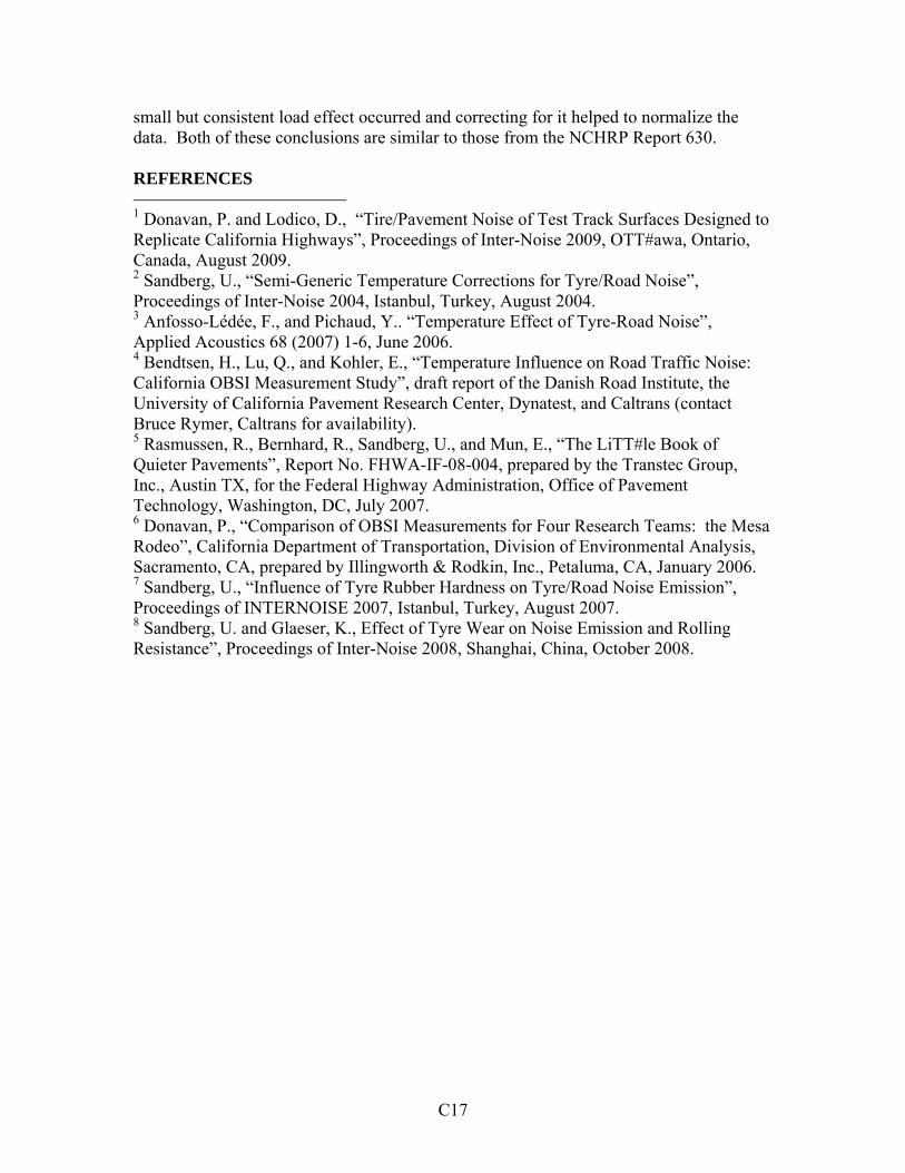
C17

small but consistent load effect occurred and correcting for it helped to normalize the data. Both of these conclusions are similar to those from the NCHRP Report 630. REFERENCES

1 Donavan, P. and Lodico, D., “Tire/Pavement Noise of Test Track Surfaces Designed to Replicate California Highways”, Proceedings of Inter-Noise 2009, OTT#awa, Ontario, Canada, August 2009. 2 Sandberg, U., “Semi-Generic Temperature Corrections for Tyre/Road Noise”, Proceedings of Inter-Noise 2004, Istanbul, Turkey, August 2004. 3 Anfosso-Lédée, F., and Pichaud, Y.. “Temperature Effect of Tyre-Road Noise”, Applied Acoustics 68 (2007) 1-6, June 2006. 4 Bendtsen, H., Lu, Q., and Kohler, E., “Temperature Influence on Road Traffic Noise: California OBSI Measurement Study”, draft report of the Danish Road Institute, the University of California Pavement Research Center, Dynatest, and Caltrans (contact Bruce Rymer, Caltrans for availability). 5 Rasmussen, R., Bernhard, R., Sandberg, U., and Mun, E., “The LiTT#le Book of Quieter Pavements”, Report No. FHWA-IF-08-004, prepared by the Transtec Group, Inc., Austin TX, for the Federal Highway Administration, Office of Pavement Technology, Washington, DC, July 2007. 6 Donavan, P., “Comparison of OBSI Measurements for Four Research Teams: the Mesa Rodeo”, California Department of Transportation, Division of Environmental Analysis, Sacramento, CA, prepared by Illingworth & Rodkin, Inc., Petaluma, CA, January 2006. 7 Sandberg, U., “Influence of Tyre Rubber Hardness on Tyre/Road Noise Emission”, Proceedings of INTERNOISE 2007, Istanbul, Turkey, August 2007. 8 Sandberg, U. and Glaeser, K., Effect of Tyre Wear on Noise Emission and Rolling Resistance”, Proceedings of Inter-Noise 2008, Shanghai, China, October 2008.

NCHRP Project 1-44 (1): Measuring Tire-Pavement Noise at the Source:

Precision and Bias Statement

APPENDIX D

Laboratory Measurement Program: Tire Noise Dynamometer Tests

APPENDIX D

Laboratory Measurement Program: Tire Noise Dynamometer Tests

TABLE OF CONTENTS

Page INTRODUCTION .................................................................................................... D-1 ROAD-WHEEL SIMULATOR TESTING.................................................................... D-1

Baseline Repeatability and Surface Comparison................................................ D-3 Influence of Added Background Noise .............................................................. D-6

Presence of Reflecting Surfaces ....................................................................... D-12 Vehicle Operating Parameters ......................................................................... D-13 OBSI Fixture Position....................................................................................... D-15

SUMMARY OF TIRE NOISE DYNAMOMETER TESTING................................... D-16 REFERENCES……… ................................................................................................. D-17

INTRODUCTION Although the bulk of the test work to be completed in quantifying precision and bias for the on-board sound intensity (OBSI) method of test is being done on-road, in conditions similar to the highway measurement application, some issues are more readily evaluated under controlled conditions in which the parameters can be varied. To do this, laboratory measurements were conducted in Phase I of this project. Much of this testing was designed to evaluate the effects of background noise on OBSI measurements. In a wind tunnel environment, noise produced by airflow on the test vehicle underbody and on the OBSI fixture was examined. Using a tire noise dynamometer with replica road surfaces, issues of background noise from other sources such as vehicles in adjacent lanes or reflections from roadside objects were evaluated. The purpose of the laboratory testing was to evaluate these background noise issues and develop criteria that would reduce the precision and bias error. The dynamometer testing is subject of this Appendix. ROAD-WHEEL SIMULATOR TESTING The road-wheel simulator or tire noise chassis dynamometer is a General Motors (GM) facility designed for tire noise testing. It consists of two independent large diameter (10 ft) rolls arranged such both tires on a single automotive axle can be tested at the same time or one at a time. The available surfaces replicate two of the pavements of the Interior Noise Roads, “smooth road” asphalt concrete (AC) and “stud damaged concrete” (SDC) portland cement concrete (PCC) pavements currently in use at the GM Proving Ground in Milford. MI. The epoxy road-wheel surfaces were made from castings of the actual test track surfaces. The actual and replica road-wheel surfaces are shown in Figure D1 and D2 for the smooth road and SDC pavements. These pavements are also similar to those used for the parameter investigations of the earlier research1 as tested at the GM proving ground facility in Mesa, AZ. The tire noise dynamometer can be operated such that it drives the tires or vehicle itself drives the dynamometer when the drive axle is placed on the road-wheel simulator. In either mode, the dynamometer can be operated up to about 70 mph. The road-wheel is housed in a semi-anechoic chamber (Figure D3)

Figure D1: Photographs the road-wheel smooth surface (left) and actual smooth AC pavement (right)

D1

with a controlled environment producing air temperature consistently in the range of 64 to 66º F.

Figure D2: Photographs the road-wheel coarse surface (left) and actual coarse, SDC pavement (right)

Figure D3: Test vehicle installed in on the tire noise chassis dynamometer setup for drive axis measurements

The testing was performed using a 2010 Chevrolet Malibu supplied by GM. On the right rear wheel position, testing on the smooth road surface was done primarily with SRTT test tire TT#9. Limited data with test tire TT#5 was also obtained for the baseline configuration. For the left rear wheel position, testing on the SDC surface was done using an older SRTT tire used for pass-by testing in this same wheel position. This same tire was also used on the smooth road surface in the left front wheel position for measurements made on the drive axle of the test vehicle. For most of the test conditions, speed was maintained at 60.5 mph (97.4 km/h) as set by the chassis dynamometer. Vehicle loading included only the weight of the OBSI instrumentation, providing estimated loading of the right rear position test tire of 697 lbs based on measurements made in conjunction with test track testing completed in February (Appendix C). The instrumentation and installation was identical to that used in the test track measurements and is shown installed on the test vehicle in Figure D4.

D2

Figure D4: Right rear test tire on the smooth road surface

The tire noise dynamometer was used to evaluate several aspects of on-road OBSI measurements. Baseline repeat measurements were conducted to define test variability using this facility and to contrast to on-road measurements. Documenting the effect of background noise and reflections from nearby objects were the primary objectives of the road-wheel simulator testing. Additional evaluations included examining the variation in OBSI level due to small increments of test speed, the fall-off in level when the probes are moved to more outboard distances, the effect of the microphone windscreens and methods of securing them, and the differences in level when the tire is driven by vehicle versus free rolling. Measurements were also made on the actual test road surfaces from which dynamometer surfaces replicated. Baseline Repeatability and Surface Comparison The first series of baseline measurements were performed on the smooth road replica surface using the test tire TT#5 in the right rear wheel position. The tire was driven by the dynamometer at a constant test speed of 60.5 mph. Per GM protocol, measurements were made after approximately 5 minutes to allow the tire to come to a constant operating temperature. Measurements were made in three blocks with the dynamometer shutdown and restarted between the blocks. Within each block nine data samples were acquired in groups of three with each sample being a five second linear average as specified in the proposed method of test1. The overall A-weighted levels for these measurements are shown in Figure D5. The variation in levels for individual data points was found to be small with an overall range of less than 0.3 dB and a standard deviation of 0.07 dB. For the individual one-third octave band levels, the average range was 0.6 dB with an average standard deviation of 0.17 dB. With the 5-minute warm-up period, the tire temperature stabilized at about 109º F. As a trend, it would be expected that the tire noise level would decrease with increasing temperature, however, that trend was not indicated in the results for the smooth road surface.

D3

After the series of measurements with TT#5, TT#9 was installed on the vehicle in the right rear wheel position. The average OBSI level for TT#9 was 0.2 dB greater than that of TT#5, consistent with the small differences observed in the test track measurements of February. For TT#9, one block of nine measurements were made to document the baseline condition and two additional repeat baselines were acquired during the course of the remainder of the testing for this tire and wheel position. The overall levels for these baseline measurements are shown in Figure D6. These data produced a range of 0.2 dB and a standard deviation of 0.07 dB with a corresponding average level of 100.7 dBA. In individual one-third octave band levels, the average range was 0.5 dB with an average standard deviation of 0.13 dB.

99

99.5

100

100.5

101

101.5

102

1 2 3 4 5 6 7 8 9 1 2 3 4 5 6 7 8 9 1 2 3 4 5 6 7 8 9

Sample Number

Ove

rall

So

un

d I

nte

ns

ity

Lev

el,

dB

A

Baseline Period #1 Baseline Period #2 Baseline Period #3

Figure D5: Overall OBSI levels for repeat runs over three baseline times – smooth road surface, tire TT#5

99

99.5

100

100.5

101

101.5

102

1 2 3 4 5 6 7 8 9 1 2 3 4 5 6 1 2 3

Smaple Number

Ove

rall

So

un

d In

ten

sity

Lev

el, d

BA

Baseline #1 Baseline #2 Baseline #3

Figure D6: Overall OBSI levels for repeat runs over three baseline times – smooth road surface tire TT#9

D4

A similar series of baseline measurements were conducted on the coarse road surface at the left rear wheel position using the passby SRTT. In this case, the measurement began shortly after the tire was brought up to operating speed in order to examined temperature warm-up effects. In this case, the tire surface temperature at the beginning of the testing was about 66º F and stabilized in the range of 96 to 98º F after the first block of measurements. As shown in Figure D7, the expected decrease in OBSI level with

105

105.5

106

106.5

107

107.5

1 3 5 7 9 11 1 3 5 7 9 2 4 6 8 1 3 2 1 3

Sample Number

Ove

rall

So

un

d In

ten

sity

Lev

el,

dB

A

Baseline #1 Baseline #2 Baseline #3 #4 #5 #6

Figure D7: Overall OBSI levels for repeat runs over three baseline times – coarse road surface passby tire

increasing temperature was observed in this case. In addition to the three blocks of initial baseline measurements, baseline data was obtained at three other times in the testing of the coarse surface. With the exception of baseline #5, these were also measured with the tire temperature was in the range of 96 to 98º F. For these cases, baseline #2, #3, #4, and #6, the range was 0.3 dB with a standard deviation of 0.1 dB producing an average OBSI level of 106.0 dBA. Baseline #5 was conducted after a period of about one hour downtime resulting in a slightly lower initial temperature of 90º F. For this case, the levels were about 0.3 dB higher than the other baselines. Unlike baseline #5, #4 and #6 were measured mid-way in their respective test sequence and were used for comparison purposes. As would be expected from Figures D6 and D7, the two tire noise dynamometer surfaces produce significantly different tire/pavement noise. As discussed above, the overall level produced by the two surfaces vary by about 5.3 dB with the coarse surface being higher. The one-third octave band levels indicate that this difference is due primarily to the lower frequencies, below 1000 Hz, where the coarse surface produces levels as much as 18 dB higher than the smooth surface (Figure D8). This result is quite consistent with the much larger aggregate content of the coarse surface. Above 1000 Hz, the levels are similar with differences of at most 2 dB in some bands. Aside from the noise level differences, the two surfaces also displayed differences in regard to tire temperature. The coarse surface produced tire temperatures and “pavement” temperatures about 12º F lower than the smooth surface even after prolonged periods of operation. The sensitivity of the tire

D5

65

70

75

80

85

90

95

100

105

400 500 630 800 1000 1250 1600 2000 2500 3150 4000 5000

1/3 Octave Band Center Frequency, Hz

So

un

d In

ten

sity

Lev

el, d

BA

Smooth Road Surface

Coarse Road Surface

Figure D8: Overall OBSI levels for repeat runs over three baseline times with Dynamometer shut down in-between – coarse road surface passby tire

noise to tire temperature was also found to be greater on the coarse surface. This suggests that tire operating temperature may be not only a function of ambient conditions (air temperature and overcast conditions), but also a function of the characteristics of the pavement itself, particularly surface roughness. The baseline measurements can also serve as lower limits on the data quality indicators for the pressure to intensity (PI) index and coherence. On the dynamometer, in the absence of airflow and any other noise sources, the values for both indicators should be “ideal”. For the PI index, the dynamometer results would produce the lowest values achievable with the difference between sound pressure and sound intensity being due to nearfield effects for the tire noise source and potentially off axis contributions of the leading edge noise sources to the trailing edge measurement and vice versa. The results of the leading and trailing edge probes on the two surfaces are shown in Figure D9. Above 630 Hz, it is seen that PI index values are all below 1.5 dB. Below 800 Hz, the values consistently increase with decreasing frequency. At these lower frequencies, the probes are clearly in the nearfield of the tire noise source as the acoustic wavelength at 630 Hz is about 20 inches compared to the measurement distance of 4 inches. As a result, the non-propagating, reactive sound field is contributing to higher sound pressure levels relative to the sound intensity levels that measure only the propagating portion of the sound field. For baseline runs, the coherence was consistently 1.0 with the exception of occasional instances of a value of 0.9 for the trailing edge probe in the 5000 Hz band only. Influence of Added Background Noise Upon completion of the baseline measurements for each surface, tests were performed to

D6

0

0.5

1

1.5

2

2.5

3

3.5

4

4.5

400 500 630 800 1000 1250 1600 2000 2500 3150 4000 5000

1/3 Octave Band Center Frequency, Hz

SI I

nd

ex,

dB

Smooth Surface Leading Edge

Smooth Surface Trailing Edge

Coarse Surface Leading Edge

Coarse Surface Trailing Edge

Figure D9: PI index for baseline measurements made on both surfaces

assess and quantify the effect of background noise on the OBSI measurements. The intent of these measurements was to simulate the influence of other vehicles near the test tire that produce a negative sound intensity vector relative to that coming from the test tire. For this purpose, a loudspeaker was placed directly opposite the test tire at a distance of 22½ inches from the sidewall of the tire or 18½ inches from the OBSI probes (Figure D10). Different levels of shaped pink noise were then broadcast toward the tire.

Measurements were conducted with the speaker source only on and then with the source on and the dynamometer operating at the 60.5 mph test speed. The speaker levels were adjusted incrementally lower until the OBSI levels matched those with the speaker turned off.

Figure D10: Right rear test tire on the smooth road surface set up for background noise evaluation

D7

The sound intensity one-third octave band spectra of the loudspeaker source are shown in Figure D11 for each increment measured along with the spectra of tire noise OBSI alone on the smooth dynamometer surface. It should be noted that all of the speaker sound

intensity levels are negative, that is, in the opposite direction of that coming from the tire. Above 1000 Hz, the spectral shapes of tire noise and the loudspeaker are similar, while below 1250 Hz, the tire noise is relatively lower implying that the error created by the background noise must be considered on a band-by-band basis. The result total sound intensity for the tire noise OBSI and the speaker generated background noise are shown in Figure D12. In this plot, the canceling effect of the negative sound intensity from the

50

55

60

65

70

75

80

85

90

95

100

105

110

400 500 630 800 1000 1250 1600 2000 2500 3150 4000 5000

1/3 Octave Band Center Frequency, Hz

So

un

d In

ten

sity

Le

vel,

dB

A

+10 dB

+5 dB

+0 dB

-5 dB

-7 dB

-8 dB

-10 dB

-12 dB

-14 dB

-16 dB

-18 dB

-22 dB

Baseline

Figure D11: Sound intensity level of various loudspeaker settings and baseline tire noise level on smooth road surface (opposite sign)

D8

65

70

75

80

85

90

95

100

400 500 630 800 1000 1250 1600 2000 2500 3150 4000 5000

1/3 Octave Band Center Frequency, Hz

So

un

d In

ten

sity

Lev

el, d

BA

+10 dB

+5 dB

+0 dB

-5 dB

-7 dB

-8 dB

-10 dB

-12 dB

-14 dB

-16 dB

-18 dB

-22 dB

Baseline

Figure D12: OBSI levels measured for at various source levels – smooth road surface

loudspeaker is apparent for the higher speaker levels, -5 to +10 dB, as indicated by dropouts in the total level in the direction from the tire or significantly reduced levels. As expected the highest level is for the baseline condition without the loudspeaker background noise and the effect of increasing levels of background noise is to reduce the total level relative to the baseline. By subtracting the measured levels with the background noise from the OBSI of tire noise alone, an error function for each speaker level can formed and is shown in Figure D13. These data can be used to set a

background threshold such that the effect of the background is to reduce the indicated OBSI level by no more than 0.4 dB in each one-third octave band (cause no more than a 0.5 dB error). Using this criterion, the allowable background noise is plotted in Figure D14 for each band. This results in essentially the usual 10 dB criteria for background

0

0.5

1

1.5

2

2.5

3

3.5

4

4.5

5

400 500 630 800 1000 1250 1600 2000 2500 3150 4000 5000

1/3 Octave Band Center Frequency, Hz

So

un

d In

ten

sity

Err

or

Lev

el, d

B

Dy +10

DY +5

Dy +0

Dy -5

Dy -7

Dy -8

Dy -10

Dy -12

Dy -14

Dy -16

Dy -18

Dy -22

Baseline

Figure D13: PIindex levels with wind noise effects added to idea smooth Tire Dynamometer PIindex levels – trailing edge

60

65

70

75

80

85

90

95

100

400 500 630 800 1000 1250 1600 2000 2500 3150 4000 5000

1/3 Octave Band Center Frequency, Hz

So

un

d In

ten

sity

Lev

el,

dB

A

Tire Noise

Allowable Background Noise

Figure D14: Allowable background noise to maintain less than a 0.5 dB error for tire noise OBSI measured on smooth road surface

D9

noise to be below the level to be measured in order to produce negligible error (i.e. 0.4 dB). To apply the results of Figure D14 to actual in-situ OBSI measurements, further consideration is required. In the situation where a vehicle is along side the test tire during the OBSI measurement, the background level produced by the adjacent tire will not be known. Further, the simulation on the dynamometer is the worst case in which the tire from the adjacent vehicle is directly along side the test tire during the entire five second averaging time. Because of these variables, it is problematic to assess the error that may occur when any vehicles are adjacent to the test tire. On the dynamometer, OBSI measurements were made with the probe at 6½ and 9¼ inches away from the tire wall in additional to the normal 4 inches. This produced a 2½ dB reduction in level for slightly more than a doubling of distance. To gain the additional 7½ dB attenuation for a tire of equal strength on an adjacent vehicle, the adjacent vehicle would need to be on the order of 5 ft or more away from the test tire. This worst case scenario is based on matching the near-field fall-off with that in the far-field using the controlled passby to OBSI relationship at 25 ft1. For adjacent tires of higher source level such as truck tires2, this distance would be considerably greater. With the difficulties in determining the potential contamination and error produced by adjacent vehicles, the PI index was considered as an indicator of this potential problem. Basically, as the contaminating background noise from an adjacent vehicle becomes stronger, the measured OBSI level becomes lower and the sound pressure level becomes higher. As a result, the PI index will increase above those levels measured when the background noise is absent. This trend can be seen in Figure D15 which plots the increase in PI index with the higher background noise level settings. To develop a PI index criterion for the error in the OBSI measurement, error is plotted versus the

0.0

0.5

1.0

1.5

2.0

2.5

3.0

3.5

4.0

4.5

5.0

Dy +0

Dy -5

Dy -7

Dy -8

Dy -10

Dy -12

Dy -14

Dy -16

Dy -18

Dy -22

Baseli

ne

Background Noise Setting

Inc

reas

e in

SI

Ind

ex o

ve

r B

as

elin

e, d

B

400 Hz

500 Hz

630 Hz

800 Hz

1000 Hz

1250 Hz

1600 Hz

2000 Hz

2500 Hz

3150 Hz

4000 Hz

5000 Hz

A-wtd

Figure D15: Increase in PIindex over baseline (no background noise) PIindex with varying amounts of background noise with frequency as a parameter

D10

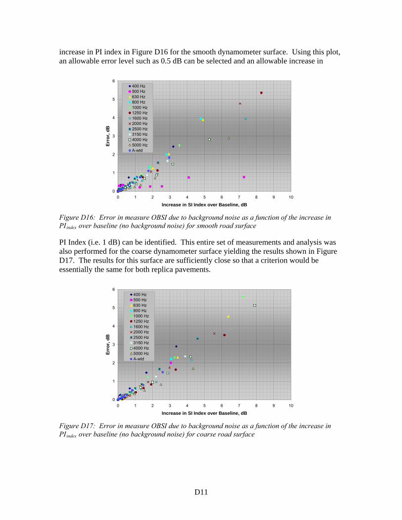
increase in PI index in Figure D16 for the smooth dynamometer surface. Using this plot, an allowable error level such as 0.5 dB can be selected and an allowable increase in

0

1

2

3

4

5

6

0 1 2 3 4 5 6 7 8 9 10

Increase in SI Index over Baseline, dB

Err

or,

dB

400 Hz500 Hz630 Hz800 Hz1000 Hz1250 Hz1600 Hz2000 Hz2500 Hz3150 Hz4000 Hz5000 HzA-wtd

Figure D16: Error in measure OBSI due to background noise as a function of the increase in PIindex over baseline (no background noise) for smooth road surface

PI Index (i.e. 1 dB) can be identified. This entire set of measurements and analysis was also performed for the coarse dynamometer surface yielding the results shown in Figure D17. The results for this surface are sufficiently close so that a criterion would be essentially the same for both replica pavements.

0

1

2

3

4

5

6

0 1 2 3 4 5 6 7 8 9 10

Increase in SI Index over Baseline, dB

Err

or,

dB

400 Hz500 Hz630 Hz800 Hz1000 Hz1250 Hz1600 Hz2000 Hz2500 Hz3150 Hz4000 Hz5000 HzA-wtd

Figure D17: Error in measure OBSI due to background noise as a function of the increase in PIindex over baseline (no background noise) for coarse road surface

D11

Presence of Reflecting Surfaces Another issue of concern in regard to the OBSI procedure is the potential effect of reflecting surfaces to side of the vehicle such as “K-rails”, Jersey barriers, bridge deck rails, etc. This issue was examined using the tire noise dynamometer by placing a large (4 by 8 ft) piece of plywood parallel to the side of the test vehicle in an upright position (Figure D18). Measurements were then made with the “barrier” incremental positioned

between 10½ and 20¼ inches from the plane of the tire sidewall. The OBSI levels measured for the smooth road surface with the reflecting panel at six different distances is shown in Figure D19 along with the baseline, no panel condition. Above 1250 Hz, the

Figure D18: Right rear test tire on the smooth road surface set up for evaluation of nearby reflecting surface

70

75

80

85

90

95

100

400 500 630 800 1000 1250 1600 2000 2500 3150 4000 5000

1/3 Octave Band Center Frequency, Hz

So

un

d I

nte

ns

ity

Lev

el,

dB

A

10½

12⅜

14½

16½

18½

20½

Baseline

Figure D19: Tire noise OBSI level for varying distance in inches of the reflecting surface from the tire sidewall on smooth road surface

D12

variations in the band levels for different positions and the baseline condition are small, less than 0.5 dB. In the lower frequency bands, more variation occurs on a band-by-band basis. To examine this in more detail, the difference, or error, between the baseline condition and reflection cases is shown in Figure D20. This presentation very clearly

-1.5

-1

-0.5

0

0.5

1

1.5

2

400 500 630 800 1000 1250 1600 2000 2500 3150 4000 5000

1/3 Octave Band Center Frequency, Hz

Err

or

Rel

ativ

e to

Bas

elin

e, d

B10½ 12⅜

14½ 16½

18½ 20½

Figure D20: Error in measured ⅓ octave band OBSI due to presence of reflecting surface at varying distance from the tire sidewall on smooth road surface

illustrates the presence of standing waves between the panel and side of the vehicle which results in varying amounts of error as a function of frequency band below 1600 Hz for any given reflector position. In general, the “peaks” in the spectra align with the standing wave modes defined by:

fn = nc/2L, n = 1,2,3,….

where f is the frequency of the standing wave mode, c is the speed of sound, and L is the separation between the panel and the side of the vehicle. Assuming these modes remain significant in the dynamic case of the vehicle passing the fixed reflecting surface, it is seen that the error in individual one-third octave bands can be between 1 and 1½ dB for a reflecting surface located within 18 ft or less of the side of the vehicle. Similar results were obtained for the coarse road surface. The overall levels for both surfaces are shown in Figure D21. From these data, maintaining a separation to a reflecting surface of 14½ inches or greater should provide an error of less 0.3 dB for either surface. As in the case of background noise from other vehicles, this simulation is the worst case in that the reflecting surface is assumed to be present during the entire 5 second averaging period. If not, the expected error would be lower. Vehicle Operating Parameters Using the tire noise dynamometer, two vehicle operating parameters could be evaluated to a precision not possible on the road. The first of these was the effect of small test variations on OBSI level. With the controlled system of the dynamometer, test speed

D13

0.0

0.1

0.2

0.3

0.4

0.5

0.6

0.7

10¼ 10½ 11½ 12⅜ 14½ 16½ 18½ 20½

Distance to Reflecting Surface, in.

Ove

rall

Err

or

Re

lati

ve

to B

ase

line,

dB

Smooth

Coarse

Figure D21: Error in measured overall OBSI due to presence of reflecting surface at varying distance from the tire sidewall on smooth and coarse road surfaces could be maintained and measured to within 0.1 mph or less. To define the speed/noise “gradient” for this facility, test speed was incremented in the range from 58.0 to 62.0 mph and resultant OSBI levels measured for both the smooth and coarse surfaces. Three OBSI five second samples were measured at each speed and average together to produce the results shown in Figure D22. For both surfaces, the standard deviation of the levels at

y = 0.25x + 85.70

R2 = 0.98

y = 0.22x + 92.70

R2 = 0.99

99

100

101

102

103

104

105

106

107

57.5 58 58.5 59 59.5 60 60.5 61 61.5 62 62.5

Speed, mph

Ove

rall

So

un

d I

nte

nsi

ty L

evel

, d

BA

Smooth Coarse

Figure D22: Change in overall OBSI level with small changes in test speed on smooth and coarse road surfaces

each speed was less than 0.05 dB. Although the relationship between vehicle speed and tire noise is expressed logarithmically, a linear regression was found to produce an equally good fit to the data. The slope for the coarse surface was found to be slightly less than the smooth, however, both were in the range identified in the parameter study performed in the previous research1. Also consistent with the earlier work, spectrum

D14

shape did not change with speed, merely increased uniformly in level with the overall level. The second vehicle operating parameter evaluated was the effect of torque applied to the test tire as would occur if OBSI measurements were made on a wheel on the drive axle. In the proposed method of test, it explicitly states that wheels on a drive axle should not be used for OBSI measurements, however the tire noise dynamometer presented a unique opportunity to readily validate that stipulation. For this testing, the front drive axle was placed on the tire noise dynamometer with the left front wheel position on the smooth road surface. To maintain a consistent direction of the rotation, the passby SRTT was used in this position. The dynamometer was then operated with the dynamometer driving the freewheeling tire (engine off) and then with the test car driving the dynamometer (engine on). This provided a simulation of a non-drive axle position (no-load), a drive axle position where torque was supplied to the tire by the vehicle driveline such as to maintain steady cruise conditions on a horizontal roadway (road-load), and a drive axle position where the supplied torque represented that required for the test vehicle to climb a 2% grade (incline load). As shown in Figure D23, the results indicated a 0.5 dB increase in overall level between the no-load and road-load case, and 1.1 dB between no-load and

75

80

85

90

95

100

105

400 500 630 800 1000 1250 1600 2000 2500 3150 4000 5000

1/3 Octave Band Center Frequency, Hz

So

un

d I

nte

nsi

ty L

evel

, d

BA

No Load - 99.8 dBA

Road Load - 100.3 dBA

Incline Load - 100.9 dBA

Figure D23: Increase in OBSI level for drive axle tire with increasing loading of the vehicle powertrain (i.e. applied torque to the drive tire)

incline-load. In the one-third octave spectra, most of the increase in level occurs in the 1000, 1250, 3150, 4000, and 5000 Hz bands with increases in the range of 2 to 3 dB. This trend is consistent other reported data on the effects of applied torque under vehicle acceleration3. OBSI Fixture Position As discussed in the section Influence of Added Background Noise, measurements were conducted on the coarse road surface to examine the fall-off of OBSI level with increased distance of the pair of probes from the standard 4-inch position. The outboard positions

D15

were 2½ inches and 5¼ inches providing more a one doubling of distance from the tire sidewall. Altogether, this produced a 2.5 dB reduction in level for the most outboard position (Figure D24). This corresponds to a linear fall-off of slightly less than 0.5

dB/inch, which is similar to the 0.2 dB/½ inch rate reported from the parameter study of the previous research1. This reduced fall-off rate compared to 6 dB/doubling of distance for a point source is indicative of being in the near-field of the tire noise source. The one-third octave spectra are seen to decrease relatively uniformly in frequency with increase distance.

70

75

80

85

90

95

100

105

400 500 630 800 1000 1250 1600 2000 2500 3150 4000 5000

1/3 Octave Band Center Frequency, Hz

So

un

d I

nte

nsi

ty L

ev

el,

dB

ABaseline - 105.9 dBA

Outboard 2.5" - 104.7 dBA

Outboard 5.25" - 103.4 dBA

Figure D24: Change in OBSI level with incremental outboard movement of the sound intensity probes relative to baseline (4”) distance to the tire sidewall

SUMMARY OF TIRE NOISE DYNAMOMETER TESTING Once stable operating parameters were achieved on the tire noise dynamometer, the typical range in overall OBSI level was about 0.3 dB with a standard deviation less than 0.1 dB. However, since test speed, environmental conditions, and wheel path were highly controlled and stop/start timing was not an issue, it is not reasonable to expect that this low amount of variation could ever consistently be achieved in on-road conditions. From the track test testing where conditions were controlled to a very high degree, variation less than 0.6 dB and standard deviations of 0.3 dB or less were achieved however, even these would be more difficult to achieve under less controlled highway measurement conditions. In regard to background noise from other sources, particularly adjacent vehicles, as would be expected, it was found that for error less than 0.5 dB, the intensity of the background noise when it is arriving on probe in the directly opposite direction of the intensity from the test tire must less than 10 dB. In normal measurement situations, it is not usually possible to know what the level of background noise. However, it appears that additional criteria on the PI index could be used to identify situations where background noise may be contributing erroneous OBSI measurements. A tentative

D16

D17

criterion of 1 dB was established for later confirmation. Also, a preliminary criterion of being 14½ inches away from any reflecting objects was established. The dynamometer measurements also confirmed the significance of test speed as a variable in OBSI measurements. Within the 60 ±1 mph limits set in the proposed method of test, the range in level was found to be 0.5 dB, similar to that found in the previous research1. Although by itself this source of variation is well within the current limit of 1 dB run-to-run variation, when accumulated with other variables, this dependence may be important. This variable was evaluated on-road later test track testing (see Chapter 4 of the main report) and it was found that correcting for speed in this small range would not improve the measurement certainty. The dynamometer measurements further clearly demonstrated that the requirement to use only non-driven axles of the test vehicle should remain in the proposed method of test. REFERENCES

1 Donavan, P. and Lodico, D., “Measuring Tire-Pavement Noise at the Source”, NCHRP Report 630, Transportation Research Board, Washington, D.C., 2009. 2 Donavan, P., “Generation of Noise by Truck and Car Tires on Various Types of Asphalt Concrete Pavements”, Proceedings of Inter-Noise 2006, Honolulu, Hawaii, December 2006. 3 Donavan, P.R., “Tire-Pavement Interaction Noise Measurement under Vehicle Operating Conditions of Cruise and Acceleration”, SAE Paper 931276, Society of Automotive Engineers Noise and Vibration Conference Proceedings, Traverse City, MI, May 1993.

NCHRP Project 1-44 (1): Measuring Tire-Pavement Noise at the Source:

Precision and Bias Statement

APPENDIX E

Laboratory Measurement Program: Wind Tunnel Tests

TABLE OF CONTENTS

Page INTRODUCTION .....................................................................................................E-1 DATA QUALITY INDICATORS ..................................................................................E-1 MEASUREMENT DESCRIPTION................................................................................E-2 WIND TUNNEL SIMULATION DIFFERENCES ........................................................E-5 RESULTS AND DISCUSSION......................................................................................E-6 Baseline Measurements .......................................................................................E-6

Test Vehicle Assessment .....................................................................................E-8 Yaw Angle (Simulated Crosswind) Assessment ..............................................E-12 Assessment of Windscreen Attachment Methods .............................................E-14 Fixture Component Self-Noise Assessment ......................................................E-14

Wind Speed…....................................................................................................E-16 ASSESSMENT OF DATA QUALITY CRITERIA .....................................................E-17 Coherence…… ..................................................................................................E-17 PI Index………..................................................................................................E-19 SUMMARY……………...............................................................................................E-22 REFERENCES……… ..................................................................................................E-22

INTRODUCTION One source of background noise and resultant inaccuracies in on-board sound intensity (OBSI) measurements is the noise induced by air flow passing the over and around the OBSI fixture, probes, and test vehicle. The Proposed Method of Test Using OBSI developed in earlier research11 did not set limits on wind condition. To gain further understanding of possible wind noise contamination effects in isolation and to determine if and what exact limits on crosswind conditions are necessary for the OBSI measurement procedure, measurements were conducted in the General Motors (GM) Aeroacoustic wind tunnel. The purpose of the wind tunnel testing performed in the current research included:

1. Assessing fine steps in vehicle yaw angle (crosswind) 2. Evaluating the variation in background noise generated by two different vehicles,

a Pontiac G6 and a Chevrolet Impala. 3. Evaluating self-noise generated by different OBSI fixture components to begin to

address fixture design improvements. 4. Assessing the ability of the data quality criteria limits recommended in the

Proposed Method of Test to identify wind noise effects on OBSI measurement. DATA QUALITY INDICATORS One aspect of the laboratory testing was to assess how well background noise effects and other problems can be identified using the OBSI quality indicators of pressure to intensity (PI) index and coherence. In principle, the sound intensity measurement will minimize the level from noise generated in the vertical plane parallel to the tire sidewall and through the fixture. For sources in this plane, the sound intensity will theoretically approach 0 as indicated in Figure E1 for incident angles of 90 or 270º. However, as the sound intensity approaches zero near 90º, the sound pressure remains high resulting in high PI index value. As a practical concern, due to small amounts of phase mismatch between sound pressure measurement channels, large values (>15 dB) of the SI index rarely occur. Further, the angular range over which the sound intensity is significantly attenuated is a relatively small angle, 90±15º for 6 dB attenuation. In cases where the background noise has a vector component in the direction of propagation, such as underbody generated airflow noise, the measured tire noise sound intensity can be increased due this background noise. However, since the underbody noise is coming to the probe at some angle, its PI index will be somewhat higher than that coming directly from the tire. In the opposite case for sound intensity coming toward the tire such as background noise from other vehicles, the measured OBSI level will be reduced somewhat as the negative intensity sums together with the positive intensity from the tire. In this case the PI index will also be raised as the sound pressure increases due to the multiple noise sources summing from all directions while the net sound intensity is smaller.

E1

Figure E1: OBSI probe directivity relative to test tire and fixture mounting on vehicle

In the laboratory tests, different background noises representing actual on-road cases were simulated and their effects on sound intensity and sound pressure levels were measured. These data were then used to examine the magnitude of the possible OBSI error for these conditions and how the influence of the background noise may be demonstrated using the data quality indicators. The results and implication of this testing are presented in the following sections. MEASUREMENT DESCRIPTION Sound intensity measurements were made in the General Motors Aerodynamics Laboratory (GMAL), the largest automotive test facility of its type in the world. The test section measures 17.7 ft high, 34.1 ft wide with a length of 69.9 ft. It is a closed circuit (continuous loop) design with 987 ft air path along its centerline. Air speed is maintained with a 43 ft diameter fan driven by a 4000-HP DC electric motor. Unlike more recent automotive tunnels, GMAL features a “closed section” in which the airflow through the test section is bounded on four sides. This and other features contribute to an unusually low value for inflow turbulence (~ 0.6%) for an automotive wind tunnel. The size of the test section was designed to achieve minimal blockage (air-flow restriction) for full size automotive vehicles for yaw angles up to ± 20 degrees. GMAL is capable of sustained wind speeds of greater than 150 mph. A 2001 acoustical upgrade succeeded in reducing individual ⅓ octave band levels by as much as 20 dB, achieving levels of 58 dB or less in all bands at 60 mph. Figure E2 shows the test vehicle placement in the wind tunnel.

E2

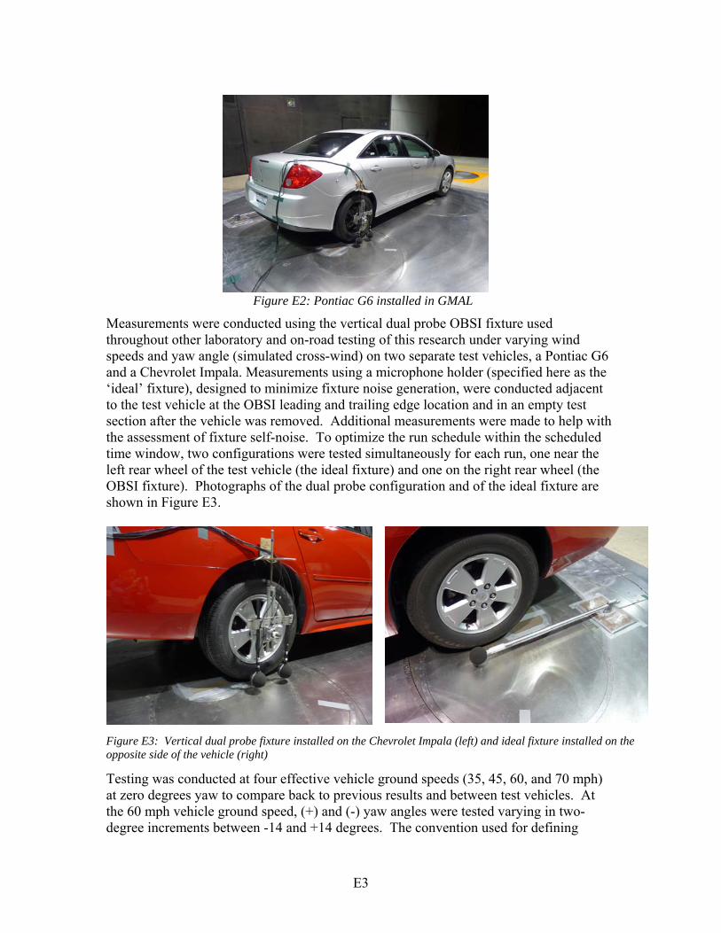
Figure E2: Pontiac G6 installed in GMAL

Measurements were conducted using the vertical dual probe OBSI fixture used throughout other laboratory and on-road testing of this research under varying wind speeds and yaw angle (simulated cross-wind) on two separate test vehicles, a Pontiac G6 and a Chevrolet Impala. Measurements using a microphone holder (specified here as the ‘ideal’ fixture), designed to minimize fixture noise generation, were conducted adjacent to the test vehicle at the OBSI leading and trailing edge location and in an empty test section after the vehicle was removed. Additional measurements were made to help with the assessment of fixture self-noise. To optimize the run schedule within the scheduled time window, two configurations were tested simultaneously for each run, one near the left rear wheel of the test vehicle (the ideal fixture) and one on the right rear wheel (the OBSI fixture). Photographs of the dual probe configuration and of the ideal fixture are shown in Figure E3.

Figure E3: Vertical dual probe fixture installed on the Chevrolet Impala (left) and ideal fixture installed on the opposite side of the vehicle (right)

Testing was conducted at four effective vehicle ground speeds (35, 45, 60, and 70 mph) at zero degrees yaw to compare back to previous results and between test vehicles. At the 60 mph vehicle ground speed, (+) and (-) yaw angles were tested varying in two-degree increments between -14 and +14 degrees. The convention used for defining

E3

positive and negative crosswind/yaw directions for the probe and test vehicle are shown in Figure E4. The test matrix is shown in Table E1. Due to the (lack of) sensitivity of the wind tunnel with respect to small changes in test speed (on the order of 0.2 mph), the

Table E1: Wind Tunnel test matrix

Direction of Travel

“+” Crosswind Direction

“–” Crosswind Direction

OBSI Fixture

Direction of Travel

wind tunnel air speed was maintained at 60 mph for runs at all yaw angles and was not increased to maintain the simulated vehicle speeds. For example, a 60 mph total air tunnel speed at a yaw angle of 10 degrees would actually simulate a vehicle speed of 59.1 mph with a crosswind of 10.4 mph. To assess the error inherent in this procedure,

“+” Crosswind Direction

“–” Crosswind Direction

OBSI Fixture Figure E4: Plan view of the test vehicle defining negative and positive crosswind (yaw) directions

Fixture Variable Speed, mph Yaw Angle, degrees

Speed 35, 45, 60, 70 mph 0 Dual Probe Crosswind Condition

60 mph -14, -12, -10, -8, -6, -4, -2, 0, +2, +4, +6, +8, +10 (also 60.9 mph),

+12, +14 (also 61.8 mph) Speed 35, 45, 60, 70 mph 0 Ideal Fixture,

LE Crosswind Condition

60 mph -14, -12, -10, -8, -6, -4, -2, 0, +2, +4, +6, +8, +10 (also 60.9 mph),

+12, +14 (also 61.8 mph)

Ch

evro

let

Imp

ala

Ideal Fixture, TE

Crosswind Condition

60 mph 0, +2, +4, +6, +8, +10 (also 60.9 mph), +12, +14 (also 61.8 mph)

Speed 35, 45, 60, 70 mph 0 Dual Probe Crosswind Condition

60 mph -14, -12, -10, -8, -6, -4, -2, 0, +2, +4, +6, +8, +10 (also 60.9 mph),

+12, +14 (also 61.8 mph) Dual Probe, LE removed

Probe Design 60 mph -10, -6, 0, +6, +10, +14

Dual Probe, TE removed

Probe Design 60 mph -10, 0, +6, +10, +14

Dual Probe Attachment Tape: No Tape, ¼ in.,

and ½ in.

60 mph 0

Po

nti

ac G

6

Ideal Fixture, 24 inch fm tire sidewall

Four Fixture configurations

60 mph -10, 0, +6, +10, +14

Empty Test Section with Ideal Probe 60 mph 0

E4

additional runs at 10 and 14 degree yaw were made with vehicle test speeds maintained at 60 mph (air tunnel speeds of 60.9 and 61.8 mph, respectively). At 10 degrees yaw, the difference between a 60 mph and 60.9 mph air tunnel speed resulted in about a 0.35 dB difference in wind induced background noise. At 14 degrees yaw, the difference was measured to be 0.8 to 0.9 dB. The measured wind induced background noise was not corrected for these differences. WIND TUNNEL SIMULATION DIFFERENCES Important differences exist between the wind tunnel simulation and the measurement of on-road flow noise. The most fundamental difference is that the source of interest, tire noise, is not present. As a result, sound intensity level and sound pressure level can only be compared to OBSI data taken on-road at a different time. For purposes of comparison, a tire/pavement noise source level was selected to be an average of five of the quietest pavements measured to date using the SRTT test tire. These included a double layer porous asphalt measured in the Netherlands2 and four of the quietest pavements measured in the test track portion of this study. The five lower noise pavement OBSI levels, along with the average of these, are shown in Figure E5. For comparison to wind

tunnel sound intensity data measured at the standard OBSI probe locations, the OBSI levels for this average ‘pavement’ were used directly and labeled “AC Pavement” figures throughout this s

70

75

80

85

90

95

100

400 500 630 800 1000 1250 1600 2000 2500 3150 4000 5000

1/3 Octave Band Center Frequency, Hz

So

un

d In

ten

sity

Lev

el,

dB

A

GM DPG Smooth AC

GM DPG ISO Track

H-K PG Ultrasmooth

H-K PG 3/8" DGAC

GMAL Reference - 2007

Avg

Figure E5: Development of an average quieter pavement tire noise spectrum foe analysis of GMAL measurement results

in the ection.

As far as the simulation itself, with on-road testing, tire rotation occurs that could result in more wind turbulence near the tire and in the wheel well area. This would tend to increase background wind flow noise levels over that in the tunnel. On the road, discounting ambient wind, the vehicle would travel at a speed relative to the pavement and there is no airflow relative to the pavement. As a result, there is no boundary layer on the road. In GMAL, the boundary layer formed between the moving tunnel air and the

E5

floor (ground plane) cannot be completely removed even when features to reduce the floor boundary layer were utilized. The presence of a boundary layer is of concern as turbulence can be generated that is not experienced on the road and boundary layer gradients may reduce the effective relative air speed experienced by the probe. On-road, the effect of the turbulence due to flow separation around the vehicle should be adequately represented in the wind tunnel, however atmospheric turbulence due to wind and temperature gradients, wind flowing over and around obstacles, etc., is not represented. Typical turbulence intensity levels as high as 20% have been reported in the literature, while the level in GMAL is about 0.6%3. Previous research of the effect of turbulence level on sound intensity measurements found that an increase in turbulence level from 1% to 5% increased the background sound pressure level measured by the SI probe by almost 10 dB at 1000 Hz4. In considering the results of this study, it should be kept in mind that the application of any criteria developed from the wind tunnel tests may require some added margin of safety for application to on-road measurements. RESULTS AND DISCUSSION Baseline Measurements In addition to the measurements conducted with the OBSI fixture, measurements were made using the ideal fixture located adjacent to the test vehicle at the OBSI leading and trailing edge locations for the Impala, at the OBSI trailing edge location for the G6, and in an empty wind tunnel test section after the vehicle was removed. The sound pressure level (SPL) should reflect flow-induced noise on the probe and fixture as well as any residual background noise in the test section. Without the vehicle present, in principle, the intensity level (IL) would be zero due to the lack of a definite noise source in the sensitive direction of the microphone pair. In practice, levels are below 45 dBA (Figure E6). When the test vehicle is introduced into the test section with the ideal probe in the

E6

40

45

50

55

60

65

70

75

80

85

90

95

100

400 500 630 800 1000 1250 1600 2000 2500 3150 4000 5000

1/3 Octave Band Center Frequency, Hz

So

un

d L

evel

, dB

A

No Car, SPL

With Car, SPL

No Car, IL

With Car, IL

AC Pavement, IL

Figure E6: Sound intensity and pressure levels with and without test vehicle in GMAL as measured with the ideal probe

OBSI measurement position, the IL and SPL levels typically increase. At the 5000 Hz frequency band, the empty test section SPL is slightly higher than level measured when the vehicle was present. This may be due to lower local wind speed created by flow around vehicle creating regions of higher pressure (separation) and hence lower air speed. Similar response was seen in prior testing5 at frequencies of 2500 Hz and above. The general increase in both SPL and IL and positive direction of the IL when the vehicle is present indicates that the vehicle itself generates measurable noise likely due to flow around and through the tire and wheel assembly and/or noise generated by flow interacting with the underbody6, 7. With the test vehicle present, the total IL background noise remains more than 10 dB below the tire noise source level for all frequencies. To further investigate the source of underbody noise, flow visualization was performed in the vicinity of the tire and wheel well. Using yarn tuffs, it was found that to the front of the tire, the flow separates with the bulk of the flow directed into the underbody area. This separation occurs approximately in the plane of the car outer body panel and outer plane of the tire sidewall. The remaining flow that proceeded past the tire and around the OBSI probes was seen to be relatively free of turbulence with the streamlines directed parallel to the plane of the tire sidewall and parallel to the ground plane. This flow split may tend to reduce flow-induced effects on the probes themselves while producing more underbody noise issues. When the ideal fixture is replaced with the OBSI fixture attached to the vehicle, the background noise levels again increase. The SPL increases by 2.9 dB on average with a range for individual ⅓ octave bands from 0.7 to 6.1 dB for the G6 (Figure E7), and 5.5

50

55

60

65

70

75

80

85

90

95

100

400 500 630 800 1000 1250 1600 2000 2500 3150 4000 5000

1/3 Octave Band Center Frequency, Hz

So

un

d L

evel

, d

BA

Dual Probe, SPL

Ideal Probe, SPL

Dual Probe, IL

Ideal Probe, IL

AC Pavement

Figure E7: Sound intensity and pressure levels with the dual and idea probes for Pontiac G6 test vehicle

dB on average with a range for individual ⅓ octave bands from 3.2 to 8.4 dB for the Impala (Figure E8). For IL, the average increases by 2.9 dB for the G6 and 4.0 dB for the Impala. The additional IL background noise generated by the fixture remains 10 dB or more below the tire source level for both vehicles for all frequencies. Through

E7

50

55

60

65

70

75

80

85

90

95

100

400 500 630 800 1000 1250 1600 2000 2500 3150 4000 5000

1/3 Octave Band Center Frequency, Hz

So

un

d L

evel

, dB

A

Dual Probe, SPL

Ideal Probe, SPL

Dual Probe, IL

Ideal Probe, IL

AC Pavement

Figure E8: Sound intensity and pressure levels with the dual and idea probes for Chevrolet Impala test vehicle

comparison of Figures E7 and E8, the levels with the dual probe on each vehicle are more similar than the levels with the ideal fixture for the two vehicles (discussed in more detail in the Test Vehicle Assessment discussion, below). Test Vehicle Assessment Overall A-Weighted SPL and IL measured at 60 mph for both vehicles, measured using the dual probe and the trailing edge position of the ‘ideal’ fixture are shown in Figures E9 and E10, compared to the AC Pavement OBSI source level. The average tire/pavement

70

75

80

85

90

95

100

14 12 10 8 6 4 2 0 -2 -4 -6 -8 -10 -12 -14

Yaw Angle, degrees

So

un

d L

eve

l, d

BA

G6, SPL

Impala, SPL

G6, IL

Impala, IL

AC Pavement

Figure E9: Overall sound intensity and pressure levels as a function of yaw angle using the dual probe for both test vehicles

E8

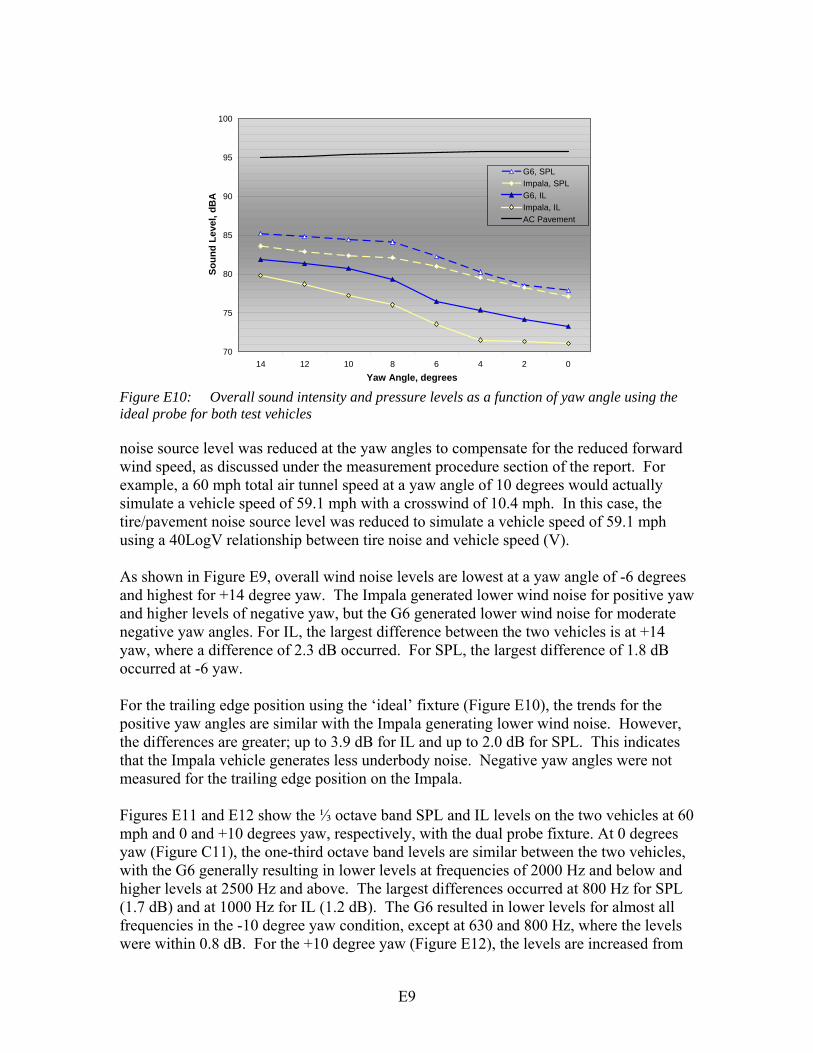
noise source level was reduced at the yaw angles to compensate for the reduced forward wind speed, as discussed under the measurement procedure section of the report. For example, a 60 mph total air tunnel speed at a yaw angle of 10 degrees would actually simulate a vehicle speed of 59.1 mph with a crosswind of 10.4 mph. In this case, the tire/pavement noise source level was reduced to simulate a vehicle speed of 59.1 mph using a 40LogV relationship between tire noise and vehicle speed (V).

70

75

80

85

90

95

100

14 12 10 8 6 4 2 0

Yaw Angle, degrees

So

un

d L

evel

, d

BA

G6, SPL

Impala, SPL

G6, IL

Impala, IL

AC Pavement

Figure E10: Overall sound intensity and pressure levels as a function of yaw angle using the ideal probe for both test vehicles

As shown in Figure E9, overall wind noise levels are lowest at a yaw angle of -6 degrees and highest for +14 degree yaw. The Impala generated lower wind noise for positive yaw and higher levels of negative yaw, but the G6 generated lower wind noise for moderate negative yaw angles. For IL, the largest difference between the two vehicles is at +14 yaw, where a difference of 2.3 dB occurred. For SPL, the largest difference of 1.8 dB occurred at -6 yaw. For the trailing edge position using the ‘ideal’ fixture (Figure E10), the trends for the positive yaw angles are similar with the Impala generating lower wind noise. However, the differences are greater; up to 3.9 dB for IL and up to 2.0 dB for SPL. This indicates that the Impala vehicle generates less underbody noise. Negative yaw angles were not measured for the trailing edge position on the Impala. Figures E11 and E12 show the ⅓ octave band SPL and IL levels on the two vehicles at 60 mph and 0 and +10 degrees yaw, respectively, with the dual probe fixture. At 0 degrees yaw (Figure C11), the one-third octave band levels are similar between the two vehicles, with the G6 generally resulting in lower levels at frequencies of 2000 Hz and below and higher levels at 2500 Hz and above. The largest differences occurred at 800 Hz for SPL (1.7 dB) and at 1000 Hz for IL (1.2 dB). The G6 resulted in lower levels for almost all frequencies in the -10 degree yaw condition, except at 630 and 800 Hz, where the levels were within 0.8 dB. For the +10 degree yaw (Figure E12), the levels are increased from

E9

the 0 and -10 degrees yaw conditions, but the spectral characteristics are similar, except at 500 Hz. Again, the G6 resulted in lower levels than the Impala, with the largest differences indicated in the 500 Hz band: 4.2 dB for IL and 1.9 dB for SPL. The results at -10 degrees yaw are reduced slightly from the 0 yaw condition, except at 1250 Hz, where the Impala shows an increased level not seen for the G6.

50

55

60

65

70

75

80

85

90

95

100

400 500 630 800 1000 1250 1600 2000 2500 3150 4000 5000

1/3 Octave Band Center Frequency, Hz

So

un

d L

evel

, dB

A

G6, SPL

Impala, SPL

G6, IL

Impala, IL

AC Pavement

Figure E11: Sound intensity and pressure levels for both test vehicles at 0 degrees yaw with the dual probe fixture

50

55

60

65

70

75

80

85

90

95

100

400 500 630 800 1000 1250 1600 2000 2500 3150 4000 5000

1/3 Octave Band Center Frequency, Hz

So

un

d L

evel

, d

BA

G6, SPL

Impala, SPL

G6, IL

Impala, IL

AC Pavement

Figure E12: Sound intensity and pressure levels for both test vehicles at +10 degrees yaw with the dual probe fixture

Figure C13 and C14 show the ⅓ octave band SPL and IL levels for the ‘ideal’ fixture on the two vehicles at 60 mph and 0 and +10 degrees yaw, respectively. At both yaw angles, the differences between the vehicles is again greater that that seen using the dual probe.

E10

The G6 resulted in higher levels at almost all frequencies for both IL and SPL at both yaw angles. At 0 degrees yaw (Figure C13), the largest differences occurred at 800 Hz for SPL (1.7 dB) and at 5000 Hz for IL (5.2 dB). For the +10 degree yaw (Figure C14), the levels are increased from the 0 degrees yaw conditions, but the spectral characteristics are generally similar. The differences between vehicles are increased in the low frequencies and decreased in the high frequencies. Again, the G6 resulted in higher levels than the Impala, with the largest differences indicated in the 800 Hz band, 5.2 dB for IL and 4.9 dB for SPL, due to an increase for the G6 vehicle that is not indicated with the Impala.

50

55

60

65

70

75

80

85

90

95

100

400 500 630 800 1000 1250 1600 2000 2500 3150 4000 5000

1/3 Octave Band Center Frequency, Hz

So

un

d L

evel

, d

BA

G6, SPL

Impala, SPL

G6, IL

Impala, IL

AC Pavement

Figure C13: Sound intensity and pressure levels for both test vehicles at 0 degrees yaw with the ideal fixture

50

55

60

65

70

75

80

85

90

95

100

400 500 630 800 1000 1250 1600 2000 2500 3150 4000 5000

1/3 Octave Band Center Frequency, Hz

So

un

d L

evel

, d

BA

G6, SPL

Impala, SPL

G6, IL

Impala, IL

AC Pavement

Figure C14: Sound intensity and pressure levels for both test vehicles at +10 degrees yaw with the ideal fixture

Figure C15 shows the results for both vehicles for the 0 yaw condition using the dual

E11

45

50

55

60

65

70

75

80

85

400 500 630 800 1000 1250 1600 2000 2500 3150 4000 5000

1/3 Octave Band Center Frequency, Hz

So

un

d P

ress

ure

Lev

el,

dB

A

Impala 35 mph Impala 45 mphImpala 70 mph Impala 60 mphG6 35 mph G6 45 mphG6 70 mph G6 60 mph

Figure C15: Sound pressure levels for both test vehicles at 0 degrees yaw with the dual probe fixture at 35, 45, 60, and 70 mph

probe at effective vehicle speeds of 35, 45, 60, and 70 mph. For the alternate vehicle speed (Figure C15), the trends were the same as for 60 mph at 0 yaw. The G6 resulted in lower levels at the low frequencies and higher levels at the higher frequencies. Yaw Angle (Simulated Crosswind) Assessment To assess the degree to which wind induced background noise could be expected to influence measured on-road tire/pavement noise levels in order to determine the limiting crosswind value(s), the measured wind induced IL and SPL levels can be compared to the average tire/pavement noise source level. As shown in Figure E9, the overall IL for both vehicles achieved a 10 dB S/N ratio for all yaw. Figures E16 and E17 show the ⅓ octave band IL levels for the G6 and Impala, respectively, at yaw angles of 0, +2, +6, +10, and +14 degrees along with the tire/pavement noise source level. As expected, the spectral characteristics were maintained with increasing level as the yaw angle was increased from 0 to +14 degrees, with some differences at 500 Hz. The 10 dB criterion is not met at 400 Hz starting at the +2 degree yaw condition for the G6 (Figure E16) and at 500 Hz starting at the +4 degree yaw condition for the Impala (Figure E17). For frequencies from 800 to 2500 Hz, the 10 dB IL criterion is met for all measured yaw angles on both vehicles. To assess the degree to which wind induced background noise could be expected to affect the tire/pavement noise source level, the wind noise IL measured at each yaw angle for each vehicle was added to the tire/pavement OBSI noise source level and the difference between the source level with and without the added wind noise was calculated. The results of these calculations are shown in Figure E18 for the overall a-weighted level and the level at 400 and 500 Hz for both vehicles.

E12

50

55

60

65

70

75

80

85

90

95

100

400 500 630 800 1000 1250 1600 2000 2500 3150 4000 5000

1/3 Octave Band Center Frequency, Hz

So

un

d In

ten

sity

Lev

el, d

BA

G6, 0 Yaw

G6, +2 Yaw

G6, +6 Yaw

G6, +10 Yaw

G6, +14 Yaw

AC Pavement

Figure E16: Sound intensity levels for both test vehicles at 0 degrees yaw with the dual probe fixture on the Pontiac G6

50

55

60

65

70

75

80

85

90

95

100

400 500 630 800 1000 1250 1600 2000 2500 3150 4000 5000

1/3 Octave Band Center Frequency, Hz

So

un

d In

ten

sity

Lev

el, d

BA

Impala, 0 Yaw

Impala, +2 Yaw

Impala, +6 Yaw

Impala, +10 Yaw

Impala, +14 Yaw

AC Pavement

Figure E17: Sound intensity levels for both test vehicles at 0 degrees yaw with the dual probe fixture on the Chevrolet Impala

As shown in Figure E18, the change in the overall tire/pavement noise source sound intensity level due to background wind noise was 0.3 dB or less in all cases. In the 500 Hz band, where the largest differences occurred, the background noise with the Impala resulted in a 0.5 dB increase in the tire/pavement noise source level at 500 Hz starting at +4 degrees yaw and a 1 dB increase at +14 degrees yaw. In the 400 Hz bands, excluding the yaw angles where ‘drop outs’ occur, the increase in the tire/pavement noise source level never exceeded 0.5 dB. The changes due to the background noise with the G6 were higher. In the 500 Hz band, the G6 background noise also resulted in a 0.5 dB increase in the tire/pavement noise source level starting at +4 degrees yaw, but resulted in a 1 dB increase at +8 degrees yaw and a 2 dB increase at +14 degrees yaw. At 400 Hz, the G6

E13

resulted in a 0.5 dB increase in the tire/pavement noise source level starting at +2 degrees yaw and a 1 dB increase at +6 degrees yaw, but never reached an increase of 2 dB.

0

1

2

3

4

5

14 12 10 8 6 4 2 0 -2 -4 -6 -8 -10 -12 -14

Yaw Angle, degrees

Incr

ease

in

So

un

d In

ten

sity

Lev

el,

dB

G6, Overall G6, 500 Hz

G6, 400 Hz Impala, Overall

Impala, 500 Hz Impala, 400 Hz

Figure E18: Increase in sound intensity levels above tire noise alone created by wind background noise for overall, 400, and 500 Hz bands

Assessment of Windscreen Attachment Methods Previous research811 found that the 3½ inch diameter spherical foam windscreen, without nose cones, was the preferred wind noise reduction device for OBSI measurement and this is the device specified in the proposed method of test1. Attachment of the windscreen to the microphone is not specified in the test method. Obviously, the attachment method should not include any intervening object in the path between the tire/pavement contact patch and the microphones. A common method is to attach the windscreens using a thin piece of tape in the direction of travel of the vehicle (see Figure E4), keeping the path between the tire/pavement contact patch and the microphone free from interfering objects. To assess the effects of tape thickness on wind turbulence generated IL, three configurations were tested; windscreens placed on the probes without any tape attachment (this would not be practical on-road), and windscreens attached with ¼ and ½ inch thick tape in the direction of travel of the vehicle. For the 0 yaw condition, no increase in sound intensity level was observed for both the ¼ and ½ inch wide tape. For sound pressure, an average increase of 0.3 dB occurred with the ½ inch wide tape, while no increase was measured with the ¼ inch wide tape. This indicates that tape thicknesses up to, ½ inch wide located in the direction of the vehicle path of travel, would not be expected to affect OBSI measurement. Fixture Component Self-Noise Assessment The dual vertical probe concept was evaluated for wind-induced noise. The potential for improvement in background noise with improvement of the fixture design can be seen in

E14

Figures E7 and E8, which compare the dual probe and ‘ideal’ fixture for both vehicles at 60 mph and 0 yaw. These figures suggest that with further development, it may be possible to reduce the wind-induced background noise of the fixture by 4 dB (for the G6 vehicle) to 6 dB (for the Impala) to achieve the same performance as the ‘ideal’ fixture. To minimize any wind-induced noise from the structure, the design of OBSI fixtures has previously focused on moving the supporting structure away from the microphones and keeping the supporting structure at a 90o angle to the sensitive axis of the probe. To assess the contribution of the leading and trailing edge dual probe components on each other, measurements were made with the G6 at the leading and trailing edge positions in the dual probe fixture without the placement of the second probe (Figure E19).

As shown in Figure E19, measurements made at the leading edge position were not notably affected by the structure of the trailing edge probe; the wind-induced IL for both conditions were within 0.4 dB for all frequencies. At the trailing edge location, small reductions occurred with the removal of the leading edge probe component; the overall a-weighted wind induced IL was reduced by 0.8 dB and the one-third octave bands were reduced by up to 1.5 dB (in the 800 Hz band). With comparison to the ‘ideal’ fixture at the trailing edge position, additional reduction is possible in frequencies of 800 Hz and below and at 2500 and 3150 Hz.

50

55

60

65

70

75

80

85

90

95

100

400 500 630 800 1000 1250 1600 2000 2500 3150 4000 5000

1/3 Octave Band Center Frequency, Hz

So

un

d In

ten

sity

Lev

el, d

BA

Trailing Edge, Dual Probe

Leading Edge, Dual Probe

Trailing Edge Probe Only

Leading Edge Probe Only

Ideal Probe at Trailing Edge

Figure E19: Sound intensity levels with and without the leading edge probe and trailing edge probe removed separately – dual probe fixture

To evaluate the amount of wind noise generated by various fixture components, measurements were also made by the ‘ideal’ fixture at a distance of 24 inches from the center of the tire sidewall and 3 inches above the floor of the wind tunnel during iterations of disassembly of the fixture attached to the vehicle (Figure E20). This distance

E15

was selected to be far enough away from the fixture so that all portions would contribute equally to the sound intensity level with respect to propagation path and angular differences. Four iterations of fixture disassembly were made (Figure E20); the full fixture, the fixture with the removal of the leading and trailing edge probe components, the fixture with the removal of the probe and crossbar, and the plate and shaft only.

50

55

60

65

70

75

80

400 500 630 800 1000 1250 1600 2000 2500 3150 4000 5000

1/3 Octave Band Center Frequency, Hz

So

un

d In

ten

sity

Lev

el, d

BA

Plate and Shaft Only

Fixutre without Probes and Crossbar

Fixture without Probes

Full Fixture

Figure E20: Sound intensity levels with different parts removed from the dual probe fixture as measured by the ideal probe 24 inches to the side

As shown in Figure E20, the largest wind-noise generating component is the probes themselves. The greatest differences (up to 3.6 dB) are seen in the frequencies from 630 to 1000 Hz and at 3150 Hz, similar to the frequencies that were found to have the potential for reduction with comparison of the dual and ‘ideal’ fixtures in Figure E19 and levels with and without the crossbar were within 1.1 dB for all frequencies. As expected, wind noise IL decreased with the removal of the entire fixture (leaving only the shaft and plate). Decreases were relatively uniform and on the order of 2.0 to 6.7 dB, with the exception of the 500 and 400 Hz bands, where again the two conditions performed within 1.1 dB. Similar results were seen at all measured yaw angles (+14, +10, +6, 0, -6, and -10 degrees). These results indicate that future fixture design should focus on optimizing the probe structures to minimize extraneous noise and turbulence. Wind Speed Testing was conducted at four wind speeds for the zero yaw angle condition, corresponding to forward travel speeds of 35, 45, 60, and 70 mph. The results for both vehicles using the dual probe fixture for the 0 yaw condition indicated that the overall SPL levels increased with speed with a relationship of 10*Log (V6.5). Using this relationship to normalize, the ⅓ octave band spectra for each wind speed essentially collapse to a single curve versus frequency.

E16

For tire/pavement noise, a wide range of VX relations have been reported ranging from around X=2.5 to X=4.59. Using the REMELs database10, a typical value of X can be taken to be 4.0. This implies that tire/pavement noise increases with speed on the order of 40*Log (V) while the wind-induced background noise increases on the order of 65*Log (V). As a result, the signal-to-noise (S/N) ratio will also be a function of speed with higher (better) ratios occurring at lower speeds. However, even though the S/N ratio is improved at lower speeds, the crosswind condition would still need to be limited for accurate tire noise OBSI measurements. This was discussed in more detail in the 2007 report5. ASSESSMENT OF DATA QUALITY CRITERIA The proposed method of test1 includes five data quality criteria. First, audio monitoring is required to identify and eliminate any data with unusual noises. Second, the direction of the sound intensity is required to be in the direction propagating away from the test tire to the microphones. Third, the PI index, defined as the sound intensity level subtracted from the sound pressure level, is required to be between -1 and +5 dB for all frequencies reported as valid. Forth, the coherence between the microphones is required to be greater than 0.8 for all frequencies below 4,000 Hz. Lastly, the range in sound intensity levels for runs made of the same pavement section are required to be within 1 dBA for the overall A-weighted sound intensity level, and within 2 dB for all 1/3 octave bands reported as valid. Of the data quality indicators, the coherence between the microphones and the PI index are the most applicable to the assessing whether wind flow induced noise is affecting the OBSI measurement. The first two criteria are provided to alert measurement operators to primary errors in measurement technique or equipment set up or operation that should be identified and remedied in the field based on cursory observations. Since the wind tunnel testing does not include a tire/pavement noise source, the run-to-run variation in levels is not applicable to the wind tunnel tests. Coherence and PI index are discussed below. Coherence For the measurement of the sound intensity, both the average pressure between two closely spaced microphones and the difference in the complex pressure between the microphones need to be accurately determined. The difference in pressure is used to calculate acoustic velocity, which is, in turn, multiplied by the average pressure to yield the sound intensity. For two closely spaced microphones, the primary difference in pressure leading to the acoustic velocity is the phase shift between the microphones. One indicator of a consistent phase relation between two signals is coherence. If there is no coherence, there is no phase relationship and hence the velocity is indeterminate. If the coherence is 1 (maximum value), a consistent phase relationship exists and the velocity can accurately determined. For this reason, coherence has historically been used as a data quality indicator for sound intensity11. In principle, it has been found that if the coherence drops to about 0.5, the SI measurement is no longer accurate.

E17

For SI measurement in flow, coherence is used as the indicator of flow induced contamination due to turbulence impinging on the two microphones12. This is different from background noise generated by flow past an object such as a vehicle underbody. For this type of background noise source, since the source is localizable (even off the sensitive axis of the SI probe), the coherence would be 1 in the absence of any flow-induced contamination. In the presence of both a noise source (either tire/pavement noise or flow generated background noise) and flow induced contamination, the coherence will depend on the relative amplitude of the two. The proposed method of test1 requires that the coherence be greater than 0.8 for all frequencies below 4,000 Hz. At higher frequencies, coherence is typically lower due to limitations in the finite difference approximation used in the algorithm for determining sound intensity11. Coherence is plotted in Figure E21 for an empty section, and the leading and trailing edge positions on both test vehicles for the 60 mph 0 yaw condition.

For the empty section, in the absence noise sources, the coherence is low, typically 0.6 or below. With the OBSI fixture on both vehicles, the background noise increases and coherence improves accordingly. Even though the background noise source level is still weak compared to tire noise as shown in Figure E6, coherence is above 0.8 for all frequencies below 4,000 Hz for both vehicles at both the leading and trailing edge positions. For actual tire noise measurements where the source levels are even higher, the coherence should be at least as high as indicated in Figure E21. Lower levels of coherence would then be an indicator of turbulence-induced contamination or other problems. This has been observed in on-road testing as problems have been identified when coherence drops below about 0.8 in frequencies from 500 and 3150 Hz. In these situations, lower coherence has been associated with equipment overloads and overheating, loose microphones not properly secured onto the preamplifiers, dirt or debris

0.0

0.2

0.4

0.6

0.8

1.0

1.2

400 500 630 800 1000 1250 1600 2000 2500 3150 4000 5000

1/3 Octave Band Center Frequency, Hz

Co

he

ren

ce

G6 LE, 0 Yaw

Impala LE, 0 Yaw

G6 TE, 0 Yaw

Impala TE, 0 Yaw

Empty Section

Figure E21: Coherence measured with no vehicle (ideal probe) and with test vehicles (dual probe) at leading and trailing edges

E18

becoming lodged in the microphone windscreens, or noise interference from other noise sources (i.e., a truck passing) influencing the data. As indicated in Figure E21, both vehicles resulted in similar coherence values at both the leading and trailing edge OBSI probe positions at 0 degrees yaw. At leading edge position, lower values of coherence were observed for the G6, with the largest differences in the 1250 and 1600 Hz bands. At the trailing edge position, coherence was similar for both vehicles, with the Impala showing slightly lower levels from 2000 to 3150 Hz. These results are in line with those from the 2007 study. At +10 yaw, the coherence for both vehicles at the leading edge position is similar to the 0 yaw condition, with levels for the Impala reduced slightly to be consistent with those for the G6. At the trailing edge position, the coherence for both vehicles drop, particularly in frequencies of 1250 Hz and below, but values continue to exceed 0.8 from 500 to 3150 Hz. At -10 yaw, coherence is increased with very similar levels for both vehicles and positions, except in the 400 and 500 Hz bands for the trailing edge position on the Impala. Again, levels exceed 0.8 for frequencies of 3150 Hz and below. PI Index The PI index is calculated by subtracting the sound intensity level from the sound pressure level. Sound intensity is a directional quantity, where as sound pressure is not directional and weights noise sources from all directions equally. For a sound source along the sensitive axis of the sound intensity measurement, both quantities would theoretically produce the same value, resulting in a PI index of zero. On the other hand, for the same noise source generated perpendicular to the sensitive axis, the sound intensity would theoretically approach zero (as indicated in Figure E1 for incident angles of 90 or 270º), where as the sound pressure level would have same value regardless of incidence angle, resulting in a high PI index value. From a practical standpoint for OBSI measurements, the angular range over which the sound intensity is significantly attenuated is a relatively small angle, 90±15º for 6 dB attenuation. Additionally, due to small amounts of phase mismatch between sound pressure measurement channels, large values of the SI index rarely occur. In OBSI measurement, airflow on the microphones and fixture due to the forward travel of the vehicle is an example of a noise source perpendicular to the sensitive axis of the OBSI measurement of the tire/pavement noise source that would not affect the OBSI measurement level. In this case, since the background noise level generated by the wind noise source is sufficiently lower in level than the tire/pavement noise source (see Figure C6), the PI index is not notably affected. However, in cases where the background noise has a turbulent vector component in the direction of propagation, such as underbody generated airflow noise, the measured tire noise sound intensity could be increased due this background noise. Additionally, since the underbody noise is coming to the probe at some angle, its PI index will be higher than that coming directly from the tire.

E19

To assess the use of PI index as an indicator for wind induced background noise effects on OBSI measurement, theoretical PI index values were calculated for the tire/pavement noise source with the wind induced background noise measured for each yaw angle on each vehicle at the 60 mph test speed. First, an AC pavement SPL level was calculated using the average 1/3 octave band SI-Index from the smooth surface dynamometer tests (discussed below), which would represent “ideal” SI-Index values due to the absence of airflow and any other noise sources. Next, the 1/3-octave band SPL and IL wind noise levels were added to the AC Pavement SPL and OBSI levels to result in SPL and IL levels for the tire/pavement noise with wind induced background noise and the difference (or PI index) between the SPL and IL levels. The results of these calculations are shown in Figures E22 and E23 for the leading edge and trailing edge positions, respectively,

0.0

1.0

2.0

3.0

4.0

5.0

6.0

7.0

400 500 630 800 1000 1250 1600 2000 2500 3150 4000 5000

1/3 Octave Band Center Frequency, Hz

PI I

nd

ex,

dB

G6 LE, +10 Yaw

G6 LE, 0 Yaw

G6 LE, -10 Yaw

Impala LE, +10 Yaw

Impala LE, 0 Yaw

Impala LE, -10 Yaw

Ideal PI-Index, LE

Figure E22: PI index levels with wind noise effects added to idea smooth Tire Dyno PI index levels – leading edge

along with the No Background Noise Condition (representing the “ideal” values). As shown in Figures E22 and E23, there was virtually no difference in PI index values with or without wind noise in the mid frequency bands (800 to 2000 Hz). Some spread is seen in the high and low frequency bands, with the largest difference between the wind and no wind cases being 1.8 dB and an increase in SI-Index correlating with an increase in wind induce background noise affects. Figure E24 shows the SI-index values for the most sensitive 500 and 5000 Hz frequency bands for both vehicles at all yaw angles. The SI-index values in these frequencies follow the general trend seen for the changes in OBSI level due to the addition of the wind induced background noise. For negative (-) yaw angles, the PI index values did not vary considerably. For positive (+) yaw angles, the PI index increased with increasing yaw angle, along with the associated change in OBSI level at both 500 and 5,000 Hz. .

E20

0.0

1.0

2.0

3.0

4.0

5.0

6.0

7.0

400 500 630 800 1000 1250 1600 2000 2500 3150 4000 5000

1/3 Octave Band Center Frequency, Hz

PI I

nd

ex,

dB

G6 TE, +10 Yaw

G6 TE, 0 Yaw

G6 TE, -10 Yaw

Impala TE, +10 Yaw

Impala TE, 0 Yaw

Impala TE, -10 Yaw

Ideal PI-Index, TE

Figure E23: PI index levels with wind noise effects added to idea smooth Tire Dyno PI index levels – trailing edge

0

1

2

3

4

5

6

7

14 12 10 8 6 4 2 0 -2 -4 -6 -8 -10 -12 -14

Yaw Angle, degrees

PI I

nd

ex,

dB

G6 LE, 500 Hz G6 LE, 5000 Hz

G6 TE, 500 Hz G6 LE, 5000 Hz

Impala LE, 500 Hz Impala LE, 5000 Hz

Impala TE, 500 Hz Impala TE, 5000 Hz

Figure E24: PI index levels with wind noise effects added to idea smooth Tire Dyno PI index levels for the 500 and 5000 Hz bands as a function of yaw angle

Based on these figures, it follows that it may be possible to use PI index as an indicator of background wind noise contamination. Currently, the proposed method of test1 requires PI index to be between -1 and +5 dB for all frequencies reported as valid. As seen in Figures E22, E23, and E24, virtually all of the wind conditions tested met this criterion, with the exception of the +12 and +14 degree yaw conditions for the Impala. Tighter maximum limits, based on an individual 1/3-octave band analysis may reduce the need for a crosswind limit.

E21

E22

SUMMARY To assess the degree to which wind induced background noise could be expected to influence measured on-road tire/pavement noise levels and in order to determine the limiting crosswind value(s), the measured wind induced IL and SPL levels were compared to a tire/pavement noise source level, calculated as an average of five of the quieter pavements measured to date. Based on 2 degree incremental steps in yaw angle from -14 to +14 degrees yaw, it was determined that OBSI levels of tire/pavement noise sources could be accurately measured for the standard vehicle test speed of 60 mph for the frequency range of 400 to 5000 Hz in the absence of any crosswind or for negative yaw angles (representing crosswinds in the direction from the vehicle toward the OBSI probe) of up to -14 degrees. For positive yaw angles (wind direction from the probe to the test vehicle) of up to +14 degrees, the overall a-weighted OBSI level of a lower noise tire/pavement noise source was affected by 0.3 dB or less. In the 500 Hz band, for the noisier of the two test vehicles, background noise resulted in a 0.5 dB increase in the tire/pavement noise source level at 500 Hz starting at +4 degrees yaw, but resulted in a 1 dB increase at +8 degrees yaw and a 2 dB increase at +14 degrees yaw. In the Proposed Method of Test, run-to-run variability of 1 dB for the overall a-weighed OBSI level and 2 dB for the individual one-third octave band are set and extreme cases were at or below this limit for all conditions. However, considering the possible accumulation of other sources of error, limiting crosswind conditions will to be considered. Based on an analysis of the PI index with respect to the influences of wind induced background noise on OBSI measurement, it appears that tighter limits on the PI index may account for crosswind conditions in which the wind induced background noise is found to affect OBSI measurement levels. The results of the wind tunnel testing indicate that limits should be addressed on an individual 1/3-octave band case with particular attention paid to the 400, 500, and 5,000 Hz bands. REFERENCES

1 Donavan, P. and Lodico, D., “Measuring Tire-Pavement Noise at the Source”, NCHRP Report 630, Transportation Research Board, Washington, D.C., 2009. 2 Donavan, P., “Tire/Pavement Noise in Europe and the United States”, Noise News International, Volume 13, Number 2, June 2005. 3 Tanida, H., Morita, K., Iida, A., and Hama, Y., “Effects of Turbulence on Aerodynamic Noise Generation of Rearview Mirrors”, Fluid Dynamic Research, Vol. 8, 1991, pp. 53-64. 4 Oswald, L., and Donavan, P., “Acoustic Intensity Measurements in Low Mach Number Flows of Moderate Turbulence Levels”, Research Publication GMR-3269, General Motors Research Laboratories, Warren, MI, April, 1980. 5 Donavan, P. and Lodico, D., “Wind Tunnel Assessment of Flow-Induced Background Noise on On-Board Tire/Pavement Noise Measurements”, Report of the California Department of Transportation Division of Environmental Analysis, Illingworth & Rodkin, Inc, Petaluma, California, February 2008

E23

6 Cogotti, A., “Aeroacoustics Development at Pininfarina”, Soc. of Automotive Engineers Technical Paper 970402, SAE International Congress and Exposition, Detroit, MI, Feb. 1997. 7 Kűnstner, R., Potthof, J., and Essers, U., “The Aero-Acoustic Wind Tunnel of Stuttgart University”, Soc. of Automotive Engineers Technical Paper 950625, SAE International Congress and Exposition, Detroit, MI, Feb. 1995. 8 Donavan, P., “Further Development of the Sound Intensity Method of Measuring Tire Noise Performance of In-Situ Pavements”, California Department of Transportation, Division of Environmental Analysis, Sacramento, CA, prepared by Illingworth & Rodkin, Inc., Petaluma, CA, January 2006. 9 Sandberg, U., and Ejsmont, J., The Tyre/Road Noise Reference Book, INFORMEX, Ejsmont & Sandberg Handelsbolag, Harg, SE-59040 Kisa, Sweden, 2002. 10 Fleming, G., Rapoza, A., and Lee, C., “Development of National Reference Energy Mean Emission Levels for the FHWA Traffic Noise Model (FHEA TNM), Version 1.0”, U.S. Department of Transportation, Report No. DOT-VNTSC-FHWA-96-2, 1996. 11 Chung, J. Y., and Blaser, D. A., “Factors Affecting Measurements of Acoustic Intensity Using the Cross-Spectral Method”, Research Report EM-493, GM Research Laboratories, Warren, MI, Dec. 1980. 12 Donavan, P. and Oswald L., “The Identification and Quantification of Truck Tire Noise Sources Under On Road Operating Conditions", Proceedings of Inter Noise 80, Miami, FL, Dec.1980

NCHRP Project 1-44 (1): Measuring Tire-Pavement Noise at the Source:

Precision and Bias Statement

APPENDIX F

Summary of Comparative OBSI Testing Rodeos

TABLE OF CONTENTS

Page INTRODUCTION .....................................................................................................F-1 OBSI COMPARISON TESTING AT NCAT .................................................................F-1

Test Description...................................................................................................F-1 Test Results…......................................................................................................F-2

Temperature…. ........................................................................................F-5 Porous Pavement Dampness…................................................................F-5 Wheel Path…...........................................................................................F-6

Summary……......................................................................................................F-7 OBSI COMPARISON TESTING AT GM YUMA PROVING GROUND....................F-8

Test Description...................................................................................................F-8 Instrumentation…. ...................................................................................F-8 Pavements…. ...........................................................................................F-8 Tires and Test Vehicles…........................................................................F-9

Test Results…......................................................................................................F-9 Initial Measurements…..........................................................................F-10 Tire Swap…...........................................................................................F-11 Test Surfaces…......................................................................................F-11 Tire Loading…. .....................................................................................F-12 Temperature…. ......................................................................................F-13 Wind…...................................................................................................F-13

Summary ……...................................................................................................F-14 OBSI COMPARISON TESTING NEAR AUSTIN, TEXAS.......................................F-14

Test Description.................................................................................................F-14 Test Results…....................................................................................................F-15

Initial Comparison…. ............................................................................F-15 Tire Hardness….....................................................................................F-16 Tire Loading…. .....................................................................................F-17 Temperature…. ......................................................................................F-17

OBSI COMPARISON TESTING NEAR ELKIN, NORTH CAROLINA ...................F-18 Test Description.................................................................................................F-18

Test Results…....................................................................................................F-19 Summary……....................................................................................................F-24

OVERALL SUMMARY OF COMPARITIVE TESTING ………..............................F-25 REFERENCES……… ..................................................................................................F-26

INTRODUCTION During the course of this research, four sets of comparative testing between OBSI users as sponsored by the Federal Pooled Fund Project TPF 135, Quiet Pavement1,2,3,4. Asummary of the results of these “rodeos” is reported here. The first set of testing was conducted at the test track of the National Center for Asphalt Technology (NCAT)

1, the second at the General Motors Desert Proving Ground in Yuma, AZ2, the third on in-service roads in the vicinity of Austin, TX3, and final set on in-service roads around Elkin, NC4. The detailed results of the comparative tests are described in the individual project reports. The results of these tests have been further analyzed under in this research in order to better understand potential contributors to precision and bias errors for multiple users in both test track and road environments. This Appendix provides discusses the results of each of the comparative tests as they pertain to the current research project. OBSI COMPARISON TESTING AT NCAT As part of the TFP 135, Illingworth and Rodkin, Inc. (IR) was tasked with providing training and support to US DOT Volpe Center personnel in their development of OBSI capability. To facilitate this process, Volpe purchased instrumentation identical to that used by IR. These systems were compared in a bench-top test using a sound intensity calibrator and were found to be within 0.3 dB of each other with 0.2 dB due a difference in acoustical calibrators. The specification of the accuracy stated by the manufacturer is ±0.2 dB, so that the calibrators were within specification limits. After purchasing a SRTT and initial field tryout testing, OBSI measurements were made at the NCAT facility over the course of three days on 22 different AC pavements by both IR and Volpe. The testing took place on November 1-3, 2010 under mostly clear and dry conditions with temperatures in the range from 59º to 77º F with the majority of the testing completed when temperatures were in the mid sixties. The measurements were not conducted back-to-back to save time and to allow the track to be used for other types of testing. The Volpe testing was conducted on November 2 and 3 while the IR spanned all three days. On November 1st, sections of porous asphalt still appeared damp from rain the previous day. These sections were tested both under this condition and clearly dry conditions on November 3rd. Test Description Descriptions of the 22 test surfaces are provided in Table F1. At variance with the proposed method of test5, OBSI measurements were averaged over 1.8 seconds instead of the specified 5 seconds as the sections were only typically about 200 ft long. Testing was done the specified 60 mph as well as at 45mph for which a 2.5 second averaging time was used. Three passes over each surface were made and averaged together and even with the shorter averaging time, the data quality indicator requirements were met. The test sections with “W” and “E” designations were on the banked ends of the test track and were only measured at 45 mph. As a result, only 18 of 22 sections were measured at the 60 mph test speed.

F1

Table F1: NCAT Test pavements and construction properties

Test Section Designation

Construction Date

Design Method

Design Gradation

Type

Max Aggregate Size (mm)

Air Voids (%)

Lift Thickness

(in)

N2 7/15/2009 FC-5 PFC 12.5 16.8 0.7

N3 7/24/2003 superpave ARZ 9.5 5.7 1.2

N4 7/28/2003 superpave ARZ 9.5 5.5 1

N5 8/3/2009 super fine 9.5 3.7 1.3

N7 7/22/2009 super fine 9.5 4.1 1.1

N8 7/28/2009 SMA SMA 19 4.7 2.6

N9 10/18/2006 SMA SMA 12.5 4.9 2

N11 8/11/2009 super fine 9.5 3.2 1.2

N12 7/31/2009 SMA SMA 12.5 4 1.7

N13 8/10/2006 OGFC OGFC 9.5 17.6 0.8

W3 9/25/2006 super dense 12.5 1.9 2.3

W5 9/25/2006 super dense 12.5 1.7 2

W6 8/21/2003 superpave ARZ 4.75 4 0.8

W8 8/23/2003 proprietary OGFC 9.5 4 1.3

S1 8/20/2003 SMA SMA 12.5 2 1.7

S3 10/4/2006 OGFC OGFC 9.5 21.8 1.3

S4 8/15/2003 OGFC OGFC 12.5 16 1.3

S7 7/30/2009 super coarse 12.5 3.3 1.7

S8 7/15/2009 FC-5 PFC 12.5 16.8 1.3

S10 7/16/2009 WMA fine 9.5 3.3 1.3

S13 7/13/2000 superpave ARZ 12.5 4.8 4

E5 9/26/2006 super dense 12.5 3.2 1.5 Both test teams used rental cars to make the OBSI measurements. Volpe used a Hyundai Sonata providing an estimated loading of 700 lbs on the SRTT in right rear wheel position. IR used a Pontiac G6 providing a 727 lbs loading on the test tire. The Volpe SRTT was essentially new with several hundred miles of use and a build date in November 2008. The average durometer hardness was 63. The IR tire was older with a build date of October 2005 and an accumulation of approximately 2000 miles. Its average durometer hardness was 68. Prior to testing, the tires were inflated to 30 psi. Test Results The overall OBSI levels measured by the Volpe and IR teams are cross-plotted in Figure F1 for the 60 mph test speed. A linear regression and best fit slope of 1 line are also shown in the figure. Generally, the levels for the Volpe team are below those of the IR by about 1 to 2 dB except for four data points between 99½ to 100 dBA. These data points are for pavements N5, 7, 11, and S10 all of which are identified as “fine” design gradation in Table 1. For the other non-porous pavements, the spectral shapes are fairly similar between the Volpe and IR data as shown in Figure F2 for test section N12. For the fine gradation pavements, the one-third octave band levels at 1000 Hz are higher for the Volpe data than for IR levels by 1 to 4 dB as shown in Figure F3 for pavement S10.

F2

For the other one-third octave bands, the Volpe levels are equal to or less than the IR levels much like those shown in Figure F2. The differences between the tires on these fine gradation pavements are also clearly seen in narrow-band spectra as shown in Figure F4 for test section N5. For the Volpe data, the peak at the tire tread passage frequency

Linear Regressiony = 0.63x + 36.50

R2 = 0.74

96

97

98

99

100

101

102

103

104

96 97 98 99 100 101 102 103 104

IR Sound Intensity Level, dBA

Vo

lpe

So

un

d I

nte

nsi

ty L

evel

, d

BA

Slope 1 Fity = 1x + 1.3σ = 1.1

1-to1 Line

Figure F1: Cross-plot of overall OBSI level for IR and Volpe teams with slope 1 fit, linear regression, and 1-to-1 line shown

60

65

70

75

80

85

90

95

100

105

400 500 630 800 1000 1250 1600 2000 2500 3150 4000 5000

1/3 Ocatve Band Center Frequency, Hz

So

un

d I

nte

nsi

ty L

evel

, d

BA

Volpe

I&R

Figure F2: ⅓ octave band OBSI level on Section N12 (½” SMA) measured by IR and Volpe teams

around 1000 Hz is clearly defined, relatively narrower in frequency than the IR data, and higher in amplitude. At higher frequencies, around 1800 to 2000 Hz, the IR data displays more frequency content at harmonics of the tread passage frequencies and higher amplitudes. On the other AC pavements, these tread pattern related effects are not so apparent as shown in Figure F5 for test section N3. This implies that there is something fundamentally different about the noise mechanisms or the dominance of certain mechanisms on these fine gradation pavements for these two tires6. When the data

F3

points for these four fine gradation sections are removed from the plot of Figure F1, the standard deviation about the slope 1 best fit drops from 1.1 dB to 0.5 dB, the slope of the regression increases from 0.6 to 0.8, and the R2 value increases from 0.7 to 0.9. Without these points, the average difference between the data sets increases from 1.3 to 1.8 dB while the range of the differences drops from 3.9 to 1.9 dB.

60

65

70

75

80

85

90

95

100

105

400 500 630 800 1000 1250 1600 2000 2500 3150 4000 5000

1/3 Octave Band Center Freqency, Hz

So

un

d In

ten

sity

Lev

el, d

BA

IR

Volpe

Figure F3: ⅓ octave band OBSI level on Section S10 (⅜” Fine) measured by IR and Volpe teams

45

50

55

60

65

70

75

80

85

90

0 500 1000 1500 2000 2500 3000 3500 4000 4500 5000

Frequency, Hz

So

un

d In

ten

sity

Lev

el, d

BA

IR

Volpe

Figure F4: Narrowband OBSI level on Section N5 (⅜” Fine ) measured by IR and Volpe teams

For the 45 mph data, the behavior noted for the fine gradation pavements is not so apparent and the average difference between the data for all pavements is 2.0 dB with a standard deviation of 0.7 dB. For 45 mph, the slope of the regression line is greater, about 1.1 and the R2 is 0.85.

F4

Temperature

45

50

55

60

65

70

75

80

85

90

0 500 1000 1500 2000 2500 3000 3500 4000 4500 5000

Frequency, Hz

So

un

d In

ten

sity

Lev

el, d

BA

IR

Volpe

Figure F5: Narrowband OBSI level on Section N3 (⅜” Superpave) measured by IR and Volpe teams

Some of the differences between the IR and Volpe data at 60 mph can be explained by temperature differences between occurring at the time of each measurement block. For “N” test sections, the temperature when the Volpe data was acquired was 65º F while it was 60º F for the IR data. For the “S” sections, the temperature was 73º F for the Volpe data and again 60º F for the IR. Using the 0.04 dB/º F trend from the test track data taken in the Phase I testing, the average difference between the two data sets becomes 1.4 dB instead of 1.8 dB with the four fine gradation data points removed and 0.9 dB instead of 1.3 dB if all data points are used. For the 45 mph, the temperature differences were generally not as large (-2 to 8º F) and the applying the adjustment only reduced the average difference by 0.1 dB. Porous Pavement Dampness In addition to the comparison of Volpe and IR results, there were two other findings of note for this research. The porous pavements of test sections S4 and S8 were measured twice on November 1st and once again on November 3rd by IR. For the first measurements, the porous pavements were visually still damped from rain occurring on October 31st. By the time the third set of measurements, the pavements were dry with no rain occurring since the 31st. The results for test section S4 are shown in Figure F6. In terms of overall level, there is essentially no difference. In the higher frequencies, starting at 1250 Hz, the levels on the damp surface are consistently higher, by as much as 2 dB in the 1600 and 2000 Hz bands. If moisture were affecting the sound absorptive properties of the pavement, it would be expected to occur in these frequencies and it would be expected that the damp levels would be higher. The results for test section S8 are somewhat different (Figure F7). The overall levels are actually higher for the dry condition by 0.7 dB and effect on higher frequencies is mixed with the damp surface producing higher levels only in the 2500 Hz band. The contribution to the overall level is

F5

dominated by the frequency bands from 630 to 1000 Hz which are generally controlled by pavement surface roughness as opposed to pavement porosity. The increase in level would be even greater if the difference in temperature were accounted for: 61º and 65º F for the damp conditions, and 73º F for dry. Similar behaviors were indicated at the 45 mph speed also.

65

70

75

80

85

90

95

100

105

400 500 630 800 1000 1250 1600 2000 2500 3150 4000 5000

1/3 Octave Band Center Frequency, Hz

So

un

d In

ters

ity

Lev

el, d

BA

S4 Damp - 103.1 dBA

S4 Damp Repeat - 103.2 dBA

S4 Dry - 102.9 dBA

Figure F6: ⅓ octave band OBSI level on Section S4 (½” porous OGAC ) for visibly damp and dry conditions

65

70

75

80

85

90

95

100

105

400 500 630 800 1000 1250 1600 2000 2500 3150 4000 5000

1/3 Octave Band Center Frequency, Hz

So

un

d In

ters

ity

Lev

el, d

BA

S8 Damp - 102.1 dBA

S8 Damp Repeat - 102.1 dBA

S8 Dry - 102.8 dBA

Figure F7: ⅓ octave band OBSI level on Section S8 (½” porous PFC ) for visibly damp and dry conditions

Wheel Path In addition to dampness, OBSI measurements were conducted in the wheel path and in the center of the lane on test sections N9 and N13. The purpose of these data were to examine potential OBSI level difference that might occur due to lateral variation of the

F6

position of the test tire in the course of a set of measurements. The results of this trial are shown in Figure F8. For N9, the levels in wheel path are about 1 dB higher overall while for N13, they are essentially equal. In both cases, the levels tend to be slightly greater in

the center (~ 1 dB) than in the wheel path. These pavements of similar age, both constructed in 2006, however, N13 is of double layer porous construction with smaller maximum aggregate size. These data suggest that effect of lateral positioning during testing will vary with pavement type even with similar trafficking.

65

70

75

80

85

90

95

100

105

400 500 630 800 1000 1250 1600 2000 2500 3150 4000 5000

1/3 Octave Band Center Frequency, Hz

So

un

d In

ters

ity

Lev

el, d

BA

N9w - 104.2 dBA

N13w - 98.1 dBA

N9c - 103.1 dBA

N13c - 98.0 dBA

Figure F8: ⅓ octave band OBSI level on Section N9 and N13 in the wheel path (w) and tire centered (c) in lane

Summary The average differences found between the Volpe and IR results are generally consistent with the results found in the test track measurements performed in this project. Given that the Volpe tire was newer than IR tire and the durometer hardness was less, it would be expected that the OBSI levels would tend to be lower. Further, the difference in tire loading between the two test teams with the Volpe tire being less loaded also leads to the expectation of the Volpe data being lower in level. As was found in the test track measurement program reported in the main body of this report, adjusting for temperature also improved the tire-to-tire comparison of the results for the NCAT data. Although the effect of porous pavement dampness measurement OBSI level was different than expected (increase with dry conditions), the results from the NCAT testing re-enforce the requirement that porous pavement should be given sufficient time to dry after rain. Two days for drying is specified in the proposed method of test and this appears to be appropriate though conservative. The issue of wheel path control during testing is not directly addressed in the initial proposed method of test but rather included in the run-to-run consistency requirements.

F7

OBSI COMPARISON TESTING AT GENERAL MOTORS YUMA PROVING GROUND As part of the TFP 135, IR and the Transtec Group International (TGI) performed an assessment of the available test roads at the new General Motors Proving Ground in Yuma, AZ in regard to their suitability for use in a large OBSI “rodeo” tentatively planned for January 20102. This afforded the opportunity for comparative OBSI testing between IR and TGI in a controlled test track environment. The testing spanned three days, December 15th through the 17th of 2009. The temperature during the test events ranged from 53º to 74º F. Dry conditions prevailed prior to and during the test such that pavement moisture was not an issue. Wind conditions varied with test day, on the 15th, wind speed was typically 8 to 11 mph, on the 16th, 15 to 17 mph, and on the 17th, 13 to 15 mph early to mid morning and 20 to 25 mph afterward. Test Description Instrumentation In this case, the measurement systems were different. IR used the commercial instrumentation described previously, while TGI used a laptop computer running software developed internally at TGI. The teams both used the same type of microphones and preamplifiers. The TGI system used external microphone power amplifiers that provided bias voltage and A-weighting filter before the signals were input to analog to digital converter boards in the laptop computer. Processing was then done to calculate sound intensity in the laptop done with internally developed and verified using Fast Fourier Transform (FFT) code. After the first set of comparative tests on December 15th, the two systems were compared in a bench-top test using a sound intensity calibrator. Some discrepancies were found which had little effect on the overall A-weighted tire noise levels. These were compensated for in the Transtec software and resulting comparison was within 0.2 dB of each other. As in the case of the NCAT testing, the final 0.2 dB was attributable to differences between the TGI and IR acoustic calibrators. For all comparisons reported here, these adjustments were made in order to eliminate any concerns about differences between the analyzer systems. Pavements The test surfaces at the Yuma PG were somewhat unique compared to actual highway pavements. Pavements designed for evaluating interior tire/pavement noise, both airborne and structure-borne, included a very fine aggregate AC, “smooth road” pavement, a coarse, large stone exposed aggregate PCC pavement, and a ground then uniform transversely cross-grooved PCC surface (Figure F9). The interior noise roads were sufficiently long such that standardized test sections of 440 ft could be readily measured. Pavements designed for vehicle exterior noise evaluation included a standard ISO 10844 test surface, standard SAE test surface and southern and northern hot mix approaches to the standard surfaces. The test sections were all 160 ft in length dictating the use of non-standard averaging times of 1.6 seconds for 60 mph and 2.8 seconds for 35

F8

mph. The surfaces all appeared to be generally similar with relatively small aggregate and primarily negative texture. Per SAE requirements, that test surface was seal coated producing a somewhat different micro texture (Figure F10).

Figure F9: Test pavements: fine aggregate AC “smooth road”(left), exposed aggregate PCC “stud damaged concrete” (middle), and ground and transversely grooved PCC

Figure F10: Exterior passby noise test surfaces – ISO unsealed AC (left) and SAE sealed AC (right) Tires and Test Vehicles The testing included four SRTT tires; two from TGI and two from IR. The IR tires include SRTT #2 and #3 that were later measured in the testing of the 1-44 (1) project. One of the TGI tires, 4206, was their current OBSI test tire while the other, 0806, had been retired from normal usage due the accumulations of test miles. As indicated in the designation numbers, both of the TGI tires were constructed in 2006 with 4206 built in November and 0806 built in February. The durometer hardness numbers for these tires averaged 69 and 72 for 4206 and 0806, respectively. IR SRTT #2 tire was older with a build date of October 2005 and an accumulation of approximately 2000 miles. Its average durometer hardness was 68. IR SRTT #3 was newer with a build date of October 2007 and average hardness of 65. Tires 4206 and SRTT #2 were swapped between the two teams as part of the overall testing. Prior to testing, the cold tires were inflated to 30 psi. The IR test vehicle was a rental Pontiac G6 which provided a baseline loading of the test of 706 lbs TGI used their normal Chevrolet Malibu test vehicle for the Yuma measurements which provided a baseline loading of 856 lbs with equipment normally stored in the trunk during testing. During the course of the testing, the effect changing tire loading measured for all test tires. Test Results

F9

Initial Measurements The overall OBSI levels measured for all four tires are shown in Figure F11 as tested on their respective team vehicles for all seven test surfaces. Of the four tires, 4206 is consistently produces the lowest level. Except for the transverse groove PCC, the levels for the other three tires are typically within 1 dB or less of each other. The levels are plotted against SRTT #3 in Figure F12. From this presentation, it is seen the slope of the regression lines between SRTT #3 and the others are essentially 1 and that the R2 values are also 1. The offset of the slope 1 line fits indicate that tire 4602 is 0.8 dB quieter than

SRTT #3 and that the levels for SRTT #2 and tire 0806 are 0.5 and 0.1 dB higher than SRTT #3. The total range the offsets between tires is 1.3 dB. There are some anomalies

90

95

100

105

110

115

SAE TestSurface

AC NorthApproach

ISO TestSurface

AC SouthApproach

AC InterorNoise

StudDamaged

PCC

TransverseGroove

Surface

So

un

d I

nte

nsi

ty L

evel

, d

BA

SRTT #3 (IR) SRTT #2 (IR)

SRTT 4206 (TGI) SRTT 0806 (TGI)

Figure F11: Comparison of overall OBSI levels measured by IR and TGI teams on their vehicles with different SRTT tires

Linear Regressiony = 0.97x + 3.04

R2 = 1.00

Linear Regressiony = 0.98x + 1.26

R2 = 1.00

Linear Regressiony = 1.00x + 0.30

R2 = 0.99

92

94

96

98

100

102

104

106

108

110

112

94 96 98 100 102 104 106 108 110 112

IR OBSI Level (SRTT #3), dBA

TG

I & IR

OB

SI L

evel

s, d

BA

SRTT 4206 (TGI)

SRTT 0806 (TGI)

SRTT #3 (IR)

Slope 1 Fit Offset = +0.1 dBStd Dev = 0.3 dB

Slope 1 Fit Offset = -0.8 dBStd Dev = 0.3 dB

Slope 1 Fit Offset = +0.5 dBStd Dev = 0.4 dB

Figure F12: Cross-plot of overall OBSI level for IR and TGI teams with slope 1 fit, linear regression, and 1-to-1 line shown

F10

in the tire behavior. Tire 4206 is older and harder than SRTT #3, however, the levels are consistently lower. Also, tire 0806 is slightly quieter than SRTT #2 (0.4 dB) although it has more mileage and a higher average hardness number of 72. The data of Figures F11 and F12 were all measured when the temperature ranged from 60 to 68º F. Given the small range, normalizing for temperature using the relationship developed in Test Track Measurements section had virtually no effect on the comparison of these data. Tire Swap After the initial set of measurements, the TGI test tire 4206 was measured on the IR test vehicle and SRTT #2 was measured on the TGI car. When measured on there own respective test team vehicle, tire 4206 was 0.8 dB higher as discussed above. When measured on the TGI vehicle, tire 4206 was only 0.1 dB higher than SRTT #2 and on the IR vehicle it was 0.2 dB higher. Considering the vehicles as the variable, the levels measured on the TGI car were on average 1.1 dB lower for both tires than on the IR car. This suggested some vehicle-to-vehicle differences and/or differences in measurements by the two sets of instrumentation. To evaluate this further, the instrumentation and operators were switched between the two vehicles and OBSI measurements completed. From this switch, it was found that the IR system produced slightly higher OBSI level than the TGI system by 0.2 dB for measurements completed on the TGI car and 0.5 dB for measurements made on IR car once adjustments were made for the 14º F temperature between the measurement sets completed on the IR car. The source of this variance was not determined. Test Surfaces In Figure F12, the unique properties of the Yuma test track surfaces are illustrated in the one-third octave band levels shown as measured on the seven test surfaces. These similar particularly when are the offsets documented above. As might be expected, the

70

75

80

85

90

95

100

105

110

400 500 630 800 1000 1250 1600 2000 2500 3150 4000 5000

1/3 Octave Band Center Frequency, Hz

So

un

d I

nte

nsi

ty L

evel

, dB

A

SAE AC North App.

AC South App. ISO

AC Int. Noise SDC

Trans. Groove

Figure F12: ⅓ octave band OBSI level for various test surfaces at the GM Proving Ground

F11

stud damaged PCC surface contain a significant amount of lower frequency energy with levels about 10 to 15 dB higher than the transverse groove PCC below 800 Hz. With a uniform groove spacing of a little more than 1”, the transverse grooved PCC displays a distinct narrow-band peak at 936 Hz elevated the levels in the 1000 Hz one-third octave band. The unsealed asphalt pavements all have similar spectra and much lower levels below 2000 Hz. The sealed SAE surface is somewhat of an anomaly in that the levels are higher than the other AC surfaces although the texture is not greater. As was found for the fine gradation NCAT pavements, this behavior appears to be dominated by noise at the tire tread passage frequencies and its harmonics which are exaggerated even compared to the PCC surfaces as shown in Figure F13 with narrow-band data.

50

55

60

65

70

75

80

85

90

95

100

105

0 500 1000 1500 2000 2500 3000 3500 4000 4500 5000

Frequency, Hz

So

un

d In

ten

sity

Lev

el, d

BA

AC Int. Noise Trans. Groove

SDC AC South App.

ISO SAE

AC North App.

Figure F13: Narrow-band OBSI level for various test surfaces at the GM Proving Ground Tire Loading The effect of load variation on was examined for SRTT #2, #3, and 4206 by increasing the loading on the test tire by adding weight to the trunk of the IR test vehicle. This produced increases of 148 lbs or 106 lbs depending on whether 250 lbs or 200 lbs were added to the trunk. Loading was also examined for SRTT 4206 and 0806 using the TGI test vehicle in which items were removed from the trunk or in which 200 lbs was added to the baseline condition with the items in the trunk. Removing the items reduced the tire loading by 68 lbs while adding 200 lbs increased it by 140 lbs. With just two points for each tire/vehicle combination, there was some variation in the rate of noise level change with increased loading. For all cases, the average rate of increase was 0.004 dB/lb with a range from 0.008 to -0.003 dB/lb and a standard deviation of 0.005 dB. The one negative rate was produced by SRTT 4206 measured on the IR test vehicle, however, when tested on the TGI vehicle, positive rates of 0.007 and 0.0001 dB/lb were measured. These results generally confirm the preliminary findings of the Task 2 test track results in that typically the OBSI level increases with tire loading, however, with the degree of scatter, the rate is more ambiguous from these data.

F12

Temperature With the exception of the early morning of December 15th and the afternoon of the 17th, the OBSI measurements were conducted in a range of about 64 to 69º F. As repeat runs at different temperatures were not explicitly included in the test matrix, this test event yielded little addition information on the effect of temperature. SRTT #2 was tested in the same baseline condition on the 15th at 64º F and then again on 17th at 56º F. Without any adjustment for temperature, the average difference between these data sets was 0.4 dB with the colder temperature producing higher levels. The slope of 0.04 dB/ºF discussed in Chapter 4 was used to adjust these data to a common temperature of 64º F. Once adjusted, the average difference was reduced to 0.1 dB. Wind In the testing completed on the 17th, some increased run-to-run variation was noted in conjunction with higher ambient wind conditions. In Table F2, the OBSI results and

wind statistics are presented for measurements conducted on SRTT #2 on the December 15th and SRTT #3 in the morning and afternoon of the 17th. During the measurements on the 17th, the wind had increased to average for the period of almost 20 mph with peak wind speeds up to an average of about 24 mph over two minute intervals. This is compared to an average of 6 mph on the 15th with an average peak of slightly more than 8 mph. Correspondingly, the run-to-run range for smooth AC pavement increased from 0.3 on the 15th to 1.0 to 1.1 dB on the 17th. Similarly, the standard deviation increased from 0.1 dB to 0.4 to 0.5 dB on the 17th. Smaller, but consistent, increases are also seen for the louder PCC pavements. Unfortunately, the test tire was different between the tests on the 15th and 17th so that no conclusions can be drawn on the effect of higher wind speed on the measured average OBSI level.

Table F2: OBSI levels measured under varying wind conditions on interior noise test roads

SRTT #2 Avg Level,

dB

OBSI Std Dev, dB

Range, dB

SRTT #3 Avg Level,

dB

OBSI Std Dev, dB

Range, dB

SRTT #3 Avg Level,

dB

OBSI Std Dev, dB

Range, dB

Smooth AC 95.8 0.1 0.3 95.3 0.5 1.0 95.5 0.4 1.1

Stud Damage PCC 109.5 0.1 0.1 110.0 0.1 0.2 110.0 0.2 0.4

Transverse Groove 107.6 0.2 0.4 107.8 0.3 0.9 107.8 0.3 0.8

Statistic Avg Wind

Speed mph

Peak Wind Speed mph

Wind Direction degrees

Avg Wind Speed mph

Peak Wind

Speed mph

Wind Direction degrees

Avg Wind Speed mph

Peak Wind

Speed mph

Wind Direction degrees

Average 6.0 8.3 272.3 19.5 23.9 293.5 19.6 24.3 300.8

Standard Deviation 1.1 1.4 15.4 1.3 1.8 3.7 1.5 1.9 5.8

Range 4.1 4.9 56.6 5.6 6.4 12.9 5.8 7.2 27.3

Test Surface

December 15, 2009 pm December 17, 2009 am December 17, 2009 pm

Summary

F13

As concluded from the NCAT comparative testing, the results of the Yuma test results of suggested that better definition of the parameter dependences of the OBSI level on temperature, tire hardness and aging, and tire loading be made. Also, with the different tire loading dependence seen from vehicle to vehicle, potential variation due to the test vehicle parameters should be examined more systematically. Once these parameter effects are definitively established, it was recommended that the data from this comparison testing be reexamined to see if the noted differences between the test teams and conditions could be further explained. Using the wind tunnel results as a guide, the effects of ambient wind conditions are recommended to be documented for on-road testing. COMPARISON ON HIGHWAYS NEAR AUSTIN, TEXAS As part of the TFP 135, back-to-back OBSI measurements of in-service pavement surfaces on highways in the vicinity of Austin, Texas were performed by Transtec Group (TGI), Texas Department of Transportation (TxDOT), and a team comprised of members of the Research Team from Illingworth & Rodkin, Inc and Lodico Acoustics, LLC (IR) on February 18th and 19th, 2010 using Standard Reference Test Tires (SRTT)3. This section summarizes the results of this comparison testing. A more complete analysis of the results can be found in the project report3. Test Description Measurements were made following the current AASHTO draft test procedure7 and generally following the proposed method of test for OBSI5. Approximate loading on the test tire for each test team including the vehicle with the driver/operator plus instrumentation is shown in Table E3, along with an overview of the measurement configuration and primary test tire for each of the three teams.

Table E3: Test Team Measurement Configuration

Parameter IR TGI TxDOT Vehicle 2010 Malibu, 4 cyl. 2008 Malibu, V6 Impala, V6

Wheel Loading ~770 lbs ~850 lbs ~880 lbs

Probe Dual Vertical Dual Vertical Single

Vertical Data Acquisition

System B&K Pulse In-House LD 3000

Primary Test Tire SRTT #3 4206 C Durometer Tire

Hardness 65 69 71

Testing was conducted on three 440-ft long in-service sections for each of three pavement types, for a total of 9 test sections. Pavement types included a porous friction course (PFC), a dense graded HMA (HMA), and a transversely tined PCC (PCC). Photographs of each pavement type are shown in Figure F15.

F14

Section 1 - Porous Friction

Course (PFC) Section 2 - Dense Graded HMA

(HMA) Section 3 - Transverse Tined PCC

(PCC) Figure F15: Photographs of Pavement Types

Testing was conducted over a temperature range of 41 to 61°F and under dry to damp pavement conditions. In addition to testing each ‘typical’ test vehicle and primary test tire combination; tire switches were performed for the SRTT#3 and the 4206 tires. All of the data was standardize to reference values of 20°C and 101.325 kPa. Test Results Initial Comparison The initial results for all three teams using their own primary test tire are shown in Figure F16 for each of the 9 test sections under dry conditions and with temperatures from about

98

99

100

101

102

103

104

105

106

107

108

1a(PFC)

1b(PFC)

1c(PFC)

2a(HMA)

2b(HMA)

2c(HMA)

3a(PCC)

3b(PCC)

3c(PCC)

Test Section

So

un

d I

nte

ns

ity

Le

vel,

dB

A

IR-SRTT3 (59°F)

TXDOT-C (59°F)

TGI-4206 (59°F)

Figure F16: Overall A-Weighted OBSI Levels for Primary Test Condition for Three Test Teams

56 to 61°F. All of measurements were performed within the limits of the NCHRP Report 630 Test Method, which specifies a maximum range for Overall A-Weighted levels of 1 dBA or less for runs made by a single test team. As shown in Figure F16, the relative differences between test teams are consistent for each pavement (i.e., for Sections 1a, 1b, and 1c, etc), but vary from surface to surface (i.e., Section 1a compared to 2b). Also, with the exception of 1b, the rank ordering of the different pavement sections at each site

F15

is the same for each team. The results from the three test teams fall within a maximum range of 2.0 dB for all of the test sections with an average range of 1.3 dB. A similar rodeo conducted in Mesa, AZ8 produced a maximum range of 2.2 dB with an average range of 1.3 dB for four test teams on nine pavement surfaces. NCHRP 1-445 research found a range of 0.8 dB with a standard deviation of 0.3 dB for ten consecutive runs with the same equipment configuration and test tire/vehicle combination on a stud damaged concrete and smooth asphalt pavement. Based on review of the 1/3-octave band spectra (shown in the Appendix for the Project Report), IR using SRTT#3 resulted in higher levels in the low frequencies (800 Hz and lower) leading to higher overall levels for the PFC pavement, where the OBSI levels are dominated by low frequency sound. TxDOT using tire C resulted in higher levels in the mid and high frequency bands (above 1250 Hz), leading to higher levels for the HMA, where the mid and higher frequencies dominate. A 1000 Hz ‘peak’ measured by TGI and IR for the transverse tined PCC sections (3a, 3b, and 3c) was not as pronounced for TxDOT, leading to lower overall levels for the TxDOT team on the PCC pavement. Tire Hardness Based on the results of tire switches, tire-to-tire variation was found to account for some of the differences between teams. Measurements performed by all three teams using all 5 different SRTT test tires resulted in a maximum range of 2.3 dB with an average range of 2.1 dB. This range was reduced considerably with the use of a single test tire; with an average range of 0.9 dB for measurements made by all three test teams using the SRTT#3 tire under variable environmental conditions and an average range of 0.6 dB for IR and TGI using the 4206 tire under similar environmental conditions; within the limits of the proposed method of test5 as specified for runs made by a single test team. Literature has reported that a 10 hardness number increase can result in an increase in tire/pavement noise of 2 to 2.5 dB9. It has also been hypothesized that tire hardness plays more of a role in differentiating pavements that produce lower levels8. For the results shown here there was no consistent trend between overall OBSI level and tire hardness. IR, which used the softest tire (SRTT#3), resulted in the highest levels for the quietest PFC pavement and TGI, which used a tire in the middle of the hardness range (4206), resulted in the lowest levels for the PFC and DGAC pavements (Figure F16). Mixed trends were also indicated with the tire switches. The softer SRTT#3 tire consistently resulted in lower levels than Tire C, which would appear to line up with the literature. However, in comparison to the middle range 4206 tire, the SRTT tire resulted in higher levels for the quietest PFC pavement, mixed results for the HMA pavement, and lower levels on the PCC. One-third octave band spectra corresponding to Figure F16 indicate that the softer, SRTT#3 tire consistently produced higher, low frequency levels and lower, high frequency level. These results indicate that there may be a more complex relationship between tire hardness and tire/pavement noise and that additional tire characteristics, such as tread depth, state of wear, etc., may also play a role. Tire Loading

F16

The tire loading varied from about 770 lbs for IR, to 850 lbs for TGI, and 880 lbs for TxDOT. Results of Task 2 of the NCHRP 1-44-1 project found that increased tire loading resulted in increased tire/pavement noise at a rate of about 0.2 dB per 100 lbs of added wheel load. For the primary configuration, IR used the lowest tire loading, about 110 lbs less than TGI and about 80 lbs less than TxDOT, but did not produce lower levels for any of the pavements and resulted in the highest levels for the PFC (Figure F16). Taking the tire out of the equation (tire switches), IR consistently resulted in levels that were higher than TGI using the same test tire. Only with the comparison between IR and TxDOT using SRTT3 did IR result in lower levels, and only for the HMA and PCC pavements. Temperature Clear trends with temperature were indicated for all three test teams for both the PFC and HMA pavement, with levels increasing as the temperature decreased. For PPC pavement, the changes were small and directionally inconsistent. The calculated temperature gradients were -0.03 to -0.068 dB/°F for the PFC, -0.062 to -0.095 dB/°F for the HMA and -0.044 to +0.006 dB/°F for the PCC. Some of the differences may have been due to the moisture on the pavement (*), which occurred during the second set of data. The calculated temperature gradient for each set of repeat data as compared to the initial set of data (59°F) is shown in Figure F17.

-0.20

-0.15

-0.10

-0.05

0.00

0.05

0.10

Tem

per

atu

re G

rad

ien

t ,

dB

/deg

rees

F

IR TGI-1

TGI-2 TxDOT-1

TxDOT-2

PFC PCCHMA

Figure F17: Temperature Gradients Based on Initial Data Sets In the previous research5 and other literature10,11,12 small but fairly consistent effects of temperature were observed over relatively small ranges. For the AC pavements (PFC and HMA), the temperature gradients were consistently negative; in line with the literature, which has found that levels decrease with increasing temperatures. However, the gradients shown in Figure F17 are higher than those typically reported in literature, which tend to be in the range of about -0.015 dB/°F. This may be due to the lower temperature

F17

range measured in this report than those in the literature. Additionally, inconsistent trends are seen between the data sets. For IR, a large difference in gradients was seen between the PFC and HMA, where as for TxDOT and the two TGI data sets, similar gradients were found for both AC pavements. As discussed previously, larger gradients were seen for both AC pavements for the second set of TGI data, which included a lower measurement temperature. For the PCC, different behaviors are seen for IR and TGI as compared to TxDOT. For IR and TGI, levels generally decreased with increasing temperature, but were within the expected run-to-run variation. TxDOT found gradients similar to the AC pavements, with levels decreasing with increasing temperatures. Literature10,11 has found PCC to perform similarly to AC in terms of temperature, with levels decreasing with increasing temperatures. Moisture was present on the pavement for some of the testing and may have influenced the results in these cases. The effects of moisture have not previously been assessed systematically and the potential effects are not known at this time. From this limited data, it appears that moisture present on the pavement surface may result in increased OBSI levels. However, the degree to which moisture affects the levels and the amount of moisture occurring before the effects are seen are not known. COMPARISON ON HIGHWAYS NEAR ELKIN, NORTH CAROLINA On September 14 and 15, 2010, the fourth in a series of TPF-5 (135) organized on-board sound intensity (OBSI) rodeos was held near the town of Elkin, NC4. The measurements were performed on several highways in the vicinity of Elkin on twelve different pavement sections. The circuit facilitated acquiring data in a relatively short time under virtually identical conditions, however, the region is hilly making it challenging to achieve and maintain constant speed in the sections. In addition to the initial comparison, there was sufficient time available that some diagnostic tests could be conducted to examine tire-to-tire differences and variation in which the teams tested the sections. Physical data for each team, such as tire hardness, tread depth, and tire loading, were also collected. All testing was done following the method of test5 developed in the previous and as well as the current American Association of State Highway Agencies (AASHTO) provisional test procedure. The teams represented the organizations of East Carolina University (ECU), the Rutgers University Center for Advanced Infrastructure and Transportation (CAIT), the US DOT Volpe Center, the American Concrete Pavement Association (ACPA), and Illingworth & Rodkin, Inc. (IR). In preparation of the testing on September 14 and 15, IR also conducted OBSI measurements using an additional test tire and test vehicle on September 13. Test Description The test vehicles and test tire build dates, durometer hardness, tread depths, loading, and relative noise level are shown in Table F4. The instrumentation used by each team was

F18

essentially identical: the same supplier for the systems to acquire and process the data, the same model of phased-matched microphones and preamplifiers for their two probe systems, and virtually identical fixtures. The dimensions for all of the teams’ probe locations were within the ± 0.25 inch tolerance specified in the OBSI procedure. The test speed was 60 mph which was verified during the first runs at two radar stations in the test circuit and monitored thereafter. Photographs of the test pavements are shown in Figure F18 and their properties are presented in Table F5. The start location at each test section was marked with a traffic cone and paint on the shoulder.

Table F4: Test Team Vehicles and Tire Parameters Tire Parameters

Team Vehicle Build Date

Hardness Number

Tread Depth,

Loading Relative

OBSI Level

ECU Chevrolet

Impala Week 36

2008 66.2 8.0 mm 817 lbs 0.1 dB

Volpe Hyundai Sonata

Week 46 2008

63.2 7.9 mm 741 lbs 0.0 dB

Rutgers Chevrolet

Malibu Week 15

2009 63.8 8.0 mm 930 lbs 0.6 dB

ACPA Chevrolet

Malibu Week 8

2006 71.1 7.7 mm 756 lbs 0.5 dB

IR - 1 Toyota Camry

Week 18 2009

65.0 8.1 mm 781 lbs 0.8 dB

IR - 2 Toyota Camry

Week 43 2007

65.5 7.9 mm 781 lbs 0.9 dB

The comparative testing included six test events over the two test days conducted under the conditions shown in Table F6. The temperature and atmospheric pressure differences were sufficient small that corrections for air density were less than 0.1 dB and as a result, no adjustments were applied. Test 1 and 2 on September 14th included the initial baseline measurements followed by a tire swap among the teams. On the morning of September 15th, the baseline conditions were repeated as the first set of measurements. Test 2 on the 15th included the baseline configuration for each team with some modification to operating procedures to examine differences noted in the data acquisition start location between the teams and variation in the location of the test tire relative to the wheel path. This was followed by a second swap of tires after a consistent baseline condition was obtained by all teams. A final test was performed on September 15th for two of the teams. Test Results Throughout the rodeo, the run-to-run variation in overall A-weighted OBSI level for each team was low. The average variation was 0.2 to 0.3 dB for each of the teams with standard deviations about those averages of only 0.1 to 0.2 dB. In only three sets of runs

F19

Figure F18: Photographs of test pavements

2 1 3

5 5a 4

8 9 7

10

Table F5: Test site pavement descriptions

Site Pavement Type Age Notes 1 Transverse-Tined Concrete 35 + years very well worn, little tining 2 NovaChip 1 year 2a NovaChip 1 year 3 S9.5 Asphalt 3 years 4 Transverse-Tined Concrete 3 years bridge deck 5 NovaChip 1 year

5A NovaChip 1 year 6 Transverse-Tined Concrete 30 + years bridge deck, well worn 7 NovaChip 1 year 8 Transverse-Tined Concrete 11 years well worn 9 Transverse-Tined Concrete 30 + years well worn 10 S9.5 Asphalt 11 years

10A S9.5 Asphalt 3 years

F20

Table F6: Test matrix times and environmental conditions

Date/Test Nominal

Start Time

Nominal End Time

Beginning Temperature

Degree F

Ending Temperature

Degree F

Beginning Pressure

inHg

Ending Pressure

inHg Sept. 14

Test 1 11:45a 12:40p 79 84 30.14 30.14 Test 2 4:30p 5:30p 88 86 30.07 30.07

Sept. 15 Test 1 11:00a 11:30a 79 81 30.22 30.22 Test 2 12:30p 1:00p 82 84 30.20 30.20 Test 3 2:45p 3:20p 88 88 30.16 30.14 Test 4 4:00p 4:30p 88 88 30.12 30.12

did the standard deviation exceed the 0.6 dB with two of those being 0.7 dB and one being 0.8 dB. The initial comparison among four of the test teams (Figure F19) resulted in an average

97

98

99

100

101

102

103

104

105

106

107

108

1 2 2a 3 4 5 5a 6 7 8 9 10 10a

Section

Ov

era

ll S

ou

nd

In

ten

sity

Le

vel

, d

BA

Volpe ECU Rutgers IR

Figure F19: Overall A-weighted OBSI levels for baseline conditions on Sept. 14th

difference of 1.2 dB from test section to section across the teams and a standard deviation if 0.5 dB. These results are consistent with previous rodeos including the TPF-5(135) sponsored rodeos in Austin and Yuma as well as another previous rodeo in Mesa organized by Caltrans as shown in Table 7. The average difference was also equivalent to that from the TPF-5(135) sponsored NCAT comparison between Volpe and IR although a larger (1.1 dB) standard deviation was encountered due to discrete tire/pavement interactions. Comparison testing on the second day of the rodeo among five teams produced an average difference of 1.5 dB and a standard deviation of 0.4 dB (Table F8). The maximum difference for any one pavement was 2.3 and 2.4 dB for Day 1 and Day 2, respectively.

F21

During the second day, variation in way the teams tested the sections was noted and adjustments were made to make the testing common. The adjustments included placement of the test tire in the same wheel path and using the same start position for data acquisition. On average these adjustments did not improve the comparison between teams, however, some small effect of both of these adjustments were documented as shown in Table F9.

Table 7: Statistics of the maximum difference between test teams on each pavement

Rodeo Event Average

Difference, dB

Standard Deviation, dB

Maximum Range, dB

Number of Teams

NC Rodeo Day 1 1.2 0.5 2.3 4 NC Rodeo Day 2 1.5 0.4 2.4 5 Mesa Rodeo 1.3 0.5 2.2 4 Texas Rodeo 1.3 0.4 2.0 3 Yuma Rodeo 1.3 0.4 2.1 2 NCAT Rodeo 1.4 1.1 2.9 2

Table F8: Comparison OBSI level for baseline testing from Sept 14th to Sept 15th

Team Average

Decrease, dB Standard

Deviation, dB Range of

Differences, dB ECU -0.6 0.3 0.9 Volpe 0.1 0.5 2.0 Rutgers -0.4 0.4 1.7 IR -0.3 0.3 1.3 Average -0.3 0.4 1.5

Table F9: Change in average OBSI levels for revised baseline operating conditions

Team Changes Average

Decrease, dB Standard

Deviation, dB Largest

Deviation, dB

ECU Start at front bumper & position in lane

-0.2 0.3 -0.8

Volpe Position in lane 0.3 0.5 1.3

Rutgers Start at front bumper 0.0 0.3 -0.7

IR Start after test tire 0.3 0.4 0.8

Through a sequence of tire swaps, it was determined that the largest contributors to team-to-team differences were the test tires. The range in tire noise level was an average of about 0.8 dB between the Volpe and IR tires with other tires falling in between (Table F10).

F22

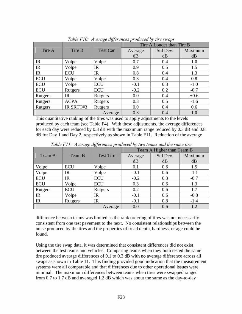
Table F10: Average differences produced by tire swaps Tire A Louder than Tire B

Tire A Tire B Test Car Average dB

Std Dev. dB

Maximum dB

IR Volpe Volpe 0.7 0.4 1.0 IR Volpe IR 0.9 0.5 1.5 IR ECU IR 0.8 0.4 1.3 ECU Volpe Volpe 0.3 0.4 0.8 ECU Volpe ECU -0.1 0.3 -1.0 ECU Rutgers ECU -0.2 0.2 -0.7 Rutgers IR Rutgers 0.0 0.4 ±0.6 Rutgers ACPA Rutgers 0.3 0.5 -1.6 Rutgers IR SRTT#3 Rutgers 0.0 0.4 0.6

Average 0.3 0.4 1.0 This quantitative ranking of the tires was used to apply adjustments to the levels produced by each team (see Table F4). With these adjustments, the average differences for each day were reduced by 0.3 dB with the maximum range reduced by 0.3 dB and 0.8 dB for Day 1 and Day 2, respectively as shown in Table F11. Reduction of the average

difference between teams was limited as the rank ordering of tires was not necessarily consistent from one test pavement to the next. No consistent relationships between the noise produced by the tires and the properties of tread depth, hardness, or age could be found.

Table F11: Average differences produced by two teams and the same tire Team A Higher than Team B

Team A Team B Test Tire Average dB

Std Dev. dB

Maximum dB

Volpe ECU Volpe 0.1 0.6 1.5 Volpe IR Volpe -0.1 0.6 -1.1 ECU IR ECU -0.2 0.3 -0.7 ECU Volpe ECU 0.3 0.6 1.3 Rutgers ECU Rutgers 0.2 0.6 1.7 IR Volpe IR -0.1 0.6 -0.8 IR Rutgers IR -0.1 0.8 -1.4

Average 0.0 0.6 1.2

Using the tire swap data, it was determined that consistent differences did not exist between the test teams and vehicles. Comparing teams when they both tested the same tire produced average differences of 0.1 to 0.3 dB with no average difference across all swaps as shown in Table 11. This finding provided good indication that the measurement systems were all comparable and that differences due to other operational issues were minimal. The maximum differences between teams when tires were swapped ranged from 0.7 to 1.7 dB and averaged 1.2 dB which was about the same as the day-to-day

F23

difference in the baseline conditions for individual teams. The effect of the different tire loading among the teams was not apparent by considering the swapped tire data alone. However, applying adjustments based on other research did indicate a small reduction in variability. After accounting for variability due to tires and test teams, some residual variation remained. For four specific test sections, higher variability was consistently observed. This variation could not be associated with any one team or tire and appears to be due combination of factors such as test site geometry possibly resulting in speed control issues, differences in tire sensitivity to specific pavements, and combined tire/vehicle effects for specific pavements. Comparison of the measurements made by the IR team on two different cars (Toyota Camry and Chevrolet Impala) indicated only very small differences (0.1 dB on average) that were less than to day-to-day differences. Repeat baseline measurements on the IR rodeo test car and tire conducted over three days were found to produce average differences and standard deviations comparable to the two-day differences measured by other teams except that range in differences was reduced by about half as shown in Table F12.

Table F12: Results of IR additional baseline testing on September 13, 14, and 15

Differences between Camry Baselines Sept 13th, 14th, & 15th Site

13th-14th 13th-15th 14th-15th Std Dev Range 1 0.5 0.1 -0.4 0.3 0.5 2 -0.1 -0.6 -0.5 0.3 0.6 3 0.1 -0.1 -0.2 0.1 0.2 4 0.2 -0.4 -0.5 0.3 0.5 5 0.8 0.7 -0.2 0.4 0.8 5a 0.1 0.7 0.6 0.4 0.7 6 0.1 -0.1 -0.2 0.1 0.2 7 0.1 -0.4 -0.5 0.3 0.5 8 0.2 -0.5 -0.7 0.4 0.7 9 -0.1 -0.3 -0.1 0.1 0.3 10 0.1 -0.6 -0.7 0.4 0.7 10a 0.3 -0.2 -0.5 0.3 0.5 Average 0.2 -0.1 -0.3 0.3 0.5 Std Dev 0.3 0.4 0.4 0.1 0.2

Abs Max 0.8 0.7 0.7 0.4 0.8

Summary In regard to improving the OBSI procedure to minimize the expected variation, two approaches could be used. The first is to tighten the requirements in the procedure for those parameters that appear to be significant. From these tests, given the lack of variation from team-to-team when testing the same tire, it appears that the current

F24

requirements on the physical set-up of the test vehicle and test fixture would not produce any further benefit. Speed control may have been a contributor to the variation both from team-to-team, run-to-run, and site-to-site, however, this can not be confirmed with the data obtained in this rodeo. Wheel path and start location may also be a factor in team- to-team variation, but these types of variation can not be controlled in the procedure itself. The largest source of variation was found to be due to tires; however, no consistent parameters (e.g. hardness, tread depth, etc.) were identified that could be further controlled. The second approach to minimizing variation is applying correction factors. In this study, applying correction factors for differences between tires did produce a reduction in the average variation between teams. However, developing a methodology for providing correction factors on an ongoing basis is problematic. Further, since variation in the relative levels produced by different tires varied with the pavement, such correction factors may not be of much benefit when testing any one pavement. Corrections for tire loading may also be considered, but further research is required to document how significantly they would reduce variation. Other correction factors that could be considered such as for environmental conditions and test speed will also require further investigation. OVERALL SUMMARY OF COMPARITIVE TESTING The measurements for all four rodeos were performed within the limits of the latest method of test5 for all of the test teams. As seen in previous studies, differences are likely due to a combination of environmental, tire, loading, and vehicle/operator variables. The method of test states that precision was expected to be 0.5 dB and bias to be 1.5 dB5. Concerning the differences between tires, the initial Method of Test did not explicitly set limits on tire hardness. In the ASTM International specification for the P225/60R16 SRTT (F 2493)13 it is stated that the durometer of the tire shall be 64±2 hardness values as measured at a stable temperature in the range from 69.8 to 77.0º F. It is assumed that these values also apply to the NCHRP procedure. In a separate ASTM standard test method (D2240-05)14, the reproducibility between laboratories is stated to have a standard deviation of 2.0. In this testing, it is clear that tire-to-tire variation is one of the primary variables between data sets. However, from this limited data set it is not clear that there is a direct correlation between tire hardness and tire/pavement level. The results of this study indicate that a more complex relationship between hardness and OBSI level than previously considered may exist, perhaps with tire hardness affecting some frequencies more than others. A greater understanding of differences between SRTT test tires and the implications on OBSI level is needed – whether this is to better define the parameters effecting the measured levels (tire hardness, tread depth, etc) or to better understand the how these parameters affect the measured levels over a variety of pavements. Controlled testing to establish a clear relationship between tire parameters such as hardness and wear and OBSI level is needed. Ultimately, functional specifications should be developed on these parameters.

F25

F26

The AASHTO Test Method procedure does not limit tire loading, but the results of the previous research5 recommended that loading be limited to 850 ± 100 lb be used. In these comparative tests, loading ranged from about 700 lbs to 930 lbs in baseline conditions. In some cases, the more lightly loaded cars produced results lower than heavier cars and in some cases not. Added weight and tire loading to baseline condition typically increased noise level for Yuma tests, however, the results display considerable scatter. As a group, the results suggest that this variable may not be independent of other vehicle and/or tire parameters. Literature has typically found an increase in tire/pavement noise with increased tire loading. The previous research found that increased tire loading resulted in increased tire/pavement noise at an average rate of about 0.2 dB per 100 lbs of added vehicle load. For the test track measurements reported earlier, the rate was 0.16 dB per 100 lbs. In the comparative testing, the previous research, and other literature, small fairly consistent effects of temperature were observed over relatively small ranges for the AC pavements. For these pavements, the expected trend of decreased noise level with increasing temperature was found. For the PCC pavement in Texas, the results were mixed and not as expected compared to the results of the track testing reported in the main body of the report and in the literature. There were no limits on temperature in the initial method of test. Because of the relatively small temperature gradients involved compared to other uncertainties, the current research specifically addresses temperature effects for the SRTT tire in a systematic way over a large range temperature and pavement types, so that the relationship can be better understood and limits or corrections could be developed. In the comparative testing, two instances damp pavement were encountered. In the Texas testing, damp pavement was suspected to be a cause of some variation, however, not conclusively demonstrated. In the NCAT testing, visible dampness was clearly of little consequence even for porous pavements. As considering the effects of temperature, tire hardness and loading did not explain all the differences in the comparative testing, other undocumented, differences between test teams may exist. In future comparative testing, it may be valuable to better document speed, wheel path, and start/stop locations as well as compare acoustic data acquisition and analysis system with bench-top methods. Also, testing under a range of environmental conditions, such as in the Texas testing, should be avoided until such time as when these varying conditions can be accounted. Tire swaps are also an invaluable tool in comparing test teams and should be part of all comparative testing. REFERENCES

1 Donavan, P.R., “Pavement Acoustics Testing at NCAT: OBSI, Sound Propagation, and Comparative Measurements”, prepared for the Washington State Department of Transportation under Agreement Y-10704 and Tire/Pavement Noise Research Consortium Pooled Fund TPF-5(135), by Illingworth & Rodkin, Inc., Petaluma CA, August 2010. 2 Donavan, P.R., “Comparative OBSI Testing at the General Motors Proving Ground in Yuma”, prepared for the Washington State Department of Transportation under

F27

Agreement Y-10704 and Tire/Pavement Noise Research Consortium Pooled Fund TPF-5(135), by Illingworth & Rodkin, Inc., Petaluma CA, August 2010. 3 Lodico, D., “Comparison OBSI Testing near Austin, TX: TxDOT Rodeo”, Prepared for the Texas Department of Transportation, the Washington State Department of Transportation under Agreement Y-10704, and Tire/Pavement Noise Research Consortium Pooled Fund TPF-5(135), by Illingworth & Rodkin, Inc., Petaluma CA, July 2010. 4 Donavan, P.R., “Comparative OBSI Testing in North Carolina: The North Carolina Rodeo”, prepared for the Washington State Department of Transportation under Agreement Y-10704 and Tire/Pavement Noise Research Consortium Pooled Fund TPF-5(135), by Illingworth & Rodkin, Inc., Petaluma CA, March 2011. 5 Donavan, P. and Lodico, D., “Measuring Tire-Pavement Noise at the Source”, NCHRP Report 630, Transportation Research Board, Washington, D.C., 2009. 6 Donavan, P. and Lodico, D., “Tire/Pavement Noise of Test Track Surfaces Designed to Replicate California Highways”, Proceedings of Inter-Noise 2009, Ottawa, Ontario, Canada, August 2009. 7“Standard Practice for Measurement of Tire/Pavement Noise Using the On-Board Sound Intensity (OBSI) Method”, TP 76-10 (Proposed), American Association of State Highway and Transportation Officials, Washington, DC, May 2009. 8 Donavan, P., “Comparison of OBSI Measurements for Four Research Teams: the Mesa Rodeo”, California Department of Transportation, Division of Environmental Analysis, Sacramento, CA, prepared by Illingworth & Rodkin, Inc., Petaluma, CA, January 2006. 9 Sandberg, U., “Influence of Tyre Rubber Hardness on Tyre/Road Noise Emission”, Proceedings of INTERNOISE 2007, Istanbul, Turkey, August 2007. 10 Sandberg, U., “Semi-Generic Temperature Corrections for Tyre/Road Noise”, Proceedings of Inter-Noise 2004, Istanbul, Turkey, August 2004. 11 Anfosso-Lédée, F., and Pichaud, Y.. “Temperature Effect of Tyre-Road Noise”, Applied Acoustics 68 (2007) 1-6, June 2006. 12 Bendtsen, H., Lu, Q., and Kohler, E., “Temperature Influence on Road Traffic Noise: California OBSI Measurement Study”, draft report of the Danish Road Institute, the University of California Pavement Research Center, Dynatest, and Caltrans (contact Bruce Rymer, Caltrans for availability). 13 F2493 Standard Specification of P225/60R16 Radial Standard Reference Test Tire, ASTM International, 100 Barr Harbor Drive, West Conshohocken, PA. 14 ASTM International, “Standard Test Method for Rubber Property – Durometer Hardness”, Designation D 2240 – 05, ASTM International, West Conshohocken, PA.