project: developing expenditure to … sector in nsw. finalreport to the nsw recreationalfishing...
TRANSCRIPT
Project Developing a cost effective state wide expenditure
survey method to measure the economic contribution of
the recreational fishing sector in NSW
Final Report to the NSW Recreational Fishing Licence Trust
NSW Department of Primary Industry November 2013
NSW RF expenditure survey‐2012
The Australian National Centre for Ocean Resources and Security (ANCORS) University of Wollongong is Australiarsquos only multidisciplinary university‐based centre dedicated to research education and training on ocean law maritime security and natural marine resource management providing policy development advice and other support services to government agencies in Australia and the wider Asia‐Pacific region as well as to regional and international organizations and ocean‐related industry
Website contact httpancorsuoweduau
Report contact Professor Alistair McIlgorm E‐mail amcilgoruoweduau Mob 0417 211 886
Acknowledgements
We thank the following people for assistance
Dr Jeff Murphy and Mr Bryan Van der Walt of NSW DPI for assistance with access to data from the
NSW Recreational Fishing Licence database
The Survey fieldwork was under taken by IRIS Research Thanks to Mr Simon Pomfret and Mr Geoff
Besnard (wwwirisorgau)
The regional economic analysis was undertaken by Western Research Institute Bathurst thanks to
Mr Tom Murphy Dr Andrew Johnson and Dr Ivan Trofimov (wwwwriorgau)
Thanks to the NSW Recreational Fishing Trusts for funding this research
The research report is issued under the standard University disclaimer
Suggested citation
McIlgorm A and J Pepperell (2013) Developing a cost effective state wide expenditure survey
method to measure the economic contribution of the recreational fishing sector in NSW in 2012 A
report to the NSW Recreational Fishing Trust NSW Department of Primary Industries November
2013 Produced by the Australian National Centre for Ocean Resources and Security (ANCORS)
University of Wollongong
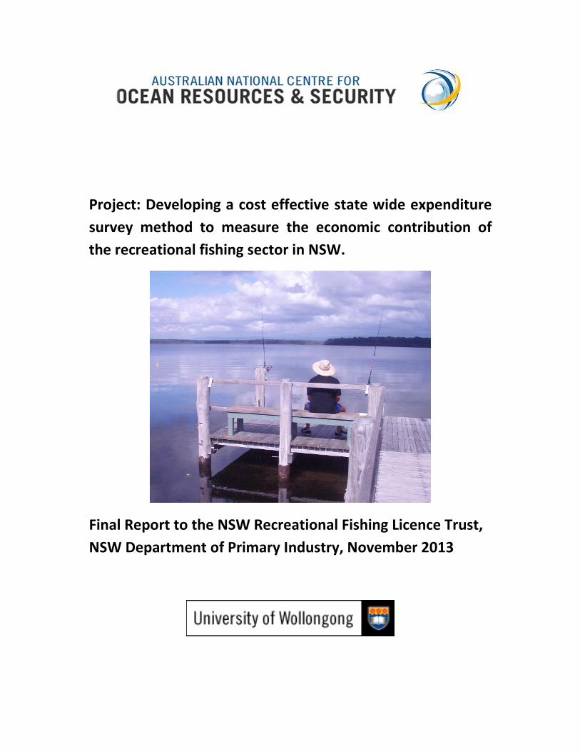
Cover photo by Alistair McIlgorm An angler enjoying estuary flathead fishing‐ South Coast NSW
2
NSW RF expenditure survey‐2012
Table of Contents
Headline results 5
Executive summary 6
1 Introduction11
11 Past recreational fishing expenditure studies and NSW 12
12 Comparing expenditure survey methods 14
13 Activity results from past studies 14
14 Discussion 15
2 The NSW Recreational Fishing Expenditure survey ndashobjectives data and methods 17
21 Objectives 17
22 Data available 17
23 Methods19
24 Estimating the total expenditure by fishers 21
3 Survey results 23
31 The fieldwork results ‐ Details of sampling and completed interviews 23
32 Fishing activity from the survey samples 26
33 Comparisons between methods and samples 29
34 Discussion of the sampling and activity results 30
34 Estimation of recreational fishing expenditure per angler 32
4 State‐wide and regional expenditure estimates 37
41 Estimating total expenditure 37
42 Expanding the sample of fishers and expenditure 37
43 State‐wide expenditure estimates 38
44 A probabilistic simulation approach to the estimation of total state recreational fishing
expenditure 42
45 Discussion 43
5 Regional economic impact estimates 45
51 Methodology 45
52 Economic impact analysis 45
53 The Economic Impact of Recreational Fishing on the Regional Economies of NSW46
54 Conclusion51
6 Developing a cost effective approach to expenditure surveys 52
61 The objectives of an recreational fishing expenditure survey 52
62 Sampling data issues and findings 52
3
NSW RF expenditure survey‐2012
63 What sample size is required 52
64 Discussion ‐ Scoping a recreational fishing expenditure survey strategy for NSW 54
65 Conclusions 55
References 57
Appendix 1 What determines recreational fisher expenditure in NSW 59
Appendix 2 Socio‐ economic groups and RFs in NSW ndash a cluster analysis 62
4
NSW RF expenditure survey‐2012
Headline results
Expenditure on Recreational Fishing in NSW
The expenditure of an estimated 773000 adult anglers in NSW in 2012 was
$1625bn on travel for recreational fishing trips fishing tackle and boat‐related items
This included $1861m of expenditure by Interstate visiting fishers The total expenditure translated
into the following impacts in the NSW economy
$342bn of economic output
$1625bn added value
$8773m household income and
14254 full time equivalent (FTE) jobs
The economic output for recreational fishing in all NSW was $342bn with an associated
employment of 14254 equivalent full time jobs These jobs are in the retail trade sector hospitality
personal and other services and in the transport and storage sector The value added was $1625bn
which is 036 of estimated gross state product in NSW Household income from recreational
fishing was $8773m in retail finance and insurance hospitality professional and technical services
and the wholesale trade sectors
Regional estimates
Based on survey data anglers spent $50196 million $51165 million $36086 million $25140
million in the NSW North Coast Sydney NSW South Coast and NSW Inland regions respectively The
economic impacts of recreational fishing on the respective regions are as follows
Region North Coast
Sydney South Coast
Inland All NSW
Output ($m) 73465 100286 39522 35381 342035
Value added ($m) 35355 49156 18417 14985 162561
Household income ($m) 16875 28888 8760 7350 87728
Employment (no) 3320 3944 1808 1539 14254
In terms of regional output valued added household income and full time equivalent employment
the absolute economic impacts of recreational fishing expenditure were the highest in Sydney
followed by NSW North Coast NSW South Coast and NSW Inland
However in relative terms economic impacts (as percentage of total income and employment
impacts in the respective regions) were the highest in NSW South Coast (167‐ 212) followed by
NSW North Coast (081‐098) NSW Inland (030‐038) and Sydney (025‐028) These relative
disparities reflect the large size of Sydney and NSW Inland economies and smaller size of NSW North
Coast and NSW South Coast economies
5
NSW RF expenditure survey‐2012
Executive summary
This study estimated the expenditure of recreational fishers (RFs) in NSW and its economic impact in
NSW and in different regions of the state
The study confirmed that there are approximately 905048 anglers in NSW of whom 773000 are
adults over 18 years of age Of these adults our survey found 65 held a Recreational Fishing
Licence (RFL) and 35 were concession and pension holders that did not require a licence
The study utilized a telephone survey to interview RFs about their activity and expenditures by two
different methods The first survey method used a traditional screening survey to locate RFs among
the general population and then interview them The second used a sample of anglers from the RFL
data base records and interviewed these fishers also Both survey approaches subdivided NSW into
the study areas of Sydney North coast South coast and Inland NSW The results from the two
methods were compared to determine if just the RFL data base could be used for surveys of the
angling population thereby reducing or obviating the need for the more expensive screening survey
method
Past recreational fishing surveys in NSW and across Australia were compared which indicated several
methodological differences in the past decade among catch and effort surveys and expenditure
surveys The survey conducted for the present study used a recall survey method as opposed to
more expensive longitudinal diary methods
Two waves of fieldwork surveying were undertaken in April and September 2012 A computer aided
telephone interview (CATI) system was used to make screening calls through its regional random
dialling facility to locate households containing at least one person who had fished in the previous 6
months When RFs were located by the screening calls they were asked to take part in a survey
about recreational fishing The CATI telephone system required more calls to ldquowhite pagerdquo numbers
than envisaged to locate the target number of RF households with up to 50 being dead numbers
There was a surprising high refusal rate with only 48 of the RFs identified choosing to complete the
survey This may have led to non respondent bias and have impacted the representativeness of the
screening survey responses Fieldworkers reported some interviewees were suspicious the survey
was ldquochecking up on licencesrdquo which may have discouraged responses
Analysis of the 2010 RFL records for the second survey confirmed that fisher contact details for the
majority of electronic records on the NSW Government Licencing Service (GLS) database were for 1
and 3 year licences The 3 day and 1 month licences sold manually were not migrated onto the GLS
data base but stored manually by NSW DPI Nevertheless the sample of RFL licence holders
accounted for the fewer 3 day and 1 month licence holder records in the total database The survey
method made telephone calls to these known RFL holders was more successful in locating fishers
than the screening survey and had a much lower refusal rate of 27
6
NSW RF expenditure survey‐2012
Sample results
Survey personnel asked fishers to recall their previous 6 months of fishing activity in terms of trips
and days fished and fishing expenditures from their last trip including fishing tackle Major boat
related expenditures were recalled for the previous 12 months The survey results for April and
September fieldwork waves were compared statistically and did not differ significantly in terms of
fishing activity for either trips or days fished Fishing trips per annum and average days fished were
significantly higher for anglers contacted via the random screening survey compared with those
from the RFL database Days fished by licensed and unlicensed fishers were not significantly
different but unlicensed fishers were found to make significantly more trips than licensed fishers
Questions on trip activity indicated that 54 of Saltwater (SW) fishers and 67 of Fresh water (FW)
fishers fished less than 5 trips a year the average SW trips being 875 trips FW 38 trips and 107
trips per annum when combined The length or fishing trips averaged between 14 and 16 days A
finding that influenced average days fished was that 3 of anglers fished over 40 trips per year ndash a
relatively high proportion of such avid anglers Overall anglers fished an average of 146 days The
total combined sample showed that 38 of fishers fished less than 5 days a year while 6 of anglers
fished in excess of 40 days per annum
All respondents provided expenditure estimates on their last trip The average fisher spent $15405
on fishing trip related items including car travel of $6974 A further $7120 was spent on tackle and
boat fuel per trip totalling an expenditure per angler of $22524 per trip
The annual fishing related boat expenditure on average in NSW was $76815 per angler with a high
range Average daily trip expenditures in SW and FW were similar but boat expenditure for SW
fishers ($95618 per annum) exceeded that of FW anglers ($36515) no doubt due to marine fishing
craft typically being larger and more costly
The expenditure patterns of NSW anglers were investigated by multiple regression and cluster
analysis to identify the drivers of RF expenditure
Multiple regression analysis identified two significant expenditure drivers to be the holding of an RFL
and number of SW fishing trips taken It also indicated that distance travelled was a significant part
of trip expenditure Fishing tackle expenditure was correlated with income but boat expenditure
was related to both the number of SW fishing trips per annum and household income
The cluster analysis revealed an overall picture of groups of ldquoordinaryrdquo fishers (approximately 85)
with low levels of activity in which household income levels may differ (half lower half higher)
secondly a group of dedicated anglers (approximately 12) who are frequent fishers and have high
expenditure and thirdly a highly avid fishing group (less than 3) with very high fishing activity and
high to very high expenditure
7
NSW RF expenditure survey‐2012
The results confirm the only previous examination of the socio‐economic characteristics of RFs in
NSW by Dominion (2003) ndash that recreational fishing is a pastime enjoyed by a diverse range of
people with a range of levels of enthusiasm crossing the entire socio‐economic spectrum
Estimating state‐wide expenditure
Total state expenditure on recreational fishing was estimated using the available RF household and
population data the estimates of trips made amounts spent per trip on tackle and annual
expenditures on boats The sample expansion was based on ABS household data and survey
responses
A problem in recreational fishing studies is the skewedness in the distribution of trip activity which
declines exponentially with the increasing number of trips made This strongly influences the
distribution of total expenditure estimates The annual expenditure by anglers is highly variable
Total state‐wide recreational fishing expenditure can be calculated as a mean value The study was
also able to estimate a distribution around the mean estimate by use of a Monte Carlo simulation
model This generated a range around the total predicted expenditure estimates with a probability
and cumulative probability for each possible level of RF state expenditure
State wide expenditure results
State‐wide expenditure on recreational fishing in NSW was estimated at $1626bn per year
including $186m by Interstate visitors (ie $1439bn from NSW residents) The simulation model
predicted that this mean of $1626bn has predicted 5 and 95 confidence intervals of $0896bn to
$3136bn The probability distribution reflects the skewedness of the trip frequency distribution as
the mean is not the most probable value but reflects the higher expenditures of the long lsquotailrsquo of
more avid anglers The predictions derived from the model explain how some RF expenditure studies
can estimate high estimates without realising their achievement is improbable
State‐wide total expenditure is much higher for SW fishers ($14bn) than for FW ($0266bn) with SW
expenditure being 86 of all expenditure and FW 14
Initial estimates of expenditures indicate that anglers living in Sydney account for 56 of total NSW
expenditure North coast 19 South coast 6 Inland 8 and interstate visitors 11 These
expenditures are adapted in the regional analysis in Chapter 5 to take account of expenditures on
trips into other regions
Regional economic impacts
To estimate the economic impacts of recreational fishing on NSW North Coast NSW South Coast
Sydney and NSW Inland regions as well as for NSW as a whole Western Research Institute (WRI)
used the 2011‐12 Simulating Impacts on Regional Economies (SIRE) input‐output model of the
respective regions and NSW as a whole Economic impacts were provided in terms of output value
added household income and full time equivalent (FTE) employment
8
NSW RF expenditure survey‐2012
Results were adjusted to account for expenditure in the regions becoming $50196 million $51165
million $36086 million and $25140 million in NSW North Coast Sydney NSW South Coast and
NSW Inland regions respectively
The economic impacts of recreational fishing on the respective regions are as follows
Region North Coast
Sydney South Coast
Inland All NSW
Output ($m) 73465 100286 39522 35381 342035
Value added ($m) 35355 49156 18417 14985 162561
Household income ($m) 16875 28888 8760 7350 87728
Employment (no) 3320 3944 1808 1539 14254
The economic output for recreational fishing in all NSW is $342bn generating associated
employment of 14254 equivalent full time jobs These jobs are in the retail trade sector hospitality
personal and other services and in the transport and storage sector
The value added is $1625bn which is 036 of estimated gross state product in NSW Household
income from recreational fishing is $8773m in the retail sector finance and insurance hospitality
professional and technical services and the wholesale trade sector
In terms of regional output valued added household income and FTE employment the absolute
economic impacts of recreational fishing were the highest in Sydney followed by NSW North Coast
NSW South Coast and NSW Inland However in relative terms economic impacts (as percentage of
total impacts ndashincome and employment in the respective regions) were the highest in NSW South Coast
(167‐ 212) followed by NSW North Coast (081‐098) NSW Inland (030‐038) and Sydney (025‐
028) These relative disparities reflect the large size of Sydney and NSW Inland economies and
smaller size of NSW North Coast and NSW South Coast economies
Developing a cost effective approach to expenditure surveys
The project examined the requirement for ongoing expenditure surveys and how these might be
met in a cost effective fashion The study recognises that the RFL data base can be used to reduce
survey costs but recommends that additional consideration needs to be given to how to use this
data base for representative estimates before fully adopting RFL based surveys to the exclusion of
screening surveys The project also examines the requirement for minimum reliable sample sizes
that may apply to future surveys and how this can reduce costs
A large‐scale expenditure survey every 5 years is recommended with either annual or biennial
updates between main surveys The simulation model used here could assist with adjusting
estimates between main surveys An additional smaller survey could be made in year three if a
need‐to‐update data was evident
9
NSW RF expenditure survey‐2012
In conclusion a full state‐wide survey using the RFL data base to sample 1000 anglers in major
regions is recommended every 5 years with an option of updating results by indexing annually or bi‐
ennially and considering a smaller survey (250 state wide or 500 for regions) in year three also
The economic impact analysis can follow the five year survey pattern and can be adjusted between
surveys Simulation modelling can also be used to provide an improved understanding of the
uncertainty surrounding expenditure estimates and may be used to confirm estimates between
main surveys also
10
NSW RF expenditure survey‐2012
1 Introduction This project was undertaken to achieve the following objective ldquoThe project will evaluate the
economic expenditure and contribution of the recreational fishing sector in NSW and determine the
most cost effective approach for future expenditure surveysrdquo (RTF project application) 1
The expenditure of recreational fishers in NSW was previously estimated by Dominion Consulting
(2003) and in the economic report of the national survey (Campbell and Murphy 2005)
This study reports the recreational expenditure and economic impacts for all of NSW and for the
four main regions in NSW Sydney North Coast South Coast and Inland NSW The expenditure of
interstate recreational fishers in NSW is also estimated
The regional economic significance of the recreational fisher (RF) expenditure in the NSW state
economy has not previously been measured Regional economic impact analysis enables the direct
and indirect benefits derived from recreational fishing expenditure to be determined and the
associated employment estimated in NSW
The report also examines the options for future expenditure surveys of RFs investigating the most
cost effective way to gain regular accurate expenditure and economic impact information on
recreational fishing activity in NSW This will include how to most effectively use the sampling frame
available via the recreational fishing licence Changes in communication technology in the last
decade may also have impacted the traditional approaches to recreational fishing surveys and as yet
new web based and social media approaches are relatively untested
The study commenced by examining recent approaches to measuring recreational fishing
expenditure in Australia and some relevant international expenditure surveys such as used in the
United States which may indicate international best practice
The use of expenditure data is a baseline measure of economic activity reflecting the dollars spent
on going fishing and on fishing equipment on an annual basis The expenditure of anglers is similar to
an expenditure on any other sport or leisure in the economy and we can use regional economic
approaches to determine the contribution and impacts of that expenditure in the NSW state
economy In contrast to expenditure surveys studies of the ldquoeconomic valuerdquo of recreational fishing
seek to determine the value of access to fishers over and above what they pay to go fishing
(Cunningham et al 1985 Galeano et al 2004 Rolfe and Prayaga 2007)
Estimating state‐wide expenditure and regional economic activity in different areas of the state can
reveal differences in regional impacts and clarify the relationship between recreational fishing
activity associated expenditure and its benefits to the state economy
1 Project title ldquoDeveloping a cost effective state wide expenditure survey method to measure the economic contribution of the recreational fishing sector in NSWrdquo NSW Recreational Fishing Trusts ‐ contract L92
11
NSW RF expenditure survey‐2012
11 Past recreational fishing expenditure studies and NSW
Past recreational fishing expenditure surveys have used slightly different methodologies depending
on the objectives of the study The general pattern in expenditure surveys is to use a field survey
method such as face to face or telephone interviews to contact and survey fishers asking questions
about fishing activity and the costs of the activity on a trip or annual basis (McIlgorm and Pepperell
1999 Dominion 2001 and 2003 Campbell and Murphy 2005 Gentner 2008) The method usually
involves recall of past fishing events over a prior fishing period usually 12 months or the keeping of
a diary to log fishing activity on an ongoing basis (Gentner 2008)
Expenditure surveys in different states of Australia prior to the year 2000 were reviewed in
McIlgorm and Pepperell (1999) The National Survey in 2001 estimated the number of recreational
fishers nationally their fishing activity and their catch using a national telephone based screening
survey to identify recreational fishing households Cooperating anglers then responded to monthly
telephone contacts via a diary based method (Henry and Lyle 2003) Respondents also recorded
expenditure over a 12 month period and enabled expenditure estimates to be produced as an
additional component of the main national survey which was designed to measure catch (Campbell
and Murphy 2005)
Campbell and Murphy (2005) estimated from the data collected in the National Survey that total
national recreational fishing expenditure in 2001 was $186bn of which $554m (307) occurred in
NSW2 Importantly these estimates did not include several categories of ancillary trip expenditure
such as food consumed while on a fishing trip eating out and entertainment (which were included in
the current study) and were therefore conservative estimates of expenditure on all items due to
fishing
In NSW a series of regional expenditure surveys using telephone and face to face survey methods
was carried out by Dominion Consulting for the 1999‐2004 period (Dominion 2001 and 2003
McIlgorm et al 2005) These studies also produced estimates of regional economic impact of
recreational fishing in the regional areas being surveyed
Other studies have provided estimates of national retail and wholesale expenditure for the fishing
tackle sector across Australia (Dominion 2003 and 2005) In 2004 $601m of fishing tackle was sold
nationally by retailers3 (Dominion 2005) However retail and wholesale tackle sales data are supply
side estimates and are only part of the estimated total annual expenditures of recreational fishers
on this activity
Non‐NSW
Recently in other states of Australia several recreational fishing expenditure studies have been
conducted Ernst and Young (2009) conducted an economic survey of recreational fishing in Victoria
2 Using consumer price index adjustment of 138 (2001‐2012) from ABS (2012) these estimates in 2012 terms would be
$256bn nationally and $765m in NSW3 The National Survey estimated tackle and bait expenditure by anglers nationally at $223m in 2000‐01 (Campbell and Murphy 2005) There has not been an attempt to reconcile actual industry tackle sales with such expenditure survey results
12
NSW RF expenditure survey‐2012
using an internet based method to sample 1000 persons and interview 200 anglers with economic
modelling estimates of the economic contribution of the sector In that study the estimated number
of fishers in Victoria were 720000 compared with a previous estimates of 550000 which resulted
in a substantial increase in the total estimated state expenditure on recreational fishing The study
raised questions about estimates of fisher populations used for expanding expenditure estimates
the age groups included in the survey (under 18s etc) the distribution of fishing trip activity and
the variation in angler expenditure levels
Using internet‐based surveys is a new area requiring assurances of representative expansion to state
wide estimates There is the potential to overestimate recreational fishing expenditures if avidity
biases are not controlled Survey design decisions all influence the accuracy of estimates of fishing
activity and hence total expenditure Another study by Ernst and Young (2011) of the Murray Darling
Basin raised similar concerns about over‐estimation of expenditure due to a high RF population
estimate and the ensuing assumed distribution of trip frequency and expenditures applying a
sensitivity analysis which only partially addressed the issue
International studies
International best practice can most likely be seen in the five‐yearly series of NOAANMFS National
recreational fishing Expenditure Surveys in the US These have generated estimates of the economic
contribution of recreational fishing activity in a series dating back to the 1970s (Steinback et al
2004 Gentner and Steinback 2008)
The NOAA‐NMFS survey has always been based on the Marine Recreational Information Program
(MRIP) which is combines two different survey approaches to estimated catch and effort These are
an intercept survey at major boat ramps and a cross‐checking telephone survey of anglers in coastal
households over a year asking anglers to recall activities over the previous two month period
(Gentner 2008 Gentner and Steinback 2008) Expenditure on some fishing related items are
collected by phone but a mail survey has also been used to collect ldquodurable expendituresrdquo such as
boats and fishing gear since 2006 (Gentner and Steinback 2008)
The latest national US RF expenditure survey was commenced in 2011 (NOAA 2011) to measure the
contribution that saltwater RF expenditure makes to the US economy particularly in terms of
employment That study found that
ldquoRecent estimates indicate there are approximately 12 million saltwater recreational anglers taking
about 85 million trips a year Combined expenditures total $31 billion dollars representing an $82
billion dollar impact and supporting half a million jobsrdquo NMFS (2012)
These US studies illustrate the economic impacts of recreational fishing expenditure in the wider
economy Our objective is to make this information available in NSW where the current economic
contribution and economic impact of recreational fishing needs to be determined and be available in
the public arena
13
NSW RF expenditure survey‐2012
12 Comparing expenditure survey methods
Any comparison of methods has to recognise that objectives in economic and expenditure studies of
RFs vary In this study we are comparing expenditure by recreational fishers and not any associated
non market values
The measure of recreational fishing total expenditure is the product of the number of fishers their
fishing activity and their expenditures in the activity annually Experience in the ABS and in previous
RF surveys indicates that household expenditure should be incorporated in the generation of state‐
wide estimates where each household will have one or more anglers and trip expenses are
ldquohouseholdrdquo related (Henry and Lyle 2003 Campbell and Murphy 2005)
While national data for the general population is available from the Australian Bureau of Statistics
(ABS) we require sampling of the general population to determine what proportion have been
recreational fishing in the study period A random telephone survey to screen the population was
used to locate recreational fishers
Each study has to decide how it will structure samples and find those to interview The telephone
screening survey of the whole general population is used to identify households with RFs (Henry and
Lyle 2003) However many fishers are below 19 years of age or may not have a phone The fisher in
a household can be recalled and surveyed with a re‐call method or engaged in a diary based method
or a postal survey (Gentner 2008) This survey approach has generally sought to obtain a random
sample of respondents who are recreational fishers
Asking recreational fishers to recall their fishing activity is a low cost single interview event but has
inherent risks of non‐response re‐call and other biases such as avidity bias where too large a
proportion of the most active fishers are interviewed (Johnson 1999) There is likely less recall bias
when a combination of survey methods are used (Gentner 2008)
Fishing activity can be measured as days fished which is an effort measure in recreational fishing
catch surveys but also as a number of fishing‐related trips taken per annum The number of trips is
the basis of expenditure estimates that vary with activity though less frequent large expenditures
such as capital boat expenditures and maintenance must also be incorporated into annual costs Trip
related expenses reflect travel most of which is road travel accommodation and food and
consumables expenditure for the fisher and their accompanying party Expenditure on small items of
fishing tackle bait and fishing consumables are also trip related Expenditure on capital items such
as boats motors and trailers is estimated on an annual basis and is often reduced pro rata for non
recreational fishing use measuring only the capital attributable to recreational fishing activity
13 Activity results from past studies
In Australia there have been numerous catch and effort surveys of recreational fishers and these
have focused on estimating fishing effort measured in days fished Prior to 2000 McIlgorm and
14
NSW RF expenditure survey‐2012
Pepperell (1999) identified 5 recreational fishing studies across Australia which estimated average
number of days fished per angler per annum at between 125 and 15 days
Since the introduction of the monthly fishing diary system in the National Survey 2001 other catch
and effort surveys covering individual states or territories have also used this method The
estimated average number of days fished per year per angler by this method has averaged 613 days
nationally and 60 days in NSW (Henry and Lyle 2003) 45 days for South Australia (Jones 2009) and
40 days in Queensland (Taylor et al 2011)
Past studies of recreational fishing expenditure have differed in methodologies used and in
categories of expenditures collected and have not generally followed the catch and effort diary
approach Activity and expenditure is seen as being trip related where a fishing trip may extend for
one or more days In comparing the expenditure recall surveys of the past decade with the catch and
effort studies a two layer view of lsquodays fished per annumrsquo becomes evident Surveys designed to
measure catch and effort indicate estimates of average days fished at circa 6 days per annum (see
above) On the other hand in surveys specifically estimating expenditure estimated days fished per
angler have been higher for example 139 days per annum in NSW (Dominion 2001) 12 days and 14
days per annum (McIlgorm et al 2005) Ernst and Young (2009 and 2011) estimated 14 trips per
annum in which case number of days fished would be in excess of this
These two approaches of expenditure surveys asking interviewees to recall expenditures in the past
year versus the monthly catch and effort diary of the National Survey still need to be reconciled in
Australia The US NOAArsquos approach with two different survey types may have some benefits to offer
future research in NSW
14 Discussion
Expenditure surveys currently face significant issues in terms of their methodology particularly due
to changes in telecommunications internet technology and the licensing of fishers all of which
potentially alter the capacity to access a non biased random sample of individual or household
expenditures that can be appropriately expanded into accurate state‐wide expenditure and
economic impact estimates This was noted in the US in circa 2008 and is why the US methodology
post 2006 has been more complex (Gentner and Steinback 2008)
The change in communications technology is particularly seen in telephone based methods where
since 2000 increasing use of mobile phones has impacted use of ldquowhite pagesrdquo home phone lines
(ACMA 2013) Likewise the number of households opting to be ex‐directory or not to take
unsolicited calls due to privacy concerns and regulations has increased The telephone based survey
industry has adapted to these changes which are on‐going but we are all in a large scale technology
transition process that impacts survey design and methodology (ACMA 2013)
The internet has potential appeal as a survey vehicle for expenditure surveys but the same issues of
gaining a random sample ie participant selection with possible avidity and non respondent biases
15
NSW RF expenditure survey‐2012
and re‐call bias are major issues The ldquosamplerdquo is unlikely to be representative of the whole
population For example currently older fishers would not be as open to internet surveying or social
media use for surveys as younger fishers
The introduction of a general RFL in some states now means that approximately 60‐70 of all fishers
in those states are licence holders The availability of contact details for NSW RFL holders has led this
project to examine whether the random screening survey to detect fishers which is the most
expensive part of traditional surveying can be substituted by lsquocaptiversquo RFL data base survey
approaches to estimate state‐wide recreational fishing expenditure However if for example
licence holders fish more frequently than non licence holders will there be a possible avidity bias if
only licence holders are surveyed (Gentner 2008) We therefore need to investigate what
conditions are required to use the RFL data base appropriately and thereby to hopefully reduce the
need for expensive screening surveys
Another aim of the study is to investigate possible behavioural issues arising from the existence of
the recreational fishing licence For example are licence holders and non‐licence holders
significantly different across a range of recreational fishing activities or socio‐economic
characteristics The possible benefits of using recreational licence records as the basis for less
expensive expenditure surveys in the future is a key element of this study
Infrequent studies of recreational fishing expenditure are separated in time and often rely on
varying methods and sample sizes resulting in variable accuracy The NSW recreational sector would
be better served by more frequent updating of measures of the contribution of the sector to the
economy This requires investigation of more cost effective recreational fishing expenditure survey
strategies Questions such as ldquohow many anglers do we need to interviewrdquo are addressed in this
study and a future expenditure survey strategy is proposed
Other surveying issues arise in attempting to address more specific issues on activity in the sector
For example is the size of a survey sample for all recreational fishers sufficient to estimate the
expenditure of particular groups of fishers such as those using recreational charter boat services
state wide Fishers using charter vessels may not be sufficiently captured in the sample sizes
possible under cost constraints since such activities are likely ldquorare eventsrdquo among NSWrsquos estimated
773000 adult fishers An alternative direct sampling of the NSW commercial charter boat fishery has
been recommended and will be reported in another project (Dominion in prep)
In this study we examined past expenditure surveys in Chapter 1 and details of the expenditure
survey approach methods and survey instruments used in the current study in Chapter 2 Chapter 3
reports the results of the survey and Chapter 4 develops NSW state expenditure estimates Chapter
5 reports the state‐wide regional economic impacts of recreational fishing expenditure and
employment estimates Chapter 6 completes the study proposing cost effective surveying of
expenditure for the future
16
NSW RF expenditure survey‐2012
2 The NSW Recreational Fishing Expenditure survey ndashobjectives data and
methods
21 Objectives
The first objective of the expenditure survey project is to provide the recreational fishing sector in
NSW with an up to date profile and estimate of recreational fishing expenditure This will require
sampling the known population of RFs for their fishing activity and expenditure patterns Part of this
objective is to gain an understanding of the regional patterns of recreational fishing activity
expenditure and economic impact in all of NSW and each of the four regions
Sydney ‐ (ABS SD region)
North coast ‐ (ABS Hunter Mid North Coast Richmond‐ Tweed SD regions )
South coast ‐ (ABS Illawarra and Lower South Coast SD and SDD regions ) and
Inland NSW‐ (ABS Central west Far west Murray Murrumbidgee Northern North Western
SD regions and Queanbeyan Snowy and southern Table and SSD regions) ABS (2011)
Expenditure of interstate angers in NSW is also considered
The NSW RFL has been in place for the past decade but it is unknown if this has altered recreational
fishing activity and expenditure by anglers It is also an objective of this study to investigate how the
RFL database may be used in expenditure survey sampling potentially reducing the need for more
expensive screening surveys of the general population to locate recreational fishers
22 Data available
221 Population and household data for NSW
Data on the population and number of households in the study regions of NSW is available from the
Australian Bureau of Statistics (ABS) Table 1 indicates the relative populations (aged between 19
and 75 years old) of the relevant statistical divisions (SD) for the areas in the study4
Table 1 The ABS population and household data on the NSW study area (ABS2011)
Area Population 2010 (gt18-75)
by region
Households by
region Rec Fishers HH
Sydney 3160897 633 1376583 557 230
North coast 835229 167 570688 231 146
South coast 350750 70 207195 84 169
Inland 649564 130 315987 128 206
Total 4996461 100 2470453 1000 202
4 SDs are now part of the ABS geographic area system replacing SD and SSD in 2011 The four study areas use the component data for reach SD area Note South coast is actually the coastal SSDs other South coast Inland SSDs being grouped with the Inland category
17
NSW RF expenditure survey‐2012
In Table 1 Sydney is seen to have the largest percentage of state population and households
followed by North Coast Inland and South Coast The variability of the relationship between
population and households is evident with Sydney having more persons per household (23)
compared with rural regions (146 to 206)
222 The RFL data system records
Recreational fishing licences are sold electronically as well as manually using a licence agent system
The NSW RFL data system has been moving from predominantly the manual system when the state
wide licence was first introduced in 2001 to an increasing proportion of electronically recorded
licence records held in the centralised NSW Government Licensing Service (GLS)
(wwwlicencenswgovau) Manual licence sales data is stored by NSW Department of Primary
Industries (NSW DPI) Therefore for the year 2010 the RF licence sales records available to this
study were either RFL sales recorded electronically in the GLS or records of the number of licences
sold manually through agents
The licence sales by agents (without an electronic terminal) are recorded manually in licence books
and sales records for all licences are submitted to NSW DPI in a monthly reconciliation process
Contact details of fishers for three day and one month licences are stored manually by NSW DPI (ie
not entered onto the GLS) The distribution of the different types of licences recorded on the GLS
means that in the 2010 data download obtained for the project in 2012 there were fewer 3 day or 1
month licence records than would be expected from total licence sales The downloaded GLS data
therefore under‐represents 1 month and 3 day licences as there were only 27 of the total sales of
these licence types entered on the GLS5 The numbers of RFL licence holders in 2010‐11 are
estimated in Table 2
Table 2 The estimated sales of different types of licence in the 2010‐11 period (Source DPI)
5 In the period July 2010‐June 2011 DPI records non GLS records as a percentage of total sales and renewals 3 day 72
1month 73 1year 49 3 year 16 Most 3 year records are on the GLS half of the 1 year and only 27 of 3 day and 1 month licences in that time period
18
NSW RF expenditure survey‐2012
Table 2 reports the estimates numbers of 3 day 1 month 1 year and 3 year RFL sold in 2010‐11 We
use this information to assist in the estimation of the total number of fishers in NSW
The number of licence sales can be adjusted to include non‐compliant fishers (assumed to be 5 of
licence holders) and the 35 of fishers not requiring a licence (as estimated in McIlgorm et al 2005
and confirmed later in this study) plus young fishers 5 to 19 years old (171 of the population ABS
2011) Using these figures a total of 905048 anglers is conservatively estimated This total also
includes interstate anglers buying licences in NSW The RFL data in the GLS system does not have
any information on non‐licence holders but does record NSW licence holders who reside in other
States
The current estimate of 905048 is less than previous NSW DPI and National Survey estimates of
close to 1 million fishers (DPI pers comm Henry and Lyle 2003) Other studies have noted a
possible decline in recreational fishing participation since the 2001 National Survey (Jones 2008) as
the method here is based on licence sales with several assumed adjustments so should not be taken
as a definitive participation estimate We chose to use the ABS household data for survey
expansions
23 Methods
The methods we used had to be able to facilitate estimation of the total expenditure of recreational
fishers state‐wide Sampling approaches were therefore designed to enable total estimates to be
developed from the samples taken
231 Sampling
We used two survey sampling approaches for the study
(a) Telephone household screening survey to identify households with a RF A random screening
survey using the home phones of 4000 households in the general population was proposed to
identify 800 anglers Each angler identified was then asked to complete an 8 minute survey of
fishing‐related activity and expenditure
(b) RFL database to contact known anglers (licence holders) A survey sample of 750 licence
holders from the RFL database was proposed to provide 500 completed 8 minute surveys of RFL
holders
232 Preparations for the fieldwork sampling survey
Ethics approval was required through the University system to conduct the survey Due to privacy
and ethical issues the fieldwork did not call ldquochildrenrdquo ie those under 19 years of age Those
fishers over 18 years of age are either licensed or are concession holders due to having a pension or
disability
A range of issues was considered in the fieldwork design
19
NSW RF expenditure survey‐2012
a) Field work survey method
In the last two decades in Australia there has been a move away from postal surveys with face to
face interviews diary keeping phone and mobile phone and internet methods being used After
considering the task we chose a telephone survey method to contact the desired audience within
budget limits The telephone survey field work was undertaken by IRIS Research a telephone
surveying marketing and research business
The market research company conducted two telephone surveys using (a) a whole population
database for the random household calls and (b) RFL licence data base records supplied from NSW
DPI
Random telephone screening surveys use survey industry databases of household telephone
numbers in different regions of NSW The household phone survey enables the survey sample
results to be related to ABS census data for the population in NSW which is essential to the process
of estimating total and regional expenditure and economic impacts of recreational fishing The
screening survey response rates contributed to sample expansions The screening survey results
include non‐licence holders and can be compared with the responses of RFL holders
For the RFL database records calls to the anglerrsquos home phone or stated mobile phone number was
the contact method Calls to a mobile phone number recorded on the RFL database assumes the
holder resides in the postcode area of their physical address in the licence record
b) Minimising biases and seasonal effects in the survey
Commonly recreational fishing surveys use a single interview of fishers asking the respondent to
recall fishing activity trips and expenditure in the ldquopast yearrdquo or ldquopast 12 monthsrdquo
The responses may be affected by the season in which fishers are asked for information In this
study a sample of anglers was interviewed in late March 2012 pre‐Easter6 asking them about their
activity and expenditure in the previous six month period that is since the previous September
2011 The second wave of interviews in September 2012 asked another different set of respondents
to recall fishing activity and expenditure since the previous April which included Easter The results
were used to test for seasonal differences in angler activity and angler expenditure For capital
expenditure items such as boats respondents were asked to recall their purchases in the past year
The desire to enquire about seasonality ran some risks in asking to recall the past six months activity
accurately as responses may also include recall and other biases (Gentner 2008) The questionnaire
initially asked participants to recall the last six months and then the past year which may have
presumed too much of the respondentrsquos memory in a limited telephone interview
c) Demographics of fisher groups
The survey was designed to investigate the different demographic clusters of anglers in NSW and
their associated expenditures For example identifying angler groups such as single fishers friends
6 Easter was 6th‐9th April in 2012
20
NSW RF expenditure survey‐2012
fishing married and middle aged and retired fisher groups would assist in understanding the
recreational fishing behaviour of these groups Other socio‐economic variables like income and age
may also impact recreational fishing expenditure
This group approach of identifying different ldquoclustersrdquo is used in the Tourism research literature (eg
grey nomads pompadours young family groups etc) and could assist future recreational fishing
expenditure research in NSW The survey results will be analysed and the statistically different fisher
groups in NSW identified This will improve managementrsquos understanding of the differences in
recreational fishing groups in NSW
233 Discussion
Usually in telephone survey methods a screening survey of the whole population is required to
locate the 10‐20 of households (depending on the region) in the general population that have a
RF living there (Henry and Lyle 2003 McIlgorm et al 2005) This is the expensive part of any
telephone survey requiring perhaps ten or more calls to contact one fisher However the random
sample from the screening survey of households can be aligned with the available ABS information
on households in NSW and so the total number of RFs in households in NSW can be estimated
The available RFL sales data and historical database of licence holders in NSW can also be used to
estimate the total number of recreational fishers The use of the RFL data base for a survey of
expenditure excludes exempted anglers such as those who are 18 years and younger and
concession card holders such as pensioners An estimated two‐thirds of the NSW fishing population
over 18 years old have a RFL (Dominion Consulting 2003 McIlgorm et al 2005) as one third are
concession holders and pensioners and are exempted
RFL contact details were available under a confidentiality agreement with NSW DPI that protected
licence holder identity but made their telephone contacts available to the projectrsquos market research
company under DPI and University ethics and research privacy protocols
Given the above two different estimates of the total number of RFs state wide can be made One
via the screening survey results combined with ABS household data and the second by use of the
direct sales records of the RFL with some adjustments for unlicensed concession holders and young
anglers Our preference was to use the general population household based approach within the
ABS data system
24 Estimating the total expenditure by fishers
The total state expenditure by RFs is a function of the number of trips taken per individual angler
and the expenditure per trip However expenditures can vary from travel expenses food and
accommodation to small trip‐related fishing tackle and equipment expenditures to other larger
annual equipment expenditures such as boats We separated the expenditures into
21
NSW RF expenditure survey‐2012
a) Fishing trip related expenditure on a range of expenses (accommodation eating out other food
and drink shopping car travel7 non‐car travel sports tours poker machines pub expenses other
expenses) Trip expenditure can be annualised by expanding by the number of trips per annum
b) Expenditure on small equipment on the last trip (rods tackle bait boat hire boat fuel charter
fees recreational fishing clothes camping gear and other related purchases) and
c) Annual expenditure on larger boat equipment (boat licence boat maintenance boat insurance
mooring expenses boat equipment and major purchase expenditure on new boat or major boat
repair in last year) This includes capital purchases in the year of the survey
Trip related expenditure per household was investigated by asking fishers about their last Saltwater
(SW) or Freshwater (FW) trip and their expenditures for both the angler and accompanying persons
The trips SW (or FW) per annum were then related to the total trips per annum state‐wide in SW (or
FW) so the total annual recreational fishing expenditure for SW (or FW) could be calculated
Minor equipment expenditure is considered to be trip related whereas expenditures on major
purchases such as boats and motors are annual expenses Although maintenance and expenditure
on repairs are expenses that can increase with activity maintenance is also included fixed
expenditures such as annual over hauls and replacing boat motors Capital expenditure on new
boats is a distinct and significant expenditure category
Sectors not covered by the survey
The Charter sector‐ The state‐wide expenditure survey included questions on anglersrsquo use of
commercial charter services but it is unknown if we can identify and determine the value of
expenditure in the entire recreational fishing Charter sector given the sample size in the study If it is
a ldquorare eventrdquo then the Charter sector would need to be surveyed separately such as a direct
Charter business survey or client survey approach (Dominion in prep) ldquoRare eventsrdquo challenge the
capacity of a sample to capture the event in a representative and statistically robust fashion
The fish guiding sector‐ RFs may choose to hire a guide and interview participants were asked to
about this expenditure Again if this is a rare event the sample size here may have inadequately
captured the value of the sector This may also apply to other recreational fishing tourism
operations
7 This included travel expenditure for which ATO rates per km were imputed depending on the engine size for the kilometres (km) stated in the questionnaire ie cubic capacity (cc) of the car for outward and return legs of the trip
22
NSW RF expenditure survey‐2012
3 Survey results
This section presents the results of the survey fieldwork in preparation for their use in the
expansions to estimate total state activity and expenditure as developed in Chapter 4 We compare
the activity and expenditure results from screening the general population to identify recreational
fishers with the more direct use of the database records of known RFL holders
31 The fieldwork results ‐ Details of sampling and completed interviews
We sampled two populations consisting of
1) persons who indicated they were fishers (a proportion of which were not licence holders)
located by a random screening survey of the total population and
2) licence holders recorded on the RFL data base
The survey fieldwork agency contacted and completed a total of 1235 interviews 613 in March and
622 in September 2012 and the data are summarised in Table 3a
Table 3a The number of surveys completed in fieldwork for both survey approaches
Fieldwork
From
screening
survey
Survey of
RFL holders Total
Mar‐12 292 321 613
Sep‐12 312 310 622
Total 604 631 1235
The random screening survey identified and completed interviews with 604 fishers all over 18 years
old of which 213 (35) were adult concession holders or pensioners not requiring a licence Table
3b presents details of the interviews identifying the survey results for fishers identified through
holding a RFL or via the random screening survey
IRIS Research undertook two sets of fieldwork telephone survey calls in April and September 2012
Each fieldwork event involved the random screening survey of the total population to locate
recreational fishers as well as survey calls to fishers holding licences on the RFL database Table 3b
shows the survey response profiles For the screening survey
The Gross sample is the initial sample of white page telephone numbers
The net sample is the gross sample less the deaddisconnected numbers and numbers of
non private dwellings businesses and faxes and modems and
The net sample is represented by the non‐contactable households the households with no
fishers and households with fishers subdivided into full responses and refusals which
included incomplete interviews
23
NSW RF expenditure survey‐2012
Table 3b The response profile of the screening survey and the RFL surveys and the two waves of
interviews within each (After Henry and Lyle 2003)
Screening Sample Wave 1 Wave 2
Gross sample 13896 100 27796 100 Sample loss 6336 46 14078 51 Net Sample 7560 100 13718 100 represented by Non‐fishing households 4116 54 6938 51 Full response 292 4 312 2
Refusals 327 4 520 4
Non contacts 2825 37 5948 43
response 327 53 312 38
refusals 292 47 520 63 Interview approaches 619 832
RFs as of households 131 107
RFL Sample Wave 1 Wave 2
Gross sample 2014 100 2706 100 Sample loss 1114 55 1569 58 Net Sample 900 100 1137 100 represented by Non‐fishing households na Full response 321 36 310 27
Refusals 94 10 90 8
Non contacts 485 54 737 65
response 321 773 310 775
refusals 94 227 90 225 Interview approaches 415 400
In Table 3b (left hand side) both waves of the screening survey of the general population recorded
between 46 and 51 of sample loss due to deaddisconnected numbers and numbers of non
private dwellings businesses and faxes and modems As a result for the second wave a greater
number of initial telephone numbers were selected and fewer call backs made in order to complete
the desired sample sizes within budget This difficulty in contacts may be due to changes in the
general white pages telephone data base information as increasingly people use other forms of
telephony such as mobiles and internet VOIP systems There have also been several developments
in privacy legislation with more people choosing not to receive unsolicited calls or using ex‐directory
numbers In 2000 80 of households were assumed to have a land line phone (Henry and Lyle
2003) but this has since declined (ACMA 2013) and mobile phone use has dramatically increased
among those under 40 years old8
Of the total net sample 37 and 43 were not contactable numbers despite repeated ringing (up
to five times in wave 1 and two times in wave 2) Another 54 and 51 of the net sample of
households contained non fishers and 8 and 6 contained someone who had been fishing in the
last six months RFs who had fished in the last six months were present in 131 and 107 of all the
households successfully contacted This is in line with expectations but there was reluctance among
a significant number of these anglers to complete the survey interview indicated by refusal rates of
47 and 63 This was unexpected but anecdotal information from interview staff indicated that
8 A recent report by ACMA (2013) indicates that ldquowhile over 90 per cent of Australian adults continue to use both fixed‐
line phones and mobile phones and largely see them as complementary services Australians are increasingly turning to
mobile technology to make their voice callsrdquo ldquoOlder Australians more commonly adhere to fixed‐line technology for voice
communication Ninety‐six per cent of those aged 65ndash69 maintain a fixed‐line service in contrast to 75 per cent of 18 to 24‐
year‐olds Among 18 to 24‐year‐olds living in share households this number drops to 60 per centrdquo ldquoEmerging technologies
such as VoIP are yet to be adopted by Australians at mainstream levelsrdquo (ACMA 2013)
24
NSW RF expenditure survey‐2012
numbers of people opted not to be interviewed because they felt that ldquothe RFL is intrusiverdquo
ldquorevenue raisingldquo and the survey was a way for authorities ldquoto find out if they had a current fishing
licencerdquo
Table 3b (right hand side) reports the fieldwork response profile for the RFL database contacts In
the survey of RFL holders issues also arose with respect to contacting existing RFs This was mainly
due to data base records being valid only up to or 2010 and by 2012 up to 55 of numbers were
found to be dead Of course it is also likely that some telephone numbers may not have been stated
accurately at the time of licence issue
Of the second RFL sample survey method 54 and 27 in waves 1 and 2 respectively were not
contactable numbers in spite of repeated ringing up to five times in waves 1 and 2 Unlike the
screening survey all of the households sampled should have contained fishers The survey
completion rate was high among angler contacted with 77 taking part in the both waves of the RFL
survey
The numbers of people surveyed as shown in Table 4 have to be considered against the populations
in each of the study areas There was a planned under sampling in the case of Sydney where
population is highest (and where the proportions of anglers is lowest) and an oversampling in the
NSW North Coast and Inland areas where populations are less This enabled sufficient responses to
be gathered for each region in the study but required re‐weighting of regional results by regional
ratios of population in some uses of the sample data later in the study
Table 4 The number of interviews for the licence and the random screening survey by region of
NSW conducted in March and September 2012
Licence survey
Region March Sept Total Sydney 94 91 185 North coast 81 69 150 South coast 30 30 60 Inland 63 58 121 Interstate 53 62 115 All NSW 321 310 631
Random survey
Sydney 50 75 125 North coast 86 78 164 South coast 23 9 32 Inland 33 37 70
Licenced 192 199 391 647 Sydney 21 35 56 North coast 46 47 93 South coast 14 11 25 Inland 19 20 39
Unlicenced 100 113 213 353 Rnd 292 312 604 All NSW 613 622 1236
Table 4 indicates that in the random sample 647 of fishers had licences and 353 had not
25
NSW RF expenditure survey‐2012
32 Fishing activity from the survey samples
Fishers were asked to recall their fishing activity and their fishing‐related expenditure over three
time periods
their last six months of fishing activity
their last fishing trip together with the expenditure involved on that trip and
their major boat expenditures in the last year
Rather than asking fishers at one point in time to recall details of activity and expenditure over a full
year (and therefore to try and reduce lsquotelescoping biasrsquo) two waves of field work interviews were
run six months apart In March 2012 and September 2012 field samples fishers were asked about
their last six months of fishing activity (this was also designed to enable any seasonality to be
assessed) Recalling days fished and expenditure over the previous year is known to include recall
bias and often a telescoping of memory Although six months is shorter than a year it may be that
there is a telescoping of the memory in respect of recalling past events and hence an unknown
component of ldquorecall biasrdquo in 6 months also In annualising results from two different fishers
recalling the last six months any bias will be compounded
Section 13 examined activity estimates from past RFE surveys in Australia and the differences
between methodologies The recreational fishing activity levels expressed as trips per annum or
days fished per annum point to the potential for recall surveys to overestimate activity in the
desired period The six month recall results were compared with previous annual trip and fishing
activity estimates in NSW and on the basis of conservatism were treated as being equivalent to bias‐
adjusted annual results The estimates of anglers when asked about their last 6 months of activity
appear to be less constrained than when recalling over the past year9 In other words it appears
there was a strong tendency to lsquotelescopersquo to the last 12 months
This is illustrative of the significant methodological divide between annual recall surveys and other
shorter term activity log approaches When the cost of diary surveys is prohibitive as is often the
case annual recall is preferred for expenditure estimation and adjustments for recall bias applied
Not applying adjustment for bias will lead to over estimates of activity and expenditure
321 Recreational fishing trips
Anglers were asked to recall the number of SW and FW trips in the past six months and also to recall
details of their last trip A trip can be just a day and may well be for many fishers who live close to
their usual fishing place but can of course be many days In each case this would be known since
they were asked the duration of their last trip in days Figure 1a plots the numerical frequency of
trips in the past year
9 Total activity estimates may have been more constrained if the same anglers had been called again or preferably in shorter 2 month periods as in the NOAA survey (Gentner 2008)
26
NSW RF expenditure survey‐2012
Figure 1a The numerical frequency of trips per annum for Saltwater and Freshwater fishing trips
0
100
200
300
400
500
600
1‐5 6‐10 11‐15 16‐20 21‐25 26‐30 31‐35 36‐40 40+
Number of trips
Trips per annum
SW Trips FW trips
Figure 1b shows that 54 of all SW anglers and 67 of all FW anglers fished 5 trips or less per year
The average number of trips per angler was SW 875 (standard deviation (sd) 145) and FW 38 (sd
86) or 107 (sd 153) trips for all fishing The declining exponential nature of the trips per annum
distribution is evident although there were 3 of trips by avid anglers who reported in excess of 40
trips per annum This distribution is highly skewed to the left and strongly influences calculation of
total expenditure estimates
Figure 1b The percentage frequency of Saltwater and Freshwater fishing trips per annum
0
10
20
30
40
50
60
70
80
1‐5 6‐10 11‐15 16‐20 21‐25 26‐30 31‐35 36‐40 40+
Percentage
frequency
Trips per annum
SW Trips FW trips
Anglers were also asked about days fished in SW and FW The relationship between trips and days
fished for 631 RL holders is reported in Table 5
27
NSW RF expenditure survey‐2012
Table 5 The days trips and length of trip for RFL Holders sampled (n= 613)
Type of fishing
day
Days Trips Daystrip of trip
time fished
SW days 6112 4189 146 817
FW days 2407 1536 157 866
The RFL survey sampled 631 fishers who fished 8470 days an average of 134 days per year
Proportionally 72 of days fished were in SW and 28 in FW Table 5 shows that the average fishing
trip was 146 days in SW and 157 days in FW of which over 80 of time was time fished in both
environments
322 Recreational fishing days
Previous catch and effort surveys have expanded data based on days fished Days fished are
presented on an annual basis in a frequency chart in Figure 2a and as percentage frequency chart in
Figure 2b
Figure 2a The frequency of days fished by all fishers (Average 146 days sd 186 days n=1231)
Figure 2a and 2b indicate that 38 of all anglers sampled fished 5 or less days per year but also that
6 of all anglers fished more than 40 days a year the latter often referred to as avid anglers The
average days fished are 146 days and given the previous estimate of 773000 adult anglers in NSW
this translates in to an estimated 116 million days fished in 2012
These activity distributions in samples are important The 36 of days below 5 days a year was less
than the 67 of the national survey (conducted in 2001) In contrast that survey also showed that
just 1 of anglers fished more than 40 days in the previous year (Henry and Lyle 2003)
28
NSW RF expenditure survey‐2012
Figure 2b The percentage frequency of days fished
In the present study this is partially explained by possible under sampling of 3 day and 1 month
licence holders though the random survey should not have been affected in this way On the other
hand the present study may well have sampled a higher proportion of avid fishers in the RFL data
base The third possibility is that angler behaviour in NSW has altered (on average) in the 12 years
since the national survey perhaps influenced by the introduction of the RFL
33 Comparisons between methods and samples
Statistical t‐tests were used to compare the trips per angler and average days fished per angler
between seasonal samples random and RFL database surveys and between licensed and unlicensed
recreational fishers
a) Are there seasonal differences in fishing activity
There is no previous literature on seasonal levels of fishing effort in NSW but we might expect to
see less days fished and fishing trips in the April to September ldquowinterrdquo period since this period does
not include Christmas However t tests revealed there was no statistically significant difference in
either the average days fished or trips per fisher across all observations between the April and the
September samples This may be partially explained by respondents to the September survey
recalling significant fishing activity at Easter time as part of ldquowinterrdquo activity
b) Are the random survey method and the RFL data base method results different
The t tests for trips indicate that those fishers in the random survey which included both licence
holders and non licence holders fished significantly more trips per year (125 v 906 trips t=395)
than fishers sampled from the RFL database This also applied to days fished with those in the
random survey fishing significantly more days (155 v 134 days t=208)
29
NSW RF expenditure survey‐2012
c) Are there differences between licenced and unlicenced fishers
Do licensed anglers fish more than unlicensed fishers When all samples are considered the average
days fished estimates show no significant difference between licensed and unlicensed fishers
However non‐licence holders made significantly more fishing trips than licence holders (128 trips v
103 t= 224)
34 Discussion of the sampling and activity results
On the basis of these results the average activity per angler whether measured in trips made or days
fished does not appear to be significantly different between seasons This result supports the
prospect of sampling recreational fishers at any time of the year asking them to recall their activity
in the last year
Fishers sampled randomly through the ldquowhite pagesrdquo made significantly more fishing trips and
fished on more days per annum than RFL holders Similarly those fishers contacted at random not
holding licenses were found to fish a similar number of days to licence holders but made
significantly more trips per annum This somewhat counter intuitive result (we might expect licence
holders to be more avid) is nevertheless consistent with concession holders and pensioners being
available to take more occasional fishing trips than the general working population might
It may also be related to the relatively high number of fishers found to have made more than 40
trips per year skewing the activity profile Where one sample is chosen at random and the other
comes from a database of known recreational fishers we may expect some avidity bias in the latter
(Johnson 1999) However this is not what we found indicating that opportunity to go fishing among
non licence holders may enable them to fish more frequently than licence holders though this
assumes we have no significant biases in the survey analysis For example ACMA (2013) states that
CATI surveys as used in our random screening survey ldquomay be biased towards those who normally
stay at home (eg older or retired people or those whose occupation is home duties)rdquo This may
indicate that those who responded had more time to go fishing than across the whole NSW
population
Non response bias and the screening survey
The most common non‐response bias is ldquounit non‐responserdquo which ldquotakes place when a randomly
sampled individual cannot be contacted or refuses to participate in a surveyrdquo (Ritz 2013) Mohadjer
et al explain ldquoThere is always a potential for item nonresponse bias whenever sample persons who
did not participate in the survey have somewhat different characteristics than those who didrdquo
In our random screening survey we had
‐ Sample losses approximately 50 of dead numbers and the potential for unit non response
bias Do those interviewees with land line numbers differ from those who have moved or
changed telephones in the past few years Privacy conditions precluded contacting non
respondents to investigate further Socio‐economically those moving away from landlines
may be younger in the working population or may have different incomes An argument
can be made either way and the extent of any bias remains unknown
30
NSW RF expenditure survey‐2012
‐ Non contactable household‐ It is unlikely these non contactable numbers for non‐RF
households or RF households would differ unless they were out fishing
‐ Refusals Why did so many people who identified themselves as having fished in the past six
months refuse to complete a short fishing interview Reasons include the dislike of surveys
intruding into their home and privacy not having the time or other general perceptions
Those who completed the interview may be keener on fishing more avid and some not
completing it because they consider their level of fishing to be trivial There was also the
indication from surveyors of fear or mistrust that the call was checking up on their licence
status In the random survey those who may have had a licence for 3 days or 1 month in the
previous six month period may not have had one at the time of the call and may have felt
vulnerable However approximately one third of all fishers are concession holders reducing
this possible vulnerability impact
In the area of survey refusals there seems to be more potential for non‐response bias in the
comparability of those who completed the survey with those who refused This cannot be directly
checked with non respondents due to privacy constraints Other independent indicators could be
used comparing ldquohellipthe distribution of respondents in the survey with associated distributions coming
from other independent surveysrdquo (Mohadjer et al 1994) We are able to compare the surveys given
their two different approaches
In the random screening survey over half of the identified fishers did not complete the survey We
can test for evidence of a response bias by comparing RFL licence holders who replied to the random
survey with RLF licence holders contacted directly in the other survey A t‐test indicated that the
mean days fished for the random RFL group (n=391) were significantly higher than the direct RFL
(n=631) survey results (158 v 134 t=211) significant at the 5 and 2 levels This is indicative of a
possible response bias as more active RFL holders appear more likely to have participated in the
random screening survey interviews than other less avid licence holders Previous adjustments made
to the data (section 32) reduced the risk to final estimates from this and other likely biases
Bias and the survey of RFL holders
The RFL survey also recorded significant levels of dead numbers although a much lower rate of
refusals The survey fieldwork team were able to ask to speak to the licence holder by name and this
may have contributed to higher completion rates Any bias in the RFL survey may then be between
responses by different licence holders Those holding 3 year licences may have significantly different
fishing activities expenditures or preferences to 1 year or 1 month and 3 day licence holders
Anecdotal evidence suggests some fishers buy several 3 day licences through the year and this may
contribute to a form of ldquodouble countingrdquo in any comparative analysis of licences The scale of this
behaviour is unknown and does not assist us in developing a sampling approach that may draw on a
representative cross section of the four licence types Further enquiries of non respondents was not
pursued due to privacy constraints
31
NSW RF expenditure survey‐2012
34 Estimation of recreational fishing expenditure per angler
Recreational fishing expenditure can be split into different categories as explained previously
a) Trip related expenditure on a range of expenses Trip expenditure can be annualised by expanding
by the number of trips per annum
b) Expenditure on small equipment and expenses on the last trip and
c) Annual expenditure on larger boat equipment This includes capital purchases in the year of the 10survey
All respondents in each area were asked about trip expenditures by all anglers in their household ndash
which averaged 202 anglers per household (see Table 7 later in report) The estimated expenditures
per angler per trip are reported in Table 6abc but state‐wide estimates in the next chapter are
based on household data
Table 6a summarises the average RF expenditure per trip for all NSW fishers (both SW and FW) in
each region for both fishing trip expenses and tackle Table 6b reports the average SW RF
expenditure per trip for all NSW regions on both fishing trip expenses and tackle Table 6c shows the
average trip expenditures for FW anglers Table 6d shows the annual expenditure on boat
expenditure for all NSW anglers SW and FW anglers combined
In Table 6ab ampc the results include fishers from Interstate who hold a NSW RFL but their major boat
and motor purchases are not assumed to have been made in NSW (Table 6d black squares)
The results in Table 6a confirm that all fishers (both SW and FW) spend 68 of trip expenses on the
fishing trip and just under 32 on equipment and fishing expenses Car travel is the major trip
expense $6974 (31 of total trip expense accommodation $ 3267 (15) and fooddrink eating out
$3594 (16) also while fishing rods and tackle hookslines and baitberley $3891(18) and boat
fuel $1650 (7) are the other major trip expenses
In Table 6b the costs of SW anglers are shown and Table 5c for FW Table 6bampc show that each
group had similar average expenditures per fishing trip (SW ‐ $22282 and FW ‐ $23024) Car travel
expenses are higher for FW fishers $9079 day versus $5955day SW but boat fuel for SW is
$1964 day versus FW $1009day
Table 6d shows that the annual NSW fisherrsquos average boat expenses per angler were $768 pa for all
NSW or broken down $856 for SW and $365 for FW fishers Boat purchase values for SW fishers
were much higher than for FW fishers which reflected the lower capital expenditure on small tinnies
for creeks dams and impoundments as opposed to offshore marine vessels The comparisons are
for the major form of fishing activity with 21 of fishers in our survey sample fishing a combination
of both SW and FW in a given year
10 Expenditure on fishing boats and larger capital items was reduced by 30 to reflect non recreational fishing use
32
NSW RF expenditure survey‐2012
Table 6a The average RF expenditure per trip for all NSW RFs in all NSW Last column is the
percentage of total spend in the All NSW total trip
Data in Aus $ Sydney North coast
South Coast
Inland Interstate All NSW of total spend per
trip Car travel (both ways) 6874 $ $ 4376 $ 4650 9871 $ 13060 $ 6974 $ 31 Accommodation 3998 $ $ 2216 $ 2112 2967 $ 6424 $ 3267 $ 15 Eating out 1478 $ $ 733 $ 1132 1572 $ 2820 $ 1342 $ 6 Other food and drink 2004 $ $ 1420 $ 2121 2881 $ 4857 $ 2252 $ 10 Shopping (souvenirmagazinesvideos) 419 $ $ 155 $ 120 607 $ 947 $ 387 $ 2 Travel-other than by car 354 $ $ 053 $ 325 040 $ -$ 160 $ 1 Sports 027 $ $ 018 $ - 034 $ 478 $ 065 $ 0 Tours 096 $ $ 007 $ 154 100 $ 022 $ 066 $ 0 Poker machines 174 $ $ 095 $ 077 124 $ 504 $ 160 $ 1 Pub 651 $ $ 347 $ 565 618 $ 1554 $ 621 $ 3 Anything else 194 $ $ 044 $ 068 134 $ 152 $ 117 $ 1 Expenditure per trip 16259 $ $ 9460 $ 11307 18946 $ 30811 $ 15405 $ 68
-$ $ - $ - -$ -$ -$ Major fishing tackle (rods reel) 2561 $ $ 1491 $ 1009 2756 $ 826 $ 1937 $ 9 Minor fishing tackle (hooks lines etc) 1106 $ $ 881 $ 713 1505 $ 2101 $ 1162 $ 5 Baitberley 1043 $ $ 559 $ 624 820 $ 938 $ 792 $ 4 Boat hire 671 $ $ 005 $ 090 139 $ 078 $ 242 $ 1 Boat fuel 2054 $ $ 1307 $ 683 1180 $ 3531 $ 1652 $ 7 Charter and fishing guide fees 647 $ $ 301 $ 043 098 $ 109 $ 323 $ 1 Fishing clothesapparel(w aders etc) 263 $ $ 177 $ 276 339 $ 143 $ 239 $ 1 Camping equipment 175 $ $ 735 $ 309 790 $ 400 $ 508 $ 2 Other fishing expenses 240 $ $ 283 $ 144 328 $ 393 $ 276 $ 1 Equipment per trip 8747 $ $ 5726 $ 3890 7939 $ 8520 $ 7120 $ 32
Total spend per trip 25007 $ $ 15185 $ 15197 26885 $ 39331 $ 22524 $ 100
Table 6b The average RF expenditure per SW trips for RFs anglers in all NSW Last column is the
percentage of All NSW total
Data in Aus $ Sydney North coast
South Coast
Inland Interstate All NSW of total spend per
trip
Car travel (both ways) 6168 $ $ 3659 $ 3915 17153 $ 12637 $ 5955 $ 27 Accommodation 4063 $ $ 2182 $ 2170 6325 $ 10959 $ 3547 $ 16 Eating out 1454 $ $ 782 $ 1151 4195 $ 5838 $ 1539 $ 7 Other food and drink 1988 $ $ 1284 $ 2321 2834 $ 6274 $ 2000 $ 9 Shopping (souvenirmagazinesvideos) 447 $ $ 164 $ 115 1620 $ 2157 $ 450 $ 2 Travel-other than by car 421 $ $ 034 $ 365 102 $ -$ 219 $ 1 Sports 033 $ $ 010 $ - 131 $ 581 $ 051 $ 0 Tours 113 $ $ 009 $ 173 280 $ -$ 086 $ 0 Poker machines 187 $ $ 112 $ 068 144 $ 865 $ 170 $ 1 Pub 694 $ $ 371 $ 612 1095 $ 2149 $ 649 $ 3 Anything else 229 $ $ 046 $ 077 -$ 405 $ 129 $ 1 Expenditure per trip 15787 $ $ 8647 $ 10947 33880 $ 41807 $ 14781 $ 66
Major fishing tackle (rods reel) 2703 $ $ 1509 $ 1136 2246 $ 541 $ 1905 $ 9 Minor fishing tackle (hooks lines etc) 1203 $ $ 742 $ 747 1087 $ 3010 $ 1035 $ 5 Baitberley 1183 $ $ 633 $ 656 1242 $ 1116 $ 899 $ 4 Boat hire 816 $ $ - $ 101 475 $ 243 $ 352 $ 2 Boat fuel 2309 $ $ 1380 $ 737 1903 $ 7946 $ 1964 $ 9 Charter and fishing guide fees 788 $ $ 370 $ 048 169 $ 338 $ 465 $ 2 Fishing clothesapparel(w aders etc) 302 $ $ 195 $ 310 270 $ -$ 245 $ 1 Camping equipment 213 $ $ 631 $ 048 936 $ 027 $ 402 $ 2 Other fishing expenses 252 $ $ 275 $ 161 234 $ 223 $ 247 $ 1 Equipment per trip 9750 $ $ 5721 $ 3943 8562 $ 13444 $ 7501 $ 34
Total spend per trip 25537 $ $ 14367 $ 14890 42442 $ 55251 $ 22282 $ 100
33
NSW RF expenditure survey‐2012
Table 6c The average RF expenditure per FW trip for RFs anglers in all NSW Last column is the
percentage of All NSW total
Data in Aus $ Sydney North coast
South Coast
Inland Interstate All NSW of total spend per
trip
Car travel (both ways) 10144 $ $ 7498 $ 10533 7358 $ 13261 $ 9079 $ 39 Accommodation 3696 $ $ 2363 $ 1654 1808 $ 4272 $ 2689 $ 12 Eating out 1591 $ $ 517 $ 981 667 $ 1388 $ 937 $ 4 Other food and drink 2077 $ $ 2014 $ 519 2897 $ 4185 $ 2771 $ 12 Shopping (souvenirmagazinesvideos) 287 $ $ 118 $ 154 258 $ 389 $ 258 $ 1 Travel-other than by car 039 $ $ 138 $ - 018 $ -$ 040 $ 0 Sports -$ $ 053 $ - -$ 429 $ 093 $ 0 Tours 015 $ $ - $ - 038 $ 032 $ 025 $ 0 Poker machines 115 $ $ 020 $ 154 117 $ 333 $ 141 $ 1 Pub 454 $ $ 245 $ 192 454 $ 1272 $ 565 $ 2 Anything else 031 $ $ 033 $ - 180 $ 032 $ 094 $ 0 Expenditure per trip 18448 $ $ 13000 $ 14187 13794 $ 25595 $ 16691 $ 72
Major fishing tackle (rods reel) 1903 $ $ 1414 $ - 2933 $ 962 $ 2002 $ 9 Minor fishing tackle (hooks lines etc) 658 $ $ 1482 $ 442 1649 $ 1669 $ 1423 $ 6 Baitberley 398 $ $ 238 $ 369 674 $ 853 $ 572 $ 2 Boat hire -$ $ 026 $ - 023 $ -$ 015 $ 0 Boat fuel 877 $ $ 988 $ 250 930 $ 1437 $ 1009 $ 4 Charter and fishing guide fees -$ $ - $ - 073 $ -$ 031 $ 0 Fishing clothesapparel(w aders etc) 085 $ $ 097 $ - 363 $ 212 $ 227 $ 1 Camping equipment -$ $ 1184 $ 2392 739 $ 577 $ 726 $ 3 Other fishing expenses 184 $ $ 319 $ 008 360 $ 474 $ 335 $ 1 Equipment per trip 4105 $ $ 5749 $ 3462 7724 $ 6184 $ 6332 $ 28
Total spend per trip 22553 $ $ 18749 $ 17648 21518 $ 31779 $ 23024 $ 100
Table 6d The average RF expenditure per annum on larger boat items for SW and FW anglers in
regions and all NSW (nb Table 6abc are per trip and Table 6d is per angler per annum)
Data in Aus $ Sydney North coast
South Coast
Inland Interstate All NSW of total spend per
trip
All NSW Boat licenceregistration 7115 $ $ 4658 $ 4407 5815 $ 8546 $ 5940 $ 8 Boat maintenance 29248 $ $ 14497 $ 9655 7935 $ 17917 $ 17504 $ 23 Boat insurance 7519 $ $ 4574 $ 3006 4145 $ 10318 $ 5754 $ 7 Marine mooring fees 7615 $ $ 1940 $ 192 122 $ 2609 $ 3179 $ 4 Boat equipment (safety etc) 15175 $ $ 7637 $ 3175 5452 $ 6015 $ 8888 $ 12 Boat purchase or motor repair 23437 $ $ 25676 $ 25865 9740 $ - 35550 $ 46 Annual boat expenditure 90109 $ $ 58982 $ 46300 33208 $ 45405 $ 76815 $ 100
Saltwater -$ $ - $ - -$ -$ -$ Boat licenceregistration 7340 $ $ 4751 $ 3583 6003 $ 13372 $ 6014 $ 6 Boat maintenance 32221 $ $ 15880 $ 9805 5356 $ 28392 $ 20829 $ 22 Boat insurance 8032 $ $ 5068 $ 3002 3960 $ 19824 $ 6458 $ 7 Marine mooring fees 8765 $ $ 2385 $ 216 030 $ 8108 $ 4505 $ 5 Boat equipment (safety etc) 17407 $ $ 7800 $ 3428 7508 $ 9230 $ 10764 $ 11 Boat purchase or motor repair 30450 $ $ 35250 $ 30000 40600 $ - 47050 $ 49 Annual boat expenditure $ 104214 $ 71134 $ 50035 63456 $ 78926 $ 95618 $ 100
Freshwater Boat licenceregistration 6073 $ $ 4255 $ 11000 5750 $ 6256 $ 5787 $ 16 Boat maintenance 15523 $ $ 8474 $ 8454 8830 $ 12949 $ 10632 $ 29 Boat insurance 5154 $ $ 2421 $ 3038 4209 $ 5809 $ 4297 $ 12 Marine mooring fees 2308 $ $ - $ - 155 $ -$ 439 $ 1 Boat equipment (safety etc) 4877 $ $ 6930 $ 1154 4738 $ 4490 $ 5011 $ 14 Boat purchase or motor repair 5000 $ $ 3150 $ 18400 5350 $ - 10350 $ 28 Annual boat expenditure 38935 $ $ 25230 $ 42046 29032 $ 29504 $ 36515 $ 100
34
NSW RF expenditure survey‐2012
In Table 6a the higher travel costs of some regional residents such as Sydney anglers Inland and
interstate fishers were evident The trip expenditure of Inland and interstate SW anglers was
significantly higher than for resident NSW anglers due to car travel accommodation food and other
trip expenses presumably to the coast (Table 6b) Table 6c shows that FW expenditure per trip was
highest for interstate fishers (eg Victorians traveling to southern NSW) and Sydney and South Coast
RFs had high travel costs travelling to desirable FW fishing locations (eg Snowy mountains etc
Dominion 2001 and 2002)
The socio‐economics of recreational fisher expenditure in NSW
The survey samples were analysed to identify some of the socio‐economic drivers of RF expenditure
in NSW The samples combined to give 1235 observations of RF expenditure and the survey
included a range of other variables Both multiple regression analysis and a cluster analysis enables
the statistically significant variables determining angler expenditure to be identified and estimated
as reported in Appendices 1 and 2 respectively
Multiple regression results
In Appendix 1 results reveal that Total recreational fishing expenditure is driven by licence status
(licence holders spending more) number of SW trips per annum and the level of household income
Age sex and regional location were found not to be statistically significant in determining total RF
expenditure
Trip expenditure was driven by licence holders and number of SW trips Trip expenditure was further
examined and was significantly influenced by licence holders SW and FW days fished and the
distance travelled on the last trip Fishing Tackle expenditure was found to be determined by
income rather than number of trips Expenditure on boats was driven by both number of SW trips
and the level of RF household income
Cluster analysis results
The expenditure of NSW RFs was also subjected to ldquocluster analysisrdquo to see the significant socio‐
economic characteristics of fisher groups as reported in Appendix 2and in Figure 3 below The cluster
analyses for expenditure on fishing trips tackle and boat expenditure are reported in Appendix 2
35
NSW RF expenditure survey‐2012
Figure 3 A cluster analysis of RF total expenditure showing the groups of significantly different
clusters of anglers identified
In Figure 3 there are four significantly different cluster groups The characteristics of the four groups
are under the ldquodescriptionrdquo row and the authors have put a label to characterise each group
Between Figure 3 and Appendix 2 the overall picture is of groups of ldquoordinaryrdquo fishers
(approximately 85) with low levels of fishing activity in which household income levels may differ
(half lower half higher) secondly a group of dedicated anglers (approximately 12) who have high
fishing activity and expenditure and finally a highly avid fishing group (less than 3) with very high
fishing activity and high to very high expenditure
The results confirm the only previous examination of the socio‐economic characteristics of RFs in
NSW by Dominion (2003) which showed that recreational fishing is a past time involving a diverse
range of people has great variety in activity levels and crosses the entire socio‐economic spectrum
36
NSW RF expenditure survey‐2012
4 State‐wide and regional expenditure estimates
41 Estimating total expenditure
This chapter describes the estimation of the total recreational fishing expenditure for RFs in NSW
and in its regions Total recreational fishing expenditure is the product of three variables
a) Number of recreational fishers or RF households (HH)
We use three approaches to estimate the total RF population in NSW by use of
1) Random telephone survey and ABS Household data and population data
2) The RFL data base and
3) Use of the screening sample and the ABS data on Households Use of the screening
survey of the general population to estimate total number of fishers11 via ABS
population data
b) Fishing trip activity fishing trip activity estimates are obtained from the telephone survey
and
c) Recreational fishing expenditure information on the expenditure per trip and annual
expenditures on equipment is obtained from the telephone survey
The product of these variables will enable us to estimate the total state‐wide recreational fishing
expenditure Expenditure is also estimated for each state region considered Saltwater and
freshwater fishing are considered separately in the state estimates through asking respondents
about the trip intention
42 Expanding the sample of fishers and expenditure
Total expenditure estimates are based on travel and fishing equipment expenses per trip and
estimates of expenditure on boat capital items These are summed to give an annual total
expenditure estimate However the estimates for the angler survey need to be expanded to give
state wide estimates These expansions are described in Box 1 below
Box 1 Explanation of key expansions
The expansion method adapts the method used in the National Survey (Henry and Lyle 2003) The
number of fisher households (FHH) was estimated as follows for each region
No of fisher Household (est) = No Households in Population (ABS) No of Fisher HH (sample)
No of HH (sample)
Example How many recreational fishers would these households include
No of Fishers 19 to 75 yrs (est) = Mean No fishers per HH (sample) No of fisher Household (est)
776496 = 202 383921 (see Table 7)
RF HH are distributed proportionally across regions by household and recreational fishers by
regional population
11 Recreational Fishers under 19 years of age are not included and need to be added if the total population figure is for all
anglers The activity and expenditure estimates are based on ages 19‐75 only
37
NSW RF expenditure survey‐2012
Information on NSW State and Regional Households by Local Government Area (LGA) were accessed
(ABS 2011) The data were aggregated by the larger SD ABS regions (eg Sydney North coast
Inland and SDD South Coast area) These identified the number of households in each of the study
regions as reported in Table 7
Table 7 The ldquototal householdsrdquo in each of the NSW study regions based on LGA data ABS (2011)
Households with recreational fishers are estimated for each study region
Area Population 2010 (gt18-75)
Households HH with RF Rec Fishers HH
RF by region
Sydney 3160897 1376583 213934 230 491232
North coast 835229 570688 88690 146 129802
South coast 350750 207195 32200 169 54510
Inland 649564 315987 49107 206 100948
Total 4996461 2470453 383931 202 776496
The RF household responses for anglersrsquo trip frequency and trip expenditure were multiplied to
produce estimates of state‐wide and regional expenditure
43 State‐wide expenditure estimates
The estimation of total expenditure for samples of recreational anglers and its expansion to regional
state‐wide and national estimates has depended on traditional statistical methods estimating the
total from means of the component distributions However while the number of households is
reasonably well estimated the frequency distribution of fishing trips is highly skewed to the left (see
Figure 1a)
The estimates of total state expenditure on recreational fishing involve multiplying the following
variables
1) Estimate of RF households ‐ the ABS has reliable estimates of households for which RF
households can be identified
2) Estimate of trips ‐ anglers state the number of trips per annum and
3) Estimate of the trip and tackle expenditure on their last trip and their capital expenditure in
the last year
Total expenditure is the product of these variables Total expenditure can be estimated as a mean
value with confidence intervals Here we used the 1237 observations in the RF sample weighting
the results in respect of regional populations as follows
a) Total annual expenditure per angler household = (($ travel expenses per trip + $ tackle
expenses per trip) number of trips )+ (annual capital expenditure per angler household)
b) Total annual expenditure in NSW = total number of anglers households total annual
expenditure per angler household
This traditional approach gives a point estimate but does not provide any information on the
probability of different expenditure levels around the mean This requires a simulation approach
38
NSW RF expenditure survey‐2012
Table 8a shows that the estimated expenditure by all NSW resident RFs in 2012 was $1439bn12 with
an additional $1861m being spent by interstate fishers making a total estimated expenditure by
recreational fishers in NSW of $1625bn in the year 2012
Considering regional expenditures total recreational fishing expenditure was highest by Sydney
anglers ‐ $903m (56 of all expenditure in NSW) followed by the North coast anglers ‐ $3008m
(19) and inter‐state anglers ‐ $ 186m (11) Total expenditure for South Coast anglers was
$1018m (6) and for Inland anglers $1308m (8)13
Expenditure on fishing trips was $793m or 49 of all recreational fishing expenditure in NSW Of
this $402m (25) was spent on fishing equipment tackle and fuel and $430m (26) was spent on
annual capital expenditures such as boats and maintenance Expenditure on SW fishing was
estimated at $1415m (87) and on FW fishing at $231m (13 of total recreational fishing
expenditure in NSW)
Table 8b shows the costs within each category
Within trip expenditure (49 of total expenditure) car travel $326m (201 of total annual
expenditure) accommodation $1859m (114) and food and eating out $188m (115)
Expenditure on fishing equipment and expenses $4025m (246) was made up of $1645m
(102) on major and minor tackle and $1027m (63) on boat fuel and
Annual boat expenditure $4305m (26) of which $1225m (75) was maintenance and
boat purchase or motor repair $1436m (88)
12 This estimate is the same as the mean value produced by the simulation shown later in this chapter It is then adjusted
for Interstate expenditure13 In Chapter 5 the regional economic analysis adapts these data to reflect the expenditure made in other regions away from home residence
39
NSW RF expenditure survey‐2012
Table 8a Estimates of the total RF expenditure for different areas of NSW and including interstate angler expenditure to give all RF expenditure in NSW
Expenditure category Sydney North coast South coast Inland All NSW Inter-state Total expend
in NSW
total expend in NSW
Trip spend 383906879 136686958 57862828 74849484 653306149 139478487 792784637 49 $ fishing equip 222891110 85965049 20624384 31116970 360597513 41975664 402573177 25 Total annual boat expenditure 296326795 81222395 23393975 24877516 425820681 4691465 430512146 26 Totals 903124785 303874402 101881187 130843970 1439724343 186145616 1625869959 100 of total expend in NSW 56 19 6 8 89 11 100 Saltwater 840749912 267431019 99200573 51715617 1259097121 140675487 1415280961 87 Freshwater 62374873 36443383 2680614 79128353 180627222 45469052 231775451 14 SW expenditure as of Total 93 88 97 40 87 84 87
40
NSW RF expenditure survey‐2012
Table 8b Estimates of the total RF expenditure for different areas of NSW and including interstate angler expenditure to give all RF expenditure in NSW
Data in Aus $ Sydney North coast South coast Inland All NSW Interstate Total expend
in NSW
of Total expend in
NSW Expenditure category Car travel (both ways) 155752824 61047851 21250669 38966591 277017934 49755399 326773333 201 Accommodation 96655736 32991275 11321758 11775540 152744309 33155541 185899850 114 Eating out 35118007 11287702 6019080 6283701 58708491 16433282 75141772 46 Other food and drink 47830881 20416270 11974310 11255861 91477322 21385714 112863036 69 Shopping (souvenirmagazinesvideos) 10396840 2377682 609238 2427428 15811187 5900718 21711905 13 Travel-other than by car 9328498 675596 1876003 157968 12038065 - 12038065 07 Sports 730303 214569 - 136952 1081824 2038576 3120401 02 Tours 2517279 121080 888633 400483 3927475 44318 3971793 02 Poker machines 4337423 1534429 364864 485304 6722021 2611177 9333198 06 Pub 16147653 5352108 3163325 2442584 27105670 7101506 34207176 21 Anything else 5091436 668396 394948 517073 6671852 1052256 7724108 05 Trip spend 383906879 136686958 57862828 74849484 653306149 139478487 792784637 488
Major fishing tackle (rods reel) 63209459 22456502 5830420 10743744 102240126 2673467 104913593 65 Minor fishing tackle (hooks lines etc) 27752247 12319663 3884279 5859337 49815525 9792034 59607560 37 Baitberley 26800952 8839913 3407290 3225829 42273984 3954942 46228926 28 Boat hire 17933756 42708 518369 561815 19056649 604762 19661412 12 Boat fuel 52493364 20044184 3811422 4649308 80998277 21742806 102741083 63 Charter and fishing guide fees 17310929 4944101 246843 386149 22888022 839948 23727969 15 Fishing clothesapparel(w aders etc) 6799431 2766227 1592134 1322337 12480129 292501 12772630 08 Camping equipment 4689522 10357115 508333 3093322 18648291 864926 19513218 12 Other fishing expenses 5901451 4194635 825295 1275129 12196509 1210277 13406786 08 $ fishing equip 222891110 85965049 20624384 31116970 360597513 41975664 402573177 248
Boat licenceregistration 22369127 6037457 1817922 4154611 34379117 4691465 39070582 24 Boat maintenance 93188042 18809323 4588346 5925940 122511651 - 122511651 75 Boat insurance 23806199 5935399 1413005 2990204 34144806 - 34144806 21 Marine mooring fees 24487619 2521793 97904 96275 27203591 - 27203591 17 Boat equipment (safety etc) 48762545 9898735 1571861 3725061 63958201 - 63958201 39 Boat purchase or motor repair 83713264 38019687 13904937 7985426 143623314 - 143623314 88 Total annual boat expenditure 296326795 81222395 23393975 24877516 425820681 4691465 430512146 265
Totals 903124785 303874402 101881187 130843970 1439724343 186145616 1625869959 1000 Saltwater 840749912 267431019 99200573 51715617 1259097121 140675487 1399772608 861 Freshwater 62374873 36443383 2680614 79128353 180627222 45469052 226096274 139 SW expenditure as of Total 93 88 97 40 87 76 86 Region as of total expenditure 56 19 6 8 11 100
41
NSW RF expenditure survey‐2012
44 A probabilistic simulation approach to the estimation of total state recreational fishing
expenditure
Simulation enabled us to estimate the probability of different outcomes from the existing data The
original sample was weighted by numbers of regional households to account for the under sampling of
Sydney and the over sampling of the North Coast in the original survey data The sample was analysed
using the SPSS v21 Monte Carlo Simulation model (IBM Corp 2012) This routine produced up to
100000 repeat runs of the predicted values of total RF state expenditure to give the probability of
different expenditure totals as shown in Figure 5a The cumulative probability is shown in Figure 5b
Figure 5a The probability of total expenditure by NSW anglers 2012
These initial probability estimates showed that the mean total state‐wide expenditure was $1473m
with 5 and 95 confidence estimates of $706m and $2952m The median value as $1196m reflecting
the skewedness of the distribution
The estimate of expenditure in NSW by interstate anglers of $1861m has also to be added The final
total NSW estimate of expenditure on recreational fishing was therefore $1625m with 5 and 95
confidence estimates of $892m‐$3136m14
14 For simplicity this assumes the distribution of the interstate results are the same as all NSW
42
NSW RF expenditure survey‐2012
Figure 5b The cumulative probability of total expenditure by NSW anglers 2012
Figure 5a and 5b indicate how the skewed distribution of trips per year by anglers and the highly annual
variable expenditure make the predicted adjusted distribution from $892m‐$3136m around an
adjusted mean $1625m and an adjusted median of $1382m The mean has a 0045 probability of being
achieved whereas lower total expenditure estimates have higher probability (Figure 5a) The
skewedness gives a threshold minimum expenditure level and a ldquotrailing tailrdquo on the right hand side
reflecting less probable high expenditure estimates
Figure 5b indicates that the mean would have a cumulative probability of 65 This shows the higher
total expenditure estimates on the right hand side of Figure 5a are pulling the mean to the right This is
why we have to be careful in RF sampling and estimation of recreational activity and expenditure This
also may explain why fishers of differing avidity and expenditure levels have considerably different
opinions on total expenditure in the sector A fisher with higher activity and expenditure would estimate
a state wide total at the right hand side of Figure 5a but while high total expenditure is possible it is
highly improbable
45 Discussion The estimated total expenditures reported in Table 8a and 8b indicate a statewide expenditure by NSW
recreational fishers and interstate anglers on items directly related to fishing of $1625m
43
NSW RF expenditure survey‐2012
The expansions to develop the final estimates took account of the differences between SW and FW
expenditure and activity and each was expanded separately Expenditure on FW fishing contributed 14
of total expenditure considerably less than the 28 of days fished reported in the sample (Table 5)
reflecting some trip and capital expenditure differences between SW and FW fishers
By region the results indicate that recreational fishing expenditure by Sydney anglers $9031m (56 of
total state recreational fishing expenditure) while North coast has $3038m (9) Interstate anglers
$1861 (11) Inland $1308m (8) and South coast $1018 (6) The survey method estimated regional
expenditures from interviews with fishers in their home region The regional economic impacts adjusts
these and produced estimates of recreational fishing expenditure and its economic impacts across all of
NSW and its main regions
There is just the previous national survey study for comparison of results The 2012 expenditure
estimate adjusted from the Campbell and Murphy (2005) national survey 2001 study is $765m This is
within the confidence intervals predicted by the current studyrsquos simulation approach
Another comparison is to deduct the trip expenditures for food and entertainment from the current
studyrsquos results to be comparable to Campbell and Murphyrsquos assumptions giving an estimate up to
$136bn15 The difference in expenditure estimates16 is primarily related to the survey methods used and
the different estimates of fishery activity the current study being higher Though the number of adults
fishing may have reduced since 2001 NSW has now a sizeable established recreational fishing licence
holder population and expenditures per angler are higher than a decade ago
Under the telephone survey interview and recall method used the current results were conservative for
this methodological approach This study has pointed to the highly skewed nature of the trip activity
among the RF population and the highly variable levels of expenditure among recreational fishers in
NSW The use of a probabilistic simulation in this study has illustrated the difficulties in estimation of
total RF expenditure and the wide distribution around the mean The adequate inclusion and possible
over‐inclusion of avid fishers are sampling problems under any of existing methodologies
The sample size and hence a higher survey cost is part of the remedy Further examination of the US
multi‐method approach may be merited (Gentner 2009) though this is a large scale national expensive
survey exercise The project results in this study are proposed as being reasonable under the
methodologies available within funding constraints and are part of a proposed ongoing expenditure
survey strategy in NSW as outlined in Chapter 6
15 There may also be differences in the treatment of capital attributable to RF definitions of maintenance and capital expenditure on motors and boats and other differences between the two studies These may likely lower this estimate 16 ($1360m‐$765m=$595m in 2012 terms)
44
NSW RF expenditure survey‐2012
5 Regional economic impact estimates This chapter of the report was compiled by Western Research Institute (WRI) WRI received the output
of this survey in terms of expenditure of respondents and based on this output modelled the
economic impacts of recreational fishing on the NSW economy and defined sub‐regions Input‐
output modelling has been employed to derive the relevant economic models and the impacts
51 Methodology
The methodology used to prepare this report included
Determination of the boundaries of the regions to be used in table construction
In consultation with the ANCORS the decision was made to construct input‐output tables for the NSW
North Coast NSW South Coast NSW Inland and Sydney regions as well as NSW as a whole Each region
was defined by aggregating statistical areas at level 4 3 or 2 or combination thereof This allowed the
formulation of regions and economies that best represented the regions of interest Specifically data
from statistical areas at level 3 of ABS Statistical Geography Standard (rather than at larger statistical
areas at level 4) was used in the construction of tables for the NSW North Coast and data from
statistical areas at level 2 was used in the construction of tables for the NSW South Coast The table
construction for Sydney region was based on the data from statistical areas at level 4 while tables for
NSW Inland region was based on the data from statistical areas at different levels (2 3 and 4) Detailed
information on statistical areas in provided in WRI (2013)
Construction of tables
The input‐output tables developed for this project were derived from the latest national table produced
by the Australian Bureau of Statistics (ABS) That table provides a detailed picture of the structure of the
economy of Australia for the year 2008‐09 A series of steps were undertaken to update the table to
2011‐12 Further information from the State Accounts (ABS Cat No 52200) labour force data from the
2011 Census and the quarterly labour force survey (ABS Cat No 6291055003) were used to develop a
state table for New South Wales at 2011‐2012 This was then regionalised to reflect the respective
regional economies of NSW North Coast NSW South Coast NSW Inland and Sydney Further details of
the procedures used in the development of a regional input‐output table are provided in WRI (2013)
52 Economic impact analysis
The economic impacts were modelled as a final demand impact (that calculates the impacts measured
by output value added household income and employment across all sectors in response to changes
in industry final demands) using the 2011‐12 Simulating Impacts on Regional Economies (SIRE) input‐
output model of NSW North Coast NSW South Coast NSW Inland Sydney and NSW as a whole The
SIRE model is superior to standard input‐output models as it provides for non‐linear relationships
between variables and is based on empirically derived (rather than assumed) coefficients In terms of
45
NSW RF expenditure survey‐2012
robustness of results it is comparable with computable general equilibrium (CGE) models whilst
minimising data requirements See WRI (2013) for a detailed description of the SIRE input‐output
model
The impacts of recreational fishing expenditure on the NSW North Coast NSW South Coast
NSW Inland and Sydney regions as well as NSW as a whole have been provided in terms of
bull Output which is the value of goods and services that are produced within an establishment
that become available for use outside that establishment plus any goods and services
produced for the organisationrsquos own final use Output is equal to total revenue plus any
internal consumption
bull Value added which is equal to gross output minus intermediate inputs Value added is
equivalent to the contribution to gross regional product (the local equivalent of gross
domestic product)
bull Household Income which measures the benefit received by regional households from
economic activity It typically refers to compensation of employees but can also include
income in return for other forms of productive activity
bull Employment which refers to full‐time equivalent (FTE) employment is a measure of the
total level of staff resources used The FTE of a full‐time staff member is equal to 10 The
FTE of a part‐time worker will be a fraction of this depending on the relative number of
hours worked
53 The Economic Impact of Recreational Fishing on the Regional Economies of NSW
The economic impact due to recreational fishing was modelled as follows
bull The expenditure survey conducted by ANCORS did not capture the location of expenditure
just the origin (postcode) of the respondent Therefore in the absence of location data an
assumption was made that the total expenditure by interstate visitors ($18614 million)
who make expenditures on recreational fishing whilst staying in NSW should be distributed
evenly across four NSW regions (ie 25 of total interstate expenditure pertaining to each
NSW region)
bull Likewise it was assumed that expenditure pertaining to the NSW North Coast NSW
South Coast and NSW Inland regions was made in these regions (eg those
respondents who indicated living in the NSW North Coast partake in recreational
fishing in the NSW North Coast and not in other areas thereby ensuring that the
money spent on recreational fishing remains in the NSW North Coast region)
46
NSW RF expenditure survey‐2012
bull For those respondents who indicated living in Sydney an assumption was made that 515
of them partake in fishing in Sydney with the remaining 485 fishing in the rest of NSW in
the following proportions NSW North Coast ndash 346 NSW South Coast ndash 485 and NSW
Inland ndash 169 (Dominion 2002 and 2004)
bull Since anglers in each of the regions make expenditure on items that may not be
produced in the region but that are imported from the rest of NSW the regional
recreational fishing expenditure was split into local and imported components using a
location quotients matrix This way WRI ensured that only local expenditure generated
economic impacts in the respective region For NSW as a whole an assumption was
made that all products that anglers purchase are produced within the state and
therefore no separation of local and imported components was performed The
economic impacts of recreational fishing on NSW were modelled using total recreational
fishing expenditure in NSW
bull In order to ensure consistency of the input‐output modelling procedure the expenditure
data was allocated in the input‐ output table to the industries (typically manufacturing
industries) where the relevant expenditure items were produced and was then
converted to basic prices See WRI (2013) for further details on sectoral allocations
bull A final demand analysis in SIRE was performed and economic impacts on NSW North Coast
NSW South Coast NSW Inland and Sydney as well as NSW as a whole were derived
The impacts of recreational fishing on the economies of the NSW North Coast NSW South Coast
NSW Inland and Sydney regions are outlined in the Table 9
Table 9 Regional expenditure and economic impacts on regional economies
Region North Coast Sydney South Coast Inland
Expenditure by postcode ($m) 30387 90312 10188 13084
Reclassified expenditure ($m) 50196 51165 36086 2514
Output ($m) 73465 100286 39522 35381
Value added ($m) 35355 49156 18417 14985
Household income ($m) 16875 28888 876 735
Employment (no) 3320 3944 1808 1539
47
NSW RF expenditure survey‐2012
NSW North Coast
Overall when flow‐on effects are taken into account recreational fishing contributes the following to
the economy of NSW North Coast
bull 3320 FTE jobs including 667 in the retail trade sector 573 in the hospitality sector
349 in the personal and other services sector and 174 in the transport and storage
sector
bull $16875 million in household income with 134 percent being in the retail trade
sector 112 percent being in the hospitality sector 76 percent being in the public
administration sector 72 percent being in the personal and other services sector and
57 percent being in the transport and storage sector
bull $35355 million in industry value added representing 081 percent of total regional
value added of the NSW North Coast region and
bull $73465 million in output
For the North Coast recreational fishing will contribute 098 percent of FTE employment in the
region when flow‐on effects are taken into account as well as 084 percent of household income and
07 percent of the estimated gross regional product of the NSW North Coast region
NSW South Coast
Overall when flow‐on effects are taken into account the recreational fishing contributes the
following to the economy of NSW South Coast
bull 1808 FTE jobs including 420 in the hospitality sector 284 in the retail trade sector
236 in the personal and other services sector 117 in the transport and storage
sector and 106 in the public administration sector
bull $8760 million in household income with 152 percent being in the hospitality sector
109 percent being in the retail trade sector 93 percent being in the public
administration sector 86 percent being in the personal and other services sector and 77
percent being in the transport and storage sector
bull $18416 million in industry value added representing 167 percent of total regional
value added of the NSW South Coast region and
bull $39522 million in output
For the South Coast recreational fishing will contribute 212 percent of FTE employment in the region
when flow‐on effects are taken into account as well as 173 percent of household income and 143
percent of the estimated gross regional product of the NSW South Coast region
48
NSW RF expenditure survey‐2012
NSW Inland
Overall when flow‐on effects are taken into account the recreational fishing contributes the
following to the economy of NSW Inland
bull 1539 FTE jobs including 289 in the hospitality sector 288 in the retail trade sector
148 in the personal and other services sector and 138 in the agriculture sector
bull $7350 million in household income with 134 percent being in the retail trade
sector 131 percent being in the hospitality sector 74 percent being in the
personal and other services sector 70 percent being in the public administration
sector and 68 percent being in the transport and storage sector
bull $14985 million in industry value added representing 030 percent of total regional
value added of the NSW Inland region and
bull $35381 million in output
Recreational fishing will contribute 038 percent of FTE employment in the NSW Inland region when
flow‐on effects are taken into account as well as 032 percent of household income and 026 percent
of the estimated gross regional product of the NSWInlandregion
Sydney
Overall when flow‐on effects are taken into account the recreational fishing contributes the following
to the economy of Sydney
bull 3944 FTE jobs including 741 in the retail trade sector 450 in the hospitality sector
366 in the personal and other services sector and 310 in the professional and
technical services sector
bull $28888 million in household income with 162 percent being in the finance and insurance
sector 113 percent being in the retail trade sector 83 percent being in the professional
and technical services sector 77 percent being in the wholesale trade sector and 63
percent being in the hospitality sector
bull $49156 million in industry value added representing 025 percent of the total regional
value added of Sydney and
bull $100286 million in output
For the Sydney region recreational fishing will contribute 028 percent of FTE employment when flow‐on
effects are taken into account as well as 025 percent of household income and 022 percent of the
estimated gross regional product of Sydney
49
NSW RF expenditure survey‐2012
NSW State economy
The impacts of recreational fishing on the state economy of the NSW are outlined in the Table 10
Table 10 NSW expenditure and economic impacts on NSW
Item Estimate
NSW Expenditure by postcode ($m) 143972
Total interstate expenditure ($ m) 18615
NSW Reclassified expenditure ($m) 162587
Output ($m) 342035
Value added ($m) 162561
Household income ($m) 87728
Employment (thousand) 14254
NSW Economy
Overall when flow‐on effects are taken into account the recreational fishing contributes the following to
the economy of NSW
bull 14254 FTE jobs including 2730 in the retail trade sector 2123 in the hospitality
sector 1389 in the personal and other services sector and 951 in the transport and
storage sector
bull $87728 million in household income with 122 percent being in the retail trade 114
percent being in the finance and insurance sector 88 percent being in the hospitality
sector 72 percent being in the professional and technical services sector and 65
percent being in the wholesale trade sector
bull $162561 million in industry value added representing 036 percent of the estimated gross
state product of the NSW and
bull $342035 million in output
50
NSW RF expenditure survey‐2012
Overall recreational fishing will contribute 046 percent of FTE employment in the NSW when flow‐on
effects are taken into account as well as 041 percent of household income and 040 percent of total
regional value added
54 Conclusion
The recreational fishing expenditure and economic impact of recreational fishing on NSW and
respective regions were substantial in absolute terms but uneven across regions
The expenditure based on place of residence was the highest in Sydney followed by NSW North
Coast NSW Inland and NSW South Coast The reallocated expenditure (ie actual expenditure
made in the region) was still the highest in Sydney (but substantially lower than postcode
expenditure) followed by expenditure in NSW North Coast NSW South Coast and NSW Inland
In terms of output valued added household income and FTE employment the absolute economic
impacts of recreational fishing were the highest in Sydney followed by NSW North Coast NSW South
Coast and NSW Inland However in relative terms economic impacts (as percentage of total in the
respective regions) were the highest in NSW South Coast (167‐ 212) followed by NSW North
Coast (081‐098) NSW Inland (030‐038) and Sydney (025‐028) These relative disparities
reflect the large size of Sydney and NSW Inland economies and smaller size of NSW North Coast and
NSW South Coast economies
51
NSW RF expenditure survey‐2012
6 Developing a cost effective approach to expenditure surveys
There have been several reoccurring issues in obtaining information on recreational fishing expenditure
in NSW The first is the lack of a series of expenditure surveys the past ones not occurring as part of an
on‐going consistent strategy The second issue is the lack of a known survey method which is repeatable
and can be compared with past surveys In both of these issues the recurrent cost of such surveys has
been unknown also
61 The objectives of an recreational fishing expenditure survey
Any survey is designed towards its objectives In developing a cost effective regular approach to
recreational fishing expenditure surveys there has to be some design decisions made in respect of the
information required For example A state‐wide expenditure estimate may be required every two years
to track and promote the value of the sector This could include a state‐wide estimate of regional
economic impact Further disaggregation by area or other variables will increase cost
62 Sampling data issues and findings
This study has considered how the use of the RFL database reduced the cost of expenditure surveys
which have traditionally used expensive random screening surveys to locate recreational fishers
Finding 1 The current study has found that there is no statistically significant difference between
seasonal samples Consequently we recommend an annual survey event being mindful of its timing
relative to Christmas January and Easter which may be periods when fishers are not at home
The RFs identified through a random screening survey process were found to make more fishing trips
and fish more days than the sample of RFs contacted through the RFL database (noting that both
samples include licence holders) However in further comparisons of days fished per angler between
licenced and unlicensed fishers no significant difference was found On the other hand unlicensed
fishers were found to undertake significantly more fishing trips than licence holders though this relates
to trip events and not necessarily to higher average expenditure ndash in other words unlicensed fishers
may make more but shorter trips to nearby destinations compared with licensed fishers
Finding 2 The RFL database can be used to sample anglers for expenditure surveys providing certain
conditions are met in terms of the different numbers of licences holders that are sampled17
63 What sample size is required
The size of a sample in statistics is important If the sample is too small there is then the risk that the null
hypothesis is wrongly rejected (ATS 2010) The size of a sample is also related to the probability level at
17 A ratio of 3 day 1 month 1 year and 3 year licence holder records is recommended The weighting would be easier for the annual and 3 year licence holders as 3 day and monthly licence holder can be repeat licence purchasers in a given year
52
NSW RF expenditure survey‐2012
which the variable is seen to be significantly different from zero eg 95 (5) or 99 (1) levels of
significance The dispersion of the distribution of the variable being examined is also important and this
is captured in the standard error of the variable
In statistics these issues are brought together in statistical ldquopower analysisrdquo where the minimum size of
a sample can be tested both prior to and even after statistical surveys to see if the sample size is
adequate ldquoThe power is the probability of detecting an effect presuming it is actually thererdquo (ATS 2010)
Sample size estimation
In this section of the report we investigate how reducing the sample size to the minimum required
number of interviews can reduce the cost of an expenditure survey The decision regarding the target
sample size for the survey has to be balanced between the levels of significance chosen for testing (1
5) and the standard error that is acceptable for the intended variables which is often related to the
estimated value called the relative standard error (RSE) 18
Table 11 shows a range of sample sizes derived for different scenarios using the ABS calculator facility at
NSS (2013) There are the two scenarios for random surveys (cases 1‐4) and two for surveys from a
population base of known participants (case 5‐6)
Table 11 Indication of the required sample sizes under different sampling and risk scenarios including
sampling of the RFL database
Case number 1 2 3 4 5 6 Sample type Random sampling Non random
Statistical input All NSW Population
All NSW Population
All NSW Population
South coast
RFL ‐1 RFL‐2
Confidence Level 99 95 95 95 95 95 Population Size 4996500 4996500 4996500 350750 480700 480700 Proportion 05 05 015 025 06 06 Confidence Interval 005 005 00294 005 005 005
Upper 055 055 01794 03 065 065 Lower 045 045 01206 02 055 055
Standard Error 0025 0025 0015 0025 003 0045 Relative Standard Error () 50 50 100 100 50 75 Sample Size 339 196 567 300 267 119
18 The RSE is the standard error expressed as a percentage of the estimate
53
NSW RF expenditure survey‐2012
In Table 11 cases 1 and 2 show the general sampling results when the confidence level is either 99 or
95 and the proportion is 05 (ie where ldquothe expected proportion of the population to have the
attribute that you are estimating from your surveyrdquo (NSS 2013) These data are often quoted but given
that RFs are more difficult to locate than a one in two assumption (proportion 05) case 3 assumes a
15 proportion for RFs and requires a sample size of 567 with a relative standard error (RSE) of 10
Reducing the sampling area to the South Coast (case 4) raises the chances of locating RFs (proportion
025) and would require 300 observations at an RSE of 10 The sampling model assumes a random
population
We also apply the model to the non‐random scenarios from the RFL data base Here cases 5 and 6 are
RFL records and hence not as random as the whole NSW population We use the model to estimate
possible minimum sample sizes when using the RFL data base population Assuming that the proportion
is 06 an RSE of 5 requires a sample of 267 and an RSE of 75 a sample size of 119 In the experience
of the authors the last sample size (119) is low given the variation in our results We recommend no less
than 250 completed surveys as a minimum sample size for state‐wide estimates If four NSW regions are
included a minimum total of 500 completed surveys would be required and be should be larger if
possible
The review of samples has shown that there is a trade off in accuracy of estimates with the number of
interviews undertaken For example in the case 3 random survey in Table 11 the RSE is 10 and
reducing this to 75 for case 3 would increase the sample size from 576 to 1008 or for 5 to 2226
The incidence of locating RFs has cost implications for surveying and this is why the careful use of the
RFL data base is attractive
Finding 3a A main state‐wide survey using the RFL data base to sample 1000 anglers in major regions is
recommended every 5 years with an option of updating results by indexing annually or bi‐ennially
andor considering a smaller survey (250 state wide or 500 for regions) in year three also
Finding 3b The economic impact analysis can follow the five year survey pattern and can be adjusted
between surveys Simulation modelling can also be used to provide an improved understanding of the
uncertainty surrounding expenditure estimates and may be used to confirm estimates between main
surveys also
64 Discussion ‐ Scoping a recreational fishing expenditure survey strategy for NSW
A recreational fishing expenditure survey strategy would aim to undertake a substantial survey every 5
years and run smaller annual or biennial updating exercises between these periods
In the future the 5 year survey could either
54
NSW RF expenditure survey‐2012
Follow past screening survey approaches of all RFs and compare results with a sample of RFL
holders as in the current study or
Use a weighted selection of 3 day 1 month 1 year and 3 year licence holder contacts to enable
a representative sample to be expanded to state‐wide totals
Before being able to categorically recommend the sole use of the RFL database only approach we would
require more information on the inter‐relationship between the random screening survey and the use of
and RFL data base records The current NSW catch and effort survey study may also provide information
on this relationship (J Murphy DPI pers comm)
As per Finding 2 we recommend further comparisons of the random screening survey approach to all
fishers with use of the RFL holdersrsquo data as in the current study Use of the RFL database alone should
be confirmed by other research on the relationship between all fishers and those who are licensed
In the years between the five year main surveys the survey results from the initial survey could be
upgraded annually (or bi‐ennially) by sampling several variables that could be used to index the changes
in the state wide expenditure estimates For example any changes detected in RF participation or
activity state population or change in licence sales could inform activity estimates Information on
recreational fishing expenditure could be influenced by annual changes in price levels as measured by
the consumer price index (cpi) and any information available from industry about retail fishing gear
prices such as those related to exchange rate variations which would impact expenditure on fishing
gear Many of these indices of economic conditions are monitored by the Australian Fishing Tackle
Association and could be referred to
The simulation modelling approach used in the current study could be re‐run annuallybiennially with
these activity and expenditure indices included and updated annual estimates produced The
reoccurrence of another survey in year 5 means there would be a cross check on the indexing of the
previous survey
The choice of 5 years for the main survey is arbitrary and could be 3 years particularly if other catch and
effort surveys are indicating significant changes in participation rates in NSW or there is evidence of
changes in other states Leaving a main survey for more than 5 years is not recommended as the public
awareness of the sectorrsquos economic contribution and associated regional benefits will reduce giving the
sector less public profile
65 Conclusions
The recreational fishing sector in NSW wishes to have more regular studies of angler expenditure and its
importance to the economy The RFL data base can be used for sampling the recreational fishing
population reducing the costs of fieldwork surveys if several conditions are followed The frequency of
55
NSW RF expenditure survey‐2012
the different licence durations needs to be chosen so as not to move away from sampling a
representative cross section of anglers of all different activity levels and possibly having over or under
emphasis of avid anglers
A main state‐wide survey using the RFL data base to sample 1000 anglers in major regions is
recommended every 5 years with an option of updating results by indexing annually or bi‐ennially and
considering a smaller survey (250 state wide or 500 for regions) in year three also The economic impact
analysis can follow the five year survey pattern and can be adjusted between surveys Simulation
modelling can also be used to provide an improved understanding of the uncertainty surrounding
expenditure estimates and may be used to confirm estimates between main surveys also
56
NSW RF expenditure survey‐2012
References
ABARES (2011) Australian Fisheries Statistics 2010 Australian Bureau of Agricultural and Resource Economics and
Sciences Australian Government p 100
ABS (2010) 1216055003 ‐ Australian Statistical Geography Standard Design of the Statistical Areas Level 4
Capital Cities and Statistical Areas Level 3 May 2010 Canberra
ABS (2011) 13381 NSW State and Regional Indicators December 2010
ABS (2012) Estimated Resident Population for New South Wales by Age by Statistical Geography Persons ndash 30
June 2011 Population by Age and Sex Regions of Australia 32350 Canberra
ACMA (2013) Convergence and Communications Report 1 Australian household consumersrsquo take‐up and use of
voice communications services Australian Communication and Media Authority report November
ATS (2010) Introduction to Power Analysis Statistical Computing Seminars
httpwwwatsuclaedustatseminarsintro_powerdefaulthtm
Campbell D and JJ Murphy (2005) The 2000‐01 National Recreational Fishing Survey Economic Report
Department of Agriculture Fisheries and Forestry GPO Box 858 Canberra ACT 2601 June
Cunningham S Dunn MR and Whitmarsh D (1985) Fisheries Economics An Introduction Mansell Publishing
London
Dominion (2001) ldquoAn economic survey of the Snowy mountain recreational trout fisheryrdquo A report by Dominion
Consulting Pty Ltd to the Freshwater Recreational Fishing Trust NSW Fisheries
Dominion (2002) ldquoNational Recreational Fishing Tackle Industry survey of the retail and wholesale sectorsrdquo A report by Dominion Consulting Pty Ltd Client Australian Fishing Tackle Association
Dominion (2003) ldquoIdentifying the recreational fishing expenditure patterns of Sydneyrsquos recreational fishers and its economic importance in regional communities of NSWrdquo Research project in conjunction with Roy Morgan Research A report by Dominion Consulting Pty Ltd for Recreational Fishing Trust NSW Fisheries
Dominion (2004) ldquoNational Recreational Fishing Tackle Industry survey of the retail and wholesale sectorsrdquo A report by Dominion Consulting Pty Ltd Client Australian Fishing Tackle Association
Dominion (in prep) An Economic Survey of the NSW Charter Boat industry NSW Recreational Trust Fund Project
Ernst amp Young (2009) An economic study of recreational fishing in Victoria A report to VRFISH Melbourne
Victoria
Ernst amp Young (2011) Economic contribution of Recreational Fishing in the Murray Darling Basin A report to
Victorian Department of Primary Industries Melbourne Victoria
Galeano D Langenkamp D Levantis C Shafron W and Redmond I (2004) Economic Value of Charter and
Recreational Fishing in Australiarsquos Eastern Tuna and Billfish Fishery ABARE eReport 0410 Canberra July
57
NSW RF expenditure survey‐2012
Gentner B (2008) Exploring survey methodologies for collecting recreational angler expenditure data International Institute of Fisheries Economics and Trade (IIFET) 2008 Vietnam Proceedings
Gentner B and S Steinback (2008) The Economic Contribution of Marine Angler Expenditures in the United States 2006 US Dep Commerce NOAA Tech Memo NMFSF SPO‐94 301 p
Henry G W and JM Lyle (2003) The National Recreational and Indigenous Fishing Survey Fisheries Research and Development Corporation (FRDC) project no 99158
IBM Corp (2012) IBM SPSS Statistics for Windows Version 210 Armonk NY IBM Corp
Jones K (2009) South Australia Recreational Fishing Survey 2007‐2008 In South Australian Fisheries Management Series Paper No 54 (Fisheries Division PIRSA) p 84
McIlgorm A and J Pepperell (1999) A National Review of the Recreational Fishing Sector A report by Dominion Consulting to Agriculture Forestry and Fisheries Australia
McIlgorm A A Macfarlane and J Pepperell (2005) ldquoThe importance of recreational fishing expenditure to the economies of two coastal towns in northern and southern NSW Port Macquarie and Bermaguirdquo A report by Dominion Consulting Pty Ltd for the Recreational Fishing Trust Fund NSW Fisheries March 2005
Mohadjer L B Bell and J Waksberg (1994) Accounting for Item Nonresponse Bias‐ National Health and Nutrition Examination Survey iii Prepared for National Centre for Health Statistics Maryland by Westat Inc November
NSS (2013) National Statistics Service‐ httpwwwnssgovaunsshomeNSFpagesSample+size+calculator
NOAA (2011) ldquoNOAA begins National Survey of the economic contributions of saltwater anglingrdquo
httpwwwnoaanewsnoaagovstories201120110222_saltwateranglinghtml (22nd Feb 2011)
NOAA (2012) ldquoRecreational Fisheries Year in Review 2012rdquo National Oceanic and Atmospheric Administration
National Marine Fisheries Service Department of Commerce
Ritz W (2013) Non‐Response Bias in Survey Sampling httpwwwtrchomecomwhite‐paper‐librarywpl‐all‐white‐papers215
Rolfe J amp Prayaga P (2007) Estimating values for recreational fishing at freshwater dams in Queensland Australian Journal of Agricultural and Resource Economics 51 157‐174
Steinback S B Gentner and J Castle (2004) ldquoThe economic importance of marine angler expenditures in the United Statesrdquo NOAA Professional Paper NMFS 2 169 p
Taylor S J Webley K McInnes (2011) The 2010 State‐wide Recreational Fishing Survey State of Queensland
Department of Agriculture Fisheries and Forestry 2012
Thomson CJ (1991) Effects of Avidity Bias on Survey Estimates of Fishing Effort and Economic Values American
Fisheries Society Symposium 12356‐366
West L D Lyle J M Matthews S R Stark K E amp Steffe A S (2012) Survey of recreational fishing in the Northern Territory 200910 Northern Territory Fisheries Department of Resources Northern Territory p128
WRI (2013) Measuring the Economic Contribution of the Recreational Fishing sector in NSW A report to ANCORS University of Wollongong by The Western Research Institute Bathurst NSW p21
58
NSW RF expenditure survey‐2012
Appendix 1 What determines recreational fisher expenditure in NSW
Linear multiple regression was used to determine the variables which are statistically significant in
determining total expenditure trip expenditures tackle expenditure and boat expenditure A range of
variables available from the interviews such as licence holder age regional location situation
household and malefemale were able to be tested for their statistical significance in relation to RF
expenditures
Total expenditure
The significant determinants of total expenditure were found to be income trips per annum and
licensed fishers who have a marginally greater total spend that unlicensed fishers Trips in SW were a
significantly higher contributor to total expenditure than days fished in FW probably related to higher
capital boat expenditure by marine fishers Licensed fishers who are generally in the workforce were
found to have marginally greater total expenditure than unlicensed fishers but only at a 10 level of
significance (see A1‐Table 1) Other variables such as age region situation household and malefemale
were not significantly different from zero at the 5 level of significance
A1‐ Table 1 Regressions results for Total Expenditure
Coefficientsa
Model Unstandardized Coefficients Standardized
Coefficients
t Sig
B Std Error Beta
1
(Constant)
LIC10
swtrips
income
-1137559
558821
43064
332455
475354
314755
12240
73522
050
099
128
-2393
1775
3518
4522
017
076
000
000
a Dependent Variable TOTALEXP
Trip expenditure
Determinants of total trip expenditure were found to be number of SW trips per annum with licence
holders spending more on trips (see A1‐Table 2a) were not significantly different from zero at the 5
level of significance
59
NSW RF expenditure survey‐2012
A1‐ Table 2a Regressions results for Trip Expenditure Coefficientsa
Model Unstandardized Coefficients Standardized
Coefficients
t Sig
B Std Error Beta
1
(Constant)
LIC10
swtrips
953678
623065
36235
185885
232860
9133
076
113
5130
2676
3967
000
008
000
a Dependent Variable TRIPSPEND
The trip expense will also be related to the days fished which is correlated with the number of trips
taken annually In A1‐Table 2b the model was altered to include days fished and kilometres travelled
Days fished in SW and FW the number of kilometres travelled and being a licence holder were all
significant variables in determining trip expenditure
A1‐ Table 2b Regressions results for Trip Expenditure with SW and FW days fished Coefficientsa
Model Unstandardized Coefficients Standardized
Coefficients
t Sig
B Std Error Beta
1
(Constant)
LIC10
SWDAYS
FWDAY
kmsa
151158
599485
83015
50750
2109
190606
223599
7460
14523
1034
073
304
096
057
793
2681
11128
3494
2039
428
007
000
000
042
a Dependent Variable TRIPSPEND
This result is a reminder of the significant expenditure made by many anglers on road travel
Tackle expenditure
Regression results reveal that Tackle expenditure is determined primarily by household income levels
(see A1‐Table 3) Other variables such as age licencing region freshwater days family situation
household and malefemale were not significantly different from zero at the 5 level of significance
A1‐ Table 3 Regressions results for Tackle Expenditure Coefficientsa
Model Unstandardized Coefficients Standardized
Coefficients
t Sig
B Std Error Beta
1 (Constant)
income
39960
17264
26312
4263 115
1519
4049
129
000
a Dependent Variable Total Tackle
60
NSW RF expenditure survey‐2012
Boat capital expenditure
The regressions show that number of SW trips and household income levels are the determinants of
Boat capital expenditure (A1‐ Table 4) other variables not being significantly different from zero
A1‐ Table 4 Regressions results for Boat Capital Expenditure
Coefficientsa
Model Unstandardized Coefficients Standardized
Coefficients
t Sig
B Std Error Beta
1
(Constant)
swtrips
income
-1175462
44403
309987
444221
11767
70336
106
124
-2646
3774
4407
008
000
000
a Dependent Variable TOTALCAP
61
NSW RF expenditure survey‐2012
Appendix 2 Socio‐ economic groups and RFs in NSW ndash a cluster analysis
Cluster analysis enables researchers to let the data determine how many statistically significant groups
(called ldquoclustersrdquo) there are in the given data set In the previous regressions we found that income19
and SW days fished were significant in predicting angler expenditure Cluster analysis can show r
patterns among groups of RFs in NSW Labels to characterise groups have been added
Total expenditure
A2‐Figure 1 RF Clusters in total expenditure
19 Household income is in the following numerical bands 1‐Under $20000 2‐ $20000 to $29999 3‐$30000 to $39999 4‐$40000 to $59999 5‐$60000 to $79999 6‐$80000 to $99999 7‐ $100000 to $119999 8‐ $120000 to $140000 9‐ $140000+
62
NSW RF expenditure survey‐2012
In A2‐Figure 1 the cluster analysis of the data shows that total expenditure has income and trips per
annum as strongest predictor of total expenditure but there are 4 statistically significant clusters as
described The authors have added a label to describe the group characteristics which are given in the
description
Trip expenditure
A2‐Figure 2 RF Clusters in trip expenditure
Trips and secondly income are the strongest predictors of trip expenditure Examining trip expenditure
leads to 4 distinct clusters We see clusters 2 and 3 (182) have high trip expenditures Some 818 of
the population have low trip expenditure with one low income (ldquobattlersrdquo) and one higher income
group (ldquoFishing break anglersrdquo)
63
NSW RF expenditure survey‐2012
Tackle expenditure
Tackle expenditure is most strongly predicted by income and is less trip related than expected There is a
cluster of 4 of higher income fishers who have very high tackle expenditure (ldquoTackle addictsrdquo)
A2‐Figure 3 RF Clusters in tackle expenditure
Tackle expenditure forms into 4 clusters with 852 of fishers fishing few trips and spending low
amounts on tackle irrespective of income
64
NSW RF expenditure survey‐2012
Capital boat expenditure
In A2 Figure 4 firstly trips and then secondly income are the strongest predictors of expenditure on
boats The highest boat expenditure is associated with 23 of fishers doing many trips but also with
the 138 of dedicated fishers
A2‐Figure 4 RF Clusters in capital boat expenditure
65
- Structure Bookmarks
-
- Project Developing a cost effective state wide expenditure survey method to measure the economic contribution of the recreational fishing sector in NSW
- Final Report to the NSW Recreational Fishing Licence Trust NSW Department of Primary Industry November 2013
-

NSW RF expenditure survey‐2012
The Australian National Centre for Ocean Resources and Security (ANCORS) University of Wollongong is Australiarsquos only multidisciplinary university‐based centre dedicated to research education and training on ocean law maritime security and natural marine resource management providing policy development advice and other support services to government agencies in Australia and the wider Asia‐Pacific region as well as to regional and international organizations and ocean‐related industry
Website contact httpancorsuoweduau
Report contact Professor Alistair McIlgorm E‐mail amcilgoruoweduau Mob 0417 211 886
Acknowledgements
We thank the following people for assistance
Dr Jeff Murphy and Mr Bryan Van der Walt of NSW DPI for assistance with access to data from the
NSW Recreational Fishing Licence database
The Survey fieldwork was under taken by IRIS Research Thanks to Mr Simon Pomfret and Mr Geoff
Besnard (wwwirisorgau)
The regional economic analysis was undertaken by Western Research Institute Bathurst thanks to
Mr Tom Murphy Dr Andrew Johnson and Dr Ivan Trofimov (wwwwriorgau)
Thanks to the NSW Recreational Fishing Trusts for funding this research
The research report is issued under the standard University disclaimer
Suggested citation
McIlgorm A and J Pepperell (2013) Developing a cost effective state wide expenditure survey
method to measure the economic contribution of the recreational fishing sector in NSW in 2012 A
report to the NSW Recreational Fishing Trust NSW Department of Primary Industries November
2013 Produced by the Australian National Centre for Ocean Resources and Security (ANCORS)
University of Wollongong
Cover photo by Alistair McIlgorm An angler enjoying estuary flathead fishing‐ South Coast NSW
2
NSW RF expenditure survey‐2012
Table of Contents
Headline results 5
Executive summary 6
1 Introduction11
11 Past recreational fishing expenditure studies and NSW 12
12 Comparing expenditure survey methods 14
13 Activity results from past studies 14
14 Discussion 15
2 The NSW Recreational Fishing Expenditure survey ndashobjectives data and methods 17
21 Objectives 17
22 Data available 17
23 Methods19
24 Estimating the total expenditure by fishers 21
3 Survey results 23
31 The fieldwork results ‐ Details of sampling and completed interviews 23
32 Fishing activity from the survey samples 26
33 Comparisons between methods and samples 29
34 Discussion of the sampling and activity results 30
34 Estimation of recreational fishing expenditure per angler 32
4 State‐wide and regional expenditure estimates 37
41 Estimating total expenditure 37
42 Expanding the sample of fishers and expenditure 37
43 State‐wide expenditure estimates 38
44 A probabilistic simulation approach to the estimation of total state recreational fishing
expenditure 42
45 Discussion 43
5 Regional economic impact estimates 45
51 Methodology 45
52 Economic impact analysis 45
53 The Economic Impact of Recreational Fishing on the Regional Economies of NSW46
54 Conclusion51
6 Developing a cost effective approach to expenditure surveys 52
61 The objectives of an recreational fishing expenditure survey 52
62 Sampling data issues and findings 52
3
NSW RF expenditure survey‐2012
63 What sample size is required 52
64 Discussion ‐ Scoping a recreational fishing expenditure survey strategy for NSW 54
65 Conclusions 55
References 57
Appendix 1 What determines recreational fisher expenditure in NSW 59
Appendix 2 Socio‐ economic groups and RFs in NSW ndash a cluster analysis 62
4
NSW RF expenditure survey‐2012
Headline results
Expenditure on Recreational Fishing in NSW
The expenditure of an estimated 773000 adult anglers in NSW in 2012 was
$1625bn on travel for recreational fishing trips fishing tackle and boat‐related items
This included $1861m of expenditure by Interstate visiting fishers The total expenditure translated
into the following impacts in the NSW economy
$342bn of economic output
$1625bn added value
$8773m household income and
14254 full time equivalent (FTE) jobs
The economic output for recreational fishing in all NSW was $342bn with an associated
employment of 14254 equivalent full time jobs These jobs are in the retail trade sector hospitality
personal and other services and in the transport and storage sector The value added was $1625bn
which is 036 of estimated gross state product in NSW Household income from recreational
fishing was $8773m in retail finance and insurance hospitality professional and technical services
and the wholesale trade sectors
Regional estimates
Based on survey data anglers spent $50196 million $51165 million $36086 million $25140
million in the NSW North Coast Sydney NSW South Coast and NSW Inland regions respectively The
economic impacts of recreational fishing on the respective regions are as follows
Region North Coast
Sydney South Coast
Inland All NSW
Output ($m) 73465 100286 39522 35381 342035
Value added ($m) 35355 49156 18417 14985 162561
Household income ($m) 16875 28888 8760 7350 87728
Employment (no) 3320 3944 1808 1539 14254
In terms of regional output valued added household income and full time equivalent employment
the absolute economic impacts of recreational fishing expenditure were the highest in Sydney
followed by NSW North Coast NSW South Coast and NSW Inland
However in relative terms economic impacts (as percentage of total income and employment
impacts in the respective regions) were the highest in NSW South Coast (167‐ 212) followed by
NSW North Coast (081‐098) NSW Inland (030‐038) and Sydney (025‐028) These relative
disparities reflect the large size of Sydney and NSW Inland economies and smaller size of NSW North
Coast and NSW South Coast economies
5
NSW RF expenditure survey‐2012
Executive summary
This study estimated the expenditure of recreational fishers (RFs) in NSW and its economic impact in
NSW and in different regions of the state
The study confirmed that there are approximately 905048 anglers in NSW of whom 773000 are
adults over 18 years of age Of these adults our survey found 65 held a Recreational Fishing
Licence (RFL) and 35 were concession and pension holders that did not require a licence
The study utilized a telephone survey to interview RFs about their activity and expenditures by two
different methods The first survey method used a traditional screening survey to locate RFs among
the general population and then interview them The second used a sample of anglers from the RFL
data base records and interviewed these fishers also Both survey approaches subdivided NSW into
the study areas of Sydney North coast South coast and Inland NSW The results from the two
methods were compared to determine if just the RFL data base could be used for surveys of the
angling population thereby reducing or obviating the need for the more expensive screening survey
method
Past recreational fishing surveys in NSW and across Australia were compared which indicated several
methodological differences in the past decade among catch and effort surveys and expenditure
surveys The survey conducted for the present study used a recall survey method as opposed to
more expensive longitudinal diary methods
Two waves of fieldwork surveying were undertaken in April and September 2012 A computer aided
telephone interview (CATI) system was used to make screening calls through its regional random
dialling facility to locate households containing at least one person who had fished in the previous 6
months When RFs were located by the screening calls they were asked to take part in a survey
about recreational fishing The CATI telephone system required more calls to ldquowhite pagerdquo numbers
than envisaged to locate the target number of RF households with up to 50 being dead numbers
There was a surprising high refusal rate with only 48 of the RFs identified choosing to complete the
survey This may have led to non respondent bias and have impacted the representativeness of the
screening survey responses Fieldworkers reported some interviewees were suspicious the survey
was ldquochecking up on licencesrdquo which may have discouraged responses
Analysis of the 2010 RFL records for the second survey confirmed that fisher contact details for the
majority of electronic records on the NSW Government Licencing Service (GLS) database were for 1
and 3 year licences The 3 day and 1 month licences sold manually were not migrated onto the GLS
data base but stored manually by NSW DPI Nevertheless the sample of RFL licence holders
accounted for the fewer 3 day and 1 month licence holder records in the total database The survey
method made telephone calls to these known RFL holders was more successful in locating fishers
than the screening survey and had a much lower refusal rate of 27
6
NSW RF expenditure survey‐2012
Sample results
Survey personnel asked fishers to recall their previous 6 months of fishing activity in terms of trips
and days fished and fishing expenditures from their last trip including fishing tackle Major boat
related expenditures were recalled for the previous 12 months The survey results for April and
September fieldwork waves were compared statistically and did not differ significantly in terms of
fishing activity for either trips or days fished Fishing trips per annum and average days fished were
significantly higher for anglers contacted via the random screening survey compared with those
from the RFL database Days fished by licensed and unlicensed fishers were not significantly
different but unlicensed fishers were found to make significantly more trips than licensed fishers
Questions on trip activity indicated that 54 of Saltwater (SW) fishers and 67 of Fresh water (FW)
fishers fished less than 5 trips a year the average SW trips being 875 trips FW 38 trips and 107
trips per annum when combined The length or fishing trips averaged between 14 and 16 days A
finding that influenced average days fished was that 3 of anglers fished over 40 trips per year ndash a
relatively high proportion of such avid anglers Overall anglers fished an average of 146 days The
total combined sample showed that 38 of fishers fished less than 5 days a year while 6 of anglers
fished in excess of 40 days per annum
All respondents provided expenditure estimates on their last trip The average fisher spent $15405
on fishing trip related items including car travel of $6974 A further $7120 was spent on tackle and
boat fuel per trip totalling an expenditure per angler of $22524 per trip
The annual fishing related boat expenditure on average in NSW was $76815 per angler with a high
range Average daily trip expenditures in SW and FW were similar but boat expenditure for SW
fishers ($95618 per annum) exceeded that of FW anglers ($36515) no doubt due to marine fishing
craft typically being larger and more costly
The expenditure patterns of NSW anglers were investigated by multiple regression and cluster
analysis to identify the drivers of RF expenditure
Multiple regression analysis identified two significant expenditure drivers to be the holding of an RFL
and number of SW fishing trips taken It also indicated that distance travelled was a significant part
of trip expenditure Fishing tackle expenditure was correlated with income but boat expenditure
was related to both the number of SW fishing trips per annum and household income
The cluster analysis revealed an overall picture of groups of ldquoordinaryrdquo fishers (approximately 85)
with low levels of activity in which household income levels may differ (half lower half higher)
secondly a group of dedicated anglers (approximately 12) who are frequent fishers and have high
expenditure and thirdly a highly avid fishing group (less than 3) with very high fishing activity and
high to very high expenditure
7
NSW RF expenditure survey‐2012
The results confirm the only previous examination of the socio‐economic characteristics of RFs in
NSW by Dominion (2003) ndash that recreational fishing is a pastime enjoyed by a diverse range of
people with a range of levels of enthusiasm crossing the entire socio‐economic spectrum
Estimating state‐wide expenditure
Total state expenditure on recreational fishing was estimated using the available RF household and
population data the estimates of trips made amounts spent per trip on tackle and annual
expenditures on boats The sample expansion was based on ABS household data and survey
responses
A problem in recreational fishing studies is the skewedness in the distribution of trip activity which
declines exponentially with the increasing number of trips made This strongly influences the
distribution of total expenditure estimates The annual expenditure by anglers is highly variable
Total state‐wide recreational fishing expenditure can be calculated as a mean value The study was
also able to estimate a distribution around the mean estimate by use of a Monte Carlo simulation
model This generated a range around the total predicted expenditure estimates with a probability
and cumulative probability for each possible level of RF state expenditure
State wide expenditure results
State‐wide expenditure on recreational fishing in NSW was estimated at $1626bn per year
including $186m by Interstate visitors (ie $1439bn from NSW residents) The simulation model
predicted that this mean of $1626bn has predicted 5 and 95 confidence intervals of $0896bn to
$3136bn The probability distribution reflects the skewedness of the trip frequency distribution as
the mean is not the most probable value but reflects the higher expenditures of the long lsquotailrsquo of
more avid anglers The predictions derived from the model explain how some RF expenditure studies
can estimate high estimates without realising their achievement is improbable
State‐wide total expenditure is much higher for SW fishers ($14bn) than for FW ($0266bn) with SW
expenditure being 86 of all expenditure and FW 14
Initial estimates of expenditures indicate that anglers living in Sydney account for 56 of total NSW
expenditure North coast 19 South coast 6 Inland 8 and interstate visitors 11 These
expenditures are adapted in the regional analysis in Chapter 5 to take account of expenditures on
trips into other regions
Regional economic impacts
To estimate the economic impacts of recreational fishing on NSW North Coast NSW South Coast
Sydney and NSW Inland regions as well as for NSW as a whole Western Research Institute (WRI)
used the 2011‐12 Simulating Impacts on Regional Economies (SIRE) input‐output model of the
respective regions and NSW as a whole Economic impacts were provided in terms of output value
added household income and full time equivalent (FTE) employment
8
NSW RF expenditure survey‐2012
Results were adjusted to account for expenditure in the regions becoming $50196 million $51165
million $36086 million and $25140 million in NSW North Coast Sydney NSW South Coast and
NSW Inland regions respectively
The economic impacts of recreational fishing on the respective regions are as follows
Region North Coast
Sydney South Coast
Inland All NSW
Output ($m) 73465 100286 39522 35381 342035
Value added ($m) 35355 49156 18417 14985 162561
Household income ($m) 16875 28888 8760 7350 87728
Employment (no) 3320 3944 1808 1539 14254
The economic output for recreational fishing in all NSW is $342bn generating associated
employment of 14254 equivalent full time jobs These jobs are in the retail trade sector hospitality
personal and other services and in the transport and storage sector
The value added is $1625bn which is 036 of estimated gross state product in NSW Household
income from recreational fishing is $8773m in the retail sector finance and insurance hospitality
professional and technical services and the wholesale trade sector
In terms of regional output valued added household income and FTE employment the absolute
economic impacts of recreational fishing were the highest in Sydney followed by NSW North Coast
NSW South Coast and NSW Inland However in relative terms economic impacts (as percentage of
total impacts ndashincome and employment in the respective regions) were the highest in NSW South Coast
(167‐ 212) followed by NSW North Coast (081‐098) NSW Inland (030‐038) and Sydney (025‐
028) These relative disparities reflect the large size of Sydney and NSW Inland economies and
smaller size of NSW North Coast and NSW South Coast economies
Developing a cost effective approach to expenditure surveys
The project examined the requirement for ongoing expenditure surveys and how these might be
met in a cost effective fashion The study recognises that the RFL data base can be used to reduce
survey costs but recommends that additional consideration needs to be given to how to use this
data base for representative estimates before fully adopting RFL based surveys to the exclusion of
screening surveys The project also examines the requirement for minimum reliable sample sizes
that may apply to future surveys and how this can reduce costs
A large‐scale expenditure survey every 5 years is recommended with either annual or biennial
updates between main surveys The simulation model used here could assist with adjusting
estimates between main surveys An additional smaller survey could be made in year three if a
need‐to‐update data was evident
9
NSW RF expenditure survey‐2012
In conclusion a full state‐wide survey using the RFL data base to sample 1000 anglers in major
regions is recommended every 5 years with an option of updating results by indexing annually or bi‐
ennially and considering a smaller survey (250 state wide or 500 for regions) in year three also
The economic impact analysis can follow the five year survey pattern and can be adjusted between
surveys Simulation modelling can also be used to provide an improved understanding of the
uncertainty surrounding expenditure estimates and may be used to confirm estimates between
main surveys also
10
NSW RF expenditure survey‐2012
1 Introduction This project was undertaken to achieve the following objective ldquoThe project will evaluate the
economic expenditure and contribution of the recreational fishing sector in NSW and determine the
most cost effective approach for future expenditure surveysrdquo (RTF project application) 1
The expenditure of recreational fishers in NSW was previously estimated by Dominion Consulting
(2003) and in the economic report of the national survey (Campbell and Murphy 2005)
This study reports the recreational expenditure and economic impacts for all of NSW and for the
four main regions in NSW Sydney North Coast South Coast and Inland NSW The expenditure of
interstate recreational fishers in NSW is also estimated
The regional economic significance of the recreational fisher (RF) expenditure in the NSW state
economy has not previously been measured Regional economic impact analysis enables the direct
and indirect benefits derived from recreational fishing expenditure to be determined and the
associated employment estimated in NSW
The report also examines the options for future expenditure surveys of RFs investigating the most
cost effective way to gain regular accurate expenditure and economic impact information on
recreational fishing activity in NSW This will include how to most effectively use the sampling frame
available via the recreational fishing licence Changes in communication technology in the last
decade may also have impacted the traditional approaches to recreational fishing surveys and as yet
new web based and social media approaches are relatively untested
The study commenced by examining recent approaches to measuring recreational fishing
expenditure in Australia and some relevant international expenditure surveys such as used in the
United States which may indicate international best practice
The use of expenditure data is a baseline measure of economic activity reflecting the dollars spent
on going fishing and on fishing equipment on an annual basis The expenditure of anglers is similar to
an expenditure on any other sport or leisure in the economy and we can use regional economic
approaches to determine the contribution and impacts of that expenditure in the NSW state
economy In contrast to expenditure surveys studies of the ldquoeconomic valuerdquo of recreational fishing
seek to determine the value of access to fishers over and above what they pay to go fishing
(Cunningham et al 1985 Galeano et al 2004 Rolfe and Prayaga 2007)
Estimating state‐wide expenditure and regional economic activity in different areas of the state can
reveal differences in regional impacts and clarify the relationship between recreational fishing
activity associated expenditure and its benefits to the state economy
1 Project title ldquoDeveloping a cost effective state wide expenditure survey method to measure the economic contribution of the recreational fishing sector in NSWrdquo NSW Recreational Fishing Trusts ‐ contract L92
11
NSW RF expenditure survey‐2012
11 Past recreational fishing expenditure studies and NSW
Past recreational fishing expenditure surveys have used slightly different methodologies depending
on the objectives of the study The general pattern in expenditure surveys is to use a field survey
method such as face to face or telephone interviews to contact and survey fishers asking questions
about fishing activity and the costs of the activity on a trip or annual basis (McIlgorm and Pepperell
1999 Dominion 2001 and 2003 Campbell and Murphy 2005 Gentner 2008) The method usually
involves recall of past fishing events over a prior fishing period usually 12 months or the keeping of
a diary to log fishing activity on an ongoing basis (Gentner 2008)
Expenditure surveys in different states of Australia prior to the year 2000 were reviewed in
McIlgorm and Pepperell (1999) The National Survey in 2001 estimated the number of recreational
fishers nationally their fishing activity and their catch using a national telephone based screening
survey to identify recreational fishing households Cooperating anglers then responded to monthly
telephone contacts via a diary based method (Henry and Lyle 2003) Respondents also recorded
expenditure over a 12 month period and enabled expenditure estimates to be produced as an
additional component of the main national survey which was designed to measure catch (Campbell
and Murphy 2005)
Campbell and Murphy (2005) estimated from the data collected in the National Survey that total
national recreational fishing expenditure in 2001 was $186bn of which $554m (307) occurred in
NSW2 Importantly these estimates did not include several categories of ancillary trip expenditure
such as food consumed while on a fishing trip eating out and entertainment (which were included in
the current study) and were therefore conservative estimates of expenditure on all items due to
fishing
In NSW a series of regional expenditure surveys using telephone and face to face survey methods
was carried out by Dominion Consulting for the 1999‐2004 period (Dominion 2001 and 2003
McIlgorm et al 2005) These studies also produced estimates of regional economic impact of
recreational fishing in the regional areas being surveyed
Other studies have provided estimates of national retail and wholesale expenditure for the fishing
tackle sector across Australia (Dominion 2003 and 2005) In 2004 $601m of fishing tackle was sold
nationally by retailers3 (Dominion 2005) However retail and wholesale tackle sales data are supply
side estimates and are only part of the estimated total annual expenditures of recreational fishers
on this activity
Non‐NSW
Recently in other states of Australia several recreational fishing expenditure studies have been
conducted Ernst and Young (2009) conducted an economic survey of recreational fishing in Victoria
2 Using consumer price index adjustment of 138 (2001‐2012) from ABS (2012) these estimates in 2012 terms would be
$256bn nationally and $765m in NSW3 The National Survey estimated tackle and bait expenditure by anglers nationally at $223m in 2000‐01 (Campbell and Murphy 2005) There has not been an attempt to reconcile actual industry tackle sales with such expenditure survey results
12
NSW RF expenditure survey‐2012
using an internet based method to sample 1000 persons and interview 200 anglers with economic
modelling estimates of the economic contribution of the sector In that study the estimated number
of fishers in Victoria were 720000 compared with a previous estimates of 550000 which resulted
in a substantial increase in the total estimated state expenditure on recreational fishing The study
raised questions about estimates of fisher populations used for expanding expenditure estimates
the age groups included in the survey (under 18s etc) the distribution of fishing trip activity and
the variation in angler expenditure levels
Using internet‐based surveys is a new area requiring assurances of representative expansion to state
wide estimates There is the potential to overestimate recreational fishing expenditures if avidity
biases are not controlled Survey design decisions all influence the accuracy of estimates of fishing
activity and hence total expenditure Another study by Ernst and Young (2011) of the Murray Darling
Basin raised similar concerns about over‐estimation of expenditure due to a high RF population
estimate and the ensuing assumed distribution of trip frequency and expenditures applying a
sensitivity analysis which only partially addressed the issue
International studies
International best practice can most likely be seen in the five‐yearly series of NOAANMFS National
recreational fishing Expenditure Surveys in the US These have generated estimates of the economic
contribution of recreational fishing activity in a series dating back to the 1970s (Steinback et al
2004 Gentner and Steinback 2008)
The NOAA‐NMFS survey has always been based on the Marine Recreational Information Program
(MRIP) which is combines two different survey approaches to estimated catch and effort These are
an intercept survey at major boat ramps and a cross‐checking telephone survey of anglers in coastal
households over a year asking anglers to recall activities over the previous two month period
(Gentner 2008 Gentner and Steinback 2008) Expenditure on some fishing related items are
collected by phone but a mail survey has also been used to collect ldquodurable expendituresrdquo such as
boats and fishing gear since 2006 (Gentner and Steinback 2008)
The latest national US RF expenditure survey was commenced in 2011 (NOAA 2011) to measure the
contribution that saltwater RF expenditure makes to the US economy particularly in terms of
employment That study found that
ldquoRecent estimates indicate there are approximately 12 million saltwater recreational anglers taking
about 85 million trips a year Combined expenditures total $31 billion dollars representing an $82
billion dollar impact and supporting half a million jobsrdquo NMFS (2012)
These US studies illustrate the economic impacts of recreational fishing expenditure in the wider
economy Our objective is to make this information available in NSW where the current economic
contribution and economic impact of recreational fishing needs to be determined and be available in
the public arena
13
NSW RF expenditure survey‐2012
12 Comparing expenditure survey methods
Any comparison of methods has to recognise that objectives in economic and expenditure studies of
RFs vary In this study we are comparing expenditure by recreational fishers and not any associated
non market values
The measure of recreational fishing total expenditure is the product of the number of fishers their
fishing activity and their expenditures in the activity annually Experience in the ABS and in previous
RF surveys indicates that household expenditure should be incorporated in the generation of state‐
wide estimates where each household will have one or more anglers and trip expenses are
ldquohouseholdrdquo related (Henry and Lyle 2003 Campbell and Murphy 2005)
While national data for the general population is available from the Australian Bureau of Statistics
(ABS) we require sampling of the general population to determine what proportion have been
recreational fishing in the study period A random telephone survey to screen the population was
used to locate recreational fishers
Each study has to decide how it will structure samples and find those to interview The telephone
screening survey of the whole general population is used to identify households with RFs (Henry and
Lyle 2003) However many fishers are below 19 years of age or may not have a phone The fisher in
a household can be recalled and surveyed with a re‐call method or engaged in a diary based method
or a postal survey (Gentner 2008) This survey approach has generally sought to obtain a random
sample of respondents who are recreational fishers
Asking recreational fishers to recall their fishing activity is a low cost single interview event but has
inherent risks of non‐response re‐call and other biases such as avidity bias where too large a
proportion of the most active fishers are interviewed (Johnson 1999) There is likely less recall bias
when a combination of survey methods are used (Gentner 2008)
Fishing activity can be measured as days fished which is an effort measure in recreational fishing
catch surveys but also as a number of fishing‐related trips taken per annum The number of trips is
the basis of expenditure estimates that vary with activity though less frequent large expenditures
such as capital boat expenditures and maintenance must also be incorporated into annual costs Trip
related expenses reflect travel most of which is road travel accommodation and food and
consumables expenditure for the fisher and their accompanying party Expenditure on small items of
fishing tackle bait and fishing consumables are also trip related Expenditure on capital items such
as boats motors and trailers is estimated on an annual basis and is often reduced pro rata for non
recreational fishing use measuring only the capital attributable to recreational fishing activity
13 Activity results from past studies
In Australia there have been numerous catch and effort surveys of recreational fishers and these
have focused on estimating fishing effort measured in days fished Prior to 2000 McIlgorm and
14
NSW RF expenditure survey‐2012
Pepperell (1999) identified 5 recreational fishing studies across Australia which estimated average
number of days fished per angler per annum at between 125 and 15 days
Since the introduction of the monthly fishing diary system in the National Survey 2001 other catch
and effort surveys covering individual states or territories have also used this method The
estimated average number of days fished per year per angler by this method has averaged 613 days
nationally and 60 days in NSW (Henry and Lyle 2003) 45 days for South Australia (Jones 2009) and
40 days in Queensland (Taylor et al 2011)
Past studies of recreational fishing expenditure have differed in methodologies used and in
categories of expenditures collected and have not generally followed the catch and effort diary
approach Activity and expenditure is seen as being trip related where a fishing trip may extend for
one or more days In comparing the expenditure recall surveys of the past decade with the catch and
effort studies a two layer view of lsquodays fished per annumrsquo becomes evident Surveys designed to
measure catch and effort indicate estimates of average days fished at circa 6 days per annum (see
above) On the other hand in surveys specifically estimating expenditure estimated days fished per
angler have been higher for example 139 days per annum in NSW (Dominion 2001) 12 days and 14
days per annum (McIlgorm et al 2005) Ernst and Young (2009 and 2011) estimated 14 trips per
annum in which case number of days fished would be in excess of this
These two approaches of expenditure surveys asking interviewees to recall expenditures in the past
year versus the monthly catch and effort diary of the National Survey still need to be reconciled in
Australia The US NOAArsquos approach with two different survey types may have some benefits to offer
future research in NSW
14 Discussion
Expenditure surveys currently face significant issues in terms of their methodology particularly due
to changes in telecommunications internet technology and the licensing of fishers all of which
potentially alter the capacity to access a non biased random sample of individual or household
expenditures that can be appropriately expanded into accurate state‐wide expenditure and
economic impact estimates This was noted in the US in circa 2008 and is why the US methodology
post 2006 has been more complex (Gentner and Steinback 2008)
The change in communications technology is particularly seen in telephone based methods where
since 2000 increasing use of mobile phones has impacted use of ldquowhite pagesrdquo home phone lines
(ACMA 2013) Likewise the number of households opting to be ex‐directory or not to take
unsolicited calls due to privacy concerns and regulations has increased The telephone based survey
industry has adapted to these changes which are on‐going but we are all in a large scale technology
transition process that impacts survey design and methodology (ACMA 2013)
The internet has potential appeal as a survey vehicle for expenditure surveys but the same issues of
gaining a random sample ie participant selection with possible avidity and non respondent biases
15
NSW RF expenditure survey‐2012
and re‐call bias are major issues The ldquosamplerdquo is unlikely to be representative of the whole
population For example currently older fishers would not be as open to internet surveying or social
media use for surveys as younger fishers
The introduction of a general RFL in some states now means that approximately 60‐70 of all fishers
in those states are licence holders The availability of contact details for NSW RFL holders has led this
project to examine whether the random screening survey to detect fishers which is the most
expensive part of traditional surveying can be substituted by lsquocaptiversquo RFL data base survey
approaches to estimate state‐wide recreational fishing expenditure However if for example
licence holders fish more frequently than non licence holders will there be a possible avidity bias if
only licence holders are surveyed (Gentner 2008) We therefore need to investigate what
conditions are required to use the RFL data base appropriately and thereby to hopefully reduce the
need for expensive screening surveys
Another aim of the study is to investigate possible behavioural issues arising from the existence of
the recreational fishing licence For example are licence holders and non‐licence holders
significantly different across a range of recreational fishing activities or socio‐economic
characteristics The possible benefits of using recreational licence records as the basis for less
expensive expenditure surveys in the future is a key element of this study
Infrequent studies of recreational fishing expenditure are separated in time and often rely on
varying methods and sample sizes resulting in variable accuracy The NSW recreational sector would
be better served by more frequent updating of measures of the contribution of the sector to the
economy This requires investigation of more cost effective recreational fishing expenditure survey
strategies Questions such as ldquohow many anglers do we need to interviewrdquo are addressed in this
study and a future expenditure survey strategy is proposed
Other surveying issues arise in attempting to address more specific issues on activity in the sector
For example is the size of a survey sample for all recreational fishers sufficient to estimate the
expenditure of particular groups of fishers such as those using recreational charter boat services
state wide Fishers using charter vessels may not be sufficiently captured in the sample sizes
possible under cost constraints since such activities are likely ldquorare eventsrdquo among NSWrsquos estimated
773000 adult fishers An alternative direct sampling of the NSW commercial charter boat fishery has
been recommended and will be reported in another project (Dominion in prep)
In this study we examined past expenditure surveys in Chapter 1 and details of the expenditure
survey approach methods and survey instruments used in the current study in Chapter 2 Chapter 3
reports the results of the survey and Chapter 4 develops NSW state expenditure estimates Chapter
5 reports the state‐wide regional economic impacts of recreational fishing expenditure and
employment estimates Chapter 6 completes the study proposing cost effective surveying of
expenditure for the future
16
NSW RF expenditure survey‐2012
2 The NSW Recreational Fishing Expenditure survey ndashobjectives data and
methods
21 Objectives
The first objective of the expenditure survey project is to provide the recreational fishing sector in
NSW with an up to date profile and estimate of recreational fishing expenditure This will require
sampling the known population of RFs for their fishing activity and expenditure patterns Part of this
objective is to gain an understanding of the regional patterns of recreational fishing activity
expenditure and economic impact in all of NSW and each of the four regions
Sydney ‐ (ABS SD region)
North coast ‐ (ABS Hunter Mid North Coast Richmond‐ Tweed SD regions )
South coast ‐ (ABS Illawarra and Lower South Coast SD and SDD regions ) and
Inland NSW‐ (ABS Central west Far west Murray Murrumbidgee Northern North Western
SD regions and Queanbeyan Snowy and southern Table and SSD regions) ABS (2011)
Expenditure of interstate angers in NSW is also considered
The NSW RFL has been in place for the past decade but it is unknown if this has altered recreational
fishing activity and expenditure by anglers It is also an objective of this study to investigate how the
RFL database may be used in expenditure survey sampling potentially reducing the need for more
expensive screening surveys of the general population to locate recreational fishers
22 Data available
221 Population and household data for NSW
Data on the population and number of households in the study regions of NSW is available from the
Australian Bureau of Statistics (ABS) Table 1 indicates the relative populations (aged between 19
and 75 years old) of the relevant statistical divisions (SD) for the areas in the study4
Table 1 The ABS population and household data on the NSW study area (ABS2011)
Area Population 2010 (gt18-75)
by region
Households by
region Rec Fishers HH
Sydney 3160897 633 1376583 557 230
North coast 835229 167 570688 231 146
South coast 350750 70 207195 84 169
Inland 649564 130 315987 128 206
Total 4996461 100 2470453 1000 202
4 SDs are now part of the ABS geographic area system replacing SD and SSD in 2011 The four study areas use the component data for reach SD area Note South coast is actually the coastal SSDs other South coast Inland SSDs being grouped with the Inland category
17
NSW RF expenditure survey‐2012
In Table 1 Sydney is seen to have the largest percentage of state population and households
followed by North Coast Inland and South Coast The variability of the relationship between
population and households is evident with Sydney having more persons per household (23)
compared with rural regions (146 to 206)
222 The RFL data system records
Recreational fishing licences are sold electronically as well as manually using a licence agent system
The NSW RFL data system has been moving from predominantly the manual system when the state
wide licence was first introduced in 2001 to an increasing proportion of electronically recorded
licence records held in the centralised NSW Government Licensing Service (GLS)
(wwwlicencenswgovau) Manual licence sales data is stored by NSW Department of Primary
Industries (NSW DPI) Therefore for the year 2010 the RF licence sales records available to this
study were either RFL sales recorded electronically in the GLS or records of the number of licences
sold manually through agents
The licence sales by agents (without an electronic terminal) are recorded manually in licence books
and sales records for all licences are submitted to NSW DPI in a monthly reconciliation process
Contact details of fishers for three day and one month licences are stored manually by NSW DPI (ie
not entered onto the GLS) The distribution of the different types of licences recorded on the GLS
means that in the 2010 data download obtained for the project in 2012 there were fewer 3 day or 1
month licence records than would be expected from total licence sales The downloaded GLS data
therefore under‐represents 1 month and 3 day licences as there were only 27 of the total sales of
these licence types entered on the GLS5 The numbers of RFL licence holders in 2010‐11 are
estimated in Table 2
Table 2 The estimated sales of different types of licence in the 2010‐11 period (Source DPI)
5 In the period July 2010‐June 2011 DPI records non GLS records as a percentage of total sales and renewals 3 day 72
1month 73 1year 49 3 year 16 Most 3 year records are on the GLS half of the 1 year and only 27 of 3 day and 1 month licences in that time period
18
NSW RF expenditure survey‐2012
Table 2 reports the estimates numbers of 3 day 1 month 1 year and 3 year RFL sold in 2010‐11 We
use this information to assist in the estimation of the total number of fishers in NSW
The number of licence sales can be adjusted to include non‐compliant fishers (assumed to be 5 of
licence holders) and the 35 of fishers not requiring a licence (as estimated in McIlgorm et al 2005
and confirmed later in this study) plus young fishers 5 to 19 years old (171 of the population ABS
2011) Using these figures a total of 905048 anglers is conservatively estimated This total also
includes interstate anglers buying licences in NSW The RFL data in the GLS system does not have
any information on non‐licence holders but does record NSW licence holders who reside in other
States
The current estimate of 905048 is less than previous NSW DPI and National Survey estimates of
close to 1 million fishers (DPI pers comm Henry and Lyle 2003) Other studies have noted a
possible decline in recreational fishing participation since the 2001 National Survey (Jones 2008) as
the method here is based on licence sales with several assumed adjustments so should not be taken
as a definitive participation estimate We chose to use the ABS household data for survey
expansions
23 Methods
The methods we used had to be able to facilitate estimation of the total expenditure of recreational
fishers state‐wide Sampling approaches were therefore designed to enable total estimates to be
developed from the samples taken
231 Sampling
We used two survey sampling approaches for the study
(a) Telephone household screening survey to identify households with a RF A random screening
survey using the home phones of 4000 households in the general population was proposed to
identify 800 anglers Each angler identified was then asked to complete an 8 minute survey of
fishing‐related activity and expenditure
(b) RFL database to contact known anglers (licence holders) A survey sample of 750 licence
holders from the RFL database was proposed to provide 500 completed 8 minute surveys of RFL
holders
232 Preparations for the fieldwork sampling survey
Ethics approval was required through the University system to conduct the survey Due to privacy
and ethical issues the fieldwork did not call ldquochildrenrdquo ie those under 19 years of age Those
fishers over 18 years of age are either licensed or are concession holders due to having a pension or
disability
A range of issues was considered in the fieldwork design
19
NSW RF expenditure survey‐2012
a) Field work survey method
In the last two decades in Australia there has been a move away from postal surveys with face to
face interviews diary keeping phone and mobile phone and internet methods being used After
considering the task we chose a telephone survey method to contact the desired audience within
budget limits The telephone survey field work was undertaken by IRIS Research a telephone
surveying marketing and research business
The market research company conducted two telephone surveys using (a) a whole population
database for the random household calls and (b) RFL licence data base records supplied from NSW
DPI
Random telephone screening surveys use survey industry databases of household telephone
numbers in different regions of NSW The household phone survey enables the survey sample
results to be related to ABS census data for the population in NSW which is essential to the process
of estimating total and regional expenditure and economic impacts of recreational fishing The
screening survey response rates contributed to sample expansions The screening survey results
include non‐licence holders and can be compared with the responses of RFL holders
For the RFL database records calls to the anglerrsquos home phone or stated mobile phone number was
the contact method Calls to a mobile phone number recorded on the RFL database assumes the
holder resides in the postcode area of their physical address in the licence record
b) Minimising biases and seasonal effects in the survey
Commonly recreational fishing surveys use a single interview of fishers asking the respondent to
recall fishing activity trips and expenditure in the ldquopast yearrdquo or ldquopast 12 monthsrdquo
The responses may be affected by the season in which fishers are asked for information In this
study a sample of anglers was interviewed in late March 2012 pre‐Easter6 asking them about their
activity and expenditure in the previous six month period that is since the previous September
2011 The second wave of interviews in September 2012 asked another different set of respondents
to recall fishing activity and expenditure since the previous April which included Easter The results
were used to test for seasonal differences in angler activity and angler expenditure For capital
expenditure items such as boats respondents were asked to recall their purchases in the past year
The desire to enquire about seasonality ran some risks in asking to recall the past six months activity
accurately as responses may also include recall and other biases (Gentner 2008) The questionnaire
initially asked participants to recall the last six months and then the past year which may have
presumed too much of the respondentrsquos memory in a limited telephone interview
c) Demographics of fisher groups
The survey was designed to investigate the different demographic clusters of anglers in NSW and
their associated expenditures For example identifying angler groups such as single fishers friends
6 Easter was 6th‐9th April in 2012
20
NSW RF expenditure survey‐2012
fishing married and middle aged and retired fisher groups would assist in understanding the
recreational fishing behaviour of these groups Other socio‐economic variables like income and age
may also impact recreational fishing expenditure
This group approach of identifying different ldquoclustersrdquo is used in the Tourism research literature (eg
grey nomads pompadours young family groups etc) and could assist future recreational fishing
expenditure research in NSW The survey results will be analysed and the statistically different fisher
groups in NSW identified This will improve managementrsquos understanding of the differences in
recreational fishing groups in NSW
233 Discussion
Usually in telephone survey methods a screening survey of the whole population is required to
locate the 10‐20 of households (depending on the region) in the general population that have a
RF living there (Henry and Lyle 2003 McIlgorm et al 2005) This is the expensive part of any
telephone survey requiring perhaps ten or more calls to contact one fisher However the random
sample from the screening survey of households can be aligned with the available ABS information
on households in NSW and so the total number of RFs in households in NSW can be estimated
The available RFL sales data and historical database of licence holders in NSW can also be used to
estimate the total number of recreational fishers The use of the RFL data base for a survey of
expenditure excludes exempted anglers such as those who are 18 years and younger and
concession card holders such as pensioners An estimated two‐thirds of the NSW fishing population
over 18 years old have a RFL (Dominion Consulting 2003 McIlgorm et al 2005) as one third are
concession holders and pensioners and are exempted
RFL contact details were available under a confidentiality agreement with NSW DPI that protected
licence holder identity but made their telephone contacts available to the projectrsquos market research
company under DPI and University ethics and research privacy protocols
Given the above two different estimates of the total number of RFs state wide can be made One
via the screening survey results combined with ABS household data and the second by use of the
direct sales records of the RFL with some adjustments for unlicensed concession holders and young
anglers Our preference was to use the general population household based approach within the
ABS data system
24 Estimating the total expenditure by fishers
The total state expenditure by RFs is a function of the number of trips taken per individual angler
and the expenditure per trip However expenditures can vary from travel expenses food and
accommodation to small trip‐related fishing tackle and equipment expenditures to other larger
annual equipment expenditures such as boats We separated the expenditures into
21
NSW RF expenditure survey‐2012
a) Fishing trip related expenditure on a range of expenses (accommodation eating out other food
and drink shopping car travel7 non‐car travel sports tours poker machines pub expenses other
expenses) Trip expenditure can be annualised by expanding by the number of trips per annum
b) Expenditure on small equipment on the last trip (rods tackle bait boat hire boat fuel charter
fees recreational fishing clothes camping gear and other related purchases) and
c) Annual expenditure on larger boat equipment (boat licence boat maintenance boat insurance
mooring expenses boat equipment and major purchase expenditure on new boat or major boat
repair in last year) This includes capital purchases in the year of the survey
Trip related expenditure per household was investigated by asking fishers about their last Saltwater
(SW) or Freshwater (FW) trip and their expenditures for both the angler and accompanying persons
The trips SW (or FW) per annum were then related to the total trips per annum state‐wide in SW (or
FW) so the total annual recreational fishing expenditure for SW (or FW) could be calculated
Minor equipment expenditure is considered to be trip related whereas expenditures on major
purchases such as boats and motors are annual expenses Although maintenance and expenditure
on repairs are expenses that can increase with activity maintenance is also included fixed
expenditures such as annual over hauls and replacing boat motors Capital expenditure on new
boats is a distinct and significant expenditure category
Sectors not covered by the survey
The Charter sector‐ The state‐wide expenditure survey included questions on anglersrsquo use of
commercial charter services but it is unknown if we can identify and determine the value of
expenditure in the entire recreational fishing Charter sector given the sample size in the study If it is
a ldquorare eventrdquo then the Charter sector would need to be surveyed separately such as a direct
Charter business survey or client survey approach (Dominion in prep) ldquoRare eventsrdquo challenge the
capacity of a sample to capture the event in a representative and statistically robust fashion
The fish guiding sector‐ RFs may choose to hire a guide and interview participants were asked to
about this expenditure Again if this is a rare event the sample size here may have inadequately
captured the value of the sector This may also apply to other recreational fishing tourism
operations
7 This included travel expenditure for which ATO rates per km were imputed depending on the engine size for the kilometres (km) stated in the questionnaire ie cubic capacity (cc) of the car for outward and return legs of the trip
22
NSW RF expenditure survey‐2012
3 Survey results
This section presents the results of the survey fieldwork in preparation for their use in the
expansions to estimate total state activity and expenditure as developed in Chapter 4 We compare
the activity and expenditure results from screening the general population to identify recreational
fishers with the more direct use of the database records of known RFL holders
31 The fieldwork results ‐ Details of sampling and completed interviews
We sampled two populations consisting of
1) persons who indicated they were fishers (a proportion of which were not licence holders)
located by a random screening survey of the total population and
2) licence holders recorded on the RFL data base
The survey fieldwork agency contacted and completed a total of 1235 interviews 613 in March and
622 in September 2012 and the data are summarised in Table 3a
Table 3a The number of surveys completed in fieldwork for both survey approaches
Fieldwork
From
screening
survey
Survey of
RFL holders Total
Mar‐12 292 321 613
Sep‐12 312 310 622
Total 604 631 1235
The random screening survey identified and completed interviews with 604 fishers all over 18 years
old of which 213 (35) were adult concession holders or pensioners not requiring a licence Table
3b presents details of the interviews identifying the survey results for fishers identified through
holding a RFL or via the random screening survey
IRIS Research undertook two sets of fieldwork telephone survey calls in April and September 2012
Each fieldwork event involved the random screening survey of the total population to locate
recreational fishers as well as survey calls to fishers holding licences on the RFL database Table 3b
shows the survey response profiles For the screening survey
The Gross sample is the initial sample of white page telephone numbers
The net sample is the gross sample less the deaddisconnected numbers and numbers of
non private dwellings businesses and faxes and modems and
The net sample is represented by the non‐contactable households the households with no
fishers and households with fishers subdivided into full responses and refusals which
included incomplete interviews
23
NSW RF expenditure survey‐2012
Table 3b The response profile of the screening survey and the RFL surveys and the two waves of
interviews within each (After Henry and Lyle 2003)
Screening Sample Wave 1 Wave 2
Gross sample 13896 100 27796 100 Sample loss 6336 46 14078 51 Net Sample 7560 100 13718 100 represented by Non‐fishing households 4116 54 6938 51 Full response 292 4 312 2
Refusals 327 4 520 4
Non contacts 2825 37 5948 43
response 327 53 312 38
refusals 292 47 520 63 Interview approaches 619 832
RFs as of households 131 107
RFL Sample Wave 1 Wave 2
Gross sample 2014 100 2706 100 Sample loss 1114 55 1569 58 Net Sample 900 100 1137 100 represented by Non‐fishing households na Full response 321 36 310 27
Refusals 94 10 90 8
Non contacts 485 54 737 65
response 321 773 310 775
refusals 94 227 90 225 Interview approaches 415 400
In Table 3b (left hand side) both waves of the screening survey of the general population recorded
between 46 and 51 of sample loss due to deaddisconnected numbers and numbers of non
private dwellings businesses and faxes and modems As a result for the second wave a greater
number of initial telephone numbers were selected and fewer call backs made in order to complete
the desired sample sizes within budget This difficulty in contacts may be due to changes in the
general white pages telephone data base information as increasingly people use other forms of
telephony such as mobiles and internet VOIP systems There have also been several developments
in privacy legislation with more people choosing not to receive unsolicited calls or using ex‐directory
numbers In 2000 80 of households were assumed to have a land line phone (Henry and Lyle
2003) but this has since declined (ACMA 2013) and mobile phone use has dramatically increased
among those under 40 years old8
Of the total net sample 37 and 43 were not contactable numbers despite repeated ringing (up
to five times in wave 1 and two times in wave 2) Another 54 and 51 of the net sample of
households contained non fishers and 8 and 6 contained someone who had been fishing in the
last six months RFs who had fished in the last six months were present in 131 and 107 of all the
households successfully contacted This is in line with expectations but there was reluctance among
a significant number of these anglers to complete the survey interview indicated by refusal rates of
47 and 63 This was unexpected but anecdotal information from interview staff indicated that
8 A recent report by ACMA (2013) indicates that ldquowhile over 90 per cent of Australian adults continue to use both fixed‐
line phones and mobile phones and largely see them as complementary services Australians are increasingly turning to
mobile technology to make their voice callsrdquo ldquoOlder Australians more commonly adhere to fixed‐line technology for voice
communication Ninety‐six per cent of those aged 65ndash69 maintain a fixed‐line service in contrast to 75 per cent of 18 to 24‐
year‐olds Among 18 to 24‐year‐olds living in share households this number drops to 60 per centrdquo ldquoEmerging technologies
such as VoIP are yet to be adopted by Australians at mainstream levelsrdquo (ACMA 2013)
24
NSW RF expenditure survey‐2012
numbers of people opted not to be interviewed because they felt that ldquothe RFL is intrusiverdquo
ldquorevenue raisingldquo and the survey was a way for authorities ldquoto find out if they had a current fishing
licencerdquo
Table 3b (right hand side) reports the fieldwork response profile for the RFL database contacts In
the survey of RFL holders issues also arose with respect to contacting existing RFs This was mainly
due to data base records being valid only up to or 2010 and by 2012 up to 55 of numbers were
found to be dead Of course it is also likely that some telephone numbers may not have been stated
accurately at the time of licence issue
Of the second RFL sample survey method 54 and 27 in waves 1 and 2 respectively were not
contactable numbers in spite of repeated ringing up to five times in waves 1 and 2 Unlike the
screening survey all of the households sampled should have contained fishers The survey
completion rate was high among angler contacted with 77 taking part in the both waves of the RFL
survey
The numbers of people surveyed as shown in Table 4 have to be considered against the populations
in each of the study areas There was a planned under sampling in the case of Sydney where
population is highest (and where the proportions of anglers is lowest) and an oversampling in the
NSW North Coast and Inland areas where populations are less This enabled sufficient responses to
be gathered for each region in the study but required re‐weighting of regional results by regional
ratios of population in some uses of the sample data later in the study
Table 4 The number of interviews for the licence and the random screening survey by region of
NSW conducted in March and September 2012
Licence survey
Region March Sept Total Sydney 94 91 185 North coast 81 69 150 South coast 30 30 60 Inland 63 58 121 Interstate 53 62 115 All NSW 321 310 631
Random survey
Sydney 50 75 125 North coast 86 78 164 South coast 23 9 32 Inland 33 37 70
Licenced 192 199 391 647 Sydney 21 35 56 North coast 46 47 93 South coast 14 11 25 Inland 19 20 39
Unlicenced 100 113 213 353 Rnd 292 312 604 All NSW 613 622 1236
Table 4 indicates that in the random sample 647 of fishers had licences and 353 had not
25
NSW RF expenditure survey‐2012
32 Fishing activity from the survey samples
Fishers were asked to recall their fishing activity and their fishing‐related expenditure over three
time periods
their last six months of fishing activity
their last fishing trip together with the expenditure involved on that trip and
their major boat expenditures in the last year
Rather than asking fishers at one point in time to recall details of activity and expenditure over a full
year (and therefore to try and reduce lsquotelescoping biasrsquo) two waves of field work interviews were
run six months apart In March 2012 and September 2012 field samples fishers were asked about
their last six months of fishing activity (this was also designed to enable any seasonality to be
assessed) Recalling days fished and expenditure over the previous year is known to include recall
bias and often a telescoping of memory Although six months is shorter than a year it may be that
there is a telescoping of the memory in respect of recalling past events and hence an unknown
component of ldquorecall biasrdquo in 6 months also In annualising results from two different fishers
recalling the last six months any bias will be compounded
Section 13 examined activity estimates from past RFE surveys in Australia and the differences
between methodologies The recreational fishing activity levels expressed as trips per annum or
days fished per annum point to the potential for recall surveys to overestimate activity in the
desired period The six month recall results were compared with previous annual trip and fishing
activity estimates in NSW and on the basis of conservatism were treated as being equivalent to bias‐
adjusted annual results The estimates of anglers when asked about their last 6 months of activity
appear to be less constrained than when recalling over the past year9 In other words it appears
there was a strong tendency to lsquotelescopersquo to the last 12 months
This is illustrative of the significant methodological divide between annual recall surveys and other
shorter term activity log approaches When the cost of diary surveys is prohibitive as is often the
case annual recall is preferred for expenditure estimation and adjustments for recall bias applied
Not applying adjustment for bias will lead to over estimates of activity and expenditure
321 Recreational fishing trips
Anglers were asked to recall the number of SW and FW trips in the past six months and also to recall
details of their last trip A trip can be just a day and may well be for many fishers who live close to
their usual fishing place but can of course be many days In each case this would be known since
they were asked the duration of their last trip in days Figure 1a plots the numerical frequency of
trips in the past year
9 Total activity estimates may have been more constrained if the same anglers had been called again or preferably in shorter 2 month periods as in the NOAA survey (Gentner 2008)
26
NSW RF expenditure survey‐2012
Figure 1a The numerical frequency of trips per annum for Saltwater and Freshwater fishing trips
0
100
200
300
400
500
600
1‐5 6‐10 11‐15 16‐20 21‐25 26‐30 31‐35 36‐40 40+
Number of trips
Trips per annum
SW Trips FW trips
Figure 1b shows that 54 of all SW anglers and 67 of all FW anglers fished 5 trips or less per year
The average number of trips per angler was SW 875 (standard deviation (sd) 145) and FW 38 (sd
86) or 107 (sd 153) trips for all fishing The declining exponential nature of the trips per annum
distribution is evident although there were 3 of trips by avid anglers who reported in excess of 40
trips per annum This distribution is highly skewed to the left and strongly influences calculation of
total expenditure estimates
Figure 1b The percentage frequency of Saltwater and Freshwater fishing trips per annum
0
10
20
30
40
50
60
70
80
1‐5 6‐10 11‐15 16‐20 21‐25 26‐30 31‐35 36‐40 40+
Percentage
frequency
Trips per annum
SW Trips FW trips
Anglers were also asked about days fished in SW and FW The relationship between trips and days
fished for 631 RL holders is reported in Table 5
27
NSW RF expenditure survey‐2012
Table 5 The days trips and length of trip for RFL Holders sampled (n= 613)
Type of fishing
day
Days Trips Daystrip of trip
time fished
SW days 6112 4189 146 817
FW days 2407 1536 157 866
The RFL survey sampled 631 fishers who fished 8470 days an average of 134 days per year
Proportionally 72 of days fished were in SW and 28 in FW Table 5 shows that the average fishing
trip was 146 days in SW and 157 days in FW of which over 80 of time was time fished in both
environments
322 Recreational fishing days
Previous catch and effort surveys have expanded data based on days fished Days fished are
presented on an annual basis in a frequency chart in Figure 2a and as percentage frequency chart in
Figure 2b
Figure 2a The frequency of days fished by all fishers (Average 146 days sd 186 days n=1231)
Figure 2a and 2b indicate that 38 of all anglers sampled fished 5 or less days per year but also that
6 of all anglers fished more than 40 days a year the latter often referred to as avid anglers The
average days fished are 146 days and given the previous estimate of 773000 adult anglers in NSW
this translates in to an estimated 116 million days fished in 2012
These activity distributions in samples are important The 36 of days below 5 days a year was less
than the 67 of the national survey (conducted in 2001) In contrast that survey also showed that
just 1 of anglers fished more than 40 days in the previous year (Henry and Lyle 2003)
28
NSW RF expenditure survey‐2012
Figure 2b The percentage frequency of days fished
In the present study this is partially explained by possible under sampling of 3 day and 1 month
licence holders though the random survey should not have been affected in this way On the other
hand the present study may well have sampled a higher proportion of avid fishers in the RFL data
base The third possibility is that angler behaviour in NSW has altered (on average) in the 12 years
since the national survey perhaps influenced by the introduction of the RFL
33 Comparisons between methods and samples
Statistical t‐tests were used to compare the trips per angler and average days fished per angler
between seasonal samples random and RFL database surveys and between licensed and unlicensed
recreational fishers
a) Are there seasonal differences in fishing activity
There is no previous literature on seasonal levels of fishing effort in NSW but we might expect to
see less days fished and fishing trips in the April to September ldquowinterrdquo period since this period does
not include Christmas However t tests revealed there was no statistically significant difference in
either the average days fished or trips per fisher across all observations between the April and the
September samples This may be partially explained by respondents to the September survey
recalling significant fishing activity at Easter time as part of ldquowinterrdquo activity
b) Are the random survey method and the RFL data base method results different
The t tests for trips indicate that those fishers in the random survey which included both licence
holders and non licence holders fished significantly more trips per year (125 v 906 trips t=395)
than fishers sampled from the RFL database This also applied to days fished with those in the
random survey fishing significantly more days (155 v 134 days t=208)
29
NSW RF expenditure survey‐2012
c) Are there differences between licenced and unlicenced fishers
Do licensed anglers fish more than unlicensed fishers When all samples are considered the average
days fished estimates show no significant difference between licensed and unlicensed fishers
However non‐licence holders made significantly more fishing trips than licence holders (128 trips v
103 t= 224)
34 Discussion of the sampling and activity results
On the basis of these results the average activity per angler whether measured in trips made or days
fished does not appear to be significantly different between seasons This result supports the
prospect of sampling recreational fishers at any time of the year asking them to recall their activity
in the last year
Fishers sampled randomly through the ldquowhite pagesrdquo made significantly more fishing trips and
fished on more days per annum than RFL holders Similarly those fishers contacted at random not
holding licenses were found to fish a similar number of days to licence holders but made
significantly more trips per annum This somewhat counter intuitive result (we might expect licence
holders to be more avid) is nevertheless consistent with concession holders and pensioners being
available to take more occasional fishing trips than the general working population might
It may also be related to the relatively high number of fishers found to have made more than 40
trips per year skewing the activity profile Where one sample is chosen at random and the other
comes from a database of known recreational fishers we may expect some avidity bias in the latter
(Johnson 1999) However this is not what we found indicating that opportunity to go fishing among
non licence holders may enable them to fish more frequently than licence holders though this
assumes we have no significant biases in the survey analysis For example ACMA (2013) states that
CATI surveys as used in our random screening survey ldquomay be biased towards those who normally
stay at home (eg older or retired people or those whose occupation is home duties)rdquo This may
indicate that those who responded had more time to go fishing than across the whole NSW
population
Non response bias and the screening survey
The most common non‐response bias is ldquounit non‐responserdquo which ldquotakes place when a randomly
sampled individual cannot be contacted or refuses to participate in a surveyrdquo (Ritz 2013) Mohadjer
et al explain ldquoThere is always a potential for item nonresponse bias whenever sample persons who
did not participate in the survey have somewhat different characteristics than those who didrdquo
In our random screening survey we had
‐ Sample losses approximately 50 of dead numbers and the potential for unit non response
bias Do those interviewees with land line numbers differ from those who have moved or
changed telephones in the past few years Privacy conditions precluded contacting non
respondents to investigate further Socio‐economically those moving away from landlines
may be younger in the working population or may have different incomes An argument
can be made either way and the extent of any bias remains unknown
30
NSW RF expenditure survey‐2012
‐ Non contactable household‐ It is unlikely these non contactable numbers for non‐RF
households or RF households would differ unless they were out fishing
‐ Refusals Why did so many people who identified themselves as having fished in the past six
months refuse to complete a short fishing interview Reasons include the dislike of surveys
intruding into their home and privacy not having the time or other general perceptions
Those who completed the interview may be keener on fishing more avid and some not
completing it because they consider their level of fishing to be trivial There was also the
indication from surveyors of fear or mistrust that the call was checking up on their licence
status In the random survey those who may have had a licence for 3 days or 1 month in the
previous six month period may not have had one at the time of the call and may have felt
vulnerable However approximately one third of all fishers are concession holders reducing
this possible vulnerability impact
In the area of survey refusals there seems to be more potential for non‐response bias in the
comparability of those who completed the survey with those who refused This cannot be directly
checked with non respondents due to privacy constraints Other independent indicators could be
used comparing ldquohellipthe distribution of respondents in the survey with associated distributions coming
from other independent surveysrdquo (Mohadjer et al 1994) We are able to compare the surveys given
their two different approaches
In the random screening survey over half of the identified fishers did not complete the survey We
can test for evidence of a response bias by comparing RFL licence holders who replied to the random
survey with RLF licence holders contacted directly in the other survey A t‐test indicated that the
mean days fished for the random RFL group (n=391) were significantly higher than the direct RFL
(n=631) survey results (158 v 134 t=211) significant at the 5 and 2 levels This is indicative of a
possible response bias as more active RFL holders appear more likely to have participated in the
random screening survey interviews than other less avid licence holders Previous adjustments made
to the data (section 32) reduced the risk to final estimates from this and other likely biases
Bias and the survey of RFL holders
The RFL survey also recorded significant levels of dead numbers although a much lower rate of
refusals The survey fieldwork team were able to ask to speak to the licence holder by name and this
may have contributed to higher completion rates Any bias in the RFL survey may then be between
responses by different licence holders Those holding 3 year licences may have significantly different
fishing activities expenditures or preferences to 1 year or 1 month and 3 day licence holders
Anecdotal evidence suggests some fishers buy several 3 day licences through the year and this may
contribute to a form of ldquodouble countingrdquo in any comparative analysis of licences The scale of this
behaviour is unknown and does not assist us in developing a sampling approach that may draw on a
representative cross section of the four licence types Further enquiries of non respondents was not
pursued due to privacy constraints
31
NSW RF expenditure survey‐2012
34 Estimation of recreational fishing expenditure per angler
Recreational fishing expenditure can be split into different categories as explained previously
a) Trip related expenditure on a range of expenses Trip expenditure can be annualised by expanding
by the number of trips per annum
b) Expenditure on small equipment and expenses on the last trip and
c) Annual expenditure on larger boat equipment This includes capital purchases in the year of the 10survey
All respondents in each area were asked about trip expenditures by all anglers in their household ndash
which averaged 202 anglers per household (see Table 7 later in report) The estimated expenditures
per angler per trip are reported in Table 6abc but state‐wide estimates in the next chapter are
based on household data
Table 6a summarises the average RF expenditure per trip for all NSW fishers (both SW and FW) in
each region for both fishing trip expenses and tackle Table 6b reports the average SW RF
expenditure per trip for all NSW regions on both fishing trip expenses and tackle Table 6c shows the
average trip expenditures for FW anglers Table 6d shows the annual expenditure on boat
expenditure for all NSW anglers SW and FW anglers combined
In Table 6ab ampc the results include fishers from Interstate who hold a NSW RFL but their major boat
and motor purchases are not assumed to have been made in NSW (Table 6d black squares)
The results in Table 6a confirm that all fishers (both SW and FW) spend 68 of trip expenses on the
fishing trip and just under 32 on equipment and fishing expenses Car travel is the major trip
expense $6974 (31 of total trip expense accommodation $ 3267 (15) and fooddrink eating out
$3594 (16) also while fishing rods and tackle hookslines and baitberley $3891(18) and boat
fuel $1650 (7) are the other major trip expenses
In Table 6b the costs of SW anglers are shown and Table 5c for FW Table 6bampc show that each
group had similar average expenditures per fishing trip (SW ‐ $22282 and FW ‐ $23024) Car travel
expenses are higher for FW fishers $9079 day versus $5955day SW but boat fuel for SW is
$1964 day versus FW $1009day
Table 6d shows that the annual NSW fisherrsquos average boat expenses per angler were $768 pa for all
NSW or broken down $856 for SW and $365 for FW fishers Boat purchase values for SW fishers
were much higher than for FW fishers which reflected the lower capital expenditure on small tinnies
for creeks dams and impoundments as opposed to offshore marine vessels The comparisons are
for the major form of fishing activity with 21 of fishers in our survey sample fishing a combination
of both SW and FW in a given year
10 Expenditure on fishing boats and larger capital items was reduced by 30 to reflect non recreational fishing use
32
NSW RF expenditure survey‐2012
Table 6a The average RF expenditure per trip for all NSW RFs in all NSW Last column is the
percentage of total spend in the All NSW total trip
Data in Aus $ Sydney North coast
South Coast
Inland Interstate All NSW of total spend per
trip Car travel (both ways) 6874 $ $ 4376 $ 4650 9871 $ 13060 $ 6974 $ 31 Accommodation 3998 $ $ 2216 $ 2112 2967 $ 6424 $ 3267 $ 15 Eating out 1478 $ $ 733 $ 1132 1572 $ 2820 $ 1342 $ 6 Other food and drink 2004 $ $ 1420 $ 2121 2881 $ 4857 $ 2252 $ 10 Shopping (souvenirmagazinesvideos) 419 $ $ 155 $ 120 607 $ 947 $ 387 $ 2 Travel-other than by car 354 $ $ 053 $ 325 040 $ -$ 160 $ 1 Sports 027 $ $ 018 $ - 034 $ 478 $ 065 $ 0 Tours 096 $ $ 007 $ 154 100 $ 022 $ 066 $ 0 Poker machines 174 $ $ 095 $ 077 124 $ 504 $ 160 $ 1 Pub 651 $ $ 347 $ 565 618 $ 1554 $ 621 $ 3 Anything else 194 $ $ 044 $ 068 134 $ 152 $ 117 $ 1 Expenditure per trip 16259 $ $ 9460 $ 11307 18946 $ 30811 $ 15405 $ 68
-$ $ - $ - -$ -$ -$ Major fishing tackle (rods reel) 2561 $ $ 1491 $ 1009 2756 $ 826 $ 1937 $ 9 Minor fishing tackle (hooks lines etc) 1106 $ $ 881 $ 713 1505 $ 2101 $ 1162 $ 5 Baitberley 1043 $ $ 559 $ 624 820 $ 938 $ 792 $ 4 Boat hire 671 $ $ 005 $ 090 139 $ 078 $ 242 $ 1 Boat fuel 2054 $ $ 1307 $ 683 1180 $ 3531 $ 1652 $ 7 Charter and fishing guide fees 647 $ $ 301 $ 043 098 $ 109 $ 323 $ 1 Fishing clothesapparel(w aders etc) 263 $ $ 177 $ 276 339 $ 143 $ 239 $ 1 Camping equipment 175 $ $ 735 $ 309 790 $ 400 $ 508 $ 2 Other fishing expenses 240 $ $ 283 $ 144 328 $ 393 $ 276 $ 1 Equipment per trip 8747 $ $ 5726 $ 3890 7939 $ 8520 $ 7120 $ 32
Total spend per trip 25007 $ $ 15185 $ 15197 26885 $ 39331 $ 22524 $ 100
Table 6b The average RF expenditure per SW trips for RFs anglers in all NSW Last column is the
percentage of All NSW total
Data in Aus $ Sydney North coast
South Coast
Inland Interstate All NSW of total spend per
trip
Car travel (both ways) 6168 $ $ 3659 $ 3915 17153 $ 12637 $ 5955 $ 27 Accommodation 4063 $ $ 2182 $ 2170 6325 $ 10959 $ 3547 $ 16 Eating out 1454 $ $ 782 $ 1151 4195 $ 5838 $ 1539 $ 7 Other food and drink 1988 $ $ 1284 $ 2321 2834 $ 6274 $ 2000 $ 9 Shopping (souvenirmagazinesvideos) 447 $ $ 164 $ 115 1620 $ 2157 $ 450 $ 2 Travel-other than by car 421 $ $ 034 $ 365 102 $ -$ 219 $ 1 Sports 033 $ $ 010 $ - 131 $ 581 $ 051 $ 0 Tours 113 $ $ 009 $ 173 280 $ -$ 086 $ 0 Poker machines 187 $ $ 112 $ 068 144 $ 865 $ 170 $ 1 Pub 694 $ $ 371 $ 612 1095 $ 2149 $ 649 $ 3 Anything else 229 $ $ 046 $ 077 -$ 405 $ 129 $ 1 Expenditure per trip 15787 $ $ 8647 $ 10947 33880 $ 41807 $ 14781 $ 66
Major fishing tackle (rods reel) 2703 $ $ 1509 $ 1136 2246 $ 541 $ 1905 $ 9 Minor fishing tackle (hooks lines etc) 1203 $ $ 742 $ 747 1087 $ 3010 $ 1035 $ 5 Baitberley 1183 $ $ 633 $ 656 1242 $ 1116 $ 899 $ 4 Boat hire 816 $ $ - $ 101 475 $ 243 $ 352 $ 2 Boat fuel 2309 $ $ 1380 $ 737 1903 $ 7946 $ 1964 $ 9 Charter and fishing guide fees 788 $ $ 370 $ 048 169 $ 338 $ 465 $ 2 Fishing clothesapparel(w aders etc) 302 $ $ 195 $ 310 270 $ -$ 245 $ 1 Camping equipment 213 $ $ 631 $ 048 936 $ 027 $ 402 $ 2 Other fishing expenses 252 $ $ 275 $ 161 234 $ 223 $ 247 $ 1 Equipment per trip 9750 $ $ 5721 $ 3943 8562 $ 13444 $ 7501 $ 34
Total spend per trip 25537 $ $ 14367 $ 14890 42442 $ 55251 $ 22282 $ 100
33
NSW RF expenditure survey‐2012
Table 6c The average RF expenditure per FW trip for RFs anglers in all NSW Last column is the
percentage of All NSW total
Data in Aus $ Sydney North coast
South Coast
Inland Interstate All NSW of total spend per
trip
Car travel (both ways) 10144 $ $ 7498 $ 10533 7358 $ 13261 $ 9079 $ 39 Accommodation 3696 $ $ 2363 $ 1654 1808 $ 4272 $ 2689 $ 12 Eating out 1591 $ $ 517 $ 981 667 $ 1388 $ 937 $ 4 Other food and drink 2077 $ $ 2014 $ 519 2897 $ 4185 $ 2771 $ 12 Shopping (souvenirmagazinesvideos) 287 $ $ 118 $ 154 258 $ 389 $ 258 $ 1 Travel-other than by car 039 $ $ 138 $ - 018 $ -$ 040 $ 0 Sports -$ $ 053 $ - -$ 429 $ 093 $ 0 Tours 015 $ $ - $ - 038 $ 032 $ 025 $ 0 Poker machines 115 $ $ 020 $ 154 117 $ 333 $ 141 $ 1 Pub 454 $ $ 245 $ 192 454 $ 1272 $ 565 $ 2 Anything else 031 $ $ 033 $ - 180 $ 032 $ 094 $ 0 Expenditure per trip 18448 $ $ 13000 $ 14187 13794 $ 25595 $ 16691 $ 72
Major fishing tackle (rods reel) 1903 $ $ 1414 $ - 2933 $ 962 $ 2002 $ 9 Minor fishing tackle (hooks lines etc) 658 $ $ 1482 $ 442 1649 $ 1669 $ 1423 $ 6 Baitberley 398 $ $ 238 $ 369 674 $ 853 $ 572 $ 2 Boat hire -$ $ 026 $ - 023 $ -$ 015 $ 0 Boat fuel 877 $ $ 988 $ 250 930 $ 1437 $ 1009 $ 4 Charter and fishing guide fees -$ $ - $ - 073 $ -$ 031 $ 0 Fishing clothesapparel(w aders etc) 085 $ $ 097 $ - 363 $ 212 $ 227 $ 1 Camping equipment -$ $ 1184 $ 2392 739 $ 577 $ 726 $ 3 Other fishing expenses 184 $ $ 319 $ 008 360 $ 474 $ 335 $ 1 Equipment per trip 4105 $ $ 5749 $ 3462 7724 $ 6184 $ 6332 $ 28
Total spend per trip 22553 $ $ 18749 $ 17648 21518 $ 31779 $ 23024 $ 100
Table 6d The average RF expenditure per annum on larger boat items for SW and FW anglers in
regions and all NSW (nb Table 6abc are per trip and Table 6d is per angler per annum)
Data in Aus $ Sydney North coast
South Coast
Inland Interstate All NSW of total spend per
trip
All NSW Boat licenceregistration 7115 $ $ 4658 $ 4407 5815 $ 8546 $ 5940 $ 8 Boat maintenance 29248 $ $ 14497 $ 9655 7935 $ 17917 $ 17504 $ 23 Boat insurance 7519 $ $ 4574 $ 3006 4145 $ 10318 $ 5754 $ 7 Marine mooring fees 7615 $ $ 1940 $ 192 122 $ 2609 $ 3179 $ 4 Boat equipment (safety etc) 15175 $ $ 7637 $ 3175 5452 $ 6015 $ 8888 $ 12 Boat purchase or motor repair 23437 $ $ 25676 $ 25865 9740 $ - 35550 $ 46 Annual boat expenditure 90109 $ $ 58982 $ 46300 33208 $ 45405 $ 76815 $ 100
Saltwater -$ $ - $ - -$ -$ -$ Boat licenceregistration 7340 $ $ 4751 $ 3583 6003 $ 13372 $ 6014 $ 6 Boat maintenance 32221 $ $ 15880 $ 9805 5356 $ 28392 $ 20829 $ 22 Boat insurance 8032 $ $ 5068 $ 3002 3960 $ 19824 $ 6458 $ 7 Marine mooring fees 8765 $ $ 2385 $ 216 030 $ 8108 $ 4505 $ 5 Boat equipment (safety etc) 17407 $ $ 7800 $ 3428 7508 $ 9230 $ 10764 $ 11 Boat purchase or motor repair 30450 $ $ 35250 $ 30000 40600 $ - 47050 $ 49 Annual boat expenditure $ 104214 $ 71134 $ 50035 63456 $ 78926 $ 95618 $ 100
Freshwater Boat licenceregistration 6073 $ $ 4255 $ 11000 5750 $ 6256 $ 5787 $ 16 Boat maintenance 15523 $ $ 8474 $ 8454 8830 $ 12949 $ 10632 $ 29 Boat insurance 5154 $ $ 2421 $ 3038 4209 $ 5809 $ 4297 $ 12 Marine mooring fees 2308 $ $ - $ - 155 $ -$ 439 $ 1 Boat equipment (safety etc) 4877 $ $ 6930 $ 1154 4738 $ 4490 $ 5011 $ 14 Boat purchase or motor repair 5000 $ $ 3150 $ 18400 5350 $ - 10350 $ 28 Annual boat expenditure 38935 $ $ 25230 $ 42046 29032 $ 29504 $ 36515 $ 100
34
NSW RF expenditure survey‐2012
In Table 6a the higher travel costs of some regional residents such as Sydney anglers Inland and
interstate fishers were evident The trip expenditure of Inland and interstate SW anglers was
significantly higher than for resident NSW anglers due to car travel accommodation food and other
trip expenses presumably to the coast (Table 6b) Table 6c shows that FW expenditure per trip was
highest for interstate fishers (eg Victorians traveling to southern NSW) and Sydney and South Coast
RFs had high travel costs travelling to desirable FW fishing locations (eg Snowy mountains etc
Dominion 2001 and 2002)
The socio‐economics of recreational fisher expenditure in NSW
The survey samples were analysed to identify some of the socio‐economic drivers of RF expenditure
in NSW The samples combined to give 1235 observations of RF expenditure and the survey
included a range of other variables Both multiple regression analysis and a cluster analysis enables
the statistically significant variables determining angler expenditure to be identified and estimated
as reported in Appendices 1 and 2 respectively
Multiple regression results
In Appendix 1 results reveal that Total recreational fishing expenditure is driven by licence status
(licence holders spending more) number of SW trips per annum and the level of household income
Age sex and regional location were found not to be statistically significant in determining total RF
expenditure
Trip expenditure was driven by licence holders and number of SW trips Trip expenditure was further
examined and was significantly influenced by licence holders SW and FW days fished and the
distance travelled on the last trip Fishing Tackle expenditure was found to be determined by
income rather than number of trips Expenditure on boats was driven by both number of SW trips
and the level of RF household income
Cluster analysis results
The expenditure of NSW RFs was also subjected to ldquocluster analysisrdquo to see the significant socio‐
economic characteristics of fisher groups as reported in Appendix 2and in Figure 3 below The cluster
analyses for expenditure on fishing trips tackle and boat expenditure are reported in Appendix 2
35
NSW RF expenditure survey‐2012
Figure 3 A cluster analysis of RF total expenditure showing the groups of significantly different
clusters of anglers identified
In Figure 3 there are four significantly different cluster groups The characteristics of the four groups
are under the ldquodescriptionrdquo row and the authors have put a label to characterise each group
Between Figure 3 and Appendix 2 the overall picture is of groups of ldquoordinaryrdquo fishers
(approximately 85) with low levels of fishing activity in which household income levels may differ
(half lower half higher) secondly a group of dedicated anglers (approximately 12) who have high
fishing activity and expenditure and finally a highly avid fishing group (less than 3) with very high
fishing activity and high to very high expenditure
The results confirm the only previous examination of the socio‐economic characteristics of RFs in
NSW by Dominion (2003) which showed that recreational fishing is a past time involving a diverse
range of people has great variety in activity levels and crosses the entire socio‐economic spectrum
36
NSW RF expenditure survey‐2012
4 State‐wide and regional expenditure estimates
41 Estimating total expenditure
This chapter describes the estimation of the total recreational fishing expenditure for RFs in NSW
and in its regions Total recreational fishing expenditure is the product of three variables
a) Number of recreational fishers or RF households (HH)
We use three approaches to estimate the total RF population in NSW by use of
1) Random telephone survey and ABS Household data and population data
2) The RFL data base and
3) Use of the screening sample and the ABS data on Households Use of the screening
survey of the general population to estimate total number of fishers11 via ABS
population data
b) Fishing trip activity fishing trip activity estimates are obtained from the telephone survey
and
c) Recreational fishing expenditure information on the expenditure per trip and annual
expenditures on equipment is obtained from the telephone survey
The product of these variables will enable us to estimate the total state‐wide recreational fishing
expenditure Expenditure is also estimated for each state region considered Saltwater and
freshwater fishing are considered separately in the state estimates through asking respondents
about the trip intention
42 Expanding the sample of fishers and expenditure
Total expenditure estimates are based on travel and fishing equipment expenses per trip and
estimates of expenditure on boat capital items These are summed to give an annual total
expenditure estimate However the estimates for the angler survey need to be expanded to give
state wide estimates These expansions are described in Box 1 below
Box 1 Explanation of key expansions
The expansion method adapts the method used in the National Survey (Henry and Lyle 2003) The
number of fisher households (FHH) was estimated as follows for each region
No of fisher Household (est) = No Households in Population (ABS) No of Fisher HH (sample)
No of HH (sample)
Example How many recreational fishers would these households include
No of Fishers 19 to 75 yrs (est) = Mean No fishers per HH (sample) No of fisher Household (est)
776496 = 202 383921 (see Table 7)
RF HH are distributed proportionally across regions by household and recreational fishers by
regional population
11 Recreational Fishers under 19 years of age are not included and need to be added if the total population figure is for all
anglers The activity and expenditure estimates are based on ages 19‐75 only
37
NSW RF expenditure survey‐2012
Information on NSW State and Regional Households by Local Government Area (LGA) were accessed
(ABS 2011) The data were aggregated by the larger SD ABS regions (eg Sydney North coast
Inland and SDD South Coast area) These identified the number of households in each of the study
regions as reported in Table 7
Table 7 The ldquototal householdsrdquo in each of the NSW study regions based on LGA data ABS (2011)
Households with recreational fishers are estimated for each study region
Area Population 2010 (gt18-75)
Households HH with RF Rec Fishers HH
RF by region
Sydney 3160897 1376583 213934 230 491232
North coast 835229 570688 88690 146 129802
South coast 350750 207195 32200 169 54510
Inland 649564 315987 49107 206 100948
Total 4996461 2470453 383931 202 776496
The RF household responses for anglersrsquo trip frequency and trip expenditure were multiplied to
produce estimates of state‐wide and regional expenditure
43 State‐wide expenditure estimates
The estimation of total expenditure for samples of recreational anglers and its expansion to regional
state‐wide and national estimates has depended on traditional statistical methods estimating the
total from means of the component distributions However while the number of households is
reasonably well estimated the frequency distribution of fishing trips is highly skewed to the left (see
Figure 1a)
The estimates of total state expenditure on recreational fishing involve multiplying the following
variables
1) Estimate of RF households ‐ the ABS has reliable estimates of households for which RF
households can be identified
2) Estimate of trips ‐ anglers state the number of trips per annum and
3) Estimate of the trip and tackle expenditure on their last trip and their capital expenditure in
the last year
Total expenditure is the product of these variables Total expenditure can be estimated as a mean
value with confidence intervals Here we used the 1237 observations in the RF sample weighting
the results in respect of regional populations as follows
a) Total annual expenditure per angler household = (($ travel expenses per trip + $ tackle
expenses per trip) number of trips )+ (annual capital expenditure per angler household)
b) Total annual expenditure in NSW = total number of anglers households total annual
expenditure per angler household
This traditional approach gives a point estimate but does not provide any information on the
probability of different expenditure levels around the mean This requires a simulation approach
38
NSW RF expenditure survey‐2012
Table 8a shows that the estimated expenditure by all NSW resident RFs in 2012 was $1439bn12 with
an additional $1861m being spent by interstate fishers making a total estimated expenditure by
recreational fishers in NSW of $1625bn in the year 2012
Considering regional expenditures total recreational fishing expenditure was highest by Sydney
anglers ‐ $903m (56 of all expenditure in NSW) followed by the North coast anglers ‐ $3008m
(19) and inter‐state anglers ‐ $ 186m (11) Total expenditure for South Coast anglers was
$1018m (6) and for Inland anglers $1308m (8)13
Expenditure on fishing trips was $793m or 49 of all recreational fishing expenditure in NSW Of
this $402m (25) was spent on fishing equipment tackle and fuel and $430m (26) was spent on
annual capital expenditures such as boats and maintenance Expenditure on SW fishing was
estimated at $1415m (87) and on FW fishing at $231m (13 of total recreational fishing
expenditure in NSW)
Table 8b shows the costs within each category
Within trip expenditure (49 of total expenditure) car travel $326m (201 of total annual
expenditure) accommodation $1859m (114) and food and eating out $188m (115)
Expenditure on fishing equipment and expenses $4025m (246) was made up of $1645m
(102) on major and minor tackle and $1027m (63) on boat fuel and
Annual boat expenditure $4305m (26) of which $1225m (75) was maintenance and
boat purchase or motor repair $1436m (88)
12 This estimate is the same as the mean value produced by the simulation shown later in this chapter It is then adjusted
for Interstate expenditure13 In Chapter 5 the regional economic analysis adapts these data to reflect the expenditure made in other regions away from home residence
39
NSW RF expenditure survey‐2012
Table 8a Estimates of the total RF expenditure for different areas of NSW and including interstate angler expenditure to give all RF expenditure in NSW
Expenditure category Sydney North coast South coast Inland All NSW Inter-state Total expend
in NSW
total expend in NSW
Trip spend 383906879 136686958 57862828 74849484 653306149 139478487 792784637 49 $ fishing equip 222891110 85965049 20624384 31116970 360597513 41975664 402573177 25 Total annual boat expenditure 296326795 81222395 23393975 24877516 425820681 4691465 430512146 26 Totals 903124785 303874402 101881187 130843970 1439724343 186145616 1625869959 100 of total expend in NSW 56 19 6 8 89 11 100 Saltwater 840749912 267431019 99200573 51715617 1259097121 140675487 1415280961 87 Freshwater 62374873 36443383 2680614 79128353 180627222 45469052 231775451 14 SW expenditure as of Total 93 88 97 40 87 84 87
40
NSW RF expenditure survey‐2012
Table 8b Estimates of the total RF expenditure for different areas of NSW and including interstate angler expenditure to give all RF expenditure in NSW
Data in Aus $ Sydney North coast South coast Inland All NSW Interstate Total expend
in NSW
of Total expend in
NSW Expenditure category Car travel (both ways) 155752824 61047851 21250669 38966591 277017934 49755399 326773333 201 Accommodation 96655736 32991275 11321758 11775540 152744309 33155541 185899850 114 Eating out 35118007 11287702 6019080 6283701 58708491 16433282 75141772 46 Other food and drink 47830881 20416270 11974310 11255861 91477322 21385714 112863036 69 Shopping (souvenirmagazinesvideos) 10396840 2377682 609238 2427428 15811187 5900718 21711905 13 Travel-other than by car 9328498 675596 1876003 157968 12038065 - 12038065 07 Sports 730303 214569 - 136952 1081824 2038576 3120401 02 Tours 2517279 121080 888633 400483 3927475 44318 3971793 02 Poker machines 4337423 1534429 364864 485304 6722021 2611177 9333198 06 Pub 16147653 5352108 3163325 2442584 27105670 7101506 34207176 21 Anything else 5091436 668396 394948 517073 6671852 1052256 7724108 05 Trip spend 383906879 136686958 57862828 74849484 653306149 139478487 792784637 488
Major fishing tackle (rods reel) 63209459 22456502 5830420 10743744 102240126 2673467 104913593 65 Minor fishing tackle (hooks lines etc) 27752247 12319663 3884279 5859337 49815525 9792034 59607560 37 Baitberley 26800952 8839913 3407290 3225829 42273984 3954942 46228926 28 Boat hire 17933756 42708 518369 561815 19056649 604762 19661412 12 Boat fuel 52493364 20044184 3811422 4649308 80998277 21742806 102741083 63 Charter and fishing guide fees 17310929 4944101 246843 386149 22888022 839948 23727969 15 Fishing clothesapparel(w aders etc) 6799431 2766227 1592134 1322337 12480129 292501 12772630 08 Camping equipment 4689522 10357115 508333 3093322 18648291 864926 19513218 12 Other fishing expenses 5901451 4194635 825295 1275129 12196509 1210277 13406786 08 $ fishing equip 222891110 85965049 20624384 31116970 360597513 41975664 402573177 248
Boat licenceregistration 22369127 6037457 1817922 4154611 34379117 4691465 39070582 24 Boat maintenance 93188042 18809323 4588346 5925940 122511651 - 122511651 75 Boat insurance 23806199 5935399 1413005 2990204 34144806 - 34144806 21 Marine mooring fees 24487619 2521793 97904 96275 27203591 - 27203591 17 Boat equipment (safety etc) 48762545 9898735 1571861 3725061 63958201 - 63958201 39 Boat purchase or motor repair 83713264 38019687 13904937 7985426 143623314 - 143623314 88 Total annual boat expenditure 296326795 81222395 23393975 24877516 425820681 4691465 430512146 265
Totals 903124785 303874402 101881187 130843970 1439724343 186145616 1625869959 1000 Saltwater 840749912 267431019 99200573 51715617 1259097121 140675487 1399772608 861 Freshwater 62374873 36443383 2680614 79128353 180627222 45469052 226096274 139 SW expenditure as of Total 93 88 97 40 87 76 86 Region as of total expenditure 56 19 6 8 11 100
41
NSW RF expenditure survey‐2012
44 A probabilistic simulation approach to the estimation of total state recreational fishing
expenditure
Simulation enabled us to estimate the probability of different outcomes from the existing data The
original sample was weighted by numbers of regional households to account for the under sampling of
Sydney and the over sampling of the North Coast in the original survey data The sample was analysed
using the SPSS v21 Monte Carlo Simulation model (IBM Corp 2012) This routine produced up to
100000 repeat runs of the predicted values of total RF state expenditure to give the probability of
different expenditure totals as shown in Figure 5a The cumulative probability is shown in Figure 5b
Figure 5a The probability of total expenditure by NSW anglers 2012
These initial probability estimates showed that the mean total state‐wide expenditure was $1473m
with 5 and 95 confidence estimates of $706m and $2952m The median value as $1196m reflecting
the skewedness of the distribution
The estimate of expenditure in NSW by interstate anglers of $1861m has also to be added The final
total NSW estimate of expenditure on recreational fishing was therefore $1625m with 5 and 95
confidence estimates of $892m‐$3136m14
14 For simplicity this assumes the distribution of the interstate results are the same as all NSW
42
NSW RF expenditure survey‐2012
Figure 5b The cumulative probability of total expenditure by NSW anglers 2012
Figure 5a and 5b indicate how the skewed distribution of trips per year by anglers and the highly annual
variable expenditure make the predicted adjusted distribution from $892m‐$3136m around an
adjusted mean $1625m and an adjusted median of $1382m The mean has a 0045 probability of being
achieved whereas lower total expenditure estimates have higher probability (Figure 5a) The
skewedness gives a threshold minimum expenditure level and a ldquotrailing tailrdquo on the right hand side
reflecting less probable high expenditure estimates
Figure 5b indicates that the mean would have a cumulative probability of 65 This shows the higher
total expenditure estimates on the right hand side of Figure 5a are pulling the mean to the right This is
why we have to be careful in RF sampling and estimation of recreational activity and expenditure This
also may explain why fishers of differing avidity and expenditure levels have considerably different
opinions on total expenditure in the sector A fisher with higher activity and expenditure would estimate
a state wide total at the right hand side of Figure 5a but while high total expenditure is possible it is
highly improbable
45 Discussion The estimated total expenditures reported in Table 8a and 8b indicate a statewide expenditure by NSW
recreational fishers and interstate anglers on items directly related to fishing of $1625m
43
NSW RF expenditure survey‐2012
The expansions to develop the final estimates took account of the differences between SW and FW
expenditure and activity and each was expanded separately Expenditure on FW fishing contributed 14
of total expenditure considerably less than the 28 of days fished reported in the sample (Table 5)
reflecting some trip and capital expenditure differences between SW and FW fishers
By region the results indicate that recreational fishing expenditure by Sydney anglers $9031m (56 of
total state recreational fishing expenditure) while North coast has $3038m (9) Interstate anglers
$1861 (11) Inland $1308m (8) and South coast $1018 (6) The survey method estimated regional
expenditures from interviews with fishers in their home region The regional economic impacts adjusts
these and produced estimates of recreational fishing expenditure and its economic impacts across all of
NSW and its main regions
There is just the previous national survey study for comparison of results The 2012 expenditure
estimate adjusted from the Campbell and Murphy (2005) national survey 2001 study is $765m This is
within the confidence intervals predicted by the current studyrsquos simulation approach
Another comparison is to deduct the trip expenditures for food and entertainment from the current
studyrsquos results to be comparable to Campbell and Murphyrsquos assumptions giving an estimate up to
$136bn15 The difference in expenditure estimates16 is primarily related to the survey methods used and
the different estimates of fishery activity the current study being higher Though the number of adults
fishing may have reduced since 2001 NSW has now a sizeable established recreational fishing licence
holder population and expenditures per angler are higher than a decade ago
Under the telephone survey interview and recall method used the current results were conservative for
this methodological approach This study has pointed to the highly skewed nature of the trip activity
among the RF population and the highly variable levels of expenditure among recreational fishers in
NSW The use of a probabilistic simulation in this study has illustrated the difficulties in estimation of
total RF expenditure and the wide distribution around the mean The adequate inclusion and possible
over‐inclusion of avid fishers are sampling problems under any of existing methodologies
The sample size and hence a higher survey cost is part of the remedy Further examination of the US
multi‐method approach may be merited (Gentner 2009) though this is a large scale national expensive
survey exercise The project results in this study are proposed as being reasonable under the
methodologies available within funding constraints and are part of a proposed ongoing expenditure
survey strategy in NSW as outlined in Chapter 6
15 There may also be differences in the treatment of capital attributable to RF definitions of maintenance and capital expenditure on motors and boats and other differences between the two studies These may likely lower this estimate 16 ($1360m‐$765m=$595m in 2012 terms)
44
NSW RF expenditure survey‐2012
5 Regional economic impact estimates This chapter of the report was compiled by Western Research Institute (WRI) WRI received the output
of this survey in terms of expenditure of respondents and based on this output modelled the
economic impacts of recreational fishing on the NSW economy and defined sub‐regions Input‐
output modelling has been employed to derive the relevant economic models and the impacts
51 Methodology
The methodology used to prepare this report included
Determination of the boundaries of the regions to be used in table construction
In consultation with the ANCORS the decision was made to construct input‐output tables for the NSW
North Coast NSW South Coast NSW Inland and Sydney regions as well as NSW as a whole Each region
was defined by aggregating statistical areas at level 4 3 or 2 or combination thereof This allowed the
formulation of regions and economies that best represented the regions of interest Specifically data
from statistical areas at level 3 of ABS Statistical Geography Standard (rather than at larger statistical
areas at level 4) was used in the construction of tables for the NSW North Coast and data from
statistical areas at level 2 was used in the construction of tables for the NSW South Coast The table
construction for Sydney region was based on the data from statistical areas at level 4 while tables for
NSW Inland region was based on the data from statistical areas at different levels (2 3 and 4) Detailed
information on statistical areas in provided in WRI (2013)
Construction of tables
The input‐output tables developed for this project were derived from the latest national table produced
by the Australian Bureau of Statistics (ABS) That table provides a detailed picture of the structure of the
economy of Australia for the year 2008‐09 A series of steps were undertaken to update the table to
2011‐12 Further information from the State Accounts (ABS Cat No 52200) labour force data from the
2011 Census and the quarterly labour force survey (ABS Cat No 6291055003) were used to develop a
state table for New South Wales at 2011‐2012 This was then regionalised to reflect the respective
regional economies of NSW North Coast NSW South Coast NSW Inland and Sydney Further details of
the procedures used in the development of a regional input‐output table are provided in WRI (2013)
52 Economic impact analysis
The economic impacts were modelled as a final demand impact (that calculates the impacts measured
by output value added household income and employment across all sectors in response to changes
in industry final demands) using the 2011‐12 Simulating Impacts on Regional Economies (SIRE) input‐
output model of NSW North Coast NSW South Coast NSW Inland Sydney and NSW as a whole The
SIRE model is superior to standard input‐output models as it provides for non‐linear relationships
between variables and is based on empirically derived (rather than assumed) coefficients In terms of
45
NSW RF expenditure survey‐2012
robustness of results it is comparable with computable general equilibrium (CGE) models whilst
minimising data requirements See WRI (2013) for a detailed description of the SIRE input‐output
model
The impacts of recreational fishing expenditure on the NSW North Coast NSW South Coast
NSW Inland and Sydney regions as well as NSW as a whole have been provided in terms of
bull Output which is the value of goods and services that are produced within an establishment
that become available for use outside that establishment plus any goods and services
produced for the organisationrsquos own final use Output is equal to total revenue plus any
internal consumption
bull Value added which is equal to gross output minus intermediate inputs Value added is
equivalent to the contribution to gross regional product (the local equivalent of gross
domestic product)
bull Household Income which measures the benefit received by regional households from
economic activity It typically refers to compensation of employees but can also include
income in return for other forms of productive activity
bull Employment which refers to full‐time equivalent (FTE) employment is a measure of the
total level of staff resources used The FTE of a full‐time staff member is equal to 10 The
FTE of a part‐time worker will be a fraction of this depending on the relative number of
hours worked
53 The Economic Impact of Recreational Fishing on the Regional Economies of NSW
The economic impact due to recreational fishing was modelled as follows
bull The expenditure survey conducted by ANCORS did not capture the location of expenditure
just the origin (postcode) of the respondent Therefore in the absence of location data an
assumption was made that the total expenditure by interstate visitors ($18614 million)
who make expenditures on recreational fishing whilst staying in NSW should be distributed
evenly across four NSW regions (ie 25 of total interstate expenditure pertaining to each
NSW region)
bull Likewise it was assumed that expenditure pertaining to the NSW North Coast NSW
South Coast and NSW Inland regions was made in these regions (eg those
respondents who indicated living in the NSW North Coast partake in recreational
fishing in the NSW North Coast and not in other areas thereby ensuring that the
money spent on recreational fishing remains in the NSW North Coast region)
46
NSW RF expenditure survey‐2012
bull For those respondents who indicated living in Sydney an assumption was made that 515
of them partake in fishing in Sydney with the remaining 485 fishing in the rest of NSW in
the following proportions NSW North Coast ndash 346 NSW South Coast ndash 485 and NSW
Inland ndash 169 (Dominion 2002 and 2004)
bull Since anglers in each of the regions make expenditure on items that may not be
produced in the region but that are imported from the rest of NSW the regional
recreational fishing expenditure was split into local and imported components using a
location quotients matrix This way WRI ensured that only local expenditure generated
economic impacts in the respective region For NSW as a whole an assumption was
made that all products that anglers purchase are produced within the state and
therefore no separation of local and imported components was performed The
economic impacts of recreational fishing on NSW were modelled using total recreational
fishing expenditure in NSW
bull In order to ensure consistency of the input‐output modelling procedure the expenditure
data was allocated in the input‐ output table to the industries (typically manufacturing
industries) where the relevant expenditure items were produced and was then
converted to basic prices See WRI (2013) for further details on sectoral allocations
bull A final demand analysis in SIRE was performed and economic impacts on NSW North Coast
NSW South Coast NSW Inland and Sydney as well as NSW as a whole were derived
The impacts of recreational fishing on the economies of the NSW North Coast NSW South Coast
NSW Inland and Sydney regions are outlined in the Table 9
Table 9 Regional expenditure and economic impacts on regional economies
Region North Coast Sydney South Coast Inland
Expenditure by postcode ($m) 30387 90312 10188 13084
Reclassified expenditure ($m) 50196 51165 36086 2514
Output ($m) 73465 100286 39522 35381
Value added ($m) 35355 49156 18417 14985
Household income ($m) 16875 28888 876 735
Employment (no) 3320 3944 1808 1539
47
NSW RF expenditure survey‐2012
NSW North Coast
Overall when flow‐on effects are taken into account recreational fishing contributes the following to
the economy of NSW North Coast
bull 3320 FTE jobs including 667 in the retail trade sector 573 in the hospitality sector
349 in the personal and other services sector and 174 in the transport and storage
sector
bull $16875 million in household income with 134 percent being in the retail trade
sector 112 percent being in the hospitality sector 76 percent being in the public
administration sector 72 percent being in the personal and other services sector and
57 percent being in the transport and storage sector
bull $35355 million in industry value added representing 081 percent of total regional
value added of the NSW North Coast region and
bull $73465 million in output
For the North Coast recreational fishing will contribute 098 percent of FTE employment in the
region when flow‐on effects are taken into account as well as 084 percent of household income and
07 percent of the estimated gross regional product of the NSW North Coast region
NSW South Coast
Overall when flow‐on effects are taken into account the recreational fishing contributes the
following to the economy of NSW South Coast
bull 1808 FTE jobs including 420 in the hospitality sector 284 in the retail trade sector
236 in the personal and other services sector 117 in the transport and storage
sector and 106 in the public administration sector
bull $8760 million in household income with 152 percent being in the hospitality sector
109 percent being in the retail trade sector 93 percent being in the public
administration sector 86 percent being in the personal and other services sector and 77
percent being in the transport and storage sector
bull $18416 million in industry value added representing 167 percent of total regional
value added of the NSW South Coast region and
bull $39522 million in output
For the South Coast recreational fishing will contribute 212 percent of FTE employment in the region
when flow‐on effects are taken into account as well as 173 percent of household income and 143
percent of the estimated gross regional product of the NSW South Coast region
48
NSW RF expenditure survey‐2012
NSW Inland
Overall when flow‐on effects are taken into account the recreational fishing contributes the
following to the economy of NSW Inland
bull 1539 FTE jobs including 289 in the hospitality sector 288 in the retail trade sector
148 in the personal and other services sector and 138 in the agriculture sector
bull $7350 million in household income with 134 percent being in the retail trade
sector 131 percent being in the hospitality sector 74 percent being in the
personal and other services sector 70 percent being in the public administration
sector and 68 percent being in the transport and storage sector
bull $14985 million in industry value added representing 030 percent of total regional
value added of the NSW Inland region and
bull $35381 million in output
Recreational fishing will contribute 038 percent of FTE employment in the NSW Inland region when
flow‐on effects are taken into account as well as 032 percent of household income and 026 percent
of the estimated gross regional product of the NSWInlandregion
Sydney
Overall when flow‐on effects are taken into account the recreational fishing contributes the following
to the economy of Sydney
bull 3944 FTE jobs including 741 in the retail trade sector 450 in the hospitality sector
366 in the personal and other services sector and 310 in the professional and
technical services sector
bull $28888 million in household income with 162 percent being in the finance and insurance
sector 113 percent being in the retail trade sector 83 percent being in the professional
and technical services sector 77 percent being in the wholesale trade sector and 63
percent being in the hospitality sector
bull $49156 million in industry value added representing 025 percent of the total regional
value added of Sydney and
bull $100286 million in output
For the Sydney region recreational fishing will contribute 028 percent of FTE employment when flow‐on
effects are taken into account as well as 025 percent of household income and 022 percent of the
estimated gross regional product of Sydney
49
NSW RF expenditure survey‐2012
NSW State economy
The impacts of recreational fishing on the state economy of the NSW are outlined in the Table 10
Table 10 NSW expenditure and economic impacts on NSW
Item Estimate
NSW Expenditure by postcode ($m) 143972
Total interstate expenditure ($ m) 18615
NSW Reclassified expenditure ($m) 162587
Output ($m) 342035
Value added ($m) 162561
Household income ($m) 87728
Employment (thousand) 14254
NSW Economy
Overall when flow‐on effects are taken into account the recreational fishing contributes the following to
the economy of NSW
bull 14254 FTE jobs including 2730 in the retail trade sector 2123 in the hospitality
sector 1389 in the personal and other services sector and 951 in the transport and
storage sector
bull $87728 million in household income with 122 percent being in the retail trade 114
percent being in the finance and insurance sector 88 percent being in the hospitality
sector 72 percent being in the professional and technical services sector and 65
percent being in the wholesale trade sector
bull $162561 million in industry value added representing 036 percent of the estimated gross
state product of the NSW and
bull $342035 million in output
50
NSW RF expenditure survey‐2012
Overall recreational fishing will contribute 046 percent of FTE employment in the NSW when flow‐on
effects are taken into account as well as 041 percent of household income and 040 percent of total
regional value added
54 Conclusion
The recreational fishing expenditure and economic impact of recreational fishing on NSW and
respective regions were substantial in absolute terms but uneven across regions
The expenditure based on place of residence was the highest in Sydney followed by NSW North
Coast NSW Inland and NSW South Coast The reallocated expenditure (ie actual expenditure
made in the region) was still the highest in Sydney (but substantially lower than postcode
expenditure) followed by expenditure in NSW North Coast NSW South Coast and NSW Inland
In terms of output valued added household income and FTE employment the absolute economic
impacts of recreational fishing were the highest in Sydney followed by NSW North Coast NSW South
Coast and NSW Inland However in relative terms economic impacts (as percentage of total in the
respective regions) were the highest in NSW South Coast (167‐ 212) followed by NSW North
Coast (081‐098) NSW Inland (030‐038) and Sydney (025‐028) These relative disparities
reflect the large size of Sydney and NSW Inland economies and smaller size of NSW North Coast and
NSW South Coast economies
51
NSW RF expenditure survey‐2012
6 Developing a cost effective approach to expenditure surveys
There have been several reoccurring issues in obtaining information on recreational fishing expenditure
in NSW The first is the lack of a series of expenditure surveys the past ones not occurring as part of an
on‐going consistent strategy The second issue is the lack of a known survey method which is repeatable
and can be compared with past surveys In both of these issues the recurrent cost of such surveys has
been unknown also
61 The objectives of an recreational fishing expenditure survey
Any survey is designed towards its objectives In developing a cost effective regular approach to
recreational fishing expenditure surveys there has to be some design decisions made in respect of the
information required For example A state‐wide expenditure estimate may be required every two years
to track and promote the value of the sector This could include a state‐wide estimate of regional
economic impact Further disaggregation by area or other variables will increase cost
62 Sampling data issues and findings
This study has considered how the use of the RFL database reduced the cost of expenditure surveys
which have traditionally used expensive random screening surveys to locate recreational fishers
Finding 1 The current study has found that there is no statistically significant difference between
seasonal samples Consequently we recommend an annual survey event being mindful of its timing
relative to Christmas January and Easter which may be periods when fishers are not at home
The RFs identified through a random screening survey process were found to make more fishing trips
and fish more days than the sample of RFs contacted through the RFL database (noting that both
samples include licence holders) However in further comparisons of days fished per angler between
licenced and unlicensed fishers no significant difference was found On the other hand unlicensed
fishers were found to undertake significantly more fishing trips than licence holders though this relates
to trip events and not necessarily to higher average expenditure ndash in other words unlicensed fishers
may make more but shorter trips to nearby destinations compared with licensed fishers
Finding 2 The RFL database can be used to sample anglers for expenditure surveys providing certain
conditions are met in terms of the different numbers of licences holders that are sampled17
63 What sample size is required
The size of a sample in statistics is important If the sample is too small there is then the risk that the null
hypothesis is wrongly rejected (ATS 2010) The size of a sample is also related to the probability level at
17 A ratio of 3 day 1 month 1 year and 3 year licence holder records is recommended The weighting would be easier for the annual and 3 year licence holders as 3 day and monthly licence holder can be repeat licence purchasers in a given year
52
NSW RF expenditure survey‐2012
which the variable is seen to be significantly different from zero eg 95 (5) or 99 (1) levels of
significance The dispersion of the distribution of the variable being examined is also important and this
is captured in the standard error of the variable
In statistics these issues are brought together in statistical ldquopower analysisrdquo where the minimum size of
a sample can be tested both prior to and even after statistical surveys to see if the sample size is
adequate ldquoThe power is the probability of detecting an effect presuming it is actually thererdquo (ATS 2010)
Sample size estimation
In this section of the report we investigate how reducing the sample size to the minimum required
number of interviews can reduce the cost of an expenditure survey The decision regarding the target
sample size for the survey has to be balanced between the levels of significance chosen for testing (1
5) and the standard error that is acceptable for the intended variables which is often related to the
estimated value called the relative standard error (RSE) 18
Table 11 shows a range of sample sizes derived for different scenarios using the ABS calculator facility at
NSS (2013) There are the two scenarios for random surveys (cases 1‐4) and two for surveys from a
population base of known participants (case 5‐6)
Table 11 Indication of the required sample sizes under different sampling and risk scenarios including
sampling of the RFL database
Case number 1 2 3 4 5 6 Sample type Random sampling Non random
Statistical input All NSW Population
All NSW Population
All NSW Population
South coast
RFL ‐1 RFL‐2
Confidence Level 99 95 95 95 95 95 Population Size 4996500 4996500 4996500 350750 480700 480700 Proportion 05 05 015 025 06 06 Confidence Interval 005 005 00294 005 005 005
Upper 055 055 01794 03 065 065 Lower 045 045 01206 02 055 055
Standard Error 0025 0025 0015 0025 003 0045 Relative Standard Error () 50 50 100 100 50 75 Sample Size 339 196 567 300 267 119
18 The RSE is the standard error expressed as a percentage of the estimate
53
NSW RF expenditure survey‐2012
In Table 11 cases 1 and 2 show the general sampling results when the confidence level is either 99 or
95 and the proportion is 05 (ie where ldquothe expected proportion of the population to have the
attribute that you are estimating from your surveyrdquo (NSS 2013) These data are often quoted but given
that RFs are more difficult to locate than a one in two assumption (proportion 05) case 3 assumes a
15 proportion for RFs and requires a sample size of 567 with a relative standard error (RSE) of 10
Reducing the sampling area to the South Coast (case 4) raises the chances of locating RFs (proportion
025) and would require 300 observations at an RSE of 10 The sampling model assumes a random
population
We also apply the model to the non‐random scenarios from the RFL data base Here cases 5 and 6 are
RFL records and hence not as random as the whole NSW population We use the model to estimate
possible minimum sample sizes when using the RFL data base population Assuming that the proportion
is 06 an RSE of 5 requires a sample of 267 and an RSE of 75 a sample size of 119 In the experience
of the authors the last sample size (119) is low given the variation in our results We recommend no less
than 250 completed surveys as a minimum sample size for state‐wide estimates If four NSW regions are
included a minimum total of 500 completed surveys would be required and be should be larger if
possible
The review of samples has shown that there is a trade off in accuracy of estimates with the number of
interviews undertaken For example in the case 3 random survey in Table 11 the RSE is 10 and
reducing this to 75 for case 3 would increase the sample size from 576 to 1008 or for 5 to 2226
The incidence of locating RFs has cost implications for surveying and this is why the careful use of the
RFL data base is attractive
Finding 3a A main state‐wide survey using the RFL data base to sample 1000 anglers in major regions is
recommended every 5 years with an option of updating results by indexing annually or bi‐ennially
andor considering a smaller survey (250 state wide or 500 for regions) in year three also
Finding 3b The economic impact analysis can follow the five year survey pattern and can be adjusted
between surveys Simulation modelling can also be used to provide an improved understanding of the
uncertainty surrounding expenditure estimates and may be used to confirm estimates between main
surveys also
64 Discussion ‐ Scoping a recreational fishing expenditure survey strategy for NSW
A recreational fishing expenditure survey strategy would aim to undertake a substantial survey every 5
years and run smaller annual or biennial updating exercises between these periods
In the future the 5 year survey could either
54
NSW RF expenditure survey‐2012
Follow past screening survey approaches of all RFs and compare results with a sample of RFL
holders as in the current study or
Use a weighted selection of 3 day 1 month 1 year and 3 year licence holder contacts to enable
a representative sample to be expanded to state‐wide totals
Before being able to categorically recommend the sole use of the RFL database only approach we would
require more information on the inter‐relationship between the random screening survey and the use of
and RFL data base records The current NSW catch and effort survey study may also provide information
on this relationship (J Murphy DPI pers comm)
As per Finding 2 we recommend further comparisons of the random screening survey approach to all
fishers with use of the RFL holdersrsquo data as in the current study Use of the RFL database alone should
be confirmed by other research on the relationship between all fishers and those who are licensed
In the years between the five year main surveys the survey results from the initial survey could be
upgraded annually (or bi‐ennially) by sampling several variables that could be used to index the changes
in the state wide expenditure estimates For example any changes detected in RF participation or
activity state population or change in licence sales could inform activity estimates Information on
recreational fishing expenditure could be influenced by annual changes in price levels as measured by
the consumer price index (cpi) and any information available from industry about retail fishing gear
prices such as those related to exchange rate variations which would impact expenditure on fishing
gear Many of these indices of economic conditions are monitored by the Australian Fishing Tackle
Association and could be referred to
The simulation modelling approach used in the current study could be re‐run annuallybiennially with
these activity and expenditure indices included and updated annual estimates produced The
reoccurrence of another survey in year 5 means there would be a cross check on the indexing of the
previous survey
The choice of 5 years for the main survey is arbitrary and could be 3 years particularly if other catch and
effort surveys are indicating significant changes in participation rates in NSW or there is evidence of
changes in other states Leaving a main survey for more than 5 years is not recommended as the public
awareness of the sectorrsquos economic contribution and associated regional benefits will reduce giving the
sector less public profile
65 Conclusions
The recreational fishing sector in NSW wishes to have more regular studies of angler expenditure and its
importance to the economy The RFL data base can be used for sampling the recreational fishing
population reducing the costs of fieldwork surveys if several conditions are followed The frequency of
55
NSW RF expenditure survey‐2012
the different licence durations needs to be chosen so as not to move away from sampling a
representative cross section of anglers of all different activity levels and possibly having over or under
emphasis of avid anglers
A main state‐wide survey using the RFL data base to sample 1000 anglers in major regions is
recommended every 5 years with an option of updating results by indexing annually or bi‐ennially and
considering a smaller survey (250 state wide or 500 for regions) in year three also The economic impact
analysis can follow the five year survey pattern and can be adjusted between surveys Simulation
modelling can also be used to provide an improved understanding of the uncertainty surrounding
expenditure estimates and may be used to confirm estimates between main surveys also
56
NSW RF expenditure survey‐2012
References
ABARES (2011) Australian Fisheries Statistics 2010 Australian Bureau of Agricultural and Resource Economics and
Sciences Australian Government p 100
ABS (2010) 1216055003 ‐ Australian Statistical Geography Standard Design of the Statistical Areas Level 4
Capital Cities and Statistical Areas Level 3 May 2010 Canberra
ABS (2011) 13381 NSW State and Regional Indicators December 2010
ABS (2012) Estimated Resident Population for New South Wales by Age by Statistical Geography Persons ndash 30
June 2011 Population by Age and Sex Regions of Australia 32350 Canberra
ACMA (2013) Convergence and Communications Report 1 Australian household consumersrsquo take‐up and use of
voice communications services Australian Communication and Media Authority report November
ATS (2010) Introduction to Power Analysis Statistical Computing Seminars
httpwwwatsuclaedustatseminarsintro_powerdefaulthtm
Campbell D and JJ Murphy (2005) The 2000‐01 National Recreational Fishing Survey Economic Report
Department of Agriculture Fisheries and Forestry GPO Box 858 Canberra ACT 2601 June
Cunningham S Dunn MR and Whitmarsh D (1985) Fisheries Economics An Introduction Mansell Publishing
London
Dominion (2001) ldquoAn economic survey of the Snowy mountain recreational trout fisheryrdquo A report by Dominion
Consulting Pty Ltd to the Freshwater Recreational Fishing Trust NSW Fisheries
Dominion (2002) ldquoNational Recreational Fishing Tackle Industry survey of the retail and wholesale sectorsrdquo A report by Dominion Consulting Pty Ltd Client Australian Fishing Tackle Association
Dominion (2003) ldquoIdentifying the recreational fishing expenditure patterns of Sydneyrsquos recreational fishers and its economic importance in regional communities of NSWrdquo Research project in conjunction with Roy Morgan Research A report by Dominion Consulting Pty Ltd for Recreational Fishing Trust NSW Fisheries
Dominion (2004) ldquoNational Recreational Fishing Tackle Industry survey of the retail and wholesale sectorsrdquo A report by Dominion Consulting Pty Ltd Client Australian Fishing Tackle Association
Dominion (in prep) An Economic Survey of the NSW Charter Boat industry NSW Recreational Trust Fund Project
Ernst amp Young (2009) An economic study of recreational fishing in Victoria A report to VRFISH Melbourne
Victoria
Ernst amp Young (2011) Economic contribution of Recreational Fishing in the Murray Darling Basin A report to
Victorian Department of Primary Industries Melbourne Victoria
Galeano D Langenkamp D Levantis C Shafron W and Redmond I (2004) Economic Value of Charter and
Recreational Fishing in Australiarsquos Eastern Tuna and Billfish Fishery ABARE eReport 0410 Canberra July
57
NSW RF expenditure survey‐2012
Gentner B (2008) Exploring survey methodologies for collecting recreational angler expenditure data International Institute of Fisheries Economics and Trade (IIFET) 2008 Vietnam Proceedings
Gentner B and S Steinback (2008) The Economic Contribution of Marine Angler Expenditures in the United States 2006 US Dep Commerce NOAA Tech Memo NMFSF SPO‐94 301 p
Henry G W and JM Lyle (2003) The National Recreational and Indigenous Fishing Survey Fisheries Research and Development Corporation (FRDC) project no 99158
IBM Corp (2012) IBM SPSS Statistics for Windows Version 210 Armonk NY IBM Corp
Jones K (2009) South Australia Recreational Fishing Survey 2007‐2008 In South Australian Fisheries Management Series Paper No 54 (Fisheries Division PIRSA) p 84
McIlgorm A and J Pepperell (1999) A National Review of the Recreational Fishing Sector A report by Dominion Consulting to Agriculture Forestry and Fisheries Australia
McIlgorm A A Macfarlane and J Pepperell (2005) ldquoThe importance of recreational fishing expenditure to the economies of two coastal towns in northern and southern NSW Port Macquarie and Bermaguirdquo A report by Dominion Consulting Pty Ltd for the Recreational Fishing Trust Fund NSW Fisheries March 2005
Mohadjer L B Bell and J Waksberg (1994) Accounting for Item Nonresponse Bias‐ National Health and Nutrition Examination Survey iii Prepared for National Centre for Health Statistics Maryland by Westat Inc November
NSS (2013) National Statistics Service‐ httpwwwnssgovaunsshomeNSFpagesSample+size+calculator
NOAA (2011) ldquoNOAA begins National Survey of the economic contributions of saltwater anglingrdquo
httpwwwnoaanewsnoaagovstories201120110222_saltwateranglinghtml (22nd Feb 2011)
NOAA (2012) ldquoRecreational Fisheries Year in Review 2012rdquo National Oceanic and Atmospheric Administration
National Marine Fisheries Service Department of Commerce
Ritz W (2013) Non‐Response Bias in Survey Sampling httpwwwtrchomecomwhite‐paper‐librarywpl‐all‐white‐papers215
Rolfe J amp Prayaga P (2007) Estimating values for recreational fishing at freshwater dams in Queensland Australian Journal of Agricultural and Resource Economics 51 157‐174
Steinback S B Gentner and J Castle (2004) ldquoThe economic importance of marine angler expenditures in the United Statesrdquo NOAA Professional Paper NMFS 2 169 p
Taylor S J Webley K McInnes (2011) The 2010 State‐wide Recreational Fishing Survey State of Queensland
Department of Agriculture Fisheries and Forestry 2012
Thomson CJ (1991) Effects of Avidity Bias on Survey Estimates of Fishing Effort and Economic Values American
Fisheries Society Symposium 12356‐366
West L D Lyle J M Matthews S R Stark K E amp Steffe A S (2012) Survey of recreational fishing in the Northern Territory 200910 Northern Territory Fisheries Department of Resources Northern Territory p128
WRI (2013) Measuring the Economic Contribution of the Recreational Fishing sector in NSW A report to ANCORS University of Wollongong by The Western Research Institute Bathurst NSW p21
58
NSW RF expenditure survey‐2012
Appendix 1 What determines recreational fisher expenditure in NSW
Linear multiple regression was used to determine the variables which are statistically significant in
determining total expenditure trip expenditures tackle expenditure and boat expenditure A range of
variables available from the interviews such as licence holder age regional location situation
household and malefemale were able to be tested for their statistical significance in relation to RF
expenditures
Total expenditure
The significant determinants of total expenditure were found to be income trips per annum and
licensed fishers who have a marginally greater total spend that unlicensed fishers Trips in SW were a
significantly higher contributor to total expenditure than days fished in FW probably related to higher
capital boat expenditure by marine fishers Licensed fishers who are generally in the workforce were
found to have marginally greater total expenditure than unlicensed fishers but only at a 10 level of
significance (see A1‐Table 1) Other variables such as age region situation household and malefemale
were not significantly different from zero at the 5 level of significance
A1‐ Table 1 Regressions results for Total Expenditure
Coefficientsa
Model Unstandardized Coefficients Standardized
Coefficients
t Sig
B Std Error Beta
1
(Constant)
LIC10
swtrips
income
-1137559
558821
43064
332455
475354
314755
12240
73522
050
099
128
-2393
1775
3518
4522
017
076
000
000
a Dependent Variable TOTALEXP
Trip expenditure
Determinants of total trip expenditure were found to be number of SW trips per annum with licence
holders spending more on trips (see A1‐Table 2a) were not significantly different from zero at the 5
level of significance
59
NSW RF expenditure survey‐2012
A1‐ Table 2a Regressions results for Trip Expenditure Coefficientsa
Model Unstandardized Coefficients Standardized
Coefficients
t Sig
B Std Error Beta
1
(Constant)
LIC10
swtrips
953678
623065
36235
185885
232860
9133
076
113
5130
2676
3967
000
008
000
a Dependent Variable TRIPSPEND
The trip expense will also be related to the days fished which is correlated with the number of trips
taken annually In A1‐Table 2b the model was altered to include days fished and kilometres travelled
Days fished in SW and FW the number of kilometres travelled and being a licence holder were all
significant variables in determining trip expenditure
A1‐ Table 2b Regressions results for Trip Expenditure with SW and FW days fished Coefficientsa
Model Unstandardized Coefficients Standardized
Coefficients
t Sig
B Std Error Beta
1
(Constant)
LIC10
SWDAYS
FWDAY
kmsa
151158
599485
83015
50750
2109
190606
223599
7460
14523
1034
073
304
096
057
793
2681
11128
3494
2039
428
007
000
000
042
a Dependent Variable TRIPSPEND
This result is a reminder of the significant expenditure made by many anglers on road travel
Tackle expenditure
Regression results reveal that Tackle expenditure is determined primarily by household income levels
(see A1‐Table 3) Other variables such as age licencing region freshwater days family situation
household and malefemale were not significantly different from zero at the 5 level of significance
A1‐ Table 3 Regressions results for Tackle Expenditure Coefficientsa
Model Unstandardized Coefficients Standardized
Coefficients
t Sig
B Std Error Beta
1 (Constant)
income
39960
17264
26312
4263 115
1519
4049
129
000
a Dependent Variable Total Tackle
60
NSW RF expenditure survey‐2012
Boat capital expenditure
The regressions show that number of SW trips and household income levels are the determinants of
Boat capital expenditure (A1‐ Table 4) other variables not being significantly different from zero
A1‐ Table 4 Regressions results for Boat Capital Expenditure
Coefficientsa
Model Unstandardized Coefficients Standardized
Coefficients
t Sig
B Std Error Beta
1
(Constant)
swtrips
income
-1175462
44403
309987
444221
11767
70336
106
124
-2646
3774
4407
008
000
000
a Dependent Variable TOTALCAP
61
NSW RF expenditure survey‐2012
Appendix 2 Socio‐ economic groups and RFs in NSW ndash a cluster analysis
Cluster analysis enables researchers to let the data determine how many statistically significant groups
(called ldquoclustersrdquo) there are in the given data set In the previous regressions we found that income19
and SW days fished were significant in predicting angler expenditure Cluster analysis can show r
patterns among groups of RFs in NSW Labels to characterise groups have been added
Total expenditure
A2‐Figure 1 RF Clusters in total expenditure
19 Household income is in the following numerical bands 1‐Under $20000 2‐ $20000 to $29999 3‐$30000 to $39999 4‐$40000 to $59999 5‐$60000 to $79999 6‐$80000 to $99999 7‐ $100000 to $119999 8‐ $120000 to $140000 9‐ $140000+
62
NSW RF expenditure survey‐2012
In A2‐Figure 1 the cluster analysis of the data shows that total expenditure has income and trips per
annum as strongest predictor of total expenditure but there are 4 statistically significant clusters as
described The authors have added a label to describe the group characteristics which are given in the
description
Trip expenditure
A2‐Figure 2 RF Clusters in trip expenditure
Trips and secondly income are the strongest predictors of trip expenditure Examining trip expenditure
leads to 4 distinct clusters We see clusters 2 and 3 (182) have high trip expenditures Some 818 of
the population have low trip expenditure with one low income (ldquobattlersrdquo) and one higher income
group (ldquoFishing break anglersrdquo)
63
NSW RF expenditure survey‐2012
Tackle expenditure
Tackle expenditure is most strongly predicted by income and is less trip related than expected There is a
cluster of 4 of higher income fishers who have very high tackle expenditure (ldquoTackle addictsrdquo)
A2‐Figure 3 RF Clusters in tackle expenditure
Tackle expenditure forms into 4 clusters with 852 of fishers fishing few trips and spending low
amounts on tackle irrespective of income
64
NSW RF expenditure survey‐2012
Capital boat expenditure
In A2 Figure 4 firstly trips and then secondly income are the strongest predictors of expenditure on
boats The highest boat expenditure is associated with 23 of fishers doing many trips but also with
the 138 of dedicated fishers
A2‐Figure 4 RF Clusters in capital boat expenditure
65
- Structure Bookmarks
-
- Project Developing a cost effective state wide expenditure survey method to measure the economic contribution of the recreational fishing sector in NSW
- Final Report to the NSW Recreational Fishing Licence Trust NSW Department of Primary Industry November 2013
-

NSW RF expenditure survey‐2012
Headline results
Expenditure on Recreational Fishing in NSW
The expenditure of an estimated 773000 adult anglers in NSW in 2012 was
$1625bn on travel for recreational fishing trips fishing tackle and boat‐related items
This included $1861m of expenditure by Interstate visiting fishers The total expenditure translated
into the following impacts in the NSW economy
$342bn of economic output
$1625bn added value
$8773m household income and
14254 full time equivalent (FTE) jobs
The economic output for recreational fishing in all NSW was $342bn with an associated
employment of 14254 equivalent full time jobs These jobs are in the retail trade sector hospitality
personal and other services and in the transport and storage sector The value added was $1625bn
which is 036 of estimated gross state product in NSW Household income from recreational
fishing was $8773m in retail finance and insurance hospitality professional and technical services
and the wholesale trade sectors
Regional estimates
Based on survey data anglers spent $50196 million $51165 million $36086 million $25140
million in the NSW North Coast Sydney NSW South Coast and NSW Inland regions respectively The
economic impacts of recreational fishing on the respective regions are as follows
Region North Coast
Sydney South Coast
Inland All NSW
Output ($m) 73465 100286 39522 35381 342035
Value added ($m) 35355 49156 18417 14985 162561
Household income ($m) 16875 28888 8760 7350 87728
Employment (no) 3320 3944 1808 1539 14254
In terms of regional output valued added household income and full time equivalent employment
the absolute economic impacts of recreational fishing expenditure were the highest in Sydney
followed by NSW North Coast NSW South Coast and NSW Inland
However in relative terms economic impacts (as percentage of total income and employment
impacts in the respective regions) were the highest in NSW South Coast (167‐ 212) followed by
NSW North Coast (081‐098) NSW Inland (030‐038) and Sydney (025‐028) These relative
disparities reflect the large size of Sydney and NSW Inland economies and smaller size of NSW North
Coast and NSW South Coast economies
5
NSW RF expenditure survey‐2012
Executive summary
This study estimated the expenditure of recreational fishers (RFs) in NSW and its economic impact in
NSW and in different regions of the state
The study confirmed that there are approximately 905048 anglers in NSW of whom 773000 are
adults over 18 years of age Of these adults our survey found 65 held a Recreational Fishing
Licence (RFL) and 35 were concession and pension holders that did not require a licence
The study utilized a telephone survey to interview RFs about their activity and expenditures by two
different methods The first survey method used a traditional screening survey to locate RFs among
the general population and then interview them The second used a sample of anglers from the RFL
data base records and interviewed these fishers also Both survey approaches subdivided NSW into
the study areas of Sydney North coast South coast and Inland NSW The results from the two
methods were compared to determine if just the RFL data base could be used for surveys of the
angling population thereby reducing or obviating the need for the more expensive screening survey
method
Past recreational fishing surveys in NSW and across Australia were compared which indicated several
methodological differences in the past decade among catch and effort surveys and expenditure
surveys The survey conducted for the present study used a recall survey method as opposed to
more expensive longitudinal diary methods
Two waves of fieldwork surveying were undertaken in April and September 2012 A computer aided
telephone interview (CATI) system was used to make screening calls through its regional random
dialling facility to locate households containing at least one person who had fished in the previous 6
months When RFs were located by the screening calls they were asked to take part in a survey
about recreational fishing The CATI telephone system required more calls to ldquowhite pagerdquo numbers
than envisaged to locate the target number of RF households with up to 50 being dead numbers
There was a surprising high refusal rate with only 48 of the RFs identified choosing to complete the
survey This may have led to non respondent bias and have impacted the representativeness of the
screening survey responses Fieldworkers reported some interviewees were suspicious the survey
was ldquochecking up on licencesrdquo which may have discouraged responses
Analysis of the 2010 RFL records for the second survey confirmed that fisher contact details for the
majority of electronic records on the NSW Government Licencing Service (GLS) database were for 1
and 3 year licences The 3 day and 1 month licences sold manually were not migrated onto the GLS
data base but stored manually by NSW DPI Nevertheless the sample of RFL licence holders
accounted for the fewer 3 day and 1 month licence holder records in the total database The survey
method made telephone calls to these known RFL holders was more successful in locating fishers
than the screening survey and had a much lower refusal rate of 27
6
NSW RF expenditure survey‐2012
Sample results
Survey personnel asked fishers to recall their previous 6 months of fishing activity in terms of trips
and days fished and fishing expenditures from their last trip including fishing tackle Major boat
related expenditures were recalled for the previous 12 months The survey results for April and
September fieldwork waves were compared statistically and did not differ significantly in terms of
fishing activity for either trips or days fished Fishing trips per annum and average days fished were
significantly higher for anglers contacted via the random screening survey compared with those
from the RFL database Days fished by licensed and unlicensed fishers were not significantly
different but unlicensed fishers were found to make significantly more trips than licensed fishers
Questions on trip activity indicated that 54 of Saltwater (SW) fishers and 67 of Fresh water (FW)
fishers fished less than 5 trips a year the average SW trips being 875 trips FW 38 trips and 107
trips per annum when combined The length or fishing trips averaged between 14 and 16 days A
finding that influenced average days fished was that 3 of anglers fished over 40 trips per year ndash a
relatively high proportion of such avid anglers Overall anglers fished an average of 146 days The
total combined sample showed that 38 of fishers fished less than 5 days a year while 6 of anglers
fished in excess of 40 days per annum
All respondents provided expenditure estimates on their last trip The average fisher spent $15405
on fishing trip related items including car travel of $6974 A further $7120 was spent on tackle and
boat fuel per trip totalling an expenditure per angler of $22524 per trip
The annual fishing related boat expenditure on average in NSW was $76815 per angler with a high
range Average daily trip expenditures in SW and FW were similar but boat expenditure for SW
fishers ($95618 per annum) exceeded that of FW anglers ($36515) no doubt due to marine fishing
craft typically being larger and more costly
The expenditure patterns of NSW anglers were investigated by multiple regression and cluster
analysis to identify the drivers of RF expenditure
Multiple regression analysis identified two significant expenditure drivers to be the holding of an RFL
and number of SW fishing trips taken It also indicated that distance travelled was a significant part
of trip expenditure Fishing tackle expenditure was correlated with income but boat expenditure
was related to both the number of SW fishing trips per annum and household income
The cluster analysis revealed an overall picture of groups of ldquoordinaryrdquo fishers (approximately 85)
with low levels of activity in which household income levels may differ (half lower half higher)
secondly a group of dedicated anglers (approximately 12) who are frequent fishers and have high
expenditure and thirdly a highly avid fishing group (less than 3) with very high fishing activity and
high to very high expenditure
7
NSW RF expenditure survey‐2012
The results confirm the only previous examination of the socio‐economic characteristics of RFs in
NSW by Dominion (2003) ndash that recreational fishing is a pastime enjoyed by a diverse range of
people with a range of levels of enthusiasm crossing the entire socio‐economic spectrum
Estimating state‐wide expenditure
Total state expenditure on recreational fishing was estimated using the available RF household and
population data the estimates of trips made amounts spent per trip on tackle and annual
expenditures on boats The sample expansion was based on ABS household data and survey
responses
A problem in recreational fishing studies is the skewedness in the distribution of trip activity which
declines exponentially with the increasing number of trips made This strongly influences the
distribution of total expenditure estimates The annual expenditure by anglers is highly variable
Total state‐wide recreational fishing expenditure can be calculated as a mean value The study was
also able to estimate a distribution around the mean estimate by use of a Monte Carlo simulation
model This generated a range around the total predicted expenditure estimates with a probability
and cumulative probability for each possible level of RF state expenditure
State wide expenditure results
State‐wide expenditure on recreational fishing in NSW was estimated at $1626bn per year
including $186m by Interstate visitors (ie $1439bn from NSW residents) The simulation model
predicted that this mean of $1626bn has predicted 5 and 95 confidence intervals of $0896bn to
$3136bn The probability distribution reflects the skewedness of the trip frequency distribution as
the mean is not the most probable value but reflects the higher expenditures of the long lsquotailrsquo of
more avid anglers The predictions derived from the model explain how some RF expenditure studies
can estimate high estimates without realising their achievement is improbable
State‐wide total expenditure is much higher for SW fishers ($14bn) than for FW ($0266bn) with SW
expenditure being 86 of all expenditure and FW 14
Initial estimates of expenditures indicate that anglers living in Sydney account for 56 of total NSW
expenditure North coast 19 South coast 6 Inland 8 and interstate visitors 11 These
expenditures are adapted in the regional analysis in Chapter 5 to take account of expenditures on
trips into other regions
Regional economic impacts
To estimate the economic impacts of recreational fishing on NSW North Coast NSW South Coast
Sydney and NSW Inland regions as well as for NSW as a whole Western Research Institute (WRI)
used the 2011‐12 Simulating Impacts on Regional Economies (SIRE) input‐output model of the
respective regions and NSW as a whole Economic impacts were provided in terms of output value
added household income and full time equivalent (FTE) employment
8
NSW RF expenditure survey‐2012
Results were adjusted to account for expenditure in the regions becoming $50196 million $51165
million $36086 million and $25140 million in NSW North Coast Sydney NSW South Coast and
NSW Inland regions respectively
The economic impacts of recreational fishing on the respective regions are as follows
Region North Coast
Sydney South Coast
Inland All NSW
Output ($m) 73465 100286 39522 35381 342035
Value added ($m) 35355 49156 18417 14985 162561
Household income ($m) 16875 28888 8760 7350 87728
Employment (no) 3320 3944 1808 1539 14254
The economic output for recreational fishing in all NSW is $342bn generating associated
employment of 14254 equivalent full time jobs These jobs are in the retail trade sector hospitality
personal and other services and in the transport and storage sector
The value added is $1625bn which is 036 of estimated gross state product in NSW Household
income from recreational fishing is $8773m in the retail sector finance and insurance hospitality
professional and technical services and the wholesale trade sector
In terms of regional output valued added household income and FTE employment the absolute
economic impacts of recreational fishing were the highest in Sydney followed by NSW North Coast
NSW South Coast and NSW Inland However in relative terms economic impacts (as percentage of
total impacts ndashincome and employment in the respective regions) were the highest in NSW South Coast
(167‐ 212) followed by NSW North Coast (081‐098) NSW Inland (030‐038) and Sydney (025‐
028) These relative disparities reflect the large size of Sydney and NSW Inland economies and
smaller size of NSW North Coast and NSW South Coast economies
Developing a cost effective approach to expenditure surveys
The project examined the requirement for ongoing expenditure surveys and how these might be
met in a cost effective fashion The study recognises that the RFL data base can be used to reduce
survey costs but recommends that additional consideration needs to be given to how to use this
data base for representative estimates before fully adopting RFL based surveys to the exclusion of
screening surveys The project also examines the requirement for minimum reliable sample sizes
that may apply to future surveys and how this can reduce costs
A large‐scale expenditure survey every 5 years is recommended with either annual or biennial
updates between main surveys The simulation model used here could assist with adjusting
estimates between main surveys An additional smaller survey could be made in year three if a
need‐to‐update data was evident
9
NSW RF expenditure survey‐2012
In conclusion a full state‐wide survey using the RFL data base to sample 1000 anglers in major
regions is recommended every 5 years with an option of updating results by indexing annually or bi‐
ennially and considering a smaller survey (250 state wide or 500 for regions) in year three also
The economic impact analysis can follow the five year survey pattern and can be adjusted between
surveys Simulation modelling can also be used to provide an improved understanding of the
uncertainty surrounding expenditure estimates and may be used to confirm estimates between
main surveys also
10
NSW RF expenditure survey‐2012
1 Introduction This project was undertaken to achieve the following objective ldquoThe project will evaluate the
economic expenditure and contribution of the recreational fishing sector in NSW and determine the
most cost effective approach for future expenditure surveysrdquo (RTF project application) 1
The expenditure of recreational fishers in NSW was previously estimated by Dominion Consulting
(2003) and in the economic report of the national survey (Campbell and Murphy 2005)
This study reports the recreational expenditure and economic impacts for all of NSW and for the
four main regions in NSW Sydney North Coast South Coast and Inland NSW The expenditure of
interstate recreational fishers in NSW is also estimated
The regional economic significance of the recreational fisher (RF) expenditure in the NSW state
economy has not previously been measured Regional economic impact analysis enables the direct
and indirect benefits derived from recreational fishing expenditure to be determined and the
associated employment estimated in NSW
The report also examines the options for future expenditure surveys of RFs investigating the most
cost effective way to gain regular accurate expenditure and economic impact information on
recreational fishing activity in NSW This will include how to most effectively use the sampling frame
available via the recreational fishing licence Changes in communication technology in the last
decade may also have impacted the traditional approaches to recreational fishing surveys and as yet
new web based and social media approaches are relatively untested
The study commenced by examining recent approaches to measuring recreational fishing
expenditure in Australia and some relevant international expenditure surveys such as used in the
United States which may indicate international best practice
The use of expenditure data is a baseline measure of economic activity reflecting the dollars spent
on going fishing and on fishing equipment on an annual basis The expenditure of anglers is similar to
an expenditure on any other sport or leisure in the economy and we can use regional economic
approaches to determine the contribution and impacts of that expenditure in the NSW state
economy In contrast to expenditure surveys studies of the ldquoeconomic valuerdquo of recreational fishing
seek to determine the value of access to fishers over and above what they pay to go fishing
(Cunningham et al 1985 Galeano et al 2004 Rolfe and Prayaga 2007)
Estimating state‐wide expenditure and regional economic activity in different areas of the state can
reveal differences in regional impacts and clarify the relationship between recreational fishing
activity associated expenditure and its benefits to the state economy
1 Project title ldquoDeveloping a cost effective state wide expenditure survey method to measure the economic contribution of the recreational fishing sector in NSWrdquo NSW Recreational Fishing Trusts ‐ contract L92
11
NSW RF expenditure survey‐2012
11 Past recreational fishing expenditure studies and NSW
Past recreational fishing expenditure surveys have used slightly different methodologies depending
on the objectives of the study The general pattern in expenditure surveys is to use a field survey
method such as face to face or telephone interviews to contact and survey fishers asking questions
about fishing activity and the costs of the activity on a trip or annual basis (McIlgorm and Pepperell
1999 Dominion 2001 and 2003 Campbell and Murphy 2005 Gentner 2008) The method usually
involves recall of past fishing events over a prior fishing period usually 12 months or the keeping of
a diary to log fishing activity on an ongoing basis (Gentner 2008)
Expenditure surveys in different states of Australia prior to the year 2000 were reviewed in
McIlgorm and Pepperell (1999) The National Survey in 2001 estimated the number of recreational
fishers nationally their fishing activity and their catch using a national telephone based screening
survey to identify recreational fishing households Cooperating anglers then responded to monthly
telephone contacts via a diary based method (Henry and Lyle 2003) Respondents also recorded
expenditure over a 12 month period and enabled expenditure estimates to be produced as an
additional component of the main national survey which was designed to measure catch (Campbell
and Murphy 2005)
Campbell and Murphy (2005) estimated from the data collected in the National Survey that total
national recreational fishing expenditure in 2001 was $186bn of which $554m (307) occurred in
NSW2 Importantly these estimates did not include several categories of ancillary trip expenditure
such as food consumed while on a fishing trip eating out and entertainment (which were included in
the current study) and were therefore conservative estimates of expenditure on all items due to
fishing
In NSW a series of regional expenditure surveys using telephone and face to face survey methods
was carried out by Dominion Consulting for the 1999‐2004 period (Dominion 2001 and 2003
McIlgorm et al 2005) These studies also produced estimates of regional economic impact of
recreational fishing in the regional areas being surveyed
Other studies have provided estimates of national retail and wholesale expenditure for the fishing
tackle sector across Australia (Dominion 2003 and 2005) In 2004 $601m of fishing tackle was sold
nationally by retailers3 (Dominion 2005) However retail and wholesale tackle sales data are supply
side estimates and are only part of the estimated total annual expenditures of recreational fishers
on this activity
Non‐NSW
Recently in other states of Australia several recreational fishing expenditure studies have been
conducted Ernst and Young (2009) conducted an economic survey of recreational fishing in Victoria
2 Using consumer price index adjustment of 138 (2001‐2012) from ABS (2012) these estimates in 2012 terms would be
$256bn nationally and $765m in NSW3 The National Survey estimated tackle and bait expenditure by anglers nationally at $223m in 2000‐01 (Campbell and Murphy 2005) There has not been an attempt to reconcile actual industry tackle sales with such expenditure survey results
12
NSW RF expenditure survey‐2012
using an internet based method to sample 1000 persons and interview 200 anglers with economic
modelling estimates of the economic contribution of the sector In that study the estimated number
of fishers in Victoria were 720000 compared with a previous estimates of 550000 which resulted
in a substantial increase in the total estimated state expenditure on recreational fishing The study
raised questions about estimates of fisher populations used for expanding expenditure estimates
the age groups included in the survey (under 18s etc) the distribution of fishing trip activity and
the variation in angler expenditure levels
Using internet‐based surveys is a new area requiring assurances of representative expansion to state
wide estimates There is the potential to overestimate recreational fishing expenditures if avidity
biases are not controlled Survey design decisions all influence the accuracy of estimates of fishing
activity and hence total expenditure Another study by Ernst and Young (2011) of the Murray Darling
Basin raised similar concerns about over‐estimation of expenditure due to a high RF population
estimate and the ensuing assumed distribution of trip frequency and expenditures applying a
sensitivity analysis which only partially addressed the issue
International studies
International best practice can most likely be seen in the five‐yearly series of NOAANMFS National
recreational fishing Expenditure Surveys in the US These have generated estimates of the economic
contribution of recreational fishing activity in a series dating back to the 1970s (Steinback et al
2004 Gentner and Steinback 2008)
The NOAA‐NMFS survey has always been based on the Marine Recreational Information Program
(MRIP) which is combines two different survey approaches to estimated catch and effort These are
an intercept survey at major boat ramps and a cross‐checking telephone survey of anglers in coastal
households over a year asking anglers to recall activities over the previous two month period
(Gentner 2008 Gentner and Steinback 2008) Expenditure on some fishing related items are
collected by phone but a mail survey has also been used to collect ldquodurable expendituresrdquo such as
boats and fishing gear since 2006 (Gentner and Steinback 2008)
The latest national US RF expenditure survey was commenced in 2011 (NOAA 2011) to measure the
contribution that saltwater RF expenditure makes to the US economy particularly in terms of
employment That study found that
ldquoRecent estimates indicate there are approximately 12 million saltwater recreational anglers taking
about 85 million trips a year Combined expenditures total $31 billion dollars representing an $82
billion dollar impact and supporting half a million jobsrdquo NMFS (2012)
These US studies illustrate the economic impacts of recreational fishing expenditure in the wider
economy Our objective is to make this information available in NSW where the current economic
contribution and economic impact of recreational fishing needs to be determined and be available in
the public arena
13
NSW RF expenditure survey‐2012
12 Comparing expenditure survey methods
Any comparison of methods has to recognise that objectives in economic and expenditure studies of
RFs vary In this study we are comparing expenditure by recreational fishers and not any associated
non market values
The measure of recreational fishing total expenditure is the product of the number of fishers their
fishing activity and their expenditures in the activity annually Experience in the ABS and in previous
RF surveys indicates that household expenditure should be incorporated in the generation of state‐
wide estimates where each household will have one or more anglers and trip expenses are
ldquohouseholdrdquo related (Henry and Lyle 2003 Campbell and Murphy 2005)
While national data for the general population is available from the Australian Bureau of Statistics
(ABS) we require sampling of the general population to determine what proportion have been
recreational fishing in the study period A random telephone survey to screen the population was
used to locate recreational fishers
Each study has to decide how it will structure samples and find those to interview The telephone
screening survey of the whole general population is used to identify households with RFs (Henry and
Lyle 2003) However many fishers are below 19 years of age or may not have a phone The fisher in
a household can be recalled and surveyed with a re‐call method or engaged in a diary based method
or a postal survey (Gentner 2008) This survey approach has generally sought to obtain a random
sample of respondents who are recreational fishers
Asking recreational fishers to recall their fishing activity is a low cost single interview event but has
inherent risks of non‐response re‐call and other biases such as avidity bias where too large a
proportion of the most active fishers are interviewed (Johnson 1999) There is likely less recall bias
when a combination of survey methods are used (Gentner 2008)
Fishing activity can be measured as days fished which is an effort measure in recreational fishing
catch surveys but also as a number of fishing‐related trips taken per annum The number of trips is
the basis of expenditure estimates that vary with activity though less frequent large expenditures
such as capital boat expenditures and maintenance must also be incorporated into annual costs Trip
related expenses reflect travel most of which is road travel accommodation and food and
consumables expenditure for the fisher and their accompanying party Expenditure on small items of
fishing tackle bait and fishing consumables are also trip related Expenditure on capital items such
as boats motors and trailers is estimated on an annual basis and is often reduced pro rata for non
recreational fishing use measuring only the capital attributable to recreational fishing activity
13 Activity results from past studies
In Australia there have been numerous catch and effort surveys of recreational fishers and these
have focused on estimating fishing effort measured in days fished Prior to 2000 McIlgorm and
14
NSW RF expenditure survey‐2012
Pepperell (1999) identified 5 recreational fishing studies across Australia which estimated average
number of days fished per angler per annum at between 125 and 15 days
Since the introduction of the monthly fishing diary system in the National Survey 2001 other catch
and effort surveys covering individual states or territories have also used this method The
estimated average number of days fished per year per angler by this method has averaged 613 days
nationally and 60 days in NSW (Henry and Lyle 2003) 45 days for South Australia (Jones 2009) and
40 days in Queensland (Taylor et al 2011)
Past studies of recreational fishing expenditure have differed in methodologies used and in
categories of expenditures collected and have not generally followed the catch and effort diary
approach Activity and expenditure is seen as being trip related where a fishing trip may extend for
one or more days In comparing the expenditure recall surveys of the past decade with the catch and
effort studies a two layer view of lsquodays fished per annumrsquo becomes evident Surveys designed to
measure catch and effort indicate estimates of average days fished at circa 6 days per annum (see
above) On the other hand in surveys specifically estimating expenditure estimated days fished per
angler have been higher for example 139 days per annum in NSW (Dominion 2001) 12 days and 14
days per annum (McIlgorm et al 2005) Ernst and Young (2009 and 2011) estimated 14 trips per
annum in which case number of days fished would be in excess of this
These two approaches of expenditure surveys asking interviewees to recall expenditures in the past
year versus the monthly catch and effort diary of the National Survey still need to be reconciled in
Australia The US NOAArsquos approach with two different survey types may have some benefits to offer
future research in NSW
14 Discussion
Expenditure surveys currently face significant issues in terms of their methodology particularly due
to changes in telecommunications internet technology and the licensing of fishers all of which
potentially alter the capacity to access a non biased random sample of individual or household
expenditures that can be appropriately expanded into accurate state‐wide expenditure and
economic impact estimates This was noted in the US in circa 2008 and is why the US methodology
post 2006 has been more complex (Gentner and Steinback 2008)
The change in communications technology is particularly seen in telephone based methods where
since 2000 increasing use of mobile phones has impacted use of ldquowhite pagesrdquo home phone lines
(ACMA 2013) Likewise the number of households opting to be ex‐directory or not to take
unsolicited calls due to privacy concerns and regulations has increased The telephone based survey
industry has adapted to these changes which are on‐going but we are all in a large scale technology
transition process that impacts survey design and methodology (ACMA 2013)
The internet has potential appeal as a survey vehicle for expenditure surveys but the same issues of
gaining a random sample ie participant selection with possible avidity and non respondent biases
15
NSW RF expenditure survey‐2012
and re‐call bias are major issues The ldquosamplerdquo is unlikely to be representative of the whole
population For example currently older fishers would not be as open to internet surveying or social
media use for surveys as younger fishers
The introduction of a general RFL in some states now means that approximately 60‐70 of all fishers
in those states are licence holders The availability of contact details for NSW RFL holders has led this
project to examine whether the random screening survey to detect fishers which is the most
expensive part of traditional surveying can be substituted by lsquocaptiversquo RFL data base survey
approaches to estimate state‐wide recreational fishing expenditure However if for example
licence holders fish more frequently than non licence holders will there be a possible avidity bias if
only licence holders are surveyed (Gentner 2008) We therefore need to investigate what
conditions are required to use the RFL data base appropriately and thereby to hopefully reduce the
need for expensive screening surveys
Another aim of the study is to investigate possible behavioural issues arising from the existence of
the recreational fishing licence For example are licence holders and non‐licence holders
significantly different across a range of recreational fishing activities or socio‐economic
characteristics The possible benefits of using recreational licence records as the basis for less
expensive expenditure surveys in the future is a key element of this study
Infrequent studies of recreational fishing expenditure are separated in time and often rely on
varying methods and sample sizes resulting in variable accuracy The NSW recreational sector would
be better served by more frequent updating of measures of the contribution of the sector to the
economy This requires investigation of more cost effective recreational fishing expenditure survey
strategies Questions such as ldquohow many anglers do we need to interviewrdquo are addressed in this
study and a future expenditure survey strategy is proposed
Other surveying issues arise in attempting to address more specific issues on activity in the sector
For example is the size of a survey sample for all recreational fishers sufficient to estimate the
expenditure of particular groups of fishers such as those using recreational charter boat services
state wide Fishers using charter vessels may not be sufficiently captured in the sample sizes
possible under cost constraints since such activities are likely ldquorare eventsrdquo among NSWrsquos estimated
773000 adult fishers An alternative direct sampling of the NSW commercial charter boat fishery has
been recommended and will be reported in another project (Dominion in prep)
In this study we examined past expenditure surveys in Chapter 1 and details of the expenditure
survey approach methods and survey instruments used in the current study in Chapter 2 Chapter 3
reports the results of the survey and Chapter 4 develops NSW state expenditure estimates Chapter
5 reports the state‐wide regional economic impacts of recreational fishing expenditure and
employment estimates Chapter 6 completes the study proposing cost effective surveying of
expenditure for the future
16
NSW RF expenditure survey‐2012
2 The NSW Recreational Fishing Expenditure survey ndashobjectives data and
methods
21 Objectives
The first objective of the expenditure survey project is to provide the recreational fishing sector in
NSW with an up to date profile and estimate of recreational fishing expenditure This will require
sampling the known population of RFs for their fishing activity and expenditure patterns Part of this
objective is to gain an understanding of the regional patterns of recreational fishing activity
expenditure and economic impact in all of NSW and each of the four regions
Sydney ‐ (ABS SD region)
North coast ‐ (ABS Hunter Mid North Coast Richmond‐ Tweed SD regions )
South coast ‐ (ABS Illawarra and Lower South Coast SD and SDD regions ) and
Inland NSW‐ (ABS Central west Far west Murray Murrumbidgee Northern North Western
SD regions and Queanbeyan Snowy and southern Table and SSD regions) ABS (2011)
Expenditure of interstate angers in NSW is also considered
The NSW RFL has been in place for the past decade but it is unknown if this has altered recreational
fishing activity and expenditure by anglers It is also an objective of this study to investigate how the
RFL database may be used in expenditure survey sampling potentially reducing the need for more
expensive screening surveys of the general population to locate recreational fishers
22 Data available
221 Population and household data for NSW
Data on the population and number of households in the study regions of NSW is available from the
Australian Bureau of Statistics (ABS) Table 1 indicates the relative populations (aged between 19
and 75 years old) of the relevant statistical divisions (SD) for the areas in the study4
Table 1 The ABS population and household data on the NSW study area (ABS2011)
Area Population 2010 (gt18-75)
by region
Households by
region Rec Fishers HH
Sydney 3160897 633 1376583 557 230
North coast 835229 167 570688 231 146
South coast 350750 70 207195 84 169
Inland 649564 130 315987 128 206
Total 4996461 100 2470453 1000 202
4 SDs are now part of the ABS geographic area system replacing SD and SSD in 2011 The four study areas use the component data for reach SD area Note South coast is actually the coastal SSDs other South coast Inland SSDs being grouped with the Inland category
17
NSW RF expenditure survey‐2012
In Table 1 Sydney is seen to have the largest percentage of state population and households
followed by North Coast Inland and South Coast The variability of the relationship between
population and households is evident with Sydney having more persons per household (23)
compared with rural regions (146 to 206)
222 The RFL data system records
Recreational fishing licences are sold electronically as well as manually using a licence agent system
The NSW RFL data system has been moving from predominantly the manual system when the state
wide licence was first introduced in 2001 to an increasing proportion of electronically recorded
licence records held in the centralised NSW Government Licensing Service (GLS)
(wwwlicencenswgovau) Manual licence sales data is stored by NSW Department of Primary
Industries (NSW DPI) Therefore for the year 2010 the RF licence sales records available to this
study were either RFL sales recorded electronically in the GLS or records of the number of licences
sold manually through agents
The licence sales by agents (without an electronic terminal) are recorded manually in licence books
and sales records for all licences are submitted to NSW DPI in a monthly reconciliation process
Contact details of fishers for three day and one month licences are stored manually by NSW DPI (ie
not entered onto the GLS) The distribution of the different types of licences recorded on the GLS
means that in the 2010 data download obtained for the project in 2012 there were fewer 3 day or 1
month licence records than would be expected from total licence sales The downloaded GLS data
therefore under‐represents 1 month and 3 day licences as there were only 27 of the total sales of
these licence types entered on the GLS5 The numbers of RFL licence holders in 2010‐11 are
estimated in Table 2
Table 2 The estimated sales of different types of licence in the 2010‐11 period (Source DPI)
5 In the period July 2010‐June 2011 DPI records non GLS records as a percentage of total sales and renewals 3 day 72
1month 73 1year 49 3 year 16 Most 3 year records are on the GLS half of the 1 year and only 27 of 3 day and 1 month licences in that time period
18
NSW RF expenditure survey‐2012
Table 2 reports the estimates numbers of 3 day 1 month 1 year and 3 year RFL sold in 2010‐11 We
use this information to assist in the estimation of the total number of fishers in NSW
The number of licence sales can be adjusted to include non‐compliant fishers (assumed to be 5 of
licence holders) and the 35 of fishers not requiring a licence (as estimated in McIlgorm et al 2005
and confirmed later in this study) plus young fishers 5 to 19 years old (171 of the population ABS
2011) Using these figures a total of 905048 anglers is conservatively estimated This total also
includes interstate anglers buying licences in NSW The RFL data in the GLS system does not have
any information on non‐licence holders but does record NSW licence holders who reside in other
States
The current estimate of 905048 is less than previous NSW DPI and National Survey estimates of
close to 1 million fishers (DPI pers comm Henry and Lyle 2003) Other studies have noted a
possible decline in recreational fishing participation since the 2001 National Survey (Jones 2008) as
the method here is based on licence sales with several assumed adjustments so should not be taken
as a definitive participation estimate We chose to use the ABS household data for survey
expansions
23 Methods
The methods we used had to be able to facilitate estimation of the total expenditure of recreational
fishers state‐wide Sampling approaches were therefore designed to enable total estimates to be
developed from the samples taken
231 Sampling
We used two survey sampling approaches for the study
(a) Telephone household screening survey to identify households with a RF A random screening
survey using the home phones of 4000 households in the general population was proposed to
identify 800 anglers Each angler identified was then asked to complete an 8 minute survey of
fishing‐related activity and expenditure
(b) RFL database to contact known anglers (licence holders) A survey sample of 750 licence
holders from the RFL database was proposed to provide 500 completed 8 minute surveys of RFL
holders
232 Preparations for the fieldwork sampling survey
Ethics approval was required through the University system to conduct the survey Due to privacy
and ethical issues the fieldwork did not call ldquochildrenrdquo ie those under 19 years of age Those
fishers over 18 years of age are either licensed or are concession holders due to having a pension or
disability
A range of issues was considered in the fieldwork design
19
NSW RF expenditure survey‐2012
a) Field work survey method
In the last two decades in Australia there has been a move away from postal surveys with face to
face interviews diary keeping phone and mobile phone and internet methods being used After
considering the task we chose a telephone survey method to contact the desired audience within
budget limits The telephone survey field work was undertaken by IRIS Research a telephone
surveying marketing and research business
The market research company conducted two telephone surveys using (a) a whole population
database for the random household calls and (b) RFL licence data base records supplied from NSW
DPI
Random telephone screening surveys use survey industry databases of household telephone
numbers in different regions of NSW The household phone survey enables the survey sample
results to be related to ABS census data for the population in NSW which is essential to the process
of estimating total and regional expenditure and economic impacts of recreational fishing The
screening survey response rates contributed to sample expansions The screening survey results
include non‐licence holders and can be compared with the responses of RFL holders
For the RFL database records calls to the anglerrsquos home phone or stated mobile phone number was
the contact method Calls to a mobile phone number recorded on the RFL database assumes the
holder resides in the postcode area of their physical address in the licence record
b) Minimising biases and seasonal effects in the survey
Commonly recreational fishing surveys use a single interview of fishers asking the respondent to
recall fishing activity trips and expenditure in the ldquopast yearrdquo or ldquopast 12 monthsrdquo
The responses may be affected by the season in which fishers are asked for information In this
study a sample of anglers was interviewed in late March 2012 pre‐Easter6 asking them about their
activity and expenditure in the previous six month period that is since the previous September
2011 The second wave of interviews in September 2012 asked another different set of respondents
to recall fishing activity and expenditure since the previous April which included Easter The results
were used to test for seasonal differences in angler activity and angler expenditure For capital
expenditure items such as boats respondents were asked to recall their purchases in the past year
The desire to enquire about seasonality ran some risks in asking to recall the past six months activity
accurately as responses may also include recall and other biases (Gentner 2008) The questionnaire
initially asked participants to recall the last six months and then the past year which may have
presumed too much of the respondentrsquos memory in a limited telephone interview
c) Demographics of fisher groups
The survey was designed to investigate the different demographic clusters of anglers in NSW and
their associated expenditures For example identifying angler groups such as single fishers friends
6 Easter was 6th‐9th April in 2012
20
NSW RF expenditure survey‐2012
fishing married and middle aged and retired fisher groups would assist in understanding the
recreational fishing behaviour of these groups Other socio‐economic variables like income and age
may also impact recreational fishing expenditure
This group approach of identifying different ldquoclustersrdquo is used in the Tourism research literature (eg
grey nomads pompadours young family groups etc) and could assist future recreational fishing
expenditure research in NSW The survey results will be analysed and the statistically different fisher
groups in NSW identified This will improve managementrsquos understanding of the differences in
recreational fishing groups in NSW
233 Discussion
Usually in telephone survey methods a screening survey of the whole population is required to
locate the 10‐20 of households (depending on the region) in the general population that have a
RF living there (Henry and Lyle 2003 McIlgorm et al 2005) This is the expensive part of any
telephone survey requiring perhaps ten or more calls to contact one fisher However the random
sample from the screening survey of households can be aligned with the available ABS information
on households in NSW and so the total number of RFs in households in NSW can be estimated
The available RFL sales data and historical database of licence holders in NSW can also be used to
estimate the total number of recreational fishers The use of the RFL data base for a survey of
expenditure excludes exempted anglers such as those who are 18 years and younger and
concession card holders such as pensioners An estimated two‐thirds of the NSW fishing population
over 18 years old have a RFL (Dominion Consulting 2003 McIlgorm et al 2005) as one third are
concession holders and pensioners and are exempted
RFL contact details were available under a confidentiality agreement with NSW DPI that protected
licence holder identity but made their telephone contacts available to the projectrsquos market research
company under DPI and University ethics and research privacy protocols
Given the above two different estimates of the total number of RFs state wide can be made One
via the screening survey results combined with ABS household data and the second by use of the
direct sales records of the RFL with some adjustments for unlicensed concession holders and young
anglers Our preference was to use the general population household based approach within the
ABS data system
24 Estimating the total expenditure by fishers
The total state expenditure by RFs is a function of the number of trips taken per individual angler
and the expenditure per trip However expenditures can vary from travel expenses food and
accommodation to small trip‐related fishing tackle and equipment expenditures to other larger
annual equipment expenditures such as boats We separated the expenditures into
21
NSW RF expenditure survey‐2012
a) Fishing trip related expenditure on a range of expenses (accommodation eating out other food
and drink shopping car travel7 non‐car travel sports tours poker machines pub expenses other
expenses) Trip expenditure can be annualised by expanding by the number of trips per annum
b) Expenditure on small equipment on the last trip (rods tackle bait boat hire boat fuel charter
fees recreational fishing clothes camping gear and other related purchases) and
c) Annual expenditure on larger boat equipment (boat licence boat maintenance boat insurance
mooring expenses boat equipment and major purchase expenditure on new boat or major boat
repair in last year) This includes capital purchases in the year of the survey
Trip related expenditure per household was investigated by asking fishers about their last Saltwater
(SW) or Freshwater (FW) trip and their expenditures for both the angler and accompanying persons
The trips SW (or FW) per annum were then related to the total trips per annum state‐wide in SW (or
FW) so the total annual recreational fishing expenditure for SW (or FW) could be calculated
Minor equipment expenditure is considered to be trip related whereas expenditures on major
purchases such as boats and motors are annual expenses Although maintenance and expenditure
on repairs are expenses that can increase with activity maintenance is also included fixed
expenditures such as annual over hauls and replacing boat motors Capital expenditure on new
boats is a distinct and significant expenditure category
Sectors not covered by the survey
The Charter sector‐ The state‐wide expenditure survey included questions on anglersrsquo use of
commercial charter services but it is unknown if we can identify and determine the value of
expenditure in the entire recreational fishing Charter sector given the sample size in the study If it is
a ldquorare eventrdquo then the Charter sector would need to be surveyed separately such as a direct
Charter business survey or client survey approach (Dominion in prep) ldquoRare eventsrdquo challenge the
capacity of a sample to capture the event in a representative and statistically robust fashion
The fish guiding sector‐ RFs may choose to hire a guide and interview participants were asked to
about this expenditure Again if this is a rare event the sample size here may have inadequately
captured the value of the sector This may also apply to other recreational fishing tourism
operations
7 This included travel expenditure for which ATO rates per km were imputed depending on the engine size for the kilometres (km) stated in the questionnaire ie cubic capacity (cc) of the car for outward and return legs of the trip
22
NSW RF expenditure survey‐2012
3 Survey results
This section presents the results of the survey fieldwork in preparation for their use in the
expansions to estimate total state activity and expenditure as developed in Chapter 4 We compare
the activity and expenditure results from screening the general population to identify recreational
fishers with the more direct use of the database records of known RFL holders
31 The fieldwork results ‐ Details of sampling and completed interviews
We sampled two populations consisting of
1) persons who indicated they were fishers (a proportion of which were not licence holders)
located by a random screening survey of the total population and
2) licence holders recorded on the RFL data base
The survey fieldwork agency contacted and completed a total of 1235 interviews 613 in March and
622 in September 2012 and the data are summarised in Table 3a
Table 3a The number of surveys completed in fieldwork for both survey approaches
Fieldwork
From
screening
survey
Survey of
RFL holders Total
Mar‐12 292 321 613
Sep‐12 312 310 622
Total 604 631 1235
The random screening survey identified and completed interviews with 604 fishers all over 18 years
old of which 213 (35) were adult concession holders or pensioners not requiring a licence Table
3b presents details of the interviews identifying the survey results for fishers identified through
holding a RFL or via the random screening survey
IRIS Research undertook two sets of fieldwork telephone survey calls in April and September 2012
Each fieldwork event involved the random screening survey of the total population to locate
recreational fishers as well as survey calls to fishers holding licences on the RFL database Table 3b
shows the survey response profiles For the screening survey
The Gross sample is the initial sample of white page telephone numbers
The net sample is the gross sample less the deaddisconnected numbers and numbers of
non private dwellings businesses and faxes and modems and
The net sample is represented by the non‐contactable households the households with no
fishers and households with fishers subdivided into full responses and refusals which
included incomplete interviews
23
NSW RF expenditure survey‐2012
Table 3b The response profile of the screening survey and the RFL surveys and the two waves of
interviews within each (After Henry and Lyle 2003)
Screening Sample Wave 1 Wave 2
Gross sample 13896 100 27796 100 Sample loss 6336 46 14078 51 Net Sample 7560 100 13718 100 represented by Non‐fishing households 4116 54 6938 51 Full response 292 4 312 2
Refusals 327 4 520 4
Non contacts 2825 37 5948 43
response 327 53 312 38
refusals 292 47 520 63 Interview approaches 619 832
RFs as of households 131 107
RFL Sample Wave 1 Wave 2
Gross sample 2014 100 2706 100 Sample loss 1114 55 1569 58 Net Sample 900 100 1137 100 represented by Non‐fishing households na Full response 321 36 310 27
Refusals 94 10 90 8
Non contacts 485 54 737 65
response 321 773 310 775
refusals 94 227 90 225 Interview approaches 415 400
In Table 3b (left hand side) both waves of the screening survey of the general population recorded
between 46 and 51 of sample loss due to deaddisconnected numbers and numbers of non
private dwellings businesses and faxes and modems As a result for the second wave a greater
number of initial telephone numbers were selected and fewer call backs made in order to complete
the desired sample sizes within budget This difficulty in contacts may be due to changes in the
general white pages telephone data base information as increasingly people use other forms of
telephony such as mobiles and internet VOIP systems There have also been several developments
in privacy legislation with more people choosing not to receive unsolicited calls or using ex‐directory
numbers In 2000 80 of households were assumed to have a land line phone (Henry and Lyle
2003) but this has since declined (ACMA 2013) and mobile phone use has dramatically increased
among those under 40 years old8
Of the total net sample 37 and 43 were not contactable numbers despite repeated ringing (up
to five times in wave 1 and two times in wave 2) Another 54 and 51 of the net sample of
households contained non fishers and 8 and 6 contained someone who had been fishing in the
last six months RFs who had fished in the last six months were present in 131 and 107 of all the
households successfully contacted This is in line with expectations but there was reluctance among
a significant number of these anglers to complete the survey interview indicated by refusal rates of
47 and 63 This was unexpected but anecdotal information from interview staff indicated that
8 A recent report by ACMA (2013) indicates that ldquowhile over 90 per cent of Australian adults continue to use both fixed‐
line phones and mobile phones and largely see them as complementary services Australians are increasingly turning to
mobile technology to make their voice callsrdquo ldquoOlder Australians more commonly adhere to fixed‐line technology for voice
communication Ninety‐six per cent of those aged 65ndash69 maintain a fixed‐line service in contrast to 75 per cent of 18 to 24‐
year‐olds Among 18 to 24‐year‐olds living in share households this number drops to 60 per centrdquo ldquoEmerging technologies
such as VoIP are yet to be adopted by Australians at mainstream levelsrdquo (ACMA 2013)
24
NSW RF expenditure survey‐2012
numbers of people opted not to be interviewed because they felt that ldquothe RFL is intrusiverdquo
ldquorevenue raisingldquo and the survey was a way for authorities ldquoto find out if they had a current fishing
licencerdquo
Table 3b (right hand side) reports the fieldwork response profile for the RFL database contacts In
the survey of RFL holders issues also arose with respect to contacting existing RFs This was mainly
due to data base records being valid only up to or 2010 and by 2012 up to 55 of numbers were
found to be dead Of course it is also likely that some telephone numbers may not have been stated
accurately at the time of licence issue
Of the second RFL sample survey method 54 and 27 in waves 1 and 2 respectively were not
contactable numbers in spite of repeated ringing up to five times in waves 1 and 2 Unlike the
screening survey all of the households sampled should have contained fishers The survey
completion rate was high among angler contacted with 77 taking part in the both waves of the RFL
survey
The numbers of people surveyed as shown in Table 4 have to be considered against the populations
in each of the study areas There was a planned under sampling in the case of Sydney where
population is highest (and where the proportions of anglers is lowest) and an oversampling in the
NSW North Coast and Inland areas where populations are less This enabled sufficient responses to
be gathered for each region in the study but required re‐weighting of regional results by regional
ratios of population in some uses of the sample data later in the study
Table 4 The number of interviews for the licence and the random screening survey by region of
NSW conducted in March and September 2012
Licence survey
Region March Sept Total Sydney 94 91 185 North coast 81 69 150 South coast 30 30 60 Inland 63 58 121 Interstate 53 62 115 All NSW 321 310 631
Random survey
Sydney 50 75 125 North coast 86 78 164 South coast 23 9 32 Inland 33 37 70
Licenced 192 199 391 647 Sydney 21 35 56 North coast 46 47 93 South coast 14 11 25 Inland 19 20 39
Unlicenced 100 113 213 353 Rnd 292 312 604 All NSW 613 622 1236
Table 4 indicates that in the random sample 647 of fishers had licences and 353 had not
25
NSW RF expenditure survey‐2012
32 Fishing activity from the survey samples
Fishers were asked to recall their fishing activity and their fishing‐related expenditure over three
time periods
their last six months of fishing activity
their last fishing trip together with the expenditure involved on that trip and
their major boat expenditures in the last year
Rather than asking fishers at one point in time to recall details of activity and expenditure over a full
year (and therefore to try and reduce lsquotelescoping biasrsquo) two waves of field work interviews were
run six months apart In March 2012 and September 2012 field samples fishers were asked about
their last six months of fishing activity (this was also designed to enable any seasonality to be
assessed) Recalling days fished and expenditure over the previous year is known to include recall
bias and often a telescoping of memory Although six months is shorter than a year it may be that
there is a telescoping of the memory in respect of recalling past events and hence an unknown
component of ldquorecall biasrdquo in 6 months also In annualising results from two different fishers
recalling the last six months any bias will be compounded
Section 13 examined activity estimates from past RFE surveys in Australia and the differences
between methodologies The recreational fishing activity levels expressed as trips per annum or
days fished per annum point to the potential for recall surveys to overestimate activity in the
desired period The six month recall results were compared with previous annual trip and fishing
activity estimates in NSW and on the basis of conservatism were treated as being equivalent to bias‐
adjusted annual results The estimates of anglers when asked about their last 6 months of activity
appear to be less constrained than when recalling over the past year9 In other words it appears
there was a strong tendency to lsquotelescopersquo to the last 12 months
This is illustrative of the significant methodological divide between annual recall surveys and other
shorter term activity log approaches When the cost of diary surveys is prohibitive as is often the
case annual recall is preferred for expenditure estimation and adjustments for recall bias applied
Not applying adjustment for bias will lead to over estimates of activity and expenditure
321 Recreational fishing trips
Anglers were asked to recall the number of SW and FW trips in the past six months and also to recall
details of their last trip A trip can be just a day and may well be for many fishers who live close to
their usual fishing place but can of course be many days In each case this would be known since
they were asked the duration of their last trip in days Figure 1a plots the numerical frequency of
trips in the past year
9 Total activity estimates may have been more constrained if the same anglers had been called again or preferably in shorter 2 month periods as in the NOAA survey (Gentner 2008)
26
NSW RF expenditure survey‐2012
Figure 1a The numerical frequency of trips per annum for Saltwater and Freshwater fishing trips
0
100
200
300
400
500
600
1‐5 6‐10 11‐15 16‐20 21‐25 26‐30 31‐35 36‐40 40+
Number of trips
Trips per annum
SW Trips FW trips
Figure 1b shows that 54 of all SW anglers and 67 of all FW anglers fished 5 trips or less per year
The average number of trips per angler was SW 875 (standard deviation (sd) 145) and FW 38 (sd
86) or 107 (sd 153) trips for all fishing The declining exponential nature of the trips per annum
distribution is evident although there were 3 of trips by avid anglers who reported in excess of 40
trips per annum This distribution is highly skewed to the left and strongly influences calculation of
total expenditure estimates
Figure 1b The percentage frequency of Saltwater and Freshwater fishing trips per annum
0
10
20
30
40
50
60
70
80
1‐5 6‐10 11‐15 16‐20 21‐25 26‐30 31‐35 36‐40 40+
Percentage
frequency
Trips per annum
SW Trips FW trips
Anglers were also asked about days fished in SW and FW The relationship between trips and days
fished for 631 RL holders is reported in Table 5
27
NSW RF expenditure survey‐2012
Table 5 The days trips and length of trip for RFL Holders sampled (n= 613)
Type of fishing
day
Days Trips Daystrip of trip
time fished
SW days 6112 4189 146 817
FW days 2407 1536 157 866
The RFL survey sampled 631 fishers who fished 8470 days an average of 134 days per year
Proportionally 72 of days fished were in SW and 28 in FW Table 5 shows that the average fishing
trip was 146 days in SW and 157 days in FW of which over 80 of time was time fished in both
environments
322 Recreational fishing days
Previous catch and effort surveys have expanded data based on days fished Days fished are
presented on an annual basis in a frequency chart in Figure 2a and as percentage frequency chart in
Figure 2b
Figure 2a The frequency of days fished by all fishers (Average 146 days sd 186 days n=1231)
Figure 2a and 2b indicate that 38 of all anglers sampled fished 5 or less days per year but also that
6 of all anglers fished more than 40 days a year the latter often referred to as avid anglers The
average days fished are 146 days and given the previous estimate of 773000 adult anglers in NSW
this translates in to an estimated 116 million days fished in 2012
These activity distributions in samples are important The 36 of days below 5 days a year was less
than the 67 of the national survey (conducted in 2001) In contrast that survey also showed that
just 1 of anglers fished more than 40 days in the previous year (Henry and Lyle 2003)
28
NSW RF expenditure survey‐2012
Figure 2b The percentage frequency of days fished
In the present study this is partially explained by possible under sampling of 3 day and 1 month
licence holders though the random survey should not have been affected in this way On the other
hand the present study may well have sampled a higher proportion of avid fishers in the RFL data
base The third possibility is that angler behaviour in NSW has altered (on average) in the 12 years
since the national survey perhaps influenced by the introduction of the RFL
33 Comparisons between methods and samples
Statistical t‐tests were used to compare the trips per angler and average days fished per angler
between seasonal samples random and RFL database surveys and between licensed and unlicensed
recreational fishers
a) Are there seasonal differences in fishing activity
There is no previous literature on seasonal levels of fishing effort in NSW but we might expect to
see less days fished and fishing trips in the April to September ldquowinterrdquo period since this period does
not include Christmas However t tests revealed there was no statistically significant difference in
either the average days fished or trips per fisher across all observations between the April and the
September samples This may be partially explained by respondents to the September survey
recalling significant fishing activity at Easter time as part of ldquowinterrdquo activity
b) Are the random survey method and the RFL data base method results different
The t tests for trips indicate that those fishers in the random survey which included both licence
holders and non licence holders fished significantly more trips per year (125 v 906 trips t=395)
than fishers sampled from the RFL database This also applied to days fished with those in the
random survey fishing significantly more days (155 v 134 days t=208)
29
NSW RF expenditure survey‐2012
c) Are there differences between licenced and unlicenced fishers
Do licensed anglers fish more than unlicensed fishers When all samples are considered the average
days fished estimates show no significant difference between licensed and unlicensed fishers
However non‐licence holders made significantly more fishing trips than licence holders (128 trips v
103 t= 224)
34 Discussion of the sampling and activity results
On the basis of these results the average activity per angler whether measured in trips made or days
fished does not appear to be significantly different between seasons This result supports the
prospect of sampling recreational fishers at any time of the year asking them to recall their activity
in the last year
Fishers sampled randomly through the ldquowhite pagesrdquo made significantly more fishing trips and
fished on more days per annum than RFL holders Similarly those fishers contacted at random not
holding licenses were found to fish a similar number of days to licence holders but made
significantly more trips per annum This somewhat counter intuitive result (we might expect licence
holders to be more avid) is nevertheless consistent with concession holders and pensioners being
available to take more occasional fishing trips than the general working population might
It may also be related to the relatively high number of fishers found to have made more than 40
trips per year skewing the activity profile Where one sample is chosen at random and the other
comes from a database of known recreational fishers we may expect some avidity bias in the latter
(Johnson 1999) However this is not what we found indicating that opportunity to go fishing among
non licence holders may enable them to fish more frequently than licence holders though this
assumes we have no significant biases in the survey analysis For example ACMA (2013) states that
CATI surveys as used in our random screening survey ldquomay be biased towards those who normally
stay at home (eg older or retired people or those whose occupation is home duties)rdquo This may
indicate that those who responded had more time to go fishing than across the whole NSW
population
Non response bias and the screening survey
The most common non‐response bias is ldquounit non‐responserdquo which ldquotakes place when a randomly
sampled individual cannot be contacted or refuses to participate in a surveyrdquo (Ritz 2013) Mohadjer
et al explain ldquoThere is always a potential for item nonresponse bias whenever sample persons who
did not participate in the survey have somewhat different characteristics than those who didrdquo
In our random screening survey we had
‐ Sample losses approximately 50 of dead numbers and the potential for unit non response
bias Do those interviewees with land line numbers differ from those who have moved or
changed telephones in the past few years Privacy conditions precluded contacting non
respondents to investigate further Socio‐economically those moving away from landlines
may be younger in the working population or may have different incomes An argument
can be made either way and the extent of any bias remains unknown
30
NSW RF expenditure survey‐2012
‐ Non contactable household‐ It is unlikely these non contactable numbers for non‐RF
households or RF households would differ unless they were out fishing
‐ Refusals Why did so many people who identified themselves as having fished in the past six
months refuse to complete a short fishing interview Reasons include the dislike of surveys
intruding into their home and privacy not having the time or other general perceptions
Those who completed the interview may be keener on fishing more avid and some not
completing it because they consider their level of fishing to be trivial There was also the
indication from surveyors of fear or mistrust that the call was checking up on their licence
status In the random survey those who may have had a licence for 3 days or 1 month in the
previous six month period may not have had one at the time of the call and may have felt
vulnerable However approximately one third of all fishers are concession holders reducing
this possible vulnerability impact
In the area of survey refusals there seems to be more potential for non‐response bias in the
comparability of those who completed the survey with those who refused This cannot be directly
checked with non respondents due to privacy constraints Other independent indicators could be
used comparing ldquohellipthe distribution of respondents in the survey with associated distributions coming
from other independent surveysrdquo (Mohadjer et al 1994) We are able to compare the surveys given
their two different approaches
In the random screening survey over half of the identified fishers did not complete the survey We
can test for evidence of a response bias by comparing RFL licence holders who replied to the random
survey with RLF licence holders contacted directly in the other survey A t‐test indicated that the
mean days fished for the random RFL group (n=391) were significantly higher than the direct RFL
(n=631) survey results (158 v 134 t=211) significant at the 5 and 2 levels This is indicative of a
possible response bias as more active RFL holders appear more likely to have participated in the
random screening survey interviews than other less avid licence holders Previous adjustments made
to the data (section 32) reduced the risk to final estimates from this and other likely biases
Bias and the survey of RFL holders
The RFL survey also recorded significant levels of dead numbers although a much lower rate of
refusals The survey fieldwork team were able to ask to speak to the licence holder by name and this
may have contributed to higher completion rates Any bias in the RFL survey may then be between
responses by different licence holders Those holding 3 year licences may have significantly different
fishing activities expenditures or preferences to 1 year or 1 month and 3 day licence holders
Anecdotal evidence suggests some fishers buy several 3 day licences through the year and this may
contribute to a form of ldquodouble countingrdquo in any comparative analysis of licences The scale of this
behaviour is unknown and does not assist us in developing a sampling approach that may draw on a
representative cross section of the four licence types Further enquiries of non respondents was not
pursued due to privacy constraints
31
NSW RF expenditure survey‐2012
34 Estimation of recreational fishing expenditure per angler
Recreational fishing expenditure can be split into different categories as explained previously
a) Trip related expenditure on a range of expenses Trip expenditure can be annualised by expanding
by the number of trips per annum
b) Expenditure on small equipment and expenses on the last trip and
c) Annual expenditure on larger boat equipment This includes capital purchases in the year of the 10survey
All respondents in each area were asked about trip expenditures by all anglers in their household ndash
which averaged 202 anglers per household (see Table 7 later in report) The estimated expenditures
per angler per trip are reported in Table 6abc but state‐wide estimates in the next chapter are
based on household data
Table 6a summarises the average RF expenditure per trip for all NSW fishers (both SW and FW) in
each region for both fishing trip expenses and tackle Table 6b reports the average SW RF
expenditure per trip for all NSW regions on both fishing trip expenses and tackle Table 6c shows the
average trip expenditures for FW anglers Table 6d shows the annual expenditure on boat
expenditure for all NSW anglers SW and FW anglers combined
In Table 6ab ampc the results include fishers from Interstate who hold a NSW RFL but their major boat
and motor purchases are not assumed to have been made in NSW (Table 6d black squares)
The results in Table 6a confirm that all fishers (both SW and FW) spend 68 of trip expenses on the
fishing trip and just under 32 on equipment and fishing expenses Car travel is the major trip
expense $6974 (31 of total trip expense accommodation $ 3267 (15) and fooddrink eating out
$3594 (16) also while fishing rods and tackle hookslines and baitberley $3891(18) and boat
fuel $1650 (7) are the other major trip expenses
In Table 6b the costs of SW anglers are shown and Table 5c for FW Table 6bampc show that each
group had similar average expenditures per fishing trip (SW ‐ $22282 and FW ‐ $23024) Car travel
expenses are higher for FW fishers $9079 day versus $5955day SW but boat fuel for SW is
$1964 day versus FW $1009day
Table 6d shows that the annual NSW fisherrsquos average boat expenses per angler were $768 pa for all
NSW or broken down $856 for SW and $365 for FW fishers Boat purchase values for SW fishers
were much higher than for FW fishers which reflected the lower capital expenditure on small tinnies
for creeks dams and impoundments as opposed to offshore marine vessels The comparisons are
for the major form of fishing activity with 21 of fishers in our survey sample fishing a combination
of both SW and FW in a given year
10 Expenditure on fishing boats and larger capital items was reduced by 30 to reflect non recreational fishing use
32
NSW RF expenditure survey‐2012
Table 6a The average RF expenditure per trip for all NSW RFs in all NSW Last column is the
percentage of total spend in the All NSW total trip
Data in Aus $ Sydney North coast
South Coast
Inland Interstate All NSW of total spend per
trip Car travel (both ways) 6874 $ $ 4376 $ 4650 9871 $ 13060 $ 6974 $ 31 Accommodation 3998 $ $ 2216 $ 2112 2967 $ 6424 $ 3267 $ 15 Eating out 1478 $ $ 733 $ 1132 1572 $ 2820 $ 1342 $ 6 Other food and drink 2004 $ $ 1420 $ 2121 2881 $ 4857 $ 2252 $ 10 Shopping (souvenirmagazinesvideos) 419 $ $ 155 $ 120 607 $ 947 $ 387 $ 2 Travel-other than by car 354 $ $ 053 $ 325 040 $ -$ 160 $ 1 Sports 027 $ $ 018 $ - 034 $ 478 $ 065 $ 0 Tours 096 $ $ 007 $ 154 100 $ 022 $ 066 $ 0 Poker machines 174 $ $ 095 $ 077 124 $ 504 $ 160 $ 1 Pub 651 $ $ 347 $ 565 618 $ 1554 $ 621 $ 3 Anything else 194 $ $ 044 $ 068 134 $ 152 $ 117 $ 1 Expenditure per trip 16259 $ $ 9460 $ 11307 18946 $ 30811 $ 15405 $ 68
-$ $ - $ - -$ -$ -$ Major fishing tackle (rods reel) 2561 $ $ 1491 $ 1009 2756 $ 826 $ 1937 $ 9 Minor fishing tackle (hooks lines etc) 1106 $ $ 881 $ 713 1505 $ 2101 $ 1162 $ 5 Baitberley 1043 $ $ 559 $ 624 820 $ 938 $ 792 $ 4 Boat hire 671 $ $ 005 $ 090 139 $ 078 $ 242 $ 1 Boat fuel 2054 $ $ 1307 $ 683 1180 $ 3531 $ 1652 $ 7 Charter and fishing guide fees 647 $ $ 301 $ 043 098 $ 109 $ 323 $ 1 Fishing clothesapparel(w aders etc) 263 $ $ 177 $ 276 339 $ 143 $ 239 $ 1 Camping equipment 175 $ $ 735 $ 309 790 $ 400 $ 508 $ 2 Other fishing expenses 240 $ $ 283 $ 144 328 $ 393 $ 276 $ 1 Equipment per trip 8747 $ $ 5726 $ 3890 7939 $ 8520 $ 7120 $ 32
Total spend per trip 25007 $ $ 15185 $ 15197 26885 $ 39331 $ 22524 $ 100
Table 6b The average RF expenditure per SW trips for RFs anglers in all NSW Last column is the
percentage of All NSW total
Data in Aus $ Sydney North coast
South Coast
Inland Interstate All NSW of total spend per
trip
Car travel (both ways) 6168 $ $ 3659 $ 3915 17153 $ 12637 $ 5955 $ 27 Accommodation 4063 $ $ 2182 $ 2170 6325 $ 10959 $ 3547 $ 16 Eating out 1454 $ $ 782 $ 1151 4195 $ 5838 $ 1539 $ 7 Other food and drink 1988 $ $ 1284 $ 2321 2834 $ 6274 $ 2000 $ 9 Shopping (souvenirmagazinesvideos) 447 $ $ 164 $ 115 1620 $ 2157 $ 450 $ 2 Travel-other than by car 421 $ $ 034 $ 365 102 $ -$ 219 $ 1 Sports 033 $ $ 010 $ - 131 $ 581 $ 051 $ 0 Tours 113 $ $ 009 $ 173 280 $ -$ 086 $ 0 Poker machines 187 $ $ 112 $ 068 144 $ 865 $ 170 $ 1 Pub 694 $ $ 371 $ 612 1095 $ 2149 $ 649 $ 3 Anything else 229 $ $ 046 $ 077 -$ 405 $ 129 $ 1 Expenditure per trip 15787 $ $ 8647 $ 10947 33880 $ 41807 $ 14781 $ 66
Major fishing tackle (rods reel) 2703 $ $ 1509 $ 1136 2246 $ 541 $ 1905 $ 9 Minor fishing tackle (hooks lines etc) 1203 $ $ 742 $ 747 1087 $ 3010 $ 1035 $ 5 Baitberley 1183 $ $ 633 $ 656 1242 $ 1116 $ 899 $ 4 Boat hire 816 $ $ - $ 101 475 $ 243 $ 352 $ 2 Boat fuel 2309 $ $ 1380 $ 737 1903 $ 7946 $ 1964 $ 9 Charter and fishing guide fees 788 $ $ 370 $ 048 169 $ 338 $ 465 $ 2 Fishing clothesapparel(w aders etc) 302 $ $ 195 $ 310 270 $ -$ 245 $ 1 Camping equipment 213 $ $ 631 $ 048 936 $ 027 $ 402 $ 2 Other fishing expenses 252 $ $ 275 $ 161 234 $ 223 $ 247 $ 1 Equipment per trip 9750 $ $ 5721 $ 3943 8562 $ 13444 $ 7501 $ 34
Total spend per trip 25537 $ $ 14367 $ 14890 42442 $ 55251 $ 22282 $ 100
33
NSW RF expenditure survey‐2012
Table 6c The average RF expenditure per FW trip for RFs anglers in all NSW Last column is the
percentage of All NSW total
Data in Aus $ Sydney North coast
South Coast
Inland Interstate All NSW of total spend per
trip
Car travel (both ways) 10144 $ $ 7498 $ 10533 7358 $ 13261 $ 9079 $ 39 Accommodation 3696 $ $ 2363 $ 1654 1808 $ 4272 $ 2689 $ 12 Eating out 1591 $ $ 517 $ 981 667 $ 1388 $ 937 $ 4 Other food and drink 2077 $ $ 2014 $ 519 2897 $ 4185 $ 2771 $ 12 Shopping (souvenirmagazinesvideos) 287 $ $ 118 $ 154 258 $ 389 $ 258 $ 1 Travel-other than by car 039 $ $ 138 $ - 018 $ -$ 040 $ 0 Sports -$ $ 053 $ - -$ 429 $ 093 $ 0 Tours 015 $ $ - $ - 038 $ 032 $ 025 $ 0 Poker machines 115 $ $ 020 $ 154 117 $ 333 $ 141 $ 1 Pub 454 $ $ 245 $ 192 454 $ 1272 $ 565 $ 2 Anything else 031 $ $ 033 $ - 180 $ 032 $ 094 $ 0 Expenditure per trip 18448 $ $ 13000 $ 14187 13794 $ 25595 $ 16691 $ 72
Major fishing tackle (rods reel) 1903 $ $ 1414 $ - 2933 $ 962 $ 2002 $ 9 Minor fishing tackle (hooks lines etc) 658 $ $ 1482 $ 442 1649 $ 1669 $ 1423 $ 6 Baitberley 398 $ $ 238 $ 369 674 $ 853 $ 572 $ 2 Boat hire -$ $ 026 $ - 023 $ -$ 015 $ 0 Boat fuel 877 $ $ 988 $ 250 930 $ 1437 $ 1009 $ 4 Charter and fishing guide fees -$ $ - $ - 073 $ -$ 031 $ 0 Fishing clothesapparel(w aders etc) 085 $ $ 097 $ - 363 $ 212 $ 227 $ 1 Camping equipment -$ $ 1184 $ 2392 739 $ 577 $ 726 $ 3 Other fishing expenses 184 $ $ 319 $ 008 360 $ 474 $ 335 $ 1 Equipment per trip 4105 $ $ 5749 $ 3462 7724 $ 6184 $ 6332 $ 28
Total spend per trip 22553 $ $ 18749 $ 17648 21518 $ 31779 $ 23024 $ 100
Table 6d The average RF expenditure per annum on larger boat items for SW and FW anglers in
regions and all NSW (nb Table 6abc are per trip and Table 6d is per angler per annum)
Data in Aus $ Sydney North coast
South Coast
Inland Interstate All NSW of total spend per
trip
All NSW Boat licenceregistration 7115 $ $ 4658 $ 4407 5815 $ 8546 $ 5940 $ 8 Boat maintenance 29248 $ $ 14497 $ 9655 7935 $ 17917 $ 17504 $ 23 Boat insurance 7519 $ $ 4574 $ 3006 4145 $ 10318 $ 5754 $ 7 Marine mooring fees 7615 $ $ 1940 $ 192 122 $ 2609 $ 3179 $ 4 Boat equipment (safety etc) 15175 $ $ 7637 $ 3175 5452 $ 6015 $ 8888 $ 12 Boat purchase or motor repair 23437 $ $ 25676 $ 25865 9740 $ - 35550 $ 46 Annual boat expenditure 90109 $ $ 58982 $ 46300 33208 $ 45405 $ 76815 $ 100
Saltwater -$ $ - $ - -$ -$ -$ Boat licenceregistration 7340 $ $ 4751 $ 3583 6003 $ 13372 $ 6014 $ 6 Boat maintenance 32221 $ $ 15880 $ 9805 5356 $ 28392 $ 20829 $ 22 Boat insurance 8032 $ $ 5068 $ 3002 3960 $ 19824 $ 6458 $ 7 Marine mooring fees 8765 $ $ 2385 $ 216 030 $ 8108 $ 4505 $ 5 Boat equipment (safety etc) 17407 $ $ 7800 $ 3428 7508 $ 9230 $ 10764 $ 11 Boat purchase or motor repair 30450 $ $ 35250 $ 30000 40600 $ - 47050 $ 49 Annual boat expenditure $ 104214 $ 71134 $ 50035 63456 $ 78926 $ 95618 $ 100
Freshwater Boat licenceregistration 6073 $ $ 4255 $ 11000 5750 $ 6256 $ 5787 $ 16 Boat maintenance 15523 $ $ 8474 $ 8454 8830 $ 12949 $ 10632 $ 29 Boat insurance 5154 $ $ 2421 $ 3038 4209 $ 5809 $ 4297 $ 12 Marine mooring fees 2308 $ $ - $ - 155 $ -$ 439 $ 1 Boat equipment (safety etc) 4877 $ $ 6930 $ 1154 4738 $ 4490 $ 5011 $ 14 Boat purchase or motor repair 5000 $ $ 3150 $ 18400 5350 $ - 10350 $ 28 Annual boat expenditure 38935 $ $ 25230 $ 42046 29032 $ 29504 $ 36515 $ 100
34
NSW RF expenditure survey‐2012
In Table 6a the higher travel costs of some regional residents such as Sydney anglers Inland and
interstate fishers were evident The trip expenditure of Inland and interstate SW anglers was
significantly higher than for resident NSW anglers due to car travel accommodation food and other
trip expenses presumably to the coast (Table 6b) Table 6c shows that FW expenditure per trip was
highest for interstate fishers (eg Victorians traveling to southern NSW) and Sydney and South Coast
RFs had high travel costs travelling to desirable FW fishing locations (eg Snowy mountains etc
Dominion 2001 and 2002)
The socio‐economics of recreational fisher expenditure in NSW
The survey samples were analysed to identify some of the socio‐economic drivers of RF expenditure
in NSW The samples combined to give 1235 observations of RF expenditure and the survey
included a range of other variables Both multiple regression analysis and a cluster analysis enables
the statistically significant variables determining angler expenditure to be identified and estimated
as reported in Appendices 1 and 2 respectively
Multiple regression results
In Appendix 1 results reveal that Total recreational fishing expenditure is driven by licence status
(licence holders spending more) number of SW trips per annum and the level of household income
Age sex and regional location were found not to be statistically significant in determining total RF
expenditure
Trip expenditure was driven by licence holders and number of SW trips Trip expenditure was further
examined and was significantly influenced by licence holders SW and FW days fished and the
distance travelled on the last trip Fishing Tackle expenditure was found to be determined by
income rather than number of trips Expenditure on boats was driven by both number of SW trips
and the level of RF household income
Cluster analysis results
The expenditure of NSW RFs was also subjected to ldquocluster analysisrdquo to see the significant socio‐
economic characteristics of fisher groups as reported in Appendix 2and in Figure 3 below The cluster
analyses for expenditure on fishing trips tackle and boat expenditure are reported in Appendix 2
35
NSW RF expenditure survey‐2012
Figure 3 A cluster analysis of RF total expenditure showing the groups of significantly different
clusters of anglers identified
In Figure 3 there are four significantly different cluster groups The characteristics of the four groups
are under the ldquodescriptionrdquo row and the authors have put a label to characterise each group
Between Figure 3 and Appendix 2 the overall picture is of groups of ldquoordinaryrdquo fishers
(approximately 85) with low levels of fishing activity in which household income levels may differ
(half lower half higher) secondly a group of dedicated anglers (approximately 12) who have high
fishing activity and expenditure and finally a highly avid fishing group (less than 3) with very high
fishing activity and high to very high expenditure
The results confirm the only previous examination of the socio‐economic characteristics of RFs in
NSW by Dominion (2003) which showed that recreational fishing is a past time involving a diverse
range of people has great variety in activity levels and crosses the entire socio‐economic spectrum
36
NSW RF expenditure survey‐2012
4 State‐wide and regional expenditure estimates
41 Estimating total expenditure
This chapter describes the estimation of the total recreational fishing expenditure for RFs in NSW
and in its regions Total recreational fishing expenditure is the product of three variables
a) Number of recreational fishers or RF households (HH)
We use three approaches to estimate the total RF population in NSW by use of
1) Random telephone survey and ABS Household data and population data
2) The RFL data base and
3) Use of the screening sample and the ABS data on Households Use of the screening
survey of the general population to estimate total number of fishers11 via ABS
population data
b) Fishing trip activity fishing trip activity estimates are obtained from the telephone survey
and
c) Recreational fishing expenditure information on the expenditure per trip and annual
expenditures on equipment is obtained from the telephone survey
The product of these variables will enable us to estimate the total state‐wide recreational fishing
expenditure Expenditure is also estimated for each state region considered Saltwater and
freshwater fishing are considered separately in the state estimates through asking respondents
about the trip intention
42 Expanding the sample of fishers and expenditure
Total expenditure estimates are based on travel and fishing equipment expenses per trip and
estimates of expenditure on boat capital items These are summed to give an annual total
expenditure estimate However the estimates for the angler survey need to be expanded to give
state wide estimates These expansions are described in Box 1 below
Box 1 Explanation of key expansions
The expansion method adapts the method used in the National Survey (Henry and Lyle 2003) The
number of fisher households (FHH) was estimated as follows for each region
No of fisher Household (est) = No Households in Population (ABS) No of Fisher HH (sample)
No of HH (sample)
Example How many recreational fishers would these households include
No of Fishers 19 to 75 yrs (est) = Mean No fishers per HH (sample) No of fisher Household (est)
776496 = 202 383921 (see Table 7)
RF HH are distributed proportionally across regions by household and recreational fishers by
regional population
11 Recreational Fishers under 19 years of age are not included and need to be added if the total population figure is for all
anglers The activity and expenditure estimates are based on ages 19‐75 only
37
NSW RF expenditure survey‐2012
Information on NSW State and Regional Households by Local Government Area (LGA) were accessed
(ABS 2011) The data were aggregated by the larger SD ABS regions (eg Sydney North coast
Inland and SDD South Coast area) These identified the number of households in each of the study
regions as reported in Table 7
Table 7 The ldquototal householdsrdquo in each of the NSW study regions based on LGA data ABS (2011)
Households with recreational fishers are estimated for each study region
Area Population 2010 (gt18-75)
Households HH with RF Rec Fishers HH
RF by region
Sydney 3160897 1376583 213934 230 491232
North coast 835229 570688 88690 146 129802
South coast 350750 207195 32200 169 54510
Inland 649564 315987 49107 206 100948
Total 4996461 2470453 383931 202 776496
The RF household responses for anglersrsquo trip frequency and trip expenditure were multiplied to
produce estimates of state‐wide and regional expenditure
43 State‐wide expenditure estimates
The estimation of total expenditure for samples of recreational anglers and its expansion to regional
state‐wide and national estimates has depended on traditional statistical methods estimating the
total from means of the component distributions However while the number of households is
reasonably well estimated the frequency distribution of fishing trips is highly skewed to the left (see
Figure 1a)
The estimates of total state expenditure on recreational fishing involve multiplying the following
variables
1) Estimate of RF households ‐ the ABS has reliable estimates of households for which RF
households can be identified
2) Estimate of trips ‐ anglers state the number of trips per annum and
3) Estimate of the trip and tackle expenditure on their last trip and their capital expenditure in
the last year
Total expenditure is the product of these variables Total expenditure can be estimated as a mean
value with confidence intervals Here we used the 1237 observations in the RF sample weighting
the results in respect of regional populations as follows
a) Total annual expenditure per angler household = (($ travel expenses per trip + $ tackle
expenses per trip) number of trips )+ (annual capital expenditure per angler household)
b) Total annual expenditure in NSW = total number of anglers households total annual
expenditure per angler household
This traditional approach gives a point estimate but does not provide any information on the
probability of different expenditure levels around the mean This requires a simulation approach
38
NSW RF expenditure survey‐2012
Table 8a shows that the estimated expenditure by all NSW resident RFs in 2012 was $1439bn12 with
an additional $1861m being spent by interstate fishers making a total estimated expenditure by
recreational fishers in NSW of $1625bn in the year 2012
Considering regional expenditures total recreational fishing expenditure was highest by Sydney
anglers ‐ $903m (56 of all expenditure in NSW) followed by the North coast anglers ‐ $3008m
(19) and inter‐state anglers ‐ $ 186m (11) Total expenditure for South Coast anglers was
$1018m (6) and for Inland anglers $1308m (8)13
Expenditure on fishing trips was $793m or 49 of all recreational fishing expenditure in NSW Of
this $402m (25) was spent on fishing equipment tackle and fuel and $430m (26) was spent on
annual capital expenditures such as boats and maintenance Expenditure on SW fishing was
estimated at $1415m (87) and on FW fishing at $231m (13 of total recreational fishing
expenditure in NSW)
Table 8b shows the costs within each category
Within trip expenditure (49 of total expenditure) car travel $326m (201 of total annual
expenditure) accommodation $1859m (114) and food and eating out $188m (115)
Expenditure on fishing equipment and expenses $4025m (246) was made up of $1645m
(102) on major and minor tackle and $1027m (63) on boat fuel and
Annual boat expenditure $4305m (26) of which $1225m (75) was maintenance and
boat purchase or motor repair $1436m (88)
12 This estimate is the same as the mean value produced by the simulation shown later in this chapter It is then adjusted
for Interstate expenditure13 In Chapter 5 the regional economic analysis adapts these data to reflect the expenditure made in other regions away from home residence
39
NSW RF expenditure survey‐2012
Table 8a Estimates of the total RF expenditure for different areas of NSW and including interstate angler expenditure to give all RF expenditure in NSW
Expenditure category Sydney North coast South coast Inland All NSW Inter-state Total expend
in NSW
total expend in NSW
Trip spend 383906879 136686958 57862828 74849484 653306149 139478487 792784637 49 $ fishing equip 222891110 85965049 20624384 31116970 360597513 41975664 402573177 25 Total annual boat expenditure 296326795 81222395 23393975 24877516 425820681 4691465 430512146 26 Totals 903124785 303874402 101881187 130843970 1439724343 186145616 1625869959 100 of total expend in NSW 56 19 6 8 89 11 100 Saltwater 840749912 267431019 99200573 51715617 1259097121 140675487 1415280961 87 Freshwater 62374873 36443383 2680614 79128353 180627222 45469052 231775451 14 SW expenditure as of Total 93 88 97 40 87 84 87
40
NSW RF expenditure survey‐2012
Table 8b Estimates of the total RF expenditure for different areas of NSW and including interstate angler expenditure to give all RF expenditure in NSW
Data in Aus $ Sydney North coast South coast Inland All NSW Interstate Total expend
in NSW
of Total expend in
NSW Expenditure category Car travel (both ways) 155752824 61047851 21250669 38966591 277017934 49755399 326773333 201 Accommodation 96655736 32991275 11321758 11775540 152744309 33155541 185899850 114 Eating out 35118007 11287702 6019080 6283701 58708491 16433282 75141772 46 Other food and drink 47830881 20416270 11974310 11255861 91477322 21385714 112863036 69 Shopping (souvenirmagazinesvideos) 10396840 2377682 609238 2427428 15811187 5900718 21711905 13 Travel-other than by car 9328498 675596 1876003 157968 12038065 - 12038065 07 Sports 730303 214569 - 136952 1081824 2038576 3120401 02 Tours 2517279 121080 888633 400483 3927475 44318 3971793 02 Poker machines 4337423 1534429 364864 485304 6722021 2611177 9333198 06 Pub 16147653 5352108 3163325 2442584 27105670 7101506 34207176 21 Anything else 5091436 668396 394948 517073 6671852 1052256 7724108 05 Trip spend 383906879 136686958 57862828 74849484 653306149 139478487 792784637 488
Major fishing tackle (rods reel) 63209459 22456502 5830420 10743744 102240126 2673467 104913593 65 Minor fishing tackle (hooks lines etc) 27752247 12319663 3884279 5859337 49815525 9792034 59607560 37 Baitberley 26800952 8839913 3407290 3225829 42273984 3954942 46228926 28 Boat hire 17933756 42708 518369 561815 19056649 604762 19661412 12 Boat fuel 52493364 20044184 3811422 4649308 80998277 21742806 102741083 63 Charter and fishing guide fees 17310929 4944101 246843 386149 22888022 839948 23727969 15 Fishing clothesapparel(w aders etc) 6799431 2766227 1592134 1322337 12480129 292501 12772630 08 Camping equipment 4689522 10357115 508333 3093322 18648291 864926 19513218 12 Other fishing expenses 5901451 4194635 825295 1275129 12196509 1210277 13406786 08 $ fishing equip 222891110 85965049 20624384 31116970 360597513 41975664 402573177 248
Boat licenceregistration 22369127 6037457 1817922 4154611 34379117 4691465 39070582 24 Boat maintenance 93188042 18809323 4588346 5925940 122511651 - 122511651 75 Boat insurance 23806199 5935399 1413005 2990204 34144806 - 34144806 21 Marine mooring fees 24487619 2521793 97904 96275 27203591 - 27203591 17 Boat equipment (safety etc) 48762545 9898735 1571861 3725061 63958201 - 63958201 39 Boat purchase or motor repair 83713264 38019687 13904937 7985426 143623314 - 143623314 88 Total annual boat expenditure 296326795 81222395 23393975 24877516 425820681 4691465 430512146 265
Totals 903124785 303874402 101881187 130843970 1439724343 186145616 1625869959 1000 Saltwater 840749912 267431019 99200573 51715617 1259097121 140675487 1399772608 861 Freshwater 62374873 36443383 2680614 79128353 180627222 45469052 226096274 139 SW expenditure as of Total 93 88 97 40 87 76 86 Region as of total expenditure 56 19 6 8 11 100
41
NSW RF expenditure survey‐2012
44 A probabilistic simulation approach to the estimation of total state recreational fishing
expenditure
Simulation enabled us to estimate the probability of different outcomes from the existing data The
original sample was weighted by numbers of regional households to account for the under sampling of
Sydney and the over sampling of the North Coast in the original survey data The sample was analysed
using the SPSS v21 Monte Carlo Simulation model (IBM Corp 2012) This routine produced up to
100000 repeat runs of the predicted values of total RF state expenditure to give the probability of
different expenditure totals as shown in Figure 5a The cumulative probability is shown in Figure 5b
Figure 5a The probability of total expenditure by NSW anglers 2012
These initial probability estimates showed that the mean total state‐wide expenditure was $1473m
with 5 and 95 confidence estimates of $706m and $2952m The median value as $1196m reflecting
the skewedness of the distribution
The estimate of expenditure in NSW by interstate anglers of $1861m has also to be added The final
total NSW estimate of expenditure on recreational fishing was therefore $1625m with 5 and 95
confidence estimates of $892m‐$3136m14
14 For simplicity this assumes the distribution of the interstate results are the same as all NSW
42
NSW RF expenditure survey‐2012
Figure 5b The cumulative probability of total expenditure by NSW anglers 2012
Figure 5a and 5b indicate how the skewed distribution of trips per year by anglers and the highly annual
variable expenditure make the predicted adjusted distribution from $892m‐$3136m around an
adjusted mean $1625m and an adjusted median of $1382m The mean has a 0045 probability of being
achieved whereas lower total expenditure estimates have higher probability (Figure 5a) The
skewedness gives a threshold minimum expenditure level and a ldquotrailing tailrdquo on the right hand side
reflecting less probable high expenditure estimates
Figure 5b indicates that the mean would have a cumulative probability of 65 This shows the higher
total expenditure estimates on the right hand side of Figure 5a are pulling the mean to the right This is
why we have to be careful in RF sampling and estimation of recreational activity and expenditure This
also may explain why fishers of differing avidity and expenditure levels have considerably different
opinions on total expenditure in the sector A fisher with higher activity and expenditure would estimate
a state wide total at the right hand side of Figure 5a but while high total expenditure is possible it is
highly improbable
45 Discussion The estimated total expenditures reported in Table 8a and 8b indicate a statewide expenditure by NSW
recreational fishers and interstate anglers on items directly related to fishing of $1625m
43
NSW RF expenditure survey‐2012
The expansions to develop the final estimates took account of the differences between SW and FW
expenditure and activity and each was expanded separately Expenditure on FW fishing contributed 14
of total expenditure considerably less than the 28 of days fished reported in the sample (Table 5)
reflecting some trip and capital expenditure differences between SW and FW fishers
By region the results indicate that recreational fishing expenditure by Sydney anglers $9031m (56 of
total state recreational fishing expenditure) while North coast has $3038m (9) Interstate anglers
$1861 (11) Inland $1308m (8) and South coast $1018 (6) The survey method estimated regional
expenditures from interviews with fishers in their home region The regional economic impacts adjusts
these and produced estimates of recreational fishing expenditure and its economic impacts across all of
NSW and its main regions
There is just the previous national survey study for comparison of results The 2012 expenditure
estimate adjusted from the Campbell and Murphy (2005) national survey 2001 study is $765m This is
within the confidence intervals predicted by the current studyrsquos simulation approach
Another comparison is to deduct the trip expenditures for food and entertainment from the current
studyrsquos results to be comparable to Campbell and Murphyrsquos assumptions giving an estimate up to
$136bn15 The difference in expenditure estimates16 is primarily related to the survey methods used and
the different estimates of fishery activity the current study being higher Though the number of adults
fishing may have reduced since 2001 NSW has now a sizeable established recreational fishing licence
holder population and expenditures per angler are higher than a decade ago
Under the telephone survey interview and recall method used the current results were conservative for
this methodological approach This study has pointed to the highly skewed nature of the trip activity
among the RF population and the highly variable levels of expenditure among recreational fishers in
NSW The use of a probabilistic simulation in this study has illustrated the difficulties in estimation of
total RF expenditure and the wide distribution around the mean The adequate inclusion and possible
over‐inclusion of avid fishers are sampling problems under any of existing methodologies
The sample size and hence a higher survey cost is part of the remedy Further examination of the US
multi‐method approach may be merited (Gentner 2009) though this is a large scale national expensive
survey exercise The project results in this study are proposed as being reasonable under the
methodologies available within funding constraints and are part of a proposed ongoing expenditure
survey strategy in NSW as outlined in Chapter 6
15 There may also be differences in the treatment of capital attributable to RF definitions of maintenance and capital expenditure on motors and boats and other differences between the two studies These may likely lower this estimate 16 ($1360m‐$765m=$595m in 2012 terms)
44
NSW RF expenditure survey‐2012
5 Regional economic impact estimates This chapter of the report was compiled by Western Research Institute (WRI) WRI received the output
of this survey in terms of expenditure of respondents and based on this output modelled the
economic impacts of recreational fishing on the NSW economy and defined sub‐regions Input‐
output modelling has been employed to derive the relevant economic models and the impacts
51 Methodology
The methodology used to prepare this report included
Determination of the boundaries of the regions to be used in table construction
In consultation with the ANCORS the decision was made to construct input‐output tables for the NSW
North Coast NSW South Coast NSW Inland and Sydney regions as well as NSW as a whole Each region
was defined by aggregating statistical areas at level 4 3 or 2 or combination thereof This allowed the
formulation of regions and economies that best represented the regions of interest Specifically data
from statistical areas at level 3 of ABS Statistical Geography Standard (rather than at larger statistical
areas at level 4) was used in the construction of tables for the NSW North Coast and data from
statistical areas at level 2 was used in the construction of tables for the NSW South Coast The table
construction for Sydney region was based on the data from statistical areas at level 4 while tables for
NSW Inland region was based on the data from statistical areas at different levels (2 3 and 4) Detailed
information on statistical areas in provided in WRI (2013)
Construction of tables
The input‐output tables developed for this project were derived from the latest national table produced
by the Australian Bureau of Statistics (ABS) That table provides a detailed picture of the structure of the
economy of Australia for the year 2008‐09 A series of steps were undertaken to update the table to
2011‐12 Further information from the State Accounts (ABS Cat No 52200) labour force data from the
2011 Census and the quarterly labour force survey (ABS Cat No 6291055003) were used to develop a
state table for New South Wales at 2011‐2012 This was then regionalised to reflect the respective
regional economies of NSW North Coast NSW South Coast NSW Inland and Sydney Further details of
the procedures used in the development of a regional input‐output table are provided in WRI (2013)
52 Economic impact analysis
The economic impacts were modelled as a final demand impact (that calculates the impacts measured
by output value added household income and employment across all sectors in response to changes
in industry final demands) using the 2011‐12 Simulating Impacts on Regional Economies (SIRE) input‐
output model of NSW North Coast NSW South Coast NSW Inland Sydney and NSW as a whole The
SIRE model is superior to standard input‐output models as it provides for non‐linear relationships
between variables and is based on empirically derived (rather than assumed) coefficients In terms of
45
NSW RF expenditure survey‐2012
robustness of results it is comparable with computable general equilibrium (CGE) models whilst
minimising data requirements See WRI (2013) for a detailed description of the SIRE input‐output
model
The impacts of recreational fishing expenditure on the NSW North Coast NSW South Coast
NSW Inland and Sydney regions as well as NSW as a whole have been provided in terms of
bull Output which is the value of goods and services that are produced within an establishment
that become available for use outside that establishment plus any goods and services
produced for the organisationrsquos own final use Output is equal to total revenue plus any
internal consumption
bull Value added which is equal to gross output minus intermediate inputs Value added is
equivalent to the contribution to gross regional product (the local equivalent of gross
domestic product)
bull Household Income which measures the benefit received by regional households from
economic activity It typically refers to compensation of employees but can also include
income in return for other forms of productive activity
bull Employment which refers to full‐time equivalent (FTE) employment is a measure of the
total level of staff resources used The FTE of a full‐time staff member is equal to 10 The
FTE of a part‐time worker will be a fraction of this depending on the relative number of
hours worked
53 The Economic Impact of Recreational Fishing on the Regional Economies of NSW
The economic impact due to recreational fishing was modelled as follows
bull The expenditure survey conducted by ANCORS did not capture the location of expenditure
just the origin (postcode) of the respondent Therefore in the absence of location data an
assumption was made that the total expenditure by interstate visitors ($18614 million)
who make expenditures on recreational fishing whilst staying in NSW should be distributed
evenly across four NSW regions (ie 25 of total interstate expenditure pertaining to each
NSW region)
bull Likewise it was assumed that expenditure pertaining to the NSW North Coast NSW
South Coast and NSW Inland regions was made in these regions (eg those
respondents who indicated living in the NSW North Coast partake in recreational
fishing in the NSW North Coast and not in other areas thereby ensuring that the
money spent on recreational fishing remains in the NSW North Coast region)
46
NSW RF expenditure survey‐2012
bull For those respondents who indicated living in Sydney an assumption was made that 515
of them partake in fishing in Sydney with the remaining 485 fishing in the rest of NSW in
the following proportions NSW North Coast ndash 346 NSW South Coast ndash 485 and NSW
Inland ndash 169 (Dominion 2002 and 2004)
bull Since anglers in each of the regions make expenditure on items that may not be
produced in the region but that are imported from the rest of NSW the regional
recreational fishing expenditure was split into local and imported components using a
location quotients matrix This way WRI ensured that only local expenditure generated
economic impacts in the respective region For NSW as a whole an assumption was
made that all products that anglers purchase are produced within the state and
therefore no separation of local and imported components was performed The
economic impacts of recreational fishing on NSW were modelled using total recreational
fishing expenditure in NSW
bull In order to ensure consistency of the input‐output modelling procedure the expenditure
data was allocated in the input‐ output table to the industries (typically manufacturing
industries) where the relevant expenditure items were produced and was then
converted to basic prices See WRI (2013) for further details on sectoral allocations
bull A final demand analysis in SIRE was performed and economic impacts on NSW North Coast
NSW South Coast NSW Inland and Sydney as well as NSW as a whole were derived
The impacts of recreational fishing on the economies of the NSW North Coast NSW South Coast
NSW Inland and Sydney regions are outlined in the Table 9
Table 9 Regional expenditure and economic impacts on regional economies
Region North Coast Sydney South Coast Inland
Expenditure by postcode ($m) 30387 90312 10188 13084
Reclassified expenditure ($m) 50196 51165 36086 2514
Output ($m) 73465 100286 39522 35381
Value added ($m) 35355 49156 18417 14985
Household income ($m) 16875 28888 876 735
Employment (no) 3320 3944 1808 1539
47
NSW RF expenditure survey‐2012
NSW North Coast
Overall when flow‐on effects are taken into account recreational fishing contributes the following to
the economy of NSW North Coast
bull 3320 FTE jobs including 667 in the retail trade sector 573 in the hospitality sector
349 in the personal and other services sector and 174 in the transport and storage
sector
bull $16875 million in household income with 134 percent being in the retail trade
sector 112 percent being in the hospitality sector 76 percent being in the public
administration sector 72 percent being in the personal and other services sector and
57 percent being in the transport and storage sector
bull $35355 million in industry value added representing 081 percent of total regional
value added of the NSW North Coast region and
bull $73465 million in output
For the North Coast recreational fishing will contribute 098 percent of FTE employment in the
region when flow‐on effects are taken into account as well as 084 percent of household income and
07 percent of the estimated gross regional product of the NSW North Coast region
NSW South Coast
Overall when flow‐on effects are taken into account the recreational fishing contributes the
following to the economy of NSW South Coast
bull 1808 FTE jobs including 420 in the hospitality sector 284 in the retail trade sector
236 in the personal and other services sector 117 in the transport and storage
sector and 106 in the public administration sector
bull $8760 million in household income with 152 percent being in the hospitality sector
109 percent being in the retail trade sector 93 percent being in the public
administration sector 86 percent being in the personal and other services sector and 77
percent being in the transport and storage sector
bull $18416 million in industry value added representing 167 percent of total regional
value added of the NSW South Coast region and
bull $39522 million in output
For the South Coast recreational fishing will contribute 212 percent of FTE employment in the region
when flow‐on effects are taken into account as well as 173 percent of household income and 143
percent of the estimated gross regional product of the NSW South Coast region
48
NSW RF expenditure survey‐2012
NSW Inland
Overall when flow‐on effects are taken into account the recreational fishing contributes the
following to the economy of NSW Inland
bull 1539 FTE jobs including 289 in the hospitality sector 288 in the retail trade sector
148 in the personal and other services sector and 138 in the agriculture sector
bull $7350 million in household income with 134 percent being in the retail trade
sector 131 percent being in the hospitality sector 74 percent being in the
personal and other services sector 70 percent being in the public administration
sector and 68 percent being in the transport and storage sector
bull $14985 million in industry value added representing 030 percent of total regional
value added of the NSW Inland region and
bull $35381 million in output
Recreational fishing will contribute 038 percent of FTE employment in the NSW Inland region when
flow‐on effects are taken into account as well as 032 percent of household income and 026 percent
of the estimated gross regional product of the NSWInlandregion
Sydney
Overall when flow‐on effects are taken into account the recreational fishing contributes the following
to the economy of Sydney
bull 3944 FTE jobs including 741 in the retail trade sector 450 in the hospitality sector
366 in the personal and other services sector and 310 in the professional and
technical services sector
bull $28888 million in household income with 162 percent being in the finance and insurance
sector 113 percent being in the retail trade sector 83 percent being in the professional
and technical services sector 77 percent being in the wholesale trade sector and 63
percent being in the hospitality sector
bull $49156 million in industry value added representing 025 percent of the total regional
value added of Sydney and
bull $100286 million in output
For the Sydney region recreational fishing will contribute 028 percent of FTE employment when flow‐on
effects are taken into account as well as 025 percent of household income and 022 percent of the
estimated gross regional product of Sydney
49
NSW RF expenditure survey‐2012
NSW State economy
The impacts of recreational fishing on the state economy of the NSW are outlined in the Table 10
Table 10 NSW expenditure and economic impacts on NSW
Item Estimate
NSW Expenditure by postcode ($m) 143972
Total interstate expenditure ($ m) 18615
NSW Reclassified expenditure ($m) 162587
Output ($m) 342035
Value added ($m) 162561
Household income ($m) 87728
Employment (thousand) 14254
NSW Economy
Overall when flow‐on effects are taken into account the recreational fishing contributes the following to
the economy of NSW
bull 14254 FTE jobs including 2730 in the retail trade sector 2123 in the hospitality
sector 1389 in the personal and other services sector and 951 in the transport and
storage sector
bull $87728 million in household income with 122 percent being in the retail trade 114
percent being in the finance and insurance sector 88 percent being in the hospitality
sector 72 percent being in the professional and technical services sector and 65
percent being in the wholesale trade sector
bull $162561 million in industry value added representing 036 percent of the estimated gross
state product of the NSW and
bull $342035 million in output
50
NSW RF expenditure survey‐2012
Overall recreational fishing will contribute 046 percent of FTE employment in the NSW when flow‐on
effects are taken into account as well as 041 percent of household income and 040 percent of total
regional value added
54 Conclusion
The recreational fishing expenditure and economic impact of recreational fishing on NSW and
respective regions were substantial in absolute terms but uneven across regions
The expenditure based on place of residence was the highest in Sydney followed by NSW North
Coast NSW Inland and NSW South Coast The reallocated expenditure (ie actual expenditure
made in the region) was still the highest in Sydney (but substantially lower than postcode
expenditure) followed by expenditure in NSW North Coast NSW South Coast and NSW Inland
In terms of output valued added household income and FTE employment the absolute economic
impacts of recreational fishing were the highest in Sydney followed by NSW North Coast NSW South
Coast and NSW Inland However in relative terms economic impacts (as percentage of total in the
respective regions) were the highest in NSW South Coast (167‐ 212) followed by NSW North
Coast (081‐098) NSW Inland (030‐038) and Sydney (025‐028) These relative disparities
reflect the large size of Sydney and NSW Inland economies and smaller size of NSW North Coast and
NSW South Coast economies
51
NSW RF expenditure survey‐2012
6 Developing a cost effective approach to expenditure surveys
There have been several reoccurring issues in obtaining information on recreational fishing expenditure
in NSW The first is the lack of a series of expenditure surveys the past ones not occurring as part of an
on‐going consistent strategy The second issue is the lack of a known survey method which is repeatable
and can be compared with past surveys In both of these issues the recurrent cost of such surveys has
been unknown also
61 The objectives of an recreational fishing expenditure survey
Any survey is designed towards its objectives In developing a cost effective regular approach to
recreational fishing expenditure surveys there has to be some design decisions made in respect of the
information required For example A state‐wide expenditure estimate may be required every two years
to track and promote the value of the sector This could include a state‐wide estimate of regional
economic impact Further disaggregation by area or other variables will increase cost
62 Sampling data issues and findings
This study has considered how the use of the RFL database reduced the cost of expenditure surveys
which have traditionally used expensive random screening surveys to locate recreational fishers
Finding 1 The current study has found that there is no statistically significant difference between
seasonal samples Consequently we recommend an annual survey event being mindful of its timing
relative to Christmas January and Easter which may be periods when fishers are not at home
The RFs identified through a random screening survey process were found to make more fishing trips
and fish more days than the sample of RFs contacted through the RFL database (noting that both
samples include licence holders) However in further comparisons of days fished per angler between
licenced and unlicensed fishers no significant difference was found On the other hand unlicensed
fishers were found to undertake significantly more fishing trips than licence holders though this relates
to trip events and not necessarily to higher average expenditure ndash in other words unlicensed fishers
may make more but shorter trips to nearby destinations compared with licensed fishers
Finding 2 The RFL database can be used to sample anglers for expenditure surveys providing certain
conditions are met in terms of the different numbers of licences holders that are sampled17
63 What sample size is required
The size of a sample in statistics is important If the sample is too small there is then the risk that the null
hypothesis is wrongly rejected (ATS 2010) The size of a sample is also related to the probability level at
17 A ratio of 3 day 1 month 1 year and 3 year licence holder records is recommended The weighting would be easier for the annual and 3 year licence holders as 3 day and monthly licence holder can be repeat licence purchasers in a given year
52
NSW RF expenditure survey‐2012
which the variable is seen to be significantly different from zero eg 95 (5) or 99 (1) levels of
significance The dispersion of the distribution of the variable being examined is also important and this
is captured in the standard error of the variable
In statistics these issues are brought together in statistical ldquopower analysisrdquo where the minimum size of
a sample can be tested both prior to and even after statistical surveys to see if the sample size is
adequate ldquoThe power is the probability of detecting an effect presuming it is actually thererdquo (ATS 2010)
Sample size estimation
In this section of the report we investigate how reducing the sample size to the minimum required
number of interviews can reduce the cost of an expenditure survey The decision regarding the target
sample size for the survey has to be balanced between the levels of significance chosen for testing (1
5) and the standard error that is acceptable for the intended variables which is often related to the
estimated value called the relative standard error (RSE) 18
Table 11 shows a range of sample sizes derived for different scenarios using the ABS calculator facility at
NSS (2013) There are the two scenarios for random surveys (cases 1‐4) and two for surveys from a
population base of known participants (case 5‐6)
Table 11 Indication of the required sample sizes under different sampling and risk scenarios including
sampling of the RFL database
Case number 1 2 3 4 5 6 Sample type Random sampling Non random
Statistical input All NSW Population
All NSW Population
All NSW Population
South coast
RFL ‐1 RFL‐2
Confidence Level 99 95 95 95 95 95 Population Size 4996500 4996500 4996500 350750 480700 480700 Proportion 05 05 015 025 06 06 Confidence Interval 005 005 00294 005 005 005
Upper 055 055 01794 03 065 065 Lower 045 045 01206 02 055 055
Standard Error 0025 0025 0015 0025 003 0045 Relative Standard Error () 50 50 100 100 50 75 Sample Size 339 196 567 300 267 119
18 The RSE is the standard error expressed as a percentage of the estimate
53
NSW RF expenditure survey‐2012
In Table 11 cases 1 and 2 show the general sampling results when the confidence level is either 99 or
95 and the proportion is 05 (ie where ldquothe expected proportion of the population to have the
attribute that you are estimating from your surveyrdquo (NSS 2013) These data are often quoted but given
that RFs are more difficult to locate than a one in two assumption (proportion 05) case 3 assumes a
15 proportion for RFs and requires a sample size of 567 with a relative standard error (RSE) of 10
Reducing the sampling area to the South Coast (case 4) raises the chances of locating RFs (proportion
025) and would require 300 observations at an RSE of 10 The sampling model assumes a random
population
We also apply the model to the non‐random scenarios from the RFL data base Here cases 5 and 6 are
RFL records and hence not as random as the whole NSW population We use the model to estimate
possible minimum sample sizes when using the RFL data base population Assuming that the proportion
is 06 an RSE of 5 requires a sample of 267 and an RSE of 75 a sample size of 119 In the experience
of the authors the last sample size (119) is low given the variation in our results We recommend no less
than 250 completed surveys as a minimum sample size for state‐wide estimates If four NSW regions are
included a minimum total of 500 completed surveys would be required and be should be larger if
possible
The review of samples has shown that there is a trade off in accuracy of estimates with the number of
interviews undertaken For example in the case 3 random survey in Table 11 the RSE is 10 and
reducing this to 75 for case 3 would increase the sample size from 576 to 1008 or for 5 to 2226
The incidence of locating RFs has cost implications for surveying and this is why the careful use of the
RFL data base is attractive
Finding 3a A main state‐wide survey using the RFL data base to sample 1000 anglers in major regions is
recommended every 5 years with an option of updating results by indexing annually or bi‐ennially
andor considering a smaller survey (250 state wide or 500 for regions) in year three also
Finding 3b The economic impact analysis can follow the five year survey pattern and can be adjusted
between surveys Simulation modelling can also be used to provide an improved understanding of the
uncertainty surrounding expenditure estimates and may be used to confirm estimates between main
surveys also
64 Discussion ‐ Scoping a recreational fishing expenditure survey strategy for NSW
A recreational fishing expenditure survey strategy would aim to undertake a substantial survey every 5
years and run smaller annual or biennial updating exercises between these periods
In the future the 5 year survey could either
54
NSW RF expenditure survey‐2012
Follow past screening survey approaches of all RFs and compare results with a sample of RFL
holders as in the current study or
Use a weighted selection of 3 day 1 month 1 year and 3 year licence holder contacts to enable
a representative sample to be expanded to state‐wide totals
Before being able to categorically recommend the sole use of the RFL database only approach we would
require more information on the inter‐relationship between the random screening survey and the use of
and RFL data base records The current NSW catch and effort survey study may also provide information
on this relationship (J Murphy DPI pers comm)
As per Finding 2 we recommend further comparisons of the random screening survey approach to all
fishers with use of the RFL holdersrsquo data as in the current study Use of the RFL database alone should
be confirmed by other research on the relationship between all fishers and those who are licensed
In the years between the five year main surveys the survey results from the initial survey could be
upgraded annually (or bi‐ennially) by sampling several variables that could be used to index the changes
in the state wide expenditure estimates For example any changes detected in RF participation or
activity state population or change in licence sales could inform activity estimates Information on
recreational fishing expenditure could be influenced by annual changes in price levels as measured by
the consumer price index (cpi) and any information available from industry about retail fishing gear
prices such as those related to exchange rate variations which would impact expenditure on fishing
gear Many of these indices of economic conditions are monitored by the Australian Fishing Tackle
Association and could be referred to
The simulation modelling approach used in the current study could be re‐run annuallybiennially with
these activity and expenditure indices included and updated annual estimates produced The
reoccurrence of another survey in year 5 means there would be a cross check on the indexing of the
previous survey
The choice of 5 years for the main survey is arbitrary and could be 3 years particularly if other catch and
effort surveys are indicating significant changes in participation rates in NSW or there is evidence of
changes in other states Leaving a main survey for more than 5 years is not recommended as the public
awareness of the sectorrsquos economic contribution and associated regional benefits will reduce giving the
sector less public profile
65 Conclusions
The recreational fishing sector in NSW wishes to have more regular studies of angler expenditure and its
importance to the economy The RFL data base can be used for sampling the recreational fishing
population reducing the costs of fieldwork surveys if several conditions are followed The frequency of
55
NSW RF expenditure survey‐2012
the different licence durations needs to be chosen so as not to move away from sampling a
representative cross section of anglers of all different activity levels and possibly having over or under
emphasis of avid anglers
A main state‐wide survey using the RFL data base to sample 1000 anglers in major regions is
recommended every 5 years with an option of updating results by indexing annually or bi‐ennially and
considering a smaller survey (250 state wide or 500 for regions) in year three also The economic impact
analysis can follow the five year survey pattern and can be adjusted between surveys Simulation
modelling can also be used to provide an improved understanding of the uncertainty surrounding
expenditure estimates and may be used to confirm estimates between main surveys also
56
NSW RF expenditure survey‐2012
References
ABARES (2011) Australian Fisheries Statistics 2010 Australian Bureau of Agricultural and Resource Economics and
Sciences Australian Government p 100
ABS (2010) 1216055003 ‐ Australian Statistical Geography Standard Design of the Statistical Areas Level 4
Capital Cities and Statistical Areas Level 3 May 2010 Canberra
ABS (2011) 13381 NSW State and Regional Indicators December 2010
ABS (2012) Estimated Resident Population for New South Wales by Age by Statistical Geography Persons ndash 30
June 2011 Population by Age and Sex Regions of Australia 32350 Canberra
ACMA (2013) Convergence and Communications Report 1 Australian household consumersrsquo take‐up and use of
voice communications services Australian Communication and Media Authority report November
ATS (2010) Introduction to Power Analysis Statistical Computing Seminars
httpwwwatsuclaedustatseminarsintro_powerdefaulthtm
Campbell D and JJ Murphy (2005) The 2000‐01 National Recreational Fishing Survey Economic Report
Department of Agriculture Fisheries and Forestry GPO Box 858 Canberra ACT 2601 June
Cunningham S Dunn MR and Whitmarsh D (1985) Fisheries Economics An Introduction Mansell Publishing
London
Dominion (2001) ldquoAn economic survey of the Snowy mountain recreational trout fisheryrdquo A report by Dominion
Consulting Pty Ltd to the Freshwater Recreational Fishing Trust NSW Fisheries
Dominion (2002) ldquoNational Recreational Fishing Tackle Industry survey of the retail and wholesale sectorsrdquo A report by Dominion Consulting Pty Ltd Client Australian Fishing Tackle Association
Dominion (2003) ldquoIdentifying the recreational fishing expenditure patterns of Sydneyrsquos recreational fishers and its economic importance in regional communities of NSWrdquo Research project in conjunction with Roy Morgan Research A report by Dominion Consulting Pty Ltd for Recreational Fishing Trust NSW Fisheries
Dominion (2004) ldquoNational Recreational Fishing Tackle Industry survey of the retail and wholesale sectorsrdquo A report by Dominion Consulting Pty Ltd Client Australian Fishing Tackle Association
Dominion (in prep) An Economic Survey of the NSW Charter Boat industry NSW Recreational Trust Fund Project
Ernst amp Young (2009) An economic study of recreational fishing in Victoria A report to VRFISH Melbourne
Victoria
Ernst amp Young (2011) Economic contribution of Recreational Fishing in the Murray Darling Basin A report to
Victorian Department of Primary Industries Melbourne Victoria
Galeano D Langenkamp D Levantis C Shafron W and Redmond I (2004) Economic Value of Charter and
Recreational Fishing in Australiarsquos Eastern Tuna and Billfish Fishery ABARE eReport 0410 Canberra July
57
NSW RF expenditure survey‐2012
Gentner B (2008) Exploring survey methodologies for collecting recreational angler expenditure data International Institute of Fisheries Economics and Trade (IIFET) 2008 Vietnam Proceedings
Gentner B and S Steinback (2008) The Economic Contribution of Marine Angler Expenditures in the United States 2006 US Dep Commerce NOAA Tech Memo NMFSF SPO‐94 301 p
Henry G W and JM Lyle (2003) The National Recreational and Indigenous Fishing Survey Fisheries Research and Development Corporation (FRDC) project no 99158
IBM Corp (2012) IBM SPSS Statistics for Windows Version 210 Armonk NY IBM Corp
Jones K (2009) South Australia Recreational Fishing Survey 2007‐2008 In South Australian Fisheries Management Series Paper No 54 (Fisheries Division PIRSA) p 84
McIlgorm A and J Pepperell (1999) A National Review of the Recreational Fishing Sector A report by Dominion Consulting to Agriculture Forestry and Fisheries Australia
McIlgorm A A Macfarlane and J Pepperell (2005) ldquoThe importance of recreational fishing expenditure to the economies of two coastal towns in northern and southern NSW Port Macquarie and Bermaguirdquo A report by Dominion Consulting Pty Ltd for the Recreational Fishing Trust Fund NSW Fisheries March 2005
Mohadjer L B Bell and J Waksberg (1994) Accounting for Item Nonresponse Bias‐ National Health and Nutrition Examination Survey iii Prepared for National Centre for Health Statistics Maryland by Westat Inc November
NSS (2013) National Statistics Service‐ httpwwwnssgovaunsshomeNSFpagesSample+size+calculator
NOAA (2011) ldquoNOAA begins National Survey of the economic contributions of saltwater anglingrdquo
httpwwwnoaanewsnoaagovstories201120110222_saltwateranglinghtml (22nd Feb 2011)
NOAA (2012) ldquoRecreational Fisheries Year in Review 2012rdquo National Oceanic and Atmospheric Administration
National Marine Fisheries Service Department of Commerce
Ritz W (2013) Non‐Response Bias in Survey Sampling httpwwwtrchomecomwhite‐paper‐librarywpl‐all‐white‐papers215
Rolfe J amp Prayaga P (2007) Estimating values for recreational fishing at freshwater dams in Queensland Australian Journal of Agricultural and Resource Economics 51 157‐174
Steinback S B Gentner and J Castle (2004) ldquoThe economic importance of marine angler expenditures in the United Statesrdquo NOAA Professional Paper NMFS 2 169 p
Taylor S J Webley K McInnes (2011) The 2010 State‐wide Recreational Fishing Survey State of Queensland
Department of Agriculture Fisheries and Forestry 2012
Thomson CJ (1991) Effects of Avidity Bias on Survey Estimates of Fishing Effort and Economic Values American
Fisheries Society Symposium 12356‐366
West L D Lyle J M Matthews S R Stark K E amp Steffe A S (2012) Survey of recreational fishing in the Northern Territory 200910 Northern Territory Fisheries Department of Resources Northern Territory p128
WRI (2013) Measuring the Economic Contribution of the Recreational Fishing sector in NSW A report to ANCORS University of Wollongong by The Western Research Institute Bathurst NSW p21
58
NSW RF expenditure survey‐2012
Appendix 1 What determines recreational fisher expenditure in NSW
Linear multiple regression was used to determine the variables which are statistically significant in
determining total expenditure trip expenditures tackle expenditure and boat expenditure A range of
variables available from the interviews such as licence holder age regional location situation
household and malefemale were able to be tested for their statistical significance in relation to RF
expenditures
Total expenditure
The significant determinants of total expenditure were found to be income trips per annum and
licensed fishers who have a marginally greater total spend that unlicensed fishers Trips in SW were a
significantly higher contributor to total expenditure than days fished in FW probably related to higher
capital boat expenditure by marine fishers Licensed fishers who are generally in the workforce were
found to have marginally greater total expenditure than unlicensed fishers but only at a 10 level of
significance (see A1‐Table 1) Other variables such as age region situation household and malefemale
were not significantly different from zero at the 5 level of significance
A1‐ Table 1 Regressions results for Total Expenditure
Coefficientsa
Model Unstandardized Coefficients Standardized
Coefficients
t Sig
B Std Error Beta
1
(Constant)
LIC10
swtrips
income
-1137559
558821
43064
332455
475354
314755
12240
73522
050
099
128
-2393
1775
3518
4522
017
076
000
000
a Dependent Variable TOTALEXP
Trip expenditure
Determinants of total trip expenditure were found to be number of SW trips per annum with licence
holders spending more on trips (see A1‐Table 2a) were not significantly different from zero at the 5
level of significance
59
NSW RF expenditure survey‐2012
A1‐ Table 2a Regressions results for Trip Expenditure Coefficientsa
Model Unstandardized Coefficients Standardized
Coefficients
t Sig
B Std Error Beta
1
(Constant)
LIC10
swtrips
953678
623065
36235
185885
232860
9133
076
113
5130
2676
3967
000
008
000
a Dependent Variable TRIPSPEND
The trip expense will also be related to the days fished which is correlated with the number of trips
taken annually In A1‐Table 2b the model was altered to include days fished and kilometres travelled
Days fished in SW and FW the number of kilometres travelled and being a licence holder were all
significant variables in determining trip expenditure
A1‐ Table 2b Regressions results for Trip Expenditure with SW and FW days fished Coefficientsa
Model Unstandardized Coefficients Standardized
Coefficients
t Sig
B Std Error Beta
1
(Constant)
LIC10
SWDAYS
FWDAY
kmsa
151158
599485
83015
50750
2109
190606
223599
7460
14523
1034
073
304
096
057
793
2681
11128
3494
2039
428
007
000
000
042
a Dependent Variable TRIPSPEND
This result is a reminder of the significant expenditure made by many anglers on road travel
Tackle expenditure
Regression results reveal that Tackle expenditure is determined primarily by household income levels
(see A1‐Table 3) Other variables such as age licencing region freshwater days family situation
household and malefemale were not significantly different from zero at the 5 level of significance
A1‐ Table 3 Regressions results for Tackle Expenditure Coefficientsa
Model Unstandardized Coefficients Standardized
Coefficients
t Sig
B Std Error Beta
1 (Constant)
income
39960
17264
26312
4263 115
1519
4049
129
000
a Dependent Variable Total Tackle
60
NSW RF expenditure survey‐2012
Boat capital expenditure
The regressions show that number of SW trips and household income levels are the determinants of
Boat capital expenditure (A1‐ Table 4) other variables not being significantly different from zero
A1‐ Table 4 Regressions results for Boat Capital Expenditure
Coefficientsa
Model Unstandardized Coefficients Standardized
Coefficients
t Sig
B Std Error Beta
1
(Constant)
swtrips
income
-1175462
44403
309987
444221
11767
70336
106
124
-2646
3774
4407
008
000
000
a Dependent Variable TOTALCAP
61
NSW RF expenditure survey‐2012
Appendix 2 Socio‐ economic groups and RFs in NSW ndash a cluster analysis
Cluster analysis enables researchers to let the data determine how many statistically significant groups
(called ldquoclustersrdquo) there are in the given data set In the previous regressions we found that income19
and SW days fished were significant in predicting angler expenditure Cluster analysis can show r
patterns among groups of RFs in NSW Labels to characterise groups have been added
Total expenditure
A2‐Figure 1 RF Clusters in total expenditure
19 Household income is in the following numerical bands 1‐Under $20000 2‐ $20000 to $29999 3‐$30000 to $39999 4‐$40000 to $59999 5‐$60000 to $79999 6‐$80000 to $99999 7‐ $100000 to $119999 8‐ $120000 to $140000 9‐ $140000+
62
NSW RF expenditure survey‐2012
In A2‐Figure 1 the cluster analysis of the data shows that total expenditure has income and trips per
annum as strongest predictor of total expenditure but there are 4 statistically significant clusters as
described The authors have added a label to describe the group characteristics which are given in the
description
Trip expenditure
A2‐Figure 2 RF Clusters in trip expenditure
Trips and secondly income are the strongest predictors of trip expenditure Examining trip expenditure
leads to 4 distinct clusters We see clusters 2 and 3 (182) have high trip expenditures Some 818 of
the population have low trip expenditure with one low income (ldquobattlersrdquo) and one higher income
group (ldquoFishing break anglersrdquo)
63
NSW RF expenditure survey‐2012
Tackle expenditure
Tackle expenditure is most strongly predicted by income and is less trip related than expected There is a
cluster of 4 of higher income fishers who have very high tackle expenditure (ldquoTackle addictsrdquo)
A2‐Figure 3 RF Clusters in tackle expenditure
Tackle expenditure forms into 4 clusters with 852 of fishers fishing few trips and spending low
amounts on tackle irrespective of income
64
NSW RF expenditure survey‐2012
Capital boat expenditure
In A2 Figure 4 firstly trips and then secondly income are the strongest predictors of expenditure on
boats The highest boat expenditure is associated with 23 of fishers doing many trips but also with
the 138 of dedicated fishers
A2‐Figure 4 RF Clusters in capital boat expenditure
65
- Structure Bookmarks
-
- Project Developing a cost effective state wide expenditure survey method to measure the economic contribution of the recreational fishing sector in NSW
- Final Report to the NSW Recreational Fishing Licence Trust NSW Department of Primary Industry November 2013
-
NSW RF expenditure survey‐2012
Sample results
Survey personnel asked fishers to recall their previous 6 months of fishing activity in terms of trips
and days fished and fishing expenditures from their last trip including fishing tackle Major boat
related expenditures were recalled for the previous 12 months The survey results for April and
September fieldwork waves were compared statistically and did not differ significantly in terms of
fishing activity for either trips or days fished Fishing trips per annum and average days fished were
significantly higher for anglers contacted via the random screening survey compared with those
from the RFL database Days fished by licensed and unlicensed fishers were not significantly
different but unlicensed fishers were found to make significantly more trips than licensed fishers
Questions on trip activity indicated that 54 of Saltwater (SW) fishers and 67 of Fresh water (FW)
fishers fished less than 5 trips a year the average SW trips being 875 trips FW 38 trips and 107
trips per annum when combined The length or fishing trips averaged between 14 and 16 days A
finding that influenced average days fished was that 3 of anglers fished over 40 trips per year ndash a
relatively high proportion of such avid anglers Overall anglers fished an average of 146 days The
total combined sample showed that 38 of fishers fished less than 5 days a year while 6 of anglers
fished in excess of 40 days per annum
All respondents provided expenditure estimates on their last trip The average fisher spent $15405
on fishing trip related items including car travel of $6974 A further $7120 was spent on tackle and
boat fuel per trip totalling an expenditure per angler of $22524 per trip
The annual fishing related boat expenditure on average in NSW was $76815 per angler with a high
range Average daily trip expenditures in SW and FW were similar but boat expenditure for SW
fishers ($95618 per annum) exceeded that of FW anglers ($36515) no doubt due to marine fishing
craft typically being larger and more costly
The expenditure patterns of NSW anglers were investigated by multiple regression and cluster
analysis to identify the drivers of RF expenditure
Multiple regression analysis identified two significant expenditure drivers to be the holding of an RFL
and number of SW fishing trips taken It also indicated that distance travelled was a significant part
of trip expenditure Fishing tackle expenditure was correlated with income but boat expenditure
was related to both the number of SW fishing trips per annum and household income
The cluster analysis revealed an overall picture of groups of ldquoordinaryrdquo fishers (approximately 85)
with low levels of activity in which household income levels may differ (half lower half higher)
secondly a group of dedicated anglers (approximately 12) who are frequent fishers and have high
expenditure and thirdly a highly avid fishing group (less than 3) with very high fishing activity and
high to very high expenditure
7
NSW RF expenditure survey‐2012
The results confirm the only previous examination of the socio‐economic characteristics of RFs in
NSW by Dominion (2003) ndash that recreational fishing is a pastime enjoyed by a diverse range of
people with a range of levels of enthusiasm crossing the entire socio‐economic spectrum
Estimating state‐wide expenditure
Total state expenditure on recreational fishing was estimated using the available RF household and
population data the estimates of trips made amounts spent per trip on tackle and annual
expenditures on boats The sample expansion was based on ABS household data and survey
responses
A problem in recreational fishing studies is the skewedness in the distribution of trip activity which
declines exponentially with the increasing number of trips made This strongly influences the
distribution of total expenditure estimates The annual expenditure by anglers is highly variable
Total state‐wide recreational fishing expenditure can be calculated as a mean value The study was
also able to estimate a distribution around the mean estimate by use of a Monte Carlo simulation
model This generated a range around the total predicted expenditure estimates with a probability
and cumulative probability for each possible level of RF state expenditure
State wide expenditure results
State‐wide expenditure on recreational fishing in NSW was estimated at $1626bn per year
including $186m by Interstate visitors (ie $1439bn from NSW residents) The simulation model
predicted that this mean of $1626bn has predicted 5 and 95 confidence intervals of $0896bn to
$3136bn The probability distribution reflects the skewedness of the trip frequency distribution as
the mean is not the most probable value but reflects the higher expenditures of the long lsquotailrsquo of
more avid anglers The predictions derived from the model explain how some RF expenditure studies
can estimate high estimates without realising their achievement is improbable
State‐wide total expenditure is much higher for SW fishers ($14bn) than for FW ($0266bn) with SW
expenditure being 86 of all expenditure and FW 14
Initial estimates of expenditures indicate that anglers living in Sydney account for 56 of total NSW
expenditure North coast 19 South coast 6 Inland 8 and interstate visitors 11 These
expenditures are adapted in the regional analysis in Chapter 5 to take account of expenditures on
trips into other regions
Regional economic impacts
To estimate the economic impacts of recreational fishing on NSW North Coast NSW South Coast
Sydney and NSW Inland regions as well as for NSW as a whole Western Research Institute (WRI)
used the 2011‐12 Simulating Impacts on Regional Economies (SIRE) input‐output model of the
respective regions and NSW as a whole Economic impacts were provided in terms of output value
added household income and full time equivalent (FTE) employment
8
NSW RF expenditure survey‐2012
Results were adjusted to account for expenditure in the regions becoming $50196 million $51165
million $36086 million and $25140 million in NSW North Coast Sydney NSW South Coast and
NSW Inland regions respectively
The economic impacts of recreational fishing on the respective regions are as follows
Region North Coast
Sydney South Coast
Inland All NSW
Output ($m) 73465 100286 39522 35381 342035
Value added ($m) 35355 49156 18417 14985 162561
Household income ($m) 16875 28888 8760 7350 87728
Employment (no) 3320 3944 1808 1539 14254
The economic output for recreational fishing in all NSW is $342bn generating associated
employment of 14254 equivalent full time jobs These jobs are in the retail trade sector hospitality
personal and other services and in the transport and storage sector
The value added is $1625bn which is 036 of estimated gross state product in NSW Household
income from recreational fishing is $8773m in the retail sector finance and insurance hospitality
professional and technical services and the wholesale trade sector
In terms of regional output valued added household income and FTE employment the absolute
economic impacts of recreational fishing were the highest in Sydney followed by NSW North Coast
NSW South Coast and NSW Inland However in relative terms economic impacts (as percentage of
total impacts ndashincome and employment in the respective regions) were the highest in NSW South Coast
(167‐ 212) followed by NSW North Coast (081‐098) NSW Inland (030‐038) and Sydney (025‐
028) These relative disparities reflect the large size of Sydney and NSW Inland economies and
smaller size of NSW North Coast and NSW South Coast economies
Developing a cost effective approach to expenditure surveys
The project examined the requirement for ongoing expenditure surveys and how these might be
met in a cost effective fashion The study recognises that the RFL data base can be used to reduce
survey costs but recommends that additional consideration needs to be given to how to use this
data base for representative estimates before fully adopting RFL based surveys to the exclusion of
screening surveys The project also examines the requirement for minimum reliable sample sizes
that may apply to future surveys and how this can reduce costs
A large‐scale expenditure survey every 5 years is recommended with either annual or biennial
updates between main surveys The simulation model used here could assist with adjusting
estimates between main surveys An additional smaller survey could be made in year three if a
need‐to‐update data was evident
9
NSW RF expenditure survey‐2012
In conclusion a full state‐wide survey using the RFL data base to sample 1000 anglers in major
regions is recommended every 5 years with an option of updating results by indexing annually or bi‐
ennially and considering a smaller survey (250 state wide or 500 for regions) in year three also
The economic impact analysis can follow the five year survey pattern and can be adjusted between
surveys Simulation modelling can also be used to provide an improved understanding of the
uncertainty surrounding expenditure estimates and may be used to confirm estimates between
main surveys also
10
NSW RF expenditure survey‐2012
1 Introduction This project was undertaken to achieve the following objective ldquoThe project will evaluate the
economic expenditure and contribution of the recreational fishing sector in NSW and determine the
most cost effective approach for future expenditure surveysrdquo (RTF project application) 1
The expenditure of recreational fishers in NSW was previously estimated by Dominion Consulting
(2003) and in the economic report of the national survey (Campbell and Murphy 2005)
This study reports the recreational expenditure and economic impacts for all of NSW and for the
four main regions in NSW Sydney North Coast South Coast and Inland NSW The expenditure of
interstate recreational fishers in NSW is also estimated
The regional economic significance of the recreational fisher (RF) expenditure in the NSW state
economy has not previously been measured Regional economic impact analysis enables the direct
and indirect benefits derived from recreational fishing expenditure to be determined and the
associated employment estimated in NSW
The report also examines the options for future expenditure surveys of RFs investigating the most
cost effective way to gain regular accurate expenditure and economic impact information on
recreational fishing activity in NSW This will include how to most effectively use the sampling frame
available via the recreational fishing licence Changes in communication technology in the last
decade may also have impacted the traditional approaches to recreational fishing surveys and as yet
new web based and social media approaches are relatively untested
The study commenced by examining recent approaches to measuring recreational fishing
expenditure in Australia and some relevant international expenditure surveys such as used in the
United States which may indicate international best practice
The use of expenditure data is a baseline measure of economic activity reflecting the dollars spent
on going fishing and on fishing equipment on an annual basis The expenditure of anglers is similar to
an expenditure on any other sport or leisure in the economy and we can use regional economic
approaches to determine the contribution and impacts of that expenditure in the NSW state
economy In contrast to expenditure surveys studies of the ldquoeconomic valuerdquo of recreational fishing
seek to determine the value of access to fishers over and above what they pay to go fishing
(Cunningham et al 1985 Galeano et al 2004 Rolfe and Prayaga 2007)
Estimating state‐wide expenditure and regional economic activity in different areas of the state can
reveal differences in regional impacts and clarify the relationship between recreational fishing
activity associated expenditure and its benefits to the state economy
1 Project title ldquoDeveloping a cost effective state wide expenditure survey method to measure the economic contribution of the recreational fishing sector in NSWrdquo NSW Recreational Fishing Trusts ‐ contract L92
11
NSW RF expenditure survey‐2012
11 Past recreational fishing expenditure studies and NSW
Past recreational fishing expenditure surveys have used slightly different methodologies depending
on the objectives of the study The general pattern in expenditure surveys is to use a field survey
method such as face to face or telephone interviews to contact and survey fishers asking questions
about fishing activity and the costs of the activity on a trip or annual basis (McIlgorm and Pepperell
1999 Dominion 2001 and 2003 Campbell and Murphy 2005 Gentner 2008) The method usually
involves recall of past fishing events over a prior fishing period usually 12 months or the keeping of
a diary to log fishing activity on an ongoing basis (Gentner 2008)
Expenditure surveys in different states of Australia prior to the year 2000 were reviewed in
McIlgorm and Pepperell (1999) The National Survey in 2001 estimated the number of recreational
fishers nationally their fishing activity and their catch using a national telephone based screening
survey to identify recreational fishing households Cooperating anglers then responded to monthly
telephone contacts via a diary based method (Henry and Lyle 2003) Respondents also recorded
expenditure over a 12 month period and enabled expenditure estimates to be produced as an
additional component of the main national survey which was designed to measure catch (Campbell
and Murphy 2005)
Campbell and Murphy (2005) estimated from the data collected in the National Survey that total
national recreational fishing expenditure in 2001 was $186bn of which $554m (307) occurred in
NSW2 Importantly these estimates did not include several categories of ancillary trip expenditure
such as food consumed while on a fishing trip eating out and entertainment (which were included in
the current study) and were therefore conservative estimates of expenditure on all items due to
fishing
In NSW a series of regional expenditure surveys using telephone and face to face survey methods
was carried out by Dominion Consulting for the 1999‐2004 period (Dominion 2001 and 2003
McIlgorm et al 2005) These studies also produced estimates of regional economic impact of
recreational fishing in the regional areas being surveyed
Other studies have provided estimates of national retail and wholesale expenditure for the fishing
tackle sector across Australia (Dominion 2003 and 2005) In 2004 $601m of fishing tackle was sold
nationally by retailers3 (Dominion 2005) However retail and wholesale tackle sales data are supply
side estimates and are only part of the estimated total annual expenditures of recreational fishers
on this activity
Non‐NSW
Recently in other states of Australia several recreational fishing expenditure studies have been
conducted Ernst and Young (2009) conducted an economic survey of recreational fishing in Victoria
2 Using consumer price index adjustment of 138 (2001‐2012) from ABS (2012) these estimates in 2012 terms would be
$256bn nationally and $765m in NSW3 The National Survey estimated tackle and bait expenditure by anglers nationally at $223m in 2000‐01 (Campbell and Murphy 2005) There has not been an attempt to reconcile actual industry tackle sales with such expenditure survey results
12
NSW RF expenditure survey‐2012
using an internet based method to sample 1000 persons and interview 200 anglers with economic
modelling estimates of the economic contribution of the sector In that study the estimated number
of fishers in Victoria were 720000 compared with a previous estimates of 550000 which resulted
in a substantial increase in the total estimated state expenditure on recreational fishing The study
raised questions about estimates of fisher populations used for expanding expenditure estimates
the age groups included in the survey (under 18s etc) the distribution of fishing trip activity and
the variation in angler expenditure levels
Using internet‐based surveys is a new area requiring assurances of representative expansion to state
wide estimates There is the potential to overestimate recreational fishing expenditures if avidity
biases are not controlled Survey design decisions all influence the accuracy of estimates of fishing
activity and hence total expenditure Another study by Ernst and Young (2011) of the Murray Darling
Basin raised similar concerns about over‐estimation of expenditure due to a high RF population
estimate and the ensuing assumed distribution of trip frequency and expenditures applying a
sensitivity analysis which only partially addressed the issue
International studies
International best practice can most likely be seen in the five‐yearly series of NOAANMFS National
recreational fishing Expenditure Surveys in the US These have generated estimates of the economic
contribution of recreational fishing activity in a series dating back to the 1970s (Steinback et al
2004 Gentner and Steinback 2008)
The NOAA‐NMFS survey has always been based on the Marine Recreational Information Program
(MRIP) which is combines two different survey approaches to estimated catch and effort These are
an intercept survey at major boat ramps and a cross‐checking telephone survey of anglers in coastal
households over a year asking anglers to recall activities over the previous two month period
(Gentner 2008 Gentner and Steinback 2008) Expenditure on some fishing related items are
collected by phone but a mail survey has also been used to collect ldquodurable expendituresrdquo such as
boats and fishing gear since 2006 (Gentner and Steinback 2008)
The latest national US RF expenditure survey was commenced in 2011 (NOAA 2011) to measure the
contribution that saltwater RF expenditure makes to the US economy particularly in terms of
employment That study found that
ldquoRecent estimates indicate there are approximately 12 million saltwater recreational anglers taking
about 85 million trips a year Combined expenditures total $31 billion dollars representing an $82
billion dollar impact and supporting half a million jobsrdquo NMFS (2012)
These US studies illustrate the economic impacts of recreational fishing expenditure in the wider
economy Our objective is to make this information available in NSW where the current economic
contribution and economic impact of recreational fishing needs to be determined and be available in
the public arena
13
NSW RF expenditure survey‐2012
12 Comparing expenditure survey methods
Any comparison of methods has to recognise that objectives in economic and expenditure studies of
RFs vary In this study we are comparing expenditure by recreational fishers and not any associated
non market values
The measure of recreational fishing total expenditure is the product of the number of fishers their
fishing activity and their expenditures in the activity annually Experience in the ABS and in previous
RF surveys indicates that household expenditure should be incorporated in the generation of state‐
wide estimates where each household will have one or more anglers and trip expenses are
ldquohouseholdrdquo related (Henry and Lyle 2003 Campbell and Murphy 2005)
While national data for the general population is available from the Australian Bureau of Statistics
(ABS) we require sampling of the general population to determine what proportion have been
recreational fishing in the study period A random telephone survey to screen the population was
used to locate recreational fishers
Each study has to decide how it will structure samples and find those to interview The telephone
screening survey of the whole general population is used to identify households with RFs (Henry and
Lyle 2003) However many fishers are below 19 years of age or may not have a phone The fisher in
a household can be recalled and surveyed with a re‐call method or engaged in a diary based method
or a postal survey (Gentner 2008) This survey approach has generally sought to obtain a random
sample of respondents who are recreational fishers
Asking recreational fishers to recall their fishing activity is a low cost single interview event but has
inherent risks of non‐response re‐call and other biases such as avidity bias where too large a
proportion of the most active fishers are interviewed (Johnson 1999) There is likely less recall bias
when a combination of survey methods are used (Gentner 2008)
Fishing activity can be measured as days fished which is an effort measure in recreational fishing
catch surveys but also as a number of fishing‐related trips taken per annum The number of trips is
the basis of expenditure estimates that vary with activity though less frequent large expenditures
such as capital boat expenditures and maintenance must also be incorporated into annual costs Trip
related expenses reflect travel most of which is road travel accommodation and food and
consumables expenditure for the fisher and their accompanying party Expenditure on small items of
fishing tackle bait and fishing consumables are also trip related Expenditure on capital items such
as boats motors and trailers is estimated on an annual basis and is often reduced pro rata for non
recreational fishing use measuring only the capital attributable to recreational fishing activity
13 Activity results from past studies
In Australia there have been numerous catch and effort surveys of recreational fishers and these
have focused on estimating fishing effort measured in days fished Prior to 2000 McIlgorm and
14
NSW RF expenditure survey‐2012
Pepperell (1999) identified 5 recreational fishing studies across Australia which estimated average
number of days fished per angler per annum at between 125 and 15 days
Since the introduction of the monthly fishing diary system in the National Survey 2001 other catch
and effort surveys covering individual states or territories have also used this method The
estimated average number of days fished per year per angler by this method has averaged 613 days
nationally and 60 days in NSW (Henry and Lyle 2003) 45 days for South Australia (Jones 2009) and
40 days in Queensland (Taylor et al 2011)
Past studies of recreational fishing expenditure have differed in methodologies used and in
categories of expenditures collected and have not generally followed the catch and effort diary
approach Activity and expenditure is seen as being trip related where a fishing trip may extend for
one or more days In comparing the expenditure recall surveys of the past decade with the catch and
effort studies a two layer view of lsquodays fished per annumrsquo becomes evident Surveys designed to
measure catch and effort indicate estimates of average days fished at circa 6 days per annum (see
above) On the other hand in surveys specifically estimating expenditure estimated days fished per
angler have been higher for example 139 days per annum in NSW (Dominion 2001) 12 days and 14
days per annum (McIlgorm et al 2005) Ernst and Young (2009 and 2011) estimated 14 trips per
annum in which case number of days fished would be in excess of this
These two approaches of expenditure surveys asking interviewees to recall expenditures in the past
year versus the monthly catch and effort diary of the National Survey still need to be reconciled in
Australia The US NOAArsquos approach with two different survey types may have some benefits to offer
future research in NSW
14 Discussion
Expenditure surveys currently face significant issues in terms of their methodology particularly due
to changes in telecommunications internet technology and the licensing of fishers all of which
potentially alter the capacity to access a non biased random sample of individual or household
expenditures that can be appropriately expanded into accurate state‐wide expenditure and
economic impact estimates This was noted in the US in circa 2008 and is why the US methodology
post 2006 has been more complex (Gentner and Steinback 2008)
The change in communications technology is particularly seen in telephone based methods where
since 2000 increasing use of mobile phones has impacted use of ldquowhite pagesrdquo home phone lines
(ACMA 2013) Likewise the number of households opting to be ex‐directory or not to take
unsolicited calls due to privacy concerns and regulations has increased The telephone based survey
industry has adapted to these changes which are on‐going but we are all in a large scale technology
transition process that impacts survey design and methodology (ACMA 2013)
The internet has potential appeal as a survey vehicle for expenditure surveys but the same issues of
gaining a random sample ie participant selection with possible avidity and non respondent biases
15
NSW RF expenditure survey‐2012
and re‐call bias are major issues The ldquosamplerdquo is unlikely to be representative of the whole
population For example currently older fishers would not be as open to internet surveying or social
media use for surveys as younger fishers
The introduction of a general RFL in some states now means that approximately 60‐70 of all fishers
in those states are licence holders The availability of contact details for NSW RFL holders has led this
project to examine whether the random screening survey to detect fishers which is the most
expensive part of traditional surveying can be substituted by lsquocaptiversquo RFL data base survey
approaches to estimate state‐wide recreational fishing expenditure However if for example
licence holders fish more frequently than non licence holders will there be a possible avidity bias if
only licence holders are surveyed (Gentner 2008) We therefore need to investigate what
conditions are required to use the RFL data base appropriately and thereby to hopefully reduce the
need for expensive screening surveys
Another aim of the study is to investigate possible behavioural issues arising from the existence of
the recreational fishing licence For example are licence holders and non‐licence holders
significantly different across a range of recreational fishing activities or socio‐economic
characteristics The possible benefits of using recreational licence records as the basis for less
expensive expenditure surveys in the future is a key element of this study
Infrequent studies of recreational fishing expenditure are separated in time and often rely on
varying methods and sample sizes resulting in variable accuracy The NSW recreational sector would
be better served by more frequent updating of measures of the contribution of the sector to the
economy This requires investigation of more cost effective recreational fishing expenditure survey
strategies Questions such as ldquohow many anglers do we need to interviewrdquo are addressed in this
study and a future expenditure survey strategy is proposed
Other surveying issues arise in attempting to address more specific issues on activity in the sector
For example is the size of a survey sample for all recreational fishers sufficient to estimate the
expenditure of particular groups of fishers such as those using recreational charter boat services
state wide Fishers using charter vessels may not be sufficiently captured in the sample sizes
possible under cost constraints since such activities are likely ldquorare eventsrdquo among NSWrsquos estimated
773000 adult fishers An alternative direct sampling of the NSW commercial charter boat fishery has
been recommended and will be reported in another project (Dominion in prep)
In this study we examined past expenditure surveys in Chapter 1 and details of the expenditure
survey approach methods and survey instruments used in the current study in Chapter 2 Chapter 3
reports the results of the survey and Chapter 4 develops NSW state expenditure estimates Chapter
5 reports the state‐wide regional economic impacts of recreational fishing expenditure and
employment estimates Chapter 6 completes the study proposing cost effective surveying of
expenditure for the future
16
NSW RF expenditure survey‐2012
2 The NSW Recreational Fishing Expenditure survey ndashobjectives data and
methods
21 Objectives
The first objective of the expenditure survey project is to provide the recreational fishing sector in
NSW with an up to date profile and estimate of recreational fishing expenditure This will require
sampling the known population of RFs for their fishing activity and expenditure patterns Part of this
objective is to gain an understanding of the regional patterns of recreational fishing activity
expenditure and economic impact in all of NSW and each of the four regions
Sydney ‐ (ABS SD region)
North coast ‐ (ABS Hunter Mid North Coast Richmond‐ Tweed SD regions )
South coast ‐ (ABS Illawarra and Lower South Coast SD and SDD regions ) and
Inland NSW‐ (ABS Central west Far west Murray Murrumbidgee Northern North Western
SD regions and Queanbeyan Snowy and southern Table and SSD regions) ABS (2011)
Expenditure of interstate angers in NSW is also considered
The NSW RFL has been in place for the past decade but it is unknown if this has altered recreational
fishing activity and expenditure by anglers It is also an objective of this study to investigate how the
RFL database may be used in expenditure survey sampling potentially reducing the need for more
expensive screening surveys of the general population to locate recreational fishers
22 Data available
221 Population and household data for NSW
Data on the population and number of households in the study regions of NSW is available from the
Australian Bureau of Statistics (ABS) Table 1 indicates the relative populations (aged between 19
and 75 years old) of the relevant statistical divisions (SD) for the areas in the study4
Table 1 The ABS population and household data on the NSW study area (ABS2011)
Area Population 2010 (gt18-75)
by region
Households by
region Rec Fishers HH
Sydney 3160897 633 1376583 557 230
North coast 835229 167 570688 231 146
South coast 350750 70 207195 84 169
Inland 649564 130 315987 128 206
Total 4996461 100 2470453 1000 202
4 SDs are now part of the ABS geographic area system replacing SD and SSD in 2011 The four study areas use the component data for reach SD area Note South coast is actually the coastal SSDs other South coast Inland SSDs being grouped with the Inland category
17
NSW RF expenditure survey‐2012
In Table 1 Sydney is seen to have the largest percentage of state population and households
followed by North Coast Inland and South Coast The variability of the relationship between
population and households is evident with Sydney having more persons per household (23)
compared with rural regions (146 to 206)
222 The RFL data system records
Recreational fishing licences are sold electronically as well as manually using a licence agent system
The NSW RFL data system has been moving from predominantly the manual system when the state
wide licence was first introduced in 2001 to an increasing proportion of electronically recorded
licence records held in the centralised NSW Government Licensing Service (GLS)
(wwwlicencenswgovau) Manual licence sales data is stored by NSW Department of Primary
Industries (NSW DPI) Therefore for the year 2010 the RF licence sales records available to this
study were either RFL sales recorded electronically in the GLS or records of the number of licences
sold manually through agents
The licence sales by agents (without an electronic terminal) are recorded manually in licence books
and sales records for all licences are submitted to NSW DPI in a monthly reconciliation process
Contact details of fishers for three day and one month licences are stored manually by NSW DPI (ie
not entered onto the GLS) The distribution of the different types of licences recorded on the GLS
means that in the 2010 data download obtained for the project in 2012 there were fewer 3 day or 1
month licence records than would be expected from total licence sales The downloaded GLS data
therefore under‐represents 1 month and 3 day licences as there were only 27 of the total sales of
these licence types entered on the GLS5 The numbers of RFL licence holders in 2010‐11 are
estimated in Table 2
Table 2 The estimated sales of different types of licence in the 2010‐11 period (Source DPI)
5 In the period July 2010‐June 2011 DPI records non GLS records as a percentage of total sales and renewals 3 day 72
1month 73 1year 49 3 year 16 Most 3 year records are on the GLS half of the 1 year and only 27 of 3 day and 1 month licences in that time period
18
NSW RF expenditure survey‐2012
Table 2 reports the estimates numbers of 3 day 1 month 1 year and 3 year RFL sold in 2010‐11 We
use this information to assist in the estimation of the total number of fishers in NSW
The number of licence sales can be adjusted to include non‐compliant fishers (assumed to be 5 of
licence holders) and the 35 of fishers not requiring a licence (as estimated in McIlgorm et al 2005
and confirmed later in this study) plus young fishers 5 to 19 years old (171 of the population ABS
2011) Using these figures a total of 905048 anglers is conservatively estimated This total also
includes interstate anglers buying licences in NSW The RFL data in the GLS system does not have
any information on non‐licence holders but does record NSW licence holders who reside in other
States
The current estimate of 905048 is less than previous NSW DPI and National Survey estimates of
close to 1 million fishers (DPI pers comm Henry and Lyle 2003) Other studies have noted a
possible decline in recreational fishing participation since the 2001 National Survey (Jones 2008) as
the method here is based on licence sales with several assumed adjustments so should not be taken
as a definitive participation estimate We chose to use the ABS household data for survey
expansions
23 Methods
The methods we used had to be able to facilitate estimation of the total expenditure of recreational
fishers state‐wide Sampling approaches were therefore designed to enable total estimates to be
developed from the samples taken
231 Sampling
We used two survey sampling approaches for the study
(a) Telephone household screening survey to identify households with a RF A random screening
survey using the home phones of 4000 households in the general population was proposed to
identify 800 anglers Each angler identified was then asked to complete an 8 minute survey of
fishing‐related activity and expenditure
(b) RFL database to contact known anglers (licence holders) A survey sample of 750 licence
holders from the RFL database was proposed to provide 500 completed 8 minute surveys of RFL
holders
232 Preparations for the fieldwork sampling survey
Ethics approval was required through the University system to conduct the survey Due to privacy
and ethical issues the fieldwork did not call ldquochildrenrdquo ie those under 19 years of age Those
fishers over 18 years of age are either licensed or are concession holders due to having a pension or
disability
A range of issues was considered in the fieldwork design
19
NSW RF expenditure survey‐2012
a) Field work survey method
In the last two decades in Australia there has been a move away from postal surveys with face to
face interviews diary keeping phone and mobile phone and internet methods being used After
considering the task we chose a telephone survey method to contact the desired audience within
budget limits The telephone survey field work was undertaken by IRIS Research a telephone
surveying marketing and research business
The market research company conducted two telephone surveys using (a) a whole population
database for the random household calls and (b) RFL licence data base records supplied from NSW
DPI
Random telephone screening surveys use survey industry databases of household telephone
numbers in different regions of NSW The household phone survey enables the survey sample
results to be related to ABS census data for the population in NSW which is essential to the process
of estimating total and regional expenditure and economic impacts of recreational fishing The
screening survey response rates contributed to sample expansions The screening survey results
include non‐licence holders and can be compared with the responses of RFL holders
For the RFL database records calls to the anglerrsquos home phone or stated mobile phone number was
the contact method Calls to a mobile phone number recorded on the RFL database assumes the
holder resides in the postcode area of their physical address in the licence record
b) Minimising biases and seasonal effects in the survey
Commonly recreational fishing surveys use a single interview of fishers asking the respondent to
recall fishing activity trips and expenditure in the ldquopast yearrdquo or ldquopast 12 monthsrdquo
The responses may be affected by the season in which fishers are asked for information In this
study a sample of anglers was interviewed in late March 2012 pre‐Easter6 asking them about their
activity and expenditure in the previous six month period that is since the previous September
2011 The second wave of interviews in September 2012 asked another different set of respondents
to recall fishing activity and expenditure since the previous April which included Easter The results
were used to test for seasonal differences in angler activity and angler expenditure For capital
expenditure items such as boats respondents were asked to recall their purchases in the past year
The desire to enquire about seasonality ran some risks in asking to recall the past six months activity
accurately as responses may also include recall and other biases (Gentner 2008) The questionnaire
initially asked participants to recall the last six months and then the past year which may have
presumed too much of the respondentrsquos memory in a limited telephone interview
c) Demographics of fisher groups
The survey was designed to investigate the different demographic clusters of anglers in NSW and
their associated expenditures For example identifying angler groups such as single fishers friends
6 Easter was 6th‐9th April in 2012
20
NSW RF expenditure survey‐2012
fishing married and middle aged and retired fisher groups would assist in understanding the
recreational fishing behaviour of these groups Other socio‐economic variables like income and age
may also impact recreational fishing expenditure
This group approach of identifying different ldquoclustersrdquo is used in the Tourism research literature (eg
grey nomads pompadours young family groups etc) and could assist future recreational fishing
expenditure research in NSW The survey results will be analysed and the statistically different fisher
groups in NSW identified This will improve managementrsquos understanding of the differences in
recreational fishing groups in NSW
233 Discussion
Usually in telephone survey methods a screening survey of the whole population is required to
locate the 10‐20 of households (depending on the region) in the general population that have a
RF living there (Henry and Lyle 2003 McIlgorm et al 2005) This is the expensive part of any
telephone survey requiring perhaps ten or more calls to contact one fisher However the random
sample from the screening survey of households can be aligned with the available ABS information
on households in NSW and so the total number of RFs in households in NSW can be estimated
The available RFL sales data and historical database of licence holders in NSW can also be used to
estimate the total number of recreational fishers The use of the RFL data base for a survey of
expenditure excludes exempted anglers such as those who are 18 years and younger and
concession card holders such as pensioners An estimated two‐thirds of the NSW fishing population
over 18 years old have a RFL (Dominion Consulting 2003 McIlgorm et al 2005) as one third are
concession holders and pensioners and are exempted
RFL contact details were available under a confidentiality agreement with NSW DPI that protected
licence holder identity but made their telephone contacts available to the projectrsquos market research
company under DPI and University ethics and research privacy protocols
Given the above two different estimates of the total number of RFs state wide can be made One
via the screening survey results combined with ABS household data and the second by use of the
direct sales records of the RFL with some adjustments for unlicensed concession holders and young
anglers Our preference was to use the general population household based approach within the
ABS data system
24 Estimating the total expenditure by fishers
The total state expenditure by RFs is a function of the number of trips taken per individual angler
and the expenditure per trip However expenditures can vary from travel expenses food and
accommodation to small trip‐related fishing tackle and equipment expenditures to other larger
annual equipment expenditures such as boats We separated the expenditures into
21
NSW RF expenditure survey‐2012
a) Fishing trip related expenditure on a range of expenses (accommodation eating out other food
and drink shopping car travel7 non‐car travel sports tours poker machines pub expenses other
expenses) Trip expenditure can be annualised by expanding by the number of trips per annum
b) Expenditure on small equipment on the last trip (rods tackle bait boat hire boat fuel charter
fees recreational fishing clothes camping gear and other related purchases) and
c) Annual expenditure on larger boat equipment (boat licence boat maintenance boat insurance
mooring expenses boat equipment and major purchase expenditure on new boat or major boat
repair in last year) This includes capital purchases in the year of the survey
Trip related expenditure per household was investigated by asking fishers about their last Saltwater
(SW) or Freshwater (FW) trip and their expenditures for both the angler and accompanying persons
The trips SW (or FW) per annum were then related to the total trips per annum state‐wide in SW (or
FW) so the total annual recreational fishing expenditure for SW (or FW) could be calculated
Minor equipment expenditure is considered to be trip related whereas expenditures on major
purchases such as boats and motors are annual expenses Although maintenance and expenditure
on repairs are expenses that can increase with activity maintenance is also included fixed
expenditures such as annual over hauls and replacing boat motors Capital expenditure on new
boats is a distinct and significant expenditure category
Sectors not covered by the survey
The Charter sector‐ The state‐wide expenditure survey included questions on anglersrsquo use of
commercial charter services but it is unknown if we can identify and determine the value of
expenditure in the entire recreational fishing Charter sector given the sample size in the study If it is
a ldquorare eventrdquo then the Charter sector would need to be surveyed separately such as a direct
Charter business survey or client survey approach (Dominion in prep) ldquoRare eventsrdquo challenge the
capacity of a sample to capture the event in a representative and statistically robust fashion
The fish guiding sector‐ RFs may choose to hire a guide and interview participants were asked to
about this expenditure Again if this is a rare event the sample size here may have inadequately
captured the value of the sector This may also apply to other recreational fishing tourism
operations
7 This included travel expenditure for which ATO rates per km were imputed depending on the engine size for the kilometres (km) stated in the questionnaire ie cubic capacity (cc) of the car for outward and return legs of the trip
22
NSW RF expenditure survey‐2012
3 Survey results
This section presents the results of the survey fieldwork in preparation for their use in the
expansions to estimate total state activity and expenditure as developed in Chapter 4 We compare
the activity and expenditure results from screening the general population to identify recreational
fishers with the more direct use of the database records of known RFL holders
31 The fieldwork results ‐ Details of sampling and completed interviews
We sampled two populations consisting of
1) persons who indicated they were fishers (a proportion of which were not licence holders)
located by a random screening survey of the total population and
2) licence holders recorded on the RFL data base
The survey fieldwork agency contacted and completed a total of 1235 interviews 613 in March and
622 in September 2012 and the data are summarised in Table 3a
Table 3a The number of surveys completed in fieldwork for both survey approaches
Fieldwork
From
screening
survey
Survey of
RFL holders Total
Mar‐12 292 321 613
Sep‐12 312 310 622
Total 604 631 1235
The random screening survey identified and completed interviews with 604 fishers all over 18 years
old of which 213 (35) were adult concession holders or pensioners not requiring a licence Table
3b presents details of the interviews identifying the survey results for fishers identified through
holding a RFL or via the random screening survey
IRIS Research undertook two sets of fieldwork telephone survey calls in April and September 2012
Each fieldwork event involved the random screening survey of the total population to locate
recreational fishers as well as survey calls to fishers holding licences on the RFL database Table 3b
shows the survey response profiles For the screening survey
The Gross sample is the initial sample of white page telephone numbers
The net sample is the gross sample less the deaddisconnected numbers and numbers of
non private dwellings businesses and faxes and modems and
The net sample is represented by the non‐contactable households the households with no
fishers and households with fishers subdivided into full responses and refusals which
included incomplete interviews
23
NSW RF expenditure survey‐2012
Table 3b The response profile of the screening survey and the RFL surveys and the two waves of
interviews within each (After Henry and Lyle 2003)
Screening Sample Wave 1 Wave 2
Gross sample 13896 100 27796 100 Sample loss 6336 46 14078 51 Net Sample 7560 100 13718 100 represented by Non‐fishing households 4116 54 6938 51 Full response 292 4 312 2
Refusals 327 4 520 4
Non contacts 2825 37 5948 43
response 327 53 312 38
refusals 292 47 520 63 Interview approaches 619 832
RFs as of households 131 107
RFL Sample Wave 1 Wave 2
Gross sample 2014 100 2706 100 Sample loss 1114 55 1569 58 Net Sample 900 100 1137 100 represented by Non‐fishing households na Full response 321 36 310 27
Refusals 94 10 90 8
Non contacts 485 54 737 65
response 321 773 310 775
refusals 94 227 90 225 Interview approaches 415 400
In Table 3b (left hand side) both waves of the screening survey of the general population recorded
between 46 and 51 of sample loss due to deaddisconnected numbers and numbers of non
private dwellings businesses and faxes and modems As a result for the second wave a greater
number of initial telephone numbers were selected and fewer call backs made in order to complete
the desired sample sizes within budget This difficulty in contacts may be due to changes in the
general white pages telephone data base information as increasingly people use other forms of
telephony such as mobiles and internet VOIP systems There have also been several developments
in privacy legislation with more people choosing not to receive unsolicited calls or using ex‐directory
numbers In 2000 80 of households were assumed to have a land line phone (Henry and Lyle
2003) but this has since declined (ACMA 2013) and mobile phone use has dramatically increased
among those under 40 years old8
Of the total net sample 37 and 43 were not contactable numbers despite repeated ringing (up
to five times in wave 1 and two times in wave 2) Another 54 and 51 of the net sample of
households contained non fishers and 8 and 6 contained someone who had been fishing in the
last six months RFs who had fished in the last six months were present in 131 and 107 of all the
households successfully contacted This is in line with expectations but there was reluctance among
a significant number of these anglers to complete the survey interview indicated by refusal rates of
47 and 63 This was unexpected but anecdotal information from interview staff indicated that
8 A recent report by ACMA (2013) indicates that ldquowhile over 90 per cent of Australian adults continue to use both fixed‐
line phones and mobile phones and largely see them as complementary services Australians are increasingly turning to
mobile technology to make their voice callsrdquo ldquoOlder Australians more commonly adhere to fixed‐line technology for voice
communication Ninety‐six per cent of those aged 65ndash69 maintain a fixed‐line service in contrast to 75 per cent of 18 to 24‐
year‐olds Among 18 to 24‐year‐olds living in share households this number drops to 60 per centrdquo ldquoEmerging technologies
such as VoIP are yet to be adopted by Australians at mainstream levelsrdquo (ACMA 2013)
24
NSW RF expenditure survey‐2012
numbers of people opted not to be interviewed because they felt that ldquothe RFL is intrusiverdquo
ldquorevenue raisingldquo and the survey was a way for authorities ldquoto find out if they had a current fishing
licencerdquo
Table 3b (right hand side) reports the fieldwork response profile for the RFL database contacts In
the survey of RFL holders issues also arose with respect to contacting existing RFs This was mainly
due to data base records being valid only up to or 2010 and by 2012 up to 55 of numbers were
found to be dead Of course it is also likely that some telephone numbers may not have been stated
accurately at the time of licence issue
Of the second RFL sample survey method 54 and 27 in waves 1 and 2 respectively were not
contactable numbers in spite of repeated ringing up to five times in waves 1 and 2 Unlike the
screening survey all of the households sampled should have contained fishers The survey
completion rate was high among angler contacted with 77 taking part in the both waves of the RFL
survey
The numbers of people surveyed as shown in Table 4 have to be considered against the populations
in each of the study areas There was a planned under sampling in the case of Sydney where
population is highest (and where the proportions of anglers is lowest) and an oversampling in the
NSW North Coast and Inland areas where populations are less This enabled sufficient responses to
be gathered for each region in the study but required re‐weighting of regional results by regional
ratios of population in some uses of the sample data later in the study
Table 4 The number of interviews for the licence and the random screening survey by region of
NSW conducted in March and September 2012
Licence survey
Region March Sept Total Sydney 94 91 185 North coast 81 69 150 South coast 30 30 60 Inland 63 58 121 Interstate 53 62 115 All NSW 321 310 631
Random survey
Sydney 50 75 125 North coast 86 78 164 South coast 23 9 32 Inland 33 37 70
Licenced 192 199 391 647 Sydney 21 35 56 North coast 46 47 93 South coast 14 11 25 Inland 19 20 39
Unlicenced 100 113 213 353 Rnd 292 312 604 All NSW 613 622 1236
Table 4 indicates that in the random sample 647 of fishers had licences and 353 had not
25
NSW RF expenditure survey‐2012
32 Fishing activity from the survey samples
Fishers were asked to recall their fishing activity and their fishing‐related expenditure over three
time periods
their last six months of fishing activity
their last fishing trip together with the expenditure involved on that trip and
their major boat expenditures in the last year
Rather than asking fishers at one point in time to recall details of activity and expenditure over a full
year (and therefore to try and reduce lsquotelescoping biasrsquo) two waves of field work interviews were
run six months apart In March 2012 and September 2012 field samples fishers were asked about
their last six months of fishing activity (this was also designed to enable any seasonality to be
assessed) Recalling days fished and expenditure over the previous year is known to include recall
bias and often a telescoping of memory Although six months is shorter than a year it may be that
there is a telescoping of the memory in respect of recalling past events and hence an unknown
component of ldquorecall biasrdquo in 6 months also In annualising results from two different fishers
recalling the last six months any bias will be compounded
Section 13 examined activity estimates from past RFE surveys in Australia and the differences
between methodologies The recreational fishing activity levels expressed as trips per annum or
days fished per annum point to the potential for recall surveys to overestimate activity in the
desired period The six month recall results were compared with previous annual trip and fishing
activity estimates in NSW and on the basis of conservatism were treated as being equivalent to bias‐
adjusted annual results The estimates of anglers when asked about their last 6 months of activity
appear to be less constrained than when recalling over the past year9 In other words it appears
there was a strong tendency to lsquotelescopersquo to the last 12 months
This is illustrative of the significant methodological divide between annual recall surveys and other
shorter term activity log approaches When the cost of diary surveys is prohibitive as is often the
case annual recall is preferred for expenditure estimation and adjustments for recall bias applied
Not applying adjustment for bias will lead to over estimates of activity and expenditure
321 Recreational fishing trips
Anglers were asked to recall the number of SW and FW trips in the past six months and also to recall
details of their last trip A trip can be just a day and may well be for many fishers who live close to
their usual fishing place but can of course be many days In each case this would be known since
they were asked the duration of their last trip in days Figure 1a plots the numerical frequency of
trips in the past year
9 Total activity estimates may have been more constrained if the same anglers had been called again or preferably in shorter 2 month periods as in the NOAA survey (Gentner 2008)
26
NSW RF expenditure survey‐2012
Figure 1a The numerical frequency of trips per annum for Saltwater and Freshwater fishing trips
0
100
200
300
400
500
600
1‐5 6‐10 11‐15 16‐20 21‐25 26‐30 31‐35 36‐40 40+
Number of trips
Trips per annum
SW Trips FW trips
Figure 1b shows that 54 of all SW anglers and 67 of all FW anglers fished 5 trips or less per year
The average number of trips per angler was SW 875 (standard deviation (sd) 145) and FW 38 (sd
86) or 107 (sd 153) trips for all fishing The declining exponential nature of the trips per annum
distribution is evident although there were 3 of trips by avid anglers who reported in excess of 40
trips per annum This distribution is highly skewed to the left and strongly influences calculation of
total expenditure estimates
Figure 1b The percentage frequency of Saltwater and Freshwater fishing trips per annum
0
10
20
30
40
50
60
70
80
1‐5 6‐10 11‐15 16‐20 21‐25 26‐30 31‐35 36‐40 40+
Percentage
frequency
Trips per annum
SW Trips FW trips
Anglers were also asked about days fished in SW and FW The relationship between trips and days
fished for 631 RL holders is reported in Table 5
27
NSW RF expenditure survey‐2012
Table 5 The days trips and length of trip for RFL Holders sampled (n= 613)
Type of fishing
day
Days Trips Daystrip of trip
time fished
SW days 6112 4189 146 817
FW days 2407 1536 157 866
The RFL survey sampled 631 fishers who fished 8470 days an average of 134 days per year
Proportionally 72 of days fished were in SW and 28 in FW Table 5 shows that the average fishing
trip was 146 days in SW and 157 days in FW of which over 80 of time was time fished in both
environments
322 Recreational fishing days
Previous catch and effort surveys have expanded data based on days fished Days fished are
presented on an annual basis in a frequency chart in Figure 2a and as percentage frequency chart in
Figure 2b
Figure 2a The frequency of days fished by all fishers (Average 146 days sd 186 days n=1231)
Figure 2a and 2b indicate that 38 of all anglers sampled fished 5 or less days per year but also that
6 of all anglers fished more than 40 days a year the latter often referred to as avid anglers The
average days fished are 146 days and given the previous estimate of 773000 adult anglers in NSW
this translates in to an estimated 116 million days fished in 2012
These activity distributions in samples are important The 36 of days below 5 days a year was less
than the 67 of the national survey (conducted in 2001) In contrast that survey also showed that
just 1 of anglers fished more than 40 days in the previous year (Henry and Lyle 2003)
28
NSW RF expenditure survey‐2012
Figure 2b The percentage frequency of days fished
In the present study this is partially explained by possible under sampling of 3 day and 1 month
licence holders though the random survey should not have been affected in this way On the other
hand the present study may well have sampled a higher proportion of avid fishers in the RFL data
base The third possibility is that angler behaviour in NSW has altered (on average) in the 12 years
since the national survey perhaps influenced by the introduction of the RFL
33 Comparisons between methods and samples
Statistical t‐tests were used to compare the trips per angler and average days fished per angler
between seasonal samples random and RFL database surveys and between licensed and unlicensed
recreational fishers
a) Are there seasonal differences in fishing activity
There is no previous literature on seasonal levels of fishing effort in NSW but we might expect to
see less days fished and fishing trips in the April to September ldquowinterrdquo period since this period does
not include Christmas However t tests revealed there was no statistically significant difference in
either the average days fished or trips per fisher across all observations between the April and the
September samples This may be partially explained by respondents to the September survey
recalling significant fishing activity at Easter time as part of ldquowinterrdquo activity
b) Are the random survey method and the RFL data base method results different
The t tests for trips indicate that those fishers in the random survey which included both licence
holders and non licence holders fished significantly more trips per year (125 v 906 trips t=395)
than fishers sampled from the RFL database This also applied to days fished with those in the
random survey fishing significantly more days (155 v 134 days t=208)
29
NSW RF expenditure survey‐2012
c) Are there differences between licenced and unlicenced fishers
Do licensed anglers fish more than unlicensed fishers When all samples are considered the average
days fished estimates show no significant difference between licensed and unlicensed fishers
However non‐licence holders made significantly more fishing trips than licence holders (128 trips v
103 t= 224)
34 Discussion of the sampling and activity results
On the basis of these results the average activity per angler whether measured in trips made or days
fished does not appear to be significantly different between seasons This result supports the
prospect of sampling recreational fishers at any time of the year asking them to recall their activity
in the last year
Fishers sampled randomly through the ldquowhite pagesrdquo made significantly more fishing trips and
fished on more days per annum than RFL holders Similarly those fishers contacted at random not
holding licenses were found to fish a similar number of days to licence holders but made
significantly more trips per annum This somewhat counter intuitive result (we might expect licence
holders to be more avid) is nevertheless consistent with concession holders and pensioners being
available to take more occasional fishing trips than the general working population might
It may also be related to the relatively high number of fishers found to have made more than 40
trips per year skewing the activity profile Where one sample is chosen at random and the other
comes from a database of known recreational fishers we may expect some avidity bias in the latter
(Johnson 1999) However this is not what we found indicating that opportunity to go fishing among
non licence holders may enable them to fish more frequently than licence holders though this
assumes we have no significant biases in the survey analysis For example ACMA (2013) states that
CATI surveys as used in our random screening survey ldquomay be biased towards those who normally
stay at home (eg older or retired people or those whose occupation is home duties)rdquo This may
indicate that those who responded had more time to go fishing than across the whole NSW
population
Non response bias and the screening survey
The most common non‐response bias is ldquounit non‐responserdquo which ldquotakes place when a randomly
sampled individual cannot be contacted or refuses to participate in a surveyrdquo (Ritz 2013) Mohadjer
et al explain ldquoThere is always a potential for item nonresponse bias whenever sample persons who
did not participate in the survey have somewhat different characteristics than those who didrdquo
In our random screening survey we had
‐ Sample losses approximately 50 of dead numbers and the potential for unit non response
bias Do those interviewees with land line numbers differ from those who have moved or
changed telephones in the past few years Privacy conditions precluded contacting non
respondents to investigate further Socio‐economically those moving away from landlines
may be younger in the working population or may have different incomes An argument
can be made either way and the extent of any bias remains unknown
30
NSW RF expenditure survey‐2012
‐ Non contactable household‐ It is unlikely these non contactable numbers for non‐RF
households or RF households would differ unless they were out fishing
‐ Refusals Why did so many people who identified themselves as having fished in the past six
months refuse to complete a short fishing interview Reasons include the dislike of surveys
intruding into their home and privacy not having the time or other general perceptions
Those who completed the interview may be keener on fishing more avid and some not
completing it because they consider their level of fishing to be trivial There was also the
indication from surveyors of fear or mistrust that the call was checking up on their licence
status In the random survey those who may have had a licence for 3 days or 1 month in the
previous six month period may not have had one at the time of the call and may have felt
vulnerable However approximately one third of all fishers are concession holders reducing
this possible vulnerability impact
In the area of survey refusals there seems to be more potential for non‐response bias in the
comparability of those who completed the survey with those who refused This cannot be directly
checked with non respondents due to privacy constraints Other independent indicators could be
used comparing ldquohellipthe distribution of respondents in the survey with associated distributions coming
from other independent surveysrdquo (Mohadjer et al 1994) We are able to compare the surveys given
their two different approaches
In the random screening survey over half of the identified fishers did not complete the survey We
can test for evidence of a response bias by comparing RFL licence holders who replied to the random
survey with RLF licence holders contacted directly in the other survey A t‐test indicated that the
mean days fished for the random RFL group (n=391) were significantly higher than the direct RFL
(n=631) survey results (158 v 134 t=211) significant at the 5 and 2 levels This is indicative of a
possible response bias as more active RFL holders appear more likely to have participated in the
random screening survey interviews than other less avid licence holders Previous adjustments made
to the data (section 32) reduced the risk to final estimates from this and other likely biases
Bias and the survey of RFL holders
The RFL survey also recorded significant levels of dead numbers although a much lower rate of
refusals The survey fieldwork team were able to ask to speak to the licence holder by name and this
may have contributed to higher completion rates Any bias in the RFL survey may then be between
responses by different licence holders Those holding 3 year licences may have significantly different
fishing activities expenditures or preferences to 1 year or 1 month and 3 day licence holders
Anecdotal evidence suggests some fishers buy several 3 day licences through the year and this may
contribute to a form of ldquodouble countingrdquo in any comparative analysis of licences The scale of this
behaviour is unknown and does not assist us in developing a sampling approach that may draw on a
representative cross section of the four licence types Further enquiries of non respondents was not
pursued due to privacy constraints
31
NSW RF expenditure survey‐2012
34 Estimation of recreational fishing expenditure per angler
Recreational fishing expenditure can be split into different categories as explained previously
a) Trip related expenditure on a range of expenses Trip expenditure can be annualised by expanding
by the number of trips per annum
b) Expenditure on small equipment and expenses on the last trip and
c) Annual expenditure on larger boat equipment This includes capital purchases in the year of the 10survey
All respondents in each area were asked about trip expenditures by all anglers in their household ndash
which averaged 202 anglers per household (see Table 7 later in report) The estimated expenditures
per angler per trip are reported in Table 6abc but state‐wide estimates in the next chapter are
based on household data
Table 6a summarises the average RF expenditure per trip for all NSW fishers (both SW and FW) in
each region for both fishing trip expenses and tackle Table 6b reports the average SW RF
expenditure per trip for all NSW regions on both fishing trip expenses and tackle Table 6c shows the
average trip expenditures for FW anglers Table 6d shows the annual expenditure on boat
expenditure for all NSW anglers SW and FW anglers combined
In Table 6ab ampc the results include fishers from Interstate who hold a NSW RFL but their major boat
and motor purchases are not assumed to have been made in NSW (Table 6d black squares)
The results in Table 6a confirm that all fishers (both SW and FW) spend 68 of trip expenses on the
fishing trip and just under 32 on equipment and fishing expenses Car travel is the major trip
expense $6974 (31 of total trip expense accommodation $ 3267 (15) and fooddrink eating out
$3594 (16) also while fishing rods and tackle hookslines and baitberley $3891(18) and boat
fuel $1650 (7) are the other major trip expenses
In Table 6b the costs of SW anglers are shown and Table 5c for FW Table 6bampc show that each
group had similar average expenditures per fishing trip (SW ‐ $22282 and FW ‐ $23024) Car travel
expenses are higher for FW fishers $9079 day versus $5955day SW but boat fuel for SW is
$1964 day versus FW $1009day
Table 6d shows that the annual NSW fisherrsquos average boat expenses per angler were $768 pa for all
NSW or broken down $856 for SW and $365 for FW fishers Boat purchase values for SW fishers
were much higher than for FW fishers which reflected the lower capital expenditure on small tinnies
for creeks dams and impoundments as opposed to offshore marine vessels The comparisons are
for the major form of fishing activity with 21 of fishers in our survey sample fishing a combination
of both SW and FW in a given year
10 Expenditure on fishing boats and larger capital items was reduced by 30 to reflect non recreational fishing use
32
NSW RF expenditure survey‐2012
Table 6a The average RF expenditure per trip for all NSW RFs in all NSW Last column is the
percentage of total spend in the All NSW total trip
Data in Aus $ Sydney North coast
South Coast
Inland Interstate All NSW of total spend per
trip Car travel (both ways) 6874 $ $ 4376 $ 4650 9871 $ 13060 $ 6974 $ 31 Accommodation 3998 $ $ 2216 $ 2112 2967 $ 6424 $ 3267 $ 15 Eating out 1478 $ $ 733 $ 1132 1572 $ 2820 $ 1342 $ 6 Other food and drink 2004 $ $ 1420 $ 2121 2881 $ 4857 $ 2252 $ 10 Shopping (souvenirmagazinesvideos) 419 $ $ 155 $ 120 607 $ 947 $ 387 $ 2 Travel-other than by car 354 $ $ 053 $ 325 040 $ -$ 160 $ 1 Sports 027 $ $ 018 $ - 034 $ 478 $ 065 $ 0 Tours 096 $ $ 007 $ 154 100 $ 022 $ 066 $ 0 Poker machines 174 $ $ 095 $ 077 124 $ 504 $ 160 $ 1 Pub 651 $ $ 347 $ 565 618 $ 1554 $ 621 $ 3 Anything else 194 $ $ 044 $ 068 134 $ 152 $ 117 $ 1 Expenditure per trip 16259 $ $ 9460 $ 11307 18946 $ 30811 $ 15405 $ 68
-$ $ - $ - -$ -$ -$ Major fishing tackle (rods reel) 2561 $ $ 1491 $ 1009 2756 $ 826 $ 1937 $ 9 Minor fishing tackle (hooks lines etc) 1106 $ $ 881 $ 713 1505 $ 2101 $ 1162 $ 5 Baitberley 1043 $ $ 559 $ 624 820 $ 938 $ 792 $ 4 Boat hire 671 $ $ 005 $ 090 139 $ 078 $ 242 $ 1 Boat fuel 2054 $ $ 1307 $ 683 1180 $ 3531 $ 1652 $ 7 Charter and fishing guide fees 647 $ $ 301 $ 043 098 $ 109 $ 323 $ 1 Fishing clothesapparel(w aders etc) 263 $ $ 177 $ 276 339 $ 143 $ 239 $ 1 Camping equipment 175 $ $ 735 $ 309 790 $ 400 $ 508 $ 2 Other fishing expenses 240 $ $ 283 $ 144 328 $ 393 $ 276 $ 1 Equipment per trip 8747 $ $ 5726 $ 3890 7939 $ 8520 $ 7120 $ 32
Total spend per trip 25007 $ $ 15185 $ 15197 26885 $ 39331 $ 22524 $ 100
Table 6b The average RF expenditure per SW trips for RFs anglers in all NSW Last column is the
percentage of All NSW total
Data in Aus $ Sydney North coast
South Coast
Inland Interstate All NSW of total spend per
trip
Car travel (both ways) 6168 $ $ 3659 $ 3915 17153 $ 12637 $ 5955 $ 27 Accommodation 4063 $ $ 2182 $ 2170 6325 $ 10959 $ 3547 $ 16 Eating out 1454 $ $ 782 $ 1151 4195 $ 5838 $ 1539 $ 7 Other food and drink 1988 $ $ 1284 $ 2321 2834 $ 6274 $ 2000 $ 9 Shopping (souvenirmagazinesvideos) 447 $ $ 164 $ 115 1620 $ 2157 $ 450 $ 2 Travel-other than by car 421 $ $ 034 $ 365 102 $ -$ 219 $ 1 Sports 033 $ $ 010 $ - 131 $ 581 $ 051 $ 0 Tours 113 $ $ 009 $ 173 280 $ -$ 086 $ 0 Poker machines 187 $ $ 112 $ 068 144 $ 865 $ 170 $ 1 Pub 694 $ $ 371 $ 612 1095 $ 2149 $ 649 $ 3 Anything else 229 $ $ 046 $ 077 -$ 405 $ 129 $ 1 Expenditure per trip 15787 $ $ 8647 $ 10947 33880 $ 41807 $ 14781 $ 66
Major fishing tackle (rods reel) 2703 $ $ 1509 $ 1136 2246 $ 541 $ 1905 $ 9 Minor fishing tackle (hooks lines etc) 1203 $ $ 742 $ 747 1087 $ 3010 $ 1035 $ 5 Baitberley 1183 $ $ 633 $ 656 1242 $ 1116 $ 899 $ 4 Boat hire 816 $ $ - $ 101 475 $ 243 $ 352 $ 2 Boat fuel 2309 $ $ 1380 $ 737 1903 $ 7946 $ 1964 $ 9 Charter and fishing guide fees 788 $ $ 370 $ 048 169 $ 338 $ 465 $ 2 Fishing clothesapparel(w aders etc) 302 $ $ 195 $ 310 270 $ -$ 245 $ 1 Camping equipment 213 $ $ 631 $ 048 936 $ 027 $ 402 $ 2 Other fishing expenses 252 $ $ 275 $ 161 234 $ 223 $ 247 $ 1 Equipment per trip 9750 $ $ 5721 $ 3943 8562 $ 13444 $ 7501 $ 34
Total spend per trip 25537 $ $ 14367 $ 14890 42442 $ 55251 $ 22282 $ 100
33
NSW RF expenditure survey‐2012
Table 6c The average RF expenditure per FW trip for RFs anglers in all NSW Last column is the
percentage of All NSW total
Data in Aus $ Sydney North coast
South Coast
Inland Interstate All NSW of total spend per
trip
Car travel (both ways) 10144 $ $ 7498 $ 10533 7358 $ 13261 $ 9079 $ 39 Accommodation 3696 $ $ 2363 $ 1654 1808 $ 4272 $ 2689 $ 12 Eating out 1591 $ $ 517 $ 981 667 $ 1388 $ 937 $ 4 Other food and drink 2077 $ $ 2014 $ 519 2897 $ 4185 $ 2771 $ 12 Shopping (souvenirmagazinesvideos) 287 $ $ 118 $ 154 258 $ 389 $ 258 $ 1 Travel-other than by car 039 $ $ 138 $ - 018 $ -$ 040 $ 0 Sports -$ $ 053 $ - -$ 429 $ 093 $ 0 Tours 015 $ $ - $ - 038 $ 032 $ 025 $ 0 Poker machines 115 $ $ 020 $ 154 117 $ 333 $ 141 $ 1 Pub 454 $ $ 245 $ 192 454 $ 1272 $ 565 $ 2 Anything else 031 $ $ 033 $ - 180 $ 032 $ 094 $ 0 Expenditure per trip 18448 $ $ 13000 $ 14187 13794 $ 25595 $ 16691 $ 72
Major fishing tackle (rods reel) 1903 $ $ 1414 $ - 2933 $ 962 $ 2002 $ 9 Minor fishing tackle (hooks lines etc) 658 $ $ 1482 $ 442 1649 $ 1669 $ 1423 $ 6 Baitberley 398 $ $ 238 $ 369 674 $ 853 $ 572 $ 2 Boat hire -$ $ 026 $ - 023 $ -$ 015 $ 0 Boat fuel 877 $ $ 988 $ 250 930 $ 1437 $ 1009 $ 4 Charter and fishing guide fees -$ $ - $ - 073 $ -$ 031 $ 0 Fishing clothesapparel(w aders etc) 085 $ $ 097 $ - 363 $ 212 $ 227 $ 1 Camping equipment -$ $ 1184 $ 2392 739 $ 577 $ 726 $ 3 Other fishing expenses 184 $ $ 319 $ 008 360 $ 474 $ 335 $ 1 Equipment per trip 4105 $ $ 5749 $ 3462 7724 $ 6184 $ 6332 $ 28
Total spend per trip 22553 $ $ 18749 $ 17648 21518 $ 31779 $ 23024 $ 100
Table 6d The average RF expenditure per annum on larger boat items for SW and FW anglers in
regions and all NSW (nb Table 6abc are per trip and Table 6d is per angler per annum)
Data in Aus $ Sydney North coast
South Coast
Inland Interstate All NSW of total spend per
trip
All NSW Boat licenceregistration 7115 $ $ 4658 $ 4407 5815 $ 8546 $ 5940 $ 8 Boat maintenance 29248 $ $ 14497 $ 9655 7935 $ 17917 $ 17504 $ 23 Boat insurance 7519 $ $ 4574 $ 3006 4145 $ 10318 $ 5754 $ 7 Marine mooring fees 7615 $ $ 1940 $ 192 122 $ 2609 $ 3179 $ 4 Boat equipment (safety etc) 15175 $ $ 7637 $ 3175 5452 $ 6015 $ 8888 $ 12 Boat purchase or motor repair 23437 $ $ 25676 $ 25865 9740 $ - 35550 $ 46 Annual boat expenditure 90109 $ $ 58982 $ 46300 33208 $ 45405 $ 76815 $ 100
Saltwater -$ $ - $ - -$ -$ -$ Boat licenceregistration 7340 $ $ 4751 $ 3583 6003 $ 13372 $ 6014 $ 6 Boat maintenance 32221 $ $ 15880 $ 9805 5356 $ 28392 $ 20829 $ 22 Boat insurance 8032 $ $ 5068 $ 3002 3960 $ 19824 $ 6458 $ 7 Marine mooring fees 8765 $ $ 2385 $ 216 030 $ 8108 $ 4505 $ 5 Boat equipment (safety etc) 17407 $ $ 7800 $ 3428 7508 $ 9230 $ 10764 $ 11 Boat purchase or motor repair 30450 $ $ 35250 $ 30000 40600 $ - 47050 $ 49 Annual boat expenditure $ 104214 $ 71134 $ 50035 63456 $ 78926 $ 95618 $ 100
Freshwater Boat licenceregistration 6073 $ $ 4255 $ 11000 5750 $ 6256 $ 5787 $ 16 Boat maintenance 15523 $ $ 8474 $ 8454 8830 $ 12949 $ 10632 $ 29 Boat insurance 5154 $ $ 2421 $ 3038 4209 $ 5809 $ 4297 $ 12 Marine mooring fees 2308 $ $ - $ - 155 $ -$ 439 $ 1 Boat equipment (safety etc) 4877 $ $ 6930 $ 1154 4738 $ 4490 $ 5011 $ 14 Boat purchase or motor repair 5000 $ $ 3150 $ 18400 5350 $ - 10350 $ 28 Annual boat expenditure 38935 $ $ 25230 $ 42046 29032 $ 29504 $ 36515 $ 100
34
NSW RF expenditure survey‐2012
In Table 6a the higher travel costs of some regional residents such as Sydney anglers Inland and
interstate fishers were evident The trip expenditure of Inland and interstate SW anglers was
significantly higher than for resident NSW anglers due to car travel accommodation food and other
trip expenses presumably to the coast (Table 6b) Table 6c shows that FW expenditure per trip was
highest for interstate fishers (eg Victorians traveling to southern NSW) and Sydney and South Coast
RFs had high travel costs travelling to desirable FW fishing locations (eg Snowy mountains etc
Dominion 2001 and 2002)
The socio‐economics of recreational fisher expenditure in NSW
The survey samples were analysed to identify some of the socio‐economic drivers of RF expenditure
in NSW The samples combined to give 1235 observations of RF expenditure and the survey
included a range of other variables Both multiple regression analysis and a cluster analysis enables
the statistically significant variables determining angler expenditure to be identified and estimated
as reported in Appendices 1 and 2 respectively
Multiple regression results
In Appendix 1 results reveal that Total recreational fishing expenditure is driven by licence status
(licence holders spending more) number of SW trips per annum and the level of household income
Age sex and regional location were found not to be statistically significant in determining total RF
expenditure
Trip expenditure was driven by licence holders and number of SW trips Trip expenditure was further
examined and was significantly influenced by licence holders SW and FW days fished and the
distance travelled on the last trip Fishing Tackle expenditure was found to be determined by
income rather than number of trips Expenditure on boats was driven by both number of SW trips
and the level of RF household income
Cluster analysis results
The expenditure of NSW RFs was also subjected to ldquocluster analysisrdquo to see the significant socio‐
economic characteristics of fisher groups as reported in Appendix 2and in Figure 3 below The cluster
analyses for expenditure on fishing trips tackle and boat expenditure are reported in Appendix 2
35
NSW RF expenditure survey‐2012
Figure 3 A cluster analysis of RF total expenditure showing the groups of significantly different
clusters of anglers identified
In Figure 3 there are four significantly different cluster groups The characteristics of the four groups
are under the ldquodescriptionrdquo row and the authors have put a label to characterise each group
Between Figure 3 and Appendix 2 the overall picture is of groups of ldquoordinaryrdquo fishers
(approximately 85) with low levels of fishing activity in which household income levels may differ
(half lower half higher) secondly a group of dedicated anglers (approximately 12) who have high
fishing activity and expenditure and finally a highly avid fishing group (less than 3) with very high
fishing activity and high to very high expenditure
The results confirm the only previous examination of the socio‐economic characteristics of RFs in
NSW by Dominion (2003) which showed that recreational fishing is a past time involving a diverse
range of people has great variety in activity levels and crosses the entire socio‐economic spectrum
36
NSW RF expenditure survey‐2012
4 State‐wide and regional expenditure estimates
41 Estimating total expenditure
This chapter describes the estimation of the total recreational fishing expenditure for RFs in NSW
and in its regions Total recreational fishing expenditure is the product of three variables
a) Number of recreational fishers or RF households (HH)
We use three approaches to estimate the total RF population in NSW by use of
1) Random telephone survey and ABS Household data and population data
2) The RFL data base and
3) Use of the screening sample and the ABS data on Households Use of the screening
survey of the general population to estimate total number of fishers11 via ABS
population data
b) Fishing trip activity fishing trip activity estimates are obtained from the telephone survey
and
c) Recreational fishing expenditure information on the expenditure per trip and annual
expenditures on equipment is obtained from the telephone survey
The product of these variables will enable us to estimate the total state‐wide recreational fishing
expenditure Expenditure is also estimated for each state region considered Saltwater and
freshwater fishing are considered separately in the state estimates through asking respondents
about the trip intention
42 Expanding the sample of fishers and expenditure
Total expenditure estimates are based on travel and fishing equipment expenses per trip and
estimates of expenditure on boat capital items These are summed to give an annual total
expenditure estimate However the estimates for the angler survey need to be expanded to give
state wide estimates These expansions are described in Box 1 below
Box 1 Explanation of key expansions
The expansion method adapts the method used in the National Survey (Henry and Lyle 2003) The
number of fisher households (FHH) was estimated as follows for each region
No of fisher Household (est) = No Households in Population (ABS) No of Fisher HH (sample)
No of HH (sample)
Example How many recreational fishers would these households include
No of Fishers 19 to 75 yrs (est) = Mean No fishers per HH (sample) No of fisher Household (est)
776496 = 202 383921 (see Table 7)
RF HH are distributed proportionally across regions by household and recreational fishers by
regional population
11 Recreational Fishers under 19 years of age are not included and need to be added if the total population figure is for all
anglers The activity and expenditure estimates are based on ages 19‐75 only
37
NSW RF expenditure survey‐2012
Information on NSW State and Regional Households by Local Government Area (LGA) were accessed
(ABS 2011) The data were aggregated by the larger SD ABS regions (eg Sydney North coast
Inland and SDD South Coast area) These identified the number of households in each of the study
regions as reported in Table 7
Table 7 The ldquototal householdsrdquo in each of the NSW study regions based on LGA data ABS (2011)
Households with recreational fishers are estimated for each study region
Area Population 2010 (gt18-75)
Households HH with RF Rec Fishers HH
RF by region
Sydney 3160897 1376583 213934 230 491232
North coast 835229 570688 88690 146 129802
South coast 350750 207195 32200 169 54510
Inland 649564 315987 49107 206 100948
Total 4996461 2470453 383931 202 776496
The RF household responses for anglersrsquo trip frequency and trip expenditure were multiplied to
produce estimates of state‐wide and regional expenditure
43 State‐wide expenditure estimates
The estimation of total expenditure for samples of recreational anglers and its expansion to regional
state‐wide and national estimates has depended on traditional statistical methods estimating the
total from means of the component distributions However while the number of households is
reasonably well estimated the frequency distribution of fishing trips is highly skewed to the left (see
Figure 1a)
The estimates of total state expenditure on recreational fishing involve multiplying the following
variables
1) Estimate of RF households ‐ the ABS has reliable estimates of households for which RF
households can be identified
2) Estimate of trips ‐ anglers state the number of trips per annum and
3) Estimate of the trip and tackle expenditure on their last trip and their capital expenditure in
the last year
Total expenditure is the product of these variables Total expenditure can be estimated as a mean
value with confidence intervals Here we used the 1237 observations in the RF sample weighting
the results in respect of regional populations as follows
a) Total annual expenditure per angler household = (($ travel expenses per trip + $ tackle
expenses per trip) number of trips )+ (annual capital expenditure per angler household)
b) Total annual expenditure in NSW = total number of anglers households total annual
expenditure per angler household
This traditional approach gives a point estimate but does not provide any information on the
probability of different expenditure levels around the mean This requires a simulation approach
38
NSW RF expenditure survey‐2012
Table 8a shows that the estimated expenditure by all NSW resident RFs in 2012 was $1439bn12 with
an additional $1861m being spent by interstate fishers making a total estimated expenditure by
recreational fishers in NSW of $1625bn in the year 2012
Considering regional expenditures total recreational fishing expenditure was highest by Sydney
anglers ‐ $903m (56 of all expenditure in NSW) followed by the North coast anglers ‐ $3008m
(19) and inter‐state anglers ‐ $ 186m (11) Total expenditure for South Coast anglers was
$1018m (6) and for Inland anglers $1308m (8)13
Expenditure on fishing trips was $793m or 49 of all recreational fishing expenditure in NSW Of
this $402m (25) was spent on fishing equipment tackle and fuel and $430m (26) was spent on
annual capital expenditures such as boats and maintenance Expenditure on SW fishing was
estimated at $1415m (87) and on FW fishing at $231m (13 of total recreational fishing
expenditure in NSW)
Table 8b shows the costs within each category
Within trip expenditure (49 of total expenditure) car travel $326m (201 of total annual
expenditure) accommodation $1859m (114) and food and eating out $188m (115)
Expenditure on fishing equipment and expenses $4025m (246) was made up of $1645m
(102) on major and minor tackle and $1027m (63) on boat fuel and
Annual boat expenditure $4305m (26) of which $1225m (75) was maintenance and
boat purchase or motor repair $1436m (88)
12 This estimate is the same as the mean value produced by the simulation shown later in this chapter It is then adjusted
for Interstate expenditure13 In Chapter 5 the regional economic analysis adapts these data to reflect the expenditure made in other regions away from home residence
39
NSW RF expenditure survey‐2012
Table 8a Estimates of the total RF expenditure for different areas of NSW and including interstate angler expenditure to give all RF expenditure in NSW
Expenditure category Sydney North coast South coast Inland All NSW Inter-state Total expend
in NSW
total expend in NSW
Trip spend 383906879 136686958 57862828 74849484 653306149 139478487 792784637 49 $ fishing equip 222891110 85965049 20624384 31116970 360597513 41975664 402573177 25 Total annual boat expenditure 296326795 81222395 23393975 24877516 425820681 4691465 430512146 26 Totals 903124785 303874402 101881187 130843970 1439724343 186145616 1625869959 100 of total expend in NSW 56 19 6 8 89 11 100 Saltwater 840749912 267431019 99200573 51715617 1259097121 140675487 1415280961 87 Freshwater 62374873 36443383 2680614 79128353 180627222 45469052 231775451 14 SW expenditure as of Total 93 88 97 40 87 84 87
40
NSW RF expenditure survey‐2012
Table 8b Estimates of the total RF expenditure for different areas of NSW and including interstate angler expenditure to give all RF expenditure in NSW
Data in Aus $ Sydney North coast South coast Inland All NSW Interstate Total expend
in NSW
of Total expend in
NSW Expenditure category Car travel (both ways) 155752824 61047851 21250669 38966591 277017934 49755399 326773333 201 Accommodation 96655736 32991275 11321758 11775540 152744309 33155541 185899850 114 Eating out 35118007 11287702 6019080 6283701 58708491 16433282 75141772 46 Other food and drink 47830881 20416270 11974310 11255861 91477322 21385714 112863036 69 Shopping (souvenirmagazinesvideos) 10396840 2377682 609238 2427428 15811187 5900718 21711905 13 Travel-other than by car 9328498 675596 1876003 157968 12038065 - 12038065 07 Sports 730303 214569 - 136952 1081824 2038576 3120401 02 Tours 2517279 121080 888633 400483 3927475 44318 3971793 02 Poker machines 4337423 1534429 364864 485304 6722021 2611177 9333198 06 Pub 16147653 5352108 3163325 2442584 27105670 7101506 34207176 21 Anything else 5091436 668396 394948 517073 6671852 1052256 7724108 05 Trip spend 383906879 136686958 57862828 74849484 653306149 139478487 792784637 488
Major fishing tackle (rods reel) 63209459 22456502 5830420 10743744 102240126 2673467 104913593 65 Minor fishing tackle (hooks lines etc) 27752247 12319663 3884279 5859337 49815525 9792034 59607560 37 Baitberley 26800952 8839913 3407290 3225829 42273984 3954942 46228926 28 Boat hire 17933756 42708 518369 561815 19056649 604762 19661412 12 Boat fuel 52493364 20044184 3811422 4649308 80998277 21742806 102741083 63 Charter and fishing guide fees 17310929 4944101 246843 386149 22888022 839948 23727969 15 Fishing clothesapparel(w aders etc) 6799431 2766227 1592134 1322337 12480129 292501 12772630 08 Camping equipment 4689522 10357115 508333 3093322 18648291 864926 19513218 12 Other fishing expenses 5901451 4194635 825295 1275129 12196509 1210277 13406786 08 $ fishing equip 222891110 85965049 20624384 31116970 360597513 41975664 402573177 248
Boat licenceregistration 22369127 6037457 1817922 4154611 34379117 4691465 39070582 24 Boat maintenance 93188042 18809323 4588346 5925940 122511651 - 122511651 75 Boat insurance 23806199 5935399 1413005 2990204 34144806 - 34144806 21 Marine mooring fees 24487619 2521793 97904 96275 27203591 - 27203591 17 Boat equipment (safety etc) 48762545 9898735 1571861 3725061 63958201 - 63958201 39 Boat purchase or motor repair 83713264 38019687 13904937 7985426 143623314 - 143623314 88 Total annual boat expenditure 296326795 81222395 23393975 24877516 425820681 4691465 430512146 265
Totals 903124785 303874402 101881187 130843970 1439724343 186145616 1625869959 1000 Saltwater 840749912 267431019 99200573 51715617 1259097121 140675487 1399772608 861 Freshwater 62374873 36443383 2680614 79128353 180627222 45469052 226096274 139 SW expenditure as of Total 93 88 97 40 87 76 86 Region as of total expenditure 56 19 6 8 11 100
41
NSW RF expenditure survey‐2012
44 A probabilistic simulation approach to the estimation of total state recreational fishing
expenditure
Simulation enabled us to estimate the probability of different outcomes from the existing data The
original sample was weighted by numbers of regional households to account for the under sampling of
Sydney and the over sampling of the North Coast in the original survey data The sample was analysed
using the SPSS v21 Monte Carlo Simulation model (IBM Corp 2012) This routine produced up to
100000 repeat runs of the predicted values of total RF state expenditure to give the probability of
different expenditure totals as shown in Figure 5a The cumulative probability is shown in Figure 5b
Figure 5a The probability of total expenditure by NSW anglers 2012
These initial probability estimates showed that the mean total state‐wide expenditure was $1473m
with 5 and 95 confidence estimates of $706m and $2952m The median value as $1196m reflecting
the skewedness of the distribution
The estimate of expenditure in NSW by interstate anglers of $1861m has also to be added The final
total NSW estimate of expenditure on recreational fishing was therefore $1625m with 5 and 95
confidence estimates of $892m‐$3136m14
14 For simplicity this assumes the distribution of the interstate results are the same as all NSW
42
NSW RF expenditure survey‐2012
Figure 5b The cumulative probability of total expenditure by NSW anglers 2012
Figure 5a and 5b indicate how the skewed distribution of trips per year by anglers and the highly annual
variable expenditure make the predicted adjusted distribution from $892m‐$3136m around an
adjusted mean $1625m and an adjusted median of $1382m The mean has a 0045 probability of being
achieved whereas lower total expenditure estimates have higher probability (Figure 5a) The
skewedness gives a threshold minimum expenditure level and a ldquotrailing tailrdquo on the right hand side
reflecting less probable high expenditure estimates
Figure 5b indicates that the mean would have a cumulative probability of 65 This shows the higher
total expenditure estimates on the right hand side of Figure 5a are pulling the mean to the right This is
why we have to be careful in RF sampling and estimation of recreational activity and expenditure This
also may explain why fishers of differing avidity and expenditure levels have considerably different
opinions on total expenditure in the sector A fisher with higher activity and expenditure would estimate
a state wide total at the right hand side of Figure 5a but while high total expenditure is possible it is
highly improbable
45 Discussion The estimated total expenditures reported in Table 8a and 8b indicate a statewide expenditure by NSW
recreational fishers and interstate anglers on items directly related to fishing of $1625m
43
NSW RF expenditure survey‐2012
The expansions to develop the final estimates took account of the differences between SW and FW
expenditure and activity and each was expanded separately Expenditure on FW fishing contributed 14
of total expenditure considerably less than the 28 of days fished reported in the sample (Table 5)
reflecting some trip and capital expenditure differences between SW and FW fishers
By region the results indicate that recreational fishing expenditure by Sydney anglers $9031m (56 of
total state recreational fishing expenditure) while North coast has $3038m (9) Interstate anglers
$1861 (11) Inland $1308m (8) and South coast $1018 (6) The survey method estimated regional
expenditures from interviews with fishers in their home region The regional economic impacts adjusts
these and produced estimates of recreational fishing expenditure and its economic impacts across all of
NSW and its main regions
There is just the previous national survey study for comparison of results The 2012 expenditure
estimate adjusted from the Campbell and Murphy (2005) national survey 2001 study is $765m This is
within the confidence intervals predicted by the current studyrsquos simulation approach
Another comparison is to deduct the trip expenditures for food and entertainment from the current
studyrsquos results to be comparable to Campbell and Murphyrsquos assumptions giving an estimate up to
$136bn15 The difference in expenditure estimates16 is primarily related to the survey methods used and
the different estimates of fishery activity the current study being higher Though the number of adults
fishing may have reduced since 2001 NSW has now a sizeable established recreational fishing licence
holder population and expenditures per angler are higher than a decade ago
Under the telephone survey interview and recall method used the current results were conservative for
this methodological approach This study has pointed to the highly skewed nature of the trip activity
among the RF population and the highly variable levels of expenditure among recreational fishers in
NSW The use of a probabilistic simulation in this study has illustrated the difficulties in estimation of
total RF expenditure and the wide distribution around the mean The adequate inclusion and possible
over‐inclusion of avid fishers are sampling problems under any of existing methodologies
The sample size and hence a higher survey cost is part of the remedy Further examination of the US
multi‐method approach may be merited (Gentner 2009) though this is a large scale national expensive
survey exercise The project results in this study are proposed as being reasonable under the
methodologies available within funding constraints and are part of a proposed ongoing expenditure
survey strategy in NSW as outlined in Chapter 6
15 There may also be differences in the treatment of capital attributable to RF definitions of maintenance and capital expenditure on motors and boats and other differences between the two studies These may likely lower this estimate 16 ($1360m‐$765m=$595m in 2012 terms)
44
NSW RF expenditure survey‐2012
5 Regional economic impact estimates This chapter of the report was compiled by Western Research Institute (WRI) WRI received the output
of this survey in terms of expenditure of respondents and based on this output modelled the
economic impacts of recreational fishing on the NSW economy and defined sub‐regions Input‐
output modelling has been employed to derive the relevant economic models and the impacts
51 Methodology
The methodology used to prepare this report included
Determination of the boundaries of the regions to be used in table construction
In consultation with the ANCORS the decision was made to construct input‐output tables for the NSW
North Coast NSW South Coast NSW Inland and Sydney regions as well as NSW as a whole Each region
was defined by aggregating statistical areas at level 4 3 or 2 or combination thereof This allowed the
formulation of regions and economies that best represented the regions of interest Specifically data
from statistical areas at level 3 of ABS Statistical Geography Standard (rather than at larger statistical
areas at level 4) was used in the construction of tables for the NSW North Coast and data from
statistical areas at level 2 was used in the construction of tables for the NSW South Coast The table
construction for Sydney region was based on the data from statistical areas at level 4 while tables for
NSW Inland region was based on the data from statistical areas at different levels (2 3 and 4) Detailed
information on statistical areas in provided in WRI (2013)
Construction of tables
The input‐output tables developed for this project were derived from the latest national table produced
by the Australian Bureau of Statistics (ABS) That table provides a detailed picture of the structure of the
economy of Australia for the year 2008‐09 A series of steps were undertaken to update the table to
2011‐12 Further information from the State Accounts (ABS Cat No 52200) labour force data from the
2011 Census and the quarterly labour force survey (ABS Cat No 6291055003) were used to develop a
state table for New South Wales at 2011‐2012 This was then regionalised to reflect the respective
regional economies of NSW North Coast NSW South Coast NSW Inland and Sydney Further details of
the procedures used in the development of a regional input‐output table are provided in WRI (2013)
52 Economic impact analysis
The economic impacts were modelled as a final demand impact (that calculates the impacts measured
by output value added household income and employment across all sectors in response to changes
in industry final demands) using the 2011‐12 Simulating Impacts on Regional Economies (SIRE) input‐
output model of NSW North Coast NSW South Coast NSW Inland Sydney and NSW as a whole The
SIRE model is superior to standard input‐output models as it provides for non‐linear relationships
between variables and is based on empirically derived (rather than assumed) coefficients In terms of
45
NSW RF expenditure survey‐2012
robustness of results it is comparable with computable general equilibrium (CGE) models whilst
minimising data requirements See WRI (2013) for a detailed description of the SIRE input‐output
model
The impacts of recreational fishing expenditure on the NSW North Coast NSW South Coast
NSW Inland and Sydney regions as well as NSW as a whole have been provided in terms of
bull Output which is the value of goods and services that are produced within an establishment
that become available for use outside that establishment plus any goods and services
produced for the organisationrsquos own final use Output is equal to total revenue plus any
internal consumption
bull Value added which is equal to gross output minus intermediate inputs Value added is
equivalent to the contribution to gross regional product (the local equivalent of gross
domestic product)
bull Household Income which measures the benefit received by regional households from
economic activity It typically refers to compensation of employees but can also include
income in return for other forms of productive activity
bull Employment which refers to full‐time equivalent (FTE) employment is a measure of the
total level of staff resources used The FTE of a full‐time staff member is equal to 10 The
FTE of a part‐time worker will be a fraction of this depending on the relative number of
hours worked
53 The Economic Impact of Recreational Fishing on the Regional Economies of NSW
The economic impact due to recreational fishing was modelled as follows
bull The expenditure survey conducted by ANCORS did not capture the location of expenditure
just the origin (postcode) of the respondent Therefore in the absence of location data an
assumption was made that the total expenditure by interstate visitors ($18614 million)
who make expenditures on recreational fishing whilst staying in NSW should be distributed
evenly across four NSW regions (ie 25 of total interstate expenditure pertaining to each
NSW region)
bull Likewise it was assumed that expenditure pertaining to the NSW North Coast NSW
South Coast and NSW Inland regions was made in these regions (eg those
respondents who indicated living in the NSW North Coast partake in recreational
fishing in the NSW North Coast and not in other areas thereby ensuring that the
money spent on recreational fishing remains in the NSW North Coast region)
46
NSW RF expenditure survey‐2012
bull For those respondents who indicated living in Sydney an assumption was made that 515
of them partake in fishing in Sydney with the remaining 485 fishing in the rest of NSW in
the following proportions NSW North Coast ndash 346 NSW South Coast ndash 485 and NSW
Inland ndash 169 (Dominion 2002 and 2004)
bull Since anglers in each of the regions make expenditure on items that may not be
produced in the region but that are imported from the rest of NSW the regional
recreational fishing expenditure was split into local and imported components using a
location quotients matrix This way WRI ensured that only local expenditure generated
economic impacts in the respective region For NSW as a whole an assumption was
made that all products that anglers purchase are produced within the state and
therefore no separation of local and imported components was performed The
economic impacts of recreational fishing on NSW were modelled using total recreational
fishing expenditure in NSW
bull In order to ensure consistency of the input‐output modelling procedure the expenditure
data was allocated in the input‐ output table to the industries (typically manufacturing
industries) where the relevant expenditure items were produced and was then
converted to basic prices See WRI (2013) for further details on sectoral allocations
bull A final demand analysis in SIRE was performed and economic impacts on NSW North Coast
NSW South Coast NSW Inland and Sydney as well as NSW as a whole were derived
The impacts of recreational fishing on the economies of the NSW North Coast NSW South Coast
NSW Inland and Sydney regions are outlined in the Table 9
Table 9 Regional expenditure and economic impacts on regional economies
Region North Coast Sydney South Coast Inland
Expenditure by postcode ($m) 30387 90312 10188 13084
Reclassified expenditure ($m) 50196 51165 36086 2514
Output ($m) 73465 100286 39522 35381
Value added ($m) 35355 49156 18417 14985
Household income ($m) 16875 28888 876 735
Employment (no) 3320 3944 1808 1539
47
NSW RF expenditure survey‐2012
NSW North Coast
Overall when flow‐on effects are taken into account recreational fishing contributes the following to
the economy of NSW North Coast
bull 3320 FTE jobs including 667 in the retail trade sector 573 in the hospitality sector
349 in the personal and other services sector and 174 in the transport and storage
sector
bull $16875 million in household income with 134 percent being in the retail trade
sector 112 percent being in the hospitality sector 76 percent being in the public
administration sector 72 percent being in the personal and other services sector and
57 percent being in the transport and storage sector
bull $35355 million in industry value added representing 081 percent of total regional
value added of the NSW North Coast region and
bull $73465 million in output
For the North Coast recreational fishing will contribute 098 percent of FTE employment in the
region when flow‐on effects are taken into account as well as 084 percent of household income and
07 percent of the estimated gross regional product of the NSW North Coast region
NSW South Coast
Overall when flow‐on effects are taken into account the recreational fishing contributes the
following to the economy of NSW South Coast
bull 1808 FTE jobs including 420 in the hospitality sector 284 in the retail trade sector
236 in the personal and other services sector 117 in the transport and storage
sector and 106 in the public administration sector
bull $8760 million in household income with 152 percent being in the hospitality sector
109 percent being in the retail trade sector 93 percent being in the public
administration sector 86 percent being in the personal and other services sector and 77
percent being in the transport and storage sector
bull $18416 million in industry value added representing 167 percent of total regional
value added of the NSW South Coast region and
bull $39522 million in output
For the South Coast recreational fishing will contribute 212 percent of FTE employment in the region
when flow‐on effects are taken into account as well as 173 percent of household income and 143
percent of the estimated gross regional product of the NSW South Coast region
48
NSW RF expenditure survey‐2012
NSW Inland
Overall when flow‐on effects are taken into account the recreational fishing contributes the
following to the economy of NSW Inland
bull 1539 FTE jobs including 289 in the hospitality sector 288 in the retail trade sector
148 in the personal and other services sector and 138 in the agriculture sector
bull $7350 million in household income with 134 percent being in the retail trade
sector 131 percent being in the hospitality sector 74 percent being in the
personal and other services sector 70 percent being in the public administration
sector and 68 percent being in the transport and storage sector
bull $14985 million in industry value added representing 030 percent of total regional
value added of the NSW Inland region and
bull $35381 million in output
Recreational fishing will contribute 038 percent of FTE employment in the NSW Inland region when
flow‐on effects are taken into account as well as 032 percent of household income and 026 percent
of the estimated gross regional product of the NSWInlandregion
Sydney
Overall when flow‐on effects are taken into account the recreational fishing contributes the following
to the economy of Sydney
bull 3944 FTE jobs including 741 in the retail trade sector 450 in the hospitality sector
366 in the personal and other services sector and 310 in the professional and
technical services sector
bull $28888 million in household income with 162 percent being in the finance and insurance
sector 113 percent being in the retail trade sector 83 percent being in the professional
and technical services sector 77 percent being in the wholesale trade sector and 63
percent being in the hospitality sector
bull $49156 million in industry value added representing 025 percent of the total regional
value added of Sydney and
bull $100286 million in output
For the Sydney region recreational fishing will contribute 028 percent of FTE employment when flow‐on
effects are taken into account as well as 025 percent of household income and 022 percent of the
estimated gross regional product of Sydney
49
NSW RF expenditure survey‐2012
NSW State economy
The impacts of recreational fishing on the state economy of the NSW are outlined in the Table 10
Table 10 NSW expenditure and economic impacts on NSW
Item Estimate
NSW Expenditure by postcode ($m) 143972
Total interstate expenditure ($ m) 18615
NSW Reclassified expenditure ($m) 162587
Output ($m) 342035
Value added ($m) 162561
Household income ($m) 87728
Employment (thousand) 14254
NSW Economy
Overall when flow‐on effects are taken into account the recreational fishing contributes the following to
the economy of NSW
bull 14254 FTE jobs including 2730 in the retail trade sector 2123 in the hospitality
sector 1389 in the personal and other services sector and 951 in the transport and
storage sector
bull $87728 million in household income with 122 percent being in the retail trade 114
percent being in the finance and insurance sector 88 percent being in the hospitality
sector 72 percent being in the professional and technical services sector and 65
percent being in the wholesale trade sector
bull $162561 million in industry value added representing 036 percent of the estimated gross
state product of the NSW and
bull $342035 million in output
50
NSW RF expenditure survey‐2012
Overall recreational fishing will contribute 046 percent of FTE employment in the NSW when flow‐on
effects are taken into account as well as 041 percent of household income and 040 percent of total
regional value added
54 Conclusion
The recreational fishing expenditure and economic impact of recreational fishing on NSW and
respective regions were substantial in absolute terms but uneven across regions
The expenditure based on place of residence was the highest in Sydney followed by NSW North
Coast NSW Inland and NSW South Coast The reallocated expenditure (ie actual expenditure
made in the region) was still the highest in Sydney (but substantially lower than postcode
expenditure) followed by expenditure in NSW North Coast NSW South Coast and NSW Inland
In terms of output valued added household income and FTE employment the absolute economic
impacts of recreational fishing were the highest in Sydney followed by NSW North Coast NSW South
Coast and NSW Inland However in relative terms economic impacts (as percentage of total in the
respective regions) were the highest in NSW South Coast (167‐ 212) followed by NSW North
Coast (081‐098) NSW Inland (030‐038) and Sydney (025‐028) These relative disparities
reflect the large size of Sydney and NSW Inland economies and smaller size of NSW North Coast and
NSW South Coast economies
51
NSW RF expenditure survey‐2012
6 Developing a cost effective approach to expenditure surveys
There have been several reoccurring issues in obtaining information on recreational fishing expenditure
in NSW The first is the lack of a series of expenditure surveys the past ones not occurring as part of an
on‐going consistent strategy The second issue is the lack of a known survey method which is repeatable
and can be compared with past surveys In both of these issues the recurrent cost of such surveys has
been unknown also
61 The objectives of an recreational fishing expenditure survey
Any survey is designed towards its objectives In developing a cost effective regular approach to
recreational fishing expenditure surveys there has to be some design decisions made in respect of the
information required For example A state‐wide expenditure estimate may be required every two years
to track and promote the value of the sector This could include a state‐wide estimate of regional
economic impact Further disaggregation by area or other variables will increase cost
62 Sampling data issues and findings
This study has considered how the use of the RFL database reduced the cost of expenditure surveys
which have traditionally used expensive random screening surveys to locate recreational fishers
Finding 1 The current study has found that there is no statistically significant difference between
seasonal samples Consequently we recommend an annual survey event being mindful of its timing
relative to Christmas January and Easter which may be periods when fishers are not at home
The RFs identified through a random screening survey process were found to make more fishing trips
and fish more days than the sample of RFs contacted through the RFL database (noting that both
samples include licence holders) However in further comparisons of days fished per angler between
licenced and unlicensed fishers no significant difference was found On the other hand unlicensed
fishers were found to undertake significantly more fishing trips than licence holders though this relates
to trip events and not necessarily to higher average expenditure ndash in other words unlicensed fishers
may make more but shorter trips to nearby destinations compared with licensed fishers
Finding 2 The RFL database can be used to sample anglers for expenditure surveys providing certain
conditions are met in terms of the different numbers of licences holders that are sampled17
63 What sample size is required
The size of a sample in statistics is important If the sample is too small there is then the risk that the null
hypothesis is wrongly rejected (ATS 2010) The size of a sample is also related to the probability level at
17 A ratio of 3 day 1 month 1 year and 3 year licence holder records is recommended The weighting would be easier for the annual and 3 year licence holders as 3 day and monthly licence holder can be repeat licence purchasers in a given year
52
NSW RF expenditure survey‐2012
which the variable is seen to be significantly different from zero eg 95 (5) or 99 (1) levels of
significance The dispersion of the distribution of the variable being examined is also important and this
is captured in the standard error of the variable
In statistics these issues are brought together in statistical ldquopower analysisrdquo where the minimum size of
a sample can be tested both prior to and even after statistical surveys to see if the sample size is
adequate ldquoThe power is the probability of detecting an effect presuming it is actually thererdquo (ATS 2010)
Sample size estimation
In this section of the report we investigate how reducing the sample size to the minimum required
number of interviews can reduce the cost of an expenditure survey The decision regarding the target
sample size for the survey has to be balanced between the levels of significance chosen for testing (1
5) and the standard error that is acceptable for the intended variables which is often related to the
estimated value called the relative standard error (RSE) 18
Table 11 shows a range of sample sizes derived for different scenarios using the ABS calculator facility at
NSS (2013) There are the two scenarios for random surveys (cases 1‐4) and two for surveys from a
population base of known participants (case 5‐6)
Table 11 Indication of the required sample sizes under different sampling and risk scenarios including
sampling of the RFL database
Case number 1 2 3 4 5 6 Sample type Random sampling Non random
Statistical input All NSW Population
All NSW Population
All NSW Population
South coast
RFL ‐1 RFL‐2
Confidence Level 99 95 95 95 95 95 Population Size 4996500 4996500 4996500 350750 480700 480700 Proportion 05 05 015 025 06 06 Confidence Interval 005 005 00294 005 005 005
Upper 055 055 01794 03 065 065 Lower 045 045 01206 02 055 055
Standard Error 0025 0025 0015 0025 003 0045 Relative Standard Error () 50 50 100 100 50 75 Sample Size 339 196 567 300 267 119
18 The RSE is the standard error expressed as a percentage of the estimate
53
NSW RF expenditure survey‐2012
In Table 11 cases 1 and 2 show the general sampling results when the confidence level is either 99 or
95 and the proportion is 05 (ie where ldquothe expected proportion of the population to have the
attribute that you are estimating from your surveyrdquo (NSS 2013) These data are often quoted but given
that RFs are more difficult to locate than a one in two assumption (proportion 05) case 3 assumes a
15 proportion for RFs and requires a sample size of 567 with a relative standard error (RSE) of 10
Reducing the sampling area to the South Coast (case 4) raises the chances of locating RFs (proportion
025) and would require 300 observations at an RSE of 10 The sampling model assumes a random
population
We also apply the model to the non‐random scenarios from the RFL data base Here cases 5 and 6 are
RFL records and hence not as random as the whole NSW population We use the model to estimate
possible minimum sample sizes when using the RFL data base population Assuming that the proportion
is 06 an RSE of 5 requires a sample of 267 and an RSE of 75 a sample size of 119 In the experience
of the authors the last sample size (119) is low given the variation in our results We recommend no less
than 250 completed surveys as a minimum sample size for state‐wide estimates If four NSW regions are
included a minimum total of 500 completed surveys would be required and be should be larger if
possible
The review of samples has shown that there is a trade off in accuracy of estimates with the number of
interviews undertaken For example in the case 3 random survey in Table 11 the RSE is 10 and
reducing this to 75 for case 3 would increase the sample size from 576 to 1008 or for 5 to 2226
The incidence of locating RFs has cost implications for surveying and this is why the careful use of the
RFL data base is attractive
Finding 3a A main state‐wide survey using the RFL data base to sample 1000 anglers in major regions is
recommended every 5 years with an option of updating results by indexing annually or bi‐ennially
andor considering a smaller survey (250 state wide or 500 for regions) in year three also
Finding 3b The economic impact analysis can follow the five year survey pattern and can be adjusted
between surveys Simulation modelling can also be used to provide an improved understanding of the
uncertainty surrounding expenditure estimates and may be used to confirm estimates between main
surveys also
64 Discussion ‐ Scoping a recreational fishing expenditure survey strategy for NSW
A recreational fishing expenditure survey strategy would aim to undertake a substantial survey every 5
years and run smaller annual or biennial updating exercises between these periods
In the future the 5 year survey could either
54
NSW RF expenditure survey‐2012
Follow past screening survey approaches of all RFs and compare results with a sample of RFL
holders as in the current study or
Use a weighted selection of 3 day 1 month 1 year and 3 year licence holder contacts to enable
a representative sample to be expanded to state‐wide totals
Before being able to categorically recommend the sole use of the RFL database only approach we would
require more information on the inter‐relationship between the random screening survey and the use of
and RFL data base records The current NSW catch and effort survey study may also provide information
on this relationship (J Murphy DPI pers comm)
As per Finding 2 we recommend further comparisons of the random screening survey approach to all
fishers with use of the RFL holdersrsquo data as in the current study Use of the RFL database alone should
be confirmed by other research on the relationship between all fishers and those who are licensed
In the years between the five year main surveys the survey results from the initial survey could be
upgraded annually (or bi‐ennially) by sampling several variables that could be used to index the changes
in the state wide expenditure estimates For example any changes detected in RF participation or
activity state population or change in licence sales could inform activity estimates Information on
recreational fishing expenditure could be influenced by annual changes in price levels as measured by
the consumer price index (cpi) and any information available from industry about retail fishing gear
prices such as those related to exchange rate variations which would impact expenditure on fishing
gear Many of these indices of economic conditions are monitored by the Australian Fishing Tackle
Association and could be referred to
The simulation modelling approach used in the current study could be re‐run annuallybiennially with
these activity and expenditure indices included and updated annual estimates produced The
reoccurrence of another survey in year 5 means there would be a cross check on the indexing of the
previous survey
The choice of 5 years for the main survey is arbitrary and could be 3 years particularly if other catch and
effort surveys are indicating significant changes in participation rates in NSW or there is evidence of
changes in other states Leaving a main survey for more than 5 years is not recommended as the public
awareness of the sectorrsquos economic contribution and associated regional benefits will reduce giving the
sector less public profile
65 Conclusions
The recreational fishing sector in NSW wishes to have more regular studies of angler expenditure and its
importance to the economy The RFL data base can be used for sampling the recreational fishing
population reducing the costs of fieldwork surveys if several conditions are followed The frequency of
55
NSW RF expenditure survey‐2012
the different licence durations needs to be chosen so as not to move away from sampling a
representative cross section of anglers of all different activity levels and possibly having over or under
emphasis of avid anglers
A main state‐wide survey using the RFL data base to sample 1000 anglers in major regions is
recommended every 5 years with an option of updating results by indexing annually or bi‐ennially and
considering a smaller survey (250 state wide or 500 for regions) in year three also The economic impact
analysis can follow the five year survey pattern and can be adjusted between surveys Simulation
modelling can also be used to provide an improved understanding of the uncertainty surrounding
expenditure estimates and may be used to confirm estimates between main surveys also
56
NSW RF expenditure survey‐2012
References
ABARES (2011) Australian Fisheries Statistics 2010 Australian Bureau of Agricultural and Resource Economics and
Sciences Australian Government p 100
ABS (2010) 1216055003 ‐ Australian Statistical Geography Standard Design of the Statistical Areas Level 4
Capital Cities and Statistical Areas Level 3 May 2010 Canberra
ABS (2011) 13381 NSW State and Regional Indicators December 2010
ABS (2012) Estimated Resident Population for New South Wales by Age by Statistical Geography Persons ndash 30
June 2011 Population by Age and Sex Regions of Australia 32350 Canberra
ACMA (2013) Convergence and Communications Report 1 Australian household consumersrsquo take‐up and use of
voice communications services Australian Communication and Media Authority report November
ATS (2010) Introduction to Power Analysis Statistical Computing Seminars
httpwwwatsuclaedustatseminarsintro_powerdefaulthtm
Campbell D and JJ Murphy (2005) The 2000‐01 National Recreational Fishing Survey Economic Report
Department of Agriculture Fisheries and Forestry GPO Box 858 Canberra ACT 2601 June
Cunningham S Dunn MR and Whitmarsh D (1985) Fisheries Economics An Introduction Mansell Publishing
London
Dominion (2001) ldquoAn economic survey of the Snowy mountain recreational trout fisheryrdquo A report by Dominion
Consulting Pty Ltd to the Freshwater Recreational Fishing Trust NSW Fisheries
Dominion (2002) ldquoNational Recreational Fishing Tackle Industry survey of the retail and wholesale sectorsrdquo A report by Dominion Consulting Pty Ltd Client Australian Fishing Tackle Association
Dominion (2003) ldquoIdentifying the recreational fishing expenditure patterns of Sydneyrsquos recreational fishers and its economic importance in regional communities of NSWrdquo Research project in conjunction with Roy Morgan Research A report by Dominion Consulting Pty Ltd for Recreational Fishing Trust NSW Fisheries
Dominion (2004) ldquoNational Recreational Fishing Tackle Industry survey of the retail and wholesale sectorsrdquo A report by Dominion Consulting Pty Ltd Client Australian Fishing Tackle Association
Dominion (in prep) An Economic Survey of the NSW Charter Boat industry NSW Recreational Trust Fund Project
Ernst amp Young (2009) An economic study of recreational fishing in Victoria A report to VRFISH Melbourne
Victoria
Ernst amp Young (2011) Economic contribution of Recreational Fishing in the Murray Darling Basin A report to
Victorian Department of Primary Industries Melbourne Victoria
Galeano D Langenkamp D Levantis C Shafron W and Redmond I (2004) Economic Value of Charter and
Recreational Fishing in Australiarsquos Eastern Tuna and Billfish Fishery ABARE eReport 0410 Canberra July
57
NSW RF expenditure survey‐2012
Gentner B (2008) Exploring survey methodologies for collecting recreational angler expenditure data International Institute of Fisheries Economics and Trade (IIFET) 2008 Vietnam Proceedings
Gentner B and S Steinback (2008) The Economic Contribution of Marine Angler Expenditures in the United States 2006 US Dep Commerce NOAA Tech Memo NMFSF SPO‐94 301 p
Henry G W and JM Lyle (2003) The National Recreational and Indigenous Fishing Survey Fisheries Research and Development Corporation (FRDC) project no 99158
IBM Corp (2012) IBM SPSS Statistics for Windows Version 210 Armonk NY IBM Corp
Jones K (2009) South Australia Recreational Fishing Survey 2007‐2008 In South Australian Fisheries Management Series Paper No 54 (Fisheries Division PIRSA) p 84
McIlgorm A and J Pepperell (1999) A National Review of the Recreational Fishing Sector A report by Dominion Consulting to Agriculture Forestry and Fisheries Australia
McIlgorm A A Macfarlane and J Pepperell (2005) ldquoThe importance of recreational fishing expenditure to the economies of two coastal towns in northern and southern NSW Port Macquarie and Bermaguirdquo A report by Dominion Consulting Pty Ltd for the Recreational Fishing Trust Fund NSW Fisheries March 2005
Mohadjer L B Bell and J Waksberg (1994) Accounting for Item Nonresponse Bias‐ National Health and Nutrition Examination Survey iii Prepared for National Centre for Health Statistics Maryland by Westat Inc November
NSS (2013) National Statistics Service‐ httpwwwnssgovaunsshomeNSFpagesSample+size+calculator
NOAA (2011) ldquoNOAA begins National Survey of the economic contributions of saltwater anglingrdquo
httpwwwnoaanewsnoaagovstories201120110222_saltwateranglinghtml (22nd Feb 2011)
NOAA (2012) ldquoRecreational Fisheries Year in Review 2012rdquo National Oceanic and Atmospheric Administration
National Marine Fisheries Service Department of Commerce
Ritz W (2013) Non‐Response Bias in Survey Sampling httpwwwtrchomecomwhite‐paper‐librarywpl‐all‐white‐papers215
Rolfe J amp Prayaga P (2007) Estimating values for recreational fishing at freshwater dams in Queensland Australian Journal of Agricultural and Resource Economics 51 157‐174
Steinback S B Gentner and J Castle (2004) ldquoThe economic importance of marine angler expenditures in the United Statesrdquo NOAA Professional Paper NMFS 2 169 p
Taylor S J Webley K McInnes (2011) The 2010 State‐wide Recreational Fishing Survey State of Queensland
Department of Agriculture Fisheries and Forestry 2012
Thomson CJ (1991) Effects of Avidity Bias on Survey Estimates of Fishing Effort and Economic Values American
Fisheries Society Symposium 12356‐366
West L D Lyle J M Matthews S R Stark K E amp Steffe A S (2012) Survey of recreational fishing in the Northern Territory 200910 Northern Territory Fisheries Department of Resources Northern Territory p128
WRI (2013) Measuring the Economic Contribution of the Recreational Fishing sector in NSW A report to ANCORS University of Wollongong by The Western Research Institute Bathurst NSW p21
58
NSW RF expenditure survey‐2012
Appendix 1 What determines recreational fisher expenditure in NSW
Linear multiple regression was used to determine the variables which are statistically significant in
determining total expenditure trip expenditures tackle expenditure and boat expenditure A range of
variables available from the interviews such as licence holder age regional location situation
household and malefemale were able to be tested for their statistical significance in relation to RF
expenditures
Total expenditure
The significant determinants of total expenditure were found to be income trips per annum and
licensed fishers who have a marginally greater total spend that unlicensed fishers Trips in SW were a
significantly higher contributor to total expenditure than days fished in FW probably related to higher
capital boat expenditure by marine fishers Licensed fishers who are generally in the workforce were
found to have marginally greater total expenditure than unlicensed fishers but only at a 10 level of
significance (see A1‐Table 1) Other variables such as age region situation household and malefemale
were not significantly different from zero at the 5 level of significance
A1‐ Table 1 Regressions results for Total Expenditure
Coefficientsa
Model Unstandardized Coefficients Standardized
Coefficients
t Sig
B Std Error Beta
1
(Constant)
LIC10
swtrips
income
-1137559
558821
43064
332455
475354
314755
12240
73522
050
099
128
-2393
1775
3518
4522
017
076
000
000
a Dependent Variable TOTALEXP
Trip expenditure
Determinants of total trip expenditure were found to be number of SW trips per annum with licence
holders spending more on trips (see A1‐Table 2a) were not significantly different from zero at the 5
level of significance
59
NSW RF expenditure survey‐2012
A1‐ Table 2a Regressions results for Trip Expenditure Coefficientsa
Model Unstandardized Coefficients Standardized
Coefficients
t Sig
B Std Error Beta
1
(Constant)
LIC10
swtrips
953678
623065
36235
185885
232860
9133
076
113
5130
2676
3967
000
008
000
a Dependent Variable TRIPSPEND
The trip expense will also be related to the days fished which is correlated with the number of trips
taken annually In A1‐Table 2b the model was altered to include days fished and kilometres travelled
Days fished in SW and FW the number of kilometres travelled and being a licence holder were all
significant variables in determining trip expenditure
A1‐ Table 2b Regressions results for Trip Expenditure with SW and FW days fished Coefficientsa
Model Unstandardized Coefficients Standardized
Coefficients
t Sig
B Std Error Beta
1
(Constant)
LIC10
SWDAYS
FWDAY
kmsa
151158
599485
83015
50750
2109
190606
223599
7460
14523
1034
073
304
096
057
793
2681
11128
3494
2039
428
007
000
000
042
a Dependent Variable TRIPSPEND
This result is a reminder of the significant expenditure made by many anglers on road travel
Tackle expenditure
Regression results reveal that Tackle expenditure is determined primarily by household income levels
(see A1‐Table 3) Other variables such as age licencing region freshwater days family situation
household and malefemale were not significantly different from zero at the 5 level of significance
A1‐ Table 3 Regressions results for Tackle Expenditure Coefficientsa
Model Unstandardized Coefficients Standardized
Coefficients
t Sig
B Std Error Beta
1 (Constant)
income
39960
17264
26312
4263 115
1519
4049
129
000
a Dependent Variable Total Tackle
60
NSW RF expenditure survey‐2012
Boat capital expenditure
The regressions show that number of SW trips and household income levels are the determinants of
Boat capital expenditure (A1‐ Table 4) other variables not being significantly different from zero
A1‐ Table 4 Regressions results for Boat Capital Expenditure
Coefficientsa
Model Unstandardized Coefficients Standardized
Coefficients
t Sig
B Std Error Beta
1
(Constant)
swtrips
income
-1175462
44403
309987
444221
11767
70336
106
124
-2646
3774
4407
008
000
000
a Dependent Variable TOTALCAP
61
NSW RF expenditure survey‐2012
Appendix 2 Socio‐ economic groups and RFs in NSW ndash a cluster analysis
Cluster analysis enables researchers to let the data determine how many statistically significant groups
(called ldquoclustersrdquo) there are in the given data set In the previous regressions we found that income19
and SW days fished were significant in predicting angler expenditure Cluster analysis can show r
patterns among groups of RFs in NSW Labels to characterise groups have been added
Total expenditure
A2‐Figure 1 RF Clusters in total expenditure
19 Household income is in the following numerical bands 1‐Under $20000 2‐ $20000 to $29999 3‐$30000 to $39999 4‐$40000 to $59999 5‐$60000 to $79999 6‐$80000 to $99999 7‐ $100000 to $119999 8‐ $120000 to $140000 9‐ $140000+
62
NSW RF expenditure survey‐2012
In A2‐Figure 1 the cluster analysis of the data shows that total expenditure has income and trips per
annum as strongest predictor of total expenditure but there are 4 statistically significant clusters as
described The authors have added a label to describe the group characteristics which are given in the
description
Trip expenditure
A2‐Figure 2 RF Clusters in trip expenditure
Trips and secondly income are the strongest predictors of trip expenditure Examining trip expenditure
leads to 4 distinct clusters We see clusters 2 and 3 (182) have high trip expenditures Some 818 of
the population have low trip expenditure with one low income (ldquobattlersrdquo) and one higher income
group (ldquoFishing break anglersrdquo)
63
NSW RF expenditure survey‐2012
Tackle expenditure
Tackle expenditure is most strongly predicted by income and is less trip related than expected There is a
cluster of 4 of higher income fishers who have very high tackle expenditure (ldquoTackle addictsrdquo)
A2‐Figure 3 RF Clusters in tackle expenditure
Tackle expenditure forms into 4 clusters with 852 of fishers fishing few trips and spending low
amounts on tackle irrespective of income
64
NSW RF expenditure survey‐2012
Capital boat expenditure
In A2 Figure 4 firstly trips and then secondly income are the strongest predictors of expenditure on
boats The highest boat expenditure is associated with 23 of fishers doing many trips but also with
the 138 of dedicated fishers
A2‐Figure 4 RF Clusters in capital boat expenditure
65
- Structure Bookmarks
-
- Project Developing a cost effective state wide expenditure survey method to measure the economic contribution of the recreational fishing sector in NSW
- Final Report to the NSW Recreational Fishing Licence Trust NSW Department of Primary Industry November 2013
-

NSW RF expenditure survey‐2012
The results confirm the only previous examination of the socio‐economic characteristics of RFs in
NSW by Dominion (2003) ndash that recreational fishing is a pastime enjoyed by a diverse range of
people with a range of levels of enthusiasm crossing the entire socio‐economic spectrum
Estimating state‐wide expenditure
Total state expenditure on recreational fishing was estimated using the available RF household and
population data the estimates of trips made amounts spent per trip on tackle and annual
expenditures on boats The sample expansion was based on ABS household data and survey
responses
A problem in recreational fishing studies is the skewedness in the distribution of trip activity which
declines exponentially with the increasing number of trips made This strongly influences the
distribution of total expenditure estimates The annual expenditure by anglers is highly variable
Total state‐wide recreational fishing expenditure can be calculated as a mean value The study was
also able to estimate a distribution around the mean estimate by use of a Monte Carlo simulation
model This generated a range around the total predicted expenditure estimates with a probability
and cumulative probability for each possible level of RF state expenditure
State wide expenditure results
State‐wide expenditure on recreational fishing in NSW was estimated at $1626bn per year
including $186m by Interstate visitors (ie $1439bn from NSW residents) The simulation model
predicted that this mean of $1626bn has predicted 5 and 95 confidence intervals of $0896bn to
$3136bn The probability distribution reflects the skewedness of the trip frequency distribution as
the mean is not the most probable value but reflects the higher expenditures of the long lsquotailrsquo of
more avid anglers The predictions derived from the model explain how some RF expenditure studies
can estimate high estimates without realising their achievement is improbable
State‐wide total expenditure is much higher for SW fishers ($14bn) than for FW ($0266bn) with SW
expenditure being 86 of all expenditure and FW 14
Initial estimates of expenditures indicate that anglers living in Sydney account for 56 of total NSW
expenditure North coast 19 South coast 6 Inland 8 and interstate visitors 11 These
expenditures are adapted in the regional analysis in Chapter 5 to take account of expenditures on
trips into other regions
Regional economic impacts
To estimate the economic impacts of recreational fishing on NSW North Coast NSW South Coast
Sydney and NSW Inland regions as well as for NSW as a whole Western Research Institute (WRI)
used the 2011‐12 Simulating Impacts on Regional Economies (SIRE) input‐output model of the
respective regions and NSW as a whole Economic impacts were provided in terms of output value
added household income and full time equivalent (FTE) employment
8
NSW RF expenditure survey‐2012
Results were adjusted to account for expenditure in the regions becoming $50196 million $51165
million $36086 million and $25140 million in NSW North Coast Sydney NSW South Coast and
NSW Inland regions respectively
The economic impacts of recreational fishing on the respective regions are as follows
Region North Coast
Sydney South Coast
Inland All NSW
Output ($m) 73465 100286 39522 35381 342035
Value added ($m) 35355 49156 18417 14985 162561
Household income ($m) 16875 28888 8760 7350 87728
Employment (no) 3320 3944 1808 1539 14254
The economic output for recreational fishing in all NSW is $342bn generating associated
employment of 14254 equivalent full time jobs These jobs are in the retail trade sector hospitality
personal and other services and in the transport and storage sector
The value added is $1625bn which is 036 of estimated gross state product in NSW Household
income from recreational fishing is $8773m in the retail sector finance and insurance hospitality
professional and technical services and the wholesale trade sector
In terms of regional output valued added household income and FTE employment the absolute
economic impacts of recreational fishing were the highest in Sydney followed by NSW North Coast
NSW South Coast and NSW Inland However in relative terms economic impacts (as percentage of
total impacts ndashincome and employment in the respective regions) were the highest in NSW South Coast
(167‐ 212) followed by NSW North Coast (081‐098) NSW Inland (030‐038) and Sydney (025‐
028) These relative disparities reflect the large size of Sydney and NSW Inland economies and
smaller size of NSW North Coast and NSW South Coast economies
Developing a cost effective approach to expenditure surveys
The project examined the requirement for ongoing expenditure surveys and how these might be
met in a cost effective fashion The study recognises that the RFL data base can be used to reduce
survey costs but recommends that additional consideration needs to be given to how to use this
data base for representative estimates before fully adopting RFL based surveys to the exclusion of
screening surveys The project also examines the requirement for minimum reliable sample sizes
that may apply to future surveys and how this can reduce costs
A large‐scale expenditure survey every 5 years is recommended with either annual or biennial
updates between main surveys The simulation model used here could assist with adjusting
estimates between main surveys An additional smaller survey could be made in year three if a
need‐to‐update data was evident
9
NSW RF expenditure survey‐2012
In conclusion a full state‐wide survey using the RFL data base to sample 1000 anglers in major
regions is recommended every 5 years with an option of updating results by indexing annually or bi‐
ennially and considering a smaller survey (250 state wide or 500 for regions) in year three also
The economic impact analysis can follow the five year survey pattern and can be adjusted between
surveys Simulation modelling can also be used to provide an improved understanding of the
uncertainty surrounding expenditure estimates and may be used to confirm estimates between
main surveys also
10
NSW RF expenditure survey‐2012
1 Introduction This project was undertaken to achieve the following objective ldquoThe project will evaluate the
economic expenditure and contribution of the recreational fishing sector in NSW and determine the
most cost effective approach for future expenditure surveysrdquo (RTF project application) 1
The expenditure of recreational fishers in NSW was previously estimated by Dominion Consulting
(2003) and in the economic report of the national survey (Campbell and Murphy 2005)
This study reports the recreational expenditure and economic impacts for all of NSW and for the
four main regions in NSW Sydney North Coast South Coast and Inland NSW The expenditure of
interstate recreational fishers in NSW is also estimated
The regional economic significance of the recreational fisher (RF) expenditure in the NSW state
economy has not previously been measured Regional economic impact analysis enables the direct
and indirect benefits derived from recreational fishing expenditure to be determined and the
associated employment estimated in NSW
The report also examines the options for future expenditure surveys of RFs investigating the most
cost effective way to gain regular accurate expenditure and economic impact information on
recreational fishing activity in NSW This will include how to most effectively use the sampling frame
available via the recreational fishing licence Changes in communication technology in the last
decade may also have impacted the traditional approaches to recreational fishing surveys and as yet
new web based and social media approaches are relatively untested
The study commenced by examining recent approaches to measuring recreational fishing
expenditure in Australia and some relevant international expenditure surveys such as used in the
United States which may indicate international best practice
The use of expenditure data is a baseline measure of economic activity reflecting the dollars spent
on going fishing and on fishing equipment on an annual basis The expenditure of anglers is similar to
an expenditure on any other sport or leisure in the economy and we can use regional economic
approaches to determine the contribution and impacts of that expenditure in the NSW state
economy In contrast to expenditure surveys studies of the ldquoeconomic valuerdquo of recreational fishing
seek to determine the value of access to fishers over and above what they pay to go fishing
(Cunningham et al 1985 Galeano et al 2004 Rolfe and Prayaga 2007)
Estimating state‐wide expenditure and regional economic activity in different areas of the state can
reveal differences in regional impacts and clarify the relationship between recreational fishing
activity associated expenditure and its benefits to the state economy
1 Project title ldquoDeveloping a cost effective state wide expenditure survey method to measure the economic contribution of the recreational fishing sector in NSWrdquo NSW Recreational Fishing Trusts ‐ contract L92
11
NSW RF expenditure survey‐2012
11 Past recreational fishing expenditure studies and NSW
Past recreational fishing expenditure surveys have used slightly different methodologies depending
on the objectives of the study The general pattern in expenditure surveys is to use a field survey
method such as face to face or telephone interviews to contact and survey fishers asking questions
about fishing activity and the costs of the activity on a trip or annual basis (McIlgorm and Pepperell
1999 Dominion 2001 and 2003 Campbell and Murphy 2005 Gentner 2008) The method usually
involves recall of past fishing events over a prior fishing period usually 12 months or the keeping of
a diary to log fishing activity on an ongoing basis (Gentner 2008)
Expenditure surveys in different states of Australia prior to the year 2000 were reviewed in
McIlgorm and Pepperell (1999) The National Survey in 2001 estimated the number of recreational
fishers nationally their fishing activity and their catch using a national telephone based screening
survey to identify recreational fishing households Cooperating anglers then responded to monthly
telephone contacts via a diary based method (Henry and Lyle 2003) Respondents also recorded
expenditure over a 12 month period and enabled expenditure estimates to be produced as an
additional component of the main national survey which was designed to measure catch (Campbell
and Murphy 2005)
Campbell and Murphy (2005) estimated from the data collected in the National Survey that total
national recreational fishing expenditure in 2001 was $186bn of which $554m (307) occurred in
NSW2 Importantly these estimates did not include several categories of ancillary trip expenditure
such as food consumed while on a fishing trip eating out and entertainment (which were included in
the current study) and were therefore conservative estimates of expenditure on all items due to
fishing
In NSW a series of regional expenditure surveys using telephone and face to face survey methods
was carried out by Dominion Consulting for the 1999‐2004 period (Dominion 2001 and 2003
McIlgorm et al 2005) These studies also produced estimates of regional economic impact of
recreational fishing in the regional areas being surveyed
Other studies have provided estimates of national retail and wholesale expenditure for the fishing
tackle sector across Australia (Dominion 2003 and 2005) In 2004 $601m of fishing tackle was sold
nationally by retailers3 (Dominion 2005) However retail and wholesale tackle sales data are supply
side estimates and are only part of the estimated total annual expenditures of recreational fishers
on this activity
Non‐NSW
Recently in other states of Australia several recreational fishing expenditure studies have been
conducted Ernst and Young (2009) conducted an economic survey of recreational fishing in Victoria
2 Using consumer price index adjustment of 138 (2001‐2012) from ABS (2012) these estimates in 2012 terms would be
$256bn nationally and $765m in NSW3 The National Survey estimated tackle and bait expenditure by anglers nationally at $223m in 2000‐01 (Campbell and Murphy 2005) There has not been an attempt to reconcile actual industry tackle sales with such expenditure survey results
12
NSW RF expenditure survey‐2012
using an internet based method to sample 1000 persons and interview 200 anglers with economic
modelling estimates of the economic contribution of the sector In that study the estimated number
of fishers in Victoria were 720000 compared with a previous estimates of 550000 which resulted
in a substantial increase in the total estimated state expenditure on recreational fishing The study
raised questions about estimates of fisher populations used for expanding expenditure estimates
the age groups included in the survey (under 18s etc) the distribution of fishing trip activity and
the variation in angler expenditure levels
Using internet‐based surveys is a new area requiring assurances of representative expansion to state
wide estimates There is the potential to overestimate recreational fishing expenditures if avidity
biases are not controlled Survey design decisions all influence the accuracy of estimates of fishing
activity and hence total expenditure Another study by Ernst and Young (2011) of the Murray Darling
Basin raised similar concerns about over‐estimation of expenditure due to a high RF population
estimate and the ensuing assumed distribution of trip frequency and expenditures applying a
sensitivity analysis which only partially addressed the issue
International studies
International best practice can most likely be seen in the five‐yearly series of NOAANMFS National
recreational fishing Expenditure Surveys in the US These have generated estimates of the economic
contribution of recreational fishing activity in a series dating back to the 1970s (Steinback et al
2004 Gentner and Steinback 2008)
The NOAA‐NMFS survey has always been based on the Marine Recreational Information Program
(MRIP) which is combines two different survey approaches to estimated catch and effort These are
an intercept survey at major boat ramps and a cross‐checking telephone survey of anglers in coastal
households over a year asking anglers to recall activities over the previous two month period
(Gentner 2008 Gentner and Steinback 2008) Expenditure on some fishing related items are
collected by phone but a mail survey has also been used to collect ldquodurable expendituresrdquo such as
boats and fishing gear since 2006 (Gentner and Steinback 2008)
The latest national US RF expenditure survey was commenced in 2011 (NOAA 2011) to measure the
contribution that saltwater RF expenditure makes to the US economy particularly in terms of
employment That study found that
ldquoRecent estimates indicate there are approximately 12 million saltwater recreational anglers taking
about 85 million trips a year Combined expenditures total $31 billion dollars representing an $82
billion dollar impact and supporting half a million jobsrdquo NMFS (2012)
These US studies illustrate the economic impacts of recreational fishing expenditure in the wider
economy Our objective is to make this information available in NSW where the current economic
contribution and economic impact of recreational fishing needs to be determined and be available in
the public arena
13
NSW RF expenditure survey‐2012
12 Comparing expenditure survey methods
Any comparison of methods has to recognise that objectives in economic and expenditure studies of
RFs vary In this study we are comparing expenditure by recreational fishers and not any associated
non market values
The measure of recreational fishing total expenditure is the product of the number of fishers their
fishing activity and their expenditures in the activity annually Experience in the ABS and in previous
RF surveys indicates that household expenditure should be incorporated in the generation of state‐
wide estimates where each household will have one or more anglers and trip expenses are
ldquohouseholdrdquo related (Henry and Lyle 2003 Campbell and Murphy 2005)
While national data for the general population is available from the Australian Bureau of Statistics
(ABS) we require sampling of the general population to determine what proportion have been
recreational fishing in the study period A random telephone survey to screen the population was
used to locate recreational fishers
Each study has to decide how it will structure samples and find those to interview The telephone
screening survey of the whole general population is used to identify households with RFs (Henry and
Lyle 2003) However many fishers are below 19 years of age or may not have a phone The fisher in
a household can be recalled and surveyed with a re‐call method or engaged in a diary based method
or a postal survey (Gentner 2008) This survey approach has generally sought to obtain a random
sample of respondents who are recreational fishers
Asking recreational fishers to recall their fishing activity is a low cost single interview event but has
inherent risks of non‐response re‐call and other biases such as avidity bias where too large a
proportion of the most active fishers are interviewed (Johnson 1999) There is likely less recall bias
when a combination of survey methods are used (Gentner 2008)
Fishing activity can be measured as days fished which is an effort measure in recreational fishing
catch surveys but also as a number of fishing‐related trips taken per annum The number of trips is
the basis of expenditure estimates that vary with activity though less frequent large expenditures
such as capital boat expenditures and maintenance must also be incorporated into annual costs Trip
related expenses reflect travel most of which is road travel accommodation and food and
consumables expenditure for the fisher and their accompanying party Expenditure on small items of
fishing tackle bait and fishing consumables are also trip related Expenditure on capital items such
as boats motors and trailers is estimated on an annual basis and is often reduced pro rata for non
recreational fishing use measuring only the capital attributable to recreational fishing activity
13 Activity results from past studies
In Australia there have been numerous catch and effort surveys of recreational fishers and these
have focused on estimating fishing effort measured in days fished Prior to 2000 McIlgorm and
14
NSW RF expenditure survey‐2012
Pepperell (1999) identified 5 recreational fishing studies across Australia which estimated average
number of days fished per angler per annum at between 125 and 15 days
Since the introduction of the monthly fishing diary system in the National Survey 2001 other catch
and effort surveys covering individual states or territories have also used this method The
estimated average number of days fished per year per angler by this method has averaged 613 days
nationally and 60 days in NSW (Henry and Lyle 2003) 45 days for South Australia (Jones 2009) and
40 days in Queensland (Taylor et al 2011)
Past studies of recreational fishing expenditure have differed in methodologies used and in
categories of expenditures collected and have not generally followed the catch and effort diary
approach Activity and expenditure is seen as being trip related where a fishing trip may extend for
one or more days In comparing the expenditure recall surveys of the past decade with the catch and
effort studies a two layer view of lsquodays fished per annumrsquo becomes evident Surveys designed to
measure catch and effort indicate estimates of average days fished at circa 6 days per annum (see
above) On the other hand in surveys specifically estimating expenditure estimated days fished per
angler have been higher for example 139 days per annum in NSW (Dominion 2001) 12 days and 14
days per annum (McIlgorm et al 2005) Ernst and Young (2009 and 2011) estimated 14 trips per
annum in which case number of days fished would be in excess of this
These two approaches of expenditure surveys asking interviewees to recall expenditures in the past
year versus the monthly catch and effort diary of the National Survey still need to be reconciled in
Australia The US NOAArsquos approach with two different survey types may have some benefits to offer
future research in NSW
14 Discussion
Expenditure surveys currently face significant issues in terms of their methodology particularly due
to changes in telecommunications internet technology and the licensing of fishers all of which
potentially alter the capacity to access a non biased random sample of individual or household
expenditures that can be appropriately expanded into accurate state‐wide expenditure and
economic impact estimates This was noted in the US in circa 2008 and is why the US methodology
post 2006 has been more complex (Gentner and Steinback 2008)
The change in communications technology is particularly seen in telephone based methods where
since 2000 increasing use of mobile phones has impacted use of ldquowhite pagesrdquo home phone lines
(ACMA 2013) Likewise the number of households opting to be ex‐directory or not to take
unsolicited calls due to privacy concerns and regulations has increased The telephone based survey
industry has adapted to these changes which are on‐going but we are all in a large scale technology
transition process that impacts survey design and methodology (ACMA 2013)
The internet has potential appeal as a survey vehicle for expenditure surveys but the same issues of
gaining a random sample ie participant selection with possible avidity and non respondent biases
15
NSW RF expenditure survey‐2012
and re‐call bias are major issues The ldquosamplerdquo is unlikely to be representative of the whole
population For example currently older fishers would not be as open to internet surveying or social
media use for surveys as younger fishers
The introduction of a general RFL in some states now means that approximately 60‐70 of all fishers
in those states are licence holders The availability of contact details for NSW RFL holders has led this
project to examine whether the random screening survey to detect fishers which is the most
expensive part of traditional surveying can be substituted by lsquocaptiversquo RFL data base survey
approaches to estimate state‐wide recreational fishing expenditure However if for example
licence holders fish more frequently than non licence holders will there be a possible avidity bias if
only licence holders are surveyed (Gentner 2008) We therefore need to investigate what
conditions are required to use the RFL data base appropriately and thereby to hopefully reduce the
need for expensive screening surveys
Another aim of the study is to investigate possible behavioural issues arising from the existence of
the recreational fishing licence For example are licence holders and non‐licence holders
significantly different across a range of recreational fishing activities or socio‐economic
characteristics The possible benefits of using recreational licence records as the basis for less
expensive expenditure surveys in the future is a key element of this study
Infrequent studies of recreational fishing expenditure are separated in time and often rely on
varying methods and sample sizes resulting in variable accuracy The NSW recreational sector would
be better served by more frequent updating of measures of the contribution of the sector to the
economy This requires investigation of more cost effective recreational fishing expenditure survey
strategies Questions such as ldquohow many anglers do we need to interviewrdquo are addressed in this
study and a future expenditure survey strategy is proposed
Other surveying issues arise in attempting to address more specific issues on activity in the sector
For example is the size of a survey sample for all recreational fishers sufficient to estimate the
expenditure of particular groups of fishers such as those using recreational charter boat services
state wide Fishers using charter vessels may not be sufficiently captured in the sample sizes
possible under cost constraints since such activities are likely ldquorare eventsrdquo among NSWrsquos estimated
773000 adult fishers An alternative direct sampling of the NSW commercial charter boat fishery has
been recommended and will be reported in another project (Dominion in prep)
In this study we examined past expenditure surveys in Chapter 1 and details of the expenditure
survey approach methods and survey instruments used in the current study in Chapter 2 Chapter 3
reports the results of the survey and Chapter 4 develops NSW state expenditure estimates Chapter
5 reports the state‐wide regional economic impacts of recreational fishing expenditure and
employment estimates Chapter 6 completes the study proposing cost effective surveying of
expenditure for the future
16
NSW RF expenditure survey‐2012
2 The NSW Recreational Fishing Expenditure survey ndashobjectives data and
methods
21 Objectives
The first objective of the expenditure survey project is to provide the recreational fishing sector in
NSW with an up to date profile and estimate of recreational fishing expenditure This will require
sampling the known population of RFs for their fishing activity and expenditure patterns Part of this
objective is to gain an understanding of the regional patterns of recreational fishing activity
expenditure and economic impact in all of NSW and each of the four regions
Sydney ‐ (ABS SD region)
North coast ‐ (ABS Hunter Mid North Coast Richmond‐ Tweed SD regions )
South coast ‐ (ABS Illawarra and Lower South Coast SD and SDD regions ) and
Inland NSW‐ (ABS Central west Far west Murray Murrumbidgee Northern North Western
SD regions and Queanbeyan Snowy and southern Table and SSD regions) ABS (2011)
Expenditure of interstate angers in NSW is also considered
The NSW RFL has been in place for the past decade but it is unknown if this has altered recreational
fishing activity and expenditure by anglers It is also an objective of this study to investigate how the
RFL database may be used in expenditure survey sampling potentially reducing the need for more
expensive screening surveys of the general population to locate recreational fishers
22 Data available
221 Population and household data for NSW
Data on the population and number of households in the study regions of NSW is available from the
Australian Bureau of Statistics (ABS) Table 1 indicates the relative populations (aged between 19
and 75 years old) of the relevant statistical divisions (SD) for the areas in the study4
Table 1 The ABS population and household data on the NSW study area (ABS2011)
Area Population 2010 (gt18-75)
by region
Households by
region Rec Fishers HH
Sydney 3160897 633 1376583 557 230
North coast 835229 167 570688 231 146
South coast 350750 70 207195 84 169
Inland 649564 130 315987 128 206
Total 4996461 100 2470453 1000 202
4 SDs are now part of the ABS geographic area system replacing SD and SSD in 2011 The four study areas use the component data for reach SD area Note South coast is actually the coastal SSDs other South coast Inland SSDs being grouped with the Inland category
17
NSW RF expenditure survey‐2012
In Table 1 Sydney is seen to have the largest percentage of state population and households
followed by North Coast Inland and South Coast The variability of the relationship between
population and households is evident with Sydney having more persons per household (23)
compared with rural regions (146 to 206)
222 The RFL data system records
Recreational fishing licences are sold electronically as well as manually using a licence agent system
The NSW RFL data system has been moving from predominantly the manual system when the state
wide licence was first introduced in 2001 to an increasing proportion of electronically recorded
licence records held in the centralised NSW Government Licensing Service (GLS)
(wwwlicencenswgovau) Manual licence sales data is stored by NSW Department of Primary
Industries (NSW DPI) Therefore for the year 2010 the RF licence sales records available to this
study were either RFL sales recorded electronically in the GLS or records of the number of licences
sold manually through agents
The licence sales by agents (without an electronic terminal) are recorded manually in licence books
and sales records for all licences are submitted to NSW DPI in a monthly reconciliation process
Contact details of fishers for three day and one month licences are stored manually by NSW DPI (ie
not entered onto the GLS) The distribution of the different types of licences recorded on the GLS
means that in the 2010 data download obtained for the project in 2012 there were fewer 3 day or 1
month licence records than would be expected from total licence sales The downloaded GLS data
therefore under‐represents 1 month and 3 day licences as there were only 27 of the total sales of
these licence types entered on the GLS5 The numbers of RFL licence holders in 2010‐11 are
estimated in Table 2
Table 2 The estimated sales of different types of licence in the 2010‐11 period (Source DPI)
5 In the period July 2010‐June 2011 DPI records non GLS records as a percentage of total sales and renewals 3 day 72
1month 73 1year 49 3 year 16 Most 3 year records are on the GLS half of the 1 year and only 27 of 3 day and 1 month licences in that time period
18
NSW RF expenditure survey‐2012
Table 2 reports the estimates numbers of 3 day 1 month 1 year and 3 year RFL sold in 2010‐11 We
use this information to assist in the estimation of the total number of fishers in NSW
The number of licence sales can be adjusted to include non‐compliant fishers (assumed to be 5 of
licence holders) and the 35 of fishers not requiring a licence (as estimated in McIlgorm et al 2005
and confirmed later in this study) plus young fishers 5 to 19 years old (171 of the population ABS
2011) Using these figures a total of 905048 anglers is conservatively estimated This total also
includes interstate anglers buying licences in NSW The RFL data in the GLS system does not have
any information on non‐licence holders but does record NSW licence holders who reside in other
States
The current estimate of 905048 is less than previous NSW DPI and National Survey estimates of
close to 1 million fishers (DPI pers comm Henry and Lyle 2003) Other studies have noted a
possible decline in recreational fishing participation since the 2001 National Survey (Jones 2008) as
the method here is based on licence sales with several assumed adjustments so should not be taken
as a definitive participation estimate We chose to use the ABS household data for survey
expansions
23 Methods
The methods we used had to be able to facilitate estimation of the total expenditure of recreational
fishers state‐wide Sampling approaches were therefore designed to enable total estimates to be
developed from the samples taken
231 Sampling
We used two survey sampling approaches for the study
(a) Telephone household screening survey to identify households with a RF A random screening
survey using the home phones of 4000 households in the general population was proposed to
identify 800 anglers Each angler identified was then asked to complete an 8 minute survey of
fishing‐related activity and expenditure
(b) RFL database to contact known anglers (licence holders) A survey sample of 750 licence
holders from the RFL database was proposed to provide 500 completed 8 minute surveys of RFL
holders
232 Preparations for the fieldwork sampling survey
Ethics approval was required through the University system to conduct the survey Due to privacy
and ethical issues the fieldwork did not call ldquochildrenrdquo ie those under 19 years of age Those
fishers over 18 years of age are either licensed or are concession holders due to having a pension or
disability
A range of issues was considered in the fieldwork design
19
NSW RF expenditure survey‐2012
a) Field work survey method
In the last two decades in Australia there has been a move away from postal surveys with face to
face interviews diary keeping phone and mobile phone and internet methods being used After
considering the task we chose a telephone survey method to contact the desired audience within
budget limits The telephone survey field work was undertaken by IRIS Research a telephone
surveying marketing and research business
The market research company conducted two telephone surveys using (a) a whole population
database for the random household calls and (b) RFL licence data base records supplied from NSW
DPI
Random telephone screening surveys use survey industry databases of household telephone
numbers in different regions of NSW The household phone survey enables the survey sample
results to be related to ABS census data for the population in NSW which is essential to the process
of estimating total and regional expenditure and economic impacts of recreational fishing The
screening survey response rates contributed to sample expansions The screening survey results
include non‐licence holders and can be compared with the responses of RFL holders
For the RFL database records calls to the anglerrsquos home phone or stated mobile phone number was
the contact method Calls to a mobile phone number recorded on the RFL database assumes the
holder resides in the postcode area of their physical address in the licence record
b) Minimising biases and seasonal effects in the survey
Commonly recreational fishing surveys use a single interview of fishers asking the respondent to
recall fishing activity trips and expenditure in the ldquopast yearrdquo or ldquopast 12 monthsrdquo
The responses may be affected by the season in which fishers are asked for information In this
study a sample of anglers was interviewed in late March 2012 pre‐Easter6 asking them about their
activity and expenditure in the previous six month period that is since the previous September
2011 The second wave of interviews in September 2012 asked another different set of respondents
to recall fishing activity and expenditure since the previous April which included Easter The results
were used to test for seasonal differences in angler activity and angler expenditure For capital
expenditure items such as boats respondents were asked to recall their purchases in the past year
The desire to enquire about seasonality ran some risks in asking to recall the past six months activity
accurately as responses may also include recall and other biases (Gentner 2008) The questionnaire
initially asked participants to recall the last six months and then the past year which may have
presumed too much of the respondentrsquos memory in a limited telephone interview
c) Demographics of fisher groups
The survey was designed to investigate the different demographic clusters of anglers in NSW and
their associated expenditures For example identifying angler groups such as single fishers friends
6 Easter was 6th‐9th April in 2012
20
NSW RF expenditure survey‐2012
fishing married and middle aged and retired fisher groups would assist in understanding the
recreational fishing behaviour of these groups Other socio‐economic variables like income and age
may also impact recreational fishing expenditure
This group approach of identifying different ldquoclustersrdquo is used in the Tourism research literature (eg
grey nomads pompadours young family groups etc) and could assist future recreational fishing
expenditure research in NSW The survey results will be analysed and the statistically different fisher
groups in NSW identified This will improve managementrsquos understanding of the differences in
recreational fishing groups in NSW
233 Discussion
Usually in telephone survey methods a screening survey of the whole population is required to
locate the 10‐20 of households (depending on the region) in the general population that have a
RF living there (Henry and Lyle 2003 McIlgorm et al 2005) This is the expensive part of any
telephone survey requiring perhaps ten or more calls to contact one fisher However the random
sample from the screening survey of households can be aligned with the available ABS information
on households in NSW and so the total number of RFs in households in NSW can be estimated
The available RFL sales data and historical database of licence holders in NSW can also be used to
estimate the total number of recreational fishers The use of the RFL data base for a survey of
expenditure excludes exempted anglers such as those who are 18 years and younger and
concession card holders such as pensioners An estimated two‐thirds of the NSW fishing population
over 18 years old have a RFL (Dominion Consulting 2003 McIlgorm et al 2005) as one third are
concession holders and pensioners and are exempted
RFL contact details were available under a confidentiality agreement with NSW DPI that protected
licence holder identity but made their telephone contacts available to the projectrsquos market research
company under DPI and University ethics and research privacy protocols
Given the above two different estimates of the total number of RFs state wide can be made One
via the screening survey results combined with ABS household data and the second by use of the
direct sales records of the RFL with some adjustments for unlicensed concession holders and young
anglers Our preference was to use the general population household based approach within the
ABS data system
24 Estimating the total expenditure by fishers
The total state expenditure by RFs is a function of the number of trips taken per individual angler
and the expenditure per trip However expenditures can vary from travel expenses food and
accommodation to small trip‐related fishing tackle and equipment expenditures to other larger
annual equipment expenditures such as boats We separated the expenditures into
21
NSW RF expenditure survey‐2012
a) Fishing trip related expenditure on a range of expenses (accommodation eating out other food
and drink shopping car travel7 non‐car travel sports tours poker machines pub expenses other
expenses) Trip expenditure can be annualised by expanding by the number of trips per annum
b) Expenditure on small equipment on the last trip (rods tackle bait boat hire boat fuel charter
fees recreational fishing clothes camping gear and other related purchases) and
c) Annual expenditure on larger boat equipment (boat licence boat maintenance boat insurance
mooring expenses boat equipment and major purchase expenditure on new boat or major boat
repair in last year) This includes capital purchases in the year of the survey
Trip related expenditure per household was investigated by asking fishers about their last Saltwater
(SW) or Freshwater (FW) trip and their expenditures for both the angler and accompanying persons
The trips SW (or FW) per annum were then related to the total trips per annum state‐wide in SW (or
FW) so the total annual recreational fishing expenditure for SW (or FW) could be calculated
Minor equipment expenditure is considered to be trip related whereas expenditures on major
purchases such as boats and motors are annual expenses Although maintenance and expenditure
on repairs are expenses that can increase with activity maintenance is also included fixed
expenditures such as annual over hauls and replacing boat motors Capital expenditure on new
boats is a distinct and significant expenditure category
Sectors not covered by the survey
The Charter sector‐ The state‐wide expenditure survey included questions on anglersrsquo use of
commercial charter services but it is unknown if we can identify and determine the value of
expenditure in the entire recreational fishing Charter sector given the sample size in the study If it is
a ldquorare eventrdquo then the Charter sector would need to be surveyed separately such as a direct
Charter business survey or client survey approach (Dominion in prep) ldquoRare eventsrdquo challenge the
capacity of a sample to capture the event in a representative and statistically robust fashion
The fish guiding sector‐ RFs may choose to hire a guide and interview participants were asked to
about this expenditure Again if this is a rare event the sample size here may have inadequately
captured the value of the sector This may also apply to other recreational fishing tourism
operations
7 This included travel expenditure for which ATO rates per km were imputed depending on the engine size for the kilometres (km) stated in the questionnaire ie cubic capacity (cc) of the car for outward and return legs of the trip
22
NSW RF expenditure survey‐2012
3 Survey results
This section presents the results of the survey fieldwork in preparation for their use in the
expansions to estimate total state activity and expenditure as developed in Chapter 4 We compare
the activity and expenditure results from screening the general population to identify recreational
fishers with the more direct use of the database records of known RFL holders
31 The fieldwork results ‐ Details of sampling and completed interviews
We sampled two populations consisting of
1) persons who indicated they were fishers (a proportion of which were not licence holders)
located by a random screening survey of the total population and
2) licence holders recorded on the RFL data base
The survey fieldwork agency contacted and completed a total of 1235 interviews 613 in March and
622 in September 2012 and the data are summarised in Table 3a
Table 3a The number of surveys completed in fieldwork for both survey approaches
Fieldwork
From
screening
survey
Survey of
RFL holders Total
Mar‐12 292 321 613
Sep‐12 312 310 622
Total 604 631 1235
The random screening survey identified and completed interviews with 604 fishers all over 18 years
old of which 213 (35) were adult concession holders or pensioners not requiring a licence Table
3b presents details of the interviews identifying the survey results for fishers identified through
holding a RFL or via the random screening survey
IRIS Research undertook two sets of fieldwork telephone survey calls in April and September 2012
Each fieldwork event involved the random screening survey of the total population to locate
recreational fishers as well as survey calls to fishers holding licences on the RFL database Table 3b
shows the survey response profiles For the screening survey
The Gross sample is the initial sample of white page telephone numbers
The net sample is the gross sample less the deaddisconnected numbers and numbers of
non private dwellings businesses and faxes and modems and
The net sample is represented by the non‐contactable households the households with no
fishers and households with fishers subdivided into full responses and refusals which
included incomplete interviews
23
NSW RF expenditure survey‐2012
Table 3b The response profile of the screening survey and the RFL surveys and the two waves of
interviews within each (After Henry and Lyle 2003)
Screening Sample Wave 1 Wave 2
Gross sample 13896 100 27796 100 Sample loss 6336 46 14078 51 Net Sample 7560 100 13718 100 represented by Non‐fishing households 4116 54 6938 51 Full response 292 4 312 2
Refusals 327 4 520 4
Non contacts 2825 37 5948 43
response 327 53 312 38
refusals 292 47 520 63 Interview approaches 619 832
RFs as of households 131 107
RFL Sample Wave 1 Wave 2
Gross sample 2014 100 2706 100 Sample loss 1114 55 1569 58 Net Sample 900 100 1137 100 represented by Non‐fishing households na Full response 321 36 310 27
Refusals 94 10 90 8
Non contacts 485 54 737 65
response 321 773 310 775
refusals 94 227 90 225 Interview approaches 415 400
In Table 3b (left hand side) both waves of the screening survey of the general population recorded
between 46 and 51 of sample loss due to deaddisconnected numbers and numbers of non
private dwellings businesses and faxes and modems As a result for the second wave a greater
number of initial telephone numbers were selected and fewer call backs made in order to complete
the desired sample sizes within budget This difficulty in contacts may be due to changes in the
general white pages telephone data base information as increasingly people use other forms of
telephony such as mobiles and internet VOIP systems There have also been several developments
in privacy legislation with more people choosing not to receive unsolicited calls or using ex‐directory
numbers In 2000 80 of households were assumed to have a land line phone (Henry and Lyle
2003) but this has since declined (ACMA 2013) and mobile phone use has dramatically increased
among those under 40 years old8
Of the total net sample 37 and 43 were not contactable numbers despite repeated ringing (up
to five times in wave 1 and two times in wave 2) Another 54 and 51 of the net sample of
households contained non fishers and 8 and 6 contained someone who had been fishing in the
last six months RFs who had fished in the last six months were present in 131 and 107 of all the
households successfully contacted This is in line with expectations but there was reluctance among
a significant number of these anglers to complete the survey interview indicated by refusal rates of
47 and 63 This was unexpected but anecdotal information from interview staff indicated that
8 A recent report by ACMA (2013) indicates that ldquowhile over 90 per cent of Australian adults continue to use both fixed‐
line phones and mobile phones and largely see them as complementary services Australians are increasingly turning to
mobile technology to make their voice callsrdquo ldquoOlder Australians more commonly adhere to fixed‐line technology for voice
communication Ninety‐six per cent of those aged 65ndash69 maintain a fixed‐line service in contrast to 75 per cent of 18 to 24‐
year‐olds Among 18 to 24‐year‐olds living in share households this number drops to 60 per centrdquo ldquoEmerging technologies
such as VoIP are yet to be adopted by Australians at mainstream levelsrdquo (ACMA 2013)
24
NSW RF expenditure survey‐2012
numbers of people opted not to be interviewed because they felt that ldquothe RFL is intrusiverdquo
ldquorevenue raisingldquo and the survey was a way for authorities ldquoto find out if they had a current fishing
licencerdquo
Table 3b (right hand side) reports the fieldwork response profile for the RFL database contacts In
the survey of RFL holders issues also arose with respect to contacting existing RFs This was mainly
due to data base records being valid only up to or 2010 and by 2012 up to 55 of numbers were
found to be dead Of course it is also likely that some telephone numbers may not have been stated
accurately at the time of licence issue
Of the second RFL sample survey method 54 and 27 in waves 1 and 2 respectively were not
contactable numbers in spite of repeated ringing up to five times in waves 1 and 2 Unlike the
screening survey all of the households sampled should have contained fishers The survey
completion rate was high among angler contacted with 77 taking part in the both waves of the RFL
survey
The numbers of people surveyed as shown in Table 4 have to be considered against the populations
in each of the study areas There was a planned under sampling in the case of Sydney where
population is highest (and where the proportions of anglers is lowest) and an oversampling in the
NSW North Coast and Inland areas where populations are less This enabled sufficient responses to
be gathered for each region in the study but required re‐weighting of regional results by regional
ratios of population in some uses of the sample data later in the study
Table 4 The number of interviews for the licence and the random screening survey by region of
NSW conducted in March and September 2012
Licence survey
Region March Sept Total Sydney 94 91 185 North coast 81 69 150 South coast 30 30 60 Inland 63 58 121 Interstate 53 62 115 All NSW 321 310 631
Random survey
Sydney 50 75 125 North coast 86 78 164 South coast 23 9 32 Inland 33 37 70
Licenced 192 199 391 647 Sydney 21 35 56 North coast 46 47 93 South coast 14 11 25 Inland 19 20 39
Unlicenced 100 113 213 353 Rnd 292 312 604 All NSW 613 622 1236
Table 4 indicates that in the random sample 647 of fishers had licences and 353 had not
25
NSW RF expenditure survey‐2012
32 Fishing activity from the survey samples
Fishers were asked to recall their fishing activity and their fishing‐related expenditure over three
time periods
their last six months of fishing activity
their last fishing trip together with the expenditure involved on that trip and
their major boat expenditures in the last year
Rather than asking fishers at one point in time to recall details of activity and expenditure over a full
year (and therefore to try and reduce lsquotelescoping biasrsquo) two waves of field work interviews were
run six months apart In March 2012 and September 2012 field samples fishers were asked about
their last six months of fishing activity (this was also designed to enable any seasonality to be
assessed) Recalling days fished and expenditure over the previous year is known to include recall
bias and often a telescoping of memory Although six months is shorter than a year it may be that
there is a telescoping of the memory in respect of recalling past events and hence an unknown
component of ldquorecall biasrdquo in 6 months also In annualising results from two different fishers
recalling the last six months any bias will be compounded
Section 13 examined activity estimates from past RFE surveys in Australia and the differences
between methodologies The recreational fishing activity levels expressed as trips per annum or
days fished per annum point to the potential for recall surveys to overestimate activity in the
desired period The six month recall results were compared with previous annual trip and fishing
activity estimates in NSW and on the basis of conservatism were treated as being equivalent to bias‐
adjusted annual results The estimates of anglers when asked about their last 6 months of activity
appear to be less constrained than when recalling over the past year9 In other words it appears
there was a strong tendency to lsquotelescopersquo to the last 12 months
This is illustrative of the significant methodological divide between annual recall surveys and other
shorter term activity log approaches When the cost of diary surveys is prohibitive as is often the
case annual recall is preferred for expenditure estimation and adjustments for recall bias applied
Not applying adjustment for bias will lead to over estimates of activity and expenditure
321 Recreational fishing trips
Anglers were asked to recall the number of SW and FW trips in the past six months and also to recall
details of their last trip A trip can be just a day and may well be for many fishers who live close to
their usual fishing place but can of course be many days In each case this would be known since
they were asked the duration of their last trip in days Figure 1a plots the numerical frequency of
trips in the past year
9 Total activity estimates may have been more constrained if the same anglers had been called again or preferably in shorter 2 month periods as in the NOAA survey (Gentner 2008)
26
NSW RF expenditure survey‐2012
Figure 1a The numerical frequency of trips per annum for Saltwater and Freshwater fishing trips
0
100
200
300
400
500
600
1‐5 6‐10 11‐15 16‐20 21‐25 26‐30 31‐35 36‐40 40+
Number of trips
Trips per annum
SW Trips FW trips
Figure 1b shows that 54 of all SW anglers and 67 of all FW anglers fished 5 trips or less per year
The average number of trips per angler was SW 875 (standard deviation (sd) 145) and FW 38 (sd
86) or 107 (sd 153) trips for all fishing The declining exponential nature of the trips per annum
distribution is evident although there were 3 of trips by avid anglers who reported in excess of 40
trips per annum This distribution is highly skewed to the left and strongly influences calculation of
total expenditure estimates
Figure 1b The percentage frequency of Saltwater and Freshwater fishing trips per annum
0
10
20
30
40
50
60
70
80
1‐5 6‐10 11‐15 16‐20 21‐25 26‐30 31‐35 36‐40 40+
Percentage
frequency
Trips per annum
SW Trips FW trips
Anglers were also asked about days fished in SW and FW The relationship between trips and days
fished for 631 RL holders is reported in Table 5
27
NSW RF expenditure survey‐2012
Table 5 The days trips and length of trip for RFL Holders sampled (n= 613)
Type of fishing
day
Days Trips Daystrip of trip
time fished
SW days 6112 4189 146 817
FW days 2407 1536 157 866
The RFL survey sampled 631 fishers who fished 8470 days an average of 134 days per year
Proportionally 72 of days fished were in SW and 28 in FW Table 5 shows that the average fishing
trip was 146 days in SW and 157 days in FW of which over 80 of time was time fished in both
environments
322 Recreational fishing days
Previous catch and effort surveys have expanded data based on days fished Days fished are
presented on an annual basis in a frequency chart in Figure 2a and as percentage frequency chart in
Figure 2b
Figure 2a The frequency of days fished by all fishers (Average 146 days sd 186 days n=1231)
Figure 2a and 2b indicate that 38 of all anglers sampled fished 5 or less days per year but also that
6 of all anglers fished more than 40 days a year the latter often referred to as avid anglers The
average days fished are 146 days and given the previous estimate of 773000 adult anglers in NSW
this translates in to an estimated 116 million days fished in 2012
These activity distributions in samples are important The 36 of days below 5 days a year was less
than the 67 of the national survey (conducted in 2001) In contrast that survey also showed that
just 1 of anglers fished more than 40 days in the previous year (Henry and Lyle 2003)
28
NSW RF expenditure survey‐2012
Figure 2b The percentage frequency of days fished
In the present study this is partially explained by possible under sampling of 3 day and 1 month
licence holders though the random survey should not have been affected in this way On the other
hand the present study may well have sampled a higher proportion of avid fishers in the RFL data
base The third possibility is that angler behaviour in NSW has altered (on average) in the 12 years
since the national survey perhaps influenced by the introduction of the RFL
33 Comparisons between methods and samples
Statistical t‐tests were used to compare the trips per angler and average days fished per angler
between seasonal samples random and RFL database surveys and between licensed and unlicensed
recreational fishers
a) Are there seasonal differences in fishing activity
There is no previous literature on seasonal levels of fishing effort in NSW but we might expect to
see less days fished and fishing trips in the April to September ldquowinterrdquo period since this period does
not include Christmas However t tests revealed there was no statistically significant difference in
either the average days fished or trips per fisher across all observations between the April and the
September samples This may be partially explained by respondents to the September survey
recalling significant fishing activity at Easter time as part of ldquowinterrdquo activity
b) Are the random survey method and the RFL data base method results different
The t tests for trips indicate that those fishers in the random survey which included both licence
holders and non licence holders fished significantly more trips per year (125 v 906 trips t=395)
than fishers sampled from the RFL database This also applied to days fished with those in the
random survey fishing significantly more days (155 v 134 days t=208)
29
NSW RF expenditure survey‐2012
c) Are there differences between licenced and unlicenced fishers
Do licensed anglers fish more than unlicensed fishers When all samples are considered the average
days fished estimates show no significant difference between licensed and unlicensed fishers
However non‐licence holders made significantly more fishing trips than licence holders (128 trips v
103 t= 224)
34 Discussion of the sampling and activity results
On the basis of these results the average activity per angler whether measured in trips made or days
fished does not appear to be significantly different between seasons This result supports the
prospect of sampling recreational fishers at any time of the year asking them to recall their activity
in the last year
Fishers sampled randomly through the ldquowhite pagesrdquo made significantly more fishing trips and
fished on more days per annum than RFL holders Similarly those fishers contacted at random not
holding licenses were found to fish a similar number of days to licence holders but made
significantly more trips per annum This somewhat counter intuitive result (we might expect licence
holders to be more avid) is nevertheless consistent with concession holders and pensioners being
available to take more occasional fishing trips than the general working population might
It may also be related to the relatively high number of fishers found to have made more than 40
trips per year skewing the activity profile Where one sample is chosen at random and the other
comes from a database of known recreational fishers we may expect some avidity bias in the latter
(Johnson 1999) However this is not what we found indicating that opportunity to go fishing among
non licence holders may enable them to fish more frequently than licence holders though this
assumes we have no significant biases in the survey analysis For example ACMA (2013) states that
CATI surveys as used in our random screening survey ldquomay be biased towards those who normally
stay at home (eg older or retired people or those whose occupation is home duties)rdquo This may
indicate that those who responded had more time to go fishing than across the whole NSW
population
Non response bias and the screening survey
The most common non‐response bias is ldquounit non‐responserdquo which ldquotakes place when a randomly
sampled individual cannot be contacted or refuses to participate in a surveyrdquo (Ritz 2013) Mohadjer
et al explain ldquoThere is always a potential for item nonresponse bias whenever sample persons who
did not participate in the survey have somewhat different characteristics than those who didrdquo
In our random screening survey we had
‐ Sample losses approximately 50 of dead numbers and the potential for unit non response
bias Do those interviewees with land line numbers differ from those who have moved or
changed telephones in the past few years Privacy conditions precluded contacting non
respondents to investigate further Socio‐economically those moving away from landlines
may be younger in the working population or may have different incomes An argument
can be made either way and the extent of any bias remains unknown
30
NSW RF expenditure survey‐2012
‐ Non contactable household‐ It is unlikely these non contactable numbers for non‐RF
households or RF households would differ unless they were out fishing
‐ Refusals Why did so many people who identified themselves as having fished in the past six
months refuse to complete a short fishing interview Reasons include the dislike of surveys
intruding into their home and privacy not having the time or other general perceptions
Those who completed the interview may be keener on fishing more avid and some not
completing it because they consider their level of fishing to be trivial There was also the
indication from surveyors of fear or mistrust that the call was checking up on their licence
status In the random survey those who may have had a licence for 3 days or 1 month in the
previous six month period may not have had one at the time of the call and may have felt
vulnerable However approximately one third of all fishers are concession holders reducing
this possible vulnerability impact
In the area of survey refusals there seems to be more potential for non‐response bias in the
comparability of those who completed the survey with those who refused This cannot be directly
checked with non respondents due to privacy constraints Other independent indicators could be
used comparing ldquohellipthe distribution of respondents in the survey with associated distributions coming
from other independent surveysrdquo (Mohadjer et al 1994) We are able to compare the surveys given
their two different approaches
In the random screening survey over half of the identified fishers did not complete the survey We
can test for evidence of a response bias by comparing RFL licence holders who replied to the random
survey with RLF licence holders contacted directly in the other survey A t‐test indicated that the
mean days fished for the random RFL group (n=391) were significantly higher than the direct RFL
(n=631) survey results (158 v 134 t=211) significant at the 5 and 2 levels This is indicative of a
possible response bias as more active RFL holders appear more likely to have participated in the
random screening survey interviews than other less avid licence holders Previous adjustments made
to the data (section 32) reduced the risk to final estimates from this and other likely biases
Bias and the survey of RFL holders
The RFL survey also recorded significant levels of dead numbers although a much lower rate of
refusals The survey fieldwork team were able to ask to speak to the licence holder by name and this
may have contributed to higher completion rates Any bias in the RFL survey may then be between
responses by different licence holders Those holding 3 year licences may have significantly different
fishing activities expenditures or preferences to 1 year or 1 month and 3 day licence holders
Anecdotal evidence suggests some fishers buy several 3 day licences through the year and this may
contribute to a form of ldquodouble countingrdquo in any comparative analysis of licences The scale of this
behaviour is unknown and does not assist us in developing a sampling approach that may draw on a
representative cross section of the four licence types Further enquiries of non respondents was not
pursued due to privacy constraints
31
NSW RF expenditure survey‐2012
34 Estimation of recreational fishing expenditure per angler
Recreational fishing expenditure can be split into different categories as explained previously
a) Trip related expenditure on a range of expenses Trip expenditure can be annualised by expanding
by the number of trips per annum
b) Expenditure on small equipment and expenses on the last trip and
c) Annual expenditure on larger boat equipment This includes capital purchases in the year of the 10survey
All respondents in each area were asked about trip expenditures by all anglers in their household ndash
which averaged 202 anglers per household (see Table 7 later in report) The estimated expenditures
per angler per trip are reported in Table 6abc but state‐wide estimates in the next chapter are
based on household data
Table 6a summarises the average RF expenditure per trip for all NSW fishers (both SW and FW) in
each region for both fishing trip expenses and tackle Table 6b reports the average SW RF
expenditure per trip for all NSW regions on both fishing trip expenses and tackle Table 6c shows the
average trip expenditures for FW anglers Table 6d shows the annual expenditure on boat
expenditure for all NSW anglers SW and FW anglers combined
In Table 6ab ampc the results include fishers from Interstate who hold a NSW RFL but their major boat
and motor purchases are not assumed to have been made in NSW (Table 6d black squares)
The results in Table 6a confirm that all fishers (both SW and FW) spend 68 of trip expenses on the
fishing trip and just under 32 on equipment and fishing expenses Car travel is the major trip
expense $6974 (31 of total trip expense accommodation $ 3267 (15) and fooddrink eating out
$3594 (16) also while fishing rods and tackle hookslines and baitberley $3891(18) and boat
fuel $1650 (7) are the other major trip expenses
In Table 6b the costs of SW anglers are shown and Table 5c for FW Table 6bampc show that each
group had similar average expenditures per fishing trip (SW ‐ $22282 and FW ‐ $23024) Car travel
expenses are higher for FW fishers $9079 day versus $5955day SW but boat fuel for SW is
$1964 day versus FW $1009day
Table 6d shows that the annual NSW fisherrsquos average boat expenses per angler were $768 pa for all
NSW or broken down $856 for SW and $365 for FW fishers Boat purchase values for SW fishers
were much higher than for FW fishers which reflected the lower capital expenditure on small tinnies
for creeks dams and impoundments as opposed to offshore marine vessels The comparisons are
for the major form of fishing activity with 21 of fishers in our survey sample fishing a combination
of both SW and FW in a given year
10 Expenditure on fishing boats and larger capital items was reduced by 30 to reflect non recreational fishing use
32
NSW RF expenditure survey‐2012
Table 6a The average RF expenditure per trip for all NSW RFs in all NSW Last column is the
percentage of total spend in the All NSW total trip
Data in Aus $ Sydney North coast
South Coast
Inland Interstate All NSW of total spend per
trip Car travel (both ways) 6874 $ $ 4376 $ 4650 9871 $ 13060 $ 6974 $ 31 Accommodation 3998 $ $ 2216 $ 2112 2967 $ 6424 $ 3267 $ 15 Eating out 1478 $ $ 733 $ 1132 1572 $ 2820 $ 1342 $ 6 Other food and drink 2004 $ $ 1420 $ 2121 2881 $ 4857 $ 2252 $ 10 Shopping (souvenirmagazinesvideos) 419 $ $ 155 $ 120 607 $ 947 $ 387 $ 2 Travel-other than by car 354 $ $ 053 $ 325 040 $ -$ 160 $ 1 Sports 027 $ $ 018 $ - 034 $ 478 $ 065 $ 0 Tours 096 $ $ 007 $ 154 100 $ 022 $ 066 $ 0 Poker machines 174 $ $ 095 $ 077 124 $ 504 $ 160 $ 1 Pub 651 $ $ 347 $ 565 618 $ 1554 $ 621 $ 3 Anything else 194 $ $ 044 $ 068 134 $ 152 $ 117 $ 1 Expenditure per trip 16259 $ $ 9460 $ 11307 18946 $ 30811 $ 15405 $ 68
-$ $ - $ - -$ -$ -$ Major fishing tackle (rods reel) 2561 $ $ 1491 $ 1009 2756 $ 826 $ 1937 $ 9 Minor fishing tackle (hooks lines etc) 1106 $ $ 881 $ 713 1505 $ 2101 $ 1162 $ 5 Baitberley 1043 $ $ 559 $ 624 820 $ 938 $ 792 $ 4 Boat hire 671 $ $ 005 $ 090 139 $ 078 $ 242 $ 1 Boat fuel 2054 $ $ 1307 $ 683 1180 $ 3531 $ 1652 $ 7 Charter and fishing guide fees 647 $ $ 301 $ 043 098 $ 109 $ 323 $ 1 Fishing clothesapparel(w aders etc) 263 $ $ 177 $ 276 339 $ 143 $ 239 $ 1 Camping equipment 175 $ $ 735 $ 309 790 $ 400 $ 508 $ 2 Other fishing expenses 240 $ $ 283 $ 144 328 $ 393 $ 276 $ 1 Equipment per trip 8747 $ $ 5726 $ 3890 7939 $ 8520 $ 7120 $ 32
Total spend per trip 25007 $ $ 15185 $ 15197 26885 $ 39331 $ 22524 $ 100
Table 6b The average RF expenditure per SW trips for RFs anglers in all NSW Last column is the
percentage of All NSW total
Data in Aus $ Sydney North coast
South Coast
Inland Interstate All NSW of total spend per
trip
Car travel (both ways) 6168 $ $ 3659 $ 3915 17153 $ 12637 $ 5955 $ 27 Accommodation 4063 $ $ 2182 $ 2170 6325 $ 10959 $ 3547 $ 16 Eating out 1454 $ $ 782 $ 1151 4195 $ 5838 $ 1539 $ 7 Other food and drink 1988 $ $ 1284 $ 2321 2834 $ 6274 $ 2000 $ 9 Shopping (souvenirmagazinesvideos) 447 $ $ 164 $ 115 1620 $ 2157 $ 450 $ 2 Travel-other than by car 421 $ $ 034 $ 365 102 $ -$ 219 $ 1 Sports 033 $ $ 010 $ - 131 $ 581 $ 051 $ 0 Tours 113 $ $ 009 $ 173 280 $ -$ 086 $ 0 Poker machines 187 $ $ 112 $ 068 144 $ 865 $ 170 $ 1 Pub 694 $ $ 371 $ 612 1095 $ 2149 $ 649 $ 3 Anything else 229 $ $ 046 $ 077 -$ 405 $ 129 $ 1 Expenditure per trip 15787 $ $ 8647 $ 10947 33880 $ 41807 $ 14781 $ 66
Major fishing tackle (rods reel) 2703 $ $ 1509 $ 1136 2246 $ 541 $ 1905 $ 9 Minor fishing tackle (hooks lines etc) 1203 $ $ 742 $ 747 1087 $ 3010 $ 1035 $ 5 Baitberley 1183 $ $ 633 $ 656 1242 $ 1116 $ 899 $ 4 Boat hire 816 $ $ - $ 101 475 $ 243 $ 352 $ 2 Boat fuel 2309 $ $ 1380 $ 737 1903 $ 7946 $ 1964 $ 9 Charter and fishing guide fees 788 $ $ 370 $ 048 169 $ 338 $ 465 $ 2 Fishing clothesapparel(w aders etc) 302 $ $ 195 $ 310 270 $ -$ 245 $ 1 Camping equipment 213 $ $ 631 $ 048 936 $ 027 $ 402 $ 2 Other fishing expenses 252 $ $ 275 $ 161 234 $ 223 $ 247 $ 1 Equipment per trip 9750 $ $ 5721 $ 3943 8562 $ 13444 $ 7501 $ 34
Total spend per trip 25537 $ $ 14367 $ 14890 42442 $ 55251 $ 22282 $ 100
33
NSW RF expenditure survey‐2012
Table 6c The average RF expenditure per FW trip for RFs anglers in all NSW Last column is the
percentage of All NSW total
Data in Aus $ Sydney North coast
South Coast
Inland Interstate All NSW of total spend per
trip
Car travel (both ways) 10144 $ $ 7498 $ 10533 7358 $ 13261 $ 9079 $ 39 Accommodation 3696 $ $ 2363 $ 1654 1808 $ 4272 $ 2689 $ 12 Eating out 1591 $ $ 517 $ 981 667 $ 1388 $ 937 $ 4 Other food and drink 2077 $ $ 2014 $ 519 2897 $ 4185 $ 2771 $ 12 Shopping (souvenirmagazinesvideos) 287 $ $ 118 $ 154 258 $ 389 $ 258 $ 1 Travel-other than by car 039 $ $ 138 $ - 018 $ -$ 040 $ 0 Sports -$ $ 053 $ - -$ 429 $ 093 $ 0 Tours 015 $ $ - $ - 038 $ 032 $ 025 $ 0 Poker machines 115 $ $ 020 $ 154 117 $ 333 $ 141 $ 1 Pub 454 $ $ 245 $ 192 454 $ 1272 $ 565 $ 2 Anything else 031 $ $ 033 $ - 180 $ 032 $ 094 $ 0 Expenditure per trip 18448 $ $ 13000 $ 14187 13794 $ 25595 $ 16691 $ 72
Major fishing tackle (rods reel) 1903 $ $ 1414 $ - 2933 $ 962 $ 2002 $ 9 Minor fishing tackle (hooks lines etc) 658 $ $ 1482 $ 442 1649 $ 1669 $ 1423 $ 6 Baitberley 398 $ $ 238 $ 369 674 $ 853 $ 572 $ 2 Boat hire -$ $ 026 $ - 023 $ -$ 015 $ 0 Boat fuel 877 $ $ 988 $ 250 930 $ 1437 $ 1009 $ 4 Charter and fishing guide fees -$ $ - $ - 073 $ -$ 031 $ 0 Fishing clothesapparel(w aders etc) 085 $ $ 097 $ - 363 $ 212 $ 227 $ 1 Camping equipment -$ $ 1184 $ 2392 739 $ 577 $ 726 $ 3 Other fishing expenses 184 $ $ 319 $ 008 360 $ 474 $ 335 $ 1 Equipment per trip 4105 $ $ 5749 $ 3462 7724 $ 6184 $ 6332 $ 28
Total spend per trip 22553 $ $ 18749 $ 17648 21518 $ 31779 $ 23024 $ 100
Table 6d The average RF expenditure per annum on larger boat items for SW and FW anglers in
regions and all NSW (nb Table 6abc are per trip and Table 6d is per angler per annum)
Data in Aus $ Sydney North coast
South Coast
Inland Interstate All NSW of total spend per
trip
All NSW Boat licenceregistration 7115 $ $ 4658 $ 4407 5815 $ 8546 $ 5940 $ 8 Boat maintenance 29248 $ $ 14497 $ 9655 7935 $ 17917 $ 17504 $ 23 Boat insurance 7519 $ $ 4574 $ 3006 4145 $ 10318 $ 5754 $ 7 Marine mooring fees 7615 $ $ 1940 $ 192 122 $ 2609 $ 3179 $ 4 Boat equipment (safety etc) 15175 $ $ 7637 $ 3175 5452 $ 6015 $ 8888 $ 12 Boat purchase or motor repair 23437 $ $ 25676 $ 25865 9740 $ - 35550 $ 46 Annual boat expenditure 90109 $ $ 58982 $ 46300 33208 $ 45405 $ 76815 $ 100
Saltwater -$ $ - $ - -$ -$ -$ Boat licenceregistration 7340 $ $ 4751 $ 3583 6003 $ 13372 $ 6014 $ 6 Boat maintenance 32221 $ $ 15880 $ 9805 5356 $ 28392 $ 20829 $ 22 Boat insurance 8032 $ $ 5068 $ 3002 3960 $ 19824 $ 6458 $ 7 Marine mooring fees 8765 $ $ 2385 $ 216 030 $ 8108 $ 4505 $ 5 Boat equipment (safety etc) 17407 $ $ 7800 $ 3428 7508 $ 9230 $ 10764 $ 11 Boat purchase or motor repair 30450 $ $ 35250 $ 30000 40600 $ - 47050 $ 49 Annual boat expenditure $ 104214 $ 71134 $ 50035 63456 $ 78926 $ 95618 $ 100
Freshwater Boat licenceregistration 6073 $ $ 4255 $ 11000 5750 $ 6256 $ 5787 $ 16 Boat maintenance 15523 $ $ 8474 $ 8454 8830 $ 12949 $ 10632 $ 29 Boat insurance 5154 $ $ 2421 $ 3038 4209 $ 5809 $ 4297 $ 12 Marine mooring fees 2308 $ $ - $ - 155 $ -$ 439 $ 1 Boat equipment (safety etc) 4877 $ $ 6930 $ 1154 4738 $ 4490 $ 5011 $ 14 Boat purchase or motor repair 5000 $ $ 3150 $ 18400 5350 $ - 10350 $ 28 Annual boat expenditure 38935 $ $ 25230 $ 42046 29032 $ 29504 $ 36515 $ 100
34
NSW RF expenditure survey‐2012
In Table 6a the higher travel costs of some regional residents such as Sydney anglers Inland and
interstate fishers were evident The trip expenditure of Inland and interstate SW anglers was
significantly higher than for resident NSW anglers due to car travel accommodation food and other
trip expenses presumably to the coast (Table 6b) Table 6c shows that FW expenditure per trip was
highest for interstate fishers (eg Victorians traveling to southern NSW) and Sydney and South Coast
RFs had high travel costs travelling to desirable FW fishing locations (eg Snowy mountains etc
Dominion 2001 and 2002)
The socio‐economics of recreational fisher expenditure in NSW
The survey samples were analysed to identify some of the socio‐economic drivers of RF expenditure
in NSW The samples combined to give 1235 observations of RF expenditure and the survey
included a range of other variables Both multiple regression analysis and a cluster analysis enables
the statistically significant variables determining angler expenditure to be identified and estimated
as reported in Appendices 1 and 2 respectively
Multiple regression results
In Appendix 1 results reveal that Total recreational fishing expenditure is driven by licence status
(licence holders spending more) number of SW trips per annum and the level of household income
Age sex and regional location were found not to be statistically significant in determining total RF
expenditure
Trip expenditure was driven by licence holders and number of SW trips Trip expenditure was further
examined and was significantly influenced by licence holders SW and FW days fished and the
distance travelled on the last trip Fishing Tackle expenditure was found to be determined by
income rather than number of trips Expenditure on boats was driven by both number of SW trips
and the level of RF household income
Cluster analysis results
The expenditure of NSW RFs was also subjected to ldquocluster analysisrdquo to see the significant socio‐
economic characteristics of fisher groups as reported in Appendix 2and in Figure 3 below The cluster
analyses for expenditure on fishing trips tackle and boat expenditure are reported in Appendix 2
35
NSW RF expenditure survey‐2012
Figure 3 A cluster analysis of RF total expenditure showing the groups of significantly different
clusters of anglers identified
In Figure 3 there are four significantly different cluster groups The characteristics of the four groups
are under the ldquodescriptionrdquo row and the authors have put a label to characterise each group
Between Figure 3 and Appendix 2 the overall picture is of groups of ldquoordinaryrdquo fishers
(approximately 85) with low levels of fishing activity in which household income levels may differ
(half lower half higher) secondly a group of dedicated anglers (approximately 12) who have high
fishing activity and expenditure and finally a highly avid fishing group (less than 3) with very high
fishing activity and high to very high expenditure
The results confirm the only previous examination of the socio‐economic characteristics of RFs in
NSW by Dominion (2003) which showed that recreational fishing is a past time involving a diverse
range of people has great variety in activity levels and crosses the entire socio‐economic spectrum
36
NSW RF expenditure survey‐2012
4 State‐wide and regional expenditure estimates
41 Estimating total expenditure
This chapter describes the estimation of the total recreational fishing expenditure for RFs in NSW
and in its regions Total recreational fishing expenditure is the product of three variables
a) Number of recreational fishers or RF households (HH)
We use three approaches to estimate the total RF population in NSW by use of
1) Random telephone survey and ABS Household data and population data
2) The RFL data base and
3) Use of the screening sample and the ABS data on Households Use of the screening
survey of the general population to estimate total number of fishers11 via ABS
population data
b) Fishing trip activity fishing trip activity estimates are obtained from the telephone survey
and
c) Recreational fishing expenditure information on the expenditure per trip and annual
expenditures on equipment is obtained from the telephone survey
The product of these variables will enable us to estimate the total state‐wide recreational fishing
expenditure Expenditure is also estimated for each state region considered Saltwater and
freshwater fishing are considered separately in the state estimates through asking respondents
about the trip intention
42 Expanding the sample of fishers and expenditure
Total expenditure estimates are based on travel and fishing equipment expenses per trip and
estimates of expenditure on boat capital items These are summed to give an annual total
expenditure estimate However the estimates for the angler survey need to be expanded to give
state wide estimates These expansions are described in Box 1 below
Box 1 Explanation of key expansions
The expansion method adapts the method used in the National Survey (Henry and Lyle 2003) The
number of fisher households (FHH) was estimated as follows for each region
No of fisher Household (est) = No Households in Population (ABS) No of Fisher HH (sample)
No of HH (sample)
Example How many recreational fishers would these households include
No of Fishers 19 to 75 yrs (est) = Mean No fishers per HH (sample) No of fisher Household (est)
776496 = 202 383921 (see Table 7)
RF HH are distributed proportionally across regions by household and recreational fishers by
regional population
11 Recreational Fishers under 19 years of age are not included and need to be added if the total population figure is for all
anglers The activity and expenditure estimates are based on ages 19‐75 only
37
NSW RF expenditure survey‐2012
Information on NSW State and Regional Households by Local Government Area (LGA) were accessed
(ABS 2011) The data were aggregated by the larger SD ABS regions (eg Sydney North coast
Inland and SDD South Coast area) These identified the number of households in each of the study
regions as reported in Table 7
Table 7 The ldquototal householdsrdquo in each of the NSW study regions based on LGA data ABS (2011)
Households with recreational fishers are estimated for each study region
Area Population 2010 (gt18-75)
Households HH with RF Rec Fishers HH
RF by region
Sydney 3160897 1376583 213934 230 491232
North coast 835229 570688 88690 146 129802
South coast 350750 207195 32200 169 54510
Inland 649564 315987 49107 206 100948
Total 4996461 2470453 383931 202 776496
The RF household responses for anglersrsquo trip frequency and trip expenditure were multiplied to
produce estimates of state‐wide and regional expenditure
43 State‐wide expenditure estimates
The estimation of total expenditure for samples of recreational anglers and its expansion to regional
state‐wide and national estimates has depended on traditional statistical methods estimating the
total from means of the component distributions However while the number of households is
reasonably well estimated the frequency distribution of fishing trips is highly skewed to the left (see
Figure 1a)
The estimates of total state expenditure on recreational fishing involve multiplying the following
variables
1) Estimate of RF households ‐ the ABS has reliable estimates of households for which RF
households can be identified
2) Estimate of trips ‐ anglers state the number of trips per annum and
3) Estimate of the trip and tackle expenditure on their last trip and their capital expenditure in
the last year
Total expenditure is the product of these variables Total expenditure can be estimated as a mean
value with confidence intervals Here we used the 1237 observations in the RF sample weighting
the results in respect of regional populations as follows
a) Total annual expenditure per angler household = (($ travel expenses per trip + $ tackle
expenses per trip) number of trips )+ (annual capital expenditure per angler household)
b) Total annual expenditure in NSW = total number of anglers households total annual
expenditure per angler household
This traditional approach gives a point estimate but does not provide any information on the
probability of different expenditure levels around the mean This requires a simulation approach
38
NSW RF expenditure survey‐2012
Table 8a shows that the estimated expenditure by all NSW resident RFs in 2012 was $1439bn12 with
an additional $1861m being spent by interstate fishers making a total estimated expenditure by
recreational fishers in NSW of $1625bn in the year 2012
Considering regional expenditures total recreational fishing expenditure was highest by Sydney
anglers ‐ $903m (56 of all expenditure in NSW) followed by the North coast anglers ‐ $3008m
(19) and inter‐state anglers ‐ $ 186m (11) Total expenditure for South Coast anglers was
$1018m (6) and for Inland anglers $1308m (8)13
Expenditure on fishing trips was $793m or 49 of all recreational fishing expenditure in NSW Of
this $402m (25) was spent on fishing equipment tackle and fuel and $430m (26) was spent on
annual capital expenditures such as boats and maintenance Expenditure on SW fishing was
estimated at $1415m (87) and on FW fishing at $231m (13 of total recreational fishing
expenditure in NSW)
Table 8b shows the costs within each category
Within trip expenditure (49 of total expenditure) car travel $326m (201 of total annual
expenditure) accommodation $1859m (114) and food and eating out $188m (115)
Expenditure on fishing equipment and expenses $4025m (246) was made up of $1645m
(102) on major and minor tackle and $1027m (63) on boat fuel and
Annual boat expenditure $4305m (26) of which $1225m (75) was maintenance and
boat purchase or motor repair $1436m (88)
12 This estimate is the same as the mean value produced by the simulation shown later in this chapter It is then adjusted
for Interstate expenditure13 In Chapter 5 the regional economic analysis adapts these data to reflect the expenditure made in other regions away from home residence
39
NSW RF expenditure survey‐2012
Table 8a Estimates of the total RF expenditure for different areas of NSW and including interstate angler expenditure to give all RF expenditure in NSW
Expenditure category Sydney North coast South coast Inland All NSW Inter-state Total expend
in NSW
total expend in NSW
Trip spend 383906879 136686958 57862828 74849484 653306149 139478487 792784637 49 $ fishing equip 222891110 85965049 20624384 31116970 360597513 41975664 402573177 25 Total annual boat expenditure 296326795 81222395 23393975 24877516 425820681 4691465 430512146 26 Totals 903124785 303874402 101881187 130843970 1439724343 186145616 1625869959 100 of total expend in NSW 56 19 6 8 89 11 100 Saltwater 840749912 267431019 99200573 51715617 1259097121 140675487 1415280961 87 Freshwater 62374873 36443383 2680614 79128353 180627222 45469052 231775451 14 SW expenditure as of Total 93 88 97 40 87 84 87
40
NSW RF expenditure survey‐2012
Table 8b Estimates of the total RF expenditure for different areas of NSW and including interstate angler expenditure to give all RF expenditure in NSW
Data in Aus $ Sydney North coast South coast Inland All NSW Interstate Total expend
in NSW
of Total expend in
NSW Expenditure category Car travel (both ways) 155752824 61047851 21250669 38966591 277017934 49755399 326773333 201 Accommodation 96655736 32991275 11321758 11775540 152744309 33155541 185899850 114 Eating out 35118007 11287702 6019080 6283701 58708491 16433282 75141772 46 Other food and drink 47830881 20416270 11974310 11255861 91477322 21385714 112863036 69 Shopping (souvenirmagazinesvideos) 10396840 2377682 609238 2427428 15811187 5900718 21711905 13 Travel-other than by car 9328498 675596 1876003 157968 12038065 - 12038065 07 Sports 730303 214569 - 136952 1081824 2038576 3120401 02 Tours 2517279 121080 888633 400483 3927475 44318 3971793 02 Poker machines 4337423 1534429 364864 485304 6722021 2611177 9333198 06 Pub 16147653 5352108 3163325 2442584 27105670 7101506 34207176 21 Anything else 5091436 668396 394948 517073 6671852 1052256 7724108 05 Trip spend 383906879 136686958 57862828 74849484 653306149 139478487 792784637 488
Major fishing tackle (rods reel) 63209459 22456502 5830420 10743744 102240126 2673467 104913593 65 Minor fishing tackle (hooks lines etc) 27752247 12319663 3884279 5859337 49815525 9792034 59607560 37 Baitberley 26800952 8839913 3407290 3225829 42273984 3954942 46228926 28 Boat hire 17933756 42708 518369 561815 19056649 604762 19661412 12 Boat fuel 52493364 20044184 3811422 4649308 80998277 21742806 102741083 63 Charter and fishing guide fees 17310929 4944101 246843 386149 22888022 839948 23727969 15 Fishing clothesapparel(w aders etc) 6799431 2766227 1592134 1322337 12480129 292501 12772630 08 Camping equipment 4689522 10357115 508333 3093322 18648291 864926 19513218 12 Other fishing expenses 5901451 4194635 825295 1275129 12196509 1210277 13406786 08 $ fishing equip 222891110 85965049 20624384 31116970 360597513 41975664 402573177 248
Boat licenceregistration 22369127 6037457 1817922 4154611 34379117 4691465 39070582 24 Boat maintenance 93188042 18809323 4588346 5925940 122511651 - 122511651 75 Boat insurance 23806199 5935399 1413005 2990204 34144806 - 34144806 21 Marine mooring fees 24487619 2521793 97904 96275 27203591 - 27203591 17 Boat equipment (safety etc) 48762545 9898735 1571861 3725061 63958201 - 63958201 39 Boat purchase or motor repair 83713264 38019687 13904937 7985426 143623314 - 143623314 88 Total annual boat expenditure 296326795 81222395 23393975 24877516 425820681 4691465 430512146 265
Totals 903124785 303874402 101881187 130843970 1439724343 186145616 1625869959 1000 Saltwater 840749912 267431019 99200573 51715617 1259097121 140675487 1399772608 861 Freshwater 62374873 36443383 2680614 79128353 180627222 45469052 226096274 139 SW expenditure as of Total 93 88 97 40 87 76 86 Region as of total expenditure 56 19 6 8 11 100
41
NSW RF expenditure survey‐2012
44 A probabilistic simulation approach to the estimation of total state recreational fishing
expenditure
Simulation enabled us to estimate the probability of different outcomes from the existing data The
original sample was weighted by numbers of regional households to account for the under sampling of
Sydney and the over sampling of the North Coast in the original survey data The sample was analysed
using the SPSS v21 Monte Carlo Simulation model (IBM Corp 2012) This routine produced up to
100000 repeat runs of the predicted values of total RF state expenditure to give the probability of
different expenditure totals as shown in Figure 5a The cumulative probability is shown in Figure 5b
Figure 5a The probability of total expenditure by NSW anglers 2012
These initial probability estimates showed that the mean total state‐wide expenditure was $1473m
with 5 and 95 confidence estimates of $706m and $2952m The median value as $1196m reflecting
the skewedness of the distribution
The estimate of expenditure in NSW by interstate anglers of $1861m has also to be added The final
total NSW estimate of expenditure on recreational fishing was therefore $1625m with 5 and 95
confidence estimates of $892m‐$3136m14
14 For simplicity this assumes the distribution of the interstate results are the same as all NSW
42
NSW RF expenditure survey‐2012
Figure 5b The cumulative probability of total expenditure by NSW anglers 2012
Figure 5a and 5b indicate how the skewed distribution of trips per year by anglers and the highly annual
variable expenditure make the predicted adjusted distribution from $892m‐$3136m around an
adjusted mean $1625m and an adjusted median of $1382m The mean has a 0045 probability of being
achieved whereas lower total expenditure estimates have higher probability (Figure 5a) The
skewedness gives a threshold minimum expenditure level and a ldquotrailing tailrdquo on the right hand side
reflecting less probable high expenditure estimates
Figure 5b indicates that the mean would have a cumulative probability of 65 This shows the higher
total expenditure estimates on the right hand side of Figure 5a are pulling the mean to the right This is
why we have to be careful in RF sampling and estimation of recreational activity and expenditure This
also may explain why fishers of differing avidity and expenditure levels have considerably different
opinions on total expenditure in the sector A fisher with higher activity and expenditure would estimate
a state wide total at the right hand side of Figure 5a but while high total expenditure is possible it is
highly improbable
45 Discussion The estimated total expenditures reported in Table 8a and 8b indicate a statewide expenditure by NSW
recreational fishers and interstate anglers on items directly related to fishing of $1625m
43
NSW RF expenditure survey‐2012
The expansions to develop the final estimates took account of the differences between SW and FW
expenditure and activity and each was expanded separately Expenditure on FW fishing contributed 14
of total expenditure considerably less than the 28 of days fished reported in the sample (Table 5)
reflecting some trip and capital expenditure differences between SW and FW fishers
By region the results indicate that recreational fishing expenditure by Sydney anglers $9031m (56 of
total state recreational fishing expenditure) while North coast has $3038m (9) Interstate anglers
$1861 (11) Inland $1308m (8) and South coast $1018 (6) The survey method estimated regional
expenditures from interviews with fishers in their home region The regional economic impacts adjusts
these and produced estimates of recreational fishing expenditure and its economic impacts across all of
NSW and its main regions
There is just the previous national survey study for comparison of results The 2012 expenditure
estimate adjusted from the Campbell and Murphy (2005) national survey 2001 study is $765m This is
within the confidence intervals predicted by the current studyrsquos simulation approach
Another comparison is to deduct the trip expenditures for food and entertainment from the current
studyrsquos results to be comparable to Campbell and Murphyrsquos assumptions giving an estimate up to
$136bn15 The difference in expenditure estimates16 is primarily related to the survey methods used and
the different estimates of fishery activity the current study being higher Though the number of adults
fishing may have reduced since 2001 NSW has now a sizeable established recreational fishing licence
holder population and expenditures per angler are higher than a decade ago
Under the telephone survey interview and recall method used the current results were conservative for
this methodological approach This study has pointed to the highly skewed nature of the trip activity
among the RF population and the highly variable levels of expenditure among recreational fishers in
NSW The use of a probabilistic simulation in this study has illustrated the difficulties in estimation of
total RF expenditure and the wide distribution around the mean The adequate inclusion and possible
over‐inclusion of avid fishers are sampling problems under any of existing methodologies
The sample size and hence a higher survey cost is part of the remedy Further examination of the US
multi‐method approach may be merited (Gentner 2009) though this is a large scale national expensive
survey exercise The project results in this study are proposed as being reasonable under the
methodologies available within funding constraints and are part of a proposed ongoing expenditure
survey strategy in NSW as outlined in Chapter 6
15 There may also be differences in the treatment of capital attributable to RF definitions of maintenance and capital expenditure on motors and boats and other differences between the two studies These may likely lower this estimate 16 ($1360m‐$765m=$595m in 2012 terms)
44
NSW RF expenditure survey‐2012
5 Regional economic impact estimates This chapter of the report was compiled by Western Research Institute (WRI) WRI received the output
of this survey in terms of expenditure of respondents and based on this output modelled the
economic impacts of recreational fishing on the NSW economy and defined sub‐regions Input‐
output modelling has been employed to derive the relevant economic models and the impacts
51 Methodology
The methodology used to prepare this report included
Determination of the boundaries of the regions to be used in table construction
In consultation with the ANCORS the decision was made to construct input‐output tables for the NSW
North Coast NSW South Coast NSW Inland and Sydney regions as well as NSW as a whole Each region
was defined by aggregating statistical areas at level 4 3 or 2 or combination thereof This allowed the
formulation of regions and economies that best represented the regions of interest Specifically data
from statistical areas at level 3 of ABS Statistical Geography Standard (rather than at larger statistical
areas at level 4) was used in the construction of tables for the NSW North Coast and data from
statistical areas at level 2 was used in the construction of tables for the NSW South Coast The table
construction for Sydney region was based on the data from statistical areas at level 4 while tables for
NSW Inland region was based on the data from statistical areas at different levels (2 3 and 4) Detailed
information on statistical areas in provided in WRI (2013)
Construction of tables
The input‐output tables developed for this project were derived from the latest national table produced
by the Australian Bureau of Statistics (ABS) That table provides a detailed picture of the structure of the
economy of Australia for the year 2008‐09 A series of steps were undertaken to update the table to
2011‐12 Further information from the State Accounts (ABS Cat No 52200) labour force data from the
2011 Census and the quarterly labour force survey (ABS Cat No 6291055003) were used to develop a
state table for New South Wales at 2011‐2012 This was then regionalised to reflect the respective
regional economies of NSW North Coast NSW South Coast NSW Inland and Sydney Further details of
the procedures used in the development of a regional input‐output table are provided in WRI (2013)
52 Economic impact analysis
The economic impacts were modelled as a final demand impact (that calculates the impacts measured
by output value added household income and employment across all sectors in response to changes
in industry final demands) using the 2011‐12 Simulating Impacts on Regional Economies (SIRE) input‐
output model of NSW North Coast NSW South Coast NSW Inland Sydney and NSW as a whole The
SIRE model is superior to standard input‐output models as it provides for non‐linear relationships
between variables and is based on empirically derived (rather than assumed) coefficients In terms of
45
NSW RF expenditure survey‐2012
robustness of results it is comparable with computable general equilibrium (CGE) models whilst
minimising data requirements See WRI (2013) for a detailed description of the SIRE input‐output
model
The impacts of recreational fishing expenditure on the NSW North Coast NSW South Coast
NSW Inland and Sydney regions as well as NSW as a whole have been provided in terms of
bull Output which is the value of goods and services that are produced within an establishment
that become available for use outside that establishment plus any goods and services
produced for the organisationrsquos own final use Output is equal to total revenue plus any
internal consumption
bull Value added which is equal to gross output minus intermediate inputs Value added is
equivalent to the contribution to gross regional product (the local equivalent of gross
domestic product)
bull Household Income which measures the benefit received by regional households from
economic activity It typically refers to compensation of employees but can also include
income in return for other forms of productive activity
bull Employment which refers to full‐time equivalent (FTE) employment is a measure of the
total level of staff resources used The FTE of a full‐time staff member is equal to 10 The
FTE of a part‐time worker will be a fraction of this depending on the relative number of
hours worked
53 The Economic Impact of Recreational Fishing on the Regional Economies of NSW
The economic impact due to recreational fishing was modelled as follows
bull The expenditure survey conducted by ANCORS did not capture the location of expenditure
just the origin (postcode) of the respondent Therefore in the absence of location data an
assumption was made that the total expenditure by interstate visitors ($18614 million)
who make expenditures on recreational fishing whilst staying in NSW should be distributed
evenly across four NSW regions (ie 25 of total interstate expenditure pertaining to each
NSW region)
bull Likewise it was assumed that expenditure pertaining to the NSW North Coast NSW
South Coast and NSW Inland regions was made in these regions (eg those
respondents who indicated living in the NSW North Coast partake in recreational
fishing in the NSW North Coast and not in other areas thereby ensuring that the
money spent on recreational fishing remains in the NSW North Coast region)
46
NSW RF expenditure survey‐2012
bull For those respondents who indicated living in Sydney an assumption was made that 515
of them partake in fishing in Sydney with the remaining 485 fishing in the rest of NSW in
the following proportions NSW North Coast ndash 346 NSW South Coast ndash 485 and NSW
Inland ndash 169 (Dominion 2002 and 2004)
bull Since anglers in each of the regions make expenditure on items that may not be
produced in the region but that are imported from the rest of NSW the regional
recreational fishing expenditure was split into local and imported components using a
location quotients matrix This way WRI ensured that only local expenditure generated
economic impacts in the respective region For NSW as a whole an assumption was
made that all products that anglers purchase are produced within the state and
therefore no separation of local and imported components was performed The
economic impacts of recreational fishing on NSW were modelled using total recreational
fishing expenditure in NSW
bull In order to ensure consistency of the input‐output modelling procedure the expenditure
data was allocated in the input‐ output table to the industries (typically manufacturing
industries) where the relevant expenditure items were produced and was then
converted to basic prices See WRI (2013) for further details on sectoral allocations
bull A final demand analysis in SIRE was performed and economic impacts on NSW North Coast
NSW South Coast NSW Inland and Sydney as well as NSW as a whole were derived
The impacts of recreational fishing on the economies of the NSW North Coast NSW South Coast
NSW Inland and Sydney regions are outlined in the Table 9
Table 9 Regional expenditure and economic impacts on regional economies
Region North Coast Sydney South Coast Inland
Expenditure by postcode ($m) 30387 90312 10188 13084
Reclassified expenditure ($m) 50196 51165 36086 2514
Output ($m) 73465 100286 39522 35381
Value added ($m) 35355 49156 18417 14985
Household income ($m) 16875 28888 876 735
Employment (no) 3320 3944 1808 1539
47
NSW RF expenditure survey‐2012
NSW North Coast
Overall when flow‐on effects are taken into account recreational fishing contributes the following to
the economy of NSW North Coast
bull 3320 FTE jobs including 667 in the retail trade sector 573 in the hospitality sector
349 in the personal and other services sector and 174 in the transport and storage
sector
bull $16875 million in household income with 134 percent being in the retail trade
sector 112 percent being in the hospitality sector 76 percent being in the public
administration sector 72 percent being in the personal and other services sector and
57 percent being in the transport and storage sector
bull $35355 million in industry value added representing 081 percent of total regional
value added of the NSW North Coast region and
bull $73465 million in output
For the North Coast recreational fishing will contribute 098 percent of FTE employment in the
region when flow‐on effects are taken into account as well as 084 percent of household income and
07 percent of the estimated gross regional product of the NSW North Coast region
NSW South Coast
Overall when flow‐on effects are taken into account the recreational fishing contributes the
following to the economy of NSW South Coast
bull 1808 FTE jobs including 420 in the hospitality sector 284 in the retail trade sector
236 in the personal and other services sector 117 in the transport and storage
sector and 106 in the public administration sector
bull $8760 million in household income with 152 percent being in the hospitality sector
109 percent being in the retail trade sector 93 percent being in the public
administration sector 86 percent being in the personal and other services sector and 77
percent being in the transport and storage sector
bull $18416 million in industry value added representing 167 percent of total regional
value added of the NSW South Coast region and
bull $39522 million in output
For the South Coast recreational fishing will contribute 212 percent of FTE employment in the region
when flow‐on effects are taken into account as well as 173 percent of household income and 143
percent of the estimated gross regional product of the NSW South Coast region
48
NSW RF expenditure survey‐2012
NSW Inland
Overall when flow‐on effects are taken into account the recreational fishing contributes the
following to the economy of NSW Inland
bull 1539 FTE jobs including 289 in the hospitality sector 288 in the retail trade sector
148 in the personal and other services sector and 138 in the agriculture sector
bull $7350 million in household income with 134 percent being in the retail trade
sector 131 percent being in the hospitality sector 74 percent being in the
personal and other services sector 70 percent being in the public administration
sector and 68 percent being in the transport and storage sector
bull $14985 million in industry value added representing 030 percent of total regional
value added of the NSW Inland region and
bull $35381 million in output
Recreational fishing will contribute 038 percent of FTE employment in the NSW Inland region when
flow‐on effects are taken into account as well as 032 percent of household income and 026 percent
of the estimated gross regional product of the NSWInlandregion
Sydney
Overall when flow‐on effects are taken into account the recreational fishing contributes the following
to the economy of Sydney
bull 3944 FTE jobs including 741 in the retail trade sector 450 in the hospitality sector
366 in the personal and other services sector and 310 in the professional and
technical services sector
bull $28888 million in household income with 162 percent being in the finance and insurance
sector 113 percent being in the retail trade sector 83 percent being in the professional
and technical services sector 77 percent being in the wholesale trade sector and 63
percent being in the hospitality sector
bull $49156 million in industry value added representing 025 percent of the total regional
value added of Sydney and
bull $100286 million in output
For the Sydney region recreational fishing will contribute 028 percent of FTE employment when flow‐on
effects are taken into account as well as 025 percent of household income and 022 percent of the
estimated gross regional product of Sydney
49
NSW RF expenditure survey‐2012
NSW State economy
The impacts of recreational fishing on the state economy of the NSW are outlined in the Table 10
Table 10 NSW expenditure and economic impacts on NSW
Item Estimate
NSW Expenditure by postcode ($m) 143972
Total interstate expenditure ($ m) 18615
NSW Reclassified expenditure ($m) 162587
Output ($m) 342035
Value added ($m) 162561
Household income ($m) 87728
Employment (thousand) 14254
NSW Economy
Overall when flow‐on effects are taken into account the recreational fishing contributes the following to
the economy of NSW
bull 14254 FTE jobs including 2730 in the retail trade sector 2123 in the hospitality
sector 1389 in the personal and other services sector and 951 in the transport and
storage sector
bull $87728 million in household income with 122 percent being in the retail trade 114
percent being in the finance and insurance sector 88 percent being in the hospitality
sector 72 percent being in the professional and technical services sector and 65
percent being in the wholesale trade sector
bull $162561 million in industry value added representing 036 percent of the estimated gross
state product of the NSW and
bull $342035 million in output
50
NSW RF expenditure survey‐2012
Overall recreational fishing will contribute 046 percent of FTE employment in the NSW when flow‐on
effects are taken into account as well as 041 percent of household income and 040 percent of total
regional value added
54 Conclusion
The recreational fishing expenditure and economic impact of recreational fishing on NSW and
respective regions were substantial in absolute terms but uneven across regions
The expenditure based on place of residence was the highest in Sydney followed by NSW North
Coast NSW Inland and NSW South Coast The reallocated expenditure (ie actual expenditure
made in the region) was still the highest in Sydney (but substantially lower than postcode
expenditure) followed by expenditure in NSW North Coast NSW South Coast and NSW Inland
In terms of output valued added household income and FTE employment the absolute economic
impacts of recreational fishing were the highest in Sydney followed by NSW North Coast NSW South
Coast and NSW Inland However in relative terms economic impacts (as percentage of total in the
respective regions) were the highest in NSW South Coast (167‐ 212) followed by NSW North
Coast (081‐098) NSW Inland (030‐038) and Sydney (025‐028) These relative disparities
reflect the large size of Sydney and NSW Inland economies and smaller size of NSW North Coast and
NSW South Coast economies
51
NSW RF expenditure survey‐2012
6 Developing a cost effective approach to expenditure surveys
There have been several reoccurring issues in obtaining information on recreational fishing expenditure
in NSW The first is the lack of a series of expenditure surveys the past ones not occurring as part of an
on‐going consistent strategy The second issue is the lack of a known survey method which is repeatable
and can be compared with past surveys In both of these issues the recurrent cost of such surveys has
been unknown also
61 The objectives of an recreational fishing expenditure survey
Any survey is designed towards its objectives In developing a cost effective regular approach to
recreational fishing expenditure surveys there has to be some design decisions made in respect of the
information required For example A state‐wide expenditure estimate may be required every two years
to track and promote the value of the sector This could include a state‐wide estimate of regional
economic impact Further disaggregation by area or other variables will increase cost
62 Sampling data issues and findings
This study has considered how the use of the RFL database reduced the cost of expenditure surveys
which have traditionally used expensive random screening surveys to locate recreational fishers
Finding 1 The current study has found that there is no statistically significant difference between
seasonal samples Consequently we recommend an annual survey event being mindful of its timing
relative to Christmas January and Easter which may be periods when fishers are not at home
The RFs identified through a random screening survey process were found to make more fishing trips
and fish more days than the sample of RFs contacted through the RFL database (noting that both
samples include licence holders) However in further comparisons of days fished per angler between
licenced and unlicensed fishers no significant difference was found On the other hand unlicensed
fishers were found to undertake significantly more fishing trips than licence holders though this relates
to trip events and not necessarily to higher average expenditure ndash in other words unlicensed fishers
may make more but shorter trips to nearby destinations compared with licensed fishers
Finding 2 The RFL database can be used to sample anglers for expenditure surveys providing certain
conditions are met in terms of the different numbers of licences holders that are sampled17
63 What sample size is required
The size of a sample in statistics is important If the sample is too small there is then the risk that the null
hypothesis is wrongly rejected (ATS 2010) The size of a sample is also related to the probability level at
17 A ratio of 3 day 1 month 1 year and 3 year licence holder records is recommended The weighting would be easier for the annual and 3 year licence holders as 3 day and monthly licence holder can be repeat licence purchasers in a given year
52
NSW RF expenditure survey‐2012
which the variable is seen to be significantly different from zero eg 95 (5) or 99 (1) levels of
significance The dispersion of the distribution of the variable being examined is also important and this
is captured in the standard error of the variable
In statistics these issues are brought together in statistical ldquopower analysisrdquo where the minimum size of
a sample can be tested both prior to and even after statistical surveys to see if the sample size is
adequate ldquoThe power is the probability of detecting an effect presuming it is actually thererdquo (ATS 2010)
Sample size estimation
In this section of the report we investigate how reducing the sample size to the minimum required
number of interviews can reduce the cost of an expenditure survey The decision regarding the target
sample size for the survey has to be balanced between the levels of significance chosen for testing (1
5) and the standard error that is acceptable for the intended variables which is often related to the
estimated value called the relative standard error (RSE) 18
Table 11 shows a range of sample sizes derived for different scenarios using the ABS calculator facility at
NSS (2013) There are the two scenarios for random surveys (cases 1‐4) and two for surveys from a
population base of known participants (case 5‐6)
Table 11 Indication of the required sample sizes under different sampling and risk scenarios including
sampling of the RFL database
Case number 1 2 3 4 5 6 Sample type Random sampling Non random
Statistical input All NSW Population
All NSW Population
All NSW Population
South coast
RFL ‐1 RFL‐2
Confidence Level 99 95 95 95 95 95 Population Size 4996500 4996500 4996500 350750 480700 480700 Proportion 05 05 015 025 06 06 Confidence Interval 005 005 00294 005 005 005
Upper 055 055 01794 03 065 065 Lower 045 045 01206 02 055 055
Standard Error 0025 0025 0015 0025 003 0045 Relative Standard Error () 50 50 100 100 50 75 Sample Size 339 196 567 300 267 119
18 The RSE is the standard error expressed as a percentage of the estimate
53
NSW RF expenditure survey‐2012
In Table 11 cases 1 and 2 show the general sampling results when the confidence level is either 99 or
95 and the proportion is 05 (ie where ldquothe expected proportion of the population to have the
attribute that you are estimating from your surveyrdquo (NSS 2013) These data are often quoted but given
that RFs are more difficult to locate than a one in two assumption (proportion 05) case 3 assumes a
15 proportion for RFs and requires a sample size of 567 with a relative standard error (RSE) of 10
Reducing the sampling area to the South Coast (case 4) raises the chances of locating RFs (proportion
025) and would require 300 observations at an RSE of 10 The sampling model assumes a random
population
We also apply the model to the non‐random scenarios from the RFL data base Here cases 5 and 6 are
RFL records and hence not as random as the whole NSW population We use the model to estimate
possible minimum sample sizes when using the RFL data base population Assuming that the proportion
is 06 an RSE of 5 requires a sample of 267 and an RSE of 75 a sample size of 119 In the experience
of the authors the last sample size (119) is low given the variation in our results We recommend no less
than 250 completed surveys as a minimum sample size for state‐wide estimates If four NSW regions are
included a minimum total of 500 completed surveys would be required and be should be larger if
possible
The review of samples has shown that there is a trade off in accuracy of estimates with the number of
interviews undertaken For example in the case 3 random survey in Table 11 the RSE is 10 and
reducing this to 75 for case 3 would increase the sample size from 576 to 1008 or for 5 to 2226
The incidence of locating RFs has cost implications for surveying and this is why the careful use of the
RFL data base is attractive
Finding 3a A main state‐wide survey using the RFL data base to sample 1000 anglers in major regions is
recommended every 5 years with an option of updating results by indexing annually or bi‐ennially
andor considering a smaller survey (250 state wide or 500 for regions) in year three also
Finding 3b The economic impact analysis can follow the five year survey pattern and can be adjusted
between surveys Simulation modelling can also be used to provide an improved understanding of the
uncertainty surrounding expenditure estimates and may be used to confirm estimates between main
surveys also
64 Discussion ‐ Scoping a recreational fishing expenditure survey strategy for NSW
A recreational fishing expenditure survey strategy would aim to undertake a substantial survey every 5
years and run smaller annual or biennial updating exercises between these periods
In the future the 5 year survey could either
54
NSW RF expenditure survey‐2012
Follow past screening survey approaches of all RFs and compare results with a sample of RFL
holders as in the current study or
Use a weighted selection of 3 day 1 month 1 year and 3 year licence holder contacts to enable
a representative sample to be expanded to state‐wide totals
Before being able to categorically recommend the sole use of the RFL database only approach we would
require more information on the inter‐relationship between the random screening survey and the use of
and RFL data base records The current NSW catch and effort survey study may also provide information
on this relationship (J Murphy DPI pers comm)
As per Finding 2 we recommend further comparisons of the random screening survey approach to all
fishers with use of the RFL holdersrsquo data as in the current study Use of the RFL database alone should
be confirmed by other research on the relationship between all fishers and those who are licensed
In the years between the five year main surveys the survey results from the initial survey could be
upgraded annually (or bi‐ennially) by sampling several variables that could be used to index the changes
in the state wide expenditure estimates For example any changes detected in RF participation or
activity state population or change in licence sales could inform activity estimates Information on
recreational fishing expenditure could be influenced by annual changes in price levels as measured by
the consumer price index (cpi) and any information available from industry about retail fishing gear
prices such as those related to exchange rate variations which would impact expenditure on fishing
gear Many of these indices of economic conditions are monitored by the Australian Fishing Tackle
Association and could be referred to
The simulation modelling approach used in the current study could be re‐run annuallybiennially with
these activity and expenditure indices included and updated annual estimates produced The
reoccurrence of another survey in year 5 means there would be a cross check on the indexing of the
previous survey
The choice of 5 years for the main survey is arbitrary and could be 3 years particularly if other catch and
effort surveys are indicating significant changes in participation rates in NSW or there is evidence of
changes in other states Leaving a main survey for more than 5 years is not recommended as the public
awareness of the sectorrsquos economic contribution and associated regional benefits will reduce giving the
sector less public profile
65 Conclusions
The recreational fishing sector in NSW wishes to have more regular studies of angler expenditure and its
importance to the economy The RFL data base can be used for sampling the recreational fishing
population reducing the costs of fieldwork surveys if several conditions are followed The frequency of
55
NSW RF expenditure survey‐2012
the different licence durations needs to be chosen so as not to move away from sampling a
representative cross section of anglers of all different activity levels and possibly having over or under
emphasis of avid anglers
A main state‐wide survey using the RFL data base to sample 1000 anglers in major regions is
recommended every 5 years with an option of updating results by indexing annually or bi‐ennially and
considering a smaller survey (250 state wide or 500 for regions) in year three also The economic impact
analysis can follow the five year survey pattern and can be adjusted between surveys Simulation
modelling can also be used to provide an improved understanding of the uncertainty surrounding
expenditure estimates and may be used to confirm estimates between main surveys also
56
NSW RF expenditure survey‐2012
References
ABARES (2011) Australian Fisheries Statistics 2010 Australian Bureau of Agricultural and Resource Economics and
Sciences Australian Government p 100
ABS (2010) 1216055003 ‐ Australian Statistical Geography Standard Design of the Statistical Areas Level 4
Capital Cities and Statistical Areas Level 3 May 2010 Canberra
ABS (2011) 13381 NSW State and Regional Indicators December 2010
ABS (2012) Estimated Resident Population for New South Wales by Age by Statistical Geography Persons ndash 30
June 2011 Population by Age and Sex Regions of Australia 32350 Canberra
ACMA (2013) Convergence and Communications Report 1 Australian household consumersrsquo take‐up and use of
voice communications services Australian Communication and Media Authority report November
ATS (2010) Introduction to Power Analysis Statistical Computing Seminars
httpwwwatsuclaedustatseminarsintro_powerdefaulthtm
Campbell D and JJ Murphy (2005) The 2000‐01 National Recreational Fishing Survey Economic Report
Department of Agriculture Fisheries and Forestry GPO Box 858 Canberra ACT 2601 June
Cunningham S Dunn MR and Whitmarsh D (1985) Fisheries Economics An Introduction Mansell Publishing
London
Dominion (2001) ldquoAn economic survey of the Snowy mountain recreational trout fisheryrdquo A report by Dominion
Consulting Pty Ltd to the Freshwater Recreational Fishing Trust NSW Fisheries
Dominion (2002) ldquoNational Recreational Fishing Tackle Industry survey of the retail and wholesale sectorsrdquo A report by Dominion Consulting Pty Ltd Client Australian Fishing Tackle Association
Dominion (2003) ldquoIdentifying the recreational fishing expenditure patterns of Sydneyrsquos recreational fishers and its economic importance in regional communities of NSWrdquo Research project in conjunction with Roy Morgan Research A report by Dominion Consulting Pty Ltd for Recreational Fishing Trust NSW Fisheries
Dominion (2004) ldquoNational Recreational Fishing Tackle Industry survey of the retail and wholesale sectorsrdquo A report by Dominion Consulting Pty Ltd Client Australian Fishing Tackle Association
Dominion (in prep) An Economic Survey of the NSW Charter Boat industry NSW Recreational Trust Fund Project
Ernst amp Young (2009) An economic study of recreational fishing in Victoria A report to VRFISH Melbourne
Victoria
Ernst amp Young (2011) Economic contribution of Recreational Fishing in the Murray Darling Basin A report to
Victorian Department of Primary Industries Melbourne Victoria
Galeano D Langenkamp D Levantis C Shafron W and Redmond I (2004) Economic Value of Charter and
Recreational Fishing in Australiarsquos Eastern Tuna and Billfish Fishery ABARE eReport 0410 Canberra July
57
NSW RF expenditure survey‐2012
Gentner B (2008) Exploring survey methodologies for collecting recreational angler expenditure data International Institute of Fisheries Economics and Trade (IIFET) 2008 Vietnam Proceedings
Gentner B and S Steinback (2008) The Economic Contribution of Marine Angler Expenditures in the United States 2006 US Dep Commerce NOAA Tech Memo NMFSF SPO‐94 301 p
Henry G W and JM Lyle (2003) The National Recreational and Indigenous Fishing Survey Fisheries Research and Development Corporation (FRDC) project no 99158
IBM Corp (2012) IBM SPSS Statistics for Windows Version 210 Armonk NY IBM Corp
Jones K (2009) South Australia Recreational Fishing Survey 2007‐2008 In South Australian Fisheries Management Series Paper No 54 (Fisheries Division PIRSA) p 84
McIlgorm A and J Pepperell (1999) A National Review of the Recreational Fishing Sector A report by Dominion Consulting to Agriculture Forestry and Fisheries Australia
McIlgorm A A Macfarlane and J Pepperell (2005) ldquoThe importance of recreational fishing expenditure to the economies of two coastal towns in northern and southern NSW Port Macquarie and Bermaguirdquo A report by Dominion Consulting Pty Ltd for the Recreational Fishing Trust Fund NSW Fisheries March 2005
Mohadjer L B Bell and J Waksberg (1994) Accounting for Item Nonresponse Bias‐ National Health and Nutrition Examination Survey iii Prepared for National Centre for Health Statistics Maryland by Westat Inc November
NSS (2013) National Statistics Service‐ httpwwwnssgovaunsshomeNSFpagesSample+size+calculator
NOAA (2011) ldquoNOAA begins National Survey of the economic contributions of saltwater anglingrdquo
httpwwwnoaanewsnoaagovstories201120110222_saltwateranglinghtml (22nd Feb 2011)
NOAA (2012) ldquoRecreational Fisheries Year in Review 2012rdquo National Oceanic and Atmospheric Administration
National Marine Fisheries Service Department of Commerce
Ritz W (2013) Non‐Response Bias in Survey Sampling httpwwwtrchomecomwhite‐paper‐librarywpl‐all‐white‐papers215
Rolfe J amp Prayaga P (2007) Estimating values for recreational fishing at freshwater dams in Queensland Australian Journal of Agricultural and Resource Economics 51 157‐174
Steinback S B Gentner and J Castle (2004) ldquoThe economic importance of marine angler expenditures in the United Statesrdquo NOAA Professional Paper NMFS 2 169 p
Taylor S J Webley K McInnes (2011) The 2010 State‐wide Recreational Fishing Survey State of Queensland
Department of Agriculture Fisheries and Forestry 2012
Thomson CJ (1991) Effects of Avidity Bias on Survey Estimates of Fishing Effort and Economic Values American
Fisheries Society Symposium 12356‐366
West L D Lyle J M Matthews S R Stark K E amp Steffe A S (2012) Survey of recreational fishing in the Northern Territory 200910 Northern Territory Fisheries Department of Resources Northern Territory p128
WRI (2013) Measuring the Economic Contribution of the Recreational Fishing sector in NSW A report to ANCORS University of Wollongong by The Western Research Institute Bathurst NSW p21
58
NSW RF expenditure survey‐2012
Appendix 1 What determines recreational fisher expenditure in NSW
Linear multiple regression was used to determine the variables which are statistically significant in
determining total expenditure trip expenditures tackle expenditure and boat expenditure A range of
variables available from the interviews such as licence holder age regional location situation
household and malefemale were able to be tested for their statistical significance in relation to RF
expenditures
Total expenditure
The significant determinants of total expenditure were found to be income trips per annum and
licensed fishers who have a marginally greater total spend that unlicensed fishers Trips in SW were a
significantly higher contributor to total expenditure than days fished in FW probably related to higher
capital boat expenditure by marine fishers Licensed fishers who are generally in the workforce were
found to have marginally greater total expenditure than unlicensed fishers but only at a 10 level of
significance (see A1‐Table 1) Other variables such as age region situation household and malefemale
were not significantly different from zero at the 5 level of significance
A1‐ Table 1 Regressions results for Total Expenditure
Coefficientsa
Model Unstandardized Coefficients Standardized
Coefficients
t Sig
B Std Error Beta
1
(Constant)
LIC10
swtrips
income
-1137559
558821
43064
332455
475354
314755
12240
73522
050
099
128
-2393
1775
3518
4522
017
076
000
000
a Dependent Variable TOTALEXP
Trip expenditure
Determinants of total trip expenditure were found to be number of SW trips per annum with licence
holders spending more on trips (see A1‐Table 2a) were not significantly different from zero at the 5
level of significance
59
NSW RF expenditure survey‐2012
A1‐ Table 2a Regressions results for Trip Expenditure Coefficientsa
Model Unstandardized Coefficients Standardized
Coefficients
t Sig
B Std Error Beta
1
(Constant)
LIC10
swtrips
953678
623065
36235
185885
232860
9133
076
113
5130
2676
3967
000
008
000
a Dependent Variable TRIPSPEND
The trip expense will also be related to the days fished which is correlated with the number of trips
taken annually In A1‐Table 2b the model was altered to include days fished and kilometres travelled
Days fished in SW and FW the number of kilometres travelled and being a licence holder were all
significant variables in determining trip expenditure
A1‐ Table 2b Regressions results for Trip Expenditure with SW and FW days fished Coefficientsa
Model Unstandardized Coefficients Standardized
Coefficients
t Sig
B Std Error Beta
1
(Constant)
LIC10
SWDAYS
FWDAY
kmsa
151158
599485
83015
50750
2109
190606
223599
7460
14523
1034
073
304
096
057
793
2681
11128
3494
2039
428
007
000
000
042
a Dependent Variable TRIPSPEND
This result is a reminder of the significant expenditure made by many anglers on road travel
Tackle expenditure
Regression results reveal that Tackle expenditure is determined primarily by household income levels
(see A1‐Table 3) Other variables such as age licencing region freshwater days family situation
household and malefemale were not significantly different from zero at the 5 level of significance
A1‐ Table 3 Regressions results for Tackle Expenditure Coefficientsa
Model Unstandardized Coefficients Standardized
Coefficients
t Sig
B Std Error Beta
1 (Constant)
income
39960
17264
26312
4263 115
1519
4049
129
000
a Dependent Variable Total Tackle
60
NSW RF expenditure survey‐2012
Boat capital expenditure
The regressions show that number of SW trips and household income levels are the determinants of
Boat capital expenditure (A1‐ Table 4) other variables not being significantly different from zero
A1‐ Table 4 Regressions results for Boat Capital Expenditure
Coefficientsa
Model Unstandardized Coefficients Standardized
Coefficients
t Sig
B Std Error Beta
1
(Constant)
swtrips
income
-1175462
44403
309987
444221
11767
70336
106
124
-2646
3774
4407
008
000
000
a Dependent Variable TOTALCAP
61
NSW RF expenditure survey‐2012
Appendix 2 Socio‐ economic groups and RFs in NSW ndash a cluster analysis
Cluster analysis enables researchers to let the data determine how many statistically significant groups
(called ldquoclustersrdquo) there are in the given data set In the previous regressions we found that income19
and SW days fished were significant in predicting angler expenditure Cluster analysis can show r
patterns among groups of RFs in NSW Labels to characterise groups have been added
Total expenditure
A2‐Figure 1 RF Clusters in total expenditure
19 Household income is in the following numerical bands 1‐Under $20000 2‐ $20000 to $29999 3‐$30000 to $39999 4‐$40000 to $59999 5‐$60000 to $79999 6‐$80000 to $99999 7‐ $100000 to $119999 8‐ $120000 to $140000 9‐ $140000+
62
NSW RF expenditure survey‐2012
In A2‐Figure 1 the cluster analysis of the data shows that total expenditure has income and trips per
annum as strongest predictor of total expenditure but there are 4 statistically significant clusters as
described The authors have added a label to describe the group characteristics which are given in the
description
Trip expenditure
A2‐Figure 2 RF Clusters in trip expenditure
Trips and secondly income are the strongest predictors of trip expenditure Examining trip expenditure
leads to 4 distinct clusters We see clusters 2 and 3 (182) have high trip expenditures Some 818 of
the population have low trip expenditure with one low income (ldquobattlersrdquo) and one higher income
group (ldquoFishing break anglersrdquo)
63
NSW RF expenditure survey‐2012
Tackle expenditure
Tackle expenditure is most strongly predicted by income and is less trip related than expected There is a
cluster of 4 of higher income fishers who have very high tackle expenditure (ldquoTackle addictsrdquo)
A2‐Figure 3 RF Clusters in tackle expenditure
Tackle expenditure forms into 4 clusters with 852 of fishers fishing few trips and spending low
amounts on tackle irrespective of income
64
NSW RF expenditure survey‐2012
Capital boat expenditure
In A2 Figure 4 firstly trips and then secondly income are the strongest predictors of expenditure on
boats The highest boat expenditure is associated with 23 of fishers doing many trips but also with
the 138 of dedicated fishers
A2‐Figure 4 RF Clusters in capital boat expenditure
65
- Structure Bookmarks
-
- Project Developing a cost effective state wide expenditure survey method to measure the economic contribution of the recreational fishing sector in NSW
- Final Report to the NSW Recreational Fishing Licence Trust NSW Department of Primary Industry November 2013
-

NSW RF expenditure survey‐2012
In conclusion a full state‐wide survey using the RFL data base to sample 1000 anglers in major
regions is recommended every 5 years with an option of updating results by indexing annually or bi‐
ennially and considering a smaller survey (250 state wide or 500 for regions) in year three also
The economic impact analysis can follow the five year survey pattern and can be adjusted between
surveys Simulation modelling can also be used to provide an improved understanding of the
uncertainty surrounding expenditure estimates and may be used to confirm estimates between
main surveys also
10
NSW RF expenditure survey‐2012
1 Introduction This project was undertaken to achieve the following objective ldquoThe project will evaluate the
economic expenditure and contribution of the recreational fishing sector in NSW and determine the
most cost effective approach for future expenditure surveysrdquo (RTF project application) 1
The expenditure of recreational fishers in NSW was previously estimated by Dominion Consulting
(2003) and in the economic report of the national survey (Campbell and Murphy 2005)
This study reports the recreational expenditure and economic impacts for all of NSW and for the
four main regions in NSW Sydney North Coast South Coast and Inland NSW The expenditure of
interstate recreational fishers in NSW is also estimated
The regional economic significance of the recreational fisher (RF) expenditure in the NSW state
economy has not previously been measured Regional economic impact analysis enables the direct
and indirect benefits derived from recreational fishing expenditure to be determined and the
associated employment estimated in NSW
The report also examines the options for future expenditure surveys of RFs investigating the most
cost effective way to gain regular accurate expenditure and economic impact information on
recreational fishing activity in NSW This will include how to most effectively use the sampling frame
available via the recreational fishing licence Changes in communication technology in the last
decade may also have impacted the traditional approaches to recreational fishing surveys and as yet
new web based and social media approaches are relatively untested
The study commenced by examining recent approaches to measuring recreational fishing
expenditure in Australia and some relevant international expenditure surveys such as used in the
United States which may indicate international best practice
The use of expenditure data is a baseline measure of economic activity reflecting the dollars spent
on going fishing and on fishing equipment on an annual basis The expenditure of anglers is similar to
an expenditure on any other sport or leisure in the economy and we can use regional economic
approaches to determine the contribution and impacts of that expenditure in the NSW state
economy In contrast to expenditure surveys studies of the ldquoeconomic valuerdquo of recreational fishing
seek to determine the value of access to fishers over and above what they pay to go fishing
(Cunningham et al 1985 Galeano et al 2004 Rolfe and Prayaga 2007)
Estimating state‐wide expenditure and regional economic activity in different areas of the state can
reveal differences in regional impacts and clarify the relationship between recreational fishing
activity associated expenditure and its benefits to the state economy
1 Project title ldquoDeveloping a cost effective state wide expenditure survey method to measure the economic contribution of the recreational fishing sector in NSWrdquo NSW Recreational Fishing Trusts ‐ contract L92
11
NSW RF expenditure survey‐2012
11 Past recreational fishing expenditure studies and NSW
Past recreational fishing expenditure surveys have used slightly different methodologies depending
on the objectives of the study The general pattern in expenditure surveys is to use a field survey
method such as face to face or telephone interviews to contact and survey fishers asking questions
about fishing activity and the costs of the activity on a trip or annual basis (McIlgorm and Pepperell
1999 Dominion 2001 and 2003 Campbell and Murphy 2005 Gentner 2008) The method usually
involves recall of past fishing events over a prior fishing period usually 12 months or the keeping of
a diary to log fishing activity on an ongoing basis (Gentner 2008)
Expenditure surveys in different states of Australia prior to the year 2000 were reviewed in
McIlgorm and Pepperell (1999) The National Survey in 2001 estimated the number of recreational
fishers nationally their fishing activity and their catch using a national telephone based screening
survey to identify recreational fishing households Cooperating anglers then responded to monthly
telephone contacts via a diary based method (Henry and Lyle 2003) Respondents also recorded
expenditure over a 12 month period and enabled expenditure estimates to be produced as an
additional component of the main national survey which was designed to measure catch (Campbell
and Murphy 2005)
Campbell and Murphy (2005) estimated from the data collected in the National Survey that total
national recreational fishing expenditure in 2001 was $186bn of which $554m (307) occurred in
NSW2 Importantly these estimates did not include several categories of ancillary trip expenditure
such as food consumed while on a fishing trip eating out and entertainment (which were included in
the current study) and were therefore conservative estimates of expenditure on all items due to
fishing
In NSW a series of regional expenditure surveys using telephone and face to face survey methods
was carried out by Dominion Consulting for the 1999‐2004 period (Dominion 2001 and 2003
McIlgorm et al 2005) These studies also produced estimates of regional economic impact of
recreational fishing in the regional areas being surveyed
Other studies have provided estimates of national retail and wholesale expenditure for the fishing
tackle sector across Australia (Dominion 2003 and 2005) In 2004 $601m of fishing tackle was sold
nationally by retailers3 (Dominion 2005) However retail and wholesale tackle sales data are supply
side estimates and are only part of the estimated total annual expenditures of recreational fishers
on this activity
Non‐NSW
Recently in other states of Australia several recreational fishing expenditure studies have been
conducted Ernst and Young (2009) conducted an economic survey of recreational fishing in Victoria
2 Using consumer price index adjustment of 138 (2001‐2012) from ABS (2012) these estimates in 2012 terms would be
$256bn nationally and $765m in NSW3 The National Survey estimated tackle and bait expenditure by anglers nationally at $223m in 2000‐01 (Campbell and Murphy 2005) There has not been an attempt to reconcile actual industry tackle sales with such expenditure survey results
12
NSW RF expenditure survey‐2012
using an internet based method to sample 1000 persons and interview 200 anglers with economic
modelling estimates of the economic contribution of the sector In that study the estimated number
of fishers in Victoria were 720000 compared with a previous estimates of 550000 which resulted
in a substantial increase in the total estimated state expenditure on recreational fishing The study
raised questions about estimates of fisher populations used for expanding expenditure estimates
the age groups included in the survey (under 18s etc) the distribution of fishing trip activity and
the variation in angler expenditure levels
Using internet‐based surveys is a new area requiring assurances of representative expansion to state
wide estimates There is the potential to overestimate recreational fishing expenditures if avidity
biases are not controlled Survey design decisions all influence the accuracy of estimates of fishing
activity and hence total expenditure Another study by Ernst and Young (2011) of the Murray Darling
Basin raised similar concerns about over‐estimation of expenditure due to a high RF population
estimate and the ensuing assumed distribution of trip frequency and expenditures applying a
sensitivity analysis which only partially addressed the issue
International studies
International best practice can most likely be seen in the five‐yearly series of NOAANMFS National
recreational fishing Expenditure Surveys in the US These have generated estimates of the economic
contribution of recreational fishing activity in a series dating back to the 1970s (Steinback et al
2004 Gentner and Steinback 2008)
The NOAA‐NMFS survey has always been based on the Marine Recreational Information Program
(MRIP) which is combines two different survey approaches to estimated catch and effort These are
an intercept survey at major boat ramps and a cross‐checking telephone survey of anglers in coastal
households over a year asking anglers to recall activities over the previous two month period
(Gentner 2008 Gentner and Steinback 2008) Expenditure on some fishing related items are
collected by phone but a mail survey has also been used to collect ldquodurable expendituresrdquo such as
boats and fishing gear since 2006 (Gentner and Steinback 2008)
The latest national US RF expenditure survey was commenced in 2011 (NOAA 2011) to measure the
contribution that saltwater RF expenditure makes to the US economy particularly in terms of
employment That study found that
ldquoRecent estimates indicate there are approximately 12 million saltwater recreational anglers taking
about 85 million trips a year Combined expenditures total $31 billion dollars representing an $82
billion dollar impact and supporting half a million jobsrdquo NMFS (2012)
These US studies illustrate the economic impacts of recreational fishing expenditure in the wider
economy Our objective is to make this information available in NSW where the current economic
contribution and economic impact of recreational fishing needs to be determined and be available in
the public arena
13
NSW RF expenditure survey‐2012
12 Comparing expenditure survey methods
Any comparison of methods has to recognise that objectives in economic and expenditure studies of
RFs vary In this study we are comparing expenditure by recreational fishers and not any associated
non market values
The measure of recreational fishing total expenditure is the product of the number of fishers their
fishing activity and their expenditures in the activity annually Experience in the ABS and in previous
RF surveys indicates that household expenditure should be incorporated in the generation of state‐
wide estimates where each household will have one or more anglers and trip expenses are
ldquohouseholdrdquo related (Henry and Lyle 2003 Campbell and Murphy 2005)
While national data for the general population is available from the Australian Bureau of Statistics
(ABS) we require sampling of the general population to determine what proportion have been
recreational fishing in the study period A random telephone survey to screen the population was
used to locate recreational fishers
Each study has to decide how it will structure samples and find those to interview The telephone
screening survey of the whole general population is used to identify households with RFs (Henry and
Lyle 2003) However many fishers are below 19 years of age or may not have a phone The fisher in
a household can be recalled and surveyed with a re‐call method or engaged in a diary based method
or a postal survey (Gentner 2008) This survey approach has generally sought to obtain a random
sample of respondents who are recreational fishers
Asking recreational fishers to recall their fishing activity is a low cost single interview event but has
inherent risks of non‐response re‐call and other biases such as avidity bias where too large a
proportion of the most active fishers are interviewed (Johnson 1999) There is likely less recall bias
when a combination of survey methods are used (Gentner 2008)
Fishing activity can be measured as days fished which is an effort measure in recreational fishing
catch surveys but also as a number of fishing‐related trips taken per annum The number of trips is
the basis of expenditure estimates that vary with activity though less frequent large expenditures
such as capital boat expenditures and maintenance must also be incorporated into annual costs Trip
related expenses reflect travel most of which is road travel accommodation and food and
consumables expenditure for the fisher and their accompanying party Expenditure on small items of
fishing tackle bait and fishing consumables are also trip related Expenditure on capital items such
as boats motors and trailers is estimated on an annual basis and is often reduced pro rata for non
recreational fishing use measuring only the capital attributable to recreational fishing activity
13 Activity results from past studies
In Australia there have been numerous catch and effort surveys of recreational fishers and these
have focused on estimating fishing effort measured in days fished Prior to 2000 McIlgorm and
14
NSW RF expenditure survey‐2012
Pepperell (1999) identified 5 recreational fishing studies across Australia which estimated average
number of days fished per angler per annum at between 125 and 15 days
Since the introduction of the monthly fishing diary system in the National Survey 2001 other catch
and effort surveys covering individual states or territories have also used this method The
estimated average number of days fished per year per angler by this method has averaged 613 days
nationally and 60 days in NSW (Henry and Lyle 2003) 45 days for South Australia (Jones 2009) and
40 days in Queensland (Taylor et al 2011)
Past studies of recreational fishing expenditure have differed in methodologies used and in
categories of expenditures collected and have not generally followed the catch and effort diary
approach Activity and expenditure is seen as being trip related where a fishing trip may extend for
one or more days In comparing the expenditure recall surveys of the past decade with the catch and
effort studies a two layer view of lsquodays fished per annumrsquo becomes evident Surveys designed to
measure catch and effort indicate estimates of average days fished at circa 6 days per annum (see
above) On the other hand in surveys specifically estimating expenditure estimated days fished per
angler have been higher for example 139 days per annum in NSW (Dominion 2001) 12 days and 14
days per annum (McIlgorm et al 2005) Ernst and Young (2009 and 2011) estimated 14 trips per
annum in which case number of days fished would be in excess of this
These two approaches of expenditure surveys asking interviewees to recall expenditures in the past
year versus the monthly catch and effort diary of the National Survey still need to be reconciled in
Australia The US NOAArsquos approach with two different survey types may have some benefits to offer
future research in NSW
14 Discussion
Expenditure surveys currently face significant issues in terms of their methodology particularly due
to changes in telecommunications internet technology and the licensing of fishers all of which
potentially alter the capacity to access a non biased random sample of individual or household
expenditures that can be appropriately expanded into accurate state‐wide expenditure and
economic impact estimates This was noted in the US in circa 2008 and is why the US methodology
post 2006 has been more complex (Gentner and Steinback 2008)
The change in communications technology is particularly seen in telephone based methods where
since 2000 increasing use of mobile phones has impacted use of ldquowhite pagesrdquo home phone lines
(ACMA 2013) Likewise the number of households opting to be ex‐directory or not to take
unsolicited calls due to privacy concerns and regulations has increased The telephone based survey
industry has adapted to these changes which are on‐going but we are all in a large scale technology
transition process that impacts survey design and methodology (ACMA 2013)
The internet has potential appeal as a survey vehicle for expenditure surveys but the same issues of
gaining a random sample ie participant selection with possible avidity and non respondent biases
15
NSW RF expenditure survey‐2012
and re‐call bias are major issues The ldquosamplerdquo is unlikely to be representative of the whole
population For example currently older fishers would not be as open to internet surveying or social
media use for surveys as younger fishers
The introduction of a general RFL in some states now means that approximately 60‐70 of all fishers
in those states are licence holders The availability of contact details for NSW RFL holders has led this
project to examine whether the random screening survey to detect fishers which is the most
expensive part of traditional surveying can be substituted by lsquocaptiversquo RFL data base survey
approaches to estimate state‐wide recreational fishing expenditure However if for example
licence holders fish more frequently than non licence holders will there be a possible avidity bias if
only licence holders are surveyed (Gentner 2008) We therefore need to investigate what
conditions are required to use the RFL data base appropriately and thereby to hopefully reduce the
need for expensive screening surveys
Another aim of the study is to investigate possible behavioural issues arising from the existence of
the recreational fishing licence For example are licence holders and non‐licence holders
significantly different across a range of recreational fishing activities or socio‐economic
characteristics The possible benefits of using recreational licence records as the basis for less
expensive expenditure surveys in the future is a key element of this study
Infrequent studies of recreational fishing expenditure are separated in time and often rely on
varying methods and sample sizes resulting in variable accuracy The NSW recreational sector would
be better served by more frequent updating of measures of the contribution of the sector to the
economy This requires investigation of more cost effective recreational fishing expenditure survey
strategies Questions such as ldquohow many anglers do we need to interviewrdquo are addressed in this
study and a future expenditure survey strategy is proposed
Other surveying issues arise in attempting to address more specific issues on activity in the sector
For example is the size of a survey sample for all recreational fishers sufficient to estimate the
expenditure of particular groups of fishers such as those using recreational charter boat services
state wide Fishers using charter vessels may not be sufficiently captured in the sample sizes
possible under cost constraints since such activities are likely ldquorare eventsrdquo among NSWrsquos estimated
773000 adult fishers An alternative direct sampling of the NSW commercial charter boat fishery has
been recommended and will be reported in another project (Dominion in prep)
In this study we examined past expenditure surveys in Chapter 1 and details of the expenditure
survey approach methods and survey instruments used in the current study in Chapter 2 Chapter 3
reports the results of the survey and Chapter 4 develops NSW state expenditure estimates Chapter
5 reports the state‐wide regional economic impacts of recreational fishing expenditure and
employment estimates Chapter 6 completes the study proposing cost effective surveying of
expenditure for the future
16
NSW RF expenditure survey‐2012
2 The NSW Recreational Fishing Expenditure survey ndashobjectives data and
methods
21 Objectives
The first objective of the expenditure survey project is to provide the recreational fishing sector in
NSW with an up to date profile and estimate of recreational fishing expenditure This will require
sampling the known population of RFs for their fishing activity and expenditure patterns Part of this
objective is to gain an understanding of the regional patterns of recreational fishing activity
expenditure and economic impact in all of NSW and each of the four regions
Sydney ‐ (ABS SD region)
North coast ‐ (ABS Hunter Mid North Coast Richmond‐ Tweed SD regions )
South coast ‐ (ABS Illawarra and Lower South Coast SD and SDD regions ) and
Inland NSW‐ (ABS Central west Far west Murray Murrumbidgee Northern North Western
SD regions and Queanbeyan Snowy and southern Table and SSD regions) ABS (2011)
Expenditure of interstate angers in NSW is also considered
The NSW RFL has been in place for the past decade but it is unknown if this has altered recreational
fishing activity and expenditure by anglers It is also an objective of this study to investigate how the
RFL database may be used in expenditure survey sampling potentially reducing the need for more
expensive screening surveys of the general population to locate recreational fishers
22 Data available
221 Population and household data for NSW
Data on the population and number of households in the study regions of NSW is available from the
Australian Bureau of Statistics (ABS) Table 1 indicates the relative populations (aged between 19
and 75 years old) of the relevant statistical divisions (SD) for the areas in the study4
Table 1 The ABS population and household data on the NSW study area (ABS2011)
Area Population 2010 (gt18-75)
by region
Households by
region Rec Fishers HH
Sydney 3160897 633 1376583 557 230
North coast 835229 167 570688 231 146
South coast 350750 70 207195 84 169
Inland 649564 130 315987 128 206
Total 4996461 100 2470453 1000 202
4 SDs are now part of the ABS geographic area system replacing SD and SSD in 2011 The four study areas use the component data for reach SD area Note South coast is actually the coastal SSDs other South coast Inland SSDs being grouped with the Inland category
17
NSW RF expenditure survey‐2012
In Table 1 Sydney is seen to have the largest percentage of state population and households
followed by North Coast Inland and South Coast The variability of the relationship between
population and households is evident with Sydney having more persons per household (23)
compared with rural regions (146 to 206)
222 The RFL data system records
Recreational fishing licences are sold electronically as well as manually using a licence agent system
The NSW RFL data system has been moving from predominantly the manual system when the state
wide licence was first introduced in 2001 to an increasing proportion of electronically recorded
licence records held in the centralised NSW Government Licensing Service (GLS)
(wwwlicencenswgovau) Manual licence sales data is stored by NSW Department of Primary
Industries (NSW DPI) Therefore for the year 2010 the RF licence sales records available to this
study were either RFL sales recorded electronically in the GLS or records of the number of licences
sold manually through agents
The licence sales by agents (without an electronic terminal) are recorded manually in licence books
and sales records for all licences are submitted to NSW DPI in a monthly reconciliation process
Contact details of fishers for three day and one month licences are stored manually by NSW DPI (ie
not entered onto the GLS) The distribution of the different types of licences recorded on the GLS
means that in the 2010 data download obtained for the project in 2012 there were fewer 3 day or 1
month licence records than would be expected from total licence sales The downloaded GLS data
therefore under‐represents 1 month and 3 day licences as there were only 27 of the total sales of
these licence types entered on the GLS5 The numbers of RFL licence holders in 2010‐11 are
estimated in Table 2
Table 2 The estimated sales of different types of licence in the 2010‐11 period (Source DPI)
5 In the period July 2010‐June 2011 DPI records non GLS records as a percentage of total sales and renewals 3 day 72
1month 73 1year 49 3 year 16 Most 3 year records are on the GLS half of the 1 year and only 27 of 3 day and 1 month licences in that time period
18
NSW RF expenditure survey‐2012
Table 2 reports the estimates numbers of 3 day 1 month 1 year and 3 year RFL sold in 2010‐11 We
use this information to assist in the estimation of the total number of fishers in NSW
The number of licence sales can be adjusted to include non‐compliant fishers (assumed to be 5 of
licence holders) and the 35 of fishers not requiring a licence (as estimated in McIlgorm et al 2005
and confirmed later in this study) plus young fishers 5 to 19 years old (171 of the population ABS
2011) Using these figures a total of 905048 anglers is conservatively estimated This total also
includes interstate anglers buying licences in NSW The RFL data in the GLS system does not have
any information on non‐licence holders but does record NSW licence holders who reside in other
States
The current estimate of 905048 is less than previous NSW DPI and National Survey estimates of
close to 1 million fishers (DPI pers comm Henry and Lyle 2003) Other studies have noted a
possible decline in recreational fishing participation since the 2001 National Survey (Jones 2008) as
the method here is based on licence sales with several assumed adjustments so should not be taken
as a definitive participation estimate We chose to use the ABS household data for survey
expansions
23 Methods
The methods we used had to be able to facilitate estimation of the total expenditure of recreational
fishers state‐wide Sampling approaches were therefore designed to enable total estimates to be
developed from the samples taken
231 Sampling
We used two survey sampling approaches for the study
(a) Telephone household screening survey to identify households with a RF A random screening
survey using the home phones of 4000 households in the general population was proposed to
identify 800 anglers Each angler identified was then asked to complete an 8 minute survey of
fishing‐related activity and expenditure
(b) RFL database to contact known anglers (licence holders) A survey sample of 750 licence
holders from the RFL database was proposed to provide 500 completed 8 minute surveys of RFL
holders
232 Preparations for the fieldwork sampling survey
Ethics approval was required through the University system to conduct the survey Due to privacy
and ethical issues the fieldwork did not call ldquochildrenrdquo ie those under 19 years of age Those
fishers over 18 years of age are either licensed or are concession holders due to having a pension or
disability
A range of issues was considered in the fieldwork design
19
NSW RF expenditure survey‐2012
a) Field work survey method
In the last two decades in Australia there has been a move away from postal surveys with face to
face interviews diary keeping phone and mobile phone and internet methods being used After
considering the task we chose a telephone survey method to contact the desired audience within
budget limits The telephone survey field work was undertaken by IRIS Research a telephone
surveying marketing and research business
The market research company conducted two telephone surveys using (a) a whole population
database for the random household calls and (b) RFL licence data base records supplied from NSW
DPI
Random telephone screening surveys use survey industry databases of household telephone
numbers in different regions of NSW The household phone survey enables the survey sample
results to be related to ABS census data for the population in NSW which is essential to the process
of estimating total and regional expenditure and economic impacts of recreational fishing The
screening survey response rates contributed to sample expansions The screening survey results
include non‐licence holders and can be compared with the responses of RFL holders
For the RFL database records calls to the anglerrsquos home phone or stated mobile phone number was
the contact method Calls to a mobile phone number recorded on the RFL database assumes the
holder resides in the postcode area of their physical address in the licence record
b) Minimising biases and seasonal effects in the survey
Commonly recreational fishing surveys use a single interview of fishers asking the respondent to
recall fishing activity trips and expenditure in the ldquopast yearrdquo or ldquopast 12 monthsrdquo
The responses may be affected by the season in which fishers are asked for information In this
study a sample of anglers was interviewed in late March 2012 pre‐Easter6 asking them about their
activity and expenditure in the previous six month period that is since the previous September
2011 The second wave of interviews in September 2012 asked another different set of respondents
to recall fishing activity and expenditure since the previous April which included Easter The results
were used to test for seasonal differences in angler activity and angler expenditure For capital
expenditure items such as boats respondents were asked to recall their purchases in the past year
The desire to enquire about seasonality ran some risks in asking to recall the past six months activity
accurately as responses may also include recall and other biases (Gentner 2008) The questionnaire
initially asked participants to recall the last six months and then the past year which may have
presumed too much of the respondentrsquos memory in a limited telephone interview
c) Demographics of fisher groups
The survey was designed to investigate the different demographic clusters of anglers in NSW and
their associated expenditures For example identifying angler groups such as single fishers friends
6 Easter was 6th‐9th April in 2012
20
NSW RF expenditure survey‐2012
fishing married and middle aged and retired fisher groups would assist in understanding the
recreational fishing behaviour of these groups Other socio‐economic variables like income and age
may also impact recreational fishing expenditure
This group approach of identifying different ldquoclustersrdquo is used in the Tourism research literature (eg
grey nomads pompadours young family groups etc) and could assist future recreational fishing
expenditure research in NSW The survey results will be analysed and the statistically different fisher
groups in NSW identified This will improve managementrsquos understanding of the differences in
recreational fishing groups in NSW
233 Discussion
Usually in telephone survey methods a screening survey of the whole population is required to
locate the 10‐20 of households (depending on the region) in the general population that have a
RF living there (Henry and Lyle 2003 McIlgorm et al 2005) This is the expensive part of any
telephone survey requiring perhaps ten or more calls to contact one fisher However the random
sample from the screening survey of households can be aligned with the available ABS information
on households in NSW and so the total number of RFs in households in NSW can be estimated
The available RFL sales data and historical database of licence holders in NSW can also be used to
estimate the total number of recreational fishers The use of the RFL data base for a survey of
expenditure excludes exempted anglers such as those who are 18 years and younger and
concession card holders such as pensioners An estimated two‐thirds of the NSW fishing population
over 18 years old have a RFL (Dominion Consulting 2003 McIlgorm et al 2005) as one third are
concession holders and pensioners and are exempted
RFL contact details were available under a confidentiality agreement with NSW DPI that protected
licence holder identity but made their telephone contacts available to the projectrsquos market research
company under DPI and University ethics and research privacy protocols
Given the above two different estimates of the total number of RFs state wide can be made One
via the screening survey results combined with ABS household data and the second by use of the
direct sales records of the RFL with some adjustments for unlicensed concession holders and young
anglers Our preference was to use the general population household based approach within the
ABS data system
24 Estimating the total expenditure by fishers
The total state expenditure by RFs is a function of the number of trips taken per individual angler
and the expenditure per trip However expenditures can vary from travel expenses food and
accommodation to small trip‐related fishing tackle and equipment expenditures to other larger
annual equipment expenditures such as boats We separated the expenditures into
21
NSW RF expenditure survey‐2012
a) Fishing trip related expenditure on a range of expenses (accommodation eating out other food
and drink shopping car travel7 non‐car travel sports tours poker machines pub expenses other
expenses) Trip expenditure can be annualised by expanding by the number of trips per annum
b) Expenditure on small equipment on the last trip (rods tackle bait boat hire boat fuel charter
fees recreational fishing clothes camping gear and other related purchases) and
c) Annual expenditure on larger boat equipment (boat licence boat maintenance boat insurance
mooring expenses boat equipment and major purchase expenditure on new boat or major boat
repair in last year) This includes capital purchases in the year of the survey
Trip related expenditure per household was investigated by asking fishers about their last Saltwater
(SW) or Freshwater (FW) trip and their expenditures for both the angler and accompanying persons
The trips SW (or FW) per annum were then related to the total trips per annum state‐wide in SW (or
FW) so the total annual recreational fishing expenditure for SW (or FW) could be calculated
Minor equipment expenditure is considered to be trip related whereas expenditures on major
purchases such as boats and motors are annual expenses Although maintenance and expenditure
on repairs are expenses that can increase with activity maintenance is also included fixed
expenditures such as annual over hauls and replacing boat motors Capital expenditure on new
boats is a distinct and significant expenditure category
Sectors not covered by the survey
The Charter sector‐ The state‐wide expenditure survey included questions on anglersrsquo use of
commercial charter services but it is unknown if we can identify and determine the value of
expenditure in the entire recreational fishing Charter sector given the sample size in the study If it is
a ldquorare eventrdquo then the Charter sector would need to be surveyed separately such as a direct
Charter business survey or client survey approach (Dominion in prep) ldquoRare eventsrdquo challenge the
capacity of a sample to capture the event in a representative and statistically robust fashion
The fish guiding sector‐ RFs may choose to hire a guide and interview participants were asked to
about this expenditure Again if this is a rare event the sample size here may have inadequately
captured the value of the sector This may also apply to other recreational fishing tourism
operations
7 This included travel expenditure for which ATO rates per km were imputed depending on the engine size for the kilometres (km) stated in the questionnaire ie cubic capacity (cc) of the car for outward and return legs of the trip
22
NSW RF expenditure survey‐2012
3 Survey results
This section presents the results of the survey fieldwork in preparation for their use in the
expansions to estimate total state activity and expenditure as developed in Chapter 4 We compare
the activity and expenditure results from screening the general population to identify recreational
fishers with the more direct use of the database records of known RFL holders
31 The fieldwork results ‐ Details of sampling and completed interviews
We sampled two populations consisting of
1) persons who indicated they were fishers (a proportion of which were not licence holders)
located by a random screening survey of the total population and
2) licence holders recorded on the RFL data base
The survey fieldwork agency contacted and completed a total of 1235 interviews 613 in March and
622 in September 2012 and the data are summarised in Table 3a
Table 3a The number of surveys completed in fieldwork for both survey approaches
Fieldwork
From
screening
survey
Survey of
RFL holders Total
Mar‐12 292 321 613
Sep‐12 312 310 622
Total 604 631 1235
The random screening survey identified and completed interviews with 604 fishers all over 18 years
old of which 213 (35) were adult concession holders or pensioners not requiring a licence Table
3b presents details of the interviews identifying the survey results for fishers identified through
holding a RFL or via the random screening survey
IRIS Research undertook two sets of fieldwork telephone survey calls in April and September 2012
Each fieldwork event involved the random screening survey of the total population to locate
recreational fishers as well as survey calls to fishers holding licences on the RFL database Table 3b
shows the survey response profiles For the screening survey
The Gross sample is the initial sample of white page telephone numbers
The net sample is the gross sample less the deaddisconnected numbers and numbers of
non private dwellings businesses and faxes and modems and
The net sample is represented by the non‐contactable households the households with no
fishers and households with fishers subdivided into full responses and refusals which
included incomplete interviews
23
NSW RF expenditure survey‐2012
Table 3b The response profile of the screening survey and the RFL surveys and the two waves of
interviews within each (After Henry and Lyle 2003)
Screening Sample Wave 1 Wave 2
Gross sample 13896 100 27796 100 Sample loss 6336 46 14078 51 Net Sample 7560 100 13718 100 represented by Non‐fishing households 4116 54 6938 51 Full response 292 4 312 2
Refusals 327 4 520 4
Non contacts 2825 37 5948 43
response 327 53 312 38
refusals 292 47 520 63 Interview approaches 619 832
RFs as of households 131 107
RFL Sample Wave 1 Wave 2
Gross sample 2014 100 2706 100 Sample loss 1114 55 1569 58 Net Sample 900 100 1137 100 represented by Non‐fishing households na Full response 321 36 310 27
Refusals 94 10 90 8
Non contacts 485 54 737 65
response 321 773 310 775
refusals 94 227 90 225 Interview approaches 415 400
In Table 3b (left hand side) both waves of the screening survey of the general population recorded
between 46 and 51 of sample loss due to deaddisconnected numbers and numbers of non
private dwellings businesses and faxes and modems As a result for the second wave a greater
number of initial telephone numbers were selected and fewer call backs made in order to complete
the desired sample sizes within budget This difficulty in contacts may be due to changes in the
general white pages telephone data base information as increasingly people use other forms of
telephony such as mobiles and internet VOIP systems There have also been several developments
in privacy legislation with more people choosing not to receive unsolicited calls or using ex‐directory
numbers In 2000 80 of households were assumed to have a land line phone (Henry and Lyle
2003) but this has since declined (ACMA 2013) and mobile phone use has dramatically increased
among those under 40 years old8
Of the total net sample 37 and 43 were not contactable numbers despite repeated ringing (up
to five times in wave 1 and two times in wave 2) Another 54 and 51 of the net sample of
households contained non fishers and 8 and 6 contained someone who had been fishing in the
last six months RFs who had fished in the last six months were present in 131 and 107 of all the
households successfully contacted This is in line with expectations but there was reluctance among
a significant number of these anglers to complete the survey interview indicated by refusal rates of
47 and 63 This was unexpected but anecdotal information from interview staff indicated that
8 A recent report by ACMA (2013) indicates that ldquowhile over 90 per cent of Australian adults continue to use both fixed‐
line phones and mobile phones and largely see them as complementary services Australians are increasingly turning to
mobile technology to make their voice callsrdquo ldquoOlder Australians more commonly adhere to fixed‐line technology for voice
communication Ninety‐six per cent of those aged 65ndash69 maintain a fixed‐line service in contrast to 75 per cent of 18 to 24‐
year‐olds Among 18 to 24‐year‐olds living in share households this number drops to 60 per centrdquo ldquoEmerging technologies
such as VoIP are yet to be adopted by Australians at mainstream levelsrdquo (ACMA 2013)
24
NSW RF expenditure survey‐2012
numbers of people opted not to be interviewed because they felt that ldquothe RFL is intrusiverdquo
ldquorevenue raisingldquo and the survey was a way for authorities ldquoto find out if they had a current fishing
licencerdquo
Table 3b (right hand side) reports the fieldwork response profile for the RFL database contacts In
the survey of RFL holders issues also arose with respect to contacting existing RFs This was mainly
due to data base records being valid only up to or 2010 and by 2012 up to 55 of numbers were
found to be dead Of course it is also likely that some telephone numbers may not have been stated
accurately at the time of licence issue
Of the second RFL sample survey method 54 and 27 in waves 1 and 2 respectively were not
contactable numbers in spite of repeated ringing up to five times in waves 1 and 2 Unlike the
screening survey all of the households sampled should have contained fishers The survey
completion rate was high among angler contacted with 77 taking part in the both waves of the RFL
survey
The numbers of people surveyed as shown in Table 4 have to be considered against the populations
in each of the study areas There was a planned under sampling in the case of Sydney where
population is highest (and where the proportions of anglers is lowest) and an oversampling in the
NSW North Coast and Inland areas where populations are less This enabled sufficient responses to
be gathered for each region in the study but required re‐weighting of regional results by regional
ratios of population in some uses of the sample data later in the study
Table 4 The number of interviews for the licence and the random screening survey by region of
NSW conducted in March and September 2012
Licence survey
Region March Sept Total Sydney 94 91 185 North coast 81 69 150 South coast 30 30 60 Inland 63 58 121 Interstate 53 62 115 All NSW 321 310 631
Random survey
Sydney 50 75 125 North coast 86 78 164 South coast 23 9 32 Inland 33 37 70
Licenced 192 199 391 647 Sydney 21 35 56 North coast 46 47 93 South coast 14 11 25 Inland 19 20 39
Unlicenced 100 113 213 353 Rnd 292 312 604 All NSW 613 622 1236
Table 4 indicates that in the random sample 647 of fishers had licences and 353 had not
25
NSW RF expenditure survey‐2012
32 Fishing activity from the survey samples
Fishers were asked to recall their fishing activity and their fishing‐related expenditure over three
time periods
their last six months of fishing activity
their last fishing trip together with the expenditure involved on that trip and
their major boat expenditures in the last year
Rather than asking fishers at one point in time to recall details of activity and expenditure over a full
year (and therefore to try and reduce lsquotelescoping biasrsquo) two waves of field work interviews were
run six months apart In March 2012 and September 2012 field samples fishers were asked about
their last six months of fishing activity (this was also designed to enable any seasonality to be
assessed) Recalling days fished and expenditure over the previous year is known to include recall
bias and often a telescoping of memory Although six months is shorter than a year it may be that
there is a telescoping of the memory in respect of recalling past events and hence an unknown
component of ldquorecall biasrdquo in 6 months also In annualising results from two different fishers
recalling the last six months any bias will be compounded
Section 13 examined activity estimates from past RFE surveys in Australia and the differences
between methodologies The recreational fishing activity levels expressed as trips per annum or
days fished per annum point to the potential for recall surveys to overestimate activity in the
desired period The six month recall results were compared with previous annual trip and fishing
activity estimates in NSW and on the basis of conservatism were treated as being equivalent to bias‐
adjusted annual results The estimates of anglers when asked about their last 6 months of activity
appear to be less constrained than when recalling over the past year9 In other words it appears
there was a strong tendency to lsquotelescopersquo to the last 12 months
This is illustrative of the significant methodological divide between annual recall surveys and other
shorter term activity log approaches When the cost of diary surveys is prohibitive as is often the
case annual recall is preferred for expenditure estimation and adjustments for recall bias applied
Not applying adjustment for bias will lead to over estimates of activity and expenditure
321 Recreational fishing trips
Anglers were asked to recall the number of SW and FW trips in the past six months and also to recall
details of their last trip A trip can be just a day and may well be for many fishers who live close to
their usual fishing place but can of course be many days In each case this would be known since
they were asked the duration of their last trip in days Figure 1a plots the numerical frequency of
trips in the past year
9 Total activity estimates may have been more constrained if the same anglers had been called again or preferably in shorter 2 month periods as in the NOAA survey (Gentner 2008)
26
NSW RF expenditure survey‐2012
Figure 1a The numerical frequency of trips per annum for Saltwater and Freshwater fishing trips
0
100
200
300
400
500
600
1‐5 6‐10 11‐15 16‐20 21‐25 26‐30 31‐35 36‐40 40+
Number of trips
Trips per annum
SW Trips FW trips
Figure 1b shows that 54 of all SW anglers and 67 of all FW anglers fished 5 trips or less per year
The average number of trips per angler was SW 875 (standard deviation (sd) 145) and FW 38 (sd
86) or 107 (sd 153) trips for all fishing The declining exponential nature of the trips per annum
distribution is evident although there were 3 of trips by avid anglers who reported in excess of 40
trips per annum This distribution is highly skewed to the left and strongly influences calculation of
total expenditure estimates
Figure 1b The percentage frequency of Saltwater and Freshwater fishing trips per annum
0
10
20
30
40
50
60
70
80
1‐5 6‐10 11‐15 16‐20 21‐25 26‐30 31‐35 36‐40 40+
Percentage
frequency
Trips per annum
SW Trips FW trips
Anglers were also asked about days fished in SW and FW The relationship between trips and days
fished for 631 RL holders is reported in Table 5
27
NSW RF expenditure survey‐2012
Table 5 The days trips and length of trip for RFL Holders sampled (n= 613)
Type of fishing
day
Days Trips Daystrip of trip
time fished
SW days 6112 4189 146 817
FW days 2407 1536 157 866
The RFL survey sampled 631 fishers who fished 8470 days an average of 134 days per year
Proportionally 72 of days fished were in SW and 28 in FW Table 5 shows that the average fishing
trip was 146 days in SW and 157 days in FW of which over 80 of time was time fished in both
environments
322 Recreational fishing days
Previous catch and effort surveys have expanded data based on days fished Days fished are
presented on an annual basis in a frequency chart in Figure 2a and as percentage frequency chart in
Figure 2b
Figure 2a The frequency of days fished by all fishers (Average 146 days sd 186 days n=1231)
Figure 2a and 2b indicate that 38 of all anglers sampled fished 5 or less days per year but also that
6 of all anglers fished more than 40 days a year the latter often referred to as avid anglers The
average days fished are 146 days and given the previous estimate of 773000 adult anglers in NSW
this translates in to an estimated 116 million days fished in 2012
These activity distributions in samples are important The 36 of days below 5 days a year was less
than the 67 of the national survey (conducted in 2001) In contrast that survey also showed that
just 1 of anglers fished more than 40 days in the previous year (Henry and Lyle 2003)
28
NSW RF expenditure survey‐2012
Figure 2b The percentage frequency of days fished
In the present study this is partially explained by possible under sampling of 3 day and 1 month
licence holders though the random survey should not have been affected in this way On the other
hand the present study may well have sampled a higher proportion of avid fishers in the RFL data
base The third possibility is that angler behaviour in NSW has altered (on average) in the 12 years
since the national survey perhaps influenced by the introduction of the RFL
33 Comparisons between methods and samples
Statistical t‐tests were used to compare the trips per angler and average days fished per angler
between seasonal samples random and RFL database surveys and between licensed and unlicensed
recreational fishers
a) Are there seasonal differences in fishing activity
There is no previous literature on seasonal levels of fishing effort in NSW but we might expect to
see less days fished and fishing trips in the April to September ldquowinterrdquo period since this period does
not include Christmas However t tests revealed there was no statistically significant difference in
either the average days fished or trips per fisher across all observations between the April and the
September samples This may be partially explained by respondents to the September survey
recalling significant fishing activity at Easter time as part of ldquowinterrdquo activity
b) Are the random survey method and the RFL data base method results different
The t tests for trips indicate that those fishers in the random survey which included both licence
holders and non licence holders fished significantly more trips per year (125 v 906 trips t=395)
than fishers sampled from the RFL database This also applied to days fished with those in the
random survey fishing significantly more days (155 v 134 days t=208)
29
NSW RF expenditure survey‐2012
c) Are there differences between licenced and unlicenced fishers
Do licensed anglers fish more than unlicensed fishers When all samples are considered the average
days fished estimates show no significant difference between licensed and unlicensed fishers
However non‐licence holders made significantly more fishing trips than licence holders (128 trips v
103 t= 224)
34 Discussion of the sampling and activity results
On the basis of these results the average activity per angler whether measured in trips made or days
fished does not appear to be significantly different between seasons This result supports the
prospect of sampling recreational fishers at any time of the year asking them to recall their activity
in the last year
Fishers sampled randomly through the ldquowhite pagesrdquo made significantly more fishing trips and
fished on more days per annum than RFL holders Similarly those fishers contacted at random not
holding licenses were found to fish a similar number of days to licence holders but made
significantly more trips per annum This somewhat counter intuitive result (we might expect licence
holders to be more avid) is nevertheless consistent with concession holders and pensioners being
available to take more occasional fishing trips than the general working population might
It may also be related to the relatively high number of fishers found to have made more than 40
trips per year skewing the activity profile Where one sample is chosen at random and the other
comes from a database of known recreational fishers we may expect some avidity bias in the latter
(Johnson 1999) However this is not what we found indicating that opportunity to go fishing among
non licence holders may enable them to fish more frequently than licence holders though this
assumes we have no significant biases in the survey analysis For example ACMA (2013) states that
CATI surveys as used in our random screening survey ldquomay be biased towards those who normally
stay at home (eg older or retired people or those whose occupation is home duties)rdquo This may
indicate that those who responded had more time to go fishing than across the whole NSW
population
Non response bias and the screening survey
The most common non‐response bias is ldquounit non‐responserdquo which ldquotakes place when a randomly
sampled individual cannot be contacted or refuses to participate in a surveyrdquo (Ritz 2013) Mohadjer
et al explain ldquoThere is always a potential for item nonresponse bias whenever sample persons who
did not participate in the survey have somewhat different characteristics than those who didrdquo
In our random screening survey we had
‐ Sample losses approximately 50 of dead numbers and the potential for unit non response
bias Do those interviewees with land line numbers differ from those who have moved or
changed telephones in the past few years Privacy conditions precluded contacting non
respondents to investigate further Socio‐economically those moving away from landlines
may be younger in the working population or may have different incomes An argument
can be made either way and the extent of any bias remains unknown
30
NSW RF expenditure survey‐2012
‐ Non contactable household‐ It is unlikely these non contactable numbers for non‐RF
households or RF households would differ unless they were out fishing
‐ Refusals Why did so many people who identified themselves as having fished in the past six
months refuse to complete a short fishing interview Reasons include the dislike of surveys
intruding into their home and privacy not having the time or other general perceptions
Those who completed the interview may be keener on fishing more avid and some not
completing it because they consider their level of fishing to be trivial There was also the
indication from surveyors of fear or mistrust that the call was checking up on their licence
status In the random survey those who may have had a licence for 3 days or 1 month in the
previous six month period may not have had one at the time of the call and may have felt
vulnerable However approximately one third of all fishers are concession holders reducing
this possible vulnerability impact
In the area of survey refusals there seems to be more potential for non‐response bias in the
comparability of those who completed the survey with those who refused This cannot be directly
checked with non respondents due to privacy constraints Other independent indicators could be
used comparing ldquohellipthe distribution of respondents in the survey with associated distributions coming
from other independent surveysrdquo (Mohadjer et al 1994) We are able to compare the surveys given
their two different approaches
In the random screening survey over half of the identified fishers did not complete the survey We
can test for evidence of a response bias by comparing RFL licence holders who replied to the random
survey with RLF licence holders contacted directly in the other survey A t‐test indicated that the
mean days fished for the random RFL group (n=391) were significantly higher than the direct RFL
(n=631) survey results (158 v 134 t=211) significant at the 5 and 2 levels This is indicative of a
possible response bias as more active RFL holders appear more likely to have participated in the
random screening survey interviews than other less avid licence holders Previous adjustments made
to the data (section 32) reduced the risk to final estimates from this and other likely biases
Bias and the survey of RFL holders
The RFL survey also recorded significant levels of dead numbers although a much lower rate of
refusals The survey fieldwork team were able to ask to speak to the licence holder by name and this
may have contributed to higher completion rates Any bias in the RFL survey may then be between
responses by different licence holders Those holding 3 year licences may have significantly different
fishing activities expenditures or preferences to 1 year or 1 month and 3 day licence holders
Anecdotal evidence suggests some fishers buy several 3 day licences through the year and this may
contribute to a form of ldquodouble countingrdquo in any comparative analysis of licences The scale of this
behaviour is unknown and does not assist us in developing a sampling approach that may draw on a
representative cross section of the four licence types Further enquiries of non respondents was not
pursued due to privacy constraints
31
NSW RF expenditure survey‐2012
34 Estimation of recreational fishing expenditure per angler
Recreational fishing expenditure can be split into different categories as explained previously
a) Trip related expenditure on a range of expenses Trip expenditure can be annualised by expanding
by the number of trips per annum
b) Expenditure on small equipment and expenses on the last trip and
c) Annual expenditure on larger boat equipment This includes capital purchases in the year of the 10survey
All respondents in each area were asked about trip expenditures by all anglers in their household ndash
which averaged 202 anglers per household (see Table 7 later in report) The estimated expenditures
per angler per trip are reported in Table 6abc but state‐wide estimates in the next chapter are
based on household data
Table 6a summarises the average RF expenditure per trip for all NSW fishers (both SW and FW) in
each region for both fishing trip expenses and tackle Table 6b reports the average SW RF
expenditure per trip for all NSW regions on both fishing trip expenses and tackle Table 6c shows the
average trip expenditures for FW anglers Table 6d shows the annual expenditure on boat
expenditure for all NSW anglers SW and FW anglers combined
In Table 6ab ampc the results include fishers from Interstate who hold a NSW RFL but their major boat
and motor purchases are not assumed to have been made in NSW (Table 6d black squares)
The results in Table 6a confirm that all fishers (both SW and FW) spend 68 of trip expenses on the
fishing trip and just under 32 on equipment and fishing expenses Car travel is the major trip
expense $6974 (31 of total trip expense accommodation $ 3267 (15) and fooddrink eating out
$3594 (16) also while fishing rods and tackle hookslines and baitberley $3891(18) and boat
fuel $1650 (7) are the other major trip expenses
In Table 6b the costs of SW anglers are shown and Table 5c for FW Table 6bampc show that each
group had similar average expenditures per fishing trip (SW ‐ $22282 and FW ‐ $23024) Car travel
expenses are higher for FW fishers $9079 day versus $5955day SW but boat fuel for SW is
$1964 day versus FW $1009day
Table 6d shows that the annual NSW fisherrsquos average boat expenses per angler were $768 pa for all
NSW or broken down $856 for SW and $365 for FW fishers Boat purchase values for SW fishers
were much higher than for FW fishers which reflected the lower capital expenditure on small tinnies
for creeks dams and impoundments as opposed to offshore marine vessels The comparisons are
for the major form of fishing activity with 21 of fishers in our survey sample fishing a combination
of both SW and FW in a given year
10 Expenditure on fishing boats and larger capital items was reduced by 30 to reflect non recreational fishing use
32
NSW RF expenditure survey‐2012
Table 6a The average RF expenditure per trip for all NSW RFs in all NSW Last column is the
percentage of total spend in the All NSW total trip
Data in Aus $ Sydney North coast
South Coast
Inland Interstate All NSW of total spend per
trip Car travel (both ways) 6874 $ $ 4376 $ 4650 9871 $ 13060 $ 6974 $ 31 Accommodation 3998 $ $ 2216 $ 2112 2967 $ 6424 $ 3267 $ 15 Eating out 1478 $ $ 733 $ 1132 1572 $ 2820 $ 1342 $ 6 Other food and drink 2004 $ $ 1420 $ 2121 2881 $ 4857 $ 2252 $ 10 Shopping (souvenirmagazinesvideos) 419 $ $ 155 $ 120 607 $ 947 $ 387 $ 2 Travel-other than by car 354 $ $ 053 $ 325 040 $ -$ 160 $ 1 Sports 027 $ $ 018 $ - 034 $ 478 $ 065 $ 0 Tours 096 $ $ 007 $ 154 100 $ 022 $ 066 $ 0 Poker machines 174 $ $ 095 $ 077 124 $ 504 $ 160 $ 1 Pub 651 $ $ 347 $ 565 618 $ 1554 $ 621 $ 3 Anything else 194 $ $ 044 $ 068 134 $ 152 $ 117 $ 1 Expenditure per trip 16259 $ $ 9460 $ 11307 18946 $ 30811 $ 15405 $ 68
-$ $ - $ - -$ -$ -$ Major fishing tackle (rods reel) 2561 $ $ 1491 $ 1009 2756 $ 826 $ 1937 $ 9 Minor fishing tackle (hooks lines etc) 1106 $ $ 881 $ 713 1505 $ 2101 $ 1162 $ 5 Baitberley 1043 $ $ 559 $ 624 820 $ 938 $ 792 $ 4 Boat hire 671 $ $ 005 $ 090 139 $ 078 $ 242 $ 1 Boat fuel 2054 $ $ 1307 $ 683 1180 $ 3531 $ 1652 $ 7 Charter and fishing guide fees 647 $ $ 301 $ 043 098 $ 109 $ 323 $ 1 Fishing clothesapparel(w aders etc) 263 $ $ 177 $ 276 339 $ 143 $ 239 $ 1 Camping equipment 175 $ $ 735 $ 309 790 $ 400 $ 508 $ 2 Other fishing expenses 240 $ $ 283 $ 144 328 $ 393 $ 276 $ 1 Equipment per trip 8747 $ $ 5726 $ 3890 7939 $ 8520 $ 7120 $ 32
Total spend per trip 25007 $ $ 15185 $ 15197 26885 $ 39331 $ 22524 $ 100
Table 6b The average RF expenditure per SW trips for RFs anglers in all NSW Last column is the
percentage of All NSW total
Data in Aus $ Sydney North coast
South Coast
Inland Interstate All NSW of total spend per
trip
Car travel (both ways) 6168 $ $ 3659 $ 3915 17153 $ 12637 $ 5955 $ 27 Accommodation 4063 $ $ 2182 $ 2170 6325 $ 10959 $ 3547 $ 16 Eating out 1454 $ $ 782 $ 1151 4195 $ 5838 $ 1539 $ 7 Other food and drink 1988 $ $ 1284 $ 2321 2834 $ 6274 $ 2000 $ 9 Shopping (souvenirmagazinesvideos) 447 $ $ 164 $ 115 1620 $ 2157 $ 450 $ 2 Travel-other than by car 421 $ $ 034 $ 365 102 $ -$ 219 $ 1 Sports 033 $ $ 010 $ - 131 $ 581 $ 051 $ 0 Tours 113 $ $ 009 $ 173 280 $ -$ 086 $ 0 Poker machines 187 $ $ 112 $ 068 144 $ 865 $ 170 $ 1 Pub 694 $ $ 371 $ 612 1095 $ 2149 $ 649 $ 3 Anything else 229 $ $ 046 $ 077 -$ 405 $ 129 $ 1 Expenditure per trip 15787 $ $ 8647 $ 10947 33880 $ 41807 $ 14781 $ 66
Major fishing tackle (rods reel) 2703 $ $ 1509 $ 1136 2246 $ 541 $ 1905 $ 9 Minor fishing tackle (hooks lines etc) 1203 $ $ 742 $ 747 1087 $ 3010 $ 1035 $ 5 Baitberley 1183 $ $ 633 $ 656 1242 $ 1116 $ 899 $ 4 Boat hire 816 $ $ - $ 101 475 $ 243 $ 352 $ 2 Boat fuel 2309 $ $ 1380 $ 737 1903 $ 7946 $ 1964 $ 9 Charter and fishing guide fees 788 $ $ 370 $ 048 169 $ 338 $ 465 $ 2 Fishing clothesapparel(w aders etc) 302 $ $ 195 $ 310 270 $ -$ 245 $ 1 Camping equipment 213 $ $ 631 $ 048 936 $ 027 $ 402 $ 2 Other fishing expenses 252 $ $ 275 $ 161 234 $ 223 $ 247 $ 1 Equipment per trip 9750 $ $ 5721 $ 3943 8562 $ 13444 $ 7501 $ 34
Total spend per trip 25537 $ $ 14367 $ 14890 42442 $ 55251 $ 22282 $ 100
33
NSW RF expenditure survey‐2012
Table 6c The average RF expenditure per FW trip for RFs anglers in all NSW Last column is the
percentage of All NSW total
Data in Aus $ Sydney North coast
South Coast
Inland Interstate All NSW of total spend per
trip
Car travel (both ways) 10144 $ $ 7498 $ 10533 7358 $ 13261 $ 9079 $ 39 Accommodation 3696 $ $ 2363 $ 1654 1808 $ 4272 $ 2689 $ 12 Eating out 1591 $ $ 517 $ 981 667 $ 1388 $ 937 $ 4 Other food and drink 2077 $ $ 2014 $ 519 2897 $ 4185 $ 2771 $ 12 Shopping (souvenirmagazinesvideos) 287 $ $ 118 $ 154 258 $ 389 $ 258 $ 1 Travel-other than by car 039 $ $ 138 $ - 018 $ -$ 040 $ 0 Sports -$ $ 053 $ - -$ 429 $ 093 $ 0 Tours 015 $ $ - $ - 038 $ 032 $ 025 $ 0 Poker machines 115 $ $ 020 $ 154 117 $ 333 $ 141 $ 1 Pub 454 $ $ 245 $ 192 454 $ 1272 $ 565 $ 2 Anything else 031 $ $ 033 $ - 180 $ 032 $ 094 $ 0 Expenditure per trip 18448 $ $ 13000 $ 14187 13794 $ 25595 $ 16691 $ 72
Major fishing tackle (rods reel) 1903 $ $ 1414 $ - 2933 $ 962 $ 2002 $ 9 Minor fishing tackle (hooks lines etc) 658 $ $ 1482 $ 442 1649 $ 1669 $ 1423 $ 6 Baitberley 398 $ $ 238 $ 369 674 $ 853 $ 572 $ 2 Boat hire -$ $ 026 $ - 023 $ -$ 015 $ 0 Boat fuel 877 $ $ 988 $ 250 930 $ 1437 $ 1009 $ 4 Charter and fishing guide fees -$ $ - $ - 073 $ -$ 031 $ 0 Fishing clothesapparel(w aders etc) 085 $ $ 097 $ - 363 $ 212 $ 227 $ 1 Camping equipment -$ $ 1184 $ 2392 739 $ 577 $ 726 $ 3 Other fishing expenses 184 $ $ 319 $ 008 360 $ 474 $ 335 $ 1 Equipment per trip 4105 $ $ 5749 $ 3462 7724 $ 6184 $ 6332 $ 28
Total spend per trip 22553 $ $ 18749 $ 17648 21518 $ 31779 $ 23024 $ 100
Table 6d The average RF expenditure per annum on larger boat items for SW and FW anglers in
regions and all NSW (nb Table 6abc are per trip and Table 6d is per angler per annum)
Data in Aus $ Sydney North coast
South Coast
Inland Interstate All NSW of total spend per
trip
All NSW Boat licenceregistration 7115 $ $ 4658 $ 4407 5815 $ 8546 $ 5940 $ 8 Boat maintenance 29248 $ $ 14497 $ 9655 7935 $ 17917 $ 17504 $ 23 Boat insurance 7519 $ $ 4574 $ 3006 4145 $ 10318 $ 5754 $ 7 Marine mooring fees 7615 $ $ 1940 $ 192 122 $ 2609 $ 3179 $ 4 Boat equipment (safety etc) 15175 $ $ 7637 $ 3175 5452 $ 6015 $ 8888 $ 12 Boat purchase or motor repair 23437 $ $ 25676 $ 25865 9740 $ - 35550 $ 46 Annual boat expenditure 90109 $ $ 58982 $ 46300 33208 $ 45405 $ 76815 $ 100
Saltwater -$ $ - $ - -$ -$ -$ Boat licenceregistration 7340 $ $ 4751 $ 3583 6003 $ 13372 $ 6014 $ 6 Boat maintenance 32221 $ $ 15880 $ 9805 5356 $ 28392 $ 20829 $ 22 Boat insurance 8032 $ $ 5068 $ 3002 3960 $ 19824 $ 6458 $ 7 Marine mooring fees 8765 $ $ 2385 $ 216 030 $ 8108 $ 4505 $ 5 Boat equipment (safety etc) 17407 $ $ 7800 $ 3428 7508 $ 9230 $ 10764 $ 11 Boat purchase or motor repair 30450 $ $ 35250 $ 30000 40600 $ - 47050 $ 49 Annual boat expenditure $ 104214 $ 71134 $ 50035 63456 $ 78926 $ 95618 $ 100
Freshwater Boat licenceregistration 6073 $ $ 4255 $ 11000 5750 $ 6256 $ 5787 $ 16 Boat maintenance 15523 $ $ 8474 $ 8454 8830 $ 12949 $ 10632 $ 29 Boat insurance 5154 $ $ 2421 $ 3038 4209 $ 5809 $ 4297 $ 12 Marine mooring fees 2308 $ $ - $ - 155 $ -$ 439 $ 1 Boat equipment (safety etc) 4877 $ $ 6930 $ 1154 4738 $ 4490 $ 5011 $ 14 Boat purchase or motor repair 5000 $ $ 3150 $ 18400 5350 $ - 10350 $ 28 Annual boat expenditure 38935 $ $ 25230 $ 42046 29032 $ 29504 $ 36515 $ 100
34
NSW RF expenditure survey‐2012
In Table 6a the higher travel costs of some regional residents such as Sydney anglers Inland and
interstate fishers were evident The trip expenditure of Inland and interstate SW anglers was
significantly higher than for resident NSW anglers due to car travel accommodation food and other
trip expenses presumably to the coast (Table 6b) Table 6c shows that FW expenditure per trip was
highest for interstate fishers (eg Victorians traveling to southern NSW) and Sydney and South Coast
RFs had high travel costs travelling to desirable FW fishing locations (eg Snowy mountains etc
Dominion 2001 and 2002)
The socio‐economics of recreational fisher expenditure in NSW
The survey samples were analysed to identify some of the socio‐economic drivers of RF expenditure
in NSW The samples combined to give 1235 observations of RF expenditure and the survey
included a range of other variables Both multiple regression analysis and a cluster analysis enables
the statistically significant variables determining angler expenditure to be identified and estimated
as reported in Appendices 1 and 2 respectively
Multiple regression results
In Appendix 1 results reveal that Total recreational fishing expenditure is driven by licence status
(licence holders spending more) number of SW trips per annum and the level of household income
Age sex and regional location were found not to be statistically significant in determining total RF
expenditure
Trip expenditure was driven by licence holders and number of SW trips Trip expenditure was further
examined and was significantly influenced by licence holders SW and FW days fished and the
distance travelled on the last trip Fishing Tackle expenditure was found to be determined by
income rather than number of trips Expenditure on boats was driven by both number of SW trips
and the level of RF household income
Cluster analysis results
The expenditure of NSW RFs was also subjected to ldquocluster analysisrdquo to see the significant socio‐
economic characteristics of fisher groups as reported in Appendix 2and in Figure 3 below The cluster
analyses for expenditure on fishing trips tackle and boat expenditure are reported in Appendix 2
35
NSW RF expenditure survey‐2012
Figure 3 A cluster analysis of RF total expenditure showing the groups of significantly different
clusters of anglers identified
In Figure 3 there are four significantly different cluster groups The characteristics of the four groups
are under the ldquodescriptionrdquo row and the authors have put a label to characterise each group
Between Figure 3 and Appendix 2 the overall picture is of groups of ldquoordinaryrdquo fishers
(approximately 85) with low levels of fishing activity in which household income levels may differ
(half lower half higher) secondly a group of dedicated anglers (approximately 12) who have high
fishing activity and expenditure and finally a highly avid fishing group (less than 3) with very high
fishing activity and high to very high expenditure
The results confirm the only previous examination of the socio‐economic characteristics of RFs in
NSW by Dominion (2003) which showed that recreational fishing is a past time involving a diverse
range of people has great variety in activity levels and crosses the entire socio‐economic spectrum
36
NSW RF expenditure survey‐2012
4 State‐wide and regional expenditure estimates
41 Estimating total expenditure
This chapter describes the estimation of the total recreational fishing expenditure for RFs in NSW
and in its regions Total recreational fishing expenditure is the product of three variables
a) Number of recreational fishers or RF households (HH)
We use three approaches to estimate the total RF population in NSW by use of
1) Random telephone survey and ABS Household data and population data
2) The RFL data base and
3) Use of the screening sample and the ABS data on Households Use of the screening
survey of the general population to estimate total number of fishers11 via ABS
population data
b) Fishing trip activity fishing trip activity estimates are obtained from the telephone survey
and
c) Recreational fishing expenditure information on the expenditure per trip and annual
expenditures on equipment is obtained from the telephone survey
The product of these variables will enable us to estimate the total state‐wide recreational fishing
expenditure Expenditure is also estimated for each state region considered Saltwater and
freshwater fishing are considered separately in the state estimates through asking respondents
about the trip intention
42 Expanding the sample of fishers and expenditure
Total expenditure estimates are based on travel and fishing equipment expenses per trip and
estimates of expenditure on boat capital items These are summed to give an annual total
expenditure estimate However the estimates for the angler survey need to be expanded to give
state wide estimates These expansions are described in Box 1 below
Box 1 Explanation of key expansions
The expansion method adapts the method used in the National Survey (Henry and Lyle 2003) The
number of fisher households (FHH) was estimated as follows for each region
No of fisher Household (est) = No Households in Population (ABS) No of Fisher HH (sample)
No of HH (sample)
Example How many recreational fishers would these households include
No of Fishers 19 to 75 yrs (est) = Mean No fishers per HH (sample) No of fisher Household (est)
776496 = 202 383921 (see Table 7)
RF HH are distributed proportionally across regions by household and recreational fishers by
regional population
11 Recreational Fishers under 19 years of age are not included and need to be added if the total population figure is for all
anglers The activity and expenditure estimates are based on ages 19‐75 only
37
NSW RF expenditure survey‐2012
Information on NSW State and Regional Households by Local Government Area (LGA) were accessed
(ABS 2011) The data were aggregated by the larger SD ABS regions (eg Sydney North coast
Inland and SDD South Coast area) These identified the number of households in each of the study
regions as reported in Table 7
Table 7 The ldquototal householdsrdquo in each of the NSW study regions based on LGA data ABS (2011)
Households with recreational fishers are estimated for each study region
Area Population 2010 (gt18-75)
Households HH with RF Rec Fishers HH
RF by region
Sydney 3160897 1376583 213934 230 491232
North coast 835229 570688 88690 146 129802
South coast 350750 207195 32200 169 54510
Inland 649564 315987 49107 206 100948
Total 4996461 2470453 383931 202 776496
The RF household responses for anglersrsquo trip frequency and trip expenditure were multiplied to
produce estimates of state‐wide and regional expenditure
43 State‐wide expenditure estimates
The estimation of total expenditure for samples of recreational anglers and its expansion to regional
state‐wide and national estimates has depended on traditional statistical methods estimating the
total from means of the component distributions However while the number of households is
reasonably well estimated the frequency distribution of fishing trips is highly skewed to the left (see
Figure 1a)
The estimates of total state expenditure on recreational fishing involve multiplying the following
variables
1) Estimate of RF households ‐ the ABS has reliable estimates of households for which RF
households can be identified
2) Estimate of trips ‐ anglers state the number of trips per annum and
3) Estimate of the trip and tackle expenditure on their last trip and their capital expenditure in
the last year
Total expenditure is the product of these variables Total expenditure can be estimated as a mean
value with confidence intervals Here we used the 1237 observations in the RF sample weighting
the results in respect of regional populations as follows
a) Total annual expenditure per angler household = (($ travel expenses per trip + $ tackle
expenses per trip) number of trips )+ (annual capital expenditure per angler household)
b) Total annual expenditure in NSW = total number of anglers households total annual
expenditure per angler household
This traditional approach gives a point estimate but does not provide any information on the
probability of different expenditure levels around the mean This requires a simulation approach
38
NSW RF expenditure survey‐2012
Table 8a shows that the estimated expenditure by all NSW resident RFs in 2012 was $1439bn12 with
an additional $1861m being spent by interstate fishers making a total estimated expenditure by
recreational fishers in NSW of $1625bn in the year 2012
Considering regional expenditures total recreational fishing expenditure was highest by Sydney
anglers ‐ $903m (56 of all expenditure in NSW) followed by the North coast anglers ‐ $3008m
(19) and inter‐state anglers ‐ $ 186m (11) Total expenditure for South Coast anglers was
$1018m (6) and for Inland anglers $1308m (8)13
Expenditure on fishing trips was $793m or 49 of all recreational fishing expenditure in NSW Of
this $402m (25) was spent on fishing equipment tackle and fuel and $430m (26) was spent on
annual capital expenditures such as boats and maintenance Expenditure on SW fishing was
estimated at $1415m (87) and on FW fishing at $231m (13 of total recreational fishing
expenditure in NSW)
Table 8b shows the costs within each category
Within trip expenditure (49 of total expenditure) car travel $326m (201 of total annual
expenditure) accommodation $1859m (114) and food and eating out $188m (115)
Expenditure on fishing equipment and expenses $4025m (246) was made up of $1645m
(102) on major and minor tackle and $1027m (63) on boat fuel and
Annual boat expenditure $4305m (26) of which $1225m (75) was maintenance and
boat purchase or motor repair $1436m (88)
12 This estimate is the same as the mean value produced by the simulation shown later in this chapter It is then adjusted
for Interstate expenditure13 In Chapter 5 the regional economic analysis adapts these data to reflect the expenditure made in other regions away from home residence
39
NSW RF expenditure survey‐2012
Table 8a Estimates of the total RF expenditure for different areas of NSW and including interstate angler expenditure to give all RF expenditure in NSW
Expenditure category Sydney North coast South coast Inland All NSW Inter-state Total expend
in NSW
total expend in NSW
Trip spend 383906879 136686958 57862828 74849484 653306149 139478487 792784637 49 $ fishing equip 222891110 85965049 20624384 31116970 360597513 41975664 402573177 25 Total annual boat expenditure 296326795 81222395 23393975 24877516 425820681 4691465 430512146 26 Totals 903124785 303874402 101881187 130843970 1439724343 186145616 1625869959 100 of total expend in NSW 56 19 6 8 89 11 100 Saltwater 840749912 267431019 99200573 51715617 1259097121 140675487 1415280961 87 Freshwater 62374873 36443383 2680614 79128353 180627222 45469052 231775451 14 SW expenditure as of Total 93 88 97 40 87 84 87
40
NSW RF expenditure survey‐2012
Table 8b Estimates of the total RF expenditure for different areas of NSW and including interstate angler expenditure to give all RF expenditure in NSW
Data in Aus $ Sydney North coast South coast Inland All NSW Interstate Total expend
in NSW
of Total expend in
NSW Expenditure category Car travel (both ways) 155752824 61047851 21250669 38966591 277017934 49755399 326773333 201 Accommodation 96655736 32991275 11321758 11775540 152744309 33155541 185899850 114 Eating out 35118007 11287702 6019080 6283701 58708491 16433282 75141772 46 Other food and drink 47830881 20416270 11974310 11255861 91477322 21385714 112863036 69 Shopping (souvenirmagazinesvideos) 10396840 2377682 609238 2427428 15811187 5900718 21711905 13 Travel-other than by car 9328498 675596 1876003 157968 12038065 - 12038065 07 Sports 730303 214569 - 136952 1081824 2038576 3120401 02 Tours 2517279 121080 888633 400483 3927475 44318 3971793 02 Poker machines 4337423 1534429 364864 485304 6722021 2611177 9333198 06 Pub 16147653 5352108 3163325 2442584 27105670 7101506 34207176 21 Anything else 5091436 668396 394948 517073 6671852 1052256 7724108 05 Trip spend 383906879 136686958 57862828 74849484 653306149 139478487 792784637 488
Major fishing tackle (rods reel) 63209459 22456502 5830420 10743744 102240126 2673467 104913593 65 Minor fishing tackle (hooks lines etc) 27752247 12319663 3884279 5859337 49815525 9792034 59607560 37 Baitberley 26800952 8839913 3407290 3225829 42273984 3954942 46228926 28 Boat hire 17933756 42708 518369 561815 19056649 604762 19661412 12 Boat fuel 52493364 20044184 3811422 4649308 80998277 21742806 102741083 63 Charter and fishing guide fees 17310929 4944101 246843 386149 22888022 839948 23727969 15 Fishing clothesapparel(w aders etc) 6799431 2766227 1592134 1322337 12480129 292501 12772630 08 Camping equipment 4689522 10357115 508333 3093322 18648291 864926 19513218 12 Other fishing expenses 5901451 4194635 825295 1275129 12196509 1210277 13406786 08 $ fishing equip 222891110 85965049 20624384 31116970 360597513 41975664 402573177 248
Boat licenceregistration 22369127 6037457 1817922 4154611 34379117 4691465 39070582 24 Boat maintenance 93188042 18809323 4588346 5925940 122511651 - 122511651 75 Boat insurance 23806199 5935399 1413005 2990204 34144806 - 34144806 21 Marine mooring fees 24487619 2521793 97904 96275 27203591 - 27203591 17 Boat equipment (safety etc) 48762545 9898735 1571861 3725061 63958201 - 63958201 39 Boat purchase or motor repair 83713264 38019687 13904937 7985426 143623314 - 143623314 88 Total annual boat expenditure 296326795 81222395 23393975 24877516 425820681 4691465 430512146 265
Totals 903124785 303874402 101881187 130843970 1439724343 186145616 1625869959 1000 Saltwater 840749912 267431019 99200573 51715617 1259097121 140675487 1399772608 861 Freshwater 62374873 36443383 2680614 79128353 180627222 45469052 226096274 139 SW expenditure as of Total 93 88 97 40 87 76 86 Region as of total expenditure 56 19 6 8 11 100
41
NSW RF expenditure survey‐2012
44 A probabilistic simulation approach to the estimation of total state recreational fishing
expenditure
Simulation enabled us to estimate the probability of different outcomes from the existing data The
original sample was weighted by numbers of regional households to account for the under sampling of
Sydney and the over sampling of the North Coast in the original survey data The sample was analysed
using the SPSS v21 Monte Carlo Simulation model (IBM Corp 2012) This routine produced up to
100000 repeat runs of the predicted values of total RF state expenditure to give the probability of
different expenditure totals as shown in Figure 5a The cumulative probability is shown in Figure 5b
Figure 5a The probability of total expenditure by NSW anglers 2012
These initial probability estimates showed that the mean total state‐wide expenditure was $1473m
with 5 and 95 confidence estimates of $706m and $2952m The median value as $1196m reflecting
the skewedness of the distribution
The estimate of expenditure in NSW by interstate anglers of $1861m has also to be added The final
total NSW estimate of expenditure on recreational fishing was therefore $1625m with 5 and 95
confidence estimates of $892m‐$3136m14
14 For simplicity this assumes the distribution of the interstate results are the same as all NSW
42
NSW RF expenditure survey‐2012
Figure 5b The cumulative probability of total expenditure by NSW anglers 2012
Figure 5a and 5b indicate how the skewed distribution of trips per year by anglers and the highly annual
variable expenditure make the predicted adjusted distribution from $892m‐$3136m around an
adjusted mean $1625m and an adjusted median of $1382m The mean has a 0045 probability of being
achieved whereas lower total expenditure estimates have higher probability (Figure 5a) The
skewedness gives a threshold minimum expenditure level and a ldquotrailing tailrdquo on the right hand side
reflecting less probable high expenditure estimates
Figure 5b indicates that the mean would have a cumulative probability of 65 This shows the higher
total expenditure estimates on the right hand side of Figure 5a are pulling the mean to the right This is
why we have to be careful in RF sampling and estimation of recreational activity and expenditure This
also may explain why fishers of differing avidity and expenditure levels have considerably different
opinions on total expenditure in the sector A fisher with higher activity and expenditure would estimate
a state wide total at the right hand side of Figure 5a but while high total expenditure is possible it is
highly improbable
45 Discussion The estimated total expenditures reported in Table 8a and 8b indicate a statewide expenditure by NSW
recreational fishers and interstate anglers on items directly related to fishing of $1625m
43
NSW RF expenditure survey‐2012
The expansions to develop the final estimates took account of the differences between SW and FW
expenditure and activity and each was expanded separately Expenditure on FW fishing contributed 14
of total expenditure considerably less than the 28 of days fished reported in the sample (Table 5)
reflecting some trip and capital expenditure differences between SW and FW fishers
By region the results indicate that recreational fishing expenditure by Sydney anglers $9031m (56 of
total state recreational fishing expenditure) while North coast has $3038m (9) Interstate anglers
$1861 (11) Inland $1308m (8) and South coast $1018 (6) The survey method estimated regional
expenditures from interviews with fishers in their home region The regional economic impacts adjusts
these and produced estimates of recreational fishing expenditure and its economic impacts across all of
NSW and its main regions
There is just the previous national survey study for comparison of results The 2012 expenditure
estimate adjusted from the Campbell and Murphy (2005) national survey 2001 study is $765m This is
within the confidence intervals predicted by the current studyrsquos simulation approach
Another comparison is to deduct the trip expenditures for food and entertainment from the current
studyrsquos results to be comparable to Campbell and Murphyrsquos assumptions giving an estimate up to
$136bn15 The difference in expenditure estimates16 is primarily related to the survey methods used and
the different estimates of fishery activity the current study being higher Though the number of adults
fishing may have reduced since 2001 NSW has now a sizeable established recreational fishing licence
holder population and expenditures per angler are higher than a decade ago
Under the telephone survey interview and recall method used the current results were conservative for
this methodological approach This study has pointed to the highly skewed nature of the trip activity
among the RF population and the highly variable levels of expenditure among recreational fishers in
NSW The use of a probabilistic simulation in this study has illustrated the difficulties in estimation of
total RF expenditure and the wide distribution around the mean The adequate inclusion and possible
over‐inclusion of avid fishers are sampling problems under any of existing methodologies
The sample size and hence a higher survey cost is part of the remedy Further examination of the US
multi‐method approach may be merited (Gentner 2009) though this is a large scale national expensive
survey exercise The project results in this study are proposed as being reasonable under the
methodologies available within funding constraints and are part of a proposed ongoing expenditure
survey strategy in NSW as outlined in Chapter 6
15 There may also be differences in the treatment of capital attributable to RF definitions of maintenance and capital expenditure on motors and boats and other differences between the two studies These may likely lower this estimate 16 ($1360m‐$765m=$595m in 2012 terms)
44
NSW RF expenditure survey‐2012
5 Regional economic impact estimates This chapter of the report was compiled by Western Research Institute (WRI) WRI received the output
of this survey in terms of expenditure of respondents and based on this output modelled the
economic impacts of recreational fishing on the NSW economy and defined sub‐regions Input‐
output modelling has been employed to derive the relevant economic models and the impacts
51 Methodology
The methodology used to prepare this report included
Determination of the boundaries of the regions to be used in table construction
In consultation with the ANCORS the decision was made to construct input‐output tables for the NSW
North Coast NSW South Coast NSW Inland and Sydney regions as well as NSW as a whole Each region
was defined by aggregating statistical areas at level 4 3 or 2 or combination thereof This allowed the
formulation of regions and economies that best represented the regions of interest Specifically data
from statistical areas at level 3 of ABS Statistical Geography Standard (rather than at larger statistical
areas at level 4) was used in the construction of tables for the NSW North Coast and data from
statistical areas at level 2 was used in the construction of tables for the NSW South Coast The table
construction for Sydney region was based on the data from statistical areas at level 4 while tables for
NSW Inland region was based on the data from statistical areas at different levels (2 3 and 4) Detailed
information on statistical areas in provided in WRI (2013)
Construction of tables
The input‐output tables developed for this project were derived from the latest national table produced
by the Australian Bureau of Statistics (ABS) That table provides a detailed picture of the structure of the
economy of Australia for the year 2008‐09 A series of steps were undertaken to update the table to
2011‐12 Further information from the State Accounts (ABS Cat No 52200) labour force data from the
2011 Census and the quarterly labour force survey (ABS Cat No 6291055003) were used to develop a
state table for New South Wales at 2011‐2012 This was then regionalised to reflect the respective
regional economies of NSW North Coast NSW South Coast NSW Inland and Sydney Further details of
the procedures used in the development of a regional input‐output table are provided in WRI (2013)
52 Economic impact analysis
The economic impacts were modelled as a final demand impact (that calculates the impacts measured
by output value added household income and employment across all sectors in response to changes
in industry final demands) using the 2011‐12 Simulating Impacts on Regional Economies (SIRE) input‐
output model of NSW North Coast NSW South Coast NSW Inland Sydney and NSW as a whole The
SIRE model is superior to standard input‐output models as it provides for non‐linear relationships
between variables and is based on empirically derived (rather than assumed) coefficients In terms of
45
NSW RF expenditure survey‐2012
robustness of results it is comparable with computable general equilibrium (CGE) models whilst
minimising data requirements See WRI (2013) for a detailed description of the SIRE input‐output
model
The impacts of recreational fishing expenditure on the NSW North Coast NSW South Coast
NSW Inland and Sydney regions as well as NSW as a whole have been provided in terms of
bull Output which is the value of goods and services that are produced within an establishment
that become available for use outside that establishment plus any goods and services
produced for the organisationrsquos own final use Output is equal to total revenue plus any
internal consumption
bull Value added which is equal to gross output minus intermediate inputs Value added is
equivalent to the contribution to gross regional product (the local equivalent of gross
domestic product)
bull Household Income which measures the benefit received by regional households from
economic activity It typically refers to compensation of employees but can also include
income in return for other forms of productive activity
bull Employment which refers to full‐time equivalent (FTE) employment is a measure of the
total level of staff resources used The FTE of a full‐time staff member is equal to 10 The
FTE of a part‐time worker will be a fraction of this depending on the relative number of
hours worked
53 The Economic Impact of Recreational Fishing on the Regional Economies of NSW
The economic impact due to recreational fishing was modelled as follows
bull The expenditure survey conducted by ANCORS did not capture the location of expenditure
just the origin (postcode) of the respondent Therefore in the absence of location data an
assumption was made that the total expenditure by interstate visitors ($18614 million)
who make expenditures on recreational fishing whilst staying in NSW should be distributed
evenly across four NSW regions (ie 25 of total interstate expenditure pertaining to each
NSW region)
bull Likewise it was assumed that expenditure pertaining to the NSW North Coast NSW
South Coast and NSW Inland regions was made in these regions (eg those
respondents who indicated living in the NSW North Coast partake in recreational
fishing in the NSW North Coast and not in other areas thereby ensuring that the
money spent on recreational fishing remains in the NSW North Coast region)
46
NSW RF expenditure survey‐2012
bull For those respondents who indicated living in Sydney an assumption was made that 515
of them partake in fishing in Sydney with the remaining 485 fishing in the rest of NSW in
the following proportions NSW North Coast ndash 346 NSW South Coast ndash 485 and NSW
Inland ndash 169 (Dominion 2002 and 2004)
bull Since anglers in each of the regions make expenditure on items that may not be
produced in the region but that are imported from the rest of NSW the regional
recreational fishing expenditure was split into local and imported components using a
location quotients matrix This way WRI ensured that only local expenditure generated
economic impacts in the respective region For NSW as a whole an assumption was
made that all products that anglers purchase are produced within the state and
therefore no separation of local and imported components was performed The
economic impacts of recreational fishing on NSW were modelled using total recreational
fishing expenditure in NSW
bull In order to ensure consistency of the input‐output modelling procedure the expenditure
data was allocated in the input‐ output table to the industries (typically manufacturing
industries) where the relevant expenditure items were produced and was then
converted to basic prices See WRI (2013) for further details on sectoral allocations
bull A final demand analysis in SIRE was performed and economic impacts on NSW North Coast
NSW South Coast NSW Inland and Sydney as well as NSW as a whole were derived
The impacts of recreational fishing on the economies of the NSW North Coast NSW South Coast
NSW Inland and Sydney regions are outlined in the Table 9
Table 9 Regional expenditure and economic impacts on regional economies
Region North Coast Sydney South Coast Inland
Expenditure by postcode ($m) 30387 90312 10188 13084
Reclassified expenditure ($m) 50196 51165 36086 2514
Output ($m) 73465 100286 39522 35381
Value added ($m) 35355 49156 18417 14985
Household income ($m) 16875 28888 876 735
Employment (no) 3320 3944 1808 1539
47
NSW RF expenditure survey‐2012
NSW North Coast
Overall when flow‐on effects are taken into account recreational fishing contributes the following to
the economy of NSW North Coast
bull 3320 FTE jobs including 667 in the retail trade sector 573 in the hospitality sector
349 in the personal and other services sector and 174 in the transport and storage
sector
bull $16875 million in household income with 134 percent being in the retail trade
sector 112 percent being in the hospitality sector 76 percent being in the public
administration sector 72 percent being in the personal and other services sector and
57 percent being in the transport and storage sector
bull $35355 million in industry value added representing 081 percent of total regional
value added of the NSW North Coast region and
bull $73465 million in output
For the North Coast recreational fishing will contribute 098 percent of FTE employment in the
region when flow‐on effects are taken into account as well as 084 percent of household income and
07 percent of the estimated gross regional product of the NSW North Coast region
NSW South Coast
Overall when flow‐on effects are taken into account the recreational fishing contributes the
following to the economy of NSW South Coast
bull 1808 FTE jobs including 420 in the hospitality sector 284 in the retail trade sector
236 in the personal and other services sector 117 in the transport and storage
sector and 106 in the public administration sector
bull $8760 million in household income with 152 percent being in the hospitality sector
109 percent being in the retail trade sector 93 percent being in the public
administration sector 86 percent being in the personal and other services sector and 77
percent being in the transport and storage sector
bull $18416 million in industry value added representing 167 percent of total regional
value added of the NSW South Coast region and
bull $39522 million in output
For the South Coast recreational fishing will contribute 212 percent of FTE employment in the region
when flow‐on effects are taken into account as well as 173 percent of household income and 143
percent of the estimated gross regional product of the NSW South Coast region
48
NSW RF expenditure survey‐2012
NSW Inland
Overall when flow‐on effects are taken into account the recreational fishing contributes the
following to the economy of NSW Inland
bull 1539 FTE jobs including 289 in the hospitality sector 288 in the retail trade sector
148 in the personal and other services sector and 138 in the agriculture sector
bull $7350 million in household income with 134 percent being in the retail trade
sector 131 percent being in the hospitality sector 74 percent being in the
personal and other services sector 70 percent being in the public administration
sector and 68 percent being in the transport and storage sector
bull $14985 million in industry value added representing 030 percent of total regional
value added of the NSW Inland region and
bull $35381 million in output
Recreational fishing will contribute 038 percent of FTE employment in the NSW Inland region when
flow‐on effects are taken into account as well as 032 percent of household income and 026 percent
of the estimated gross regional product of the NSWInlandregion
Sydney
Overall when flow‐on effects are taken into account the recreational fishing contributes the following
to the economy of Sydney
bull 3944 FTE jobs including 741 in the retail trade sector 450 in the hospitality sector
366 in the personal and other services sector and 310 in the professional and
technical services sector
bull $28888 million in household income with 162 percent being in the finance and insurance
sector 113 percent being in the retail trade sector 83 percent being in the professional
and technical services sector 77 percent being in the wholesale trade sector and 63
percent being in the hospitality sector
bull $49156 million in industry value added representing 025 percent of the total regional
value added of Sydney and
bull $100286 million in output
For the Sydney region recreational fishing will contribute 028 percent of FTE employment when flow‐on
effects are taken into account as well as 025 percent of household income and 022 percent of the
estimated gross regional product of Sydney
49
NSW RF expenditure survey‐2012
NSW State economy
The impacts of recreational fishing on the state economy of the NSW are outlined in the Table 10
Table 10 NSW expenditure and economic impacts on NSW
Item Estimate
NSW Expenditure by postcode ($m) 143972
Total interstate expenditure ($ m) 18615
NSW Reclassified expenditure ($m) 162587
Output ($m) 342035
Value added ($m) 162561
Household income ($m) 87728
Employment (thousand) 14254
NSW Economy
Overall when flow‐on effects are taken into account the recreational fishing contributes the following to
the economy of NSW
bull 14254 FTE jobs including 2730 in the retail trade sector 2123 in the hospitality
sector 1389 in the personal and other services sector and 951 in the transport and
storage sector
bull $87728 million in household income with 122 percent being in the retail trade 114
percent being in the finance and insurance sector 88 percent being in the hospitality
sector 72 percent being in the professional and technical services sector and 65
percent being in the wholesale trade sector
bull $162561 million in industry value added representing 036 percent of the estimated gross
state product of the NSW and
bull $342035 million in output
50
NSW RF expenditure survey‐2012
Overall recreational fishing will contribute 046 percent of FTE employment in the NSW when flow‐on
effects are taken into account as well as 041 percent of household income and 040 percent of total
regional value added
54 Conclusion
The recreational fishing expenditure and economic impact of recreational fishing on NSW and
respective regions were substantial in absolute terms but uneven across regions
The expenditure based on place of residence was the highest in Sydney followed by NSW North
Coast NSW Inland and NSW South Coast The reallocated expenditure (ie actual expenditure
made in the region) was still the highest in Sydney (but substantially lower than postcode
expenditure) followed by expenditure in NSW North Coast NSW South Coast and NSW Inland
In terms of output valued added household income and FTE employment the absolute economic
impacts of recreational fishing were the highest in Sydney followed by NSW North Coast NSW South
Coast and NSW Inland However in relative terms economic impacts (as percentage of total in the
respective regions) were the highest in NSW South Coast (167‐ 212) followed by NSW North
Coast (081‐098) NSW Inland (030‐038) and Sydney (025‐028) These relative disparities
reflect the large size of Sydney and NSW Inland economies and smaller size of NSW North Coast and
NSW South Coast economies
51
NSW RF expenditure survey‐2012
6 Developing a cost effective approach to expenditure surveys
There have been several reoccurring issues in obtaining information on recreational fishing expenditure
in NSW The first is the lack of a series of expenditure surveys the past ones not occurring as part of an
on‐going consistent strategy The second issue is the lack of a known survey method which is repeatable
and can be compared with past surveys In both of these issues the recurrent cost of such surveys has
been unknown also
61 The objectives of an recreational fishing expenditure survey
Any survey is designed towards its objectives In developing a cost effective regular approach to
recreational fishing expenditure surveys there has to be some design decisions made in respect of the
information required For example A state‐wide expenditure estimate may be required every two years
to track and promote the value of the sector This could include a state‐wide estimate of regional
economic impact Further disaggregation by area or other variables will increase cost
62 Sampling data issues and findings
This study has considered how the use of the RFL database reduced the cost of expenditure surveys
which have traditionally used expensive random screening surveys to locate recreational fishers
Finding 1 The current study has found that there is no statistically significant difference between
seasonal samples Consequently we recommend an annual survey event being mindful of its timing
relative to Christmas January and Easter which may be periods when fishers are not at home
The RFs identified through a random screening survey process were found to make more fishing trips
and fish more days than the sample of RFs contacted through the RFL database (noting that both
samples include licence holders) However in further comparisons of days fished per angler between
licenced and unlicensed fishers no significant difference was found On the other hand unlicensed
fishers were found to undertake significantly more fishing trips than licence holders though this relates
to trip events and not necessarily to higher average expenditure ndash in other words unlicensed fishers
may make more but shorter trips to nearby destinations compared with licensed fishers
Finding 2 The RFL database can be used to sample anglers for expenditure surveys providing certain
conditions are met in terms of the different numbers of licences holders that are sampled17
63 What sample size is required
The size of a sample in statistics is important If the sample is too small there is then the risk that the null
hypothesis is wrongly rejected (ATS 2010) The size of a sample is also related to the probability level at
17 A ratio of 3 day 1 month 1 year and 3 year licence holder records is recommended The weighting would be easier for the annual and 3 year licence holders as 3 day and monthly licence holder can be repeat licence purchasers in a given year
52
NSW RF expenditure survey‐2012
which the variable is seen to be significantly different from zero eg 95 (5) or 99 (1) levels of
significance The dispersion of the distribution of the variable being examined is also important and this
is captured in the standard error of the variable
In statistics these issues are brought together in statistical ldquopower analysisrdquo where the minimum size of
a sample can be tested both prior to and even after statistical surveys to see if the sample size is
adequate ldquoThe power is the probability of detecting an effect presuming it is actually thererdquo (ATS 2010)
Sample size estimation
In this section of the report we investigate how reducing the sample size to the minimum required
number of interviews can reduce the cost of an expenditure survey The decision regarding the target
sample size for the survey has to be balanced between the levels of significance chosen for testing (1
5) and the standard error that is acceptable for the intended variables which is often related to the
estimated value called the relative standard error (RSE) 18
Table 11 shows a range of sample sizes derived for different scenarios using the ABS calculator facility at
NSS (2013) There are the two scenarios for random surveys (cases 1‐4) and two for surveys from a
population base of known participants (case 5‐6)
Table 11 Indication of the required sample sizes under different sampling and risk scenarios including
sampling of the RFL database
Case number 1 2 3 4 5 6 Sample type Random sampling Non random
Statistical input All NSW Population
All NSW Population
All NSW Population
South coast
RFL ‐1 RFL‐2
Confidence Level 99 95 95 95 95 95 Population Size 4996500 4996500 4996500 350750 480700 480700 Proportion 05 05 015 025 06 06 Confidence Interval 005 005 00294 005 005 005
Upper 055 055 01794 03 065 065 Lower 045 045 01206 02 055 055
Standard Error 0025 0025 0015 0025 003 0045 Relative Standard Error () 50 50 100 100 50 75 Sample Size 339 196 567 300 267 119
18 The RSE is the standard error expressed as a percentage of the estimate
53
NSW RF expenditure survey‐2012
In Table 11 cases 1 and 2 show the general sampling results when the confidence level is either 99 or
95 and the proportion is 05 (ie where ldquothe expected proportion of the population to have the
attribute that you are estimating from your surveyrdquo (NSS 2013) These data are often quoted but given
that RFs are more difficult to locate than a one in two assumption (proportion 05) case 3 assumes a
15 proportion for RFs and requires a sample size of 567 with a relative standard error (RSE) of 10
Reducing the sampling area to the South Coast (case 4) raises the chances of locating RFs (proportion
025) and would require 300 observations at an RSE of 10 The sampling model assumes a random
population
We also apply the model to the non‐random scenarios from the RFL data base Here cases 5 and 6 are
RFL records and hence not as random as the whole NSW population We use the model to estimate
possible minimum sample sizes when using the RFL data base population Assuming that the proportion
is 06 an RSE of 5 requires a sample of 267 and an RSE of 75 a sample size of 119 In the experience
of the authors the last sample size (119) is low given the variation in our results We recommend no less
than 250 completed surveys as a minimum sample size for state‐wide estimates If four NSW regions are
included a minimum total of 500 completed surveys would be required and be should be larger if
possible
The review of samples has shown that there is a trade off in accuracy of estimates with the number of
interviews undertaken For example in the case 3 random survey in Table 11 the RSE is 10 and
reducing this to 75 for case 3 would increase the sample size from 576 to 1008 or for 5 to 2226
The incidence of locating RFs has cost implications for surveying and this is why the careful use of the
RFL data base is attractive
Finding 3a A main state‐wide survey using the RFL data base to sample 1000 anglers in major regions is
recommended every 5 years with an option of updating results by indexing annually or bi‐ennially
andor considering a smaller survey (250 state wide or 500 for regions) in year three also
Finding 3b The economic impact analysis can follow the five year survey pattern and can be adjusted
between surveys Simulation modelling can also be used to provide an improved understanding of the
uncertainty surrounding expenditure estimates and may be used to confirm estimates between main
surveys also
64 Discussion ‐ Scoping a recreational fishing expenditure survey strategy for NSW
A recreational fishing expenditure survey strategy would aim to undertake a substantial survey every 5
years and run smaller annual or biennial updating exercises between these periods
In the future the 5 year survey could either
54
NSW RF expenditure survey‐2012
Follow past screening survey approaches of all RFs and compare results with a sample of RFL
holders as in the current study or
Use a weighted selection of 3 day 1 month 1 year and 3 year licence holder contacts to enable
a representative sample to be expanded to state‐wide totals
Before being able to categorically recommend the sole use of the RFL database only approach we would
require more information on the inter‐relationship between the random screening survey and the use of
and RFL data base records The current NSW catch and effort survey study may also provide information
on this relationship (J Murphy DPI pers comm)
As per Finding 2 we recommend further comparisons of the random screening survey approach to all
fishers with use of the RFL holdersrsquo data as in the current study Use of the RFL database alone should
be confirmed by other research on the relationship between all fishers and those who are licensed
In the years between the five year main surveys the survey results from the initial survey could be
upgraded annually (or bi‐ennially) by sampling several variables that could be used to index the changes
in the state wide expenditure estimates For example any changes detected in RF participation or
activity state population or change in licence sales could inform activity estimates Information on
recreational fishing expenditure could be influenced by annual changes in price levels as measured by
the consumer price index (cpi) and any information available from industry about retail fishing gear
prices such as those related to exchange rate variations which would impact expenditure on fishing
gear Many of these indices of economic conditions are monitored by the Australian Fishing Tackle
Association and could be referred to
The simulation modelling approach used in the current study could be re‐run annuallybiennially with
these activity and expenditure indices included and updated annual estimates produced The
reoccurrence of another survey in year 5 means there would be a cross check on the indexing of the
previous survey
The choice of 5 years for the main survey is arbitrary and could be 3 years particularly if other catch and
effort surveys are indicating significant changes in participation rates in NSW or there is evidence of
changes in other states Leaving a main survey for more than 5 years is not recommended as the public
awareness of the sectorrsquos economic contribution and associated regional benefits will reduce giving the
sector less public profile
65 Conclusions
The recreational fishing sector in NSW wishes to have more regular studies of angler expenditure and its
importance to the economy The RFL data base can be used for sampling the recreational fishing
population reducing the costs of fieldwork surveys if several conditions are followed The frequency of
55
NSW RF expenditure survey‐2012
the different licence durations needs to be chosen so as not to move away from sampling a
representative cross section of anglers of all different activity levels and possibly having over or under
emphasis of avid anglers
A main state‐wide survey using the RFL data base to sample 1000 anglers in major regions is
recommended every 5 years with an option of updating results by indexing annually or bi‐ennially and
considering a smaller survey (250 state wide or 500 for regions) in year three also The economic impact
analysis can follow the five year survey pattern and can be adjusted between surveys Simulation
modelling can also be used to provide an improved understanding of the uncertainty surrounding
expenditure estimates and may be used to confirm estimates between main surveys also
56
NSW RF expenditure survey‐2012
References
ABARES (2011) Australian Fisheries Statistics 2010 Australian Bureau of Agricultural and Resource Economics and
Sciences Australian Government p 100
ABS (2010) 1216055003 ‐ Australian Statistical Geography Standard Design of the Statistical Areas Level 4
Capital Cities and Statistical Areas Level 3 May 2010 Canberra
ABS (2011) 13381 NSW State and Regional Indicators December 2010
ABS (2012) Estimated Resident Population for New South Wales by Age by Statistical Geography Persons ndash 30
June 2011 Population by Age and Sex Regions of Australia 32350 Canberra
ACMA (2013) Convergence and Communications Report 1 Australian household consumersrsquo take‐up and use of
voice communications services Australian Communication and Media Authority report November
ATS (2010) Introduction to Power Analysis Statistical Computing Seminars
httpwwwatsuclaedustatseminarsintro_powerdefaulthtm
Campbell D and JJ Murphy (2005) The 2000‐01 National Recreational Fishing Survey Economic Report
Department of Agriculture Fisheries and Forestry GPO Box 858 Canberra ACT 2601 June
Cunningham S Dunn MR and Whitmarsh D (1985) Fisheries Economics An Introduction Mansell Publishing
London
Dominion (2001) ldquoAn economic survey of the Snowy mountain recreational trout fisheryrdquo A report by Dominion
Consulting Pty Ltd to the Freshwater Recreational Fishing Trust NSW Fisheries
Dominion (2002) ldquoNational Recreational Fishing Tackle Industry survey of the retail and wholesale sectorsrdquo A report by Dominion Consulting Pty Ltd Client Australian Fishing Tackle Association
Dominion (2003) ldquoIdentifying the recreational fishing expenditure patterns of Sydneyrsquos recreational fishers and its economic importance in regional communities of NSWrdquo Research project in conjunction with Roy Morgan Research A report by Dominion Consulting Pty Ltd for Recreational Fishing Trust NSW Fisheries
Dominion (2004) ldquoNational Recreational Fishing Tackle Industry survey of the retail and wholesale sectorsrdquo A report by Dominion Consulting Pty Ltd Client Australian Fishing Tackle Association
Dominion (in prep) An Economic Survey of the NSW Charter Boat industry NSW Recreational Trust Fund Project
Ernst amp Young (2009) An economic study of recreational fishing in Victoria A report to VRFISH Melbourne
Victoria
Ernst amp Young (2011) Economic contribution of Recreational Fishing in the Murray Darling Basin A report to
Victorian Department of Primary Industries Melbourne Victoria
Galeano D Langenkamp D Levantis C Shafron W and Redmond I (2004) Economic Value of Charter and
Recreational Fishing in Australiarsquos Eastern Tuna and Billfish Fishery ABARE eReport 0410 Canberra July
57
NSW RF expenditure survey‐2012
Gentner B (2008) Exploring survey methodologies for collecting recreational angler expenditure data International Institute of Fisheries Economics and Trade (IIFET) 2008 Vietnam Proceedings
Gentner B and S Steinback (2008) The Economic Contribution of Marine Angler Expenditures in the United States 2006 US Dep Commerce NOAA Tech Memo NMFSF SPO‐94 301 p
Henry G W and JM Lyle (2003) The National Recreational and Indigenous Fishing Survey Fisheries Research and Development Corporation (FRDC) project no 99158
IBM Corp (2012) IBM SPSS Statistics for Windows Version 210 Armonk NY IBM Corp
Jones K (2009) South Australia Recreational Fishing Survey 2007‐2008 In South Australian Fisheries Management Series Paper No 54 (Fisheries Division PIRSA) p 84
McIlgorm A and J Pepperell (1999) A National Review of the Recreational Fishing Sector A report by Dominion Consulting to Agriculture Forestry and Fisheries Australia
McIlgorm A A Macfarlane and J Pepperell (2005) ldquoThe importance of recreational fishing expenditure to the economies of two coastal towns in northern and southern NSW Port Macquarie and Bermaguirdquo A report by Dominion Consulting Pty Ltd for the Recreational Fishing Trust Fund NSW Fisheries March 2005
Mohadjer L B Bell and J Waksberg (1994) Accounting for Item Nonresponse Bias‐ National Health and Nutrition Examination Survey iii Prepared for National Centre for Health Statistics Maryland by Westat Inc November
NSS (2013) National Statistics Service‐ httpwwwnssgovaunsshomeNSFpagesSample+size+calculator
NOAA (2011) ldquoNOAA begins National Survey of the economic contributions of saltwater anglingrdquo
httpwwwnoaanewsnoaagovstories201120110222_saltwateranglinghtml (22nd Feb 2011)
NOAA (2012) ldquoRecreational Fisheries Year in Review 2012rdquo National Oceanic and Atmospheric Administration
National Marine Fisheries Service Department of Commerce
Ritz W (2013) Non‐Response Bias in Survey Sampling httpwwwtrchomecomwhite‐paper‐librarywpl‐all‐white‐papers215
Rolfe J amp Prayaga P (2007) Estimating values for recreational fishing at freshwater dams in Queensland Australian Journal of Agricultural and Resource Economics 51 157‐174
Steinback S B Gentner and J Castle (2004) ldquoThe economic importance of marine angler expenditures in the United Statesrdquo NOAA Professional Paper NMFS 2 169 p
Taylor S J Webley K McInnes (2011) The 2010 State‐wide Recreational Fishing Survey State of Queensland
Department of Agriculture Fisheries and Forestry 2012
Thomson CJ (1991) Effects of Avidity Bias on Survey Estimates of Fishing Effort and Economic Values American
Fisheries Society Symposium 12356‐366
West L D Lyle J M Matthews S R Stark K E amp Steffe A S (2012) Survey of recreational fishing in the Northern Territory 200910 Northern Territory Fisheries Department of Resources Northern Territory p128
WRI (2013) Measuring the Economic Contribution of the Recreational Fishing sector in NSW A report to ANCORS University of Wollongong by The Western Research Institute Bathurst NSW p21
58
NSW RF expenditure survey‐2012
Appendix 1 What determines recreational fisher expenditure in NSW
Linear multiple regression was used to determine the variables which are statistically significant in
determining total expenditure trip expenditures tackle expenditure and boat expenditure A range of
variables available from the interviews such as licence holder age regional location situation
household and malefemale were able to be tested for their statistical significance in relation to RF
expenditures
Total expenditure
The significant determinants of total expenditure were found to be income trips per annum and
licensed fishers who have a marginally greater total spend that unlicensed fishers Trips in SW were a
significantly higher contributor to total expenditure than days fished in FW probably related to higher
capital boat expenditure by marine fishers Licensed fishers who are generally in the workforce were
found to have marginally greater total expenditure than unlicensed fishers but only at a 10 level of
significance (see A1‐Table 1) Other variables such as age region situation household and malefemale
were not significantly different from zero at the 5 level of significance
A1‐ Table 1 Regressions results for Total Expenditure
Coefficientsa
Model Unstandardized Coefficients Standardized
Coefficients
t Sig
B Std Error Beta
1
(Constant)
LIC10
swtrips
income
-1137559
558821
43064
332455
475354
314755
12240
73522
050
099
128
-2393
1775
3518
4522
017
076
000
000
a Dependent Variable TOTALEXP
Trip expenditure
Determinants of total trip expenditure were found to be number of SW trips per annum with licence
holders spending more on trips (see A1‐Table 2a) were not significantly different from zero at the 5
level of significance
59
NSW RF expenditure survey‐2012
A1‐ Table 2a Regressions results for Trip Expenditure Coefficientsa
Model Unstandardized Coefficients Standardized
Coefficients
t Sig
B Std Error Beta
1
(Constant)
LIC10
swtrips
953678
623065
36235
185885
232860
9133
076
113
5130
2676
3967
000
008
000
a Dependent Variable TRIPSPEND
The trip expense will also be related to the days fished which is correlated with the number of trips
taken annually In A1‐Table 2b the model was altered to include days fished and kilometres travelled
Days fished in SW and FW the number of kilometres travelled and being a licence holder were all
significant variables in determining trip expenditure
A1‐ Table 2b Regressions results for Trip Expenditure with SW and FW days fished Coefficientsa
Model Unstandardized Coefficients Standardized
Coefficients
t Sig
B Std Error Beta
1
(Constant)
LIC10
SWDAYS
FWDAY
kmsa
151158
599485
83015
50750
2109
190606
223599
7460
14523
1034
073
304
096
057
793
2681
11128
3494
2039
428
007
000
000
042
a Dependent Variable TRIPSPEND
This result is a reminder of the significant expenditure made by many anglers on road travel
Tackle expenditure
Regression results reveal that Tackle expenditure is determined primarily by household income levels
(see A1‐Table 3) Other variables such as age licencing region freshwater days family situation
household and malefemale were not significantly different from zero at the 5 level of significance
A1‐ Table 3 Regressions results for Tackle Expenditure Coefficientsa
Model Unstandardized Coefficients Standardized
Coefficients
t Sig
B Std Error Beta
1 (Constant)
income
39960
17264
26312
4263 115
1519
4049
129
000
a Dependent Variable Total Tackle
60
NSW RF expenditure survey‐2012
Boat capital expenditure
The regressions show that number of SW trips and household income levels are the determinants of
Boat capital expenditure (A1‐ Table 4) other variables not being significantly different from zero
A1‐ Table 4 Regressions results for Boat Capital Expenditure
Coefficientsa
Model Unstandardized Coefficients Standardized
Coefficients
t Sig
B Std Error Beta
1
(Constant)
swtrips
income
-1175462
44403
309987
444221
11767
70336
106
124
-2646
3774
4407
008
000
000
a Dependent Variable TOTALCAP
61
NSW RF expenditure survey‐2012
Appendix 2 Socio‐ economic groups and RFs in NSW ndash a cluster analysis
Cluster analysis enables researchers to let the data determine how many statistically significant groups
(called ldquoclustersrdquo) there are in the given data set In the previous regressions we found that income19
and SW days fished were significant in predicting angler expenditure Cluster analysis can show r
patterns among groups of RFs in NSW Labels to characterise groups have been added
Total expenditure
A2‐Figure 1 RF Clusters in total expenditure
19 Household income is in the following numerical bands 1‐Under $20000 2‐ $20000 to $29999 3‐$30000 to $39999 4‐$40000 to $59999 5‐$60000 to $79999 6‐$80000 to $99999 7‐ $100000 to $119999 8‐ $120000 to $140000 9‐ $140000+
62
NSW RF expenditure survey‐2012
In A2‐Figure 1 the cluster analysis of the data shows that total expenditure has income and trips per
annum as strongest predictor of total expenditure but there are 4 statistically significant clusters as
described The authors have added a label to describe the group characteristics which are given in the
description
Trip expenditure
A2‐Figure 2 RF Clusters in trip expenditure
Trips and secondly income are the strongest predictors of trip expenditure Examining trip expenditure
leads to 4 distinct clusters We see clusters 2 and 3 (182) have high trip expenditures Some 818 of
the population have low trip expenditure with one low income (ldquobattlersrdquo) and one higher income
group (ldquoFishing break anglersrdquo)
63
NSW RF expenditure survey‐2012
Tackle expenditure
Tackle expenditure is most strongly predicted by income and is less trip related than expected There is a
cluster of 4 of higher income fishers who have very high tackle expenditure (ldquoTackle addictsrdquo)
A2‐Figure 3 RF Clusters in tackle expenditure
Tackle expenditure forms into 4 clusters with 852 of fishers fishing few trips and spending low
amounts on tackle irrespective of income
64
NSW RF expenditure survey‐2012
Capital boat expenditure
In A2 Figure 4 firstly trips and then secondly income are the strongest predictors of expenditure on
boats The highest boat expenditure is associated with 23 of fishers doing many trips but also with
the 138 of dedicated fishers
A2‐Figure 4 RF Clusters in capital boat expenditure
65
- Structure Bookmarks
-
- Project Developing a cost effective state wide expenditure survey method to measure the economic contribution of the recreational fishing sector in NSW
- Final Report to the NSW Recreational Fishing Licence Trust NSW Department of Primary Industry November 2013
-
NSW RF expenditure survey‐2012
11 Past recreational fishing expenditure studies and NSW
Past recreational fishing expenditure surveys have used slightly different methodologies depending
on the objectives of the study The general pattern in expenditure surveys is to use a field survey
method such as face to face or telephone interviews to contact and survey fishers asking questions
about fishing activity and the costs of the activity on a trip or annual basis (McIlgorm and Pepperell
1999 Dominion 2001 and 2003 Campbell and Murphy 2005 Gentner 2008) The method usually
involves recall of past fishing events over a prior fishing period usually 12 months or the keeping of
a diary to log fishing activity on an ongoing basis (Gentner 2008)
Expenditure surveys in different states of Australia prior to the year 2000 were reviewed in
McIlgorm and Pepperell (1999) The National Survey in 2001 estimated the number of recreational
fishers nationally their fishing activity and their catch using a national telephone based screening
survey to identify recreational fishing households Cooperating anglers then responded to monthly
telephone contacts via a diary based method (Henry and Lyle 2003) Respondents also recorded
expenditure over a 12 month period and enabled expenditure estimates to be produced as an
additional component of the main national survey which was designed to measure catch (Campbell
and Murphy 2005)
Campbell and Murphy (2005) estimated from the data collected in the National Survey that total
national recreational fishing expenditure in 2001 was $186bn of which $554m (307) occurred in
NSW2 Importantly these estimates did not include several categories of ancillary trip expenditure
such as food consumed while on a fishing trip eating out and entertainment (which were included in
the current study) and were therefore conservative estimates of expenditure on all items due to
fishing
In NSW a series of regional expenditure surveys using telephone and face to face survey methods
was carried out by Dominion Consulting for the 1999‐2004 period (Dominion 2001 and 2003
McIlgorm et al 2005) These studies also produced estimates of regional economic impact of
recreational fishing in the regional areas being surveyed
Other studies have provided estimates of national retail and wholesale expenditure for the fishing
tackle sector across Australia (Dominion 2003 and 2005) In 2004 $601m of fishing tackle was sold
nationally by retailers3 (Dominion 2005) However retail and wholesale tackle sales data are supply
side estimates and are only part of the estimated total annual expenditures of recreational fishers
on this activity
Non‐NSW
Recently in other states of Australia several recreational fishing expenditure studies have been
conducted Ernst and Young (2009) conducted an economic survey of recreational fishing in Victoria
2 Using consumer price index adjustment of 138 (2001‐2012) from ABS (2012) these estimates in 2012 terms would be
$256bn nationally and $765m in NSW3 The National Survey estimated tackle and bait expenditure by anglers nationally at $223m in 2000‐01 (Campbell and Murphy 2005) There has not been an attempt to reconcile actual industry tackle sales with such expenditure survey results
12
NSW RF expenditure survey‐2012
using an internet based method to sample 1000 persons and interview 200 anglers with economic
modelling estimates of the economic contribution of the sector In that study the estimated number
of fishers in Victoria were 720000 compared with a previous estimates of 550000 which resulted
in a substantial increase in the total estimated state expenditure on recreational fishing The study
raised questions about estimates of fisher populations used for expanding expenditure estimates
the age groups included in the survey (under 18s etc) the distribution of fishing trip activity and
the variation in angler expenditure levels
Using internet‐based surveys is a new area requiring assurances of representative expansion to state
wide estimates There is the potential to overestimate recreational fishing expenditures if avidity
biases are not controlled Survey design decisions all influence the accuracy of estimates of fishing
activity and hence total expenditure Another study by Ernst and Young (2011) of the Murray Darling
Basin raised similar concerns about over‐estimation of expenditure due to a high RF population
estimate and the ensuing assumed distribution of trip frequency and expenditures applying a
sensitivity analysis which only partially addressed the issue
International studies
International best practice can most likely be seen in the five‐yearly series of NOAANMFS National
recreational fishing Expenditure Surveys in the US These have generated estimates of the economic
contribution of recreational fishing activity in a series dating back to the 1970s (Steinback et al
2004 Gentner and Steinback 2008)
The NOAA‐NMFS survey has always been based on the Marine Recreational Information Program
(MRIP) which is combines two different survey approaches to estimated catch and effort These are
an intercept survey at major boat ramps and a cross‐checking telephone survey of anglers in coastal
households over a year asking anglers to recall activities over the previous two month period
(Gentner 2008 Gentner and Steinback 2008) Expenditure on some fishing related items are
collected by phone but a mail survey has also been used to collect ldquodurable expendituresrdquo such as
boats and fishing gear since 2006 (Gentner and Steinback 2008)
The latest national US RF expenditure survey was commenced in 2011 (NOAA 2011) to measure the
contribution that saltwater RF expenditure makes to the US economy particularly in terms of
employment That study found that
ldquoRecent estimates indicate there are approximately 12 million saltwater recreational anglers taking
about 85 million trips a year Combined expenditures total $31 billion dollars representing an $82
billion dollar impact and supporting half a million jobsrdquo NMFS (2012)
These US studies illustrate the economic impacts of recreational fishing expenditure in the wider
economy Our objective is to make this information available in NSW where the current economic
contribution and economic impact of recreational fishing needs to be determined and be available in
the public arena
13
NSW RF expenditure survey‐2012
12 Comparing expenditure survey methods
Any comparison of methods has to recognise that objectives in economic and expenditure studies of
RFs vary In this study we are comparing expenditure by recreational fishers and not any associated
non market values
The measure of recreational fishing total expenditure is the product of the number of fishers their
fishing activity and their expenditures in the activity annually Experience in the ABS and in previous
RF surveys indicates that household expenditure should be incorporated in the generation of state‐
wide estimates where each household will have one or more anglers and trip expenses are
ldquohouseholdrdquo related (Henry and Lyle 2003 Campbell and Murphy 2005)
While national data for the general population is available from the Australian Bureau of Statistics
(ABS) we require sampling of the general population to determine what proportion have been
recreational fishing in the study period A random telephone survey to screen the population was
used to locate recreational fishers
Each study has to decide how it will structure samples and find those to interview The telephone
screening survey of the whole general population is used to identify households with RFs (Henry and
Lyle 2003) However many fishers are below 19 years of age or may not have a phone The fisher in
a household can be recalled and surveyed with a re‐call method or engaged in a diary based method
or a postal survey (Gentner 2008) This survey approach has generally sought to obtain a random
sample of respondents who are recreational fishers
Asking recreational fishers to recall their fishing activity is a low cost single interview event but has
inherent risks of non‐response re‐call and other biases such as avidity bias where too large a
proportion of the most active fishers are interviewed (Johnson 1999) There is likely less recall bias
when a combination of survey methods are used (Gentner 2008)
Fishing activity can be measured as days fished which is an effort measure in recreational fishing
catch surveys but also as a number of fishing‐related trips taken per annum The number of trips is
the basis of expenditure estimates that vary with activity though less frequent large expenditures
such as capital boat expenditures and maintenance must also be incorporated into annual costs Trip
related expenses reflect travel most of which is road travel accommodation and food and
consumables expenditure for the fisher and their accompanying party Expenditure on small items of
fishing tackle bait and fishing consumables are also trip related Expenditure on capital items such
as boats motors and trailers is estimated on an annual basis and is often reduced pro rata for non
recreational fishing use measuring only the capital attributable to recreational fishing activity
13 Activity results from past studies
In Australia there have been numerous catch and effort surveys of recreational fishers and these
have focused on estimating fishing effort measured in days fished Prior to 2000 McIlgorm and
14
NSW RF expenditure survey‐2012
Pepperell (1999) identified 5 recreational fishing studies across Australia which estimated average
number of days fished per angler per annum at between 125 and 15 days
Since the introduction of the monthly fishing diary system in the National Survey 2001 other catch
and effort surveys covering individual states or territories have also used this method The
estimated average number of days fished per year per angler by this method has averaged 613 days
nationally and 60 days in NSW (Henry and Lyle 2003) 45 days for South Australia (Jones 2009) and
40 days in Queensland (Taylor et al 2011)
Past studies of recreational fishing expenditure have differed in methodologies used and in
categories of expenditures collected and have not generally followed the catch and effort diary
approach Activity and expenditure is seen as being trip related where a fishing trip may extend for
one or more days In comparing the expenditure recall surveys of the past decade with the catch and
effort studies a two layer view of lsquodays fished per annumrsquo becomes evident Surveys designed to
measure catch and effort indicate estimates of average days fished at circa 6 days per annum (see
above) On the other hand in surveys specifically estimating expenditure estimated days fished per
angler have been higher for example 139 days per annum in NSW (Dominion 2001) 12 days and 14
days per annum (McIlgorm et al 2005) Ernst and Young (2009 and 2011) estimated 14 trips per
annum in which case number of days fished would be in excess of this
These two approaches of expenditure surveys asking interviewees to recall expenditures in the past
year versus the monthly catch and effort diary of the National Survey still need to be reconciled in
Australia The US NOAArsquos approach with two different survey types may have some benefits to offer
future research in NSW
14 Discussion
Expenditure surveys currently face significant issues in terms of their methodology particularly due
to changes in telecommunications internet technology and the licensing of fishers all of which
potentially alter the capacity to access a non biased random sample of individual or household
expenditures that can be appropriately expanded into accurate state‐wide expenditure and
economic impact estimates This was noted in the US in circa 2008 and is why the US methodology
post 2006 has been more complex (Gentner and Steinback 2008)
The change in communications technology is particularly seen in telephone based methods where
since 2000 increasing use of mobile phones has impacted use of ldquowhite pagesrdquo home phone lines
(ACMA 2013) Likewise the number of households opting to be ex‐directory or not to take
unsolicited calls due to privacy concerns and regulations has increased The telephone based survey
industry has adapted to these changes which are on‐going but we are all in a large scale technology
transition process that impacts survey design and methodology (ACMA 2013)
The internet has potential appeal as a survey vehicle for expenditure surveys but the same issues of
gaining a random sample ie participant selection with possible avidity and non respondent biases
15
NSW RF expenditure survey‐2012
and re‐call bias are major issues The ldquosamplerdquo is unlikely to be representative of the whole
population For example currently older fishers would not be as open to internet surveying or social
media use for surveys as younger fishers
The introduction of a general RFL in some states now means that approximately 60‐70 of all fishers
in those states are licence holders The availability of contact details for NSW RFL holders has led this
project to examine whether the random screening survey to detect fishers which is the most
expensive part of traditional surveying can be substituted by lsquocaptiversquo RFL data base survey
approaches to estimate state‐wide recreational fishing expenditure However if for example
licence holders fish more frequently than non licence holders will there be a possible avidity bias if
only licence holders are surveyed (Gentner 2008) We therefore need to investigate what
conditions are required to use the RFL data base appropriately and thereby to hopefully reduce the
need for expensive screening surveys
Another aim of the study is to investigate possible behavioural issues arising from the existence of
the recreational fishing licence For example are licence holders and non‐licence holders
significantly different across a range of recreational fishing activities or socio‐economic
characteristics The possible benefits of using recreational licence records as the basis for less
expensive expenditure surveys in the future is a key element of this study
Infrequent studies of recreational fishing expenditure are separated in time and often rely on
varying methods and sample sizes resulting in variable accuracy The NSW recreational sector would
be better served by more frequent updating of measures of the contribution of the sector to the
economy This requires investigation of more cost effective recreational fishing expenditure survey
strategies Questions such as ldquohow many anglers do we need to interviewrdquo are addressed in this
study and a future expenditure survey strategy is proposed
Other surveying issues arise in attempting to address more specific issues on activity in the sector
For example is the size of a survey sample for all recreational fishers sufficient to estimate the
expenditure of particular groups of fishers such as those using recreational charter boat services
state wide Fishers using charter vessels may not be sufficiently captured in the sample sizes
possible under cost constraints since such activities are likely ldquorare eventsrdquo among NSWrsquos estimated
773000 adult fishers An alternative direct sampling of the NSW commercial charter boat fishery has
been recommended and will be reported in another project (Dominion in prep)
In this study we examined past expenditure surveys in Chapter 1 and details of the expenditure
survey approach methods and survey instruments used in the current study in Chapter 2 Chapter 3
reports the results of the survey and Chapter 4 develops NSW state expenditure estimates Chapter
5 reports the state‐wide regional economic impacts of recreational fishing expenditure and
employment estimates Chapter 6 completes the study proposing cost effective surveying of
expenditure for the future
16
NSW RF expenditure survey‐2012
2 The NSW Recreational Fishing Expenditure survey ndashobjectives data and
methods
21 Objectives
The first objective of the expenditure survey project is to provide the recreational fishing sector in
NSW with an up to date profile and estimate of recreational fishing expenditure This will require
sampling the known population of RFs for their fishing activity and expenditure patterns Part of this
objective is to gain an understanding of the regional patterns of recreational fishing activity
expenditure and economic impact in all of NSW and each of the four regions
Sydney ‐ (ABS SD region)
North coast ‐ (ABS Hunter Mid North Coast Richmond‐ Tweed SD regions )
South coast ‐ (ABS Illawarra and Lower South Coast SD and SDD regions ) and
Inland NSW‐ (ABS Central west Far west Murray Murrumbidgee Northern North Western
SD regions and Queanbeyan Snowy and southern Table and SSD regions) ABS (2011)
Expenditure of interstate angers in NSW is also considered
The NSW RFL has been in place for the past decade but it is unknown if this has altered recreational
fishing activity and expenditure by anglers It is also an objective of this study to investigate how the
RFL database may be used in expenditure survey sampling potentially reducing the need for more
expensive screening surveys of the general population to locate recreational fishers
22 Data available
221 Population and household data for NSW
Data on the population and number of households in the study regions of NSW is available from the
Australian Bureau of Statistics (ABS) Table 1 indicates the relative populations (aged between 19
and 75 years old) of the relevant statistical divisions (SD) for the areas in the study4
Table 1 The ABS population and household data on the NSW study area (ABS2011)
Area Population 2010 (gt18-75)
by region
Households by
region Rec Fishers HH
Sydney 3160897 633 1376583 557 230
North coast 835229 167 570688 231 146
South coast 350750 70 207195 84 169
Inland 649564 130 315987 128 206
Total 4996461 100 2470453 1000 202
4 SDs are now part of the ABS geographic area system replacing SD and SSD in 2011 The four study areas use the component data for reach SD area Note South coast is actually the coastal SSDs other South coast Inland SSDs being grouped with the Inland category
17
NSW RF expenditure survey‐2012
In Table 1 Sydney is seen to have the largest percentage of state population and households
followed by North Coast Inland and South Coast The variability of the relationship between
population and households is evident with Sydney having more persons per household (23)
compared with rural regions (146 to 206)
222 The RFL data system records
Recreational fishing licences are sold electronically as well as manually using a licence agent system
The NSW RFL data system has been moving from predominantly the manual system when the state
wide licence was first introduced in 2001 to an increasing proportion of electronically recorded
licence records held in the centralised NSW Government Licensing Service (GLS)
(wwwlicencenswgovau) Manual licence sales data is stored by NSW Department of Primary
Industries (NSW DPI) Therefore for the year 2010 the RF licence sales records available to this
study were either RFL sales recorded electronically in the GLS or records of the number of licences
sold manually through agents
The licence sales by agents (without an electronic terminal) are recorded manually in licence books
and sales records for all licences are submitted to NSW DPI in a monthly reconciliation process
Contact details of fishers for three day and one month licences are stored manually by NSW DPI (ie
not entered onto the GLS) The distribution of the different types of licences recorded on the GLS
means that in the 2010 data download obtained for the project in 2012 there were fewer 3 day or 1
month licence records than would be expected from total licence sales The downloaded GLS data
therefore under‐represents 1 month and 3 day licences as there were only 27 of the total sales of
these licence types entered on the GLS5 The numbers of RFL licence holders in 2010‐11 are
estimated in Table 2
Table 2 The estimated sales of different types of licence in the 2010‐11 period (Source DPI)
5 In the period July 2010‐June 2011 DPI records non GLS records as a percentage of total sales and renewals 3 day 72
1month 73 1year 49 3 year 16 Most 3 year records are on the GLS half of the 1 year and only 27 of 3 day and 1 month licences in that time period
18
NSW RF expenditure survey‐2012
Table 2 reports the estimates numbers of 3 day 1 month 1 year and 3 year RFL sold in 2010‐11 We
use this information to assist in the estimation of the total number of fishers in NSW
The number of licence sales can be adjusted to include non‐compliant fishers (assumed to be 5 of
licence holders) and the 35 of fishers not requiring a licence (as estimated in McIlgorm et al 2005
and confirmed later in this study) plus young fishers 5 to 19 years old (171 of the population ABS
2011) Using these figures a total of 905048 anglers is conservatively estimated This total also
includes interstate anglers buying licences in NSW The RFL data in the GLS system does not have
any information on non‐licence holders but does record NSW licence holders who reside in other
States
The current estimate of 905048 is less than previous NSW DPI and National Survey estimates of
close to 1 million fishers (DPI pers comm Henry and Lyle 2003) Other studies have noted a
possible decline in recreational fishing participation since the 2001 National Survey (Jones 2008) as
the method here is based on licence sales with several assumed adjustments so should not be taken
as a definitive participation estimate We chose to use the ABS household data for survey
expansions
23 Methods
The methods we used had to be able to facilitate estimation of the total expenditure of recreational
fishers state‐wide Sampling approaches were therefore designed to enable total estimates to be
developed from the samples taken
231 Sampling
We used two survey sampling approaches for the study
(a) Telephone household screening survey to identify households with a RF A random screening
survey using the home phones of 4000 households in the general population was proposed to
identify 800 anglers Each angler identified was then asked to complete an 8 minute survey of
fishing‐related activity and expenditure
(b) RFL database to contact known anglers (licence holders) A survey sample of 750 licence
holders from the RFL database was proposed to provide 500 completed 8 minute surveys of RFL
holders
232 Preparations for the fieldwork sampling survey
Ethics approval was required through the University system to conduct the survey Due to privacy
and ethical issues the fieldwork did not call ldquochildrenrdquo ie those under 19 years of age Those
fishers over 18 years of age are either licensed or are concession holders due to having a pension or
disability
A range of issues was considered in the fieldwork design
19
NSW RF expenditure survey‐2012
a) Field work survey method
In the last two decades in Australia there has been a move away from postal surveys with face to
face interviews diary keeping phone and mobile phone and internet methods being used After
considering the task we chose a telephone survey method to contact the desired audience within
budget limits The telephone survey field work was undertaken by IRIS Research a telephone
surveying marketing and research business
The market research company conducted two telephone surveys using (a) a whole population
database for the random household calls and (b) RFL licence data base records supplied from NSW
DPI
Random telephone screening surveys use survey industry databases of household telephone
numbers in different regions of NSW The household phone survey enables the survey sample
results to be related to ABS census data for the population in NSW which is essential to the process
of estimating total and regional expenditure and economic impacts of recreational fishing The
screening survey response rates contributed to sample expansions The screening survey results
include non‐licence holders and can be compared with the responses of RFL holders
For the RFL database records calls to the anglerrsquos home phone or stated mobile phone number was
the contact method Calls to a mobile phone number recorded on the RFL database assumes the
holder resides in the postcode area of their physical address in the licence record
b) Minimising biases and seasonal effects in the survey
Commonly recreational fishing surveys use a single interview of fishers asking the respondent to
recall fishing activity trips and expenditure in the ldquopast yearrdquo or ldquopast 12 monthsrdquo
The responses may be affected by the season in which fishers are asked for information In this
study a sample of anglers was interviewed in late March 2012 pre‐Easter6 asking them about their
activity and expenditure in the previous six month period that is since the previous September
2011 The second wave of interviews in September 2012 asked another different set of respondents
to recall fishing activity and expenditure since the previous April which included Easter The results
were used to test for seasonal differences in angler activity and angler expenditure For capital
expenditure items such as boats respondents were asked to recall their purchases in the past year
The desire to enquire about seasonality ran some risks in asking to recall the past six months activity
accurately as responses may also include recall and other biases (Gentner 2008) The questionnaire
initially asked participants to recall the last six months and then the past year which may have
presumed too much of the respondentrsquos memory in a limited telephone interview
c) Demographics of fisher groups
The survey was designed to investigate the different demographic clusters of anglers in NSW and
their associated expenditures For example identifying angler groups such as single fishers friends
6 Easter was 6th‐9th April in 2012
20
NSW RF expenditure survey‐2012
fishing married and middle aged and retired fisher groups would assist in understanding the
recreational fishing behaviour of these groups Other socio‐economic variables like income and age
may also impact recreational fishing expenditure
This group approach of identifying different ldquoclustersrdquo is used in the Tourism research literature (eg
grey nomads pompadours young family groups etc) and could assist future recreational fishing
expenditure research in NSW The survey results will be analysed and the statistically different fisher
groups in NSW identified This will improve managementrsquos understanding of the differences in
recreational fishing groups in NSW
233 Discussion
Usually in telephone survey methods a screening survey of the whole population is required to
locate the 10‐20 of households (depending on the region) in the general population that have a
RF living there (Henry and Lyle 2003 McIlgorm et al 2005) This is the expensive part of any
telephone survey requiring perhaps ten or more calls to contact one fisher However the random
sample from the screening survey of households can be aligned with the available ABS information
on households in NSW and so the total number of RFs in households in NSW can be estimated
The available RFL sales data and historical database of licence holders in NSW can also be used to
estimate the total number of recreational fishers The use of the RFL data base for a survey of
expenditure excludes exempted anglers such as those who are 18 years and younger and
concession card holders such as pensioners An estimated two‐thirds of the NSW fishing population
over 18 years old have a RFL (Dominion Consulting 2003 McIlgorm et al 2005) as one third are
concession holders and pensioners and are exempted
RFL contact details were available under a confidentiality agreement with NSW DPI that protected
licence holder identity but made their telephone contacts available to the projectrsquos market research
company under DPI and University ethics and research privacy protocols
Given the above two different estimates of the total number of RFs state wide can be made One
via the screening survey results combined with ABS household data and the second by use of the
direct sales records of the RFL with some adjustments for unlicensed concession holders and young
anglers Our preference was to use the general population household based approach within the
ABS data system
24 Estimating the total expenditure by fishers
The total state expenditure by RFs is a function of the number of trips taken per individual angler
and the expenditure per trip However expenditures can vary from travel expenses food and
accommodation to small trip‐related fishing tackle and equipment expenditures to other larger
annual equipment expenditures such as boats We separated the expenditures into
21
NSW RF expenditure survey‐2012
a) Fishing trip related expenditure on a range of expenses (accommodation eating out other food
and drink shopping car travel7 non‐car travel sports tours poker machines pub expenses other
expenses) Trip expenditure can be annualised by expanding by the number of trips per annum
b) Expenditure on small equipment on the last trip (rods tackle bait boat hire boat fuel charter
fees recreational fishing clothes camping gear and other related purchases) and
c) Annual expenditure on larger boat equipment (boat licence boat maintenance boat insurance
mooring expenses boat equipment and major purchase expenditure on new boat or major boat
repair in last year) This includes capital purchases in the year of the survey
Trip related expenditure per household was investigated by asking fishers about their last Saltwater
(SW) or Freshwater (FW) trip and their expenditures for both the angler and accompanying persons
The trips SW (or FW) per annum were then related to the total trips per annum state‐wide in SW (or
FW) so the total annual recreational fishing expenditure for SW (or FW) could be calculated
Minor equipment expenditure is considered to be trip related whereas expenditures on major
purchases such as boats and motors are annual expenses Although maintenance and expenditure
on repairs are expenses that can increase with activity maintenance is also included fixed
expenditures such as annual over hauls and replacing boat motors Capital expenditure on new
boats is a distinct and significant expenditure category
Sectors not covered by the survey
The Charter sector‐ The state‐wide expenditure survey included questions on anglersrsquo use of
commercial charter services but it is unknown if we can identify and determine the value of
expenditure in the entire recreational fishing Charter sector given the sample size in the study If it is
a ldquorare eventrdquo then the Charter sector would need to be surveyed separately such as a direct
Charter business survey or client survey approach (Dominion in prep) ldquoRare eventsrdquo challenge the
capacity of a sample to capture the event in a representative and statistically robust fashion
The fish guiding sector‐ RFs may choose to hire a guide and interview participants were asked to
about this expenditure Again if this is a rare event the sample size here may have inadequately
captured the value of the sector This may also apply to other recreational fishing tourism
operations
7 This included travel expenditure for which ATO rates per km were imputed depending on the engine size for the kilometres (km) stated in the questionnaire ie cubic capacity (cc) of the car for outward and return legs of the trip
22
NSW RF expenditure survey‐2012
3 Survey results
This section presents the results of the survey fieldwork in preparation for their use in the
expansions to estimate total state activity and expenditure as developed in Chapter 4 We compare
the activity and expenditure results from screening the general population to identify recreational
fishers with the more direct use of the database records of known RFL holders
31 The fieldwork results ‐ Details of sampling and completed interviews
We sampled two populations consisting of
1) persons who indicated they were fishers (a proportion of which were not licence holders)
located by a random screening survey of the total population and
2) licence holders recorded on the RFL data base
The survey fieldwork agency contacted and completed a total of 1235 interviews 613 in March and
622 in September 2012 and the data are summarised in Table 3a
Table 3a The number of surveys completed in fieldwork for both survey approaches
Fieldwork
From
screening
survey
Survey of
RFL holders Total
Mar‐12 292 321 613
Sep‐12 312 310 622
Total 604 631 1235
The random screening survey identified and completed interviews with 604 fishers all over 18 years
old of which 213 (35) were adult concession holders or pensioners not requiring a licence Table
3b presents details of the interviews identifying the survey results for fishers identified through
holding a RFL or via the random screening survey
IRIS Research undertook two sets of fieldwork telephone survey calls in April and September 2012
Each fieldwork event involved the random screening survey of the total population to locate
recreational fishers as well as survey calls to fishers holding licences on the RFL database Table 3b
shows the survey response profiles For the screening survey
The Gross sample is the initial sample of white page telephone numbers
The net sample is the gross sample less the deaddisconnected numbers and numbers of
non private dwellings businesses and faxes and modems and
The net sample is represented by the non‐contactable households the households with no
fishers and households with fishers subdivided into full responses and refusals which
included incomplete interviews
23
NSW RF expenditure survey‐2012
Table 3b The response profile of the screening survey and the RFL surveys and the two waves of
interviews within each (After Henry and Lyle 2003)
Screening Sample Wave 1 Wave 2
Gross sample 13896 100 27796 100 Sample loss 6336 46 14078 51 Net Sample 7560 100 13718 100 represented by Non‐fishing households 4116 54 6938 51 Full response 292 4 312 2
Refusals 327 4 520 4
Non contacts 2825 37 5948 43
response 327 53 312 38
refusals 292 47 520 63 Interview approaches 619 832
RFs as of households 131 107
RFL Sample Wave 1 Wave 2
Gross sample 2014 100 2706 100 Sample loss 1114 55 1569 58 Net Sample 900 100 1137 100 represented by Non‐fishing households na Full response 321 36 310 27
Refusals 94 10 90 8
Non contacts 485 54 737 65
response 321 773 310 775
refusals 94 227 90 225 Interview approaches 415 400
In Table 3b (left hand side) both waves of the screening survey of the general population recorded
between 46 and 51 of sample loss due to deaddisconnected numbers and numbers of non
private dwellings businesses and faxes and modems As a result for the second wave a greater
number of initial telephone numbers were selected and fewer call backs made in order to complete
the desired sample sizes within budget This difficulty in contacts may be due to changes in the
general white pages telephone data base information as increasingly people use other forms of
telephony such as mobiles and internet VOIP systems There have also been several developments
in privacy legislation with more people choosing not to receive unsolicited calls or using ex‐directory
numbers In 2000 80 of households were assumed to have a land line phone (Henry and Lyle
2003) but this has since declined (ACMA 2013) and mobile phone use has dramatically increased
among those under 40 years old8
Of the total net sample 37 and 43 were not contactable numbers despite repeated ringing (up
to five times in wave 1 and two times in wave 2) Another 54 and 51 of the net sample of
households contained non fishers and 8 and 6 contained someone who had been fishing in the
last six months RFs who had fished in the last six months were present in 131 and 107 of all the
households successfully contacted This is in line with expectations but there was reluctance among
a significant number of these anglers to complete the survey interview indicated by refusal rates of
47 and 63 This was unexpected but anecdotal information from interview staff indicated that
8 A recent report by ACMA (2013) indicates that ldquowhile over 90 per cent of Australian adults continue to use both fixed‐
line phones and mobile phones and largely see them as complementary services Australians are increasingly turning to
mobile technology to make their voice callsrdquo ldquoOlder Australians more commonly adhere to fixed‐line technology for voice
communication Ninety‐six per cent of those aged 65ndash69 maintain a fixed‐line service in contrast to 75 per cent of 18 to 24‐
year‐olds Among 18 to 24‐year‐olds living in share households this number drops to 60 per centrdquo ldquoEmerging technologies
such as VoIP are yet to be adopted by Australians at mainstream levelsrdquo (ACMA 2013)
24
NSW RF expenditure survey‐2012
numbers of people opted not to be interviewed because they felt that ldquothe RFL is intrusiverdquo
ldquorevenue raisingldquo and the survey was a way for authorities ldquoto find out if they had a current fishing
licencerdquo
Table 3b (right hand side) reports the fieldwork response profile for the RFL database contacts In
the survey of RFL holders issues also arose with respect to contacting existing RFs This was mainly
due to data base records being valid only up to or 2010 and by 2012 up to 55 of numbers were
found to be dead Of course it is also likely that some telephone numbers may not have been stated
accurately at the time of licence issue
Of the second RFL sample survey method 54 and 27 in waves 1 and 2 respectively were not
contactable numbers in spite of repeated ringing up to five times in waves 1 and 2 Unlike the
screening survey all of the households sampled should have contained fishers The survey
completion rate was high among angler contacted with 77 taking part in the both waves of the RFL
survey
The numbers of people surveyed as shown in Table 4 have to be considered against the populations
in each of the study areas There was a planned under sampling in the case of Sydney where
population is highest (and where the proportions of anglers is lowest) and an oversampling in the
NSW North Coast and Inland areas where populations are less This enabled sufficient responses to
be gathered for each region in the study but required re‐weighting of regional results by regional
ratios of population in some uses of the sample data later in the study
Table 4 The number of interviews for the licence and the random screening survey by region of
NSW conducted in March and September 2012
Licence survey
Region March Sept Total Sydney 94 91 185 North coast 81 69 150 South coast 30 30 60 Inland 63 58 121 Interstate 53 62 115 All NSW 321 310 631
Random survey
Sydney 50 75 125 North coast 86 78 164 South coast 23 9 32 Inland 33 37 70
Licenced 192 199 391 647 Sydney 21 35 56 North coast 46 47 93 South coast 14 11 25 Inland 19 20 39
Unlicenced 100 113 213 353 Rnd 292 312 604 All NSW 613 622 1236
Table 4 indicates that in the random sample 647 of fishers had licences and 353 had not
25
NSW RF expenditure survey‐2012
32 Fishing activity from the survey samples
Fishers were asked to recall their fishing activity and their fishing‐related expenditure over three
time periods
their last six months of fishing activity
their last fishing trip together with the expenditure involved on that trip and
their major boat expenditures in the last year
Rather than asking fishers at one point in time to recall details of activity and expenditure over a full
year (and therefore to try and reduce lsquotelescoping biasrsquo) two waves of field work interviews were
run six months apart In March 2012 and September 2012 field samples fishers were asked about
their last six months of fishing activity (this was also designed to enable any seasonality to be
assessed) Recalling days fished and expenditure over the previous year is known to include recall
bias and often a telescoping of memory Although six months is shorter than a year it may be that
there is a telescoping of the memory in respect of recalling past events and hence an unknown
component of ldquorecall biasrdquo in 6 months also In annualising results from two different fishers
recalling the last six months any bias will be compounded
Section 13 examined activity estimates from past RFE surveys in Australia and the differences
between methodologies The recreational fishing activity levels expressed as trips per annum or
days fished per annum point to the potential for recall surveys to overestimate activity in the
desired period The six month recall results were compared with previous annual trip and fishing
activity estimates in NSW and on the basis of conservatism were treated as being equivalent to bias‐
adjusted annual results The estimates of anglers when asked about their last 6 months of activity
appear to be less constrained than when recalling over the past year9 In other words it appears
there was a strong tendency to lsquotelescopersquo to the last 12 months
This is illustrative of the significant methodological divide between annual recall surveys and other
shorter term activity log approaches When the cost of diary surveys is prohibitive as is often the
case annual recall is preferred for expenditure estimation and adjustments for recall bias applied
Not applying adjustment for bias will lead to over estimates of activity and expenditure
321 Recreational fishing trips
Anglers were asked to recall the number of SW and FW trips in the past six months and also to recall
details of their last trip A trip can be just a day and may well be for many fishers who live close to
their usual fishing place but can of course be many days In each case this would be known since
they were asked the duration of their last trip in days Figure 1a plots the numerical frequency of
trips in the past year
9 Total activity estimates may have been more constrained if the same anglers had been called again or preferably in shorter 2 month periods as in the NOAA survey (Gentner 2008)
26
NSW RF expenditure survey‐2012
Figure 1a The numerical frequency of trips per annum for Saltwater and Freshwater fishing trips
0
100
200
300
400
500
600
1‐5 6‐10 11‐15 16‐20 21‐25 26‐30 31‐35 36‐40 40+
Number of trips
Trips per annum
SW Trips FW trips
Figure 1b shows that 54 of all SW anglers and 67 of all FW anglers fished 5 trips or less per year
The average number of trips per angler was SW 875 (standard deviation (sd) 145) and FW 38 (sd
86) or 107 (sd 153) trips for all fishing The declining exponential nature of the trips per annum
distribution is evident although there were 3 of trips by avid anglers who reported in excess of 40
trips per annum This distribution is highly skewed to the left and strongly influences calculation of
total expenditure estimates
Figure 1b The percentage frequency of Saltwater and Freshwater fishing trips per annum
0
10
20
30
40
50
60
70
80
1‐5 6‐10 11‐15 16‐20 21‐25 26‐30 31‐35 36‐40 40+
Percentage
frequency
Trips per annum
SW Trips FW trips
Anglers were also asked about days fished in SW and FW The relationship between trips and days
fished for 631 RL holders is reported in Table 5
27
NSW RF expenditure survey‐2012
Table 5 The days trips and length of trip for RFL Holders sampled (n= 613)
Type of fishing
day
Days Trips Daystrip of trip
time fished
SW days 6112 4189 146 817
FW days 2407 1536 157 866
The RFL survey sampled 631 fishers who fished 8470 days an average of 134 days per year
Proportionally 72 of days fished were in SW and 28 in FW Table 5 shows that the average fishing
trip was 146 days in SW and 157 days in FW of which over 80 of time was time fished in both
environments
322 Recreational fishing days
Previous catch and effort surveys have expanded data based on days fished Days fished are
presented on an annual basis in a frequency chart in Figure 2a and as percentage frequency chart in
Figure 2b
Figure 2a The frequency of days fished by all fishers (Average 146 days sd 186 days n=1231)
Figure 2a and 2b indicate that 38 of all anglers sampled fished 5 or less days per year but also that
6 of all anglers fished more than 40 days a year the latter often referred to as avid anglers The
average days fished are 146 days and given the previous estimate of 773000 adult anglers in NSW
this translates in to an estimated 116 million days fished in 2012
These activity distributions in samples are important The 36 of days below 5 days a year was less
than the 67 of the national survey (conducted in 2001) In contrast that survey also showed that
just 1 of anglers fished more than 40 days in the previous year (Henry and Lyle 2003)
28
NSW RF expenditure survey‐2012
Figure 2b The percentage frequency of days fished
In the present study this is partially explained by possible under sampling of 3 day and 1 month
licence holders though the random survey should not have been affected in this way On the other
hand the present study may well have sampled a higher proportion of avid fishers in the RFL data
base The third possibility is that angler behaviour in NSW has altered (on average) in the 12 years
since the national survey perhaps influenced by the introduction of the RFL
33 Comparisons between methods and samples
Statistical t‐tests were used to compare the trips per angler and average days fished per angler
between seasonal samples random and RFL database surveys and between licensed and unlicensed
recreational fishers
a) Are there seasonal differences in fishing activity
There is no previous literature on seasonal levels of fishing effort in NSW but we might expect to
see less days fished and fishing trips in the April to September ldquowinterrdquo period since this period does
not include Christmas However t tests revealed there was no statistically significant difference in
either the average days fished or trips per fisher across all observations between the April and the
September samples This may be partially explained by respondents to the September survey
recalling significant fishing activity at Easter time as part of ldquowinterrdquo activity
b) Are the random survey method and the RFL data base method results different
The t tests for trips indicate that those fishers in the random survey which included both licence
holders and non licence holders fished significantly more trips per year (125 v 906 trips t=395)
than fishers sampled from the RFL database This also applied to days fished with those in the
random survey fishing significantly more days (155 v 134 days t=208)
29
NSW RF expenditure survey‐2012
c) Are there differences between licenced and unlicenced fishers
Do licensed anglers fish more than unlicensed fishers When all samples are considered the average
days fished estimates show no significant difference between licensed and unlicensed fishers
However non‐licence holders made significantly more fishing trips than licence holders (128 trips v
103 t= 224)
34 Discussion of the sampling and activity results
On the basis of these results the average activity per angler whether measured in trips made or days
fished does not appear to be significantly different between seasons This result supports the
prospect of sampling recreational fishers at any time of the year asking them to recall their activity
in the last year
Fishers sampled randomly through the ldquowhite pagesrdquo made significantly more fishing trips and
fished on more days per annum than RFL holders Similarly those fishers contacted at random not
holding licenses were found to fish a similar number of days to licence holders but made
significantly more trips per annum This somewhat counter intuitive result (we might expect licence
holders to be more avid) is nevertheless consistent with concession holders and pensioners being
available to take more occasional fishing trips than the general working population might
It may also be related to the relatively high number of fishers found to have made more than 40
trips per year skewing the activity profile Where one sample is chosen at random and the other
comes from a database of known recreational fishers we may expect some avidity bias in the latter
(Johnson 1999) However this is not what we found indicating that opportunity to go fishing among
non licence holders may enable them to fish more frequently than licence holders though this
assumes we have no significant biases in the survey analysis For example ACMA (2013) states that
CATI surveys as used in our random screening survey ldquomay be biased towards those who normally
stay at home (eg older or retired people or those whose occupation is home duties)rdquo This may
indicate that those who responded had more time to go fishing than across the whole NSW
population
Non response bias and the screening survey
The most common non‐response bias is ldquounit non‐responserdquo which ldquotakes place when a randomly
sampled individual cannot be contacted or refuses to participate in a surveyrdquo (Ritz 2013) Mohadjer
et al explain ldquoThere is always a potential for item nonresponse bias whenever sample persons who
did not participate in the survey have somewhat different characteristics than those who didrdquo
In our random screening survey we had
‐ Sample losses approximately 50 of dead numbers and the potential for unit non response
bias Do those interviewees with land line numbers differ from those who have moved or
changed telephones in the past few years Privacy conditions precluded contacting non
respondents to investigate further Socio‐economically those moving away from landlines
may be younger in the working population or may have different incomes An argument
can be made either way and the extent of any bias remains unknown
30
NSW RF expenditure survey‐2012
‐ Non contactable household‐ It is unlikely these non contactable numbers for non‐RF
households or RF households would differ unless they were out fishing
‐ Refusals Why did so many people who identified themselves as having fished in the past six
months refuse to complete a short fishing interview Reasons include the dislike of surveys
intruding into their home and privacy not having the time or other general perceptions
Those who completed the interview may be keener on fishing more avid and some not
completing it because they consider their level of fishing to be trivial There was also the
indication from surveyors of fear or mistrust that the call was checking up on their licence
status In the random survey those who may have had a licence for 3 days or 1 month in the
previous six month period may not have had one at the time of the call and may have felt
vulnerable However approximately one third of all fishers are concession holders reducing
this possible vulnerability impact
In the area of survey refusals there seems to be more potential for non‐response bias in the
comparability of those who completed the survey with those who refused This cannot be directly
checked with non respondents due to privacy constraints Other independent indicators could be
used comparing ldquohellipthe distribution of respondents in the survey with associated distributions coming
from other independent surveysrdquo (Mohadjer et al 1994) We are able to compare the surveys given
their two different approaches
In the random screening survey over half of the identified fishers did not complete the survey We
can test for evidence of a response bias by comparing RFL licence holders who replied to the random
survey with RLF licence holders contacted directly in the other survey A t‐test indicated that the
mean days fished for the random RFL group (n=391) were significantly higher than the direct RFL
(n=631) survey results (158 v 134 t=211) significant at the 5 and 2 levels This is indicative of a
possible response bias as more active RFL holders appear more likely to have participated in the
random screening survey interviews than other less avid licence holders Previous adjustments made
to the data (section 32) reduced the risk to final estimates from this and other likely biases
Bias and the survey of RFL holders
The RFL survey also recorded significant levels of dead numbers although a much lower rate of
refusals The survey fieldwork team were able to ask to speak to the licence holder by name and this
may have contributed to higher completion rates Any bias in the RFL survey may then be between
responses by different licence holders Those holding 3 year licences may have significantly different
fishing activities expenditures or preferences to 1 year or 1 month and 3 day licence holders
Anecdotal evidence suggests some fishers buy several 3 day licences through the year and this may
contribute to a form of ldquodouble countingrdquo in any comparative analysis of licences The scale of this
behaviour is unknown and does not assist us in developing a sampling approach that may draw on a
representative cross section of the four licence types Further enquiries of non respondents was not
pursued due to privacy constraints
31
NSW RF expenditure survey‐2012
34 Estimation of recreational fishing expenditure per angler
Recreational fishing expenditure can be split into different categories as explained previously
a) Trip related expenditure on a range of expenses Trip expenditure can be annualised by expanding
by the number of trips per annum
b) Expenditure on small equipment and expenses on the last trip and
c) Annual expenditure on larger boat equipment This includes capital purchases in the year of the 10survey
All respondents in each area were asked about trip expenditures by all anglers in their household ndash
which averaged 202 anglers per household (see Table 7 later in report) The estimated expenditures
per angler per trip are reported in Table 6abc but state‐wide estimates in the next chapter are
based on household data
Table 6a summarises the average RF expenditure per trip for all NSW fishers (both SW and FW) in
each region for both fishing trip expenses and tackle Table 6b reports the average SW RF
expenditure per trip for all NSW regions on both fishing trip expenses and tackle Table 6c shows the
average trip expenditures for FW anglers Table 6d shows the annual expenditure on boat
expenditure for all NSW anglers SW and FW anglers combined
In Table 6ab ampc the results include fishers from Interstate who hold a NSW RFL but their major boat
and motor purchases are not assumed to have been made in NSW (Table 6d black squares)
The results in Table 6a confirm that all fishers (both SW and FW) spend 68 of trip expenses on the
fishing trip and just under 32 on equipment and fishing expenses Car travel is the major trip
expense $6974 (31 of total trip expense accommodation $ 3267 (15) and fooddrink eating out
$3594 (16) also while fishing rods and tackle hookslines and baitberley $3891(18) and boat
fuel $1650 (7) are the other major trip expenses
In Table 6b the costs of SW anglers are shown and Table 5c for FW Table 6bampc show that each
group had similar average expenditures per fishing trip (SW ‐ $22282 and FW ‐ $23024) Car travel
expenses are higher for FW fishers $9079 day versus $5955day SW but boat fuel for SW is
$1964 day versus FW $1009day
Table 6d shows that the annual NSW fisherrsquos average boat expenses per angler were $768 pa for all
NSW or broken down $856 for SW and $365 for FW fishers Boat purchase values for SW fishers
were much higher than for FW fishers which reflected the lower capital expenditure on small tinnies
for creeks dams and impoundments as opposed to offshore marine vessels The comparisons are
for the major form of fishing activity with 21 of fishers in our survey sample fishing a combination
of both SW and FW in a given year
10 Expenditure on fishing boats and larger capital items was reduced by 30 to reflect non recreational fishing use
32
NSW RF expenditure survey‐2012
Table 6a The average RF expenditure per trip for all NSW RFs in all NSW Last column is the
percentage of total spend in the All NSW total trip
Data in Aus $ Sydney North coast
South Coast
Inland Interstate All NSW of total spend per
trip Car travel (both ways) 6874 $ $ 4376 $ 4650 9871 $ 13060 $ 6974 $ 31 Accommodation 3998 $ $ 2216 $ 2112 2967 $ 6424 $ 3267 $ 15 Eating out 1478 $ $ 733 $ 1132 1572 $ 2820 $ 1342 $ 6 Other food and drink 2004 $ $ 1420 $ 2121 2881 $ 4857 $ 2252 $ 10 Shopping (souvenirmagazinesvideos) 419 $ $ 155 $ 120 607 $ 947 $ 387 $ 2 Travel-other than by car 354 $ $ 053 $ 325 040 $ -$ 160 $ 1 Sports 027 $ $ 018 $ - 034 $ 478 $ 065 $ 0 Tours 096 $ $ 007 $ 154 100 $ 022 $ 066 $ 0 Poker machines 174 $ $ 095 $ 077 124 $ 504 $ 160 $ 1 Pub 651 $ $ 347 $ 565 618 $ 1554 $ 621 $ 3 Anything else 194 $ $ 044 $ 068 134 $ 152 $ 117 $ 1 Expenditure per trip 16259 $ $ 9460 $ 11307 18946 $ 30811 $ 15405 $ 68
-$ $ - $ - -$ -$ -$ Major fishing tackle (rods reel) 2561 $ $ 1491 $ 1009 2756 $ 826 $ 1937 $ 9 Minor fishing tackle (hooks lines etc) 1106 $ $ 881 $ 713 1505 $ 2101 $ 1162 $ 5 Baitberley 1043 $ $ 559 $ 624 820 $ 938 $ 792 $ 4 Boat hire 671 $ $ 005 $ 090 139 $ 078 $ 242 $ 1 Boat fuel 2054 $ $ 1307 $ 683 1180 $ 3531 $ 1652 $ 7 Charter and fishing guide fees 647 $ $ 301 $ 043 098 $ 109 $ 323 $ 1 Fishing clothesapparel(w aders etc) 263 $ $ 177 $ 276 339 $ 143 $ 239 $ 1 Camping equipment 175 $ $ 735 $ 309 790 $ 400 $ 508 $ 2 Other fishing expenses 240 $ $ 283 $ 144 328 $ 393 $ 276 $ 1 Equipment per trip 8747 $ $ 5726 $ 3890 7939 $ 8520 $ 7120 $ 32
Total spend per trip 25007 $ $ 15185 $ 15197 26885 $ 39331 $ 22524 $ 100
Table 6b The average RF expenditure per SW trips for RFs anglers in all NSW Last column is the
percentage of All NSW total
Data in Aus $ Sydney North coast
South Coast
Inland Interstate All NSW of total spend per
trip
Car travel (both ways) 6168 $ $ 3659 $ 3915 17153 $ 12637 $ 5955 $ 27 Accommodation 4063 $ $ 2182 $ 2170 6325 $ 10959 $ 3547 $ 16 Eating out 1454 $ $ 782 $ 1151 4195 $ 5838 $ 1539 $ 7 Other food and drink 1988 $ $ 1284 $ 2321 2834 $ 6274 $ 2000 $ 9 Shopping (souvenirmagazinesvideos) 447 $ $ 164 $ 115 1620 $ 2157 $ 450 $ 2 Travel-other than by car 421 $ $ 034 $ 365 102 $ -$ 219 $ 1 Sports 033 $ $ 010 $ - 131 $ 581 $ 051 $ 0 Tours 113 $ $ 009 $ 173 280 $ -$ 086 $ 0 Poker machines 187 $ $ 112 $ 068 144 $ 865 $ 170 $ 1 Pub 694 $ $ 371 $ 612 1095 $ 2149 $ 649 $ 3 Anything else 229 $ $ 046 $ 077 -$ 405 $ 129 $ 1 Expenditure per trip 15787 $ $ 8647 $ 10947 33880 $ 41807 $ 14781 $ 66
Major fishing tackle (rods reel) 2703 $ $ 1509 $ 1136 2246 $ 541 $ 1905 $ 9 Minor fishing tackle (hooks lines etc) 1203 $ $ 742 $ 747 1087 $ 3010 $ 1035 $ 5 Baitberley 1183 $ $ 633 $ 656 1242 $ 1116 $ 899 $ 4 Boat hire 816 $ $ - $ 101 475 $ 243 $ 352 $ 2 Boat fuel 2309 $ $ 1380 $ 737 1903 $ 7946 $ 1964 $ 9 Charter and fishing guide fees 788 $ $ 370 $ 048 169 $ 338 $ 465 $ 2 Fishing clothesapparel(w aders etc) 302 $ $ 195 $ 310 270 $ -$ 245 $ 1 Camping equipment 213 $ $ 631 $ 048 936 $ 027 $ 402 $ 2 Other fishing expenses 252 $ $ 275 $ 161 234 $ 223 $ 247 $ 1 Equipment per trip 9750 $ $ 5721 $ 3943 8562 $ 13444 $ 7501 $ 34
Total spend per trip 25537 $ $ 14367 $ 14890 42442 $ 55251 $ 22282 $ 100
33
NSW RF expenditure survey‐2012
Table 6c The average RF expenditure per FW trip for RFs anglers in all NSW Last column is the
percentage of All NSW total
Data in Aus $ Sydney North coast
South Coast
Inland Interstate All NSW of total spend per
trip
Car travel (both ways) 10144 $ $ 7498 $ 10533 7358 $ 13261 $ 9079 $ 39 Accommodation 3696 $ $ 2363 $ 1654 1808 $ 4272 $ 2689 $ 12 Eating out 1591 $ $ 517 $ 981 667 $ 1388 $ 937 $ 4 Other food and drink 2077 $ $ 2014 $ 519 2897 $ 4185 $ 2771 $ 12 Shopping (souvenirmagazinesvideos) 287 $ $ 118 $ 154 258 $ 389 $ 258 $ 1 Travel-other than by car 039 $ $ 138 $ - 018 $ -$ 040 $ 0 Sports -$ $ 053 $ - -$ 429 $ 093 $ 0 Tours 015 $ $ - $ - 038 $ 032 $ 025 $ 0 Poker machines 115 $ $ 020 $ 154 117 $ 333 $ 141 $ 1 Pub 454 $ $ 245 $ 192 454 $ 1272 $ 565 $ 2 Anything else 031 $ $ 033 $ - 180 $ 032 $ 094 $ 0 Expenditure per trip 18448 $ $ 13000 $ 14187 13794 $ 25595 $ 16691 $ 72
Major fishing tackle (rods reel) 1903 $ $ 1414 $ - 2933 $ 962 $ 2002 $ 9 Minor fishing tackle (hooks lines etc) 658 $ $ 1482 $ 442 1649 $ 1669 $ 1423 $ 6 Baitberley 398 $ $ 238 $ 369 674 $ 853 $ 572 $ 2 Boat hire -$ $ 026 $ - 023 $ -$ 015 $ 0 Boat fuel 877 $ $ 988 $ 250 930 $ 1437 $ 1009 $ 4 Charter and fishing guide fees -$ $ - $ - 073 $ -$ 031 $ 0 Fishing clothesapparel(w aders etc) 085 $ $ 097 $ - 363 $ 212 $ 227 $ 1 Camping equipment -$ $ 1184 $ 2392 739 $ 577 $ 726 $ 3 Other fishing expenses 184 $ $ 319 $ 008 360 $ 474 $ 335 $ 1 Equipment per trip 4105 $ $ 5749 $ 3462 7724 $ 6184 $ 6332 $ 28
Total spend per trip 22553 $ $ 18749 $ 17648 21518 $ 31779 $ 23024 $ 100
Table 6d The average RF expenditure per annum on larger boat items for SW and FW anglers in
regions and all NSW (nb Table 6abc are per trip and Table 6d is per angler per annum)
Data in Aus $ Sydney North coast
South Coast
Inland Interstate All NSW of total spend per
trip
All NSW Boat licenceregistration 7115 $ $ 4658 $ 4407 5815 $ 8546 $ 5940 $ 8 Boat maintenance 29248 $ $ 14497 $ 9655 7935 $ 17917 $ 17504 $ 23 Boat insurance 7519 $ $ 4574 $ 3006 4145 $ 10318 $ 5754 $ 7 Marine mooring fees 7615 $ $ 1940 $ 192 122 $ 2609 $ 3179 $ 4 Boat equipment (safety etc) 15175 $ $ 7637 $ 3175 5452 $ 6015 $ 8888 $ 12 Boat purchase or motor repair 23437 $ $ 25676 $ 25865 9740 $ - 35550 $ 46 Annual boat expenditure 90109 $ $ 58982 $ 46300 33208 $ 45405 $ 76815 $ 100
Saltwater -$ $ - $ - -$ -$ -$ Boat licenceregistration 7340 $ $ 4751 $ 3583 6003 $ 13372 $ 6014 $ 6 Boat maintenance 32221 $ $ 15880 $ 9805 5356 $ 28392 $ 20829 $ 22 Boat insurance 8032 $ $ 5068 $ 3002 3960 $ 19824 $ 6458 $ 7 Marine mooring fees 8765 $ $ 2385 $ 216 030 $ 8108 $ 4505 $ 5 Boat equipment (safety etc) 17407 $ $ 7800 $ 3428 7508 $ 9230 $ 10764 $ 11 Boat purchase or motor repair 30450 $ $ 35250 $ 30000 40600 $ - 47050 $ 49 Annual boat expenditure $ 104214 $ 71134 $ 50035 63456 $ 78926 $ 95618 $ 100
Freshwater Boat licenceregistration 6073 $ $ 4255 $ 11000 5750 $ 6256 $ 5787 $ 16 Boat maintenance 15523 $ $ 8474 $ 8454 8830 $ 12949 $ 10632 $ 29 Boat insurance 5154 $ $ 2421 $ 3038 4209 $ 5809 $ 4297 $ 12 Marine mooring fees 2308 $ $ - $ - 155 $ -$ 439 $ 1 Boat equipment (safety etc) 4877 $ $ 6930 $ 1154 4738 $ 4490 $ 5011 $ 14 Boat purchase or motor repair 5000 $ $ 3150 $ 18400 5350 $ - 10350 $ 28 Annual boat expenditure 38935 $ $ 25230 $ 42046 29032 $ 29504 $ 36515 $ 100
34
NSW RF expenditure survey‐2012
In Table 6a the higher travel costs of some regional residents such as Sydney anglers Inland and
interstate fishers were evident The trip expenditure of Inland and interstate SW anglers was
significantly higher than for resident NSW anglers due to car travel accommodation food and other
trip expenses presumably to the coast (Table 6b) Table 6c shows that FW expenditure per trip was
highest for interstate fishers (eg Victorians traveling to southern NSW) and Sydney and South Coast
RFs had high travel costs travelling to desirable FW fishing locations (eg Snowy mountains etc
Dominion 2001 and 2002)
The socio‐economics of recreational fisher expenditure in NSW
The survey samples were analysed to identify some of the socio‐economic drivers of RF expenditure
in NSW The samples combined to give 1235 observations of RF expenditure and the survey
included a range of other variables Both multiple regression analysis and a cluster analysis enables
the statistically significant variables determining angler expenditure to be identified and estimated
as reported in Appendices 1 and 2 respectively
Multiple regression results
In Appendix 1 results reveal that Total recreational fishing expenditure is driven by licence status
(licence holders spending more) number of SW trips per annum and the level of household income
Age sex and regional location were found not to be statistically significant in determining total RF
expenditure
Trip expenditure was driven by licence holders and number of SW trips Trip expenditure was further
examined and was significantly influenced by licence holders SW and FW days fished and the
distance travelled on the last trip Fishing Tackle expenditure was found to be determined by
income rather than number of trips Expenditure on boats was driven by both number of SW trips
and the level of RF household income
Cluster analysis results
The expenditure of NSW RFs was also subjected to ldquocluster analysisrdquo to see the significant socio‐
economic characteristics of fisher groups as reported in Appendix 2and in Figure 3 below The cluster
analyses for expenditure on fishing trips tackle and boat expenditure are reported in Appendix 2
35
NSW RF expenditure survey‐2012
Figure 3 A cluster analysis of RF total expenditure showing the groups of significantly different
clusters of anglers identified
In Figure 3 there are four significantly different cluster groups The characteristics of the four groups
are under the ldquodescriptionrdquo row and the authors have put a label to characterise each group
Between Figure 3 and Appendix 2 the overall picture is of groups of ldquoordinaryrdquo fishers
(approximately 85) with low levels of fishing activity in which household income levels may differ
(half lower half higher) secondly a group of dedicated anglers (approximately 12) who have high
fishing activity and expenditure and finally a highly avid fishing group (less than 3) with very high
fishing activity and high to very high expenditure
The results confirm the only previous examination of the socio‐economic characteristics of RFs in
NSW by Dominion (2003) which showed that recreational fishing is a past time involving a diverse
range of people has great variety in activity levels and crosses the entire socio‐economic spectrum
36
NSW RF expenditure survey‐2012
4 State‐wide and regional expenditure estimates
41 Estimating total expenditure
This chapter describes the estimation of the total recreational fishing expenditure for RFs in NSW
and in its regions Total recreational fishing expenditure is the product of three variables
a) Number of recreational fishers or RF households (HH)
We use three approaches to estimate the total RF population in NSW by use of
1) Random telephone survey and ABS Household data and population data
2) The RFL data base and
3) Use of the screening sample and the ABS data on Households Use of the screening
survey of the general population to estimate total number of fishers11 via ABS
population data
b) Fishing trip activity fishing trip activity estimates are obtained from the telephone survey
and
c) Recreational fishing expenditure information on the expenditure per trip and annual
expenditures on equipment is obtained from the telephone survey
The product of these variables will enable us to estimate the total state‐wide recreational fishing
expenditure Expenditure is also estimated for each state region considered Saltwater and
freshwater fishing are considered separately in the state estimates through asking respondents
about the trip intention
42 Expanding the sample of fishers and expenditure
Total expenditure estimates are based on travel and fishing equipment expenses per trip and
estimates of expenditure on boat capital items These are summed to give an annual total
expenditure estimate However the estimates for the angler survey need to be expanded to give
state wide estimates These expansions are described in Box 1 below
Box 1 Explanation of key expansions
The expansion method adapts the method used in the National Survey (Henry and Lyle 2003) The
number of fisher households (FHH) was estimated as follows for each region
No of fisher Household (est) = No Households in Population (ABS) No of Fisher HH (sample)
No of HH (sample)
Example How many recreational fishers would these households include
No of Fishers 19 to 75 yrs (est) = Mean No fishers per HH (sample) No of fisher Household (est)
776496 = 202 383921 (see Table 7)
RF HH are distributed proportionally across regions by household and recreational fishers by
regional population
11 Recreational Fishers under 19 years of age are not included and need to be added if the total population figure is for all
anglers The activity and expenditure estimates are based on ages 19‐75 only
37
NSW RF expenditure survey‐2012
Information on NSW State and Regional Households by Local Government Area (LGA) were accessed
(ABS 2011) The data were aggregated by the larger SD ABS regions (eg Sydney North coast
Inland and SDD South Coast area) These identified the number of households in each of the study
regions as reported in Table 7
Table 7 The ldquototal householdsrdquo in each of the NSW study regions based on LGA data ABS (2011)
Households with recreational fishers are estimated for each study region
Area Population 2010 (gt18-75)
Households HH with RF Rec Fishers HH
RF by region
Sydney 3160897 1376583 213934 230 491232
North coast 835229 570688 88690 146 129802
South coast 350750 207195 32200 169 54510
Inland 649564 315987 49107 206 100948
Total 4996461 2470453 383931 202 776496
The RF household responses for anglersrsquo trip frequency and trip expenditure were multiplied to
produce estimates of state‐wide and regional expenditure
43 State‐wide expenditure estimates
The estimation of total expenditure for samples of recreational anglers and its expansion to regional
state‐wide and national estimates has depended on traditional statistical methods estimating the
total from means of the component distributions However while the number of households is
reasonably well estimated the frequency distribution of fishing trips is highly skewed to the left (see
Figure 1a)
The estimates of total state expenditure on recreational fishing involve multiplying the following
variables
1) Estimate of RF households ‐ the ABS has reliable estimates of households for which RF
households can be identified
2) Estimate of trips ‐ anglers state the number of trips per annum and
3) Estimate of the trip and tackle expenditure on their last trip and their capital expenditure in
the last year
Total expenditure is the product of these variables Total expenditure can be estimated as a mean
value with confidence intervals Here we used the 1237 observations in the RF sample weighting
the results in respect of regional populations as follows
a) Total annual expenditure per angler household = (($ travel expenses per trip + $ tackle
expenses per trip) number of trips )+ (annual capital expenditure per angler household)
b) Total annual expenditure in NSW = total number of anglers households total annual
expenditure per angler household
This traditional approach gives a point estimate but does not provide any information on the
probability of different expenditure levels around the mean This requires a simulation approach
38
NSW RF expenditure survey‐2012
Table 8a shows that the estimated expenditure by all NSW resident RFs in 2012 was $1439bn12 with
an additional $1861m being spent by interstate fishers making a total estimated expenditure by
recreational fishers in NSW of $1625bn in the year 2012
Considering regional expenditures total recreational fishing expenditure was highest by Sydney
anglers ‐ $903m (56 of all expenditure in NSW) followed by the North coast anglers ‐ $3008m
(19) and inter‐state anglers ‐ $ 186m (11) Total expenditure for South Coast anglers was
$1018m (6) and for Inland anglers $1308m (8)13
Expenditure on fishing trips was $793m or 49 of all recreational fishing expenditure in NSW Of
this $402m (25) was spent on fishing equipment tackle and fuel and $430m (26) was spent on
annual capital expenditures such as boats and maintenance Expenditure on SW fishing was
estimated at $1415m (87) and on FW fishing at $231m (13 of total recreational fishing
expenditure in NSW)
Table 8b shows the costs within each category
Within trip expenditure (49 of total expenditure) car travel $326m (201 of total annual
expenditure) accommodation $1859m (114) and food and eating out $188m (115)
Expenditure on fishing equipment and expenses $4025m (246) was made up of $1645m
(102) on major and minor tackle and $1027m (63) on boat fuel and
Annual boat expenditure $4305m (26) of which $1225m (75) was maintenance and
boat purchase or motor repair $1436m (88)
12 This estimate is the same as the mean value produced by the simulation shown later in this chapter It is then adjusted
for Interstate expenditure13 In Chapter 5 the regional economic analysis adapts these data to reflect the expenditure made in other regions away from home residence
39
NSW RF expenditure survey‐2012
Table 8a Estimates of the total RF expenditure for different areas of NSW and including interstate angler expenditure to give all RF expenditure in NSW
Expenditure category Sydney North coast South coast Inland All NSW Inter-state Total expend
in NSW
total expend in NSW
Trip spend 383906879 136686958 57862828 74849484 653306149 139478487 792784637 49 $ fishing equip 222891110 85965049 20624384 31116970 360597513 41975664 402573177 25 Total annual boat expenditure 296326795 81222395 23393975 24877516 425820681 4691465 430512146 26 Totals 903124785 303874402 101881187 130843970 1439724343 186145616 1625869959 100 of total expend in NSW 56 19 6 8 89 11 100 Saltwater 840749912 267431019 99200573 51715617 1259097121 140675487 1415280961 87 Freshwater 62374873 36443383 2680614 79128353 180627222 45469052 231775451 14 SW expenditure as of Total 93 88 97 40 87 84 87
40
NSW RF expenditure survey‐2012
Table 8b Estimates of the total RF expenditure for different areas of NSW and including interstate angler expenditure to give all RF expenditure in NSW
Data in Aus $ Sydney North coast South coast Inland All NSW Interstate Total expend
in NSW
of Total expend in
NSW Expenditure category Car travel (both ways) 155752824 61047851 21250669 38966591 277017934 49755399 326773333 201 Accommodation 96655736 32991275 11321758 11775540 152744309 33155541 185899850 114 Eating out 35118007 11287702 6019080 6283701 58708491 16433282 75141772 46 Other food and drink 47830881 20416270 11974310 11255861 91477322 21385714 112863036 69 Shopping (souvenirmagazinesvideos) 10396840 2377682 609238 2427428 15811187 5900718 21711905 13 Travel-other than by car 9328498 675596 1876003 157968 12038065 - 12038065 07 Sports 730303 214569 - 136952 1081824 2038576 3120401 02 Tours 2517279 121080 888633 400483 3927475 44318 3971793 02 Poker machines 4337423 1534429 364864 485304 6722021 2611177 9333198 06 Pub 16147653 5352108 3163325 2442584 27105670 7101506 34207176 21 Anything else 5091436 668396 394948 517073 6671852 1052256 7724108 05 Trip spend 383906879 136686958 57862828 74849484 653306149 139478487 792784637 488
Major fishing tackle (rods reel) 63209459 22456502 5830420 10743744 102240126 2673467 104913593 65 Minor fishing tackle (hooks lines etc) 27752247 12319663 3884279 5859337 49815525 9792034 59607560 37 Baitberley 26800952 8839913 3407290 3225829 42273984 3954942 46228926 28 Boat hire 17933756 42708 518369 561815 19056649 604762 19661412 12 Boat fuel 52493364 20044184 3811422 4649308 80998277 21742806 102741083 63 Charter and fishing guide fees 17310929 4944101 246843 386149 22888022 839948 23727969 15 Fishing clothesapparel(w aders etc) 6799431 2766227 1592134 1322337 12480129 292501 12772630 08 Camping equipment 4689522 10357115 508333 3093322 18648291 864926 19513218 12 Other fishing expenses 5901451 4194635 825295 1275129 12196509 1210277 13406786 08 $ fishing equip 222891110 85965049 20624384 31116970 360597513 41975664 402573177 248
Boat licenceregistration 22369127 6037457 1817922 4154611 34379117 4691465 39070582 24 Boat maintenance 93188042 18809323 4588346 5925940 122511651 - 122511651 75 Boat insurance 23806199 5935399 1413005 2990204 34144806 - 34144806 21 Marine mooring fees 24487619 2521793 97904 96275 27203591 - 27203591 17 Boat equipment (safety etc) 48762545 9898735 1571861 3725061 63958201 - 63958201 39 Boat purchase or motor repair 83713264 38019687 13904937 7985426 143623314 - 143623314 88 Total annual boat expenditure 296326795 81222395 23393975 24877516 425820681 4691465 430512146 265
Totals 903124785 303874402 101881187 130843970 1439724343 186145616 1625869959 1000 Saltwater 840749912 267431019 99200573 51715617 1259097121 140675487 1399772608 861 Freshwater 62374873 36443383 2680614 79128353 180627222 45469052 226096274 139 SW expenditure as of Total 93 88 97 40 87 76 86 Region as of total expenditure 56 19 6 8 11 100
41
NSW RF expenditure survey‐2012
44 A probabilistic simulation approach to the estimation of total state recreational fishing
expenditure
Simulation enabled us to estimate the probability of different outcomes from the existing data The
original sample was weighted by numbers of regional households to account for the under sampling of
Sydney and the over sampling of the North Coast in the original survey data The sample was analysed
using the SPSS v21 Monte Carlo Simulation model (IBM Corp 2012) This routine produced up to
100000 repeat runs of the predicted values of total RF state expenditure to give the probability of
different expenditure totals as shown in Figure 5a The cumulative probability is shown in Figure 5b
Figure 5a The probability of total expenditure by NSW anglers 2012
These initial probability estimates showed that the mean total state‐wide expenditure was $1473m
with 5 and 95 confidence estimates of $706m and $2952m The median value as $1196m reflecting
the skewedness of the distribution
The estimate of expenditure in NSW by interstate anglers of $1861m has also to be added The final
total NSW estimate of expenditure on recreational fishing was therefore $1625m with 5 and 95
confidence estimates of $892m‐$3136m14
14 For simplicity this assumes the distribution of the interstate results are the same as all NSW
42
NSW RF expenditure survey‐2012
Figure 5b The cumulative probability of total expenditure by NSW anglers 2012
Figure 5a and 5b indicate how the skewed distribution of trips per year by anglers and the highly annual
variable expenditure make the predicted adjusted distribution from $892m‐$3136m around an
adjusted mean $1625m and an adjusted median of $1382m The mean has a 0045 probability of being
achieved whereas lower total expenditure estimates have higher probability (Figure 5a) The
skewedness gives a threshold minimum expenditure level and a ldquotrailing tailrdquo on the right hand side
reflecting less probable high expenditure estimates
Figure 5b indicates that the mean would have a cumulative probability of 65 This shows the higher
total expenditure estimates on the right hand side of Figure 5a are pulling the mean to the right This is
why we have to be careful in RF sampling and estimation of recreational activity and expenditure This
also may explain why fishers of differing avidity and expenditure levels have considerably different
opinions on total expenditure in the sector A fisher with higher activity and expenditure would estimate
a state wide total at the right hand side of Figure 5a but while high total expenditure is possible it is
highly improbable
45 Discussion The estimated total expenditures reported in Table 8a and 8b indicate a statewide expenditure by NSW
recreational fishers and interstate anglers on items directly related to fishing of $1625m
43
NSW RF expenditure survey‐2012
The expansions to develop the final estimates took account of the differences between SW and FW
expenditure and activity and each was expanded separately Expenditure on FW fishing contributed 14
of total expenditure considerably less than the 28 of days fished reported in the sample (Table 5)
reflecting some trip and capital expenditure differences between SW and FW fishers
By region the results indicate that recreational fishing expenditure by Sydney anglers $9031m (56 of
total state recreational fishing expenditure) while North coast has $3038m (9) Interstate anglers
$1861 (11) Inland $1308m (8) and South coast $1018 (6) The survey method estimated regional
expenditures from interviews with fishers in their home region The regional economic impacts adjusts
these and produced estimates of recreational fishing expenditure and its economic impacts across all of
NSW and its main regions
There is just the previous national survey study for comparison of results The 2012 expenditure
estimate adjusted from the Campbell and Murphy (2005) national survey 2001 study is $765m This is
within the confidence intervals predicted by the current studyrsquos simulation approach
Another comparison is to deduct the trip expenditures for food and entertainment from the current
studyrsquos results to be comparable to Campbell and Murphyrsquos assumptions giving an estimate up to
$136bn15 The difference in expenditure estimates16 is primarily related to the survey methods used and
the different estimates of fishery activity the current study being higher Though the number of adults
fishing may have reduced since 2001 NSW has now a sizeable established recreational fishing licence
holder population and expenditures per angler are higher than a decade ago
Under the telephone survey interview and recall method used the current results were conservative for
this methodological approach This study has pointed to the highly skewed nature of the trip activity
among the RF population and the highly variable levels of expenditure among recreational fishers in
NSW The use of a probabilistic simulation in this study has illustrated the difficulties in estimation of
total RF expenditure and the wide distribution around the mean The adequate inclusion and possible
over‐inclusion of avid fishers are sampling problems under any of existing methodologies
The sample size and hence a higher survey cost is part of the remedy Further examination of the US
multi‐method approach may be merited (Gentner 2009) though this is a large scale national expensive
survey exercise The project results in this study are proposed as being reasonable under the
methodologies available within funding constraints and are part of a proposed ongoing expenditure
survey strategy in NSW as outlined in Chapter 6
15 There may also be differences in the treatment of capital attributable to RF definitions of maintenance and capital expenditure on motors and boats and other differences between the two studies These may likely lower this estimate 16 ($1360m‐$765m=$595m in 2012 terms)
44
NSW RF expenditure survey‐2012
5 Regional economic impact estimates This chapter of the report was compiled by Western Research Institute (WRI) WRI received the output
of this survey in terms of expenditure of respondents and based on this output modelled the
economic impacts of recreational fishing on the NSW economy and defined sub‐regions Input‐
output modelling has been employed to derive the relevant economic models and the impacts
51 Methodology
The methodology used to prepare this report included
Determination of the boundaries of the regions to be used in table construction
In consultation with the ANCORS the decision was made to construct input‐output tables for the NSW
North Coast NSW South Coast NSW Inland and Sydney regions as well as NSW as a whole Each region
was defined by aggregating statistical areas at level 4 3 or 2 or combination thereof This allowed the
formulation of regions and economies that best represented the regions of interest Specifically data
from statistical areas at level 3 of ABS Statistical Geography Standard (rather than at larger statistical
areas at level 4) was used in the construction of tables for the NSW North Coast and data from
statistical areas at level 2 was used in the construction of tables for the NSW South Coast The table
construction for Sydney region was based on the data from statistical areas at level 4 while tables for
NSW Inland region was based on the data from statistical areas at different levels (2 3 and 4) Detailed
information on statistical areas in provided in WRI (2013)
Construction of tables
The input‐output tables developed for this project were derived from the latest national table produced
by the Australian Bureau of Statistics (ABS) That table provides a detailed picture of the structure of the
economy of Australia for the year 2008‐09 A series of steps were undertaken to update the table to
2011‐12 Further information from the State Accounts (ABS Cat No 52200) labour force data from the
2011 Census and the quarterly labour force survey (ABS Cat No 6291055003) were used to develop a
state table for New South Wales at 2011‐2012 This was then regionalised to reflect the respective
regional economies of NSW North Coast NSW South Coast NSW Inland and Sydney Further details of
the procedures used in the development of a regional input‐output table are provided in WRI (2013)
52 Economic impact analysis
The economic impacts were modelled as a final demand impact (that calculates the impacts measured
by output value added household income and employment across all sectors in response to changes
in industry final demands) using the 2011‐12 Simulating Impacts on Regional Economies (SIRE) input‐
output model of NSW North Coast NSW South Coast NSW Inland Sydney and NSW as a whole The
SIRE model is superior to standard input‐output models as it provides for non‐linear relationships
between variables and is based on empirically derived (rather than assumed) coefficients In terms of
45
NSW RF expenditure survey‐2012
robustness of results it is comparable with computable general equilibrium (CGE) models whilst
minimising data requirements See WRI (2013) for a detailed description of the SIRE input‐output
model
The impacts of recreational fishing expenditure on the NSW North Coast NSW South Coast
NSW Inland and Sydney regions as well as NSW as a whole have been provided in terms of
bull Output which is the value of goods and services that are produced within an establishment
that become available for use outside that establishment plus any goods and services
produced for the organisationrsquos own final use Output is equal to total revenue plus any
internal consumption
bull Value added which is equal to gross output minus intermediate inputs Value added is
equivalent to the contribution to gross regional product (the local equivalent of gross
domestic product)
bull Household Income which measures the benefit received by regional households from
economic activity It typically refers to compensation of employees but can also include
income in return for other forms of productive activity
bull Employment which refers to full‐time equivalent (FTE) employment is a measure of the
total level of staff resources used The FTE of a full‐time staff member is equal to 10 The
FTE of a part‐time worker will be a fraction of this depending on the relative number of
hours worked
53 The Economic Impact of Recreational Fishing on the Regional Economies of NSW
The economic impact due to recreational fishing was modelled as follows
bull The expenditure survey conducted by ANCORS did not capture the location of expenditure
just the origin (postcode) of the respondent Therefore in the absence of location data an
assumption was made that the total expenditure by interstate visitors ($18614 million)
who make expenditures on recreational fishing whilst staying in NSW should be distributed
evenly across four NSW regions (ie 25 of total interstate expenditure pertaining to each
NSW region)
bull Likewise it was assumed that expenditure pertaining to the NSW North Coast NSW
South Coast and NSW Inland regions was made in these regions (eg those
respondents who indicated living in the NSW North Coast partake in recreational
fishing in the NSW North Coast and not in other areas thereby ensuring that the
money spent on recreational fishing remains in the NSW North Coast region)
46
NSW RF expenditure survey‐2012
bull For those respondents who indicated living in Sydney an assumption was made that 515
of them partake in fishing in Sydney with the remaining 485 fishing in the rest of NSW in
the following proportions NSW North Coast ndash 346 NSW South Coast ndash 485 and NSW
Inland ndash 169 (Dominion 2002 and 2004)
bull Since anglers in each of the regions make expenditure on items that may not be
produced in the region but that are imported from the rest of NSW the regional
recreational fishing expenditure was split into local and imported components using a
location quotients matrix This way WRI ensured that only local expenditure generated
economic impacts in the respective region For NSW as a whole an assumption was
made that all products that anglers purchase are produced within the state and
therefore no separation of local and imported components was performed The
economic impacts of recreational fishing on NSW were modelled using total recreational
fishing expenditure in NSW
bull In order to ensure consistency of the input‐output modelling procedure the expenditure
data was allocated in the input‐ output table to the industries (typically manufacturing
industries) where the relevant expenditure items were produced and was then
converted to basic prices See WRI (2013) for further details on sectoral allocations
bull A final demand analysis in SIRE was performed and economic impacts on NSW North Coast
NSW South Coast NSW Inland and Sydney as well as NSW as a whole were derived
The impacts of recreational fishing on the economies of the NSW North Coast NSW South Coast
NSW Inland and Sydney regions are outlined in the Table 9
Table 9 Regional expenditure and economic impacts on regional economies
Region North Coast Sydney South Coast Inland
Expenditure by postcode ($m) 30387 90312 10188 13084
Reclassified expenditure ($m) 50196 51165 36086 2514
Output ($m) 73465 100286 39522 35381
Value added ($m) 35355 49156 18417 14985
Household income ($m) 16875 28888 876 735
Employment (no) 3320 3944 1808 1539
47
NSW RF expenditure survey‐2012
NSW North Coast
Overall when flow‐on effects are taken into account recreational fishing contributes the following to
the economy of NSW North Coast
bull 3320 FTE jobs including 667 in the retail trade sector 573 in the hospitality sector
349 in the personal and other services sector and 174 in the transport and storage
sector
bull $16875 million in household income with 134 percent being in the retail trade
sector 112 percent being in the hospitality sector 76 percent being in the public
administration sector 72 percent being in the personal and other services sector and
57 percent being in the transport and storage sector
bull $35355 million in industry value added representing 081 percent of total regional
value added of the NSW North Coast region and
bull $73465 million in output
For the North Coast recreational fishing will contribute 098 percent of FTE employment in the
region when flow‐on effects are taken into account as well as 084 percent of household income and
07 percent of the estimated gross regional product of the NSW North Coast region
NSW South Coast
Overall when flow‐on effects are taken into account the recreational fishing contributes the
following to the economy of NSW South Coast
bull 1808 FTE jobs including 420 in the hospitality sector 284 in the retail trade sector
236 in the personal and other services sector 117 in the transport and storage
sector and 106 in the public administration sector
bull $8760 million in household income with 152 percent being in the hospitality sector
109 percent being in the retail trade sector 93 percent being in the public
administration sector 86 percent being in the personal and other services sector and 77
percent being in the transport and storage sector
bull $18416 million in industry value added representing 167 percent of total regional
value added of the NSW South Coast region and
bull $39522 million in output
For the South Coast recreational fishing will contribute 212 percent of FTE employment in the region
when flow‐on effects are taken into account as well as 173 percent of household income and 143
percent of the estimated gross regional product of the NSW South Coast region
48
NSW RF expenditure survey‐2012
NSW Inland
Overall when flow‐on effects are taken into account the recreational fishing contributes the
following to the economy of NSW Inland
bull 1539 FTE jobs including 289 in the hospitality sector 288 in the retail trade sector
148 in the personal and other services sector and 138 in the agriculture sector
bull $7350 million in household income with 134 percent being in the retail trade
sector 131 percent being in the hospitality sector 74 percent being in the
personal and other services sector 70 percent being in the public administration
sector and 68 percent being in the transport and storage sector
bull $14985 million in industry value added representing 030 percent of total regional
value added of the NSW Inland region and
bull $35381 million in output
Recreational fishing will contribute 038 percent of FTE employment in the NSW Inland region when
flow‐on effects are taken into account as well as 032 percent of household income and 026 percent
of the estimated gross regional product of the NSWInlandregion
Sydney
Overall when flow‐on effects are taken into account the recreational fishing contributes the following
to the economy of Sydney
bull 3944 FTE jobs including 741 in the retail trade sector 450 in the hospitality sector
366 in the personal and other services sector and 310 in the professional and
technical services sector
bull $28888 million in household income with 162 percent being in the finance and insurance
sector 113 percent being in the retail trade sector 83 percent being in the professional
and technical services sector 77 percent being in the wholesale trade sector and 63
percent being in the hospitality sector
bull $49156 million in industry value added representing 025 percent of the total regional
value added of Sydney and
bull $100286 million in output
For the Sydney region recreational fishing will contribute 028 percent of FTE employment when flow‐on
effects are taken into account as well as 025 percent of household income and 022 percent of the
estimated gross regional product of Sydney
49
NSW RF expenditure survey‐2012
NSW State economy
The impacts of recreational fishing on the state economy of the NSW are outlined in the Table 10
Table 10 NSW expenditure and economic impacts on NSW
Item Estimate
NSW Expenditure by postcode ($m) 143972
Total interstate expenditure ($ m) 18615
NSW Reclassified expenditure ($m) 162587
Output ($m) 342035
Value added ($m) 162561
Household income ($m) 87728
Employment (thousand) 14254
NSW Economy
Overall when flow‐on effects are taken into account the recreational fishing contributes the following to
the economy of NSW
bull 14254 FTE jobs including 2730 in the retail trade sector 2123 in the hospitality
sector 1389 in the personal and other services sector and 951 in the transport and
storage sector
bull $87728 million in household income with 122 percent being in the retail trade 114
percent being in the finance and insurance sector 88 percent being in the hospitality
sector 72 percent being in the professional and technical services sector and 65
percent being in the wholesale trade sector
bull $162561 million in industry value added representing 036 percent of the estimated gross
state product of the NSW and
bull $342035 million in output
50
NSW RF expenditure survey‐2012
Overall recreational fishing will contribute 046 percent of FTE employment in the NSW when flow‐on
effects are taken into account as well as 041 percent of household income and 040 percent of total
regional value added
54 Conclusion
The recreational fishing expenditure and economic impact of recreational fishing on NSW and
respective regions were substantial in absolute terms but uneven across regions
The expenditure based on place of residence was the highest in Sydney followed by NSW North
Coast NSW Inland and NSW South Coast The reallocated expenditure (ie actual expenditure
made in the region) was still the highest in Sydney (but substantially lower than postcode
expenditure) followed by expenditure in NSW North Coast NSW South Coast and NSW Inland
In terms of output valued added household income and FTE employment the absolute economic
impacts of recreational fishing were the highest in Sydney followed by NSW North Coast NSW South
Coast and NSW Inland However in relative terms economic impacts (as percentage of total in the
respective regions) were the highest in NSW South Coast (167‐ 212) followed by NSW North
Coast (081‐098) NSW Inland (030‐038) and Sydney (025‐028) These relative disparities
reflect the large size of Sydney and NSW Inland economies and smaller size of NSW North Coast and
NSW South Coast economies
51
NSW RF expenditure survey‐2012
6 Developing a cost effective approach to expenditure surveys
There have been several reoccurring issues in obtaining information on recreational fishing expenditure
in NSW The first is the lack of a series of expenditure surveys the past ones not occurring as part of an
on‐going consistent strategy The second issue is the lack of a known survey method which is repeatable
and can be compared with past surveys In both of these issues the recurrent cost of such surveys has
been unknown also
61 The objectives of an recreational fishing expenditure survey
Any survey is designed towards its objectives In developing a cost effective regular approach to
recreational fishing expenditure surveys there has to be some design decisions made in respect of the
information required For example A state‐wide expenditure estimate may be required every two years
to track and promote the value of the sector This could include a state‐wide estimate of regional
economic impact Further disaggregation by area or other variables will increase cost
62 Sampling data issues and findings
This study has considered how the use of the RFL database reduced the cost of expenditure surveys
which have traditionally used expensive random screening surveys to locate recreational fishers
Finding 1 The current study has found that there is no statistically significant difference between
seasonal samples Consequently we recommend an annual survey event being mindful of its timing
relative to Christmas January and Easter which may be periods when fishers are not at home
The RFs identified through a random screening survey process were found to make more fishing trips
and fish more days than the sample of RFs contacted through the RFL database (noting that both
samples include licence holders) However in further comparisons of days fished per angler between
licenced and unlicensed fishers no significant difference was found On the other hand unlicensed
fishers were found to undertake significantly more fishing trips than licence holders though this relates
to trip events and not necessarily to higher average expenditure ndash in other words unlicensed fishers
may make more but shorter trips to nearby destinations compared with licensed fishers
Finding 2 The RFL database can be used to sample anglers for expenditure surveys providing certain
conditions are met in terms of the different numbers of licences holders that are sampled17
63 What sample size is required
The size of a sample in statistics is important If the sample is too small there is then the risk that the null
hypothesis is wrongly rejected (ATS 2010) The size of a sample is also related to the probability level at
17 A ratio of 3 day 1 month 1 year and 3 year licence holder records is recommended The weighting would be easier for the annual and 3 year licence holders as 3 day and monthly licence holder can be repeat licence purchasers in a given year
52
NSW RF expenditure survey‐2012
which the variable is seen to be significantly different from zero eg 95 (5) or 99 (1) levels of
significance The dispersion of the distribution of the variable being examined is also important and this
is captured in the standard error of the variable
In statistics these issues are brought together in statistical ldquopower analysisrdquo where the minimum size of
a sample can be tested both prior to and even after statistical surveys to see if the sample size is
adequate ldquoThe power is the probability of detecting an effect presuming it is actually thererdquo (ATS 2010)
Sample size estimation
In this section of the report we investigate how reducing the sample size to the minimum required
number of interviews can reduce the cost of an expenditure survey The decision regarding the target
sample size for the survey has to be balanced between the levels of significance chosen for testing (1
5) and the standard error that is acceptable for the intended variables which is often related to the
estimated value called the relative standard error (RSE) 18
Table 11 shows a range of sample sizes derived for different scenarios using the ABS calculator facility at
NSS (2013) There are the two scenarios for random surveys (cases 1‐4) and two for surveys from a
population base of known participants (case 5‐6)
Table 11 Indication of the required sample sizes under different sampling and risk scenarios including
sampling of the RFL database
Case number 1 2 3 4 5 6 Sample type Random sampling Non random
Statistical input All NSW Population
All NSW Population
All NSW Population
South coast
RFL ‐1 RFL‐2
Confidence Level 99 95 95 95 95 95 Population Size 4996500 4996500 4996500 350750 480700 480700 Proportion 05 05 015 025 06 06 Confidence Interval 005 005 00294 005 005 005
Upper 055 055 01794 03 065 065 Lower 045 045 01206 02 055 055
Standard Error 0025 0025 0015 0025 003 0045 Relative Standard Error () 50 50 100 100 50 75 Sample Size 339 196 567 300 267 119
18 The RSE is the standard error expressed as a percentage of the estimate
53
NSW RF expenditure survey‐2012
In Table 11 cases 1 and 2 show the general sampling results when the confidence level is either 99 or
95 and the proportion is 05 (ie where ldquothe expected proportion of the population to have the
attribute that you are estimating from your surveyrdquo (NSS 2013) These data are often quoted but given
that RFs are more difficult to locate than a one in two assumption (proportion 05) case 3 assumes a
15 proportion for RFs and requires a sample size of 567 with a relative standard error (RSE) of 10
Reducing the sampling area to the South Coast (case 4) raises the chances of locating RFs (proportion
025) and would require 300 observations at an RSE of 10 The sampling model assumes a random
population
We also apply the model to the non‐random scenarios from the RFL data base Here cases 5 and 6 are
RFL records and hence not as random as the whole NSW population We use the model to estimate
possible minimum sample sizes when using the RFL data base population Assuming that the proportion
is 06 an RSE of 5 requires a sample of 267 and an RSE of 75 a sample size of 119 In the experience
of the authors the last sample size (119) is low given the variation in our results We recommend no less
than 250 completed surveys as a minimum sample size for state‐wide estimates If four NSW regions are
included a minimum total of 500 completed surveys would be required and be should be larger if
possible
The review of samples has shown that there is a trade off in accuracy of estimates with the number of
interviews undertaken For example in the case 3 random survey in Table 11 the RSE is 10 and
reducing this to 75 for case 3 would increase the sample size from 576 to 1008 or for 5 to 2226
The incidence of locating RFs has cost implications for surveying and this is why the careful use of the
RFL data base is attractive
Finding 3a A main state‐wide survey using the RFL data base to sample 1000 anglers in major regions is
recommended every 5 years with an option of updating results by indexing annually or bi‐ennially
andor considering a smaller survey (250 state wide or 500 for regions) in year three also
Finding 3b The economic impact analysis can follow the five year survey pattern and can be adjusted
between surveys Simulation modelling can also be used to provide an improved understanding of the
uncertainty surrounding expenditure estimates and may be used to confirm estimates between main
surveys also
64 Discussion ‐ Scoping a recreational fishing expenditure survey strategy for NSW
A recreational fishing expenditure survey strategy would aim to undertake a substantial survey every 5
years and run smaller annual or biennial updating exercises between these periods
In the future the 5 year survey could either
54
NSW RF expenditure survey‐2012
Follow past screening survey approaches of all RFs and compare results with a sample of RFL
holders as in the current study or
Use a weighted selection of 3 day 1 month 1 year and 3 year licence holder contacts to enable
a representative sample to be expanded to state‐wide totals
Before being able to categorically recommend the sole use of the RFL database only approach we would
require more information on the inter‐relationship between the random screening survey and the use of
and RFL data base records The current NSW catch and effort survey study may also provide information
on this relationship (J Murphy DPI pers comm)
As per Finding 2 we recommend further comparisons of the random screening survey approach to all
fishers with use of the RFL holdersrsquo data as in the current study Use of the RFL database alone should
be confirmed by other research on the relationship between all fishers and those who are licensed
In the years between the five year main surveys the survey results from the initial survey could be
upgraded annually (or bi‐ennially) by sampling several variables that could be used to index the changes
in the state wide expenditure estimates For example any changes detected in RF participation or
activity state population or change in licence sales could inform activity estimates Information on
recreational fishing expenditure could be influenced by annual changes in price levels as measured by
the consumer price index (cpi) and any information available from industry about retail fishing gear
prices such as those related to exchange rate variations which would impact expenditure on fishing
gear Many of these indices of economic conditions are monitored by the Australian Fishing Tackle
Association and could be referred to
The simulation modelling approach used in the current study could be re‐run annuallybiennially with
these activity and expenditure indices included and updated annual estimates produced The
reoccurrence of another survey in year 5 means there would be a cross check on the indexing of the
previous survey
The choice of 5 years for the main survey is arbitrary and could be 3 years particularly if other catch and
effort surveys are indicating significant changes in participation rates in NSW or there is evidence of
changes in other states Leaving a main survey for more than 5 years is not recommended as the public
awareness of the sectorrsquos economic contribution and associated regional benefits will reduce giving the
sector less public profile
65 Conclusions
The recreational fishing sector in NSW wishes to have more regular studies of angler expenditure and its
importance to the economy The RFL data base can be used for sampling the recreational fishing
population reducing the costs of fieldwork surveys if several conditions are followed The frequency of
55
NSW RF expenditure survey‐2012
the different licence durations needs to be chosen so as not to move away from sampling a
representative cross section of anglers of all different activity levels and possibly having over or under
emphasis of avid anglers
A main state‐wide survey using the RFL data base to sample 1000 anglers in major regions is
recommended every 5 years with an option of updating results by indexing annually or bi‐ennially and
considering a smaller survey (250 state wide or 500 for regions) in year three also The economic impact
analysis can follow the five year survey pattern and can be adjusted between surveys Simulation
modelling can also be used to provide an improved understanding of the uncertainty surrounding
expenditure estimates and may be used to confirm estimates between main surveys also
56
NSW RF expenditure survey‐2012
References
ABARES (2011) Australian Fisheries Statistics 2010 Australian Bureau of Agricultural and Resource Economics and
Sciences Australian Government p 100
ABS (2010) 1216055003 ‐ Australian Statistical Geography Standard Design of the Statistical Areas Level 4
Capital Cities and Statistical Areas Level 3 May 2010 Canberra
ABS (2011) 13381 NSW State and Regional Indicators December 2010
ABS (2012) Estimated Resident Population for New South Wales by Age by Statistical Geography Persons ndash 30
June 2011 Population by Age and Sex Regions of Australia 32350 Canberra
ACMA (2013) Convergence and Communications Report 1 Australian household consumersrsquo take‐up and use of
voice communications services Australian Communication and Media Authority report November
ATS (2010) Introduction to Power Analysis Statistical Computing Seminars
httpwwwatsuclaedustatseminarsintro_powerdefaulthtm
Campbell D and JJ Murphy (2005) The 2000‐01 National Recreational Fishing Survey Economic Report
Department of Agriculture Fisheries and Forestry GPO Box 858 Canberra ACT 2601 June
Cunningham S Dunn MR and Whitmarsh D (1985) Fisheries Economics An Introduction Mansell Publishing
London
Dominion (2001) ldquoAn economic survey of the Snowy mountain recreational trout fisheryrdquo A report by Dominion
Consulting Pty Ltd to the Freshwater Recreational Fishing Trust NSW Fisheries
Dominion (2002) ldquoNational Recreational Fishing Tackle Industry survey of the retail and wholesale sectorsrdquo A report by Dominion Consulting Pty Ltd Client Australian Fishing Tackle Association
Dominion (2003) ldquoIdentifying the recreational fishing expenditure patterns of Sydneyrsquos recreational fishers and its economic importance in regional communities of NSWrdquo Research project in conjunction with Roy Morgan Research A report by Dominion Consulting Pty Ltd for Recreational Fishing Trust NSW Fisheries
Dominion (2004) ldquoNational Recreational Fishing Tackle Industry survey of the retail and wholesale sectorsrdquo A report by Dominion Consulting Pty Ltd Client Australian Fishing Tackle Association
Dominion (in prep) An Economic Survey of the NSW Charter Boat industry NSW Recreational Trust Fund Project
Ernst amp Young (2009) An economic study of recreational fishing in Victoria A report to VRFISH Melbourne
Victoria
Ernst amp Young (2011) Economic contribution of Recreational Fishing in the Murray Darling Basin A report to
Victorian Department of Primary Industries Melbourne Victoria
Galeano D Langenkamp D Levantis C Shafron W and Redmond I (2004) Economic Value of Charter and
Recreational Fishing in Australiarsquos Eastern Tuna and Billfish Fishery ABARE eReport 0410 Canberra July
57
NSW RF expenditure survey‐2012
Gentner B (2008) Exploring survey methodologies for collecting recreational angler expenditure data International Institute of Fisheries Economics and Trade (IIFET) 2008 Vietnam Proceedings
Gentner B and S Steinback (2008) The Economic Contribution of Marine Angler Expenditures in the United States 2006 US Dep Commerce NOAA Tech Memo NMFSF SPO‐94 301 p
Henry G W and JM Lyle (2003) The National Recreational and Indigenous Fishing Survey Fisheries Research and Development Corporation (FRDC) project no 99158
IBM Corp (2012) IBM SPSS Statistics for Windows Version 210 Armonk NY IBM Corp
Jones K (2009) South Australia Recreational Fishing Survey 2007‐2008 In South Australian Fisheries Management Series Paper No 54 (Fisheries Division PIRSA) p 84
McIlgorm A and J Pepperell (1999) A National Review of the Recreational Fishing Sector A report by Dominion Consulting to Agriculture Forestry and Fisheries Australia
McIlgorm A A Macfarlane and J Pepperell (2005) ldquoThe importance of recreational fishing expenditure to the economies of two coastal towns in northern and southern NSW Port Macquarie and Bermaguirdquo A report by Dominion Consulting Pty Ltd for the Recreational Fishing Trust Fund NSW Fisheries March 2005
Mohadjer L B Bell and J Waksberg (1994) Accounting for Item Nonresponse Bias‐ National Health and Nutrition Examination Survey iii Prepared for National Centre for Health Statistics Maryland by Westat Inc November
NSS (2013) National Statistics Service‐ httpwwwnssgovaunsshomeNSFpagesSample+size+calculator
NOAA (2011) ldquoNOAA begins National Survey of the economic contributions of saltwater anglingrdquo
httpwwwnoaanewsnoaagovstories201120110222_saltwateranglinghtml (22nd Feb 2011)
NOAA (2012) ldquoRecreational Fisheries Year in Review 2012rdquo National Oceanic and Atmospheric Administration
National Marine Fisheries Service Department of Commerce
Ritz W (2013) Non‐Response Bias in Survey Sampling httpwwwtrchomecomwhite‐paper‐librarywpl‐all‐white‐papers215
Rolfe J amp Prayaga P (2007) Estimating values for recreational fishing at freshwater dams in Queensland Australian Journal of Agricultural and Resource Economics 51 157‐174
Steinback S B Gentner and J Castle (2004) ldquoThe economic importance of marine angler expenditures in the United Statesrdquo NOAA Professional Paper NMFS 2 169 p
Taylor S J Webley K McInnes (2011) The 2010 State‐wide Recreational Fishing Survey State of Queensland
Department of Agriculture Fisheries and Forestry 2012
Thomson CJ (1991) Effects of Avidity Bias on Survey Estimates of Fishing Effort and Economic Values American
Fisheries Society Symposium 12356‐366
West L D Lyle J M Matthews S R Stark K E amp Steffe A S (2012) Survey of recreational fishing in the Northern Territory 200910 Northern Territory Fisheries Department of Resources Northern Territory p128
WRI (2013) Measuring the Economic Contribution of the Recreational Fishing sector in NSW A report to ANCORS University of Wollongong by The Western Research Institute Bathurst NSW p21
58
NSW RF expenditure survey‐2012
Appendix 1 What determines recreational fisher expenditure in NSW
Linear multiple regression was used to determine the variables which are statistically significant in
determining total expenditure trip expenditures tackle expenditure and boat expenditure A range of
variables available from the interviews such as licence holder age regional location situation
household and malefemale were able to be tested for their statistical significance in relation to RF
expenditures
Total expenditure
The significant determinants of total expenditure were found to be income trips per annum and
licensed fishers who have a marginally greater total spend that unlicensed fishers Trips in SW were a
significantly higher contributor to total expenditure than days fished in FW probably related to higher
capital boat expenditure by marine fishers Licensed fishers who are generally in the workforce were
found to have marginally greater total expenditure than unlicensed fishers but only at a 10 level of
significance (see A1‐Table 1) Other variables such as age region situation household and malefemale
were not significantly different from zero at the 5 level of significance
A1‐ Table 1 Regressions results for Total Expenditure
Coefficientsa
Model Unstandardized Coefficients Standardized
Coefficients
t Sig
B Std Error Beta
1
(Constant)
LIC10
swtrips
income
-1137559
558821
43064
332455
475354
314755
12240
73522
050
099
128
-2393
1775
3518
4522
017
076
000
000
a Dependent Variable TOTALEXP
Trip expenditure
Determinants of total trip expenditure were found to be number of SW trips per annum with licence
holders spending more on trips (see A1‐Table 2a) were not significantly different from zero at the 5
level of significance
59
NSW RF expenditure survey‐2012
A1‐ Table 2a Regressions results for Trip Expenditure Coefficientsa
Model Unstandardized Coefficients Standardized
Coefficients
t Sig
B Std Error Beta
1
(Constant)
LIC10
swtrips
953678
623065
36235
185885
232860
9133
076
113
5130
2676
3967
000
008
000
a Dependent Variable TRIPSPEND
The trip expense will also be related to the days fished which is correlated with the number of trips
taken annually In A1‐Table 2b the model was altered to include days fished and kilometres travelled
Days fished in SW and FW the number of kilometres travelled and being a licence holder were all
significant variables in determining trip expenditure
A1‐ Table 2b Regressions results for Trip Expenditure with SW and FW days fished Coefficientsa
Model Unstandardized Coefficients Standardized
Coefficients
t Sig
B Std Error Beta
1
(Constant)
LIC10
SWDAYS
FWDAY
kmsa
151158
599485
83015
50750
2109
190606
223599
7460
14523
1034
073
304
096
057
793
2681
11128
3494
2039
428
007
000
000
042
a Dependent Variable TRIPSPEND
This result is a reminder of the significant expenditure made by many anglers on road travel
Tackle expenditure
Regression results reveal that Tackle expenditure is determined primarily by household income levels
(see A1‐Table 3) Other variables such as age licencing region freshwater days family situation
household and malefemale were not significantly different from zero at the 5 level of significance
A1‐ Table 3 Regressions results for Tackle Expenditure Coefficientsa
Model Unstandardized Coefficients Standardized
Coefficients
t Sig
B Std Error Beta
1 (Constant)
income
39960
17264
26312
4263 115
1519
4049
129
000
a Dependent Variable Total Tackle
60
NSW RF expenditure survey‐2012
Boat capital expenditure
The regressions show that number of SW trips and household income levels are the determinants of
Boat capital expenditure (A1‐ Table 4) other variables not being significantly different from zero
A1‐ Table 4 Regressions results for Boat Capital Expenditure
Coefficientsa
Model Unstandardized Coefficients Standardized
Coefficients
t Sig
B Std Error Beta
1
(Constant)
swtrips
income
-1175462
44403
309987
444221
11767
70336
106
124
-2646
3774
4407
008
000
000
a Dependent Variable TOTALCAP
61
NSW RF expenditure survey‐2012
Appendix 2 Socio‐ economic groups and RFs in NSW ndash a cluster analysis
Cluster analysis enables researchers to let the data determine how many statistically significant groups
(called ldquoclustersrdquo) there are in the given data set In the previous regressions we found that income19
and SW days fished were significant in predicting angler expenditure Cluster analysis can show r
patterns among groups of RFs in NSW Labels to characterise groups have been added
Total expenditure
A2‐Figure 1 RF Clusters in total expenditure
19 Household income is in the following numerical bands 1‐Under $20000 2‐ $20000 to $29999 3‐$30000 to $39999 4‐$40000 to $59999 5‐$60000 to $79999 6‐$80000 to $99999 7‐ $100000 to $119999 8‐ $120000 to $140000 9‐ $140000+
62
NSW RF expenditure survey‐2012
In A2‐Figure 1 the cluster analysis of the data shows that total expenditure has income and trips per
annum as strongest predictor of total expenditure but there are 4 statistically significant clusters as
described The authors have added a label to describe the group characteristics which are given in the
description
Trip expenditure
A2‐Figure 2 RF Clusters in trip expenditure
Trips and secondly income are the strongest predictors of trip expenditure Examining trip expenditure
leads to 4 distinct clusters We see clusters 2 and 3 (182) have high trip expenditures Some 818 of
the population have low trip expenditure with one low income (ldquobattlersrdquo) and one higher income
group (ldquoFishing break anglersrdquo)
63
NSW RF expenditure survey‐2012
Tackle expenditure
Tackle expenditure is most strongly predicted by income and is less trip related than expected There is a
cluster of 4 of higher income fishers who have very high tackle expenditure (ldquoTackle addictsrdquo)
A2‐Figure 3 RF Clusters in tackle expenditure
Tackle expenditure forms into 4 clusters with 852 of fishers fishing few trips and spending low
amounts on tackle irrespective of income
64
NSW RF expenditure survey‐2012
Capital boat expenditure
In A2 Figure 4 firstly trips and then secondly income are the strongest predictors of expenditure on
boats The highest boat expenditure is associated with 23 of fishers doing many trips but also with
the 138 of dedicated fishers
A2‐Figure 4 RF Clusters in capital boat expenditure
65
- Structure Bookmarks
-
- Project Developing a cost effective state wide expenditure survey method to measure the economic contribution of the recreational fishing sector in NSW
- Final Report to the NSW Recreational Fishing Licence Trust NSW Department of Primary Industry November 2013
-

NSW RF expenditure survey‐2012
12 Comparing expenditure survey methods
Any comparison of methods has to recognise that objectives in economic and expenditure studies of
RFs vary In this study we are comparing expenditure by recreational fishers and not any associated
non market values
The measure of recreational fishing total expenditure is the product of the number of fishers their
fishing activity and their expenditures in the activity annually Experience in the ABS and in previous
RF surveys indicates that household expenditure should be incorporated in the generation of state‐
wide estimates where each household will have one or more anglers and trip expenses are
ldquohouseholdrdquo related (Henry and Lyle 2003 Campbell and Murphy 2005)
While national data for the general population is available from the Australian Bureau of Statistics
(ABS) we require sampling of the general population to determine what proportion have been
recreational fishing in the study period A random telephone survey to screen the population was
used to locate recreational fishers
Each study has to decide how it will structure samples and find those to interview The telephone
screening survey of the whole general population is used to identify households with RFs (Henry and
Lyle 2003) However many fishers are below 19 years of age or may not have a phone The fisher in
a household can be recalled and surveyed with a re‐call method or engaged in a diary based method
or a postal survey (Gentner 2008) This survey approach has generally sought to obtain a random
sample of respondents who are recreational fishers
Asking recreational fishers to recall their fishing activity is a low cost single interview event but has
inherent risks of non‐response re‐call and other biases such as avidity bias where too large a
proportion of the most active fishers are interviewed (Johnson 1999) There is likely less recall bias
when a combination of survey methods are used (Gentner 2008)
Fishing activity can be measured as days fished which is an effort measure in recreational fishing
catch surveys but also as a number of fishing‐related trips taken per annum The number of trips is
the basis of expenditure estimates that vary with activity though less frequent large expenditures
such as capital boat expenditures and maintenance must also be incorporated into annual costs Trip
related expenses reflect travel most of which is road travel accommodation and food and
consumables expenditure for the fisher and their accompanying party Expenditure on small items of
fishing tackle bait and fishing consumables are also trip related Expenditure on capital items such
as boats motors and trailers is estimated on an annual basis and is often reduced pro rata for non
recreational fishing use measuring only the capital attributable to recreational fishing activity
13 Activity results from past studies
In Australia there have been numerous catch and effort surveys of recreational fishers and these
have focused on estimating fishing effort measured in days fished Prior to 2000 McIlgorm and
14
NSW RF expenditure survey‐2012
Pepperell (1999) identified 5 recreational fishing studies across Australia which estimated average
number of days fished per angler per annum at between 125 and 15 days
Since the introduction of the monthly fishing diary system in the National Survey 2001 other catch
and effort surveys covering individual states or territories have also used this method The
estimated average number of days fished per year per angler by this method has averaged 613 days
nationally and 60 days in NSW (Henry and Lyle 2003) 45 days for South Australia (Jones 2009) and
40 days in Queensland (Taylor et al 2011)
Past studies of recreational fishing expenditure have differed in methodologies used and in
categories of expenditures collected and have not generally followed the catch and effort diary
approach Activity and expenditure is seen as being trip related where a fishing trip may extend for
one or more days In comparing the expenditure recall surveys of the past decade with the catch and
effort studies a two layer view of lsquodays fished per annumrsquo becomes evident Surveys designed to
measure catch and effort indicate estimates of average days fished at circa 6 days per annum (see
above) On the other hand in surveys specifically estimating expenditure estimated days fished per
angler have been higher for example 139 days per annum in NSW (Dominion 2001) 12 days and 14
days per annum (McIlgorm et al 2005) Ernst and Young (2009 and 2011) estimated 14 trips per
annum in which case number of days fished would be in excess of this
These two approaches of expenditure surveys asking interviewees to recall expenditures in the past
year versus the monthly catch and effort diary of the National Survey still need to be reconciled in
Australia The US NOAArsquos approach with two different survey types may have some benefits to offer
future research in NSW
14 Discussion
Expenditure surveys currently face significant issues in terms of their methodology particularly due
to changes in telecommunications internet technology and the licensing of fishers all of which
potentially alter the capacity to access a non biased random sample of individual or household
expenditures that can be appropriately expanded into accurate state‐wide expenditure and
economic impact estimates This was noted in the US in circa 2008 and is why the US methodology
post 2006 has been more complex (Gentner and Steinback 2008)
The change in communications technology is particularly seen in telephone based methods where
since 2000 increasing use of mobile phones has impacted use of ldquowhite pagesrdquo home phone lines
(ACMA 2013) Likewise the number of households opting to be ex‐directory or not to take
unsolicited calls due to privacy concerns and regulations has increased The telephone based survey
industry has adapted to these changes which are on‐going but we are all in a large scale technology
transition process that impacts survey design and methodology (ACMA 2013)
The internet has potential appeal as a survey vehicle for expenditure surveys but the same issues of
gaining a random sample ie participant selection with possible avidity and non respondent biases
15
NSW RF expenditure survey‐2012
and re‐call bias are major issues The ldquosamplerdquo is unlikely to be representative of the whole
population For example currently older fishers would not be as open to internet surveying or social
media use for surveys as younger fishers
The introduction of a general RFL in some states now means that approximately 60‐70 of all fishers
in those states are licence holders The availability of contact details for NSW RFL holders has led this
project to examine whether the random screening survey to detect fishers which is the most
expensive part of traditional surveying can be substituted by lsquocaptiversquo RFL data base survey
approaches to estimate state‐wide recreational fishing expenditure However if for example
licence holders fish more frequently than non licence holders will there be a possible avidity bias if
only licence holders are surveyed (Gentner 2008) We therefore need to investigate what
conditions are required to use the RFL data base appropriately and thereby to hopefully reduce the
need for expensive screening surveys
Another aim of the study is to investigate possible behavioural issues arising from the existence of
the recreational fishing licence For example are licence holders and non‐licence holders
significantly different across a range of recreational fishing activities or socio‐economic
characteristics The possible benefits of using recreational licence records as the basis for less
expensive expenditure surveys in the future is a key element of this study
Infrequent studies of recreational fishing expenditure are separated in time and often rely on
varying methods and sample sizes resulting in variable accuracy The NSW recreational sector would
be better served by more frequent updating of measures of the contribution of the sector to the
economy This requires investigation of more cost effective recreational fishing expenditure survey
strategies Questions such as ldquohow many anglers do we need to interviewrdquo are addressed in this
study and a future expenditure survey strategy is proposed
Other surveying issues arise in attempting to address more specific issues on activity in the sector
For example is the size of a survey sample for all recreational fishers sufficient to estimate the
expenditure of particular groups of fishers such as those using recreational charter boat services
state wide Fishers using charter vessels may not be sufficiently captured in the sample sizes
possible under cost constraints since such activities are likely ldquorare eventsrdquo among NSWrsquos estimated
773000 adult fishers An alternative direct sampling of the NSW commercial charter boat fishery has
been recommended and will be reported in another project (Dominion in prep)
In this study we examined past expenditure surveys in Chapter 1 and details of the expenditure
survey approach methods and survey instruments used in the current study in Chapter 2 Chapter 3
reports the results of the survey and Chapter 4 develops NSW state expenditure estimates Chapter
5 reports the state‐wide regional economic impacts of recreational fishing expenditure and
employment estimates Chapter 6 completes the study proposing cost effective surveying of
expenditure for the future
16
NSW RF expenditure survey‐2012
2 The NSW Recreational Fishing Expenditure survey ndashobjectives data and
methods
21 Objectives
The first objective of the expenditure survey project is to provide the recreational fishing sector in
NSW with an up to date profile and estimate of recreational fishing expenditure This will require
sampling the known population of RFs for their fishing activity and expenditure patterns Part of this
objective is to gain an understanding of the regional patterns of recreational fishing activity
expenditure and economic impact in all of NSW and each of the four regions
Sydney ‐ (ABS SD region)
North coast ‐ (ABS Hunter Mid North Coast Richmond‐ Tweed SD regions )
South coast ‐ (ABS Illawarra and Lower South Coast SD and SDD regions ) and
Inland NSW‐ (ABS Central west Far west Murray Murrumbidgee Northern North Western
SD regions and Queanbeyan Snowy and southern Table and SSD regions) ABS (2011)
Expenditure of interstate angers in NSW is also considered
The NSW RFL has been in place for the past decade but it is unknown if this has altered recreational
fishing activity and expenditure by anglers It is also an objective of this study to investigate how the
RFL database may be used in expenditure survey sampling potentially reducing the need for more
expensive screening surveys of the general population to locate recreational fishers
22 Data available
221 Population and household data for NSW
Data on the population and number of households in the study regions of NSW is available from the
Australian Bureau of Statistics (ABS) Table 1 indicates the relative populations (aged between 19
and 75 years old) of the relevant statistical divisions (SD) for the areas in the study4
Table 1 The ABS population and household data on the NSW study area (ABS2011)
Area Population 2010 (gt18-75)
by region
Households by
region Rec Fishers HH
Sydney 3160897 633 1376583 557 230
North coast 835229 167 570688 231 146
South coast 350750 70 207195 84 169
Inland 649564 130 315987 128 206
Total 4996461 100 2470453 1000 202
4 SDs are now part of the ABS geographic area system replacing SD and SSD in 2011 The four study areas use the component data for reach SD area Note South coast is actually the coastal SSDs other South coast Inland SSDs being grouped with the Inland category
17
NSW RF expenditure survey‐2012
In Table 1 Sydney is seen to have the largest percentage of state population and households
followed by North Coast Inland and South Coast The variability of the relationship between
population and households is evident with Sydney having more persons per household (23)
compared with rural regions (146 to 206)
222 The RFL data system records
Recreational fishing licences are sold electronically as well as manually using a licence agent system
The NSW RFL data system has been moving from predominantly the manual system when the state
wide licence was first introduced in 2001 to an increasing proportion of electronically recorded
licence records held in the centralised NSW Government Licensing Service (GLS)
(wwwlicencenswgovau) Manual licence sales data is stored by NSW Department of Primary
Industries (NSW DPI) Therefore for the year 2010 the RF licence sales records available to this
study were either RFL sales recorded electronically in the GLS or records of the number of licences
sold manually through agents
The licence sales by agents (without an electronic terminal) are recorded manually in licence books
and sales records for all licences are submitted to NSW DPI in a monthly reconciliation process
Contact details of fishers for three day and one month licences are stored manually by NSW DPI (ie
not entered onto the GLS) The distribution of the different types of licences recorded on the GLS
means that in the 2010 data download obtained for the project in 2012 there were fewer 3 day or 1
month licence records than would be expected from total licence sales The downloaded GLS data
therefore under‐represents 1 month and 3 day licences as there were only 27 of the total sales of
these licence types entered on the GLS5 The numbers of RFL licence holders in 2010‐11 are
estimated in Table 2
Table 2 The estimated sales of different types of licence in the 2010‐11 period (Source DPI)
5 In the period July 2010‐June 2011 DPI records non GLS records as a percentage of total sales and renewals 3 day 72
1month 73 1year 49 3 year 16 Most 3 year records are on the GLS half of the 1 year and only 27 of 3 day and 1 month licences in that time period
18
NSW RF expenditure survey‐2012
Table 2 reports the estimates numbers of 3 day 1 month 1 year and 3 year RFL sold in 2010‐11 We
use this information to assist in the estimation of the total number of fishers in NSW
The number of licence sales can be adjusted to include non‐compliant fishers (assumed to be 5 of
licence holders) and the 35 of fishers not requiring a licence (as estimated in McIlgorm et al 2005
and confirmed later in this study) plus young fishers 5 to 19 years old (171 of the population ABS
2011) Using these figures a total of 905048 anglers is conservatively estimated This total also
includes interstate anglers buying licences in NSW The RFL data in the GLS system does not have
any information on non‐licence holders but does record NSW licence holders who reside in other
States
The current estimate of 905048 is less than previous NSW DPI and National Survey estimates of
close to 1 million fishers (DPI pers comm Henry and Lyle 2003) Other studies have noted a
possible decline in recreational fishing participation since the 2001 National Survey (Jones 2008) as
the method here is based on licence sales with several assumed adjustments so should not be taken
as a definitive participation estimate We chose to use the ABS household data for survey
expansions
23 Methods
The methods we used had to be able to facilitate estimation of the total expenditure of recreational
fishers state‐wide Sampling approaches were therefore designed to enable total estimates to be
developed from the samples taken
231 Sampling
We used two survey sampling approaches for the study
(a) Telephone household screening survey to identify households with a RF A random screening
survey using the home phones of 4000 households in the general population was proposed to
identify 800 anglers Each angler identified was then asked to complete an 8 minute survey of
fishing‐related activity and expenditure
(b) RFL database to contact known anglers (licence holders) A survey sample of 750 licence
holders from the RFL database was proposed to provide 500 completed 8 minute surveys of RFL
holders
232 Preparations for the fieldwork sampling survey
Ethics approval was required through the University system to conduct the survey Due to privacy
and ethical issues the fieldwork did not call ldquochildrenrdquo ie those under 19 years of age Those
fishers over 18 years of age are either licensed or are concession holders due to having a pension or
disability
A range of issues was considered in the fieldwork design
19
NSW RF expenditure survey‐2012
a) Field work survey method
In the last two decades in Australia there has been a move away from postal surveys with face to
face interviews diary keeping phone and mobile phone and internet methods being used After
considering the task we chose a telephone survey method to contact the desired audience within
budget limits The telephone survey field work was undertaken by IRIS Research a telephone
surveying marketing and research business
The market research company conducted two telephone surveys using (a) a whole population
database for the random household calls and (b) RFL licence data base records supplied from NSW
DPI
Random telephone screening surveys use survey industry databases of household telephone
numbers in different regions of NSW The household phone survey enables the survey sample
results to be related to ABS census data for the population in NSW which is essential to the process
of estimating total and regional expenditure and economic impacts of recreational fishing The
screening survey response rates contributed to sample expansions The screening survey results
include non‐licence holders and can be compared with the responses of RFL holders
For the RFL database records calls to the anglerrsquos home phone or stated mobile phone number was
the contact method Calls to a mobile phone number recorded on the RFL database assumes the
holder resides in the postcode area of their physical address in the licence record
b) Minimising biases and seasonal effects in the survey
Commonly recreational fishing surveys use a single interview of fishers asking the respondent to
recall fishing activity trips and expenditure in the ldquopast yearrdquo or ldquopast 12 monthsrdquo
The responses may be affected by the season in which fishers are asked for information In this
study a sample of anglers was interviewed in late March 2012 pre‐Easter6 asking them about their
activity and expenditure in the previous six month period that is since the previous September
2011 The second wave of interviews in September 2012 asked another different set of respondents
to recall fishing activity and expenditure since the previous April which included Easter The results
were used to test for seasonal differences in angler activity and angler expenditure For capital
expenditure items such as boats respondents were asked to recall their purchases in the past year
The desire to enquire about seasonality ran some risks in asking to recall the past six months activity
accurately as responses may also include recall and other biases (Gentner 2008) The questionnaire
initially asked participants to recall the last six months and then the past year which may have
presumed too much of the respondentrsquos memory in a limited telephone interview
c) Demographics of fisher groups
The survey was designed to investigate the different demographic clusters of anglers in NSW and
their associated expenditures For example identifying angler groups such as single fishers friends
6 Easter was 6th‐9th April in 2012
20
NSW RF expenditure survey‐2012
fishing married and middle aged and retired fisher groups would assist in understanding the
recreational fishing behaviour of these groups Other socio‐economic variables like income and age
may also impact recreational fishing expenditure
This group approach of identifying different ldquoclustersrdquo is used in the Tourism research literature (eg
grey nomads pompadours young family groups etc) and could assist future recreational fishing
expenditure research in NSW The survey results will be analysed and the statistically different fisher
groups in NSW identified This will improve managementrsquos understanding of the differences in
recreational fishing groups in NSW
233 Discussion
Usually in telephone survey methods a screening survey of the whole population is required to
locate the 10‐20 of households (depending on the region) in the general population that have a
RF living there (Henry and Lyle 2003 McIlgorm et al 2005) This is the expensive part of any
telephone survey requiring perhaps ten or more calls to contact one fisher However the random
sample from the screening survey of households can be aligned with the available ABS information
on households in NSW and so the total number of RFs in households in NSW can be estimated
The available RFL sales data and historical database of licence holders in NSW can also be used to
estimate the total number of recreational fishers The use of the RFL data base for a survey of
expenditure excludes exempted anglers such as those who are 18 years and younger and
concession card holders such as pensioners An estimated two‐thirds of the NSW fishing population
over 18 years old have a RFL (Dominion Consulting 2003 McIlgorm et al 2005) as one third are
concession holders and pensioners and are exempted
RFL contact details were available under a confidentiality agreement with NSW DPI that protected
licence holder identity but made their telephone contacts available to the projectrsquos market research
company under DPI and University ethics and research privacy protocols
Given the above two different estimates of the total number of RFs state wide can be made One
via the screening survey results combined with ABS household data and the second by use of the
direct sales records of the RFL with some adjustments for unlicensed concession holders and young
anglers Our preference was to use the general population household based approach within the
ABS data system
24 Estimating the total expenditure by fishers
The total state expenditure by RFs is a function of the number of trips taken per individual angler
and the expenditure per trip However expenditures can vary from travel expenses food and
accommodation to small trip‐related fishing tackle and equipment expenditures to other larger
annual equipment expenditures such as boats We separated the expenditures into
21
NSW RF expenditure survey‐2012
a) Fishing trip related expenditure on a range of expenses (accommodation eating out other food
and drink shopping car travel7 non‐car travel sports tours poker machines pub expenses other
expenses) Trip expenditure can be annualised by expanding by the number of trips per annum
b) Expenditure on small equipment on the last trip (rods tackle bait boat hire boat fuel charter
fees recreational fishing clothes camping gear and other related purchases) and
c) Annual expenditure on larger boat equipment (boat licence boat maintenance boat insurance
mooring expenses boat equipment and major purchase expenditure on new boat or major boat
repair in last year) This includes capital purchases in the year of the survey
Trip related expenditure per household was investigated by asking fishers about their last Saltwater
(SW) or Freshwater (FW) trip and their expenditures for both the angler and accompanying persons
The trips SW (or FW) per annum were then related to the total trips per annum state‐wide in SW (or
FW) so the total annual recreational fishing expenditure for SW (or FW) could be calculated
Minor equipment expenditure is considered to be trip related whereas expenditures on major
purchases such as boats and motors are annual expenses Although maintenance and expenditure
on repairs are expenses that can increase with activity maintenance is also included fixed
expenditures such as annual over hauls and replacing boat motors Capital expenditure on new
boats is a distinct and significant expenditure category
Sectors not covered by the survey
The Charter sector‐ The state‐wide expenditure survey included questions on anglersrsquo use of
commercial charter services but it is unknown if we can identify and determine the value of
expenditure in the entire recreational fishing Charter sector given the sample size in the study If it is
a ldquorare eventrdquo then the Charter sector would need to be surveyed separately such as a direct
Charter business survey or client survey approach (Dominion in prep) ldquoRare eventsrdquo challenge the
capacity of a sample to capture the event in a representative and statistically robust fashion
The fish guiding sector‐ RFs may choose to hire a guide and interview participants were asked to
about this expenditure Again if this is a rare event the sample size here may have inadequately
captured the value of the sector This may also apply to other recreational fishing tourism
operations
7 This included travel expenditure for which ATO rates per km were imputed depending on the engine size for the kilometres (km) stated in the questionnaire ie cubic capacity (cc) of the car for outward and return legs of the trip
22
NSW RF expenditure survey‐2012
3 Survey results
This section presents the results of the survey fieldwork in preparation for their use in the
expansions to estimate total state activity and expenditure as developed in Chapter 4 We compare
the activity and expenditure results from screening the general population to identify recreational
fishers with the more direct use of the database records of known RFL holders
31 The fieldwork results ‐ Details of sampling and completed interviews
We sampled two populations consisting of
1) persons who indicated they were fishers (a proportion of which were not licence holders)
located by a random screening survey of the total population and
2) licence holders recorded on the RFL data base
The survey fieldwork agency contacted and completed a total of 1235 interviews 613 in March and
622 in September 2012 and the data are summarised in Table 3a
Table 3a The number of surveys completed in fieldwork for both survey approaches
Fieldwork
From
screening
survey
Survey of
RFL holders Total
Mar‐12 292 321 613
Sep‐12 312 310 622
Total 604 631 1235
The random screening survey identified and completed interviews with 604 fishers all over 18 years
old of which 213 (35) were adult concession holders or pensioners not requiring a licence Table
3b presents details of the interviews identifying the survey results for fishers identified through
holding a RFL or via the random screening survey
IRIS Research undertook two sets of fieldwork telephone survey calls in April and September 2012
Each fieldwork event involved the random screening survey of the total population to locate
recreational fishers as well as survey calls to fishers holding licences on the RFL database Table 3b
shows the survey response profiles For the screening survey
The Gross sample is the initial sample of white page telephone numbers
The net sample is the gross sample less the deaddisconnected numbers and numbers of
non private dwellings businesses and faxes and modems and
The net sample is represented by the non‐contactable households the households with no
fishers and households with fishers subdivided into full responses and refusals which
included incomplete interviews
23
NSW RF expenditure survey‐2012
Table 3b The response profile of the screening survey and the RFL surveys and the two waves of
interviews within each (After Henry and Lyle 2003)
Screening Sample Wave 1 Wave 2
Gross sample 13896 100 27796 100 Sample loss 6336 46 14078 51 Net Sample 7560 100 13718 100 represented by Non‐fishing households 4116 54 6938 51 Full response 292 4 312 2
Refusals 327 4 520 4
Non contacts 2825 37 5948 43
response 327 53 312 38
refusals 292 47 520 63 Interview approaches 619 832
RFs as of households 131 107
RFL Sample Wave 1 Wave 2
Gross sample 2014 100 2706 100 Sample loss 1114 55 1569 58 Net Sample 900 100 1137 100 represented by Non‐fishing households na Full response 321 36 310 27
Refusals 94 10 90 8
Non contacts 485 54 737 65
response 321 773 310 775
refusals 94 227 90 225 Interview approaches 415 400
In Table 3b (left hand side) both waves of the screening survey of the general population recorded
between 46 and 51 of sample loss due to deaddisconnected numbers and numbers of non
private dwellings businesses and faxes and modems As a result for the second wave a greater
number of initial telephone numbers were selected and fewer call backs made in order to complete
the desired sample sizes within budget This difficulty in contacts may be due to changes in the
general white pages telephone data base information as increasingly people use other forms of
telephony such as mobiles and internet VOIP systems There have also been several developments
in privacy legislation with more people choosing not to receive unsolicited calls or using ex‐directory
numbers In 2000 80 of households were assumed to have a land line phone (Henry and Lyle
2003) but this has since declined (ACMA 2013) and mobile phone use has dramatically increased
among those under 40 years old8
Of the total net sample 37 and 43 were not contactable numbers despite repeated ringing (up
to five times in wave 1 and two times in wave 2) Another 54 and 51 of the net sample of
households contained non fishers and 8 and 6 contained someone who had been fishing in the
last six months RFs who had fished in the last six months were present in 131 and 107 of all the
households successfully contacted This is in line with expectations but there was reluctance among
a significant number of these anglers to complete the survey interview indicated by refusal rates of
47 and 63 This was unexpected but anecdotal information from interview staff indicated that
8 A recent report by ACMA (2013) indicates that ldquowhile over 90 per cent of Australian adults continue to use both fixed‐
line phones and mobile phones and largely see them as complementary services Australians are increasingly turning to
mobile technology to make their voice callsrdquo ldquoOlder Australians more commonly adhere to fixed‐line technology for voice
communication Ninety‐six per cent of those aged 65ndash69 maintain a fixed‐line service in contrast to 75 per cent of 18 to 24‐
year‐olds Among 18 to 24‐year‐olds living in share households this number drops to 60 per centrdquo ldquoEmerging technologies
such as VoIP are yet to be adopted by Australians at mainstream levelsrdquo (ACMA 2013)
24
NSW RF expenditure survey‐2012
numbers of people opted not to be interviewed because they felt that ldquothe RFL is intrusiverdquo
ldquorevenue raisingldquo and the survey was a way for authorities ldquoto find out if they had a current fishing
licencerdquo
Table 3b (right hand side) reports the fieldwork response profile for the RFL database contacts In
the survey of RFL holders issues also arose with respect to contacting existing RFs This was mainly
due to data base records being valid only up to or 2010 and by 2012 up to 55 of numbers were
found to be dead Of course it is also likely that some telephone numbers may not have been stated
accurately at the time of licence issue
Of the second RFL sample survey method 54 and 27 in waves 1 and 2 respectively were not
contactable numbers in spite of repeated ringing up to five times in waves 1 and 2 Unlike the
screening survey all of the households sampled should have contained fishers The survey
completion rate was high among angler contacted with 77 taking part in the both waves of the RFL
survey
The numbers of people surveyed as shown in Table 4 have to be considered against the populations
in each of the study areas There was a planned under sampling in the case of Sydney where
population is highest (and where the proportions of anglers is lowest) and an oversampling in the
NSW North Coast and Inland areas where populations are less This enabled sufficient responses to
be gathered for each region in the study but required re‐weighting of regional results by regional
ratios of population in some uses of the sample data later in the study
Table 4 The number of interviews for the licence and the random screening survey by region of
NSW conducted in March and September 2012
Licence survey
Region March Sept Total Sydney 94 91 185 North coast 81 69 150 South coast 30 30 60 Inland 63 58 121 Interstate 53 62 115 All NSW 321 310 631
Random survey
Sydney 50 75 125 North coast 86 78 164 South coast 23 9 32 Inland 33 37 70
Licenced 192 199 391 647 Sydney 21 35 56 North coast 46 47 93 South coast 14 11 25 Inland 19 20 39
Unlicenced 100 113 213 353 Rnd 292 312 604 All NSW 613 622 1236
Table 4 indicates that in the random sample 647 of fishers had licences and 353 had not
25
NSW RF expenditure survey‐2012
32 Fishing activity from the survey samples
Fishers were asked to recall their fishing activity and their fishing‐related expenditure over three
time periods
their last six months of fishing activity
their last fishing trip together with the expenditure involved on that trip and
their major boat expenditures in the last year
Rather than asking fishers at one point in time to recall details of activity and expenditure over a full
year (and therefore to try and reduce lsquotelescoping biasrsquo) two waves of field work interviews were
run six months apart In March 2012 and September 2012 field samples fishers were asked about
their last six months of fishing activity (this was also designed to enable any seasonality to be
assessed) Recalling days fished and expenditure over the previous year is known to include recall
bias and often a telescoping of memory Although six months is shorter than a year it may be that
there is a telescoping of the memory in respect of recalling past events and hence an unknown
component of ldquorecall biasrdquo in 6 months also In annualising results from two different fishers
recalling the last six months any bias will be compounded
Section 13 examined activity estimates from past RFE surveys in Australia and the differences
between methodologies The recreational fishing activity levels expressed as trips per annum or
days fished per annum point to the potential for recall surveys to overestimate activity in the
desired period The six month recall results were compared with previous annual trip and fishing
activity estimates in NSW and on the basis of conservatism were treated as being equivalent to bias‐
adjusted annual results The estimates of anglers when asked about their last 6 months of activity
appear to be less constrained than when recalling over the past year9 In other words it appears
there was a strong tendency to lsquotelescopersquo to the last 12 months
This is illustrative of the significant methodological divide between annual recall surveys and other
shorter term activity log approaches When the cost of diary surveys is prohibitive as is often the
case annual recall is preferred for expenditure estimation and adjustments for recall bias applied
Not applying adjustment for bias will lead to over estimates of activity and expenditure
321 Recreational fishing trips
Anglers were asked to recall the number of SW and FW trips in the past six months and also to recall
details of their last trip A trip can be just a day and may well be for many fishers who live close to
their usual fishing place but can of course be many days In each case this would be known since
they were asked the duration of their last trip in days Figure 1a plots the numerical frequency of
trips in the past year
9 Total activity estimates may have been more constrained if the same anglers had been called again or preferably in shorter 2 month periods as in the NOAA survey (Gentner 2008)
26
NSW RF expenditure survey‐2012
Figure 1a The numerical frequency of trips per annum for Saltwater and Freshwater fishing trips
0
100
200
300
400
500
600
1‐5 6‐10 11‐15 16‐20 21‐25 26‐30 31‐35 36‐40 40+
Number of trips
Trips per annum
SW Trips FW trips
Figure 1b shows that 54 of all SW anglers and 67 of all FW anglers fished 5 trips or less per year
The average number of trips per angler was SW 875 (standard deviation (sd) 145) and FW 38 (sd
86) or 107 (sd 153) trips for all fishing The declining exponential nature of the trips per annum
distribution is evident although there were 3 of trips by avid anglers who reported in excess of 40
trips per annum This distribution is highly skewed to the left and strongly influences calculation of
total expenditure estimates
Figure 1b The percentage frequency of Saltwater and Freshwater fishing trips per annum
0
10
20
30
40
50
60
70
80
1‐5 6‐10 11‐15 16‐20 21‐25 26‐30 31‐35 36‐40 40+
Percentage
frequency
Trips per annum
SW Trips FW trips
Anglers were also asked about days fished in SW and FW The relationship between trips and days
fished for 631 RL holders is reported in Table 5
27
NSW RF expenditure survey‐2012
Table 5 The days trips and length of trip for RFL Holders sampled (n= 613)
Type of fishing
day
Days Trips Daystrip of trip
time fished
SW days 6112 4189 146 817
FW days 2407 1536 157 866
The RFL survey sampled 631 fishers who fished 8470 days an average of 134 days per year
Proportionally 72 of days fished were in SW and 28 in FW Table 5 shows that the average fishing
trip was 146 days in SW and 157 days in FW of which over 80 of time was time fished in both
environments
322 Recreational fishing days
Previous catch and effort surveys have expanded data based on days fished Days fished are
presented on an annual basis in a frequency chart in Figure 2a and as percentage frequency chart in
Figure 2b
Figure 2a The frequency of days fished by all fishers (Average 146 days sd 186 days n=1231)
Figure 2a and 2b indicate that 38 of all anglers sampled fished 5 or less days per year but also that
6 of all anglers fished more than 40 days a year the latter often referred to as avid anglers The
average days fished are 146 days and given the previous estimate of 773000 adult anglers in NSW
this translates in to an estimated 116 million days fished in 2012
These activity distributions in samples are important The 36 of days below 5 days a year was less
than the 67 of the national survey (conducted in 2001) In contrast that survey also showed that
just 1 of anglers fished more than 40 days in the previous year (Henry and Lyle 2003)
28
NSW RF expenditure survey‐2012
Figure 2b The percentage frequency of days fished
In the present study this is partially explained by possible under sampling of 3 day and 1 month
licence holders though the random survey should not have been affected in this way On the other
hand the present study may well have sampled a higher proportion of avid fishers in the RFL data
base The third possibility is that angler behaviour in NSW has altered (on average) in the 12 years
since the national survey perhaps influenced by the introduction of the RFL
33 Comparisons between methods and samples
Statistical t‐tests were used to compare the trips per angler and average days fished per angler
between seasonal samples random and RFL database surveys and between licensed and unlicensed
recreational fishers
a) Are there seasonal differences in fishing activity
There is no previous literature on seasonal levels of fishing effort in NSW but we might expect to
see less days fished and fishing trips in the April to September ldquowinterrdquo period since this period does
not include Christmas However t tests revealed there was no statistically significant difference in
either the average days fished or trips per fisher across all observations between the April and the
September samples This may be partially explained by respondents to the September survey
recalling significant fishing activity at Easter time as part of ldquowinterrdquo activity
b) Are the random survey method and the RFL data base method results different
The t tests for trips indicate that those fishers in the random survey which included both licence
holders and non licence holders fished significantly more trips per year (125 v 906 trips t=395)
than fishers sampled from the RFL database This also applied to days fished with those in the
random survey fishing significantly more days (155 v 134 days t=208)
29
NSW RF expenditure survey‐2012
c) Are there differences between licenced and unlicenced fishers
Do licensed anglers fish more than unlicensed fishers When all samples are considered the average
days fished estimates show no significant difference between licensed and unlicensed fishers
However non‐licence holders made significantly more fishing trips than licence holders (128 trips v
103 t= 224)
34 Discussion of the sampling and activity results
On the basis of these results the average activity per angler whether measured in trips made or days
fished does not appear to be significantly different between seasons This result supports the
prospect of sampling recreational fishers at any time of the year asking them to recall their activity
in the last year
Fishers sampled randomly through the ldquowhite pagesrdquo made significantly more fishing trips and
fished on more days per annum than RFL holders Similarly those fishers contacted at random not
holding licenses were found to fish a similar number of days to licence holders but made
significantly more trips per annum This somewhat counter intuitive result (we might expect licence
holders to be more avid) is nevertheless consistent with concession holders and pensioners being
available to take more occasional fishing trips than the general working population might
It may also be related to the relatively high number of fishers found to have made more than 40
trips per year skewing the activity profile Where one sample is chosen at random and the other
comes from a database of known recreational fishers we may expect some avidity bias in the latter
(Johnson 1999) However this is not what we found indicating that opportunity to go fishing among
non licence holders may enable them to fish more frequently than licence holders though this
assumes we have no significant biases in the survey analysis For example ACMA (2013) states that
CATI surveys as used in our random screening survey ldquomay be biased towards those who normally
stay at home (eg older or retired people or those whose occupation is home duties)rdquo This may
indicate that those who responded had more time to go fishing than across the whole NSW
population
Non response bias and the screening survey
The most common non‐response bias is ldquounit non‐responserdquo which ldquotakes place when a randomly
sampled individual cannot be contacted or refuses to participate in a surveyrdquo (Ritz 2013) Mohadjer
et al explain ldquoThere is always a potential for item nonresponse bias whenever sample persons who
did not participate in the survey have somewhat different characteristics than those who didrdquo
In our random screening survey we had
‐ Sample losses approximately 50 of dead numbers and the potential for unit non response
bias Do those interviewees with land line numbers differ from those who have moved or
changed telephones in the past few years Privacy conditions precluded contacting non
respondents to investigate further Socio‐economically those moving away from landlines
may be younger in the working population or may have different incomes An argument
can be made either way and the extent of any bias remains unknown
30
NSW RF expenditure survey‐2012
‐ Non contactable household‐ It is unlikely these non contactable numbers for non‐RF
households or RF households would differ unless they were out fishing
‐ Refusals Why did so many people who identified themselves as having fished in the past six
months refuse to complete a short fishing interview Reasons include the dislike of surveys
intruding into their home and privacy not having the time or other general perceptions
Those who completed the interview may be keener on fishing more avid and some not
completing it because they consider their level of fishing to be trivial There was also the
indication from surveyors of fear or mistrust that the call was checking up on their licence
status In the random survey those who may have had a licence for 3 days or 1 month in the
previous six month period may not have had one at the time of the call and may have felt
vulnerable However approximately one third of all fishers are concession holders reducing
this possible vulnerability impact
In the area of survey refusals there seems to be more potential for non‐response bias in the
comparability of those who completed the survey with those who refused This cannot be directly
checked with non respondents due to privacy constraints Other independent indicators could be
used comparing ldquohellipthe distribution of respondents in the survey with associated distributions coming
from other independent surveysrdquo (Mohadjer et al 1994) We are able to compare the surveys given
their two different approaches
In the random screening survey over half of the identified fishers did not complete the survey We
can test for evidence of a response bias by comparing RFL licence holders who replied to the random
survey with RLF licence holders contacted directly in the other survey A t‐test indicated that the
mean days fished for the random RFL group (n=391) were significantly higher than the direct RFL
(n=631) survey results (158 v 134 t=211) significant at the 5 and 2 levels This is indicative of a
possible response bias as more active RFL holders appear more likely to have participated in the
random screening survey interviews than other less avid licence holders Previous adjustments made
to the data (section 32) reduced the risk to final estimates from this and other likely biases
Bias and the survey of RFL holders
The RFL survey also recorded significant levels of dead numbers although a much lower rate of
refusals The survey fieldwork team were able to ask to speak to the licence holder by name and this
may have contributed to higher completion rates Any bias in the RFL survey may then be between
responses by different licence holders Those holding 3 year licences may have significantly different
fishing activities expenditures or preferences to 1 year or 1 month and 3 day licence holders
Anecdotal evidence suggests some fishers buy several 3 day licences through the year and this may
contribute to a form of ldquodouble countingrdquo in any comparative analysis of licences The scale of this
behaviour is unknown and does not assist us in developing a sampling approach that may draw on a
representative cross section of the four licence types Further enquiries of non respondents was not
pursued due to privacy constraints
31
NSW RF expenditure survey‐2012
34 Estimation of recreational fishing expenditure per angler
Recreational fishing expenditure can be split into different categories as explained previously
a) Trip related expenditure on a range of expenses Trip expenditure can be annualised by expanding
by the number of trips per annum
b) Expenditure on small equipment and expenses on the last trip and
c) Annual expenditure on larger boat equipment This includes capital purchases in the year of the 10survey
All respondents in each area were asked about trip expenditures by all anglers in their household ndash
which averaged 202 anglers per household (see Table 7 later in report) The estimated expenditures
per angler per trip are reported in Table 6abc but state‐wide estimates in the next chapter are
based on household data
Table 6a summarises the average RF expenditure per trip for all NSW fishers (both SW and FW) in
each region for both fishing trip expenses and tackle Table 6b reports the average SW RF
expenditure per trip for all NSW regions on both fishing trip expenses and tackle Table 6c shows the
average trip expenditures for FW anglers Table 6d shows the annual expenditure on boat
expenditure for all NSW anglers SW and FW anglers combined
In Table 6ab ampc the results include fishers from Interstate who hold a NSW RFL but their major boat
and motor purchases are not assumed to have been made in NSW (Table 6d black squares)
The results in Table 6a confirm that all fishers (both SW and FW) spend 68 of trip expenses on the
fishing trip and just under 32 on equipment and fishing expenses Car travel is the major trip
expense $6974 (31 of total trip expense accommodation $ 3267 (15) and fooddrink eating out
$3594 (16) also while fishing rods and tackle hookslines and baitberley $3891(18) and boat
fuel $1650 (7) are the other major trip expenses
In Table 6b the costs of SW anglers are shown and Table 5c for FW Table 6bampc show that each
group had similar average expenditures per fishing trip (SW ‐ $22282 and FW ‐ $23024) Car travel
expenses are higher for FW fishers $9079 day versus $5955day SW but boat fuel for SW is
$1964 day versus FW $1009day
Table 6d shows that the annual NSW fisherrsquos average boat expenses per angler were $768 pa for all
NSW or broken down $856 for SW and $365 for FW fishers Boat purchase values for SW fishers
were much higher than for FW fishers which reflected the lower capital expenditure on small tinnies
for creeks dams and impoundments as opposed to offshore marine vessels The comparisons are
for the major form of fishing activity with 21 of fishers in our survey sample fishing a combination
of both SW and FW in a given year
10 Expenditure on fishing boats and larger capital items was reduced by 30 to reflect non recreational fishing use
32
NSW RF expenditure survey‐2012
Table 6a The average RF expenditure per trip for all NSW RFs in all NSW Last column is the
percentage of total spend in the All NSW total trip
Data in Aus $ Sydney North coast
South Coast
Inland Interstate All NSW of total spend per
trip Car travel (both ways) 6874 $ $ 4376 $ 4650 9871 $ 13060 $ 6974 $ 31 Accommodation 3998 $ $ 2216 $ 2112 2967 $ 6424 $ 3267 $ 15 Eating out 1478 $ $ 733 $ 1132 1572 $ 2820 $ 1342 $ 6 Other food and drink 2004 $ $ 1420 $ 2121 2881 $ 4857 $ 2252 $ 10 Shopping (souvenirmagazinesvideos) 419 $ $ 155 $ 120 607 $ 947 $ 387 $ 2 Travel-other than by car 354 $ $ 053 $ 325 040 $ -$ 160 $ 1 Sports 027 $ $ 018 $ - 034 $ 478 $ 065 $ 0 Tours 096 $ $ 007 $ 154 100 $ 022 $ 066 $ 0 Poker machines 174 $ $ 095 $ 077 124 $ 504 $ 160 $ 1 Pub 651 $ $ 347 $ 565 618 $ 1554 $ 621 $ 3 Anything else 194 $ $ 044 $ 068 134 $ 152 $ 117 $ 1 Expenditure per trip 16259 $ $ 9460 $ 11307 18946 $ 30811 $ 15405 $ 68
-$ $ - $ - -$ -$ -$ Major fishing tackle (rods reel) 2561 $ $ 1491 $ 1009 2756 $ 826 $ 1937 $ 9 Minor fishing tackle (hooks lines etc) 1106 $ $ 881 $ 713 1505 $ 2101 $ 1162 $ 5 Baitberley 1043 $ $ 559 $ 624 820 $ 938 $ 792 $ 4 Boat hire 671 $ $ 005 $ 090 139 $ 078 $ 242 $ 1 Boat fuel 2054 $ $ 1307 $ 683 1180 $ 3531 $ 1652 $ 7 Charter and fishing guide fees 647 $ $ 301 $ 043 098 $ 109 $ 323 $ 1 Fishing clothesapparel(w aders etc) 263 $ $ 177 $ 276 339 $ 143 $ 239 $ 1 Camping equipment 175 $ $ 735 $ 309 790 $ 400 $ 508 $ 2 Other fishing expenses 240 $ $ 283 $ 144 328 $ 393 $ 276 $ 1 Equipment per trip 8747 $ $ 5726 $ 3890 7939 $ 8520 $ 7120 $ 32
Total spend per trip 25007 $ $ 15185 $ 15197 26885 $ 39331 $ 22524 $ 100
Table 6b The average RF expenditure per SW trips for RFs anglers in all NSW Last column is the
percentage of All NSW total
Data in Aus $ Sydney North coast
South Coast
Inland Interstate All NSW of total spend per
trip
Car travel (both ways) 6168 $ $ 3659 $ 3915 17153 $ 12637 $ 5955 $ 27 Accommodation 4063 $ $ 2182 $ 2170 6325 $ 10959 $ 3547 $ 16 Eating out 1454 $ $ 782 $ 1151 4195 $ 5838 $ 1539 $ 7 Other food and drink 1988 $ $ 1284 $ 2321 2834 $ 6274 $ 2000 $ 9 Shopping (souvenirmagazinesvideos) 447 $ $ 164 $ 115 1620 $ 2157 $ 450 $ 2 Travel-other than by car 421 $ $ 034 $ 365 102 $ -$ 219 $ 1 Sports 033 $ $ 010 $ - 131 $ 581 $ 051 $ 0 Tours 113 $ $ 009 $ 173 280 $ -$ 086 $ 0 Poker machines 187 $ $ 112 $ 068 144 $ 865 $ 170 $ 1 Pub 694 $ $ 371 $ 612 1095 $ 2149 $ 649 $ 3 Anything else 229 $ $ 046 $ 077 -$ 405 $ 129 $ 1 Expenditure per trip 15787 $ $ 8647 $ 10947 33880 $ 41807 $ 14781 $ 66
Major fishing tackle (rods reel) 2703 $ $ 1509 $ 1136 2246 $ 541 $ 1905 $ 9 Minor fishing tackle (hooks lines etc) 1203 $ $ 742 $ 747 1087 $ 3010 $ 1035 $ 5 Baitberley 1183 $ $ 633 $ 656 1242 $ 1116 $ 899 $ 4 Boat hire 816 $ $ - $ 101 475 $ 243 $ 352 $ 2 Boat fuel 2309 $ $ 1380 $ 737 1903 $ 7946 $ 1964 $ 9 Charter and fishing guide fees 788 $ $ 370 $ 048 169 $ 338 $ 465 $ 2 Fishing clothesapparel(w aders etc) 302 $ $ 195 $ 310 270 $ -$ 245 $ 1 Camping equipment 213 $ $ 631 $ 048 936 $ 027 $ 402 $ 2 Other fishing expenses 252 $ $ 275 $ 161 234 $ 223 $ 247 $ 1 Equipment per trip 9750 $ $ 5721 $ 3943 8562 $ 13444 $ 7501 $ 34
Total spend per trip 25537 $ $ 14367 $ 14890 42442 $ 55251 $ 22282 $ 100
33
NSW RF expenditure survey‐2012
Table 6c The average RF expenditure per FW trip for RFs anglers in all NSW Last column is the
percentage of All NSW total
Data in Aus $ Sydney North coast
South Coast
Inland Interstate All NSW of total spend per
trip
Car travel (both ways) 10144 $ $ 7498 $ 10533 7358 $ 13261 $ 9079 $ 39 Accommodation 3696 $ $ 2363 $ 1654 1808 $ 4272 $ 2689 $ 12 Eating out 1591 $ $ 517 $ 981 667 $ 1388 $ 937 $ 4 Other food and drink 2077 $ $ 2014 $ 519 2897 $ 4185 $ 2771 $ 12 Shopping (souvenirmagazinesvideos) 287 $ $ 118 $ 154 258 $ 389 $ 258 $ 1 Travel-other than by car 039 $ $ 138 $ - 018 $ -$ 040 $ 0 Sports -$ $ 053 $ - -$ 429 $ 093 $ 0 Tours 015 $ $ - $ - 038 $ 032 $ 025 $ 0 Poker machines 115 $ $ 020 $ 154 117 $ 333 $ 141 $ 1 Pub 454 $ $ 245 $ 192 454 $ 1272 $ 565 $ 2 Anything else 031 $ $ 033 $ - 180 $ 032 $ 094 $ 0 Expenditure per trip 18448 $ $ 13000 $ 14187 13794 $ 25595 $ 16691 $ 72
Major fishing tackle (rods reel) 1903 $ $ 1414 $ - 2933 $ 962 $ 2002 $ 9 Minor fishing tackle (hooks lines etc) 658 $ $ 1482 $ 442 1649 $ 1669 $ 1423 $ 6 Baitberley 398 $ $ 238 $ 369 674 $ 853 $ 572 $ 2 Boat hire -$ $ 026 $ - 023 $ -$ 015 $ 0 Boat fuel 877 $ $ 988 $ 250 930 $ 1437 $ 1009 $ 4 Charter and fishing guide fees -$ $ - $ - 073 $ -$ 031 $ 0 Fishing clothesapparel(w aders etc) 085 $ $ 097 $ - 363 $ 212 $ 227 $ 1 Camping equipment -$ $ 1184 $ 2392 739 $ 577 $ 726 $ 3 Other fishing expenses 184 $ $ 319 $ 008 360 $ 474 $ 335 $ 1 Equipment per trip 4105 $ $ 5749 $ 3462 7724 $ 6184 $ 6332 $ 28
Total spend per trip 22553 $ $ 18749 $ 17648 21518 $ 31779 $ 23024 $ 100
Table 6d The average RF expenditure per annum on larger boat items for SW and FW anglers in
regions and all NSW (nb Table 6abc are per trip and Table 6d is per angler per annum)
Data in Aus $ Sydney North coast
South Coast
Inland Interstate All NSW of total spend per
trip
All NSW Boat licenceregistration 7115 $ $ 4658 $ 4407 5815 $ 8546 $ 5940 $ 8 Boat maintenance 29248 $ $ 14497 $ 9655 7935 $ 17917 $ 17504 $ 23 Boat insurance 7519 $ $ 4574 $ 3006 4145 $ 10318 $ 5754 $ 7 Marine mooring fees 7615 $ $ 1940 $ 192 122 $ 2609 $ 3179 $ 4 Boat equipment (safety etc) 15175 $ $ 7637 $ 3175 5452 $ 6015 $ 8888 $ 12 Boat purchase or motor repair 23437 $ $ 25676 $ 25865 9740 $ - 35550 $ 46 Annual boat expenditure 90109 $ $ 58982 $ 46300 33208 $ 45405 $ 76815 $ 100
Saltwater -$ $ - $ - -$ -$ -$ Boat licenceregistration 7340 $ $ 4751 $ 3583 6003 $ 13372 $ 6014 $ 6 Boat maintenance 32221 $ $ 15880 $ 9805 5356 $ 28392 $ 20829 $ 22 Boat insurance 8032 $ $ 5068 $ 3002 3960 $ 19824 $ 6458 $ 7 Marine mooring fees 8765 $ $ 2385 $ 216 030 $ 8108 $ 4505 $ 5 Boat equipment (safety etc) 17407 $ $ 7800 $ 3428 7508 $ 9230 $ 10764 $ 11 Boat purchase or motor repair 30450 $ $ 35250 $ 30000 40600 $ - 47050 $ 49 Annual boat expenditure $ 104214 $ 71134 $ 50035 63456 $ 78926 $ 95618 $ 100
Freshwater Boat licenceregistration 6073 $ $ 4255 $ 11000 5750 $ 6256 $ 5787 $ 16 Boat maintenance 15523 $ $ 8474 $ 8454 8830 $ 12949 $ 10632 $ 29 Boat insurance 5154 $ $ 2421 $ 3038 4209 $ 5809 $ 4297 $ 12 Marine mooring fees 2308 $ $ - $ - 155 $ -$ 439 $ 1 Boat equipment (safety etc) 4877 $ $ 6930 $ 1154 4738 $ 4490 $ 5011 $ 14 Boat purchase or motor repair 5000 $ $ 3150 $ 18400 5350 $ - 10350 $ 28 Annual boat expenditure 38935 $ $ 25230 $ 42046 29032 $ 29504 $ 36515 $ 100
34
NSW RF expenditure survey‐2012
In Table 6a the higher travel costs of some regional residents such as Sydney anglers Inland and
interstate fishers were evident The trip expenditure of Inland and interstate SW anglers was
significantly higher than for resident NSW anglers due to car travel accommodation food and other
trip expenses presumably to the coast (Table 6b) Table 6c shows that FW expenditure per trip was
highest for interstate fishers (eg Victorians traveling to southern NSW) and Sydney and South Coast
RFs had high travel costs travelling to desirable FW fishing locations (eg Snowy mountains etc
Dominion 2001 and 2002)
The socio‐economics of recreational fisher expenditure in NSW
The survey samples were analysed to identify some of the socio‐economic drivers of RF expenditure
in NSW The samples combined to give 1235 observations of RF expenditure and the survey
included a range of other variables Both multiple regression analysis and a cluster analysis enables
the statistically significant variables determining angler expenditure to be identified and estimated
as reported in Appendices 1 and 2 respectively
Multiple regression results
In Appendix 1 results reveal that Total recreational fishing expenditure is driven by licence status
(licence holders spending more) number of SW trips per annum and the level of household income
Age sex and regional location were found not to be statistically significant in determining total RF
expenditure
Trip expenditure was driven by licence holders and number of SW trips Trip expenditure was further
examined and was significantly influenced by licence holders SW and FW days fished and the
distance travelled on the last trip Fishing Tackle expenditure was found to be determined by
income rather than number of trips Expenditure on boats was driven by both number of SW trips
and the level of RF household income
Cluster analysis results
The expenditure of NSW RFs was also subjected to ldquocluster analysisrdquo to see the significant socio‐
economic characteristics of fisher groups as reported in Appendix 2and in Figure 3 below The cluster
analyses for expenditure on fishing trips tackle and boat expenditure are reported in Appendix 2
35
NSW RF expenditure survey‐2012
Figure 3 A cluster analysis of RF total expenditure showing the groups of significantly different
clusters of anglers identified
In Figure 3 there are four significantly different cluster groups The characteristics of the four groups
are under the ldquodescriptionrdquo row and the authors have put a label to characterise each group
Between Figure 3 and Appendix 2 the overall picture is of groups of ldquoordinaryrdquo fishers
(approximately 85) with low levels of fishing activity in which household income levels may differ
(half lower half higher) secondly a group of dedicated anglers (approximately 12) who have high
fishing activity and expenditure and finally a highly avid fishing group (less than 3) with very high
fishing activity and high to very high expenditure
The results confirm the only previous examination of the socio‐economic characteristics of RFs in
NSW by Dominion (2003) which showed that recreational fishing is a past time involving a diverse
range of people has great variety in activity levels and crosses the entire socio‐economic spectrum
36
NSW RF expenditure survey‐2012
4 State‐wide and regional expenditure estimates
41 Estimating total expenditure
This chapter describes the estimation of the total recreational fishing expenditure for RFs in NSW
and in its regions Total recreational fishing expenditure is the product of three variables
a) Number of recreational fishers or RF households (HH)
We use three approaches to estimate the total RF population in NSW by use of
1) Random telephone survey and ABS Household data and population data
2) The RFL data base and
3) Use of the screening sample and the ABS data on Households Use of the screening
survey of the general population to estimate total number of fishers11 via ABS
population data
b) Fishing trip activity fishing trip activity estimates are obtained from the telephone survey
and
c) Recreational fishing expenditure information on the expenditure per trip and annual
expenditures on equipment is obtained from the telephone survey
The product of these variables will enable us to estimate the total state‐wide recreational fishing
expenditure Expenditure is also estimated for each state region considered Saltwater and
freshwater fishing are considered separately in the state estimates through asking respondents
about the trip intention
42 Expanding the sample of fishers and expenditure
Total expenditure estimates are based on travel and fishing equipment expenses per trip and
estimates of expenditure on boat capital items These are summed to give an annual total
expenditure estimate However the estimates for the angler survey need to be expanded to give
state wide estimates These expansions are described in Box 1 below
Box 1 Explanation of key expansions
The expansion method adapts the method used in the National Survey (Henry and Lyle 2003) The
number of fisher households (FHH) was estimated as follows for each region
No of fisher Household (est) = No Households in Population (ABS) No of Fisher HH (sample)
No of HH (sample)
Example How many recreational fishers would these households include
No of Fishers 19 to 75 yrs (est) = Mean No fishers per HH (sample) No of fisher Household (est)
776496 = 202 383921 (see Table 7)
RF HH are distributed proportionally across regions by household and recreational fishers by
regional population
11 Recreational Fishers under 19 years of age are not included and need to be added if the total population figure is for all
anglers The activity and expenditure estimates are based on ages 19‐75 only
37
NSW RF expenditure survey‐2012
Information on NSW State and Regional Households by Local Government Area (LGA) were accessed
(ABS 2011) The data were aggregated by the larger SD ABS regions (eg Sydney North coast
Inland and SDD South Coast area) These identified the number of households in each of the study
regions as reported in Table 7
Table 7 The ldquototal householdsrdquo in each of the NSW study regions based on LGA data ABS (2011)
Households with recreational fishers are estimated for each study region
Area Population 2010 (gt18-75)
Households HH with RF Rec Fishers HH
RF by region
Sydney 3160897 1376583 213934 230 491232
North coast 835229 570688 88690 146 129802
South coast 350750 207195 32200 169 54510
Inland 649564 315987 49107 206 100948
Total 4996461 2470453 383931 202 776496
The RF household responses for anglersrsquo trip frequency and trip expenditure were multiplied to
produce estimates of state‐wide and regional expenditure
43 State‐wide expenditure estimates
The estimation of total expenditure for samples of recreational anglers and its expansion to regional
state‐wide and national estimates has depended on traditional statistical methods estimating the
total from means of the component distributions However while the number of households is
reasonably well estimated the frequency distribution of fishing trips is highly skewed to the left (see
Figure 1a)
The estimates of total state expenditure on recreational fishing involve multiplying the following
variables
1) Estimate of RF households ‐ the ABS has reliable estimates of households for which RF
households can be identified
2) Estimate of trips ‐ anglers state the number of trips per annum and
3) Estimate of the trip and tackle expenditure on their last trip and their capital expenditure in
the last year
Total expenditure is the product of these variables Total expenditure can be estimated as a mean
value with confidence intervals Here we used the 1237 observations in the RF sample weighting
the results in respect of regional populations as follows
a) Total annual expenditure per angler household = (($ travel expenses per trip + $ tackle
expenses per trip) number of trips )+ (annual capital expenditure per angler household)
b) Total annual expenditure in NSW = total number of anglers households total annual
expenditure per angler household
This traditional approach gives a point estimate but does not provide any information on the
probability of different expenditure levels around the mean This requires a simulation approach
38
NSW RF expenditure survey‐2012
Table 8a shows that the estimated expenditure by all NSW resident RFs in 2012 was $1439bn12 with
an additional $1861m being spent by interstate fishers making a total estimated expenditure by
recreational fishers in NSW of $1625bn in the year 2012
Considering regional expenditures total recreational fishing expenditure was highest by Sydney
anglers ‐ $903m (56 of all expenditure in NSW) followed by the North coast anglers ‐ $3008m
(19) and inter‐state anglers ‐ $ 186m (11) Total expenditure for South Coast anglers was
$1018m (6) and for Inland anglers $1308m (8)13
Expenditure on fishing trips was $793m or 49 of all recreational fishing expenditure in NSW Of
this $402m (25) was spent on fishing equipment tackle and fuel and $430m (26) was spent on
annual capital expenditures such as boats and maintenance Expenditure on SW fishing was
estimated at $1415m (87) and on FW fishing at $231m (13 of total recreational fishing
expenditure in NSW)
Table 8b shows the costs within each category
Within trip expenditure (49 of total expenditure) car travel $326m (201 of total annual
expenditure) accommodation $1859m (114) and food and eating out $188m (115)
Expenditure on fishing equipment and expenses $4025m (246) was made up of $1645m
(102) on major and minor tackle and $1027m (63) on boat fuel and
Annual boat expenditure $4305m (26) of which $1225m (75) was maintenance and
boat purchase or motor repair $1436m (88)
12 This estimate is the same as the mean value produced by the simulation shown later in this chapter It is then adjusted
for Interstate expenditure13 In Chapter 5 the regional economic analysis adapts these data to reflect the expenditure made in other regions away from home residence
39
NSW RF expenditure survey‐2012
Table 8a Estimates of the total RF expenditure for different areas of NSW and including interstate angler expenditure to give all RF expenditure in NSW
Expenditure category Sydney North coast South coast Inland All NSW Inter-state Total expend
in NSW
total expend in NSW
Trip spend 383906879 136686958 57862828 74849484 653306149 139478487 792784637 49 $ fishing equip 222891110 85965049 20624384 31116970 360597513 41975664 402573177 25 Total annual boat expenditure 296326795 81222395 23393975 24877516 425820681 4691465 430512146 26 Totals 903124785 303874402 101881187 130843970 1439724343 186145616 1625869959 100 of total expend in NSW 56 19 6 8 89 11 100 Saltwater 840749912 267431019 99200573 51715617 1259097121 140675487 1415280961 87 Freshwater 62374873 36443383 2680614 79128353 180627222 45469052 231775451 14 SW expenditure as of Total 93 88 97 40 87 84 87
40
NSW RF expenditure survey‐2012
Table 8b Estimates of the total RF expenditure for different areas of NSW and including interstate angler expenditure to give all RF expenditure in NSW
Data in Aus $ Sydney North coast South coast Inland All NSW Interstate Total expend
in NSW
of Total expend in
NSW Expenditure category Car travel (both ways) 155752824 61047851 21250669 38966591 277017934 49755399 326773333 201 Accommodation 96655736 32991275 11321758 11775540 152744309 33155541 185899850 114 Eating out 35118007 11287702 6019080 6283701 58708491 16433282 75141772 46 Other food and drink 47830881 20416270 11974310 11255861 91477322 21385714 112863036 69 Shopping (souvenirmagazinesvideos) 10396840 2377682 609238 2427428 15811187 5900718 21711905 13 Travel-other than by car 9328498 675596 1876003 157968 12038065 - 12038065 07 Sports 730303 214569 - 136952 1081824 2038576 3120401 02 Tours 2517279 121080 888633 400483 3927475 44318 3971793 02 Poker machines 4337423 1534429 364864 485304 6722021 2611177 9333198 06 Pub 16147653 5352108 3163325 2442584 27105670 7101506 34207176 21 Anything else 5091436 668396 394948 517073 6671852 1052256 7724108 05 Trip spend 383906879 136686958 57862828 74849484 653306149 139478487 792784637 488
Major fishing tackle (rods reel) 63209459 22456502 5830420 10743744 102240126 2673467 104913593 65 Minor fishing tackle (hooks lines etc) 27752247 12319663 3884279 5859337 49815525 9792034 59607560 37 Baitberley 26800952 8839913 3407290 3225829 42273984 3954942 46228926 28 Boat hire 17933756 42708 518369 561815 19056649 604762 19661412 12 Boat fuel 52493364 20044184 3811422 4649308 80998277 21742806 102741083 63 Charter and fishing guide fees 17310929 4944101 246843 386149 22888022 839948 23727969 15 Fishing clothesapparel(w aders etc) 6799431 2766227 1592134 1322337 12480129 292501 12772630 08 Camping equipment 4689522 10357115 508333 3093322 18648291 864926 19513218 12 Other fishing expenses 5901451 4194635 825295 1275129 12196509 1210277 13406786 08 $ fishing equip 222891110 85965049 20624384 31116970 360597513 41975664 402573177 248
Boat licenceregistration 22369127 6037457 1817922 4154611 34379117 4691465 39070582 24 Boat maintenance 93188042 18809323 4588346 5925940 122511651 - 122511651 75 Boat insurance 23806199 5935399 1413005 2990204 34144806 - 34144806 21 Marine mooring fees 24487619 2521793 97904 96275 27203591 - 27203591 17 Boat equipment (safety etc) 48762545 9898735 1571861 3725061 63958201 - 63958201 39 Boat purchase or motor repair 83713264 38019687 13904937 7985426 143623314 - 143623314 88 Total annual boat expenditure 296326795 81222395 23393975 24877516 425820681 4691465 430512146 265
Totals 903124785 303874402 101881187 130843970 1439724343 186145616 1625869959 1000 Saltwater 840749912 267431019 99200573 51715617 1259097121 140675487 1399772608 861 Freshwater 62374873 36443383 2680614 79128353 180627222 45469052 226096274 139 SW expenditure as of Total 93 88 97 40 87 76 86 Region as of total expenditure 56 19 6 8 11 100
41
NSW RF expenditure survey‐2012
44 A probabilistic simulation approach to the estimation of total state recreational fishing
expenditure
Simulation enabled us to estimate the probability of different outcomes from the existing data The
original sample was weighted by numbers of regional households to account for the under sampling of
Sydney and the over sampling of the North Coast in the original survey data The sample was analysed
using the SPSS v21 Monte Carlo Simulation model (IBM Corp 2012) This routine produced up to
100000 repeat runs of the predicted values of total RF state expenditure to give the probability of
different expenditure totals as shown in Figure 5a The cumulative probability is shown in Figure 5b
Figure 5a The probability of total expenditure by NSW anglers 2012
These initial probability estimates showed that the mean total state‐wide expenditure was $1473m
with 5 and 95 confidence estimates of $706m and $2952m The median value as $1196m reflecting
the skewedness of the distribution
The estimate of expenditure in NSW by interstate anglers of $1861m has also to be added The final
total NSW estimate of expenditure on recreational fishing was therefore $1625m with 5 and 95
confidence estimates of $892m‐$3136m14
14 For simplicity this assumes the distribution of the interstate results are the same as all NSW
42
NSW RF expenditure survey‐2012
Figure 5b The cumulative probability of total expenditure by NSW anglers 2012
Figure 5a and 5b indicate how the skewed distribution of trips per year by anglers and the highly annual
variable expenditure make the predicted adjusted distribution from $892m‐$3136m around an
adjusted mean $1625m and an adjusted median of $1382m The mean has a 0045 probability of being
achieved whereas lower total expenditure estimates have higher probability (Figure 5a) The
skewedness gives a threshold minimum expenditure level and a ldquotrailing tailrdquo on the right hand side
reflecting less probable high expenditure estimates
Figure 5b indicates that the mean would have a cumulative probability of 65 This shows the higher
total expenditure estimates on the right hand side of Figure 5a are pulling the mean to the right This is
why we have to be careful in RF sampling and estimation of recreational activity and expenditure This
also may explain why fishers of differing avidity and expenditure levels have considerably different
opinions on total expenditure in the sector A fisher with higher activity and expenditure would estimate
a state wide total at the right hand side of Figure 5a but while high total expenditure is possible it is
highly improbable
45 Discussion The estimated total expenditures reported in Table 8a and 8b indicate a statewide expenditure by NSW
recreational fishers and interstate anglers on items directly related to fishing of $1625m
43
NSW RF expenditure survey‐2012
The expansions to develop the final estimates took account of the differences between SW and FW
expenditure and activity and each was expanded separately Expenditure on FW fishing contributed 14
of total expenditure considerably less than the 28 of days fished reported in the sample (Table 5)
reflecting some trip and capital expenditure differences between SW and FW fishers
By region the results indicate that recreational fishing expenditure by Sydney anglers $9031m (56 of
total state recreational fishing expenditure) while North coast has $3038m (9) Interstate anglers
$1861 (11) Inland $1308m (8) and South coast $1018 (6) The survey method estimated regional
expenditures from interviews with fishers in their home region The regional economic impacts adjusts
these and produced estimates of recreational fishing expenditure and its economic impacts across all of
NSW and its main regions
There is just the previous national survey study for comparison of results The 2012 expenditure
estimate adjusted from the Campbell and Murphy (2005) national survey 2001 study is $765m This is
within the confidence intervals predicted by the current studyrsquos simulation approach
Another comparison is to deduct the trip expenditures for food and entertainment from the current
studyrsquos results to be comparable to Campbell and Murphyrsquos assumptions giving an estimate up to
$136bn15 The difference in expenditure estimates16 is primarily related to the survey methods used and
the different estimates of fishery activity the current study being higher Though the number of adults
fishing may have reduced since 2001 NSW has now a sizeable established recreational fishing licence
holder population and expenditures per angler are higher than a decade ago
Under the telephone survey interview and recall method used the current results were conservative for
this methodological approach This study has pointed to the highly skewed nature of the trip activity
among the RF population and the highly variable levels of expenditure among recreational fishers in
NSW The use of a probabilistic simulation in this study has illustrated the difficulties in estimation of
total RF expenditure and the wide distribution around the mean The adequate inclusion and possible
over‐inclusion of avid fishers are sampling problems under any of existing methodologies
The sample size and hence a higher survey cost is part of the remedy Further examination of the US
multi‐method approach may be merited (Gentner 2009) though this is a large scale national expensive
survey exercise The project results in this study are proposed as being reasonable under the
methodologies available within funding constraints and are part of a proposed ongoing expenditure
survey strategy in NSW as outlined in Chapter 6
15 There may also be differences in the treatment of capital attributable to RF definitions of maintenance and capital expenditure on motors and boats and other differences between the two studies These may likely lower this estimate 16 ($1360m‐$765m=$595m in 2012 terms)
44
NSW RF expenditure survey‐2012
5 Regional economic impact estimates This chapter of the report was compiled by Western Research Institute (WRI) WRI received the output
of this survey in terms of expenditure of respondents and based on this output modelled the
economic impacts of recreational fishing on the NSW economy and defined sub‐regions Input‐
output modelling has been employed to derive the relevant economic models and the impacts
51 Methodology
The methodology used to prepare this report included
Determination of the boundaries of the regions to be used in table construction
In consultation with the ANCORS the decision was made to construct input‐output tables for the NSW
North Coast NSW South Coast NSW Inland and Sydney regions as well as NSW as a whole Each region
was defined by aggregating statistical areas at level 4 3 or 2 or combination thereof This allowed the
formulation of regions and economies that best represented the regions of interest Specifically data
from statistical areas at level 3 of ABS Statistical Geography Standard (rather than at larger statistical
areas at level 4) was used in the construction of tables for the NSW North Coast and data from
statistical areas at level 2 was used in the construction of tables for the NSW South Coast The table
construction for Sydney region was based on the data from statistical areas at level 4 while tables for
NSW Inland region was based on the data from statistical areas at different levels (2 3 and 4) Detailed
information on statistical areas in provided in WRI (2013)
Construction of tables
The input‐output tables developed for this project were derived from the latest national table produced
by the Australian Bureau of Statistics (ABS) That table provides a detailed picture of the structure of the
economy of Australia for the year 2008‐09 A series of steps were undertaken to update the table to
2011‐12 Further information from the State Accounts (ABS Cat No 52200) labour force data from the
2011 Census and the quarterly labour force survey (ABS Cat No 6291055003) were used to develop a
state table for New South Wales at 2011‐2012 This was then regionalised to reflect the respective
regional economies of NSW North Coast NSW South Coast NSW Inland and Sydney Further details of
the procedures used in the development of a regional input‐output table are provided in WRI (2013)
52 Economic impact analysis
The economic impacts were modelled as a final demand impact (that calculates the impacts measured
by output value added household income and employment across all sectors in response to changes
in industry final demands) using the 2011‐12 Simulating Impacts on Regional Economies (SIRE) input‐
output model of NSW North Coast NSW South Coast NSW Inland Sydney and NSW as a whole The
SIRE model is superior to standard input‐output models as it provides for non‐linear relationships
between variables and is based on empirically derived (rather than assumed) coefficients In terms of
45
NSW RF expenditure survey‐2012
robustness of results it is comparable with computable general equilibrium (CGE) models whilst
minimising data requirements See WRI (2013) for a detailed description of the SIRE input‐output
model
The impacts of recreational fishing expenditure on the NSW North Coast NSW South Coast
NSW Inland and Sydney regions as well as NSW as a whole have been provided in terms of
bull Output which is the value of goods and services that are produced within an establishment
that become available for use outside that establishment plus any goods and services
produced for the organisationrsquos own final use Output is equal to total revenue plus any
internal consumption
bull Value added which is equal to gross output minus intermediate inputs Value added is
equivalent to the contribution to gross regional product (the local equivalent of gross
domestic product)
bull Household Income which measures the benefit received by regional households from
economic activity It typically refers to compensation of employees but can also include
income in return for other forms of productive activity
bull Employment which refers to full‐time equivalent (FTE) employment is a measure of the
total level of staff resources used The FTE of a full‐time staff member is equal to 10 The
FTE of a part‐time worker will be a fraction of this depending on the relative number of
hours worked
53 The Economic Impact of Recreational Fishing on the Regional Economies of NSW
The economic impact due to recreational fishing was modelled as follows
bull The expenditure survey conducted by ANCORS did not capture the location of expenditure
just the origin (postcode) of the respondent Therefore in the absence of location data an
assumption was made that the total expenditure by interstate visitors ($18614 million)
who make expenditures on recreational fishing whilst staying in NSW should be distributed
evenly across four NSW regions (ie 25 of total interstate expenditure pertaining to each
NSW region)
bull Likewise it was assumed that expenditure pertaining to the NSW North Coast NSW
South Coast and NSW Inland regions was made in these regions (eg those
respondents who indicated living in the NSW North Coast partake in recreational
fishing in the NSW North Coast and not in other areas thereby ensuring that the
money spent on recreational fishing remains in the NSW North Coast region)
46
NSW RF expenditure survey‐2012
bull For those respondents who indicated living in Sydney an assumption was made that 515
of them partake in fishing in Sydney with the remaining 485 fishing in the rest of NSW in
the following proportions NSW North Coast ndash 346 NSW South Coast ndash 485 and NSW
Inland ndash 169 (Dominion 2002 and 2004)
bull Since anglers in each of the regions make expenditure on items that may not be
produced in the region but that are imported from the rest of NSW the regional
recreational fishing expenditure was split into local and imported components using a
location quotients matrix This way WRI ensured that only local expenditure generated
economic impacts in the respective region For NSW as a whole an assumption was
made that all products that anglers purchase are produced within the state and
therefore no separation of local and imported components was performed The
economic impacts of recreational fishing on NSW were modelled using total recreational
fishing expenditure in NSW
bull In order to ensure consistency of the input‐output modelling procedure the expenditure
data was allocated in the input‐ output table to the industries (typically manufacturing
industries) where the relevant expenditure items were produced and was then
converted to basic prices See WRI (2013) for further details on sectoral allocations
bull A final demand analysis in SIRE was performed and economic impacts on NSW North Coast
NSW South Coast NSW Inland and Sydney as well as NSW as a whole were derived
The impacts of recreational fishing on the economies of the NSW North Coast NSW South Coast
NSW Inland and Sydney regions are outlined in the Table 9
Table 9 Regional expenditure and economic impacts on regional economies
Region North Coast Sydney South Coast Inland
Expenditure by postcode ($m) 30387 90312 10188 13084
Reclassified expenditure ($m) 50196 51165 36086 2514
Output ($m) 73465 100286 39522 35381
Value added ($m) 35355 49156 18417 14985
Household income ($m) 16875 28888 876 735
Employment (no) 3320 3944 1808 1539
47
NSW RF expenditure survey‐2012
NSW North Coast
Overall when flow‐on effects are taken into account recreational fishing contributes the following to
the economy of NSW North Coast
bull 3320 FTE jobs including 667 in the retail trade sector 573 in the hospitality sector
349 in the personal and other services sector and 174 in the transport and storage
sector
bull $16875 million in household income with 134 percent being in the retail trade
sector 112 percent being in the hospitality sector 76 percent being in the public
administration sector 72 percent being in the personal and other services sector and
57 percent being in the transport and storage sector
bull $35355 million in industry value added representing 081 percent of total regional
value added of the NSW North Coast region and
bull $73465 million in output
For the North Coast recreational fishing will contribute 098 percent of FTE employment in the
region when flow‐on effects are taken into account as well as 084 percent of household income and
07 percent of the estimated gross regional product of the NSW North Coast region
NSW South Coast
Overall when flow‐on effects are taken into account the recreational fishing contributes the
following to the economy of NSW South Coast
bull 1808 FTE jobs including 420 in the hospitality sector 284 in the retail trade sector
236 in the personal and other services sector 117 in the transport and storage
sector and 106 in the public administration sector
bull $8760 million in household income with 152 percent being in the hospitality sector
109 percent being in the retail trade sector 93 percent being in the public
administration sector 86 percent being in the personal and other services sector and 77
percent being in the transport and storage sector
bull $18416 million in industry value added representing 167 percent of total regional
value added of the NSW South Coast region and
bull $39522 million in output
For the South Coast recreational fishing will contribute 212 percent of FTE employment in the region
when flow‐on effects are taken into account as well as 173 percent of household income and 143
percent of the estimated gross regional product of the NSW South Coast region
48
NSW RF expenditure survey‐2012
NSW Inland
Overall when flow‐on effects are taken into account the recreational fishing contributes the
following to the economy of NSW Inland
bull 1539 FTE jobs including 289 in the hospitality sector 288 in the retail trade sector
148 in the personal and other services sector and 138 in the agriculture sector
bull $7350 million in household income with 134 percent being in the retail trade
sector 131 percent being in the hospitality sector 74 percent being in the
personal and other services sector 70 percent being in the public administration
sector and 68 percent being in the transport and storage sector
bull $14985 million in industry value added representing 030 percent of total regional
value added of the NSW Inland region and
bull $35381 million in output
Recreational fishing will contribute 038 percent of FTE employment in the NSW Inland region when
flow‐on effects are taken into account as well as 032 percent of household income and 026 percent
of the estimated gross regional product of the NSWInlandregion
Sydney
Overall when flow‐on effects are taken into account the recreational fishing contributes the following
to the economy of Sydney
bull 3944 FTE jobs including 741 in the retail trade sector 450 in the hospitality sector
366 in the personal and other services sector and 310 in the professional and
technical services sector
bull $28888 million in household income with 162 percent being in the finance and insurance
sector 113 percent being in the retail trade sector 83 percent being in the professional
and technical services sector 77 percent being in the wholesale trade sector and 63
percent being in the hospitality sector
bull $49156 million in industry value added representing 025 percent of the total regional
value added of Sydney and
bull $100286 million in output
For the Sydney region recreational fishing will contribute 028 percent of FTE employment when flow‐on
effects are taken into account as well as 025 percent of household income and 022 percent of the
estimated gross regional product of Sydney
49
NSW RF expenditure survey‐2012
NSW State economy
The impacts of recreational fishing on the state economy of the NSW are outlined in the Table 10
Table 10 NSW expenditure and economic impacts on NSW
Item Estimate
NSW Expenditure by postcode ($m) 143972
Total interstate expenditure ($ m) 18615
NSW Reclassified expenditure ($m) 162587
Output ($m) 342035
Value added ($m) 162561
Household income ($m) 87728
Employment (thousand) 14254
NSW Economy
Overall when flow‐on effects are taken into account the recreational fishing contributes the following to
the economy of NSW
bull 14254 FTE jobs including 2730 in the retail trade sector 2123 in the hospitality
sector 1389 in the personal and other services sector and 951 in the transport and
storage sector
bull $87728 million in household income with 122 percent being in the retail trade 114
percent being in the finance and insurance sector 88 percent being in the hospitality
sector 72 percent being in the professional and technical services sector and 65
percent being in the wholesale trade sector
bull $162561 million in industry value added representing 036 percent of the estimated gross
state product of the NSW and
bull $342035 million in output
50
NSW RF expenditure survey‐2012
Overall recreational fishing will contribute 046 percent of FTE employment in the NSW when flow‐on
effects are taken into account as well as 041 percent of household income and 040 percent of total
regional value added
54 Conclusion
The recreational fishing expenditure and economic impact of recreational fishing on NSW and
respective regions were substantial in absolute terms but uneven across regions
The expenditure based on place of residence was the highest in Sydney followed by NSW North
Coast NSW Inland and NSW South Coast The reallocated expenditure (ie actual expenditure
made in the region) was still the highest in Sydney (but substantially lower than postcode
expenditure) followed by expenditure in NSW North Coast NSW South Coast and NSW Inland
In terms of output valued added household income and FTE employment the absolute economic
impacts of recreational fishing were the highest in Sydney followed by NSW North Coast NSW South
Coast and NSW Inland However in relative terms economic impacts (as percentage of total in the
respective regions) were the highest in NSW South Coast (167‐ 212) followed by NSW North
Coast (081‐098) NSW Inland (030‐038) and Sydney (025‐028) These relative disparities
reflect the large size of Sydney and NSW Inland economies and smaller size of NSW North Coast and
NSW South Coast economies
51
NSW RF expenditure survey‐2012
6 Developing a cost effective approach to expenditure surveys
There have been several reoccurring issues in obtaining information on recreational fishing expenditure
in NSW The first is the lack of a series of expenditure surveys the past ones not occurring as part of an
on‐going consistent strategy The second issue is the lack of a known survey method which is repeatable
and can be compared with past surveys In both of these issues the recurrent cost of such surveys has
been unknown also
61 The objectives of an recreational fishing expenditure survey
Any survey is designed towards its objectives In developing a cost effective regular approach to
recreational fishing expenditure surveys there has to be some design decisions made in respect of the
information required For example A state‐wide expenditure estimate may be required every two years
to track and promote the value of the sector This could include a state‐wide estimate of regional
economic impact Further disaggregation by area or other variables will increase cost
62 Sampling data issues and findings
This study has considered how the use of the RFL database reduced the cost of expenditure surveys
which have traditionally used expensive random screening surveys to locate recreational fishers
Finding 1 The current study has found that there is no statistically significant difference between
seasonal samples Consequently we recommend an annual survey event being mindful of its timing
relative to Christmas January and Easter which may be periods when fishers are not at home
The RFs identified through a random screening survey process were found to make more fishing trips
and fish more days than the sample of RFs contacted through the RFL database (noting that both
samples include licence holders) However in further comparisons of days fished per angler between
licenced and unlicensed fishers no significant difference was found On the other hand unlicensed
fishers were found to undertake significantly more fishing trips than licence holders though this relates
to trip events and not necessarily to higher average expenditure ndash in other words unlicensed fishers
may make more but shorter trips to nearby destinations compared with licensed fishers
Finding 2 The RFL database can be used to sample anglers for expenditure surveys providing certain
conditions are met in terms of the different numbers of licences holders that are sampled17
63 What sample size is required
The size of a sample in statistics is important If the sample is too small there is then the risk that the null
hypothesis is wrongly rejected (ATS 2010) The size of a sample is also related to the probability level at
17 A ratio of 3 day 1 month 1 year and 3 year licence holder records is recommended The weighting would be easier for the annual and 3 year licence holders as 3 day and monthly licence holder can be repeat licence purchasers in a given year
52
NSW RF expenditure survey‐2012
which the variable is seen to be significantly different from zero eg 95 (5) or 99 (1) levels of
significance The dispersion of the distribution of the variable being examined is also important and this
is captured in the standard error of the variable
In statistics these issues are brought together in statistical ldquopower analysisrdquo where the minimum size of
a sample can be tested both prior to and even after statistical surveys to see if the sample size is
adequate ldquoThe power is the probability of detecting an effect presuming it is actually thererdquo (ATS 2010)
Sample size estimation
In this section of the report we investigate how reducing the sample size to the minimum required
number of interviews can reduce the cost of an expenditure survey The decision regarding the target
sample size for the survey has to be balanced between the levels of significance chosen for testing (1
5) and the standard error that is acceptable for the intended variables which is often related to the
estimated value called the relative standard error (RSE) 18
Table 11 shows a range of sample sizes derived for different scenarios using the ABS calculator facility at
NSS (2013) There are the two scenarios for random surveys (cases 1‐4) and two for surveys from a
population base of known participants (case 5‐6)
Table 11 Indication of the required sample sizes under different sampling and risk scenarios including
sampling of the RFL database
Case number 1 2 3 4 5 6 Sample type Random sampling Non random
Statistical input All NSW Population
All NSW Population
All NSW Population
South coast
RFL ‐1 RFL‐2
Confidence Level 99 95 95 95 95 95 Population Size 4996500 4996500 4996500 350750 480700 480700 Proportion 05 05 015 025 06 06 Confidence Interval 005 005 00294 005 005 005
Upper 055 055 01794 03 065 065 Lower 045 045 01206 02 055 055
Standard Error 0025 0025 0015 0025 003 0045 Relative Standard Error () 50 50 100 100 50 75 Sample Size 339 196 567 300 267 119
18 The RSE is the standard error expressed as a percentage of the estimate
53
NSW RF expenditure survey‐2012
In Table 11 cases 1 and 2 show the general sampling results when the confidence level is either 99 or
95 and the proportion is 05 (ie where ldquothe expected proportion of the population to have the
attribute that you are estimating from your surveyrdquo (NSS 2013) These data are often quoted but given
that RFs are more difficult to locate than a one in two assumption (proportion 05) case 3 assumes a
15 proportion for RFs and requires a sample size of 567 with a relative standard error (RSE) of 10
Reducing the sampling area to the South Coast (case 4) raises the chances of locating RFs (proportion
025) and would require 300 observations at an RSE of 10 The sampling model assumes a random
population
We also apply the model to the non‐random scenarios from the RFL data base Here cases 5 and 6 are
RFL records and hence not as random as the whole NSW population We use the model to estimate
possible minimum sample sizes when using the RFL data base population Assuming that the proportion
is 06 an RSE of 5 requires a sample of 267 and an RSE of 75 a sample size of 119 In the experience
of the authors the last sample size (119) is low given the variation in our results We recommend no less
than 250 completed surveys as a minimum sample size for state‐wide estimates If four NSW regions are
included a minimum total of 500 completed surveys would be required and be should be larger if
possible
The review of samples has shown that there is a trade off in accuracy of estimates with the number of
interviews undertaken For example in the case 3 random survey in Table 11 the RSE is 10 and
reducing this to 75 for case 3 would increase the sample size from 576 to 1008 or for 5 to 2226
The incidence of locating RFs has cost implications for surveying and this is why the careful use of the
RFL data base is attractive
Finding 3a A main state‐wide survey using the RFL data base to sample 1000 anglers in major regions is
recommended every 5 years with an option of updating results by indexing annually or bi‐ennially
andor considering a smaller survey (250 state wide or 500 for regions) in year three also
Finding 3b The economic impact analysis can follow the five year survey pattern and can be adjusted
between surveys Simulation modelling can also be used to provide an improved understanding of the
uncertainty surrounding expenditure estimates and may be used to confirm estimates between main
surveys also
64 Discussion ‐ Scoping a recreational fishing expenditure survey strategy for NSW
A recreational fishing expenditure survey strategy would aim to undertake a substantial survey every 5
years and run smaller annual or biennial updating exercises between these periods
In the future the 5 year survey could either
54
NSW RF expenditure survey‐2012
Follow past screening survey approaches of all RFs and compare results with a sample of RFL
holders as in the current study or
Use a weighted selection of 3 day 1 month 1 year and 3 year licence holder contacts to enable
a representative sample to be expanded to state‐wide totals
Before being able to categorically recommend the sole use of the RFL database only approach we would
require more information on the inter‐relationship between the random screening survey and the use of
and RFL data base records The current NSW catch and effort survey study may also provide information
on this relationship (J Murphy DPI pers comm)
As per Finding 2 we recommend further comparisons of the random screening survey approach to all
fishers with use of the RFL holdersrsquo data as in the current study Use of the RFL database alone should
be confirmed by other research on the relationship between all fishers and those who are licensed
In the years between the five year main surveys the survey results from the initial survey could be
upgraded annually (or bi‐ennially) by sampling several variables that could be used to index the changes
in the state wide expenditure estimates For example any changes detected in RF participation or
activity state population or change in licence sales could inform activity estimates Information on
recreational fishing expenditure could be influenced by annual changes in price levels as measured by
the consumer price index (cpi) and any information available from industry about retail fishing gear
prices such as those related to exchange rate variations which would impact expenditure on fishing
gear Many of these indices of economic conditions are monitored by the Australian Fishing Tackle
Association and could be referred to
The simulation modelling approach used in the current study could be re‐run annuallybiennially with
these activity and expenditure indices included and updated annual estimates produced The
reoccurrence of another survey in year 5 means there would be a cross check on the indexing of the
previous survey
The choice of 5 years for the main survey is arbitrary and could be 3 years particularly if other catch and
effort surveys are indicating significant changes in participation rates in NSW or there is evidence of
changes in other states Leaving a main survey for more than 5 years is not recommended as the public
awareness of the sectorrsquos economic contribution and associated regional benefits will reduce giving the
sector less public profile
65 Conclusions
The recreational fishing sector in NSW wishes to have more regular studies of angler expenditure and its
importance to the economy The RFL data base can be used for sampling the recreational fishing
population reducing the costs of fieldwork surveys if several conditions are followed The frequency of
55
NSW RF expenditure survey‐2012
the different licence durations needs to be chosen so as not to move away from sampling a
representative cross section of anglers of all different activity levels and possibly having over or under
emphasis of avid anglers
A main state‐wide survey using the RFL data base to sample 1000 anglers in major regions is
recommended every 5 years with an option of updating results by indexing annually or bi‐ennially and
considering a smaller survey (250 state wide or 500 for regions) in year three also The economic impact
analysis can follow the five year survey pattern and can be adjusted between surveys Simulation
modelling can also be used to provide an improved understanding of the uncertainty surrounding
expenditure estimates and may be used to confirm estimates between main surveys also
56
NSW RF expenditure survey‐2012
References
ABARES (2011) Australian Fisheries Statistics 2010 Australian Bureau of Agricultural and Resource Economics and
Sciences Australian Government p 100
ABS (2010) 1216055003 ‐ Australian Statistical Geography Standard Design of the Statistical Areas Level 4
Capital Cities and Statistical Areas Level 3 May 2010 Canberra
ABS (2011) 13381 NSW State and Regional Indicators December 2010
ABS (2012) Estimated Resident Population for New South Wales by Age by Statistical Geography Persons ndash 30
June 2011 Population by Age and Sex Regions of Australia 32350 Canberra
ACMA (2013) Convergence and Communications Report 1 Australian household consumersrsquo take‐up and use of
voice communications services Australian Communication and Media Authority report November
ATS (2010) Introduction to Power Analysis Statistical Computing Seminars
httpwwwatsuclaedustatseminarsintro_powerdefaulthtm
Campbell D and JJ Murphy (2005) The 2000‐01 National Recreational Fishing Survey Economic Report
Department of Agriculture Fisheries and Forestry GPO Box 858 Canberra ACT 2601 June
Cunningham S Dunn MR and Whitmarsh D (1985) Fisheries Economics An Introduction Mansell Publishing
London
Dominion (2001) ldquoAn economic survey of the Snowy mountain recreational trout fisheryrdquo A report by Dominion
Consulting Pty Ltd to the Freshwater Recreational Fishing Trust NSW Fisheries
Dominion (2002) ldquoNational Recreational Fishing Tackle Industry survey of the retail and wholesale sectorsrdquo A report by Dominion Consulting Pty Ltd Client Australian Fishing Tackle Association
Dominion (2003) ldquoIdentifying the recreational fishing expenditure patterns of Sydneyrsquos recreational fishers and its economic importance in regional communities of NSWrdquo Research project in conjunction with Roy Morgan Research A report by Dominion Consulting Pty Ltd for Recreational Fishing Trust NSW Fisheries
Dominion (2004) ldquoNational Recreational Fishing Tackle Industry survey of the retail and wholesale sectorsrdquo A report by Dominion Consulting Pty Ltd Client Australian Fishing Tackle Association
Dominion (in prep) An Economic Survey of the NSW Charter Boat industry NSW Recreational Trust Fund Project
Ernst amp Young (2009) An economic study of recreational fishing in Victoria A report to VRFISH Melbourne
Victoria
Ernst amp Young (2011) Economic contribution of Recreational Fishing in the Murray Darling Basin A report to
Victorian Department of Primary Industries Melbourne Victoria
Galeano D Langenkamp D Levantis C Shafron W and Redmond I (2004) Economic Value of Charter and
Recreational Fishing in Australiarsquos Eastern Tuna and Billfish Fishery ABARE eReport 0410 Canberra July
57
NSW RF expenditure survey‐2012
Gentner B (2008) Exploring survey methodologies for collecting recreational angler expenditure data International Institute of Fisheries Economics and Trade (IIFET) 2008 Vietnam Proceedings
Gentner B and S Steinback (2008) The Economic Contribution of Marine Angler Expenditures in the United States 2006 US Dep Commerce NOAA Tech Memo NMFSF SPO‐94 301 p
Henry G W and JM Lyle (2003) The National Recreational and Indigenous Fishing Survey Fisheries Research and Development Corporation (FRDC) project no 99158
IBM Corp (2012) IBM SPSS Statistics for Windows Version 210 Armonk NY IBM Corp
Jones K (2009) South Australia Recreational Fishing Survey 2007‐2008 In South Australian Fisheries Management Series Paper No 54 (Fisheries Division PIRSA) p 84
McIlgorm A and J Pepperell (1999) A National Review of the Recreational Fishing Sector A report by Dominion Consulting to Agriculture Forestry and Fisheries Australia
McIlgorm A A Macfarlane and J Pepperell (2005) ldquoThe importance of recreational fishing expenditure to the economies of two coastal towns in northern and southern NSW Port Macquarie and Bermaguirdquo A report by Dominion Consulting Pty Ltd for the Recreational Fishing Trust Fund NSW Fisheries March 2005
Mohadjer L B Bell and J Waksberg (1994) Accounting for Item Nonresponse Bias‐ National Health and Nutrition Examination Survey iii Prepared for National Centre for Health Statistics Maryland by Westat Inc November
NSS (2013) National Statistics Service‐ httpwwwnssgovaunsshomeNSFpagesSample+size+calculator
NOAA (2011) ldquoNOAA begins National Survey of the economic contributions of saltwater anglingrdquo
httpwwwnoaanewsnoaagovstories201120110222_saltwateranglinghtml (22nd Feb 2011)
NOAA (2012) ldquoRecreational Fisheries Year in Review 2012rdquo National Oceanic and Atmospheric Administration
National Marine Fisheries Service Department of Commerce
Ritz W (2013) Non‐Response Bias in Survey Sampling httpwwwtrchomecomwhite‐paper‐librarywpl‐all‐white‐papers215
Rolfe J amp Prayaga P (2007) Estimating values for recreational fishing at freshwater dams in Queensland Australian Journal of Agricultural and Resource Economics 51 157‐174
Steinback S B Gentner and J Castle (2004) ldquoThe economic importance of marine angler expenditures in the United Statesrdquo NOAA Professional Paper NMFS 2 169 p
Taylor S J Webley K McInnes (2011) The 2010 State‐wide Recreational Fishing Survey State of Queensland
Department of Agriculture Fisheries and Forestry 2012
Thomson CJ (1991) Effects of Avidity Bias on Survey Estimates of Fishing Effort and Economic Values American
Fisheries Society Symposium 12356‐366
West L D Lyle J M Matthews S R Stark K E amp Steffe A S (2012) Survey of recreational fishing in the Northern Territory 200910 Northern Territory Fisheries Department of Resources Northern Territory p128
WRI (2013) Measuring the Economic Contribution of the Recreational Fishing sector in NSW A report to ANCORS University of Wollongong by The Western Research Institute Bathurst NSW p21
58
NSW RF expenditure survey‐2012
Appendix 1 What determines recreational fisher expenditure in NSW
Linear multiple regression was used to determine the variables which are statistically significant in
determining total expenditure trip expenditures tackle expenditure and boat expenditure A range of
variables available from the interviews such as licence holder age regional location situation
household and malefemale were able to be tested for their statistical significance in relation to RF
expenditures
Total expenditure
The significant determinants of total expenditure were found to be income trips per annum and
licensed fishers who have a marginally greater total spend that unlicensed fishers Trips in SW were a
significantly higher contributor to total expenditure than days fished in FW probably related to higher
capital boat expenditure by marine fishers Licensed fishers who are generally in the workforce were
found to have marginally greater total expenditure than unlicensed fishers but only at a 10 level of
significance (see A1‐Table 1) Other variables such as age region situation household and malefemale
were not significantly different from zero at the 5 level of significance
A1‐ Table 1 Regressions results for Total Expenditure
Coefficientsa
Model Unstandardized Coefficients Standardized
Coefficients
t Sig
B Std Error Beta
1
(Constant)
LIC10
swtrips
income
-1137559
558821
43064
332455
475354
314755
12240
73522
050
099
128
-2393
1775
3518
4522
017
076
000
000
a Dependent Variable TOTALEXP
Trip expenditure
Determinants of total trip expenditure were found to be number of SW trips per annum with licence
holders spending more on trips (see A1‐Table 2a) were not significantly different from zero at the 5
level of significance
59
NSW RF expenditure survey‐2012
A1‐ Table 2a Regressions results for Trip Expenditure Coefficientsa
Model Unstandardized Coefficients Standardized
Coefficients
t Sig
B Std Error Beta
1
(Constant)
LIC10
swtrips
953678
623065
36235
185885
232860
9133
076
113
5130
2676
3967
000
008
000
a Dependent Variable TRIPSPEND
The trip expense will also be related to the days fished which is correlated with the number of trips
taken annually In A1‐Table 2b the model was altered to include days fished and kilometres travelled
Days fished in SW and FW the number of kilometres travelled and being a licence holder were all
significant variables in determining trip expenditure
A1‐ Table 2b Regressions results for Trip Expenditure with SW and FW days fished Coefficientsa
Model Unstandardized Coefficients Standardized
Coefficients
t Sig
B Std Error Beta
1
(Constant)
LIC10
SWDAYS
FWDAY
kmsa
151158
599485
83015
50750
2109
190606
223599
7460
14523
1034
073
304
096
057
793
2681
11128
3494
2039
428
007
000
000
042
a Dependent Variable TRIPSPEND
This result is a reminder of the significant expenditure made by many anglers on road travel
Tackle expenditure
Regression results reveal that Tackle expenditure is determined primarily by household income levels
(see A1‐Table 3) Other variables such as age licencing region freshwater days family situation
household and malefemale were not significantly different from zero at the 5 level of significance
A1‐ Table 3 Regressions results for Tackle Expenditure Coefficientsa
Model Unstandardized Coefficients Standardized
Coefficients
t Sig
B Std Error Beta
1 (Constant)
income
39960
17264
26312
4263 115
1519
4049
129
000
a Dependent Variable Total Tackle
60
NSW RF expenditure survey‐2012
Boat capital expenditure
The regressions show that number of SW trips and household income levels are the determinants of
Boat capital expenditure (A1‐ Table 4) other variables not being significantly different from zero
A1‐ Table 4 Regressions results for Boat Capital Expenditure
Coefficientsa
Model Unstandardized Coefficients Standardized
Coefficients
t Sig
B Std Error Beta
1
(Constant)
swtrips
income
-1175462
44403
309987
444221
11767
70336
106
124
-2646
3774
4407
008
000
000
a Dependent Variable TOTALCAP
61
NSW RF expenditure survey‐2012
Appendix 2 Socio‐ economic groups and RFs in NSW ndash a cluster analysis
Cluster analysis enables researchers to let the data determine how many statistically significant groups
(called ldquoclustersrdquo) there are in the given data set In the previous regressions we found that income19
and SW days fished were significant in predicting angler expenditure Cluster analysis can show r
patterns among groups of RFs in NSW Labels to characterise groups have been added
Total expenditure
A2‐Figure 1 RF Clusters in total expenditure
19 Household income is in the following numerical bands 1‐Under $20000 2‐ $20000 to $29999 3‐$30000 to $39999 4‐$40000 to $59999 5‐$60000 to $79999 6‐$80000 to $99999 7‐ $100000 to $119999 8‐ $120000 to $140000 9‐ $140000+
62
NSW RF expenditure survey‐2012
In A2‐Figure 1 the cluster analysis of the data shows that total expenditure has income and trips per
annum as strongest predictor of total expenditure but there are 4 statistically significant clusters as
described The authors have added a label to describe the group characteristics which are given in the
description
Trip expenditure
A2‐Figure 2 RF Clusters in trip expenditure
Trips and secondly income are the strongest predictors of trip expenditure Examining trip expenditure
leads to 4 distinct clusters We see clusters 2 and 3 (182) have high trip expenditures Some 818 of
the population have low trip expenditure with one low income (ldquobattlersrdquo) and one higher income
group (ldquoFishing break anglersrdquo)
63
NSW RF expenditure survey‐2012
Tackle expenditure
Tackle expenditure is most strongly predicted by income and is less trip related than expected There is a
cluster of 4 of higher income fishers who have very high tackle expenditure (ldquoTackle addictsrdquo)
A2‐Figure 3 RF Clusters in tackle expenditure
Tackle expenditure forms into 4 clusters with 852 of fishers fishing few trips and spending low
amounts on tackle irrespective of income
64
NSW RF expenditure survey‐2012
Capital boat expenditure
In A2 Figure 4 firstly trips and then secondly income are the strongest predictors of expenditure on
boats The highest boat expenditure is associated with 23 of fishers doing many trips but also with
the 138 of dedicated fishers
A2‐Figure 4 RF Clusters in capital boat expenditure
65
- Structure Bookmarks
-
- Project Developing a cost effective state wide expenditure survey method to measure the economic contribution of the recreational fishing sector in NSW
- Final Report to the NSW Recreational Fishing Licence Trust NSW Department of Primary Industry November 2013
-
NSW RF expenditure survey‐2012
and re‐call bias are major issues The ldquosamplerdquo is unlikely to be representative of the whole
population For example currently older fishers would not be as open to internet surveying or social
media use for surveys as younger fishers
The introduction of a general RFL in some states now means that approximately 60‐70 of all fishers
in those states are licence holders The availability of contact details for NSW RFL holders has led this
project to examine whether the random screening survey to detect fishers which is the most
expensive part of traditional surveying can be substituted by lsquocaptiversquo RFL data base survey
approaches to estimate state‐wide recreational fishing expenditure However if for example
licence holders fish more frequently than non licence holders will there be a possible avidity bias if
only licence holders are surveyed (Gentner 2008) We therefore need to investigate what
conditions are required to use the RFL data base appropriately and thereby to hopefully reduce the
need for expensive screening surveys
Another aim of the study is to investigate possible behavioural issues arising from the existence of
the recreational fishing licence For example are licence holders and non‐licence holders
significantly different across a range of recreational fishing activities or socio‐economic
characteristics The possible benefits of using recreational licence records as the basis for less
expensive expenditure surveys in the future is a key element of this study
Infrequent studies of recreational fishing expenditure are separated in time and often rely on
varying methods and sample sizes resulting in variable accuracy The NSW recreational sector would
be better served by more frequent updating of measures of the contribution of the sector to the
economy This requires investigation of more cost effective recreational fishing expenditure survey
strategies Questions such as ldquohow many anglers do we need to interviewrdquo are addressed in this
study and a future expenditure survey strategy is proposed
Other surveying issues arise in attempting to address more specific issues on activity in the sector
For example is the size of a survey sample for all recreational fishers sufficient to estimate the
expenditure of particular groups of fishers such as those using recreational charter boat services
state wide Fishers using charter vessels may not be sufficiently captured in the sample sizes
possible under cost constraints since such activities are likely ldquorare eventsrdquo among NSWrsquos estimated
773000 adult fishers An alternative direct sampling of the NSW commercial charter boat fishery has
been recommended and will be reported in another project (Dominion in prep)
In this study we examined past expenditure surveys in Chapter 1 and details of the expenditure
survey approach methods and survey instruments used in the current study in Chapter 2 Chapter 3
reports the results of the survey and Chapter 4 develops NSW state expenditure estimates Chapter
5 reports the state‐wide regional economic impacts of recreational fishing expenditure and
employment estimates Chapter 6 completes the study proposing cost effective surveying of
expenditure for the future
16
NSW RF expenditure survey‐2012
2 The NSW Recreational Fishing Expenditure survey ndashobjectives data and
methods
21 Objectives
The first objective of the expenditure survey project is to provide the recreational fishing sector in
NSW with an up to date profile and estimate of recreational fishing expenditure This will require
sampling the known population of RFs for their fishing activity and expenditure patterns Part of this
objective is to gain an understanding of the regional patterns of recreational fishing activity
expenditure and economic impact in all of NSW and each of the four regions
Sydney ‐ (ABS SD region)
North coast ‐ (ABS Hunter Mid North Coast Richmond‐ Tweed SD regions )
South coast ‐ (ABS Illawarra and Lower South Coast SD and SDD regions ) and
Inland NSW‐ (ABS Central west Far west Murray Murrumbidgee Northern North Western
SD regions and Queanbeyan Snowy and southern Table and SSD regions) ABS (2011)
Expenditure of interstate angers in NSW is also considered
The NSW RFL has been in place for the past decade but it is unknown if this has altered recreational
fishing activity and expenditure by anglers It is also an objective of this study to investigate how the
RFL database may be used in expenditure survey sampling potentially reducing the need for more
expensive screening surveys of the general population to locate recreational fishers
22 Data available
221 Population and household data for NSW
Data on the population and number of households in the study regions of NSW is available from the
Australian Bureau of Statistics (ABS) Table 1 indicates the relative populations (aged between 19
and 75 years old) of the relevant statistical divisions (SD) for the areas in the study4
Table 1 The ABS population and household data on the NSW study area (ABS2011)
Area Population 2010 (gt18-75)
by region
Households by
region Rec Fishers HH
Sydney 3160897 633 1376583 557 230
North coast 835229 167 570688 231 146
South coast 350750 70 207195 84 169
Inland 649564 130 315987 128 206
Total 4996461 100 2470453 1000 202
4 SDs are now part of the ABS geographic area system replacing SD and SSD in 2011 The four study areas use the component data for reach SD area Note South coast is actually the coastal SSDs other South coast Inland SSDs being grouped with the Inland category
17
NSW RF expenditure survey‐2012
In Table 1 Sydney is seen to have the largest percentage of state population and households
followed by North Coast Inland and South Coast The variability of the relationship between
population and households is evident with Sydney having more persons per household (23)
compared with rural regions (146 to 206)
222 The RFL data system records
Recreational fishing licences are sold electronically as well as manually using a licence agent system
The NSW RFL data system has been moving from predominantly the manual system when the state
wide licence was first introduced in 2001 to an increasing proportion of electronically recorded
licence records held in the centralised NSW Government Licensing Service (GLS)
(wwwlicencenswgovau) Manual licence sales data is stored by NSW Department of Primary
Industries (NSW DPI) Therefore for the year 2010 the RF licence sales records available to this
study were either RFL sales recorded electronically in the GLS or records of the number of licences
sold manually through agents
The licence sales by agents (without an electronic terminal) are recorded manually in licence books
and sales records for all licences are submitted to NSW DPI in a monthly reconciliation process
Contact details of fishers for three day and one month licences are stored manually by NSW DPI (ie
not entered onto the GLS) The distribution of the different types of licences recorded on the GLS
means that in the 2010 data download obtained for the project in 2012 there were fewer 3 day or 1
month licence records than would be expected from total licence sales The downloaded GLS data
therefore under‐represents 1 month and 3 day licences as there were only 27 of the total sales of
these licence types entered on the GLS5 The numbers of RFL licence holders in 2010‐11 are
estimated in Table 2
Table 2 The estimated sales of different types of licence in the 2010‐11 period (Source DPI)
5 In the period July 2010‐June 2011 DPI records non GLS records as a percentage of total sales and renewals 3 day 72
1month 73 1year 49 3 year 16 Most 3 year records are on the GLS half of the 1 year and only 27 of 3 day and 1 month licences in that time period
18
NSW RF expenditure survey‐2012
Table 2 reports the estimates numbers of 3 day 1 month 1 year and 3 year RFL sold in 2010‐11 We
use this information to assist in the estimation of the total number of fishers in NSW
The number of licence sales can be adjusted to include non‐compliant fishers (assumed to be 5 of
licence holders) and the 35 of fishers not requiring a licence (as estimated in McIlgorm et al 2005
and confirmed later in this study) plus young fishers 5 to 19 years old (171 of the population ABS
2011) Using these figures a total of 905048 anglers is conservatively estimated This total also
includes interstate anglers buying licences in NSW The RFL data in the GLS system does not have
any information on non‐licence holders but does record NSW licence holders who reside in other
States
The current estimate of 905048 is less than previous NSW DPI and National Survey estimates of
close to 1 million fishers (DPI pers comm Henry and Lyle 2003) Other studies have noted a
possible decline in recreational fishing participation since the 2001 National Survey (Jones 2008) as
the method here is based on licence sales with several assumed adjustments so should not be taken
as a definitive participation estimate We chose to use the ABS household data for survey
expansions
23 Methods
The methods we used had to be able to facilitate estimation of the total expenditure of recreational
fishers state‐wide Sampling approaches were therefore designed to enable total estimates to be
developed from the samples taken
231 Sampling
We used two survey sampling approaches for the study
(a) Telephone household screening survey to identify households with a RF A random screening
survey using the home phones of 4000 households in the general population was proposed to
identify 800 anglers Each angler identified was then asked to complete an 8 minute survey of
fishing‐related activity and expenditure
(b) RFL database to contact known anglers (licence holders) A survey sample of 750 licence
holders from the RFL database was proposed to provide 500 completed 8 minute surveys of RFL
holders
232 Preparations for the fieldwork sampling survey
Ethics approval was required through the University system to conduct the survey Due to privacy
and ethical issues the fieldwork did not call ldquochildrenrdquo ie those under 19 years of age Those
fishers over 18 years of age are either licensed or are concession holders due to having a pension or
disability
A range of issues was considered in the fieldwork design
19
NSW RF expenditure survey‐2012
a) Field work survey method
In the last two decades in Australia there has been a move away from postal surveys with face to
face interviews diary keeping phone and mobile phone and internet methods being used After
considering the task we chose a telephone survey method to contact the desired audience within
budget limits The telephone survey field work was undertaken by IRIS Research a telephone
surveying marketing and research business
The market research company conducted two telephone surveys using (a) a whole population
database for the random household calls and (b) RFL licence data base records supplied from NSW
DPI
Random telephone screening surveys use survey industry databases of household telephone
numbers in different regions of NSW The household phone survey enables the survey sample
results to be related to ABS census data for the population in NSW which is essential to the process
of estimating total and regional expenditure and economic impacts of recreational fishing The
screening survey response rates contributed to sample expansions The screening survey results
include non‐licence holders and can be compared with the responses of RFL holders
For the RFL database records calls to the anglerrsquos home phone or stated mobile phone number was
the contact method Calls to a mobile phone number recorded on the RFL database assumes the
holder resides in the postcode area of their physical address in the licence record
b) Minimising biases and seasonal effects in the survey
Commonly recreational fishing surveys use a single interview of fishers asking the respondent to
recall fishing activity trips and expenditure in the ldquopast yearrdquo or ldquopast 12 monthsrdquo
The responses may be affected by the season in which fishers are asked for information In this
study a sample of anglers was interviewed in late March 2012 pre‐Easter6 asking them about their
activity and expenditure in the previous six month period that is since the previous September
2011 The second wave of interviews in September 2012 asked another different set of respondents
to recall fishing activity and expenditure since the previous April which included Easter The results
were used to test for seasonal differences in angler activity and angler expenditure For capital
expenditure items such as boats respondents were asked to recall their purchases in the past year
The desire to enquire about seasonality ran some risks in asking to recall the past six months activity
accurately as responses may also include recall and other biases (Gentner 2008) The questionnaire
initially asked participants to recall the last six months and then the past year which may have
presumed too much of the respondentrsquos memory in a limited telephone interview
c) Demographics of fisher groups
The survey was designed to investigate the different demographic clusters of anglers in NSW and
their associated expenditures For example identifying angler groups such as single fishers friends
6 Easter was 6th‐9th April in 2012
20
NSW RF expenditure survey‐2012
fishing married and middle aged and retired fisher groups would assist in understanding the
recreational fishing behaviour of these groups Other socio‐economic variables like income and age
may also impact recreational fishing expenditure
This group approach of identifying different ldquoclustersrdquo is used in the Tourism research literature (eg
grey nomads pompadours young family groups etc) and could assist future recreational fishing
expenditure research in NSW The survey results will be analysed and the statistically different fisher
groups in NSW identified This will improve managementrsquos understanding of the differences in
recreational fishing groups in NSW
233 Discussion
Usually in telephone survey methods a screening survey of the whole population is required to
locate the 10‐20 of households (depending on the region) in the general population that have a
RF living there (Henry and Lyle 2003 McIlgorm et al 2005) This is the expensive part of any
telephone survey requiring perhaps ten or more calls to contact one fisher However the random
sample from the screening survey of households can be aligned with the available ABS information
on households in NSW and so the total number of RFs in households in NSW can be estimated
The available RFL sales data and historical database of licence holders in NSW can also be used to
estimate the total number of recreational fishers The use of the RFL data base for a survey of
expenditure excludes exempted anglers such as those who are 18 years and younger and
concession card holders such as pensioners An estimated two‐thirds of the NSW fishing population
over 18 years old have a RFL (Dominion Consulting 2003 McIlgorm et al 2005) as one third are
concession holders and pensioners and are exempted
RFL contact details were available under a confidentiality agreement with NSW DPI that protected
licence holder identity but made their telephone contacts available to the projectrsquos market research
company under DPI and University ethics and research privacy protocols
Given the above two different estimates of the total number of RFs state wide can be made One
via the screening survey results combined with ABS household data and the second by use of the
direct sales records of the RFL with some adjustments for unlicensed concession holders and young
anglers Our preference was to use the general population household based approach within the
ABS data system
24 Estimating the total expenditure by fishers
The total state expenditure by RFs is a function of the number of trips taken per individual angler
and the expenditure per trip However expenditures can vary from travel expenses food and
accommodation to small trip‐related fishing tackle and equipment expenditures to other larger
annual equipment expenditures such as boats We separated the expenditures into
21
NSW RF expenditure survey‐2012
a) Fishing trip related expenditure on a range of expenses (accommodation eating out other food
and drink shopping car travel7 non‐car travel sports tours poker machines pub expenses other
expenses) Trip expenditure can be annualised by expanding by the number of trips per annum
b) Expenditure on small equipment on the last trip (rods tackle bait boat hire boat fuel charter
fees recreational fishing clothes camping gear and other related purchases) and
c) Annual expenditure on larger boat equipment (boat licence boat maintenance boat insurance
mooring expenses boat equipment and major purchase expenditure on new boat or major boat
repair in last year) This includes capital purchases in the year of the survey
Trip related expenditure per household was investigated by asking fishers about their last Saltwater
(SW) or Freshwater (FW) trip and their expenditures for both the angler and accompanying persons
The trips SW (or FW) per annum were then related to the total trips per annum state‐wide in SW (or
FW) so the total annual recreational fishing expenditure for SW (or FW) could be calculated
Minor equipment expenditure is considered to be trip related whereas expenditures on major
purchases such as boats and motors are annual expenses Although maintenance and expenditure
on repairs are expenses that can increase with activity maintenance is also included fixed
expenditures such as annual over hauls and replacing boat motors Capital expenditure on new
boats is a distinct and significant expenditure category
Sectors not covered by the survey
The Charter sector‐ The state‐wide expenditure survey included questions on anglersrsquo use of
commercial charter services but it is unknown if we can identify and determine the value of
expenditure in the entire recreational fishing Charter sector given the sample size in the study If it is
a ldquorare eventrdquo then the Charter sector would need to be surveyed separately such as a direct
Charter business survey or client survey approach (Dominion in prep) ldquoRare eventsrdquo challenge the
capacity of a sample to capture the event in a representative and statistically robust fashion
The fish guiding sector‐ RFs may choose to hire a guide and interview participants were asked to
about this expenditure Again if this is a rare event the sample size here may have inadequately
captured the value of the sector This may also apply to other recreational fishing tourism
operations
7 This included travel expenditure for which ATO rates per km were imputed depending on the engine size for the kilometres (km) stated in the questionnaire ie cubic capacity (cc) of the car for outward and return legs of the trip
22
NSW RF expenditure survey‐2012
3 Survey results
This section presents the results of the survey fieldwork in preparation for their use in the
expansions to estimate total state activity and expenditure as developed in Chapter 4 We compare
the activity and expenditure results from screening the general population to identify recreational
fishers with the more direct use of the database records of known RFL holders
31 The fieldwork results ‐ Details of sampling and completed interviews
We sampled two populations consisting of
1) persons who indicated they were fishers (a proportion of which were not licence holders)
located by a random screening survey of the total population and
2) licence holders recorded on the RFL data base
The survey fieldwork agency contacted and completed a total of 1235 interviews 613 in March and
622 in September 2012 and the data are summarised in Table 3a
Table 3a The number of surveys completed in fieldwork for both survey approaches
Fieldwork
From
screening
survey
Survey of
RFL holders Total
Mar‐12 292 321 613
Sep‐12 312 310 622
Total 604 631 1235
The random screening survey identified and completed interviews with 604 fishers all over 18 years
old of which 213 (35) were adult concession holders or pensioners not requiring a licence Table
3b presents details of the interviews identifying the survey results for fishers identified through
holding a RFL or via the random screening survey
IRIS Research undertook two sets of fieldwork telephone survey calls in April and September 2012
Each fieldwork event involved the random screening survey of the total population to locate
recreational fishers as well as survey calls to fishers holding licences on the RFL database Table 3b
shows the survey response profiles For the screening survey
The Gross sample is the initial sample of white page telephone numbers
The net sample is the gross sample less the deaddisconnected numbers and numbers of
non private dwellings businesses and faxes and modems and
The net sample is represented by the non‐contactable households the households with no
fishers and households with fishers subdivided into full responses and refusals which
included incomplete interviews
23
NSW RF expenditure survey‐2012
Table 3b The response profile of the screening survey and the RFL surveys and the two waves of
interviews within each (After Henry and Lyle 2003)
Screening Sample Wave 1 Wave 2
Gross sample 13896 100 27796 100 Sample loss 6336 46 14078 51 Net Sample 7560 100 13718 100 represented by Non‐fishing households 4116 54 6938 51 Full response 292 4 312 2
Refusals 327 4 520 4
Non contacts 2825 37 5948 43
response 327 53 312 38
refusals 292 47 520 63 Interview approaches 619 832
RFs as of households 131 107
RFL Sample Wave 1 Wave 2
Gross sample 2014 100 2706 100 Sample loss 1114 55 1569 58 Net Sample 900 100 1137 100 represented by Non‐fishing households na Full response 321 36 310 27
Refusals 94 10 90 8
Non contacts 485 54 737 65
response 321 773 310 775
refusals 94 227 90 225 Interview approaches 415 400
In Table 3b (left hand side) both waves of the screening survey of the general population recorded
between 46 and 51 of sample loss due to deaddisconnected numbers and numbers of non
private dwellings businesses and faxes and modems As a result for the second wave a greater
number of initial telephone numbers were selected and fewer call backs made in order to complete
the desired sample sizes within budget This difficulty in contacts may be due to changes in the
general white pages telephone data base information as increasingly people use other forms of
telephony such as mobiles and internet VOIP systems There have also been several developments
in privacy legislation with more people choosing not to receive unsolicited calls or using ex‐directory
numbers In 2000 80 of households were assumed to have a land line phone (Henry and Lyle
2003) but this has since declined (ACMA 2013) and mobile phone use has dramatically increased
among those under 40 years old8
Of the total net sample 37 and 43 were not contactable numbers despite repeated ringing (up
to five times in wave 1 and two times in wave 2) Another 54 and 51 of the net sample of
households contained non fishers and 8 and 6 contained someone who had been fishing in the
last six months RFs who had fished in the last six months were present in 131 and 107 of all the
households successfully contacted This is in line with expectations but there was reluctance among
a significant number of these anglers to complete the survey interview indicated by refusal rates of
47 and 63 This was unexpected but anecdotal information from interview staff indicated that
8 A recent report by ACMA (2013) indicates that ldquowhile over 90 per cent of Australian adults continue to use both fixed‐
line phones and mobile phones and largely see them as complementary services Australians are increasingly turning to
mobile technology to make their voice callsrdquo ldquoOlder Australians more commonly adhere to fixed‐line technology for voice
communication Ninety‐six per cent of those aged 65ndash69 maintain a fixed‐line service in contrast to 75 per cent of 18 to 24‐
year‐olds Among 18 to 24‐year‐olds living in share households this number drops to 60 per centrdquo ldquoEmerging technologies
such as VoIP are yet to be adopted by Australians at mainstream levelsrdquo (ACMA 2013)
24
NSW RF expenditure survey‐2012
numbers of people opted not to be interviewed because they felt that ldquothe RFL is intrusiverdquo
ldquorevenue raisingldquo and the survey was a way for authorities ldquoto find out if they had a current fishing
licencerdquo
Table 3b (right hand side) reports the fieldwork response profile for the RFL database contacts In
the survey of RFL holders issues also arose with respect to contacting existing RFs This was mainly
due to data base records being valid only up to or 2010 and by 2012 up to 55 of numbers were
found to be dead Of course it is also likely that some telephone numbers may not have been stated
accurately at the time of licence issue
Of the second RFL sample survey method 54 and 27 in waves 1 and 2 respectively were not
contactable numbers in spite of repeated ringing up to five times in waves 1 and 2 Unlike the
screening survey all of the households sampled should have contained fishers The survey
completion rate was high among angler contacted with 77 taking part in the both waves of the RFL
survey
The numbers of people surveyed as shown in Table 4 have to be considered against the populations
in each of the study areas There was a planned under sampling in the case of Sydney where
population is highest (and where the proportions of anglers is lowest) and an oversampling in the
NSW North Coast and Inland areas where populations are less This enabled sufficient responses to
be gathered for each region in the study but required re‐weighting of regional results by regional
ratios of population in some uses of the sample data later in the study
Table 4 The number of interviews for the licence and the random screening survey by region of
NSW conducted in March and September 2012
Licence survey
Region March Sept Total Sydney 94 91 185 North coast 81 69 150 South coast 30 30 60 Inland 63 58 121 Interstate 53 62 115 All NSW 321 310 631
Random survey
Sydney 50 75 125 North coast 86 78 164 South coast 23 9 32 Inland 33 37 70
Licenced 192 199 391 647 Sydney 21 35 56 North coast 46 47 93 South coast 14 11 25 Inland 19 20 39
Unlicenced 100 113 213 353 Rnd 292 312 604 All NSW 613 622 1236
Table 4 indicates that in the random sample 647 of fishers had licences and 353 had not
25
NSW RF expenditure survey‐2012
32 Fishing activity from the survey samples
Fishers were asked to recall their fishing activity and their fishing‐related expenditure over three
time periods
their last six months of fishing activity
their last fishing trip together with the expenditure involved on that trip and
their major boat expenditures in the last year
Rather than asking fishers at one point in time to recall details of activity and expenditure over a full
year (and therefore to try and reduce lsquotelescoping biasrsquo) two waves of field work interviews were
run six months apart In March 2012 and September 2012 field samples fishers were asked about
their last six months of fishing activity (this was also designed to enable any seasonality to be
assessed) Recalling days fished and expenditure over the previous year is known to include recall
bias and often a telescoping of memory Although six months is shorter than a year it may be that
there is a telescoping of the memory in respect of recalling past events and hence an unknown
component of ldquorecall biasrdquo in 6 months also In annualising results from two different fishers
recalling the last six months any bias will be compounded
Section 13 examined activity estimates from past RFE surveys in Australia and the differences
between methodologies The recreational fishing activity levels expressed as trips per annum or
days fished per annum point to the potential for recall surveys to overestimate activity in the
desired period The six month recall results were compared with previous annual trip and fishing
activity estimates in NSW and on the basis of conservatism were treated as being equivalent to bias‐
adjusted annual results The estimates of anglers when asked about their last 6 months of activity
appear to be less constrained than when recalling over the past year9 In other words it appears
there was a strong tendency to lsquotelescopersquo to the last 12 months
This is illustrative of the significant methodological divide between annual recall surveys and other
shorter term activity log approaches When the cost of diary surveys is prohibitive as is often the
case annual recall is preferred for expenditure estimation and adjustments for recall bias applied
Not applying adjustment for bias will lead to over estimates of activity and expenditure
321 Recreational fishing trips
Anglers were asked to recall the number of SW and FW trips in the past six months and also to recall
details of their last trip A trip can be just a day and may well be for many fishers who live close to
their usual fishing place but can of course be many days In each case this would be known since
they were asked the duration of their last trip in days Figure 1a plots the numerical frequency of
trips in the past year
9 Total activity estimates may have been more constrained if the same anglers had been called again or preferably in shorter 2 month periods as in the NOAA survey (Gentner 2008)
26
NSW RF expenditure survey‐2012
Figure 1a The numerical frequency of trips per annum for Saltwater and Freshwater fishing trips
0
100
200
300
400
500
600
1‐5 6‐10 11‐15 16‐20 21‐25 26‐30 31‐35 36‐40 40+
Number of trips
Trips per annum
SW Trips FW trips
Figure 1b shows that 54 of all SW anglers and 67 of all FW anglers fished 5 trips or less per year
The average number of trips per angler was SW 875 (standard deviation (sd) 145) and FW 38 (sd
86) or 107 (sd 153) trips for all fishing The declining exponential nature of the trips per annum
distribution is evident although there were 3 of trips by avid anglers who reported in excess of 40
trips per annum This distribution is highly skewed to the left and strongly influences calculation of
total expenditure estimates
Figure 1b The percentage frequency of Saltwater and Freshwater fishing trips per annum
0
10
20
30
40
50
60
70
80
1‐5 6‐10 11‐15 16‐20 21‐25 26‐30 31‐35 36‐40 40+
Percentage
frequency
Trips per annum
SW Trips FW trips
Anglers were also asked about days fished in SW and FW The relationship between trips and days
fished for 631 RL holders is reported in Table 5
27
NSW RF expenditure survey‐2012
Table 5 The days trips and length of trip for RFL Holders sampled (n= 613)
Type of fishing
day
Days Trips Daystrip of trip
time fished
SW days 6112 4189 146 817
FW days 2407 1536 157 866
The RFL survey sampled 631 fishers who fished 8470 days an average of 134 days per year
Proportionally 72 of days fished were in SW and 28 in FW Table 5 shows that the average fishing
trip was 146 days in SW and 157 days in FW of which over 80 of time was time fished in both
environments
322 Recreational fishing days
Previous catch and effort surveys have expanded data based on days fished Days fished are
presented on an annual basis in a frequency chart in Figure 2a and as percentage frequency chart in
Figure 2b
Figure 2a The frequency of days fished by all fishers (Average 146 days sd 186 days n=1231)
Figure 2a and 2b indicate that 38 of all anglers sampled fished 5 or less days per year but also that
6 of all anglers fished more than 40 days a year the latter often referred to as avid anglers The
average days fished are 146 days and given the previous estimate of 773000 adult anglers in NSW
this translates in to an estimated 116 million days fished in 2012
These activity distributions in samples are important The 36 of days below 5 days a year was less
than the 67 of the national survey (conducted in 2001) In contrast that survey also showed that
just 1 of anglers fished more than 40 days in the previous year (Henry and Lyle 2003)
28
NSW RF expenditure survey‐2012
Figure 2b The percentage frequency of days fished
In the present study this is partially explained by possible under sampling of 3 day and 1 month
licence holders though the random survey should not have been affected in this way On the other
hand the present study may well have sampled a higher proportion of avid fishers in the RFL data
base The third possibility is that angler behaviour in NSW has altered (on average) in the 12 years
since the national survey perhaps influenced by the introduction of the RFL
33 Comparisons between methods and samples
Statistical t‐tests were used to compare the trips per angler and average days fished per angler
between seasonal samples random and RFL database surveys and between licensed and unlicensed
recreational fishers
a) Are there seasonal differences in fishing activity
There is no previous literature on seasonal levels of fishing effort in NSW but we might expect to
see less days fished and fishing trips in the April to September ldquowinterrdquo period since this period does
not include Christmas However t tests revealed there was no statistically significant difference in
either the average days fished or trips per fisher across all observations between the April and the
September samples This may be partially explained by respondents to the September survey
recalling significant fishing activity at Easter time as part of ldquowinterrdquo activity
b) Are the random survey method and the RFL data base method results different
The t tests for trips indicate that those fishers in the random survey which included both licence
holders and non licence holders fished significantly more trips per year (125 v 906 trips t=395)
than fishers sampled from the RFL database This also applied to days fished with those in the
random survey fishing significantly more days (155 v 134 days t=208)
29
NSW RF expenditure survey‐2012
c) Are there differences between licenced and unlicenced fishers
Do licensed anglers fish more than unlicensed fishers When all samples are considered the average
days fished estimates show no significant difference between licensed and unlicensed fishers
However non‐licence holders made significantly more fishing trips than licence holders (128 trips v
103 t= 224)
34 Discussion of the sampling and activity results
On the basis of these results the average activity per angler whether measured in trips made or days
fished does not appear to be significantly different between seasons This result supports the
prospect of sampling recreational fishers at any time of the year asking them to recall their activity
in the last year
Fishers sampled randomly through the ldquowhite pagesrdquo made significantly more fishing trips and
fished on more days per annum than RFL holders Similarly those fishers contacted at random not
holding licenses were found to fish a similar number of days to licence holders but made
significantly more trips per annum This somewhat counter intuitive result (we might expect licence
holders to be more avid) is nevertheless consistent with concession holders and pensioners being
available to take more occasional fishing trips than the general working population might
It may also be related to the relatively high number of fishers found to have made more than 40
trips per year skewing the activity profile Where one sample is chosen at random and the other
comes from a database of known recreational fishers we may expect some avidity bias in the latter
(Johnson 1999) However this is not what we found indicating that opportunity to go fishing among
non licence holders may enable them to fish more frequently than licence holders though this
assumes we have no significant biases in the survey analysis For example ACMA (2013) states that
CATI surveys as used in our random screening survey ldquomay be biased towards those who normally
stay at home (eg older or retired people or those whose occupation is home duties)rdquo This may
indicate that those who responded had more time to go fishing than across the whole NSW
population
Non response bias and the screening survey
The most common non‐response bias is ldquounit non‐responserdquo which ldquotakes place when a randomly
sampled individual cannot be contacted or refuses to participate in a surveyrdquo (Ritz 2013) Mohadjer
et al explain ldquoThere is always a potential for item nonresponse bias whenever sample persons who
did not participate in the survey have somewhat different characteristics than those who didrdquo
In our random screening survey we had
‐ Sample losses approximately 50 of dead numbers and the potential for unit non response
bias Do those interviewees with land line numbers differ from those who have moved or
changed telephones in the past few years Privacy conditions precluded contacting non
respondents to investigate further Socio‐economically those moving away from landlines
may be younger in the working population or may have different incomes An argument
can be made either way and the extent of any bias remains unknown
30
NSW RF expenditure survey‐2012
‐ Non contactable household‐ It is unlikely these non contactable numbers for non‐RF
households or RF households would differ unless they were out fishing
‐ Refusals Why did so many people who identified themselves as having fished in the past six
months refuse to complete a short fishing interview Reasons include the dislike of surveys
intruding into their home and privacy not having the time or other general perceptions
Those who completed the interview may be keener on fishing more avid and some not
completing it because they consider their level of fishing to be trivial There was also the
indication from surveyors of fear or mistrust that the call was checking up on their licence
status In the random survey those who may have had a licence for 3 days or 1 month in the
previous six month period may not have had one at the time of the call and may have felt
vulnerable However approximately one third of all fishers are concession holders reducing
this possible vulnerability impact
In the area of survey refusals there seems to be more potential for non‐response bias in the
comparability of those who completed the survey with those who refused This cannot be directly
checked with non respondents due to privacy constraints Other independent indicators could be
used comparing ldquohellipthe distribution of respondents in the survey with associated distributions coming
from other independent surveysrdquo (Mohadjer et al 1994) We are able to compare the surveys given
their two different approaches
In the random screening survey over half of the identified fishers did not complete the survey We
can test for evidence of a response bias by comparing RFL licence holders who replied to the random
survey with RLF licence holders contacted directly in the other survey A t‐test indicated that the
mean days fished for the random RFL group (n=391) were significantly higher than the direct RFL
(n=631) survey results (158 v 134 t=211) significant at the 5 and 2 levels This is indicative of a
possible response bias as more active RFL holders appear more likely to have participated in the
random screening survey interviews than other less avid licence holders Previous adjustments made
to the data (section 32) reduced the risk to final estimates from this and other likely biases
Bias and the survey of RFL holders
The RFL survey also recorded significant levels of dead numbers although a much lower rate of
refusals The survey fieldwork team were able to ask to speak to the licence holder by name and this
may have contributed to higher completion rates Any bias in the RFL survey may then be between
responses by different licence holders Those holding 3 year licences may have significantly different
fishing activities expenditures or preferences to 1 year or 1 month and 3 day licence holders
Anecdotal evidence suggests some fishers buy several 3 day licences through the year and this may
contribute to a form of ldquodouble countingrdquo in any comparative analysis of licences The scale of this
behaviour is unknown and does not assist us in developing a sampling approach that may draw on a
representative cross section of the four licence types Further enquiries of non respondents was not
pursued due to privacy constraints
31
NSW RF expenditure survey‐2012
34 Estimation of recreational fishing expenditure per angler
Recreational fishing expenditure can be split into different categories as explained previously
a) Trip related expenditure on a range of expenses Trip expenditure can be annualised by expanding
by the number of trips per annum
b) Expenditure on small equipment and expenses on the last trip and
c) Annual expenditure on larger boat equipment This includes capital purchases in the year of the 10survey
All respondents in each area were asked about trip expenditures by all anglers in their household ndash
which averaged 202 anglers per household (see Table 7 later in report) The estimated expenditures
per angler per trip are reported in Table 6abc but state‐wide estimates in the next chapter are
based on household data
Table 6a summarises the average RF expenditure per trip for all NSW fishers (both SW and FW) in
each region for both fishing trip expenses and tackle Table 6b reports the average SW RF
expenditure per trip for all NSW regions on both fishing trip expenses and tackle Table 6c shows the
average trip expenditures for FW anglers Table 6d shows the annual expenditure on boat
expenditure for all NSW anglers SW and FW anglers combined
In Table 6ab ampc the results include fishers from Interstate who hold a NSW RFL but their major boat
and motor purchases are not assumed to have been made in NSW (Table 6d black squares)
The results in Table 6a confirm that all fishers (both SW and FW) spend 68 of trip expenses on the
fishing trip and just under 32 on equipment and fishing expenses Car travel is the major trip
expense $6974 (31 of total trip expense accommodation $ 3267 (15) and fooddrink eating out
$3594 (16) also while fishing rods and tackle hookslines and baitberley $3891(18) and boat
fuel $1650 (7) are the other major trip expenses
In Table 6b the costs of SW anglers are shown and Table 5c for FW Table 6bampc show that each
group had similar average expenditures per fishing trip (SW ‐ $22282 and FW ‐ $23024) Car travel
expenses are higher for FW fishers $9079 day versus $5955day SW but boat fuel for SW is
$1964 day versus FW $1009day
Table 6d shows that the annual NSW fisherrsquos average boat expenses per angler were $768 pa for all
NSW or broken down $856 for SW and $365 for FW fishers Boat purchase values for SW fishers
were much higher than for FW fishers which reflected the lower capital expenditure on small tinnies
for creeks dams and impoundments as opposed to offshore marine vessels The comparisons are
for the major form of fishing activity with 21 of fishers in our survey sample fishing a combination
of both SW and FW in a given year
10 Expenditure on fishing boats and larger capital items was reduced by 30 to reflect non recreational fishing use
32
NSW RF expenditure survey‐2012
Table 6a The average RF expenditure per trip for all NSW RFs in all NSW Last column is the
percentage of total spend in the All NSW total trip
Data in Aus $ Sydney North coast
South Coast
Inland Interstate All NSW of total spend per
trip Car travel (both ways) 6874 $ $ 4376 $ 4650 9871 $ 13060 $ 6974 $ 31 Accommodation 3998 $ $ 2216 $ 2112 2967 $ 6424 $ 3267 $ 15 Eating out 1478 $ $ 733 $ 1132 1572 $ 2820 $ 1342 $ 6 Other food and drink 2004 $ $ 1420 $ 2121 2881 $ 4857 $ 2252 $ 10 Shopping (souvenirmagazinesvideos) 419 $ $ 155 $ 120 607 $ 947 $ 387 $ 2 Travel-other than by car 354 $ $ 053 $ 325 040 $ -$ 160 $ 1 Sports 027 $ $ 018 $ - 034 $ 478 $ 065 $ 0 Tours 096 $ $ 007 $ 154 100 $ 022 $ 066 $ 0 Poker machines 174 $ $ 095 $ 077 124 $ 504 $ 160 $ 1 Pub 651 $ $ 347 $ 565 618 $ 1554 $ 621 $ 3 Anything else 194 $ $ 044 $ 068 134 $ 152 $ 117 $ 1 Expenditure per trip 16259 $ $ 9460 $ 11307 18946 $ 30811 $ 15405 $ 68
-$ $ - $ - -$ -$ -$ Major fishing tackle (rods reel) 2561 $ $ 1491 $ 1009 2756 $ 826 $ 1937 $ 9 Minor fishing tackle (hooks lines etc) 1106 $ $ 881 $ 713 1505 $ 2101 $ 1162 $ 5 Baitberley 1043 $ $ 559 $ 624 820 $ 938 $ 792 $ 4 Boat hire 671 $ $ 005 $ 090 139 $ 078 $ 242 $ 1 Boat fuel 2054 $ $ 1307 $ 683 1180 $ 3531 $ 1652 $ 7 Charter and fishing guide fees 647 $ $ 301 $ 043 098 $ 109 $ 323 $ 1 Fishing clothesapparel(w aders etc) 263 $ $ 177 $ 276 339 $ 143 $ 239 $ 1 Camping equipment 175 $ $ 735 $ 309 790 $ 400 $ 508 $ 2 Other fishing expenses 240 $ $ 283 $ 144 328 $ 393 $ 276 $ 1 Equipment per trip 8747 $ $ 5726 $ 3890 7939 $ 8520 $ 7120 $ 32
Total spend per trip 25007 $ $ 15185 $ 15197 26885 $ 39331 $ 22524 $ 100
Table 6b The average RF expenditure per SW trips for RFs anglers in all NSW Last column is the
percentage of All NSW total
Data in Aus $ Sydney North coast
South Coast
Inland Interstate All NSW of total spend per
trip
Car travel (both ways) 6168 $ $ 3659 $ 3915 17153 $ 12637 $ 5955 $ 27 Accommodation 4063 $ $ 2182 $ 2170 6325 $ 10959 $ 3547 $ 16 Eating out 1454 $ $ 782 $ 1151 4195 $ 5838 $ 1539 $ 7 Other food and drink 1988 $ $ 1284 $ 2321 2834 $ 6274 $ 2000 $ 9 Shopping (souvenirmagazinesvideos) 447 $ $ 164 $ 115 1620 $ 2157 $ 450 $ 2 Travel-other than by car 421 $ $ 034 $ 365 102 $ -$ 219 $ 1 Sports 033 $ $ 010 $ - 131 $ 581 $ 051 $ 0 Tours 113 $ $ 009 $ 173 280 $ -$ 086 $ 0 Poker machines 187 $ $ 112 $ 068 144 $ 865 $ 170 $ 1 Pub 694 $ $ 371 $ 612 1095 $ 2149 $ 649 $ 3 Anything else 229 $ $ 046 $ 077 -$ 405 $ 129 $ 1 Expenditure per trip 15787 $ $ 8647 $ 10947 33880 $ 41807 $ 14781 $ 66
Major fishing tackle (rods reel) 2703 $ $ 1509 $ 1136 2246 $ 541 $ 1905 $ 9 Minor fishing tackle (hooks lines etc) 1203 $ $ 742 $ 747 1087 $ 3010 $ 1035 $ 5 Baitberley 1183 $ $ 633 $ 656 1242 $ 1116 $ 899 $ 4 Boat hire 816 $ $ - $ 101 475 $ 243 $ 352 $ 2 Boat fuel 2309 $ $ 1380 $ 737 1903 $ 7946 $ 1964 $ 9 Charter and fishing guide fees 788 $ $ 370 $ 048 169 $ 338 $ 465 $ 2 Fishing clothesapparel(w aders etc) 302 $ $ 195 $ 310 270 $ -$ 245 $ 1 Camping equipment 213 $ $ 631 $ 048 936 $ 027 $ 402 $ 2 Other fishing expenses 252 $ $ 275 $ 161 234 $ 223 $ 247 $ 1 Equipment per trip 9750 $ $ 5721 $ 3943 8562 $ 13444 $ 7501 $ 34
Total spend per trip 25537 $ $ 14367 $ 14890 42442 $ 55251 $ 22282 $ 100
33
NSW RF expenditure survey‐2012
Table 6c The average RF expenditure per FW trip for RFs anglers in all NSW Last column is the
percentage of All NSW total
Data in Aus $ Sydney North coast
South Coast
Inland Interstate All NSW of total spend per
trip
Car travel (both ways) 10144 $ $ 7498 $ 10533 7358 $ 13261 $ 9079 $ 39 Accommodation 3696 $ $ 2363 $ 1654 1808 $ 4272 $ 2689 $ 12 Eating out 1591 $ $ 517 $ 981 667 $ 1388 $ 937 $ 4 Other food and drink 2077 $ $ 2014 $ 519 2897 $ 4185 $ 2771 $ 12 Shopping (souvenirmagazinesvideos) 287 $ $ 118 $ 154 258 $ 389 $ 258 $ 1 Travel-other than by car 039 $ $ 138 $ - 018 $ -$ 040 $ 0 Sports -$ $ 053 $ - -$ 429 $ 093 $ 0 Tours 015 $ $ - $ - 038 $ 032 $ 025 $ 0 Poker machines 115 $ $ 020 $ 154 117 $ 333 $ 141 $ 1 Pub 454 $ $ 245 $ 192 454 $ 1272 $ 565 $ 2 Anything else 031 $ $ 033 $ - 180 $ 032 $ 094 $ 0 Expenditure per trip 18448 $ $ 13000 $ 14187 13794 $ 25595 $ 16691 $ 72
Major fishing tackle (rods reel) 1903 $ $ 1414 $ - 2933 $ 962 $ 2002 $ 9 Minor fishing tackle (hooks lines etc) 658 $ $ 1482 $ 442 1649 $ 1669 $ 1423 $ 6 Baitberley 398 $ $ 238 $ 369 674 $ 853 $ 572 $ 2 Boat hire -$ $ 026 $ - 023 $ -$ 015 $ 0 Boat fuel 877 $ $ 988 $ 250 930 $ 1437 $ 1009 $ 4 Charter and fishing guide fees -$ $ - $ - 073 $ -$ 031 $ 0 Fishing clothesapparel(w aders etc) 085 $ $ 097 $ - 363 $ 212 $ 227 $ 1 Camping equipment -$ $ 1184 $ 2392 739 $ 577 $ 726 $ 3 Other fishing expenses 184 $ $ 319 $ 008 360 $ 474 $ 335 $ 1 Equipment per trip 4105 $ $ 5749 $ 3462 7724 $ 6184 $ 6332 $ 28
Total spend per trip 22553 $ $ 18749 $ 17648 21518 $ 31779 $ 23024 $ 100
Table 6d The average RF expenditure per annum on larger boat items for SW and FW anglers in
regions and all NSW (nb Table 6abc are per trip and Table 6d is per angler per annum)
Data in Aus $ Sydney North coast
South Coast
Inland Interstate All NSW of total spend per
trip
All NSW Boat licenceregistration 7115 $ $ 4658 $ 4407 5815 $ 8546 $ 5940 $ 8 Boat maintenance 29248 $ $ 14497 $ 9655 7935 $ 17917 $ 17504 $ 23 Boat insurance 7519 $ $ 4574 $ 3006 4145 $ 10318 $ 5754 $ 7 Marine mooring fees 7615 $ $ 1940 $ 192 122 $ 2609 $ 3179 $ 4 Boat equipment (safety etc) 15175 $ $ 7637 $ 3175 5452 $ 6015 $ 8888 $ 12 Boat purchase or motor repair 23437 $ $ 25676 $ 25865 9740 $ - 35550 $ 46 Annual boat expenditure 90109 $ $ 58982 $ 46300 33208 $ 45405 $ 76815 $ 100
Saltwater -$ $ - $ - -$ -$ -$ Boat licenceregistration 7340 $ $ 4751 $ 3583 6003 $ 13372 $ 6014 $ 6 Boat maintenance 32221 $ $ 15880 $ 9805 5356 $ 28392 $ 20829 $ 22 Boat insurance 8032 $ $ 5068 $ 3002 3960 $ 19824 $ 6458 $ 7 Marine mooring fees 8765 $ $ 2385 $ 216 030 $ 8108 $ 4505 $ 5 Boat equipment (safety etc) 17407 $ $ 7800 $ 3428 7508 $ 9230 $ 10764 $ 11 Boat purchase or motor repair 30450 $ $ 35250 $ 30000 40600 $ - 47050 $ 49 Annual boat expenditure $ 104214 $ 71134 $ 50035 63456 $ 78926 $ 95618 $ 100
Freshwater Boat licenceregistration 6073 $ $ 4255 $ 11000 5750 $ 6256 $ 5787 $ 16 Boat maintenance 15523 $ $ 8474 $ 8454 8830 $ 12949 $ 10632 $ 29 Boat insurance 5154 $ $ 2421 $ 3038 4209 $ 5809 $ 4297 $ 12 Marine mooring fees 2308 $ $ - $ - 155 $ -$ 439 $ 1 Boat equipment (safety etc) 4877 $ $ 6930 $ 1154 4738 $ 4490 $ 5011 $ 14 Boat purchase or motor repair 5000 $ $ 3150 $ 18400 5350 $ - 10350 $ 28 Annual boat expenditure 38935 $ $ 25230 $ 42046 29032 $ 29504 $ 36515 $ 100
34
NSW RF expenditure survey‐2012
In Table 6a the higher travel costs of some regional residents such as Sydney anglers Inland and
interstate fishers were evident The trip expenditure of Inland and interstate SW anglers was
significantly higher than for resident NSW anglers due to car travel accommodation food and other
trip expenses presumably to the coast (Table 6b) Table 6c shows that FW expenditure per trip was
highest for interstate fishers (eg Victorians traveling to southern NSW) and Sydney and South Coast
RFs had high travel costs travelling to desirable FW fishing locations (eg Snowy mountains etc
Dominion 2001 and 2002)
The socio‐economics of recreational fisher expenditure in NSW
The survey samples were analysed to identify some of the socio‐economic drivers of RF expenditure
in NSW The samples combined to give 1235 observations of RF expenditure and the survey
included a range of other variables Both multiple regression analysis and a cluster analysis enables
the statistically significant variables determining angler expenditure to be identified and estimated
as reported in Appendices 1 and 2 respectively
Multiple regression results
In Appendix 1 results reveal that Total recreational fishing expenditure is driven by licence status
(licence holders spending more) number of SW trips per annum and the level of household income
Age sex and regional location were found not to be statistically significant in determining total RF
expenditure
Trip expenditure was driven by licence holders and number of SW trips Trip expenditure was further
examined and was significantly influenced by licence holders SW and FW days fished and the
distance travelled on the last trip Fishing Tackle expenditure was found to be determined by
income rather than number of trips Expenditure on boats was driven by both number of SW trips
and the level of RF household income
Cluster analysis results
The expenditure of NSW RFs was also subjected to ldquocluster analysisrdquo to see the significant socio‐
economic characteristics of fisher groups as reported in Appendix 2and in Figure 3 below The cluster
analyses for expenditure on fishing trips tackle and boat expenditure are reported in Appendix 2
35
NSW RF expenditure survey‐2012
Figure 3 A cluster analysis of RF total expenditure showing the groups of significantly different
clusters of anglers identified
In Figure 3 there are four significantly different cluster groups The characteristics of the four groups
are under the ldquodescriptionrdquo row and the authors have put a label to characterise each group
Between Figure 3 and Appendix 2 the overall picture is of groups of ldquoordinaryrdquo fishers
(approximately 85) with low levels of fishing activity in which household income levels may differ
(half lower half higher) secondly a group of dedicated anglers (approximately 12) who have high
fishing activity and expenditure and finally a highly avid fishing group (less than 3) with very high
fishing activity and high to very high expenditure
The results confirm the only previous examination of the socio‐economic characteristics of RFs in
NSW by Dominion (2003) which showed that recreational fishing is a past time involving a diverse
range of people has great variety in activity levels and crosses the entire socio‐economic spectrum
36
NSW RF expenditure survey‐2012
4 State‐wide and regional expenditure estimates
41 Estimating total expenditure
This chapter describes the estimation of the total recreational fishing expenditure for RFs in NSW
and in its regions Total recreational fishing expenditure is the product of three variables
a) Number of recreational fishers or RF households (HH)
We use three approaches to estimate the total RF population in NSW by use of
1) Random telephone survey and ABS Household data and population data
2) The RFL data base and
3) Use of the screening sample and the ABS data on Households Use of the screening
survey of the general population to estimate total number of fishers11 via ABS
population data
b) Fishing trip activity fishing trip activity estimates are obtained from the telephone survey
and
c) Recreational fishing expenditure information on the expenditure per trip and annual
expenditures on equipment is obtained from the telephone survey
The product of these variables will enable us to estimate the total state‐wide recreational fishing
expenditure Expenditure is also estimated for each state region considered Saltwater and
freshwater fishing are considered separately in the state estimates through asking respondents
about the trip intention
42 Expanding the sample of fishers and expenditure
Total expenditure estimates are based on travel and fishing equipment expenses per trip and
estimates of expenditure on boat capital items These are summed to give an annual total
expenditure estimate However the estimates for the angler survey need to be expanded to give
state wide estimates These expansions are described in Box 1 below
Box 1 Explanation of key expansions
The expansion method adapts the method used in the National Survey (Henry and Lyle 2003) The
number of fisher households (FHH) was estimated as follows for each region
No of fisher Household (est) = No Households in Population (ABS) No of Fisher HH (sample)
No of HH (sample)
Example How many recreational fishers would these households include
No of Fishers 19 to 75 yrs (est) = Mean No fishers per HH (sample) No of fisher Household (est)
776496 = 202 383921 (see Table 7)
RF HH are distributed proportionally across regions by household and recreational fishers by
regional population
11 Recreational Fishers under 19 years of age are not included and need to be added if the total population figure is for all
anglers The activity and expenditure estimates are based on ages 19‐75 only
37
NSW RF expenditure survey‐2012
Information on NSW State and Regional Households by Local Government Area (LGA) were accessed
(ABS 2011) The data were aggregated by the larger SD ABS regions (eg Sydney North coast
Inland and SDD South Coast area) These identified the number of households in each of the study
regions as reported in Table 7
Table 7 The ldquototal householdsrdquo in each of the NSW study regions based on LGA data ABS (2011)
Households with recreational fishers are estimated for each study region
Area Population 2010 (gt18-75)
Households HH with RF Rec Fishers HH
RF by region
Sydney 3160897 1376583 213934 230 491232
North coast 835229 570688 88690 146 129802
South coast 350750 207195 32200 169 54510
Inland 649564 315987 49107 206 100948
Total 4996461 2470453 383931 202 776496
The RF household responses for anglersrsquo trip frequency and trip expenditure were multiplied to
produce estimates of state‐wide and regional expenditure
43 State‐wide expenditure estimates
The estimation of total expenditure for samples of recreational anglers and its expansion to regional
state‐wide and national estimates has depended on traditional statistical methods estimating the
total from means of the component distributions However while the number of households is
reasonably well estimated the frequency distribution of fishing trips is highly skewed to the left (see
Figure 1a)
The estimates of total state expenditure on recreational fishing involve multiplying the following
variables
1) Estimate of RF households ‐ the ABS has reliable estimates of households for which RF
households can be identified
2) Estimate of trips ‐ anglers state the number of trips per annum and
3) Estimate of the trip and tackle expenditure on their last trip and their capital expenditure in
the last year
Total expenditure is the product of these variables Total expenditure can be estimated as a mean
value with confidence intervals Here we used the 1237 observations in the RF sample weighting
the results in respect of regional populations as follows
a) Total annual expenditure per angler household = (($ travel expenses per trip + $ tackle
expenses per trip) number of trips )+ (annual capital expenditure per angler household)
b) Total annual expenditure in NSW = total number of anglers households total annual
expenditure per angler household
This traditional approach gives a point estimate but does not provide any information on the
probability of different expenditure levels around the mean This requires a simulation approach
38
NSW RF expenditure survey‐2012
Table 8a shows that the estimated expenditure by all NSW resident RFs in 2012 was $1439bn12 with
an additional $1861m being spent by interstate fishers making a total estimated expenditure by
recreational fishers in NSW of $1625bn in the year 2012
Considering regional expenditures total recreational fishing expenditure was highest by Sydney
anglers ‐ $903m (56 of all expenditure in NSW) followed by the North coast anglers ‐ $3008m
(19) and inter‐state anglers ‐ $ 186m (11) Total expenditure for South Coast anglers was
$1018m (6) and for Inland anglers $1308m (8)13
Expenditure on fishing trips was $793m or 49 of all recreational fishing expenditure in NSW Of
this $402m (25) was spent on fishing equipment tackle and fuel and $430m (26) was spent on
annual capital expenditures such as boats and maintenance Expenditure on SW fishing was
estimated at $1415m (87) and on FW fishing at $231m (13 of total recreational fishing
expenditure in NSW)
Table 8b shows the costs within each category
Within trip expenditure (49 of total expenditure) car travel $326m (201 of total annual
expenditure) accommodation $1859m (114) and food and eating out $188m (115)
Expenditure on fishing equipment and expenses $4025m (246) was made up of $1645m
(102) on major and minor tackle and $1027m (63) on boat fuel and
Annual boat expenditure $4305m (26) of which $1225m (75) was maintenance and
boat purchase or motor repair $1436m (88)
12 This estimate is the same as the mean value produced by the simulation shown later in this chapter It is then adjusted
for Interstate expenditure13 In Chapter 5 the regional economic analysis adapts these data to reflect the expenditure made in other regions away from home residence
39
NSW RF expenditure survey‐2012
Table 8a Estimates of the total RF expenditure for different areas of NSW and including interstate angler expenditure to give all RF expenditure in NSW
Expenditure category Sydney North coast South coast Inland All NSW Inter-state Total expend
in NSW
total expend in NSW
Trip spend 383906879 136686958 57862828 74849484 653306149 139478487 792784637 49 $ fishing equip 222891110 85965049 20624384 31116970 360597513 41975664 402573177 25 Total annual boat expenditure 296326795 81222395 23393975 24877516 425820681 4691465 430512146 26 Totals 903124785 303874402 101881187 130843970 1439724343 186145616 1625869959 100 of total expend in NSW 56 19 6 8 89 11 100 Saltwater 840749912 267431019 99200573 51715617 1259097121 140675487 1415280961 87 Freshwater 62374873 36443383 2680614 79128353 180627222 45469052 231775451 14 SW expenditure as of Total 93 88 97 40 87 84 87
40
NSW RF expenditure survey‐2012
Table 8b Estimates of the total RF expenditure for different areas of NSW and including interstate angler expenditure to give all RF expenditure in NSW
Data in Aus $ Sydney North coast South coast Inland All NSW Interstate Total expend
in NSW
of Total expend in
NSW Expenditure category Car travel (both ways) 155752824 61047851 21250669 38966591 277017934 49755399 326773333 201 Accommodation 96655736 32991275 11321758 11775540 152744309 33155541 185899850 114 Eating out 35118007 11287702 6019080 6283701 58708491 16433282 75141772 46 Other food and drink 47830881 20416270 11974310 11255861 91477322 21385714 112863036 69 Shopping (souvenirmagazinesvideos) 10396840 2377682 609238 2427428 15811187 5900718 21711905 13 Travel-other than by car 9328498 675596 1876003 157968 12038065 - 12038065 07 Sports 730303 214569 - 136952 1081824 2038576 3120401 02 Tours 2517279 121080 888633 400483 3927475 44318 3971793 02 Poker machines 4337423 1534429 364864 485304 6722021 2611177 9333198 06 Pub 16147653 5352108 3163325 2442584 27105670 7101506 34207176 21 Anything else 5091436 668396 394948 517073 6671852 1052256 7724108 05 Trip spend 383906879 136686958 57862828 74849484 653306149 139478487 792784637 488
Major fishing tackle (rods reel) 63209459 22456502 5830420 10743744 102240126 2673467 104913593 65 Minor fishing tackle (hooks lines etc) 27752247 12319663 3884279 5859337 49815525 9792034 59607560 37 Baitberley 26800952 8839913 3407290 3225829 42273984 3954942 46228926 28 Boat hire 17933756 42708 518369 561815 19056649 604762 19661412 12 Boat fuel 52493364 20044184 3811422 4649308 80998277 21742806 102741083 63 Charter and fishing guide fees 17310929 4944101 246843 386149 22888022 839948 23727969 15 Fishing clothesapparel(w aders etc) 6799431 2766227 1592134 1322337 12480129 292501 12772630 08 Camping equipment 4689522 10357115 508333 3093322 18648291 864926 19513218 12 Other fishing expenses 5901451 4194635 825295 1275129 12196509 1210277 13406786 08 $ fishing equip 222891110 85965049 20624384 31116970 360597513 41975664 402573177 248
Boat licenceregistration 22369127 6037457 1817922 4154611 34379117 4691465 39070582 24 Boat maintenance 93188042 18809323 4588346 5925940 122511651 - 122511651 75 Boat insurance 23806199 5935399 1413005 2990204 34144806 - 34144806 21 Marine mooring fees 24487619 2521793 97904 96275 27203591 - 27203591 17 Boat equipment (safety etc) 48762545 9898735 1571861 3725061 63958201 - 63958201 39 Boat purchase or motor repair 83713264 38019687 13904937 7985426 143623314 - 143623314 88 Total annual boat expenditure 296326795 81222395 23393975 24877516 425820681 4691465 430512146 265
Totals 903124785 303874402 101881187 130843970 1439724343 186145616 1625869959 1000 Saltwater 840749912 267431019 99200573 51715617 1259097121 140675487 1399772608 861 Freshwater 62374873 36443383 2680614 79128353 180627222 45469052 226096274 139 SW expenditure as of Total 93 88 97 40 87 76 86 Region as of total expenditure 56 19 6 8 11 100
41
NSW RF expenditure survey‐2012
44 A probabilistic simulation approach to the estimation of total state recreational fishing
expenditure
Simulation enabled us to estimate the probability of different outcomes from the existing data The
original sample was weighted by numbers of regional households to account for the under sampling of
Sydney and the over sampling of the North Coast in the original survey data The sample was analysed
using the SPSS v21 Monte Carlo Simulation model (IBM Corp 2012) This routine produced up to
100000 repeat runs of the predicted values of total RF state expenditure to give the probability of
different expenditure totals as shown in Figure 5a The cumulative probability is shown in Figure 5b
Figure 5a The probability of total expenditure by NSW anglers 2012
These initial probability estimates showed that the mean total state‐wide expenditure was $1473m
with 5 and 95 confidence estimates of $706m and $2952m The median value as $1196m reflecting
the skewedness of the distribution
The estimate of expenditure in NSW by interstate anglers of $1861m has also to be added The final
total NSW estimate of expenditure on recreational fishing was therefore $1625m with 5 and 95
confidence estimates of $892m‐$3136m14
14 For simplicity this assumes the distribution of the interstate results are the same as all NSW
42
NSW RF expenditure survey‐2012
Figure 5b The cumulative probability of total expenditure by NSW anglers 2012
Figure 5a and 5b indicate how the skewed distribution of trips per year by anglers and the highly annual
variable expenditure make the predicted adjusted distribution from $892m‐$3136m around an
adjusted mean $1625m and an adjusted median of $1382m The mean has a 0045 probability of being
achieved whereas lower total expenditure estimates have higher probability (Figure 5a) The
skewedness gives a threshold minimum expenditure level and a ldquotrailing tailrdquo on the right hand side
reflecting less probable high expenditure estimates
Figure 5b indicates that the mean would have a cumulative probability of 65 This shows the higher
total expenditure estimates on the right hand side of Figure 5a are pulling the mean to the right This is
why we have to be careful in RF sampling and estimation of recreational activity and expenditure This
also may explain why fishers of differing avidity and expenditure levels have considerably different
opinions on total expenditure in the sector A fisher with higher activity and expenditure would estimate
a state wide total at the right hand side of Figure 5a but while high total expenditure is possible it is
highly improbable
45 Discussion The estimated total expenditures reported in Table 8a and 8b indicate a statewide expenditure by NSW
recreational fishers and interstate anglers on items directly related to fishing of $1625m
43
NSW RF expenditure survey‐2012
The expansions to develop the final estimates took account of the differences between SW and FW
expenditure and activity and each was expanded separately Expenditure on FW fishing contributed 14
of total expenditure considerably less than the 28 of days fished reported in the sample (Table 5)
reflecting some trip and capital expenditure differences between SW and FW fishers
By region the results indicate that recreational fishing expenditure by Sydney anglers $9031m (56 of
total state recreational fishing expenditure) while North coast has $3038m (9) Interstate anglers
$1861 (11) Inland $1308m (8) and South coast $1018 (6) The survey method estimated regional
expenditures from interviews with fishers in their home region The regional economic impacts adjusts
these and produced estimates of recreational fishing expenditure and its economic impacts across all of
NSW and its main regions
There is just the previous national survey study for comparison of results The 2012 expenditure
estimate adjusted from the Campbell and Murphy (2005) national survey 2001 study is $765m This is
within the confidence intervals predicted by the current studyrsquos simulation approach
Another comparison is to deduct the trip expenditures for food and entertainment from the current
studyrsquos results to be comparable to Campbell and Murphyrsquos assumptions giving an estimate up to
$136bn15 The difference in expenditure estimates16 is primarily related to the survey methods used and
the different estimates of fishery activity the current study being higher Though the number of adults
fishing may have reduced since 2001 NSW has now a sizeable established recreational fishing licence
holder population and expenditures per angler are higher than a decade ago
Under the telephone survey interview and recall method used the current results were conservative for
this methodological approach This study has pointed to the highly skewed nature of the trip activity
among the RF population and the highly variable levels of expenditure among recreational fishers in
NSW The use of a probabilistic simulation in this study has illustrated the difficulties in estimation of
total RF expenditure and the wide distribution around the mean The adequate inclusion and possible
over‐inclusion of avid fishers are sampling problems under any of existing methodologies
The sample size and hence a higher survey cost is part of the remedy Further examination of the US
multi‐method approach may be merited (Gentner 2009) though this is a large scale national expensive
survey exercise The project results in this study are proposed as being reasonable under the
methodologies available within funding constraints and are part of a proposed ongoing expenditure
survey strategy in NSW as outlined in Chapter 6
15 There may also be differences in the treatment of capital attributable to RF definitions of maintenance and capital expenditure on motors and boats and other differences between the two studies These may likely lower this estimate 16 ($1360m‐$765m=$595m in 2012 terms)
44
NSW RF expenditure survey‐2012
5 Regional economic impact estimates This chapter of the report was compiled by Western Research Institute (WRI) WRI received the output
of this survey in terms of expenditure of respondents and based on this output modelled the
economic impacts of recreational fishing on the NSW economy and defined sub‐regions Input‐
output modelling has been employed to derive the relevant economic models and the impacts
51 Methodology
The methodology used to prepare this report included
Determination of the boundaries of the regions to be used in table construction
In consultation with the ANCORS the decision was made to construct input‐output tables for the NSW
North Coast NSW South Coast NSW Inland and Sydney regions as well as NSW as a whole Each region
was defined by aggregating statistical areas at level 4 3 or 2 or combination thereof This allowed the
formulation of regions and economies that best represented the regions of interest Specifically data
from statistical areas at level 3 of ABS Statistical Geography Standard (rather than at larger statistical
areas at level 4) was used in the construction of tables for the NSW North Coast and data from
statistical areas at level 2 was used in the construction of tables for the NSW South Coast The table
construction for Sydney region was based on the data from statistical areas at level 4 while tables for
NSW Inland region was based on the data from statistical areas at different levels (2 3 and 4) Detailed
information on statistical areas in provided in WRI (2013)
Construction of tables
The input‐output tables developed for this project were derived from the latest national table produced
by the Australian Bureau of Statistics (ABS) That table provides a detailed picture of the structure of the
economy of Australia for the year 2008‐09 A series of steps were undertaken to update the table to
2011‐12 Further information from the State Accounts (ABS Cat No 52200) labour force data from the
2011 Census and the quarterly labour force survey (ABS Cat No 6291055003) were used to develop a
state table for New South Wales at 2011‐2012 This was then regionalised to reflect the respective
regional economies of NSW North Coast NSW South Coast NSW Inland and Sydney Further details of
the procedures used in the development of a regional input‐output table are provided in WRI (2013)
52 Economic impact analysis
The economic impacts were modelled as a final demand impact (that calculates the impacts measured
by output value added household income and employment across all sectors in response to changes
in industry final demands) using the 2011‐12 Simulating Impacts on Regional Economies (SIRE) input‐
output model of NSW North Coast NSW South Coast NSW Inland Sydney and NSW as a whole The
SIRE model is superior to standard input‐output models as it provides for non‐linear relationships
between variables and is based on empirically derived (rather than assumed) coefficients In terms of
45
NSW RF expenditure survey‐2012
robustness of results it is comparable with computable general equilibrium (CGE) models whilst
minimising data requirements See WRI (2013) for a detailed description of the SIRE input‐output
model
The impacts of recreational fishing expenditure on the NSW North Coast NSW South Coast
NSW Inland and Sydney regions as well as NSW as a whole have been provided in terms of
bull Output which is the value of goods and services that are produced within an establishment
that become available for use outside that establishment plus any goods and services
produced for the organisationrsquos own final use Output is equal to total revenue plus any
internal consumption
bull Value added which is equal to gross output minus intermediate inputs Value added is
equivalent to the contribution to gross regional product (the local equivalent of gross
domestic product)
bull Household Income which measures the benefit received by regional households from
economic activity It typically refers to compensation of employees but can also include
income in return for other forms of productive activity
bull Employment which refers to full‐time equivalent (FTE) employment is a measure of the
total level of staff resources used The FTE of a full‐time staff member is equal to 10 The
FTE of a part‐time worker will be a fraction of this depending on the relative number of
hours worked
53 The Economic Impact of Recreational Fishing on the Regional Economies of NSW
The economic impact due to recreational fishing was modelled as follows
bull The expenditure survey conducted by ANCORS did not capture the location of expenditure
just the origin (postcode) of the respondent Therefore in the absence of location data an
assumption was made that the total expenditure by interstate visitors ($18614 million)
who make expenditures on recreational fishing whilst staying in NSW should be distributed
evenly across four NSW regions (ie 25 of total interstate expenditure pertaining to each
NSW region)
bull Likewise it was assumed that expenditure pertaining to the NSW North Coast NSW
South Coast and NSW Inland regions was made in these regions (eg those
respondents who indicated living in the NSW North Coast partake in recreational
fishing in the NSW North Coast and not in other areas thereby ensuring that the
money spent on recreational fishing remains in the NSW North Coast region)
46
NSW RF expenditure survey‐2012
bull For those respondents who indicated living in Sydney an assumption was made that 515
of them partake in fishing in Sydney with the remaining 485 fishing in the rest of NSW in
the following proportions NSW North Coast ndash 346 NSW South Coast ndash 485 and NSW
Inland ndash 169 (Dominion 2002 and 2004)
bull Since anglers in each of the regions make expenditure on items that may not be
produced in the region but that are imported from the rest of NSW the regional
recreational fishing expenditure was split into local and imported components using a
location quotients matrix This way WRI ensured that only local expenditure generated
economic impacts in the respective region For NSW as a whole an assumption was
made that all products that anglers purchase are produced within the state and
therefore no separation of local and imported components was performed The
economic impacts of recreational fishing on NSW were modelled using total recreational
fishing expenditure in NSW
bull In order to ensure consistency of the input‐output modelling procedure the expenditure
data was allocated in the input‐ output table to the industries (typically manufacturing
industries) where the relevant expenditure items were produced and was then
converted to basic prices See WRI (2013) for further details on sectoral allocations
bull A final demand analysis in SIRE was performed and economic impacts on NSW North Coast
NSW South Coast NSW Inland and Sydney as well as NSW as a whole were derived
The impacts of recreational fishing on the economies of the NSW North Coast NSW South Coast
NSW Inland and Sydney regions are outlined in the Table 9
Table 9 Regional expenditure and economic impacts on regional economies
Region North Coast Sydney South Coast Inland
Expenditure by postcode ($m) 30387 90312 10188 13084
Reclassified expenditure ($m) 50196 51165 36086 2514
Output ($m) 73465 100286 39522 35381
Value added ($m) 35355 49156 18417 14985
Household income ($m) 16875 28888 876 735
Employment (no) 3320 3944 1808 1539
47
NSW RF expenditure survey‐2012
NSW North Coast
Overall when flow‐on effects are taken into account recreational fishing contributes the following to
the economy of NSW North Coast
bull 3320 FTE jobs including 667 in the retail trade sector 573 in the hospitality sector
349 in the personal and other services sector and 174 in the transport and storage
sector
bull $16875 million in household income with 134 percent being in the retail trade
sector 112 percent being in the hospitality sector 76 percent being in the public
administration sector 72 percent being in the personal and other services sector and
57 percent being in the transport and storage sector
bull $35355 million in industry value added representing 081 percent of total regional
value added of the NSW North Coast region and
bull $73465 million in output
For the North Coast recreational fishing will contribute 098 percent of FTE employment in the
region when flow‐on effects are taken into account as well as 084 percent of household income and
07 percent of the estimated gross regional product of the NSW North Coast region
NSW South Coast
Overall when flow‐on effects are taken into account the recreational fishing contributes the
following to the economy of NSW South Coast
bull 1808 FTE jobs including 420 in the hospitality sector 284 in the retail trade sector
236 in the personal and other services sector 117 in the transport and storage
sector and 106 in the public administration sector
bull $8760 million in household income with 152 percent being in the hospitality sector
109 percent being in the retail trade sector 93 percent being in the public
administration sector 86 percent being in the personal and other services sector and 77
percent being in the transport and storage sector
bull $18416 million in industry value added representing 167 percent of total regional
value added of the NSW South Coast region and
bull $39522 million in output
For the South Coast recreational fishing will contribute 212 percent of FTE employment in the region
when flow‐on effects are taken into account as well as 173 percent of household income and 143
percent of the estimated gross regional product of the NSW South Coast region
48
NSW RF expenditure survey‐2012
NSW Inland
Overall when flow‐on effects are taken into account the recreational fishing contributes the
following to the economy of NSW Inland
bull 1539 FTE jobs including 289 in the hospitality sector 288 in the retail trade sector
148 in the personal and other services sector and 138 in the agriculture sector
bull $7350 million in household income with 134 percent being in the retail trade
sector 131 percent being in the hospitality sector 74 percent being in the
personal and other services sector 70 percent being in the public administration
sector and 68 percent being in the transport and storage sector
bull $14985 million in industry value added representing 030 percent of total regional
value added of the NSW Inland region and
bull $35381 million in output
Recreational fishing will contribute 038 percent of FTE employment in the NSW Inland region when
flow‐on effects are taken into account as well as 032 percent of household income and 026 percent
of the estimated gross regional product of the NSWInlandregion
Sydney
Overall when flow‐on effects are taken into account the recreational fishing contributes the following
to the economy of Sydney
bull 3944 FTE jobs including 741 in the retail trade sector 450 in the hospitality sector
366 in the personal and other services sector and 310 in the professional and
technical services sector
bull $28888 million in household income with 162 percent being in the finance and insurance
sector 113 percent being in the retail trade sector 83 percent being in the professional
and technical services sector 77 percent being in the wholesale trade sector and 63
percent being in the hospitality sector
bull $49156 million in industry value added representing 025 percent of the total regional
value added of Sydney and
bull $100286 million in output
For the Sydney region recreational fishing will contribute 028 percent of FTE employment when flow‐on
effects are taken into account as well as 025 percent of household income and 022 percent of the
estimated gross regional product of Sydney
49
NSW RF expenditure survey‐2012
NSW State economy
The impacts of recreational fishing on the state economy of the NSW are outlined in the Table 10
Table 10 NSW expenditure and economic impacts on NSW
Item Estimate
NSW Expenditure by postcode ($m) 143972
Total interstate expenditure ($ m) 18615
NSW Reclassified expenditure ($m) 162587
Output ($m) 342035
Value added ($m) 162561
Household income ($m) 87728
Employment (thousand) 14254
NSW Economy
Overall when flow‐on effects are taken into account the recreational fishing contributes the following to
the economy of NSW
bull 14254 FTE jobs including 2730 in the retail trade sector 2123 in the hospitality
sector 1389 in the personal and other services sector and 951 in the transport and
storage sector
bull $87728 million in household income with 122 percent being in the retail trade 114
percent being in the finance and insurance sector 88 percent being in the hospitality
sector 72 percent being in the professional and technical services sector and 65
percent being in the wholesale trade sector
bull $162561 million in industry value added representing 036 percent of the estimated gross
state product of the NSW and
bull $342035 million in output
50
NSW RF expenditure survey‐2012
Overall recreational fishing will contribute 046 percent of FTE employment in the NSW when flow‐on
effects are taken into account as well as 041 percent of household income and 040 percent of total
regional value added
54 Conclusion
The recreational fishing expenditure and economic impact of recreational fishing on NSW and
respective regions were substantial in absolute terms but uneven across regions
The expenditure based on place of residence was the highest in Sydney followed by NSW North
Coast NSW Inland and NSW South Coast The reallocated expenditure (ie actual expenditure
made in the region) was still the highest in Sydney (but substantially lower than postcode
expenditure) followed by expenditure in NSW North Coast NSW South Coast and NSW Inland
In terms of output valued added household income and FTE employment the absolute economic
impacts of recreational fishing were the highest in Sydney followed by NSW North Coast NSW South
Coast and NSW Inland However in relative terms economic impacts (as percentage of total in the
respective regions) were the highest in NSW South Coast (167‐ 212) followed by NSW North
Coast (081‐098) NSW Inland (030‐038) and Sydney (025‐028) These relative disparities
reflect the large size of Sydney and NSW Inland economies and smaller size of NSW North Coast and
NSW South Coast economies
51
NSW RF expenditure survey‐2012
6 Developing a cost effective approach to expenditure surveys
There have been several reoccurring issues in obtaining information on recreational fishing expenditure
in NSW The first is the lack of a series of expenditure surveys the past ones not occurring as part of an
on‐going consistent strategy The second issue is the lack of a known survey method which is repeatable
and can be compared with past surveys In both of these issues the recurrent cost of such surveys has
been unknown also
61 The objectives of an recreational fishing expenditure survey
Any survey is designed towards its objectives In developing a cost effective regular approach to
recreational fishing expenditure surveys there has to be some design decisions made in respect of the
information required For example A state‐wide expenditure estimate may be required every two years
to track and promote the value of the sector This could include a state‐wide estimate of regional
economic impact Further disaggregation by area or other variables will increase cost
62 Sampling data issues and findings
This study has considered how the use of the RFL database reduced the cost of expenditure surveys
which have traditionally used expensive random screening surveys to locate recreational fishers
Finding 1 The current study has found that there is no statistically significant difference between
seasonal samples Consequently we recommend an annual survey event being mindful of its timing
relative to Christmas January and Easter which may be periods when fishers are not at home
The RFs identified through a random screening survey process were found to make more fishing trips
and fish more days than the sample of RFs contacted through the RFL database (noting that both
samples include licence holders) However in further comparisons of days fished per angler between
licenced and unlicensed fishers no significant difference was found On the other hand unlicensed
fishers were found to undertake significantly more fishing trips than licence holders though this relates
to trip events and not necessarily to higher average expenditure ndash in other words unlicensed fishers
may make more but shorter trips to nearby destinations compared with licensed fishers
Finding 2 The RFL database can be used to sample anglers for expenditure surveys providing certain
conditions are met in terms of the different numbers of licences holders that are sampled17
63 What sample size is required
The size of a sample in statistics is important If the sample is too small there is then the risk that the null
hypothesis is wrongly rejected (ATS 2010) The size of a sample is also related to the probability level at
17 A ratio of 3 day 1 month 1 year and 3 year licence holder records is recommended The weighting would be easier for the annual and 3 year licence holders as 3 day and monthly licence holder can be repeat licence purchasers in a given year
52
NSW RF expenditure survey‐2012
which the variable is seen to be significantly different from zero eg 95 (5) or 99 (1) levels of
significance The dispersion of the distribution of the variable being examined is also important and this
is captured in the standard error of the variable
In statistics these issues are brought together in statistical ldquopower analysisrdquo where the minimum size of
a sample can be tested both prior to and even after statistical surveys to see if the sample size is
adequate ldquoThe power is the probability of detecting an effect presuming it is actually thererdquo (ATS 2010)
Sample size estimation
In this section of the report we investigate how reducing the sample size to the minimum required
number of interviews can reduce the cost of an expenditure survey The decision regarding the target
sample size for the survey has to be balanced between the levels of significance chosen for testing (1
5) and the standard error that is acceptable for the intended variables which is often related to the
estimated value called the relative standard error (RSE) 18
Table 11 shows a range of sample sizes derived for different scenarios using the ABS calculator facility at
NSS (2013) There are the two scenarios for random surveys (cases 1‐4) and two for surveys from a
population base of known participants (case 5‐6)
Table 11 Indication of the required sample sizes under different sampling and risk scenarios including
sampling of the RFL database
Case number 1 2 3 4 5 6 Sample type Random sampling Non random
Statistical input All NSW Population
All NSW Population
All NSW Population
South coast
RFL ‐1 RFL‐2
Confidence Level 99 95 95 95 95 95 Population Size 4996500 4996500 4996500 350750 480700 480700 Proportion 05 05 015 025 06 06 Confidence Interval 005 005 00294 005 005 005
Upper 055 055 01794 03 065 065 Lower 045 045 01206 02 055 055
Standard Error 0025 0025 0015 0025 003 0045 Relative Standard Error () 50 50 100 100 50 75 Sample Size 339 196 567 300 267 119
18 The RSE is the standard error expressed as a percentage of the estimate
53
NSW RF expenditure survey‐2012
In Table 11 cases 1 and 2 show the general sampling results when the confidence level is either 99 or
95 and the proportion is 05 (ie where ldquothe expected proportion of the population to have the
attribute that you are estimating from your surveyrdquo (NSS 2013) These data are often quoted but given
that RFs are more difficult to locate than a one in two assumption (proportion 05) case 3 assumes a
15 proportion for RFs and requires a sample size of 567 with a relative standard error (RSE) of 10
Reducing the sampling area to the South Coast (case 4) raises the chances of locating RFs (proportion
025) and would require 300 observations at an RSE of 10 The sampling model assumes a random
population
We also apply the model to the non‐random scenarios from the RFL data base Here cases 5 and 6 are
RFL records and hence not as random as the whole NSW population We use the model to estimate
possible minimum sample sizes when using the RFL data base population Assuming that the proportion
is 06 an RSE of 5 requires a sample of 267 and an RSE of 75 a sample size of 119 In the experience
of the authors the last sample size (119) is low given the variation in our results We recommend no less
than 250 completed surveys as a minimum sample size for state‐wide estimates If four NSW regions are
included a minimum total of 500 completed surveys would be required and be should be larger if
possible
The review of samples has shown that there is a trade off in accuracy of estimates with the number of
interviews undertaken For example in the case 3 random survey in Table 11 the RSE is 10 and
reducing this to 75 for case 3 would increase the sample size from 576 to 1008 or for 5 to 2226
The incidence of locating RFs has cost implications for surveying and this is why the careful use of the
RFL data base is attractive
Finding 3a A main state‐wide survey using the RFL data base to sample 1000 anglers in major regions is
recommended every 5 years with an option of updating results by indexing annually or bi‐ennially
andor considering a smaller survey (250 state wide or 500 for regions) in year three also
Finding 3b The economic impact analysis can follow the five year survey pattern and can be adjusted
between surveys Simulation modelling can also be used to provide an improved understanding of the
uncertainty surrounding expenditure estimates and may be used to confirm estimates between main
surveys also
64 Discussion ‐ Scoping a recreational fishing expenditure survey strategy for NSW
A recreational fishing expenditure survey strategy would aim to undertake a substantial survey every 5
years and run smaller annual or biennial updating exercises between these periods
In the future the 5 year survey could either
54
NSW RF expenditure survey‐2012
Follow past screening survey approaches of all RFs and compare results with a sample of RFL
holders as in the current study or
Use a weighted selection of 3 day 1 month 1 year and 3 year licence holder contacts to enable
a representative sample to be expanded to state‐wide totals
Before being able to categorically recommend the sole use of the RFL database only approach we would
require more information on the inter‐relationship between the random screening survey and the use of
and RFL data base records The current NSW catch and effort survey study may also provide information
on this relationship (J Murphy DPI pers comm)
As per Finding 2 we recommend further comparisons of the random screening survey approach to all
fishers with use of the RFL holdersrsquo data as in the current study Use of the RFL database alone should
be confirmed by other research on the relationship between all fishers and those who are licensed
In the years between the five year main surveys the survey results from the initial survey could be
upgraded annually (or bi‐ennially) by sampling several variables that could be used to index the changes
in the state wide expenditure estimates For example any changes detected in RF participation or
activity state population or change in licence sales could inform activity estimates Information on
recreational fishing expenditure could be influenced by annual changes in price levels as measured by
the consumer price index (cpi) and any information available from industry about retail fishing gear
prices such as those related to exchange rate variations which would impact expenditure on fishing
gear Many of these indices of economic conditions are monitored by the Australian Fishing Tackle
Association and could be referred to
The simulation modelling approach used in the current study could be re‐run annuallybiennially with
these activity and expenditure indices included and updated annual estimates produced The
reoccurrence of another survey in year 5 means there would be a cross check on the indexing of the
previous survey
The choice of 5 years for the main survey is arbitrary and could be 3 years particularly if other catch and
effort surveys are indicating significant changes in participation rates in NSW or there is evidence of
changes in other states Leaving a main survey for more than 5 years is not recommended as the public
awareness of the sectorrsquos economic contribution and associated regional benefits will reduce giving the
sector less public profile
65 Conclusions
The recreational fishing sector in NSW wishes to have more regular studies of angler expenditure and its
importance to the economy The RFL data base can be used for sampling the recreational fishing
population reducing the costs of fieldwork surveys if several conditions are followed The frequency of
55
NSW RF expenditure survey‐2012
the different licence durations needs to be chosen so as not to move away from sampling a
representative cross section of anglers of all different activity levels and possibly having over or under
emphasis of avid anglers
A main state‐wide survey using the RFL data base to sample 1000 anglers in major regions is
recommended every 5 years with an option of updating results by indexing annually or bi‐ennially and
considering a smaller survey (250 state wide or 500 for regions) in year three also The economic impact
analysis can follow the five year survey pattern and can be adjusted between surveys Simulation
modelling can also be used to provide an improved understanding of the uncertainty surrounding
expenditure estimates and may be used to confirm estimates between main surveys also
56
NSW RF expenditure survey‐2012
References
ABARES (2011) Australian Fisheries Statistics 2010 Australian Bureau of Agricultural and Resource Economics and
Sciences Australian Government p 100
ABS (2010) 1216055003 ‐ Australian Statistical Geography Standard Design of the Statistical Areas Level 4
Capital Cities and Statistical Areas Level 3 May 2010 Canberra
ABS (2011) 13381 NSW State and Regional Indicators December 2010
ABS (2012) Estimated Resident Population for New South Wales by Age by Statistical Geography Persons ndash 30
June 2011 Population by Age and Sex Regions of Australia 32350 Canberra
ACMA (2013) Convergence and Communications Report 1 Australian household consumersrsquo take‐up and use of
voice communications services Australian Communication and Media Authority report November
ATS (2010) Introduction to Power Analysis Statistical Computing Seminars
httpwwwatsuclaedustatseminarsintro_powerdefaulthtm
Campbell D and JJ Murphy (2005) The 2000‐01 National Recreational Fishing Survey Economic Report
Department of Agriculture Fisheries and Forestry GPO Box 858 Canberra ACT 2601 June
Cunningham S Dunn MR and Whitmarsh D (1985) Fisheries Economics An Introduction Mansell Publishing
London
Dominion (2001) ldquoAn economic survey of the Snowy mountain recreational trout fisheryrdquo A report by Dominion
Consulting Pty Ltd to the Freshwater Recreational Fishing Trust NSW Fisheries
Dominion (2002) ldquoNational Recreational Fishing Tackle Industry survey of the retail and wholesale sectorsrdquo A report by Dominion Consulting Pty Ltd Client Australian Fishing Tackle Association
Dominion (2003) ldquoIdentifying the recreational fishing expenditure patterns of Sydneyrsquos recreational fishers and its economic importance in regional communities of NSWrdquo Research project in conjunction with Roy Morgan Research A report by Dominion Consulting Pty Ltd for Recreational Fishing Trust NSW Fisheries
Dominion (2004) ldquoNational Recreational Fishing Tackle Industry survey of the retail and wholesale sectorsrdquo A report by Dominion Consulting Pty Ltd Client Australian Fishing Tackle Association
Dominion (in prep) An Economic Survey of the NSW Charter Boat industry NSW Recreational Trust Fund Project
Ernst amp Young (2009) An economic study of recreational fishing in Victoria A report to VRFISH Melbourne
Victoria
Ernst amp Young (2011) Economic contribution of Recreational Fishing in the Murray Darling Basin A report to
Victorian Department of Primary Industries Melbourne Victoria
Galeano D Langenkamp D Levantis C Shafron W and Redmond I (2004) Economic Value of Charter and
Recreational Fishing in Australiarsquos Eastern Tuna and Billfish Fishery ABARE eReport 0410 Canberra July
57
NSW RF expenditure survey‐2012
Gentner B (2008) Exploring survey methodologies for collecting recreational angler expenditure data International Institute of Fisheries Economics and Trade (IIFET) 2008 Vietnam Proceedings
Gentner B and S Steinback (2008) The Economic Contribution of Marine Angler Expenditures in the United States 2006 US Dep Commerce NOAA Tech Memo NMFSF SPO‐94 301 p
Henry G W and JM Lyle (2003) The National Recreational and Indigenous Fishing Survey Fisheries Research and Development Corporation (FRDC) project no 99158
IBM Corp (2012) IBM SPSS Statistics for Windows Version 210 Armonk NY IBM Corp
Jones K (2009) South Australia Recreational Fishing Survey 2007‐2008 In South Australian Fisheries Management Series Paper No 54 (Fisheries Division PIRSA) p 84
McIlgorm A and J Pepperell (1999) A National Review of the Recreational Fishing Sector A report by Dominion Consulting to Agriculture Forestry and Fisheries Australia
McIlgorm A A Macfarlane and J Pepperell (2005) ldquoThe importance of recreational fishing expenditure to the economies of two coastal towns in northern and southern NSW Port Macquarie and Bermaguirdquo A report by Dominion Consulting Pty Ltd for the Recreational Fishing Trust Fund NSW Fisheries March 2005
Mohadjer L B Bell and J Waksberg (1994) Accounting for Item Nonresponse Bias‐ National Health and Nutrition Examination Survey iii Prepared for National Centre for Health Statistics Maryland by Westat Inc November
NSS (2013) National Statistics Service‐ httpwwwnssgovaunsshomeNSFpagesSample+size+calculator
NOAA (2011) ldquoNOAA begins National Survey of the economic contributions of saltwater anglingrdquo
httpwwwnoaanewsnoaagovstories201120110222_saltwateranglinghtml (22nd Feb 2011)
NOAA (2012) ldquoRecreational Fisheries Year in Review 2012rdquo National Oceanic and Atmospheric Administration
National Marine Fisheries Service Department of Commerce
Ritz W (2013) Non‐Response Bias in Survey Sampling httpwwwtrchomecomwhite‐paper‐librarywpl‐all‐white‐papers215
Rolfe J amp Prayaga P (2007) Estimating values for recreational fishing at freshwater dams in Queensland Australian Journal of Agricultural and Resource Economics 51 157‐174
Steinback S B Gentner and J Castle (2004) ldquoThe economic importance of marine angler expenditures in the United Statesrdquo NOAA Professional Paper NMFS 2 169 p
Taylor S J Webley K McInnes (2011) The 2010 State‐wide Recreational Fishing Survey State of Queensland
Department of Agriculture Fisheries and Forestry 2012
Thomson CJ (1991) Effects of Avidity Bias on Survey Estimates of Fishing Effort and Economic Values American
Fisheries Society Symposium 12356‐366
West L D Lyle J M Matthews S R Stark K E amp Steffe A S (2012) Survey of recreational fishing in the Northern Territory 200910 Northern Territory Fisheries Department of Resources Northern Territory p128
WRI (2013) Measuring the Economic Contribution of the Recreational Fishing sector in NSW A report to ANCORS University of Wollongong by The Western Research Institute Bathurst NSW p21
58
NSW RF expenditure survey‐2012
Appendix 1 What determines recreational fisher expenditure in NSW
Linear multiple regression was used to determine the variables which are statistically significant in
determining total expenditure trip expenditures tackle expenditure and boat expenditure A range of
variables available from the interviews such as licence holder age regional location situation
household and malefemale were able to be tested for their statistical significance in relation to RF
expenditures
Total expenditure
The significant determinants of total expenditure were found to be income trips per annum and
licensed fishers who have a marginally greater total spend that unlicensed fishers Trips in SW were a
significantly higher contributor to total expenditure than days fished in FW probably related to higher
capital boat expenditure by marine fishers Licensed fishers who are generally in the workforce were
found to have marginally greater total expenditure than unlicensed fishers but only at a 10 level of
significance (see A1‐Table 1) Other variables such as age region situation household and malefemale
were not significantly different from zero at the 5 level of significance
A1‐ Table 1 Regressions results for Total Expenditure
Coefficientsa
Model Unstandardized Coefficients Standardized
Coefficients
t Sig
B Std Error Beta
1
(Constant)
LIC10
swtrips
income
-1137559
558821
43064
332455
475354
314755
12240
73522
050
099
128
-2393
1775
3518
4522
017
076
000
000
a Dependent Variable TOTALEXP
Trip expenditure
Determinants of total trip expenditure were found to be number of SW trips per annum with licence
holders spending more on trips (see A1‐Table 2a) were not significantly different from zero at the 5
level of significance
59
NSW RF expenditure survey‐2012
A1‐ Table 2a Regressions results for Trip Expenditure Coefficientsa
Model Unstandardized Coefficients Standardized
Coefficients
t Sig
B Std Error Beta
1
(Constant)
LIC10
swtrips
953678
623065
36235
185885
232860
9133
076
113
5130
2676
3967
000
008
000
a Dependent Variable TRIPSPEND
The trip expense will also be related to the days fished which is correlated with the number of trips
taken annually In A1‐Table 2b the model was altered to include days fished and kilometres travelled
Days fished in SW and FW the number of kilometres travelled and being a licence holder were all
significant variables in determining trip expenditure
A1‐ Table 2b Regressions results for Trip Expenditure with SW and FW days fished Coefficientsa
Model Unstandardized Coefficients Standardized
Coefficients
t Sig
B Std Error Beta
1
(Constant)
LIC10
SWDAYS
FWDAY
kmsa
151158
599485
83015
50750
2109
190606
223599
7460
14523
1034
073
304
096
057
793
2681
11128
3494
2039
428
007
000
000
042
a Dependent Variable TRIPSPEND
This result is a reminder of the significant expenditure made by many anglers on road travel
Tackle expenditure
Regression results reveal that Tackle expenditure is determined primarily by household income levels
(see A1‐Table 3) Other variables such as age licencing region freshwater days family situation
household and malefemale were not significantly different from zero at the 5 level of significance
A1‐ Table 3 Regressions results for Tackle Expenditure Coefficientsa
Model Unstandardized Coefficients Standardized
Coefficients
t Sig
B Std Error Beta
1 (Constant)
income
39960
17264
26312
4263 115
1519
4049
129
000
a Dependent Variable Total Tackle
60
NSW RF expenditure survey‐2012
Boat capital expenditure
The regressions show that number of SW trips and household income levels are the determinants of
Boat capital expenditure (A1‐ Table 4) other variables not being significantly different from zero
A1‐ Table 4 Regressions results for Boat Capital Expenditure
Coefficientsa
Model Unstandardized Coefficients Standardized
Coefficients
t Sig
B Std Error Beta
1
(Constant)
swtrips
income
-1175462
44403
309987
444221
11767
70336
106
124
-2646
3774
4407
008
000
000
a Dependent Variable TOTALCAP
61
NSW RF expenditure survey‐2012
Appendix 2 Socio‐ economic groups and RFs in NSW ndash a cluster analysis
Cluster analysis enables researchers to let the data determine how many statistically significant groups
(called ldquoclustersrdquo) there are in the given data set In the previous regressions we found that income19
and SW days fished were significant in predicting angler expenditure Cluster analysis can show r
patterns among groups of RFs in NSW Labels to characterise groups have been added
Total expenditure
A2‐Figure 1 RF Clusters in total expenditure
19 Household income is in the following numerical bands 1‐Under $20000 2‐ $20000 to $29999 3‐$30000 to $39999 4‐$40000 to $59999 5‐$60000 to $79999 6‐$80000 to $99999 7‐ $100000 to $119999 8‐ $120000 to $140000 9‐ $140000+
62
NSW RF expenditure survey‐2012
In A2‐Figure 1 the cluster analysis of the data shows that total expenditure has income and trips per
annum as strongest predictor of total expenditure but there are 4 statistically significant clusters as
described The authors have added a label to describe the group characteristics which are given in the
description
Trip expenditure
A2‐Figure 2 RF Clusters in trip expenditure
Trips and secondly income are the strongest predictors of trip expenditure Examining trip expenditure
leads to 4 distinct clusters We see clusters 2 and 3 (182) have high trip expenditures Some 818 of
the population have low trip expenditure with one low income (ldquobattlersrdquo) and one higher income
group (ldquoFishing break anglersrdquo)
63
NSW RF expenditure survey‐2012
Tackle expenditure
Tackle expenditure is most strongly predicted by income and is less trip related than expected There is a
cluster of 4 of higher income fishers who have very high tackle expenditure (ldquoTackle addictsrdquo)
A2‐Figure 3 RF Clusters in tackle expenditure
Tackle expenditure forms into 4 clusters with 852 of fishers fishing few trips and spending low
amounts on tackle irrespective of income
64
NSW RF expenditure survey‐2012
Capital boat expenditure
In A2 Figure 4 firstly trips and then secondly income are the strongest predictors of expenditure on
boats The highest boat expenditure is associated with 23 of fishers doing many trips but also with
the 138 of dedicated fishers
A2‐Figure 4 RF Clusters in capital boat expenditure
65
- Structure Bookmarks
-
- Project Developing a cost effective state wide expenditure survey method to measure the economic contribution of the recreational fishing sector in NSW
- Final Report to the NSW Recreational Fishing Licence Trust NSW Department of Primary Industry November 2013
-

NSW RF expenditure survey‐2012
2 The NSW Recreational Fishing Expenditure survey ndashobjectives data and
methods
21 Objectives
The first objective of the expenditure survey project is to provide the recreational fishing sector in
NSW with an up to date profile and estimate of recreational fishing expenditure This will require
sampling the known population of RFs for their fishing activity and expenditure patterns Part of this
objective is to gain an understanding of the regional patterns of recreational fishing activity
expenditure and economic impact in all of NSW and each of the four regions
Sydney ‐ (ABS SD region)
North coast ‐ (ABS Hunter Mid North Coast Richmond‐ Tweed SD regions )
South coast ‐ (ABS Illawarra and Lower South Coast SD and SDD regions ) and
Inland NSW‐ (ABS Central west Far west Murray Murrumbidgee Northern North Western
SD regions and Queanbeyan Snowy and southern Table and SSD regions) ABS (2011)
Expenditure of interstate angers in NSW is also considered
The NSW RFL has been in place for the past decade but it is unknown if this has altered recreational
fishing activity and expenditure by anglers It is also an objective of this study to investigate how the
RFL database may be used in expenditure survey sampling potentially reducing the need for more
expensive screening surveys of the general population to locate recreational fishers
22 Data available
221 Population and household data for NSW
Data on the population and number of households in the study regions of NSW is available from the
Australian Bureau of Statistics (ABS) Table 1 indicates the relative populations (aged between 19
and 75 years old) of the relevant statistical divisions (SD) for the areas in the study4
Table 1 The ABS population and household data on the NSW study area (ABS2011)
Area Population 2010 (gt18-75)
by region
Households by
region Rec Fishers HH
Sydney 3160897 633 1376583 557 230
North coast 835229 167 570688 231 146
South coast 350750 70 207195 84 169
Inland 649564 130 315987 128 206
Total 4996461 100 2470453 1000 202
4 SDs are now part of the ABS geographic area system replacing SD and SSD in 2011 The four study areas use the component data for reach SD area Note South coast is actually the coastal SSDs other South coast Inland SSDs being grouped with the Inland category
17
NSW RF expenditure survey‐2012
In Table 1 Sydney is seen to have the largest percentage of state population and households
followed by North Coast Inland and South Coast The variability of the relationship between
population and households is evident with Sydney having more persons per household (23)
compared with rural regions (146 to 206)
222 The RFL data system records
Recreational fishing licences are sold electronically as well as manually using a licence agent system
The NSW RFL data system has been moving from predominantly the manual system when the state
wide licence was first introduced in 2001 to an increasing proportion of electronically recorded
licence records held in the centralised NSW Government Licensing Service (GLS)
(wwwlicencenswgovau) Manual licence sales data is stored by NSW Department of Primary
Industries (NSW DPI) Therefore for the year 2010 the RF licence sales records available to this
study were either RFL sales recorded electronically in the GLS or records of the number of licences
sold manually through agents
The licence sales by agents (without an electronic terminal) are recorded manually in licence books
and sales records for all licences are submitted to NSW DPI in a monthly reconciliation process
Contact details of fishers for three day and one month licences are stored manually by NSW DPI (ie
not entered onto the GLS) The distribution of the different types of licences recorded on the GLS
means that in the 2010 data download obtained for the project in 2012 there were fewer 3 day or 1
month licence records than would be expected from total licence sales The downloaded GLS data
therefore under‐represents 1 month and 3 day licences as there were only 27 of the total sales of
these licence types entered on the GLS5 The numbers of RFL licence holders in 2010‐11 are
estimated in Table 2
Table 2 The estimated sales of different types of licence in the 2010‐11 period (Source DPI)
5 In the period July 2010‐June 2011 DPI records non GLS records as a percentage of total sales and renewals 3 day 72
1month 73 1year 49 3 year 16 Most 3 year records are on the GLS half of the 1 year and only 27 of 3 day and 1 month licences in that time period
18
NSW RF expenditure survey‐2012
Table 2 reports the estimates numbers of 3 day 1 month 1 year and 3 year RFL sold in 2010‐11 We
use this information to assist in the estimation of the total number of fishers in NSW
The number of licence sales can be adjusted to include non‐compliant fishers (assumed to be 5 of
licence holders) and the 35 of fishers not requiring a licence (as estimated in McIlgorm et al 2005
and confirmed later in this study) plus young fishers 5 to 19 years old (171 of the population ABS
2011) Using these figures a total of 905048 anglers is conservatively estimated This total also
includes interstate anglers buying licences in NSW The RFL data in the GLS system does not have
any information on non‐licence holders but does record NSW licence holders who reside in other
States
The current estimate of 905048 is less than previous NSW DPI and National Survey estimates of
close to 1 million fishers (DPI pers comm Henry and Lyle 2003) Other studies have noted a
possible decline in recreational fishing participation since the 2001 National Survey (Jones 2008) as
the method here is based on licence sales with several assumed adjustments so should not be taken
as a definitive participation estimate We chose to use the ABS household data for survey
expansions
23 Methods
The methods we used had to be able to facilitate estimation of the total expenditure of recreational
fishers state‐wide Sampling approaches were therefore designed to enable total estimates to be
developed from the samples taken
231 Sampling
We used two survey sampling approaches for the study
(a) Telephone household screening survey to identify households with a RF A random screening
survey using the home phones of 4000 households in the general population was proposed to
identify 800 anglers Each angler identified was then asked to complete an 8 minute survey of
fishing‐related activity and expenditure
(b) RFL database to contact known anglers (licence holders) A survey sample of 750 licence
holders from the RFL database was proposed to provide 500 completed 8 minute surveys of RFL
holders
232 Preparations for the fieldwork sampling survey
Ethics approval was required through the University system to conduct the survey Due to privacy
and ethical issues the fieldwork did not call ldquochildrenrdquo ie those under 19 years of age Those
fishers over 18 years of age are either licensed or are concession holders due to having a pension or
disability
A range of issues was considered in the fieldwork design
19
NSW RF expenditure survey‐2012
a) Field work survey method
In the last two decades in Australia there has been a move away from postal surveys with face to
face interviews diary keeping phone and mobile phone and internet methods being used After
considering the task we chose a telephone survey method to contact the desired audience within
budget limits The telephone survey field work was undertaken by IRIS Research a telephone
surveying marketing and research business
The market research company conducted two telephone surveys using (a) a whole population
database for the random household calls and (b) RFL licence data base records supplied from NSW
DPI
Random telephone screening surveys use survey industry databases of household telephone
numbers in different regions of NSW The household phone survey enables the survey sample
results to be related to ABS census data for the population in NSW which is essential to the process
of estimating total and regional expenditure and economic impacts of recreational fishing The
screening survey response rates contributed to sample expansions The screening survey results
include non‐licence holders and can be compared with the responses of RFL holders
For the RFL database records calls to the anglerrsquos home phone or stated mobile phone number was
the contact method Calls to a mobile phone number recorded on the RFL database assumes the
holder resides in the postcode area of their physical address in the licence record
b) Minimising biases and seasonal effects in the survey
Commonly recreational fishing surveys use a single interview of fishers asking the respondent to
recall fishing activity trips and expenditure in the ldquopast yearrdquo or ldquopast 12 monthsrdquo
The responses may be affected by the season in which fishers are asked for information In this
study a sample of anglers was interviewed in late March 2012 pre‐Easter6 asking them about their
activity and expenditure in the previous six month period that is since the previous September
2011 The second wave of interviews in September 2012 asked another different set of respondents
to recall fishing activity and expenditure since the previous April which included Easter The results
were used to test for seasonal differences in angler activity and angler expenditure For capital
expenditure items such as boats respondents were asked to recall their purchases in the past year
The desire to enquire about seasonality ran some risks in asking to recall the past six months activity
accurately as responses may also include recall and other biases (Gentner 2008) The questionnaire
initially asked participants to recall the last six months and then the past year which may have
presumed too much of the respondentrsquos memory in a limited telephone interview
c) Demographics of fisher groups
The survey was designed to investigate the different demographic clusters of anglers in NSW and
their associated expenditures For example identifying angler groups such as single fishers friends
6 Easter was 6th‐9th April in 2012
20
NSW RF expenditure survey‐2012
fishing married and middle aged and retired fisher groups would assist in understanding the
recreational fishing behaviour of these groups Other socio‐economic variables like income and age
may also impact recreational fishing expenditure
This group approach of identifying different ldquoclustersrdquo is used in the Tourism research literature (eg
grey nomads pompadours young family groups etc) and could assist future recreational fishing
expenditure research in NSW The survey results will be analysed and the statistically different fisher
groups in NSW identified This will improve managementrsquos understanding of the differences in
recreational fishing groups in NSW
233 Discussion
Usually in telephone survey methods a screening survey of the whole population is required to
locate the 10‐20 of households (depending on the region) in the general population that have a
RF living there (Henry and Lyle 2003 McIlgorm et al 2005) This is the expensive part of any
telephone survey requiring perhaps ten or more calls to contact one fisher However the random
sample from the screening survey of households can be aligned with the available ABS information
on households in NSW and so the total number of RFs in households in NSW can be estimated
The available RFL sales data and historical database of licence holders in NSW can also be used to
estimate the total number of recreational fishers The use of the RFL data base for a survey of
expenditure excludes exempted anglers such as those who are 18 years and younger and
concession card holders such as pensioners An estimated two‐thirds of the NSW fishing population
over 18 years old have a RFL (Dominion Consulting 2003 McIlgorm et al 2005) as one third are
concession holders and pensioners and are exempted
RFL contact details were available under a confidentiality agreement with NSW DPI that protected
licence holder identity but made their telephone contacts available to the projectrsquos market research
company under DPI and University ethics and research privacy protocols
Given the above two different estimates of the total number of RFs state wide can be made One
via the screening survey results combined with ABS household data and the second by use of the
direct sales records of the RFL with some adjustments for unlicensed concession holders and young
anglers Our preference was to use the general population household based approach within the
ABS data system
24 Estimating the total expenditure by fishers
The total state expenditure by RFs is a function of the number of trips taken per individual angler
and the expenditure per trip However expenditures can vary from travel expenses food and
accommodation to small trip‐related fishing tackle and equipment expenditures to other larger
annual equipment expenditures such as boats We separated the expenditures into
21
NSW RF expenditure survey‐2012
a) Fishing trip related expenditure on a range of expenses (accommodation eating out other food
and drink shopping car travel7 non‐car travel sports tours poker machines pub expenses other
expenses) Trip expenditure can be annualised by expanding by the number of trips per annum
b) Expenditure on small equipment on the last trip (rods tackle bait boat hire boat fuel charter
fees recreational fishing clothes camping gear and other related purchases) and
c) Annual expenditure on larger boat equipment (boat licence boat maintenance boat insurance
mooring expenses boat equipment and major purchase expenditure on new boat or major boat
repair in last year) This includes capital purchases in the year of the survey
Trip related expenditure per household was investigated by asking fishers about their last Saltwater
(SW) or Freshwater (FW) trip and their expenditures for both the angler and accompanying persons
The trips SW (or FW) per annum were then related to the total trips per annum state‐wide in SW (or
FW) so the total annual recreational fishing expenditure for SW (or FW) could be calculated
Minor equipment expenditure is considered to be trip related whereas expenditures on major
purchases such as boats and motors are annual expenses Although maintenance and expenditure
on repairs are expenses that can increase with activity maintenance is also included fixed
expenditures such as annual over hauls and replacing boat motors Capital expenditure on new
boats is a distinct and significant expenditure category
Sectors not covered by the survey
The Charter sector‐ The state‐wide expenditure survey included questions on anglersrsquo use of
commercial charter services but it is unknown if we can identify and determine the value of
expenditure in the entire recreational fishing Charter sector given the sample size in the study If it is
a ldquorare eventrdquo then the Charter sector would need to be surveyed separately such as a direct
Charter business survey or client survey approach (Dominion in prep) ldquoRare eventsrdquo challenge the
capacity of a sample to capture the event in a representative and statistically robust fashion
The fish guiding sector‐ RFs may choose to hire a guide and interview participants were asked to
about this expenditure Again if this is a rare event the sample size here may have inadequately
captured the value of the sector This may also apply to other recreational fishing tourism
operations
7 This included travel expenditure for which ATO rates per km were imputed depending on the engine size for the kilometres (km) stated in the questionnaire ie cubic capacity (cc) of the car for outward and return legs of the trip
22
NSW RF expenditure survey‐2012
3 Survey results
This section presents the results of the survey fieldwork in preparation for their use in the
expansions to estimate total state activity and expenditure as developed in Chapter 4 We compare
the activity and expenditure results from screening the general population to identify recreational
fishers with the more direct use of the database records of known RFL holders
31 The fieldwork results ‐ Details of sampling and completed interviews
We sampled two populations consisting of
1) persons who indicated they were fishers (a proportion of which were not licence holders)
located by a random screening survey of the total population and
2) licence holders recorded on the RFL data base
The survey fieldwork agency contacted and completed a total of 1235 interviews 613 in March and
622 in September 2012 and the data are summarised in Table 3a
Table 3a The number of surveys completed in fieldwork for both survey approaches
Fieldwork
From
screening
survey
Survey of
RFL holders Total
Mar‐12 292 321 613
Sep‐12 312 310 622
Total 604 631 1235
The random screening survey identified and completed interviews with 604 fishers all over 18 years
old of which 213 (35) were adult concession holders or pensioners not requiring a licence Table
3b presents details of the interviews identifying the survey results for fishers identified through
holding a RFL or via the random screening survey
IRIS Research undertook two sets of fieldwork telephone survey calls in April and September 2012
Each fieldwork event involved the random screening survey of the total population to locate
recreational fishers as well as survey calls to fishers holding licences on the RFL database Table 3b
shows the survey response profiles For the screening survey
The Gross sample is the initial sample of white page telephone numbers
The net sample is the gross sample less the deaddisconnected numbers and numbers of
non private dwellings businesses and faxes and modems and
The net sample is represented by the non‐contactable households the households with no
fishers and households with fishers subdivided into full responses and refusals which
included incomplete interviews
23
NSW RF expenditure survey‐2012
Table 3b The response profile of the screening survey and the RFL surveys and the two waves of
interviews within each (After Henry and Lyle 2003)
Screening Sample Wave 1 Wave 2
Gross sample 13896 100 27796 100 Sample loss 6336 46 14078 51 Net Sample 7560 100 13718 100 represented by Non‐fishing households 4116 54 6938 51 Full response 292 4 312 2
Refusals 327 4 520 4
Non contacts 2825 37 5948 43
response 327 53 312 38
refusals 292 47 520 63 Interview approaches 619 832
RFs as of households 131 107
RFL Sample Wave 1 Wave 2
Gross sample 2014 100 2706 100 Sample loss 1114 55 1569 58 Net Sample 900 100 1137 100 represented by Non‐fishing households na Full response 321 36 310 27
Refusals 94 10 90 8
Non contacts 485 54 737 65
response 321 773 310 775
refusals 94 227 90 225 Interview approaches 415 400
In Table 3b (left hand side) both waves of the screening survey of the general population recorded
between 46 and 51 of sample loss due to deaddisconnected numbers and numbers of non
private dwellings businesses and faxes and modems As a result for the second wave a greater
number of initial telephone numbers were selected and fewer call backs made in order to complete
the desired sample sizes within budget This difficulty in contacts may be due to changes in the
general white pages telephone data base information as increasingly people use other forms of
telephony such as mobiles and internet VOIP systems There have also been several developments
in privacy legislation with more people choosing not to receive unsolicited calls or using ex‐directory
numbers In 2000 80 of households were assumed to have a land line phone (Henry and Lyle
2003) but this has since declined (ACMA 2013) and mobile phone use has dramatically increased
among those under 40 years old8
Of the total net sample 37 and 43 were not contactable numbers despite repeated ringing (up
to five times in wave 1 and two times in wave 2) Another 54 and 51 of the net sample of
households contained non fishers and 8 and 6 contained someone who had been fishing in the
last six months RFs who had fished in the last six months were present in 131 and 107 of all the
households successfully contacted This is in line with expectations but there was reluctance among
a significant number of these anglers to complete the survey interview indicated by refusal rates of
47 and 63 This was unexpected but anecdotal information from interview staff indicated that
8 A recent report by ACMA (2013) indicates that ldquowhile over 90 per cent of Australian adults continue to use both fixed‐
line phones and mobile phones and largely see them as complementary services Australians are increasingly turning to
mobile technology to make their voice callsrdquo ldquoOlder Australians more commonly adhere to fixed‐line technology for voice
communication Ninety‐six per cent of those aged 65ndash69 maintain a fixed‐line service in contrast to 75 per cent of 18 to 24‐
year‐olds Among 18 to 24‐year‐olds living in share households this number drops to 60 per centrdquo ldquoEmerging technologies
such as VoIP are yet to be adopted by Australians at mainstream levelsrdquo (ACMA 2013)
24
NSW RF expenditure survey‐2012
numbers of people opted not to be interviewed because they felt that ldquothe RFL is intrusiverdquo
ldquorevenue raisingldquo and the survey was a way for authorities ldquoto find out if they had a current fishing
licencerdquo
Table 3b (right hand side) reports the fieldwork response profile for the RFL database contacts In
the survey of RFL holders issues also arose with respect to contacting existing RFs This was mainly
due to data base records being valid only up to or 2010 and by 2012 up to 55 of numbers were
found to be dead Of course it is also likely that some telephone numbers may not have been stated
accurately at the time of licence issue
Of the second RFL sample survey method 54 and 27 in waves 1 and 2 respectively were not
contactable numbers in spite of repeated ringing up to five times in waves 1 and 2 Unlike the
screening survey all of the households sampled should have contained fishers The survey
completion rate was high among angler contacted with 77 taking part in the both waves of the RFL
survey
The numbers of people surveyed as shown in Table 4 have to be considered against the populations
in each of the study areas There was a planned under sampling in the case of Sydney where
population is highest (and where the proportions of anglers is lowest) and an oversampling in the
NSW North Coast and Inland areas where populations are less This enabled sufficient responses to
be gathered for each region in the study but required re‐weighting of regional results by regional
ratios of population in some uses of the sample data later in the study
Table 4 The number of interviews for the licence and the random screening survey by region of
NSW conducted in March and September 2012
Licence survey
Region March Sept Total Sydney 94 91 185 North coast 81 69 150 South coast 30 30 60 Inland 63 58 121 Interstate 53 62 115 All NSW 321 310 631
Random survey
Sydney 50 75 125 North coast 86 78 164 South coast 23 9 32 Inland 33 37 70
Licenced 192 199 391 647 Sydney 21 35 56 North coast 46 47 93 South coast 14 11 25 Inland 19 20 39
Unlicenced 100 113 213 353 Rnd 292 312 604 All NSW 613 622 1236
Table 4 indicates that in the random sample 647 of fishers had licences and 353 had not
25
NSW RF expenditure survey‐2012
32 Fishing activity from the survey samples
Fishers were asked to recall their fishing activity and their fishing‐related expenditure over three
time periods
their last six months of fishing activity
their last fishing trip together with the expenditure involved on that trip and
their major boat expenditures in the last year
Rather than asking fishers at one point in time to recall details of activity and expenditure over a full
year (and therefore to try and reduce lsquotelescoping biasrsquo) two waves of field work interviews were
run six months apart In March 2012 and September 2012 field samples fishers were asked about
their last six months of fishing activity (this was also designed to enable any seasonality to be
assessed) Recalling days fished and expenditure over the previous year is known to include recall
bias and often a telescoping of memory Although six months is shorter than a year it may be that
there is a telescoping of the memory in respect of recalling past events and hence an unknown
component of ldquorecall biasrdquo in 6 months also In annualising results from two different fishers
recalling the last six months any bias will be compounded
Section 13 examined activity estimates from past RFE surveys in Australia and the differences
between methodologies The recreational fishing activity levels expressed as trips per annum or
days fished per annum point to the potential for recall surveys to overestimate activity in the
desired period The six month recall results were compared with previous annual trip and fishing
activity estimates in NSW and on the basis of conservatism were treated as being equivalent to bias‐
adjusted annual results The estimates of anglers when asked about their last 6 months of activity
appear to be less constrained than when recalling over the past year9 In other words it appears
there was a strong tendency to lsquotelescopersquo to the last 12 months
This is illustrative of the significant methodological divide between annual recall surveys and other
shorter term activity log approaches When the cost of diary surveys is prohibitive as is often the
case annual recall is preferred for expenditure estimation and adjustments for recall bias applied
Not applying adjustment for bias will lead to over estimates of activity and expenditure
321 Recreational fishing trips
Anglers were asked to recall the number of SW and FW trips in the past six months and also to recall
details of their last trip A trip can be just a day and may well be for many fishers who live close to
their usual fishing place but can of course be many days In each case this would be known since
they were asked the duration of their last trip in days Figure 1a plots the numerical frequency of
trips in the past year
9 Total activity estimates may have been more constrained if the same anglers had been called again or preferably in shorter 2 month periods as in the NOAA survey (Gentner 2008)
26
NSW RF expenditure survey‐2012
Figure 1a The numerical frequency of trips per annum for Saltwater and Freshwater fishing trips
0
100
200
300
400
500
600
1‐5 6‐10 11‐15 16‐20 21‐25 26‐30 31‐35 36‐40 40+
Number of trips
Trips per annum
SW Trips FW trips
Figure 1b shows that 54 of all SW anglers and 67 of all FW anglers fished 5 trips or less per year
The average number of trips per angler was SW 875 (standard deviation (sd) 145) and FW 38 (sd
86) or 107 (sd 153) trips for all fishing The declining exponential nature of the trips per annum
distribution is evident although there were 3 of trips by avid anglers who reported in excess of 40
trips per annum This distribution is highly skewed to the left and strongly influences calculation of
total expenditure estimates
Figure 1b The percentage frequency of Saltwater and Freshwater fishing trips per annum
0
10
20
30
40
50
60
70
80
1‐5 6‐10 11‐15 16‐20 21‐25 26‐30 31‐35 36‐40 40+
Percentage
frequency
Trips per annum
SW Trips FW trips
Anglers were also asked about days fished in SW and FW The relationship between trips and days
fished for 631 RL holders is reported in Table 5
27
NSW RF expenditure survey‐2012
Table 5 The days trips and length of trip for RFL Holders sampled (n= 613)
Type of fishing
day
Days Trips Daystrip of trip
time fished
SW days 6112 4189 146 817
FW days 2407 1536 157 866
The RFL survey sampled 631 fishers who fished 8470 days an average of 134 days per year
Proportionally 72 of days fished were in SW and 28 in FW Table 5 shows that the average fishing
trip was 146 days in SW and 157 days in FW of which over 80 of time was time fished in both
environments
322 Recreational fishing days
Previous catch and effort surveys have expanded data based on days fished Days fished are
presented on an annual basis in a frequency chart in Figure 2a and as percentage frequency chart in
Figure 2b
Figure 2a The frequency of days fished by all fishers (Average 146 days sd 186 days n=1231)
Figure 2a and 2b indicate that 38 of all anglers sampled fished 5 or less days per year but also that
6 of all anglers fished more than 40 days a year the latter often referred to as avid anglers The
average days fished are 146 days and given the previous estimate of 773000 adult anglers in NSW
this translates in to an estimated 116 million days fished in 2012
These activity distributions in samples are important The 36 of days below 5 days a year was less
than the 67 of the national survey (conducted in 2001) In contrast that survey also showed that
just 1 of anglers fished more than 40 days in the previous year (Henry and Lyle 2003)
28
NSW RF expenditure survey‐2012
Figure 2b The percentage frequency of days fished
In the present study this is partially explained by possible under sampling of 3 day and 1 month
licence holders though the random survey should not have been affected in this way On the other
hand the present study may well have sampled a higher proportion of avid fishers in the RFL data
base The third possibility is that angler behaviour in NSW has altered (on average) in the 12 years
since the national survey perhaps influenced by the introduction of the RFL
33 Comparisons between methods and samples
Statistical t‐tests were used to compare the trips per angler and average days fished per angler
between seasonal samples random and RFL database surveys and between licensed and unlicensed
recreational fishers
a) Are there seasonal differences in fishing activity
There is no previous literature on seasonal levels of fishing effort in NSW but we might expect to
see less days fished and fishing trips in the April to September ldquowinterrdquo period since this period does
not include Christmas However t tests revealed there was no statistically significant difference in
either the average days fished or trips per fisher across all observations between the April and the
September samples This may be partially explained by respondents to the September survey
recalling significant fishing activity at Easter time as part of ldquowinterrdquo activity
b) Are the random survey method and the RFL data base method results different
The t tests for trips indicate that those fishers in the random survey which included both licence
holders and non licence holders fished significantly more trips per year (125 v 906 trips t=395)
than fishers sampled from the RFL database This also applied to days fished with those in the
random survey fishing significantly more days (155 v 134 days t=208)
29
NSW RF expenditure survey‐2012
c) Are there differences between licenced and unlicenced fishers
Do licensed anglers fish more than unlicensed fishers When all samples are considered the average
days fished estimates show no significant difference between licensed and unlicensed fishers
However non‐licence holders made significantly more fishing trips than licence holders (128 trips v
103 t= 224)
34 Discussion of the sampling and activity results
On the basis of these results the average activity per angler whether measured in trips made or days
fished does not appear to be significantly different between seasons This result supports the
prospect of sampling recreational fishers at any time of the year asking them to recall their activity
in the last year
Fishers sampled randomly through the ldquowhite pagesrdquo made significantly more fishing trips and
fished on more days per annum than RFL holders Similarly those fishers contacted at random not
holding licenses were found to fish a similar number of days to licence holders but made
significantly more trips per annum This somewhat counter intuitive result (we might expect licence
holders to be more avid) is nevertheless consistent with concession holders and pensioners being
available to take more occasional fishing trips than the general working population might
It may also be related to the relatively high number of fishers found to have made more than 40
trips per year skewing the activity profile Where one sample is chosen at random and the other
comes from a database of known recreational fishers we may expect some avidity bias in the latter
(Johnson 1999) However this is not what we found indicating that opportunity to go fishing among
non licence holders may enable them to fish more frequently than licence holders though this
assumes we have no significant biases in the survey analysis For example ACMA (2013) states that
CATI surveys as used in our random screening survey ldquomay be biased towards those who normally
stay at home (eg older or retired people or those whose occupation is home duties)rdquo This may
indicate that those who responded had more time to go fishing than across the whole NSW
population
Non response bias and the screening survey
The most common non‐response bias is ldquounit non‐responserdquo which ldquotakes place when a randomly
sampled individual cannot be contacted or refuses to participate in a surveyrdquo (Ritz 2013) Mohadjer
et al explain ldquoThere is always a potential for item nonresponse bias whenever sample persons who
did not participate in the survey have somewhat different characteristics than those who didrdquo
In our random screening survey we had
‐ Sample losses approximately 50 of dead numbers and the potential for unit non response
bias Do those interviewees with land line numbers differ from those who have moved or
changed telephones in the past few years Privacy conditions precluded contacting non
respondents to investigate further Socio‐economically those moving away from landlines
may be younger in the working population or may have different incomes An argument
can be made either way and the extent of any bias remains unknown
30
NSW RF expenditure survey‐2012
‐ Non contactable household‐ It is unlikely these non contactable numbers for non‐RF
households or RF households would differ unless they were out fishing
‐ Refusals Why did so many people who identified themselves as having fished in the past six
months refuse to complete a short fishing interview Reasons include the dislike of surveys
intruding into their home and privacy not having the time or other general perceptions
Those who completed the interview may be keener on fishing more avid and some not
completing it because they consider their level of fishing to be trivial There was also the
indication from surveyors of fear or mistrust that the call was checking up on their licence
status In the random survey those who may have had a licence for 3 days or 1 month in the
previous six month period may not have had one at the time of the call and may have felt
vulnerable However approximately one third of all fishers are concession holders reducing
this possible vulnerability impact
In the area of survey refusals there seems to be more potential for non‐response bias in the
comparability of those who completed the survey with those who refused This cannot be directly
checked with non respondents due to privacy constraints Other independent indicators could be
used comparing ldquohellipthe distribution of respondents in the survey with associated distributions coming
from other independent surveysrdquo (Mohadjer et al 1994) We are able to compare the surveys given
their two different approaches
In the random screening survey over half of the identified fishers did not complete the survey We
can test for evidence of a response bias by comparing RFL licence holders who replied to the random
survey with RLF licence holders contacted directly in the other survey A t‐test indicated that the
mean days fished for the random RFL group (n=391) were significantly higher than the direct RFL
(n=631) survey results (158 v 134 t=211) significant at the 5 and 2 levels This is indicative of a
possible response bias as more active RFL holders appear more likely to have participated in the
random screening survey interviews than other less avid licence holders Previous adjustments made
to the data (section 32) reduced the risk to final estimates from this and other likely biases
Bias and the survey of RFL holders
The RFL survey also recorded significant levels of dead numbers although a much lower rate of
refusals The survey fieldwork team were able to ask to speak to the licence holder by name and this
may have contributed to higher completion rates Any bias in the RFL survey may then be between
responses by different licence holders Those holding 3 year licences may have significantly different
fishing activities expenditures or preferences to 1 year or 1 month and 3 day licence holders
Anecdotal evidence suggests some fishers buy several 3 day licences through the year and this may
contribute to a form of ldquodouble countingrdquo in any comparative analysis of licences The scale of this
behaviour is unknown and does not assist us in developing a sampling approach that may draw on a
representative cross section of the four licence types Further enquiries of non respondents was not
pursued due to privacy constraints
31
NSW RF expenditure survey‐2012
34 Estimation of recreational fishing expenditure per angler
Recreational fishing expenditure can be split into different categories as explained previously
a) Trip related expenditure on a range of expenses Trip expenditure can be annualised by expanding
by the number of trips per annum
b) Expenditure on small equipment and expenses on the last trip and
c) Annual expenditure on larger boat equipment This includes capital purchases in the year of the 10survey
All respondents in each area were asked about trip expenditures by all anglers in their household ndash
which averaged 202 anglers per household (see Table 7 later in report) The estimated expenditures
per angler per trip are reported in Table 6abc but state‐wide estimates in the next chapter are
based on household data
Table 6a summarises the average RF expenditure per trip for all NSW fishers (both SW and FW) in
each region for both fishing trip expenses and tackle Table 6b reports the average SW RF
expenditure per trip for all NSW regions on both fishing trip expenses and tackle Table 6c shows the
average trip expenditures for FW anglers Table 6d shows the annual expenditure on boat
expenditure for all NSW anglers SW and FW anglers combined
In Table 6ab ampc the results include fishers from Interstate who hold a NSW RFL but their major boat
and motor purchases are not assumed to have been made in NSW (Table 6d black squares)
The results in Table 6a confirm that all fishers (both SW and FW) spend 68 of trip expenses on the
fishing trip and just under 32 on equipment and fishing expenses Car travel is the major trip
expense $6974 (31 of total trip expense accommodation $ 3267 (15) and fooddrink eating out
$3594 (16) also while fishing rods and tackle hookslines and baitberley $3891(18) and boat
fuel $1650 (7) are the other major trip expenses
In Table 6b the costs of SW anglers are shown and Table 5c for FW Table 6bampc show that each
group had similar average expenditures per fishing trip (SW ‐ $22282 and FW ‐ $23024) Car travel
expenses are higher for FW fishers $9079 day versus $5955day SW but boat fuel for SW is
$1964 day versus FW $1009day
Table 6d shows that the annual NSW fisherrsquos average boat expenses per angler were $768 pa for all
NSW or broken down $856 for SW and $365 for FW fishers Boat purchase values for SW fishers
were much higher than for FW fishers which reflected the lower capital expenditure on small tinnies
for creeks dams and impoundments as opposed to offshore marine vessels The comparisons are
for the major form of fishing activity with 21 of fishers in our survey sample fishing a combination
of both SW and FW in a given year
10 Expenditure on fishing boats and larger capital items was reduced by 30 to reflect non recreational fishing use
32
NSW RF expenditure survey‐2012
Table 6a The average RF expenditure per trip for all NSW RFs in all NSW Last column is the
percentage of total spend in the All NSW total trip
Data in Aus $ Sydney North coast
South Coast
Inland Interstate All NSW of total spend per
trip Car travel (both ways) 6874 $ $ 4376 $ 4650 9871 $ 13060 $ 6974 $ 31 Accommodation 3998 $ $ 2216 $ 2112 2967 $ 6424 $ 3267 $ 15 Eating out 1478 $ $ 733 $ 1132 1572 $ 2820 $ 1342 $ 6 Other food and drink 2004 $ $ 1420 $ 2121 2881 $ 4857 $ 2252 $ 10 Shopping (souvenirmagazinesvideos) 419 $ $ 155 $ 120 607 $ 947 $ 387 $ 2 Travel-other than by car 354 $ $ 053 $ 325 040 $ -$ 160 $ 1 Sports 027 $ $ 018 $ - 034 $ 478 $ 065 $ 0 Tours 096 $ $ 007 $ 154 100 $ 022 $ 066 $ 0 Poker machines 174 $ $ 095 $ 077 124 $ 504 $ 160 $ 1 Pub 651 $ $ 347 $ 565 618 $ 1554 $ 621 $ 3 Anything else 194 $ $ 044 $ 068 134 $ 152 $ 117 $ 1 Expenditure per trip 16259 $ $ 9460 $ 11307 18946 $ 30811 $ 15405 $ 68
-$ $ - $ - -$ -$ -$ Major fishing tackle (rods reel) 2561 $ $ 1491 $ 1009 2756 $ 826 $ 1937 $ 9 Minor fishing tackle (hooks lines etc) 1106 $ $ 881 $ 713 1505 $ 2101 $ 1162 $ 5 Baitberley 1043 $ $ 559 $ 624 820 $ 938 $ 792 $ 4 Boat hire 671 $ $ 005 $ 090 139 $ 078 $ 242 $ 1 Boat fuel 2054 $ $ 1307 $ 683 1180 $ 3531 $ 1652 $ 7 Charter and fishing guide fees 647 $ $ 301 $ 043 098 $ 109 $ 323 $ 1 Fishing clothesapparel(w aders etc) 263 $ $ 177 $ 276 339 $ 143 $ 239 $ 1 Camping equipment 175 $ $ 735 $ 309 790 $ 400 $ 508 $ 2 Other fishing expenses 240 $ $ 283 $ 144 328 $ 393 $ 276 $ 1 Equipment per trip 8747 $ $ 5726 $ 3890 7939 $ 8520 $ 7120 $ 32
Total spend per trip 25007 $ $ 15185 $ 15197 26885 $ 39331 $ 22524 $ 100
Table 6b The average RF expenditure per SW trips for RFs anglers in all NSW Last column is the
percentage of All NSW total
Data in Aus $ Sydney North coast
South Coast
Inland Interstate All NSW of total spend per
trip
Car travel (both ways) 6168 $ $ 3659 $ 3915 17153 $ 12637 $ 5955 $ 27 Accommodation 4063 $ $ 2182 $ 2170 6325 $ 10959 $ 3547 $ 16 Eating out 1454 $ $ 782 $ 1151 4195 $ 5838 $ 1539 $ 7 Other food and drink 1988 $ $ 1284 $ 2321 2834 $ 6274 $ 2000 $ 9 Shopping (souvenirmagazinesvideos) 447 $ $ 164 $ 115 1620 $ 2157 $ 450 $ 2 Travel-other than by car 421 $ $ 034 $ 365 102 $ -$ 219 $ 1 Sports 033 $ $ 010 $ - 131 $ 581 $ 051 $ 0 Tours 113 $ $ 009 $ 173 280 $ -$ 086 $ 0 Poker machines 187 $ $ 112 $ 068 144 $ 865 $ 170 $ 1 Pub 694 $ $ 371 $ 612 1095 $ 2149 $ 649 $ 3 Anything else 229 $ $ 046 $ 077 -$ 405 $ 129 $ 1 Expenditure per trip 15787 $ $ 8647 $ 10947 33880 $ 41807 $ 14781 $ 66
Major fishing tackle (rods reel) 2703 $ $ 1509 $ 1136 2246 $ 541 $ 1905 $ 9 Minor fishing tackle (hooks lines etc) 1203 $ $ 742 $ 747 1087 $ 3010 $ 1035 $ 5 Baitberley 1183 $ $ 633 $ 656 1242 $ 1116 $ 899 $ 4 Boat hire 816 $ $ - $ 101 475 $ 243 $ 352 $ 2 Boat fuel 2309 $ $ 1380 $ 737 1903 $ 7946 $ 1964 $ 9 Charter and fishing guide fees 788 $ $ 370 $ 048 169 $ 338 $ 465 $ 2 Fishing clothesapparel(w aders etc) 302 $ $ 195 $ 310 270 $ -$ 245 $ 1 Camping equipment 213 $ $ 631 $ 048 936 $ 027 $ 402 $ 2 Other fishing expenses 252 $ $ 275 $ 161 234 $ 223 $ 247 $ 1 Equipment per trip 9750 $ $ 5721 $ 3943 8562 $ 13444 $ 7501 $ 34
Total spend per trip 25537 $ $ 14367 $ 14890 42442 $ 55251 $ 22282 $ 100
33
NSW RF expenditure survey‐2012
Table 6c The average RF expenditure per FW trip for RFs anglers in all NSW Last column is the
percentage of All NSW total
Data in Aus $ Sydney North coast
South Coast
Inland Interstate All NSW of total spend per
trip
Car travel (both ways) 10144 $ $ 7498 $ 10533 7358 $ 13261 $ 9079 $ 39 Accommodation 3696 $ $ 2363 $ 1654 1808 $ 4272 $ 2689 $ 12 Eating out 1591 $ $ 517 $ 981 667 $ 1388 $ 937 $ 4 Other food and drink 2077 $ $ 2014 $ 519 2897 $ 4185 $ 2771 $ 12 Shopping (souvenirmagazinesvideos) 287 $ $ 118 $ 154 258 $ 389 $ 258 $ 1 Travel-other than by car 039 $ $ 138 $ - 018 $ -$ 040 $ 0 Sports -$ $ 053 $ - -$ 429 $ 093 $ 0 Tours 015 $ $ - $ - 038 $ 032 $ 025 $ 0 Poker machines 115 $ $ 020 $ 154 117 $ 333 $ 141 $ 1 Pub 454 $ $ 245 $ 192 454 $ 1272 $ 565 $ 2 Anything else 031 $ $ 033 $ - 180 $ 032 $ 094 $ 0 Expenditure per trip 18448 $ $ 13000 $ 14187 13794 $ 25595 $ 16691 $ 72
Major fishing tackle (rods reel) 1903 $ $ 1414 $ - 2933 $ 962 $ 2002 $ 9 Minor fishing tackle (hooks lines etc) 658 $ $ 1482 $ 442 1649 $ 1669 $ 1423 $ 6 Baitberley 398 $ $ 238 $ 369 674 $ 853 $ 572 $ 2 Boat hire -$ $ 026 $ - 023 $ -$ 015 $ 0 Boat fuel 877 $ $ 988 $ 250 930 $ 1437 $ 1009 $ 4 Charter and fishing guide fees -$ $ - $ - 073 $ -$ 031 $ 0 Fishing clothesapparel(w aders etc) 085 $ $ 097 $ - 363 $ 212 $ 227 $ 1 Camping equipment -$ $ 1184 $ 2392 739 $ 577 $ 726 $ 3 Other fishing expenses 184 $ $ 319 $ 008 360 $ 474 $ 335 $ 1 Equipment per trip 4105 $ $ 5749 $ 3462 7724 $ 6184 $ 6332 $ 28
Total spend per trip 22553 $ $ 18749 $ 17648 21518 $ 31779 $ 23024 $ 100
Table 6d The average RF expenditure per annum on larger boat items for SW and FW anglers in
regions and all NSW (nb Table 6abc are per trip and Table 6d is per angler per annum)
Data in Aus $ Sydney North coast
South Coast
Inland Interstate All NSW of total spend per
trip
All NSW Boat licenceregistration 7115 $ $ 4658 $ 4407 5815 $ 8546 $ 5940 $ 8 Boat maintenance 29248 $ $ 14497 $ 9655 7935 $ 17917 $ 17504 $ 23 Boat insurance 7519 $ $ 4574 $ 3006 4145 $ 10318 $ 5754 $ 7 Marine mooring fees 7615 $ $ 1940 $ 192 122 $ 2609 $ 3179 $ 4 Boat equipment (safety etc) 15175 $ $ 7637 $ 3175 5452 $ 6015 $ 8888 $ 12 Boat purchase or motor repair 23437 $ $ 25676 $ 25865 9740 $ - 35550 $ 46 Annual boat expenditure 90109 $ $ 58982 $ 46300 33208 $ 45405 $ 76815 $ 100
Saltwater -$ $ - $ - -$ -$ -$ Boat licenceregistration 7340 $ $ 4751 $ 3583 6003 $ 13372 $ 6014 $ 6 Boat maintenance 32221 $ $ 15880 $ 9805 5356 $ 28392 $ 20829 $ 22 Boat insurance 8032 $ $ 5068 $ 3002 3960 $ 19824 $ 6458 $ 7 Marine mooring fees 8765 $ $ 2385 $ 216 030 $ 8108 $ 4505 $ 5 Boat equipment (safety etc) 17407 $ $ 7800 $ 3428 7508 $ 9230 $ 10764 $ 11 Boat purchase or motor repair 30450 $ $ 35250 $ 30000 40600 $ - 47050 $ 49 Annual boat expenditure $ 104214 $ 71134 $ 50035 63456 $ 78926 $ 95618 $ 100
Freshwater Boat licenceregistration 6073 $ $ 4255 $ 11000 5750 $ 6256 $ 5787 $ 16 Boat maintenance 15523 $ $ 8474 $ 8454 8830 $ 12949 $ 10632 $ 29 Boat insurance 5154 $ $ 2421 $ 3038 4209 $ 5809 $ 4297 $ 12 Marine mooring fees 2308 $ $ - $ - 155 $ -$ 439 $ 1 Boat equipment (safety etc) 4877 $ $ 6930 $ 1154 4738 $ 4490 $ 5011 $ 14 Boat purchase or motor repair 5000 $ $ 3150 $ 18400 5350 $ - 10350 $ 28 Annual boat expenditure 38935 $ $ 25230 $ 42046 29032 $ 29504 $ 36515 $ 100
34
NSW RF expenditure survey‐2012
In Table 6a the higher travel costs of some regional residents such as Sydney anglers Inland and
interstate fishers were evident The trip expenditure of Inland and interstate SW anglers was
significantly higher than for resident NSW anglers due to car travel accommodation food and other
trip expenses presumably to the coast (Table 6b) Table 6c shows that FW expenditure per trip was
highest for interstate fishers (eg Victorians traveling to southern NSW) and Sydney and South Coast
RFs had high travel costs travelling to desirable FW fishing locations (eg Snowy mountains etc
Dominion 2001 and 2002)
The socio‐economics of recreational fisher expenditure in NSW
The survey samples were analysed to identify some of the socio‐economic drivers of RF expenditure
in NSW The samples combined to give 1235 observations of RF expenditure and the survey
included a range of other variables Both multiple regression analysis and a cluster analysis enables
the statistically significant variables determining angler expenditure to be identified and estimated
as reported in Appendices 1 and 2 respectively
Multiple regression results
In Appendix 1 results reveal that Total recreational fishing expenditure is driven by licence status
(licence holders spending more) number of SW trips per annum and the level of household income
Age sex and regional location were found not to be statistically significant in determining total RF
expenditure
Trip expenditure was driven by licence holders and number of SW trips Trip expenditure was further
examined and was significantly influenced by licence holders SW and FW days fished and the
distance travelled on the last trip Fishing Tackle expenditure was found to be determined by
income rather than number of trips Expenditure on boats was driven by both number of SW trips
and the level of RF household income
Cluster analysis results
The expenditure of NSW RFs was also subjected to ldquocluster analysisrdquo to see the significant socio‐
economic characteristics of fisher groups as reported in Appendix 2and in Figure 3 below The cluster
analyses for expenditure on fishing trips tackle and boat expenditure are reported in Appendix 2
35
NSW RF expenditure survey‐2012
Figure 3 A cluster analysis of RF total expenditure showing the groups of significantly different
clusters of anglers identified
In Figure 3 there are four significantly different cluster groups The characteristics of the four groups
are under the ldquodescriptionrdquo row and the authors have put a label to characterise each group
Between Figure 3 and Appendix 2 the overall picture is of groups of ldquoordinaryrdquo fishers
(approximately 85) with low levels of fishing activity in which household income levels may differ
(half lower half higher) secondly a group of dedicated anglers (approximately 12) who have high
fishing activity and expenditure and finally a highly avid fishing group (less than 3) with very high
fishing activity and high to very high expenditure
The results confirm the only previous examination of the socio‐economic characteristics of RFs in
NSW by Dominion (2003) which showed that recreational fishing is a past time involving a diverse
range of people has great variety in activity levels and crosses the entire socio‐economic spectrum
36
NSW RF expenditure survey‐2012
4 State‐wide and regional expenditure estimates
41 Estimating total expenditure
This chapter describes the estimation of the total recreational fishing expenditure for RFs in NSW
and in its regions Total recreational fishing expenditure is the product of three variables
a) Number of recreational fishers or RF households (HH)
We use three approaches to estimate the total RF population in NSW by use of
1) Random telephone survey and ABS Household data and population data
2) The RFL data base and
3) Use of the screening sample and the ABS data on Households Use of the screening
survey of the general population to estimate total number of fishers11 via ABS
population data
b) Fishing trip activity fishing trip activity estimates are obtained from the telephone survey
and
c) Recreational fishing expenditure information on the expenditure per trip and annual
expenditures on equipment is obtained from the telephone survey
The product of these variables will enable us to estimate the total state‐wide recreational fishing
expenditure Expenditure is also estimated for each state region considered Saltwater and
freshwater fishing are considered separately in the state estimates through asking respondents
about the trip intention
42 Expanding the sample of fishers and expenditure
Total expenditure estimates are based on travel and fishing equipment expenses per trip and
estimates of expenditure on boat capital items These are summed to give an annual total
expenditure estimate However the estimates for the angler survey need to be expanded to give
state wide estimates These expansions are described in Box 1 below
Box 1 Explanation of key expansions
The expansion method adapts the method used in the National Survey (Henry and Lyle 2003) The
number of fisher households (FHH) was estimated as follows for each region
No of fisher Household (est) = No Households in Population (ABS) No of Fisher HH (sample)
No of HH (sample)
Example How many recreational fishers would these households include
No of Fishers 19 to 75 yrs (est) = Mean No fishers per HH (sample) No of fisher Household (est)
776496 = 202 383921 (see Table 7)
RF HH are distributed proportionally across regions by household and recreational fishers by
regional population
11 Recreational Fishers under 19 years of age are not included and need to be added if the total population figure is for all
anglers The activity and expenditure estimates are based on ages 19‐75 only
37
NSW RF expenditure survey‐2012
Information on NSW State and Regional Households by Local Government Area (LGA) were accessed
(ABS 2011) The data were aggregated by the larger SD ABS regions (eg Sydney North coast
Inland and SDD South Coast area) These identified the number of households in each of the study
regions as reported in Table 7
Table 7 The ldquototal householdsrdquo in each of the NSW study regions based on LGA data ABS (2011)
Households with recreational fishers are estimated for each study region
Area Population 2010 (gt18-75)
Households HH with RF Rec Fishers HH
RF by region
Sydney 3160897 1376583 213934 230 491232
North coast 835229 570688 88690 146 129802
South coast 350750 207195 32200 169 54510
Inland 649564 315987 49107 206 100948
Total 4996461 2470453 383931 202 776496
The RF household responses for anglersrsquo trip frequency and trip expenditure were multiplied to
produce estimates of state‐wide and regional expenditure
43 State‐wide expenditure estimates
The estimation of total expenditure for samples of recreational anglers and its expansion to regional
state‐wide and national estimates has depended on traditional statistical methods estimating the
total from means of the component distributions However while the number of households is
reasonably well estimated the frequency distribution of fishing trips is highly skewed to the left (see
Figure 1a)
The estimates of total state expenditure on recreational fishing involve multiplying the following
variables
1) Estimate of RF households ‐ the ABS has reliable estimates of households for which RF
households can be identified
2) Estimate of trips ‐ anglers state the number of trips per annum and
3) Estimate of the trip and tackle expenditure on their last trip and their capital expenditure in
the last year
Total expenditure is the product of these variables Total expenditure can be estimated as a mean
value with confidence intervals Here we used the 1237 observations in the RF sample weighting
the results in respect of regional populations as follows
a) Total annual expenditure per angler household = (($ travel expenses per trip + $ tackle
expenses per trip) number of trips )+ (annual capital expenditure per angler household)
b) Total annual expenditure in NSW = total number of anglers households total annual
expenditure per angler household
This traditional approach gives a point estimate but does not provide any information on the
probability of different expenditure levels around the mean This requires a simulation approach
38
NSW RF expenditure survey‐2012
Table 8a shows that the estimated expenditure by all NSW resident RFs in 2012 was $1439bn12 with
an additional $1861m being spent by interstate fishers making a total estimated expenditure by
recreational fishers in NSW of $1625bn in the year 2012
Considering regional expenditures total recreational fishing expenditure was highest by Sydney
anglers ‐ $903m (56 of all expenditure in NSW) followed by the North coast anglers ‐ $3008m
(19) and inter‐state anglers ‐ $ 186m (11) Total expenditure for South Coast anglers was
$1018m (6) and for Inland anglers $1308m (8)13
Expenditure on fishing trips was $793m or 49 of all recreational fishing expenditure in NSW Of
this $402m (25) was spent on fishing equipment tackle and fuel and $430m (26) was spent on
annual capital expenditures such as boats and maintenance Expenditure on SW fishing was
estimated at $1415m (87) and on FW fishing at $231m (13 of total recreational fishing
expenditure in NSW)
Table 8b shows the costs within each category
Within trip expenditure (49 of total expenditure) car travel $326m (201 of total annual
expenditure) accommodation $1859m (114) and food and eating out $188m (115)
Expenditure on fishing equipment and expenses $4025m (246) was made up of $1645m
(102) on major and minor tackle and $1027m (63) on boat fuel and
Annual boat expenditure $4305m (26) of which $1225m (75) was maintenance and
boat purchase or motor repair $1436m (88)
12 This estimate is the same as the mean value produced by the simulation shown later in this chapter It is then adjusted
for Interstate expenditure13 In Chapter 5 the regional economic analysis adapts these data to reflect the expenditure made in other regions away from home residence
39
NSW RF expenditure survey‐2012
Table 8a Estimates of the total RF expenditure for different areas of NSW and including interstate angler expenditure to give all RF expenditure in NSW
Expenditure category Sydney North coast South coast Inland All NSW Inter-state Total expend
in NSW
total expend in NSW
Trip spend 383906879 136686958 57862828 74849484 653306149 139478487 792784637 49 $ fishing equip 222891110 85965049 20624384 31116970 360597513 41975664 402573177 25 Total annual boat expenditure 296326795 81222395 23393975 24877516 425820681 4691465 430512146 26 Totals 903124785 303874402 101881187 130843970 1439724343 186145616 1625869959 100 of total expend in NSW 56 19 6 8 89 11 100 Saltwater 840749912 267431019 99200573 51715617 1259097121 140675487 1415280961 87 Freshwater 62374873 36443383 2680614 79128353 180627222 45469052 231775451 14 SW expenditure as of Total 93 88 97 40 87 84 87
40
NSW RF expenditure survey‐2012
Table 8b Estimates of the total RF expenditure for different areas of NSW and including interstate angler expenditure to give all RF expenditure in NSW
Data in Aus $ Sydney North coast South coast Inland All NSW Interstate Total expend
in NSW
of Total expend in
NSW Expenditure category Car travel (both ways) 155752824 61047851 21250669 38966591 277017934 49755399 326773333 201 Accommodation 96655736 32991275 11321758 11775540 152744309 33155541 185899850 114 Eating out 35118007 11287702 6019080 6283701 58708491 16433282 75141772 46 Other food and drink 47830881 20416270 11974310 11255861 91477322 21385714 112863036 69 Shopping (souvenirmagazinesvideos) 10396840 2377682 609238 2427428 15811187 5900718 21711905 13 Travel-other than by car 9328498 675596 1876003 157968 12038065 - 12038065 07 Sports 730303 214569 - 136952 1081824 2038576 3120401 02 Tours 2517279 121080 888633 400483 3927475 44318 3971793 02 Poker machines 4337423 1534429 364864 485304 6722021 2611177 9333198 06 Pub 16147653 5352108 3163325 2442584 27105670 7101506 34207176 21 Anything else 5091436 668396 394948 517073 6671852 1052256 7724108 05 Trip spend 383906879 136686958 57862828 74849484 653306149 139478487 792784637 488
Major fishing tackle (rods reel) 63209459 22456502 5830420 10743744 102240126 2673467 104913593 65 Minor fishing tackle (hooks lines etc) 27752247 12319663 3884279 5859337 49815525 9792034 59607560 37 Baitberley 26800952 8839913 3407290 3225829 42273984 3954942 46228926 28 Boat hire 17933756 42708 518369 561815 19056649 604762 19661412 12 Boat fuel 52493364 20044184 3811422 4649308 80998277 21742806 102741083 63 Charter and fishing guide fees 17310929 4944101 246843 386149 22888022 839948 23727969 15 Fishing clothesapparel(w aders etc) 6799431 2766227 1592134 1322337 12480129 292501 12772630 08 Camping equipment 4689522 10357115 508333 3093322 18648291 864926 19513218 12 Other fishing expenses 5901451 4194635 825295 1275129 12196509 1210277 13406786 08 $ fishing equip 222891110 85965049 20624384 31116970 360597513 41975664 402573177 248
Boat licenceregistration 22369127 6037457 1817922 4154611 34379117 4691465 39070582 24 Boat maintenance 93188042 18809323 4588346 5925940 122511651 - 122511651 75 Boat insurance 23806199 5935399 1413005 2990204 34144806 - 34144806 21 Marine mooring fees 24487619 2521793 97904 96275 27203591 - 27203591 17 Boat equipment (safety etc) 48762545 9898735 1571861 3725061 63958201 - 63958201 39 Boat purchase or motor repair 83713264 38019687 13904937 7985426 143623314 - 143623314 88 Total annual boat expenditure 296326795 81222395 23393975 24877516 425820681 4691465 430512146 265
Totals 903124785 303874402 101881187 130843970 1439724343 186145616 1625869959 1000 Saltwater 840749912 267431019 99200573 51715617 1259097121 140675487 1399772608 861 Freshwater 62374873 36443383 2680614 79128353 180627222 45469052 226096274 139 SW expenditure as of Total 93 88 97 40 87 76 86 Region as of total expenditure 56 19 6 8 11 100
41
NSW RF expenditure survey‐2012
44 A probabilistic simulation approach to the estimation of total state recreational fishing
expenditure
Simulation enabled us to estimate the probability of different outcomes from the existing data The
original sample was weighted by numbers of regional households to account for the under sampling of
Sydney and the over sampling of the North Coast in the original survey data The sample was analysed
using the SPSS v21 Monte Carlo Simulation model (IBM Corp 2012) This routine produced up to
100000 repeat runs of the predicted values of total RF state expenditure to give the probability of
different expenditure totals as shown in Figure 5a The cumulative probability is shown in Figure 5b
Figure 5a The probability of total expenditure by NSW anglers 2012
These initial probability estimates showed that the mean total state‐wide expenditure was $1473m
with 5 and 95 confidence estimates of $706m and $2952m The median value as $1196m reflecting
the skewedness of the distribution
The estimate of expenditure in NSW by interstate anglers of $1861m has also to be added The final
total NSW estimate of expenditure on recreational fishing was therefore $1625m with 5 and 95
confidence estimates of $892m‐$3136m14
14 For simplicity this assumes the distribution of the interstate results are the same as all NSW
42
NSW RF expenditure survey‐2012
Figure 5b The cumulative probability of total expenditure by NSW anglers 2012
Figure 5a and 5b indicate how the skewed distribution of trips per year by anglers and the highly annual
variable expenditure make the predicted adjusted distribution from $892m‐$3136m around an
adjusted mean $1625m and an adjusted median of $1382m The mean has a 0045 probability of being
achieved whereas lower total expenditure estimates have higher probability (Figure 5a) The
skewedness gives a threshold minimum expenditure level and a ldquotrailing tailrdquo on the right hand side
reflecting less probable high expenditure estimates
Figure 5b indicates that the mean would have a cumulative probability of 65 This shows the higher
total expenditure estimates on the right hand side of Figure 5a are pulling the mean to the right This is
why we have to be careful in RF sampling and estimation of recreational activity and expenditure This
also may explain why fishers of differing avidity and expenditure levels have considerably different
opinions on total expenditure in the sector A fisher with higher activity and expenditure would estimate
a state wide total at the right hand side of Figure 5a but while high total expenditure is possible it is
highly improbable
45 Discussion The estimated total expenditures reported in Table 8a and 8b indicate a statewide expenditure by NSW
recreational fishers and interstate anglers on items directly related to fishing of $1625m
43
NSW RF expenditure survey‐2012
The expansions to develop the final estimates took account of the differences between SW and FW
expenditure and activity and each was expanded separately Expenditure on FW fishing contributed 14
of total expenditure considerably less than the 28 of days fished reported in the sample (Table 5)
reflecting some trip and capital expenditure differences between SW and FW fishers
By region the results indicate that recreational fishing expenditure by Sydney anglers $9031m (56 of
total state recreational fishing expenditure) while North coast has $3038m (9) Interstate anglers
$1861 (11) Inland $1308m (8) and South coast $1018 (6) The survey method estimated regional
expenditures from interviews with fishers in their home region The regional economic impacts adjusts
these and produced estimates of recreational fishing expenditure and its economic impacts across all of
NSW and its main regions
There is just the previous national survey study for comparison of results The 2012 expenditure
estimate adjusted from the Campbell and Murphy (2005) national survey 2001 study is $765m This is
within the confidence intervals predicted by the current studyrsquos simulation approach
Another comparison is to deduct the trip expenditures for food and entertainment from the current
studyrsquos results to be comparable to Campbell and Murphyrsquos assumptions giving an estimate up to
$136bn15 The difference in expenditure estimates16 is primarily related to the survey methods used and
the different estimates of fishery activity the current study being higher Though the number of adults
fishing may have reduced since 2001 NSW has now a sizeable established recreational fishing licence
holder population and expenditures per angler are higher than a decade ago
Under the telephone survey interview and recall method used the current results were conservative for
this methodological approach This study has pointed to the highly skewed nature of the trip activity
among the RF population and the highly variable levels of expenditure among recreational fishers in
NSW The use of a probabilistic simulation in this study has illustrated the difficulties in estimation of
total RF expenditure and the wide distribution around the mean The adequate inclusion and possible
over‐inclusion of avid fishers are sampling problems under any of existing methodologies
The sample size and hence a higher survey cost is part of the remedy Further examination of the US
multi‐method approach may be merited (Gentner 2009) though this is a large scale national expensive
survey exercise The project results in this study are proposed as being reasonable under the
methodologies available within funding constraints and are part of a proposed ongoing expenditure
survey strategy in NSW as outlined in Chapter 6
15 There may also be differences in the treatment of capital attributable to RF definitions of maintenance and capital expenditure on motors and boats and other differences between the two studies These may likely lower this estimate 16 ($1360m‐$765m=$595m in 2012 terms)
44
NSW RF expenditure survey‐2012
5 Regional economic impact estimates This chapter of the report was compiled by Western Research Institute (WRI) WRI received the output
of this survey in terms of expenditure of respondents and based on this output modelled the
economic impacts of recreational fishing on the NSW economy and defined sub‐regions Input‐
output modelling has been employed to derive the relevant economic models and the impacts
51 Methodology
The methodology used to prepare this report included
Determination of the boundaries of the regions to be used in table construction
In consultation with the ANCORS the decision was made to construct input‐output tables for the NSW
North Coast NSW South Coast NSW Inland and Sydney regions as well as NSW as a whole Each region
was defined by aggregating statistical areas at level 4 3 or 2 or combination thereof This allowed the
formulation of regions and economies that best represented the regions of interest Specifically data
from statistical areas at level 3 of ABS Statistical Geography Standard (rather than at larger statistical
areas at level 4) was used in the construction of tables for the NSW North Coast and data from
statistical areas at level 2 was used in the construction of tables for the NSW South Coast The table
construction for Sydney region was based on the data from statistical areas at level 4 while tables for
NSW Inland region was based on the data from statistical areas at different levels (2 3 and 4) Detailed
information on statistical areas in provided in WRI (2013)
Construction of tables
The input‐output tables developed for this project were derived from the latest national table produced
by the Australian Bureau of Statistics (ABS) That table provides a detailed picture of the structure of the
economy of Australia for the year 2008‐09 A series of steps were undertaken to update the table to
2011‐12 Further information from the State Accounts (ABS Cat No 52200) labour force data from the
2011 Census and the quarterly labour force survey (ABS Cat No 6291055003) were used to develop a
state table for New South Wales at 2011‐2012 This was then regionalised to reflect the respective
regional economies of NSW North Coast NSW South Coast NSW Inland and Sydney Further details of
the procedures used in the development of a regional input‐output table are provided in WRI (2013)
52 Economic impact analysis
The economic impacts were modelled as a final demand impact (that calculates the impacts measured
by output value added household income and employment across all sectors in response to changes
in industry final demands) using the 2011‐12 Simulating Impacts on Regional Economies (SIRE) input‐
output model of NSW North Coast NSW South Coast NSW Inland Sydney and NSW as a whole The
SIRE model is superior to standard input‐output models as it provides for non‐linear relationships
between variables and is based on empirically derived (rather than assumed) coefficients In terms of
45
NSW RF expenditure survey‐2012
robustness of results it is comparable with computable general equilibrium (CGE) models whilst
minimising data requirements See WRI (2013) for a detailed description of the SIRE input‐output
model
The impacts of recreational fishing expenditure on the NSW North Coast NSW South Coast
NSW Inland and Sydney regions as well as NSW as a whole have been provided in terms of
bull Output which is the value of goods and services that are produced within an establishment
that become available for use outside that establishment plus any goods and services
produced for the organisationrsquos own final use Output is equal to total revenue plus any
internal consumption
bull Value added which is equal to gross output minus intermediate inputs Value added is
equivalent to the contribution to gross regional product (the local equivalent of gross
domestic product)
bull Household Income which measures the benefit received by regional households from
economic activity It typically refers to compensation of employees but can also include
income in return for other forms of productive activity
bull Employment which refers to full‐time equivalent (FTE) employment is a measure of the
total level of staff resources used The FTE of a full‐time staff member is equal to 10 The
FTE of a part‐time worker will be a fraction of this depending on the relative number of
hours worked
53 The Economic Impact of Recreational Fishing on the Regional Economies of NSW
The economic impact due to recreational fishing was modelled as follows
bull The expenditure survey conducted by ANCORS did not capture the location of expenditure
just the origin (postcode) of the respondent Therefore in the absence of location data an
assumption was made that the total expenditure by interstate visitors ($18614 million)
who make expenditures on recreational fishing whilst staying in NSW should be distributed
evenly across four NSW regions (ie 25 of total interstate expenditure pertaining to each
NSW region)
bull Likewise it was assumed that expenditure pertaining to the NSW North Coast NSW
South Coast and NSW Inland regions was made in these regions (eg those
respondents who indicated living in the NSW North Coast partake in recreational
fishing in the NSW North Coast and not in other areas thereby ensuring that the
money spent on recreational fishing remains in the NSW North Coast region)
46
NSW RF expenditure survey‐2012
bull For those respondents who indicated living in Sydney an assumption was made that 515
of them partake in fishing in Sydney with the remaining 485 fishing in the rest of NSW in
the following proportions NSW North Coast ndash 346 NSW South Coast ndash 485 and NSW
Inland ndash 169 (Dominion 2002 and 2004)
bull Since anglers in each of the regions make expenditure on items that may not be
produced in the region but that are imported from the rest of NSW the regional
recreational fishing expenditure was split into local and imported components using a
location quotients matrix This way WRI ensured that only local expenditure generated
economic impacts in the respective region For NSW as a whole an assumption was
made that all products that anglers purchase are produced within the state and
therefore no separation of local and imported components was performed The
economic impacts of recreational fishing on NSW were modelled using total recreational
fishing expenditure in NSW
bull In order to ensure consistency of the input‐output modelling procedure the expenditure
data was allocated in the input‐ output table to the industries (typically manufacturing
industries) where the relevant expenditure items were produced and was then
converted to basic prices See WRI (2013) for further details on sectoral allocations
bull A final demand analysis in SIRE was performed and economic impacts on NSW North Coast
NSW South Coast NSW Inland and Sydney as well as NSW as a whole were derived
The impacts of recreational fishing on the economies of the NSW North Coast NSW South Coast
NSW Inland and Sydney regions are outlined in the Table 9
Table 9 Regional expenditure and economic impacts on regional economies
Region North Coast Sydney South Coast Inland
Expenditure by postcode ($m) 30387 90312 10188 13084
Reclassified expenditure ($m) 50196 51165 36086 2514
Output ($m) 73465 100286 39522 35381
Value added ($m) 35355 49156 18417 14985
Household income ($m) 16875 28888 876 735
Employment (no) 3320 3944 1808 1539
47
NSW RF expenditure survey‐2012
NSW North Coast
Overall when flow‐on effects are taken into account recreational fishing contributes the following to
the economy of NSW North Coast
bull 3320 FTE jobs including 667 in the retail trade sector 573 in the hospitality sector
349 in the personal and other services sector and 174 in the transport and storage
sector
bull $16875 million in household income with 134 percent being in the retail trade
sector 112 percent being in the hospitality sector 76 percent being in the public
administration sector 72 percent being in the personal and other services sector and
57 percent being in the transport and storage sector
bull $35355 million in industry value added representing 081 percent of total regional
value added of the NSW North Coast region and
bull $73465 million in output
For the North Coast recreational fishing will contribute 098 percent of FTE employment in the
region when flow‐on effects are taken into account as well as 084 percent of household income and
07 percent of the estimated gross regional product of the NSW North Coast region
NSW South Coast
Overall when flow‐on effects are taken into account the recreational fishing contributes the
following to the economy of NSW South Coast
bull 1808 FTE jobs including 420 in the hospitality sector 284 in the retail trade sector
236 in the personal and other services sector 117 in the transport and storage
sector and 106 in the public administration sector
bull $8760 million in household income with 152 percent being in the hospitality sector
109 percent being in the retail trade sector 93 percent being in the public
administration sector 86 percent being in the personal and other services sector and 77
percent being in the transport and storage sector
bull $18416 million in industry value added representing 167 percent of total regional
value added of the NSW South Coast region and
bull $39522 million in output
For the South Coast recreational fishing will contribute 212 percent of FTE employment in the region
when flow‐on effects are taken into account as well as 173 percent of household income and 143
percent of the estimated gross regional product of the NSW South Coast region
48
NSW RF expenditure survey‐2012
NSW Inland
Overall when flow‐on effects are taken into account the recreational fishing contributes the
following to the economy of NSW Inland
bull 1539 FTE jobs including 289 in the hospitality sector 288 in the retail trade sector
148 in the personal and other services sector and 138 in the agriculture sector
bull $7350 million in household income with 134 percent being in the retail trade
sector 131 percent being in the hospitality sector 74 percent being in the
personal and other services sector 70 percent being in the public administration
sector and 68 percent being in the transport and storage sector
bull $14985 million in industry value added representing 030 percent of total regional
value added of the NSW Inland region and
bull $35381 million in output
Recreational fishing will contribute 038 percent of FTE employment in the NSW Inland region when
flow‐on effects are taken into account as well as 032 percent of household income and 026 percent
of the estimated gross regional product of the NSWInlandregion
Sydney
Overall when flow‐on effects are taken into account the recreational fishing contributes the following
to the economy of Sydney
bull 3944 FTE jobs including 741 in the retail trade sector 450 in the hospitality sector
366 in the personal and other services sector and 310 in the professional and
technical services sector
bull $28888 million in household income with 162 percent being in the finance and insurance
sector 113 percent being in the retail trade sector 83 percent being in the professional
and technical services sector 77 percent being in the wholesale trade sector and 63
percent being in the hospitality sector
bull $49156 million in industry value added representing 025 percent of the total regional
value added of Sydney and
bull $100286 million in output
For the Sydney region recreational fishing will contribute 028 percent of FTE employment when flow‐on
effects are taken into account as well as 025 percent of household income and 022 percent of the
estimated gross regional product of Sydney
49
NSW RF expenditure survey‐2012
NSW State economy
The impacts of recreational fishing on the state economy of the NSW are outlined in the Table 10
Table 10 NSW expenditure and economic impacts on NSW
Item Estimate
NSW Expenditure by postcode ($m) 143972
Total interstate expenditure ($ m) 18615
NSW Reclassified expenditure ($m) 162587
Output ($m) 342035
Value added ($m) 162561
Household income ($m) 87728
Employment (thousand) 14254
NSW Economy
Overall when flow‐on effects are taken into account the recreational fishing contributes the following to
the economy of NSW
bull 14254 FTE jobs including 2730 in the retail trade sector 2123 in the hospitality
sector 1389 in the personal and other services sector and 951 in the transport and
storage sector
bull $87728 million in household income with 122 percent being in the retail trade 114
percent being in the finance and insurance sector 88 percent being in the hospitality
sector 72 percent being in the professional and technical services sector and 65
percent being in the wholesale trade sector
bull $162561 million in industry value added representing 036 percent of the estimated gross
state product of the NSW and
bull $342035 million in output
50
NSW RF expenditure survey‐2012
Overall recreational fishing will contribute 046 percent of FTE employment in the NSW when flow‐on
effects are taken into account as well as 041 percent of household income and 040 percent of total
regional value added
54 Conclusion
The recreational fishing expenditure and economic impact of recreational fishing on NSW and
respective regions were substantial in absolute terms but uneven across regions
The expenditure based on place of residence was the highest in Sydney followed by NSW North
Coast NSW Inland and NSW South Coast The reallocated expenditure (ie actual expenditure
made in the region) was still the highest in Sydney (but substantially lower than postcode
expenditure) followed by expenditure in NSW North Coast NSW South Coast and NSW Inland
In terms of output valued added household income and FTE employment the absolute economic
impacts of recreational fishing were the highest in Sydney followed by NSW North Coast NSW South
Coast and NSW Inland However in relative terms economic impacts (as percentage of total in the
respective regions) were the highest in NSW South Coast (167‐ 212) followed by NSW North
Coast (081‐098) NSW Inland (030‐038) and Sydney (025‐028) These relative disparities
reflect the large size of Sydney and NSW Inland economies and smaller size of NSW North Coast and
NSW South Coast economies
51
NSW RF expenditure survey‐2012
6 Developing a cost effective approach to expenditure surveys
There have been several reoccurring issues in obtaining information on recreational fishing expenditure
in NSW The first is the lack of a series of expenditure surveys the past ones not occurring as part of an
on‐going consistent strategy The second issue is the lack of a known survey method which is repeatable
and can be compared with past surveys In both of these issues the recurrent cost of such surveys has
been unknown also
61 The objectives of an recreational fishing expenditure survey
Any survey is designed towards its objectives In developing a cost effective regular approach to
recreational fishing expenditure surveys there has to be some design decisions made in respect of the
information required For example A state‐wide expenditure estimate may be required every two years
to track and promote the value of the sector This could include a state‐wide estimate of regional
economic impact Further disaggregation by area or other variables will increase cost
62 Sampling data issues and findings
This study has considered how the use of the RFL database reduced the cost of expenditure surveys
which have traditionally used expensive random screening surveys to locate recreational fishers
Finding 1 The current study has found that there is no statistically significant difference between
seasonal samples Consequently we recommend an annual survey event being mindful of its timing
relative to Christmas January and Easter which may be periods when fishers are not at home
The RFs identified through a random screening survey process were found to make more fishing trips
and fish more days than the sample of RFs contacted through the RFL database (noting that both
samples include licence holders) However in further comparisons of days fished per angler between
licenced and unlicensed fishers no significant difference was found On the other hand unlicensed
fishers were found to undertake significantly more fishing trips than licence holders though this relates
to trip events and not necessarily to higher average expenditure ndash in other words unlicensed fishers
may make more but shorter trips to nearby destinations compared with licensed fishers
Finding 2 The RFL database can be used to sample anglers for expenditure surveys providing certain
conditions are met in terms of the different numbers of licences holders that are sampled17
63 What sample size is required
The size of a sample in statistics is important If the sample is too small there is then the risk that the null
hypothesis is wrongly rejected (ATS 2010) The size of a sample is also related to the probability level at
17 A ratio of 3 day 1 month 1 year and 3 year licence holder records is recommended The weighting would be easier for the annual and 3 year licence holders as 3 day and monthly licence holder can be repeat licence purchasers in a given year
52
NSW RF expenditure survey‐2012
which the variable is seen to be significantly different from zero eg 95 (5) or 99 (1) levels of
significance The dispersion of the distribution of the variable being examined is also important and this
is captured in the standard error of the variable
In statistics these issues are brought together in statistical ldquopower analysisrdquo where the minimum size of
a sample can be tested both prior to and even after statistical surveys to see if the sample size is
adequate ldquoThe power is the probability of detecting an effect presuming it is actually thererdquo (ATS 2010)
Sample size estimation
In this section of the report we investigate how reducing the sample size to the minimum required
number of interviews can reduce the cost of an expenditure survey The decision regarding the target
sample size for the survey has to be balanced between the levels of significance chosen for testing (1
5) and the standard error that is acceptable for the intended variables which is often related to the
estimated value called the relative standard error (RSE) 18
Table 11 shows a range of sample sizes derived for different scenarios using the ABS calculator facility at
NSS (2013) There are the two scenarios for random surveys (cases 1‐4) and two for surveys from a
population base of known participants (case 5‐6)
Table 11 Indication of the required sample sizes under different sampling and risk scenarios including
sampling of the RFL database
Case number 1 2 3 4 5 6 Sample type Random sampling Non random
Statistical input All NSW Population
All NSW Population
All NSW Population
South coast
RFL ‐1 RFL‐2
Confidence Level 99 95 95 95 95 95 Population Size 4996500 4996500 4996500 350750 480700 480700 Proportion 05 05 015 025 06 06 Confidence Interval 005 005 00294 005 005 005
Upper 055 055 01794 03 065 065 Lower 045 045 01206 02 055 055
Standard Error 0025 0025 0015 0025 003 0045 Relative Standard Error () 50 50 100 100 50 75 Sample Size 339 196 567 300 267 119
18 The RSE is the standard error expressed as a percentage of the estimate
53
NSW RF expenditure survey‐2012
In Table 11 cases 1 and 2 show the general sampling results when the confidence level is either 99 or
95 and the proportion is 05 (ie where ldquothe expected proportion of the population to have the
attribute that you are estimating from your surveyrdquo (NSS 2013) These data are often quoted but given
that RFs are more difficult to locate than a one in two assumption (proportion 05) case 3 assumes a
15 proportion for RFs and requires a sample size of 567 with a relative standard error (RSE) of 10
Reducing the sampling area to the South Coast (case 4) raises the chances of locating RFs (proportion
025) and would require 300 observations at an RSE of 10 The sampling model assumes a random
population
We also apply the model to the non‐random scenarios from the RFL data base Here cases 5 and 6 are
RFL records and hence not as random as the whole NSW population We use the model to estimate
possible minimum sample sizes when using the RFL data base population Assuming that the proportion
is 06 an RSE of 5 requires a sample of 267 and an RSE of 75 a sample size of 119 In the experience
of the authors the last sample size (119) is low given the variation in our results We recommend no less
than 250 completed surveys as a minimum sample size for state‐wide estimates If four NSW regions are
included a minimum total of 500 completed surveys would be required and be should be larger if
possible
The review of samples has shown that there is a trade off in accuracy of estimates with the number of
interviews undertaken For example in the case 3 random survey in Table 11 the RSE is 10 and
reducing this to 75 for case 3 would increase the sample size from 576 to 1008 or for 5 to 2226
The incidence of locating RFs has cost implications for surveying and this is why the careful use of the
RFL data base is attractive
Finding 3a A main state‐wide survey using the RFL data base to sample 1000 anglers in major regions is
recommended every 5 years with an option of updating results by indexing annually or bi‐ennially
andor considering a smaller survey (250 state wide or 500 for regions) in year three also
Finding 3b The economic impact analysis can follow the five year survey pattern and can be adjusted
between surveys Simulation modelling can also be used to provide an improved understanding of the
uncertainty surrounding expenditure estimates and may be used to confirm estimates between main
surveys also
64 Discussion ‐ Scoping a recreational fishing expenditure survey strategy for NSW
A recreational fishing expenditure survey strategy would aim to undertake a substantial survey every 5
years and run smaller annual or biennial updating exercises between these periods
In the future the 5 year survey could either
54
NSW RF expenditure survey‐2012
Follow past screening survey approaches of all RFs and compare results with a sample of RFL
holders as in the current study or
Use a weighted selection of 3 day 1 month 1 year and 3 year licence holder contacts to enable
a representative sample to be expanded to state‐wide totals
Before being able to categorically recommend the sole use of the RFL database only approach we would
require more information on the inter‐relationship between the random screening survey and the use of
and RFL data base records The current NSW catch and effort survey study may also provide information
on this relationship (J Murphy DPI pers comm)
As per Finding 2 we recommend further comparisons of the random screening survey approach to all
fishers with use of the RFL holdersrsquo data as in the current study Use of the RFL database alone should
be confirmed by other research on the relationship between all fishers and those who are licensed
In the years between the five year main surveys the survey results from the initial survey could be
upgraded annually (or bi‐ennially) by sampling several variables that could be used to index the changes
in the state wide expenditure estimates For example any changes detected in RF participation or
activity state population or change in licence sales could inform activity estimates Information on
recreational fishing expenditure could be influenced by annual changes in price levels as measured by
the consumer price index (cpi) and any information available from industry about retail fishing gear
prices such as those related to exchange rate variations which would impact expenditure on fishing
gear Many of these indices of economic conditions are monitored by the Australian Fishing Tackle
Association and could be referred to
The simulation modelling approach used in the current study could be re‐run annuallybiennially with
these activity and expenditure indices included and updated annual estimates produced The
reoccurrence of another survey in year 5 means there would be a cross check on the indexing of the
previous survey
The choice of 5 years for the main survey is arbitrary and could be 3 years particularly if other catch and
effort surveys are indicating significant changes in participation rates in NSW or there is evidence of
changes in other states Leaving a main survey for more than 5 years is not recommended as the public
awareness of the sectorrsquos economic contribution and associated regional benefits will reduce giving the
sector less public profile
65 Conclusions
The recreational fishing sector in NSW wishes to have more regular studies of angler expenditure and its
importance to the economy The RFL data base can be used for sampling the recreational fishing
population reducing the costs of fieldwork surveys if several conditions are followed The frequency of
55
NSW RF expenditure survey‐2012
the different licence durations needs to be chosen so as not to move away from sampling a
representative cross section of anglers of all different activity levels and possibly having over or under
emphasis of avid anglers
A main state‐wide survey using the RFL data base to sample 1000 anglers in major regions is
recommended every 5 years with an option of updating results by indexing annually or bi‐ennially and
considering a smaller survey (250 state wide or 500 for regions) in year three also The economic impact
analysis can follow the five year survey pattern and can be adjusted between surveys Simulation
modelling can also be used to provide an improved understanding of the uncertainty surrounding
expenditure estimates and may be used to confirm estimates between main surveys also
56
NSW RF expenditure survey‐2012
References
ABARES (2011) Australian Fisheries Statistics 2010 Australian Bureau of Agricultural and Resource Economics and
Sciences Australian Government p 100
ABS (2010) 1216055003 ‐ Australian Statistical Geography Standard Design of the Statistical Areas Level 4
Capital Cities and Statistical Areas Level 3 May 2010 Canberra
ABS (2011) 13381 NSW State and Regional Indicators December 2010
ABS (2012) Estimated Resident Population for New South Wales by Age by Statistical Geography Persons ndash 30
June 2011 Population by Age and Sex Regions of Australia 32350 Canberra
ACMA (2013) Convergence and Communications Report 1 Australian household consumersrsquo take‐up and use of
voice communications services Australian Communication and Media Authority report November
ATS (2010) Introduction to Power Analysis Statistical Computing Seminars
httpwwwatsuclaedustatseminarsintro_powerdefaulthtm
Campbell D and JJ Murphy (2005) The 2000‐01 National Recreational Fishing Survey Economic Report
Department of Agriculture Fisheries and Forestry GPO Box 858 Canberra ACT 2601 June
Cunningham S Dunn MR and Whitmarsh D (1985) Fisheries Economics An Introduction Mansell Publishing
London
Dominion (2001) ldquoAn economic survey of the Snowy mountain recreational trout fisheryrdquo A report by Dominion
Consulting Pty Ltd to the Freshwater Recreational Fishing Trust NSW Fisheries
Dominion (2002) ldquoNational Recreational Fishing Tackle Industry survey of the retail and wholesale sectorsrdquo A report by Dominion Consulting Pty Ltd Client Australian Fishing Tackle Association
Dominion (2003) ldquoIdentifying the recreational fishing expenditure patterns of Sydneyrsquos recreational fishers and its economic importance in regional communities of NSWrdquo Research project in conjunction with Roy Morgan Research A report by Dominion Consulting Pty Ltd for Recreational Fishing Trust NSW Fisheries
Dominion (2004) ldquoNational Recreational Fishing Tackle Industry survey of the retail and wholesale sectorsrdquo A report by Dominion Consulting Pty Ltd Client Australian Fishing Tackle Association
Dominion (in prep) An Economic Survey of the NSW Charter Boat industry NSW Recreational Trust Fund Project
Ernst amp Young (2009) An economic study of recreational fishing in Victoria A report to VRFISH Melbourne
Victoria
Ernst amp Young (2011) Economic contribution of Recreational Fishing in the Murray Darling Basin A report to
Victorian Department of Primary Industries Melbourne Victoria
Galeano D Langenkamp D Levantis C Shafron W and Redmond I (2004) Economic Value of Charter and
Recreational Fishing in Australiarsquos Eastern Tuna and Billfish Fishery ABARE eReport 0410 Canberra July
57
NSW RF expenditure survey‐2012
Gentner B (2008) Exploring survey methodologies for collecting recreational angler expenditure data International Institute of Fisheries Economics and Trade (IIFET) 2008 Vietnam Proceedings
Gentner B and S Steinback (2008) The Economic Contribution of Marine Angler Expenditures in the United States 2006 US Dep Commerce NOAA Tech Memo NMFSF SPO‐94 301 p
Henry G W and JM Lyle (2003) The National Recreational and Indigenous Fishing Survey Fisheries Research and Development Corporation (FRDC) project no 99158
IBM Corp (2012) IBM SPSS Statistics for Windows Version 210 Armonk NY IBM Corp
Jones K (2009) South Australia Recreational Fishing Survey 2007‐2008 In South Australian Fisheries Management Series Paper No 54 (Fisheries Division PIRSA) p 84
McIlgorm A and J Pepperell (1999) A National Review of the Recreational Fishing Sector A report by Dominion Consulting to Agriculture Forestry and Fisheries Australia
McIlgorm A A Macfarlane and J Pepperell (2005) ldquoThe importance of recreational fishing expenditure to the economies of two coastal towns in northern and southern NSW Port Macquarie and Bermaguirdquo A report by Dominion Consulting Pty Ltd for the Recreational Fishing Trust Fund NSW Fisheries March 2005
Mohadjer L B Bell and J Waksberg (1994) Accounting for Item Nonresponse Bias‐ National Health and Nutrition Examination Survey iii Prepared for National Centre for Health Statistics Maryland by Westat Inc November
NSS (2013) National Statistics Service‐ httpwwwnssgovaunsshomeNSFpagesSample+size+calculator
NOAA (2011) ldquoNOAA begins National Survey of the economic contributions of saltwater anglingrdquo
httpwwwnoaanewsnoaagovstories201120110222_saltwateranglinghtml (22nd Feb 2011)
NOAA (2012) ldquoRecreational Fisheries Year in Review 2012rdquo National Oceanic and Atmospheric Administration
National Marine Fisheries Service Department of Commerce
Ritz W (2013) Non‐Response Bias in Survey Sampling httpwwwtrchomecomwhite‐paper‐librarywpl‐all‐white‐papers215
Rolfe J amp Prayaga P (2007) Estimating values for recreational fishing at freshwater dams in Queensland Australian Journal of Agricultural and Resource Economics 51 157‐174
Steinback S B Gentner and J Castle (2004) ldquoThe economic importance of marine angler expenditures in the United Statesrdquo NOAA Professional Paper NMFS 2 169 p
Taylor S J Webley K McInnes (2011) The 2010 State‐wide Recreational Fishing Survey State of Queensland
Department of Agriculture Fisheries and Forestry 2012
Thomson CJ (1991) Effects of Avidity Bias on Survey Estimates of Fishing Effort and Economic Values American
Fisheries Society Symposium 12356‐366
West L D Lyle J M Matthews S R Stark K E amp Steffe A S (2012) Survey of recreational fishing in the Northern Territory 200910 Northern Territory Fisheries Department of Resources Northern Territory p128
WRI (2013) Measuring the Economic Contribution of the Recreational Fishing sector in NSW A report to ANCORS University of Wollongong by The Western Research Institute Bathurst NSW p21
58
NSW RF expenditure survey‐2012
Appendix 1 What determines recreational fisher expenditure in NSW
Linear multiple regression was used to determine the variables which are statistically significant in
determining total expenditure trip expenditures tackle expenditure and boat expenditure A range of
variables available from the interviews such as licence holder age regional location situation
household and malefemale were able to be tested for their statistical significance in relation to RF
expenditures
Total expenditure
The significant determinants of total expenditure were found to be income trips per annum and
licensed fishers who have a marginally greater total spend that unlicensed fishers Trips in SW were a
significantly higher contributor to total expenditure than days fished in FW probably related to higher
capital boat expenditure by marine fishers Licensed fishers who are generally in the workforce were
found to have marginally greater total expenditure than unlicensed fishers but only at a 10 level of
significance (see A1‐Table 1) Other variables such as age region situation household and malefemale
were not significantly different from zero at the 5 level of significance
A1‐ Table 1 Regressions results for Total Expenditure
Coefficientsa
Model Unstandardized Coefficients Standardized
Coefficients
t Sig
B Std Error Beta
1
(Constant)
LIC10
swtrips
income
-1137559
558821
43064
332455
475354
314755
12240
73522
050
099
128
-2393
1775
3518
4522
017
076
000
000
a Dependent Variable TOTALEXP
Trip expenditure
Determinants of total trip expenditure were found to be number of SW trips per annum with licence
holders spending more on trips (see A1‐Table 2a) were not significantly different from zero at the 5
level of significance
59
NSW RF expenditure survey‐2012
A1‐ Table 2a Regressions results for Trip Expenditure Coefficientsa
Model Unstandardized Coefficients Standardized
Coefficients
t Sig
B Std Error Beta
1
(Constant)
LIC10
swtrips
953678
623065
36235
185885
232860
9133
076
113
5130
2676
3967
000
008
000
a Dependent Variable TRIPSPEND
The trip expense will also be related to the days fished which is correlated with the number of trips
taken annually In A1‐Table 2b the model was altered to include days fished and kilometres travelled
Days fished in SW and FW the number of kilometres travelled and being a licence holder were all
significant variables in determining trip expenditure
A1‐ Table 2b Regressions results for Trip Expenditure with SW and FW days fished Coefficientsa
Model Unstandardized Coefficients Standardized
Coefficients
t Sig
B Std Error Beta
1
(Constant)
LIC10
SWDAYS
FWDAY
kmsa
151158
599485
83015
50750
2109
190606
223599
7460
14523
1034
073
304
096
057
793
2681
11128
3494
2039
428
007
000
000
042
a Dependent Variable TRIPSPEND
This result is a reminder of the significant expenditure made by many anglers on road travel
Tackle expenditure
Regression results reveal that Tackle expenditure is determined primarily by household income levels
(see A1‐Table 3) Other variables such as age licencing region freshwater days family situation
household and malefemale were not significantly different from zero at the 5 level of significance
A1‐ Table 3 Regressions results for Tackle Expenditure Coefficientsa
Model Unstandardized Coefficients Standardized
Coefficients
t Sig
B Std Error Beta
1 (Constant)
income
39960
17264
26312
4263 115
1519
4049
129
000
a Dependent Variable Total Tackle
60
NSW RF expenditure survey‐2012
Boat capital expenditure
The regressions show that number of SW trips and household income levels are the determinants of
Boat capital expenditure (A1‐ Table 4) other variables not being significantly different from zero
A1‐ Table 4 Regressions results for Boat Capital Expenditure
Coefficientsa
Model Unstandardized Coefficients Standardized
Coefficients
t Sig
B Std Error Beta
1
(Constant)
swtrips
income
-1175462
44403
309987
444221
11767
70336
106
124
-2646
3774
4407
008
000
000
a Dependent Variable TOTALCAP
61
NSW RF expenditure survey‐2012
Appendix 2 Socio‐ economic groups and RFs in NSW ndash a cluster analysis
Cluster analysis enables researchers to let the data determine how many statistically significant groups
(called ldquoclustersrdquo) there are in the given data set In the previous regressions we found that income19
and SW days fished were significant in predicting angler expenditure Cluster analysis can show r
patterns among groups of RFs in NSW Labels to characterise groups have been added
Total expenditure
A2‐Figure 1 RF Clusters in total expenditure
19 Household income is in the following numerical bands 1‐Under $20000 2‐ $20000 to $29999 3‐$30000 to $39999 4‐$40000 to $59999 5‐$60000 to $79999 6‐$80000 to $99999 7‐ $100000 to $119999 8‐ $120000 to $140000 9‐ $140000+
62
NSW RF expenditure survey‐2012
In A2‐Figure 1 the cluster analysis of the data shows that total expenditure has income and trips per
annum as strongest predictor of total expenditure but there are 4 statistically significant clusters as
described The authors have added a label to describe the group characteristics which are given in the
description
Trip expenditure
A2‐Figure 2 RF Clusters in trip expenditure
Trips and secondly income are the strongest predictors of trip expenditure Examining trip expenditure
leads to 4 distinct clusters We see clusters 2 and 3 (182) have high trip expenditures Some 818 of
the population have low trip expenditure with one low income (ldquobattlersrdquo) and one higher income
group (ldquoFishing break anglersrdquo)
63
NSW RF expenditure survey‐2012
Tackle expenditure
Tackle expenditure is most strongly predicted by income and is less trip related than expected There is a
cluster of 4 of higher income fishers who have very high tackle expenditure (ldquoTackle addictsrdquo)
A2‐Figure 3 RF Clusters in tackle expenditure
Tackle expenditure forms into 4 clusters with 852 of fishers fishing few trips and spending low
amounts on tackle irrespective of income
64
NSW RF expenditure survey‐2012
Capital boat expenditure
In A2 Figure 4 firstly trips and then secondly income are the strongest predictors of expenditure on
boats The highest boat expenditure is associated with 23 of fishers doing many trips but also with
the 138 of dedicated fishers
A2‐Figure 4 RF Clusters in capital boat expenditure
65
- Structure Bookmarks
-
- Project Developing a cost effective state wide expenditure survey method to measure the economic contribution of the recreational fishing sector in NSW
- Final Report to the NSW Recreational Fishing Licence Trust NSW Department of Primary Industry November 2013
-
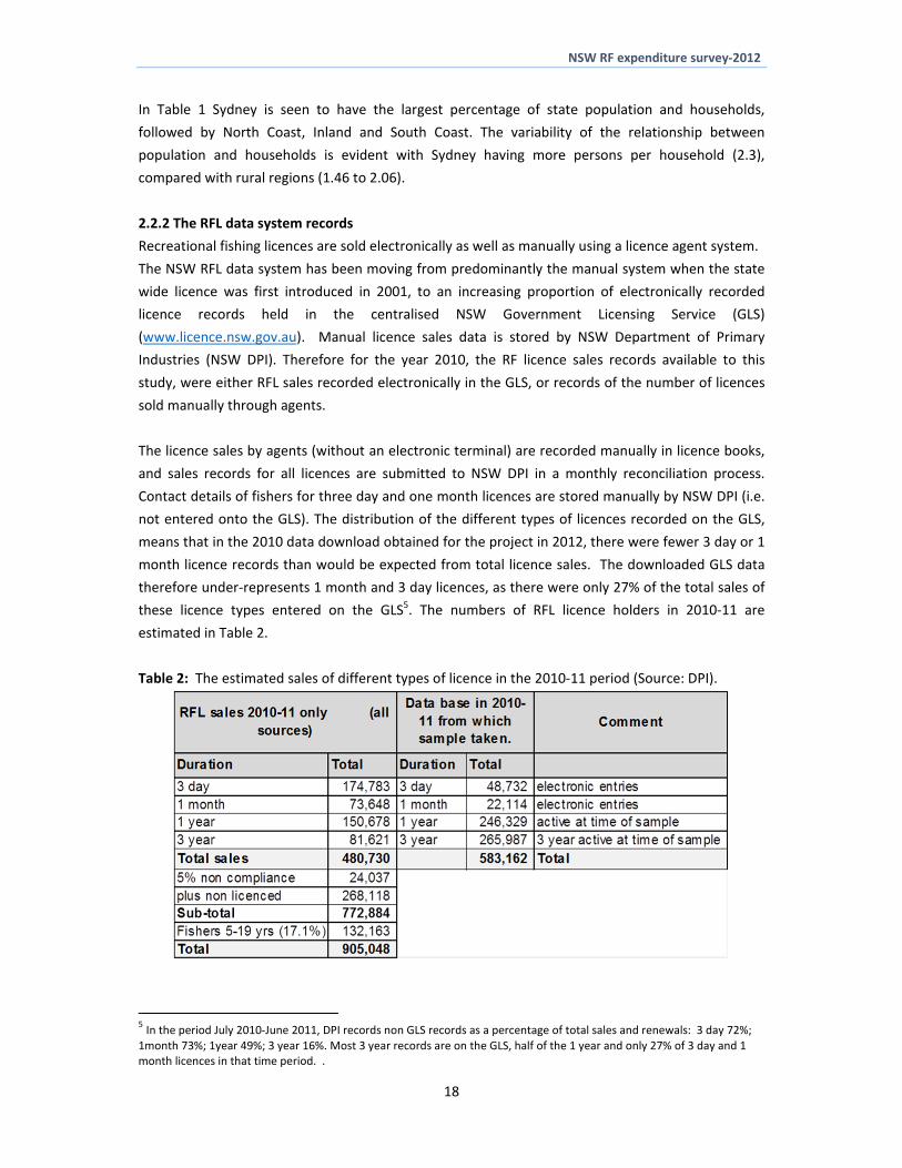
NSW RF expenditure survey‐2012
Table 2 reports the estimates numbers of 3 day 1 month 1 year and 3 year RFL sold in 2010‐11 We
use this information to assist in the estimation of the total number of fishers in NSW
The number of licence sales can be adjusted to include non‐compliant fishers (assumed to be 5 of
licence holders) and the 35 of fishers not requiring a licence (as estimated in McIlgorm et al 2005
and confirmed later in this study) plus young fishers 5 to 19 years old (171 of the population ABS
2011) Using these figures a total of 905048 anglers is conservatively estimated This total also
includes interstate anglers buying licences in NSW The RFL data in the GLS system does not have
any information on non‐licence holders but does record NSW licence holders who reside in other
States
The current estimate of 905048 is less than previous NSW DPI and National Survey estimates of
close to 1 million fishers (DPI pers comm Henry and Lyle 2003) Other studies have noted a
possible decline in recreational fishing participation since the 2001 National Survey (Jones 2008) as
the method here is based on licence sales with several assumed adjustments so should not be taken
as a definitive participation estimate We chose to use the ABS household data for survey
expansions
23 Methods
The methods we used had to be able to facilitate estimation of the total expenditure of recreational
fishers state‐wide Sampling approaches were therefore designed to enable total estimates to be
developed from the samples taken
231 Sampling
We used two survey sampling approaches for the study
(a) Telephone household screening survey to identify households with a RF A random screening
survey using the home phones of 4000 households in the general population was proposed to
identify 800 anglers Each angler identified was then asked to complete an 8 minute survey of
fishing‐related activity and expenditure
(b) RFL database to contact known anglers (licence holders) A survey sample of 750 licence
holders from the RFL database was proposed to provide 500 completed 8 minute surveys of RFL
holders
232 Preparations for the fieldwork sampling survey
Ethics approval was required through the University system to conduct the survey Due to privacy
and ethical issues the fieldwork did not call ldquochildrenrdquo ie those under 19 years of age Those
fishers over 18 years of age are either licensed or are concession holders due to having a pension or
disability
A range of issues was considered in the fieldwork design
19
NSW RF expenditure survey‐2012
a) Field work survey method
In the last two decades in Australia there has been a move away from postal surveys with face to
face interviews diary keeping phone and mobile phone and internet methods being used After
considering the task we chose a telephone survey method to contact the desired audience within
budget limits The telephone survey field work was undertaken by IRIS Research a telephone
surveying marketing and research business
The market research company conducted two telephone surveys using (a) a whole population
database for the random household calls and (b) RFL licence data base records supplied from NSW
DPI
Random telephone screening surveys use survey industry databases of household telephone
numbers in different regions of NSW The household phone survey enables the survey sample
results to be related to ABS census data for the population in NSW which is essential to the process
of estimating total and regional expenditure and economic impacts of recreational fishing The
screening survey response rates contributed to sample expansions The screening survey results
include non‐licence holders and can be compared with the responses of RFL holders
For the RFL database records calls to the anglerrsquos home phone or stated mobile phone number was
the contact method Calls to a mobile phone number recorded on the RFL database assumes the
holder resides in the postcode area of their physical address in the licence record
b) Minimising biases and seasonal effects in the survey
Commonly recreational fishing surveys use a single interview of fishers asking the respondent to
recall fishing activity trips and expenditure in the ldquopast yearrdquo or ldquopast 12 monthsrdquo
The responses may be affected by the season in which fishers are asked for information In this
study a sample of anglers was interviewed in late March 2012 pre‐Easter6 asking them about their
activity and expenditure in the previous six month period that is since the previous September
2011 The second wave of interviews in September 2012 asked another different set of respondents
to recall fishing activity and expenditure since the previous April which included Easter The results
were used to test for seasonal differences in angler activity and angler expenditure For capital
expenditure items such as boats respondents were asked to recall their purchases in the past year
The desire to enquire about seasonality ran some risks in asking to recall the past six months activity
accurately as responses may also include recall and other biases (Gentner 2008) The questionnaire
initially asked participants to recall the last six months and then the past year which may have
presumed too much of the respondentrsquos memory in a limited telephone interview
c) Demographics of fisher groups
The survey was designed to investigate the different demographic clusters of anglers in NSW and
their associated expenditures For example identifying angler groups such as single fishers friends
6 Easter was 6th‐9th April in 2012
20
NSW RF expenditure survey‐2012
fishing married and middle aged and retired fisher groups would assist in understanding the
recreational fishing behaviour of these groups Other socio‐economic variables like income and age
may also impact recreational fishing expenditure
This group approach of identifying different ldquoclustersrdquo is used in the Tourism research literature (eg
grey nomads pompadours young family groups etc) and could assist future recreational fishing
expenditure research in NSW The survey results will be analysed and the statistically different fisher
groups in NSW identified This will improve managementrsquos understanding of the differences in
recreational fishing groups in NSW
233 Discussion
Usually in telephone survey methods a screening survey of the whole population is required to
locate the 10‐20 of households (depending on the region) in the general population that have a
RF living there (Henry and Lyle 2003 McIlgorm et al 2005) This is the expensive part of any
telephone survey requiring perhaps ten or more calls to contact one fisher However the random
sample from the screening survey of households can be aligned with the available ABS information
on households in NSW and so the total number of RFs in households in NSW can be estimated
The available RFL sales data and historical database of licence holders in NSW can also be used to
estimate the total number of recreational fishers The use of the RFL data base for a survey of
expenditure excludes exempted anglers such as those who are 18 years and younger and
concession card holders such as pensioners An estimated two‐thirds of the NSW fishing population
over 18 years old have a RFL (Dominion Consulting 2003 McIlgorm et al 2005) as one third are
concession holders and pensioners and are exempted
RFL contact details were available under a confidentiality agreement with NSW DPI that protected
licence holder identity but made their telephone contacts available to the projectrsquos market research
company under DPI and University ethics and research privacy protocols
Given the above two different estimates of the total number of RFs state wide can be made One
via the screening survey results combined with ABS household data and the second by use of the
direct sales records of the RFL with some adjustments for unlicensed concession holders and young
anglers Our preference was to use the general population household based approach within the
ABS data system
24 Estimating the total expenditure by fishers
The total state expenditure by RFs is a function of the number of trips taken per individual angler
and the expenditure per trip However expenditures can vary from travel expenses food and
accommodation to small trip‐related fishing tackle and equipment expenditures to other larger
annual equipment expenditures such as boats We separated the expenditures into
21
NSW RF expenditure survey‐2012
a) Fishing trip related expenditure on a range of expenses (accommodation eating out other food
and drink shopping car travel7 non‐car travel sports tours poker machines pub expenses other
expenses) Trip expenditure can be annualised by expanding by the number of trips per annum
b) Expenditure on small equipment on the last trip (rods tackle bait boat hire boat fuel charter
fees recreational fishing clothes camping gear and other related purchases) and
c) Annual expenditure on larger boat equipment (boat licence boat maintenance boat insurance
mooring expenses boat equipment and major purchase expenditure on new boat or major boat
repair in last year) This includes capital purchases in the year of the survey
Trip related expenditure per household was investigated by asking fishers about their last Saltwater
(SW) or Freshwater (FW) trip and their expenditures for both the angler and accompanying persons
The trips SW (or FW) per annum were then related to the total trips per annum state‐wide in SW (or
FW) so the total annual recreational fishing expenditure for SW (or FW) could be calculated
Minor equipment expenditure is considered to be trip related whereas expenditures on major
purchases such as boats and motors are annual expenses Although maintenance and expenditure
on repairs are expenses that can increase with activity maintenance is also included fixed
expenditures such as annual over hauls and replacing boat motors Capital expenditure on new
boats is a distinct and significant expenditure category
Sectors not covered by the survey
The Charter sector‐ The state‐wide expenditure survey included questions on anglersrsquo use of
commercial charter services but it is unknown if we can identify and determine the value of
expenditure in the entire recreational fishing Charter sector given the sample size in the study If it is
a ldquorare eventrdquo then the Charter sector would need to be surveyed separately such as a direct
Charter business survey or client survey approach (Dominion in prep) ldquoRare eventsrdquo challenge the
capacity of a sample to capture the event in a representative and statistically robust fashion
The fish guiding sector‐ RFs may choose to hire a guide and interview participants were asked to
about this expenditure Again if this is a rare event the sample size here may have inadequately
captured the value of the sector This may also apply to other recreational fishing tourism
operations
7 This included travel expenditure for which ATO rates per km were imputed depending on the engine size for the kilometres (km) stated in the questionnaire ie cubic capacity (cc) of the car for outward and return legs of the trip
22
NSW RF expenditure survey‐2012
3 Survey results
This section presents the results of the survey fieldwork in preparation for their use in the
expansions to estimate total state activity and expenditure as developed in Chapter 4 We compare
the activity and expenditure results from screening the general population to identify recreational
fishers with the more direct use of the database records of known RFL holders
31 The fieldwork results ‐ Details of sampling and completed interviews
We sampled two populations consisting of
1) persons who indicated they were fishers (a proportion of which were not licence holders)
located by a random screening survey of the total population and
2) licence holders recorded on the RFL data base
The survey fieldwork agency contacted and completed a total of 1235 interviews 613 in March and
622 in September 2012 and the data are summarised in Table 3a
Table 3a The number of surveys completed in fieldwork for both survey approaches
Fieldwork
From
screening
survey
Survey of
RFL holders Total
Mar‐12 292 321 613
Sep‐12 312 310 622
Total 604 631 1235
The random screening survey identified and completed interviews with 604 fishers all over 18 years
old of which 213 (35) were adult concession holders or pensioners not requiring a licence Table
3b presents details of the interviews identifying the survey results for fishers identified through
holding a RFL or via the random screening survey
IRIS Research undertook two sets of fieldwork telephone survey calls in April and September 2012
Each fieldwork event involved the random screening survey of the total population to locate
recreational fishers as well as survey calls to fishers holding licences on the RFL database Table 3b
shows the survey response profiles For the screening survey
The Gross sample is the initial sample of white page telephone numbers
The net sample is the gross sample less the deaddisconnected numbers and numbers of
non private dwellings businesses and faxes and modems and
The net sample is represented by the non‐contactable households the households with no
fishers and households with fishers subdivided into full responses and refusals which
included incomplete interviews
23
NSW RF expenditure survey‐2012
Table 3b The response profile of the screening survey and the RFL surveys and the two waves of
interviews within each (After Henry and Lyle 2003)
Screening Sample Wave 1 Wave 2
Gross sample 13896 100 27796 100 Sample loss 6336 46 14078 51 Net Sample 7560 100 13718 100 represented by Non‐fishing households 4116 54 6938 51 Full response 292 4 312 2
Refusals 327 4 520 4
Non contacts 2825 37 5948 43
response 327 53 312 38
refusals 292 47 520 63 Interview approaches 619 832
RFs as of households 131 107
RFL Sample Wave 1 Wave 2
Gross sample 2014 100 2706 100 Sample loss 1114 55 1569 58 Net Sample 900 100 1137 100 represented by Non‐fishing households na Full response 321 36 310 27
Refusals 94 10 90 8
Non contacts 485 54 737 65
response 321 773 310 775
refusals 94 227 90 225 Interview approaches 415 400
In Table 3b (left hand side) both waves of the screening survey of the general population recorded
between 46 and 51 of sample loss due to deaddisconnected numbers and numbers of non
private dwellings businesses and faxes and modems As a result for the second wave a greater
number of initial telephone numbers were selected and fewer call backs made in order to complete
the desired sample sizes within budget This difficulty in contacts may be due to changes in the
general white pages telephone data base information as increasingly people use other forms of
telephony such as mobiles and internet VOIP systems There have also been several developments
in privacy legislation with more people choosing not to receive unsolicited calls or using ex‐directory
numbers In 2000 80 of households were assumed to have a land line phone (Henry and Lyle
2003) but this has since declined (ACMA 2013) and mobile phone use has dramatically increased
among those under 40 years old8
Of the total net sample 37 and 43 were not contactable numbers despite repeated ringing (up
to five times in wave 1 and two times in wave 2) Another 54 and 51 of the net sample of
households contained non fishers and 8 and 6 contained someone who had been fishing in the
last six months RFs who had fished in the last six months were present in 131 and 107 of all the
households successfully contacted This is in line with expectations but there was reluctance among
a significant number of these anglers to complete the survey interview indicated by refusal rates of
47 and 63 This was unexpected but anecdotal information from interview staff indicated that
8 A recent report by ACMA (2013) indicates that ldquowhile over 90 per cent of Australian adults continue to use both fixed‐
line phones and mobile phones and largely see them as complementary services Australians are increasingly turning to
mobile technology to make their voice callsrdquo ldquoOlder Australians more commonly adhere to fixed‐line technology for voice
communication Ninety‐six per cent of those aged 65ndash69 maintain a fixed‐line service in contrast to 75 per cent of 18 to 24‐
year‐olds Among 18 to 24‐year‐olds living in share households this number drops to 60 per centrdquo ldquoEmerging technologies
such as VoIP are yet to be adopted by Australians at mainstream levelsrdquo (ACMA 2013)
24
NSW RF expenditure survey‐2012
numbers of people opted not to be interviewed because they felt that ldquothe RFL is intrusiverdquo
ldquorevenue raisingldquo and the survey was a way for authorities ldquoto find out if they had a current fishing
licencerdquo
Table 3b (right hand side) reports the fieldwork response profile for the RFL database contacts In
the survey of RFL holders issues also arose with respect to contacting existing RFs This was mainly
due to data base records being valid only up to or 2010 and by 2012 up to 55 of numbers were
found to be dead Of course it is also likely that some telephone numbers may not have been stated
accurately at the time of licence issue
Of the second RFL sample survey method 54 and 27 in waves 1 and 2 respectively were not
contactable numbers in spite of repeated ringing up to five times in waves 1 and 2 Unlike the
screening survey all of the households sampled should have contained fishers The survey
completion rate was high among angler contacted with 77 taking part in the both waves of the RFL
survey
The numbers of people surveyed as shown in Table 4 have to be considered against the populations
in each of the study areas There was a planned under sampling in the case of Sydney where
population is highest (and where the proportions of anglers is lowest) and an oversampling in the
NSW North Coast and Inland areas where populations are less This enabled sufficient responses to
be gathered for each region in the study but required re‐weighting of regional results by regional
ratios of population in some uses of the sample data later in the study
Table 4 The number of interviews for the licence and the random screening survey by region of
NSW conducted in March and September 2012
Licence survey
Region March Sept Total Sydney 94 91 185 North coast 81 69 150 South coast 30 30 60 Inland 63 58 121 Interstate 53 62 115 All NSW 321 310 631
Random survey
Sydney 50 75 125 North coast 86 78 164 South coast 23 9 32 Inland 33 37 70
Licenced 192 199 391 647 Sydney 21 35 56 North coast 46 47 93 South coast 14 11 25 Inland 19 20 39
Unlicenced 100 113 213 353 Rnd 292 312 604 All NSW 613 622 1236
Table 4 indicates that in the random sample 647 of fishers had licences and 353 had not
25
NSW RF expenditure survey‐2012
32 Fishing activity from the survey samples
Fishers were asked to recall their fishing activity and their fishing‐related expenditure over three
time periods
their last six months of fishing activity
their last fishing trip together with the expenditure involved on that trip and
their major boat expenditures in the last year
Rather than asking fishers at one point in time to recall details of activity and expenditure over a full
year (and therefore to try and reduce lsquotelescoping biasrsquo) two waves of field work interviews were
run six months apart In March 2012 and September 2012 field samples fishers were asked about
their last six months of fishing activity (this was also designed to enable any seasonality to be
assessed) Recalling days fished and expenditure over the previous year is known to include recall
bias and often a telescoping of memory Although six months is shorter than a year it may be that
there is a telescoping of the memory in respect of recalling past events and hence an unknown
component of ldquorecall biasrdquo in 6 months also In annualising results from two different fishers
recalling the last six months any bias will be compounded
Section 13 examined activity estimates from past RFE surveys in Australia and the differences
between methodologies The recreational fishing activity levels expressed as trips per annum or
days fished per annum point to the potential for recall surveys to overestimate activity in the
desired period The six month recall results were compared with previous annual trip and fishing
activity estimates in NSW and on the basis of conservatism were treated as being equivalent to bias‐
adjusted annual results The estimates of anglers when asked about their last 6 months of activity
appear to be less constrained than when recalling over the past year9 In other words it appears
there was a strong tendency to lsquotelescopersquo to the last 12 months
This is illustrative of the significant methodological divide between annual recall surveys and other
shorter term activity log approaches When the cost of diary surveys is prohibitive as is often the
case annual recall is preferred for expenditure estimation and adjustments for recall bias applied
Not applying adjustment for bias will lead to over estimates of activity and expenditure
321 Recreational fishing trips
Anglers were asked to recall the number of SW and FW trips in the past six months and also to recall
details of their last trip A trip can be just a day and may well be for many fishers who live close to
their usual fishing place but can of course be many days In each case this would be known since
they were asked the duration of their last trip in days Figure 1a plots the numerical frequency of
trips in the past year
9 Total activity estimates may have been more constrained if the same anglers had been called again or preferably in shorter 2 month periods as in the NOAA survey (Gentner 2008)
26
NSW RF expenditure survey‐2012
Figure 1a The numerical frequency of trips per annum for Saltwater and Freshwater fishing trips
0
100
200
300
400
500
600
1‐5 6‐10 11‐15 16‐20 21‐25 26‐30 31‐35 36‐40 40+
Number of trips
Trips per annum
SW Trips FW trips
Figure 1b shows that 54 of all SW anglers and 67 of all FW anglers fished 5 trips or less per year
The average number of trips per angler was SW 875 (standard deviation (sd) 145) and FW 38 (sd
86) or 107 (sd 153) trips for all fishing The declining exponential nature of the trips per annum
distribution is evident although there were 3 of trips by avid anglers who reported in excess of 40
trips per annum This distribution is highly skewed to the left and strongly influences calculation of
total expenditure estimates
Figure 1b The percentage frequency of Saltwater and Freshwater fishing trips per annum
0
10
20
30
40
50
60
70
80
1‐5 6‐10 11‐15 16‐20 21‐25 26‐30 31‐35 36‐40 40+
Percentage
frequency
Trips per annum
SW Trips FW trips
Anglers were also asked about days fished in SW and FW The relationship between trips and days
fished for 631 RL holders is reported in Table 5
27
NSW RF expenditure survey‐2012
Table 5 The days trips and length of trip for RFL Holders sampled (n= 613)
Type of fishing
day
Days Trips Daystrip of trip
time fished
SW days 6112 4189 146 817
FW days 2407 1536 157 866
The RFL survey sampled 631 fishers who fished 8470 days an average of 134 days per year
Proportionally 72 of days fished were in SW and 28 in FW Table 5 shows that the average fishing
trip was 146 days in SW and 157 days in FW of which over 80 of time was time fished in both
environments
322 Recreational fishing days
Previous catch and effort surveys have expanded data based on days fished Days fished are
presented on an annual basis in a frequency chart in Figure 2a and as percentage frequency chart in
Figure 2b
Figure 2a The frequency of days fished by all fishers (Average 146 days sd 186 days n=1231)
Figure 2a and 2b indicate that 38 of all anglers sampled fished 5 or less days per year but also that
6 of all anglers fished more than 40 days a year the latter often referred to as avid anglers The
average days fished are 146 days and given the previous estimate of 773000 adult anglers in NSW
this translates in to an estimated 116 million days fished in 2012
These activity distributions in samples are important The 36 of days below 5 days a year was less
than the 67 of the national survey (conducted in 2001) In contrast that survey also showed that
just 1 of anglers fished more than 40 days in the previous year (Henry and Lyle 2003)
28
NSW RF expenditure survey‐2012
Figure 2b The percentage frequency of days fished
In the present study this is partially explained by possible under sampling of 3 day and 1 month
licence holders though the random survey should not have been affected in this way On the other
hand the present study may well have sampled a higher proportion of avid fishers in the RFL data
base The third possibility is that angler behaviour in NSW has altered (on average) in the 12 years
since the national survey perhaps influenced by the introduction of the RFL
33 Comparisons between methods and samples
Statistical t‐tests were used to compare the trips per angler and average days fished per angler
between seasonal samples random and RFL database surveys and between licensed and unlicensed
recreational fishers
a) Are there seasonal differences in fishing activity
There is no previous literature on seasonal levels of fishing effort in NSW but we might expect to
see less days fished and fishing trips in the April to September ldquowinterrdquo period since this period does
not include Christmas However t tests revealed there was no statistically significant difference in
either the average days fished or trips per fisher across all observations between the April and the
September samples This may be partially explained by respondents to the September survey
recalling significant fishing activity at Easter time as part of ldquowinterrdquo activity
b) Are the random survey method and the RFL data base method results different
The t tests for trips indicate that those fishers in the random survey which included both licence
holders and non licence holders fished significantly more trips per year (125 v 906 trips t=395)
than fishers sampled from the RFL database This also applied to days fished with those in the
random survey fishing significantly more days (155 v 134 days t=208)
29
NSW RF expenditure survey‐2012
c) Are there differences between licenced and unlicenced fishers
Do licensed anglers fish more than unlicensed fishers When all samples are considered the average
days fished estimates show no significant difference between licensed and unlicensed fishers
However non‐licence holders made significantly more fishing trips than licence holders (128 trips v
103 t= 224)
34 Discussion of the sampling and activity results
On the basis of these results the average activity per angler whether measured in trips made or days
fished does not appear to be significantly different between seasons This result supports the
prospect of sampling recreational fishers at any time of the year asking them to recall their activity
in the last year
Fishers sampled randomly through the ldquowhite pagesrdquo made significantly more fishing trips and
fished on more days per annum than RFL holders Similarly those fishers contacted at random not
holding licenses were found to fish a similar number of days to licence holders but made
significantly more trips per annum This somewhat counter intuitive result (we might expect licence
holders to be more avid) is nevertheless consistent with concession holders and pensioners being
available to take more occasional fishing trips than the general working population might
It may also be related to the relatively high number of fishers found to have made more than 40
trips per year skewing the activity profile Where one sample is chosen at random and the other
comes from a database of known recreational fishers we may expect some avidity bias in the latter
(Johnson 1999) However this is not what we found indicating that opportunity to go fishing among
non licence holders may enable them to fish more frequently than licence holders though this
assumes we have no significant biases in the survey analysis For example ACMA (2013) states that
CATI surveys as used in our random screening survey ldquomay be biased towards those who normally
stay at home (eg older or retired people or those whose occupation is home duties)rdquo This may
indicate that those who responded had more time to go fishing than across the whole NSW
population
Non response bias and the screening survey
The most common non‐response bias is ldquounit non‐responserdquo which ldquotakes place when a randomly
sampled individual cannot be contacted or refuses to participate in a surveyrdquo (Ritz 2013) Mohadjer
et al explain ldquoThere is always a potential for item nonresponse bias whenever sample persons who
did not participate in the survey have somewhat different characteristics than those who didrdquo
In our random screening survey we had
‐ Sample losses approximately 50 of dead numbers and the potential for unit non response
bias Do those interviewees with land line numbers differ from those who have moved or
changed telephones in the past few years Privacy conditions precluded contacting non
respondents to investigate further Socio‐economically those moving away from landlines
may be younger in the working population or may have different incomes An argument
can be made either way and the extent of any bias remains unknown
30
NSW RF expenditure survey‐2012
‐ Non contactable household‐ It is unlikely these non contactable numbers for non‐RF
households or RF households would differ unless they were out fishing
‐ Refusals Why did so many people who identified themselves as having fished in the past six
months refuse to complete a short fishing interview Reasons include the dislike of surveys
intruding into their home and privacy not having the time or other general perceptions
Those who completed the interview may be keener on fishing more avid and some not
completing it because they consider their level of fishing to be trivial There was also the
indication from surveyors of fear or mistrust that the call was checking up on their licence
status In the random survey those who may have had a licence for 3 days or 1 month in the
previous six month period may not have had one at the time of the call and may have felt
vulnerable However approximately one third of all fishers are concession holders reducing
this possible vulnerability impact
In the area of survey refusals there seems to be more potential for non‐response bias in the
comparability of those who completed the survey with those who refused This cannot be directly
checked with non respondents due to privacy constraints Other independent indicators could be
used comparing ldquohellipthe distribution of respondents in the survey with associated distributions coming
from other independent surveysrdquo (Mohadjer et al 1994) We are able to compare the surveys given
their two different approaches
In the random screening survey over half of the identified fishers did not complete the survey We
can test for evidence of a response bias by comparing RFL licence holders who replied to the random
survey with RLF licence holders contacted directly in the other survey A t‐test indicated that the
mean days fished for the random RFL group (n=391) were significantly higher than the direct RFL
(n=631) survey results (158 v 134 t=211) significant at the 5 and 2 levels This is indicative of a
possible response bias as more active RFL holders appear more likely to have participated in the
random screening survey interviews than other less avid licence holders Previous adjustments made
to the data (section 32) reduced the risk to final estimates from this and other likely biases
Bias and the survey of RFL holders
The RFL survey also recorded significant levels of dead numbers although a much lower rate of
refusals The survey fieldwork team were able to ask to speak to the licence holder by name and this
may have contributed to higher completion rates Any bias in the RFL survey may then be between
responses by different licence holders Those holding 3 year licences may have significantly different
fishing activities expenditures or preferences to 1 year or 1 month and 3 day licence holders
Anecdotal evidence suggests some fishers buy several 3 day licences through the year and this may
contribute to a form of ldquodouble countingrdquo in any comparative analysis of licences The scale of this
behaviour is unknown and does not assist us in developing a sampling approach that may draw on a
representative cross section of the four licence types Further enquiries of non respondents was not
pursued due to privacy constraints
31
NSW RF expenditure survey‐2012
34 Estimation of recreational fishing expenditure per angler
Recreational fishing expenditure can be split into different categories as explained previously
a) Trip related expenditure on a range of expenses Trip expenditure can be annualised by expanding
by the number of trips per annum
b) Expenditure on small equipment and expenses on the last trip and
c) Annual expenditure on larger boat equipment This includes capital purchases in the year of the 10survey
All respondents in each area were asked about trip expenditures by all anglers in their household ndash
which averaged 202 anglers per household (see Table 7 later in report) The estimated expenditures
per angler per trip are reported in Table 6abc but state‐wide estimates in the next chapter are
based on household data
Table 6a summarises the average RF expenditure per trip for all NSW fishers (both SW and FW) in
each region for both fishing trip expenses and tackle Table 6b reports the average SW RF
expenditure per trip for all NSW regions on both fishing trip expenses and tackle Table 6c shows the
average trip expenditures for FW anglers Table 6d shows the annual expenditure on boat
expenditure for all NSW anglers SW and FW anglers combined
In Table 6ab ampc the results include fishers from Interstate who hold a NSW RFL but their major boat
and motor purchases are not assumed to have been made in NSW (Table 6d black squares)
The results in Table 6a confirm that all fishers (both SW and FW) spend 68 of trip expenses on the
fishing trip and just under 32 on equipment and fishing expenses Car travel is the major trip
expense $6974 (31 of total trip expense accommodation $ 3267 (15) and fooddrink eating out
$3594 (16) also while fishing rods and tackle hookslines and baitberley $3891(18) and boat
fuel $1650 (7) are the other major trip expenses
In Table 6b the costs of SW anglers are shown and Table 5c for FW Table 6bampc show that each
group had similar average expenditures per fishing trip (SW ‐ $22282 and FW ‐ $23024) Car travel
expenses are higher for FW fishers $9079 day versus $5955day SW but boat fuel for SW is
$1964 day versus FW $1009day
Table 6d shows that the annual NSW fisherrsquos average boat expenses per angler were $768 pa for all
NSW or broken down $856 for SW and $365 for FW fishers Boat purchase values for SW fishers
were much higher than for FW fishers which reflected the lower capital expenditure on small tinnies
for creeks dams and impoundments as opposed to offshore marine vessels The comparisons are
for the major form of fishing activity with 21 of fishers in our survey sample fishing a combination
of both SW and FW in a given year
10 Expenditure on fishing boats and larger capital items was reduced by 30 to reflect non recreational fishing use
32
NSW RF expenditure survey‐2012
Table 6a The average RF expenditure per trip for all NSW RFs in all NSW Last column is the
percentage of total spend in the All NSW total trip
Data in Aus $ Sydney North coast
South Coast
Inland Interstate All NSW of total spend per
trip Car travel (both ways) 6874 $ $ 4376 $ 4650 9871 $ 13060 $ 6974 $ 31 Accommodation 3998 $ $ 2216 $ 2112 2967 $ 6424 $ 3267 $ 15 Eating out 1478 $ $ 733 $ 1132 1572 $ 2820 $ 1342 $ 6 Other food and drink 2004 $ $ 1420 $ 2121 2881 $ 4857 $ 2252 $ 10 Shopping (souvenirmagazinesvideos) 419 $ $ 155 $ 120 607 $ 947 $ 387 $ 2 Travel-other than by car 354 $ $ 053 $ 325 040 $ -$ 160 $ 1 Sports 027 $ $ 018 $ - 034 $ 478 $ 065 $ 0 Tours 096 $ $ 007 $ 154 100 $ 022 $ 066 $ 0 Poker machines 174 $ $ 095 $ 077 124 $ 504 $ 160 $ 1 Pub 651 $ $ 347 $ 565 618 $ 1554 $ 621 $ 3 Anything else 194 $ $ 044 $ 068 134 $ 152 $ 117 $ 1 Expenditure per trip 16259 $ $ 9460 $ 11307 18946 $ 30811 $ 15405 $ 68
-$ $ - $ - -$ -$ -$ Major fishing tackle (rods reel) 2561 $ $ 1491 $ 1009 2756 $ 826 $ 1937 $ 9 Minor fishing tackle (hooks lines etc) 1106 $ $ 881 $ 713 1505 $ 2101 $ 1162 $ 5 Baitberley 1043 $ $ 559 $ 624 820 $ 938 $ 792 $ 4 Boat hire 671 $ $ 005 $ 090 139 $ 078 $ 242 $ 1 Boat fuel 2054 $ $ 1307 $ 683 1180 $ 3531 $ 1652 $ 7 Charter and fishing guide fees 647 $ $ 301 $ 043 098 $ 109 $ 323 $ 1 Fishing clothesapparel(w aders etc) 263 $ $ 177 $ 276 339 $ 143 $ 239 $ 1 Camping equipment 175 $ $ 735 $ 309 790 $ 400 $ 508 $ 2 Other fishing expenses 240 $ $ 283 $ 144 328 $ 393 $ 276 $ 1 Equipment per trip 8747 $ $ 5726 $ 3890 7939 $ 8520 $ 7120 $ 32
Total spend per trip 25007 $ $ 15185 $ 15197 26885 $ 39331 $ 22524 $ 100
Table 6b The average RF expenditure per SW trips for RFs anglers in all NSW Last column is the
percentage of All NSW total
Data in Aus $ Sydney North coast
South Coast
Inland Interstate All NSW of total spend per
trip
Car travel (both ways) 6168 $ $ 3659 $ 3915 17153 $ 12637 $ 5955 $ 27 Accommodation 4063 $ $ 2182 $ 2170 6325 $ 10959 $ 3547 $ 16 Eating out 1454 $ $ 782 $ 1151 4195 $ 5838 $ 1539 $ 7 Other food and drink 1988 $ $ 1284 $ 2321 2834 $ 6274 $ 2000 $ 9 Shopping (souvenirmagazinesvideos) 447 $ $ 164 $ 115 1620 $ 2157 $ 450 $ 2 Travel-other than by car 421 $ $ 034 $ 365 102 $ -$ 219 $ 1 Sports 033 $ $ 010 $ - 131 $ 581 $ 051 $ 0 Tours 113 $ $ 009 $ 173 280 $ -$ 086 $ 0 Poker machines 187 $ $ 112 $ 068 144 $ 865 $ 170 $ 1 Pub 694 $ $ 371 $ 612 1095 $ 2149 $ 649 $ 3 Anything else 229 $ $ 046 $ 077 -$ 405 $ 129 $ 1 Expenditure per trip 15787 $ $ 8647 $ 10947 33880 $ 41807 $ 14781 $ 66
Major fishing tackle (rods reel) 2703 $ $ 1509 $ 1136 2246 $ 541 $ 1905 $ 9 Minor fishing tackle (hooks lines etc) 1203 $ $ 742 $ 747 1087 $ 3010 $ 1035 $ 5 Baitberley 1183 $ $ 633 $ 656 1242 $ 1116 $ 899 $ 4 Boat hire 816 $ $ - $ 101 475 $ 243 $ 352 $ 2 Boat fuel 2309 $ $ 1380 $ 737 1903 $ 7946 $ 1964 $ 9 Charter and fishing guide fees 788 $ $ 370 $ 048 169 $ 338 $ 465 $ 2 Fishing clothesapparel(w aders etc) 302 $ $ 195 $ 310 270 $ -$ 245 $ 1 Camping equipment 213 $ $ 631 $ 048 936 $ 027 $ 402 $ 2 Other fishing expenses 252 $ $ 275 $ 161 234 $ 223 $ 247 $ 1 Equipment per trip 9750 $ $ 5721 $ 3943 8562 $ 13444 $ 7501 $ 34
Total spend per trip 25537 $ $ 14367 $ 14890 42442 $ 55251 $ 22282 $ 100
33
NSW RF expenditure survey‐2012
Table 6c The average RF expenditure per FW trip for RFs anglers in all NSW Last column is the
percentage of All NSW total
Data in Aus $ Sydney North coast
South Coast
Inland Interstate All NSW of total spend per
trip
Car travel (both ways) 10144 $ $ 7498 $ 10533 7358 $ 13261 $ 9079 $ 39 Accommodation 3696 $ $ 2363 $ 1654 1808 $ 4272 $ 2689 $ 12 Eating out 1591 $ $ 517 $ 981 667 $ 1388 $ 937 $ 4 Other food and drink 2077 $ $ 2014 $ 519 2897 $ 4185 $ 2771 $ 12 Shopping (souvenirmagazinesvideos) 287 $ $ 118 $ 154 258 $ 389 $ 258 $ 1 Travel-other than by car 039 $ $ 138 $ - 018 $ -$ 040 $ 0 Sports -$ $ 053 $ - -$ 429 $ 093 $ 0 Tours 015 $ $ - $ - 038 $ 032 $ 025 $ 0 Poker machines 115 $ $ 020 $ 154 117 $ 333 $ 141 $ 1 Pub 454 $ $ 245 $ 192 454 $ 1272 $ 565 $ 2 Anything else 031 $ $ 033 $ - 180 $ 032 $ 094 $ 0 Expenditure per trip 18448 $ $ 13000 $ 14187 13794 $ 25595 $ 16691 $ 72
Major fishing tackle (rods reel) 1903 $ $ 1414 $ - 2933 $ 962 $ 2002 $ 9 Minor fishing tackle (hooks lines etc) 658 $ $ 1482 $ 442 1649 $ 1669 $ 1423 $ 6 Baitberley 398 $ $ 238 $ 369 674 $ 853 $ 572 $ 2 Boat hire -$ $ 026 $ - 023 $ -$ 015 $ 0 Boat fuel 877 $ $ 988 $ 250 930 $ 1437 $ 1009 $ 4 Charter and fishing guide fees -$ $ - $ - 073 $ -$ 031 $ 0 Fishing clothesapparel(w aders etc) 085 $ $ 097 $ - 363 $ 212 $ 227 $ 1 Camping equipment -$ $ 1184 $ 2392 739 $ 577 $ 726 $ 3 Other fishing expenses 184 $ $ 319 $ 008 360 $ 474 $ 335 $ 1 Equipment per trip 4105 $ $ 5749 $ 3462 7724 $ 6184 $ 6332 $ 28
Total spend per trip 22553 $ $ 18749 $ 17648 21518 $ 31779 $ 23024 $ 100
Table 6d The average RF expenditure per annum on larger boat items for SW and FW anglers in
regions and all NSW (nb Table 6abc are per trip and Table 6d is per angler per annum)
Data in Aus $ Sydney North coast
South Coast
Inland Interstate All NSW of total spend per
trip
All NSW Boat licenceregistration 7115 $ $ 4658 $ 4407 5815 $ 8546 $ 5940 $ 8 Boat maintenance 29248 $ $ 14497 $ 9655 7935 $ 17917 $ 17504 $ 23 Boat insurance 7519 $ $ 4574 $ 3006 4145 $ 10318 $ 5754 $ 7 Marine mooring fees 7615 $ $ 1940 $ 192 122 $ 2609 $ 3179 $ 4 Boat equipment (safety etc) 15175 $ $ 7637 $ 3175 5452 $ 6015 $ 8888 $ 12 Boat purchase or motor repair 23437 $ $ 25676 $ 25865 9740 $ - 35550 $ 46 Annual boat expenditure 90109 $ $ 58982 $ 46300 33208 $ 45405 $ 76815 $ 100
Saltwater -$ $ - $ - -$ -$ -$ Boat licenceregistration 7340 $ $ 4751 $ 3583 6003 $ 13372 $ 6014 $ 6 Boat maintenance 32221 $ $ 15880 $ 9805 5356 $ 28392 $ 20829 $ 22 Boat insurance 8032 $ $ 5068 $ 3002 3960 $ 19824 $ 6458 $ 7 Marine mooring fees 8765 $ $ 2385 $ 216 030 $ 8108 $ 4505 $ 5 Boat equipment (safety etc) 17407 $ $ 7800 $ 3428 7508 $ 9230 $ 10764 $ 11 Boat purchase or motor repair 30450 $ $ 35250 $ 30000 40600 $ - 47050 $ 49 Annual boat expenditure $ 104214 $ 71134 $ 50035 63456 $ 78926 $ 95618 $ 100
Freshwater Boat licenceregistration 6073 $ $ 4255 $ 11000 5750 $ 6256 $ 5787 $ 16 Boat maintenance 15523 $ $ 8474 $ 8454 8830 $ 12949 $ 10632 $ 29 Boat insurance 5154 $ $ 2421 $ 3038 4209 $ 5809 $ 4297 $ 12 Marine mooring fees 2308 $ $ - $ - 155 $ -$ 439 $ 1 Boat equipment (safety etc) 4877 $ $ 6930 $ 1154 4738 $ 4490 $ 5011 $ 14 Boat purchase or motor repair 5000 $ $ 3150 $ 18400 5350 $ - 10350 $ 28 Annual boat expenditure 38935 $ $ 25230 $ 42046 29032 $ 29504 $ 36515 $ 100
34
NSW RF expenditure survey‐2012
In Table 6a the higher travel costs of some regional residents such as Sydney anglers Inland and
interstate fishers were evident The trip expenditure of Inland and interstate SW anglers was
significantly higher than for resident NSW anglers due to car travel accommodation food and other
trip expenses presumably to the coast (Table 6b) Table 6c shows that FW expenditure per trip was
highest for interstate fishers (eg Victorians traveling to southern NSW) and Sydney and South Coast
RFs had high travel costs travelling to desirable FW fishing locations (eg Snowy mountains etc
Dominion 2001 and 2002)
The socio‐economics of recreational fisher expenditure in NSW
The survey samples were analysed to identify some of the socio‐economic drivers of RF expenditure
in NSW The samples combined to give 1235 observations of RF expenditure and the survey
included a range of other variables Both multiple regression analysis and a cluster analysis enables
the statistically significant variables determining angler expenditure to be identified and estimated
as reported in Appendices 1 and 2 respectively
Multiple regression results
In Appendix 1 results reveal that Total recreational fishing expenditure is driven by licence status
(licence holders spending more) number of SW trips per annum and the level of household income
Age sex and regional location were found not to be statistically significant in determining total RF
expenditure
Trip expenditure was driven by licence holders and number of SW trips Trip expenditure was further
examined and was significantly influenced by licence holders SW and FW days fished and the
distance travelled on the last trip Fishing Tackle expenditure was found to be determined by
income rather than number of trips Expenditure on boats was driven by both number of SW trips
and the level of RF household income
Cluster analysis results
The expenditure of NSW RFs was also subjected to ldquocluster analysisrdquo to see the significant socio‐
economic characteristics of fisher groups as reported in Appendix 2and in Figure 3 below The cluster
analyses for expenditure on fishing trips tackle and boat expenditure are reported in Appendix 2
35
NSW RF expenditure survey‐2012
Figure 3 A cluster analysis of RF total expenditure showing the groups of significantly different
clusters of anglers identified
In Figure 3 there are four significantly different cluster groups The characteristics of the four groups
are under the ldquodescriptionrdquo row and the authors have put a label to characterise each group
Between Figure 3 and Appendix 2 the overall picture is of groups of ldquoordinaryrdquo fishers
(approximately 85) with low levels of fishing activity in which household income levels may differ
(half lower half higher) secondly a group of dedicated anglers (approximately 12) who have high
fishing activity and expenditure and finally a highly avid fishing group (less than 3) with very high
fishing activity and high to very high expenditure
The results confirm the only previous examination of the socio‐economic characteristics of RFs in
NSW by Dominion (2003) which showed that recreational fishing is a past time involving a diverse
range of people has great variety in activity levels and crosses the entire socio‐economic spectrum
36
NSW RF expenditure survey‐2012
4 State‐wide and regional expenditure estimates
41 Estimating total expenditure
This chapter describes the estimation of the total recreational fishing expenditure for RFs in NSW
and in its regions Total recreational fishing expenditure is the product of three variables
a) Number of recreational fishers or RF households (HH)
We use three approaches to estimate the total RF population in NSW by use of
1) Random telephone survey and ABS Household data and population data
2) The RFL data base and
3) Use of the screening sample and the ABS data on Households Use of the screening
survey of the general population to estimate total number of fishers11 via ABS
population data
b) Fishing trip activity fishing trip activity estimates are obtained from the telephone survey
and
c) Recreational fishing expenditure information on the expenditure per trip and annual
expenditures on equipment is obtained from the telephone survey
The product of these variables will enable us to estimate the total state‐wide recreational fishing
expenditure Expenditure is also estimated for each state region considered Saltwater and
freshwater fishing are considered separately in the state estimates through asking respondents
about the trip intention
42 Expanding the sample of fishers and expenditure
Total expenditure estimates are based on travel and fishing equipment expenses per trip and
estimates of expenditure on boat capital items These are summed to give an annual total
expenditure estimate However the estimates for the angler survey need to be expanded to give
state wide estimates These expansions are described in Box 1 below
Box 1 Explanation of key expansions
The expansion method adapts the method used in the National Survey (Henry and Lyle 2003) The
number of fisher households (FHH) was estimated as follows for each region
No of fisher Household (est) = No Households in Population (ABS) No of Fisher HH (sample)
No of HH (sample)
Example How many recreational fishers would these households include
No of Fishers 19 to 75 yrs (est) = Mean No fishers per HH (sample) No of fisher Household (est)
776496 = 202 383921 (see Table 7)
RF HH are distributed proportionally across regions by household and recreational fishers by
regional population
11 Recreational Fishers under 19 years of age are not included and need to be added if the total population figure is for all
anglers The activity and expenditure estimates are based on ages 19‐75 only
37
NSW RF expenditure survey‐2012
Information on NSW State and Regional Households by Local Government Area (LGA) were accessed
(ABS 2011) The data were aggregated by the larger SD ABS regions (eg Sydney North coast
Inland and SDD South Coast area) These identified the number of households in each of the study
regions as reported in Table 7
Table 7 The ldquototal householdsrdquo in each of the NSW study regions based on LGA data ABS (2011)
Households with recreational fishers are estimated for each study region
Area Population 2010 (gt18-75)
Households HH with RF Rec Fishers HH
RF by region
Sydney 3160897 1376583 213934 230 491232
North coast 835229 570688 88690 146 129802
South coast 350750 207195 32200 169 54510
Inland 649564 315987 49107 206 100948
Total 4996461 2470453 383931 202 776496
The RF household responses for anglersrsquo trip frequency and trip expenditure were multiplied to
produce estimates of state‐wide and regional expenditure
43 State‐wide expenditure estimates
The estimation of total expenditure for samples of recreational anglers and its expansion to regional
state‐wide and national estimates has depended on traditional statistical methods estimating the
total from means of the component distributions However while the number of households is
reasonably well estimated the frequency distribution of fishing trips is highly skewed to the left (see
Figure 1a)
The estimates of total state expenditure on recreational fishing involve multiplying the following
variables
1) Estimate of RF households ‐ the ABS has reliable estimates of households for which RF
households can be identified
2) Estimate of trips ‐ anglers state the number of trips per annum and
3) Estimate of the trip and tackle expenditure on their last trip and their capital expenditure in
the last year
Total expenditure is the product of these variables Total expenditure can be estimated as a mean
value with confidence intervals Here we used the 1237 observations in the RF sample weighting
the results in respect of regional populations as follows
a) Total annual expenditure per angler household = (($ travel expenses per trip + $ tackle
expenses per trip) number of trips )+ (annual capital expenditure per angler household)
b) Total annual expenditure in NSW = total number of anglers households total annual
expenditure per angler household
This traditional approach gives a point estimate but does not provide any information on the
probability of different expenditure levels around the mean This requires a simulation approach
38
NSW RF expenditure survey‐2012
Table 8a shows that the estimated expenditure by all NSW resident RFs in 2012 was $1439bn12 with
an additional $1861m being spent by interstate fishers making a total estimated expenditure by
recreational fishers in NSW of $1625bn in the year 2012
Considering regional expenditures total recreational fishing expenditure was highest by Sydney
anglers ‐ $903m (56 of all expenditure in NSW) followed by the North coast anglers ‐ $3008m
(19) and inter‐state anglers ‐ $ 186m (11) Total expenditure for South Coast anglers was
$1018m (6) and for Inland anglers $1308m (8)13
Expenditure on fishing trips was $793m or 49 of all recreational fishing expenditure in NSW Of
this $402m (25) was spent on fishing equipment tackle and fuel and $430m (26) was spent on
annual capital expenditures such as boats and maintenance Expenditure on SW fishing was
estimated at $1415m (87) and on FW fishing at $231m (13 of total recreational fishing
expenditure in NSW)
Table 8b shows the costs within each category
Within trip expenditure (49 of total expenditure) car travel $326m (201 of total annual
expenditure) accommodation $1859m (114) and food and eating out $188m (115)
Expenditure on fishing equipment and expenses $4025m (246) was made up of $1645m
(102) on major and minor tackle and $1027m (63) on boat fuel and
Annual boat expenditure $4305m (26) of which $1225m (75) was maintenance and
boat purchase or motor repair $1436m (88)
12 This estimate is the same as the mean value produced by the simulation shown later in this chapter It is then adjusted
for Interstate expenditure13 In Chapter 5 the regional economic analysis adapts these data to reflect the expenditure made in other regions away from home residence
39
NSW RF expenditure survey‐2012
Table 8a Estimates of the total RF expenditure for different areas of NSW and including interstate angler expenditure to give all RF expenditure in NSW
Expenditure category Sydney North coast South coast Inland All NSW Inter-state Total expend
in NSW
total expend in NSW
Trip spend 383906879 136686958 57862828 74849484 653306149 139478487 792784637 49 $ fishing equip 222891110 85965049 20624384 31116970 360597513 41975664 402573177 25 Total annual boat expenditure 296326795 81222395 23393975 24877516 425820681 4691465 430512146 26 Totals 903124785 303874402 101881187 130843970 1439724343 186145616 1625869959 100 of total expend in NSW 56 19 6 8 89 11 100 Saltwater 840749912 267431019 99200573 51715617 1259097121 140675487 1415280961 87 Freshwater 62374873 36443383 2680614 79128353 180627222 45469052 231775451 14 SW expenditure as of Total 93 88 97 40 87 84 87
40
NSW RF expenditure survey‐2012
Table 8b Estimates of the total RF expenditure for different areas of NSW and including interstate angler expenditure to give all RF expenditure in NSW
Data in Aus $ Sydney North coast South coast Inland All NSW Interstate Total expend
in NSW
of Total expend in
NSW Expenditure category Car travel (both ways) 155752824 61047851 21250669 38966591 277017934 49755399 326773333 201 Accommodation 96655736 32991275 11321758 11775540 152744309 33155541 185899850 114 Eating out 35118007 11287702 6019080 6283701 58708491 16433282 75141772 46 Other food and drink 47830881 20416270 11974310 11255861 91477322 21385714 112863036 69 Shopping (souvenirmagazinesvideos) 10396840 2377682 609238 2427428 15811187 5900718 21711905 13 Travel-other than by car 9328498 675596 1876003 157968 12038065 - 12038065 07 Sports 730303 214569 - 136952 1081824 2038576 3120401 02 Tours 2517279 121080 888633 400483 3927475 44318 3971793 02 Poker machines 4337423 1534429 364864 485304 6722021 2611177 9333198 06 Pub 16147653 5352108 3163325 2442584 27105670 7101506 34207176 21 Anything else 5091436 668396 394948 517073 6671852 1052256 7724108 05 Trip spend 383906879 136686958 57862828 74849484 653306149 139478487 792784637 488
Major fishing tackle (rods reel) 63209459 22456502 5830420 10743744 102240126 2673467 104913593 65 Minor fishing tackle (hooks lines etc) 27752247 12319663 3884279 5859337 49815525 9792034 59607560 37 Baitberley 26800952 8839913 3407290 3225829 42273984 3954942 46228926 28 Boat hire 17933756 42708 518369 561815 19056649 604762 19661412 12 Boat fuel 52493364 20044184 3811422 4649308 80998277 21742806 102741083 63 Charter and fishing guide fees 17310929 4944101 246843 386149 22888022 839948 23727969 15 Fishing clothesapparel(w aders etc) 6799431 2766227 1592134 1322337 12480129 292501 12772630 08 Camping equipment 4689522 10357115 508333 3093322 18648291 864926 19513218 12 Other fishing expenses 5901451 4194635 825295 1275129 12196509 1210277 13406786 08 $ fishing equip 222891110 85965049 20624384 31116970 360597513 41975664 402573177 248
Boat licenceregistration 22369127 6037457 1817922 4154611 34379117 4691465 39070582 24 Boat maintenance 93188042 18809323 4588346 5925940 122511651 - 122511651 75 Boat insurance 23806199 5935399 1413005 2990204 34144806 - 34144806 21 Marine mooring fees 24487619 2521793 97904 96275 27203591 - 27203591 17 Boat equipment (safety etc) 48762545 9898735 1571861 3725061 63958201 - 63958201 39 Boat purchase or motor repair 83713264 38019687 13904937 7985426 143623314 - 143623314 88 Total annual boat expenditure 296326795 81222395 23393975 24877516 425820681 4691465 430512146 265
Totals 903124785 303874402 101881187 130843970 1439724343 186145616 1625869959 1000 Saltwater 840749912 267431019 99200573 51715617 1259097121 140675487 1399772608 861 Freshwater 62374873 36443383 2680614 79128353 180627222 45469052 226096274 139 SW expenditure as of Total 93 88 97 40 87 76 86 Region as of total expenditure 56 19 6 8 11 100
41
NSW RF expenditure survey‐2012
44 A probabilistic simulation approach to the estimation of total state recreational fishing
expenditure
Simulation enabled us to estimate the probability of different outcomes from the existing data The
original sample was weighted by numbers of regional households to account for the under sampling of
Sydney and the over sampling of the North Coast in the original survey data The sample was analysed
using the SPSS v21 Monte Carlo Simulation model (IBM Corp 2012) This routine produced up to
100000 repeat runs of the predicted values of total RF state expenditure to give the probability of
different expenditure totals as shown in Figure 5a The cumulative probability is shown in Figure 5b
Figure 5a The probability of total expenditure by NSW anglers 2012
These initial probability estimates showed that the mean total state‐wide expenditure was $1473m
with 5 and 95 confidence estimates of $706m and $2952m The median value as $1196m reflecting
the skewedness of the distribution
The estimate of expenditure in NSW by interstate anglers of $1861m has also to be added The final
total NSW estimate of expenditure on recreational fishing was therefore $1625m with 5 and 95
confidence estimates of $892m‐$3136m14
14 For simplicity this assumes the distribution of the interstate results are the same as all NSW
42
NSW RF expenditure survey‐2012
Figure 5b The cumulative probability of total expenditure by NSW anglers 2012
Figure 5a and 5b indicate how the skewed distribution of trips per year by anglers and the highly annual
variable expenditure make the predicted adjusted distribution from $892m‐$3136m around an
adjusted mean $1625m and an adjusted median of $1382m The mean has a 0045 probability of being
achieved whereas lower total expenditure estimates have higher probability (Figure 5a) The
skewedness gives a threshold minimum expenditure level and a ldquotrailing tailrdquo on the right hand side
reflecting less probable high expenditure estimates
Figure 5b indicates that the mean would have a cumulative probability of 65 This shows the higher
total expenditure estimates on the right hand side of Figure 5a are pulling the mean to the right This is
why we have to be careful in RF sampling and estimation of recreational activity and expenditure This
also may explain why fishers of differing avidity and expenditure levels have considerably different
opinions on total expenditure in the sector A fisher with higher activity and expenditure would estimate
a state wide total at the right hand side of Figure 5a but while high total expenditure is possible it is
highly improbable
45 Discussion The estimated total expenditures reported in Table 8a and 8b indicate a statewide expenditure by NSW
recreational fishers and interstate anglers on items directly related to fishing of $1625m
43
NSW RF expenditure survey‐2012
The expansions to develop the final estimates took account of the differences between SW and FW
expenditure and activity and each was expanded separately Expenditure on FW fishing contributed 14
of total expenditure considerably less than the 28 of days fished reported in the sample (Table 5)
reflecting some trip and capital expenditure differences between SW and FW fishers
By region the results indicate that recreational fishing expenditure by Sydney anglers $9031m (56 of
total state recreational fishing expenditure) while North coast has $3038m (9) Interstate anglers
$1861 (11) Inland $1308m (8) and South coast $1018 (6) The survey method estimated regional
expenditures from interviews with fishers in their home region The regional economic impacts adjusts
these and produced estimates of recreational fishing expenditure and its economic impacts across all of
NSW and its main regions
There is just the previous national survey study for comparison of results The 2012 expenditure
estimate adjusted from the Campbell and Murphy (2005) national survey 2001 study is $765m This is
within the confidence intervals predicted by the current studyrsquos simulation approach
Another comparison is to deduct the trip expenditures for food and entertainment from the current
studyrsquos results to be comparable to Campbell and Murphyrsquos assumptions giving an estimate up to
$136bn15 The difference in expenditure estimates16 is primarily related to the survey methods used and
the different estimates of fishery activity the current study being higher Though the number of adults
fishing may have reduced since 2001 NSW has now a sizeable established recreational fishing licence
holder population and expenditures per angler are higher than a decade ago
Under the telephone survey interview and recall method used the current results were conservative for
this methodological approach This study has pointed to the highly skewed nature of the trip activity
among the RF population and the highly variable levels of expenditure among recreational fishers in
NSW The use of a probabilistic simulation in this study has illustrated the difficulties in estimation of
total RF expenditure and the wide distribution around the mean The adequate inclusion and possible
over‐inclusion of avid fishers are sampling problems under any of existing methodologies
The sample size and hence a higher survey cost is part of the remedy Further examination of the US
multi‐method approach may be merited (Gentner 2009) though this is a large scale national expensive
survey exercise The project results in this study are proposed as being reasonable under the
methodologies available within funding constraints and are part of a proposed ongoing expenditure
survey strategy in NSW as outlined in Chapter 6
15 There may also be differences in the treatment of capital attributable to RF definitions of maintenance and capital expenditure on motors and boats and other differences between the two studies These may likely lower this estimate 16 ($1360m‐$765m=$595m in 2012 terms)
44
NSW RF expenditure survey‐2012
5 Regional economic impact estimates This chapter of the report was compiled by Western Research Institute (WRI) WRI received the output
of this survey in terms of expenditure of respondents and based on this output modelled the
economic impacts of recreational fishing on the NSW economy and defined sub‐regions Input‐
output modelling has been employed to derive the relevant economic models and the impacts
51 Methodology
The methodology used to prepare this report included
Determination of the boundaries of the regions to be used in table construction
In consultation with the ANCORS the decision was made to construct input‐output tables for the NSW
North Coast NSW South Coast NSW Inland and Sydney regions as well as NSW as a whole Each region
was defined by aggregating statistical areas at level 4 3 or 2 or combination thereof This allowed the
formulation of regions and economies that best represented the regions of interest Specifically data
from statistical areas at level 3 of ABS Statistical Geography Standard (rather than at larger statistical
areas at level 4) was used in the construction of tables for the NSW North Coast and data from
statistical areas at level 2 was used in the construction of tables for the NSW South Coast The table
construction for Sydney region was based on the data from statistical areas at level 4 while tables for
NSW Inland region was based on the data from statistical areas at different levels (2 3 and 4) Detailed
information on statistical areas in provided in WRI (2013)
Construction of tables
The input‐output tables developed for this project were derived from the latest national table produced
by the Australian Bureau of Statistics (ABS) That table provides a detailed picture of the structure of the
economy of Australia for the year 2008‐09 A series of steps were undertaken to update the table to
2011‐12 Further information from the State Accounts (ABS Cat No 52200) labour force data from the
2011 Census and the quarterly labour force survey (ABS Cat No 6291055003) were used to develop a
state table for New South Wales at 2011‐2012 This was then regionalised to reflect the respective
regional economies of NSW North Coast NSW South Coast NSW Inland and Sydney Further details of
the procedures used in the development of a regional input‐output table are provided in WRI (2013)
52 Economic impact analysis
The economic impacts were modelled as a final demand impact (that calculates the impacts measured
by output value added household income and employment across all sectors in response to changes
in industry final demands) using the 2011‐12 Simulating Impacts on Regional Economies (SIRE) input‐
output model of NSW North Coast NSW South Coast NSW Inland Sydney and NSW as a whole The
SIRE model is superior to standard input‐output models as it provides for non‐linear relationships
between variables and is based on empirically derived (rather than assumed) coefficients In terms of
45
NSW RF expenditure survey‐2012
robustness of results it is comparable with computable general equilibrium (CGE) models whilst
minimising data requirements See WRI (2013) for a detailed description of the SIRE input‐output
model
The impacts of recreational fishing expenditure on the NSW North Coast NSW South Coast
NSW Inland and Sydney regions as well as NSW as a whole have been provided in terms of
bull Output which is the value of goods and services that are produced within an establishment
that become available for use outside that establishment plus any goods and services
produced for the organisationrsquos own final use Output is equal to total revenue plus any
internal consumption
bull Value added which is equal to gross output minus intermediate inputs Value added is
equivalent to the contribution to gross regional product (the local equivalent of gross
domestic product)
bull Household Income which measures the benefit received by regional households from
economic activity It typically refers to compensation of employees but can also include
income in return for other forms of productive activity
bull Employment which refers to full‐time equivalent (FTE) employment is a measure of the
total level of staff resources used The FTE of a full‐time staff member is equal to 10 The
FTE of a part‐time worker will be a fraction of this depending on the relative number of
hours worked
53 The Economic Impact of Recreational Fishing on the Regional Economies of NSW
The economic impact due to recreational fishing was modelled as follows
bull The expenditure survey conducted by ANCORS did not capture the location of expenditure
just the origin (postcode) of the respondent Therefore in the absence of location data an
assumption was made that the total expenditure by interstate visitors ($18614 million)
who make expenditures on recreational fishing whilst staying in NSW should be distributed
evenly across four NSW regions (ie 25 of total interstate expenditure pertaining to each
NSW region)
bull Likewise it was assumed that expenditure pertaining to the NSW North Coast NSW
South Coast and NSW Inland regions was made in these regions (eg those
respondents who indicated living in the NSW North Coast partake in recreational
fishing in the NSW North Coast and not in other areas thereby ensuring that the
money spent on recreational fishing remains in the NSW North Coast region)
46
NSW RF expenditure survey‐2012
bull For those respondents who indicated living in Sydney an assumption was made that 515
of them partake in fishing in Sydney with the remaining 485 fishing in the rest of NSW in
the following proportions NSW North Coast ndash 346 NSW South Coast ndash 485 and NSW
Inland ndash 169 (Dominion 2002 and 2004)
bull Since anglers in each of the regions make expenditure on items that may not be
produced in the region but that are imported from the rest of NSW the regional
recreational fishing expenditure was split into local and imported components using a
location quotients matrix This way WRI ensured that only local expenditure generated
economic impacts in the respective region For NSW as a whole an assumption was
made that all products that anglers purchase are produced within the state and
therefore no separation of local and imported components was performed The
economic impacts of recreational fishing on NSW were modelled using total recreational
fishing expenditure in NSW
bull In order to ensure consistency of the input‐output modelling procedure the expenditure
data was allocated in the input‐ output table to the industries (typically manufacturing
industries) where the relevant expenditure items were produced and was then
converted to basic prices See WRI (2013) for further details on sectoral allocations
bull A final demand analysis in SIRE was performed and economic impacts on NSW North Coast
NSW South Coast NSW Inland and Sydney as well as NSW as a whole were derived
The impacts of recreational fishing on the economies of the NSW North Coast NSW South Coast
NSW Inland and Sydney regions are outlined in the Table 9
Table 9 Regional expenditure and economic impacts on regional economies
Region North Coast Sydney South Coast Inland
Expenditure by postcode ($m) 30387 90312 10188 13084
Reclassified expenditure ($m) 50196 51165 36086 2514
Output ($m) 73465 100286 39522 35381
Value added ($m) 35355 49156 18417 14985
Household income ($m) 16875 28888 876 735
Employment (no) 3320 3944 1808 1539
47
NSW RF expenditure survey‐2012
NSW North Coast
Overall when flow‐on effects are taken into account recreational fishing contributes the following to
the economy of NSW North Coast
bull 3320 FTE jobs including 667 in the retail trade sector 573 in the hospitality sector
349 in the personal and other services sector and 174 in the transport and storage
sector
bull $16875 million in household income with 134 percent being in the retail trade
sector 112 percent being in the hospitality sector 76 percent being in the public
administration sector 72 percent being in the personal and other services sector and
57 percent being in the transport and storage sector
bull $35355 million in industry value added representing 081 percent of total regional
value added of the NSW North Coast region and
bull $73465 million in output
For the North Coast recreational fishing will contribute 098 percent of FTE employment in the
region when flow‐on effects are taken into account as well as 084 percent of household income and
07 percent of the estimated gross regional product of the NSW North Coast region
NSW South Coast
Overall when flow‐on effects are taken into account the recreational fishing contributes the
following to the economy of NSW South Coast
bull 1808 FTE jobs including 420 in the hospitality sector 284 in the retail trade sector
236 in the personal and other services sector 117 in the transport and storage
sector and 106 in the public administration sector
bull $8760 million in household income with 152 percent being in the hospitality sector
109 percent being in the retail trade sector 93 percent being in the public
administration sector 86 percent being in the personal and other services sector and 77
percent being in the transport and storage sector
bull $18416 million in industry value added representing 167 percent of total regional
value added of the NSW South Coast region and
bull $39522 million in output
For the South Coast recreational fishing will contribute 212 percent of FTE employment in the region
when flow‐on effects are taken into account as well as 173 percent of household income and 143
percent of the estimated gross regional product of the NSW South Coast region
48
NSW RF expenditure survey‐2012
NSW Inland
Overall when flow‐on effects are taken into account the recreational fishing contributes the
following to the economy of NSW Inland
bull 1539 FTE jobs including 289 in the hospitality sector 288 in the retail trade sector
148 in the personal and other services sector and 138 in the agriculture sector
bull $7350 million in household income with 134 percent being in the retail trade
sector 131 percent being in the hospitality sector 74 percent being in the
personal and other services sector 70 percent being in the public administration
sector and 68 percent being in the transport and storage sector
bull $14985 million in industry value added representing 030 percent of total regional
value added of the NSW Inland region and
bull $35381 million in output
Recreational fishing will contribute 038 percent of FTE employment in the NSW Inland region when
flow‐on effects are taken into account as well as 032 percent of household income and 026 percent
of the estimated gross regional product of the NSWInlandregion
Sydney
Overall when flow‐on effects are taken into account the recreational fishing contributes the following
to the economy of Sydney
bull 3944 FTE jobs including 741 in the retail trade sector 450 in the hospitality sector
366 in the personal and other services sector and 310 in the professional and
technical services sector
bull $28888 million in household income with 162 percent being in the finance and insurance
sector 113 percent being in the retail trade sector 83 percent being in the professional
and technical services sector 77 percent being in the wholesale trade sector and 63
percent being in the hospitality sector
bull $49156 million in industry value added representing 025 percent of the total regional
value added of Sydney and
bull $100286 million in output
For the Sydney region recreational fishing will contribute 028 percent of FTE employment when flow‐on
effects are taken into account as well as 025 percent of household income and 022 percent of the
estimated gross regional product of Sydney
49
NSW RF expenditure survey‐2012
NSW State economy
The impacts of recreational fishing on the state economy of the NSW are outlined in the Table 10
Table 10 NSW expenditure and economic impacts on NSW
Item Estimate
NSW Expenditure by postcode ($m) 143972
Total interstate expenditure ($ m) 18615
NSW Reclassified expenditure ($m) 162587
Output ($m) 342035
Value added ($m) 162561
Household income ($m) 87728
Employment (thousand) 14254
NSW Economy
Overall when flow‐on effects are taken into account the recreational fishing contributes the following to
the economy of NSW
bull 14254 FTE jobs including 2730 in the retail trade sector 2123 in the hospitality
sector 1389 in the personal and other services sector and 951 in the transport and
storage sector
bull $87728 million in household income with 122 percent being in the retail trade 114
percent being in the finance and insurance sector 88 percent being in the hospitality
sector 72 percent being in the professional and technical services sector and 65
percent being in the wholesale trade sector
bull $162561 million in industry value added representing 036 percent of the estimated gross
state product of the NSW and
bull $342035 million in output
50
NSW RF expenditure survey‐2012
Overall recreational fishing will contribute 046 percent of FTE employment in the NSW when flow‐on
effects are taken into account as well as 041 percent of household income and 040 percent of total
regional value added
54 Conclusion
The recreational fishing expenditure and economic impact of recreational fishing on NSW and
respective regions were substantial in absolute terms but uneven across regions
The expenditure based on place of residence was the highest in Sydney followed by NSW North
Coast NSW Inland and NSW South Coast The reallocated expenditure (ie actual expenditure
made in the region) was still the highest in Sydney (but substantially lower than postcode
expenditure) followed by expenditure in NSW North Coast NSW South Coast and NSW Inland
In terms of output valued added household income and FTE employment the absolute economic
impacts of recreational fishing were the highest in Sydney followed by NSW North Coast NSW South
Coast and NSW Inland However in relative terms economic impacts (as percentage of total in the
respective regions) were the highest in NSW South Coast (167‐ 212) followed by NSW North
Coast (081‐098) NSW Inland (030‐038) and Sydney (025‐028) These relative disparities
reflect the large size of Sydney and NSW Inland economies and smaller size of NSW North Coast and
NSW South Coast economies
51
NSW RF expenditure survey‐2012
6 Developing a cost effective approach to expenditure surveys
There have been several reoccurring issues in obtaining information on recreational fishing expenditure
in NSW The first is the lack of a series of expenditure surveys the past ones not occurring as part of an
on‐going consistent strategy The second issue is the lack of a known survey method which is repeatable
and can be compared with past surveys In both of these issues the recurrent cost of such surveys has
been unknown also
61 The objectives of an recreational fishing expenditure survey
Any survey is designed towards its objectives In developing a cost effective regular approach to
recreational fishing expenditure surveys there has to be some design decisions made in respect of the
information required For example A state‐wide expenditure estimate may be required every two years
to track and promote the value of the sector This could include a state‐wide estimate of regional
economic impact Further disaggregation by area or other variables will increase cost
62 Sampling data issues and findings
This study has considered how the use of the RFL database reduced the cost of expenditure surveys
which have traditionally used expensive random screening surveys to locate recreational fishers
Finding 1 The current study has found that there is no statistically significant difference between
seasonal samples Consequently we recommend an annual survey event being mindful of its timing
relative to Christmas January and Easter which may be periods when fishers are not at home
The RFs identified through a random screening survey process were found to make more fishing trips
and fish more days than the sample of RFs contacted through the RFL database (noting that both
samples include licence holders) However in further comparisons of days fished per angler between
licenced and unlicensed fishers no significant difference was found On the other hand unlicensed
fishers were found to undertake significantly more fishing trips than licence holders though this relates
to trip events and not necessarily to higher average expenditure ndash in other words unlicensed fishers
may make more but shorter trips to nearby destinations compared with licensed fishers
Finding 2 The RFL database can be used to sample anglers for expenditure surveys providing certain
conditions are met in terms of the different numbers of licences holders that are sampled17
63 What sample size is required
The size of a sample in statistics is important If the sample is too small there is then the risk that the null
hypothesis is wrongly rejected (ATS 2010) The size of a sample is also related to the probability level at
17 A ratio of 3 day 1 month 1 year and 3 year licence holder records is recommended The weighting would be easier for the annual and 3 year licence holders as 3 day and monthly licence holder can be repeat licence purchasers in a given year
52
NSW RF expenditure survey‐2012
which the variable is seen to be significantly different from zero eg 95 (5) or 99 (1) levels of
significance The dispersion of the distribution of the variable being examined is also important and this
is captured in the standard error of the variable
In statistics these issues are brought together in statistical ldquopower analysisrdquo where the minimum size of
a sample can be tested both prior to and even after statistical surveys to see if the sample size is
adequate ldquoThe power is the probability of detecting an effect presuming it is actually thererdquo (ATS 2010)
Sample size estimation
In this section of the report we investigate how reducing the sample size to the minimum required
number of interviews can reduce the cost of an expenditure survey The decision regarding the target
sample size for the survey has to be balanced between the levels of significance chosen for testing (1
5) and the standard error that is acceptable for the intended variables which is often related to the
estimated value called the relative standard error (RSE) 18
Table 11 shows a range of sample sizes derived for different scenarios using the ABS calculator facility at
NSS (2013) There are the two scenarios for random surveys (cases 1‐4) and two for surveys from a
population base of known participants (case 5‐6)
Table 11 Indication of the required sample sizes under different sampling and risk scenarios including
sampling of the RFL database
Case number 1 2 3 4 5 6 Sample type Random sampling Non random
Statistical input All NSW Population
All NSW Population
All NSW Population
South coast
RFL ‐1 RFL‐2
Confidence Level 99 95 95 95 95 95 Population Size 4996500 4996500 4996500 350750 480700 480700 Proportion 05 05 015 025 06 06 Confidence Interval 005 005 00294 005 005 005
Upper 055 055 01794 03 065 065 Lower 045 045 01206 02 055 055
Standard Error 0025 0025 0015 0025 003 0045 Relative Standard Error () 50 50 100 100 50 75 Sample Size 339 196 567 300 267 119
18 The RSE is the standard error expressed as a percentage of the estimate
53
NSW RF expenditure survey‐2012
In Table 11 cases 1 and 2 show the general sampling results when the confidence level is either 99 or
95 and the proportion is 05 (ie where ldquothe expected proportion of the population to have the
attribute that you are estimating from your surveyrdquo (NSS 2013) These data are often quoted but given
that RFs are more difficult to locate than a one in two assumption (proportion 05) case 3 assumes a
15 proportion for RFs and requires a sample size of 567 with a relative standard error (RSE) of 10
Reducing the sampling area to the South Coast (case 4) raises the chances of locating RFs (proportion
025) and would require 300 observations at an RSE of 10 The sampling model assumes a random
population
We also apply the model to the non‐random scenarios from the RFL data base Here cases 5 and 6 are
RFL records and hence not as random as the whole NSW population We use the model to estimate
possible minimum sample sizes when using the RFL data base population Assuming that the proportion
is 06 an RSE of 5 requires a sample of 267 and an RSE of 75 a sample size of 119 In the experience
of the authors the last sample size (119) is low given the variation in our results We recommend no less
than 250 completed surveys as a minimum sample size for state‐wide estimates If four NSW regions are
included a minimum total of 500 completed surveys would be required and be should be larger if
possible
The review of samples has shown that there is a trade off in accuracy of estimates with the number of
interviews undertaken For example in the case 3 random survey in Table 11 the RSE is 10 and
reducing this to 75 for case 3 would increase the sample size from 576 to 1008 or for 5 to 2226
The incidence of locating RFs has cost implications for surveying and this is why the careful use of the
RFL data base is attractive
Finding 3a A main state‐wide survey using the RFL data base to sample 1000 anglers in major regions is
recommended every 5 years with an option of updating results by indexing annually or bi‐ennially
andor considering a smaller survey (250 state wide or 500 for regions) in year three also
Finding 3b The economic impact analysis can follow the five year survey pattern and can be adjusted
between surveys Simulation modelling can also be used to provide an improved understanding of the
uncertainty surrounding expenditure estimates and may be used to confirm estimates between main
surveys also
64 Discussion ‐ Scoping a recreational fishing expenditure survey strategy for NSW
A recreational fishing expenditure survey strategy would aim to undertake a substantial survey every 5
years and run smaller annual or biennial updating exercises between these periods
In the future the 5 year survey could either
54
NSW RF expenditure survey‐2012
Follow past screening survey approaches of all RFs and compare results with a sample of RFL
holders as in the current study or
Use a weighted selection of 3 day 1 month 1 year and 3 year licence holder contacts to enable
a representative sample to be expanded to state‐wide totals
Before being able to categorically recommend the sole use of the RFL database only approach we would
require more information on the inter‐relationship between the random screening survey and the use of
and RFL data base records The current NSW catch and effort survey study may also provide information
on this relationship (J Murphy DPI pers comm)
As per Finding 2 we recommend further comparisons of the random screening survey approach to all
fishers with use of the RFL holdersrsquo data as in the current study Use of the RFL database alone should
be confirmed by other research on the relationship between all fishers and those who are licensed
In the years between the five year main surveys the survey results from the initial survey could be
upgraded annually (or bi‐ennially) by sampling several variables that could be used to index the changes
in the state wide expenditure estimates For example any changes detected in RF participation or
activity state population or change in licence sales could inform activity estimates Information on
recreational fishing expenditure could be influenced by annual changes in price levels as measured by
the consumer price index (cpi) and any information available from industry about retail fishing gear
prices such as those related to exchange rate variations which would impact expenditure on fishing
gear Many of these indices of economic conditions are monitored by the Australian Fishing Tackle
Association and could be referred to
The simulation modelling approach used in the current study could be re‐run annuallybiennially with
these activity and expenditure indices included and updated annual estimates produced The
reoccurrence of another survey in year 5 means there would be a cross check on the indexing of the
previous survey
The choice of 5 years for the main survey is arbitrary and could be 3 years particularly if other catch and
effort surveys are indicating significant changes in participation rates in NSW or there is evidence of
changes in other states Leaving a main survey for more than 5 years is not recommended as the public
awareness of the sectorrsquos economic contribution and associated regional benefits will reduce giving the
sector less public profile
65 Conclusions
The recreational fishing sector in NSW wishes to have more regular studies of angler expenditure and its
importance to the economy The RFL data base can be used for sampling the recreational fishing
population reducing the costs of fieldwork surveys if several conditions are followed The frequency of
55
NSW RF expenditure survey‐2012
the different licence durations needs to be chosen so as not to move away from sampling a
representative cross section of anglers of all different activity levels and possibly having over or under
emphasis of avid anglers
A main state‐wide survey using the RFL data base to sample 1000 anglers in major regions is
recommended every 5 years with an option of updating results by indexing annually or bi‐ennially and
considering a smaller survey (250 state wide or 500 for regions) in year three also The economic impact
analysis can follow the five year survey pattern and can be adjusted between surveys Simulation
modelling can also be used to provide an improved understanding of the uncertainty surrounding
expenditure estimates and may be used to confirm estimates between main surveys also
56
NSW RF expenditure survey‐2012
References
ABARES (2011) Australian Fisheries Statistics 2010 Australian Bureau of Agricultural and Resource Economics and
Sciences Australian Government p 100
ABS (2010) 1216055003 ‐ Australian Statistical Geography Standard Design of the Statistical Areas Level 4
Capital Cities and Statistical Areas Level 3 May 2010 Canberra
ABS (2011) 13381 NSW State and Regional Indicators December 2010
ABS (2012) Estimated Resident Population for New South Wales by Age by Statistical Geography Persons ndash 30
June 2011 Population by Age and Sex Regions of Australia 32350 Canberra
ACMA (2013) Convergence and Communications Report 1 Australian household consumersrsquo take‐up and use of
voice communications services Australian Communication and Media Authority report November
ATS (2010) Introduction to Power Analysis Statistical Computing Seminars
httpwwwatsuclaedustatseminarsintro_powerdefaulthtm
Campbell D and JJ Murphy (2005) The 2000‐01 National Recreational Fishing Survey Economic Report
Department of Agriculture Fisheries and Forestry GPO Box 858 Canberra ACT 2601 June
Cunningham S Dunn MR and Whitmarsh D (1985) Fisheries Economics An Introduction Mansell Publishing
London
Dominion (2001) ldquoAn economic survey of the Snowy mountain recreational trout fisheryrdquo A report by Dominion
Consulting Pty Ltd to the Freshwater Recreational Fishing Trust NSW Fisheries
Dominion (2002) ldquoNational Recreational Fishing Tackle Industry survey of the retail and wholesale sectorsrdquo A report by Dominion Consulting Pty Ltd Client Australian Fishing Tackle Association
Dominion (2003) ldquoIdentifying the recreational fishing expenditure patterns of Sydneyrsquos recreational fishers and its economic importance in regional communities of NSWrdquo Research project in conjunction with Roy Morgan Research A report by Dominion Consulting Pty Ltd for Recreational Fishing Trust NSW Fisheries
Dominion (2004) ldquoNational Recreational Fishing Tackle Industry survey of the retail and wholesale sectorsrdquo A report by Dominion Consulting Pty Ltd Client Australian Fishing Tackle Association
Dominion (in prep) An Economic Survey of the NSW Charter Boat industry NSW Recreational Trust Fund Project
Ernst amp Young (2009) An economic study of recreational fishing in Victoria A report to VRFISH Melbourne
Victoria
Ernst amp Young (2011) Economic contribution of Recreational Fishing in the Murray Darling Basin A report to
Victorian Department of Primary Industries Melbourne Victoria
Galeano D Langenkamp D Levantis C Shafron W and Redmond I (2004) Economic Value of Charter and
Recreational Fishing in Australiarsquos Eastern Tuna and Billfish Fishery ABARE eReport 0410 Canberra July
57
NSW RF expenditure survey‐2012
Gentner B (2008) Exploring survey methodologies for collecting recreational angler expenditure data International Institute of Fisheries Economics and Trade (IIFET) 2008 Vietnam Proceedings
Gentner B and S Steinback (2008) The Economic Contribution of Marine Angler Expenditures in the United States 2006 US Dep Commerce NOAA Tech Memo NMFSF SPO‐94 301 p
Henry G W and JM Lyle (2003) The National Recreational and Indigenous Fishing Survey Fisheries Research and Development Corporation (FRDC) project no 99158
IBM Corp (2012) IBM SPSS Statistics for Windows Version 210 Armonk NY IBM Corp
Jones K (2009) South Australia Recreational Fishing Survey 2007‐2008 In South Australian Fisheries Management Series Paper No 54 (Fisheries Division PIRSA) p 84
McIlgorm A and J Pepperell (1999) A National Review of the Recreational Fishing Sector A report by Dominion Consulting to Agriculture Forestry and Fisheries Australia
McIlgorm A A Macfarlane and J Pepperell (2005) ldquoThe importance of recreational fishing expenditure to the economies of two coastal towns in northern and southern NSW Port Macquarie and Bermaguirdquo A report by Dominion Consulting Pty Ltd for the Recreational Fishing Trust Fund NSW Fisheries March 2005
Mohadjer L B Bell and J Waksberg (1994) Accounting for Item Nonresponse Bias‐ National Health and Nutrition Examination Survey iii Prepared for National Centre for Health Statistics Maryland by Westat Inc November
NSS (2013) National Statistics Service‐ httpwwwnssgovaunsshomeNSFpagesSample+size+calculator
NOAA (2011) ldquoNOAA begins National Survey of the economic contributions of saltwater anglingrdquo
httpwwwnoaanewsnoaagovstories201120110222_saltwateranglinghtml (22nd Feb 2011)
NOAA (2012) ldquoRecreational Fisheries Year in Review 2012rdquo National Oceanic and Atmospheric Administration
National Marine Fisheries Service Department of Commerce
Ritz W (2013) Non‐Response Bias in Survey Sampling httpwwwtrchomecomwhite‐paper‐librarywpl‐all‐white‐papers215
Rolfe J amp Prayaga P (2007) Estimating values for recreational fishing at freshwater dams in Queensland Australian Journal of Agricultural and Resource Economics 51 157‐174
Steinback S B Gentner and J Castle (2004) ldquoThe economic importance of marine angler expenditures in the United Statesrdquo NOAA Professional Paper NMFS 2 169 p
Taylor S J Webley K McInnes (2011) The 2010 State‐wide Recreational Fishing Survey State of Queensland
Department of Agriculture Fisheries and Forestry 2012
Thomson CJ (1991) Effects of Avidity Bias on Survey Estimates of Fishing Effort and Economic Values American
Fisheries Society Symposium 12356‐366
West L D Lyle J M Matthews S R Stark K E amp Steffe A S (2012) Survey of recreational fishing in the Northern Territory 200910 Northern Territory Fisheries Department of Resources Northern Territory p128
WRI (2013) Measuring the Economic Contribution of the Recreational Fishing sector in NSW A report to ANCORS University of Wollongong by The Western Research Institute Bathurst NSW p21
58
NSW RF expenditure survey‐2012
Appendix 1 What determines recreational fisher expenditure in NSW
Linear multiple regression was used to determine the variables which are statistically significant in
determining total expenditure trip expenditures tackle expenditure and boat expenditure A range of
variables available from the interviews such as licence holder age regional location situation
household and malefemale were able to be tested for their statistical significance in relation to RF
expenditures
Total expenditure
The significant determinants of total expenditure were found to be income trips per annum and
licensed fishers who have a marginally greater total spend that unlicensed fishers Trips in SW were a
significantly higher contributor to total expenditure than days fished in FW probably related to higher
capital boat expenditure by marine fishers Licensed fishers who are generally in the workforce were
found to have marginally greater total expenditure than unlicensed fishers but only at a 10 level of
significance (see A1‐Table 1) Other variables such as age region situation household and malefemale
were not significantly different from zero at the 5 level of significance
A1‐ Table 1 Regressions results for Total Expenditure
Coefficientsa
Model Unstandardized Coefficients Standardized
Coefficients
t Sig
B Std Error Beta
1
(Constant)
LIC10
swtrips
income
-1137559
558821
43064
332455
475354
314755
12240
73522
050
099
128
-2393
1775
3518
4522
017
076
000
000
a Dependent Variable TOTALEXP
Trip expenditure
Determinants of total trip expenditure were found to be number of SW trips per annum with licence
holders spending more on trips (see A1‐Table 2a) were not significantly different from zero at the 5
level of significance
59
NSW RF expenditure survey‐2012
A1‐ Table 2a Regressions results for Trip Expenditure Coefficientsa
Model Unstandardized Coefficients Standardized
Coefficients
t Sig
B Std Error Beta
1
(Constant)
LIC10
swtrips
953678
623065
36235
185885
232860
9133
076
113
5130
2676
3967
000
008
000
a Dependent Variable TRIPSPEND
The trip expense will also be related to the days fished which is correlated with the number of trips
taken annually In A1‐Table 2b the model was altered to include days fished and kilometres travelled
Days fished in SW and FW the number of kilometres travelled and being a licence holder were all
significant variables in determining trip expenditure
A1‐ Table 2b Regressions results for Trip Expenditure with SW and FW days fished Coefficientsa
Model Unstandardized Coefficients Standardized
Coefficients
t Sig
B Std Error Beta
1
(Constant)
LIC10
SWDAYS
FWDAY
kmsa
151158
599485
83015
50750
2109
190606
223599
7460
14523
1034
073
304
096
057
793
2681
11128
3494
2039
428
007
000
000
042
a Dependent Variable TRIPSPEND
This result is a reminder of the significant expenditure made by many anglers on road travel
Tackle expenditure
Regression results reveal that Tackle expenditure is determined primarily by household income levels
(see A1‐Table 3) Other variables such as age licencing region freshwater days family situation
household and malefemale were not significantly different from zero at the 5 level of significance
A1‐ Table 3 Regressions results for Tackle Expenditure Coefficientsa
Model Unstandardized Coefficients Standardized
Coefficients
t Sig
B Std Error Beta
1 (Constant)
income
39960
17264
26312
4263 115
1519
4049
129
000
a Dependent Variable Total Tackle
60
NSW RF expenditure survey‐2012
Boat capital expenditure
The regressions show that number of SW trips and household income levels are the determinants of
Boat capital expenditure (A1‐ Table 4) other variables not being significantly different from zero
A1‐ Table 4 Regressions results for Boat Capital Expenditure
Coefficientsa
Model Unstandardized Coefficients Standardized
Coefficients
t Sig
B Std Error Beta
1
(Constant)
swtrips
income
-1175462
44403
309987
444221
11767
70336
106
124
-2646
3774
4407
008
000
000
a Dependent Variable TOTALCAP
61
NSW RF expenditure survey‐2012
Appendix 2 Socio‐ economic groups and RFs in NSW ndash a cluster analysis
Cluster analysis enables researchers to let the data determine how many statistically significant groups
(called ldquoclustersrdquo) there are in the given data set In the previous regressions we found that income19
and SW days fished were significant in predicting angler expenditure Cluster analysis can show r
patterns among groups of RFs in NSW Labels to characterise groups have been added
Total expenditure
A2‐Figure 1 RF Clusters in total expenditure
19 Household income is in the following numerical bands 1‐Under $20000 2‐ $20000 to $29999 3‐$30000 to $39999 4‐$40000 to $59999 5‐$60000 to $79999 6‐$80000 to $99999 7‐ $100000 to $119999 8‐ $120000 to $140000 9‐ $140000+
62
NSW RF expenditure survey‐2012
In A2‐Figure 1 the cluster analysis of the data shows that total expenditure has income and trips per
annum as strongest predictor of total expenditure but there are 4 statistically significant clusters as
described The authors have added a label to describe the group characteristics which are given in the
description
Trip expenditure
A2‐Figure 2 RF Clusters in trip expenditure
Trips and secondly income are the strongest predictors of trip expenditure Examining trip expenditure
leads to 4 distinct clusters We see clusters 2 and 3 (182) have high trip expenditures Some 818 of
the population have low trip expenditure with one low income (ldquobattlersrdquo) and one higher income
group (ldquoFishing break anglersrdquo)
63
NSW RF expenditure survey‐2012
Tackle expenditure
Tackle expenditure is most strongly predicted by income and is less trip related than expected There is a
cluster of 4 of higher income fishers who have very high tackle expenditure (ldquoTackle addictsrdquo)
A2‐Figure 3 RF Clusters in tackle expenditure
Tackle expenditure forms into 4 clusters with 852 of fishers fishing few trips and spending low
amounts on tackle irrespective of income
64
NSW RF expenditure survey‐2012
Capital boat expenditure
In A2 Figure 4 firstly trips and then secondly income are the strongest predictors of expenditure on
boats The highest boat expenditure is associated with 23 of fishers doing many trips but also with
the 138 of dedicated fishers
A2‐Figure 4 RF Clusters in capital boat expenditure
65
- Structure Bookmarks
-
- Project Developing a cost effective state wide expenditure survey method to measure the economic contribution of the recreational fishing sector in NSW
- Final Report to the NSW Recreational Fishing Licence Trust NSW Department of Primary Industry November 2013
-
NSW RF expenditure survey‐2012
a) Field work survey method
In the last two decades in Australia there has been a move away from postal surveys with face to
face interviews diary keeping phone and mobile phone and internet methods being used After
considering the task we chose a telephone survey method to contact the desired audience within
budget limits The telephone survey field work was undertaken by IRIS Research a telephone
surveying marketing and research business
The market research company conducted two telephone surveys using (a) a whole population
database for the random household calls and (b) RFL licence data base records supplied from NSW
DPI
Random telephone screening surveys use survey industry databases of household telephone
numbers in different regions of NSW The household phone survey enables the survey sample
results to be related to ABS census data for the population in NSW which is essential to the process
of estimating total and regional expenditure and economic impacts of recreational fishing The
screening survey response rates contributed to sample expansions The screening survey results
include non‐licence holders and can be compared with the responses of RFL holders
For the RFL database records calls to the anglerrsquos home phone or stated mobile phone number was
the contact method Calls to a mobile phone number recorded on the RFL database assumes the
holder resides in the postcode area of their physical address in the licence record
b) Minimising biases and seasonal effects in the survey
Commonly recreational fishing surveys use a single interview of fishers asking the respondent to
recall fishing activity trips and expenditure in the ldquopast yearrdquo or ldquopast 12 monthsrdquo
The responses may be affected by the season in which fishers are asked for information In this
study a sample of anglers was interviewed in late March 2012 pre‐Easter6 asking them about their
activity and expenditure in the previous six month period that is since the previous September
2011 The second wave of interviews in September 2012 asked another different set of respondents
to recall fishing activity and expenditure since the previous April which included Easter The results
were used to test for seasonal differences in angler activity and angler expenditure For capital
expenditure items such as boats respondents were asked to recall their purchases in the past year
The desire to enquire about seasonality ran some risks in asking to recall the past six months activity
accurately as responses may also include recall and other biases (Gentner 2008) The questionnaire
initially asked participants to recall the last six months and then the past year which may have
presumed too much of the respondentrsquos memory in a limited telephone interview
c) Demographics of fisher groups
The survey was designed to investigate the different demographic clusters of anglers in NSW and
their associated expenditures For example identifying angler groups such as single fishers friends
6 Easter was 6th‐9th April in 2012
20
NSW RF expenditure survey‐2012
fishing married and middle aged and retired fisher groups would assist in understanding the
recreational fishing behaviour of these groups Other socio‐economic variables like income and age
may also impact recreational fishing expenditure
This group approach of identifying different ldquoclustersrdquo is used in the Tourism research literature (eg
grey nomads pompadours young family groups etc) and could assist future recreational fishing
expenditure research in NSW The survey results will be analysed and the statistically different fisher
groups in NSW identified This will improve managementrsquos understanding of the differences in
recreational fishing groups in NSW
233 Discussion
Usually in telephone survey methods a screening survey of the whole population is required to
locate the 10‐20 of households (depending on the region) in the general population that have a
RF living there (Henry and Lyle 2003 McIlgorm et al 2005) This is the expensive part of any
telephone survey requiring perhaps ten or more calls to contact one fisher However the random
sample from the screening survey of households can be aligned with the available ABS information
on households in NSW and so the total number of RFs in households in NSW can be estimated
The available RFL sales data and historical database of licence holders in NSW can also be used to
estimate the total number of recreational fishers The use of the RFL data base for a survey of
expenditure excludes exempted anglers such as those who are 18 years and younger and
concession card holders such as pensioners An estimated two‐thirds of the NSW fishing population
over 18 years old have a RFL (Dominion Consulting 2003 McIlgorm et al 2005) as one third are
concession holders and pensioners and are exempted
RFL contact details were available under a confidentiality agreement with NSW DPI that protected
licence holder identity but made their telephone contacts available to the projectrsquos market research
company under DPI and University ethics and research privacy protocols
Given the above two different estimates of the total number of RFs state wide can be made One
via the screening survey results combined with ABS household data and the second by use of the
direct sales records of the RFL with some adjustments for unlicensed concession holders and young
anglers Our preference was to use the general population household based approach within the
ABS data system
24 Estimating the total expenditure by fishers
The total state expenditure by RFs is a function of the number of trips taken per individual angler
and the expenditure per trip However expenditures can vary from travel expenses food and
accommodation to small trip‐related fishing tackle and equipment expenditures to other larger
annual equipment expenditures such as boats We separated the expenditures into
21
NSW RF expenditure survey‐2012
a) Fishing trip related expenditure on a range of expenses (accommodation eating out other food
and drink shopping car travel7 non‐car travel sports tours poker machines pub expenses other
expenses) Trip expenditure can be annualised by expanding by the number of trips per annum
b) Expenditure on small equipment on the last trip (rods tackle bait boat hire boat fuel charter
fees recreational fishing clothes camping gear and other related purchases) and
c) Annual expenditure on larger boat equipment (boat licence boat maintenance boat insurance
mooring expenses boat equipment and major purchase expenditure on new boat or major boat
repair in last year) This includes capital purchases in the year of the survey
Trip related expenditure per household was investigated by asking fishers about their last Saltwater
(SW) or Freshwater (FW) trip and their expenditures for both the angler and accompanying persons
The trips SW (or FW) per annum were then related to the total trips per annum state‐wide in SW (or
FW) so the total annual recreational fishing expenditure for SW (or FW) could be calculated
Minor equipment expenditure is considered to be trip related whereas expenditures on major
purchases such as boats and motors are annual expenses Although maintenance and expenditure
on repairs are expenses that can increase with activity maintenance is also included fixed
expenditures such as annual over hauls and replacing boat motors Capital expenditure on new
boats is a distinct and significant expenditure category
Sectors not covered by the survey
The Charter sector‐ The state‐wide expenditure survey included questions on anglersrsquo use of
commercial charter services but it is unknown if we can identify and determine the value of
expenditure in the entire recreational fishing Charter sector given the sample size in the study If it is
a ldquorare eventrdquo then the Charter sector would need to be surveyed separately such as a direct
Charter business survey or client survey approach (Dominion in prep) ldquoRare eventsrdquo challenge the
capacity of a sample to capture the event in a representative and statistically robust fashion
The fish guiding sector‐ RFs may choose to hire a guide and interview participants were asked to
about this expenditure Again if this is a rare event the sample size here may have inadequately
captured the value of the sector This may also apply to other recreational fishing tourism
operations
7 This included travel expenditure for which ATO rates per km were imputed depending on the engine size for the kilometres (km) stated in the questionnaire ie cubic capacity (cc) of the car for outward and return legs of the trip
22
NSW RF expenditure survey‐2012
3 Survey results
This section presents the results of the survey fieldwork in preparation for their use in the
expansions to estimate total state activity and expenditure as developed in Chapter 4 We compare
the activity and expenditure results from screening the general population to identify recreational
fishers with the more direct use of the database records of known RFL holders
31 The fieldwork results ‐ Details of sampling and completed interviews
We sampled two populations consisting of
1) persons who indicated they were fishers (a proportion of which were not licence holders)
located by a random screening survey of the total population and
2) licence holders recorded on the RFL data base
The survey fieldwork agency contacted and completed a total of 1235 interviews 613 in March and
622 in September 2012 and the data are summarised in Table 3a
Table 3a The number of surveys completed in fieldwork for both survey approaches
Fieldwork
From
screening
survey
Survey of
RFL holders Total
Mar‐12 292 321 613
Sep‐12 312 310 622
Total 604 631 1235
The random screening survey identified and completed interviews with 604 fishers all over 18 years
old of which 213 (35) were adult concession holders or pensioners not requiring a licence Table
3b presents details of the interviews identifying the survey results for fishers identified through
holding a RFL or via the random screening survey
IRIS Research undertook two sets of fieldwork telephone survey calls in April and September 2012
Each fieldwork event involved the random screening survey of the total population to locate
recreational fishers as well as survey calls to fishers holding licences on the RFL database Table 3b
shows the survey response profiles For the screening survey
The Gross sample is the initial sample of white page telephone numbers
The net sample is the gross sample less the deaddisconnected numbers and numbers of
non private dwellings businesses and faxes and modems and
The net sample is represented by the non‐contactable households the households with no
fishers and households with fishers subdivided into full responses and refusals which
included incomplete interviews
23
NSW RF expenditure survey‐2012
Table 3b The response profile of the screening survey and the RFL surveys and the two waves of
interviews within each (After Henry and Lyle 2003)
Screening Sample Wave 1 Wave 2
Gross sample 13896 100 27796 100 Sample loss 6336 46 14078 51 Net Sample 7560 100 13718 100 represented by Non‐fishing households 4116 54 6938 51 Full response 292 4 312 2
Refusals 327 4 520 4
Non contacts 2825 37 5948 43
response 327 53 312 38
refusals 292 47 520 63 Interview approaches 619 832
RFs as of households 131 107
RFL Sample Wave 1 Wave 2
Gross sample 2014 100 2706 100 Sample loss 1114 55 1569 58 Net Sample 900 100 1137 100 represented by Non‐fishing households na Full response 321 36 310 27
Refusals 94 10 90 8
Non contacts 485 54 737 65
response 321 773 310 775
refusals 94 227 90 225 Interview approaches 415 400
In Table 3b (left hand side) both waves of the screening survey of the general population recorded
between 46 and 51 of sample loss due to deaddisconnected numbers and numbers of non
private dwellings businesses and faxes and modems As a result for the second wave a greater
number of initial telephone numbers were selected and fewer call backs made in order to complete
the desired sample sizes within budget This difficulty in contacts may be due to changes in the
general white pages telephone data base information as increasingly people use other forms of
telephony such as mobiles and internet VOIP systems There have also been several developments
in privacy legislation with more people choosing not to receive unsolicited calls or using ex‐directory
numbers In 2000 80 of households were assumed to have a land line phone (Henry and Lyle
2003) but this has since declined (ACMA 2013) and mobile phone use has dramatically increased
among those under 40 years old8
Of the total net sample 37 and 43 were not contactable numbers despite repeated ringing (up
to five times in wave 1 and two times in wave 2) Another 54 and 51 of the net sample of
households contained non fishers and 8 and 6 contained someone who had been fishing in the
last six months RFs who had fished in the last six months were present in 131 and 107 of all the
households successfully contacted This is in line with expectations but there was reluctance among
a significant number of these anglers to complete the survey interview indicated by refusal rates of
47 and 63 This was unexpected but anecdotal information from interview staff indicated that
8 A recent report by ACMA (2013) indicates that ldquowhile over 90 per cent of Australian adults continue to use both fixed‐
line phones and mobile phones and largely see them as complementary services Australians are increasingly turning to
mobile technology to make their voice callsrdquo ldquoOlder Australians more commonly adhere to fixed‐line technology for voice
communication Ninety‐six per cent of those aged 65ndash69 maintain a fixed‐line service in contrast to 75 per cent of 18 to 24‐
year‐olds Among 18 to 24‐year‐olds living in share households this number drops to 60 per centrdquo ldquoEmerging technologies
such as VoIP are yet to be adopted by Australians at mainstream levelsrdquo (ACMA 2013)
24
NSW RF expenditure survey‐2012
numbers of people opted not to be interviewed because they felt that ldquothe RFL is intrusiverdquo
ldquorevenue raisingldquo and the survey was a way for authorities ldquoto find out if they had a current fishing
licencerdquo
Table 3b (right hand side) reports the fieldwork response profile for the RFL database contacts In
the survey of RFL holders issues also arose with respect to contacting existing RFs This was mainly
due to data base records being valid only up to or 2010 and by 2012 up to 55 of numbers were
found to be dead Of course it is also likely that some telephone numbers may not have been stated
accurately at the time of licence issue
Of the second RFL sample survey method 54 and 27 in waves 1 and 2 respectively were not
contactable numbers in spite of repeated ringing up to five times in waves 1 and 2 Unlike the
screening survey all of the households sampled should have contained fishers The survey
completion rate was high among angler contacted with 77 taking part in the both waves of the RFL
survey
The numbers of people surveyed as shown in Table 4 have to be considered against the populations
in each of the study areas There was a planned under sampling in the case of Sydney where
population is highest (and where the proportions of anglers is lowest) and an oversampling in the
NSW North Coast and Inland areas where populations are less This enabled sufficient responses to
be gathered for each region in the study but required re‐weighting of regional results by regional
ratios of population in some uses of the sample data later in the study
Table 4 The number of interviews for the licence and the random screening survey by region of
NSW conducted in March and September 2012
Licence survey
Region March Sept Total Sydney 94 91 185 North coast 81 69 150 South coast 30 30 60 Inland 63 58 121 Interstate 53 62 115 All NSW 321 310 631
Random survey
Sydney 50 75 125 North coast 86 78 164 South coast 23 9 32 Inland 33 37 70
Licenced 192 199 391 647 Sydney 21 35 56 North coast 46 47 93 South coast 14 11 25 Inland 19 20 39
Unlicenced 100 113 213 353 Rnd 292 312 604 All NSW 613 622 1236
Table 4 indicates that in the random sample 647 of fishers had licences and 353 had not
25
NSW RF expenditure survey‐2012
32 Fishing activity from the survey samples
Fishers were asked to recall their fishing activity and their fishing‐related expenditure over three
time periods
their last six months of fishing activity
their last fishing trip together with the expenditure involved on that trip and
their major boat expenditures in the last year
Rather than asking fishers at one point in time to recall details of activity and expenditure over a full
year (and therefore to try and reduce lsquotelescoping biasrsquo) two waves of field work interviews were
run six months apart In March 2012 and September 2012 field samples fishers were asked about
their last six months of fishing activity (this was also designed to enable any seasonality to be
assessed) Recalling days fished and expenditure over the previous year is known to include recall
bias and often a telescoping of memory Although six months is shorter than a year it may be that
there is a telescoping of the memory in respect of recalling past events and hence an unknown
component of ldquorecall biasrdquo in 6 months also In annualising results from two different fishers
recalling the last six months any bias will be compounded
Section 13 examined activity estimates from past RFE surveys in Australia and the differences
between methodologies The recreational fishing activity levels expressed as trips per annum or
days fished per annum point to the potential for recall surveys to overestimate activity in the
desired period The six month recall results were compared with previous annual trip and fishing
activity estimates in NSW and on the basis of conservatism were treated as being equivalent to bias‐
adjusted annual results The estimates of anglers when asked about their last 6 months of activity
appear to be less constrained than when recalling over the past year9 In other words it appears
there was a strong tendency to lsquotelescopersquo to the last 12 months
This is illustrative of the significant methodological divide between annual recall surveys and other
shorter term activity log approaches When the cost of diary surveys is prohibitive as is often the
case annual recall is preferred for expenditure estimation and adjustments for recall bias applied
Not applying adjustment for bias will lead to over estimates of activity and expenditure
321 Recreational fishing trips
Anglers were asked to recall the number of SW and FW trips in the past six months and also to recall
details of their last trip A trip can be just a day and may well be for many fishers who live close to
their usual fishing place but can of course be many days In each case this would be known since
they were asked the duration of their last trip in days Figure 1a plots the numerical frequency of
trips in the past year
9 Total activity estimates may have been more constrained if the same anglers had been called again or preferably in shorter 2 month periods as in the NOAA survey (Gentner 2008)
26
NSW RF expenditure survey‐2012
Figure 1a The numerical frequency of trips per annum for Saltwater and Freshwater fishing trips
0
100
200
300
400
500
600
1‐5 6‐10 11‐15 16‐20 21‐25 26‐30 31‐35 36‐40 40+
Number of trips
Trips per annum
SW Trips FW trips
Figure 1b shows that 54 of all SW anglers and 67 of all FW anglers fished 5 trips or less per year
The average number of trips per angler was SW 875 (standard deviation (sd) 145) and FW 38 (sd
86) or 107 (sd 153) trips for all fishing The declining exponential nature of the trips per annum
distribution is evident although there were 3 of trips by avid anglers who reported in excess of 40
trips per annum This distribution is highly skewed to the left and strongly influences calculation of
total expenditure estimates
Figure 1b The percentage frequency of Saltwater and Freshwater fishing trips per annum
0
10
20
30
40
50
60
70
80
1‐5 6‐10 11‐15 16‐20 21‐25 26‐30 31‐35 36‐40 40+
Percentage
frequency
Trips per annum
SW Trips FW trips
Anglers were also asked about days fished in SW and FW The relationship between trips and days
fished for 631 RL holders is reported in Table 5
27
NSW RF expenditure survey‐2012
Table 5 The days trips and length of trip for RFL Holders sampled (n= 613)
Type of fishing
day
Days Trips Daystrip of trip
time fished
SW days 6112 4189 146 817
FW days 2407 1536 157 866
The RFL survey sampled 631 fishers who fished 8470 days an average of 134 days per year
Proportionally 72 of days fished were in SW and 28 in FW Table 5 shows that the average fishing
trip was 146 days in SW and 157 days in FW of which over 80 of time was time fished in both
environments
322 Recreational fishing days
Previous catch and effort surveys have expanded data based on days fished Days fished are
presented on an annual basis in a frequency chart in Figure 2a and as percentage frequency chart in
Figure 2b
Figure 2a The frequency of days fished by all fishers (Average 146 days sd 186 days n=1231)
Figure 2a and 2b indicate that 38 of all anglers sampled fished 5 or less days per year but also that
6 of all anglers fished more than 40 days a year the latter often referred to as avid anglers The
average days fished are 146 days and given the previous estimate of 773000 adult anglers in NSW
this translates in to an estimated 116 million days fished in 2012
These activity distributions in samples are important The 36 of days below 5 days a year was less
than the 67 of the national survey (conducted in 2001) In contrast that survey also showed that
just 1 of anglers fished more than 40 days in the previous year (Henry and Lyle 2003)
28
NSW RF expenditure survey‐2012
Figure 2b The percentage frequency of days fished
In the present study this is partially explained by possible under sampling of 3 day and 1 month
licence holders though the random survey should not have been affected in this way On the other
hand the present study may well have sampled a higher proportion of avid fishers in the RFL data
base The third possibility is that angler behaviour in NSW has altered (on average) in the 12 years
since the national survey perhaps influenced by the introduction of the RFL
33 Comparisons between methods and samples
Statistical t‐tests were used to compare the trips per angler and average days fished per angler
between seasonal samples random and RFL database surveys and between licensed and unlicensed
recreational fishers
a) Are there seasonal differences in fishing activity
There is no previous literature on seasonal levels of fishing effort in NSW but we might expect to
see less days fished and fishing trips in the April to September ldquowinterrdquo period since this period does
not include Christmas However t tests revealed there was no statistically significant difference in
either the average days fished or trips per fisher across all observations between the April and the
September samples This may be partially explained by respondents to the September survey
recalling significant fishing activity at Easter time as part of ldquowinterrdquo activity
b) Are the random survey method and the RFL data base method results different
The t tests for trips indicate that those fishers in the random survey which included both licence
holders and non licence holders fished significantly more trips per year (125 v 906 trips t=395)
than fishers sampled from the RFL database This also applied to days fished with those in the
random survey fishing significantly more days (155 v 134 days t=208)
29
NSW RF expenditure survey‐2012
c) Are there differences between licenced and unlicenced fishers
Do licensed anglers fish more than unlicensed fishers When all samples are considered the average
days fished estimates show no significant difference between licensed and unlicensed fishers
However non‐licence holders made significantly more fishing trips than licence holders (128 trips v
103 t= 224)
34 Discussion of the sampling and activity results
On the basis of these results the average activity per angler whether measured in trips made or days
fished does not appear to be significantly different between seasons This result supports the
prospect of sampling recreational fishers at any time of the year asking them to recall their activity
in the last year
Fishers sampled randomly through the ldquowhite pagesrdquo made significantly more fishing trips and
fished on more days per annum than RFL holders Similarly those fishers contacted at random not
holding licenses were found to fish a similar number of days to licence holders but made
significantly more trips per annum This somewhat counter intuitive result (we might expect licence
holders to be more avid) is nevertheless consistent with concession holders and pensioners being
available to take more occasional fishing trips than the general working population might
It may also be related to the relatively high number of fishers found to have made more than 40
trips per year skewing the activity profile Where one sample is chosen at random and the other
comes from a database of known recreational fishers we may expect some avidity bias in the latter
(Johnson 1999) However this is not what we found indicating that opportunity to go fishing among
non licence holders may enable them to fish more frequently than licence holders though this
assumes we have no significant biases in the survey analysis For example ACMA (2013) states that
CATI surveys as used in our random screening survey ldquomay be biased towards those who normally
stay at home (eg older or retired people or those whose occupation is home duties)rdquo This may
indicate that those who responded had more time to go fishing than across the whole NSW
population
Non response bias and the screening survey
The most common non‐response bias is ldquounit non‐responserdquo which ldquotakes place when a randomly
sampled individual cannot be contacted or refuses to participate in a surveyrdquo (Ritz 2013) Mohadjer
et al explain ldquoThere is always a potential for item nonresponse bias whenever sample persons who
did not participate in the survey have somewhat different characteristics than those who didrdquo
In our random screening survey we had
‐ Sample losses approximately 50 of dead numbers and the potential for unit non response
bias Do those interviewees with land line numbers differ from those who have moved or
changed telephones in the past few years Privacy conditions precluded contacting non
respondents to investigate further Socio‐economically those moving away from landlines
may be younger in the working population or may have different incomes An argument
can be made either way and the extent of any bias remains unknown
30
NSW RF expenditure survey‐2012
‐ Non contactable household‐ It is unlikely these non contactable numbers for non‐RF
households or RF households would differ unless they were out fishing
‐ Refusals Why did so many people who identified themselves as having fished in the past six
months refuse to complete a short fishing interview Reasons include the dislike of surveys
intruding into their home and privacy not having the time or other general perceptions
Those who completed the interview may be keener on fishing more avid and some not
completing it because they consider their level of fishing to be trivial There was also the
indication from surveyors of fear or mistrust that the call was checking up on their licence
status In the random survey those who may have had a licence for 3 days or 1 month in the
previous six month period may not have had one at the time of the call and may have felt
vulnerable However approximately one third of all fishers are concession holders reducing
this possible vulnerability impact
In the area of survey refusals there seems to be more potential for non‐response bias in the
comparability of those who completed the survey with those who refused This cannot be directly
checked with non respondents due to privacy constraints Other independent indicators could be
used comparing ldquohellipthe distribution of respondents in the survey with associated distributions coming
from other independent surveysrdquo (Mohadjer et al 1994) We are able to compare the surveys given
their two different approaches
In the random screening survey over half of the identified fishers did not complete the survey We
can test for evidence of a response bias by comparing RFL licence holders who replied to the random
survey with RLF licence holders contacted directly in the other survey A t‐test indicated that the
mean days fished for the random RFL group (n=391) were significantly higher than the direct RFL
(n=631) survey results (158 v 134 t=211) significant at the 5 and 2 levels This is indicative of a
possible response bias as more active RFL holders appear more likely to have participated in the
random screening survey interviews than other less avid licence holders Previous adjustments made
to the data (section 32) reduced the risk to final estimates from this and other likely biases
Bias and the survey of RFL holders
The RFL survey also recorded significant levels of dead numbers although a much lower rate of
refusals The survey fieldwork team were able to ask to speak to the licence holder by name and this
may have contributed to higher completion rates Any bias in the RFL survey may then be between
responses by different licence holders Those holding 3 year licences may have significantly different
fishing activities expenditures or preferences to 1 year or 1 month and 3 day licence holders
Anecdotal evidence suggests some fishers buy several 3 day licences through the year and this may
contribute to a form of ldquodouble countingrdquo in any comparative analysis of licences The scale of this
behaviour is unknown and does not assist us in developing a sampling approach that may draw on a
representative cross section of the four licence types Further enquiries of non respondents was not
pursued due to privacy constraints
31
NSW RF expenditure survey‐2012
34 Estimation of recreational fishing expenditure per angler
Recreational fishing expenditure can be split into different categories as explained previously
a) Trip related expenditure on a range of expenses Trip expenditure can be annualised by expanding
by the number of trips per annum
b) Expenditure on small equipment and expenses on the last trip and
c) Annual expenditure on larger boat equipment This includes capital purchases in the year of the 10survey
All respondents in each area were asked about trip expenditures by all anglers in their household ndash
which averaged 202 anglers per household (see Table 7 later in report) The estimated expenditures
per angler per trip are reported in Table 6abc but state‐wide estimates in the next chapter are
based on household data
Table 6a summarises the average RF expenditure per trip for all NSW fishers (both SW and FW) in
each region for both fishing trip expenses and tackle Table 6b reports the average SW RF
expenditure per trip for all NSW regions on both fishing trip expenses and tackle Table 6c shows the
average trip expenditures for FW anglers Table 6d shows the annual expenditure on boat
expenditure for all NSW anglers SW and FW anglers combined
In Table 6ab ampc the results include fishers from Interstate who hold a NSW RFL but their major boat
and motor purchases are not assumed to have been made in NSW (Table 6d black squares)
The results in Table 6a confirm that all fishers (both SW and FW) spend 68 of trip expenses on the
fishing trip and just under 32 on equipment and fishing expenses Car travel is the major trip
expense $6974 (31 of total trip expense accommodation $ 3267 (15) and fooddrink eating out
$3594 (16) also while fishing rods and tackle hookslines and baitberley $3891(18) and boat
fuel $1650 (7) are the other major trip expenses
In Table 6b the costs of SW anglers are shown and Table 5c for FW Table 6bampc show that each
group had similar average expenditures per fishing trip (SW ‐ $22282 and FW ‐ $23024) Car travel
expenses are higher for FW fishers $9079 day versus $5955day SW but boat fuel for SW is
$1964 day versus FW $1009day
Table 6d shows that the annual NSW fisherrsquos average boat expenses per angler were $768 pa for all
NSW or broken down $856 for SW and $365 for FW fishers Boat purchase values for SW fishers
were much higher than for FW fishers which reflected the lower capital expenditure on small tinnies
for creeks dams and impoundments as opposed to offshore marine vessels The comparisons are
for the major form of fishing activity with 21 of fishers in our survey sample fishing a combination
of both SW and FW in a given year
10 Expenditure on fishing boats and larger capital items was reduced by 30 to reflect non recreational fishing use
32
NSW RF expenditure survey‐2012
Table 6a The average RF expenditure per trip for all NSW RFs in all NSW Last column is the
percentage of total spend in the All NSW total trip
Data in Aus $ Sydney North coast
South Coast
Inland Interstate All NSW of total spend per
trip Car travel (both ways) 6874 $ $ 4376 $ 4650 9871 $ 13060 $ 6974 $ 31 Accommodation 3998 $ $ 2216 $ 2112 2967 $ 6424 $ 3267 $ 15 Eating out 1478 $ $ 733 $ 1132 1572 $ 2820 $ 1342 $ 6 Other food and drink 2004 $ $ 1420 $ 2121 2881 $ 4857 $ 2252 $ 10 Shopping (souvenirmagazinesvideos) 419 $ $ 155 $ 120 607 $ 947 $ 387 $ 2 Travel-other than by car 354 $ $ 053 $ 325 040 $ -$ 160 $ 1 Sports 027 $ $ 018 $ - 034 $ 478 $ 065 $ 0 Tours 096 $ $ 007 $ 154 100 $ 022 $ 066 $ 0 Poker machines 174 $ $ 095 $ 077 124 $ 504 $ 160 $ 1 Pub 651 $ $ 347 $ 565 618 $ 1554 $ 621 $ 3 Anything else 194 $ $ 044 $ 068 134 $ 152 $ 117 $ 1 Expenditure per trip 16259 $ $ 9460 $ 11307 18946 $ 30811 $ 15405 $ 68
-$ $ - $ - -$ -$ -$ Major fishing tackle (rods reel) 2561 $ $ 1491 $ 1009 2756 $ 826 $ 1937 $ 9 Minor fishing tackle (hooks lines etc) 1106 $ $ 881 $ 713 1505 $ 2101 $ 1162 $ 5 Baitberley 1043 $ $ 559 $ 624 820 $ 938 $ 792 $ 4 Boat hire 671 $ $ 005 $ 090 139 $ 078 $ 242 $ 1 Boat fuel 2054 $ $ 1307 $ 683 1180 $ 3531 $ 1652 $ 7 Charter and fishing guide fees 647 $ $ 301 $ 043 098 $ 109 $ 323 $ 1 Fishing clothesapparel(w aders etc) 263 $ $ 177 $ 276 339 $ 143 $ 239 $ 1 Camping equipment 175 $ $ 735 $ 309 790 $ 400 $ 508 $ 2 Other fishing expenses 240 $ $ 283 $ 144 328 $ 393 $ 276 $ 1 Equipment per trip 8747 $ $ 5726 $ 3890 7939 $ 8520 $ 7120 $ 32
Total spend per trip 25007 $ $ 15185 $ 15197 26885 $ 39331 $ 22524 $ 100
Table 6b The average RF expenditure per SW trips for RFs anglers in all NSW Last column is the
percentage of All NSW total
Data in Aus $ Sydney North coast
South Coast
Inland Interstate All NSW of total spend per
trip
Car travel (both ways) 6168 $ $ 3659 $ 3915 17153 $ 12637 $ 5955 $ 27 Accommodation 4063 $ $ 2182 $ 2170 6325 $ 10959 $ 3547 $ 16 Eating out 1454 $ $ 782 $ 1151 4195 $ 5838 $ 1539 $ 7 Other food and drink 1988 $ $ 1284 $ 2321 2834 $ 6274 $ 2000 $ 9 Shopping (souvenirmagazinesvideos) 447 $ $ 164 $ 115 1620 $ 2157 $ 450 $ 2 Travel-other than by car 421 $ $ 034 $ 365 102 $ -$ 219 $ 1 Sports 033 $ $ 010 $ - 131 $ 581 $ 051 $ 0 Tours 113 $ $ 009 $ 173 280 $ -$ 086 $ 0 Poker machines 187 $ $ 112 $ 068 144 $ 865 $ 170 $ 1 Pub 694 $ $ 371 $ 612 1095 $ 2149 $ 649 $ 3 Anything else 229 $ $ 046 $ 077 -$ 405 $ 129 $ 1 Expenditure per trip 15787 $ $ 8647 $ 10947 33880 $ 41807 $ 14781 $ 66
Major fishing tackle (rods reel) 2703 $ $ 1509 $ 1136 2246 $ 541 $ 1905 $ 9 Minor fishing tackle (hooks lines etc) 1203 $ $ 742 $ 747 1087 $ 3010 $ 1035 $ 5 Baitberley 1183 $ $ 633 $ 656 1242 $ 1116 $ 899 $ 4 Boat hire 816 $ $ - $ 101 475 $ 243 $ 352 $ 2 Boat fuel 2309 $ $ 1380 $ 737 1903 $ 7946 $ 1964 $ 9 Charter and fishing guide fees 788 $ $ 370 $ 048 169 $ 338 $ 465 $ 2 Fishing clothesapparel(w aders etc) 302 $ $ 195 $ 310 270 $ -$ 245 $ 1 Camping equipment 213 $ $ 631 $ 048 936 $ 027 $ 402 $ 2 Other fishing expenses 252 $ $ 275 $ 161 234 $ 223 $ 247 $ 1 Equipment per trip 9750 $ $ 5721 $ 3943 8562 $ 13444 $ 7501 $ 34
Total spend per trip 25537 $ $ 14367 $ 14890 42442 $ 55251 $ 22282 $ 100
33
NSW RF expenditure survey‐2012
Table 6c The average RF expenditure per FW trip for RFs anglers in all NSW Last column is the
percentage of All NSW total
Data in Aus $ Sydney North coast
South Coast
Inland Interstate All NSW of total spend per
trip
Car travel (both ways) 10144 $ $ 7498 $ 10533 7358 $ 13261 $ 9079 $ 39 Accommodation 3696 $ $ 2363 $ 1654 1808 $ 4272 $ 2689 $ 12 Eating out 1591 $ $ 517 $ 981 667 $ 1388 $ 937 $ 4 Other food and drink 2077 $ $ 2014 $ 519 2897 $ 4185 $ 2771 $ 12 Shopping (souvenirmagazinesvideos) 287 $ $ 118 $ 154 258 $ 389 $ 258 $ 1 Travel-other than by car 039 $ $ 138 $ - 018 $ -$ 040 $ 0 Sports -$ $ 053 $ - -$ 429 $ 093 $ 0 Tours 015 $ $ - $ - 038 $ 032 $ 025 $ 0 Poker machines 115 $ $ 020 $ 154 117 $ 333 $ 141 $ 1 Pub 454 $ $ 245 $ 192 454 $ 1272 $ 565 $ 2 Anything else 031 $ $ 033 $ - 180 $ 032 $ 094 $ 0 Expenditure per trip 18448 $ $ 13000 $ 14187 13794 $ 25595 $ 16691 $ 72
Major fishing tackle (rods reel) 1903 $ $ 1414 $ - 2933 $ 962 $ 2002 $ 9 Minor fishing tackle (hooks lines etc) 658 $ $ 1482 $ 442 1649 $ 1669 $ 1423 $ 6 Baitberley 398 $ $ 238 $ 369 674 $ 853 $ 572 $ 2 Boat hire -$ $ 026 $ - 023 $ -$ 015 $ 0 Boat fuel 877 $ $ 988 $ 250 930 $ 1437 $ 1009 $ 4 Charter and fishing guide fees -$ $ - $ - 073 $ -$ 031 $ 0 Fishing clothesapparel(w aders etc) 085 $ $ 097 $ - 363 $ 212 $ 227 $ 1 Camping equipment -$ $ 1184 $ 2392 739 $ 577 $ 726 $ 3 Other fishing expenses 184 $ $ 319 $ 008 360 $ 474 $ 335 $ 1 Equipment per trip 4105 $ $ 5749 $ 3462 7724 $ 6184 $ 6332 $ 28
Total spend per trip 22553 $ $ 18749 $ 17648 21518 $ 31779 $ 23024 $ 100
Table 6d The average RF expenditure per annum on larger boat items for SW and FW anglers in
regions and all NSW (nb Table 6abc are per trip and Table 6d is per angler per annum)
Data in Aus $ Sydney North coast
South Coast
Inland Interstate All NSW of total spend per
trip
All NSW Boat licenceregistration 7115 $ $ 4658 $ 4407 5815 $ 8546 $ 5940 $ 8 Boat maintenance 29248 $ $ 14497 $ 9655 7935 $ 17917 $ 17504 $ 23 Boat insurance 7519 $ $ 4574 $ 3006 4145 $ 10318 $ 5754 $ 7 Marine mooring fees 7615 $ $ 1940 $ 192 122 $ 2609 $ 3179 $ 4 Boat equipment (safety etc) 15175 $ $ 7637 $ 3175 5452 $ 6015 $ 8888 $ 12 Boat purchase or motor repair 23437 $ $ 25676 $ 25865 9740 $ - 35550 $ 46 Annual boat expenditure 90109 $ $ 58982 $ 46300 33208 $ 45405 $ 76815 $ 100
Saltwater -$ $ - $ - -$ -$ -$ Boat licenceregistration 7340 $ $ 4751 $ 3583 6003 $ 13372 $ 6014 $ 6 Boat maintenance 32221 $ $ 15880 $ 9805 5356 $ 28392 $ 20829 $ 22 Boat insurance 8032 $ $ 5068 $ 3002 3960 $ 19824 $ 6458 $ 7 Marine mooring fees 8765 $ $ 2385 $ 216 030 $ 8108 $ 4505 $ 5 Boat equipment (safety etc) 17407 $ $ 7800 $ 3428 7508 $ 9230 $ 10764 $ 11 Boat purchase or motor repair 30450 $ $ 35250 $ 30000 40600 $ - 47050 $ 49 Annual boat expenditure $ 104214 $ 71134 $ 50035 63456 $ 78926 $ 95618 $ 100
Freshwater Boat licenceregistration 6073 $ $ 4255 $ 11000 5750 $ 6256 $ 5787 $ 16 Boat maintenance 15523 $ $ 8474 $ 8454 8830 $ 12949 $ 10632 $ 29 Boat insurance 5154 $ $ 2421 $ 3038 4209 $ 5809 $ 4297 $ 12 Marine mooring fees 2308 $ $ - $ - 155 $ -$ 439 $ 1 Boat equipment (safety etc) 4877 $ $ 6930 $ 1154 4738 $ 4490 $ 5011 $ 14 Boat purchase or motor repair 5000 $ $ 3150 $ 18400 5350 $ - 10350 $ 28 Annual boat expenditure 38935 $ $ 25230 $ 42046 29032 $ 29504 $ 36515 $ 100
34
NSW RF expenditure survey‐2012
In Table 6a the higher travel costs of some regional residents such as Sydney anglers Inland and
interstate fishers were evident The trip expenditure of Inland and interstate SW anglers was
significantly higher than for resident NSW anglers due to car travel accommodation food and other
trip expenses presumably to the coast (Table 6b) Table 6c shows that FW expenditure per trip was
highest for interstate fishers (eg Victorians traveling to southern NSW) and Sydney and South Coast
RFs had high travel costs travelling to desirable FW fishing locations (eg Snowy mountains etc
Dominion 2001 and 2002)
The socio‐economics of recreational fisher expenditure in NSW
The survey samples were analysed to identify some of the socio‐economic drivers of RF expenditure
in NSW The samples combined to give 1235 observations of RF expenditure and the survey
included a range of other variables Both multiple regression analysis and a cluster analysis enables
the statistically significant variables determining angler expenditure to be identified and estimated
as reported in Appendices 1 and 2 respectively
Multiple regression results
In Appendix 1 results reveal that Total recreational fishing expenditure is driven by licence status
(licence holders spending more) number of SW trips per annum and the level of household income
Age sex and regional location were found not to be statistically significant in determining total RF
expenditure
Trip expenditure was driven by licence holders and number of SW trips Trip expenditure was further
examined and was significantly influenced by licence holders SW and FW days fished and the
distance travelled on the last trip Fishing Tackle expenditure was found to be determined by
income rather than number of trips Expenditure on boats was driven by both number of SW trips
and the level of RF household income
Cluster analysis results
The expenditure of NSW RFs was also subjected to ldquocluster analysisrdquo to see the significant socio‐
economic characteristics of fisher groups as reported in Appendix 2and in Figure 3 below The cluster
analyses for expenditure on fishing trips tackle and boat expenditure are reported in Appendix 2
35
NSW RF expenditure survey‐2012
Figure 3 A cluster analysis of RF total expenditure showing the groups of significantly different
clusters of anglers identified
In Figure 3 there are four significantly different cluster groups The characteristics of the four groups
are under the ldquodescriptionrdquo row and the authors have put a label to characterise each group
Between Figure 3 and Appendix 2 the overall picture is of groups of ldquoordinaryrdquo fishers
(approximately 85) with low levels of fishing activity in which household income levels may differ
(half lower half higher) secondly a group of dedicated anglers (approximately 12) who have high
fishing activity and expenditure and finally a highly avid fishing group (less than 3) with very high
fishing activity and high to very high expenditure
The results confirm the only previous examination of the socio‐economic characteristics of RFs in
NSW by Dominion (2003) which showed that recreational fishing is a past time involving a diverse
range of people has great variety in activity levels and crosses the entire socio‐economic spectrum
36
NSW RF expenditure survey‐2012
4 State‐wide and regional expenditure estimates
41 Estimating total expenditure
This chapter describes the estimation of the total recreational fishing expenditure for RFs in NSW
and in its regions Total recreational fishing expenditure is the product of three variables
a) Number of recreational fishers or RF households (HH)
We use three approaches to estimate the total RF population in NSW by use of
1) Random telephone survey and ABS Household data and population data
2) The RFL data base and
3) Use of the screening sample and the ABS data on Households Use of the screening
survey of the general population to estimate total number of fishers11 via ABS
population data
b) Fishing trip activity fishing trip activity estimates are obtained from the telephone survey
and
c) Recreational fishing expenditure information on the expenditure per trip and annual
expenditures on equipment is obtained from the telephone survey
The product of these variables will enable us to estimate the total state‐wide recreational fishing
expenditure Expenditure is also estimated for each state region considered Saltwater and
freshwater fishing are considered separately in the state estimates through asking respondents
about the trip intention
42 Expanding the sample of fishers and expenditure
Total expenditure estimates are based on travel and fishing equipment expenses per trip and
estimates of expenditure on boat capital items These are summed to give an annual total
expenditure estimate However the estimates for the angler survey need to be expanded to give
state wide estimates These expansions are described in Box 1 below
Box 1 Explanation of key expansions
The expansion method adapts the method used in the National Survey (Henry and Lyle 2003) The
number of fisher households (FHH) was estimated as follows for each region
No of fisher Household (est) = No Households in Population (ABS) No of Fisher HH (sample)
No of HH (sample)
Example How many recreational fishers would these households include
No of Fishers 19 to 75 yrs (est) = Mean No fishers per HH (sample) No of fisher Household (est)
776496 = 202 383921 (see Table 7)
RF HH are distributed proportionally across regions by household and recreational fishers by
regional population
11 Recreational Fishers under 19 years of age are not included and need to be added if the total population figure is for all
anglers The activity and expenditure estimates are based on ages 19‐75 only
37
NSW RF expenditure survey‐2012
Information on NSW State and Regional Households by Local Government Area (LGA) were accessed
(ABS 2011) The data were aggregated by the larger SD ABS regions (eg Sydney North coast
Inland and SDD South Coast area) These identified the number of households in each of the study
regions as reported in Table 7
Table 7 The ldquototal householdsrdquo in each of the NSW study regions based on LGA data ABS (2011)
Households with recreational fishers are estimated for each study region
Area Population 2010 (gt18-75)
Households HH with RF Rec Fishers HH
RF by region
Sydney 3160897 1376583 213934 230 491232
North coast 835229 570688 88690 146 129802
South coast 350750 207195 32200 169 54510
Inland 649564 315987 49107 206 100948
Total 4996461 2470453 383931 202 776496
The RF household responses for anglersrsquo trip frequency and trip expenditure were multiplied to
produce estimates of state‐wide and regional expenditure
43 State‐wide expenditure estimates
The estimation of total expenditure for samples of recreational anglers and its expansion to regional
state‐wide and national estimates has depended on traditional statistical methods estimating the
total from means of the component distributions However while the number of households is
reasonably well estimated the frequency distribution of fishing trips is highly skewed to the left (see
Figure 1a)
The estimates of total state expenditure on recreational fishing involve multiplying the following
variables
1) Estimate of RF households ‐ the ABS has reliable estimates of households for which RF
households can be identified
2) Estimate of trips ‐ anglers state the number of trips per annum and
3) Estimate of the trip and tackle expenditure on their last trip and their capital expenditure in
the last year
Total expenditure is the product of these variables Total expenditure can be estimated as a mean
value with confidence intervals Here we used the 1237 observations in the RF sample weighting
the results in respect of regional populations as follows
a) Total annual expenditure per angler household = (($ travel expenses per trip + $ tackle
expenses per trip) number of trips )+ (annual capital expenditure per angler household)
b) Total annual expenditure in NSW = total number of anglers households total annual
expenditure per angler household
This traditional approach gives a point estimate but does not provide any information on the
probability of different expenditure levels around the mean This requires a simulation approach
38
NSW RF expenditure survey‐2012
Table 8a shows that the estimated expenditure by all NSW resident RFs in 2012 was $1439bn12 with
an additional $1861m being spent by interstate fishers making a total estimated expenditure by
recreational fishers in NSW of $1625bn in the year 2012
Considering regional expenditures total recreational fishing expenditure was highest by Sydney
anglers ‐ $903m (56 of all expenditure in NSW) followed by the North coast anglers ‐ $3008m
(19) and inter‐state anglers ‐ $ 186m (11) Total expenditure for South Coast anglers was
$1018m (6) and for Inland anglers $1308m (8)13
Expenditure on fishing trips was $793m or 49 of all recreational fishing expenditure in NSW Of
this $402m (25) was spent on fishing equipment tackle and fuel and $430m (26) was spent on
annual capital expenditures such as boats and maintenance Expenditure on SW fishing was
estimated at $1415m (87) and on FW fishing at $231m (13 of total recreational fishing
expenditure in NSW)
Table 8b shows the costs within each category
Within trip expenditure (49 of total expenditure) car travel $326m (201 of total annual
expenditure) accommodation $1859m (114) and food and eating out $188m (115)
Expenditure on fishing equipment and expenses $4025m (246) was made up of $1645m
(102) on major and minor tackle and $1027m (63) on boat fuel and
Annual boat expenditure $4305m (26) of which $1225m (75) was maintenance and
boat purchase or motor repair $1436m (88)
12 This estimate is the same as the mean value produced by the simulation shown later in this chapter It is then adjusted
for Interstate expenditure13 In Chapter 5 the regional economic analysis adapts these data to reflect the expenditure made in other regions away from home residence
39
NSW RF expenditure survey‐2012
Table 8a Estimates of the total RF expenditure for different areas of NSW and including interstate angler expenditure to give all RF expenditure in NSW
Expenditure category Sydney North coast South coast Inland All NSW Inter-state Total expend
in NSW
total expend in NSW
Trip spend 383906879 136686958 57862828 74849484 653306149 139478487 792784637 49 $ fishing equip 222891110 85965049 20624384 31116970 360597513 41975664 402573177 25 Total annual boat expenditure 296326795 81222395 23393975 24877516 425820681 4691465 430512146 26 Totals 903124785 303874402 101881187 130843970 1439724343 186145616 1625869959 100 of total expend in NSW 56 19 6 8 89 11 100 Saltwater 840749912 267431019 99200573 51715617 1259097121 140675487 1415280961 87 Freshwater 62374873 36443383 2680614 79128353 180627222 45469052 231775451 14 SW expenditure as of Total 93 88 97 40 87 84 87
40
NSW RF expenditure survey‐2012
Table 8b Estimates of the total RF expenditure for different areas of NSW and including interstate angler expenditure to give all RF expenditure in NSW
Data in Aus $ Sydney North coast South coast Inland All NSW Interstate Total expend
in NSW
of Total expend in
NSW Expenditure category Car travel (both ways) 155752824 61047851 21250669 38966591 277017934 49755399 326773333 201 Accommodation 96655736 32991275 11321758 11775540 152744309 33155541 185899850 114 Eating out 35118007 11287702 6019080 6283701 58708491 16433282 75141772 46 Other food and drink 47830881 20416270 11974310 11255861 91477322 21385714 112863036 69 Shopping (souvenirmagazinesvideos) 10396840 2377682 609238 2427428 15811187 5900718 21711905 13 Travel-other than by car 9328498 675596 1876003 157968 12038065 - 12038065 07 Sports 730303 214569 - 136952 1081824 2038576 3120401 02 Tours 2517279 121080 888633 400483 3927475 44318 3971793 02 Poker machines 4337423 1534429 364864 485304 6722021 2611177 9333198 06 Pub 16147653 5352108 3163325 2442584 27105670 7101506 34207176 21 Anything else 5091436 668396 394948 517073 6671852 1052256 7724108 05 Trip spend 383906879 136686958 57862828 74849484 653306149 139478487 792784637 488
Major fishing tackle (rods reel) 63209459 22456502 5830420 10743744 102240126 2673467 104913593 65 Minor fishing tackle (hooks lines etc) 27752247 12319663 3884279 5859337 49815525 9792034 59607560 37 Baitberley 26800952 8839913 3407290 3225829 42273984 3954942 46228926 28 Boat hire 17933756 42708 518369 561815 19056649 604762 19661412 12 Boat fuel 52493364 20044184 3811422 4649308 80998277 21742806 102741083 63 Charter and fishing guide fees 17310929 4944101 246843 386149 22888022 839948 23727969 15 Fishing clothesapparel(w aders etc) 6799431 2766227 1592134 1322337 12480129 292501 12772630 08 Camping equipment 4689522 10357115 508333 3093322 18648291 864926 19513218 12 Other fishing expenses 5901451 4194635 825295 1275129 12196509 1210277 13406786 08 $ fishing equip 222891110 85965049 20624384 31116970 360597513 41975664 402573177 248
Boat licenceregistration 22369127 6037457 1817922 4154611 34379117 4691465 39070582 24 Boat maintenance 93188042 18809323 4588346 5925940 122511651 - 122511651 75 Boat insurance 23806199 5935399 1413005 2990204 34144806 - 34144806 21 Marine mooring fees 24487619 2521793 97904 96275 27203591 - 27203591 17 Boat equipment (safety etc) 48762545 9898735 1571861 3725061 63958201 - 63958201 39 Boat purchase or motor repair 83713264 38019687 13904937 7985426 143623314 - 143623314 88 Total annual boat expenditure 296326795 81222395 23393975 24877516 425820681 4691465 430512146 265
Totals 903124785 303874402 101881187 130843970 1439724343 186145616 1625869959 1000 Saltwater 840749912 267431019 99200573 51715617 1259097121 140675487 1399772608 861 Freshwater 62374873 36443383 2680614 79128353 180627222 45469052 226096274 139 SW expenditure as of Total 93 88 97 40 87 76 86 Region as of total expenditure 56 19 6 8 11 100
41
NSW RF expenditure survey‐2012
44 A probabilistic simulation approach to the estimation of total state recreational fishing
expenditure
Simulation enabled us to estimate the probability of different outcomes from the existing data The
original sample was weighted by numbers of regional households to account for the under sampling of
Sydney and the over sampling of the North Coast in the original survey data The sample was analysed
using the SPSS v21 Monte Carlo Simulation model (IBM Corp 2012) This routine produced up to
100000 repeat runs of the predicted values of total RF state expenditure to give the probability of
different expenditure totals as shown in Figure 5a The cumulative probability is shown in Figure 5b
Figure 5a The probability of total expenditure by NSW anglers 2012
These initial probability estimates showed that the mean total state‐wide expenditure was $1473m
with 5 and 95 confidence estimates of $706m and $2952m The median value as $1196m reflecting
the skewedness of the distribution
The estimate of expenditure in NSW by interstate anglers of $1861m has also to be added The final
total NSW estimate of expenditure on recreational fishing was therefore $1625m with 5 and 95
confidence estimates of $892m‐$3136m14
14 For simplicity this assumes the distribution of the interstate results are the same as all NSW
42
NSW RF expenditure survey‐2012
Figure 5b The cumulative probability of total expenditure by NSW anglers 2012
Figure 5a and 5b indicate how the skewed distribution of trips per year by anglers and the highly annual
variable expenditure make the predicted adjusted distribution from $892m‐$3136m around an
adjusted mean $1625m and an adjusted median of $1382m The mean has a 0045 probability of being
achieved whereas lower total expenditure estimates have higher probability (Figure 5a) The
skewedness gives a threshold minimum expenditure level and a ldquotrailing tailrdquo on the right hand side
reflecting less probable high expenditure estimates
Figure 5b indicates that the mean would have a cumulative probability of 65 This shows the higher
total expenditure estimates on the right hand side of Figure 5a are pulling the mean to the right This is
why we have to be careful in RF sampling and estimation of recreational activity and expenditure This
also may explain why fishers of differing avidity and expenditure levels have considerably different
opinions on total expenditure in the sector A fisher with higher activity and expenditure would estimate
a state wide total at the right hand side of Figure 5a but while high total expenditure is possible it is
highly improbable
45 Discussion The estimated total expenditures reported in Table 8a and 8b indicate a statewide expenditure by NSW
recreational fishers and interstate anglers on items directly related to fishing of $1625m
43
NSW RF expenditure survey‐2012
The expansions to develop the final estimates took account of the differences between SW and FW
expenditure and activity and each was expanded separately Expenditure on FW fishing contributed 14
of total expenditure considerably less than the 28 of days fished reported in the sample (Table 5)
reflecting some trip and capital expenditure differences between SW and FW fishers
By region the results indicate that recreational fishing expenditure by Sydney anglers $9031m (56 of
total state recreational fishing expenditure) while North coast has $3038m (9) Interstate anglers
$1861 (11) Inland $1308m (8) and South coast $1018 (6) The survey method estimated regional
expenditures from interviews with fishers in their home region The regional economic impacts adjusts
these and produced estimates of recreational fishing expenditure and its economic impacts across all of
NSW and its main regions
There is just the previous national survey study for comparison of results The 2012 expenditure
estimate adjusted from the Campbell and Murphy (2005) national survey 2001 study is $765m This is
within the confidence intervals predicted by the current studyrsquos simulation approach
Another comparison is to deduct the trip expenditures for food and entertainment from the current
studyrsquos results to be comparable to Campbell and Murphyrsquos assumptions giving an estimate up to
$136bn15 The difference in expenditure estimates16 is primarily related to the survey methods used and
the different estimates of fishery activity the current study being higher Though the number of adults
fishing may have reduced since 2001 NSW has now a sizeable established recreational fishing licence
holder population and expenditures per angler are higher than a decade ago
Under the telephone survey interview and recall method used the current results were conservative for
this methodological approach This study has pointed to the highly skewed nature of the trip activity
among the RF population and the highly variable levels of expenditure among recreational fishers in
NSW The use of a probabilistic simulation in this study has illustrated the difficulties in estimation of
total RF expenditure and the wide distribution around the mean The adequate inclusion and possible
over‐inclusion of avid fishers are sampling problems under any of existing methodologies
The sample size and hence a higher survey cost is part of the remedy Further examination of the US
multi‐method approach may be merited (Gentner 2009) though this is a large scale national expensive
survey exercise The project results in this study are proposed as being reasonable under the
methodologies available within funding constraints and are part of a proposed ongoing expenditure
survey strategy in NSW as outlined in Chapter 6
15 There may also be differences in the treatment of capital attributable to RF definitions of maintenance and capital expenditure on motors and boats and other differences between the two studies These may likely lower this estimate 16 ($1360m‐$765m=$595m in 2012 terms)
44
NSW RF expenditure survey‐2012
5 Regional economic impact estimates This chapter of the report was compiled by Western Research Institute (WRI) WRI received the output
of this survey in terms of expenditure of respondents and based on this output modelled the
economic impacts of recreational fishing on the NSW economy and defined sub‐regions Input‐
output modelling has been employed to derive the relevant economic models and the impacts
51 Methodology
The methodology used to prepare this report included
Determination of the boundaries of the regions to be used in table construction
In consultation with the ANCORS the decision was made to construct input‐output tables for the NSW
North Coast NSW South Coast NSW Inland and Sydney regions as well as NSW as a whole Each region
was defined by aggregating statistical areas at level 4 3 or 2 or combination thereof This allowed the
formulation of regions and economies that best represented the regions of interest Specifically data
from statistical areas at level 3 of ABS Statistical Geography Standard (rather than at larger statistical
areas at level 4) was used in the construction of tables for the NSW North Coast and data from
statistical areas at level 2 was used in the construction of tables for the NSW South Coast The table
construction for Sydney region was based on the data from statistical areas at level 4 while tables for
NSW Inland region was based on the data from statistical areas at different levels (2 3 and 4) Detailed
information on statistical areas in provided in WRI (2013)
Construction of tables
The input‐output tables developed for this project were derived from the latest national table produced
by the Australian Bureau of Statistics (ABS) That table provides a detailed picture of the structure of the
economy of Australia for the year 2008‐09 A series of steps were undertaken to update the table to
2011‐12 Further information from the State Accounts (ABS Cat No 52200) labour force data from the
2011 Census and the quarterly labour force survey (ABS Cat No 6291055003) were used to develop a
state table for New South Wales at 2011‐2012 This was then regionalised to reflect the respective
regional economies of NSW North Coast NSW South Coast NSW Inland and Sydney Further details of
the procedures used in the development of a regional input‐output table are provided in WRI (2013)
52 Economic impact analysis
The economic impacts were modelled as a final demand impact (that calculates the impacts measured
by output value added household income and employment across all sectors in response to changes
in industry final demands) using the 2011‐12 Simulating Impacts on Regional Economies (SIRE) input‐
output model of NSW North Coast NSW South Coast NSW Inland Sydney and NSW as a whole The
SIRE model is superior to standard input‐output models as it provides for non‐linear relationships
between variables and is based on empirically derived (rather than assumed) coefficients In terms of
45
NSW RF expenditure survey‐2012
robustness of results it is comparable with computable general equilibrium (CGE) models whilst
minimising data requirements See WRI (2013) for a detailed description of the SIRE input‐output
model
The impacts of recreational fishing expenditure on the NSW North Coast NSW South Coast
NSW Inland and Sydney regions as well as NSW as a whole have been provided in terms of
bull Output which is the value of goods and services that are produced within an establishment
that become available for use outside that establishment plus any goods and services
produced for the organisationrsquos own final use Output is equal to total revenue plus any
internal consumption
bull Value added which is equal to gross output minus intermediate inputs Value added is
equivalent to the contribution to gross regional product (the local equivalent of gross
domestic product)
bull Household Income which measures the benefit received by regional households from
economic activity It typically refers to compensation of employees but can also include
income in return for other forms of productive activity
bull Employment which refers to full‐time equivalent (FTE) employment is a measure of the
total level of staff resources used The FTE of a full‐time staff member is equal to 10 The
FTE of a part‐time worker will be a fraction of this depending on the relative number of
hours worked
53 The Economic Impact of Recreational Fishing on the Regional Economies of NSW
The economic impact due to recreational fishing was modelled as follows
bull The expenditure survey conducted by ANCORS did not capture the location of expenditure
just the origin (postcode) of the respondent Therefore in the absence of location data an
assumption was made that the total expenditure by interstate visitors ($18614 million)
who make expenditures on recreational fishing whilst staying in NSW should be distributed
evenly across four NSW regions (ie 25 of total interstate expenditure pertaining to each
NSW region)
bull Likewise it was assumed that expenditure pertaining to the NSW North Coast NSW
South Coast and NSW Inland regions was made in these regions (eg those
respondents who indicated living in the NSW North Coast partake in recreational
fishing in the NSW North Coast and not in other areas thereby ensuring that the
money spent on recreational fishing remains in the NSW North Coast region)
46
NSW RF expenditure survey‐2012
bull For those respondents who indicated living in Sydney an assumption was made that 515
of them partake in fishing in Sydney with the remaining 485 fishing in the rest of NSW in
the following proportions NSW North Coast ndash 346 NSW South Coast ndash 485 and NSW
Inland ndash 169 (Dominion 2002 and 2004)
bull Since anglers in each of the regions make expenditure on items that may not be
produced in the region but that are imported from the rest of NSW the regional
recreational fishing expenditure was split into local and imported components using a
location quotients matrix This way WRI ensured that only local expenditure generated
economic impacts in the respective region For NSW as a whole an assumption was
made that all products that anglers purchase are produced within the state and
therefore no separation of local and imported components was performed The
economic impacts of recreational fishing on NSW were modelled using total recreational
fishing expenditure in NSW
bull In order to ensure consistency of the input‐output modelling procedure the expenditure
data was allocated in the input‐ output table to the industries (typically manufacturing
industries) where the relevant expenditure items were produced and was then
converted to basic prices See WRI (2013) for further details on sectoral allocations
bull A final demand analysis in SIRE was performed and economic impacts on NSW North Coast
NSW South Coast NSW Inland and Sydney as well as NSW as a whole were derived
The impacts of recreational fishing on the economies of the NSW North Coast NSW South Coast
NSW Inland and Sydney regions are outlined in the Table 9
Table 9 Regional expenditure and economic impacts on regional economies
Region North Coast Sydney South Coast Inland
Expenditure by postcode ($m) 30387 90312 10188 13084
Reclassified expenditure ($m) 50196 51165 36086 2514
Output ($m) 73465 100286 39522 35381
Value added ($m) 35355 49156 18417 14985
Household income ($m) 16875 28888 876 735
Employment (no) 3320 3944 1808 1539
47
NSW RF expenditure survey‐2012
NSW North Coast
Overall when flow‐on effects are taken into account recreational fishing contributes the following to
the economy of NSW North Coast
bull 3320 FTE jobs including 667 in the retail trade sector 573 in the hospitality sector
349 in the personal and other services sector and 174 in the transport and storage
sector
bull $16875 million in household income with 134 percent being in the retail trade
sector 112 percent being in the hospitality sector 76 percent being in the public
administration sector 72 percent being in the personal and other services sector and
57 percent being in the transport and storage sector
bull $35355 million in industry value added representing 081 percent of total regional
value added of the NSW North Coast region and
bull $73465 million in output
For the North Coast recreational fishing will contribute 098 percent of FTE employment in the
region when flow‐on effects are taken into account as well as 084 percent of household income and
07 percent of the estimated gross regional product of the NSW North Coast region
NSW South Coast
Overall when flow‐on effects are taken into account the recreational fishing contributes the
following to the economy of NSW South Coast
bull 1808 FTE jobs including 420 in the hospitality sector 284 in the retail trade sector
236 in the personal and other services sector 117 in the transport and storage
sector and 106 in the public administration sector
bull $8760 million in household income with 152 percent being in the hospitality sector
109 percent being in the retail trade sector 93 percent being in the public
administration sector 86 percent being in the personal and other services sector and 77
percent being in the transport and storage sector
bull $18416 million in industry value added representing 167 percent of total regional
value added of the NSW South Coast region and
bull $39522 million in output
For the South Coast recreational fishing will contribute 212 percent of FTE employment in the region
when flow‐on effects are taken into account as well as 173 percent of household income and 143
percent of the estimated gross regional product of the NSW South Coast region
48
NSW RF expenditure survey‐2012
NSW Inland
Overall when flow‐on effects are taken into account the recreational fishing contributes the
following to the economy of NSW Inland
bull 1539 FTE jobs including 289 in the hospitality sector 288 in the retail trade sector
148 in the personal and other services sector and 138 in the agriculture sector
bull $7350 million in household income with 134 percent being in the retail trade
sector 131 percent being in the hospitality sector 74 percent being in the
personal and other services sector 70 percent being in the public administration
sector and 68 percent being in the transport and storage sector
bull $14985 million in industry value added representing 030 percent of total regional
value added of the NSW Inland region and
bull $35381 million in output
Recreational fishing will contribute 038 percent of FTE employment in the NSW Inland region when
flow‐on effects are taken into account as well as 032 percent of household income and 026 percent
of the estimated gross regional product of the NSWInlandregion
Sydney
Overall when flow‐on effects are taken into account the recreational fishing contributes the following
to the economy of Sydney
bull 3944 FTE jobs including 741 in the retail trade sector 450 in the hospitality sector
366 in the personal and other services sector and 310 in the professional and
technical services sector
bull $28888 million in household income with 162 percent being in the finance and insurance
sector 113 percent being in the retail trade sector 83 percent being in the professional
and technical services sector 77 percent being in the wholesale trade sector and 63
percent being in the hospitality sector
bull $49156 million in industry value added representing 025 percent of the total regional
value added of Sydney and
bull $100286 million in output
For the Sydney region recreational fishing will contribute 028 percent of FTE employment when flow‐on
effects are taken into account as well as 025 percent of household income and 022 percent of the
estimated gross regional product of Sydney
49
NSW RF expenditure survey‐2012
NSW State economy
The impacts of recreational fishing on the state economy of the NSW are outlined in the Table 10
Table 10 NSW expenditure and economic impacts on NSW
Item Estimate
NSW Expenditure by postcode ($m) 143972
Total interstate expenditure ($ m) 18615
NSW Reclassified expenditure ($m) 162587
Output ($m) 342035
Value added ($m) 162561
Household income ($m) 87728
Employment (thousand) 14254
NSW Economy
Overall when flow‐on effects are taken into account the recreational fishing contributes the following to
the economy of NSW
bull 14254 FTE jobs including 2730 in the retail trade sector 2123 in the hospitality
sector 1389 in the personal and other services sector and 951 in the transport and
storage sector
bull $87728 million in household income with 122 percent being in the retail trade 114
percent being in the finance and insurance sector 88 percent being in the hospitality
sector 72 percent being in the professional and technical services sector and 65
percent being in the wholesale trade sector
bull $162561 million in industry value added representing 036 percent of the estimated gross
state product of the NSW and
bull $342035 million in output
50
NSW RF expenditure survey‐2012
Overall recreational fishing will contribute 046 percent of FTE employment in the NSW when flow‐on
effects are taken into account as well as 041 percent of household income and 040 percent of total
regional value added
54 Conclusion
The recreational fishing expenditure and economic impact of recreational fishing on NSW and
respective regions were substantial in absolute terms but uneven across regions
The expenditure based on place of residence was the highest in Sydney followed by NSW North
Coast NSW Inland and NSW South Coast The reallocated expenditure (ie actual expenditure
made in the region) was still the highest in Sydney (but substantially lower than postcode
expenditure) followed by expenditure in NSW North Coast NSW South Coast and NSW Inland
In terms of output valued added household income and FTE employment the absolute economic
impacts of recreational fishing were the highest in Sydney followed by NSW North Coast NSW South
Coast and NSW Inland However in relative terms economic impacts (as percentage of total in the
respective regions) were the highest in NSW South Coast (167‐ 212) followed by NSW North
Coast (081‐098) NSW Inland (030‐038) and Sydney (025‐028) These relative disparities
reflect the large size of Sydney and NSW Inland economies and smaller size of NSW North Coast and
NSW South Coast economies
51
NSW RF expenditure survey‐2012
6 Developing a cost effective approach to expenditure surveys
There have been several reoccurring issues in obtaining information on recreational fishing expenditure
in NSW The first is the lack of a series of expenditure surveys the past ones not occurring as part of an
on‐going consistent strategy The second issue is the lack of a known survey method which is repeatable
and can be compared with past surveys In both of these issues the recurrent cost of such surveys has
been unknown also
61 The objectives of an recreational fishing expenditure survey
Any survey is designed towards its objectives In developing a cost effective regular approach to
recreational fishing expenditure surveys there has to be some design decisions made in respect of the
information required For example A state‐wide expenditure estimate may be required every two years
to track and promote the value of the sector This could include a state‐wide estimate of regional
economic impact Further disaggregation by area or other variables will increase cost
62 Sampling data issues and findings
This study has considered how the use of the RFL database reduced the cost of expenditure surveys
which have traditionally used expensive random screening surveys to locate recreational fishers
Finding 1 The current study has found that there is no statistically significant difference between
seasonal samples Consequently we recommend an annual survey event being mindful of its timing
relative to Christmas January and Easter which may be periods when fishers are not at home
The RFs identified through a random screening survey process were found to make more fishing trips
and fish more days than the sample of RFs contacted through the RFL database (noting that both
samples include licence holders) However in further comparisons of days fished per angler between
licenced and unlicensed fishers no significant difference was found On the other hand unlicensed
fishers were found to undertake significantly more fishing trips than licence holders though this relates
to trip events and not necessarily to higher average expenditure ndash in other words unlicensed fishers
may make more but shorter trips to nearby destinations compared with licensed fishers
Finding 2 The RFL database can be used to sample anglers for expenditure surveys providing certain
conditions are met in terms of the different numbers of licences holders that are sampled17
63 What sample size is required
The size of a sample in statistics is important If the sample is too small there is then the risk that the null
hypothesis is wrongly rejected (ATS 2010) The size of a sample is also related to the probability level at
17 A ratio of 3 day 1 month 1 year and 3 year licence holder records is recommended The weighting would be easier for the annual and 3 year licence holders as 3 day and monthly licence holder can be repeat licence purchasers in a given year
52
NSW RF expenditure survey‐2012
which the variable is seen to be significantly different from zero eg 95 (5) or 99 (1) levels of
significance The dispersion of the distribution of the variable being examined is also important and this
is captured in the standard error of the variable
In statistics these issues are brought together in statistical ldquopower analysisrdquo where the minimum size of
a sample can be tested both prior to and even after statistical surveys to see if the sample size is
adequate ldquoThe power is the probability of detecting an effect presuming it is actually thererdquo (ATS 2010)
Sample size estimation
In this section of the report we investigate how reducing the sample size to the minimum required
number of interviews can reduce the cost of an expenditure survey The decision regarding the target
sample size for the survey has to be balanced between the levels of significance chosen for testing (1
5) and the standard error that is acceptable for the intended variables which is often related to the
estimated value called the relative standard error (RSE) 18
Table 11 shows a range of sample sizes derived for different scenarios using the ABS calculator facility at
NSS (2013) There are the two scenarios for random surveys (cases 1‐4) and two for surveys from a
population base of known participants (case 5‐6)
Table 11 Indication of the required sample sizes under different sampling and risk scenarios including
sampling of the RFL database
Case number 1 2 3 4 5 6 Sample type Random sampling Non random
Statistical input All NSW Population
All NSW Population
All NSW Population
South coast
RFL ‐1 RFL‐2
Confidence Level 99 95 95 95 95 95 Population Size 4996500 4996500 4996500 350750 480700 480700 Proportion 05 05 015 025 06 06 Confidence Interval 005 005 00294 005 005 005
Upper 055 055 01794 03 065 065 Lower 045 045 01206 02 055 055
Standard Error 0025 0025 0015 0025 003 0045 Relative Standard Error () 50 50 100 100 50 75 Sample Size 339 196 567 300 267 119
18 The RSE is the standard error expressed as a percentage of the estimate
53
NSW RF expenditure survey‐2012
In Table 11 cases 1 and 2 show the general sampling results when the confidence level is either 99 or
95 and the proportion is 05 (ie where ldquothe expected proportion of the population to have the
attribute that you are estimating from your surveyrdquo (NSS 2013) These data are often quoted but given
that RFs are more difficult to locate than a one in two assumption (proportion 05) case 3 assumes a
15 proportion for RFs and requires a sample size of 567 with a relative standard error (RSE) of 10
Reducing the sampling area to the South Coast (case 4) raises the chances of locating RFs (proportion
025) and would require 300 observations at an RSE of 10 The sampling model assumes a random
population
We also apply the model to the non‐random scenarios from the RFL data base Here cases 5 and 6 are
RFL records and hence not as random as the whole NSW population We use the model to estimate
possible minimum sample sizes when using the RFL data base population Assuming that the proportion
is 06 an RSE of 5 requires a sample of 267 and an RSE of 75 a sample size of 119 In the experience
of the authors the last sample size (119) is low given the variation in our results We recommend no less
than 250 completed surveys as a minimum sample size for state‐wide estimates If four NSW regions are
included a minimum total of 500 completed surveys would be required and be should be larger if
possible
The review of samples has shown that there is a trade off in accuracy of estimates with the number of
interviews undertaken For example in the case 3 random survey in Table 11 the RSE is 10 and
reducing this to 75 for case 3 would increase the sample size from 576 to 1008 or for 5 to 2226
The incidence of locating RFs has cost implications for surveying and this is why the careful use of the
RFL data base is attractive
Finding 3a A main state‐wide survey using the RFL data base to sample 1000 anglers in major regions is
recommended every 5 years with an option of updating results by indexing annually or bi‐ennially
andor considering a smaller survey (250 state wide or 500 for regions) in year three also
Finding 3b The economic impact analysis can follow the five year survey pattern and can be adjusted
between surveys Simulation modelling can also be used to provide an improved understanding of the
uncertainty surrounding expenditure estimates and may be used to confirm estimates between main
surveys also
64 Discussion ‐ Scoping a recreational fishing expenditure survey strategy for NSW
A recreational fishing expenditure survey strategy would aim to undertake a substantial survey every 5
years and run smaller annual or biennial updating exercises between these periods
In the future the 5 year survey could either
54
NSW RF expenditure survey‐2012
Follow past screening survey approaches of all RFs and compare results with a sample of RFL
holders as in the current study or
Use a weighted selection of 3 day 1 month 1 year and 3 year licence holder contacts to enable
a representative sample to be expanded to state‐wide totals
Before being able to categorically recommend the sole use of the RFL database only approach we would
require more information on the inter‐relationship between the random screening survey and the use of
and RFL data base records The current NSW catch and effort survey study may also provide information
on this relationship (J Murphy DPI pers comm)
As per Finding 2 we recommend further comparisons of the random screening survey approach to all
fishers with use of the RFL holdersrsquo data as in the current study Use of the RFL database alone should
be confirmed by other research on the relationship between all fishers and those who are licensed
In the years between the five year main surveys the survey results from the initial survey could be
upgraded annually (or bi‐ennially) by sampling several variables that could be used to index the changes
in the state wide expenditure estimates For example any changes detected in RF participation or
activity state population or change in licence sales could inform activity estimates Information on
recreational fishing expenditure could be influenced by annual changes in price levels as measured by
the consumer price index (cpi) and any information available from industry about retail fishing gear
prices such as those related to exchange rate variations which would impact expenditure on fishing
gear Many of these indices of economic conditions are monitored by the Australian Fishing Tackle
Association and could be referred to
The simulation modelling approach used in the current study could be re‐run annuallybiennially with
these activity and expenditure indices included and updated annual estimates produced The
reoccurrence of another survey in year 5 means there would be a cross check on the indexing of the
previous survey
The choice of 5 years for the main survey is arbitrary and could be 3 years particularly if other catch and
effort surveys are indicating significant changes in participation rates in NSW or there is evidence of
changes in other states Leaving a main survey for more than 5 years is not recommended as the public
awareness of the sectorrsquos economic contribution and associated regional benefits will reduce giving the
sector less public profile
65 Conclusions
The recreational fishing sector in NSW wishes to have more regular studies of angler expenditure and its
importance to the economy The RFL data base can be used for sampling the recreational fishing
population reducing the costs of fieldwork surveys if several conditions are followed The frequency of
55
NSW RF expenditure survey‐2012
the different licence durations needs to be chosen so as not to move away from sampling a
representative cross section of anglers of all different activity levels and possibly having over or under
emphasis of avid anglers
A main state‐wide survey using the RFL data base to sample 1000 anglers in major regions is
recommended every 5 years with an option of updating results by indexing annually or bi‐ennially and
considering a smaller survey (250 state wide or 500 for regions) in year three also The economic impact
analysis can follow the five year survey pattern and can be adjusted between surveys Simulation
modelling can also be used to provide an improved understanding of the uncertainty surrounding
expenditure estimates and may be used to confirm estimates between main surveys also
56
NSW RF expenditure survey‐2012
References
ABARES (2011) Australian Fisheries Statistics 2010 Australian Bureau of Agricultural and Resource Economics and
Sciences Australian Government p 100
ABS (2010) 1216055003 ‐ Australian Statistical Geography Standard Design of the Statistical Areas Level 4
Capital Cities and Statistical Areas Level 3 May 2010 Canberra
ABS (2011) 13381 NSW State and Regional Indicators December 2010
ABS (2012) Estimated Resident Population for New South Wales by Age by Statistical Geography Persons ndash 30
June 2011 Population by Age and Sex Regions of Australia 32350 Canberra
ACMA (2013) Convergence and Communications Report 1 Australian household consumersrsquo take‐up and use of
voice communications services Australian Communication and Media Authority report November
ATS (2010) Introduction to Power Analysis Statistical Computing Seminars
httpwwwatsuclaedustatseminarsintro_powerdefaulthtm
Campbell D and JJ Murphy (2005) The 2000‐01 National Recreational Fishing Survey Economic Report
Department of Agriculture Fisheries and Forestry GPO Box 858 Canberra ACT 2601 June
Cunningham S Dunn MR and Whitmarsh D (1985) Fisheries Economics An Introduction Mansell Publishing
London
Dominion (2001) ldquoAn economic survey of the Snowy mountain recreational trout fisheryrdquo A report by Dominion
Consulting Pty Ltd to the Freshwater Recreational Fishing Trust NSW Fisheries
Dominion (2002) ldquoNational Recreational Fishing Tackle Industry survey of the retail and wholesale sectorsrdquo A report by Dominion Consulting Pty Ltd Client Australian Fishing Tackle Association
Dominion (2003) ldquoIdentifying the recreational fishing expenditure patterns of Sydneyrsquos recreational fishers and its economic importance in regional communities of NSWrdquo Research project in conjunction with Roy Morgan Research A report by Dominion Consulting Pty Ltd for Recreational Fishing Trust NSW Fisheries
Dominion (2004) ldquoNational Recreational Fishing Tackle Industry survey of the retail and wholesale sectorsrdquo A report by Dominion Consulting Pty Ltd Client Australian Fishing Tackle Association
Dominion (in prep) An Economic Survey of the NSW Charter Boat industry NSW Recreational Trust Fund Project
Ernst amp Young (2009) An economic study of recreational fishing in Victoria A report to VRFISH Melbourne
Victoria
Ernst amp Young (2011) Economic contribution of Recreational Fishing in the Murray Darling Basin A report to
Victorian Department of Primary Industries Melbourne Victoria
Galeano D Langenkamp D Levantis C Shafron W and Redmond I (2004) Economic Value of Charter and
Recreational Fishing in Australiarsquos Eastern Tuna and Billfish Fishery ABARE eReport 0410 Canberra July
57
NSW RF expenditure survey‐2012
Gentner B (2008) Exploring survey methodologies for collecting recreational angler expenditure data International Institute of Fisheries Economics and Trade (IIFET) 2008 Vietnam Proceedings
Gentner B and S Steinback (2008) The Economic Contribution of Marine Angler Expenditures in the United States 2006 US Dep Commerce NOAA Tech Memo NMFSF SPO‐94 301 p
Henry G W and JM Lyle (2003) The National Recreational and Indigenous Fishing Survey Fisheries Research and Development Corporation (FRDC) project no 99158
IBM Corp (2012) IBM SPSS Statistics for Windows Version 210 Armonk NY IBM Corp
Jones K (2009) South Australia Recreational Fishing Survey 2007‐2008 In South Australian Fisheries Management Series Paper No 54 (Fisheries Division PIRSA) p 84
McIlgorm A and J Pepperell (1999) A National Review of the Recreational Fishing Sector A report by Dominion Consulting to Agriculture Forestry and Fisheries Australia
McIlgorm A A Macfarlane and J Pepperell (2005) ldquoThe importance of recreational fishing expenditure to the economies of two coastal towns in northern and southern NSW Port Macquarie and Bermaguirdquo A report by Dominion Consulting Pty Ltd for the Recreational Fishing Trust Fund NSW Fisheries March 2005
Mohadjer L B Bell and J Waksberg (1994) Accounting for Item Nonresponse Bias‐ National Health and Nutrition Examination Survey iii Prepared for National Centre for Health Statistics Maryland by Westat Inc November
NSS (2013) National Statistics Service‐ httpwwwnssgovaunsshomeNSFpagesSample+size+calculator
NOAA (2011) ldquoNOAA begins National Survey of the economic contributions of saltwater anglingrdquo
httpwwwnoaanewsnoaagovstories201120110222_saltwateranglinghtml (22nd Feb 2011)
NOAA (2012) ldquoRecreational Fisheries Year in Review 2012rdquo National Oceanic and Atmospheric Administration
National Marine Fisheries Service Department of Commerce
Ritz W (2013) Non‐Response Bias in Survey Sampling httpwwwtrchomecomwhite‐paper‐librarywpl‐all‐white‐papers215
Rolfe J amp Prayaga P (2007) Estimating values for recreational fishing at freshwater dams in Queensland Australian Journal of Agricultural and Resource Economics 51 157‐174
Steinback S B Gentner and J Castle (2004) ldquoThe economic importance of marine angler expenditures in the United Statesrdquo NOAA Professional Paper NMFS 2 169 p
Taylor S J Webley K McInnes (2011) The 2010 State‐wide Recreational Fishing Survey State of Queensland
Department of Agriculture Fisheries and Forestry 2012
Thomson CJ (1991) Effects of Avidity Bias on Survey Estimates of Fishing Effort and Economic Values American
Fisheries Society Symposium 12356‐366
West L D Lyle J M Matthews S R Stark K E amp Steffe A S (2012) Survey of recreational fishing in the Northern Territory 200910 Northern Territory Fisheries Department of Resources Northern Territory p128
WRI (2013) Measuring the Economic Contribution of the Recreational Fishing sector in NSW A report to ANCORS University of Wollongong by The Western Research Institute Bathurst NSW p21
58
NSW RF expenditure survey‐2012
Appendix 1 What determines recreational fisher expenditure in NSW
Linear multiple regression was used to determine the variables which are statistically significant in
determining total expenditure trip expenditures tackle expenditure and boat expenditure A range of
variables available from the interviews such as licence holder age regional location situation
household and malefemale were able to be tested for their statistical significance in relation to RF
expenditures
Total expenditure
The significant determinants of total expenditure were found to be income trips per annum and
licensed fishers who have a marginally greater total spend that unlicensed fishers Trips in SW were a
significantly higher contributor to total expenditure than days fished in FW probably related to higher
capital boat expenditure by marine fishers Licensed fishers who are generally in the workforce were
found to have marginally greater total expenditure than unlicensed fishers but only at a 10 level of
significance (see A1‐Table 1) Other variables such as age region situation household and malefemale
were not significantly different from zero at the 5 level of significance
A1‐ Table 1 Regressions results for Total Expenditure
Coefficientsa
Model Unstandardized Coefficients Standardized
Coefficients
t Sig
B Std Error Beta
1
(Constant)
LIC10
swtrips
income
-1137559
558821
43064
332455
475354
314755
12240
73522
050
099
128
-2393
1775
3518
4522
017
076
000
000
a Dependent Variable TOTALEXP
Trip expenditure
Determinants of total trip expenditure were found to be number of SW trips per annum with licence
holders spending more on trips (see A1‐Table 2a) were not significantly different from zero at the 5
level of significance
59
NSW RF expenditure survey‐2012
A1‐ Table 2a Regressions results for Trip Expenditure Coefficientsa
Model Unstandardized Coefficients Standardized
Coefficients
t Sig
B Std Error Beta
1
(Constant)
LIC10
swtrips
953678
623065
36235
185885
232860
9133
076
113
5130
2676
3967
000
008
000
a Dependent Variable TRIPSPEND
The trip expense will also be related to the days fished which is correlated with the number of trips
taken annually In A1‐Table 2b the model was altered to include days fished and kilometres travelled
Days fished in SW and FW the number of kilometres travelled and being a licence holder were all
significant variables in determining trip expenditure
A1‐ Table 2b Regressions results for Trip Expenditure with SW and FW days fished Coefficientsa
Model Unstandardized Coefficients Standardized
Coefficients
t Sig
B Std Error Beta
1
(Constant)
LIC10
SWDAYS
FWDAY
kmsa
151158
599485
83015
50750
2109
190606
223599
7460
14523
1034
073
304
096
057
793
2681
11128
3494
2039
428
007
000
000
042
a Dependent Variable TRIPSPEND
This result is a reminder of the significant expenditure made by many anglers on road travel
Tackle expenditure
Regression results reveal that Tackle expenditure is determined primarily by household income levels
(see A1‐Table 3) Other variables such as age licencing region freshwater days family situation
household and malefemale were not significantly different from zero at the 5 level of significance
A1‐ Table 3 Regressions results for Tackle Expenditure Coefficientsa
Model Unstandardized Coefficients Standardized
Coefficients
t Sig
B Std Error Beta
1 (Constant)
income
39960
17264
26312
4263 115
1519
4049
129
000
a Dependent Variable Total Tackle
60
NSW RF expenditure survey‐2012
Boat capital expenditure
The regressions show that number of SW trips and household income levels are the determinants of
Boat capital expenditure (A1‐ Table 4) other variables not being significantly different from zero
A1‐ Table 4 Regressions results for Boat Capital Expenditure
Coefficientsa
Model Unstandardized Coefficients Standardized
Coefficients
t Sig
B Std Error Beta
1
(Constant)
swtrips
income
-1175462
44403
309987
444221
11767
70336
106
124
-2646
3774
4407
008
000
000
a Dependent Variable TOTALCAP
61
NSW RF expenditure survey‐2012
Appendix 2 Socio‐ economic groups and RFs in NSW ndash a cluster analysis
Cluster analysis enables researchers to let the data determine how many statistically significant groups
(called ldquoclustersrdquo) there are in the given data set In the previous regressions we found that income19
and SW days fished were significant in predicting angler expenditure Cluster analysis can show r
patterns among groups of RFs in NSW Labels to characterise groups have been added
Total expenditure
A2‐Figure 1 RF Clusters in total expenditure
19 Household income is in the following numerical bands 1‐Under $20000 2‐ $20000 to $29999 3‐$30000 to $39999 4‐$40000 to $59999 5‐$60000 to $79999 6‐$80000 to $99999 7‐ $100000 to $119999 8‐ $120000 to $140000 9‐ $140000+
62
NSW RF expenditure survey‐2012
In A2‐Figure 1 the cluster analysis of the data shows that total expenditure has income and trips per
annum as strongest predictor of total expenditure but there are 4 statistically significant clusters as
described The authors have added a label to describe the group characteristics which are given in the
description
Trip expenditure
A2‐Figure 2 RF Clusters in trip expenditure
Trips and secondly income are the strongest predictors of trip expenditure Examining trip expenditure
leads to 4 distinct clusters We see clusters 2 and 3 (182) have high trip expenditures Some 818 of
the population have low trip expenditure with one low income (ldquobattlersrdquo) and one higher income
group (ldquoFishing break anglersrdquo)
63
NSW RF expenditure survey‐2012
Tackle expenditure
Tackle expenditure is most strongly predicted by income and is less trip related than expected There is a
cluster of 4 of higher income fishers who have very high tackle expenditure (ldquoTackle addictsrdquo)
A2‐Figure 3 RF Clusters in tackle expenditure
Tackle expenditure forms into 4 clusters with 852 of fishers fishing few trips and spending low
amounts on tackle irrespective of income
64
NSW RF expenditure survey‐2012
Capital boat expenditure
In A2 Figure 4 firstly trips and then secondly income are the strongest predictors of expenditure on
boats The highest boat expenditure is associated with 23 of fishers doing many trips but also with
the 138 of dedicated fishers
A2‐Figure 4 RF Clusters in capital boat expenditure
65
- Structure Bookmarks
-
- Project Developing a cost effective state wide expenditure survey method to measure the economic contribution of the recreational fishing sector in NSW
- Final Report to the NSW Recreational Fishing Licence Trust NSW Department of Primary Industry November 2013
-

NSW RF expenditure survey‐2012
Table 3b The response profile of the screening survey and the RFL surveys and the two waves of
interviews within each (After Henry and Lyle 2003)
Screening Sample Wave 1 Wave 2
Gross sample 13896 100 27796 100 Sample loss 6336 46 14078 51 Net Sample 7560 100 13718 100 represented by Non‐fishing households 4116 54 6938 51 Full response 292 4 312 2
Refusals 327 4 520 4
Non contacts 2825 37 5948 43
response 327 53 312 38
refusals 292 47 520 63 Interview approaches 619 832
RFs as of households 131 107
RFL Sample Wave 1 Wave 2
Gross sample 2014 100 2706 100 Sample loss 1114 55 1569 58 Net Sample 900 100 1137 100 represented by Non‐fishing households na Full response 321 36 310 27
Refusals 94 10 90 8
Non contacts 485 54 737 65
response 321 773 310 775
refusals 94 227 90 225 Interview approaches 415 400
In Table 3b (left hand side) both waves of the screening survey of the general population recorded
between 46 and 51 of sample loss due to deaddisconnected numbers and numbers of non
private dwellings businesses and faxes and modems As a result for the second wave a greater
number of initial telephone numbers were selected and fewer call backs made in order to complete
the desired sample sizes within budget This difficulty in contacts may be due to changes in the
general white pages telephone data base information as increasingly people use other forms of
telephony such as mobiles and internet VOIP systems There have also been several developments
in privacy legislation with more people choosing not to receive unsolicited calls or using ex‐directory
numbers In 2000 80 of households were assumed to have a land line phone (Henry and Lyle
2003) but this has since declined (ACMA 2013) and mobile phone use has dramatically increased
among those under 40 years old8
Of the total net sample 37 and 43 were not contactable numbers despite repeated ringing (up
to five times in wave 1 and two times in wave 2) Another 54 and 51 of the net sample of
households contained non fishers and 8 and 6 contained someone who had been fishing in the
last six months RFs who had fished in the last six months were present in 131 and 107 of all the
households successfully contacted This is in line with expectations but there was reluctance among
a significant number of these anglers to complete the survey interview indicated by refusal rates of
47 and 63 This was unexpected but anecdotal information from interview staff indicated that
8 A recent report by ACMA (2013) indicates that ldquowhile over 90 per cent of Australian adults continue to use both fixed‐
line phones and mobile phones and largely see them as complementary services Australians are increasingly turning to
mobile technology to make their voice callsrdquo ldquoOlder Australians more commonly adhere to fixed‐line technology for voice
communication Ninety‐six per cent of those aged 65ndash69 maintain a fixed‐line service in contrast to 75 per cent of 18 to 24‐
year‐olds Among 18 to 24‐year‐olds living in share households this number drops to 60 per centrdquo ldquoEmerging technologies
such as VoIP are yet to be adopted by Australians at mainstream levelsrdquo (ACMA 2013)
24
NSW RF expenditure survey‐2012
numbers of people opted not to be interviewed because they felt that ldquothe RFL is intrusiverdquo
ldquorevenue raisingldquo and the survey was a way for authorities ldquoto find out if they had a current fishing
licencerdquo
Table 3b (right hand side) reports the fieldwork response profile for the RFL database contacts In
the survey of RFL holders issues also arose with respect to contacting existing RFs This was mainly
due to data base records being valid only up to or 2010 and by 2012 up to 55 of numbers were
found to be dead Of course it is also likely that some telephone numbers may not have been stated
accurately at the time of licence issue
Of the second RFL sample survey method 54 and 27 in waves 1 and 2 respectively were not
contactable numbers in spite of repeated ringing up to five times in waves 1 and 2 Unlike the
screening survey all of the households sampled should have contained fishers The survey
completion rate was high among angler contacted with 77 taking part in the both waves of the RFL
survey
The numbers of people surveyed as shown in Table 4 have to be considered against the populations
in each of the study areas There was a planned under sampling in the case of Sydney where
population is highest (and where the proportions of anglers is lowest) and an oversampling in the
NSW North Coast and Inland areas where populations are less This enabled sufficient responses to
be gathered for each region in the study but required re‐weighting of regional results by regional
ratios of population in some uses of the sample data later in the study
Table 4 The number of interviews for the licence and the random screening survey by region of
NSW conducted in March and September 2012
Licence survey
Region March Sept Total Sydney 94 91 185 North coast 81 69 150 South coast 30 30 60 Inland 63 58 121 Interstate 53 62 115 All NSW 321 310 631
Random survey
Sydney 50 75 125 North coast 86 78 164 South coast 23 9 32 Inland 33 37 70
Licenced 192 199 391 647 Sydney 21 35 56 North coast 46 47 93 South coast 14 11 25 Inland 19 20 39
Unlicenced 100 113 213 353 Rnd 292 312 604 All NSW 613 622 1236
Table 4 indicates that in the random sample 647 of fishers had licences and 353 had not
25
NSW RF expenditure survey‐2012
32 Fishing activity from the survey samples
Fishers were asked to recall their fishing activity and their fishing‐related expenditure over three
time periods
their last six months of fishing activity
their last fishing trip together with the expenditure involved on that trip and
their major boat expenditures in the last year
Rather than asking fishers at one point in time to recall details of activity and expenditure over a full
year (and therefore to try and reduce lsquotelescoping biasrsquo) two waves of field work interviews were
run six months apart In March 2012 and September 2012 field samples fishers were asked about
their last six months of fishing activity (this was also designed to enable any seasonality to be
assessed) Recalling days fished and expenditure over the previous year is known to include recall
bias and often a telescoping of memory Although six months is shorter than a year it may be that
there is a telescoping of the memory in respect of recalling past events and hence an unknown
component of ldquorecall biasrdquo in 6 months also In annualising results from two different fishers
recalling the last six months any bias will be compounded
Section 13 examined activity estimates from past RFE surveys in Australia and the differences
between methodologies The recreational fishing activity levels expressed as trips per annum or
days fished per annum point to the potential for recall surveys to overestimate activity in the
desired period The six month recall results were compared with previous annual trip and fishing
activity estimates in NSW and on the basis of conservatism were treated as being equivalent to bias‐
adjusted annual results The estimates of anglers when asked about their last 6 months of activity
appear to be less constrained than when recalling over the past year9 In other words it appears
there was a strong tendency to lsquotelescopersquo to the last 12 months
This is illustrative of the significant methodological divide between annual recall surveys and other
shorter term activity log approaches When the cost of diary surveys is prohibitive as is often the
case annual recall is preferred for expenditure estimation and adjustments for recall bias applied
Not applying adjustment for bias will lead to over estimates of activity and expenditure
321 Recreational fishing trips
Anglers were asked to recall the number of SW and FW trips in the past six months and also to recall
details of their last trip A trip can be just a day and may well be for many fishers who live close to
their usual fishing place but can of course be many days In each case this would be known since
they were asked the duration of their last trip in days Figure 1a plots the numerical frequency of
trips in the past year
9 Total activity estimates may have been more constrained if the same anglers had been called again or preferably in shorter 2 month periods as in the NOAA survey (Gentner 2008)
26
NSW RF expenditure survey‐2012
Figure 1a The numerical frequency of trips per annum for Saltwater and Freshwater fishing trips
0
100
200
300
400
500
600
1‐5 6‐10 11‐15 16‐20 21‐25 26‐30 31‐35 36‐40 40+
Number of trips
Trips per annum
SW Trips FW trips
Figure 1b shows that 54 of all SW anglers and 67 of all FW anglers fished 5 trips or less per year
The average number of trips per angler was SW 875 (standard deviation (sd) 145) and FW 38 (sd
86) or 107 (sd 153) trips for all fishing The declining exponential nature of the trips per annum
distribution is evident although there were 3 of trips by avid anglers who reported in excess of 40
trips per annum This distribution is highly skewed to the left and strongly influences calculation of
total expenditure estimates
Figure 1b The percentage frequency of Saltwater and Freshwater fishing trips per annum
0
10
20
30
40
50
60
70
80
1‐5 6‐10 11‐15 16‐20 21‐25 26‐30 31‐35 36‐40 40+
Percentage
frequency
Trips per annum
SW Trips FW trips
Anglers were also asked about days fished in SW and FW The relationship between trips and days
fished for 631 RL holders is reported in Table 5
27
NSW RF expenditure survey‐2012
Table 5 The days trips and length of trip for RFL Holders sampled (n= 613)
Type of fishing
day
Days Trips Daystrip of trip
time fished
SW days 6112 4189 146 817
FW days 2407 1536 157 866
The RFL survey sampled 631 fishers who fished 8470 days an average of 134 days per year
Proportionally 72 of days fished were in SW and 28 in FW Table 5 shows that the average fishing
trip was 146 days in SW and 157 days in FW of which over 80 of time was time fished in both
environments
322 Recreational fishing days
Previous catch and effort surveys have expanded data based on days fished Days fished are
presented on an annual basis in a frequency chart in Figure 2a and as percentage frequency chart in
Figure 2b
Figure 2a The frequency of days fished by all fishers (Average 146 days sd 186 days n=1231)
Figure 2a and 2b indicate that 38 of all anglers sampled fished 5 or less days per year but also that
6 of all anglers fished more than 40 days a year the latter often referred to as avid anglers The
average days fished are 146 days and given the previous estimate of 773000 adult anglers in NSW
this translates in to an estimated 116 million days fished in 2012
These activity distributions in samples are important The 36 of days below 5 days a year was less
than the 67 of the national survey (conducted in 2001) In contrast that survey also showed that
just 1 of anglers fished more than 40 days in the previous year (Henry and Lyle 2003)
28
NSW RF expenditure survey‐2012
Figure 2b The percentage frequency of days fished
In the present study this is partially explained by possible under sampling of 3 day and 1 month
licence holders though the random survey should not have been affected in this way On the other
hand the present study may well have sampled a higher proportion of avid fishers in the RFL data
base The third possibility is that angler behaviour in NSW has altered (on average) in the 12 years
since the national survey perhaps influenced by the introduction of the RFL
33 Comparisons between methods and samples
Statistical t‐tests were used to compare the trips per angler and average days fished per angler
between seasonal samples random and RFL database surveys and between licensed and unlicensed
recreational fishers
a) Are there seasonal differences in fishing activity
There is no previous literature on seasonal levels of fishing effort in NSW but we might expect to
see less days fished and fishing trips in the April to September ldquowinterrdquo period since this period does
not include Christmas However t tests revealed there was no statistically significant difference in
either the average days fished or trips per fisher across all observations between the April and the
September samples This may be partially explained by respondents to the September survey
recalling significant fishing activity at Easter time as part of ldquowinterrdquo activity
b) Are the random survey method and the RFL data base method results different
The t tests for trips indicate that those fishers in the random survey which included both licence
holders and non licence holders fished significantly more trips per year (125 v 906 trips t=395)
than fishers sampled from the RFL database This also applied to days fished with those in the
random survey fishing significantly more days (155 v 134 days t=208)
29
NSW RF expenditure survey‐2012
c) Are there differences between licenced and unlicenced fishers
Do licensed anglers fish more than unlicensed fishers When all samples are considered the average
days fished estimates show no significant difference between licensed and unlicensed fishers
However non‐licence holders made significantly more fishing trips than licence holders (128 trips v
103 t= 224)
34 Discussion of the sampling and activity results
On the basis of these results the average activity per angler whether measured in trips made or days
fished does not appear to be significantly different between seasons This result supports the
prospect of sampling recreational fishers at any time of the year asking them to recall their activity
in the last year
Fishers sampled randomly through the ldquowhite pagesrdquo made significantly more fishing trips and
fished on more days per annum than RFL holders Similarly those fishers contacted at random not
holding licenses were found to fish a similar number of days to licence holders but made
significantly more trips per annum This somewhat counter intuitive result (we might expect licence
holders to be more avid) is nevertheless consistent with concession holders and pensioners being
available to take more occasional fishing trips than the general working population might
It may also be related to the relatively high number of fishers found to have made more than 40
trips per year skewing the activity profile Where one sample is chosen at random and the other
comes from a database of known recreational fishers we may expect some avidity bias in the latter
(Johnson 1999) However this is not what we found indicating that opportunity to go fishing among
non licence holders may enable them to fish more frequently than licence holders though this
assumes we have no significant biases in the survey analysis For example ACMA (2013) states that
CATI surveys as used in our random screening survey ldquomay be biased towards those who normally
stay at home (eg older or retired people or those whose occupation is home duties)rdquo This may
indicate that those who responded had more time to go fishing than across the whole NSW
population
Non response bias and the screening survey
The most common non‐response bias is ldquounit non‐responserdquo which ldquotakes place when a randomly
sampled individual cannot be contacted or refuses to participate in a surveyrdquo (Ritz 2013) Mohadjer
et al explain ldquoThere is always a potential for item nonresponse bias whenever sample persons who
did not participate in the survey have somewhat different characteristics than those who didrdquo
In our random screening survey we had
‐ Sample losses approximately 50 of dead numbers and the potential for unit non response
bias Do those interviewees with land line numbers differ from those who have moved or
changed telephones in the past few years Privacy conditions precluded contacting non
respondents to investigate further Socio‐economically those moving away from landlines
may be younger in the working population or may have different incomes An argument
can be made either way and the extent of any bias remains unknown
30
NSW RF expenditure survey‐2012
‐ Non contactable household‐ It is unlikely these non contactable numbers for non‐RF
households or RF households would differ unless they were out fishing
‐ Refusals Why did so many people who identified themselves as having fished in the past six
months refuse to complete a short fishing interview Reasons include the dislike of surveys
intruding into their home and privacy not having the time or other general perceptions
Those who completed the interview may be keener on fishing more avid and some not
completing it because they consider their level of fishing to be trivial There was also the
indication from surveyors of fear or mistrust that the call was checking up on their licence
status In the random survey those who may have had a licence for 3 days or 1 month in the
previous six month period may not have had one at the time of the call and may have felt
vulnerable However approximately one third of all fishers are concession holders reducing
this possible vulnerability impact
In the area of survey refusals there seems to be more potential for non‐response bias in the
comparability of those who completed the survey with those who refused This cannot be directly
checked with non respondents due to privacy constraints Other independent indicators could be
used comparing ldquohellipthe distribution of respondents in the survey with associated distributions coming
from other independent surveysrdquo (Mohadjer et al 1994) We are able to compare the surveys given
their two different approaches
In the random screening survey over half of the identified fishers did not complete the survey We
can test for evidence of a response bias by comparing RFL licence holders who replied to the random
survey with RLF licence holders contacted directly in the other survey A t‐test indicated that the
mean days fished for the random RFL group (n=391) were significantly higher than the direct RFL
(n=631) survey results (158 v 134 t=211) significant at the 5 and 2 levels This is indicative of a
possible response bias as more active RFL holders appear more likely to have participated in the
random screening survey interviews than other less avid licence holders Previous adjustments made
to the data (section 32) reduced the risk to final estimates from this and other likely biases
Bias and the survey of RFL holders
The RFL survey also recorded significant levels of dead numbers although a much lower rate of
refusals The survey fieldwork team were able to ask to speak to the licence holder by name and this
may have contributed to higher completion rates Any bias in the RFL survey may then be between
responses by different licence holders Those holding 3 year licences may have significantly different
fishing activities expenditures or preferences to 1 year or 1 month and 3 day licence holders
Anecdotal evidence suggests some fishers buy several 3 day licences through the year and this may
contribute to a form of ldquodouble countingrdquo in any comparative analysis of licences The scale of this
behaviour is unknown and does not assist us in developing a sampling approach that may draw on a
representative cross section of the four licence types Further enquiries of non respondents was not
pursued due to privacy constraints
31
NSW RF expenditure survey‐2012
34 Estimation of recreational fishing expenditure per angler
Recreational fishing expenditure can be split into different categories as explained previously
a) Trip related expenditure on a range of expenses Trip expenditure can be annualised by expanding
by the number of trips per annum
b) Expenditure on small equipment and expenses on the last trip and
c) Annual expenditure on larger boat equipment This includes capital purchases in the year of the 10survey
All respondents in each area were asked about trip expenditures by all anglers in their household ndash
which averaged 202 anglers per household (see Table 7 later in report) The estimated expenditures
per angler per trip are reported in Table 6abc but state‐wide estimates in the next chapter are
based on household data
Table 6a summarises the average RF expenditure per trip for all NSW fishers (both SW and FW) in
each region for both fishing trip expenses and tackle Table 6b reports the average SW RF
expenditure per trip for all NSW regions on both fishing trip expenses and tackle Table 6c shows the
average trip expenditures for FW anglers Table 6d shows the annual expenditure on boat
expenditure for all NSW anglers SW and FW anglers combined
In Table 6ab ampc the results include fishers from Interstate who hold a NSW RFL but their major boat
and motor purchases are not assumed to have been made in NSW (Table 6d black squares)
The results in Table 6a confirm that all fishers (both SW and FW) spend 68 of trip expenses on the
fishing trip and just under 32 on equipment and fishing expenses Car travel is the major trip
expense $6974 (31 of total trip expense accommodation $ 3267 (15) and fooddrink eating out
$3594 (16) also while fishing rods and tackle hookslines and baitberley $3891(18) and boat
fuel $1650 (7) are the other major trip expenses
In Table 6b the costs of SW anglers are shown and Table 5c for FW Table 6bampc show that each
group had similar average expenditures per fishing trip (SW ‐ $22282 and FW ‐ $23024) Car travel
expenses are higher for FW fishers $9079 day versus $5955day SW but boat fuel for SW is
$1964 day versus FW $1009day
Table 6d shows that the annual NSW fisherrsquos average boat expenses per angler were $768 pa for all
NSW or broken down $856 for SW and $365 for FW fishers Boat purchase values for SW fishers
were much higher than for FW fishers which reflected the lower capital expenditure on small tinnies
for creeks dams and impoundments as opposed to offshore marine vessels The comparisons are
for the major form of fishing activity with 21 of fishers in our survey sample fishing a combination
of both SW and FW in a given year
10 Expenditure on fishing boats and larger capital items was reduced by 30 to reflect non recreational fishing use
32
NSW RF expenditure survey‐2012
Table 6a The average RF expenditure per trip for all NSW RFs in all NSW Last column is the
percentage of total spend in the All NSW total trip
Data in Aus $ Sydney North coast
South Coast
Inland Interstate All NSW of total spend per
trip Car travel (both ways) 6874 $ $ 4376 $ 4650 9871 $ 13060 $ 6974 $ 31 Accommodation 3998 $ $ 2216 $ 2112 2967 $ 6424 $ 3267 $ 15 Eating out 1478 $ $ 733 $ 1132 1572 $ 2820 $ 1342 $ 6 Other food and drink 2004 $ $ 1420 $ 2121 2881 $ 4857 $ 2252 $ 10 Shopping (souvenirmagazinesvideos) 419 $ $ 155 $ 120 607 $ 947 $ 387 $ 2 Travel-other than by car 354 $ $ 053 $ 325 040 $ -$ 160 $ 1 Sports 027 $ $ 018 $ - 034 $ 478 $ 065 $ 0 Tours 096 $ $ 007 $ 154 100 $ 022 $ 066 $ 0 Poker machines 174 $ $ 095 $ 077 124 $ 504 $ 160 $ 1 Pub 651 $ $ 347 $ 565 618 $ 1554 $ 621 $ 3 Anything else 194 $ $ 044 $ 068 134 $ 152 $ 117 $ 1 Expenditure per trip 16259 $ $ 9460 $ 11307 18946 $ 30811 $ 15405 $ 68
-$ $ - $ - -$ -$ -$ Major fishing tackle (rods reel) 2561 $ $ 1491 $ 1009 2756 $ 826 $ 1937 $ 9 Minor fishing tackle (hooks lines etc) 1106 $ $ 881 $ 713 1505 $ 2101 $ 1162 $ 5 Baitberley 1043 $ $ 559 $ 624 820 $ 938 $ 792 $ 4 Boat hire 671 $ $ 005 $ 090 139 $ 078 $ 242 $ 1 Boat fuel 2054 $ $ 1307 $ 683 1180 $ 3531 $ 1652 $ 7 Charter and fishing guide fees 647 $ $ 301 $ 043 098 $ 109 $ 323 $ 1 Fishing clothesapparel(w aders etc) 263 $ $ 177 $ 276 339 $ 143 $ 239 $ 1 Camping equipment 175 $ $ 735 $ 309 790 $ 400 $ 508 $ 2 Other fishing expenses 240 $ $ 283 $ 144 328 $ 393 $ 276 $ 1 Equipment per trip 8747 $ $ 5726 $ 3890 7939 $ 8520 $ 7120 $ 32
Total spend per trip 25007 $ $ 15185 $ 15197 26885 $ 39331 $ 22524 $ 100
Table 6b The average RF expenditure per SW trips for RFs anglers in all NSW Last column is the
percentage of All NSW total
Data in Aus $ Sydney North coast
South Coast
Inland Interstate All NSW of total spend per
trip
Car travel (both ways) 6168 $ $ 3659 $ 3915 17153 $ 12637 $ 5955 $ 27 Accommodation 4063 $ $ 2182 $ 2170 6325 $ 10959 $ 3547 $ 16 Eating out 1454 $ $ 782 $ 1151 4195 $ 5838 $ 1539 $ 7 Other food and drink 1988 $ $ 1284 $ 2321 2834 $ 6274 $ 2000 $ 9 Shopping (souvenirmagazinesvideos) 447 $ $ 164 $ 115 1620 $ 2157 $ 450 $ 2 Travel-other than by car 421 $ $ 034 $ 365 102 $ -$ 219 $ 1 Sports 033 $ $ 010 $ - 131 $ 581 $ 051 $ 0 Tours 113 $ $ 009 $ 173 280 $ -$ 086 $ 0 Poker machines 187 $ $ 112 $ 068 144 $ 865 $ 170 $ 1 Pub 694 $ $ 371 $ 612 1095 $ 2149 $ 649 $ 3 Anything else 229 $ $ 046 $ 077 -$ 405 $ 129 $ 1 Expenditure per trip 15787 $ $ 8647 $ 10947 33880 $ 41807 $ 14781 $ 66
Major fishing tackle (rods reel) 2703 $ $ 1509 $ 1136 2246 $ 541 $ 1905 $ 9 Minor fishing tackle (hooks lines etc) 1203 $ $ 742 $ 747 1087 $ 3010 $ 1035 $ 5 Baitberley 1183 $ $ 633 $ 656 1242 $ 1116 $ 899 $ 4 Boat hire 816 $ $ - $ 101 475 $ 243 $ 352 $ 2 Boat fuel 2309 $ $ 1380 $ 737 1903 $ 7946 $ 1964 $ 9 Charter and fishing guide fees 788 $ $ 370 $ 048 169 $ 338 $ 465 $ 2 Fishing clothesapparel(w aders etc) 302 $ $ 195 $ 310 270 $ -$ 245 $ 1 Camping equipment 213 $ $ 631 $ 048 936 $ 027 $ 402 $ 2 Other fishing expenses 252 $ $ 275 $ 161 234 $ 223 $ 247 $ 1 Equipment per trip 9750 $ $ 5721 $ 3943 8562 $ 13444 $ 7501 $ 34
Total spend per trip 25537 $ $ 14367 $ 14890 42442 $ 55251 $ 22282 $ 100
33
NSW RF expenditure survey‐2012
Table 6c The average RF expenditure per FW trip for RFs anglers in all NSW Last column is the
percentage of All NSW total
Data in Aus $ Sydney North coast
South Coast
Inland Interstate All NSW of total spend per
trip
Car travel (both ways) 10144 $ $ 7498 $ 10533 7358 $ 13261 $ 9079 $ 39 Accommodation 3696 $ $ 2363 $ 1654 1808 $ 4272 $ 2689 $ 12 Eating out 1591 $ $ 517 $ 981 667 $ 1388 $ 937 $ 4 Other food and drink 2077 $ $ 2014 $ 519 2897 $ 4185 $ 2771 $ 12 Shopping (souvenirmagazinesvideos) 287 $ $ 118 $ 154 258 $ 389 $ 258 $ 1 Travel-other than by car 039 $ $ 138 $ - 018 $ -$ 040 $ 0 Sports -$ $ 053 $ - -$ 429 $ 093 $ 0 Tours 015 $ $ - $ - 038 $ 032 $ 025 $ 0 Poker machines 115 $ $ 020 $ 154 117 $ 333 $ 141 $ 1 Pub 454 $ $ 245 $ 192 454 $ 1272 $ 565 $ 2 Anything else 031 $ $ 033 $ - 180 $ 032 $ 094 $ 0 Expenditure per trip 18448 $ $ 13000 $ 14187 13794 $ 25595 $ 16691 $ 72
Major fishing tackle (rods reel) 1903 $ $ 1414 $ - 2933 $ 962 $ 2002 $ 9 Minor fishing tackle (hooks lines etc) 658 $ $ 1482 $ 442 1649 $ 1669 $ 1423 $ 6 Baitberley 398 $ $ 238 $ 369 674 $ 853 $ 572 $ 2 Boat hire -$ $ 026 $ - 023 $ -$ 015 $ 0 Boat fuel 877 $ $ 988 $ 250 930 $ 1437 $ 1009 $ 4 Charter and fishing guide fees -$ $ - $ - 073 $ -$ 031 $ 0 Fishing clothesapparel(w aders etc) 085 $ $ 097 $ - 363 $ 212 $ 227 $ 1 Camping equipment -$ $ 1184 $ 2392 739 $ 577 $ 726 $ 3 Other fishing expenses 184 $ $ 319 $ 008 360 $ 474 $ 335 $ 1 Equipment per trip 4105 $ $ 5749 $ 3462 7724 $ 6184 $ 6332 $ 28
Total spend per trip 22553 $ $ 18749 $ 17648 21518 $ 31779 $ 23024 $ 100
Table 6d The average RF expenditure per annum on larger boat items for SW and FW anglers in
regions and all NSW (nb Table 6abc are per trip and Table 6d is per angler per annum)
Data in Aus $ Sydney North coast
South Coast
Inland Interstate All NSW of total spend per
trip
All NSW Boat licenceregistration 7115 $ $ 4658 $ 4407 5815 $ 8546 $ 5940 $ 8 Boat maintenance 29248 $ $ 14497 $ 9655 7935 $ 17917 $ 17504 $ 23 Boat insurance 7519 $ $ 4574 $ 3006 4145 $ 10318 $ 5754 $ 7 Marine mooring fees 7615 $ $ 1940 $ 192 122 $ 2609 $ 3179 $ 4 Boat equipment (safety etc) 15175 $ $ 7637 $ 3175 5452 $ 6015 $ 8888 $ 12 Boat purchase or motor repair 23437 $ $ 25676 $ 25865 9740 $ - 35550 $ 46 Annual boat expenditure 90109 $ $ 58982 $ 46300 33208 $ 45405 $ 76815 $ 100
Saltwater -$ $ - $ - -$ -$ -$ Boat licenceregistration 7340 $ $ 4751 $ 3583 6003 $ 13372 $ 6014 $ 6 Boat maintenance 32221 $ $ 15880 $ 9805 5356 $ 28392 $ 20829 $ 22 Boat insurance 8032 $ $ 5068 $ 3002 3960 $ 19824 $ 6458 $ 7 Marine mooring fees 8765 $ $ 2385 $ 216 030 $ 8108 $ 4505 $ 5 Boat equipment (safety etc) 17407 $ $ 7800 $ 3428 7508 $ 9230 $ 10764 $ 11 Boat purchase or motor repair 30450 $ $ 35250 $ 30000 40600 $ - 47050 $ 49 Annual boat expenditure $ 104214 $ 71134 $ 50035 63456 $ 78926 $ 95618 $ 100
Freshwater Boat licenceregistration 6073 $ $ 4255 $ 11000 5750 $ 6256 $ 5787 $ 16 Boat maintenance 15523 $ $ 8474 $ 8454 8830 $ 12949 $ 10632 $ 29 Boat insurance 5154 $ $ 2421 $ 3038 4209 $ 5809 $ 4297 $ 12 Marine mooring fees 2308 $ $ - $ - 155 $ -$ 439 $ 1 Boat equipment (safety etc) 4877 $ $ 6930 $ 1154 4738 $ 4490 $ 5011 $ 14 Boat purchase or motor repair 5000 $ $ 3150 $ 18400 5350 $ - 10350 $ 28 Annual boat expenditure 38935 $ $ 25230 $ 42046 29032 $ 29504 $ 36515 $ 100
34
NSW RF expenditure survey‐2012
In Table 6a the higher travel costs of some regional residents such as Sydney anglers Inland and
interstate fishers were evident The trip expenditure of Inland and interstate SW anglers was
significantly higher than for resident NSW anglers due to car travel accommodation food and other
trip expenses presumably to the coast (Table 6b) Table 6c shows that FW expenditure per trip was
highest for interstate fishers (eg Victorians traveling to southern NSW) and Sydney and South Coast
RFs had high travel costs travelling to desirable FW fishing locations (eg Snowy mountains etc
Dominion 2001 and 2002)
The socio‐economics of recreational fisher expenditure in NSW
The survey samples were analysed to identify some of the socio‐economic drivers of RF expenditure
in NSW The samples combined to give 1235 observations of RF expenditure and the survey
included a range of other variables Both multiple regression analysis and a cluster analysis enables
the statistically significant variables determining angler expenditure to be identified and estimated
as reported in Appendices 1 and 2 respectively
Multiple regression results
In Appendix 1 results reveal that Total recreational fishing expenditure is driven by licence status
(licence holders spending more) number of SW trips per annum and the level of household income
Age sex and regional location were found not to be statistically significant in determining total RF
expenditure
Trip expenditure was driven by licence holders and number of SW trips Trip expenditure was further
examined and was significantly influenced by licence holders SW and FW days fished and the
distance travelled on the last trip Fishing Tackle expenditure was found to be determined by
income rather than number of trips Expenditure on boats was driven by both number of SW trips
and the level of RF household income
Cluster analysis results
The expenditure of NSW RFs was also subjected to ldquocluster analysisrdquo to see the significant socio‐
economic characteristics of fisher groups as reported in Appendix 2and in Figure 3 below The cluster
analyses for expenditure on fishing trips tackle and boat expenditure are reported in Appendix 2
35
NSW RF expenditure survey‐2012
Figure 3 A cluster analysis of RF total expenditure showing the groups of significantly different
clusters of anglers identified
In Figure 3 there are four significantly different cluster groups The characteristics of the four groups
are under the ldquodescriptionrdquo row and the authors have put a label to characterise each group
Between Figure 3 and Appendix 2 the overall picture is of groups of ldquoordinaryrdquo fishers
(approximately 85) with low levels of fishing activity in which household income levels may differ
(half lower half higher) secondly a group of dedicated anglers (approximately 12) who have high
fishing activity and expenditure and finally a highly avid fishing group (less than 3) with very high
fishing activity and high to very high expenditure
The results confirm the only previous examination of the socio‐economic characteristics of RFs in
NSW by Dominion (2003) which showed that recreational fishing is a past time involving a diverse
range of people has great variety in activity levels and crosses the entire socio‐economic spectrum
36
NSW RF expenditure survey‐2012
4 State‐wide and regional expenditure estimates
41 Estimating total expenditure
This chapter describes the estimation of the total recreational fishing expenditure for RFs in NSW
and in its regions Total recreational fishing expenditure is the product of three variables
a) Number of recreational fishers or RF households (HH)
We use three approaches to estimate the total RF population in NSW by use of
1) Random telephone survey and ABS Household data and population data
2) The RFL data base and
3) Use of the screening sample and the ABS data on Households Use of the screening
survey of the general population to estimate total number of fishers11 via ABS
population data
b) Fishing trip activity fishing trip activity estimates are obtained from the telephone survey
and
c) Recreational fishing expenditure information on the expenditure per trip and annual
expenditures on equipment is obtained from the telephone survey
The product of these variables will enable us to estimate the total state‐wide recreational fishing
expenditure Expenditure is also estimated for each state region considered Saltwater and
freshwater fishing are considered separately in the state estimates through asking respondents
about the trip intention
42 Expanding the sample of fishers and expenditure
Total expenditure estimates are based on travel and fishing equipment expenses per trip and
estimates of expenditure on boat capital items These are summed to give an annual total
expenditure estimate However the estimates for the angler survey need to be expanded to give
state wide estimates These expansions are described in Box 1 below
Box 1 Explanation of key expansions
The expansion method adapts the method used in the National Survey (Henry and Lyle 2003) The
number of fisher households (FHH) was estimated as follows for each region
No of fisher Household (est) = No Households in Population (ABS) No of Fisher HH (sample)
No of HH (sample)
Example How many recreational fishers would these households include
No of Fishers 19 to 75 yrs (est) = Mean No fishers per HH (sample) No of fisher Household (est)
776496 = 202 383921 (see Table 7)
RF HH are distributed proportionally across regions by household and recreational fishers by
regional population
11 Recreational Fishers under 19 years of age are not included and need to be added if the total population figure is for all
anglers The activity and expenditure estimates are based on ages 19‐75 only
37
NSW RF expenditure survey‐2012
Information on NSW State and Regional Households by Local Government Area (LGA) were accessed
(ABS 2011) The data were aggregated by the larger SD ABS regions (eg Sydney North coast
Inland and SDD South Coast area) These identified the number of households in each of the study
regions as reported in Table 7
Table 7 The ldquototal householdsrdquo in each of the NSW study regions based on LGA data ABS (2011)
Households with recreational fishers are estimated for each study region
Area Population 2010 (gt18-75)
Households HH with RF Rec Fishers HH
RF by region
Sydney 3160897 1376583 213934 230 491232
North coast 835229 570688 88690 146 129802
South coast 350750 207195 32200 169 54510
Inland 649564 315987 49107 206 100948
Total 4996461 2470453 383931 202 776496
The RF household responses for anglersrsquo trip frequency and trip expenditure were multiplied to
produce estimates of state‐wide and regional expenditure
43 State‐wide expenditure estimates
The estimation of total expenditure for samples of recreational anglers and its expansion to regional
state‐wide and national estimates has depended on traditional statistical methods estimating the
total from means of the component distributions However while the number of households is
reasonably well estimated the frequency distribution of fishing trips is highly skewed to the left (see
Figure 1a)
The estimates of total state expenditure on recreational fishing involve multiplying the following
variables
1) Estimate of RF households ‐ the ABS has reliable estimates of households for which RF
households can be identified
2) Estimate of trips ‐ anglers state the number of trips per annum and
3) Estimate of the trip and tackle expenditure on their last trip and their capital expenditure in
the last year
Total expenditure is the product of these variables Total expenditure can be estimated as a mean
value with confidence intervals Here we used the 1237 observations in the RF sample weighting
the results in respect of regional populations as follows
a) Total annual expenditure per angler household = (($ travel expenses per trip + $ tackle
expenses per trip) number of trips )+ (annual capital expenditure per angler household)
b) Total annual expenditure in NSW = total number of anglers households total annual
expenditure per angler household
This traditional approach gives a point estimate but does not provide any information on the
probability of different expenditure levels around the mean This requires a simulation approach
38
NSW RF expenditure survey‐2012
Table 8a shows that the estimated expenditure by all NSW resident RFs in 2012 was $1439bn12 with
an additional $1861m being spent by interstate fishers making a total estimated expenditure by
recreational fishers in NSW of $1625bn in the year 2012
Considering regional expenditures total recreational fishing expenditure was highest by Sydney
anglers ‐ $903m (56 of all expenditure in NSW) followed by the North coast anglers ‐ $3008m
(19) and inter‐state anglers ‐ $ 186m (11) Total expenditure for South Coast anglers was
$1018m (6) and for Inland anglers $1308m (8)13
Expenditure on fishing trips was $793m or 49 of all recreational fishing expenditure in NSW Of
this $402m (25) was spent on fishing equipment tackle and fuel and $430m (26) was spent on
annual capital expenditures such as boats and maintenance Expenditure on SW fishing was
estimated at $1415m (87) and on FW fishing at $231m (13 of total recreational fishing
expenditure in NSW)
Table 8b shows the costs within each category
Within trip expenditure (49 of total expenditure) car travel $326m (201 of total annual
expenditure) accommodation $1859m (114) and food and eating out $188m (115)
Expenditure on fishing equipment and expenses $4025m (246) was made up of $1645m
(102) on major and minor tackle and $1027m (63) on boat fuel and
Annual boat expenditure $4305m (26) of which $1225m (75) was maintenance and
boat purchase or motor repair $1436m (88)
12 This estimate is the same as the mean value produced by the simulation shown later in this chapter It is then adjusted
for Interstate expenditure13 In Chapter 5 the regional economic analysis adapts these data to reflect the expenditure made in other regions away from home residence
39
NSW RF expenditure survey‐2012
Table 8a Estimates of the total RF expenditure for different areas of NSW and including interstate angler expenditure to give all RF expenditure in NSW
Expenditure category Sydney North coast South coast Inland All NSW Inter-state Total expend
in NSW
total expend in NSW
Trip spend 383906879 136686958 57862828 74849484 653306149 139478487 792784637 49 $ fishing equip 222891110 85965049 20624384 31116970 360597513 41975664 402573177 25 Total annual boat expenditure 296326795 81222395 23393975 24877516 425820681 4691465 430512146 26 Totals 903124785 303874402 101881187 130843970 1439724343 186145616 1625869959 100 of total expend in NSW 56 19 6 8 89 11 100 Saltwater 840749912 267431019 99200573 51715617 1259097121 140675487 1415280961 87 Freshwater 62374873 36443383 2680614 79128353 180627222 45469052 231775451 14 SW expenditure as of Total 93 88 97 40 87 84 87
40
NSW RF expenditure survey‐2012
Table 8b Estimates of the total RF expenditure for different areas of NSW and including interstate angler expenditure to give all RF expenditure in NSW
Data in Aus $ Sydney North coast South coast Inland All NSW Interstate Total expend
in NSW
of Total expend in
NSW Expenditure category Car travel (both ways) 155752824 61047851 21250669 38966591 277017934 49755399 326773333 201 Accommodation 96655736 32991275 11321758 11775540 152744309 33155541 185899850 114 Eating out 35118007 11287702 6019080 6283701 58708491 16433282 75141772 46 Other food and drink 47830881 20416270 11974310 11255861 91477322 21385714 112863036 69 Shopping (souvenirmagazinesvideos) 10396840 2377682 609238 2427428 15811187 5900718 21711905 13 Travel-other than by car 9328498 675596 1876003 157968 12038065 - 12038065 07 Sports 730303 214569 - 136952 1081824 2038576 3120401 02 Tours 2517279 121080 888633 400483 3927475 44318 3971793 02 Poker machines 4337423 1534429 364864 485304 6722021 2611177 9333198 06 Pub 16147653 5352108 3163325 2442584 27105670 7101506 34207176 21 Anything else 5091436 668396 394948 517073 6671852 1052256 7724108 05 Trip spend 383906879 136686958 57862828 74849484 653306149 139478487 792784637 488
Major fishing tackle (rods reel) 63209459 22456502 5830420 10743744 102240126 2673467 104913593 65 Minor fishing tackle (hooks lines etc) 27752247 12319663 3884279 5859337 49815525 9792034 59607560 37 Baitberley 26800952 8839913 3407290 3225829 42273984 3954942 46228926 28 Boat hire 17933756 42708 518369 561815 19056649 604762 19661412 12 Boat fuel 52493364 20044184 3811422 4649308 80998277 21742806 102741083 63 Charter and fishing guide fees 17310929 4944101 246843 386149 22888022 839948 23727969 15 Fishing clothesapparel(w aders etc) 6799431 2766227 1592134 1322337 12480129 292501 12772630 08 Camping equipment 4689522 10357115 508333 3093322 18648291 864926 19513218 12 Other fishing expenses 5901451 4194635 825295 1275129 12196509 1210277 13406786 08 $ fishing equip 222891110 85965049 20624384 31116970 360597513 41975664 402573177 248
Boat licenceregistration 22369127 6037457 1817922 4154611 34379117 4691465 39070582 24 Boat maintenance 93188042 18809323 4588346 5925940 122511651 - 122511651 75 Boat insurance 23806199 5935399 1413005 2990204 34144806 - 34144806 21 Marine mooring fees 24487619 2521793 97904 96275 27203591 - 27203591 17 Boat equipment (safety etc) 48762545 9898735 1571861 3725061 63958201 - 63958201 39 Boat purchase or motor repair 83713264 38019687 13904937 7985426 143623314 - 143623314 88 Total annual boat expenditure 296326795 81222395 23393975 24877516 425820681 4691465 430512146 265
Totals 903124785 303874402 101881187 130843970 1439724343 186145616 1625869959 1000 Saltwater 840749912 267431019 99200573 51715617 1259097121 140675487 1399772608 861 Freshwater 62374873 36443383 2680614 79128353 180627222 45469052 226096274 139 SW expenditure as of Total 93 88 97 40 87 76 86 Region as of total expenditure 56 19 6 8 11 100
41
NSW RF expenditure survey‐2012
44 A probabilistic simulation approach to the estimation of total state recreational fishing
expenditure
Simulation enabled us to estimate the probability of different outcomes from the existing data The
original sample was weighted by numbers of regional households to account for the under sampling of
Sydney and the over sampling of the North Coast in the original survey data The sample was analysed
using the SPSS v21 Monte Carlo Simulation model (IBM Corp 2012) This routine produced up to
100000 repeat runs of the predicted values of total RF state expenditure to give the probability of
different expenditure totals as shown in Figure 5a The cumulative probability is shown in Figure 5b
Figure 5a The probability of total expenditure by NSW anglers 2012
These initial probability estimates showed that the mean total state‐wide expenditure was $1473m
with 5 and 95 confidence estimates of $706m and $2952m The median value as $1196m reflecting
the skewedness of the distribution
The estimate of expenditure in NSW by interstate anglers of $1861m has also to be added The final
total NSW estimate of expenditure on recreational fishing was therefore $1625m with 5 and 95
confidence estimates of $892m‐$3136m14
14 For simplicity this assumes the distribution of the interstate results are the same as all NSW
42
NSW RF expenditure survey‐2012
Figure 5b The cumulative probability of total expenditure by NSW anglers 2012
Figure 5a and 5b indicate how the skewed distribution of trips per year by anglers and the highly annual
variable expenditure make the predicted adjusted distribution from $892m‐$3136m around an
adjusted mean $1625m and an adjusted median of $1382m The mean has a 0045 probability of being
achieved whereas lower total expenditure estimates have higher probability (Figure 5a) The
skewedness gives a threshold minimum expenditure level and a ldquotrailing tailrdquo on the right hand side
reflecting less probable high expenditure estimates
Figure 5b indicates that the mean would have a cumulative probability of 65 This shows the higher
total expenditure estimates on the right hand side of Figure 5a are pulling the mean to the right This is
why we have to be careful in RF sampling and estimation of recreational activity and expenditure This
also may explain why fishers of differing avidity and expenditure levels have considerably different
opinions on total expenditure in the sector A fisher with higher activity and expenditure would estimate
a state wide total at the right hand side of Figure 5a but while high total expenditure is possible it is
highly improbable
45 Discussion The estimated total expenditures reported in Table 8a and 8b indicate a statewide expenditure by NSW
recreational fishers and interstate anglers on items directly related to fishing of $1625m
43
NSW RF expenditure survey‐2012
The expansions to develop the final estimates took account of the differences between SW and FW
expenditure and activity and each was expanded separately Expenditure on FW fishing contributed 14
of total expenditure considerably less than the 28 of days fished reported in the sample (Table 5)
reflecting some trip and capital expenditure differences between SW and FW fishers
By region the results indicate that recreational fishing expenditure by Sydney anglers $9031m (56 of
total state recreational fishing expenditure) while North coast has $3038m (9) Interstate anglers
$1861 (11) Inland $1308m (8) and South coast $1018 (6) The survey method estimated regional
expenditures from interviews with fishers in their home region The regional economic impacts adjusts
these and produced estimates of recreational fishing expenditure and its economic impacts across all of
NSW and its main regions
There is just the previous national survey study for comparison of results The 2012 expenditure
estimate adjusted from the Campbell and Murphy (2005) national survey 2001 study is $765m This is
within the confidence intervals predicted by the current studyrsquos simulation approach
Another comparison is to deduct the trip expenditures for food and entertainment from the current
studyrsquos results to be comparable to Campbell and Murphyrsquos assumptions giving an estimate up to
$136bn15 The difference in expenditure estimates16 is primarily related to the survey methods used and
the different estimates of fishery activity the current study being higher Though the number of adults
fishing may have reduced since 2001 NSW has now a sizeable established recreational fishing licence
holder population and expenditures per angler are higher than a decade ago
Under the telephone survey interview and recall method used the current results were conservative for
this methodological approach This study has pointed to the highly skewed nature of the trip activity
among the RF population and the highly variable levels of expenditure among recreational fishers in
NSW The use of a probabilistic simulation in this study has illustrated the difficulties in estimation of
total RF expenditure and the wide distribution around the mean The adequate inclusion and possible
over‐inclusion of avid fishers are sampling problems under any of existing methodologies
The sample size and hence a higher survey cost is part of the remedy Further examination of the US
multi‐method approach may be merited (Gentner 2009) though this is a large scale national expensive
survey exercise The project results in this study are proposed as being reasonable under the
methodologies available within funding constraints and are part of a proposed ongoing expenditure
survey strategy in NSW as outlined in Chapter 6
15 There may also be differences in the treatment of capital attributable to RF definitions of maintenance and capital expenditure on motors and boats and other differences between the two studies These may likely lower this estimate 16 ($1360m‐$765m=$595m in 2012 terms)
44
NSW RF expenditure survey‐2012
5 Regional economic impact estimates This chapter of the report was compiled by Western Research Institute (WRI) WRI received the output
of this survey in terms of expenditure of respondents and based on this output modelled the
economic impacts of recreational fishing on the NSW economy and defined sub‐regions Input‐
output modelling has been employed to derive the relevant economic models and the impacts
51 Methodology
The methodology used to prepare this report included
Determination of the boundaries of the regions to be used in table construction
In consultation with the ANCORS the decision was made to construct input‐output tables for the NSW
North Coast NSW South Coast NSW Inland and Sydney regions as well as NSW as a whole Each region
was defined by aggregating statistical areas at level 4 3 or 2 or combination thereof This allowed the
formulation of regions and economies that best represented the regions of interest Specifically data
from statistical areas at level 3 of ABS Statistical Geography Standard (rather than at larger statistical
areas at level 4) was used in the construction of tables for the NSW North Coast and data from
statistical areas at level 2 was used in the construction of tables for the NSW South Coast The table
construction for Sydney region was based on the data from statistical areas at level 4 while tables for
NSW Inland region was based on the data from statistical areas at different levels (2 3 and 4) Detailed
information on statistical areas in provided in WRI (2013)
Construction of tables
The input‐output tables developed for this project were derived from the latest national table produced
by the Australian Bureau of Statistics (ABS) That table provides a detailed picture of the structure of the
economy of Australia for the year 2008‐09 A series of steps were undertaken to update the table to
2011‐12 Further information from the State Accounts (ABS Cat No 52200) labour force data from the
2011 Census and the quarterly labour force survey (ABS Cat No 6291055003) were used to develop a
state table for New South Wales at 2011‐2012 This was then regionalised to reflect the respective
regional economies of NSW North Coast NSW South Coast NSW Inland and Sydney Further details of
the procedures used in the development of a regional input‐output table are provided in WRI (2013)
52 Economic impact analysis
The economic impacts were modelled as a final demand impact (that calculates the impacts measured
by output value added household income and employment across all sectors in response to changes
in industry final demands) using the 2011‐12 Simulating Impacts on Regional Economies (SIRE) input‐
output model of NSW North Coast NSW South Coast NSW Inland Sydney and NSW as a whole The
SIRE model is superior to standard input‐output models as it provides for non‐linear relationships
between variables and is based on empirically derived (rather than assumed) coefficients In terms of
45
NSW RF expenditure survey‐2012
robustness of results it is comparable with computable general equilibrium (CGE) models whilst
minimising data requirements See WRI (2013) for a detailed description of the SIRE input‐output
model
The impacts of recreational fishing expenditure on the NSW North Coast NSW South Coast
NSW Inland and Sydney regions as well as NSW as a whole have been provided in terms of
bull Output which is the value of goods and services that are produced within an establishment
that become available for use outside that establishment plus any goods and services
produced for the organisationrsquos own final use Output is equal to total revenue plus any
internal consumption
bull Value added which is equal to gross output minus intermediate inputs Value added is
equivalent to the contribution to gross regional product (the local equivalent of gross
domestic product)
bull Household Income which measures the benefit received by regional households from
economic activity It typically refers to compensation of employees but can also include
income in return for other forms of productive activity
bull Employment which refers to full‐time equivalent (FTE) employment is a measure of the
total level of staff resources used The FTE of a full‐time staff member is equal to 10 The
FTE of a part‐time worker will be a fraction of this depending on the relative number of
hours worked
53 The Economic Impact of Recreational Fishing on the Regional Economies of NSW
The economic impact due to recreational fishing was modelled as follows
bull The expenditure survey conducted by ANCORS did not capture the location of expenditure
just the origin (postcode) of the respondent Therefore in the absence of location data an
assumption was made that the total expenditure by interstate visitors ($18614 million)
who make expenditures on recreational fishing whilst staying in NSW should be distributed
evenly across four NSW regions (ie 25 of total interstate expenditure pertaining to each
NSW region)
bull Likewise it was assumed that expenditure pertaining to the NSW North Coast NSW
South Coast and NSW Inland regions was made in these regions (eg those
respondents who indicated living in the NSW North Coast partake in recreational
fishing in the NSW North Coast and not in other areas thereby ensuring that the
money spent on recreational fishing remains in the NSW North Coast region)
46
NSW RF expenditure survey‐2012
bull For those respondents who indicated living in Sydney an assumption was made that 515
of them partake in fishing in Sydney with the remaining 485 fishing in the rest of NSW in
the following proportions NSW North Coast ndash 346 NSW South Coast ndash 485 and NSW
Inland ndash 169 (Dominion 2002 and 2004)
bull Since anglers in each of the regions make expenditure on items that may not be
produced in the region but that are imported from the rest of NSW the regional
recreational fishing expenditure was split into local and imported components using a
location quotients matrix This way WRI ensured that only local expenditure generated
economic impacts in the respective region For NSW as a whole an assumption was
made that all products that anglers purchase are produced within the state and
therefore no separation of local and imported components was performed The
economic impacts of recreational fishing on NSW were modelled using total recreational
fishing expenditure in NSW
bull In order to ensure consistency of the input‐output modelling procedure the expenditure
data was allocated in the input‐ output table to the industries (typically manufacturing
industries) where the relevant expenditure items were produced and was then
converted to basic prices See WRI (2013) for further details on sectoral allocations
bull A final demand analysis in SIRE was performed and economic impacts on NSW North Coast
NSW South Coast NSW Inland and Sydney as well as NSW as a whole were derived
The impacts of recreational fishing on the economies of the NSW North Coast NSW South Coast
NSW Inland and Sydney regions are outlined in the Table 9
Table 9 Regional expenditure and economic impacts on regional economies
Region North Coast Sydney South Coast Inland
Expenditure by postcode ($m) 30387 90312 10188 13084
Reclassified expenditure ($m) 50196 51165 36086 2514
Output ($m) 73465 100286 39522 35381
Value added ($m) 35355 49156 18417 14985
Household income ($m) 16875 28888 876 735
Employment (no) 3320 3944 1808 1539
47
NSW RF expenditure survey‐2012
NSW North Coast
Overall when flow‐on effects are taken into account recreational fishing contributes the following to
the economy of NSW North Coast
bull 3320 FTE jobs including 667 in the retail trade sector 573 in the hospitality sector
349 in the personal and other services sector and 174 in the transport and storage
sector
bull $16875 million in household income with 134 percent being in the retail trade
sector 112 percent being in the hospitality sector 76 percent being in the public
administration sector 72 percent being in the personal and other services sector and
57 percent being in the transport and storage sector
bull $35355 million in industry value added representing 081 percent of total regional
value added of the NSW North Coast region and
bull $73465 million in output
For the North Coast recreational fishing will contribute 098 percent of FTE employment in the
region when flow‐on effects are taken into account as well as 084 percent of household income and
07 percent of the estimated gross regional product of the NSW North Coast region
NSW South Coast
Overall when flow‐on effects are taken into account the recreational fishing contributes the
following to the economy of NSW South Coast
bull 1808 FTE jobs including 420 in the hospitality sector 284 in the retail trade sector
236 in the personal and other services sector 117 in the transport and storage
sector and 106 in the public administration sector
bull $8760 million in household income with 152 percent being in the hospitality sector
109 percent being in the retail trade sector 93 percent being in the public
administration sector 86 percent being in the personal and other services sector and 77
percent being in the transport and storage sector
bull $18416 million in industry value added representing 167 percent of total regional
value added of the NSW South Coast region and
bull $39522 million in output
For the South Coast recreational fishing will contribute 212 percent of FTE employment in the region
when flow‐on effects are taken into account as well as 173 percent of household income and 143
percent of the estimated gross regional product of the NSW South Coast region
48
NSW RF expenditure survey‐2012
NSW Inland
Overall when flow‐on effects are taken into account the recreational fishing contributes the
following to the economy of NSW Inland
bull 1539 FTE jobs including 289 in the hospitality sector 288 in the retail trade sector
148 in the personal and other services sector and 138 in the agriculture sector
bull $7350 million in household income with 134 percent being in the retail trade
sector 131 percent being in the hospitality sector 74 percent being in the
personal and other services sector 70 percent being in the public administration
sector and 68 percent being in the transport and storage sector
bull $14985 million in industry value added representing 030 percent of total regional
value added of the NSW Inland region and
bull $35381 million in output
Recreational fishing will contribute 038 percent of FTE employment in the NSW Inland region when
flow‐on effects are taken into account as well as 032 percent of household income and 026 percent
of the estimated gross regional product of the NSWInlandregion
Sydney
Overall when flow‐on effects are taken into account the recreational fishing contributes the following
to the economy of Sydney
bull 3944 FTE jobs including 741 in the retail trade sector 450 in the hospitality sector
366 in the personal and other services sector and 310 in the professional and
technical services sector
bull $28888 million in household income with 162 percent being in the finance and insurance
sector 113 percent being in the retail trade sector 83 percent being in the professional
and technical services sector 77 percent being in the wholesale trade sector and 63
percent being in the hospitality sector
bull $49156 million in industry value added representing 025 percent of the total regional
value added of Sydney and
bull $100286 million in output
For the Sydney region recreational fishing will contribute 028 percent of FTE employment when flow‐on
effects are taken into account as well as 025 percent of household income and 022 percent of the
estimated gross regional product of Sydney
49
NSW RF expenditure survey‐2012
NSW State economy
The impacts of recreational fishing on the state economy of the NSW are outlined in the Table 10
Table 10 NSW expenditure and economic impacts on NSW
Item Estimate
NSW Expenditure by postcode ($m) 143972
Total interstate expenditure ($ m) 18615
NSW Reclassified expenditure ($m) 162587
Output ($m) 342035
Value added ($m) 162561
Household income ($m) 87728
Employment (thousand) 14254
NSW Economy
Overall when flow‐on effects are taken into account the recreational fishing contributes the following to
the economy of NSW
bull 14254 FTE jobs including 2730 in the retail trade sector 2123 in the hospitality
sector 1389 in the personal and other services sector and 951 in the transport and
storage sector
bull $87728 million in household income with 122 percent being in the retail trade 114
percent being in the finance and insurance sector 88 percent being in the hospitality
sector 72 percent being in the professional and technical services sector and 65
percent being in the wholesale trade sector
bull $162561 million in industry value added representing 036 percent of the estimated gross
state product of the NSW and
bull $342035 million in output
50
NSW RF expenditure survey‐2012
Overall recreational fishing will contribute 046 percent of FTE employment in the NSW when flow‐on
effects are taken into account as well as 041 percent of household income and 040 percent of total
regional value added
54 Conclusion
The recreational fishing expenditure and economic impact of recreational fishing on NSW and
respective regions were substantial in absolute terms but uneven across regions
The expenditure based on place of residence was the highest in Sydney followed by NSW North
Coast NSW Inland and NSW South Coast The reallocated expenditure (ie actual expenditure
made in the region) was still the highest in Sydney (but substantially lower than postcode
expenditure) followed by expenditure in NSW North Coast NSW South Coast and NSW Inland
In terms of output valued added household income and FTE employment the absolute economic
impacts of recreational fishing were the highest in Sydney followed by NSW North Coast NSW South
Coast and NSW Inland However in relative terms economic impacts (as percentage of total in the
respective regions) were the highest in NSW South Coast (167‐ 212) followed by NSW North
Coast (081‐098) NSW Inland (030‐038) and Sydney (025‐028) These relative disparities
reflect the large size of Sydney and NSW Inland economies and smaller size of NSW North Coast and
NSW South Coast economies
51
NSW RF expenditure survey‐2012
6 Developing a cost effective approach to expenditure surveys
There have been several reoccurring issues in obtaining information on recreational fishing expenditure
in NSW The first is the lack of a series of expenditure surveys the past ones not occurring as part of an
on‐going consistent strategy The second issue is the lack of a known survey method which is repeatable
and can be compared with past surveys In both of these issues the recurrent cost of such surveys has
been unknown also
61 The objectives of an recreational fishing expenditure survey
Any survey is designed towards its objectives In developing a cost effective regular approach to
recreational fishing expenditure surveys there has to be some design decisions made in respect of the
information required For example A state‐wide expenditure estimate may be required every two years
to track and promote the value of the sector This could include a state‐wide estimate of regional
economic impact Further disaggregation by area or other variables will increase cost
62 Sampling data issues and findings
This study has considered how the use of the RFL database reduced the cost of expenditure surveys
which have traditionally used expensive random screening surveys to locate recreational fishers
Finding 1 The current study has found that there is no statistically significant difference between
seasonal samples Consequently we recommend an annual survey event being mindful of its timing
relative to Christmas January and Easter which may be periods when fishers are not at home
The RFs identified through a random screening survey process were found to make more fishing trips
and fish more days than the sample of RFs contacted through the RFL database (noting that both
samples include licence holders) However in further comparisons of days fished per angler between
licenced and unlicensed fishers no significant difference was found On the other hand unlicensed
fishers were found to undertake significantly more fishing trips than licence holders though this relates
to trip events and not necessarily to higher average expenditure ndash in other words unlicensed fishers
may make more but shorter trips to nearby destinations compared with licensed fishers
Finding 2 The RFL database can be used to sample anglers for expenditure surveys providing certain
conditions are met in terms of the different numbers of licences holders that are sampled17
63 What sample size is required
The size of a sample in statistics is important If the sample is too small there is then the risk that the null
hypothesis is wrongly rejected (ATS 2010) The size of a sample is also related to the probability level at
17 A ratio of 3 day 1 month 1 year and 3 year licence holder records is recommended The weighting would be easier for the annual and 3 year licence holders as 3 day and monthly licence holder can be repeat licence purchasers in a given year
52
NSW RF expenditure survey‐2012
which the variable is seen to be significantly different from zero eg 95 (5) or 99 (1) levels of
significance The dispersion of the distribution of the variable being examined is also important and this
is captured in the standard error of the variable
In statistics these issues are brought together in statistical ldquopower analysisrdquo where the minimum size of
a sample can be tested both prior to and even after statistical surveys to see if the sample size is
adequate ldquoThe power is the probability of detecting an effect presuming it is actually thererdquo (ATS 2010)
Sample size estimation
In this section of the report we investigate how reducing the sample size to the minimum required
number of interviews can reduce the cost of an expenditure survey The decision regarding the target
sample size for the survey has to be balanced between the levels of significance chosen for testing (1
5) and the standard error that is acceptable for the intended variables which is often related to the
estimated value called the relative standard error (RSE) 18
Table 11 shows a range of sample sizes derived for different scenarios using the ABS calculator facility at
NSS (2013) There are the two scenarios for random surveys (cases 1‐4) and two for surveys from a
population base of known participants (case 5‐6)
Table 11 Indication of the required sample sizes under different sampling and risk scenarios including
sampling of the RFL database
Case number 1 2 3 4 5 6 Sample type Random sampling Non random
Statistical input All NSW Population
All NSW Population
All NSW Population
South coast
RFL ‐1 RFL‐2
Confidence Level 99 95 95 95 95 95 Population Size 4996500 4996500 4996500 350750 480700 480700 Proportion 05 05 015 025 06 06 Confidence Interval 005 005 00294 005 005 005
Upper 055 055 01794 03 065 065 Lower 045 045 01206 02 055 055
Standard Error 0025 0025 0015 0025 003 0045 Relative Standard Error () 50 50 100 100 50 75 Sample Size 339 196 567 300 267 119
18 The RSE is the standard error expressed as a percentage of the estimate
53
NSW RF expenditure survey‐2012
In Table 11 cases 1 and 2 show the general sampling results when the confidence level is either 99 or
95 and the proportion is 05 (ie where ldquothe expected proportion of the population to have the
attribute that you are estimating from your surveyrdquo (NSS 2013) These data are often quoted but given
that RFs are more difficult to locate than a one in two assumption (proportion 05) case 3 assumes a
15 proportion for RFs and requires a sample size of 567 with a relative standard error (RSE) of 10
Reducing the sampling area to the South Coast (case 4) raises the chances of locating RFs (proportion
025) and would require 300 observations at an RSE of 10 The sampling model assumes a random
population
We also apply the model to the non‐random scenarios from the RFL data base Here cases 5 and 6 are
RFL records and hence not as random as the whole NSW population We use the model to estimate
possible minimum sample sizes when using the RFL data base population Assuming that the proportion
is 06 an RSE of 5 requires a sample of 267 and an RSE of 75 a sample size of 119 In the experience
of the authors the last sample size (119) is low given the variation in our results We recommend no less
than 250 completed surveys as a minimum sample size for state‐wide estimates If four NSW regions are
included a minimum total of 500 completed surveys would be required and be should be larger if
possible
The review of samples has shown that there is a trade off in accuracy of estimates with the number of
interviews undertaken For example in the case 3 random survey in Table 11 the RSE is 10 and
reducing this to 75 for case 3 would increase the sample size from 576 to 1008 or for 5 to 2226
The incidence of locating RFs has cost implications for surveying and this is why the careful use of the
RFL data base is attractive
Finding 3a A main state‐wide survey using the RFL data base to sample 1000 anglers in major regions is
recommended every 5 years with an option of updating results by indexing annually or bi‐ennially
andor considering a smaller survey (250 state wide or 500 for regions) in year three also
Finding 3b The economic impact analysis can follow the five year survey pattern and can be adjusted
between surveys Simulation modelling can also be used to provide an improved understanding of the
uncertainty surrounding expenditure estimates and may be used to confirm estimates between main
surveys also
64 Discussion ‐ Scoping a recreational fishing expenditure survey strategy for NSW
A recreational fishing expenditure survey strategy would aim to undertake a substantial survey every 5
years and run smaller annual or biennial updating exercises between these periods
In the future the 5 year survey could either
54
NSW RF expenditure survey‐2012
Follow past screening survey approaches of all RFs and compare results with a sample of RFL
holders as in the current study or
Use a weighted selection of 3 day 1 month 1 year and 3 year licence holder contacts to enable
a representative sample to be expanded to state‐wide totals
Before being able to categorically recommend the sole use of the RFL database only approach we would
require more information on the inter‐relationship between the random screening survey and the use of
and RFL data base records The current NSW catch and effort survey study may also provide information
on this relationship (J Murphy DPI pers comm)
As per Finding 2 we recommend further comparisons of the random screening survey approach to all
fishers with use of the RFL holdersrsquo data as in the current study Use of the RFL database alone should
be confirmed by other research on the relationship between all fishers and those who are licensed
In the years between the five year main surveys the survey results from the initial survey could be
upgraded annually (or bi‐ennially) by sampling several variables that could be used to index the changes
in the state wide expenditure estimates For example any changes detected in RF participation or
activity state population or change in licence sales could inform activity estimates Information on
recreational fishing expenditure could be influenced by annual changes in price levels as measured by
the consumer price index (cpi) and any information available from industry about retail fishing gear
prices such as those related to exchange rate variations which would impact expenditure on fishing
gear Many of these indices of economic conditions are monitored by the Australian Fishing Tackle
Association and could be referred to
The simulation modelling approach used in the current study could be re‐run annuallybiennially with
these activity and expenditure indices included and updated annual estimates produced The
reoccurrence of another survey in year 5 means there would be a cross check on the indexing of the
previous survey
The choice of 5 years for the main survey is arbitrary and could be 3 years particularly if other catch and
effort surveys are indicating significant changes in participation rates in NSW or there is evidence of
changes in other states Leaving a main survey for more than 5 years is not recommended as the public
awareness of the sectorrsquos economic contribution and associated regional benefits will reduce giving the
sector less public profile
65 Conclusions
The recreational fishing sector in NSW wishes to have more regular studies of angler expenditure and its
importance to the economy The RFL data base can be used for sampling the recreational fishing
population reducing the costs of fieldwork surveys if several conditions are followed The frequency of
55
NSW RF expenditure survey‐2012
the different licence durations needs to be chosen so as not to move away from sampling a
representative cross section of anglers of all different activity levels and possibly having over or under
emphasis of avid anglers
A main state‐wide survey using the RFL data base to sample 1000 anglers in major regions is
recommended every 5 years with an option of updating results by indexing annually or bi‐ennially and
considering a smaller survey (250 state wide or 500 for regions) in year three also The economic impact
analysis can follow the five year survey pattern and can be adjusted between surveys Simulation
modelling can also be used to provide an improved understanding of the uncertainty surrounding
expenditure estimates and may be used to confirm estimates between main surveys also
56
NSW RF expenditure survey‐2012
References
ABARES (2011) Australian Fisheries Statistics 2010 Australian Bureau of Agricultural and Resource Economics and
Sciences Australian Government p 100
ABS (2010) 1216055003 ‐ Australian Statistical Geography Standard Design of the Statistical Areas Level 4
Capital Cities and Statistical Areas Level 3 May 2010 Canberra
ABS (2011) 13381 NSW State and Regional Indicators December 2010
ABS (2012) Estimated Resident Population for New South Wales by Age by Statistical Geography Persons ndash 30
June 2011 Population by Age and Sex Regions of Australia 32350 Canberra
ACMA (2013) Convergence and Communications Report 1 Australian household consumersrsquo take‐up and use of
voice communications services Australian Communication and Media Authority report November
ATS (2010) Introduction to Power Analysis Statistical Computing Seminars
httpwwwatsuclaedustatseminarsintro_powerdefaulthtm
Campbell D and JJ Murphy (2005) The 2000‐01 National Recreational Fishing Survey Economic Report
Department of Agriculture Fisheries and Forestry GPO Box 858 Canberra ACT 2601 June
Cunningham S Dunn MR and Whitmarsh D (1985) Fisheries Economics An Introduction Mansell Publishing
London
Dominion (2001) ldquoAn economic survey of the Snowy mountain recreational trout fisheryrdquo A report by Dominion
Consulting Pty Ltd to the Freshwater Recreational Fishing Trust NSW Fisheries
Dominion (2002) ldquoNational Recreational Fishing Tackle Industry survey of the retail and wholesale sectorsrdquo A report by Dominion Consulting Pty Ltd Client Australian Fishing Tackle Association
Dominion (2003) ldquoIdentifying the recreational fishing expenditure patterns of Sydneyrsquos recreational fishers and its economic importance in regional communities of NSWrdquo Research project in conjunction with Roy Morgan Research A report by Dominion Consulting Pty Ltd for Recreational Fishing Trust NSW Fisheries
Dominion (2004) ldquoNational Recreational Fishing Tackle Industry survey of the retail and wholesale sectorsrdquo A report by Dominion Consulting Pty Ltd Client Australian Fishing Tackle Association
Dominion (in prep) An Economic Survey of the NSW Charter Boat industry NSW Recreational Trust Fund Project
Ernst amp Young (2009) An economic study of recreational fishing in Victoria A report to VRFISH Melbourne
Victoria
Ernst amp Young (2011) Economic contribution of Recreational Fishing in the Murray Darling Basin A report to
Victorian Department of Primary Industries Melbourne Victoria
Galeano D Langenkamp D Levantis C Shafron W and Redmond I (2004) Economic Value of Charter and
Recreational Fishing in Australiarsquos Eastern Tuna and Billfish Fishery ABARE eReport 0410 Canberra July
57
NSW RF expenditure survey‐2012
Gentner B (2008) Exploring survey methodologies for collecting recreational angler expenditure data International Institute of Fisheries Economics and Trade (IIFET) 2008 Vietnam Proceedings
Gentner B and S Steinback (2008) The Economic Contribution of Marine Angler Expenditures in the United States 2006 US Dep Commerce NOAA Tech Memo NMFSF SPO‐94 301 p
Henry G W and JM Lyle (2003) The National Recreational and Indigenous Fishing Survey Fisheries Research and Development Corporation (FRDC) project no 99158
IBM Corp (2012) IBM SPSS Statistics for Windows Version 210 Armonk NY IBM Corp
Jones K (2009) South Australia Recreational Fishing Survey 2007‐2008 In South Australian Fisheries Management Series Paper No 54 (Fisheries Division PIRSA) p 84
McIlgorm A and J Pepperell (1999) A National Review of the Recreational Fishing Sector A report by Dominion Consulting to Agriculture Forestry and Fisheries Australia
McIlgorm A A Macfarlane and J Pepperell (2005) ldquoThe importance of recreational fishing expenditure to the economies of two coastal towns in northern and southern NSW Port Macquarie and Bermaguirdquo A report by Dominion Consulting Pty Ltd for the Recreational Fishing Trust Fund NSW Fisheries March 2005
Mohadjer L B Bell and J Waksberg (1994) Accounting for Item Nonresponse Bias‐ National Health and Nutrition Examination Survey iii Prepared for National Centre for Health Statistics Maryland by Westat Inc November
NSS (2013) National Statistics Service‐ httpwwwnssgovaunsshomeNSFpagesSample+size+calculator
NOAA (2011) ldquoNOAA begins National Survey of the economic contributions of saltwater anglingrdquo
httpwwwnoaanewsnoaagovstories201120110222_saltwateranglinghtml (22nd Feb 2011)
NOAA (2012) ldquoRecreational Fisheries Year in Review 2012rdquo National Oceanic and Atmospheric Administration
National Marine Fisheries Service Department of Commerce
Ritz W (2013) Non‐Response Bias in Survey Sampling httpwwwtrchomecomwhite‐paper‐librarywpl‐all‐white‐papers215
Rolfe J amp Prayaga P (2007) Estimating values for recreational fishing at freshwater dams in Queensland Australian Journal of Agricultural and Resource Economics 51 157‐174
Steinback S B Gentner and J Castle (2004) ldquoThe economic importance of marine angler expenditures in the United Statesrdquo NOAA Professional Paper NMFS 2 169 p
Taylor S J Webley K McInnes (2011) The 2010 State‐wide Recreational Fishing Survey State of Queensland
Department of Agriculture Fisheries and Forestry 2012
Thomson CJ (1991) Effects of Avidity Bias on Survey Estimates of Fishing Effort and Economic Values American
Fisheries Society Symposium 12356‐366
West L D Lyle J M Matthews S R Stark K E amp Steffe A S (2012) Survey of recreational fishing in the Northern Territory 200910 Northern Territory Fisheries Department of Resources Northern Territory p128
WRI (2013) Measuring the Economic Contribution of the Recreational Fishing sector in NSW A report to ANCORS University of Wollongong by The Western Research Institute Bathurst NSW p21
58
NSW RF expenditure survey‐2012
Appendix 1 What determines recreational fisher expenditure in NSW
Linear multiple regression was used to determine the variables which are statistically significant in
determining total expenditure trip expenditures tackle expenditure and boat expenditure A range of
variables available from the interviews such as licence holder age regional location situation
household and malefemale were able to be tested for their statistical significance in relation to RF
expenditures
Total expenditure
The significant determinants of total expenditure were found to be income trips per annum and
licensed fishers who have a marginally greater total spend that unlicensed fishers Trips in SW were a
significantly higher contributor to total expenditure than days fished in FW probably related to higher
capital boat expenditure by marine fishers Licensed fishers who are generally in the workforce were
found to have marginally greater total expenditure than unlicensed fishers but only at a 10 level of
significance (see A1‐Table 1) Other variables such as age region situation household and malefemale
were not significantly different from zero at the 5 level of significance
A1‐ Table 1 Regressions results for Total Expenditure
Coefficientsa
Model Unstandardized Coefficients Standardized
Coefficients
t Sig
B Std Error Beta
1
(Constant)
LIC10
swtrips
income
-1137559
558821
43064
332455
475354
314755
12240
73522
050
099
128
-2393
1775
3518
4522
017
076
000
000
a Dependent Variable TOTALEXP
Trip expenditure
Determinants of total trip expenditure were found to be number of SW trips per annum with licence
holders spending more on trips (see A1‐Table 2a) were not significantly different from zero at the 5
level of significance
59
NSW RF expenditure survey‐2012
A1‐ Table 2a Regressions results for Trip Expenditure Coefficientsa
Model Unstandardized Coefficients Standardized
Coefficients
t Sig
B Std Error Beta
1
(Constant)
LIC10
swtrips
953678
623065
36235
185885
232860
9133
076
113
5130
2676
3967
000
008
000
a Dependent Variable TRIPSPEND
The trip expense will also be related to the days fished which is correlated with the number of trips
taken annually In A1‐Table 2b the model was altered to include days fished and kilometres travelled
Days fished in SW and FW the number of kilometres travelled and being a licence holder were all
significant variables in determining trip expenditure
A1‐ Table 2b Regressions results for Trip Expenditure with SW and FW days fished Coefficientsa
Model Unstandardized Coefficients Standardized
Coefficients
t Sig
B Std Error Beta
1
(Constant)
LIC10
SWDAYS
FWDAY
kmsa
151158
599485
83015
50750
2109
190606
223599
7460
14523
1034
073
304
096
057
793
2681
11128
3494
2039
428
007
000
000
042
a Dependent Variable TRIPSPEND
This result is a reminder of the significant expenditure made by many anglers on road travel
Tackle expenditure
Regression results reveal that Tackle expenditure is determined primarily by household income levels
(see A1‐Table 3) Other variables such as age licencing region freshwater days family situation
household and malefemale were not significantly different from zero at the 5 level of significance
A1‐ Table 3 Regressions results for Tackle Expenditure Coefficientsa
Model Unstandardized Coefficients Standardized
Coefficients
t Sig
B Std Error Beta
1 (Constant)
income
39960
17264
26312
4263 115
1519
4049
129
000
a Dependent Variable Total Tackle
60
NSW RF expenditure survey‐2012
Boat capital expenditure
The regressions show that number of SW trips and household income levels are the determinants of
Boat capital expenditure (A1‐ Table 4) other variables not being significantly different from zero
A1‐ Table 4 Regressions results for Boat Capital Expenditure
Coefficientsa
Model Unstandardized Coefficients Standardized
Coefficients
t Sig
B Std Error Beta
1
(Constant)
swtrips
income
-1175462
44403
309987
444221
11767
70336
106
124
-2646
3774
4407
008
000
000
a Dependent Variable TOTALCAP
61
NSW RF expenditure survey‐2012
Appendix 2 Socio‐ economic groups and RFs in NSW ndash a cluster analysis
Cluster analysis enables researchers to let the data determine how many statistically significant groups
(called ldquoclustersrdquo) there are in the given data set In the previous regressions we found that income19
and SW days fished were significant in predicting angler expenditure Cluster analysis can show r
patterns among groups of RFs in NSW Labels to characterise groups have been added
Total expenditure
A2‐Figure 1 RF Clusters in total expenditure
19 Household income is in the following numerical bands 1‐Under $20000 2‐ $20000 to $29999 3‐$30000 to $39999 4‐$40000 to $59999 5‐$60000 to $79999 6‐$80000 to $99999 7‐ $100000 to $119999 8‐ $120000 to $140000 9‐ $140000+
62
NSW RF expenditure survey‐2012
In A2‐Figure 1 the cluster analysis of the data shows that total expenditure has income and trips per
annum as strongest predictor of total expenditure but there are 4 statistically significant clusters as
described The authors have added a label to describe the group characteristics which are given in the
description
Trip expenditure
A2‐Figure 2 RF Clusters in trip expenditure
Trips and secondly income are the strongest predictors of trip expenditure Examining trip expenditure
leads to 4 distinct clusters We see clusters 2 and 3 (182) have high trip expenditures Some 818 of
the population have low trip expenditure with one low income (ldquobattlersrdquo) and one higher income
group (ldquoFishing break anglersrdquo)
63
NSW RF expenditure survey‐2012
Tackle expenditure
Tackle expenditure is most strongly predicted by income and is less trip related than expected There is a
cluster of 4 of higher income fishers who have very high tackle expenditure (ldquoTackle addictsrdquo)
A2‐Figure 3 RF Clusters in tackle expenditure
Tackle expenditure forms into 4 clusters with 852 of fishers fishing few trips and spending low
amounts on tackle irrespective of income
64
NSW RF expenditure survey‐2012
Capital boat expenditure
In A2 Figure 4 firstly trips and then secondly income are the strongest predictors of expenditure on
boats The highest boat expenditure is associated with 23 of fishers doing many trips but also with
the 138 of dedicated fishers
A2‐Figure 4 RF Clusters in capital boat expenditure
65
- Structure Bookmarks
-
- Project Developing a cost effective state wide expenditure survey method to measure the economic contribution of the recreational fishing sector in NSW
- Final Report to the NSW Recreational Fishing Licence Trust NSW Department of Primary Industry November 2013
-
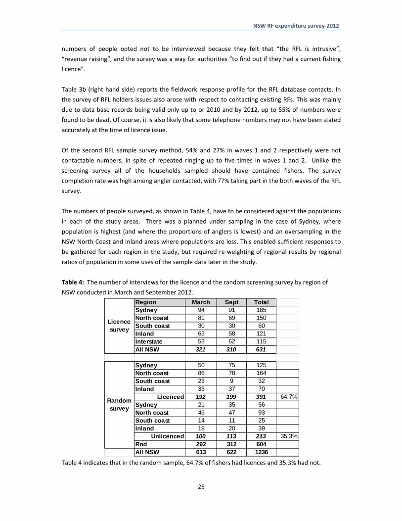
NSW RF expenditure survey‐2012
32 Fishing activity from the survey samples
Fishers were asked to recall their fishing activity and their fishing‐related expenditure over three
time periods
their last six months of fishing activity
their last fishing trip together with the expenditure involved on that trip and
their major boat expenditures in the last year
Rather than asking fishers at one point in time to recall details of activity and expenditure over a full
year (and therefore to try and reduce lsquotelescoping biasrsquo) two waves of field work interviews were
run six months apart In March 2012 and September 2012 field samples fishers were asked about
their last six months of fishing activity (this was also designed to enable any seasonality to be
assessed) Recalling days fished and expenditure over the previous year is known to include recall
bias and often a telescoping of memory Although six months is shorter than a year it may be that
there is a telescoping of the memory in respect of recalling past events and hence an unknown
component of ldquorecall biasrdquo in 6 months also In annualising results from two different fishers
recalling the last six months any bias will be compounded
Section 13 examined activity estimates from past RFE surveys in Australia and the differences
between methodologies The recreational fishing activity levels expressed as trips per annum or
days fished per annum point to the potential for recall surveys to overestimate activity in the
desired period The six month recall results were compared with previous annual trip and fishing
activity estimates in NSW and on the basis of conservatism were treated as being equivalent to bias‐
adjusted annual results The estimates of anglers when asked about their last 6 months of activity
appear to be less constrained than when recalling over the past year9 In other words it appears
there was a strong tendency to lsquotelescopersquo to the last 12 months
This is illustrative of the significant methodological divide between annual recall surveys and other
shorter term activity log approaches When the cost of diary surveys is prohibitive as is often the
case annual recall is preferred for expenditure estimation and adjustments for recall bias applied
Not applying adjustment for bias will lead to over estimates of activity and expenditure
321 Recreational fishing trips
Anglers were asked to recall the number of SW and FW trips in the past six months and also to recall
details of their last trip A trip can be just a day and may well be for many fishers who live close to
their usual fishing place but can of course be many days In each case this would be known since
they were asked the duration of their last trip in days Figure 1a plots the numerical frequency of
trips in the past year
9 Total activity estimates may have been more constrained if the same anglers had been called again or preferably in shorter 2 month periods as in the NOAA survey (Gentner 2008)
26
NSW RF expenditure survey‐2012
Figure 1a The numerical frequency of trips per annum for Saltwater and Freshwater fishing trips
0
100
200
300
400
500
600
1‐5 6‐10 11‐15 16‐20 21‐25 26‐30 31‐35 36‐40 40+
Number of trips
Trips per annum
SW Trips FW trips
Figure 1b shows that 54 of all SW anglers and 67 of all FW anglers fished 5 trips or less per year
The average number of trips per angler was SW 875 (standard deviation (sd) 145) and FW 38 (sd
86) or 107 (sd 153) trips for all fishing The declining exponential nature of the trips per annum
distribution is evident although there were 3 of trips by avid anglers who reported in excess of 40
trips per annum This distribution is highly skewed to the left and strongly influences calculation of
total expenditure estimates
Figure 1b The percentage frequency of Saltwater and Freshwater fishing trips per annum
0
10
20
30
40
50
60
70
80
1‐5 6‐10 11‐15 16‐20 21‐25 26‐30 31‐35 36‐40 40+
Percentage
frequency
Trips per annum
SW Trips FW trips
Anglers were also asked about days fished in SW and FW The relationship between trips and days
fished for 631 RL holders is reported in Table 5
27
NSW RF expenditure survey‐2012
Table 5 The days trips and length of trip for RFL Holders sampled (n= 613)
Type of fishing
day
Days Trips Daystrip of trip
time fished
SW days 6112 4189 146 817
FW days 2407 1536 157 866
The RFL survey sampled 631 fishers who fished 8470 days an average of 134 days per year
Proportionally 72 of days fished were in SW and 28 in FW Table 5 shows that the average fishing
trip was 146 days in SW and 157 days in FW of which over 80 of time was time fished in both
environments
322 Recreational fishing days
Previous catch and effort surveys have expanded data based on days fished Days fished are
presented on an annual basis in a frequency chart in Figure 2a and as percentage frequency chart in
Figure 2b
Figure 2a The frequency of days fished by all fishers (Average 146 days sd 186 days n=1231)
Figure 2a and 2b indicate that 38 of all anglers sampled fished 5 or less days per year but also that
6 of all anglers fished more than 40 days a year the latter often referred to as avid anglers The
average days fished are 146 days and given the previous estimate of 773000 adult anglers in NSW
this translates in to an estimated 116 million days fished in 2012
These activity distributions in samples are important The 36 of days below 5 days a year was less
than the 67 of the national survey (conducted in 2001) In contrast that survey also showed that
just 1 of anglers fished more than 40 days in the previous year (Henry and Lyle 2003)
28
NSW RF expenditure survey‐2012
Figure 2b The percentage frequency of days fished
In the present study this is partially explained by possible under sampling of 3 day and 1 month
licence holders though the random survey should not have been affected in this way On the other
hand the present study may well have sampled a higher proportion of avid fishers in the RFL data
base The third possibility is that angler behaviour in NSW has altered (on average) in the 12 years
since the national survey perhaps influenced by the introduction of the RFL
33 Comparisons between methods and samples
Statistical t‐tests were used to compare the trips per angler and average days fished per angler
between seasonal samples random and RFL database surveys and between licensed and unlicensed
recreational fishers
a) Are there seasonal differences in fishing activity
There is no previous literature on seasonal levels of fishing effort in NSW but we might expect to
see less days fished and fishing trips in the April to September ldquowinterrdquo period since this period does
not include Christmas However t tests revealed there was no statistically significant difference in
either the average days fished or trips per fisher across all observations between the April and the
September samples This may be partially explained by respondents to the September survey
recalling significant fishing activity at Easter time as part of ldquowinterrdquo activity
b) Are the random survey method and the RFL data base method results different
The t tests for trips indicate that those fishers in the random survey which included both licence
holders and non licence holders fished significantly more trips per year (125 v 906 trips t=395)
than fishers sampled from the RFL database This also applied to days fished with those in the
random survey fishing significantly more days (155 v 134 days t=208)
29
NSW RF expenditure survey‐2012
c) Are there differences between licenced and unlicenced fishers
Do licensed anglers fish more than unlicensed fishers When all samples are considered the average
days fished estimates show no significant difference between licensed and unlicensed fishers
However non‐licence holders made significantly more fishing trips than licence holders (128 trips v
103 t= 224)
34 Discussion of the sampling and activity results
On the basis of these results the average activity per angler whether measured in trips made or days
fished does not appear to be significantly different between seasons This result supports the
prospect of sampling recreational fishers at any time of the year asking them to recall their activity
in the last year
Fishers sampled randomly through the ldquowhite pagesrdquo made significantly more fishing trips and
fished on more days per annum than RFL holders Similarly those fishers contacted at random not
holding licenses were found to fish a similar number of days to licence holders but made
significantly more trips per annum This somewhat counter intuitive result (we might expect licence
holders to be more avid) is nevertheless consistent with concession holders and pensioners being
available to take more occasional fishing trips than the general working population might
It may also be related to the relatively high number of fishers found to have made more than 40
trips per year skewing the activity profile Where one sample is chosen at random and the other
comes from a database of known recreational fishers we may expect some avidity bias in the latter
(Johnson 1999) However this is not what we found indicating that opportunity to go fishing among
non licence holders may enable them to fish more frequently than licence holders though this
assumes we have no significant biases in the survey analysis For example ACMA (2013) states that
CATI surveys as used in our random screening survey ldquomay be biased towards those who normally
stay at home (eg older or retired people or those whose occupation is home duties)rdquo This may
indicate that those who responded had more time to go fishing than across the whole NSW
population
Non response bias and the screening survey
The most common non‐response bias is ldquounit non‐responserdquo which ldquotakes place when a randomly
sampled individual cannot be contacted or refuses to participate in a surveyrdquo (Ritz 2013) Mohadjer
et al explain ldquoThere is always a potential for item nonresponse bias whenever sample persons who
did not participate in the survey have somewhat different characteristics than those who didrdquo
In our random screening survey we had
‐ Sample losses approximately 50 of dead numbers and the potential for unit non response
bias Do those interviewees with land line numbers differ from those who have moved or
changed telephones in the past few years Privacy conditions precluded contacting non
respondents to investigate further Socio‐economically those moving away from landlines
may be younger in the working population or may have different incomes An argument
can be made either way and the extent of any bias remains unknown
30
NSW RF expenditure survey‐2012
‐ Non contactable household‐ It is unlikely these non contactable numbers for non‐RF
households or RF households would differ unless they were out fishing
‐ Refusals Why did so many people who identified themselves as having fished in the past six
months refuse to complete a short fishing interview Reasons include the dislike of surveys
intruding into their home and privacy not having the time or other general perceptions
Those who completed the interview may be keener on fishing more avid and some not
completing it because they consider their level of fishing to be trivial There was also the
indication from surveyors of fear or mistrust that the call was checking up on their licence
status In the random survey those who may have had a licence for 3 days or 1 month in the
previous six month period may not have had one at the time of the call and may have felt
vulnerable However approximately one third of all fishers are concession holders reducing
this possible vulnerability impact
In the area of survey refusals there seems to be more potential for non‐response bias in the
comparability of those who completed the survey with those who refused This cannot be directly
checked with non respondents due to privacy constraints Other independent indicators could be
used comparing ldquohellipthe distribution of respondents in the survey with associated distributions coming
from other independent surveysrdquo (Mohadjer et al 1994) We are able to compare the surveys given
their two different approaches
In the random screening survey over half of the identified fishers did not complete the survey We
can test for evidence of a response bias by comparing RFL licence holders who replied to the random
survey with RLF licence holders contacted directly in the other survey A t‐test indicated that the
mean days fished for the random RFL group (n=391) were significantly higher than the direct RFL
(n=631) survey results (158 v 134 t=211) significant at the 5 and 2 levels This is indicative of a
possible response bias as more active RFL holders appear more likely to have participated in the
random screening survey interviews than other less avid licence holders Previous adjustments made
to the data (section 32) reduced the risk to final estimates from this and other likely biases
Bias and the survey of RFL holders
The RFL survey also recorded significant levels of dead numbers although a much lower rate of
refusals The survey fieldwork team were able to ask to speak to the licence holder by name and this
may have contributed to higher completion rates Any bias in the RFL survey may then be between
responses by different licence holders Those holding 3 year licences may have significantly different
fishing activities expenditures or preferences to 1 year or 1 month and 3 day licence holders
Anecdotal evidence suggests some fishers buy several 3 day licences through the year and this may
contribute to a form of ldquodouble countingrdquo in any comparative analysis of licences The scale of this
behaviour is unknown and does not assist us in developing a sampling approach that may draw on a
representative cross section of the four licence types Further enquiries of non respondents was not
pursued due to privacy constraints
31
NSW RF expenditure survey‐2012
34 Estimation of recreational fishing expenditure per angler
Recreational fishing expenditure can be split into different categories as explained previously
a) Trip related expenditure on a range of expenses Trip expenditure can be annualised by expanding
by the number of trips per annum
b) Expenditure on small equipment and expenses on the last trip and
c) Annual expenditure on larger boat equipment This includes capital purchases in the year of the 10survey
All respondents in each area were asked about trip expenditures by all anglers in their household ndash
which averaged 202 anglers per household (see Table 7 later in report) The estimated expenditures
per angler per trip are reported in Table 6abc but state‐wide estimates in the next chapter are
based on household data
Table 6a summarises the average RF expenditure per trip for all NSW fishers (both SW and FW) in
each region for both fishing trip expenses and tackle Table 6b reports the average SW RF
expenditure per trip for all NSW regions on both fishing trip expenses and tackle Table 6c shows the
average trip expenditures for FW anglers Table 6d shows the annual expenditure on boat
expenditure for all NSW anglers SW and FW anglers combined
In Table 6ab ampc the results include fishers from Interstate who hold a NSW RFL but their major boat
and motor purchases are not assumed to have been made in NSW (Table 6d black squares)
The results in Table 6a confirm that all fishers (both SW and FW) spend 68 of trip expenses on the
fishing trip and just under 32 on equipment and fishing expenses Car travel is the major trip
expense $6974 (31 of total trip expense accommodation $ 3267 (15) and fooddrink eating out
$3594 (16) also while fishing rods and tackle hookslines and baitberley $3891(18) and boat
fuel $1650 (7) are the other major trip expenses
In Table 6b the costs of SW anglers are shown and Table 5c for FW Table 6bampc show that each
group had similar average expenditures per fishing trip (SW ‐ $22282 and FW ‐ $23024) Car travel
expenses are higher for FW fishers $9079 day versus $5955day SW but boat fuel for SW is
$1964 day versus FW $1009day
Table 6d shows that the annual NSW fisherrsquos average boat expenses per angler were $768 pa for all
NSW or broken down $856 for SW and $365 for FW fishers Boat purchase values for SW fishers
were much higher than for FW fishers which reflected the lower capital expenditure on small tinnies
for creeks dams and impoundments as opposed to offshore marine vessels The comparisons are
for the major form of fishing activity with 21 of fishers in our survey sample fishing a combination
of both SW and FW in a given year
10 Expenditure on fishing boats and larger capital items was reduced by 30 to reflect non recreational fishing use
32
NSW RF expenditure survey‐2012
Table 6a The average RF expenditure per trip for all NSW RFs in all NSW Last column is the
percentage of total spend in the All NSW total trip
Data in Aus $ Sydney North coast
South Coast
Inland Interstate All NSW of total spend per
trip Car travel (both ways) 6874 $ $ 4376 $ 4650 9871 $ 13060 $ 6974 $ 31 Accommodation 3998 $ $ 2216 $ 2112 2967 $ 6424 $ 3267 $ 15 Eating out 1478 $ $ 733 $ 1132 1572 $ 2820 $ 1342 $ 6 Other food and drink 2004 $ $ 1420 $ 2121 2881 $ 4857 $ 2252 $ 10 Shopping (souvenirmagazinesvideos) 419 $ $ 155 $ 120 607 $ 947 $ 387 $ 2 Travel-other than by car 354 $ $ 053 $ 325 040 $ -$ 160 $ 1 Sports 027 $ $ 018 $ - 034 $ 478 $ 065 $ 0 Tours 096 $ $ 007 $ 154 100 $ 022 $ 066 $ 0 Poker machines 174 $ $ 095 $ 077 124 $ 504 $ 160 $ 1 Pub 651 $ $ 347 $ 565 618 $ 1554 $ 621 $ 3 Anything else 194 $ $ 044 $ 068 134 $ 152 $ 117 $ 1 Expenditure per trip 16259 $ $ 9460 $ 11307 18946 $ 30811 $ 15405 $ 68
-$ $ - $ - -$ -$ -$ Major fishing tackle (rods reel) 2561 $ $ 1491 $ 1009 2756 $ 826 $ 1937 $ 9 Minor fishing tackle (hooks lines etc) 1106 $ $ 881 $ 713 1505 $ 2101 $ 1162 $ 5 Baitberley 1043 $ $ 559 $ 624 820 $ 938 $ 792 $ 4 Boat hire 671 $ $ 005 $ 090 139 $ 078 $ 242 $ 1 Boat fuel 2054 $ $ 1307 $ 683 1180 $ 3531 $ 1652 $ 7 Charter and fishing guide fees 647 $ $ 301 $ 043 098 $ 109 $ 323 $ 1 Fishing clothesapparel(w aders etc) 263 $ $ 177 $ 276 339 $ 143 $ 239 $ 1 Camping equipment 175 $ $ 735 $ 309 790 $ 400 $ 508 $ 2 Other fishing expenses 240 $ $ 283 $ 144 328 $ 393 $ 276 $ 1 Equipment per trip 8747 $ $ 5726 $ 3890 7939 $ 8520 $ 7120 $ 32
Total spend per trip 25007 $ $ 15185 $ 15197 26885 $ 39331 $ 22524 $ 100
Table 6b The average RF expenditure per SW trips for RFs anglers in all NSW Last column is the
percentage of All NSW total
Data in Aus $ Sydney North coast
South Coast
Inland Interstate All NSW of total spend per
trip
Car travel (both ways) 6168 $ $ 3659 $ 3915 17153 $ 12637 $ 5955 $ 27 Accommodation 4063 $ $ 2182 $ 2170 6325 $ 10959 $ 3547 $ 16 Eating out 1454 $ $ 782 $ 1151 4195 $ 5838 $ 1539 $ 7 Other food and drink 1988 $ $ 1284 $ 2321 2834 $ 6274 $ 2000 $ 9 Shopping (souvenirmagazinesvideos) 447 $ $ 164 $ 115 1620 $ 2157 $ 450 $ 2 Travel-other than by car 421 $ $ 034 $ 365 102 $ -$ 219 $ 1 Sports 033 $ $ 010 $ - 131 $ 581 $ 051 $ 0 Tours 113 $ $ 009 $ 173 280 $ -$ 086 $ 0 Poker machines 187 $ $ 112 $ 068 144 $ 865 $ 170 $ 1 Pub 694 $ $ 371 $ 612 1095 $ 2149 $ 649 $ 3 Anything else 229 $ $ 046 $ 077 -$ 405 $ 129 $ 1 Expenditure per trip 15787 $ $ 8647 $ 10947 33880 $ 41807 $ 14781 $ 66
Major fishing tackle (rods reel) 2703 $ $ 1509 $ 1136 2246 $ 541 $ 1905 $ 9 Minor fishing tackle (hooks lines etc) 1203 $ $ 742 $ 747 1087 $ 3010 $ 1035 $ 5 Baitberley 1183 $ $ 633 $ 656 1242 $ 1116 $ 899 $ 4 Boat hire 816 $ $ - $ 101 475 $ 243 $ 352 $ 2 Boat fuel 2309 $ $ 1380 $ 737 1903 $ 7946 $ 1964 $ 9 Charter and fishing guide fees 788 $ $ 370 $ 048 169 $ 338 $ 465 $ 2 Fishing clothesapparel(w aders etc) 302 $ $ 195 $ 310 270 $ -$ 245 $ 1 Camping equipment 213 $ $ 631 $ 048 936 $ 027 $ 402 $ 2 Other fishing expenses 252 $ $ 275 $ 161 234 $ 223 $ 247 $ 1 Equipment per trip 9750 $ $ 5721 $ 3943 8562 $ 13444 $ 7501 $ 34
Total spend per trip 25537 $ $ 14367 $ 14890 42442 $ 55251 $ 22282 $ 100
33
NSW RF expenditure survey‐2012
Table 6c The average RF expenditure per FW trip for RFs anglers in all NSW Last column is the
percentage of All NSW total
Data in Aus $ Sydney North coast
South Coast
Inland Interstate All NSW of total spend per
trip
Car travel (both ways) 10144 $ $ 7498 $ 10533 7358 $ 13261 $ 9079 $ 39 Accommodation 3696 $ $ 2363 $ 1654 1808 $ 4272 $ 2689 $ 12 Eating out 1591 $ $ 517 $ 981 667 $ 1388 $ 937 $ 4 Other food and drink 2077 $ $ 2014 $ 519 2897 $ 4185 $ 2771 $ 12 Shopping (souvenirmagazinesvideos) 287 $ $ 118 $ 154 258 $ 389 $ 258 $ 1 Travel-other than by car 039 $ $ 138 $ - 018 $ -$ 040 $ 0 Sports -$ $ 053 $ - -$ 429 $ 093 $ 0 Tours 015 $ $ - $ - 038 $ 032 $ 025 $ 0 Poker machines 115 $ $ 020 $ 154 117 $ 333 $ 141 $ 1 Pub 454 $ $ 245 $ 192 454 $ 1272 $ 565 $ 2 Anything else 031 $ $ 033 $ - 180 $ 032 $ 094 $ 0 Expenditure per trip 18448 $ $ 13000 $ 14187 13794 $ 25595 $ 16691 $ 72
Major fishing tackle (rods reel) 1903 $ $ 1414 $ - 2933 $ 962 $ 2002 $ 9 Minor fishing tackle (hooks lines etc) 658 $ $ 1482 $ 442 1649 $ 1669 $ 1423 $ 6 Baitberley 398 $ $ 238 $ 369 674 $ 853 $ 572 $ 2 Boat hire -$ $ 026 $ - 023 $ -$ 015 $ 0 Boat fuel 877 $ $ 988 $ 250 930 $ 1437 $ 1009 $ 4 Charter and fishing guide fees -$ $ - $ - 073 $ -$ 031 $ 0 Fishing clothesapparel(w aders etc) 085 $ $ 097 $ - 363 $ 212 $ 227 $ 1 Camping equipment -$ $ 1184 $ 2392 739 $ 577 $ 726 $ 3 Other fishing expenses 184 $ $ 319 $ 008 360 $ 474 $ 335 $ 1 Equipment per trip 4105 $ $ 5749 $ 3462 7724 $ 6184 $ 6332 $ 28
Total spend per trip 22553 $ $ 18749 $ 17648 21518 $ 31779 $ 23024 $ 100
Table 6d The average RF expenditure per annum on larger boat items for SW and FW anglers in
regions and all NSW (nb Table 6abc are per trip and Table 6d is per angler per annum)
Data in Aus $ Sydney North coast
South Coast
Inland Interstate All NSW of total spend per
trip
All NSW Boat licenceregistration 7115 $ $ 4658 $ 4407 5815 $ 8546 $ 5940 $ 8 Boat maintenance 29248 $ $ 14497 $ 9655 7935 $ 17917 $ 17504 $ 23 Boat insurance 7519 $ $ 4574 $ 3006 4145 $ 10318 $ 5754 $ 7 Marine mooring fees 7615 $ $ 1940 $ 192 122 $ 2609 $ 3179 $ 4 Boat equipment (safety etc) 15175 $ $ 7637 $ 3175 5452 $ 6015 $ 8888 $ 12 Boat purchase or motor repair 23437 $ $ 25676 $ 25865 9740 $ - 35550 $ 46 Annual boat expenditure 90109 $ $ 58982 $ 46300 33208 $ 45405 $ 76815 $ 100
Saltwater -$ $ - $ - -$ -$ -$ Boat licenceregistration 7340 $ $ 4751 $ 3583 6003 $ 13372 $ 6014 $ 6 Boat maintenance 32221 $ $ 15880 $ 9805 5356 $ 28392 $ 20829 $ 22 Boat insurance 8032 $ $ 5068 $ 3002 3960 $ 19824 $ 6458 $ 7 Marine mooring fees 8765 $ $ 2385 $ 216 030 $ 8108 $ 4505 $ 5 Boat equipment (safety etc) 17407 $ $ 7800 $ 3428 7508 $ 9230 $ 10764 $ 11 Boat purchase or motor repair 30450 $ $ 35250 $ 30000 40600 $ - 47050 $ 49 Annual boat expenditure $ 104214 $ 71134 $ 50035 63456 $ 78926 $ 95618 $ 100
Freshwater Boat licenceregistration 6073 $ $ 4255 $ 11000 5750 $ 6256 $ 5787 $ 16 Boat maintenance 15523 $ $ 8474 $ 8454 8830 $ 12949 $ 10632 $ 29 Boat insurance 5154 $ $ 2421 $ 3038 4209 $ 5809 $ 4297 $ 12 Marine mooring fees 2308 $ $ - $ - 155 $ -$ 439 $ 1 Boat equipment (safety etc) 4877 $ $ 6930 $ 1154 4738 $ 4490 $ 5011 $ 14 Boat purchase or motor repair 5000 $ $ 3150 $ 18400 5350 $ - 10350 $ 28 Annual boat expenditure 38935 $ $ 25230 $ 42046 29032 $ 29504 $ 36515 $ 100
34
NSW RF expenditure survey‐2012
In Table 6a the higher travel costs of some regional residents such as Sydney anglers Inland and
interstate fishers were evident The trip expenditure of Inland and interstate SW anglers was
significantly higher than for resident NSW anglers due to car travel accommodation food and other
trip expenses presumably to the coast (Table 6b) Table 6c shows that FW expenditure per trip was
highest for interstate fishers (eg Victorians traveling to southern NSW) and Sydney and South Coast
RFs had high travel costs travelling to desirable FW fishing locations (eg Snowy mountains etc
Dominion 2001 and 2002)
The socio‐economics of recreational fisher expenditure in NSW
The survey samples were analysed to identify some of the socio‐economic drivers of RF expenditure
in NSW The samples combined to give 1235 observations of RF expenditure and the survey
included a range of other variables Both multiple regression analysis and a cluster analysis enables
the statistically significant variables determining angler expenditure to be identified and estimated
as reported in Appendices 1 and 2 respectively
Multiple regression results
In Appendix 1 results reveal that Total recreational fishing expenditure is driven by licence status
(licence holders spending more) number of SW trips per annum and the level of household income
Age sex and regional location were found not to be statistically significant in determining total RF
expenditure
Trip expenditure was driven by licence holders and number of SW trips Trip expenditure was further
examined and was significantly influenced by licence holders SW and FW days fished and the
distance travelled on the last trip Fishing Tackle expenditure was found to be determined by
income rather than number of trips Expenditure on boats was driven by both number of SW trips
and the level of RF household income
Cluster analysis results
The expenditure of NSW RFs was also subjected to ldquocluster analysisrdquo to see the significant socio‐
economic characteristics of fisher groups as reported in Appendix 2and in Figure 3 below The cluster
analyses for expenditure on fishing trips tackle and boat expenditure are reported in Appendix 2
35
NSW RF expenditure survey‐2012
Figure 3 A cluster analysis of RF total expenditure showing the groups of significantly different
clusters of anglers identified
In Figure 3 there are four significantly different cluster groups The characteristics of the four groups
are under the ldquodescriptionrdquo row and the authors have put a label to characterise each group
Between Figure 3 and Appendix 2 the overall picture is of groups of ldquoordinaryrdquo fishers
(approximately 85) with low levels of fishing activity in which household income levels may differ
(half lower half higher) secondly a group of dedicated anglers (approximately 12) who have high
fishing activity and expenditure and finally a highly avid fishing group (less than 3) with very high
fishing activity and high to very high expenditure
The results confirm the only previous examination of the socio‐economic characteristics of RFs in
NSW by Dominion (2003) which showed that recreational fishing is a past time involving a diverse
range of people has great variety in activity levels and crosses the entire socio‐economic spectrum
36
NSW RF expenditure survey‐2012
4 State‐wide and regional expenditure estimates
41 Estimating total expenditure
This chapter describes the estimation of the total recreational fishing expenditure for RFs in NSW
and in its regions Total recreational fishing expenditure is the product of three variables
a) Number of recreational fishers or RF households (HH)
We use three approaches to estimate the total RF population in NSW by use of
1) Random telephone survey and ABS Household data and population data
2) The RFL data base and
3) Use of the screening sample and the ABS data on Households Use of the screening
survey of the general population to estimate total number of fishers11 via ABS
population data
b) Fishing trip activity fishing trip activity estimates are obtained from the telephone survey
and
c) Recreational fishing expenditure information on the expenditure per trip and annual
expenditures on equipment is obtained from the telephone survey
The product of these variables will enable us to estimate the total state‐wide recreational fishing
expenditure Expenditure is also estimated for each state region considered Saltwater and
freshwater fishing are considered separately in the state estimates through asking respondents
about the trip intention
42 Expanding the sample of fishers and expenditure
Total expenditure estimates are based on travel and fishing equipment expenses per trip and
estimates of expenditure on boat capital items These are summed to give an annual total
expenditure estimate However the estimates for the angler survey need to be expanded to give
state wide estimates These expansions are described in Box 1 below
Box 1 Explanation of key expansions
The expansion method adapts the method used in the National Survey (Henry and Lyle 2003) The
number of fisher households (FHH) was estimated as follows for each region
No of fisher Household (est) = No Households in Population (ABS) No of Fisher HH (sample)
No of HH (sample)
Example How many recreational fishers would these households include
No of Fishers 19 to 75 yrs (est) = Mean No fishers per HH (sample) No of fisher Household (est)
776496 = 202 383921 (see Table 7)
RF HH are distributed proportionally across regions by household and recreational fishers by
regional population
11 Recreational Fishers under 19 years of age are not included and need to be added if the total population figure is for all
anglers The activity and expenditure estimates are based on ages 19‐75 only
37
NSW RF expenditure survey‐2012
Information on NSW State and Regional Households by Local Government Area (LGA) were accessed
(ABS 2011) The data were aggregated by the larger SD ABS regions (eg Sydney North coast
Inland and SDD South Coast area) These identified the number of households in each of the study
regions as reported in Table 7
Table 7 The ldquototal householdsrdquo in each of the NSW study regions based on LGA data ABS (2011)
Households with recreational fishers are estimated for each study region
Area Population 2010 (gt18-75)
Households HH with RF Rec Fishers HH
RF by region
Sydney 3160897 1376583 213934 230 491232
North coast 835229 570688 88690 146 129802
South coast 350750 207195 32200 169 54510
Inland 649564 315987 49107 206 100948
Total 4996461 2470453 383931 202 776496
The RF household responses for anglersrsquo trip frequency and trip expenditure were multiplied to
produce estimates of state‐wide and regional expenditure
43 State‐wide expenditure estimates
The estimation of total expenditure for samples of recreational anglers and its expansion to regional
state‐wide and national estimates has depended on traditional statistical methods estimating the
total from means of the component distributions However while the number of households is
reasonably well estimated the frequency distribution of fishing trips is highly skewed to the left (see
Figure 1a)
The estimates of total state expenditure on recreational fishing involve multiplying the following
variables
1) Estimate of RF households ‐ the ABS has reliable estimates of households for which RF
households can be identified
2) Estimate of trips ‐ anglers state the number of trips per annum and
3) Estimate of the trip and tackle expenditure on their last trip and their capital expenditure in
the last year
Total expenditure is the product of these variables Total expenditure can be estimated as a mean
value with confidence intervals Here we used the 1237 observations in the RF sample weighting
the results in respect of regional populations as follows
a) Total annual expenditure per angler household = (($ travel expenses per trip + $ tackle
expenses per trip) number of trips )+ (annual capital expenditure per angler household)
b) Total annual expenditure in NSW = total number of anglers households total annual
expenditure per angler household
This traditional approach gives a point estimate but does not provide any information on the
probability of different expenditure levels around the mean This requires a simulation approach
38
NSW RF expenditure survey‐2012
Table 8a shows that the estimated expenditure by all NSW resident RFs in 2012 was $1439bn12 with
an additional $1861m being spent by interstate fishers making a total estimated expenditure by
recreational fishers in NSW of $1625bn in the year 2012
Considering regional expenditures total recreational fishing expenditure was highest by Sydney
anglers ‐ $903m (56 of all expenditure in NSW) followed by the North coast anglers ‐ $3008m
(19) and inter‐state anglers ‐ $ 186m (11) Total expenditure for South Coast anglers was
$1018m (6) and for Inland anglers $1308m (8)13
Expenditure on fishing trips was $793m or 49 of all recreational fishing expenditure in NSW Of
this $402m (25) was spent on fishing equipment tackle and fuel and $430m (26) was spent on
annual capital expenditures such as boats and maintenance Expenditure on SW fishing was
estimated at $1415m (87) and on FW fishing at $231m (13 of total recreational fishing
expenditure in NSW)
Table 8b shows the costs within each category
Within trip expenditure (49 of total expenditure) car travel $326m (201 of total annual
expenditure) accommodation $1859m (114) and food and eating out $188m (115)
Expenditure on fishing equipment and expenses $4025m (246) was made up of $1645m
(102) on major and minor tackle and $1027m (63) on boat fuel and
Annual boat expenditure $4305m (26) of which $1225m (75) was maintenance and
boat purchase or motor repair $1436m (88)
12 This estimate is the same as the mean value produced by the simulation shown later in this chapter It is then adjusted
for Interstate expenditure13 In Chapter 5 the regional economic analysis adapts these data to reflect the expenditure made in other regions away from home residence
39
NSW RF expenditure survey‐2012
Table 8a Estimates of the total RF expenditure for different areas of NSW and including interstate angler expenditure to give all RF expenditure in NSW
Expenditure category Sydney North coast South coast Inland All NSW Inter-state Total expend
in NSW
total expend in NSW
Trip spend 383906879 136686958 57862828 74849484 653306149 139478487 792784637 49 $ fishing equip 222891110 85965049 20624384 31116970 360597513 41975664 402573177 25 Total annual boat expenditure 296326795 81222395 23393975 24877516 425820681 4691465 430512146 26 Totals 903124785 303874402 101881187 130843970 1439724343 186145616 1625869959 100 of total expend in NSW 56 19 6 8 89 11 100 Saltwater 840749912 267431019 99200573 51715617 1259097121 140675487 1415280961 87 Freshwater 62374873 36443383 2680614 79128353 180627222 45469052 231775451 14 SW expenditure as of Total 93 88 97 40 87 84 87
40
NSW RF expenditure survey‐2012
Table 8b Estimates of the total RF expenditure for different areas of NSW and including interstate angler expenditure to give all RF expenditure in NSW
Data in Aus $ Sydney North coast South coast Inland All NSW Interstate Total expend
in NSW
of Total expend in
NSW Expenditure category Car travel (both ways) 155752824 61047851 21250669 38966591 277017934 49755399 326773333 201 Accommodation 96655736 32991275 11321758 11775540 152744309 33155541 185899850 114 Eating out 35118007 11287702 6019080 6283701 58708491 16433282 75141772 46 Other food and drink 47830881 20416270 11974310 11255861 91477322 21385714 112863036 69 Shopping (souvenirmagazinesvideos) 10396840 2377682 609238 2427428 15811187 5900718 21711905 13 Travel-other than by car 9328498 675596 1876003 157968 12038065 - 12038065 07 Sports 730303 214569 - 136952 1081824 2038576 3120401 02 Tours 2517279 121080 888633 400483 3927475 44318 3971793 02 Poker machines 4337423 1534429 364864 485304 6722021 2611177 9333198 06 Pub 16147653 5352108 3163325 2442584 27105670 7101506 34207176 21 Anything else 5091436 668396 394948 517073 6671852 1052256 7724108 05 Trip spend 383906879 136686958 57862828 74849484 653306149 139478487 792784637 488
Major fishing tackle (rods reel) 63209459 22456502 5830420 10743744 102240126 2673467 104913593 65 Minor fishing tackle (hooks lines etc) 27752247 12319663 3884279 5859337 49815525 9792034 59607560 37 Baitberley 26800952 8839913 3407290 3225829 42273984 3954942 46228926 28 Boat hire 17933756 42708 518369 561815 19056649 604762 19661412 12 Boat fuel 52493364 20044184 3811422 4649308 80998277 21742806 102741083 63 Charter and fishing guide fees 17310929 4944101 246843 386149 22888022 839948 23727969 15 Fishing clothesapparel(w aders etc) 6799431 2766227 1592134 1322337 12480129 292501 12772630 08 Camping equipment 4689522 10357115 508333 3093322 18648291 864926 19513218 12 Other fishing expenses 5901451 4194635 825295 1275129 12196509 1210277 13406786 08 $ fishing equip 222891110 85965049 20624384 31116970 360597513 41975664 402573177 248
Boat licenceregistration 22369127 6037457 1817922 4154611 34379117 4691465 39070582 24 Boat maintenance 93188042 18809323 4588346 5925940 122511651 - 122511651 75 Boat insurance 23806199 5935399 1413005 2990204 34144806 - 34144806 21 Marine mooring fees 24487619 2521793 97904 96275 27203591 - 27203591 17 Boat equipment (safety etc) 48762545 9898735 1571861 3725061 63958201 - 63958201 39 Boat purchase or motor repair 83713264 38019687 13904937 7985426 143623314 - 143623314 88 Total annual boat expenditure 296326795 81222395 23393975 24877516 425820681 4691465 430512146 265
Totals 903124785 303874402 101881187 130843970 1439724343 186145616 1625869959 1000 Saltwater 840749912 267431019 99200573 51715617 1259097121 140675487 1399772608 861 Freshwater 62374873 36443383 2680614 79128353 180627222 45469052 226096274 139 SW expenditure as of Total 93 88 97 40 87 76 86 Region as of total expenditure 56 19 6 8 11 100
41
NSW RF expenditure survey‐2012
44 A probabilistic simulation approach to the estimation of total state recreational fishing
expenditure
Simulation enabled us to estimate the probability of different outcomes from the existing data The
original sample was weighted by numbers of regional households to account for the under sampling of
Sydney and the over sampling of the North Coast in the original survey data The sample was analysed
using the SPSS v21 Monte Carlo Simulation model (IBM Corp 2012) This routine produced up to
100000 repeat runs of the predicted values of total RF state expenditure to give the probability of
different expenditure totals as shown in Figure 5a The cumulative probability is shown in Figure 5b
Figure 5a The probability of total expenditure by NSW anglers 2012
These initial probability estimates showed that the mean total state‐wide expenditure was $1473m
with 5 and 95 confidence estimates of $706m and $2952m The median value as $1196m reflecting
the skewedness of the distribution
The estimate of expenditure in NSW by interstate anglers of $1861m has also to be added The final
total NSW estimate of expenditure on recreational fishing was therefore $1625m with 5 and 95
confidence estimates of $892m‐$3136m14
14 For simplicity this assumes the distribution of the interstate results are the same as all NSW
42
NSW RF expenditure survey‐2012
Figure 5b The cumulative probability of total expenditure by NSW anglers 2012
Figure 5a and 5b indicate how the skewed distribution of trips per year by anglers and the highly annual
variable expenditure make the predicted adjusted distribution from $892m‐$3136m around an
adjusted mean $1625m and an adjusted median of $1382m The mean has a 0045 probability of being
achieved whereas lower total expenditure estimates have higher probability (Figure 5a) The
skewedness gives a threshold minimum expenditure level and a ldquotrailing tailrdquo on the right hand side
reflecting less probable high expenditure estimates
Figure 5b indicates that the mean would have a cumulative probability of 65 This shows the higher
total expenditure estimates on the right hand side of Figure 5a are pulling the mean to the right This is
why we have to be careful in RF sampling and estimation of recreational activity and expenditure This
also may explain why fishers of differing avidity and expenditure levels have considerably different
opinions on total expenditure in the sector A fisher with higher activity and expenditure would estimate
a state wide total at the right hand side of Figure 5a but while high total expenditure is possible it is
highly improbable
45 Discussion The estimated total expenditures reported in Table 8a and 8b indicate a statewide expenditure by NSW
recreational fishers and interstate anglers on items directly related to fishing of $1625m
43
NSW RF expenditure survey‐2012
The expansions to develop the final estimates took account of the differences between SW and FW
expenditure and activity and each was expanded separately Expenditure on FW fishing contributed 14
of total expenditure considerably less than the 28 of days fished reported in the sample (Table 5)
reflecting some trip and capital expenditure differences between SW and FW fishers
By region the results indicate that recreational fishing expenditure by Sydney anglers $9031m (56 of
total state recreational fishing expenditure) while North coast has $3038m (9) Interstate anglers
$1861 (11) Inland $1308m (8) and South coast $1018 (6) The survey method estimated regional
expenditures from interviews with fishers in their home region The regional economic impacts adjusts
these and produced estimates of recreational fishing expenditure and its economic impacts across all of
NSW and its main regions
There is just the previous national survey study for comparison of results The 2012 expenditure
estimate adjusted from the Campbell and Murphy (2005) national survey 2001 study is $765m This is
within the confidence intervals predicted by the current studyrsquos simulation approach
Another comparison is to deduct the trip expenditures for food and entertainment from the current
studyrsquos results to be comparable to Campbell and Murphyrsquos assumptions giving an estimate up to
$136bn15 The difference in expenditure estimates16 is primarily related to the survey methods used and
the different estimates of fishery activity the current study being higher Though the number of adults
fishing may have reduced since 2001 NSW has now a sizeable established recreational fishing licence
holder population and expenditures per angler are higher than a decade ago
Under the telephone survey interview and recall method used the current results were conservative for
this methodological approach This study has pointed to the highly skewed nature of the trip activity
among the RF population and the highly variable levels of expenditure among recreational fishers in
NSW The use of a probabilistic simulation in this study has illustrated the difficulties in estimation of
total RF expenditure and the wide distribution around the mean The adequate inclusion and possible
over‐inclusion of avid fishers are sampling problems under any of existing methodologies
The sample size and hence a higher survey cost is part of the remedy Further examination of the US
multi‐method approach may be merited (Gentner 2009) though this is a large scale national expensive
survey exercise The project results in this study are proposed as being reasonable under the
methodologies available within funding constraints and are part of a proposed ongoing expenditure
survey strategy in NSW as outlined in Chapter 6
15 There may also be differences in the treatment of capital attributable to RF definitions of maintenance and capital expenditure on motors and boats and other differences between the two studies These may likely lower this estimate 16 ($1360m‐$765m=$595m in 2012 terms)
44
NSW RF expenditure survey‐2012
5 Regional economic impact estimates This chapter of the report was compiled by Western Research Institute (WRI) WRI received the output
of this survey in terms of expenditure of respondents and based on this output modelled the
economic impacts of recreational fishing on the NSW economy and defined sub‐regions Input‐
output modelling has been employed to derive the relevant economic models and the impacts
51 Methodology
The methodology used to prepare this report included
Determination of the boundaries of the regions to be used in table construction
In consultation with the ANCORS the decision was made to construct input‐output tables for the NSW
North Coast NSW South Coast NSW Inland and Sydney regions as well as NSW as a whole Each region
was defined by aggregating statistical areas at level 4 3 or 2 or combination thereof This allowed the
formulation of regions and economies that best represented the regions of interest Specifically data
from statistical areas at level 3 of ABS Statistical Geography Standard (rather than at larger statistical
areas at level 4) was used in the construction of tables for the NSW North Coast and data from
statistical areas at level 2 was used in the construction of tables for the NSW South Coast The table
construction for Sydney region was based on the data from statistical areas at level 4 while tables for
NSW Inland region was based on the data from statistical areas at different levels (2 3 and 4) Detailed
information on statistical areas in provided in WRI (2013)
Construction of tables
The input‐output tables developed for this project were derived from the latest national table produced
by the Australian Bureau of Statistics (ABS) That table provides a detailed picture of the structure of the
economy of Australia for the year 2008‐09 A series of steps were undertaken to update the table to
2011‐12 Further information from the State Accounts (ABS Cat No 52200) labour force data from the
2011 Census and the quarterly labour force survey (ABS Cat No 6291055003) were used to develop a
state table for New South Wales at 2011‐2012 This was then regionalised to reflect the respective
regional economies of NSW North Coast NSW South Coast NSW Inland and Sydney Further details of
the procedures used in the development of a regional input‐output table are provided in WRI (2013)
52 Economic impact analysis
The economic impacts were modelled as a final demand impact (that calculates the impacts measured
by output value added household income and employment across all sectors in response to changes
in industry final demands) using the 2011‐12 Simulating Impacts on Regional Economies (SIRE) input‐
output model of NSW North Coast NSW South Coast NSW Inland Sydney and NSW as a whole The
SIRE model is superior to standard input‐output models as it provides for non‐linear relationships
between variables and is based on empirically derived (rather than assumed) coefficients In terms of
45
NSW RF expenditure survey‐2012
robustness of results it is comparable with computable general equilibrium (CGE) models whilst
minimising data requirements See WRI (2013) for a detailed description of the SIRE input‐output
model
The impacts of recreational fishing expenditure on the NSW North Coast NSW South Coast
NSW Inland and Sydney regions as well as NSW as a whole have been provided in terms of
bull Output which is the value of goods and services that are produced within an establishment
that become available for use outside that establishment plus any goods and services
produced for the organisationrsquos own final use Output is equal to total revenue plus any
internal consumption
bull Value added which is equal to gross output minus intermediate inputs Value added is
equivalent to the contribution to gross regional product (the local equivalent of gross
domestic product)
bull Household Income which measures the benefit received by regional households from
economic activity It typically refers to compensation of employees but can also include
income in return for other forms of productive activity
bull Employment which refers to full‐time equivalent (FTE) employment is a measure of the
total level of staff resources used The FTE of a full‐time staff member is equal to 10 The
FTE of a part‐time worker will be a fraction of this depending on the relative number of
hours worked
53 The Economic Impact of Recreational Fishing on the Regional Economies of NSW
The economic impact due to recreational fishing was modelled as follows
bull The expenditure survey conducted by ANCORS did not capture the location of expenditure
just the origin (postcode) of the respondent Therefore in the absence of location data an
assumption was made that the total expenditure by interstate visitors ($18614 million)
who make expenditures on recreational fishing whilst staying in NSW should be distributed
evenly across four NSW regions (ie 25 of total interstate expenditure pertaining to each
NSW region)
bull Likewise it was assumed that expenditure pertaining to the NSW North Coast NSW
South Coast and NSW Inland regions was made in these regions (eg those
respondents who indicated living in the NSW North Coast partake in recreational
fishing in the NSW North Coast and not in other areas thereby ensuring that the
money spent on recreational fishing remains in the NSW North Coast region)
46
NSW RF expenditure survey‐2012
bull For those respondents who indicated living in Sydney an assumption was made that 515
of them partake in fishing in Sydney with the remaining 485 fishing in the rest of NSW in
the following proportions NSW North Coast ndash 346 NSW South Coast ndash 485 and NSW
Inland ndash 169 (Dominion 2002 and 2004)
bull Since anglers in each of the regions make expenditure on items that may not be
produced in the region but that are imported from the rest of NSW the regional
recreational fishing expenditure was split into local and imported components using a
location quotients matrix This way WRI ensured that only local expenditure generated
economic impacts in the respective region For NSW as a whole an assumption was
made that all products that anglers purchase are produced within the state and
therefore no separation of local and imported components was performed The
economic impacts of recreational fishing on NSW were modelled using total recreational
fishing expenditure in NSW
bull In order to ensure consistency of the input‐output modelling procedure the expenditure
data was allocated in the input‐ output table to the industries (typically manufacturing
industries) where the relevant expenditure items were produced and was then
converted to basic prices See WRI (2013) for further details on sectoral allocations
bull A final demand analysis in SIRE was performed and economic impacts on NSW North Coast
NSW South Coast NSW Inland and Sydney as well as NSW as a whole were derived
The impacts of recreational fishing on the economies of the NSW North Coast NSW South Coast
NSW Inland and Sydney regions are outlined in the Table 9
Table 9 Regional expenditure and economic impacts on regional economies
Region North Coast Sydney South Coast Inland
Expenditure by postcode ($m) 30387 90312 10188 13084
Reclassified expenditure ($m) 50196 51165 36086 2514
Output ($m) 73465 100286 39522 35381
Value added ($m) 35355 49156 18417 14985
Household income ($m) 16875 28888 876 735
Employment (no) 3320 3944 1808 1539
47
NSW RF expenditure survey‐2012
NSW North Coast
Overall when flow‐on effects are taken into account recreational fishing contributes the following to
the economy of NSW North Coast
bull 3320 FTE jobs including 667 in the retail trade sector 573 in the hospitality sector
349 in the personal and other services sector and 174 in the transport and storage
sector
bull $16875 million in household income with 134 percent being in the retail trade
sector 112 percent being in the hospitality sector 76 percent being in the public
administration sector 72 percent being in the personal and other services sector and
57 percent being in the transport and storage sector
bull $35355 million in industry value added representing 081 percent of total regional
value added of the NSW North Coast region and
bull $73465 million in output
For the North Coast recreational fishing will contribute 098 percent of FTE employment in the
region when flow‐on effects are taken into account as well as 084 percent of household income and
07 percent of the estimated gross regional product of the NSW North Coast region
NSW South Coast
Overall when flow‐on effects are taken into account the recreational fishing contributes the
following to the economy of NSW South Coast
bull 1808 FTE jobs including 420 in the hospitality sector 284 in the retail trade sector
236 in the personal and other services sector 117 in the transport and storage
sector and 106 in the public administration sector
bull $8760 million in household income with 152 percent being in the hospitality sector
109 percent being in the retail trade sector 93 percent being in the public
administration sector 86 percent being in the personal and other services sector and 77
percent being in the transport and storage sector
bull $18416 million in industry value added representing 167 percent of total regional
value added of the NSW South Coast region and
bull $39522 million in output
For the South Coast recreational fishing will contribute 212 percent of FTE employment in the region
when flow‐on effects are taken into account as well as 173 percent of household income and 143
percent of the estimated gross regional product of the NSW South Coast region
48
NSW RF expenditure survey‐2012
NSW Inland
Overall when flow‐on effects are taken into account the recreational fishing contributes the
following to the economy of NSW Inland
bull 1539 FTE jobs including 289 in the hospitality sector 288 in the retail trade sector
148 in the personal and other services sector and 138 in the agriculture sector
bull $7350 million in household income with 134 percent being in the retail trade
sector 131 percent being in the hospitality sector 74 percent being in the
personal and other services sector 70 percent being in the public administration
sector and 68 percent being in the transport and storage sector
bull $14985 million in industry value added representing 030 percent of total regional
value added of the NSW Inland region and
bull $35381 million in output
Recreational fishing will contribute 038 percent of FTE employment in the NSW Inland region when
flow‐on effects are taken into account as well as 032 percent of household income and 026 percent
of the estimated gross regional product of the NSWInlandregion
Sydney
Overall when flow‐on effects are taken into account the recreational fishing contributes the following
to the economy of Sydney
bull 3944 FTE jobs including 741 in the retail trade sector 450 in the hospitality sector
366 in the personal and other services sector and 310 in the professional and
technical services sector
bull $28888 million in household income with 162 percent being in the finance and insurance
sector 113 percent being in the retail trade sector 83 percent being in the professional
and technical services sector 77 percent being in the wholesale trade sector and 63
percent being in the hospitality sector
bull $49156 million in industry value added representing 025 percent of the total regional
value added of Sydney and
bull $100286 million in output
For the Sydney region recreational fishing will contribute 028 percent of FTE employment when flow‐on
effects are taken into account as well as 025 percent of household income and 022 percent of the
estimated gross regional product of Sydney
49
NSW RF expenditure survey‐2012
NSW State economy
The impacts of recreational fishing on the state economy of the NSW are outlined in the Table 10
Table 10 NSW expenditure and economic impacts on NSW
Item Estimate
NSW Expenditure by postcode ($m) 143972
Total interstate expenditure ($ m) 18615
NSW Reclassified expenditure ($m) 162587
Output ($m) 342035
Value added ($m) 162561
Household income ($m) 87728
Employment (thousand) 14254
NSW Economy
Overall when flow‐on effects are taken into account the recreational fishing contributes the following to
the economy of NSW
bull 14254 FTE jobs including 2730 in the retail trade sector 2123 in the hospitality
sector 1389 in the personal and other services sector and 951 in the transport and
storage sector
bull $87728 million in household income with 122 percent being in the retail trade 114
percent being in the finance and insurance sector 88 percent being in the hospitality
sector 72 percent being in the professional and technical services sector and 65
percent being in the wholesale trade sector
bull $162561 million in industry value added representing 036 percent of the estimated gross
state product of the NSW and
bull $342035 million in output
50
NSW RF expenditure survey‐2012
Overall recreational fishing will contribute 046 percent of FTE employment in the NSW when flow‐on
effects are taken into account as well as 041 percent of household income and 040 percent of total
regional value added
54 Conclusion
The recreational fishing expenditure and economic impact of recreational fishing on NSW and
respective regions were substantial in absolute terms but uneven across regions
The expenditure based on place of residence was the highest in Sydney followed by NSW North
Coast NSW Inland and NSW South Coast The reallocated expenditure (ie actual expenditure
made in the region) was still the highest in Sydney (but substantially lower than postcode
expenditure) followed by expenditure in NSW North Coast NSW South Coast and NSW Inland
In terms of output valued added household income and FTE employment the absolute economic
impacts of recreational fishing were the highest in Sydney followed by NSW North Coast NSW South
Coast and NSW Inland However in relative terms economic impacts (as percentage of total in the
respective regions) were the highest in NSW South Coast (167‐ 212) followed by NSW North
Coast (081‐098) NSW Inland (030‐038) and Sydney (025‐028) These relative disparities
reflect the large size of Sydney and NSW Inland economies and smaller size of NSW North Coast and
NSW South Coast economies
51
NSW RF expenditure survey‐2012
6 Developing a cost effective approach to expenditure surveys
There have been several reoccurring issues in obtaining information on recreational fishing expenditure
in NSW The first is the lack of a series of expenditure surveys the past ones not occurring as part of an
on‐going consistent strategy The second issue is the lack of a known survey method which is repeatable
and can be compared with past surveys In both of these issues the recurrent cost of such surveys has
been unknown also
61 The objectives of an recreational fishing expenditure survey
Any survey is designed towards its objectives In developing a cost effective regular approach to
recreational fishing expenditure surveys there has to be some design decisions made in respect of the
information required For example A state‐wide expenditure estimate may be required every two years
to track and promote the value of the sector This could include a state‐wide estimate of regional
economic impact Further disaggregation by area or other variables will increase cost
62 Sampling data issues and findings
This study has considered how the use of the RFL database reduced the cost of expenditure surveys
which have traditionally used expensive random screening surveys to locate recreational fishers
Finding 1 The current study has found that there is no statistically significant difference between
seasonal samples Consequently we recommend an annual survey event being mindful of its timing
relative to Christmas January and Easter which may be periods when fishers are not at home
The RFs identified through a random screening survey process were found to make more fishing trips
and fish more days than the sample of RFs contacted through the RFL database (noting that both
samples include licence holders) However in further comparisons of days fished per angler between
licenced and unlicensed fishers no significant difference was found On the other hand unlicensed
fishers were found to undertake significantly more fishing trips than licence holders though this relates
to trip events and not necessarily to higher average expenditure ndash in other words unlicensed fishers
may make more but shorter trips to nearby destinations compared with licensed fishers
Finding 2 The RFL database can be used to sample anglers for expenditure surveys providing certain
conditions are met in terms of the different numbers of licences holders that are sampled17
63 What sample size is required
The size of a sample in statistics is important If the sample is too small there is then the risk that the null
hypothesis is wrongly rejected (ATS 2010) The size of a sample is also related to the probability level at
17 A ratio of 3 day 1 month 1 year and 3 year licence holder records is recommended The weighting would be easier for the annual and 3 year licence holders as 3 day and monthly licence holder can be repeat licence purchasers in a given year
52
NSW RF expenditure survey‐2012
which the variable is seen to be significantly different from zero eg 95 (5) or 99 (1) levels of
significance The dispersion of the distribution of the variable being examined is also important and this
is captured in the standard error of the variable
In statistics these issues are brought together in statistical ldquopower analysisrdquo where the minimum size of
a sample can be tested both prior to and even after statistical surveys to see if the sample size is
adequate ldquoThe power is the probability of detecting an effect presuming it is actually thererdquo (ATS 2010)
Sample size estimation
In this section of the report we investigate how reducing the sample size to the minimum required
number of interviews can reduce the cost of an expenditure survey The decision regarding the target
sample size for the survey has to be balanced between the levels of significance chosen for testing (1
5) and the standard error that is acceptable for the intended variables which is often related to the
estimated value called the relative standard error (RSE) 18
Table 11 shows a range of sample sizes derived for different scenarios using the ABS calculator facility at
NSS (2013) There are the two scenarios for random surveys (cases 1‐4) and two for surveys from a
population base of known participants (case 5‐6)
Table 11 Indication of the required sample sizes under different sampling and risk scenarios including
sampling of the RFL database
Case number 1 2 3 4 5 6 Sample type Random sampling Non random
Statistical input All NSW Population
All NSW Population
All NSW Population
South coast
RFL ‐1 RFL‐2
Confidence Level 99 95 95 95 95 95 Population Size 4996500 4996500 4996500 350750 480700 480700 Proportion 05 05 015 025 06 06 Confidence Interval 005 005 00294 005 005 005
Upper 055 055 01794 03 065 065 Lower 045 045 01206 02 055 055
Standard Error 0025 0025 0015 0025 003 0045 Relative Standard Error () 50 50 100 100 50 75 Sample Size 339 196 567 300 267 119
18 The RSE is the standard error expressed as a percentage of the estimate
53
NSW RF expenditure survey‐2012
In Table 11 cases 1 and 2 show the general sampling results when the confidence level is either 99 or
95 and the proportion is 05 (ie where ldquothe expected proportion of the population to have the
attribute that you are estimating from your surveyrdquo (NSS 2013) These data are often quoted but given
that RFs are more difficult to locate than a one in two assumption (proportion 05) case 3 assumes a
15 proportion for RFs and requires a sample size of 567 with a relative standard error (RSE) of 10
Reducing the sampling area to the South Coast (case 4) raises the chances of locating RFs (proportion
025) and would require 300 observations at an RSE of 10 The sampling model assumes a random
population
We also apply the model to the non‐random scenarios from the RFL data base Here cases 5 and 6 are
RFL records and hence not as random as the whole NSW population We use the model to estimate
possible minimum sample sizes when using the RFL data base population Assuming that the proportion
is 06 an RSE of 5 requires a sample of 267 and an RSE of 75 a sample size of 119 In the experience
of the authors the last sample size (119) is low given the variation in our results We recommend no less
than 250 completed surveys as a minimum sample size for state‐wide estimates If four NSW regions are
included a minimum total of 500 completed surveys would be required and be should be larger if
possible
The review of samples has shown that there is a trade off in accuracy of estimates with the number of
interviews undertaken For example in the case 3 random survey in Table 11 the RSE is 10 and
reducing this to 75 for case 3 would increase the sample size from 576 to 1008 or for 5 to 2226
The incidence of locating RFs has cost implications for surveying and this is why the careful use of the
RFL data base is attractive
Finding 3a A main state‐wide survey using the RFL data base to sample 1000 anglers in major regions is
recommended every 5 years with an option of updating results by indexing annually or bi‐ennially
andor considering a smaller survey (250 state wide or 500 for regions) in year three also
Finding 3b The economic impact analysis can follow the five year survey pattern and can be adjusted
between surveys Simulation modelling can also be used to provide an improved understanding of the
uncertainty surrounding expenditure estimates and may be used to confirm estimates between main
surveys also
64 Discussion ‐ Scoping a recreational fishing expenditure survey strategy for NSW
A recreational fishing expenditure survey strategy would aim to undertake a substantial survey every 5
years and run smaller annual or biennial updating exercises between these periods
In the future the 5 year survey could either
54
NSW RF expenditure survey‐2012
Follow past screening survey approaches of all RFs and compare results with a sample of RFL
holders as in the current study or
Use a weighted selection of 3 day 1 month 1 year and 3 year licence holder contacts to enable
a representative sample to be expanded to state‐wide totals
Before being able to categorically recommend the sole use of the RFL database only approach we would
require more information on the inter‐relationship between the random screening survey and the use of
and RFL data base records The current NSW catch and effort survey study may also provide information
on this relationship (J Murphy DPI pers comm)
As per Finding 2 we recommend further comparisons of the random screening survey approach to all
fishers with use of the RFL holdersrsquo data as in the current study Use of the RFL database alone should
be confirmed by other research on the relationship between all fishers and those who are licensed
In the years between the five year main surveys the survey results from the initial survey could be
upgraded annually (or bi‐ennially) by sampling several variables that could be used to index the changes
in the state wide expenditure estimates For example any changes detected in RF participation or
activity state population or change in licence sales could inform activity estimates Information on
recreational fishing expenditure could be influenced by annual changes in price levels as measured by
the consumer price index (cpi) and any information available from industry about retail fishing gear
prices such as those related to exchange rate variations which would impact expenditure on fishing
gear Many of these indices of economic conditions are monitored by the Australian Fishing Tackle
Association and could be referred to
The simulation modelling approach used in the current study could be re‐run annuallybiennially with
these activity and expenditure indices included and updated annual estimates produced The
reoccurrence of another survey in year 5 means there would be a cross check on the indexing of the
previous survey
The choice of 5 years for the main survey is arbitrary and could be 3 years particularly if other catch and
effort surveys are indicating significant changes in participation rates in NSW or there is evidence of
changes in other states Leaving a main survey for more than 5 years is not recommended as the public
awareness of the sectorrsquos economic contribution and associated regional benefits will reduce giving the
sector less public profile
65 Conclusions
The recreational fishing sector in NSW wishes to have more regular studies of angler expenditure and its
importance to the economy The RFL data base can be used for sampling the recreational fishing
population reducing the costs of fieldwork surveys if several conditions are followed The frequency of
55
NSW RF expenditure survey‐2012
the different licence durations needs to be chosen so as not to move away from sampling a
representative cross section of anglers of all different activity levels and possibly having over or under
emphasis of avid anglers
A main state‐wide survey using the RFL data base to sample 1000 anglers in major regions is
recommended every 5 years with an option of updating results by indexing annually or bi‐ennially and
considering a smaller survey (250 state wide or 500 for regions) in year three also The economic impact
analysis can follow the five year survey pattern and can be adjusted between surveys Simulation
modelling can also be used to provide an improved understanding of the uncertainty surrounding
expenditure estimates and may be used to confirm estimates between main surveys also
56
NSW RF expenditure survey‐2012
References
ABARES (2011) Australian Fisheries Statistics 2010 Australian Bureau of Agricultural and Resource Economics and
Sciences Australian Government p 100
ABS (2010) 1216055003 ‐ Australian Statistical Geography Standard Design of the Statistical Areas Level 4
Capital Cities and Statistical Areas Level 3 May 2010 Canberra
ABS (2011) 13381 NSW State and Regional Indicators December 2010
ABS (2012) Estimated Resident Population for New South Wales by Age by Statistical Geography Persons ndash 30
June 2011 Population by Age and Sex Regions of Australia 32350 Canberra
ACMA (2013) Convergence and Communications Report 1 Australian household consumersrsquo take‐up and use of
voice communications services Australian Communication and Media Authority report November
ATS (2010) Introduction to Power Analysis Statistical Computing Seminars
httpwwwatsuclaedustatseminarsintro_powerdefaulthtm
Campbell D and JJ Murphy (2005) The 2000‐01 National Recreational Fishing Survey Economic Report
Department of Agriculture Fisheries and Forestry GPO Box 858 Canberra ACT 2601 June
Cunningham S Dunn MR and Whitmarsh D (1985) Fisheries Economics An Introduction Mansell Publishing
London
Dominion (2001) ldquoAn economic survey of the Snowy mountain recreational trout fisheryrdquo A report by Dominion
Consulting Pty Ltd to the Freshwater Recreational Fishing Trust NSW Fisheries
Dominion (2002) ldquoNational Recreational Fishing Tackle Industry survey of the retail and wholesale sectorsrdquo A report by Dominion Consulting Pty Ltd Client Australian Fishing Tackle Association
Dominion (2003) ldquoIdentifying the recreational fishing expenditure patterns of Sydneyrsquos recreational fishers and its economic importance in regional communities of NSWrdquo Research project in conjunction with Roy Morgan Research A report by Dominion Consulting Pty Ltd for Recreational Fishing Trust NSW Fisheries
Dominion (2004) ldquoNational Recreational Fishing Tackle Industry survey of the retail and wholesale sectorsrdquo A report by Dominion Consulting Pty Ltd Client Australian Fishing Tackle Association
Dominion (in prep) An Economic Survey of the NSW Charter Boat industry NSW Recreational Trust Fund Project
Ernst amp Young (2009) An economic study of recreational fishing in Victoria A report to VRFISH Melbourne
Victoria
Ernst amp Young (2011) Economic contribution of Recreational Fishing in the Murray Darling Basin A report to
Victorian Department of Primary Industries Melbourne Victoria
Galeano D Langenkamp D Levantis C Shafron W and Redmond I (2004) Economic Value of Charter and
Recreational Fishing in Australiarsquos Eastern Tuna and Billfish Fishery ABARE eReport 0410 Canberra July
57
NSW RF expenditure survey‐2012
Gentner B (2008) Exploring survey methodologies for collecting recreational angler expenditure data International Institute of Fisheries Economics and Trade (IIFET) 2008 Vietnam Proceedings
Gentner B and S Steinback (2008) The Economic Contribution of Marine Angler Expenditures in the United States 2006 US Dep Commerce NOAA Tech Memo NMFSF SPO‐94 301 p
Henry G W and JM Lyle (2003) The National Recreational and Indigenous Fishing Survey Fisheries Research and Development Corporation (FRDC) project no 99158
IBM Corp (2012) IBM SPSS Statistics for Windows Version 210 Armonk NY IBM Corp
Jones K (2009) South Australia Recreational Fishing Survey 2007‐2008 In South Australian Fisheries Management Series Paper No 54 (Fisheries Division PIRSA) p 84
McIlgorm A and J Pepperell (1999) A National Review of the Recreational Fishing Sector A report by Dominion Consulting to Agriculture Forestry and Fisheries Australia
McIlgorm A A Macfarlane and J Pepperell (2005) ldquoThe importance of recreational fishing expenditure to the economies of two coastal towns in northern and southern NSW Port Macquarie and Bermaguirdquo A report by Dominion Consulting Pty Ltd for the Recreational Fishing Trust Fund NSW Fisheries March 2005
Mohadjer L B Bell and J Waksberg (1994) Accounting for Item Nonresponse Bias‐ National Health and Nutrition Examination Survey iii Prepared for National Centre for Health Statistics Maryland by Westat Inc November
NSS (2013) National Statistics Service‐ httpwwwnssgovaunsshomeNSFpagesSample+size+calculator
NOAA (2011) ldquoNOAA begins National Survey of the economic contributions of saltwater anglingrdquo
httpwwwnoaanewsnoaagovstories201120110222_saltwateranglinghtml (22nd Feb 2011)
NOAA (2012) ldquoRecreational Fisheries Year in Review 2012rdquo National Oceanic and Atmospheric Administration
National Marine Fisheries Service Department of Commerce
Ritz W (2013) Non‐Response Bias in Survey Sampling httpwwwtrchomecomwhite‐paper‐librarywpl‐all‐white‐papers215
Rolfe J amp Prayaga P (2007) Estimating values for recreational fishing at freshwater dams in Queensland Australian Journal of Agricultural and Resource Economics 51 157‐174
Steinback S B Gentner and J Castle (2004) ldquoThe economic importance of marine angler expenditures in the United Statesrdquo NOAA Professional Paper NMFS 2 169 p
Taylor S J Webley K McInnes (2011) The 2010 State‐wide Recreational Fishing Survey State of Queensland
Department of Agriculture Fisheries and Forestry 2012
Thomson CJ (1991) Effects of Avidity Bias on Survey Estimates of Fishing Effort and Economic Values American
Fisheries Society Symposium 12356‐366
West L D Lyle J M Matthews S R Stark K E amp Steffe A S (2012) Survey of recreational fishing in the Northern Territory 200910 Northern Territory Fisheries Department of Resources Northern Territory p128
WRI (2013) Measuring the Economic Contribution of the Recreational Fishing sector in NSW A report to ANCORS University of Wollongong by The Western Research Institute Bathurst NSW p21
58
NSW RF expenditure survey‐2012
Appendix 1 What determines recreational fisher expenditure in NSW
Linear multiple regression was used to determine the variables which are statistically significant in
determining total expenditure trip expenditures tackle expenditure and boat expenditure A range of
variables available from the interviews such as licence holder age regional location situation
household and malefemale were able to be tested for their statistical significance in relation to RF
expenditures
Total expenditure
The significant determinants of total expenditure were found to be income trips per annum and
licensed fishers who have a marginally greater total spend that unlicensed fishers Trips in SW were a
significantly higher contributor to total expenditure than days fished in FW probably related to higher
capital boat expenditure by marine fishers Licensed fishers who are generally in the workforce were
found to have marginally greater total expenditure than unlicensed fishers but only at a 10 level of
significance (see A1‐Table 1) Other variables such as age region situation household and malefemale
were not significantly different from zero at the 5 level of significance
A1‐ Table 1 Regressions results for Total Expenditure
Coefficientsa
Model Unstandardized Coefficients Standardized
Coefficients
t Sig
B Std Error Beta
1
(Constant)
LIC10
swtrips
income
-1137559
558821
43064
332455
475354
314755
12240
73522
050
099
128
-2393
1775
3518
4522
017
076
000
000
a Dependent Variable TOTALEXP
Trip expenditure
Determinants of total trip expenditure were found to be number of SW trips per annum with licence
holders spending more on trips (see A1‐Table 2a) were not significantly different from zero at the 5
level of significance
59
NSW RF expenditure survey‐2012
A1‐ Table 2a Regressions results for Trip Expenditure Coefficientsa
Model Unstandardized Coefficients Standardized
Coefficients
t Sig
B Std Error Beta
1
(Constant)
LIC10
swtrips
953678
623065
36235
185885
232860
9133
076
113
5130
2676
3967
000
008
000
a Dependent Variable TRIPSPEND
The trip expense will also be related to the days fished which is correlated with the number of trips
taken annually In A1‐Table 2b the model was altered to include days fished and kilometres travelled
Days fished in SW and FW the number of kilometres travelled and being a licence holder were all
significant variables in determining trip expenditure
A1‐ Table 2b Regressions results for Trip Expenditure with SW and FW days fished Coefficientsa
Model Unstandardized Coefficients Standardized
Coefficients
t Sig
B Std Error Beta
1
(Constant)
LIC10
SWDAYS
FWDAY
kmsa
151158
599485
83015
50750
2109
190606
223599
7460
14523
1034
073
304
096
057
793
2681
11128
3494
2039
428
007
000
000
042
a Dependent Variable TRIPSPEND
This result is a reminder of the significant expenditure made by many anglers on road travel
Tackle expenditure
Regression results reveal that Tackle expenditure is determined primarily by household income levels
(see A1‐Table 3) Other variables such as age licencing region freshwater days family situation
household and malefemale were not significantly different from zero at the 5 level of significance
A1‐ Table 3 Regressions results for Tackle Expenditure Coefficientsa
Model Unstandardized Coefficients Standardized
Coefficients
t Sig
B Std Error Beta
1 (Constant)
income
39960
17264
26312
4263 115
1519
4049
129
000
a Dependent Variable Total Tackle
60
NSW RF expenditure survey‐2012
Boat capital expenditure
The regressions show that number of SW trips and household income levels are the determinants of
Boat capital expenditure (A1‐ Table 4) other variables not being significantly different from zero
A1‐ Table 4 Regressions results for Boat Capital Expenditure
Coefficientsa
Model Unstandardized Coefficients Standardized
Coefficients
t Sig
B Std Error Beta
1
(Constant)
swtrips
income
-1175462
44403
309987
444221
11767
70336
106
124
-2646
3774
4407
008
000
000
a Dependent Variable TOTALCAP
61
NSW RF expenditure survey‐2012
Appendix 2 Socio‐ economic groups and RFs in NSW ndash a cluster analysis
Cluster analysis enables researchers to let the data determine how many statistically significant groups
(called ldquoclustersrdquo) there are in the given data set In the previous regressions we found that income19
and SW days fished were significant in predicting angler expenditure Cluster analysis can show r
patterns among groups of RFs in NSW Labels to characterise groups have been added
Total expenditure
A2‐Figure 1 RF Clusters in total expenditure
19 Household income is in the following numerical bands 1‐Under $20000 2‐ $20000 to $29999 3‐$30000 to $39999 4‐$40000 to $59999 5‐$60000 to $79999 6‐$80000 to $99999 7‐ $100000 to $119999 8‐ $120000 to $140000 9‐ $140000+
62
NSW RF expenditure survey‐2012
In A2‐Figure 1 the cluster analysis of the data shows that total expenditure has income and trips per
annum as strongest predictor of total expenditure but there are 4 statistically significant clusters as
described The authors have added a label to describe the group characteristics which are given in the
description
Trip expenditure
A2‐Figure 2 RF Clusters in trip expenditure
Trips and secondly income are the strongest predictors of trip expenditure Examining trip expenditure
leads to 4 distinct clusters We see clusters 2 and 3 (182) have high trip expenditures Some 818 of
the population have low trip expenditure with one low income (ldquobattlersrdquo) and one higher income
group (ldquoFishing break anglersrdquo)
63
NSW RF expenditure survey‐2012
Tackle expenditure
Tackle expenditure is most strongly predicted by income and is less trip related than expected There is a
cluster of 4 of higher income fishers who have very high tackle expenditure (ldquoTackle addictsrdquo)
A2‐Figure 3 RF Clusters in tackle expenditure
Tackle expenditure forms into 4 clusters with 852 of fishers fishing few trips and spending low
amounts on tackle irrespective of income
64
NSW RF expenditure survey‐2012
Capital boat expenditure
In A2 Figure 4 firstly trips and then secondly income are the strongest predictors of expenditure on
boats The highest boat expenditure is associated with 23 of fishers doing many trips but also with
the 138 of dedicated fishers
A2‐Figure 4 RF Clusters in capital boat expenditure
65
- Structure Bookmarks
-
- Project Developing a cost effective state wide expenditure survey method to measure the economic contribution of the recreational fishing sector in NSW
- Final Report to the NSW Recreational Fishing Licence Trust NSW Department of Primary Industry November 2013
-
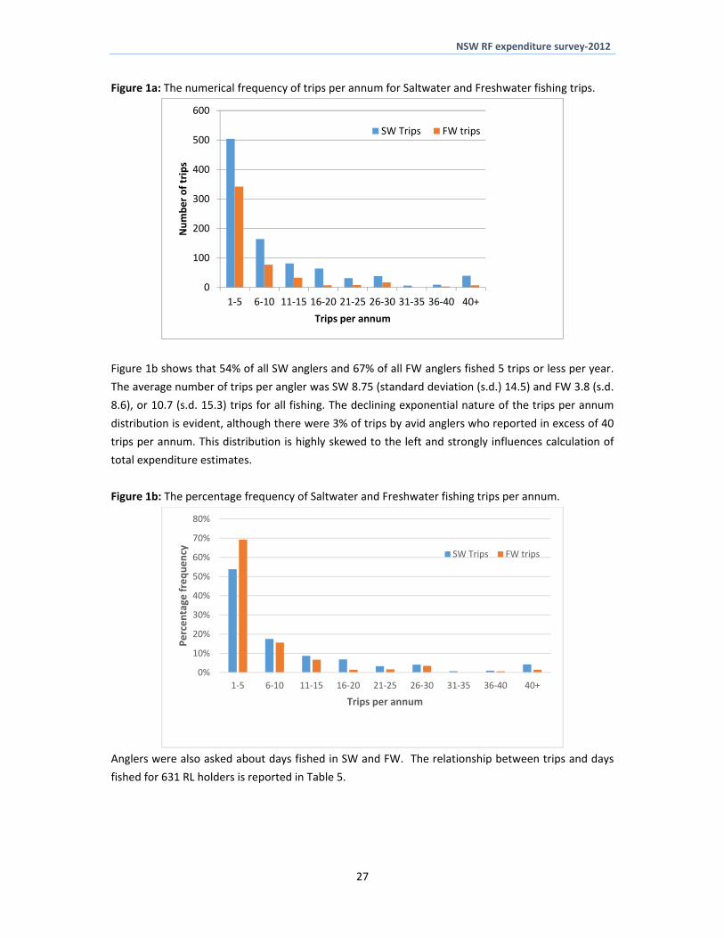
NSW RF expenditure survey‐2012
Figure 1a The numerical frequency of trips per annum for Saltwater and Freshwater fishing trips
0
100
200
300
400
500
600
1‐5 6‐10 11‐15 16‐20 21‐25 26‐30 31‐35 36‐40 40+
Number of trips
Trips per annum
SW Trips FW trips
Figure 1b shows that 54 of all SW anglers and 67 of all FW anglers fished 5 trips or less per year
The average number of trips per angler was SW 875 (standard deviation (sd) 145) and FW 38 (sd
86) or 107 (sd 153) trips for all fishing The declining exponential nature of the trips per annum
distribution is evident although there were 3 of trips by avid anglers who reported in excess of 40
trips per annum This distribution is highly skewed to the left and strongly influences calculation of
total expenditure estimates
Figure 1b The percentage frequency of Saltwater and Freshwater fishing trips per annum
0
10
20
30
40
50
60
70
80
1‐5 6‐10 11‐15 16‐20 21‐25 26‐30 31‐35 36‐40 40+
Percentage
frequency
Trips per annum
SW Trips FW trips
Anglers were also asked about days fished in SW and FW The relationship between trips and days
fished for 631 RL holders is reported in Table 5
27
NSW RF expenditure survey‐2012
Table 5 The days trips and length of trip for RFL Holders sampled (n= 613)
Type of fishing
day
Days Trips Daystrip of trip
time fished
SW days 6112 4189 146 817
FW days 2407 1536 157 866
The RFL survey sampled 631 fishers who fished 8470 days an average of 134 days per year
Proportionally 72 of days fished were in SW and 28 in FW Table 5 shows that the average fishing
trip was 146 days in SW and 157 days in FW of which over 80 of time was time fished in both
environments
322 Recreational fishing days
Previous catch and effort surveys have expanded data based on days fished Days fished are
presented on an annual basis in a frequency chart in Figure 2a and as percentage frequency chart in
Figure 2b
Figure 2a The frequency of days fished by all fishers (Average 146 days sd 186 days n=1231)
Figure 2a and 2b indicate that 38 of all anglers sampled fished 5 or less days per year but also that
6 of all anglers fished more than 40 days a year the latter often referred to as avid anglers The
average days fished are 146 days and given the previous estimate of 773000 adult anglers in NSW
this translates in to an estimated 116 million days fished in 2012
These activity distributions in samples are important The 36 of days below 5 days a year was less
than the 67 of the national survey (conducted in 2001) In contrast that survey also showed that
just 1 of anglers fished more than 40 days in the previous year (Henry and Lyle 2003)
28
NSW RF expenditure survey‐2012
Figure 2b The percentage frequency of days fished
In the present study this is partially explained by possible under sampling of 3 day and 1 month
licence holders though the random survey should not have been affected in this way On the other
hand the present study may well have sampled a higher proportion of avid fishers in the RFL data
base The third possibility is that angler behaviour in NSW has altered (on average) in the 12 years
since the national survey perhaps influenced by the introduction of the RFL
33 Comparisons between methods and samples
Statistical t‐tests were used to compare the trips per angler and average days fished per angler
between seasonal samples random and RFL database surveys and between licensed and unlicensed
recreational fishers
a) Are there seasonal differences in fishing activity
There is no previous literature on seasonal levels of fishing effort in NSW but we might expect to
see less days fished and fishing trips in the April to September ldquowinterrdquo period since this period does
not include Christmas However t tests revealed there was no statistically significant difference in
either the average days fished or trips per fisher across all observations between the April and the
September samples This may be partially explained by respondents to the September survey
recalling significant fishing activity at Easter time as part of ldquowinterrdquo activity
b) Are the random survey method and the RFL data base method results different
The t tests for trips indicate that those fishers in the random survey which included both licence
holders and non licence holders fished significantly more trips per year (125 v 906 trips t=395)
than fishers sampled from the RFL database This also applied to days fished with those in the
random survey fishing significantly more days (155 v 134 days t=208)
29
NSW RF expenditure survey‐2012
c) Are there differences between licenced and unlicenced fishers
Do licensed anglers fish more than unlicensed fishers When all samples are considered the average
days fished estimates show no significant difference between licensed and unlicensed fishers
However non‐licence holders made significantly more fishing trips than licence holders (128 trips v
103 t= 224)
34 Discussion of the sampling and activity results
On the basis of these results the average activity per angler whether measured in trips made or days
fished does not appear to be significantly different between seasons This result supports the
prospect of sampling recreational fishers at any time of the year asking them to recall their activity
in the last year
Fishers sampled randomly through the ldquowhite pagesrdquo made significantly more fishing trips and
fished on more days per annum than RFL holders Similarly those fishers contacted at random not
holding licenses were found to fish a similar number of days to licence holders but made
significantly more trips per annum This somewhat counter intuitive result (we might expect licence
holders to be more avid) is nevertheless consistent with concession holders and pensioners being
available to take more occasional fishing trips than the general working population might
It may also be related to the relatively high number of fishers found to have made more than 40
trips per year skewing the activity profile Where one sample is chosen at random and the other
comes from a database of known recreational fishers we may expect some avidity bias in the latter
(Johnson 1999) However this is not what we found indicating that opportunity to go fishing among
non licence holders may enable them to fish more frequently than licence holders though this
assumes we have no significant biases in the survey analysis For example ACMA (2013) states that
CATI surveys as used in our random screening survey ldquomay be biased towards those who normally
stay at home (eg older or retired people or those whose occupation is home duties)rdquo This may
indicate that those who responded had more time to go fishing than across the whole NSW
population
Non response bias and the screening survey
The most common non‐response bias is ldquounit non‐responserdquo which ldquotakes place when a randomly
sampled individual cannot be contacted or refuses to participate in a surveyrdquo (Ritz 2013) Mohadjer
et al explain ldquoThere is always a potential for item nonresponse bias whenever sample persons who
did not participate in the survey have somewhat different characteristics than those who didrdquo
In our random screening survey we had
‐ Sample losses approximately 50 of dead numbers and the potential for unit non response
bias Do those interviewees with land line numbers differ from those who have moved or
changed telephones in the past few years Privacy conditions precluded contacting non
respondents to investigate further Socio‐economically those moving away from landlines
may be younger in the working population or may have different incomes An argument
can be made either way and the extent of any bias remains unknown
30
NSW RF expenditure survey‐2012
‐ Non contactable household‐ It is unlikely these non contactable numbers for non‐RF
households or RF households would differ unless they were out fishing
‐ Refusals Why did so many people who identified themselves as having fished in the past six
months refuse to complete a short fishing interview Reasons include the dislike of surveys
intruding into their home and privacy not having the time or other general perceptions
Those who completed the interview may be keener on fishing more avid and some not
completing it because they consider their level of fishing to be trivial There was also the
indication from surveyors of fear or mistrust that the call was checking up on their licence
status In the random survey those who may have had a licence for 3 days or 1 month in the
previous six month period may not have had one at the time of the call and may have felt
vulnerable However approximately one third of all fishers are concession holders reducing
this possible vulnerability impact
In the area of survey refusals there seems to be more potential for non‐response bias in the
comparability of those who completed the survey with those who refused This cannot be directly
checked with non respondents due to privacy constraints Other independent indicators could be
used comparing ldquohellipthe distribution of respondents in the survey with associated distributions coming
from other independent surveysrdquo (Mohadjer et al 1994) We are able to compare the surveys given
their two different approaches
In the random screening survey over half of the identified fishers did not complete the survey We
can test for evidence of a response bias by comparing RFL licence holders who replied to the random
survey with RLF licence holders contacted directly in the other survey A t‐test indicated that the
mean days fished for the random RFL group (n=391) were significantly higher than the direct RFL
(n=631) survey results (158 v 134 t=211) significant at the 5 and 2 levels This is indicative of a
possible response bias as more active RFL holders appear more likely to have participated in the
random screening survey interviews than other less avid licence holders Previous adjustments made
to the data (section 32) reduced the risk to final estimates from this and other likely biases
Bias and the survey of RFL holders
The RFL survey also recorded significant levels of dead numbers although a much lower rate of
refusals The survey fieldwork team were able to ask to speak to the licence holder by name and this
may have contributed to higher completion rates Any bias in the RFL survey may then be between
responses by different licence holders Those holding 3 year licences may have significantly different
fishing activities expenditures or preferences to 1 year or 1 month and 3 day licence holders
Anecdotal evidence suggests some fishers buy several 3 day licences through the year and this may
contribute to a form of ldquodouble countingrdquo in any comparative analysis of licences The scale of this
behaviour is unknown and does not assist us in developing a sampling approach that may draw on a
representative cross section of the four licence types Further enquiries of non respondents was not
pursued due to privacy constraints
31
NSW RF expenditure survey‐2012
34 Estimation of recreational fishing expenditure per angler
Recreational fishing expenditure can be split into different categories as explained previously
a) Trip related expenditure on a range of expenses Trip expenditure can be annualised by expanding
by the number of trips per annum
b) Expenditure on small equipment and expenses on the last trip and
c) Annual expenditure on larger boat equipment This includes capital purchases in the year of the 10survey
All respondents in each area were asked about trip expenditures by all anglers in their household ndash
which averaged 202 anglers per household (see Table 7 later in report) The estimated expenditures
per angler per trip are reported in Table 6abc but state‐wide estimates in the next chapter are
based on household data
Table 6a summarises the average RF expenditure per trip for all NSW fishers (both SW and FW) in
each region for both fishing trip expenses and tackle Table 6b reports the average SW RF
expenditure per trip for all NSW regions on both fishing trip expenses and tackle Table 6c shows the
average trip expenditures for FW anglers Table 6d shows the annual expenditure on boat
expenditure for all NSW anglers SW and FW anglers combined
In Table 6ab ampc the results include fishers from Interstate who hold a NSW RFL but their major boat
and motor purchases are not assumed to have been made in NSW (Table 6d black squares)
The results in Table 6a confirm that all fishers (both SW and FW) spend 68 of trip expenses on the
fishing trip and just under 32 on equipment and fishing expenses Car travel is the major trip
expense $6974 (31 of total trip expense accommodation $ 3267 (15) and fooddrink eating out
$3594 (16) also while fishing rods and tackle hookslines and baitberley $3891(18) and boat
fuel $1650 (7) are the other major trip expenses
In Table 6b the costs of SW anglers are shown and Table 5c for FW Table 6bampc show that each
group had similar average expenditures per fishing trip (SW ‐ $22282 and FW ‐ $23024) Car travel
expenses are higher for FW fishers $9079 day versus $5955day SW but boat fuel for SW is
$1964 day versus FW $1009day
Table 6d shows that the annual NSW fisherrsquos average boat expenses per angler were $768 pa for all
NSW or broken down $856 for SW and $365 for FW fishers Boat purchase values for SW fishers
were much higher than for FW fishers which reflected the lower capital expenditure on small tinnies
for creeks dams and impoundments as opposed to offshore marine vessels The comparisons are
for the major form of fishing activity with 21 of fishers in our survey sample fishing a combination
of both SW and FW in a given year
10 Expenditure on fishing boats and larger capital items was reduced by 30 to reflect non recreational fishing use
32
NSW RF expenditure survey‐2012
Table 6a The average RF expenditure per trip for all NSW RFs in all NSW Last column is the
percentage of total spend in the All NSW total trip
Data in Aus $ Sydney North coast
South Coast
Inland Interstate All NSW of total spend per
trip Car travel (both ways) 6874 $ $ 4376 $ 4650 9871 $ 13060 $ 6974 $ 31 Accommodation 3998 $ $ 2216 $ 2112 2967 $ 6424 $ 3267 $ 15 Eating out 1478 $ $ 733 $ 1132 1572 $ 2820 $ 1342 $ 6 Other food and drink 2004 $ $ 1420 $ 2121 2881 $ 4857 $ 2252 $ 10 Shopping (souvenirmagazinesvideos) 419 $ $ 155 $ 120 607 $ 947 $ 387 $ 2 Travel-other than by car 354 $ $ 053 $ 325 040 $ -$ 160 $ 1 Sports 027 $ $ 018 $ - 034 $ 478 $ 065 $ 0 Tours 096 $ $ 007 $ 154 100 $ 022 $ 066 $ 0 Poker machines 174 $ $ 095 $ 077 124 $ 504 $ 160 $ 1 Pub 651 $ $ 347 $ 565 618 $ 1554 $ 621 $ 3 Anything else 194 $ $ 044 $ 068 134 $ 152 $ 117 $ 1 Expenditure per trip 16259 $ $ 9460 $ 11307 18946 $ 30811 $ 15405 $ 68
-$ $ - $ - -$ -$ -$ Major fishing tackle (rods reel) 2561 $ $ 1491 $ 1009 2756 $ 826 $ 1937 $ 9 Minor fishing tackle (hooks lines etc) 1106 $ $ 881 $ 713 1505 $ 2101 $ 1162 $ 5 Baitberley 1043 $ $ 559 $ 624 820 $ 938 $ 792 $ 4 Boat hire 671 $ $ 005 $ 090 139 $ 078 $ 242 $ 1 Boat fuel 2054 $ $ 1307 $ 683 1180 $ 3531 $ 1652 $ 7 Charter and fishing guide fees 647 $ $ 301 $ 043 098 $ 109 $ 323 $ 1 Fishing clothesapparel(w aders etc) 263 $ $ 177 $ 276 339 $ 143 $ 239 $ 1 Camping equipment 175 $ $ 735 $ 309 790 $ 400 $ 508 $ 2 Other fishing expenses 240 $ $ 283 $ 144 328 $ 393 $ 276 $ 1 Equipment per trip 8747 $ $ 5726 $ 3890 7939 $ 8520 $ 7120 $ 32
Total spend per trip 25007 $ $ 15185 $ 15197 26885 $ 39331 $ 22524 $ 100
Table 6b The average RF expenditure per SW trips for RFs anglers in all NSW Last column is the
percentage of All NSW total
Data in Aus $ Sydney North coast
South Coast
Inland Interstate All NSW of total spend per
trip
Car travel (both ways) 6168 $ $ 3659 $ 3915 17153 $ 12637 $ 5955 $ 27 Accommodation 4063 $ $ 2182 $ 2170 6325 $ 10959 $ 3547 $ 16 Eating out 1454 $ $ 782 $ 1151 4195 $ 5838 $ 1539 $ 7 Other food and drink 1988 $ $ 1284 $ 2321 2834 $ 6274 $ 2000 $ 9 Shopping (souvenirmagazinesvideos) 447 $ $ 164 $ 115 1620 $ 2157 $ 450 $ 2 Travel-other than by car 421 $ $ 034 $ 365 102 $ -$ 219 $ 1 Sports 033 $ $ 010 $ - 131 $ 581 $ 051 $ 0 Tours 113 $ $ 009 $ 173 280 $ -$ 086 $ 0 Poker machines 187 $ $ 112 $ 068 144 $ 865 $ 170 $ 1 Pub 694 $ $ 371 $ 612 1095 $ 2149 $ 649 $ 3 Anything else 229 $ $ 046 $ 077 -$ 405 $ 129 $ 1 Expenditure per trip 15787 $ $ 8647 $ 10947 33880 $ 41807 $ 14781 $ 66
Major fishing tackle (rods reel) 2703 $ $ 1509 $ 1136 2246 $ 541 $ 1905 $ 9 Minor fishing tackle (hooks lines etc) 1203 $ $ 742 $ 747 1087 $ 3010 $ 1035 $ 5 Baitberley 1183 $ $ 633 $ 656 1242 $ 1116 $ 899 $ 4 Boat hire 816 $ $ - $ 101 475 $ 243 $ 352 $ 2 Boat fuel 2309 $ $ 1380 $ 737 1903 $ 7946 $ 1964 $ 9 Charter and fishing guide fees 788 $ $ 370 $ 048 169 $ 338 $ 465 $ 2 Fishing clothesapparel(w aders etc) 302 $ $ 195 $ 310 270 $ -$ 245 $ 1 Camping equipment 213 $ $ 631 $ 048 936 $ 027 $ 402 $ 2 Other fishing expenses 252 $ $ 275 $ 161 234 $ 223 $ 247 $ 1 Equipment per trip 9750 $ $ 5721 $ 3943 8562 $ 13444 $ 7501 $ 34
Total spend per trip 25537 $ $ 14367 $ 14890 42442 $ 55251 $ 22282 $ 100
33
NSW RF expenditure survey‐2012
Table 6c The average RF expenditure per FW trip for RFs anglers in all NSW Last column is the
percentage of All NSW total
Data in Aus $ Sydney North coast
South Coast
Inland Interstate All NSW of total spend per
trip
Car travel (both ways) 10144 $ $ 7498 $ 10533 7358 $ 13261 $ 9079 $ 39 Accommodation 3696 $ $ 2363 $ 1654 1808 $ 4272 $ 2689 $ 12 Eating out 1591 $ $ 517 $ 981 667 $ 1388 $ 937 $ 4 Other food and drink 2077 $ $ 2014 $ 519 2897 $ 4185 $ 2771 $ 12 Shopping (souvenirmagazinesvideos) 287 $ $ 118 $ 154 258 $ 389 $ 258 $ 1 Travel-other than by car 039 $ $ 138 $ - 018 $ -$ 040 $ 0 Sports -$ $ 053 $ - -$ 429 $ 093 $ 0 Tours 015 $ $ - $ - 038 $ 032 $ 025 $ 0 Poker machines 115 $ $ 020 $ 154 117 $ 333 $ 141 $ 1 Pub 454 $ $ 245 $ 192 454 $ 1272 $ 565 $ 2 Anything else 031 $ $ 033 $ - 180 $ 032 $ 094 $ 0 Expenditure per trip 18448 $ $ 13000 $ 14187 13794 $ 25595 $ 16691 $ 72
Major fishing tackle (rods reel) 1903 $ $ 1414 $ - 2933 $ 962 $ 2002 $ 9 Minor fishing tackle (hooks lines etc) 658 $ $ 1482 $ 442 1649 $ 1669 $ 1423 $ 6 Baitberley 398 $ $ 238 $ 369 674 $ 853 $ 572 $ 2 Boat hire -$ $ 026 $ - 023 $ -$ 015 $ 0 Boat fuel 877 $ $ 988 $ 250 930 $ 1437 $ 1009 $ 4 Charter and fishing guide fees -$ $ - $ - 073 $ -$ 031 $ 0 Fishing clothesapparel(w aders etc) 085 $ $ 097 $ - 363 $ 212 $ 227 $ 1 Camping equipment -$ $ 1184 $ 2392 739 $ 577 $ 726 $ 3 Other fishing expenses 184 $ $ 319 $ 008 360 $ 474 $ 335 $ 1 Equipment per trip 4105 $ $ 5749 $ 3462 7724 $ 6184 $ 6332 $ 28
Total spend per trip 22553 $ $ 18749 $ 17648 21518 $ 31779 $ 23024 $ 100
Table 6d The average RF expenditure per annum on larger boat items for SW and FW anglers in
regions and all NSW (nb Table 6abc are per trip and Table 6d is per angler per annum)
Data in Aus $ Sydney North coast
South Coast
Inland Interstate All NSW of total spend per
trip
All NSW Boat licenceregistration 7115 $ $ 4658 $ 4407 5815 $ 8546 $ 5940 $ 8 Boat maintenance 29248 $ $ 14497 $ 9655 7935 $ 17917 $ 17504 $ 23 Boat insurance 7519 $ $ 4574 $ 3006 4145 $ 10318 $ 5754 $ 7 Marine mooring fees 7615 $ $ 1940 $ 192 122 $ 2609 $ 3179 $ 4 Boat equipment (safety etc) 15175 $ $ 7637 $ 3175 5452 $ 6015 $ 8888 $ 12 Boat purchase or motor repair 23437 $ $ 25676 $ 25865 9740 $ - 35550 $ 46 Annual boat expenditure 90109 $ $ 58982 $ 46300 33208 $ 45405 $ 76815 $ 100
Saltwater -$ $ - $ - -$ -$ -$ Boat licenceregistration 7340 $ $ 4751 $ 3583 6003 $ 13372 $ 6014 $ 6 Boat maintenance 32221 $ $ 15880 $ 9805 5356 $ 28392 $ 20829 $ 22 Boat insurance 8032 $ $ 5068 $ 3002 3960 $ 19824 $ 6458 $ 7 Marine mooring fees 8765 $ $ 2385 $ 216 030 $ 8108 $ 4505 $ 5 Boat equipment (safety etc) 17407 $ $ 7800 $ 3428 7508 $ 9230 $ 10764 $ 11 Boat purchase or motor repair 30450 $ $ 35250 $ 30000 40600 $ - 47050 $ 49 Annual boat expenditure $ 104214 $ 71134 $ 50035 63456 $ 78926 $ 95618 $ 100
Freshwater Boat licenceregistration 6073 $ $ 4255 $ 11000 5750 $ 6256 $ 5787 $ 16 Boat maintenance 15523 $ $ 8474 $ 8454 8830 $ 12949 $ 10632 $ 29 Boat insurance 5154 $ $ 2421 $ 3038 4209 $ 5809 $ 4297 $ 12 Marine mooring fees 2308 $ $ - $ - 155 $ -$ 439 $ 1 Boat equipment (safety etc) 4877 $ $ 6930 $ 1154 4738 $ 4490 $ 5011 $ 14 Boat purchase or motor repair 5000 $ $ 3150 $ 18400 5350 $ - 10350 $ 28 Annual boat expenditure 38935 $ $ 25230 $ 42046 29032 $ 29504 $ 36515 $ 100
34
NSW RF expenditure survey‐2012
In Table 6a the higher travel costs of some regional residents such as Sydney anglers Inland and
interstate fishers were evident The trip expenditure of Inland and interstate SW anglers was
significantly higher than for resident NSW anglers due to car travel accommodation food and other
trip expenses presumably to the coast (Table 6b) Table 6c shows that FW expenditure per trip was
highest for interstate fishers (eg Victorians traveling to southern NSW) and Sydney and South Coast
RFs had high travel costs travelling to desirable FW fishing locations (eg Snowy mountains etc
Dominion 2001 and 2002)
The socio‐economics of recreational fisher expenditure in NSW
The survey samples were analysed to identify some of the socio‐economic drivers of RF expenditure
in NSW The samples combined to give 1235 observations of RF expenditure and the survey
included a range of other variables Both multiple regression analysis and a cluster analysis enables
the statistically significant variables determining angler expenditure to be identified and estimated
as reported in Appendices 1 and 2 respectively
Multiple regression results
In Appendix 1 results reveal that Total recreational fishing expenditure is driven by licence status
(licence holders spending more) number of SW trips per annum and the level of household income
Age sex and regional location were found not to be statistically significant in determining total RF
expenditure
Trip expenditure was driven by licence holders and number of SW trips Trip expenditure was further
examined and was significantly influenced by licence holders SW and FW days fished and the
distance travelled on the last trip Fishing Tackle expenditure was found to be determined by
income rather than number of trips Expenditure on boats was driven by both number of SW trips
and the level of RF household income
Cluster analysis results
The expenditure of NSW RFs was also subjected to ldquocluster analysisrdquo to see the significant socio‐
economic characteristics of fisher groups as reported in Appendix 2and in Figure 3 below The cluster
analyses for expenditure on fishing trips tackle and boat expenditure are reported in Appendix 2
35
NSW RF expenditure survey‐2012
Figure 3 A cluster analysis of RF total expenditure showing the groups of significantly different
clusters of anglers identified
In Figure 3 there are four significantly different cluster groups The characteristics of the four groups
are under the ldquodescriptionrdquo row and the authors have put a label to characterise each group
Between Figure 3 and Appendix 2 the overall picture is of groups of ldquoordinaryrdquo fishers
(approximately 85) with low levels of fishing activity in which household income levels may differ
(half lower half higher) secondly a group of dedicated anglers (approximately 12) who have high
fishing activity and expenditure and finally a highly avid fishing group (less than 3) with very high
fishing activity and high to very high expenditure
The results confirm the only previous examination of the socio‐economic characteristics of RFs in
NSW by Dominion (2003) which showed that recreational fishing is a past time involving a diverse
range of people has great variety in activity levels and crosses the entire socio‐economic spectrum
36
NSW RF expenditure survey‐2012
4 State‐wide and regional expenditure estimates
41 Estimating total expenditure
This chapter describes the estimation of the total recreational fishing expenditure for RFs in NSW
and in its regions Total recreational fishing expenditure is the product of three variables
a) Number of recreational fishers or RF households (HH)
We use three approaches to estimate the total RF population in NSW by use of
1) Random telephone survey and ABS Household data and population data
2) The RFL data base and
3) Use of the screening sample and the ABS data on Households Use of the screening
survey of the general population to estimate total number of fishers11 via ABS
population data
b) Fishing trip activity fishing trip activity estimates are obtained from the telephone survey
and
c) Recreational fishing expenditure information on the expenditure per trip and annual
expenditures on equipment is obtained from the telephone survey
The product of these variables will enable us to estimate the total state‐wide recreational fishing
expenditure Expenditure is also estimated for each state region considered Saltwater and
freshwater fishing are considered separately in the state estimates through asking respondents
about the trip intention
42 Expanding the sample of fishers and expenditure
Total expenditure estimates are based on travel and fishing equipment expenses per trip and
estimates of expenditure on boat capital items These are summed to give an annual total
expenditure estimate However the estimates for the angler survey need to be expanded to give
state wide estimates These expansions are described in Box 1 below
Box 1 Explanation of key expansions
The expansion method adapts the method used in the National Survey (Henry and Lyle 2003) The
number of fisher households (FHH) was estimated as follows for each region
No of fisher Household (est) = No Households in Population (ABS) No of Fisher HH (sample)
No of HH (sample)
Example How many recreational fishers would these households include
No of Fishers 19 to 75 yrs (est) = Mean No fishers per HH (sample) No of fisher Household (est)
776496 = 202 383921 (see Table 7)
RF HH are distributed proportionally across regions by household and recreational fishers by
regional population
11 Recreational Fishers under 19 years of age are not included and need to be added if the total population figure is for all
anglers The activity and expenditure estimates are based on ages 19‐75 only
37
NSW RF expenditure survey‐2012
Information on NSW State and Regional Households by Local Government Area (LGA) were accessed
(ABS 2011) The data were aggregated by the larger SD ABS regions (eg Sydney North coast
Inland and SDD South Coast area) These identified the number of households in each of the study
regions as reported in Table 7
Table 7 The ldquototal householdsrdquo in each of the NSW study regions based on LGA data ABS (2011)
Households with recreational fishers are estimated for each study region
Area Population 2010 (gt18-75)
Households HH with RF Rec Fishers HH
RF by region
Sydney 3160897 1376583 213934 230 491232
North coast 835229 570688 88690 146 129802
South coast 350750 207195 32200 169 54510
Inland 649564 315987 49107 206 100948
Total 4996461 2470453 383931 202 776496
The RF household responses for anglersrsquo trip frequency and trip expenditure were multiplied to
produce estimates of state‐wide and regional expenditure
43 State‐wide expenditure estimates
The estimation of total expenditure for samples of recreational anglers and its expansion to regional
state‐wide and national estimates has depended on traditional statistical methods estimating the
total from means of the component distributions However while the number of households is
reasonably well estimated the frequency distribution of fishing trips is highly skewed to the left (see
Figure 1a)
The estimates of total state expenditure on recreational fishing involve multiplying the following
variables
1) Estimate of RF households ‐ the ABS has reliable estimates of households for which RF
households can be identified
2) Estimate of trips ‐ anglers state the number of trips per annum and
3) Estimate of the trip and tackle expenditure on their last trip and their capital expenditure in
the last year
Total expenditure is the product of these variables Total expenditure can be estimated as a mean
value with confidence intervals Here we used the 1237 observations in the RF sample weighting
the results in respect of regional populations as follows
a) Total annual expenditure per angler household = (($ travel expenses per trip + $ tackle
expenses per trip) number of trips )+ (annual capital expenditure per angler household)
b) Total annual expenditure in NSW = total number of anglers households total annual
expenditure per angler household
This traditional approach gives a point estimate but does not provide any information on the
probability of different expenditure levels around the mean This requires a simulation approach
38
NSW RF expenditure survey‐2012
Table 8a shows that the estimated expenditure by all NSW resident RFs in 2012 was $1439bn12 with
an additional $1861m being spent by interstate fishers making a total estimated expenditure by
recreational fishers in NSW of $1625bn in the year 2012
Considering regional expenditures total recreational fishing expenditure was highest by Sydney
anglers ‐ $903m (56 of all expenditure in NSW) followed by the North coast anglers ‐ $3008m
(19) and inter‐state anglers ‐ $ 186m (11) Total expenditure for South Coast anglers was
$1018m (6) and for Inland anglers $1308m (8)13
Expenditure on fishing trips was $793m or 49 of all recreational fishing expenditure in NSW Of
this $402m (25) was spent on fishing equipment tackle and fuel and $430m (26) was spent on
annual capital expenditures such as boats and maintenance Expenditure on SW fishing was
estimated at $1415m (87) and on FW fishing at $231m (13 of total recreational fishing
expenditure in NSW)
Table 8b shows the costs within each category
Within trip expenditure (49 of total expenditure) car travel $326m (201 of total annual
expenditure) accommodation $1859m (114) and food and eating out $188m (115)
Expenditure on fishing equipment and expenses $4025m (246) was made up of $1645m
(102) on major and minor tackle and $1027m (63) on boat fuel and
Annual boat expenditure $4305m (26) of which $1225m (75) was maintenance and
boat purchase or motor repair $1436m (88)
12 This estimate is the same as the mean value produced by the simulation shown later in this chapter It is then adjusted
for Interstate expenditure13 In Chapter 5 the regional economic analysis adapts these data to reflect the expenditure made in other regions away from home residence
39
NSW RF expenditure survey‐2012
Table 8a Estimates of the total RF expenditure for different areas of NSW and including interstate angler expenditure to give all RF expenditure in NSW
Expenditure category Sydney North coast South coast Inland All NSW Inter-state Total expend
in NSW
total expend in NSW
Trip spend 383906879 136686958 57862828 74849484 653306149 139478487 792784637 49 $ fishing equip 222891110 85965049 20624384 31116970 360597513 41975664 402573177 25 Total annual boat expenditure 296326795 81222395 23393975 24877516 425820681 4691465 430512146 26 Totals 903124785 303874402 101881187 130843970 1439724343 186145616 1625869959 100 of total expend in NSW 56 19 6 8 89 11 100 Saltwater 840749912 267431019 99200573 51715617 1259097121 140675487 1415280961 87 Freshwater 62374873 36443383 2680614 79128353 180627222 45469052 231775451 14 SW expenditure as of Total 93 88 97 40 87 84 87
40
NSW RF expenditure survey‐2012
Table 8b Estimates of the total RF expenditure for different areas of NSW and including interstate angler expenditure to give all RF expenditure in NSW
Data in Aus $ Sydney North coast South coast Inland All NSW Interstate Total expend
in NSW
of Total expend in
NSW Expenditure category Car travel (both ways) 155752824 61047851 21250669 38966591 277017934 49755399 326773333 201 Accommodation 96655736 32991275 11321758 11775540 152744309 33155541 185899850 114 Eating out 35118007 11287702 6019080 6283701 58708491 16433282 75141772 46 Other food and drink 47830881 20416270 11974310 11255861 91477322 21385714 112863036 69 Shopping (souvenirmagazinesvideos) 10396840 2377682 609238 2427428 15811187 5900718 21711905 13 Travel-other than by car 9328498 675596 1876003 157968 12038065 - 12038065 07 Sports 730303 214569 - 136952 1081824 2038576 3120401 02 Tours 2517279 121080 888633 400483 3927475 44318 3971793 02 Poker machines 4337423 1534429 364864 485304 6722021 2611177 9333198 06 Pub 16147653 5352108 3163325 2442584 27105670 7101506 34207176 21 Anything else 5091436 668396 394948 517073 6671852 1052256 7724108 05 Trip spend 383906879 136686958 57862828 74849484 653306149 139478487 792784637 488
Major fishing tackle (rods reel) 63209459 22456502 5830420 10743744 102240126 2673467 104913593 65 Minor fishing tackle (hooks lines etc) 27752247 12319663 3884279 5859337 49815525 9792034 59607560 37 Baitberley 26800952 8839913 3407290 3225829 42273984 3954942 46228926 28 Boat hire 17933756 42708 518369 561815 19056649 604762 19661412 12 Boat fuel 52493364 20044184 3811422 4649308 80998277 21742806 102741083 63 Charter and fishing guide fees 17310929 4944101 246843 386149 22888022 839948 23727969 15 Fishing clothesapparel(w aders etc) 6799431 2766227 1592134 1322337 12480129 292501 12772630 08 Camping equipment 4689522 10357115 508333 3093322 18648291 864926 19513218 12 Other fishing expenses 5901451 4194635 825295 1275129 12196509 1210277 13406786 08 $ fishing equip 222891110 85965049 20624384 31116970 360597513 41975664 402573177 248
Boat licenceregistration 22369127 6037457 1817922 4154611 34379117 4691465 39070582 24 Boat maintenance 93188042 18809323 4588346 5925940 122511651 - 122511651 75 Boat insurance 23806199 5935399 1413005 2990204 34144806 - 34144806 21 Marine mooring fees 24487619 2521793 97904 96275 27203591 - 27203591 17 Boat equipment (safety etc) 48762545 9898735 1571861 3725061 63958201 - 63958201 39 Boat purchase or motor repair 83713264 38019687 13904937 7985426 143623314 - 143623314 88 Total annual boat expenditure 296326795 81222395 23393975 24877516 425820681 4691465 430512146 265
Totals 903124785 303874402 101881187 130843970 1439724343 186145616 1625869959 1000 Saltwater 840749912 267431019 99200573 51715617 1259097121 140675487 1399772608 861 Freshwater 62374873 36443383 2680614 79128353 180627222 45469052 226096274 139 SW expenditure as of Total 93 88 97 40 87 76 86 Region as of total expenditure 56 19 6 8 11 100
41
NSW RF expenditure survey‐2012
44 A probabilistic simulation approach to the estimation of total state recreational fishing
expenditure
Simulation enabled us to estimate the probability of different outcomes from the existing data The
original sample was weighted by numbers of regional households to account for the under sampling of
Sydney and the over sampling of the North Coast in the original survey data The sample was analysed
using the SPSS v21 Monte Carlo Simulation model (IBM Corp 2012) This routine produced up to
100000 repeat runs of the predicted values of total RF state expenditure to give the probability of
different expenditure totals as shown in Figure 5a The cumulative probability is shown in Figure 5b
Figure 5a The probability of total expenditure by NSW anglers 2012
These initial probability estimates showed that the mean total state‐wide expenditure was $1473m
with 5 and 95 confidence estimates of $706m and $2952m The median value as $1196m reflecting
the skewedness of the distribution
The estimate of expenditure in NSW by interstate anglers of $1861m has also to be added The final
total NSW estimate of expenditure on recreational fishing was therefore $1625m with 5 and 95
confidence estimates of $892m‐$3136m14
14 For simplicity this assumes the distribution of the interstate results are the same as all NSW
42
NSW RF expenditure survey‐2012
Figure 5b The cumulative probability of total expenditure by NSW anglers 2012
Figure 5a and 5b indicate how the skewed distribution of trips per year by anglers and the highly annual
variable expenditure make the predicted adjusted distribution from $892m‐$3136m around an
adjusted mean $1625m and an adjusted median of $1382m The mean has a 0045 probability of being
achieved whereas lower total expenditure estimates have higher probability (Figure 5a) The
skewedness gives a threshold minimum expenditure level and a ldquotrailing tailrdquo on the right hand side
reflecting less probable high expenditure estimates
Figure 5b indicates that the mean would have a cumulative probability of 65 This shows the higher
total expenditure estimates on the right hand side of Figure 5a are pulling the mean to the right This is
why we have to be careful in RF sampling and estimation of recreational activity and expenditure This
also may explain why fishers of differing avidity and expenditure levels have considerably different
opinions on total expenditure in the sector A fisher with higher activity and expenditure would estimate
a state wide total at the right hand side of Figure 5a but while high total expenditure is possible it is
highly improbable
45 Discussion The estimated total expenditures reported in Table 8a and 8b indicate a statewide expenditure by NSW
recreational fishers and interstate anglers on items directly related to fishing of $1625m
43
NSW RF expenditure survey‐2012
The expansions to develop the final estimates took account of the differences between SW and FW
expenditure and activity and each was expanded separately Expenditure on FW fishing contributed 14
of total expenditure considerably less than the 28 of days fished reported in the sample (Table 5)
reflecting some trip and capital expenditure differences between SW and FW fishers
By region the results indicate that recreational fishing expenditure by Sydney anglers $9031m (56 of
total state recreational fishing expenditure) while North coast has $3038m (9) Interstate anglers
$1861 (11) Inland $1308m (8) and South coast $1018 (6) The survey method estimated regional
expenditures from interviews with fishers in their home region The regional economic impacts adjusts
these and produced estimates of recreational fishing expenditure and its economic impacts across all of
NSW and its main regions
There is just the previous national survey study for comparison of results The 2012 expenditure
estimate adjusted from the Campbell and Murphy (2005) national survey 2001 study is $765m This is
within the confidence intervals predicted by the current studyrsquos simulation approach
Another comparison is to deduct the trip expenditures for food and entertainment from the current
studyrsquos results to be comparable to Campbell and Murphyrsquos assumptions giving an estimate up to
$136bn15 The difference in expenditure estimates16 is primarily related to the survey methods used and
the different estimates of fishery activity the current study being higher Though the number of adults
fishing may have reduced since 2001 NSW has now a sizeable established recreational fishing licence
holder population and expenditures per angler are higher than a decade ago
Under the telephone survey interview and recall method used the current results were conservative for
this methodological approach This study has pointed to the highly skewed nature of the trip activity
among the RF population and the highly variable levels of expenditure among recreational fishers in
NSW The use of a probabilistic simulation in this study has illustrated the difficulties in estimation of
total RF expenditure and the wide distribution around the mean The adequate inclusion and possible
over‐inclusion of avid fishers are sampling problems under any of existing methodologies
The sample size and hence a higher survey cost is part of the remedy Further examination of the US
multi‐method approach may be merited (Gentner 2009) though this is a large scale national expensive
survey exercise The project results in this study are proposed as being reasonable under the
methodologies available within funding constraints and are part of a proposed ongoing expenditure
survey strategy in NSW as outlined in Chapter 6
15 There may also be differences in the treatment of capital attributable to RF definitions of maintenance and capital expenditure on motors and boats and other differences between the two studies These may likely lower this estimate 16 ($1360m‐$765m=$595m in 2012 terms)
44
NSW RF expenditure survey‐2012
5 Regional economic impact estimates This chapter of the report was compiled by Western Research Institute (WRI) WRI received the output
of this survey in terms of expenditure of respondents and based on this output modelled the
economic impacts of recreational fishing on the NSW economy and defined sub‐regions Input‐
output modelling has been employed to derive the relevant economic models and the impacts
51 Methodology
The methodology used to prepare this report included
Determination of the boundaries of the regions to be used in table construction
In consultation with the ANCORS the decision was made to construct input‐output tables for the NSW
North Coast NSW South Coast NSW Inland and Sydney regions as well as NSW as a whole Each region
was defined by aggregating statistical areas at level 4 3 or 2 or combination thereof This allowed the
formulation of regions and economies that best represented the regions of interest Specifically data
from statistical areas at level 3 of ABS Statistical Geography Standard (rather than at larger statistical
areas at level 4) was used in the construction of tables for the NSW North Coast and data from
statistical areas at level 2 was used in the construction of tables for the NSW South Coast The table
construction for Sydney region was based on the data from statistical areas at level 4 while tables for
NSW Inland region was based on the data from statistical areas at different levels (2 3 and 4) Detailed
information on statistical areas in provided in WRI (2013)
Construction of tables
The input‐output tables developed for this project were derived from the latest national table produced
by the Australian Bureau of Statistics (ABS) That table provides a detailed picture of the structure of the
economy of Australia for the year 2008‐09 A series of steps were undertaken to update the table to
2011‐12 Further information from the State Accounts (ABS Cat No 52200) labour force data from the
2011 Census and the quarterly labour force survey (ABS Cat No 6291055003) were used to develop a
state table for New South Wales at 2011‐2012 This was then regionalised to reflect the respective
regional economies of NSW North Coast NSW South Coast NSW Inland and Sydney Further details of
the procedures used in the development of a regional input‐output table are provided in WRI (2013)
52 Economic impact analysis
The economic impacts were modelled as a final demand impact (that calculates the impacts measured
by output value added household income and employment across all sectors in response to changes
in industry final demands) using the 2011‐12 Simulating Impacts on Regional Economies (SIRE) input‐
output model of NSW North Coast NSW South Coast NSW Inland Sydney and NSW as a whole The
SIRE model is superior to standard input‐output models as it provides for non‐linear relationships
between variables and is based on empirically derived (rather than assumed) coefficients In terms of
45
NSW RF expenditure survey‐2012
robustness of results it is comparable with computable general equilibrium (CGE) models whilst
minimising data requirements See WRI (2013) for a detailed description of the SIRE input‐output
model
The impacts of recreational fishing expenditure on the NSW North Coast NSW South Coast
NSW Inland and Sydney regions as well as NSW as a whole have been provided in terms of
bull Output which is the value of goods and services that are produced within an establishment
that become available for use outside that establishment plus any goods and services
produced for the organisationrsquos own final use Output is equal to total revenue plus any
internal consumption
bull Value added which is equal to gross output minus intermediate inputs Value added is
equivalent to the contribution to gross regional product (the local equivalent of gross
domestic product)
bull Household Income which measures the benefit received by regional households from
economic activity It typically refers to compensation of employees but can also include
income in return for other forms of productive activity
bull Employment which refers to full‐time equivalent (FTE) employment is a measure of the
total level of staff resources used The FTE of a full‐time staff member is equal to 10 The
FTE of a part‐time worker will be a fraction of this depending on the relative number of
hours worked
53 The Economic Impact of Recreational Fishing on the Regional Economies of NSW
The economic impact due to recreational fishing was modelled as follows
bull The expenditure survey conducted by ANCORS did not capture the location of expenditure
just the origin (postcode) of the respondent Therefore in the absence of location data an
assumption was made that the total expenditure by interstate visitors ($18614 million)
who make expenditures on recreational fishing whilst staying in NSW should be distributed
evenly across four NSW regions (ie 25 of total interstate expenditure pertaining to each
NSW region)
bull Likewise it was assumed that expenditure pertaining to the NSW North Coast NSW
South Coast and NSW Inland regions was made in these regions (eg those
respondents who indicated living in the NSW North Coast partake in recreational
fishing in the NSW North Coast and not in other areas thereby ensuring that the
money spent on recreational fishing remains in the NSW North Coast region)
46
NSW RF expenditure survey‐2012
bull For those respondents who indicated living in Sydney an assumption was made that 515
of them partake in fishing in Sydney with the remaining 485 fishing in the rest of NSW in
the following proportions NSW North Coast ndash 346 NSW South Coast ndash 485 and NSW
Inland ndash 169 (Dominion 2002 and 2004)
bull Since anglers in each of the regions make expenditure on items that may not be
produced in the region but that are imported from the rest of NSW the regional
recreational fishing expenditure was split into local and imported components using a
location quotients matrix This way WRI ensured that only local expenditure generated
economic impacts in the respective region For NSW as a whole an assumption was
made that all products that anglers purchase are produced within the state and
therefore no separation of local and imported components was performed The
economic impacts of recreational fishing on NSW were modelled using total recreational
fishing expenditure in NSW
bull In order to ensure consistency of the input‐output modelling procedure the expenditure
data was allocated in the input‐ output table to the industries (typically manufacturing
industries) where the relevant expenditure items were produced and was then
converted to basic prices See WRI (2013) for further details on sectoral allocations
bull A final demand analysis in SIRE was performed and economic impacts on NSW North Coast
NSW South Coast NSW Inland and Sydney as well as NSW as a whole were derived
The impacts of recreational fishing on the economies of the NSW North Coast NSW South Coast
NSW Inland and Sydney regions are outlined in the Table 9
Table 9 Regional expenditure and economic impacts on regional economies
Region North Coast Sydney South Coast Inland
Expenditure by postcode ($m) 30387 90312 10188 13084
Reclassified expenditure ($m) 50196 51165 36086 2514
Output ($m) 73465 100286 39522 35381
Value added ($m) 35355 49156 18417 14985
Household income ($m) 16875 28888 876 735
Employment (no) 3320 3944 1808 1539
47
NSW RF expenditure survey‐2012
NSW North Coast
Overall when flow‐on effects are taken into account recreational fishing contributes the following to
the economy of NSW North Coast
bull 3320 FTE jobs including 667 in the retail trade sector 573 in the hospitality sector
349 in the personal and other services sector and 174 in the transport and storage
sector
bull $16875 million in household income with 134 percent being in the retail trade
sector 112 percent being in the hospitality sector 76 percent being in the public
administration sector 72 percent being in the personal and other services sector and
57 percent being in the transport and storage sector
bull $35355 million in industry value added representing 081 percent of total regional
value added of the NSW North Coast region and
bull $73465 million in output
For the North Coast recreational fishing will contribute 098 percent of FTE employment in the
region when flow‐on effects are taken into account as well as 084 percent of household income and
07 percent of the estimated gross regional product of the NSW North Coast region
NSW South Coast
Overall when flow‐on effects are taken into account the recreational fishing contributes the
following to the economy of NSW South Coast
bull 1808 FTE jobs including 420 in the hospitality sector 284 in the retail trade sector
236 in the personal and other services sector 117 in the transport and storage
sector and 106 in the public administration sector
bull $8760 million in household income with 152 percent being in the hospitality sector
109 percent being in the retail trade sector 93 percent being in the public
administration sector 86 percent being in the personal and other services sector and 77
percent being in the transport and storage sector
bull $18416 million in industry value added representing 167 percent of total regional
value added of the NSW South Coast region and
bull $39522 million in output
For the South Coast recreational fishing will contribute 212 percent of FTE employment in the region
when flow‐on effects are taken into account as well as 173 percent of household income and 143
percent of the estimated gross regional product of the NSW South Coast region
48
NSW RF expenditure survey‐2012
NSW Inland
Overall when flow‐on effects are taken into account the recreational fishing contributes the
following to the economy of NSW Inland
bull 1539 FTE jobs including 289 in the hospitality sector 288 in the retail trade sector
148 in the personal and other services sector and 138 in the agriculture sector
bull $7350 million in household income with 134 percent being in the retail trade
sector 131 percent being in the hospitality sector 74 percent being in the
personal and other services sector 70 percent being in the public administration
sector and 68 percent being in the transport and storage sector
bull $14985 million in industry value added representing 030 percent of total regional
value added of the NSW Inland region and
bull $35381 million in output
Recreational fishing will contribute 038 percent of FTE employment in the NSW Inland region when
flow‐on effects are taken into account as well as 032 percent of household income and 026 percent
of the estimated gross regional product of the NSWInlandregion
Sydney
Overall when flow‐on effects are taken into account the recreational fishing contributes the following
to the economy of Sydney
bull 3944 FTE jobs including 741 in the retail trade sector 450 in the hospitality sector
366 in the personal and other services sector and 310 in the professional and
technical services sector
bull $28888 million in household income with 162 percent being in the finance and insurance
sector 113 percent being in the retail trade sector 83 percent being in the professional
and technical services sector 77 percent being in the wholesale trade sector and 63
percent being in the hospitality sector
bull $49156 million in industry value added representing 025 percent of the total regional
value added of Sydney and
bull $100286 million in output
For the Sydney region recreational fishing will contribute 028 percent of FTE employment when flow‐on
effects are taken into account as well as 025 percent of household income and 022 percent of the
estimated gross regional product of Sydney
49
NSW RF expenditure survey‐2012
NSW State economy
The impacts of recreational fishing on the state economy of the NSW are outlined in the Table 10
Table 10 NSW expenditure and economic impacts on NSW
Item Estimate
NSW Expenditure by postcode ($m) 143972
Total interstate expenditure ($ m) 18615
NSW Reclassified expenditure ($m) 162587
Output ($m) 342035
Value added ($m) 162561
Household income ($m) 87728
Employment (thousand) 14254
NSW Economy
Overall when flow‐on effects are taken into account the recreational fishing contributes the following to
the economy of NSW
bull 14254 FTE jobs including 2730 in the retail trade sector 2123 in the hospitality
sector 1389 in the personal and other services sector and 951 in the transport and
storage sector
bull $87728 million in household income with 122 percent being in the retail trade 114
percent being in the finance and insurance sector 88 percent being in the hospitality
sector 72 percent being in the professional and technical services sector and 65
percent being in the wholesale trade sector
bull $162561 million in industry value added representing 036 percent of the estimated gross
state product of the NSW and
bull $342035 million in output
50
NSW RF expenditure survey‐2012
Overall recreational fishing will contribute 046 percent of FTE employment in the NSW when flow‐on
effects are taken into account as well as 041 percent of household income and 040 percent of total
regional value added
54 Conclusion
The recreational fishing expenditure and economic impact of recreational fishing on NSW and
respective regions were substantial in absolute terms but uneven across regions
The expenditure based on place of residence was the highest in Sydney followed by NSW North
Coast NSW Inland and NSW South Coast The reallocated expenditure (ie actual expenditure
made in the region) was still the highest in Sydney (but substantially lower than postcode
expenditure) followed by expenditure in NSW North Coast NSW South Coast and NSW Inland
In terms of output valued added household income and FTE employment the absolute economic
impacts of recreational fishing were the highest in Sydney followed by NSW North Coast NSW South
Coast and NSW Inland However in relative terms economic impacts (as percentage of total in the
respective regions) were the highest in NSW South Coast (167‐ 212) followed by NSW North
Coast (081‐098) NSW Inland (030‐038) and Sydney (025‐028) These relative disparities
reflect the large size of Sydney and NSW Inland economies and smaller size of NSW North Coast and
NSW South Coast economies
51
NSW RF expenditure survey‐2012
6 Developing a cost effective approach to expenditure surveys
There have been several reoccurring issues in obtaining information on recreational fishing expenditure
in NSW The first is the lack of a series of expenditure surveys the past ones not occurring as part of an
on‐going consistent strategy The second issue is the lack of a known survey method which is repeatable
and can be compared with past surveys In both of these issues the recurrent cost of such surveys has
been unknown also
61 The objectives of an recreational fishing expenditure survey
Any survey is designed towards its objectives In developing a cost effective regular approach to
recreational fishing expenditure surveys there has to be some design decisions made in respect of the
information required For example A state‐wide expenditure estimate may be required every two years
to track and promote the value of the sector This could include a state‐wide estimate of regional
economic impact Further disaggregation by area or other variables will increase cost
62 Sampling data issues and findings
This study has considered how the use of the RFL database reduced the cost of expenditure surveys
which have traditionally used expensive random screening surveys to locate recreational fishers
Finding 1 The current study has found that there is no statistically significant difference between
seasonal samples Consequently we recommend an annual survey event being mindful of its timing
relative to Christmas January and Easter which may be periods when fishers are not at home
The RFs identified through a random screening survey process were found to make more fishing trips
and fish more days than the sample of RFs contacted through the RFL database (noting that both
samples include licence holders) However in further comparisons of days fished per angler between
licenced and unlicensed fishers no significant difference was found On the other hand unlicensed
fishers were found to undertake significantly more fishing trips than licence holders though this relates
to trip events and not necessarily to higher average expenditure ndash in other words unlicensed fishers
may make more but shorter trips to nearby destinations compared with licensed fishers
Finding 2 The RFL database can be used to sample anglers for expenditure surveys providing certain
conditions are met in terms of the different numbers of licences holders that are sampled17
63 What sample size is required
The size of a sample in statistics is important If the sample is too small there is then the risk that the null
hypothesis is wrongly rejected (ATS 2010) The size of a sample is also related to the probability level at
17 A ratio of 3 day 1 month 1 year and 3 year licence holder records is recommended The weighting would be easier for the annual and 3 year licence holders as 3 day and monthly licence holder can be repeat licence purchasers in a given year
52
NSW RF expenditure survey‐2012
which the variable is seen to be significantly different from zero eg 95 (5) or 99 (1) levels of
significance The dispersion of the distribution of the variable being examined is also important and this
is captured in the standard error of the variable
In statistics these issues are brought together in statistical ldquopower analysisrdquo where the minimum size of
a sample can be tested both prior to and even after statistical surveys to see if the sample size is
adequate ldquoThe power is the probability of detecting an effect presuming it is actually thererdquo (ATS 2010)
Sample size estimation
In this section of the report we investigate how reducing the sample size to the minimum required
number of interviews can reduce the cost of an expenditure survey The decision regarding the target
sample size for the survey has to be balanced between the levels of significance chosen for testing (1
5) and the standard error that is acceptable for the intended variables which is often related to the
estimated value called the relative standard error (RSE) 18
Table 11 shows a range of sample sizes derived for different scenarios using the ABS calculator facility at
NSS (2013) There are the two scenarios for random surveys (cases 1‐4) and two for surveys from a
population base of known participants (case 5‐6)
Table 11 Indication of the required sample sizes under different sampling and risk scenarios including
sampling of the RFL database
Case number 1 2 3 4 5 6 Sample type Random sampling Non random
Statistical input All NSW Population
All NSW Population
All NSW Population
South coast
RFL ‐1 RFL‐2
Confidence Level 99 95 95 95 95 95 Population Size 4996500 4996500 4996500 350750 480700 480700 Proportion 05 05 015 025 06 06 Confidence Interval 005 005 00294 005 005 005
Upper 055 055 01794 03 065 065 Lower 045 045 01206 02 055 055
Standard Error 0025 0025 0015 0025 003 0045 Relative Standard Error () 50 50 100 100 50 75 Sample Size 339 196 567 300 267 119
18 The RSE is the standard error expressed as a percentage of the estimate
53
NSW RF expenditure survey‐2012
In Table 11 cases 1 and 2 show the general sampling results when the confidence level is either 99 or
95 and the proportion is 05 (ie where ldquothe expected proportion of the population to have the
attribute that you are estimating from your surveyrdquo (NSS 2013) These data are often quoted but given
that RFs are more difficult to locate than a one in two assumption (proportion 05) case 3 assumes a
15 proportion for RFs and requires a sample size of 567 with a relative standard error (RSE) of 10
Reducing the sampling area to the South Coast (case 4) raises the chances of locating RFs (proportion
025) and would require 300 observations at an RSE of 10 The sampling model assumes a random
population
We also apply the model to the non‐random scenarios from the RFL data base Here cases 5 and 6 are
RFL records and hence not as random as the whole NSW population We use the model to estimate
possible minimum sample sizes when using the RFL data base population Assuming that the proportion
is 06 an RSE of 5 requires a sample of 267 and an RSE of 75 a sample size of 119 In the experience
of the authors the last sample size (119) is low given the variation in our results We recommend no less
than 250 completed surveys as a minimum sample size for state‐wide estimates If four NSW regions are
included a minimum total of 500 completed surveys would be required and be should be larger if
possible
The review of samples has shown that there is a trade off in accuracy of estimates with the number of
interviews undertaken For example in the case 3 random survey in Table 11 the RSE is 10 and
reducing this to 75 for case 3 would increase the sample size from 576 to 1008 or for 5 to 2226
The incidence of locating RFs has cost implications for surveying and this is why the careful use of the
RFL data base is attractive
Finding 3a A main state‐wide survey using the RFL data base to sample 1000 anglers in major regions is
recommended every 5 years with an option of updating results by indexing annually or bi‐ennially
andor considering a smaller survey (250 state wide or 500 for regions) in year three also
Finding 3b The economic impact analysis can follow the five year survey pattern and can be adjusted
between surveys Simulation modelling can also be used to provide an improved understanding of the
uncertainty surrounding expenditure estimates and may be used to confirm estimates between main
surveys also
64 Discussion ‐ Scoping a recreational fishing expenditure survey strategy for NSW
A recreational fishing expenditure survey strategy would aim to undertake a substantial survey every 5
years and run smaller annual or biennial updating exercises between these periods
In the future the 5 year survey could either
54
NSW RF expenditure survey‐2012
Follow past screening survey approaches of all RFs and compare results with a sample of RFL
holders as in the current study or
Use a weighted selection of 3 day 1 month 1 year and 3 year licence holder contacts to enable
a representative sample to be expanded to state‐wide totals
Before being able to categorically recommend the sole use of the RFL database only approach we would
require more information on the inter‐relationship between the random screening survey and the use of
and RFL data base records The current NSW catch and effort survey study may also provide information
on this relationship (J Murphy DPI pers comm)
As per Finding 2 we recommend further comparisons of the random screening survey approach to all
fishers with use of the RFL holdersrsquo data as in the current study Use of the RFL database alone should
be confirmed by other research on the relationship between all fishers and those who are licensed
In the years between the five year main surveys the survey results from the initial survey could be
upgraded annually (or bi‐ennially) by sampling several variables that could be used to index the changes
in the state wide expenditure estimates For example any changes detected in RF participation or
activity state population or change in licence sales could inform activity estimates Information on
recreational fishing expenditure could be influenced by annual changes in price levels as measured by
the consumer price index (cpi) and any information available from industry about retail fishing gear
prices such as those related to exchange rate variations which would impact expenditure on fishing
gear Many of these indices of economic conditions are monitored by the Australian Fishing Tackle
Association and could be referred to
The simulation modelling approach used in the current study could be re‐run annuallybiennially with
these activity and expenditure indices included and updated annual estimates produced The
reoccurrence of another survey in year 5 means there would be a cross check on the indexing of the
previous survey
The choice of 5 years for the main survey is arbitrary and could be 3 years particularly if other catch and
effort surveys are indicating significant changes in participation rates in NSW or there is evidence of
changes in other states Leaving a main survey for more than 5 years is not recommended as the public
awareness of the sectorrsquos economic contribution and associated regional benefits will reduce giving the
sector less public profile
65 Conclusions
The recreational fishing sector in NSW wishes to have more regular studies of angler expenditure and its
importance to the economy The RFL data base can be used for sampling the recreational fishing
population reducing the costs of fieldwork surveys if several conditions are followed The frequency of
55
NSW RF expenditure survey‐2012
the different licence durations needs to be chosen so as not to move away from sampling a
representative cross section of anglers of all different activity levels and possibly having over or under
emphasis of avid anglers
A main state‐wide survey using the RFL data base to sample 1000 anglers in major regions is
recommended every 5 years with an option of updating results by indexing annually or bi‐ennially and
considering a smaller survey (250 state wide or 500 for regions) in year three also The economic impact
analysis can follow the five year survey pattern and can be adjusted between surveys Simulation
modelling can also be used to provide an improved understanding of the uncertainty surrounding
expenditure estimates and may be used to confirm estimates between main surveys also
56
NSW RF expenditure survey‐2012
References
ABARES (2011) Australian Fisheries Statistics 2010 Australian Bureau of Agricultural and Resource Economics and
Sciences Australian Government p 100
ABS (2010) 1216055003 ‐ Australian Statistical Geography Standard Design of the Statistical Areas Level 4
Capital Cities and Statistical Areas Level 3 May 2010 Canberra
ABS (2011) 13381 NSW State and Regional Indicators December 2010
ABS (2012) Estimated Resident Population for New South Wales by Age by Statistical Geography Persons ndash 30
June 2011 Population by Age and Sex Regions of Australia 32350 Canberra
ACMA (2013) Convergence and Communications Report 1 Australian household consumersrsquo take‐up and use of
voice communications services Australian Communication and Media Authority report November
ATS (2010) Introduction to Power Analysis Statistical Computing Seminars
httpwwwatsuclaedustatseminarsintro_powerdefaulthtm
Campbell D and JJ Murphy (2005) The 2000‐01 National Recreational Fishing Survey Economic Report
Department of Agriculture Fisheries and Forestry GPO Box 858 Canberra ACT 2601 June
Cunningham S Dunn MR and Whitmarsh D (1985) Fisheries Economics An Introduction Mansell Publishing
London
Dominion (2001) ldquoAn economic survey of the Snowy mountain recreational trout fisheryrdquo A report by Dominion
Consulting Pty Ltd to the Freshwater Recreational Fishing Trust NSW Fisheries
Dominion (2002) ldquoNational Recreational Fishing Tackle Industry survey of the retail and wholesale sectorsrdquo A report by Dominion Consulting Pty Ltd Client Australian Fishing Tackle Association
Dominion (2003) ldquoIdentifying the recreational fishing expenditure patterns of Sydneyrsquos recreational fishers and its economic importance in regional communities of NSWrdquo Research project in conjunction with Roy Morgan Research A report by Dominion Consulting Pty Ltd for Recreational Fishing Trust NSW Fisheries
Dominion (2004) ldquoNational Recreational Fishing Tackle Industry survey of the retail and wholesale sectorsrdquo A report by Dominion Consulting Pty Ltd Client Australian Fishing Tackle Association
Dominion (in prep) An Economic Survey of the NSW Charter Boat industry NSW Recreational Trust Fund Project
Ernst amp Young (2009) An economic study of recreational fishing in Victoria A report to VRFISH Melbourne
Victoria
Ernst amp Young (2011) Economic contribution of Recreational Fishing in the Murray Darling Basin A report to
Victorian Department of Primary Industries Melbourne Victoria
Galeano D Langenkamp D Levantis C Shafron W and Redmond I (2004) Economic Value of Charter and
Recreational Fishing in Australiarsquos Eastern Tuna and Billfish Fishery ABARE eReport 0410 Canberra July
57
NSW RF expenditure survey‐2012
Gentner B (2008) Exploring survey methodologies for collecting recreational angler expenditure data International Institute of Fisheries Economics and Trade (IIFET) 2008 Vietnam Proceedings
Gentner B and S Steinback (2008) The Economic Contribution of Marine Angler Expenditures in the United States 2006 US Dep Commerce NOAA Tech Memo NMFSF SPO‐94 301 p
Henry G W and JM Lyle (2003) The National Recreational and Indigenous Fishing Survey Fisheries Research and Development Corporation (FRDC) project no 99158
IBM Corp (2012) IBM SPSS Statistics for Windows Version 210 Armonk NY IBM Corp
Jones K (2009) South Australia Recreational Fishing Survey 2007‐2008 In South Australian Fisheries Management Series Paper No 54 (Fisheries Division PIRSA) p 84
McIlgorm A and J Pepperell (1999) A National Review of the Recreational Fishing Sector A report by Dominion Consulting to Agriculture Forestry and Fisheries Australia
McIlgorm A A Macfarlane and J Pepperell (2005) ldquoThe importance of recreational fishing expenditure to the economies of two coastal towns in northern and southern NSW Port Macquarie and Bermaguirdquo A report by Dominion Consulting Pty Ltd for the Recreational Fishing Trust Fund NSW Fisheries March 2005
Mohadjer L B Bell and J Waksberg (1994) Accounting for Item Nonresponse Bias‐ National Health and Nutrition Examination Survey iii Prepared for National Centre for Health Statistics Maryland by Westat Inc November
NSS (2013) National Statistics Service‐ httpwwwnssgovaunsshomeNSFpagesSample+size+calculator
NOAA (2011) ldquoNOAA begins National Survey of the economic contributions of saltwater anglingrdquo
httpwwwnoaanewsnoaagovstories201120110222_saltwateranglinghtml (22nd Feb 2011)
NOAA (2012) ldquoRecreational Fisheries Year in Review 2012rdquo National Oceanic and Atmospheric Administration
National Marine Fisheries Service Department of Commerce
Ritz W (2013) Non‐Response Bias in Survey Sampling httpwwwtrchomecomwhite‐paper‐librarywpl‐all‐white‐papers215
Rolfe J amp Prayaga P (2007) Estimating values for recreational fishing at freshwater dams in Queensland Australian Journal of Agricultural and Resource Economics 51 157‐174
Steinback S B Gentner and J Castle (2004) ldquoThe economic importance of marine angler expenditures in the United Statesrdquo NOAA Professional Paper NMFS 2 169 p
Taylor S J Webley K McInnes (2011) The 2010 State‐wide Recreational Fishing Survey State of Queensland
Department of Agriculture Fisheries and Forestry 2012
Thomson CJ (1991) Effects of Avidity Bias on Survey Estimates of Fishing Effort and Economic Values American
Fisheries Society Symposium 12356‐366
West L D Lyle J M Matthews S R Stark K E amp Steffe A S (2012) Survey of recreational fishing in the Northern Territory 200910 Northern Territory Fisheries Department of Resources Northern Territory p128
WRI (2013) Measuring the Economic Contribution of the Recreational Fishing sector in NSW A report to ANCORS University of Wollongong by The Western Research Institute Bathurst NSW p21
58
NSW RF expenditure survey‐2012
Appendix 1 What determines recreational fisher expenditure in NSW
Linear multiple regression was used to determine the variables which are statistically significant in
determining total expenditure trip expenditures tackle expenditure and boat expenditure A range of
variables available from the interviews such as licence holder age regional location situation
household and malefemale were able to be tested for their statistical significance in relation to RF
expenditures
Total expenditure
The significant determinants of total expenditure were found to be income trips per annum and
licensed fishers who have a marginally greater total spend that unlicensed fishers Trips in SW were a
significantly higher contributor to total expenditure than days fished in FW probably related to higher
capital boat expenditure by marine fishers Licensed fishers who are generally in the workforce were
found to have marginally greater total expenditure than unlicensed fishers but only at a 10 level of
significance (see A1‐Table 1) Other variables such as age region situation household and malefemale
were not significantly different from zero at the 5 level of significance
A1‐ Table 1 Regressions results for Total Expenditure
Coefficientsa
Model Unstandardized Coefficients Standardized
Coefficients
t Sig
B Std Error Beta
1
(Constant)
LIC10
swtrips
income
-1137559
558821
43064
332455
475354
314755
12240
73522
050
099
128
-2393
1775
3518
4522
017
076
000
000
a Dependent Variable TOTALEXP
Trip expenditure
Determinants of total trip expenditure were found to be number of SW trips per annum with licence
holders spending more on trips (see A1‐Table 2a) were not significantly different from zero at the 5
level of significance
59
NSW RF expenditure survey‐2012
A1‐ Table 2a Regressions results for Trip Expenditure Coefficientsa
Model Unstandardized Coefficients Standardized
Coefficients
t Sig
B Std Error Beta
1
(Constant)
LIC10
swtrips
953678
623065
36235
185885
232860
9133
076
113
5130
2676
3967
000
008
000
a Dependent Variable TRIPSPEND
The trip expense will also be related to the days fished which is correlated with the number of trips
taken annually In A1‐Table 2b the model was altered to include days fished and kilometres travelled
Days fished in SW and FW the number of kilometres travelled and being a licence holder were all
significant variables in determining trip expenditure
A1‐ Table 2b Regressions results for Trip Expenditure with SW and FW days fished Coefficientsa
Model Unstandardized Coefficients Standardized
Coefficients
t Sig
B Std Error Beta
1
(Constant)
LIC10
SWDAYS
FWDAY
kmsa
151158
599485
83015
50750
2109
190606
223599
7460
14523
1034
073
304
096
057
793
2681
11128
3494
2039
428
007
000
000
042
a Dependent Variable TRIPSPEND
This result is a reminder of the significant expenditure made by many anglers on road travel
Tackle expenditure
Regression results reveal that Tackle expenditure is determined primarily by household income levels
(see A1‐Table 3) Other variables such as age licencing region freshwater days family situation
household and malefemale were not significantly different from zero at the 5 level of significance
A1‐ Table 3 Regressions results for Tackle Expenditure Coefficientsa
Model Unstandardized Coefficients Standardized
Coefficients
t Sig
B Std Error Beta
1 (Constant)
income
39960
17264
26312
4263 115
1519
4049
129
000
a Dependent Variable Total Tackle
60
NSW RF expenditure survey‐2012
Boat capital expenditure
The regressions show that number of SW trips and household income levels are the determinants of
Boat capital expenditure (A1‐ Table 4) other variables not being significantly different from zero
A1‐ Table 4 Regressions results for Boat Capital Expenditure
Coefficientsa
Model Unstandardized Coefficients Standardized
Coefficients
t Sig
B Std Error Beta
1
(Constant)
swtrips
income
-1175462
44403
309987
444221
11767
70336
106
124
-2646
3774
4407
008
000
000
a Dependent Variable TOTALCAP
61
NSW RF expenditure survey‐2012
Appendix 2 Socio‐ economic groups and RFs in NSW ndash a cluster analysis
Cluster analysis enables researchers to let the data determine how many statistically significant groups
(called ldquoclustersrdquo) there are in the given data set In the previous regressions we found that income19
and SW days fished were significant in predicting angler expenditure Cluster analysis can show r
patterns among groups of RFs in NSW Labels to characterise groups have been added
Total expenditure
A2‐Figure 1 RF Clusters in total expenditure
19 Household income is in the following numerical bands 1‐Under $20000 2‐ $20000 to $29999 3‐$30000 to $39999 4‐$40000 to $59999 5‐$60000 to $79999 6‐$80000 to $99999 7‐ $100000 to $119999 8‐ $120000 to $140000 9‐ $140000+
62
NSW RF expenditure survey‐2012
In A2‐Figure 1 the cluster analysis of the data shows that total expenditure has income and trips per
annum as strongest predictor of total expenditure but there are 4 statistically significant clusters as
described The authors have added a label to describe the group characteristics which are given in the
description
Trip expenditure
A2‐Figure 2 RF Clusters in trip expenditure
Trips and secondly income are the strongest predictors of trip expenditure Examining trip expenditure
leads to 4 distinct clusters We see clusters 2 and 3 (182) have high trip expenditures Some 818 of
the population have low trip expenditure with one low income (ldquobattlersrdquo) and one higher income
group (ldquoFishing break anglersrdquo)
63
NSW RF expenditure survey‐2012
Tackle expenditure
Tackle expenditure is most strongly predicted by income and is less trip related than expected There is a
cluster of 4 of higher income fishers who have very high tackle expenditure (ldquoTackle addictsrdquo)
A2‐Figure 3 RF Clusters in tackle expenditure
Tackle expenditure forms into 4 clusters with 852 of fishers fishing few trips and spending low
amounts on tackle irrespective of income
64
NSW RF expenditure survey‐2012
Capital boat expenditure
In A2 Figure 4 firstly trips and then secondly income are the strongest predictors of expenditure on
boats The highest boat expenditure is associated with 23 of fishers doing many trips but also with
the 138 of dedicated fishers
A2‐Figure 4 RF Clusters in capital boat expenditure
65
- Structure Bookmarks
-
- Project Developing a cost effective state wide expenditure survey method to measure the economic contribution of the recreational fishing sector in NSW
- Final Report to the NSW Recreational Fishing Licence Trust NSW Department of Primary Industry November 2013
-
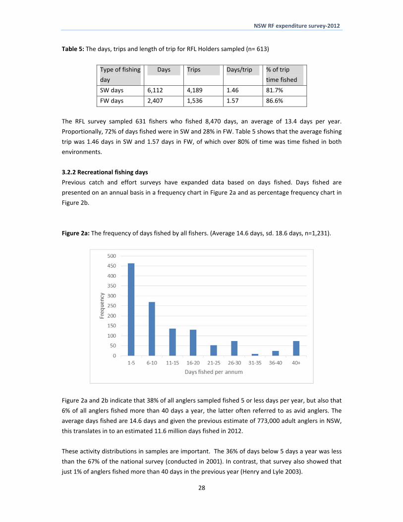
NSW RF expenditure survey‐2012
Table 5 The days trips and length of trip for RFL Holders sampled (n= 613)
Type of fishing
day
Days Trips Daystrip of trip
time fished
SW days 6112 4189 146 817
FW days 2407 1536 157 866
The RFL survey sampled 631 fishers who fished 8470 days an average of 134 days per year
Proportionally 72 of days fished were in SW and 28 in FW Table 5 shows that the average fishing
trip was 146 days in SW and 157 days in FW of which over 80 of time was time fished in both
environments
322 Recreational fishing days
Previous catch and effort surveys have expanded data based on days fished Days fished are
presented on an annual basis in a frequency chart in Figure 2a and as percentage frequency chart in
Figure 2b
Figure 2a The frequency of days fished by all fishers (Average 146 days sd 186 days n=1231)
Figure 2a and 2b indicate that 38 of all anglers sampled fished 5 or less days per year but also that
6 of all anglers fished more than 40 days a year the latter often referred to as avid anglers The
average days fished are 146 days and given the previous estimate of 773000 adult anglers in NSW
this translates in to an estimated 116 million days fished in 2012
These activity distributions in samples are important The 36 of days below 5 days a year was less
than the 67 of the national survey (conducted in 2001) In contrast that survey also showed that
just 1 of anglers fished more than 40 days in the previous year (Henry and Lyle 2003)
28
NSW RF expenditure survey‐2012
Figure 2b The percentage frequency of days fished
In the present study this is partially explained by possible under sampling of 3 day and 1 month
licence holders though the random survey should not have been affected in this way On the other
hand the present study may well have sampled a higher proportion of avid fishers in the RFL data
base The third possibility is that angler behaviour in NSW has altered (on average) in the 12 years
since the national survey perhaps influenced by the introduction of the RFL
33 Comparisons between methods and samples
Statistical t‐tests were used to compare the trips per angler and average days fished per angler
between seasonal samples random and RFL database surveys and between licensed and unlicensed
recreational fishers
a) Are there seasonal differences in fishing activity
There is no previous literature on seasonal levels of fishing effort in NSW but we might expect to
see less days fished and fishing trips in the April to September ldquowinterrdquo period since this period does
not include Christmas However t tests revealed there was no statistically significant difference in
either the average days fished or trips per fisher across all observations between the April and the
September samples This may be partially explained by respondents to the September survey
recalling significant fishing activity at Easter time as part of ldquowinterrdquo activity
b) Are the random survey method and the RFL data base method results different
The t tests for trips indicate that those fishers in the random survey which included both licence
holders and non licence holders fished significantly more trips per year (125 v 906 trips t=395)
than fishers sampled from the RFL database This also applied to days fished with those in the
random survey fishing significantly more days (155 v 134 days t=208)
29
NSW RF expenditure survey‐2012
c) Are there differences between licenced and unlicenced fishers
Do licensed anglers fish more than unlicensed fishers When all samples are considered the average
days fished estimates show no significant difference between licensed and unlicensed fishers
However non‐licence holders made significantly more fishing trips than licence holders (128 trips v
103 t= 224)
34 Discussion of the sampling and activity results
On the basis of these results the average activity per angler whether measured in trips made or days
fished does not appear to be significantly different between seasons This result supports the
prospect of sampling recreational fishers at any time of the year asking them to recall their activity
in the last year
Fishers sampled randomly through the ldquowhite pagesrdquo made significantly more fishing trips and
fished on more days per annum than RFL holders Similarly those fishers contacted at random not
holding licenses were found to fish a similar number of days to licence holders but made
significantly more trips per annum This somewhat counter intuitive result (we might expect licence
holders to be more avid) is nevertheless consistent with concession holders and pensioners being
available to take more occasional fishing trips than the general working population might
It may also be related to the relatively high number of fishers found to have made more than 40
trips per year skewing the activity profile Where one sample is chosen at random and the other
comes from a database of known recreational fishers we may expect some avidity bias in the latter
(Johnson 1999) However this is not what we found indicating that opportunity to go fishing among
non licence holders may enable them to fish more frequently than licence holders though this
assumes we have no significant biases in the survey analysis For example ACMA (2013) states that
CATI surveys as used in our random screening survey ldquomay be biased towards those who normally
stay at home (eg older or retired people or those whose occupation is home duties)rdquo This may
indicate that those who responded had more time to go fishing than across the whole NSW
population
Non response bias and the screening survey
The most common non‐response bias is ldquounit non‐responserdquo which ldquotakes place when a randomly
sampled individual cannot be contacted or refuses to participate in a surveyrdquo (Ritz 2013) Mohadjer
et al explain ldquoThere is always a potential for item nonresponse bias whenever sample persons who
did not participate in the survey have somewhat different characteristics than those who didrdquo
In our random screening survey we had
‐ Sample losses approximately 50 of dead numbers and the potential for unit non response
bias Do those interviewees with land line numbers differ from those who have moved or
changed telephones in the past few years Privacy conditions precluded contacting non
respondents to investigate further Socio‐economically those moving away from landlines
may be younger in the working population or may have different incomes An argument
can be made either way and the extent of any bias remains unknown
30
NSW RF expenditure survey‐2012
‐ Non contactable household‐ It is unlikely these non contactable numbers for non‐RF
households or RF households would differ unless they were out fishing
‐ Refusals Why did so many people who identified themselves as having fished in the past six
months refuse to complete a short fishing interview Reasons include the dislike of surveys
intruding into their home and privacy not having the time or other general perceptions
Those who completed the interview may be keener on fishing more avid and some not
completing it because they consider their level of fishing to be trivial There was also the
indication from surveyors of fear or mistrust that the call was checking up on their licence
status In the random survey those who may have had a licence for 3 days or 1 month in the
previous six month period may not have had one at the time of the call and may have felt
vulnerable However approximately one third of all fishers are concession holders reducing
this possible vulnerability impact
In the area of survey refusals there seems to be more potential for non‐response bias in the
comparability of those who completed the survey with those who refused This cannot be directly
checked with non respondents due to privacy constraints Other independent indicators could be
used comparing ldquohellipthe distribution of respondents in the survey with associated distributions coming
from other independent surveysrdquo (Mohadjer et al 1994) We are able to compare the surveys given
their two different approaches
In the random screening survey over half of the identified fishers did not complete the survey We
can test for evidence of a response bias by comparing RFL licence holders who replied to the random
survey with RLF licence holders contacted directly in the other survey A t‐test indicated that the
mean days fished for the random RFL group (n=391) were significantly higher than the direct RFL
(n=631) survey results (158 v 134 t=211) significant at the 5 and 2 levels This is indicative of a
possible response bias as more active RFL holders appear more likely to have participated in the
random screening survey interviews than other less avid licence holders Previous adjustments made
to the data (section 32) reduced the risk to final estimates from this and other likely biases
Bias and the survey of RFL holders
The RFL survey also recorded significant levels of dead numbers although a much lower rate of
refusals The survey fieldwork team were able to ask to speak to the licence holder by name and this
may have contributed to higher completion rates Any bias in the RFL survey may then be between
responses by different licence holders Those holding 3 year licences may have significantly different
fishing activities expenditures or preferences to 1 year or 1 month and 3 day licence holders
Anecdotal evidence suggests some fishers buy several 3 day licences through the year and this may
contribute to a form of ldquodouble countingrdquo in any comparative analysis of licences The scale of this
behaviour is unknown and does not assist us in developing a sampling approach that may draw on a
representative cross section of the four licence types Further enquiries of non respondents was not
pursued due to privacy constraints
31
NSW RF expenditure survey‐2012
34 Estimation of recreational fishing expenditure per angler
Recreational fishing expenditure can be split into different categories as explained previously
a) Trip related expenditure on a range of expenses Trip expenditure can be annualised by expanding
by the number of trips per annum
b) Expenditure on small equipment and expenses on the last trip and
c) Annual expenditure on larger boat equipment This includes capital purchases in the year of the 10survey
All respondents in each area were asked about trip expenditures by all anglers in their household ndash
which averaged 202 anglers per household (see Table 7 later in report) The estimated expenditures
per angler per trip are reported in Table 6abc but state‐wide estimates in the next chapter are
based on household data
Table 6a summarises the average RF expenditure per trip for all NSW fishers (both SW and FW) in
each region for both fishing trip expenses and tackle Table 6b reports the average SW RF
expenditure per trip for all NSW regions on both fishing trip expenses and tackle Table 6c shows the
average trip expenditures for FW anglers Table 6d shows the annual expenditure on boat
expenditure for all NSW anglers SW and FW anglers combined
In Table 6ab ampc the results include fishers from Interstate who hold a NSW RFL but their major boat
and motor purchases are not assumed to have been made in NSW (Table 6d black squares)
The results in Table 6a confirm that all fishers (both SW and FW) spend 68 of trip expenses on the
fishing trip and just under 32 on equipment and fishing expenses Car travel is the major trip
expense $6974 (31 of total trip expense accommodation $ 3267 (15) and fooddrink eating out
$3594 (16) also while fishing rods and tackle hookslines and baitberley $3891(18) and boat
fuel $1650 (7) are the other major trip expenses
In Table 6b the costs of SW anglers are shown and Table 5c for FW Table 6bampc show that each
group had similar average expenditures per fishing trip (SW ‐ $22282 and FW ‐ $23024) Car travel
expenses are higher for FW fishers $9079 day versus $5955day SW but boat fuel for SW is
$1964 day versus FW $1009day
Table 6d shows that the annual NSW fisherrsquos average boat expenses per angler were $768 pa for all
NSW or broken down $856 for SW and $365 for FW fishers Boat purchase values for SW fishers
were much higher than for FW fishers which reflected the lower capital expenditure on small tinnies
for creeks dams and impoundments as opposed to offshore marine vessels The comparisons are
for the major form of fishing activity with 21 of fishers in our survey sample fishing a combination
of both SW and FW in a given year
10 Expenditure on fishing boats and larger capital items was reduced by 30 to reflect non recreational fishing use
32
NSW RF expenditure survey‐2012
Table 6a The average RF expenditure per trip for all NSW RFs in all NSW Last column is the
percentage of total spend in the All NSW total trip
Data in Aus $ Sydney North coast
South Coast
Inland Interstate All NSW of total spend per
trip Car travel (both ways) 6874 $ $ 4376 $ 4650 9871 $ 13060 $ 6974 $ 31 Accommodation 3998 $ $ 2216 $ 2112 2967 $ 6424 $ 3267 $ 15 Eating out 1478 $ $ 733 $ 1132 1572 $ 2820 $ 1342 $ 6 Other food and drink 2004 $ $ 1420 $ 2121 2881 $ 4857 $ 2252 $ 10 Shopping (souvenirmagazinesvideos) 419 $ $ 155 $ 120 607 $ 947 $ 387 $ 2 Travel-other than by car 354 $ $ 053 $ 325 040 $ -$ 160 $ 1 Sports 027 $ $ 018 $ - 034 $ 478 $ 065 $ 0 Tours 096 $ $ 007 $ 154 100 $ 022 $ 066 $ 0 Poker machines 174 $ $ 095 $ 077 124 $ 504 $ 160 $ 1 Pub 651 $ $ 347 $ 565 618 $ 1554 $ 621 $ 3 Anything else 194 $ $ 044 $ 068 134 $ 152 $ 117 $ 1 Expenditure per trip 16259 $ $ 9460 $ 11307 18946 $ 30811 $ 15405 $ 68
-$ $ - $ - -$ -$ -$ Major fishing tackle (rods reel) 2561 $ $ 1491 $ 1009 2756 $ 826 $ 1937 $ 9 Minor fishing tackle (hooks lines etc) 1106 $ $ 881 $ 713 1505 $ 2101 $ 1162 $ 5 Baitberley 1043 $ $ 559 $ 624 820 $ 938 $ 792 $ 4 Boat hire 671 $ $ 005 $ 090 139 $ 078 $ 242 $ 1 Boat fuel 2054 $ $ 1307 $ 683 1180 $ 3531 $ 1652 $ 7 Charter and fishing guide fees 647 $ $ 301 $ 043 098 $ 109 $ 323 $ 1 Fishing clothesapparel(w aders etc) 263 $ $ 177 $ 276 339 $ 143 $ 239 $ 1 Camping equipment 175 $ $ 735 $ 309 790 $ 400 $ 508 $ 2 Other fishing expenses 240 $ $ 283 $ 144 328 $ 393 $ 276 $ 1 Equipment per trip 8747 $ $ 5726 $ 3890 7939 $ 8520 $ 7120 $ 32
Total spend per trip 25007 $ $ 15185 $ 15197 26885 $ 39331 $ 22524 $ 100
Table 6b The average RF expenditure per SW trips for RFs anglers in all NSW Last column is the
percentage of All NSW total
Data in Aus $ Sydney North coast
South Coast
Inland Interstate All NSW of total spend per
trip
Car travel (both ways) 6168 $ $ 3659 $ 3915 17153 $ 12637 $ 5955 $ 27 Accommodation 4063 $ $ 2182 $ 2170 6325 $ 10959 $ 3547 $ 16 Eating out 1454 $ $ 782 $ 1151 4195 $ 5838 $ 1539 $ 7 Other food and drink 1988 $ $ 1284 $ 2321 2834 $ 6274 $ 2000 $ 9 Shopping (souvenirmagazinesvideos) 447 $ $ 164 $ 115 1620 $ 2157 $ 450 $ 2 Travel-other than by car 421 $ $ 034 $ 365 102 $ -$ 219 $ 1 Sports 033 $ $ 010 $ - 131 $ 581 $ 051 $ 0 Tours 113 $ $ 009 $ 173 280 $ -$ 086 $ 0 Poker machines 187 $ $ 112 $ 068 144 $ 865 $ 170 $ 1 Pub 694 $ $ 371 $ 612 1095 $ 2149 $ 649 $ 3 Anything else 229 $ $ 046 $ 077 -$ 405 $ 129 $ 1 Expenditure per trip 15787 $ $ 8647 $ 10947 33880 $ 41807 $ 14781 $ 66
Major fishing tackle (rods reel) 2703 $ $ 1509 $ 1136 2246 $ 541 $ 1905 $ 9 Minor fishing tackle (hooks lines etc) 1203 $ $ 742 $ 747 1087 $ 3010 $ 1035 $ 5 Baitberley 1183 $ $ 633 $ 656 1242 $ 1116 $ 899 $ 4 Boat hire 816 $ $ - $ 101 475 $ 243 $ 352 $ 2 Boat fuel 2309 $ $ 1380 $ 737 1903 $ 7946 $ 1964 $ 9 Charter and fishing guide fees 788 $ $ 370 $ 048 169 $ 338 $ 465 $ 2 Fishing clothesapparel(w aders etc) 302 $ $ 195 $ 310 270 $ -$ 245 $ 1 Camping equipment 213 $ $ 631 $ 048 936 $ 027 $ 402 $ 2 Other fishing expenses 252 $ $ 275 $ 161 234 $ 223 $ 247 $ 1 Equipment per trip 9750 $ $ 5721 $ 3943 8562 $ 13444 $ 7501 $ 34
Total spend per trip 25537 $ $ 14367 $ 14890 42442 $ 55251 $ 22282 $ 100
33
NSW RF expenditure survey‐2012
Table 6c The average RF expenditure per FW trip for RFs anglers in all NSW Last column is the
percentage of All NSW total
Data in Aus $ Sydney North coast
South Coast
Inland Interstate All NSW of total spend per
trip
Car travel (both ways) 10144 $ $ 7498 $ 10533 7358 $ 13261 $ 9079 $ 39 Accommodation 3696 $ $ 2363 $ 1654 1808 $ 4272 $ 2689 $ 12 Eating out 1591 $ $ 517 $ 981 667 $ 1388 $ 937 $ 4 Other food and drink 2077 $ $ 2014 $ 519 2897 $ 4185 $ 2771 $ 12 Shopping (souvenirmagazinesvideos) 287 $ $ 118 $ 154 258 $ 389 $ 258 $ 1 Travel-other than by car 039 $ $ 138 $ - 018 $ -$ 040 $ 0 Sports -$ $ 053 $ - -$ 429 $ 093 $ 0 Tours 015 $ $ - $ - 038 $ 032 $ 025 $ 0 Poker machines 115 $ $ 020 $ 154 117 $ 333 $ 141 $ 1 Pub 454 $ $ 245 $ 192 454 $ 1272 $ 565 $ 2 Anything else 031 $ $ 033 $ - 180 $ 032 $ 094 $ 0 Expenditure per trip 18448 $ $ 13000 $ 14187 13794 $ 25595 $ 16691 $ 72
Major fishing tackle (rods reel) 1903 $ $ 1414 $ - 2933 $ 962 $ 2002 $ 9 Minor fishing tackle (hooks lines etc) 658 $ $ 1482 $ 442 1649 $ 1669 $ 1423 $ 6 Baitberley 398 $ $ 238 $ 369 674 $ 853 $ 572 $ 2 Boat hire -$ $ 026 $ - 023 $ -$ 015 $ 0 Boat fuel 877 $ $ 988 $ 250 930 $ 1437 $ 1009 $ 4 Charter and fishing guide fees -$ $ - $ - 073 $ -$ 031 $ 0 Fishing clothesapparel(w aders etc) 085 $ $ 097 $ - 363 $ 212 $ 227 $ 1 Camping equipment -$ $ 1184 $ 2392 739 $ 577 $ 726 $ 3 Other fishing expenses 184 $ $ 319 $ 008 360 $ 474 $ 335 $ 1 Equipment per trip 4105 $ $ 5749 $ 3462 7724 $ 6184 $ 6332 $ 28
Total spend per trip 22553 $ $ 18749 $ 17648 21518 $ 31779 $ 23024 $ 100
Table 6d The average RF expenditure per annum on larger boat items for SW and FW anglers in
regions and all NSW (nb Table 6abc are per trip and Table 6d is per angler per annum)
Data in Aus $ Sydney North coast
South Coast
Inland Interstate All NSW of total spend per
trip
All NSW Boat licenceregistration 7115 $ $ 4658 $ 4407 5815 $ 8546 $ 5940 $ 8 Boat maintenance 29248 $ $ 14497 $ 9655 7935 $ 17917 $ 17504 $ 23 Boat insurance 7519 $ $ 4574 $ 3006 4145 $ 10318 $ 5754 $ 7 Marine mooring fees 7615 $ $ 1940 $ 192 122 $ 2609 $ 3179 $ 4 Boat equipment (safety etc) 15175 $ $ 7637 $ 3175 5452 $ 6015 $ 8888 $ 12 Boat purchase or motor repair 23437 $ $ 25676 $ 25865 9740 $ - 35550 $ 46 Annual boat expenditure 90109 $ $ 58982 $ 46300 33208 $ 45405 $ 76815 $ 100
Saltwater -$ $ - $ - -$ -$ -$ Boat licenceregistration 7340 $ $ 4751 $ 3583 6003 $ 13372 $ 6014 $ 6 Boat maintenance 32221 $ $ 15880 $ 9805 5356 $ 28392 $ 20829 $ 22 Boat insurance 8032 $ $ 5068 $ 3002 3960 $ 19824 $ 6458 $ 7 Marine mooring fees 8765 $ $ 2385 $ 216 030 $ 8108 $ 4505 $ 5 Boat equipment (safety etc) 17407 $ $ 7800 $ 3428 7508 $ 9230 $ 10764 $ 11 Boat purchase or motor repair 30450 $ $ 35250 $ 30000 40600 $ - 47050 $ 49 Annual boat expenditure $ 104214 $ 71134 $ 50035 63456 $ 78926 $ 95618 $ 100
Freshwater Boat licenceregistration 6073 $ $ 4255 $ 11000 5750 $ 6256 $ 5787 $ 16 Boat maintenance 15523 $ $ 8474 $ 8454 8830 $ 12949 $ 10632 $ 29 Boat insurance 5154 $ $ 2421 $ 3038 4209 $ 5809 $ 4297 $ 12 Marine mooring fees 2308 $ $ - $ - 155 $ -$ 439 $ 1 Boat equipment (safety etc) 4877 $ $ 6930 $ 1154 4738 $ 4490 $ 5011 $ 14 Boat purchase or motor repair 5000 $ $ 3150 $ 18400 5350 $ - 10350 $ 28 Annual boat expenditure 38935 $ $ 25230 $ 42046 29032 $ 29504 $ 36515 $ 100
34
NSW RF expenditure survey‐2012
In Table 6a the higher travel costs of some regional residents such as Sydney anglers Inland and
interstate fishers were evident The trip expenditure of Inland and interstate SW anglers was
significantly higher than for resident NSW anglers due to car travel accommodation food and other
trip expenses presumably to the coast (Table 6b) Table 6c shows that FW expenditure per trip was
highest for interstate fishers (eg Victorians traveling to southern NSW) and Sydney and South Coast
RFs had high travel costs travelling to desirable FW fishing locations (eg Snowy mountains etc
Dominion 2001 and 2002)
The socio‐economics of recreational fisher expenditure in NSW
The survey samples were analysed to identify some of the socio‐economic drivers of RF expenditure
in NSW The samples combined to give 1235 observations of RF expenditure and the survey
included a range of other variables Both multiple regression analysis and a cluster analysis enables
the statistically significant variables determining angler expenditure to be identified and estimated
as reported in Appendices 1 and 2 respectively
Multiple regression results
In Appendix 1 results reveal that Total recreational fishing expenditure is driven by licence status
(licence holders spending more) number of SW trips per annum and the level of household income
Age sex and regional location were found not to be statistically significant in determining total RF
expenditure
Trip expenditure was driven by licence holders and number of SW trips Trip expenditure was further
examined and was significantly influenced by licence holders SW and FW days fished and the
distance travelled on the last trip Fishing Tackle expenditure was found to be determined by
income rather than number of trips Expenditure on boats was driven by both number of SW trips
and the level of RF household income
Cluster analysis results
The expenditure of NSW RFs was also subjected to ldquocluster analysisrdquo to see the significant socio‐
economic characteristics of fisher groups as reported in Appendix 2and in Figure 3 below The cluster
analyses for expenditure on fishing trips tackle and boat expenditure are reported in Appendix 2
35
NSW RF expenditure survey‐2012
Figure 3 A cluster analysis of RF total expenditure showing the groups of significantly different
clusters of anglers identified
In Figure 3 there are four significantly different cluster groups The characteristics of the four groups
are under the ldquodescriptionrdquo row and the authors have put a label to characterise each group
Between Figure 3 and Appendix 2 the overall picture is of groups of ldquoordinaryrdquo fishers
(approximately 85) with low levels of fishing activity in which household income levels may differ
(half lower half higher) secondly a group of dedicated anglers (approximately 12) who have high
fishing activity and expenditure and finally a highly avid fishing group (less than 3) with very high
fishing activity and high to very high expenditure
The results confirm the only previous examination of the socio‐economic characteristics of RFs in
NSW by Dominion (2003) which showed that recreational fishing is a past time involving a diverse
range of people has great variety in activity levels and crosses the entire socio‐economic spectrum
36
NSW RF expenditure survey‐2012
4 State‐wide and regional expenditure estimates
41 Estimating total expenditure
This chapter describes the estimation of the total recreational fishing expenditure for RFs in NSW
and in its regions Total recreational fishing expenditure is the product of three variables
a) Number of recreational fishers or RF households (HH)
We use three approaches to estimate the total RF population in NSW by use of
1) Random telephone survey and ABS Household data and population data
2) The RFL data base and
3) Use of the screening sample and the ABS data on Households Use of the screening
survey of the general population to estimate total number of fishers11 via ABS
population data
b) Fishing trip activity fishing trip activity estimates are obtained from the telephone survey
and
c) Recreational fishing expenditure information on the expenditure per trip and annual
expenditures on equipment is obtained from the telephone survey
The product of these variables will enable us to estimate the total state‐wide recreational fishing
expenditure Expenditure is also estimated for each state region considered Saltwater and
freshwater fishing are considered separately in the state estimates through asking respondents
about the trip intention
42 Expanding the sample of fishers and expenditure
Total expenditure estimates are based on travel and fishing equipment expenses per trip and
estimates of expenditure on boat capital items These are summed to give an annual total
expenditure estimate However the estimates for the angler survey need to be expanded to give
state wide estimates These expansions are described in Box 1 below
Box 1 Explanation of key expansions
The expansion method adapts the method used in the National Survey (Henry and Lyle 2003) The
number of fisher households (FHH) was estimated as follows for each region
No of fisher Household (est) = No Households in Population (ABS) No of Fisher HH (sample)
No of HH (sample)
Example How many recreational fishers would these households include
No of Fishers 19 to 75 yrs (est) = Mean No fishers per HH (sample) No of fisher Household (est)
776496 = 202 383921 (see Table 7)
RF HH are distributed proportionally across regions by household and recreational fishers by
regional population
11 Recreational Fishers under 19 years of age are not included and need to be added if the total population figure is for all
anglers The activity and expenditure estimates are based on ages 19‐75 only
37
NSW RF expenditure survey‐2012
Information on NSW State and Regional Households by Local Government Area (LGA) were accessed
(ABS 2011) The data were aggregated by the larger SD ABS regions (eg Sydney North coast
Inland and SDD South Coast area) These identified the number of households in each of the study
regions as reported in Table 7
Table 7 The ldquototal householdsrdquo in each of the NSW study regions based on LGA data ABS (2011)
Households with recreational fishers are estimated for each study region
Area Population 2010 (gt18-75)
Households HH with RF Rec Fishers HH
RF by region
Sydney 3160897 1376583 213934 230 491232
North coast 835229 570688 88690 146 129802
South coast 350750 207195 32200 169 54510
Inland 649564 315987 49107 206 100948
Total 4996461 2470453 383931 202 776496
The RF household responses for anglersrsquo trip frequency and trip expenditure were multiplied to
produce estimates of state‐wide and regional expenditure
43 State‐wide expenditure estimates
The estimation of total expenditure for samples of recreational anglers and its expansion to regional
state‐wide and national estimates has depended on traditional statistical methods estimating the
total from means of the component distributions However while the number of households is
reasonably well estimated the frequency distribution of fishing trips is highly skewed to the left (see
Figure 1a)
The estimates of total state expenditure on recreational fishing involve multiplying the following
variables
1) Estimate of RF households ‐ the ABS has reliable estimates of households for which RF
households can be identified
2) Estimate of trips ‐ anglers state the number of trips per annum and
3) Estimate of the trip and tackle expenditure on their last trip and their capital expenditure in
the last year
Total expenditure is the product of these variables Total expenditure can be estimated as a mean
value with confidence intervals Here we used the 1237 observations in the RF sample weighting
the results in respect of regional populations as follows
a) Total annual expenditure per angler household = (($ travel expenses per trip + $ tackle
expenses per trip) number of trips )+ (annual capital expenditure per angler household)
b) Total annual expenditure in NSW = total number of anglers households total annual
expenditure per angler household
This traditional approach gives a point estimate but does not provide any information on the
probability of different expenditure levels around the mean This requires a simulation approach
38
NSW RF expenditure survey‐2012
Table 8a shows that the estimated expenditure by all NSW resident RFs in 2012 was $1439bn12 with
an additional $1861m being spent by interstate fishers making a total estimated expenditure by
recreational fishers in NSW of $1625bn in the year 2012
Considering regional expenditures total recreational fishing expenditure was highest by Sydney
anglers ‐ $903m (56 of all expenditure in NSW) followed by the North coast anglers ‐ $3008m
(19) and inter‐state anglers ‐ $ 186m (11) Total expenditure for South Coast anglers was
$1018m (6) and for Inland anglers $1308m (8)13
Expenditure on fishing trips was $793m or 49 of all recreational fishing expenditure in NSW Of
this $402m (25) was spent on fishing equipment tackle and fuel and $430m (26) was spent on
annual capital expenditures such as boats and maintenance Expenditure on SW fishing was
estimated at $1415m (87) and on FW fishing at $231m (13 of total recreational fishing
expenditure in NSW)
Table 8b shows the costs within each category
Within trip expenditure (49 of total expenditure) car travel $326m (201 of total annual
expenditure) accommodation $1859m (114) and food and eating out $188m (115)
Expenditure on fishing equipment and expenses $4025m (246) was made up of $1645m
(102) on major and minor tackle and $1027m (63) on boat fuel and
Annual boat expenditure $4305m (26) of which $1225m (75) was maintenance and
boat purchase or motor repair $1436m (88)
12 This estimate is the same as the mean value produced by the simulation shown later in this chapter It is then adjusted
for Interstate expenditure13 In Chapter 5 the regional economic analysis adapts these data to reflect the expenditure made in other regions away from home residence
39
NSW RF expenditure survey‐2012
Table 8a Estimates of the total RF expenditure for different areas of NSW and including interstate angler expenditure to give all RF expenditure in NSW
Expenditure category Sydney North coast South coast Inland All NSW Inter-state Total expend
in NSW
total expend in NSW
Trip spend 383906879 136686958 57862828 74849484 653306149 139478487 792784637 49 $ fishing equip 222891110 85965049 20624384 31116970 360597513 41975664 402573177 25 Total annual boat expenditure 296326795 81222395 23393975 24877516 425820681 4691465 430512146 26 Totals 903124785 303874402 101881187 130843970 1439724343 186145616 1625869959 100 of total expend in NSW 56 19 6 8 89 11 100 Saltwater 840749912 267431019 99200573 51715617 1259097121 140675487 1415280961 87 Freshwater 62374873 36443383 2680614 79128353 180627222 45469052 231775451 14 SW expenditure as of Total 93 88 97 40 87 84 87
40
NSW RF expenditure survey‐2012
Table 8b Estimates of the total RF expenditure for different areas of NSW and including interstate angler expenditure to give all RF expenditure in NSW
Data in Aus $ Sydney North coast South coast Inland All NSW Interstate Total expend
in NSW
of Total expend in
NSW Expenditure category Car travel (both ways) 155752824 61047851 21250669 38966591 277017934 49755399 326773333 201 Accommodation 96655736 32991275 11321758 11775540 152744309 33155541 185899850 114 Eating out 35118007 11287702 6019080 6283701 58708491 16433282 75141772 46 Other food and drink 47830881 20416270 11974310 11255861 91477322 21385714 112863036 69 Shopping (souvenirmagazinesvideos) 10396840 2377682 609238 2427428 15811187 5900718 21711905 13 Travel-other than by car 9328498 675596 1876003 157968 12038065 - 12038065 07 Sports 730303 214569 - 136952 1081824 2038576 3120401 02 Tours 2517279 121080 888633 400483 3927475 44318 3971793 02 Poker machines 4337423 1534429 364864 485304 6722021 2611177 9333198 06 Pub 16147653 5352108 3163325 2442584 27105670 7101506 34207176 21 Anything else 5091436 668396 394948 517073 6671852 1052256 7724108 05 Trip spend 383906879 136686958 57862828 74849484 653306149 139478487 792784637 488
Major fishing tackle (rods reel) 63209459 22456502 5830420 10743744 102240126 2673467 104913593 65 Minor fishing tackle (hooks lines etc) 27752247 12319663 3884279 5859337 49815525 9792034 59607560 37 Baitberley 26800952 8839913 3407290 3225829 42273984 3954942 46228926 28 Boat hire 17933756 42708 518369 561815 19056649 604762 19661412 12 Boat fuel 52493364 20044184 3811422 4649308 80998277 21742806 102741083 63 Charter and fishing guide fees 17310929 4944101 246843 386149 22888022 839948 23727969 15 Fishing clothesapparel(w aders etc) 6799431 2766227 1592134 1322337 12480129 292501 12772630 08 Camping equipment 4689522 10357115 508333 3093322 18648291 864926 19513218 12 Other fishing expenses 5901451 4194635 825295 1275129 12196509 1210277 13406786 08 $ fishing equip 222891110 85965049 20624384 31116970 360597513 41975664 402573177 248
Boat licenceregistration 22369127 6037457 1817922 4154611 34379117 4691465 39070582 24 Boat maintenance 93188042 18809323 4588346 5925940 122511651 - 122511651 75 Boat insurance 23806199 5935399 1413005 2990204 34144806 - 34144806 21 Marine mooring fees 24487619 2521793 97904 96275 27203591 - 27203591 17 Boat equipment (safety etc) 48762545 9898735 1571861 3725061 63958201 - 63958201 39 Boat purchase or motor repair 83713264 38019687 13904937 7985426 143623314 - 143623314 88 Total annual boat expenditure 296326795 81222395 23393975 24877516 425820681 4691465 430512146 265
Totals 903124785 303874402 101881187 130843970 1439724343 186145616 1625869959 1000 Saltwater 840749912 267431019 99200573 51715617 1259097121 140675487 1399772608 861 Freshwater 62374873 36443383 2680614 79128353 180627222 45469052 226096274 139 SW expenditure as of Total 93 88 97 40 87 76 86 Region as of total expenditure 56 19 6 8 11 100
41
NSW RF expenditure survey‐2012
44 A probabilistic simulation approach to the estimation of total state recreational fishing
expenditure
Simulation enabled us to estimate the probability of different outcomes from the existing data The
original sample was weighted by numbers of regional households to account for the under sampling of
Sydney and the over sampling of the North Coast in the original survey data The sample was analysed
using the SPSS v21 Monte Carlo Simulation model (IBM Corp 2012) This routine produced up to
100000 repeat runs of the predicted values of total RF state expenditure to give the probability of
different expenditure totals as shown in Figure 5a The cumulative probability is shown in Figure 5b
Figure 5a The probability of total expenditure by NSW anglers 2012
These initial probability estimates showed that the mean total state‐wide expenditure was $1473m
with 5 and 95 confidence estimates of $706m and $2952m The median value as $1196m reflecting
the skewedness of the distribution
The estimate of expenditure in NSW by interstate anglers of $1861m has also to be added The final
total NSW estimate of expenditure on recreational fishing was therefore $1625m with 5 and 95
confidence estimates of $892m‐$3136m14
14 For simplicity this assumes the distribution of the interstate results are the same as all NSW
42
NSW RF expenditure survey‐2012
Figure 5b The cumulative probability of total expenditure by NSW anglers 2012
Figure 5a and 5b indicate how the skewed distribution of trips per year by anglers and the highly annual
variable expenditure make the predicted adjusted distribution from $892m‐$3136m around an
adjusted mean $1625m and an adjusted median of $1382m The mean has a 0045 probability of being
achieved whereas lower total expenditure estimates have higher probability (Figure 5a) The
skewedness gives a threshold minimum expenditure level and a ldquotrailing tailrdquo on the right hand side
reflecting less probable high expenditure estimates
Figure 5b indicates that the mean would have a cumulative probability of 65 This shows the higher
total expenditure estimates on the right hand side of Figure 5a are pulling the mean to the right This is
why we have to be careful in RF sampling and estimation of recreational activity and expenditure This
also may explain why fishers of differing avidity and expenditure levels have considerably different
opinions on total expenditure in the sector A fisher with higher activity and expenditure would estimate
a state wide total at the right hand side of Figure 5a but while high total expenditure is possible it is
highly improbable
45 Discussion The estimated total expenditures reported in Table 8a and 8b indicate a statewide expenditure by NSW
recreational fishers and interstate anglers on items directly related to fishing of $1625m
43
NSW RF expenditure survey‐2012
The expansions to develop the final estimates took account of the differences between SW and FW
expenditure and activity and each was expanded separately Expenditure on FW fishing contributed 14
of total expenditure considerably less than the 28 of days fished reported in the sample (Table 5)
reflecting some trip and capital expenditure differences between SW and FW fishers
By region the results indicate that recreational fishing expenditure by Sydney anglers $9031m (56 of
total state recreational fishing expenditure) while North coast has $3038m (9) Interstate anglers
$1861 (11) Inland $1308m (8) and South coast $1018 (6) The survey method estimated regional
expenditures from interviews with fishers in their home region The regional economic impacts adjusts
these and produced estimates of recreational fishing expenditure and its economic impacts across all of
NSW and its main regions
There is just the previous national survey study for comparison of results The 2012 expenditure
estimate adjusted from the Campbell and Murphy (2005) national survey 2001 study is $765m This is
within the confidence intervals predicted by the current studyrsquos simulation approach
Another comparison is to deduct the trip expenditures for food and entertainment from the current
studyrsquos results to be comparable to Campbell and Murphyrsquos assumptions giving an estimate up to
$136bn15 The difference in expenditure estimates16 is primarily related to the survey methods used and
the different estimates of fishery activity the current study being higher Though the number of adults
fishing may have reduced since 2001 NSW has now a sizeable established recreational fishing licence
holder population and expenditures per angler are higher than a decade ago
Under the telephone survey interview and recall method used the current results were conservative for
this methodological approach This study has pointed to the highly skewed nature of the trip activity
among the RF population and the highly variable levels of expenditure among recreational fishers in
NSW The use of a probabilistic simulation in this study has illustrated the difficulties in estimation of
total RF expenditure and the wide distribution around the mean The adequate inclusion and possible
over‐inclusion of avid fishers are sampling problems under any of existing methodologies
The sample size and hence a higher survey cost is part of the remedy Further examination of the US
multi‐method approach may be merited (Gentner 2009) though this is a large scale national expensive
survey exercise The project results in this study are proposed as being reasonable under the
methodologies available within funding constraints and are part of a proposed ongoing expenditure
survey strategy in NSW as outlined in Chapter 6
15 There may also be differences in the treatment of capital attributable to RF definitions of maintenance and capital expenditure on motors and boats and other differences between the two studies These may likely lower this estimate 16 ($1360m‐$765m=$595m in 2012 terms)
44
NSW RF expenditure survey‐2012
5 Regional economic impact estimates This chapter of the report was compiled by Western Research Institute (WRI) WRI received the output
of this survey in terms of expenditure of respondents and based on this output modelled the
economic impacts of recreational fishing on the NSW economy and defined sub‐regions Input‐
output modelling has been employed to derive the relevant economic models and the impacts
51 Methodology
The methodology used to prepare this report included
Determination of the boundaries of the regions to be used in table construction
In consultation with the ANCORS the decision was made to construct input‐output tables for the NSW
North Coast NSW South Coast NSW Inland and Sydney regions as well as NSW as a whole Each region
was defined by aggregating statistical areas at level 4 3 or 2 or combination thereof This allowed the
formulation of regions and economies that best represented the regions of interest Specifically data
from statistical areas at level 3 of ABS Statistical Geography Standard (rather than at larger statistical
areas at level 4) was used in the construction of tables for the NSW North Coast and data from
statistical areas at level 2 was used in the construction of tables for the NSW South Coast The table
construction for Sydney region was based on the data from statistical areas at level 4 while tables for
NSW Inland region was based on the data from statistical areas at different levels (2 3 and 4) Detailed
information on statistical areas in provided in WRI (2013)
Construction of tables
The input‐output tables developed for this project were derived from the latest national table produced
by the Australian Bureau of Statistics (ABS) That table provides a detailed picture of the structure of the
economy of Australia for the year 2008‐09 A series of steps were undertaken to update the table to
2011‐12 Further information from the State Accounts (ABS Cat No 52200) labour force data from the
2011 Census and the quarterly labour force survey (ABS Cat No 6291055003) were used to develop a
state table for New South Wales at 2011‐2012 This was then regionalised to reflect the respective
regional economies of NSW North Coast NSW South Coast NSW Inland and Sydney Further details of
the procedures used in the development of a regional input‐output table are provided in WRI (2013)
52 Economic impact analysis
The economic impacts were modelled as a final demand impact (that calculates the impacts measured
by output value added household income and employment across all sectors in response to changes
in industry final demands) using the 2011‐12 Simulating Impacts on Regional Economies (SIRE) input‐
output model of NSW North Coast NSW South Coast NSW Inland Sydney and NSW as a whole The
SIRE model is superior to standard input‐output models as it provides for non‐linear relationships
between variables and is based on empirically derived (rather than assumed) coefficients In terms of
45
NSW RF expenditure survey‐2012
robustness of results it is comparable with computable general equilibrium (CGE) models whilst
minimising data requirements See WRI (2013) for a detailed description of the SIRE input‐output
model
The impacts of recreational fishing expenditure on the NSW North Coast NSW South Coast
NSW Inland and Sydney regions as well as NSW as a whole have been provided in terms of
bull Output which is the value of goods and services that are produced within an establishment
that become available for use outside that establishment plus any goods and services
produced for the organisationrsquos own final use Output is equal to total revenue plus any
internal consumption
bull Value added which is equal to gross output minus intermediate inputs Value added is
equivalent to the contribution to gross regional product (the local equivalent of gross
domestic product)
bull Household Income which measures the benefit received by regional households from
economic activity It typically refers to compensation of employees but can also include
income in return for other forms of productive activity
bull Employment which refers to full‐time equivalent (FTE) employment is a measure of the
total level of staff resources used The FTE of a full‐time staff member is equal to 10 The
FTE of a part‐time worker will be a fraction of this depending on the relative number of
hours worked
53 The Economic Impact of Recreational Fishing on the Regional Economies of NSW
The economic impact due to recreational fishing was modelled as follows
bull The expenditure survey conducted by ANCORS did not capture the location of expenditure
just the origin (postcode) of the respondent Therefore in the absence of location data an
assumption was made that the total expenditure by interstate visitors ($18614 million)
who make expenditures on recreational fishing whilst staying in NSW should be distributed
evenly across four NSW regions (ie 25 of total interstate expenditure pertaining to each
NSW region)
bull Likewise it was assumed that expenditure pertaining to the NSW North Coast NSW
South Coast and NSW Inland regions was made in these regions (eg those
respondents who indicated living in the NSW North Coast partake in recreational
fishing in the NSW North Coast and not in other areas thereby ensuring that the
money spent on recreational fishing remains in the NSW North Coast region)
46
NSW RF expenditure survey‐2012
bull For those respondents who indicated living in Sydney an assumption was made that 515
of them partake in fishing in Sydney with the remaining 485 fishing in the rest of NSW in
the following proportions NSW North Coast ndash 346 NSW South Coast ndash 485 and NSW
Inland ndash 169 (Dominion 2002 and 2004)
bull Since anglers in each of the regions make expenditure on items that may not be
produced in the region but that are imported from the rest of NSW the regional
recreational fishing expenditure was split into local and imported components using a
location quotients matrix This way WRI ensured that only local expenditure generated
economic impacts in the respective region For NSW as a whole an assumption was
made that all products that anglers purchase are produced within the state and
therefore no separation of local and imported components was performed The
economic impacts of recreational fishing on NSW were modelled using total recreational
fishing expenditure in NSW
bull In order to ensure consistency of the input‐output modelling procedure the expenditure
data was allocated in the input‐ output table to the industries (typically manufacturing
industries) where the relevant expenditure items were produced and was then
converted to basic prices See WRI (2013) for further details on sectoral allocations
bull A final demand analysis in SIRE was performed and economic impacts on NSW North Coast
NSW South Coast NSW Inland and Sydney as well as NSW as a whole were derived
The impacts of recreational fishing on the economies of the NSW North Coast NSW South Coast
NSW Inland and Sydney regions are outlined in the Table 9
Table 9 Regional expenditure and economic impacts on regional economies
Region North Coast Sydney South Coast Inland
Expenditure by postcode ($m) 30387 90312 10188 13084
Reclassified expenditure ($m) 50196 51165 36086 2514
Output ($m) 73465 100286 39522 35381
Value added ($m) 35355 49156 18417 14985
Household income ($m) 16875 28888 876 735
Employment (no) 3320 3944 1808 1539
47
NSW RF expenditure survey‐2012
NSW North Coast
Overall when flow‐on effects are taken into account recreational fishing contributes the following to
the economy of NSW North Coast
bull 3320 FTE jobs including 667 in the retail trade sector 573 in the hospitality sector
349 in the personal and other services sector and 174 in the transport and storage
sector
bull $16875 million in household income with 134 percent being in the retail trade
sector 112 percent being in the hospitality sector 76 percent being in the public
administration sector 72 percent being in the personal and other services sector and
57 percent being in the transport and storage sector
bull $35355 million in industry value added representing 081 percent of total regional
value added of the NSW North Coast region and
bull $73465 million in output
For the North Coast recreational fishing will contribute 098 percent of FTE employment in the
region when flow‐on effects are taken into account as well as 084 percent of household income and
07 percent of the estimated gross regional product of the NSW North Coast region
NSW South Coast
Overall when flow‐on effects are taken into account the recreational fishing contributes the
following to the economy of NSW South Coast
bull 1808 FTE jobs including 420 in the hospitality sector 284 in the retail trade sector
236 in the personal and other services sector 117 in the transport and storage
sector and 106 in the public administration sector
bull $8760 million in household income with 152 percent being in the hospitality sector
109 percent being in the retail trade sector 93 percent being in the public
administration sector 86 percent being in the personal and other services sector and 77
percent being in the transport and storage sector
bull $18416 million in industry value added representing 167 percent of total regional
value added of the NSW South Coast region and
bull $39522 million in output
For the South Coast recreational fishing will contribute 212 percent of FTE employment in the region
when flow‐on effects are taken into account as well as 173 percent of household income and 143
percent of the estimated gross regional product of the NSW South Coast region
48
NSW RF expenditure survey‐2012
NSW Inland
Overall when flow‐on effects are taken into account the recreational fishing contributes the
following to the economy of NSW Inland
bull 1539 FTE jobs including 289 in the hospitality sector 288 in the retail trade sector
148 in the personal and other services sector and 138 in the agriculture sector
bull $7350 million in household income with 134 percent being in the retail trade
sector 131 percent being in the hospitality sector 74 percent being in the
personal and other services sector 70 percent being in the public administration
sector and 68 percent being in the transport and storage sector
bull $14985 million in industry value added representing 030 percent of total regional
value added of the NSW Inland region and
bull $35381 million in output
Recreational fishing will contribute 038 percent of FTE employment in the NSW Inland region when
flow‐on effects are taken into account as well as 032 percent of household income and 026 percent
of the estimated gross regional product of the NSWInlandregion
Sydney
Overall when flow‐on effects are taken into account the recreational fishing contributes the following
to the economy of Sydney
bull 3944 FTE jobs including 741 in the retail trade sector 450 in the hospitality sector
366 in the personal and other services sector and 310 in the professional and
technical services sector
bull $28888 million in household income with 162 percent being in the finance and insurance
sector 113 percent being in the retail trade sector 83 percent being in the professional
and technical services sector 77 percent being in the wholesale trade sector and 63
percent being in the hospitality sector
bull $49156 million in industry value added representing 025 percent of the total regional
value added of Sydney and
bull $100286 million in output
For the Sydney region recreational fishing will contribute 028 percent of FTE employment when flow‐on
effects are taken into account as well as 025 percent of household income and 022 percent of the
estimated gross regional product of Sydney
49
NSW RF expenditure survey‐2012
NSW State economy
The impacts of recreational fishing on the state economy of the NSW are outlined in the Table 10
Table 10 NSW expenditure and economic impacts on NSW
Item Estimate
NSW Expenditure by postcode ($m) 143972
Total interstate expenditure ($ m) 18615
NSW Reclassified expenditure ($m) 162587
Output ($m) 342035
Value added ($m) 162561
Household income ($m) 87728
Employment (thousand) 14254
NSW Economy
Overall when flow‐on effects are taken into account the recreational fishing contributes the following to
the economy of NSW
bull 14254 FTE jobs including 2730 in the retail trade sector 2123 in the hospitality
sector 1389 in the personal and other services sector and 951 in the transport and
storage sector
bull $87728 million in household income with 122 percent being in the retail trade 114
percent being in the finance and insurance sector 88 percent being in the hospitality
sector 72 percent being in the professional and technical services sector and 65
percent being in the wholesale trade sector
bull $162561 million in industry value added representing 036 percent of the estimated gross
state product of the NSW and
bull $342035 million in output
50
NSW RF expenditure survey‐2012
Overall recreational fishing will contribute 046 percent of FTE employment in the NSW when flow‐on
effects are taken into account as well as 041 percent of household income and 040 percent of total
regional value added
54 Conclusion
The recreational fishing expenditure and economic impact of recreational fishing on NSW and
respective regions were substantial in absolute terms but uneven across regions
The expenditure based on place of residence was the highest in Sydney followed by NSW North
Coast NSW Inland and NSW South Coast The reallocated expenditure (ie actual expenditure
made in the region) was still the highest in Sydney (but substantially lower than postcode
expenditure) followed by expenditure in NSW North Coast NSW South Coast and NSW Inland
In terms of output valued added household income and FTE employment the absolute economic
impacts of recreational fishing were the highest in Sydney followed by NSW North Coast NSW South
Coast and NSW Inland However in relative terms economic impacts (as percentage of total in the
respective regions) were the highest in NSW South Coast (167‐ 212) followed by NSW North
Coast (081‐098) NSW Inland (030‐038) and Sydney (025‐028) These relative disparities
reflect the large size of Sydney and NSW Inland economies and smaller size of NSW North Coast and
NSW South Coast economies
51
NSW RF expenditure survey‐2012
6 Developing a cost effective approach to expenditure surveys
There have been several reoccurring issues in obtaining information on recreational fishing expenditure
in NSW The first is the lack of a series of expenditure surveys the past ones not occurring as part of an
on‐going consistent strategy The second issue is the lack of a known survey method which is repeatable
and can be compared with past surveys In both of these issues the recurrent cost of such surveys has
been unknown also
61 The objectives of an recreational fishing expenditure survey
Any survey is designed towards its objectives In developing a cost effective regular approach to
recreational fishing expenditure surveys there has to be some design decisions made in respect of the
information required For example A state‐wide expenditure estimate may be required every two years
to track and promote the value of the sector This could include a state‐wide estimate of regional
economic impact Further disaggregation by area or other variables will increase cost
62 Sampling data issues and findings
This study has considered how the use of the RFL database reduced the cost of expenditure surveys
which have traditionally used expensive random screening surveys to locate recreational fishers
Finding 1 The current study has found that there is no statistically significant difference between
seasonal samples Consequently we recommend an annual survey event being mindful of its timing
relative to Christmas January and Easter which may be periods when fishers are not at home
The RFs identified through a random screening survey process were found to make more fishing trips
and fish more days than the sample of RFs contacted through the RFL database (noting that both
samples include licence holders) However in further comparisons of days fished per angler between
licenced and unlicensed fishers no significant difference was found On the other hand unlicensed
fishers were found to undertake significantly more fishing trips than licence holders though this relates
to trip events and not necessarily to higher average expenditure ndash in other words unlicensed fishers
may make more but shorter trips to nearby destinations compared with licensed fishers
Finding 2 The RFL database can be used to sample anglers for expenditure surveys providing certain
conditions are met in terms of the different numbers of licences holders that are sampled17
63 What sample size is required
The size of a sample in statistics is important If the sample is too small there is then the risk that the null
hypothesis is wrongly rejected (ATS 2010) The size of a sample is also related to the probability level at
17 A ratio of 3 day 1 month 1 year and 3 year licence holder records is recommended The weighting would be easier for the annual and 3 year licence holders as 3 day and monthly licence holder can be repeat licence purchasers in a given year
52
NSW RF expenditure survey‐2012
which the variable is seen to be significantly different from zero eg 95 (5) or 99 (1) levels of
significance The dispersion of the distribution of the variable being examined is also important and this
is captured in the standard error of the variable
In statistics these issues are brought together in statistical ldquopower analysisrdquo where the minimum size of
a sample can be tested both prior to and even after statistical surveys to see if the sample size is
adequate ldquoThe power is the probability of detecting an effect presuming it is actually thererdquo (ATS 2010)
Sample size estimation
In this section of the report we investigate how reducing the sample size to the minimum required
number of interviews can reduce the cost of an expenditure survey The decision regarding the target
sample size for the survey has to be balanced between the levels of significance chosen for testing (1
5) and the standard error that is acceptable for the intended variables which is often related to the
estimated value called the relative standard error (RSE) 18
Table 11 shows a range of sample sizes derived for different scenarios using the ABS calculator facility at
NSS (2013) There are the two scenarios for random surveys (cases 1‐4) and two for surveys from a
population base of known participants (case 5‐6)
Table 11 Indication of the required sample sizes under different sampling and risk scenarios including
sampling of the RFL database
Case number 1 2 3 4 5 6 Sample type Random sampling Non random
Statistical input All NSW Population
All NSW Population
All NSW Population
South coast
RFL ‐1 RFL‐2
Confidence Level 99 95 95 95 95 95 Population Size 4996500 4996500 4996500 350750 480700 480700 Proportion 05 05 015 025 06 06 Confidence Interval 005 005 00294 005 005 005
Upper 055 055 01794 03 065 065 Lower 045 045 01206 02 055 055
Standard Error 0025 0025 0015 0025 003 0045 Relative Standard Error () 50 50 100 100 50 75 Sample Size 339 196 567 300 267 119
18 The RSE is the standard error expressed as a percentage of the estimate
53
NSW RF expenditure survey‐2012
In Table 11 cases 1 and 2 show the general sampling results when the confidence level is either 99 or
95 and the proportion is 05 (ie where ldquothe expected proportion of the population to have the
attribute that you are estimating from your surveyrdquo (NSS 2013) These data are often quoted but given
that RFs are more difficult to locate than a one in two assumption (proportion 05) case 3 assumes a
15 proportion for RFs and requires a sample size of 567 with a relative standard error (RSE) of 10
Reducing the sampling area to the South Coast (case 4) raises the chances of locating RFs (proportion
025) and would require 300 observations at an RSE of 10 The sampling model assumes a random
population
We also apply the model to the non‐random scenarios from the RFL data base Here cases 5 and 6 are
RFL records and hence not as random as the whole NSW population We use the model to estimate
possible minimum sample sizes when using the RFL data base population Assuming that the proportion
is 06 an RSE of 5 requires a sample of 267 and an RSE of 75 a sample size of 119 In the experience
of the authors the last sample size (119) is low given the variation in our results We recommend no less
than 250 completed surveys as a minimum sample size for state‐wide estimates If four NSW regions are
included a minimum total of 500 completed surveys would be required and be should be larger if
possible
The review of samples has shown that there is a trade off in accuracy of estimates with the number of
interviews undertaken For example in the case 3 random survey in Table 11 the RSE is 10 and
reducing this to 75 for case 3 would increase the sample size from 576 to 1008 or for 5 to 2226
The incidence of locating RFs has cost implications for surveying and this is why the careful use of the
RFL data base is attractive
Finding 3a A main state‐wide survey using the RFL data base to sample 1000 anglers in major regions is
recommended every 5 years with an option of updating results by indexing annually or bi‐ennially
andor considering a smaller survey (250 state wide or 500 for regions) in year three also
Finding 3b The economic impact analysis can follow the five year survey pattern and can be adjusted
between surveys Simulation modelling can also be used to provide an improved understanding of the
uncertainty surrounding expenditure estimates and may be used to confirm estimates between main
surveys also
64 Discussion ‐ Scoping a recreational fishing expenditure survey strategy for NSW
A recreational fishing expenditure survey strategy would aim to undertake a substantial survey every 5
years and run smaller annual or biennial updating exercises between these periods
In the future the 5 year survey could either
54
NSW RF expenditure survey‐2012
Follow past screening survey approaches of all RFs and compare results with a sample of RFL
holders as in the current study or
Use a weighted selection of 3 day 1 month 1 year and 3 year licence holder contacts to enable
a representative sample to be expanded to state‐wide totals
Before being able to categorically recommend the sole use of the RFL database only approach we would
require more information on the inter‐relationship between the random screening survey and the use of
and RFL data base records The current NSW catch and effort survey study may also provide information
on this relationship (J Murphy DPI pers comm)
As per Finding 2 we recommend further comparisons of the random screening survey approach to all
fishers with use of the RFL holdersrsquo data as in the current study Use of the RFL database alone should
be confirmed by other research on the relationship between all fishers and those who are licensed
In the years between the five year main surveys the survey results from the initial survey could be
upgraded annually (or bi‐ennially) by sampling several variables that could be used to index the changes
in the state wide expenditure estimates For example any changes detected in RF participation or
activity state population or change in licence sales could inform activity estimates Information on
recreational fishing expenditure could be influenced by annual changes in price levels as measured by
the consumer price index (cpi) and any information available from industry about retail fishing gear
prices such as those related to exchange rate variations which would impact expenditure on fishing
gear Many of these indices of economic conditions are monitored by the Australian Fishing Tackle
Association and could be referred to
The simulation modelling approach used in the current study could be re‐run annuallybiennially with
these activity and expenditure indices included and updated annual estimates produced The
reoccurrence of another survey in year 5 means there would be a cross check on the indexing of the
previous survey
The choice of 5 years for the main survey is arbitrary and could be 3 years particularly if other catch and
effort surveys are indicating significant changes in participation rates in NSW or there is evidence of
changes in other states Leaving a main survey for more than 5 years is not recommended as the public
awareness of the sectorrsquos economic contribution and associated regional benefits will reduce giving the
sector less public profile
65 Conclusions
The recreational fishing sector in NSW wishes to have more regular studies of angler expenditure and its
importance to the economy The RFL data base can be used for sampling the recreational fishing
population reducing the costs of fieldwork surveys if several conditions are followed The frequency of
55
NSW RF expenditure survey‐2012
the different licence durations needs to be chosen so as not to move away from sampling a
representative cross section of anglers of all different activity levels and possibly having over or under
emphasis of avid anglers
A main state‐wide survey using the RFL data base to sample 1000 anglers in major regions is
recommended every 5 years with an option of updating results by indexing annually or bi‐ennially and
considering a smaller survey (250 state wide or 500 for regions) in year three also The economic impact
analysis can follow the five year survey pattern and can be adjusted between surveys Simulation
modelling can also be used to provide an improved understanding of the uncertainty surrounding
expenditure estimates and may be used to confirm estimates between main surveys also
56
NSW RF expenditure survey‐2012
References
ABARES (2011) Australian Fisheries Statistics 2010 Australian Bureau of Agricultural and Resource Economics and
Sciences Australian Government p 100
ABS (2010) 1216055003 ‐ Australian Statistical Geography Standard Design of the Statistical Areas Level 4
Capital Cities and Statistical Areas Level 3 May 2010 Canberra
ABS (2011) 13381 NSW State and Regional Indicators December 2010
ABS (2012) Estimated Resident Population for New South Wales by Age by Statistical Geography Persons ndash 30
June 2011 Population by Age and Sex Regions of Australia 32350 Canberra
ACMA (2013) Convergence and Communications Report 1 Australian household consumersrsquo take‐up and use of
voice communications services Australian Communication and Media Authority report November
ATS (2010) Introduction to Power Analysis Statistical Computing Seminars
httpwwwatsuclaedustatseminarsintro_powerdefaulthtm
Campbell D and JJ Murphy (2005) The 2000‐01 National Recreational Fishing Survey Economic Report
Department of Agriculture Fisheries and Forestry GPO Box 858 Canberra ACT 2601 June
Cunningham S Dunn MR and Whitmarsh D (1985) Fisheries Economics An Introduction Mansell Publishing
London
Dominion (2001) ldquoAn economic survey of the Snowy mountain recreational trout fisheryrdquo A report by Dominion
Consulting Pty Ltd to the Freshwater Recreational Fishing Trust NSW Fisheries
Dominion (2002) ldquoNational Recreational Fishing Tackle Industry survey of the retail and wholesale sectorsrdquo A report by Dominion Consulting Pty Ltd Client Australian Fishing Tackle Association
Dominion (2003) ldquoIdentifying the recreational fishing expenditure patterns of Sydneyrsquos recreational fishers and its economic importance in regional communities of NSWrdquo Research project in conjunction with Roy Morgan Research A report by Dominion Consulting Pty Ltd for Recreational Fishing Trust NSW Fisheries
Dominion (2004) ldquoNational Recreational Fishing Tackle Industry survey of the retail and wholesale sectorsrdquo A report by Dominion Consulting Pty Ltd Client Australian Fishing Tackle Association
Dominion (in prep) An Economic Survey of the NSW Charter Boat industry NSW Recreational Trust Fund Project
Ernst amp Young (2009) An economic study of recreational fishing in Victoria A report to VRFISH Melbourne
Victoria
Ernst amp Young (2011) Economic contribution of Recreational Fishing in the Murray Darling Basin A report to
Victorian Department of Primary Industries Melbourne Victoria
Galeano D Langenkamp D Levantis C Shafron W and Redmond I (2004) Economic Value of Charter and
Recreational Fishing in Australiarsquos Eastern Tuna and Billfish Fishery ABARE eReport 0410 Canberra July
57
NSW RF expenditure survey‐2012
Gentner B (2008) Exploring survey methodologies for collecting recreational angler expenditure data International Institute of Fisheries Economics and Trade (IIFET) 2008 Vietnam Proceedings
Gentner B and S Steinback (2008) The Economic Contribution of Marine Angler Expenditures in the United States 2006 US Dep Commerce NOAA Tech Memo NMFSF SPO‐94 301 p
Henry G W and JM Lyle (2003) The National Recreational and Indigenous Fishing Survey Fisheries Research and Development Corporation (FRDC) project no 99158
IBM Corp (2012) IBM SPSS Statistics for Windows Version 210 Armonk NY IBM Corp
Jones K (2009) South Australia Recreational Fishing Survey 2007‐2008 In South Australian Fisheries Management Series Paper No 54 (Fisheries Division PIRSA) p 84
McIlgorm A and J Pepperell (1999) A National Review of the Recreational Fishing Sector A report by Dominion Consulting to Agriculture Forestry and Fisheries Australia
McIlgorm A A Macfarlane and J Pepperell (2005) ldquoThe importance of recreational fishing expenditure to the economies of two coastal towns in northern and southern NSW Port Macquarie and Bermaguirdquo A report by Dominion Consulting Pty Ltd for the Recreational Fishing Trust Fund NSW Fisheries March 2005
Mohadjer L B Bell and J Waksberg (1994) Accounting for Item Nonresponse Bias‐ National Health and Nutrition Examination Survey iii Prepared for National Centre for Health Statistics Maryland by Westat Inc November
NSS (2013) National Statistics Service‐ httpwwwnssgovaunsshomeNSFpagesSample+size+calculator
NOAA (2011) ldquoNOAA begins National Survey of the economic contributions of saltwater anglingrdquo
httpwwwnoaanewsnoaagovstories201120110222_saltwateranglinghtml (22nd Feb 2011)
NOAA (2012) ldquoRecreational Fisheries Year in Review 2012rdquo National Oceanic and Atmospheric Administration
National Marine Fisheries Service Department of Commerce
Ritz W (2013) Non‐Response Bias in Survey Sampling httpwwwtrchomecomwhite‐paper‐librarywpl‐all‐white‐papers215
Rolfe J amp Prayaga P (2007) Estimating values for recreational fishing at freshwater dams in Queensland Australian Journal of Agricultural and Resource Economics 51 157‐174
Steinback S B Gentner and J Castle (2004) ldquoThe economic importance of marine angler expenditures in the United Statesrdquo NOAA Professional Paper NMFS 2 169 p
Taylor S J Webley K McInnes (2011) The 2010 State‐wide Recreational Fishing Survey State of Queensland
Department of Agriculture Fisheries and Forestry 2012
Thomson CJ (1991) Effects of Avidity Bias on Survey Estimates of Fishing Effort and Economic Values American
Fisheries Society Symposium 12356‐366
West L D Lyle J M Matthews S R Stark K E amp Steffe A S (2012) Survey of recreational fishing in the Northern Territory 200910 Northern Territory Fisheries Department of Resources Northern Territory p128
WRI (2013) Measuring the Economic Contribution of the Recreational Fishing sector in NSW A report to ANCORS University of Wollongong by The Western Research Institute Bathurst NSW p21
58
NSW RF expenditure survey‐2012
Appendix 1 What determines recreational fisher expenditure in NSW
Linear multiple regression was used to determine the variables which are statistically significant in
determining total expenditure trip expenditures tackle expenditure and boat expenditure A range of
variables available from the interviews such as licence holder age regional location situation
household and malefemale were able to be tested for their statistical significance in relation to RF
expenditures
Total expenditure
The significant determinants of total expenditure were found to be income trips per annum and
licensed fishers who have a marginally greater total spend that unlicensed fishers Trips in SW were a
significantly higher contributor to total expenditure than days fished in FW probably related to higher
capital boat expenditure by marine fishers Licensed fishers who are generally in the workforce were
found to have marginally greater total expenditure than unlicensed fishers but only at a 10 level of
significance (see A1‐Table 1) Other variables such as age region situation household and malefemale
were not significantly different from zero at the 5 level of significance
A1‐ Table 1 Regressions results for Total Expenditure
Coefficientsa
Model Unstandardized Coefficients Standardized
Coefficients
t Sig
B Std Error Beta
1
(Constant)
LIC10
swtrips
income
-1137559
558821
43064
332455
475354
314755
12240
73522
050
099
128
-2393
1775
3518
4522
017
076
000
000
a Dependent Variable TOTALEXP
Trip expenditure
Determinants of total trip expenditure were found to be number of SW trips per annum with licence
holders spending more on trips (see A1‐Table 2a) were not significantly different from zero at the 5
level of significance
59
NSW RF expenditure survey‐2012
A1‐ Table 2a Regressions results for Trip Expenditure Coefficientsa
Model Unstandardized Coefficients Standardized
Coefficients
t Sig
B Std Error Beta
1
(Constant)
LIC10
swtrips
953678
623065
36235
185885
232860
9133
076
113
5130
2676
3967
000
008
000
a Dependent Variable TRIPSPEND
The trip expense will also be related to the days fished which is correlated with the number of trips
taken annually In A1‐Table 2b the model was altered to include days fished and kilometres travelled
Days fished in SW and FW the number of kilometres travelled and being a licence holder were all
significant variables in determining trip expenditure
A1‐ Table 2b Regressions results for Trip Expenditure with SW and FW days fished Coefficientsa
Model Unstandardized Coefficients Standardized
Coefficients
t Sig
B Std Error Beta
1
(Constant)
LIC10
SWDAYS
FWDAY
kmsa
151158
599485
83015
50750
2109
190606
223599
7460
14523
1034
073
304
096
057
793
2681
11128
3494
2039
428
007
000
000
042
a Dependent Variable TRIPSPEND
This result is a reminder of the significant expenditure made by many anglers on road travel
Tackle expenditure
Regression results reveal that Tackle expenditure is determined primarily by household income levels
(see A1‐Table 3) Other variables such as age licencing region freshwater days family situation
household and malefemale were not significantly different from zero at the 5 level of significance
A1‐ Table 3 Regressions results for Tackle Expenditure Coefficientsa
Model Unstandardized Coefficients Standardized
Coefficients
t Sig
B Std Error Beta
1 (Constant)
income
39960
17264
26312
4263 115
1519
4049
129
000
a Dependent Variable Total Tackle
60
NSW RF expenditure survey‐2012
Boat capital expenditure
The regressions show that number of SW trips and household income levels are the determinants of
Boat capital expenditure (A1‐ Table 4) other variables not being significantly different from zero
A1‐ Table 4 Regressions results for Boat Capital Expenditure
Coefficientsa
Model Unstandardized Coefficients Standardized
Coefficients
t Sig
B Std Error Beta
1
(Constant)
swtrips
income
-1175462
44403
309987
444221
11767
70336
106
124
-2646
3774
4407
008
000
000
a Dependent Variable TOTALCAP
61
NSW RF expenditure survey‐2012
Appendix 2 Socio‐ economic groups and RFs in NSW ndash a cluster analysis
Cluster analysis enables researchers to let the data determine how many statistically significant groups
(called ldquoclustersrdquo) there are in the given data set In the previous regressions we found that income19
and SW days fished were significant in predicting angler expenditure Cluster analysis can show r
patterns among groups of RFs in NSW Labels to characterise groups have been added
Total expenditure
A2‐Figure 1 RF Clusters in total expenditure
19 Household income is in the following numerical bands 1‐Under $20000 2‐ $20000 to $29999 3‐$30000 to $39999 4‐$40000 to $59999 5‐$60000 to $79999 6‐$80000 to $99999 7‐ $100000 to $119999 8‐ $120000 to $140000 9‐ $140000+
62
NSW RF expenditure survey‐2012
In A2‐Figure 1 the cluster analysis of the data shows that total expenditure has income and trips per
annum as strongest predictor of total expenditure but there are 4 statistically significant clusters as
described The authors have added a label to describe the group characteristics which are given in the
description
Trip expenditure
A2‐Figure 2 RF Clusters in trip expenditure
Trips and secondly income are the strongest predictors of trip expenditure Examining trip expenditure
leads to 4 distinct clusters We see clusters 2 and 3 (182) have high trip expenditures Some 818 of
the population have low trip expenditure with one low income (ldquobattlersrdquo) and one higher income
group (ldquoFishing break anglersrdquo)
63
NSW RF expenditure survey‐2012
Tackle expenditure
Tackle expenditure is most strongly predicted by income and is less trip related than expected There is a
cluster of 4 of higher income fishers who have very high tackle expenditure (ldquoTackle addictsrdquo)
A2‐Figure 3 RF Clusters in tackle expenditure
Tackle expenditure forms into 4 clusters with 852 of fishers fishing few trips and spending low
amounts on tackle irrespective of income
64
NSW RF expenditure survey‐2012
Capital boat expenditure
In A2 Figure 4 firstly trips and then secondly income are the strongest predictors of expenditure on
boats The highest boat expenditure is associated with 23 of fishers doing many trips but also with
the 138 of dedicated fishers
A2‐Figure 4 RF Clusters in capital boat expenditure
65
- Structure Bookmarks
-
- Project Developing a cost effective state wide expenditure survey method to measure the economic contribution of the recreational fishing sector in NSW
- Final Report to the NSW Recreational Fishing Licence Trust NSW Department of Primary Industry November 2013
-
NSW RF expenditure survey‐2012
Figure 2b The percentage frequency of days fished
In the present study this is partially explained by possible under sampling of 3 day and 1 month
licence holders though the random survey should not have been affected in this way On the other
hand the present study may well have sampled a higher proportion of avid fishers in the RFL data
base The third possibility is that angler behaviour in NSW has altered (on average) in the 12 years
since the national survey perhaps influenced by the introduction of the RFL
33 Comparisons between methods and samples
Statistical t‐tests were used to compare the trips per angler and average days fished per angler
between seasonal samples random and RFL database surveys and between licensed and unlicensed
recreational fishers
a) Are there seasonal differences in fishing activity
There is no previous literature on seasonal levels of fishing effort in NSW but we might expect to
see less days fished and fishing trips in the April to September ldquowinterrdquo period since this period does
not include Christmas However t tests revealed there was no statistically significant difference in
either the average days fished or trips per fisher across all observations between the April and the
September samples This may be partially explained by respondents to the September survey
recalling significant fishing activity at Easter time as part of ldquowinterrdquo activity
b) Are the random survey method and the RFL data base method results different
The t tests for trips indicate that those fishers in the random survey which included both licence
holders and non licence holders fished significantly more trips per year (125 v 906 trips t=395)
than fishers sampled from the RFL database This also applied to days fished with those in the
random survey fishing significantly more days (155 v 134 days t=208)
29
NSW RF expenditure survey‐2012
c) Are there differences between licenced and unlicenced fishers
Do licensed anglers fish more than unlicensed fishers When all samples are considered the average
days fished estimates show no significant difference between licensed and unlicensed fishers
However non‐licence holders made significantly more fishing trips than licence holders (128 trips v
103 t= 224)
34 Discussion of the sampling and activity results
On the basis of these results the average activity per angler whether measured in trips made or days
fished does not appear to be significantly different between seasons This result supports the
prospect of sampling recreational fishers at any time of the year asking them to recall their activity
in the last year
Fishers sampled randomly through the ldquowhite pagesrdquo made significantly more fishing trips and
fished on more days per annum than RFL holders Similarly those fishers contacted at random not
holding licenses were found to fish a similar number of days to licence holders but made
significantly more trips per annum This somewhat counter intuitive result (we might expect licence
holders to be more avid) is nevertheless consistent with concession holders and pensioners being
available to take more occasional fishing trips than the general working population might
It may also be related to the relatively high number of fishers found to have made more than 40
trips per year skewing the activity profile Where one sample is chosen at random and the other
comes from a database of known recreational fishers we may expect some avidity bias in the latter
(Johnson 1999) However this is not what we found indicating that opportunity to go fishing among
non licence holders may enable them to fish more frequently than licence holders though this
assumes we have no significant biases in the survey analysis For example ACMA (2013) states that
CATI surveys as used in our random screening survey ldquomay be biased towards those who normally
stay at home (eg older or retired people or those whose occupation is home duties)rdquo This may
indicate that those who responded had more time to go fishing than across the whole NSW
population
Non response bias and the screening survey
The most common non‐response bias is ldquounit non‐responserdquo which ldquotakes place when a randomly
sampled individual cannot be contacted or refuses to participate in a surveyrdquo (Ritz 2013) Mohadjer
et al explain ldquoThere is always a potential for item nonresponse bias whenever sample persons who
did not participate in the survey have somewhat different characteristics than those who didrdquo
In our random screening survey we had
‐ Sample losses approximately 50 of dead numbers and the potential for unit non response
bias Do those interviewees with land line numbers differ from those who have moved or
changed telephones in the past few years Privacy conditions precluded contacting non
respondents to investigate further Socio‐economically those moving away from landlines
may be younger in the working population or may have different incomes An argument
can be made either way and the extent of any bias remains unknown
30
NSW RF expenditure survey‐2012
‐ Non contactable household‐ It is unlikely these non contactable numbers for non‐RF
households or RF households would differ unless they were out fishing
‐ Refusals Why did so many people who identified themselves as having fished in the past six
months refuse to complete a short fishing interview Reasons include the dislike of surveys
intruding into their home and privacy not having the time or other general perceptions
Those who completed the interview may be keener on fishing more avid and some not
completing it because they consider their level of fishing to be trivial There was also the
indication from surveyors of fear or mistrust that the call was checking up on their licence
status In the random survey those who may have had a licence for 3 days or 1 month in the
previous six month period may not have had one at the time of the call and may have felt
vulnerable However approximately one third of all fishers are concession holders reducing
this possible vulnerability impact
In the area of survey refusals there seems to be more potential for non‐response bias in the
comparability of those who completed the survey with those who refused This cannot be directly
checked with non respondents due to privacy constraints Other independent indicators could be
used comparing ldquohellipthe distribution of respondents in the survey with associated distributions coming
from other independent surveysrdquo (Mohadjer et al 1994) We are able to compare the surveys given
their two different approaches
In the random screening survey over half of the identified fishers did not complete the survey We
can test for evidence of a response bias by comparing RFL licence holders who replied to the random
survey with RLF licence holders contacted directly in the other survey A t‐test indicated that the
mean days fished for the random RFL group (n=391) were significantly higher than the direct RFL
(n=631) survey results (158 v 134 t=211) significant at the 5 and 2 levels This is indicative of a
possible response bias as more active RFL holders appear more likely to have participated in the
random screening survey interviews than other less avid licence holders Previous adjustments made
to the data (section 32) reduced the risk to final estimates from this and other likely biases
Bias and the survey of RFL holders
The RFL survey also recorded significant levels of dead numbers although a much lower rate of
refusals The survey fieldwork team were able to ask to speak to the licence holder by name and this
may have contributed to higher completion rates Any bias in the RFL survey may then be between
responses by different licence holders Those holding 3 year licences may have significantly different
fishing activities expenditures or preferences to 1 year or 1 month and 3 day licence holders
Anecdotal evidence suggests some fishers buy several 3 day licences through the year and this may
contribute to a form of ldquodouble countingrdquo in any comparative analysis of licences The scale of this
behaviour is unknown and does not assist us in developing a sampling approach that may draw on a
representative cross section of the four licence types Further enquiries of non respondents was not
pursued due to privacy constraints
31
NSW RF expenditure survey‐2012
34 Estimation of recreational fishing expenditure per angler
Recreational fishing expenditure can be split into different categories as explained previously
a) Trip related expenditure on a range of expenses Trip expenditure can be annualised by expanding
by the number of trips per annum
b) Expenditure on small equipment and expenses on the last trip and
c) Annual expenditure on larger boat equipment This includes capital purchases in the year of the 10survey
All respondents in each area were asked about trip expenditures by all anglers in their household ndash
which averaged 202 anglers per household (see Table 7 later in report) The estimated expenditures
per angler per trip are reported in Table 6abc but state‐wide estimates in the next chapter are
based on household data
Table 6a summarises the average RF expenditure per trip for all NSW fishers (both SW and FW) in
each region for both fishing trip expenses and tackle Table 6b reports the average SW RF
expenditure per trip for all NSW regions on both fishing trip expenses and tackle Table 6c shows the
average trip expenditures for FW anglers Table 6d shows the annual expenditure on boat
expenditure for all NSW anglers SW and FW anglers combined
In Table 6ab ampc the results include fishers from Interstate who hold a NSW RFL but their major boat
and motor purchases are not assumed to have been made in NSW (Table 6d black squares)
The results in Table 6a confirm that all fishers (both SW and FW) spend 68 of trip expenses on the
fishing trip and just under 32 on equipment and fishing expenses Car travel is the major trip
expense $6974 (31 of total trip expense accommodation $ 3267 (15) and fooddrink eating out
$3594 (16) also while fishing rods and tackle hookslines and baitberley $3891(18) and boat
fuel $1650 (7) are the other major trip expenses
In Table 6b the costs of SW anglers are shown and Table 5c for FW Table 6bampc show that each
group had similar average expenditures per fishing trip (SW ‐ $22282 and FW ‐ $23024) Car travel
expenses are higher for FW fishers $9079 day versus $5955day SW but boat fuel for SW is
$1964 day versus FW $1009day
Table 6d shows that the annual NSW fisherrsquos average boat expenses per angler were $768 pa for all
NSW or broken down $856 for SW and $365 for FW fishers Boat purchase values for SW fishers
were much higher than for FW fishers which reflected the lower capital expenditure on small tinnies
for creeks dams and impoundments as opposed to offshore marine vessels The comparisons are
for the major form of fishing activity with 21 of fishers in our survey sample fishing a combination
of both SW and FW in a given year
10 Expenditure on fishing boats and larger capital items was reduced by 30 to reflect non recreational fishing use
32
NSW RF expenditure survey‐2012
Table 6a The average RF expenditure per trip for all NSW RFs in all NSW Last column is the
percentage of total spend in the All NSW total trip
Data in Aus $ Sydney North coast
South Coast
Inland Interstate All NSW of total spend per
trip Car travel (both ways) 6874 $ $ 4376 $ 4650 9871 $ 13060 $ 6974 $ 31 Accommodation 3998 $ $ 2216 $ 2112 2967 $ 6424 $ 3267 $ 15 Eating out 1478 $ $ 733 $ 1132 1572 $ 2820 $ 1342 $ 6 Other food and drink 2004 $ $ 1420 $ 2121 2881 $ 4857 $ 2252 $ 10 Shopping (souvenirmagazinesvideos) 419 $ $ 155 $ 120 607 $ 947 $ 387 $ 2 Travel-other than by car 354 $ $ 053 $ 325 040 $ -$ 160 $ 1 Sports 027 $ $ 018 $ - 034 $ 478 $ 065 $ 0 Tours 096 $ $ 007 $ 154 100 $ 022 $ 066 $ 0 Poker machines 174 $ $ 095 $ 077 124 $ 504 $ 160 $ 1 Pub 651 $ $ 347 $ 565 618 $ 1554 $ 621 $ 3 Anything else 194 $ $ 044 $ 068 134 $ 152 $ 117 $ 1 Expenditure per trip 16259 $ $ 9460 $ 11307 18946 $ 30811 $ 15405 $ 68
-$ $ - $ - -$ -$ -$ Major fishing tackle (rods reel) 2561 $ $ 1491 $ 1009 2756 $ 826 $ 1937 $ 9 Minor fishing tackle (hooks lines etc) 1106 $ $ 881 $ 713 1505 $ 2101 $ 1162 $ 5 Baitberley 1043 $ $ 559 $ 624 820 $ 938 $ 792 $ 4 Boat hire 671 $ $ 005 $ 090 139 $ 078 $ 242 $ 1 Boat fuel 2054 $ $ 1307 $ 683 1180 $ 3531 $ 1652 $ 7 Charter and fishing guide fees 647 $ $ 301 $ 043 098 $ 109 $ 323 $ 1 Fishing clothesapparel(w aders etc) 263 $ $ 177 $ 276 339 $ 143 $ 239 $ 1 Camping equipment 175 $ $ 735 $ 309 790 $ 400 $ 508 $ 2 Other fishing expenses 240 $ $ 283 $ 144 328 $ 393 $ 276 $ 1 Equipment per trip 8747 $ $ 5726 $ 3890 7939 $ 8520 $ 7120 $ 32
Total spend per trip 25007 $ $ 15185 $ 15197 26885 $ 39331 $ 22524 $ 100
Table 6b The average RF expenditure per SW trips for RFs anglers in all NSW Last column is the
percentage of All NSW total
Data in Aus $ Sydney North coast
South Coast
Inland Interstate All NSW of total spend per
trip
Car travel (both ways) 6168 $ $ 3659 $ 3915 17153 $ 12637 $ 5955 $ 27 Accommodation 4063 $ $ 2182 $ 2170 6325 $ 10959 $ 3547 $ 16 Eating out 1454 $ $ 782 $ 1151 4195 $ 5838 $ 1539 $ 7 Other food and drink 1988 $ $ 1284 $ 2321 2834 $ 6274 $ 2000 $ 9 Shopping (souvenirmagazinesvideos) 447 $ $ 164 $ 115 1620 $ 2157 $ 450 $ 2 Travel-other than by car 421 $ $ 034 $ 365 102 $ -$ 219 $ 1 Sports 033 $ $ 010 $ - 131 $ 581 $ 051 $ 0 Tours 113 $ $ 009 $ 173 280 $ -$ 086 $ 0 Poker machines 187 $ $ 112 $ 068 144 $ 865 $ 170 $ 1 Pub 694 $ $ 371 $ 612 1095 $ 2149 $ 649 $ 3 Anything else 229 $ $ 046 $ 077 -$ 405 $ 129 $ 1 Expenditure per trip 15787 $ $ 8647 $ 10947 33880 $ 41807 $ 14781 $ 66
Major fishing tackle (rods reel) 2703 $ $ 1509 $ 1136 2246 $ 541 $ 1905 $ 9 Minor fishing tackle (hooks lines etc) 1203 $ $ 742 $ 747 1087 $ 3010 $ 1035 $ 5 Baitberley 1183 $ $ 633 $ 656 1242 $ 1116 $ 899 $ 4 Boat hire 816 $ $ - $ 101 475 $ 243 $ 352 $ 2 Boat fuel 2309 $ $ 1380 $ 737 1903 $ 7946 $ 1964 $ 9 Charter and fishing guide fees 788 $ $ 370 $ 048 169 $ 338 $ 465 $ 2 Fishing clothesapparel(w aders etc) 302 $ $ 195 $ 310 270 $ -$ 245 $ 1 Camping equipment 213 $ $ 631 $ 048 936 $ 027 $ 402 $ 2 Other fishing expenses 252 $ $ 275 $ 161 234 $ 223 $ 247 $ 1 Equipment per trip 9750 $ $ 5721 $ 3943 8562 $ 13444 $ 7501 $ 34
Total spend per trip 25537 $ $ 14367 $ 14890 42442 $ 55251 $ 22282 $ 100
33
NSW RF expenditure survey‐2012
Table 6c The average RF expenditure per FW trip for RFs anglers in all NSW Last column is the
percentage of All NSW total
Data in Aus $ Sydney North coast
South Coast
Inland Interstate All NSW of total spend per
trip
Car travel (both ways) 10144 $ $ 7498 $ 10533 7358 $ 13261 $ 9079 $ 39 Accommodation 3696 $ $ 2363 $ 1654 1808 $ 4272 $ 2689 $ 12 Eating out 1591 $ $ 517 $ 981 667 $ 1388 $ 937 $ 4 Other food and drink 2077 $ $ 2014 $ 519 2897 $ 4185 $ 2771 $ 12 Shopping (souvenirmagazinesvideos) 287 $ $ 118 $ 154 258 $ 389 $ 258 $ 1 Travel-other than by car 039 $ $ 138 $ - 018 $ -$ 040 $ 0 Sports -$ $ 053 $ - -$ 429 $ 093 $ 0 Tours 015 $ $ - $ - 038 $ 032 $ 025 $ 0 Poker machines 115 $ $ 020 $ 154 117 $ 333 $ 141 $ 1 Pub 454 $ $ 245 $ 192 454 $ 1272 $ 565 $ 2 Anything else 031 $ $ 033 $ - 180 $ 032 $ 094 $ 0 Expenditure per trip 18448 $ $ 13000 $ 14187 13794 $ 25595 $ 16691 $ 72
Major fishing tackle (rods reel) 1903 $ $ 1414 $ - 2933 $ 962 $ 2002 $ 9 Minor fishing tackle (hooks lines etc) 658 $ $ 1482 $ 442 1649 $ 1669 $ 1423 $ 6 Baitberley 398 $ $ 238 $ 369 674 $ 853 $ 572 $ 2 Boat hire -$ $ 026 $ - 023 $ -$ 015 $ 0 Boat fuel 877 $ $ 988 $ 250 930 $ 1437 $ 1009 $ 4 Charter and fishing guide fees -$ $ - $ - 073 $ -$ 031 $ 0 Fishing clothesapparel(w aders etc) 085 $ $ 097 $ - 363 $ 212 $ 227 $ 1 Camping equipment -$ $ 1184 $ 2392 739 $ 577 $ 726 $ 3 Other fishing expenses 184 $ $ 319 $ 008 360 $ 474 $ 335 $ 1 Equipment per trip 4105 $ $ 5749 $ 3462 7724 $ 6184 $ 6332 $ 28
Total spend per trip 22553 $ $ 18749 $ 17648 21518 $ 31779 $ 23024 $ 100
Table 6d The average RF expenditure per annum on larger boat items for SW and FW anglers in
regions and all NSW (nb Table 6abc are per trip and Table 6d is per angler per annum)
Data in Aus $ Sydney North coast
South Coast
Inland Interstate All NSW of total spend per
trip
All NSW Boat licenceregistration 7115 $ $ 4658 $ 4407 5815 $ 8546 $ 5940 $ 8 Boat maintenance 29248 $ $ 14497 $ 9655 7935 $ 17917 $ 17504 $ 23 Boat insurance 7519 $ $ 4574 $ 3006 4145 $ 10318 $ 5754 $ 7 Marine mooring fees 7615 $ $ 1940 $ 192 122 $ 2609 $ 3179 $ 4 Boat equipment (safety etc) 15175 $ $ 7637 $ 3175 5452 $ 6015 $ 8888 $ 12 Boat purchase or motor repair 23437 $ $ 25676 $ 25865 9740 $ - 35550 $ 46 Annual boat expenditure 90109 $ $ 58982 $ 46300 33208 $ 45405 $ 76815 $ 100
Saltwater -$ $ - $ - -$ -$ -$ Boat licenceregistration 7340 $ $ 4751 $ 3583 6003 $ 13372 $ 6014 $ 6 Boat maintenance 32221 $ $ 15880 $ 9805 5356 $ 28392 $ 20829 $ 22 Boat insurance 8032 $ $ 5068 $ 3002 3960 $ 19824 $ 6458 $ 7 Marine mooring fees 8765 $ $ 2385 $ 216 030 $ 8108 $ 4505 $ 5 Boat equipment (safety etc) 17407 $ $ 7800 $ 3428 7508 $ 9230 $ 10764 $ 11 Boat purchase or motor repair 30450 $ $ 35250 $ 30000 40600 $ - 47050 $ 49 Annual boat expenditure $ 104214 $ 71134 $ 50035 63456 $ 78926 $ 95618 $ 100
Freshwater Boat licenceregistration 6073 $ $ 4255 $ 11000 5750 $ 6256 $ 5787 $ 16 Boat maintenance 15523 $ $ 8474 $ 8454 8830 $ 12949 $ 10632 $ 29 Boat insurance 5154 $ $ 2421 $ 3038 4209 $ 5809 $ 4297 $ 12 Marine mooring fees 2308 $ $ - $ - 155 $ -$ 439 $ 1 Boat equipment (safety etc) 4877 $ $ 6930 $ 1154 4738 $ 4490 $ 5011 $ 14 Boat purchase or motor repair 5000 $ $ 3150 $ 18400 5350 $ - 10350 $ 28 Annual boat expenditure 38935 $ $ 25230 $ 42046 29032 $ 29504 $ 36515 $ 100
34
NSW RF expenditure survey‐2012
In Table 6a the higher travel costs of some regional residents such as Sydney anglers Inland and
interstate fishers were evident The trip expenditure of Inland and interstate SW anglers was
significantly higher than for resident NSW anglers due to car travel accommodation food and other
trip expenses presumably to the coast (Table 6b) Table 6c shows that FW expenditure per trip was
highest for interstate fishers (eg Victorians traveling to southern NSW) and Sydney and South Coast
RFs had high travel costs travelling to desirable FW fishing locations (eg Snowy mountains etc
Dominion 2001 and 2002)
The socio‐economics of recreational fisher expenditure in NSW
The survey samples were analysed to identify some of the socio‐economic drivers of RF expenditure
in NSW The samples combined to give 1235 observations of RF expenditure and the survey
included a range of other variables Both multiple regression analysis and a cluster analysis enables
the statistically significant variables determining angler expenditure to be identified and estimated
as reported in Appendices 1 and 2 respectively
Multiple regression results
In Appendix 1 results reveal that Total recreational fishing expenditure is driven by licence status
(licence holders spending more) number of SW trips per annum and the level of household income
Age sex and regional location were found not to be statistically significant in determining total RF
expenditure
Trip expenditure was driven by licence holders and number of SW trips Trip expenditure was further
examined and was significantly influenced by licence holders SW and FW days fished and the
distance travelled on the last trip Fishing Tackle expenditure was found to be determined by
income rather than number of trips Expenditure on boats was driven by both number of SW trips
and the level of RF household income
Cluster analysis results
The expenditure of NSW RFs was also subjected to ldquocluster analysisrdquo to see the significant socio‐
economic characteristics of fisher groups as reported in Appendix 2and in Figure 3 below The cluster
analyses for expenditure on fishing trips tackle and boat expenditure are reported in Appendix 2
35
NSW RF expenditure survey‐2012
Figure 3 A cluster analysis of RF total expenditure showing the groups of significantly different
clusters of anglers identified
In Figure 3 there are four significantly different cluster groups The characteristics of the four groups
are under the ldquodescriptionrdquo row and the authors have put a label to characterise each group
Between Figure 3 and Appendix 2 the overall picture is of groups of ldquoordinaryrdquo fishers
(approximately 85) with low levels of fishing activity in which household income levels may differ
(half lower half higher) secondly a group of dedicated anglers (approximately 12) who have high
fishing activity and expenditure and finally a highly avid fishing group (less than 3) with very high
fishing activity and high to very high expenditure
The results confirm the only previous examination of the socio‐economic characteristics of RFs in
NSW by Dominion (2003) which showed that recreational fishing is a past time involving a diverse
range of people has great variety in activity levels and crosses the entire socio‐economic spectrum
36
NSW RF expenditure survey‐2012
4 State‐wide and regional expenditure estimates
41 Estimating total expenditure
This chapter describes the estimation of the total recreational fishing expenditure for RFs in NSW
and in its regions Total recreational fishing expenditure is the product of three variables
a) Number of recreational fishers or RF households (HH)
We use three approaches to estimate the total RF population in NSW by use of
1) Random telephone survey and ABS Household data and population data
2) The RFL data base and
3) Use of the screening sample and the ABS data on Households Use of the screening
survey of the general population to estimate total number of fishers11 via ABS
population data
b) Fishing trip activity fishing trip activity estimates are obtained from the telephone survey
and
c) Recreational fishing expenditure information on the expenditure per trip and annual
expenditures on equipment is obtained from the telephone survey
The product of these variables will enable us to estimate the total state‐wide recreational fishing
expenditure Expenditure is also estimated for each state region considered Saltwater and
freshwater fishing are considered separately in the state estimates through asking respondents
about the trip intention
42 Expanding the sample of fishers and expenditure
Total expenditure estimates are based on travel and fishing equipment expenses per trip and
estimates of expenditure on boat capital items These are summed to give an annual total
expenditure estimate However the estimates for the angler survey need to be expanded to give
state wide estimates These expansions are described in Box 1 below
Box 1 Explanation of key expansions
The expansion method adapts the method used in the National Survey (Henry and Lyle 2003) The
number of fisher households (FHH) was estimated as follows for each region
No of fisher Household (est) = No Households in Population (ABS) No of Fisher HH (sample)
No of HH (sample)
Example How many recreational fishers would these households include
No of Fishers 19 to 75 yrs (est) = Mean No fishers per HH (sample) No of fisher Household (est)
776496 = 202 383921 (see Table 7)
RF HH are distributed proportionally across regions by household and recreational fishers by
regional population
11 Recreational Fishers under 19 years of age are not included and need to be added if the total population figure is for all
anglers The activity and expenditure estimates are based on ages 19‐75 only
37
NSW RF expenditure survey‐2012
Information on NSW State and Regional Households by Local Government Area (LGA) were accessed
(ABS 2011) The data were aggregated by the larger SD ABS regions (eg Sydney North coast
Inland and SDD South Coast area) These identified the number of households in each of the study
regions as reported in Table 7
Table 7 The ldquototal householdsrdquo in each of the NSW study regions based on LGA data ABS (2011)
Households with recreational fishers are estimated for each study region
Area Population 2010 (gt18-75)
Households HH with RF Rec Fishers HH
RF by region
Sydney 3160897 1376583 213934 230 491232
North coast 835229 570688 88690 146 129802
South coast 350750 207195 32200 169 54510
Inland 649564 315987 49107 206 100948
Total 4996461 2470453 383931 202 776496
The RF household responses for anglersrsquo trip frequency and trip expenditure were multiplied to
produce estimates of state‐wide and regional expenditure
43 State‐wide expenditure estimates
The estimation of total expenditure for samples of recreational anglers and its expansion to regional
state‐wide and national estimates has depended on traditional statistical methods estimating the
total from means of the component distributions However while the number of households is
reasonably well estimated the frequency distribution of fishing trips is highly skewed to the left (see
Figure 1a)
The estimates of total state expenditure on recreational fishing involve multiplying the following
variables
1) Estimate of RF households ‐ the ABS has reliable estimates of households for which RF
households can be identified
2) Estimate of trips ‐ anglers state the number of trips per annum and
3) Estimate of the trip and tackle expenditure on their last trip and their capital expenditure in
the last year
Total expenditure is the product of these variables Total expenditure can be estimated as a mean
value with confidence intervals Here we used the 1237 observations in the RF sample weighting
the results in respect of regional populations as follows
a) Total annual expenditure per angler household = (($ travel expenses per trip + $ tackle
expenses per trip) number of trips )+ (annual capital expenditure per angler household)
b) Total annual expenditure in NSW = total number of anglers households total annual
expenditure per angler household
This traditional approach gives a point estimate but does not provide any information on the
probability of different expenditure levels around the mean This requires a simulation approach
38
NSW RF expenditure survey‐2012
Table 8a shows that the estimated expenditure by all NSW resident RFs in 2012 was $1439bn12 with
an additional $1861m being spent by interstate fishers making a total estimated expenditure by
recreational fishers in NSW of $1625bn in the year 2012
Considering regional expenditures total recreational fishing expenditure was highest by Sydney
anglers ‐ $903m (56 of all expenditure in NSW) followed by the North coast anglers ‐ $3008m
(19) and inter‐state anglers ‐ $ 186m (11) Total expenditure for South Coast anglers was
$1018m (6) and for Inland anglers $1308m (8)13
Expenditure on fishing trips was $793m or 49 of all recreational fishing expenditure in NSW Of
this $402m (25) was spent on fishing equipment tackle and fuel and $430m (26) was spent on
annual capital expenditures such as boats and maintenance Expenditure on SW fishing was
estimated at $1415m (87) and on FW fishing at $231m (13 of total recreational fishing
expenditure in NSW)
Table 8b shows the costs within each category
Within trip expenditure (49 of total expenditure) car travel $326m (201 of total annual
expenditure) accommodation $1859m (114) and food and eating out $188m (115)
Expenditure on fishing equipment and expenses $4025m (246) was made up of $1645m
(102) on major and minor tackle and $1027m (63) on boat fuel and
Annual boat expenditure $4305m (26) of which $1225m (75) was maintenance and
boat purchase or motor repair $1436m (88)
12 This estimate is the same as the mean value produced by the simulation shown later in this chapter It is then adjusted
for Interstate expenditure13 In Chapter 5 the regional economic analysis adapts these data to reflect the expenditure made in other regions away from home residence
39
NSW RF expenditure survey‐2012
Table 8a Estimates of the total RF expenditure for different areas of NSW and including interstate angler expenditure to give all RF expenditure in NSW
Expenditure category Sydney North coast South coast Inland All NSW Inter-state Total expend
in NSW
total expend in NSW
Trip spend 383906879 136686958 57862828 74849484 653306149 139478487 792784637 49 $ fishing equip 222891110 85965049 20624384 31116970 360597513 41975664 402573177 25 Total annual boat expenditure 296326795 81222395 23393975 24877516 425820681 4691465 430512146 26 Totals 903124785 303874402 101881187 130843970 1439724343 186145616 1625869959 100 of total expend in NSW 56 19 6 8 89 11 100 Saltwater 840749912 267431019 99200573 51715617 1259097121 140675487 1415280961 87 Freshwater 62374873 36443383 2680614 79128353 180627222 45469052 231775451 14 SW expenditure as of Total 93 88 97 40 87 84 87
40
NSW RF expenditure survey‐2012
Table 8b Estimates of the total RF expenditure for different areas of NSW and including interstate angler expenditure to give all RF expenditure in NSW
Data in Aus $ Sydney North coast South coast Inland All NSW Interstate Total expend
in NSW
of Total expend in
NSW Expenditure category Car travel (both ways) 155752824 61047851 21250669 38966591 277017934 49755399 326773333 201 Accommodation 96655736 32991275 11321758 11775540 152744309 33155541 185899850 114 Eating out 35118007 11287702 6019080 6283701 58708491 16433282 75141772 46 Other food and drink 47830881 20416270 11974310 11255861 91477322 21385714 112863036 69 Shopping (souvenirmagazinesvideos) 10396840 2377682 609238 2427428 15811187 5900718 21711905 13 Travel-other than by car 9328498 675596 1876003 157968 12038065 - 12038065 07 Sports 730303 214569 - 136952 1081824 2038576 3120401 02 Tours 2517279 121080 888633 400483 3927475 44318 3971793 02 Poker machines 4337423 1534429 364864 485304 6722021 2611177 9333198 06 Pub 16147653 5352108 3163325 2442584 27105670 7101506 34207176 21 Anything else 5091436 668396 394948 517073 6671852 1052256 7724108 05 Trip spend 383906879 136686958 57862828 74849484 653306149 139478487 792784637 488
Major fishing tackle (rods reel) 63209459 22456502 5830420 10743744 102240126 2673467 104913593 65 Minor fishing tackle (hooks lines etc) 27752247 12319663 3884279 5859337 49815525 9792034 59607560 37 Baitberley 26800952 8839913 3407290 3225829 42273984 3954942 46228926 28 Boat hire 17933756 42708 518369 561815 19056649 604762 19661412 12 Boat fuel 52493364 20044184 3811422 4649308 80998277 21742806 102741083 63 Charter and fishing guide fees 17310929 4944101 246843 386149 22888022 839948 23727969 15 Fishing clothesapparel(w aders etc) 6799431 2766227 1592134 1322337 12480129 292501 12772630 08 Camping equipment 4689522 10357115 508333 3093322 18648291 864926 19513218 12 Other fishing expenses 5901451 4194635 825295 1275129 12196509 1210277 13406786 08 $ fishing equip 222891110 85965049 20624384 31116970 360597513 41975664 402573177 248
Boat licenceregistration 22369127 6037457 1817922 4154611 34379117 4691465 39070582 24 Boat maintenance 93188042 18809323 4588346 5925940 122511651 - 122511651 75 Boat insurance 23806199 5935399 1413005 2990204 34144806 - 34144806 21 Marine mooring fees 24487619 2521793 97904 96275 27203591 - 27203591 17 Boat equipment (safety etc) 48762545 9898735 1571861 3725061 63958201 - 63958201 39 Boat purchase or motor repair 83713264 38019687 13904937 7985426 143623314 - 143623314 88 Total annual boat expenditure 296326795 81222395 23393975 24877516 425820681 4691465 430512146 265
Totals 903124785 303874402 101881187 130843970 1439724343 186145616 1625869959 1000 Saltwater 840749912 267431019 99200573 51715617 1259097121 140675487 1399772608 861 Freshwater 62374873 36443383 2680614 79128353 180627222 45469052 226096274 139 SW expenditure as of Total 93 88 97 40 87 76 86 Region as of total expenditure 56 19 6 8 11 100
41
NSW RF expenditure survey‐2012
44 A probabilistic simulation approach to the estimation of total state recreational fishing
expenditure
Simulation enabled us to estimate the probability of different outcomes from the existing data The
original sample was weighted by numbers of regional households to account for the under sampling of
Sydney and the over sampling of the North Coast in the original survey data The sample was analysed
using the SPSS v21 Monte Carlo Simulation model (IBM Corp 2012) This routine produced up to
100000 repeat runs of the predicted values of total RF state expenditure to give the probability of
different expenditure totals as shown in Figure 5a The cumulative probability is shown in Figure 5b
Figure 5a The probability of total expenditure by NSW anglers 2012
These initial probability estimates showed that the mean total state‐wide expenditure was $1473m
with 5 and 95 confidence estimates of $706m and $2952m The median value as $1196m reflecting
the skewedness of the distribution
The estimate of expenditure in NSW by interstate anglers of $1861m has also to be added The final
total NSW estimate of expenditure on recreational fishing was therefore $1625m with 5 and 95
confidence estimates of $892m‐$3136m14
14 For simplicity this assumes the distribution of the interstate results are the same as all NSW
42
NSW RF expenditure survey‐2012
Figure 5b The cumulative probability of total expenditure by NSW anglers 2012
Figure 5a and 5b indicate how the skewed distribution of trips per year by anglers and the highly annual
variable expenditure make the predicted adjusted distribution from $892m‐$3136m around an
adjusted mean $1625m and an adjusted median of $1382m The mean has a 0045 probability of being
achieved whereas lower total expenditure estimates have higher probability (Figure 5a) The
skewedness gives a threshold minimum expenditure level and a ldquotrailing tailrdquo on the right hand side
reflecting less probable high expenditure estimates
Figure 5b indicates that the mean would have a cumulative probability of 65 This shows the higher
total expenditure estimates on the right hand side of Figure 5a are pulling the mean to the right This is
why we have to be careful in RF sampling and estimation of recreational activity and expenditure This
also may explain why fishers of differing avidity and expenditure levels have considerably different
opinions on total expenditure in the sector A fisher with higher activity and expenditure would estimate
a state wide total at the right hand side of Figure 5a but while high total expenditure is possible it is
highly improbable
45 Discussion The estimated total expenditures reported in Table 8a and 8b indicate a statewide expenditure by NSW
recreational fishers and interstate anglers on items directly related to fishing of $1625m
43
NSW RF expenditure survey‐2012
The expansions to develop the final estimates took account of the differences between SW and FW
expenditure and activity and each was expanded separately Expenditure on FW fishing contributed 14
of total expenditure considerably less than the 28 of days fished reported in the sample (Table 5)
reflecting some trip and capital expenditure differences between SW and FW fishers
By region the results indicate that recreational fishing expenditure by Sydney anglers $9031m (56 of
total state recreational fishing expenditure) while North coast has $3038m (9) Interstate anglers
$1861 (11) Inland $1308m (8) and South coast $1018 (6) The survey method estimated regional
expenditures from interviews with fishers in their home region The regional economic impacts adjusts
these and produced estimates of recreational fishing expenditure and its economic impacts across all of
NSW and its main regions
There is just the previous national survey study for comparison of results The 2012 expenditure
estimate adjusted from the Campbell and Murphy (2005) national survey 2001 study is $765m This is
within the confidence intervals predicted by the current studyrsquos simulation approach
Another comparison is to deduct the trip expenditures for food and entertainment from the current
studyrsquos results to be comparable to Campbell and Murphyrsquos assumptions giving an estimate up to
$136bn15 The difference in expenditure estimates16 is primarily related to the survey methods used and
the different estimates of fishery activity the current study being higher Though the number of adults
fishing may have reduced since 2001 NSW has now a sizeable established recreational fishing licence
holder population and expenditures per angler are higher than a decade ago
Under the telephone survey interview and recall method used the current results were conservative for
this methodological approach This study has pointed to the highly skewed nature of the trip activity
among the RF population and the highly variable levels of expenditure among recreational fishers in
NSW The use of a probabilistic simulation in this study has illustrated the difficulties in estimation of
total RF expenditure and the wide distribution around the mean The adequate inclusion and possible
over‐inclusion of avid fishers are sampling problems under any of existing methodologies
The sample size and hence a higher survey cost is part of the remedy Further examination of the US
multi‐method approach may be merited (Gentner 2009) though this is a large scale national expensive
survey exercise The project results in this study are proposed as being reasonable under the
methodologies available within funding constraints and are part of a proposed ongoing expenditure
survey strategy in NSW as outlined in Chapter 6
15 There may also be differences in the treatment of capital attributable to RF definitions of maintenance and capital expenditure on motors and boats and other differences between the two studies These may likely lower this estimate 16 ($1360m‐$765m=$595m in 2012 terms)
44
NSW RF expenditure survey‐2012
5 Regional economic impact estimates This chapter of the report was compiled by Western Research Institute (WRI) WRI received the output
of this survey in terms of expenditure of respondents and based on this output modelled the
economic impacts of recreational fishing on the NSW economy and defined sub‐regions Input‐
output modelling has been employed to derive the relevant economic models and the impacts
51 Methodology
The methodology used to prepare this report included
Determination of the boundaries of the regions to be used in table construction
In consultation with the ANCORS the decision was made to construct input‐output tables for the NSW
North Coast NSW South Coast NSW Inland and Sydney regions as well as NSW as a whole Each region
was defined by aggregating statistical areas at level 4 3 or 2 or combination thereof This allowed the
formulation of regions and economies that best represented the regions of interest Specifically data
from statistical areas at level 3 of ABS Statistical Geography Standard (rather than at larger statistical
areas at level 4) was used in the construction of tables for the NSW North Coast and data from
statistical areas at level 2 was used in the construction of tables for the NSW South Coast The table
construction for Sydney region was based on the data from statistical areas at level 4 while tables for
NSW Inland region was based on the data from statistical areas at different levels (2 3 and 4) Detailed
information on statistical areas in provided in WRI (2013)
Construction of tables
The input‐output tables developed for this project were derived from the latest national table produced
by the Australian Bureau of Statistics (ABS) That table provides a detailed picture of the structure of the
economy of Australia for the year 2008‐09 A series of steps were undertaken to update the table to
2011‐12 Further information from the State Accounts (ABS Cat No 52200) labour force data from the
2011 Census and the quarterly labour force survey (ABS Cat No 6291055003) were used to develop a
state table for New South Wales at 2011‐2012 This was then regionalised to reflect the respective
regional economies of NSW North Coast NSW South Coast NSW Inland and Sydney Further details of
the procedures used in the development of a regional input‐output table are provided in WRI (2013)
52 Economic impact analysis
The economic impacts were modelled as a final demand impact (that calculates the impacts measured
by output value added household income and employment across all sectors in response to changes
in industry final demands) using the 2011‐12 Simulating Impacts on Regional Economies (SIRE) input‐
output model of NSW North Coast NSW South Coast NSW Inland Sydney and NSW as a whole The
SIRE model is superior to standard input‐output models as it provides for non‐linear relationships
between variables and is based on empirically derived (rather than assumed) coefficients In terms of
45
NSW RF expenditure survey‐2012
robustness of results it is comparable with computable general equilibrium (CGE) models whilst
minimising data requirements See WRI (2013) for a detailed description of the SIRE input‐output
model
The impacts of recreational fishing expenditure on the NSW North Coast NSW South Coast
NSW Inland and Sydney regions as well as NSW as a whole have been provided in terms of
bull Output which is the value of goods and services that are produced within an establishment
that become available for use outside that establishment plus any goods and services
produced for the organisationrsquos own final use Output is equal to total revenue plus any
internal consumption
bull Value added which is equal to gross output minus intermediate inputs Value added is
equivalent to the contribution to gross regional product (the local equivalent of gross
domestic product)
bull Household Income which measures the benefit received by regional households from
economic activity It typically refers to compensation of employees but can also include
income in return for other forms of productive activity
bull Employment which refers to full‐time equivalent (FTE) employment is a measure of the
total level of staff resources used The FTE of a full‐time staff member is equal to 10 The
FTE of a part‐time worker will be a fraction of this depending on the relative number of
hours worked
53 The Economic Impact of Recreational Fishing on the Regional Economies of NSW
The economic impact due to recreational fishing was modelled as follows
bull The expenditure survey conducted by ANCORS did not capture the location of expenditure
just the origin (postcode) of the respondent Therefore in the absence of location data an
assumption was made that the total expenditure by interstate visitors ($18614 million)
who make expenditures on recreational fishing whilst staying in NSW should be distributed
evenly across four NSW regions (ie 25 of total interstate expenditure pertaining to each
NSW region)
bull Likewise it was assumed that expenditure pertaining to the NSW North Coast NSW
South Coast and NSW Inland regions was made in these regions (eg those
respondents who indicated living in the NSW North Coast partake in recreational
fishing in the NSW North Coast and not in other areas thereby ensuring that the
money spent on recreational fishing remains in the NSW North Coast region)
46
NSW RF expenditure survey‐2012
bull For those respondents who indicated living in Sydney an assumption was made that 515
of them partake in fishing in Sydney with the remaining 485 fishing in the rest of NSW in
the following proportions NSW North Coast ndash 346 NSW South Coast ndash 485 and NSW
Inland ndash 169 (Dominion 2002 and 2004)
bull Since anglers in each of the regions make expenditure on items that may not be
produced in the region but that are imported from the rest of NSW the regional
recreational fishing expenditure was split into local and imported components using a
location quotients matrix This way WRI ensured that only local expenditure generated
economic impacts in the respective region For NSW as a whole an assumption was
made that all products that anglers purchase are produced within the state and
therefore no separation of local and imported components was performed The
economic impacts of recreational fishing on NSW were modelled using total recreational
fishing expenditure in NSW
bull In order to ensure consistency of the input‐output modelling procedure the expenditure
data was allocated in the input‐ output table to the industries (typically manufacturing
industries) where the relevant expenditure items were produced and was then
converted to basic prices See WRI (2013) for further details on sectoral allocations
bull A final demand analysis in SIRE was performed and economic impacts on NSW North Coast
NSW South Coast NSW Inland and Sydney as well as NSW as a whole were derived
The impacts of recreational fishing on the economies of the NSW North Coast NSW South Coast
NSW Inland and Sydney regions are outlined in the Table 9
Table 9 Regional expenditure and economic impacts on regional economies
Region North Coast Sydney South Coast Inland
Expenditure by postcode ($m) 30387 90312 10188 13084
Reclassified expenditure ($m) 50196 51165 36086 2514
Output ($m) 73465 100286 39522 35381
Value added ($m) 35355 49156 18417 14985
Household income ($m) 16875 28888 876 735
Employment (no) 3320 3944 1808 1539
47
NSW RF expenditure survey‐2012
NSW North Coast
Overall when flow‐on effects are taken into account recreational fishing contributes the following to
the economy of NSW North Coast
bull 3320 FTE jobs including 667 in the retail trade sector 573 in the hospitality sector
349 in the personal and other services sector and 174 in the transport and storage
sector
bull $16875 million in household income with 134 percent being in the retail trade
sector 112 percent being in the hospitality sector 76 percent being in the public
administration sector 72 percent being in the personal and other services sector and
57 percent being in the transport and storage sector
bull $35355 million in industry value added representing 081 percent of total regional
value added of the NSW North Coast region and
bull $73465 million in output
For the North Coast recreational fishing will contribute 098 percent of FTE employment in the
region when flow‐on effects are taken into account as well as 084 percent of household income and
07 percent of the estimated gross regional product of the NSW North Coast region
NSW South Coast
Overall when flow‐on effects are taken into account the recreational fishing contributes the
following to the economy of NSW South Coast
bull 1808 FTE jobs including 420 in the hospitality sector 284 in the retail trade sector
236 in the personal and other services sector 117 in the transport and storage
sector and 106 in the public administration sector
bull $8760 million in household income with 152 percent being in the hospitality sector
109 percent being in the retail trade sector 93 percent being in the public
administration sector 86 percent being in the personal and other services sector and 77
percent being in the transport and storage sector
bull $18416 million in industry value added representing 167 percent of total regional
value added of the NSW South Coast region and
bull $39522 million in output
For the South Coast recreational fishing will contribute 212 percent of FTE employment in the region
when flow‐on effects are taken into account as well as 173 percent of household income and 143
percent of the estimated gross regional product of the NSW South Coast region
48
NSW RF expenditure survey‐2012
NSW Inland
Overall when flow‐on effects are taken into account the recreational fishing contributes the
following to the economy of NSW Inland
bull 1539 FTE jobs including 289 in the hospitality sector 288 in the retail trade sector
148 in the personal and other services sector and 138 in the agriculture sector
bull $7350 million in household income with 134 percent being in the retail trade
sector 131 percent being in the hospitality sector 74 percent being in the
personal and other services sector 70 percent being in the public administration
sector and 68 percent being in the transport and storage sector
bull $14985 million in industry value added representing 030 percent of total regional
value added of the NSW Inland region and
bull $35381 million in output
Recreational fishing will contribute 038 percent of FTE employment in the NSW Inland region when
flow‐on effects are taken into account as well as 032 percent of household income and 026 percent
of the estimated gross regional product of the NSWInlandregion
Sydney
Overall when flow‐on effects are taken into account the recreational fishing contributes the following
to the economy of Sydney
bull 3944 FTE jobs including 741 in the retail trade sector 450 in the hospitality sector
366 in the personal and other services sector and 310 in the professional and
technical services sector
bull $28888 million in household income with 162 percent being in the finance and insurance
sector 113 percent being in the retail trade sector 83 percent being in the professional
and technical services sector 77 percent being in the wholesale trade sector and 63
percent being in the hospitality sector
bull $49156 million in industry value added representing 025 percent of the total regional
value added of Sydney and
bull $100286 million in output
For the Sydney region recreational fishing will contribute 028 percent of FTE employment when flow‐on
effects are taken into account as well as 025 percent of household income and 022 percent of the
estimated gross regional product of Sydney
49
NSW RF expenditure survey‐2012
NSW State economy
The impacts of recreational fishing on the state economy of the NSW are outlined in the Table 10
Table 10 NSW expenditure and economic impacts on NSW
Item Estimate
NSW Expenditure by postcode ($m) 143972
Total interstate expenditure ($ m) 18615
NSW Reclassified expenditure ($m) 162587
Output ($m) 342035
Value added ($m) 162561
Household income ($m) 87728
Employment (thousand) 14254
NSW Economy
Overall when flow‐on effects are taken into account the recreational fishing contributes the following to
the economy of NSW
bull 14254 FTE jobs including 2730 in the retail trade sector 2123 in the hospitality
sector 1389 in the personal and other services sector and 951 in the transport and
storage sector
bull $87728 million in household income with 122 percent being in the retail trade 114
percent being in the finance and insurance sector 88 percent being in the hospitality
sector 72 percent being in the professional and technical services sector and 65
percent being in the wholesale trade sector
bull $162561 million in industry value added representing 036 percent of the estimated gross
state product of the NSW and
bull $342035 million in output
50
NSW RF expenditure survey‐2012
Overall recreational fishing will contribute 046 percent of FTE employment in the NSW when flow‐on
effects are taken into account as well as 041 percent of household income and 040 percent of total
regional value added
54 Conclusion
The recreational fishing expenditure and economic impact of recreational fishing on NSW and
respective regions were substantial in absolute terms but uneven across regions
The expenditure based on place of residence was the highest in Sydney followed by NSW North
Coast NSW Inland and NSW South Coast The reallocated expenditure (ie actual expenditure
made in the region) was still the highest in Sydney (but substantially lower than postcode
expenditure) followed by expenditure in NSW North Coast NSW South Coast and NSW Inland
In terms of output valued added household income and FTE employment the absolute economic
impacts of recreational fishing were the highest in Sydney followed by NSW North Coast NSW South
Coast and NSW Inland However in relative terms economic impacts (as percentage of total in the
respective regions) were the highest in NSW South Coast (167‐ 212) followed by NSW North
Coast (081‐098) NSW Inland (030‐038) and Sydney (025‐028) These relative disparities
reflect the large size of Sydney and NSW Inland economies and smaller size of NSW North Coast and
NSW South Coast economies
51
NSW RF expenditure survey‐2012
6 Developing a cost effective approach to expenditure surveys
There have been several reoccurring issues in obtaining information on recreational fishing expenditure
in NSW The first is the lack of a series of expenditure surveys the past ones not occurring as part of an
on‐going consistent strategy The second issue is the lack of a known survey method which is repeatable
and can be compared with past surveys In both of these issues the recurrent cost of such surveys has
been unknown also
61 The objectives of an recreational fishing expenditure survey
Any survey is designed towards its objectives In developing a cost effective regular approach to
recreational fishing expenditure surveys there has to be some design decisions made in respect of the
information required For example A state‐wide expenditure estimate may be required every two years
to track and promote the value of the sector This could include a state‐wide estimate of regional
economic impact Further disaggregation by area or other variables will increase cost
62 Sampling data issues and findings
This study has considered how the use of the RFL database reduced the cost of expenditure surveys
which have traditionally used expensive random screening surveys to locate recreational fishers
Finding 1 The current study has found that there is no statistically significant difference between
seasonal samples Consequently we recommend an annual survey event being mindful of its timing
relative to Christmas January and Easter which may be periods when fishers are not at home
The RFs identified through a random screening survey process were found to make more fishing trips
and fish more days than the sample of RFs contacted through the RFL database (noting that both
samples include licence holders) However in further comparisons of days fished per angler between
licenced and unlicensed fishers no significant difference was found On the other hand unlicensed
fishers were found to undertake significantly more fishing trips than licence holders though this relates
to trip events and not necessarily to higher average expenditure ndash in other words unlicensed fishers
may make more but shorter trips to nearby destinations compared with licensed fishers
Finding 2 The RFL database can be used to sample anglers for expenditure surveys providing certain
conditions are met in terms of the different numbers of licences holders that are sampled17
63 What sample size is required
The size of a sample in statistics is important If the sample is too small there is then the risk that the null
hypothesis is wrongly rejected (ATS 2010) The size of a sample is also related to the probability level at
17 A ratio of 3 day 1 month 1 year and 3 year licence holder records is recommended The weighting would be easier for the annual and 3 year licence holders as 3 day and monthly licence holder can be repeat licence purchasers in a given year
52
NSW RF expenditure survey‐2012
which the variable is seen to be significantly different from zero eg 95 (5) or 99 (1) levels of
significance The dispersion of the distribution of the variable being examined is also important and this
is captured in the standard error of the variable
In statistics these issues are brought together in statistical ldquopower analysisrdquo where the minimum size of
a sample can be tested both prior to and even after statistical surveys to see if the sample size is
adequate ldquoThe power is the probability of detecting an effect presuming it is actually thererdquo (ATS 2010)
Sample size estimation
In this section of the report we investigate how reducing the sample size to the minimum required
number of interviews can reduce the cost of an expenditure survey The decision regarding the target
sample size for the survey has to be balanced between the levels of significance chosen for testing (1
5) and the standard error that is acceptable for the intended variables which is often related to the
estimated value called the relative standard error (RSE) 18
Table 11 shows a range of sample sizes derived for different scenarios using the ABS calculator facility at
NSS (2013) There are the two scenarios for random surveys (cases 1‐4) and two for surveys from a
population base of known participants (case 5‐6)
Table 11 Indication of the required sample sizes under different sampling and risk scenarios including
sampling of the RFL database
Case number 1 2 3 4 5 6 Sample type Random sampling Non random
Statistical input All NSW Population
All NSW Population
All NSW Population
South coast
RFL ‐1 RFL‐2
Confidence Level 99 95 95 95 95 95 Population Size 4996500 4996500 4996500 350750 480700 480700 Proportion 05 05 015 025 06 06 Confidence Interval 005 005 00294 005 005 005
Upper 055 055 01794 03 065 065 Lower 045 045 01206 02 055 055
Standard Error 0025 0025 0015 0025 003 0045 Relative Standard Error () 50 50 100 100 50 75 Sample Size 339 196 567 300 267 119
18 The RSE is the standard error expressed as a percentage of the estimate
53
NSW RF expenditure survey‐2012
In Table 11 cases 1 and 2 show the general sampling results when the confidence level is either 99 or
95 and the proportion is 05 (ie where ldquothe expected proportion of the population to have the
attribute that you are estimating from your surveyrdquo (NSS 2013) These data are often quoted but given
that RFs are more difficult to locate than a one in two assumption (proportion 05) case 3 assumes a
15 proportion for RFs and requires a sample size of 567 with a relative standard error (RSE) of 10
Reducing the sampling area to the South Coast (case 4) raises the chances of locating RFs (proportion
025) and would require 300 observations at an RSE of 10 The sampling model assumes a random
population
We also apply the model to the non‐random scenarios from the RFL data base Here cases 5 and 6 are
RFL records and hence not as random as the whole NSW population We use the model to estimate
possible minimum sample sizes when using the RFL data base population Assuming that the proportion
is 06 an RSE of 5 requires a sample of 267 and an RSE of 75 a sample size of 119 In the experience
of the authors the last sample size (119) is low given the variation in our results We recommend no less
than 250 completed surveys as a minimum sample size for state‐wide estimates If four NSW regions are
included a minimum total of 500 completed surveys would be required and be should be larger if
possible
The review of samples has shown that there is a trade off in accuracy of estimates with the number of
interviews undertaken For example in the case 3 random survey in Table 11 the RSE is 10 and
reducing this to 75 for case 3 would increase the sample size from 576 to 1008 or for 5 to 2226
The incidence of locating RFs has cost implications for surveying and this is why the careful use of the
RFL data base is attractive
Finding 3a A main state‐wide survey using the RFL data base to sample 1000 anglers in major regions is
recommended every 5 years with an option of updating results by indexing annually or bi‐ennially
andor considering a smaller survey (250 state wide or 500 for regions) in year three also
Finding 3b The economic impact analysis can follow the five year survey pattern and can be adjusted
between surveys Simulation modelling can also be used to provide an improved understanding of the
uncertainty surrounding expenditure estimates and may be used to confirm estimates between main
surveys also
64 Discussion ‐ Scoping a recreational fishing expenditure survey strategy for NSW
A recreational fishing expenditure survey strategy would aim to undertake a substantial survey every 5
years and run smaller annual or biennial updating exercises between these periods
In the future the 5 year survey could either
54
NSW RF expenditure survey‐2012
Follow past screening survey approaches of all RFs and compare results with a sample of RFL
holders as in the current study or
Use a weighted selection of 3 day 1 month 1 year and 3 year licence holder contacts to enable
a representative sample to be expanded to state‐wide totals
Before being able to categorically recommend the sole use of the RFL database only approach we would
require more information on the inter‐relationship between the random screening survey and the use of
and RFL data base records The current NSW catch and effort survey study may also provide information
on this relationship (J Murphy DPI pers comm)
As per Finding 2 we recommend further comparisons of the random screening survey approach to all
fishers with use of the RFL holdersrsquo data as in the current study Use of the RFL database alone should
be confirmed by other research on the relationship between all fishers and those who are licensed
In the years between the five year main surveys the survey results from the initial survey could be
upgraded annually (or bi‐ennially) by sampling several variables that could be used to index the changes
in the state wide expenditure estimates For example any changes detected in RF participation or
activity state population or change in licence sales could inform activity estimates Information on
recreational fishing expenditure could be influenced by annual changes in price levels as measured by
the consumer price index (cpi) and any information available from industry about retail fishing gear
prices such as those related to exchange rate variations which would impact expenditure on fishing
gear Many of these indices of economic conditions are monitored by the Australian Fishing Tackle
Association and could be referred to
The simulation modelling approach used in the current study could be re‐run annuallybiennially with
these activity and expenditure indices included and updated annual estimates produced The
reoccurrence of another survey in year 5 means there would be a cross check on the indexing of the
previous survey
The choice of 5 years for the main survey is arbitrary and could be 3 years particularly if other catch and
effort surveys are indicating significant changes in participation rates in NSW or there is evidence of
changes in other states Leaving a main survey for more than 5 years is not recommended as the public
awareness of the sectorrsquos economic contribution and associated regional benefits will reduce giving the
sector less public profile
65 Conclusions
The recreational fishing sector in NSW wishes to have more regular studies of angler expenditure and its
importance to the economy The RFL data base can be used for sampling the recreational fishing
population reducing the costs of fieldwork surveys if several conditions are followed The frequency of
55
NSW RF expenditure survey‐2012
the different licence durations needs to be chosen so as not to move away from sampling a
representative cross section of anglers of all different activity levels and possibly having over or under
emphasis of avid anglers
A main state‐wide survey using the RFL data base to sample 1000 anglers in major regions is
recommended every 5 years with an option of updating results by indexing annually or bi‐ennially and
considering a smaller survey (250 state wide or 500 for regions) in year three also The economic impact
analysis can follow the five year survey pattern and can be adjusted between surveys Simulation
modelling can also be used to provide an improved understanding of the uncertainty surrounding
expenditure estimates and may be used to confirm estimates between main surveys also
56
NSW RF expenditure survey‐2012
References
ABARES (2011) Australian Fisheries Statistics 2010 Australian Bureau of Agricultural and Resource Economics and
Sciences Australian Government p 100
ABS (2010) 1216055003 ‐ Australian Statistical Geography Standard Design of the Statistical Areas Level 4
Capital Cities and Statistical Areas Level 3 May 2010 Canberra
ABS (2011) 13381 NSW State and Regional Indicators December 2010
ABS (2012) Estimated Resident Population for New South Wales by Age by Statistical Geography Persons ndash 30
June 2011 Population by Age and Sex Regions of Australia 32350 Canberra
ACMA (2013) Convergence and Communications Report 1 Australian household consumersrsquo take‐up and use of
voice communications services Australian Communication and Media Authority report November
ATS (2010) Introduction to Power Analysis Statistical Computing Seminars
httpwwwatsuclaedustatseminarsintro_powerdefaulthtm
Campbell D and JJ Murphy (2005) The 2000‐01 National Recreational Fishing Survey Economic Report
Department of Agriculture Fisheries and Forestry GPO Box 858 Canberra ACT 2601 June
Cunningham S Dunn MR and Whitmarsh D (1985) Fisheries Economics An Introduction Mansell Publishing
London
Dominion (2001) ldquoAn economic survey of the Snowy mountain recreational trout fisheryrdquo A report by Dominion
Consulting Pty Ltd to the Freshwater Recreational Fishing Trust NSW Fisheries
Dominion (2002) ldquoNational Recreational Fishing Tackle Industry survey of the retail and wholesale sectorsrdquo A report by Dominion Consulting Pty Ltd Client Australian Fishing Tackle Association
Dominion (2003) ldquoIdentifying the recreational fishing expenditure patterns of Sydneyrsquos recreational fishers and its economic importance in regional communities of NSWrdquo Research project in conjunction with Roy Morgan Research A report by Dominion Consulting Pty Ltd for Recreational Fishing Trust NSW Fisheries
Dominion (2004) ldquoNational Recreational Fishing Tackle Industry survey of the retail and wholesale sectorsrdquo A report by Dominion Consulting Pty Ltd Client Australian Fishing Tackle Association
Dominion (in prep) An Economic Survey of the NSW Charter Boat industry NSW Recreational Trust Fund Project
Ernst amp Young (2009) An economic study of recreational fishing in Victoria A report to VRFISH Melbourne
Victoria
Ernst amp Young (2011) Economic contribution of Recreational Fishing in the Murray Darling Basin A report to
Victorian Department of Primary Industries Melbourne Victoria
Galeano D Langenkamp D Levantis C Shafron W and Redmond I (2004) Economic Value of Charter and
Recreational Fishing in Australiarsquos Eastern Tuna and Billfish Fishery ABARE eReport 0410 Canberra July
57
NSW RF expenditure survey‐2012
Gentner B (2008) Exploring survey methodologies for collecting recreational angler expenditure data International Institute of Fisheries Economics and Trade (IIFET) 2008 Vietnam Proceedings
Gentner B and S Steinback (2008) The Economic Contribution of Marine Angler Expenditures in the United States 2006 US Dep Commerce NOAA Tech Memo NMFSF SPO‐94 301 p
Henry G W and JM Lyle (2003) The National Recreational and Indigenous Fishing Survey Fisheries Research and Development Corporation (FRDC) project no 99158
IBM Corp (2012) IBM SPSS Statistics for Windows Version 210 Armonk NY IBM Corp
Jones K (2009) South Australia Recreational Fishing Survey 2007‐2008 In South Australian Fisheries Management Series Paper No 54 (Fisheries Division PIRSA) p 84
McIlgorm A and J Pepperell (1999) A National Review of the Recreational Fishing Sector A report by Dominion Consulting to Agriculture Forestry and Fisheries Australia
McIlgorm A A Macfarlane and J Pepperell (2005) ldquoThe importance of recreational fishing expenditure to the economies of two coastal towns in northern and southern NSW Port Macquarie and Bermaguirdquo A report by Dominion Consulting Pty Ltd for the Recreational Fishing Trust Fund NSW Fisheries March 2005
Mohadjer L B Bell and J Waksberg (1994) Accounting for Item Nonresponse Bias‐ National Health and Nutrition Examination Survey iii Prepared for National Centre for Health Statistics Maryland by Westat Inc November
NSS (2013) National Statistics Service‐ httpwwwnssgovaunsshomeNSFpagesSample+size+calculator
NOAA (2011) ldquoNOAA begins National Survey of the economic contributions of saltwater anglingrdquo
httpwwwnoaanewsnoaagovstories201120110222_saltwateranglinghtml (22nd Feb 2011)
NOAA (2012) ldquoRecreational Fisheries Year in Review 2012rdquo National Oceanic and Atmospheric Administration
National Marine Fisheries Service Department of Commerce
Ritz W (2013) Non‐Response Bias in Survey Sampling httpwwwtrchomecomwhite‐paper‐librarywpl‐all‐white‐papers215
Rolfe J amp Prayaga P (2007) Estimating values for recreational fishing at freshwater dams in Queensland Australian Journal of Agricultural and Resource Economics 51 157‐174
Steinback S B Gentner and J Castle (2004) ldquoThe economic importance of marine angler expenditures in the United Statesrdquo NOAA Professional Paper NMFS 2 169 p
Taylor S J Webley K McInnes (2011) The 2010 State‐wide Recreational Fishing Survey State of Queensland
Department of Agriculture Fisheries and Forestry 2012
Thomson CJ (1991) Effects of Avidity Bias on Survey Estimates of Fishing Effort and Economic Values American
Fisheries Society Symposium 12356‐366
West L D Lyle J M Matthews S R Stark K E amp Steffe A S (2012) Survey of recreational fishing in the Northern Territory 200910 Northern Territory Fisheries Department of Resources Northern Territory p128
WRI (2013) Measuring the Economic Contribution of the Recreational Fishing sector in NSW A report to ANCORS University of Wollongong by The Western Research Institute Bathurst NSW p21
58
NSW RF expenditure survey‐2012
Appendix 1 What determines recreational fisher expenditure in NSW
Linear multiple regression was used to determine the variables which are statistically significant in
determining total expenditure trip expenditures tackle expenditure and boat expenditure A range of
variables available from the interviews such as licence holder age regional location situation
household and malefemale were able to be tested for their statistical significance in relation to RF
expenditures
Total expenditure
The significant determinants of total expenditure were found to be income trips per annum and
licensed fishers who have a marginally greater total spend that unlicensed fishers Trips in SW were a
significantly higher contributor to total expenditure than days fished in FW probably related to higher
capital boat expenditure by marine fishers Licensed fishers who are generally in the workforce were
found to have marginally greater total expenditure than unlicensed fishers but only at a 10 level of
significance (see A1‐Table 1) Other variables such as age region situation household and malefemale
were not significantly different from zero at the 5 level of significance
A1‐ Table 1 Regressions results for Total Expenditure
Coefficientsa
Model Unstandardized Coefficients Standardized
Coefficients
t Sig
B Std Error Beta
1
(Constant)
LIC10
swtrips
income
-1137559
558821
43064
332455
475354
314755
12240
73522
050
099
128
-2393
1775
3518
4522
017
076
000
000
a Dependent Variable TOTALEXP
Trip expenditure
Determinants of total trip expenditure were found to be number of SW trips per annum with licence
holders spending more on trips (see A1‐Table 2a) were not significantly different from zero at the 5
level of significance
59
NSW RF expenditure survey‐2012
A1‐ Table 2a Regressions results for Trip Expenditure Coefficientsa
Model Unstandardized Coefficients Standardized
Coefficients
t Sig
B Std Error Beta
1
(Constant)
LIC10
swtrips
953678
623065
36235
185885
232860
9133
076
113
5130
2676
3967
000
008
000
a Dependent Variable TRIPSPEND
The trip expense will also be related to the days fished which is correlated with the number of trips
taken annually In A1‐Table 2b the model was altered to include days fished and kilometres travelled
Days fished in SW and FW the number of kilometres travelled and being a licence holder were all
significant variables in determining trip expenditure
A1‐ Table 2b Regressions results for Trip Expenditure with SW and FW days fished Coefficientsa
Model Unstandardized Coefficients Standardized
Coefficients
t Sig
B Std Error Beta
1
(Constant)
LIC10
SWDAYS
FWDAY
kmsa
151158
599485
83015
50750
2109
190606
223599
7460
14523
1034
073
304
096
057
793
2681
11128
3494
2039
428
007
000
000
042
a Dependent Variable TRIPSPEND
This result is a reminder of the significant expenditure made by many anglers on road travel
Tackle expenditure
Regression results reveal that Tackle expenditure is determined primarily by household income levels
(see A1‐Table 3) Other variables such as age licencing region freshwater days family situation
household and malefemale were not significantly different from zero at the 5 level of significance
A1‐ Table 3 Regressions results for Tackle Expenditure Coefficientsa
Model Unstandardized Coefficients Standardized
Coefficients
t Sig
B Std Error Beta
1 (Constant)
income
39960
17264
26312
4263 115
1519
4049
129
000
a Dependent Variable Total Tackle
60
NSW RF expenditure survey‐2012
Boat capital expenditure
The regressions show that number of SW trips and household income levels are the determinants of
Boat capital expenditure (A1‐ Table 4) other variables not being significantly different from zero
A1‐ Table 4 Regressions results for Boat Capital Expenditure
Coefficientsa
Model Unstandardized Coefficients Standardized
Coefficients
t Sig
B Std Error Beta
1
(Constant)
swtrips
income
-1175462
44403
309987
444221
11767
70336
106
124
-2646
3774
4407
008
000
000
a Dependent Variable TOTALCAP
61
NSW RF expenditure survey‐2012
Appendix 2 Socio‐ economic groups and RFs in NSW ndash a cluster analysis
Cluster analysis enables researchers to let the data determine how many statistically significant groups
(called ldquoclustersrdquo) there are in the given data set In the previous regressions we found that income19
and SW days fished were significant in predicting angler expenditure Cluster analysis can show r
patterns among groups of RFs in NSW Labels to characterise groups have been added
Total expenditure
A2‐Figure 1 RF Clusters in total expenditure
19 Household income is in the following numerical bands 1‐Under $20000 2‐ $20000 to $29999 3‐$30000 to $39999 4‐$40000 to $59999 5‐$60000 to $79999 6‐$80000 to $99999 7‐ $100000 to $119999 8‐ $120000 to $140000 9‐ $140000+
62
NSW RF expenditure survey‐2012
In A2‐Figure 1 the cluster analysis of the data shows that total expenditure has income and trips per
annum as strongest predictor of total expenditure but there are 4 statistically significant clusters as
described The authors have added a label to describe the group characteristics which are given in the
description
Trip expenditure
A2‐Figure 2 RF Clusters in trip expenditure
Trips and secondly income are the strongest predictors of trip expenditure Examining trip expenditure
leads to 4 distinct clusters We see clusters 2 and 3 (182) have high trip expenditures Some 818 of
the population have low trip expenditure with one low income (ldquobattlersrdquo) and one higher income
group (ldquoFishing break anglersrdquo)
63
NSW RF expenditure survey‐2012
Tackle expenditure
Tackle expenditure is most strongly predicted by income and is less trip related than expected There is a
cluster of 4 of higher income fishers who have very high tackle expenditure (ldquoTackle addictsrdquo)
A2‐Figure 3 RF Clusters in tackle expenditure
Tackle expenditure forms into 4 clusters with 852 of fishers fishing few trips and spending low
amounts on tackle irrespective of income
64
NSW RF expenditure survey‐2012
Capital boat expenditure
In A2 Figure 4 firstly trips and then secondly income are the strongest predictors of expenditure on
boats The highest boat expenditure is associated with 23 of fishers doing many trips but also with
the 138 of dedicated fishers
A2‐Figure 4 RF Clusters in capital boat expenditure
65
- Structure Bookmarks
-
- Project Developing a cost effective state wide expenditure survey method to measure the economic contribution of the recreational fishing sector in NSW
- Final Report to the NSW Recreational Fishing Licence Trust NSW Department of Primary Industry November 2013
-

NSW RF expenditure survey‐2012
34 Estimation of recreational fishing expenditure per angler
Recreational fishing expenditure can be split into different categories as explained previously
a) Trip related expenditure on a range of expenses Trip expenditure can be annualised by expanding
by the number of trips per annum
b) Expenditure on small equipment and expenses on the last trip and
c) Annual expenditure on larger boat equipment This includes capital purchases in the year of the 10survey
All respondents in each area were asked about trip expenditures by all anglers in their household ndash
which averaged 202 anglers per household (see Table 7 later in report) The estimated expenditures
per angler per trip are reported in Table 6abc but state‐wide estimates in the next chapter are
based on household data
Table 6a summarises the average RF expenditure per trip for all NSW fishers (both SW and FW) in
each region for both fishing trip expenses and tackle Table 6b reports the average SW RF
expenditure per trip for all NSW regions on both fishing trip expenses and tackle Table 6c shows the
average trip expenditures for FW anglers Table 6d shows the annual expenditure on boat
expenditure for all NSW anglers SW and FW anglers combined
In Table 6ab ampc the results include fishers from Interstate who hold a NSW RFL but their major boat
and motor purchases are not assumed to have been made in NSW (Table 6d black squares)
The results in Table 6a confirm that all fishers (both SW and FW) spend 68 of trip expenses on the
fishing trip and just under 32 on equipment and fishing expenses Car travel is the major trip
expense $6974 (31 of total trip expense accommodation $ 3267 (15) and fooddrink eating out
$3594 (16) also while fishing rods and tackle hookslines and baitberley $3891(18) and boat
fuel $1650 (7) are the other major trip expenses
In Table 6b the costs of SW anglers are shown and Table 5c for FW Table 6bampc show that each
group had similar average expenditures per fishing trip (SW ‐ $22282 and FW ‐ $23024) Car travel
expenses are higher for FW fishers $9079 day versus $5955day SW but boat fuel for SW is
$1964 day versus FW $1009day
Table 6d shows that the annual NSW fisherrsquos average boat expenses per angler were $768 pa for all
NSW or broken down $856 for SW and $365 for FW fishers Boat purchase values for SW fishers
were much higher than for FW fishers which reflected the lower capital expenditure on small tinnies
for creeks dams and impoundments as opposed to offshore marine vessels The comparisons are
for the major form of fishing activity with 21 of fishers in our survey sample fishing a combination
of both SW and FW in a given year
10 Expenditure on fishing boats and larger capital items was reduced by 30 to reflect non recreational fishing use
32
NSW RF expenditure survey‐2012
Table 6a The average RF expenditure per trip for all NSW RFs in all NSW Last column is the
percentage of total spend in the All NSW total trip
Data in Aus $ Sydney North coast
South Coast
Inland Interstate All NSW of total spend per
trip Car travel (both ways) 6874 $ $ 4376 $ 4650 9871 $ 13060 $ 6974 $ 31 Accommodation 3998 $ $ 2216 $ 2112 2967 $ 6424 $ 3267 $ 15 Eating out 1478 $ $ 733 $ 1132 1572 $ 2820 $ 1342 $ 6 Other food and drink 2004 $ $ 1420 $ 2121 2881 $ 4857 $ 2252 $ 10 Shopping (souvenirmagazinesvideos) 419 $ $ 155 $ 120 607 $ 947 $ 387 $ 2 Travel-other than by car 354 $ $ 053 $ 325 040 $ -$ 160 $ 1 Sports 027 $ $ 018 $ - 034 $ 478 $ 065 $ 0 Tours 096 $ $ 007 $ 154 100 $ 022 $ 066 $ 0 Poker machines 174 $ $ 095 $ 077 124 $ 504 $ 160 $ 1 Pub 651 $ $ 347 $ 565 618 $ 1554 $ 621 $ 3 Anything else 194 $ $ 044 $ 068 134 $ 152 $ 117 $ 1 Expenditure per trip 16259 $ $ 9460 $ 11307 18946 $ 30811 $ 15405 $ 68
-$ $ - $ - -$ -$ -$ Major fishing tackle (rods reel) 2561 $ $ 1491 $ 1009 2756 $ 826 $ 1937 $ 9 Minor fishing tackle (hooks lines etc) 1106 $ $ 881 $ 713 1505 $ 2101 $ 1162 $ 5 Baitberley 1043 $ $ 559 $ 624 820 $ 938 $ 792 $ 4 Boat hire 671 $ $ 005 $ 090 139 $ 078 $ 242 $ 1 Boat fuel 2054 $ $ 1307 $ 683 1180 $ 3531 $ 1652 $ 7 Charter and fishing guide fees 647 $ $ 301 $ 043 098 $ 109 $ 323 $ 1 Fishing clothesapparel(w aders etc) 263 $ $ 177 $ 276 339 $ 143 $ 239 $ 1 Camping equipment 175 $ $ 735 $ 309 790 $ 400 $ 508 $ 2 Other fishing expenses 240 $ $ 283 $ 144 328 $ 393 $ 276 $ 1 Equipment per trip 8747 $ $ 5726 $ 3890 7939 $ 8520 $ 7120 $ 32
Total spend per trip 25007 $ $ 15185 $ 15197 26885 $ 39331 $ 22524 $ 100
Table 6b The average RF expenditure per SW trips for RFs anglers in all NSW Last column is the
percentage of All NSW total
Data in Aus $ Sydney North coast
South Coast
Inland Interstate All NSW of total spend per
trip
Car travel (both ways) 6168 $ $ 3659 $ 3915 17153 $ 12637 $ 5955 $ 27 Accommodation 4063 $ $ 2182 $ 2170 6325 $ 10959 $ 3547 $ 16 Eating out 1454 $ $ 782 $ 1151 4195 $ 5838 $ 1539 $ 7 Other food and drink 1988 $ $ 1284 $ 2321 2834 $ 6274 $ 2000 $ 9 Shopping (souvenirmagazinesvideos) 447 $ $ 164 $ 115 1620 $ 2157 $ 450 $ 2 Travel-other than by car 421 $ $ 034 $ 365 102 $ -$ 219 $ 1 Sports 033 $ $ 010 $ - 131 $ 581 $ 051 $ 0 Tours 113 $ $ 009 $ 173 280 $ -$ 086 $ 0 Poker machines 187 $ $ 112 $ 068 144 $ 865 $ 170 $ 1 Pub 694 $ $ 371 $ 612 1095 $ 2149 $ 649 $ 3 Anything else 229 $ $ 046 $ 077 -$ 405 $ 129 $ 1 Expenditure per trip 15787 $ $ 8647 $ 10947 33880 $ 41807 $ 14781 $ 66
Major fishing tackle (rods reel) 2703 $ $ 1509 $ 1136 2246 $ 541 $ 1905 $ 9 Minor fishing tackle (hooks lines etc) 1203 $ $ 742 $ 747 1087 $ 3010 $ 1035 $ 5 Baitberley 1183 $ $ 633 $ 656 1242 $ 1116 $ 899 $ 4 Boat hire 816 $ $ - $ 101 475 $ 243 $ 352 $ 2 Boat fuel 2309 $ $ 1380 $ 737 1903 $ 7946 $ 1964 $ 9 Charter and fishing guide fees 788 $ $ 370 $ 048 169 $ 338 $ 465 $ 2 Fishing clothesapparel(w aders etc) 302 $ $ 195 $ 310 270 $ -$ 245 $ 1 Camping equipment 213 $ $ 631 $ 048 936 $ 027 $ 402 $ 2 Other fishing expenses 252 $ $ 275 $ 161 234 $ 223 $ 247 $ 1 Equipment per trip 9750 $ $ 5721 $ 3943 8562 $ 13444 $ 7501 $ 34
Total spend per trip 25537 $ $ 14367 $ 14890 42442 $ 55251 $ 22282 $ 100
33
NSW RF expenditure survey‐2012
Table 6c The average RF expenditure per FW trip for RFs anglers in all NSW Last column is the
percentage of All NSW total
Data in Aus $ Sydney North coast
South Coast
Inland Interstate All NSW of total spend per
trip
Car travel (both ways) 10144 $ $ 7498 $ 10533 7358 $ 13261 $ 9079 $ 39 Accommodation 3696 $ $ 2363 $ 1654 1808 $ 4272 $ 2689 $ 12 Eating out 1591 $ $ 517 $ 981 667 $ 1388 $ 937 $ 4 Other food and drink 2077 $ $ 2014 $ 519 2897 $ 4185 $ 2771 $ 12 Shopping (souvenirmagazinesvideos) 287 $ $ 118 $ 154 258 $ 389 $ 258 $ 1 Travel-other than by car 039 $ $ 138 $ - 018 $ -$ 040 $ 0 Sports -$ $ 053 $ - -$ 429 $ 093 $ 0 Tours 015 $ $ - $ - 038 $ 032 $ 025 $ 0 Poker machines 115 $ $ 020 $ 154 117 $ 333 $ 141 $ 1 Pub 454 $ $ 245 $ 192 454 $ 1272 $ 565 $ 2 Anything else 031 $ $ 033 $ - 180 $ 032 $ 094 $ 0 Expenditure per trip 18448 $ $ 13000 $ 14187 13794 $ 25595 $ 16691 $ 72
Major fishing tackle (rods reel) 1903 $ $ 1414 $ - 2933 $ 962 $ 2002 $ 9 Minor fishing tackle (hooks lines etc) 658 $ $ 1482 $ 442 1649 $ 1669 $ 1423 $ 6 Baitberley 398 $ $ 238 $ 369 674 $ 853 $ 572 $ 2 Boat hire -$ $ 026 $ - 023 $ -$ 015 $ 0 Boat fuel 877 $ $ 988 $ 250 930 $ 1437 $ 1009 $ 4 Charter and fishing guide fees -$ $ - $ - 073 $ -$ 031 $ 0 Fishing clothesapparel(w aders etc) 085 $ $ 097 $ - 363 $ 212 $ 227 $ 1 Camping equipment -$ $ 1184 $ 2392 739 $ 577 $ 726 $ 3 Other fishing expenses 184 $ $ 319 $ 008 360 $ 474 $ 335 $ 1 Equipment per trip 4105 $ $ 5749 $ 3462 7724 $ 6184 $ 6332 $ 28
Total spend per trip 22553 $ $ 18749 $ 17648 21518 $ 31779 $ 23024 $ 100
Table 6d The average RF expenditure per annum on larger boat items for SW and FW anglers in
regions and all NSW (nb Table 6abc are per trip and Table 6d is per angler per annum)
Data in Aus $ Sydney North coast
South Coast
Inland Interstate All NSW of total spend per
trip
All NSW Boat licenceregistration 7115 $ $ 4658 $ 4407 5815 $ 8546 $ 5940 $ 8 Boat maintenance 29248 $ $ 14497 $ 9655 7935 $ 17917 $ 17504 $ 23 Boat insurance 7519 $ $ 4574 $ 3006 4145 $ 10318 $ 5754 $ 7 Marine mooring fees 7615 $ $ 1940 $ 192 122 $ 2609 $ 3179 $ 4 Boat equipment (safety etc) 15175 $ $ 7637 $ 3175 5452 $ 6015 $ 8888 $ 12 Boat purchase or motor repair 23437 $ $ 25676 $ 25865 9740 $ - 35550 $ 46 Annual boat expenditure 90109 $ $ 58982 $ 46300 33208 $ 45405 $ 76815 $ 100
Saltwater -$ $ - $ - -$ -$ -$ Boat licenceregistration 7340 $ $ 4751 $ 3583 6003 $ 13372 $ 6014 $ 6 Boat maintenance 32221 $ $ 15880 $ 9805 5356 $ 28392 $ 20829 $ 22 Boat insurance 8032 $ $ 5068 $ 3002 3960 $ 19824 $ 6458 $ 7 Marine mooring fees 8765 $ $ 2385 $ 216 030 $ 8108 $ 4505 $ 5 Boat equipment (safety etc) 17407 $ $ 7800 $ 3428 7508 $ 9230 $ 10764 $ 11 Boat purchase or motor repair 30450 $ $ 35250 $ 30000 40600 $ - 47050 $ 49 Annual boat expenditure $ 104214 $ 71134 $ 50035 63456 $ 78926 $ 95618 $ 100
Freshwater Boat licenceregistration 6073 $ $ 4255 $ 11000 5750 $ 6256 $ 5787 $ 16 Boat maintenance 15523 $ $ 8474 $ 8454 8830 $ 12949 $ 10632 $ 29 Boat insurance 5154 $ $ 2421 $ 3038 4209 $ 5809 $ 4297 $ 12 Marine mooring fees 2308 $ $ - $ - 155 $ -$ 439 $ 1 Boat equipment (safety etc) 4877 $ $ 6930 $ 1154 4738 $ 4490 $ 5011 $ 14 Boat purchase or motor repair 5000 $ $ 3150 $ 18400 5350 $ - 10350 $ 28 Annual boat expenditure 38935 $ $ 25230 $ 42046 29032 $ 29504 $ 36515 $ 100
34
NSW RF expenditure survey‐2012
In Table 6a the higher travel costs of some regional residents such as Sydney anglers Inland and
interstate fishers were evident The trip expenditure of Inland and interstate SW anglers was
significantly higher than for resident NSW anglers due to car travel accommodation food and other
trip expenses presumably to the coast (Table 6b) Table 6c shows that FW expenditure per trip was
highest for interstate fishers (eg Victorians traveling to southern NSW) and Sydney and South Coast
RFs had high travel costs travelling to desirable FW fishing locations (eg Snowy mountains etc
Dominion 2001 and 2002)
The socio‐economics of recreational fisher expenditure in NSW
The survey samples were analysed to identify some of the socio‐economic drivers of RF expenditure
in NSW The samples combined to give 1235 observations of RF expenditure and the survey
included a range of other variables Both multiple regression analysis and a cluster analysis enables
the statistically significant variables determining angler expenditure to be identified and estimated
as reported in Appendices 1 and 2 respectively
Multiple regression results
In Appendix 1 results reveal that Total recreational fishing expenditure is driven by licence status
(licence holders spending more) number of SW trips per annum and the level of household income
Age sex and regional location were found not to be statistically significant in determining total RF
expenditure
Trip expenditure was driven by licence holders and number of SW trips Trip expenditure was further
examined and was significantly influenced by licence holders SW and FW days fished and the
distance travelled on the last trip Fishing Tackle expenditure was found to be determined by
income rather than number of trips Expenditure on boats was driven by both number of SW trips
and the level of RF household income
Cluster analysis results
The expenditure of NSW RFs was also subjected to ldquocluster analysisrdquo to see the significant socio‐
economic characteristics of fisher groups as reported in Appendix 2and in Figure 3 below The cluster
analyses for expenditure on fishing trips tackle and boat expenditure are reported in Appendix 2
35
NSW RF expenditure survey‐2012
Figure 3 A cluster analysis of RF total expenditure showing the groups of significantly different
clusters of anglers identified
In Figure 3 there are four significantly different cluster groups The characteristics of the four groups
are under the ldquodescriptionrdquo row and the authors have put a label to characterise each group
Between Figure 3 and Appendix 2 the overall picture is of groups of ldquoordinaryrdquo fishers
(approximately 85) with low levels of fishing activity in which household income levels may differ
(half lower half higher) secondly a group of dedicated anglers (approximately 12) who have high
fishing activity and expenditure and finally a highly avid fishing group (less than 3) with very high
fishing activity and high to very high expenditure
The results confirm the only previous examination of the socio‐economic characteristics of RFs in
NSW by Dominion (2003) which showed that recreational fishing is a past time involving a diverse
range of people has great variety in activity levels and crosses the entire socio‐economic spectrum
36
NSW RF expenditure survey‐2012
4 State‐wide and regional expenditure estimates
41 Estimating total expenditure
This chapter describes the estimation of the total recreational fishing expenditure for RFs in NSW
and in its regions Total recreational fishing expenditure is the product of three variables
a) Number of recreational fishers or RF households (HH)
We use three approaches to estimate the total RF population in NSW by use of
1) Random telephone survey and ABS Household data and population data
2) The RFL data base and
3) Use of the screening sample and the ABS data on Households Use of the screening
survey of the general population to estimate total number of fishers11 via ABS
population data
b) Fishing trip activity fishing trip activity estimates are obtained from the telephone survey
and
c) Recreational fishing expenditure information on the expenditure per trip and annual
expenditures on equipment is obtained from the telephone survey
The product of these variables will enable us to estimate the total state‐wide recreational fishing
expenditure Expenditure is also estimated for each state region considered Saltwater and
freshwater fishing are considered separately in the state estimates through asking respondents
about the trip intention
42 Expanding the sample of fishers and expenditure
Total expenditure estimates are based on travel and fishing equipment expenses per trip and
estimates of expenditure on boat capital items These are summed to give an annual total
expenditure estimate However the estimates for the angler survey need to be expanded to give
state wide estimates These expansions are described in Box 1 below
Box 1 Explanation of key expansions
The expansion method adapts the method used in the National Survey (Henry and Lyle 2003) The
number of fisher households (FHH) was estimated as follows for each region
No of fisher Household (est) = No Households in Population (ABS) No of Fisher HH (sample)
No of HH (sample)
Example How many recreational fishers would these households include
No of Fishers 19 to 75 yrs (est) = Mean No fishers per HH (sample) No of fisher Household (est)
776496 = 202 383921 (see Table 7)
RF HH are distributed proportionally across regions by household and recreational fishers by
regional population
11 Recreational Fishers under 19 years of age are not included and need to be added if the total population figure is for all
anglers The activity and expenditure estimates are based on ages 19‐75 only
37
NSW RF expenditure survey‐2012
Information on NSW State and Regional Households by Local Government Area (LGA) were accessed
(ABS 2011) The data were aggregated by the larger SD ABS regions (eg Sydney North coast
Inland and SDD South Coast area) These identified the number of households in each of the study
regions as reported in Table 7
Table 7 The ldquototal householdsrdquo in each of the NSW study regions based on LGA data ABS (2011)
Households with recreational fishers are estimated for each study region
Area Population 2010 (gt18-75)
Households HH with RF Rec Fishers HH
RF by region
Sydney 3160897 1376583 213934 230 491232
North coast 835229 570688 88690 146 129802
South coast 350750 207195 32200 169 54510
Inland 649564 315987 49107 206 100948
Total 4996461 2470453 383931 202 776496
The RF household responses for anglersrsquo trip frequency and trip expenditure were multiplied to
produce estimates of state‐wide and regional expenditure
43 State‐wide expenditure estimates
The estimation of total expenditure for samples of recreational anglers and its expansion to regional
state‐wide and national estimates has depended on traditional statistical methods estimating the
total from means of the component distributions However while the number of households is
reasonably well estimated the frequency distribution of fishing trips is highly skewed to the left (see
Figure 1a)
The estimates of total state expenditure on recreational fishing involve multiplying the following
variables
1) Estimate of RF households ‐ the ABS has reliable estimates of households for which RF
households can be identified
2) Estimate of trips ‐ anglers state the number of trips per annum and
3) Estimate of the trip and tackle expenditure on their last trip and their capital expenditure in
the last year
Total expenditure is the product of these variables Total expenditure can be estimated as a mean
value with confidence intervals Here we used the 1237 observations in the RF sample weighting
the results in respect of regional populations as follows
a) Total annual expenditure per angler household = (($ travel expenses per trip + $ tackle
expenses per trip) number of trips )+ (annual capital expenditure per angler household)
b) Total annual expenditure in NSW = total number of anglers households total annual
expenditure per angler household
This traditional approach gives a point estimate but does not provide any information on the
probability of different expenditure levels around the mean This requires a simulation approach
38
NSW RF expenditure survey‐2012
Table 8a shows that the estimated expenditure by all NSW resident RFs in 2012 was $1439bn12 with
an additional $1861m being spent by interstate fishers making a total estimated expenditure by
recreational fishers in NSW of $1625bn in the year 2012
Considering regional expenditures total recreational fishing expenditure was highest by Sydney
anglers ‐ $903m (56 of all expenditure in NSW) followed by the North coast anglers ‐ $3008m
(19) and inter‐state anglers ‐ $ 186m (11) Total expenditure for South Coast anglers was
$1018m (6) and for Inland anglers $1308m (8)13
Expenditure on fishing trips was $793m or 49 of all recreational fishing expenditure in NSW Of
this $402m (25) was spent on fishing equipment tackle and fuel and $430m (26) was spent on
annual capital expenditures such as boats and maintenance Expenditure on SW fishing was
estimated at $1415m (87) and on FW fishing at $231m (13 of total recreational fishing
expenditure in NSW)
Table 8b shows the costs within each category
Within trip expenditure (49 of total expenditure) car travel $326m (201 of total annual
expenditure) accommodation $1859m (114) and food and eating out $188m (115)
Expenditure on fishing equipment and expenses $4025m (246) was made up of $1645m
(102) on major and minor tackle and $1027m (63) on boat fuel and
Annual boat expenditure $4305m (26) of which $1225m (75) was maintenance and
boat purchase or motor repair $1436m (88)
12 This estimate is the same as the mean value produced by the simulation shown later in this chapter It is then adjusted
for Interstate expenditure13 In Chapter 5 the regional economic analysis adapts these data to reflect the expenditure made in other regions away from home residence
39
NSW RF expenditure survey‐2012
Table 8a Estimates of the total RF expenditure for different areas of NSW and including interstate angler expenditure to give all RF expenditure in NSW
Expenditure category Sydney North coast South coast Inland All NSW Inter-state Total expend
in NSW
total expend in NSW
Trip spend 383906879 136686958 57862828 74849484 653306149 139478487 792784637 49 $ fishing equip 222891110 85965049 20624384 31116970 360597513 41975664 402573177 25 Total annual boat expenditure 296326795 81222395 23393975 24877516 425820681 4691465 430512146 26 Totals 903124785 303874402 101881187 130843970 1439724343 186145616 1625869959 100 of total expend in NSW 56 19 6 8 89 11 100 Saltwater 840749912 267431019 99200573 51715617 1259097121 140675487 1415280961 87 Freshwater 62374873 36443383 2680614 79128353 180627222 45469052 231775451 14 SW expenditure as of Total 93 88 97 40 87 84 87
40
NSW RF expenditure survey‐2012
Table 8b Estimates of the total RF expenditure for different areas of NSW and including interstate angler expenditure to give all RF expenditure in NSW
Data in Aus $ Sydney North coast South coast Inland All NSW Interstate Total expend
in NSW
of Total expend in
NSW Expenditure category Car travel (both ways) 155752824 61047851 21250669 38966591 277017934 49755399 326773333 201 Accommodation 96655736 32991275 11321758 11775540 152744309 33155541 185899850 114 Eating out 35118007 11287702 6019080 6283701 58708491 16433282 75141772 46 Other food and drink 47830881 20416270 11974310 11255861 91477322 21385714 112863036 69 Shopping (souvenirmagazinesvideos) 10396840 2377682 609238 2427428 15811187 5900718 21711905 13 Travel-other than by car 9328498 675596 1876003 157968 12038065 - 12038065 07 Sports 730303 214569 - 136952 1081824 2038576 3120401 02 Tours 2517279 121080 888633 400483 3927475 44318 3971793 02 Poker machines 4337423 1534429 364864 485304 6722021 2611177 9333198 06 Pub 16147653 5352108 3163325 2442584 27105670 7101506 34207176 21 Anything else 5091436 668396 394948 517073 6671852 1052256 7724108 05 Trip spend 383906879 136686958 57862828 74849484 653306149 139478487 792784637 488
Major fishing tackle (rods reel) 63209459 22456502 5830420 10743744 102240126 2673467 104913593 65 Minor fishing tackle (hooks lines etc) 27752247 12319663 3884279 5859337 49815525 9792034 59607560 37 Baitberley 26800952 8839913 3407290 3225829 42273984 3954942 46228926 28 Boat hire 17933756 42708 518369 561815 19056649 604762 19661412 12 Boat fuel 52493364 20044184 3811422 4649308 80998277 21742806 102741083 63 Charter and fishing guide fees 17310929 4944101 246843 386149 22888022 839948 23727969 15 Fishing clothesapparel(w aders etc) 6799431 2766227 1592134 1322337 12480129 292501 12772630 08 Camping equipment 4689522 10357115 508333 3093322 18648291 864926 19513218 12 Other fishing expenses 5901451 4194635 825295 1275129 12196509 1210277 13406786 08 $ fishing equip 222891110 85965049 20624384 31116970 360597513 41975664 402573177 248
Boat licenceregistration 22369127 6037457 1817922 4154611 34379117 4691465 39070582 24 Boat maintenance 93188042 18809323 4588346 5925940 122511651 - 122511651 75 Boat insurance 23806199 5935399 1413005 2990204 34144806 - 34144806 21 Marine mooring fees 24487619 2521793 97904 96275 27203591 - 27203591 17 Boat equipment (safety etc) 48762545 9898735 1571861 3725061 63958201 - 63958201 39 Boat purchase or motor repair 83713264 38019687 13904937 7985426 143623314 - 143623314 88 Total annual boat expenditure 296326795 81222395 23393975 24877516 425820681 4691465 430512146 265
Totals 903124785 303874402 101881187 130843970 1439724343 186145616 1625869959 1000 Saltwater 840749912 267431019 99200573 51715617 1259097121 140675487 1399772608 861 Freshwater 62374873 36443383 2680614 79128353 180627222 45469052 226096274 139 SW expenditure as of Total 93 88 97 40 87 76 86 Region as of total expenditure 56 19 6 8 11 100
41
NSW RF expenditure survey‐2012
44 A probabilistic simulation approach to the estimation of total state recreational fishing
expenditure
Simulation enabled us to estimate the probability of different outcomes from the existing data The
original sample was weighted by numbers of regional households to account for the under sampling of
Sydney and the over sampling of the North Coast in the original survey data The sample was analysed
using the SPSS v21 Monte Carlo Simulation model (IBM Corp 2012) This routine produced up to
100000 repeat runs of the predicted values of total RF state expenditure to give the probability of
different expenditure totals as shown in Figure 5a The cumulative probability is shown in Figure 5b
Figure 5a The probability of total expenditure by NSW anglers 2012
These initial probability estimates showed that the mean total state‐wide expenditure was $1473m
with 5 and 95 confidence estimates of $706m and $2952m The median value as $1196m reflecting
the skewedness of the distribution
The estimate of expenditure in NSW by interstate anglers of $1861m has also to be added The final
total NSW estimate of expenditure on recreational fishing was therefore $1625m with 5 and 95
confidence estimates of $892m‐$3136m14
14 For simplicity this assumes the distribution of the interstate results are the same as all NSW
42
NSW RF expenditure survey‐2012
Figure 5b The cumulative probability of total expenditure by NSW anglers 2012
Figure 5a and 5b indicate how the skewed distribution of trips per year by anglers and the highly annual
variable expenditure make the predicted adjusted distribution from $892m‐$3136m around an
adjusted mean $1625m and an adjusted median of $1382m The mean has a 0045 probability of being
achieved whereas lower total expenditure estimates have higher probability (Figure 5a) The
skewedness gives a threshold minimum expenditure level and a ldquotrailing tailrdquo on the right hand side
reflecting less probable high expenditure estimates
Figure 5b indicates that the mean would have a cumulative probability of 65 This shows the higher
total expenditure estimates on the right hand side of Figure 5a are pulling the mean to the right This is
why we have to be careful in RF sampling and estimation of recreational activity and expenditure This
also may explain why fishers of differing avidity and expenditure levels have considerably different
opinions on total expenditure in the sector A fisher with higher activity and expenditure would estimate
a state wide total at the right hand side of Figure 5a but while high total expenditure is possible it is
highly improbable
45 Discussion The estimated total expenditures reported in Table 8a and 8b indicate a statewide expenditure by NSW
recreational fishers and interstate anglers on items directly related to fishing of $1625m
43
NSW RF expenditure survey‐2012
The expansions to develop the final estimates took account of the differences between SW and FW
expenditure and activity and each was expanded separately Expenditure on FW fishing contributed 14
of total expenditure considerably less than the 28 of days fished reported in the sample (Table 5)
reflecting some trip and capital expenditure differences between SW and FW fishers
By region the results indicate that recreational fishing expenditure by Sydney anglers $9031m (56 of
total state recreational fishing expenditure) while North coast has $3038m (9) Interstate anglers
$1861 (11) Inland $1308m (8) and South coast $1018 (6) The survey method estimated regional
expenditures from interviews with fishers in their home region The regional economic impacts adjusts
these and produced estimates of recreational fishing expenditure and its economic impacts across all of
NSW and its main regions
There is just the previous national survey study for comparison of results The 2012 expenditure
estimate adjusted from the Campbell and Murphy (2005) national survey 2001 study is $765m This is
within the confidence intervals predicted by the current studyrsquos simulation approach
Another comparison is to deduct the trip expenditures for food and entertainment from the current
studyrsquos results to be comparable to Campbell and Murphyrsquos assumptions giving an estimate up to
$136bn15 The difference in expenditure estimates16 is primarily related to the survey methods used and
the different estimates of fishery activity the current study being higher Though the number of adults
fishing may have reduced since 2001 NSW has now a sizeable established recreational fishing licence
holder population and expenditures per angler are higher than a decade ago
Under the telephone survey interview and recall method used the current results were conservative for
this methodological approach This study has pointed to the highly skewed nature of the trip activity
among the RF population and the highly variable levels of expenditure among recreational fishers in
NSW The use of a probabilistic simulation in this study has illustrated the difficulties in estimation of
total RF expenditure and the wide distribution around the mean The adequate inclusion and possible
over‐inclusion of avid fishers are sampling problems under any of existing methodologies
The sample size and hence a higher survey cost is part of the remedy Further examination of the US
multi‐method approach may be merited (Gentner 2009) though this is a large scale national expensive
survey exercise The project results in this study are proposed as being reasonable under the
methodologies available within funding constraints and are part of a proposed ongoing expenditure
survey strategy in NSW as outlined in Chapter 6
15 There may also be differences in the treatment of capital attributable to RF definitions of maintenance and capital expenditure on motors and boats and other differences between the two studies These may likely lower this estimate 16 ($1360m‐$765m=$595m in 2012 terms)
44
NSW RF expenditure survey‐2012
5 Regional economic impact estimates This chapter of the report was compiled by Western Research Institute (WRI) WRI received the output
of this survey in terms of expenditure of respondents and based on this output modelled the
economic impacts of recreational fishing on the NSW economy and defined sub‐regions Input‐
output modelling has been employed to derive the relevant economic models and the impacts
51 Methodology
The methodology used to prepare this report included
Determination of the boundaries of the regions to be used in table construction
In consultation with the ANCORS the decision was made to construct input‐output tables for the NSW
North Coast NSW South Coast NSW Inland and Sydney regions as well as NSW as a whole Each region
was defined by aggregating statistical areas at level 4 3 or 2 or combination thereof This allowed the
formulation of regions and economies that best represented the regions of interest Specifically data
from statistical areas at level 3 of ABS Statistical Geography Standard (rather than at larger statistical
areas at level 4) was used in the construction of tables for the NSW North Coast and data from
statistical areas at level 2 was used in the construction of tables for the NSW South Coast The table
construction for Sydney region was based on the data from statistical areas at level 4 while tables for
NSW Inland region was based on the data from statistical areas at different levels (2 3 and 4) Detailed
information on statistical areas in provided in WRI (2013)
Construction of tables
The input‐output tables developed for this project were derived from the latest national table produced
by the Australian Bureau of Statistics (ABS) That table provides a detailed picture of the structure of the
economy of Australia for the year 2008‐09 A series of steps were undertaken to update the table to
2011‐12 Further information from the State Accounts (ABS Cat No 52200) labour force data from the
2011 Census and the quarterly labour force survey (ABS Cat No 6291055003) were used to develop a
state table for New South Wales at 2011‐2012 This was then regionalised to reflect the respective
regional economies of NSW North Coast NSW South Coast NSW Inland and Sydney Further details of
the procedures used in the development of a regional input‐output table are provided in WRI (2013)
52 Economic impact analysis
The economic impacts were modelled as a final demand impact (that calculates the impacts measured
by output value added household income and employment across all sectors in response to changes
in industry final demands) using the 2011‐12 Simulating Impacts on Regional Economies (SIRE) input‐
output model of NSW North Coast NSW South Coast NSW Inland Sydney and NSW as a whole The
SIRE model is superior to standard input‐output models as it provides for non‐linear relationships
between variables and is based on empirically derived (rather than assumed) coefficients In terms of
45
NSW RF expenditure survey‐2012
robustness of results it is comparable with computable general equilibrium (CGE) models whilst
minimising data requirements See WRI (2013) for a detailed description of the SIRE input‐output
model
The impacts of recreational fishing expenditure on the NSW North Coast NSW South Coast
NSW Inland and Sydney regions as well as NSW as a whole have been provided in terms of
bull Output which is the value of goods and services that are produced within an establishment
that become available for use outside that establishment plus any goods and services
produced for the organisationrsquos own final use Output is equal to total revenue plus any
internal consumption
bull Value added which is equal to gross output minus intermediate inputs Value added is
equivalent to the contribution to gross regional product (the local equivalent of gross
domestic product)
bull Household Income which measures the benefit received by regional households from
economic activity It typically refers to compensation of employees but can also include
income in return for other forms of productive activity
bull Employment which refers to full‐time equivalent (FTE) employment is a measure of the
total level of staff resources used The FTE of a full‐time staff member is equal to 10 The
FTE of a part‐time worker will be a fraction of this depending on the relative number of
hours worked
53 The Economic Impact of Recreational Fishing on the Regional Economies of NSW
The economic impact due to recreational fishing was modelled as follows
bull The expenditure survey conducted by ANCORS did not capture the location of expenditure
just the origin (postcode) of the respondent Therefore in the absence of location data an
assumption was made that the total expenditure by interstate visitors ($18614 million)
who make expenditures on recreational fishing whilst staying in NSW should be distributed
evenly across four NSW regions (ie 25 of total interstate expenditure pertaining to each
NSW region)
bull Likewise it was assumed that expenditure pertaining to the NSW North Coast NSW
South Coast and NSW Inland regions was made in these regions (eg those
respondents who indicated living in the NSW North Coast partake in recreational
fishing in the NSW North Coast and not in other areas thereby ensuring that the
money spent on recreational fishing remains in the NSW North Coast region)
46
NSW RF expenditure survey‐2012
bull For those respondents who indicated living in Sydney an assumption was made that 515
of them partake in fishing in Sydney with the remaining 485 fishing in the rest of NSW in
the following proportions NSW North Coast ndash 346 NSW South Coast ndash 485 and NSW
Inland ndash 169 (Dominion 2002 and 2004)
bull Since anglers in each of the regions make expenditure on items that may not be
produced in the region but that are imported from the rest of NSW the regional
recreational fishing expenditure was split into local and imported components using a
location quotients matrix This way WRI ensured that only local expenditure generated
economic impacts in the respective region For NSW as a whole an assumption was
made that all products that anglers purchase are produced within the state and
therefore no separation of local and imported components was performed The
economic impacts of recreational fishing on NSW were modelled using total recreational
fishing expenditure in NSW
bull In order to ensure consistency of the input‐output modelling procedure the expenditure
data was allocated in the input‐ output table to the industries (typically manufacturing
industries) where the relevant expenditure items were produced and was then
converted to basic prices See WRI (2013) for further details on sectoral allocations
bull A final demand analysis in SIRE was performed and economic impacts on NSW North Coast
NSW South Coast NSW Inland and Sydney as well as NSW as a whole were derived
The impacts of recreational fishing on the economies of the NSW North Coast NSW South Coast
NSW Inland and Sydney regions are outlined in the Table 9
Table 9 Regional expenditure and economic impacts on regional economies
Region North Coast Sydney South Coast Inland
Expenditure by postcode ($m) 30387 90312 10188 13084
Reclassified expenditure ($m) 50196 51165 36086 2514
Output ($m) 73465 100286 39522 35381
Value added ($m) 35355 49156 18417 14985
Household income ($m) 16875 28888 876 735
Employment (no) 3320 3944 1808 1539
47
NSW RF expenditure survey‐2012
NSW North Coast
Overall when flow‐on effects are taken into account recreational fishing contributes the following to
the economy of NSW North Coast
bull 3320 FTE jobs including 667 in the retail trade sector 573 in the hospitality sector
349 in the personal and other services sector and 174 in the transport and storage
sector
bull $16875 million in household income with 134 percent being in the retail trade
sector 112 percent being in the hospitality sector 76 percent being in the public
administration sector 72 percent being in the personal and other services sector and
57 percent being in the transport and storage sector
bull $35355 million in industry value added representing 081 percent of total regional
value added of the NSW North Coast region and
bull $73465 million in output
For the North Coast recreational fishing will contribute 098 percent of FTE employment in the
region when flow‐on effects are taken into account as well as 084 percent of household income and
07 percent of the estimated gross regional product of the NSW North Coast region
NSW South Coast
Overall when flow‐on effects are taken into account the recreational fishing contributes the
following to the economy of NSW South Coast
bull 1808 FTE jobs including 420 in the hospitality sector 284 in the retail trade sector
236 in the personal and other services sector 117 in the transport and storage
sector and 106 in the public administration sector
bull $8760 million in household income with 152 percent being in the hospitality sector
109 percent being in the retail trade sector 93 percent being in the public
administration sector 86 percent being in the personal and other services sector and 77
percent being in the transport and storage sector
bull $18416 million in industry value added representing 167 percent of total regional
value added of the NSW South Coast region and
bull $39522 million in output
For the South Coast recreational fishing will contribute 212 percent of FTE employment in the region
when flow‐on effects are taken into account as well as 173 percent of household income and 143
percent of the estimated gross regional product of the NSW South Coast region
48
NSW RF expenditure survey‐2012
NSW Inland
Overall when flow‐on effects are taken into account the recreational fishing contributes the
following to the economy of NSW Inland
bull 1539 FTE jobs including 289 in the hospitality sector 288 in the retail trade sector
148 in the personal and other services sector and 138 in the agriculture sector
bull $7350 million in household income with 134 percent being in the retail trade
sector 131 percent being in the hospitality sector 74 percent being in the
personal and other services sector 70 percent being in the public administration
sector and 68 percent being in the transport and storage sector
bull $14985 million in industry value added representing 030 percent of total regional
value added of the NSW Inland region and
bull $35381 million in output
Recreational fishing will contribute 038 percent of FTE employment in the NSW Inland region when
flow‐on effects are taken into account as well as 032 percent of household income and 026 percent
of the estimated gross regional product of the NSWInlandregion
Sydney
Overall when flow‐on effects are taken into account the recreational fishing contributes the following
to the economy of Sydney
bull 3944 FTE jobs including 741 in the retail trade sector 450 in the hospitality sector
366 in the personal and other services sector and 310 in the professional and
technical services sector
bull $28888 million in household income with 162 percent being in the finance and insurance
sector 113 percent being in the retail trade sector 83 percent being in the professional
and technical services sector 77 percent being in the wholesale trade sector and 63
percent being in the hospitality sector
bull $49156 million in industry value added representing 025 percent of the total regional
value added of Sydney and
bull $100286 million in output
For the Sydney region recreational fishing will contribute 028 percent of FTE employment when flow‐on
effects are taken into account as well as 025 percent of household income and 022 percent of the
estimated gross regional product of Sydney
49
NSW RF expenditure survey‐2012
NSW State economy
The impacts of recreational fishing on the state economy of the NSW are outlined in the Table 10
Table 10 NSW expenditure and economic impacts on NSW
Item Estimate
NSW Expenditure by postcode ($m) 143972
Total interstate expenditure ($ m) 18615
NSW Reclassified expenditure ($m) 162587
Output ($m) 342035
Value added ($m) 162561
Household income ($m) 87728
Employment (thousand) 14254
NSW Economy
Overall when flow‐on effects are taken into account the recreational fishing contributes the following to
the economy of NSW
bull 14254 FTE jobs including 2730 in the retail trade sector 2123 in the hospitality
sector 1389 in the personal and other services sector and 951 in the transport and
storage sector
bull $87728 million in household income with 122 percent being in the retail trade 114
percent being in the finance and insurance sector 88 percent being in the hospitality
sector 72 percent being in the professional and technical services sector and 65
percent being in the wholesale trade sector
bull $162561 million in industry value added representing 036 percent of the estimated gross
state product of the NSW and
bull $342035 million in output
50
NSW RF expenditure survey‐2012
Overall recreational fishing will contribute 046 percent of FTE employment in the NSW when flow‐on
effects are taken into account as well as 041 percent of household income and 040 percent of total
regional value added
54 Conclusion
The recreational fishing expenditure and economic impact of recreational fishing on NSW and
respective regions were substantial in absolute terms but uneven across regions
The expenditure based on place of residence was the highest in Sydney followed by NSW North
Coast NSW Inland and NSW South Coast The reallocated expenditure (ie actual expenditure
made in the region) was still the highest in Sydney (but substantially lower than postcode
expenditure) followed by expenditure in NSW North Coast NSW South Coast and NSW Inland
In terms of output valued added household income and FTE employment the absolute economic
impacts of recreational fishing were the highest in Sydney followed by NSW North Coast NSW South
Coast and NSW Inland However in relative terms economic impacts (as percentage of total in the
respective regions) were the highest in NSW South Coast (167‐ 212) followed by NSW North
Coast (081‐098) NSW Inland (030‐038) and Sydney (025‐028) These relative disparities
reflect the large size of Sydney and NSW Inland economies and smaller size of NSW North Coast and
NSW South Coast economies
51
NSW RF expenditure survey‐2012
6 Developing a cost effective approach to expenditure surveys
There have been several reoccurring issues in obtaining information on recreational fishing expenditure
in NSW The first is the lack of a series of expenditure surveys the past ones not occurring as part of an
on‐going consistent strategy The second issue is the lack of a known survey method which is repeatable
and can be compared with past surveys In both of these issues the recurrent cost of such surveys has
been unknown also
61 The objectives of an recreational fishing expenditure survey
Any survey is designed towards its objectives In developing a cost effective regular approach to
recreational fishing expenditure surveys there has to be some design decisions made in respect of the
information required For example A state‐wide expenditure estimate may be required every two years
to track and promote the value of the sector This could include a state‐wide estimate of regional
economic impact Further disaggregation by area or other variables will increase cost
62 Sampling data issues and findings
This study has considered how the use of the RFL database reduced the cost of expenditure surveys
which have traditionally used expensive random screening surveys to locate recreational fishers
Finding 1 The current study has found that there is no statistically significant difference between
seasonal samples Consequently we recommend an annual survey event being mindful of its timing
relative to Christmas January and Easter which may be periods when fishers are not at home
The RFs identified through a random screening survey process were found to make more fishing trips
and fish more days than the sample of RFs contacted through the RFL database (noting that both
samples include licence holders) However in further comparisons of days fished per angler between
licenced and unlicensed fishers no significant difference was found On the other hand unlicensed
fishers were found to undertake significantly more fishing trips than licence holders though this relates
to trip events and not necessarily to higher average expenditure ndash in other words unlicensed fishers
may make more but shorter trips to nearby destinations compared with licensed fishers
Finding 2 The RFL database can be used to sample anglers for expenditure surveys providing certain
conditions are met in terms of the different numbers of licences holders that are sampled17
63 What sample size is required
The size of a sample in statistics is important If the sample is too small there is then the risk that the null
hypothesis is wrongly rejected (ATS 2010) The size of a sample is also related to the probability level at
17 A ratio of 3 day 1 month 1 year and 3 year licence holder records is recommended The weighting would be easier for the annual and 3 year licence holders as 3 day and monthly licence holder can be repeat licence purchasers in a given year
52
NSW RF expenditure survey‐2012
which the variable is seen to be significantly different from zero eg 95 (5) or 99 (1) levels of
significance The dispersion of the distribution of the variable being examined is also important and this
is captured in the standard error of the variable
In statistics these issues are brought together in statistical ldquopower analysisrdquo where the minimum size of
a sample can be tested both prior to and even after statistical surveys to see if the sample size is
adequate ldquoThe power is the probability of detecting an effect presuming it is actually thererdquo (ATS 2010)
Sample size estimation
In this section of the report we investigate how reducing the sample size to the minimum required
number of interviews can reduce the cost of an expenditure survey The decision regarding the target
sample size for the survey has to be balanced between the levels of significance chosen for testing (1
5) and the standard error that is acceptable for the intended variables which is often related to the
estimated value called the relative standard error (RSE) 18
Table 11 shows a range of sample sizes derived for different scenarios using the ABS calculator facility at
NSS (2013) There are the two scenarios for random surveys (cases 1‐4) and two for surveys from a
population base of known participants (case 5‐6)
Table 11 Indication of the required sample sizes under different sampling and risk scenarios including
sampling of the RFL database
Case number 1 2 3 4 5 6 Sample type Random sampling Non random
Statistical input All NSW Population
All NSW Population
All NSW Population
South coast
RFL ‐1 RFL‐2
Confidence Level 99 95 95 95 95 95 Population Size 4996500 4996500 4996500 350750 480700 480700 Proportion 05 05 015 025 06 06 Confidence Interval 005 005 00294 005 005 005
Upper 055 055 01794 03 065 065 Lower 045 045 01206 02 055 055
Standard Error 0025 0025 0015 0025 003 0045 Relative Standard Error () 50 50 100 100 50 75 Sample Size 339 196 567 300 267 119
18 The RSE is the standard error expressed as a percentage of the estimate
53
NSW RF expenditure survey‐2012
In Table 11 cases 1 and 2 show the general sampling results when the confidence level is either 99 or
95 and the proportion is 05 (ie where ldquothe expected proportion of the population to have the
attribute that you are estimating from your surveyrdquo (NSS 2013) These data are often quoted but given
that RFs are more difficult to locate than a one in two assumption (proportion 05) case 3 assumes a
15 proportion for RFs and requires a sample size of 567 with a relative standard error (RSE) of 10
Reducing the sampling area to the South Coast (case 4) raises the chances of locating RFs (proportion
025) and would require 300 observations at an RSE of 10 The sampling model assumes a random
population
We also apply the model to the non‐random scenarios from the RFL data base Here cases 5 and 6 are
RFL records and hence not as random as the whole NSW population We use the model to estimate
possible minimum sample sizes when using the RFL data base population Assuming that the proportion
is 06 an RSE of 5 requires a sample of 267 and an RSE of 75 a sample size of 119 In the experience
of the authors the last sample size (119) is low given the variation in our results We recommend no less
than 250 completed surveys as a minimum sample size for state‐wide estimates If four NSW regions are
included a minimum total of 500 completed surveys would be required and be should be larger if
possible
The review of samples has shown that there is a trade off in accuracy of estimates with the number of
interviews undertaken For example in the case 3 random survey in Table 11 the RSE is 10 and
reducing this to 75 for case 3 would increase the sample size from 576 to 1008 or for 5 to 2226
The incidence of locating RFs has cost implications for surveying and this is why the careful use of the
RFL data base is attractive
Finding 3a A main state‐wide survey using the RFL data base to sample 1000 anglers in major regions is
recommended every 5 years with an option of updating results by indexing annually or bi‐ennially
andor considering a smaller survey (250 state wide or 500 for regions) in year three also
Finding 3b The economic impact analysis can follow the five year survey pattern and can be adjusted
between surveys Simulation modelling can also be used to provide an improved understanding of the
uncertainty surrounding expenditure estimates and may be used to confirm estimates between main
surveys also
64 Discussion ‐ Scoping a recreational fishing expenditure survey strategy for NSW
A recreational fishing expenditure survey strategy would aim to undertake a substantial survey every 5
years and run smaller annual or biennial updating exercises between these periods
In the future the 5 year survey could either
54
NSW RF expenditure survey‐2012
Follow past screening survey approaches of all RFs and compare results with a sample of RFL
holders as in the current study or
Use a weighted selection of 3 day 1 month 1 year and 3 year licence holder contacts to enable
a representative sample to be expanded to state‐wide totals
Before being able to categorically recommend the sole use of the RFL database only approach we would
require more information on the inter‐relationship between the random screening survey and the use of
and RFL data base records The current NSW catch and effort survey study may also provide information
on this relationship (J Murphy DPI pers comm)
As per Finding 2 we recommend further comparisons of the random screening survey approach to all
fishers with use of the RFL holdersrsquo data as in the current study Use of the RFL database alone should
be confirmed by other research on the relationship between all fishers and those who are licensed
In the years between the five year main surveys the survey results from the initial survey could be
upgraded annually (or bi‐ennially) by sampling several variables that could be used to index the changes
in the state wide expenditure estimates For example any changes detected in RF participation or
activity state population or change in licence sales could inform activity estimates Information on
recreational fishing expenditure could be influenced by annual changes in price levels as measured by
the consumer price index (cpi) and any information available from industry about retail fishing gear
prices such as those related to exchange rate variations which would impact expenditure on fishing
gear Many of these indices of economic conditions are monitored by the Australian Fishing Tackle
Association and could be referred to
The simulation modelling approach used in the current study could be re‐run annuallybiennially with
these activity and expenditure indices included and updated annual estimates produced The
reoccurrence of another survey in year 5 means there would be a cross check on the indexing of the
previous survey
The choice of 5 years for the main survey is arbitrary and could be 3 years particularly if other catch and
effort surveys are indicating significant changes in participation rates in NSW or there is evidence of
changes in other states Leaving a main survey for more than 5 years is not recommended as the public
awareness of the sectorrsquos economic contribution and associated regional benefits will reduce giving the
sector less public profile
65 Conclusions
The recreational fishing sector in NSW wishes to have more regular studies of angler expenditure and its
importance to the economy The RFL data base can be used for sampling the recreational fishing
population reducing the costs of fieldwork surveys if several conditions are followed The frequency of
55
NSW RF expenditure survey‐2012
the different licence durations needs to be chosen so as not to move away from sampling a
representative cross section of anglers of all different activity levels and possibly having over or under
emphasis of avid anglers
A main state‐wide survey using the RFL data base to sample 1000 anglers in major regions is
recommended every 5 years with an option of updating results by indexing annually or bi‐ennially and
considering a smaller survey (250 state wide or 500 for regions) in year three also The economic impact
analysis can follow the five year survey pattern and can be adjusted between surveys Simulation
modelling can also be used to provide an improved understanding of the uncertainty surrounding
expenditure estimates and may be used to confirm estimates between main surveys also
56
NSW RF expenditure survey‐2012
References
ABARES (2011) Australian Fisheries Statistics 2010 Australian Bureau of Agricultural and Resource Economics and
Sciences Australian Government p 100
ABS (2010) 1216055003 ‐ Australian Statistical Geography Standard Design of the Statistical Areas Level 4
Capital Cities and Statistical Areas Level 3 May 2010 Canberra
ABS (2011) 13381 NSW State and Regional Indicators December 2010
ABS (2012) Estimated Resident Population for New South Wales by Age by Statistical Geography Persons ndash 30
June 2011 Population by Age and Sex Regions of Australia 32350 Canberra
ACMA (2013) Convergence and Communications Report 1 Australian household consumersrsquo take‐up and use of
voice communications services Australian Communication and Media Authority report November
ATS (2010) Introduction to Power Analysis Statistical Computing Seminars
httpwwwatsuclaedustatseminarsintro_powerdefaulthtm
Campbell D and JJ Murphy (2005) The 2000‐01 National Recreational Fishing Survey Economic Report
Department of Agriculture Fisheries and Forestry GPO Box 858 Canberra ACT 2601 June
Cunningham S Dunn MR and Whitmarsh D (1985) Fisheries Economics An Introduction Mansell Publishing
London
Dominion (2001) ldquoAn economic survey of the Snowy mountain recreational trout fisheryrdquo A report by Dominion
Consulting Pty Ltd to the Freshwater Recreational Fishing Trust NSW Fisheries
Dominion (2002) ldquoNational Recreational Fishing Tackle Industry survey of the retail and wholesale sectorsrdquo A report by Dominion Consulting Pty Ltd Client Australian Fishing Tackle Association
Dominion (2003) ldquoIdentifying the recreational fishing expenditure patterns of Sydneyrsquos recreational fishers and its economic importance in regional communities of NSWrdquo Research project in conjunction with Roy Morgan Research A report by Dominion Consulting Pty Ltd for Recreational Fishing Trust NSW Fisheries
Dominion (2004) ldquoNational Recreational Fishing Tackle Industry survey of the retail and wholesale sectorsrdquo A report by Dominion Consulting Pty Ltd Client Australian Fishing Tackle Association
Dominion (in prep) An Economic Survey of the NSW Charter Boat industry NSW Recreational Trust Fund Project
Ernst amp Young (2009) An economic study of recreational fishing in Victoria A report to VRFISH Melbourne
Victoria
Ernst amp Young (2011) Economic contribution of Recreational Fishing in the Murray Darling Basin A report to
Victorian Department of Primary Industries Melbourne Victoria
Galeano D Langenkamp D Levantis C Shafron W and Redmond I (2004) Economic Value of Charter and
Recreational Fishing in Australiarsquos Eastern Tuna and Billfish Fishery ABARE eReport 0410 Canberra July
57
NSW RF expenditure survey‐2012
Gentner B (2008) Exploring survey methodologies for collecting recreational angler expenditure data International Institute of Fisheries Economics and Trade (IIFET) 2008 Vietnam Proceedings
Gentner B and S Steinback (2008) The Economic Contribution of Marine Angler Expenditures in the United States 2006 US Dep Commerce NOAA Tech Memo NMFSF SPO‐94 301 p
Henry G W and JM Lyle (2003) The National Recreational and Indigenous Fishing Survey Fisheries Research and Development Corporation (FRDC) project no 99158
IBM Corp (2012) IBM SPSS Statistics for Windows Version 210 Armonk NY IBM Corp
Jones K (2009) South Australia Recreational Fishing Survey 2007‐2008 In South Australian Fisheries Management Series Paper No 54 (Fisheries Division PIRSA) p 84
McIlgorm A and J Pepperell (1999) A National Review of the Recreational Fishing Sector A report by Dominion Consulting to Agriculture Forestry and Fisheries Australia
McIlgorm A A Macfarlane and J Pepperell (2005) ldquoThe importance of recreational fishing expenditure to the economies of two coastal towns in northern and southern NSW Port Macquarie and Bermaguirdquo A report by Dominion Consulting Pty Ltd for the Recreational Fishing Trust Fund NSW Fisheries March 2005
Mohadjer L B Bell and J Waksberg (1994) Accounting for Item Nonresponse Bias‐ National Health and Nutrition Examination Survey iii Prepared for National Centre for Health Statistics Maryland by Westat Inc November
NSS (2013) National Statistics Service‐ httpwwwnssgovaunsshomeNSFpagesSample+size+calculator
NOAA (2011) ldquoNOAA begins National Survey of the economic contributions of saltwater anglingrdquo
httpwwwnoaanewsnoaagovstories201120110222_saltwateranglinghtml (22nd Feb 2011)
NOAA (2012) ldquoRecreational Fisheries Year in Review 2012rdquo National Oceanic and Atmospheric Administration
National Marine Fisheries Service Department of Commerce
Ritz W (2013) Non‐Response Bias in Survey Sampling httpwwwtrchomecomwhite‐paper‐librarywpl‐all‐white‐papers215
Rolfe J amp Prayaga P (2007) Estimating values for recreational fishing at freshwater dams in Queensland Australian Journal of Agricultural and Resource Economics 51 157‐174
Steinback S B Gentner and J Castle (2004) ldquoThe economic importance of marine angler expenditures in the United Statesrdquo NOAA Professional Paper NMFS 2 169 p
Taylor S J Webley K McInnes (2011) The 2010 State‐wide Recreational Fishing Survey State of Queensland
Department of Agriculture Fisheries and Forestry 2012
Thomson CJ (1991) Effects of Avidity Bias on Survey Estimates of Fishing Effort and Economic Values American
Fisheries Society Symposium 12356‐366
West L D Lyle J M Matthews S R Stark K E amp Steffe A S (2012) Survey of recreational fishing in the Northern Territory 200910 Northern Territory Fisheries Department of Resources Northern Territory p128
WRI (2013) Measuring the Economic Contribution of the Recreational Fishing sector in NSW A report to ANCORS University of Wollongong by The Western Research Institute Bathurst NSW p21
58
NSW RF expenditure survey‐2012
Appendix 1 What determines recreational fisher expenditure in NSW
Linear multiple regression was used to determine the variables which are statistically significant in
determining total expenditure trip expenditures tackle expenditure and boat expenditure A range of
variables available from the interviews such as licence holder age regional location situation
household and malefemale were able to be tested for their statistical significance in relation to RF
expenditures
Total expenditure
The significant determinants of total expenditure were found to be income trips per annum and
licensed fishers who have a marginally greater total spend that unlicensed fishers Trips in SW were a
significantly higher contributor to total expenditure than days fished in FW probably related to higher
capital boat expenditure by marine fishers Licensed fishers who are generally in the workforce were
found to have marginally greater total expenditure than unlicensed fishers but only at a 10 level of
significance (see A1‐Table 1) Other variables such as age region situation household and malefemale
were not significantly different from zero at the 5 level of significance
A1‐ Table 1 Regressions results for Total Expenditure
Coefficientsa
Model Unstandardized Coefficients Standardized
Coefficients
t Sig
B Std Error Beta
1
(Constant)
LIC10
swtrips
income
-1137559
558821
43064
332455
475354
314755
12240
73522
050
099
128
-2393
1775
3518
4522
017
076
000
000
a Dependent Variable TOTALEXP
Trip expenditure
Determinants of total trip expenditure were found to be number of SW trips per annum with licence
holders spending more on trips (see A1‐Table 2a) were not significantly different from zero at the 5
level of significance
59
NSW RF expenditure survey‐2012
A1‐ Table 2a Regressions results for Trip Expenditure Coefficientsa
Model Unstandardized Coefficients Standardized
Coefficients
t Sig
B Std Error Beta
1
(Constant)
LIC10
swtrips
953678
623065
36235
185885
232860
9133
076
113
5130
2676
3967
000
008
000
a Dependent Variable TRIPSPEND
The trip expense will also be related to the days fished which is correlated with the number of trips
taken annually In A1‐Table 2b the model was altered to include days fished and kilometres travelled
Days fished in SW and FW the number of kilometres travelled and being a licence holder were all
significant variables in determining trip expenditure
A1‐ Table 2b Regressions results for Trip Expenditure with SW and FW days fished Coefficientsa
Model Unstandardized Coefficients Standardized
Coefficients
t Sig
B Std Error Beta
1
(Constant)
LIC10
SWDAYS
FWDAY
kmsa
151158
599485
83015
50750
2109
190606
223599
7460
14523
1034
073
304
096
057
793
2681
11128
3494
2039
428
007
000
000
042
a Dependent Variable TRIPSPEND
This result is a reminder of the significant expenditure made by many anglers on road travel
Tackle expenditure
Regression results reveal that Tackle expenditure is determined primarily by household income levels
(see A1‐Table 3) Other variables such as age licencing region freshwater days family situation
household and malefemale were not significantly different from zero at the 5 level of significance
A1‐ Table 3 Regressions results for Tackle Expenditure Coefficientsa
Model Unstandardized Coefficients Standardized
Coefficients
t Sig
B Std Error Beta
1 (Constant)
income
39960
17264
26312
4263 115
1519
4049
129
000
a Dependent Variable Total Tackle
60
NSW RF expenditure survey‐2012
Boat capital expenditure
The regressions show that number of SW trips and household income levels are the determinants of
Boat capital expenditure (A1‐ Table 4) other variables not being significantly different from zero
A1‐ Table 4 Regressions results for Boat Capital Expenditure
Coefficientsa
Model Unstandardized Coefficients Standardized
Coefficients
t Sig
B Std Error Beta
1
(Constant)
swtrips
income
-1175462
44403
309987
444221
11767
70336
106
124
-2646
3774
4407
008
000
000
a Dependent Variable TOTALCAP
61
NSW RF expenditure survey‐2012
Appendix 2 Socio‐ economic groups and RFs in NSW ndash a cluster analysis
Cluster analysis enables researchers to let the data determine how many statistically significant groups
(called ldquoclustersrdquo) there are in the given data set In the previous regressions we found that income19
and SW days fished were significant in predicting angler expenditure Cluster analysis can show r
patterns among groups of RFs in NSW Labels to characterise groups have been added
Total expenditure
A2‐Figure 1 RF Clusters in total expenditure
19 Household income is in the following numerical bands 1‐Under $20000 2‐ $20000 to $29999 3‐$30000 to $39999 4‐$40000 to $59999 5‐$60000 to $79999 6‐$80000 to $99999 7‐ $100000 to $119999 8‐ $120000 to $140000 9‐ $140000+
62
NSW RF expenditure survey‐2012
In A2‐Figure 1 the cluster analysis of the data shows that total expenditure has income and trips per
annum as strongest predictor of total expenditure but there are 4 statistically significant clusters as
described The authors have added a label to describe the group characteristics which are given in the
description
Trip expenditure
A2‐Figure 2 RF Clusters in trip expenditure
Trips and secondly income are the strongest predictors of trip expenditure Examining trip expenditure
leads to 4 distinct clusters We see clusters 2 and 3 (182) have high trip expenditures Some 818 of
the population have low trip expenditure with one low income (ldquobattlersrdquo) and one higher income
group (ldquoFishing break anglersrdquo)
63
NSW RF expenditure survey‐2012
Tackle expenditure
Tackle expenditure is most strongly predicted by income and is less trip related than expected There is a
cluster of 4 of higher income fishers who have very high tackle expenditure (ldquoTackle addictsrdquo)
A2‐Figure 3 RF Clusters in tackle expenditure
Tackle expenditure forms into 4 clusters with 852 of fishers fishing few trips and spending low
amounts on tackle irrespective of income
64
NSW RF expenditure survey‐2012
Capital boat expenditure
In A2 Figure 4 firstly trips and then secondly income are the strongest predictors of expenditure on
boats The highest boat expenditure is associated with 23 of fishers doing many trips but also with
the 138 of dedicated fishers
A2‐Figure 4 RF Clusters in capital boat expenditure
65
- Structure Bookmarks
-
- Project Developing a cost effective state wide expenditure survey method to measure the economic contribution of the recreational fishing sector in NSW
- Final Report to the NSW Recreational Fishing Licence Trust NSW Department of Primary Industry November 2013
-
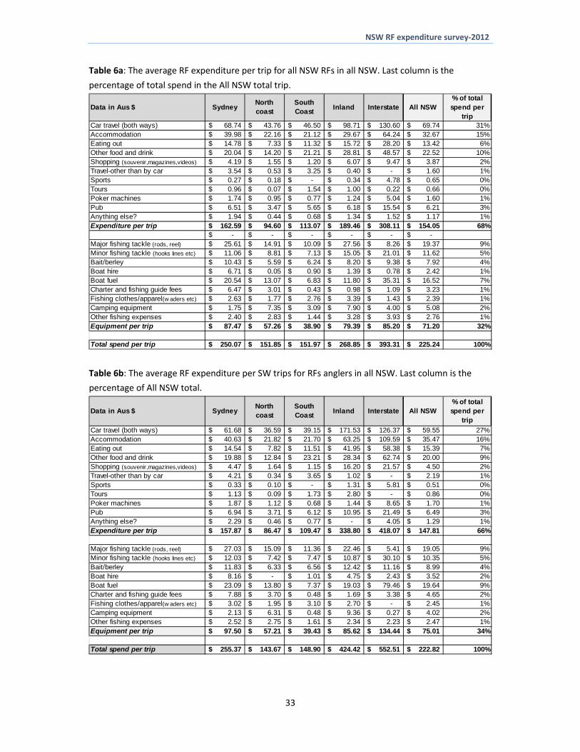
NSW RF expenditure survey‐2012
Table 6c The average RF expenditure per FW trip for RFs anglers in all NSW Last column is the
percentage of All NSW total
Data in Aus $ Sydney North coast
South Coast
Inland Interstate All NSW of total spend per
trip
Car travel (both ways) 10144 $ $ 7498 $ 10533 7358 $ 13261 $ 9079 $ 39 Accommodation 3696 $ $ 2363 $ 1654 1808 $ 4272 $ 2689 $ 12 Eating out 1591 $ $ 517 $ 981 667 $ 1388 $ 937 $ 4 Other food and drink 2077 $ $ 2014 $ 519 2897 $ 4185 $ 2771 $ 12 Shopping (souvenirmagazinesvideos) 287 $ $ 118 $ 154 258 $ 389 $ 258 $ 1 Travel-other than by car 039 $ $ 138 $ - 018 $ -$ 040 $ 0 Sports -$ $ 053 $ - -$ 429 $ 093 $ 0 Tours 015 $ $ - $ - 038 $ 032 $ 025 $ 0 Poker machines 115 $ $ 020 $ 154 117 $ 333 $ 141 $ 1 Pub 454 $ $ 245 $ 192 454 $ 1272 $ 565 $ 2 Anything else 031 $ $ 033 $ - 180 $ 032 $ 094 $ 0 Expenditure per trip 18448 $ $ 13000 $ 14187 13794 $ 25595 $ 16691 $ 72
Major fishing tackle (rods reel) 1903 $ $ 1414 $ - 2933 $ 962 $ 2002 $ 9 Minor fishing tackle (hooks lines etc) 658 $ $ 1482 $ 442 1649 $ 1669 $ 1423 $ 6 Baitberley 398 $ $ 238 $ 369 674 $ 853 $ 572 $ 2 Boat hire -$ $ 026 $ - 023 $ -$ 015 $ 0 Boat fuel 877 $ $ 988 $ 250 930 $ 1437 $ 1009 $ 4 Charter and fishing guide fees -$ $ - $ - 073 $ -$ 031 $ 0 Fishing clothesapparel(w aders etc) 085 $ $ 097 $ - 363 $ 212 $ 227 $ 1 Camping equipment -$ $ 1184 $ 2392 739 $ 577 $ 726 $ 3 Other fishing expenses 184 $ $ 319 $ 008 360 $ 474 $ 335 $ 1 Equipment per trip 4105 $ $ 5749 $ 3462 7724 $ 6184 $ 6332 $ 28
Total spend per trip 22553 $ $ 18749 $ 17648 21518 $ 31779 $ 23024 $ 100
Table 6d The average RF expenditure per annum on larger boat items for SW and FW anglers in
regions and all NSW (nb Table 6abc are per trip and Table 6d is per angler per annum)
Data in Aus $ Sydney North coast
South Coast
Inland Interstate All NSW of total spend per
trip
All NSW Boat licenceregistration 7115 $ $ 4658 $ 4407 5815 $ 8546 $ 5940 $ 8 Boat maintenance 29248 $ $ 14497 $ 9655 7935 $ 17917 $ 17504 $ 23 Boat insurance 7519 $ $ 4574 $ 3006 4145 $ 10318 $ 5754 $ 7 Marine mooring fees 7615 $ $ 1940 $ 192 122 $ 2609 $ 3179 $ 4 Boat equipment (safety etc) 15175 $ $ 7637 $ 3175 5452 $ 6015 $ 8888 $ 12 Boat purchase or motor repair 23437 $ $ 25676 $ 25865 9740 $ - 35550 $ 46 Annual boat expenditure 90109 $ $ 58982 $ 46300 33208 $ 45405 $ 76815 $ 100
Saltwater -$ $ - $ - -$ -$ -$ Boat licenceregistration 7340 $ $ 4751 $ 3583 6003 $ 13372 $ 6014 $ 6 Boat maintenance 32221 $ $ 15880 $ 9805 5356 $ 28392 $ 20829 $ 22 Boat insurance 8032 $ $ 5068 $ 3002 3960 $ 19824 $ 6458 $ 7 Marine mooring fees 8765 $ $ 2385 $ 216 030 $ 8108 $ 4505 $ 5 Boat equipment (safety etc) 17407 $ $ 7800 $ 3428 7508 $ 9230 $ 10764 $ 11 Boat purchase or motor repair 30450 $ $ 35250 $ 30000 40600 $ - 47050 $ 49 Annual boat expenditure $ 104214 $ 71134 $ 50035 63456 $ 78926 $ 95618 $ 100
Freshwater Boat licenceregistration 6073 $ $ 4255 $ 11000 5750 $ 6256 $ 5787 $ 16 Boat maintenance 15523 $ $ 8474 $ 8454 8830 $ 12949 $ 10632 $ 29 Boat insurance 5154 $ $ 2421 $ 3038 4209 $ 5809 $ 4297 $ 12 Marine mooring fees 2308 $ $ - $ - 155 $ -$ 439 $ 1 Boat equipment (safety etc) 4877 $ $ 6930 $ 1154 4738 $ 4490 $ 5011 $ 14 Boat purchase or motor repair 5000 $ $ 3150 $ 18400 5350 $ - 10350 $ 28 Annual boat expenditure 38935 $ $ 25230 $ 42046 29032 $ 29504 $ 36515 $ 100
34
NSW RF expenditure survey‐2012
In Table 6a the higher travel costs of some regional residents such as Sydney anglers Inland and
interstate fishers were evident The trip expenditure of Inland and interstate SW anglers was
significantly higher than for resident NSW anglers due to car travel accommodation food and other
trip expenses presumably to the coast (Table 6b) Table 6c shows that FW expenditure per trip was
highest for interstate fishers (eg Victorians traveling to southern NSW) and Sydney and South Coast
RFs had high travel costs travelling to desirable FW fishing locations (eg Snowy mountains etc
Dominion 2001 and 2002)
The socio‐economics of recreational fisher expenditure in NSW
The survey samples were analysed to identify some of the socio‐economic drivers of RF expenditure
in NSW The samples combined to give 1235 observations of RF expenditure and the survey
included a range of other variables Both multiple regression analysis and a cluster analysis enables
the statistically significant variables determining angler expenditure to be identified and estimated
as reported in Appendices 1 and 2 respectively
Multiple regression results
In Appendix 1 results reveal that Total recreational fishing expenditure is driven by licence status
(licence holders spending more) number of SW trips per annum and the level of household income
Age sex and regional location were found not to be statistically significant in determining total RF
expenditure
Trip expenditure was driven by licence holders and number of SW trips Trip expenditure was further
examined and was significantly influenced by licence holders SW and FW days fished and the
distance travelled on the last trip Fishing Tackle expenditure was found to be determined by
income rather than number of trips Expenditure on boats was driven by both number of SW trips
and the level of RF household income
Cluster analysis results
The expenditure of NSW RFs was also subjected to ldquocluster analysisrdquo to see the significant socio‐
economic characteristics of fisher groups as reported in Appendix 2and in Figure 3 below The cluster
analyses for expenditure on fishing trips tackle and boat expenditure are reported in Appendix 2
35
NSW RF expenditure survey‐2012
Figure 3 A cluster analysis of RF total expenditure showing the groups of significantly different
clusters of anglers identified
In Figure 3 there are four significantly different cluster groups The characteristics of the four groups
are under the ldquodescriptionrdquo row and the authors have put a label to characterise each group
Between Figure 3 and Appendix 2 the overall picture is of groups of ldquoordinaryrdquo fishers
(approximately 85) with low levels of fishing activity in which household income levels may differ
(half lower half higher) secondly a group of dedicated anglers (approximately 12) who have high
fishing activity and expenditure and finally a highly avid fishing group (less than 3) with very high
fishing activity and high to very high expenditure
The results confirm the only previous examination of the socio‐economic characteristics of RFs in
NSW by Dominion (2003) which showed that recreational fishing is a past time involving a diverse
range of people has great variety in activity levels and crosses the entire socio‐economic spectrum
36
NSW RF expenditure survey‐2012
4 State‐wide and regional expenditure estimates
41 Estimating total expenditure
This chapter describes the estimation of the total recreational fishing expenditure for RFs in NSW
and in its regions Total recreational fishing expenditure is the product of three variables
a) Number of recreational fishers or RF households (HH)
We use three approaches to estimate the total RF population in NSW by use of
1) Random telephone survey and ABS Household data and population data
2) The RFL data base and
3) Use of the screening sample and the ABS data on Households Use of the screening
survey of the general population to estimate total number of fishers11 via ABS
population data
b) Fishing trip activity fishing trip activity estimates are obtained from the telephone survey
and
c) Recreational fishing expenditure information on the expenditure per trip and annual
expenditures on equipment is obtained from the telephone survey
The product of these variables will enable us to estimate the total state‐wide recreational fishing
expenditure Expenditure is also estimated for each state region considered Saltwater and
freshwater fishing are considered separately in the state estimates through asking respondents
about the trip intention
42 Expanding the sample of fishers and expenditure
Total expenditure estimates are based on travel and fishing equipment expenses per trip and
estimates of expenditure on boat capital items These are summed to give an annual total
expenditure estimate However the estimates for the angler survey need to be expanded to give
state wide estimates These expansions are described in Box 1 below
Box 1 Explanation of key expansions
The expansion method adapts the method used in the National Survey (Henry and Lyle 2003) The
number of fisher households (FHH) was estimated as follows for each region
No of fisher Household (est) = No Households in Population (ABS) No of Fisher HH (sample)
No of HH (sample)
Example How many recreational fishers would these households include
No of Fishers 19 to 75 yrs (est) = Mean No fishers per HH (sample) No of fisher Household (est)
776496 = 202 383921 (see Table 7)
RF HH are distributed proportionally across regions by household and recreational fishers by
regional population
11 Recreational Fishers under 19 years of age are not included and need to be added if the total population figure is for all
anglers The activity and expenditure estimates are based on ages 19‐75 only
37
NSW RF expenditure survey‐2012
Information on NSW State and Regional Households by Local Government Area (LGA) were accessed
(ABS 2011) The data were aggregated by the larger SD ABS regions (eg Sydney North coast
Inland and SDD South Coast area) These identified the number of households in each of the study
regions as reported in Table 7
Table 7 The ldquototal householdsrdquo in each of the NSW study regions based on LGA data ABS (2011)
Households with recreational fishers are estimated for each study region
Area Population 2010 (gt18-75)
Households HH with RF Rec Fishers HH
RF by region
Sydney 3160897 1376583 213934 230 491232
North coast 835229 570688 88690 146 129802
South coast 350750 207195 32200 169 54510
Inland 649564 315987 49107 206 100948
Total 4996461 2470453 383931 202 776496
The RF household responses for anglersrsquo trip frequency and trip expenditure were multiplied to
produce estimates of state‐wide and regional expenditure
43 State‐wide expenditure estimates
The estimation of total expenditure for samples of recreational anglers and its expansion to regional
state‐wide and national estimates has depended on traditional statistical methods estimating the
total from means of the component distributions However while the number of households is
reasonably well estimated the frequency distribution of fishing trips is highly skewed to the left (see
Figure 1a)
The estimates of total state expenditure on recreational fishing involve multiplying the following
variables
1) Estimate of RF households ‐ the ABS has reliable estimates of households for which RF
households can be identified
2) Estimate of trips ‐ anglers state the number of trips per annum and
3) Estimate of the trip and tackle expenditure on their last trip and their capital expenditure in
the last year
Total expenditure is the product of these variables Total expenditure can be estimated as a mean
value with confidence intervals Here we used the 1237 observations in the RF sample weighting
the results in respect of regional populations as follows
a) Total annual expenditure per angler household = (($ travel expenses per trip + $ tackle
expenses per trip) number of trips )+ (annual capital expenditure per angler household)
b) Total annual expenditure in NSW = total number of anglers households total annual
expenditure per angler household
This traditional approach gives a point estimate but does not provide any information on the
probability of different expenditure levels around the mean This requires a simulation approach
38
NSW RF expenditure survey‐2012
Table 8a shows that the estimated expenditure by all NSW resident RFs in 2012 was $1439bn12 with
an additional $1861m being spent by interstate fishers making a total estimated expenditure by
recreational fishers in NSW of $1625bn in the year 2012
Considering regional expenditures total recreational fishing expenditure was highest by Sydney
anglers ‐ $903m (56 of all expenditure in NSW) followed by the North coast anglers ‐ $3008m
(19) and inter‐state anglers ‐ $ 186m (11) Total expenditure for South Coast anglers was
$1018m (6) and for Inland anglers $1308m (8)13
Expenditure on fishing trips was $793m or 49 of all recreational fishing expenditure in NSW Of
this $402m (25) was spent on fishing equipment tackle and fuel and $430m (26) was spent on
annual capital expenditures such as boats and maintenance Expenditure on SW fishing was
estimated at $1415m (87) and on FW fishing at $231m (13 of total recreational fishing
expenditure in NSW)
Table 8b shows the costs within each category
Within trip expenditure (49 of total expenditure) car travel $326m (201 of total annual
expenditure) accommodation $1859m (114) and food and eating out $188m (115)
Expenditure on fishing equipment and expenses $4025m (246) was made up of $1645m
(102) on major and minor tackle and $1027m (63) on boat fuel and
Annual boat expenditure $4305m (26) of which $1225m (75) was maintenance and
boat purchase or motor repair $1436m (88)
12 This estimate is the same as the mean value produced by the simulation shown later in this chapter It is then adjusted
for Interstate expenditure13 In Chapter 5 the regional economic analysis adapts these data to reflect the expenditure made in other regions away from home residence
39
NSW RF expenditure survey‐2012
Table 8a Estimates of the total RF expenditure for different areas of NSW and including interstate angler expenditure to give all RF expenditure in NSW
Expenditure category Sydney North coast South coast Inland All NSW Inter-state Total expend
in NSW
total expend in NSW
Trip spend 383906879 136686958 57862828 74849484 653306149 139478487 792784637 49 $ fishing equip 222891110 85965049 20624384 31116970 360597513 41975664 402573177 25 Total annual boat expenditure 296326795 81222395 23393975 24877516 425820681 4691465 430512146 26 Totals 903124785 303874402 101881187 130843970 1439724343 186145616 1625869959 100 of total expend in NSW 56 19 6 8 89 11 100 Saltwater 840749912 267431019 99200573 51715617 1259097121 140675487 1415280961 87 Freshwater 62374873 36443383 2680614 79128353 180627222 45469052 231775451 14 SW expenditure as of Total 93 88 97 40 87 84 87
40
NSW RF expenditure survey‐2012
Table 8b Estimates of the total RF expenditure for different areas of NSW and including interstate angler expenditure to give all RF expenditure in NSW
Data in Aus $ Sydney North coast South coast Inland All NSW Interstate Total expend
in NSW
of Total expend in
NSW Expenditure category Car travel (both ways) 155752824 61047851 21250669 38966591 277017934 49755399 326773333 201 Accommodation 96655736 32991275 11321758 11775540 152744309 33155541 185899850 114 Eating out 35118007 11287702 6019080 6283701 58708491 16433282 75141772 46 Other food and drink 47830881 20416270 11974310 11255861 91477322 21385714 112863036 69 Shopping (souvenirmagazinesvideos) 10396840 2377682 609238 2427428 15811187 5900718 21711905 13 Travel-other than by car 9328498 675596 1876003 157968 12038065 - 12038065 07 Sports 730303 214569 - 136952 1081824 2038576 3120401 02 Tours 2517279 121080 888633 400483 3927475 44318 3971793 02 Poker machines 4337423 1534429 364864 485304 6722021 2611177 9333198 06 Pub 16147653 5352108 3163325 2442584 27105670 7101506 34207176 21 Anything else 5091436 668396 394948 517073 6671852 1052256 7724108 05 Trip spend 383906879 136686958 57862828 74849484 653306149 139478487 792784637 488
Major fishing tackle (rods reel) 63209459 22456502 5830420 10743744 102240126 2673467 104913593 65 Minor fishing tackle (hooks lines etc) 27752247 12319663 3884279 5859337 49815525 9792034 59607560 37 Baitberley 26800952 8839913 3407290 3225829 42273984 3954942 46228926 28 Boat hire 17933756 42708 518369 561815 19056649 604762 19661412 12 Boat fuel 52493364 20044184 3811422 4649308 80998277 21742806 102741083 63 Charter and fishing guide fees 17310929 4944101 246843 386149 22888022 839948 23727969 15 Fishing clothesapparel(w aders etc) 6799431 2766227 1592134 1322337 12480129 292501 12772630 08 Camping equipment 4689522 10357115 508333 3093322 18648291 864926 19513218 12 Other fishing expenses 5901451 4194635 825295 1275129 12196509 1210277 13406786 08 $ fishing equip 222891110 85965049 20624384 31116970 360597513 41975664 402573177 248
Boat licenceregistration 22369127 6037457 1817922 4154611 34379117 4691465 39070582 24 Boat maintenance 93188042 18809323 4588346 5925940 122511651 - 122511651 75 Boat insurance 23806199 5935399 1413005 2990204 34144806 - 34144806 21 Marine mooring fees 24487619 2521793 97904 96275 27203591 - 27203591 17 Boat equipment (safety etc) 48762545 9898735 1571861 3725061 63958201 - 63958201 39 Boat purchase or motor repair 83713264 38019687 13904937 7985426 143623314 - 143623314 88 Total annual boat expenditure 296326795 81222395 23393975 24877516 425820681 4691465 430512146 265
Totals 903124785 303874402 101881187 130843970 1439724343 186145616 1625869959 1000 Saltwater 840749912 267431019 99200573 51715617 1259097121 140675487 1399772608 861 Freshwater 62374873 36443383 2680614 79128353 180627222 45469052 226096274 139 SW expenditure as of Total 93 88 97 40 87 76 86 Region as of total expenditure 56 19 6 8 11 100
41
NSW RF expenditure survey‐2012
44 A probabilistic simulation approach to the estimation of total state recreational fishing
expenditure
Simulation enabled us to estimate the probability of different outcomes from the existing data The
original sample was weighted by numbers of regional households to account for the under sampling of
Sydney and the over sampling of the North Coast in the original survey data The sample was analysed
using the SPSS v21 Monte Carlo Simulation model (IBM Corp 2012) This routine produced up to
100000 repeat runs of the predicted values of total RF state expenditure to give the probability of
different expenditure totals as shown in Figure 5a The cumulative probability is shown in Figure 5b
Figure 5a The probability of total expenditure by NSW anglers 2012
These initial probability estimates showed that the mean total state‐wide expenditure was $1473m
with 5 and 95 confidence estimates of $706m and $2952m The median value as $1196m reflecting
the skewedness of the distribution
The estimate of expenditure in NSW by interstate anglers of $1861m has also to be added The final
total NSW estimate of expenditure on recreational fishing was therefore $1625m with 5 and 95
confidence estimates of $892m‐$3136m14
14 For simplicity this assumes the distribution of the interstate results are the same as all NSW
42
NSW RF expenditure survey‐2012
Figure 5b The cumulative probability of total expenditure by NSW anglers 2012
Figure 5a and 5b indicate how the skewed distribution of trips per year by anglers and the highly annual
variable expenditure make the predicted adjusted distribution from $892m‐$3136m around an
adjusted mean $1625m and an adjusted median of $1382m The mean has a 0045 probability of being
achieved whereas lower total expenditure estimates have higher probability (Figure 5a) The
skewedness gives a threshold minimum expenditure level and a ldquotrailing tailrdquo on the right hand side
reflecting less probable high expenditure estimates
Figure 5b indicates that the mean would have a cumulative probability of 65 This shows the higher
total expenditure estimates on the right hand side of Figure 5a are pulling the mean to the right This is
why we have to be careful in RF sampling and estimation of recreational activity and expenditure This
also may explain why fishers of differing avidity and expenditure levels have considerably different
opinions on total expenditure in the sector A fisher with higher activity and expenditure would estimate
a state wide total at the right hand side of Figure 5a but while high total expenditure is possible it is
highly improbable
45 Discussion The estimated total expenditures reported in Table 8a and 8b indicate a statewide expenditure by NSW
recreational fishers and interstate anglers on items directly related to fishing of $1625m
43
NSW RF expenditure survey‐2012
The expansions to develop the final estimates took account of the differences between SW and FW
expenditure and activity and each was expanded separately Expenditure on FW fishing contributed 14
of total expenditure considerably less than the 28 of days fished reported in the sample (Table 5)
reflecting some trip and capital expenditure differences between SW and FW fishers
By region the results indicate that recreational fishing expenditure by Sydney anglers $9031m (56 of
total state recreational fishing expenditure) while North coast has $3038m (9) Interstate anglers
$1861 (11) Inland $1308m (8) and South coast $1018 (6) The survey method estimated regional
expenditures from interviews with fishers in their home region The regional economic impacts adjusts
these and produced estimates of recreational fishing expenditure and its economic impacts across all of
NSW and its main regions
There is just the previous national survey study for comparison of results The 2012 expenditure
estimate adjusted from the Campbell and Murphy (2005) national survey 2001 study is $765m This is
within the confidence intervals predicted by the current studyrsquos simulation approach
Another comparison is to deduct the trip expenditures for food and entertainment from the current
studyrsquos results to be comparable to Campbell and Murphyrsquos assumptions giving an estimate up to
$136bn15 The difference in expenditure estimates16 is primarily related to the survey methods used and
the different estimates of fishery activity the current study being higher Though the number of adults
fishing may have reduced since 2001 NSW has now a sizeable established recreational fishing licence
holder population and expenditures per angler are higher than a decade ago
Under the telephone survey interview and recall method used the current results were conservative for
this methodological approach This study has pointed to the highly skewed nature of the trip activity
among the RF population and the highly variable levels of expenditure among recreational fishers in
NSW The use of a probabilistic simulation in this study has illustrated the difficulties in estimation of
total RF expenditure and the wide distribution around the mean The adequate inclusion and possible
over‐inclusion of avid fishers are sampling problems under any of existing methodologies
The sample size and hence a higher survey cost is part of the remedy Further examination of the US
multi‐method approach may be merited (Gentner 2009) though this is a large scale national expensive
survey exercise The project results in this study are proposed as being reasonable under the
methodologies available within funding constraints and are part of a proposed ongoing expenditure
survey strategy in NSW as outlined in Chapter 6
15 There may also be differences in the treatment of capital attributable to RF definitions of maintenance and capital expenditure on motors and boats and other differences between the two studies These may likely lower this estimate 16 ($1360m‐$765m=$595m in 2012 terms)
44
NSW RF expenditure survey‐2012
5 Regional economic impact estimates This chapter of the report was compiled by Western Research Institute (WRI) WRI received the output
of this survey in terms of expenditure of respondents and based on this output modelled the
economic impacts of recreational fishing on the NSW economy and defined sub‐regions Input‐
output modelling has been employed to derive the relevant economic models and the impacts
51 Methodology
The methodology used to prepare this report included
Determination of the boundaries of the regions to be used in table construction
In consultation with the ANCORS the decision was made to construct input‐output tables for the NSW
North Coast NSW South Coast NSW Inland and Sydney regions as well as NSW as a whole Each region
was defined by aggregating statistical areas at level 4 3 or 2 or combination thereof This allowed the
formulation of regions and economies that best represented the regions of interest Specifically data
from statistical areas at level 3 of ABS Statistical Geography Standard (rather than at larger statistical
areas at level 4) was used in the construction of tables for the NSW North Coast and data from
statistical areas at level 2 was used in the construction of tables for the NSW South Coast The table
construction for Sydney region was based on the data from statistical areas at level 4 while tables for
NSW Inland region was based on the data from statistical areas at different levels (2 3 and 4) Detailed
information on statistical areas in provided in WRI (2013)
Construction of tables
The input‐output tables developed for this project were derived from the latest national table produced
by the Australian Bureau of Statistics (ABS) That table provides a detailed picture of the structure of the
economy of Australia for the year 2008‐09 A series of steps were undertaken to update the table to
2011‐12 Further information from the State Accounts (ABS Cat No 52200) labour force data from the
2011 Census and the quarterly labour force survey (ABS Cat No 6291055003) were used to develop a
state table for New South Wales at 2011‐2012 This was then regionalised to reflect the respective
regional economies of NSW North Coast NSW South Coast NSW Inland and Sydney Further details of
the procedures used in the development of a regional input‐output table are provided in WRI (2013)
52 Economic impact analysis
The economic impacts were modelled as a final demand impact (that calculates the impacts measured
by output value added household income and employment across all sectors in response to changes
in industry final demands) using the 2011‐12 Simulating Impacts on Regional Economies (SIRE) input‐
output model of NSW North Coast NSW South Coast NSW Inland Sydney and NSW as a whole The
SIRE model is superior to standard input‐output models as it provides for non‐linear relationships
between variables and is based on empirically derived (rather than assumed) coefficients In terms of
45
NSW RF expenditure survey‐2012
robustness of results it is comparable with computable general equilibrium (CGE) models whilst
minimising data requirements See WRI (2013) for a detailed description of the SIRE input‐output
model
The impacts of recreational fishing expenditure on the NSW North Coast NSW South Coast
NSW Inland and Sydney regions as well as NSW as a whole have been provided in terms of
bull Output which is the value of goods and services that are produced within an establishment
that become available for use outside that establishment plus any goods and services
produced for the organisationrsquos own final use Output is equal to total revenue plus any
internal consumption
bull Value added which is equal to gross output minus intermediate inputs Value added is
equivalent to the contribution to gross regional product (the local equivalent of gross
domestic product)
bull Household Income which measures the benefit received by regional households from
economic activity It typically refers to compensation of employees but can also include
income in return for other forms of productive activity
bull Employment which refers to full‐time equivalent (FTE) employment is a measure of the
total level of staff resources used The FTE of a full‐time staff member is equal to 10 The
FTE of a part‐time worker will be a fraction of this depending on the relative number of
hours worked
53 The Economic Impact of Recreational Fishing on the Regional Economies of NSW
The economic impact due to recreational fishing was modelled as follows
bull The expenditure survey conducted by ANCORS did not capture the location of expenditure
just the origin (postcode) of the respondent Therefore in the absence of location data an
assumption was made that the total expenditure by interstate visitors ($18614 million)
who make expenditures on recreational fishing whilst staying in NSW should be distributed
evenly across four NSW regions (ie 25 of total interstate expenditure pertaining to each
NSW region)
bull Likewise it was assumed that expenditure pertaining to the NSW North Coast NSW
South Coast and NSW Inland regions was made in these regions (eg those
respondents who indicated living in the NSW North Coast partake in recreational
fishing in the NSW North Coast and not in other areas thereby ensuring that the
money spent on recreational fishing remains in the NSW North Coast region)
46
NSW RF expenditure survey‐2012
bull For those respondents who indicated living in Sydney an assumption was made that 515
of them partake in fishing in Sydney with the remaining 485 fishing in the rest of NSW in
the following proportions NSW North Coast ndash 346 NSW South Coast ndash 485 and NSW
Inland ndash 169 (Dominion 2002 and 2004)
bull Since anglers in each of the regions make expenditure on items that may not be
produced in the region but that are imported from the rest of NSW the regional
recreational fishing expenditure was split into local and imported components using a
location quotients matrix This way WRI ensured that only local expenditure generated
economic impacts in the respective region For NSW as a whole an assumption was
made that all products that anglers purchase are produced within the state and
therefore no separation of local and imported components was performed The
economic impacts of recreational fishing on NSW were modelled using total recreational
fishing expenditure in NSW
bull In order to ensure consistency of the input‐output modelling procedure the expenditure
data was allocated in the input‐ output table to the industries (typically manufacturing
industries) where the relevant expenditure items were produced and was then
converted to basic prices See WRI (2013) for further details on sectoral allocations
bull A final demand analysis in SIRE was performed and economic impacts on NSW North Coast
NSW South Coast NSW Inland and Sydney as well as NSW as a whole were derived
The impacts of recreational fishing on the economies of the NSW North Coast NSW South Coast
NSW Inland and Sydney regions are outlined in the Table 9
Table 9 Regional expenditure and economic impacts on regional economies
Region North Coast Sydney South Coast Inland
Expenditure by postcode ($m) 30387 90312 10188 13084
Reclassified expenditure ($m) 50196 51165 36086 2514
Output ($m) 73465 100286 39522 35381
Value added ($m) 35355 49156 18417 14985
Household income ($m) 16875 28888 876 735
Employment (no) 3320 3944 1808 1539
47
NSW RF expenditure survey‐2012
NSW North Coast
Overall when flow‐on effects are taken into account recreational fishing contributes the following to
the economy of NSW North Coast
bull 3320 FTE jobs including 667 in the retail trade sector 573 in the hospitality sector
349 in the personal and other services sector and 174 in the transport and storage
sector
bull $16875 million in household income with 134 percent being in the retail trade
sector 112 percent being in the hospitality sector 76 percent being in the public
administration sector 72 percent being in the personal and other services sector and
57 percent being in the transport and storage sector
bull $35355 million in industry value added representing 081 percent of total regional
value added of the NSW North Coast region and
bull $73465 million in output
For the North Coast recreational fishing will contribute 098 percent of FTE employment in the
region when flow‐on effects are taken into account as well as 084 percent of household income and
07 percent of the estimated gross regional product of the NSW North Coast region
NSW South Coast
Overall when flow‐on effects are taken into account the recreational fishing contributes the
following to the economy of NSW South Coast
bull 1808 FTE jobs including 420 in the hospitality sector 284 in the retail trade sector
236 in the personal and other services sector 117 in the transport and storage
sector and 106 in the public administration sector
bull $8760 million in household income with 152 percent being in the hospitality sector
109 percent being in the retail trade sector 93 percent being in the public
administration sector 86 percent being in the personal and other services sector and 77
percent being in the transport and storage sector
bull $18416 million in industry value added representing 167 percent of total regional
value added of the NSW South Coast region and
bull $39522 million in output
For the South Coast recreational fishing will contribute 212 percent of FTE employment in the region
when flow‐on effects are taken into account as well as 173 percent of household income and 143
percent of the estimated gross regional product of the NSW South Coast region
48
NSW RF expenditure survey‐2012
NSW Inland
Overall when flow‐on effects are taken into account the recreational fishing contributes the
following to the economy of NSW Inland
bull 1539 FTE jobs including 289 in the hospitality sector 288 in the retail trade sector
148 in the personal and other services sector and 138 in the agriculture sector
bull $7350 million in household income with 134 percent being in the retail trade
sector 131 percent being in the hospitality sector 74 percent being in the
personal and other services sector 70 percent being in the public administration
sector and 68 percent being in the transport and storage sector
bull $14985 million in industry value added representing 030 percent of total regional
value added of the NSW Inland region and
bull $35381 million in output
Recreational fishing will contribute 038 percent of FTE employment in the NSW Inland region when
flow‐on effects are taken into account as well as 032 percent of household income and 026 percent
of the estimated gross regional product of the NSWInlandregion
Sydney
Overall when flow‐on effects are taken into account the recreational fishing contributes the following
to the economy of Sydney
bull 3944 FTE jobs including 741 in the retail trade sector 450 in the hospitality sector
366 in the personal and other services sector and 310 in the professional and
technical services sector
bull $28888 million in household income with 162 percent being in the finance and insurance
sector 113 percent being in the retail trade sector 83 percent being in the professional
and technical services sector 77 percent being in the wholesale trade sector and 63
percent being in the hospitality sector
bull $49156 million in industry value added representing 025 percent of the total regional
value added of Sydney and
bull $100286 million in output
For the Sydney region recreational fishing will contribute 028 percent of FTE employment when flow‐on
effects are taken into account as well as 025 percent of household income and 022 percent of the
estimated gross regional product of Sydney
49
NSW RF expenditure survey‐2012
NSW State economy
The impacts of recreational fishing on the state economy of the NSW are outlined in the Table 10
Table 10 NSW expenditure and economic impacts on NSW
Item Estimate
NSW Expenditure by postcode ($m) 143972
Total interstate expenditure ($ m) 18615
NSW Reclassified expenditure ($m) 162587
Output ($m) 342035
Value added ($m) 162561
Household income ($m) 87728
Employment (thousand) 14254
NSW Economy
Overall when flow‐on effects are taken into account the recreational fishing contributes the following to
the economy of NSW
bull 14254 FTE jobs including 2730 in the retail trade sector 2123 in the hospitality
sector 1389 in the personal and other services sector and 951 in the transport and
storage sector
bull $87728 million in household income with 122 percent being in the retail trade 114
percent being in the finance and insurance sector 88 percent being in the hospitality
sector 72 percent being in the professional and technical services sector and 65
percent being in the wholesale trade sector
bull $162561 million in industry value added representing 036 percent of the estimated gross
state product of the NSW and
bull $342035 million in output
50
NSW RF expenditure survey‐2012
Overall recreational fishing will contribute 046 percent of FTE employment in the NSW when flow‐on
effects are taken into account as well as 041 percent of household income and 040 percent of total
regional value added
54 Conclusion
The recreational fishing expenditure and economic impact of recreational fishing on NSW and
respective regions were substantial in absolute terms but uneven across regions
The expenditure based on place of residence was the highest in Sydney followed by NSW North
Coast NSW Inland and NSW South Coast The reallocated expenditure (ie actual expenditure
made in the region) was still the highest in Sydney (but substantially lower than postcode
expenditure) followed by expenditure in NSW North Coast NSW South Coast and NSW Inland
In terms of output valued added household income and FTE employment the absolute economic
impacts of recreational fishing were the highest in Sydney followed by NSW North Coast NSW South
Coast and NSW Inland However in relative terms economic impacts (as percentage of total in the
respective regions) were the highest in NSW South Coast (167‐ 212) followed by NSW North
Coast (081‐098) NSW Inland (030‐038) and Sydney (025‐028) These relative disparities
reflect the large size of Sydney and NSW Inland economies and smaller size of NSW North Coast and
NSW South Coast economies
51
NSW RF expenditure survey‐2012
6 Developing a cost effective approach to expenditure surveys
There have been several reoccurring issues in obtaining information on recreational fishing expenditure
in NSW The first is the lack of a series of expenditure surveys the past ones not occurring as part of an
on‐going consistent strategy The second issue is the lack of a known survey method which is repeatable
and can be compared with past surveys In both of these issues the recurrent cost of such surveys has
been unknown also
61 The objectives of an recreational fishing expenditure survey
Any survey is designed towards its objectives In developing a cost effective regular approach to
recreational fishing expenditure surveys there has to be some design decisions made in respect of the
information required For example A state‐wide expenditure estimate may be required every two years
to track and promote the value of the sector This could include a state‐wide estimate of regional
economic impact Further disaggregation by area or other variables will increase cost
62 Sampling data issues and findings
This study has considered how the use of the RFL database reduced the cost of expenditure surveys
which have traditionally used expensive random screening surveys to locate recreational fishers
Finding 1 The current study has found that there is no statistically significant difference between
seasonal samples Consequently we recommend an annual survey event being mindful of its timing
relative to Christmas January and Easter which may be periods when fishers are not at home
The RFs identified through a random screening survey process were found to make more fishing trips
and fish more days than the sample of RFs contacted through the RFL database (noting that both
samples include licence holders) However in further comparisons of days fished per angler between
licenced and unlicensed fishers no significant difference was found On the other hand unlicensed
fishers were found to undertake significantly more fishing trips than licence holders though this relates
to trip events and not necessarily to higher average expenditure ndash in other words unlicensed fishers
may make more but shorter trips to nearby destinations compared with licensed fishers
Finding 2 The RFL database can be used to sample anglers for expenditure surveys providing certain
conditions are met in terms of the different numbers of licences holders that are sampled17
63 What sample size is required
The size of a sample in statistics is important If the sample is too small there is then the risk that the null
hypothesis is wrongly rejected (ATS 2010) The size of a sample is also related to the probability level at
17 A ratio of 3 day 1 month 1 year and 3 year licence holder records is recommended The weighting would be easier for the annual and 3 year licence holders as 3 day and monthly licence holder can be repeat licence purchasers in a given year
52
NSW RF expenditure survey‐2012
which the variable is seen to be significantly different from zero eg 95 (5) or 99 (1) levels of
significance The dispersion of the distribution of the variable being examined is also important and this
is captured in the standard error of the variable
In statistics these issues are brought together in statistical ldquopower analysisrdquo where the minimum size of
a sample can be tested both prior to and even after statistical surveys to see if the sample size is
adequate ldquoThe power is the probability of detecting an effect presuming it is actually thererdquo (ATS 2010)
Sample size estimation
In this section of the report we investigate how reducing the sample size to the minimum required
number of interviews can reduce the cost of an expenditure survey The decision regarding the target
sample size for the survey has to be balanced between the levels of significance chosen for testing (1
5) and the standard error that is acceptable for the intended variables which is often related to the
estimated value called the relative standard error (RSE) 18
Table 11 shows a range of sample sizes derived for different scenarios using the ABS calculator facility at
NSS (2013) There are the two scenarios for random surveys (cases 1‐4) and two for surveys from a
population base of known participants (case 5‐6)
Table 11 Indication of the required sample sizes under different sampling and risk scenarios including
sampling of the RFL database
Case number 1 2 3 4 5 6 Sample type Random sampling Non random
Statistical input All NSW Population
All NSW Population
All NSW Population
South coast
RFL ‐1 RFL‐2
Confidence Level 99 95 95 95 95 95 Population Size 4996500 4996500 4996500 350750 480700 480700 Proportion 05 05 015 025 06 06 Confidence Interval 005 005 00294 005 005 005
Upper 055 055 01794 03 065 065 Lower 045 045 01206 02 055 055
Standard Error 0025 0025 0015 0025 003 0045 Relative Standard Error () 50 50 100 100 50 75 Sample Size 339 196 567 300 267 119
18 The RSE is the standard error expressed as a percentage of the estimate
53
NSW RF expenditure survey‐2012
In Table 11 cases 1 and 2 show the general sampling results when the confidence level is either 99 or
95 and the proportion is 05 (ie where ldquothe expected proportion of the population to have the
attribute that you are estimating from your surveyrdquo (NSS 2013) These data are often quoted but given
that RFs are more difficult to locate than a one in two assumption (proportion 05) case 3 assumes a
15 proportion for RFs and requires a sample size of 567 with a relative standard error (RSE) of 10
Reducing the sampling area to the South Coast (case 4) raises the chances of locating RFs (proportion
025) and would require 300 observations at an RSE of 10 The sampling model assumes a random
population
We also apply the model to the non‐random scenarios from the RFL data base Here cases 5 and 6 are
RFL records and hence not as random as the whole NSW population We use the model to estimate
possible minimum sample sizes when using the RFL data base population Assuming that the proportion
is 06 an RSE of 5 requires a sample of 267 and an RSE of 75 a sample size of 119 In the experience
of the authors the last sample size (119) is low given the variation in our results We recommend no less
than 250 completed surveys as a minimum sample size for state‐wide estimates If four NSW regions are
included a minimum total of 500 completed surveys would be required and be should be larger if
possible
The review of samples has shown that there is a trade off in accuracy of estimates with the number of
interviews undertaken For example in the case 3 random survey in Table 11 the RSE is 10 and
reducing this to 75 for case 3 would increase the sample size from 576 to 1008 or for 5 to 2226
The incidence of locating RFs has cost implications for surveying and this is why the careful use of the
RFL data base is attractive
Finding 3a A main state‐wide survey using the RFL data base to sample 1000 anglers in major regions is
recommended every 5 years with an option of updating results by indexing annually or bi‐ennially
andor considering a smaller survey (250 state wide or 500 for regions) in year three also
Finding 3b The economic impact analysis can follow the five year survey pattern and can be adjusted
between surveys Simulation modelling can also be used to provide an improved understanding of the
uncertainty surrounding expenditure estimates and may be used to confirm estimates between main
surveys also
64 Discussion ‐ Scoping a recreational fishing expenditure survey strategy for NSW
A recreational fishing expenditure survey strategy would aim to undertake a substantial survey every 5
years and run smaller annual or biennial updating exercises between these periods
In the future the 5 year survey could either
54
NSW RF expenditure survey‐2012
Follow past screening survey approaches of all RFs and compare results with a sample of RFL
holders as in the current study or
Use a weighted selection of 3 day 1 month 1 year and 3 year licence holder contacts to enable
a representative sample to be expanded to state‐wide totals
Before being able to categorically recommend the sole use of the RFL database only approach we would
require more information on the inter‐relationship between the random screening survey and the use of
and RFL data base records The current NSW catch and effort survey study may also provide information
on this relationship (J Murphy DPI pers comm)
As per Finding 2 we recommend further comparisons of the random screening survey approach to all
fishers with use of the RFL holdersrsquo data as in the current study Use of the RFL database alone should
be confirmed by other research on the relationship between all fishers and those who are licensed
In the years between the five year main surveys the survey results from the initial survey could be
upgraded annually (or bi‐ennially) by sampling several variables that could be used to index the changes
in the state wide expenditure estimates For example any changes detected in RF participation or
activity state population or change in licence sales could inform activity estimates Information on
recreational fishing expenditure could be influenced by annual changes in price levels as measured by
the consumer price index (cpi) and any information available from industry about retail fishing gear
prices such as those related to exchange rate variations which would impact expenditure on fishing
gear Many of these indices of economic conditions are monitored by the Australian Fishing Tackle
Association and could be referred to
The simulation modelling approach used in the current study could be re‐run annuallybiennially with
these activity and expenditure indices included and updated annual estimates produced The
reoccurrence of another survey in year 5 means there would be a cross check on the indexing of the
previous survey
The choice of 5 years for the main survey is arbitrary and could be 3 years particularly if other catch and
effort surveys are indicating significant changes in participation rates in NSW or there is evidence of
changes in other states Leaving a main survey for more than 5 years is not recommended as the public
awareness of the sectorrsquos economic contribution and associated regional benefits will reduce giving the
sector less public profile
65 Conclusions
The recreational fishing sector in NSW wishes to have more regular studies of angler expenditure and its
importance to the economy The RFL data base can be used for sampling the recreational fishing
population reducing the costs of fieldwork surveys if several conditions are followed The frequency of
55
NSW RF expenditure survey‐2012
the different licence durations needs to be chosen so as not to move away from sampling a
representative cross section of anglers of all different activity levels and possibly having over or under
emphasis of avid anglers
A main state‐wide survey using the RFL data base to sample 1000 anglers in major regions is
recommended every 5 years with an option of updating results by indexing annually or bi‐ennially and
considering a smaller survey (250 state wide or 500 for regions) in year three also The economic impact
analysis can follow the five year survey pattern and can be adjusted between surveys Simulation
modelling can also be used to provide an improved understanding of the uncertainty surrounding
expenditure estimates and may be used to confirm estimates between main surveys also
56
NSW RF expenditure survey‐2012
References
ABARES (2011) Australian Fisheries Statistics 2010 Australian Bureau of Agricultural and Resource Economics and
Sciences Australian Government p 100
ABS (2010) 1216055003 ‐ Australian Statistical Geography Standard Design of the Statistical Areas Level 4
Capital Cities and Statistical Areas Level 3 May 2010 Canberra
ABS (2011) 13381 NSW State and Regional Indicators December 2010
ABS (2012) Estimated Resident Population for New South Wales by Age by Statistical Geography Persons ndash 30
June 2011 Population by Age and Sex Regions of Australia 32350 Canberra
ACMA (2013) Convergence and Communications Report 1 Australian household consumersrsquo take‐up and use of
voice communications services Australian Communication and Media Authority report November
ATS (2010) Introduction to Power Analysis Statistical Computing Seminars
httpwwwatsuclaedustatseminarsintro_powerdefaulthtm
Campbell D and JJ Murphy (2005) The 2000‐01 National Recreational Fishing Survey Economic Report
Department of Agriculture Fisheries and Forestry GPO Box 858 Canberra ACT 2601 June
Cunningham S Dunn MR and Whitmarsh D (1985) Fisheries Economics An Introduction Mansell Publishing
London
Dominion (2001) ldquoAn economic survey of the Snowy mountain recreational trout fisheryrdquo A report by Dominion
Consulting Pty Ltd to the Freshwater Recreational Fishing Trust NSW Fisheries
Dominion (2002) ldquoNational Recreational Fishing Tackle Industry survey of the retail and wholesale sectorsrdquo A report by Dominion Consulting Pty Ltd Client Australian Fishing Tackle Association
Dominion (2003) ldquoIdentifying the recreational fishing expenditure patterns of Sydneyrsquos recreational fishers and its economic importance in regional communities of NSWrdquo Research project in conjunction with Roy Morgan Research A report by Dominion Consulting Pty Ltd for Recreational Fishing Trust NSW Fisheries
Dominion (2004) ldquoNational Recreational Fishing Tackle Industry survey of the retail and wholesale sectorsrdquo A report by Dominion Consulting Pty Ltd Client Australian Fishing Tackle Association
Dominion (in prep) An Economic Survey of the NSW Charter Boat industry NSW Recreational Trust Fund Project
Ernst amp Young (2009) An economic study of recreational fishing in Victoria A report to VRFISH Melbourne
Victoria
Ernst amp Young (2011) Economic contribution of Recreational Fishing in the Murray Darling Basin A report to
Victorian Department of Primary Industries Melbourne Victoria
Galeano D Langenkamp D Levantis C Shafron W and Redmond I (2004) Economic Value of Charter and
Recreational Fishing in Australiarsquos Eastern Tuna and Billfish Fishery ABARE eReport 0410 Canberra July
57
NSW RF expenditure survey‐2012
Gentner B (2008) Exploring survey methodologies for collecting recreational angler expenditure data International Institute of Fisheries Economics and Trade (IIFET) 2008 Vietnam Proceedings
Gentner B and S Steinback (2008) The Economic Contribution of Marine Angler Expenditures in the United States 2006 US Dep Commerce NOAA Tech Memo NMFSF SPO‐94 301 p
Henry G W and JM Lyle (2003) The National Recreational and Indigenous Fishing Survey Fisheries Research and Development Corporation (FRDC) project no 99158
IBM Corp (2012) IBM SPSS Statistics for Windows Version 210 Armonk NY IBM Corp
Jones K (2009) South Australia Recreational Fishing Survey 2007‐2008 In South Australian Fisheries Management Series Paper No 54 (Fisheries Division PIRSA) p 84
McIlgorm A and J Pepperell (1999) A National Review of the Recreational Fishing Sector A report by Dominion Consulting to Agriculture Forestry and Fisheries Australia
McIlgorm A A Macfarlane and J Pepperell (2005) ldquoThe importance of recreational fishing expenditure to the economies of two coastal towns in northern and southern NSW Port Macquarie and Bermaguirdquo A report by Dominion Consulting Pty Ltd for the Recreational Fishing Trust Fund NSW Fisheries March 2005
Mohadjer L B Bell and J Waksberg (1994) Accounting for Item Nonresponse Bias‐ National Health and Nutrition Examination Survey iii Prepared for National Centre for Health Statistics Maryland by Westat Inc November
NSS (2013) National Statistics Service‐ httpwwwnssgovaunsshomeNSFpagesSample+size+calculator
NOAA (2011) ldquoNOAA begins National Survey of the economic contributions of saltwater anglingrdquo
httpwwwnoaanewsnoaagovstories201120110222_saltwateranglinghtml (22nd Feb 2011)
NOAA (2012) ldquoRecreational Fisheries Year in Review 2012rdquo National Oceanic and Atmospheric Administration
National Marine Fisheries Service Department of Commerce
Ritz W (2013) Non‐Response Bias in Survey Sampling httpwwwtrchomecomwhite‐paper‐librarywpl‐all‐white‐papers215
Rolfe J amp Prayaga P (2007) Estimating values for recreational fishing at freshwater dams in Queensland Australian Journal of Agricultural and Resource Economics 51 157‐174
Steinback S B Gentner and J Castle (2004) ldquoThe economic importance of marine angler expenditures in the United Statesrdquo NOAA Professional Paper NMFS 2 169 p
Taylor S J Webley K McInnes (2011) The 2010 State‐wide Recreational Fishing Survey State of Queensland
Department of Agriculture Fisheries and Forestry 2012
Thomson CJ (1991) Effects of Avidity Bias on Survey Estimates of Fishing Effort and Economic Values American
Fisheries Society Symposium 12356‐366
West L D Lyle J M Matthews S R Stark K E amp Steffe A S (2012) Survey of recreational fishing in the Northern Territory 200910 Northern Territory Fisheries Department of Resources Northern Territory p128
WRI (2013) Measuring the Economic Contribution of the Recreational Fishing sector in NSW A report to ANCORS University of Wollongong by The Western Research Institute Bathurst NSW p21
58
NSW RF expenditure survey‐2012
Appendix 1 What determines recreational fisher expenditure in NSW
Linear multiple regression was used to determine the variables which are statistically significant in
determining total expenditure trip expenditures tackle expenditure and boat expenditure A range of
variables available from the interviews such as licence holder age regional location situation
household and malefemale were able to be tested for their statistical significance in relation to RF
expenditures
Total expenditure
The significant determinants of total expenditure were found to be income trips per annum and
licensed fishers who have a marginally greater total spend that unlicensed fishers Trips in SW were a
significantly higher contributor to total expenditure than days fished in FW probably related to higher
capital boat expenditure by marine fishers Licensed fishers who are generally in the workforce were
found to have marginally greater total expenditure than unlicensed fishers but only at a 10 level of
significance (see A1‐Table 1) Other variables such as age region situation household and malefemale
were not significantly different from zero at the 5 level of significance
A1‐ Table 1 Regressions results for Total Expenditure
Coefficientsa
Model Unstandardized Coefficients Standardized
Coefficients
t Sig
B Std Error Beta
1
(Constant)
LIC10
swtrips
income
-1137559
558821
43064
332455
475354
314755
12240
73522
050
099
128
-2393
1775
3518
4522
017
076
000
000
a Dependent Variable TOTALEXP
Trip expenditure
Determinants of total trip expenditure were found to be number of SW trips per annum with licence
holders spending more on trips (see A1‐Table 2a) were not significantly different from zero at the 5
level of significance
59
NSW RF expenditure survey‐2012
A1‐ Table 2a Regressions results for Trip Expenditure Coefficientsa
Model Unstandardized Coefficients Standardized
Coefficients
t Sig
B Std Error Beta
1
(Constant)
LIC10
swtrips
953678
623065
36235
185885
232860
9133
076
113
5130
2676
3967
000
008
000
a Dependent Variable TRIPSPEND
The trip expense will also be related to the days fished which is correlated with the number of trips
taken annually In A1‐Table 2b the model was altered to include days fished and kilometres travelled
Days fished in SW and FW the number of kilometres travelled and being a licence holder were all
significant variables in determining trip expenditure
A1‐ Table 2b Regressions results for Trip Expenditure with SW and FW days fished Coefficientsa
Model Unstandardized Coefficients Standardized
Coefficients
t Sig
B Std Error Beta
1
(Constant)
LIC10
SWDAYS
FWDAY
kmsa
151158
599485
83015
50750
2109
190606
223599
7460
14523
1034
073
304
096
057
793
2681
11128
3494
2039
428
007
000
000
042
a Dependent Variable TRIPSPEND
This result is a reminder of the significant expenditure made by many anglers on road travel
Tackle expenditure
Regression results reveal that Tackle expenditure is determined primarily by household income levels
(see A1‐Table 3) Other variables such as age licencing region freshwater days family situation
household and malefemale were not significantly different from zero at the 5 level of significance
A1‐ Table 3 Regressions results for Tackle Expenditure Coefficientsa
Model Unstandardized Coefficients Standardized
Coefficients
t Sig
B Std Error Beta
1 (Constant)
income
39960
17264
26312
4263 115
1519
4049
129
000
a Dependent Variable Total Tackle
60
NSW RF expenditure survey‐2012
Boat capital expenditure
The regressions show that number of SW trips and household income levels are the determinants of
Boat capital expenditure (A1‐ Table 4) other variables not being significantly different from zero
A1‐ Table 4 Regressions results for Boat Capital Expenditure
Coefficientsa
Model Unstandardized Coefficients Standardized
Coefficients
t Sig
B Std Error Beta
1
(Constant)
swtrips
income
-1175462
44403
309987
444221
11767
70336
106
124
-2646
3774
4407
008
000
000
a Dependent Variable TOTALCAP
61
NSW RF expenditure survey‐2012
Appendix 2 Socio‐ economic groups and RFs in NSW ndash a cluster analysis
Cluster analysis enables researchers to let the data determine how many statistically significant groups
(called ldquoclustersrdquo) there are in the given data set In the previous regressions we found that income19
and SW days fished were significant in predicting angler expenditure Cluster analysis can show r
patterns among groups of RFs in NSW Labels to characterise groups have been added
Total expenditure
A2‐Figure 1 RF Clusters in total expenditure
19 Household income is in the following numerical bands 1‐Under $20000 2‐ $20000 to $29999 3‐$30000 to $39999 4‐$40000 to $59999 5‐$60000 to $79999 6‐$80000 to $99999 7‐ $100000 to $119999 8‐ $120000 to $140000 9‐ $140000+
62
NSW RF expenditure survey‐2012
In A2‐Figure 1 the cluster analysis of the data shows that total expenditure has income and trips per
annum as strongest predictor of total expenditure but there are 4 statistically significant clusters as
described The authors have added a label to describe the group characteristics which are given in the
description
Trip expenditure
A2‐Figure 2 RF Clusters in trip expenditure
Trips and secondly income are the strongest predictors of trip expenditure Examining trip expenditure
leads to 4 distinct clusters We see clusters 2 and 3 (182) have high trip expenditures Some 818 of
the population have low trip expenditure with one low income (ldquobattlersrdquo) and one higher income
group (ldquoFishing break anglersrdquo)
63
NSW RF expenditure survey‐2012
Tackle expenditure
Tackle expenditure is most strongly predicted by income and is less trip related than expected There is a
cluster of 4 of higher income fishers who have very high tackle expenditure (ldquoTackle addictsrdquo)
A2‐Figure 3 RF Clusters in tackle expenditure
Tackle expenditure forms into 4 clusters with 852 of fishers fishing few trips and spending low
amounts on tackle irrespective of income
64
NSW RF expenditure survey‐2012
Capital boat expenditure
In A2 Figure 4 firstly trips and then secondly income are the strongest predictors of expenditure on
boats The highest boat expenditure is associated with 23 of fishers doing many trips but also with
the 138 of dedicated fishers
A2‐Figure 4 RF Clusters in capital boat expenditure
65
- Structure Bookmarks
-
- Project Developing a cost effective state wide expenditure survey method to measure the economic contribution of the recreational fishing sector in NSW
- Final Report to the NSW Recreational Fishing Licence Trust NSW Department of Primary Industry November 2013
-
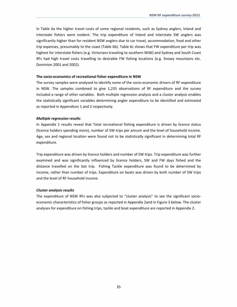
NSW RF expenditure survey‐2012
In Table 6a the higher travel costs of some regional residents such as Sydney anglers Inland and
interstate fishers were evident The trip expenditure of Inland and interstate SW anglers was
significantly higher than for resident NSW anglers due to car travel accommodation food and other
trip expenses presumably to the coast (Table 6b) Table 6c shows that FW expenditure per trip was
highest for interstate fishers (eg Victorians traveling to southern NSW) and Sydney and South Coast
RFs had high travel costs travelling to desirable FW fishing locations (eg Snowy mountains etc
Dominion 2001 and 2002)
The socio‐economics of recreational fisher expenditure in NSW
The survey samples were analysed to identify some of the socio‐economic drivers of RF expenditure
in NSW The samples combined to give 1235 observations of RF expenditure and the survey
included a range of other variables Both multiple regression analysis and a cluster analysis enables
the statistically significant variables determining angler expenditure to be identified and estimated
as reported in Appendices 1 and 2 respectively
Multiple regression results
In Appendix 1 results reveal that Total recreational fishing expenditure is driven by licence status
(licence holders spending more) number of SW trips per annum and the level of household income
Age sex and regional location were found not to be statistically significant in determining total RF
expenditure
Trip expenditure was driven by licence holders and number of SW trips Trip expenditure was further
examined and was significantly influenced by licence holders SW and FW days fished and the
distance travelled on the last trip Fishing Tackle expenditure was found to be determined by
income rather than number of trips Expenditure on boats was driven by both number of SW trips
and the level of RF household income
Cluster analysis results
The expenditure of NSW RFs was also subjected to ldquocluster analysisrdquo to see the significant socio‐
economic characteristics of fisher groups as reported in Appendix 2and in Figure 3 below The cluster
analyses for expenditure on fishing trips tackle and boat expenditure are reported in Appendix 2
35
NSW RF expenditure survey‐2012
Figure 3 A cluster analysis of RF total expenditure showing the groups of significantly different
clusters of anglers identified
In Figure 3 there are four significantly different cluster groups The characteristics of the four groups
are under the ldquodescriptionrdquo row and the authors have put a label to characterise each group
Between Figure 3 and Appendix 2 the overall picture is of groups of ldquoordinaryrdquo fishers
(approximately 85) with low levels of fishing activity in which household income levels may differ
(half lower half higher) secondly a group of dedicated anglers (approximately 12) who have high
fishing activity and expenditure and finally a highly avid fishing group (less than 3) with very high
fishing activity and high to very high expenditure
The results confirm the only previous examination of the socio‐economic characteristics of RFs in
NSW by Dominion (2003) which showed that recreational fishing is a past time involving a diverse
range of people has great variety in activity levels and crosses the entire socio‐economic spectrum
36
NSW RF expenditure survey‐2012
4 State‐wide and regional expenditure estimates
41 Estimating total expenditure
This chapter describes the estimation of the total recreational fishing expenditure for RFs in NSW
and in its regions Total recreational fishing expenditure is the product of three variables
a) Number of recreational fishers or RF households (HH)
We use three approaches to estimate the total RF population in NSW by use of
1) Random telephone survey and ABS Household data and population data
2) The RFL data base and
3) Use of the screening sample and the ABS data on Households Use of the screening
survey of the general population to estimate total number of fishers11 via ABS
population data
b) Fishing trip activity fishing trip activity estimates are obtained from the telephone survey
and
c) Recreational fishing expenditure information on the expenditure per trip and annual
expenditures on equipment is obtained from the telephone survey
The product of these variables will enable us to estimate the total state‐wide recreational fishing
expenditure Expenditure is also estimated for each state region considered Saltwater and
freshwater fishing are considered separately in the state estimates through asking respondents
about the trip intention
42 Expanding the sample of fishers and expenditure
Total expenditure estimates are based on travel and fishing equipment expenses per trip and
estimates of expenditure on boat capital items These are summed to give an annual total
expenditure estimate However the estimates for the angler survey need to be expanded to give
state wide estimates These expansions are described in Box 1 below
Box 1 Explanation of key expansions
The expansion method adapts the method used in the National Survey (Henry and Lyle 2003) The
number of fisher households (FHH) was estimated as follows for each region
No of fisher Household (est) = No Households in Population (ABS) No of Fisher HH (sample)
No of HH (sample)
Example How many recreational fishers would these households include
No of Fishers 19 to 75 yrs (est) = Mean No fishers per HH (sample) No of fisher Household (est)
776496 = 202 383921 (see Table 7)
RF HH are distributed proportionally across regions by household and recreational fishers by
regional population
11 Recreational Fishers under 19 years of age are not included and need to be added if the total population figure is for all
anglers The activity and expenditure estimates are based on ages 19‐75 only
37
NSW RF expenditure survey‐2012
Information on NSW State and Regional Households by Local Government Area (LGA) were accessed
(ABS 2011) The data were aggregated by the larger SD ABS regions (eg Sydney North coast
Inland and SDD South Coast area) These identified the number of households in each of the study
regions as reported in Table 7
Table 7 The ldquototal householdsrdquo in each of the NSW study regions based on LGA data ABS (2011)
Households with recreational fishers are estimated for each study region
Area Population 2010 (gt18-75)
Households HH with RF Rec Fishers HH
RF by region
Sydney 3160897 1376583 213934 230 491232
North coast 835229 570688 88690 146 129802
South coast 350750 207195 32200 169 54510
Inland 649564 315987 49107 206 100948
Total 4996461 2470453 383931 202 776496
The RF household responses for anglersrsquo trip frequency and trip expenditure were multiplied to
produce estimates of state‐wide and regional expenditure
43 State‐wide expenditure estimates
The estimation of total expenditure for samples of recreational anglers and its expansion to regional
state‐wide and national estimates has depended on traditional statistical methods estimating the
total from means of the component distributions However while the number of households is
reasonably well estimated the frequency distribution of fishing trips is highly skewed to the left (see
Figure 1a)
The estimates of total state expenditure on recreational fishing involve multiplying the following
variables
1) Estimate of RF households ‐ the ABS has reliable estimates of households for which RF
households can be identified
2) Estimate of trips ‐ anglers state the number of trips per annum and
3) Estimate of the trip and tackle expenditure on their last trip and their capital expenditure in
the last year
Total expenditure is the product of these variables Total expenditure can be estimated as a mean
value with confidence intervals Here we used the 1237 observations in the RF sample weighting
the results in respect of regional populations as follows
a) Total annual expenditure per angler household = (($ travel expenses per trip + $ tackle
expenses per trip) number of trips )+ (annual capital expenditure per angler household)
b) Total annual expenditure in NSW = total number of anglers households total annual
expenditure per angler household
This traditional approach gives a point estimate but does not provide any information on the
probability of different expenditure levels around the mean This requires a simulation approach
38
NSW RF expenditure survey‐2012
Table 8a shows that the estimated expenditure by all NSW resident RFs in 2012 was $1439bn12 with
an additional $1861m being spent by interstate fishers making a total estimated expenditure by
recreational fishers in NSW of $1625bn in the year 2012
Considering regional expenditures total recreational fishing expenditure was highest by Sydney
anglers ‐ $903m (56 of all expenditure in NSW) followed by the North coast anglers ‐ $3008m
(19) and inter‐state anglers ‐ $ 186m (11) Total expenditure for South Coast anglers was
$1018m (6) and for Inland anglers $1308m (8)13
Expenditure on fishing trips was $793m or 49 of all recreational fishing expenditure in NSW Of
this $402m (25) was spent on fishing equipment tackle and fuel and $430m (26) was spent on
annual capital expenditures such as boats and maintenance Expenditure on SW fishing was
estimated at $1415m (87) and on FW fishing at $231m (13 of total recreational fishing
expenditure in NSW)
Table 8b shows the costs within each category
Within trip expenditure (49 of total expenditure) car travel $326m (201 of total annual
expenditure) accommodation $1859m (114) and food and eating out $188m (115)
Expenditure on fishing equipment and expenses $4025m (246) was made up of $1645m
(102) on major and minor tackle and $1027m (63) on boat fuel and
Annual boat expenditure $4305m (26) of which $1225m (75) was maintenance and
boat purchase or motor repair $1436m (88)
12 This estimate is the same as the mean value produced by the simulation shown later in this chapter It is then adjusted
for Interstate expenditure13 In Chapter 5 the regional economic analysis adapts these data to reflect the expenditure made in other regions away from home residence
39
NSW RF expenditure survey‐2012
Table 8a Estimates of the total RF expenditure for different areas of NSW and including interstate angler expenditure to give all RF expenditure in NSW
Expenditure category Sydney North coast South coast Inland All NSW Inter-state Total expend
in NSW
total expend in NSW
Trip spend 383906879 136686958 57862828 74849484 653306149 139478487 792784637 49 $ fishing equip 222891110 85965049 20624384 31116970 360597513 41975664 402573177 25 Total annual boat expenditure 296326795 81222395 23393975 24877516 425820681 4691465 430512146 26 Totals 903124785 303874402 101881187 130843970 1439724343 186145616 1625869959 100 of total expend in NSW 56 19 6 8 89 11 100 Saltwater 840749912 267431019 99200573 51715617 1259097121 140675487 1415280961 87 Freshwater 62374873 36443383 2680614 79128353 180627222 45469052 231775451 14 SW expenditure as of Total 93 88 97 40 87 84 87
40
NSW RF expenditure survey‐2012
Table 8b Estimates of the total RF expenditure for different areas of NSW and including interstate angler expenditure to give all RF expenditure in NSW
Data in Aus $ Sydney North coast South coast Inland All NSW Interstate Total expend
in NSW
of Total expend in
NSW Expenditure category Car travel (both ways) 155752824 61047851 21250669 38966591 277017934 49755399 326773333 201 Accommodation 96655736 32991275 11321758 11775540 152744309 33155541 185899850 114 Eating out 35118007 11287702 6019080 6283701 58708491 16433282 75141772 46 Other food and drink 47830881 20416270 11974310 11255861 91477322 21385714 112863036 69 Shopping (souvenirmagazinesvideos) 10396840 2377682 609238 2427428 15811187 5900718 21711905 13 Travel-other than by car 9328498 675596 1876003 157968 12038065 - 12038065 07 Sports 730303 214569 - 136952 1081824 2038576 3120401 02 Tours 2517279 121080 888633 400483 3927475 44318 3971793 02 Poker machines 4337423 1534429 364864 485304 6722021 2611177 9333198 06 Pub 16147653 5352108 3163325 2442584 27105670 7101506 34207176 21 Anything else 5091436 668396 394948 517073 6671852 1052256 7724108 05 Trip spend 383906879 136686958 57862828 74849484 653306149 139478487 792784637 488
Major fishing tackle (rods reel) 63209459 22456502 5830420 10743744 102240126 2673467 104913593 65 Minor fishing tackle (hooks lines etc) 27752247 12319663 3884279 5859337 49815525 9792034 59607560 37 Baitberley 26800952 8839913 3407290 3225829 42273984 3954942 46228926 28 Boat hire 17933756 42708 518369 561815 19056649 604762 19661412 12 Boat fuel 52493364 20044184 3811422 4649308 80998277 21742806 102741083 63 Charter and fishing guide fees 17310929 4944101 246843 386149 22888022 839948 23727969 15 Fishing clothesapparel(w aders etc) 6799431 2766227 1592134 1322337 12480129 292501 12772630 08 Camping equipment 4689522 10357115 508333 3093322 18648291 864926 19513218 12 Other fishing expenses 5901451 4194635 825295 1275129 12196509 1210277 13406786 08 $ fishing equip 222891110 85965049 20624384 31116970 360597513 41975664 402573177 248
Boat licenceregistration 22369127 6037457 1817922 4154611 34379117 4691465 39070582 24 Boat maintenance 93188042 18809323 4588346 5925940 122511651 - 122511651 75 Boat insurance 23806199 5935399 1413005 2990204 34144806 - 34144806 21 Marine mooring fees 24487619 2521793 97904 96275 27203591 - 27203591 17 Boat equipment (safety etc) 48762545 9898735 1571861 3725061 63958201 - 63958201 39 Boat purchase or motor repair 83713264 38019687 13904937 7985426 143623314 - 143623314 88 Total annual boat expenditure 296326795 81222395 23393975 24877516 425820681 4691465 430512146 265
Totals 903124785 303874402 101881187 130843970 1439724343 186145616 1625869959 1000 Saltwater 840749912 267431019 99200573 51715617 1259097121 140675487 1399772608 861 Freshwater 62374873 36443383 2680614 79128353 180627222 45469052 226096274 139 SW expenditure as of Total 93 88 97 40 87 76 86 Region as of total expenditure 56 19 6 8 11 100
41
NSW RF expenditure survey‐2012
44 A probabilistic simulation approach to the estimation of total state recreational fishing
expenditure
Simulation enabled us to estimate the probability of different outcomes from the existing data The
original sample was weighted by numbers of regional households to account for the under sampling of
Sydney and the over sampling of the North Coast in the original survey data The sample was analysed
using the SPSS v21 Monte Carlo Simulation model (IBM Corp 2012) This routine produced up to
100000 repeat runs of the predicted values of total RF state expenditure to give the probability of
different expenditure totals as shown in Figure 5a The cumulative probability is shown in Figure 5b
Figure 5a The probability of total expenditure by NSW anglers 2012
These initial probability estimates showed that the mean total state‐wide expenditure was $1473m
with 5 and 95 confidence estimates of $706m and $2952m The median value as $1196m reflecting
the skewedness of the distribution
The estimate of expenditure in NSW by interstate anglers of $1861m has also to be added The final
total NSW estimate of expenditure on recreational fishing was therefore $1625m with 5 and 95
confidence estimates of $892m‐$3136m14
14 For simplicity this assumes the distribution of the interstate results are the same as all NSW
42
NSW RF expenditure survey‐2012
Figure 5b The cumulative probability of total expenditure by NSW anglers 2012
Figure 5a and 5b indicate how the skewed distribution of trips per year by anglers and the highly annual
variable expenditure make the predicted adjusted distribution from $892m‐$3136m around an
adjusted mean $1625m and an adjusted median of $1382m The mean has a 0045 probability of being
achieved whereas lower total expenditure estimates have higher probability (Figure 5a) The
skewedness gives a threshold minimum expenditure level and a ldquotrailing tailrdquo on the right hand side
reflecting less probable high expenditure estimates
Figure 5b indicates that the mean would have a cumulative probability of 65 This shows the higher
total expenditure estimates on the right hand side of Figure 5a are pulling the mean to the right This is
why we have to be careful in RF sampling and estimation of recreational activity and expenditure This
also may explain why fishers of differing avidity and expenditure levels have considerably different
opinions on total expenditure in the sector A fisher with higher activity and expenditure would estimate
a state wide total at the right hand side of Figure 5a but while high total expenditure is possible it is
highly improbable
45 Discussion The estimated total expenditures reported in Table 8a and 8b indicate a statewide expenditure by NSW
recreational fishers and interstate anglers on items directly related to fishing of $1625m
43
NSW RF expenditure survey‐2012
The expansions to develop the final estimates took account of the differences between SW and FW
expenditure and activity and each was expanded separately Expenditure on FW fishing contributed 14
of total expenditure considerably less than the 28 of days fished reported in the sample (Table 5)
reflecting some trip and capital expenditure differences between SW and FW fishers
By region the results indicate that recreational fishing expenditure by Sydney anglers $9031m (56 of
total state recreational fishing expenditure) while North coast has $3038m (9) Interstate anglers
$1861 (11) Inland $1308m (8) and South coast $1018 (6) The survey method estimated regional
expenditures from interviews with fishers in their home region The regional economic impacts adjusts
these and produced estimates of recreational fishing expenditure and its economic impacts across all of
NSW and its main regions
There is just the previous national survey study for comparison of results The 2012 expenditure
estimate adjusted from the Campbell and Murphy (2005) national survey 2001 study is $765m This is
within the confidence intervals predicted by the current studyrsquos simulation approach
Another comparison is to deduct the trip expenditures for food and entertainment from the current
studyrsquos results to be comparable to Campbell and Murphyrsquos assumptions giving an estimate up to
$136bn15 The difference in expenditure estimates16 is primarily related to the survey methods used and
the different estimates of fishery activity the current study being higher Though the number of adults
fishing may have reduced since 2001 NSW has now a sizeable established recreational fishing licence
holder population and expenditures per angler are higher than a decade ago
Under the telephone survey interview and recall method used the current results were conservative for
this methodological approach This study has pointed to the highly skewed nature of the trip activity
among the RF population and the highly variable levels of expenditure among recreational fishers in
NSW The use of a probabilistic simulation in this study has illustrated the difficulties in estimation of
total RF expenditure and the wide distribution around the mean The adequate inclusion and possible
over‐inclusion of avid fishers are sampling problems under any of existing methodologies
The sample size and hence a higher survey cost is part of the remedy Further examination of the US
multi‐method approach may be merited (Gentner 2009) though this is a large scale national expensive
survey exercise The project results in this study are proposed as being reasonable under the
methodologies available within funding constraints and are part of a proposed ongoing expenditure
survey strategy in NSW as outlined in Chapter 6
15 There may also be differences in the treatment of capital attributable to RF definitions of maintenance and capital expenditure on motors and boats and other differences between the two studies These may likely lower this estimate 16 ($1360m‐$765m=$595m in 2012 terms)
44
NSW RF expenditure survey‐2012
5 Regional economic impact estimates This chapter of the report was compiled by Western Research Institute (WRI) WRI received the output
of this survey in terms of expenditure of respondents and based on this output modelled the
economic impacts of recreational fishing on the NSW economy and defined sub‐regions Input‐
output modelling has been employed to derive the relevant economic models and the impacts
51 Methodology
The methodology used to prepare this report included
Determination of the boundaries of the regions to be used in table construction
In consultation with the ANCORS the decision was made to construct input‐output tables for the NSW
North Coast NSW South Coast NSW Inland and Sydney regions as well as NSW as a whole Each region
was defined by aggregating statistical areas at level 4 3 or 2 or combination thereof This allowed the
formulation of regions and economies that best represented the regions of interest Specifically data
from statistical areas at level 3 of ABS Statistical Geography Standard (rather than at larger statistical
areas at level 4) was used in the construction of tables for the NSW North Coast and data from
statistical areas at level 2 was used in the construction of tables for the NSW South Coast The table
construction for Sydney region was based on the data from statistical areas at level 4 while tables for
NSW Inland region was based on the data from statistical areas at different levels (2 3 and 4) Detailed
information on statistical areas in provided in WRI (2013)
Construction of tables
The input‐output tables developed for this project were derived from the latest national table produced
by the Australian Bureau of Statistics (ABS) That table provides a detailed picture of the structure of the
economy of Australia for the year 2008‐09 A series of steps were undertaken to update the table to
2011‐12 Further information from the State Accounts (ABS Cat No 52200) labour force data from the
2011 Census and the quarterly labour force survey (ABS Cat No 6291055003) were used to develop a
state table for New South Wales at 2011‐2012 This was then regionalised to reflect the respective
regional economies of NSW North Coast NSW South Coast NSW Inland and Sydney Further details of
the procedures used in the development of a regional input‐output table are provided in WRI (2013)
52 Economic impact analysis
The economic impacts were modelled as a final demand impact (that calculates the impacts measured
by output value added household income and employment across all sectors in response to changes
in industry final demands) using the 2011‐12 Simulating Impacts on Regional Economies (SIRE) input‐
output model of NSW North Coast NSW South Coast NSW Inland Sydney and NSW as a whole The
SIRE model is superior to standard input‐output models as it provides for non‐linear relationships
between variables and is based on empirically derived (rather than assumed) coefficients In terms of
45
NSW RF expenditure survey‐2012
robustness of results it is comparable with computable general equilibrium (CGE) models whilst
minimising data requirements See WRI (2013) for a detailed description of the SIRE input‐output
model
The impacts of recreational fishing expenditure on the NSW North Coast NSW South Coast
NSW Inland and Sydney regions as well as NSW as a whole have been provided in terms of
bull Output which is the value of goods and services that are produced within an establishment
that become available for use outside that establishment plus any goods and services
produced for the organisationrsquos own final use Output is equal to total revenue plus any
internal consumption
bull Value added which is equal to gross output minus intermediate inputs Value added is
equivalent to the contribution to gross regional product (the local equivalent of gross
domestic product)
bull Household Income which measures the benefit received by regional households from
economic activity It typically refers to compensation of employees but can also include
income in return for other forms of productive activity
bull Employment which refers to full‐time equivalent (FTE) employment is a measure of the
total level of staff resources used The FTE of a full‐time staff member is equal to 10 The
FTE of a part‐time worker will be a fraction of this depending on the relative number of
hours worked
53 The Economic Impact of Recreational Fishing on the Regional Economies of NSW
The economic impact due to recreational fishing was modelled as follows
bull The expenditure survey conducted by ANCORS did not capture the location of expenditure
just the origin (postcode) of the respondent Therefore in the absence of location data an
assumption was made that the total expenditure by interstate visitors ($18614 million)
who make expenditures on recreational fishing whilst staying in NSW should be distributed
evenly across four NSW regions (ie 25 of total interstate expenditure pertaining to each
NSW region)
bull Likewise it was assumed that expenditure pertaining to the NSW North Coast NSW
South Coast and NSW Inland regions was made in these regions (eg those
respondents who indicated living in the NSW North Coast partake in recreational
fishing in the NSW North Coast and not in other areas thereby ensuring that the
money spent on recreational fishing remains in the NSW North Coast region)
46
NSW RF expenditure survey‐2012
bull For those respondents who indicated living in Sydney an assumption was made that 515
of them partake in fishing in Sydney with the remaining 485 fishing in the rest of NSW in
the following proportions NSW North Coast ndash 346 NSW South Coast ndash 485 and NSW
Inland ndash 169 (Dominion 2002 and 2004)
bull Since anglers in each of the regions make expenditure on items that may not be
produced in the region but that are imported from the rest of NSW the regional
recreational fishing expenditure was split into local and imported components using a
location quotients matrix This way WRI ensured that only local expenditure generated
economic impacts in the respective region For NSW as a whole an assumption was
made that all products that anglers purchase are produced within the state and
therefore no separation of local and imported components was performed The
economic impacts of recreational fishing on NSW were modelled using total recreational
fishing expenditure in NSW
bull In order to ensure consistency of the input‐output modelling procedure the expenditure
data was allocated in the input‐ output table to the industries (typically manufacturing
industries) where the relevant expenditure items were produced and was then
converted to basic prices See WRI (2013) for further details on sectoral allocations
bull A final demand analysis in SIRE was performed and economic impacts on NSW North Coast
NSW South Coast NSW Inland and Sydney as well as NSW as a whole were derived
The impacts of recreational fishing on the economies of the NSW North Coast NSW South Coast
NSW Inland and Sydney regions are outlined in the Table 9
Table 9 Regional expenditure and economic impacts on regional economies
Region North Coast Sydney South Coast Inland
Expenditure by postcode ($m) 30387 90312 10188 13084
Reclassified expenditure ($m) 50196 51165 36086 2514
Output ($m) 73465 100286 39522 35381
Value added ($m) 35355 49156 18417 14985
Household income ($m) 16875 28888 876 735
Employment (no) 3320 3944 1808 1539
47
NSW RF expenditure survey‐2012
NSW North Coast
Overall when flow‐on effects are taken into account recreational fishing contributes the following to
the economy of NSW North Coast
bull 3320 FTE jobs including 667 in the retail trade sector 573 in the hospitality sector
349 in the personal and other services sector and 174 in the transport and storage
sector
bull $16875 million in household income with 134 percent being in the retail trade
sector 112 percent being in the hospitality sector 76 percent being in the public
administration sector 72 percent being in the personal and other services sector and
57 percent being in the transport and storage sector
bull $35355 million in industry value added representing 081 percent of total regional
value added of the NSW North Coast region and
bull $73465 million in output
For the North Coast recreational fishing will contribute 098 percent of FTE employment in the
region when flow‐on effects are taken into account as well as 084 percent of household income and
07 percent of the estimated gross regional product of the NSW North Coast region
NSW South Coast
Overall when flow‐on effects are taken into account the recreational fishing contributes the
following to the economy of NSW South Coast
bull 1808 FTE jobs including 420 in the hospitality sector 284 in the retail trade sector
236 in the personal and other services sector 117 in the transport and storage
sector and 106 in the public administration sector
bull $8760 million in household income with 152 percent being in the hospitality sector
109 percent being in the retail trade sector 93 percent being in the public
administration sector 86 percent being in the personal and other services sector and 77
percent being in the transport and storage sector
bull $18416 million in industry value added representing 167 percent of total regional
value added of the NSW South Coast region and
bull $39522 million in output
For the South Coast recreational fishing will contribute 212 percent of FTE employment in the region
when flow‐on effects are taken into account as well as 173 percent of household income and 143
percent of the estimated gross regional product of the NSW South Coast region
48
NSW RF expenditure survey‐2012
NSW Inland
Overall when flow‐on effects are taken into account the recreational fishing contributes the
following to the economy of NSW Inland
bull 1539 FTE jobs including 289 in the hospitality sector 288 in the retail trade sector
148 in the personal and other services sector and 138 in the agriculture sector
bull $7350 million in household income with 134 percent being in the retail trade
sector 131 percent being in the hospitality sector 74 percent being in the
personal and other services sector 70 percent being in the public administration
sector and 68 percent being in the transport and storage sector
bull $14985 million in industry value added representing 030 percent of total regional
value added of the NSW Inland region and
bull $35381 million in output
Recreational fishing will contribute 038 percent of FTE employment in the NSW Inland region when
flow‐on effects are taken into account as well as 032 percent of household income and 026 percent
of the estimated gross regional product of the NSWInlandregion
Sydney
Overall when flow‐on effects are taken into account the recreational fishing contributes the following
to the economy of Sydney
bull 3944 FTE jobs including 741 in the retail trade sector 450 in the hospitality sector
366 in the personal and other services sector and 310 in the professional and
technical services sector
bull $28888 million in household income with 162 percent being in the finance and insurance
sector 113 percent being in the retail trade sector 83 percent being in the professional
and technical services sector 77 percent being in the wholesale trade sector and 63
percent being in the hospitality sector
bull $49156 million in industry value added representing 025 percent of the total regional
value added of Sydney and
bull $100286 million in output
For the Sydney region recreational fishing will contribute 028 percent of FTE employment when flow‐on
effects are taken into account as well as 025 percent of household income and 022 percent of the
estimated gross regional product of Sydney
49
NSW RF expenditure survey‐2012
NSW State economy
The impacts of recreational fishing on the state economy of the NSW are outlined in the Table 10
Table 10 NSW expenditure and economic impacts on NSW
Item Estimate
NSW Expenditure by postcode ($m) 143972
Total interstate expenditure ($ m) 18615
NSW Reclassified expenditure ($m) 162587
Output ($m) 342035
Value added ($m) 162561
Household income ($m) 87728
Employment (thousand) 14254
NSW Economy
Overall when flow‐on effects are taken into account the recreational fishing contributes the following to
the economy of NSW
bull 14254 FTE jobs including 2730 in the retail trade sector 2123 in the hospitality
sector 1389 in the personal and other services sector and 951 in the transport and
storage sector
bull $87728 million in household income with 122 percent being in the retail trade 114
percent being in the finance and insurance sector 88 percent being in the hospitality
sector 72 percent being in the professional and technical services sector and 65
percent being in the wholesale trade sector
bull $162561 million in industry value added representing 036 percent of the estimated gross
state product of the NSW and
bull $342035 million in output
50
NSW RF expenditure survey‐2012
Overall recreational fishing will contribute 046 percent of FTE employment in the NSW when flow‐on
effects are taken into account as well as 041 percent of household income and 040 percent of total
regional value added
54 Conclusion
The recreational fishing expenditure and economic impact of recreational fishing on NSW and
respective regions were substantial in absolute terms but uneven across regions
The expenditure based on place of residence was the highest in Sydney followed by NSW North
Coast NSW Inland and NSW South Coast The reallocated expenditure (ie actual expenditure
made in the region) was still the highest in Sydney (but substantially lower than postcode
expenditure) followed by expenditure in NSW North Coast NSW South Coast and NSW Inland
In terms of output valued added household income and FTE employment the absolute economic
impacts of recreational fishing were the highest in Sydney followed by NSW North Coast NSW South
Coast and NSW Inland However in relative terms economic impacts (as percentage of total in the
respective regions) were the highest in NSW South Coast (167‐ 212) followed by NSW North
Coast (081‐098) NSW Inland (030‐038) and Sydney (025‐028) These relative disparities
reflect the large size of Sydney and NSW Inland economies and smaller size of NSW North Coast and
NSW South Coast economies
51
NSW RF expenditure survey‐2012
6 Developing a cost effective approach to expenditure surveys
There have been several reoccurring issues in obtaining information on recreational fishing expenditure
in NSW The first is the lack of a series of expenditure surveys the past ones not occurring as part of an
on‐going consistent strategy The second issue is the lack of a known survey method which is repeatable
and can be compared with past surveys In both of these issues the recurrent cost of such surveys has
been unknown also
61 The objectives of an recreational fishing expenditure survey
Any survey is designed towards its objectives In developing a cost effective regular approach to
recreational fishing expenditure surveys there has to be some design decisions made in respect of the
information required For example A state‐wide expenditure estimate may be required every two years
to track and promote the value of the sector This could include a state‐wide estimate of regional
economic impact Further disaggregation by area or other variables will increase cost
62 Sampling data issues and findings
This study has considered how the use of the RFL database reduced the cost of expenditure surveys
which have traditionally used expensive random screening surveys to locate recreational fishers
Finding 1 The current study has found that there is no statistically significant difference between
seasonal samples Consequently we recommend an annual survey event being mindful of its timing
relative to Christmas January and Easter which may be periods when fishers are not at home
The RFs identified through a random screening survey process were found to make more fishing trips
and fish more days than the sample of RFs contacted through the RFL database (noting that both
samples include licence holders) However in further comparisons of days fished per angler between
licenced and unlicensed fishers no significant difference was found On the other hand unlicensed
fishers were found to undertake significantly more fishing trips than licence holders though this relates
to trip events and not necessarily to higher average expenditure ndash in other words unlicensed fishers
may make more but shorter trips to nearby destinations compared with licensed fishers
Finding 2 The RFL database can be used to sample anglers for expenditure surveys providing certain
conditions are met in terms of the different numbers of licences holders that are sampled17
63 What sample size is required
The size of a sample in statistics is important If the sample is too small there is then the risk that the null
hypothesis is wrongly rejected (ATS 2010) The size of a sample is also related to the probability level at
17 A ratio of 3 day 1 month 1 year and 3 year licence holder records is recommended The weighting would be easier for the annual and 3 year licence holders as 3 day and monthly licence holder can be repeat licence purchasers in a given year
52
NSW RF expenditure survey‐2012
which the variable is seen to be significantly different from zero eg 95 (5) or 99 (1) levels of
significance The dispersion of the distribution of the variable being examined is also important and this
is captured in the standard error of the variable
In statistics these issues are brought together in statistical ldquopower analysisrdquo where the minimum size of
a sample can be tested both prior to and even after statistical surveys to see if the sample size is
adequate ldquoThe power is the probability of detecting an effect presuming it is actually thererdquo (ATS 2010)
Sample size estimation
In this section of the report we investigate how reducing the sample size to the minimum required
number of interviews can reduce the cost of an expenditure survey The decision regarding the target
sample size for the survey has to be balanced between the levels of significance chosen for testing (1
5) and the standard error that is acceptable for the intended variables which is often related to the
estimated value called the relative standard error (RSE) 18
Table 11 shows a range of sample sizes derived for different scenarios using the ABS calculator facility at
NSS (2013) There are the two scenarios for random surveys (cases 1‐4) and two for surveys from a
population base of known participants (case 5‐6)
Table 11 Indication of the required sample sizes under different sampling and risk scenarios including
sampling of the RFL database
Case number 1 2 3 4 5 6 Sample type Random sampling Non random
Statistical input All NSW Population
All NSW Population
All NSW Population
South coast
RFL ‐1 RFL‐2
Confidence Level 99 95 95 95 95 95 Population Size 4996500 4996500 4996500 350750 480700 480700 Proportion 05 05 015 025 06 06 Confidence Interval 005 005 00294 005 005 005
Upper 055 055 01794 03 065 065 Lower 045 045 01206 02 055 055
Standard Error 0025 0025 0015 0025 003 0045 Relative Standard Error () 50 50 100 100 50 75 Sample Size 339 196 567 300 267 119
18 The RSE is the standard error expressed as a percentage of the estimate
53
NSW RF expenditure survey‐2012
In Table 11 cases 1 and 2 show the general sampling results when the confidence level is either 99 or
95 and the proportion is 05 (ie where ldquothe expected proportion of the population to have the
attribute that you are estimating from your surveyrdquo (NSS 2013) These data are often quoted but given
that RFs are more difficult to locate than a one in two assumption (proportion 05) case 3 assumes a
15 proportion for RFs and requires a sample size of 567 with a relative standard error (RSE) of 10
Reducing the sampling area to the South Coast (case 4) raises the chances of locating RFs (proportion
025) and would require 300 observations at an RSE of 10 The sampling model assumes a random
population
We also apply the model to the non‐random scenarios from the RFL data base Here cases 5 and 6 are
RFL records and hence not as random as the whole NSW population We use the model to estimate
possible minimum sample sizes when using the RFL data base population Assuming that the proportion
is 06 an RSE of 5 requires a sample of 267 and an RSE of 75 a sample size of 119 In the experience
of the authors the last sample size (119) is low given the variation in our results We recommend no less
than 250 completed surveys as a minimum sample size for state‐wide estimates If four NSW regions are
included a minimum total of 500 completed surveys would be required and be should be larger if
possible
The review of samples has shown that there is a trade off in accuracy of estimates with the number of
interviews undertaken For example in the case 3 random survey in Table 11 the RSE is 10 and
reducing this to 75 for case 3 would increase the sample size from 576 to 1008 or for 5 to 2226
The incidence of locating RFs has cost implications for surveying and this is why the careful use of the
RFL data base is attractive
Finding 3a A main state‐wide survey using the RFL data base to sample 1000 anglers in major regions is
recommended every 5 years with an option of updating results by indexing annually or bi‐ennially
andor considering a smaller survey (250 state wide or 500 for regions) in year three also
Finding 3b The economic impact analysis can follow the five year survey pattern and can be adjusted
between surveys Simulation modelling can also be used to provide an improved understanding of the
uncertainty surrounding expenditure estimates and may be used to confirm estimates between main
surveys also
64 Discussion ‐ Scoping a recreational fishing expenditure survey strategy for NSW
A recreational fishing expenditure survey strategy would aim to undertake a substantial survey every 5
years and run smaller annual or biennial updating exercises between these periods
In the future the 5 year survey could either
54
NSW RF expenditure survey‐2012
Follow past screening survey approaches of all RFs and compare results with a sample of RFL
holders as in the current study or
Use a weighted selection of 3 day 1 month 1 year and 3 year licence holder contacts to enable
a representative sample to be expanded to state‐wide totals
Before being able to categorically recommend the sole use of the RFL database only approach we would
require more information on the inter‐relationship between the random screening survey and the use of
and RFL data base records The current NSW catch and effort survey study may also provide information
on this relationship (J Murphy DPI pers comm)
As per Finding 2 we recommend further comparisons of the random screening survey approach to all
fishers with use of the RFL holdersrsquo data as in the current study Use of the RFL database alone should
be confirmed by other research on the relationship between all fishers and those who are licensed
In the years between the five year main surveys the survey results from the initial survey could be
upgraded annually (or bi‐ennially) by sampling several variables that could be used to index the changes
in the state wide expenditure estimates For example any changes detected in RF participation or
activity state population or change in licence sales could inform activity estimates Information on
recreational fishing expenditure could be influenced by annual changes in price levels as measured by
the consumer price index (cpi) and any information available from industry about retail fishing gear
prices such as those related to exchange rate variations which would impact expenditure on fishing
gear Many of these indices of economic conditions are monitored by the Australian Fishing Tackle
Association and could be referred to
The simulation modelling approach used in the current study could be re‐run annuallybiennially with
these activity and expenditure indices included and updated annual estimates produced The
reoccurrence of another survey in year 5 means there would be a cross check on the indexing of the
previous survey
The choice of 5 years for the main survey is arbitrary and could be 3 years particularly if other catch and
effort surveys are indicating significant changes in participation rates in NSW or there is evidence of
changes in other states Leaving a main survey for more than 5 years is not recommended as the public
awareness of the sectorrsquos economic contribution and associated regional benefits will reduce giving the
sector less public profile
65 Conclusions
The recreational fishing sector in NSW wishes to have more regular studies of angler expenditure and its
importance to the economy The RFL data base can be used for sampling the recreational fishing
population reducing the costs of fieldwork surveys if several conditions are followed The frequency of
55
NSW RF expenditure survey‐2012
the different licence durations needs to be chosen so as not to move away from sampling a
representative cross section of anglers of all different activity levels and possibly having over or under
emphasis of avid anglers
A main state‐wide survey using the RFL data base to sample 1000 anglers in major regions is
recommended every 5 years with an option of updating results by indexing annually or bi‐ennially and
considering a smaller survey (250 state wide or 500 for regions) in year three also The economic impact
analysis can follow the five year survey pattern and can be adjusted between surveys Simulation
modelling can also be used to provide an improved understanding of the uncertainty surrounding
expenditure estimates and may be used to confirm estimates between main surveys also
56
NSW RF expenditure survey‐2012
References
ABARES (2011) Australian Fisheries Statistics 2010 Australian Bureau of Agricultural and Resource Economics and
Sciences Australian Government p 100
ABS (2010) 1216055003 ‐ Australian Statistical Geography Standard Design of the Statistical Areas Level 4
Capital Cities and Statistical Areas Level 3 May 2010 Canberra
ABS (2011) 13381 NSW State and Regional Indicators December 2010
ABS (2012) Estimated Resident Population for New South Wales by Age by Statistical Geography Persons ndash 30
June 2011 Population by Age and Sex Regions of Australia 32350 Canberra
ACMA (2013) Convergence and Communications Report 1 Australian household consumersrsquo take‐up and use of
voice communications services Australian Communication and Media Authority report November
ATS (2010) Introduction to Power Analysis Statistical Computing Seminars
httpwwwatsuclaedustatseminarsintro_powerdefaulthtm
Campbell D and JJ Murphy (2005) The 2000‐01 National Recreational Fishing Survey Economic Report
Department of Agriculture Fisheries and Forestry GPO Box 858 Canberra ACT 2601 June
Cunningham S Dunn MR and Whitmarsh D (1985) Fisheries Economics An Introduction Mansell Publishing
London
Dominion (2001) ldquoAn economic survey of the Snowy mountain recreational trout fisheryrdquo A report by Dominion
Consulting Pty Ltd to the Freshwater Recreational Fishing Trust NSW Fisheries
Dominion (2002) ldquoNational Recreational Fishing Tackle Industry survey of the retail and wholesale sectorsrdquo A report by Dominion Consulting Pty Ltd Client Australian Fishing Tackle Association
Dominion (2003) ldquoIdentifying the recreational fishing expenditure patterns of Sydneyrsquos recreational fishers and its economic importance in regional communities of NSWrdquo Research project in conjunction with Roy Morgan Research A report by Dominion Consulting Pty Ltd for Recreational Fishing Trust NSW Fisheries
Dominion (2004) ldquoNational Recreational Fishing Tackle Industry survey of the retail and wholesale sectorsrdquo A report by Dominion Consulting Pty Ltd Client Australian Fishing Tackle Association
Dominion (in prep) An Economic Survey of the NSW Charter Boat industry NSW Recreational Trust Fund Project
Ernst amp Young (2009) An economic study of recreational fishing in Victoria A report to VRFISH Melbourne
Victoria
Ernst amp Young (2011) Economic contribution of Recreational Fishing in the Murray Darling Basin A report to
Victorian Department of Primary Industries Melbourne Victoria
Galeano D Langenkamp D Levantis C Shafron W and Redmond I (2004) Economic Value of Charter and
Recreational Fishing in Australiarsquos Eastern Tuna and Billfish Fishery ABARE eReport 0410 Canberra July
57
NSW RF expenditure survey‐2012
Gentner B (2008) Exploring survey methodologies for collecting recreational angler expenditure data International Institute of Fisheries Economics and Trade (IIFET) 2008 Vietnam Proceedings
Gentner B and S Steinback (2008) The Economic Contribution of Marine Angler Expenditures in the United States 2006 US Dep Commerce NOAA Tech Memo NMFSF SPO‐94 301 p
Henry G W and JM Lyle (2003) The National Recreational and Indigenous Fishing Survey Fisheries Research and Development Corporation (FRDC) project no 99158
IBM Corp (2012) IBM SPSS Statistics for Windows Version 210 Armonk NY IBM Corp
Jones K (2009) South Australia Recreational Fishing Survey 2007‐2008 In South Australian Fisheries Management Series Paper No 54 (Fisheries Division PIRSA) p 84
McIlgorm A and J Pepperell (1999) A National Review of the Recreational Fishing Sector A report by Dominion Consulting to Agriculture Forestry and Fisheries Australia
McIlgorm A A Macfarlane and J Pepperell (2005) ldquoThe importance of recreational fishing expenditure to the economies of two coastal towns in northern and southern NSW Port Macquarie and Bermaguirdquo A report by Dominion Consulting Pty Ltd for the Recreational Fishing Trust Fund NSW Fisheries March 2005
Mohadjer L B Bell and J Waksberg (1994) Accounting for Item Nonresponse Bias‐ National Health and Nutrition Examination Survey iii Prepared for National Centre for Health Statistics Maryland by Westat Inc November
NSS (2013) National Statistics Service‐ httpwwwnssgovaunsshomeNSFpagesSample+size+calculator
NOAA (2011) ldquoNOAA begins National Survey of the economic contributions of saltwater anglingrdquo
httpwwwnoaanewsnoaagovstories201120110222_saltwateranglinghtml (22nd Feb 2011)
NOAA (2012) ldquoRecreational Fisheries Year in Review 2012rdquo National Oceanic and Atmospheric Administration
National Marine Fisheries Service Department of Commerce
Ritz W (2013) Non‐Response Bias in Survey Sampling httpwwwtrchomecomwhite‐paper‐librarywpl‐all‐white‐papers215
Rolfe J amp Prayaga P (2007) Estimating values for recreational fishing at freshwater dams in Queensland Australian Journal of Agricultural and Resource Economics 51 157‐174
Steinback S B Gentner and J Castle (2004) ldquoThe economic importance of marine angler expenditures in the United Statesrdquo NOAA Professional Paper NMFS 2 169 p
Taylor S J Webley K McInnes (2011) The 2010 State‐wide Recreational Fishing Survey State of Queensland
Department of Agriculture Fisheries and Forestry 2012
Thomson CJ (1991) Effects of Avidity Bias on Survey Estimates of Fishing Effort and Economic Values American
Fisheries Society Symposium 12356‐366
West L D Lyle J M Matthews S R Stark K E amp Steffe A S (2012) Survey of recreational fishing in the Northern Territory 200910 Northern Territory Fisheries Department of Resources Northern Territory p128
WRI (2013) Measuring the Economic Contribution of the Recreational Fishing sector in NSW A report to ANCORS University of Wollongong by The Western Research Institute Bathurst NSW p21
58
NSW RF expenditure survey‐2012
Appendix 1 What determines recreational fisher expenditure in NSW
Linear multiple regression was used to determine the variables which are statistically significant in
determining total expenditure trip expenditures tackle expenditure and boat expenditure A range of
variables available from the interviews such as licence holder age regional location situation
household and malefemale were able to be tested for their statistical significance in relation to RF
expenditures
Total expenditure
The significant determinants of total expenditure were found to be income trips per annum and
licensed fishers who have a marginally greater total spend that unlicensed fishers Trips in SW were a
significantly higher contributor to total expenditure than days fished in FW probably related to higher
capital boat expenditure by marine fishers Licensed fishers who are generally in the workforce were
found to have marginally greater total expenditure than unlicensed fishers but only at a 10 level of
significance (see A1‐Table 1) Other variables such as age region situation household and malefemale
were not significantly different from zero at the 5 level of significance
A1‐ Table 1 Regressions results for Total Expenditure
Coefficientsa
Model Unstandardized Coefficients Standardized
Coefficients
t Sig
B Std Error Beta
1
(Constant)
LIC10
swtrips
income
-1137559
558821
43064
332455
475354
314755
12240
73522
050
099
128
-2393
1775
3518
4522
017
076
000
000
a Dependent Variable TOTALEXP
Trip expenditure
Determinants of total trip expenditure were found to be number of SW trips per annum with licence
holders spending more on trips (see A1‐Table 2a) were not significantly different from zero at the 5
level of significance
59
NSW RF expenditure survey‐2012
A1‐ Table 2a Regressions results for Trip Expenditure Coefficientsa
Model Unstandardized Coefficients Standardized
Coefficients
t Sig
B Std Error Beta
1
(Constant)
LIC10
swtrips
953678
623065
36235
185885
232860
9133
076
113
5130
2676
3967
000
008
000
a Dependent Variable TRIPSPEND
The trip expense will also be related to the days fished which is correlated with the number of trips
taken annually In A1‐Table 2b the model was altered to include days fished and kilometres travelled
Days fished in SW and FW the number of kilometres travelled and being a licence holder were all
significant variables in determining trip expenditure
A1‐ Table 2b Regressions results for Trip Expenditure with SW and FW days fished Coefficientsa
Model Unstandardized Coefficients Standardized
Coefficients
t Sig
B Std Error Beta
1
(Constant)
LIC10
SWDAYS
FWDAY
kmsa
151158
599485
83015
50750
2109
190606
223599
7460
14523
1034
073
304
096
057
793
2681
11128
3494
2039
428
007
000
000
042
a Dependent Variable TRIPSPEND
This result is a reminder of the significant expenditure made by many anglers on road travel
Tackle expenditure
Regression results reveal that Tackle expenditure is determined primarily by household income levels
(see A1‐Table 3) Other variables such as age licencing region freshwater days family situation
household and malefemale were not significantly different from zero at the 5 level of significance
A1‐ Table 3 Regressions results for Tackle Expenditure Coefficientsa
Model Unstandardized Coefficients Standardized
Coefficients
t Sig
B Std Error Beta
1 (Constant)
income
39960
17264
26312
4263 115
1519
4049
129
000
a Dependent Variable Total Tackle
60
NSW RF expenditure survey‐2012
Boat capital expenditure
The regressions show that number of SW trips and household income levels are the determinants of
Boat capital expenditure (A1‐ Table 4) other variables not being significantly different from zero
A1‐ Table 4 Regressions results for Boat Capital Expenditure
Coefficientsa
Model Unstandardized Coefficients Standardized
Coefficients
t Sig
B Std Error Beta
1
(Constant)
swtrips
income
-1175462
44403
309987
444221
11767
70336
106
124
-2646
3774
4407
008
000
000
a Dependent Variable TOTALCAP
61
NSW RF expenditure survey‐2012
Appendix 2 Socio‐ economic groups and RFs in NSW ndash a cluster analysis
Cluster analysis enables researchers to let the data determine how many statistically significant groups
(called ldquoclustersrdquo) there are in the given data set In the previous regressions we found that income19
and SW days fished were significant in predicting angler expenditure Cluster analysis can show r
patterns among groups of RFs in NSW Labels to characterise groups have been added
Total expenditure
A2‐Figure 1 RF Clusters in total expenditure
19 Household income is in the following numerical bands 1‐Under $20000 2‐ $20000 to $29999 3‐$30000 to $39999 4‐$40000 to $59999 5‐$60000 to $79999 6‐$80000 to $99999 7‐ $100000 to $119999 8‐ $120000 to $140000 9‐ $140000+
62
NSW RF expenditure survey‐2012
In A2‐Figure 1 the cluster analysis of the data shows that total expenditure has income and trips per
annum as strongest predictor of total expenditure but there are 4 statistically significant clusters as
described The authors have added a label to describe the group characteristics which are given in the
description
Trip expenditure
A2‐Figure 2 RF Clusters in trip expenditure
Trips and secondly income are the strongest predictors of trip expenditure Examining trip expenditure
leads to 4 distinct clusters We see clusters 2 and 3 (182) have high trip expenditures Some 818 of
the population have low trip expenditure with one low income (ldquobattlersrdquo) and one higher income
group (ldquoFishing break anglersrdquo)
63
NSW RF expenditure survey‐2012
Tackle expenditure
Tackle expenditure is most strongly predicted by income and is less trip related than expected There is a
cluster of 4 of higher income fishers who have very high tackle expenditure (ldquoTackle addictsrdquo)
A2‐Figure 3 RF Clusters in tackle expenditure
Tackle expenditure forms into 4 clusters with 852 of fishers fishing few trips and spending low
amounts on tackle irrespective of income
64
NSW RF expenditure survey‐2012
Capital boat expenditure
In A2 Figure 4 firstly trips and then secondly income are the strongest predictors of expenditure on
boats The highest boat expenditure is associated with 23 of fishers doing many trips but also with
the 138 of dedicated fishers
A2‐Figure 4 RF Clusters in capital boat expenditure
65
- Structure Bookmarks
-
- Project Developing a cost effective state wide expenditure survey method to measure the economic contribution of the recreational fishing sector in NSW
- Final Report to the NSW Recreational Fishing Licence Trust NSW Department of Primary Industry November 2013
-
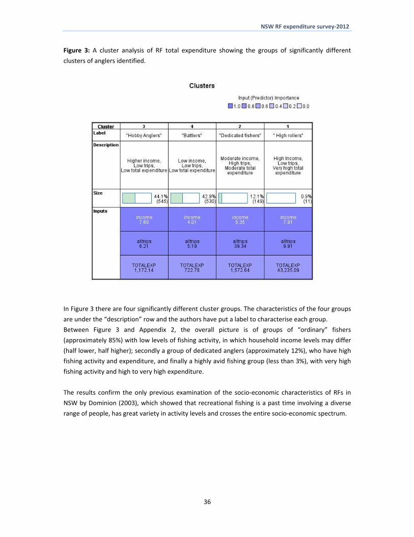
NSW RF expenditure survey‐2012
4 State‐wide and regional expenditure estimates
41 Estimating total expenditure
This chapter describes the estimation of the total recreational fishing expenditure for RFs in NSW
and in its regions Total recreational fishing expenditure is the product of three variables
a) Number of recreational fishers or RF households (HH)
We use three approaches to estimate the total RF population in NSW by use of
1) Random telephone survey and ABS Household data and population data
2) The RFL data base and
3) Use of the screening sample and the ABS data on Households Use of the screening
survey of the general population to estimate total number of fishers11 via ABS
population data
b) Fishing trip activity fishing trip activity estimates are obtained from the telephone survey
and
c) Recreational fishing expenditure information on the expenditure per trip and annual
expenditures on equipment is obtained from the telephone survey
The product of these variables will enable us to estimate the total state‐wide recreational fishing
expenditure Expenditure is also estimated for each state region considered Saltwater and
freshwater fishing are considered separately in the state estimates through asking respondents
about the trip intention
42 Expanding the sample of fishers and expenditure
Total expenditure estimates are based on travel and fishing equipment expenses per trip and
estimates of expenditure on boat capital items These are summed to give an annual total
expenditure estimate However the estimates for the angler survey need to be expanded to give
state wide estimates These expansions are described in Box 1 below
Box 1 Explanation of key expansions
The expansion method adapts the method used in the National Survey (Henry and Lyle 2003) The
number of fisher households (FHH) was estimated as follows for each region
No of fisher Household (est) = No Households in Population (ABS) No of Fisher HH (sample)
No of HH (sample)
Example How many recreational fishers would these households include
No of Fishers 19 to 75 yrs (est) = Mean No fishers per HH (sample) No of fisher Household (est)
776496 = 202 383921 (see Table 7)
RF HH are distributed proportionally across regions by household and recreational fishers by
regional population
11 Recreational Fishers under 19 years of age are not included and need to be added if the total population figure is for all
anglers The activity and expenditure estimates are based on ages 19‐75 only
37
NSW RF expenditure survey‐2012
Information on NSW State and Regional Households by Local Government Area (LGA) were accessed
(ABS 2011) The data were aggregated by the larger SD ABS regions (eg Sydney North coast
Inland and SDD South Coast area) These identified the number of households in each of the study
regions as reported in Table 7
Table 7 The ldquototal householdsrdquo in each of the NSW study regions based on LGA data ABS (2011)
Households with recreational fishers are estimated for each study region
Area Population 2010 (gt18-75)
Households HH with RF Rec Fishers HH
RF by region
Sydney 3160897 1376583 213934 230 491232
North coast 835229 570688 88690 146 129802
South coast 350750 207195 32200 169 54510
Inland 649564 315987 49107 206 100948
Total 4996461 2470453 383931 202 776496
The RF household responses for anglersrsquo trip frequency and trip expenditure were multiplied to
produce estimates of state‐wide and regional expenditure
43 State‐wide expenditure estimates
The estimation of total expenditure for samples of recreational anglers and its expansion to regional
state‐wide and national estimates has depended on traditional statistical methods estimating the
total from means of the component distributions However while the number of households is
reasonably well estimated the frequency distribution of fishing trips is highly skewed to the left (see
Figure 1a)
The estimates of total state expenditure on recreational fishing involve multiplying the following
variables
1) Estimate of RF households ‐ the ABS has reliable estimates of households for which RF
households can be identified
2) Estimate of trips ‐ anglers state the number of trips per annum and
3) Estimate of the trip and tackle expenditure on their last trip and their capital expenditure in
the last year
Total expenditure is the product of these variables Total expenditure can be estimated as a mean
value with confidence intervals Here we used the 1237 observations in the RF sample weighting
the results in respect of regional populations as follows
a) Total annual expenditure per angler household = (($ travel expenses per trip + $ tackle
expenses per trip) number of trips )+ (annual capital expenditure per angler household)
b) Total annual expenditure in NSW = total number of anglers households total annual
expenditure per angler household
This traditional approach gives a point estimate but does not provide any information on the
probability of different expenditure levels around the mean This requires a simulation approach
38
NSW RF expenditure survey‐2012
Table 8a shows that the estimated expenditure by all NSW resident RFs in 2012 was $1439bn12 with
an additional $1861m being spent by interstate fishers making a total estimated expenditure by
recreational fishers in NSW of $1625bn in the year 2012
Considering regional expenditures total recreational fishing expenditure was highest by Sydney
anglers ‐ $903m (56 of all expenditure in NSW) followed by the North coast anglers ‐ $3008m
(19) and inter‐state anglers ‐ $ 186m (11) Total expenditure for South Coast anglers was
$1018m (6) and for Inland anglers $1308m (8)13
Expenditure on fishing trips was $793m or 49 of all recreational fishing expenditure in NSW Of
this $402m (25) was spent on fishing equipment tackle and fuel and $430m (26) was spent on
annual capital expenditures such as boats and maintenance Expenditure on SW fishing was
estimated at $1415m (87) and on FW fishing at $231m (13 of total recreational fishing
expenditure in NSW)
Table 8b shows the costs within each category
Within trip expenditure (49 of total expenditure) car travel $326m (201 of total annual
expenditure) accommodation $1859m (114) and food and eating out $188m (115)
Expenditure on fishing equipment and expenses $4025m (246) was made up of $1645m
(102) on major and minor tackle and $1027m (63) on boat fuel and
Annual boat expenditure $4305m (26) of which $1225m (75) was maintenance and
boat purchase or motor repair $1436m (88)
12 This estimate is the same as the mean value produced by the simulation shown later in this chapter It is then adjusted
for Interstate expenditure13 In Chapter 5 the regional economic analysis adapts these data to reflect the expenditure made in other regions away from home residence
39
NSW RF expenditure survey‐2012
Table 8a Estimates of the total RF expenditure for different areas of NSW and including interstate angler expenditure to give all RF expenditure in NSW
Expenditure category Sydney North coast South coast Inland All NSW Inter-state Total expend
in NSW
total expend in NSW
Trip spend 383906879 136686958 57862828 74849484 653306149 139478487 792784637 49 $ fishing equip 222891110 85965049 20624384 31116970 360597513 41975664 402573177 25 Total annual boat expenditure 296326795 81222395 23393975 24877516 425820681 4691465 430512146 26 Totals 903124785 303874402 101881187 130843970 1439724343 186145616 1625869959 100 of total expend in NSW 56 19 6 8 89 11 100 Saltwater 840749912 267431019 99200573 51715617 1259097121 140675487 1415280961 87 Freshwater 62374873 36443383 2680614 79128353 180627222 45469052 231775451 14 SW expenditure as of Total 93 88 97 40 87 84 87
40
NSW RF expenditure survey‐2012
Table 8b Estimates of the total RF expenditure for different areas of NSW and including interstate angler expenditure to give all RF expenditure in NSW
Data in Aus $ Sydney North coast South coast Inland All NSW Interstate Total expend
in NSW
of Total expend in
NSW Expenditure category Car travel (both ways) 155752824 61047851 21250669 38966591 277017934 49755399 326773333 201 Accommodation 96655736 32991275 11321758 11775540 152744309 33155541 185899850 114 Eating out 35118007 11287702 6019080 6283701 58708491 16433282 75141772 46 Other food and drink 47830881 20416270 11974310 11255861 91477322 21385714 112863036 69 Shopping (souvenirmagazinesvideos) 10396840 2377682 609238 2427428 15811187 5900718 21711905 13 Travel-other than by car 9328498 675596 1876003 157968 12038065 - 12038065 07 Sports 730303 214569 - 136952 1081824 2038576 3120401 02 Tours 2517279 121080 888633 400483 3927475 44318 3971793 02 Poker machines 4337423 1534429 364864 485304 6722021 2611177 9333198 06 Pub 16147653 5352108 3163325 2442584 27105670 7101506 34207176 21 Anything else 5091436 668396 394948 517073 6671852 1052256 7724108 05 Trip spend 383906879 136686958 57862828 74849484 653306149 139478487 792784637 488
Major fishing tackle (rods reel) 63209459 22456502 5830420 10743744 102240126 2673467 104913593 65 Minor fishing tackle (hooks lines etc) 27752247 12319663 3884279 5859337 49815525 9792034 59607560 37 Baitberley 26800952 8839913 3407290 3225829 42273984 3954942 46228926 28 Boat hire 17933756 42708 518369 561815 19056649 604762 19661412 12 Boat fuel 52493364 20044184 3811422 4649308 80998277 21742806 102741083 63 Charter and fishing guide fees 17310929 4944101 246843 386149 22888022 839948 23727969 15 Fishing clothesapparel(w aders etc) 6799431 2766227 1592134 1322337 12480129 292501 12772630 08 Camping equipment 4689522 10357115 508333 3093322 18648291 864926 19513218 12 Other fishing expenses 5901451 4194635 825295 1275129 12196509 1210277 13406786 08 $ fishing equip 222891110 85965049 20624384 31116970 360597513 41975664 402573177 248
Boat licenceregistration 22369127 6037457 1817922 4154611 34379117 4691465 39070582 24 Boat maintenance 93188042 18809323 4588346 5925940 122511651 - 122511651 75 Boat insurance 23806199 5935399 1413005 2990204 34144806 - 34144806 21 Marine mooring fees 24487619 2521793 97904 96275 27203591 - 27203591 17 Boat equipment (safety etc) 48762545 9898735 1571861 3725061 63958201 - 63958201 39 Boat purchase or motor repair 83713264 38019687 13904937 7985426 143623314 - 143623314 88 Total annual boat expenditure 296326795 81222395 23393975 24877516 425820681 4691465 430512146 265
Totals 903124785 303874402 101881187 130843970 1439724343 186145616 1625869959 1000 Saltwater 840749912 267431019 99200573 51715617 1259097121 140675487 1399772608 861 Freshwater 62374873 36443383 2680614 79128353 180627222 45469052 226096274 139 SW expenditure as of Total 93 88 97 40 87 76 86 Region as of total expenditure 56 19 6 8 11 100
41
NSW RF expenditure survey‐2012
44 A probabilistic simulation approach to the estimation of total state recreational fishing
expenditure
Simulation enabled us to estimate the probability of different outcomes from the existing data The
original sample was weighted by numbers of regional households to account for the under sampling of
Sydney and the over sampling of the North Coast in the original survey data The sample was analysed
using the SPSS v21 Monte Carlo Simulation model (IBM Corp 2012) This routine produced up to
100000 repeat runs of the predicted values of total RF state expenditure to give the probability of
different expenditure totals as shown in Figure 5a The cumulative probability is shown in Figure 5b
Figure 5a The probability of total expenditure by NSW anglers 2012
These initial probability estimates showed that the mean total state‐wide expenditure was $1473m
with 5 and 95 confidence estimates of $706m and $2952m The median value as $1196m reflecting
the skewedness of the distribution
The estimate of expenditure in NSW by interstate anglers of $1861m has also to be added The final
total NSW estimate of expenditure on recreational fishing was therefore $1625m with 5 and 95
confidence estimates of $892m‐$3136m14
14 For simplicity this assumes the distribution of the interstate results are the same as all NSW
42
NSW RF expenditure survey‐2012
Figure 5b The cumulative probability of total expenditure by NSW anglers 2012
Figure 5a and 5b indicate how the skewed distribution of trips per year by anglers and the highly annual
variable expenditure make the predicted adjusted distribution from $892m‐$3136m around an
adjusted mean $1625m and an adjusted median of $1382m The mean has a 0045 probability of being
achieved whereas lower total expenditure estimates have higher probability (Figure 5a) The
skewedness gives a threshold minimum expenditure level and a ldquotrailing tailrdquo on the right hand side
reflecting less probable high expenditure estimates
Figure 5b indicates that the mean would have a cumulative probability of 65 This shows the higher
total expenditure estimates on the right hand side of Figure 5a are pulling the mean to the right This is
why we have to be careful in RF sampling and estimation of recreational activity and expenditure This
also may explain why fishers of differing avidity and expenditure levels have considerably different
opinions on total expenditure in the sector A fisher with higher activity and expenditure would estimate
a state wide total at the right hand side of Figure 5a but while high total expenditure is possible it is
highly improbable
45 Discussion The estimated total expenditures reported in Table 8a and 8b indicate a statewide expenditure by NSW
recreational fishers and interstate anglers on items directly related to fishing of $1625m
43
NSW RF expenditure survey‐2012
The expansions to develop the final estimates took account of the differences between SW and FW
expenditure and activity and each was expanded separately Expenditure on FW fishing contributed 14
of total expenditure considerably less than the 28 of days fished reported in the sample (Table 5)
reflecting some trip and capital expenditure differences between SW and FW fishers
By region the results indicate that recreational fishing expenditure by Sydney anglers $9031m (56 of
total state recreational fishing expenditure) while North coast has $3038m (9) Interstate anglers
$1861 (11) Inland $1308m (8) and South coast $1018 (6) The survey method estimated regional
expenditures from interviews with fishers in their home region The regional economic impacts adjusts
these and produced estimates of recreational fishing expenditure and its economic impacts across all of
NSW and its main regions
There is just the previous national survey study for comparison of results The 2012 expenditure
estimate adjusted from the Campbell and Murphy (2005) national survey 2001 study is $765m This is
within the confidence intervals predicted by the current studyrsquos simulation approach
Another comparison is to deduct the trip expenditures for food and entertainment from the current
studyrsquos results to be comparable to Campbell and Murphyrsquos assumptions giving an estimate up to
$136bn15 The difference in expenditure estimates16 is primarily related to the survey methods used and
the different estimates of fishery activity the current study being higher Though the number of adults
fishing may have reduced since 2001 NSW has now a sizeable established recreational fishing licence
holder population and expenditures per angler are higher than a decade ago
Under the telephone survey interview and recall method used the current results were conservative for
this methodological approach This study has pointed to the highly skewed nature of the trip activity
among the RF population and the highly variable levels of expenditure among recreational fishers in
NSW The use of a probabilistic simulation in this study has illustrated the difficulties in estimation of
total RF expenditure and the wide distribution around the mean The adequate inclusion and possible
over‐inclusion of avid fishers are sampling problems under any of existing methodologies
The sample size and hence a higher survey cost is part of the remedy Further examination of the US
multi‐method approach may be merited (Gentner 2009) though this is a large scale national expensive
survey exercise The project results in this study are proposed as being reasonable under the
methodologies available within funding constraints and are part of a proposed ongoing expenditure
survey strategy in NSW as outlined in Chapter 6
15 There may also be differences in the treatment of capital attributable to RF definitions of maintenance and capital expenditure on motors and boats and other differences between the two studies These may likely lower this estimate 16 ($1360m‐$765m=$595m in 2012 terms)
44
NSW RF expenditure survey‐2012
5 Regional economic impact estimates This chapter of the report was compiled by Western Research Institute (WRI) WRI received the output
of this survey in terms of expenditure of respondents and based on this output modelled the
economic impacts of recreational fishing on the NSW economy and defined sub‐regions Input‐
output modelling has been employed to derive the relevant economic models and the impacts
51 Methodology
The methodology used to prepare this report included
Determination of the boundaries of the regions to be used in table construction
In consultation with the ANCORS the decision was made to construct input‐output tables for the NSW
North Coast NSW South Coast NSW Inland and Sydney regions as well as NSW as a whole Each region
was defined by aggregating statistical areas at level 4 3 or 2 or combination thereof This allowed the
formulation of regions and economies that best represented the regions of interest Specifically data
from statistical areas at level 3 of ABS Statistical Geography Standard (rather than at larger statistical
areas at level 4) was used in the construction of tables for the NSW North Coast and data from
statistical areas at level 2 was used in the construction of tables for the NSW South Coast The table
construction for Sydney region was based on the data from statistical areas at level 4 while tables for
NSW Inland region was based on the data from statistical areas at different levels (2 3 and 4) Detailed
information on statistical areas in provided in WRI (2013)
Construction of tables
The input‐output tables developed for this project were derived from the latest national table produced
by the Australian Bureau of Statistics (ABS) That table provides a detailed picture of the structure of the
economy of Australia for the year 2008‐09 A series of steps were undertaken to update the table to
2011‐12 Further information from the State Accounts (ABS Cat No 52200) labour force data from the
2011 Census and the quarterly labour force survey (ABS Cat No 6291055003) were used to develop a
state table for New South Wales at 2011‐2012 This was then regionalised to reflect the respective
regional economies of NSW North Coast NSW South Coast NSW Inland and Sydney Further details of
the procedures used in the development of a regional input‐output table are provided in WRI (2013)
52 Economic impact analysis
The economic impacts were modelled as a final demand impact (that calculates the impacts measured
by output value added household income and employment across all sectors in response to changes
in industry final demands) using the 2011‐12 Simulating Impacts on Regional Economies (SIRE) input‐
output model of NSW North Coast NSW South Coast NSW Inland Sydney and NSW as a whole The
SIRE model is superior to standard input‐output models as it provides for non‐linear relationships
between variables and is based on empirically derived (rather than assumed) coefficients In terms of
45
NSW RF expenditure survey‐2012
robustness of results it is comparable with computable general equilibrium (CGE) models whilst
minimising data requirements See WRI (2013) for a detailed description of the SIRE input‐output
model
The impacts of recreational fishing expenditure on the NSW North Coast NSW South Coast
NSW Inland and Sydney regions as well as NSW as a whole have been provided in terms of
bull Output which is the value of goods and services that are produced within an establishment
that become available for use outside that establishment plus any goods and services
produced for the organisationrsquos own final use Output is equal to total revenue plus any
internal consumption
bull Value added which is equal to gross output minus intermediate inputs Value added is
equivalent to the contribution to gross regional product (the local equivalent of gross
domestic product)
bull Household Income which measures the benefit received by regional households from
economic activity It typically refers to compensation of employees but can also include
income in return for other forms of productive activity
bull Employment which refers to full‐time equivalent (FTE) employment is a measure of the
total level of staff resources used The FTE of a full‐time staff member is equal to 10 The
FTE of a part‐time worker will be a fraction of this depending on the relative number of
hours worked
53 The Economic Impact of Recreational Fishing on the Regional Economies of NSW
The economic impact due to recreational fishing was modelled as follows
bull The expenditure survey conducted by ANCORS did not capture the location of expenditure
just the origin (postcode) of the respondent Therefore in the absence of location data an
assumption was made that the total expenditure by interstate visitors ($18614 million)
who make expenditures on recreational fishing whilst staying in NSW should be distributed
evenly across four NSW regions (ie 25 of total interstate expenditure pertaining to each
NSW region)
bull Likewise it was assumed that expenditure pertaining to the NSW North Coast NSW
South Coast and NSW Inland regions was made in these regions (eg those
respondents who indicated living in the NSW North Coast partake in recreational
fishing in the NSW North Coast and not in other areas thereby ensuring that the
money spent on recreational fishing remains in the NSW North Coast region)
46
NSW RF expenditure survey‐2012
bull For those respondents who indicated living in Sydney an assumption was made that 515
of them partake in fishing in Sydney with the remaining 485 fishing in the rest of NSW in
the following proportions NSW North Coast ndash 346 NSW South Coast ndash 485 and NSW
Inland ndash 169 (Dominion 2002 and 2004)
bull Since anglers in each of the regions make expenditure on items that may not be
produced in the region but that are imported from the rest of NSW the regional
recreational fishing expenditure was split into local and imported components using a
location quotients matrix This way WRI ensured that only local expenditure generated
economic impacts in the respective region For NSW as a whole an assumption was
made that all products that anglers purchase are produced within the state and
therefore no separation of local and imported components was performed The
economic impacts of recreational fishing on NSW were modelled using total recreational
fishing expenditure in NSW
bull In order to ensure consistency of the input‐output modelling procedure the expenditure
data was allocated in the input‐ output table to the industries (typically manufacturing
industries) where the relevant expenditure items were produced and was then
converted to basic prices See WRI (2013) for further details on sectoral allocations
bull A final demand analysis in SIRE was performed and economic impacts on NSW North Coast
NSW South Coast NSW Inland and Sydney as well as NSW as a whole were derived
The impacts of recreational fishing on the economies of the NSW North Coast NSW South Coast
NSW Inland and Sydney regions are outlined in the Table 9
Table 9 Regional expenditure and economic impacts on regional economies
Region North Coast Sydney South Coast Inland
Expenditure by postcode ($m) 30387 90312 10188 13084
Reclassified expenditure ($m) 50196 51165 36086 2514
Output ($m) 73465 100286 39522 35381
Value added ($m) 35355 49156 18417 14985
Household income ($m) 16875 28888 876 735
Employment (no) 3320 3944 1808 1539
47
NSW RF expenditure survey‐2012
NSW North Coast
Overall when flow‐on effects are taken into account recreational fishing contributes the following to
the economy of NSW North Coast
bull 3320 FTE jobs including 667 in the retail trade sector 573 in the hospitality sector
349 in the personal and other services sector and 174 in the transport and storage
sector
bull $16875 million in household income with 134 percent being in the retail trade
sector 112 percent being in the hospitality sector 76 percent being in the public
administration sector 72 percent being in the personal and other services sector and
57 percent being in the transport and storage sector
bull $35355 million in industry value added representing 081 percent of total regional
value added of the NSW North Coast region and
bull $73465 million in output
For the North Coast recreational fishing will contribute 098 percent of FTE employment in the
region when flow‐on effects are taken into account as well as 084 percent of household income and
07 percent of the estimated gross regional product of the NSW North Coast region
NSW South Coast
Overall when flow‐on effects are taken into account the recreational fishing contributes the
following to the economy of NSW South Coast
bull 1808 FTE jobs including 420 in the hospitality sector 284 in the retail trade sector
236 in the personal and other services sector 117 in the transport and storage
sector and 106 in the public administration sector
bull $8760 million in household income with 152 percent being in the hospitality sector
109 percent being in the retail trade sector 93 percent being in the public
administration sector 86 percent being in the personal and other services sector and 77
percent being in the transport and storage sector
bull $18416 million in industry value added representing 167 percent of total regional
value added of the NSW South Coast region and
bull $39522 million in output
For the South Coast recreational fishing will contribute 212 percent of FTE employment in the region
when flow‐on effects are taken into account as well as 173 percent of household income and 143
percent of the estimated gross regional product of the NSW South Coast region
48
NSW RF expenditure survey‐2012
NSW Inland
Overall when flow‐on effects are taken into account the recreational fishing contributes the
following to the economy of NSW Inland
bull 1539 FTE jobs including 289 in the hospitality sector 288 in the retail trade sector
148 in the personal and other services sector and 138 in the agriculture sector
bull $7350 million in household income with 134 percent being in the retail trade
sector 131 percent being in the hospitality sector 74 percent being in the
personal and other services sector 70 percent being in the public administration
sector and 68 percent being in the transport and storage sector
bull $14985 million in industry value added representing 030 percent of total regional
value added of the NSW Inland region and
bull $35381 million in output
Recreational fishing will contribute 038 percent of FTE employment in the NSW Inland region when
flow‐on effects are taken into account as well as 032 percent of household income and 026 percent
of the estimated gross regional product of the NSWInlandregion
Sydney
Overall when flow‐on effects are taken into account the recreational fishing contributes the following
to the economy of Sydney
bull 3944 FTE jobs including 741 in the retail trade sector 450 in the hospitality sector
366 in the personal and other services sector and 310 in the professional and
technical services sector
bull $28888 million in household income with 162 percent being in the finance and insurance
sector 113 percent being in the retail trade sector 83 percent being in the professional
and technical services sector 77 percent being in the wholesale trade sector and 63
percent being in the hospitality sector
bull $49156 million in industry value added representing 025 percent of the total regional
value added of Sydney and
bull $100286 million in output
For the Sydney region recreational fishing will contribute 028 percent of FTE employment when flow‐on
effects are taken into account as well as 025 percent of household income and 022 percent of the
estimated gross regional product of Sydney
49
NSW RF expenditure survey‐2012
NSW State economy
The impacts of recreational fishing on the state economy of the NSW are outlined in the Table 10
Table 10 NSW expenditure and economic impacts on NSW
Item Estimate
NSW Expenditure by postcode ($m) 143972
Total interstate expenditure ($ m) 18615
NSW Reclassified expenditure ($m) 162587
Output ($m) 342035
Value added ($m) 162561
Household income ($m) 87728
Employment (thousand) 14254
NSW Economy
Overall when flow‐on effects are taken into account the recreational fishing contributes the following to
the economy of NSW
bull 14254 FTE jobs including 2730 in the retail trade sector 2123 in the hospitality
sector 1389 in the personal and other services sector and 951 in the transport and
storage sector
bull $87728 million in household income with 122 percent being in the retail trade 114
percent being in the finance and insurance sector 88 percent being in the hospitality
sector 72 percent being in the professional and technical services sector and 65
percent being in the wholesale trade sector
bull $162561 million in industry value added representing 036 percent of the estimated gross
state product of the NSW and
bull $342035 million in output
50
NSW RF expenditure survey‐2012
Overall recreational fishing will contribute 046 percent of FTE employment in the NSW when flow‐on
effects are taken into account as well as 041 percent of household income and 040 percent of total
regional value added
54 Conclusion
The recreational fishing expenditure and economic impact of recreational fishing on NSW and
respective regions were substantial in absolute terms but uneven across regions
The expenditure based on place of residence was the highest in Sydney followed by NSW North
Coast NSW Inland and NSW South Coast The reallocated expenditure (ie actual expenditure
made in the region) was still the highest in Sydney (but substantially lower than postcode
expenditure) followed by expenditure in NSW North Coast NSW South Coast and NSW Inland
In terms of output valued added household income and FTE employment the absolute economic
impacts of recreational fishing were the highest in Sydney followed by NSW North Coast NSW South
Coast and NSW Inland However in relative terms economic impacts (as percentage of total in the
respective regions) were the highest in NSW South Coast (167‐ 212) followed by NSW North
Coast (081‐098) NSW Inland (030‐038) and Sydney (025‐028) These relative disparities
reflect the large size of Sydney and NSW Inland economies and smaller size of NSW North Coast and
NSW South Coast economies
51
NSW RF expenditure survey‐2012
6 Developing a cost effective approach to expenditure surveys
There have been several reoccurring issues in obtaining information on recreational fishing expenditure
in NSW The first is the lack of a series of expenditure surveys the past ones not occurring as part of an
on‐going consistent strategy The second issue is the lack of a known survey method which is repeatable
and can be compared with past surveys In both of these issues the recurrent cost of such surveys has
been unknown also
61 The objectives of an recreational fishing expenditure survey
Any survey is designed towards its objectives In developing a cost effective regular approach to
recreational fishing expenditure surveys there has to be some design decisions made in respect of the
information required For example A state‐wide expenditure estimate may be required every two years
to track and promote the value of the sector This could include a state‐wide estimate of regional
economic impact Further disaggregation by area or other variables will increase cost
62 Sampling data issues and findings
This study has considered how the use of the RFL database reduced the cost of expenditure surveys
which have traditionally used expensive random screening surveys to locate recreational fishers
Finding 1 The current study has found that there is no statistically significant difference between
seasonal samples Consequently we recommend an annual survey event being mindful of its timing
relative to Christmas January and Easter which may be periods when fishers are not at home
The RFs identified through a random screening survey process were found to make more fishing trips
and fish more days than the sample of RFs contacted through the RFL database (noting that both
samples include licence holders) However in further comparisons of days fished per angler between
licenced and unlicensed fishers no significant difference was found On the other hand unlicensed
fishers were found to undertake significantly more fishing trips than licence holders though this relates
to trip events and not necessarily to higher average expenditure ndash in other words unlicensed fishers
may make more but shorter trips to nearby destinations compared with licensed fishers
Finding 2 The RFL database can be used to sample anglers for expenditure surveys providing certain
conditions are met in terms of the different numbers of licences holders that are sampled17
63 What sample size is required
The size of a sample in statistics is important If the sample is too small there is then the risk that the null
hypothesis is wrongly rejected (ATS 2010) The size of a sample is also related to the probability level at
17 A ratio of 3 day 1 month 1 year and 3 year licence holder records is recommended The weighting would be easier for the annual and 3 year licence holders as 3 day and monthly licence holder can be repeat licence purchasers in a given year
52
NSW RF expenditure survey‐2012
which the variable is seen to be significantly different from zero eg 95 (5) or 99 (1) levels of
significance The dispersion of the distribution of the variable being examined is also important and this
is captured in the standard error of the variable
In statistics these issues are brought together in statistical ldquopower analysisrdquo where the minimum size of
a sample can be tested both prior to and even after statistical surveys to see if the sample size is
adequate ldquoThe power is the probability of detecting an effect presuming it is actually thererdquo (ATS 2010)
Sample size estimation
In this section of the report we investigate how reducing the sample size to the minimum required
number of interviews can reduce the cost of an expenditure survey The decision regarding the target
sample size for the survey has to be balanced between the levels of significance chosen for testing (1
5) and the standard error that is acceptable for the intended variables which is often related to the
estimated value called the relative standard error (RSE) 18
Table 11 shows a range of sample sizes derived for different scenarios using the ABS calculator facility at
NSS (2013) There are the two scenarios for random surveys (cases 1‐4) and two for surveys from a
population base of known participants (case 5‐6)
Table 11 Indication of the required sample sizes under different sampling and risk scenarios including
sampling of the RFL database
Case number 1 2 3 4 5 6 Sample type Random sampling Non random
Statistical input All NSW Population
All NSW Population
All NSW Population
South coast
RFL ‐1 RFL‐2
Confidence Level 99 95 95 95 95 95 Population Size 4996500 4996500 4996500 350750 480700 480700 Proportion 05 05 015 025 06 06 Confidence Interval 005 005 00294 005 005 005
Upper 055 055 01794 03 065 065 Lower 045 045 01206 02 055 055
Standard Error 0025 0025 0015 0025 003 0045 Relative Standard Error () 50 50 100 100 50 75 Sample Size 339 196 567 300 267 119
18 The RSE is the standard error expressed as a percentage of the estimate
53
NSW RF expenditure survey‐2012
In Table 11 cases 1 and 2 show the general sampling results when the confidence level is either 99 or
95 and the proportion is 05 (ie where ldquothe expected proportion of the population to have the
attribute that you are estimating from your surveyrdquo (NSS 2013) These data are often quoted but given
that RFs are more difficult to locate than a one in two assumption (proportion 05) case 3 assumes a
15 proportion for RFs and requires a sample size of 567 with a relative standard error (RSE) of 10
Reducing the sampling area to the South Coast (case 4) raises the chances of locating RFs (proportion
025) and would require 300 observations at an RSE of 10 The sampling model assumes a random
population
We also apply the model to the non‐random scenarios from the RFL data base Here cases 5 and 6 are
RFL records and hence not as random as the whole NSW population We use the model to estimate
possible minimum sample sizes when using the RFL data base population Assuming that the proportion
is 06 an RSE of 5 requires a sample of 267 and an RSE of 75 a sample size of 119 In the experience
of the authors the last sample size (119) is low given the variation in our results We recommend no less
than 250 completed surveys as a minimum sample size for state‐wide estimates If four NSW regions are
included a minimum total of 500 completed surveys would be required and be should be larger if
possible
The review of samples has shown that there is a trade off in accuracy of estimates with the number of
interviews undertaken For example in the case 3 random survey in Table 11 the RSE is 10 and
reducing this to 75 for case 3 would increase the sample size from 576 to 1008 or for 5 to 2226
The incidence of locating RFs has cost implications for surveying and this is why the careful use of the
RFL data base is attractive
Finding 3a A main state‐wide survey using the RFL data base to sample 1000 anglers in major regions is
recommended every 5 years with an option of updating results by indexing annually or bi‐ennially
andor considering a smaller survey (250 state wide or 500 for regions) in year three also
Finding 3b The economic impact analysis can follow the five year survey pattern and can be adjusted
between surveys Simulation modelling can also be used to provide an improved understanding of the
uncertainty surrounding expenditure estimates and may be used to confirm estimates between main
surveys also
64 Discussion ‐ Scoping a recreational fishing expenditure survey strategy for NSW
A recreational fishing expenditure survey strategy would aim to undertake a substantial survey every 5
years and run smaller annual or biennial updating exercises between these periods
In the future the 5 year survey could either
54
NSW RF expenditure survey‐2012
Follow past screening survey approaches of all RFs and compare results with a sample of RFL
holders as in the current study or
Use a weighted selection of 3 day 1 month 1 year and 3 year licence holder contacts to enable
a representative sample to be expanded to state‐wide totals
Before being able to categorically recommend the sole use of the RFL database only approach we would
require more information on the inter‐relationship between the random screening survey and the use of
and RFL data base records The current NSW catch and effort survey study may also provide information
on this relationship (J Murphy DPI pers comm)
As per Finding 2 we recommend further comparisons of the random screening survey approach to all
fishers with use of the RFL holdersrsquo data as in the current study Use of the RFL database alone should
be confirmed by other research on the relationship between all fishers and those who are licensed
In the years between the five year main surveys the survey results from the initial survey could be
upgraded annually (or bi‐ennially) by sampling several variables that could be used to index the changes
in the state wide expenditure estimates For example any changes detected in RF participation or
activity state population or change in licence sales could inform activity estimates Information on
recreational fishing expenditure could be influenced by annual changes in price levels as measured by
the consumer price index (cpi) and any information available from industry about retail fishing gear
prices such as those related to exchange rate variations which would impact expenditure on fishing
gear Many of these indices of economic conditions are monitored by the Australian Fishing Tackle
Association and could be referred to
The simulation modelling approach used in the current study could be re‐run annuallybiennially with
these activity and expenditure indices included and updated annual estimates produced The
reoccurrence of another survey in year 5 means there would be a cross check on the indexing of the
previous survey
The choice of 5 years for the main survey is arbitrary and could be 3 years particularly if other catch and
effort surveys are indicating significant changes in participation rates in NSW or there is evidence of
changes in other states Leaving a main survey for more than 5 years is not recommended as the public
awareness of the sectorrsquos economic contribution and associated regional benefits will reduce giving the
sector less public profile
65 Conclusions
The recreational fishing sector in NSW wishes to have more regular studies of angler expenditure and its
importance to the economy The RFL data base can be used for sampling the recreational fishing
population reducing the costs of fieldwork surveys if several conditions are followed The frequency of
55
NSW RF expenditure survey‐2012
the different licence durations needs to be chosen so as not to move away from sampling a
representative cross section of anglers of all different activity levels and possibly having over or under
emphasis of avid anglers
A main state‐wide survey using the RFL data base to sample 1000 anglers in major regions is
recommended every 5 years with an option of updating results by indexing annually or bi‐ennially and
considering a smaller survey (250 state wide or 500 for regions) in year three also The economic impact
analysis can follow the five year survey pattern and can be adjusted between surveys Simulation
modelling can also be used to provide an improved understanding of the uncertainty surrounding
expenditure estimates and may be used to confirm estimates between main surveys also
56
NSW RF expenditure survey‐2012
References
ABARES (2011) Australian Fisheries Statistics 2010 Australian Bureau of Agricultural and Resource Economics and
Sciences Australian Government p 100
ABS (2010) 1216055003 ‐ Australian Statistical Geography Standard Design of the Statistical Areas Level 4
Capital Cities and Statistical Areas Level 3 May 2010 Canberra
ABS (2011) 13381 NSW State and Regional Indicators December 2010
ABS (2012) Estimated Resident Population for New South Wales by Age by Statistical Geography Persons ndash 30
June 2011 Population by Age and Sex Regions of Australia 32350 Canberra
ACMA (2013) Convergence and Communications Report 1 Australian household consumersrsquo take‐up and use of
voice communications services Australian Communication and Media Authority report November
ATS (2010) Introduction to Power Analysis Statistical Computing Seminars
httpwwwatsuclaedustatseminarsintro_powerdefaulthtm
Campbell D and JJ Murphy (2005) The 2000‐01 National Recreational Fishing Survey Economic Report
Department of Agriculture Fisheries and Forestry GPO Box 858 Canberra ACT 2601 June
Cunningham S Dunn MR and Whitmarsh D (1985) Fisheries Economics An Introduction Mansell Publishing
London
Dominion (2001) ldquoAn economic survey of the Snowy mountain recreational trout fisheryrdquo A report by Dominion
Consulting Pty Ltd to the Freshwater Recreational Fishing Trust NSW Fisheries
Dominion (2002) ldquoNational Recreational Fishing Tackle Industry survey of the retail and wholesale sectorsrdquo A report by Dominion Consulting Pty Ltd Client Australian Fishing Tackle Association
Dominion (2003) ldquoIdentifying the recreational fishing expenditure patterns of Sydneyrsquos recreational fishers and its economic importance in regional communities of NSWrdquo Research project in conjunction with Roy Morgan Research A report by Dominion Consulting Pty Ltd for Recreational Fishing Trust NSW Fisheries
Dominion (2004) ldquoNational Recreational Fishing Tackle Industry survey of the retail and wholesale sectorsrdquo A report by Dominion Consulting Pty Ltd Client Australian Fishing Tackle Association
Dominion (in prep) An Economic Survey of the NSW Charter Boat industry NSW Recreational Trust Fund Project
Ernst amp Young (2009) An economic study of recreational fishing in Victoria A report to VRFISH Melbourne
Victoria
Ernst amp Young (2011) Economic contribution of Recreational Fishing in the Murray Darling Basin A report to
Victorian Department of Primary Industries Melbourne Victoria
Galeano D Langenkamp D Levantis C Shafron W and Redmond I (2004) Economic Value of Charter and
Recreational Fishing in Australiarsquos Eastern Tuna and Billfish Fishery ABARE eReport 0410 Canberra July
57
NSW RF expenditure survey‐2012
Gentner B (2008) Exploring survey methodologies for collecting recreational angler expenditure data International Institute of Fisheries Economics and Trade (IIFET) 2008 Vietnam Proceedings
Gentner B and S Steinback (2008) The Economic Contribution of Marine Angler Expenditures in the United States 2006 US Dep Commerce NOAA Tech Memo NMFSF SPO‐94 301 p
Henry G W and JM Lyle (2003) The National Recreational and Indigenous Fishing Survey Fisheries Research and Development Corporation (FRDC) project no 99158
IBM Corp (2012) IBM SPSS Statistics for Windows Version 210 Armonk NY IBM Corp
Jones K (2009) South Australia Recreational Fishing Survey 2007‐2008 In South Australian Fisheries Management Series Paper No 54 (Fisheries Division PIRSA) p 84
McIlgorm A and J Pepperell (1999) A National Review of the Recreational Fishing Sector A report by Dominion Consulting to Agriculture Forestry and Fisheries Australia
McIlgorm A A Macfarlane and J Pepperell (2005) ldquoThe importance of recreational fishing expenditure to the economies of two coastal towns in northern and southern NSW Port Macquarie and Bermaguirdquo A report by Dominion Consulting Pty Ltd for the Recreational Fishing Trust Fund NSW Fisheries March 2005
Mohadjer L B Bell and J Waksberg (1994) Accounting for Item Nonresponse Bias‐ National Health and Nutrition Examination Survey iii Prepared for National Centre for Health Statistics Maryland by Westat Inc November
NSS (2013) National Statistics Service‐ httpwwwnssgovaunsshomeNSFpagesSample+size+calculator
NOAA (2011) ldquoNOAA begins National Survey of the economic contributions of saltwater anglingrdquo
httpwwwnoaanewsnoaagovstories201120110222_saltwateranglinghtml (22nd Feb 2011)
NOAA (2012) ldquoRecreational Fisheries Year in Review 2012rdquo National Oceanic and Atmospheric Administration
National Marine Fisheries Service Department of Commerce
Ritz W (2013) Non‐Response Bias in Survey Sampling httpwwwtrchomecomwhite‐paper‐librarywpl‐all‐white‐papers215
Rolfe J amp Prayaga P (2007) Estimating values for recreational fishing at freshwater dams in Queensland Australian Journal of Agricultural and Resource Economics 51 157‐174
Steinback S B Gentner and J Castle (2004) ldquoThe economic importance of marine angler expenditures in the United Statesrdquo NOAA Professional Paper NMFS 2 169 p
Taylor S J Webley K McInnes (2011) The 2010 State‐wide Recreational Fishing Survey State of Queensland
Department of Agriculture Fisheries and Forestry 2012
Thomson CJ (1991) Effects of Avidity Bias on Survey Estimates of Fishing Effort and Economic Values American
Fisheries Society Symposium 12356‐366
West L D Lyle J M Matthews S R Stark K E amp Steffe A S (2012) Survey of recreational fishing in the Northern Territory 200910 Northern Territory Fisheries Department of Resources Northern Territory p128
WRI (2013) Measuring the Economic Contribution of the Recreational Fishing sector in NSW A report to ANCORS University of Wollongong by The Western Research Institute Bathurst NSW p21
58
NSW RF expenditure survey‐2012
Appendix 1 What determines recreational fisher expenditure in NSW
Linear multiple regression was used to determine the variables which are statistically significant in
determining total expenditure trip expenditures tackle expenditure and boat expenditure A range of
variables available from the interviews such as licence holder age regional location situation
household and malefemale were able to be tested for their statistical significance in relation to RF
expenditures
Total expenditure
The significant determinants of total expenditure were found to be income trips per annum and
licensed fishers who have a marginally greater total spend that unlicensed fishers Trips in SW were a
significantly higher contributor to total expenditure than days fished in FW probably related to higher
capital boat expenditure by marine fishers Licensed fishers who are generally in the workforce were
found to have marginally greater total expenditure than unlicensed fishers but only at a 10 level of
significance (see A1‐Table 1) Other variables such as age region situation household and malefemale
were not significantly different from zero at the 5 level of significance
A1‐ Table 1 Regressions results for Total Expenditure
Coefficientsa
Model Unstandardized Coefficients Standardized
Coefficients
t Sig
B Std Error Beta
1
(Constant)
LIC10
swtrips
income
-1137559
558821
43064
332455
475354
314755
12240
73522
050
099
128
-2393
1775
3518
4522
017
076
000
000
a Dependent Variable TOTALEXP
Trip expenditure
Determinants of total trip expenditure were found to be number of SW trips per annum with licence
holders spending more on trips (see A1‐Table 2a) were not significantly different from zero at the 5
level of significance
59
NSW RF expenditure survey‐2012
A1‐ Table 2a Regressions results for Trip Expenditure Coefficientsa
Model Unstandardized Coefficients Standardized
Coefficients
t Sig
B Std Error Beta
1
(Constant)
LIC10
swtrips
953678
623065
36235
185885
232860
9133
076
113
5130
2676
3967
000
008
000
a Dependent Variable TRIPSPEND
The trip expense will also be related to the days fished which is correlated with the number of trips
taken annually In A1‐Table 2b the model was altered to include days fished and kilometres travelled
Days fished in SW and FW the number of kilometres travelled and being a licence holder were all
significant variables in determining trip expenditure
A1‐ Table 2b Regressions results for Trip Expenditure with SW and FW days fished Coefficientsa
Model Unstandardized Coefficients Standardized
Coefficients
t Sig
B Std Error Beta
1
(Constant)
LIC10
SWDAYS
FWDAY
kmsa
151158
599485
83015
50750
2109
190606
223599
7460
14523
1034
073
304
096
057
793
2681
11128
3494
2039
428
007
000
000
042
a Dependent Variable TRIPSPEND
This result is a reminder of the significant expenditure made by many anglers on road travel
Tackle expenditure
Regression results reveal that Tackle expenditure is determined primarily by household income levels
(see A1‐Table 3) Other variables such as age licencing region freshwater days family situation
household and malefemale were not significantly different from zero at the 5 level of significance
A1‐ Table 3 Regressions results for Tackle Expenditure Coefficientsa
Model Unstandardized Coefficients Standardized
Coefficients
t Sig
B Std Error Beta
1 (Constant)
income
39960
17264
26312
4263 115
1519
4049
129
000
a Dependent Variable Total Tackle
60
NSW RF expenditure survey‐2012
Boat capital expenditure
The regressions show that number of SW trips and household income levels are the determinants of
Boat capital expenditure (A1‐ Table 4) other variables not being significantly different from zero
A1‐ Table 4 Regressions results for Boat Capital Expenditure
Coefficientsa
Model Unstandardized Coefficients Standardized
Coefficients
t Sig
B Std Error Beta
1
(Constant)
swtrips
income
-1175462
44403
309987
444221
11767
70336
106
124
-2646
3774
4407
008
000
000
a Dependent Variable TOTALCAP
61
NSW RF expenditure survey‐2012
Appendix 2 Socio‐ economic groups and RFs in NSW ndash a cluster analysis
Cluster analysis enables researchers to let the data determine how many statistically significant groups
(called ldquoclustersrdquo) there are in the given data set In the previous regressions we found that income19
and SW days fished were significant in predicting angler expenditure Cluster analysis can show r
patterns among groups of RFs in NSW Labels to characterise groups have been added
Total expenditure
A2‐Figure 1 RF Clusters in total expenditure
19 Household income is in the following numerical bands 1‐Under $20000 2‐ $20000 to $29999 3‐$30000 to $39999 4‐$40000 to $59999 5‐$60000 to $79999 6‐$80000 to $99999 7‐ $100000 to $119999 8‐ $120000 to $140000 9‐ $140000+
62
NSW RF expenditure survey‐2012
In A2‐Figure 1 the cluster analysis of the data shows that total expenditure has income and trips per
annum as strongest predictor of total expenditure but there are 4 statistically significant clusters as
described The authors have added a label to describe the group characteristics which are given in the
description
Trip expenditure
A2‐Figure 2 RF Clusters in trip expenditure
Trips and secondly income are the strongest predictors of trip expenditure Examining trip expenditure
leads to 4 distinct clusters We see clusters 2 and 3 (182) have high trip expenditures Some 818 of
the population have low trip expenditure with one low income (ldquobattlersrdquo) and one higher income
group (ldquoFishing break anglersrdquo)
63
NSW RF expenditure survey‐2012
Tackle expenditure
Tackle expenditure is most strongly predicted by income and is less trip related than expected There is a
cluster of 4 of higher income fishers who have very high tackle expenditure (ldquoTackle addictsrdquo)
A2‐Figure 3 RF Clusters in tackle expenditure
Tackle expenditure forms into 4 clusters with 852 of fishers fishing few trips and spending low
amounts on tackle irrespective of income
64
NSW RF expenditure survey‐2012
Capital boat expenditure
In A2 Figure 4 firstly trips and then secondly income are the strongest predictors of expenditure on
boats The highest boat expenditure is associated with 23 of fishers doing many trips but also with
the 138 of dedicated fishers
A2‐Figure 4 RF Clusters in capital boat expenditure
65
- Structure Bookmarks
-
- Project Developing a cost effective state wide expenditure survey method to measure the economic contribution of the recreational fishing sector in NSW
- Final Report to the NSW Recreational Fishing Licence Trust NSW Department of Primary Industry November 2013
-
NSW RF expenditure survey‐2012
Information on NSW State and Regional Households by Local Government Area (LGA) were accessed
(ABS 2011) The data were aggregated by the larger SD ABS regions (eg Sydney North coast
Inland and SDD South Coast area) These identified the number of households in each of the study
regions as reported in Table 7
Table 7 The ldquototal householdsrdquo in each of the NSW study regions based on LGA data ABS (2011)
Households with recreational fishers are estimated for each study region
Area Population 2010 (gt18-75)
Households HH with RF Rec Fishers HH
RF by region
Sydney 3160897 1376583 213934 230 491232
North coast 835229 570688 88690 146 129802
South coast 350750 207195 32200 169 54510
Inland 649564 315987 49107 206 100948
Total 4996461 2470453 383931 202 776496
The RF household responses for anglersrsquo trip frequency and trip expenditure were multiplied to
produce estimates of state‐wide and regional expenditure
43 State‐wide expenditure estimates
The estimation of total expenditure for samples of recreational anglers and its expansion to regional
state‐wide and national estimates has depended on traditional statistical methods estimating the
total from means of the component distributions However while the number of households is
reasonably well estimated the frequency distribution of fishing trips is highly skewed to the left (see
Figure 1a)
The estimates of total state expenditure on recreational fishing involve multiplying the following
variables
1) Estimate of RF households ‐ the ABS has reliable estimates of households for which RF
households can be identified
2) Estimate of trips ‐ anglers state the number of trips per annum and
3) Estimate of the trip and tackle expenditure on their last trip and their capital expenditure in
the last year
Total expenditure is the product of these variables Total expenditure can be estimated as a mean
value with confidence intervals Here we used the 1237 observations in the RF sample weighting
the results in respect of regional populations as follows
a) Total annual expenditure per angler household = (($ travel expenses per trip + $ tackle
expenses per trip) number of trips )+ (annual capital expenditure per angler household)
b) Total annual expenditure in NSW = total number of anglers households total annual
expenditure per angler household
This traditional approach gives a point estimate but does not provide any information on the
probability of different expenditure levels around the mean This requires a simulation approach
38
NSW RF expenditure survey‐2012
Table 8a shows that the estimated expenditure by all NSW resident RFs in 2012 was $1439bn12 with
an additional $1861m being spent by interstate fishers making a total estimated expenditure by
recreational fishers in NSW of $1625bn in the year 2012
Considering regional expenditures total recreational fishing expenditure was highest by Sydney
anglers ‐ $903m (56 of all expenditure in NSW) followed by the North coast anglers ‐ $3008m
(19) and inter‐state anglers ‐ $ 186m (11) Total expenditure for South Coast anglers was
$1018m (6) and for Inland anglers $1308m (8)13
Expenditure on fishing trips was $793m or 49 of all recreational fishing expenditure in NSW Of
this $402m (25) was spent on fishing equipment tackle and fuel and $430m (26) was spent on
annual capital expenditures such as boats and maintenance Expenditure on SW fishing was
estimated at $1415m (87) and on FW fishing at $231m (13 of total recreational fishing
expenditure in NSW)
Table 8b shows the costs within each category
Within trip expenditure (49 of total expenditure) car travel $326m (201 of total annual
expenditure) accommodation $1859m (114) and food and eating out $188m (115)
Expenditure on fishing equipment and expenses $4025m (246) was made up of $1645m
(102) on major and minor tackle and $1027m (63) on boat fuel and
Annual boat expenditure $4305m (26) of which $1225m (75) was maintenance and
boat purchase or motor repair $1436m (88)
12 This estimate is the same as the mean value produced by the simulation shown later in this chapter It is then adjusted
for Interstate expenditure13 In Chapter 5 the regional economic analysis adapts these data to reflect the expenditure made in other regions away from home residence
39
NSW RF expenditure survey‐2012
Table 8a Estimates of the total RF expenditure for different areas of NSW and including interstate angler expenditure to give all RF expenditure in NSW
Expenditure category Sydney North coast South coast Inland All NSW Inter-state Total expend
in NSW
total expend in NSW
Trip spend 383906879 136686958 57862828 74849484 653306149 139478487 792784637 49 $ fishing equip 222891110 85965049 20624384 31116970 360597513 41975664 402573177 25 Total annual boat expenditure 296326795 81222395 23393975 24877516 425820681 4691465 430512146 26 Totals 903124785 303874402 101881187 130843970 1439724343 186145616 1625869959 100 of total expend in NSW 56 19 6 8 89 11 100 Saltwater 840749912 267431019 99200573 51715617 1259097121 140675487 1415280961 87 Freshwater 62374873 36443383 2680614 79128353 180627222 45469052 231775451 14 SW expenditure as of Total 93 88 97 40 87 84 87
40
NSW RF expenditure survey‐2012
Table 8b Estimates of the total RF expenditure for different areas of NSW and including interstate angler expenditure to give all RF expenditure in NSW
Data in Aus $ Sydney North coast South coast Inland All NSW Interstate Total expend
in NSW
of Total expend in
NSW Expenditure category Car travel (both ways) 155752824 61047851 21250669 38966591 277017934 49755399 326773333 201 Accommodation 96655736 32991275 11321758 11775540 152744309 33155541 185899850 114 Eating out 35118007 11287702 6019080 6283701 58708491 16433282 75141772 46 Other food and drink 47830881 20416270 11974310 11255861 91477322 21385714 112863036 69 Shopping (souvenirmagazinesvideos) 10396840 2377682 609238 2427428 15811187 5900718 21711905 13 Travel-other than by car 9328498 675596 1876003 157968 12038065 - 12038065 07 Sports 730303 214569 - 136952 1081824 2038576 3120401 02 Tours 2517279 121080 888633 400483 3927475 44318 3971793 02 Poker machines 4337423 1534429 364864 485304 6722021 2611177 9333198 06 Pub 16147653 5352108 3163325 2442584 27105670 7101506 34207176 21 Anything else 5091436 668396 394948 517073 6671852 1052256 7724108 05 Trip spend 383906879 136686958 57862828 74849484 653306149 139478487 792784637 488
Major fishing tackle (rods reel) 63209459 22456502 5830420 10743744 102240126 2673467 104913593 65 Minor fishing tackle (hooks lines etc) 27752247 12319663 3884279 5859337 49815525 9792034 59607560 37 Baitberley 26800952 8839913 3407290 3225829 42273984 3954942 46228926 28 Boat hire 17933756 42708 518369 561815 19056649 604762 19661412 12 Boat fuel 52493364 20044184 3811422 4649308 80998277 21742806 102741083 63 Charter and fishing guide fees 17310929 4944101 246843 386149 22888022 839948 23727969 15 Fishing clothesapparel(w aders etc) 6799431 2766227 1592134 1322337 12480129 292501 12772630 08 Camping equipment 4689522 10357115 508333 3093322 18648291 864926 19513218 12 Other fishing expenses 5901451 4194635 825295 1275129 12196509 1210277 13406786 08 $ fishing equip 222891110 85965049 20624384 31116970 360597513 41975664 402573177 248
Boat licenceregistration 22369127 6037457 1817922 4154611 34379117 4691465 39070582 24 Boat maintenance 93188042 18809323 4588346 5925940 122511651 - 122511651 75 Boat insurance 23806199 5935399 1413005 2990204 34144806 - 34144806 21 Marine mooring fees 24487619 2521793 97904 96275 27203591 - 27203591 17 Boat equipment (safety etc) 48762545 9898735 1571861 3725061 63958201 - 63958201 39 Boat purchase or motor repair 83713264 38019687 13904937 7985426 143623314 - 143623314 88 Total annual boat expenditure 296326795 81222395 23393975 24877516 425820681 4691465 430512146 265
Totals 903124785 303874402 101881187 130843970 1439724343 186145616 1625869959 1000 Saltwater 840749912 267431019 99200573 51715617 1259097121 140675487 1399772608 861 Freshwater 62374873 36443383 2680614 79128353 180627222 45469052 226096274 139 SW expenditure as of Total 93 88 97 40 87 76 86 Region as of total expenditure 56 19 6 8 11 100
41
NSW RF expenditure survey‐2012
44 A probabilistic simulation approach to the estimation of total state recreational fishing
expenditure
Simulation enabled us to estimate the probability of different outcomes from the existing data The
original sample was weighted by numbers of regional households to account for the under sampling of
Sydney and the over sampling of the North Coast in the original survey data The sample was analysed
using the SPSS v21 Monte Carlo Simulation model (IBM Corp 2012) This routine produced up to
100000 repeat runs of the predicted values of total RF state expenditure to give the probability of
different expenditure totals as shown in Figure 5a The cumulative probability is shown in Figure 5b
Figure 5a The probability of total expenditure by NSW anglers 2012
These initial probability estimates showed that the mean total state‐wide expenditure was $1473m
with 5 and 95 confidence estimates of $706m and $2952m The median value as $1196m reflecting
the skewedness of the distribution
The estimate of expenditure in NSW by interstate anglers of $1861m has also to be added The final
total NSW estimate of expenditure on recreational fishing was therefore $1625m with 5 and 95
confidence estimates of $892m‐$3136m14
14 For simplicity this assumes the distribution of the interstate results are the same as all NSW
42
NSW RF expenditure survey‐2012
Figure 5b The cumulative probability of total expenditure by NSW anglers 2012
Figure 5a and 5b indicate how the skewed distribution of trips per year by anglers and the highly annual
variable expenditure make the predicted adjusted distribution from $892m‐$3136m around an
adjusted mean $1625m and an adjusted median of $1382m The mean has a 0045 probability of being
achieved whereas lower total expenditure estimates have higher probability (Figure 5a) The
skewedness gives a threshold minimum expenditure level and a ldquotrailing tailrdquo on the right hand side
reflecting less probable high expenditure estimates
Figure 5b indicates that the mean would have a cumulative probability of 65 This shows the higher
total expenditure estimates on the right hand side of Figure 5a are pulling the mean to the right This is
why we have to be careful in RF sampling and estimation of recreational activity and expenditure This
also may explain why fishers of differing avidity and expenditure levels have considerably different
opinions on total expenditure in the sector A fisher with higher activity and expenditure would estimate
a state wide total at the right hand side of Figure 5a but while high total expenditure is possible it is
highly improbable
45 Discussion The estimated total expenditures reported in Table 8a and 8b indicate a statewide expenditure by NSW
recreational fishers and interstate anglers on items directly related to fishing of $1625m
43
NSW RF expenditure survey‐2012
The expansions to develop the final estimates took account of the differences between SW and FW
expenditure and activity and each was expanded separately Expenditure on FW fishing contributed 14
of total expenditure considerably less than the 28 of days fished reported in the sample (Table 5)
reflecting some trip and capital expenditure differences between SW and FW fishers
By region the results indicate that recreational fishing expenditure by Sydney anglers $9031m (56 of
total state recreational fishing expenditure) while North coast has $3038m (9) Interstate anglers
$1861 (11) Inland $1308m (8) and South coast $1018 (6) The survey method estimated regional
expenditures from interviews with fishers in their home region The regional economic impacts adjusts
these and produced estimates of recreational fishing expenditure and its economic impacts across all of
NSW and its main regions
There is just the previous national survey study for comparison of results The 2012 expenditure
estimate adjusted from the Campbell and Murphy (2005) national survey 2001 study is $765m This is
within the confidence intervals predicted by the current studyrsquos simulation approach
Another comparison is to deduct the trip expenditures for food and entertainment from the current
studyrsquos results to be comparable to Campbell and Murphyrsquos assumptions giving an estimate up to
$136bn15 The difference in expenditure estimates16 is primarily related to the survey methods used and
the different estimates of fishery activity the current study being higher Though the number of adults
fishing may have reduced since 2001 NSW has now a sizeable established recreational fishing licence
holder population and expenditures per angler are higher than a decade ago
Under the telephone survey interview and recall method used the current results were conservative for
this methodological approach This study has pointed to the highly skewed nature of the trip activity
among the RF population and the highly variable levels of expenditure among recreational fishers in
NSW The use of a probabilistic simulation in this study has illustrated the difficulties in estimation of
total RF expenditure and the wide distribution around the mean The adequate inclusion and possible
over‐inclusion of avid fishers are sampling problems under any of existing methodologies
The sample size and hence a higher survey cost is part of the remedy Further examination of the US
multi‐method approach may be merited (Gentner 2009) though this is a large scale national expensive
survey exercise The project results in this study are proposed as being reasonable under the
methodologies available within funding constraints and are part of a proposed ongoing expenditure
survey strategy in NSW as outlined in Chapter 6
15 There may also be differences in the treatment of capital attributable to RF definitions of maintenance and capital expenditure on motors and boats and other differences between the two studies These may likely lower this estimate 16 ($1360m‐$765m=$595m in 2012 terms)
44
NSW RF expenditure survey‐2012
5 Regional economic impact estimates This chapter of the report was compiled by Western Research Institute (WRI) WRI received the output
of this survey in terms of expenditure of respondents and based on this output modelled the
economic impacts of recreational fishing on the NSW economy and defined sub‐regions Input‐
output modelling has been employed to derive the relevant economic models and the impacts
51 Methodology
The methodology used to prepare this report included
Determination of the boundaries of the regions to be used in table construction
In consultation with the ANCORS the decision was made to construct input‐output tables for the NSW
North Coast NSW South Coast NSW Inland and Sydney regions as well as NSW as a whole Each region
was defined by aggregating statistical areas at level 4 3 or 2 or combination thereof This allowed the
formulation of regions and economies that best represented the regions of interest Specifically data
from statistical areas at level 3 of ABS Statistical Geography Standard (rather than at larger statistical
areas at level 4) was used in the construction of tables for the NSW North Coast and data from
statistical areas at level 2 was used in the construction of tables for the NSW South Coast The table
construction for Sydney region was based on the data from statistical areas at level 4 while tables for
NSW Inland region was based on the data from statistical areas at different levels (2 3 and 4) Detailed
information on statistical areas in provided in WRI (2013)
Construction of tables
The input‐output tables developed for this project were derived from the latest national table produced
by the Australian Bureau of Statistics (ABS) That table provides a detailed picture of the structure of the
economy of Australia for the year 2008‐09 A series of steps were undertaken to update the table to
2011‐12 Further information from the State Accounts (ABS Cat No 52200) labour force data from the
2011 Census and the quarterly labour force survey (ABS Cat No 6291055003) were used to develop a
state table for New South Wales at 2011‐2012 This was then regionalised to reflect the respective
regional economies of NSW North Coast NSW South Coast NSW Inland and Sydney Further details of
the procedures used in the development of a regional input‐output table are provided in WRI (2013)
52 Economic impact analysis
The economic impacts were modelled as a final demand impact (that calculates the impacts measured
by output value added household income and employment across all sectors in response to changes
in industry final demands) using the 2011‐12 Simulating Impacts on Regional Economies (SIRE) input‐
output model of NSW North Coast NSW South Coast NSW Inland Sydney and NSW as a whole The
SIRE model is superior to standard input‐output models as it provides for non‐linear relationships
between variables and is based on empirically derived (rather than assumed) coefficients In terms of
45
NSW RF expenditure survey‐2012
robustness of results it is comparable with computable general equilibrium (CGE) models whilst
minimising data requirements See WRI (2013) for a detailed description of the SIRE input‐output
model
The impacts of recreational fishing expenditure on the NSW North Coast NSW South Coast
NSW Inland and Sydney regions as well as NSW as a whole have been provided in terms of
bull Output which is the value of goods and services that are produced within an establishment
that become available for use outside that establishment plus any goods and services
produced for the organisationrsquos own final use Output is equal to total revenue plus any
internal consumption
bull Value added which is equal to gross output minus intermediate inputs Value added is
equivalent to the contribution to gross regional product (the local equivalent of gross
domestic product)
bull Household Income which measures the benefit received by regional households from
economic activity It typically refers to compensation of employees but can also include
income in return for other forms of productive activity
bull Employment which refers to full‐time equivalent (FTE) employment is a measure of the
total level of staff resources used The FTE of a full‐time staff member is equal to 10 The
FTE of a part‐time worker will be a fraction of this depending on the relative number of
hours worked
53 The Economic Impact of Recreational Fishing on the Regional Economies of NSW
The economic impact due to recreational fishing was modelled as follows
bull The expenditure survey conducted by ANCORS did not capture the location of expenditure
just the origin (postcode) of the respondent Therefore in the absence of location data an
assumption was made that the total expenditure by interstate visitors ($18614 million)
who make expenditures on recreational fishing whilst staying in NSW should be distributed
evenly across four NSW regions (ie 25 of total interstate expenditure pertaining to each
NSW region)
bull Likewise it was assumed that expenditure pertaining to the NSW North Coast NSW
South Coast and NSW Inland regions was made in these regions (eg those
respondents who indicated living in the NSW North Coast partake in recreational
fishing in the NSW North Coast and not in other areas thereby ensuring that the
money spent on recreational fishing remains in the NSW North Coast region)
46
NSW RF expenditure survey‐2012
bull For those respondents who indicated living in Sydney an assumption was made that 515
of them partake in fishing in Sydney with the remaining 485 fishing in the rest of NSW in
the following proportions NSW North Coast ndash 346 NSW South Coast ndash 485 and NSW
Inland ndash 169 (Dominion 2002 and 2004)
bull Since anglers in each of the regions make expenditure on items that may not be
produced in the region but that are imported from the rest of NSW the regional
recreational fishing expenditure was split into local and imported components using a
location quotients matrix This way WRI ensured that only local expenditure generated
economic impacts in the respective region For NSW as a whole an assumption was
made that all products that anglers purchase are produced within the state and
therefore no separation of local and imported components was performed The
economic impacts of recreational fishing on NSW were modelled using total recreational
fishing expenditure in NSW
bull In order to ensure consistency of the input‐output modelling procedure the expenditure
data was allocated in the input‐ output table to the industries (typically manufacturing
industries) where the relevant expenditure items were produced and was then
converted to basic prices See WRI (2013) for further details on sectoral allocations
bull A final demand analysis in SIRE was performed and economic impacts on NSW North Coast
NSW South Coast NSW Inland and Sydney as well as NSW as a whole were derived
The impacts of recreational fishing on the economies of the NSW North Coast NSW South Coast
NSW Inland and Sydney regions are outlined in the Table 9
Table 9 Regional expenditure and economic impacts on regional economies
Region North Coast Sydney South Coast Inland
Expenditure by postcode ($m) 30387 90312 10188 13084
Reclassified expenditure ($m) 50196 51165 36086 2514
Output ($m) 73465 100286 39522 35381
Value added ($m) 35355 49156 18417 14985
Household income ($m) 16875 28888 876 735
Employment (no) 3320 3944 1808 1539
47
NSW RF expenditure survey‐2012
NSW North Coast
Overall when flow‐on effects are taken into account recreational fishing contributes the following to
the economy of NSW North Coast
bull 3320 FTE jobs including 667 in the retail trade sector 573 in the hospitality sector
349 in the personal and other services sector and 174 in the transport and storage
sector
bull $16875 million in household income with 134 percent being in the retail trade
sector 112 percent being in the hospitality sector 76 percent being in the public
administration sector 72 percent being in the personal and other services sector and
57 percent being in the transport and storage sector
bull $35355 million in industry value added representing 081 percent of total regional
value added of the NSW North Coast region and
bull $73465 million in output
For the North Coast recreational fishing will contribute 098 percent of FTE employment in the
region when flow‐on effects are taken into account as well as 084 percent of household income and
07 percent of the estimated gross regional product of the NSW North Coast region
NSW South Coast
Overall when flow‐on effects are taken into account the recreational fishing contributes the
following to the economy of NSW South Coast
bull 1808 FTE jobs including 420 in the hospitality sector 284 in the retail trade sector
236 in the personal and other services sector 117 in the transport and storage
sector and 106 in the public administration sector
bull $8760 million in household income with 152 percent being in the hospitality sector
109 percent being in the retail trade sector 93 percent being in the public
administration sector 86 percent being in the personal and other services sector and 77
percent being in the transport and storage sector
bull $18416 million in industry value added representing 167 percent of total regional
value added of the NSW South Coast region and
bull $39522 million in output
For the South Coast recreational fishing will contribute 212 percent of FTE employment in the region
when flow‐on effects are taken into account as well as 173 percent of household income and 143
percent of the estimated gross regional product of the NSW South Coast region
48
NSW RF expenditure survey‐2012
NSW Inland
Overall when flow‐on effects are taken into account the recreational fishing contributes the
following to the economy of NSW Inland
bull 1539 FTE jobs including 289 in the hospitality sector 288 in the retail trade sector
148 in the personal and other services sector and 138 in the agriculture sector
bull $7350 million in household income with 134 percent being in the retail trade
sector 131 percent being in the hospitality sector 74 percent being in the
personal and other services sector 70 percent being in the public administration
sector and 68 percent being in the transport and storage sector
bull $14985 million in industry value added representing 030 percent of total regional
value added of the NSW Inland region and
bull $35381 million in output
Recreational fishing will contribute 038 percent of FTE employment in the NSW Inland region when
flow‐on effects are taken into account as well as 032 percent of household income and 026 percent
of the estimated gross regional product of the NSWInlandregion
Sydney
Overall when flow‐on effects are taken into account the recreational fishing contributes the following
to the economy of Sydney
bull 3944 FTE jobs including 741 in the retail trade sector 450 in the hospitality sector
366 in the personal and other services sector and 310 in the professional and
technical services sector
bull $28888 million in household income with 162 percent being in the finance and insurance
sector 113 percent being in the retail trade sector 83 percent being in the professional
and technical services sector 77 percent being in the wholesale trade sector and 63
percent being in the hospitality sector
bull $49156 million in industry value added representing 025 percent of the total regional
value added of Sydney and
bull $100286 million in output
For the Sydney region recreational fishing will contribute 028 percent of FTE employment when flow‐on
effects are taken into account as well as 025 percent of household income and 022 percent of the
estimated gross regional product of Sydney
49
NSW RF expenditure survey‐2012
NSW State economy
The impacts of recreational fishing on the state economy of the NSW are outlined in the Table 10
Table 10 NSW expenditure and economic impacts on NSW
Item Estimate
NSW Expenditure by postcode ($m) 143972
Total interstate expenditure ($ m) 18615
NSW Reclassified expenditure ($m) 162587
Output ($m) 342035
Value added ($m) 162561
Household income ($m) 87728
Employment (thousand) 14254
NSW Economy
Overall when flow‐on effects are taken into account the recreational fishing contributes the following to
the economy of NSW
bull 14254 FTE jobs including 2730 in the retail trade sector 2123 in the hospitality
sector 1389 in the personal and other services sector and 951 in the transport and
storage sector
bull $87728 million in household income with 122 percent being in the retail trade 114
percent being in the finance and insurance sector 88 percent being in the hospitality
sector 72 percent being in the professional and technical services sector and 65
percent being in the wholesale trade sector
bull $162561 million in industry value added representing 036 percent of the estimated gross
state product of the NSW and
bull $342035 million in output
50
NSW RF expenditure survey‐2012
Overall recreational fishing will contribute 046 percent of FTE employment in the NSW when flow‐on
effects are taken into account as well as 041 percent of household income and 040 percent of total
regional value added
54 Conclusion
The recreational fishing expenditure and economic impact of recreational fishing on NSW and
respective regions were substantial in absolute terms but uneven across regions
The expenditure based on place of residence was the highest in Sydney followed by NSW North
Coast NSW Inland and NSW South Coast The reallocated expenditure (ie actual expenditure
made in the region) was still the highest in Sydney (but substantially lower than postcode
expenditure) followed by expenditure in NSW North Coast NSW South Coast and NSW Inland
In terms of output valued added household income and FTE employment the absolute economic
impacts of recreational fishing were the highest in Sydney followed by NSW North Coast NSW South
Coast and NSW Inland However in relative terms economic impacts (as percentage of total in the
respective regions) were the highest in NSW South Coast (167‐ 212) followed by NSW North
Coast (081‐098) NSW Inland (030‐038) and Sydney (025‐028) These relative disparities
reflect the large size of Sydney and NSW Inland economies and smaller size of NSW North Coast and
NSW South Coast economies
51
NSW RF expenditure survey‐2012
6 Developing a cost effective approach to expenditure surveys
There have been several reoccurring issues in obtaining information on recreational fishing expenditure
in NSW The first is the lack of a series of expenditure surveys the past ones not occurring as part of an
on‐going consistent strategy The second issue is the lack of a known survey method which is repeatable
and can be compared with past surveys In both of these issues the recurrent cost of such surveys has
been unknown also
61 The objectives of an recreational fishing expenditure survey
Any survey is designed towards its objectives In developing a cost effective regular approach to
recreational fishing expenditure surveys there has to be some design decisions made in respect of the
information required For example A state‐wide expenditure estimate may be required every two years
to track and promote the value of the sector This could include a state‐wide estimate of regional
economic impact Further disaggregation by area or other variables will increase cost
62 Sampling data issues and findings
This study has considered how the use of the RFL database reduced the cost of expenditure surveys
which have traditionally used expensive random screening surveys to locate recreational fishers
Finding 1 The current study has found that there is no statistically significant difference between
seasonal samples Consequently we recommend an annual survey event being mindful of its timing
relative to Christmas January and Easter which may be periods when fishers are not at home
The RFs identified through a random screening survey process were found to make more fishing trips
and fish more days than the sample of RFs contacted through the RFL database (noting that both
samples include licence holders) However in further comparisons of days fished per angler between
licenced and unlicensed fishers no significant difference was found On the other hand unlicensed
fishers were found to undertake significantly more fishing trips than licence holders though this relates
to trip events and not necessarily to higher average expenditure ndash in other words unlicensed fishers
may make more but shorter trips to nearby destinations compared with licensed fishers
Finding 2 The RFL database can be used to sample anglers for expenditure surveys providing certain
conditions are met in terms of the different numbers of licences holders that are sampled17
63 What sample size is required
The size of a sample in statistics is important If the sample is too small there is then the risk that the null
hypothesis is wrongly rejected (ATS 2010) The size of a sample is also related to the probability level at
17 A ratio of 3 day 1 month 1 year and 3 year licence holder records is recommended The weighting would be easier for the annual and 3 year licence holders as 3 day and monthly licence holder can be repeat licence purchasers in a given year
52
NSW RF expenditure survey‐2012
which the variable is seen to be significantly different from zero eg 95 (5) or 99 (1) levels of
significance The dispersion of the distribution of the variable being examined is also important and this
is captured in the standard error of the variable
In statistics these issues are brought together in statistical ldquopower analysisrdquo where the minimum size of
a sample can be tested both prior to and even after statistical surveys to see if the sample size is
adequate ldquoThe power is the probability of detecting an effect presuming it is actually thererdquo (ATS 2010)
Sample size estimation
In this section of the report we investigate how reducing the sample size to the minimum required
number of interviews can reduce the cost of an expenditure survey The decision regarding the target
sample size for the survey has to be balanced between the levels of significance chosen for testing (1
5) and the standard error that is acceptable for the intended variables which is often related to the
estimated value called the relative standard error (RSE) 18
Table 11 shows a range of sample sizes derived for different scenarios using the ABS calculator facility at
NSS (2013) There are the two scenarios for random surveys (cases 1‐4) and two for surveys from a
population base of known participants (case 5‐6)
Table 11 Indication of the required sample sizes under different sampling and risk scenarios including
sampling of the RFL database
Case number 1 2 3 4 5 6 Sample type Random sampling Non random
Statistical input All NSW Population
All NSW Population
All NSW Population
South coast
RFL ‐1 RFL‐2
Confidence Level 99 95 95 95 95 95 Population Size 4996500 4996500 4996500 350750 480700 480700 Proportion 05 05 015 025 06 06 Confidence Interval 005 005 00294 005 005 005
Upper 055 055 01794 03 065 065 Lower 045 045 01206 02 055 055
Standard Error 0025 0025 0015 0025 003 0045 Relative Standard Error () 50 50 100 100 50 75 Sample Size 339 196 567 300 267 119
18 The RSE is the standard error expressed as a percentage of the estimate
53
NSW RF expenditure survey‐2012
In Table 11 cases 1 and 2 show the general sampling results when the confidence level is either 99 or
95 and the proportion is 05 (ie where ldquothe expected proportion of the population to have the
attribute that you are estimating from your surveyrdquo (NSS 2013) These data are often quoted but given
that RFs are more difficult to locate than a one in two assumption (proportion 05) case 3 assumes a
15 proportion for RFs and requires a sample size of 567 with a relative standard error (RSE) of 10
Reducing the sampling area to the South Coast (case 4) raises the chances of locating RFs (proportion
025) and would require 300 observations at an RSE of 10 The sampling model assumes a random
population
We also apply the model to the non‐random scenarios from the RFL data base Here cases 5 and 6 are
RFL records and hence not as random as the whole NSW population We use the model to estimate
possible minimum sample sizes when using the RFL data base population Assuming that the proportion
is 06 an RSE of 5 requires a sample of 267 and an RSE of 75 a sample size of 119 In the experience
of the authors the last sample size (119) is low given the variation in our results We recommend no less
than 250 completed surveys as a minimum sample size for state‐wide estimates If four NSW regions are
included a minimum total of 500 completed surveys would be required and be should be larger if
possible
The review of samples has shown that there is a trade off in accuracy of estimates with the number of
interviews undertaken For example in the case 3 random survey in Table 11 the RSE is 10 and
reducing this to 75 for case 3 would increase the sample size from 576 to 1008 or for 5 to 2226
The incidence of locating RFs has cost implications for surveying and this is why the careful use of the
RFL data base is attractive
Finding 3a A main state‐wide survey using the RFL data base to sample 1000 anglers in major regions is
recommended every 5 years with an option of updating results by indexing annually or bi‐ennially
andor considering a smaller survey (250 state wide or 500 for regions) in year three also
Finding 3b The economic impact analysis can follow the five year survey pattern and can be adjusted
between surveys Simulation modelling can also be used to provide an improved understanding of the
uncertainty surrounding expenditure estimates and may be used to confirm estimates between main
surveys also
64 Discussion ‐ Scoping a recreational fishing expenditure survey strategy for NSW
A recreational fishing expenditure survey strategy would aim to undertake a substantial survey every 5
years and run smaller annual or biennial updating exercises between these periods
In the future the 5 year survey could either
54
NSW RF expenditure survey‐2012
Follow past screening survey approaches of all RFs and compare results with a sample of RFL
holders as in the current study or
Use a weighted selection of 3 day 1 month 1 year and 3 year licence holder contacts to enable
a representative sample to be expanded to state‐wide totals
Before being able to categorically recommend the sole use of the RFL database only approach we would
require more information on the inter‐relationship between the random screening survey and the use of
and RFL data base records The current NSW catch and effort survey study may also provide information
on this relationship (J Murphy DPI pers comm)
As per Finding 2 we recommend further comparisons of the random screening survey approach to all
fishers with use of the RFL holdersrsquo data as in the current study Use of the RFL database alone should
be confirmed by other research on the relationship between all fishers and those who are licensed
In the years between the five year main surveys the survey results from the initial survey could be
upgraded annually (or bi‐ennially) by sampling several variables that could be used to index the changes
in the state wide expenditure estimates For example any changes detected in RF participation or
activity state population or change in licence sales could inform activity estimates Information on
recreational fishing expenditure could be influenced by annual changes in price levels as measured by
the consumer price index (cpi) and any information available from industry about retail fishing gear
prices such as those related to exchange rate variations which would impact expenditure on fishing
gear Many of these indices of economic conditions are monitored by the Australian Fishing Tackle
Association and could be referred to
The simulation modelling approach used in the current study could be re‐run annuallybiennially with
these activity and expenditure indices included and updated annual estimates produced The
reoccurrence of another survey in year 5 means there would be a cross check on the indexing of the
previous survey
The choice of 5 years for the main survey is arbitrary and could be 3 years particularly if other catch and
effort surveys are indicating significant changes in participation rates in NSW or there is evidence of
changes in other states Leaving a main survey for more than 5 years is not recommended as the public
awareness of the sectorrsquos economic contribution and associated regional benefits will reduce giving the
sector less public profile
65 Conclusions
The recreational fishing sector in NSW wishes to have more regular studies of angler expenditure and its
importance to the economy The RFL data base can be used for sampling the recreational fishing
population reducing the costs of fieldwork surveys if several conditions are followed The frequency of
55
NSW RF expenditure survey‐2012
the different licence durations needs to be chosen so as not to move away from sampling a
representative cross section of anglers of all different activity levels and possibly having over or under
emphasis of avid anglers
A main state‐wide survey using the RFL data base to sample 1000 anglers in major regions is
recommended every 5 years with an option of updating results by indexing annually or bi‐ennially and
considering a smaller survey (250 state wide or 500 for regions) in year three also The economic impact
analysis can follow the five year survey pattern and can be adjusted between surveys Simulation
modelling can also be used to provide an improved understanding of the uncertainty surrounding
expenditure estimates and may be used to confirm estimates between main surveys also
56
NSW RF expenditure survey‐2012
References
ABARES (2011) Australian Fisheries Statistics 2010 Australian Bureau of Agricultural and Resource Economics and
Sciences Australian Government p 100
ABS (2010) 1216055003 ‐ Australian Statistical Geography Standard Design of the Statistical Areas Level 4
Capital Cities and Statistical Areas Level 3 May 2010 Canberra
ABS (2011) 13381 NSW State and Regional Indicators December 2010
ABS (2012) Estimated Resident Population for New South Wales by Age by Statistical Geography Persons ndash 30
June 2011 Population by Age and Sex Regions of Australia 32350 Canberra
ACMA (2013) Convergence and Communications Report 1 Australian household consumersrsquo take‐up and use of
voice communications services Australian Communication and Media Authority report November
ATS (2010) Introduction to Power Analysis Statistical Computing Seminars
httpwwwatsuclaedustatseminarsintro_powerdefaulthtm
Campbell D and JJ Murphy (2005) The 2000‐01 National Recreational Fishing Survey Economic Report
Department of Agriculture Fisheries and Forestry GPO Box 858 Canberra ACT 2601 June
Cunningham S Dunn MR and Whitmarsh D (1985) Fisheries Economics An Introduction Mansell Publishing
London
Dominion (2001) ldquoAn economic survey of the Snowy mountain recreational trout fisheryrdquo A report by Dominion
Consulting Pty Ltd to the Freshwater Recreational Fishing Trust NSW Fisheries
Dominion (2002) ldquoNational Recreational Fishing Tackle Industry survey of the retail and wholesale sectorsrdquo A report by Dominion Consulting Pty Ltd Client Australian Fishing Tackle Association
Dominion (2003) ldquoIdentifying the recreational fishing expenditure patterns of Sydneyrsquos recreational fishers and its economic importance in regional communities of NSWrdquo Research project in conjunction with Roy Morgan Research A report by Dominion Consulting Pty Ltd for Recreational Fishing Trust NSW Fisheries
Dominion (2004) ldquoNational Recreational Fishing Tackle Industry survey of the retail and wholesale sectorsrdquo A report by Dominion Consulting Pty Ltd Client Australian Fishing Tackle Association
Dominion (in prep) An Economic Survey of the NSW Charter Boat industry NSW Recreational Trust Fund Project
Ernst amp Young (2009) An economic study of recreational fishing in Victoria A report to VRFISH Melbourne
Victoria
Ernst amp Young (2011) Economic contribution of Recreational Fishing in the Murray Darling Basin A report to
Victorian Department of Primary Industries Melbourne Victoria
Galeano D Langenkamp D Levantis C Shafron W and Redmond I (2004) Economic Value of Charter and
Recreational Fishing in Australiarsquos Eastern Tuna and Billfish Fishery ABARE eReport 0410 Canberra July
57
NSW RF expenditure survey‐2012
Gentner B (2008) Exploring survey methodologies for collecting recreational angler expenditure data International Institute of Fisheries Economics and Trade (IIFET) 2008 Vietnam Proceedings
Gentner B and S Steinback (2008) The Economic Contribution of Marine Angler Expenditures in the United States 2006 US Dep Commerce NOAA Tech Memo NMFSF SPO‐94 301 p
Henry G W and JM Lyle (2003) The National Recreational and Indigenous Fishing Survey Fisheries Research and Development Corporation (FRDC) project no 99158
IBM Corp (2012) IBM SPSS Statistics for Windows Version 210 Armonk NY IBM Corp
Jones K (2009) South Australia Recreational Fishing Survey 2007‐2008 In South Australian Fisheries Management Series Paper No 54 (Fisheries Division PIRSA) p 84
McIlgorm A and J Pepperell (1999) A National Review of the Recreational Fishing Sector A report by Dominion Consulting to Agriculture Forestry and Fisheries Australia
McIlgorm A A Macfarlane and J Pepperell (2005) ldquoThe importance of recreational fishing expenditure to the economies of two coastal towns in northern and southern NSW Port Macquarie and Bermaguirdquo A report by Dominion Consulting Pty Ltd for the Recreational Fishing Trust Fund NSW Fisheries March 2005
Mohadjer L B Bell and J Waksberg (1994) Accounting for Item Nonresponse Bias‐ National Health and Nutrition Examination Survey iii Prepared for National Centre for Health Statistics Maryland by Westat Inc November
NSS (2013) National Statistics Service‐ httpwwwnssgovaunsshomeNSFpagesSample+size+calculator
NOAA (2011) ldquoNOAA begins National Survey of the economic contributions of saltwater anglingrdquo
httpwwwnoaanewsnoaagovstories201120110222_saltwateranglinghtml (22nd Feb 2011)
NOAA (2012) ldquoRecreational Fisheries Year in Review 2012rdquo National Oceanic and Atmospheric Administration
National Marine Fisheries Service Department of Commerce
Ritz W (2013) Non‐Response Bias in Survey Sampling httpwwwtrchomecomwhite‐paper‐librarywpl‐all‐white‐papers215
Rolfe J amp Prayaga P (2007) Estimating values for recreational fishing at freshwater dams in Queensland Australian Journal of Agricultural and Resource Economics 51 157‐174
Steinback S B Gentner and J Castle (2004) ldquoThe economic importance of marine angler expenditures in the United Statesrdquo NOAA Professional Paper NMFS 2 169 p
Taylor S J Webley K McInnes (2011) The 2010 State‐wide Recreational Fishing Survey State of Queensland
Department of Agriculture Fisheries and Forestry 2012
Thomson CJ (1991) Effects of Avidity Bias on Survey Estimates of Fishing Effort and Economic Values American
Fisheries Society Symposium 12356‐366
West L D Lyle J M Matthews S R Stark K E amp Steffe A S (2012) Survey of recreational fishing in the Northern Territory 200910 Northern Territory Fisheries Department of Resources Northern Territory p128
WRI (2013) Measuring the Economic Contribution of the Recreational Fishing sector in NSW A report to ANCORS University of Wollongong by The Western Research Institute Bathurst NSW p21
58
NSW RF expenditure survey‐2012
Appendix 1 What determines recreational fisher expenditure in NSW
Linear multiple regression was used to determine the variables which are statistically significant in
determining total expenditure trip expenditures tackle expenditure and boat expenditure A range of
variables available from the interviews such as licence holder age regional location situation
household and malefemale were able to be tested for their statistical significance in relation to RF
expenditures
Total expenditure
The significant determinants of total expenditure were found to be income trips per annum and
licensed fishers who have a marginally greater total spend that unlicensed fishers Trips in SW were a
significantly higher contributor to total expenditure than days fished in FW probably related to higher
capital boat expenditure by marine fishers Licensed fishers who are generally in the workforce were
found to have marginally greater total expenditure than unlicensed fishers but only at a 10 level of
significance (see A1‐Table 1) Other variables such as age region situation household and malefemale
were not significantly different from zero at the 5 level of significance
A1‐ Table 1 Regressions results for Total Expenditure
Coefficientsa
Model Unstandardized Coefficients Standardized
Coefficients
t Sig
B Std Error Beta
1
(Constant)
LIC10
swtrips
income
-1137559
558821
43064
332455
475354
314755
12240
73522
050
099
128
-2393
1775
3518
4522
017
076
000
000
a Dependent Variable TOTALEXP
Trip expenditure
Determinants of total trip expenditure were found to be number of SW trips per annum with licence
holders spending more on trips (see A1‐Table 2a) were not significantly different from zero at the 5
level of significance
59
NSW RF expenditure survey‐2012
A1‐ Table 2a Regressions results for Trip Expenditure Coefficientsa
Model Unstandardized Coefficients Standardized
Coefficients
t Sig
B Std Error Beta
1
(Constant)
LIC10
swtrips
953678
623065
36235
185885
232860
9133
076
113
5130
2676
3967
000
008
000
a Dependent Variable TRIPSPEND
The trip expense will also be related to the days fished which is correlated with the number of trips
taken annually In A1‐Table 2b the model was altered to include days fished and kilometres travelled
Days fished in SW and FW the number of kilometres travelled and being a licence holder were all
significant variables in determining trip expenditure
A1‐ Table 2b Regressions results for Trip Expenditure with SW and FW days fished Coefficientsa
Model Unstandardized Coefficients Standardized
Coefficients
t Sig
B Std Error Beta
1
(Constant)
LIC10
SWDAYS
FWDAY
kmsa
151158
599485
83015
50750
2109
190606
223599
7460
14523
1034
073
304
096
057
793
2681
11128
3494
2039
428
007
000
000
042
a Dependent Variable TRIPSPEND
This result is a reminder of the significant expenditure made by many anglers on road travel
Tackle expenditure
Regression results reveal that Tackle expenditure is determined primarily by household income levels
(see A1‐Table 3) Other variables such as age licencing region freshwater days family situation
household and malefemale were not significantly different from zero at the 5 level of significance
A1‐ Table 3 Regressions results for Tackle Expenditure Coefficientsa
Model Unstandardized Coefficients Standardized
Coefficients
t Sig
B Std Error Beta
1 (Constant)
income
39960
17264
26312
4263 115
1519
4049
129
000
a Dependent Variable Total Tackle
60
NSW RF expenditure survey‐2012
Boat capital expenditure
The regressions show that number of SW trips and household income levels are the determinants of
Boat capital expenditure (A1‐ Table 4) other variables not being significantly different from zero
A1‐ Table 4 Regressions results for Boat Capital Expenditure
Coefficientsa
Model Unstandardized Coefficients Standardized
Coefficients
t Sig
B Std Error Beta
1
(Constant)
swtrips
income
-1175462
44403
309987
444221
11767
70336
106
124
-2646
3774
4407
008
000
000
a Dependent Variable TOTALCAP
61
NSW RF expenditure survey‐2012
Appendix 2 Socio‐ economic groups and RFs in NSW ndash a cluster analysis
Cluster analysis enables researchers to let the data determine how many statistically significant groups
(called ldquoclustersrdquo) there are in the given data set In the previous regressions we found that income19
and SW days fished were significant in predicting angler expenditure Cluster analysis can show r
patterns among groups of RFs in NSW Labels to characterise groups have been added
Total expenditure
A2‐Figure 1 RF Clusters in total expenditure
19 Household income is in the following numerical bands 1‐Under $20000 2‐ $20000 to $29999 3‐$30000 to $39999 4‐$40000 to $59999 5‐$60000 to $79999 6‐$80000 to $99999 7‐ $100000 to $119999 8‐ $120000 to $140000 9‐ $140000+
62
NSW RF expenditure survey‐2012
In A2‐Figure 1 the cluster analysis of the data shows that total expenditure has income and trips per
annum as strongest predictor of total expenditure but there are 4 statistically significant clusters as
described The authors have added a label to describe the group characteristics which are given in the
description
Trip expenditure
A2‐Figure 2 RF Clusters in trip expenditure
Trips and secondly income are the strongest predictors of trip expenditure Examining trip expenditure
leads to 4 distinct clusters We see clusters 2 and 3 (182) have high trip expenditures Some 818 of
the population have low trip expenditure with one low income (ldquobattlersrdquo) and one higher income
group (ldquoFishing break anglersrdquo)
63
NSW RF expenditure survey‐2012
Tackle expenditure
Tackle expenditure is most strongly predicted by income and is less trip related than expected There is a
cluster of 4 of higher income fishers who have very high tackle expenditure (ldquoTackle addictsrdquo)
A2‐Figure 3 RF Clusters in tackle expenditure
Tackle expenditure forms into 4 clusters with 852 of fishers fishing few trips and spending low
amounts on tackle irrespective of income
64
NSW RF expenditure survey‐2012
Capital boat expenditure
In A2 Figure 4 firstly trips and then secondly income are the strongest predictors of expenditure on
boats The highest boat expenditure is associated with 23 of fishers doing many trips but also with
the 138 of dedicated fishers
A2‐Figure 4 RF Clusters in capital boat expenditure
65
- Structure Bookmarks
-
- Project Developing a cost effective state wide expenditure survey method to measure the economic contribution of the recreational fishing sector in NSW
- Final Report to the NSW Recreational Fishing Licence Trust NSW Department of Primary Industry November 2013
-

NSW RF expenditure survey‐2012
5 Regional economic impact estimates This chapter of the report was compiled by Western Research Institute (WRI) WRI received the output
of this survey in terms of expenditure of respondents and based on this output modelled the
economic impacts of recreational fishing on the NSW economy and defined sub‐regions Input‐
output modelling has been employed to derive the relevant economic models and the impacts
51 Methodology
The methodology used to prepare this report included
Determination of the boundaries of the regions to be used in table construction
In consultation with the ANCORS the decision was made to construct input‐output tables for the NSW
North Coast NSW South Coast NSW Inland and Sydney regions as well as NSW as a whole Each region
was defined by aggregating statistical areas at level 4 3 or 2 or combination thereof This allowed the
formulation of regions and economies that best represented the regions of interest Specifically data
from statistical areas at level 3 of ABS Statistical Geography Standard (rather than at larger statistical
areas at level 4) was used in the construction of tables for the NSW North Coast and data from
statistical areas at level 2 was used in the construction of tables for the NSW South Coast The table
construction for Sydney region was based on the data from statistical areas at level 4 while tables for
NSW Inland region was based on the data from statistical areas at different levels (2 3 and 4) Detailed
information on statistical areas in provided in WRI (2013)
Construction of tables
The input‐output tables developed for this project were derived from the latest national table produced
by the Australian Bureau of Statistics (ABS) That table provides a detailed picture of the structure of the
economy of Australia for the year 2008‐09 A series of steps were undertaken to update the table to
2011‐12 Further information from the State Accounts (ABS Cat No 52200) labour force data from the
2011 Census and the quarterly labour force survey (ABS Cat No 6291055003) were used to develop a
state table for New South Wales at 2011‐2012 This was then regionalised to reflect the respective
regional economies of NSW North Coast NSW South Coast NSW Inland and Sydney Further details of
the procedures used in the development of a regional input‐output table are provided in WRI (2013)
52 Economic impact analysis
The economic impacts were modelled as a final demand impact (that calculates the impacts measured
by output value added household income and employment across all sectors in response to changes
in industry final demands) using the 2011‐12 Simulating Impacts on Regional Economies (SIRE) input‐
output model of NSW North Coast NSW South Coast NSW Inland Sydney and NSW as a whole The
SIRE model is superior to standard input‐output models as it provides for non‐linear relationships
between variables and is based on empirically derived (rather than assumed) coefficients In terms of
45
NSW RF expenditure survey‐2012
robustness of results it is comparable with computable general equilibrium (CGE) models whilst
minimising data requirements See WRI (2013) for a detailed description of the SIRE input‐output
model
The impacts of recreational fishing expenditure on the NSW North Coast NSW South Coast
NSW Inland and Sydney regions as well as NSW as a whole have been provided in terms of
bull Output which is the value of goods and services that are produced within an establishment
that become available for use outside that establishment plus any goods and services
produced for the organisationrsquos own final use Output is equal to total revenue plus any
internal consumption
bull Value added which is equal to gross output minus intermediate inputs Value added is
equivalent to the contribution to gross regional product (the local equivalent of gross
domestic product)
bull Household Income which measures the benefit received by regional households from
economic activity It typically refers to compensation of employees but can also include
income in return for other forms of productive activity
bull Employment which refers to full‐time equivalent (FTE) employment is a measure of the
total level of staff resources used The FTE of a full‐time staff member is equal to 10 The
FTE of a part‐time worker will be a fraction of this depending on the relative number of
hours worked
53 The Economic Impact of Recreational Fishing on the Regional Economies of NSW
The economic impact due to recreational fishing was modelled as follows
bull The expenditure survey conducted by ANCORS did not capture the location of expenditure
just the origin (postcode) of the respondent Therefore in the absence of location data an
assumption was made that the total expenditure by interstate visitors ($18614 million)
who make expenditures on recreational fishing whilst staying in NSW should be distributed
evenly across four NSW regions (ie 25 of total interstate expenditure pertaining to each
NSW region)
bull Likewise it was assumed that expenditure pertaining to the NSW North Coast NSW
South Coast and NSW Inland regions was made in these regions (eg those
respondents who indicated living in the NSW North Coast partake in recreational
fishing in the NSW North Coast and not in other areas thereby ensuring that the
money spent on recreational fishing remains in the NSW North Coast region)
46
NSW RF expenditure survey‐2012
bull For those respondents who indicated living in Sydney an assumption was made that 515
of them partake in fishing in Sydney with the remaining 485 fishing in the rest of NSW in
the following proportions NSW North Coast ndash 346 NSW South Coast ndash 485 and NSW
Inland ndash 169 (Dominion 2002 and 2004)
bull Since anglers in each of the regions make expenditure on items that may not be
produced in the region but that are imported from the rest of NSW the regional
recreational fishing expenditure was split into local and imported components using a
location quotients matrix This way WRI ensured that only local expenditure generated
economic impacts in the respective region For NSW as a whole an assumption was
made that all products that anglers purchase are produced within the state and
therefore no separation of local and imported components was performed The
economic impacts of recreational fishing on NSW were modelled using total recreational
fishing expenditure in NSW
bull In order to ensure consistency of the input‐output modelling procedure the expenditure
data was allocated in the input‐ output table to the industries (typically manufacturing
industries) where the relevant expenditure items were produced and was then
converted to basic prices See WRI (2013) for further details on sectoral allocations
bull A final demand analysis in SIRE was performed and economic impacts on NSW North Coast
NSW South Coast NSW Inland and Sydney as well as NSW as a whole were derived
The impacts of recreational fishing on the economies of the NSW North Coast NSW South Coast
NSW Inland and Sydney regions are outlined in the Table 9
Table 9 Regional expenditure and economic impacts on regional economies
Region North Coast Sydney South Coast Inland
Expenditure by postcode ($m) 30387 90312 10188 13084
Reclassified expenditure ($m) 50196 51165 36086 2514
Output ($m) 73465 100286 39522 35381
Value added ($m) 35355 49156 18417 14985
Household income ($m) 16875 28888 876 735
Employment (no) 3320 3944 1808 1539
47
NSW RF expenditure survey‐2012
NSW North Coast
Overall when flow‐on effects are taken into account recreational fishing contributes the following to
the economy of NSW North Coast
bull 3320 FTE jobs including 667 in the retail trade sector 573 in the hospitality sector
349 in the personal and other services sector and 174 in the transport and storage
sector
bull $16875 million in household income with 134 percent being in the retail trade
sector 112 percent being in the hospitality sector 76 percent being in the public
administration sector 72 percent being in the personal and other services sector and
57 percent being in the transport and storage sector
bull $35355 million in industry value added representing 081 percent of total regional
value added of the NSW North Coast region and
bull $73465 million in output
For the North Coast recreational fishing will contribute 098 percent of FTE employment in the
region when flow‐on effects are taken into account as well as 084 percent of household income and
07 percent of the estimated gross regional product of the NSW North Coast region
NSW South Coast
Overall when flow‐on effects are taken into account the recreational fishing contributes the
following to the economy of NSW South Coast
bull 1808 FTE jobs including 420 in the hospitality sector 284 in the retail trade sector
236 in the personal and other services sector 117 in the transport and storage
sector and 106 in the public administration sector
bull $8760 million in household income with 152 percent being in the hospitality sector
109 percent being in the retail trade sector 93 percent being in the public
administration sector 86 percent being in the personal and other services sector and 77
percent being in the transport and storage sector
bull $18416 million in industry value added representing 167 percent of total regional
value added of the NSW South Coast region and
bull $39522 million in output
For the South Coast recreational fishing will contribute 212 percent of FTE employment in the region
when flow‐on effects are taken into account as well as 173 percent of household income and 143
percent of the estimated gross regional product of the NSW South Coast region
48
NSW RF expenditure survey‐2012
NSW Inland
Overall when flow‐on effects are taken into account the recreational fishing contributes the
following to the economy of NSW Inland
bull 1539 FTE jobs including 289 in the hospitality sector 288 in the retail trade sector
148 in the personal and other services sector and 138 in the agriculture sector
bull $7350 million in household income with 134 percent being in the retail trade
sector 131 percent being in the hospitality sector 74 percent being in the
personal and other services sector 70 percent being in the public administration
sector and 68 percent being in the transport and storage sector
bull $14985 million in industry value added representing 030 percent of total regional
value added of the NSW Inland region and
bull $35381 million in output
Recreational fishing will contribute 038 percent of FTE employment in the NSW Inland region when
flow‐on effects are taken into account as well as 032 percent of household income and 026 percent
of the estimated gross regional product of the NSWInlandregion
Sydney
Overall when flow‐on effects are taken into account the recreational fishing contributes the following
to the economy of Sydney
bull 3944 FTE jobs including 741 in the retail trade sector 450 in the hospitality sector
366 in the personal and other services sector and 310 in the professional and
technical services sector
bull $28888 million in household income with 162 percent being in the finance and insurance
sector 113 percent being in the retail trade sector 83 percent being in the professional
and technical services sector 77 percent being in the wholesale trade sector and 63
percent being in the hospitality sector
bull $49156 million in industry value added representing 025 percent of the total regional
value added of Sydney and
bull $100286 million in output
For the Sydney region recreational fishing will contribute 028 percent of FTE employment when flow‐on
effects are taken into account as well as 025 percent of household income and 022 percent of the
estimated gross regional product of Sydney
49
NSW RF expenditure survey‐2012
NSW State economy
The impacts of recreational fishing on the state economy of the NSW are outlined in the Table 10
Table 10 NSW expenditure and economic impacts on NSW
Item Estimate
NSW Expenditure by postcode ($m) 143972
Total interstate expenditure ($ m) 18615
NSW Reclassified expenditure ($m) 162587
Output ($m) 342035
Value added ($m) 162561
Household income ($m) 87728
Employment (thousand) 14254
NSW Economy
Overall when flow‐on effects are taken into account the recreational fishing contributes the following to
the economy of NSW
bull 14254 FTE jobs including 2730 in the retail trade sector 2123 in the hospitality
sector 1389 in the personal and other services sector and 951 in the transport and
storage sector
bull $87728 million in household income with 122 percent being in the retail trade 114
percent being in the finance and insurance sector 88 percent being in the hospitality
sector 72 percent being in the professional and technical services sector and 65
percent being in the wholesale trade sector
bull $162561 million in industry value added representing 036 percent of the estimated gross
state product of the NSW and
bull $342035 million in output
50
NSW RF expenditure survey‐2012
Overall recreational fishing will contribute 046 percent of FTE employment in the NSW when flow‐on
effects are taken into account as well as 041 percent of household income and 040 percent of total
regional value added
54 Conclusion
The recreational fishing expenditure and economic impact of recreational fishing on NSW and
respective regions were substantial in absolute terms but uneven across regions
The expenditure based on place of residence was the highest in Sydney followed by NSW North
Coast NSW Inland and NSW South Coast The reallocated expenditure (ie actual expenditure
made in the region) was still the highest in Sydney (but substantially lower than postcode
expenditure) followed by expenditure in NSW North Coast NSW South Coast and NSW Inland
In terms of output valued added household income and FTE employment the absolute economic
impacts of recreational fishing were the highest in Sydney followed by NSW North Coast NSW South
Coast and NSW Inland However in relative terms economic impacts (as percentage of total in the
respective regions) were the highest in NSW South Coast (167‐ 212) followed by NSW North
Coast (081‐098) NSW Inland (030‐038) and Sydney (025‐028) These relative disparities
reflect the large size of Sydney and NSW Inland economies and smaller size of NSW North Coast and
NSW South Coast economies
51
NSW RF expenditure survey‐2012
6 Developing a cost effective approach to expenditure surveys
There have been several reoccurring issues in obtaining information on recreational fishing expenditure
in NSW The first is the lack of a series of expenditure surveys the past ones not occurring as part of an
on‐going consistent strategy The second issue is the lack of a known survey method which is repeatable
and can be compared with past surveys In both of these issues the recurrent cost of such surveys has
been unknown also
61 The objectives of an recreational fishing expenditure survey
Any survey is designed towards its objectives In developing a cost effective regular approach to
recreational fishing expenditure surveys there has to be some design decisions made in respect of the
information required For example A state‐wide expenditure estimate may be required every two years
to track and promote the value of the sector This could include a state‐wide estimate of regional
economic impact Further disaggregation by area or other variables will increase cost
62 Sampling data issues and findings
This study has considered how the use of the RFL database reduced the cost of expenditure surveys
which have traditionally used expensive random screening surveys to locate recreational fishers
Finding 1 The current study has found that there is no statistically significant difference between
seasonal samples Consequently we recommend an annual survey event being mindful of its timing
relative to Christmas January and Easter which may be periods when fishers are not at home
The RFs identified through a random screening survey process were found to make more fishing trips
and fish more days than the sample of RFs contacted through the RFL database (noting that both
samples include licence holders) However in further comparisons of days fished per angler between
licenced and unlicensed fishers no significant difference was found On the other hand unlicensed
fishers were found to undertake significantly more fishing trips than licence holders though this relates
to trip events and not necessarily to higher average expenditure ndash in other words unlicensed fishers
may make more but shorter trips to nearby destinations compared with licensed fishers
Finding 2 The RFL database can be used to sample anglers for expenditure surveys providing certain
conditions are met in terms of the different numbers of licences holders that are sampled17
63 What sample size is required
The size of a sample in statistics is important If the sample is too small there is then the risk that the null
hypothesis is wrongly rejected (ATS 2010) The size of a sample is also related to the probability level at
17 A ratio of 3 day 1 month 1 year and 3 year licence holder records is recommended The weighting would be easier for the annual and 3 year licence holders as 3 day and monthly licence holder can be repeat licence purchasers in a given year
52
NSW RF expenditure survey‐2012
which the variable is seen to be significantly different from zero eg 95 (5) or 99 (1) levels of
significance The dispersion of the distribution of the variable being examined is also important and this
is captured in the standard error of the variable
In statistics these issues are brought together in statistical ldquopower analysisrdquo where the minimum size of
a sample can be tested both prior to and even after statistical surveys to see if the sample size is
adequate ldquoThe power is the probability of detecting an effect presuming it is actually thererdquo (ATS 2010)
Sample size estimation
In this section of the report we investigate how reducing the sample size to the minimum required
number of interviews can reduce the cost of an expenditure survey The decision regarding the target
sample size for the survey has to be balanced between the levels of significance chosen for testing (1
5) and the standard error that is acceptable for the intended variables which is often related to the
estimated value called the relative standard error (RSE) 18
Table 11 shows a range of sample sizes derived for different scenarios using the ABS calculator facility at
NSS (2013) There are the two scenarios for random surveys (cases 1‐4) and two for surveys from a
population base of known participants (case 5‐6)
Table 11 Indication of the required sample sizes under different sampling and risk scenarios including
sampling of the RFL database
Case number 1 2 3 4 5 6 Sample type Random sampling Non random
Statistical input All NSW Population
All NSW Population
All NSW Population
South coast
RFL ‐1 RFL‐2
Confidence Level 99 95 95 95 95 95 Population Size 4996500 4996500 4996500 350750 480700 480700 Proportion 05 05 015 025 06 06 Confidence Interval 005 005 00294 005 005 005
Upper 055 055 01794 03 065 065 Lower 045 045 01206 02 055 055
Standard Error 0025 0025 0015 0025 003 0045 Relative Standard Error () 50 50 100 100 50 75 Sample Size 339 196 567 300 267 119
18 The RSE is the standard error expressed as a percentage of the estimate
53
NSW RF expenditure survey‐2012
In Table 11 cases 1 and 2 show the general sampling results when the confidence level is either 99 or
95 and the proportion is 05 (ie where ldquothe expected proportion of the population to have the
attribute that you are estimating from your surveyrdquo (NSS 2013) These data are often quoted but given
that RFs are more difficult to locate than a one in two assumption (proportion 05) case 3 assumes a
15 proportion for RFs and requires a sample size of 567 with a relative standard error (RSE) of 10
Reducing the sampling area to the South Coast (case 4) raises the chances of locating RFs (proportion
025) and would require 300 observations at an RSE of 10 The sampling model assumes a random
population
We also apply the model to the non‐random scenarios from the RFL data base Here cases 5 and 6 are
RFL records and hence not as random as the whole NSW population We use the model to estimate
possible minimum sample sizes when using the RFL data base population Assuming that the proportion
is 06 an RSE of 5 requires a sample of 267 and an RSE of 75 a sample size of 119 In the experience
of the authors the last sample size (119) is low given the variation in our results We recommend no less
than 250 completed surveys as a minimum sample size for state‐wide estimates If four NSW regions are
included a minimum total of 500 completed surveys would be required and be should be larger if
possible
The review of samples has shown that there is a trade off in accuracy of estimates with the number of
interviews undertaken For example in the case 3 random survey in Table 11 the RSE is 10 and
reducing this to 75 for case 3 would increase the sample size from 576 to 1008 or for 5 to 2226
The incidence of locating RFs has cost implications for surveying and this is why the careful use of the
RFL data base is attractive
Finding 3a A main state‐wide survey using the RFL data base to sample 1000 anglers in major regions is
recommended every 5 years with an option of updating results by indexing annually or bi‐ennially
andor considering a smaller survey (250 state wide or 500 for regions) in year three also
Finding 3b The economic impact analysis can follow the five year survey pattern and can be adjusted
between surveys Simulation modelling can also be used to provide an improved understanding of the
uncertainty surrounding expenditure estimates and may be used to confirm estimates between main
surveys also
64 Discussion ‐ Scoping a recreational fishing expenditure survey strategy for NSW
A recreational fishing expenditure survey strategy would aim to undertake a substantial survey every 5
years and run smaller annual or biennial updating exercises between these periods
In the future the 5 year survey could either
54
NSW RF expenditure survey‐2012
Follow past screening survey approaches of all RFs and compare results with a sample of RFL
holders as in the current study or
Use a weighted selection of 3 day 1 month 1 year and 3 year licence holder contacts to enable
a representative sample to be expanded to state‐wide totals
Before being able to categorically recommend the sole use of the RFL database only approach we would
require more information on the inter‐relationship between the random screening survey and the use of
and RFL data base records The current NSW catch and effort survey study may also provide information
on this relationship (J Murphy DPI pers comm)
As per Finding 2 we recommend further comparisons of the random screening survey approach to all
fishers with use of the RFL holdersrsquo data as in the current study Use of the RFL database alone should
be confirmed by other research on the relationship between all fishers and those who are licensed
In the years between the five year main surveys the survey results from the initial survey could be
upgraded annually (or bi‐ennially) by sampling several variables that could be used to index the changes
in the state wide expenditure estimates For example any changes detected in RF participation or
activity state population or change in licence sales could inform activity estimates Information on
recreational fishing expenditure could be influenced by annual changes in price levels as measured by
the consumer price index (cpi) and any information available from industry about retail fishing gear
prices such as those related to exchange rate variations which would impact expenditure on fishing
gear Many of these indices of economic conditions are monitored by the Australian Fishing Tackle
Association and could be referred to
The simulation modelling approach used in the current study could be re‐run annuallybiennially with
these activity and expenditure indices included and updated annual estimates produced The
reoccurrence of another survey in year 5 means there would be a cross check on the indexing of the
previous survey
The choice of 5 years for the main survey is arbitrary and could be 3 years particularly if other catch and
effort surveys are indicating significant changes in participation rates in NSW or there is evidence of
changes in other states Leaving a main survey for more than 5 years is not recommended as the public
awareness of the sectorrsquos economic contribution and associated regional benefits will reduce giving the
sector less public profile
65 Conclusions
The recreational fishing sector in NSW wishes to have more regular studies of angler expenditure and its
importance to the economy The RFL data base can be used for sampling the recreational fishing
population reducing the costs of fieldwork surveys if several conditions are followed The frequency of
55
NSW RF expenditure survey‐2012
the different licence durations needs to be chosen so as not to move away from sampling a
representative cross section of anglers of all different activity levels and possibly having over or under
emphasis of avid anglers
A main state‐wide survey using the RFL data base to sample 1000 anglers in major regions is
recommended every 5 years with an option of updating results by indexing annually or bi‐ennially and
considering a smaller survey (250 state wide or 500 for regions) in year three also The economic impact
analysis can follow the five year survey pattern and can be adjusted between surveys Simulation
modelling can also be used to provide an improved understanding of the uncertainty surrounding
expenditure estimates and may be used to confirm estimates between main surveys also
56
NSW RF expenditure survey‐2012
References
ABARES (2011) Australian Fisheries Statistics 2010 Australian Bureau of Agricultural and Resource Economics and
Sciences Australian Government p 100
ABS (2010) 1216055003 ‐ Australian Statistical Geography Standard Design of the Statistical Areas Level 4
Capital Cities and Statistical Areas Level 3 May 2010 Canberra
ABS (2011) 13381 NSW State and Regional Indicators December 2010
ABS (2012) Estimated Resident Population for New South Wales by Age by Statistical Geography Persons ndash 30
June 2011 Population by Age and Sex Regions of Australia 32350 Canberra
ACMA (2013) Convergence and Communications Report 1 Australian household consumersrsquo take‐up and use of
voice communications services Australian Communication and Media Authority report November
ATS (2010) Introduction to Power Analysis Statistical Computing Seminars
httpwwwatsuclaedustatseminarsintro_powerdefaulthtm
Campbell D and JJ Murphy (2005) The 2000‐01 National Recreational Fishing Survey Economic Report
Department of Agriculture Fisheries and Forestry GPO Box 858 Canberra ACT 2601 June
Cunningham S Dunn MR and Whitmarsh D (1985) Fisheries Economics An Introduction Mansell Publishing
London
Dominion (2001) ldquoAn economic survey of the Snowy mountain recreational trout fisheryrdquo A report by Dominion
Consulting Pty Ltd to the Freshwater Recreational Fishing Trust NSW Fisheries
Dominion (2002) ldquoNational Recreational Fishing Tackle Industry survey of the retail and wholesale sectorsrdquo A report by Dominion Consulting Pty Ltd Client Australian Fishing Tackle Association
Dominion (2003) ldquoIdentifying the recreational fishing expenditure patterns of Sydneyrsquos recreational fishers and its economic importance in regional communities of NSWrdquo Research project in conjunction with Roy Morgan Research A report by Dominion Consulting Pty Ltd for Recreational Fishing Trust NSW Fisheries
Dominion (2004) ldquoNational Recreational Fishing Tackle Industry survey of the retail and wholesale sectorsrdquo A report by Dominion Consulting Pty Ltd Client Australian Fishing Tackle Association
Dominion (in prep) An Economic Survey of the NSW Charter Boat industry NSW Recreational Trust Fund Project
Ernst amp Young (2009) An economic study of recreational fishing in Victoria A report to VRFISH Melbourne
Victoria
Ernst amp Young (2011) Economic contribution of Recreational Fishing in the Murray Darling Basin A report to
Victorian Department of Primary Industries Melbourne Victoria
Galeano D Langenkamp D Levantis C Shafron W and Redmond I (2004) Economic Value of Charter and
Recreational Fishing in Australiarsquos Eastern Tuna and Billfish Fishery ABARE eReport 0410 Canberra July
57
NSW RF expenditure survey‐2012
Gentner B (2008) Exploring survey methodologies for collecting recreational angler expenditure data International Institute of Fisheries Economics and Trade (IIFET) 2008 Vietnam Proceedings
Gentner B and S Steinback (2008) The Economic Contribution of Marine Angler Expenditures in the United States 2006 US Dep Commerce NOAA Tech Memo NMFSF SPO‐94 301 p
Henry G W and JM Lyle (2003) The National Recreational and Indigenous Fishing Survey Fisheries Research and Development Corporation (FRDC) project no 99158
IBM Corp (2012) IBM SPSS Statistics for Windows Version 210 Armonk NY IBM Corp
Jones K (2009) South Australia Recreational Fishing Survey 2007‐2008 In South Australian Fisheries Management Series Paper No 54 (Fisheries Division PIRSA) p 84
McIlgorm A and J Pepperell (1999) A National Review of the Recreational Fishing Sector A report by Dominion Consulting to Agriculture Forestry and Fisheries Australia
McIlgorm A A Macfarlane and J Pepperell (2005) ldquoThe importance of recreational fishing expenditure to the economies of two coastal towns in northern and southern NSW Port Macquarie and Bermaguirdquo A report by Dominion Consulting Pty Ltd for the Recreational Fishing Trust Fund NSW Fisheries March 2005
Mohadjer L B Bell and J Waksberg (1994) Accounting for Item Nonresponse Bias‐ National Health and Nutrition Examination Survey iii Prepared for National Centre for Health Statistics Maryland by Westat Inc November
NSS (2013) National Statistics Service‐ httpwwwnssgovaunsshomeNSFpagesSample+size+calculator
NOAA (2011) ldquoNOAA begins National Survey of the economic contributions of saltwater anglingrdquo
httpwwwnoaanewsnoaagovstories201120110222_saltwateranglinghtml (22nd Feb 2011)
NOAA (2012) ldquoRecreational Fisheries Year in Review 2012rdquo National Oceanic and Atmospheric Administration
National Marine Fisheries Service Department of Commerce
Ritz W (2013) Non‐Response Bias in Survey Sampling httpwwwtrchomecomwhite‐paper‐librarywpl‐all‐white‐papers215
Rolfe J amp Prayaga P (2007) Estimating values for recreational fishing at freshwater dams in Queensland Australian Journal of Agricultural and Resource Economics 51 157‐174
Steinback S B Gentner and J Castle (2004) ldquoThe economic importance of marine angler expenditures in the United Statesrdquo NOAA Professional Paper NMFS 2 169 p
Taylor S J Webley K McInnes (2011) The 2010 State‐wide Recreational Fishing Survey State of Queensland
Department of Agriculture Fisheries and Forestry 2012
Thomson CJ (1991) Effects of Avidity Bias on Survey Estimates of Fishing Effort and Economic Values American
Fisheries Society Symposium 12356‐366
West L D Lyle J M Matthews S R Stark K E amp Steffe A S (2012) Survey of recreational fishing in the Northern Territory 200910 Northern Territory Fisheries Department of Resources Northern Territory p128
WRI (2013) Measuring the Economic Contribution of the Recreational Fishing sector in NSW A report to ANCORS University of Wollongong by The Western Research Institute Bathurst NSW p21
58
NSW RF expenditure survey‐2012
Appendix 1 What determines recreational fisher expenditure in NSW
Linear multiple regression was used to determine the variables which are statistically significant in
determining total expenditure trip expenditures tackle expenditure and boat expenditure A range of
variables available from the interviews such as licence holder age regional location situation
household and malefemale were able to be tested for their statistical significance in relation to RF
expenditures
Total expenditure
The significant determinants of total expenditure were found to be income trips per annum and
licensed fishers who have a marginally greater total spend that unlicensed fishers Trips in SW were a
significantly higher contributor to total expenditure than days fished in FW probably related to higher
capital boat expenditure by marine fishers Licensed fishers who are generally in the workforce were
found to have marginally greater total expenditure than unlicensed fishers but only at a 10 level of
significance (see A1‐Table 1) Other variables such as age region situation household and malefemale
were not significantly different from zero at the 5 level of significance
A1‐ Table 1 Regressions results for Total Expenditure
Coefficientsa
Model Unstandardized Coefficients Standardized
Coefficients
t Sig
B Std Error Beta
1
(Constant)
LIC10
swtrips
income
-1137559
558821
43064
332455
475354
314755
12240
73522
050
099
128
-2393
1775
3518
4522
017
076
000
000
a Dependent Variable TOTALEXP
Trip expenditure
Determinants of total trip expenditure were found to be number of SW trips per annum with licence
holders spending more on trips (see A1‐Table 2a) were not significantly different from zero at the 5
level of significance
59
NSW RF expenditure survey‐2012
A1‐ Table 2a Regressions results for Trip Expenditure Coefficientsa
Model Unstandardized Coefficients Standardized
Coefficients
t Sig
B Std Error Beta
1
(Constant)
LIC10
swtrips
953678
623065
36235
185885
232860
9133
076
113
5130
2676
3967
000
008
000
a Dependent Variable TRIPSPEND
The trip expense will also be related to the days fished which is correlated with the number of trips
taken annually In A1‐Table 2b the model was altered to include days fished and kilometres travelled
Days fished in SW and FW the number of kilometres travelled and being a licence holder were all
significant variables in determining trip expenditure
A1‐ Table 2b Regressions results for Trip Expenditure with SW and FW days fished Coefficientsa
Model Unstandardized Coefficients Standardized
Coefficients
t Sig
B Std Error Beta
1
(Constant)
LIC10
SWDAYS
FWDAY
kmsa
151158
599485
83015
50750
2109
190606
223599
7460
14523
1034
073
304
096
057
793
2681
11128
3494
2039
428
007
000
000
042
a Dependent Variable TRIPSPEND
This result is a reminder of the significant expenditure made by many anglers on road travel
Tackle expenditure
Regression results reveal that Tackle expenditure is determined primarily by household income levels
(see A1‐Table 3) Other variables such as age licencing region freshwater days family situation
household and malefemale were not significantly different from zero at the 5 level of significance
A1‐ Table 3 Regressions results for Tackle Expenditure Coefficientsa
Model Unstandardized Coefficients Standardized
Coefficients
t Sig
B Std Error Beta
1 (Constant)
income
39960
17264
26312
4263 115
1519
4049
129
000
a Dependent Variable Total Tackle
60
NSW RF expenditure survey‐2012
Boat capital expenditure
The regressions show that number of SW trips and household income levels are the determinants of
Boat capital expenditure (A1‐ Table 4) other variables not being significantly different from zero
A1‐ Table 4 Regressions results for Boat Capital Expenditure
Coefficientsa
Model Unstandardized Coefficients Standardized
Coefficients
t Sig
B Std Error Beta
1
(Constant)
swtrips
income
-1175462
44403
309987
444221
11767
70336
106
124
-2646
3774
4407
008
000
000
a Dependent Variable TOTALCAP
61
NSW RF expenditure survey‐2012
Appendix 2 Socio‐ economic groups and RFs in NSW ndash a cluster analysis
Cluster analysis enables researchers to let the data determine how many statistically significant groups
(called ldquoclustersrdquo) there are in the given data set In the previous regressions we found that income19
and SW days fished were significant in predicting angler expenditure Cluster analysis can show r
patterns among groups of RFs in NSW Labels to characterise groups have been added
Total expenditure
A2‐Figure 1 RF Clusters in total expenditure
19 Household income is in the following numerical bands 1‐Under $20000 2‐ $20000 to $29999 3‐$30000 to $39999 4‐$40000 to $59999 5‐$60000 to $79999 6‐$80000 to $99999 7‐ $100000 to $119999 8‐ $120000 to $140000 9‐ $140000+
62
NSW RF expenditure survey‐2012
In A2‐Figure 1 the cluster analysis of the data shows that total expenditure has income and trips per
annum as strongest predictor of total expenditure but there are 4 statistically significant clusters as
described The authors have added a label to describe the group characteristics which are given in the
description
Trip expenditure
A2‐Figure 2 RF Clusters in trip expenditure
Trips and secondly income are the strongest predictors of trip expenditure Examining trip expenditure
leads to 4 distinct clusters We see clusters 2 and 3 (182) have high trip expenditures Some 818 of
the population have low trip expenditure with one low income (ldquobattlersrdquo) and one higher income
group (ldquoFishing break anglersrdquo)
63
NSW RF expenditure survey‐2012
Tackle expenditure
Tackle expenditure is most strongly predicted by income and is less trip related than expected There is a
cluster of 4 of higher income fishers who have very high tackle expenditure (ldquoTackle addictsrdquo)
A2‐Figure 3 RF Clusters in tackle expenditure
Tackle expenditure forms into 4 clusters with 852 of fishers fishing few trips and spending low
amounts on tackle irrespective of income
64
NSW RF expenditure survey‐2012
Capital boat expenditure
In A2 Figure 4 firstly trips and then secondly income are the strongest predictors of expenditure on
boats The highest boat expenditure is associated with 23 of fishers doing many trips but also with
the 138 of dedicated fishers
A2‐Figure 4 RF Clusters in capital boat expenditure
65
- Structure Bookmarks
-
- Project Developing a cost effective state wide expenditure survey method to measure the economic contribution of the recreational fishing sector in NSW
- Final Report to the NSW Recreational Fishing Licence Trust NSW Department of Primary Industry November 2013
-
NSW RF expenditure survey‐2012
NSW Inland
Overall when flow‐on effects are taken into account the recreational fishing contributes the
following to the economy of NSW Inland
bull 1539 FTE jobs including 289 in the hospitality sector 288 in the retail trade sector
148 in the personal and other services sector and 138 in the agriculture sector
bull $7350 million in household income with 134 percent being in the retail trade
sector 131 percent being in the hospitality sector 74 percent being in the
personal and other services sector 70 percent being in the public administration
sector and 68 percent being in the transport and storage sector
bull $14985 million in industry value added representing 030 percent of total regional
value added of the NSW Inland region and
bull $35381 million in output
Recreational fishing will contribute 038 percent of FTE employment in the NSW Inland region when
flow‐on effects are taken into account as well as 032 percent of household income and 026 percent
of the estimated gross regional product of the NSWInlandregion
Sydney
Overall when flow‐on effects are taken into account the recreational fishing contributes the following
to the economy of Sydney
bull 3944 FTE jobs including 741 in the retail trade sector 450 in the hospitality sector
366 in the personal and other services sector and 310 in the professional and
technical services sector
bull $28888 million in household income with 162 percent being in the finance and insurance
sector 113 percent being in the retail trade sector 83 percent being in the professional
and technical services sector 77 percent being in the wholesale trade sector and 63
percent being in the hospitality sector
bull $49156 million in industry value added representing 025 percent of the total regional
value added of Sydney and
bull $100286 million in output
For the Sydney region recreational fishing will contribute 028 percent of FTE employment when flow‐on
effects are taken into account as well as 025 percent of household income and 022 percent of the
estimated gross regional product of Sydney
49
NSW RF expenditure survey‐2012
NSW State economy
The impacts of recreational fishing on the state economy of the NSW are outlined in the Table 10
Table 10 NSW expenditure and economic impacts on NSW
Item Estimate
NSW Expenditure by postcode ($m) 143972
Total interstate expenditure ($ m) 18615
NSW Reclassified expenditure ($m) 162587
Output ($m) 342035
Value added ($m) 162561
Household income ($m) 87728
Employment (thousand) 14254
NSW Economy
Overall when flow‐on effects are taken into account the recreational fishing contributes the following to
the economy of NSW
bull 14254 FTE jobs including 2730 in the retail trade sector 2123 in the hospitality
sector 1389 in the personal and other services sector and 951 in the transport and
storage sector
bull $87728 million in household income with 122 percent being in the retail trade 114
percent being in the finance and insurance sector 88 percent being in the hospitality
sector 72 percent being in the professional and technical services sector and 65
percent being in the wholesale trade sector
bull $162561 million in industry value added representing 036 percent of the estimated gross
state product of the NSW and
bull $342035 million in output
50
NSW RF expenditure survey‐2012
Overall recreational fishing will contribute 046 percent of FTE employment in the NSW when flow‐on
effects are taken into account as well as 041 percent of household income and 040 percent of total
regional value added
54 Conclusion
The recreational fishing expenditure and economic impact of recreational fishing on NSW and
respective regions were substantial in absolute terms but uneven across regions
The expenditure based on place of residence was the highest in Sydney followed by NSW North
Coast NSW Inland and NSW South Coast The reallocated expenditure (ie actual expenditure
made in the region) was still the highest in Sydney (but substantially lower than postcode
expenditure) followed by expenditure in NSW North Coast NSW South Coast and NSW Inland
In terms of output valued added household income and FTE employment the absolute economic
impacts of recreational fishing were the highest in Sydney followed by NSW North Coast NSW South
Coast and NSW Inland However in relative terms economic impacts (as percentage of total in the
respective regions) were the highest in NSW South Coast (167‐ 212) followed by NSW North
Coast (081‐098) NSW Inland (030‐038) and Sydney (025‐028) These relative disparities
reflect the large size of Sydney and NSW Inland economies and smaller size of NSW North Coast and
NSW South Coast economies
51
NSW RF expenditure survey‐2012
6 Developing a cost effective approach to expenditure surveys
There have been several reoccurring issues in obtaining information on recreational fishing expenditure
in NSW The first is the lack of a series of expenditure surveys the past ones not occurring as part of an
on‐going consistent strategy The second issue is the lack of a known survey method which is repeatable
and can be compared with past surveys In both of these issues the recurrent cost of such surveys has
been unknown also
61 The objectives of an recreational fishing expenditure survey
Any survey is designed towards its objectives In developing a cost effective regular approach to
recreational fishing expenditure surveys there has to be some design decisions made in respect of the
information required For example A state‐wide expenditure estimate may be required every two years
to track and promote the value of the sector This could include a state‐wide estimate of regional
economic impact Further disaggregation by area or other variables will increase cost
62 Sampling data issues and findings
This study has considered how the use of the RFL database reduced the cost of expenditure surveys
which have traditionally used expensive random screening surveys to locate recreational fishers
Finding 1 The current study has found that there is no statistically significant difference between
seasonal samples Consequently we recommend an annual survey event being mindful of its timing
relative to Christmas January and Easter which may be periods when fishers are not at home
The RFs identified through a random screening survey process were found to make more fishing trips
and fish more days than the sample of RFs contacted through the RFL database (noting that both
samples include licence holders) However in further comparisons of days fished per angler between
licenced and unlicensed fishers no significant difference was found On the other hand unlicensed
fishers were found to undertake significantly more fishing trips than licence holders though this relates
to trip events and not necessarily to higher average expenditure ndash in other words unlicensed fishers
may make more but shorter trips to nearby destinations compared with licensed fishers
Finding 2 The RFL database can be used to sample anglers for expenditure surveys providing certain
conditions are met in terms of the different numbers of licences holders that are sampled17
63 What sample size is required
The size of a sample in statistics is important If the sample is too small there is then the risk that the null
hypothesis is wrongly rejected (ATS 2010) The size of a sample is also related to the probability level at
17 A ratio of 3 day 1 month 1 year and 3 year licence holder records is recommended The weighting would be easier for the annual and 3 year licence holders as 3 day and monthly licence holder can be repeat licence purchasers in a given year
52
NSW RF expenditure survey‐2012
which the variable is seen to be significantly different from zero eg 95 (5) or 99 (1) levels of
significance The dispersion of the distribution of the variable being examined is also important and this
is captured in the standard error of the variable
In statistics these issues are brought together in statistical ldquopower analysisrdquo where the minimum size of
a sample can be tested both prior to and even after statistical surveys to see if the sample size is
adequate ldquoThe power is the probability of detecting an effect presuming it is actually thererdquo (ATS 2010)
Sample size estimation
In this section of the report we investigate how reducing the sample size to the minimum required
number of interviews can reduce the cost of an expenditure survey The decision regarding the target
sample size for the survey has to be balanced between the levels of significance chosen for testing (1
5) and the standard error that is acceptable for the intended variables which is often related to the
estimated value called the relative standard error (RSE) 18
Table 11 shows a range of sample sizes derived for different scenarios using the ABS calculator facility at
NSS (2013) There are the two scenarios for random surveys (cases 1‐4) and two for surveys from a
population base of known participants (case 5‐6)
Table 11 Indication of the required sample sizes under different sampling and risk scenarios including
sampling of the RFL database
Case number 1 2 3 4 5 6 Sample type Random sampling Non random
Statistical input All NSW Population
All NSW Population
All NSW Population
South coast
RFL ‐1 RFL‐2
Confidence Level 99 95 95 95 95 95 Population Size 4996500 4996500 4996500 350750 480700 480700 Proportion 05 05 015 025 06 06 Confidence Interval 005 005 00294 005 005 005
Upper 055 055 01794 03 065 065 Lower 045 045 01206 02 055 055
Standard Error 0025 0025 0015 0025 003 0045 Relative Standard Error () 50 50 100 100 50 75 Sample Size 339 196 567 300 267 119
18 The RSE is the standard error expressed as a percentage of the estimate
53
NSW RF expenditure survey‐2012
In Table 11 cases 1 and 2 show the general sampling results when the confidence level is either 99 or
95 and the proportion is 05 (ie where ldquothe expected proportion of the population to have the
attribute that you are estimating from your surveyrdquo (NSS 2013) These data are often quoted but given
that RFs are more difficult to locate than a one in two assumption (proportion 05) case 3 assumes a
15 proportion for RFs and requires a sample size of 567 with a relative standard error (RSE) of 10
Reducing the sampling area to the South Coast (case 4) raises the chances of locating RFs (proportion
025) and would require 300 observations at an RSE of 10 The sampling model assumes a random
population
We also apply the model to the non‐random scenarios from the RFL data base Here cases 5 and 6 are
RFL records and hence not as random as the whole NSW population We use the model to estimate
possible minimum sample sizes when using the RFL data base population Assuming that the proportion
is 06 an RSE of 5 requires a sample of 267 and an RSE of 75 a sample size of 119 In the experience
of the authors the last sample size (119) is low given the variation in our results We recommend no less
than 250 completed surveys as a minimum sample size for state‐wide estimates If four NSW regions are
included a minimum total of 500 completed surveys would be required and be should be larger if
possible
The review of samples has shown that there is a trade off in accuracy of estimates with the number of
interviews undertaken For example in the case 3 random survey in Table 11 the RSE is 10 and
reducing this to 75 for case 3 would increase the sample size from 576 to 1008 or for 5 to 2226
The incidence of locating RFs has cost implications for surveying and this is why the careful use of the
RFL data base is attractive
Finding 3a A main state‐wide survey using the RFL data base to sample 1000 anglers in major regions is
recommended every 5 years with an option of updating results by indexing annually or bi‐ennially
andor considering a smaller survey (250 state wide or 500 for regions) in year three also
Finding 3b The economic impact analysis can follow the five year survey pattern and can be adjusted
between surveys Simulation modelling can also be used to provide an improved understanding of the
uncertainty surrounding expenditure estimates and may be used to confirm estimates between main
surveys also
64 Discussion ‐ Scoping a recreational fishing expenditure survey strategy for NSW
A recreational fishing expenditure survey strategy would aim to undertake a substantial survey every 5
years and run smaller annual or biennial updating exercises between these periods
In the future the 5 year survey could either
54
NSW RF expenditure survey‐2012
Follow past screening survey approaches of all RFs and compare results with a sample of RFL
holders as in the current study or
Use a weighted selection of 3 day 1 month 1 year and 3 year licence holder contacts to enable
a representative sample to be expanded to state‐wide totals
Before being able to categorically recommend the sole use of the RFL database only approach we would
require more information on the inter‐relationship between the random screening survey and the use of
and RFL data base records The current NSW catch and effort survey study may also provide information
on this relationship (J Murphy DPI pers comm)
As per Finding 2 we recommend further comparisons of the random screening survey approach to all
fishers with use of the RFL holdersrsquo data as in the current study Use of the RFL database alone should
be confirmed by other research on the relationship between all fishers and those who are licensed
In the years between the five year main surveys the survey results from the initial survey could be
upgraded annually (or bi‐ennially) by sampling several variables that could be used to index the changes
in the state wide expenditure estimates For example any changes detected in RF participation or
activity state population or change in licence sales could inform activity estimates Information on
recreational fishing expenditure could be influenced by annual changes in price levels as measured by
the consumer price index (cpi) and any information available from industry about retail fishing gear
prices such as those related to exchange rate variations which would impact expenditure on fishing
gear Many of these indices of economic conditions are monitored by the Australian Fishing Tackle
Association and could be referred to
The simulation modelling approach used in the current study could be re‐run annuallybiennially with
these activity and expenditure indices included and updated annual estimates produced The
reoccurrence of another survey in year 5 means there would be a cross check on the indexing of the
previous survey
The choice of 5 years for the main survey is arbitrary and could be 3 years particularly if other catch and
effort surveys are indicating significant changes in participation rates in NSW or there is evidence of
changes in other states Leaving a main survey for more than 5 years is not recommended as the public
awareness of the sectorrsquos economic contribution and associated regional benefits will reduce giving the
sector less public profile
65 Conclusions
The recreational fishing sector in NSW wishes to have more regular studies of angler expenditure and its
importance to the economy The RFL data base can be used for sampling the recreational fishing
population reducing the costs of fieldwork surveys if several conditions are followed The frequency of
55
NSW RF expenditure survey‐2012
the different licence durations needs to be chosen so as not to move away from sampling a
representative cross section of anglers of all different activity levels and possibly having over or under
emphasis of avid anglers
A main state‐wide survey using the RFL data base to sample 1000 anglers in major regions is
recommended every 5 years with an option of updating results by indexing annually or bi‐ennially and
considering a smaller survey (250 state wide or 500 for regions) in year three also The economic impact
analysis can follow the five year survey pattern and can be adjusted between surveys Simulation
modelling can also be used to provide an improved understanding of the uncertainty surrounding
expenditure estimates and may be used to confirm estimates between main surveys also
56
NSW RF expenditure survey‐2012
References
ABARES (2011) Australian Fisheries Statistics 2010 Australian Bureau of Agricultural and Resource Economics and
Sciences Australian Government p 100
ABS (2010) 1216055003 ‐ Australian Statistical Geography Standard Design of the Statistical Areas Level 4
Capital Cities and Statistical Areas Level 3 May 2010 Canberra
ABS (2011) 13381 NSW State and Regional Indicators December 2010
ABS (2012) Estimated Resident Population for New South Wales by Age by Statistical Geography Persons ndash 30
June 2011 Population by Age and Sex Regions of Australia 32350 Canberra
ACMA (2013) Convergence and Communications Report 1 Australian household consumersrsquo take‐up and use of
voice communications services Australian Communication and Media Authority report November
ATS (2010) Introduction to Power Analysis Statistical Computing Seminars
httpwwwatsuclaedustatseminarsintro_powerdefaulthtm
Campbell D and JJ Murphy (2005) The 2000‐01 National Recreational Fishing Survey Economic Report
Department of Agriculture Fisheries and Forestry GPO Box 858 Canberra ACT 2601 June
Cunningham S Dunn MR and Whitmarsh D (1985) Fisheries Economics An Introduction Mansell Publishing
London
Dominion (2001) ldquoAn economic survey of the Snowy mountain recreational trout fisheryrdquo A report by Dominion
Consulting Pty Ltd to the Freshwater Recreational Fishing Trust NSW Fisheries
Dominion (2002) ldquoNational Recreational Fishing Tackle Industry survey of the retail and wholesale sectorsrdquo A report by Dominion Consulting Pty Ltd Client Australian Fishing Tackle Association
Dominion (2003) ldquoIdentifying the recreational fishing expenditure patterns of Sydneyrsquos recreational fishers and its economic importance in regional communities of NSWrdquo Research project in conjunction with Roy Morgan Research A report by Dominion Consulting Pty Ltd for Recreational Fishing Trust NSW Fisheries
Dominion (2004) ldquoNational Recreational Fishing Tackle Industry survey of the retail and wholesale sectorsrdquo A report by Dominion Consulting Pty Ltd Client Australian Fishing Tackle Association
Dominion (in prep) An Economic Survey of the NSW Charter Boat industry NSW Recreational Trust Fund Project
Ernst amp Young (2009) An economic study of recreational fishing in Victoria A report to VRFISH Melbourne
Victoria
Ernst amp Young (2011) Economic contribution of Recreational Fishing in the Murray Darling Basin A report to
Victorian Department of Primary Industries Melbourne Victoria
Galeano D Langenkamp D Levantis C Shafron W and Redmond I (2004) Economic Value of Charter and
Recreational Fishing in Australiarsquos Eastern Tuna and Billfish Fishery ABARE eReport 0410 Canberra July
57
NSW RF expenditure survey‐2012
Gentner B (2008) Exploring survey methodologies for collecting recreational angler expenditure data International Institute of Fisheries Economics and Trade (IIFET) 2008 Vietnam Proceedings
Gentner B and S Steinback (2008) The Economic Contribution of Marine Angler Expenditures in the United States 2006 US Dep Commerce NOAA Tech Memo NMFSF SPO‐94 301 p
Henry G W and JM Lyle (2003) The National Recreational and Indigenous Fishing Survey Fisheries Research and Development Corporation (FRDC) project no 99158
IBM Corp (2012) IBM SPSS Statistics for Windows Version 210 Armonk NY IBM Corp
Jones K (2009) South Australia Recreational Fishing Survey 2007‐2008 In South Australian Fisheries Management Series Paper No 54 (Fisheries Division PIRSA) p 84
McIlgorm A and J Pepperell (1999) A National Review of the Recreational Fishing Sector A report by Dominion Consulting to Agriculture Forestry and Fisheries Australia
McIlgorm A A Macfarlane and J Pepperell (2005) ldquoThe importance of recreational fishing expenditure to the economies of two coastal towns in northern and southern NSW Port Macquarie and Bermaguirdquo A report by Dominion Consulting Pty Ltd for the Recreational Fishing Trust Fund NSW Fisheries March 2005
Mohadjer L B Bell and J Waksberg (1994) Accounting for Item Nonresponse Bias‐ National Health and Nutrition Examination Survey iii Prepared for National Centre for Health Statistics Maryland by Westat Inc November
NSS (2013) National Statistics Service‐ httpwwwnssgovaunsshomeNSFpagesSample+size+calculator
NOAA (2011) ldquoNOAA begins National Survey of the economic contributions of saltwater anglingrdquo
httpwwwnoaanewsnoaagovstories201120110222_saltwateranglinghtml (22nd Feb 2011)
NOAA (2012) ldquoRecreational Fisheries Year in Review 2012rdquo National Oceanic and Atmospheric Administration
National Marine Fisheries Service Department of Commerce
Ritz W (2013) Non‐Response Bias in Survey Sampling httpwwwtrchomecomwhite‐paper‐librarywpl‐all‐white‐papers215
Rolfe J amp Prayaga P (2007) Estimating values for recreational fishing at freshwater dams in Queensland Australian Journal of Agricultural and Resource Economics 51 157‐174
Steinback S B Gentner and J Castle (2004) ldquoThe economic importance of marine angler expenditures in the United Statesrdquo NOAA Professional Paper NMFS 2 169 p
Taylor S J Webley K McInnes (2011) The 2010 State‐wide Recreational Fishing Survey State of Queensland
Department of Agriculture Fisheries and Forestry 2012
Thomson CJ (1991) Effects of Avidity Bias on Survey Estimates of Fishing Effort and Economic Values American
Fisheries Society Symposium 12356‐366
West L D Lyle J M Matthews S R Stark K E amp Steffe A S (2012) Survey of recreational fishing in the Northern Territory 200910 Northern Territory Fisheries Department of Resources Northern Territory p128
WRI (2013) Measuring the Economic Contribution of the Recreational Fishing sector in NSW A report to ANCORS University of Wollongong by The Western Research Institute Bathurst NSW p21
58
NSW RF expenditure survey‐2012
Appendix 1 What determines recreational fisher expenditure in NSW
Linear multiple regression was used to determine the variables which are statistically significant in
determining total expenditure trip expenditures tackle expenditure and boat expenditure A range of
variables available from the interviews such as licence holder age regional location situation
household and malefemale were able to be tested for their statistical significance in relation to RF
expenditures
Total expenditure
The significant determinants of total expenditure were found to be income trips per annum and
licensed fishers who have a marginally greater total spend that unlicensed fishers Trips in SW were a
significantly higher contributor to total expenditure than days fished in FW probably related to higher
capital boat expenditure by marine fishers Licensed fishers who are generally in the workforce were
found to have marginally greater total expenditure than unlicensed fishers but only at a 10 level of
significance (see A1‐Table 1) Other variables such as age region situation household and malefemale
were not significantly different from zero at the 5 level of significance
A1‐ Table 1 Regressions results for Total Expenditure
Coefficientsa
Model Unstandardized Coefficients Standardized
Coefficients
t Sig
B Std Error Beta
1
(Constant)
LIC10
swtrips
income
-1137559
558821
43064
332455
475354
314755
12240
73522
050
099
128
-2393
1775
3518
4522
017
076
000
000
a Dependent Variable TOTALEXP
Trip expenditure
Determinants of total trip expenditure were found to be number of SW trips per annum with licence
holders spending more on trips (see A1‐Table 2a) were not significantly different from zero at the 5
level of significance
59
NSW RF expenditure survey‐2012
A1‐ Table 2a Regressions results for Trip Expenditure Coefficientsa
Model Unstandardized Coefficients Standardized
Coefficients
t Sig
B Std Error Beta
1
(Constant)
LIC10
swtrips
953678
623065
36235
185885
232860
9133
076
113
5130
2676
3967
000
008
000
a Dependent Variable TRIPSPEND
The trip expense will also be related to the days fished which is correlated with the number of trips
taken annually In A1‐Table 2b the model was altered to include days fished and kilometres travelled
Days fished in SW and FW the number of kilometres travelled and being a licence holder were all
significant variables in determining trip expenditure
A1‐ Table 2b Regressions results for Trip Expenditure with SW and FW days fished Coefficientsa
Model Unstandardized Coefficients Standardized
Coefficients
t Sig
B Std Error Beta
1
(Constant)
LIC10
SWDAYS
FWDAY
kmsa
151158
599485
83015
50750
2109
190606
223599
7460
14523
1034
073
304
096
057
793
2681
11128
3494
2039
428
007
000
000
042
a Dependent Variable TRIPSPEND
This result is a reminder of the significant expenditure made by many anglers on road travel
Tackle expenditure
Regression results reveal that Tackle expenditure is determined primarily by household income levels
(see A1‐Table 3) Other variables such as age licencing region freshwater days family situation
household and malefemale were not significantly different from zero at the 5 level of significance
A1‐ Table 3 Regressions results for Tackle Expenditure Coefficientsa
Model Unstandardized Coefficients Standardized
Coefficients
t Sig
B Std Error Beta
1 (Constant)
income
39960
17264
26312
4263 115
1519
4049
129
000
a Dependent Variable Total Tackle
60
NSW RF expenditure survey‐2012
Boat capital expenditure
The regressions show that number of SW trips and household income levels are the determinants of
Boat capital expenditure (A1‐ Table 4) other variables not being significantly different from zero
A1‐ Table 4 Regressions results for Boat Capital Expenditure
Coefficientsa
Model Unstandardized Coefficients Standardized
Coefficients
t Sig
B Std Error Beta
1
(Constant)
swtrips
income
-1175462
44403
309987
444221
11767
70336
106
124
-2646
3774
4407
008
000
000
a Dependent Variable TOTALCAP
61
NSW RF expenditure survey‐2012
Appendix 2 Socio‐ economic groups and RFs in NSW ndash a cluster analysis
Cluster analysis enables researchers to let the data determine how many statistically significant groups
(called ldquoclustersrdquo) there are in the given data set In the previous regressions we found that income19
and SW days fished were significant in predicting angler expenditure Cluster analysis can show r
patterns among groups of RFs in NSW Labels to characterise groups have been added
Total expenditure
A2‐Figure 1 RF Clusters in total expenditure
19 Household income is in the following numerical bands 1‐Under $20000 2‐ $20000 to $29999 3‐$30000 to $39999 4‐$40000 to $59999 5‐$60000 to $79999 6‐$80000 to $99999 7‐ $100000 to $119999 8‐ $120000 to $140000 9‐ $140000+
62
NSW RF expenditure survey‐2012
In A2‐Figure 1 the cluster analysis of the data shows that total expenditure has income and trips per
annum as strongest predictor of total expenditure but there are 4 statistically significant clusters as
described The authors have added a label to describe the group characteristics which are given in the
description
Trip expenditure
A2‐Figure 2 RF Clusters in trip expenditure
Trips and secondly income are the strongest predictors of trip expenditure Examining trip expenditure
leads to 4 distinct clusters We see clusters 2 and 3 (182) have high trip expenditures Some 818 of
the population have low trip expenditure with one low income (ldquobattlersrdquo) and one higher income
group (ldquoFishing break anglersrdquo)
63
NSW RF expenditure survey‐2012
Tackle expenditure
Tackle expenditure is most strongly predicted by income and is less trip related than expected There is a
cluster of 4 of higher income fishers who have very high tackle expenditure (ldquoTackle addictsrdquo)
A2‐Figure 3 RF Clusters in tackle expenditure
Tackle expenditure forms into 4 clusters with 852 of fishers fishing few trips and spending low
amounts on tackle irrespective of income
64
NSW RF expenditure survey‐2012
Capital boat expenditure
In A2 Figure 4 firstly trips and then secondly income are the strongest predictors of expenditure on
boats The highest boat expenditure is associated with 23 of fishers doing many trips but also with
the 138 of dedicated fishers
A2‐Figure 4 RF Clusters in capital boat expenditure
65
- Structure Bookmarks
-
- Project Developing a cost effective state wide expenditure survey method to measure the economic contribution of the recreational fishing sector in NSW
- Final Report to the NSW Recreational Fishing Licence Trust NSW Department of Primary Industry November 2013
-
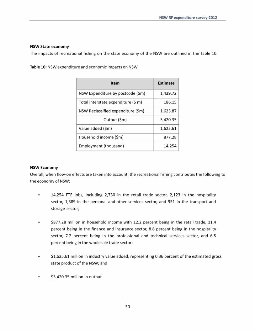
NSW RF expenditure survey‐2012
6 Developing a cost effective approach to expenditure surveys
There have been several reoccurring issues in obtaining information on recreational fishing expenditure
in NSW The first is the lack of a series of expenditure surveys the past ones not occurring as part of an
on‐going consistent strategy The second issue is the lack of a known survey method which is repeatable
and can be compared with past surveys In both of these issues the recurrent cost of such surveys has
been unknown also
61 The objectives of an recreational fishing expenditure survey
Any survey is designed towards its objectives In developing a cost effective regular approach to
recreational fishing expenditure surveys there has to be some design decisions made in respect of the
information required For example A state‐wide expenditure estimate may be required every two years
to track and promote the value of the sector This could include a state‐wide estimate of regional
economic impact Further disaggregation by area or other variables will increase cost
62 Sampling data issues and findings
This study has considered how the use of the RFL database reduced the cost of expenditure surveys
which have traditionally used expensive random screening surveys to locate recreational fishers
Finding 1 The current study has found that there is no statistically significant difference between
seasonal samples Consequently we recommend an annual survey event being mindful of its timing
relative to Christmas January and Easter which may be periods when fishers are not at home
The RFs identified through a random screening survey process were found to make more fishing trips
and fish more days than the sample of RFs contacted through the RFL database (noting that both
samples include licence holders) However in further comparisons of days fished per angler between
licenced and unlicensed fishers no significant difference was found On the other hand unlicensed
fishers were found to undertake significantly more fishing trips than licence holders though this relates
to trip events and not necessarily to higher average expenditure ndash in other words unlicensed fishers
may make more but shorter trips to nearby destinations compared with licensed fishers
Finding 2 The RFL database can be used to sample anglers for expenditure surveys providing certain
conditions are met in terms of the different numbers of licences holders that are sampled17
63 What sample size is required
The size of a sample in statistics is important If the sample is too small there is then the risk that the null
hypothesis is wrongly rejected (ATS 2010) The size of a sample is also related to the probability level at
17 A ratio of 3 day 1 month 1 year and 3 year licence holder records is recommended The weighting would be easier for the annual and 3 year licence holders as 3 day and monthly licence holder can be repeat licence purchasers in a given year
52
NSW RF expenditure survey‐2012
which the variable is seen to be significantly different from zero eg 95 (5) or 99 (1) levels of
significance The dispersion of the distribution of the variable being examined is also important and this
is captured in the standard error of the variable
In statistics these issues are brought together in statistical ldquopower analysisrdquo where the minimum size of
a sample can be tested both prior to and even after statistical surveys to see if the sample size is
adequate ldquoThe power is the probability of detecting an effect presuming it is actually thererdquo (ATS 2010)
Sample size estimation
In this section of the report we investigate how reducing the sample size to the minimum required
number of interviews can reduce the cost of an expenditure survey The decision regarding the target
sample size for the survey has to be balanced between the levels of significance chosen for testing (1
5) and the standard error that is acceptable for the intended variables which is often related to the
estimated value called the relative standard error (RSE) 18
Table 11 shows a range of sample sizes derived for different scenarios using the ABS calculator facility at
NSS (2013) There are the two scenarios for random surveys (cases 1‐4) and two for surveys from a
population base of known participants (case 5‐6)
Table 11 Indication of the required sample sizes under different sampling and risk scenarios including
sampling of the RFL database
Case number 1 2 3 4 5 6 Sample type Random sampling Non random
Statistical input All NSW Population
All NSW Population
All NSW Population
South coast
RFL ‐1 RFL‐2
Confidence Level 99 95 95 95 95 95 Population Size 4996500 4996500 4996500 350750 480700 480700 Proportion 05 05 015 025 06 06 Confidence Interval 005 005 00294 005 005 005
Upper 055 055 01794 03 065 065 Lower 045 045 01206 02 055 055
Standard Error 0025 0025 0015 0025 003 0045 Relative Standard Error () 50 50 100 100 50 75 Sample Size 339 196 567 300 267 119
18 The RSE is the standard error expressed as a percentage of the estimate
53
NSW RF expenditure survey‐2012
In Table 11 cases 1 and 2 show the general sampling results when the confidence level is either 99 or
95 and the proportion is 05 (ie where ldquothe expected proportion of the population to have the
attribute that you are estimating from your surveyrdquo (NSS 2013) These data are often quoted but given
that RFs are more difficult to locate than a one in two assumption (proportion 05) case 3 assumes a
15 proportion for RFs and requires a sample size of 567 with a relative standard error (RSE) of 10
Reducing the sampling area to the South Coast (case 4) raises the chances of locating RFs (proportion
025) and would require 300 observations at an RSE of 10 The sampling model assumes a random
population
We also apply the model to the non‐random scenarios from the RFL data base Here cases 5 and 6 are
RFL records and hence not as random as the whole NSW population We use the model to estimate
possible minimum sample sizes when using the RFL data base population Assuming that the proportion
is 06 an RSE of 5 requires a sample of 267 and an RSE of 75 a sample size of 119 In the experience
of the authors the last sample size (119) is low given the variation in our results We recommend no less
than 250 completed surveys as a minimum sample size for state‐wide estimates If four NSW regions are
included a minimum total of 500 completed surveys would be required and be should be larger if
possible
The review of samples has shown that there is a trade off in accuracy of estimates with the number of
interviews undertaken For example in the case 3 random survey in Table 11 the RSE is 10 and
reducing this to 75 for case 3 would increase the sample size from 576 to 1008 or for 5 to 2226
The incidence of locating RFs has cost implications for surveying and this is why the careful use of the
RFL data base is attractive
Finding 3a A main state‐wide survey using the RFL data base to sample 1000 anglers in major regions is
recommended every 5 years with an option of updating results by indexing annually or bi‐ennially
andor considering a smaller survey (250 state wide or 500 for regions) in year three also
Finding 3b The economic impact analysis can follow the five year survey pattern and can be adjusted
between surveys Simulation modelling can also be used to provide an improved understanding of the
uncertainty surrounding expenditure estimates and may be used to confirm estimates between main
surveys also
64 Discussion ‐ Scoping a recreational fishing expenditure survey strategy for NSW
A recreational fishing expenditure survey strategy would aim to undertake a substantial survey every 5
years and run smaller annual or biennial updating exercises between these periods
In the future the 5 year survey could either
54
NSW RF expenditure survey‐2012
Follow past screening survey approaches of all RFs and compare results with a sample of RFL
holders as in the current study or
Use a weighted selection of 3 day 1 month 1 year and 3 year licence holder contacts to enable
a representative sample to be expanded to state‐wide totals
Before being able to categorically recommend the sole use of the RFL database only approach we would
require more information on the inter‐relationship between the random screening survey and the use of
and RFL data base records The current NSW catch and effort survey study may also provide information
on this relationship (J Murphy DPI pers comm)
As per Finding 2 we recommend further comparisons of the random screening survey approach to all
fishers with use of the RFL holdersrsquo data as in the current study Use of the RFL database alone should
be confirmed by other research on the relationship between all fishers and those who are licensed
In the years between the five year main surveys the survey results from the initial survey could be
upgraded annually (or bi‐ennially) by sampling several variables that could be used to index the changes
in the state wide expenditure estimates For example any changes detected in RF participation or
activity state population or change in licence sales could inform activity estimates Information on
recreational fishing expenditure could be influenced by annual changes in price levels as measured by
the consumer price index (cpi) and any information available from industry about retail fishing gear
prices such as those related to exchange rate variations which would impact expenditure on fishing
gear Many of these indices of economic conditions are monitored by the Australian Fishing Tackle
Association and could be referred to
The simulation modelling approach used in the current study could be re‐run annuallybiennially with
these activity and expenditure indices included and updated annual estimates produced The
reoccurrence of another survey in year 5 means there would be a cross check on the indexing of the
previous survey
The choice of 5 years for the main survey is arbitrary and could be 3 years particularly if other catch and
effort surveys are indicating significant changes in participation rates in NSW or there is evidence of
changes in other states Leaving a main survey for more than 5 years is not recommended as the public
awareness of the sectorrsquos economic contribution and associated regional benefits will reduce giving the
sector less public profile
65 Conclusions
The recreational fishing sector in NSW wishes to have more regular studies of angler expenditure and its
importance to the economy The RFL data base can be used for sampling the recreational fishing
population reducing the costs of fieldwork surveys if several conditions are followed The frequency of
55
NSW RF expenditure survey‐2012
the different licence durations needs to be chosen so as not to move away from sampling a
representative cross section of anglers of all different activity levels and possibly having over or under
emphasis of avid anglers
A main state‐wide survey using the RFL data base to sample 1000 anglers in major regions is
recommended every 5 years with an option of updating results by indexing annually or bi‐ennially and
considering a smaller survey (250 state wide or 500 for regions) in year three also The economic impact
analysis can follow the five year survey pattern and can be adjusted between surveys Simulation
modelling can also be used to provide an improved understanding of the uncertainty surrounding
expenditure estimates and may be used to confirm estimates between main surveys also
56
NSW RF expenditure survey‐2012
References
ABARES (2011) Australian Fisheries Statistics 2010 Australian Bureau of Agricultural and Resource Economics and
Sciences Australian Government p 100
ABS (2010) 1216055003 ‐ Australian Statistical Geography Standard Design of the Statistical Areas Level 4
Capital Cities and Statistical Areas Level 3 May 2010 Canberra
ABS (2011) 13381 NSW State and Regional Indicators December 2010
ABS (2012) Estimated Resident Population for New South Wales by Age by Statistical Geography Persons ndash 30
June 2011 Population by Age and Sex Regions of Australia 32350 Canberra
ACMA (2013) Convergence and Communications Report 1 Australian household consumersrsquo take‐up and use of
voice communications services Australian Communication and Media Authority report November
ATS (2010) Introduction to Power Analysis Statistical Computing Seminars
httpwwwatsuclaedustatseminarsintro_powerdefaulthtm
Campbell D and JJ Murphy (2005) The 2000‐01 National Recreational Fishing Survey Economic Report
Department of Agriculture Fisheries and Forestry GPO Box 858 Canberra ACT 2601 June
Cunningham S Dunn MR and Whitmarsh D (1985) Fisheries Economics An Introduction Mansell Publishing
London
Dominion (2001) ldquoAn economic survey of the Snowy mountain recreational trout fisheryrdquo A report by Dominion
Consulting Pty Ltd to the Freshwater Recreational Fishing Trust NSW Fisheries
Dominion (2002) ldquoNational Recreational Fishing Tackle Industry survey of the retail and wholesale sectorsrdquo A report by Dominion Consulting Pty Ltd Client Australian Fishing Tackle Association
Dominion (2003) ldquoIdentifying the recreational fishing expenditure patterns of Sydneyrsquos recreational fishers and its economic importance in regional communities of NSWrdquo Research project in conjunction with Roy Morgan Research A report by Dominion Consulting Pty Ltd for Recreational Fishing Trust NSW Fisheries
Dominion (2004) ldquoNational Recreational Fishing Tackle Industry survey of the retail and wholesale sectorsrdquo A report by Dominion Consulting Pty Ltd Client Australian Fishing Tackle Association
Dominion (in prep) An Economic Survey of the NSW Charter Boat industry NSW Recreational Trust Fund Project
Ernst amp Young (2009) An economic study of recreational fishing in Victoria A report to VRFISH Melbourne
Victoria
Ernst amp Young (2011) Economic contribution of Recreational Fishing in the Murray Darling Basin A report to
Victorian Department of Primary Industries Melbourne Victoria
Galeano D Langenkamp D Levantis C Shafron W and Redmond I (2004) Economic Value of Charter and
Recreational Fishing in Australiarsquos Eastern Tuna and Billfish Fishery ABARE eReport 0410 Canberra July
57
NSW RF expenditure survey‐2012
Gentner B (2008) Exploring survey methodologies for collecting recreational angler expenditure data International Institute of Fisheries Economics and Trade (IIFET) 2008 Vietnam Proceedings
Gentner B and S Steinback (2008) The Economic Contribution of Marine Angler Expenditures in the United States 2006 US Dep Commerce NOAA Tech Memo NMFSF SPO‐94 301 p
Henry G W and JM Lyle (2003) The National Recreational and Indigenous Fishing Survey Fisheries Research and Development Corporation (FRDC) project no 99158
IBM Corp (2012) IBM SPSS Statistics for Windows Version 210 Armonk NY IBM Corp
Jones K (2009) South Australia Recreational Fishing Survey 2007‐2008 In South Australian Fisheries Management Series Paper No 54 (Fisheries Division PIRSA) p 84
McIlgorm A and J Pepperell (1999) A National Review of the Recreational Fishing Sector A report by Dominion Consulting to Agriculture Forestry and Fisheries Australia
McIlgorm A A Macfarlane and J Pepperell (2005) ldquoThe importance of recreational fishing expenditure to the economies of two coastal towns in northern and southern NSW Port Macquarie and Bermaguirdquo A report by Dominion Consulting Pty Ltd for the Recreational Fishing Trust Fund NSW Fisheries March 2005
Mohadjer L B Bell and J Waksberg (1994) Accounting for Item Nonresponse Bias‐ National Health and Nutrition Examination Survey iii Prepared for National Centre for Health Statistics Maryland by Westat Inc November
NSS (2013) National Statistics Service‐ httpwwwnssgovaunsshomeNSFpagesSample+size+calculator
NOAA (2011) ldquoNOAA begins National Survey of the economic contributions of saltwater anglingrdquo
httpwwwnoaanewsnoaagovstories201120110222_saltwateranglinghtml (22nd Feb 2011)
NOAA (2012) ldquoRecreational Fisheries Year in Review 2012rdquo National Oceanic and Atmospheric Administration
National Marine Fisheries Service Department of Commerce
Ritz W (2013) Non‐Response Bias in Survey Sampling httpwwwtrchomecomwhite‐paper‐librarywpl‐all‐white‐papers215
Rolfe J amp Prayaga P (2007) Estimating values for recreational fishing at freshwater dams in Queensland Australian Journal of Agricultural and Resource Economics 51 157‐174
Steinback S B Gentner and J Castle (2004) ldquoThe economic importance of marine angler expenditures in the United Statesrdquo NOAA Professional Paper NMFS 2 169 p
Taylor S J Webley K McInnes (2011) The 2010 State‐wide Recreational Fishing Survey State of Queensland
Department of Agriculture Fisheries and Forestry 2012
Thomson CJ (1991) Effects of Avidity Bias on Survey Estimates of Fishing Effort and Economic Values American
Fisheries Society Symposium 12356‐366
West L D Lyle J M Matthews S R Stark K E amp Steffe A S (2012) Survey of recreational fishing in the Northern Territory 200910 Northern Territory Fisheries Department of Resources Northern Territory p128
WRI (2013) Measuring the Economic Contribution of the Recreational Fishing sector in NSW A report to ANCORS University of Wollongong by The Western Research Institute Bathurst NSW p21
58
NSW RF expenditure survey‐2012
Appendix 1 What determines recreational fisher expenditure in NSW
Linear multiple regression was used to determine the variables which are statistically significant in
determining total expenditure trip expenditures tackle expenditure and boat expenditure A range of
variables available from the interviews such as licence holder age regional location situation
household and malefemale were able to be tested for their statistical significance in relation to RF
expenditures
Total expenditure
The significant determinants of total expenditure were found to be income trips per annum and
licensed fishers who have a marginally greater total spend that unlicensed fishers Trips in SW were a
significantly higher contributor to total expenditure than days fished in FW probably related to higher
capital boat expenditure by marine fishers Licensed fishers who are generally in the workforce were
found to have marginally greater total expenditure than unlicensed fishers but only at a 10 level of
significance (see A1‐Table 1) Other variables such as age region situation household and malefemale
were not significantly different from zero at the 5 level of significance
A1‐ Table 1 Regressions results for Total Expenditure
Coefficientsa
Model Unstandardized Coefficients Standardized
Coefficients
t Sig
B Std Error Beta
1
(Constant)
LIC10
swtrips
income
-1137559
558821
43064
332455
475354
314755
12240
73522
050
099
128
-2393
1775
3518
4522
017
076
000
000
a Dependent Variable TOTALEXP
Trip expenditure
Determinants of total trip expenditure were found to be number of SW trips per annum with licence
holders spending more on trips (see A1‐Table 2a) were not significantly different from zero at the 5
level of significance
59
NSW RF expenditure survey‐2012
A1‐ Table 2a Regressions results for Trip Expenditure Coefficientsa
Model Unstandardized Coefficients Standardized
Coefficients
t Sig
B Std Error Beta
1
(Constant)
LIC10
swtrips
953678
623065
36235
185885
232860
9133
076
113
5130
2676
3967
000
008
000
a Dependent Variable TRIPSPEND
The trip expense will also be related to the days fished which is correlated with the number of trips
taken annually In A1‐Table 2b the model was altered to include days fished and kilometres travelled
Days fished in SW and FW the number of kilometres travelled and being a licence holder were all
significant variables in determining trip expenditure
A1‐ Table 2b Regressions results for Trip Expenditure with SW and FW days fished Coefficientsa
Model Unstandardized Coefficients Standardized
Coefficients
t Sig
B Std Error Beta
1
(Constant)
LIC10
SWDAYS
FWDAY
kmsa
151158
599485
83015
50750
2109
190606
223599
7460
14523
1034
073
304
096
057
793
2681
11128
3494
2039
428
007
000
000
042
a Dependent Variable TRIPSPEND
This result is a reminder of the significant expenditure made by many anglers on road travel
Tackle expenditure
Regression results reveal that Tackle expenditure is determined primarily by household income levels
(see A1‐Table 3) Other variables such as age licencing region freshwater days family situation
household and malefemale were not significantly different from zero at the 5 level of significance
A1‐ Table 3 Regressions results for Tackle Expenditure Coefficientsa
Model Unstandardized Coefficients Standardized
Coefficients
t Sig
B Std Error Beta
1 (Constant)
income
39960
17264
26312
4263 115
1519
4049
129
000
a Dependent Variable Total Tackle
60
NSW RF expenditure survey‐2012
Boat capital expenditure
The regressions show that number of SW trips and household income levels are the determinants of
Boat capital expenditure (A1‐ Table 4) other variables not being significantly different from zero
A1‐ Table 4 Regressions results for Boat Capital Expenditure
Coefficientsa
Model Unstandardized Coefficients Standardized
Coefficients
t Sig
B Std Error Beta
1
(Constant)
swtrips
income
-1175462
44403
309987
444221
11767
70336
106
124
-2646
3774
4407
008
000
000
a Dependent Variable TOTALCAP
61
NSW RF expenditure survey‐2012
Appendix 2 Socio‐ economic groups and RFs in NSW ndash a cluster analysis
Cluster analysis enables researchers to let the data determine how many statistically significant groups
(called ldquoclustersrdquo) there are in the given data set In the previous regressions we found that income19
and SW days fished were significant in predicting angler expenditure Cluster analysis can show r
patterns among groups of RFs in NSW Labels to characterise groups have been added
Total expenditure
A2‐Figure 1 RF Clusters in total expenditure
19 Household income is in the following numerical bands 1‐Under $20000 2‐ $20000 to $29999 3‐$30000 to $39999 4‐$40000 to $59999 5‐$60000 to $79999 6‐$80000 to $99999 7‐ $100000 to $119999 8‐ $120000 to $140000 9‐ $140000+
62
NSW RF expenditure survey‐2012
In A2‐Figure 1 the cluster analysis of the data shows that total expenditure has income and trips per
annum as strongest predictor of total expenditure but there are 4 statistically significant clusters as
described The authors have added a label to describe the group characteristics which are given in the
description
Trip expenditure
A2‐Figure 2 RF Clusters in trip expenditure
Trips and secondly income are the strongest predictors of trip expenditure Examining trip expenditure
leads to 4 distinct clusters We see clusters 2 and 3 (182) have high trip expenditures Some 818 of
the population have low trip expenditure with one low income (ldquobattlersrdquo) and one higher income
group (ldquoFishing break anglersrdquo)
63
NSW RF expenditure survey‐2012
Tackle expenditure
Tackle expenditure is most strongly predicted by income and is less trip related than expected There is a
cluster of 4 of higher income fishers who have very high tackle expenditure (ldquoTackle addictsrdquo)
A2‐Figure 3 RF Clusters in tackle expenditure
Tackle expenditure forms into 4 clusters with 852 of fishers fishing few trips and spending low
amounts on tackle irrespective of income
64
NSW RF expenditure survey‐2012
Capital boat expenditure
In A2 Figure 4 firstly trips and then secondly income are the strongest predictors of expenditure on
boats The highest boat expenditure is associated with 23 of fishers doing many trips but also with
the 138 of dedicated fishers
A2‐Figure 4 RF Clusters in capital boat expenditure
65
- Structure Bookmarks
-
- Project Developing a cost effective state wide expenditure survey method to measure the economic contribution of the recreational fishing sector in NSW
- Final Report to the NSW Recreational Fishing Licence Trust NSW Department of Primary Industry November 2013
-
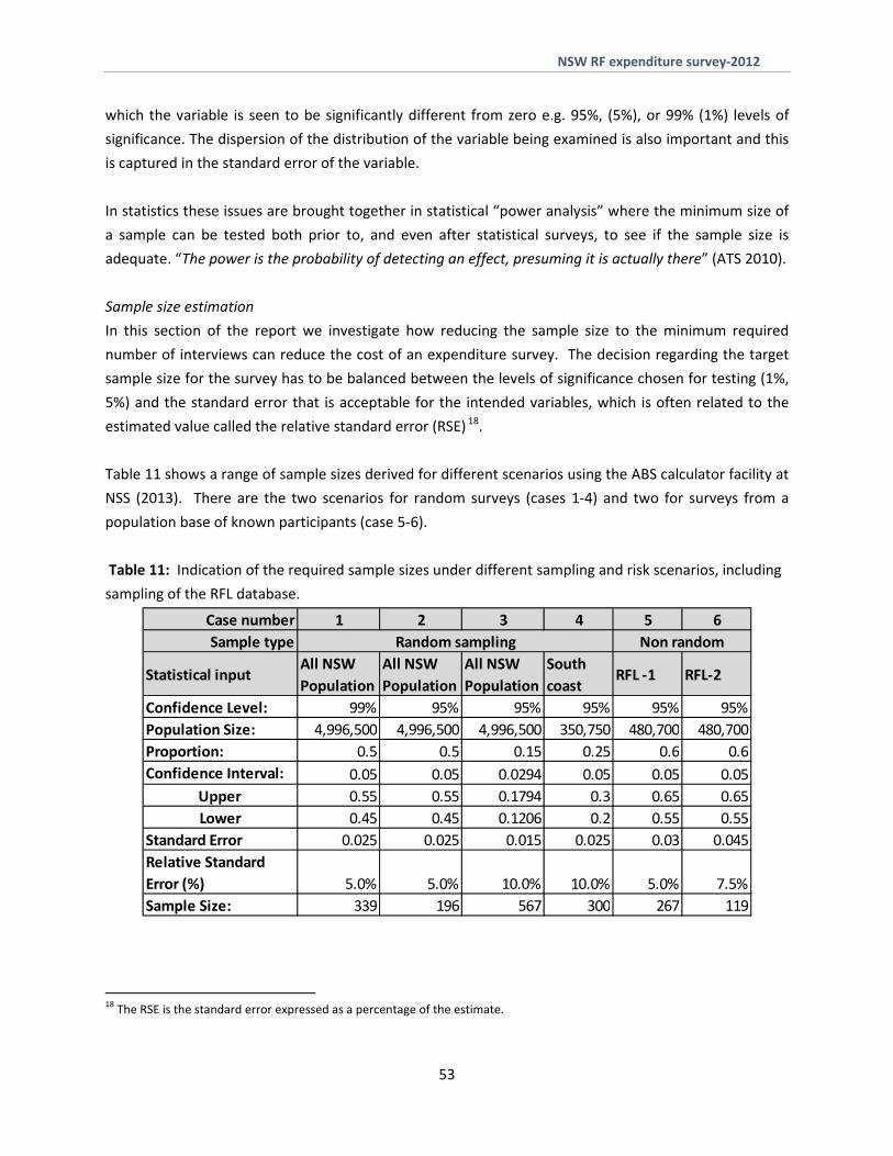
NSW RF expenditure survey‐2012
References
ABARES (2011) Australian Fisheries Statistics 2010 Australian Bureau of Agricultural and Resource Economics and
Sciences Australian Government p 100
ABS (2010) 1216055003 ‐ Australian Statistical Geography Standard Design of the Statistical Areas Level 4
Capital Cities and Statistical Areas Level 3 May 2010 Canberra
ABS (2011) 13381 NSW State and Regional Indicators December 2010
ABS (2012) Estimated Resident Population for New South Wales by Age by Statistical Geography Persons ndash 30
June 2011 Population by Age and Sex Regions of Australia 32350 Canberra
ACMA (2013) Convergence and Communications Report 1 Australian household consumersrsquo take‐up and use of
voice communications services Australian Communication and Media Authority report November
ATS (2010) Introduction to Power Analysis Statistical Computing Seminars
httpwwwatsuclaedustatseminarsintro_powerdefaulthtm
Campbell D and JJ Murphy (2005) The 2000‐01 National Recreational Fishing Survey Economic Report
Department of Agriculture Fisheries and Forestry GPO Box 858 Canberra ACT 2601 June
Cunningham S Dunn MR and Whitmarsh D (1985) Fisheries Economics An Introduction Mansell Publishing
London
Dominion (2001) ldquoAn economic survey of the Snowy mountain recreational trout fisheryrdquo A report by Dominion
Consulting Pty Ltd to the Freshwater Recreational Fishing Trust NSW Fisheries
Dominion (2002) ldquoNational Recreational Fishing Tackle Industry survey of the retail and wholesale sectorsrdquo A report by Dominion Consulting Pty Ltd Client Australian Fishing Tackle Association
Dominion (2003) ldquoIdentifying the recreational fishing expenditure patterns of Sydneyrsquos recreational fishers and its economic importance in regional communities of NSWrdquo Research project in conjunction with Roy Morgan Research A report by Dominion Consulting Pty Ltd for Recreational Fishing Trust NSW Fisheries
Dominion (2004) ldquoNational Recreational Fishing Tackle Industry survey of the retail and wholesale sectorsrdquo A report by Dominion Consulting Pty Ltd Client Australian Fishing Tackle Association
Dominion (in prep) An Economic Survey of the NSW Charter Boat industry NSW Recreational Trust Fund Project
Ernst amp Young (2009) An economic study of recreational fishing in Victoria A report to VRFISH Melbourne
Victoria
Ernst amp Young (2011) Economic contribution of Recreational Fishing in the Murray Darling Basin A report to
Victorian Department of Primary Industries Melbourne Victoria
Galeano D Langenkamp D Levantis C Shafron W and Redmond I (2004) Economic Value of Charter and
Recreational Fishing in Australiarsquos Eastern Tuna and Billfish Fishery ABARE eReport 0410 Canberra July
57
NSW RF expenditure survey‐2012
Gentner B (2008) Exploring survey methodologies for collecting recreational angler expenditure data International Institute of Fisheries Economics and Trade (IIFET) 2008 Vietnam Proceedings
Gentner B and S Steinback (2008) The Economic Contribution of Marine Angler Expenditures in the United States 2006 US Dep Commerce NOAA Tech Memo NMFSF SPO‐94 301 p
Henry G W and JM Lyle (2003) The National Recreational and Indigenous Fishing Survey Fisheries Research and Development Corporation (FRDC) project no 99158
IBM Corp (2012) IBM SPSS Statistics for Windows Version 210 Armonk NY IBM Corp
Jones K (2009) South Australia Recreational Fishing Survey 2007‐2008 In South Australian Fisheries Management Series Paper No 54 (Fisheries Division PIRSA) p 84
McIlgorm A and J Pepperell (1999) A National Review of the Recreational Fishing Sector A report by Dominion Consulting to Agriculture Forestry and Fisheries Australia
McIlgorm A A Macfarlane and J Pepperell (2005) ldquoThe importance of recreational fishing expenditure to the economies of two coastal towns in northern and southern NSW Port Macquarie and Bermaguirdquo A report by Dominion Consulting Pty Ltd for the Recreational Fishing Trust Fund NSW Fisheries March 2005
Mohadjer L B Bell and J Waksberg (1994) Accounting for Item Nonresponse Bias‐ National Health and Nutrition Examination Survey iii Prepared for National Centre for Health Statistics Maryland by Westat Inc November
NSS (2013) National Statistics Service‐ httpwwwnssgovaunsshomeNSFpagesSample+size+calculator
NOAA (2011) ldquoNOAA begins National Survey of the economic contributions of saltwater anglingrdquo
httpwwwnoaanewsnoaagovstories201120110222_saltwateranglinghtml (22nd Feb 2011)
NOAA (2012) ldquoRecreational Fisheries Year in Review 2012rdquo National Oceanic and Atmospheric Administration
National Marine Fisheries Service Department of Commerce
Ritz W (2013) Non‐Response Bias in Survey Sampling httpwwwtrchomecomwhite‐paper‐librarywpl‐all‐white‐papers215
Rolfe J amp Prayaga P (2007) Estimating values for recreational fishing at freshwater dams in Queensland Australian Journal of Agricultural and Resource Economics 51 157‐174
Steinback S B Gentner and J Castle (2004) ldquoThe economic importance of marine angler expenditures in the United Statesrdquo NOAA Professional Paper NMFS 2 169 p
Taylor S J Webley K McInnes (2011) The 2010 State‐wide Recreational Fishing Survey State of Queensland
Department of Agriculture Fisheries and Forestry 2012
Thomson CJ (1991) Effects of Avidity Bias on Survey Estimates of Fishing Effort and Economic Values American
Fisheries Society Symposium 12356‐366
West L D Lyle J M Matthews S R Stark K E amp Steffe A S (2012) Survey of recreational fishing in the Northern Territory 200910 Northern Territory Fisheries Department of Resources Northern Territory p128
WRI (2013) Measuring the Economic Contribution of the Recreational Fishing sector in NSW A report to ANCORS University of Wollongong by The Western Research Institute Bathurst NSW p21
58
NSW RF expenditure survey‐2012
Appendix 1 What determines recreational fisher expenditure in NSW
Linear multiple regression was used to determine the variables which are statistically significant in
determining total expenditure trip expenditures tackle expenditure and boat expenditure A range of
variables available from the interviews such as licence holder age regional location situation
household and malefemale were able to be tested for their statistical significance in relation to RF
expenditures
Total expenditure
The significant determinants of total expenditure were found to be income trips per annum and
licensed fishers who have a marginally greater total spend that unlicensed fishers Trips in SW were a
significantly higher contributor to total expenditure than days fished in FW probably related to higher
capital boat expenditure by marine fishers Licensed fishers who are generally in the workforce were
found to have marginally greater total expenditure than unlicensed fishers but only at a 10 level of
significance (see A1‐Table 1) Other variables such as age region situation household and malefemale
were not significantly different from zero at the 5 level of significance
A1‐ Table 1 Regressions results for Total Expenditure
Coefficientsa
Model Unstandardized Coefficients Standardized
Coefficients
t Sig
B Std Error Beta
1
(Constant)
LIC10
swtrips
income
-1137559
558821
43064
332455
475354
314755
12240
73522
050
099
128
-2393
1775
3518
4522
017
076
000
000
a Dependent Variable TOTALEXP
Trip expenditure
Determinants of total trip expenditure were found to be number of SW trips per annum with licence
holders spending more on trips (see A1‐Table 2a) were not significantly different from zero at the 5
level of significance
59
NSW RF expenditure survey‐2012
A1‐ Table 2a Regressions results for Trip Expenditure Coefficientsa
Model Unstandardized Coefficients Standardized
Coefficients
t Sig
B Std Error Beta
1
(Constant)
LIC10
swtrips
953678
623065
36235
185885
232860
9133
076
113
5130
2676
3967
000
008
000
a Dependent Variable TRIPSPEND
The trip expense will also be related to the days fished which is correlated with the number of trips
taken annually In A1‐Table 2b the model was altered to include days fished and kilometres travelled
Days fished in SW and FW the number of kilometres travelled and being a licence holder were all
significant variables in determining trip expenditure
A1‐ Table 2b Regressions results for Trip Expenditure with SW and FW days fished Coefficientsa
Model Unstandardized Coefficients Standardized
Coefficients
t Sig
B Std Error Beta
1
(Constant)
LIC10
SWDAYS
FWDAY
kmsa
151158
599485
83015
50750
2109
190606
223599
7460
14523
1034
073
304
096
057
793
2681
11128
3494
2039
428
007
000
000
042
a Dependent Variable TRIPSPEND
This result is a reminder of the significant expenditure made by many anglers on road travel
Tackle expenditure
Regression results reveal that Tackle expenditure is determined primarily by household income levels
(see A1‐Table 3) Other variables such as age licencing region freshwater days family situation
household and malefemale were not significantly different from zero at the 5 level of significance
A1‐ Table 3 Regressions results for Tackle Expenditure Coefficientsa
Model Unstandardized Coefficients Standardized
Coefficients
t Sig
B Std Error Beta
1 (Constant)
income
39960
17264
26312
4263 115
1519
4049
129
000
a Dependent Variable Total Tackle
60
NSW RF expenditure survey‐2012
Boat capital expenditure
The regressions show that number of SW trips and household income levels are the determinants of
Boat capital expenditure (A1‐ Table 4) other variables not being significantly different from zero
A1‐ Table 4 Regressions results for Boat Capital Expenditure
Coefficientsa
Model Unstandardized Coefficients Standardized
Coefficients
t Sig
B Std Error Beta
1
(Constant)
swtrips
income
-1175462
44403
309987
444221
11767
70336
106
124
-2646
3774
4407
008
000
000
a Dependent Variable TOTALCAP
61
NSW RF expenditure survey‐2012
Appendix 2 Socio‐ economic groups and RFs in NSW ndash a cluster analysis
Cluster analysis enables researchers to let the data determine how many statistically significant groups
(called ldquoclustersrdquo) there are in the given data set In the previous regressions we found that income19
and SW days fished were significant in predicting angler expenditure Cluster analysis can show r
patterns among groups of RFs in NSW Labels to characterise groups have been added
Total expenditure
A2‐Figure 1 RF Clusters in total expenditure
19 Household income is in the following numerical bands 1‐Under $20000 2‐ $20000 to $29999 3‐$30000 to $39999 4‐$40000 to $59999 5‐$60000 to $79999 6‐$80000 to $99999 7‐ $100000 to $119999 8‐ $120000 to $140000 9‐ $140000+
62
NSW RF expenditure survey‐2012
In A2‐Figure 1 the cluster analysis of the data shows that total expenditure has income and trips per
annum as strongest predictor of total expenditure but there are 4 statistically significant clusters as
described The authors have added a label to describe the group characteristics which are given in the
description
Trip expenditure
A2‐Figure 2 RF Clusters in trip expenditure
Trips and secondly income are the strongest predictors of trip expenditure Examining trip expenditure
leads to 4 distinct clusters We see clusters 2 and 3 (182) have high trip expenditures Some 818 of
the population have low trip expenditure with one low income (ldquobattlersrdquo) and one higher income
group (ldquoFishing break anglersrdquo)
63
NSW RF expenditure survey‐2012
Tackle expenditure
Tackle expenditure is most strongly predicted by income and is less trip related than expected There is a
cluster of 4 of higher income fishers who have very high tackle expenditure (ldquoTackle addictsrdquo)
A2‐Figure 3 RF Clusters in tackle expenditure
Tackle expenditure forms into 4 clusters with 852 of fishers fishing few trips and spending low
amounts on tackle irrespective of income
64
NSW RF expenditure survey‐2012
Capital boat expenditure
In A2 Figure 4 firstly trips and then secondly income are the strongest predictors of expenditure on
boats The highest boat expenditure is associated with 23 of fishers doing many trips but also with
the 138 of dedicated fishers
A2‐Figure 4 RF Clusters in capital boat expenditure
65
- Structure Bookmarks
-
- Project Developing a cost effective state wide expenditure survey method to measure the economic contribution of the recreational fishing sector in NSW
- Final Report to the NSW Recreational Fishing Licence Trust NSW Department of Primary Industry November 2013
-
NSW RF expenditure survey‐2012
Gentner B (2008) Exploring survey methodologies for collecting recreational angler expenditure data International Institute of Fisheries Economics and Trade (IIFET) 2008 Vietnam Proceedings
Gentner B and S Steinback (2008) The Economic Contribution of Marine Angler Expenditures in the United States 2006 US Dep Commerce NOAA Tech Memo NMFSF SPO‐94 301 p
Henry G W and JM Lyle (2003) The National Recreational and Indigenous Fishing Survey Fisheries Research and Development Corporation (FRDC) project no 99158
IBM Corp (2012) IBM SPSS Statistics for Windows Version 210 Armonk NY IBM Corp
Jones K (2009) South Australia Recreational Fishing Survey 2007‐2008 In South Australian Fisheries Management Series Paper No 54 (Fisheries Division PIRSA) p 84
McIlgorm A and J Pepperell (1999) A National Review of the Recreational Fishing Sector A report by Dominion Consulting to Agriculture Forestry and Fisheries Australia
McIlgorm A A Macfarlane and J Pepperell (2005) ldquoThe importance of recreational fishing expenditure to the economies of two coastal towns in northern and southern NSW Port Macquarie and Bermaguirdquo A report by Dominion Consulting Pty Ltd for the Recreational Fishing Trust Fund NSW Fisheries March 2005
Mohadjer L B Bell and J Waksberg (1994) Accounting for Item Nonresponse Bias‐ National Health and Nutrition Examination Survey iii Prepared for National Centre for Health Statistics Maryland by Westat Inc November
NSS (2013) National Statistics Service‐ httpwwwnssgovaunsshomeNSFpagesSample+size+calculator
NOAA (2011) ldquoNOAA begins National Survey of the economic contributions of saltwater anglingrdquo
httpwwwnoaanewsnoaagovstories201120110222_saltwateranglinghtml (22nd Feb 2011)
NOAA (2012) ldquoRecreational Fisheries Year in Review 2012rdquo National Oceanic and Atmospheric Administration
National Marine Fisheries Service Department of Commerce
Ritz W (2013) Non‐Response Bias in Survey Sampling httpwwwtrchomecomwhite‐paper‐librarywpl‐all‐white‐papers215
Rolfe J amp Prayaga P (2007) Estimating values for recreational fishing at freshwater dams in Queensland Australian Journal of Agricultural and Resource Economics 51 157‐174
Steinback S B Gentner and J Castle (2004) ldquoThe economic importance of marine angler expenditures in the United Statesrdquo NOAA Professional Paper NMFS 2 169 p
Taylor S J Webley K McInnes (2011) The 2010 State‐wide Recreational Fishing Survey State of Queensland
Department of Agriculture Fisheries and Forestry 2012
Thomson CJ (1991) Effects of Avidity Bias on Survey Estimates of Fishing Effort and Economic Values American
Fisheries Society Symposium 12356‐366
West L D Lyle J M Matthews S R Stark K E amp Steffe A S (2012) Survey of recreational fishing in the Northern Territory 200910 Northern Territory Fisheries Department of Resources Northern Territory p128
WRI (2013) Measuring the Economic Contribution of the Recreational Fishing sector in NSW A report to ANCORS University of Wollongong by The Western Research Institute Bathurst NSW p21
58
NSW RF expenditure survey‐2012
Appendix 1 What determines recreational fisher expenditure in NSW
Linear multiple regression was used to determine the variables which are statistically significant in
determining total expenditure trip expenditures tackle expenditure and boat expenditure A range of
variables available from the interviews such as licence holder age regional location situation
household and malefemale were able to be tested for their statistical significance in relation to RF
expenditures
Total expenditure
The significant determinants of total expenditure were found to be income trips per annum and
licensed fishers who have a marginally greater total spend that unlicensed fishers Trips in SW were a
significantly higher contributor to total expenditure than days fished in FW probably related to higher
capital boat expenditure by marine fishers Licensed fishers who are generally in the workforce were
found to have marginally greater total expenditure than unlicensed fishers but only at a 10 level of
significance (see A1‐Table 1) Other variables such as age region situation household and malefemale
were not significantly different from zero at the 5 level of significance
A1‐ Table 1 Regressions results for Total Expenditure
Coefficientsa
Model Unstandardized Coefficients Standardized
Coefficients
t Sig
B Std Error Beta
1
(Constant)
LIC10
swtrips
income
-1137559
558821
43064
332455
475354
314755
12240
73522
050
099
128
-2393
1775
3518
4522
017
076
000
000
a Dependent Variable TOTALEXP
Trip expenditure
Determinants of total trip expenditure were found to be number of SW trips per annum with licence
holders spending more on trips (see A1‐Table 2a) were not significantly different from zero at the 5
level of significance
59
NSW RF expenditure survey‐2012
A1‐ Table 2a Regressions results for Trip Expenditure Coefficientsa
Model Unstandardized Coefficients Standardized
Coefficients
t Sig
B Std Error Beta
1
(Constant)
LIC10
swtrips
953678
623065
36235
185885
232860
9133
076
113
5130
2676
3967
000
008
000
a Dependent Variable TRIPSPEND
The trip expense will also be related to the days fished which is correlated with the number of trips
taken annually In A1‐Table 2b the model was altered to include days fished and kilometres travelled
Days fished in SW and FW the number of kilometres travelled and being a licence holder were all
significant variables in determining trip expenditure
A1‐ Table 2b Regressions results for Trip Expenditure with SW and FW days fished Coefficientsa
Model Unstandardized Coefficients Standardized
Coefficients
t Sig
B Std Error Beta
1
(Constant)
LIC10
SWDAYS
FWDAY
kmsa
151158
599485
83015
50750
2109
190606
223599
7460
14523
1034
073
304
096
057
793
2681
11128
3494
2039
428
007
000
000
042
a Dependent Variable TRIPSPEND
This result is a reminder of the significant expenditure made by many anglers on road travel
Tackle expenditure
Regression results reveal that Tackle expenditure is determined primarily by household income levels
(see A1‐Table 3) Other variables such as age licencing region freshwater days family situation
household and malefemale were not significantly different from zero at the 5 level of significance
A1‐ Table 3 Regressions results for Tackle Expenditure Coefficientsa
Model Unstandardized Coefficients Standardized
Coefficients
t Sig
B Std Error Beta
1 (Constant)
income
39960
17264
26312
4263 115
1519
4049
129
000
a Dependent Variable Total Tackle
60
NSW RF expenditure survey‐2012
Boat capital expenditure
The regressions show that number of SW trips and household income levels are the determinants of
Boat capital expenditure (A1‐ Table 4) other variables not being significantly different from zero
A1‐ Table 4 Regressions results for Boat Capital Expenditure
Coefficientsa
Model Unstandardized Coefficients Standardized
Coefficients
t Sig
B Std Error Beta
1
(Constant)
swtrips
income
-1175462
44403
309987
444221
11767
70336
106
124
-2646
3774
4407
008
000
000
a Dependent Variable TOTALCAP
61
NSW RF expenditure survey‐2012
Appendix 2 Socio‐ economic groups and RFs in NSW ndash a cluster analysis
Cluster analysis enables researchers to let the data determine how many statistically significant groups
(called ldquoclustersrdquo) there are in the given data set In the previous regressions we found that income19
and SW days fished were significant in predicting angler expenditure Cluster analysis can show r
patterns among groups of RFs in NSW Labels to characterise groups have been added
Total expenditure
A2‐Figure 1 RF Clusters in total expenditure
19 Household income is in the following numerical bands 1‐Under $20000 2‐ $20000 to $29999 3‐$30000 to $39999 4‐$40000 to $59999 5‐$60000 to $79999 6‐$80000 to $99999 7‐ $100000 to $119999 8‐ $120000 to $140000 9‐ $140000+
62
NSW RF expenditure survey‐2012
In A2‐Figure 1 the cluster analysis of the data shows that total expenditure has income and trips per
annum as strongest predictor of total expenditure but there are 4 statistically significant clusters as
described The authors have added a label to describe the group characteristics which are given in the
description
Trip expenditure
A2‐Figure 2 RF Clusters in trip expenditure
Trips and secondly income are the strongest predictors of trip expenditure Examining trip expenditure
leads to 4 distinct clusters We see clusters 2 and 3 (182) have high trip expenditures Some 818 of
the population have low trip expenditure with one low income (ldquobattlersrdquo) and one higher income
group (ldquoFishing break anglersrdquo)
63
NSW RF expenditure survey‐2012
Tackle expenditure
Tackle expenditure is most strongly predicted by income and is less trip related than expected There is a
cluster of 4 of higher income fishers who have very high tackle expenditure (ldquoTackle addictsrdquo)
A2‐Figure 3 RF Clusters in tackle expenditure
Tackle expenditure forms into 4 clusters with 852 of fishers fishing few trips and spending low
amounts on tackle irrespective of income
64
NSW RF expenditure survey‐2012
Capital boat expenditure
In A2 Figure 4 firstly trips and then secondly income are the strongest predictors of expenditure on
boats The highest boat expenditure is associated with 23 of fishers doing many trips but also with
the 138 of dedicated fishers
A2‐Figure 4 RF Clusters in capital boat expenditure
65
- Structure Bookmarks
-
- Project Developing a cost effective state wide expenditure survey method to measure the economic contribution of the recreational fishing sector in NSW
- Final Report to the NSW Recreational Fishing Licence Trust NSW Department of Primary Industry November 2013
-

NSW RF expenditure survey‐2012
A1‐ Table 2a Regressions results for Trip Expenditure Coefficientsa
Model Unstandardized Coefficients Standardized
Coefficients
t Sig
B Std Error Beta
1
(Constant)
LIC10
swtrips
953678
623065
36235
185885
232860
9133
076
113
5130
2676
3967
000
008
000
a Dependent Variable TRIPSPEND
The trip expense will also be related to the days fished which is correlated with the number of trips
taken annually In A1‐Table 2b the model was altered to include days fished and kilometres travelled
Days fished in SW and FW the number of kilometres travelled and being a licence holder were all
significant variables in determining trip expenditure
A1‐ Table 2b Regressions results for Trip Expenditure with SW and FW days fished Coefficientsa
Model Unstandardized Coefficients Standardized
Coefficients
t Sig
B Std Error Beta
1
(Constant)
LIC10
SWDAYS
FWDAY
kmsa
151158
599485
83015
50750
2109
190606
223599
7460
14523
1034
073
304
096
057
793
2681
11128
3494
2039
428
007
000
000
042
a Dependent Variable TRIPSPEND
This result is a reminder of the significant expenditure made by many anglers on road travel
Tackle expenditure
Regression results reveal that Tackle expenditure is determined primarily by household income levels
(see A1‐Table 3) Other variables such as age licencing region freshwater days family situation
household and malefemale were not significantly different from zero at the 5 level of significance
A1‐ Table 3 Regressions results for Tackle Expenditure Coefficientsa
Model Unstandardized Coefficients Standardized
Coefficients
t Sig
B Std Error Beta
1 (Constant)
income
39960
17264
26312
4263 115
1519
4049
129
000
a Dependent Variable Total Tackle
60
NSW RF expenditure survey‐2012
Boat capital expenditure
The regressions show that number of SW trips and household income levels are the determinants of
Boat capital expenditure (A1‐ Table 4) other variables not being significantly different from zero
A1‐ Table 4 Regressions results for Boat Capital Expenditure
Coefficientsa
Model Unstandardized Coefficients Standardized
Coefficients
t Sig
B Std Error Beta
1
(Constant)
swtrips
income
-1175462
44403
309987
444221
11767
70336
106
124
-2646
3774
4407
008
000
000
a Dependent Variable TOTALCAP
61
NSW RF expenditure survey‐2012
Appendix 2 Socio‐ economic groups and RFs in NSW ndash a cluster analysis
Cluster analysis enables researchers to let the data determine how many statistically significant groups
(called ldquoclustersrdquo) there are in the given data set In the previous regressions we found that income19
and SW days fished were significant in predicting angler expenditure Cluster analysis can show r
patterns among groups of RFs in NSW Labels to characterise groups have been added
Total expenditure
A2‐Figure 1 RF Clusters in total expenditure
19 Household income is in the following numerical bands 1‐Under $20000 2‐ $20000 to $29999 3‐$30000 to $39999 4‐$40000 to $59999 5‐$60000 to $79999 6‐$80000 to $99999 7‐ $100000 to $119999 8‐ $120000 to $140000 9‐ $140000+
62
NSW RF expenditure survey‐2012
In A2‐Figure 1 the cluster analysis of the data shows that total expenditure has income and trips per
annum as strongest predictor of total expenditure but there are 4 statistically significant clusters as
described The authors have added a label to describe the group characteristics which are given in the
description
Trip expenditure
A2‐Figure 2 RF Clusters in trip expenditure
Trips and secondly income are the strongest predictors of trip expenditure Examining trip expenditure
leads to 4 distinct clusters We see clusters 2 and 3 (182) have high trip expenditures Some 818 of
the population have low trip expenditure with one low income (ldquobattlersrdquo) and one higher income
group (ldquoFishing break anglersrdquo)
63
NSW RF expenditure survey‐2012
Tackle expenditure
Tackle expenditure is most strongly predicted by income and is less trip related than expected There is a
cluster of 4 of higher income fishers who have very high tackle expenditure (ldquoTackle addictsrdquo)
A2‐Figure 3 RF Clusters in tackle expenditure
Tackle expenditure forms into 4 clusters with 852 of fishers fishing few trips and spending low
amounts on tackle irrespective of income
64
NSW RF expenditure survey‐2012
Capital boat expenditure
In A2 Figure 4 firstly trips and then secondly income are the strongest predictors of expenditure on
boats The highest boat expenditure is associated with 23 of fishers doing many trips but also with
the 138 of dedicated fishers
A2‐Figure 4 RF Clusters in capital boat expenditure
65
- Structure Bookmarks
-
- Project Developing a cost effective state wide expenditure survey method to measure the economic contribution of the recreational fishing sector in NSW
- Final Report to the NSW Recreational Fishing Licence Trust NSW Department of Primary Industry November 2013
-
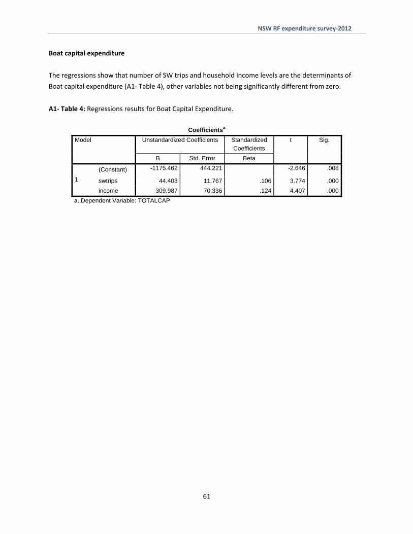
NSW RF expenditure survey‐2012
In A2‐Figure 1 the cluster analysis of the data shows that total expenditure has income and trips per
annum as strongest predictor of total expenditure but there are 4 statistically significant clusters as
described The authors have added a label to describe the group characteristics which are given in the
description
Trip expenditure
A2‐Figure 2 RF Clusters in trip expenditure
Trips and secondly income are the strongest predictors of trip expenditure Examining trip expenditure
leads to 4 distinct clusters We see clusters 2 and 3 (182) have high trip expenditures Some 818 of
the population have low trip expenditure with one low income (ldquobattlersrdquo) and one higher income
group (ldquoFishing break anglersrdquo)
63
NSW RF expenditure survey‐2012
Tackle expenditure
Tackle expenditure is most strongly predicted by income and is less trip related than expected There is a
cluster of 4 of higher income fishers who have very high tackle expenditure (ldquoTackle addictsrdquo)
A2‐Figure 3 RF Clusters in tackle expenditure
Tackle expenditure forms into 4 clusters with 852 of fishers fishing few trips and spending low
amounts on tackle irrespective of income
64
NSW RF expenditure survey‐2012
Capital boat expenditure
In A2 Figure 4 firstly trips and then secondly income are the strongest predictors of expenditure on
boats The highest boat expenditure is associated with 23 of fishers doing many trips but also with
the 138 of dedicated fishers
A2‐Figure 4 RF Clusters in capital boat expenditure
65
- Structure Bookmarks
-
- Project Developing a cost effective state wide expenditure survey method to measure the economic contribution of the recreational fishing sector in NSW
- Final Report to the NSW Recreational Fishing Licence Trust NSW Department of Primary Industry November 2013
-
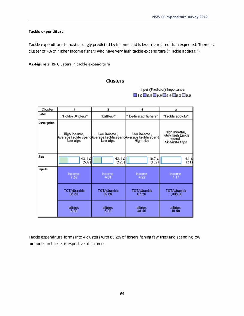
NSW RF expenditure survey‐2012
Capital boat expenditure
In A2 Figure 4 firstly trips and then secondly income are the strongest predictors of expenditure on
boats The highest boat expenditure is associated with 23 of fishers doing many trips but also with
the 138 of dedicated fishers
A2‐Figure 4 RF Clusters in capital boat expenditure
65
- Structure Bookmarks
-
- Project Developing a cost effective state wide expenditure survey method to measure the economic contribution of the recreational fishing sector in NSW
- Final Report to the NSW Recreational Fishing Licence Trust NSW Department of Primary Industry November 2013
-