1

Project number: 265138 Project name: New methodologies for multi-hazard and multi-risk

assessment methods for Europe Project acronym: MATRIX Theme: ENV.2010.6.1.3.4

Multi-risk evaluation and mitigation strategies Start date: 01.10.2010 End date: 31.12.2013 (39 months) Deliverable: D7.3: Naples test case Version: Draft Responsible partner: AMRA Month due: M38 Month delivered: Primary authors(a):

Alexander Garcia-Aristizabal Angela Di Ruocco Warner Marzocchi 12.2013

_______________________________ _________________ Signature Date (a)

see the Acknowledgements section for a full list of people contributing to this document

Reviewer:

Kevin Fleming 12.2013 _______________________________ _________________ Signature Date Authorised: Kevin Fleming 12.2013 _______________________________ _________________ Signature Date

Dissemination Level

PU Public

PP Restricted to other programme participants (including the Commission Services)

RE Restricted to a group specified by the consortium (including the Commission Services)

X

CO Confidential, only for members of the consortium (including the Commission Services)

2

3

Abstract

Considering only the natural sources of environmental hazards for the Naples city area, the main hazards that can be identified are (1) Volcanic hazards, which encompasses the active volcanoes of Somma-Vesuvius, Phlegrean Fields and the island of Ischia; Seismic hazards, due both to active faulting in the Campanian Apennines and to earthquakes arising from the three active volcanoes in the Naples area; Hydrogeological hazards, mainly due to flash floods, pyroclastic flows and rock falls due to slope instability; and Tsunami hazards, whose origin may be associated with earthquakes with epicentres in the sea or in coastal areas, coastal or submarine landslides, and volcanic eruptions (in this case, possible sources are volcanic activity on Ischia and Vesuvius, and submarine volcanoes in the low Tyrrhenian Sea).

After collecting the data for the analyses, the Arenella was the target area in which it was possible to retrieve high resolution data, hence its selection as the pilot area for the analyses in the project. In this report, a summary of all the activities performed for the Naples test case within the framework of the MATRIX project is presented. It therefore constitutes a collection of the main results of different deliverables produced in the project. In particular, section 2 is a summary of the single hazard and risk assessments performed. Section 3 presents the results of the assessment of interactions and cascading effects. Finally, section 4 summarizes the results of interactions with local stakeholders in Naples.

Keywords: Naples test case, MATRIX project, single hazard and risk assessment, cascading effects and interactions, Social and institutional barriers for effective decision making using multi-risk data

4

5

Acknowledgments

The research leading to these results has received funding from the European Commission’s Seventh Framework Programme [FP7/2007-2013] under grant agreement n° 265138.

Different partners from the MATRIX project have collaborated in the preparation of this

report. Below we present a list of all people who participated in this document’s production

(alphabetical order of institutions):

- AMRA:

Alexander Garcia-Aristizabal, Angela Di Ruocco, Warner Marzocchi, Jacopo Selva.

- IIASA:

Anna Scolobig.

6

7

Table of contents

1 Introduction ................................................................................................................. 12

2 Single hazards and risk assessment ........................................................................... 16

2.1 Volcanic ash-fall hazard and risk ......................................................................... 16

2.1.1 Nodes describing the volcanic hazard (Nodes 1 to 8) .................................... 16

2.1.2 Nodes describing Damage: Node D0 (inventory), node D1 (physical

vulnerabilities) and Node D3 (Exposure) ..................................................................... 17

2.2 Seismic hazard and risk ...................................................................................... 22

3 Multi-hazard assessment for cascading effects Naples: considering interactions ....... 25

3.1 Identification of scenarios for the Naples test case .............................................. 25

3.2 Scenarios of cascading effects analysed in the Naples test case........................ 27

3.2.1 Volcanic earthquakes and seismic swarms triggered by volcanic unrest

(scenario 1) ................................................................................................................. 27

Scenario description ................................................................................................ 27

Kinds of interactions ................................................................................................ 28

Temporal aspects .................................................................................................... 28

Analysis ................................................................................................................... 29

Example considering the Campi Flegrei area ...................................................... 30

3.2.2 Scenario 2: Simultaneous occurrence of ash-fall and earthquake hazards

(interaction at vulnerability level) ................................................................................. 34

Scenario description ................................................................................................ 34

Kind of interactions .................................................................................................. 34

Temporal aspects .................................................................................................... 35

Analysis ................................................................................................................... 35

4 Interactions with stakeholders in Naples: Identification of social and institutional

barriers to effective decision-making and governance in the case of multiple hazards ...... 44

5 Summary ..................................................................................................................... 46

The Naples test case provided the opportunity to test different methodologies developed in

the MATRIX project in specific activities of single- and multi-risk assessments. In

particular, we can summarize the following main results: .................................................. 46

In WP2, a procedure based on Bayesian analyses has been developed and applied to

the Naples test case in order to calculate volcanic risk (considering ash fall). It is worth

noting that the methodology proposed is general enough to be easily implemented for

other kind of risks; .............................................................................................................. 46

In WP3, a conceptual framework to analyse interactions and cascade effects was

developed. This framework was implemented in the Naples test case allowing us to

8

analyse the effects of interactions between two risk sources (seismic and volcanic) at

different levels. ................................................................................................................... 46

The results of the interaction analysis and multi-risk assessment for this particular

scenario were used in the WP6 for the identification of social and institutional barriers to

effective decision-making and governance when considering multiple hazards. ............... 46

References ........................................................................................................................ 47

9

List of Figures

Figure 1. Study area for the Naples test case. ................................................................... 12

Figure 2. Map of the target areas: Camaldoli, Arenella, and Furigrotta ............................. 14

Figure 3. Components of risk defining the event tree used in this study. ........................... 16

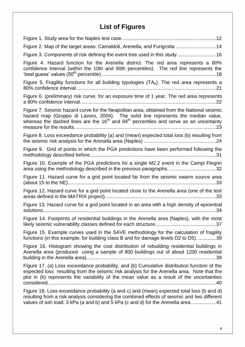
Figure 4. Hazard function for the Arenella district. The red area represents a 80% confidence interval (within the 10th and 90th percentiles). The red line represents the ‘best guess’ values (50th percentile) ................................................................................... 18

Figure 5. Fragility functions for all building typologies (TAk). The red area represents a 80% confidence interval. .................................................................................................... 21

Figure 6. (preliminary) risk curve, for an exposure time of 1 year. The red area represents a 80% confidence interval. ................................................................................................. 22

Figure 7. Seismic hazard curve for the Neapolitan area, obtained from the National seismic hazard map (Gruppo di Lavoro, 2004). The solid line represents the median value, whereas the dashed lines are the 16th and 84th percentiles and serve as an uncertainty measure for the results. ..................................................................................................... 23

Figure 8. Loss exceedance probability (a) and (mean) expected total loss (b) resulting from the seismic risk analysis for the Arenella area (Naples) .................................................... 24

Figure 9. Grid of points in which the PGA predictions have been performed following the methodology described before ........................................................................................... 31

Figure 10. Example of the PGA predictions for a single M2.2 event in the Campi Flegrei area using the methodology described in the previous paragraphs. .................................. 32

Figure 11. Hazard curve for a grid point located far from the seismic swarm source area (about 15 to the NE)........................................................................................................... 33

Figure 12. Hazard curve for a grid point located close to the Arenella area (one of the test areas defined in the MATRIX project). ............................................................................... 33

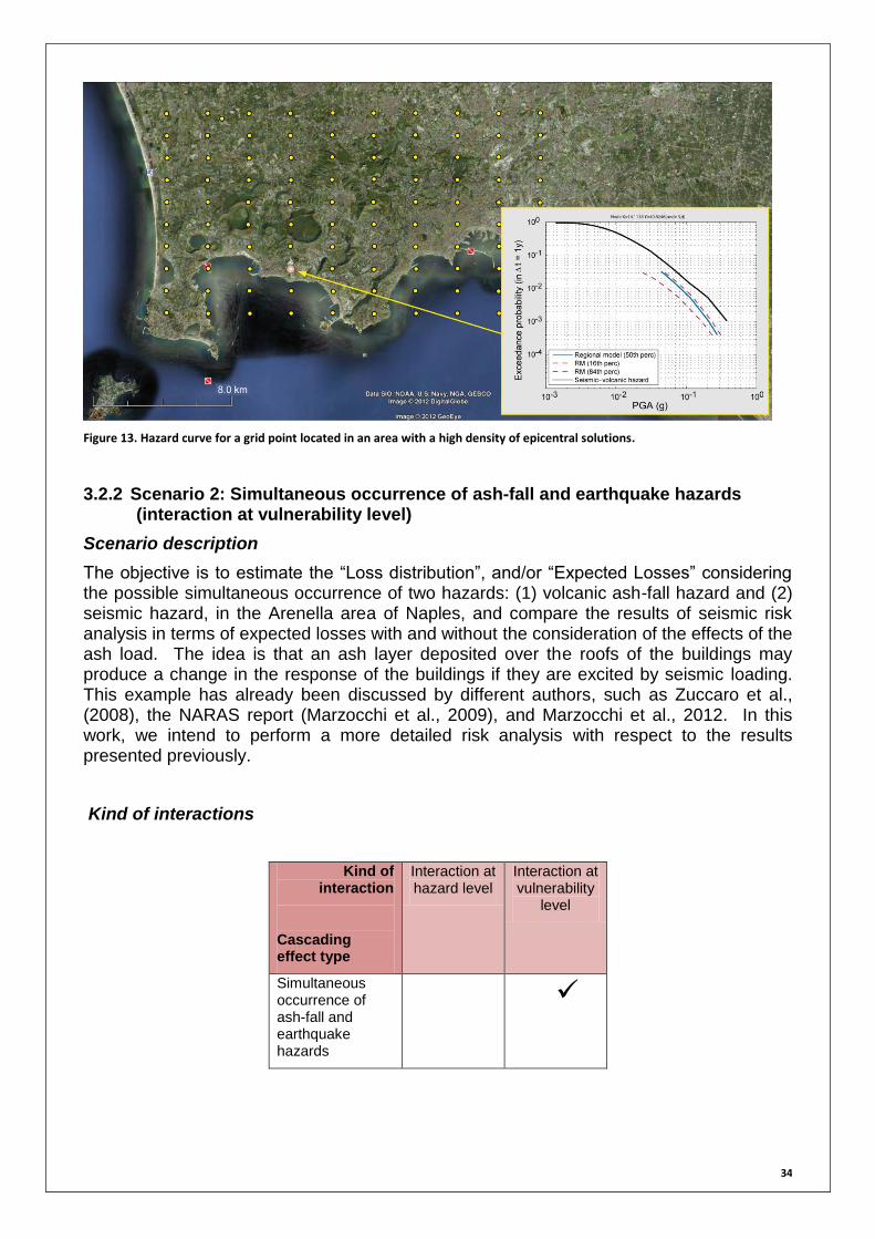
Figure 13. Hazard curve for a grid point located in an area with a high density of epicentral solutions. ............................................................................................................................ 34

Figure 14. Footprints of residential buildings in the Arenella area (Naples), with the most likely seismic vulnerability classes defined for each structure. ........................................... 37

Figure 15. Example curves used in the SAVE methodology for the calculation of fragility functions (in this example, for building class B and for damage levels D2 to D5). ............. 39

Figure 16. Histogram showing the cost distribution of rebuilding residential buildings in Arenella area (produced using a sample of 800 buildings out of about 1200 residential building in the Arenella area). ............................................................................................ 39

Figure 17. (a) Loss exceedance probability, and (b) Cumulative distribution function of the expected loss resulting from the seismic risk analysis for the Arenella area. Note that the plot in (b) represents the variability of the mean value as a result of the uncertainties considered. ........................................................................................................................ 40

Figure 18. Loss exceedance probability (a and c) and (mean) expected total loss (b and d) resulting from a risk analysis considering the combined effects of seismic and two different values of ash load: 3 kPa (a and b) and 5 kPa (c and d) for the Arenella area. ................. 41

10

Figure 19. Summary of results of the exceedance probabilities of loss for the three considered scenarios: (1) seismic, (2) seismic+3kPa ash load, and (3) seismic+5kPa ash load. ................................................................................................................................... 42

Figure 20. Summary of results of the expected losses (mean values) for the three considered scenarios: (1) seismic, (2) seismic+3kPa ash load, and (3) seismic+5kPa ash load. ................................................................................................................................... 42

11

List of Tables

Table 1. Summary of some relevant parameters and data from the three selected areas of interest in Naples for multi-type hazard and risk analysis: Canaldoli, Arenella, and Fuorigrotta (LS – landslide and rockfalls, EQ – earthquakes, VE – volcanic eruptions, WF – wildfires). ......................................................................................................................... 14

Table 2. Application’s taxonomy TA, from Spence et al. (2005) ........................................ 18

Table 3. Node D0, best estimate of p(TAi|TA(ISTAT)) ........................................................... 19

Table 4. Taxonomy relative to FM2, from Spence et al. (2005) ......................................... 19

Table 5. Node D1, association between input FMs and application’s TA .......................... 20

Table 6. Node D2, alpha values of (posterior) Dirichlet distribution. .................................. 21

Table 7. Possible cascade scenarios for the Naples test case (from MATRIX D3.3). ........ 26

Table 8. Time scales of interest for the volcanic earthquake hazard produced by triggered seismicity during volcanic unrests ...................................................................................... 29

Table 9. Time scales of interest for the cascading effect considering the simultaneous occurrence of volcanic ash-fall and earthquake hazards ................................................... 35

Table 10. Seismic-building structures classification (from Zuccaro et al., 2008) ................ 36

Table 11. Classification of damage to masonry buildings, according to the European Macroseismic Scale (EMS98, Grünthal, 1998) .................................................................. 38

Table 12. Seismic intensity increment for corresponding ash loads (from Zuccaro et al., 2008).................................................................................................................................. 39

12

1 Introduction

Naples is located in south west Italy on a bay along the Tyrrhenian coast in the inner-most part of the Gulf of Naples. It is in the midst of two volcanic areas, the Phlegrean Fields and Mount Vesuvius. From the eastern hills of the Phlegrean Fields, the city slopes down northward to the Campanian Plain and south-eastward to the slopes of Mt. Vesuvius.

The eastern area of Naples consists of a wide floodplain (the Sebeto river hollow) while the western urban area of Naples consists of the Bagnoli Plain and the remains of 4 ancient volcanic hollows generated by the Phlegrean Fields volcanism (Chiaia, Neapolis, Fuorigrotta and Soccavo, see Figure 1). The urban area of Naples is mainly composed of hills, most of them with heights ranging from 150 to 452 meters.

Figure 1. Study area for the Naples test case.

The geological history of the whole territory is complex: the latest substrate is mainly composed of volcanic debris. The Campania region is fragile and is exposed to several environmental risks, both natural and anthropogenic, that have in recent centuries caused disastrous events resulting in thousands of victims, massive loss of property and huge damage to the cultural heritage. Considering only the latter half of the 20th century, in Campania there were about 3300 victims of natural disasters (e.g., 2734 in the 1980 Irpinia earthquake, 40 in the 1944 eruption of Vesuvius and the rest due mainly to landslides and floods). In fact, Campania is the Italian region that has suffered the highest number of fatalities from natural catastrophes: more than 40% of the total for Italy. In particular, considering only the natural sources of environmental hazards for the Naples city area, the main hazards are:

Volcanic hazard, which encompasses the active volcanoes of Somma-Vesuvius, Phlegrean Fields and the island of Ischia;

13

Seismic hazard, due both to active faulting in the Campanian Apennines and to earthquakes arising from the three active volcanoes in the Naples area;

Hydrogeological hazard, mainly due to flash floods, mudflows and rock falls due to slope instability;

Tsunami hazard, whose origin may be associated with earthquakes whose epicentres are in the sea or in coastal areas, coastal or submarine landslides, and volcanic eruptions (in this case, possible sources are volcanic activity on Ischia and Vesuvius, and submarine volcanoes in the low Tyrrhenian Sea).

Forest fires, which in the last few years have been reported in the city of Naples, mainly during the summer period. For example, more than 40 forest fires were registered in 2011 (Department of Agriculture, Campania Region 2012, and MATRIX deliverable D6.3 “Social and institutional barriers to effective multi-hazard decision making”).

While the volcanic and seismic hazards can affect the whole city (with an intensity varying from place to place), the areas prone to the tsunami and hydrogeological hazards are respectively located on the coast and close to unstable slopes. In particular, in the Phlegrean Fields, the sectors mainly susceptible to landslides or rock falls are located along steep tuff slopes, in pyroclastic deposits and, in some places, in lavas. The recurrent morphologies are associated with the caldera rims, slopes of the coastal fault and the escarpments bordering river valleys.

Considering the area of the city of Naples, the parts susceptible to landslides and rock falls are mainly located near the outcrops of Campanian Ignimbrite and Neapolitan Yellow Tuff on the Camaldoli hill (Soccavo and Pianura side). Similar events of lower intensity have been observed on the Posillipo hill, which is mainly composed of Neapolitan Yellow Tuff, along the slopes on the side of the Fuorigrotta district and along the tuff cliffs of Coroglio.

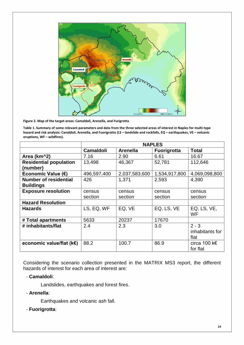
In the MATRIX project, three target areas within the Naples city area have been selected for multi-type hazard and risk analysis. These areas have been selected according to the spatial distribution of natural hazards and the available information about the elements at risk. The selected target areas are: Camaldoli, Fuorigrotta and Arenella (Figure 2). Some characteristics of the three areas, namely their areas, numbers of inhabitants, numbers of residential and commercial buildings, etc., are summarized in Table 1.

14

Figure 2. Map of the target areas: Camaldoli, Arenella, and Furigrotta

Table 1. Summary of some relevant parameters and data from the three selected areas of interest in Naples for multi-type hazard and risk analysis: Canaldoli, Arenella, and Fuorigrotta (LS – landslide and rockfalls, EQ – earthquakes, VE – volcanic eruptions, WF – wildfires).

NAPLES

Camaldoli Arenella Fuorigrotta Total

Area (km^2) 7.16 2.90 6.61 16.67

Residential population (number)

13,498 46,367 52,781 112,646

Economic Value (€) 496,597,400 2,037,583,600 1,534,917,800 4,069,098,800

Number of residential Buildings

426 1,371 2,593 4,390

Exposure resolution census section

census section

census section

census section

Hazard Resolution

Hazards LS, EQ, WF EQ, VE EQ, LS, VE EQ, LS, VE, WF

# Total apartments 5633 20237 17670

# inhabitants/flat 2.4 2.3 3.0 2 - 3 inhabitants for flat

economic value/flat (k€) 88.2 100.7 86.9 circa 100 k€ for flat

Considering the scenario collection presented in the MATRIX MS3 report, the different hazards of interest for each area of interest are:

- Camaldoli:

Landslides, earthquakes and forest fires.

- Arenella:

Earthquakes and volcanic ash fall.

- Fuorigrotta:

15

Earthquakes and volcanic hazards (such as vent opening, ash fall, and pyroclastic flows).

After collecting the data for the analyses, the Arenella was selected as the target area, as it was possible to retrieve high resolution data.

This report summarizes all the activities performed in the Naples test case within the framework of the MATRIX project. First, a summary of the results dealing with single hazard and risk assessment is presented. Then, section 3 presents the results of the assessment of interactions and cascading effects and finally, in section 4, the results of interactions with local stakeholders are discussed.

16

2 Single hazards and risk assessment

In this section we will consider only the natural sources of environmental hazards for the Naples city area, as outlined in the previous section.

In the framework of MATRIX project, for the test case in Naples two hazard sources have been considered for quantitative hazard and risk analyses: volcanic ash-fall and earthquakes.

2.1 Volcanic ash-fall hazard and risk

The volcanic ash-fall hazard and risk assessment performed in the MATRIX project in the Naples test case was performed within the framework of WP2 “Single type risk assessment and comparability” and presented in the Deliverable D2.2 “Uncertainty Quantification”. This involved a quantitative application of a Bayesian event tree approach developed for the quantification and propagation of uncertainties in the case of volcanic risk assessment.

For simplicity, the event tree is presented divided according to two general components of risk, namely hazard and damage, each of which can be regarded as a sub-event tree. The sub-event tree for the volcanic hazard assessment corresponds to the procedure described in the BET_VH model (Marzocchi et al., 2010, Selva et al., 2010), whereas the sub-event tree for the Damage is composed of three elements (nodes), relative to inventory definition (that here we call node D0), fragility functions (i.e., physical vulnerability, node D1), and losses (node D2). For simplicity, we describe the two components independently, but together they form a more general event tree (Figure 3):

Figure 3. Components of risk defining the event tree used in this study.

2.1.1 Nodes describing the volcanic hazard (Nodes 1 to 8)

The Bayesian event tree approach for volcanic hazard assessment (BET_VH) is a methodology already described in the literature (e.g., Marzocchi et al., 2010, Selva et al., 2010) and is the procedure used as the reference for the volcanic hazard assessment in this document. A brief description is provided in the following paragraphs, but for a more detailed description the reader is invited to consult the original papers.

Let’s assume that the function [θk] represents the probability density function of the

random variable ,describing the probability of the jth event at the kth node. The distribution [θk] has to be unimodal and with domain [0,1] because the random variable is a probability. A suitable distribution with these requirements is the Beta distribution (e.g., Marzocchi et al., 2004). The key point of this strategy is that the available empirical and theoretical information can modify the mean and variance of this probability distribution. In general, we can consider all of the available information determines the mean of the distribution (which we can consider to be the aleatory uncertainty), while the variance of the distribution, can be considered as the epistemic uncertainty, is modified (usually

17

significantly reduced) by having more data available. The PDF associated with is calculated by following two steps (based on a common procedure of Bayesian analysis, e.g., Gelman et al., 1995): first, an “initial” (prior) distribution is defined (as a Beta/Dirichlet distribution, depending if the node has two or more possible outcomes) taking into account all the theoretical beliefs; then, this information is “updated” by considering past (observed) data (encoded as a Binomial/multinomial distribution) using Bayes’ theorem. Detailed descriptions of each node can be found in the Deliverable D2.2 and in the referenced works.

2.1.2 Nodes describing Damage: Node D0 (inventory), node D1 (physical vulnerabilities) and Node D3 (Exposure)

The treatment of epistemic uncertainty in damage estimates is here done using the methodology whose development is still in progress within the on-going Italian project ByMuR (Bayesian Multi-Risk, ByMuR 2010-2013; Selva et al. 2012a). The method, for each typology of physical structure, can be summarized in the following logical steps:

Definition of the application’s Taxonomy (TA), Intensity Measure (IM), Damage states (DSs) and losses (L), referred to as the “application metrics”. In this description “application” is referred to the specific case analysed in the problem.

Collection of applicable Fragility Models (FMs), to be mapped in the application metrics (TA, IM and DSs). A weight to each model is assigned, based on its applicability in the target area, or due to its credibility as defined by expert opinion;

Collection of the input data for the target area (Inventory), to be mapped into the application metrics (TA, L).

Note that the first step is the harmonization of intensity measures, and the definition of the typologies of structures and relative damage states. In practice, this means that it should be defined one common reference metric for the whole application, hereinafter referred to as [IM, TA, DS, L], in order to prepare a common base for merging different vulnerability/losses models. This process may imply a drastic reduction of classes of exposed elements with respect to single-model applications. This fact is in common to all processes of comparison among models. For example, the comparison among FMs performed in the EU-FP7 project SYNER-G1 (SYNER-G 2010-2012) implied the use of one reference IM (for example Peak Ground Acceleration, PGA, for seismic hazard), the conversion of all models to this IM, the definition of only two damage states (“yielding” and “collapse”), and the definition of correlations between the original and target (common) taxonomy (Crowley et al. 2011).

The Bayesian assessment of damages, as described above in general terms, may be undertaken using an Event Tree logic. For each asset in the target area, we define the following nodes (for details, see D2.2):

Node D0 “Inventory”: classification of assets according to the TA.

Node D1 “Fragility”: assessment of DS, for each typology in the TA and each IM.

Node D2 “Losses”: assessment of L, for each DS of each asset.

The treatment of uncertainties based on a Bayesian event tree approach is applied to quantify the ash-fall volcanic hazard and risk in one of the target areas defined for the Naples test case in MATRIX (Arenella, for details see, e.g., MATRIX Deliverables D2.2 for the methodology and D3.3 “Scenarios of cascade events” for the test case definition). The resulting risk curves are computed through Monte-Carlo simulations, combining the

1 http://www.vce.at/SYNER-G/

18

conditional probabilities at all the nodes of the Event Tree, separately for each IM level (scenario). The exercise developed in D2.2 is restricted to the assessment of tangible economic losses in residential structures, in particular, to direct losses associated with physical damages to the roofs due to the accumulation of volcanic ash.

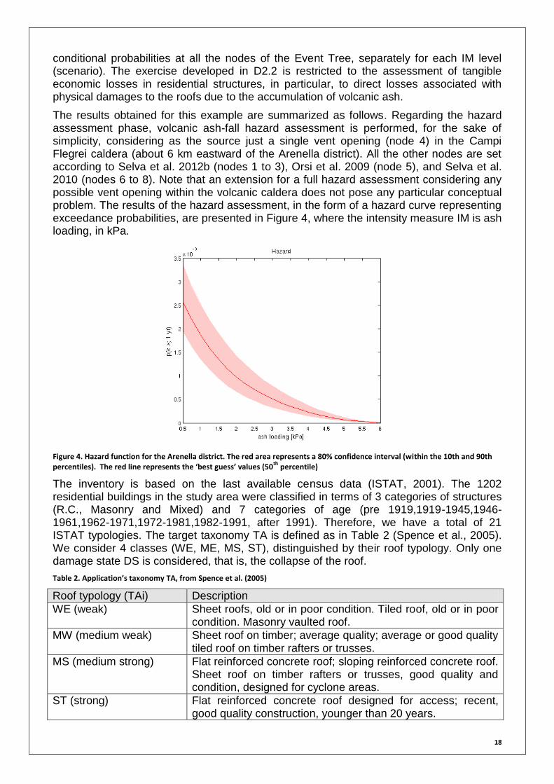
The results obtained for this example are summarized as follows. Regarding the hazard assessment phase, volcanic ash-fall hazard assessment is performed, for the sake of simplicity, considering as the source just a single vent opening (node 4) in the Campi Flegrei caldera (about 6 km eastward of the Arenella district). All the other nodes are set according to Selva et al. 2012b (nodes 1 to 3), Orsi et al. 2009 (node 5), and Selva et al. 2010 (nodes 6 to 8). Note that an extension for a full hazard assessment considering any possible vent opening within the volcanic caldera does not pose any particular conceptual problem. The results of the hazard assessment, in the form of a hazard curve representing exceedance probabilities, are presented in Figure 4, where the intensity measure IM is ash loading, in kPa.

Figure 4. Hazard function for the Arenella district. The red area represents a 80% confidence interval (within the 10th and 90th percentiles). The red line represents the ‘best guess’ values (50

th percentile)

The inventory is based on the last available census data (ISTAT, 2001). The 1202 residential buildings in the study area were classified in terms of 3 categories of structures (R.C., Masonry and Mixed) and 7 categories of age (pre 1919,1919-1945,1946-1961,1962-1971,1972-1981,1982-1991, after 1991). Therefore, we have a total of 21 ISTAT typologies. The target taxonomy TA is defined as in Table 2 (Spence et al., 2005). We consider 4 classes (WE, ME, MS, ST), distinguished by their roof typology. Only one damage state DS is considered, that is, the collapse of the roof.

Table 2. Application’s taxonomy TA, from Spence et al. (2005)

Roof typology (TAi) Description

WE (weak) Sheet roofs, old or in poor condition. Tiled roof, old or in poor condition. Masonry vaulted roof.

MW (medium weak) Sheet roof on timber; average quality; average or good quality tiled roof on timber rafters or trusses.

MS (medium strong) Flat reinforced concrete roof; sloping reinforced concrete roof. Sheet roof on timber rafters or trusses, good quality and condition, designed for cyclone areas.

ST (strong) Flat reinforced concrete roof designed for access; recent, good quality construction, younger than 20 years.

19

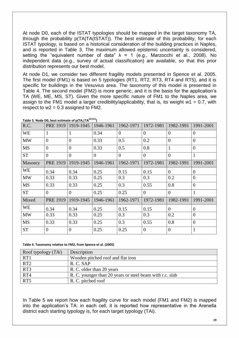
At node D0, each of the ISTAT typologies should be mapped in the target taxonomy TA, through the probability p(TA|TA(ISTAT)). The best estimate of this probability, for each ISTAT typology, is based on a historical consideration of the building practices in Naples, and is reported in Table 3. The maximum allowed epistemic uncertainty is considered, setting the “equivalent number of data” λ = 1 (e.g., Marzocchi et al., 2008). No independent data (e.g., survey of actual classification) are available, so that this prior distribution represents our best model.

At node D1, we consider two different fragility models presented in Spence et al. 2005. The first model (FM1) is based on 5 typologies (RT1, RT2, RT3, RT4 and RT5), and it is specific for buildings in the Vesuvius area. The taxonomy of this model is presented in Table 4. The second model (FM2) is more generic, and it is the basis for the application’s TA (WE, ME, MS, ST). Given the more specific nature of FM1 to the Naples area, we assign to the FM1 model a larger credibility/applicability, that is, its weight w1 = 0.7, with respect to w2 = 0.3 assigned to FM2.

Table 3. Node D0, best estimate of p(TAi|TA

(ISTAT))

R.C. PRE 1919 1919-1945 1946-1961 1962-1971 1972-1981 1982-1991 1991-2001

WE 1 1 0.34 0 0 0 0

MW 0 0 0.33 0.5 0.2 0 0

MS 0 0 0.33 0.5 0.8 1 0

ST 0 0 0 0 0 0 1

Masonry PRE 1919 1919-1945 1946-1961 1962-1971 1972-1981 1982-1991 1991-2001

WE 0.34 0.34 0.25 0.15 0.15 0 0

MW 0.33 0.33 0.25 0.3 0.3 0.2 0

MS 0.33 0.33 0.25 0.3 0.55 0.8 0

ST 0 0 0.25 0.25 0 0 1

Mixed PRE 1919 1919-1945 1946-1961 1962-1971 1972-1981 1982-1991 1991-2001

WE 0.34 0.34 0.25 0.15 0.15 0 0

MW 0.33 0.33 0.25 0.3 0.3 0.2 0

MS 0.33 0.33 0.25 0.3 0.55 0.8 0

ST 0 0 0.25 0.25 0 0 1

Table 4. Taxonomy relative to FM2, from Spence et al. (2005)

Roof typology (TAi) Description

RT1 Wooden pitched roof and flat iron

RT2 R. C. SAP

RT3 R. C. older than 20 years

RT4 R. C. younger than 20 years or steel beam with r.c. slab

RT5 R. C. pitched roof

In Table 5 we report how each fragility curve for each model (FM1 and FM2) is mapped into the application’s TA: in each cell, it is reported how representative in the Arenella district each starting typology is, for each target typology (TAi).

20

Table 5. Node D1, association between input FMs and application’s TA

Application’s TA

WE MW MS ST

FM1

RT1 0 0.5 0 0

RT2 0 0.5 0 0

RT3 0 0 1 0

RT4 0 0 0 1

RT5 0 0 0 0

FM2

WE 1 0 0 0

MW 0 1 0 0

MS 0 0 1 0

ST 0 0 0 1

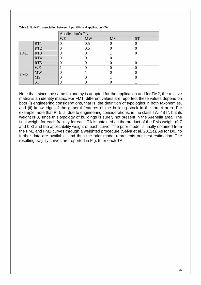
Note that, since the same taxonomy is adopted for the application and for FM2, the relative matrix is an identity matrix. For FM1, different values are reported: these values depend on both (i) engineering considerations, that is, the definition of typologies in both taxonomies, and (ii) knowledge of the general features of the building stock in the target area. For example, note that RT5 is, due to engineering considerations, in the class TAi=”ST”, but its weight is 0, since this typology of buildings is surely not present in the Arenella area. The final weight for each fragility for each TA is obtained as the product of the FMs weight (0.7 and 0.3) and the applicability weight of each curve. The prior model is finally obtained from the FM1 and FM2 curves through a weighted procedure (Selva et al. 2012a). As for D0, no further data are available, and thus the prior model represents our best estimation. The resulting fragility curves are reported in Fig. 5 for each TA.

21

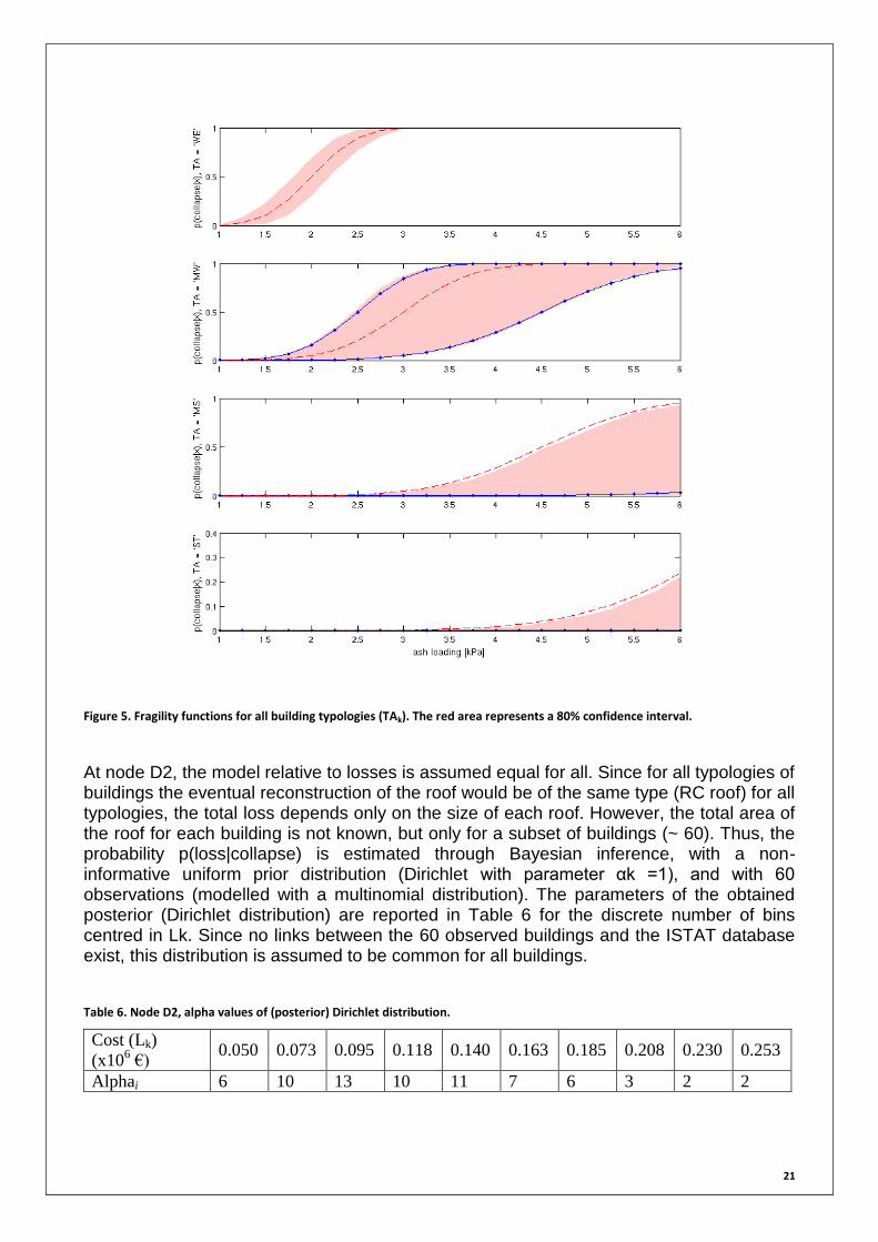
Figure 5. Fragility functions for all building typologies (TAk). The red area represents a 80% confidence interval.

At node D2, the model relative to losses is assumed equal for all. Since for all typologies of buildings the eventual reconstruction of the roof would be of the same type (RC roof) for all typologies, the total loss depends only on the size of each roof. However, the total area of the roof for each building is not known, but only for a subset of buildings (~ 60). Thus, the probability p(loss|collapse) is estimated through Bayesian inference, with a non-informative uniform prior distribution (Dirichlet with parameter αk =1), and with 60 observations (modelled with a multinomial distribution). The parameters of the obtained posterior (Dirichlet distribution) are reported in Table 6 for the discrete number of bins centred in Lk. Since no links between the 60 observed buildings and the ISTAT database exist, this distribution is assumed to be common for all buildings.

Table 6. Node D2, alpha values of (posterior) Dirichlet distribution.

Cost (Lk)

(x106 €)

0.050 0.073 0.095 0.118 0.140 0.163 0.185 0.208 0.230 0.253

Alphai 6 10 13 10 11 7 6 3 2 2

22

The resulting risk curves are computed through Monte-Carlo simulations, combining the conditional probabilities at all the nodes of the Event Tree, separately for each IM level (scenario). With regards to epistemic uncertainty, the probability relative to each node is sampled from each distribution, providing an explicit evaluation of the epistemic uncertainty at the node. More precisely, for each IM, it is assessed by the probability of exceedance, in the exposure time ΔT, of given threshold value of losses l. That is:

[p(>l; IM, ΔT)]=[p(>l|IM)] [p(IM; ΔT)]

where [x] indicates the distribution of x; p(IM; ΔT) is obtained from nodes 1 to 8 (hazard assessment), while p(>l|IM) from nodes D0 to D2 (damage assessment). The contributions of all IMs are then summed at several level of confidence (percentiles), providing a proxy of the total variability of risk assessment (Selva et al. 2012a).

The resulting risk curve is assessed by sampling from the distribution at all nodes, set as described above, and it is reported in Figure 6. The best estimate is relative to the 50th percentiles, and the confidence interval is represented by the 10th and 90th percentiles.

Figure 6. (preliminary) risk curve, for an exposure time of 1 year. The red area represents a 80% confidence interval.

2.2 Seismic hazard and risk

For the Naples test case, the seismic risk has been considered as part of the activities of one of the two interaction scenarios analysed as examples of the multi-hazard / multi-risk environment (for details see Section 3). For this reason, a detailed description of the process for the seismic risk assessment is presented in section 3.2.2, where the interaction scenario characterized by the simultaneous effect of earthquakes and volcanic ash-fall is presented. In this part, a brief description of the adopted process is presented.

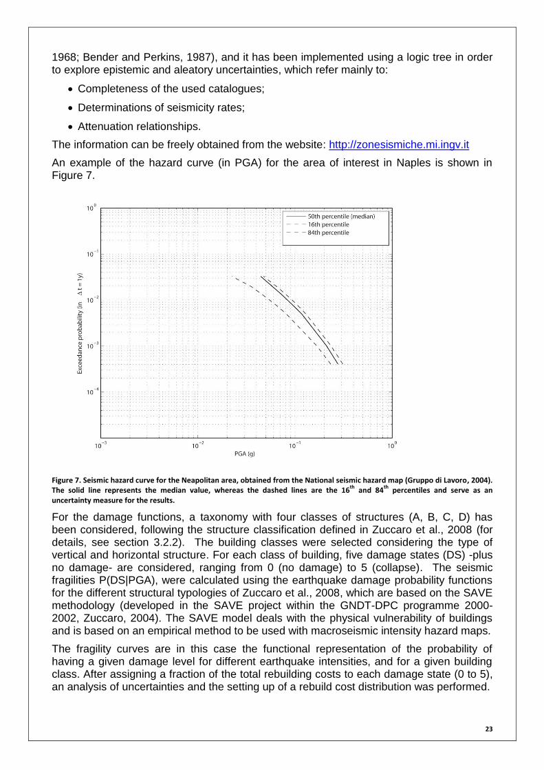
The seismic hazard information has been obtained from the Italian national seismic hazard map produced by the Istituto Nazionale di Geofisica e Vulcanologia - INGV (e.g., Gruppo di Lavoro, 2004; Meletti and Montaldo, 2007). The intensity measure for seismic hazard is available as both macro-seismic intensity, and in PGA (g). The method used by the INGV for the seismic hazard assessment is based on the standard method of Cornell (Cornell,

23

1968; Bender and Perkins, 1987), and it has been implemented using a logic tree in order to explore epistemic and aleatory uncertainties, which refer mainly to:

Completeness of the used catalogues;

Determinations of seismicity rates;

Attenuation relationships.

The information can be freely obtained from the website: http://zonesismiche.mi.ingv.it

An example of the hazard curve (in PGA) for the area of interest in Naples is shown in Figure 7.

Figure 7. Seismic hazard curve for the Neapolitan area, obtained from the National seismic hazard map (Gruppo di Lavoro, 2004). The solid line represents the median value, whereas the dashed lines are the 16

th and 84

th percentiles and serve as an

uncertainty measure for the results.

For the damage functions, a taxonomy with four classes of structures (A, B, C, D) has been considered, following the structure classification defined in Zuccaro et al., 2008 (for details, see section 3.2.2). The building classes were selected considering the type of vertical and horizontal structure. For each class of building, five damage states (DS) -plus no damage- are considered, ranging from 0 (no damage) to 5 (collapse). The seismic fragilities P(DS|PGA), were calculated using the earthquake damage probability functions for the different structural typologies of Zuccaro et al., 2008, which are based on the SAVE methodology (developed in the SAVE project within the GNDT-DPC programme 2000-2002, Zuccaro, 2004). The SAVE model deals with the physical vulnerability of buildings and is based on an empirical method to be used with macroseismic intensity hazard maps.

The fragility curves are in this case the functional representation of the probability of having a given damage level for different earthquake intensities, and for a given building class. After assigning a fraction of the total rebuilding costs to each damage state (0 to 5), an analysis of uncertainties and the setting up of a rebuild cost distribution was performed.

24

As mentioned before, a more detailed description of the process for the seismic risk assessment is presented in section 3.2.2, where the interaction scenario characterized by the simultaneous effect of earthquakes and volcanic ash-fall is presented.

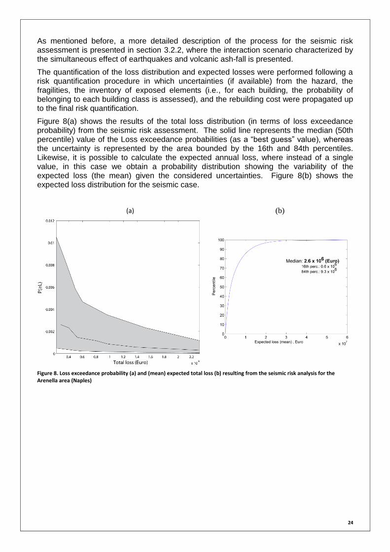
The quantification of the loss distribution and expected losses were performed following a risk quantification procedure in which uncertainties (if available) from the hazard, the fragilities, the inventory of exposed elements (i.e., for each building, the probability of belonging to each building class is assessed), and the rebuilding cost were propagated up to the final risk quantification.

Figure 8(a) shows the results of the total loss distribution (in terms of loss exceedance probability) from the seismic risk assessment. The solid line represents the median (50th percentile) value of the Loss exceedance probabilities (as a “best guess” value), whereas the uncertainty is represented by the area bounded by the 16th and 84th percentiles. Likewise, it is possible to calculate the expected annual loss, where instead of a single value, in this case we obtain a probability distribution showing the variability of the expected loss (the mean) given the considered uncertainties. Figure 8(b) shows the expected loss distribution for the seismic case.

(a) (b)

Figure 8. Loss exceedance probability (a) and (mean) expected total loss (b) resulting from the seismic risk analysis for the Arenella area (Naples)

25

3 Multi-hazard assessment for cascading effects Naples: considering interactions

The core of the probabilistic assessment of cascading effects in a multi-hazard problem consists of the identification of the possible interactions that are likely to occur and that may result in an amplification of the expected damages in a given area of interest. This concept is also the fundamental part of a holistic multi-risk analysis.

Within the framework of Work Package 3 of the MATRIX project, two possible kinds of interactions have been described, namely: (1) interactions at the hazard level, in which the occurrence of a given initial ‘triggering’ event, entails a modification of the probability of occurrence of a secondary event, and (2) interaction at the vulnerability (or damage) level, in which the main interest is to assess the effects that the occurrence of one event (the first one occurring in time) may have on the response of the exposed elements to another event (which may be of the same kind as the former, but also a different type of hazard). Implicitly, a combination of both kinds of interactions is another possibility, in which case, in the discussion about interactions at the vulnerability level, both dependent and independent hazards have been considered as possible scenarios. A detailed description of the probabilistic framework to quantify both kinds of interaction can be found in deliverable D3.4 of the MATRIX project (Garcia-Aristizabal et al., 2013a).

3.1 Identification of scenarios for the Naples test case

An important initial step towards the assessment of cascading effects is the identification of possible scenarios. The term “scenario” is used in a wide range of fields and so different interpretations can be found in practical applications. In general, a scenario may be considered as a synoptic, plausible and consistent representation of an event or series of actions and events (e.g., see MATRIX deliverable D3.3, Garcia-Aristizabal et al., 2013b). In particular, it must be plausible because it must fall within the limits of what might conceivably happen, and must be consistent in the sense that the combined logic used to construct a scenario must not have any built-in inconsistencies.

The process of scenario identification is the first and fundamental step towards a quantitative multi-risk assessment that considers cascading effects. To achieve the required complete set of scenarios, different strategies can be adopted, ranging from event-tree-like to fault-tree-like strategies. In many applications, an adaptive method combining both kinds of approaches is applied in order to ensure an exhaustive exploration of scenarios. From the multi-risk assessment point of view, the cascading scenarios of main interest are those that produce an amplification of the effects arising from these hazards when compared to those produced by the single events.

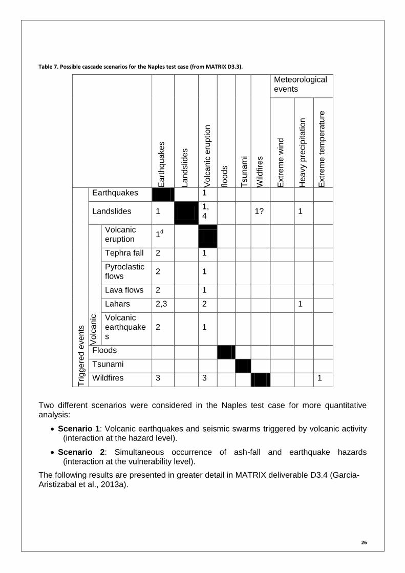
With a set of cascading scenarios of interest, their quantification can be achieved by adopting different strategies, for example, by analysing databases of past events, performing physical modelling for the propagation of the intensity measures of interest, and/or by performing expert elicitations in order to obtain information about extremely complex problems, or in these cases, with poor data or needing rapid analysis. Table 7 summarizes the main chains of cascade events identified for the different hazards affecting the Naples test city.

26

Table 7. Possible cascade scenarios for the Naples test case (from MATRIX D3.3).

Ea

rthqu

ake

s

La

nd

slid

es

Vo

lcan

ic e

rup

tion

(in

ge

ne

ral)

flo

od

s

Tsun

am

i

Wild

fire

s

Meteorological events

Extr

em

e w

ind

Hea

vy p

recip

ita

tio

n

Extr

em

e t

em

pe

ratu

re

Trigg

ere

d e

ve

nts

Earthquakes 1

Landslides 1 1,4

1? 1

Vo

lcan

ic

Volcanic eruption

1d

Tephra fall 2 1

Pyroclastic flows

2 1

Lava flows 2 1

Lahars 2,3 2 1

Volcanic earthquakes

2 1

Floods

Tsunami

Wildfires 3 3 1

Two different scenarios were considered in the Naples test case for more quantitative analysis:

Scenario 1: Volcanic earthquakes and seismic swarms triggered by volcanic activity (interaction at the hazard level).

Scenario 2: Simultaneous occurrence of ash-fall and earthquake hazards (interaction at the vulnerability level).

The following results are presented in greater detail in MATRIX deliverable D3.4 (Garcia-Aristizabal et al., 2013a).

27

3.2 Scenarios of cascading effects analysed in the Naples test case

This section summarizes the quantitative analysis of interaction scenarios performed in the Naples test case and that have been presented in the MATRIX deliverable D3.4 (Garcia-Aristizabal et al., 2013a).

3.2.1 Volcanic earthquakes and seismic swarms triggered by volcanic unrest (scenario 1)

Naples is located in the midst of two volcanic areas, the Phlegrean Fields (in the western side) and Mount Vesuvius (in the E-NE side). It is a case of a densely populated area located near active volcanoes, particularly in the Campi Flegrei area. The Campi Flegrei is dominated by a resurgent nested caldera resulting from two main collapse events related to the formation of the 37 ka Campanian Ignimbrite and the 12 ka Neapolitan Yellow Tuff (e.g., Rosi et al., 1983; Orsi et al., 1992). The Campi Flegrei caldera (CFc) comprises both submerged and continental parts on the western portion of the Bay of Naples, and appears to have undergone resurgence since 10-15 ky (Orsi et al., 1996). The latest eruption occurred in 1538 during which the Monte Nuovo scoria cone was generated (Di Vito et al., 1987).

During the last four decades it has experienced a huge uplift phase, which reached about 3.5 m in 1985, after which a subsidence phase started (e.g., Troise et al., 2008). Unrest episodes (e.g., from 1969 to 1972 and from mid-1982 to December 1984, Barberi et al., 1984) have been observed, during which swarms of volcanic seismic events were recorded (Dvorak and Gasparini, 1991; De Natale et al., 1995; Troise et al., 1997).

Scenario description

Eruption forecasting refers, in general, to the assessment of the occurrence probability of a given eruptive event, whereas volcanic hazards are normally associated with the generation of superficial and evident phenomena that usually accompany eruptions (e.g., lava, pyroclastic flows, tephra fall, lahars, etc.). Nevertheless, during the evolution of a volcanic system from a quiescent state to an eruptive state, a large number of small- to moderate-sized earthquakes occur.

In fact, periods of volcanic unrest are normally accompanied by (volcanic) seismic activity located directly below the volcano (Endo et al., 1981; Sawada and Aramaki, 1989; Matsumura et al., 1991; Oshima et al., 1991; Power et al., 1994; Garcia-Aristizabal et al., 2007), and/or by triggered seismic swarms (sometimes categorized as ‘distant volcano-tectonic events’, e.g., White and Power, 2002) associated with fault systems nearby the volcano (e.g., Minakami, 1974; Shimizu et al., 1992; Wolfe, 1992; Legrand et al., 2002).

Several of the world’s active volcanoes are located near densely populated areas (for example, in Italy (e.g., Naples), Japan (e.g., Tokyo), Mexico (e.g., Mexico D.F.), Colombia (e.g., Manizales), Ecuador (e.g., Quito)), and therefore the seismic hazard associated with pre-eruptive earthquake activity can be considered from a cascading effect perspective within a multi-risk framework.

The problem to be analysed is to assess the possible effect that local seismicity (normally characterized by many shallow micro-earthquakes) triggered during volcanic unrest may have in the area where the volcano is located, and compare it with the general seismic hazard analysis. In fact, seismic swarms triggered by volcanic unrest activity are composed of a high number of shallow events (rates are higher than normal seismicity of

28

the area), with generally low magnitude. Nevertheless, from a seismic hazard point of view, they may be of interest when exposed elements (e.g., populated areas or facilities of interest) are located very close to the volcano, since they are generally very shallow (few kilometres depth).

In the Neapolitan area, this case may be of particular interest given the highly urbanized area in the surroundings of Campi Flegrei. For example, two unrest episodes (called bradisisma, from the Greek word for “slow earthquake”) occurred from 1969 to 1972 and from mid-1982 to December 1984 (Barberi et al., 1984). The first episode produced a net uplift of about 1.7 m (Troise et al., 2008), with only weak seismic activity was recorded during this phase. The second event presented a similar uplift pattern, but compared to the previous one, this episode was accompanied by greater seismicity, both in terms of the number of earthquakes and their magnitude (Dvorak and Gasparini, 1991; De Natale et al., 1995; Troise et al., 1997). Shallow earthquake hypocentres (depths from 1 to 4 km) occurred from mid-1983 to December 1984 and were able to cause damage to buildings in the Pozzuoli area (e.g., Troise et al., 2008).

A magnitude 4.2 earthquake with its epicentre in Pozzuoli occurred on October 4, 1983. In 1984, the town was almost completely evacuated and about 40,000 people were relocated. The total uplift recorded between January 1982 and December 1984 amounted to 1.8 m. Since the end of 1984, the ground has started to subside with a peak subsidence rate of about 7–8 cm/year in 1985 and at a progressively slower rate until 2001–2002, when the subsidence ended and about 0.9 m of the total uplift was recovered (De Natale et al., 2006). Superimposed on the subsidence phase were some small and fast uplift episodes which occurred in 1989, 1994, and 2000, i.e., with an apparent period of about 5–6 years (Gaeta et al., 2003; Lanari et al., 2004). These smaller uplift episodes reached a maximum uplift of about 1–8 cm, lasted 4–10 months, and were accompanied by seismic swarms of small earthquakes (ML<2) lasting from a few days to 1–2 months (Troise et al., 2008).

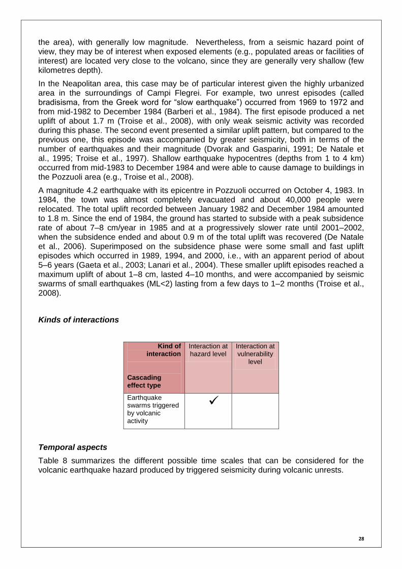
Kinds of interactions

Kind of interaction

Cascading effect type

Interaction at hazard level

Interaction at vulnerability

level

Earthquake swarms triggered by volcanic activity

Temporal aspects

Table 8 summarizes the different possible time scales that can be considered for the volcanic earthquake hazard produced by triggered seismicity during volcanic unrests.

29

Table 8. Time scales of interest for the volcanic earthquake hazard produced by triggered seismicity during volcanic unrests

Time scale

Cascading effect type

Several seconds to few minutes

Several minutes to few hours

Several hours to few

days

Several days to few

months

Several months to few years

Several or many years

Earthquake swarms triggered by volcanic activity

?

Analysis

As described in the introductory part, volcanic unrest practically always triggers volcanic seismic swarms; then, assuming that the probability that a volcano entering into unrest triggers a seismic swarm is 1, we may be interested in quantifying the seismo-volcanic hazard as the probability that a given intensity measure (of the volcanic earthquake hazard) exceeds a certain threshold value.

Considering the general expression for interactions at the hazard level defined in the MATRIX deliverable D3.4 and taking in account the triggering event in a binary fashion (occurrence/ non-occurrence of the volcanic unrest), the explicit expression for the seismic hazard considering the seismic/volcanic interaction can be expressed as:

Equation 1

The first term in Equation 1 corresponds to the assessment of the hazard component derived from a volcanic swarm, whereas the second element is the hazard component due to all the other possible sources (e.g., all those considered for the national seismic hazard). For simplicity in the description, we will refer to the calculations in the first term

as , and those in the second term as . Then, the “interaction” term can be expressed as .

where is a PGA intensity due to a seismic event during a volcanic swarm, and is a volcanic unrest event.

To quantify the expression , we adopt the following procedure:

Identification of the available seismo-volcanic swarm catalogues (Necessary information: earthquake locations and magnitudes);

Estimate of the activity rate, and frequency-magnitude relationships for the sequence;

Selection of the appropriate attenuation law for the volcanic earthquakes,

Propagation of the intensity measure ;

Estimate the exceedance probabilities (with respect to threshold values) at each spatial location;

In this example, we have analysed a seismic swarm occurred in the Campi Flegrei area.

30

Example considering the Campi Flegrei area

Data catalogue

For this exercise, different synthetic catalogues where built with the same spatial and frequency-magnitude characteristics of the seismic swarm that occurred during the 1983-1984 unrest at Campi Flegrei (source of data: De Natale et al., 1987; Vilardo et al., 1991; Troise et al., 1997; Orsi et al., 1999).

Activity rates and frequency-magnitude relationships

Values of the Gutenberg-Richter parameters have been adopted from literature, in particular, from De Natale et al., 1987 and Vilardo et al., 1991. The b value ( 0.92±0.04) is from De Natale et al., 1987, and the temporal and spatial changes, ranging from 0.61 to 1.35, are from Vilardo et al., 1991).

Attenuation law model for the volcanic earthquakes

The characteristic low magnitude and shallow location of volcanic earthquakes, as well as the particular conditions of seismic energy attenuation in volcanic areas, make the direct use of regional attenuation laws that are often used in seismic hazard analysis very difficult. For this reason, specific scale relationships are often used in volcanic zones. In this work, we follow the methodology proposed by De Natale et al., 1988, which has been also applied by Malagnini and Montaldo (2004) to define the attenuation relationships for the volcanic seismogenetic zones of the Italian seismic hazard map.

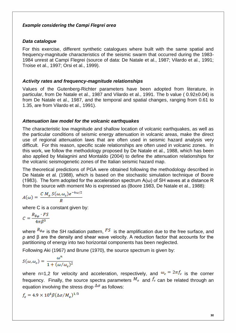
The theoretical predictions of PGA were obtained following the methodology described in De Natale et al. (1988), which is based on the stochastic simulation technique of Boore (1983). The form adopted for the acceleration spectrum A(ω) of SH waves at a distance R from the source with moment Mo is expressed as (Boore 1983, De Natale et al., 1988):

where C is a constant given by:

where is the SH radiation pattern, is the amplification due to the free surface, and ρ and β are the density and shear wave velocity. A reduction factor that accounts for the partitioning of energy into two horizontal components has been neglected.

Following Aki (1967) and Brune (1970), the source spectrum is given by:

where n=1,2 for velocity and acceleration, respectively, and is the corner

frequency. Finally, the source spectra parameters and can be related through an

equation involving the stress drop as follows:

31

where is in Hz, in km/seg, in bars and in dyne cm. In agreement with the setting defined for the elaboration of the Italian seismic hazard map, the stress drop for the

Campi Flegrei area has been set to a constant value bar (e.g., Malagnini and Montaldo, 2004).

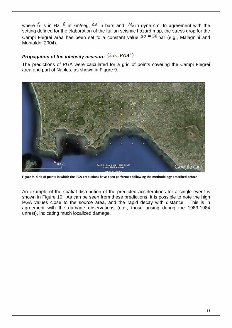
Propagation of the intensity measure

The predictions of PGA were calculated for a grid of points covering the Campi Flegrei area and part of Naples, as shown in Figure 9.

Figure 9. Grid of points in which the PGA predictions have been performed following the methodology described before

An example of the spatial distribution of the predicted accelerations for a single event is shown in Figure 10. As can be seen from these predictions, it is possible to note the high PGA values close to the source area, and the rapid decay with distance. This is in agreement with the damage observations (e.g., those arising during the 1983-1984 unrest), indicating much localized damage.

32

Figure 10. Example of the PGA predictions for a single M2.2 event in the Campi Flegrei area using the methodology described in the previous paragraphs.

Estimating the exceedance probabilities

Exceedance rates and probabilities were computed at each grid point ( year). In order to highlight the contribution of each component at different points of the grid, in the following plots we report the results for the two conditional probabilities represented in

Equation 1. Note that in particular, the conditional probability can be very important for representing short-term assessments conditioned to eventual on-going

unrest. Finally, the absolute values of can be computed by adding the

probability of unrest factor, , and its complement, as in Equation 1.

Figure 11 to Figure 13 present examples of the final solutions at three different points. These figures show the two conditional probabilities represented in Equation 1. In particular, the conditional probability in the second term of Equation 1 has been derived from the Italian seismic hazard map (median, 16th and 84th percentiles, hereinafter INGV_HC).

Figure 11 represents the hazard curve in a point located at about 15 km from the source. Given the rapid attenuation with distance, the curve derived for the volcanic earthquakes is located quite below the INGV_HC, indicating that at this distance, the effects of the volcanic seismic swarm in Campi Flegrei are practically negligible. A similar conclusion can be drawn looking at Figure 12, which shows the hazard curve in the Arenella area (of interest for the Naples test case in MATRIX).

Conversely, if we look at a point located in the higher density of epicentral solutions, as shown in Figure 13, which means at a smaller source-to-site distance, the volcanic-earthquake hazard curve is characterized by higher probability values with respect to the INGV_HC.

33

Figure 11. Hazard curve for a grid point located far from the seismic swarm source area (about 15 to the NE).

Figure 12. Hazard curve for a grid point located close to the Arenella area (one of the test areas defined in the MATRIX project).

34

Figure 13. Hazard curve for a grid point located in an area with a high density of epicentral solutions.

3.2.2 Scenario 2: Simultaneous occurrence of ash-fall and earthquake hazards (interaction at vulnerability level)

Scenario description

The objective is to estimate the “Loss distribution”, and/or “Expected Losses” considering the possible simultaneous occurrence of two hazards: (1) volcanic ash-fall hazard and (2) seismic hazard, in the Arenella area of Naples, and compare the results of seismic risk analysis in terms of expected losses with and without the consideration of the effects of the ash load. The idea is that an ash layer deposited over the roofs of the buildings may produce a change in the response of the buildings if they are excited by seismic loading. This example has already been discussed by different authors, such as Zuccaro et al., (2008), the NARAS report (Marzocchi et al., 2009), and Marzocchi et al., 2012. In this work, we intend to perform a more detailed risk analysis with respect to the results presented previously.

Kind of interactions

Kind of interaction

Cascading effect type

Interaction at hazard level

Interaction at vulnerability

level

Simultaneous occurrence of ash-fall and earthquake hazards

35

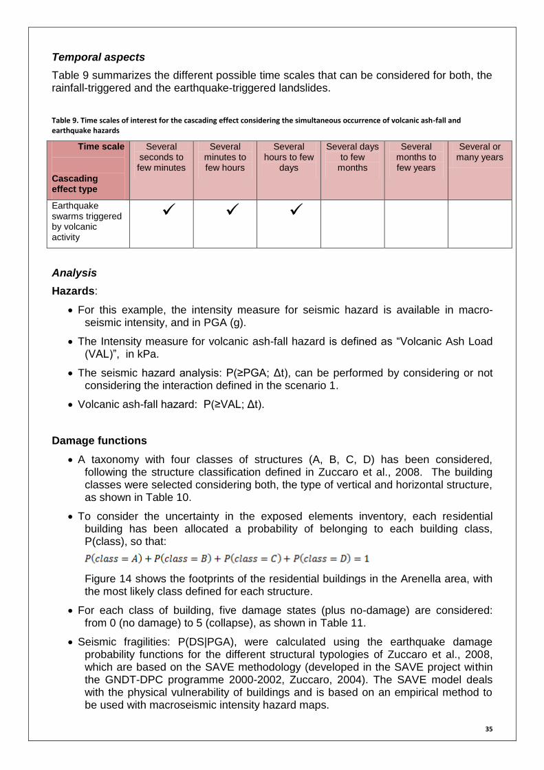
Temporal aspects

Table 9 summarizes the different possible time scales that can be considered for both, the rainfall-triggered and the earthquake-triggered landslides.

Table 9. Time scales of interest for the cascading effect considering the simultaneous occurrence of volcanic ash-fall and earthquake hazards

Time scale

Cascading effect type

Several seconds to few minutes

Several minutes to few hours

Several hours to few

days

Several days to few

months

Several months to few years

Several or many years

Earthquake swarms triggered by volcanic activity

Analysis

Hazards:

For this example, the intensity measure for seismic hazard is available in macro-seismic intensity, and in PGA (g).

The Intensity measure for volcanic ash-fall hazard is defined as “Volcanic Ash Load (VAL)”, in kPa.

The seismic hazard analysis: P(≥PGA; Δt), can be performed by considering or not considering the interaction defined in the scenario 1.

Volcanic ash-fall hazard: P(≥VAL; Δt).

Damage functions

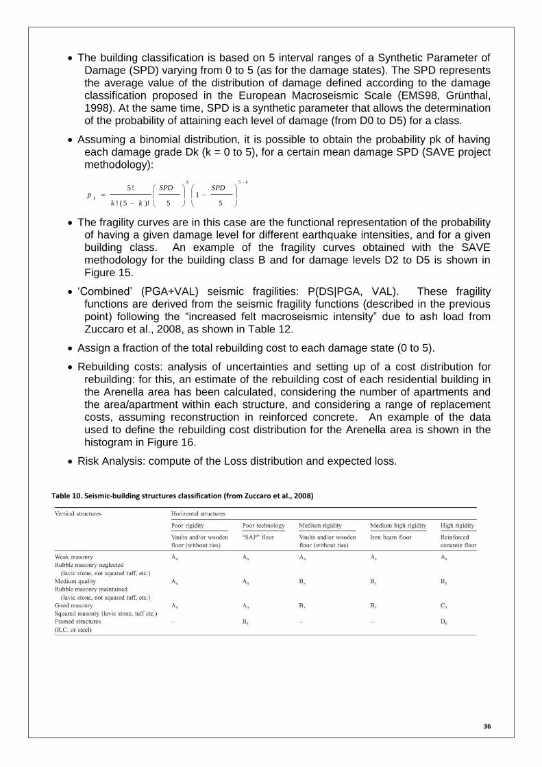
A taxonomy with four classes of structures (A, B, C, D) has been considered, following the structure classification defined in Zuccaro et al., 2008. The building classes were selected considering both, the type of vertical and horizontal structure, as shown in Table 10.

To consider the uncertainty in the exposed elements inventory, each residential building has been allocated a probability of belonging to each building class, P(class), so that:

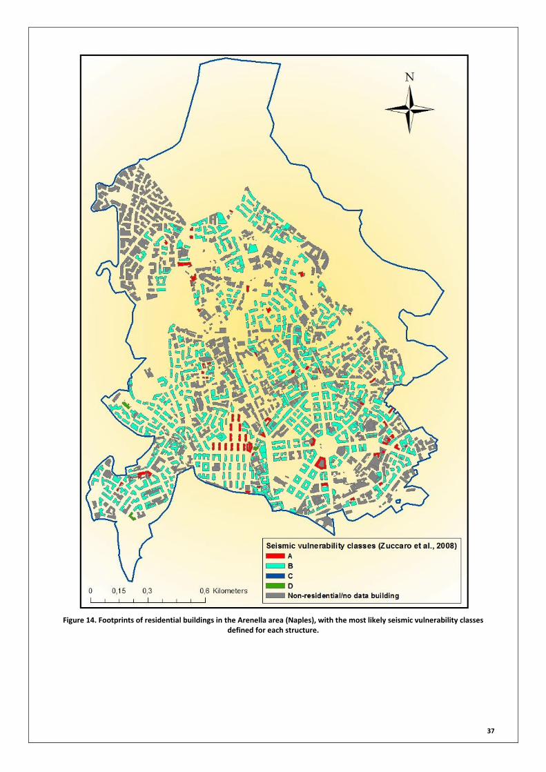
Figure 14 shows the footprints of the residential buildings in the Arenella area, with the most likely class defined for each structure.

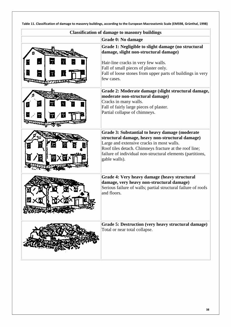
For each class of building, five damage states (plus no-damage) are considered: from 0 (no damage) to 5 (collapse), as shown in Table 11.

Seismic fragilities: P(DS|PGA), were calculated using the earthquake damage probability functions for the different structural typologies of Zuccaro et al., 2008, which are based on the SAVE methodology (developed in the SAVE project within the GNDT-DPC programme 2000-2002, Zuccaro, 2004). The SAVE model deals with the physical vulnerability of buildings and is based on an empirical method to be used with macroseismic intensity hazard maps.

36

The building classification is based on 5 interval ranges of a Synthetic Parameter of Damage (SPD) varying from 0 to 5 (as for the damage states). The SPD represents the average value of the distribution of damage defined according to the damage classification proposed in the European Macroseismic Scale (EMS98, Grünthal, 1998). At the same time, SPD is a synthetic parameter that allows the determination of the probability of attaining each level of damage (from D0 to D5) for a class.

Assuming a binomial distribution, it is possible to obtain the probability pk of having each damage grade Dk (k = 0 to 5), for a certain mean damage SPD (SAVE project methodology):

kk

k

SPDSPD

kk

p

5

5

1

5)!5(!

!5

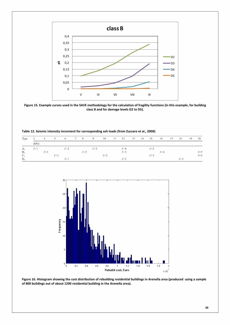
The fragility curves are in this case are the functional representation of the probability of having a given damage level for different earthquake intensities, and for a given building class. An example of the fragility curves obtained with the SAVE methodology for the building class B and for damage levels D2 to D5 is shown in Figure 15.

‘Combined’ (PGA+VAL) seismic fragilities: P(DS|PGA, VAL). These fragility functions are derived from the seismic fragility functions (described in the previous point) following the “increased felt macroseismic intensity” due to ash load from Zuccaro et al., 2008, as shown in Table 12.

Assign a fraction of the total rebuilding cost to each damage state (0 to 5).

Rebuilding costs: analysis of uncertainties and setting up of a cost distribution for rebuilding: for this, an estimate of the rebuilding cost of each residential building in the Arenella area has been calculated, considering the number of apartments and the area/apartment within each structure, and considering a range of replacement costs, assuming reconstruction in reinforced concrete. An example of the data used to define the rebuilding cost distribution for the Arenella area is shown in the histogram in Figure 16.

Risk Analysis: compute of the Loss distribution and expected loss.

Table 10. Seismic-building structures classification (from Zuccaro et al., 2008)

37

Figure 14. Footprints of residential buildings in the Arenella area (Naples), with the most likely seismic vulnerability classes defined for each structure.

38

Table 11. Classification of damage to masonry buildings, according to the European Macroseismic Scale (EMS98, Grünthal, 1998)

Classification of damage to masonry buildings

Grade 0: No damage

Grade 1: Negligible to slight damage (no structural

damage, slight non-structural damage)

Hair-line cracks in very few walls.

Fall of small pieces of plaster only.

Fall of loose stones from upper parts of buildings in very

few cases.

Grade 2: Moderate damage (slight structural damage,

moderate non-structural damage) Cracks in many walls.

Fall of fairly large pieces of plaster.

Partial collapse of chimneys.

Grade 3: Substantial to heavy damage (moderate

structural damage, heavy non-structural damage) Large and extensive cracks in most walls.

Roof tiles detach. Chimneys fracture at the roof line;

failure of individual non-structural elements (partitions,

gable walls).

Grade 4: Very heavy damage (heavy structural

damage, very heavy non-structural damage) Serious failure of walls; partial structural failure of roofs

and floors.

Grade 5: Destruction (very heavy structural damage) Total or near total collapse.

39

0

0,05

0,1

0,15

0,2

0,25

0,3

0,35

0,4

V VI VII VIII IX

pk

class B

D2

D3

D4

D5

Figure 15. Example curves used in the SAVE methodology for the calculation of fragility functions (in this example, for building class B and for damage levels D2 to D5).

Table 12. Seismic intensity increment for corresponding ash loads (from Zuccaro et al., 2008)

Figure 16. Histogram showing the cost distribution of rebuilding residential buildings in Arenella area (produced using a sample of 800 buildings out of about 1200 residential building in the Arenella area).

40

Results

Using all the information presented in the previous section, the quantification of the loss distribution and expected losses was performed following a risk quantification procedure in which uncertainties (if available) from the hazard, the fragilities, the inventory of exposed elements (i.e., for each building, the probability of belonging to each building class is assessed), and the rebuilding cost were propagated to the final risk quantification.

Figure 17a shows the results of the total loss distribution (in terms of loss exceedance probability) considering only the seismic hazard (i.e., with no ash accumulation). This result has already been presented in Section 2.2. The solid line represents the median (50th percentile) value of the Loss exceedance probabilities (as a “best guess” value), whereas the uncertainty area is bounded by the 16th and 84th percentiles. Likewise, it is possible to calculate the “expected loss”, where instead of a single value, in this case we obtain a probability distribution showing the variability of the expected loss given the considered uncertainties. Figure 17b shows the expected loss distribution for the seismic case (i.e., the case without considering the effects of the volcanic ash load).

(a) (b)

Figure 17. (a) Loss exceedance probability, and (b) Cumulative distribution function of the expected loss resulting from the seismic risk analysis for the Arenella area. Note that the plot in (b) represents the variability of the mean value as a result of the uncertainties considered.

Next, considering the effects of a given intensity value of ash load over the residential structures in Arenella, we estimated the loss distribution and expected loss considering different values of ash load. Here we show the results obtained for the combined seismic and volcanic ash load considering 3 and 5 kPa of ash load over the roofs in Figure 18.

41

(a) (b)

(c) (d)

Figure 18. Loss exceedance probability (a and c) and (mean) expected total loss (b and d) resulting from a risk analysis considering the combined effects of seismic and two different values of ash load: 3 kPa (a and b) and 5 kPa (c and d) for the Arenella area.

Note that the probabilities reported in Figure 18 are conditioned to the occurrence of a given intensity of the volcanic ash hazard (i.e. are P(≥L | VAL), for VAL=3 and 5 kPa). Including the term of the probabilistic volcanic hazard assessment (i.e., P(VAL)), the long-term assessment can be performed. In this example, we only compare the single scenarios of loss given the presence of an ash load. The following figures (Figure 19 and Figure 20) summarize the results of the three scenarios considered in this work: (1) seismic, (2) seismic+3kPa ash load, and (3) seismic+5kPa ash load.

42

Figure 19. Summary of results of the exceedance probabilities of loss for the three considered scenarios: (1) seismic, (2) seismic+3kPa ash load, and (3) seismic+5kPa ash load.

Figure 20. Summary of results of the expected losses (mean values) for the three considered scenarios: (1) seismic, (2) seismic+3kPa ash load, and (3) seismic+5kPa ash load.

43

Figure 20 in particular can be useful to compare the expected losses (and their variability) in the different scenarios. It is worth noting that the CDF of the scenario with 3kPa is very close to the CD of the pure seismic case (with no ash), whereas a more consistent distance is observed for the curve with 5 kPa. Taking in consideration the median of the curves, for an ash load variation of 3kPa (from 0 to 3kPa), there was an increase of the expected losses of about 19%; in the second case, an increase of 2 kPa (from 3 to 5kPa) of ash load implied an increase of about five times in the expected losses.

44

4 Interactions with stakeholders in Naples: Identification of social and institutional barriers to effective decision-making and governance in the case of multiple hazards

Napoli was one of the test sites for research about the social and institutional barriers to effective decision-making and governance in the case of multiple hazards. This work is reported in deliverable D6.3 of the MATRIX project (Scolobig et al., 2012).

The starting point for the empirical research was that before new methodologies (as are being developed in the other work packages of the MATRIX project) are implemented into existing risk management systems, not only the technical, but also social and institutional issues need to be taken into account.

To better understand these issues, the first step was the assessment of the current situation. This was performed by describing the architecture of risk management regimes and by profiling the key characteristics of risk governance within diverse natural hazard contexts. This formed the basis for the description of the strengths and weaknesses of the existing system, as well as the institutional benefits and barriers to effective multi-risk governance.

The research design included a documentary analysis of legal, regulatory and policy documents, twenty-one semi-structured interviews with practitioners in Naples, a focus group with experts and researchers and two feedback workshops, one with stakeholders at the local level (i.e., held in Naples) and one at the national level (also including stakeholders of other European countries, held in Bonn). The risks considered included volcanic eruptions, earthquakes, floods, landslides, and fires.

The results provide a comparative evaluation of risk governance which covers issues such as:

stakeholders and governance level, i.e., a description of the key agencies and authorities in charge of risk management, their roles and responsibilities, including the degree of centralization of the risk management regime;

decision support tools and mitigation measures, i.e., description and evaluation of the science-based decision support tools developed by public agencies or private consultants (hazard, exposure and vulnerability maps, monitoring and warning systems, emergency plans, and risk mitigation measures);

stakeholder cooperation and communication, i.e., information related to the cooperation and exchange of knowledge among actors, as well as their involvement in the risk decision making processes (including, for example, public availability of hazard/risk assessments, planning integration at different levels, balance between governance tasks and resources, multi-stakeholder participation in decision making, etc.).

The results show that local authorities have developed adequate decision support tools for most of the hazards considered, but the same is not true for interagency cooperation and communication, thus including how the knowledge produced in the science domain feeds back into the policy and practice domain.

The focus groups and workshops with practitioners and stakeholders revealed how addressing multiple hazards/risks can lead to considerable institutional improvements in terms of the efficiency of risk and emergency management. At the same time, the results

45

illustrate the institutional barriers to the adoption of these methods that are related, for example, to the division between the communities of geological and meteorological practitioners. Due to the different educational and professional development paths, the support tools and decision-making processes – and even the language used – for geological hazards has evolved differently from meteorological or technological hazards.

Moreover, the difficulties in interagency communication for hazards managed at different levels (e.g., national vs. regional), the scarcity of public/private partnership, the lack of an emergency plan with information about multiple hazards and risks, and the research-practice divide represent serious threats to the implementation of multi-hazard and multi-risk approaches.

46

5 Summary

The Naples test case provided the opportunity to test different methodologies developed in the MATRIX project in specific activities of single- and multi-risk assessments. In particular, we can summarize the following main results:

In WP2, a procedure based on Bayesian analyses has been developed and applied to the Naples test case in order to calculate volcanic risk (considering ash fall). It is worth noting that the methodology proposed is general enough to be easily implemented for other kind of risks;

In WP3, a conceptual framework to analyse interactions and cascade effects was developed. This framework was implemented in the Naples test case allowing us to analyse the effects of interactions between two risk sources (seismic and volcanic) at different levels.

The results of the interaction analysis and multi-risk assessment for this particular scenario were used in the WP6 for the identification of social and institutional barriers to effective decision-making and governance when considering multiple hazards.

47

References

Aki, K (1967). Scaling law of seismic spectrum, J Geophys. Res., 72, 1217-1231

Barberi, F., D. P. Hill, F. Innocenti, G. Luongo, and M. Treuil (Eds.) (1984), The 1982 – 1984 Bradyseismic crisis at Phlegrean Fields (Italy), Bull. Volcanol., 47, 173 – 411.

Bender, B., Perkins D.M. (1987): Seisrisk III: A computer program for seismic hazard estimation. U.S. Geological Survey Bulletin, 1772 , 48 pp.

Boore, D. M., 1983. Stochastic simulation of high-frequency ground motions based on seismological models of the radiated spectra, Bulletin of the Seismological Society of America, Vol 73, No 6, pp. 1865-1894

Brune, J. N. (1970), Tectonic stress and the spectra of seismic shear waves from earthquakes, J. Geophys. Res., 75(26), 4997–5009, doi:10.1029/JB075i026p04997.

ByMuR (2010-2013), Bayesian Multi-Risk assessment: a case study for Natural Risks in the city of Naples, Italian project funded by MIUR, http://bymur.bo.ingv.it

Commission staff working paper: “Risk assessment and mapping guidelines for disaster management”, European Commission, Brussels, December 2010.

Cornell C.A. (1968): Engineering seismic risk analysis. Bull. Seism. Soc. Am., 58, 1583- 1606.

Crowley, H. et al. (2011), Fragility functions for common RC building types in Europe, Deliverable D3.1, SYNER-G project.

De Natale, G., E. Faccioli, and A . Zollo, 1988. Scaling of Peak Ground Motions from Digital Recordings of Small Earthquakes at Campi Flegrei, Southern Italy. PAGEOPH, 126(1).

De Natale, G., G. Iannaccone, M . Martini, and A . Zollo, 1987. Seismic Sources and Attenuation Properties at the Campi Flegrei Volcanic Area, PAGEOPH, 125(6).

De Natale, G., A. Zollo, A. Ferraro, and J. Virieux (1995), Accurate fault mechanism determinations for a 1984 earthquake swarm at Campi Flegrei caldera (Italy) during an unrest episode: Implications for volcanological research, J. Geophys. Res., 100, 24,167 – 24,185.

De Natale, G., C. Troise, F. Pingue, G. Mastrolorenzo, L. Pappalardo, and E. Boschi (2006), The Campi Flegrei caldera: Unrest mechanisms and hazards, in Mechanisms of Activity and Unrest at Large Calderas, edited by C. Troise, G. De Natale, and C. R. J. Kilburn, Geol. Soc. London Spec. Publ., 269, 25 – 45.

Department of Agriculture, Campania Region (2012), Piano antincendio boschivo, Regione Campania, Napoli.

Di Vito M., Lirer L., Mastrolorenzo G., Rolandi G. (1987) The 1538 Monte Nuovo eruption (Campi Flegrei, Italy), Bull. Volcanol., 49, pp. 608-615

Dvorak, J.J., Gasparini, P., 1991. History of earthquakes and vertical ground movement in Campi Flegrei caldera, Southern Italy: comparison of precursory events to the A.D. 1538 eruption of Monte Nuovo and of activity since 1968. J. Volcanol. Geotherm. Res., 48, 77–92.

48

Endo, E., Malone, S., Noson, L., Weaver, C., 1981. Locations magnitudes and statistics of the March 20 – May 18 earthquake sequence. U.S. Geol. Surv. Prof. Pap. 1250, 93 – 107 US Govt. Printing Office, Washington, DC.

Gaeta, F.S., Peluso, F., Arienzo, I., Castagnolo, D., De Natale, G., Milano, G., Albanese, C., Mita, D.G., 2003. A physical appraisal of a new aspect of bradyseism: the miniuplifts. J. Geophys. Res., 108(B8), 2363, doi:10.1029/2002JB001913.

Garcia-Aristizabal, A., W. Marzocchi and A. Di Ruocco, 2013a. Probabilistic framework for the assessment of hazard interactions in a multi-risk framework. Deliverable D3.4, New methodologies for multi-hazard and multi-risk assessment methods for Europe (MATRIX project), contract No. 265138.

Garcia-Aristizabal, A., A. Di Ruocco, and W. Marzocchi (with: S. Tyagunov, S. Vorogushyn, K. Fleming, and N. Desramaut), 2013b. Scenarios of cascade events, Deliverable D3.3, New methodologies for multi-hazard and multi-risk assessment methods for Europe (MATRIX project), contract No. 265138.

Garcia-Aristizabal, A., H. Kumagai, P. Samaniego, P. Mothes, H. Yepes, and M. Monzier (2007). Seismic, petrologic and geodetic analyses of the 1999 dome-forming eruption of Guagua Pichincha volcano, Ecuador, J. Volcanol. Geoth. Res., 161(4), 333-351. DOI: 10.1016/j.jvolgeores.2006.12.007

Grünthal, G. (editor) (1998). “Cahiers du Centre Européen de Géodynamique et de Séismologie: Volume 15 – European Macroseismic Scale 1998”, European Center for Geodynamics and Seismology, Luxembourg.

Gruppo di Lavoro (2004). Redazione della mappa di pericolosità sismica prevista dall’Ordinanza

Lanari, R., Berardino, P., Borgstroem, S., Del Gaudio, C., De Martino, P., Fornaro, G., Guarino, S., Ricciardi, G., Sansosti, E., Lundgren, P., 2004. The use of IFSAR and classical geodetic technique for caldera unrest episodes: application to the Campi Flegrei uplift event of 2000. J. Volcanol. Geotherm. Res., 133, 247–260.

Lee, KH; and D.V. Rosowsky, (2006). Fragility analysis of woodframe buildings considering combined snow and earthquake loading. Structural Safety, 28(3), 289-303.

Legrand, D, A. Calahorrano, B. Guillier, L. Rivera, M. Ruiz, D. Villagómez, H. Yepes (2002), Stress tensor analysis of the 1998–1999 tectonic swarm of northern Quito related to the volcanic swarm of Guagua Pichincha volcano, Ecuador, Tectonophysics, 344, pp. 15–36

Malagnini, L. and V. Montaldo, 2004. Relazioni di attenuazione del moto del suolo: App.3 al Rapporto Conclusivo. Gruppo di Lavoro per la redazione della mappa di pericolosità sismica (Ordinanza PCM 20.03.03, n.3274) Istituto Nazionale di Geofisica e Vulcanologia, Italy.

Marzocchi, W., M.L. Mastellone, S. Di Ruocco, P. Novelli, E. Romeo, and P. Gasparini, 2009. Principles of multi-risk assessment: interactions amongst natural and man-induced risks, Project Report (FP6 NARAS project), European Commission, Directorate-General Research – Environment, contract No. 511264.

Marzocchi, W., A. Garcia-Aristizabal, P. Gasparini, M. L. Mastellone, and A. Di Ruocco (2012). Basic principles of multi-risk assessment: a case study in Italy, Nat. Hazards, 62(2), 551-573. DOI: 10.1007/s11069-012-0092-x

49

Marzocchi, W., and J.D. Zechar (2011), Earthquake Forecasting and Earthquake Prediction: Different Approaches for Obtaining the Best Model. Seismological Research Letters 82(3): 442-448.

Marzocchi, W., L. Sandri and J. Selva, (2010), BET_VH: a probabilistic tool for long-term volcanic hazard assessment. Bull. Volcanol. 72, 705-716.

Marzocchi, W., Sandri, L, Selva, J. (2008), BET_EF: a probabilistic tool for long- and short-term eruption forecasting, Bull. Volcanol., 70, 623-632, doi:10.1007/s00445-007-0157-y

Marzocchi, W., Sandri, L., Gasparini, P., Newhall, C. and Boschi, E. (2004), Quantifying probabilities of volcanic events: The example of volcanic hazard at Mount Vesuvius, J. Geophys. Res., 109, B11201, DOI: 10.1029/2004JB003155.

Matsumura, S., Ohkubo, T., Imoto, M., 1991. Seismic swarm activity in and around the Izu Peninsula preceding the volcanic eruption of July 13, 1989. J. Phys. Earth 39, 93 – 106.

Meletti, C. and V. Montaldo (2007). Deliverable D2: Valutazioni di ag (16mo, 50mo e 84mo percentile) con le seguenti probabilità di superamento in 50 anni: 81%, 63%, 50%, 39%, 30%, 22%, 5%, 2%, rispettivamente corrispondenti a periodi di ritorno di 30, 50, 72, 100, 140, 200, 1000 e 2500 anni. Task 1, Convenzione INGV-DPC 2004 – 2006 / Progetto S1

Minakami, T., 1974. Seismology of volcanoes in Japan. In: Civette, L., et al. (Eds.), Physical Volcanology Developments in Solid Earth Geophysics, vol. 6. Elsevier, Amsterdam, pp. 1 – 27.

Orsi, G., M. D'Antonio, S. de Vita, and G. Gallo (1992), The Neapolitan Yellow Tuff, a large-magnitude trachytic phreatoplinian eruption: eruptive dynamics, magma withdrawal and caldera collapse, Journal of Volcanology and Geothermal Research, Vol. 53, 1-4, 275–287.

Orsi, G., S. De Vita, and M. Di Vito (1996), The restless, resurgent Campi Flegrei nested caldera (Italy): Constraints on its evolution and configuration, J. Volcanol. Geotherm. Res., 74, 179 – 214.

Orsi, G., L. Civetta, C. Del Gaudio, S. de Vita, M.A. Di Vito, R. Isaia, S.M. Petrazzuoli, G.P. Ricciardi, C. Ricco, (1999). Short-term ground deformations and seismicity in the resurgent Campi Flegrei caldera, Italy: an example of active block-resurgence in a densely populated area. Journal of Volcanology and Geothermal Research 91, 415–451

Orsi, G., Di Vito, M.A., Selva, J., Marzocchi, W. (2009), Long-term forecast of eruption style and size at Campi Flegrei caldera (Italy), Earth and Planetary Science Letters (287): 265–276

Oshima, S., Tsuchide, M., Kato, S., Okubo, S., Watanabe, K., Kudo, K., Ossaka, J., 1991. Birth of a submarine volcano «Teishi Knoll». J. Phys. Earth 39, 1 – 19.

Power, J., Lahr, J., Page, R., Chouet, B., Stephens, C., Harlow, D., Murray, T., Davies, J., 1994. Seismic evolution of the 1989 - 1990 eruption sequence of Redoubt volcano, Alaska. J. Volcanol. Geotherm. Res. 62, 69 – 94.

Sawada, Y., Aramaki, S., 1989. O-shima report. Bull. Volcanic Eruptions (26), Suppl. to Bull. Volcanol. 51, 31 – 36.

Scolobig A., Vinchon C., Komendantova N., Bengoubou-Valerius M., Patt A., Gasparini P., Di Ruocco A., Baills A., Revellière A. (2012) Social and institutional barriers to effective multi-hazard decision making, Deliverable 6.3, Matrix project, New methodologies for

50

multi-hazard and multi-risk assessment methods for Europe, European Commission 7th Framework Programme. http://matrix.gpi.kit.edu/, 134 pp.

Selva, J. 2013. Long-term multi-risk assessment: statistical treatment of interaction among risks. Natural Hazards, Volume 67, Issue 2, pp 701-722

Selva, J., Agryroudis, S, and K. Pitilakis, (2012a), Impact on loss/risk assessments of inter-model variability in vulnerability analysis, submitted

Selva, J., Costa, A., Marzocchi, W., Sandri, L., (2010), BET_VH: exploring the influence of natural uncertainties on long-term hazard from tephra fallout at Campi Flegrei (Italy). Bull. Volcanol. 72, 717-733.

Selva, J., Marzocchi, W., Papale, P. and Sandri, L. (2012b). Operational eruption forecasting at high-risk volcanoes: the case of Campi Flegrei, Naples, submitted

Shimizu, H., Umakoshi, K., Matsuwo, N., Ohta, K., 1992. Seismological observations of Unzen volcano before and during the 1990 – 1992 eruption. In: Yanagi, T., Okada, H., Ohta, K. (Eds.), Unzen Volcano: The 1990 – 1992 Eruption. The Nishi-nippon & Kyushu University Press, Kyushu, pp. 38 – 43.

Spence, R.J.S., Kelman, I., Baxter, P.J., Zuccaro G., S. Petrazzuoli (2005), Residential building and occupant vulnerability to tephra fall, Natural Hazard and Earth System Sciences, 5, 477-494.

SYNER-G (2010-2012), Systemic seismic vulnerability and risk analysis for buildings, lifeline networks and infrastructures safety gain”, European Research Project funded by FP7, http://www.syner-g.eu

Troise, C., G. De Natale, and F. Pingue, 1997. A model for earthquake generation during unrest episodes at Campi Flegrei and Rabaul calderas, Geophys. Res. Letters, Vol. 24, No.13, 1575-1578

Troise, C, G. De Natale, F. Pingue, U. Tammaro, P. De Martino, F. Obrizzo and E. Boschi (2008), A New Uplift Episode at Campi Flegrei Caldera (Southern Italy): Implications for Unrest Interpretation and Eruption Hazard Evaluation; in: “Developments in Volcanology”, Volume 10, ISSN 1871-644X, DOI 10.1016/S1871-644X(07)00010-1

Vilardo, G., G. Alessio, and G. Luongo, 1991. Analysis of the magnitude-frequency distribution for the 1983-1984 earthquake activity of Campi Flegrei, Italy, ournal of Volcanology and Geothermal Research, 48 ( 1991 ) 115-125

White, R. A., and J.A. Power (2001), Distal Volcano-Tectonic Earthquakes (DVT's): Diagnosis and Use in Eruption Forecasting. Abstract U32A-0001, AGU Fall Meeting

Wolfe, E., 1992. The 1991 Eruptions of Mount Pinatubo, Philippines. Earthquakes Volcanoes, vol. 23. US Govt. Printing Office, Washington, DC, pp. 5 – 37.

Zuccaro, G. 2004. Inventory and vulnerability for residential buildings at National territorial level, risk maps and socio-economic losses – Naples, 2004 (in italian); CD publishing the results of the Task 1 for SAVE, INGV/GNDT Project, PQ 2000-2002

Zuccaro, G., F. Cacace, R.J.S. Spence, and P. J. Baxter, 2008. Impact of explosive eruption scenarios at Vesuvius. J Volcanol. Geotherm. Res., 178, 416-453.