A Thesis

by

JESUS JAIME LEAL CHAPA

Submitted to the O�ce of Graduate and Professional Studies ofTexas A&M University

in partial ful�llment of the requirements for the degree of

MASTER OF SCIENCE

Chair of Committee, Eduardo GildinCommittee Members, Yalchin Efendiev

John KilloughHead of Department, A. Daniel Hill

December 2016

Major Subject: Petroleum Engineering

Copyright 2016 Jesus Jaime Leal Chapa

PROPER ORTHOGONAL DECOMPOSITION FOR PRESSURE

PRECONDITIONING FOR THE GMRES ALGORITHM..

ABSTRACT

The linear solver in a typical reservoir simulator consumes around 60 to 70 % of

the total simulation time. To speed up the solution of the linear systems we will use

a two stage preconditioner, where the �rst stage is the ILU preconditioner and the

second stage is obtained with a technique of Reduction of Order Modelling (ROM)

called Proper Orthogonal Decomposition (POD). The bene�ts of using this method

is that it is relatively easy to implement because it doesn't require big modi�cations

in existing code. There is already research in this area with positive results, but the

method has been tested with the Richardson Algorithm. This is not a very realistic

scenario given that there are better solvers widely available. The objective of this the-

sis is to test the method with the Generalized Minimal Residual Method (GMRES).

The results validate the �ndings that two stage preconditioner improves the perfor-

mance of the Richardson algorithm, however it doesn't improve the performance of

the GMRES algorithm. The drawback is that although the two stage preconditioner

increases convergence it is too costly to compute. And the time saved by the de-

crease in the number of iterations is o�set by the increase in time in preconditioner

computation.

ii

DEDICATION

I dedicate this thesis to my brothers Luis and Fernando.

iii

ACKNOWLEDGEMENTS

I would like to acknowledge my adviser Dr. Eduardo Gildin for his support and

guidance during my degree.

This thesis was possible thanks to a full scholarship from the Consejo Nacional

de Ciencia y Tecnología.

iv

NOMENCLATURE

POD Proper Orthogonal Decomposition

SVD Singular Value Decomposition

ROM Reduced Order Modeling

ILU Incomplete LU Factorization

LU Lower Diagonal, Upper Diagonal

GMRES Generalized Minimum Residual Method

CPR Constrained Pressure Residual

AMG Algebraic Multigrid

MILU Incomplete LU Preconditioner

MPOD POD Preconditioner

MPOD+ILU Two Stage POD + ILU Preconditioner

M−1 Inverse of the Preconditioner

Φ Orthogonal Basis

Ψ Projection Operator

P Pressure

S Saturation

Po Oil Pressure

Sw Water Saturation

U Left Basis Vectors

S Diagonal Matrix With Singular Values

V Right Basis Vectors

v

σ Singular Value

ρ Density

c Compressibility

φ Porosity

µ Viscosity

k Permeability

g Gravity

z Depth

q Flow

t Time

|| · || Matrix and Vector Norm

vi

TABLE OF CONTENTS

Page

ABSTRACT . . . . . . . . . . . . . . . . . . . . . . . . . . . . . . . . . . . . ii

DEDICATION . . . . . . . . . . . . . . . . . . . . . . . . . . . . . . . . . . . iii

ACKNOWLEDGEMENTS . . . . . . . . . . . . . . . . . . . . . . . . . . . . iv

NOMENCLATURE . . . . . . . . . . . . . . . . . . . . . . . . . . . . . . . . v

TABLE OF CONTENTS . . . . . . . . . . . . . . . . . . . . . . . . . . . . . vii

LIST OF FIGURES . . . . . . . . . . . . . . . . . . . . . . . . . . . . . . . . ix

LIST OF TABLES . . . . . . . . . . . . . . . . . . . . . . . . . . . . . . . . . xi

1. INTRODUCTION . . . . . . . . . . . . . . . . . . . . . . . . . . . . . . . 1

1.1 Introduction . . . . . . . . . . . . . . . . . . . . . . . . . . . . . . . . 11.2 Literature Review . . . . . . . . . . . . . . . . . . . . . . . . . . . . . 21.3 Scope of this Thesis . . . . . . . . . . . . . . . . . . . . . . . . . . . . 6

2. LINEAR SOLVERS AND RESERVOIR SIMULATION . . . . . . . . . . . 8

2.1 Linear Solvers . . . . . . . . . . . . . . . . . . . . . . . . . . . . . . . 82.1.1 Iterative Solvers . . . . . . . . . . . . . . . . . . . . . . . . . . 8

2.2 Preconditioners . . . . . . . . . . . . . . . . . . . . . . . . . . . . . . 102.2.1 ILU Preconditioner . . . . . . . . . . . . . . . . . . . . . . . . 12

2.3 Reservoir Simulator Overview . . . . . . . . . . . . . . . . . . . . . . 14

3. POD BASED PRECONDITIONING . . . . . . . . . . . . . . . . . . . . . 17

3.1 Introduction to Model Reduction by Proper Orthogonal Decomposition 173.2 POD Preconditioner Derivation . . . . . . . . . . . . . . . . . . . . . 203.3 Snapshots Method Framework . . . . . . . . . . . . . . . . . . . . . . 23

3.3.1 O�ine Stage . . . . . . . . . . . . . . . . . . . . . . . . . . . . 243.3.2 Online Stage . . . . . . . . . . . . . . . . . . . . . . . . . . . . 25

4. NUMERICAL EXPERIMENTS . . . . . . . . . . . . . . . . . . . . . . . . 27

vii

4.1 The Reservoir Models . . . . . . . . . . . . . . . . . . . . . . . . . . . 274.1.1 Model 1: Simple Model . . . . . . . . . . . . . . . . . . . . . . 274.1.2 Model 2: Realistic Model . . . . . . . . . . . . . . . . . . . . . 28

4.2 Numerical Experiments. Model 1 . . . . . . . . . . . . . . . . . . . . 324.2.1 Energy vs Basis Number . . . . . . . . . . . . . . . . . . . . . 324.2.2 Residual Error Analysis . . . . . . . . . . . . . . . . . . . . . 324.2.3 Performance Improvement . . . . . . . . . . . . . . . . . . . . 33

4.3 Numerical Experiments. Model 2 . . . . . . . . . . . . . . . . . . . . 394.3.1 Energy vs Basis Number . . . . . . . . . . . . . . . . . . . . . 394.3.2 Residual Error Analysis . . . . . . . . . . . . . . . . . . . . . 404.3.3 Performance Improvement . . . . . . . . . . . . . . . . . . . . 40

5. CONCLUSIONS . . . . . . . . . . . . . . . . . . . . . . . . . . . . . . . . 42

REFERENCES . . . . . . . . . . . . . . . . . . . . . . . . . . . . . . . . . . . 45

viii

LIST OF FIGURES

FIGURE Page

1.1 Big O complexity and its e�ect in the number of computations. From[1]. . . . . . . . . . . . . . . . . . . . . . . . . . . . . . . . . . . . . 4

2.1 Example of residual error vs iteration number. The blue line corre-sponds to when the system is preconditioned and the red line to whenthe system is not preconditioned. . . . . . . . . . . . . . . . . . . . . 11

2.2 Observe the structure of L and U, in the ILU(0) decomposition. From[2]. . . . . . . . . . . . . . . . . . . . . . . . . . . . . . . . . . . . . . 13

2.3 E�ect of droptol in number of iterations required to solve the systemof equations. . . . . . . . . . . . . . . . . . . . . . . . . . . . . . . . 13

2.4 Reservoir simulation work�ow. . . . . . . . . . . . . . . . . . . . . . . 15

3.1 Singular value decomposition. . . . . . . . . . . . . . . . . . . . . . . 19

3.2 Framework. . . . . . . . . . . . . . . . . . . . . . . . . . . . . . . . . 23

4.1 Model 1. Simple square reservoir. . . . . . . . . . . . . . . . . . . . . 30

4.2 Fluid properties. . . . . . . . . . . . . . . . . . . . . . . . . . . . . . 31

4.3 Model 2. Realistic reservoir model. . . . . . . . . . . . . . . . . . . . 31

4.4 Model 1. Energy of POD basis vectors. . . . . . . . . . . . . . . . . 33

4.5 Model 1. Relative residual error vs. iteration number, for the Richard-son and GMRES algorithm preconditioned with MILU and MILU+POD. 34

4.6 Model 1. Simulation time improvement for the Richardson algorithm.E�ect of number of layers and number of cells. . . . . . . . . . . . . . 36

4.7 Model 1. Simulation time improvement for the GMRES algorithm.E�ect of number of layers and number of cells. . . . . . . . . . . . . . 37

4.8 Model 1. Simulation time improvement for the GMRES algorithm.Case when the full simulation schedule is the same as the trainingschedule. . . . . . . . . . . . . . . . . . . . . . . . . . . . . . . . . . . 38

ix

4.9 Model 2. Energy of POD basis vectors. . . . . . . . . . . . . . . . . 39

4.10 Model 2. Residual error vs. iteration number for the GMRES algorithm. 40

x

LIST OF TABLES

TABLE Page

4.1 Model 1. Simple reservoir model speci�cations. . . . . . . . . . . . . . 28

4.2 Fluid properties. . . . . . . . . . . . . . . . . . . . . . . . . . . . . . 29

4.3 Model 2. Realistic reservoir model speci�cations. . . . . . . . . . . . . 29

4.4 Model 1. Percentage improvement in the order of error reduction.Richardson algorithm. . . . . . . . . . . . . . . . . . . . . . . . . . . 34

4.5 Model 1. Percentage improvement in the order of error reduction.GMRES algorithm. . . . . . . . . . . . . . . . . . . . . . . . . . . . . 34

4.6 Model 2. Performance of MILU+POD over MILU . The units of timeare 103 seconds. . . . . . . . . . . . . . . . . . . . . . . . . . . . . . . 41

4.7 MILU+POD computation time and memory allocation for Model 2. . . 41

xi

1. INTRODUCTION

1.1 Introduction

In the early stages of reservoir simulation development, the reservoir models were

small and two dimensional, with 102 to 103 cells. Current modern reservoir simulators

run giant three dimensional reservoir models with a number of cells in the order of 106

and upwards [3, 4]. Depending on the type of discretization of the partial di�erential

equations and on the number of �uid phases being simulated, this leads to very large

systems of linear equations that have to be solved for each timestep. The capability

that we have today of performing this type of simulations is possible thanks to the

steady increase in the computing power of computers and the availability of high

performance computing.

Despite all of this computing power, it becomes time consuming to run simulations

in the context of history matching and optimization , where thousands of simulations

must be run to obtain the solution to a problem [4]. Therefore, it is important to

�nd ways to speed up the solution of the simulations. We should point out that this

is not a new problem, and many techniques have been developed to achieve this.

The bottleneck of the typical reservoir simulator is the linear solver, which con-

sumes around 60 to 70% of the total simulation time [5] . An improvement in the

linear solver improves the simulator greatly, so in this thesis we will focus on en-

hancing the preconditioner for the linear system solvers. Some of the methods to

decrease the simulation time are preconditioning techniques and reduced order mod-

eling (ROM) techniques. Preconditioning consists of multiplying the linear system

by a preconditioner matrix that makes the system easier to solve and increases the

order of convergence of the iterative solvers [6]. There are many types of precondi-

1

tioners, but the most widely used in the context of reservoir simulation is the ILU

preconditioner (MILU) [5]. On the other hand, ROM reduces a high order system

to a low order system that accurately represents the main characteristics of the high

order model but that is faster to solve due to its lower number of equations [7, 5, 8, 9].

This leads to cases were it is possible to decrease the number of equations that de-

scribe the reservoir from hundreds of thousands to a few dozen equations, that is a

three to four fold reduction [4].

One of the disadvantages of ROM techniques is that they require to make mod-

i�cations to the linear solver module of the simulator [10], and depending on the

simulator this may or may not be straightforward to implement.

In this thesis we will study the pressure preconditioner proposed by Rui in [10]. It

is derived from the ROM technique called Proper Orthogonal Decomposition (POD),

and it has the advantage that its implementation in the simulator does not require

to make intrusive modi�cations to existing code. This preconditioner also has the

potential of performing better than typical preconditioners, such as MILU . The goal

is to enhance the capabilities of MILU by means of POD.

1.2 Literature Review

Reservoir simulation began in the mid 1950's and since its inception it has become

an important quantitative and qualitative tool for predicting the �ow of the di�erent

�uid phases in the subsurface [3]. Reservoir simulation has evolved from handling

two dimensional reservoir models with simple geometry to solving highly complex

heterogenoeus models with complex geometry and millions of cells .

The main advances in reservoir simulation have been closely tied to advances in

linear solvers and preconditioning techniques. This is because about 60 % and up

to 90 % of the total simulation time is spent solving the linear system of equations

2

resulting from the discretization of the partial di�erential equations that describe the

porous media �uid �ow [5, 11]. Solving these linear systems is challenging because

of their size and because they are highly sparse.

The linear solvers can be classi�ed as either direct solvers or iterative solvers. The

direct solvers, such as Gaussian elimination and LU factorization, are only suitable

for small matrices because they consume much more resources than iterative solvers

and also because they scale poorly with the number of cells [12]. For that reason

iterative solvers are preferred.

There are many iterative linear solvers but the most widely used in reservoir sim-

ulation are the Generalized Minimal Residual Method (GMRES) and ORTHOMIN

[13, 14]. However , the most advanced solvers belong to the Algebraic Multigrid

(AMG) Methods [15, 16, 17, 18]. According to the authors in [19], AMG meth-

ods are an "ideal solver for large-scale scienti�c simulation", because they can solve

linear systems with N unknowns with O(N) work. Also, with the use of parallel

computing, ever larger problems can be solved on proportionally larger parallel com-

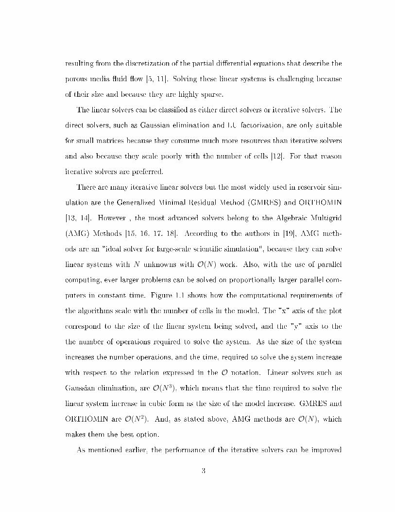
puters in constant time. Figure 1.1 shows how the computational requirements of

the algorithms scale with the number of cells in the model. The "x" axis of the plot

correspond to the size of the linear system being solved, and the "y" axis to the

the number of operations required to solve the system. As the size of the system

increases the number operations, and the time, required to solve the system increase

with respect to the relation expressed in the O notation. Linear solvers such as

Gaussian elimination, are O(N3), which means that the time required to solve the

linear system increase in cubic form as the size of the model increase. GMRES and

ORTHOMIN are O(N2). And, as stated above, AMG methods are O(N), which

makes them the best option.

As mentioned earlier, the performance of the iterative solvers can be improved

3

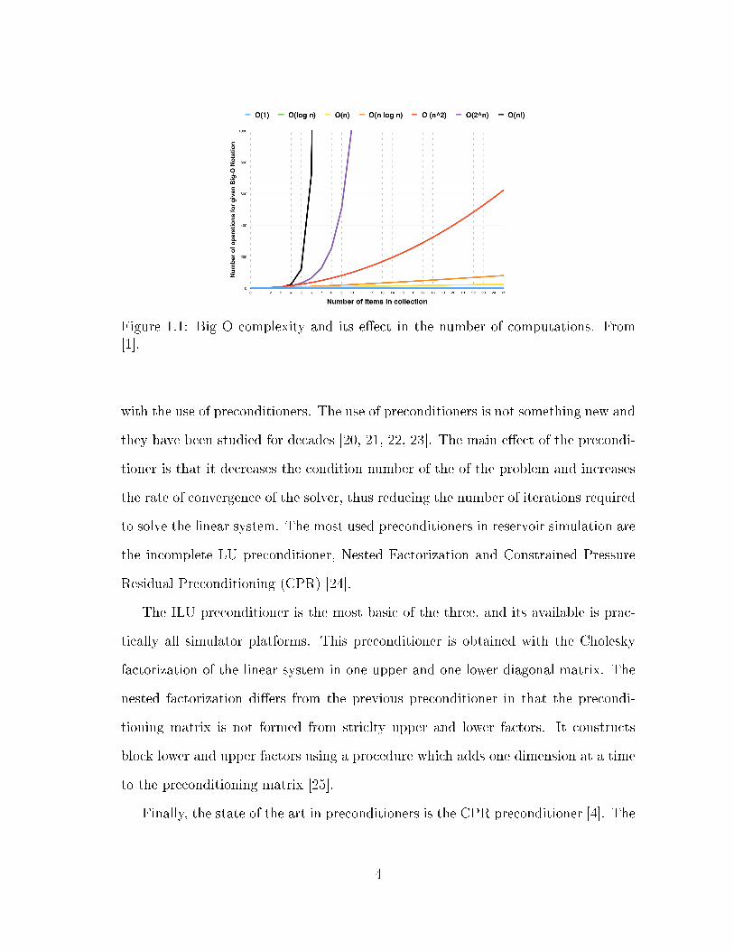
Figure 1.1: Big O complexity and its e�ect in the number of computations. From[1].

with the use of preconditioners. The use of preconditioners is not something new and

they have been studied for decades [20, 21, 22, 23]. The main e�ect of the precondi-

tioner is that it decreases the condition number of the of the problem and increases

the rate of convergence of the solver, thus reducing the number of iterations required

to solve the linear system. The most used preconditioners in reservoir simulation are

the incomplete LU preconditioner, Nested Factorization and Constrained Pressure

Residual Preconditioning (CPR) [24].

The ILU preconditioner is the most basic of the three, and its available is prac-

tically all simulator platforms. This preconditioner is obtained with the Cholesky

factorization of the linear system in one upper and one lower diagonal matrix. The

nested factorization di�ers from the previous preconditioner in that the precondi-

tioning matrix is not formed from striclty upper and lower factors. It constructs

block lower and upper factors using a procedure which adds one dimension at a time

to the preconditioning matrix [25].

Finally, the state of the art in preconditioners is the CPR preconditioner [4]. The

4

CPR preconditioner is more e�cient that the ILU preconditioner. The CPR precon-

ditioner is a two-stage preconditioner, which solves a submatrix from the pressure

equation using multigrid methods and then uses the ILU methods to solve the whole

system [26].

Preconditioners can also be obtained by exploiting the nature of the problem be-

ing solved, this type of preconditioners are called called physics based precondition-

ers. In [10] a POD based pressure preconditioner for a reservoir simulator is derived.

From this, a two stage preconditioner M−1ILU+POD was created. This preconditioner

was tested in a water �ooding simulation with the Richardson algorithm as the lin-

ear iterative solver. The �ndings were that the M−1ILU+POD preconditioner increases

the order of error reduction in the iterative solver. Nevertheless, the Richardson

algorithm is not the state of the art in iterative linear solvers, as explained above

the most sophisticated solver is AMG, but because this solver is not available in all

commercial and research simulators, the most widely available and second best op-

tion would be the GMRES + ILU combination [4]. That is the reason that the focus

of this thesis is in that solver and preconditioner combination and how to improve

upon them.

Regarding ROM and POD, the application of model reduction techniques, and in

speci�c, the Proper Orthogonal Decomposition technique is very wide. It has been

used to create reduced order models of the pressure and saturation matrix in reservoir

simulators [4]. It has been used to replace the �rst stage preconditioner of a reservoir

simulator [27], it has also been used in history matching, in inverse problems, and in

probabilistic inverse modeling to speed up Monte Carlo simulations.

We will implement proper orthogonal decomposition to reservoir simulation with

the snapshot based algorithm. There are many recommendations for the success-

ful implementation of this algorithm found in the literature. To this end, it was

5

determined that the number of basis vectors required to capture the behavior of

the system is at most two times the number of wells in the reservoir [27]. For the

case where the pressure and saturation equations are uncoupled, snapshots of both

variables are collected and then the POD procedure is applied to each set of snap-

shots independently to precondition each linear system [4]. It was also found that

clustering of the snapshots with the k-means method is bene�cial. The clustering is

relatively inexpensive and allows for a more representative basis space and decrease

the number of basis vectors required in the reduced basis matrix [4]. Another prac-

tical recommendation was to compute the quality of the basis, it is inexpensive to

compute and it indicates if the current reduced basis is a good basis for the current

problem being solved [10].

1.3 Scope of this Thesis

The scope of this thesis is to implement a physics based preconditioner derived

with the aid of POD in the Matlab Reservoir Simulation Toolbox (MRST), and to test

whether the GMRES solver performs better with it than with the most commonly

used preconditioner MILU .

We began with a literature review in Section 1.2 to explore the state of the art in

linear solvers and preconditioners in reservoir simulators. Then, in Section 3, we will

introduce Proper Orthogonal Decomposition and we will use this technique to derive

a preconditioner. To this end, we will also suggest a framework, or step by step pro-

cedure, to implement this method in the already existing reservoir simulator MRST

without tedious modi�cations of the original code. In Section 4, this framework is

�rst tested in a simple square reservoir model with increasing geometric complex-

ity to study the conditions in which this preconditioner performs better. Then, we

will test the framework in a realistic reservoir model. We will also compare the two

6

preconditioners with two linear solvers, the Richardson algorithm and the GMRES

method. Finally, Section 5 contains the conclusions and recommendations for future

work in this topic.

7

2. LINEAR SOLVERS AND RESERVOIR SIMULATION

In this section we will introduce linear solvers and preconditioners. And we will

focus on the iterative solvers such as Richardson iteration and GMRES. We will

also give an overview of the reservoir simulator and then we will explain where the

linear solver and preconditioner come into play. We will also show how to obtain the

discretized version of the partial di�erential equation (PDE) that describes the �ow

of oil and water in the subsurface.

2.1 Linear Solvers

For the following explanations we will consider the linear system of equations

in Equation (2.1). Where A ∈ Rn×n is a non-sigular square matrix. And x ∈ Rn,

b ∈ Rn, are vectors. We wish to solve for the vector of unknowns x.

Ax = b (2.1)

A linear solver is an algorithm that solves for the vector of unknowns, x. There

are many linear solvers, but they can be classi�ed as either direct or iterative. As

mentioned in Section 1.2 the direct solvers are not suitable for solving the large

system of equations in a reservoir simulator.

2.1.1 Iterative Solvers

The two iterative solvers that are going to be considered in this thesis are the

Richardson iteration and the Generalized Minimal Residual Method (GMRES). The

algorithms are shown in pseudocode in Algorithm 2.1 and Algorithm 2.2. For an

in depth explanation of the solution of linear systems in reservoir simulation please

8

refer to [11].

Algorithm 2.1 Richardson algorithm

1: A, b← given2: k ← 0, initialize iteration counter3: tol← set error tolerance4: x0 ← initial guess5: r0 ← ||b− Ax0||6: while (error < tol) do:7: xk+1 ← xk + (b− Axk)8: k ← k + 19: error← ||b−Ax||

||r0||

A concept that is going to become useful in Section 4 is that of the order of error

reduction. The residual error is de�ned as Equation (2.2), where the exponent k of

vector x denotes the iteration number. If we make a plot of the log of residual error

in the y axis and the iteration number in the x axis, as in Figure 2.1, we can see

how rapidly the residual error is decreased. The slope of that plot is called the order

of error reduction. The higher this number is the better, because it means that less

iterations, and therefore less computation time, is required to reach the solution of

the linear system.

residual error =||b− Axk||||b− Ax0||

(2.2)

The data in Figure 2.1 comes from solving a random linear system of equations

with the Richardson solvers, and plotting the residual error after each iteration. As it

is expected, the order of error reduction is higher when the system is preconditioned.

9

Algorithm 2.2 GMRES from [11]

1: x← initial guess2: r0 ← b− Ax03: β = ||r0||24: v1 = r0

β

5: For the(k + 1)× kmatrixHk = hij, setHk = 0

6: for j = 1,2,...,k do7: wj = Avj

8: hij ← (vi)Twjfor i = 1, 2, ..., j9: wj ← wj −

∑ji=1 hijv

i

10: hj+1,j ← ||wj||211: if hj+1,j = 0 then12: k = j13: else

14: vj+1 = wj

hj+1,j

15: qk ← min(||βe1 −Hkqk||2)16: xk = x0 + V kqk

2.2 Preconditioners

In this section we will give a small introduction to preconditioners and in speci�c

to the MILU preconditioner. For the linear system (2.1), the condition number is

de�ned as (2.3), where || · || is a matrix norm. The condition number gives an esti-

mation of the loss of accuracy when solving the linear system (2.1). If the condition

number is (2.4), then we can estimate a loss of accuracy of k digits. If the condi-

tion number is in�nite the linear system is singular and can't be solved. When the

condition number is "too large" then the system is ill conditioned [28].

cond(A) = ||A|| · ||A−1|| (2.3)

cond(A) = 10k (2.4)

10

Figure 2.1: Example of residual error vs iteration number. The blue line correspondsto when the system is preconditioned and the red line to when the system is notpreconditioned.

In some cases, the condition number can be improved and the system can be

made better conditioned, with a preconditioner M ∈ Rn×n. A preconditioner is a

non-singular matrix that decreases the condition number of the original system and

that increases the order of convergence of the original system. One desirable property

of the preconditioner is that it should approximate the inverse of matrix A, while

at the same time being less computationally expensive to compute. Equation (2.5),

is an example of a preconditioner multiplying the original system from the left, also

called left preconditioning. The objective is to lower the condition number of the

system as shown in Equation (2.6).

M−1Ax = M−1b (2.5)

cond(A) > cond(M−1A) (2.6)

11

2.2.1 ILU Preconditioner

There are di�erent options for a preconditioner, but we should emphasize thath

there is not a correct "option" for all systems. Designing and picking a good precon-

ditioner is problem dependent and may require several experiments. For reservoir

simulation the incomplete LU factorization, MILU , (2.10) has been the most com-

monly used preconditioner for two-phase �ow [4]. In the complete LU decomposition,

see Equation (2.7), the original matrix is decomposed into a lower (L) and an upper

(U) triangular matrix. For sparse matrices, as is the case for reservoir simulation,

L and U are usually less sparse than A, so computing the exact decomposition can

become very expensive. Thus instead we compute an approximation, or incomplete

LU factorization, as shown in (2.9). If in the incomplete LU factorization, the ma-

trices L and U are selected so that they conserve the sparsity pattern of the original

matrix, the ILU is called ILU(0). The visual representation of this decomposition

is in Figure 2.2. One important parameter in ILU algorithms, as the one available

in MATLAB, is droptol [29]. This is a speci�ed threshold below which nonzero

entries are replaced by zeros. By increasing this value, the number of nonzero entries

increases. There exists a trade o�, by increasing the droptol, the preconditioner

is computed faster, but the quality of the preconditioner decreases, and so does the

converge rate of the solver.

Figure 2.3 shows the e�ect of the value of droptol of MILU in the rate of con-

vergence of the GMRES algorithm. For this plot, MILU was computed with varying

values of droptol and then it was used to precondition the solver. The plot shows

that as droptol increases the order of error reduction also increases.

12

A = LU (2.7)

A−1 = (LU)−1 = U−1L−1 (2.8)

A ≈ LU (2.9)

A−1 ≈M−1ILU =

(LU)−1

= U−1L−1 (2.10)

Figure 2.2: Observe the structure of L and U, in the ILU(0) decomposition. From[2].

Figure 2.3: E�ect of droptol in number of iterations required to solve the systemof equations.

13

2.3 Reservoir Simulator Overview

A reservoir simulator is a type of porous media �ow simulator that is used to

simulate the �ow of oil, gas and water in the reservoir rock [3].

The partial di�erential equation that describe the �uid �ow in three dimensions

is Equation (2.11). Where l stands for the �uid phase, o for oil and w for water.

∇ ·([khlBl

(Pl + γlz)

])=

d

dt

(φSlBl

)−Ql (2.11)

(T +

1

δtB

)P n+1o =

−1

δtBP n

o +Q (2.12)

R(P n+1o ) =

−1

δtBP n

o +Q−(T +

1

δtB

)P n+1o (2.13)

The discretized form of the partial di�erential equations can be written in matrix

form as (2.12). Where T is the transmissibility matrix, B is the accumulation matrix,

Po is the oil pressure vector, and Q is the �ow vector. And where the subscript n

denotes the current timestep and n + 1 denotes the next timestep. In this case the

equations were written with the Fully Implicit formulation. The residual form of the

equation is (2.13).

The structure of the matrices in Equation (2.12) depends on the grid ordering,

the number of dimensions of the problem, and on the type of discretization applied

to Equation (2.11). For a 3D problem, with a Cartesian grid, natural grid ordering

and with the �nite di�erence method the matrices result as follow. Matrix T is a

square heptadiagonal block matrix, with a size of (n ∗ f) × (n ∗ f), where n is the

number of cells and f is the number of �uid phases. Matrix B, is a block diagonal

14

matrix with the same dimensions as T . Vector Q, has a length of (n ∗ f).

Figure 2.4 shows the basic work�ow of a reservoir simulator. The diagram shows

a linear solver that solves for the oil pressure vector for a determined timestep. For

this thesis we use the Fully Implicit formulation of the equations. In Figure 2.4 it is

shown how nested inside each timestep iteration there is a Newton Raphson iteration.

For each Newton Raphson iteration the iterative linear solver solves (2.14).

Figure 2.4: Reservoir simulation work�ow.

For the Fully Implicit Method we solve (2.14) for the oil pressure, and (2.15)

for the water saturation for each time step. JPo and JSw are the Jacobian of the

oil pressure and of the water saturation respectively. The inverse of the Jacobian is

constructed explicitly, because constructing the Jacobian and then performing the

inverse function would be too expensive. For small systems this equation can be

solved with a direct solver but for bigger systems an iterative solver is employed. For

the iterative solvers the solution from the previous timestep is usually used as the

15

�rst guess of the solution of the next timestep.

P n+1o = P n+1

o − J−1Po·R(P n+1

o ) (2.14)

Sn+1w = Sn+1

w − J−1Sw·R(Sn+1

w ) (2.15)

16

3. POD BASED PRECONDITIONING

In this section we will explain the Proper Orthogonal Decomposition method and

then use it to derive the preconditioner MPOD. We will use this preconditioner to

create the two stage preconditioner MPOD+ILU . In the last part of the section we

will show and explain the framework that is going to be used to implement this

preconditioner in a reservoir simulator.

3.1 Introduction to Model Reduction by Proper Orthogonal Decomposition

The aim of Reduced Order Modeling (ROM) is to transform a high dimensional

model to a lower dimensional one without losing accuracy to a certain degree [7]. By

reducing the number of dimensions, in other words, the number of equations that

represent the system, the model can be solved faster. There are many techniques in

ROM, one of them is Proper Orthogonal Decomposition (POD) [30]. POD is used to

extract basis functions from experimental data or detailed simulations of high dimen-

sional systems for subsequent use in Galerkin projections that yield low dimensional

models. A very straightforward introduction to proper orthogonal decomposition

and its application in data analysis can be found in [7]. The author of the tutorial

de�nes POD as a "powerful and elegant method of data analysis aimed at obtaining

low dimensional approximate descriptions of high dimensional systems (HDS)". For

other introductory material also refer to [31] and [32].

We will explain POD in the in�nite dimensional case, then in the �nite dimen-

sional case, and �nally we will point the correspondence between the two. For the

in�nite dimensional case, we begin with the objective of approximating (3.1) over

some domain of interest as a �nite sum. z(x, t) is a function with a spatial coordinate

x and a temporal coordinate t. The approximation becomes exact as M approaches

17

in�nity. There are many options for the space function Φk(x), for each choice of

Φk(x), the sequence of time functions ak(t) is di�erent. For the choice of POD the

sequence of functions Φk(x) is orthonormal to each other. To choose the functions,

apart of orthonormality, the other criteria for selection is that "the approximation

for each M is as good as possible in least square sense" [7], as to minimize Equation

(3.2) That is that the �rst n basis functions give the best possible n-term approx-

imation. These ordered orthonormal functions are the proper orthogonal nodes for

the function z(x, t). The expression in (3.1) is called the POD of z(x, t).

z(x, t) ≈M∑k=1

ak(t)Φk(x) (3.1)

M∑i=1

∫ T

0

||z(x, t)− ak(t)Φk(x)||2dt (3.2)

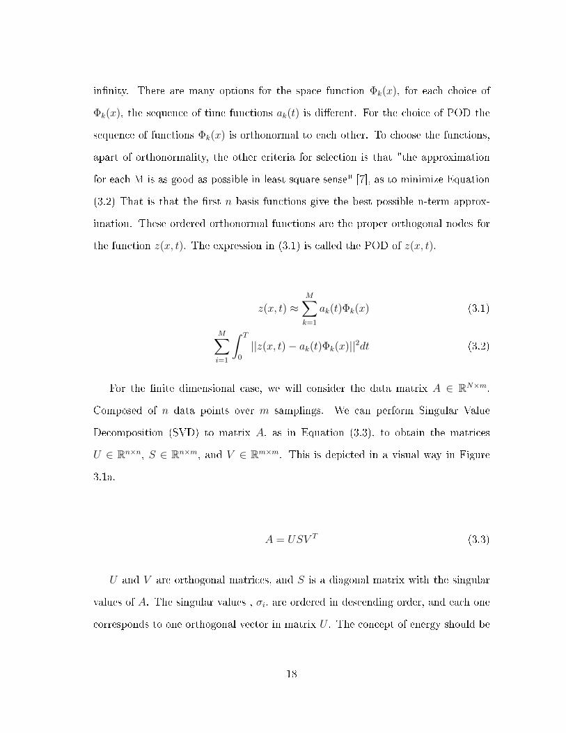
For the �nite dimensional case, we will consider the data matrix A ∈ RN×m.

Composed of n data points over m samplings. We can perform Singular Value

Decomposition (SVD) to matrix A, as in Equation (3.3), to obtain the matrices

U ∈ Rn×n, S ∈ Rn×m, and V ∈ Rm×m. This is depicted in a visual way in Figure

3.1a.

A = USV T (3.3)

U and V are orthogonal matrices, and S is a diagonal matrix with the singular

values of A. The singular values , σi, are ordered in descending order, and each one

corresponds to one orthogonal vector in matrix U . The concept of energy should be

18

(a) Graphical depiction of SVD.

(b) Energy plot. The vertical

axis is the log(σi).

Figure 3.1: Singular value decomposition.

introduced now. Energy is de�ned as σ2i . The cumulative energy is de�ned as (3.4).

Where k ≤ m. The energy can be though as the information contribution of each

orthogonal vector. A typical plot of energy vs. vector number is Figure 3.1b. It can

be seen that most of the energy is represented by a few orthogonal vectors.

Cumulative Energy =

∑ki=1 σ

2i∑m

i=1 σ2i

(3.4)

The correspondence between the in�nite case and the �nite case is illustrated as

follows. Equation (3.3) can be written as (3.5). Where qk and vk are the k columns of

Q and V correspondingly. Equation (3.5) is the discrete form of (3.1). The function

z(x, t) is represented by matrix A, the function ak(t) is represented by qk and Φ(x)

19

by vTk .

A = (US)V T = QV T =m∑k=1

qkvTk (3.5)

To obtain a lower dimensional approximation of A we need only to select the �rst

k basis vectors corresponding to the �rst k singular values. Equation (3.6), where

U ∈ Rn×k, S ∈ Rk×k, and V ∈ Rk×n, is the optimum k order approximation of A, in

the least squares sense. The value of k is selected as to conserve a desirable amount

of energy of the original system, usually k is selected so that (3.4) is 0.99 or more.

A ≈ U SV T (3.6)

3.2 POD Preconditioner Derivation

In [10] the derivation of the preconditioner starting from the linear system of

equations is explained. The derivation starts with ROM-POD, then proceeds to

explain how to create the preconditioner and how to measure the quality of the

basis. The projection preferred is the Galerkin Projection. It is preferred because

stability is guaranteed for SPD matrices and the Jacobian matrices for the pressure

equation are usually SPD matrices.

The derivation of the preconditioner proceeds as follows.

Ax = b (3.7)

20

Where A is n× n. To reduce the order of (3.7)

x = Φz (3.8)

Where Φ is the POD basis, with l columns , and l << n

AΦz = b (3.9)

(3.9) is an overdetermined system, we need to project the full set of equations into

a lower dimensoinal space. With the projeciton operator Ψ

ΨTAΦz = ΨT b (3.10)

z = (ΨTAΦ)−1ΨT b (3.11)

Substituting previous equation in (3.8)

x = Φ(ΨTAΦ)−1ΨT b (3.12)

And from (3.7)

x = Φ(ΨTAΦ)−1ΨT b ≈ A−1b (3.13)

If the projection scheme is the Galerkin projection, then

Ψ = Φ (3.14)

x = Φ(ΦTAΦ)−1ΦT b ≈ A−1b (3.15)

21

Rui shows in [10] that of the three possible choices for the projection operator;

identity matrix, least-squares projector (LSP) or Petrov-Galerkin, and Galerkin; the

Galerkin projector is better than the other two. We choose this projector.

Therefore, the preconditioner becomes,

M−1POD = Φ(ΦTAΦ)−1ΦT (3.16)

To create the two-stage preconditioner with MPOD and MILU , we follow the proce-

dure in [33]. To advance from iteration i to iteration i+1 in a two-stage preconditioner

can be expressed as Equation (3.17) and (3.18).

xi+ 12

= xi + d1 = xi +M−11 (b− Axi) (3.17)

xi+1 = xi+ 12

+ d2 = xi+ 12

+M−12 (b− Axi+ 1

2) (3.18)

By combining the two equations we obtain the following

xi+1 = xi +M−13 (b− Axi) (3.19)

Where

M−13 = M−1

1 +M−12 (I − AM−1

1 ) (3.20)

So, for our case, the two stage preconditioner becomes

M−1POD+ILU = M−1

POD +M−1ILU

(I − AM−1

POD

)(3.21)

22

To measure if the basis used to create the preconditioner is good for the current

linear system being solved we can measure the quality of it. The quality of the basis

is de�ned as Equation (3.22) for the Galerkin projection and it should be less than

10−1. If the quality is less than this value, then we can continue using the same basis,

if it is higher than this, then we should recompute the basis.

||(I − AM−1PODb)||2

||b||2(3.22)

3.3 Snapshots Method Framework

The framework used in this thesis can be described as in Figure 3.2. Each step

will be explained in detail in the sections below.

Figure 3.2: Framework.

23

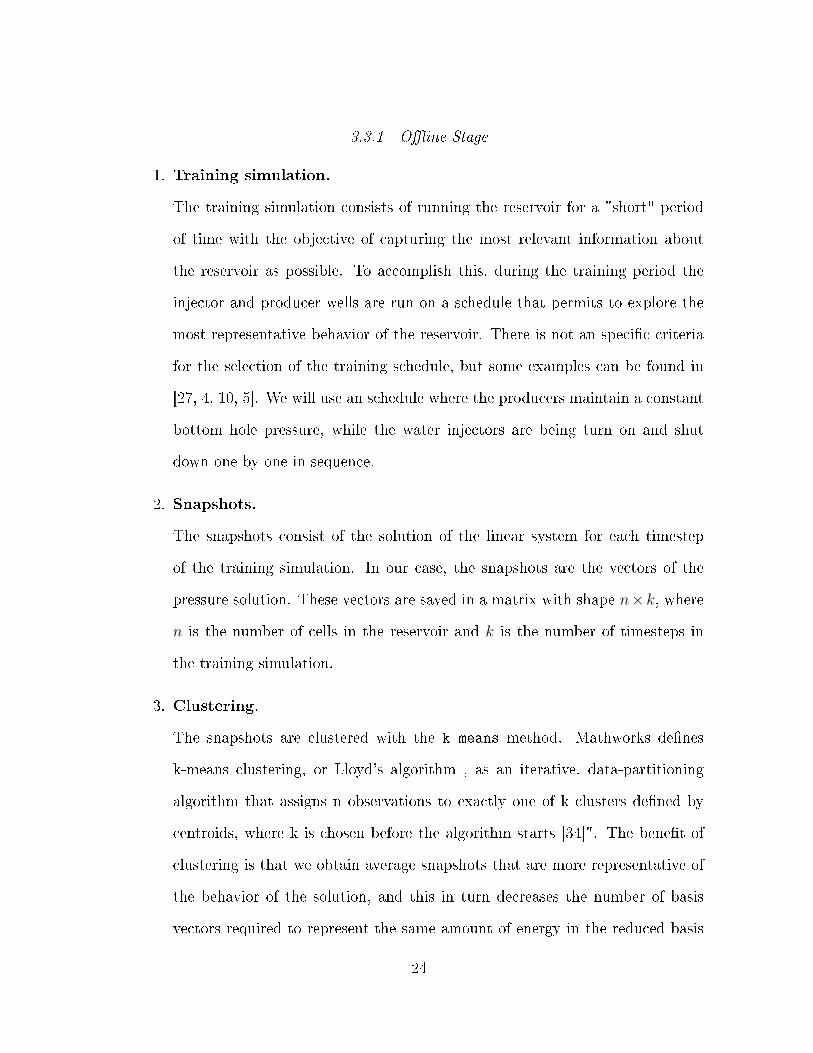
3.3.1 O�ine Stage

1. Training simulation.

The training simulation consists of running the reservoir for a "short" period

of time with the objective of capturing the most relevant information about

the reservoir as possible. To accomplish this, during the training period the

injector and producer wells are run on a schedule that permits to explore the

most representative behavior of the reservoir. There is not an speci�c criteria

for the selection of the training schedule, but some examples can be found in

[27, 4, 10, 5]. We will use an schedule where the producers maintain a constant

bottom hole pressure, while the water injectors are being turn on and shut

down one by one in sequence.

2. Snapshots.

The snapshots consist of the solution of the linear system for each timestep

of the training simulation. In our case, the snapshots are the vectors of the

pressure solution. These vectors are saved in a matrix with shape n×k, where

n is the number of cells in the reservoir and k is the number of timesteps in

the training simulation.

3. Clustering.

The snapshots are clustered with the k-means method. Mathworks de�nes

k-means clustering, or Lloyd's algorithm , as an iterative, data-partitioning

algorithm that assigns n observations to exactly one of k clusters de�ned by

centroids, where k is chosen before the algorithm starts [34]". The bene�t of

clustering is that we obtain average snapshots that are more representative of

the behavior of the solution, and this in turn decreases the number of basis

vectors required to represent the same amount of energy in the reduced basis

24

matrix [4].

4. Singular Value Decomposition.

In this step we perform the SVD of the snapshots matrix as depicted in Equa-

tion (3.3) and in Figure 3.1a. Here, only the full basis matrix U , and the

singular value matrix S, are of interest.

5. Selection of basis vectors.

In this step we construct the reduced basis matrix, Uk , by selecting the basis

vectors that contribute the most energy and discarding the rest. Usually, the

basis vectors are selected so that at least 99 % of the cumulative energy is con-

served. Following the recommendation in [27], at most two times the number

of vectors as the number of wells are needed in the reduced basis matrix.

The previous steps correspond to the o�ine part of the process. Unless an

adaptive approach is desired, once the basis vectors have been selected they

will remain �xed for the rest of the subsequent simulations.

3.3.2 Online Stage

1. Full simulation.

In this step, the full simulation is run. For each time step of the simulation the

preconditioner (3.21) has to be calculated and then the iterative linear solver

is ran.

2. Adaptive step.

If an adaptive approach is desired, the quality of the reduced basis is evaluated

at each time with Equation (3.22). If the quality is not good, then the basis

needs to be updated. There are two approaches that can be used to update the

basis. One is to perform a SVD on all the previous solutions and recompute

25

the full reduced basis. The drawback of this method is that it required to

store all the previous pressure solutions. A second option, presented in [35],

is to expand the basis matrix by one column with the previous solution. This

method has the advantage that it is inexpensive to compute.

26

4. NUMERICAL EXPERIMENTS

We will perform numerical experiments with the Matlab Reservoir Simulation

Toolbox (MRST). in two reservoir models. Model 1 is a simple square reservoir

and Model 2 is a realistic reservoir model consisting of the �rst layer of the SPE10

benchmark model.

The objective of the experiments is to test the framework presented in Section 3.3

and discover whether the GMRES performs better when it is preconditioned with the

two stage preconditioner MPOD+ILU than when it is preconditioned with the single

stage MILU . To measure the performance improvements we will use two metrics.

The �rst metric will be the order of error reduction, as explained in Section 2.1.1,

of the algorithm. The order of error reduction will tell use how rapidly the residual

error decreases per each iteration. A positive result will be obtained if the order of

error reduction increases, because that means than the number of iterations required

to solve the system decrease. The second metric is the computational cost, measured

as the total time required to run the simulation, and the memory requirements. The

MATLAB pro�ling tool is going to be used for this purpose. A positive result will

be obtained if the total computational cost decrease.

4.1 The Reservoir Models

4.1.1 Model 1: Simple Model

The simple reservoir model is a square reservoir with a size of L×L×H. Where

L is the number of cells in one side of the reservoir and H is the number of layers. L

takes the values of 10, 15 and 20. And H takes the values of 1, 2 and 3. That means

that the smallest reservoir has 100 cells while the biggest has 1,200 cells. In all the

cases, there are �ve wells in a �ve spot pattern. Four oil producers surrounding a

27

water injector in the middle of the reservoir to simulate a water �ooding scenario.

The reservoir is shown in Figure 4.1 and its parameters in the rock Table 4.1.

The �uid used in all the simulations is composed of two phases, water and oil.

The phases are immiscible and incompressible. The properties of the �uid are in

Table 4.2. The capillary pressure curve and the relative permeability curves, are in

Figure 4.2.

The rock is incompressbile. The porosity �eld comes from a random gaussian dis-

tribution calculated using the function gaussianField of MRST. The target values

for the porosity are [0.002, 0.3], with a standard deviation of 0.65. The permeability

was calculated with the Carman Kozeny relation, as in Equation (4.1) [3].

K =φ3 × (1E−5)2

(0.81 ∗ 72 ∗ (1− φ)2)(4.1)

Dimensions L× L×HNumber of cells from 100 to 1200

Injectors 1Producers 5Fluid black oilRock incompressible

Table 4.1: Model 1. Simple reservoir model speci�cations.

4.1.2 Model 2: Realistic Model

The second reservoir model is the �rst layer of the SPE10 reservoir model. With

a total of 13,200 cells. This model has 5 water injector wells and 5 oil producer

wells in an irregular pattern. In this model we will also be simulating a water

28

Fluid Water Oil

Density (kg

m3) 1,000 700

Viscosity (cp) 1 10Compressibility (psi−1) 0 0

Table 4.2: Fluid properties.

�ooding scenario. This model with the well locations is shown in Figure 4.3. The

rock properties are heterogeneous and are the original properties included with the

benchmark model [36]. The �uid properties are the same as the ones used in Model

1.

Dimensions 1st layer of SPE10Number of cells 13,200

Injectors 5Producers 5Fluid black oilRock incompressible

Table 4.3: Model 2. Realistic reservoir model speci�cations.

29

(a) Petrophysical properties. Porosity and permeability �elds.

(b) 3D Model View

Figure 4.1: Model 1. Simple square reservoir.

30

(a) Capillary pressure. (b) Relative permeability. The red line is

kro and the blue line is krw .

Figure 4.2: Fluid properties.

(a) 3D Model View

Figure 4.3: Model 2. Realistic reservoir model.

31

4.2 Numerical Experiments. Model 1

For the �rst numerical experiment we use Model 1 with the objective to compare

the performance of the GMRES and Richardson solvers, see Section 2.1.1, precon-

ditioned with MILU and MILU+POD. For the reduced orthogonal basis we use the

criteria of conserving at least 99 % of the energy, that was accomplished by using

the �rst �ve basis vectors. For the training period we will run the simulation for

25 timesteps corresponding to a total of 86 days, while we turn on and o� the oil

producers in sequence. During this training period, when a producer is turned on,

the bottom hole pressure is maintained at 5,500 psia. The injector well is set at 300

bbl/day.

The criteria for stopping the solvers is when the relative error of 1E−8 has been

reached. To obtain the LU decomposition, the MATLAB function ilu was used with

a droptol of 1E−3.

4.2.1 Energy vs Basis Number

The snapshots matrix of the pressure solution has the dimensions of n×k. Where

n is the number of cells and k is the number of timesteps in the training schedule, in

this case 25. SVD was performed to the snapshots matrix to obtain the basis vectors

and their singular values. Figure 4.4 shows the energy of the basis vectors. Figure

4.4a shows the plot of the energy contributed by each of the basis vectors. Figure

4.4b shows the cumulative energy vs. number of basis vectors. As can be seen, with

just �ve basis vectors we capture 99.99% of the energy of the system.

4.2.2 Residual Error Analysis

Figure 4.5 shows the residual error vs. the iteration number for the Richardson

and GMRES solvers when they are preconditioned with MILU and MPOD+ILU .

32

(a) Log of energy vs basis vector num-

ber.

(b) Cumulative energy vs basis vector

number.

Figure 4.4: Model 1. Energy of POD basis vectors.

These two plots are for the case of three layers, and for a single timestep, but these

results are similar for all timesteps and number of layers. The error reduction for the

GMRES algorithm is shown in Figure 4.5b. When the solver is preconditioned with

MILU it takes 13 iterations to converge. On the other hand, when the preconditioner

MPOD+ILU is used, it converges in only 10 iterations. The order of error reduction is

0.62 and 0.85, correspondingly. In Figure 4.5a the error reduction for the Richardson

algorithm is shown. TheMILU converges in 337 iterations whileMPOD+ILU converges

in 23 iterations. The order of error reduction increased from 0.024 to 0.28. Table 4.4

and Table 4.5 show the improvement in the order of error reduction when MILU is

substituted by MPOD+ILU .

4.2.3 Performance Improvement

Figure 4.6 and Figure 4.7 show the time improvement for the preconditioner

calculation time, solver time and total simulation time. For the Richardson solver,

for all cases, the MILU+POD preconditioner performs better, with savings in time of

at least 60% and up to 85%. For the GMRES solver there are not savings in time

33

(a) Richardson (b) GMRES

Figure 4.5: Model 1. Relative residual error vs. iteration number, for the Richardsonand GMRES algorithm preconditioned with MILU and MILU+POD.

Number of cellsNumber of layers 10 15 20

1 31.45 39.64 229.982 197.90 212.36 878.173 400.5 423.3 1,099.2

Table 4.4: Model 1. Percentage improvement in the order of error reduction.Richardson algorithm.

Number of cellsNumber of layers 10 15 20

1 15.87 17.53 -1.382 34.50 43.49 21.873 23.72 15.03 37.02

Table 4.5: Model 1. Percentage improvement in the order of error reduction. GMRESalgorithm.

34

with the two stage preconditioner. The total simulation time increases by at least

50% and up to 500 %. The reasons for this will be explained in detail in Section

5. But the main reason is that for the GMRES algorithm, the increase in the order

of converge and decrease in the number of iterations is not big enough to o�set the

increased cost of computing the two stage preconditioner. It can also be seen in

the plots that the most consuming part of the solution procedure is to generate the

preconditioner.

Another numerical experiment was run to understand the reason behind the bad

performance of the two stage preconditioner. We simulated the three layer square

reservoir for the condition where the well schedule for the full simulation is the same

as the schedule for the training simulation. The results are shown in Figure 4.8. Once

again, we obtain that the two stage preconditioner increases the total simulation time

from -180 % to -600 %. Because the two schedules were the same one, we can narrow

the bad performance cause to the implementation of the method. This is con�rmed

when we do the code pro�ling in Section 4.3.

35

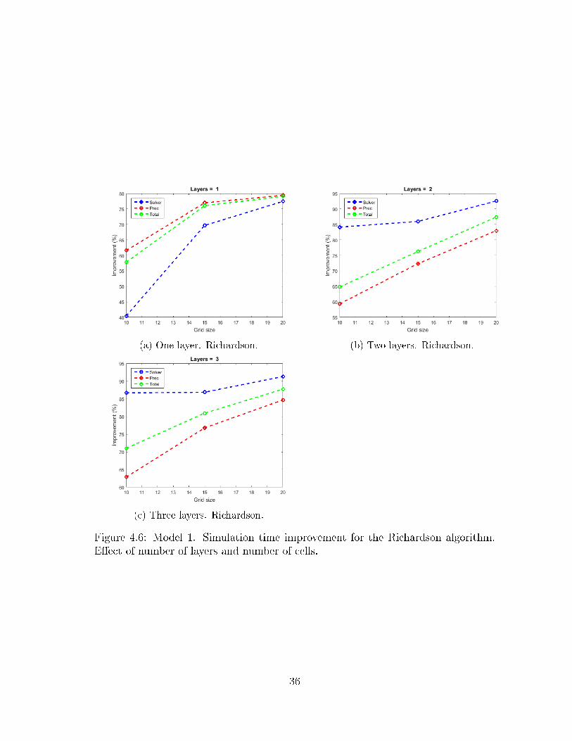
(a) One layer. Richardson. (b) Two layers. Richardson.

(c) Three layers. Richardson.

Figure 4.6: Model 1. Simulation time improvement for the Richardson algorithm.E�ect of number of layers and number of cells.

36

(a) One layer. GMRES. (b) Two layers. GMRES.

(c) Three layers. GMRES.

Figure 4.7: Model 1. Simulation time improvement for the GMRES algorithm. E�ectof number of layers and number of cells.

37

Figure 4.8: Model 1. Simulation time improvement for the GMRES algorithm. Casewhen the full simulation schedule is the same as the training schedule.

38

4.3 Numerical Experiments. Model 2

For the second numerical experiment we use Model 2. The training schedule has

26 timesteps and adds to 86.5 days, while the full simulation schedule has a duration

of 866 days and consists of 103 timesteps . For this model we will measure the

performance of the GMRES algorithm preconditioned with MILU and MPOD+ILU .

4.3.1 Energy vs Basis Number

The plots of the energy of the basis vectors for Model 2 are in Figure 4.9. As in

the previous model, there are a total of 25 basis vectors, Figure 4.9a. The cumulative

energy plot, Figure 4.9b shows that with only 5 basis vectors almost 100% of the

energy of the system is represented, nevertheless we decided to use 10 basis vectors

in the reduced basis matrix.

(a) Log of energy vs basis vector num-

ber.

(b) Cumulative energy vs basis vector

number.

Figure 4.9: Model 2. Energy of POD basis vectors.

39

4.3.2 Residual Error Analysis

Figure 4.10 shows the order of the error reduction for the GMRES solver with

the MILU and MILU+POD preconditioners. The order of error reduction is 0.244 for

the �rst case and 0.4114 for the second case, resulting in an improvement of 68.67 %.

The number of iterations needed to solve for the pressure inside the Newton Raphson

iteration was 35 for MILU and 20 for MPOD+ILU .

(a) Day 10. (b) Day 236.

Figure 4.10: Model 2. Residual error vs. iteration number for the GMRES algorithm.

4.3.3 Performance Improvement

The time improvement is shown in Table 4.6. When the GMRES solver is precon-

ditioned with MILU+POD the solver performs worse than when it is preconditioned

with MILU . In both categories, total time spent solving the system and total time

spent computing the preconditioner, the two stage preconditioner performance is

worse. The total simulation time increased from 0.122E3 seconds to 1.189E3 sec-

onds, this represents an increase of 873 %.

40

MILU MILU+POD

Total solver time 0.117 0.184Total preconditioner computation time 0.005 1.005

Total 0.122 1.189Improvement -873 %

Table 4.6: Model 2. Performance of MILU+POD over MILU . The units of time are103 seconds.

Operation Time % Memory(MB)[L,U] = ilu(A) 3.1 171

M_pod = basis * ((basis'* A *basis)\basis') 18.5 70,977M_ilu_pod= U \(L \(eye(m)-A*M_pod)) + M_pod 77.6 70,977

Table 4.7: MILU+POD computation time and memory allocation for Model 2.

41

5. CONCLUSIONS

The results from the numerical experiments with Model 1 and Model 2 clearly

show that the the new preconditioner MPOD+ILU is an improvement over MILU only

if it used with the Richardson solver. For GMRES, the time performance is lowered

with MPOD+ILU .

First we will talk about the improvement in the order of error reduction of

MPOD+ILU over MILU . For the Richardson algorithm, see Table 4.4 , the improve-

ment increases as the size and the number of layers of the reservoir model increase.

For one layer and 100 cells the improvement is of 31.45%, and for 3 layers with 1,200

cells the improvement is of 1,099.2 %. This is visualized in the plots of residual error

vs. iteration number in Figure 4.5. For GMRES, Table 4.5, there is not a clear

pattern for the improvement in error reduction. It increases and decreases as the

number of layers and number of cells increase. And for the case of one layer and

400 cells, the new preconditioner in fact has a negative e�ect. Also, for GMRES

the improvements range from 15 to 44 %, while for Richardson algorithm they range

from 31 to 1,100 %.

Continuing with the analysis of the time improvements of the preconditioners.

Figures 4.6 and 4.7 show the time improvements resulting with the two stage pre-

conditioner. For the Richardson solver the simulation time decreases by at least 60%

and up to 85%.

For the GMRES algorithm, on the other hand, there is no time improvements.

Even tough the number of iterations per timestep are decreased, preconditioning the

solver with MPOD+ILU takes much more time and the total time to solve the system

increases from 50 % to 500 %.

42

There are two main reasons why MPOD+ILU is more time consuming. The �rst

reason is that it is more time consuming to compute the two stage preconditioner

than the one stage ILU preconditioner and the second reason is that it is also more

time consuming to apply the preconditioner to the linear system. For the �rst point,

MILU only requires an ILU decomposition, while MPOD+ILU , besides an ILU decom-

position requires to compute MPOD and MILU+POD for each iteration loop. Analysis

of the Model 2 simulation with the Matlab pro�ling tool are shown in Table 4.7.

Computing MILU consumes 3.1% of the time, while M−1POD consumes another 18.5

%. The remaining 77.6 % of the time is spent computing the two stage precon-

ditioner. These operations are costly because the reduced basis matrix Φ is fully

dense. This results in MPOD and MPOD+ILU being also fully dense. This bring us

to the second point. Applying the dense preconditioner is more costly than applying

a sparse preconditioner. As shown in 4.6, GMRES plus the two stage precondioner,

consumes more total time, even though the number of iterations was decreased in

average from 35 to 20 in each timestep.

Also, another drawback with the two stage preconditioner is that it consumes

more memory storing the dense matrices. Table 4.7 also shows the memory con-

sumption. MATLAB allocates 414.6 times more memory for MPOD and MPOD+ILU ,

than for MILU .

So, we can conclude that when the time spent creating and applying the two

stage preconditioner is o�set by the decreased number of iterations, using the two

stage preconditioner makes sense. This condition is only met for the Richardson

algorithm, where the number of iterations is decreased greatly as discussed before.

We also want to mention that the conclusions obtained have only been observed

for the solvers and models that we simulated and that more extensive test with

other reservoir models and solvers are necessary to make a more general conclusion.

43

Furthermore, for this thesis we only performed numerical experiments. A theoretical

analysis of the algorithm would be better to make a general statement about the

method.

44

REFERENCES

[1] F. Kiprop. (2015) freecodecamp. [Online]. Available: https://medium.

freecodecamp.com/my-�rst-foray-into-technology-c5b6e83fe8f1

[2] J. Alden. (1998) Computational electrochemistry. [Online]. Available: http:

//compton.chem.ox.ac.uk/john/Thesis/4/4.html

[3] K.-A. Lie, An Introduction to Reservoir Simulation Using MATLAB. Oslo,

Norway: SINTEF ICT, Departement of Applied Mathematics, 2015.

[4] M. A. Cardoso, L. J. Durlofsky, and P. Sarma, �Development and application of

reduced-order modeling procedures for subsurface �ow simulation,� International

Journal for Numerical Methods in Engineering, vol. 77, no. 9, pp. 1322�1350,

2009.

[5] M. Ghasemi, �Model order reduction in porous media �ow simulation and opti-

mization,� Thesis, "Texas A and M University", 2015.

[6] G. H. Golub and C. F. Van Loan, Matrix Computations, 3rd ed. The Johns

Hopkins University Press, 1996.

[7] A. Chatterjee, �An introduction to the proper orthogonal decomposition,� Current

Science, vol. 78, no. 7, pp. 808�817, 2000.

[8] E. Gildin, M. Ghasemi, A. Romanovskay, Y. Efendiev et al., �Nonlinear complex-

ity reduction for fast simulation of �ow in heterogeneous porous media,� in SPE

Reservoir Simulation Symposium. Society of Petroleum Engineers, 2013.

[9] M. Ghasemi, Y. Yang, E. Gildin, Y. R. Efendiev, and V. M. Calo, �Fast mul-

tiscale reservoir simulations using pod-deim model reduction,� in SPE reservoir

simulation symposium, 2015.

[10] R. Jiang, �Pressure preconditioning using proper orthogonal decomposition,� The-

45

sis, Stanford University, 2013.

[11] Z. Chen, G. Huan, and Y. Ma, Computational methods for multiphase �ows in

porous media. Siam, 2006, vol. 2.

[12] H. Price, K. Coats et al., �Direct methods in reservoir simulation,� Society of

Petroleum Engineers Journal, vol. 14, no. 03, pp. 295�308, 1974.

[13] Y. Saad and M. H. Schultz, �Gmres: a generalized minimal residual algorithm for

solving nonsymmetric linear systems,� Society for Industrial and Applied Mathe-

matics, vol. 7, no. 3, p. 14, 1986.

[14] P. Vinsome et al., �Orthomin, an iterative method for solving sparse sets of si-

multaneous linear equations,� in SPE Symposium on Numerical Simulation of

Reservoir Performance. Society of Petroleum Engineers, 1976.

[15] A. Papadopoulos and H. Tchelepi, �Block smoothed amg preconditioning for oil

reservoir simulation systems,� Technical report, Oxford University, Tech. Rep.,

2003.

[16] J. Wallis et al., �Incomplete gaussian elimination as a preconditioning for gener-

alized conjugate gradient acceleration,� 1983.

[17] J. Wallis, R. Kendall, T. Little et al., �Constrained residual acceleration of con-

jugate residual methods,� 1985.

[18] B. Aksoylu and H. Klie, �A family of physics-based preconditioners for solving el-

liptic equations on highly heterogeneous media,� Applied Numerical Mathematics,

vol. 59, no. 6, pp. 1159�1186, 2009.

[19] R. Falgout, �An introduction to algebraic multigrid,� Comput Sci Eng, vol. 8,

p. 24, 2006.

[20] J. W. Watts III et al., �A conjugate gradient-truncated direct method for the iter-

ative solution of the reservoir simulation pressure equation,� Society of Petroleum

Engineers Journal, vol. 21, no. 03, pp. 345�353, 1981.

46

[21] G. A. Behie and P. Forsyth, Jr, �Incomplete factorization methods for fully im-

plicit simulation of enhanced oil recovery,� SIAM Journal on Scienti�c and Sta-

tistical Computing, vol. 5, no. 3, pp. 543�561, 1984.

[22] A. Behie, P. Vinsome et al., �Block iterative methods for fully implicit reservoir

simulation,� Society of Petroleum Engineers Journal, vol. 22, no. 05, pp. 658�668,

1982.

[23] J. Meyerink et al., �Iterative methods for the solution of linear equations based

on incomplete block factorization of the matrix,� 1983.

[24] S. International. (2016) Reservoir simulation linear equation solver. [Online].

Available: http://petrowiki.org/Reservoir_simulation_linear_equation_solver

[25] J. Appleyard et al., �Nested factorization,� in SPE Reservoir Simulation Sympo-

sium. Society of Petroleum Engineers, 1983.

[26] H. Liu, K. Wang, and Z. Chen, �A family of constrained pressure residual pre-

conditioners for parallel reservoir simulations,� Numerical Linear Algebra with

Applications, vol. 23, no. 1, pp. 120�146, 2016.

[27] P. Astrid, G. Papaioannou, J. Vink, and J. Jansen, �Pressure preconditioning

using proper orthogonal decomposition,� Society of Petroleum Engineers, 2011.

[28] D. Lichtblau and E. W. Weisstein, �Condition number.�

[29] MathWorks. (2016) ilu. [Online]. Available: https://www.mathworks.com/help/

matlab/ref/ilu.html

[30] S. Volkwein, �Model reduction using proper orthogonal decomposition,� 2011.

[31] S. Jackman, �Principal components and images,� pp. 1�10, March 9, 2010 2010.

[32] M. Richardson, �Principal component analysis,� May 2009 2009.

[33] J. Van der Linden, �Development of a de�ation-based linear solver in reservoir

simulation,� Ph.D. dissertation, TU Delft, Delft University of Technology, 2013.

[34] MathWorks. (2016) kmeans. [Online]. Available: https://www.mathworks.com/

47

help/stats/kmeans.html

[35] Y. Efendiev, E. Gildin, and Y. Yang, �Online adaptive local-global model

reduction for �ows in heterogeneous porous media,� Computation, vol. 4,

no. 2, p. 22, Jun 2016. [Online]. Available: http://dx.doi.org/10.3390/

computation4020022

[36] SINTEF. (2008) Geoscale - direct reservoir simulation on geocellular

models. [Online]. Available: https://www.sintef.no/projectweb/geoscale/results/

msmfem/spe10/

48