proximity detection with mobile clients - universiteit twente€¦ · working at alcatel-lucent,...

E!cient proximity detection among mobile clientsusing the GSM network

Thesis for Master Embedded Systems, departement Computer ScienceDesign and Analysis of Communication Systems (DACS),

Faculty of Electrical Engineering, Mathematics and Computer Science,University of Twente

by Ing M.T. WittemanOctober 18, 2007

Supervising committee:

Dr. Maarten Wegdam (Alcatel-Lucent, Bell-Labs Europe)Dr. Ir. Geert Heijenk (University of Twente)Fei Liu, M.Sc. (University of Twente)Ir. Jacco Brok (Alcatel-Lucent, Bell-Labs Europe)Ir. Ing. Harold Teunissen (Alcatel-Lucent, Bell-Labs Europe)

Abstract

Personalized services, such as customized ringtone recommendations and locationbased services increase the popularity of mobile phones. A location based service(LBS) is a type of personalized service that uses the location of the mobile user.Proximity detection is defined as the capability of a location based service toautomatically detect when a pair of mobile users is closer to each other than acertain proximity distance. To realize this function the location of the mobileusers have to be permanently tracked.

The main objective of this research is to find to what extent it is possible touse GSM cell-ids for proximity detections among mobile entities. We studied thetypical GSM characteristics and the state of the art proximity detection algorithmsfound in literature. All the proximity algorithms we found use X, Y coordinatesas location identifier. Dynamic Circles by George True et. al. was stated inliterature to perform the best. This algorithm is used as inspiration for four newalgorithms that use the GSM network to implement proximity detection. Theproposed algorithms are divided into two groups, the basic group and the graphgroup. The basic group contains two algorithms that use the information availablein the GSM network, called cell-id algorithm and LAC algorithm. The graphgroup uses a cell-id graph representing all the cell switches, to get more e!cientalgorithms. This group contains two algorithms, named Graph1 algorithm andGraph2 algorithm.

For the comparison of the algorithms a simulator was developed. The simulatorcan simulate the amount of messages, the tra!c over TCP/IP, missed proximitiesand the accuracy of proximity distance using GSM. The input data of the simulatorare user movement paths. These paths can be generated or can be real logged datagathered by a mobile device.

For a realistic cell topology it was found that the median of di"erences betweenreal distance and cell-id distance is around 1100 meters. Using GSM cells aslocation identifier introduces missed proximities, i.e. false negatives. We foundthat for a realistic cell layer and a proximity distance of 1100 meters the numberof missed proximities is 3.5% of the total proximity detections.

A simulation of a distributed scenario, representing rush hour, stated that forlow density of users the Graph algorithms outperform the Basic algorithms interms of generated messages and tra!c. From this simulation it is found that for30 buddies a user consumes a total of 30MB of data tra!c per month.

i

Preface

In front of you is my thesis for concluding my Master Embedded Systems.I preferred to complete the last part of my academic study not at the uni-versity. An assignment about context aware application was available atAlcatel Lucent(ALU) Bell-Labs Europe. The assignment was to develop anapplication that uses context, e.g. calendar, location and temperature, tomake life easier. Bell-Labs Europe was interested in the deployment of suchan application: should it be a client based application or could it better bemore server oriented, or maybe hybrid? Unfortunately, for most of the con-text aware applications it was already obvious which parts of the applicationshould be client side and which server side. There was no challenge in theassignment.

Jacco Brok (ALU) came with another problem related to context awareapplications: The possibility to detect if two mobile users are within thevicinity of each other. After some literature study it was found that peoplealready had done research on so called proximity detection algorithms, todetect if two mobile targets approach each other within a certain predefineddistance. The algorithms were e!cient, in terms of number of messages, butused GPS as a location identifier on the client side. From the experience ofcolleagues and from literature we concluded that GPS was not suitable forthe application. The application had to run continuously, GPS drains thebattery and has poor coverage, e.g. you need to have ’line of sight’, insidebuildings you will not get a GPS fix or coordinate. Because the applicationis deployed on mobile GSM devices, the question arose: ’Why not use theGSM network?’ The final assignment was born.

I became part of WorkPackage 2: ’context aware applications’. Thiswork package is part of the Awareness project within Freeband. I enjoyedthe work meetings; it gave me insight in a large interesting research projectwith several partners. Working at Alcatel-Lucent, Bell-Labs Europe was veryinteresting, I enjoyed working at the location in Enschede.

Maarten WittemanOctober 2007 Twente

iii

Acknowledgments

A lot of people were involved in my graduation project. They helped mewith problems or just gave feedback to the several technical sessions aboutmy work. I especially would like to thank the following persons:

Maarten Wegdam, from Alcatel-Lucent, Bell-Labs Europe, supervisedmy graduation project, first as member of my committee and later as firstsupervisor. Maarten has helped me during the second half of the period tofinish the project with this thesis. I would like to thank Maarten for his helpand time he always took to discuss my problems.

I would also like to thank Jacco Brok for being my first supervisor beforehe left Alcatel-Lucent. Jacco helped me to form a challenging and interestingassignment and I enjoyed the discussions and useful tips from Jacco duringthe first half of the assignment.

Geert Heijenk and Fei Lui have supervised me from the university onbehalf of the DACS chair. I would like to thank them for their time, helpfultips, discussions and input during the committee meetings and for reviewingmy thesis.

Harold Teunissen, former manager of the Bell-Labs department in En-schede, became a member of the committee when Jacco left ALU and Maartenwas promoted to first supervisor on behalf of ALU. I would like to thankHarold for his input and support during my graduation period and manag-ing during the whole period. Harold unfortunately, for me, also switched joband left the committee 2 months before I finished my master Thesis.

Erik Meeuwissen and Willem Romijn from the Bell-Labs location in Hil-versum helped me understanding the di!culties when developing applica-tions using the GSM network. I would like to thank them for the interestingdiscussions, feedback and help during the project.

I had a lot of fun with the colleagues at the Bell-Labs location in Enschedeand a lot of interesting discussions about my project or other projects, orjust innovative ideas. I would like to thank all the colleagues of Bell-LabsEnschede: Ronald, Arjen, Dennis, Dirk-Jaap, Richa and Sue for the relaxingconversations.

I presented a lot of my work in WorkPackage 2 of the Awareness project,

v

part of Freeband. The people from WP2 gave me useful feedback on the workand problems I presented. I would like to thank them and especially MartinWibbels and Johan Koolwaaij for providing me access to the Cell-locatordatabase of Telematics Institute Enschede.

I had a lot of fun and relaxing times with my flatmates and study col-leagues during my study and graduation. It helped me to relax during mystudy.

Finally I would like to thank my parents, sister and brother for giving meall the chances I had, for supporting me, for believing in my capabilities andfor never doubting me.

vi

Contents

Abstract i

Preface iii

Acknowledgments v

1 Introduction 1

1.1 Motivation . . . . . . . . . . . . . . . . . . . . . . . . . . . . . 1

1.2 Research Question . . . . . . . . . . . . . . . . . . . . . . . . 2

1.3 Scope . . . . . . . . . . . . . . . . . . . . . . . . . . . . . . . 3

1.4 Approach . . . . . . . . . . . . . . . . . . . . . . . . . . . . . 4

1.5 Document structure . . . . . . . . . . . . . . . . . . . . . . . . 5

2 Related work 7

2.1 GSM network characteristics . . . . . . . . . . . . . . . . . . . 7

2.1.1 Network topology . . . . . . . . . . . . . . . . . . . . . 7

2.1.2 GSM cell-id handovers . . . . . . . . . . . . . . . . . . 11

2.1.3 Oscillation experiment . . . . . . . . . . . . . . . . . . 13

2.2 Proximity detection algorithms . . . . . . . . . . . . . . . . . 13

2.2.1 Simple methods to detect proximity . . . . . . . . . . . 13

2.2.2 Strips-Algorithm . . . . . . . . . . . . . . . . . . . . . 14

2.2.3 Strips and cell-ids . . . . . . . . . . . . . . . . . . . . . 16

2.2.4 Dynamic Circles . . . . . . . . . . . . . . . . . . . . . . 16

2.2.5 Dynamic Circles and cell-ids . . . . . . . . . . . . . . . 17

2.2.6 Dead Reckoning . . . . . . . . . . . . . . . . . . . . . . 17

2.2.7 Dead-Reckoning and cell-ids . . . . . . . . . . . . . . . 18

2.2.8 Comparison . . . . . . . . . . . . . . . . . . . . . . . . 18

2.2.9 Algorithms and cell-ids . . . . . . . . . . . . . . . . . . 20

2.3 GPS energy consumption . . . . . . . . . . . . . . . . . . . . . 21

vii

3 Algorithms 233.1 Di"erent deployments . . . . . . . . . . . . . . . . . . . . . . . 233.2 Definitions used in strategies . . . . . . . . . . . . . . . . . . . 243.3 Cell-ID algorithm . . . . . . . . . . . . . . . . . . . . . . . . . 25

3.3.1 Limitations . . . . . . . . . . . . . . . . . . . . . . . . 273.4 LAC algorithm . . . . . . . . . . . . . . . . . . . . . . . . . . 27

3.4.1 Limitations . . . . . . . . . . . . . . . . . . . . . . . . 283.5 Graph1 algorithm . . . . . . . . . . . . . . . . . . . . . . . . . 28

3.5.1 Limitations . . . . . . . . . . . . . . . . . . . . . . . . 323.6 Graph2 algorithm . . . . . . . . . . . . . . . . . . . . . . . . . 33

3.6.1 limitations . . . . . . . . . . . . . . . . . . . . . . . . . 333.7 Summary algorithms . . . . . . . . . . . . . . . . . . . . . . . 343.8 Application improvement: Exclude clients . . . . . . . . . . . 343.9 Alternative algorithm: Peer to peer . . . . . . . . . . . . . . . 35

4 Simulation Environment 374.1 User mobility modelling . . . . . . . . . . . . . . . . . . . . . 384.2 Simulator . . . . . . . . . . . . . . . . . . . . . . . . . . . . . 394.3 Handovers and Oscillation . . . . . . . . . . . . . . . . . . . . 414.4 Real user paths . . . . . . . . . . . . . . . . . . . . . . . . . . 424.5 GPRS tra!c . . . . . . . . . . . . . . . . . . . . . . . . . . . . 434.6 Simulation scenarios . . . . . . . . . . . . . . . . . . . . . . . 44

5 Simulation 475.1 Confidence level and interval . . . . . . . . . . . . . . . . . . . 475.2 GPS versus GSM cell-id accuracy . . . . . . . . . . . . . . . . 495.3 Distributed scenario . . . . . . . . . . . . . . . . . . . . . . . 535.4 Chasing cars scenario . . . . . . . . . . . . . . . . . . . . . . . 565.5 Amount of data used, costs . . . . . . . . . . . . . . . . . . . 585.6 Real user paths . . . . . . . . . . . . . . . . . . . . . . . . . . 58

6 Conclusions and Future Work 616.1 Conclusion . . . . . . . . . . . . . . . . . . . . . . . . . . . . . 616.2 Future work . . . . . . . . . . . . . . . . . . . . . . . . . . . . 62

6.2.1 Adaptive algorithms . . . . . . . . . . . . . . . . . . . 626.2.2 Realistic cell-id layer . . . . . . . . . . . . . . . . . . . 626.2.3 Data tra!c . . . . . . . . . . . . . . . . . . . . . . . . 636.2.4 Multiple operators . . . . . . . . . . . . . . . . . . . . 63

A DVD: Simulator and Demos 65

viii

Acronyms

LBS Location Based Service LBS is a service that uses the location of theentity.

GSM Global System for Mobile communication. GSM is the new standardfor digital cellular communication in Europe.

GPS Global Positioning System. GPS is the Global Navigation SatelliteSystem. Utilizing a constellation of at least 24 medium Earth orbitsatellites that transmit precise microwave signals, the system enables aGPS receiver to determine its location, speed and direction.

cell-id Cell Identifier. cell-id is the cell identifier of an antenna, the mobilephone has this identification number of the antenna it is connected to.

MS Mobile Station. MS is a mobile device that is capable of connecting toa GSM radio cell.

BTS Base Transceiver Station BTS comprises all radio equipment, i.e.antennas, signal processing, amplifiers necessary for radio transmissions

LA Location Area LA all the Base Transceiver Stations connected to thesame Mobile Services Switching Center are in the same location area.Each Mobile Services Switching Center forms its own Location Area withits unique identifier called the Location Area Code

LAC Location Area Code LAC unique identifier for Location Areas. A setof neighbouring cell-identifiers form a LAC

BSC Base Station Controller BSC manages the Base Transceiver Stationsand handles the handovers from one Base Transceiver Station to anotherBase Transceiver Station.

XML eXtensible Markup Language XML A general-purpose markuplanguage. It is an extensible language because it allows its users to define

ix

their own tags. Its primary purpose is to facilitate the sharing of dataacross di"erent information systems, particularly via the Internet

MSC Mobile Services Switching Center. MSC is the digital switch that setup connections to other Mobile Services Switching Centers and to theBase Station ControllerS to provide communication between MobileStations

ARPU Average Revenue Per User ARPU This states how much money thecompany makes from the average user. This is the revenue from theservices provided divided by the number of users buying those services

GPRS General Packet Radio Service GPRS Medium to access the internetvia an air-interface with transfer rates up to 115 kbit/s. Operators cancharge on the ammount of data instead of the connection time.

UMTS Universal Mobile Telecommunications Service UMTS ThirdGeneration (3G) broadband packet-based transmission of text, digitizedvoice, video and multimedia at data rates up to 2Mbit/s

TCP/IP Transmission Control Protocol / Internet Protocol TCP/IP O"ersthe functionality for hosts to create connections to other hosts, overwhich they can exchange streams of data using Stream sockets.

POI Point Of Interests POI is a specific point location that someone mayfind useful or interesting.

x

Chapter 1

Introduction

1.1 Motivation

Mobile phones have become part of our lives. We can stay connected wher-ever we are and whenever we need to with our mobile phones. Originallymobile phones were only used for telephony, nowadays they have evolvedto all type of mobile internet services. By personalising mobile services theAverage Revenue Per User (ARPU) increases and the churn reduces for anoperator. Personalized services can vary from customized ringtone recom-mendations to Location Based Service (LBS) [HK03]. This thesis focuses onthe latter.

Imagine that you are visiting a foreign city and it is lunch time, youcan simply use your mobile phone to locate the nearby restaurant [Stea].Another example of a LBS are the projects E911 and E112. E911 and E112are both emergency services that will enable mobile, or cellular, phones toprocess 911 or 112 emergency calls and enable emergency services to locatethe geographic position of the caller [UE].

Most of the current LBSs are based on the distance between a mobileentity and a static entity, e.q. Point Of Interests (POI), or just about thelocation of the mobile user, like the E911 and E112 services. Some LBSservices however deal with the distance between two mobile entities, e.g. adating service that checks your personal interests with other mobile users inyour vicinity and ”breaks the ice” for you. The focus of this thesis is on aspecific subcategory of these LBS services, namely services that notify userswhen specific other users are in the vicinity.

A typical example is that you are notified if a friend of you is in thevicinity, perhaps you will call your friend to make an appointment. Thistype of LBS is called proximity detection. This is a typical type of servicethat runs continuously. Existing implementations of this type of service inliterature and/or deployed are all based on Global Positioning System (GPS)

1

1 . Introduction

to determine the location of the mobile user. It is very energy consuming tocontinuously use GPS to determine the mobile users location [Cha98]. Ontop of that, most mobile phones, on the market, do not have an onboardGPS device.

We therefore focus on an alternative way to determine the users’ po-sition using the cell structure/topology of the Global System for Mobilecommunication (GSM) network as a location identifier. A mobile phoneis connected to a GSM network with antennas. Each antenna has a uniquenumber called a cell-id. The mobile phone knows this cell-id and is triggeredwhen the cell-id changes, i.e. switching to another antenna.

1.2 Research Question

Given this introduction to proximity detection and the GSM network a mainresearch question can be formulated:

To what extent is it possible to use GSM cell-ids for proximity detectionsamong mobile entities?

In order to answer this question, and to narrow down the field of research,a number of sub questions are formulated. These sub questions guide theresearch process and will be answered in the conclusion in section 6.1.

1. What are the characteristics of GSM networks that are relevant fordetermining the location of users, e.g. cell-id topology and size of cells?

2. What is the impact of oscillation (switching between cell-ids while themobile client is at one place) on the proximity detection?

3. What are the current implementations of proximity detection algo-rithms, and are they suitable when GSM cell-ids are used as locationidentifier?

4. What are e!cient proximity detection algorithms using the character-istics of GSM networks?

5. Which set of mobility scenarios is a good representation of the move-ment of people?

6. What is the di"erence in accuracy between the proximity distance de-termined using cell-ids and using GPS?

2

1.3 Scope

7. What is the number of missed proximities or false negatives if a GSMnetwork topology is used to detect proximity?

8. What proximity detection algorithms generate the least amount ofbandwidth, and how much is this?

1.3 Scope

This section describes the decisions made to scope the research project.To find the usefulness of cell-ids as location identifier for proximity de-

tection the application ’buddy detection’ is used to focus the research. Eachuser has a list of friends with mobile phones (e.g. the phone book uses tagsfor friends the user wants to detect). This list of friends is used to form abuddy list, this list states from which friends you want to be notified if theyare in the vicinity. Proximity must be detected between those users if theyapproach each other.

To answer the main objective and sub questions simulations are doneon four new algorithms using the GSM network to detect proximity. Forthese simulations, scenarios are defined that cover realistic movement of peo-ple. A distributed scenario, representing rush hour tra!c in a city, is usedto compare the algorithms, in terms of number of messages and data traf-fic. This scenario is often used in literature to simulate users [AEM+04,TWK06]. Other simulations are done to answer the subquestions about ac-curacy, missed proximities and data tra!c.

Realistic generated user movement or real movement data retrieved fromlogs of mobile devices is used for the simulations. The cell layer, represent-ing the GSM network topology, used in the simulations can be a generatedhexagonal topology or a real topology. The real topology is taken from acell-id database from Telematics Institute [KW]. This database is filled withGPS coordinates and the cell-id detected at that point. Di"erent networktopologies of di"erent operators are stored in this database. For this researchone Dutch operator is used from this database.

In one country di"erent operators coexist. Each is with its own networkand own network topology. This research uses cell-ids to provide proximitydetection so the network topology is of importance. Since each operatoruses a di"erent topology it is not possible to detect proximity between twousers subscribed to di"erent operators without creating a mapping of thedi"erent topologies. In this research all the users are connected to the samenetwork with one topology of cell-ids. From this network only the GSM cellsare used and not the Universal Mobile Telecommunications Service (UMTS)

3

1 . Introduction

cells. UMTS cells are typical smaller than GSM cells, but the coverage isstill less than the coverage of the GSM network.

Privacy is a major issue when developing LBSs, the privacy aspect ofproximity detection, is not discussed in this research.

1.4 Approach

To tackle the questions described above the research is divided in four phases:

• First phase: Literature study. The two main topics that are studiedare GSM network characteristics and proximity detection algorithms.Di"erent characteristics, e.g. Cell Identifier (cell-id) handovers, oscil-lation, network topology, mobile phone data are studied. The state ofthe art proximity detection algorithms or closely related to proximitydetection is investigated. Beside these two main topics for a realisticsimulations, a study is done on mobility models and tools that gen-erate user movement using mobility models, i.e. CanuMobiSim andVanetMobisim [Steb, HF].

• Second phase: Define new proximity detection algorithms. Use thegathered knowledge of the first phase to define di"erent proximity de-tection algorithms that use the GSM network as location identifier.

• Third phase: Simulate using generated mobility paths and real loggeddata, to find an answer to the amount of messages, data tra!c, accu-racy between cell-ids and GPS, the number of missed proximities andthe amount of data tra!c. Develop a simulator that has the followingtasks:

– Link the mobility path generators to the simulation environment

– Use Mathworks Matlab to implement and simulate the algorithmsusing the input data of the mobility path generators

– Implement a realistic cell layer to find an answer about the accu-racy and missed proximities.

– Gather data out of the simulations that are used to evaluate thealgorithms.

• Fourth phase: Evaluate and conclude. Use real data, in terms of arealistic topology and real logged user-paths to illustrate the algorithmswith real data and draw conclusions using the evaluation of the fournew proximity detection algorithms.

4

1.5 Document structure

1.5 Document structure

The remainder of this thesis is structured as follows. Chapter 2 is titledRelated Work and describes the typical characteristics of GSM networks, e.g.handovers/cell switches and oscillation, that are relevant for this research. Toillustrate the oscillation the results of an experiment are described after thecharacteristics of GSM networks. The state of the art proximity detectionalgorithms from literature are also discussed in Chapter 2. The strong andweak points are mentioned and the algorithms are evaluated if the GSMnetwork is used as location identifier. At the end of chapter 2 an experimentis described to illustrate the high energy consumption of GPS.

After the Related Work four new algorithms that detect proximity usingthe GSM network are introduced in Chapter 3. These algorithms were de-veloped during this research. The strong and weak points of the algorithmsare discussed. The simulation environment is outlined in Chapter 4, the sim-ulation process and the generation of the input data is explained. Chapter 5cover the simulations that were done to find answers to the research questionand sub questions. How the confidence level/interval is calculated ’on the fly’in the simulator is discussed. The accuracy of GPS versus cell-id as locationidentifier is discussed and the missed proximities or false negatives simula-tion is discussed. The four algorithms are compared against each other, interms of messages and data tra!c, using a distributed scenario, representingrush hour movement. At the end of Chapter 5 an illustration of the amountof data tra!c is given and a simulation run with real logged data is given.Chapter 6 concludes the research and presents future work.

5

1 . Introduction

6

Chapter 2

Related work

This chapter describes the related work. First the characteristics of GSMnetworks are discussed, that are relevant for proximity detection. Next, cur-rent proximity detection algorithms we found in literature are described, i.e.Strips, Dynamic circles and Dead-reckoning. These algorithms are basedon latitude and longitude coordinates, e.q. GPS, of the users. For each ofthe proximity detection algorithms, found in literature, the issues there arewith applying these algorithms to GSM cell-ids are discussed. At the endthis chapter illustrates the energy consumption of GPS on a high-end mobiledevice.

2.1 GSM network characteristics

This section outlines characteristics of GSM networks that are relevant forproximity detection, e.g. the topology, GSM cell-id switches and oscillation.

2.1.1 Network topology

To explain the network topology some background information is neededabout the system architecture of GSM. GSM is a cellular network. A cellularnetwork is a radio network made up of a number of transmitters, called aBase Transceiver Station (BTS), each with its own radio cell. This radio cellcan be sectorized resulting in multiple cell-ids per radio cell. The advantagesof using more cells instead of one big cell to cover the same area are:

• increased capacity

• reduced power usage

• better coverage

7

2 . Related work

cell

cell

cell

MS

BTS

BTS

BTS

BSC BSC

MSC MSC

MS

MS

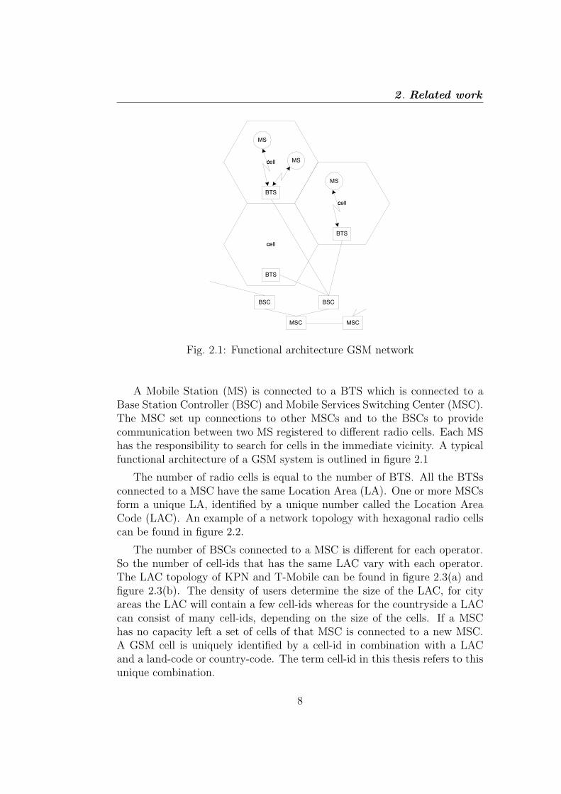
Fig. 2.1: Functional architecture GSM network

A Mobile Station (MS) is connected to a BTS which is connected to aBase Station Controller (BSC) and Mobile Services Switching Center (MSC).The MSC set up connections to other MSCs and to the BSCs to providecommunication between two MS registered to di"erent radio cells. Each MShas the responsibility to search for cells in the immediate vicinity. A typicalfunctional architecture of a GSM system is outlined in figure 2.1

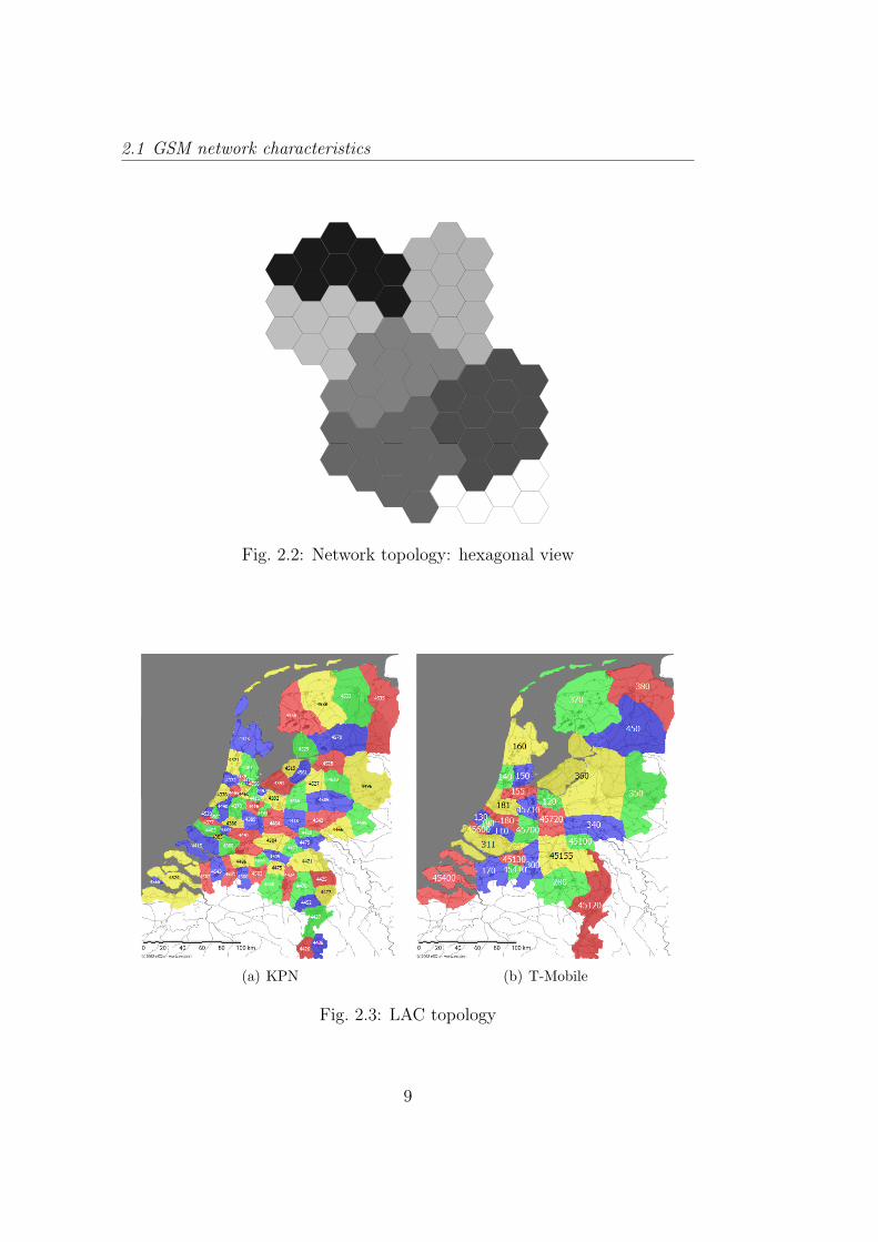
The number of radio cells is equal to the number of BTS. All the BTSsconnected to a MSC have the same Location Area (LA). One or more MSCsform a unique LA, identified by a unique number called the Location AreaCode (LAC). An example of a network topology with hexagonal radio cellscan be found in figure 2.2.

The number of BSCs connected to a MSC is di"erent for each operator.So the number of cell-ids that has the same LAC vary with each operator.The LAC topology of KPN and T-Mobile can be found in figure 2.3(a) andfigure 2.3(b). The density of users determine the size of the LAC, for cityareas the LAC will contain a few cell-ids whereas for the countryside a LACcan consist of many cell-ids, depending on the size of the cells. If a MSChas no capacity left a set of cells of that MSC is connected to a new MSC.A GSM cell is uniquely identified by a cell-id in combination with a LACand a land-code or country-code. The term cell-id in this thesis refers to thisunique combination.

8


Fig. 2.2: Network topology: hexagonal view

(a) KPN (b) T-Mobile

Fig. 2.3: LAC topology

9

2 . Related work

City of Enschede

Latit

ude

Longitude

Fig. 2.4: GSM Cells: area of Enschede

An often used simplification of the network topology is represented as aconcatenation of hexagonal radio cells in literature [NR04, HJ04a, LR05]. Inpractise this is not the case, in fact a lot of overlap is introduced to get agood coverage. The shape of a cell is not hexagonal but a polygon, shapedby reflections, distortion, influence of buildings, etc. Di"erent people arecreating databases with cell-id information gathered by mobile devices withGPS modules [KW]. From this data it can be concluded that a mobile phonecan be in di"erent cell-ids at the same place and overlap exists in the cell-idtopology. A good example is the network topology for Enschede. Enschedeis covered with three macro cells, i.e. cell size 1.5km till 15km, and a lot ofnormal cells, i.e. cell size 100m till 1500m, and pico cells, i.e. cell size 10mto 100m. The cell-id layer of Enschede can be found in figure 2.4 [KW].

The size of one cell is determined by the capacity needed in that area.For urban areas the size of a cell varies from 10 to 1000 meter. In countrysides cells can be up to 15km. For example, in the Netherlands the maximumsize of a cell that was found is 15km [KW]. For the area of Enschede (seealso figure 2.4, Borne and Almelo the total number of di"erent cell measure-ments is 863, see table 2.1. These measurements are from 1 Dutch operator,i.e. KPN. The database has not su!cient measurements to determine thediameters of every cell. The 184 cells with a diameter of 0 only have a fewmeasurements and therefore have this 0 diameter. The other cells that havea diameter larger than zero have more than 10 measurements.

10


Diameter Number Diameter Number Diameter Number0 184 4000 48 10000 1

250 71 5000 7 11000 2500 65 6000 18 12000 1

1000 158 7000 8 13000 12000 200 8000 2 14000 13000 93

Tab. 2.1: Cell-sizes (diameter in meters) of area Enschede, Borne and Almelo(lat: 51.9-53, lon: 5.8-7.2)

2.1.2 GSM cell-id handovers

If a user has a conversation in a car on the highway with his mobile phone, hewill drive through a lot of radio cells. The conversation must not be cut-o" ifthe phone switches to a new cell. This switching betweens cells and channelswhen a phone call is in progress is called handover or hando" [Sch03].

There are four types of handovers:

• Switching channels in the same cell.

• Switching cells under control of the same BSC

• Switching cells under the control of di"erent BSCs, but belonging tothe same MSC

• Switching cells under control of di"erent MSCs

The first two types of handover are called internal because they involveonly BSC, and MSC is notified only on completion of the handover. Theother two types of handover are called external because they involve MSC.For the proximity detection the last three handovers are of influence becausethey change the cell-id.

A handover may be initiated by the BSC or can by initiated by the MS.The MS scans the channels of up to 16 neighbouring cells, and forms a listof the six best candidates for possible handover. This list is updated to theBSC at least once per second. This information is used by the BSC andMSC for the so called handover algorithm. This handover algorithm takesthe decision of switching to a new cell of let the MS connected to the currentcell.

There are two basic algorithms for making handover decision for di"erentcriteria:

11

2 . Related work

x

x

Fig. 2.5: Late cell-switches result in di"erent cell sizes

• Minimum acceptable performance. If signal degrades beyond somepoint, transmission power is increased. If power increase does not leadto improve, handover is performed. Disadvantages: increasing trans-mission power may cause interference with neighbour cell.

• Power budget. Use handover to improve transmission quality in thesame or lower power level. This method avoids neighbour cell interfer-ence, but is quite complicated.

A side e"ect of the handover algorithms is oscillation. If a mobile phoneis in one place, it is still switched to the other cells. This happens becausethe signal quality changes. For example atmosphere changes, people interferethe signals; other mobile phones enter your cell or other input parameters ofthe handover algorithms change [osc05, KDK00].

This research is about proximity detection using the current GSM cell-id of a MS and it could be that proximity is detected between two usersbecause of oscillation, because a user can oscillate to the cell of the buddy.If the oscillation is between two neighbouring cells, there is minor impacton the quality of proximity, in terms of proximity distance. The proximitydistance will be less accurate because the size of cells can vary. In figure 2.5is an illustration of two users moving to each others cell. Both users havea handover or cell switch on di"erent places. Somewhere in the grey (theshaded part) area the users will switch from cell according to the handoveralgorithms. In figure 2.5 this happens at the x-marks in the grey area.

The second type of oscillation is when a user falls back into an overlappingmacro cell. If this is the case and two buddies are in the same macro cell, theproximity distance between two users is large. This type of oscillation has amajor impact on the detection of proximity and the accuracy of proximitydistance.

12

2.2 Proximity detection algorithms

all CIDs CID 46982 CID 46984 CID 47270 CID 13622Average time in cell 0:27:58 0:34:55 0:25:58 0:07:36 0:08:38Max time in cell 18:00:00 18:00:00 13:00:00 1:59:19 3:54:36Min time in cell 0:00:04 0:00:13 0:00:04 0:00:17 0:00:18Nr measurements 564 269 223 34 38

Tab. 2.2: Oscillation of a mobile device on one place

2.1.3 Oscillation experiment

An experiment was done on oscillation to illustrate the oscillation betweenneighbour cells, the results can be found in table 2.2. A GSM mobile devicewas placed on a spot where already di"erent cell-ids were measured. Thedevice was left for 7 days on the same spot and registered each cell-id changewith time stamp. In these 7 days the device was connected with 4 di"erentcell-ids. The longest time in cell-id 46982 was 3 days and 20 hours. Thismeasurement is left out of table 2.2 to get a better overview. A total of 564cell switches are detected in 7 days, with a minimum stay time of around 10seconds and the longest time of 18 hours (without the 3 day measurement).The average time in a cell is around 30 minutes.


This section first describes simple periodic algorithms to detect proxim-ity. Then three relevant, more e!cient, proximity detection algorithmsfound in literature are discussed, i.e. Strips algorithm by Arnon Amir etal. [AEM+04], Dynamic circles by Alex Kupper et al. [KT06] and DeadReckoning by George Treu et al. [TWK06]. In the papers they do simula-tions to validate their algorithms. As location identifier of the mobile userGPS coordinates are used, the limits of GPS are not taken into account.For each algorithm the impact of using GSM cell-ids as location identifier isdiscussed.

2.2.1 Simple methods to detect proximity

Proximity detection is all about knowing the location of the users and calcu-late the distance between users to see if the users are in the vicinity. To keeptrack of the location of users the following update algorithms were found inliterature:

• Polling: The location server requests the current position fix from the

13

2 . Related work

mobile device. This may happen upon request from the application,on a periodic basis, or according to a caching strategy applied at thelocation server.

• Periodic position update: The device triggers a position update ifa pre-defined time interval has elapsed since the last position update.

• Distance-based position update: The mobile device sends a po-sition update if the line-of-sight distance between the last reportedposition and the current position exceeds a pre-defined threshold.

These update methods are periodic in time or in travelled distance. Thiswill result in unnecessary location updates, e.g. if periodic position update isused the user will send updates regardless if he is moving, so the same locationis updated several times. This is not e!cient and these update methods arenot considered for proximity detection using GSM cell-ids. The three moreintelligent algorithms are discussed in the remainder of this section.

2.2.2 Strips-Algorithm

Arnon Amir et al. present an algorithm, called the Strips-algorithm to detectif a buddy is nearby [AEM+04]. To determine the location of a mobile userGPS coordinates are used. The evaluation of the algorithm is done using theIBM city simulator [Cit]. The strips-algorithm has the task to: ’Whenever afriend moves into the user’s vicinity, both users are notified by a proximityalert message’. A friend is one that is predefined by enrolment or by matchingthe personal profiles of users.’

Let a, b be two users whose Euclidean distance denoted by |a!b|, is largerthan R (R is the width of a strip). Let l(a, b) denote the bisector of the lineconnecting a and b; i.e., the line consisting of all points of equal distance froma and b. S(a, b) is the infinite strip of width R whose central axis is l(a, b).See figure 2.6. This strip can be of di"erent shapes, its desired propertiesare to have a Hausdor! distance > R. A Hausdor" distance is the maximumdistance of a set to the nearest point in the other set. The idea behind thismethod is that as long as neither a or bi enters S(a, bi), they do not need toexchange location update messages. If two users are notified with a messagethat they are within each others vicinity, a circle is computed around the twousers. The radius of this circle is determined by R/2 + 2" !, centered at themidpoint of the line connecting the two friends. (! is the desired tolerancefor producing the proximity alert). If one of the users leaves the circle thedistance between the users is calculated. When the distance is smaller than

14


the proximity distance, a new circle is computed, otherwise a new strip iscalculated.

bisectorl(a,b)

S(a,b)

a

b

R

a

b2

b3

b4

b1S(a,b4 )

S(a,b3 )

S(a,b2 )

S(a,b1 )l(a,b4 )

l(a,b1 )l(a,b2 )

l(a,b3 )

(P)

Fig. 2.6: Left: setting a new static strip of width R around the bisectorbetween two mobile users. Right: user a does not need to update stripswhile moving inside the internal region (P ).

The psuedo code of the Strips Algorithm can be found in Algorithm 1.D(a) is the datastructure of a, it contains all strips S(abi). e is the error ofthe location of the user.

SelfMotion()while moving do

a = ReadSelfLocation()Test(Distance(a))if a enters Strip(a,bi) or MsgReceived(bi) then

StripUpdate(bi)end

endAlgorithm 1: Strips: SelfMotion

To decrease the computational load of the mobile clients, they proposean approximated Strips algorithm. Instead of maintaining a convex region ofpossibly #(n) edges, for n friends, it maintains an approximated polygon ofa fixed number of edges, at fixed, predetermined slopes. The region createdby the polygon is called the internal region, denoted by (P ). See right sideof Figure 2.6.

15

2 . Related work

StripUpdate(bi)send a’s location to bi

receive bi’s locationif |a-bi |< R + ! then

ProximityAlert(”bi is nearby”)Delete(D(a), S(a,bi))

elseCompute S(a,bi)Update D(a), D(bi) with S(a,bi)

endAlgorithm 2: Strips: StripUpdate

2.2.3 Strips and cell-ids

If the strips strategy is used with GSM cell-ids it is hard to define a strip.This strip must be infinite long, so that users cannot enter the area of theother user without crossing the bisector. A simple formula can be calculated,representing the bisector, for each user when using coordinates, e.g. GPSlatitude and longitude. With a cell-id topology it is harder to define a strip.First problem is the length of the strip. It could be shorter but then thereis a possibility that the users cross the strip without knowing, i.e. movingaround the strip. The second problem has to do with oscillation and macrocells. A user could switch to a macro cell that is not part of the strip andliterally jump over the bisector. A solution could be to add all the nearbymacro cells, and overlapping cells to the strip, but this will result in largesets of cell-ids for the strip. These sets have to be exchanged between thetwo users and make the strategy very ine!cient.

Another issue with strips is the peer to peer part. For each buddy a usermust keep a strip and calculates if he crosses the strip. With an increasinglist of buddies the amount of resources used grows. The number of messagesis equal to the number of users in your buddy group.

2.2.4 Dynamic Circles

Kupper and Treu present a method that looks like the strips-algorithm butthey use circles instead of border regions [KT06]. They suggest some im-provements to the algorithm and state that its outperforming the Strips-algorithm. In figure 2.7 each target is surrounded by a circular uncertaintyarea called A, which, from the location servers point of view, narrows downit’s possible whereabouts. The circles are chosen in a way that, without re-porting a position update, the mutual distance between two targets cannot

16


fall below the proximity distance dp. The centre of the circle is the last knownposition of the user. The distance between the circles determines the size ofthe circle. This distance needs to be above the proximity detection distance.

k

j

m

p ro x. d is t.

A i

A j

A k

A m

A : u n ce rta in ty a re ai

Fig. 2.7: Dynamic Centered Circles DCC strategy

2.2.5 Dynamic Circles and cell-ids

It is possible to define a set of cells to create a free region representing thecircle in dynamic circles. But to find this set of cells, the knowledge of thetopology is needed in the form of a graph. This graph must contain all thecells as vertexes and all the cell switches as edges.

2.2.6 Dead Reckoning

The newest proximity detection algorithm in literature is called dead reckon-ing. This algorithm uses the movement patterns of the observed targets todetect proximity [TWK06]. Based on a previously reported position that hasbeen accompanied by additional information, such as speed and direction ofthe target, the mobile device and the location server simultaneously computethe current position of the device by a shared prediction function f . If thedevice detects that the so-derived position deviates from its actual positionby more than a pre-defined threshold, it reports a position update. Severalways for computing f are known in the literature. True et. al. use the

17

2 . Related work

direction and the speed of the mobile users to come to a shared predictionfunction.

prox. dis t.

AI

AJ

A: uncer tainty area

J

I

Fig. 2.8: Measuring the smallest possible distance between the uncertaintyareas created by the proposed dead reckoning algorithm

Figure 2.8 shows the computation of the smallest possible distance (spd)between i and j in a possible situation during execution of the strategy. Theuncertainty area Ai of target i resembles a ring segment. The sector angleis determined by the direction of "vi and the angular threshold a, which isapplied in both directions. The speed of the user determines the size of A.

2.2.7 Dead-Reckoning and cell-ids

Using dead-reckoning in combination with GSM cell-ids it is almost not pos-sible to find a prediction function to predict the user’s location. Withoutthe knowledge of the network topology it is not possible to determine the fu-ture cells the user will be in. Meeuwissen et.al. [MRB07] have found, usingthe history of visited cells by a user, an algorithm that can approximate theEstimated Time of Arrival to predefined locations.

2.2.8 Comparison

The writers of the last algorithm, dead reckoning, have implemented thethree algorithms in a simulator [TWK06]. All the algorithms use a latitudelongitude as location identifier e.g., GPS, so the algorithms can use the same

18


(a) Number of uplink messages (b) Number of downlink messages

Fig. 2.9: Algorithms evaluated with pedestrian scenario [TWK06]

input data. The size of the simulation area is fixed and covers an area of5km2. A proximity distance of 500m was used throughout the simulation.The number of users vary from 5 to 60 users and each user has the otherusers as buddies. The pedestrian was defined to have a maximum speedof 10km/h, which can be compared to a slow jog. However, his preferredvelocities were set to 5km/h and 3km/h. The car scenario assumes a topspeed of 55km/h and 8lkm/h to simulate slow rush-hour tra!c. For di"er-ent scenario’s di"erent algorithms are performing the best, though in generaldead reckoning seems to perform best. In comparison to the strips algo-rithm the number of uplink messages are fewer but the number of downlinkmessages are increased (up and downlink with the server). Dead reckoningis outperforming the dynamic circles algorithm when increasing the averagespeed. The direction in which the users move determines also the qualityof the algorithm. In Figures 2.2.8 and 2.2.8 pedestrian movement is usedto evaluate the three di"erent algorithms. For this type of movement thedynamic circle algorithms perform better than dead reckoning and strips. Infigures 2.2.8 and 2.2.8 car movement is used to evaluate the algorithms. Itis clear that dead reckoning is the algorithm that uses the lowest numberof update messages per terminal when the average speed of the terminalsincreases [TWK06].

19

2 . Related work

(a) Number of uplink messages (b) Number of downlink messages

Fig. 2.10: Algorithms evaluated with car scenario [TWK06]

2.2.9 Algorithms and cell-ids

All these algorithms use a XY coordinate, e.g. GPS latitude and longitude,as location of the mobile user. It is hard to use these algorithms with GSMcell-ids as a location identifier. For strips it is almost impossible to define astrip using GSM cell-ids, it at least requires a lot of resources. Using the dead-reckoning strategy it is hard to define the user’s direction and to estimatea travelling speed, because of the di"erent sizes of cell-ids. The dynamiccircles strategy is the most promising algorithm when using GSM cell-ids aslocation identifier. The idea of free moving regions can also be accomplishedby using GSM cell-ids. The free region is then a set of GSM cell-ids. So thealgorithms are hard to use one on one but are used as inspiration for the newalgorithms using GSM cell-ids.

20

2.3 GPS energy consumption

Conditions Current GPS Backlightprogram o"; backlight o" 26mAprogram o"; backlight on 97mA 71mAprogram on; GPS o"; backlight o" 28mAprogram on; GPS o"; backlight on 98mA 70mAprogram on; GPS on; backlight o" 141mA 113mAprogram on; GPS on; backlight on 212mA 114mA 71mAprogram on; GPS o"; screen o" 18mAprogram on; GPS on; screen o" 130mA

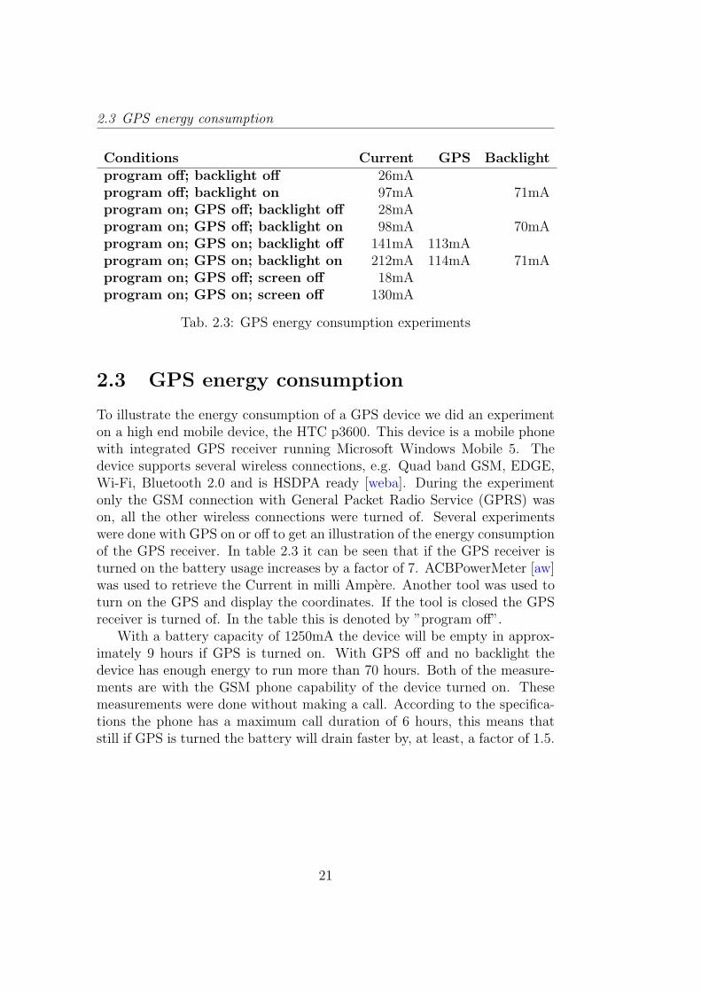
Tab. 2.3: GPS energy consumption experiments

2.3 GPS energy consumption

To illustrate the energy consumption of a GPS device we did an experimenton a high end mobile device, the HTC p3600. This device is a mobile phonewith integrated GPS receiver running Microsoft Windows Mobile 5. Thedevice supports several wireless connections, e.g. Quad band GSM, EDGE,Wi-Fi, Bluetooth 2.0 and is HSDPA ready [weba]. During the experimentonly the GSM connection with General Packet Radio Service (GPRS) wason, all the other wireless connections were turned of. Several experimentswere done with GPS on or o" to get an illustration of the energy consumptionof the GPS receiver. In table 2.3 it can be seen that if the GPS receiver isturned on the battery usage increases by a factor of 7. ACBPowerMeter [aw]was used to retrieve the Current in milli Ampere. Another tool was used toturn on the GPS and display the coordinates. If the tool is closed the GPSreceiver is turned of. In the table this is denoted by ”program o"”.

With a battery capacity of 1250mA the device will be empty in approx-imately 9 hours if GPS is turned on. With GPS o" and no backlight thedevice has enough energy to run more than 70 hours. Both of the measure-ments are with the GSM phone capability of the device turned on. Thesemeasurements were done without making a call. According to the specifica-tions the phone has a maximum call duration of 6 hours, this means thatstill if GPS is turned the battery will drain faster by, at least, a factor of 1.5.

21

2 . Related work

22

Chapter 3

Algorithms

This chapter first explains three di"erent deployments of algorithms, i.e.client to client, client to server and hybrid, using GSM cell-ids. Next, defi-nitions are presented that are used in the explanation of the four proximitydetection algorithms simulated during this research. These four proximitydetection algorithms are client to server based deployed. The algorithms aredivided into two groups, the Basic group and the graph Group. The BasicGroup has two basic algorithms using only the available information from theGSM network. They are named, the Cell-ID algorithm and LAC algorithm.The Graph Group uses more information about the network topology in theform of a cell-id graph, representing each cell switch. This group containstwo algorithms named the Graph1 and Graph2 Algorithm. At the end ofthis chapter additions are discussed and an alternative algorithm is given ifa client to client deployment is used. The limitations and possibilities of thisalgorithm are discussed.

3.1 Di"erent deployments

For proximity and separation detection between two or more clients, threedeployments are possible:

• Client to client; or peer 2 peer, this can be compared with the serverlessimplementation of the Strips algorithm in section 2.2.2. Each client hasthe same responsibilities of the algorithm.

• Client to server; each client reports to an server and the server han-dles most of the responsibilities of the algorithms. Client only sendsupdates. This deployment can be compared to the dynamic circlesalgorithm in section 2.2.4.

• Hybrid method: The algorithm is divided over clients, servers and net-work.

23

3 . Algorithms

In the related work of G. True and Kupper the client to server deploy-ments are performing better than the client to client deployments of thealgorithms under all conditions [AEM+04, TWK06, KT06]. This is due tothe e"ect that client to client deployments generate more messages on anupdate. For example: if a client has 2 buddies, it has to send both buddies alocation update, whereas with an client to server deployment the client onlyhas to send 1 update message to the server. For this research also a client toserver deployment is used. Simulations are done on four new proximity algo-rithms that use the GSM network to detect proximity and separation. Eachalgorithm uses di"erent information of the GSM network to detect proxim-ity and separation. We defined the following four new proximity detectionalgorithms:

1. Cell-ID algorithm; uses only the cell-ids available on the client toupdate to the server as location identifier. Location updates are doneon each cell switch.

2. LAC algorithm; This algorithm uses the LAC and land-code alsoavailable on the client. Location updates are done on each cell, LACor land-code switch.

3. Graph1 algorithm; The server has knowledge of the topology in theform of a cell-id graph. This is used to return a set of neighboringcell-ids to the client. Location updates are done if the client leaves theset of cell-ids returned from the server.

4. Graph2 algorithm; Comparable to the graph1 algorithm, but nowthe server returns larger sets of cell-ids instead of only the neighboringcell-ids of the client.

These algorithms send a proximity notification whenever users are in thesame cell-id. As stated before this cell-id is unique combination of, cell-id,LAC and country-code. The algorithms do not send a ’goodbye’ notificationif users are no longer within each others vicinity.

3.2 Definitions used in strategies

The following definitions are used for all four strategies:

• Proximity distance is defined as the distance to detect proximity. Inthe related work with GPS solutions this distance is in meters, usingGSM cells to detect proximity this distance is expressed in cells. For

24

3.3 Cell-ID algorithm

the comparison of the four new introduced algorithms in this thesis, theproximity distance is one cell-id. This means that proximity is detectedif two clients are in the same cell, with corresponding same cell-id.

• Proximity detection is defined as the detection that two mobileclients approach each other within a predefined proximity distance.

• Proximity area after proximity is detected two clients are put ina proximity area, to denote that those clients just had a proximitydetection. For the four algorithms this is the cell-id were proximity isdetected.

• Separation detection , whenever one of these clients leaves this prox-imity area, separation is detected. If this is the case both clients areinformed that they are no longer connected.

• Free-area is the area in which the client can move without sendinglocation updates to the server.

• Location update this term is used as an update of the location of aclient in the algorithms. This is not the location update from the GSMnetwork when switching to a new LA.

3.3 Cell-ID algorithm

The first algorithm to implement proximity detection uses only the cell-idsavailable on the mobile phone. As stated in section 2.1.2 the mobile phonereceives a new cell-id upon a cell switch. On the mobile phone it is easy todetect this switching event. The client has the responsibility to update hisnew cell-id to the server upon each cell switch. See figure 3.1.

Upon a location update the server checks for proximity or separation.Four di"erent scenarios can occur:

• There are no other clients in the new cell-id, no reply message is needed

• There is/are other client(s) in the new cell-id, send back a proximitynotification

• The client is currently in proximity area and leaves the cell-id, clientsare no longer connected and no action is needed

• The client is currently in a proximity area and leaves the cell-id andother clients are in the new cell-id, proximity messages are send and anew proximity area is formed.

25

3 . Algorithms

Send new cell-id

end

cell-id switch interrupt

Fig. 3.1: client-side cell-id algorithm

Send clients

'proximity alert'

Location update client

Was in

proximity area?

no

Other client

in new cell?yes

No action, client

needs no update

no

No action, clients

need no updateyes

Fig. 3.2: server-side cell-id algorithm

26

3.4 LAC algorithm

x

x

o

o

D

X : user position

O : connected cell

D : d istance

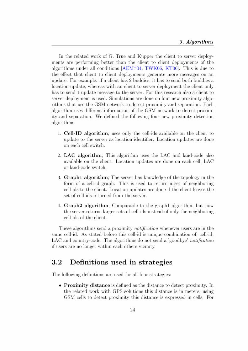
Fig. 3.3: Proximity missed

In figure 3.2 the working of the server-side of the algorithm can be found.

3.3.1 Limitations

The proximity distance is limited to the maximum size of a cell, becauseonly the current cell-id is used in this algorithm. This means that proximityis only detected when clients are in the same cell-id. A consequence is thattwo clients could be close to each other but are in di"erent cells. For anillustration of this problem see figure 3.3. The client positions are markedwith an ’X’, the distance between the two clients is D and the ’o’ marksthe cell-id the clients are in. The two clients are in a di"erent cell but thedistance ’D’ between the clients is much smaller than the proximity distance,the size of a cell. So, although D is smaller than the cell radius, proximity isnot detected, because the clients are not in the same cell. The flexibility ofthis algorithm is limited to a single cell proximity distance. It is not possibleto have a proximity distance of 2 or more cell-ids.

3.4 LAC algorithm

The second algorithm uses the LAC and land-code of the GSM network,also available on the mobile phone. The algorithm is the same as the firstalgorithm but also checks if a client is alone in a LAC. If so the clientonly needs to update if he leaves the LAC and no longer on each cell-idswitch. If other clients are in the same LAC the client must update on eachcell-id switch. The same update technique is used when using land-codes.The proximity area can also be a land-code or LAC next to a cell-id. Theproximity area default is a cell-id. The client has the responsibility to sendonly an update to the server respecting the current free-area of the user. This

27

3 . Algorithms

C ell- id sw itchhandover

C ur rent free-area =land-code?

C ur rent free-area =LAC ?

yes yes

land-code changed?

send update toserver

Yes

no

LAC changed?


yes

N o actionneeded nono

Send update toserverno

Fig. 3.4: client-side LAC algorithm

free-area can be a cell-id, LAC or land-code. The decision flow can be foundin figure 3.4.

In figure 3.5 the flowchart of the server-side can be found. The client-sidehas the responsibility to update according to the free-area received of theserver. If the free-area is a LAC, the client only needs to send an update tothe server if the LAC he is in changes.

3.4.1 Limitations

The LAC algorithm uses more information about the cell-id and clusteringof cell-ids than the first algorithm which only uses cell-ids. The advantage ofthe LAC algorithm is that if a client is alone in a LAC or land-code the clientonly needs to send updates upon a switch of a LAC or land-code, respectively.A disadvantage is that if another client enters your LAC the server has toupdate both clients, this result in more downlink messages in comparison tothe cell-id algorithm. As can be seen in figures 3.5,3.4 the complexity of thealgorithm increases on both the client and server side.

3.5 Graph1 algorithm

This algorithm uses the cell-id topology information as a graph. A neighbourof a cell is a cell in which you can come within one cell-id switch. This doesnot have to mean that cells are real neighbours, because macro cells create a

28


Send clients

'proxim ity a ler t'

area-sw itch

update client

W as in

proxim ity area?

no

Other client

in land -code?yes

yes

Other client

in LAC ?

Other client

in ce ll ?yes yes

Send client

free-area

area=cell -id

Send client

free-area

area=LAC

Send client free -

area area=land-

code

nonono

Send clients w ith

free-area=land-code

new free-area

Send clients w ith

free-area=LAC

new free-areafor a ll clients w hose

free-area is affected

> 1 clients le ft in

proxim ity area

Send only client

new free-areano

for rem ain ing clients

Fig. 3.5: server-side LAC algorithm

29

3 . Algorithms

46381

11578

21813

89685 95732

27459

46381 63815

81744

18794

26841

68752

82156

Fig. 3.6: Cell-id Graph, representing all cell-switches

lot of overlap it could be that there are multiple antennas between the twoneighbouring cell antennas. In the cell-id graph each cell is a vertex and eachneighbour of that cell is connected with an edge.

A graphical representation of this graph can be found in figure 3.6. Cell-id89685 probably is a macro cell, because it has many neighbours.

Using this extra information of the network it is possible to create analgorithm with more possibilities. The proximity distance is no longer limitedto one cell-id, as in the first two strategies, but could be multiple cells usingthe graph. The free area can be multiple cells. The server can detect if otherclients are in the adjacent cells, of the current cell the client is in, if not thesecells can be added to the free-area. It is also possible to state, with a certainprobability, if a cell is a macro cell. This could give more information aboutthe distance between two clients. If both clients are in the same cell thatprobably is a macro cell the distance between the two clients could be up to15km (in the Netherlands).

The complexity of the algorithm on the client side is similar to the LACalgorithm. The client will receive a set of cell-ids from server in which hecan move freely. The client has the responsibility to use this list on a cell-idswitch to detect if an update to the server is needed. If the client is in acell-id that is part of this free list it does not have to update otherwise theserver is informed about the current cell-id. See figure 3.7 for the decisionflow.

The free-area returned to the client consists of the new cell-id of the clientand the neighbouring free cell-ids of this new cell-id. If a neighbour cell isalready occupied this cell-id is excluded from the list.

The complexity of the algorithm on the server is much greater than withthe previous two strategies. Upon an update the server has to lookup thecell-id in the cell-id graph and check for proximity, free areas and separation.In figure 3.8 the server-side of the cell-id graph algorithm is outlined.

If a client A enters the free area of client B the server will send only the

30


C ell- id sw itchhandover

C ell- id in set of free-area cell- ids?

no


yes N o actionneeded

Fig. 3.7: Client-side: Graph1 algorithm

area-sw itch

update client

W as in

proxim ity area?

no

yes

Send client free-area

area=set of current

ce ll - id and neighbour

ce ll - ids

> 1 clients le ft in

proxim ity area

Send only client

new free-areayes

for rem ain ing client

no

In other clients

free-area?

Other client in

ce ll - id?yes

Send other clients

'proxim ity a ler t'yes

Send other client

free-area update

no

Fig. 3.8: Server-side: Graph1 algorithm

31

3 . Algorithms

0 200 400 600 800 10000

100

200

300

400

500

600

700

800

900

1000

x10 meters

x10

met

ers

Fig. 3.9: Snapshot Graph1 algorithm

current cell-id back as free area for client A. The server also sends a messageto client B to remove that cell-id from his free area.

For an example of a snapshot of the graph1 algorithm see figure 3.9. The’*’ marks are the assigned cells to users, the ’x’ marks.

3.5.1 Limitations

The algorithm is much more flexible, because it can support di"erent prox-imity distances. The cell-id graph can be used to detect proximity if a clientis multiple cells away. The cell-id graph however must be harvested fromthe network. This is a costly operation and changes if the operator decidesto place a new antenna to get better coverage. It is also possible that anantenna is moved, the cell-id graph has to be updated.

If the density of clients is high, the neighbouring cells of a client areprobably occupied. This result in a fallback to the first algorithm, the cell-idgraph, on the client-side. The server still has to do the computations for thefree-area per client.

32


0 200 400 600 800 10000

100

200

300

400

500

600

700

800

900

1000

x10 meters

x10

met

ers

Fig. 3.10: Snapshot Graph2 algorithm


Using the idea of the graph1 algorithm, an extended version of the graph1algorithm is found. The size of the free-area, so the set of free cell-ids, couldbe larger if the density, in terms of clients and number of total cells, is low.The client can move free in this set of cell-ids so a bigger set will result infewer update messages to the server. The neighbour cells of the first ring ofneighbour cells are also checked for free cells. For an example of a snapshotof the graph2 algorithm see figure 3.10. The ’*’ marks are the assigned cellsto users, the ’x’ marks.

3.6.1 limitations

A drawback of this algorithm is the number of server based updates to theuser if a client enters another client’s free-area. The free-area of that clienthas to be updated so the server needs to send a message to this client.

33

3 . Algorithms

Cell-ID LAC Graph1 Graph2Uplink messages !! +! + ++

Downlink message ++ + +! !!Proximity distance 1 1 1+ 1+Client complexity ++ + + +Server complexity ++ + +! +!

Resources ++ ++ !! !!

Tab. 3.1: Comparison algorithms: ++ is good, !! is bad

3.7 Summary algorithms

The cell-ID algorithm is very basic and the complexity is low. Disadvantageis that upon each cell switch an update must be send. Another disadvantageis that the proximity distance is limited to the same cell. The same holdsfor the LAC algorithm. The LAC algorithm will introduce less client-sideupdates but the server initiated messages increase. This is due to the factthat users will enter occupied LACs, the user owning the LAC has to beinformed that he has to switch to a cell-id as free-area.

The graph group can have a proximity distance of multiple cells, usingthe cell-id graph. These algorithms have just as the LAC algorithm thedisadvantage of generating more server initiated messages if a user entersanother’s free-area and no proximity is detected. This e"ect is even largerin the graph group. Each user has a free area, so the probability that auser enters another users free-area increases. See table 3.1 for a completecomparison of the four algorithms, in the table a ++ denotes an advantageof the algorithm and a !! a disadvantage.

3.8 Application improvement: Exclude clients

Using the cell-id graph it is possible, at the server side, to ignore buddies froma buddy list of a client, for an amount of time for example. This could bewishful if proximity is just detected between two clients and the client doesnot want to be notified for a day if that client is in the vicinity again. Theserver can than ignore this client after proximity detection, in the calculationof the new free area for the clients. This results in larger free areas, resultingin fewer location updates.

The server needs a mechanism to include the buddy again in the buddygroup after a criterion e.g., a period of time or a distance based criteria. In

34

3.9 Alternative algorithm: Peer to peer

x

x

A

B

o

o

x

x

x

x

x

x

x

o

o

o

o o

o

o

Fig. 3.11: Larger free areas possible because of exclusion of buddies

figure 3.11 an example is given after a proximity is detected between client Aand B. The clients are separated and no longer in each other’s buddy group,so the free-area for both clients covers also the cell-id of the other client. Theproximity distance is a cell-id, the group of light grey filled cells is the freearea of client A and client B. This improvement to the application is notsimulated during this research, but will improve all four algorithms, becausethe buddy group is smaller.

3.9 Alternative algorithm: Peer to peer

The previous four algorithms, which were simulated for this research, areall client to server deployed. The client has only the responsibility to sendlocation updates to the server, triggered by di"erent parameters, e.g. a set ofcell-ids. As mentioned before it is also possible to have another deployment,namely client to client or peer to peer. This section describes the advantagesand disadvantages of using a client to client deployment to implement prox-imity detection using GSM networks. This client to client algorithm is notimplemented and not simulated for this research.

With the cell-id graph it is possible to let the server find a set of cell-idsfor a client in which this client can move freely, without sending locationupdates. With the previous strategies the server calculated this free-areausing all the other free-areas of clients to create a non-overlapping free-areafor a client. This results in a layer with clustered cells, representing the

35

3 . Algorithms

free-areas. These clusters do not overlap for all clients.Another solution would be to create free-areas for each pair of clients.

This way it is possible to increase the size of the free-area for the clients,because with the calculation of the free-area only the free-area of the otherclient is taken into account. So for each buddy the client has to keep trackof a free-area specific for that client. The client has now the responsibility ofcalculating the free-area for each buddy. So each client must have the cell-id graph. The maintenance and resources are di!cult in this deployment.Updates of the cell-id graph must be sent to all clients instead of only to theserver. The client must be able to store the cell-id graph.

The complexity of the proximity detection algorithm on the client sideincreases, because it now has to check on each cell switch if none of the free-areas are left. So if a client has a lot of buddies it has to check all thosefree-areas. If N is the number of clients, the client has to check N free-areas. To detect proximity the client must also request the cell-id of anotherclient if the client enters the other client’s free-area. So the responsibility ofdetecting proximity is shifted from the server to the clients. This result inmore messages than with a client to server deployment, clients must requestthe cell-id of the other client to detect proximity.

So this algorithm can return much larger free-area than the previousstrategies, this will result in less location updates of clients. The complexityis increased and the algorithm will be less scalable, on client, than the otherdeployments.

36

Chapter 4

Simulation Environment

For the simulation of the four algorithms from chapter 3 a simulator wasdeveloped in Mathworks Matlab [webb]. This simulator is developed to sim-ulate the four algorithms with di"erent mobility scenarios. This chapterdescribes the possibilities of the simulator.

First a diagram is given about the simulator that is used as guideline forthis chapter. The diagram can be found in figure 4.1. The bold block isresearch done by other people. The inputs of the simulator are the mobilitypaths, generated by two java mobility pattern generators, i.e. CanuMobiSimand an extension on CanuMobiSim, VanetMobiSim [Steb, HF]. This is workdone previously by people working at the university of Stuttgart and theInstitut Eurecom and Politecnico di Torino and is explained in the followingsection. This generated data is parsed to a Matlab format and used as datato evaluate the algorithms. The additions to easily create input data orparameters for the simulator, e.g. parsers, batch files and tracing of realroadmaps, are not discussed in this thesis.

Mobility path

generators

Parser: convert

output of

generators

Simulator :

simulate clients

Cell-id layer:

hexagonal or user

specified

Roadmap: input

parameters

Output

Algorithms

Sim ulator

Fig. 4.1: Block diagram simulator

37

4 . Simulation Environment

4.1 User mobility modelling

The first part of the simulator is the generation of the input data, the mo-bility patterns of users. To get realistic generated paths for the simulation aliterature study was done on user mobility modelling. The best and free gen-erator that had the necessary options, e.g. variable speed, road map, activitybased patterns, was CanuMobiSim [Steb]. Jerome Harri et. al. have made anextension to CanuMobiSim that adds, among other things, vehicular mod-els and the option to create own roadmaps, it is called VanetMobiSim [HF].Among a lot of di"erent mobility models, implemented in CanuMobisim andVanetMobiSim, the Intelligent Driver Motion and the Smooth Motion aresupported. These two models are used in the literature often and are usedfor the simulation of the new four proximity detection algorithms. Both mod-els generate car and pedestrian paths with velocities that have been adaptedto closely fit with real deployment [HFB05].

It is also possible to log the movement of real users, using a GPS mobiledevice. This is realistic, but it is hard to harvest enough traces to get acomplete dataset that covers most of the movement of users.

The input of the generators is in eXtensible Markup Language (XML).Simple tags are used to set variables, e.g. < dimx > and < dimy > for thesize of the universe(generation area); and < step > for the step size. Thisstep size determines the amount of maximum milliseconds between each stepof a user.

VanetMobiSim adds the Spatial Model to CanuMobiSim and has the op-tion to generate or create your own roadmaps. A graph in the generatorsrepresents this roadmap. This random graph is built by applying a Voronoitessellation(this is a special kind of decomposition of a metric space deter-mined by distances to the specified discrete set of nodes in the universe) toa set of randomly distributed points. It is possible to define areas (clus-ters) with di"erent node densities, creating a non-homogeneous graph. Forthis research a tool is also implemented to trace a roadmap and generatethe XML data for a user defined graph. The mobility generators use thisgraph(roadmap) to generate the paths.

The output of these generators is a text file. This text file contains foreach user a time and location coordinate. The time is increasing with apredefined step and indicates the user’s position at that time. This outputdata is used as input data for the simulator, written in Mathworks Matlab.For an example of the output data see table 4.1

Although the generators produce realistic movement for users, there isno model implemented for day-to-day trips of humans. So it is not possible

38

4.2 Simulator

$node_(19) set X_ 746.000001$node_(19) set Y_ 954.000001

$ns_ at 0.0 "$node_(10) setdest 652.8500009928754 371.000001 0.3"$ns_ at 0.0 "$node_(11) setdest 285.1460135821853 889.0343569016907 0.3"

Tab. 4.1: output example mobility path generator

to generate the movement of a worker for example or of a housewife eachwith their typical activity patterns. It is possible to produce trips accordingto automaton of activity sequences in specific mobility models. The tripsare then produced between points of movement area belonging to spatialenvironment. For path searching, Dijkstra shortest-path algorithm [Dij59] orDials STOCH algorithm [Dia71] can be used. So it is possible to implementa model that generates day-to-day real life paths but it is not included inthe generators. We did not implement this model and use only the availablemodels in the movement generators during this research.

Another limitation of the tool is the excessive use of resources. Thegenerators are implemented in Java, and use a lot of memory and CPUif larger universes are defined. If the number of users in the universe isincreased the amount of resources used also increase. This is a problemin the simulation of the use cases with a large area, it is not possible togenerate mobility patterns for 100 users in a 10km2 universe. A solution tothis problem is to set the universe to 1km2 and decrease the speed of theusers in proportion to the virtual universe of 10km2. The last step to createthis virtual universe is to set the amount of cells on the area as if it where acell topology for 10km2. The step size of the users is far less than the size ofcells, so no inaccuracy is introduced using this workaround. Increasing thestep size could be an alternative solution but the size of the simulation areadetermines the memory usage. With the first solution the memory used bythe generator stays the same.

4.2 Simulator

For the comparison and evaluation of the algorithms a simulator has beendeveloped using Mathworks Matlab. The simulator consist out of five main

39


parts: (see the simulator part in figure 4.1)

1. Parsers; to parse the output files of the generators and the logged data

2. Simulator; the heart of the simulator, reads the paths and simulatesthe users in time

3. Layers; cell-id layer, adds a generated or gathered cell-id topology

4. Viewer; the GUI of the simulator, displays the users movement andcell-id topology

5. Algorithms; the algorithms for proximity detection

The parsers can parse di"erent formats of raw user movement data intoone single Matlab ready format. The cell-id layer can be a generated topologyconsisting of hexagonal cells (size is variable) or be a close to real cell-idtopology generated with information of the database of Telematics Institute[KW]. To follow the working of the algorithms a viewer is designed that showsthe users movement in time. The speed is adjustable and the tracking of usersis optional. The algorithms can use the data available in the simulator, e.g.the user’s location and the cell-id layer.

The real location of the users in terms of x,y coordinates is available inthe simulator. When proximity is detected using GSM cell-ids it is possibleto compare the real proximity distance with the distance measured in cell-ids. The accuracy of the proximity distance measured using GSM cell-idtopology can be calculated. The real location of the users can also be usedto detect false positives and false negatives. A false positive is that thereis no proximity but a proximity notification is sent to the users and a falsenegative is a missed proximity notification.To sum up the following variables can be gathered during the simulation.

• Number of messages sent from the client to the server

• Number of messages sent back to the clients from the server divided in:

– Location update messages, server assigns new free area for a users

– Proximity area messages, server assigns two users with a separa-tion area

– Proximity detection messages, notify users in each others vicinity

• The total number of proximity detections (For realistic topology):

40

4.3 Handovers and Oscillation

– The di"erence in proximity distance of the real distance and themaximum distance that can be calculated using the diameters ofthe cells.

– The missed proximities or false negatives, for a predefined prox-imity distance in meters.

4.3 Handovers and Oscillation

The simulator can also simulate the handover or cell-switch between two ad-jacent cells. A grey area is defined by creating overlap between two adjacentcells. In this grey area the user can switch to the other cell. The probabilityof switching is equally distributed in this grey area. It is hard to model thehandovers/cell-switches, because a lot of variables are used in the algorithmsthat decide the handovers, e.g. atmosphere, power and if you are in a call.In figure 4.2 the points where users switch from cells are marked with a #.

200 300 400 500 600450

500

550

600

650

700

750

800

x10 meters

x10

met

ers

Fig. 4.2: Cell-switch position of users marked with #

Oscillation is also implemented using a timer with a random variable. Ifa user is in a place where two cells overlap a cell-switch can occur to theother cell and back. The timer is set for each user.

41


4.4 Real user paths

Next to the generated movement of users, the algorithms are validated withreal user logged paths. Two devices are used to gather the data, the HTCP3600 with onboard GPS receiver and the Qtek S200 with Bluetooth GPSreceiver. A small application gathers the cell-id switches and the GPS coor-dinates (interval of 3 seconds) and stores the data in a file. This file can beused as input for the simulator using the parsers. To get proximity detectionat least two di"erent persons have to log their paths. For this research thegroup of people logging their paths are all people having a ’nine to five job’and are colleague that don’t live in each others neighbourhood. Thereforethe data gathered is mostly limited to proximities at work or at meetingsin other cities. Some paths of people are time shifted to create proximitydetections, if this is the case it will be mentioned in the evaluation sectionand explained what kind of time-shift is done. An example of a path of twousers can be found in figure 4.3. The x-marks are the logged path of one userand the 0-marks of the other. The di"erent colours are used to indicate thecell switches.

4.9 4.95 5 5.0551.56

51.58

51.6

51.62

51.64

51.66

51.68

51.7

51.72

Longitude

Latit

ude

cell−switch

cell−switchproximity detected

User A

User B

Fig. 4.3: Two logged user paths approaching eachother

42

4.5 GPRS tra"c

CS 1 slot 2 slots 3 slots 4 slots 5 slots 6 slots 7 slots 8 slotsCS-1 9.05 18.2 27.15 36.2 45.25 54.3 63.35 72.4CS-2 13.4 26.8 40.2 53.6 67 80.4 93.8 107.2CS-3 15.6 31.2 46.8 62.4 78 93.6 109.2 124.8CS-4 21.4 42.8 64.2 85.6 107 128.4 149.8 171.2

Tab. 4.2: GPRS data rates in kbit/s per Coding Scheme [Sch03]

4.5 GPRS tra!c

The simulator has an implemented Transmission Control Protocol / InternetProtocol (TCP/IP) tra!c model to calculate the data tra!c over GPRSper user. First some background is given about GPRS and than is explainedhow data tra!c is calculated using TCP/IP. The messages between the clientand the server will be sent via TCP/IP over GPRS. GPRS can o"er e!cientwireless access to external IP-based networks, e.g. the internet. The mainbenefit for users of GPRS is the ’always on’ characteristics, no connectionhas to be set up prior to data transfer. The transfer rates are specified by theavailable time slots in TDMA and the Coding Scheme. The coding scheme ischosen by the system depending on the current error rate. Today, a typicalMS is a class 10 device using CS-2, which results in a receiving rate of 53.6kbit/s and a sending rate of 26.8 kbit/s. See table 4.2 for a complete overviewof the data rates.

For the simulations devices of class 10 are used, resulting in 4 receivingslots and 2 sending slots with a maximum of 5 slots. [Sch03]. TCP/IPwill be used as transmission protocol. The messages are divided in uplinkand downlink messages. The TCP and IP header are both 20 bytes andare the overhead of each packet with a maximum data size of 1500 bytes.To set up a TCP/IP connection a synchronisation must be done. First aSYN(synchronisation) message is send to the server from the client, the serverwill respond with an SYN acknowledge message and the client will return anACK (acknowledge) message. It is possible to send the data with the lastACK. See figure 4.4(a) for the handshake. With this background informationthe data tra!c can be monitored per user. If a client wants to send a locationupdate it will cost 3"40 = 120 bytes for the synchronisation and 40 + data-bytes for sending the packet with the data. If the server sends a reply messageit will sent acknowledge or a packet with data. To respect the TCP/IPprotocol the connection has to be closed. This can be done by sending apacket with FIN flag set on. This results in an acknowledge message fromthe other side, so 80 bytes of tra!c are used to close a TCP/IP connection.

43


Client Server

SYNC

ACK

SYNC ACK

(a) TCP Synchronisation

Client Server

FIN

ACK

FIN & ACK

(b) TCP Termination

Fig. 4.4: TCP/IP

The server side has to close the connection with the same handshake soanother 80 bytes are used. See also figure 4.4(b). If the connection is madethe information/data needed for the algorithms can be sent. As stated beforea GSM cell is uniquely identified by a cell-id, LAC, and land-code. Each ofthese variables are 2 bytes in size in the simulation. In the third and fourthstrategy this will result in bigger packets, because multiple cells are sendback to the client from the user representing a free-area.

4.6 Simulation scenarios

The simulation input set is defined according to scenarios, di"erent movementof users and special scenarios. The scenarios are covering the major part ofuser movement and are used in the latter phases of the research to evaluatethe algorithms on di"erent areas.

Using the generators it is possible to assign minimum, maximum speedsand acceleration to groups of users. For this research three categories of usersare defined(all ground-travel), the speed as well as the acceleration withineach category is variable:

• Pedestrians (3-5km/h)

• Bikers (15-20km/h)

• Car/train(fast travel) (60-120km/h)

When simulating all three categories of users is mixed equal, 1/3rd ofpedestrians, 1/3rd of bikers and 1/3rd fast moving tra!c. A buddy group

44

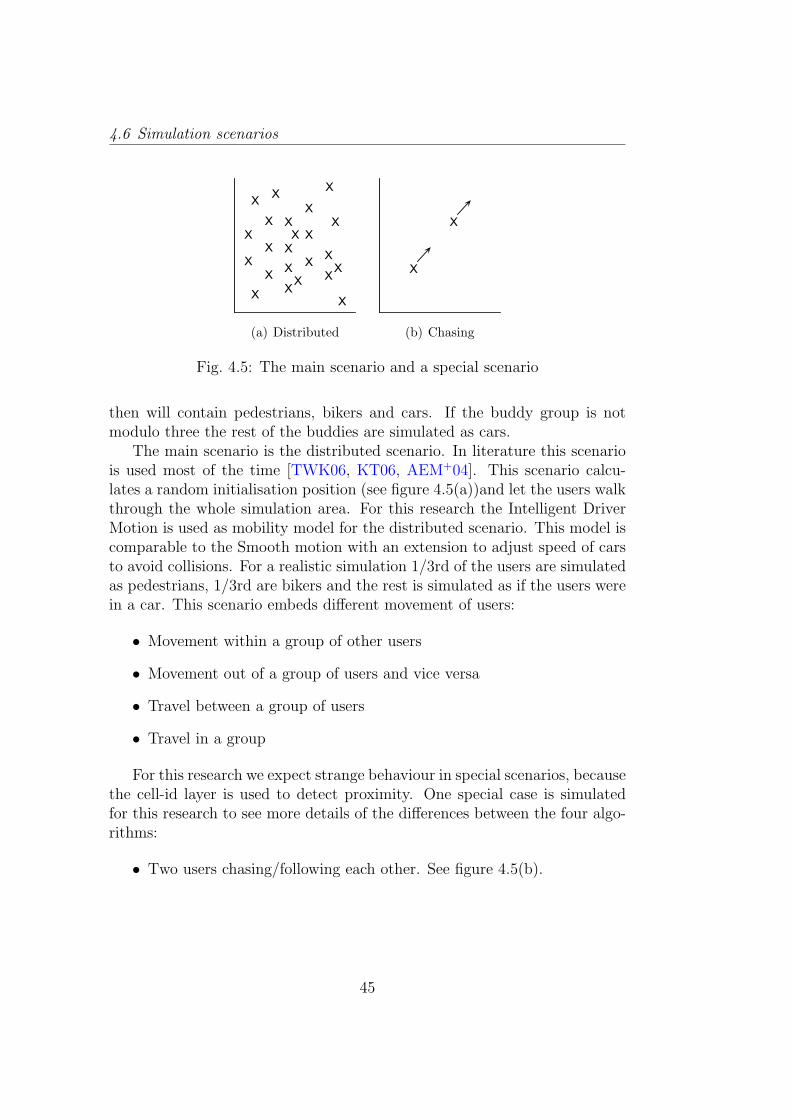
4.6 Simulation scenarios

X

XX

X

XX

X X

X

X

XX

X

XX

X X

X

XX

XXX

(a) Distributed

X

X

(b) Chasing

Fig. 4.5: The main scenario and a special scenario

then will contain pedestrians, bikers and cars. If the buddy group is notmodulo three the rest of the buddies are simulated as cars.

The main scenario is the distributed scenario. In literature this scenariois used most of the time [TWK06, KT06, AEM+04]. This scenario calcu-lates a random initialisation position (see figure 4.5(a))and let the users walkthrough the whole simulation area. For this research the Intelligent DriverMotion is used as mobility model for the distributed scenario. This model iscomparable to the Smooth motion with an extension to adjust speed of carsto avoid collisions. For a realistic simulation 1/3rd of the users are simulatedas pedestrians, 1/3rd are bikers and the rest is simulated as if the users werein a car. This scenario embeds di"erent movement of users:

• Movement within a group of other users

• Movement out of a group of users and vice versa

• Travel between a group of users

• Travel in a group

For this research we expect strange behaviour in special scenarios, becausethe cell-id layer is used to detect proximity. One special case is simulatedfor this research to see more details of the di"erences between the four algo-rithms:

• Two users chasing/following each other. See figure 4.5(b).

45


46

Chapter 5

Simulation

This Chapter describes the simulations done on the four new introducedproximity detection algorithms using the GSM network. The simulator of theprevious Chapter 4 is used. First an explanation and example is given aboutthe confidence level and interval. The confidence level and interval are usedto state that the simulations are reliable. The accuracy of GPS versus GSMcell-ids is simulated using a realistic topology extracted from the telematicadatabase [KW]. A distributed scenario, often used in literature, is used toscale the number of users and get the di"erences in performance, in termsof number of messages and data tra!c, of the four algorithms. A typicalscenario is used to show the e"ects of chasing clients on the algorithms. Anillustration is given about the amount of data used, using the distributedscenario. At the end of the chapter a simulation run is illustrated using reallogged data.

5.1 Confidence level and interval

Because randomly generated paths, according to mobility models, are usedfor the simulations a confidence level is chosen and confidence interval iscalculated. This is done to get a reliable simulation. In literature a confidencelevel of 95% is often used [HJ04b]. With 95% probability the real mean iswithin the found interval, which is typically the mean of di"erent runs ± arelative precision !. Usually the relative precision of the estimators is chosento be 0.05 or 5% of the estimated values.

To come to a confidence level of 95% a large number of runs (n > 30)must be done, using the same parameters except the random placement andmovement of users. If the number of runs is less than 30 it is possible thatthe result is biased. For each simulation run in this chapter the confidencelevel and interval is calculated, to get a reliable run.

A 100(1! #/2) confidence interval is calculated as follows [HJ04b]:

47

5 . Simulation

X ± z(1!!/2)$$n

(5.1)

Where X is the mean of the samples in set X. $ is the standard deviationof the set of samples. The z-factor or the (1!#/2)-quantile of a unit normalvariate is selected from table A3.5.1 in [S.M87]. For a confidence level of 95%(# = 0.05) the factor z0.975 = 1.96.

To illustrate the calculation of the confidence interval an example is giventhat calculates the confidence interval over a set of 50 simulation runs. Onesimulation run has a length of 200 hours and simulates the user movementof 5 users. Each user has 4 buddies. The area of the simulation is a middlesized area of 15km by 15km with a suburban roadmap. The average numberof proximity detections per user per run of 200 hours can be found in figure5.1.

0 5 10 15 20 25 30 35 40 45 500

100

200

300

400

500

600

700

800

900

1000

Pro

xim

ity d

etec

tions

per

use

r

Number of runs

total hits

Fig. 5.1: 50 simulation runs of 200 hours on a city area of 15x15km

The mean X = 920 of n = 50 runs. $ = 40.5514 Filling in the equation5.1 results in the following confidence interval in which the real mean is foundwith 95% probability:

920! 1.96" 40.5514$50

% 909 (5.2)

920 + 1.96" 40.5514$50

% 931 (5.3)

To see if the set of samples follows a normal distribution the normalprobability plot can be found in figure 5.2. The points in figure 5.2 form a

48

5.2 GPS versus GSM cell-id accuracy

780 800 820 840 860 880 900 920

0.010.020.050.10

0.25

0.50

0.75

0.900.950.980.99

Number of proximity hits per user

Pro

babi

lity

Normal Probability Plot

prox hitsnormal distribution

Fig. 5.2: Normal probabiltiy plot of samples

nearly linear pattern, which indicates that the normal distribution is a goodmodel for the simulation data set.

In the simulator the calculation of the confidence interval is done ’on thefly’. This means that the simulation is terminated if the desired precisionis reached, with respect to the minimum of 30 runs. See figure 5.3 for theprocess of simulation. Because the part that generates the mobility part isindependent of the simulator one replication is one simulation run of multiplehours of user movement data, in the example above it was 200 hours per run.This results in di"erences in the calculation of the confidence interval persimulation, due to the granularity. In the simulation Graphs the confidenceinterval is displayed in the title of the figures. For example if the Conf.Int. is < 2%, this means that for all the simulation points in the graph theconfidence interval is lower than ± 2%.


Using the cell-ids from ’Telematica Instituut’ it is possible to create a realisticcell-id layer. The data from the database of the area of Enschede is notcomplete, but it could be used to create a layer via extrapolation. To createthis layer, first the dubious measurements are filtered out, i.e. cell-ids witha zero LAC and the cells with 10 or less measurements. After this filteringonly 338 of the 863 cells are left over. This layer has a lot of white spotswhere no coverage is, this is not realistic, because in the Netherlands almost

49

5 . Simulation

Star t

One run

C alculate

confidence

interval

D esired interval?

&&

( runs > 30)?

no

End yes

Fig. 5.3: Simulation process to confidence interval

everywhere there is coverage. To get a realistic layer that has coverage, a partof the cell layer (with coverage) is taken out of the filtered data and copiedseveral times to create a larger layer. This new layer can be found in figure5.4. We are focusing on the simulation scenario of an urban environment.

The simulation area is 1000x1000 units (1000x1000 for faster simulations)in figure 5.4, so the cell layer is larger than the simulation area. This is doneto get a realistic situation, i.e. to avoid strange behaviour at the borders ofthe simulation area. This area can be compared to 25x25km in real life. Ifa user is in a white spot of the layer, where there is no coverage of cells, theuser is not connected to a cell. This is done to keep realistic diameter sizeof cells. Therefore no proximity will be detected in any of these white spots.After a run of 100 users of 10 hours using the ’Intelligent Driver Motion’model of VanetMobiSim [HF] 23780 proximity detections are simulated. Foreach of these proximity detections the diameter of the cell (the cell whereproximity is detected) and the real distance between users is stored. Sincethe cell-layer is used to detect proximity users can only be informed with anaccuracy corresponding to the diameter of the current cell where proximityis detected. This means that if proximity is detected between two users themaximum distance between those users is the diameter of the cell, in whichthe proximity is detected. Proximity must then be detected if two users arein the same cell.

In figure 5.5(a) a histogram can be found of the di"erences between thereal distance between two users and the distance that is found using the

50


kilometers

kilo

met

ers

0 5 10 15 20 25 30

0

5

10

15

20

25

30

-5

Fig. 5.4: Extrapolated realistic cell-id layer (25x25km)

diameter of cells. These distances are calculated upon proximity detectionbetween those users. In figure 5.5(b) the normal probability distribution canbe found of these di"erences. It can be seen that the maximum di"erencebetween the real distance and the cell distance is around 2900m and thesmallest di"erence 0. The di"erence can be zero if both users are at the edgeof a cell. The average di"erence is approximately 1100m.

The accuracy of proximity distance using GSM cell-ids is limited to thediameters of the di"erent cell-sizes as mentioned before. It is possible thattwo users are within a certain range of ,for example, 500 meters and proximityis not detected using the GSM cell layer. This is called a missed proximity,also often called a false negative. The realistic cell-id layer is used to illustratethe number of missed proximities, see table 5.1. This table displays thetotal missed proximity detections. The total number of proximity detectionsduring this run was 11800 and the total number of users 50. The simulationarea is an area of 25x25km. The average size of the cells is approximately1100m. Around this proximity distance the number of missed proximities is41 or 3.5% of the average total number of proximity detections.

51

5 . Simulation

0 500 1000 1500 2000 2500 30000

20

40

60

80

100

120

Differences in distance between real and cell−id distance (meters)

Num

ber

of sam

ple

s

Histogram of differences in distance between real and cell−id distance

(a) Histogram di"erences

0 500 1000 1500 2000 2500 3000

0.0010.0030.010.020.050.10

0.25

0.50

0.75

0.900.950.980.99

0.9970.999

Difference between real and cell−id distance

Pro

babi

lity

Normal Probability Plot

sampledistribution

(b) Normal probability distribution

Fig. 5.5: GSM proximity distance di"erences

Distance Missed proximity Percentage(1180)900 258 21.8%

1000 92 7.8%1100 41 3.5%1200 28 2.4%1300 26 2.2%

Tab. 5.1: Missed proximities per user per 10 hours

52

5.3 Distributed scenario

0 200 400 600 800 1000 12000

100

200

300

400

500

600

700

800

900

(a) medium: 140 cells (10x10km)

0 200 400 600 800 1000 1200

100

200

300

400

500

600

700

800

900

(b) large: 680 cells (25x25km)

Fig. 5.6: Distributed scenario large and small simulation


To compare the di"erent algorithms, a run is done with distributed users.The total number of users is scaled in the same simulation area. This sce-nario is mostly used in literature to compare proximity detection algorithms[AEM+04]. A voronoi graph is used as a roadmap. The clusters in the voronoigraph are representative for an suburban area [Cho97]. Two simulations areexecuted with di"erent simulation areas. A medium area of approximately140 cells (representing 10x10km) and a large area of 680 cells (representing26x26km). The two simulation areas can be found in figures 5.6(a),5.6(b),these are snapshots during a simulation run. The users are the ’x’ marks andthe lines are the corresponding paths of the users. The hexagonal grid rep-resents the cell-id layer. The ’o’ marks in the centre of the hexagons denotethe current cell the user is connected to.

The four algorithms, Cell-id, LAC, Graph1 and Graph2, are simulatedwith the distributed scenario input data. First the medium size simulation isevaluated (see also figure 5.6(a). The LAC algorithm is left out of the figuresof the medium size simulation, because it performs the same as the Cell-idalgorithm. In the medium area the number of LACs is 1 or 2, this is too lowfor the LAC algorithm to have an advantage. As seen before in section 2.1.1the number of cells that form a LAC are more than 40 cells, only the area ofAmsterdam for the KPN topology has fewer cells in a LAC.

53

5 . Simulation

10 20 30 40 50 60

200

300

400

500

600

700

800

900

1000Uplink messages (confidence interval < 2%)

Number of users(each user has other users as buddy)

Avg

# o

f upl

ink

mes

sage

s pe

r use

r per

hou

r

Cell−idGraph1Graph2

A B C

(a) Uplink messages

10 20 30 40 50 60100

200

300

400

500

600

700

800

900

1000

Downlink messages (confidence < 2%)

Number of users(each user has other users as buddy)Avg

# o

f dow

nlin

k m

essa

ges

per u

ser p

er h

our

Cell−idGraph1Dynamic

A B

(b) Downlink messages

Fig. 5.7: Up and Downlink messages medium area

The output of the simulator is the number of uplink messages (see figure5.7(a)) and downlink (see figure 5.7(b)) messages. On the Y-axis of thegraphs is the average total number of messages per user per hour displayed.The number of users is scaled and each user has the other users as buddy. Infigure 5.7(a) the graph algorithms generate less uplink messages, see area Aand B. The Graph2 algorithm outperforms Graph1 for a low density of users,see area A. This breakpoint lays around 4 users. The graph algorithms takebenefit of the free cells that are available if there is a low density of users.

Around 16 users the number of uplink messages equals for the cell-idalgorithm and the Graph1 algorithm. If the downlink messages are alsotaken into account (total messages per user per hour) this break-even pointis around 10 users, for the cell-id and Graph1 algorithm.

The simulator can also keep track of the data usage per user. TCP/IP issimulated over a GPRS connection. In figures 5.8(a) and 5.8(b) the tra!c inKbytes per user per hour is displayed. The same breakpoint as seen with thenumber of messages returns here. For 5 users or less, the Graph2 algorithmgenerates the lowest amount of uplink data (area A). Up to 17 users,theGraph1 algorithm generates less uplink data than the cell-id algorithm.

With more users the graph1 algorithm and the graph2 algorithm generatemore downlink data. This data is generated by messages initiated from theserver. If a user enters another user’s free-area, and no proximity is detected,this user has to be informed that his free-area is a"ected. A new TCP/IP

54


5 10 15 20 25 30

8

10

12

14

16

18

20

22

24

26

28Bytes uplink (conf. int. < 2%)


Avg

tota

l Kby

tes

send

per

use

r per

hou

r


A B C

(a) Uplink tra!c

5 10 15 20 25 30

10

15

20

25

30

Bytes downlink (conf. int. < 2%)

Number of users(each user has other users as buddy)A

vg to

tal K

byte

s re

ceiv

ed p

er u

ser p

er h

our


A B

(b) Downlink tra!c

Fig. 5.8: Up and Downlink tra!c medium area

connection has to be set up with the a"ected user. This e"ect can be seenin figure 5.8(b), displaying the downlink tra!c. The breakpoint lays around5 users.

The total tra!c in Kbytes per user per hour can be found in figure 5.9.In this medium area of 140 cells the graph2 algorithm only outperform theother algorithms if 3 or less users are in the area, in the figure this is markedwith an ’A’. The Graph1 algorithm generates the fewest amount of totaldata tra!c fo 9 users or less, see area ’B’. In area ’C’ the cell-id algorithm isperforming the best.

So the Graph algorithms need a low density of users to perform well, interms of number of messages and data tra!c. This is due to the fact thatthe Graph algorithms simply need to have free cells to assign to users. Thegraph algorithms have the disadvantage of generating more downlink data.If a user enters a free area of another user, the free area of both users needsto be updated, resulting in two messages.

Another simulation run was done on a larger area, because the high den-sity of users in a medium area a"ects the performance of the graph algo-rithms. The simulation area contains a cell-layer of 680 cells, this representsan area of 25x25km. In figure 5.10(a) the total data tra!c can be found forthe simulation run of the large area. As can be concluded from the figure, theGraph2 algorithm performs best up to 10 users (see area ’A’ in figure 5.10(a)).In area ’B’ the Graph1 algorithm outperforms the other algorithms, in terms

55

5 . Simulation

5 10 15 20 25 30

15

20

25

30

35

40

45

50

55

Total Traffic: uplink + downlink (conf. int. < 2%)


Avg

tota

l tra

ffic

in K

byte

s pe

r use

r per

hou

r


BA C

Fig. 5.9: Total tra!c medium area

of data tra!c. After this breakpoint, 30 users, the basic cell-id generates thelowest amount of data tra!c (area ’C’).

Compared to the medium area of 140 cells, the Graph algorithms performbetter. The LAC algorithm has the advantage of multiple LACs, but thewinnings are very small, it is negligible. This is why the LAC algorithmgraph is left out of figure 5.10(a).

In figure 5.10(b) it can be seen that, if the density of users is high enough,the algorithms perform the same. In other words, all the algorithms fall backto the cell-id level, as used in the cell-id algorithm. For the Graph algorithmsa free-area is simply one cell-id, because there are no free cells available toform a free-area.

5.4 Chasing cars scenario

A typical scenario could be that two users are travelling in the same directionwith di"erent speeds. Two users are on the same highway and approacheach other several times, because of the other tra!c. This special case issimulated to see how the di"erent algorithms react, in terms of messages anddata tra!c. Two users are simulated using an activity model to generatechasing data. Two nodes are placed on the simulation area, with a distance

56

5.4 Chasing cars scenario

10 20 30 40 50 6010

20

30

40

50

60

70

80

90

100

Total Traffic: uplink + downlink (conf. int. < 4%)


Avg

tota

l tra

ffic

in K

byte

s pe

r use

r per

hou

r

Cell−idLacGraph1Graph2

A B C

(a) Total Tra!c large area, zoom

50 100 150 2000

20

40

60

80

100

120

140Total Traffic: uplink + downlink (conf. int. < 4%)

Number of users(each user has other users as buddy)A

vg to

tal t

raffi

c in

Kby

tes

per u

ser p

er h

our

Cell−idLacGraph1Graph2

(b) Total Tra!c large area

Fig. 5.10: Total data tra!c large area (25x25km)

cell-id LAC graph1 graph2uplink messages 34368 34368 31409 29456downlink messages 25626 25626 27865 27196total messages 59994 59994 59274 56652uplink Kb 1362 1362 1239 1161downlink Kb 1027 1027 1176 1210total Kb 2389 2389 2415 2371

Tab. 5.2: Chasing cars scenario results

of 10 km, the medium area cell-id layer is used. The two users chase eachother and 1358 proximities are generated, the users speed varies and theywill catch up due to di"erent velocities and accelerations. The simulationruntime was 100 hours. The results of the simulation runs, using the chasingcars data, of the four algorithms: cell-id, LAC, Graph1 and Graph2 can befound in table 5.2. This is the average data of 30 runs of 100 hour. The datadisplayed is the average data per user per 100 hours.

The LAC algorithm has no advantage of using LACs or landcodes in thechasing cars scenario, because the users are in the same LAC all the time.This results in the same messages and the same data tra!c as for the cell-id algorithm. The graph2 algorithm can take the advantage of assigningmultiple cells to one of the users, only two users are in the area so the

57

5 . Simulation

density of users is low. As seen in the distributed scenario simulation theGraph algorithms perform better for a low density of users. So during thechase run it occurs that two or more cells are between the two users. Thisa"ects both the total number of messages and the total tra!c over 100 hoursof chasing data.

5.5 Amount of data used, costs

For the application it is very important that the costs, in terms of money, forthe users are acceptable next to the energy consumption. The applicationhas to run continuously to detect proximity with other users. Using thesimulation results of the distributed scenario an estimation can be done aboutthe cost per user per month. This scenario simulates a lot of mobility of usersand therefore results in a lot of tra!c. This is probably the case in rush hourso this is the case for about 3 or 4 hours per work day. On a normal workday the rest of the time you probably be at the o!ce and at night you willbe sleeping, depending on the job. Using the distributed scenario the upperbound of costs per month can be calculated.

The data of the medium simulation is taken to illustrate the possiblecosts for a user with 30 buddies. At 30 buddies the tra!c for one user isaround 45 Kbytes per hour, see figure 5.9. This results in a data tra!c of45 " 24 = 1080Kb, or %1Mb. Per month this is about 30Mb. This is a lot,but nowadays the providers have flat fee subscriptions. And the distributedscenario is used and as stated before this can be compared to rush hourmovement, so in general the data usage will be much lower than 30Mb permonth.

5.6 Real user paths

As mentioned in chapter 4 it is also possible to input real user data. A userlogs his movement using a GPS and GSM enabled device. An example oftwo paths of di"erent users can be found in figure 4.2. This path is used toillustrate how the four algorithms react on real measurements. The numberof cell-id switches for the short path is 86 and for the other user it is 240. Intable 5.3 and 5.4 the results of the algorithm runs can be found.

The LAC algorithm is performing so well, in terms of messages and datatra!c, because the two users approach each other from di"erent directions.So they both can use the LACs as free-area. The Graph2 algorithm alsoperforms better than the Graph1 algorithm. Because no other users are in

58

5.6 Real user paths

cell-id LAC graph1 graph2uplink messages 909 75 549 429downlink messages 732 50 492 412total messages 1641 125 1041 841uplink bytes 36840 3050 22200 17320downlink bytes 30540 2000 20940 17740total bytes 67380 5050 42690 35060

Tab. 5.3: Real measurements: user 1

cell-id LAC graph1 graph2uplink messages 414 30 285 240downlink messages 380 20 294 264total messages 794 50 579 504uplink bytes 16732 1220 11486 9656downlink bytes 16240 800 12800 11600total bytes 32972 2020 24286 21256

Tab. 5.4: Real measurements: user 2

the way all the cell-ids are free and can be assigned to the user to form afree-area. The Graph2 algorithm creates a larger free-area than the Graph1algorithm.

59

5 . Simulation

60

Chapter 6

Conclusions and Future Work

This chapter describes the conclusions found during this research from thesimulations. After the conclusions future work is outlined.

6.1 Conclusion

Using the gathered GSM cell data from the Telematics Institute it was foundthat the average diameter of a cell is 1100m. Cell size varies from 10meter,pico cells, to 13km, macro cells.

Dynamic circles was found the best performing proximity detection al-gorithm in literature, in terms of number of messages. GPS coordinates areused as location identifier, but GPS needs a line of sight to calculate a po-sition. Inside buildings, next to high buildings and in woods the coverageis poor or even no coverage. GPS cannot be used as continuous locationidentifier, because of energy consumption.

Two groups of algorithms that detect proximity using the GSM networkwere defined. The Basic group consists of the algorithms using only theinformation available from the GSM network. Two algorithms are part ofthis group, i.e. the cell-id and LAC algorithm. The second group uses acell-id graph representing the network topology. The Graph1 and Graph2algorithms are part of this group. All four, client-server deployed, algorithmsuse the GSM cell-ids as location identifiers for users. The Graph group cano"er a proximity distance of multiple cells, the Basic group can only detectproximity in the same cell.

A simulator was developed capable of simulating the four algorithmsagainst realistic generated user movement or real logged paths. The sim-ulator can generate a hexagonal layer or a realistic layer can be used torepresent the GSM network topology. The number of messages, the datatra!c, the accuracy of the GSM cell layer and the missed proximities or falsenegatives can be simulated.

61

6 . Conclusions and Future Work

For the extrapolated cell layer of the area of Borne the accuracy of theGSM layer is around 1100m. The number of missed proximities for thisrealistic layer is 3.5% of the average number of proximity detections peruser, a static proximity distance of 1100m is used.

To compare the algorithms the proximity distance is defined as the samecell, so if two users are in the same cell proximity is detected. From thesimulation of the distributed scenario it can be concluded that for a lowdensity of users the Graph group outperforms the Basic Group. For a largesize area, with 680 GSM cells, the Graph1 algorithm outperforms the cell-idalgorithm for 30 buddies or less. For the medium size area, with 140 cells, thisbreakpoint is 17 users. With a very high density of users, each cell is occupied,the algorithms perform the same as the cell-id algorithm. Algorithms using afree-area, as with the Graph group, generate more server initiated messagesif a user enters another user’s free-area. The LAC algorithm is a minorimprovement on the cell-id algorithm, because the size of LACs is large inthe Netherlands, i.e. size of city or larger.

The amount of data tra!c used by a client with 30 buddies in a monthis less than 30Mb.

6.2 Future work

This section describes future work, what could be done to improve the sim-ulations. And what could make the application more valuable.

6.2.1 Adaptive algorithms

The algorithms presented in this thesis are all static algorithms. For futureresearch an adaptive or dynamic algorithm could be defined. In the calcula-tion of the free-area the direction and speed of the user could be taken in toaccount. Using this information the probability that a user stays longer init’s free-area increases. Also the size of the free-area could be made depen-dent on the density of users. So if a user is in a city the free-area should besmall, if the user is in the country side the free-area should be large.

6.2.2 Realistic cell-id layer

The public cell-id database of Telematica Institute was used during this re-search to create a realistic layer. Too few measurements resulted in an ex-trapolated layer used for simulations. For further research a cell-id layercould be better modelled. Solutions to get a better database could be:

62

6.2 Future work

• Use the community to gather more cell-id measurements. To reallypush people to gather data, awards could be given if someone has col-lected 100 unique cell-ids. This will trigger the user to gather moremeasurements.

• With a group of people systematically walks patterns to get all themeasurements. Repeat this several times to detect possible changes inthe topology, due to atmosphere or changes by the operator.

• Sell the application to the operator and use their information abouttheir own topology.

6.2.3 Data tra!c

CanuMobiSim and VanetMobiSim were used to generate realistic user move-ment. These generators lack the ability to generate movement for a user inreal-life e.g., go to work, eat, watch TV and go to sleep patterns. If a goodestimation of data tra!c is needed this type of user movement needs to begenerated. It is also possible to give users a GPS enabled mobile GSM de-vice and do a trial. This trial will require a lot of data and users to generateenough proximity detections to get a good estimation of the average datausage in a month.

6.2.4 Multiple operators

For this research only one operator is used to implement proximity detection.It could be that the application is used with di"erent operators, to add morevalue to the personalized service. If a client has a buddy that uses anotheroperator it is possible to detect proximity. Di"erent operators have di"erentnetwork topologies and di"erent cell sizes. As seen before each operator hasa di"erent method to form LACs for example. If the application needs tosupport multiple operators the following could be done:

• Create a new topology that merges all the di"erent topologies to createa single topology at the server side. This server needs to be in themiddle of the two operators and receive location updates of both users.With this merged topology it can detect proximity.

• Make use of a translation database of cell-ids to GPS coordinates. TheGPS coordinates are representing the centres of mass of the cell-id theuser is in. If this is done for both users with di"erent operators theGPS translated coordinates could be used to detect proximity.

63

6 . Conclusions and Future Work

64

Appendix A

DVD: Simulator and Demos

E!cient proximity detection among mobile clients using the GSM network.ing M.T.Witteman

This DVD is part of the graduation research done on proximity detectionusing the GSM network. It contains the simulator, all the tools, demo’s,other files used to achieve the simulation results that can be found in theThesis. All parts of the simulator are developed in Matworks Matlab. Eachdirectory contains a Readme.txt explaining the contents of that directoryand examples of using the contents.

DVD contents:

AccuracyAndMissedProximities:

This folder contains the simulation done with a realistic layer extrapo-lated from the area of Borne to get an answer to the subquestion about theaccuracy of the GSM network and about the missed proximities.

CanuMobiSim and VanetMobiSim:

These folders contain the work, previously done on generating realisticuser movement paths. Both the tools are written in JAVA and are usedto generate the data for the simulations. See LargeSizeRun and Medium-SizeRun for the usage of these generators.

JAVAwsdlCellLocatorDatabase:

This folder contains the JAVA application that can request cell-ids fromthe Telematica Database. It can request lat,longs from cell-ids, but it canalso request all the cell-ids in a certain latitude longitude rectangle. The

65

A. DVD: Simulator and Demos

latter is used to get the cell layer from borne.

LargeSizeRun and MediumSizeRun:

These folders contain the batch files to generate the input data en thebatch files to scale the number of users per algorithm. These batch files alsoimplement the calculation of the confidence interval on the fly.

ParseLoggedData:

This folder contains the parsers for the log files from the Cumular appli-cation. The parsers take the log files and convert it to matlab files, that canbe directly imported in Matlab.

ParseNSoutput2matlab:

This folder contains the C++ implementation of the parsers for the JAVAmobility path generators CanuMobiSim and VanetMobiSim. The parsers inmatlab format can be found in folder ParsersMobilityData

ParsersMobilityData:

This folder contains the parsers written in matlab to parse the outputdata of the JAVA mobility path generators CanuMobiSim and VanetMo-biSim to matlab ready data

TelinDataViewJAVA and TelinDataViewKML:

These folders contain parsers to view the data from the CellLocatordatabase from Telematica Instituut. The TelinDataViewJAVA views thedata retrieved with the JAVA wsdl application found in folder JAVAwsdl-CellLocatorDatabase. The TelinDataViewKML folder contains a viewer thatcan display the data saved from Google Earth. Johan Koolwaaij and MartinWibbels have developed a network link that enables you to view the cell-idsin Google Earth, Google Earth has the option to save that data to a KMLfile. The contents of the file looks a lot like XML. The viewer in Telin-DataViewKML use these KML files to display the cells

RealLoggedDataRun:

Simulating Real logged data. The real logged data is used as input for

66

the four algorithms. The output is the number of messages, up and downlinkand the tra!c up and downlink.

TraceMap:

Tracemap is a tool written in Matlab to trace real maps and generate aroadmap graph that can be used for CanuMobiSim and VanetMobiSim todefine a user graph representing a roadmap.

Demos:

Demos contains several graphical demos of the algorithms and movies ofthe algorithms

ScaleUser:

A C++ console tool that takes two input files and generates a set ofXML input files for CanuMobiSim and VanetMobiSim in which the numberof users is scaled.

Other:

Containing other files used for the research

67

A. DVD: Simulator and Demos

68

Bibliography

[AEM+04] Arnon Amir, Alon Efrat, Jussi Myllymaki, Lingeshwaran Pala-niappan, and Kevin Wampler. Buddy tracking — e!cient prox-imity detection among mobile friends, 2004.

[aw] acbPocketSoft website. acbpocketsoft: acbpowermeter.

[Cha98] Kanwar Chadha. The global positioning system: Challenges inbringing gps to mainstream consumers. IEEE Explore, 1998.

[Cho97] Howie Choset. Incremental construction of the generalizedvoronoi diagram, the generalized voronoi graph, and the hier-archical generalized voronoi graph. In Proceedings of the FirstCGC Workshop on Computational Geometry, October 1997.

[Cit] IBM Citysimulator. alphaworks: City simulator: Overview.

[Dia71] R.B. Dial. A probabilistic multipath tra!c assignment modelwhich obviates path enumeration. Transportation Research, (5),1971.

[Dij59] E.W. Dijkstra. A note on two problems in connection with graphs,Numerische Mathematik, volume 1. Numerische Mathematik,1959.

[HF] Jerome Harri and Marco Fiore. Vanetmobisim - vehicular ad hocnetwork mobility extension to the canumobisim framework.

[HFB05] Jerome Haerri, Fethi Filali, and Christian Bonnet. On the appli-cation of mobility predictions to multipoint relaying in MANETs:kinetic multipoint relays. In AINTEC 2005, Asian Internet Engi-neering Conference, December 13 - 15, 2005, Bangkok, Thailand- Also published in LNCS Volume 3837, Dec 2005.

69

Bibliography

[HJ04a] Jahan Hassan and Sanjay Jha. Design and analysis of locationmanagement schemes for a new light-weight wireless network.Computer Communications, 27(8):743–750, 2004.

[HJ04b] Mahbub Hassan and Rai Jain. High performance TCP/IP net-working: Concepts, Issues and Solutions. Pearson Prentice Hall,Upper Saddle River, NJ 07458, 2004.

[HK03] Shuk Ying Ho and Sai Ho Kwok. The attraction of personal-ized service for users in mobile commerce: an empirical study.SIGecom Exch., 3(4):10–18, 2003.

[KDK00] S. Kyriazakos, D. Drakoulis, and G. Karetsos. Optimization ofthe handover algorithm based on the position of the mobile ter-minals. IEEE, 2000.

[KT06] Axel Kupper and Georg Treu. E!cient proximity and separationdetection among mobile targets for supporting location-basedcommunity services. SIGMOBILE Mob. Comput. Commun. Rev.,10(3):1–12, 2006.

[KW] J. Koolwaaij and M. Wibbels. Gsm cells, mapping cellid to gpscoordinates.

[LR05] Pasi Lehtimaki and Kimmo Raivio. A som based approach for vi-sualization of gsm network performance data. In IEA/AIE’2005:Proceedings of the 18th international conference on Innovationsin Applied Artificial Intelligence, pages 588–598, London, UK,2005. Springer-Verlag.

[MRB07] E. Meeuwissen, W. Romijn, and J. Brok. Estimated time ofarrival and estimated location, 2007.

[NR04] Subrata Nandi and Manish K. Raushan. An e!cient implementa-tion of distance-based update scheme using directional cell iden-tification codes. In IWDC, page 535, 2004.

[osc05] Validation of an improved location-based handover algorithm us-ing gsm measurement data. IEEE Transactions on Mobile Com-puting, 4(5):530–536, 2005. Member-Hsin-Piao Lin and StudentMember-Rong-Terng Juang and Member-Ding-Bing Lin.

[Sch03] Jochen Schiller. Mobile communications 2nd. Addison-WesleyPearson Education, Edinburgh Gate, Harlow, England, 2003.

70

Bibliography

[S.M87] S.M.Ross. Introduction to Probability and Statistics for Engineersand Scientists. John Wiley and Sons, New York, 1987.

[Stea] Charles Steinfield. The development of location based servicesin mobile commerce. http://www.msu.edu/user/steinfie/elifelbschap.pdf.

[Steb] Illya Stephanov. Canumobisim - a framework for user mobilitymodeling.

[TWK06] Georg Treu, Thomas Wilder, and Axel Kupper. E!cient prox-imity detection among mobile targets with dead reckoning. InMobiWac ’06: Proceedings of the international workshop on Mo-bility management and wireless access, pages 75–83, New York,NY, USA, 2006. ACM Press.

[UE] USA and Europe. Everything you want to know about e911 ande112. http://www.globallocate.com/RESOURCES/RESOURCES_MAIN_f3.htm.

[weba] HTC website. Htc: Products: Htc p3600.

[webb] Mathworks Matlab website. Mathworks matlab.

71

http://www.globallocate.com/RESOURCES/RESOURCES_MAIN_f3.htm

http://www.msu.edu/user/steinfie/elifelbschap.pdf

http://www.msu.edu/user/steinfie/elifelbschap.pdf

http://www.globallocate.com/RESOURCES/RESOURCES_MAIN_f3.htm

proximity detection with mobile clients - universiteit twente€¦ · working at alcatel-lucent,...

Documents